Universal properties of Self-Organized Localized Structures
245
Universal properties of Self-Organized Localized Structures Hendrik Ulrich B¨ odeker 2007
-
Upload
khangminh22 -
Category
Documents
-
view
1 -
download
0
Transcript of Universal properties of Self-Organized Localized Structures

Universal properties
of Self-Organized
Localized Structures
Hendrik Ulrich Bodeker
2007


Experimentelle Physik
Universal propertiesof Self-Organized
Localized Structures
Inaugural-Disserationzur Erlangung des Doktorgrades
der Naturwissenschaften im Fachbereich Physikder mathematisch-naturwissenschaftlichen Fakultat
der westfalischen Wilhelms-Universitat Munster
vorgelegt von
Hendrik Ulrich Bodeker
aus Bielefeld
-2007-

Dekan: Prof. Dr. J. P. Wessels
Erster Gutachter: Prof. Dr. H.-G. Purwins
Zweiter Gutachter: Prof. Dr. R. Friedrich
Tag der mundlichen Prufung: 14.05.2007
Tag der Promotion: 13.07.2007

Zusammenfassung
In der Geschichte der Physik hat das Teilchenkonzept bei der Beschreibung vonProzessen auf zahlreichen raumlichen und zeitlichen Skalen eine zentrale Rolle gespielt,angefangen bei der Beschreibung subatomarer Prozessen auf sehr kleinen Skalen biszu Prozessen wie der Dynamik von Sternen und Planeten auf extrem grossen Skalen.In den letzten Jahren galt ein besonderes wissenschaftliches Interesse selbstorganisiertenteilchenartigen Strukturen in selbstorganisierenden Systemen. Solche Strukturen konnenin einer Vielzahl raumlich ausgedehnter physikalischer Systeme beobachtet werden, soz.B. in nichtlinearen optischen Systemen, Gasentladungen, Halbleitern, granularen Me-dien und hydrodynamischen Systemen. Trotz großer Unterschiede in den mikroskopi-schen Eigenschaften der genannten Systeme zeigen die lokalisierten Strukturen eineVielzahl ahnlicher, scheinbar universeller Eigenschaften auf vergroberten raumlichen undzeitlichen Skalen. Sie konnen als Ganzes generiert und vernichtet werden, propagieren, incharakteristischer Weise wechselwirken (Beispiele sind Streuung und die Bildung gebun-dener Zustande) und dynamisch ihre Form verandern.
Ziel dieser Arbeit ist es, einen Beitrag zur Aufklarung der ahnlichen Eigenschaftenvon selbstorganisierten teilchenartigen lokalisierten Strukturen in den unterschiedlichenSystemen zu leisten. Dissipative Systeme sind dabei von zentralem Interesse. DieArbeit beginnt mit der theoretischen Betrachtung einiger Prototyp-Modellsystemewie Reaktions-Diffusions-, Ginzburg-Landau und Swift-Hohenberg-Gleichungen, die je-weils eine großere Klasse verschiedener experimenteller Systeme reprasentieren, in de-nen lokalisierte Strukturen beobachtet werden konnen. Da sich die Gleichungen inihrer Natur stark unterscheiden und alle lokalisierten Strukturen in subkritischen Bi-furkationen generiert werden, ist das bisherige Verstandnis der qualitativen ahnlichenPhanomene in Bezug auf lokaliserte Strukturen noch sehr beschrankt. Besonderes Inter-esse gilt daher dem Auffinden von Mechanismen, die das Zusammenwirken verschiedenerKomponenten der jeweiligen Gleichungen bei Bildung, Dynamik und Wechselwirkunglokalisierter Strukturen anschaulich machen. Auf diese Art und Weise ergeben sich einigeallgemeine Konzepte, die den grundsatzlich verschiedenen Gleichungstypen gemein sind.
Um eine einheitliche Basis fur den Vergleich der Dynamik und Wechselwirkunglokalisierter Strukturen in den Feldgleichungen zu schaffen, konnen letztere mitadiabatischen Eliminationsmethoden auf gewohnliche Differentialgleichungen reduziertwerden. Diese Gleichungen beschreiben die dynamische Entwicklung von langsamveranderlichen Großen der einzelnen lokalisierten Strukturen, typische Beispiele sindPosition, Geschwindigkeit und langsame innere Freiheitsgrade. Die reduzierte Beschrei-bung ist trotz der unterschiedlichen Feldgleichungen von ahnlicher Struktur, die oftmaßgeblich von den kontinuierlichen Symmetrien in den Feldgleichungen beeinflußtwird. Unter gewissen Umstanden ergeben sich sogar starke formale Ahnlichkeiten zu denNewton-Gleichungen der klassischen Mechanik. Im Detail werden eine Zahl konkreter
i
Probleme behandelt, darunter Drift von lokalisierten Strukturen in Gradienten, intrin-sische Propagation, periodische Formanderungen und verschiedene Arten der Wechsel-wirkung. Auch der Einfluß von Rauschen in den Feld- und Teilchengleichungen wirddiskutiert.
Nach dem gegenwartigen Stand der Technik sind die Moglichkeiten der numerischenUntersuchung einer großeren Anzahl wechselwirkender lokalisierter Strukturen und ihrerLangzeitdynamik auf der Basis von Feldgleichungen starken Beschrankungen unterwor-fen. Daher bieten die reduzierten Gleichungen erstmals die Moglichkeit, statistischeEigenschaften großer Teilchenensembles zu untersuchen. Von besonderem Interesse istdabei ein Vergleich lokalisierter Strukturen und klassischer Newtonscher Masseteilchen.Hierbei stellt sich heraus, daß die Fahigkeit lokalisierter Strukturen, intrinsisch zupropagieren, fur eine ganze Reihe neuartiger dynamischer Phanomene verantwortlichist, die kein klassisches Analogon aufweisen. In diesem Kontext wird zunachst ana-lytisch die Dynamik von zwei lokalisierten Strukturen untersucht, bevor auch großereEnsembles mit Hilfe numerischer Methoden betrachtet werden. Auch Ensembles in-trinsisch propagierender Teilchen unter dem Einfluß von Rauschen (aktive BrownscheTeilchen) sind von Interesse.
Strukturen mit teilchenartigen Eigenschaften treten nicht ausschließlich in physikali-schen Systemen auf, sondern existieren auch in biologischen Systemen, z.B. in Formvon Zellen. In diesem Fall existiert generell keine Feldbeschreibung und es ist da-her kaum moglich, eine selbstkonsistente Beschreibung des dynamischen Verhaltens zufinden. Wir betrachten dieses Problem fur die eukaryotische Zelle Dictyostelium dis-coideum, die vielen Biologen als Prototyp-System dient. Eine zentrale Grundlage fur dieUntersuchung der Dynamik einzelner Zellen bilden mikrofluidische Anordnungen. MitMethoden der stochstischen Datenanalyse gelingt es, aus experimentell gewonnenen Zell-trajektorien Langevin-Gleichungen fur die Dynamik isolierter Zellen abzuleiten, die eineTeilchenbeschreibung darstellen und starke Ahnlichkeiten zu den reduzieren Gleichun-gen fur selbstorganisierte Strukturen in physikalischen Systemen aufweisen. Desweiterenkann der Einfluß verschiedener chemischer Stimuli auf deterministische und stochastis-che Anteile der Dynamik bestimmt werden, was Ruckschlusse auf die zugrunde liegendenProzesse innerhalb der Zellen ermoglicht.
ii

Abstract
Throughout the history of physics, the concept of particles has always played a centralrole, going from very small scales as involved in the description of sub-atomic structuresup to very large scales as relevant e.g. for the dynamics of stars and planets. In recenttimes, much scientific interest has been dedicated to localized, particle-like structuresin systems capable of showing self-organization. The latter can be observed in variousphysical spatially extended systems like nonlinear optical systems, gas-discharges, semi-conductors, granular media and hydrodynamic systems. Looking at the properties ofthe localized structures in these systems, it turns out that in spite of strong differences inthe underlying physical microscopic processes, many structures have similar, apparentlyuniversal characteristics on coarser spatial and temporal scales. They can be generatedand annihilated, propagate, interact, show scattering processes as well as the formationof bound states and may perform dynamic deformations of their shape.
This work tries to contribute to explaining the similar behavior of the self-organizedparticle-like localized structures (LSs) in different systems. The focus of interest lies onsystems in which dissipative processes play an essential role. In detail, we first considerseveral prototype systems like reaction-diffusion, Ginzburg-Landau or Swift-Hohenbergequations which each represent a number of different experimental systems capable ofexhibiting LSs. As the equations are structurally rather diverse in nature and all LSare generated in subcritical bifurcations, there is currently a rather limited understand-ing of the qualitative similarities in the dynamics of the LSs. Consequently, particularemphasis is put on finding illustrative mechanisms which help to understand how theindividual constituents of each equation interact in order to allow for the formation, dy-namics and interaction of LSs. In this way, a number of basic concepts can be identifiedthat are common in systems of very different nature.
A common basis for comparing the dynamics of single and several weakly interactingLSs in different types of systems can be created reducing the field equations to ordi-nary differential equations by methods of adiabatic elimination. The reduced equationsdescribe the evolution of quantities like positions, velocities and slowly varying inter-nal degrees of freedom of the LSs. Even for rather different types of field equationsthe reduced equations are of similar structure, often being essentially influenced by thecontinuous symmetries present in the field equations. In particular, in some situationsthere are strong formal similarities to those equations describing the dynamics of classi-cal Newtonian mass particles. Several concrete problems are addressed, including driftof LSs in spatial inhomogeneities, intrinsic propagation, periodic oscillations in shapeand different types of interaction behavior. Also, the effect of noise in the field equationsand its consequences for the reduced equations are discussed.
As due to current limitations of computational methods the interaction of only small
iii

numbers of LSs can be simulated numerically on the basis of field equations when sta-tistical properties or long-time dynamics are of interest, the derivations of the reducedequations essentially enables the investigation of statistical large particle ensembles. Aparticularly interesting point is the comparison of LSs to classical Newton particles. Itis found that the property of many LSs to propagate intrinsically is responsible for anumber of dynamic processes that are very different from their classical counterpart.We first carry out analytic considerations for the dynamics of two localized structuresbefore larger ensembles consisting of many LSs are investigated with the help of numer-ical simulations. Also, ensembles of actively propagating particles propagating underthe influence of noise (active Brownian particles) are analyzed.
Objects with particle-like properties are not found exclusively in the field of physics,but exist also in biological systems, for example in the form of cells. For these structures,there generally exists no description on the level of field equations and consequently isis hardly possible to find a self-consistent description of the dynamical behavior. Weaddress this problem for the eukaryotic cell Dictyostelium discoideum which serves as aprototype system for many biologists. A basis for the experimental observation of thedynamics of isolated cells is provided by the use of microfluidic devices. Using methodsof stochastic data analysis, Langevin equations for the motion of isolated cells can beextracted from experimentally recorded cell trajectories, representing a description ofthe cell dynamics on a particle level and showing strong formal similarities to the reducedequations for LSs in physical systems. Furthermore, the dependence of deterministic andstochastic parts of the dynamics on different chemical stimuli can be estimated, givingimportant implications for the underlying processes inside the cells.
iv

Contents
1 Introduction 11.1 Self-organized localized structures and the particle concept . . . . . . . 11.2 A historical survey . . . . . . . . . . . . . . . . . . . . . . . . . . . . . . 31.3 LSs, dissipation and attractors . . . . . . . . . . . . . . . . . . . . . . . 61.4 Particle phenomenology and the role of dissipation . . . . . . . . . . . . 10
2 Models and mechanisms 132.1 Reaction-diffusion systems . . . . . . . . . . . . . . . . . . . . . . . . . . 14
2.1.1 One-component systems . . . . . . . . . . . . . . . . . . . . . . . 152.1.2 Two-component systems . . . . . . . . . . . . . . . . . . . . . . . 23
2.1.2.1 The excitable case . . . . . . . . . . . . . . . . . . . . . 262.1.2.2 The bistable case . . . . . . . . . . . . . . . . . . . . . 40
2.1.3 Three-component systems . . . . . . . . . . . . . . . . . . . . . . 442.2 Ginzburg-Landau equations . . . . . . . . . . . . . . . . . . . . . . . . . 49
2.2.1 The formation of LSs . . . . . . . . . . . . . . . . . . . . . . . . 512.2.2 Dynamics of LSs . . . . . . . . . . . . . . . . . . . . . . . . . . . 602.2.3 Variations of the GL equation . . . . . . . . . . . . . . . . . . . . 66
2.3 Swift-Hohenberg equations . . . . . . . . . . . . . . . . . . . . . . . . . 692.3.1 General properties . . . . . . . . . . . . . . . . . . . . . . . . . . 692.3.2 LSs in the real SH equation . . . . . . . . . . . . . . . . . . . . . 712.3.3 LSs in the complex SH equation . . . . . . . . . . . . . . . . . . 75
2.4 Summary on mechanisms . . . . . . . . . . . . . . . . . . . . . . . . . . 78
3 Particle description of LSs 833.1 The concept of order parameters . . . . . . . . . . . . . . . . . . . . . . 833.2 Dynamics of single structures . . . . . . . . . . . . . . . . . . . . . . . . 84
3.2.1 Trial function methods . . . . . . . . . . . . . . . . . . . . . . . . 843.2.2 Projection based methods . . . . . . . . . . . . . . . . . . . . . . 87
3.2.2.1 Formal derivation . . . . . . . . . . . . . . . . . . . . . 883.2.2.2 Perturbative techniques and normal forms . . . . . . . 943.2.2.3 Perturbative approach on the level of the field equations 95
3.2.3 Normal forms for the dynamics of single LSs . . . . . . . . . . . 1063.3 Interaction of structures . . . . . . . . . . . . . . . . . . . . . . . . . . . 107
3.3.1 Weak interaction and trial-function methods . . . . . . . . . . . 1083.3.2 Weak interaction and projection methods . . . . . . . . . . . . . 1083.3.3 Examples for interacting LSs . . . . . . . . . . . . . . . . . . . . 112
v

3.3.4 Symmetries, dynamics and interaction processes . . . . . . . . . 1183.4 Stochastic and fluctuating systems . . . . . . . . . . . . . . . . . . . . . 121
3.4.1 General theory . . . . . . . . . . . . . . . . . . . . . . . . . . . . 1213.4.2 Noise correlations in the order parameter equations . . . . . . . . 124
4 Many-body Systems 1314.1 Non-fluctuating systems . . . . . . . . . . . . . . . . . . . . . . . . . . . 132
4.1.1 Analytic considerations in one-dimensional systems . . . . . . . . 1334.1.2 Analytic considerations in two-dimensional systems . . . . . . . . 1374.1.3 Numerical calculations in two-dimensional systems . . . . . . . . 141
4.1.3.1 Free propagation . . . . . . . . . . . . . . . . . . . . . . 1414.1.3.2 Confined motion . . . . . . . . . . . . . . . . . . . . . . 1464.1.3.3 Excitation and switching fronts . . . . . . . . . . . . . . 150
4.2 Fluctuating systems . . . . . . . . . . . . . . . . . . . . . . . . . . . . . 1564.2.1 Numerical considerations in two-dimensional systems . . . . . . . 156
4.2.1.1 Bound state of two active Brownian particles . . . . . . 1574.2.1.2 Bound state of many active Brownian particles . . . . . 1624.2.1.3 “Phase transitions” . . . . . . . . . . . . . . . . . . . . 165
5 Excursion to biology: the dynamics of cells 1755.1 Cells as particle-like structures . . . . . . . . . . . . . . . . . . . . . . . 1765.2 Experimental techniques . . . . . . . . . . . . . . . . . . . . . . . . . . . 1765.3 Directed and undirected motion . . . . . . . . . . . . . . . . . . . . . . . 181
5.3.1 Experimental results . . . . . . . . . . . . . . . . . . . . . . . . . 1815.3.2 Conclusions for directed motion . . . . . . . . . . . . . . . . . . . 184
5.4 Stochastic motion of cells . . . . . . . . . . . . . . . . . . . . . . . . . . 1875.4.1 Stochastic analysis . . . . . . . . . . . . . . . . . . . . . . . . . . 1885.4.2 Discussion of the results . . . . . . . . . . . . . . . . . . . . . . . 197
6 Conclusions and outlook 1996.1 Summary of the work . . . . . . . . . . . . . . . . . . . . . . . . . . . . 1996.2 Open questions and further progress . . . . . . . . . . . . . . . . . . . . 201
Bibliography 203
vi

Chapter 1
Introduction
1.1 Self-organized localized structures and the particleconcept
Throughout the history of physics, there are numerous examples for successful theories inwhich the concept of particles or particle-like structures plays a central role. Already theGreek philosophers believed in the existence of atoms of which all matter is composed.In this way, they notionally divided the objects of natural perception into subunits thatmay undergo interaction, reducing the understanding of nature to that of understandingthe properties of atoms and their interrelations. In order for a concept of subdivision ingeneral and a particle concept in particular to work, the single particles should retaintheir individuality to a large extent while interacting. As a general rule, particle modelsare the more convincing as the smaller the number of subunits, the simpler the postulatedinteraction and the broader the scope of application.
We point out two theories related to the particle image which are of particular rel-evance due to their extremely wide range of application. On the one hand, there isclassical mechanics capable of describing (with appropriate extensions) the dynamics ofvery small particles like electrons in a plasma to very large objects like stars on the scaleof light years. On the other hand, there is the concept of the atom and the periodictable which represents an essential basis for explaining the structure of matter. Further-more, atoms themselves again consist of subunits like for example electrons, neutronsand protons. To understand processes on larger scales, extended particle concepts playan important role, going from molecules to particles in emulsions and aerosols, grains ingranular media and precipitations in alloys. Less evident examples are “quasi-particles”like phonons, magnons and Cooper pairs.
Looking at recent scientific developments, an increased interest has developed inparticle-like structures that can be observed on scales above micrometers and -seconds,their existence and dynamics including self-organization as an essential ingredient. Typ-ical examples include living cells, swarms of birds or fish, myosin heads on actin filamentsas well as flow of traffic or pedestrians. However, most animate systems are too com-plex to understand on the basis of quantitative models at the current state of researchalthough there are some examples of particle-like structures like nerve pulses for whicha reasonable amount of understanding could already be obtained.
Recent investigations in the field of complex systems have focussed on a number of
1

2 Introduction
a. c. c. d.
e. f. g. h.
membranepotential
Figure 1.1: Examples for experimentally observed LSs in dissipative systems: a. planar acgas-discharge system [1], b. planar dc gas-discharge system [2], c. optical single feedback system[3], d. oscillating granular medium [4], e. nerve pulse [5], f. chemical reaction on a catalyticsurface [6], g. binary fluid mixture [7], h. semiconductor device [8].
unanimated systems capable of showing the formation of stable localized structures withparticle-like properties (LSs) that are particularly suitable to access both experimentallyand theoretically. These systems include gas-discharges, semiconductors, optical sys-tems, granular media and hydrodynamical as well as chemical systems (Fig. 1.1). All ofthe above examples belong to the class of dissipative, nonlinear and spatially extendedsystems. The mechanisms responsible for the formation of the LSs are far from beingwell understood in many of the systems up to now. A particularly fascinating aspectis even less clarified: while the systems are very different on a microscopical level, onlarge scales the dynamics of the LSs shows clear similarities. This idea of “universal”behavior is frequently encountered during research on nonlinear systems. As an exam-ple, in very different finite-dimensional dynamical systems, close to special points wherethe dynamics becomes slow (typically supercritical bifurcation points) the behavior ofthe system is determined by only a small number of slowly evolving quantities. Usingmethods of adiabatic elimination like the center manifold theory, it is often possiblefor such systems to reduce the system to a low-dimensional normal form. The latterare identical for very different systems, allowing for a systematic classification of thepossible bifurcations according to criteria like the symmetries of the equations. Normalform theories have also been developed for infinite-dimensional systems, for example forthe supercritical transition from a homogeneous to a globally patterned state. Unfortu-nately, the exploration of the universal properties of LS is far less advanced than it is thecase for supercritical bifurcations as the generation of LSs generally occurs in subcriticalbifurcations. In this situation, methods like standard perturbation theory can not beapplied.
This work tries to contribute to the attempt to overcome the above problems and to
1.2 A historical survey 3
explain the common properties of LSs. The largest part of the investigation focusses onsystems in which dissipation plays an essential role. In the remaining introduction, wewill look at the history of research on LSs and discuss some key ideas like the role ofdissipation, attractors and the definition of LSs. In Chap. 2 we try to explain how LSsare stabilized in different types of field equations and which effects are responsible fordynamic phenomena. Due to the lack of generally applicable mathematical techniques,we put particular emphasis on finding illustrative mechanisms, an aspect that has beenneglected in many other theoretical works. In detail, we will have a look at reaction-diffusion, Ginzburg-Landau or Swift-Hohenberg types of equations. While many otherequations are known to exhibit the formation of LSs as well, the above equations canbe considered prototypical and capable of representing larger classes of experimentalsystems. Another important aspect is given by the fact that once a stable LS is knownto exist, it can undergo changes in its shape during its dynamical evolution. If thedeformations are not too strong, it is indeed possible under appropriate circumstancesto reduce the field equations to ordinary differential equations using methods of adiabaticelimination. In Chap. 3 we present mathematical methods suitable to accomplish thistask and apply them to a number of selected problems involving both isolated andinteracting LSs. We will see that on the level of the reduced equations, the dynamicscan be described in terms of certain normal forms, there providing a good basis forexplaining similarities in the dynamical behavior. Also, we deal with the influence ofnoise. Apart from reflecting the particle-like behavior of the LSs, the reduced equationsalso offer a method to treat the dynamics and interaction of large ensembles of LSs,which is usually only possible to a rather limited amount on the basis of field equationsdue to technical limitations of current computational means. In Chap. 4, investigate thelong-time behavior of large ensembles of LSs and compare our finding to classical Newtonparticles. For actively propagating LSs, a number of new phenomena are found thathave no classical counterpart. Again, also the influence of fluctuations on the dynamicsis considered as well. Finally, in Chap. 5 we make an excursion to the field of biologywhere objects with particle-like behavior can be found in the form of living cells. Usingmethods of stochastic data analysis, we will find a reduced dynamical description thatreveals formal similarities with the LSs found in physical systems.
1.2 A historical survey
The fact that structures preserve their shape and properties in the course of time andtherefore can be considered as a localized, solitary entity on appropriately chosen scaleshas been known for a long time. However, the explicit idea that in particular in inan-imate systems structures do not simply exist, but can be generated on a homogeneousbackground state due to mechanisms of self-organization became part of the generalperception only in the last decades. In the following, we want to give a rough sketch ofsome important historic developments in research on LSs.
As early as in 1831 Faraday saw solitary LSs in a vibrating layer of fine powder [9]which today would probably be termed oscillons. Shortly afterwards, Russell observeda solitary water wave on a channel generated by a stopping ship which propagatedalong the channel without dispersing for several kilometers before decaying [10]. At thetime of the above discoveries, the individual observations were considered as curious

4 Introduction
phenomena, however they neither triggered an extensive further research nor led toan attempt to compare them. It is known that Russell performed experiments in alarge water tank in the following years, finding that two water waves may pass througheach other when colliding. Russell’s observations were supported by theoretical worksperformed by Lord Rayleigh [11] and Boussinesq [12] around 1870. These finally ledto the derivation of the KdV equation allowing for solitary solutions by Korteweg andde Vries in 1895 [13]. It was realized that the KdV equation is conservative in thesense that one can define an energy which remained conserved during the dynamicalevolution. On the experimental side, around 1900 most experimental works on LSscommonly exploited dissipative effects. In 1900 Ostwald conducted experiments on thepropagation of chemical pulses on metallic wires [14]. Lehmann found the formation oflocalized anode spots only two years later [15].
Conservative and dissipative systems received almost equal interest until about 1955,around which a number of highly influential works was published. On the dissipativeside, one may mention the discovery of the mechanisms of nerve pulse excitation byHodgkin and Huxley in 1952 [5] and the simulation of nerve pulse propagation usingreaction-diffusion equations and real electrical networks [16]. With an increase of thequality of semiconductor materials from about 1960 onwards the formation of currentfilaments has been reported for various circumstances. On the conservative side, thespecial role of the KdV equation was realized by Zabusky and Kruskal in 1965 [17].They demonstrated that the KdV equation is completely integrable [21] and introducedthe inverse scattering technique, which is a way to produce analytical solutions of thenonlinear partial differential equation by transforming the problem to a linear one.Furthermore, they introduced the term “soliton” as a name for the localized solitarysolutions of the KdV equation. Although the works on both nerve pulses and the KdVequation can be considered as highly relevant from a modern point of view, they did nottrigger similar historical developments. In the wake of Zabusky’s and Kruskal’s work, alarge amount of research was invested in LSs as solution of conservative equations. Inparticular, one may mention that in 1972 Zakharov and Shabat found another integrableequation and thus demonstrated that the inverse scattering technique is universal andcan be applied to a whole class of physically interesting equations [18]. In comparison,
a. b.
1960 1970 1980 1990 20000
50
100
150
year
cita
tion
rate
1960 1970 1980 1990 20000
50
100
150
year
cita
tion
rate
Figure 1.2: Citation rate of a. the three “conservative works” [17] (black), [18] (medium grey)and [19] (light grey) as well as b. the “dissipative works”[5] (black), [20] (medium grey) and [16](light grey) as a function of the year according to the ISI database (November 2006).

1.2 A historical survey 5
the interest in dissipative structures remained rather low and remained part of the cor-responding individual fields of research (for example solid state physics [22–24] etc). Wewant to quantify this aspect by looking at the yearly citation rates of highly cited arti-cles on conservative and dissipative structures according to the ISI database (Fig. 1.2).For the conservative side, we choose the above mentioned works [17] and [18] as wellas an highly cited article by Strauss [19] on solitons in higher dimensions. DissipativeLSs are represented by [5] and [16] as well as the work of Turing on reaction-diffusionequations [20] although the latter is not dealing directly with LSs. Comparing the leftgraph (conservative case) with the right graph (dissipative case), we indeed see thatunlike the dissipative case, the number of conservative citations strongly increases after1970 with respect to the citation rate in later years.
One may ask for the reason of the explosive increase on works dealing with conserva-tive LSs. A likely explanation is the point that the introduction of the inverse scatteringtheory did not only allow for finding analytical solutions of nonlinear partial differentialequations in a time where numerical techniques were hardly available, but established aconnection to various branches of mathematical sciences. Hence, the conservative sys-tems dominated research in the following decade. Up to about 1990 it was commonagreement to reserve the term “soliton” for solitary solutions of special nonlinear dif-ferential equations like the KdV, the nonlinear Schrodinger (NLS) or the sine-Gordon(SG) equation that were integrable and that could be treated via the inverse scatteringtechnique (see for example [25] for an overview). The equations usually allow for stablesolutions only in one spatial dimension. Soon people got interested in stable LSs alsoin higher-dimensional systems. These can be found by extending the original equationswith additional conservative terms (for example higher-order polynomials) which breakthe integrability of the system. Already here a first conflict arose whether the LSs inthe extended systems should be called solitons as well. The term “solitary wave” wasintroduced for LSs in conservative, yet non-integrable systems. One should again pointout that the largest part of works on conservative systems at the time was theoretical.
The overall situation changed after 1980. Fig. 1.2 shows that in this time the workson dissipative LSs experienced a significant increase in their citation rate. Aside fromadvances in mathematical techniques, an important aspect of this evolution is that com-puters with a sufficiently large numerical capacities became available for regular researchgroups so that analytic solutions were no longer a premise for a theoretical treatment.The first systems investigated were reaction-diffusion equations and different forms ofthe Ginzburg-Landau (GL) equation. On the experimental side, a number of differentsystems carrying LSs was investigated, many of them involving charge transport [26–29].As on the conservative side much research had already been carried out, people becameinterested in weak dissipative perturbations of the original conservative equations. Inthis case, using perturbative techniques often analytical solutions were possible to ob-tain (see for example [30] and references therein), showing details of how the solitonsdecay in the long-time limit. An experimental motivation for the theoretical works wasgiven by the fact that around 1980 the evolution of lasers and materials had advancedfar enough to produce the first solitons in glass fibers, which suffered weak losses duringpropagation and in the stationary case can be described using the weakly perturbedconservative equations. In order to distinguish the solitary LSs in strongly and weaklydissipative systems from those in conservative systems, a number of different terms wasintroduced, e.g autosoliton (in the Russian literature), spot, pulse and filament. The no-

6 Introduction
tion “dissipative soliton” which basically summarizes all important properties appearedin an article title the first time in 1981 [31], but was likely only accepted at that timebecause the author Petviashvili was already very famous.
After 1990, the interest in LSs in dissipative systems continuously grew (compareFig. 1.2), accompanied by an increased focussing on self-organization in general. In con-trast, the number of works on the classical soliton equations stagnated. Dissipative LSswere found in gas-discharges, semiconductors, optical systems, granular media, hydro-dynamics and electrical networks, just to name a few (Fig. 1.1). It became commonlyaccepted to use the term “dissipative soliton” for LSs in dissipative systems [32–34].Other more specialized terms were also created, for example oscillon or cavity soliton.More details on these recent developments will be given throughout this work. Althoughmany similarities concerning the phenomenology of the different systems were realized,attempts to compare findings in different classes of systems are just beginning to emerge.One reason for this problem may be the different terminologies and general concepts inthe individual fields.
1.3 LSs, dissipation and attractors
Looking at the different terms for LSs introduced in the historical development, one mayask what a good definition for a self-organized, particle-like solitary LS may be. A ratherstrict definition may state that the LS must be a stable stationary localized state in asystem with much larger spatial extension that can coexist with a purely homogeneousstationary state for the same system parameters and that exists independent of thesystem boundaries. Furthermore, the interaction between several LSs should vanish fora large mutual distance, and on a sufficiently large domain an arbitrary number of LSsshould be able to exist.
Many structures in dissipative systems fulfil these claims, and the same holds forconservative systems as well although some care has to be taken concerning the stabilitydefinition (see our consideration on attractors below). However, as we will see in thecourse of this work there are some structures which fulfil most of the claims above andwould intuitively be considered to be of solitary nature, but nonetheless violate the strictdefinition. In certain scenarios, the background state is not stationary and homogeneous,but either patterned with low amplitude or homogeneously oscillating in time. In othercases, the assumption on vanishing interaction for large distances is violated. Here, sometype of “integral coupling” occurs that may potentially put the LSs under competition.Nonetheless, it is often reasonable to accept these violations from the strict definitionas long as the LSs keep most of their solitary properties.
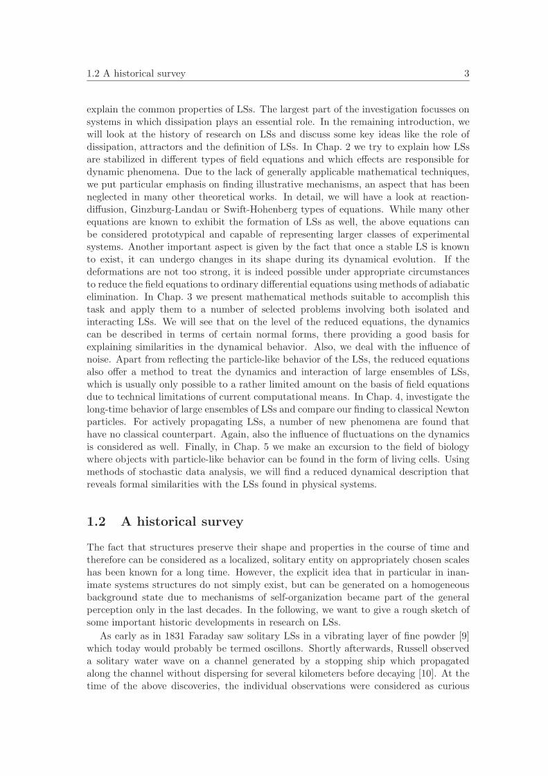
We want to address the aspect how the above definition of LSs can be applied ina given experimental system. In most cases the latter are typically three-dimensionalin space, with one direction being different from the other ones as it marks the maindirection in which energy and material is transported. Typical examples are given bygas-discharges with one main direction of the external applied electric field or opticalsystems with one main propagation direction of the incident light beam. The three-dimensional structures often have a filamentary shape directed along the main directionof transport, so that it is common to identify LSs in a two-dimensional plane perpen-dicular to the main direction as the structures are clearly localized here (Fig. 1.3). The
1.3 LSs, dissipation and attractors 7
z0
xy
z
t
Figure 1.3: Definition of LSs in a three-dimensional system: formation of a filamentary struc-ture in three-dimensional space with the main direction z and homogeneous boundary conditions.In a fixed perpendicular x-y-plane with z = z0 (dashed lines), the structure is localized and un-dergoes a temporal evolution, thereby defining a LS.
corresponding theoretical models then either describe the full spatial evolution of thesystem as a function of time or the temporal evolution in the perpendicular plane. Theabove definition can be applied in both dissipative and conservative systems (examplesfor LSs in the conservative case are given by water waves or specially designed electricalnetworks [25]).
A distinction between conservative and dissipative systems seems to be a naturalway of classifying pattern-forming systems as from the experience obtained in otherfield of physics this point makes a central difference in the dynamic behavior of theunderlying system. Often, conservative systems even have several conserved quantities,which can be used to implicitly define the dynamics of the system and which restrict theevolution to special manifolds. Solutions from a certain region of the phase space aregenerally known to be incapable of asymptotically approaching a compact attractor, as itis possible for dissipative systems. Unfortunately, theoretically the aspect of dissipativityis essentially not trivial in the context of LSs because although many systems capableof forming of LSs require an input of energy or material to work, it is unclear in whichway a transformation of one form of energy to the other is relevant for the formation ofLSs. In some systems like chemical ones, there is not even a clear definition of energyavailable so that there is currently no unique definition of conservative and dissipativesystems in general. In the following, we will briefly discuss a number of concepts, but itwill become obvious that all of them have certain drawbacks.
1. In many classical systems, there is often a clear intuition of what energy physicallymeans. Hence, when the system is perturbed, one may check how the energyfunction or functional evolves under the perturbation. As a simple example, onemay consider the damped harmonic oscillator
∂2t x+ ε∂tx+ x = 0 (1.1)
where in the conservative case ε = 0 the overall energy E = (∂tx)2/2 + x2/2 isconstant. It is easy to see that in the general case, ∂tE = −ε(∂tx)2, showing

8 Introduction
that energy is dissipated in the non-resting state. The same idea can usually beapplied to classical soliton equations like the nonlinear Schrodinger (NLS) equationin which the integral of the energy density is conserved.
2. Gradient systems can be identified by the fact that the evolution of their statevector q can be described by the gradient of a functional, i.e.
∂tq = −∂F (q)∂q
. (1.2)
Depending on the type of system, F is referred to as free energy, enthalpy, Lya-punov functional etc. Note that Eq. (1.2) has no classical limit. Nevertheless, thesystem evolves in such a way that F (q) is reduced and the minimum of F (q) corre-sponds to the stable final state in agreement with the intuitive idea of dissipation.
3. A rather abstract definition of conservation can be given in finite-dimensional sys-tems by looking at evolution of small volumes in phase space. When an arbitraryvolume element stays conserved in measure during the dynamic evolution, thesystem is called conservative. In systems of the form
∂tq = f(q) (1.3)
with q ∈ Rn, f ∈ R
n, there is an easy criterion to check the conservation propertyas the phase space volume is conserved if and only if
div f = 0. (1.4)
Furthermore, in dissipative systems attractors in a certain region are only possibleif the phase space is contracted. However, there are two drawbacks concerning thisdefinition. First, for arbitrary types of systems the definition may appear ratherabstract and can potentially not be connected to classical energy functionals. Sec-ond, there is currently no method of transferring the criterion from system of finitedimensionality to such of infinite one, including in particular partial differentialequations.
4. Attractors are generally encountered only for dissipative system (we will discussthis aspect in more detail below). Hence, the observation of an attractor gives agood indication that dissipation plays a role. However, some care has to be takenconcerning this point. As an example, a (conservative) system of ideal gas particlesin thermodynamical equilibrium always tends to show a Maxwellian distribution,so that care has to be taken about the exact definition of the term attractor.
5. All conservative systems are invariant under the time reversal transformation t→−t. If necessary, the latter is accompanied by the corresponding transformations ofsome physical quantities, for example, velocities and magnetic fields must changesign as well. Correspondingly one may define a dissipative system as a system

1.3 LSs, dissipation and attractors 9
that is not invariant under the time reversal transformation. This is probably themost general definition, evidently implying certain restriction on the dynamics ofthe system in question. We will therefore generally stick to this definition unlessone of the other definitions offers particular advantages.
Commonly it is stated that an exclusive feature of dissipative systems is the existenceof attractors. Mathematically, these attractors can be defined in the following way[35, 36]. One defines an evolution operator f(·, t) that maps the initial state of thesystem q(t = 0) onto the state q(t = t0 > 0). Then the attractor A is a closed subset ofthe phase space such that
1. A is invariant under f ,
2. there is a neighborhood of A called B(A) (the basin of attraction for A) of finitemeasure with B(A) = s| for all neighborhoods N A there is a time T so that forall t > T f(t, s) ∈ N. In other words B(A) is the set of points who ’enter A inthe limit’,
3. there is no subset of A with the above properties.
In the context of LSs, the applicability of the above definition may cause some pecu-liarities. Let us first consider an infinitely extended system and an initial perturbationof the ground state that should cause a LS to form. In dissipative systems, the per-turbation may converge to a LS of fixed shape. If the initial perturbation however isinfinitesimally displaced the resulting LS will show the same displacement so that oneobtains problems with the closedness of the attractor. The problem can be overcome bydefining appropriate equivalence classes via shifts with respect to the continuous symme-tries present in the system. In this sense, one now usually observed that slight changesof the shape of the initial perturbation cause the same structure to appear so that theLS is “point-like in phase space” and fulfils the attractor definition above. Consideringthe same situation for conservative systems, an initial perturbation of the ground statewill have a defined overall energy that cannot vanish in the course of time. However, itis commonly found that a LS forms and the excessive energy is radiated away, thereby“vanishing at infinity”. Changing the form of the perturbation not only results in ashift with respect to the continuous symmetries of the system, but also in the shape it-self. The possible solutions can usually be characterized as a continuous one-parametricfamily. Here is an important difference to the dissipative systems, the initial conditionsare still attracted when appropriate equivalence classes are defined, however intuitivelyone would not consider the attractor as “point-like”. Furthermore, the infinite domainin some sense takes over the role of a dissipative sink.
When going to finite domains, the difference between conservative and dissipativesystems becomes more evident. When supplying the conservative systems with “conser-vative” (for example periodic) boundary conditions the energy cannot leave the domainand commonly no convergence to an asymptotic state is found. In contrast, dissipativesystems may converge to a point-like structure even with “conservative boundaries”.We see that with sufficient care, we may attribute to dissipative systems the existenceof localized attractors, especially when using the definition of broken time-reversal sym-metry.

10 Introduction
1.4 Particle phenomenology and the role of dissipation
In the above section we have discussed that one of the most significant differences be-tween conservative and dissipative systems is the existence of “point-like” attractors, inparticular on finite domains. One may now ask whether there are also essential differ-ences concerning the phenomenology of elementary dynamical processes involving LSs.In this context, elementary dynamical processes shall be defined as generic behavior ofthe solutions of the underlying field equations reflecting the solitary and particle-like be-havior of the LSs. Typical examples are given by single LSs which propagate or changetheir shape as well as several LSs interacting with different outcomes, preserving theirshape or being generated and annihilated. Table 1.1 gives an overview of elementaryprocesses frequently reported in the literature for conservative and dissipative equations.We only consider theoretical systems here to ensure that the nature of the system canbe clearly determined according to one of the definitions of dissipativity discussed in thelast section. The meaning of most phenomena should be directly clear, however we wantto make some remarks. The term “free propagation” refers to the possibility for a solu-tion to propagate with an arbitrary velocity that just depends on the initial conditions.In contrast, the term “intrinsic propagation” refers to the phenomena that there is onespecial dynamically stabilized propagation velocity to which the solution converges inthe long-time limit. The term “breathing” characterized periodic deformations of theshape of the LS. In a merging or fusion event, two LSs collide with one structure re-maining, whereas in an annihilation event the structures become totally extinct. Moredetails on the individual phenomena in particular for dissipative systems can be found
singlestationary
manystationary
arbitraryvelocity
intrinsicvelocity
conservativecase
[17, 25] [25] [25] not found
dissipativecase
[37] [34, 38, 39] [40] [37, 41, 42]
breathing scattering,repulsion
interpenetra-tion
bound states
conservativecase
[43, 44] [45–48] [49] [50, 51]
dissipativecase
[52, 53] [54, 55] [56, 57] [58, 59]
rotatingclusters
propagatingclusters
merging,annihilation
generation
conservativecase
[50] [60] [45, 47] [61]
dissipativecase
[55, 62, 63] [55] [55] [55]
Table 1.1: Overview on the existence of different “elementary processes” involving LSs inconservative and dissipative systems. A citation indicates that the corresponding process hasbeen documented and gives the source.

1.4 Particle phenomenology and the role of dissipation 11
in the course of this work.As the table shows, most phenomena can actually be found in both conservative
and dissipative systems. An exception is given by intrinsic propagation which is onlyfound for dissipative systems as it contradicts the Galilean invariance which all classicalsoliton equations possess. Consequently, the phenomenology of LSs in conservative anddissipative system is not strictly different. On the other hand, looking in more detailon the number of references which report on the individual phenomena it turns outthat there are certain phenomena that are characteristic for the individual types ofsystems and mark exceptions in the opposite type. As an example, the interpenetrationof two LSs in a collision event is frequently found in integrable conservative systems andweak dissipative modifications, but seldom observed in strongly dissipative systems. Incontrast, intrinsic instabilities like breathing are characteristically found in dissipativesystems.

12 Introduction

Chapter 2
Models and mechanisms
In the introduction, we have briefly mentioned different classes of experimental systemsin which LSs can be found and shown some images of typical findings (Fig. 1.1). In orderto describe the individual systems, different types of models have been developed, goingfrom microscopic descriptions on the level of individual particles (based for example onsingle grains for granular media) over continuum models like reaction-diffusion systemsto very universal amplitude-type of equations like Ginzburg-Landau models which canbe applied to very different systems. While some of the models are closely connected tofirst-principle considerations, others have been set up only on a phenomenological basis.
In spite of a large number of theoretical works on the formation of LSs, two importantaspects are often attributed only a minor role. On the one hand, a comparison of themodel predictions with experimental findings is frequently neglected, in particular ona quantitative level. Second, although many interesting processes are found either inan analytical or numerical way, in many cases no mechanisms are given to obtain anintuitive image of the underlying processes. As the aim of this work lies on findingcommon properties of LSs in different systems, we will focus in particular on the secondaspect. To this end, we have a closer look at three types of equations each of whichare known to be capable of describing different classes of experimental systems. Theseequations are reaction-diffusion, Ginzburg-Landau and Swift-Hohenberg equations. Theindividual equations can be derived rather rigourously for some experiments and havebeen phenomenologically motivated to hold for an extended number of systems.
In our investigation, we try to give necessary perquisites for the existence of LSs aswell as mechanisms explaining the formation of LSs as interplay of different dynamicaleffects. Similar considerations are carried out for the dynamic destabilization of LSsin bifurcations (for example to propagating or breathing states) and the interaction ofseveral LSs. At the end of the chapter, we discuss whether there are some generalprinciples that the above equations have in common.
A technical issue that remains to be discussed before starting is that parts of thischapter heavily rely on finding numerical solutions of time-dependent deterministic fieldequations. Most numerical simulations presented in this and partly in the followingchapters have been carried out using the program “COMSOL Multiphysics” which iscapable of solving coupled nonlinear partial differential equations using finite elementmethods. Here, the space of interest is discretized using a fixed grid of triangularelements which in one spatial dimension correspond to equidistant points. The typicalnumber of base points used to produce the results presented below lie around 2000
13

14 Models and mechanisms
for a one-dimensional and around 20000 for a squared two-dimensional domain. Thetime step is performed implicitly and with a variable step width determined by settingcritical limits for the error estimates in each time step. As solver algorithm for thelinear problems occurring during the solution of the overall nonlinear problem, a directmethod using fast algorithms of the BLAS library is used. While the numerical methodsdo not stand in the center of this work and shall therefore not be treated in too muchdetail further onwards, it should be pointed out that the validity of the results wasassured in different ways. First, the spatial discretization, the setting on the time stepsand the solver type was modified to assure that a variation of these quantities does notaffect the results. Second, selected problems were implemented into C code with finitedifference methods using algorithms according to the numerical recipes book [64] and anexplicit time stepping procedure. Third, previously documented results of other authors(both numerical and analytical) were reproduced and compared. In this sense, the usedprocedures for the numerical simulations can be considered to work correctly.
2.1 Reaction-diffusion systems
In spatially extended chemical systems, locally the presence of one species may influencethe concentration of all species in the system by reactions, i.e. generation or depletion ofmaterial. Furthermore, material transport can occur. If the dominant mode of transportis diffusion (and other mechanisms of transport are not accounted for), the correspondingsystem is called reaction-diffusion system. In many cases, there is a sufficiently highamount of different reactants present in the reaction volume to describe the dynamics inthe continuum limit by using the concentrations of different species. The correspondingmodels then are locally parabolic differential equations of the form
∂tq(x, t) = D∆q(x, t) + R(q(x, t)), (2.1)
where q is a vector containing the concentration of the relevant reagents. The first termon the right hand side accounts for diffusion in the system (D is a matrix of diffusioncoefficients) and we want to make the assumption that the latter is a linear process withD being homogeneous and isotropic. The second term models all local reactions.
Chemical reactions may generally involve large and complex cascades of differentsteps in which a variety of different excited states may play a role. Most reaction-diffusion systems are therefore considered on such time scales where only a small numberof slow reaction steps dominate the dynamics, formally corresponding to an adiabaticelimination of the fast scales. The component vector q in the corresponding equationsis then rather low-dimensional (compare for example [65–69]). The derivation of theequations itself can be carried out in a variety of different ways, for example by directlysetting up rate equations [70], in a semi-phenomenological way via equivalent circuitconsiderations [55] or other qualitative arguments [71] and finally by simply postulatinga certain structure [72, 73]. More detailed overviews are for example given by [74–77].
Chemical reactions in gel reactors and also temperature pulses on surfaces can bedescribed rather directly using reaction-diffusion equations, examples can be found in[67, 69, 78, 79]. However, reaction-diffusion equations can also be set up for systemswhich one would not directly associate with this type of description of first glance. There

2.1 Reaction-diffusion systems 15
are experiments on discrete electrical networks consisting of up to several thousands ofcoupled cells with a nonlinear current-voltage characteristic which can be described bydiscrete reaction-diffusion equations [32, 80–82]. In this context, the components q rep-resent current and voltage for each cell. Using equivalent circuit considerations, it hasalso been argued that planar gas-discharges with high-ohmic barrier can be consideredas reaction-diffusion systems if lateral drift effects can be neglected [55]. Similar ar-guments have been applied to semiconductor devices [83–85]. Recently, the connectionof reaction-diffusion systems to charge-transport systems has been corroborated via arather rigorous derivation of a reaction-diffusion system from drift-diffusion equationsusing techniques of adiabatic elimination [86].
Unfortunately, up to date there is no systematic classification of reaction-diffusionsystem according to possible structures or other relevant features due to the manypossibilities for the number of components, the reaction functions etc. Consequentlythere are many rather independent works in different equations treating similar problems(see Table 2.1 for an overview). We will see that the possibilities to obtain LSs inone-component systems are rather limited. In two-component systems, stationary LSsare possible in any spatial dimension, but propagating structures are only found inthe one-dimensional case unless global coupling terms are introduced. Going to three-component systems may overcome the latter restriction. Consequently, based on thepossible phenomenology as well as the number of components and spatial dimensions acertain hierarchy can be built up, as we will explain in more detail at the end of thissection.
2.1.1 One-component systems
The most simple type of reaction-diffusion systems which were also investigated mostearly are one-component systems, in particular in one spatial dimension [119, 120], where(2.1) is referred to as KPP (Kolmogorov-Petrovsky-Piscounov) equation. Particularlyfrequently considered versions are the Fisher equation with R(q) = q − q2 [119] thatdescribes spreading of biological populations, the Newell-Whitehead-Segel equation [121,122] with R(q) = q − q3 first introduced to describe Rayleigh-Benard convection, theZeldovich equation with R(q) = q(1− q)(q−α) and 0 < α < 1 that arises in combustiontheory [123] and its special degenerate realization with R(q) = q2− q3 that is sometimesreferred to as Zeldovich equation as well [124]. First, we will have a look at stationarysolutions either in a fixed or a moving frame. To find the latter, one may introduce aframe moving with arbitrary velocity c via the transformation t→ t, x→ ξ− ct in orderto find both standing and moving solutions, yielding
∂tq = D∂2ξξq +R(q) + c∂ξq. (2.2)
Stationary fronts and localized solutions of (2.2) consequently are heteroclinic and ho-moclinic orbits of the hyperbolic equation (parameterized by ξ) obtained in the case∂tq = 0 with the function q(ξ) taking those values for ξ → ±∞ which are stable rootsof the reaction function. It is clear that a monostable reaction function can not yield aheteroclinic orbit, so that fronts are not possible in this case. But also no localized so-lutions are possible for the monostable system: generally, the reaction alone will locally

16 Models and mechanisms
Type
ofsystem
sp.dim
.single
LSs
interactiondetails
Ferrocyanide-iodate-sulfite1,2
[67,87][87]
bistablem
edia,breathing
spots,self
replicationB
elousov-Zhabotinsky-like
1[88–90]
[90]B
russelator,traveling
pulses,mesa-type
patterns1,2
[91,92]photosensitive
BZ,pulse
trains,Oregonator
2[69,93]
[68]B
Zin
Aerosol
OT
Microem
ulstion,standing
andm
ovingw
aves,stationary
andoscillating
LSs,
oscillatoryclusters
Gray-Scott
model
2[70]
[94]glycolysis,
stationaryspots,self-replication
1,2[54,95]
[54,95]stat.
andm
ovingLSs,scattering,
annihilation,replication
Bonhoeffer
and1
[16,37]FhN
:pulse
propagationon
nerveaxons
Fitzhugh-N
agumo
2,3[41,55,
96][38,58,
97]stat.
andm
ovingLSs,scattering,
molecules,
[55,98]generation
andannihilation
1[52,99]
BvP
:standing
andm
oving,breathing
andw
igglingLSs
piecewise
linearm
odels1,2
[72,100–103][72,102,
103]m
ovingLSs,collisions,
scattering,bound
statessem
iconductorm
odels1
[104–108]diodes,heating,
standingand
moving
filaments
bloodclotting
1[109–111]
runningpulses,m
ultihumped
LSs
Systems
with
specialproperties
Systems
with
integralcoupling
1,2[79,102,112–114]
[102,115]
Systems
with
crossdiffusion
1[116–118]
[116–118]running
pulses,waves,
collisions,splitting,
interaction
Tab
le2.1:
Overview
overdifferent
works
inreaction-diffusion
systems

2.1 Reaction-diffusion systems 17
return the system to the stable stationary state independent of the local initial condi-tion, and diffusion will support this effect. In a next step, one could therefore considera multistable system with two stable stationary solutions q0 and q2 and one unstablesolution q1 in between, for example by choosing as reaction function a cubic polynomialR(q) = λq − q3 + κ1 with an appropriate choice of λ and κ1. In the bistable reactionfunction, basically both homo- and heteroclinic orbits should be possible as the localdynamics is not trivial as in the monostable case. Indeed many one-component systemsincluding the above example allow for both types of solutions, however front solutionsare generically stable while localized solutions are unstable.
We will first give a formal mathematical proof for this point before explaining thephysical reasons. For non-moving solutions (c = 0) with q0(ξ) being the stationarysolution in question and q(ξ, t) being an infinitesimal perturbation such that q = q0 + q,the perturbation is subject to the linear evolution equation
∂tq(ξ, t) = D∂2ξξ q(ξ, t) +R′(q0)q(ξ, t). (2.3)
With the ansatz q(ξ, t) =∑nψn(ξ) exp(−λnt) where the index may represent both a
discrete or a continuous spectrum we get the eigenvalue problem
λnψn(ξ) = H(ψn(ξ)), H = −D∂2ξξ −R′(q0), (2.4)
where negative eigenvalues result in the instability of the solution. The differentialoperator in (2.3) is of Schrodinger type and for the discrete spectrum one can expect ψ0
to have no zeros, ψ1 to have only one zero, ψ2 only two and so on, i.e. the eigenfunctionscan be sorted to an increasing number of knots, and the magnitude of the correspondingreal eigenvalue increases monotonically. On the other hand, as the system of interest istranslationally invariant, ∂ξq0(ξ) is a neutral eigenfunction with the eigenvalue λ = 0.One may now see that for a nontrivial solitary solution with q0(−∞) = q0(∞), thefunction q0(ξ) is not monotonic. Therefore the eigenfunction ψ = q′0(ξ) should have atleast one zero, and the corresponding eigenvalue λ = 0 can not be the lowest one. Thelatter is therefore negative and the LS is unstable [74]. The same argument shows that afront is stable if it changes monotonically from q0(−∞) to q0(∞). For moving solutionswith c = 0, the above arguments can not be directly applied, and significantly greaterefforts are necessary. More details can be found for example in [125, 126].
Although the above proof is very universal and easy to understand, it gives no in-formation about the physical reasons for the instability of the homoclinic orbits. Anillustrative argument can only be given for the rather special case that the LS can beconsidered as an asymptotic superposition of a front-antifront pair (Fig. 2.1a). We dis-cuss this case in more detail because it is of particular relevance in the context of globalcoupling effects (see below). For the combined front-antifront solution, Bode chose arepresentation of a front-antifront pair as
q(x, t) = qf (x− p1(t)) + qf (p2(t) − x) − q2 + r(x, t) (2.5)
with qf denoting the unperturbed front solution, q2 the upper stationary homogeneousstate and a small r as the deviation from the purely linear superposition [127]. Inserting

18 Models and mechanisms
this ansatz in the evolution equation and performing a multiscale expansion (comparealso the next chapter), he found that for the concrete reaction function R(q) = λq −q3 + κ1, the distance between the fronts evolves according to
∂td21(t) = ∂t[p2(t) − p1(t)] = −2c− aD1 −R′(q2)
Dexp
(− [
1 −R′(q2)D
]1/2d21(t))
(2.6)
where as above c is the velocity of the unperturbed front qf and a > 0 is a constantfactor. Note that c < 0 corresponds to an extending upper state q2 for the isolated frontand that R′(q2) < 0 if q2 is stable.
The relation (2.6) shows that while for c > 0 the solution fronts permanently ap-proach, for c < 0 a stationary state should be possible (Fig. 2.1a). Let us first lookwhich system properties determine the velocity of the unperturbed front. One may ex-ploit an analogy between a stationary solution of (2.2) and a damped particle movingin a potential V (q) by rewriting (2.2) in the stationary case as
0 = D∂2ξξq +
∂V (q)∂q
+ c∂ξq, (2.7)
where V (q) is an antiderivative of R(q). Looking for stationary heteroclinic solutions of(2.7) depending on c, the mechanical analogy with a classical mass particle in a potential(ξ takes the role of time) tells us that for ξ → −∞ the particle must start in a stablestate corresponding to a local maximum of V (q) and then move through a potentialvalley with an unstable fixed point as minimum to the other maximum for ξ → +∞.In this image, c determines a linear damping factor. With ∂ξq = 0 at ±∞, during itsmotion through the potential, the energy difference between the maxima must exactlybe balanced by the gain or loss due to the friction term. This balance condition directlyproduced the relation
c =(V (q2) − V (q1)) − (V (q0) − V (q1))
∞∫−∞
(∂ξq(ξ))2 dξ=
V (q2) − V (q0)∞∫
−∞(∂ξq(ξ))2 dξ
. (2.8)
The relation reflects the so-called Maxwell rule: if there is one dominant stable homo-geneous state, a propagating front switches the system from the non-dominant to thedominant state. A measure for this “dominance” is given by the surface under the po-tential function V (q) (compare Fig. 2.1b). Only if both states are equal (i.e. the areasare the same), the front is at rest.
With this, we can now come back to our front-antifront solution. For c = 0, (2.6)tells us that two fronts generally attract although the strength of attraction decaysexponentially with distance. The physical reason for this attraction is as follows: whenlinearly superposing two front solutions, the action of the linear diffusive term is simplythe sum of its action on the individual fronts. The reaction function however is nonlinear,and one may find by looking at the slope of R(q) close to the upper fixed point q2 (dashedline in Fig. 2.1a) that R(qf (p1 + d)) > R(qf (x + d) + qf (p2(t) − d) − q2) for d ≈ d21,

2.1 Reaction-diffusion systems 19
a. b. c.
c-c
position x
vari
able
q
variable qf(q
)
q0 q1
q2
distance d21
Figure 2.1: Illustrations of the stability of a front-antifront domain in one-component systems:a. expansion and contraction of a front-antifront domain due to a finite front velocity c andmutual front attraction, b. Maxwell rule for the front velocity: the grey shaded areas under thecubic function R(q) (solid line) are a measure for the dominance of the stable homogeneous states(compare Eq. (2.8)). c. Schematic illustration of the two summands in (2.6) (solid grey and blackline) forming an unstable fixed point. When the front-velocity becomes distance-dependent forexample via an integral term (dashed grey line), the fixed point may become stable if the sumof the slopes in the fixed point becomes negative (dotted line).
meaning that the production of material due to the superposition of two front solutiondecreases in the connecting region compared to the production caused by the individualfront. With diffusion transporting material to the sides, the local concentration of qcontinues decaying in the course of time, corresponding to an attraction of the fronts.Note that the argument works also for a not purely linear-cubic form of the reactionfunction as long as the slope of the latter decreases near the upper fixed point q2.
We see from (2.6) that while for c < 0 there indeed may exist a fixed point, it is alwaysunstable as the slope of the second term is positive for all values of d21 (Fig. 2.1c). Thereason for this that the case c < 0 corresponds to fronts moving away from each other,which must be compensated by the attraction of the fronts to produce a stationary state.As the interaction becomes weaker for larger separation, attraction dominates for smalland repulsion for large separations which evidently leads to instability. The instablestationary solution forms a “critical germ” or “critical nucleus”: initial conditions lyingentirely below the nucleus collapse to the ground state q0, while solutions above switchthe system to the upper state q2.
The arguments for LSs in one dimension may also be applied in a similar way tohigher-dimensional systems. While again no localized solutions are possible for themonostable case, in the bistable case we may again try to construct a domain solutionfrom a front solution. In two spatial dimensions, instead of “flipping” a front to obtain alocalized state, one now has to revolve the front to obtain a domain state with rotationalsymmetry. When shifting the center of rotation to the origin, by switching to polarcoordinates the starting equation becomes
∂tq = D∂2rrq +
D
r∂rq +
D
r2∂2
θθq +R(q). (2.9)
The second term on the right-hand side reflects that the area of rings around the origin

20 Models and mechanisms
increases proportional to their radius. Consequently, if diffusion occurs at the bound-ary of a circular domain centered around the origin, the material has more space tospread compared to the one-dimensional case which formally causes the additional driftcontribution. Neglecting for a moment the third “angular derivative” term and lookingat radii large compared to typical diffusion lengths (with r ≈ R), introducing the newvariable ξ = r − c(R)t we may rewrite (2.9) as
∂tq = D∂2ξξq +
(DR
+ c(R))∂ξq +R(q). (2.10)
which is very similar to our result (2.2) for the one-dimensional case in a moving frame(compare also [75]). For R → ∞ we find C(R) = c with c being the velocity of theone-dimensional front as defined above so that C(R) = c−D/R. From this, we directlysee even without considering the angular term that domains are again unstable: startingwith a domain with radius R0 and c(R0) > 0, the domain expands to a radius R1 > R0
and we see that c(R1) > C(R0). This means that c(R0) is a lower bound for thefront velocity for all times and the domain expands indefinitely. With an analogousargument, one finds that initially shrinking domains keep shrinking, so that there isagain one instable critical nucleus between two global homogeneous states. For threespatial dimensions, the results can directly be applied as well as in the radial part ofthe Laplacian, only the pre-factor D/r in front of the “drift term” has to be replacedby 2D
r .In order to obtain LSs in one-component systems in spite of the above-mentioned
problems, one may perform a modification that works in other types of equations aswell. When the localized solution collapses or expands, the global amount of “material”is reduced or increased with respect to the previously present amount. Introducing aglobal coupling term for example by the substitution
κ1 → k1,eff := κ1 − κ2
∫Ω
(q − q0) dx, (2.11)
in our concrete example with cubic polynomical, the system tends to dynamically sta-bilize the integral amount of material in the system. If the overall deviation from q0becomes too large, material production is globally reduced or increased, depending onthe sign of the deviation.
To obtain an illustration for the action of the integral term in one spatial dimen-sion, one may exemplarily consider a front-antifront structure as shown in Fig. 2.1a, forsimplicity on a very large but finite domain. We know from (2.6) that without inte-gral term, the structure is unstable since c is constant. Taking now the integral intoaccount, let us assume that the domain would get infinitesimally larger. In this case,k1,eff would decrease, thereby making the lower homogeneous state more dominant. Asa consequence, the velocity c(k1,eff) of the isolated fronts would decrease as well. Fora shrinking domain, the opposite effect is encountered. Practically, this means that cimplicitly becomes a function of the front-antifront distance as well. If for given pa-rameters there exists a fixed point of (2.6) with c = c(d21) and the stabilizing action ofthe integral term (its strength characterized by κ2) can overcompensate the first mutual

2.1 Reaction-diffusion systems 21
front attraction, the front-antifront pair can be stabilized. This is illustrated in Fig. 2.1cshowing that how the sum of the slopes in the fixed point becomes negative.
Also for two-dimensional structures an analytic proof of the stabilization of domainsby integral terms was given, which however took into account only the radial part ofthe Laplacian [128]. A remaining question therefore is whether the angular part of theLaplacian is capable of destabilizing the LS or whether the domains are completelystable. For a number of examples, a numerical calculation of the eigenvalues and eigen-modes of the linearization of the reaction-diffusion system around the domain solutionwith integral term shows that indeed the LSs are completely stable (data not shown).One may also use the above arguments to make this stability plausible. As an example,we take a stable domain structure in two dimensions which we perturb with an shiftedGaussian distribution G(x, y) = A exp[−(x2 + (y − d)2)/σ2]. The initial state quicklyrelaxes to a domain with a bump-like deformation in one side (Fig. 2.2a1). The figureoutlines the shape of the domain with a black contour line at q = 0.8, and the whitecircle indicates that the local curvature of the front between the two stable states in-side the bump is much larger than in the unperturbed region. This implies that drivenby curvature the front locally retracts rather quickly, thereby reducing the deforma-tion. The local curvature then decreases (compare the sequence a1 to a3) and locallycauses a re-increase of the front velocity. In the long-time limit, a coaction of integral-
a1. a2. a3.
-2 0 2
-2
0
2
-1
1
3
-31 3-1-3
position x
posi
tion
y
-2 0 2
-2
0
2
-1
1
3
-31 3-1-3
position x
posi
tion
y
-2 0 2
-2
0
2
-1
1
3
-31 3-1-3
position x
posi
tion
y
ff
−c1
c1
b1. b2. b3.
-4 0 4
-4
0
4
-2
2
6
-62 6-2-6
position x
posi
tion
y
-4 0 4
-4
0
4
-2
2
6
-62 6-2-6
position x
posi
tion
y
-4 0 4
-4
0
4
-2
2
6
-62 6-2-6
position x
posi
tion
y
ff
−c1
c1
Figure 2.2: Dynamics of domain structures in bistable one-component systems with globalcoupling. a. Perturbation of a stable domain structure with a Gaussian pulse (A = 2.2, d = 1.1,σ = 0.4) and the corresponding distribution of q at t = 30 (a1), t = 80 (a2) and t = 800 (a3).The black line is a contour line at q = 0.8 and the white circle indicates the local curvature ofthe deformation caused by the perturbation. b. Competition of two LSs: a stationary LS anda structure perturbed as in a. are put under competition by integral coupling. Both structuresshrink until the perturbed LS “eats up” the unperturbed one, times t = 30 (b1), t = 200 (b2)and t = 1000 (b3). Parameters: λ = 1.2, κ1 = 0.05, κ2 = −0.0045, D = 0.001, scale c1 = 1.2.

22 Models and mechanisms
and curvature-dependent contributions to the velocity cause the original rotationallysymmetric domain state to be restored.
One large drawback of the integral stabilization is given by the fact that not morethat one LS can be stabilized: when two or more not perfectly equal structures arepresent in the system, they are put in mutual competition by integral coupling terms[112, 128, 129], so that except for a single final structure all solitons are “eaten up”by their competitors. This is illustrated in the sequence in Fig. 2.2b1 - b3 where onestationary and one stationary LS perturbed as above are placed one one domain for thesame parameters as in a1 - a3. Because too much material is present in the system, thelower state dominates and both LSs start decreasing in size (b1). During this process,the local curvature of the structures increases which accelerates the shrinking process.Once both LSs have about half their original size (b2), the shrinking process due tothe integral coupling comes to a stop, however there is still the curvature-dependentpart. Here it is important to recognize that in the considered case, the perturbed LSis slightly larger at this point of time. When both structures continue shrinking, theintegral term now opposes this tendency equally for both LSs. However, the curvature-driven shrinking effect is stronger for the smaller structure. In consequence, the largerdomain can grow in size and decelerate its shrinking process in favor of the smaller onewhose shrinking process accelerates (b3). Eventually, the smaller LS vanishes and thesurviving structure converges towards its stationary shape.
Concluding our results on one-component systems, we may state that while the forma-tion of LSs is only possible to a rather limited extent without the use of global coupling,the underlying mechanisms play a central role also in systems with more components.One-component bistable systems with global coupling can be realized experimentally forexample on electric networks consisting of many coupled cells with a nonlinear S-shaped
a. b.
0 2 4 6 8 10
0
2
4
6
8
10
current I/mA
voltage
U/V
0 32 64 96 128
0
2
4
6
cell number
curr
ent
I/m
A
Figure 2.3: Domains in one-dimensional one-component reaction-diffusion systems experimen-tally realized by coupled cells with nonlinear current-voltage characteristic coupled to a discreteelectrical network [32, 80–82]. a. S-shaped current-voltage characteristic of a single networkcell corresponding to the nonlinear reaction function R(q). b. Domain structures stabilized byglobal coupling. The plot shows the current in each cell against the cell number. The domainsize can be increased by decreasing the global coupling resistor from R0 = 17.3 Ω (solid line) toR0 = 12.6 Ω (dashed line), which can be interpreted as decreasing κ2 in (2.11). Other parametersusing the notation of the above references: U0 = 13.67 V, RU = 0, RV = 426 Ω, L = 33 mH,C = 0, RI = 1 kΩ.

2.1 Reaction-diffusion systems 23
current-voltage characteristic (Fig. 2.3a) that can be described by a discrete reaction-diffusion equation [32, 80–82]. As the reacting component can be identified with thecurrent through the cells, a global coupling can be realized in a simple fashion via aglobal series resistor. Fig. 2.3 shows domain structures in a parameter range where theexternally applied voltage U0 is chosen in such a way that the system is bistable andthe low current state is dominant. As the series resistor R0 can be identified with κ2
in (2.11), an increase of the latter causes the domain size to shrink as expected fromtheory.
2.1.2 Two-component systems
From the above consideration, is becomes plausible that in order to generically exhibitthe formation of several stable LSs without global coupling, reaction-diffusion equationsmust at least have two components. It is reasonable to write the general representationof such a system in the form
(τu∂tuτv∂tv
)=(d2
u 00 d2
v
)(∆u∆v
)+(F (u, v)G(u, v)
), (2.12)
where compared to the general formulation (2.1) we have split the diffusion constantsinto typical diffusion times and lengths. In order to keep compatibility with a number ofprevious works, one may furthermore express time in units of the characteristic activatordiffusion time τu. With the definition τ := τv/τu, this yields
(∂tuτ∂tv
)=(d2
u 00 d2
v
)(∆u∆v
)+(F (u, v)G(u, v)
), (2.13)
so that time-dependent phenomena can be investigated by varying the ratio τ insteadof the individual constants. In order to find LSs in two-component systems, certainpremises have to be fulfilled. Following the classical argument of Turing [20], first ofall at least one ground state q0 must exist that is linearly stable against perturbations.Checking which types of two-component systems are suitable, one may perturb a po-tential homogeneous ground state of a given system against the exponential functionsqkeik·x, k ∈ R
n and look at the linear growth rates. The linearization yields
∂tqk = R′(q0)qk − k2dqk, (2.14)
where R′(q0) is the Jacobi matrix of the linearization of R = (F (u, v), G(u, v)/τ) aroundq0 and d is the matrix with the “new” diffusion constants d2
u and d2v/τ . Using the well-
known trace and determinant criterion for the stability of two-component first ordersystems, one finds that the homogeneous stationary solution is linearly stable againstdisturbances if and only if the conditions
Tr(R′ − k2d) = TrR′ − k2Trd < TrR′ < 0 (2.15)

24 Models and mechanisms
and
Det(R′ − k2d ) = DetR′ − (d2uGv + d2
vFu)k2
τ+ d2
ud2v
k4
τ> 0 (2.16)
are fulfilled for any wave number k, where the coefficients have to be taken at thestationary state. This directly implies that as a necessary condition the Jacobi matrixof the linearization around the ground state must have the following signs (compare forexample also [55, 127]):
I
(+ −+ −
) (+ +− −
) ( − +− +
) ( − −+ +
),
II
( − ++ −
) ( − −− −
),
III
( − −+ −
) ( − +− −
).
(2.17)
Here, we have three equivalence classes of reaction-diffusion systems. The classes aredefined by the three transformations exchange of variables as well as reflection of uand v at the ground state in order to preserve the diagonal character of the diffusionmatrix. If the trace stability criterion (2.15) is violated for a finite k, it is also violatedfor k = 0 in all three classes. Therefore, the first wave number to become unstable viathe trace condition is always k = 0, typically resulting in a Hopf bifurcation. LSs aregenerally created in two-component reaction-diffusion systems closely before a globaldestabilization sets in. To the best of the authors knowledge, the formation of LSs inreaction-diffusion systems has only been observed up to now in systems in which a finitewave number has the largest growth rate close to the onset of the first global instability,which seems natural as LSs have a dominant finite wavelength themselves that is oftenfound to coincidence with that of the underlying most dominant mode. A finite wavenumber becoming unstable without k = 0 being unstable as well can however be realizedvia the determinant criterion (2.16) if one additionally claims
d2uGv + d2
vFu > 0. (2.18)
Equivalence class I is different from the classes II and III as the former is the onlyclass for which (2.18) can be fulfilled. If the determinant criterion is violated withoutthe trace criterion being violated and (2.18) holds, generically the growth of a stripeor hexagonal pattern is encountered, the corresponding bifurcation is also referred toas Turing bifurcation. As stated above, LSs are usually found below the onset of theTuring instability, but the corresponding wavelength nevertheless plays a strong role forthe localized structure. According to its first representative, class I is named the class ofactivator-inhibitor systems: while the activating component (at least close to the groundstate) stimulates the production of both species, the inhibitor has an opposite effect.
We will illustrate the mechanisms to generate localized structures via an example,choosing (
∂tuτ∂tv
)=(d2
u 00 d2
v
)(∆u∆v
)+(f(u) − κ3vu− v
)(2.19)

2.1 Reaction-diffusion systems 25
a. b.
κ3
1τ
κ1
kcκ1,c
wave number k
f′ (
u0(κ
1))
qHn
(k)
and
UTn
(k)
qHn (k)
qTn (k) a
b
c
component u
com
ponen
tv
q0
q2
q2
Figure 2.4: Turing and Hopf instabilities illustrated for the special example (2.19). a. Implicitdependence of f ′(u0) on κ1 (left half) as well as Turing and Hopf stability boundaries (righthalf) according to (2.20). By increasing κ1 from small values, at a critical value κ1,c a singlewave number kc becomes instable, marking the point of the Turing bifurcation in our example.b. Nullclines of the system for different values of λ and κ1 = 0, κ3 = 1. Note that the regionof self-activation (positive slope of f(u)) marked by the grey shadings changes in size when λ isvaried.
with f(u) = λu − u3 + κ1 which was used by Fitzhugh and Nagumo to model nervetransmission [16, 37]. Other types of systems generally follow the similar basic principles.We will first carry out the above wave-number considerations for the concrete case. Thestability conditions then read
qHn (k) =
1τ
+ (d2u +
1τd2
v)k2 > f ′(u0) = λ− 3u2
0,
qTn (k) =
κ3
1 + d2vk
2+ d2
uk2 > f ′(u0) = λ− 3u2
0.(2.20)
In its right half, Fig. 2.4a shows the stability boundary curves for a concrete example.As for our choice of parameters the claim (2.18) is fulfilled, the minimum of the Turingcurve lies below the Hopf curve. Furthermore, the parameters were chosen in such away that there are three stationary homogeneous states of the system, labeled q0 (theground state of interest), q1 and q2 (Fig. 2.4b). We may now choose for example to varyκ1, causing the slope of f in the point q0 to change (left side of Fig. 2.4a). At a criticalvalue κ1,c, the slope f ′(u0(κ1)) is such that exactly one wave number kc violates thestability condition, marking the onset of the Turing instability. If κ1 is changed further,a whole band of wave vectors becomes potentially unstable (marked by a dashed line inFig. 2.4a), and one faces a problem of nonlinear wave number selection.
The S-shaped characteristic in the above example marks a prototype nonlinearityfor the formation of LSs in reaction-diffusion systems. Generally one distinguishes twocases: the system can either be excitable or bistable. In the first case, one stable fixedpoint exist, and two stable as well as one instable fixed point otherwise. In both cases,a sufficiently high perturbation of the stationary state can locally activate the system,meaning that the system leaves the fixed point on an orbit that eventually returns to the

26 Models and mechanisms
fixed point (possible in both cases) or approaches another fixed point (in the bistablecase).
2.1.2.1 The excitable case
For the formation of LSs, spatial coupling by diffusion plays an essential role. In thefollowing, we will focus on three possible mechanisms of the formation of LSs whichdiffer in both diffusion and reaction part. Starting with the excitable case, we make adistinction between an excitable medium with fast activator and one with fast inhibitor.The question which case we deal with can be answered by looking at τ in (2.19), ifτ 1, we speak of a fast activator, and of a fast inhibitor if τ 1. In order to findthe formation of LSs in the fast activator case, one typically has to require d2
u > d2v .
The typical formation of LSs then occurs as follows [130]: initially, a small perturbationdrives the system out of the ground state. When τ is large, the reaction in the activatorcomponent is much faster than the reaction in the inhibitor component if both areapproximately equally fast for τ ≈ 1. Consequently, the activator grows fast while theinhibitor only grows slowly. In the diagram of the local reaction phase space spannedby u and v, this corresponds to a motion mainly to the right (compare Fig. 2.5a). Inparallel, diffusion starts spreading material to the sides, in particular activator material.Finally, the activator nullcline is approached, and the activator reaction gets ratherslow. Now, the inhibitor reaction can fully set in, and the dynamics evolves mainlyalong the activator nullcline until the activator reaction becomes fast again. This partof the dynamics is sometimes also referred to as excitable part (coinciding with theterminology for the whole scenario).
a. b.
-1.0 -0.5 0.0 0.5 1.0-0.6
-0.4
-0.2
-0.0
0.2
u
v
-2 -1 0 1 2-1.0
-0.5
0.0
0.5
1.0
x
u,v
Figure 2.5: Formation of a running pulse in an excitable medium with fast activator: a.nullclines of the “effective” reaction functions F (u, v) and G(u, v)/τ for the system (2.19). Thegrey curve corresponds to a traveling pulse solution (u(x), v(x)), parameterized by space. b.Activator and inhibitor distributions of the traveling pulse. Parameters: λ = 0.71, κ1 = −0.25,d2
u = 9.64 · 10−4, d2v = 1.1 · 10−4, τ = 20.
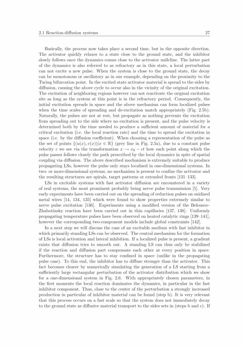
2.1 Reaction-diffusion systems 27
Basically, the process now takes place a second time, but in the opposite direction.The activator quickly relaxes to a state close to the ground state, and the inhibitorslowly follows once the dynamics comes close to the activator nullcline. The latter partof the dynamics is also referred to as refractory as in this state, a local perturbationcan not excite a new pulse. When the system is close to the ground state, the decaycan be monotonous or oscillatory as in our example, depending on the proximity to theTuring bifurcation point. In the excited state activator material is spread to the sides bydiffusion, causing the above cycle to occur also in the vicinity of the original excitation.The excitation of neighboring regions however can not reactivate the original excitationsite as long as the system at this point is in the refractory period. Consequently, theinitial excitation spreads in space and the above mechanism can form localized pulseswhen the time scales of spreading and de-excitation match appropriately (Fig. 2.5b).Naturally, the pulses are not at rest, but propagate as nothing prevents the excitationfrom spreading out to the side where no excitation is present, and the pulse velocity isdetermined both by the time needed to produce a sufficient amount of material for acritical excitation (i.e. the local reaction rate) and the time to spread the excitation inspace (i.e. by the diffusion coefficient). When choosing a representation of the pulse asthe set of points (u(x), v(x))|x ∈ R (grey line in Fig. 2.5a), due to a constant pulsevelocity c we see via the transformation x → x0 − ct how each point along which thepulse passes follows closely the path prescribed by the local dynamics in spite of spatialcoupling via diffusion. The above described mechanism is extremely suitable to producepropagating LSs, however the pulse only stays localized in one-dimensional systems. Intwo- or more-dimensional systems, no mechanism is present to confine the activator andthe resulting structures are spirals, target patterns or extended fronts [131–133].
LSs in excitable systems with fast activator diffusion are encountered in a varietyof real systems, the most prominent probably being nerve pulse transmission [5]. Veryearly experiments have been carried out on the spreading of reduction pulses on oxidizedmetal wires [14, 134, 135] which were found to show properties extremely similar tonerve pulse excitation [136]. Experiments using a modified version of the Belousov-Zhabotinsky reaction have been carried out in thin capillaries [137, 138]. Uniformlypropagating temperature pulses have been observed on heated catalytic rings [139–141],however the corresponding two-component models include global constraints [142].
In a next step we will discuss the case of an excitable medium with fast inhibitor inwhich primarily standing LSs can be observed. The central mechanism for the formationof LSs is local activation and lateral inhibition. If a localized pulse is present, a gradientexists that diffusion tries to smooth out. A standing LS can thus only be stabilizedif the reaction and diffusion part compensate each other at every position in space.Furthermore, the structure has to stay confined in space (unlike in the propagatingpulse case). To this end, the inhibitor has to diffuse stronger than the activator. Thisfact becomes clearer by numerically simulating the generation of a LS starting from asufficiently large rectangular perturbation of the activator distribution which we showfor a one-dimensional system in Fig. 2.6. With appropriately chosen parameters, inthe first moments the local reaction dominates the dynamics, in particular in the fastinhibitor component. Thus, close to the center of the perturbation a strongly increasedproduction in particular of inhibitor material can be found (step b). It is very relevantthat this process occurs on a fast scale so that the system does not immediately decayto the ground state as diffusive material transport to the sides sets in (steps b and c). If

28 Models and mechanisms
a. d.
b. e.
c. f.
Figure 2.6: LS forming from a rectangular activator perturbation of [0.02 × 0.75] on thehomogeneous ground state in an excitable two-component reaction-diffusion system (2.13) withcubic nonlinearity (compare text) in one spatial dimension. The solid and dashed lines shows uand v as a function of space for different times (t = 0, 0.1, 0.5, 1, 10 and 100, in the last image thesolution has converged). Parameters: d2
u = 10−4, d2v = 9.64 · 10−4, λ = 0.8, κ1 = −0.1, κ3 = 1,
τ = 0.1, plot region [−0.4, 0.4]× [−0.6, 0.5].
the inhibitor diffuses faster than the activator, a surplus of activator producing materialis left in the center of the structure to compensate losses by diffusion. This effect alsoconfines the structure: due to diffusive transport inhibitor will dominate at the flanksof the structure, preventing the excited state from spreading to the sides (leading to atypical dip at the side of the structure, steps c-e). As the dip itself produces a smallgradient opposed to the gradient generated by the bulk of the LS, the above effect mayrepeat itself on a smaller scale, leading to oscillatorily decaying tails as visible in thepicture (steps e-f). The oscillatory tails are typically observed when the system is closeto a Turing destabilization. According to (2.20), the minimum of the Turing nullclinelies at
kc =((κ3
d2ud
2v
)1/2 − 1d2
v
)1/2(2.21)
leading to a dominant wave length of λc = 0.13 for the parameters used to produceFig. 2.6 in good agreement with the outcome of the simulation. The simulation inFig. 2.6 can be repeated on a two-dimensional domain for the same parameters, showinga similar result. However, the width of the initial excitation as to be chosen at leastdouble as large as in Fig. 2.6 due to an enhanced diffusion when going from one- totwo-dimensional coordinates.
According to (2.20), one possibility to move further away from the Turing instabilityboundary is by increasing λ (which also implies approaching the bistable situation we
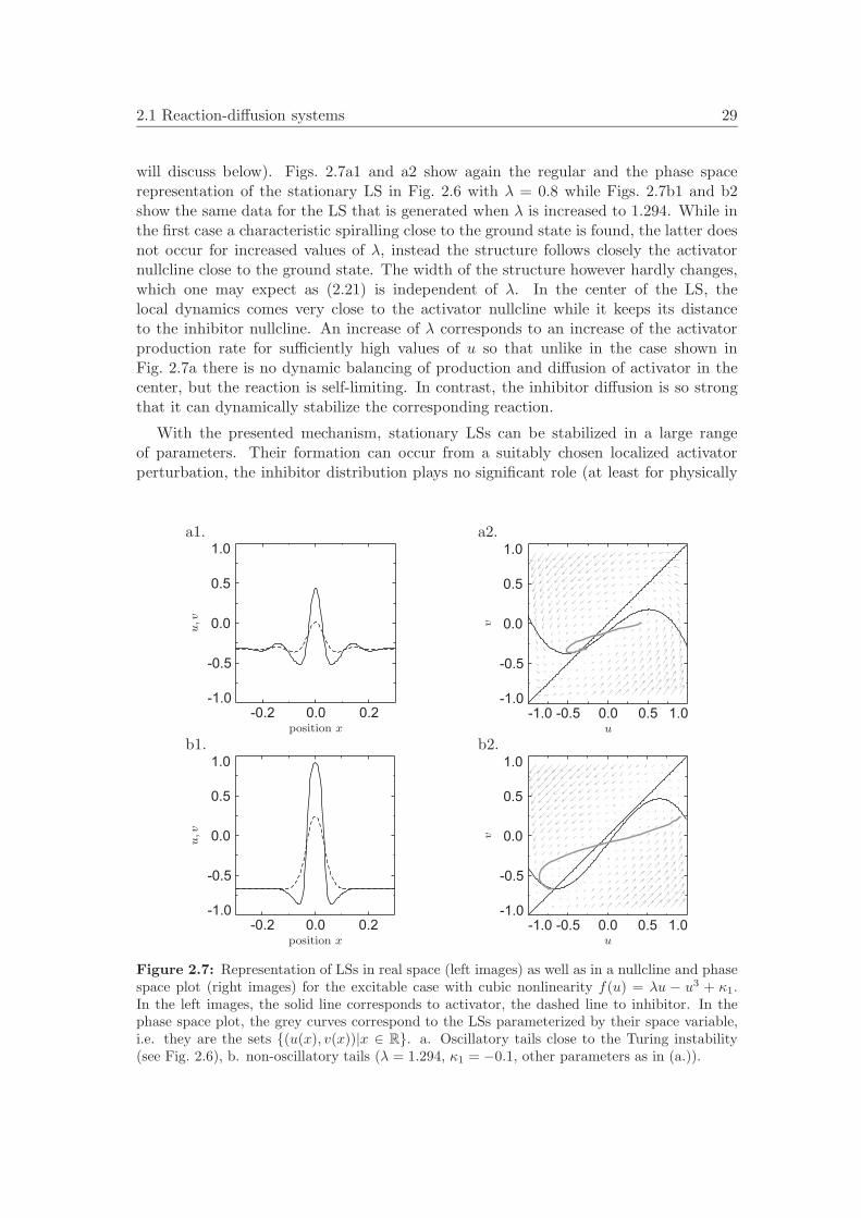
2.1 Reaction-diffusion systems 29
will discuss below). Figs. 2.7a1 and a2 show again the regular and the phase spacerepresentation of the stationary LS in Fig. 2.6 with λ = 0.8 while Figs. 2.7b1 and b2show the same data for the LS that is generated when λ is increased to 1.294. While inthe first case a characteristic spiralling close to the ground state is found, the latter doesnot occur for increased values of λ, instead the structure follows closely the activatornullcline close to the ground state. The width of the structure however hardly changes,which one may expect as (2.21) is independent of λ. In the center of the LS, thelocal dynamics comes very close to the activator nullcline while it keeps its distanceto the inhibitor nullcline. An increase of λ corresponds to an increase of the activatorproduction rate for sufficiently high values of u so that unlike in the case shown inFig. 2.7a there is no dynamic balancing of production and diffusion of activator in thecenter, but the reaction is self-limiting. In contrast, the inhibitor diffusion is so strongthat it can dynamically stabilize the corresponding reaction.
With the presented mechanism, stationary LSs can be stabilized in a large rangeof parameters. Their formation can occur from a suitably chosen localized activatorperturbation, the inhibitor distribution plays no significant role (at least for physically
a1. a2.
-1.0
-0.5
0.0
0.5
1.0
-0.2 0.0 0.2position x
u,v
-1.0 -0.5 0.0 0.5 1.0-1.0
-0.5
0.0
0.5
1.0
u
v
b1. b2.
-1.0
-0.5
0.0
0.5
1.0
-0.2 0.0 0.2position x
u,v
-1.0
-0.5
0.0
0.5
1.0
-1.0 -0.5 0.0 0.5 1.0u
v
Figure 2.7: Representation of LSs in real space (left images) as well as in a nullcline and phasespace plot (right images) for the excitable case with cubic nonlinearity f(u) = λu − u3 + κ1.In the left images, the solid line corresponds to activator, the dashed line to inhibitor. In thephase space plot, the grey curves correspond to the LSs parameterized by their space variable,i.e. they are the sets (u(x), v(x))|x ∈ R. a. Oscillatory tails close to the Turing instability(see Fig. 2.6), b. non-oscillatory tails (λ = 1.294, κ1 = −0.1, other parameters as in (a.)).

30 Models and mechanisms
diffusion lengths time scale ration τ reaction to initial condition
d2u < d2
v ≈ d2 τ < 1 formation of stable LSd2 d2
u > d2v τ 1 decay to ground state
d2 d2u > d2
v τ > 1 coexistence of LS and oscillatingbackground (Hopf)
d2 ≈ d2u > d2
v τ < 1 decay to ground stated2 ≈ d2
u > d2v τ > 1 spreading of running pulses
d2u > d2
v d2 arbitrary decay to ground stated2
u, d2v d2 τ 1 decay to ground state
initial cond. below critical nucleusd2
u d2v arbitrary decay to ground state
d2u d2
v rather arbitrary Turing destabilizationd2
u < d2v τ > 1 Hopf destabilization
d2u, d
2v d2 τ < 1 decay to ground state,
dominance of local reaction
Table 2.2: Evolution of the two-component system (2.13) with F (u, v) = f(u) − κ3v + κ1,G(u, v) = u − v, f(u) = λu − u3, λ = 0.8, κ1 = −0.1, κ3 = 1 (excitable case) and the initialcondition used in Fig. 2.6 for different values of τ and the diffusion coefficients d2
u and d2v. The
first entry corresponds to Fig. 2.6, implying d2 = 10−3.
reasonable choices) as long as the coefficient τ is small enough. However, when theparameter values leave a certain region in parameter space, the LS can lose its stabilityin several ways. First, we will have a look at the generation scenario presented inFig. 2.6 and explore how the system reacts if the parameters are changed. To thisend, we keep the initial condition fixed (thereby selecting a length scale in the system)and vary d2
u, d2v and τ . A brief overview of the following system evolution is given in
Table 2.2. If the inhibitor reacts too slow (τ becomes large), it can not follow changes ofthe activator fast enough. In most cases, the initial activator perturbation then simplydecays. However, for very large τ a Hopf destabilization may occur, causing the systemto oscillate globally. A special case is given by d2
u > d2v, as here one may also arrive at the
nerve pulse mechanism discussed above. If d2u d2
v, the inhibitor can diffuse very far andcause gradients far away from the center of the structure. This generally leads to Turingdestabilization. If both activator and inhibitor diffusion proportionally become largerand the initial perturbation stays the same, the latter may decay before a structure canform as too much material is transported away because a sufficiently large perturbation(a critical nucleus) must be present in order to allow the reaction to compensate lossesby diffusion. If both activator and inhibitor diffusion proportionally become smaller(again with the original initial perturbation), the perturbation also decays as diffusioncan not act and the domination of local reaction drives the perturbation to the groundstate.
In a second step, let us assume that a stationary stable solution has been generatedfor a given set of parameters and that starting from this initial condition one or severalparameters are varied. Basically, there are different types of possible destabilizationsand even for a concrete example a systematic classification may be difficult. We will
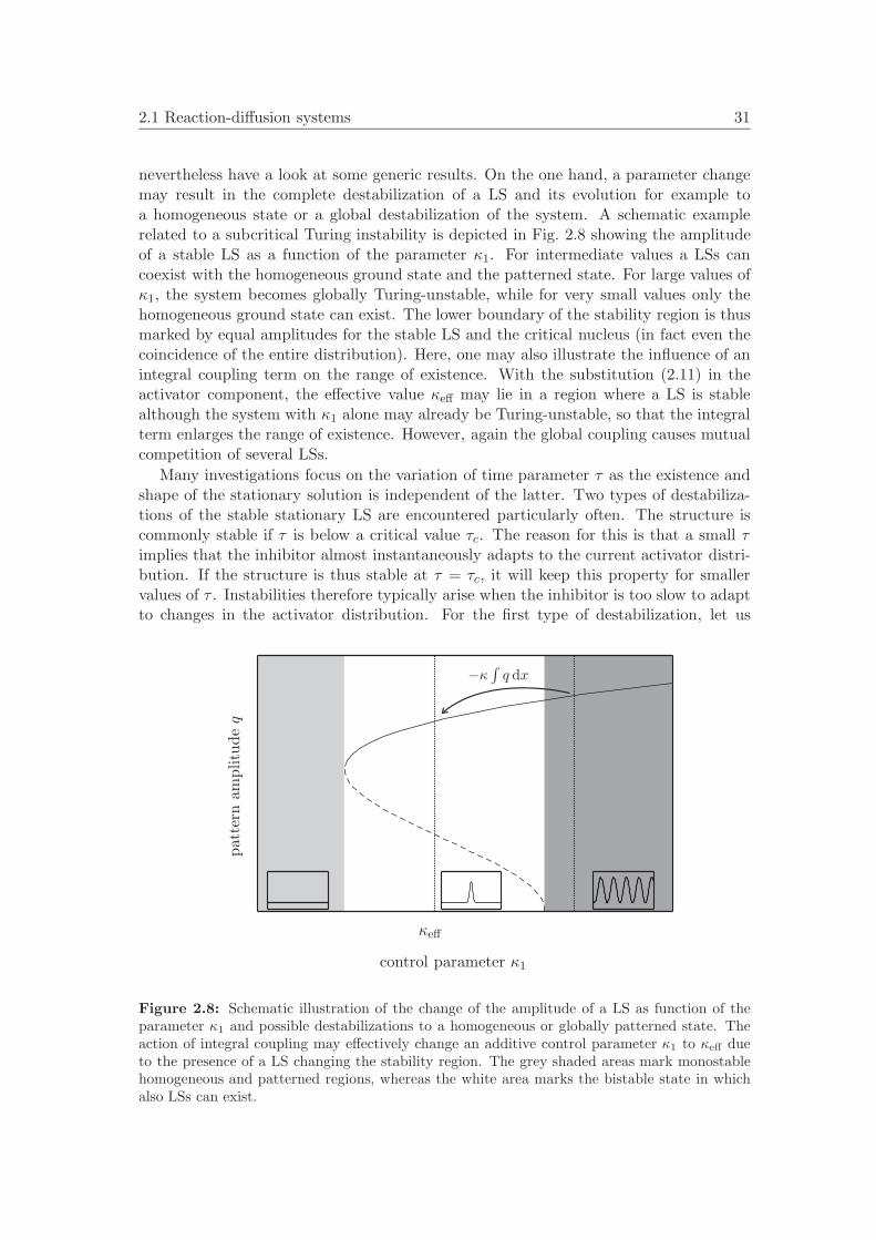
2.1 Reaction-diffusion systems 31
nevertheless have a look at some generic results. On the one hand, a parameter changemay result in the complete destabilization of a LS and its evolution for example toa homogeneous state or a global destabilization of the system. A schematic examplerelated to a subcritical Turing instability is depicted in Fig. 2.8 showing the amplitudeof a stable LS as a function of the parameter κ1. For intermediate values a LSs cancoexist with the homogeneous ground state and the patterned state. For large values ofκ1, the system becomes globally Turing-unstable, while for very small values only thehomogeneous ground state can exist. The lower boundary of the stability region is thusmarked by equal amplitudes for the stable LS and the critical nucleus (in fact even thecoincidence of the entire distribution). Here, one may also illustrate the influence of anintegral coupling term on the range of existence. With the substitution (2.11) in theactivator component, the effective value κeff may lie in a region where a LS is stablealthough the system with κ1 alone may already be Turing-unstable, so that the integralterm enlarges the range of existence. However, again the global coupling causes mutualcompetition of several LSs.
Many investigations focus on the variation of time parameter τ as the existence andshape of the stationary solution is independent of the latter. Two types of destabiliza-tions of the stable stationary LS are encountered particularly often. The structure iscommonly stable if τ is below a critical value τc. The reason for this is that a small τimplies that the inhibitor almost instantaneously adapts to the current activator distri-bution. If the structure is thus stable at τ = τc, it will keep this property for smallervalues of τ . Instabilities therefore typically arise when the inhibitor is too slow to adaptto changes in the activator distribution. For the first type of destabilization, let us
control parameter κ1
patt
ern
ampl
itud
eq
κeff
−κ ∫ q dx
Figure 2.8: Schematic illustration of the change of the amplitude of a LS as function of theparameter κ1 and possible destabilizations to a homogeneous or globally patterned state. Theaction of integral coupling may effectively change an additive control parameter κ1 to κeff dueto the presence of a LS changing the stability region. The grey shaded areas mark monostablehomogeneous and patterned regions, whereas the white area marks the bistable state in whichalso LSs can exist.

32 Models and mechanisms
a1. a2. b1. b2.
-1.0 0.0 1.0
0
20
40
60
80
100
position x
tim
et
-1.0 0.0 1.0
0
20
40
60
80
100
position xtim
et
-0.6 -0.3 0.0 0.3 1.6
0
50
100
150
position x
tim
et
-0.6 -0.3 0.0 0.3 1.6
0
50
100
150
position x
tim
et
ff
c1
c2
Figure 2.9: Instabilities of single LSs in two-component excitable systems and one spatial di-mensions. a. Space-time plots showing the activator and inhibitor distributions of an intrinsicallypropagating LS as a function of time. Note the strong asymmetry in the structure. Parameters:λ = 4.67, d2
u = 0.0015, d2v = 0.01, κ1 = −1.126, κ4 = −3.33, τ = 4, periodic boundary condi-
tions, scaling: c1 = −2.2, c2 = 2.2 (a1), c1 = −1.5, c2 = 0.6 (a2). b. Space-time plots showingthe activator and inhibitor distributions of a breathing LS as a function of time. The horizontalline marks a point of time as orientation for the explanations in the text. Parameters as in a.except for d2
u = 4.67 · 10−4, τ = 5, scaling: c1 = −2, c2 = 2 (b1), c1 = −1.5, c2 = 0.5 (b2).
assume that an asymmetric perturbation is added to the structure, for example in theform of the derivative of the LS itself. A fast inhibitor would quickly follow this defor-mation and stabilize the structure, resulting in a pure displacement. A slow inhibitorhowever can not immediately follow, so that the activator has the chance to increasematerial production at the side where no inhibitor is present. On the opposite side, theinhibitor is dominant and can locally reduce the concentration of both species. Thismechanism may produce a dynamically stabilized uniformly propagating state: a smalldisplacement may grow as with larger τ , the activator diffusion time in relation to itsinhibitor counterpart becomes smaller so that activator can spread further to the frontof the moving pulse. On the other hand, as activator and inhibitor evolution are coupledby local reactions, the displacement of their distributions can not grow arbitrarily large.
Fig. 2.9a shows a numerical example of an intrinsically propagating structure sta-bilized by the described mechanism. The corresponding bifurcation from a stationaryto a moving solution is referred to as drift or traveling bifurcation [41, 113, 143]. Inthe two-component system, a detailed numerical investigation (data not shown) whichis corroborated by different statements in the literature [99, 113, 143] turns out thatthe drift bifurcation generically occurs subcritically. In particular, there is a region ofhysteresis in which both standing and traveling state are stable. Consequently, a pertur-bation of finite size is required to switch the system from the standing to the travelingstate. One may look at the representation of a uniformly traveling pulse (parameterizedby the space variable) in the phase space of the local reaction as previously done forstationary solutions (Fig. 2.10a). It turns out that this representation yields a homo-clinic loop similar to that encountered for nerve pulse propagation (compare Fig. 2.5),showing that the mechanism causing the propagation is basically the same. For thegiven example, the decrease of d2
u with respect to d2v can be compensated by an increase
of τ until the ration of d2u and d2
v is approximately in the order of 0.1.
Experimentally, it is often hard to distinguish whether in a two-component systemone deals with fast or slow activator diffusion, particularly because the drift bifurcationoccurs subcritically. Consequently, our references [5, 14, 134, 135, 137–141] given above

2.1 Reaction-diffusion systems 33
for the “nerve pulse mode” may also belong to the above discussed mechanism. Addi-tional examples arise in planar one-dimensional gas-discharges with high-ohmic barrier[32, 144–146] which have been modeled phenomenologically on the basis of reaction-diffusion systems, and also in p-n-p-n semiconductor devices [104, 106, 147, 148].
A second type of generic destabilization is that to a “breathing” state in which theLS stays at a fixed position in space but performs periodic oscillations of its shape(Fig. 2.9b). It has been shown that for the Fitzhugh-Nagumo type of nonlinearity thistype of destabilization is preferred to the traveling destabilization over large rangesof parameters [100, 149, 150]. In the oscillatory instability a complex conjugate pairof eigenvalues of the linearization operator around the stationary solution crosses theimaginary axis while the neutral eigenmode of translation remains non-degenerate. Thelinearization of the system (2.19) around a state (u(x), v(x)) reads
(∂tuτ∂tv
)=(d2
uud2
vv
)+(λ− 3u2 −1
1 −1
)(uv
), (2.22)
with u and v denoting the derivation from the state of interest in this special case.Neglecting diffusion for a moment, we see from the linearized reaction function by acomparison with (2.15) in the case k = 0 that for τ large enough, the local system iscapable of performing self-sustained oscillations around the state (u, v).
To understand the breathing dynamics shown exemplarily in Fig. 2.9b, diffusionhas to be incorporated into the consideration. Starting with the state marked with ahorizontal line, we see both a narrow activator and inhibitor peak. While the activator
a. b.
-2 -1 0 1 2-2.00
-1.25
-0.50
0.25
1.00
activator u
inhib
itor
v
-2 -1 0 1 2-2.00
-1.25
-0.50
0.25
1.00
activator u
inhib
itor
v
Figure 2.10: Dynamics shown in Fig. 2.9 in the representation of the local reaction space assets (u(x, t0), v(x, t0))|x ∈ R, the black lines show the nullclines of the reaction functions. a.The red line is representation of the stationary propagating pulse, compare also the nerve pulsemechanism shown in Fig. 2.5. b. The blue lines (from dark to light blue) illustrate the breathingmotion of the LS, starting from the point of time marked by a dashed line in Fig. 2.9b, the timeinterval between successive lines is ∆t = 4. Note that the period length of the breathing motionis T ≈ 24.

34 Models and mechanisms
concentration in the center lies slightly above the equilibrium value relative to the valuefor the stationary LS, the inhibitor concentration is far below the equilibrium value(again in relation to the stationary LS). Both distributions are narrower than theircounterparts in the stationary solution and therefore start spreading to the sides bydiffusion, in particular the inhibitor. While the activator decreases only slightly dueto this process, the slow inhibitor increases its concentration so strongly due to thelocal oscillating dynamics of the reaction that this process can overcompensate thelosses by diffusion. This can be visualized rather well by choosing a representation inthe local phase space (Fig. 2.10b). In the course of time, there is then a surplus ofinhibitor distributed over the whole support of the LS. Eventually, the increase of theinhibitor concentration in the center stops, and two effects set in. On the one hand,the global surplus of inhibitor causes a decay of the structure especially at those pointswhere no fast activator is present, i.e. in the tails up to the flanks of the activatordistribution. Both activator and inhibitor peaks thus become narrower. Second, thelocal dynamics and the diffusive losses cause the inhibitor in the center to decay stronglywhile the activator can thereby slightly rise again, completing the breathing cycle. Asa consequence, we have an activator peak which mainly changes its width but not itsheight and an inhibitor peak alternating strongly in width and height. In the center,activator and inhibitor oscillations are in anti-phase, but the phase difference becomessmaller away from the center due to the effect of diffusion.
Many authors have numerically calculate unstable eigenvalues and the correspond-ing eigenmodes of the linearization around the stationary LS as function of the variedparameters, thereby showing that if the time constants of the system are varied, thedestabilization of the LS commonly occurs either to a traveling or a breathing state[75, 149, 151, 152]. Different excitations are theoretically possible, but the correspond-ing threshold for the bifurcation parameter usually lies so high that one of the otherbifurcations occurs before. Nevertheless, secondary destabilizations are possible. In thiscase, several instability mechanisms may come into play simultaneously. The outcomemay be different: while in some situations one of the mechanisms is so dominant thatits corresponding instability determines the system in the long-time limit, in other situ-ations a combined action is possible. In the latter case, the resulting state is a movingand breathing state in which the velocity is coupled to the shape of the LS.
In quasi one-dimensional experiments, contrary to theoretical predictions breathingphenomena have been found only rarely. An observation that may be considered as amanifestation of a modified breathing instability is rocking, i.e. a periodic shift of a LSin position on a very short length scale. This phenomenon has been found in planar dcgas-discharges with high-ohmic barrier [144, 146] as well as in p-n-p-n semiconductordevices [147, 153].
Note that concerning instabilities of LSs in two-component excitable systems, wehave considered up to now only one-dimensional examples. Theoretically the aboveinstabilities can also occur in two or more spatial dimensions. A closer look howeverreveals an important difference between drift and breathing instability. Going fromone to two or more dimensions, the stationary LS in the latter case features rotationalsymmetry. While the breathing instability is compatible with this symmetry in thesense that in the course of the instability the symmetry stays preserved for all times,the drift instability violates this symmetry in one direction while preserving a mirrorsymmetry in the orthogonal direction. This generically leads to a second instability,

2.1 Reaction-diffusion systems 35
as the following considerations show. In a potential propagating state, activator andinhibitor distribution should be shifted with respect to each other. Due to diffusion, theactivator in the front will not only spread in the propagation direction but also laterally.While this process may trigger the production of inhibitor material at the sides, thelatter is too slow to effectively confine the structure in the direction orthogonal to thepropagation direction. The result is commonly a lateral growth to a “banana-shaped”state which in the long-time limit evolves to a planar excitation front infinitely extendedorthogonal to the propagation direction, in particular when the activator diffusion islarge. The same problem is encountered when considering the nerve-pulse mode inwhich the activator diffusion is larger than the inhibitor diffusion, explaining why nerve-pulse-like phenomena in two-component systems are commonly investigated only in one
a1. a2. a3. a4.
-0.5 0.0 0.5
-0.5
0.0
0.5
position x
posi
tion
y
-0.5 0.0 0.5
-0.5
0.0
0.5
position x
posi
tion
y
-0.5 0.0 0.5
-0.5
0.0
0.5
position x
posi
tion
y
-0.5 0.0 0.5
-0.5
0.0
0.5
position x
posi
tion
y
ff
c1
c2
b1. b2. b3. b4.
-1.0 -0.5 0.0 0.5 1.0
-1.0
-0.5
0.0
0.5
1.0
position x
posi
tion
y
-1.0 -0.5 0.0 0.5 1.0
-1.0
-0.5
0.0
0.5
1.0
position x
posi
tion
y
-1.0 -0.5 0.0 0.5 1.0
0
10
20
30
50
40
position x
tim
et/
106
-1.0 -0.5 0.0 0.5 1.0
-1.0
-0.5
0.0
0.5
1.0
position x
posi
tion
y
ff
c1
c2
c1. c2. c3. c4.
-1.0 -0.5 0.0 0.5 1.0
-1.0
-0.5
0.0
0.5
1.0
position x
posi
tion
y
-1.0 -0.5 0.0 0.5 1.0
-1.0
-0.5
0.0
0.5
1.0
position x
posi
tion
y
-1.0 -0.5 0.0 0.5 1.0
-1.0
-0.5
0.0
0.5
1.0
position x
posi
tion
y
-1.0 -0.5 0.0 0.5 1.0
-1.0
-0.5
0.0
0.5
1.0
position x
posi
tion
y
ff
c1
c2
Figure 2.11: Instabilities of single LSs in two-component excitable systems and two spatialdimensions. a. Sequence showing the activator distribution u of the two-dimensional equivalentof a drift instability leading to the formation of a running planar front (times t = 4, 8, 12 and16 from 1 to 4). Parameters: λ = 4.67, d2
u = 0.002, d2v = 0.01, κ1 = −1.126, κ3 = −3.33, τ = 3,
c1 = −1. c2 = 3.5. As initial conditions, the stationary activator and inhibitor concentrationsfor lower τ were displaced by d = 0.05. b. Breathing instability: activator distribution u att = 0 and t = 6 (1 and 2), slice cut through the distribution as a function of time (3) and realpart of the critical eigenmode responsible for the bifurcation (4). Parameters as in a. exceptfor d2
u = 0.004, κ1 = −1, τ = 1.33, c1 = −1.75. c2 = 2. c. Time sequence of the activatordistribution u showing a destabilization due to a decrease of d2
u resulting in the growth of a“dentritic” pattern (1. t = 50, 2. t = 100, 3. t = 200). The last image shows the dominantmode in the destabilization explaining the branching into two new branches. Parameters as ina. except d2
u = 0.001, κ1 = −1.14, τ = 0, c1 = −2. c2 = 2.

36 Models and mechanisms
spatial dimension. The whole process of the destabilization is visualized in the sequencedepicted in Fig. 2.11a. It should be pointed out that some analytical works claim that itis possible to obtain a propagating structure in the two-dimensional case [154], however,no numerical proof was given in this case.
Breathing instabilities are indeed generically found in two-component excitable sys-tems if no asymmetric instability precedes the corresponding destabilization, a numericalexample is provided in Fig. 2.11b. For bifurcation parameters other than the time con-stant τ , modes different from the above mentioned ones may become unstable in theprimary bifurcation. A problem for the analytical treatment is given by the fact thatthe stationary distribution changes its shape before the destabilization point, althoughsome special cases can still be dealt with [96]. In Fig. 2.11c we show an example where adestabilization occurs by decreasing d2
u. Here, several modes become unstable in the bi-furcation which occurs even for τ = 0, and in our numerical example even the discretiza-tion of the active area is sufficient to break the radial symmetry of the initial condition.One slightly asymmetric mode dominates the instability in the long-time limit ratherindependent of the initial conditions (see d4). As this mode has an only weakly brokenthreefold discrete rotational symmetry, one observes characteristic branching processesin which one existing branch splits into two new ones, thereby inducing the growth of akind of “dendrite-like” pattern.
One may ask what additional mechanisms can be used to stabilize propagating LSsin the two-component system in two or more spatial dimensions. As during the decay ofthe running pulse too much material is produced at the sides of the pulse, analogouslyto the one-component case global coupling (in particular global inhibition) may helpto stabilize a single LS as described above also in the propagating case [129, 155, 156].A frequently problem however is again given by mutual competition of the LSs: non-equally shaped LSs are put into competition by global coupling, and one frequently findsthat one LS may grow in favor of the other LSs in the system, so that in the long-timelimit only one structure survives [112, 129]. At this point, one has to remark that forsymmetric initial conditions, several standing or propagating LSs can exist and interact[102, 113]. The decay due to the integral term in the considered case was found to occurso slow that one may observe interaction of the transient structures on a fast time-scale. Furthermore, there are works on two-component systems in one dimension whichindicate the generation of two stable running LSs from an asymmetric initial condition[78, 79].
In the experiment, different types of dynamical destabilizations of LSs in two-dimensional reaction-diffusion type systems have been found. On the one hand, in-trinsically traveling isolated LSs have been observed in planar dc gas-discharge systemswith high-ohmic barrier and integral series resistor [157, 158]. However, the dynamicsis overlaid by fluctuations so that stochastic data analysis methods have to be used tovisualize the intrinsic propagation (compare also Sec. 3.2.2.3 below). Breathing has sofar only been observed in bistable systems which we will discuss below.
The next point we want to address is the interaction of LSs in excitable media. Ifno global coupling is present in the system, basically an arbitrary number of remoteLSs can coexist independently. When the distance becomes smaller so that the LSsslightly overlap, one observes weak interaction during which the nature of the LSs staysessentially preserved. As we have seen from the previous examples, the decay of the LSscan be oscillatory or non-oscillatory. In the first case, one may generally expect a mixed

2.1 Reaction-diffusion systems 37
attractive-repulsive type of interaction, so that mutual lock-in of the LSs is possible,which is also observed for other types of systems. When the decay is non-oscillatory,both mixed and purely repulsive interaction is possible, see below. An understandingof the mechanisms of interaction is usually possible in terms of local transport andthe activation-inhibition-principle, as we will illustrate in the following example in twospatial dimensions.
In our two-component Fitzhugh-Nagumo-type system, we can choose the parametersin such a way that the decay of the LSs is non-oscillatory. Furthermore, choice issuch that the individual stationary LSs are stable in both one and two dimensions,making the consideration rather independent of the spatial dimension. We choose alinear superposition of two weakly overlapping LSs in two spatial dimensions as initialcondition (a slice cut through the distributions along the connecting line of the LSs isshown in Fig. 2.12a). The numerical simulation shows that in the course of time theLSs separate until they do no longer overlap. In order to understand this observation,we may plot the time derivatives ∂tu and ∂tv along the connection line of the LSs as afunction of time and space in a filled contour plot (Fig. 2.12b and c). From Fig. 2.12awhich shows u, v and in particular ∂tu in the first instant of the simulation as a thickdotted line, we may see that due to the nonlinear reaction function, close to the centerwhere the overlap of the LSs is strongest the amount of activator material starts todecrease strongly. The reason for this is that while the diffusive fluxes simply add updue to the linear diffusion operator, the production of activator is smaller than twicethe value for a single LS due to the nonlinear reaction function. Instantly afterwards,the decrease of activator concentration causes the concentration of the fast inhibitor inthe same region to drop as well. This is also illustrated by blue regions in the center ofFigs. 2.12b and c for small times, note the nonlinear color scaling. As diffusion sets in,material is transported from the sides to the depletion zone in the center to compensate
a. b. c.
-1
0
1
2
3
4
-0.5 0.0 0.5x
u,v
,∂tu
-0.5 0.0 0.5
-0.8
0.2
0
10
20
30
40
50
x
tim
et
-0.5 0.0 0.50
10
20
30
40
50
-0.3
0.045
x
tim
et
Figure 2.12: a. Activator (black) and inhibitor (red) distributions along the connection line oftwo stationary two-dimensional distinct LSs with ground state shifted to the origin (dashed lines)and their linear superposition (solid lines) as well as the resulting change ∂tu of the activatorconcentration (blue dashed line). b. and c. Resulting change ∂tu of activator concentrationand ∂tv of inhibitor concentration, resp., as contour plot depending on space and time. Thethick lines indicate the positions of the centers of mass of the LSs (in detail, solid lines markthe center of the u and dashed lines the center of the v distribution). Parameters: λ = 4.67,d2
u = 4.67 · 10−3, d2v = 0.01, κ1 = −1.126, κ3 = −3.33, τ = 0.1

38 Models and mechanisms
a. b. c.
-0.4 -0.2 0.0 0.2 0.4
-0.5
0.0
0.5
1.0
x
u,∂
tu/5· 1
0−
3
-0.5
0.0
0.5
1.0
-0.4 -0.2 0.0 0.2 0.4
xu,∂
tu/5· 1
0−
3
-0.5
0.0
0.5
1.0
-0.4 -0.2 0.0 0.2 0.4
x
u,∂
tu/5·1
0−
3
Figure 2.13: Activator distributions u of single and superposed two-dimensional LSs withoscillatory tails (dashed and solid black lines) and resulting instantaneous activator change ∂tu(grey lines) at different distances of the LSs (a. d = 0.2, b. d = 0.25, c. d = 0.3) correspondingto attraction, repulsion and stable lock-in, resp. Parameters: λ = 0.72, d2
u = 1.1 · 10−4, d2v =
9.64 · 10−4, κ1 = −0.1, κ3 = 1.
the steepening of the concentration gradients. As the inhibitor diffusion is much strongerthan the activator diffusion, the inhibitor distributions are shifted towards the center toa larger extent than the activator distribution (compare the widths of the blue regions).We have seen above that this asymmetry induces a motion of the LSs to the sides, givingan explanation for the repulsive interaction. The mechanisms works as long as the LSsoverlap, however the strength of the effect decreases with distance.
Let us now assume that the LSs have oscillatory tails. Here, aside from the abovedescribed repulsion also lock-in behavior, i.e. a mixed attractive-repulsive interaction ispossible. With our considerations for non-oscillatory tails above, the explanation of thisbehavior is rather straight forward. Non-oscillatory tails typically exhibit a monotonousevolution of the tails shape once a certain distance from the center is reached, typicallyleading to a decrease of the material concentration in the center when the LSs are closeto each other. The superposition of oscillatory tails at different distances however al-lows for a much later range of concentration values to be reached, from “constructive”to “destructive” superposition. The result of the nonlinear superposition depend onthe properties of the nonlinearity in the system, however in the first instants one maygenerally find increased production, decay or the reaction function to be in equilibrium(Fig. 2.13a-c). If the initial concentration in the center decays, one may use the sameargumentation as for the non-oscillatory case to see that the LSs increase their dis-tance. On the other hand, if production is increased, material diffuses away from thecenter to the sides. As the inhibitor diffuses stronger, a surplus of inhibitor builds upin the outer regions of the LS, causing an attractive interaction. To the best of theauthors knowledge, in reaction-diffusion systems that were considered up to now a non-oscillatory decay for interacting LSs without intrinsic velocity was always found to leadto repulsion. There are actually some situations in which a number of one-dimensionalLSs intrinsically propagating in the same direction may form a bound state or a wholepulse train with a dynamically stabilized distance of the LSs in spite of a non-oscillatorydecay [159–161]. However, it seems that the stabilization of the bound state is due toan interplay of intrinsic propagation and repulsion (i.e. a “stacking” similar to a traffic

2.1 Reaction-diffusion systems 39
jam) so that the bound state is not possible without the intrinsic propagation.Without intrinsic propagation, the number of possible interaction processes is rather
limited. Breathing LSs may be positioned at a small mutual distance so that the tailsoverlap. In this case, numerical simulations carried out by the author for the system(2.19) have shown that unless the initial phase difference of the oscillations of two LSsequals ∆φ = 0 or π, the displacement of the LSs is accompanied by a synchronizationof the phase difference taking place as long as the tails of the structures overlap to asignificant amount. If the interaction is purely repulsive, after the separation both LSsoscillate independently with their (equal) intrinsic frequency.
Propagation of the LSs for the two-component system without integral coupling isonly possible in one spatial dimension. Let us only consider such interaction processesfor which the isolated LSs are initially in a stable state, implying that they propagatewith their intrinsic velocity. Fig. 2.9a shows that in this case there is a strong symmetrybreaking of the structure just as in the nerve pulse mode depicted in Fig. 2.5 so that whentwo pulses collide, the leading activator distributions meet without a significant amountof inhibitor being present and directly merge. The resulting state is then surroundedby the trailing large inhibitor concentrations which change only on slow timescales. Asa consequence, independent of the exact diffusion constants and time scales the genericoutcome of a collision is the annihilation of the involved LSs. A potential alternativeis given if the parameters are chosen in such a way that the system is in the narrowbistability regime of standing and moving structures, in this case the merging event mayalso result in the formation of one standing structure.
We have pointed out above that using global coupling terms may stabilize isolated LSsthat are otherwise unstable in more than one spatial dimension. In [113], it was shownthat the generically subcritical drift bifurcation could be turned into a supercritical onewith the help of integral terms. In this context, collision events were simulated withsymmetrical initial conditions, exploiting the fact that initial small asymmetries (for
a. b.
position x/mm
tim
et/
s
position x/mm
tim
et/
s
Figure 2.14: Space-time plot of stacking (a.) and merging (b.) of quasi one-dimensionalrunning pulses in capillary tubes observed in a modified version of the Belousov-Zhabotinskyreaction. Bright color indicates the oxidized excited state of the medium whereas dark colorrepresents the rest state. The two depicted scenarios have been found for different concentrationsof bromate and cyclohexanedione [137].

40 Models and mechanisms
example due to numeric discretization) evolved so slow that collisions would take place ona faster timescale. In this context, scattering events, merging processes and generationof new LSs were found. As the situation can be interpreted as a special limiting case ofa three-component system, we will discuss further details in the corresponding section.
In the experiment, propagating pulses can be observed for example in thin capillar-ies. Co-propagating pulses may interact and either show stacking or merging of twosuccessive LSs while counterpropagating pulses generally annihilate in good agreementwith our considerations above ([137, 138], see also Fig. 2.14). Mutual annihilation wasalso observed for propagating pulses on oxidized metal wires [135].
2.1.2.2 The bistable case
Looking at the literature on two-component reaction-diffusion systems, most works focuson the excitable case. Nonetheless, stable LSs can exist in two-component bistablesystems without global coupling as well. Two-component bistable systems allow forthe generation of two types of LSs, domain solutions as well as structures generatedaccording in the “excitable mode”. The existence of the latter type of structure is dueto the fact that the excitable and bistable case show strong similarities concerning thephase flow and the topology in those parts of the local phase space which are relevant forthe formation of LSs. However, some differences arise as we will explain in the following.
We have seen above that bistable one-component systems may exhibit domain-typesolutions which are however generally unstable or marginally stable if no mechanismslike global coupling are present to stabilize the domain size. The latter are potentiallyundesired to avoid mutual competition of the LSs. Stability considerations for domainsolutions in two-component systems can be treated in analogy with the one-componentcase. To this end, Eq. (2.5) for the two-component case is extended to
q(x, t) = qf (x− p1(t)) + qf (p2(t) − x) − q2 + r(x, t) (2.23)
with qf denoting the unperturbed front solutions, and evolution equations for the frontdistance are derived using singular perturbation analysis. The free front velocity c canbe determined by transforming the system into a moving frame, directly yielding
c = − H(q2) −H(q0)〈ux|ux〉 − τ〈vx|vx〉 with H(q) =
u∫u0
f(s) ds− uv +12v2. (2.24)
The distance of the interacting fronts is then a result of the intrinsic front dynamics andthe front interaction. For τ = 0, a complete analytical solution was given in [127] whichreads
∂td21(t) = −2c+ F (d21(t)) with F (d) = a1 exp(−b1d) + a2 exp(−b2d(t)). (2.25)
The coefficients a1, a2, b1 and b2 depend on the system parameters and one generallyfinds b1 > b2 > 0. While details are given in [127], we just want to state the result

2.1 Reaction-diffusion systems 41
that one may distinguish three cases schematically depicted in Fig. 2.15. First, inthe case f ′(u2) < d2
u/d2v − 2du/dv one has a1 < 0 < a2 and the front interaction is
asymptotically repulsive (note that the first summand in the interaction force dominatesfor large distances). Even if there is a c leading to a stationary state according to (2.25)(corresponding to an intersection point of the black and the grey line in Fig. 2.15a), thelatter is unstable. Second, for d2
u/d2v +2du/dv < f ′(u2) < d2
u/d2v +2du/dv the coefficients
a1 and a2 are complex and the interaction varies between repulsion and attraction withthe front distance. Here, both stable and instable lock-in points may be possible foreither sign of c (Fig. 2.15b). Third, for d2
u/d2v +2du/dv < f ′(u2) < 1 there is a1 > 0 > a2
and the fronts are attracting asymptotically. Here, a stable lock-in is possible when thesign of c is positive (Fig. 2.15c). Note that a generalization to the case of finite τ ispossible and yields qualitatively similar results as long as τ < 1 (then, the denominatorof (2.24) remains positive). In particular, when considering the case of oscillatorilydecaying fronts (Fig. 2.15b), the mechanism responsible for the lock-in behavior is thesame as for oscillatory tails of LSs in excitable system discussed above. In contrast, whenlooking back at the one-component case, by linearizing (2.2) around the ground state forc = 0 one may directly see that for a positive diffusion coefficient and a stable groundstate (meaning a positive prefactor in the linearized reaction function) no oscillationsclose to this state are possible so that the above lock-in mechanism can not work inone-component systems. Further analytical details on the formation of domains can eg.be found in [127, 162].
While the above considerations show that the extension from one to two componentsenables the formation of stable domain structures, the latter are found only seldom andeven in their range of existence they are very susceptible to perturbations. The reasonfor this is that in domain structures, a rather weak overlap of two fronts in the centralregion has to compensate for the intrinsic motion of the individual fronts. The absolutevalue of the front velocity therefore has to be rather small as well. However, an equalityof the upper and the lower state according to the dominance rule (2.24) is not the usual
a. b. c.
distance d21
forc
eF
(d21)
distance d21
forc
eF
(d21)
distance d21
forc
eF
(d21)
Figure 2.15: Schematic illustration of the possibility of two fronts to form a domain state. Thefigures show the interaction force F (d) according to (2.25) for large distances a. for repulsion ofthe fronts, b. for mixed attractive-repulsive behavior, c. for attraction of the fronts. The greyline marks a value of 2c for which intersection points with the interaction function are possible,corresponding to stable and instable lock-in distances of the two fronts.

42 Models and mechanisms
a. b. c.
-1.0 -0.5 0.0 0.5 1.0
0
250
500
750
1000
position x
tim
et
-1.0 -0.5 0.0 0.5 1.0
0
0.5
1
1.5
position xtim
et/
106
-1.0 -0.5 0.0 0.5 1.0
0
250
500
750
1000
position x
tim
et
ff
−c1
c1
Figure 2.16: Formation of one-dimensional LSs in the form of wide domains by locking oftwo fronts with oscillatory tails. a. The front velocities are too high (κ1 = 0.01), causing thesystem to switch to the upper state. c. The front velocity is low enough (κ1 = −10−5) so thatthe oscillatory tails can lock in to form a stable domain. c. The negative front velocity is toohigh (κ1 = −0.01) so that the tails can not prevent the front from collapsing. Instead of thesystem switching to the low state, three stable narrow LSs are created during the process. Otherparameters: λ = 1.294, d2
u = 10−4, d2v = 9.64 ·10−4, τ = 0, κ3 = 1, scale c1 = 1, initial condition:
superposition of two standing fronts found for κ1 = 0 with a distance d = 0.4.
case so that the front velocities are often too large to allow for the formation of anequilibrium state according to (2.25). There is however a second possibility to formLSs via the excitable mechanism also in the bistable scenario which is encountered inmost cases. We will illustrate the idea using a numerical example. During our studyon excitable systems above, in Fig. 2.7 we have chosen κ1 = −0.1 and have induced atransition from oscillatory to non-oscillatory tails by going from λ = 0.8 to 1.294. Asλ > 1 in the latter case, by moving κ1 to zero and keeping λ fixed we may turn theexcitable system into a bistable one. In the bistable case, standing or moving frontsolutions exist in a large range of parameters and can easily be found numerically byusing step functions as initial conditions. For our choice of parameter, these fronts haveoscillatory tails and hence should be suitable to produce a front-antifront domain viathe above mechanism. The front velocity can be controlled via κ1, the case κ1 = 0corresponds to stationary fronts as upper and lower state are equal.
In Fig. 2.16a, we choose an initial condition in which the oscillatory tails weaklyoverlap in the central region by linearly superposing two isolated fronts and choose apositive κ1 = 0.01 implying the dominance of the upper state. Although the front veloc-ity is rather low, we find that it is still so high the oscillating tails can not compensatethe motion and the system is globally switched to the upper state. In b. we chooseκ1 = −10−5, implying a very weak dominance of the lower state. In this situation, theinteraction can compensate the front motion and a stable domain structure is formed.Moreover, the simulation shows that there is indeed a finite interval of front velocitiesover which this state can be generated although the region of existence is very smalland very small perturbations are sufficient to destroy the integrity of the domain struc-ture. Finally, in c. with κ1 = −0.01 the lower state is too dominant for a domain toform, however instead of switching the system to the low state, several narrow LSs aregenerated which form a stable cluster. In contrast to the wide domain, the narrow LSscan not be considered as weak superposition of two front solutions. For other initialconditions, also other numbers of LSs as well as isolated LSs can be generated. They

2.1 Reaction-diffusion systems 43
are much more robust to perturbations and exist also in the region where the domainsare possible.
An explanation for the two types of structures is given by the representation in thereaction phase space (Fig. 2.17). The domain structure shown in Fig. 2.17b correspondsto an heteroclinic orbit connecting the two stable fixed points of the local dynamics.In contrast, by comparing the narrow structure in Fig. 2.17c with the excitable caseshown in Fig. 2.7b we find that the narrow LS can be considered to be created viathe excitable mechanism in spite of the bistability of the system. In other words, theexistence of a second fixed point corresponding to the upper state plays no role as longas the phase space below qualitatively agrees with the excitable case as the inhibitordiffusion prevents the system from locally coming close to this point anyway. We maytherefore apply or arguments from the excitable case to the bistable case as well as longas the structures are formed via the excitable mechanism. Indeed, it was possible toreproduce basically all dynamical phenomena from the excitable case in the bistablesituation as well (data not shown) whereby in all situations the LS corresponded to theexcitable situation. In contrast, it was not possible to produce dynamic destabilizationsof the domain structures that did not lead to an immediate decay.
In the experiment, bistable systems have been considered in the form of theferrocyanide-iodate-sulfate reaction in gel reactors for which both two- [67] and four-component models [87] have been proposed. Observations include domain states whichgrow in time and eventually perform periodic oscillation which however are related tointeractions of the domain state with the system boundaries [67]. Also a self-replicationscenario has been found in which domains grow and finally break up into several new do-mains so that a characteristic average domain size stays preserved in the course of time[163]. It should be pointed out that experimentally no isolated stable stationary domainshave been observed, which is in good agreement with our theoretical considerations onthe stability of these structures.
a. b.
-1.0
-0.5
0.0
0.5
1.0
-1.0 -0.5 0.0 0.5 1.0component u
com
ponen
tv
-1.0
-0.5
0.0
0.5
1.0
-1.0 -0.5 0.0 0.5 1.0component u
com
ponen
tv
Figure 2.17: Representation of LSs in a nullcline and phase space plot for the bistable case:a. domain structure corresponding to that shown in Fig. 2.16b, b. structure formed via the“excitable mechanism” corresponding to a single structure as formed in Fig. 2.16c.

44 Models and mechanisms
2.1.3 Three-component systems
Up to now, we have tried to build up a systematic description of reaction-diffusionsystems on the number of reacting components and the spatial dimension. In one-component systems a rather complete description is available, and also in two-componentsystems the classification according to the criterion of excitability and bistability worksrather well. Both cases turn out be be rather closely connected as the topology of thephase space is similar in the relevant parts. Going to three- or even more-componentsystems, up to now no systematic investigations have been carried out and consequentlyno general statements on the existence of LSs exist. A central problem in this contextis that in two-component systems, the mechanism of the formation of LSs is closelyconnected to the existence of a loop or at least semi-loop in the local phase space sothat production could be compensated by diffusion. While one may speculate thatthis principle will remain of central importance for systems with more components, thecomplexity of the local phase space alone may increase so vastly for three componentsthat a systematic access appears rather difficult.
Due to these problems, we will not make an attempt towards a possible classifica-tion here. Instead, we will look back at the findings in two-component systems and askwhat types of dynamics were not possible in these systems. In one dimension, we havefound that intrinsic propagation and breathing are possible, thus allowing for a numberof interaction phenomena. However, the possible outcomes of interaction processes arerather limited. Furthermore, propagating structures could be generated only in subcriti-cal bifurcations. In two and more dimensions, propagation was not possible unless globalcoupling was used, thereby greatly reducing the number of possible dynamical processes.A brief overview is on these aspects given in Table 2.3. All observations are related toone essential point. Propagation demands a symmetry breaking that can be realized inreaction-diffusion systems of the discussed type by a delayed reaction of the inhibitorwith respect to the activator. Stabilization of a LS on the other hand demands the op-posite situation: a fast reaction of the inhibiting component. Both requirements can be
exi-stence1 LS
exi-stencen LSs
driftbif.sub-criti-cal
driftbif.su-per-criti-cal
brea-thing
osci-llatingtails
1 comp. monost. n n n n n n1 comp. bistable n n n n n n1 comp. bist. integral y n n n n n2 comp. 1D y y y n y y2 comp. 2D y y ? ? y y2 comp. 2D integral y n y y y y3 comp. y y y y y y
Table 2.3: Summary of the possible existence and observability of different important phenom-ena in the reaction-diffusion systems investigated in this work.

2.1 Reaction-diffusion systems 45
realized in a non-contradictious way only in one spatial dimension. In three-componentsystems, the two tasks of the inhibitor can be split up to be taken over by two sep-arate components, a fast and a slow one. The fast component (with a long diffusionrange) may confine the structure while the slow one may control potential bifurcations.A straight-forward extension of the two-component extension Fitzhugh-Nagumo typesystem is given by [38]
∂tu
τ∂tvθ∂tw
=
d2
u 0 00 d2
v 00 0 d2
w
∆u
∆v∆w
+
λu− u3 − κ3v − κ4w + κ1
u− vu− w
, (2.26)
and the stationary two-component solutions for u and v can be re-obtained by the choiceλ → λ+ κ4, dw = 0. For θ sufficiently small and d2
u d2v, inhibitor keeps surrounding
the LS, and the previously presented subcritical bifurcations turn into supercritical onesif induced by a change of θ (more analytical details on this point are given in the nextchapter). In particular for θ = 0, w adapts instantaneously to u and the solution ofd2
w∆w − w = −u reads
w(x, t) =∫G(x,y)u(y, t) dy (2.27)
where G is an appropriate Green function being a weak solution for the inhomogeneouslinear differential equation d2
w∆w − w = −δ(x) in the domain of interest. In one di-mension on an infinite domain, the Green function for the problem of interest is givenby
G(x, y) =1
2dwexp
(− |x− y|
dw
), (2.28)
showing that for θ = 0 the third component acts like an integral coupling with a kernelof limited range. In some sense, the previously discussed global coupling can thereforebe considered to correspond to a stabilizing component with infinite diffusion length.
With the three-component extension (2.26), stable propagating LSs are possible inall finite numbers of spatial dimensions and the propagation velocity can take values ina continuous interval from zero to a finite value. For very small velocities of the LSs,only the tails of the LSs overlap when two or more LSs come close to each other. Asthe coupling structure of the system (2.26) is linear in both inhibitors, the interactionmechanism presented in Figs. 2.12 and (2.13) can be directly generalized, so that oneeither finds repulsion (i.e. scattering events) or a potentially a lock-in in the case ofoscillatory tails if the velocity is high enough to overcome an initial repulsion for largedistances. The two cases are depicted in Figs. 2.18 and 2.19, respectively, the centraldifference in the initial conditions is the time constant τ which is larger in the secondcase and thus causes a higher intrinsic velocity.
When the interacting LSs however approach each other up to a distance where theircores themselves overlap (which is the case for intrinsic high velocities), one generallyobserves phenomena where the structure of the individual LS does not stay preserved.Typically, in this case generation and annihilation of LSs occurs. An outcome of such a
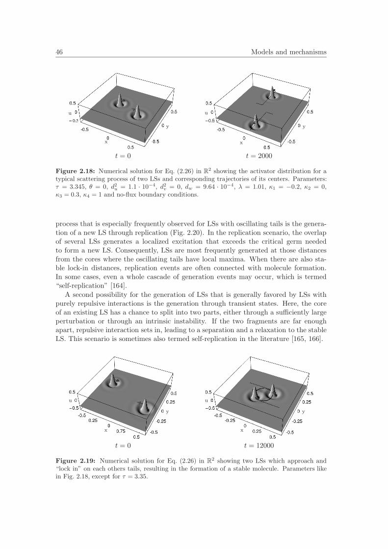
46 Models and mechanisms
x
y
u
x
y
u
t = 0 t = 2000
Figure 2.18: Numerical solution for Eq. (2.26) in R2 showing the activator distribution for a
typical scattering process of two LSs and corresponding trajectories of its centers. Parameters:τ = 3.345, θ = 0, d2
u = 1.1 · 10−4, d2v = 0, dw = 9.64 · 10−4, λ = 1.01, κ1 = −0.2, κ2 = 0,
κ3 = 0.3, κ4 = 1 and no-flux boundary conditions.
process that is especially frequently observed for LSs with oscillating tails is the genera-tion of a new LS through replication (Fig. 2.20). In the replication scenario, the overlapof several LSs generates a localized excitation that exceeds the critical germ neededto form a new LS. Consequently, LSs are most frequently generated at those distancesfrom the cores where the oscillating tails have local maxima. When there are also sta-ble lock-in distances, replication events are often connected with molecule formation.In some cases, even a whole cascade of generation events may occur, which is termed“self-replication” [164].
A second possibility for the generation of LSs that is generally favored by LSs withpurely repulsive interactions is the generation through transient states. Here, the coreof an existing LS has a chance to split into two parts, either through a sufficiently largeperturbation or through an intrinsic instability. If the two fragments are far enoughapart, repulsive interaction sets in, leading to a separation and a relaxation to the stableLS. This scenario is sometimes also termed self-replication in the literature [165, 166].
x
y
u
x
y
u
t = 0 t = 12000
Figure 2.19: Numerical solution for Eq. (2.26) in R2 showing two LSs which approach and
“lock in” on each others tails, resulting in the formation of a stable molecule. Parameters likein Fig. 2.18, except for τ = 3.35.

2.1 Reaction-diffusion systems 47
x
y
u
x
y
u
t = 0 t = 425
Figure 2.20: Numerical solution for Eq. (2.26) in R2 demonstrating the generation of a new
LS through “replication”. Parameters like in Fig. 2.18, except for τ = 3.47.
Similar to generation, there are two scenarios for the annihilation of LSs, one againpreferred by LSs with mixed, the other one by such with purely repulsive interaction.The first case is called annihilation by extinction (see Fig. 2.21). The cores of twocolliding approach each other until they feel the presence of inhibitor material in thetail around the other core. The fast inhibitor in the tail starts reducing the surplus ofactivator on its side of the core while the inhibitor pursuing the core reduces the activatoron the opposed side. As the activator has no possibility to keep a stable distance fromthe inhibitor, this mostly leads to a decay of all colliding LSs.
In the repulsive case, annihilation of two LSs usually occurs via merging. As ontheir leading sides the LSs have no regions of increased inhibitor concentration due tooscillatory tails at high velocities the activator distributions may come close withoutsuffering significant losses. Depending on the relation of local reaction and diffusion,either the merged state decays as a whole (as typical for the nerve pulse case) or relaxesto a stable state with approximately the extension of the merged state, which is a singleLS. The reason why the survival of a single LS is more likely than in the nerve pulse
x
y
u
x
y
u
t = 0 t = 528
Figure 2.21: Numerical solution for Eq. (2.26) in R2 demonstrating the annihilation of two
fast LSs in a head-on collision. Parameters like in Fig. 2.18, except for τ = 3.59.

48 Models and mechanisms
case is because the asymmetry of the structure is usually not as large. For reasons ofcompleteness one should mention that merging can also happen for LS with mixed-typeinteractions, although it is not very likely.
We want to mention that the above explanations on interaction processes partly relyon the fact that the inhibitor components are not coupled in a nonlinear fashion. Sucha nonlinear coupling may produce a variety of new effects [54, 167]. Further studies onthe dynamics and interaction of LSs in three-component systems can for example befound in [55, 164, 168–170].
There are a number of experimental systems that reproduce the theoretically pre-dicted phenomena for three- and more-component systems. A significant coincidence isfound for planar dc gas-discharge systems with high-ohmic barrier. Here, all phenomenadepicted in Figs. 2.18-2.21 can be observed [2, 55, 171–173]. Examples for phenomenarelated to weak interaction during which the nature of the LSs stays preserved (scat-tering, bound states) are given in the next chapter. The experimental counterpart of ageneration event due to the overlap of several LSs as shown in Fig. 2.20 is depicted inFig. 2.22. A breathing type of dynamics was found for LSs in a Belousov-Zhabotinskyreaction dispersed in a flat layer of Aerosol micro-emulsion [69], in this case the reactionwas modeled using both three- and four-component systems. Intrinsically propagat-ing elongated concentration pulses and their interaction (collision, interpenetration andannihilation) were observed for the catalytic oxidation of CO using O2 on platinumsurfaces under low-pressure conditions [6]. A three-component model was found to re-produce these phenomena [174], however calculations were carried out just in one spatialdimension.
At the end of the section on reaction-diffusion systems, we again want to pointout that while a large variety of different reaction-diffusion was investigation also withrespect to LSs (Table 2.1), most works do not aim at obtaining generally applicable
a. b.
- 4
- 2
024
420- 2- 40
20
40
60
80
0
20
0
0
0
x/mm
y/m
mj/
Am
−2
j/A
m−
2
- 4
- 2
024
420- 2- 40
20
40
60
80
0
20
0
0
0
x/mm
y/m
mj/
Am
−2
j/A
m−
2
Figure 2.22: Experimentally observed generation of a LS in the form of a current filamentfound in a two-dimensional planar dc gas-discharge system with high-ohmic barrier. The imagesshow the average current density distribution in the discharge plane recorded with an exposuretime texp = 0.2 ms. The time interval between the two images (a.) and (b.) is 104 ms [2, 55].Note the analogy to the numerically obtained result in Fig. 2.20.

2.2 Ginzburg-Landau equations 49
mechanisms. Implicitly or explicitly however, the above presented mechanisms alwaysplay an important role. A very interesting aspect that we have not treated here (butconcerning which related works are listed in the table) is the influence of cross-diffusion.
2.2 Ginzburg-Landau equations
Ginzburg-Landau (GL) equations are complex field equations without convection terms.The name originates from works by Ginzburg and Landau on superconductivity [175],where the first GL equation appeared. Nowadays, this class of nonlinear wave equationsdescribes a large variety of systems, for example in optics, Bose-Einstein condensation,liquid crystals and even string theory (see [176] and references cited therein).
In most typical applications of the GL equation the underlying system exhibits fastoscillations, for example with a gigahertz frequency in nonlinear optical systems, whereasthe observed times scales for patterns are considerably longer. Hence, a natural approachis to consider a slow envelope of the wave and to make the ansatz
E(x, t) = E(x, t) exp(iωt+ iϕ(x, t)
)+ c.c., (2.29)
where for simplicity a scalar electrical field is considered. The enveloping amplitude Eand the phase ϕ are considered as slow functions on the time scale 2π/ω of the un-derlying oscillations. The GL equation describes the evolution of the complex scalarq := E exp(ıϕ). This also matches the experimental observations, where detectors mea-sure only quantities averaged over the fast timescales.
The most frequently encountered cubic version of the GL equation, first phenomeno-logically introduced by Newell and Whitehead [177], reads
∂tq = (dr + idi)∆q + lrq + (cr + ici)|q|2q. (2.30)
Here di and ci describe linear dispersion and nonlinear frequency shifts of the underlyingwave, the other coefficients result from dissipative effects. The parameters lr and craccount for linear and nonlinear gain at the central frequency, the “diffusion” termdr∆q accounts for spectral filtering [34].
Aside from the usual translational invariance in space, Eq. (2.30) is invariant underphase shifts of q → q exp(iϕ) (gauge symmetry). This simply reflect the fact that therepresentation (2.29) must be invariant under arbitrary time shifts and therefore anyconstant phase can be added to ϕ(x, t). That is also the reason why Eq. (2.30) containsno second order powers in q and only one of four possible third order products, theother terms do not possess the required symmetry. This aspect can also be understoodas follows: when a system oscillates with a frequency ω, nonlinearities will generatehigher (multiple) harmonics. If one is interested in the behavior of the original waveamplitude, only such parts of the nonlinearities may be considered which leave theoriginal frequency unaltered.
There are two basic ways how a GL equation can be obtained. In a number of systemsa rather straightforward derivation is available, for example by starting from the Maxwell

50 Models and mechanisms
equations in optic systems. Using the paraxial approximation, these equations can becast into the so-called paraxial wave equation, which in three spatial dimensions reads
∂zq(x, t) = − i
2k
(∆⊥ + k2χ
)q(x, t). (2.31)
Here, k is the wave vector of the fast-oscillating electromagnetic field and z denotesthe main propagation direction. The complex dielectric susceptibility χ depends on theaveraged electrical field, therefore one immediately obtains a generalized GL equationwhen assuming χ = χ(|q|2) and identifying z = t. Optical systems with saturablenonlinearities often lead to a GL equation of the form [178, 179]
∂tq = (dr + idi)∆q + f(|q|2)q,f(|q|2) = lr +
sr + isi
1 + c|q|2 .(2.32)
The above type of nonlinearity can for example be derived by considering the Maxwell-Bloch equations for a laser resonator with a fast medium. After an elimination of thefast atomic variables the corresponding model equations can be cast into the form [180]
∂tq = (Dr + iDi)∆q + (lr − β)q +pq
1 + |q|2/Ig ,
∂tβ = γ(β0 − β(1 +
|q|2Is
)),
(2.33)
where q represents the envelope of the electric field and β is a measure for the saturationof the absorber with a maximum value β0. The coefficientγ is the relaxation rate of theabsorber and Ig and Is are gain and absorption saturation intensities (see also [181]).By neglecting the inertia of the absorber (γ 1), from (2.33) one obtains the Ginzburg-Landau type equation
∂tq = (Dr + iDi)∆q + lrq +pq
1 + |q|2/Ig − βq
1 + |q|2/Is (2.34)
which basically is a special version of (2.32) as all local terms contain only real coefficient,meaning that they are dissipative in nature. While some works directly use saturablefunctions, others expand the nonlinearity in terms of |q|, thereby arriving at a cubic or,more general, quintic GL equation
∂tq = (dr + idi)∆q + lrA+ (cr + ici)|q|2q + (qr + iqi)|q|4q, (2.35)
which plays a particular role for LSs. Note that while any function f(|q|2) than canbe Taylor-expanded may produce a decomposition as in (2.35) and thus it is sometimes

2.2 Ginzburg-Landau equations 51
argued that (2.35) can be considered as a generic nonlinearity, an agreement with asaturable nonlinearity as in (2.32) is only given if |q| does not exceed a certain magnitude.
The second way of obtaining a GL equation is rather indirect and demands a numberof transformations and simplifications to bring the dynamic system to its normal formnear the instability threshold. In this context, q(x, t) is a slow order parameter, theonset of instability is described by the term lrq and the nonlinear terms result from anexpansion of the nonlinearity around the stationary solution q = 0. Usually in thesecases at most a qualitative comparison with the experiment is available. Note alsothat LSs are large-amplitude structures generated in subcritical bifurcations, a separatejustification of the amplitude expansion is therefore required. Concrete examples of thederivation of GL equations can for example be found in [182, 183] for Rayleigh-Benardconvection, in [184–187] for optical systems and in [188, 189] for chemical systems. Arelation to experiments on binary liquids was pointed out in [7, 190, 191]. GL-typeequations in combination with additional equations are the basis for example for modelsfor oscillons [192] in vibrated granular media.
While many different extensions and variations of the cubic GL equation exist, wefirst restrict ourselves to the above introduced systems with one scalar amplitude. Wewill also leave behind the connection of the GL equation to a concrete physical systemand consider q(x, t) as the only quantity of interest.
2.2.1 The formation of LSs
Formally, Eq. (2.30) can be considered as a hybrid structure of the classical nonlinearSchrodinger (NLS) equation
i∂tq + di∆q + ci|q|2q = 0 (2.36)
obtained in the limiting case dr = lr = cr = 0 and a reaction diffusion equation
∂tq = dr∆q + lrq + cr|q|2q (2.37)
obtained for di = ci = 0. Eq. (2.37) allows real solutions and is sometimes also referredto as a real Ginzburg-Landau equation.
Close to the individual limiting cases, one may try to understand the formation ofLSs as a perturbation of the limiting case. The NLS equation is conservative and canbe derived from a Hamiltonian function
H :=∫Ω
(di
2|∇q|2 − ci
4|q|4)
dnx, (2.38)
so that the energy is only redistributed in space but not produced or dissipated in thesystem. Localized solutions exist if dici > 0, i.e., when the contributions of the dispersionand nonlinearity are opposed to each other. The central mechanism for the formation ofclassical solitons in the NLS equation is the balance of dispersion by nonlinear effects.In Fourier space a soliton can be represented as a wave packet that would decay in the

52 Models and mechanisms
sole presence of dispersion due to the different velocities of the individual frequencycomponents. Due to the nonlinear frequency shift the velocities are matched exactly, sothat the packet propagates as a whole.
In one spatial dimension the solitons are stable and the NLS equation possesses aremarkable property: it is completely integrable via the inverse scattering technique [18].This property is unique, when extending the NLS equation by higher order or saturablenonlinearities, integrability breaks down although soliton solutions are still possible. Inparticular, for initial conditions close to a stable soliton the extraneous energy is radiatedaway. In two and three dimensions the solitons of (2.36) are unstable and can collapse(meaning in this special context that they evolve to a singularity in finite time). Forinstance, in three dimensions the collapsing solution asymptotically obeys the scalingrelation
|q(x, t)| =1√t0 − t
f(x√t0 − t
), (2.39)
and blows up to a singularity at t = t0, the latter time being determined by the initialconditions [193]. In a more general quintic Schrodinger equation the collapse can bestopped for large amplitudes where higher nonlinearities become important. In thiscase stable solitons exist also in several spatial dimensions.
Contrary to the above “wave” explanations, the solution of the dissipative reaction-diffusion Eq.(2.37) can best be understood in terms of local transport of material. Forlr > 0 material is produced by the linear term and diffuses away due to the term dr∆q.The production usually has a nonlinear cut-off by the term cr|q|2q with cr < 0. Thereforethe local concentration of matter can not increase indefinitely.
In order to see that the GL equation generically is different from both reaction-diffusion and nonlinear Schrodinger equation, one may rewrite (2.35) in terms of thereal and imaginary part, yielding (with q = a+ ib)
∂ta = dr∆a− di∆b+ lra+ (a2 + b2)(cra− cib) + (a2 + b2)2(qra− qib),
∂tb = di∆a+ dr∆b+ lrb+ (a2 + b2)(cia+ crb) + (a2 + b2)2(qia+ qrb).(2.40)
This system can formally be considered as a reaction-diffusion system with a complicatednonlinearity and a general (non-diagonal) diffusion matrix. One should note howeverthat the “cross-diffusion” terms have conservative nature and do not describe any realtime-irreversible diffusion. This fundamentally changes the qualitative properties of thefull equation with respect to the two extreme cases. The cross-diffusion term is easilyunderstandable in the frequency image, however the effect of classical diffusion thenbecomes difficult to understand.
Let us start with some necessary conditions for the existence of LSs. Eq. (2.40)shows that the growth rate of a homogeneous perturbation of the ground state q = 0is directly given by lr, hence the linear stability of the background q = 0 immediatelyrequires lr < 0. In the case lr > 0, the background becomes unstable, but for cr < 0another homogeneous state can become stable instead. Generally, the latter case maybe referred to as supercritical GL equation as a continuous transition from one stateto the other can be induced via a change of lr. There is only one special type of LSpossible in this situation, the Nozaki-Bekki shock-hole pair, which we will discuss below.

2.2 Ginzburg-Landau equations 53
Another conclusion of the coefficients can immediately be found by considering a smallperturbation consisting of an extremely narrow spike. In the region of the spike, the“diffusion” terms will dominate all other terms, and a negative dr would lead to a furthergrowth of the spike. From this we obtain dr > 0 for the stability of the background.Perturbing the ground state q = 0 against plane waves with the wave vector k (a goodstarting point is provided by (2.40)) yields the trace stability criterion
−drk2 + lr < 0 (2.41)
and the determinant criterion
(lr − drk2)2 + dik
4 = (d2r + d2
i )k4 − 2lrdrk
2 + l2r > 0. (2.42)
As a result, we see that for dr > 0, lr < 0 both stability criteria hold and the dominantwave number is always zero. As LSs should exist on an homogeneous background, theremust be a “driving” effect opposing the local decay of the solution. For lr < 0 this effectmust come from the third-order term, or more exactly from its real part, so we have torequire cr > 0. Then, the highest-order terms should cause a saturation, so one mayrequire cr > 0, qr < 0. This situation in which most results on LSs are obtained can bereferred to as subcritical GL equation. We can now see that in this situation there isone “driving” effect, associated with the constant cr, which is opposed by two or three“damping” effects, associated with dr, lr and qr. In order to quantify this aspect ina better way, motivated by the classical NLS equation one may define a local energydensity ρ = |q|2 and an impulse density m = 2diIm(q∗∇q). The local evolution of ρ inthe quintic case is given by
∂tρ+ ∇ · m = S = dr(q∆q∗ + q∗∆q) + 2lrρ+ 2crρ2 + 2qrρ3. (2.43)
This expression has the form of a continuity equation with the flux m and a sourceterm which vanishes in the conservative limit of the GL equation. Note that in thisdecomposition, diffusive contributions are included in the source term. It is not possibleto define a diffusive flux of ρ similar to the conservative flux as ρ is a nonlinear functionof the originally diffusing quantities.
We will see that the energy consideration can give a variety of explanations forphenomena related to LSs as it enables a discussion in terms of local transport. Ananalytical expression for the impulse evolution can be given as well, but is not writtenout here. Defining an global energy Γ and a global momentum M via
Γ :=∫Ω
ρdx, (2.44)
M := 2diIm(∫
Ω
q∗∇q dx). (2.45)

54 Models and mechanisms
a. b.
-40 -20 0 20 400.0
0.2
0.4
0.6
0.8
1.0
hole
shock
position x
|q|
-40 -20 0 20 40-1.0
-0.5
0.0
0.5
1.0
position x
Re(
q)
Figure 2.23: Nozaki-Bekki holes. a. Uniformly traveling Nokazi-Bekki hole shock pair in thedistribution of |q| as solution of the supercritical GL equation (parameters dr = 1, di = 0.5,lr = 1, cr = −1, ci = −2.3, periodic boundary conditions). The arrow indicates the directionof propagation. b. The (physically relevant) real part of q for the situation depicted in a., theposition of shock and hole are marked by dashed lines. The shock emits waves that are absorbedby the hole.
one can write the corresponding evolution equations as
∂tΓ = 2∫Ω
(lrρ+ crρ2 + qrρ
3 − dr|∂xq|2)dx, (2.46)
∂tM = 2 Im( ∫
Ω
(lrq + crρq + qrρ2q + dr∆q)∇q∗dx
). (2.47)
Eq. (2.43) now shows that the formation of LSs in the GL equation can be interpretedas the coaction of two mechanisms: on the one hand, there is nonlinearity balancingdispersion like in classical soliton equations. Furthermore, there is a local gain and lossof energy and impulse, and in a stationary state their quantities have to be globallybalanced.
As mentioned before, most results on LSs can be obtained in the subcritical GLequation. The only LSs that are known to exist in the supercritical case are found inthe cubic one-dimensional version of the GL equation without quintic terms. Here, forlr > 0, cr < 0 there is a single stable ground state of finite amplitude |q|. On thisground state, there can exist a bound shock-hole pair also referred to as Nozaki-Bekkipair (Fig. 2.23a) over an extended range of the parameter space. Following our energyconsiderations (2.43), one finds that the shock acts as energy source while the hole actsas a sink. Looking at the real part of the complex amplitude (Fig. 2.23b), one mayfurthermore see that the shock emits plane waves which are absorbed when hitting ahole. The dominance of a finite wave number in this case is no contradiction to (2.42)as a positive lr allows for a finite wave number to be the most unstable one. While theNozaki-Bekki hole-shock pairs have a number of interesting properties connected withLSs, here we no not want to discuss these in detail and refer to the literature instead[176]. The reason for this is that the Nozali-Bekki pairs are structurally unstable andlose their stability once the cubic coefficients do not vanish any more so that they canbe considered as non-generic in some sense.

2.2 Ginzburg-Landau equations 55
The regions of existence of stable LSs in the subcritical quintic GL equation havebeen investigated in different ways. When the GL equation can be considered as aslightly perturbed conservative system close to the nonlinear Schrodinger equation orits generalizations, analytical results can be obtained using perturbation theory [30, 194],otherwise often numerical investigations are necessary. The first investigations carriedout were done in one-dimensional systems. Here, a number of analytical solutions areknown [195–197], however most of them turn out to be unstable except close to theconservative limit. Two possibilities of determining stability regions are either given bynumerical analysis and by the use of trial functions (see Sec. 3.2.1). In one-dimensionalsystems, there is a rather complete overview on the regions of existence for LSs [198, 199],which we will briefly summarize in the following. One may state that as the cubic gainhas to balance all losses in the system, an increase of the losses in the system generallydemands the gain to go up in order to keep the LS stable. Concerning the “diffusioncoefficient” dr, all stable localized solutions lie in the region where the cubic GL equationhas an unstable background. Furthermore, the solutions lie in bands, i.e. for fixed dr,there is a lower and an upper limit for cr where solitons become unstable, markingregions where the LS either decays to the ground state or spreads out in front-likemanner, switching the system to the upper stable state. Of course, changing lr and qrshifts the bands in the directions one would intuitively expect. Concerning changes of“quintic losses”, the region where LSs can exist becomes broader if the absolute valueof qr increases. In this context, the correction qi of the “nonlinear refractive index” canhave either sign, however, the region of existence of LSs is wider for positive qi. Theexistence of LSs in the GL equation was also shown for two [40, 59, 62, 200, 201] andeven three spatial dimension [202], although the percentage of works on this case is muchlower then for example in reaction-diffusion systems. A possible reason for this may bethat the number of available analytical methods on one dimension is much greater forthe GL equation due to its relation to classical soliton equations.
Let us start by illustrating the mechanisms responsible for the formation of radiallysymmetric LSs. For this special case, there are no fundamental differences between one-and more-dimensional systems, in contrast to LSs with topological charge which we willconsider later on. Let us illustrate the general ideas on two concrete examples in twospatial dimensions: the saturable GL equation with two saturable terms (2.34) resultingfrom modeling saturable absorbers and the quintic-cubic GL equation (2.35). We choosethe parameters in both cases so that stable radially symmetric LSs can form, namely
dr = 0.06, di = 1, lr = −1, a0 = 2, b = 10, g0 = 2.11; (2.48)dr = 0.5, di = 1, lr = −0.5, cr = 2.5, ci = 1, qr = −1, qi = −0.1. (2.49)
Looking at these parameters, we see that in the first case (2.48) dr di so that spatialcoupling is mainly due to dispersion, hence we can expect the LS to form mainly dueto a balance of dissipative local and conservative transport terms. The second case(2.49) is more complex as all coefficients are of the same magnitude. For both cases,we plot three graphs (Fig. 2.24). The first ones (a1 and b1) show the local “reactionfunction” in the phase space representation previously introduced for reaction-diffusionsystems. The phase space itself is spanned by a and b. The LS parameterized by itsradial coordinate is also plotted. Note that in both cases the structure oscillates in time,

56 Models and mechanisms
a1. a2. a3.
-2 -1 0 1 2-2
-1
0
1
2
Re(q)
Im(q
)
0.0 0.5 1.0 1.5-0.6
-0.4
-0.2
-0.0
0.2
a
∂ta
-15
-10
-5
0
5
10
15
-15 150 5-5 10-10position x
posi
tion
y
ff
−c1
c1
b1. b2. b3.
-2 -1 0 1 2-2
-1
0
1
2
Re(q)
Im(q
)
0 1 2 3 4-1.5
-1.0
-0.5
0.0
0.5
1.0
1.5
a
∂ta,∂
tb/
10
-10 0 5 10-10
-5
0
5
10
-5position x
posi
tion
y
ff
−c1
c1
Figure 2.24: Mechanisms of the formation of LSs in the GL equation. a. Stabilization of LSsin the saturable GL equation with parameters according to (2.48). a1. Nullclines of the local”reaction” functions, phase flow and LS parameterized by its radial coordinate in the phasespace spanned by a = Re(q) and b = Im(q). a2. Derivative a as a function of a for b = 0. a3.Contour plots of |q| (upper part, c1 = 1), the local source terms (lower left part, c1 = 0.1) andall source terms (lower right part, c1 = 0.1). b. Stabilization of LSs in the cubic-quintic GLequation with parameters according to (2.49). The graphs show the same quantities as in a; inb2, additionally the derivative ∂tb is plotted. For b3, we used the scales c1 = 1.6 (upper half)and c1 = 4.5 (lower half).
which corresponds to a rotation of the solution around the origin of the phase space withconstant velocity. We see that in the saturable case, we have bistability between |q| = 0and a finite value of |q|, and in its center the LS takes values of |q| slightly above thefinite equilibrium value. The structure has no internal spatial oscillations in its real partas according to the stability criterion (2.42) the dominant wave number is zero. We maylook at the changes due to the local dynamics for a fixed value of b depicted in a2 forb = 0. Here, we see that above a certain threshold, “material” is produced up to theequilibrium value of |q| and depleted otherwise.
Following (2.43), we may define local dissipative source terms whose position-dependent values with and without diffusive contributions are plotted in the left andright lower half of (a3). As previously predicted, diffusion plays no significant role be-cause of the smallness of dr. Comparing those regions where energy is produced anddepleted with the shape of the LS itself (upper half of a3), we see that energy is pro-duced in a ring-shaped zone corresponding the flanks of the LS. From here, dispersiontransports the energy to those regions in the center of the LS and in the tails whereenergy sinks are located. To visualize this effect, we have plotted stream lines of mover the surface plot in (a3) which point in- and outwards from a critical radius located

2.2 Ginzburg-Landau equations 57
inside the energy production zone. We may compare this situation to that in reaction-diffusion systems. In the latter type of system, we also have material production closeto the center of the structure and transport (of diffusive type) into the tails where ma-terial is depleted. An important difference however is that while diffusive fluxes alwayscorrespond to a transport downward a gradient, the dispersive transport can also oc-cur against the gradient of local energy density. One may introduce polar coordinates,q = |q| exp(iφ), into the above definition of the flux to see that m = 2di|q|2∇φ. Fromthis it follows that the direction of the diffusive flux is determined by the local phasemodulation of the solution. As the representation in the a-b-phase has a characteristicS-shape, we have two signs of the phase gradient in agreement with the two flux direc-tions in (a3). Consequently, in the above case a dissipative sink is possible in the centerof the structure, which is commonly not encountered in reaction-diffusion systems.
Let us now consider the second case, which is more complex due to the increaseddiffusion coefficient and the mixed real-imaginary local terms. In the phase-space repre-sentation, there exist again two stable values of |q|, however, there is now a stable limitcycle for the finite value, implying that a rotation around the origin is already inducedby the local terms. This is in contrast to our previous example, where the rotation re-sulted from dispersion alone which provided coupling between real and imaginary part.Again, the tip of the LSs lies slightly above the stable value given by the limit cycle.This implies again a decrease of the local variables (b2) and a loss of energy (lower leftof b3) due to the local dynamics. A feature that is rather difficult to see in (a3) butwhich must necessarily exist due to the stability of the ground state is a region of energyloss due to local dissipative terms in the tails of the LS. A closer inspection shows thatthere is indeed such a region, but the loss rate is very small compared to those rates inthe center and on the flanks. When diffusive contributions are also taken into accountin the dissipative source terms (right lower half of b3), we see that this implies lossesin most parts of the structure, which result in a larger sink in the center and a reducedenergy production in the flanks. In the tails however, the situation is special becausethe diffusive terms transport so much energy into this region that the coaction of localdynamics and diffusion results in energy production everywhere in the tails. By lookingat the local phase gradient we see that although the phase modulation is much strongerthan in the saturable example due to the dominance of the conservative local terms(compare the dashed line in b2), the phase gradient has one sign independent of thespatial position. This reflects the fact that as diffusion eliminates the energy sink inthe tails, the only energy sink left is in the center so that all conservative energy flux isdirected from large to small radii (compare the stream lines in b3).
Above we mentioned that for radially symmetric LSs there are no fundamental dif-ferences in the stabilizing mechanisms. However, unlike the one-dimensional case, intwo or more dimensions there may exist a whole discrete family of stable LSs with dif-ferent topological charge that can be stable for the same parameters (see for example[63, 201]). For radially symmetric intensity distributions, the members of the family canbe represented in two dimensions using polar coordinates as
qm(r, θ) = Am(r) exp(i(φm(r) +mθ + ωt)
). (2.50)
We will have a closer look on LSs with topological charge (sometimes also termed topo-logical or vortex solitons) using the parameters (2.48) and (2.49). Both sets have the

58 Models and mechanisms
a1. a2. b1. b2.
-20 0 10 20-20
-10
0
10
20
-10
position x
posi
tion
y
-20 0 10 20-20
-10
0
10
20
-10
position xposi
tion
y-10 0 5 10
-10
-5
0
5
10
-5
position x
posi
tion
y
-10 0 5 10-10
-5
0
5
10
-5
position x
posi
tion
y
ff
−c1
c1
Figure 2.25: LSs with topological charge m = 1 for the parameter sets (2.48) (a1 and a2) aswell as (2.49) (b1 and b2). The first images show the amplitude |q| (upper half) and the localand total dissipative energy production (lower left and right half) as done in Fig. 2.24a3 and b3for the case m = 0. The second images show the local phase of the field. The scales used areq1 = 0.9 (a1 upper half), q1 = 0.2 (a2 lower half), q1 = 1.75 (b1 upper half), c1 = 0.1 (b2 lowerhalf), c1 = π (a2 and b2).
special property that in two dimension they allow for LSs with m = 0 and m = ±1to coexist. The “charge” m affects the flow of energy in the structure. To visualizethis effect, we consider again the local production and loss of energy plotting the samequantities as in Fig. 2.24a3 and b3. Looking first at the amplitude of the structures inthe saturable and cubic-quintic case (Fig. 2.25a1 and b1), we see in both cases a ring-likestructure in which the maximal amplitude is taken for a finite distance from the center.In both cases, the maximum again lies slightly above the upper stable stationary state.Turning now first to the saturable case, we see three regions where the local dynamicscauses losses (Fig. 2.25a1): close to the center of the LS, close to where the maximalamplitude is taken and in the tails. There are now two gain regions on the inner andouter flanks. Again diffusion plays no significant role, so that conservative energy trans-port has to compensate the losses. With the given arrangements of zones where loss andgain takes place, for the energy flux there must be one stable fixed point in the center ofthe LS, surrounded by three limit cycles with alternating stability. As explained abovethe direction of energy transport is determined by the local gradient of the phase. Thelatter is plotted as a function of space in Fig. 2.25a2. We see that the vorticity of thefield gradient has the same sign everywhere, reflecting the dominance of the term mθ inthe polar representation of the solution.
Turning to the cubic-quintic case, the shape of the amplitude distribution is similarto the first example. Looking at the local source terms (Fig. 2.25b1), we again see threezones of energy loss and two zones of energy gain as above. However, there is a significantchange of energy transport due to diffusion. Transport via the latter occurs in radialdirection from the radius where the amplitude is maximal both to the center and to thetails. This effect increases energy losses close to the maximal amplitude, but acts as asource in the center and in the tails which can even overcompensate losses due to thelocal dynamics. Conservative energy transport now does not have to compensate lossesin three zones, but only close to the maximal amplitude. Consequently, the topology ofthe conservative energy flow is much more simple consisting only of one unstable fixedpoint in the middle and a stable limit cycle. We will see below that this may affect theinteraction behavior of the LSs in a significant way.
It is interesting to note that non-bell-shaped LSs can also be formed without vorticity.

2.2 Ginzburg-Landau equations 59
In one-dimensional systems where no vorticity is possible for topological reasons it ispossible to obtain multi-humped solutions which were termed composite solitons [203].The latter types can be obtained from the usual bell-shaped LSs by increasing the gainin the system, and a comparison of the global energy with other possible patterns revealsthat composite solitons are actually a tight compound state composed of a normal LS andone or two front structures. A composite soliton can not exist in two or more dimensionsas fronts are not localized in more than one dimension. Increasing the energy gain abovea critical threshold therefore typically results in a transition wave globally switching thesystem to a high-energy state [201].
In spite of many theoretical works on the GL equation, a direct comparison withexperimental works has been carried out only rarely in the literature. As mentioned inthe beginning of this section, optical resonators partly filled with saturable absorbers candirectly be described using a GL equation with saturable nonlinearity. Fig. 2.26 showsdifferent clusters of basically rotationally symmetric bell-shaped LSs found in such aset-up. Unfortunately, to the authors knowledge this system is the only one in whicha direct comparison of experiment and theory on the basis of a rigorous derivation wasperformed. For some other experimental systems, it was possible to derive equationsthat are structurally rather similar to the types of GL equations discussed above, butnonetheless show some differences. An example for such a system are single mirrorfeedback systems in which LSs with oscillatory tails [3, 205] as well as whole families ofLSs can be found [206]. In [207] a model of the form
∂tq = idi∆q + lrq + br(|q|2 + |u|2)u (2.51)
was proposed, where u represents the incoming light field. Eq. (2.51) has the samesymmetries as the regular GL equation but a different local nonlinearity. Last but notleast there are experimental systems in which LSs have been found and for which aconnection to the GL equation has been established only on a loose phenomenologicalbasis. Such systems include oscillons in granular media ([4], see [192, 208] for theory)and binary liquid convection ([209–211], see [7, 191] for theory).
a. b. c. d.
Figure 2.26: a-d: Clusters consisting of different numbers of LSs observed in a resonatorset-up with a nearly confocal resonator geometry and partly filled with a saturable absorbingmedium. The structures are obtained starting from a patterned state found for high input powerby lowering and re-increasing the input rate of the pumping laser. From a. to d. the time afterwhich to pump rate is re-increased becomes smaller [204].

60 Models and mechanisms
2.2.2 Dynamics of LSs
Let us now come to dynamical processes, starting with one LS in one spatial dimension.One may first ask whether there exist propagating LSs like for example in reaction-diffusion systems. There are basically two possibilities of obtaining a LS with the re-quired properties. A rather simple possibility is to choose the parameters is such a waythat the system is Galilean invariant, which is for example the case for dr = 0 [40, 195].This of course allows for LSs with arbitrary velocity, but the latter is determined by theinitial conditions and is not dynamically stabilized. Furthermore, the choice of param-eters is rather non-generic. A second type of LS that can indeed propagate intrinsicallywith a dynamically stabilized velocity in one spatial dimension is given by a compoundstate of a stationary LS and a propagating front [203]. The velocity of the compoundstate is always lower than for the single front. One may note that the transition from astanding to a moving state is accompanied by a strong deformation (Fig. 2.27a) and thusthe transition is subcritical, so consequently standing and the moving states can coexistin a range of parameters. A symmetric and thus non-propagating composite structure isobtained in a subcritical bifurcation from the moving LS by again increasing the gain inthe system (for example by increasing cr in the cubic-quintic case). One also finds othertypes of destabilizations for single LSs in one dimension. Among these are periodically
a. b1. b2.
-5 0 50.0
0.5
1.0
1.5
2.0
posi
tion
y
|q|
-30
-20
-10
0
10
20
30
-30 300 10-10 20-20position x
posi
tion
y
-30
-20
-10
0
10
20
30
-30 300 10-10 20-20position x
posi
tion
y
ff
c1
c2
b3. b4. b5.
-30
-20
-10
0
10
20
30
-30 300 10-10 20-20position x
posi
tion
y
-30
-20
-10
0
10
20
30
-30 300 10-10 20-20position x
posi
tion
y
-30
-20
-10
0
10
20
30
-30 300 10-10 20-20position x
posi
tion
y
ff
c1
c2
Figure 2.27: Propagating LSs and their interaction in the GL equation. a. Amplitude |q| of astable symmetrical LS (solid line) and a propagating compound state composed of a LS and amoving front (dashed line) coexisting for the same parameters in one spatial dimension. b. Space-time plots of two colliding compound structures for various initial mutual phase differences ∆φ:(b1) ∆φ = 0, (b2) ∆φ = π/4, (b3) ∆φ = π/3, (b4) ∆φ = 3π/4, (b5) ∆φ = π. Other parameters:dr = 0.5, di = 1, lr = −0.1, cr = 1.8, ci = 1, qr = −0.8, qi = −0.1, scale c1 = 0, c2 = 1.6.

2.2 Ginzburg-Landau equations 61
pulsating or breathing [212, 213] as well as “exploding” LSs [214], i.e. LSs which retaintheir shape for some time before performing chaotic oscillations in their size and shapebefore returning to the original state.
In two or more spatial dimensions, the situation is different from that in one di-mension. While in systems with Galilean invariance propagation is still possible, themoving compound state of front and LS can not exist. Although there is currently norigorous proof, it seems likely that similar to the findings in reaction-diffusion systemsthe introduction of another component or field with a second time-scale is necessaryto observe intrinsic propagation (compare for example [42]). However, other types ofdestabilizations like stable periodic oscillations are possible in the GL equation withoutmodifications [202]. A possibility to obtain a propagating state is to break the restrictionthat only one single LS is involved, we will discuss more details in the following.
LSs in the GL equation are capable of forming bound states and well of performingdifferent interaction processes. We have seen that in reaction-diffusion systems, concern-ing the weak interaction of stationary LSs the distance between the structures plays anessential role. This holds for LSs in the GL equation as well, however another importantquantity is the phase difference between the LSs involved in the interaction process.Again, the mechanism responsible for the interaction processes are due to a coaction oflocal dynamics and transport as we will illustrate in some examples. To this end, we willtake the stationary LSs obtained for the parameter sets (2.48) and (2.49) and place twoLSs at such a distance that the overlap is only weak. In more detail, we first look atstructure without topological charge and consider the three phase differences ∆φ = 0,pi2 and π.
For the saturable case (Fig. 2.28a) we choose the initial distance d = 12 and look atamplitudes, dissipative production as well as conservative energy flux as a function ofspace at times t1 = 1 and t2 = 20. It is worth noting that the complete evolution ofthe interaction process takes place on a time interval of ∆t ≈ 30. For a phase difference∆φ = 0 (Fig. 2.28a1), we see that although for isolated LSs energy losses occur in thetails, in the initial stage at time t1 there is a “constructive” overlap of the structuresalong their connecting line in the sense that the amplitude become so large that gaintakes place. Furthermore, conservative energy flux takes place into the central region.Close to the center the flow lines bend sharply up- and downwards. In the course oftime, the amplitude increases in the center which further enhances the energy-producingmechanisms. The center finally reaches the upper stable state, however the resultingstructure is too broad to exist. The structure now contracts, first along the originalconnection line (compare the state at t2) and then in the orthogonal direction alongwhich energy has been transported by conservative flux. As a final state, only one LSin the center remains. Looking now at ∆φ = π/2 (Fig. 2.28a2), we see that there is anasymmetry both in the initial amplitudes as well as in the conservative energy flux. Dueto the nonlinear superposition, the LS on the left is smaller compared to its equilibriumstate and surrounded by a wide loss zone, in particular close to the center of the initialdistribution. In contrast, the LS on the right is wider than usual and has an extendedzone of gain close to the center of the initial distribution. The dynamics is evidentlya result of this initial setting: the structure on the right hand side initially grows insize, but due to the lossy region close to the second LS the LSs can not merge. Instead,the right LS after some time relaxes to its initial size performing a slight motion tothe left. In contrast, the left LS starts shrinking at first, encountering losses primarily

62 Models and mechanisms
a1. a2. a3.
-20 0 10 20-20
-10
0
10
20
-10position x
posi
tion
y
-20 0 10 20-20
-10
0
10
20
-10position x
posi
tion
y-20 0 10 20
-20
-10
0
10
20
-10position x
posi
tion
y
ff
−c1
c1
-20 0 10 20-20
-10
0
10
20
-10position x
posi
tion
y
-20 0 10 20-20
-10
0
10
20
-10position x
posi
tion
y
-20 0 10 20-20
-10
0
10
20
-10position x
posi
tion
yff
−c1
c1
b1. b2. b3.
-10 0 5 10-10
-5
0
5
10
-5position x
posi
tion
y
-10 0 5 10-10
-5
0
5
10
-5position x
posi
tion
y
-10 0 5 10-10
-5
0
5
10
-5position x
posi
tion
y
ff
−c1
c1
-10 0 5 10-10
-5
0
5
10
-5position x
posi
tion
y
-10 0 5 10-10
-5
0
5
10
-5position x
posi
tion
y
-10 0 5 10-10
-5
0
5
10
-5position x
posi
tion
y
ff
−c1
c1
Figure 2.28: Interaction of two stationary LSs with no topological charge in the two-dimensional GL equation and different initial phase differences of the LSs. The upper halfof each image shows |q| as a function of space, while the lower half shows the overall dissipativeenergy production. Conservative energy stream lines are added. a. Saturable case for the pa-rameters (2.48) and an initial separation d = 12. From the initial conditions, each upper imagewas taken at t1 = 1 and each lower image was taken at t2 = 20. The scale for |q| is c1 = 1.2 andc1 = 0.4 for the dissipative energy production. The initial phase differences are (a1) ∆φ = 0,(a2) ∆φ = π/2 and (a3) ∆φ = π. b. Cubic-quintic case for the parameters (2.49) and an initialseparation d = 6. Each upper image was taken at t1 = 1 and each lower image was taken att2 = 12. The scale for |q| are c1 = 1.65 and c1 = 5, respectively, the initial phase differences areas in a.

2.2 Ginzburg-Landau equations 63
at its right-hand side. This also reduces the losses in its center, so that the resultingconservative energy transports causes a shift of the LS to the left. If we now finally lookat the situation ∆φ = π (Fig. 2.28a3), we see that initially each LS is surrounded by alossy region similar to that found for the isolated states. In the center, losses and gainare almost in balance. In this situation, there is only a very weak repulsion of the LSs.
We may compare our findings in the saturable case with the cubic-quintic case(Fig. 2.28b). As the LSs have a smaller extension, we choose the initial separationas d = 6, furthermore we look at times t1 = 1 and t2 = 12 (the whole interaction processtakes on an interval of about ∆t = 16). For the phase difference ∆φ = 0 (Fig. 2.28b1),we again have dissipative energy production in the center. Although unlike the sat-urable case due to the influence of diffusion conservative energy transport takes placeaway from the center of the “molecule” to the center of the individual structures, dis-sipative gain in the center is so strong that the upper stationary state can be reached.Then, the dynamics is basically similar to the saturable case, the structure contractsuntil a single LS in the center remains. For ∆φ = π/2 (Fig. 2.28b2), there is an essentialdifference to the saturable case. For the chosen initial separation, diffusive energy trans-port from the centers of the individual LSs is efficient enough to overcompensate thelosses in the center of the overall initial distribution (exactly this effect was not presentin the saturable case). We know already that when the distribution in between the LSsexperiences overall gain, usually the LSs merge, which exactly is observed here as well.Finally, the case ∆φ = π (Fig. 2.28b3) is strongly similar to the saturable case: theoverlap results in an almost vanishing energy production in the center causing a weakrepulsion.
With the above behavior, we have found interaction processes typical for a num-ber of optical systems: attraction and merging for constructive overlap, repulsion fordestructive overlap. Note however that this is not a general rule. When consideringfor example an overlap of LSs with ∆φ = 0 and a large initial separation, it is poten-tially possible to enhance losses in the tails due to the nonlinear superposition whichcommonly results in repulsion. A combination of repulsion and attraction may resultin stable lock-in distances of the LSs which are present without the LSs showing os-cillatory tails. As an example, in the classical cubic-quintic GL equation it was foundthat two LSs with a phase difference ∆φ = 0 or ∆φ = π may not form bound states,while states with ∆φ = π/2 may be either weakly stable or unstable, but always restless[39, 62, 215, 216]. In contrast to this, in the GL equation with saturation one may findthe opposite situation with stable lock-in distances for ∆φ = 0, π [63, 217].
In reaction-diffusion systems, we have seen that a number of new dynamical phenom-ena may arise when the LSs propagate with an intrinsic velocity. As mentioned above,in the one-dimensional GL equation such structures can be generated systems via a sub-critical bifurcation for a sufficiently high dissipative gain in the system. In Fig. 2.27b,we have a look at the central collisions of two of the structures shown in Fig. 2.27a fora number of initial phase differences between the colliding structures. Independent ofthe phase difference, the interaction is strong in the sense that the shape of the individ-ual LSs is not preserved, making it difficult to explain the outcome of the interactionprocess. For the symmetric situation ∆φ = 0 (b1), we may expect a constructive su-perposition of the LSs before the actual collision which results in energy production.The outcome of the collision process is a symmetrical oscillating compound state. Itsoverall energy is close to the above-mentioned composite soliton state consisting of two

64 Models and mechanisms
fronts and a LS, but the coefficient dr is to small to stabilize the latter. Increasing thephase difference to ∆φ = π/4 (b2), we face an asymmetric situation in which the overallamount of energy in the system is reduced during the collision. As a consequence, theoutcome is the survival of only one propagating LS. The losses in the collision can beincreased when choosing ∆φ = π/2 (b3). The collision now results in the generation ofa standing LS whose integral energy lies below the propagating state, but which coexistswith the latter for the chosen set of parameters. The situation is similar for ∆φ = 3π/4(b4). Finally, for ∆φ = π (b5) the losses are reduced so that an instable bound stateof two standing LSs forms up. However, perturbing this state (not shown in the figure)results in the generation of a running LS.
In two- and more-dimensional systems the generation of intrinsically propagating LSsdue to an increase of the gain coefficients does not work, commonly the system in thiscase globally switches to the upper state. One possibility to overcome this problem isto make the system Galilean-invariant by choosing dr = 0 which basically works in anyspatial dimension. Interaction events in this case have been investigated in [40]. Wetherefore do not want to go into too much detail here, in summary, both weak andstrong interaction are possible, and scattering, merging and annihilation have beenobserved. Alternatively, one may arrange a number of stationary LSs to form a rigidcluster [218]. To this end, neighboring LSs must have a suitable phase difference ∆φn
which is π in the saturable case. In Fig. 2.29a, we have composed a triangular cluster ofthree LSs. With respect to the leading LS, the trailing LSs both have a phase differenceof ∆φn = π (compare Fig. 2.29b). The fact that the trailing LSs have a mutual phasedifference of ∆φn = 0 does influence the stability of the arrangement as these LSs aretoo far apart from each other to interact significantly. We seen from the local energyproduction that in between the LSs the production and dissipation of energy is almostin balance. In spite of the stationarity of its constituents, the cluster propagates witha dynamically stabilized finite velocity, the only symmetry axis marks the direction ofpropagation. Note however that no bifurcation between standing and moving state cantake place. Using our knowledge about the interaction between single stationary LSs,we may explain the outcome of a central collision of two counter-propagating clustersfor varying initial phase differences ∆φc between the individual clusters. Starting with∆φc = 0 (Fig. 2.29a), the leading LSs of the clusters collide with equal phase, resultingin a merging process as already seen in Fig. 2.28a1. During the transient phase, thecentral compound experiences a strong decay, and the trailing LSs are repulsed from thecenter. The comparison with Fig. 2.28 also helps to understand the case ∆φc = π/2.We have seen that the two stationary LSs are not equal and one structure may pushthe other away. This is also of central importance for the cluster collision: while the“pushing part” of the cluster (which is delayed by a quarter of an oscillation period, rightside of the figure) keeps its shape during the collision, the leading LS of the pushed part(on the left side) quickly changes its direction of propagation, thereby inducing a flipof the whole cluster along an axis perpendicular to its symmetry axis (this is indicatedby two white arrows in the figure). The final state is a large compound of two stackedclusters with the same orientation which conducts oscillations while propagating to theleft. Finally, we have learned that for ∆φc = π two isolated LSs can form a bound state.This occurs also in the cluster collision during which a stable stationary compound ofsix LSs is formed, all neighboring LSs have a phase difference of π. Due to the symmetryof the resulting state, the cluster remains at rest.
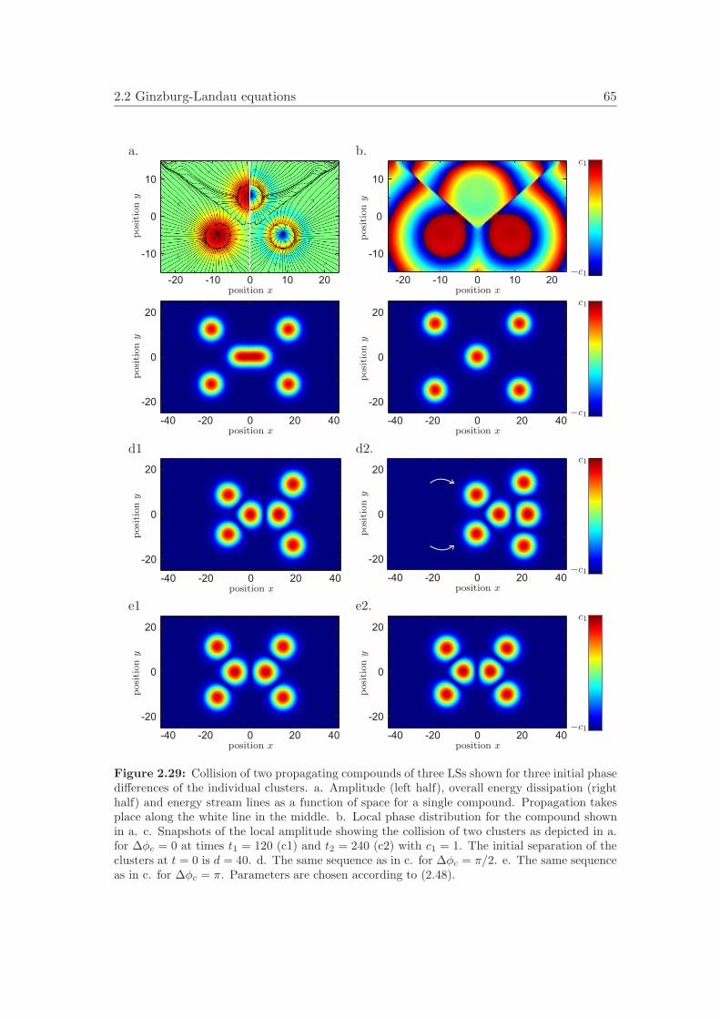
2.2 Ginzburg-Landau equations 65
a. b.
-20 -10 0 10 20
-10
0
10
position x
posi
tion
y
-20 -10 0 10 20
-10
0
10
position x
posi
tion
y
ff
−c1
c1
-40 -20 0 20 40
-20
0
20
position x
posi
tion
y
-40 -20 0 20 40
-20
0
20
position x
posi
tion
y
ff
−c1
c1
d1 d2.
-40 -20 0 20 40
-20
0
20
position x
posi
tion
y
-40 -20 0 20 40
-20
0
20
position x
posi
tion
y
ff
−c1
c1
e1 e2.
-40 -20 0 20 40
-20
0
20
position x
posi
tion
y
-40 -20 0 20 40
-20
0
20
position x
posi
tion
y
ff
−c1
c1
Figure 2.29: Collision of two propagating compounds of three LSs shown for three initial phasedifferences of the individual clusters. a. Amplitude (left half), overall energy dissipation (righthalf) and energy stream lines as a function of space for a single compound. Propagation takesplace along the white line in the middle. b. Local phase distribution for the compound shownin a. c. Snapshots of the local amplitude showing the collision of two clusters as depicted in a.for ∆φc = 0 at times t1 = 120 (c1) and t2 = 240 (c2) with c1 = 1. The initial separation of theclusters at t = 0 is d = 40. d. The same sequence as in c. for ∆φc = π/2. e. The same sequenceas in c. for ∆φc = π. Parameters are chosen according to (2.48).

66 Models and mechanisms
A last point that we want to address in the context of interacting LSs is the influ-ence of topological charge in the interaction processes. Here, rotational and curvilinearmotion of whole clusters as well as of parts of clusters can be found [63]. The effects canbe understood in a similar way as the linear propagation of clusters without topologicalcharge. The arrangement of several LSs with topological charge in a cluster may breakthe rotational symmetry of a system but preserve a degree of symmetry high enoughto prevent propagation of the center. The outcome is then typically a purely rotationalmotion. When the degree of symmetry becomes low enough, curvilinear motion may setin. One may again distinguish between weak and strong interaction. In the latter case,closely connected compound of several LSs may form that may rotate in the course oftime.
One may ask which dynamical phenomena discussed above have up to now been ob-served in the experiment. In [204], as depicted in Figs. 2.26c and d clusters of stationaryLSs have been found. There seems to be a well-defined lock-in distance when the LSsare close although the LSs show no oscillatory tails, which agrees with the theoreti-cal predictions. Oscillons in granular media show similar properties. In addition, onemay state that generally no intrinsic propagation of single LSs has been reported fortwo-dimensional systems which are related to the GL equation. Unfortunately, experi-mentally observed dynamical interaction processes of several LSs have up to now hardlybeen reported for systems directly related to the GL equation. Nonetheless, in particu-lar the mechanisms shown for interaction processes (attraction of LSs with equal phase,repulsion for opposite phase) are found in a number of other experimental systems withself-focussing media such as photorefractive media [219]
2.2.3 Variations of the GL equation
Up to now, we have discussed the dynamics of LSs in the classic cubic-quintic GLequation and some closely related other versions. Different extensions and modificationsto these equations have been made in the course of research, either physically motivatedor artificially. The connection between the different versions is much clearer than forexample in reaction-diffusion systems. In the following, we will give a brief overviewand present consequences for the observed phenomena.
• Anisotropy, external pumping etc.
The “standard“ cubic-quintic or saturable GL equation itself allows for a number ofextensions to account for special properties of the underlying system. It was foundthat systems with anisotropically distributed coefficients allow for anisotropicallyshaped stable LSs [220]. When the system under consideration is parametricallyexcited (for example pumped by an external beam), the simplest way to accountfor this effect is to add additional terms plq
∗+ipc|q|2q∗ to the GL equation (see forexample [221]). These additional terms break the gauge symmetry of the originalequations, but nevertheless LSs can exist. Another possibility to break the isotropyof the original equations is to consider nonlinear gradient terms [212]. In this case,single propagating LSs are possible.
• Coupled systems of GL equations
As explained in the beginning, a single GL equation may describe the amplitudeof a fast-oscillating field with frequency ω. In order to model several frequencies

2.2 Ginzburg-Landau equations 67
(for example higher harmonics of ω), one may thus consider a set of coupled GLequations, in which the mixed nonlinearities reflect the nonlinear frequency mixing(see for example [222]). A similar situation is given for the case of a cascaded setof quadratic nonlinearities, which may show properties similar to those expectedfor cubic and higher nonlinearities [222–224]. Coupled GL equations were alsoderived for binary mixture convention where the amplitude dynamics couples toother slow modes in the system [225, 226]. An important point is that coupled GLequations have stable localized solutions even if the individual equations have noquintic or saturable terms. As the coupled systems can be considered to consistof multiple components, the LSs are in this case also termed vector solitons inthe literature. Generically, the coupled equations show a larger variety of possiblephenomena due to an increased number of degrees of freedom, for example thecoexistence of differently sized pulses [226]. When considering coupled equationsfor counterpropagating beams, one generally obtains “convective” terms of theform ±v · ∇q, which can not be transformed away as for a single equation. Inthese equations, LSs may be convected in opposite directions and thus collide,opening up the possibility of a variety of interaction phenomena [227, 228].
Apart from the coupling of several GL equations, one may also look at a GLequation coupled to other types of equations. As an example, one may couplea GL equation to a simple linear dissipative equation in order to stabilize anotherwise globally unstable background, so that LSs can exist in an otherwise un-stable regime [53]. The combination of GL equations with equations for chargetransport(for example drift-diffusion) or temperature may describe LSs in activecavities, photorefractive systems etc. [229]. We already mentioned that the in-troduction of a slowly varying temperature field may lead to intrinsic propagation[42, 230].
• Discrete GL equations
There is a number of systems described by GL equations that are discrete andlattice-like in nature. Examples are given by photonic crystals, semiconductorlaser arrays and nonlinear oscillators. While some investigations consider the directdiscrete analogue of the GL equation where terms involving no spatial couplingstay local [231], others make generalizations where cubic or quintic terms arenonlocal in space [232, 233]. Basically, the discretized GL equation retains someproperties of its continuous counterpart, for example the fact that to find stableLSs, nonlinearities higher than cubic ones have to be considered [234].
Some findings however have no continuous counterpart. One finds both singlepoint (on site) LSs, two point (intrasite) LSs [231], LSs distributed over manysites [233] and even coexistence of different types. Furthermore, the dispersionproperties and the sequences of bifurcations are different from both conservativediscrete and continuous dissipative systems.
We end our section on Ginzburg-Landau equations with an overview table on pub-lished works on the GL equation (Table 2.4). Further overviews and reviews are forexample given in [30, 34, 187, 248, 249].

68 Models and mechanisms
systemphenom
enonliterature
detailscubic
GL
equationN
ozaki-Bekki
holes[176]
structurallyunstable
cubic-quinticG
Lequation
existenceof
LSs
[30,62,
194,198,
199,201,
235]perturbation
theory/
numerics
propagationof
singleLSs
[40,195,203,212]
intrinsicor
Galilean
invarianceother
typesof
destabilizations[212–214]
breathing,explosions
weak
interaction[39,
62,215,
216]com
pareSec.
3.3strong
interaction[40,
203]m
erging/
annihilationsaturable
GL
equationexistence
ofLSs
[200,236]
perturbationtheory
/num
ericsdynam
icsof
singleLSs
[202]breathing
weak
interaction[59,
63,217]
compare
Sec.3.3
stronginteraction
[63]com
poundstates
extensions/modifications
anisotropy,driving
[220,221]
changedsym
metry
propertiesof
theG
Lequation
discreteG
L[231–234]
newtypes
ofLSs
coupledequations
[222–228]extended
dynamics
realSH
equationlocalized
Turing
patterns[237–243]
Liapunov
functionalnonlinear
spatialcoupling
[244]preference
ofsquares
complex
SHequation
existenceof
LSs
[57]num
erics1D
/2Dinteraction
[57]collisions,
interpenetrationanisotropy
[245]“w
orms”
nonlinearspatial
coupling[246,
247]square
patterns,oscillons
Tab
le2.4:
Overview
overdifferent
works
onthe
GL
equationand
theSH
equation.

2.3 Swift-Hohenberg equations 69
2.3 Swift-Hohenberg equations
2.3.1 General properties
In the preceding section, we have seen that the GL equation can be considered as aprototype equation for a large number of different systems. It can be derived either ina direct fashion (typically for optical systems with fast nonlinear medium) or indirectly(in a variety of other systems). In this section, we will consider the Swift-Hohenberg(SH) equation, which can in some sense be considered as a generalization of the GLequation. It can be written as
∂tq = (sr + isi)∆2q + (dr + idi)∆q + lrq + (cr + ici)|q|2q + (qr + iqi)|q|4q, (2.52)
so that the essential difference to the quintic complex GL equation (2.35) are the fourthorder derivative terms on the right-hand side. Before turning to the discussion how theadditional terms influence the solutions compared for example to the GL equation, wewill briefly have a look at the origin of the equation. For many optical systems, thereaction of the nonlinear medium to the exposure of an incident light beam is ratherslow. A typical example is given by a photorefractive crystal which can be described bythe set of equations [250]
∂tq = κ[−1(1 + iβ)q + in∗ + ia∆q], (2.53)
∂tn = −γ[n− in− nsq∗
1 + |q|2 ] (2.54)
with q representing the normalized electric field of the incident light wave and n beingthe photorefractive index, all other parameters are constants. While in the saturableabsorber example (2.33) in the GL section we have adiabatically eliminated the medium,here usually γ κ so that one may adiabatically eliminate the field, i.e. setting ∂tq = 0.On a new time scale τ = γt this yield the relation
∂τq = −(1 − i)q +ins
1 + iβ − ia∆q∗
1 + |q|2 . (2.55)
By tailor-expanding both differential the operator and the ”saturable” term on which itacts, one finally obtains
∂τq = (ns
2− 1)(1 − i)q − (1 + i)|q|2q − i
ns
2(β − 1 − a∆)q − ns
8(β − 1 − a∆)2q. (2.56)
We now have obtained a cubic version of (2.53), one may still recognize how the fourthorder derivative results from the Taylor expansion of the differential operator. A numberof other examples from the optical field can be found for example in [181, 251, 252]. SHequations have also been proposed to describe oscillons in vibrated granular media [244],the dynamics of flames [253] or electroconvection [245]. As in the GL equation, in some

70 Models and mechanisms
a. b.
-6 -4 -2 0 2 4 6
-0.5
0.0
0.5
1.0
position x
am
plitu
de
A
0 1 2 3 4
0
5
10
15
wave vector k
ω(k
)
Figure 2.30: Effect of the fourth-order derivative terms in the SH equation. a. Real secondorder derivative (dashed line) acting on a Gaussian distribution in one spatial dimension (solidline), thereby increasing the local curvature in regions where it is already positive (marked ingrey) and decreasing it in regions of negative curvature. The consequence is a steepening of thestructure typically leading to instability. b. A typical dispersion relation ω = k2 (solid line)with a globally positive group velocity space as encountered for example in the GL equationis modified by the additional imaginary fourth order derivative so that the group velocity maylocally become negative (dashed line, ω = k2 − 0.04k4).
cases one finds real versions of the SH equation [240] which can be obtained by settingall “imaginary coefficients” to zero.
We now want to shed some light on the meaning of the new terms related to fourth-order derivatives. Turning to the real part sr, the corresponding term in the SH equa-tions can be considered as “superdiffusion”. In Fig. 2.30a, we show the action of su-perdiffusion on a Gaussian pulse. While normal diffusion has the effect of smoothingout gradients in the course of time, superdiffusion tries to smooth out the second orderspatial derivative. For a curve q(x), the local curvature κ is given by relation
κ(x) =∂2
xq√1 + (∂xq)2
3/2≈ ∂2
xq for (∂xq)2 1 (2.57)
so that for not too steep curves superdiffusion can be interpreted to increase the cur-vature of a given distribution. As the effect is the stronger the larger the curvature,the Gaussian in Fig. 2.30a typically steepens at the positions marked by the arrows,thereby leading to instability. As the fourth order term dominates all other terms onsmall spatial scales, we have to claim sr < 0 to avoid a global instability. Looking atthe fourth order derivative with imaginary coefficient, we may recall for a plane waves,a general dispersion relation in one spatial dimension can be written in the form
ω(k) = ω0 + ∂kω(k0)(k − k0) +12∂2
kω(k0)(k − k0)2 +16∂3
kω(k0)(k − k0)3
+124∂4
kω(k0)(k − k0)4 + . . .(2.58)
While the phase velocity ∂kω(k0) can always be eliminated by a transformation to amoving frame, generally ∂2
kω(k0) (corresponding to the group velocity) does not vanish.

2.3 Swift-Hohenberg equations 71
Fourier-transforming the SH equation (2.52) shows that the latter coefficient is directlyrelated to di. While higher order terms are thus not accounted for in the GL equa-tion, the SH equation contains the coefficient si which is related to the fourth-ordercoefficient of the Taylor expansion (2.58). The third-order Taylor coefficient would re-sult from third-order derivatives in the underlying field equation which are not presentin the SH equation. From this we may conclude that the SH equation may only ac-count for situations in which the general dispersion relation (2.58) has no third-ordercontributions.
Before coming to LSs, let us now compare plane-wave stability in the GL and the SHequation. The analogues of the stability criteria (2.41) and (2.42) of the GL equationfor the SH equation take the form
srk4 − drk
2 + lr < 0 (2.59)
according to the trace criterion and
(s2r + s2i )k8 − 2(drsr + disi)k6 + (d2
r + d2i + lrsr)k4 − 2lrdrk
2 + l2r > 0. (2.60)
according to the determinant criterion. From (2.59) and the claim lr < 0 to stabilizethe homogeneous ground state q = 0 we directly see that we have to require sr < 0,meaning that the superdiffusion has a stabilizing effect. We may now distinguish twocases. In the GL equation we had to require dr > 0 which leads to an enhancement ofstability in (2.59) and (2.60). In such a situation and with disi being sufficiently small,k = 0 remains the wave number most close to instability for the SH equation as well.Usually, the fourth order derivatives are then only small corrections to their second ordercounterparts, and no fundamental differences to the GL equation can be expected sothat for the formation and dynamics of LSs the arguments from Sec. 2.2 can be applied.A comparison of the GL and the SH equation in this case can be found in [254].
The situation becomes fundamentally different however if dr < 0. The process of“anti-diffusion” seems rather unintuitive when the actual transport of matter is involved(although such processes indeed exist [244, 245]), but occurs rather naturally in opticalsystems for example when considering resonators or cavities with a detuning from theresonance frequency [237, 247]. We will hence focus on this case in the following.
2.3.2 LSs in the real SH equation
We will first consider the real SH equation for a real amplitude q. An inspection of(2.59) and (2.60) shows that for dr < 0 small enough a whole band of finite k-valuemay become unstable while k = 0 remains stable. A generic observation in this case isthe formation of stripes and sometimes also hexagons in a Turing instability dependingon the properties of the higher order local terms. LSs in this type of equation wereinvestigated for example in [239] and are generated due to an elementary mechanismthat leads to localization also in more complex versions of the SH equation. We firstconsider a case in which the parameters are chosen such that although cr > 0 andqr < 0, the only stable stationary state is q = 0. In addition, the system can be broughtclose enough to a subcritical Turing instability such that the ground state q = 0 and

72 Models and mechanisms
a. b. c.
-100 -50 0 50 100
-1.5
-1.0
-0.5
0
0.5
1.0
1.5
position x
am
plitu
de
q
-20 -10 0 10 20
-20
-10
0
10
20
position xposi
tion
y-20 -10 0 10 20
-20
-10
0
10
20
position x
posi
tion
y
ff
−c1
c1
Figure 2.31: LSs in the real SH equation. a. One-dimensional stable localized patterneddomains (Turing structures) of different width on a homogeneous background state. Note theweakly bound state of two domains on the left side. Parameters: lr = −2.6, cr = 3, qr = −1,dr = −2, sr = −1. b-c. Localized stable stripe and square patterns in two spatial dimensionscoexisting for the same parameters as in a. except for lr = −2.505, scale c1 = 1.7. Compare also[239].
a spatially modulated state can coexist. Similar to one-component bistable reaction-diffusion systems for which we considered domains of one homogeneous state on thebackground of the other state, following an idea by Pomeau [255] one may considerlocalized domains of the modulated state on a homogeneous background state. It turnsout that contrary to the reaction-diffusion case, the modulated state can indeed existand form stable domains of various widths on the background state (Fig. 2.31a). Thestructures exist over extended ranges of the system parameters. However, it is found byassociating with the SH equation the Liapunov functional
L = −∫ ( lr − d2
r4sr
2q2 +
cr4q4 +
qr6q6 +
sr
2([dr
2sr+ ∂xx]q)2
)dx (2.61)
via the relation ∂tq = −δL/δq that stable LSs can only exist if the “energy” of thehomogeneous ground state lies below that of the patterned state [239]. In other words,the homogeneous state must be the dominant one. At this point, we should recall that inthe reaction-diffusion case a domain structure can be considered as the result of a weaktwo-front interaction compensating the motion of the isolated fronts. In the SH casehowever, one state is strongly modulated such that in order to change the extensionof the latter, one stable structure of large amplitude has to be replaced by anotherstate. Consequently, it is evident that when considering the structure in the SH caseas composed of two front as well, the front interaction is much stronger so that thestructure stays stable in a large parameter range.
Stable localized domains can also exist in more than one spatial dimension. Here,two possible generalizations of the one-dimensional structure exist. On the one hand,as reported in [239] the domain may keep its characteristic modulation length in onlyone direction (Fig. 2.31b). In the orthogonal direction the curvature of the structureis rather small, which is favorable compared to a state with higher curvature due toa lower energy according to the generalization of the Liapunov functional (2.61). The

2.3 Swift-Hohenberg equations 73
number of oscillations of the stable structure is again dependent on the initial conditions.However, there is also a second type of stale LS which in contradiction to [239] can existfor the same parameters as the state depicted in Fig. 2.31b and in particular without theintroduction of local symmetry breaking terms. This state is shown in Fig. 2.31c: we seethat here the characteristic length of the one-dimensional system is preserved in bothdirections and we thus obtain a stable localized square pattern which can be regardedas generic extension of the one-dimensional structure. Note that the square structuremay be generated from unsymmetrical initial conditions (to produce Fig. 2.31c, we usedthe initial condition q(x, y, 0) = 2.5 exp(−(x2 + y2)/152) sin(x/1.2) sin(x/1.5)).
LSs in the real SH equation can also be found in the case lr > 0, cr < 0 and qr = 0.The difference to the above considered case is that the system has two equally dominantstable homogeneous states qh = ±√−lr/cr while the state q = 0 becomes unstable. Notethat for the same choice of the parameters in the case of the GL equation, the only LSsare the structurally unstable Nozaki-Bekki holes. In one spatial dimension, one againencounters localized Turing structures on a homogeneous background which seem to bestabilized analogously to their counterparts in the case lr < 0. It is interesting to notethat similar results can also be found when one generalizes the local terms according to
f(q) = mr + lrq + nrq2 + crq
3 + . . . (2.62)
(see for example [237, 242]), showing that the structures in the SH equation are indeedstructurally stable. LSs in this case may exist also in more than one dimension and werefirst observed in connection with domain patterns [240]. Looking at the stability regimesof different stationary states (patterns and LSs) by varying the individual parametersin (2.62) [237], one finds strong indications for the statement that the existence range oflocalized patterned domains coincidences with the intersection of the regions where atleast one stable homogeneous state and globally extended Turing states exist. In par-ticular, if the nonlinear function (2.62) allows for bistability of two homogeneous states
a. b. c.
-40 -20 0 20 40
-1.5
-1.0
-0.5
0
0.5
1.0
1.5
position x
am
plitu
de
q
-20 -10 0 10 20
-1.5
-1.0
-0.5
0
0.5
1.0
1.5
position x
am
plitu
de
q
-20 -10 0 10 20
-20
-10
0
10
20
position x
posi
tion
y
ff
c1
c2
Figure 2.32: Coexistence of homogeneous, patterned and localized states. a. For bistability oftwo homogeneous states, LSs with equal amplitude can exist on both backgrounds (black andgrey lines). b. Multistability of two homogeneous states, the Turing pattern (grey line) anda LSs in one spatial dimension, note that the amplitude of the LS matches that of the Turingpattern. c. Hexagonal arrangement of LSs in two spatial dimensions due to mixed attractive-repulsive interaction caused by oscillatory tails of the LSs, scale c1 = −1.1, c2 = 1.3. Parameters:lr = 0.84, cr = −1, qr = 0, dr = −2, sr = −0.4.

74 Models and mechanisms
with the patterned state, a localized patterned domain can exist on either background(Fig. 2.32a).
An interesting aspect is given by the comparison of the localized patterned domainswith the domain structures encountered for example in bistable reaction-diffusion sys-tems (compare Fig. 2.16). To clarify this aspect, we may exemplarily consider a LS withonly one central peak existing on one of two possible ground states (Fig. 2.32b). Withthe LS existing on the lower state as background state, one finds that the amplitude ofthe LS corresponds to the underlying Turing pattern and thus lies significantly abovethe upper homogeneous state. This is in contrast to Fig. 2.16 where only small oscil-lations around the upper homogeneous state are encountered. Consequently, one mayconsider the structure to be dynamically stabilized as observed for example for excitablereaction-diffusion systems or the subcritical GL equation (Fig. 2.24).
As the Turing wavelength is always dominant when LSs exist for the real SH equation,it was also argued that oscillatory tails may help in stabilizing the individual structures[241]. In any case, the tails may cause a stable lock-in of two LSs which may also leadto the formation of larger clusters, typically with hexagonal arrangement (Fig. 2.32c,compare also Fig. 2.31a). In this sense, larger domains with several peaks can also beinterpreted as an arrangement of several individual structures with very small lock-indistances. Note that by comparing the situation to one-component reaction-diffusionsystems in which the decay of a structure to the ground state is always monotonic andrequires a second component to become oscillatory it becomes clear from (2.59) and(2.60) that the oscillatory tails in the SH case are the result of an interplay of secondand fourth-order spatial derivatives.
Aside from interacting stationary LSs and transients during the generation of LSs,the possible dynamics in the real SH equation appears to be rather limited. This aspectis connected to the existence of the Liapunov functional (2.61) which imposes strongrestrictions to the possible dynamics. Note also that a variety of effects could be inducedin two-component reaction-diffusion systems by a slow response of one component, whichis not possible for the real SH equation either. Before turning to the complex version ofthe SH equation, we want to mention a number of analytical works treating the localizeddomains in terms of amplitude equations [242]. In particular, a relation to the conceptof homoclinic snaking was considered [243]. Furthermore, the role of the Liapunovfunctional (2.61) and appropriate generalizations was discussed in more detail [238].Extensions of the real SH equation by nonlinear gradient terms have been proposed,which are for example of the form [244]
e(q) = f1∇ · [(∇q)3] − f2q(∇q)2 − f3q2∆q. (2.63)
The additional terms may cause the system to favor a special type of pattern (for ex-ample squares) which may phenomenologically account for corresponding experimentalobservations.
An experimental example for which a real supercritical SH equation could be derivedin a rather rigorous way [258] are systems involving degenerate wave mixing. The ex-perimental set-up is basically a resonator partly filled with a saturable medium, but thepumping is done with several beams via an active medium like BaTiO3 [259]. Conse-quently, the phase of the optical field can not take arbitrary values but is coupled to

2.3 Swift-Hohenberg equations 75
a. b. c. d.
Figure 2.33: Experimentally recorded sequence showing the coexistence of a LS and a frontconnecting two domains in degenerate four-wave wave mixing in BaTiO3. The figures show theintensity distribution in the set-up as a function of time, the LS retains it shape while the domainboundary contracts. The time interval between successive images was not given in the originalreference [256], however can be assumed to lie in the order of a few seconds by comparison withother works [257].
the phase of the pumping fields. A good agreement between the predictions of the SHequation and the experimental observations was found. In particular, it was observedthat domain-type solutions separated by steep fronts and LSs as shown in Fig. 2.32can coexist [256, 257]. Fig. 2.33 shows an experimentally recorded sequence depicting acontracting domain and a stable LS that keeps its shape in the course of time. A looseconnection was also argued to exist between the real SH equation and forces chemicalreactions like the Belousov-Zhabotinsky reaction in which also domain boundaries andLSs have been found [260].
2.3.3 LSs in the complex SH equation
While we have shown the existence of a variety of different LSs in the real SH equation,generally no dynamical phenomena are observed due to the existence of a Liapunovfunctional. This situation changes when turning to the complex SH equation. Just asthe complex GL equation shows hybrid properties of the NLS equation and reaction-diffusion systems, the complex SH equation takes a similar role with respect to the realSH equation and the complex GL equation.
An essential feature of the LSs in the real SH equation with dr < 0 is the coexistenceof a short and a longer spatial wavelength so that the LSs could be considered as localizedTuring domains. The LSs in the complex SH equation preserve this property even whenthe “imaginary” coefficients become large [57]. We start by again first considering one-dimensional systems. Fig. 2.34a shows for a one-dimensional domain structure. Thedistribution of |q| (left half of the image) is stationary and consists of several peaks withvery steep valleys in between. A look at the real part of q (right half of the image)shows that similar to the complex GL equation, the structure oscillates periodicallyin its phase so that both real and imaginary parts of the q-distribution correspond tostanding waves. Similar to the real SH equation, using different initial conditions variousdomain structures of different width can be created whose internal structure is alwaysdominated by the same wavelength.
Considering the domains structures as stationary LSs, it is interesting to note thatalso traveling LSs are possible for the same system parameters. Fig. 2.34b shows atypical solution obtained for the parameters of Fig. 2.34a. Contrary to the domainstructures, the running LS has a fixed extension. A look at the amplitude |q| reveals

76 Models and mechanisms
a. b. c.
-60 -40 -20 0 20 40 600
50
100
150
position x
tim
et
-60 -40 -20 0 20 40 600
50
100
150
position xtim
et
0.25
0.30
0.35
2.50 2.52 2.54 2.560
20
40
60
80
100
cr
v,w
ff
c1
c2
d. e. f.
-60 -40 -20 0 20 40 600
100
200
150
50
position x
tim
et
-60 -40 -20 0 20 40 600
100
200
150
50
position x
tim
et
0
5
10
15
20
25
-60 -40 -20 0 20 40 60position x
tim
et
ff
c1
c2
Figure 2.34: Structures in the one-dimensional complex SH equation. a. Space-time plotshowing |q| (left half) and Re(q) (right half) for a domain structure internally consisting of astanding wave pattern. Parameters: lr = −2.1, cr = 2.5, ci = 0.5, qr = −1, qi = 0, dr = −2,di = 0.3, sr = −1, si = 0, scale c1 = −1.5, c2 = 1.5, b. Space-time plot showing |q| (lefthalf) and Re(q) (right half) for a traveling LS coexisting with the domain structure in a., c.dependence on the width w (grey triangles, left scale) and the velocity v (black squares, rightscale) of the traveling structure shown in b. as a function of cr, d. and e. space-time plot of|q| for collisions of two traveling LSs as shown in b. for ∆φ = 0 and ∆φ = π/2, scale c1 = 0,c2 = 1.5, f. space-time plot of |q| showing a collision with ∆φ = 0 resulting in interpenetration,note the changed parameters lr = −1.7, ci = 1, di = 2.
a strongly asymmetric shape of the envelope, however the distribution of Re(q) showsthat in a co-moving frame the structure has again the form of a standing wave patternwith the same dominant short scale as the standing domains. After a relaxation ofinitial transients the propagation velocity is constant in time. As the coexistence ofstanding and propagating structures already indicates, the latter are generated in asubcritical bifurcation. This is confirmed by starting with an existing structure andvarying the corresponding system parameters in small steps. We illustrate the resultsof the procedure by varying cr, the real coefficient in front of the cubic term which weidentified as being responsible for local energy gain in the complex cubic GL equation.In Fig. 2.34c we plot the propagation velocity (black squares) and the width of thepropagating pulse (defined via the distribution above the critical amplitude |qb| = 0.8)under a variation of cr while keeping the other parameters constant. Below cr = 2.495the traveling LS can not exist. Above the critical value there is a region in which thepulse exhibits an almost constant width and velocity. At cr = 2.535, this behaviorchanges in a drastic way. The initial pulse widens as the leading edge of the pulsepropagates with a higher velocity than the trailing one. After some time, the trailingedge adapts its velocity and a pulse of constant width stabilized which is larger than

2.3 Swift-Hohenberg equations 77
that obtained for smaller values of cr. In addition, the velocity decreases significantly.The large jump in the velocity curve of Fig. 2.34c indicates that a subcritical bifurcationmay have taken place. Above the bifurcation point, the width of the stationary pulseincreases extremely strongly with the parameter. It remains to be clarified whether therunning pulses may become arbitrary wide when further increasing cr.
The running LSs in the complex SH equation show a certain similarity with those inthe complex GL equation (compare Fig. 2.27). However, an important difference ariseswhen going from one to two spatial dimensions. Up to now, no isolated running LSshave been observed in the two-dimensional GL equation although asymmetric compoundstates were found to move intrinsically. In contrast, the complex SH equation allowsfor isolated propagating LSs [57]. Such a structure is depicted in Fig. 2.35a. While theenvelope |q| of the structure shows only a weak derivation from radial symmetry, a lookat Re(q) reveals that internally the LS consists of a single period of the standing wavepattern also found in the one dimensional case (compare Fig. 2.34b).
With the existence of intrinsically propagating LSs in one and two dimensions, variousinteraction processes become possible. As in the complex GL equation, the mutualphase difference of the interacting LSs has a significant relevance for the outcome ofthe interaction process. In the one-dimensional case, we may repeat the simulationson collision processes shown in Fig. 2.27. Figs. 2.34d and e show space-time plots oftwo colliding counter-propagating structures for ∆φ = 0 and ∆φ = π/2, respectively.Considering the first case, the result of the collision is the formation of a stable symmetricdomain structure. One may recall that we found a similar result in the GL equation,here the outcome in the corresponding collision is a symmetric composite soliton if theinitial energy in the system is high enough. For ∆φ = π/2, the LSs merge and form asingle traveling LS. This scenario in direct analogy to the GL case. Varying the systemparameters in such a way that the “conservative” coefficients become more dominant(but dissipative terms are still significant), one may also observe a phenomenon that istypically associated with classical soliton equations: Fig. 2.34f shows an interpenetrationevent with two LSs merging into a compound state which again re-emits two pulses ofthe original shape. The outcome of the event thereby is independent of ∆φ. In spite ofa apparent similarity to classical soliton behavior, one should keep in mind that whilein classical soliton equations the energy stays globally conserved, in the collision eventshown in Fig. 2.34e the same quantity increases by a factor 2 before relaxing to its initialvalue in the long-time limit.
In two dimensions, aside from interpenetration processes as reported in [57] similarto the one-dimensional case a number of different interaction processes can be found.We exemplarily depict two of them in Figs 2.35b and c. Here we have simulated thecentral collision of two structures as shown in Figs 2.35a for ∆φ = 0 and ∆φ = π/2,the dynamics of the process is visualized via a space-time plot of the |q|-distributionalong the connecting line of the LSs. In the first case, the LSs approach until they feel arepulsive interaction and then change their direction of motion. During the collision, athird LS is formed in the center (note the similarity to the reaction-diffusion example inFig. 2.20), however it decays again in the course of time. In the second case, one againhas repulsive interaction, however one LS decays after the collision. For ∆φ = π (notshown here), both LSs are annihilated in the collision. Additional simulations can becarried out for non-central collisions. Here, one either observes weak interaction leadingto scattering or one of the processes described above.

78 Models and mechanisms
a. b. c.
-20 -10 0 10 20-20
0
20
10
-10
position x
posi
tion
y
0
5
10
15
20
25
-40 -20 0 20 40position x
tim
et
0
5
10
15
20
25
-40 -20 0 20 40position x
tim
et
ff
c1
c2
Figure 2.35: Traveling LSs in the two-dimensional complex SH equation. a. Distributions of |q|(left half) and Re(q) (right half) for a LS traveling upwards. Parameters: lr = −1.5, cr = 2.35,ci = 2, qr = −1, qi = 0, dr = −2, di = 2.5, sr = −1, si = 0, scale c1 = 0, c2 = 1.5 (left half),c1 = −0.75, c2 = 0.75 (right half), b and c. space-time plots showing the central collisions oftwo LSs as depicted in a. via the distribution of |q| along the connecting line of the LSs for aphase difference ∆φ = 0 and ∆φ = π/2, scale c1 = 0, c2 = 1.7.
As a last point, one should mention that like for the complex GL equation and the realSH equation different extensions have been proposed for the complex SH equation. Inorder to model pattern formation in electroconvection, an anisotropic two-dimensionalSH equation has been proposed [245]. Here, worm-like structures with particle-likeproperties have been found. Other works deal with terms similar those to in (2.63).These terms either arise for example from an approximation of underlying first-principleequations [247] or phenomenologically like in our example for the real SH equation [246].
Note that a tabular summary on the literature dealing with LSs in the SH equationis contained in Table 2.4.
2.4 Summary on mechanisms
In this chapter, we have discussed how LSs are generated in three different classes ofmodel systems, what conditions are necessary for their stability and how dynamicaldestabilizations can occur. Concerning our goal to investigate the universal propertiesof LSs, the generation of LSs poses the largest problems as on a first glance the discussedsystems show large discrepancies. As an example, while reaction-diffusion systems arenaturally discussed in terms of local transport, the complex GL equation does not in-stantaneously offer the same intuition. However, we have seen that by looking at localenergy and impulse functionals a certain analogy can be established as in this way theconcept of transport can be introduced into the GL equation as well. In this sense, theSH equation can be considered as a hybrid structure involving mechanisms from bothreaction-diffusion and GL equations.
In the following, we want to try to summarize our findings on a more detached level.Rather independent of the exact type of system under consideration the most elementarytype of solution in the presence of bistability between two homogeneous states is a frontsolution. An asymptotic superposition of a front-antifront pair to a domain solutionthus appears to be the most simple way to construct a localized solution. The stabilityof such a structure can then be interpreted to be the consequence of a balance between

2.4 Summary on mechanisms 79
a. b. c.
distance d
forc
eF
(d)
A=const.
position x
q 0q 2
position x
q 0q 2
d. e. f.
position x
q 0q 2
position x
q 0q 2
position x
q 0q 2
Figure 2.36: Schematic illustration of mechanisms capable of stabilizing LSs. a. In an asymp-totic front-antifront superposition the front dynamics (grey lines) must be balanced by inter-action forces (black lines), b. global constraints regulate the deviation from the ground state(grey area), c. domains of patterned states on a homogeneous background, d-f. balance of localgain (red arrows) and loss (blue arrows) by diffusion, dispersion and other transport mechanisms(dashed and dotted arrows).
the dynamics of the isolated fronts and the interaction caused by the nonlinearities inthe system (Fig. 2.36a, compare also Fig. 2.15). If there exists a separation at whichthe effects compensate each other, the corresponding state os stable only if the overallattraction of the pair get stronger when the distance gets larger and vice versa. Thisis for example possible when the mutual interaction is repulsive and the individualfronts without interaction approach each other or when the interaction strength oscillateswith distance. The latter phenomenon is typically observed when the system is closeto a global instability with a dominant finite wave number (for example a Turing ormodulational instability).
While the front-antifront structure seems conceptually rather simple to realize, it isobserved only seldom in many systems, which is due to two primary reasons. On theone hand, an asymptotic superpositions of two fronts yields an interaction force thatis rather weak in strength. Consequently, the front velocities must be small as well tobalance this effect. While in some systems the bistable states are totally equal due tosymmetry reasons, in most known examples one of the states dominates so strongly thatthe velocities of the transition front are too high to allow for a domain structure to form.The second problem concerning domains arises in two or more spatial dimensions. Here,domains arise as revolved one-dimensional front structures. In this way, the action ofspatial coupling terms at the transition boundary depends on its local curvature whichin turn affects the front velocity as well. This may lead to curvature-driven instabilities

80 Models and mechanisms
in which deformations of the rotationally symmetric structure are enhanced, therebyleading to a decay of the structure.
Due to the above arguments, in many systems there are additional mechanisms lead-ing to stabilization or the LSs exist to to a dynamical balance as we will explain below.A method of stabilization that works in almost all types of systems is the introductionof global coupling terms or constraints that limit the overall deviation of the systemfrom a ground state (marked in grey in Fig. 2.36b). A single LS is generally very stableunder these conditions, however the coupling implies long-ranged interactions and sev-eral LSs are mutually put into competition, often leading to then survival of only onestructure. A possibility to avoid this problem is by introducing integral coupling termswith kernels living on a bound support [261] so that the interaction range of a given LSbecomes finite. In our section on the SH equation, we have also seen one may considerlocalize domains of a patterned state on a homogeneous background (Fig. 2.36c). Themechanisms stabilizing the pattern are generally rather strong in nature and may thusbe used to avoid the problems for two homogeneous states [255].
Many LSs can not be considered as domain states (i.e. as a combination of individ-ually stable structures), but as the result of a strongly dynamic interplay of local termsand transport mechanisms. A typical situation is depicted in Fig. 2.36d, illustratinga LS on a lower homogeneous state with its peak lying significantly “below” a secondupper homogeneous state. Close to the individual homogeneous states, the local dy-namics will evolve towards the respecting equilibria (compare the colored arrows in thefigure) so that the effect of diffusion (dotted line) is a natural mechanism to compen-sate for the local dynamics. When the tip of the LS lies above the upper homogeneousstate, transport must be directed from the flanks of the structure both to the tails andto the center (Fig. 2.36e) which can typically be realized by dispersion as in the GLequation. Generally, one observed an interplay of different types of spatial transport(Fig. 2.36f) whose net effect must be balanced by local terms. An example is given bythe complex SH equation. A parameter-dependent stability analysis of LSs in a givensystem can generally be connected rather well with opposing mechanisms of transportand production.
The balance of production and transport becomes particularly relevant when in-vestigating interaction of LSs. In the discussed examples, satisfying explanations forinteraction processes could be found by first considering the nonlinearity on the systemlocally acting on the superposed solution of two LSs and comparing this result with theindividual local dynamics. In a second step, the reaction of the transport mechanismsto the resulting perturbations was used to explain the dynamic evolution.
The mechanisms for dynamic destabilizations of LSs turn out to be manifold, how-ever again some common aspects can be found. A particularly relevant process is thepropagation of LSs. One finds that the latter is occurs in two ways. Either the sys-tem of interest in Galilean invariant or the structure has dynamically induced brokensymmetry at least with respect to one axis. This may either be the case for a singlestructure or an asymmetric compound composed of several structures. The prior caseis often connected to symmetry-breaking bifurcations of an originally symmetric state.
Looking at the model equations we have considered so far, an essential differenceis that the spatial coupling terms appear in a linear fashion. A generic example fornonlinear spatial coupling is found for hydrodynamic systems in which the normal time
2.4 Summary on mechanisms 81
derivative is replaced by the substantial derivative
d
dt=
∂
∂t+ (v∇) (2.64)
with v representing a macroscopic flow. Another example arises in drift-diffusion equa-tions which can be used to model LSs in systems with charge transport [262]. Nonlineartransport terms may cause an essential change in the mechanisms responsible for the for-mation of LSs, possible consequences may range from simple advection of LSs [263] up todeveloped turbulence. It will remain a task for future works to investigate mechanismsand universal properties in these kinds of systems.

82 Models and mechanisms

Chapter 3
Particle description of LSs
3.1 The concept of order parameters
In the previous section, we have considered different types of models which find appli-cation in a larger class of experimental systems and which exhibit the formation of LSs.In particular, several basic mechanisms leading to the formation and dynamics of LSscould be identified. Nonetheless, many aspects remain connected to special properties ofthe underlying field equations. To explore the universal aspects of the particle-like be-havior of LSs in different systems, it would be good to have a description of the particlephenomenology on a level which is structurally more uniform than the field equations.
While setting up such a “normal form description” for the generation of LSs posessevere problems due to the subcritical nature of the generation process, we have seenthat once stable LSs are known to exist for a given system, possible destabilizationsof the stationary state often occur supercritically, implying that there are only smallchanges in the shape of the structure. The same holds for the case of weak interaction,meaning that during the interaction process under consideration the tails of the LSsoverlap only weakly so that the shape again stays essentially preserved. Consequently,as long as only weak deformations of a fixed number of LSs are encountered during thedynamic evolution (which excludes for example generation and annihilation processes),many systems indeed offer the possibility to reduce the dynamic description to a low-dimensional system of ordinary differential equations with structure similar to thoseequations encountered either in the normal form theory for supercritical bifurcations orin classical Newton particle.
The basis for the derivation is provided by adiabatically eliminating most degreesof freedom of the field equations and considering just the slowest timescales. As it hasbeen proposed by Haken [264, 265], the variables corresponding to these slow degreesof freedom are also termed order parameters (the term was adapted from the theory ofphase transitions). In Hakens original interpretation, the order parameters were usuallydirect physical quantities like positions, amplitudes, velocities of the LSs. A closely re-lated idea is given by the concept of the center manifold to which the dynamics shouldquickly converge [266]. While being rather rigorous concerning the underlying mathe-matical theory, the application of the center manifold theory has the consequence thatthe resulting equations in some cases do not only describe the evolution of direct physi-cal quantities, but also of rather unphysical “mixed quantities” (for example products of
83

84 Particle description of LSs
direct quantities), making an intuitive understanding more difficult. In the following, wewill use the term order parameter as a general expression for a slowly evolving quantityindependent of the method of derivation.
In the context of LSs, the idea of order parameters in many situations provides apossibility to compare and classify the possible dynamical evolution of different systemsin a much more simple fashion that on the level of the underlying field equations. Also,the comparison for example with the dynamics in classical Newton equations becomesmuch easier. As we will see in the course of this chapter, the general structure of theorder parameter equations is often essentially influenced by the continuous symmetriesof the system so that a knowledge of the latter already allows for a basic prediction ofthe possible dynamical phenomena.
3.2 Dynamics of single structures
After the observation of LSs in a given system, a frequently asked question is how im-portant quantities like position, velocity or amplitude evolve either as a function of timeor of the system parameters. For LSs in the classical NLS, KdV and SG equations, theabove questions can be generally be answered in a direct way as complete analytic solu-tions are available via the inverse scattering theory. However, already when consideringperturbed versions of the classical equations, significant problems arise. In some cases,inverse scattering techniques can still be applied to obtain analytical solutions [267, 268].However, there are strong restrictions for the use of this method, in particular when theequation of interest can not be considered as perturbed version of a classical equation.
In current research, to the authors knowledge there are two main methods to overcomethe above problems by reducing the complexity of the system. The first one which wewill refer to as “trial-function based method” relies on the existence of an approximateanalytical solution whose time-dependent parameters serve as order parameters. Whilewe will briefly review some more details below, one may stress that the necessity of ananalytical form usually demands a close relation of the field equation of interest to aclassical field equation like the NLS or the KdV equation for which exact solutions areknown. The second technique relies on a weakly nonlinear analysis of deviations fromthe stationary state which are expressed in terms of eigenmodes of the correspondinglinearization operator. The amplitudes of the eigenmodes become time-dependent, andfast modes are adiabatically eliminated to extract the slow dynamics. As this techniquehas a wider range of applicability we will put the main focus on this point in the following.An overview on the current literature focussing on the topic of order parameter equationsis given in Table 3.1, including also interaction phenomena which we will treat furtherbelow.
3.2.1 Trial function methods
Trial function based methods can be applied when an approximate analytical solution fora LS in a given system is known, which is usually the case either when the field equationunder consideration is a modification of a classical soliton equation or when one has beenable to find a numerical solution which can be fitted with an analytical expression. Asa precondition for the method to work, one has to require that in the parameter rangeof interest, the shape of the solution varies only slightly. The central ideal is to capture

3.2 Dynamics of single structures 85
tech
niqu
ety
peof
syst
emci
tation
deta
ilssi
ngle
LSs
tria
lfu
nction
sm
omen
tum
and
tria
lfu
nction
GL
[199
,21
3,26
9]fr
onts
,pu
lse
stab
ility
,pu
lsat
ing
LSs
doub
lew
ellφ
4[2
70]
Lan
gevi
neq
uation
Ham
ilton
ian/
Lag
rang
ian
Lan
dau-
Lifs
chitz,
Hei
senb
erg
chai
n[2
71,27
2]pe
rtur
bed
cons
erva
tive
syst
ems
min
imiz
atio
nof
resi
dual
ener
gype
rtur
bed
NLS,
GL
[273
–275
]di
sper
sion
-man
aged
fiber
spr
ojec
tion
-bas
edpe
rtur
bed
NLS,
forc
edG
L[2
76,27
7]tr
avel
ing
puls
esFitzh
ugh-
Nag
umo
type
[41,
96,98
,278
]dr
iftbi
furc
atio
nse
mic
ondu
ctor
mod
el[4
2]pr
op.
byte
mpe
ratu
refie
ldin
tera
ctio
nof
LSs
mod
eex
pans
ion
KS
equa
tion
[279
]Fo
urie
rtr
ialfu
nction
inve
rse
scat
teri
ngba
sed
pert
urbe
dN
LS/
GL
[215
,28
0,28
1]“K
arpm
an-S
olov
’ev”
appr
oach
Lag
rang
ian
pert
urbe
d/co
uple
dN
LS
[282
–285
]va
riou
sfo
rms
ofpe
rtur
bation
seff
ective
Ham
ilton
ian
pert
.N
LS/
GL
equa
tion
[216
,28
6,28
7]in
tera
ctio
npo
tent
ials
mom
entu
meq
ns.
NLS/
GL/K
dVeq
uation
[39,
288]
proj
ection
-bas
edG
L-b
ased
eqns
.[5
9,62
,21
7]as
ympt
otic
expr
essi
ons
reac
tion
-diff
usio
n[2
89,29
0]pu
lse
trai
nsre
action
-diff
usio
n[5
8,16
9]in
ner
degr
ees
offr
eedo
mB
enne
yeq
uation
[291
,29
2]pu
lse
trai
nsot
hers
[293
,29
4]ne
ural
and
active
-dis
pers
ive
med
ia
Tab
le3.
1:O
verv
iew
oncu
rren
tlit
erat
ure
deal
ing
wit
hor
der
para
met
ereq
uation
sfo
rsi
ngle
and
inte
ract
ing
LSs
divi
ded
acco
rdin
gto
the
met
hods
used
and
whe
ther
sing
leor
inte
ract
ing
LSs
are
trea
ted.

86 Particle description of LSs
temporal changes in the shape of the LS by making the parameters characterizing thesolution (for example position, width, amplitude, velocity) explicitly time-dependent,thereby artificially choosing the analytic parameters as order parameters of the problem.Obviously, the choice of this trial solution confines the dynamics of the solution to apart of the parameter space without a rigorous justification by center-manifold theoryetc, but it is found that nevertheless the idea works in a number of cases.
A central problem is that when inserting a trial ansatz with time-dependent param-eters into the field equation, it will generally not be an exact solution of the system.Consequently, if order parameter equations are obtained by direct insertion, they cangenerally not be fulfilled and produce a contradiction. A solution to this problem thatoriginates from mechanics is to find a “weaker” evolution equation that still reflects theimportant parts of the dynamics while at the same time being compatible with the trialsolution. Depending on the individual problem, there are different possibilities to ob-tain the new evolution equation, but the overall strategy is similar in all cases: the localequation is replaced by an integral one. One possible approach is that of moments [295],which is also widely used in many mathematical and physical disciplines, for example instatistics. In the context of nonlinear field equations and LSs, moment integrals of thelocal fields as well as more complicated integral relations play an important role becausein several systems the position of the LSs as well as general conservation laws can beexpressed via such integrals. A typical example is given by the NLS equation (2.36)where the conservation of the particle number is expressed by the integral relation
∫|q|2 dV + i
∫(q∇q∗ − q∗∇q)dS = 0 (3.1)
between volume and surface integrals. In some cases such expressions lead to importantfurther conclusions. As an example, for the NLS equation one may consider the evolutionof the “virial” moment integral [296]
I(t) =∫r2|q|2 dV (3.2)
that is calculated using the “probability” function |q(x, t)|2. A direct calculation showsthat
d2I
dt2=(
2n
+ 1)H − (n− 2)
∫|∇q|2 dV (3.3)
where H is the conserving Hamiltonian function and n is the spatial dimension of thesystem. The connection to trial function methods is made by using the integral relationsas weakened evolution equation for the parameterized solution. A good application ofthis approach is given by the complex GL equation that can be rewritten in the form
i∂tq + di∂2xq + ci|q|2q = i(lrq + dr∂
2xq + cr|q|2q + qr|q|4q). (3.4)
The integral relations are obtained similarly to (3.1) but contain more complicated termson the right-hand side with integrals proportional to the dissipative coefficients dr, lr,

3.2 Dynamics of single structures 87
cr and qr. The vital choice of the trial function is motivated by the one-dimensionallocalized solution of the NLS equation, but again contains time dependent parameters.According to [199, 213, 269] such an approach provides a very good correspondencebetween the full solution and the reduced dynamics.
Other authors suggested to obtain new evolution equations by minimizing the residualenergy, i.e. the functional
E =∫
|q(x, t) − qtr(p, t)|2 dx, (3.5)
where q and qtr represent real and trial solution and p the order parameters. In thisway, the solution is supposed to remain close to the phase space of the original solution,however, there is usually no rigorous justification for this claim.
A third possibility is to set up a Hamiltonian or Lagrangian formulation. This wasfor example done for the complex GL equation in [297], where for the radially symmetriccase the equation was expressed via two Lagrangians as
δ
δq∗
∫ (Lc + iLq
)rD−1 dr = 0, (3.6)
where the conservative (real) part has the standard form
Lc =i
2(q∂tq
∗ − q∗∂tq) + |∇q|2 − 12|∇q|2 − qi
3|∇q|6 (3.7)
whereas the dissipative (imaginary) part is
Lq = lr|q|2 − dr|∇q|2 +cr2|∇q|2 +
qr3|∇q|6. (3.8)
As trial function, a reasonable choice that was originally introduced for the optical fibers[298] is
q = A(t) exp[− r2
2R(t)2+ iC(t)r2 + iΦ(t)
]. (3.9)
Inserting (3.9) into the evolution equation, one gets a system of four coupled first orderordinary differential equations for the unknown parameters.
As our examples indicate, trial function based methods are frequently applied inoptical problems, but for example not in reaction diffusion equations where no integralconservation equations exist.
3.2.2 Projection based methods
An alternative and more universally applicable approach to trial function methods isgiven by “projection based methods”. Here, order parameters are determined in a rig-orous way using the linearization problem around a stationary solution, and evolution

88 Particle description of LSs
equations for the relevant modes are obtained by projections or solvability conditions.In a general framework, one may choose a fixed set of parameters and formally eliminateall fast modes adiabatically [299]. We will first consider this method which shows theorigin of different terms in the order parameter equations and carry out a generalizationto include degenerated eigenmodes. A problem in this case is given by the fact that onemay not directly say how the order parameter equations change under a variation ofthe system parameters. Concerning this point we will show how normal forms can beestimated using the symmetries of the system under consideration close to bifurcationpoints. Another problem is that the derived expressions contain infinite sums. To over-come the above problems, an alternative option is to conduct a perturbative treatmenton the level of the original field equations.
3.2.2.1 Formal derivation
To illustrate the procedure of formally obtaining order parameter equations, we willstart with a general field equation
∂tq = F (q,σ), (3.10)
which represents most of the model systems introduced in Chap. 2. Here, q(x, t) is thevector describing the state of system at a given time and point in space, σ representsthe parameters and F is a functional which may contain derivatives and integrals alike.As LSs generally exist on a stable homogeneous background, we will shift this state intothe origin, so that F (0) = 0. Furthermore, for some parameters there should exist astationary localized solution, which we will denote by q0(x). For an arbitrary, but smallperturbation of the stationary state, it is reasonable to decompose the general solutionas the sum of the stationary state and a derivation, i.e.
q(x, t) = q0(x) + q(x, t). (3.11)
As the stationarity of q0 corresponds to F (q0,σ) = 0, the function F may be expandedaround this solution using Frechet derivatives if both the functional F and the functionq fulfill certain regularity issues. The result is then
∂tq = F ′(q0,σ)q + F ′′(q0,σ) : q : q + . . . (3.12)
Here, F ′ is a linear operator, and F ′′ denotes a functional quadratic in q etc.The linear stability analysis starts by only taking the linear equation into account,
i.e.
∂tq = F ′(q0,σ)q. (3.13)
It is reasonable to express q and q in terms of eigenmodes of F ′ in order to decouplethe problem. They are defined by
F ′(q0,σ)φi(x) = λiφi(x) (3.14)

3.2 Dynamics of single structures 89
with the index denoting both discrete, continuous or mixed sets. For the eigenvaluedecomposition of F ′, there are two basic possibilities: the operator can either have a(generalized) complete spectrum, in which case the operator is a member of the class ofspectral operators, or the spectrum is incomplete or overcomplete. Here, we will focuson the first case which is generally assumed to hold for most practical problems. If F ′ isself-adjoint, the eigenvalues are real and there exists a corresponding basis of orthogonaleigenmodes which may form a discrete, continuous or mixed set. The evolution equation(3.13) for q then has an explicit solution, namely
q =∑
i
diφi(x) exp(λit), (3.15)
with coefficients di depending on the initial conditions. We have used the (discrete)sum sign here for simplicity, however generally summation may comprise integration aswell. The reason for this choice is that in contrast to many works dealing with spatiallyextended patterns, in the fairly largest part of works connected with LSs the “relevantmodes” are part of the discrete spectrum.
In many physically relevant cases the linear operator F ′ is not self-adjoint, and thecorresponding theory is more complex. This situation is of particular relevance for su-percritical bifurcations of LSs in which an operator with an otherwise complete spectrummay lose this property when a real eigenvalue passes the imaginary axis due to a changeof the system parameters. Furthermore, there are systems with a natural degeneracyof eigenmodes for example due to Galilean invariance. If the simple eigenvalues formno complete set, one may try to construct a generalized complete basis by consideringJordan chains for the degenerated eigenvalues (see for example [300] for more details onspectral operators). The Jordan chains are defined via the generalized eigenmodes φj
i ,given by
(F ′ − λi)jφji = 0, (F ′ − λi)j−1φj
i = 0. (3.16)
In a matrix representation of F ′, the occurrence of generalized eigenmodes correspondsto the fact that the matrix can not be fully diagonalized and instead, Jordan blocksappear. Instead of considering fixed amplitudes di for an eigenmode φi as in (3.15), onemay instead look at the generalization
q =∑
i
Ji(x, t) exp(λit). (3.17)
where
Ji :=n(i)∑j=0
di,j
j∑k=0
φki t
j−k (3.18)
with n(i) denoting the dimension of the subspace spanned by the generalized eigenmodesof the eigenvalue λi.
Treating now such cases where at least a generalized complete spectrum is available,(3.17) may give us information about the stability of the LSs: as all summands in (3.18)
90 Particle description of LSs
are algebraic in time, from (3.17) it is obvious that an infinitesimal perturbation decaysif the real part of all eigenvalues involved in the decomposition is negative (meaning thatthe solution is linearly stable). If there are modes with Re(λi) > 0, these modes willgrow exponentially in the linear system, although in the full system the growth will beaffected by nonlinear effects. The real parts of the λi can be considered as the inverseof a characteristic time of growth or decay, and the imaginary part of the eigenvaluesdetermines whether the growth or decay is monotonous or oscillatory. Obviously, themodes with Re(λi) ≈ 0 are of particular relevance even if their real part is not strictlypositive. A central idea of the projection-based methods is that one makes a transitionfrom constant to time-dependent amplitudes of the eigenmodes so that the amplitudesof the critical modes become the order parameters. While generally the critical modescan also be part of the continuous spectrum, this case is hardly discussed in the currentliterature, so we will focus on the discrete case.
Basically, critical modes can arise in two ways. First, they are generated by allcontinuous symmetries of a system. Each symmetry-related variable ci can be associatedwith a whole continuous family of stationary solutions q(x, ci) which be generated froman initial solution q(x, 0). Examples are given by
q0(x, ci) = q0(x − ciei) translational invariance, (3.19)q0(x, cj) = q0(R(cj)x) rotational invariance, (3.20)
where R represents an orthogonal matrix. The list may also contain Galilean invariance,however, in many systems the shape of the LS changes with the velocity in a nontrivialway, so that it is difficult to give a general form in this case. Also, hidden symmetrieslike scaling transformations may arise. From the stationarity of the transformed solutionone immediately sees that
∂
∂ciF (q(x, ci)) = F ′(q(x, ci))
∂
∂ciq(x, ci) = 0, (3.21)
i.e. the derivative of the solution with respect to ci is a critical mode being the generatorof the corresponding symmetry group. Second, aside from these modes which are alwayscritical, a change of the system parameters can cause previously uncritical modes tobecome critical as well. When decomposing a general solution as q = q0 + q, in orderto ensure |q| |q0| in the course of time when a continuous symmetry is present inthe system one may define the symmetry group operator D(c) to act as D(c)q0(x,0) =q0(x, c). Then one may write the general solution as
q(x, t) = D(c(t))(q0(x,0) +
∑i
n(i)∑j=0
γij(t)φji (x,0)
). (3.22)
Comparing the representation (3.22) to (3.17) which was used in the linear case, onemay now see that the simple time dependence di exp(−λit) from the linear case hasbeen replaced by general time-dependent amplitudes γi(t) in order to account for non-linearities and non-decaying perturbations. Second, in (3.17) the individual terms were

3.2 Dynamics of single structures 91
sorted to eigenvalues end elements of the Jordan chains. In order to simplify notation,we will split up the Jordan chains and instead sort the sum according to eigenmodesand (generalized) eigenvalues.
While the critical modes due to symmetries have been taken care of introducing theparameters c, other critical modes resulting from bifurcations are accounted for by q.Inserting (3.22) into the evolution equation yields (compare also Eq. (3.12))
∂tc · ∇c[q0(x, c) +∑
i
n(i)∑j=0
γijφji (x, c)]
+∑
i
n(i)∑j=0
∂tγiφji (x, c) = F ′
q0q(x, c, t) + F ′′
q0(q(x, c, t)) : q(x, c, t) : q(x, c, t) + . . . ,
(3.23)
A central problem is now to extract appropriate equations for the time-dependent am-plitudes. To this end, the corresponding modes have to be “projected out” of Eq. (3.23).This technique is frequently applied in linear systems, for example in quantum mechan-ics. Suitable projectors can be found by considering by the adjoint operator of F ′ (withrespect to the canonical scalar product in L2(Rn) or another suitably chosen space),denoted by F ′†. It has the same symmetries and eigenvalues as F ′ except for com-plex conjugation, however the eigenmodes are generally different as the operators underconsideration are usually not self-adjoint . We will use the notation
(F ′†(q0,∇,σ) − λ∗i
)jφF ′†,j
i (x) = 0. (3.24)
The product for two (generalized) eigenvectors of F ′† and F ′ is always zero when theybelong to different eigenvalues, which is a very useful property for the projection. Forthe same eigenvalue, there is no similarly clear statement, at least when the eigenvalueis degenerated. The problem is that an eigenvalue φF ′†,j
i is not automatically a suitableprojector for φj
i . However, using an appropriate orthogonality decomposition method
one may always linearly combine the (generalized) eigenmodes φF ′†,ji of F ′† for a given
eigenvalue (i.e. for fixed i and j = 0, . . . , n(i)) to construct projectors Φji (x, c) which
fulfill the orthogonality relation
〈Φmk |φn
l 〉 = δk,lδm,n (3.25)
and can be normalized so that they fulfill also the completeness relation
∑l,n(l)
|φnl (x, c)〉〈Φn
l (x, c)| = id, (3.26)
which explains their suitability for the projection. In other works, the use of projectionsis sometimes introduced with a different argumentation, for example to obtain a solv-ability condition according to the Fredholm alternative or in order to rule out resonantterms.

92 Particle description of LSs
Let us first assume that no generalized eigenmodes appear. This situation generi-cally occurs when the system is either sufficiently far below a bifurcation point or whenthe system is close to a bifurcation point which is marked by a pair of complex conju-gate eigenvalues crossing the imaginary axis. In order to assure the uniqueness of thedecomposition (3.22), we claim
〈Φji (x, c)|φ1
0,ci(x, c)〉 = 0. (3.27)
where φ10,ci
= ∂ciq0. When carrying out the projection for an arbitrary mode (criticalor non-critical) one finds
∂tγi +∑
k
∂tckγk〈Φ1i |φ1
k〉 = λiγi +∑k,l
Piklγkγl + . . . , (3.28)
where Pikl is defined by
Pikl = 〈Φ1i |F ′′(q0,σ) : φ1
k : φ1l 〉. (3.29)
An analogous statements holds for the ci as well, namely
∂tci +∑
k
∂tck〈Φ10,ci
|φ1k〉 =
∑k,l
Piklγkγl + . . . , (3.30)
note that in this particular case λi = 0. The fact that the left hand side expressions in(3.28) and (3.30) potentially contain more than one spatial derivative term is a conse-quence of considering the problem in a moving reference frame (see (3.23)).
A further general treatment of the equations (3.28) and (3.30) is difficult due tothe second term on the left hand side. Friedrich proposed a complete explicit formalsolution for the case of constant c [299]. In this case, the problematic terms vanish.Then, distinguishing between critical and noncritical mode we rename the γi by αi
and βj, where the αi denote slow, critical modes (index c) and the βj denote fast,non-critical modes (index nc). The slaving principle implies that there are functionalrelations βj(t) = βj(αi(t)) so that the entire dynamics is reflected by the αi(t).
We know that on a long-time scale, the amplitude of non-critical modes decay, so thatthe critical modes contribute the main part to the sum in (3.28). Neglecting the smallcontributions of the non-critical modes, the linear inhomogeneous equation is explicitlysolvable [299], yielding
βj =
t∫−∞
exp(λj(t− t′))[ c∑
k,l
Pjklαk(t′)αl(t′) + . . .]dt′. (3.31)
Here, the c over the sum sign shall indicate that a summation should take place justover the critical modes. The dots indicate that in general, higher order terms can be
3.2 Dynamics of single structures 93
taken into account, which necessary if the second order terms vanish for some reasonor resonance effects occur (see below), the index c over the sum sign reflects that thesummation has to be done for critical modes only (this notation will also be used in thefollowing equations). The fast decay of the non-critical modes can be used for a furthersimplification of (3.31): on the (fast) time scale for which the exponential in (3.31) yieldsa significant contribution to the integral, the possible significant change in αk(t′) andαl(t′) may only be due to a fast phase shift (as no restrictions on the imaginary partsof the corresponding λk and λl were made). Hence we assume
αk(t′) ≈ exp(iIm(λk)(t′ − t)
)αk(t), (3.32)
yielding an explicit solution of Eq. (3.31):
βj(t) =c∑
k,l
Pjkl
i Im(λk + λl) − λjαk(t)αl(t). (3.33)
With this expression, we have formally found a system of order parameter equationsfor the critical modes. Note that resonances can not appear in the summands of (3.33)as the real part of the λj is always different from zero. Inserting the above result into(3.28) one finds that when only nonlinearities up to cubic order are considered, relevantcontributions to the sum are only given if at least one of the modes in the product iscritical, yielding the important result
∂tαi = λiαi +c∑
k,l
Piklαkαl +c∑
k,l,m
( nc∑j
(Pijk + Pikj)Pjlm
i Im(λl + λm) − λj
)αk(t)αl(t)αm(t). (3.34)
where c and nc marks summation over critical and noncritical modes. When generalizedeigenmodes have to be taken into account in the above derivation, the result is basicallysimilar to (3.34), however some changes arise in the linear part. For those eigenvalueswhose eigenspace is non-degenerate we obtain the same result as in (3.34) except forthe fact that the generalized eigenmodes have to be included in the summation overthe critical modes. In contrast, for those modes whose eigenvalues are degenerate, theequivalent to (3.34) reads
∂tαji = λiα
ji + (1 − δn(i),j)α
j+1i +
c∑k,l
Pj(i),klαkαl + . . . . (3.35)
We recall that i denotes the eigenvalue, j the order of the eigenmode and n(i) the degreeof degeneracy of the eigenvalue. The coefficient Pj(i),kl implies to use the projector modeφj
p,i in (3.29). Although (3.34) illustrates in a rather clear fashion where the individualcontributions to the nonlinear terms of the order parameter equations result from, aslight disadvantage is given by the fact that the coefficients in the equation require acalculation of an infinite sum.

94 Particle description of LSs
3.2.2.2 Perturbative techniques and normal forms
We see that with the above method, a complete analytical solution is possible for fixedparameters when continuous symmetries do not have to be considered. A question thatgenerally can not be answered directly is how the coefficients of a given equation behaveunder a change of the system parameters. This problem arises for example when askingfor normal forms of supercritical bifurcations. Furthermore, continuous symmetries arerelevant in a number of cases as well, for example in the context of drift bifurcations.
A perturbative approach may be helpful to overcome the above problems. Lookingfirst at the formal derivation sketched above, one may try to perturb the order parameterequation obtained for given fixed parameters. This method allows for the derivation ofsome normal forms in an easy way, so that we briefly look at this point. We will startby assuming that a pair of complex conjugate eigenvalues crosses the imaginary axisaway from the origin in a supercritical bifurcation of a stationary LS. This scenariois typical for example when the a rotationally symmetric LSs undergoes a bifurcationto a breathing state. We denote the amplitudes of these modes by α1 and α∗
1, thecorresponding eigenmodes are complex conjugate. Generic order parameter induced bythe symmetries of the system are the position p of the LS as well as one or several angles θcharacterizing the angular orientation of the LS. In order to make a connection to (3.34),we have to assume that these order parameters are not affected in the bifurcation, whichis typical for a breathing destabilization. In the bifurcation point, according to (3.34)we then have
∂tα1 = iωα0+c∑
k,l
Piklαkαl+c∑
k,l,m
( nc∑j
(Pijk + Pikj)Pjlm
i Im(λl + λm) − λj
)αk(t)αl(t)αm(t)+. . . (3.36)
We may ask which terms must vanish if the resonance condition between different har-monics are not fulfilled. Due to the dominance of the linear term one may choose arepresentation α1(t) = A(t) exp(iωt) where the time-dependence of A(t) is slow. Then,we may only look at those terms which oscillate with the frequency ω. No expressionsquadratic in the critical modes may yield such terms (compare also our considerationfor example on the GL equation in the previous chapter) so that (3.36) simplifies to
∂tα1 = iωα1 + P |α1|2α1 + . . . (3.37)
where P abbreviates the infinite sum leading to the cubic expression (its sign should benegative for a supercritical bifurcation). The complex conjugate value must fulfill ananalogous equation, namely the complex conjugate version of (3.37). When we slightlymove away from the bifurcation point, the critical modes remain critical, and (3.37)turns into
∂tα1 =(ε+ i(ω + f1(ε))
)α1 +
(P + f2(ε)
)|α1|2α1 + . . . , (3.38)
where ε 1 and f1(ε) is an unknown function of O(ε). In order for the derivation tobe correct, α must be small enough, more precisely we have to require P |α|2 ∼ O(ε).Therefore, we may neglect f2(ε) with respect to the other terms. Rewriting (3.38) in
3.2 Dynamics of single structures 95
terms of the above introduced polar coordinates and combining with the equation forthe complex conjugate eigenvalue yields
∂tA = εA+ P |A|2A+ . . . , (3.39)
i.e. the normal form of a Hopf bifurcation as one would expect for well-known consider-ations in low-dimensional systems, when a discrete pair of eigenvalue becomes unstable.Note that the frequency change of the underlying oscillation is determined by f1. Typicalexamples have been presented in the last chapter, for example in form of the breathingdestabilization in Sec. 2.1.2.1.
In the experiment, breathing LSs are for example found in reaction-diffusion sys-tems like the ferrocyanide-iodate-sulphite or Belousov-Zhabotinsky reaction in a two-dimensional gel reactor [67, 69], as rocking current filaments in p-n-p-n devices [147, 153],as cavity solitons in semiconductor microresonators [301, 302] or in the form of solitonpulsation in fiber lasers [213]. Unfortunately, to the authors knowledge up to now nocharacteristic scaling relation according to (3.39) was measured.
3.2.2.3 Perturbative approach on the level of the field equations
When one is interested in the evolution of order parameters related to continuous sym-metries or in finding concrete values for the coefficients in the order parameter equations,it is often reasonable to start the perturbative analysis on the level of the field equationsand the mode decomposition itself. We begin our treatment of this aspect using (3.23)as a starting point. The latter equation was split into fast and slow modes with largeand small amplitudes, however the approach contained no quantitative statements onthis issue. The key approach to this problem is usually to consider the system eitherbelow or only closely above a supercritical bifurcation point. For simplicity, we willassume that the bifurcation can be expressed through the change of one parameter σ(i.e. it is of codimension 1, which is the generic case), the reference solution is then givenby (q0, σ0), where σ0 marks the bifurcation point. We introduce a smallness parameterε 1 that quantifies the deviation from the state of interest from this stationary statevia the definition σ = σ0 + εσ1 + ε2σ2 + . . .. All quantities depending on q and σ willgenerally experience small deviations from the stationary values depending on (q0, σ0)and can hence be expanded in powers of ε. In particular we have
F ′q0
(σ) = F ′0q0
(σ0) + εF ′1q0
(σ0) + . . . , (3.40)
F ′′q0
(σ) = F ′′0q0
(σ0) + εF ′′1q0
(σ0) + . . . (3.41)
The deformation of the LS from the stationary state can also be decomposed in ε, andwe rewrite the solution of the system as
q(x, t) = q0(x, c) + εα·φ(x, c) + ε2r(x, t). (3.42)
In this abbreviating notation, we have written the sum over the critical modes as ascalar product, and the non-critical modes have been lumped up into the summand r

96 Particle description of LSs
as their significance in the solution is low. As a last aspect, one may use the parameterε to introduce different time scales by defining Ti := εit, i ∈ N0. Considering these timescales as independent, one generally has to assume that non-critical modes live on all timescales (i.e. r = r(T0, T1, T2, T3)) while depending on the problem under consideration,often special assumptions for the slow critical modes critical modes can be made (forexample by taking c(t) = c(T1, T2, T3)). The big advantage of the perturbative approachis that while from the general consideration (3.12) it is not directly clear up to whichorder nonlinear terms have to be considered, the precision of the multiscale expansion isdetermined by the orders of ε taken into account. Inserting all terms into the evolutionequation (3.12), one obtains
∞∑l=0
εl∂Tl[q0 + εα·φ + ε2r] = F (q0) + F ′0
q0[εα·φ + ε2r] + F ′′0
q0[εα·φ + ε2r]2
+εF ′1q0
(σ0)[εα·φ + ε2r] + εF ′′1q0
(σ0)[εα·φ + ε2r]2 + . . . ,
(3.43)
where the dependencies on different time scales were not explicitly written out topreserve a certain overview. Eq. (3.43) is then sorted according to orders of ε and theresulting hierarchy is evaluated. Note that aiming to obtain a certain normal form,most works do not take the full expansion (3.43) into account, but already assumecertain terms to vanish, to be irrelevant or scale just to appear in certain orders of ε. Inparticular, many summands in the second term of the formal calculation (3.28) appearin a higher order of ε and can thus potentially be eliminated in the calculation. Theproblem of the expansion is that the outcome of the calculation is sometimes ratherhard to estimate a priori. We will consider two examples below, one of low and one ofhigher complexity.
Example 1: Spatial inhomogeneities
Many experimental systems face the problem of showing slight spatially inhomoge-neously distributed parameters, for example due to material preparation, non-planarbeam profiles etc. The system under consideration is thus almost translationally in-variant with a slight perturbation depending on the spatial coordinates. Examples forconcrete situations can be found for example in [303, 304] for a Fitzhugh-Nagumo typereaction diffusion systems with a special parameter choice (vanishing inhibitor diffusionconstant). Examples from optics are dealt with in [305, 306], however it should be notedthat in these works the phase invariance of the system is broken so that only one criticalmodes has to be considered (see below).
The problem of small additive inhomogeneities can be modeled by introducing a smallperturbation in the general field equation:
∂tq − F (q,∇,∫,σ) = εI(x). (3.44)
For ε = 0, we assume the existence of a stable solution q0, in any case with transla-tional invariance. In a first step, the LS is furthermore considered to exhibit rotational

3.2 Dynamics of single structures 97
symmetry, and ho hidden invariances (for example with respect to phase shifts etc) aresupposed to be present. Then, c = p, i.e. the only slowly varying parameter is theposition of the LS. The equation has to be projected onto the neutral modes of trans-lation, and the only contribution to (3.43) on the right-hand side arises from I(x). Asfurthermore the coupling to other non-critical modes is of order O(ε2) or higher, definingφ1
0,ξ = ∂ξq0 we find
∂tpξ = ε〈Φ10,ξ(p)|I(x)〉, ξ = x, y, . . . , (3.45)
meaning that generally, the LS will drift due to the inhomogeneity.Considering as an illustration the reaction-diffusion system (2.19), for each spatial
direction ξ the neutral modes at the position p are given by the derivative of the sta-tionary solution in this direction, i.e. φ1
0,ξ(x,p) = ∂ξq0(x − p) = (∂ξu0, ∂ξv0)(x − p).From this also generally valid statement, one may find for the special system that thecorresponding projector modes are (except for normalization) given by Φ1
0,ξ(x − p) =(∂ξu0,−κ3τ∂ξv0)(x − p) (see for example [96]). Eq. (3.45) thus tells us that when agradient is applied in the ξ-direction to the u-component on a scale long compared tothe width of the LS, the latter will start to drift up the gradient. In contrast, if agradient is applied to an inhibitor component, the LS will drift downward the gradient.In particular, for a linear approximation in the form I(x) = (au(ξ− p0), av(ξ− p0)), thedrift velocity is constant and can be determined analytically, yielding
c = ε
∫(auξ∂ξu0 − avξ∂ξv0)dx∫
((∂ξu0)2 − κ3τ(∂ξv0)2)dx= −ε
∫(au(u0 − uh) − av(v0 − vh))dx∫
((∂ξu0)2 − κ3τ(∂ξv0)2)dx. (3.46)
Here, uh and vh denote the homogeneous ground state. Note that this statement holdsfor τκ3 < 1 and it was made use of the fact that the decay of the LS to the groundstate is stronger than linear. The above relation shows that a simultaneous applicationof an appropriately chosen gradient in several components may even result in a standingtrapped LS.
In the reaction-diffusion system under consideration the above results can be un-derstood as follows. Let us assume that an increasing gradient is applied only to theactivator component (Fig. 3.1a). Then, activator production is enhanced on the righthand side of the LS and reduced on the left hand side. As the inhibitor reacts quicklyfor stationary structures away from any bifurcation points, the overall amount of ma-terial on the left side is reduced, while on the right side material can spread further tothe sides, which in combination results in an effective shift of the LS to the right. Incontrast, the same gradient applied to the inhibitor (Fig. 3.1b) has the opposite effect.Inhibitor concentration is increased on the right and reduced on the left. Consequently,material concentration in generally diminished on the right, which on the left activatorhas the chance to increase, efficiently corresponding to a shift of the LS to the left.
In Fig. 3.1c, we compare our analytical predictions with solutions of the full fieldequation. To this end, we choose two cases with a LS starting in the origin (meaningpξ(t = 0) = 0). The first one corresponds to a linear gradient in the activator componentwith ε = 0.03, au = 1, av = 0 (the parameters imply a gradient weakly varying in spacewith respect to the size of the LS). The second case shows a trapping event by aninhomogeneity and is given by ε = 0.01 and I(x) = (sin(ξ/au), 0), au = 0.015. Note

98 Particle description of LSs
a. b. c.
position x
u,v
,∂tu,∂
tv
position x
u,v
,∂tu,∂
tv
0 50 100 150 2000
5
10
15
20
25
1.
2.
time t
pξ(t
)/10−
3
Figure 3.1: Drift of a LS as solution of the reaction-diffusion system (2.19) in parametergradients: a. application of a linear gradient (thick solid line) to the LS (activator u andinhibitor v as thin solid lines). The arrows indicate the local change in the activator growth,while the dashed and dotted line shows the resulting overall change of activator and inhibitor,respectively. b. The same scenario with the inhomogeneity applied to the inhibitor component,the arrows indicate the change of inhibitor production, everything else as in (a.). c. Change ofthe position of the LS as a function of time according to the full field equations (solid line) and tothe reduced equations (dashed lines) for the two spatial inhomogeneities (1. linear perturbationand 2. sinusoidal perturbation) as given in the text. Parameters: λ = 0.71, d2
u = 1.1 · 10−4,d2
v = 9.64 · 10−4, κ1 = −0.1, κ3 = 1, τ = 0.3.
that in this case the gradient varies strongly on the typical length scale of a LS whichlies in the range l ≈ 0.1. In the second case no complete analytical solution is possible,but one may at least find the simplification
∂tpξ = ε
∫sin(ξ/au)∂ξu0(ξ − pξ)dx∫((∂ξu0)2 − κ3τ(∂ξv0)2)dx
= − ε
au
∫(u0 − uh) cos((ξ + pξ)/au)dx∫
((∂ξu0)2 − κ3τ(∂ξv0)2)dx. (3.47)
In both cases there is an extremely good agreement between full and order parameterequations. The trapping site in the considered case is a consequence of the asymmetriccritical eigenmode and the symmetry with respect to the trapping point. Also, from thefigure one may see the overdamped character of the dynamics when the LS gets trappedby the oscillatory inhomogeneity.
When the structure under consideration contrary to our examples has no rotationalsymmetry although the system itself shows this symmetry, a rotational mode may alsocome into play. This is for example the case for deformed LSs or rigid molecules. Intwo spatial dimensions, the structure can then be additionally characterized by an angleθ (i.e. q0 = q0(x,p, θ)) for which we have an additional equation analogous to (3.45).Consequently, the structure may propagate and rotate at the same time.
Finally, a generalization of the above considerations to other “non-additive” inhomo-geneities is rather straightforward. One may for example consider a stationary LS inthe inhomogeneous reaction-diffusion system
∂tq = ∇ · (D0 + εD1(x))∇q + R0(q) + εR1q (3.48)

3.2 Dynamics of single structures 99
where R1 is assumed to be a linear operator resulting as lowest order term from aperturbative expansion as given by (3.42). Then, the lowest nontrivial order in ε yields
∂tpξ = ε〈Φ10,ξ(x,p)|D1(x)∆q0 + ∇ · D1(x)∇q0 + R1q0〉. (3.49)
The presented argumentation is applicable in a lot of different systems. In opti-cal systems, the phase of the solution generally plays an important role and is nat-urally influenced by inhomogeneities as well. In this case, for a LS of the formq0(x) = |q0(x)| exp(iθ) the order parameters are c0 = p and c1 = φ, and aside fromthe nondegenerate translational eigenmodes φ1
0,ξ = ∂ξq0 a second type of nondegeneratecritical eigenmode having the form φ1
1 = ∂φq0 = iq0 becomes relevant. It is orthogonalto the Goldstone modes so that the dynamics of position and phase do not couple in alow-order approximation and one obtains
∂tpξ = ε〈Φ10,ξ(p, θ)|I(x)〉, ξ = x, y, . . . ,
∂tθ = ε〈Φ11(p, θ)|I(x)〉, ξ = x, y, . . . ,
(3.50)
To the authors knowledge there is currently no treatment of this case in the literature,which may be due to the fact that the projector mode for the angle is hard to findanalytically and can only be obtained numerically (e.g by using a shooting methodwhen the asymptotic decay to the ground state is known).
In the experiment, a drift of LSs in gradients was reported in a large number ofsystems. Examples include semiconductor microresonators and VCSELs [302, 307–309],saturable absorbers in resonator setups [180, 310], liquid crystal light valves [311],single mirror feedback set-ups [3] and oscillons in vibrated granular media [4]. Externalgradients have been used to trap LSs at well-defined positions to use them or optical
a1. b1. c1.
a2. b2. c2.
a3. b3. c3.
a4. b4. c4.
Figure 3.2: Drift of LSs in spatial gradients experimentally observed in pumped optical cavitieswith saturable absorber. The sequence in a. corresponds to a motion with constant velocityobtained by detuning the resonator mirrors, the time interval between successive images is ∆t =6 s. Sequences b. and c. were obtained by moving one of the resonator lenses creating a trappingsite in the middle of the images, here ∆t = 3 s. The width of all images corresponds to l = 6 mm.

100 Particle description of LSs
data processing and logic operations [308, 309, 312]. The author himself has carried out(unpublished) work in planar gas-discharge systems with high-ohmic barrier in whichvia external illumination with visible light a checkerboard modulation could be inducedin the high-ohmic electrode so that LSs could be trapped in the areas of low resistivity.Furthermore, a local excitation by laser light could be used to guide the individualLSs from one trapping site to another. In Fig. 3.2 we show observations of driftingLSs in a saturable absorber set-up from [180, 302]: the first line shows a sequence ofa LS drifting with constant velocity along a gradient just as for the reaction-diffusionexample (3.46). The other two lines show trapping events with a trapping site in thecenter of the images in analogy to (3.47).
Example 2: Drift bifurcation
Our second example deals with a bifurcation from standing to moving LSs. A supercrit-ical realization of a drift bifurcation can be obtained in reaction-diffusion systems likethe three-component system (2.26). Here, the transition from standing to moving LSscan be induced by making at least one component slow, for example by increasing thecorresponding time constants τ or θ. The first derivation of a reduced description insuch systems was done for moving fronts by Bode et al. [278, 303] for a special limitingcase (vanishing inhibitor diffusion). Later on an extension to a three component systemand LSs was done, again for a special limiting case so that the system could be rewrittenas a two-component system with integral coupling [58]. A more general approach wasproposed by Moskalenko [313] which however relied on a special decomposition of thelinearized operators. In the same way, a description of breathing LSs was derived [314].Here, we want to use the generally valid approach (3.43) as a starting point for theanalysis. Considering the time constants of the reaction-diffusion system as bifurcationparameters, the general system (3.10) takes the more simple form
∂tq = M(σ)F (q,∇), (3.51)
if none of the time constants becomes zero, i.e. the left hand side factorizes into aparameter- and a derivative-dependent part. In the drift bifurcation, the critical eigen-modes φ appearing in the bifurcation are the generalized eigenmodes of the neutralmodes of translation. We hence assume c = p(T1, T2, . . .) (i.e. q(x, c) = q(x − p)),meaning that the position of the structure changes just on slow timescales. First, weaddress the case that the stationary state has no special symmetry properties as thenonly one generalized eigenmode has to be considered. It belongs to a neutral mode in acertain direction ξ, and we define φ1
0,ξ := ∂ξq0 so that the generalized eigenmode is φ20,ξ.
Both the amplitude α for φ20,ξ and the remainder term r are initially assumed to have a
dynamics on all timescales. The eigenvalues of the modes corresponding to the orthog-onal directions are assumed to be far enough away from the imaginary axis so that theydo not become relevant for the dynamics even when increasing the relevant parametersabove the bifurcation point for the critical mode. Then the evolution equation in the

3.2 Dynamics of single structures 101
perturbative expansion (3.43) reads
∞∑l=0
εl∂Tl[q0 + εαφ2
0,ξ + ε2r]
=(M0 + εM1 + ε2M 2
)(F (q0) + F ′[εαφ2
0,ξ + ε2r]
+12ε2α2F ′′ :φ2
0,ξ :φ20,ξ +
16ε3α3F ′′′ :φ2
0,ξ :φ20,ξ :φ2
0,ξ + ε3αF ′′ :φ20,ξ :r
).
(3.52)
Here, all expressions contributing at least one term up to third order have been takeninto account. In particular, we have expanded the matrix of time constants M(σ) interms of ε, where ε is a measure for the distance from the bifurcation point. Generically,one would thus assume σ = εσ − σ0, Mn = σn∂n
σ M(σ)|σ=σ0. We will return to this
aspect in more detail further below.Evaluating the zeroth order of (3.52) yields the equation for the stationary solution.
The first order equation is
− (∂T1pξ)φ20,ξ + (∂T0α)φ2
0,ξ = αM 0[F′φ2
0,ξ + M1F′q0]
=⇒ (∂T1pξ)φ10,ξ − (∂T0α)φ2
0,ξ = −αφ10,ξ
(3.53)
From this, using suitable projections we obtain the important result ∂T0α = 0 and hence∂T1pξ = −α. In the second order, we have
− (∂T2pξ)φ10,ξ + (∂T1α)φ2
0,ξ − α(∂T1pξ)(∂ξφ20,ξ) + ∂T0r
= M0(F′r +
12α2F ′′ : φ2
0,ξ : φ20,ξ) + αM1F
′φ20,ξ + M2F (q0).
(3.54)
Since p varies only slowly in time, we may use
0 = ∂T0〈Φ20,ξ|r〉 = 〈∂T0Φ
20,ξ|r〉 + 〈Φ2
0,ξ|∂T0r〉= −〈∂T0p · ∇Φ2
0,ξ|r〉 + 〈φ20,ξ|∂T0r〉 = 〈Φ2
0,ξ|∂T0r〉(3.55)
to eliminate the last term on the left hand side. The projection of the equation on thesuitable modes for the α-component in this case gives us ∂T1α = k1α+ k2α
2, where weintroduced the abbreviations
k1 = 〈Φ20,ξ|M 1F
′φ20,ξ〉, (3.56)
k2 = 〈Φ20,ξ|M 0F
′′ : φ20,ξ : φ2
0,ξ〉 + 〈Φ20,ξ|∂ξφ
20,ξ〉. (3.57)
All expressions from (3.55) which do not contribute to (3.56) and (3.57) vanish dueto the orthogonality properties of the projector Φ2
0,ξ. After returning to the original

102 Particle description of LSs
timescales and rescaling −εα→ α with ε = σ − σ0, we directly obtain the normal formof the bifurcation which reads
∂tpξ = α
∂tα = (σ − σ0)k1α− k2α2.
(3.58)
As we have found a complete description on the timescale T1, quadratic terms in thescaling of the bifurcation parameter play no role in deriving the normal form of thebifurcation which is of transcritical type. Basically, it is also possible to consider a situ-ation where the critical eigenvalues passing the imaginary axis lie very closely together,however in this situation the scalars will have to be replaced by appropriate tensors.
The result raises the question what happens if the stationary state shows additionalsymmetries which would for example be the case if we start with a LS showing pointsymmetry with respect to its center. As a consequence, the coefficient k2 as defined in(3.57) vanishes for any direction one considers. This makes it necessary to take intoaccount higher-order expressions in ε. The first and second order expansions stay thesame as above while the third-order equation yields
− (∂T3pξ)φ10,ξ + (∂T2α)φ2
0,ξ − α(∂T2pξ)(∂ξφ20,ξ) + ∂T1r
= α3M0(16F ′′′ : φ2
0,ξ : φ20,ξ : φ2
0,ξ + αF ′′ :φ20,ξ :r)
+ M1(F′r +
12α2F ′′ :φ2
0,ξ :φ20,ξ) + αM2F
′φ20,ξ.
(3.59)
The evolution of pξ on the time scale T2 is obtained from (3.54) using the projector forthe neutral eigenmode and the corresponding orthogonality relations,
∂T2pξ = α2〈Φ10,ξ|∂ξφ
20,ξ〉 −
12〈Φ1
0,ξ|M0F′′ : φ2
0,ξ : φ20,ξ〉 − α〈Φ1
0,ξ|M1F′ : φ2
0,ξ〉 (3.60)
The first two terms on the right hand side vanish as they correspond to integrations overuneven functions, however the third term does generally not vanish unless M 1 vanishes.Coming to the evolution of α on the time scale T2, we find
∂T2α = 〈Φ20,ξ|∂T1r〉 +
16〈Φ2
0,ξ|M0F′′′ : φ2
0,ξ : φ20,ξ : φ2
0,ξ〉 − α〈Φ20,ξ|M1F
′ : φ20,ξ〉
+ α〈Φ20,ξ|M0F
′′ : φ20,ξ : r〉 + 〈Φ2
0,ξ|M1F′ : r〉 + α〈Φ2
0,ξ|M2F′ : φ2
0,ξ〉(3.61)
The third term on the left hand side of (3.59) does not contribute due to symmetryreasons, and analogously to (3.55) one may derive
0 = ∂T1〈Φ20,ξ|r〉 = α〈∂ξΦ2
0,ξ|r〉 + 〈Φ20,ξ|∂T1r〉 (3.62)

3.2 Dynamics of single structures 103
The remaining problem is to express r by critical modes. To this end, one may reconsider(3.54) and insert the expressions we have derived above:
M0F′r − ∂T0r
=α(〈Φ10,ξ|M1F
′ : φ20,ξ〉φ1
0,ξ − M1F′ : φ2
0,ξ) + α2(∂ξφ20,ξ −
12M0F
′′ : φ20,ξ : φ2
0,ξ).
(3.63)
The only chance of solving this equation explicitly is by considering a situation in whichr does not depend on T0. As however ∂T0α = ∂T0pξ = 0 and the remainder term consistsof stable modes, one may assume that after a very short time r relaxes from any initialcondition to a state in which there is only a dependence on the slower time scales of thedominant modes. In this case, the second term on the left hand side vanishes and onehas an inhomogeneous time-independent equation to determine r from stable modes.An important aspect is that when solving (3.63) for r (which can be formally expressedby applying the inverse operator of M0F
′ to the equation), r can be inserted in (3.61)and thus produces terms in second and third order in α so that the equation doesnot represent the normal form of the bifurcation (nevertheless the result is correct andcontains just terms in pξ and α).
One may now try to transform the equation into normal form, but as a more simplesolution to the problem one may note that all terms producing quadratic terms vanishif M 1 vanishes. As M (σ) is a fixed given function, the only chance of eliminating M1
is to change the scaling of the bifurcation parameter from σ = εσ− σ0 to σ = ε2σ − σ0.In this case, the first term in the regular Taylor expansion of M (σ) is quadratic in ε(i.e. M2 = σ∂σ M(σ)|σ=σ0
), and M1 vanishes as there are only integer powers in aTaylor expansion. With S denoting the solution of (3.63) for M1, collecting all termsand performing the same scalings as in the transcritical case the final result is
∂tpξ = α
∂tα = (σ − σ0)k1α− k3|α|2α,(3.64)
with k1 according to (3.56) and
k3 = 〈∂ξΦ20,ξ|S〉 − 1
6〈Φ2
0,ξ|M0N′′′ : φ2
0,ξ : φ20,ξ : φ2
0,ξ〉 + 〈Φ20,ξ|N ′′ : φ2
0,ξ : S〉. (3.65)
This result agrees with the findings of Moskalenko [313]. As all directions ξ are equalfor a rotationally symmetric structure, one may also replace the scalar variables pxi andα with vector variables p and α, respectively.
Looking back at the scaling problem, we may note that when deriving a reducedequation of the general form
∂ta = εa+N(a) = c2a2 + c3a
3 + . . . , (3.66)
in order form the derivation to remain valid one has to require εa ≈ N(a). Genericallyc2 = 0 and one finds ε ∼ a as in the transcritical case. When for symmetry reasonshowever c2 = 0, the characteristic scaling is
√ε ∼ a.
104 Particle description of LSs
As we will need a explicitly treatable example when coming to the weak interactionof LSs below, we will make a connection between the general theory and a special caseof the concrete system (2.26), namely dv = 0, θ = 0, which was analyzed in [58]. Inthis case, the three-component system can be transformed into a two-component systemwith integral coupling, namely
∂tu = Lu+ n(u) −κ3v,
τ∂tv = u −v (3.67)
where we have used the definitions
Lu = d2u∆u−
∫Ω
G(x − x′)u(x′)dnx′ + f ′(uh)u, (3.68)
n(u) = f(u+ uh) − f(uh) − f ′(uh)u (3.69)
Here, uh is the homogeneous ground state and G is the Green function for the Laplaceoperator on the domain under consideration (compare also the explanation in relationto Eq. (2.27)). In the reduced system no time constants vanish any more and explicitexpressions for the generalized eigenmodes are available. Furthermore, the system hasradially symmetric stationary solutions so that we have to calculate k1 and k3. As θ hasbeen fixed in the three-component system, τ must become bifurcation parameter. Onemay then quickly check that the relevant modes in the spatial direction ξ (except fornormalization) are given by
φ10,ξ =
(∂ξu0
∂ξu0
), φ2
0,ξ =(
0−∂ξ
u0κ3
), (3.70)
Φ10,ξ =
(∂ξ
u0κ3
0
), Φ2
0,ξ =(∂ξu0
−∂ξu0
). (3.71)
With this expressions and τc denoting the value of τ where the bifurcation takes place,according to (3.56) we have
k1 =
〈(∂ξu0
−∂ξu0
)|(
0 00 − 1
τ2c
)(1 00 τc
)(∂ξu0
∂ξu0
)〉
〈(∂ξu0
−∂ξu0
)|(
0−∂ξ
u0κ3
)〉
= κ23. (3.72)
The more complex calculation of k3 also becomes rather simple as the generalized neu-tral eigenmode has a zero in its first component, which is related to the fact that anonlinearity is present only in the u-equation of (3.67). First, Eq. (3.63) can directly besolved, yielding A = (0, ∂ξξu0/κ
23). Furthermore, only the first summand on the r.h.s.

3.2 Dynamics of single structures 105
of (3.65) yields a contribution to k3, the other ones vanish. The result is
k3 =
〈(∂ξξu0
−∂ξξu0
)|(
0∂ξξ
u0
κ23
)〉
〈(∂ξu0
−∂ξu0
)|(
0−∂ξ
u0κ3
)〉
=1κ3
〈(∂ξξu0)2〉〈(∂ξu0)2〉 , (3.73)
so that combining all expressions yields
∂tp = α
∂tα = (τ − τc)κ23α +
〈(∂ξξu)2〉κ3〈u2
1,ξ〉|αi|2αi.
(3.74)
Note that the central problem for the treatment of (2.26) when going away from thechoice dv = 0, θ = 0 lies in the analytical calculation of the generalized eigenmodes.This is related to the fact that the structure of the linearization operator F ′ greatlysimplifies for the special case. On the other hand, independent of the simplification oncethe eigenmodes are known their equivalents for the adjoint operator F ′† can always begiven explicitly [96]. Consequently, concrete values for the coefficients in the generalcase can to be obtained by finding a numerical solution for P
Experimentally, LSs traveling with a well-defined velocity have been observedin particular in electric transport systems, for example one-dimensional planar dc-discharges with high-ohmic barrier [32, 144–146] or p-n-p-n semiconductor devices[104, 106, 147, 148]. Other examples arise in chemical systems of reaction-diffusiontype, for example as temperature pulses on catalytic surfaces [6, 139–141] or in ex-citable media filled into thin capillaries [137, 138]. Also examples in optics are known[315]. However, a transition from moving to traveling states was for a long time onlyknown for spatially extended patterns including the Faraday instability [316], cellularflame patterns [317], the printers instability [318] and Rayleigh-Benard convection [319].For isolated LSs, to the authors knowledge the only drift bifurcation was observed forrotationally symmetric structures in planar dc and ac gas-discharge systems. Here, thedeterministic dynamics is overlayed by strong fluctuations. While we will treat the as-pect of fluctuation in much more detail in Sec. 3.4 and the following chapters, at thispoint we may state that in order to separate deterministic and stochastic parts of themotion of the LSs, the dynamics was generally assumed to be described by a stochasticLangevin equation
∂tp = α, ∂tα = h(α)α
α+R(α)Γ(t), (3.75)
with Γ(t) representing normalized noise forces and unknown functions h and R. Bothfunctions could be determined using stochastic analysis methods based on conditionalaverages without further assumptions [2, 157, 158], and it turned out that the cubicfunction (3.64) could always give a satisfying representation of the experimentally ob-tained values of h(α) in the dc case (compare Fig. 3.3a). In addition, by changing
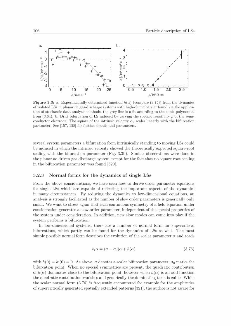
106 Particle description of LSs
a. b.
0 5 10 15 20 25-4
-3
-2
-1
0
1
α/mm s−1
h(α
)/102m
ms−
2
0
2
1
3
4
0.5 1.0 1.5 2.52.0
ρ/106Ω cm
α2 0/102m
m2s−
2
Figure 3.3: a. Experimentally determined function h(α) (compare (3.75)) from the dynamicsof isolated LSs in planar dc gas-discharge systems with high-ohmic barrier found via the applica-tion of stochastic data analysis methods, the grey line is a fit according to the cubic polynomialfrom (3.64). b. Drift bifurcation of LS induced by varying the specific resistivity ρ of the semi-conductor electrode. The square of the intrinsic velocity α0 scales linearly with the bifurcationparameter. See [157, 158] for further details and parameters.
several system parameters a bifurcation from intrinsically standing to moving LSs couldbe induced in which the intrinsic velocity showed the theoretically expected square-rootscaling with the bifurcation parameter (Fig. 3.3b). Similar observations were done inthe planar ac-driven gas-discharge system except for the fact that no square-root scalingin the bifurcation parameter was found [320].
3.2.3 Normal forms for the dynamics of single LSs
From the above considerations, we have seen how to derive order parameter equationsfor single LSs which are capable of reflecting the important aspects of the dynamicsin many circumstances. By reducing the dynamics to low-dimensional equations, ananalysis is strongly facilitated as the number of slow order parameters is generically onlysmall. We want to stress again that each continuous symmetry of a field equation underconsideration generates a slow order parameter, independent of the special properties ofthe system under consideration. In addition, new slow modes can come into play if thesystem performs a bifurcation.
In low-dimensional systems, there are a number of normal form for supercriticalbifurcations, which partly can be found for the dynamics of LSs as well. The mostsimple possible normal form describes the evolution of the scalar parameter α and reads
∂tα = (σ − σ0)α+ h(α) (3.76)
with h(0) = h′(0) = 0. As above, σ denotes a scalar bifurcation parameter, σ0 marks thebifurcation point. When no special symmetries are present, the quadratic contributionof h(α) dominates close to the bifurcation point, however when h(α) is an odd functionthe quadratic contribution vanishes and generically the dominating term is cubic. Whilethe scalar normal form (3.76) is frequently encountered for example for the amplitudesof supercritically generated spatially extended patterns [321], the author is not aware for
3.3 Interaction of structures 107
any examples concerning dynamic destabilizations of LSs. In contrast, the Hopf normalform
∂tA = (σ − σ0)A+ |A|2A (3.77)
for the amplitude A is frequently found when considering for example breathing LSs andother periodic processes. Note that in neither (3.76) nor (3.77) the critical modes α andA may be given by continuous symmetry parameters. The reason for this is that as thedynamics is equivalent for all choices of the continuous symmetry parameters, the righthand side expressions of (3.76) and (3.77) can not contain these quantities explicitly.
A possible explanation for the fact that (3.76) is typically not encountered for LSsmay lie in the fact that when a real eigenvalue passes the origin in a bifurcation, it coin-cidences with commonly present zero eigenvalues resulting from continuous symmetries.Although theoretically exceptions may be possible for special types of linear operators,in most cases it is found that in this situation the zero eigenvalue becomes degenerate.The corresponding normal form then reads
∂tα1 = α2,
∂tα2 = (σ − σ0)α2 + h(α2).(3.78)
with h having the same properties as in (3.76). We have discussed a special realizationabove in the context of drift bifurcations. Basically, an interesting aspect is given bybifurcations of higher co-dimensionality, which is found for example when a drift- and abreathing instability coincidence. Unfortunately, such cases have not been discussed inthe literature so far.
3.3 Interaction of structures
Generally, LSs may interact in complex ways involving many degrees of freedom. Theconcept of order parameters we are currently discussing however relies on the fact thatonly a few quantities evolve slowly dominating the dynamics of the whole system. In thecontext of single LSs, in order to derive equations we had to assume that either in theparameter range of interest the changes in the shape of the LSs could be characterized bya few parameters or alternatively and more generally applicable that the deformationsare only small compared to the structure itself. Basically, these ideas also apply whenmaking an extension to several interacting LSs. In nonlinear field equations, the influenceof one LS on another is based on the fact that the superposition of two solutions generallygenerates no new solution but induces a dynamic change of the state of the system. Aconceptually important case which often allows for an analytical treatment case is thatof weak interaction, meaning that the overlap of the structures is so small that they stayessentially preserved in the course of the dynamics and that the change of their shape isagain small compared to themselves. This of course excludes processes like generationand annihilation of LSs from the description.
Basically, the above introduced classification according to trial function andprojection-based methods can also be applied for interaction processes of LSs. We willthus consider briefly the trial-function based approach before coming to projection-basedtechniques.

108 Particle description of LSs
3.3.1 Weak interaction and trial-function methods
For classical soliton equations, inverse scattering transforms were the method of choice todeal with the interaction of LSs. However, when considering perturbed versions of theseequations, the direct applicability of inverse scattering mathods is rather limited [322,323]. One of the first solutions to this problem was proposed by Karpman and Solov‘ev[324]. The central idea is that appropriately parameterized trial functions should enterthe inverse scattering technique in order to obtain approximate evolution equations forthe parameters. As an advantage, it is not necessary to claim that the trial functionsalways exactly fulfil the evolution equation, examples can be found in [215, 280, 281].A second approach is to find a Lagrangian or Hamiltonian formulation for the evolutionequation, so that the original problem becomes related to a variational principle [282–285]. Typically, a linear superposition of a two or n single localized solutions is insertedinto the new evolution equation in order to obtain the order parameter equations. Forinstance, one may insert a parameterized solution q1 + q2 into the Hamiltonian H(q)and decompose the result as
H(q1 + q2) = H(q1) +H(q2) +Hint, (3.79)
where Hint is now the interaction Hamiltonian from which the interaction potentialcan be determined. Weak dissipation may be taken into account by modifying thetrial function in an appropriate way. In this case, in a first approximation only thetails of the LSs are affected, while is reflected for example by oscillations in space.The calculation scheme (3.79) is then applied to the dominant conservative part ofthe equation [216, 286, 287]. In particular, for large distances of the LSs a repulsiveinteraction for the purely conservative case may turn to a mixed attractive-repulsiveinteraction via the dissipative contributions, thereby allowing for the formation of boundstates of LSs.
A alternative to the above approach is to use existing integral evolution equations formomentum, energy etc. instead of the Lagrangian evolution equation [39, 288]. Notethat all techniques presented here rely on the relation of the evolution of the evolutionequation to a classical soliton equation.
3.3.2 Weak interaction and projection methods
In the context of single LSs projection-based methods provide access to systems even ifno relation to classical equations exists. The underlying basic strategy remains the samewhen treating interaction phenomena: dividing the changes in the shape of the structureinto fast and slow modes and projecting out the relevant information. For single LSs,the central problem was to carry out projections onto a nonlinear function F (q) whereq was a sum of modes. For two or more LSs, am aspect of major importance is thus anappropriate decomposition of the nonlinearity acting on the overlapping LSs in orderto make a connection to the theory of isolated LSs. In the following, we will only treat“weak interaction” meaning that he overlap of the LSs is not too large and they mainlyretain their shape in the course of time. Then, the state of the system differs from thesimple superposition of two stationary solutions only in a small function r. The goal of

3.3 Interaction of structures 109
the following section is to develop a decomposition
F (q1 + q2 + r) = F (q1) + F (q2) + R (3.80)
where R is again small, and in particular to develop approximate, practically usableexpressions for the function R. It is then clear that the above results for single LSs canbe applied to F (q1) and F (q2), and the interaction can be determined by treating R.
Compared to a standard expansion, the problem of a decomposition as proposedin (3.80) is that both q1 and q2 have large amplitudes alone at different positions inspace. To the authors knowledge, the problem was first dealt with by Elphick et al.who were interested in uniformly traveling pulse trains [289–291]. They proposed asolution motivated by the so-called tight-binding approximation in solid state physicswhich has afterwards been used by practically all authors dealing with weak interactionand projection methods, examples are given by [58, 59, 62, 217, 293, 294]. The key ideais to use a single unperturbed LS whose dynamics is to be evaluated as starting pointand to expand operators applied to perturbed versions of the LS as Taylor expansion.Considering (3.80) and taking q1 as reference solution, the decomposition in this casereads
F (q1 + q2 + r) = F (q1) + F ′(q1)[q2 + r] + . . . , (3.81)
higher orders are commonly not taken into account. The projectors used for the problemare the same as for the isolated LSs. While the use of (3.81) has produced reasonableresults (at least when a comparison of full and reduced equations was done, see forexample [58]), there are two problems arising. First, the solution around which theoperator F is expanded should be large compared to the perturbation so that subsequentterms of the series decrease in size. This certainly holds in the center of q1, but not inbetween the LSs where q1 and q2 are of equal amplitude. Second, when F becomes linearthe interaction terms should vanish in any order of the expansion which is definitely notthe case for (3.81).
In order to overcome the problem, we develop a “three-point expansion” as shown inthe following. Let us assume that the overlap of the LSs can be described as
F (q1 + q2) = F (q1) + F (q2) − F (0) +O(ε), (3.82)
where the smallness parameter ε characterizes the weak nonlinear superposition deter-mined by the shape and the distance of the LSs. As the desired expansion shouldwork similar to a classical Taylor expansion, one may symmetrize terms from the Taylorexpansion as
T 0 = F (q1) + F (q2),T 1 = F ′(q1)q2 + F ′(q2)q1,
T 2 =12F ′′(q1) : q2 : q1 +
12F ′′(q2) : q1 : q1,

110 Particle description of LSs
etc. Each term in T n contains either n vectors from q1 or q2. The Tailor expansion ofF (q1 + q2) around 0, i.e., far from the both LSs, should also contain only symmetricalcombinations of q1 or q2. Combining terms containing p fields with q1 and q fields q2
such that max(p, q) = n, we can introduce “correction fields” gn, defined as
g0 = F (0),g1 = F ′(0)q1 + F ′(0)q2 + F ′′(0) : q1 : q2,
g2 =12F ′′(0) : q1 : q1 +
12F ′′(0) : q2 : q2 +
12F ′′′(0) : q1 : q1 : q2
+12F ′′′(0) : q2 : q2 : q1 +
14F ′′′(0) : q1 : q1 : q2 : q2,
and so on. With the above results, one finds that in each order of ε, the “three-pointexpansion”
F (q1 + q2) = (T 0 − g0) + . . .+ (T n − gn) +O(εn) (3.83)
is valid everywhere in space. Furthermore, we have a precise error estimation availableif perturbation analysis is to be applied.
With (3.83) and the findings for single LSs, we can now write down the order pa-rameter equations for interacting LSs. Using the notation from Eq. (3.22) with theabbreviation
qk(x, t) = q0k(x, ck1(t), ck2(t), . . .) + rk(x, ck1(t), ck2(t), . . .), (3.84)
we insert the solution q = q01 + q02 + r into the evolution equation, where we havedefined r = r1 + r2. The uniformly small rest term r can be expressed either througheigenmodes at the “coordinates” c1 or c2. In the first case, we have
− ∂tc1 · ∇c1q01 − ∂tc2 · ∇c2q02 +∑
i
n(i)∑j
∂tγi1φji1(x, c1)
= F (q01 + q02) + F ′(q01 + q02)r + . . . ,
(3.85)
where the operator F is now expanded around q01+q02. On the right hand side, we havenow the nonlinear superposition of the two unperturbed localized solutions for which wedeveloped a method of decomposition above, which one may directly insert:
F (q01 + q02 + r) = F (q01 + q02) + F ′(q01 + q02)r + . . .
= F (q01) + F (q02) + F I(q1)q2 + F I(q2)q1 + F ′(q01)r + F ′(q02)r − F ′(0)r + . . .
(3.86)
where the first order “interaction operator” F I is defined via
F I(q1)q2 = F ′(q1)q2 − F ′(0)q2 −12F ′′(0) : q2 : q2. (3.87)
3.3 Interaction of structures 111
Note that in (3.86), the operators resulting from Frechet derivatives like F ′(q01 + q02)are expanded the same way as F itself.
We want to illustrate what general results one may expect for the order parameterdescription of LSs before treating some special examples. To this end, let us assume thatwe are dealing with a case for which no degenerate eigenvalues appear in the spectrumof F ′(q0i) (with i = 1, 2) and there is only one critical eigenmode for each LS. The latteris likely to be connected to a continuous symmetry so that q0i = q0(x, ci). Focussingon the structure q1, one may express r in terms of uncritical eigenmodes belonging tothis structure. We thus rewrite (3.86) as
∂tr + ∂tc1∂cr(c1) − F ′(q01 + q02)r= ∂tr + ∂tc1∂cr(c1) − F ′(q01)r − F ′(q02)r + F ′(0)r
= +F I(q01)q02 + F I(q02)q01 − ∂tc1∂cq01 − ∂tc2∂cq02.
(3.88)
According to the Fredholm alternative, the equation is solvable if no resonant termsappear, meaning in particular that the projection of the left hand side onto 〈Φ1
0(c1)|vanishes. As we have note yet made quantitative statements on the weakness of theinteraction, we now want to specify that ∂tc2〈Φ1
0(c1)|φ10(c2)〉 = O(ε2) which can for
example be obtained by claiming ∂tc2 ∼ εc2 and q01q02 ∼ ε. Then, the first order resultis
∂tc1 = 〈Φ10(c1)|F I(q01)q02 + F I(q02)q01〉, (3.89)
an analogous result can be obtained for the second LS as well.Next, we consider the case of degeneracy when a second critical eigenmode for each
critical mode appears. Then, the term r does not only consist of uncritical modesand can be written as r = α1(t)φ2
0(c1) + α2(t)φ20(c2) + R with R now containing only
uncritical modes. The argument with which the remainder terms have been eliminatedin (3.88) can be extended to generalized eigenmodes [292] and thus be applied to removeterms in R. As a result, we find
∂tc1 + ∂tc1α1〈Φ10(c1)|∂cφ
20(c1)〉 = α1 + 〈Φ1
0(c1)|F I(q01)q02 + F I(q02)q01〉,∂tα1 + ∂tc1α1〈Φ2
0(c1)|∂cφ20(c1)〉 = 〈Φ2
0(c1)|F I(q01)q02 + F I(q02)q01〉.(3.90)
Note that in many examples (like the one on the NLS equation below), the productterms on the left-hand side as well as potentially some terms on the right-hand sidevanish for symmetry reasons.
Our previous example on the active propagation of LSs shows that in some casesit is necessary to include higher order terms in the perturbation analysis. However,with (3.83) a precise estimate can be given which interaction terms have to be includedin the analysis, and the perturbative expansion (3.52) can be generalized accordingly.Generally, the lowest order of the analysis in which interaction terms enter is n, definedby q01q02 ∼ εn, so that the distance between the LSs is of essential importance. Whenthe distance between the LSs is large and the interaction term (3.87) enters in the

112 Particle description of LSs
highest order analyzed, the interaction terms are generally of central force nature. Inthe opposite case when the distance between the LSs becomes small and the interactionenters in low order, higher order terms may result in a coupling of force terms with othercritical modes and hence destroy the central force nature of the interaction. However, asthe corresponding terms result from the nonlinear superposition of small perturbationsof the first LS with the second one or its perturbations, these contributions are muchsmaller than the main term.
3.3.3 Examples for interacting LSs
In the following, we will illustrate the general theory of weak interaction on severalexamples of increasing complexity.
Example 1: Cubic-quintic complex GL equation
In our first example, we consider the interaction of two stationary LSs in the one-dimensional cubic-quintic GL equation
∂tq = (dr + idi)∆q + lrq + (cr + ici)|q|2q + (qr + iqi)|q|4q (3.91)
using the above introduced methods. As we need some stationary solutions as startingpoint and as the LSs are generically oscillating sinusoidally with a frequency ω, we willconsider the equation in a co-rotating frame. We treat only stationary solutions withrotational symmetry and no topological charge (see [62] for an example with topologicalcharge), so that the critical modes that have to be considered are the neutral modes inthe direction of the connection line between the LSs (which we assume to point alongthe x-axis) and those corresponding to a phase-shift of the LSs. For reasons of simplicitywe will furthermore only consider two equal LSs so that the relative phase differencedoes not change during interaction. Correspondingly, the only slow order parameter canbe chosen to be the x-position pi,x of the LSs.
In order to deal with real operators, we will use a representation of the GL equationin real and imaginary part according to (2.40). The linearization F ′ of the operator Faround a stationary solution (a1, b1) is determined then by the 2x2 matrix (F ′
ij), wherethe matrix elements are given by
F ′11 = dr∂xx + lr + cr(a2
1 + b21) + 2a1(cra1 − cib1)
+ qr(a21 + b21)
2 + 4a1(a21 + b21)(qra1 − cib1),
F ′12 = −di∂xx + ω − ci(a2
1 + b21) + 2b1(cra1 − cib1)
− qi(a21 + b21)
2 + 4b1(a21 + b21)(qra1 − qib1),
F ′21 = di∂xx − ω + ci(a2
1 + b21) + 2a1(cia1 + crb1)
+ qi(a21 + b21)
2 + 4a1(a21 + b21)(qia1 + qrb1),
F ′22 = dr∂xx + lr + cr(a2
1 + b21) + 2b1(cia1 + crb1)
+ qr(a21 + b21)
2 + 4b1(a21 + b21)(qia1 + crb1).
(3.92)

3.3 Interaction of structures 113
For the linearization operator, F ′† = (F ′ji). While the relevant neutral mode φ1
0 for F ′
with respect to the LS number 1 are of course given by (a1,x, b1,x), it is not possible togive a related analytical expression for the neutral mode of the adjoint operator, whichmust directly be the correct projector mode as the problem is not degenerated. We willthus calculate it numerically by using a relaxation method, i.e. solving the equation∂tΦ1
0 = F ′†Φ10 for its stationary solution. As last ingredient, we need an expression for
the interaction function. With the definition (3.87), one finds
F Ia (a1, b1)[a2, b2] = [cr(a2
1 + b21) + 2a1(cra1 − cib1)
+ qr(a21 + b21)
2 + 4a1(a21 + b21)(qra1 − qib1)]a2
+ [−ci(a21 + b21) + 2b1(cra1 − cib1)
− qi(a21 + b21)
2 + 4b1(a21 + b21)(qra1 − qib1)]b2,
F Ib (a1, b1)[a2, b2] = [cr(a2
1 + b21) + 2b1(cia1 + crb1)
+ qr(a21 + b21)
2 + 4b1(a21 + b21)(qia1 + qrb1)]b2
+ [ci(a21 + b21) + 2a1(cia1 + crb1)
+ qi(a21 + b21)
2 + 4a1(a21 + b21)(qia1 + qrb1)]a2.
(3.93)
One may now choose a set of parameters and calculate the reduced equations, which areof the general form
∂tpi,x = F (|pi − pj|) pi − pj
|pi − pj| with i, j = 1, 2, i = j. (3.94)
Structurally, this type of interaction law is also encountered for overdamped classicalparticles. An example for an interaction function in the one-dimensional case is shownin Fig. 3.4a on the left-hand side. As parameters, we have used dr = di = 0.5,lr = qr = qi = −0.1, cr = 0.52, ci = 1. One may test the correctness of the resultsby comparing the analytical predictions with simulations of the full GL equation.The positions of the LSs in the full equations can then be defined as correspondingcenters of mass of the LS above a certain threshold. As the graph in the right-handside of Fig. 3.4a shows, there is extremely good agreements of the results for differentinitial separations. Extending the analysis to more general situations, a relative phasedifference of the LSs may be included in the calculation which becomes a second orderparameter. This situation was analyzed for very weakly overlapping tails in [217], butno comparison with numerically obtained trajectories was given.
Example 2: Nonlinear Schrodinger equation
Although not a dissipative system, we will take a look at the 1D NLS equation (2.36)using a projection-based method as it shows some interesting properties like Galileaninvariance and has a fully analytical solution. Previous works have dealt with thisexample using inverse scattering techniques. The treatment of the NLS equation canin some sense be considered as a special case of example 1 discussed above which oneobtains by choosing almost all parameters as zero, except for di = −1, ci = −1. We will

114 Particle description of LSs
a1. a2.
6 7 8 9 10
0
1
2
3
4
distance d
103F
(d)
0 200 400 600 800
6.0
6.4
6.8
7.2
7.6
8.0
8.4
time t
dis
tance
d
b1. b2.
6 8 10 12 14
-5
-4
-3
-2
-1
0
distance d
102F
(d)
0 10 20 30 40
8
10
12
14
time t
dis
tance
d
c1. c2.
0.2 0.4
0
0.3 0.5
-2
-1
0
1
2
distance d
105F
(d)
0 200 400 600 800 1000
0.0
0.2
0.4
0.6
0.8
time t
dis
tance
d
Figure 3.4: Interaction of LSs in the reduced description. The left hand images depict thefunction F (d) while a comparison of the distance d of two interacting LSs as a function of timeaccording to numerical simulations of the full field equations (solid line) and to the reducedequations (dashed line) is shown on the right. a. Two in-phase LSs in the one-dimensionalGL equation for two different initial separations, b. two in-phase LSs in the one-dimensionalNLS equation for two different initial separations, c. two LSs in the two-dimensional reaction-diffusion system (2.26) for τ = 3.35 (scattering) and τ = 3.375 (formation of a bound state).For parameters see text.
again consider only the case of interacting LSs with equal phase. The equation has theinteresting property that a fully integrable, and in particular an analytical solution fora single LS can be given. To obtain a stationary solution we go to a co-rotating frame,so that one possible representation of a stationary solution at the position pi is givenby the real-valued function qi = (
√2 sech(x− pi), 0) (where we choose a representation
in real and imaginary part). Again we will consider only the case of interacting LSswith equal phase. As the NLS does not only have invariances with respect to shifts inposition and phase but also Galilean invariance, one may expect a natural degeneracy

3.3 Interaction of structures 115
of the neutral mode in spite of the stationarity of the LSs. Therefore, the generalizedeigenmodes of the neutral modes come into play. As the linearized operator F ′ greatlysimplifies compared to the GL example, one may find the generalized eigenmode bydirectly solving the equation φ1
0 = F ′φ20 with φ1
0 = (√
2 sech(x) tanh(x), 0). The solutionreads φ2
0 = (0,−x tanh(x)/√
2). In addition, the operator F ′ is antisymmetric, sothat one may also find the neutral and generalized eigenmode of the adjoint operatoranalytically. Except for normalization, one finds that the projectors for the structureqi are given by Φ1
0 = (−x tanh(x)/√
2, 0) and Φ20 = (0,
√2 sech2(x)). Evaluating the
equations according to the developed formalism yields
∂tpi = vi,
∂tvi = F (|pi − pj|) pi − pj
|pi − pj | with i, j = 1, 2, i = j.(3.95)
This result shows that within the used approximation, the LSs in the NLS behave likeclassical particles interacting under a central force. The interaction function which onemay have expected to be present in the position equation vanishes due to the Galileaninvariance of the original equations. For two in-phase LSs, the relevant interactionoperator for F (d) in the velocity equation reads F I(a1, b1)[a2, b2] = 3(a2
1a2 +a1a22) as we
have chosen b1 = b2 = 0, and by inserting the above given expression for the projectorsthe expression can be given analytically, yielding
F (d) = 2 csch(d)4(24d − 12dcosh(d) + 12d cosh(2d)+ 9 sinh(d) − 18 sinh(2d) + sinh(3d)).
(3.96)
The function is depicted in Fig. 3.4b in the left graph, and the comparison to thefull numerical simulation is done in the right graph, again for two different initialseparations of the LSs.
Example 3: Reaction-diffusion equation with actively propagating LSs
Our third and most complex example deals with the interaction of LSs with inner degreesof freedom in reaction-diffusion equations. As shown by our second example for isolatedLSs, in reaction-diffusion systems one finds supercritical bifurcations from standing totraveling LSs. When several LSs with excited inner degrees of freedom interact, weexpect from the general theory that in first order we have a linear superposition ofthe effects of the inner degrees of freedom and the interaction terms. Although thecorresponding equations should be structurally similar to the second example involvingthe NLS equation, the degeneracy now arises from a bifurcation and not from a Galileaninvariance of the system. Depending on the symmetry of the stationary solution, wehave shown that for single LSs, one may either expect a normal form given by (3.58)or (3.64). When looking at the concrete example (2.26) in two spatial dimensions,we encounter rotationally symmetric LSs corresponding to the second case. Similarto the GL example we face the problem that it is difficult to calculate some requiredmodes analytically. However, in this case the problem lies in the determination of the

116 Particle description of LSs
generalized eigenmodes. When the latter are known, the adjoint modes can be givenanalytically. We have the choice of either calculating the generalized modes numericallyor to consider a case where analytical expressions are known. For our model system,the second case is for example given in the parameter limit dw → 0, θ → 0.
In [58], the problem was treated using the decomposition (3.81) instead of the moreexact decomposition (3.86). After a number of steps, one obtained the final result
∂tpi = αi + F (|pi − pj |)/κ3
pi − pj
|pi − pj|,
∂tαi = (τ − τc)κ23αi +
〈(∂ξξu1)2〉κ3〈(∂ξu1)2〉 |αi|2αi + F (|pi − pj |)
pi − pj
|pi − pj |(3.97)
with τc marking the bifurcation point of the drift bifurcation. The results turned out tobe rather appropriate to represent the dynamics of the full field equations. The reasonfor this will be explained in the following. The only nonlinear function in (2.26) appearsin the activator equation and reads f(u) = λu− u3 + κ1, furthermore the u-componentof the generalized eigenmodes P vanishes for the special case dw → 0, θ → 0. With uh
denoting the homogeneous ground state, we have
f(u1 + u2 + uh + ε2r)
= λu1 − u31 + λu2 − u3
2 − 3u2h(u1 + u2) − 3uh(u2
1 + u22) − 3(u2
1u2 + u22u1) − 6uhu1u2
+ ε2r(λ− 3u2h − 6uh(u1 + u2) − 3(u2
1 + u22) − 6u1u2) − 3ε4r2(uh + u1 + u2) + ε6r3.
(3.98)
This expression is also produced by the general decomposition method (3.86). In con-trast, the decomposition (3.81) yields
f(u1 + u2 + uh + ε2r) = f(u1 + uh) + f ′(u1 + uh)(u2 + ε2r)
= λu1 − u31 + λu2 − 3u2
h(u1 + u2) − 3uh(u21 + u3
2) − 6uhu1u2
− ε2r(λ− 3u2h − 6uhu1 − 3u2
1).
(3.99)
The reason for the good results produced by (3.99) is that when projecting both equa-tions on a projector mode 〈Φi(u1)| (meaning the projector belongs to the solution u1)and claiming u1u2 ∼ O(ε2), we find
〈Φi(u1)|f(u1 + u2 + uh + ε2r) − [f(u1 + uh) + f ′(u1 + uh)(u2 + ε2r)]〉 = O(ε4).(3.100)
As the second example in Sec. 3.2.2.3 has shown that the evaluation must only beperformed up to third order, the difference in the results is only a small error of fourthorder in ε. Thus, the interaction function up to this small error is determined by thefirst order term interaction operator (3.87), namely
F (|pi − pj|) =〈ui,ξ| − 3(u2
i uj + u2jui) − 6uhuiuj〉
〈u1,ξ|u1,ξ〉 , (3.101)

3.3 Interaction of structures 117
For the numerical test in which we consider a head-on collision of two LSs, we choosethe other parameters in such a way that the stationary LSs show an oscillatory decay.Correspondingly, the resulting interaction function (Fig. 3.4c) oscillates with distance.In [58] it was suggested to fit this type of interaction law with the analytic expression
F (d) =−d1
d1/2exp(−d2d) cos(d3(d− d4)) (3.102)
where the di are fit coefficients as this function reflects the decay of Bessel functionfor large values. As it is not too reasonable to start simulations with different initialseparations like in the other examples due to the active propagation of the LSs, insteadwe vary the intrinsic velocity via the parameter τ . While for small intrinsic velocitiesresulting in a scattering event of the LSs the agreement is very good, there are somedeviations for larger intrinsic velocities, leading to the formation of a bound state. Thereason for this is that in the bound state case, the LSs approach each other further thanin the other examples we discussed so far. Consequently, higher order correction termsmay come into play in this case. Nevertheless, the final state is correctly predicted alsoby the low-order approximation.
The fact that the complete solution of the u-component can be represented as u =u1 +u2 +uh + ε2r is due to the special choice dw → 0, θ → 0. For arbitrary parameters,we instead have to use the more general form u = u1 + u2 + uh + ε(α1P1 + α2P2) + ε2rwith the Pi being the u-components of φ2
0(pi), the generalized neutral eigenmodes oftranslation for the structure i. With a scaling u1u2 ∼ O(ε2), terms with Pi couple tothe unperturbed structure uj in third order in ε, thus breaking the central force natureof the interaction as previously mentioned above. In order to avoid this in the generalcase, one has to claim u1u2 ∼ O(εn) with n > 2, implying that the derivation would holdonly for larger distances. Using the general decomposition (3.86) however theoreticallyleads to correct results in arbitrary order of ε (for the GL and NLS examples above, itwas even possible to claim u1u2 ∼ ε).
In experimental systems, weak interaction processes manifest themselves in variousways. The perhaps most significant one is the formation of bound states consistingof two or several LSs, which can for example be found for current filaments in planargas-discharges of both dc [171, 172, 325–327] and ac type [1, 328], oscillons in granularmedia and colloidal suspensions [4, 329, 330], electrical networks [331], chemical pulses[137, 138], liquid crystal light valves [332–334], saturable absorbers [204] or semicon-ductor microresonators [308, 335]. In a number of systems, typical lock-in distancescould be connected to oscillatory tails of the LSs [3, 311, 328, 336, 337]. The onlydirect measurement of an interaction law was up to now carried out in planar dc gas-discharge systems [173]. Here, the individual LSs propagate under the combined actionof intrinsic drive, interaction and the influence of noise (Fig.3.5a). Furthermore, it isfound that bound states are possible and may exist over a longer period of time beforebreaking up (Fig.3.5b). In order to determine an interaction law from experimental dataa phenomenological extension of the Langevin equation (3.75) in the form
∂tpi = αi, ∂tαi = h(αi)αi
αi+∑i=j
F (dij)dij
dij+R(αi)Γi(t) (3.103)

118 Particle description of LSs
a. b. c.
-7.5 0.0 7.5-7.5
0.0
7.5
-5.0
5.0
2.5
-2.5
-2.5-5.0 5.02.5
position x/mm
posi
tion
y/m
m
0 20 40 600
5
10
15
20
time t/s
dis
tance
d/m
m1.5 2.0 2.5 3.0 3.5
-100
-50
0
50
100
150
200
250
distance d/mm
F(d
)/m
ms−
2
Figure 3.5: Trajectories (a.) and time evolution of the distance (b.) for two interacting LSs inplanar dc gas-discharge systems propagating under the influence of noise. The LSs form a boundstate over about 35 s before the molecules break up. c. Typical example for an interaction lawfound with the analysis method described in the text, the grey line is a fit according to (3.102).See [173] for further details.
was proposed whose deterministic part has the same form as (3.97) if in the latter systemthe coupling in the p-equation is neglected. Using means of stochastic data analysis theinteraction function F (d) could be determined from experimental data in several cases forthe interaction of two LSs, a characteristic example is depicted in Fig.3.5c. The resultscan be well represented by the theoretically proposed oscillating function (3.102). Inthose cases in which oscillatory tails could be seen, stable lock-in distances were foundto coincidence with a constructive overlap of the tails. Neglecting potential interactionfunctions in the pi-equation of (3.103) is necessary to access the experimental data asonly position and velocity are measurable quantities. In the next chapter we will discussin more detail the influence of different coupling structures for actively propagating andinteracting LSs, however we may already state here that if only two LSs are considered,in many examples the coupling in the p-equation has only minor influence.
3.3.4 Symmetries, dynamics and interaction processes
Considering particle concepts for example in classical Newton mechanics, many impor-tant concepts are closely connected to the structure of the underlying equations. Termslike energy, momentum, angular momentum etc which today have become extremelyintuitive for most physicists arise as conserved quantities via the corresponding forcebalance equations.
Turning to self-organized LSs, we find ordinary differential equations for a small num-ber of slowly varying quantities. When position and velocity appear as order parameters,the structure of the reduced equations formally shows strong parallels to classical New-ton equations. One may therefore consider the latter as manifestation of the particle-likenature of the LSs. Of course, when comparing the structure of the reduced equationswith classical particle equations, potential similarities arise on a mathematical, not aphysical level. This means that while the phenomenology of the dynamics may be simi-lar or equal to a classical situation, a comparison of physical mechanisms is usually notpossible (ideas like mass for example do not exist for LSs).
While a systematic classification of the behavior of LSs according the properties ofthe underlying field equation is missing so far, our considerations already allow for some

3.3 Interaction of structures 119
interesting statements. Generically, systems in which LSs exist will have only transla-tional and rotational invariance. Different examples have shown that for a rotationallysymmetric stationary solution sufficiently far below a bifurcation point, only the posi-tion will appear as symmetry-induced order parameter, so that in the presence of smallinhomogeneities and neighboring LSs, the system will be determined by equations of theform
∂tpi = f(pi) + g(pi − pj). (3.104)
Here, f reflects the influence of inhomogeneities and g accounts for weak interaction.This expression formally corresponds to the equation for interacting, overdamped New-tonian particles moving in an external potential. In our example on the classical NLSequation translational invariance together with Galilean invariance for two interactingLSs with equal phase results in the structure
∂tpi = vi[+f1(pi)],∂tvi = [f2(pi)] + g(pi − pj),
(3.105)
due to a natural degeneracy of the eigenvalues. The resulting behavior then directlycorresponds to what one would expect for classical particles. The Galilean invarianceof the field equation is reflected by the same property of the reduced equation. Weakinhomogeneities may break the Galilean invariance and thus result in the terms put inangular brackets. Finally, our example on LSs in reaction-diffusion systems has shownthat entirely “unclassical” behavior can be found in the form of active propagation withthe general form
∂tpi = vi + f1(pi) + g1(pi − pj),
∂tvi = h(vi) + f2(pi) + g2(pi − pj).(3.106)
While the coupled set of two first order equations (3.106) reflects some “inert” behaviorof the LSs, the latter is due to an additional inner degree of freedom that is excited ina bifurcation. In more detail, the inner degree of freedom with a slow time constantcouples to the neutral modes responsible for the translation of the structure (one first-order ODE), and the inner degree of freedom is excited by itself (resulting in a secondfirst-order ODE). In the long-time limit the dynamics of isolated LSs will thus not bedetermined by the initial conditions (for example the initial velocity), but by the innerdegrees of freedom. The resulting type of dynamics is totally untypical for classicalparticles where no inner degrees of freedom are considered or where they are at leastdecoupled from propagation. We have seen that the active propagation (3.106) arisesfrom a degeneracy of eigenvalues in the bifurcation point. In the non-degenerate case, aHopf bifurcation to for example a breathing structures is generic. In a codimension-twopoint or further above a codimension-one point, there can also be a coaction of travelingand breathing.
Looking at the structure of the equations (3.104) - (3.106), one may give a roughestimate of typical dynamical phenomena that can occur in the considered situation

120 Particle description of LSs
Eq. (3.104) Eq. (3.105) Eq. (3.106)propagation no arbitrary velocity fixed velocityrepulsion yes yes yespinning yes yes yeslock-in yes yes yesscattering no yes yesoscillating molecules no yes yesrotating molecules no yes yesreaction to perturbation ch. of position ch. of direction ch. of direction(long-time limit) and velocity
Table 3.2: Overview on possible dynamical phenomena for LSs described by the equations(3.104) - (3.106).
(Table 3.2). In the case of stationary LSs, the overdamped motion puts strong restrictionon the dynamics. In the long time-limit, the structures can not perform a motion with afinite velocity, the only change to induce a shift of the position is by local inhomogeneitiesor perturbations. Furthermore, even in the latter case there can be no oscillations aroundpotential resting points due to for example a trapping inhomogeneity. Consequently,without interaction a potential trapping site will definitely trap a LS that comes closeenough. In systems with Galilean invariance, one may basically encounter all phenomenathat are known for classical particles as long as the order parameter approximation isvalid. In particular, each LS may have a different velocity in the long-time limit, andperturbations may change these velocities continuously. While spatial inhomogeneitiesbreak the Galilean invariance of the system and consequently also of the underlyingfield equations, for small perturbations their influence manifests in the field equationsas additional additive space-dependent terms. In this way, the system gets a hybridcharacter between classical and overdamped motion, whether one type of dynamicsdominates depends on the type of system. The active propagation basically allowsfor most of the classical dynamical phenomena to occur as well as the particles showsome “inert” behavior due to their inner degree of freedom. Nevertheless, the couplingstructure of the equations is generally more complex and the active propagation onlyallows for one absolute velocity of isolated LSs in the long time limit. We will discussthe new features of this kind of dynamics in more detail in the next chapter.
While it is not too difficult to systematically classify the possible types of dynam-ics when only the “standard” symmetries (translation, rotation, Galilean) are present,the situation is currently not as clear for hidden symmetries like invariance with re-spect to phase shifts, scaling transformations etc. While the above presented projectiontechniques are technically capable of dealing with this problem, it is likely that grouptheoretic methods have to be applied to give a general classification. Last but not least,even when it is possible to calculate analytically or numerically the functions in (3.104)- (3.106) as well as other order parameter equations, an understanding of their natureis essentially connected to the specific mechanisms in the underlying system.

3.4 Stochastic and fluctuating systems 121
3.4 Stochastic and fluctuating systems
3.4.1 General theory
In many physical systems noise is present and affects the dynamics of LS (see for example[157, 158, 320] as well as Fig. 3.5). In order to account for these effects, one mayeither extend the above derived order parameter equations in a phenomenological wayor introduce noise terms already on the level of the underlying field equations. Dependingon the system, sources of noise may be thermal fluctuations, fast generation processes,coupled heat-baths, external radiation etc. In the following, we want to explore hownoisy processes in the field equations influence the dynamics of LSs on the level of orderparameter equations. A potential way of modeling the influence of noise is by extendingthe field equations (3.10) to
∂tq = F (q,∇,σ) −→ ∂tq = F (q,∇,σ) + M(q)Γ(x, t). (3.107)
where M = mη(q)δηµ is a diagonal matrix with noise amplitudes as entries and Γ isa vector with normalized noise forces (η and µ represent the components of q). Thestatistical properties of the noise forces are essential for the dynamics of the equation. Inorder to do an analytical calculation, we will assume that the noise forces have vanishingmean, are Gaussian distributed and are δ-correlated in space and time, i.e.
⟨Γη(x, t)Γµ(x′, t′)
⟩E
= 2δηµδ(x − x′)δ(t− t′), (3.108)
where the brackets with index E denote the ensemble average. Furthermore, the noiseamplitudes are assumed to be so small that the action of the fluctuations does notendanger the integrity of the LS, for example by annihilation or generation of other LSs.An analysis of the latter type of processes is for example given in [338].
The stochastic generalization given by Eq. (3.107) implies that the “amplitudes” ci,and γj appearing in the eigenmode decomposition become random variables becausethey are subjected to fluctuating forces. In detail, in the stochastic case Eq. (3.23)becomes
−∂tc · ∇c[q0 + q] +∂
∂tq = F (q) + M(q)Γ. (3.109)
Projecting on the individual eigenmodes as in the deterministic case, we obtain in thenon-degenerate case
∂tγi + ·∑
k
∂tckγk〈Φ1i |∂ck
φ1k〉 = λiγi + 〈Φ1
i |N (q)〉 + 〈Φ1i |M(q)Γ〉, (3.110)
the generalizations for the ci and the degenerate case should be obvious.Let us start with a single LS and the most simple case that we are far below any
bifurcation points, meaning that the dynamics only has to be considered on very slow

122 Particle description of LSs
time scales. Considering only translational invariance, the only critical modes are as-sociated with the position and the amplitudes of all other modes relax to zero. Thecorresponding terms drop out of (3.110), and we obtain
∂tpξ = 〈Φ10,ξ|M(q0)Γ〉. (3.111)
Physically this means that at each instant the structure experiences a deformation bynoise which instantaneously relaxes so that only a neutral displacement remains. Theresult agrees with results reported in earlier works for propagating kinks in bistable one-component reaction-diffusion systems [339] and should be generic for arbitrary types ofsystems.
In a next step, we may exemplarily consider a situation where a neutral generalizedeigenmode influences the dynamics. Looking at the perturbation analysis carried outin our second example in Sec. 3.2.2.3, we have seen that different time scales come intoplay in this situation. In particular, as we see from Eqns. (3.53) and (3.54) on the timescale T1 of the perturbation analysis uncritical modes already appear, however withoutinfluencing the dynamics. We thus have to develop a way to treat the fluctuations forthe non-critical modes. The difference between deterministic and stochastic case is thatthe stochastic generalizations of the deterministic equations contain additional termsζi,nc defined as
ζi,nc(t) = 〈Φ1i |M(q)Γ(t)〉. (3.112)
Distinguishing between fast and slow deterministic modes (with amplitudes βk and αi,respectively), we may again try to express the amplitudes βk of the non-critical modesin terms of the amplitudes αi. Taking the fluctuating contributions ζi,nc into account,we obtain relations of the form
βk = hk(α) +Wk(α, ζk,nc). (3.113)
The fluctuating contributions of the non-critical modes, however, can usually be ne-glected because they are small with respect to the fluctuating contributions of the crit-ical modes [340, 341]. Neglecting the terms Wk in Eq. (3.113), we can eliminate thenon-critical modes in the amplitude equations of the critical modes just as in the deter-ministic case. Furthermore, we again make the approximation M(q) ≈ M(q0). Then,we obtain in the non-degenerate case
∂tαi = gi(α) + 〈Φ1i |M(q0)Γ〉 (3.114)
with the gi being the same functions as in the deterministic case.For the drift bifurcation, the same idea can be applied. As a generalization of (3.111)
in the presence of a generalized eigenmode one thus finds
∂tpξ = fξ(α) + 〈Φ10,ξ|M (q0)Γ〉 (3.115)

3.4 Stochastic and fluctuating systems 123
with fξ(α) = 〈Φ10,ξ|F (q)〉 under the above approximations. Equations for the compo-
nents of α are obtained in an analogous way with the help of suitable projectors Φ20,ξ.
In sum, we have shown that in the stochastic case we need to add particular fluctuatingcomponents to the deterministic relations given for example by Eq. (3.34). The result-ing stochastic evolution equations for p and α in our above example written in vectornotation read
∂tp = α + Φ10,ξ|M(q0)Γ(x, t)〉,
∂tα = g(α) + 〈Φ20,ξ|M(q0)Γ(x, t)〉, (3.116)
showing that in general, all order parameters will be influenced by the noise in thesystem.
In order to explore the properties of the noise terms in more detail, we calculate thefirst and second moment of the noise forces componentwise. In the following equations,the indexes ξ and χ denote spatial directions (i.e. mutually orthogonal modes), and asabove, η and µ denote the individual components of the occurring modes. Also, in orderto improve the overview, we will denote the scalar product by an index x in order todistinguish it from the ensemble average, which is as before denoted with the index E.For the first moment, one finds
⟨〈(Φ1
0,ξ)η|mη(q0) Γη(x, t)〉x⟩
E=∫Ω
mη(q0)GP,ξ,η
⟨Γη(x, t)
⟩E
dnx = 0. (3.117)
The second moment yields the relation
⟨〈(Φ1
0,ξ)η(x − p(t))|mη(q0(x − p(t))) Γη(x, t)〉x×〈(Φ1
0,χ)µ(x′ − p(t′))|mµ(q0(x′ − p(t′))) Γµ((x′), t′)〉x′
⟩E
=∫Ω
∫Ω
mη(q0(x − p(t)))mµ(q0(x′ − p(t′)))(Φ1
0,ξ)η(x − p(t)) (Φ10,χ)µ(x′ − p(t′))
×⟨Γη(x, t)Γµ(x′, t′)
⟩E
dnxdnx′
= 2∫Ω
∫Ω
mη(q0(x − p(t)))mµ(q0(x′ − p(t′)))(Φ1
0,ξ)η(x − p(t))(Φ10,χ)µ(x′ − p(t))
×δ(x − x′)δ(t− t′) dnxdnx′
= 2〈m2η(q0)(Φ
10,ξ)
2η〉xδηµδξχδ(t − t′). (3.118)
An analogous result is obtained for the projections on the other critical modes. Thisshows that the projections keep the property of being δ-correlated in time. However,analogously to (3.118) one may calculate the correlations of the noise forces obtainedusing different projectors and thereby show that the noise forces in the equations for thedifferent order parameters obtained according to (3.114) are not necessarily independent

124 Particle description of LSs
of each other (unlike the noise forces in the different components in the original fieldequation). Considering for example additive noise in the field equations, the coefficientmη can be drawn out of the integral in (3.118), and one sees that the correlation fordifferent noise terms only vanishes if the projectors are orthogonal.
The extension of regular field equations by stochastic terms may generally bring in awide range of different timescales affecting all modes. In order to overcome this problem,we have neglected the fluctuating forces ζi,nc that act on the amplitudes of non-criticalmodes. That is, we have put the expressions Wk in Eq. (3.113) equal to zero becausethe noise amplitudes of these fluctuating forces are usually much smaller than the noiseamplitudes of the fluctuating forces related to the critical modes. Nevertheless, theseweakly interacting fluctuating forces can also affect the amplitude dynamics of the criti-cal modes. The quality of the approximation thus essentially depends on the propertiesof the linearization spectrum and the time scales for which the reduced equations arederived. Generally, the results are the better the slower the time scale on which thereduced equations are to hold and the larger the gap between the eigenvalues belongingto critical and non-critical modes.
In order to explicitly account for the impacts of the fluctuating forces ζi,nc, one gen-erally has two options. First, one may try to derive analytical expressions for Wk (forexamples see [340, 341]). If we substitute such an analytical expression into q, we willsee that q depends on the fluctuating components ζi,nc: q(α,β) → q(α, ζi,nc). As aresult, the Langevin equations for the αi and βi will in any case involve multiplicativenoise terms. Another origin of multiplicative noise may be higher order corrections toour approximation M(q) ≈ M (q0) we made above. As an alternative to this approach,the impact of a particular fluctuating forces ζi,nc can be examined by adding the corre-sponding amplitude βi to the set of critical modes. Accordingly, the amplitude vectorα would read α = (α1, . . . , αM , βi). This second approach will yield additive noiseLangevin equations if additive noise is considered in the field equation. Comparing thetwo approaches, we see that multiplicative noise terms can arise due to projections fromhigher dimensional phase spaces to lower dimensional ones. This finding is in line withour notion about the origin of multiplicative noise sources [342]. Multiplicative noiseforces originate from fluctuating parameters which in more comprehensive descriptionswould satisfy additive noise Langevin equations.
Looking at the case where degenerate eigenvalues connected to propagation come intoplay, we find that the general form of the order parameter equations for propagating LSsin noisy field equations is more complex than the frequently used phenomenologicallyintroduced form for active Brownian particles. The latter is mostly introduced on aphenomenological basis. While a rigorous approach is possible when a Hamilton functioncan be set up for the system [343], no general approach has been available for dissipativefield equations for which actively propagating localized solutions are observed.
3.4.2 Noise correlations in the order parameter equations
Particle-like behavior under the influence of noise is known to exist in the form of Brow-nian motion of particles since the experimental investigations by Brown and Brongniartin 1827 and the fundamental theoretical works by Bachelier [344], Smoluchowski [345]and Einstein [346]. In its simplest form, the basis of modeling of Brownian motion is

3.4 Stochastic and fluctuating systems 125
given by the Langevin equation
∂tp = α, ∂tα = −γα +RΓ(t), (3.119)
describing the acceleration α of a Brownian particle as the superposition of a deter-ministic part −γα with damping coefficient γ and a stochastic part with additive noiseforces which in most theoretical works are assumed to be δ-correlated. The physical mo-tivation for using an equation of the form (3.119) can be manifold. In order to describethe motion of microscopic particles, one had to assume frequent collisions of a singleparticle with neighboring particles, leading to both deterministic and stochastic parts inthe equation. The stochastic part is also frequently motivated by a coupled heat bath[347], where the noise amplitudes are considered as a measure of the temperature. Inmany situations, Eq. (3.119) can be validated by tracing Brownian particles and ana-lyzing the corresponding distribution functions. In addition, many systems allow for arigorous derivation of Eq. (3.119) from basic mechanical equations using standard sta-tistical techniques. Comparing (3.119) to (3.116), aside from generalized deterministicfunctions f and g we find noise forces in both components which may even be correlated.
Many recent investigations deal with phenomenological extensions of Eq. (3.119),which are often of the form
∂tpi = αi, ∂tαi = g(αi) +∑i=j
F (dij) + R(αi)Γi(t). (3.120)
Eq. (3.120) describes the motion of a Brownian particle with index i and a generalizeddeterministic part under a force F caused by other Brownian particles with index j = i,where dij is given by xi − xj and the Γi are statistically independent Langevin forces.A frequent choice of g(α) is given by g(α) = k1α− k3|α|2α leading to active Brownianmotion, which is a phenomenological model for the dynamics of self-propelled objects.Types of Eq. (3.120) are encountered when modeling grains in dusty plasmas [348],myosin head on actin filaments [349, 350], swarms of fishes and daphnia [351], trafficflow [352] and even sociological systems [353]. For this choice of g(α) we also havea strong connection to the intrinsic dynamics of LSs we have derived in the previoussections when considering the dynamics of an isolated LS.
In the following, our goal is to explore the influence of driving both componentsp and α with noise as found in the previous section and compare the findings to thephenomenological model of active Brownian motion. When considering only the α-equation which is independent of p, Eqns. (3.116) and (3.120) for a single particle andadditive noise (meaning R(α) = R) are almost equal. For this equation alone a fewproperties can still be given analytically with standard means [354], for example thestationary solution of the Fokker-Planck equation which reads
P (α) = N exp( 1R2
(k1
2α2 − k3
4α4)). (3.121)
Due to the nonlinearity of the equation however, many interesting quantities are ratherdifficult to obtain analytically. Therefore, in order to explore the influence of noise in

126 Particle description of LSs
several coupled equations in a first step we will consider the linear equation
∂tp = α+Rp(sΓp(t) +√
1 − s2Γα(t)),∂tα = −k1α+RαΓα(t)
(3.122)
with s ∈ [0, 1]. It may be considered as a model for an active particle below a driftbifurcation in the limit of small particle velocities so that nonlinear terms in α can beneglected. The second equation exactly corresponds to (3.119) while the first equationcontains two driving terms. The noise forces Γp and Γα are assumed to be uncorrelated,so that for s = 0, both components are driven independently. In contrast, for s = 1 thedriving in both components is equal. For classical Brownian motion, it is well known thatthe mean squared displacement of a particle as a function of time scales linearly withthe latter for sufficiently large times [354]. In the following, we will show analyticallyhow the mean squared displacement (in one spatial dimension) behaves for the extension(3.122). As a starting point, we integrate the first equation of (3.122) in time to obtain
〈(p(t) − p(0))2〉
= 〈t∫
0
∂tp(t1) dt1
t∫0
∂tp(t2) dt2〉
= 〈t∫
0
t∫0
[α(t1) +Rp(sΓp(t1) + s′Γα(t1))][α(t2) +Rp(sΓp(t2) + s′Γα(t2))] dt1dt2〉
= 〈t∫
0
t∫0
[α(t1)α(t2) +Rpα(t1)[sΓp(t2) + s′Γα(t2)] +Rpα(t2)[sΓp(t1) + s′Γα(t1)]
+R2p(s
2Γp(t1)Γp(t2) + s′2Γα(t1)Γα(t2) + 2ss′Γp(t1)Γα(t2))] dt1dt2〉
=
t∫0
t∫0
〈α(t1)α(t2)〉dt1dt2 + 2Rp
t∫0
t∫0
〈α(t1)[sΓp(t2) + s′Γα(t2)]〉dt1dt2
+
t∫0
t∫0
〈R2p(s
2Γp(t1)Γp(t2) + s′2Γα(t1)Γα(t2))〉dt1dt2
= I1 + I2 + I3. (3.123)
Here, we have introduced the abbreviation s′ =√
1 − s2 and exploited the fact that Γp
and Γα are assumed to be uncorrelated. In the following, we will evaluate the threeintegral expressions Ii, i = 1, 2, 3 as defined in the last line of (3.123). The first oneis encountered also in the context of classical Brownian particles and can be solved by

3.4 Stochastic and fluctuating systems 127
inserting the second equation of (3.122) (compare also [354]):
I1 =
t∫0
t∫0
〈[α(0)ek1t1 +Rα
t1∫0
ek1(t1−t′1)Γα(t′1) dt′1]
×[α(0)ek1t2 +Rα
t2∫0
ek1(t2−t′2)Γα(t′2) dt′2]〉dt1dt2
=
t∫0
t∫0
[α(0)2e−k1(t1+t2) + 2R2α
t1∫0
t2∫0
e−k1(t1+t2−t′1−t′2)δ(t′1 − t′2) dt′1dt′2]dt1dt2
=
t∫0
t∫0
[α(0)2e−k1(t1+t2) +R2
α
k1(e−k1|t1−t2| − e−k1(t1+t2))] dt1dt2
= (α(0)2 − R2α
k1)(1 − e−k1t)2
k21
+ 2R2
α
k21
t+ 2R2
α
k31
(1 − e−k1t) t→∞−→ 2R2
α
k21
t (3.124)
The second integral describes the driving via the noise correlation:
I2 = 2
t∫0
t∫0
〈[α(0)e−k1t1 +Rα
t1∫0
e−k1(t1−t′1)Γα(t′1) dt′1][Rp(sΓp(t2) + s′Γα(t2))]〉dt1dt2
= 2
t∫0
t∫0
〈α(0)e−k1tRp[sΓp(t2) + s′Γα(t2)] +RpRα
t1∫0
e−k1(t1−t′1)sΓp(t2)Γα(t′1) dt′1
+RpRα
t1∫0
e−k1(t1−t′1)s′Γα(t2)Γα(t′1) dt′1〉dt1dt2
= 4RpRαs′
t∫0
t∫0
t1∫0
e−k1(t1−t′1)δ(t2 − t′1) dt′1dt1dt2
= 4RpRαs′
t∫0
t∫0
e−k1(t1−t2)Θ(t1 − t2) dt1dt2 =4RpRαs
′
k1
t∫0
(1 − e−k1t1) dt1
=4RpRαs
′
k1(t− 1 − e−k1t
k1) t→∞−→ 4RpRαs
′
k1t. (3.125)
The last integral is the most simple to evaluate and reads
I3 = R2p
t∫0
t∫0
(s2δ(t1 − t2) + s′2δ(t1 − t2)) dt1dt2 = 2R2pt (3.126)

128 Particle description of LSs
As final result, we may state that when for large times the initial conditions play no roleany longer, the mean squared displacement behaves as
〈(p(t) − p(0))2 ≈ 2(R2
α
k21
+2RpRα
√1 − s2
k1+R2
p)t. (3.127)
This shows that we have three contributions to the displacement: the noisy driving inthe p- and α-component and an additional term monotonously increasing in strengthwhen the noise forces in the components become more correlated.
In a next step, we will have a look at the case
∂tp = α+Rp(sΓp(t) +√
1 − s2Γα(t)),
∂tα = k1α− k3|α|2α+RαΓα(t).(3.128)
The nonlinearity in the second equation poses severe problems for the analytical cal-culation of a number of quantities, so that we have to rely on numerical calculationsfor many of the following results. To this end, we will use a standard explicit discretestochastic integration of (3.128) (compare [354]) given by
p(t+ ∆t) = p(t) + ∆tα(t) +√
∆tRp(sΓp(t) +√
1 − s2Γα(t)),
α(t+ ∆t) = α(t) + ∆t(k1α(t) − k3|α(t)|2α(t)) +√
∆tRαΓα(t).(3.129)
When using the parameters of Fig. 3.4c (k1 ≈ 0.001, k3 ≈ 6500, F (d) as in Fig. 3.4c)a characteristic time scale of the dynamics is T1 = 100 − 1000. The time step of thesimulations is chosen as T2 = 0.01. Varying this time step by an order of magnitudewithout does not change the results, showing that this choice is reasonable.
The first quantity of interest is the average mean squared value of α given by thesecond equation, i.e.
〈α2〉 =
∞∫0
α2P (α) dα
∞∫0
P (α) dα(3.130)
with P (α) according to (3.121). While an analytical solution is basically possible, it hasa rather complicated form (involving several error functions) so that we fix k1 and k3
and look at the mean squared value of α as a function of R (Fig. 3.6a). We see thatfor vanishing noise amplitudes the average value coincidences with the intrinsic velocityand then first goes down with increasing noise amplitude. Here, the PDF of α widensfrom a δ-peak and in average shifts to smaller values of α. There is a noise value wherethe mean squared velocity takes a minimum value before monotonously re-increasing.Here, the fluctuating parts starts dominating the dynamics and only the cubic dampingof the intrinsic driving remains relevant.
To investigate the dependence of the mean squared displacement for Rp = 0 (classicalactive Brownian motion) and selected values of Rα, we choose an initial condition α(0) =

3.4 Stochastic and fluctuating systems 129
a. b.
0.0 0.5 1.0 1.5 2.01.0
1.2
1.4
1.6
1.8
2.0
noise amplitude Rα/10−5
〈α2〉/
10−
7
0 1 2 3 4 50
2
1
2
3
4
56
1
3
time t/104
〈(p(t
)−
p(0
))2〉/
102
c. d.
1
0 1 2 3 4 50
1
2
3
4
5
23
4
5
time t/104
〈(p(t
)−
p(0
))2〉/
102
0 1 2 3 4 50
2 23
45
1
3
1
time t/104
〈(p(t
)−
p(0
))2〉/
102
Figure 3.6: Ensemble averages for the evolution equation (3.128). a. Expectation value of α2
as a function of Rα according to (3.130). b. Average mean squared displacement for Rp = 0 andRα = 10−7 (1.), 1.5 · 10−6 (2.), 4.5 · 10−6 (3.), 6 · 10−6 (4.), 9 · 10−6 (5.), 5 · 10−5 (6.). c. Averagemean squared displacement for Rα = 4.5 · 10−6, s = 0 and Rp = 5 · 10−3 (1.), Rp = ·10−2
(2.), Rp = 2 · 10−2 (3.), Rp = 4 · 10−2 (3.), Rp = 6 · 10−2 (6.). d. c. Average mean squareddisplacement for Rα = 4.5 · 10−6, Rp = 2 · 10−2 and s = 0 (1.), s = 0.25 (2.), s = 0.5 (3.),s = 0.75 (4.) and s = 1 (5.). The last three figures have been obtained by simulating 10000ensemble members with α(0) = 0, time step ∆t = 0.01.
0 and simulate 10000 realizations of the stochastic process using (3.129) with the abovetime step. A closer inspection shows that the initial conditions influence the dynamicsfor about ∆T = 1000 so that the total time for the simulation is taken as T = 50000,the results are shown in Fig. 3.6b. For Rα ≈ 0 we see a square scaling which directlyresults from a constant velocity stabilized by intrinsic propagation. Increasing the noiseamplitude now first reflects the findings for the mean squared velocity: the mean squaredvelocity goes down and the square scaling turns into a linear scaling, the intermediatecurves can be represented by power laws with powers monotonically going from 2 to1. A surprising property can be found for high noise amplitudes: although the meansquared velocity according to (3.130) re-increases for large noise amplitudes, the meansquared displacements continues to monotonically decrease in strength. Even if the noiseamplitude exceeds the minimum of Fig. 3.6a by one or several orders of magnitude. Thefindings however are not in direct contradiction as (3.130) is the stationary solution ofthe Fokker-Planck equation belonging to the second equation of (3.129) and does notconsider that the direction of motion can be reversed when the noise amplitudes arehigh enough. Together with the cubic damping for high velocities, this process resultsin a strong variation of the current velocity and a very small net displacement.

130 Particle description of LSs
Next, we will look at the effect of an additional driving in the p-component, firstfor s = 0. To this end, we choose a fixed value of Rα = 4.5 · 10−6 corresponding tocurve 3 in Fig. 3.6b so that in the α-equation the intrinsic drive still plays a significantrole. Again 10000 ensemble members have been simulated for selected values of Rp
and s = 0 (Fig. 3.6c). In our treatment of the linear case (see Eq. (3.123)) we havefound an uncorrelated driving in the p- and α-components results in two contributionsto the displacement (above termed I1 and I3). The details of the derivation indicatethat we should expect the term I3 to be the same in the nonlinear case as well. Indeed,subtracting the curve for Rp = 0 from the curves for Rp > 0 depicted in Fig. 3.6b, wefind (data not shown) that the difference curves grow linear in time with a slope λ = R2
p
just as predicted by (3.126).The last simulation (Fig. 3.6d) deals with the influence of correlated driving. For
Rα = 4.5 · 10−6 and Rp = 2 · 10−2 with increasing s the displacement grows in strength.The same result can be found also for other values of Rp and Rα. Unfortunately we haveno analytical prediction for the dependence of the curves on s, however the simulationsshow that the dependence is not linear as for Eq. (3.122).
We want to remark that to the authors knowledge, there are no closed analyticexpressions for the mean-squared displacement in the case of active propagation so far.While we have treated only the one-dimensional case, in two or more dimensions thesituation is different as while the intrinsic driving also stabilizes a certain value of theabsolute velocity, the direction of propagation represents a neutral manifold. Thus, forthe case that the propagation velocity stays constant and noise changes only the directionof propagation, there are analytical estimates for the mean-squared displacement byintroducing an effective angular diffusion constant in the description via the Fokker-Planck equation [355, 356].

Chapter 4
Many-body Systems
In the last chapter, we have seen how the infinite-dimensional field equations describingLSs could be reduced to finite-dimensional ODEs for relevant slow quantities like po-sitions, velocities and inner degrees of freedom. This level of description has three bigadvantages. First, it reveals strong formal similarities to the equations encountered inclassical mechanics when position or velocity appear as relevant order parameters, thusrepresenting a manifestation of the particle image on a mathematical basis. Second, ananalytical and numerical treatment of complex processes involving many LSs is easierthan in the infinite-dimensional system and for large particle numbers on long timescales even essentially enables a practical access. Third, the dynamic evolution of theODEs is much easier to understand intuitively.
Once the reduced equations have been derived for a given field equation, they canbe considered rather independently of the underlying field description whose propertiesare only reflected by the structures of the ODEs and the coefficients in the equations.In the spirit of universal properties of LSs, the goal of this chapter is therefore not toexplore the properties of a fixed type of reduced system belonging to one special fieldequation. Instead, we want to explore how the interplay of different mechanisms inthe reduced equations produced various dynamical many-body phenomena and whatdifferences arise for example in the dynamics of active and classical Newton particles.
Motivated from our findings from the last chapter, as a starting point we may considera general evolution equation of the form
pi = αi +∑j =i
F 1(pj − pi) +R1Γi,1(t),
αi = k1αi − k3|αi|2αi +∑j =i
F 2(pj − pi) +R2Γi,2(t).(4.1)
Here, the indices i and j denote the different LSs. Eq. (4.1) contains many of the differentreduced equations discussed previously. For F 1 = 0, k1 = k3 = R1 = R2 = 0, we haveNewton equations for the dynamics of classical particles and LSs in the translationallyinvariant NLS equation. With F 1 = 0, R1 = 0 we obtain the prototype equationscommonly to as a phenomenological model for active Brownian motion [357], for examplein the context of dusty plasmas [348], myosin heads on actin filaments [349, 350], swarmsof fishes and daphnia [351], traffic flow [352] and even sociological systems [353]. The
131

132 Many-body Systems
choice R1 = R2 = 0 yields the deterministic motion of LSs in reaction-diffusion systemswe derived above. The system (4.1) provides our “workbench” for this chapter. Wewill vary one or several coefficients and “switch on and off” different terms in order toexplore the action of the individual constituents of the system.
All parameters together with the functions F 1 and F 2 and the properties of the noiseforces Γ1,2(t) produce a very high-dimensional parameter space although some param-eters can be eliminated by renormalizing the variables. While many of our analyticstatements on two-particle interaction below do not depend on a special choice of theabove quantities, for numerical simulations we have to choose fixed values at least forsome quantities. The most important choice is related to the interaction function. Wehave seen in Fig. 3.4 that attractive, repulsive as well as mixed types of short-rangedinteraction forces are possible. Furthermore, in the literature also long-ranged inter-actions have been considered in the context of active Brownian particles [358]. In thefollowing, we will mainly considered mixed attractive-repulsive interactions as boundstates are generic for the latter. In some sense, the mixed-type interaction can be con-sidered prototypical not only for LSs but can be found in a similar form also for classicalparticles with van-der-Waals-like types of interaction typically associated with a Morseor Lennard-Jones potential.
A good choice for an oscillatory interaction function is given by the function depictedin Fig. 3.4c which we derived rigorously from a reaction-diffusion system. Aside fromrepresenting a realistic example, the interaction function has the advantage that theanalytic fitting function (3.101) is available. However, the function was obtained forweakly interacting LSs and thus holds only above a certain minimal distance. In theoriginal field equations, an approach of two LSs to a smaller distance potentially resultsin events like fusion, generation etc which we can not account for in our current con-sideration on the basis of ODEs. While we therefore generally try to choose the othersystem parameters in such a way that the distances stay above the critical minimaldistance, a further approach can not always be avoided. Unfortunately, for the fittingfunction (3.101) we have F (d) → 0 for d → 0, i.e. an additional lock-in distance at theorigin. To ensure that the LSs do not lock in at this point, we extend our analyticalfitting function (3.101) as
F (d) =
−d1
d1/2 exp(−d2d) cos(d3(d− d4)) for d > d4 − πd3
d1
d1/2 exp(−d2d) otherwise. (4.2)
In this way, the function is essentially the same as before in the range where the originalderivation is valid and becomes strongly repulsive for small distances as F (d) ∼ d−1/2
for d→ 0. We want to state (data not shown here) that the numerical results are alwaysstrongly similar for different extensions of (3.101) as long as the interaction is purelyrepulsive for small d.
4.1 Non-fluctuating systems
In the first half of this chapter, we explore deterministic dynamics that are obtained bychoosing R1 = R2 = 0 in (4.1). We will first consider a number of dynamical phenomenainvolving only two LSs (bound states, oscillation, rotation) and their dependence on

4.1 Non-fluctuating systems 133
two central aspects. First, we want to compare classical Newton particles with activeparticles under similar conditions. Second, we want to find out how a more complexcoupling structure with F1(d) = 0 which is not encountered for classical particles altersthe dynamical properties. Later on, we turn to processes involving larger numbers ofLSs.
4.1.1 Analytic considerations in one-dimensional systems
Case 1: Starting with two LSs in one spatial dimension, we first consider the “classic”Newtonian case determined by the evolution equation
pi = αi, αi = F2(pj − pi). (4.3)
Under the transformations d− = p2 − p1, d+ = (p2 + p1)/2 the equation turns into
d− = 2F2(d−), d+ = 0. (4.4)
This reflects the well-known result that under central force interaction, the center of massof two particles propagates unperturbed while the central force influences the relativedistance. One may thus consider (4.4) as an equation of motion for an undamped singleparticle in the potential V (d), where the latter is the negative antiderivative of F2(d).In particular, it is well possible that when F2(d) oscillates with distance, the particleundergoes a periodic oscillation in one of the potential valleys if the initial conditionsare appropriate. The minima of the potential V (d) correspond to stable fixed points ofF (d).
Case 2: In a next step, we will consider the extension
pi = αi + F1(pj − pi), αi = F2(pj − pi), (4.5)
which has no direct mechanical counterpart, but helps clarifying the influence of theextended coupling structure in more complex situations. Going again to central coordi-nates, one finds
d− = 2F2(d−) + 2F ′1(d−)d−, d+ = 0. (4.6)
Using the image of a single particle in the potential V (d) as above, we now encountera position-dependent change of the velocity determined by F ′
1(d). Motivated by ourfindings for reaction-diffusion equations, we may consider in particular F1 ∼ F2. Lookingat an oscillation in the potential valley around a point d0 for this particular case, wehave F ′
1(d0) < 0 when the fixed point is stable. Thus, the oscillation is damped forsmall oscillation amplitudes and d− will converge to d0. Consequently, for the specialchoice of the “force functions” a uniformly propagating stationary molecule of LSs ispreferred with respect to an oscillating cluster. For other choices of F1(d) and F2(d),this statement is generally not valid.

134 Many-body Systems
Case 3: In order to explore the interplay of active propagation and interaction, wewill now analyze
pi = αi, αi = k1αi − k3|αi|2αi + F2(pj − pi). (4.7)
In spite of the nonlinearity in the equation it is again reasonable to transform (4.7) intocentral coordinates. As a result, we have
d− = k1d− − k3d−(14d2− + 3d2
+) + 2F2(d−),
d+ = k1d+ − k3d+(34d2− + d2
+).(4.8)
The possible dynamics in the four-dimensional phase space of (4.8) is already quitecomplicated. Let us therefore consider first the second equation alone. For fixed d−, ithas fixed points characterized by d2
+,0 = (k1−k332 d
2−)/b, which can either be zero or twosymmetric finite values. As d2− is always positive, the dynamics is such that the systemtries to converge against one of the fixed points which can however move to other valuesin the course of time if the restriction of fixed d− is dropped. If d+,0 manages to reachzero at t = t0 (which holds for example if a < b3
2 d2− for a sufficiently long time interval)
the acceleration of the center vanishes for all t > t0 so that the center stays at restarbitrarily long afterwards. In contrast, for a finite d+,0 this does not hold as changesin d− modify the position of the fixed point.
Let us point out two particularly relevant scenarios in combination with the firstequation. If the dynamics is such that the initial separation d− is close to a stable fixedpoint d0 of F2(d) with |d+| |d−| close to d+,0, d− converges to zero because of thelarge cubic damping rate, and d− converges to d0, marking a stable stationary stateindependent of d+. In this case, the second equation can be solved directly, and inthe long-time limit one arrives at d2
+ = k1/k3. In other words, if the LSs start with aconfiguration close enough to a moving bound state, in the long-time limit one obtainsthe latter propagating with the intrinsic velocity of the single LSs.
The second scenario we are interested in occurs when initially the center of the LSsis close to resting and the LSs approach each other. In this case, |d+| |d−|, and asdiscussed above d+,0 is likely to take the stable fixed point zero. Then, the first equationin (4.8) can be interpreted as an equation of motion for a single active particle at theposition d− in a potential given by 2V (d−). It is intuitively not clear whether in thissituation the particle will oscillate, perform a chaotic type of motion, escape from thepotential or come to rest. We therefore choose a suitable representation of the problemby decomposing it into a conservative and a dissipative part. Introducing the “impulse”and ”position” variables q′ = d− and p′ = d−, for d+ = 0 the system (4.8) can berewritten as
q′ =∂H(q′, p′)
∂p′, p′ = −∂H(q′, p′)
∂q′+ k(p′)
∂H(q′, p′)∂p′
with H(q′, p′) =p′22
+ 2V (q′), k(p′) = k1 − k3
4|p′|2.
(4.9)
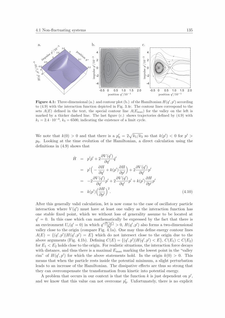
4.1 Non-fluctuating systems 135
a. b. c.
0
0.1
0.2-5.0
-2.5
0
2.5
5.0
0
-6
positionq ′im
pulse
p′ /10
−3
H(q
′ ,p′
)/10−
6
-0.5 0 0.5 1.0 1.5 2.0
4
2
0
-2
-4
position q′/10−1im
puls
ep′ /
10−
3-0.5 0 0.5 1.0 1.5 2.0
4
2
0
-2
-4
position q′/10−1
impuls
ep′ /
10−
3
Figure 4.1: Three-dimensional (a.) and contour plot (b.) of the HamiltonianH(q′, p′) accordingto (4.9) with the interaction function depicted in Fig. 3.4c. The contour lines correspond to thesets A(E) defined in the text, the special contour line A(Emax) for the valley on the left ismarked by a thicker dashed line. The last figure (c.) shows trajectories defined by (4.9) withk1 = 2.4 · 10−4, k3 = 6500, indicating the existence of a limit cycle.
We note that k(0) > 0 and that there is a p′0 = 2√k1/k3 so that k(p′) < 0 for p′ >
p0. Looking at the time evolution of the Hamiltonian, a direct calculation using thedefinitions in (4.9) shows that
H = p′p′ + 2∂V (q′)∂q′
q′
= p′(− ∂H
∂q′+ k(p′)
∂H
∂p′)
+ 2∂V (q′)∂q′
p′
= −2∂V (q′)∂q′
p′ + 2∂V (q′)∂q′
p′ + k(p′)∂H
∂p′p′
= k(p′)(∂H∂p′)2. (4.10)
After this generally valid calculation, let is now come to the case of oscillatory particleinteraction where V (q′) must have at least one valley as the interaction function hasone stable fixed point, which we without loss of generality assume to be located atq′ = 0. In this case which can mathematically be expressed by the fact that there isan environment Uε(q′ = 0) in which q′ ∂V (q′)
∂q′ > 0, H(q′, p′) also forms a two-dimensionalvalley close to the origin (compare Fig. 4.1a). One may thus define energy contour linesA(E) = (q′, p′)|H(q′, p′) = E which do not intersect close to the origin due to theabove arguments (Fig. 4.1b). Defining C(E) = (q′, p′)|H(q′, p′) < E, C(E1) ⊂ C(E2)for E1 < E2 holds close to the origin. For realistic situations, the interaction force decayswith distance, and thus there is a maximal Emax marking the lowest point in the “valleyrim” of H(q′, p′) for which the above statements hold. In the origin k(0) > 0. Thismeans that when the particle rests inside the potential minimum, a slight perturbationleads to an increase of the Hamiltonian. The dissipative effects are thus so strong thatthey can overcompensate the transformation from kinetic into potential energy.
A problem that occurs in our context is that the function k is just dependent on p′,and we know that this value can not overcome p′0. Unfortunately, there is no explicit

136 Many-body Systems
a. b.
0 0.5 1.0 1.5
-6
-4
-2
0
2
4
6
time t/103
αi/10−
4
0 0.5 1.0 1.5
-6
-4
-2
0
2
4
6
time t/103
αi/10−
4
Figure 4.2: Oscillating and propagating bound states of two LSs. a. Time evolution ofthe variables αi, i = 1, 2 (black and grey lines) according to (4.7) with an interaction functionF2(d) = 0, F2(d) = F (d) with F (d) as in Fig. 3.4c, an initial separation d− = 0.18, k1 = 2.4·10−3,k3 = 6500 and α1(0) = 0, α2(0) = 3 · 10−5. The result is the formation of a stable oscillatingmolecule. b. The same situation and initial conditions, this time with F1(d) = F (d)/0.3. Theoutcome is the formation of a propagating bound state.
bound on q′ so that one has to rely on a phase space plot of the dynamics given by (4.9)so prove the existence of a stable limit cycle in the Hamilton valley (see Fig. 4.1c). It isnoteworthy to point out that for an equation of the form
∂tp = α+ F 1(p), ∂tα = k1α− k3|α|2α+ F 2(p), (4.11)
which describes a single active particle interacting with a spatial inhomogeneity (com-pare Eq. (3.106)) it is also possible to find a Hamiltonian formulation similar to (4.9) inwhich the function k dependent on both p′ and q′. In this case, there is a closed contourline with H = Eb for which k(p′, q′) = 0 and where k < 0 in a region outside the areamarked by this contour line. If in such a case the parameters are such that Eb < Emax aparticle starting in C(Eb) is confined by the energy line A(Eb), and we thus know thatwe have a confined two-dimensional dynamics inside C(Emax) with an (single) unstablefixed point inside the Poincare-Bendixon theorem can be applied [359], saying that thedynamics will converge against a stable limit cycle. The corresponding calculation israther lengthy and shall not be carried out at this point, but can be found in detail in[360].
Case 4: We now consider the dynamic equation
pi = αi + F1(pj − pi), αi = k1αi − k3|αi|2αi + F2(pj − pi) (4.12)
which reflects the deterministic evolution of intrinsically propagating and interacting LSsin reaction-diffusion systems. Compared to case 3, the more complex coupling structuremakes analytical statements much more difficult. We want to stress however one centralpoint. It is clear that (4.12) represents a hybrid case of (4.5) and (4.7). For the formerequation, we have seen that the oscillations are suppressed if F1(d) ∼ F2(d) while for thelatter an oscillating state is generic for appropriate initial conditions as given above. A

4.1 Non-fluctuating systems 137
number of numerical simulations confirms that the double coupling structure in (4.12)also suppresses oscillations in spite of the active propagation of the individual LSs.This is visualized in Fig. 4.2. Here we simulate the evolution of two LSs with almostvanishing initial values of α. To break the symmetry of the initial conditions, the initialvalues of α are given an extremely small difference. Fig. 4.2a shows the evolution ofthe α-component for case 3 discussed above. As analytically predicted, both LSs areaccelerated by the interaction force and form a molecule with a center at rest and theindividual particles performing antiphase oscillations. In Fig. 4.2b we use the sameconditions except for a change of the coupling structure (F1(d) = F2(d)/0.3). The resultis that the extremely small difference in the initial velocities is sufficient to break thesymmetry of the long-time solution so that the LSs form a bound state propagating ina direction determined by the initial conditions with the mutual distance of the LSsrelaxing to a constant value.
In the course of this chapter we will see that the above observations are essential forexplaining a variety of phenomena involving the dynamics of large numbers of LSs.
4.1.2 Analytic considerations in two-dimensional systems
From our one-dimensional examples, we have already obtained some information onbound, uniformly propagating and oscillating states. Generalizing the equations of mo-tion to two spatial dimensions, the dynamics may become significantly more complex dueto the different topology of the two-dimensional space. As our interest lies particularlyon long-time solutions, we will only have a look at bound states without oscillations.In two-dimensional space, these states do not necessarily have to propagating uniformlyalong a line with a fixed distance vector, but instead it is also possible that two LSsform a rotating pair. For a closer look on this issue, we will again use the hierarchy ofsystems from above.
Case 1: The two-dimensional generalization of (4.3) leads to
d− = 2F2(d−)d−d−
, d+ = 0. (4.13)
where d− = p2 − p1, d+ = (p2 + p1)/2. This problem which effectively corresponds tothe motion of a single particle under a central force potential is well known in classicalmechanics for example for the motion of planets, and thus the solution is straightforward.Both energy E and angular momentum L defined by
E =d2−2
+L2
2d2−+ 2V (d−), L = d− × d−, (4.14)
are conserved, and thus the problem can be described by the motion of a single particlein the effective potential
Veff(d−) =L2
2d2−+ 2V (d−). (4.15)
This is illustrated for two different values of L in Fig. 4.3a, again with the oscillatoryinteraction function from Fig. 3.4c. The initial conditions determine the conserved value

138 Many-body Systems
a. b.
0.2 0.4
0
2
4
0.3 0.5
distance d
pote
ntial
Veff(d
)/10−
6
E
rmin rmax0.2 0.4
-2
-1
0
1
2
3
0.3 0.5
distance d
forc
eF
2(d
)/10−
5
Figure 4.3: Bound rotating states of LSs in two dimensions. a. Effective potential Veff(d)according to (4.14) with the interaction function from Fig. 3.4c and the three cases L = 0 (solidline), L = 1.5 · 10−4 (dashed line) and L = 3 · 10−4 (dotted line). For a given total energy Eand an angular momentum L, the distance can oscillate between rmin and rmax if the initialconditions lie inside a potential valley. b. Formal compensation of the interaction force F (d)(solid line) by the formal centrifugal forces as given by the first case in (4.26). The latter aredepicted for k1/k3 = 2 ·10−7 (dashed line) and k1/k3 = 5 ·10−7 (dotted line), leading to differentnumbers of stable and instable fixed points.
of L and thus also the point whether Veff(d−) has local minima or not. When the initialconditions are chosen in such a way that the particle starts inside a potential valley andthe energy does not exceed the local boundaries of the valley, the particle oscillates insidethe valley between two radii rmin and rmax, meaning that returning to the two-particleimage, the particles form a rotating state with a distance varying periodically in time.In order to stabilize a constant radius, the energy has to be chosen such that it takesdirectly the value of a local potential minimum, the initial radius of course has to matchthis choice as well. Note that due to the first term on the right-hand side of (4.15),the constant radii will not directly correspond to stable lock-in points of the interactionforce.
Case 2: Considering the case
pi = αi + F1(|pj − pi|)pj − pi
|pj − pi|, αi = F2(|pj − pi|)
pj − pi
|pj − pi|, (4.16)
the energy arguments used in the first case can not be applied directly. Following an ideaproposed by Moskalenko [313], we will thus introduce the four variables s1 = |p2 −p1|2,s2 = |α2 + α1|2/4, s3 = |α2 − α1|2 and s4 = (p2 − p1) · (α2 − α1), furthermore weintroduce fi(s1) = Fi(|pj − pi|)/|pj − pi|. This helps in producing a certain analogy tothe one-dimensional case. To reduce the dimensionality of the whole problem, one mayassume that in a stationary state, both LSs are equal in the sense that α1 = α2. Then,(4.16) simplifies to
s1 = 2s4 + 4f1(s1)s1,s3 = 4f2(s1)s4,s4 = s3 + 2f1(s1)s4 + 2f2(s1)s1.
(4.17)

4.1 Non-fluctuating systems 139
As we are only interested in stationary solutions, we directly see from the second equationthat either f2(s1) = 0 or s4 = 0. The first case leads to s3 + 2f1(s1)s4 = 0 while thesecond case implies f1(s1) = 0, s3 + 2f2(s1)s1 = 0. For arbitrary functions f1 andf2, either of the relations can generally be fulfilled. However, f1 ∼ f2 directly leadsto s3 = 0, implying that the LSs propagate in parallel so that no rotating molecule ispossible.
Case 3: With the above introduced abbreviations, our next case
pi = αi, αi = k1αi − k3|αi|2αi + F2(|pj − pi|)pj − pi
|pj − pi|, (4.18)
can be transformed into
s1 = 2s4,s2 = 8k1s2 − 2k3(4s2 + s3)s2,
s3 = 2k1s3 − k3
2(4s2 + s3)s3 + 4f2(s1)s4,
s4 = s3 + k1s4 − k3
4(4s2 + s3)s4 + 2f2(s1)s1.
(4.19)
This directly tells us s4 = 0 in the stationary state, so that (4.19) simplifies to
0 = 8k1s2 − 2k3(4s2 + s3)s2,
0 = 2k1s3 − k3
2(4s2 + s3)s3,
0 = s3 + 2f2(s1)s1.
(4.20)
As we want to avoid parallel propagation we claim s3 = 0, so that we can conclude
4s2 + s3 = 4k1
k3, f2(s1) = −2
k1k3
− s2
s1. (4.21)
This basically allows for a whole number of possible combinations of s1, s2 and s4.However, numerical simulations (data not shown) indicate that starting from arbitraryinitial conditions generically either a propagating state or a state with s2 = 0, i.e. amolecule with a resting center, is formed. The reason for this is similar to the one-dimensional counterpart discussed above: for α1 = α2, the second equation in (4.19)shows that once s2 vanishes during the dynamical evolution, it remains zero independentof the evolution of the other variables. The statements remains valid also if the strictequality of the αi is softened up, which is confirmed by an analysis of the full equation(4.18).
Case 4: The most complicated scenario is given by the structure
pi = αi+F1(|pj−pi|)pj − pi
|pj − pi|, αi = k1αi−k3|αi|2αi+F2(|pj−pi|)
pj − pi
|pj − pi|, (4.22)

140 Many-body Systems
which under the above assumptions is equivalent to
s1 = 2s4 + 4f1(s1)s1,s2 = 8k1s2 − 2k3(4s2 + s3)s2,
s3 = 2k1s3 − k3
2(4s2 + s3)s3 + 4f2(s1)s4,
s4 = s3 + 2f1(s1)s4 + k1s4 − k3
4(4s2 + s3)s4 + 2f2(s1)s1.
(4.23)
As in case 3, the second equation for s2 = 0 implies 4s2 + s3 = 4k1k3
, from which weconclude f2(s1)s4 = 0. Assuming s4 = 0, one may subsequently derive that all si areexcept s1 are zero, which is physically senseless. Therefore, f2(s1) = 0. For arbitrary f1
this yields the relation s1s3 = s24 which together with the first equation gives a numberof stationary solutions. For the special case f1 ∼ f2 however, we again find s3 = s4 = 0meaning that no rotating states exist. As a consequence, we drop our first assumptionand consider s2 = 0, i.e. antiparallel vectors αi(t). This of course simplifies the last twoequations of the system (4.23). However, in order to produce a result comparable tocase 3, we have to make further assumptions of the relation of f1(s1) and f2(s1), namelyf1 = f2. Then the third and fourth equation can be recombined yielding
0 = s4 + 2f2(s1)s1,
0 = (s3 − s4)(2k1 − 2 − k3
2s3),
0 = 2k1s3 − k3
2s23 + 4f2(s1)s4.
(4.24)
For small k1, because of s3 > 0 the second relation of (4.24) implies s3 = s4. The finalform is thus
s3 = s4 = −2f2(s1)s1, f2(s1) = −2k1k3
4k3
+ s1. (4.25)
Comparing the results for the different cases, we can draw the following conclusion.Generally, there are different possible rotating states depending on the interaction func-tions. While the double coupling structure with F1 ∼ F2 forbids rotating states incase 2, the additional action of active propagation re-enables their existence. While inthe single-coupling case with active propagation the velocity is perpendicular to the lineconnecting the LSs (s4 = 0), this condition is not necessary for the double-couplingcase. On the other hand, at least for F1 = F2 the center of the structures must rest inthe latter case, while this condition in not necessary in the first case. As a potentiallysurprising fact, we find that a central condition for the stable bound states with s2 = 0in both cases is the balance of two forces reading
F2(d) = −2k1k3
dand F2(d) = −2
k1k3
4k3d + d
, (4.26)

4.1 Non-fluctuating systems 141
for single and double coupling, respectively. An illustration of this balance in the firstcase is given in Fig. 4.3b, reminding of the balance of centrifugal and attracting forcesthat can also be derived from the classical consideration of case 1 when considering aforce instead of an energy balance (compare (4.14)). The second case is qualitativelyextremely similar.
4.1.3 Numerical calculations in two-dimensional systems
We now turn to systems with larger numbers of particles. In this context, the expression“large” refers to particle numbers around 100 and not around 1023 as frequently con-sidered for classical systems in the thermodynamical limit. The reason for this choiceis not only of practical nature, but related to the fact that the number of LSs that canpossibly be generated in experimental systems does usually not exceed 100. Even iflarger numbers could be generated, the latter would lie far below the numbers consid-ered in the thermodynamical limit. Like in classical mechanics, analytic statements forthe “microscopic” dynamics of than more three particles can hardly be obtained, so thatwe will have to rely mainly on numerical calculations. However, the above discussionof two-particle interactions provides a basic for understanding important parts of themany-particle dynamics.
As we deal with deterministic systems of coupled ODEs in the following, we willuse a standard fourth-order Runge-Kutta scheme in the numerical simulations. Thecentral algorithms were implemented by M. Rottger, details can be found in [361]. Inthe latter work, details proving the efficiency of the used methods were given, so thecentral concern at this point remains the choice of adequate time steps for the chosenparameter values. Most investigations use the same parameters as in Sec. 3.4.2 so unlessotherwise stated we keep the time step of the simulations at ∆T1 = 0.01. Discrete timederivatives are determined on a time scale T2 = 10. Both T1 and T2 can be varied (inparticular increased) by an order of magnitude without changing the results, howeverwe stick to the above choice to be capable of keeping the same time scale when it comesto the simulation of stochastic Langevin equations further below, where in particularthe choice of T2 is a more delicate matter.
4.1.3.1 Free propagation
One of the conceptually most simple situations to consider is the free and unboundedmotion of many particles. Our goal in this case is to compare the characteristics of thedynamics for classical particles and different realizations of active particles. A first steptowards an exploration of this subject was done by Rottger who conducted simulationsof the double coupling case [361]. In the following numerical simulations, we wantto keep a fixed average particle density. To this end, we consider a squared area ofsize 4 × 4 with periodic boundary conditions and 81 particles. In all simulations, theinteraction function F2(d) is that given by Fig. 3.4c either in the classic, single or doublecoupled version, and in the latter case we choose F1(d) = F2(d)/0.3 which corresponds tothe rigorous derivation from the reaction-diffusion field equations. As initial condition,all particles are equally distributed by arranging them on a square grid. The initialseparation of the particles is so large that they do not feel the forces caused by the otherparticles when the simulation starts. Furthermore, the initial velocities of the individual

142 Many-body Systems
particles are chosen randomly in such a way that all propagation angles are equallyprobable while the absolute velocity is equally distributed in an interval [0, 2α0] so thatthe average velocity is α0.
For classical particles the initial conditions determine the global energy and momen-tum which remain conserved in time. The question whether two particles can approachto a certain distance can be answered by energy arguments: let us assume that only twoparticles collide, then a transformation to center-of-mass coordinates (compare (4.13))shows that the motion can be described by the dynamics of a single particle in the ef-fective potential (4.15). When two particles approach from a large distance, a potentiallocking event can only take place when the kinetic energy of the single particle in thereduced description is high enough to cross the potential barriers caused by the oscil-lating interaction function. The energy is minimal for a central collision and takes thevalue Emin for the angular momentum L = 0, indicated by a grey line in Fig. 4.3a.
In the following, we will consider two situations. In the first one, α0 = 3 · 10−4 sothat when two particles collide with velocity α0 in a central collision, for the energyof the reduced particle we have Er ≈ 0.4Emin. In the second situation, we have α0 =1.52 · 10−3, resulting in Er ≈ 10Emin. For these choices, only two of the theoreticallyinfinitely many lock-in positions of the interaction function are of practical relevance dueto the exponential decay of the interaction strength. Looking at the case α0 = 3 · 10−4,shortly after the start of the simulation we first see a stage in which the particles remainessentially isolated and perform various collisions leading to thermalization (a snapshotof the dynamics is shown in Fig. 4.4a1). Concerning the plot, we have to give a numberof explanations: the size of the circle representing a particle is chosen such that thediameter corresponds to the smallest possible stable lock-in distance for the interactionfunction (4.2). The color is a measure for the current value of α, the smallest valuetaken during the whole simulation corresponds to pure blue and the largest value topure red (see [361] for details). The color scale goes via green for intermediate values,pure green corresponds to α0. Comparing Fig. 4.4a1 to a2 which is taken significantlylater, the colors already indicate that thermalization has changed the velocity spectrum,in particular, there are some very fast LSs in the tail of the corresponding distribution.These particles have enough energy to reach overcome the repulsive interaction of otherLSs and reach stable lock-in distances. When during the collision a sufficient amountof impulse is transferred the collision partners, the energy of the LS may become sosmall that it can not leave the trapping potential. This leads to the formation of largerclusters as indicated by a black circle in the second figure. Generally, we find a flowingequilibrium between clusters and single LSs with the properties of a classical liquid state.
When the overall kinetic energy is increased, it is easier for particles to approacheach other up to close distances, however, trapping also becomes more difficult as theparticles have more energy available to leave the trapping potential. An increase ofα0 to 1.52 · 10−3 has some directly visible consequences for the dynamics (Fig. 4.4b).Again, after a short transient in which the particles thermalize (Fig. 4.4b1) a flowingequilibrium is reached (Fig. 4.4b2). Compared to α0 = 3 · 10−4, the number of largerclusters has strongly decreased to almost zero in the long-time limit as two collidingparticles almost always separate instantly after a collision. The reason for this is thateven after thermalization, the kinetic energy of the particles is in most cases larger thanthe energy needed to leave the trapping potential. Consequently, the state shown in

4.1 Non-fluctuating systems 143
a1. a2.
b1. b2.
αmin αmaxα0
Figure 4.4: Free propagation of Newton particles with an oscillatory type of interaction func-tion. a. Dynamics of 81 “classical” particles on the domain Ω = [−2, 2] × [−2, 2] with periodicboundary conditions, an interaction function F2(d) as shown in Fig. 3.4c and initial conditionsas given in the text for α0 = 3 · 10−4 at times t = 8400 (a1) and t = 42000 (a2). The largecircle indicates a transient bound complexes of several particles. b. Corresponding sequence forα0 = 1.52 · 10−3, also for t = 8400 (b1) and t = 42000 (b2).
Fig. 4.4b has all properties of a gaseous phase.Considering now the case of active propagation, we may again distinguish between the
prototype model with single coupling in the velocity component or the double couplingderived from the dynamics of LSs in reaction-diffusion systems. Both cases turn outto be basically equivalent in their long-time behavior for high intrinsic velocities whilesome differences arise for low intrinsic velocities. Over a large range of parameters, themotion can essentially be characterized by the quantity α0 which now is defined as theintrinsic particle velocity (k1/k3)1/2 although of course the exact results depend on k1
and k3 individually. All absolute particle velocities quickly converge to this value if theinitial separation of the particles is large enough.
For the single-coupling case, we choose the same values of α0 as in the classical casevia the choice k3 = 6500 as well as k1 = 0.0006 and k1 = 0.015, respectively. In both

144 Many-body Systems
cases, the long-time behavior of the system is completely different from the classicalcase. For small intrinsic velocity (Fig. 4.5a), in the long time limit most particles lock inat the second smallest possible lock-in distance with respect to their nearest neighbors.However, due to the chosen particle density and the rather weak interaction strengthat this distance the whole structures is not rigid. Instead, the particles oscillate aroundtheir equilibrium positions and the cluster experiences permanent deformations. Insummary, although the cluster shows the long-ranged correlations typical for a solid,the state is “elastic” and experiences permanent changes of its structures. The situationbecomes different when going to larger values of α0. While we have experienced theformation of a gaseous state for classical propagation, in the active propagation casewe find that the particles quickly lock in at the smallest possible distance and form anumber of smaller clusters (Fig. 4.5b1) which finally collide and merge into one largecluster (Fig. 4.5b2) with a very rigid structure. In this state, all LSs propagate with theintrinsic velocity in the same direction. One should note that for a large cluster it is
a1. a2.
b1. b2.
αmin αmaxα0
Figure 4.5: a. Dynamics of 81 active single-coupled particles with α0 = 3 ·10−4 realized by thechoice k1 = 0.0006 and k3 = 6500. All other conditions are as in Fig. 4.4. b. The same situationwith k1 = 0.015, resulting in α0 = 1.52 · 10−3.

4.1 Non-fluctuating systems 145
a1. a2.
b1. b2.
αmin αmaxα0
Figure 4.6: a. Dynamics of 81 active double-coupled particles with F1(d) = F2(d)/0.3, allother conditions as given in Fig. 4.5a and b.
easier to “absorb” smaller clusters than for a smaller one because its spatial extensionsterically hinders the particles from re-escaping after a collision.
A central difference between classical dynamics and active propagation is that in theclassical case, the particles can change their velocity only due to interaction, and energyand impulse are conserved. In the active case, both quantities are not conserved, andtwo rather independent mechanisms are available to change the velocity. Thus whentwo active particles are at a stable lock-in distance, the cluster can reach the intrinsicvelocity without a change of this distance and without the necessity of the presenceof other LSs to which energy and momentum have to be transferred to reduce thesequantities for itself.
Fig. 4.6 corresponds to Fig. 4.5 except that the double coupling structure was used(with F1(d) = F2(d)/0.3 as found for the reaction-diffusion example). Here we see thatfor a given intrinsic velocity the same lock-in distances as in the single-coupling case arepreferred. However, while for large α0 the dynamics is principally the same, for the caseof small intrinsic velocities a difference arises: the individual LSs do not oscillate around

146 Many-body Systems
their equilibrium positions in the long-time limit, but instead the cluster propagatesuniformly with its intrinsic velocity. This finding is directly connected to our analyticalconsiderations in Sec. 4.1.1. Here, we have found that while the single-coupling stateprefers oscillating states under many circumstances, the double-coupling dampens theseoscillations and causes a uniform propagation (compare also Fig. 4.2).
4.1.3.2 Confined motion
Under randomly chosen initial conditions, the unconfined propagation of active particlestypically with oscillatory interaction leads to the formation of one large cluster indepen-dent of how the equations are coupled. Another interesting scenario can be constructedby looking at experiments in planar ac gas-discharge systems in which many LSs areconfined in a domain of circular shape [362]. In this case, it was found that the LSsarrange on an almost hexagonal grid and perform a collective rotational motion aroundthe center of the domain. It is very likely that the phenomenon is due to active mo-tion combined with a mixed attractive-repulsive interaction law. This is supported bythe fact that for a given geometry and fixed parameters, in the experiment exactly onevalue for the absolute angular velocity can be observed. Furthermore, stable co-rotatingdefects in the hexagonal structure have been found, which do not match the assump-tion of a purely repulsive interaction between the LSs as encountered for example forCoulomb crystals [363]. We want to clarify whether the experimental observations canbe reproduced by the reduced equations we have been discussing so far. While the activepropagation of single LSs in the mentioned ac gas-discharge systems has been verifiedand quantitatively measured [320], unfortunately there are currently no measurementson interaction laws. A complete set of parameters both for single and interacting LSsis available for planar dc gas-discharge systems ([157, 173], compare also Fig. 3.5), butin these systems no rotational motion was observed as it was not possible to generateenough LSs due to experimental limitations.
To overcome this problem, we choose the parameter set for the dc case. The parame-ters are obtained via stochastic analysis methods for which a coupling structure with aninteraction force only in the α-component was assumed (termed case 3 above). It wasshown [173] that the experimentally obtained interaction force could be well representedusing the analytical interaction function (4.2) originally derived for reaction-diffusionsystems. This is not too surprising as the function reflects the decay of Bessel functionsfor large arguments, the latter typically appearing in the context of describing the su-perposition of exponentially decaying oscillatory tails. The parameters characterizingthe interaction are taken as d1 = 1386, d2 = 1.2167, d3 = 5.27957 and d4 = −1.604exclusively in this section. A direct connection to experimental data can be obtainedby taking all units as multiples of millimeters and seconds. In the experiments, thedomain in which the LSs propagate is confined by a mechanical spacer which the LSscan not penetrate. We will model this confinement by a repulsive force which vanishesinside a circular domain and quickly increases in strength outside. Shifting the centerof the domain to the origin, the additional force can be conveniently expressed in polarcoordinates as
F sp(r) =
0 for r < r0c(r − r0)2eθ for r ≥ r0
. (4.27)

4.1 Non-fluctuating systems 147
a1. a2. a3. a4
b1. b2. b3. b4
c1. c2. c3. c4
01
23
45
67
8
10
1112
1314
1516
1718
1920
2122
2324
2526
27
2829
3031
3233
3435
3637
3839
4041
4243
4445
46
4748
4950
5152
5354
5556
5758
5960
6162
6364
65
6667
6869
7071
7273
7475
7677
7879
80
8182
8384
0
1
2
3
4
5
6
7
8
10
11
12
13
14
15
16
17
18
19
20
21
22
23
24
25
26
27
28
29
30
31
32
33
34
35
36
37
38
39
40
41
42
43
44
45
46
47
48
49
50
51
52
53
54
55
56
57
58
59
60
61
62
63
64
65
66
67
68
69
70
71
72
73
74
75
76
77
78
79
80
81
82
83
84
01234567810
1112131415161718192021222324252627 28293031323334353637 383940414243444546 47484950515253545556 575859606162636465
666768697071727374757677787980
81828384
0
1
2
3
4
5
6
7
8
10
11
12
13
14
15
16
17
18
19
20
21
22
23
24
25
26
27
28
29
30
31
32
33
34
35
36
37
38
39
40
41
42
43
44
45
46
47
48
49
50
51
52
53
54
55
56
57
58
59
60
61
62
63
64
65
66
67
68
69
70
71
72
73
74
75
76
77
78
79
80
81
82
83
84
Figure 4.7: Rotation of a hexagonal cluster of active particles (k1 = 0.8, k3 = −0.042) withc = 200 as described in the text. a. Simulation with small spacer radius r0 = 4. The snapshotswere taken at t = 8, 9, 10 and 11 from (a1 to a4). The color-coding corresponds to that usedin Fig. 4.5, one LSs was marked in white to indicate the course of the dynamics. b. The samesequence as in a., however with r0 = 16. c. Repetition of the simulation in a. with a higherintrinsic velocity (k1 = 2) producing oscillations of the cluster. This is also indicted by theparticle trajectory for one rotation plotted in the first figure.
With this choice, the repulsing force by the spacer is always directed to the origin. Forsetting the repulsion strength c, we have to state that in the experiment, the intrinsicvelocities of the particles lie between v = 0 and v = 20. By choosing c = 200, the LSscan hardly penetrate the circular boundary defined by r = r0. Finally, the parametersfor the active propagation are taken as k1 = 0.8, k3 = −0.042 so that α0 = 4.36. Noisewhich is always present in the experiment is neglected in the current investigation. Wewill see that most experimental observations are reproduced also without noise.
As we change the parameters in the functions significantly with respect to our pre-vious investigations (which is exclusively done in this section), we have to rethink ourconsideration on the time step used for the numerical simulation. Consequently, thesimulation time step is decreased to ∆T1 = 5 · 10−5 while the ratio of T1 and T2 is keptthe same as before. To determine the initial conditions for the simulation, we note thatin the experiment the LSs are arranged on a almost hexagonal grid which is typical

148 Many-body Systems
a. b.
5 10 15 200
1
2
3
4
radius r0
1/〈ω
〉
0 1 2 3 40.70
0.75
0.80
0.85
0.90
coefficient k1
r i/r 0
Figure 4.8: Detailed analysis of rotating particle clusters. a. Dependence of the reciprocalaveraged rotational velocity 〈ω〉 on the radius r0 for the parameters used in Figs. 4.7a and bshowing a linear dependence. b. Ratio ri/r0 for different values of the coefficient k1 determinedfor r0 = 10.
for attractive-repulsive interaction functions like (4.2) because the most dense stablearrangement in which the LSs are positioned on stable lock-in points of the interactionforce caused by their neighbors is just the hexagonal one. We thus create a hexagonalgrid with the lock-in distances of nearest neighbors just corresponding to the smalleststable fixed point of (4.2). One LS is positioned in the origin, and only those membersof the grid for which r ≤ r0 are kept. As initial velocity, we take an already rotatingstate via αx = α0py/r0, αy = −α0px/r0.
Numerical simulations have been carried out for different r0 ranging from r0 = 4 tor0 = 20. Qualitatively the dynamics is similar in all cases, as can be seen from Fig. 4.7aand b for r0 = 8 and r0 = 16. For the above choice of parameters, the interaction forcesare strong enough to keep the LSs close to their equilibrium positions to that the wholehexagonal arrangements of clusters rotates as one solid body. The colors indicate thatfor all radii of the domain, those LSs which are close to the boundary of the domainmove with their equilibrium velocity. This of course directly implies that the LSs closerto the origin must on average move with a velocity smaller than the intrinsic one, whichcan also be seem from the figures. An interesting point is given by the fact that withthe special initial conditions given above, the cluster can even perform a stable rotationfor c = 0, i.e. without a confining area. The same rotating motion can also be inducedusing random initial conditions, which however now requires a confining area to causethe initial transient process to develop in the correct way.
Before coming to some quantitative investigations, we briefly want to address thepoint what happens when the intrinsic velocity is increased, for example via a changeof the coefficient k1. For k1 ≈ 2, the overall motion is still dominated by rotation,while in particular the inner LSs begin conducting oscillations around their equilibriumpositions, which is shown in Fig. 4.7c using again r0 = 8 as in Fig. 4.7a. The LSs closeto the boundary are less affected, however their dynamics shows small oscillations aswell (see for example the trajectory plotted in Fig. 4.7c1). A further increase of theintrinsic velocity increases the strength of the fluctuations, and the rotational motion ofthe cluster is superimposed with a breathing-like dynamics in radial direction. Finally,when the intrinsic velocity becomes too high the LSs can overcome the forces keeping

4.1 Non-fluctuating systems 149
them near their equilibrium position and the solid structure decays to a ring-like one.In the following, we are interested in the rotating structure for small intrinsic veloc-
ities such that the rotating state is essentially isotropic with respect to its center. InFig. 4.8a, we investigate the dependence of the time-averaged rotation velocity 〈ω〉 of thecluster around the origin (which is rather well-defined for the state under considerationand determined in the time interval shown in Fig. 4.7) as a function of the radius r0.The figure shows that in a good approximation 〈ω〉 ∼ 1/r0. From this dependence, onemay directly estimate that the ratio ri/r0 with ri denoting the radius for which the LSspropagate with the intrinsic velocity α0 is more or less independent of r0. We may thustake a fixed radius r0 = 10 and look at the values of ri/r0 as a function of α0 by varyingthe coefficient k1. The results are shown in Fig. 4.8b. For the whole range of velocities iswhich a stable rotation can be observed, the ratio ri/r0 lies slightly above 0.8, meaningthat only those LSs close to the outer boundary of the structure move faster than theintrinsic velocity. It should however be kept in mind that on the one hand, the numberof structures propagating with a given velocity increases linearly with the distance rfrom the origin and that on the other hand, the “torque” on the cluster caused by theparticles becomes larger with increasing radius. A closer look on Fig. 4.8b reveals thatthe ratio ri/r0 slightly increases with increasing intrinsic velocity. A rather intuitiveexplanation for this can be given by considering that the LSs remain exactly on theirequilibrium positions only when the cluster is at rest or when the interaction strengthbecomes extremely large. During rotation, the particles experience “centrifugal forces”that increase their distance from the center of rotation. With all particles increasingtheir distance to the origin due to this effect the more the higher the intrinsic velocity,the ratio ri/r0 must naturally increase as well.
Another point we want to address is the rotation of structures with defects whichis also observed in the experiments. Basically, one may state that over a large rangeof radii r0, one may remove one or several LSs from the cluster and still observe arather regular rotational motion. A central aspect in this context is that removing LSsgenerally breaks the discrete rotational symmetry of the system and produces a shift ofthe center of mass of the cluster, which will cause the latter to change its position duringthe dynamical evolution. Furthermore, replacing LSs by defects generally weakens the
a. b.
1
2
3
45
6
0 2 4 60.80
0.82
0.84
number of defects
aver
.ro
t.vel
.〈ω
〉
Figure 4.9: a. Rotating cluster for r0 = 6 with all other parameters as given in Fig. 4.7a.The numbers indicate the sequence in which the particles are taken away to create defects. b.Average angular velocity of the cluster depending on the number of defects.

150 Many-body Systems
forces with which the LSs are kept at their positions so that oscillations of the clusterbecome more likely. All these effects may influence the rotational motion in a rathercomplex way. In order to get reasonable quantitative statements on the motion withdefects, we choose the case r0 = 6 where the cluster is small enough to see a clear effect.We conduct a number of simulations in which up to 6 LSs propagating with a velocityslower than the intrinsic one are removed from the cluster (the sequence is shown inFig. 4.9a). The resulting average angular velocities are shown in Fig. 4.9b, showing amonotonous decrease of the velocity the more particles are taken away.
There are two likely mechanisms to explain the observations which may act simul-taneously in the analyzed case. First, the rotational velocity of the cluster is a balancebetween those LSs in the inside of the cluster which propagate slower than the intrin-sic velocity and thus try to accelerate and those at the boundary which propagate toofast and thus try to decelerate. When taking away LSs that are trying to acceleratethe cluster, those decelerating become more dominant and can thus reduce the overallangular velocity of the cluster. Second, the more LSs are taken away, the weaker theforces that keep the remaining particles at their equilibrium positions. Thus oscillationsas those shown in Fig. 4.7c occur even for small intrinsic velocities and (although smallin amplitude) may reduce the mean angular velocity. In order to eliminate the secondeffect in future works, potentially a modification of the interaction function stiffeningthe cluster structure may be helpful.
As a last point, we want to briefly comment on rotating structures for classical parti-cles. When the rotational velocity is low and the interaction forces can essentially keepthe particles on their equilibrium positions, the structure can be assigned a moment ofinertia and standard textbook techniques can be applied for the treatment of rotationalmotion. In particular, for appropriate initial conditions any rotational velocity can berealized. For random initial velocities, the cluster can still perform a rotational motionwhich is accompanied by a bouncing motion in the trapping potential as numerical in-vestigations can prove (data not shown). As our main motivation for the considerationof confined motion were experimental observations of active particles, we do not wantto go into more detail on this point here.
4.1.3.3 Excitation and switching fronts
Above, we have seen an example for many actively propagating LSs forming one moreor less rigid body. In a good approximation, the rotating state could be considered asstationary because the absolute velocities of the LSs remained constant after the decayof initial transients. Although the particles were propagating intrinsically, the behaviorof the cluster showed a number of similarities with solids consisting of classical particleslike molecules or ions. For classical particles in lattice arrangements, it is long knownthat they can conduct characteristic types of oscillations around their lattice positionsand localized excitations with particle-like properties like phonons can arise. It is thusinteresting to ask how excitations and perturbations spread and potentially disperse inactive media.
In order to determine an appropriate setting to investigate the spreading of exci-tations in extended clusters, we may recall that in [361] the central collision of twoquadratic clusters of 11 × 11 LSs in the double-coupling case for one intrinsic velocityand a hexagonal arrangement was analyzed. Here, it was found that the clusters were

4.1 Non-fluctuating systems 151
compressed during collision and that this compression occurred on a timescale fasterthan that of the intrinsic propagation. In the following, motivated by these findingswe want to use the presented scenario to produce excitations in clusters. A genuineadvantage of letting two clusters collide is that the clusters can be arranged in such away that they are initially in a stable equilibrium. As due to the size of the cluster in[361] the velocity of the excitation was likely to be influenced by boundary effects, weextend the cluster to 9×100 particles and a symmetric arrangement with respect to theinitial direction of propagation (Fig. 4.10a). The latter point ensures that in a centralcollision with a second cluster excitations propagate mainly in this direction, which isnot necessarily the case when using an asymmetrical cluster as in [361].
In the following simulations, we switch back to the interaction functions used inSec. 4.1.3.1, the range of velocities and the time steps for the simulations are adaptedaccordingly. In the simulation, the initial velocity of all particles is the same and cor-responds to the intrinsic one in the case of active propagation so that the whole clustermoves to the right retaining its shape in the course of time. To save simulation time,instead if simulating two clusters the whole structure is placed into a rectangular do-main with no-flux Neumann boundary conditions. In this way, the cluster propagateshomogeneously until its front end comes close to the right boundary of the domain. Thecollision with the boundary is then equivalent with a mirror cluster which is reflectedat the boundary.
For low intrinsic velocities (which we will consider exclusively in the following), theparticles in the front of the moving solid are forced to stop abruptly when collidingwith the boundary while those further away from the collision zone do not yet feel thecollision due to the short-ranged interactions. As a result, they continue their motion tothe boundary, resulting in a compression of the solid with respect to its initial shape. Dueto the repulsive interaction for small particle distances, the following particles have tolower their velocity as well and eventually come to a stop, triggering a whole compressionfront to run through the cluster along its main axis. The direction of motion is essentiallydetermined by the symmetry of the cluster, fronts in any direction can be generated bychoosing appropriate asymmetric clusters.
The whole compression process is visualized in the sequence of images shown inFig. 4.10a. The initial state in green shows that the cluster is in equilibrium. Thesecond image was taken directly after the cluster hit the boundary showing the initialphase of the compression wave which moves through the cluster with almost constantvelocity. When reaching the end of the cluster, the particles of the very end have thepossibility of reversing their direction without being obstructed by other particles. Oncethey switch direction, their intrinsic drive stabilizes propagation opposite to the initialdirection. The particles pull their neighbors with them, and as the effect is enhancedby the intrinsic drive of the particles, a second front, this time of decompressing type,runs to the cluster from left to right. When reaching the right end, the intrinsic driveco-acting with the pulling particles is strong enough to detach the whole cluster fromthe wall. The whole state then converges to equilibrium with some additional quicklydecaying fronts running to the cluster.
In order to see how the particles behave in the compressed state, we have chosen twoparticles (marked in white in Fig. 4.10a) whose αx-component we plot as a function oftime in Fig. 4.10b. The black vertical lines in the figure indicate where the snapshotshave been taken. It becomes clear that in the compressed state, the particles are not

152 Many-body Systems
a1.
a2.
a3.
a4.
a5.
a6.
a7.
b.
0-6
0
6
5000 10000 15000
time t
αx(t
)/10−
4
Figure 4.10: Compression fronts in clusters of active particles. a. Collision of a cluster of 9×100LSs with the boundary of the domain Ω = [−4, 18]× [−0.4, 2]. The color of each LS marks thecurrent absolute value of the corresponding inner degree of freedom α as in the previous figures.Times the snapshots are taken are 1: 0, 2: 3222, 3: 5040, 4: 5814, 5: 6636, 6: 7446, 7: 8400. b.x-component of the α-vector as a function of time for the two LSs in the center and on the rightof the cluster are marked with white color(grey line central LS, black line right LS). The verticalblack lines indicate the times used in a. Parameters: k1 = 0.0015, all others as in Fig. 4.6.

4.1 Non-fluctuating systems 153
a1.
a2.
a3.
a4.
a5.
a6.
a7.
b.
0 5000 10000 15000-8
0
8
time t
αx(t
)/10−
4
Figure 4.11: Repetition of the simulation of Fig. 4.10 with an underlying classical particledynamics, all other conditions (in particular α0) are the same.
at rest but perform an almost periodical oscillatory type of motion. Furthermore, thefrequency of the oscillation increases with increasing compression of the cluster.
Following the above observations, one may ask two questions. First, how wouldclassical particles and active particles with single coupling behave in the same situationand second, how does the choice of the intrinsic velocity influence the dynamics. Starting
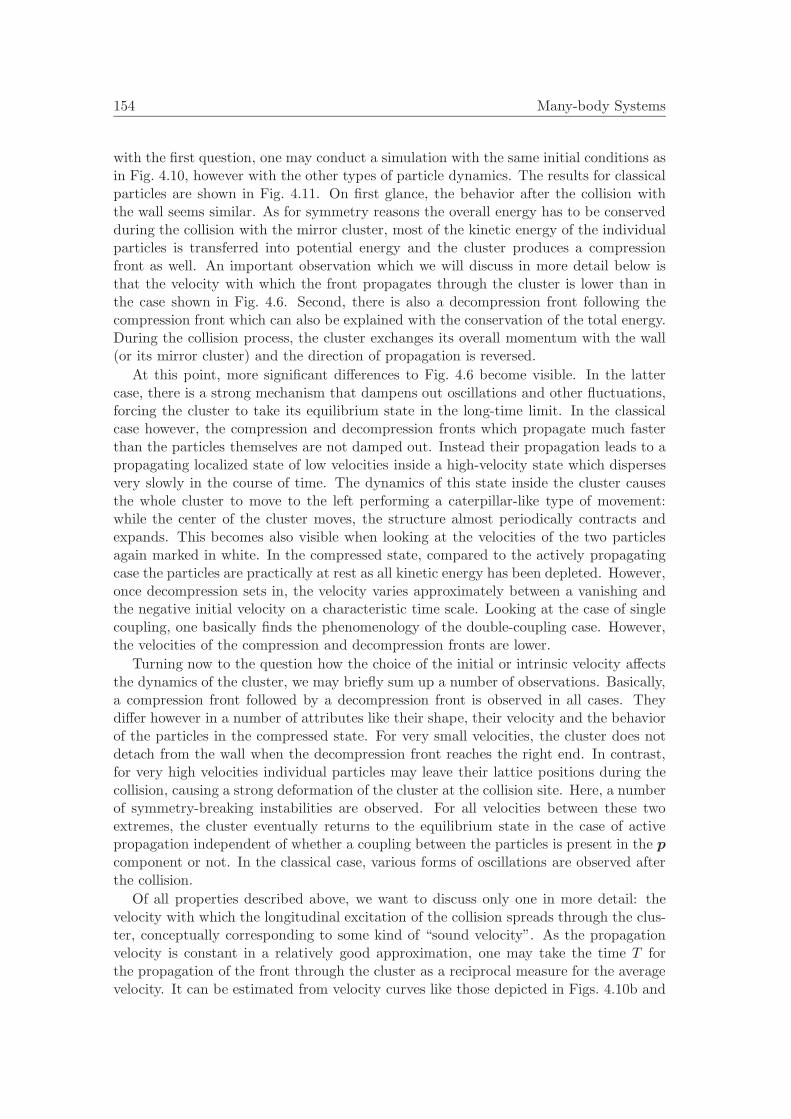
154 Many-body Systems
with the first question, one may conduct a simulation with the same initial conditions asin Fig. 4.10, however with the other types of particle dynamics. The results for classicalparticles are shown in Fig. 4.11. On first glance, the behavior after the collision withthe wall seems similar. As for symmetry reasons the overall energy has to be conservedduring the collision with the mirror cluster, most of the kinetic energy of the individualparticles is transferred into potential energy and the cluster produces a compressionfront as well. An important observation which we will discuss in more detail below isthat the velocity with which the front propagates through the cluster is lower than inthe case shown in Fig. 4.6. Second, there is also a decompression front following thecompression front which can also be explained with the conservation of the total energy.During the collision process, the cluster exchanges its overall momentum with the wall(or its mirror cluster) and the direction of propagation is reversed.
At this point, more significant differences to Fig. 4.6 become visible. In the lattercase, there is a strong mechanism that dampens out oscillations and other fluctuations,forcing the cluster to take its equilibrium state in the long-time limit. In the classicalcase however, the compression and decompression fronts which propagate much fasterthan the particles themselves are not damped out. Instead their propagation leads to apropagating localized state of low velocities inside a high-velocity state which dispersesvery slowly in the course of time. The dynamics of this state inside the cluster causesthe whole cluster to move to the left performing a caterpillar-like type of movement:while the center of the cluster moves, the structure almost periodically contracts andexpands. This becomes also visible when looking at the velocities of the two particlesagain marked in white. In the compressed state, compared to the actively propagatingcase the particles are practically at rest as all kinetic energy has been depleted. However,once decompression sets in, the velocity varies approximately between a vanishing andthe negative initial velocity on a characteristic time scale. Looking at the case of singlecoupling, one basically finds the phenomenology of the double-coupling case. However,the velocities of the compression and decompression fronts are lower.
Turning now to the question how the choice of the initial or intrinsic velocity affectsthe dynamics of the cluster, we may briefly sum up a number of observations. Basically,a compression front followed by a decompression front is observed in all cases. Theydiffer however in a number of attributes like their shape, their velocity and the behaviorof the particles in the compressed state. For very small velocities, the cluster does notdetach from the wall when the decompression front reaches the right end. In contrast,for very high velocities individual particles may leave their lattice positions during thecollision, causing a strong deformation of the cluster at the collision site. Here, a numberof symmetry-breaking instabilities are observed. For all velocities between these twoextremes, the cluster eventually returns to the equilibrium state in the case of activepropagation independent of whether a coupling between the particles is present in the pcomponent or not. In the classical case, various forms of oscillations are observed afterthe collision.
Of all properties described above, we want to discuss only one in more detail: thevelocity with which the longitudinal excitation of the collision spreads through the clus-ter, conceptually corresponding to some kind of “sound velocity”. As the propagationvelocity is constant in a relatively good approximation, one may take the time T forthe propagation of the front through the cluster as a reciprocal measure for the averagevelocity. It can be estimated from velocity curves like those depicted in Figs. 4.10b and

4.1 Non-fluctuating systems 155
a. b.
0 2
1.6
1.8
2.0
2.2
31
k1/10−3
pro
pagati
on
tim
e∆
T/103
1.6
1.8
2.0
2.2
0 2 31
k1/10−3
pro
pagati
on
tim
e∆
T/103
Figure 4.12: Velocities of compression and decompression fronts. a. Propagation time T forcompression fronts as exemplarily depicted in Fig. 4.10 to pass through the whole cluster as afunction of the driving parameter k1 in the case of double coupling (black points) and singlecoupling (dark grey points). All other conditions correspond to Fig. 4.10. The light grey pointscorrespond to the classical case where for a given value of k1 the initial velocity of the clusterwas chosen to correspond to the intrinsic velocity in the case of active propagation. b. The sameplot as in a. for the decompression front following the compression front.
4.11b for particles at the ends of the cluster although a certain uncertainty remains asit is not always clear how to precisely define the moment when the excitation arrives atthe point of interest. The reason why we do not define a velocity associated with T isthat it is not entirely clear which length scale has to be taken into account due to thecontraction of the cluster.
Fig. 4.12a shows the results for the compression front in the double-coupling, thesingle coupling and the classical case as discussed above. The values are shown as afunction of the driving parameter k1 controlling the active propagation while keepingall other parameters fixed. In the case of classical Newton equations an initial velocityof the particles was chosen that corresponds to the intrinsic velocity for the given valueof k3 in the case of active propagation. As central result, one may state that for agiven dynamics equation with fixed interaction functions, the front velocity does notsignificantly depend on the velocity with which the cluster has been propagating beforethe collision (the potential error of each measurement lies in the region of ∆T = 100).Furthermore, the cases of classical dynamics and active propagation with coupling onlyin the α-component practically coincide. In contrast, for the interaction function in bothcomponents the propagation of the compression front through the cluster takes about15% less time. As the compression front is followed by a decompression front which canagain be associated a characteristic propagation time, in Fig. 4.12b we plot the latteragain as a function of k1. Here some data points are missing as in particular for highvelocities the decompression is overlaid by oscillations so strongly that the determinationof the propagation time is not possible. Within the error of the determination, we findquantitatively the same results as for the compression front.
Analyzing the above results, one may state that for the Galilean-invariant system ofclassical Newton equations, one may transform the system to a moving frame, showingthat the situation of a uniformly cluster colliding with its mirror image is equivalentto a resting cluster which is excited on one side with a short local compression pulse.In this terminology, the velocity with which the cluster moves in the resting frame

156 Many-body Systems
determines the properties of the excitation in the co-moving frame. It is then not toosurprising that the velocity with which the excitation front spreads is independent ofthe excitation as it is known that the latter for classical solids depends only on thematerial parameters density and compression module. This statement holds of courseonly if in the stationary frame the velocity of the propagating cluster is smaller than the“sound velocity” which is true for the case considered above. Adding active propagationto the dynamic equations breaks the Galilean invariance of the system. Nevertheless,at least for the chosen parameters obviously the results are not essentially influenced.It is likely that the particles are coupled so stiffly that the velocity relaxes to a valueclose to zero on a time scale so short that the active propagation can not significantlycontribute to the dynamics. When the coupling structure of the equations is changedvia an additional force term in the position equation, the front velocity becomes larger.This is due to the proportionality of the forces in both components as the action of theforce in the α-component is enhanced.
4.2 Fluctuating systems
In recent years, a good amount of work has been invested in exploring the dynamics ofmany particles under the influence of noise, in particular for the previously introducedactive Brownian particles (compare Sec. 3.4.2). We have seen that the general evolutionequation (4.1) together with possible correlations in the noise forces has extremely manydegrees of freedom and contains the standard models for active Brownian particles asspecial case. In order to have the possibility of comparing our results with most otherworks of the current literature, we will not consider the Langevin equations with noiseforces in both components as derived in Sec. 3.4 but instead look at the system
pi = αi +∑i=j
F 1(dij),
αi = k1α − k3|α|2α +∑i=j
F 2(dij) +RαΓi(t),(4.28)
which corresponds to (3.120) in the case of active propagation and additive noise forF 1 = F 2 = 0. In most of the following investigations, we will vary the intrinsic velocityvia the parameter k1 and the fluctuation strength given by Rα, furthermore we willlook at the influence of the force term F 1. A comparison with classical particles in thiscase is not reasonable as the noise forces correspond to a permanent energy input intothe system that has to be compensated by a dissipative mechanism for high particlevelocities to prevent the system from diverging [364]. Such a mechanism is only presentif k1 < 0 or k3 < 0.
4.2.1 Numerical considerations in two-dimensional systems
For evolution equations with noisy contributions it is basically clear that in contrastto the deterministic case any quantitative consideration may involve only statisticalstatements, for example on distribution functions or moments. To obtain the latterfor systems involving active propagation, in recent years there have been attempts to

4.2 Fluctuating systems 157
apply techniques of statistical mechanics to noisy canonical-dissipative systems as in-troduced for a special deterministic case in Sec. 4.1.1. The central idea is to solve theFokker-Planck equation belonging to the Langevin equation (4.28) in order to obtainthe corresponding probability distribution function. To this end, one may try to rewrite(3.120) as
∂tqi =∂H
∂pi,
∂tpi = −∂H∂qi
− k(H)∂H
∂pi+R(H)Γi(t),
(4.29)
(compare (4.9)) with an appropriately chosen Hamiltonian whose properties facilitatesolving the Fokker-Planck equation, the latter reading
∂tP +∑
i
(pi∂P
∂qi− ∂H
∂pi
∂P
∂pi
)=∑
i
∂
∂pi
(k(H)P +
12R2(H)
∂P
∂pi
)(4.30)
for this special case [365]. Unfortunately, analytic solutions are only available in specialcases, for example when considering a single particle in a potential [366], linearly coupledparticles in one-dimensional systems under special symmetry assumptions [367] or whencoupling between the individual particles is neglected [365]. Otherwise, one usually hasto resort to numerical simulations which is in the spirit of the methods we used abovefor many particles in the deterministic case.
4.2.1.1 Bound state of two active Brownian particles
Similar to our considerations on deterministic motion, we will start with only very fewactive particles. As we have already produced a number of results for single particlesin Sec. 3.4.2, the next case of higher complexity is thus given by a bound state of twoLSs under the influence of noise as it it depicted for an experimental system in Fig. 3.5.We will study this case using the parameters of Sec. 4.1.3.1 varying the parameters k1
(thereby changing the intrinsic velocity) and Rα (the noise amplitude). Both parametersare kept low enough to ensure that the bound state stays preserved in the course of time.In order to characterize the dynamics of the state of interest, we look at two quantities:the velocity of the center of mass of the cluster, i.e. v = ∂t(p1 + p2)/2, as a measurefor the translational motion and the angular velocity ω of the cluster with respect to itscurrent center. The latter is defined in the following way: a system of polar coordinatesis moved along with the center of mass so that the position of one fixed LS can be givenby a radius r and an angle θ in this coordinate frame. The angular velocity is thendefined as the temporal derivative of θ. As white noise forces are nowhere differentiable,velocity and other quantities involving time derivatives are defined via a first order finitedifference scheme.
A technical issue we have to address before starting is the correct choice of time stepsfor the numerical simulation and the determination of time-derivative expressions. Inthe noise-free case where we have used a standard Runge-Kutta scheme to integrate

158 Many-body Systems
a1. a2. a3.
b. c.
0
2
4
5
3
1
0 0.5 1 21.5
noise amplitude Rα/10−5
a1
a2
a3
〈v〉/
10−
4
1
3
0 0.5 10
2
21.5
a1
a2a3
noise amplitude R/10−5
〈|ω|〉/
10−
3
Figure 4.13: Dynamics of a two-particle molecule in the double-coupling case. a. Trajectoriesof two active particles forming a bound state shown over a time interval ∆T = 50000 fork1 = 1.05 · 10−3 and k3 = 6500 resulting in the intrinsic velocity α0 = 1.05 · 10−4 and noiseamplitudes of Rα = 0.15 · 10−5 (a1), 0.6 · 10−5 (a2) and 1.2 · 10−5 (a3). b. Average velocityof the center of the cluster as a function of Rα and α0. The α0-dependence is visualized usingcurves with different grey scales, from dark to light grey they correspond to k3 = 6500 andk1 = −0.3 · 10−3, 0.15 · 10−3, 0.6 · 10−3, 1.05 · 10−3 and 1.5 · 10−3. Each point was determinedover a total averaging period of ∆t = 5 · 105. c. Average absolute angular velocity of the clusterwith respect to its center shown using the same coloring and conditions as in b.
numerically the differential equations, the trajectories are smooth and the determina-tion of discrete derivatives poses no significant problems as long as the time step T2
for the discrete time derivatives is also small enough, but larger than the time step T1
of the numeric integration. The simulation of Langevin equations is performed usingthe standard forward stochastic integration scheme given by (3.129). For the followingresults, we again use the algorithm implemented by Rottger [361] or appropriate modi-fications. As the characteristic time scale for the chosen parameters in the deterministiccounterpart lies in the order of 100−1000, we keep a time step on the order of T1 = 0.01for the simulations (as in the Runge-Kutta case). It can be ensured by a variation ofT1 that the results are statistically independent of this variation. In order to determinetime derivatives, we also choose the intermediate time scale T2 ≈ 1000T1 as before inthe Runge-Kutta case. A closer inspection shows that in the presence of noise, thistime scale is the smallest one on which the dynamics is due to both deterministic andstochastic parts. A variation of T2 by an order of magnitude quantitatively changesthe results for average time derivatives by about 20% but does not cause qualitative

4.2 Fluctuating systems 159
changes.We start with the double coupling structure of the reduced equations which turns
out to produce results more simple to understand than the single-coupling case. TwoLSs are positioned at an initial distance for which a stable molecule is possible in thecase of vanishing initial velocity. The intrinsic velocity is varied between zero (corre-sponding to a purely damping effect of the deterministic velocity-dependent part) andmedium values. Fig. 4.13a depicts trajectories of the two LSs recorded for α0 = 4 · 10−4
and noise amplitudes of Rα = 1.5 · 10−6, 6 · 10−6 and 12 · 10−6. For very low noiseamplitudes (Fig. 4.13a1), the constituents of the molecule are almost at rest while thecenter propagates with intrinsic velocity. The weak noise forces can affect the dynamicsto a significant extent only on a slow time-scale and induce gradual changes in the di-rection of propagation and the orientation of the molecule. With increasing strength ofthe fluctuations, their influence on the motion of the molecule becomes more dominant(Fig. 4.13a2). Aside from changing the main direction of motion, one may recognize thatfrom time to time the fluctuations switch the system from an essentially propagating toan essentially rotating state in which the center of the molecule is at rest. The samefluctuations may however have the opposite effect and perturb the rotational motion infavor of a translational one. Even higher fluctuations increase the number of events inwhich the system switches to rotational motion at a given time (Fig. 4.13a3).
With the above observations in mind, we can now come to the discussion of the quan-titative results depicted in Fig. 4.13b and c. To produce the figures, very long seriesof trajectories for every parameter combination have been produced over an interval∆T = 5 · 105 and the time-averaged velocities and angular velocities have been deter-mined. It is assumed that for the Markov process, the ensemble average can be replacedby a time average. For negative k1 (black curves), without noise the molecule can neitherpropagate nor rotate on long time-scales. The fluctuations drive both types of dynamicsas the molecules move closely along the neutral manifold defined by a free motion of thecenter together with a fixed distance of the particles. Consequently, the average valuesof both v and ω increase monotonically with increasing fluctuation strength. When
0.0 0.5 1.0 1.5 2.0 2.50
1
2
3
4
5
noise amplitude Rα/10−5
〈|α|〉/
10−
4
Figure 4.14: Expectation values of |α| for a single active Brownian particle in the one-dimensional case calculated analogously to (3.130) for different intrinsic velocities as a functionof the noise amplitude Rα. The choice of parameters for the active propagation correspondsto Fig. 4.13 (meaning k3 = 6500 and k1 = −0.3 · 10−3, 0.15 · 10−3, 0.6 · 10−3, 1.05 · 10−3 and1.5 · 10−3) which is also indicated by the grey-scale color coding of the different lines.

160 Many-body Systems
the parameter k1 is now increased above the drift bifurcation point, for vanishing noiseamplitudes the cluster generically propagates as a whole with its intrinsic velocity. Fluc-tuations can now induce a slow rotational motion of the cluster or even cause the systemto temporally switch to a purely rotating state. We may compare our findings for theaverage absolute velocity v with the expectation value of |α| in the one-dimensional casewhich can be calculated analytically as in (3.130) for the same parameters that havebeen used in the two-dimensional simulation. The corresponding curves are shown inFig. 4.14, and one immediately recognizes a strong quantitative agreement to Fig. 4.13b.
The agreement of the curves allows for a number of conclusions. A single activelypropagating particle in two dimensions has a dynamically stabilized velocity, yet a neu-tral manifold given by the direction of propagation. When combining two LSs to amolecule, the interaction force alone produces a one-dimensional neutral manifold (theorientation of the molecule). If the LSs move in opposite directions, this may produce arotational motion along this manifold consistent with the neutral manifold of the single-particle motion. If the propagation direction is the same however, a state is stabilized inwhich the direction of propagation is perpendicular to the connecting axis between theLSs. As Fig. 4.13a1 shows, this state is preferably taken for small noise intensities. As wehave previously shown that the double coupling structure strongly suppresses antiphaseoscillations along the connecting axis of the LSs (and a closer inspection indeed showsthat the distance between the LSs undergoes weak fluctuations), the essential effect wesee in the velocity curve is the perturbations of the noise caused in the main direction ofpropagation. For higher noise amplitudes, the system can switch between the rotatingand the propagating state, and a closer inspection shows that for high noise amplitudeswe can estimate that typically 〈|ω|〉d0/2 ≈ 〈v〉/2 with d0 denoting the equilibrium dis-tance. This reflects the observation that about half the time the molecule performs arather uniform propagation that then switches to a rotating state. In summary, theanalogy to a single particle in one dimension results from the suppression of oscillationsalong the connecting line of the LSs.
In a next step, we may ask whether there are any differences in the dynamics whenconsidering the single-coupling case with F1 = 0. The answer depends slightly on thepoint of view. For many initial conditions, the system evolves to a state that is rathersimilar to that observed for the same parameters in the double coupling case in thesense that the averaged characteristic quantities like center and angular velocity showa qualitatively similar dependence on the noise amplitude. An example is shown inFig. 4.15a1 which is rather equivalent to Fig. 4.13a1. A closer look however shows thatthe curves for 〈v〉 to not agree quantitatively in particular for low to intermediate noiseamplitudes and generally take smaller values in the single-coupling case. The mostlikely reason for the observation of this effect is the lack of suppression of antiphaseoscillations along the connecting line of the LS. The pure oscillations in one spatialdimension correspond to a resting center of the LSs in the absence of noise, so thateven in two dimensions and in coaction with other mechanisms a reduced velocity of thecenter can be expected.
The most significant difference to the double coupling case however does not lie inthe above quantitative difference of the expectation values for the average velocity, butin the fact that for the case of double-coupling virtually all initial conditions convergeto a state with the same statistical properties. This marks the central difference in thesingle coupling case in particular for high intrinsic velocities. As we see in Figs. 4.15b

4.2 Fluctuating systems 161
a1. a2. a3.
b. c.
0
1
2
3
4
5
0 0.5 1 21.5
a1
a2
a3
noise amplitude Rα/10−5
〈v〉/
10−
4
0
2
4
6
0 0.5 1 21.5
noise amplitude Rα/10−5
a1
a2
a3
〈|ω|〉/
10−
3
Figure 4.15: Dynamics of a two-particle molecule in the single-coupling case. a. Trajectoriesof the bound state shown over a time interval ∆T = 50000 for the parameters marked by redcircles in b and c. b. Average velocity of the center of the cluster as a function of Rα and α0,the coloring, conditions and parameters corresponds to Fig. 4.13. Note that unlike the resultsin the latter figure, the state of the system can depend on the initial conditions (compare thered circles, for explanations see text). c. Average absolute angular velocity of the cluster withrespect to its center shown using the same coloring as in b.
and 4.15c, there are some parameter values for which two values of the velocities aredepicted. One state generally is the equivalent to the curves in Fig. 4.13 while the otherlies far away from it. The reason for this is the existence of two “noisy attractors”. Toexplain this term, let us consider for example the situation with a = 0.00105 for a smallnoise amplitude R = 1.5 · 10−6. There are two possible states for this choice of param-eters which are highlighted in Fig. 4.15b and c using red circles. Typical trajectoriescorresponding to the two states are shown in Figs. 4.15a1 and a2 explaining the differentpossible states. Certain initial conditions lead to an extremely stable rotational motionof the two particles (a1). The weak noise amplitudes can displace the center only veryslowly in this situation. As a result, the angular velocity is rather high while the centeris almost at rest. Other initial conditions lead to a state (a2) which is equivalent to thatdepicted in Fig. 4.13a1. A second type of deviation from the expected curves arises forvery high noise amplitudes (Fig. 4.15a3). Here, it turns out that the molecule breaks upafter being bound over a certain period. In conclusion, we may state that comparing thesingle- and double coupling situation basically produces the same dynamics for certaininitial conditions with two differences: the double-coupling with noise favors a propa-gating with respect to a rotating state and stabilizes the bound state as it suppresses

162 Many-body Systems
a. b. c.
0 2 4 6 8 10
0
2
4
6
8
10
x/mm
y/m
m
0 2 4 6 8 10
0
2
4
6
8
10
x/mm
y/m
m
0 2 4 6 8 10
0
2
4
6
8
10
x/mm
y/m
m
↓ ↓ ↓
0 2 4 6 8 10
0
2
4
6
8
10
x/mm
y/m
m
0 2 4 6 8 10
0
2
4
6
8
10
x/mm
y/m
m
0 2 4 6 8 10
0
2
4
6
8
10
x/mm
y/m
mFigure 4.16: Typical clusters of a. three, b. four and c. five LSs observed in a planar dcgas-discharge system indicating with high-ohmic barrier. One may observe a change of theconfigurations in the course of time due to fluctuations and intrinsic dynamics (from upper tolower row). For details see [2].
oscillations.Further investigations on active particles under the influence of noise may take into
account the interaction of three or more particles. This situation is also found in exper-imental systems like planar gas-discharge systems (Fig. 4.16). In particular, one findsthat there are several stable conformations in which the LSs arrange over and extendedinterval of time (like the triangular and the stretched cluster depicted in Fig. 4.16a) andthat fluctuations may then induce switching processes between the different states.
4.2.1.2 Bound state of many active Brownian particles
As in the deterministic case, one may look at the dynamics of many LSs instead ofonly two. For a long time, there has been interest in the collective motion of “classical”random walkers and diffusion-limited aggregation [368], for example as description forthe growth of neurons [369] or the generation of rough surfaces [370]. In recent times, thistopic has been expanded to active Brownian motion to describe the motion of swarms[351, 371–373] and interesting new processes like noise-induced transitions have beenobserved [358]. Most investigations have been performed for long-ranged interactions,either to simplify calculations or to keep the swarms of active particles localized. Theshort-ranged interactions appearing in the context of LSs in this context may producea number of differences compared to the long-ranged case.
When many particles are on a domain, it makes sense to ask for both bound andunbound states as similar to large ensembles of classical particles, noise may induce thebreaking and generation of clusters leading to a characteristic flowing equilibrium. In a

4.2 Fluctuating systems 163
first step however, we want to investigate the dynamics of a single large cluster for noiseamplitudes low enough that the integrity of the cluster remains preserved in the courseof time. This restriction allows for a comparison with the two-particle case above. Wewill again use 81 active particles for the simulation. They are initially arranged on ahexagonal grid with an equilibrium distance as previously encountered for the investi-gations on compression fronts above, the cluster itself is of square shape. Similar to thetwo-particle case, the velocity of the center of the cluster as well as the average abso-lute angular velocity with respect to the center should represent reasonable quantitiesto characterize the dynamics. Furthermore, we use exactly the same parameters andconstants as in Figs. 4.13 and 4.15, the results for double- and single coupling are shownin Fig. 4.17.
In the figure, we see that in contrast to the case of two active particles, the curves lookrather different in the two cases. For the double-coupling scenario, the mean velocityof the cluster for vanishing noise amplitudes corresponds to the intrinsic velocity andthen decreases monotonically with increasing noise amplitudes until the cluster losesits integrity and breaks up (Fig. 4.17b1). This is different from the case of two activeparticles where the initial decrease is quickly followed by a re-increase. The angularvelocity grows almost linearly with the noise amplitude (Fig. 4.17b2). For the single-coupling case, the situation is completely different. Generically, the average velocity ofthe cluster is far below the intrinsic velocity, even for very small noise amplitudes andindependent of the intrinsic velocity itself (Fig. 4.17c1). It grows monotonically withincreasing noise amplitude at a small rate. On the other hand, the angular velocity ofthe cluster is generally higher, in particular for small noise amplitudes (Fig. 4.17c2).An important aspect that has to be pointed out is that for small noise amplitudes andsufficiently high intrinsic velocities, in both single- and double-coupling case there aresome initial conditions in which behavior different from the generic dynamics is observed.Concerning this scenario, for the double-coupling case we may find the typical behaviorof the single-coupling case (if the initial velocity of the LSs is close to zero) and viceversa (if the initial velocity of the LSs is high and uniformly directed), some examplesare marked in the figures by red circles. The “bistability region” is larger the higher theintrinsic velocity.
To find an explanation for the observed behavior, we have a look at particle tra-jectories in the bistable region for the single-coupling case. Extending our domain to[−8, 8] × [−8, 8] (which does not influence the results due to periodic boundary condi-tions) and plotting trajectories of two particles at opposite ends of the cluster offersa way to facilitate a comparison with the two-particle case (Figs. 4.13 and 4.15). InFig. 4.17a1 we see that the (ungeneric) case of a high velocity of the center is compara-ble with the two-particle case. The cluster propagates almost uniformly in one direction,and the fluctuations induce a slow variation in the angular orientation. In Fig. 4.17a2we see the generic situation for the single-coupling case. The main part of the motion ofthe individual particles is an oscillation in the “potential” generated by the neighboringparticles. This effect is much stronger than in the two-particle case as except at theboundaries, each LS is now surrounded by 6 nearest neighbors. As a consequence, thenet displacement of the cluster in the course of time is very small. A look at the averageabsolute angular velocity shows already rather high values for small noise amplitudes.This is however no consequence of a persistent rotational motion like in the two-particlecase, but rather due to a rocking motion of the whole cluster that permanently expe-

164 Many-body Systems
a1. a2.
b1. b2.
0.0 0.5 1.0 1.5 2.00
1
2
3
4
5
noise amplitude Rα/10−5
〈v〉/
10−
4
0.0 0.5 1.0 1.5 2.00
2
4
6
8
10
noise amplitude Rα/10−5
〈|ω|〉/
10−
4
c1. c2.
0
1
2
3
4
5
0.0 0.5 1.0 1.5 2.00.0 0.5 1.0 1.5 2.0
a2
a1
noise amplitude Rα/10−5noise amplitude Rα/10−5
〈v〉/
10−
4
0
2
4
6
8
10
0.0 0.5 1.0 1.5 2.0
a2
a1
noise amplitude Rα/10−5
〈|ω|〉/
10−
4
Figure 4.17: Dynamics of a single stable cluster of 81 actively propagating LSs for the singleand double-coupling case of the underlying equations. a. Trajectories of the bound state shownover a time interval ∆T = 50000 on the domain [−8, 8]×[−8, 8] and periodic boundary conditionsfor the parameters marked by red circles in c. (single coupling case). b. Average velocity of thecenter of the cluster (b1) and average absolute angular velocity (b2) with respect to its centeras a function of R and α0 in the double-coupling case, the coloring, conditions and parameterscorresponds to Fig. 4.13. c. The same quantities as in b. plotted for the single-coupling case.
riences changes of its shape so that the angular velocity frequently changes sign. Thestatement stay valid when going to large noise amplitude: while the product 〈|ω|〉dc/2with dc denoting the average diameter of the cluster take values close to α0, the ”effec-tive” velocity of the LSs at the boundary of the cluster considered on long time scalesis an order of magnitude lower.
In the double-coupling case, due to the large number of neighbors for each individual

4.2 Fluctuating systems 165
LS there is a strong suppression of cluster oscillations. The noise amplitude Rα at whichfor higher intrinsic velocities a local minimum of 〈v〉 is reached is about three times ashigh as in the case of a two-particle molecule, which coincides with the fact that theinteraction force experienced by LSs in the bulk is trice as high. The values for theaverage angular velocity are rather small for small noise amplitudes which can againbe explained by the suppression of cluster oscillations. For high noise amplitudes, theangular velocity takes about half the value compared to the single-coupling case. Again,this effect is not due to a persistent motion on a long time scale but to fast changes onshort time scales.
With the above findings and our analytic investigations for two particles, we can nowgive a complete characterization of the possible dynamics. The intrinsic motion causesan inert behavior of the active particle that tries to produce a uniform propagation ofparticle clusters. If only two particles are present, the oscillatory interaction generatesa stable lock-in distance, however a neutral manifold is given by the angular orientationof the molecule. Noise causes a displacement of the cluster and in parallel a driftalong the neutral manifold corresponding to a rotational motion. The velocity of thecenter quickly drops with increasing noise amplitude because a rotational motion alonga neutral manifold can easily be induced. Qualitatively and quantitatively a possiblecoupling in the position equation plays no essential role although for single couplingan atypical purely rotational motion is possible. Turning to many particles, the LSsinside a large cluster are trapped in potential generated by six nearest neighbors sothat no neutral manifold of rotation exists any more. The cluster may now propagateas a whole or the individual particles may oscillate in the trapping potential. Fromour considerations on two LSs we have learned that a coupling function in the positionequation which has stable fixed points at the same positions as the coupling function inthe velocity equation suppresses oscillations. Hence it is natural that the generic statein the double-coupling case is the one moving with intrinsic velocity. The decrease inthe center velocity with increasing fluctuations is now not primarily due to a rotationalmotion of the cluster, but due to the fact that the oscillations drive the LSs into anoscillating state that is not favored by the deterministic dynamics. For the single-coupling case, the oscillating state generally is the favored one, so that the oscillationsare just amplified by the presence of noise.
4.2.1.3 “Phase transitions”
Up to now, we have only considered bound states of either two or many actively propa-gating LSs. When looking at classical Brownian motion, one way to derive the underlyingLangevin equations is considering a system of damped coupled particles in an externalheat bath. With this in mind, the noise amplitude R in the Langevin equations is some-times also considered as a measure for the temperature of the external heat bath [347].For classical particles with a thermodynamically well defined temperature it is knownthat large ensembles of particles can change their state of aggregation in different typesof phase transitions with characteristic properties. In this section, we are interested inthe analogue of these transitions for actively propagating particles.
We may start in an elementary phenomenological fashion by taking a number of LSswith the same conditions already used above several times and look at typical states ofthe system for noise amplitudes so high that the particles stop arranging in just one large

166 Many-body Systems
a1. a2. a3.
αmin αmaxα0
b1. b2. b3.
0 0.3 0.6 0.9 1.2 1.50
20
40
60
80
100
PC
Fg(d
)
distance d
0 0.3 0.6 0.9 1.2 1.50
5
10
15
20
25
PC
Fg(d
)
distance d
0 0.3 0.6 0.9 1.2 1.50123456
PC
Fg(d
)distance d
Figure 4.18: Snapshot of the particle distribution at t = 2.5 · 105 and pair correlation functiong(d) for k1 = 2.4 · 10−3, k3 = 6500 and (a1, b1) Rα = 3 · 10−5, (a2, b2) Rα = 6 · 10−5, (a3, b3)Rα = 9 · 10−5.
cluster. We will start with the double-coupling structure of the underlying equations.Compared to the analysis of a single large cluster, we will this time use a range of largerintrinsic velocities for reasons that will become obvious in the following. Figs. 4.18a1-a3show snapshots of typical states of the system for k1 = 0.0042 and noise amplitudes ofRα = 3 · 10−5, 6 · 10−5 and 9 · 10−5. They were taken after a long simulation time sothat the resulting state can be considered as independent of the initial conditions. Thefirst image corresponds again to one large solid which generically forms for virtually allinitial conditions at small noise amplitudes. Directly above the corresponding value ofthe noise amplitude, the cluster starts to decay into several smaller ones, a typical stateis depicted in the second image. These smaller clusters are accompanied by a numberof isolated LSs. Single or several LS may attach or detach from the clusters so that adynamical equilibrium is formed. With increasing noise amplitudes, the average clustersize decays (third image) until on average most LSs are isolated. This observation hasqualitative similarities with the dynamics of classical particles under an increase of theirmean kinetic energy (compare Fig. 4.4).
It is intuitively rather obvious that the state of aggregation changes in the sequencedepicted in Fig. 4.18a. A central criterion is that for low noise amplitudes, there is ahomogeneous state of high particle density, while for very high noise amplitudes thereis again a homogeneous state of low particle density. It is thus interesting to ask aboutthe nature of the transition between these states. To this end, we first have to reviewsome basic points on phase transitions in systems with classical particles. Commonly,the idea of phase transitions is discussed in systems of classical particles with particle

4.2 Fluctuating systems 167
a. b.
gas
liquid
solid
Tt Tc T
pt
pc
p
Tc
T1 < Tc
T2 > Tc
p
V
Figure 4.19: Schematic illustration of phase transitions for ensembles of classical particles. a.Phase diagram for water in the plane spanned by pressure p and temperature T , the indices tand c mark the triple and the critical point, respectively. b. Phase diagram for a liquid-gastransition of a real gas in the plane spanned by pressure p and volume V . They grey area marksa region in which gaseous and liquid phase can coexist. For T2 > Tc, no distinction between thephases is possible.
numbers in the order of N = 1023, allowing for statements in the “thermodynamicallimit”. A phase is defined as a macroscopically homogeneous state characterized byproperties like density, magnetization, crystalline stricture, dipole moment etc. A phasetransition is then defined as a bifurcation in which the system changes from one to asecond phase which differ in at least one of the characteristic properties. If two or morephases coexist, the number of particles in the phase boundary is so small that it can beneglected.
According to the classical definition by Ehrenfest [374], transitions between differentphases can be classified via the free energy of the system. Changing the temperature ofthe system, one or several derivatives of the free energy generally show a discontinuityin the transition point with the lowest order showing this property determining theorder of the phase transition. Also more modern definitions of phase transitions relyon the existence of an energy functional: in first order transitions, investing a certainamount of latent heat the system switches from one state to the other via mixed stateregimes in which both phases exist. Second order transitions have no latent heat andare of continuous type as there is only an infinitesimal difference on the properties ofthe different states at the transition point.
Let us look at two classical examples for phase transitions. The first one arises in thep−T phase diagram of water, where depending on the parameters either isolated gaseous,liquid and solid states as well as mixed states may exist (Fig. 4.19a). Increasing forexample the temperature for fixed pressure (dashed line), one may cross the coexistenceline of solid and liquid state, thereby inducing a first order phase transition as there is alarge discrepancy in density between liquid and solid state. A typical p−V phase diagramfor a liquid-gas transition is shown in Fig. 4.19b. Following the dashed line marking aconstant temperature T1, one goes from a region of liquid state through an extendedregion of two coexisting phases to a purely gaseous state in a first-order transition. Thedotted line at the critical temperature TC marks the critical temperature above whichgaseous and liquid state cannot be distinguished. Following the line, at the transition

168 Many-body Systems
point between gas and liquid there is only an infinitesimal difference in the macroscopicproperties of the phases, and one has a second-order transition. Close to the transitionpoint, several characteristic quantities like the correlation length dc commonly show apower law scaling
dc(T ) ∼ (T − Tc)µ (4.31)
with a universal exponent µ. For higher temperature T2 > Tc (dash-dotted line), notransition takes place.
A problem arising in the theoretical treatment of phase transitions and the relationto LSs is the transitions are characterized by an irregular behavior (discontinuities,singularities) of the corresponding thermodynamical potentials. For LSs however, theconcepts of energy, latent heat and thermodynamic potentials etc have no meaning.Another obstacle arises as we are interested in describing ensembles of LSs with particlenumbers usually between 10 and 100 (in extreme cases potentially up to 1000). Oneshould be aware that also classical particle ensembles of this size may have propertiessignificantly different from those in the thermodynamic limit [375–377].
Given the above problems, we may ask whether the transitions as shown in Fig. 4.18share at least some common properties of classical phase transitions. In his work [361],Rottger analyzed the dynamics of active particles under the influence of noise and pro-posed to use two characteristic quantities to characterize the states of interest. The firstone is the spatial pair correlation function [378], defined in two spatial dimensions as
g(d) =N
d
⟨∑i
∑j =i
δ(d − dij)
⟩. (4.32)
Here, dij is the distance between the LSs i and j, N is a normalization factor and thebrackets denote a suitable average (usually the ensemble average, we will again use atemporal average). While long-ranged correlations reflect the long-ranged order of asolid state, short-ranged correlations reflect the characteristics of fluids or gases. Thecharacteristic length on which (4.32) decays to a constant (meaning that no correlationsare present for larger distances d) is defined as correlation length dc. In practice, theevaluation of the average in (4.32) is carried out by counting the occurring values ofthe distance in terms of a histogram. Note that (4.32) is different from the expressionin Rottger’s work as he did not carry out the division by the distance d in front of theaverage. In addition, the correlation function is only evaluated for values of d that donot exceed half the length of the active area to avoid problems with infinite numbers ofmirror particles occurring for periodic boundary conditions. Last but not least, the areabelow the distribution is normalized to one in the analyzed range of distances. Someworks prefer a normalization such that g(d) → 1 for d → ∞, which however is notalways possible in our case when considering purely solid states where g(d) → 0 due tothe finite number of particles considered (see below).
For the application of (4.32), after starting the simulation the data in an initialperiod of ∆t0 = 105 were ignored in order to ensure that the state of the system was(statistically) independent of the initial conditions. The remaining simulation of length∆t1 = 7·105 was evaluated by analyzing successive snapshots with a time interval ∆t1 =

4.2 Fluctuating systems 169
a1. a2.
0
20
40
60
80
100
63 4 5 7 8 9
noise amplitude Rα/ · 10−5
aver
.cl
ust
ersi
ze
0
20
40
60
80
100
63 4 5 7 8 9
noise amplitude Rα/ · 10−5
aver
.cl
ust
ersi
ze
a3. a4.
0
20
40
60
80
100
63 4 5 7 8 9
noise amplitude Rα/ · 10−5
aver
.cl
ust
ersi
ze
0
20
40
60
80
100
63 4 5 7 8 9
noise amplitude Rα/ · 10−5
aver
.cl
ust
ersi
ze
b1. b2.
0 2 4 6 80
20
40
60
80
100
noise amplitude Rα/ · 10−5
aver
.cl
ust
ersi
ze
0
20
40
60
80
100
0 2 4 6 8
noise amplitude Rα/ · 10−5
aver
.cl
ust
ersi
ze
b3. b4.
0
20
40
60
80
100
0 2 4 6 8
noise amplitude Rα/ · 10−5
aver
.cl
ust
ersi
ze
0
20
40
60
80
100
0 2 4 6 8
noise amplitude Rα/ · 10−5
aver
.cl
ust
ersi
ze
Figure 4.20: Decay of large clusters due to noise. a. Average cluster size and its variance (errorbars) depending on Rα in the double-coupling case for different values of k1a (a1. k1 = 0.6 ·10−3,a2. k1 = 2.4 · 10−3, a3. k1 = 4.2 · 10−3, a4. k1 = 6.0 · 10−3) obtained from a simulation over atotal time interval of ∆t = 8 · 105. The data contributing to the averaged expressions have beentaken after an initial interval of ∆t0 = 105 to ensure that the initial conditions have no influenceon the outcome. b. Repetition of the investigations performed in a. for the single-coupling casewith F1(d) = 0 with otherwise the same conditions.

170 Many-body Systems
2000 in between, the results are shown in Fig. 4.18b. The multi-peaked distribution inb1 clearly indicates that we are dealing with a solid state, the decay of the function forlarge distances is essentially due to the limited area and the chosen particle density. Theincrease of the noise amplitude then leads to a decay of the long ranged correlations.The correlation function in b2 is typical for a liquid state which is characterized by smallclusters and isolated particles. Here only a short-ranged correlation remains. The thirdstate is not entirely easy to classify. While the short-ranged correlations have decayedfurther and mainly only one nearest-neighbor peak remains, the state has properties thatcould be attributed either to a liquid or a gaseous state (compare for example [379, 380]for examples with classical particles).
Rottger’s second suggestion was to look at the size of the two largest connectedclusters in the system as a function of time, where a cluster is defined as a particlecompound in which all cluster members have another member to whom its distancedoes not exceed a critical value dc. For the interaction function under consideration, itturns out that a reasonable choice is given by dc = 1.15d0 where d0 is the first stable lock-in distance. With this all LSs can be uniquely assigned to one cluster. Different fromRottger’s original idea, we will look at the mean size of all clusters present in the systemand characterize the properties of the flowing equilibrium by the corresponding variancein time. The results of this analysis is depicted in Fig. 4.20a for different intrinsicvelocities (k1 = 0.6 · 10−3, 2.4 · 10−3, 4.2 · 10−3, and 6.0 · 10−3) and noise amplitudesRα. For small noise amplitudes, all figures show a plateau region with almost vanishingvariance. Here, we have a completely solid, crystalline state with only one cluster. In theopposite case of very high noise amplitudes, the average cluster size takes values closelyabove one, again with very small variance. Here, most LSs are on average isolated whilesome are bound in small clusters for short time intervals.
Let us now look at the transition between the two states. First, the stability of thesolid state increases with increasing coefficient k1 (i.e. increasing intrinsic velocity),which is clear from the above discussed fact that the intrinsic drive to restore particlevelocities to the equilibrium velocity is stronger if k1 is increased and also from the factthat the average velocities are higher themselves. Note that this effect has no counterpartin the field of classical particles. Once a sufficient noise threshold for the breakup ofthe cluster has been reached, the average cluster size decreases monotonically with thenoise amplitude. Here, it turns out that the decrease becomes steeper when the intrinsicvelocity is increased: while the decay takes place over a noise amplitude interval of morethan ∆R = 3 · 10−6 at k1 = 0.6 · 10−3, the corresponding interval at k1 = 6.0 · 10−3 hasa width smaller than ∆R = 10−6. For very high noise amplitudes, almost no clusters ofLSs are present in the system any more (due to the finite particle density, there is alsoa finite probability for the LSs to come close to each other, however the average periodof existence for a cluster is very small).
Let us now look at the single coupling case with F1(d) = 0 and re-perform theinvestigation with the same parameters (Fig. 4.20b). We have extended the displayedrange of noise amplitudes up to lower values. For small intrinsic velocities, we again havea stable plateau at small noise amplitudes corresponding to a solid state. The results alsohave a quantitative similarity to the double-coupling case. Significant changes howevercan be observed for larger noise amplitudes. The region in which the solid state existsbecomes smaller, and for k1 = 6.0 ·10−3 the cluster starts decaying even for the smallestnoise amplitudes so that no purely solid state exists in this case.

4.2 Fluctuating systems 171
In order to get more insight into the dynamics for the different situation, we haveto consider other characteristic quantities as well. For classical Brownian particles, it iscommon to look at the mean squared kinetic energy E = 〈v2/2〉 although the systemis not conservative in nature. Motivated by the analogy to our system, we may lookat this quantity as well as the velocity is an important dynamical property. Figs. 4.21aand b show the dependence of the mean squared velocity on the noise amplitude forthe different intrinsic velocities already used above in the double- and single couplingcase after the system has reached a flowing equilibrium. In either figure, the results forsmall noise amplitudes reflect the findings of Sec. 4.2.1.2. Looking first at the double-coupling case, we see that at small intrinsic velocities (k1 = 2.4 · 10−3 and 4.2 · 10−3)the velocity curves increase monotonically and approach a linear shape at high noiseamplitudes of Rα ≈ 8 · 10−5. For higher intrinsic velocities, one may recognize threeregions of characteristic scaling: one in which the slope of the curve decreases, one regionof re-increasing with nonlinear scaling and one region of linear scaling. Interestingly, thecurve in the first two regions can be represented by power laws of the form
〈v2〉(R) = a|Rα −Rc|µ (4.33)
as is indicated exemplarily indicated by grey lines in Figs. 4.21, however the fit coef-ficients a, Rc and µ all vary for the different curves and also for the first and secondregion.
It is important to realize that the noise amplitude for which the slope of the curveschanges from negative to positive values coincidences with the value where the solidstructure starts breaking up into smaller substructures. In Fig. 4.13 we have seen thatfor smaller clusters or isolated LSs, in the corresponding range of noise amplitudes anincrease of the mean squared velocity can be expected. For very high noise amplitudes,most LSs are isolated, and we find a linear scaling similar to Fig. 3.128 for isolatedstructures.
For the single-coupling case, as expected from Fig.4.17b the mean squared velocityincreases monotonously with the noise amplitude. For high noise amplitudes the scalingof all curves becomes linear with the same slope (but not the same offset) as in thedouble coupling counterpart. For lower noise amplitudes, the dynamics is essentiallydominated by oscillations of the individual LSs around their equilibrium positions untilthe cluster starts to decay, and again power law fits according to (4.33) can be used torepresent the data in a satisfying way (exemplarily indicated by a grey line in Fig.4.17b).Unfortunately, also in this case no universal exponents are found.
An interesting point is given by the question of the dependence of the observedphenomena on the particle number. To explore this point, we choose k1 = 6.0 ·10−3 , thedouble coupling case and increase the particle number to 1225 while the domain size isincreased to [−9.72, 9.72] × [−9.72, 9.72] (in this way, the average particle density staysthe same as in the simulations with 81 particles). By reducing the overall simulationtime to 4 · 105 and increasing the time step to ∆T1 = 0.05, on a single processor thetime for each run takes about one week. In this way, 15 simulations for different noiseamplitudes have been carried out. Two central results may be given. First, the noiseamplitude necessary to break up the solid state grows about 50% compared to thesituation with 81 particles. A possible reason for this observation is that by increasing

172 Many-body Systems
a. b.
00.0
0.5
1.0
1.5
2.0
0.5 1.51.0
noise amplitude Rα/ · 10−4
〈v2〉/
· 10−
6
0 0.5 1.51.00.0
0.5
1.0
1.5
2.0
noise amplitude Rα/ · 10−4
〈v2〉/
· 10−
6
Figure 4.21: Evolution of moments during cluster decay. a. Average mean squared velocityof the LSs depending on Rα for different values of k1 (diamonds: k1 = 0.6 · 10−3, triangles:k1 = 2.4 · 10−3, squares: k1 = 4.2 · 10−3, crosses: k1 = 6.0 · 10−3) in the double-coupling case. b.The same quantities for the single-coupling case.
the particle number by an order of magnitude, in the solid state the ratio of LSs inthe bulk compared to those in the cluster boundaries greatly increases. As a separationfrom the cluster is facilitated for LSs at the boundaries, the threshold for breakup maybe smaller for smaller clusters.
A second important observation is that when the cluster size is increased, qualitativelythe behavior of the system remains the same, implying in particular a finite transitionregion in which two states of aggregation coexist. We visualize this result with threecorrelation functions for low, medium and high noise amplitudes that we have obtainedthe same way we did for 81 particles. Fig. 4.22a shows the correlation function of asolid state. One observes a plateau of oscillations of almost equal amplitude up to d ≈ 3where the correlation function starts to decay. The correlation function in the transitionregion (Fig. 4.22b) has two characteristic parts: a very high first peak resulting from thecollision of isolated LSs and then a number of much lower peaks with a characteristicdecay caused by several larger clusters simultaneously present in the system. Going tovery high noise amplitudes, only the first peak survives, indicating an almost gaseous
a. b. c.
0 2 4 60.0
0.1
0.2
0.3
0.4
0.5
distance d
PC
Fg(d
)
0 2 4 60.0
0.5
1.0
1.5
2.0
2.5
distance d
PC
Fg(d
)
0 2 4 60.0
0.1
0.2
0.3
0.4
0.5
distance d
PC
Fg(d
)
Figure 4.22: Pair correlation functions for a transition from a solid-like phase (a.) over amixed state (b.) to a liquid-like phase (c.) in a large ensemble of 1225 particles. Parameters:k1 = 6.0 · 10−3, active area [−9.72, 9.72]× [−9.72, 9.72], all other conditions as in Fig. 4.18.

4.2 Fluctuating systems 173
a. b. c. d.
Figure 4.23: Snapshots showing the dynamics of many LSs in a planar dc gas-discharge systemwith high-ohmic barrier on a active area of diameter D = 20 mm. The sequence a-d correspondsto a transition from a solid-like to a gas-like state induced by decreasing the specific resistivityof the semiconductor electrode. For details see [172].
state.As a conclusion to our findings, we may state that increasing the noise amplitudes for
a given intrinsic particle dynamics, one always observed a transition from a solid-like to aliquid or gas-like state of aggregation, accompanied by an extended region of coexistencebetween the two states. In this state, one may clearly distinguish the individual phasesfor example according to their densities. Universal scaling laws as typically encounterednear critical points could not be determined so far although some properties individuallyscale with power laws. In this sense, one may see a certain analogy to the first-ordertransition of classical particles shown in Fig. 4.19b. In future investigations, one couldtry to apply more criteria characterizing the individual phases (compare for example[381, 382]) to get a better image of the nature of the transition.
In the experiment, different states of aggregation of LSs could be observed for exam-ple in planar dc gas-discharge systems with high-ohmic barrier. Here, around 50 LSscan coexist in the discharge plane. For high values of the semiconductor resistivity, asolid states forms which preserved in the course of time (Fig. 4.23a). Decreasing theresistivity leads to individual LSs to separate from the cluster (Fig. 4.23b) and thento a transition to a gas-like state (Figs. 4.23c and d). During the process, the particlenumber decreases as there are collisions which lead to annihilation of one or several LSs.A likely explanation for the observations is given by Fig. 3.3b, showing that the intrinsicvelocity may increase when the semiconductor resistivity is lowered. A comparison withFig. 4.20 then indeed shows that increasing the intrinsic velocity may induce the desiredtransition. Unfortunately, there are currently no investigations on the question of howthe individual parameters in the gas-discharge system influence the fluctuating forces inthe system.
There as several other experimental systems capable of carrying a sufficient numberof LSs to show many-body dynamics, however, the observation of different states of ag-gregation has not been reported for potentially different reasons. A promising candidateto find the desired type of dynamics are planar ac gas-discharge systems showing manyphenomenological similarities to their dc counterpart. While it is even easier to generatemany LSs in this kind of system, up to now mostly solid arrangements have been found.When the density of the LSs was lowered, a collision of two structures often led to fusionor annihilation [320, 383]. Nonetheless, many interesting many-particle phenomena have

174 Many-body Systems
been found in this system as well. Theoretically also generation and annihilation eventscould be accounted for in the Langevin equations by dynamically changing the numberof equations according to the phenomena of interest. As an example, a generation couldbe described by adding a particle with random initial velocity and a position sufficientlyfar away from the other particles. Also optical systems allow for the observation ofmany LSs. In set-ups involving liquid crystal light valves, many LSs with oscillatorytails may form and interact in a characteristic way during a short transient phase aftertheir generation, however quickly afterwards the particles become pinned and stationary[311, 312, 384]. Here, the LSs are likely to show no intrinsic propagation and the noisein the system is to weak to overcome pinning effects in the system. Nonetheless, asnoisy dynamics has been at least mentioned for a number of other optical systems, it islikely that in optical systems many-particle phenomena will be considered in the futureas well. A third type of system that is likely to show the desired type of dynamics arevibrated granular media and colloidal suspensions [4, 330].

Chapter 5
Excursion to biology: thedynamics of cells
Throughout this work, we have dealt with LSs in different types of inanimate systems.Starting from field equations, it was possible to derive reduced equations by methodsof adiabatic elimination, which in turn could be used to deal with large ensembles ofLSs. In this way, taking the field equations as a fundamental starting point we havedeveloped a certain hierarchy of increasingly complex processes.
We have already mentioned that aside from the above kind of LSs, other types of“structures with particle-like properties” can be encountered in the field of researchon complex systems. Many of them arise in the field of biology or life sciences ingeneral, examples are given by cells, swarms of birds, fish, ants, pedestrians or cars.One the one hand, the interest in such structures matches one of the declared long-timegoals of researchers working on the field of nonlinear dynamics and self-organization:the application of the knowledge obtained during research in the field of life sciences.However, while some authors have almost euphorically claimed to be able to describebiological patterns such as animal fur coatings with theoretical models (see the book ofMurray [385] for a good example), some care has to be taken.
One of the primary problems is that for the systems considered for example in biol-ogy the dynamics is significantly more complex than in physical systems. Biochemicalprocesses usually involve large cycles of slow and complexly coupled reactions. Often, anexact knowledge of important steps is extremely difficult to acquire, also because quanti-tative reproducibility in the experimental works is a problematic issue. As a consequence,the methodology in biology is different from that in physics. There are generically nofirst principle approaches (i.e. models developed from first principle equations whichcan be compared to the experiment), but instead the system under consideration is firstonly described at most on a qualitative (yet non-mathematical) level. In particular, onemay try to see correlations between different processes, which may then lead to a roughimage of the complex connection between them. Up to now, the number of attempts toovercome these problems is rather low (see for example [386–389]).
In this chapter, we make an excursion to the field of biology and explore some detailsof the dynamics of living cells. From a general point of view, cells certainly show manyproperties as we have encountered them for LSs in inanimate systems: they are solitary,very robust with respect to perturbations, have (many) active internal degrees of freedom
175
176 Excursion to biology: the dynamics of cells
and show dynamics and interaction phenomena. On the other hand, the similaritiesarise only on a purely phenomenological level and have no theoretical background onthe basis of model considerations etc. Among other things, we will see that model-freeanalysis methods allow to find a self-consistent description of cell motion on the basisof stochastic differential equations.
5.1 Cells as particle-like structures
Cells have a fundamental role for biological systems as they can be considered as “build-ing blocks” for structures of higher complexity. Similar to the way of proceeding inphysical systems, there are certain prototype systems on which systematic research iscarried out in order to transfer the obtained knowledge to other systems. For eukaryoticcells, such a prototype system is given by the social ameba Dictyostelium discoideum[390], which is in particular well established for the investigation of cell motility andchemotaxis [391–396]. While the first term refers to the undirected and stochastic mo-tion of isolated cells, the latter is defined as the ability of cells to perform a partlydirected motion along chemical gradients. Chemotaxis plays an essential role for thedevelopmental cycle of Dictyostelium [397]: in a hostile environment in which only alow amount of nutrients is available, single starving Dictyostelium cells are able to emitpulses of cyclic adenosine 3′,5′-monophosphate (cAMP) for which other cells developreceptors during the starvation process. The receptors arranged over the cell body givethe cell directional information about the gradient of the signal, and with each cell mov-ing in the direction of the cAMP signals, an aggregation phase sets in during whichlarge numbers of cells arranges on a rotating spiral [390]. This marks the beginning ofa differentiation phase: the spiral evolves to a slug-like structure which rises into thevertical to a fruiting body. While the cells forming the stalk die, the tip emits new sporesforming isolated cells, so that the cells in the tip reproduce their genetic information.
While each phase in the life cycle of Dictyostelium shows a lot of interesting prop-erties, in the following we are only interested in the directed and undirected motion ofisolated cells.
5.2 Experimental techniques
In current research on Dictyostelium, there is a certain gap in development: while thelast decade has witnessed a rapid advance in deciphering the molecular pathways thatgovern the directional response of a cell to chemoattracting agents [397, 398], the overallpicture that links the molecular details of intracellular signaling to the macroscopicmovement of cells is only beginning to emerge. One important reason for this is that inorder to obtain reliable and reproducible experimental results, precisely controlled andtunable environments are required. Compared to similar problems in physical set-ups,living organisms are even more sensitive to external influences of all kinds.
Basically, there are a number of demands an experimental set-up for the investigationof isolated cells has to fulfill. First, cells are usually of a typical size of some micrometers,so that microscopical technique must be applied for data acquisition with which the set-up has to be compatible. Second, spatial homogeneity is very important. Third, cellsmay release different chemicals from their body, thereby altering their environment. A

5.2 Experimental techniques 177
5mm
x
y
cell inlet
outlet
inlet 2: c = cmax
inlet 1: c = 0c = 0
c = cmax
Figure 5.1: Original layout of the microfluidic device used to produce linear gradients, con-sisting of three inlets, an outlet, a mixing cascade and the main observation channel. Thecolor coding corresponds to numerical simulations of Eqns. (5.1) and (5.2) with parameters andboundary conditions as given in the text, illustrating the functionality of the device.
good set-up should therefore be capable of quickly removing such perturbations. Last,when experiments in chemical gradients are to be carried out, concentration profilesshould be possible to produce with a given precision on a time scale fast with respect tothe characteristic scales of the cell motion. In the typical chemotaxis assays, concentra-tion profiles are established by diffusion from a chemical source through porous mediaor a small gap to a sink [399–405]. In most cases, the concentration profile is establishedslowly and continues to change over time. One notable exception is the design by Fisheret al [401] where temporally stable gradients were established by running solutions ofdifferent concentrations through semipermeable fibers embedded in an agarose gel.
All of these chambers have the disadvantage that they do not allow the removal ofany chemicals released by the cells themselves. The above problems can be avoided byusing microfluidic devices which combine a number of features that make them optimallysuited for the study of chemotactic behavior. Aside from allowing a precise manipula-tion of the concentration profile [406–408] and reducing the transition time to establisha stable linear gradient to the order of a few seconds or less, microfluidic devices canalso control the concentration of substances released by the cells themselves and thus re-place a dynamically changing concentration distribution with an externally controllablechemical environment. So far, microfluidic devices have been applied to the migration ofneutrophils [409], bacteria [410], and cancer cells [411]. In the following investigations,microfluidic techniques are used to study Dictyostelium chemotaxis in spatially linearand temporally stable cAMP gradients.
The device we use consists of two basic parts. The first one is a pyramidal mixingcascade with two inlets whose layout is to scale depicted in Fig. 5.1. The channels havea common height h = 50µm. Solutions of minimal (zero) and maximal (cmax) cAMPconcentrations are introduced into the device using an automated syringe pumping sys-tem through the inlets. The flow velocity through the cascade with a velocity so lowthat the fluid flow stays always laminar. At each bifurcation in the network, the flow isparted into an upper and a lower branch and diffusively mixed with the flow from theneighboring channels. In this way, from two incoming channels with the concentrations

178 Excursion to biology: the dynamics of cells
c1 and c2 three new channels with the concentrations c1, (c1 + c2)/2 and c2 are createdat each bifurcation. This produces well defined concentration steps with high precisionbefore all branches are finally merged in a single channel making up the second partof the device. It has dimensions of 50µm × 525µm × 5000µm. When the individualchannels are merged in the main channel, diffusion turns the fine concentration stepsinto a linear gradient perpendicular to the direction of the flow.
While we do not want to go into too many details on the production of the device (seee.g [412] for this issue), we quickly recall some basic steps. Photolithographic techniquesare used to produce a relief of the network on top of a silicon wafer. A photoresistivecoating is spun onto the waver and soft-baked before a photomask with the layout of thedevice is placed onto the layer and illuminated with ultraviolet light. The coating is thenhard-baked, and the substrate is chemically removed where the photoresist has not beenexposed to UV light. The master waver with the relief thus represents a positive imageof the device. The network is produced by pouring PDMS (polydimethylsiloxane), asilicon-based organic polymer onto the waver, which hardens in the course of time andturns from a viscous liquid to an elastic solid. The PDMS strip with the negative imagecan then be removed. To finish the device, the bottom of the strip is sealed with aglass coverslip after activating the PDMS surface in a plasma cleaner. In- and outletsfor different fluids are produced by drilling small holes through the PDMS strip andconnecting them via plastic hoses. The inflow rates through the hoses can be preciselycontrolled by syringe pumps.
In order to illustrate the mechanism and to assure the functionality of the device,one may numerically find the concentration profiles inside the device by first solving thethree-dimensional incompressible Navier-Stokes equation
∂tu + (u · ∇)u = −1ρ∇p+ ν∆u, ∇ · u = 0, (5.1)
where u is the fluid velocity, p is the pressure ρ is the density of the fluid and ν isthe kinematic viscosity. The parameters were taken for water (ρ = 10−12 gµm−3, ν =106 µm2 s−1), and as boundary conditions a constant inflow velocity (u = 3250µm s−1)as well as a vanishing pressure at the outflow were used, all other boundaries have no-slipconditions. With the stationary solution u, one may then solve the convection-diffusionequation
∂tc = D∆c− u · ∇c+R(c), (5.2)
where c is the concentration of cAMP, D the cAMP diffusivity in water (assumed to beD = 400µm2 s−1 according to [413]) and R is the local reaction rate which was set to zeroin a first step. As boundary conditions, fixed concentrations were given at the inflow, atthe outflow a purely convective flux was assumed and all other walls were supposed tohave no-flux (i.e. isolating) boundary conditions. The result in Fig. 5.1 shows that forthe given parameters the mixing cascade quickly generated the desired concentrationvalues at the each bifurcation. Fig. 5.2 shows a slice through the three-dimensionalconcentration profiles at the beginning and the end of the main channel averaged over thechannel height as black lines, confirming that an almost linear gradient develops aboutd = 100µm away from the channel wall where the concentration is almost constant and

5.2 Experimental techniques 179
0 100 200 300 400 500
0
50
0
0.5
1
width y/µm
hei
ght
z/µm
conc.
c/c m
ax
Figure 5.2: Slice cut through the concentration profile the main channel of the device depictedin Fig. 5.1. The colored background (bottom and left scale) shows the results of spatiallyresolved 2-photon microscopy (scale as in Fig. 5.1), and the white line (bottom and right scale)corresponds to the density averaged over the height coordinate. The solid and dashed blackline show the corresponding quantity at the beginning and the end of the channel obtained bythree-dimensional numeric simulations of Eqns. (5.1) and (5.2) with parameters as given in thetext.
that the flow velocity is high enough that the gradient is not washed out by diffusionover the length of the channel. The numerically obtained results can even be compareddirectly with experiments. To this end, one may use fluorescein instead of cAMP in thedevice whose concentration can be measured in the three-dimensional space by 2-photonimaging techniques. The resulting slice cut through the concentration distribution atthe beginning of the channel is displayed in Fig. 5.2 as colored background, and theconcentration averaged over the channel height is shown as white line, showing verygood agreement with the numerical results.
Before presenting the experimental results, we want to point out one more importantaspect that has been completely neglected in works on cells in microfluidic devices sofar. It is rather intuitively clear that in order to provide a stable gradient over the lengthof the channel, the fluid velocity must be so high that a diffusive decay of the gradientis prevented, presenting a lower bound for suitable flow velocities. An upper bound iscertainly given by the premise that the flow should not cause mechanical deformationsof the cells. There is however another effect which lowers this upper bound even further,at least for the analysis of chemotaxis. To understand this effect, let us assume the cellas a small, impenetrable obstacle in the fluid flow on the bottom of the device. As thefluid is incompressible, during their transition along the obstacle small fluid elementsundergo a strong change in velocity. In particular, numerical investigations show thatthe part of the fluid which gets very close to the cell surface comes from a very smallvolume element in front of the cell. This means that in the absence of diffusion, aconcentration gradient convectively transported to the cell will not reach its surface dueto the formation of a special boundary layer. Of course, further away from the cell theconcentration profile is not influenced by the obstacle. In order for the cell to “feel” theconcentration gradient, it is thus necessary that the concentration profile is transferreddiffusively into the boundary layer before the flow has passed the obstacle. In otherwords, the ratio of convective and diffusive transport, expressed by the dimensionlessPeclet number Pe = Lu/D where L is a typical scale (for example the diameter of thecell) must lie in an appropriate range.
A further illustration is given in Fig. 5.3. Here, a semisphere of diameter L = 15µm

180 Excursion to biology: the dynamics of cells
a1. a2.1.3
1.0
0.7
0.04
0.02
0.00
b1. b2.1.3
1.0
0.7
0.04
0.02
0.00
c1. c2.1.3
1.0
0.7
0.04
0.02
0.00
Figure 5.3: Numerical simulations of Eqns. (5.1) and (5.2) showing the shielding of the cellsurface from external gradients at high flow velocities. The left figures show the fluid flowaround a semi-spherical obstacle for different flow velocities in the form of flow lines and thecorresponding concentration profile on the cell and wall surfaces resulting from an an initiallylinear profile on the left. The right hand side shows the absolute value of the gradient locallytangent to the surface and its direction in the form of small arrows. The Peclet numbers are a.Pe = 2, b. Pe = 20 and c. Pe = 200. For further explanations see text.
was placed on the bottom of the channel in the main device and numerical calculationsfor the flow and concentration profiles were carried out for different inflow velocities.The simulations for Fig. 5.3a was carried out for Pe = 2. A flow enters the cell fromthe left and leaves the cell at the right, as also indicated by the black streamlines. Ittransports in a linear concentration gradient perpendicular to the main flow directionwhose value on the surface of the channel and the cell are color-coded in Fig. 5.3a1.In order so see whether the “correct” value of the gradient arrives at the cell, theabsolute value of the gradient tangent to the surface is displayed color-coded in a2, thecorresponding gradient direction is indicated by small black arrows. As one may see, thedeviations from the ideal value (which is 0.02 in our case and shown as a green color)are not too large and lie around 10 to 15 percent. However, additional simulationsshows that the gradient decays by diffusion over the total channel length of l = 5mm,so that the flow velocity is too small in (a.). Figs. 5.3b and c show essentially the samecontent as before, however with Peclet numbers of 20 and 200. It turns out that for

5.3 Directed and undirected motion 181
the intermediate flow velocity there is the gradient on the cell surface takes the desiredvalue almost everywhere and the gradient can persist over the full channel length. Athigh flow velocities the above-described shielding effect sets in, so that there is almost nogradient on the cell surface. In additional simulations, the inside of the cell was modeledas a sink by choosing R(c) = −γc with different values of γ under the constraint of acontinuous connection of the concentration profile inside and outside, but it was foundthat the results were not influenced by this modification in a significant way.
In conclusion, the numerical simulations show that sufficient care has to be takenin the choice of the parameters for the experiment. With this preparations, all of thefollowing experiments were carried out in such a way that the above perquisites are met.In order to assure equal initial conditions in each experiment, the following protocolfor cell preparation was used: AX3-derived strain WF38 Dictyostelium cells, whichexpress a green fluorescent protein fused to the pleckstrin-homology (PH) domain ofthe cytosolic regulator of adenylyl cyclase (CRAC), were grown in shaking suspensionof HL5 nutrient solution (56mM glucose, 10 g/l peptic peptone, 5 g/l yeast extract,2.5mM Na2HPO4, 2.6mM KH2PO4, penicillin, streptomycin, gentamycin, pH 6.5) andrenewed from frozen stock every four weeks. For all experiments, 2ml of cell suspensionat 2 · 106 cells/ml were concentrated by centrifugation at 100 g for ∆t = 20 s. Thesupernatant was removed and the cells were resuspended, loaded into the main channel,and allowed to settle and attach to the bottom glass coverslip for half an hour. Carewas taken to avoid the formation of cell clusters and uneven distributions throughoutthe loading process. After a four hour period of development in slowly running buffersolution (5mM Na2HPO4, 5mM KH2PO4, 2mM MgSO4 and 0.2mM CaCl2, pH 6.2,flow speed of about u = 320mm/s) in which the cells were able to signal each other, acAMP concentration profile was established in the main channel within ∆t = 30 s.
For each experiment, the cellular dynamics was recorded for the first hour followingthe establishment of the gradient in a region close to the inlet of the main channelusing an inverted wide field Olympus IX-71 microscope coupled to a Qimaging RetigaEXI firewire CCD camera. We used a 10x dry objective to capture the whole width ofthe channel in a 1360x1036 pixel frame. Unless otherwise noted, images were taken atintervals of 30 seconds. The trajectories of cells were extracted from the experimentaldata using the following procedure: the phase-contrast information was transformedinto intensity information by applying a Sobel edge detection, followed by a blurringof the individual images. The centers of the cells were then identified as the centersof connected regions with intensity above a given threshold. From the positions inthe individual frames, two-dimensional trajectories were determined using a nearest-neighbor particle tracking algorithm. The quality of this procedure was checked bycomparing with manually obtained tracks.
5.3 Directed and undirected motion
5.3.1 Experimental results
A first series of experiments has been performed with two spatially homogeneous cAMPconcentration of c = 0nM and c = 100nM as well as with gradients between zero anddifferent maximal levels of cAMP concentration from cmax = 10−3 nM to cmax = 104 nMin steps of one order of magnitude. With the gradient extending over d = 300µm, the

182 Excursion to biology: the dynamics of cells
a. b.
0 100 200 300 400 500 600
0
100
200
300
400
500
600
ϑx
y
length x/µm
wid
thy/µm
0 100 200 300 400 500 600
0
100
200
300
400
500
600
length x/µm
wid
thy/µm
Figure 5.4: Phase contrast images of the initial cell distribution for experiments in buffersolution (a.) and a gradient with ∇c = 0.033 nM/µm (b). The dynamical evolution is indicatedby cell tracks which were obtained using an automated tracking algorithm as described in thetext and correspond to time intervals of approximately half an hour.
latter corresponds to values from ∇c = 3.3 · 10−6 to 33 nM/µm. For each experimenta new gradient device was produced and the correct gradient steepness was verified bymeasurement of the fluorescence from a small amount of fluorescein in the solution.Due to the high precision of the microfabrication process, different devices had equalperformance.
In the absence of cAMP, the cells are generally not at rest, but perform a randomtype of motion. Fig. 5.4a shows typical trajectories determined using the above describedcomputer algorithm. The average cell velocity for this case can be determined as v =4.19µm/min. The histograms of the velocity components vx and vy are symmetric withrespect to the origin and the propagation angles (defined in Fig. 5.4a) are practicallyuniformly distributed, as shown in Figs. 5.5a1 and a2, respectively. As no preferreddirection can be observed, it is confirmed that cell motion is not influenced by flow-induced shear forces in the set-up. In a similar manner, cells have been examinedat a 100 nM homogeneous cAMP concentration. A slightly higher average velocity ofv = 4.19µm/min has been observed and again the propagation angles were isotropicallydistributed. In order to understand the details of the observed random walk and theslightly different average velocities at varied constant cAMP concentrations, one mayuse stochastic analysis techniques to which we will turn below in Sec. 5.4.
Considering now the gradient case, a directional response can be found when thegradient steepness exceeded a threshold value of ∇c = 10−3 nM/µm, below a similarbehavior to the non-gradient case is found. Typical cell tracks for the former case aredepicted in Fig. 5.4b for ∇c = 0.033 nm/µm. The distribution of velocity componentsand propagation angles are shown in Figs. 5.5b1 and b2. While the vx distribution issimilar to the non-gradient case, the vy distribution is strongly skewed into the directionof the gradient. The angular distribution exhibits a pronounced peak at θ = 90 corre-sponding to the direction of the gradient. From the distributions it becomes clear thatalthough there is a net propagation of the cells in the direction of the gradient, there arestrong stochastic deviations which sometimes even lead to phases of motion against the

5.3 Directed and undirected motion 183
a1. b1.
-20 -10 0 10 200
5
10
15
20
velocity vx,y/µm s−1
PD
FP
(vx
,y)/
%
-30 30
15
10
5
020100-10-20
velocity vx,y/µm s−1
PD
FP
(vx
,y)/
%
a2. b2.
0 60 120 180 240 300 3600.0
2.5
5.0
7.5
angle θ/
PD
FP
(θ)/
%
0 60 120 180 240 300 3600.0
2.5
5.0
7.5
angle θ/
PD
FP
(θ)/
%
Figure 5.5: Experimentally obtained histograms of for the velocity components vx (red) andvy (blue) as well for the propagation angle θ for the trajectories depicted in defined in Fig. 5.4with corresponding letters.
gradient. To give an overview of the parameter dependency, the results for the averagevx and vy velocities as well as the average motility as a function of concentration gra-
10-6 10-4 10-2 100 102
0
2
4
6
8
10
conc. gradient ∇c/nM µm−1
vel
oci
tyv,v
x,v
y/µm
min
−1
Figure 5.6: Average velocity components vx (red diamonds), vy (chemotactic velocity, bluediamonds) as well as absolute velocity (squares) measured for different cAMP gradients. Thebars indicate the spread in velocities (see text).

184 Excursion to biology: the dynamics of cells
a. b.
100 200 300 400-20
-10
0
10
20
position y/µm
vel
oci
tyv
y/µm
s−1
100 200 300 4000
10
20
30
position y/µm
vel
oci
tyv/µm
s−1
Figure 5.7: Scatter plot of experimentally measured velocity values for vy (a.) and v (b.)depending on the position in the cAMP gradient for the example case ∇c = 3.3 nM/µm. Thered dots mark the average values taken in the five bins separated by vertical dashed lines.
dients are summarized in Fig. 5.6. The velocity component vy averaged in time is alsoreferred to as chemotactic velocity as it characterizes the net migration of cells againstthe external gradient. The figure also provides error bars, however, in this special casethey do not reflect the variance of the velocity distributions which are very large dueto the stochastic nature of the dynamics. Instead, the region of the linear gradient hasbeen divided into five equal bins and the cell dynamics was evaluated separately withineach bin (Fig. 5.7). The bars then indicate the range of mean velocity values obtainedby this binning procedure.
Above a threshold of ∇c = 10−3 nM/µm, both motility and chemotactic velocityincrease significantly with increasing gradient. For concentration gradients above ∇c =10−1 nM/µm, motility and chemotactic velocity then become approximately indepen-dent of the gradient. Note that the average motility for these gradients (v ≈ 9µm/min)is comparable to the motility observed in cells that had been developed to peak motilityby external pulsing of cAMP [414–416]. Thus, cells developed in our microfluidic deviceare at a similar developmental stage as cells developed using traditional pulsing tech-niques. For even higher gradients, i.e. ∇c > 3.3 nM/µm, both quantities decay rapidlyto the sub-threshold values.
5.3.2 Conclusions for directed motion
From the above data, two main conclusions can be drawn. First, as indicated in Fig. 5.7and confirmed via an analysis of the scatter plots for other gradients, the absolute level oflocal cAMP concentration seems to have no influence on the chemotactic velocity, exceptin regions of very low or very high cAMP concentrations. Directed motion appears tobe determined by the absolute steepness of the gradient only.
Second, as a function of the cAMP gradient, four characteristic situations can beclearly distinguished (compare Fig. 5.6). In the subthreshold regime below 10−3 nM/µm,no directed motion can be observed. It is highly probable that in this regime, too fewcAMP molecules hit the receptors in order to generate a signal in the cell.
At the threshold for directed motion, the gradient takes a value of ∆c = 3.3 ×10⁻³ nM/µm, spanned from zero to cmax = 10nM. In the following, we will estimatehow many cAMP receptors are sending signals to the cell when the cells travels through

5.3 Directed and undirected motion 185
the gradient. One has to be aware that as explained in Sec. 5.2, the transport of cAMPmolecules is both determined by fluid flow and diffusion. The following considerationwill show that at the above mentioned threshold, chemical equilibrium in cAMP con-centration is well established, but that for higher values, unbinding processes at thereceptors may be transport limited. Very close to the cell, transport occurs only bydiffusion due to the vanishing flow velocity on the cell surface. The thickness δD ofthe corresponding diffusion boundary layer is given by δD ≈ δUSc−1/3, where δU is thethickness of the viscous boundary layer and Sc is the Schmidt number, given by theratio of kinematic viscosity ν and cAMP diffusivity D [417]. Inserting the values alsoused in the FEM simulation, one finds Sc ≈ 2500. In the estimation of the viscousboundary layer thickness, the geometry of the cell plays a role. In the most simple ap-proximation, δU = Re−1/2L, where L is the characteristic length of the cell (we assumeL = 7.5µm), and Re = µL/D is the Reynolds number. Hence one finds δU = 110µmand δD = 8.3µm.
Knowing the length on which diffusion dominates, it is possible to estimate whetherbinding and unbinding processes to cAMP receptors are reaction or transport limitedvia the Damkohler number Da, which gives the ratio of reaction and diffusion velocities.The latter is readily obtained by the term D/δD ≈ 50µm s−1. The first number canbe obtained by assuming Langmuir chemisorption kinetics, where the attachment anddetachment of cAMP molecules to the corresponding receptors is described by on andoff reaction rates. These are given by Ron = konc(1 − θ)n and Roff = koffθn, wherekon and koff are the on and off rate constants, θ = c
c+koff/konis the receptor occupancy
relative to its maximum value, c is the cAMP concentration and n is the surface numberdensity of cAMP receptors. In equilibrium, i.e Ron = Roff, we have
θ =c
c+Kd(5.3)
where Kd = koff/kon. Some authors report the existence of several kinetic receptorforms of cAR1 having different affinity and possibly different density [418, 419], howeverin order to simplify the argumentation we will assume a spherical cell with N = 77000uniformly distributed receptors [420], an off rate of koff ≈ 1 s−1 [421] and an intermediatevalue of Kd ≈ 100 nM. As the reaction velocity is obtained from the reaction rate bydividing by c [417], all necessary values are known, resulting in Daon ≈ 0.03(1 − θ) andDaoff ≈ 7θ. This shows that while binding is always close to being reaction controlled,the unbinding can become transport limited for higher concentrations. However, at thethreshold of directed motion Daoff ≈ 0.04, i.e. that there is an equilibrium betweenflowing bulk and surface cAMP concentration.
If Daoff is small enough for a given cAMP concentration, chemical equilibrium isachieved and it is easy to estimate the relative receptor density θ from (5.3). This isparticularly useful when comparing the signals generated at the front and the rear ofa cell migrating in a given cAMP gradient. To this end, we will assume that at thethreshold concentration, a cell of length lc = 2L with receptors uniformly distributedon its surface is in the middle of the gradient. In this case, the concentration at therear end of the cell is cr = 0.475 nM , while the concentration at the front end iscf = 0.525 nM. From Eq. (5.3) it then follows that the corresponding relative siteoccupancies are θr = 0.473% and θr = 0.522% (compare also Table 5.1). Assuming that

186 Excursion to biology: the dynamics of cells
cmax = 2c (nM) θr (%) θrN θf (%) θf N (θf − θr)N0.01 0.005 1 0.005 1 00.1 0.048 12 0.052 13 1
1 0.473 118 0.522 131 1310 4.535 1134 4.988 1247 113
100 32.203 8051 34.426 8607 5561000 82.609 20652 85 21000 348
10000 97.938 24485 98.131 24533 48
Table 5.1: Occupancy rates and numbers for the receptor cAR1 at front and rear of a cell inthe middle of the gradient as well as difference in occupancy as a function of maximum cAMPconcentration according to Eq. (5.3) using Kd = 100 nM.
of the N = 77000 receptors, the cell has N = 25000 binding sites available on both frontand rear, the number of occupied sites in equilibrium would be 118 versus 131. Thesame calculation can be done at other positions in the gradient. One finds that whilethe absolute number of occupied receptors may change from about zero to more than250, the difference of occupied receptors at front and back is always the same. Thisobservation should be compared to the fact that the chemotactic velocity was found tobe dependent on the absolute value of the gradient, but not on the concentration itself.
Finally, one may ask what the maximum possible flow-enhanced diffusive flux to thecell surface may be. An upper bound can be found by assuming that the cell is exposedto cAMP for the first time, meaning that the concentration adjacent to the surface iszero and the concentration in the bulk is c0. In this case, the diffusive flux is givenby Dc0/δD [417]. With the above flow conditions and c0 = 0.5 nM at the thresholdfor directed motion, multiplying the resulting flux by the area of the hemispherical cellyields that 5000 cAMP molecules per second hit each cell. This would correspond to0.07 cAMP molecules per receptor and second. Assuming a processing time of at mostminutes (for example comparable to the period of cAMP waves during aggregation[390]), this suggests that the initial response requires high amplification of a chemicalsignal subject to shot noise.
In the directional regime, the chemotactic velocity increases with increasing cAMPgradient. The cAMP transport remains reaction limited, and the absolute difference inreceptor occupancy at front and rear of the cells increases. For steep cAMP gradients, aplateau regime is entered. Choosing Daoff = 1 shows that the beginning of the plateauregion coincides with the cAMP desorption becoming transport limited. As at the sametime, the absorption of cAMP molecules stays diffusion limited, one may assume thatthe receptor occupancies are actually higher that the values in Table 5.1 based on achemical equilibrium.
In extremely high gradients, one observes a complete loss of any directional response,where the behavior corresponds to the dynamical state observed in the subthresholdregime. As this phenomenon occurs for concentration values of about c = 5µM, onemay use (5.3) to find a lower bound for the receptor occupancy in this case (Table 5.1).The calculation shows that while the difference in the number of occupied receptors islarger than at the threshold for directed motion, at least 98 % of all sites are occupiedon average. As steep gradients correspond to high local chemoattractant concentrations

5.4 Stochastic motion of cells 187
over large parts of the channel, an easy way to explain the cells’ loss of directionalmotion is to assume that the receptors on the cell surfaces get completely saturated,preventing the cells from sensing any cAMP gradient at all. One should however beaware that other authors have proposed that at high cAMP concentrations, on overalldesensibilization of cAMP receptors may occur (through alteration in binding propertiesor covalent modification, compare for example [418]), which may also play a role.
The above considerations raise two important questions: first, how long does it take acell to measure the occupancy of its receptors in order to eliminate the influence of noiseand large offsets, and second, how can a small difference in receptor occupancy lead toa strongly amplified downstream response? The small numbers suggest that stochasticeffects on the shot-noise level play a role in chemotactic gradient sensing. However, mostcurrent models are based on continuum approximations [389, 422] and the developmentof a stochastic approach is only beginning to emerge [423].
Last but not least, the findings can be compared with those of other authors indifferent set-ups. The observed directional response for gradients steeper than ∇c =10−3 nM/µm is in excellent agreement with the value of ∇c = 3.6·10−3 nM/µm reportedby Mato et al. [424]. The maximum chemotactic response between ∇c = 0.01 and0.1 nM/µm matches the observation by Varnum and Soll [425] who found a maximalchemotactic velocity at ∇c = 0.01 nM/µm. A similar value of ∇c = 0.05 nM/µmwasalso reported by Vicker et al. [426]. The rapid decrease in chemotactic velocity forsteep gradients, i.e. high cAMP concentrations, was also reported by Varnum andSoll [425]. For shallow gradients however, our results do not agree with the data ofVarnum and Soll, who observed a constant level of high motility also for small cAMPconcentrations. This can be explained by the differences in the experimental setup.Most of the previous work was carried out in gradient chambers where concentrationprofiles build up through pure diffusion. Waste products and chemical signals secretedby the cells can accumulate inside these chambers. In a microfluidic device, the effectof waste products and mutual signaling between cells is significantly decreased due toa continuous fluid flow. This leads to different results in the regime of low cAMPconcentrations. Fisher et al. [401] have minimized the effect of secreted substances byusing appropriate mutants. For comparison, we have translated our data into accuracyof chemotaxis [401, 427] (data not shown). The maximal chemotactic response occursfor similar gradient values Fig. 5 in [401]. However, Fisher et al. report a continuousincrease in chemotactic motion with increasing gradient, while we observed a pronouncedlower threshold at ∇c = 10−3 nM/µm.
5.4 Stochastic motion of cells
With the above experiments, we have been able give an answer to the question how theeffective chemotactic motion of cells is connected to the chemical gradient in the system.However, we have also seen that both for directed and indirected motion the dynamicsis accompanied by a random walk type of dynamics. From this, two further questionsarise: first, what is the nature of the random motion and second, is the latter influencedby cAMP or at the variations observed for example in the average velocity for constantcAMP concentrations just accidental?
Looking at the general state of research, one may remark that a number of elaborate

188 Excursion to biology: the dynamics of cells
models of bacterial motility have been developed, see for example [428] and referencestherein. Much less is known about the migratory dynamics of eukaryotic cells. In mostcases, they are modeled as persistent random walkers that are described by an Ornstein-Uhlenbeck process with additional persistence in the direction of motion [429, 430]. Thisconcept has been successfully applied to describe the motile behavior in various higherorganisms [431–433]. In recent years, an increasing number of cases was reported thatcould not be described by the concept of a persistent random walker [434]. In particular,exponential [435] and Tsallis’ distributions [436, 437] were observed in contrast to theGaussian velocity distribution that is expected for an Ornstein-Uhlenbeck process. Also,Levy walk models have been proposed to account for ballistic dispersion of migratingamebas [438].
The basic reason for the many different types of models and descriptions lies in factthat as common for biological systems, there are generally no first principle modelsavailable so that most models are motivated by a phenomenological similarity with theexperimental observations. Nevertheless, from our experience with LSs in inanimatesystems it seems reasonable to assume that a low-dimensional model with only few or-der parameters may be suitable to deal with this situation as well even if the orderparameters are introduced on a phenomenological level. For the largest part of thecommonly used models, a number of different characteristic quantities can be analyt-ically calculated, the latter including moments, velocity distributions, autocorrelationfunctions and other statistical measures that can also be derived from experimentaltime-lapse observations of motile cells. As practically all models have been proposedon a phenomenological level, generally no a-priori statements on the magnitude of theparameters appearing in the models can be given from first-principle considerations.Therefore, typically the quantities of interest are fitted to the experimental results andit is checked whether a good and contradiction-free representation can be obtained. Acentral problem of this approach however is that qualitatively different models mayproduce similar distributions or other characteristic quantities so that is often hard todecide which model is more suitable to reflect the experimental observations.
5.4.1 Stochastic analysis
In the following, we will approach the above problem using model-free analysis methods,restricting us to the non-gradient case in this work. To provide an experimental basis, aseries of experiments was performed with undeveloped cells as well as developed cells inbuffer solution and constant cAMP concentrations of c = 10nM and c = 100nM. Usinga automatized movable microscope state, instead of one a sequence of five images of thechannel could be taken, thereby greatly increasing the amount of available data points.Last but not least, the image acquisition interval was decreased to values up to 5 secondsin some of the experiments. Fig. 5.8a shows a typical trajectory of a single cell obtainedat the corresponding high acquisition rate of f = 0.2/s. A first visual inspection showsthat one may distinguish two “modes” of motion. On the one hand, there are timeintervals in which the cell performs a rather erratic motion while the net propagationis only rather small. On the other hand, there are phases in which the motion seemsrather directed and the cell changes position in an almost jump-like manner. While thismay give a first indication that the motion is not of classical Brownian type, one mayconsider the PDF for example for the velocity component vx (Fig. 5.8b). As it is well

5.4 Stochastic motion of cells 189
a. b.
-20 -10 0 10 20-20
-10
0
10
20
x
y
position x/µm
posi
tion
y/µm
-20 -10 0 10 200
2
4
6
8
velocity vx/µm s−1
PD
Fof
vx/%
Figure 5.8: Random motion if Dictyostelium cells in isotropic environments. a. Trajectory ofthe center of a cell performing a random type of motion at a constant cAMP concentration of10 nM. Each dot corresponds to a step of ∆t = 5 s. b. Corresponding velocity distribution ofthe vx component for several cells and Gaussian fit.
known, for Brownian motion each velocity component should individually be Gaussiandistributed. A fit to the PDF however shows that while an approximate correspondenceis given for low velocities, the tails of the distribution are much too fat to fit the Gaussianprediction.
Instead of postulating an extended model producing heavy-tailed distributions, wewill use a stochastic analysis methods that could already be successfully applied inthe context of investigating the stochastic dynamics of current filaments in planar gas-discharge systems [96, 157, 158, 173, 320]. While details are given in the literature, wewill repeat the basic steps for completeness. As a minimum conjecture, we can expectthat there are both deterministic and stochastic contributions to the movement of acell. A generally applicable approach is given by assuming an underlying Langevin-typeequation of the form
v = h(v) + R(v)Γ(t), (5.4)
for the velocity v(t) of the center of the moving structure [340, 354]. Here, h(v) denotesthe deterministic and R(v)Γ(t) the stochastic part of motion. The latter containsnormalized noise forces Γ(t) for which the correlation time should decay fast with respectto the time scale of the average cell velocity so that one may ideally assume white noise,
〈Γi(t)〉 = 0, 〈Γi(t)Γj(t′)〉 = δijδ(t− t′). (5.5)
The approach assumes that no interaction occurs with other cells, which is a goodapproximation if the loading density in the microfluidic channel is not too high so thatcollision events are rare. Then, the general functions h and R can be determined froma trajectory v(t) that is a solution of (5.4) without any further assumptions on their

190 Excursion to biology: the dynamics of cells
shape using conditional averages:
hi(v0) = lim∆t→0
1∆t
〈vi(t+ ∆t) − vi(t)〉|v(t)=v0, (5.6)
Rki(v0)Rkj(v0) =12
lim∆t→0
1∆t
〈(vi(t+ ∆t) − vi(t))
×(vj(t+ ∆t) − vj(t))T 〉∣∣v(t)=v0
. (5.7)
Here, the Langevin equation in the case of multiplicative noise is interpreted accordingti Ito, otherwise spurious drift terms have to be considered in (5.6). As explainedin [157], taking a finite time-step ∆t in the above equations changes the results onthe analysis, however, decreasing the time-step further and further usually causes acontinuous convergence to the correct result. As in the practical data analysis also onlya finite amount of data points is available, the exact conditional average is replaced by abinning procedure during which the space of the random variables is divided into smallbins, yielding
hi(v0) ≈ 1∆t
〈vi(t+ ∆t) − vi(t)〉|v(t)≈v0, (5.8)
Rki(v0)Rkj(v0) ≈ 12∆t
〈(vi(t+ ∆t) − vi(t)(vj(t+ ∆t) − vj(t))T 〉∣∣v(t)≈v0
. (5.9)
An additional problem in real-life applications arises from the fact that the claim ofwhite noise (5.5) can never exactly be fulfilled. Therefore, the approximation of whitenoise is only valid on sufficiently long time-scales, but does not hold for very short time-scales. Correlations in the fluctuating forces destroy the validity of (5.6) and (5.7) andcause typically a characteristic divergence of the conditional averages if the time-stepcomes into the range of the noise correlation time. Consequently, the time-step has tobe chosen in such a way that it is as small as possible but larger than the correlationtime of the fluctuating forces.
a. b.
0 200 400 600 800
0.0
0.2
0.4
0.6
0.8
1.0
time t/s
AC
F/P
CF
0 200 400 600 800
0.0
0.2
0.4
0.6
0.8
1.0
time t/s
AC
F/P
CF
Figure 5.9: Auto- and cross correlation functions for cells in development buffer (a.) andafter two hours of exposure to cAMP with c = 10 nM (b.). The solid and dashed black linescorrespond to autocorrelation functions of vx and vy, respectively, while the grey line marks thevx-vy cross correlation function.

5.4 Stochastic motion of cells 191
For the concrete analysis of the experimental call tracks, one may first consider thefact that great care has been taken for the spatially homogeneous preparation of theexperiments. In a next step, one may check the above assumptions on correlation timesby first looking at auto- and cross correlation functions of the experimentally measuredvelocity time series. While in the periods where a strongly erratic motion is observedthe correlation even between successive steps is very small, the correlation functions forthe whole velocity series shows a strong decay for short times followed by a slow decayover about ten minutes, as shown for the cases of buffer solution and a constant cAMPconcentration of c = 10nM in Fig. 5.9a and b, respectively. One has to be aware thatthe correlation curves arise from a coaction of deterministic and stochastic dynamicsand thus do not allow for a direct conclusion about the correlation time of the noiseforces alone. Motivated by the above findings, we will start with the assumption that(5.4) is approximately valid on a time scale of ∆t = 30 s. Evaluating the experimentaltrajectories using (5.6) and (5.7) (data not shows) reveals within the precision of theaveraging procedure that the general Langevin equation (5.4) is isotropic in velocityspace, meaning that it can be simplified to
v = h(v)v
v+R(v)Γ(t). (5.10)
While for the deterministic part this also directly follows from symmetry arguments,it should be pointed out that the dependence R(v) couples the velocity components vx
and vy so that they are no longer independent. However, as we will discuss below thiscoupling does not only produce self-consistent results, but also matches the mechanismfor cell propagation. As the relevant functions are now one-dimensional, the conditionalaverage based analysis also can be executed in a quasi one-dimensional way [157, 173]yielding
h(v0) ≈⟨(v(t+ ∆t) − v(t))
∆t· v(t)v(t)
⟩∣∣∣∣|v(t)|≈v0
(5.11)
and
R(v0) ≈⟨(vx(t+ ∆t) − vx(t))2 + (vy(t+ ∆t) − vy(t))2
4∆t
⟩∣∣∣∣|v(t)|≈v0
. (5.12)
All results we will present and discuss in the following have been obtained via theone-dimensional analysis as the resolution is generally much better than for the two-dimensional analysis.
In order to analyze and compare the cell dynamics in different environments, a seriesof experiments was performed in the following way. After inserting the cells into thechannel the latter have been exposed to a flow of buffer solution for one hour. Afterwards,the environment of interest was created in the channel, which typically took less than 30seconds to build up. The cell motion was then recorded for several hours. For the dataevaluation, the data were binned into intervals of one hour and all data sets were analyzedindividually. As it turns out, the dynamics is qualitatively similar in all analyzed cases(Figs. 5.10 and 5.11). As for classical Brownian motion, in the deterministic part of

192 Excursion to biology: the dynamics of cells
a1. a1.
0 2 4 6 8 10 12
-15
-10
-5
0
v/µm min−1
h(v
)/µm
min
−2
0 2 4 6 8 10 120
5
10
15
v/µm min−1
R(v
)/µm
min
−3/2
b1. b2.
0 2 4 6 8 10 12
-15
-10
-5
0
v/µm min−1
h(v
)/µm
min
−2
0 2 4 6 8 10 120
5
10
15
v/µm min−1
R(v
)/µm
min
−3/2
Figure 5.10: Deterministic and stochastic contributions to the cell motion estimated usingEqs. (5.11) and (5.12) for cells in development buffer (a1 and a1) and 10 nM of cAMP (b1 andb2). Color coding: black = pre-exposure time in development buffer, blue = first hour, red =second hour, orange = third hour, yellow = fourth hour.
the dynamics the acceleration is almost proportional to the velocity with a negativeproportionality constant. The difference to classical Brownian dynamics must thus liein the stochastic part. Indeed, there is no constant noise amplitude (i.e. additivenoise), instead R(v) increases strongly with increasing velocity (i.e. multiplicative noise).Again, there is an almost linear slope of the curve. Several further comments on thefigures can be made. First, one may test the dependence of the results on the time step∆t. To this end, for several cases the latter was varied from ∆t = 10 s to ∆t = 120 s.The results show no significant dependence on the time step, indicating that as discussedabove the time step is small enough to obtain a good convergence to the ideal “Markov”result and that the noise correlation time lies below 10 s. Second, the averaging processis rather good for velocities of v < 12.5µm/min and still of acceptable quality up tov < 25µm/min, for higher velocities the convergence towards the correct result is notcomplete due to the limited number of data points. Unfortunately, it is difficult togive a measure for the local convergence of the averaging procedure in each bin as theindividual distributions are of non-standard type (like Gaussian, Poisson etc) and thusno analytic expressions for the error of the mean value are known.
Turning now to more details on the concrete results and the influence of differentenvironments, Fig. 5.10 shows both functions h(v) and R(v) for developed cells during a1-hour exposure to development buffer followed a. by another exposure to development

5.4 Stochastic motion of cells 193
buffer and b. by an exposure to cAMP (c = 10nM) for the same time. The resultsare displayed only for v < 12.5µm/min where very good convergence could be achieved.The analysis shows that during a permanent exposure to development buffer, there is nolong-term change in the dynamic behavior of the cells, allowing for the conclusion that nofatiguing or other processes take place inside the cells that affect its motion. A slightlydifferent situation is encountered however when the cell is exposed to cAMP. Beforethe exposure, a comparison of Figs. 5.10a and b shows that the dynamical behaviorof the cells is quantitatively the same in both experiments. After the exposure, thenoise amplitude still remains the same independent of the exposure to cAMP. In thedeterministic part of the dynamics, there is however a certain change. Directly after theexposure to cAMP, the deterministic damping decreases about 15%, which in coactionwith the unaltered fluctuating part leads to an increased motility of the cell. In thecourse of time however, the cell seem to adapt to its new environment, so that thedamping re-increases until reaching its original value after about three hours. The trendeven continues and the damping rate exceeds its original value, making the cell effectivelyslower compared to the buffer solution case.
Carrying out the same analysis in a cAMP environment with a concentration c =100nM and for undeveloped cells, as for the development buffer case no change in thecourse of time was observed. This raises the question whether the changes in the 10 nMcases are statistically significant or just an artifact due to a lack of convergence. Toclarify this question, a second series of analogue experiments was carried out. Whilethe results for undeveloped cells, 0 nM and 100 nM were found to be the same as in thefirst experiment, in the 10 nM case again a variation was found, however only about halfas large as in the case depicted in Fig. 5.10b. This makes it rather difficult to decidewhether there is a slow change due to an adaption to stimulating chemicals in the courseof time or not.
As with the available amount of data question of the time-dependence is difficultto clarify, in the following we will assume that no time-dependence is present and use
a. b.
0 5 10 15 20 25
-40
-30
-20
-10
0
v/µm min−1
h(v
)/µm
min
−2
0
5
10
15
20
25
0 5 10 15 20 25
v/µm min−1
R(v
)/µm
min
−3/2
Figure 5.11: a. Deterministic and b. stochastic contributions to the cell motion estimatedusing Eqns. (5.11) and (5.12) for undeveloped cells (black squares) as well as developed cellsin 0 nM cAMP (dark grey triangles), 10 nM cAMP (medium grey triangles) and 100 nM cAMP(light grey squares). The 0 nM case was fitted with the expressions given in the text yieldingα = 2.027, β = 0.662, γ = 1.383, η = 5.3687, µ = 0.55263, in b. the solid line is the Levy andthe dashed line is the Tsallis fit.

194 Excursion to biology: the dynamics of cells
all available data for a given chemical environment in a single analysis to improve theresolution for higher velocity values up to v = 25µm/min. Fig. 5.11 shows the de-terministic and stochastic part for the four analyzed cases. As a result, we find thatthe noise amplitude as a function of velocity is quantitatively the same in all cases. Inthe damping rate however, there is a clear difference that is statistically significant inany case. Compared to the dynamics of developed cells without cAMP stimulation, thedamping for the undeveloped cells is about 50 % higher. The results of 0 nM cAMP and100 nM cAMP practically coincidence. Last but not least, cells which are stimulatedwith 10 nM cAMP are most motile as their damping rate is about 30 to 40 % lower thanin the development buffer environment.
With the above model-free analysis, we have basically obtained a complete character-ization of the cell motion in a stochastic sense, and all relevant quantities like momentsand correlations can be calculated. Before coming to a discussion of the results on abiological level, we want to make a connection to other models which as explained abovetend to derive results on the bases of distribution functions and other related quantities.Following the stochastic analysis, it seems reasonable to fit the parameter-free estimateswith analytic expressions h(v) = −γv and R(v) = α + βv where the coefficients maydepend on the environment and on time. As the latter dependence is extremely slow,it can be neglected on the typical time scale of the cell motion. One may now askwhat form the corresponding stationary velocity PDF is. As it is rather well-known[340, 354], for each Langevin equation a unique evolution equation for the velocity PDFcan be derived, which is referred to as Fokker-Planck equation in the Markov case. Iden-tifying the functions in the Langevin equations with the first and second Kramers-Moyalcoefficients of the Fokker-Planck equation, the latter reads
∂tP (vx, vy) = −∂vi(D1i (vx, vy)P (vx, vy)) + ∂2
vivj(D2
ij(vx, vy)P (vx, vy)) (5.13)
with i, j = x, y, D1i (vx, vy) = −γvi and D2
ij(vx, vy) = δij(α + β√v2x + v2
y)2. Eq. (5.13)can be rewritten as a continuity equation for the probability density flux:
∂tP (vx, vy) = −∂viji with ji = −γviP − ∂vi(α+ βv)2P. (5.14)
With the isotropy in phase space, the stationary solution should be isotropic as well, i.e.Pst(vx, vy) = Pst(v, θ) = Pst(v). As boundary conditions, we have the natural conditionPst(v) → 0 and ∂viPst(v) → 0 for v → ∞. Via (5.14), one may directly conclude ji = 0in the stationary case. In order to solve the second equation in (5.14) with vanishingji, one may introduce G(v) = (α+ βv)Pst (compare for example [354]). This yields thenew evolution equation
∂viG(v) +γvi
(α+ βv)2G(v) = ∂vG(v) +
γv
(α+ βv)2G(v) = 0. (5.15)
The latter equality holds as ∂viG = ∂vG∂viv = ∂vGvi/v. This ODE is now easy tosolve, and the solution reads
G(v) = G0
(∫v
γ exp(v′
(α + βv′)2) dv′
). (5.16)

5.4 Stochastic motion of cells 195
As a consequence, one directly finds
Pst(v) =N0
(α+ βv)2(∫
v
γ exp(v′
(α + βv′)2) dv′
)
=N0
(α+ βv)2+γ/β2 exp(− αγ
β2(α+ βv)
).
(5.17)
From (5.17) we can directly see that
∂vi(α+ βv)2Pst(v) = − N0γv
(α+ βv)2(∫
v
γ exp(v′
(α+ βv′)2) dv′
)∂viv
=N0γvi
(α+ βv)2( ∫
v
γ exp(v′
(α+ βv′)2) dv′
)
= −γviPst(v).
(5.18)
meaning that ji = 0 so that the correct solution of (5.14) is indeed given by (5.17). Itis interesting to discuss the limiting cases of small and large velocity given by α βvand α βv, respectively. In the first case, the PDF from (5.17) turns into
Pst(v) ≈ N1 exp(− γv2
2α2
). (5.19)
This is the Gaussian distribution one would expect for classical Brownian motion, whichshould be intuitively clear as the multiplicative noise is almost additive for small veloci-ties. Consequently, under these conditions the Langevin equation describes an Ornstein-Uhlenbeck process leading to (5.19). In the opposite case of high velocities, the expo-nential is close to unity, yielding the power law
Pst(v) ≈ N2v−2−γ/β2
. (5.20)
As there are no first principle considerations which could be applied the find the velocityPDF of the cells (and thus demand the functions h and R to be fitted by linear functions),some works suggest [436, 437] that the random motion could be determined by a Tsallisstatistics [439–441]. The central idea here is that the system tries to maximize thegeneralized entropy
Sq =∫P q(v) dv − 1
1 − q(5.21)
where q is a measure for the non-extensivity of the system of interest. It can be shownthat the most simple way of producing a stationary distribution which maximizes (5.21)via a Langevin equation is by substituting the linear expression for the noise amplitude

196 Excursion to biology: the dynamics of cells
from above by the expression R2(v) = η + µv2. Analogously to our calculation (5.15)-(5.18), one may quickly check that
Pst(v) = N3(η + µv2)1+γ/(2µ). (5.22)
The asymptotics for this solution are rather similar to (5.17): for η µv2 we have
Pst(v) ≈ N4 exp(− γv2
2η
)(5.23)
and the case η µv2 yielding again a power law
Pst(v) ≈ N5v−2−γ/µ. (5.24)
Note in particular that the definition (5.21) implies that the exponent 1+γ/(2µ) shouldcorrespond to 1/(1 − q), which is equivalent to q = γ/(γ + 2µ).
To test the self-consistence of the stochastic analysis and to check which fit matchesbetter the experimental data, we may for example consider the case of cells in develop-ment buffer and fit the different analytic functions h(v) and R(v) to the experimentalcurves from Fig. 5.11. The resulting curves have been added to the figure to facilitatea comparison with the measured data points (the fit coefficients are given in the fig-ure caption). While both curves yield an acceptable representation of the experimentaldata, a slightly better coincidence is obtained for a linear fit of the noise amplitude (solidline). As the distribution Pst(v, θ) should not depend on the angular coordinate due tothe isotropy of the phase space, we may furthermore improve the experimental deter-mination of Pst(v) by considering the integral distribution over the angular coordinate,i.e.
Pst(v) =
2π∫0
Pst(v, θ) dθ. (5.25)
Fig. 5.12a shows this distribution as well as the analytic predictions (5.17) and (5.22)with the fit coefficients from the stochastic analysis in linear representation. Althoughvelocity values up to v = 25µm/min have been used to find the fit coefficients, it turnsout reasonable to compare the velocity PDFs up to the maximal measured values ofv ≈ 37.5µm/min. Both linear and Tsallis curve basically reproduce the experimentallymeasured PDF, there are however some deviations for small velocities to to 5µm/min.The latter are larger for the linear and smaller for the Tsallis fit. As the values of thePDF are rather small for high velocities, it is worth looking at the tail of the distributionin a double-logarithmic plot (Fig. 5.12b). As expected from theoretical predictions, thetail of the PDF forms a straight line in the representation, corresponding to a powerlaw. One may see that for the given case, the linear fit of the noise amplitude producesa better coincidence with the measured data than the Tsallis prediction. The coefficientq as a measure for the non-extensivity of the system can be estimated to be q = 0.56.

5.4 Stochastic motion of cells 197
a. b.
0 200.0
0.2
0.1
0.3
10 30
v/µm min−1
Pst
(v)
1 1010
-4
10-3
10-2
10-1
ln[v]
ln[P
st(v
)]
Figure 5.12: Comparison of experimental measured velocity PDFs and prediction of thestochastic analysis. a. Experimentally measured stationary velocity PDF Pst(v) as definedin (5.25) for cells in development buffer and fit according to Eqns. (5.17) (solid line) and (5.22)(dashed line) using the fit coefficients given in Fig. 5.11. b. The same data in double-logarithmicplot.
Results for the PDF similar to the above shown ones can also be found for the otherchemical environments under investigation. Deviations from the theoretical predictionsoccur in particular for very small velocity values. Basically, this may have two potentialreasons. On the one hand, there may be some additional effects for small velocitiesthat are not included in the Langevin equation set up above. On the other hand, avelocity of v = 5µm/min corresponds to a displacement of two pixels in one frame. Asthe experimental images shown in Fig. 5.4 have been taken with a total resolution ofapproximately 400 pixels, an error of 1 pixel per frame in the determination of the cellposition may easily result from the tracking algorithm. This “measurement noise” mayplay a role in particular for small cell velocities.
5.4.2 Discussion of the results
The above stochastic analysis has revealed that Dictyostelium cells in environments ofconstant cAMP concentration propagate according to a damped type of motion overlayedby multiplicative fluctuations. This reflects the qualitative properties of the observedrandom walks. We have seen that in certain phases, the motion is rather erratic andconfined to a small region of space. In this state, the velocity is low and the dynamicsis essentially of Brownian type. When accidentally the velocity becomes high enoughvia the fluctuations, the noise amplitude rises strongly as well. This may induce a shortphase of “jump-like” dynamics in which a rather directed type of motion is observed.The cell can thereby change its position before the velocity becomes again so low thatthe dynamics switches back to a Brownian type. This kind of motion belongs to theclass of Levy walks [442, 443] and offers several advantages compared for example topure Brownian motion from an evolutionary point of view. It has been pointed outthat Levy walks are an efficient search algorithm [444] and have been proposed as amodel for motion of soil amebas [438] and as search flight patterns of albatrosses [445].The Tsallis approach proposed by some other authors [436, 437] can also be used tofind consistent results with the stochastic analysis and leads to similar statistics as thelinear representation of the multiplicative noise. In this context it is important to recall

198 Excursion to biology: the dynamics of cells
that Tsallis statistics was originally developed as a thermodynamical approach to fractalsystems [439] and has re-interpreted more recently in terms of superstatistical systems[446].
Shenderov and Sheetz have developed a detailed model of Dictyostelium discoideumlocomotion based on the observation of inversely correlated periods of turning and move-ment [447]. While the overall shape of our velocity PDFs is similar to their result, in theabove presented case better agreement with the experimental data for large velocitiesis found, which can be attributed to the presence of multiplicative noise. Moreover wehave not included any specific model assumptions to derive the stochastic equations ofmotion and thus assume that our approach can be readily applied to other cellular sys-tems. For example, in their study of human keratinocytes and fibroblasts, Selmeczi et al.also employed conditional averaging for the analysis of their data [434]. However, theydid not exploit the connection to the Kramers-Moyal coefficients of the correspondingFokker-Plack equation, which can be used to directly obtain the velocity PDF withoutany further assumptions.
With respect to the investigations carried out in this work, one may point out thatwe have encountered the Langevin equations obtained by stochastic data analysis meth-ods for cells also in the context of self-organized LSs. Although we have artificiallyintroduced the velocity of the cells as phenomenological order parameter to characterizethe dynamics, it is astonishing that formally very similar results are found. In physi-cal systems, usually two types of noisy dynamics are distinguished. On the one hand,there is classical Brownian motion which can be considered as passive in the sense thatthe action of external mechanisms drives the particle under consideration which wouldotherwise either be at rest. The other scenario is active Brownian motion where thepassive deterministic motion turns to intrinsic, dynamically stabilized motion which issuperimposed by noise [351, 373]. The existence of both phenomena for LSs was provenexperimentally using the above introduced methods of conditional averages (compareFig. 3.3 and the related remarks). According to this classification, the dynamics of thecells of passive type. Note however that the noisy contributions to cell motion do notarise from thermodynamic fluctuations caused by external heat baths or other cells asexpected in the classical Brownian problem. They are generated by the cells themselvesso that the movement may still be considered “active” in a biological sense. Detailedobservations of eukaryotic cells have shown that the individual cell, capable of changingits shape in the course of time, extends a membrane process named lamellipodium whichis driven by the polymerization of actin [390]. The perpetual formation and retractionof pseudopodia can be interpreted as a disordered walking motion.
While details of the connection between the determined Langevin equation and thebiological processes inside the cell have to be clarified in future works, a number of im-plications arise as immediate consequences of the above observations. Only the dampingof the cells seems to be affected by cAMP. This indicates that two different mechanismsmay be responsible for damping and propulsion. One may speculate that while thenoisy part of the dynamics is due to pseudopodia, damping is caused by the limitationsof potential cell body deformations. A potential adaption to the presence to cAMP inthe course of time occurs for those cAMP concentrations for which an onset of directedmotion has been observed. Finally, the stochastic analysis technique in future worksmay be extended to include directed motion in gradients.

Chapter 6
Conclusions and outlook
6.1 Summary of the work
Self-organized LSs can be observed in a large variety of different experimental systemsand have received a significant amount of theoretical interest in the last decade. Thereare two important reasons for the fascination caused by these objects. One the one hand,although being spatially extended objects theoretically described by field variables, LSsshow many particle-like properties like robustness with respect to perturbations, prop-agation, scattering, bound states and other complex interaction phenomena. A numberof potential applications has been suggested, for example in the context of informationtransmission and the realization of logic operations [308, 312, 384]. On the other hand,the formation of LSs seems to be a rather universal phenomena. While the individualsystems capable of showing LSs come from various branches of physics and are very dif-ferent in nature (one may for example mention optics, gas-discharges, chemical systems,granular media or semiconductors), the phenomenology of the particle-like behavior isalways similar. Many researchers consider understanding the physical systems as a firststep in accomplishing the long-time goal of investigating complex systems in biology andlife sciences in general.
A significant amount of research has been carried out to investigate the details ofpattern formation in the individual fields, however up to now the aspect of explainingthe common features of the individual systems has only been addressed rather sparsely.A potential reason for this may be the fact that even in the individual fields, thereis often a lack of understanding concerning illustrative mechanisms. To approach theabove problems, in this work we have dealt with four complexes of questions, eachcorresponding to one of the foregoing main chapters.
The first one (Chap. 2) has focussed on the mechanisms responsible for the stabi-lization and dynamics of LSs in a number of system classes. The relevance of thesemechanisms is due to the fact that LSs are generally generated subcritically and nonormal form theory for the system equations is available up to now. This reflects thecurrent situation in the field of nonlinear PDEs in general: unlike in the field of linearPDEs where to large extents a systematic classification of the behavior of the PDEsaccording to a few characteristic properties (like the parabolic, hyperbolic or ellipticnature of the equations) can be given, for most nonlinear problems only a toolbox-likecollection of techniques is available. In the chapter, we have treated reaction-diffusion,
199

200 Conclusions and outlook
Ginzburg-Landau and Swift-Hohenberg equations and have found common mechanismslike front-locking, dynamic stabilization due to various forms of transport and interac-tion processes as a consequence of nonlinear superposition and spatial coupling whichappear in a similar form in all types of systems. Also more specific mechanisms responsi-ble for different instabilities of stationary LSs like propagation and breathing have beendiscussed.
The results of the first chapter have shown that on the basis of field equations alonethe particle-like dynamics of LSs and their universal properties can not be understoodin a satisfying way as there are still large discrepancies in the nature of the individualsystems. A key approach to deal with this issue is given by the concept of slowly varyingorder parameters representing the basis for reducing the field equations to ODEs bytechniques of adiabatic elimination. In Chap. 3 we have presented different ways ofderiving the reduced equations. For isolated LSs, we have discussed drift in gradients aswell as propagating and breathing destabilizations. Furthermore, a new decompositionmethod was developed to treat nonlinear operators acting on many LSs, allowing fora rigorous treatment of many interacting LSs. Here, we have dealt with examples ofreaction-diffusion, Ginzburg-Landau and nonlinear Schrodinger type. We have pointedout that slow modes can either be connected to continuous symmetries or bifurcationsand presented a number of example cases, indicating that a knowledge of the systemsymmetries alone offers a great deal of information on the possible structure of thereduced particle description. In addition, also the influence of fluctuation field for thedynamics of LSs was discussed and a connection to classical Brownian motion was made.
A great advantage of the reduced description is the possibility to treat the dynamicsof large ensembles of LSs on long time scales which would be impossible on the levelof the field equations due to limitations in current computational methods. This topichas been dealt with in Chap. 4 which is divided into three parts. In the first one, wehave carried out analytic considerations on the dynamics of two interacting structuresand compared the properties of actively propagating and interacting LSs with that ofclassical Newton particles. While larger numbers of LSs can only be treated numerically,the analytic considerations reveal a number of important aspects helping to understandthe more complicated cases. The second part focussed on the deterministic dynamics oflager numbers of LSs (i.e. without the influence of fluctuations). Here we have foundstrong clustering tendencies for active propagation as well as compression fronts androtational motion in confined spaces. Taking fluctuations into account, a number ofother phenomena may arise which include noise induced transitions and the existenceof different states of aggregation similar to classical many-particle systems.
In the last chapter (Chap. 5), we have made an excursion to the field of life sci-ences and investigated the dynamics of Dictyostelium discoideum cells which representa prototype organism in biology. As reproducibility of experimental observations ismuch more difficult to obtain in animate systems, microfluidic devices have been usedto provide a well-controllable environment in which the reaction of the cells to chemicalstimuli with cyclic adenosine-mono-phosphate (cAMP) could be investigated. In chemi-cal gradients, a directed motion of the cells (chemotaxis) can be found, and a thresholdconcentration for the onset of this phenomenon was observed. A complete quantitativedescription of the cell dynamics in isotropic environments could be obtained by applyingmethods of stochastic data analysis, using the velocity of the cells as phenomenologi-cal order parameter. Thereby it was found that the cells perform random Levy walks

6.2 Open questions and further progress 201
and that stimulation with cAMP affects only the deterministic part of the cell motion.Furthermore, the application of the analysis shows that although for cells generally nodescription on the level of field equations is available, the dynamics on coarse spatialand temporal case strongly resembles that of LSs propagating under the influence ofnoise.
6.2 Open questions and further progress
Investigating mechanisms explaining the formation and dynamics of LSs, we have fo-cussed on three rather frequently encountered classes of systems. Each of the systems isclosely related to a number of different experimental systems. While we have comparedour theoretical finding with experimental results whenever possible, a general problemin research on LSs is that often such a comparison is lacking in the literature. Further-more, while models of the GL and SH type are argued to reflect the properties of varioustypes of systems, a rigorous derivation from first-principle considerations is often notcarried out. An important, yet time-consuming task would be to apply the knowledgegained in this and related works to models designed for specific experiments, therebyallow for a more systematic comparison of theory and experiment. A second challengethat is far from being accomplished is to find mechanisms in systems with nonlinear spa-tial coupling terms as frequently encountered in hydrodynamics and electrical transportsystems.
Our considerations on reducing the equations for the dynamic evolution of LSs toODEs have shown that the structure of the reduced equations typically is essentiallyconnected to the symmetries of the underlying field equations. While we have consideredsingle and interacting structures in systems with generic types of symmetries (transla-tion, rotation, Galilean), an important next step would lie in a systematic classificationusing methods of group theory. In particular, the role of hidden symmetries like phaseshifts of solutions and their coupling to the generic symmetries should be looked uponin more detail.
The dynamical properties of larger ensembles of LSs, possibly in the presence ofnoise, has only been considered rather rarely up to now. The motivation to studyfor example the interaction of active Brownian particles currently rather arises fromproblems encountered in life sciences like swarming of fish or pedestrians. The topicis of particular interest as there exists a great amount of knowledge in the field ofclassical particle ensembles. As many theoretical methods are related to the concept ofenergy however, they can no longer be applied when looking at LSs. Nonetheless, thereare both similarities and unknown new phenomena whose treatment may demand thedevelopment of new statistic methods.
In the field of physics, works that later on have been considered as particularlyimportant have in many cases either allowed for general and widely applicable statementsor lead to potential applications. An interest in the universal properties of LSs thusputs a particular emphasis on the first point. Concerning the second one, up to now thenumber of applications realized in the field of self-organization and LSs is rather limited(one possibility are LSs in optics for data processing). Here, a great change for manyinteresting potential discoveries may arise.

202 Conclusions and outlook
Bibliography
[1] E. Ammelt, D. Schweng, and H.-G. Purwins. Spatio-Temporal Pattern Formationin a Lateral High-Frequency Glow Discharge System. Phys. Lett. A, 179, 348–354,1993.
[2] H. U. Bodeker. Dynamik und Wechselwirkung dissipativer Solitonen in einerplanaren Gleichspannungs-Gasentladung. Master’s thesis, Institut fur AngewandtePhysik, Westfalische Wilhelms-Universitat Munster, 2003.
[3] B. Schapers, M. Feldmann, T. Ackemann, and W. Lange. Interaction of LocalizedStructures in an Optical Pattern-formation System. Phys. Rev. Lett., 85(4), 748–751, 2000.
[4] P. B. Umbanhowar, F. Melo, and H. L. Swinney. Localized excitations in a verti-cally vibrated granular layer. Nature, 382(6594), 793–796, 1996.
[5] A. L. Hodgkin and A. F. Huxley. A quantitative description of membrane currentand its application to conduction and excitation in nerve. J. Physiol., 117(4),500–544, 1952.
[6] H. H. Rotermund, S. Jakubith, A. von Oertzen, and G. Ertl. Solitons in a surfacereaction. Phys. Rev. Lett., 66(23), 3083–3086, 1991.
[7] G. Ahlers. Experiments with pattern-forming systems. Physica D, 51(1-3), 421–443, 1991.
[8] K. M. Mayer, J. Parisi, and R. P. Huebener. Imaging of self-generated multifila-mentary current patterns in GaAs. Z. Phys. B., 71(2), 171–178, 1988.
[9] M. Faraday. On the forms and states assumed by fluids in contact with vibratingelastic surfaces. Philos. Trans. Royal Soc. London, 121(1-4), 319–340, 1831.
[10] J. S. Russell. Report on Waves. In Report of the fourteenth meeting of the BritishAssociation for the Advancement of Science. York 1844, pages 311–390, London,1845.
[11] J. W. Rayleigh. On waves. Philosoph. Mag., 1(5), 257–279, 1876.
[12] J. Boussinesq. Theorie de l’intumescence liquide appelee onde solitaire ou detranslation, se propageant dans un canal rectangulaire. Comp. Rend. Acad. Sc.Paris, 72, 755–759, 1871.
203

204 BIBLIOGRAPHY
[13] D. J. Korteweg and H. de Vries. On the change of form of long waves advancingin a rectangular channel, and on a new type of stationary waves. Philos. Mag.,39, 422–443, 1895.
[14] W. Ostwald. Periodische Erscheinungen bei der Auflosung des Chroms in Sauren.Z. Phys. Chem., 35, 33–76, 1900.
[15] O. Lehmann. Gasentladungen in weiten Gefassen. Ann. Phys., 4(7), 1–28, 1902.
[16] J. Nagumo, S. Arimoto, and S. Yoshizawa. An active pulse transmissin line sim-ulating nerve axon. Proc. Inst. Radio Engin. Electr., 50, 2061–2070, 1962.
[17] N. J. Zabusky and M. D. Kruskal. Interactions of solitons in a collisionless plasmaand the recurrence of initial states. Phys. Rev. Lett., 15, 240–243, 1965.
[18] V. E. Zakharov and A. B. Shabat. Exact theory of 2-dimensional self-focusing andone-dimensional self-modulation of waves in nonlinear media. Sov. Phys. JETP,34(1), 62–69, 1972.
[19] W. A. Strauss. Existence of solitary waves in higher dimensions. Comm. Math.Phys., 55(2), 149–162, 1977.
[20] A. M. Turing. The chemical basis of morphogenesis. Philos. Trans. Royal Soc. B,237, 37–72, 1952.
[21] M. Krupa, B. Sandstede, and P. Szmolyan. Korteweg-deVries Equation and Gen-eralizations. 5. Uniqueness And Nonexistence Of Polynomial Conservation Laws.J. Math. Phys., 11(3), 952–960, 1970.
[22] A. M. Barnett and H. A. Jensen. Observation of Current Filaments in Semi-Insulating GaAs. Appl. Phys. Lett., 12(10), 341–342, 1968.
[23] C. N. Berglund. Thermal filaments in Vanadium dioxide. IEEE Transact. ElectronDev., 16(5), 432–437, 1969.
[24] A. M. Barnett. Filament Formation. In R. K. Williardson and A. C. Beer, editors,Semiconductors and Semimetals, volume 6, pages 141–200. Academic Press, NewYork, 1970.
[25] M. Remoissenet. Waves Called Solitons: Concepts and Experiments. Springer,Berlin, 3. edition, 1999.
[26] H. Baumann, R. Symanczyk, C. Radehaus, H.-G. Purwins, and D. Jager. Prop-erties of Solitary Current Filaments in Silicon Pin Diodes. Phys. Lett. A, 123,421–424, 1987.
[27] U. Rau, J. Peinke, J. Parisi, and R. P. Huebener. Switching behavior of currentfilaments in p-germanium connected in parallel. Z. Phys. B., 71(3), 305–310, 1988.
[28] A. Brandl, M. Volcker, and W. Prettl. Reconstruction of the spatial structure ofcurrent filaments in n-GaAs in a magnetic field. Appl. Phys. Lett., 55(3), 238–240,1989.

BIBLIOGRAPHY 205
[29] H. Willebrand, C. Radehaus, F.-J. Niedernostheide, R. Dohmen, and H.-G. Pur-wins. Observation of Solitary Filaments and Spatially Periodic Patterns in a DCGas-Discharge System. Phys. Lett. A, 149, 131–138, 1990.
[30] Y. S. Kivshar and B. A. Malomed. Dynamics of solitons in nearly integrablesystems. Rev. Mod. Phys., 61(4), 763–915, 1989.
[31] V. I. Tetviashvili. Multidimensional and dissipative solitons. Physica D, 3(1-2),329–334, 1981.
[32] M. Bode and H.-G. Purwins. Pattern formation in reaction-diffusion systems –dissipative solitons in physical systems. Physica D, 86, 53–63, 1995.
[33] C. I. Christov and M. G. Velarde. Dissipative Solitons. Physica D, 86, 323–347,1995.
[34] N. Akhmediev and A. Ankiewicz. Dissipative Solitons. Lecture Notes in Physics.Springer, Berlin, 2005.
[35] D. Ruelle. Small Random Perturbations of Dynamical Systems and the Definitionof Attractors. Comm. Math. Phys., 82(1), 138–151, 1981.
[36] J. Milnor. On the Concept of Attractor. Comm. Math. Phys., 99(2), 177–195,1985.
[37] R. FitzHugh. Impulses and physiological states in theoretical models of nervemembrane. Biophys. J., 1, 445, 1961.
[38] C. P. Schenk, M. Or-Guil, M. Bode, and H.-G. Purwins. Interacting pulses inthree-component reaction-diffusion-systems on two-dimensional domains. Phys.Rev. Lett., 78, 3781–3783, 1997.
[39] N. N. Akhmediev, A. Ankiewicz, and J. M. Soto-Crespo. Multisoliton Solutionsof the Complex Ginzburg-Landau Equation. Phys. Rev. Lett., 79(21), 4047–4050,1997.
[40] H. Sakaguchi. Motion of pulses and vortices in the cubic-quintic complex Ginzburg-Landau equation without viscosity. Physica D, 210, 128–148, 2005.
[41] M. Or-Guil, M. Bode, C. P. Schenk, and H.-G. Purwins. Spot bifurcations in three-component reaction-diffusion systems: The onset of propagation. Phys. Rev. E,57(6), 6432–6437, 1998.
[42] A. J. Scroggie, J. M. McSloy, and W. J. Firth. Self-propelled cavity solitons insemiconductor microcavities. Phys. Rev. E, 66, 036607, 2002.
[43] G. L. Lamb Jr. Elements of Soliton Theory. Wiley Interscience, New York, 1980.
[44] V. G. Makhankov. Soliton Phenomenology. Kluwer Academic Publishers, Norwell,1990.
[45] D. E. Edmundson and R. H. Enns. Fully three-dimensional collisions of bistablelight bullets. Opt. Lett., 18(19), 1609–1611, 1993.

206 BIBLIOGRAPHY
[46] D. E. Edmundson and R. H. Enns. Particlelike nature of colliding three-dimensional optical solitons. Phys. Rev. A, 51(3), 2491–2498, 1995.
[47] V. V. Steblina, Y. S. Kivshar, and A. V. Buryak. Scattering and spiraling ofsolitons in a bulk quadratic medium. Opt. Lett., 23(3), 156–158, 1998.
[48] G. Fibich and B. Ilan. Optical light bullets in a pure Kerr medium. Opt. Lett.,29(8), 887–889, 2004.
[49] D. E. Edmundson and R. H. Enns. Robust bistable light bullets. Opt. Lett., 17(8),586–588, 1992.
[50] A. S. Desyatnikov and Y. S. Kivshar. Rotating optical soliton clusters. Phys. Rev.Lett., 88(5), 053901, 2002.
[51] L.-C. Crasovan, Y. V. Kartashov, D. Mihalache, L. Torner, Y. S: Kivshar, andV. M. Perez-Garcıa. Soliton “molecules”: Robust clusters of spatiotemporal opti-cal solitons. Phys. Rev. E, 67, 046610, 2003.
[52] M. Suzuki, T. Ohta, M. Mimura, and H. Sakaguchi. Breathing and wigglingmotions in three-species laterally inhibitory systems. Phys. Rev. E, 52(4), 3645–3655, 1995.
[53] H. Sakaguchi and B. A. Malomed. Breathing and randomly walking pulses in asemilinear Ginzburg-Landau system. Physica D, 147, 273–282, 2000.
[54] Y. Nishiura, T. Teramoto, and K.-I. Ueda. Scattering of travelling spots in dissi-pative systems. Chaos, 15(047509), 2005.
[55] H.-G. Purwins, H. U. Bodeker, and A. W. Liehr. Dissipative Solitons in Reaction-Diffusion Systems. In N. Akhmediev and A. Ankiewicz, editors, Dissipative Soli-tons, Lectures Notes in Physics, Berlin, 2005. Springer.
[56] J. Kosek and M. Marek. Collision-stable waves in excitable reaction-diffusionsystems. Phys. Rev. Lett., 74(11), 2134–2137, 1995.
[57] H. Sakaguchi and H. R. Brandt. Localized patterns for the quintic complex Swift-Hohenberg equation. Physica D, 117, 95–105, 1998.
[58] M. Bode, A. W. Liehr, C. P. Schenk, and H.-G. Purwins. Interaction of DissipativeSolitons: Particle-like Behaviour of Localized Structures in a Three-ComponentReaction-Diffusion System. Physica D, 161, 45–66, 2002.
[59] A. G. Vladimirov, J. M. McSloy, D. V. Skryabin, and W. J. Firth. Two-dimensionalclusters of solitary structures in driven optical cavities. Phys. Rev. E, 65(046606),1–11, 2002.
[60] A. S. Desyatnikov and Y. S. Kivshar. Spatial optical solitons and soliton clustescarrying an angular momentum. J. Opt. B, 4, S58–S65, 2002.
[61] S. Gatz and J. Herrmann. Soliton propagation and soliton collision in double-doped fibers with a non-Kerr-like nonlinear refractive-index change. Opt. Lett.,17(7), 484–486, 1992.

BIBLIOGRAPHY 207
[62] D. V. Skryabin and A. G. Vladimirov. Vortex induced rotation of clusters of welllocalized states in the complex Ginzburg-Landau equation. Phys. Rev. Lett., 89(4),044101, 2002.
[63] N. N. Rosanov, S. V. Fedorov, and A. N. Shatsev. Two-dimensional laser solitoncomplexes with weak, strong and mixed coupling. Appl. Phys. B, 81(7), 937–943,2005.
[64] W. H. Press, B. P. Flannery, S. A. Teukolsky, and W. T. Vetterling. Numeri-cal Recipes in C. The Art of Scientific Computing. Second Edition. CambridgeUniversity Press, Cambridge, 1996.
[65] K. J. Lee, W. D. McCormick, Q. Ouyang, and H. L. Swinney. Pattern Formationby Interacting Chemical Fronts. Science, 261, 192–194, 1993.
[66] O. Jensen, V. O. Pannbacker, E. Mosekilde, G. Dewel, and P. Borckmans. Local-ized structures and front propagation in the Lengyer-Epstein model. Phys. Rev.E, 50(2), 736–749, 1994.
[67] D. Haim, G. Li, Q. Ouyang, W. D. Mccormick, H. L. Swinney, A. Hagberg, andE. Meron. Breathing spots in a reaction-diffusion system. Phys. Rev. Lett., 77(1),190–193, 1996.
[68] V. K. Vanag and I. R. Epstein. Pattern formation in a tunable medium: TheBelousov-Zhabotinsky reaction in an aerosol OT microemulsion. Phys. Rev. Lett.,87(22), 228301, 2001.
[69] V. K. Vanag and I. R. Epstein. Stationary and Oscillatory Localized Patterns,and Subcritical Bifurcations. Phys. Rev. Lett., 92(12), 128301, 2004.
[70] P. K. Maini, K. J. Painter, and N. P. Chau. Spatial pattern formation in chemicaland biological systems. J. Chem. Soc. Faraday Trans., 93, 3601–3610, 1997.
[71] Y. A. Astrov. Phase transition in an ensemble of dissipative solitons of a Turingsystem. Phys. Rev. E, 67, 035203, 2003.
[72] V. I. Nekorkin and V. B. Kazantsev. Autowaves and solitons in a three-componentreaction-diffusion system. Int. J. Bif. Chaos, 12(11), 2421–2433, 2002.
[73] O. Descalzi, Y. Hayase, and H. R. Brand. Analytical approach to localized struc-tures in a simple reaction-diffusion system. Phys. Rev. E, 69, 026121, 2004.
[74] P. C. Fife. Mathematical Aspects of Reacting and Diffusing Systems, volume 28 ofLecture Notes in Biomathematics. Springer, Berlin, 1979.
[75] A. S. Mikhailov. Foundations of Synergetics I. Distributed Active Systems, vol-ume 51 of Springer Series in Synergetics. Springer, Berlin, 1990.
[76] B. S. Kerner and V. V. Osipov. Autosolitons. A New Approach to Problems ofSelf-Organization and Turbulence, volume 61 of Fundamental Theories of Physics.Kluwer Academic Publishers, Dordrecht, 1994.

208 BIBLIOGRAPHY
[77] J. Smoller. Shock Waves and Reaction Diffusion Equations. Springer, New York,2 edition, 1994.
[78] U. Middya, M. Sheintuch, M. D. Graham, and D. Luss. Patterns of temperaturepulses on electrically heated catalytic ribbons. Physica D, 63(3-4), 393–409, 1993.
[79] U. Middya, M. D. Graham, D. Luss, and M. Sheintuch. Pattern selection incontrolled reaction-diffusion systems. J. Chem. Phys., 98(4), 2823–2836, 1993.
[80] H.-G. Purwins and C. Radehaus. Pattern Formation on Analogue Parallel Net-works. In H. Haken, editor, Neural and Synergetic Computers, volume 42, pages137–154. Springer Series in Synergetics, 1988.
[81] H.-G. Purwins, C. Radehaus, T. Dirksmeyer, R. Dohmen, R. Schmeling, andH. Willebrand. Application of the Activator Inhibitor Principle to Physical Sys-tems. Phys. Lett. A, 136, 480–484, 1989.
[82] T. Dirksmeyer, R.Schmeling, J. Berkemeier, and H.-G. Purwins. Experiments onthe Formation of Stationary Spatial Structures on a Network of Coupled ElectricalOscillators. In D. Walgraef and N. M. Ghoniem, editors, Proceedings of the NATOAdvanced Study Institute on Patterns, Defects and Materials Instabilities Cargese,France, September 4 - 15, 1989, volume 183 of NATO ASI series : Series E,Applied sciences, pages 91–107, Dordrecht, 1990. Kluwer.
[83] A. Wacker and E. Scholl. Spiking in an activator-inhibitor model for elements withS-shaped negative differential conductivity. Z. Phys. B, 93(4), 431–436, 1994.
[84] F.-J. Niedernostheide, H.-J. Schulze, S. Bose, A. Wacker, and e. Scholl. Spikingin semiconductor device: experiments and comparison with a model. Phys. Rev.E, 54(2), 1253–1260, 1996.
[85] M. Meixner, P. Rodin, E. Scholl, and A. Wacker. Lateral current density frontsin globally coupled bistable semiconductors with S- or Z-shaped current voltagecharacteristics. Europ. Phys. J. B, 13(1), 157–168, 2000.
[86] S. Amiranashvili, S. V. Gurevich, and H.-G. Purwins. Ionization fronts in planardc discharge systems with high-ohmic electrode. Phys. Rev. E, 71, 066404, 2005.
[87] K. J. Lee and H. L. Swinney. Lamellar structures and self-replicating spots in areaction-diffusion system. Phys. Rev. E, 51(3), 1899–1915, 1995.
[88] V. V. Osipov and C. B. Muratov. Ultrafast traveling spike autosolitons in reaction-diffusion systems. Phys. Rev. Lett., 75(2), 338–41, 1995.
[89] G. Nicolis and I. Prigogine. Self-Organization in Nonequlibrium Systems. Wiley,New York, 1997.
[90] T. Kolokolnikov, T. Erneux, and J. Wei. Mesa-type patterns in the one-dimensional Brusselator and their stability. Physica D, 214(1), 63–77, 2006.
[91] G. Bogdiogov and H. Engel. Oscillatory Dispersion and Coexisiting Stable PulseTrains in an Excitable Medium. Phys. Rev. Lett., 90(14), 148302, 2003.

BIBLIOGRAPHY 209
[92] V. S. Zykov and K. Showalter. Wave Front Interaction Model of Stabilized Prop-agating Wave Segments. Phys. Rev. Lett., 94, 068302, 2005.
[93] V. K. Vanag and I. R. Epstein. Dash waves in a reaction-diffusion system. Phys.Rev. Lett., 90(9), 098301, 2003.
[94] J. E. Pearson. Complex Patterns in a Simple System. Science, 261(9), 189–192,1993.
[95] Y. Nishiura, T. Teramoto, and K.-I. Ueda. Scattering and separators in dissipativesystems. Phys. Rev. E, 67(056210), 2003.
[96] S. V. Gurevich, H. U. Bodeker, A. S. Moskalenko, A. W. Liehr, and H.-G. Purwins.Drift Bifurcation of Dissipative Solitons due to a Change of Shape: Experimentand Theory. Physica D, 199(1-2), 115–128, 2003.
[97] C. P. Schenk, P. Schutz, M. Bode, and H.-G. Purwins. Interaction of self-organizedquasiparticles in a two-dimensional reaction-diffusion-system: The formation ofmolecules. Phys. Rev. E, 57(6), 6480–6486, 1998.
[98] A. S. Moskalenko, A. W. Liehr, and H.-G. Purwins. Rotational bifurcation oflocalized dissipative structures. Europhy. Lett., 63(3), 361–367, 2003.
[99] A. Ito and T. Ohta. Self-organization in an excitable reaction-diffusion system.III. Motionless localized versus propagating-pulse solutions. Phys. Rev. A, 45(12),8374–8382, 1992.
[100] T. Ohta, M. Mimura, and R. Kobayashi. Higher-dimensional localized patterns inexcitable media. Physica D, 34(1-2), 115–144, 1989.
[101] H. Hempel, I. Schebesch, and L. Schimansky-Geier. Travelling pulses in reaction-diffusion systems under global constraints. Europ. Phys. J. B, 2(3), 399–407, 1998.
[102] S. Kawaguchi and M. Mimura. Collision of Travelling Waves in a Reaction-Diffusion System with Global Coupling Effect. SIAM J. Appl. Math., 59(3), 920–941, 1999.
[103] E. P. Zemskov, V. S. Zykov, K. Kassner, and S. C. Mller. Stability of travelingfronts in a piecewise-linear reactiondiffusion system. Nonlinearity, 13, 2063–2076,2000.
[104] F.-J. Niedernostheide, M. Arps, R. Dohmen, H. Willebrand, and H.-G. Purwins.Spatial and Spatio-Temporal Patterns in pnpn Semiconductor Devices. Phys. stat.sol. b, 172, 249, 1992.
[105] F.-J. Niedernostheide, M. Ardes, M. Or-Guil, and H.-G. Purwins. SpatiotemporalBehaviour of Localized Current Filaments in p-n-p-n Diodes: Numerical Calcula-tions and Comparison with Experimental Results. Phys. Rev. B, 49, 7370–7384,1994.

210 BIBLIOGRAPHY
[106] E. Scholl, F. J. Niedernostheide, J. Parisi, W. Prettl, and H.-G. Purwins. Forma-tion of Spatio-Temporal Structures in Semiconductors. In F. H. Busse and S. C.Muller, editors, Evolution of Spontaneous Structures in Dissipative ContinuousSystems, pages 446–494. Springer, Berlin, 1998.
[107] P. Rodin. Theory of traveling filaments in bistable semiconductor structures. Phys.Rev. B, 69, 045307, 2004.
[108] P. Rodin. Onset of thermally driven self-motion of a current filemant in a bistablesemiconductor structure. Phys. Rev. B, 71, 085309, 2005.
[109] E. S. Lobanova and F. I. Ataullakhanov. Unstable trigger waves induce variousintricate dynamic regimes in a reaction-diffusion system of blood clotting. Phys.Rev. Lett., 91(13), 138301, 2003.
[110] E. S. Lobanova, E. E. Shnol, and F. I. Ataullakhanov. Complex dynamics of theformation of spatially localized standing structures in the vicinity of saddle-nodebifurcations of waves in the reaction-diffusion model of blood clotting. Phys. Rev.E, 70, 032903, 2004.
[111] E. S. Lobanova and F. I. Ataullakhanov. Running pulses of complex shape in areaction-diffusion model. Phys. Rev. Lett., 93, 098303, 2004.
[112] L. Schimansky-Geier, C. Zulicke, and E. Scholl. Domain formation due to Ostwaldripening in bistable systems far from equilibrium. Z. Phys. B, 84, 433–441, 1991.
[113] K. Krischer and A. Mikhailov. Bifurcation to traveling spots in reaction-diffusionsystems. Phys. Rev. Lett., 73(23), 3165–3168, 1994.
[114] A. Alekseev, S. Bose, P. Rodin, and E. Scholl. Stability of current filaments in abistable semiconductor system with global coupling. Phys. Rev. E, 57(3), 2640–2649, 1998.
[115] D. Battogtokh, M. Hildebrand, K. Krischer, and A. S. Mikhailov. Nucleationkinetics and global coupling in reaction-diffusion systems. Phys. Rep., 288(1–6),435–456, 1997.
[116] M. A. Tsyganov, J. Brindley, A. V. Holden, and V. N. Biktashev. Soliton-likephenomena in one-dimensional cross-diffusion systems: a predator-prey pursuitand evasion example. Physica D, 197(1–2), 18–33, 2004.
[117] M. A. Tsyganov and V. N. Biktashev. Half-soliton interaction of population taxiswaves in predator-prey systems with pursuit and evasion. Phys. Rev. E, 70, 031901,2004.
[118] V. N. Biktashev and M. A. Tsyganov. Solitary waves in excitable systems withcross-diffusion. Proc. Royal Soc. London A, 461(2064), 3711–3730, 2005.
[119] R. A. Fisher. The wave of advance of an advantageous gene. Ann. Eugenics, 7,355–369, 1937.

BIBLIOGRAPHY 211
[120] A. Kolmogorov, I. Petrovsky, and N. Piscounov. Investigation of a diffusion equa-tion connected to the growth of materials, and application to a problem in biology.Moscow Univ. Bull. Math. A, 1, 1–25, 1937.
[121] A. C. Newell and J. A. Whitehead. Finite Bandwidth, finite amplitude convection.J. Fluid Mech., 38(2), 279–303, 1969.
[122] L. A. Segel. Distant side-walls cause slow amplitude modulation of cellular con-vection. J. Fluid Mech., 38(1), 203, 1969.
[123] Y. B. Zeldovich and D. A. Frank-Kamenetsky. A theory of thermal propagationof flame. Acta Physicochim. URSS, 9, 341–350, 1938.
[124] B. H. Gilding and R. Kersner. Travelling Waves in Nonlinear Diffusion ConvectionReaction. Birkhauser, Basel, 2004.
[125] U. Ebert and W. van Saarloos. Front propagation into unstable states: universalalgebraic convergence towards uniformly translating pulled fronts. Physica D, 146,1–99, 2000.
[126] W. van Saarloos. Front propagation into unstable states. Phys. Rep., 386, 29–222,2003.
[127] M. Bode. Beschreibung strukturbildender Prozesse in eindimensionalen Reaktions-Diffusions-Systemen durch Reduktion auf Amplitudengleichungen und Elemen-tarstrukturen. Dissertation, Institut fur Angewandte Physik, WestfalischeWilhelms-Universitat Munster, 1993.
[128] L. Schimansky-Geier, C. Zulicke, and E. Scholl. Growth of Domains Under GlobalConstraints. Physica A, 188(1-3), 436–442, 1992.
[129] L. Schimansky-Geier, H. Hempel, R. Bartussel, and C. Zulicke. Analysis ofdomain-solutions in reaction-diffusion systems. Z. Phys. B, 96(3), 417–427, 1995.
[130] E. Meron. Pattern formation in excitable media. Phys. Rep., 218(1), 1–66, 1992.
[131] E. Meron and P. Pelce. Model for spiral wave formation in excitable media. Phys.Rev. Lett., 60(18), 1880–1883, 1988.
[132] D. Barkley. Linear stability analysis of rotating spiral waves in excitable media.Phys. Rev. Lett., 68(13), 2090–3, 1992.
[133] A. S. Mikhailov, V. A. Davydov, and V. S. Zykov. Complex dynamics of spiralwaves and motion of curves. Physica D, 70(1-2), 1–39, 1994.
[134] R. S. Lillie. Transmission of activation in passive metals as a model of the proto-plasmic or nervous type of transmission. Science, 48(1229), 51, 1918.
[135] R. Suzuki. Electrochemical neuron model. Adv. Biophys., 9, 115–156, 1976.
[136] K. F. Bonhoeffer. Activation of passive iron as a model for the excitation of nerve.J. Gen. Physiol., 32(1), 69–91, 1947.

212 BIBLIOGRAPHY
[137] C. T. Hamik, N. Manz, and O. Steinbock. Anomalous Dispersion and AttractivePulse Interaction in the 1,4-Cyclohexanedione Belousov-Zhabotinsky Reaction. J.Phys. Chem. A, 105(25), 6144–6153, 2001.
[138] C. T. Hamik and O. Steinbock. Excitation waves in reaction-diffusion media withnon-monotonic dispersion relations. New. J. Phys., 5(58), 1–12, 2003.
[139] S. L. Lane and D. Luss. Rotating temperature pulse during hydrogen oxidationon an nickel ring. Phys. Rev. Lett., 70(6), 830–832, 1993.
[140] M. D. Graham, S. L. Lane, and D. Luss. Temperature pulse dynamics on acatalytic ring. J. Phys. Chem., 97(29), 7564–7571, 1993.
[141] S. Y. Yamamoto, C. M. Surko, M. B. Maple, and R. K. Pina. Pulse Propagationin the Catalytic Oxidation of Carbon Monoxide on Platinum. Phys. Rev. Lett.,74(20), 4071–4074, 1995.
[142] M. D. Graham, U. Middya, and D. Luss. Pulses and Global Bifurcations in aNonlocal Reaction-Diffusion System. Phys. Rev. E, 48(4), 2917–2923, 1993.
[143] T. Ohta, J. Kiyose, and M. Mimura. Collision of propagating pulses in a reaction-diffusion system. J. Phys. Soc. Japan, 66(5), 1551–1558, 1997.
[144] H. Willebrand, T. Hunteler, F.-J. Niedernostheide, R. Dohmen, and H.-G. Pur-wins. Periodic and Turbulent Behavior of Solitary Structures in Distributed ActiveMedia. Phys. Rev. A, 45(12), 8766–8775, 1992.
[145] H. Willebrand, F.-J. Niedernostheide, R. Dohmen, and H.-G. Purwins. Stationaryand Dynamic Patterns of Current Density in Gas-Discharge Systems. In L. Rens-ing, editor, Oscillations and Morphogenesis, pages 81–109. M. Dekker, New York,1993.
[146] E. Ammelt, Yu. Astrov, and H.-G. Purwins. Pattern Formation in Gas Dis-charge Systems. In H. Engel, F.-J. Niedernostheide, H.-G. Purwins, and E. Scholl,editors, Self-Organization in Activator-Inhibitor-Systems: Semiconductors, Gas-Discharge, and Chemical Media, pages 22–27, 1996.
[147] F.-J. Niedernostheide, B. S. Kerner, and H.-G. Purwins. Spontanous Appearanceof Rocking Localized Current Filaments in a Nonequilibrium Distributive System.Phys. Rev. B, 46, 7559, 1992.
[148] F.-J. Niedernostheide. Nonlinear Dynamics and Pattern Formation in Semicon-ductors and Devices. Springer, Berlin, 1995.
[149] S. Koga and Y. Kuramoto. Localized patterns in reaction-diffusion systems. Prog.Theor. Phys., 63(1), 106–121, 1980.
[150] T. Ohta, A. Ito, and A. Tetsuka. Self-organization in an excitable reaction-diffusionsystem: synchronization of oscillatory domains in one dimension. Phys. Rev. A,42(6), 3225–32, 1990.
BIBLIOGRAPHY 213
[151] Y. Nishiura and M. Mimura. Layer oscillations in reaction-diffusion systems. SIAMJ. Appl. Math., 49(2), 481–514, 1989.
[152] C. P. Schenk. Numerische und analytische Untersuchung solitarer Strukturen inzwei- und dreikomponentigen Reaktions-Diffusions-Systemen. Dissertation, Insti-tut fur Angewandte Physik, Westfalische Wilhelms-Universitat Munster, 1999.
[153] F.-J. Niedernostheide, R. Dohmen, H. Willebrand, B. S. Kerner, and H.-G. Pur-wins. Transition from Pulsating to Rocking Localized Structures in NonlinearDissipative Distributive Media with Global Inhibition. Physica D, 69, 425–435,1993.
[154] L. M. Pismen. Nonlocal Boundary Dynamics of Traveling Spots in a Reaction-Diffusion System. Phys. Rev. Lett., 86(15), 548–551, 2001.
[155] H.-G. Purwins, G. Klempt, and J. Berkemeier. Temporal and Spatial Structuresof Nonlinear Dynamical Systems. Festkorperprobleme, 27, 27–61, 1987.
[156] T. Ohta. Pulse dynamics in a reaction-diffusion system. Physica D, 151(1), 61–72,2001.
[157] H. U. Bodeker, M. C. Rottger, A. W. Liehr, T. D. Frank, R. Friedrich, and H.-G.Purwins. Noise-covered drift bifurcation of dissipative solitons in a planar gas-discharge system. Phys. Rev. E, 67, 056220, 2003.
[158] A. W. Liehr, H. U. Bodeker, M. C. Rottger, T. D. Frank, R. Friedrich, and H.-G.Purwins. Drift bifurcation detection for dissipative solitons. New. J. Phys., 5,89.1–89.9, 2003.
[159] E. Yanagida. Branching of double pulse solutions from single solutions in nerveaxon equations. J. Diff. Eq., 66, 243–262, 1987.
[160] M. Or-Guil, I. G. Kevrekidis, and M. Bar. Stable bound states of pulses in anexcitable medium. Physica D, 135(1-2), 154–174, 2000.
[161] N. Manz and O. Steinbock. Dynamics of excitation pulses with attractive inter-action: Kinematic analysis and chemical wave experiments. Phys. Rev. E, 70,066213, 12004.
[162] B. Sandstede and A. Scheel. Gluing unstable fronts and backs together can producestable pulses. Nonlinearity, 13(5), 1465–1482, 2000.
[163] K.-J. Lee, W. D. McCormick, J. E. Pearson, and H. L. Swinney. Experimentalobservation of self-replicating spots in a reaction-diffusion system. Nature, 369,215–218, 1994.
[164] A. W. Liehr, A. S. Moskalenko, M. C. Rottger, J. Berkemeier, and H.-G. Purwins.Replication of Dissipative Solitons by Many-Particle Interaction. In E. Krause andW. Jager, editors, High Performance Computing in Science and Engineering ’02,pages 48–61. Springer, 2003.

214 BIBLIOGRAPHY
[165] C. B. Muratov. Self-replication and splitting of domain patterns in reaction-diffusion systems with the fast inhibitor. Phys. Rev. E, 54(4), 3369–3376, 1996.
[166] Y. Hayase and T. Ohta. Self-replicating pulses and Sierpinski gaskets in excitablemedia. Phys. Rev. E, 62(5), 5998–6003, 2000.
[167] H. Meinhardt. Out-of-phase oscillations and traveliong waves with unusual prop-erties: the use of three-component systems in biology. Physica D, 99, 264–277,2004.
[168] A. W. Liehr, M. Bode, and H.-G. Purwins. The Generation of Dissipative Quasi-Particles near Turing’s Bifurcation in Three-Dimensional Reaction-Diffusion-Systems. In E. Krause and W. Jager, editors, High Performance Computing inScience and Engineering 2000. Transactions of the High Performance ComputingCenter, Stuttgart (HLRS) 2000, pages 425–439. Springer, 2001.
[169] A. W. Liehr, A. S. Moskalenko, Yu. A. Astrov, M. Bode, and H.-G. Purwins.Rotating Bound States of Dissipative Solitons in systems of reaction-diffusion type.Europ. Phys. J. B, 37, 199–204, 2004.
[170] L. Yang, A. M. Zhabotinsky, and I. R. Epstein. Jumping solitary waves in an au-tonomous reaction-diffusion system with subcritical wave instability. Phys. Chem.Chem. Phys., 8, 4647–4651, 2006.
[171] Y. A. Astrov and Y. A. Logvin. Formation of Clusters of Localized States in aGas Discharge System via a Self-Completion Scenario. Phys. Rev. Lett., 79(16),2983–2986, 1997.
[172] Y. A. Astrov and H.-G. Purwins. Plasma Spots in a Gas Discharge System: Birth,Scattering and Formation of Molecules. Phys. Lett. A, 283, 349–354, 2001.
[173] H. U. Bodeker, A. W. Liehr, T. D. Frank, R. Friedrich, and H.-G. Purwins. Mea-suring the interaction law of dissipative solitons. New. J. Phys., 6, 62.1–62.18,2004.
[174] M. Bar, M. Eiswirth, H. H. Rotermund, and G. Ertl. Solitary-wave phenomena inan excitable surface reaction. Phys. Rev. Lett., 69(6), 945–948, 1992.
[175] V. L. Ginzburg and L. D. Landau. On the theory of superconductivity. Sov. Phys.JETP, 20, 1064–1082, 1950.
[176] I. S. Aranson and L. Kramer. The complex Ginzburg-Landau equation. Rev. Mod.Phys., 74(1), 99–143, 2002.
[177] A. C. Newell and J. A. Whitehead. Review of the finite bandwidth concept.In H. H. E. Leipholz, editor, Instability of Continuous Systems, pages 284–289.Springer-Verlag, Berlin, 1971.
[178] H. R. Brand and R. J. Deissler. Stable localized solutions in nonlinear optics withlarge dissipation. Physica A, 204(1-4), 87–95, 1994.

BIBLIOGRAPHY 215
[179] S. V. Fedotov, A. G. Vladimirov, G. V. Khodova, and N. N. Rosanov. Effect offrequency detuning and finite relaxation rates on laser localized structures. Phys.Rev. E, 61(5), 5814–5824, 2000.
[180] V. B. Tarananko, K. Staliunas, and C. O. Weiss. Spatial soliton laser: localizedstructure in a laser with a saturable absorber in a self-imaging resonator. Phys.Rev. A, 56, 1582–1591, 1997.
[181] K. Staliunas and V. J. Sanchez-Morcillo. Transverse Patterns in Nonlinear OpticalResonators, volume 183 of Springer Tracts in Modern Physics. Springer, Berlin,2003.
[182] C. Normand and Y. Pomeau. Convective instability: a physicist‘s approach. Rev.Mod. Phys., 49(3), 581–623, 1977.
[183] W. Schopf and W. Zimmermann. Results on wave patterns in binary fluid con-vection. Phys. Rev. A, 41(2), 1145–1148, 1990.
[184] G.L. Oppo, G. D’Alessandro, and W. J. Firth. Spatiotemporal instabilities oflasers in models reduced via center manifold techniques. Phys. Rev. A, 44(7),4712–4720, 1991.
[185] K. Staliunas. Laser Ginzburg-Landau equation and laser hydrodynamics. Phys.Rev. A, 48(2), 1573–1581, 1993.
[186] A. Hasegawa and Y. Kodama, editors. Solitons in Optical Communications. Ox-ford University Press, New York, 1995.
[187] N. N. Rosanov. Spatial Hysteresis and Optical Patterns. Springer, Berlin, 2002.
[188] Y. Kuramoto. Chemical Oscillations, Waves and Turbulence, volume 19 ofSpringer Series in Synergetics. Springer, Berlin, 1984.
[189] F. Hynne, P. G. Sørensen, and T. Møller. Complete optimization of models ofthe Belousov-Zhabotinsky reaction at a Hopf bifurcation. J. Chem. Phys., 98(1),219–230, 1993.
[190] H. R. Brand, P. S. Lomdahl, and A. C. Newell. Benjamin-Deir turbulence inconvective binary fluid mixtures. Physica D, 23(1-3), 345–361, 1986.
[191] H. R. Brand, P. S. Lomdahl, and A. C. Newell. Evolution of the order parameterin situations with broken rotational symmetry. Phys. Lett. A, 118(2), 67–73, 1986.
[192] L. S. Tsimring and I. S. Aranson. Localized and Cellular Patterns in a VibratedGranular Layer. Phys. Rev. Lett., 79(2), 213–216, 1997.
[193] J. J. Rasmussen and K. Rypdal. Blowup in nonlinear Schrodinger equation I: ageneral review. Phys. Scr., 33, 481–497, 1986.
[194] T. Kapitula and B. Sandstede. Stability of bright solitary-wave solutions to per-turbed nonlinear Schrodinger equations. Physica D, 124(1-3), 58–103, 1998.

216 BIBLIOGRAPHY
[195] W. van Saarloos and P. C. Hohenberg. Fronts, pulses, sources and sinks in gener-alized complex Ginzburg-Landau equations. Physica D, 56(4), 303–67, 1992.
[196] P. Marcq, H. Chate, and R. Conte. Exact solutions of the one-dimensional quinticcomplex Ginzburg-Landau equation. Physica D, 73, 305–317, 1994.
[197] N. N. Akhmediev, A. Ankiewicz, and J. M. Soto-Crespo. Singularities and specialsolutions of the cubic-quintic Ginzburg-Landau equation. Phys. Rev. E, 53(1),1190–1201, 1997.
[198] J. M. Soto-Crespo, N. Akhmediev, and A. Ankiewicz. Stability of the pulselikesolutions of the quintic complex Gilzburg-Landau equation. J. Opt. Soc. Am. B,13(7), 1439–1449, 1996.
[199] E. N. Tsoy. Dynamic models for dissipative localized waves of the complexGinzburg-Landau equation. Phys. Rev. E, 73, 036621, 2006.
[200] W. J. Firth and A. J. Scroggie. Optical bullet holes: robust controllable localizedstates of a nonlinear cavity. Phys. Rev. Lett., 76, 1623–1626, 1996.
[201] L.-C. Crasovan, B. A. Malomed, and D. Mihalache. Stable vortex solitons in thetwo-dimensional Ginzburg-Landau equation. Phys. Rev. E, 63, 016605, 2000.
[202] A. G. Vladimirov, S. V. Fedorov, N. A. Kaliteevskii, G. V. Khodova, and N. N.Rosanov. Numerical investigation of laser localized structures. J. Opt. B, 1, 101–106, 1999.
[203] V. V. Afanasjev, N. Akhmediev, and J. M. Soto-Crespo. Three forms of localizedsolutions for the quintic complex Ginzburg-Landau equation. Phys. Rev. E, 53(2),1931–1939, 1996.
[204] G. Slekys, K. Staliunas, and C. O. Weiss. Spatial localized structures in resonatorswith saturable absorber. Opt. Comm., 149(1-3), 113–116, 1998.
[205] B. Schapers, T. Ackemann, and W. Lange. Robust control of switching of localizedstructures and its dynamics in a single-mirror feedback scheme. J. Opt. Soc. Am.B, 19(4), 707–715, 2002.
[206] M. Pesch, E. Große-Westhoff, T. Ackemann, and W. Lange. Observation of aDiscrete Family of Dissipative Solitons in a Nonlinear Optical System. Phys. Rev.Lett., 95, 143906, 2005.
[207] N. N. Rozanov. Localized Optical Structures in the SCheme of a Nonlinear Layerwith a Feedback Mirror. Opt. Spectrosc., 88(2), 276–279, 2000.
[208] I. S. Aranson and L. S. Tsimring. Pattern and collective behavior in granularmedia: Theoretical Concepts. Rev. Mod. Phys., 78, 641–692, 2006.
[209] J. J. Niemela, G. Ahlers, and D. S. Cannell. Localized Traveling-Wave States inBinary-Fluid Convection. Phys. Rev. Lett., 64(12), 1365–1368, 1990.
[210] K. E. Anderson and R. P. Behringer. Traveling wave convection patterns in anannular cell. Physica D, 51(1-3), 444–449, 1991.

BIBLIOGRAPHY 217
[211] P. Kolodner. Stable, unstable, and defected confined states of traveling-waveconvection. Phys. Rev. E, 50(4), 2731–2755, 1994.
[212] O. Descalzi. Static, oscillating modulus, and moving pulses in the one-dimensionalquintic complex Ginzburg-Landau equation: An analytic approach. Phys. Rev. E,72, 046210, 2005.
[213] E. N. Tsoy and N. Akhmediev. Bifurcation from stationary to pulsating solitonsin the cubic-quintic complex Ginzburg-Landau equation. Phys. Lett. A, 343, 417–422, 2005.
[214] J. M. Soto-Crespo, N. Akhmediev, and A. Ankiewicz. Pulsating, creeping, anderupting solitons in dissipative systems. Phys. Rev. Lett., 85(14), 2937–2940, 2000.
[215] V. V. Afanasjev, B. A. Malomed, and P. L. Chu. Stability of Bound States ofPulses in the Ginzburg-Landau Equations. Phys. Rev. E, 56(5), 6020–6025, 1997.
[216] B. A. Malomed. Potential of interaction between two- and three-dimensional soli-tons. Phys. Rev. E, 58(6), 7928–7933, 1998.
[217] A. G. Vladimirov, G. V. Khodova, and N. N. Rosanov. Stable bound states ofone-dimensional autosolitons in a bistable layer. Phys. Rev. E, 63(056607), 1–6,2001.
[218] N. N. Rosanov, S. V. Fedorov, and A. N. Shatsev. Motion of clusters of weaklycoupled two-dimensional cavity solitons. J. Exp. Theor. Phys., 102(4), 547–555,2006.
[219] C. Denz, M. Schwab, and C. Weilnau. Transverse-Pattern Formation in Pho-torefractive Optics, volume 188 of Springer Tracts in Modern Physics. Springer,Berlin, 2003.
[220] H. Sakaguchi and B. A. Malomed. Stable localized pulses and zigzag striptesin a two-dimensional diffractive-diffusive Ginzburg-Landau equation. Physica D,159(1-2), 91–100, 2001.
[221] S. Longhi. Perturbation of parametrically excited solitary waves. Phys. Rev. E,55(1), 1060–1070, 1997.
[222] G. J. de Valcarcel, E. Roldan, and K. Stalunias. Cavity solitons in nondegenerateoptical parametric oscillation. Opt. Comm., 181, 207–213, 2000.
[223] L.-C. Crasovan, B. A. Malomed, D. Mihalache, D. Mazilu, and F. Lederer. Stablesolitons of quadratic Ginzburg-Landau equations. Phys. Rev. E, 62(1), 1322–1327,2000.
[224] A. V. Buryak, P. Di Trapani, D. V. Skryabin, and S. Trillo. Optical solitons dueto quadratic nonlinearities: from basic physics to futuristic applications. Phys.Rep., 370, 63–235, 2002.
[225] H. Riecke. Self-Trapping of Travelling-Wave Pulses in Binary Mixture Convection.Phys. Rev. Lett., 68(3), 301–304, 1992.

218 BIBLIOGRAPHY
[226] H. Riecke and W.-J. Rappel. Coexisting Pulses in a Model for Binary-MixtureConvection. Phys. Rev. Lett., 68(3), 4035–4038, 1995.
[227] R. J. Deissler and H. R. Brand. Interaction of two-dimensional localized solutionsnear a weakly inverted bifurcation. Phys. Rev. A, 44(6), R3411–R3414, 1991.
[228] R. J. Deissler and H. R. Brand. Interaction of Breathing Localized Solutions forSubcritical Bifurcations. Phys. Rev. Lett., 74(24), 4847–4850, 1995.
[229] V. J. Sanchez-Morcillo, I. Perez-Arjona, F. Silva, G. J. de Valcarcel, and E. Roldan.Vectorial Kerr-cavity solitons. Opt. Lett., 25(13), 957–959, 2000.
[230] R. Kheradmand, L. A. Lugiato, G. Tissoni, M. Brambilla, and H. Tajalli. Rotatingand Fugitive Cavity Solitons in semiconductor microresonators. Opt. Expr., 11(26),3612–3621, 2005.
[231] N. K. Efremidis and D. N. Christodoulides. Discrete Ginzburg-Landau solitons.Phys. Rev. E, 67, 026606, 2003.
[232] F. K. Abdullaev, A. A. Abdumahkm, and B. A. Umarov. Autosoliton in Ablowitz-Ladik chain-with linear damping and nonlinear amplification. Phys. Lett. A,305(6), 371–376, 2002.
[233] K.-I. Maruno, A. Ankiewicz, and N. Akhmediev. Dissipative solitons of the discretecomplex cubic-quintic Ginzburg-Landau equation. Phys. Lett. A, 347, 231–240,2005.
[234] J. M. Soto-Crespo, A. Ankiewicz, and N. Akhmediev. Motion and stability proper-ties of solitons in discrete dissipative structures. Phys. Lett. A, 314(1-2), 126–130,2003.
[235] V. Hakim, M. Rabaud, H. Thome, and Y. Couder. Directional growth in viscousfingering. In P. Coullet, editor, New trends in nonlinear dynamics and pattern-forming phenomena: the geometry of nonequilibrium, page 327 ff. Plenum Press,New York, 1990.
[236] B. A. Malomed, A. G. Vladimirov, G. V. Khodova, and N. N. Rosanov. Stableautosolitons in dispersive media with saturable gain and absorption. Phys. Lett.A, 274(3-4), 111–116, 2000.
[237] M. Tlidi, P. Mandel, and R. Lefever. Localized Structures and Localized Patternsin Optical Bistability. Phys. Rev. Lett., 73(5), 640–643, 1994.
[238] L. Y. Glebsky and L. M. Lerman. On small stationary lolcaized solutions for thegeneralized 1-D Swift-Hohenberg equation. Chaos, 5(2), 1054–1500, 1995.
[239] H. Sakaguchi and H. R. Brandt. Stable localized solutions of arbitrary length forthe quintic Swift-Hohenberg equation. Physica D, 97(1-3), 274–285, 1996.
[240] K. Staliunas and V. J. Sanchez-Morcillo. Dynamics of phase domains in the Swift-Hohenberg equation. Phys. Lett. A, 241, 28–34, 1998.

BIBLIOGRAPHY 219
[241] V. J. Sanchez-Morcillo and K. Staliunas. Stability of localized structures in theSwift-Hohenberg equation. Phys. Rev. E, 60, 6153–6156, 1999.
[242] C. J. Budd and R. Kuske. Localized periodic patterns for the non-symmetricgeneralized Swift-Hohenberg equation. Physica D, 208, 73–95, 2005.
[243] J. Burke and E. Knobloch. Localized states in the generalized Swift-Hohenbergequation. Phys. Rev. E, 73, 056211, 2006.
[244] C. Crawford and H. Riecke. Oscillon-type structures and their interaction in aSwift-Hohenberg model. Physica D, 129, 83–92, 1999.
[245] Y. Tu. Worm structure in the modified Swift-Hohenberg equation for electrocon-vection. Phys. Rev. E, 56(4), R3765–R3768, 1997.
[246] H. Sakaguchi and H. R. Brandt. Standing Wave Localized Squares in Pattern-Forming Nonequilibrium Systems. J. Phys. II, 7, 1325–1330, 1997.
[247] V. J. Sanchez-Morcillo, E. Roldan, G. J. de Valcarcel, and K. Staliunas. Gener-alized complex Swift-Hohenberg equation for optical parametric oscillators. Phys.Rev. A, 56(4), 3237–3244, 1997.
[248] S. Trillo and W. Torruellas. Spatial Solitons, volume 82 of Springer Series inOptical Sciences. Springer, Berlin, 2001.
[249] Y. S. Kivshar and G. P. Agrawal. Optical Solitons. From Fibers to PhotonicCrystals. Academic press, London, 2003.
[250] K. Staliunas, M. F. H. Tarrojo, G. Slekys, C. O. Weiss, and L. Dambly. Analogybetween photorefractive oscillators and class-A lasers. Phys. Rev. A, 51(5), 4140–4151, 1995.
[251] J. LEga, J. V. Moloney, and A. C. Newell. Universal description of laser dynamicsnear threshold. Physica D, 83(4), 478–498, 1995.
[252] S. Longhi and A. Geraci. Swift-Hohenberg equation for optical parametric oscil-lators. Phys. Rev. A, 54(5), 4581–4584, 1996.
[253] A. A. Golovin, B. J. Matkowsky, and A. A. Nepomnyashchy. A complex Swift-Hohenberg equation coupled to the Goldstone mode in the nonlinear dynamics offlames. Physica D, 179, 183–210, 2003.
[254] J. M. Soto-Crespo and N. Akhmediev. Composite solitons and two-pulse gen-eration in passively mode-locked lasers modeled by the complex quintic Swift-Hohenberg equation. Phys. Rev. E, 66, 066610, 2002.
[255] Y. Pomeau. Front motion, metastability and subcritical bifurcations in hydrody-namics. Physica D, 23, 3–11, 1986.
[256] V. B. Tarananko, M. Zander, P. Wobben, and C. O. Weiss. Stability of localizedstructures in degenerate wave mixing. Appl. Phys. B, 69, 337–339, 1999.

220 BIBLIOGRAPHY
[257] V. B. Tarananko, K. Staliunas, and C. O. Weiss. Pattern formation and localizedstructures in degenerate optical parametric mixing. Phys. Rev. Lett., 81, 2236–2239, 1998.
[258] G. J. de Valcarcel, K. Staliunas, E. Roldan, and V. J. Sanchez-Morcillo. Transversepatterns in degenerate optical parametric oscillation and degenerate four-wavemixing. Phys. Rev. A, 54(2), 1609–1624, 2000.
[259] C. O. Weiss, M. Vaupel, K. Staliunas, G. Slekys, and W. B. Taranenko. Solitonsand vortices in lasers. Appl. Phys. B, 68, 151–168, 1999.
[260] V. Petrov, Q. Ouyang, and H. L. Swinney. Resonant pattern formation in achemical system. Nature, 388(6643), 655–657, 1997.
[261] J. von Hardenberg, E. Meron, M. Shachak, and Y. Zarmi. Diversity of VegetationPatterns and Desertification. Phys. Rev. Lett., 87(19), 198101, 2001.
[262] L. Stollenwerk, S. Amiranashvili, J.-P. Boeuf, and H.-G. Purwins. Measurementand 3D simulation of self-organized filaments in a barrier discharge. Phys. Rev.Lett., 96(25), 255001, 2006.
[263] Y. Kobayashi and M. Sano. Aggregated spots and waving loops in a reaction-advection-diffusion system with a global coupling. Phys. Rev. E, 73(1), 015104,2006.
[264] H. Haken. Synergetics, An Introduction. 3rd ed. Springer Ser. Synergetics, Berlin,Heidelberg, New York, 1983.
[265] H. Haken. Advanced Synergetics. Instability Hierarchies of Self-Organizing Sys-tems and Devices, volume 20 of Springer Ser. Syn. Berlin, 2 edition, 1987.
[266] J. Guckenheimer and P. Holmes. Nonlinear Oscillations, Dynamical Systems andBifurcations of Vector Fields. Springer, New York, 1983.
[267] V. I. Karpman. Soliton evolution in the presence of perturbation. Phys. Scr.,20(3–4), 462–478, 1979.
[268] D. J. Kaup and A. C. Newell. Evolution equations, singular dispersion-relations,and moving eigenvalues. Adv. Math., 31(1), 67–100, 1979.
[269] A. Ankiewicz and N. Akhmediev. Moving fronts for complex Ginzburg-Landauequation with Raman term. Phys. Rev. E, 58(5), 6723–6727, 1998.
[270] G. Lythe and F. G. Mertens. Rice’s ansatz for overdamped φ4 kinks at finitetemperature. Phys. Rev. E, 67, 027601, 2003.
[271] M. Meister, F. G. Mertens, and A. Sanchez. Soliton diffusion on the classical,isotropic Heisenberg chain. Europ. J. Phys. B, 20, 405–417, 2003.
[272] J. P. Zagarodny, Y. Gaididei, D. D. Sheka, J.-G. Caputo, and F. G. Mertens.Importance of the Internal Shape Mode in Magnetic Vortex Dynamics. Phys.Rev. Lett., 93(16), 167201, 2004.

BIBLIOGRAPHY 221
[273] P. Tchofo Dinda, A. B. Moubissi, and K. Nakkeeran. Collective variable theoryfor optical solitons in fibers. Phys. Rev. E, 64, 016608, 2000.
[274] P. Tchofo Dinda, A. B. Moubissi, and K. Nakkeeran. A collective variable approachfor dispersion-managed solitons. J. Phys. A, 34, L103–L110, 2001.
[275] S. I. Fewo, J. Atangana, A. Kenfack-Jiotsa, and T. C. Kofane. Dispersion-managedsolitons in the cubic complex Ginzburg-Landau equation as perturbations of non-linear Schrodinger equation. Opt. Comm., 252, 138–149, 2005.
[276] C. Elphick and E. Meron. Localized structures in surface waves. Phys. Rev. A,40(6), 3226–3229, 1989.
[277] C. Elphick, A. Hagberg, B. A. Malomed, and E. Meron. On the Origin of TravelingPulses in Bistable Systems. Phys. Lett. A, 230(1-2), 33–37, 1997.
[278] M. Bode. Front-bifurcations in reaction-diffusion systems with inhomogeneousparameter distributions. Physica D, 106(3–4), 270–286, 1997.
[279] C. M. Alfaro, R. D. Benguria, and M. C. Depassier. Finite mode analysis of thegeneralized Kuramoto-Sivashinsky equation. Physica D, 61, 1–5, 1992.
[280] V. S. Gerdjikov, I. M. Uzunov, E. G. Evstatiev, and G. L. Diankov. NonlinearSchrodinger equation and N-soliton interactions: Generalized Karpman-Solov’evapproach and the complex Toda chain. Phys. Rev. E, 55, 6039–6060, 1997.
[281] V. S. Gerdjikov, B. B. Baizakov, M. Salerno, and N. A. Kostov. Adiabatic N-soliton interactions of Bode-Einstein condensates in external potentials. Phys.Rev. E, 73, 046606, 2006.
[282] D. Anderson and M. Lisak. Bandwidth limits due to mutual pulse interaction inoptical soliton communication systems. Opt. Lett., 11(3), 174–176, 1986.
[283] I. V. Barashenkov and E. V. Zemlyanaya. Stable Complexes of ParametricallyDriven, Damped Nonlinear Schrodinger Solitons. Phys. Rev. Lett., 83(13), 2568–2571, 1999.
[284] A. V. Buryak, Y. S. Kivshar, M.-F. Shih, and M. Segev. Induced Coherence andStable Soliton Spiraling. Phys. Rev. Lett., 82(1), 81–84, 1999.
[285] J. A. Posth, E. W. Laedke, T. Schafer, and K. H. Spatschek. Quasi-particleapproach for interacting optical multiple pulses. Opt. Comm., 246, 529–544, 2005.
[286] B. A. Malomed. Bound Solitons in the Nonlinear Schrodinger-Ginzburg-LandauEquation. Phys. Rev. A, 44(10), 6954–6957, 1991.
[287] A. Maimistov, B. Malomed, and A. Desyatnikov. A potential of incoherent ap-praction between multidimensional solitons. Phys. Lett. A, 254, 179–184, 1999.
[288] P. G. Kevredikis, A. Khare, and A. Saxena. Solitary wave interactions in dispersiveequations using Manton’s approach. Phys. Rev. E, 70, 057603, 2004.

222 BIBLIOGRAPHY
[289] C. Elphick, E. Meron, J. Rinzel, and E. A. Spiegel. Impulse patterning and relax-ational propagation in excitable media. J. Theor. Biol., 146, 149–268, 1990.
[290] C. Elphick, E. Meron, and E. A. Spiegel. Patterns of propagating pulses. SIAMJ. Appl. Math., 50(2), 490–503, 1990.
[291] C. Elphick, G. R. Ierley, O. Regev, and E. A. Spiegel. Interacting localized struc-tures with Galilean invariance. Phys. Rev. A, 44(2), 1110–1122, 1991.
[292] S.-I. Ei and T. Ohta. Equation of motion for interacting pulses. Phys. Rev. E,50(6), 4672–4678, 1994.
[293] S. Saprykin, E. A. Demekhin, and Kalliadasis S. Self-Organization of Two-Dimensional Waves in an Active Dispersive-Dissipative Nonlinear Medium. Phys.Rev. Lett., 94, 224101, 2005.
[294] P. C. Bressloff. Weakly interacting pulses in synaptically coupled neural networks.SIAM J. Appl. Math., 66(1), 57–81, 2005.
[295] A. I. Maimistov. Evolution of solitary waves which are approximately solitons ofa nonlinear Schrodinger equation. J. Exp. Theor. Phys., 77(5), 727–731, 1993.
[296] V. I. Kruglov, V. M. Volkol, R. A. Vlasov, and V. V. Drits. Anto-waveguidepropagation and the collapse of spiral light beams in non-linear media. J. Phys.A, 21, 4381–4395, 1988.
[297] V. Skarka and N. B. Aleksic. Stability Criterion for Dissipative Solutions ofthe One-, Two-, and Three-dimensional Complex Cubic-Quintic Ginzburg-LandauEquations. Phys. Rev. Lett., 96, 013903, 2006.
[298] D. Anderson. Variational approach to nonlinear pulse propagation in optical fibers.Phys. Rev. A, 27(6), 3135–3145, 1983.
[299] R. Friedrich. Group Theoretic Methods in the Theory of Pattern Formation. InG. Radons, W. Just, and P. Haussler, editors, Collective dynamics of nonlinearand disordered systems, pages 61–84. Springer, Berlin, 2004.
[300] R. D. Richtmyer. Principles of Advanced Mathematical Physics, volume I.Springer-Verlag, Berlin, 1985.
[301] V. B. Tarananko, C. O. Weiss, and W. Stolz. Spatial solitons in a pumped semi-conductor resonator. Opt. Lett., 26(20), 1574–1576, 2001.
[302] V. B. Tarananko, G. Slekys, and C. O. Weiss. Spatial resonator solitons. Chaos,13(2), 777–790, 2003.
[303] P. Schutz, M. Bode, and H.-G. Purwins. Bifurcations of Front Dynamics in aReaction-Diffusion System with Spatial Inhomogeneities. Physica D, 82(4), 382–397, 1995.
[304] A. Kulka, M. Bode, and H.-G. Purwins. On the Influence of Inhomogeneities in aReaction Diffusion System. Phys. Lett. A, 203, 33–39, 1995.
BIBLIOGRAPHY 223
[305] T. Maggipinto, M. Brambilla, G. K. Harkness, and W. J. Firth. Cavity solitonsin semiconductor microresonators: Existence, stability, and dynamical properties.Phys. Rev. E, 62(6), 8726–8739, 2000.
[306] A. J. Scroggie, J. Jeffers, G. McCartney, and G.-L. Oppo. Reversible solitonmotion. Phys. Rev. E, 71, 046602, 2005.
[307] V. B. Tarananko, I. Ganne, R. J. Kuszelewecz, and C. O. Weiss. Patterns andlocalized structures in semiconductor resonators. Phys. Rev. A, 61, 063818, 2000.
[308] S. Barland, J. R. Tredicce, M. Brambilla, L. A. Lugiato, S. Balle, M. Giudici,T. Maggipinto, L. Spinelli, G. Tissoni, T. Knodl, M. Miller, and R. Jager. Cavitysolitons as pixels in semiconductor microcavities. Nature, 419(6980), 699–702,2002.
[309] X. Hachair, S. Barland, L. Furfaro, M. Guidici, S. Balle, J. R. Tredicce, M. Bram-billa, T. Maggipinto, I. M. Perrini, G. Tissoni, and L. Luigato. Cavity solitons inbroad-area vertical-cavity surface-emitting lasers below threshold. Phys. Rev. A,69, 043817, 2004.
[310] M. Saffman, D. Montgomery, and D. Z. Anderson. Collapse of transverse-modecontinuum in a self-imaging photorefractively pumped ring resonator. Opt. Lett.,19, 518–520, 1994.
[311] B. Gutlich, R. Neubecker, M. Kreutzer, and T. Tschudi. Control and manipulationof solitary structures in a nonlinear optical single feedback experiment. Chaos,13(1), 239–246, 2003.
[312] B. Gutlich, H. Zimmermann, C. Denz, R. Neubecker, M. Kreutzer, and T. Tschudi.Forcing and control of localized states in optical single feedback systems. Appl.Phys. B, 81, 927–936, 2005.
[313] A. S. Moskalenko. Dynamische gebundene Zustande und Drift-Rotations-Dynamikvon dissipativen Solitonen. Master’s thesis, Institut fur Angewandte Physik,Westfalische Wilhelms-Universitat Munster, 2002.
[314] S. V. Gurevich, Sh. Amiranashvili, and H.-G. Purwins. Breathing dissipativesolitons in three-component reaction-diffusion system. Phys. Rev. E, 74, 066201,2006.
[315] K. Staliunas, V. B. Taranenko, G. Slekys, R. Viselga, and C. O. Weiss. Movingspatial solitons in active nonlinear-optical resonators. Phys. Rev. A, 57(1), 599–604, 1998.
[316] J. P. Gollub and C. W. Meyer. Symmetry-breaking instability on a fluid surface.Physica D, 6, 337–346, 1983.
[317] G. H. Gunaratne, M. E., and M. Gorman. Asymmetric cells and rotating rings incellular flames. Mod. Phys. Lett. B, 10(28), 1379–1387, 1996.

224 BIBLIOGRAPHY
[318] M. Rabaud, Y. Couder, and S. Michalland. Wavelength selection and transientsin the one-dimensional array of cells of the printer’s instability. Europ. J. Mech.B, 10(2), 253–260, 1991.
[319] V. Steinberg, G. Ahlers, and D. S. Cannell. Pattern formation and wave-numberselection by Rayleigh-Benard convection in a cylindrical container. Phys. Scr., 32,534–547, 1985.
[320] L. Stollenwerk and H.-G. Purwins. Drift Bifurcation of Dissipative Solitons inBarrier Gas Discharge. Europhy. Lett., 70(1), 22–28, 2005.
[321] M. C. Cross and P. C. Hohenberg. Pattern formation outside of equilibrium. Rev.Mod. Phys., 65(3), 851–1112, 1993.
[322] K. A. Gorshkov, L. A. Ostrovskiy, and V. V. Papko. Interactions and bound statesof solitons as classical particles. J. Exp. Theor. Phys., 44, 306–311, 1976.
[323] Y. Kodama and K. Nozaki. Soliton interaction in optical fibers. Opt. Lett., 12(12),1038–1040, 1987.
[324] V. I. Karpman and V. V. Solov’ev. A perturbational approach to the two-solitonsystems. Physical D, 3(3), 487–502, 1981.
[325] H. Willebrand. Strukturbildung in lateral ausgedehnten Gasentladungssystemen.Dissertation, Institut fur Angewandte Physik, Westfalische Wilhelms-UniversitatMunster, 1992.
[326] S. Nasuno. Dancing ”atoms” and ”molecules” of luminous gas-discharge spots.Chaos, 13(3), 1010–1013, 2003.
[327] K. H. Schoenbach, M. Moselhy, and W. Shi. Self-organization in cathode boundarylayer microdischarges. Plasma Sources Sci. Techn., 13, 177–185, 2004.
[328] I. Brauer. Experimentelle und numerische Untersuchungen zur Strukturbildungin dielektrischen Barrierenentladungen. PhD thesis, Westfalische Wilhelms–Universitat Munster, 2000.
[329] O. Lioubashevski, H. Arbell, and J. Fineberg. Dissipative Solitary States in DrivenSurface Waves. Phys. Rev. Lett., 76(21), 3959–3962, 1996.
[330] O. Lioubashevski, Y. Hamiel, A. Agnon, Z. Reches, and J. Fineberg. Oscillonsand propagating solitary waves in a vertically vibrated colloidal suspension. Phys.Rev. Lett., 83(16), 3190–3193, 1999.
[331] R. Schmeling. Experimentelle und numberische Untersuchungen von Strukturenin einem Reaktions-Diffusions-System anhand eines elektrischen Netzwerkes. Dis-sertation, Institut fur Angewandte Physik, Westfalische Wilhelms-UniversitatMunster, 1994.
[332] S. Residori and T. Nagaya A. Petrossian. Optocal localised structures and theirdynamics. Europhy. Lett., 63(4), 531–537, 2003.
BIBLIOGRAPHY 225
[333] S. Residori, A. Petrossian, T. Nagaya, C. S. Riera, and M. G. Clerc. Fronts andlocalized structures in an liquid-crystal-light-valve with optical feedback. PhysicaD, 199(1-2), 149–165, 2004.
[334] M. G. Clerc, A. Petrossian, and S. Residori. Bouncing localized states in a liquid-crystal light-valve experiment. Phys. Rev. E, 71, 015205, 2005.
[335] Y. Larionova and C. O. Weiss. Spatial semiconductor resonator solitons withoptical pumping. Opt. Expr., 13(26), 10711–10716, 2005.
[336] P. L. Ramazza, E. Benkler, S. Ducci, S. Boccaletti, and F. T. Arecci. Tailoring theprofile and interaction of optical localized structures. Phys. Rev. E, 65, 066204,2002.
[337] P. L. Ramazza, S. Boccaletti, U. Bortolozzo, and F. T. Arecci. Control of localizedstructures in an optical feedback interferometer. Chaos, 13(1), 335–341, 2003.
[338] B. Lindner, J. Garcıa-Ojalvo, A. Neiman, and L. Schimansky-Geier. Effects ofnoise in excitable systems. Phys. Rep., 392, 321–424, 2004.
[339] L. Schimansky-Geier and C. Zulicke. Kink propagation induced by multiplicativenoise. Z. Phys. B, 82, 157–162, 1991.
[340] C. W. Gardiner. Handbook of stochastic methods. Springer, Berlin, 2 edition, 1997.
[341] H. Haken. Synergetics: Introduction and Advanced topics. Springer, Berlin, 2004.
[342] W. Horsthemke and R. Lefever. Noise-induced transitions. Springer, Berlin, 1984.
[343] W. C. Kerr and A. J. Graham. Generalized phase space version of Langevinequations and associated Fokker-Planck equations. Europ. Phys. J. B, 15, 305–311, 2000.
[344] L. Bachelier. Theorie de la speculation. Ann. Scient. Ecole Norm. Super., 17,21–86, 1900.
[345] M. von Smoluchowski. Zur kinetischen Theorie der Brownschen Molekularbewe-gung und der Suspensionen. Ann. Phys., 21, 756–780, 1906.
[346] A. Einstein. Zur Theorie der Brownschen Bewegung. Ann. Phys., 17, 549, 1905.
[347] S. Kim. Brownian motion in assemblies of coupled harmonic oscillators. J. Math.Phys., 15(5), 578–582, 1974.
[348] J. Dunkel, W. Ebeling, and S. A. Trigger. Active and passive Brownian motion ofcharged particles in two-dimensional plasma models. Phys. Rev. E, 70(2), 046406,2004.
[349] F. Julicher and J. Prost. Cooperative Molecular Motors. Phys. Rev. Lett., 75(13),2618–2621, 1995.
[350] A. Buonocore and L. M. Ricciardi. Exploiting thermal noise for an efficient acto-myosin sliding mechanism. Math. Biosci., 182(1), 139–149, 2003.

226 BIBLIOGRAPHY
[351] N. Komin, U. Erdmann, and L. Schimasky-Geier. Random walk theory appliedto Daphnia motion. Fluct. Noise Lett., 4(1), L151–L159, 2004.
[352] D. Helbing. Traffic and related self-driven many-particle systems. Rev. Mod. Phys.,73(4), 1067–1141, 2001.
[353] F. Schweitzer and J. A. Holyst. Modelling collective opinion formation by meansof active Brownian particles. Europ. Phys. J. B, 15(4), 723–732, 2000.
[354] H. Risken. The Fokker-Planck-Equation. Methods of Solution and Applications.Springer, Berlin, 2 edition, 1996.
[355] A. S. Mikhailov and D. Meinkohn. Self-motion in physico-chemical systems farfrom thermal equilibrium, volume 484 of Lecture Notes in Physics, pages 334–345.Springer, 1997.
[356] U. Erdmann, W. Ebeling, L. Schimansky-Geier, and F. Schweitzer. Brownianparticles far from equilibrium. Europ. Phys. J. B, 15, 105–113, 2000.
[357] W. Ebeling and I. M. Sokolov. Statistical Thermodynamics and Stochastic Theoryof Nonequilibrium Systems. World Scientific, Singapore, 2004.
[358] U. Erdmann, W. Ebeling, and A. S. Mikhailov. Noise-induced transition fromtranslational to rotational motion of swarms. Phys. Rev. E, 71, 051904, 2005.
[359] F. Verhulst. Nonlinear differential equations and dynamical systems. Springer,Berlin, 2 edition, 1996.
[360] H. U. Bodeker, T. D. Frank, R. Friedrich, and H.-G. Purwins. Stochastic dynamicsof dissipative solitons in gas-discharge systems, volume 89 of Special Review Bookfor Research Signpost. Transworld Research Network, 2006.
[361] M. C. Rottger. Numerische Untersuchungen zur reduzierten Dynamik dissipativerSolitonen in einem dreikomponentigen Reaktions-Diffusions-System. Master’s the-sis, Institut fur Angewandte Physik, Westfalische Wilhelms-Universitat Munster,2003.
[362] A. L. Zanin, E. L. Gurevich, A. S. Moskalenko, H. U. Boedeker, and H.-G. Purwins.Rotating hexagonal pattern in a dielectric barrier discharge system. Phys. Rev.E, 70(3), 036202, 2004.
[363] J. H. Chu and I. Lin. Direct Observation of Coulomb Crystals and Liquids inStrongly Coupled RF Dusty Plasmas. Phys. Rev. Lett., 72(25), 4009–4012, 1994.
[364] F. Schweitzer. Brownian Agents and Active Particles. Collective Dynamics in theNatural and Social Sciences, volume 16 of Springer Series in Synergetics. Springer,Berlin, 2003.
[365] F. Schweitzer, W. Ebeling, and B. Tilch. Statistical mechanics of canonical-dissipative systems and applicaltions to swarm dynamics. Phys. Rev. E, 64, 021110,2001.

BIBLIOGRAPHY 227
[366] M. L Deng and W. Q. Zhu. Stationary motion of active Brownian particles. Phys.Rev. E, 69, 046105, 2004.
[367] A. S. Mikhailov and D. H. Zanette. Noise-induced breakdown of coherent collectivemotion in swarms. Phys. Rev. E, 60(4), 4571–4575, 1999.
[368] F. Schweitzer and L. Schimansky-Geier. Clustering of active walkers in a twocomponent system. Physica A, 206(4-6), 359–379, 1994.
[369] R. D. Kayser, L. K. Aberle, R. D. Pochy, and L. Lam. Active walker models -tracks and landscapes. Physica A, 191(1-4), 17–24, 1992.
[370] R. D. Pochy, R. D. Kayser, L. K. Aberle, and L. Lam. Boltzmann active walkersand rough surfaces. Physica D, 66(1-2), 166–171, 1993.
[371] U. Erdmann, W. Ebeling, and V. S. Anishchenko. Excitation of rotational modesin two-dimensional systems of driven Brownian particles. Phys. Rev. E, 65(6),061106, 2002.
[372] U. Erdmann, W. Ebeling, L. Schimansky-Geier, and F. Schweitzer. Collectivemotion of Brownian particles with hydrodynamic interactions. Fluct. Noise Lett.,3(2), L145–L154, 2003.
[373] R. Mach and F. Schweitzer. Multi-agent model of biological swarming. Advancesin artificial life, Proceedings lecture notes in artificial intelligence, 2801, 810–820,2003.
[374] P. Ehrenfest. Phasenumwandlungen im ublichen und erweiterten Sinn, klassifiziertnach den entsprechenden Singularitaten des thermodynamischen Potentials. Proc.Kon. Akad. Amsterdam, 36(75b), 153–157, 1934.
[375] M. D’Agostino, F. Gulminelli, P. Chomaz, M. Bruno, F. Cannata, R. Bougault,F. Gramegna, I. Iori, N. Le Neindre, G.V. Margagliotti, A. Moroni, and G. Van-nini. Negative heat capacity in the critical region of nuclear fragmentation: anexperimental evidence of the liquid-gas phase transition. Physics Letters B, 473,219–225, 2000.
[376] M. Schmidt, R. Kusche, T. Hippler, J. Donges, W. Kronmuller, B. von Issendorff,and H. Haberland. Negative Heat Capacity for a Cluster of 147 Sodium Atoms.Phys. Rev. Lett., 86(7), 1191–1194, 2001.
[377] M. Plazanet, C. Floare, M. R. Johnson, R. Schweins, and H. P. Trommsdorff.Freezing on heating of liquid solutions. J. Chem. Phys., 121(11), 5031–5034, 2004.
[378] J. W. Tester and M. Modell. Thermodynamics and Its Applications. Prentice HallInternational Series in the Physical and Chemical Engineering Sciences. PrenticeHall PTR, New Jersey, 3 edition, 1997.
[379] M. A. Pokrant, A. A. Broyles, and T. Dunn. Pair-correlation functions for partiallyionized hydrogen. Phys. Rev. A, 10(1), 379–392, 1974.

228 BIBLIOGRAPHY
[380] D. E. O’Reilly. Oxygen-oxygen pair correlation function for computer-simulatedliquid water. J. Chem. Phys., 63(12), 5432–5433, 1975.
[381] D. G. Grier and C. A. Murray. The microscopic dynamics of freezing in supercooledcolloidal fluids. J. Chem. Phys., 100(12), 9088–9095, 1994.
[382] R. A. Quinn, C. Cui, J. Goree, J. B. Pieper, H. Thomas, and G. E. Morfill.Structural analysis of a Coulomb lattice in a disty plasma. Phys. Rev. E, 53(3),R2049–R2052, 1996.
[383] I. Muller, E. Ammelt, and H.-G. Purwins. Interaction of Filaments in a A.C.-Driven Planar Gas Discharge System. In Int. Conf. on Phenoma in Ionized GasesICPIG XXIII, volume II-182 - II-183, Toulouse, France, 17.7.-22.7.1997, 1997.
[384] U. Bortolozzo and S. Residori. Storage of Localized Structure Matrices in NematicLiquid Crystals. Phys. Rev. Lett., 96, 037801, 2006.
[385] J. D. Murray. Mathematical Biology. Springer, Berlin, 1993.
[386] H. Meinhardt and M. Klingler. A Model for Pattern Formation on the Shells ofMolluscs. J. Theor. Biol., 126, 63–89, 1987.
[387] B. N. Vasiev, P. Hogeweg, and A. V. Panfilov. Simulation of Dictyostelium dis-coideum aggregation via reaction-diffusion model. Phys. Rev. Lett., 73(23), 3173–3176, 1994.
[388] B. Vasiev, F. Siegert, and C. J. Weijer. A Hydrodynamic model for Dictyosteliumdiscoideum Mound Formation. J. Theor. Biol., 184(4), 441–50, 1997.
[389] H. Meinhardt and A. Gierer. Pattern formation by local self-activation and lateralinhibition. BioEssays, 22, 752–760, 2000.
[390] R. H. Kessin. Dictyostelium: Evolution, Cell Biology, and the Development ofMulticellularity. Cambridge University Press, Philadelphia, 2001.
[391] R. A. Arkowitz. Responding to attraction: chemotaxis and chemotropism in Dic-tyostelium and yeast. Trends Cell Biol., 9(1), 20–27, 1999.
[392] R. L Chisholm and R. A. Firtel. Insights into morphogenesis from a simple devel-opmental system. Nature Rev. Molec. Cell Biol., 5(7), 531–541, 2004.
[393] R. A. Firtel and R. Meili. Dictyostelium: a model for regulated cell movementduring morphogenesis. Curr. Op. Gen. Dev., 10(4), 421–427, 2000.
[394] A. R. Kimmel and C. A. Parent. The signal to move: D. discoideum go orienteer-ing. Science, 300(5625), 1525–1527, 2003.
[395] M. Meima and P. Schaap. Dictyostelium development - Socializing through cAMP.Sem. Cell Dev. Biol., 10(6), 567–576, 1999.
[396] H. P. Williams and A. J. Harwood. Cell polarity and Dictyostelium development.Curr. Op. Microbiol., 6(6), 621–627, 2003.

BIBLIOGRAPHY 229
[397] P. J. M. van Haastert and P. N. Devreotes. Chemotaxis: signalling the wayforward. Nature Rev. Mol. Cell Biol., 5, 626–634, 2004.
[398] C. A. Parent and P. N. Devreotes. A cell’s sense of direction. Science, 284(5415),765–770, 1999.
[399] S. Boyden. The chemotactic effect of mixtures of antibody and antigen on poly-morphonuclear leukocytes. J. Exp. Med., 115, 453–459, 1962.
[400] J. E. Cutler and J. J. Munoz. A simple in vitro method for studies on chemotaxis.Proc. Soc. Exp. Biol. Med., 147(2), 471–474, 1974.
[401] P. R. Fisher, R. Merkl, and G. Gerisch. Quantitative analysis of cell motility andchemotaxis in Dictyostelium discoideum by using an image processing system anda novel chemotaxis chamber providing stationary chemical gradients. J. Cell Biol.,108, 973–984, 1989.
[402] R. D. Nelson, P. G. Quie, and R. L. Simmons. Chemotaxis under agarose: a newand simple method for measuring chemotaxis and spontaneous migration of humanpolymorphonuclear leukocytes and monocytes. J. Immunol., 115(6), 1650–1656,1975.
[403] D. Zicha, G. A. Dunn, and A. F. Brown. A new direct viewing chemotaxis chamber.J. Cell Sci., 99(4), 769–775, 1991.
[404] S. H. Zigmond. Mechanisms of sensing chemical gradients by polymorphonuclearleukocytes. Nature, 249(456), 450–452, 1974.
[405] S. H. Zigmond. Ability of polymorphonuclear leukocytes to orient in gradients ofchemotactic factors. J. Cell Biol., 75(2), 606–616, 1977.
[406] D. T. Chiu, N. L. Jeon, S. Huang, R. S. Kane, C. J. Wargo, I. S. Choi, D. E.Ingber, and G. M. Whitesides. Patterned deposition of cells and proteins ontosurfaces by using three-dimensional microfluidic systems. Proc. Nat. Acad. Sci.USA, 97(6), 2408–2413, 2000.
[407] N. L. Jeon, S. K. W. Dertinger, D. T. Chiu, I. S. Choi, A. D. Stroock, andG. M. Whitesides. Generation of solution and surface gradients using microfluidicsystems. Langmuir, 16(22), 8311–8316, 2000.
[408] N. L. Jeon, H. Baskaran, S. K. W. Dertinger, G. M. Whitesides, L. van de Wa-tern, and M. Toner. Neutrophil chemotaxis in linear and complex gradients ofinterleukin-8 formed in a microfabricated device. Nature Biotech., 20(82), 826–830, 2002.
[409] F. Lin, W. Saadi, S. W. Rhee, S. J. Wang, S. Mittal, and N. L. Jeon. Generation ofdynamic temporal and spatial concentration gradients using microfluidic devices.Lab on a Chip, 4(3), 164–167, 2004.
[410] R. Thar and M. Kuhl. Bacteria are not too small for spatial sensing of chemicalgradients: an experimental evidence. Proc. Nat. Acad. Sci. USA, 100(10), 5748–5753, 2003.

230 BIBLIOGRAPHY
[411] S. J. Wang, W. Saadi, F. Lin, C.M.-C. Nguyen, and N. L. Jeon. Differential effectsof EGF gradient profiles on MDA-MB-231 breast cancer cell chemotaxis. Exp. CellResearch, 300(1), 180–189, 2004.
[412] D. S. Rhoads, S. M. Nadkarni, L. Song, C. Voeltz, E. Bodenschatz, and J. L.Guan. Using microfluidic channel networks to generate gradients for studying cellmigration. Meth. Mol. Biol., 294, 347–357, 2005.
[413] W. J. Bowen and H. L. Martin. The diffusion of adenosine triphosphate throughaqueous solutions. Arch. Biochem. Biophys., 107, 30–36, 1964.
[414] D. J. Wessels, H. Zhang, J. Reynolds, K. Daniels, P. Heid, S. J. Lu, A. Kuspa,G. Shaulsky, W. F. Loomis, and D. R. Soll. The internal phosphodiesterase RegAis essential for the suppression of lateral pseudopods during Dictyostelium chemo-taxis. Molec. Biol. Cell, 11(8), 2803–2820, 2000.
[415] D. J. Wessels, R. Bricks, S. Kuhl, V. Stepanovic, K. J. Daniels, G. Weeks, C. J.Lim, G. Spiegelman, D. Fuller, N. Iranfar, W. F. Loomis, and D. R. Soll. RasCplays a role in transduction of temporal gradient information in the cyclic-AMPwave of Dictyostelium discoideum. Eukar. cell, 3(3), 6466–662, 2004.
[416] V. Stepanovic, D. Wessels, K. Daniels, W. F. Loomis, and D. R. Soll. Intracel-lular role of adenylyl cyclase in regulation of lateral pseudopod formation duringDictyostelium chemotaxis. Eukar. Cell, 4(4), 775–786, 2005.
[417] R. F. Probstein. Physico-Chemical Hydrodynamics. Wiley-Interscience, New York,1994.
[418] P. M. W. Janssens and P. J. M. van Haastert. Molecular basis of transmembranesignal transduction in Dictyostelium discoideum. Microbiol. Rev., 51(4), 396–418,1987.
[419] D. Dormann, J. Y. Kim, P. N. Devreotes, and C. J. Weijer. cAMP receptor affinitycontrols wave dynamics, geometry and morphogenesis in Dictyostelium. J. CellSci., 114(13), 2513–2523, 2001.
[420] R. L. Johnson, R. A. Vaughan, M. J. Caterina, P. J. M. Van Haastert, and P. N.Devreotes. Overexpression of the cAMP Receptor 1 in Growing DictyosteliumCells. Biochem., 30(28), 6982–6986, 1991.
[421] M. Ueda, Y. Sako, T. Tanaka, P. Devreotes, and T. Yanagida. Single-moleculeanalysis of chemotactic signalling in Dictyostelium. Science, 294(5543), 864–867,2001.
[422] M. Postma and P. J. M. van Haastert. A Diffusion-Translocation model for Gra-dient Sensing by Chemotactic Cells. Biophys. J., 81(3), 1314–1323, 2001.
[423] D. Ishii, K. L. Ishikawa, T. Fujita, and M. Nakazawa. Stochastic modelling forgradient sensing by chemotactic cells. Sci. Technol. Adv. Mat., 5, 715–718, 2004.

BIBLIOGRAPHY 231
[424] J. M. Mato, A. Losada, V. Nanjundiah, and T. M. Konijn. Signal input for achemotactic response in the cellular slime mold Dictyostelium discoideum. Proc.Nat. Acad. Sci. USA, 72(12), 4991–4993, 1975.
[425] B. Varnum and D. R. Soll. Effects of cAMP on single cell motility in Dictyostelium.J. Cell Biol., 99(3), 1151–1155, 1984.
[426] M. G. Vicker, W. Schill, and K. Drescher. Chemoattraction and chemotaxisin Dictyostelium discoideum: myxameba cannot read spatial gradients of cyclicadenosine-monophosphate. J. Cell Biol., 98, 2204–2214, 1984.
[427] K. V. Mardia and P. E. Jupp. Directional Statistics. Wiley, Chichester, New York,2000.
[428] H. C. Berg. E. coli in motion. Springer, New York, 2003.
[429] R. Furth. Die Brownsche Bewegung bei Berucksichtigung einer Persistenz derBewegungsrichtung. Mit Anwendungen auf die Bewegung lebender Infusorien. Z.Phys. A, 2(3), 244–256, 1920.
[430] M. H. Gail and C. W. Boone. The locomotion of mouse fibroblasts in tissueculture. Biophys. J., 10(10), 980–992, 1970.
[431] G. A. Dunn and A. F. Brown. A unified approach to analysing cell motility. J.Cell Sci. Suppl., 8, 81–102, 1987.
[432] R. S. Hartman, K. Lau, W. Chou, and T. D. Coates. The fundamental motor ofthe human neutrophil is not random: evidence for local non-Markov movement inneutrophils. Biophys. J., 76(6), 2535–2545, 1994.
[433] E. L. Ionides, K. S. Fang, R. R. Isseroff, and G. F. Oster. Stochastic models forcell motion and taxis. J. Math. Biol., 48, 23–37, 2004.
[434] D. Selmeczi, S. Mosler, P. H. Hagedorn, N. B. Larsen, and H. Flyvbjerg. CellMotility as Persistent Random Motion: Theories from Experiments. Biophys. J.,89(2), 912–931, 2005.
[435] A. Czirok, K. Schlett, E. Madarasz, and T. Vicsek. Exponential Distribution ofLocomotion Activity in Cell Cultures. Phys. Rev. Lett., 81(14), 3038–3041, 1998.
[436] A. Upadhyaya, J. P. Rieu, J. A. Glazier, and Y. Sawada. Anomalous diffusion andnon-Gaussian velocity distribution of Hydra cells in cellular aggragates. PhysicaA, 293, 549–558, 2001.
[437] S. Thurner, N. Wick, R. Hanel, R. Sedivy, and L. Huber. Anomalous diffusion ondynamical networks: a model for interacting epithelial cell migration. Physica A,320, 475–484, 2003.
[438] M. Lewandowsky, B. S. White, and F. L. Schuster. Random Movement of SoilAmebas. Acta Protozool., 36, 237–248, 1997.
[439] C. Tsallis. Possible generalization of Boltzmann-Gibbs statistics. J. Stat. Phys.,52(1-2), 479–487, 1988.

232 BIBLIOGRAPHY
[440] C. Tsallis, S. V. F. Levy, A. M. C. Souza, and R. Maynard. Statistical-mechanicalfoundation of the ubiquity of Levy distributions in nature. Phys. Rev. Lett., 75(20),3589–3593, 1995.
[441] S. Abe and Y. Okamoto. Nonextensive statistical mechanics and its applications.Springer, Berlin, 2001.
[442] J.-P. Bouchaud and A. Georges. Preswitching electrical properties, ’forming’, andswitching in amorphous chalcogenide alloy threshold and memory devices. Phys.Rep., 195(4-5), 127–293, 1990.
[443] M. F. Shlesinger, G. M. Zaslavsky, and J. Klafter. Strange Kinetics. Nature,363(6424), 31–37, 1993.
[444] G. M. Viswanathan, S. Buldyrev, S. Havlin, G. M. E. da Luz, E. P. Raposo, andH. E. Stanley. Optimizing the success of random searches. Nature, 401, 911–914,1999.
[445] G. M. Viswanathan, V. Afanasyev, S. V. Buldyrev, E. J. Murphy, P. A. Prince,and H. E. Stanley. Levy flight search patterns of wandering albatrosses. Nature,381, 413–415, 1996.
[446] C. Beck and E. G. D. Cohen. Superstatistics. Physica A, 322, 267–275, 2003.
[447] A. D. Shenderov and M. P. Sheetz. Inversely correlated cycles in speed and turningin an Ameba: An oscillatory model of cell locomotion. Biophys. J., 72(5), 2382–2389, 1997.

I am deeply indebted to Prof. Dr. H.-G. Purwins for allowing me to carry out thiswork and providing me with many opportunities for stimulating discussions that greatlyimproved my understanding of basic physical problems.
Dr. J. Berkemeier provided practical help and support in many situations.I am also very grateful to the members of my workgroup “Pattern formation in
Nonlinear Systems” for the permanent exchange of knowledge, the mutual help andthe pleasant atmosphere. In particular I would like to acknowledge the help by Dr. Sh.Amiranashvili, Dr. S. Gurevich and Dr. A. W. Liehr on many theoretical and numericalproblems.
Dr. T. D. Frank and Prof. Dr. R. Friedrich provided advice and experience in manyproblems related to stochastic problems and the reduced particle description.
Many thanks go to Prof. Dr. E. Bodenschatz for providing me with the possibilityto work in his group at Cornell University and to carry out a fruitful collaboration onthe dynamics of cells together with Dr. C. Beta and various other colleagues.
Finally, I would like to acknowledge the support of my parents, relatives and friendswho have helped me in various ways. Very special thanks go to S. Halfmann for givingme strength and confidence at all times.
Munster, 04.03.2007