Measurement of deeply virtual Compton scattering at HERA

Measurement of Deeply VirtualCompton Scattering at HERA

Vom Fachbereich Physik

der Universitat Dortmund

und der Faculte des Sciences

Universite Libre de Bruxelles

zur Erlangung des akademischen Grades

eines Doktors der Naturwissenschaftengenehmigte

Dissertation

von

Diplom–Physiker Rainer Stamen

aus Ense

Dortmund

November 2001

Abstract

In this thesis the results of the first measurement of Deeply Virtual Compton Scattering inelectron–proton collisions at HERA are presented. The analysed data were taken with theH1 detector during the 1997 data taking period corresponding to an integrated luminosityof 8 pb−1. The differential cross sections dσ

dQ2 and dσdW of the reaction ep → eγp have been

measured in the kinematic domain 2 < Q2 < 20GeV2, 30 < W < 120GeV and |t| < 1GeV2.After subtracting the contribution of the Bethe–Heitler process the photon proton cross sectionfor the DVCS process σγ∗p−→γp has been determined. The results are compared to QCD basedcalculations which are able to describe the measurement.

Kurzfassung

Die Ergebnisse der ersten Messung tiefvirtueller Comptonstreuung in Elektron–Proton Kollisio-nen bei HERA werden vorgestellt. Die analysierten Daten wurden mit dem H1 Detektor wahrendder Datennahmeperiode 1997 aufgezeichnet und entsprechen einer integrierten Luminositat von8 pb−1. Die differentiellen Wirkungsquerschnitte dσ

dQ2 und dσdW fur die Reaktion ep→ eγp wurden

im kinematischen Bereich 2 < Q2 < 20GeV2, 30 < W < 120GeV und |t| < 1GeV2 gemessen.Nach Abzug des Beitrags des Bethe–Heitler Prozesses, wurde der Photon Proton Wirkungsquer-schnitt σγ∗p−→γp bestimmt. Die Ergebnisse werden mit QCD basierten Berechnungen verglichen,die in der Lage sind die Messung zu beschreiben.

Resume

La presente these de doctorat porte sur l’analyse des donnees accumulees par l’experience H1aupres du collisionneur electron-proton HERA. Ce travail presente, pour la premiere fois, lamesure de la section efficace de la diffusion Compton profondement virtuel. Cette mesure utiliseles evenements collectes durant la prise de donnees de 1997, accumulant une luminosite de 8pb−1. La section efficace de la reaction ep→ eγp est presentee differentiellement en dσ

dQ2 et dσdW ,

dans la domaine 2 < Q2 < 20GeV2, 30 < W < 120GeV et |t| < 1GeV2. Apres la soustration ducontribution Bethe–Heitler la section efficace photon–proton σγ∗p−→γp est extrahit. Les resultatsobtenus sont en bon accords avec certaines predictions basees sur les calculs de chromodynamiquequantique.

Contents

1 Introduction 1

1.1 Deep Inelastic Scattering and the Structure of the Proton . . . . . . . . . . . . . 1

1.2 Diffractive Scattering . . . . . . . . . . . . . . . . . . . . . . . . . . . . . . . . . . 10

1.3 Generalised Parton Distributions . . . . . . . . . . . . . . . . . . . . . . . . . . . 21

2 Deeply Virtual Compton Scattering 27

2.1 Deeply Virtual Compton Scattering . . . . . . . . . . . . . . . . . . . . . . . . . 27

2.2 Determination of GPD’s from the DVCS Measurement . . . . . . . . . . . . . . . 29

2.3 Theoretical Predictions . . . . . . . . . . . . . . . . . . . . . . . . . . . . . . . . . 30

2.4 MC Programs . . . . . . . . . . . . . . . . . . . . . . . . . . . . . . . . . . . . . . 34

3 HERA and H1 37

3.1 The Electron–Proton Collider HERA . . . . . . . . . . . . . . . . . . . . . . . . . 37

3.2 The H1 Experiment . . . . . . . . . . . . . . . . . . . . . . . . . . . . . . . . . . 39

4 Event selection 49

4.1 Analysis Strategy . . . . . . . . . . . . . . . . . . . . . . . . . . . . . . . . . . . . 49

4.2 Preselection . . . . . . . . . . . . . . . . . . . . . . . . . . . . . . . . . . . . . . . 50

4.3 Final Selection Criteria . . . . . . . . . . . . . . . . . . . . . . . . . . . . . . . . 53

4.4 Calibration of the LAr Calorimeter . . . . . . . . . . . . . . . . . . . . . . . . . . 56

4.5 Reconstruction of the Event Kinematics . . . . . . . . . . . . . . . . . . . . . . . 57

4.6 Control Sample . . . . . . . . . . . . . . . . . . . . . . . . . . . . . . . . . . . . . 60

4.7 DVCS Enriched Sample . . . . . . . . . . . . . . . . . . . . . . . . . . . . . . . . 65

5 Cross Section Measurement 73

5.1 Cross Section Determination . . . . . . . . . . . . . . . . . . . . . . . . . . . . . 73

5.2 The ep Cross Section . . . . . . . . . . . . . . . . . . . . . . . . . . . . . . . . . . 80

5.3 Systematic Errors . . . . . . . . . . . . . . . . . . . . . . . . . . . . . . . . . . . . 81

i

5.4 The γ∗p Cross Section . . . . . . . . . . . . . . . . . . . . . . . . . . . . . . . . . 82

6 Discussion of the Results 87

Summary 90

A TINTIN: A DVCS MC program 91

Acknowledgements 93

Bibliography 94

ii

Chapter 1

Introduction

In high energy lepton–hadron scattering experiments an elementary particle, the lepton, is prob-ing the hadron, a composite particle and thus delivers an excellent tool to investigate the hadronsstructure. The results of early experiments led to the partonic picture of hadrons, in which they(e.g. the proton) consist of quarks. This was refined by more precise data and was one ofthe foundations of Quantum Chromo Dynamics (QCD) the quantum field theory of the stronginteraction which describes hadron interactions on the basis of quarks and gluons (partons).Nowadays one of the aims of such lepton–hadron scattering experiments is the precise measure-ment of the parton density functions and the determination of the strong coupling constant αs.This provides the possibility for very sensitive tests of the validity of different approximationmethods which are applied in perturbative QCD calculations.

At the ep–collider HERA1 a class of reactions has been ‘rediscovered’ the so called diffractiveinteractions which in the past have been observed in soft hadron–hadron scattering experimentsand which are successfully described in the framework of Regge theory. The aim of currentmeasurements of diffractive interactions is to understand these in the framework of perturbativeQCD. Deeply Virtual Compton Scattering (DVCS), the reaction under investigation in thisthesis, is a diffractive process for which pQCD calculations are expected to be reliable, andwhich furthermore opens the possibility to extract information about the structure of the protonwhich exceeds the meanwhile well known parton density functions.

The measurement of DVCS was proposed to access the generalised parton distributions whichare generalisations of the ordinary parton densities and which exhibit also information aboutelastic form factors and the spin structure of the proton.

1.1 Deep Inelastic Scattering and the Structure of the Proton

In this section a general introduction to Deep Inelastic Scattering (DIS) is presented. Thekinematic variables which define the process are introduced and the cross section is defined interms of the two structure functions F2 and FL. These are discussed in the framework of thequark–parton model which is then refined by discussing the basic properties of perturbativeQCD. At the end of this section our current knowledge about the partonic structure of theproton is presented.

1Hadron Elektron Ring Anlage

1

Deep Inelastic Scattering (DIS)

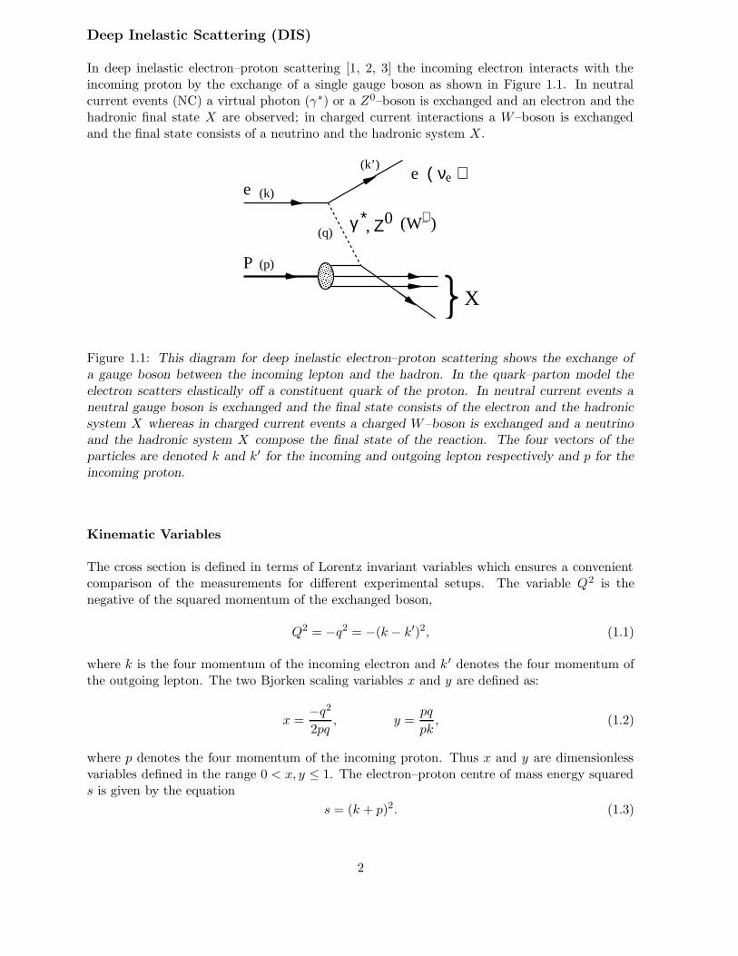
In deep inelastic electron–proton scattering [1, 2, 3] the incoming electron interacts with theincoming proton by the exchange of a single gauge boson as shown in Figure 1.1. In neutralcurrent events (NC) a virtual photon (γ∗) or a Z0–boson is exchanged and an electron and thehadronic final state X are observed; in charged current interactions a W–boson is exchangedand the final state consists of a neutrino and the hadronic system X.

e (k)

e (

��

��

ν(k’)e )

(q)

(p)

γ ∗, Ζ0 (W )+−

}X

P

Figure 1.1: This diagram for deep inelastic electron–proton scattering shows the exchange ofa gauge boson between the incoming lepton and the hadron. In the quark–parton model theelectron scatters elastically off a constituent quark of the proton. In neutral current events aneutral gauge boson is exchanged and the final state consists of the electron and the hadronicsystem X whereas in charged current events a charged W–boson is exchanged and a neutrinoand the hadronic system X compose the final state of the reaction. The four vectors of theparticles are denoted k and k′ for the incoming and outgoing lepton respectively and p for theincoming proton.

Kinematic Variables

The cross section is defined in terms of Lorentz invariant variables which ensures a convenientcomparison of the measurements for different experimental setups. The variable Q2 is thenegative of the squared momentum of the exchanged boson,

Q2 = −q2 = −(k − k′)2, (1.1)

where k is the four momentum of the incoming electron and k ′ denotes the four momentum ofthe outgoing lepton. The two Bjorken scaling variables x and y are defined as:

x =−q22pq

, y =pq

pk, (1.2)

where p denotes the four momentum of the incoming proton. Thus x and y are dimensionlessvariables defined in the range 0 < x, y ≤ 1. The electron–proton centre of mass energy squareds is given by the equation

s = (k + p)2. (1.3)

2

At fixed centre of mass energy√s, only two of these four variables are independent due to energy

momentum conservation2. When neglecting the electron and proton masses they are connectedby the relation

Q2 = xys. (1.4)

In addition W is defined as the centre of mass energy of the exchanged boson and the incomingproton

W 2 = (q + p)2 ' ys−Q2. (1.5)

Definition of the Cross Section and the Structure Function F2

The cross section for neutral current ep interactions is defined such that it takes into account thedifferent couplings of the gauge bosons to the electron and the propagator terms. In the regionof low Q2 (Q2 � M2

Z0) only photon exchange contributes, resulting in a drastic simplificationof the cross section expression. The Z0 exchange and the interference between Z0 and photonexchange can be neglected safely since the gauge boson masses enter the cross section by thepropagator terms which leads to the following ratios for the contributions of the Z 0 exchangeand the interference w.r.t. the contribution from single photon exchange to the cross section:

σ(Z0

)

σ (γ∗)∼

(Q2

Q2 +M2Z0

)2

, (1.6)

σ(γ∗Z0

)

σ (γ∗)∼

(Q2

Q2 +M2Z0

). (1.7)

At low Q2 the differential electron–proton cross section can be written as:

d2σ(x,Q2

)

dxdQ2=

4πα2em

xQ4

[(1 − y +

y2

2

)F2

(x,Q2

)− y2

2FL

(x,Q2

)](1.8)

where αem denotes the electromagnetic coupling constant and the structure functions F2 andFL depend on the internal structure of the proton. They have to be determined experimentallysince they currently cannot be calculated from first principles although non perturbative QCDmethods based on lattice QCD exist [4]. The structure function F2 is proportional to the sum ofthe cross sections for the exchange of longitudinally and transversely polarised photons whereasFL only depends on the cross section for the exchange of longitudinally polarised photons. Inthe kinematic region of not too large y the contribution of the structure function FL can beneglected and the cross section mainly depends on F2. A compilation of the most precise F2

measurements is shown in Figure 1.2 [5, 6, 7, 8, 9, 10, 11, 12]. The structure function F2 isshown as a function of the photon virtuality Q2 for different values of the scaling variable x.For values of x ∼ 0.2 F2 is independent of Q2 which was first observed at SLAC [13, 14] andis known as scaling. For larger x values the structure functions decreases with increasing Q2

whereas the opposite behaviour is observed for smaller values of x. The observation of scalingled to the advent of the quark–parton model [15, 16, 17, 18] which was refined by the observationof scaling violations [19] for large and small values of x. These effects have been successfullydescribed in the framework of Quantum Chromo Dynamics (QCD) [20, 21, 22, 23].

2The reaction is assumed to be independent on the azimuthal angle and therefore this degree of freedom hasnot been considered.

3

0

2

4

6

8

10

12

14

16

1 10 102

103

104

105

ZEUS+H1

Q2 (GeV2)

Fem

+ci(x

)2

ZEUS 96/97

H1 94/97

NMC, BCDMS, E665

ZEUS NLO QCD Fit(prel. 2001)

H1 NLO QCD Fit

Figure 1.2: Compilation of the most precise F2 measurements up to date in dependence of Q2

for different values of x. The data in the region of low Q2 and medium to large x are takenby fixed target experiments. These kinematic region has been extended by about 2 orders ofmagnitude in x and Q2 by the HERA experiments H1 and ZEUS. The data are compared tonext to leading order QCD fits which are able to reproduce the measurements in the wholekinematic range [5, 6, 7, 8, 9, 10, 11, 12].

The Quark Parton Model

The observation of scaling at SLAC in the kinematic region 1 < Q2 < 10GeV2 for x ' 0.2 wasinterpreted by Bjorken and Paschos [15, 16] and by Feynman [17, 18] as being due to the partonic

4

structure of the proton. In a Thompson–model of the proton in which the proton is an extendedparticle consisting of a continuous charge distribution a steeply falling structure function F2

would be expected for all values of x as may be understood as follows. The wavelength of thevirtual photon is proportional to the inverse of its virtuality λ ∼ 1/

√−q2 which means that

the photon probes smaller distances for larger Q2 values and therefore it would be sensitive tosmaller and smaller fractions of the total electric charge of the proton. Since the coupling of thephoton is proportional to the charge this would lead to an F2 falling with increasing values ofQ2 for all values of x.

In the quark–parton model the proton consists of three point-like partons which can be identifiedwith the quarks introduced by Gell–Mann and Zweig [24, 25] to explain the spectroscopic hadrondata. The proton is built from two up–quarks with fractional charge 2/3 and one down–quarkwith fractional charge -1/3. In this model the electron scatters elastically off one of the threequarks by single photon exchange. Since the time scale of the interaction is very small incomparison to interactions between the constituent quarks the proton can be treated for crosssection calculations as an incoherent sum of these three quarks. This model leads to the observedscaling behaviour and the structure function F2 may then be written as

F2 (x) =∑

f

e2fxqf (x) (1.9)

where ef is the charge of the struck quark and qf (x) are the quark density functions. In thismodel, x can be interpreted, in the infinite momentum frame, as the momentum fraction of theprotons momentum carried by the struck quark.

By exploring a larger region in the x–Q2 plane the violation of the scaling behaviour was observedas mentionend before. In addition it was found when summing up the momentum carried by thequarks that only a fraction of the total proton momentum is carried by these partons. Theseeffects can be understood in the framework of Quantum Chromo Dynamics (QCD).

Quantum Chromo Dynamics (QCD)

Quantum Chromo Dynamics is the quantum field theory for strong interactions. With the largesuccess of Quantum Electrodynamics (QED) in describing electromagnetic interactions at highenergies it was recognised that renormisable quantum field theories are the most appropriateway to describe interactions of high energy particles. Until the advent of QCD a phenomeno-logical theory the so called Regge theory existed which was able to describe soft hadron–hadroninteractions (see chapter 1.2). With the observation of the substructure of hadrons a new theoryfor strong interactions became necessary.

In QCD the proton is built from quarks (as in the quark–parton model) which are spin 1/2fermions. These are bound together by gluons which are the spin 1 gauge bosons of QCD, anon–abelian gauge theory invariant under SU(3) colour symmetry. In the framework of QCDcolour corresponds to a new degree of freedom which takes the role of the electric charge inQED. It is carried by the quarks and in contrast to QED also by the gauge bosons, the gluonsas a consequence of the non–abelian character of the theory. This leads to a self coupling of thegluons and hence to fundamental differences between QCD and QED.

5

Renormalisation and the Running Coupling

In perturbative QCD calculations divergent integrals appear which are treated by a renormali-sation scheme and hence lead to an effective coupling constant αs

(µ2

r

)depending on the energy

scale µ2r. The requirement that the calculated cross sections are independent of the renor-

malisation scale µ2r leads to the Renormalisation Group Equation (RGE) which in leading log.

approximation (LLA) leads to the scale dependence of the coupling constant:

αs

(µ2

r

)=

12π

(33 − 2nf ) ln(µ2

r/Λ2QCD

) . (1.10)

ΛQCD is a free parameter which has to be determined by experiments. It represents the lowerlimit of µr for which perturbative QCD calculations are expected to be predictive. nf is thenumber of quark flavours with mass m2

q < µ2r. In contrast to QED the effective strong coupling

constant αs is decreasing for larger values of µ2r as consequense of the gluon self coupling.

The two extremes of small and large µ2r which by the uncertainty principle correspond to large

and small distances respectively, are called infrared slavery and asymptotic freedom. In theregion of infrared slavery αs is large and perturbative QCD calculations are not applicable.This long range effect is responsible for the confinement of partons in bound states, the hadrons.In the region of asymptotic freedom αs is small and the perturbative expansion series (in powersof αs) of QCD calculations is expected to converge fast which means that quarks can be treatedas free particles.

In a pQCD calculation to a fixed order in αs the cross section depends on the renormalisationscale µ2

r through the coupling constant αs

(µ2

r

). When calculating up to all orders the terms

involving µ2r cancel and the cross section becomes independent of the renormalisation scale.

The Factorisation in DIS

The theorem of factorisation has been proven for hard scattering [26] and states that short rangeeffects in the scattering amplitude, calculable in pQCD, can be separated from long range effectswhich are accounted to the parton density functions (pdf’s). The proton structure function F2

can be written as

F2

(x,Q2

)=

∑

i=q,q,g

∫ 1

xdξfi

(ξ, µ2

r, µ2f , αs

)· CV

i

(x

ξ,Q2

µ2r

, µ2f , αs

). (1.11)

In this decomposition µ2f is the factorisation scale, fi are the parton density functions and CV

i

are the coefficient functions. These describe the interaction of the exchanged boson V with aquark i (see Figure 1.3) which is calculable in perturbative QCD. The factorisation scale µ2

f

defines the energy scale above which additional parton emissions from the quark are included inthe perturbative QCD calculation. Long range effects which are not calculable in pQCD (e.g.parton emission with k2

T < µ2f ) are absorbed in the parton density functions fi which therefore

also become dependent on the factorisation scale µ2f . The parton density functions fi can be

interpreted in leading order calculations as probability to find a parton of type i for a certainvalue of x in the hadron. These are universal functions which only depend on the hadron typewhereas the coefficient functions CV

i are process dependent.

6

fq/P(x)

σγ*qγ*

fq/P(x,µf 2)

γ*

σγ*q(µf 2)

µf

kT>µf

kT<µf

(a) (b)

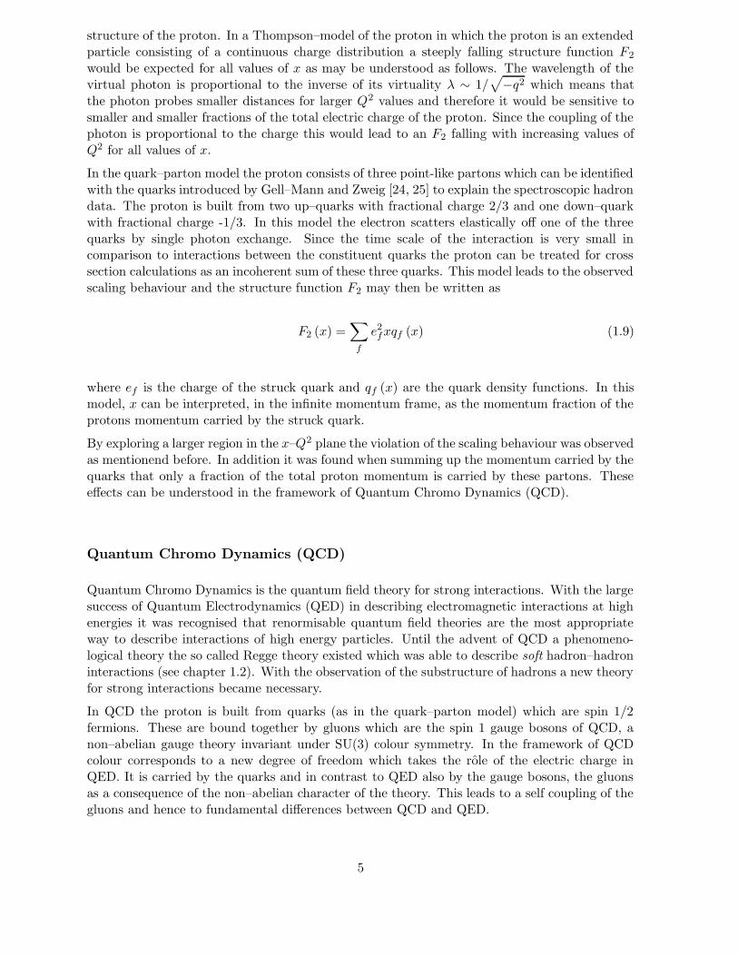
Figure 1.3: a) Leading order diagram for the interaction of the virtual photon with a quark of theproton. b) In NLO calculations diagrams with e.g. additional parton emission have to be takeninto account. The factorisation theorem states that parton emission with a large scale is takeninto account in the scattering amplitude, calculable in pQCD whereas parton emission below thescale µf is absorbed in the parton density function which has to be determined experimentally.

Parton Density Functions

Since the parton density functions cannot be calculated from first principles they have to beextracted from the experimental data although perturbative QCD calculations predict the evolu-tion (e.g. inQ2) of parton densities once they are known at at a certain starting point (fi

(x,Q2

0

)).

The proton structure function F2 can be developed in a perturbation series in powers of αs whichcontains terms αs ln

(Q2/Q2

o

), αs ln (1/x) and mixed terms αs

(Q2/Q2

o

)ln (1/x). Three different

kind of evolution equations exist differing in the choice of terms added up from this perturbativeexpansion. The evolution of the parton density functions corresponds to a ladder diagram shownin Figure 1.4 and the summation of certain terms can be interpreted as ordering in either kT orx of the rungs from the ladder (see e.g. [27]).

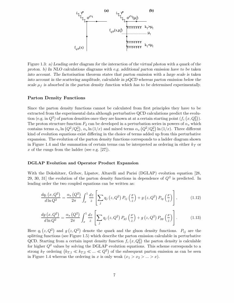
DGLAP Evolution and Operator Product Expansion

With the Dokshitzer, Gribov, Lipatov, Altarelli and Parisi (DGLAP) evolution equation [28,29, 30, 31] the evolution of the parton density functions in dependence of Q2 is predicted. Inleading order the two coupled equations can be written as:

dqi(x,Q2

)

d lnQ2=αs

(Q2

)

2π

∫ 1

x

dz

z

∑

j

qj(z,Q2

)Pij

(xz

)+ g

(z,Q2

)Pig

(xz

) , (1.12)

dg(x,Q2

)

d lnQ2=αs

(Q2

)

2π

∫ 1

x

dz

z

∑

j

qj(z,Q2

)Pgj

(xz

)+ g

(z,Q2

)Pgg

(xz

) . (1.13)

Here qi(z,Q2

)and g

(z,Q2

)denote the quark and the gluon density functions. Pij are the

splitting functions (see Figure 1.5) which describe the parton emission calculable in perturbativeQCD. Starting from a certain input density function fi

(x,Q2

0

)the parton density is calculable

for higher Q2 values by solving the DGLAP evolution equations. This scheme corresponds to astrong kT ordering

(kT,1 � kT,2 � ...� Q2

)of the subsequent parton emission as can be seen

in Figure 1.4 whereas the ordering in x is only weak (x1 > x2 > ... > x).

7

e

e′

γ*

q

q_

p

x

Q2

x1 , kT,1

xi , kT,i

xi+1 , kT,i+1

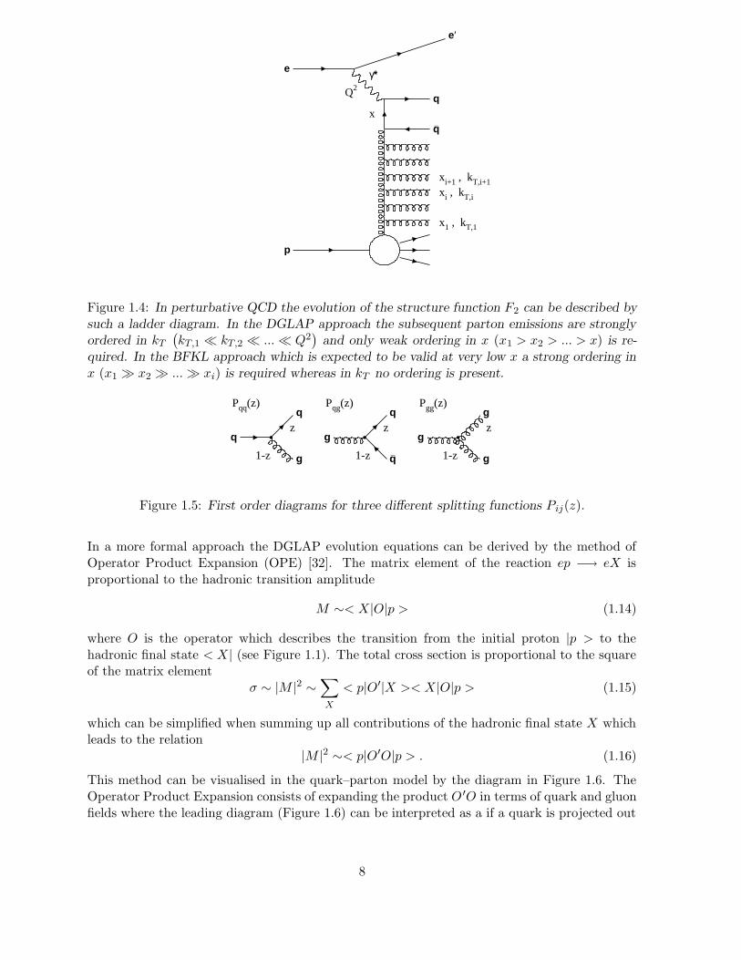
Figure 1.4: In perturbative QCD the evolution of the structure function F2 can be described bysuch a ladder diagram. In the DGLAP approach the subsequent parton emissions are stronglyordered in kT

(kT,1 � kT,2 � ...� Q2

)and only weak ordering in x (x1 > x2 > ... > x) is re-

quired. In the BFKL approach which is expected to be valid at very low x a strong ordering inx (x1 � x2 � ...� xi) is required whereas in kT no ordering is present.

q

q

g

z

1-z

Pqq(z)

g

q

q_

z

1-z

Pqg(z)

g

g

g

z

1-z

Pgg(z)

Figure 1.5: First order diagrams for three different splitting functions Pij(z).

In a more formal approach the DGLAP evolution equations can be derived by the method ofOperator Product Expansion (OPE) [32]. The matrix element of the reaction ep −→ eX isproportional to the hadronic transition amplitude

M ∼< X|O|p > (1.14)

where O is the operator which describes the transition from the initial proton |p > to thehadronic final state < X| (see Figure 1.1). The total cross section is proportional to the squareof the matrix element

σ ∼ |M |2 ∼∑

X

< p|O′|X >< X|O|p > (1.15)

which can be simplified when summing up all contributions of the hadronic final state X whichleads to the relation

|M |2 ∼< p|O′O|p > . (1.16)

This method can be visualised in the quark–parton model by the diagram in Figure 1.6. TheOperator Product Expansion consists of expanding the product O ′O in terms of quark and gluonfields where the leading diagram (Figure 1.6) can be interpreted as a if a quark is projected out

8

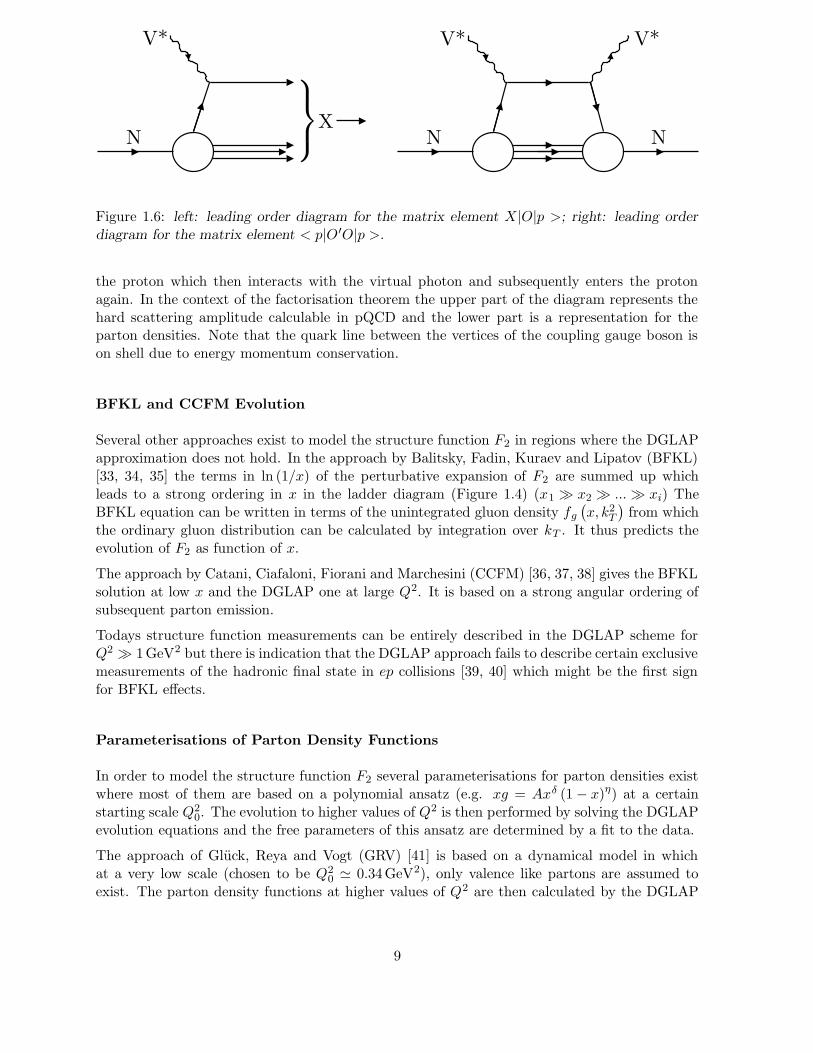
Figure 1.6: left: leading order diagram for the matrix element X|O|p >; right: leading orderdiagram for the matrix element < p|O ′O|p >.

the proton which then interacts with the virtual photon and subsequently enters the protonagain. In the context of the factorisation theorem the upper part of the diagram represents thehard scattering amplitude calculable in pQCD and the lower part is a representation for theparton densities. Note that the quark line between the vertices of the coupling gauge boson ison shell due to energy momentum conservation.

BFKL and CCFM Evolution

Several other approaches exist to model the structure function F2 in regions where the DGLAPapproximation does not hold. In the approach by Balitsky, Fadin, Kuraev and Lipatov (BFKL)[33, 34, 35] the terms in ln (1/x) of the perturbative expansion of F2 are summed up whichleads to a strong ordering in x in the ladder diagram (Figure 1.4) (x1 � x2 � ...� xi) TheBFKL equation can be written in terms of the unintegrated gluon density fg

(x, k2

T

)from which

the ordinary gluon distribution can be calculated by integration over kT . It thus predicts theevolution of F2 as function of x.

The approach by Catani, Ciafaloni, Fiorani and Marchesini (CCFM) [36, 37, 38] gives the BFKLsolution at low x and the DGLAP one at large Q2. It is based on a strong angular ordering ofsubsequent parton emission.

Todays structure function measurements can be entirely described in the DGLAP scheme forQ2 � 1GeV2 but there is indication that the DGLAP approach fails to describe certain exclusivemeasurements of the hadronic final state in ep collisions [39, 40] which might be the first signfor BFKL effects.

Parameterisations of Parton Density Functions

In order to model the structure function F2 several parameterisations for parton densities existwhere most of them are based on a polynomial ansatz (e.g. xg = Axδ (1 − x)η) at a certainstarting scale Q2

0. The evolution to higher values of Q2 is then performed by solving the DGLAPevolution equations and the free parameters of this ansatz are determined by a fit to the data.

The approach of Gluck, Reya and Vogt (GRV) [41] is based on a dynamical model in whichat a very low scale (chosen to be Q2

0 ' 0.34GeV2), only valence like partons are assumed toexist. The parton density functions at higher values of Q2 are then calculated by the DGLAP

9

evolution equations.

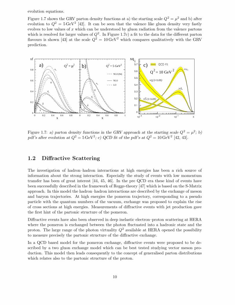
Figure 1.7 shows the GRV parton density functions at a) the starting scale Q2 = µ2 and b) afterevolution to Q2 = 5GeV2 [42]. It can be seen that the valence like gluon density very fastlyevolves to low values of x which can be understood by gluon radiation from the valence partonswhich is resolved for larger values of Q2. In Figure 1.7c) a fit to the data for the different partonflavours is shown [43] at the scale Q2 = 10GeV2 which compares qualitatively with the GRVprediction.

0

0.2

0.4

0.6

0.8

0 0.2 0.4 0.6 0.8

Q2 = µ2

x

xf

uv

g

dv

d–

u

Q2 = 5 GeV2

x

NLO (94)

NLO

LOuv

g

dv

d–

us

0

0.2

0.4

0.6

0.8

0 0.2 0.4 0.6 0.8 1

=2 2Qb)

10 GeV

c)a)i

xq

Figure 1.7: a) parton density functions in the GRV approach at the starting scale Q2 = µ2; b)pdf’s after evolution at Q2 = 5GeV2; c) QCD fit of the pdf’s at Q2 = 10GeV2 [42, 43].

1.2 Diffractive Scattering

The investigation of hadron–hadron interactions at high energies has been a rich source ofinformation about the strong interaction. Especially the study of events with low momentumtransfer has been of great interest [44, 45, 46]. In the pre QCD era these kind of events havebeen successfully described in the framework of Regge-theory [47] which is based on the S-Matrixapproach. In this model the hadron–hadron interactions are described by the exchange of mesonand baryon trajectories. At high energies the pomeron trajectory, corresponding to a pseudoparticle with the quantum numbers of the vacuum, exchange was proposed to explain the riseof cross sections at high energies. Measurements of diffractive events with jet production gavethe first hint of the partonic structure of the pomeron.

Diffractive events have also been observed in deep inelastic electron–proton scattering at HERAwhere the pomeron is exchanged between the photon fluctuated into a hadronic state and theproton. The large range of the photon virtuality Q2 available at HERA opened the possibilityto measure precisely the partonic structure of the diffractive exchange.

In a QCD based model for the pomeron exchange, diffractive events were proposed to be de-scribed by a two gluon exchange model which can be best tested studying vector meson pro-duction. This model then leads consequently to the concept of generalised parton distributionswhich relates also to the partonic structure of the proton.

10

Diffractive Scattering in Soft Hadron–Hadron Interactions

Experimental Observations

In Figure 1.8 the cross section for elastic proton–proton scattering is plotted for different centreof mass energies as a function of |t| where t is the squared momentum transfer between the twohadrons [46]. For low centre of mass energies a falling cross–section is observed where the slopegets steeper towards higher centre of mass energies. In addition a minimum and a maximumappear. This shape is similar to the diffraction pattern as observed when a plane wave of lightpasses a disc. The shape of the cross section down to the first minimum can be approximated

Figure 1.8: Compilation of measurements of the differential cross section for elastic pp scatteringas a function of |t| for different values of the centre of mass energy [46].

11

by an exponential function of the form3:

dσ

dt=

(dσ

dt

)∣∣∣∣t=0

e−b|t| (1.17)

with b ∼ 10GeV−2.

The data can be interpreted in the spirit of the similarity between optical and hadronic diffraction[45]. In this picture one discusses the scattering of a fast hadron represented by a plane wave inthe field of a hadron at rest. In optical diffraction the following formula holds for kR� 1:

I

I0' 1 − R2

4k2θ2 (1.18)

which describes the fraction of observed intensity w.r.t. the initial intensity as a function of thediffraction angle θ, where R is the radius of the disc and k denotes the wave number of theincident light wave. If one relates the scattering angle θ to the momentum transfer t in hadron–hadron interactions, the wave number k to the momentum of the hadrons, and the radius of thedisc R to the mass of the pion one can deduce a t-slope b of b = 12.5GeV−2 resulting in theright order of magnitude as measured.

Aspects of Regge Theory

The only theory to describe soft hadron–hadron interactions is Regge theory [47]. Apart fromthe fact that it was invented well before QCD, it still provides the only possibility to predictcross sections for these kind of reactions since perturbative QCD calculations are not applicabledue to the absence of a hard scale in the process.

Regge theory was introduced in the framework of non–relativistic quantum mechanics and gen-eralised the idea of Yukawa explaining particle interactions by the exchange of virtual particles.Later it was generalised to also describe relativistic particle interactions. It is based on S-Matrixtheory which connects the wave function of the initial state |i > with that of the final state |f >by the relation:

|f >= S|i > . (1.19)

The foundations of Regge–theory are the following axioms:

• The superposition principle states that a particle state ψγ can be decomposed linearly inthe form |ψγ >= α|ψα > +β|ψβ > correctly taking into account the selection rules.

• The forces are required to be of short range. This is fulfilled for strong interactions sincethe interaction range is of the order of the inverse of the pion mass: R ∼ 1/mπ ∼ 10−15 m.

• The Lorentz invariance principle states that the S-Matrix is a Lorentz scalar which itselfonly depends on Lorentz scalars.

• The unitarity requirement which corresponds to the conservation of probability states thatS†S = 1 = SS†.

• Maximal analyticity of first order is required (see below).

3Note that in a more careful analysis the sum of two exponatial funtions has to be used [46]

12

• Generalisation of angular momentum in the complex plane is introduced (see below).

If one considers the reaction A+B −→ C +D. The Mandelstam variables sij are real numbersdefined by relationes of the form sij = (±Pi ± Pj)

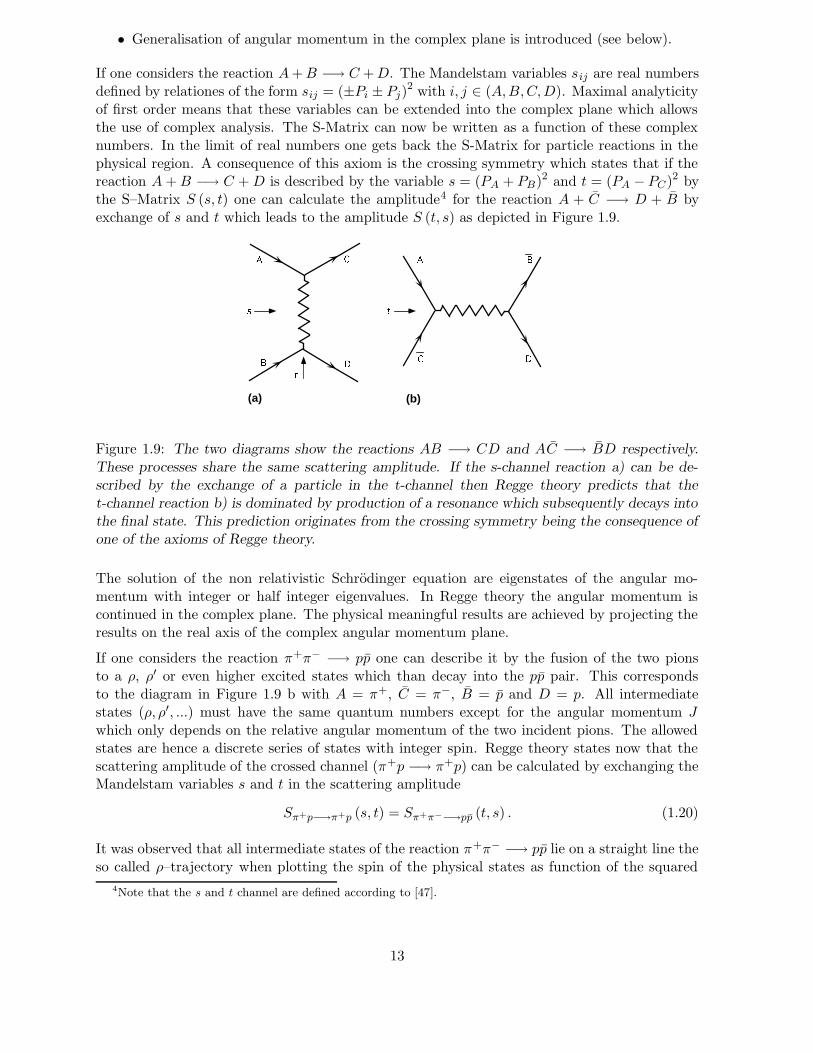
2 with i, j ∈ (A,B,C,D). Maximal analyticityof first order means that these variables can be extended into the complex plane which allowsthe use of complex analysis. The S-Matrix can now be written as a function of these complexnumbers. In the limit of real numbers one gets back the S-Matrix for particle reactions in thephysical region. A consequence of this axiom is the crossing symmetry which states that if thereaction A+B −→ C +D is described by the variable s = (PA + PB)2 and t = (PA − PC)2 bythe S–Matrix S (s, t) one can calculate the amplitude4 for the reaction A + C −→ D + B byexchange of s and t which leads to the amplitude S (t, s) as depicted in Figure 1.9.

(a) (b)

Figure 1.9: The two diagrams show the reactions AB −→ CD and AC −→ BD respectively.These processes share the same scattering amplitude. If the s-channel reaction a) can be de-scribed by the exchange of a particle in the t-channel then Regge theory predicts that thet-channel reaction b) is dominated by production of a resonance which subsequently decays intothe final state. This prediction originates from the crossing symmetry being the consequence ofone of the axioms of Regge theory.

The solution of the non relativistic Schrodinger equation are eigenstates of the angular mo-mentum with integer or half integer eigenvalues. In Regge theory the angular momentum iscontinued in the complex plane. The physical meaningful results are achieved by projecting theresults on the real axis of the complex angular momentum plane.

If one considers the reaction π+π− −→ pp one can describe it by the fusion of the two pionsto a ρ, ρ′ or even higher excited states which than decay into the pp pair. This correspondsto the diagram in Figure 1.9 b with A = π+, C = π−, B = p and D = p. All intermediatestates (ρ, ρ′, ...) must have the same quantum numbers except for the angular momentum Jwhich only depends on the relative angular momentum of the two incident pions. The allowedstates are hence a discrete series of states with integer spin. Regge theory states now that thescattering amplitude of the crossed channel (π+p −→ π+p) can be calculated by exchanging theMandelstam variables s and t in the scattering amplitude

Sπ+p−→π+p (s, t) = Sπ+π−−→pp (t, s) . (1.20)

It was observed that all intermediate states of the reaction π+π− −→ pp lie on a straight line theso called ρ–trajectory when plotting the spin of the physical states as function of the squared

4Note that the s and t channel are defined according to [47].

13

mass which is shown in Figure 1.10. The ρ–trajectory connects the s–channel (t < 0) andt–channel (t > 0) region which corresponds in this example to the reaction π+p −→ π+p witht = m2. When extending the trajectory into the s–channel region the value α(t) = Re(J) isused to predict cross sections for the crossed channel (see below) which agrees well with theobservations. The trajectory depends on the intercept α(0) = α0 and the slope α′

α(t) = α0 + α′ · t. (1.21)

Figure 1.10 shows that the measurements of the ρ trajectory in the s–channel region agree wellwith the prediction when continuing the Regge trajectory from the t–channel region into thes–channel region. A large amount of data from hadron–hadron scattering can be explained byRegge theory using the known meson and baryon spectra as origin for Regge trajectories.

0

0.5

1

1.5

2

2.5

3

-0.5 0 0.5 1 1.5 2 2.5 3

s-channel t-channelphysical physicalregion region

M2 = t (GeV2)

J =

Re(

α(t)

)

s channel pointsStates contributing to the ρ trajectory (ρ, ρ3)Additional Reggeon trajectory states (f2, ω, a2, ω3)

Figure 1.10: The ρ trajectory: In the t–channel region the bound states (ρ, ρ3) are shown. Astraight line through these states is continued into the s–channel region where it is compared todata from hadron–hadron interactions.

The total cross section for hadron–hadron interactions is connected to the imaginary part of theforward scattering amplitude A by the optical theorem which states

σtot(AB) ∼ 1

sImA (AB −→ AB) (s, t = 0). (1.22)

Hence this relation can be used to calculate total cross sections when knowing the scatteringamplitude. Regge theory provides predictions e.g. for the energy dependence of total crosssection:

σtot ∼ s2α(0)−2, (1.23)

where s is the centre of mass energy of the hadron–hadron interaction. The measurement ofthe energy dependence of the cross section therefore provides access to the intercept α0 of thetrajectory. When measuring the t–dependence of cross sections also the determination of theslope α′ becomes possible (see Figure 1.10).

14

It was observed (see Figure 1.11) that the total cross section decreases with energy for lowenergies which is explained by Regge–trajectories originating from the known baryon and mesonspectra whereas the rise of the cross section for high energies was not expected. To account for

��

"!$#&%$')(�*,+

-./10 203 456

1 10 100100

150

200

Figure 1.11: Compilation of measurements for total hadron–hadron cross sections as a functionof the centre of mass energy

√s for different hadron types. a) proton–proton and proton–

antiproton cross sections; b) π+p and π−p cross sections; c) photon–proton cross sections, wherethe photon can be treated as hadron in the vector meson dominance model (see text) [48].

this rise the Pomeron trajectory was introduced which is characterised by the quantum numbersof the vacuum. From the rise of σtot for different reactions the Pomeron trajectory can bederived [48]:

α(t) = 1.08 + 0.25 · t. (1.24)

It is measured in the s–channel region and a real particle in the t–channel regime is expectedbut not yet found. This particle is most probably glueball, i.e. a composite state of two valence

15

gluons with the quantum numbers of the vacuum.

With introduction of the Pomeron trajectory also the observations discussed at the beginningof this section can be explained. The shrinkage of the diffractive peak can be predicted sinceRegge theory states:

b = b0 + 2α′ln

(s

s0

)(1.25)

and the double peak structure of the differential cross section as function of t at high energies(see Figure 1.8) can be explained by interference between single and multiple Pomeron exchange.

Following the idea by Ingelmann and Schlein [49] the structure of the vacuum exchange wasinvestigated using diffractive events in presence of a hard scale suitable to resolve the partonicstructure of the Pomeron. In proton–antiproton interactions this was done studying diffractiveevents with high transverse momentum jets. The measured cross section for this kind of eventshas been interpreted to be dominated by a large gluon content of the Pomeron [50, 51]. Followingthe same idea at HERA diffractive events have been investigated in the presence of a hard scale.

Diffraction in Electron–Proton Interactions

In the first years of HERA operation a widely unexpected large amount of diffractive events wasobserved [52, 53, 54, 55].

Inclusive Diffraction in Electron–Proton Interactions

Such events are identified by the presence of a large gap in rapidity η5 in which no particleproduction is observed. The corresponding diagram for diffraction in electro–production isshown in Figure 1.12. The hadronic system Y propagates in the direction of the incomingproton while the system X is observed in the central part of the detector. Due to the highcentre of mass energy in the photon–proton system it can be assumed that for the main partof the available phase space Pomeron exchange is dominant. In order to account for the newdegrees of freedom for diffractive processes it is necessary to introduce the additional kinematicvariables

M2X = p2

X , M2Y = P 2

Y , t = (P − pY )2 ,

xIP =q · (P − pY )

q · P , β =x

xIP=

−q22q · (P − PY )

,

where MX and MY are the invariant masses of the hadronic systems X and Y and t is themomentum transfer squared at the proton vertex. xIP can be interpreted as the longitudinalmomentum carried by the exchanged Pomeron whereas β is the momentum fraction of the struckquark w.r.t. the pomeron momentum.

The cross section for diffractive DIS as depicted in Figure 1.12 can be written as a five folddifferential cross section depending on: xIP , β, Q2, MY and t. Since MY and t cannot bemeasured at present one must integrate over these variables obtaining a three fold differential

5η is defined as η = − 1

2ln

(tan θ

2

)

16

cross section which is then related to the diffractive structure function FD(3)2 introduced similarly

to the inclusive proton structure function F2 [57]:

d3σep−→eXY

dxdβdQ2=

4πα2em

β2Q4

(1 − y +

y2

2

)F

D(3)2 . (1.26)

Following the idea of Ingelmann and Schlein [49] the virtual photon which is emitted by theincoming electron can probe the structure of the Pomeron with different spatial resolution ac-cording to its virtuality Q2. As factorisation was proven to hold for this process [56] the differ-ential cross section can be analysed in terms of a hard scattering amplitude and parton densityfunctions similarly to inclusive DIS. The structure function F D

2 (3) was further assumed to fac-torise into a Pomeron flux and a Pomeron structure function which then was analysed in termsof parton distributions for the Pomeron. The QCD analysis indicated a large gluon component[57] which is in line with the results from jet production in hadron–hadron interactions [51].

X

Y{

{

t

γ( pX)

( pY)

Largest gapin event

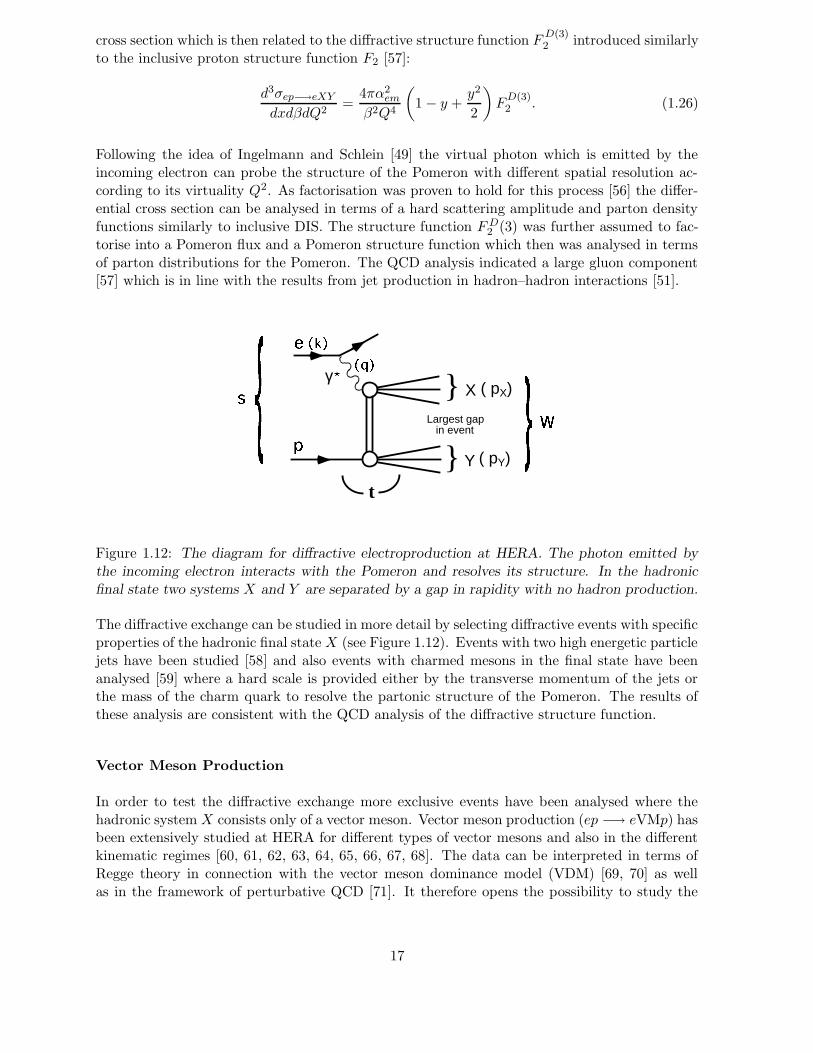
Figure 1.12: The diagram for diffractive electroproduction at HERA. The photon emitted bythe incoming electron interacts with the Pomeron and resolves its structure. In the hadronicfinal state two systems X and Y are separated by a gap in rapidity with no hadron production.

The diffractive exchange can be studied in more detail by selecting diffractive events with specificproperties of the hadronic final state X (see Figure 1.12). Events with two high energetic particlejets have been studied [58] and also events with charmed mesons in the final state have beenanalysed [59] where a hard scale is provided either by the transverse momentum of the jets orthe mass of the charm quark to resolve the partonic structure of the Pomeron. The results ofthese analysis are consistent with the QCD analysis of the diffractive structure function.

Vector Meson Production

In order to test the diffractive exchange more exclusive events have been analysed where thehadronic system X consists only of a vector meson. Vector meson production (ep −→ eVMp) hasbeen extensively studied at HERA for different types of vector mesons and also in the differentkinematic regimes [60, 61, 62, 63, 64, 65, 66, 67, 68]. The data can be interpreted in terms ofRegge theory in connection with the vector meson dominance model (VDM) [69, 70] as wellas in the framework of perturbative QCD [71]. It therefore opens the possibility to study the

17

applicability of both approaches and allows a separation of effects calculable in perturbativeQCD from soft physics observed in hadron–hadron interactions.

In the VDM the photon emitted by the incoming electron fluctuates into a vector meson whichthen scatters diffractively on the proton as depicted in Figure 1.13. In the VDM the productionof vector mesons with the same quantum numbers as the photon is described (i.e. ρ, ω, φ, ...)since the Pomeron is characterised by the quantum numbers of the vacuum.

��

��

��

��

��

p

e

e

VM

p

|P

Figure 1.13: Diagram for vector meson production in the vector meson dominance model inconjunction with Regge theory. The incoming electron emits a photon (real or virtual) whichfluctuates into a hadronic system, the vector meson, which subsequently interacts with theproton by pomeron exchange. Only the production of vector mesons with the same quantumnumbers as the photon are described within this model since the pomeron carries the quantumnumbers of the vacuum.

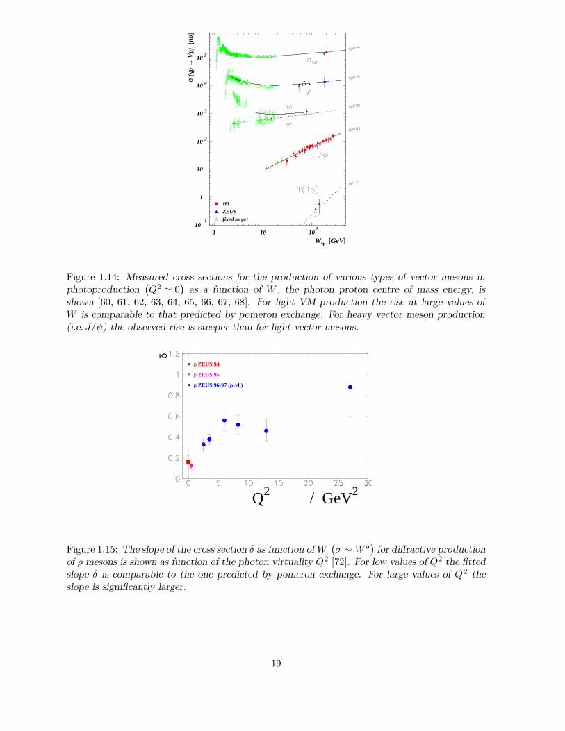
Figure 1.14 shows the measured cross section for vector meson production in photoproduction(Q2 ' 0

)as a function of W , the photon–proton centre of mass energy. For the production of

light vector mesons (ρ, φ and ω) the rise of the cross section at high W can be described asbefore in the framework of Regge theory by the exchange of the known Pomeron trajectory.The photoproduction of light vector mesons belongs therefore to the class of soft diffractiveinteractions. In the presence of a hard scale µ2 as is the case for J/ψ production with µ2 = m2

c ,where the charm mass provides the hard scale, the rise of the cross section is steeper thanpredicted by Regge theory.

For light vector meson production a hard scale can be introduced by selecting events in thekinematic domain Q2 > few GeV2. Here a similar behaviour can be observed indicating, thatthe rise of the cross section for high values of W becomes steeper when Q2 rises. This can beseen in Figure 1.15 where the slope δ of the cross section as function of W

(σ ∼W δ

)is shown

for different values of Q2. For low Q2 the rise of the cross section is comparable to the risepredicted by Regge theory. For large values of Q2 the rise is significantly larger. These kindof interactions are called hard diffractive interactions and expected to be calculable within theframework of perturbative QCD since the presence of a hard scale ensures convergence of theperturbation series.

In summary this means that in the presence of a hard scale Regge theory is not able anymore

18

Wγp [GeV]

σ (γ

p →

Vp)

[nb

]

H1

ZEUS

fixed target10

-1

1

10

10 2

10 3

10 4

10 5

1 10 102

Figure 1.14: Measured cross sections for the production of various types of vector mesons inphotoproduction

(Q2 ' 0

)as a function of W , the photon proton centre of mass energy, is

shown [60, 61, 62, 63, 64, 65, 66, 67, 68]. For light VM production the rise at large values ofW is comparable to that predicted by pomeron exchange. For heavy vector meson production(i.e. J/ψ) the observed rise is steeper than for light vector mesons.

ρ ZEUS 94

ρ ZEUS 95

ρ ZEUS 96-97 (prel.)

Q2 GeV2

δ

Q 2/2 GeV

Figure 1.15: The slope of the cross section δ as function ofW(σ ∼W δ

)for diffractive production

of ρ mesons is shown as function of the photon virtuality Q2 [72]. For low values of Q2 the fittedslope δ is comparable to the one predicted by pomeron exchange. For large values of Q2 theslope is significantly larger.

19

to describe diffractive processes. Due to the presence of a hard scale these kind of interactionsare expected to be calculable in the framework of perturbative QCD. The investigation of theseprocesses can be used to study the transition from soft to hard processes by varying the hardscale either by variation of the mass of the final vector meson, by the investigation of eventsin different regions of the photon virtuality Q2 or by studying events with a large momentumtransfer t at the proton vertex.

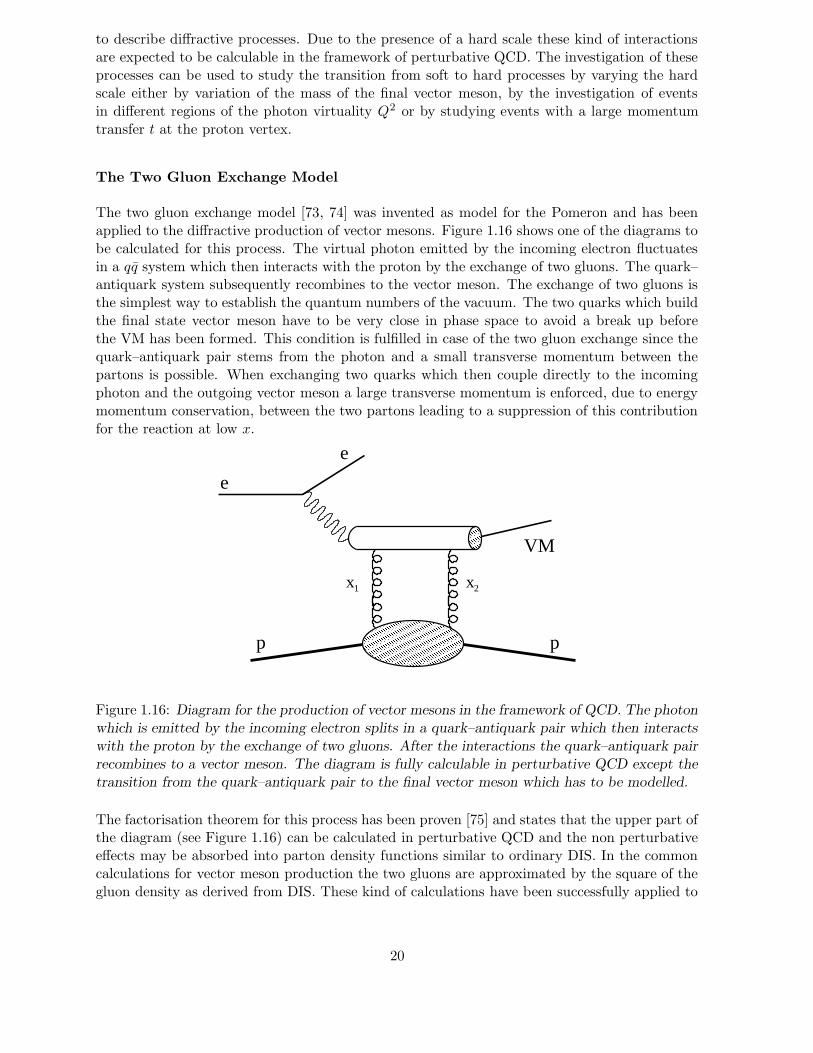
The Two Gluon Exchange Model

The two gluon exchange model [73, 74] was invented as model for the Pomeron and has beenapplied to the diffractive production of vector mesons. Figure 1.16 shows one of the diagrams tobe calculated for this process. The virtual photon emitted by the incoming electron fluctuatesin a qq system which then interacts with the proton by the exchange of two gluons. The quark–antiquark system subsequently recombines to the vector meson. The exchange of two gluons isthe simplest way to establish the quantum numbers of the vacuum. The two quarks which buildthe final state vector meson have to be very close in phase space to avoid a break up beforethe VM has been formed. This condition is fulfilled in case of the two gluon exchange since thequark–antiquark pair stems from the photon and a small transverse momentum between thepartons is possible. When exchanging two quarks which then couple directly to the incomingphoton and the outgoing vector meson a large transverse momentum is enforced, due to energymomentum conservation, between the two partons leading to a suppression of this contributionfor the reaction at low x.

��

��

��

��

2

e

e

p p

VM

x1 x

Figure 1.16: Diagram for the production of vector mesons in the framework of QCD. The photonwhich is emitted by the incoming electron splits in a quark–antiquark pair which then interactswith the proton by the exchange of two gluons. After the interactions the quark–antiquark pairrecombines to a vector meson. The diagram is fully calculable in perturbative QCD except thetransition from the quark–antiquark pair to the final vector meson which has to be modelled.

The factorisation theorem for this process has been proven [75] and states that the upper part ofthe diagram (see Figure 1.16) can be calculated in perturbative QCD and the non perturbativeeffects may be absorbed into parton density functions similar to ordinary DIS. In the commoncalculations for vector meson production the two gluons are approximated by the square of thegluon density as derived from DIS. These kind of calculations have been successfully applied to

20

predict the rise of the cross section for diffractive J/ψ production as function of W .

The approximation of the two gluon exchange by the square of the ordinary gluon density holdsfor low Q2 and not too heavy vector mesons. In the domain of large Q2 or for the production ofheavy vector mesons (e.g. Υ) it is expected that an additional effect has to be taken into accountwhen calculating cross sections. In case of photoproduction

(Q2 ' 0

)of heavy vector mesons

the almost real photon interacting with the proton is transformed to a vector meson with themass squared M 2

VM (see Figure 1.16). Energy momentum conservation implies a longitudinalmomentum transfer from the lower to the upper part of the diagram and hence x1 6= x2 wherex1 and x2 are the longitudinal momentum fractions of the two exchanged gluons. The differencein longitudinal momentum of the two participating partons is:

x1 − x2 =Q2 +M2

V /4

W 2(1.27)

where MV is the mass of the produced vector meson. In order to account for this effect theordinary parton densities have been extended to the so called generalised parton distributions(GPD’s) which become important for the calculations of cross sections for large values of Q2,heavy vector mesons and for low values of W . In particular for the production of Υ mesonsGPD’s have to be used to explain the measured cross sections (see below).

1.3 Generalised Parton Distributions

Generalised Parton distributions (GPD’s) 6 are functions which generalise and interpolate be-tween different types of functions characterising the structure of the proton (nucleons). Inparticular the parton density functions as measured in DIS do not provide enough informationneeded for cross section predictions of certain reactions (e.g. vector meson production). Elasticform factors, unpolarised and polarised parton distributions can be derived from GPD’s whenintegrating over or taking boundary values of these functions.

The concept of GPD’s arose from three different theoretical studies7. Geyer et al. studied therelation between the Altarelli–Parisi evolution for parton distributions and the Brodsky–Lepageevolution for meson wave functions [77, 78, 79, 80]. The introduced interpolating functions areessentially what is nowadays called GPD’s. Jain and Ralston studied hard processes involvinghadron helicity flip in terms of an off–diagonal transition amplitude [81]. These can be used toderive elastic form factors. Finally Ji introduced off–forward parton distributions to describethe spin structure of the nucleon [82, 83]. He also proposed the measurement of Deeply VirtualCompton Scattering to extract these new distributions from the data [83].

Definition of GPD’s

In this section the formal definition of GPD’s is reviewed following the nomenclature of Ji [82, 83].Additional definitions exist (e.g. [84]) which are basically equivalent and transformation formulaehave been provided to switch between different nomenclatures.

6The term Generalised Parton Distribution is nowadays commonly used and comprises all names introducedin the past which originate from the different usage of these functions. Historically the terms: off–diagonal,non–diagonal, off–forward and non–forward parton distribution are used as well as skewed parton distributions.

7For a historical review see [76].

21

In section 1 it has been discussed that the standard parton distributions are obtained in theframework of Operator Product Expansion (OPE) from the squared proton wave function for allpartonic configurations containing a parton with specified polarisation and longitudinal momen-tum x. After application of the factorisation theorem the hadronic matrix element < p|O ′O|p >can be identified with the parton density function which is interpreted as the probability forfinding such a parton in the proton. Figure 1.17a) shows the graphical representation of thismatrix element.

In contrast to this GPD’s are defined as hadronic matrix elements of two unequal hadronic wavefunctions representing the incoming and outgoing nucleon (e.g. for VM production) < p ′|O|p >where |p > denotes the wave function of the incoming proton and |p′ > represents the outgoingproton [85]. In Figure 1.17b) and c) the corresponding diagrams are shown.

In comparison to standard DIS two kinematic regimes exist, the so called DGLAP region (Figure1.17b) and the ERBL region (Figure 1.17c). In the DGLAP region (|x| > ξ) the matrix elementis interpreted as emission of a parton with longitudinal momentum (x + ξ) · p where p is themomentum of the incident proton and subsequent absorption of a parton with longitudinalmomentum (x− ξ) ·p. For the ERBL region (|x| < ξ) which has no counterpart to standard DISthe matrix element is interpreted as emission of a di–parton system with longitudinal momenta(x+ξ) ·p and (−x+ξ) ·p. In case of quarks the two parton system consists of a quark–antiquarkpair.

The standard parton density functions are defined on the cross section level whereas the GPD’sare functions defined on the amplitude level, i.e. when calculating cross sections (e.g. for vectormeson production) the GPD’s enter the calculation of the scattering amplitude which then issquared to achieve the cross section expression.

(a)

p p

x x x+ξ x−ξ +ξx−+ξx

p’

(b)

p p’

(c)

p

Figure 1.17: Diagrams representing the hadronic matrix elements: a) for standard DIS and b)and c) for the generalised parton distribution. In contrast to parton densities in standard DISthe GPD’s are defined by hadronic matrix elements of unequal hadronic wave functions. Onedistinguishes between the DGLAP b) and ERBL c) region.

The generalised parton distributions can formally be defined by Fourier transforms of thehadronic matrix elements:

∫dλ

2πeiλx〈P ′|ψ(−λn)γµψ(λn)|P 〉 = H(x, ξ, t) u(P ′)γµu(P )

+ E(x, ξ, t) u(P ′)iσµν∆ν

2Mu(P ), (1.28)

∫dλ

2πeiλx〈P ′|ψ(−λn)γµγ5ψ(λn)|P 〉 = H(x, ξ, t) u(P ′)γµγ5u(P )

+ E(x, ξ, t) u(P ′)∆µγ5

2Mu(P ) (1.29)

22

where |P 〉 and 〈P ′| represent the quantum numbers of the incoming and outgoing protonrespectively (including differences for the spin state). The operators ψ(−λn)γµψ(λn) andψ(−λn)γµγ5ψ(λn) select the parton with certain properties from the hadronic wave functions.∆µ is defined as ∆µ = p′µ − pµ in the infinite momentum frame, t = ∆2, u(P ) and u(P ′) denotethe Dirac spinors of the hadron. An examination of the helicity structure of the scatteringamplitude shows that there are exactly four independent generalised parton distributions. Thefunctions H, E, H and E are defined for the different quark flavours as well as for the gluon.

The reference system is chosen such that the initial and final nucleon have longitudinal momenta(1+ξ)pµ and (1−ξ)pµ, and the outgoing and incoming partons carry the longitudinal momentum(x+ξ)pµ and (x−ξ)pµ, respectively. Due to energy momentum conservation x and ξ are restrictedto

0 < ξ <

√−t√

M2 − t/4, (1.30)

−1 < x < 1. (1.31)

The distributions Hq and Eq are summed over the quark helicities, whereas Hq and Eq involvethe difference between right and left handed quarks and therefore contain information aboutthe spin structure of the proton. The chiral-even distributions H and H survive in the forwardlimit, (i.e. H(x, ξ, t) 6= 0 and E(x, ξ, t) 6= 0 for ξ = 0 and t = 0) in which the nucleon helicityis conserved, while the chiral-odd distributions E and E allow for the possibility of a nucleonhelicity flip. The change of the nucleon helicity in case of helicity conservation for the quarks ispossible when orbital momentum is transferred by the two partons.

The evolution equations for the generalised parton distributions are modified DGLAP evolutionequations in the DGLAP regime (|x| > ξ) whereas in the ERBL region (|x| < ξ) the Brodsky–Lepage evolution equations are used which originate from the study of evolution equations formeson wave functions[92, 93].

Sum rules and boundary conditions for GPD’s

Several sum rules and boundary conditions for GPD’s exist, thus drastically restricting thepossibilities of models for GPD’s.

The Nucleon Spin Structure

The spin of the nucleon can be decomposed in components which are carried by the quarks andby the gluons [82]: −→

J N =−→J q +

−→J g. (1.32)

It can now be shown that:

Jq,g =1

2

(Aq,g(0) +Bq,g(0)

)(1.33)

with ∫ 1

−1dx x

(H(x, ξ, t) +E(x, ξ, t)

)= A(t) +B(t) (1.34)

where the integral over the functions H and E has to be evaluated for the quark and for thegluon distributions. The ξ–dependence drops out when calculating the integral.

23

The Parton Density Functions

The generalised parton distributions contain information of both the ordinary forward partondistributions and electromagnetic nucleon form factors. In the limit ∆µ −→ 0 one restores theordinary quark and the quark helicity distributions q(x) and ∆q(x) for x > 0:

H(x, 0, 0) = q(x), H(x, 0, 0) = ∆q(x). (1.35)

The Elastic Form Factors

The first moment of the generalised parton distributions is related to the nucleon form factors:∫ 1

−1dxH(x, ξ, t) = F1(t) , (1.36)

∫ 1

−1dxE(x, ξ, t) = F2(t) , (1.37)

∫ 1

−1dxH(x, ξ, t) = GA(t) , (1.38)

∫ 1

−1dxE(x, ξ, t) = GP (t) , (1.39)

where F1 and F2 are the Dirac and Pauli form factors which can be related by linear combinationsto the electric and magnetic form factors GE and GM . GA and GP represent the axial andpseudo-scalar form factors of the nucleon.

Models for GPD’s

In this section the model for GPD’s from Radyushkin based on Double Distributions will beoutlined [80, 84, 86, 87]. Other approaches based on the MIT bag model [76], hadronic lightcone wave functions [85] or the chiral quark soliton model [88, 89] are not discussed.

In addition to the boundary conditions discussed for GPD’s they have to fulfil a polynomialitycondition which is a non trivial consequence from Lorentz invariance. It states that the Mellinmoments of the order N of the GPD should by polynomials of the maximal order N + 1:

∫ 1

−1dx xN Hq (x, ξ) = h

q(N)0 + h

q(N)2 ξ2 + ...+ h

q(N)N+1ξ

N+1, (1.40)

∫ 1

−1dx xN Eq (x, ξ) = e

q(N)0 + e

q(N)2 ξ2 + ...+ e

q(N)N+1ξ

N+1. (1.41)

This condition is satisfied when deriving GPD’s from Double Distributions (DD) which are twodimensional functions F (x′, y′) defined in a certain region of the x′–y′ plane. The GPD is thencalculated from the Double Distribution by the reduction formula:

Hq (x, ξ) =

∫ 1

−1dx′

∫ 1−|x′|

−1+|x′|dy′ δ

(x′ + ξy′ − x

)F

(x′, y′

). (1.42)

In this ansatz the t–dependence has already been factorised out

Hq (x, ξ, t) = Hq (x, ξ) ·G (t) (1.43)

24

which is a reasonable for HERA kinematics(xBj < 10−2

)[83].

Using this ansatz the polynomiality condition is automatically fulfilled independent of the actualform of the double distribution F (x′, y′). In the model from Radyushkin the Double Distributionis further factorised in two functions:

F(x′, y′

)= πq

(x′, y′

)f q

(x′

)(1.44)

where πq (x′, y′) is the profile function and f q (x′) is the ordinary parton distribution. Thischoice restaurates the ordinary parton density for ξ = 0 as required by equation 1.35. In orderto satisfy this condition the profile function π (x′, y′), which is the only unknown quantity inthis model, has to fulfil the following integral equation:

∫ 1−|x′|

−1+|x′|dy′π

(x′, y′

)= 1. (1.45)

The shape of the profile function then determines the effect of the GPD’s on the cross sectioncalculation.

Since the Double Distribution fulfil the polynomial condition except that the highest term inthe polynomial is always 0 an additional term has been introduced by Polyakov and Weiss [90]which accounts for the highest term in the polynomial.

This ansatz is chosen for a certain scale Q20. Once the GPD’s are determined at Q2 = Q2

0

they can be evolved in the DGLAP region (|x| > ξ) similar to the DGLAP evolution equationswith a kernel that depends on the longitudinal momentum transfer ξ and in the ERBL region(|x| < ξ) evolve according to equations similar to the ERBL evolution equations [92, 93] formeson distribution amplitudes.

GPD’s in Practice

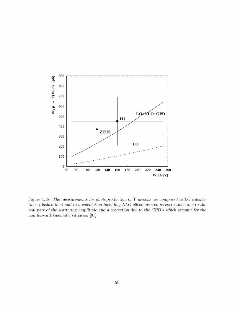
The first comparison of GPD based calculations with measurements has been done in an analysisby Martin, Ryskin and Teubner when they calculated the cross section for photoproduction of Υmesons [91]. In Figure 1.18 the cross section measurements from H1 and ZEUS are compared totwo different calculations, one based on the leading order expression and the other one includingan enhancement factor originating from GPD’s. The leading log QCD calculation leads to thesimple formula:

dσ

dt(γp→ V p)

∣∣∣∣t=0

=α2

sΓVee

3αM5V

16π3

[xg

(x,M2

V

4

)]2

(1.46)

where ΓVee is the partial width of the V → ee decay, αs is the QCD coupling constant, α = 1/137

is the QED coupling constant and g(x, µ2) is the gluon density measured at x = M 2V /4W

2

and the scale µ = mQ ' MV /2. The LO prediction is well below the measurements althoughthe statistical errors are still quite large. This calculation has been corrected for four differenteffects.

Relativistic corrections and NLO QCD corrections lead to a change of the predicted cross sectionby 7% and 20% respectively. Formula 1.46 accounts only for the imaginary part of the scatteringamplitude. When restoring the real part of the QCD amplitude the cross section has to beenhanced by about 50%. The largest correction originates from effects when using generalisedparton distributions. It has been found to account for an enhancement of about a factor of 2.When comparing the measured cross section with the corrected calculation a better descriptionof the data can be observed.

25

W [GeV]

σ(γ

p →

Υ(1

S) p

) [

pb]

LO+NLO+GPD

LO

H1

ZEUS

0

100

200

300

400

500

600

700

800

900

60 80 100 120 140 160 180 200 220 240 260

Figure 1.18: The measurements for photoproduction of Υ mesons are compared to LO calcula-tions (dashed line) and to a calculation including NLO effects as well as corrections due to thereal part of the scattering amplitude and a correction due to the GPD’s which account for thenon forward kinematic situation [91].

26

Chapter 2

Deeply Virtual Compton Scattering

2.1 Deeply Virtual Compton Scattering

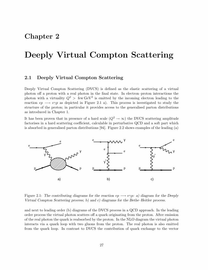
Deeply Virtual Compton Scattering (DVCS) is defined as the elastic scattering of a virtualphoton off a proton with a real photon in the final state. In electron–proton interactions thephoton with a virtuality Q2 > few GeV2 is emitted by the incoming electron leading to thereaction ep −→ eγp as depicted in Figure 2.1 a). This process is investigated to study thestructure of the proton; in particular it provides access to the generalised parton distributionsas introduced in Chapter 1.

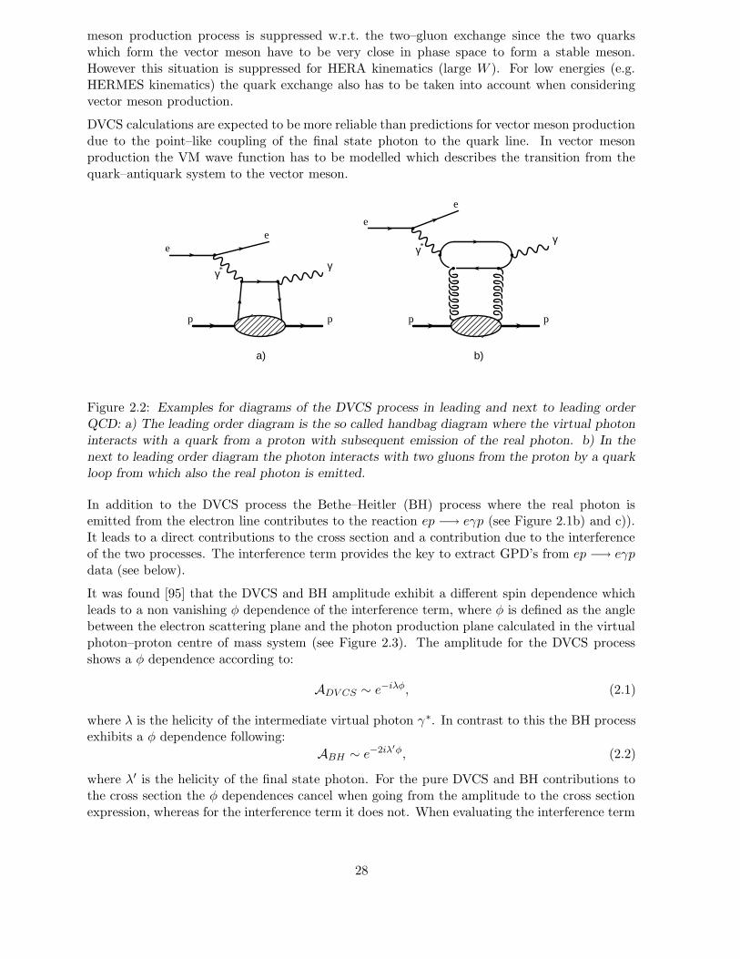
It has been proven that in presence of a hard scale (Q2 → ∞) the DVCS scattering amplitudefactorises in a hard scattering coefficient, calculable in perturbative QCD and a soft part whichis absorbed in generalised parton distributions [94]. Figure 2.2 shows examples of the leading (a)

e

e

γ

p p

γ *

e e

e

γ

p p

γ *

e e

γ *

p p

γ

a) b) c)

Figure 2.1: The contributing diagrams for the reaction ep −→ eγp: a) diagram for the DeeplyVirtual Compton Scattering process; b) and c) diagrams for the Bethe–Heitler process.

and next to leading order (b) diagrams of the DVCS process in a QCD approach. In the leadingorder process the virtual photon scatters off a quark originating from the proton. After emissionof the real photon the quark is reabsorbed by the proton. In the NLO diagram the virtual photoninteracts via a quark loop with two gluons from the proton. The real photon is also emittedfrom the quark loop. In contrast to DVCS the contribution of quark exchange to the vector

27

meson production process is suppressed w.r.t. the two–gluon exchange since the two quarkswhich form the vector meson have to be very close in phase space to form a stable meson.However this situation is suppressed for HERA kinematics (large W ). For low energies (e.g.HERMES kinematics) the quark exchange also has to be taken into account when consideringvector meson production.

DVCS calculations are expected to be more reliable than predictions for vector meson productiondue to the point–like coupling of the final state photon to the quark line. In vector mesonproduction the VM wave function has to be modelled which describes the transition from thequark–antiquark system to the vector meson.

e e

γ *

p p

γ

e

e

γ *

p p

γ

a) b)

Figure 2.2: Examples for diagrams of the DVCS process in leading and next to leading orderQCD: a) The leading order diagram is the so called handbag diagram where the virtual photoninteracts with a quark from a proton with subsequent emission of the real photon. b) In thenext to leading order diagram the photon interacts with two gluons from the proton by a quarkloop from which also the real photon is emitted.

In addition to the DVCS process the Bethe–Heitler (BH) process where the real photon isemitted from the electron line contributes to the reaction ep −→ eγp (see Figure 2.1b) and c)).It leads to a direct contributions to the cross section and a contribution due to the interferenceof the two processes. The interference term provides the key to extract GPD’s from ep −→ eγpdata (see below).

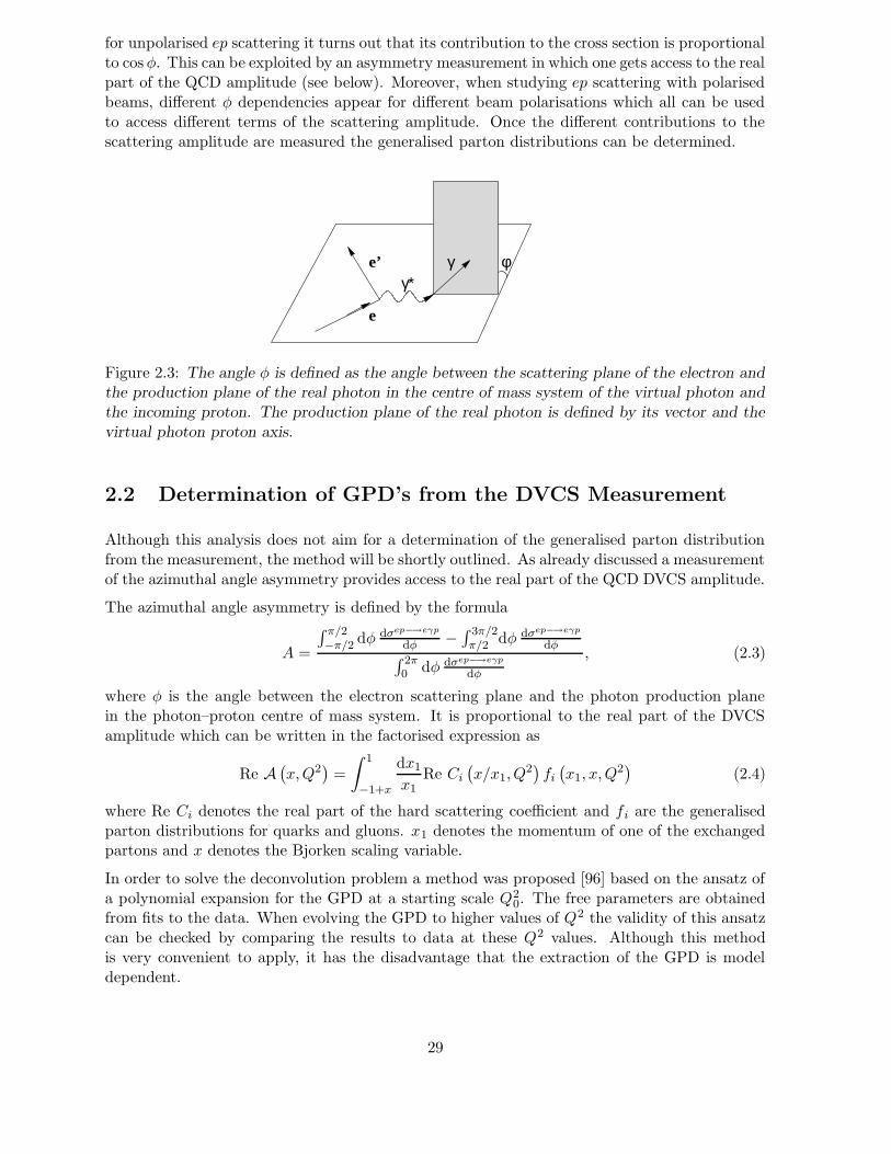
It was found [95] that the DVCS and BH amplitude exhibit a different spin dependence whichleads to a non vanishing φ dependence of the interference term, where φ is defined as the anglebetween the electron scattering plane and the photon production plane calculated in the virtualphoton–proton centre of mass system (see Figure 2.3). The amplitude for the DVCS processshows a φ dependence according to:

ADV CS ∼ e−iλφ, (2.1)

where λ is the helicity of the intermediate virtual photon γ∗. In contrast to this the BH processexhibits a φ dependence following:

ABH ∼ e−2iλ′φ, (2.2)

where λ′ is the helicity of the final state photon. For the pure DVCS and BH contributions tothe cross section the φ dependences cancel when going from the amplitude to the cross sectionexpression, whereas for the interference term it does not. When evaluating the interference term

28

for unpolarised ep scattering it turns out that its contribution to the cross section is proportionalto cosφ. This can be exploited by an asymmetry measurement in which one gets access to the realpart of the QCD amplitude (see below). Moreover, when studying ep scattering with polarisedbeams, different φ dependencies appear for different beam polarisations which all can be usedto access different terms of the scattering amplitude. Once the different contributions to thescattering amplitude are measured the generalised parton distributions can be determined.

φγγ∗

e’

e

Figure 2.3: The angle φ is defined as the angle between the scattering plane of the electron andthe production plane of the real photon in the centre of mass system of the virtual photon andthe incoming proton. The production plane of the real photon is defined by its vector and thevirtual photon proton axis.

2.2 Determination of GPD’s from the DVCS Measurement

Although this analysis does not aim for a determination of the generalised parton distributionfrom the measurement, the method will be shortly outlined. As already discussed a measurementof the azimuthal angle asymmetry provides access to the real part of the QCD DVCS amplitude.

The azimuthal angle asymmetry is defined by the formula

A =

∫ π/2−π/2 dφ dσep−→eγp

dφ −∫ 3π/2π/2 dφ dσep−→eγp

dφ∫ 2π0 dφ dσep−→eγp

dφ

, (2.3)

where φ is the angle between the electron scattering plane and the photon production planein the photon–proton centre of mass system. It is proportional to the real part of the DVCSamplitude which can be written in the factorised expression as

Re A(x,Q2

)=

∫ 1

−1+x

dx1

x1Re Ci

(x/x1, Q

2)fi

(x1, x,Q

2)

(2.4)

where Re Ci denotes the real part of the hard scattering coefficient and fi are the generalisedparton distributions for quarks and gluons. x1 denotes the momentum of one of the exchangedpartons and x denotes the Bjorken scaling variable.

In order to solve the deconvolution problem a method was proposed [96] based on the ansatz ofa polynomial expansion for the GPD at a starting scale Q2

0. The free parameters are obtainedfrom fits to the data. When evolving the GPD to higher values of Q2 the validity of this ansatzcan be checked by comparing the results to data at these Q2 values. Although this methodis very convenient to apply, it has the disadvantage that the extraction of the GPD is modeldependent.

29

2.3 Theoretical Predictions

The Model from Frankfurt, Freund and Strikman

Similar to ordinary DIS it is possible to calculate the Q2 evolution for the scattering amplitudeof Deeply Virtual Compton Scattering above a normalisation point Q2

0 ∼ few GeV2 [97]. Belowthis point the scattering amplitude is dominated by non–perturbative effects which prevents theusage of pQCD.

It was found ([98] and references therein) that the aligned jet model provides a reasonabledescription of the structure function F2. When using the Gribov dispersion relation the ratio Rof the imaginary parts for the DIS amplitude (in terms of the photon–proton amplitude) andthe DVCS amplitude can be calculated as:

R =ImA (γ∗ + p −→ γ∗ + p)t=0

ImA (γ∗ + p −→ γ + p)t=0

≈ 0.5 (2.5)

for Q20 ≈ 2 − 3GeV2. The DVCS process can now be calculated by a sum of soft and hard

contributions where the soft contribution has been taken from this aligned jet model estimateand the hard contribution can be calculated in the framework of QCD evolution equations. Thisleads to the following expression for the evolution of the DVCS scattering amplitude1:

ImA(x,Q2, Q2

0

)= ImA

(x,Q2

0

)

+ 4π2αem

∫ Q2

Q20

dQ′2

Q′2

∫ 1

x

dx1

x1

[Pqg (x/x1,∆/x1) g

(x1, x2, Q

′2)

(2.6)

+ Pqq (x/x1,∆/x1) q(x1, x2, Q

′2)]

where Pqg and Pqq are the evolution kernels for generalised parton distributions. Using thisrelation the value for R has been estimated for the kinematic range accessible in this analysisas R ≈ 0.55, almost independent on Q2 and x [97]. The real part of the DVCS amplitude hasbeen calculated using a dispersion relation:

η =ReAImA =

π

2

d ln (xImA)

d ln 1x

. (2.7)

These relationes can now be used to calculate the complete cross section for the DVCS process.The imaginary part of the DIS amplitude ImA (γ∗ + p −→ γ∗ + p)t=0 has been connected viathe optical theorem to the DIS cross section which can be expressed in terms of the protonstructure function F2, such that F2 enters the cross section expression (see below). The valueof R accounts for the effect of the generalised parton densities.

The BH process is calculable within the framework of QED using the electro–magnetic formfactors GE and GM . The complete differential cross section for the reaction ep −→ eγp is de-composed into the sum of three terms; the DVCS contribution, the BH term and the interferenceterm.

dσep→eγp

dxdydtdφ=

dσDVCS

dxdydtdφ+

dσBH

dxdydtdφ+

dσInt

dxdydtdφ, (2.8)

1Note the different convention w.r.t. chapter 1.3.

30

dσDVCS

dxdydtdφ=

πα3s(1 + (1 − y)2

)

4R2Q6e−b|t|F 2

2

(x,Q2

) (1 + η2

), (2.9)

dσBH

dxdydtdφ=

α3sy2(1 + (1 − y)2

)

π|t|Q4 (1 − y)

G2E(t) + |t|

4m2pG2

M (t)

1 + |t|4m2

p

, (2.10)

dσInt

dxdydtdφ= ±

ηα3sy(1 + (1 − y)2

)

2RQ5√|t|(1 − y)

e−b|t|/2F2

(x,Q2

) GE(t) + |t|4m2

pGM (t)

1 + |t|4m2

p

cos φ. (2.11)

Note that the prediction for the DVCS process is valid at t = tmin where t is the momentumtransfer at the proton vertex. The model assumes the t-dependence to follow an exponentialfunction: dσ

dt ∼ e−b|t| which is an ansatz that has been successfully applied to diffractive processesin the region of low |t| (e.g. ρ vector meson production [60]). The interference term shows thecosφ dependence which has been discussed already at the beginning of this chapter. The signof the interference term depends on the polarity of the lepton beam.

Colour Dipole Models

General Properties of Colour Dipole Models

The Colour dipole model of diffraction [99] provides a simple unified picture of diffractive pro-

cesses. It is able to reproduce the inclusive diffractive structure function FD(3)2 as well as exclu-

sive reactions like vector meson production. Recently this model has been used to predict crosssections for the DVCS process. It is based on the assumption of a factorisation of the reactionin three subprocesses which are well separated in time. In the proton rest frame the incomingvirtual photon fluctuates into a quark antiquark pair well before the interaction with the proton.The formation time for the dipole is τ ∼ 1/Mpx which for HERA kinematics (x ≤ 0.01) is muchlonger than the typical time scale for strong interactions τ ∼ 1/mπ. The subsequent formationof the hadronic final state (i.e. the photon in case of DVCS) from the scattered dipole is againmuch longer than the interaction time with the target. This justifies the basic assumption ofthe dipole model that the cross section for the interaction of the dipole is independent of howit is formed. The following factorisation formula for the scattering amplitude A, also visualisedin Figure 2.4, can be derived

A (γ∗p −→ γp) =

∫ψin

γ∗σdψoutγ , (2.12)

where the incoming and outgoing photon are denoted by the wave functions ψ inγ∗ and ψout

γ , re-spectively. It is integrated over all dipole sizes R and all momentum fractions z of the quarkfrom the quark–antiquark dipole (see below). The cross section σd describes the interaction ofthe dipole with the proton. The colour dipole is assumed to be unchanged during the inter-action. The different types of dipole models differ very strongly in their assumptions and themethod used to derive the dipole cross section. In general the models make assumptions on thedecomposition of dipole cross section; free parameters are derived from fits to the data. Thereexists no model which is able to derive the dipole cross section from first principles. Althoughthe photon wave function is in principle calculable within perturbation theory (at least in leadingorder) some theories modify it to account for confinement effects for large dipoles.

31

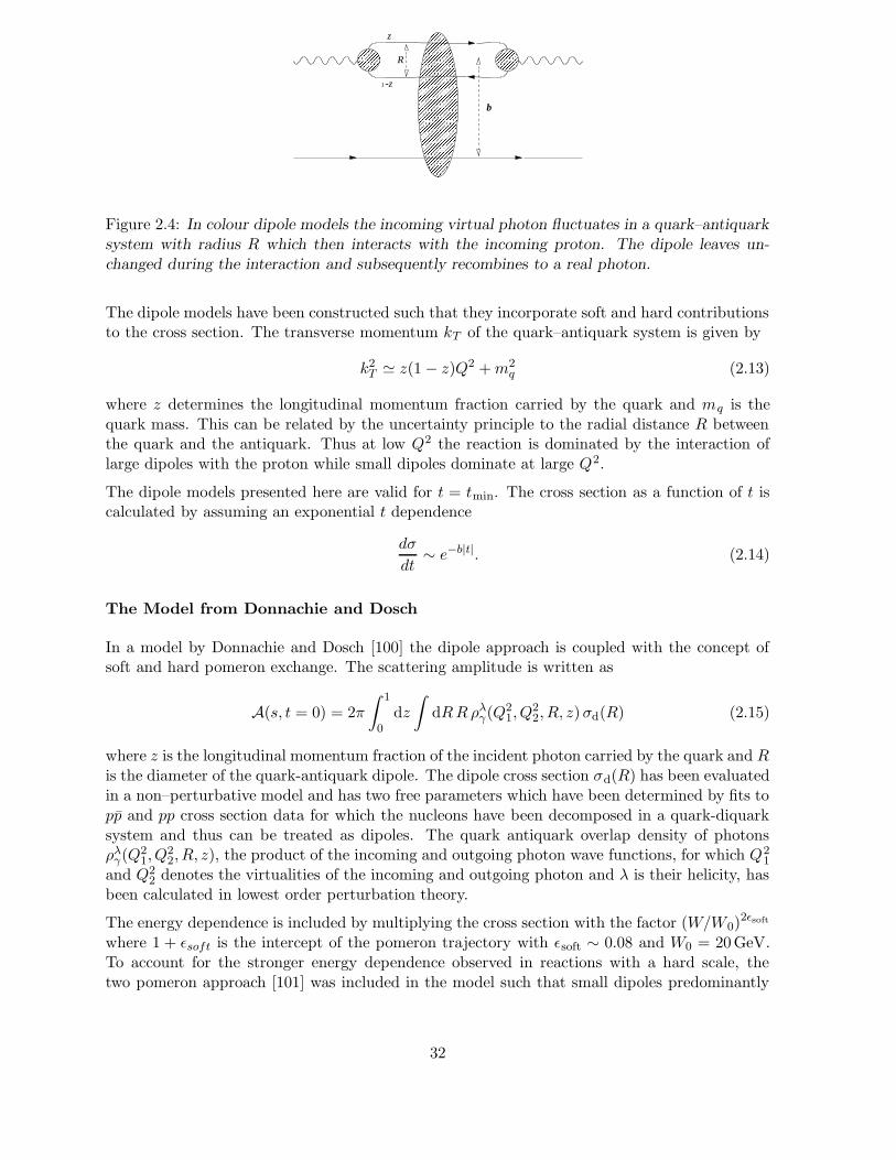
1

��

��

��

��

��

��

-z

z

b

R

Figure 2.4: In colour dipole models the incoming virtual photon fluctuates in a quark–antiquarksystem with radius R which then interacts with the incoming proton. The dipole leaves un-changed during the interaction and subsequently recombines to a real photon.

The dipole models have been constructed such that they incorporate soft and hard contributionsto the cross section. The transverse momentum kT of the quark–antiquark system is given by

k2T ' z(1 − z)Q2 +m2

q (2.13)

where z determines the longitudinal momentum fraction carried by the quark and mq is thequark mass. This can be related by the uncertainty principle to the radial distance R betweenthe quark and the antiquark. Thus at low Q2 the reaction is dominated by the interaction oflarge dipoles with the proton while small dipoles dominate at large Q2.

The dipole models presented here are valid for t = tmin. The cross section as a function of t iscalculated by assuming an exponential t dependence

dσ

dt∼ e−b|t|. (2.14)

The Model from Donnachie and Dosch

In a model by Donnachie and Dosch [100] the dipole approach is coupled with the concept ofsoft and hard pomeron exchange. The scattering amplitude is written as

A(s, t = 0) = 2π

∫ 1

0dz

∫dRRρλ

γ(Q21, Q

22, R, z)σd(R) (2.15)

where z is the longitudinal momentum fraction of the incident photon carried by the quark and Ris the diameter of the quark-antiquark dipole. The dipole cross section σd(R) has been evaluatedin a non–perturbative model and has two free parameters which have been determined by fits topp and pp cross section data for which the nucleons have been decomposed in a quark-diquarksystem and thus can be treated as dipoles. The quark antiquark overlap density of photonsρλ

γ(Q21, Q

22, R, z), the product of the incoming and outgoing photon wave functions, for which Q2

1

and Q22 denotes the virtualities of the incoming and outgoing photon and λ is their helicity, has

been calculated in lowest order perturbation theory.

The energy dependence is included by multiplying the cross section with the factor (W/W0)2εsoft

where 1 + εsoft is the intercept of the pomeron trajectory with εsoft ∼ 0.08 and W0 = 20GeV.To account for the stronger energy dependence observed in reactions with a hard scale, thetwo pomeron approach [101] was included in the model such that small dipoles predominantly

32

interact by the exchange of the hard pomeron component whereas large dipoles interact viathe soft pomeron component. Finally Donnachie and Dosch obtain the expression for the crosssection at t = tmin.

dσ

dt(Q2,W, t = tmin) =

1

16π

(rsoft(Q

2)(W/W0)0.16 + rhard(Q2)(W/W0)

0.84)2

× 311 µb/GeV2 (2.16)

where W0 = 20 GeV and

rsoft(Q2) =

(5.33 − 1.33 · e(−4Q2/Q2

0) + 5.37Q2/Q20

)−1,

rhard(Q2) =

(49.42 − 7.65 · e(−4Q2/Q2

0) + 4.94Q2/Q20

)−1(2.17)

with Q20 = 1 GeV2.

The Model of Forshaw, Kerley and Shaw

A model by Forshaw, Kerley and Shaw (FKS) [102, 103] assumes that the dipole cross sectiondepends solely on the properties of the dipole proton system itself, independent of the photonvirtuality Q2, which means that it depends only on the photon–proton centre of mass energy Wand on the size of the dipole R. The idea is to extract information on the dipole cross sectionby assuming a reasonable flexible form to fit the diffractive structure function and the totalphoton–proton cross section. The cross section is decomposed into two terms to account for softand hard contributions

σd

(W 2, R

)= σd soft

(W 2, R

)+ σd hard

(W 2, R

). (2.18)

The functions σd soft

(W 2, R

)and σd hard

(W 2, R

)have been chosen such that for small dipoles

the hard contribution dominates while at low Q2 σd soft

(W 2, R

)contributes most.

The wave functions of the incoming and outgoing photon have been calculated in leading orderperturbation theory and multiplied by an enhancement factor to increase contributions fromlarge dipoles. This procedure is justified by the fact that for small Q2 < 4m2

q the wavefunctionbecomes sensitive to the quark mass and that confinement effects are expected to become sizable.The quark mass has been chosen such that m2

q = 0.08GeV2 which corresponds to the constituentquark mass.

The Model of McDermott, Frankfurt, Guzey and Strikman

In another model of McDermott, Frankfurt, Guzey and Strikman (MFGS) [102, 104] the dipolecross section σd

(Q2,W,R

)depends on both, the virtuality of the photon Q2 and the photon

proton centre of mass energy W . It is divided into three parts depending on the dipole size R.For small dipoles R < RC the cross section is directly related to the LO gluon distribution ofthe proton

σd (x,R < RC) =π2R2

3αs

(Q2

)xg

(x′, Q2

), (2.19)

33

where x′ and Q2 are functions of x and Q2 depending on the dipole size R. The underlyingmodel for this cross section is the two–gluon–exchange model discussed earlier2. The upperbound RC depends on Q2 and is RC = 0.246 fm for Q2 = 2.6GeV2. For large dipoles above thepion radius R > Rπ = 0.65 fm the cross section has been modelled by the function

σd (R > Rπ) = σ (πp)3R2

2R2 +Rπ

(x0

x

)0.08(2.20)

independent on Q2 where x0 = 0.01 has been chosen such that at R = Rπ σd matches the totalpion proton cross section σ (πp) = 24 mb. In the intermediate region RC < R < Rπ the dipolecross section is interpolated linearly.

This model focuses on the region of small dipoles and is hence only expected to be valid forQ2 > 1 GeV2 where the contribution from large dipoles is expected to be negligible. For theactual predictions of the cross section a generalised gluon distribution has been used.

Predictions Based on Generalised Parton Distributions

All models discussed above depend on different assumptions how hard and soft effects contributeto the DVCS cross section. Freund and McDermott presented [105, 106, 107] the first completeQCD calculation based on generalised parton densities. The used GPD is based on the modelof Radyushkin (see chapter 1.3) which uses Double Distributions to derive them. The profilefunction πi (x′, y′) has been chosen as:

πi(x′, y′

)=

3

4

(1 − |x′|)2 − y′2

(1 − |x′|)3(2.21)

which leads in combination with the ordinary parton distributions (GRV [42] and MRST’ [108]have been used) to predictions for the DVCS amplitude. It was calculated in leading orderand next to leading order QCD by calculating the coefficient function and solving the evolutionequations.

Depending on the actually used parton distribution large differences (factor 2–3) on the ampli-tude level can be observed which illustrates the high sensitivity of the cross section on effectsdue to the skewedness effects. These prediction do not yet exist on cross section level whichwould be a crucial test for GPD based models.

2.4 MC Programs

The final state of the reaction ep −→ eγp consists of an electron, a photon and a proton, wherethe electron and photon are detected with the H1 detector3. In order to extract the cross sectionfrom the measured event rate, MC simulations are performed using event generators as input.They generate the four vectors for the final state particles of the interactions which are thensubjected to a detailed detector simulation. Six different MC programs have been used to studythe signal as well as different background contributions.

2Note that the dipole cross section σd enters the amplitude (Equation 2.12). When calculating the cross sectionit depends quadratically on the dipole cross section and the gluon density as naively expected for the two gluonexchange model.

3For a detailed discussion of the analysis strategy see chapter 4.1.

34

TINTIN

The event generator TINTIN, developed in the framework of this thesis (for a detailed descriptionsee appendix A), is a program which generates the four vectors of the final state particles forthe reaction ep −→ eγp where the kinematic variables are generated according to the predictedcross section by the calculations of Frankfurt, Freund and Strikman (see chapter 2.3). Theprogram is able to generate events for the BH process, the DVCS process and the sum of theBH and DVCS process taking the interference term into account4. The most dominant QEDradiative correction, the emission of a real photon from the incoming electron is implemented inthe program.

COMPTON 2.0

The MC program COMPTON 2.0 [110, 111, 112] is used to generate events for the Bethe–Heitler process. It generates the elastic contribution as well as inelastic events. The programuses an exact calculation based on helicity amplitudes where the coupling to the proton is givenby the electromagnetic form factors (GE and GM ) for the elastic contributions. The inelasticcontribution is divided into two regimes the resonance region (MX < 1.8GeV) and the inelasticcontinuum (MX > 1.8GeV) where MX is the invariant mass of the hadronic final state. Forthe resonance region the three proton resonances ∆(1232), N ∗(1520) and N ∗(1688) have beentaken into account and the corresponding cross sections are derived from measurements. In theregion of the inelastic continuum the cross section has been taken from early F2 measurements.As will be discussed in chapter 4 the cross section simulation of the inelastic Bethe–Heitlerevents has been modified according to a revised set of experimental data. The emission of a realphoton from the initial electron which is expected to be the dominant higher order QED effectis implemented.

DIFFVM

The MC program DIFFVM [113] was designed to simulate the process of diffractive vector mesonproduction ep −→ e VM X where VM denotes the produced vector meson and X the hadronicfinal state, separated by a rapidity gap from the vector meson. The predictions of the programare based on the vector meson dominance model (VDM) and Regge theory as discussed in section1.2. The virtual photon emitted by the incoming electron fluctuates into a vector meson whichsubsequently scatters off the proton. For the hadronic system X the resonant region as well asthe inelastic continuum are taken into account. The program generates the four vectors of thefinal state particles including the decay products of the produced vector meson.

The DIFFVM program generates different vector meson channels, i.e. all vector mesons whichhave the same quantum numbers as the virtual photon (ω, ρ, φ ...). It can be used to generateelastic vector meson production as well as resonance production and the inelastic continuum.

4The free parameters have been set in the event generation to the following values: the t–slope parameterb = 7 GeV−2, the phase of the QCD amplitude, ηQCD = 1 − π

2

(0.176 + 0.33 ln Q2

)[109] and the sensitivity to

the skewedness of the parton densities R = 0.55 [97]. The proton structure function F2 as extracted from the H1data has been used [5].

35

GRAPE

The event generator GRAPE [114] is used to simulate the reaction e+p −→ e+e−e+p. Thepredicted cross section is based on a calculation of the full matrix element taking all contributingdiagrams into account. In the kinematic range relevant for this analysis the cross section isdominated by the two photon process where the photon emitted by the incoming positroninteracts with a photon emitted from the proton by the production of an electron positron pair.Using the GRAPE MC program it is again possible to generate the full final state for the elasticand the inelastic reaction.

DJANGO and HERWIG

The MC program DJANGO ([115] and references therein) is a standard DIS event generatorwhich is used for the generation of inclusive deep inelastic scattering events. It is a combinationof the programs LEPTO, HERACLES, ARIADNE and JETSET where the program LEPTOcalculates the DIS Matrix element. It is interfaced to HERACLES for calculation of the QEDradiative corrections. The program ARIADNE simulates the subsequent emission of partonswith a large transverse momentum. The results of this program are then interfaced to JETSETwhich performs the simulation of the fragmention based on the Lund String model. The programproduces the four vectors of all final state particles.

The HERWIG program [116] is also a standard DIS event generator similar to the DJANGOprogram. The basic difference between the two programs relevant for this analysis is the use ofa different fragmentation scheme. In contrast to the Lund fragmentation scheme which is usedin DJANGO the HERWIG program is based on the cluster fragmentation.

36

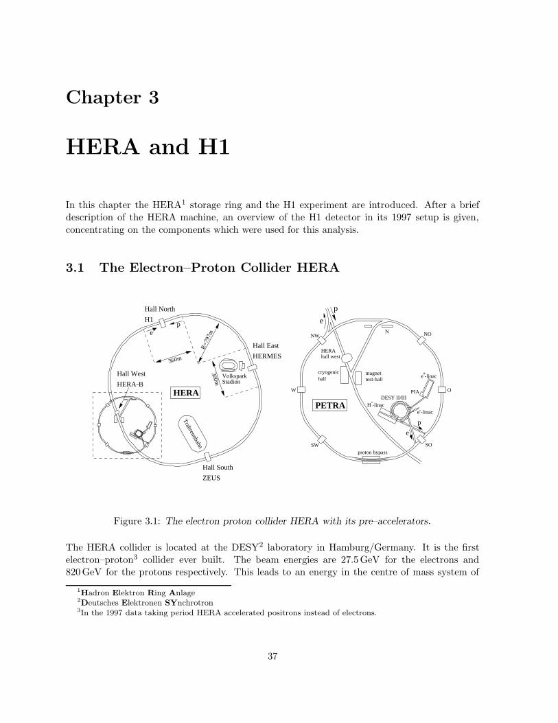
Chapter 3

HERA and H1

In this chapter the HERA1 storage ring and the H1 experiment are introduced. After a briefdescription of the HERA machine, an overview of the H1 detector in its 1997 setup is given,concentrating on the components which were used for this analysis.

3.1 The Electron–Proton Collider HERA

Hall North

H1

Hall East

HERMES

Hall South

ZEUS

HERA

HERAhall west

PETRA

cryogenichall

Hall West

HERA-B

magnettest-hall

DESY II/IIIPIA

e -linac+

e -linac-

-H -linac

NWN NO

O

SOSW

W

proton bypass

p

e

ep

VolksparkStadion

360m

360m

R=7

97m

e

p

Trabrennbahn

Figure 3.1: The electron proton collider HERA with its pre–accelerators.

The HERA collider is located at the DESY2 laboratory in Hamburg/Germany. It is the firstelectron–proton3 collider ever built. The beam energies are 27.5GeV for the electrons and820GeV for the protons respectively. This leads to an energy in the centre of mass system of

1Hadron Elektron Ring Anlage

2Deutsches Elektronen SYnchrotron

3In the 1997 data taking period HERA accelerated positrons instead of electrons.

37

√s ' 300GeV, which is more than 10 times higher than in formerly performed fixed target

experiments. The two beam lines are located in the same tunnel with a circumference of 6.3 km.The electron ring is equipped with dipole magnets with a field strength of 0.17T. The protonring consists of superconducting dipole magnets with a field strength of 4.7T. The protonenergy is limited by the field strength of the bending magnets while the maximum electronenergy is determined by the power of the cavities which accelerate the electrons and compensatefor the energy loss due to synchrotron radiation. The energy loss of protons due to synchrotronradiation can be neglected due to their high mass.

Figure 3.1 shows an overview of HERA and its pre–accelerators. The electrons are provided bya 500MeV linear accelerator which are then ramped up in DESY II (to 7GeV) and PETRA (to12GeV). After injection into HERA they are brought to their final beam energy. The protonsare produced by passing H− ions with an energy of 50MeV through a stripping foil where theions loose their two electrons. The protons are collected in bunches and accelerated in DESY III(to 7.5GeV) and in PETRA (to 40GeV) and afterwards injected into HERA and acceleratedto their final beam energy. Both the electrons and the protons are stored in bunches of 1010

to 1011 particles which circulate in opposite direction in the HERA storage ring. The timebetween two bunch crossings is 96 ns which leads to a total number of 220 bunches for both theelectron and the proton ring. They are filled such that typically 175 of these bunches collideand the additional bunches are filled either for the electrons, the protons or none of them. Thelifetime of the proton beam is about 100 hours, whereas the lifetime of the electron beam isabout 10 hours which leads to a typical duration of 12 hours for a luminosity fill. By the year2000 an electron current of 40mA and a proton current of 90mA was routiniously achievedleading to peak luminosity of 1.5 ∗ 1031 cm−2s−1 which corresponds to the design value.

The electron and the proton beam are brought to collisions at two interaction points. Aroundthese the experiments H1 and ZEUS are constructed and take data since 1992. There are twoadditional fixed target experiments built at the HERA collider. The HERMES detector is aspectrometer which takes data since 1995 and studies interactions of polarised electrons fromthe electron beam with a polarised gas target (H2, D, He). The aim of this experiment isto study the spin structure of the proton and related processes. The HERA–B experimentwas commissioned in 2000 and is a forward spectrometer which uses an internal wire target toproduce interactions between protons from the Halo of the proton beam and nucleons of thetarget wire. The aim of this experiment is to study CP–violation in the system of neutral B–mesons. This experiment serves also as a charm factory, which opens the possibility to studyQCD with heavy quarks at high energies.

Figure 3.2 shows the time structure of a typical proton bunch in the HERA storage ring [117]. Athreefold structure is observed where the main bunch is accompanied by two so called satellitebunches 5 ns before and after the main peak which are typically a factor 10 to 100 smaller.The interval of 5 ns between the main and the satellite bunch originates from the properties ofthe high frequency system of the HERA accelerating units. The frequency of the acceleratingsystem is 200MHz leading to a stable point in the seperatrix each 5 ns. The distribution of theproton bunches is very broad in the PETRA accelerating system. When transmitting them tothe HERA ring about 7% of the protons do not enter the main bunch but one of the satellitebunches. In the present analysis one cannot distinguish whether the final state particles originatefrom an interaction of an electron with a proton from the main or the satellite bunch. Thereforethe effect of satellite bunch interactions has to be taken into account when analysing the data.

Since September 2000 the data taking has been stopped and the HERA accelerator and the

38

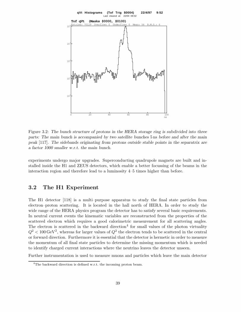
qVt Histograms (Tof Trig $0004) 22/4/97 9:52

010

110

210

310

410

0 20 40 60 80 100ns

Entries: 70129 Overflow: 0 Underflow: 0 Mean: 56 R.M.S.: 6Tof qVt (Masks $0000, $0100)

Last cleared at: 22/04 09:02

Figure 3.2: The bunch structure of protons in the HERA storage ring is subdivided into threeparts: The main bunch is accompanied by two satellite bunches 5 ns before and after the mainpeak [117]. The sidebands originating from protons outside stable points in the separatrix area factor 1000 smaller w.r.t. the main bunch.

experiments undergo major upgrades. Superconducting quadrupole magnets are built and in-stalled inside the H1 and ZEUS detectors, which enable a better focussing of the beams in theinteraction region and therefore lead to a luminosity 4–5 times higher than before.

3.2 The H1 Experiment

The H1 detector [118] is a multi–purpose apparatus to study the final state particles fromelectron–proton scattering. It is located in the hall north of HERA. In order to study thewide range of the HERA physics program the detector has to satisfy several basic requirements.In neutral current events the kinematic variables are reconstructed from the properties of thescattered electron which requires a good calorimetric measurement for all scattering angles.The electron is scattered in the backward direction4 for small values of the photon virtualityQ2 < 100GeV2, whereas for larger values of Q2 the electron tends to be scattered in the centralor forward direction. Furthermore it is essential that the detector is hermetic in order to measurethe momentum of all final state particles to determine the missing momentum which is neededto identify charged current interactions where the neutrino leaves the detector unseen.

Further instrumentation is used to measure muons and particles which leave the main detector

4The backward direction is defined w.r.t. the incoming proton beam.

39

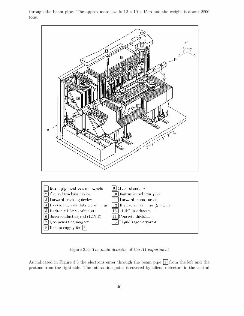
through the beam pipe. The approximate size is 12 × 10 × 15m and the weight is about 2800tons.

x

y

z

θ φ

�

��

� �� ! "$#�%��'&)(��*��,+-�. /0�,�1�)+ �23�)+ ��&)4��5��6�1�,7��8&-� �9 :;��<�)+)#�6�,�1�)�=�>��+)%��'?�%�4��@ A�%�+)BC��+-�*�)+ ��&)4��5��1�,7D�E&-� �� A�%�+)BF��+-�6*#�%��G%�+)%��E�H IJ25�=&-�)+)%K��,�L�8&NMPOQ+N&,�25%�+<�56�,�)�,+ �. �R�K&)41BTSU&,�2�%�+L��6�,�)�,+FV)W��1/R�2YXZ [Q��1+)%K��E&RMPOQ+\&��=25%�+L��6�,�)�,+ �@ ]�M3^N_`&,�25%�+<�56�,�)�,+a W�#��,+-&-%��1#�&-�L�5��6&-%��b23V ��S5�ZQcQX ��H /0%��&-+)�,�)�F�<(��-28��5��d /0%K6��,��)��L��e��f�,� �=Z M��8g�#1�E�h��+)��%��&i+G?�%1�L�-��j [F�-2b�5#�k�L#��125?*lm%�+ d

Figure 3.3: The main detector of the H1 experiment

As indicated in Figure 3.3 the electrons enter through the beam pipe 1 from the left and theprotons from the right side. The interaction point is covered by silicon detectors in the central

40

and the backward region which are followed by the central 2 and forward 3 tracking detectors.

These are surrounded by a large calorimeter system consisting of a Spaghetti calorimeter 12

in the backward and a Liquid Argon calorimeter 4 and 5 in the central and forward region.Both calorimeters are divided into an electromagnetic and hadronic section. An additionalplug calorimeter 13 is installed in the forward direction close to the beam pipe. The LAr

calorimeter is surrounded by a superconducting coil 6 which provides a homogeneous magnetic

field of 1.15T along the tracking region. The iron return yoke 10 of the magnet is instrumentedwith streamer tubes and is used to detect muons and to measure energy leakage from hadrons notfully contained in the LAr calorimeter. The forward muon detector 11 is used to identify andmeasure the momentum of penetrating muons in the forward direction through the use of driftchambers and a toroidal magnet. In positive z–direction about 23m from the interaction pointin direction of the incoming protons a set of scintillating detectors is used to identify fragmentsfrom electron–proton collisions which leave the main detector through the beam pipe. At about100m a hadron calorimeter is placed to measure neutrons which can emerge from electron–protoncollisions scattered under low angles. In negative z direction two electromagnetic calorimetersare situated to measure the final state particles from the Bremsstrahlung process which is usedto determine the luminosity.

A right handed co–ordinate system is used with the origin at the centre of the central jet chamber.The positive z–direction is defined as being along the proton beam direction, x towards the centreof the HERA ring and y vertically upwards. The z axis corresponds to θ = 0 and the positivex–axis to φ = 0 when using polar co–ordinates. The detector components used in this analysisare now described in detail.

The Central Tracking System

The central tracking devices are part of the large tracking system (see Figure 3.4) of the H1detector. It covers the angular range 15o < θ < 165o with full azimuthal acceptance. Its maincomponents are two large concentric drift chambers (CJC1 and CJC2) with a length of 2.2m.CJC1 (CJC2) consists of 30 (60) cells with 24 (32) sense wires (Figure 3.4) parallel to the zaxis. Its inner radius is 20.3 (53.0) cm and its outer radius 45.1 (84.4) cm respectively. The driftcells are inclined by about 30◦ with respect to the radial direction. The space point resolutionin (r, φ) is 170µm and 2.2 cm in z using a charge division method.

The resolution in z is much improved by the usage of z–chambers (CIZ and COZ) with wiresperpendicular to the beam axis. They are located inside and outside of CJC1 at a radius of18 cm and 47 cm, respectively. CIZ and COZ are divided into 15 and 24 drift cells with 4 sensewires per cell. The achieved resolution in z is 260µm.

Charged particles are bent by the homogeneous magnetic field of 1.15T provided by the super-conducting coil around the LAr calorimeter. The combination of CJC1 and CJC2 with the z–chambers leads to momentum resolution for the track measurement of σ (pT ) /pT < 0.01·pT /GeV

In addition to the drift chambers two multi–wire proportional chambers (CIP and COP) deliverfast signals used for trigger purposes.

41

Figure 3.4: The H1 tracking system: left) longitudinal view; right) transverse view.

The LAr Calorimeter

The LAr calorimeter [119] (see Figure 3.5) provides energy measurement in the range 4o <θ < 154o with full azimuthal coverage. In z–direction it is segmented into 8 wheels which eachconsist of 8 octants in φ. The six central wheels are divided into an electromagnetic and ahadronic section each, whereas the most forward wheel consists of two hadronic sections. Themost backward wheel (BBE) consists only of an electromagnetic section and is also divided into 8sections in φ. The LAr calorimeter is a sampling calorimeter which is located in a cryostat. Theelectromagnetic section consists of 2.4mm thick lead absorber plates which are supplementedwith high voltage and readout plates. The 2.35mm gaps are filled with liquid Argon whichserves as active material. Depending on the polar angle θ the depth of the electromagnetic sec-tion corresponds to 20 – 30 radiation length. The hadronic section consists of 19mm stainlesssteel absorber plates with a double gap of 2.4mm filled with liquid Argon. This correspondsin total to 5 to 8 hadronic interaction lengths. The energy resolution for electromagnetic in-teracting particles, i.e. electrons and photons was determined from test beam measurementsto be σ(E)/E ' 11%/

√E/GeV ⊕ 1%. The absolute energy scale for the measurement of high

energetic electrons is known to a precision of 2%.

The energy resolution for hadrons is σ(E)/E ' 50%/√E/GeV ⊕ 2%. The LAr calorimeter is

non compensating, i.e. the response to hadrons is about 30% smaller w.r.t. electrons with thesame energy. This is corrected offline using a weighting technique. The main advantages of theliquid Argon technique are good stability, homogeneouty of the response, ease of calibration andfine granularity which opens the possibility to measure the scattering angles of photons withhigh precision. The total number of read–out channels is about 45000.

The Spacal and the BDC

The Spaghetti calorimeter, Spacal, [120] (see Figure 3.6) provides energy measurement in thebackward region in the range 154◦ < θ < 178◦ with full azimuthal coverage. It is a samplingcalorimeter with lead as absorber material and scintillating fibres as active material. The Spacalis divided into an electromagnetic and a hadronic section with a lead to fibre ratio of 2.3 : 1 and3.4 : 1, respectively. The electromagnetic section consists of cells of the size 40.5×40.5×225mm.

42

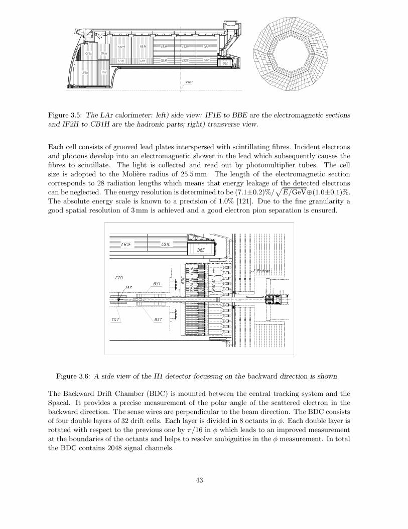
Figure 3.5: The LAr calorimeter: left) side view: IF1E to BBE are the electromagnetic sectionsand IF2H to CB1H are the hadronic parts; right) transverse view.

Each cell consists of grooved lead plates interspersed with scintillating fibres. Incident electronsand photons develop into an electromagnetic shower in the lead which subsequently causes thefibres to scintillate. The light is collected and read out by photomultiplier tubes. The cellsize is adopted to the Moliere radius of 25.5mm. The length of the electromagnetic sectioncorresponds to 28 radiation lengths which means that energy leakage of the detected electronscan be neglected. The energy resolution is determined to be (7.1±0.2)%/

√E/GeV⊕(1.0±0.1)%.

The absolute energy scale is known to a precision of 1.0% [121]. Due to the fine granularity agood spatial resolution of 3mm is achieved and a good electron pion separation is ensured.

Figure 3.6: A side view of the H1 detector focussing on the backward direction is shown.

The Backward Drift Chamber (BDC) is mounted between the central tracking system and theSpacal. It provides a precise measurement of the polar angle of the scattered electron in thebackward direction. The sense wires are perpendicular to the beam direction. The BDC consistsof four double layers of 32 drift cells. Each layer is divided in 8 octants in φ. Each double layer isrotated with respect to the previous one by π/16 in φ which leads to an improved measurementat the boundaries of the octants and helps to resolve ambiguities in the φ measurement. In totalthe BDC contains 2048 signal channels.

43

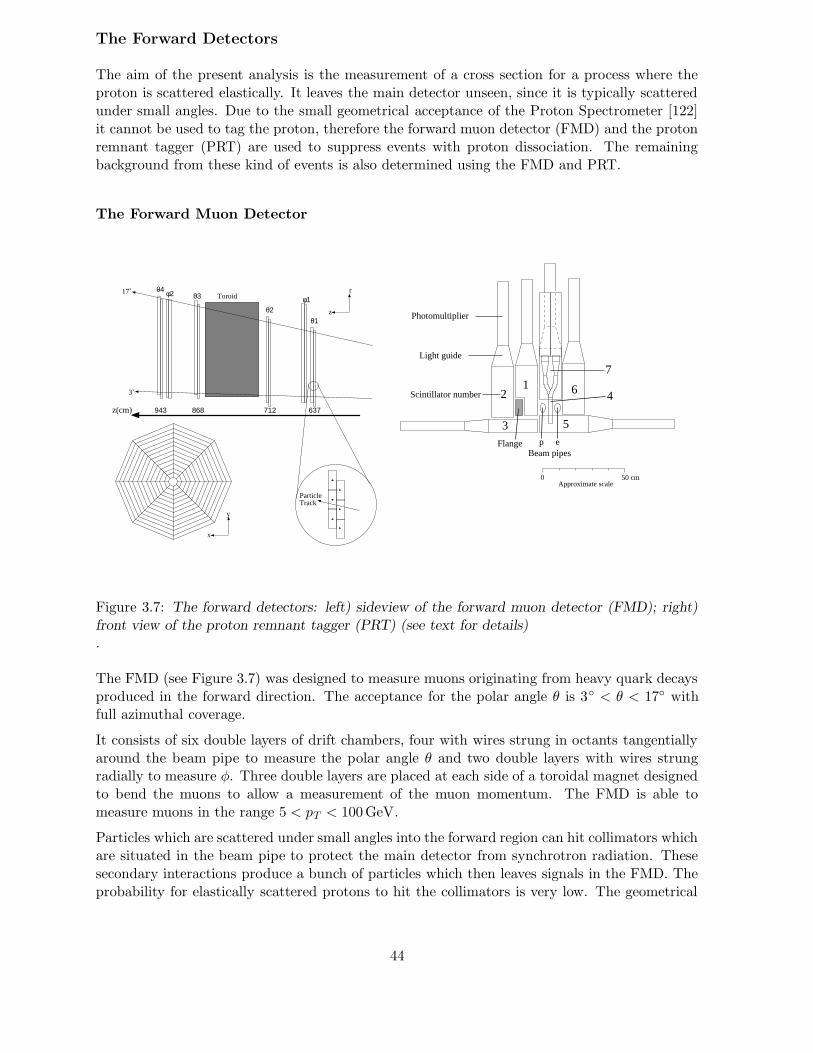
The Forward Detectors

The aim of the present analysis is the measurement of a cross section for a process where theproton is scattered elastically. It leaves the main detector unseen, since it is typically scatteredunder small angles. Due to the small geometrical acceptance of the Proton Spectrometer [122]it cannot be used to tag the proton, therefore the forward muon detector (FMD) and the protonremnant tagger (PRT) are used to suppress events with proton dissociation. The remainingbackground from these kind of events is also determined using the FMD and PRT.

The Forward Muon Detector

z(cm)

17˚

3˚

Toroidθ4 φ2 θ3

θ2φ1

θ1z

r

ParticleTrack

y

x

637712868943

0 50 cm

Light guide

Photomultiplier

p eFlangeBeam pipes

Approximate scale

2

3

4

5

6

7

Scintillator number1

Figure 3.7: The forward detectors: left) sideview of the forward muon detector (FMD); right)front view of the proton remnant tagger (PRT) (see text for details).

The FMD (see Figure 3.7) was designed to measure muons originating from heavy quark decaysproduced in the forward direction. The acceptance for the polar angle θ is 3◦ < θ < 17◦ withfull azimuthal coverage.

It consists of six double layers of drift chambers, four with wires strung in octants tangentiallyaround the beam pipe to measure the polar angle θ and two double layers with wires strungradially to measure φ. Three double layers are placed at each side of a toroidal magnet designedto bend the muons to allow a measurement of the muon momentum. The FMD is able tomeasure muons in the range 5 < pT < 100GeV.

Particles which are scattered under small angles into the forward region can hit collimators whichare situated in the beam pipe to protect the main detector from synchrotron radiation. Thesesecondary interactions produce a bunch of particles which then leaves signals in the FMD. Theprobability for elastically scattered protons to hit the collimators is very low. The geometrical

44

acceptance of the FMD corresponds to the region 1 < η < 2.5. Due to the position of thecollimators this acceptance is extended to the region 3.2 < η < 5.5 [123]. Therefore signals inthe FMD are a good signature for events where the proton does not scatter elastically.

The Proton Remnant Tagger

The PRT (see Figure 3.7) is located at +24m in the forward direction inside the HERA tunnel. Itconsists of seven scintillators arranged around and between the electron and proton beam pipe.Each component consists of two scintillator sheets. The induced signals are passed througha light guide to photomultipliers. The PRT is sensitive to particles produced in the range5 < η < 7. It is as well as the FMD sensitive to particles which originate from secondaryinteraction of the hadrons emerging from proton dissociation events which extends the sensitivityfor particles detection up to η = 7.5 [123].

The Luminosity System and the Time of Flight System

Figure 3.8: The luminosity system consists of the electron tagger (ET) and the photon detector(PD) both located upstream w.r.t. the H1 detector. A typical Bethe–Heitler event is shown withsignals in both detectors.

An important ingredient to measure a cross section is the precise determination of the integratedluminosity. Normally the measurement of a process with a well known cross section is used tosatisfy this demand. At HERA the Bethe–Heitler process ep −→ eγp, where the electron and thephoton are produced in the same direction as the incoming electron, is used for the luminositymeasurement. It is fully calculable to high precision in QED.

Figure 3.8 shows the layout of the luminosity system. It consists of the electron tagger (ET)located at z = −33.4m and the photon detector (PD) at z = −102.9m which are two elec-

45

tromagnetic calorimeters. Both hodoscopes are crystal Cerenkov counters with high radiationresistance and good energy, spatial and time resolution. The scattered electrons from the Bethe–Heitler process are bent by a set of low-β quadrupole magnets before they leave the beam pipeat z = −27.3m through an exit window and hit the electron tagger. The scattered photonsare dominantly scattered under small angles. They leave the proton beam pipe undisturbed atz = −92.3m where the beam pipe bends upwards; they then reach the photon detector. ThePD is shielded from synchrotron radiation by a lead filter. A water Cerenkov counter is usedto estimate the energy deposited by photons in the lead absorber. This is necessary to deter-mine the energy of the scattered photon in the Bethe–Heitler process. The ET and the PD aremounted on movable platforms which are retracted during injection to protect the systems fromradiation damage.

Two different methods exist to determine the luminosity:

• Coincidence method: The simultaneous measurement of an electron in the ET and aphoton in the PD is required.

• Photon method: The luminosity is measured from the rate of detected photons alone.

The photon method is used for the final determination of the luminosity due to the smallersystematic uncertainties. The luminosity is determined using the formula:

L =N ep

BH(Eγ > Emin)

σBH(Eγ > Emin), (3.1)

where N epBH(Eγ > Emin) denotes the number of selected events with an energy Eγ larger than

a minimal energy Emin measured by the photon detector. σBH(Eγ > Emin) denotes the crosssection for the production of photons in that kinematic range. N ep

BH(Eγ > Emin) has to becorrected for trigger efficiencies, acceptance of the photon detector which depends on the rundependent tilt of the beam and the pile up effect where more than one Bethe–Heitler process ina bunch crossing happens. The final systematic uncertainty is 1.5%.

The Time–of–Flight (ToF) system [117] rejects background from interactions of beam particleswith residual atoms in the beam pipe or from interactions of beam particles with the beampipe. At several positions scintillators are placed inside and outside the main detector. Basedon the precisely known beam structure time windows are set to distinguish between backgroundand useful physics events. The main part of the ToF system is the veto wall a double wall ofscintillators situated at −8.1 < z < −6.5m. In addition to the ToF system also the Spacal witha very good time resolution provides information on the interaction timing.

The Trigger and Data Acquisition

The bunch crossing rate inside the H1 detector is 10.4MHz whereas the physics rate is onlyabout 10Hz. Since it is technically impossible to readout the whole detector information foreach bunch crossing a three level trigger system was designed to reduce subsequently the rateof triggered events such that the readout rate is reasonable small.

The trigger system consists of a chain of four trigger levels from which three are actually imple-mented.

46

• The level 1 trigger consists of a hardwired trigger logic with 128 subtriggers. These arebuilt by logical combinations from 128 trigger elements provided by the different detectorsubsystems. The L1 trigger is fully pipelined and thus dead time free. Its decision timeis 2.3µs. After a positive trigger decision at level 1 the pipelines are stopped and thetrigger data are submitted to the level 2 trigger systems. Almost all subdetectors delivera trigger signal. For this analysis a subtrigger is used (for details see below) which usesonly information of the Spacal inclusive electron trigger and the Time–of–Flight system.

• The level 2 trigger consists of two subsystems: a topological trigger [124, 125] and atrigger based on neural networks. Both systems use the combination of signals from thedifferent detector subsystem. The topological trigger takes a decision on the basis ofpattern recognition which is hardwired in the electronics. An electron is e.g. identified bythe combination of a track and cluster which are found close to each other in the θ–φ plane.The data for the neural network trigger are preprocessed and subsequently used as inputfor fast processors on which beforehand trained neural networks are implemented. Thedecision time for this trigger level is 20µs in which the detector is not able to take events.After a positive level 2 decision the readout of data starts. Each subsystem delivers theirdata via an optical fibre ring to the event builder which collects the data and submits itto the level 4 filter farm.

• The level 4 trigger consists in a farm of processors on which event reconstruction isperformed and subsequently decision algorithms decide whether an event is taken or not.Up to 40 events are processed asynchronously with a processing time of about 100msfor each event. After the acceptance of an event the data are submitted to the DESYcomputer centre where they are written to tape.

The data taking is organised in so called luminosity runs which last for about 10 to 60 minutes.The duration time is chosen such that during the run, conditions do not change drastically. Afterinjection of beams and the ramping to the final energies the trigger rates are typically quite highdue to the high instantaneous luminosity. The instantaneous luminosity decreases throughout asingle luminosity fill which leads to a drop of the trigger rate. Hence to cope optimally use of theprovided luminosity, the trigger setup is divided in four phases. Directly after lumi tuning whenthe high voltage of the tracking devices is not yet switched on data are taken in phase 1. Afterthe HV is on phase 2 starts where the trigger rate is still quite high necessitating prescalingof subtriggers with high rate. These subtriggers are typically triggers which are designed totrigger low Q2 processes or triggers which suffer from beam related background conditions.With improving data taking conditions the phase is switched from 2 to 3 and 4 where in thelatter none of the main physics triggers is prescaled.

The Subtrigger S3

The level 1 subtrigger S3 used in this analysis consists of a logical combination of the inclusiveelectron trigger (IET) and trigger elements provided by the Time of Flight system. The IET isbased on an energy deposition in the Spacal with the aim of detecting electron candidates. Thisis achieved by a sliding window technique. In Figure 3.9 the cell structure of the Spacal is shown.A presum of four Spacal cells is calculated representing one trigger cell. Four trigger cells arethen combined two one trigger tower which overlap such that each trigger cell contributes tofour trigger towers. If the energy in one trigger tower exceeds a certain threshold the trigger bitis set.

47

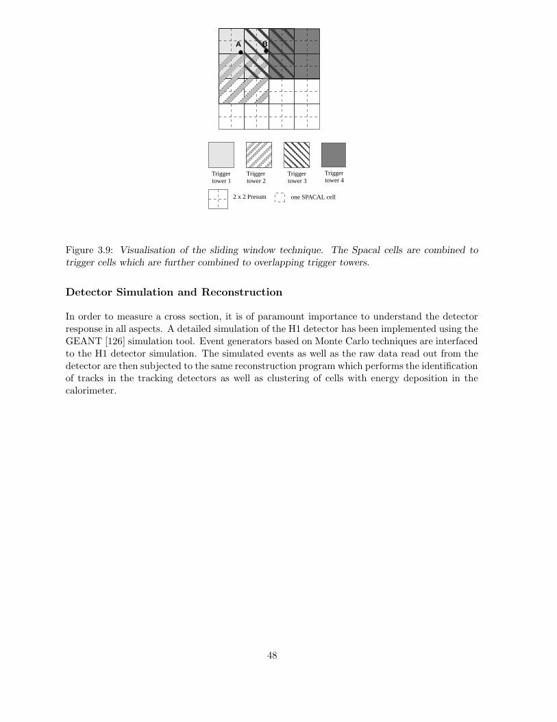
Trigger tower 1

Trigger tower 2

Trigger tower 3

2 x 2 Presum one SPACAL cell

B A

Trigger tower 4

Figure 3.9: Visualisation of the sliding window technique. The Spacal cells are combined totrigger cells which are further combined to overlapping trigger towers.

Detector Simulation and Reconstruction

In order to measure a cross section, it is of paramount importance to understand the detectorresponse in all aspects. A detailed simulation of the H1 detector has been implemented using theGEANT [126] simulation tool. Event generators based on Monte Carlo techniques are interfacedto the H1 detector simulation. The simulated events as well as the raw data read out from thedetector are then subjected to the same reconstruction program which performs the identificationof tracks in the tracking detectors as well as clustering of cells with energy deposition in thecalorimeter.

48

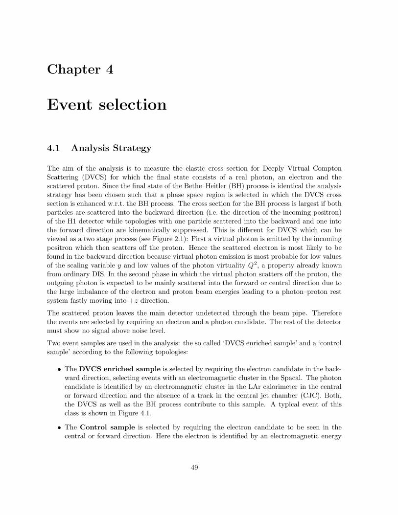
Chapter 4

Event selection

4.1 Analysis Strategy

The aim of the analysis is to measure the elastic cross section for Deeply Virtual ComptonScattering (DVCS) for which the final state consists of a real photon, an electron and thescattered proton. Since the final state of the Bethe–Heitler (BH) process is identical the analysisstrategy has been chosen such that a phase space region is selected in which the DVCS crosssection is enhanced w.r.t. the BH process. The cross section for the BH process is largest if bothparticles are scattered into the backward direction (i.e. the direction of the incoming positron)of the H1 detector while topologies with one particle scattered into the backward and one intothe forward direction are kinematically suppressed. This is different for DVCS which can beviewed as a two stage process (see Figure 2.1): First a virtual photon is emitted by the incomingpositron which then scatters off the proton. Hence the scattered electron is most likely to befound in the backward direction because virtual photon emission is most probable for low valuesof the scaling variable y and low values of the photon virtuality Q2, a property already knownfrom ordinary DIS. In the second phase in which the virtual photon scatters off the proton, theoutgoing photon is expected to be mainly scattered into the forward or central direction due tothe large imbalance of the electron and proton beam energies leading to a photon–proton restsystem fastly moving into +z direction.

The scattered proton leaves the main detector undetected through the beam pipe. Thereforethe events are selected by requiring an electron and a photon candidate. The rest of the detectormust show no signal above noise level.

Two event samples are used in the analysis: the so called ‘DVCS enriched sample’ and a ‘controlsample’ according to the following topologies:

• The DVCS enriched sample is selected by requiring the electron candidate in the back-ward direction, selecting events with an electromagnetic cluster in the Spacal. The photoncandidate is identified by an electromagnetic cluster in the LAr calorimeter in the centralor forward direction and the absence of a track in the central jet chamber (CJC). Both,the DVCS as well as the BH process contribute to this sample. A typical event of thisclass is shown in Figure 4.1.

• The Control sample is selected by requiring the electron candidate to be seen in thecentral or forward direction. Here the electron is identified by an electromagnetic energy

49

deposition in the LAr calorimeter and a reconstructed track in the CJC associated to theelectromagnetic cluster. The photon candidate is to be found in the backward directionrequiring an electromagnetic cluster in the Spacal. This sample is expected to be dom-inated by the BH process. The contribution of the DVCS process is highly suppressedsince events of this topology would correspond to very high values of Q2 which are kine-matically suppressed. This suppression is expected to be smaller for BH events w.r.t. theDVCS process (see equation 2.9–2.10). A typical event of this sample is shown in Figure4.2.

Figure 4.1: An event of the DVCS enriched sample. It is identified by the presence of twoelectromagnetic clusters, one in the backward calorimeter Spacal and one in the LAr calorimeter.The photon candidate associated with the cluster in the LAr calorimeter is identified by theproperties of the cluster and the absence of a matching track. The electron candidate in theSpacal must fulfill certain cluster properties. All subdetectors show no additional signal abovenoise level.

4.2 Preselection

A preselection based on the detector status, luminosity and trigger conditions is performed toensure a high quality of the data used in the analysis.

Run and HV Selection

The 1997 data taking period corresponds to the runs 176421 - 201519 with an integrated lumi-nosity of 23.7 pb−1.

50

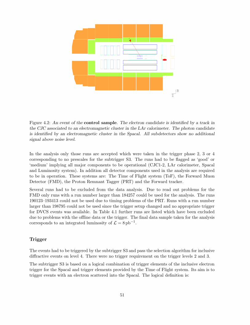
Figure 4.2: An event of the control sample. The electron candidate is identified by a track inthe CJC associated to an electromagnetic cluster in the LAr calorimeter. The photon candidateis identified by an electromagnetic cluster in the Spacal. All subdetectors show no additionalsignal above noise level.

In the analysis only those runs are accepted which were taken in the trigger phase 2, 3 or 4corresponding to no prescales for the subtrigger S3. The runs had to be flagged as ‘good’ or‘medium’ implying all major components to be operational (CJC1-2, LAr calorimeter, Spacaland Luminosity system). In addition all detector components used in the analysis are requiredto be in operation. These systems are: The Time of Flight system (ToF), the Forward MuonDetector (FMD), the Proton Remnant Tagger (PRT) and the Forward tracker.

Several runs had to be excluded from the data analysis. Due to read out problems for theFMD only runs with a run number larger than 184257 could be used for the analysis. The runs190123–193413 could not be used due to timing problems of the PRT. Runs with a run numberlarger than 198795 could not be used since the trigger setup changed and no appropriate triggerfor DVCS events was available. In Table 4.1 further runs are listed which have been excludeddue to problems with the offline data or the trigger. The final data sample taken for the analysiscorresponds to an integrated luminosity of L = 8pb−1.

Trigger

The events had to be triggered by the subtrigger S3 and pass the selection algorithm for inclusivediffractive events on level 4. There were no trigger requirement on the trigger levels 2 and 3.

The subtrigger S3 is based on a logical combination of trigger elements of the inclusive electrontrigger for the Spacal and trigger elements provided by the Time of Flight system. Its aim is totrigger events with an electron scattered into the Spacal. The logical definition is:

51

run number reason for exclusion

runrange: 184257 – 190080

185665 offline data not available186515 offline data not available186752 offline data not available187859 offline data not available188142 offline data not available188595 offline data not available

runrange: 193434 – 198795

193433 – 193462 trigger malfunctioning193502 – 193526 trigger malfunctioning

195678 offline data not available195932 – 196376 trigger malfunctioning

197036 offline data corrupted

Table 4.1: List of excluded runs due to problems with the offline data or the level 1 trigger.

(SPCLe IET 2.and.SPCLe ToF E 2).and. ((.not.SPCLh AToF E 1).and.(.not.BToF BG)).and.((.not.VETO inner BG).and.(.not.VETO Outer BG)).and. (FToF IA.or.(.not.FToF BG)).

The trigger element SPCLe IET 2 is set for events with a locally concentrated energy depositionin the electromagnetic part of the Spacal above an energy of 6.5GeV. The total electromagneticenergy deposited in the Spacal is required to be larger than 12GeV by the trigger elementSPCLe ToF E 2 whereas no signal in the hadronic section of the Spacal is allowed in a timewindow outside the nominal ep interactions by the trigger element SPCLh AToF E 1. All furtherrequired trigger elements are provided by the Time of Flight system and summarised in Table 4.2.

trigger element meaning

BToF BG Backward ToF Background

VETO inner BG inner Veto wall Background

VETO Outer BG outer Veto wall Background

FToF IA Forward ToF Interaction

FToF BG Forward ToF Background

Table 4.2: List of trigger elements which are part of subtrigger S3. A trigger element is markedwith the term ‘Interaction’ (IA) when the detector was triggered in a time window which corre-sponds to nominal ep collision time. It is marked with ‘Background’ (BG) when it was triggeredoutside this time window.

The Level 4 selection algorithm used to select DVCS events was originally designed to flaginclusive diffractive DIS events with a low value of the photon virtuality Q2. It requires anelectron candidate to be found on the first trigger level; the diffractive selection is performedusing the rapidity gap method which identifies events with no signal in the forward direction.It is based on three requirements: the absence of a signal in the PRT, the absence of a signal

52

above noise level in the FMD and no signal in the forward part of the LAr calorimeter

∑

all layers

hitsPRT = 0,

∑

layer 1,2,3

hitsFMD ≤ 1,

ηmax < 3.2

where hitsPRT and hitsFMD denote the number of hits in the proton remnant tagger and theforward muon detector respectively. ηmax is the rapidity value of the most forward energydeposition in the LAr calorimeter above a threshold of 0.5GeV.

4.3 Final Selection Criteria

The final selection is based on the detection of two electromagnetic clusters, one in the Spacal andone in the LAr calorimeter which are subsequently identified as electron and photon accordingto the response of the tracking devices. In order to identify events with an elastically scatteredproton there must be no additional signal registered by the detector above noise level. Thefollowing selection criteria have been applied:

• Spacal selection

The DVCS process is expected to be dominated by so called kinematic peak events wherethe energy of the scattered electron is close to the initial electron beam energy. Thisproperty is already known from ordinary DIS events in the same kinematic region in xand Q2. Thus events are selected with one electromagnetic cluster in the Spacal withan energy above 15GeV and a cluster radius rcl < 3.5 cm. The cluster radius is theenergy weighted sum of the distance of all cells contributing to the cluster to the centre ofgravity of the cluster [127]. It is a measure for the lateral extension of the electromagneticshower. Electromagnetic interacting particles (i.e. electrons and photons) are found toproduce smaller clusters than hadrons which makes the applied cut a powerful tool tosuppress background initiated from hadrons. Some fiducial cuts on the impact positionare applied to ensure that only events are selected where the electromagnetic cluster iscorrectly measured (see below).

• LAr selection

Events are selected with a cluster in the LAr calorimeter with a transverse momentumPT > 1GeV. The cluster is selected using the QESCAT algorithm which has been de-signed to separate clusters originating from electrons and photons from clusters initiatedby hadrons. It requires that more than 90% of the energy of the cluster is deposited in theelectromagnetic section of the LAr calorimeter. Furthermore the cluster must be compactin the sense that it shows a small transverse dispersion and that 95% of the energy aredeposited in a core of not more than five cells for the calorimeter wheels CB1 and CB2and not more than nine cells for the calorimeter wheels CB3, FB1 and FB2. Clusters havebeen selected with an impact position zcl > −150 cm. This cut is motivated by the anal-ysis strategy to select only photon candidates in the central or forward region of the LArcalorimeter. The exact value has been chosen such that the centre of gravity of the clusteris not too close to the crack between the CB1 and the BBE (see Figure 3.5). Additional

53

fiducial cuts have been applied taking only well measured electromagnetic clusters intoaccount (see below).

• Track selection

The DVCS enriched sample and the control sample are classified according to the positionof the photon and the electron candidate. The identification of these is performed usingtracks measured with the central jet chamber.

– In case of the control sample the electron is scattered into the central or forwarddirection and the photon is scattered in the backward direction. The electron isidentified by a track which is reconstructed using the CJC and associated to theelectromagnetic cluster in the LAr calorimeter. The electromagnetic cluster in theSpacal is then assumed to be the photon.

– For the DVCS enriched sample the photon in the LAr calorimeter is identifiedby the absence of a track in the CJC. The electromagnetic cluster in the Spacal isthen assumed to be the electron. A track for the electron candidate cannot be recon-structed due to the limited geometrical acceptance of the CJC; the electromagneticclusters are dominantly found in the inner part of the Spacal which is not covered bythe central jet chamber.

If more than one track is reconstructed using the CJC the event is rejected.

The reconstruction program provides two classes of tracks, one where the track is fittedto the interaction vertex and the other class for which tracks have been reconstructed butnot fitted to the interaction vertex. For electrons it is likely that they emit a photon bythe Bremsstrahlungs process when they cross the detector material (beam pipe, supportstructure, electronics, ...). If this happens the electron leaves its original direction whichmakes it impossible for the track reconstruction program to fit the track to the interactionvertex. It is important to take these kind of tracks into account since a misidentification ofelectrons as photons would spoil the measurement of the DVCS process. It has been foundthat the number of events in the control sample is increased by 3.5% when taking intoaccount tracks which have not been fitted to the interaction vertex which is consistent withan independent analysis [128]. In addition the events of the DVCS enriched sample havebeen scanned with the event display program to cross check that the track veto conditionhas been correctly applied.

• Elastic selection

Since the proton leaves the main detector through the beam pipe undetected and no furtherparticles are produced, the detector should show no additional signal above noise level.To reduce background from other process (including non–elastic DVCS events) additionalveto conditions have been applied.

– Veto condition for the CJCIf a track can be reconstructed with the CJC it has to be associated with the elec-tromagnetic cluster in the Spacal or the LAr calorimeter. In case no association ispossible or more than one reconstructed track is found the event is rejected.

– Veto condition for the LAr calorimeterIt is required that apart from the selected cluster in the LAr calorimeter no additionalcluster with an energy Ecl > 0.5GeV is found. This cut has been chosen according tothe noise distribution of the LAr calorimeter. A lower cut would lead to a rejection of

54

too many events leading to an increase of the statistical error for the measurement.The effect of this cut and the rejection of events due to noise has been taken intoaccount in the MC simulations, in which the noise is not directly simulated but thesimulated LAr calorimeter signals are overlayed with signals from randomly triggereddata. By this procedure the LAr noise is correctly taken into account when applyingthe same cuts for data and MC simulation.

– Veto conditions for the forward detectorsThe forward detectors, i. e. the FMD and PRT are used to suppress the contributionfrom inelastic events where the proton is excited into a higher state which subse-quently decays as well as events from the inelastic continuum. For these kind ofevents it is likely that one or more of the final state particles hit the beam pipe orcollimators originally designed to constrain the beam aperture and protect the detec-tor from synchrotron radiation. This leads to a shower of secondary particles whicheventually gives a signal in the FMD or PRT. At large |t| > 1GeV2 even the scatteredproton could hit the scintillator pads of the PRT directly. It is required that no hitis observed in layer 0 and 1 of the PRT. All additional layers show almost no signalsince they suffered from radiation damage and were thus not taken into account. Forthe FMD it was required that the sum of hit pairs in the first three layers is not largerthan 1.

Figure 4.3 [130] shows the hit multiplicity distributions in the forward muon detector andthe proton remnant tagger for inclusive DIS events. The data are compared to the sumof an inclusive DIS MC and a MC which generates diffractive events. For both the FMDand the PRT the data are well described by the MC simulation. The good description ofthe PRT response has been achieved by a decrease of its efficiency in the MC simulationsof about 50% as was observed for the 1997 data taking period due to radiation damage.Two independent methods have been developed to account for this effect which both ledto the same results [130, 131]. The remaining differences for the FMD and PRT have beentaken into account in the determination of the systematic error.

a) b)

Figure 4.3: Distributions of a) the number of hits in the forward muon detector and b) theproton remnant tagger (PRT). The data (black points) are compared to the sum of an inclusiveDIS and a diffractive MC simulation (shaded and white histogram) [130].

• Fiducial Cuts

Due to the malfunctioning of parts of the different subdetectors additional fiducial cuts

55

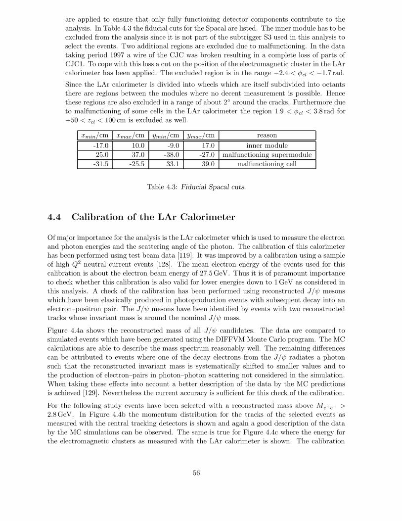
are applied to ensure that only fully functioning detector components contribute to theanalysis. In Table 4.3 the fiducial cuts for the Spacal are listed. The inner module has to beexcluded from the analysis since it is not part of the subtrigger S3 used in this analysis toselect the events. Two additional regions are excluded due to malfunctioning. In the datataking period 1997 a wire of the CJC was broken resulting in a complete loss of parts ofCJC1. To cope with this loss a cut on the position of the electromagnetic cluster in the LArcalorimeter has been applied. The excluded region is in the range −2.4 < φcl < −1.7 rad.

Since the LAr calorimeter is divided into wheels which are itself subdivided into octantsthere are regions between the modules where no decent measurement is possible. Hencethese regions are also excluded in a range of about 2◦ around the cracks. Furthermore dueto malfunctioning of some cells in the LAr calorimeter the region 1.9 < φcl < 3.8 rad for−50 < zcl < 100 cm is excluded as well.

xmin/cm xmax/cm ymin/cm ymax/cm reason

-17.0 10.0 -9.0 17.0 inner module

25.0 37.0 -38.0 -27.0 malfunctioning supermodule

-31.5 -25.5 33.1 39.0 malfunctioning cell

Table 4.3: Fiducial Spacal cuts.

4.4 Calibration of the LAr Calorimeter

Of major importance for the analysis is the LAr calorimeter which is used to measure the electronand photon energies and the scattering angle of the photon. The calibration of this calorimeterhas been performed using test beam data [119]. It was improved by a calibration using a sampleof high Q2 neutral current events [128]. The mean electron energy of the events used for thiscalibration is about the electron beam energy of 27.5GeV. Thus it is of paramount importanceto check whether this calibration is also valid for lower energies down to 1GeV as considered inthis analysis. A check of the calibration has been performed using reconstructed J/ψ mesonswhich have been elastically produced in photoproduction events with subsequent decay into anelectron–positron pair. The J/ψ mesons have been identified by events with two reconstructedtracks whose invariant mass is around the nominal J/ψ mass.

Figure 4.4a shows the reconstructed mass of all J/ψ candidates. The data are compared tosimulated events which have been generated using the DIFFVM Monte Carlo program. The MCcalculations are able to describe the mass spectrum reasonably well. The remaining differencescan be attributed to events where one of the decay electrons from the J/ψ radiates a photonsuch that the reconstructed invariant mass is systematically shifted to smaller values and tothe production of electron–pairs in photon–photon scattering not considered in the simulation.When taking these effects into account a better description of the data by the MC predictionsis achieved [129]. Nevertheless the current accuracy is sufficient for this check of the calibration.

For the following study events have been selected with a reconstructed mass above Me+e− >2.8GeV. In Figure 4.4b the momentum distribution for the tracks of the selected events asmeasured with the central tracking detectors is shown and again a good description of the databy the MC simulations can be observed. The same is true for Figure 4.4c where the energy forthe electromagnetic clusters as measured with the LAr calorimeter is shown. The calibration

56

studies are completed by comparing the ratio of the cluster energy and the momentum of thetrack between data and MC (Figure 4.4d). Again good agreement is observed. For high energiesthe uncertainty on the energy scale is quoted to be 2%. In this analysis this uncertainty hasbeen conservatively estimated to 4% as can be inferred from the deviations seen in Figures 4.4eand 4.4f where the cluster energies have been increased and, respectively, decreased by 4%.

4.5 Reconstruction of the Event Kinematics

The kinematic variables of the reaction ep −→ eγp can be determined from the scattering anglesand the energies of the final state electron and photon. Due to energy momentum conservationthe determination of the kinematics is overconstrained which results in the possibility to usedifferent reconstruction methods, i.e. the electron method where the kinematics is reconstructedfrom the scattered electron angle and energy, the double angle method where the kinematics isreconstructed from the scattering angles of the electron and the photon and the hadron methodwhere it is determined from the scattering angle and energy of the final state photon. Thedouble angle method was found to give the best resolution of both kinematic variables Q2 andW which are calculated according to the following formulae:

Q2 = 4E20

sin θγ (1 + cos θe)

sin θγ + sin θe − sin (θe + θγ), (4.1)

x =E0

Ep

sin θγ + sin θe + sin (θe + θγ)

sin θγ + sin θe − sin (θe + θγ), (4.2)

W 2 =Q2

x(1 − x) (4.3)

where E0 and Ep denote the energies of the incident electron and proton beam, respectively.The polar scattering angles of the final state electron and photon are θe and θγ . Figure 4.5 showsthe resolution of the kinematic variables Q2 and W . For the control sample the reconstructedtrack in the CJC determines the interaction vertex given by the intersection of the reconstructedtrack with the beam line. In case of the DVCS enriched sample the interaction vertex cannotby reconstructed due to the absence of a track. Therefore the nominal vertex position, zvertex =1.7 cm, estimated with the control sample (see Section 4.6) , has been used to determine thescattering angles in combination with the reconstructed positions of the selected clusters in theLAr and Spacal calorimeter. The resolution for the reconstruction of the kinematic variable Q2

is significantly degraded due to the unknown z–position of the event vertex. It changes from3% to 13% whereas the resolution for W leaves almost unchanged at 5%

When correcting the DVCS sample for the detector acceptance it is important to include con-tributions from events originating from ep–collisions which happened at the position (zvertex =67.5 cm) where electrons interact with the satellite bunch. For these kind of events the kinematicvariables are systematically misreconstructed. Since a fraction of 3.5% of the events originatefrom the forward satellite vertex this effect cannot be neglected and is thus accounted when cal-culating the acceptance correction (see chapter 5). The effect is strongest for the reconstructionof Q2 as shown in Figure 4.5a. The resolution of the kinematic variables Q2 and W is shown asdetermined using a MC simulation of events generated with the TINTIN program.

The variable t can be calculated in good approximation from the vectorial sum of the transversemomenta of the final state electron and photon:

t = −|−−→PTe +−−→PTγ |2 (4.4)

57

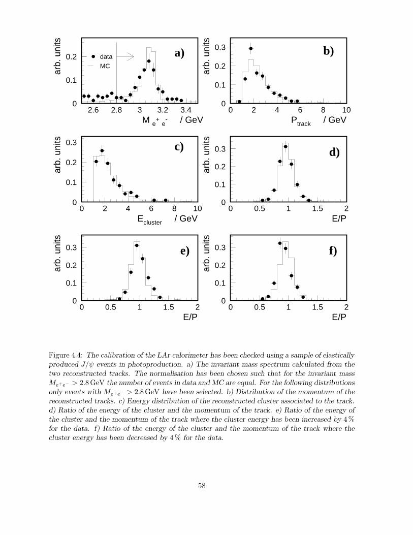
0

0.1

0.2

2.6 2.8 3 3.2 3.40

0.1

0.2

0.3

0 2 4 6 8 10

0

0.1

0.2

0.3

0 2 4 6 8 100

0.1

0.2

0.3

0 0.5 1 1.5 2

0

0.1

0.2

0.3

0 0.5 1 1.5 2

data

MC

a)

M e+ e- / GeV

arb.

uni

tsb)

Ptrack / GeV

arb.

uni

ts

c)

Ecluster / GeV

arb.

uni

ts

d)

E/Par

b. u

nits

e)

E/P

arb.

uni

ts

f)

E/P

arb.

uni

ts

0

0.1

0.2

0.3

0 0.5 1 1.5 2

Figure 4.4: The calibration of the LAr calorimeter has been checked using a sample of elasticallyproduced J/ψ events in photoproduction. a) The invariant mass spectrum calculated from thetwo reconstructed tracks. The normalisation has been chosen such that for the invariant massMe+e− > 2.8GeV the number of events in data and MC are equal. For the following distributionsonly events with Me+e− > 2.8GeV have been selected. b) Distribution of the momentum of thereconstructed tracks. c) Energy distribution of the reconstructed cluster associated to the track.d) Ratio of the energy of the cluster and the momentum of the track. e) Ratio of the energy ofthe cluster and the momentum of the track where the cluster energy has been increased by 4%for the data. f) Ratio of the energy of the cluster and the momentum of the track where thecluster energy has been decreased by 4% for the data.

58

0

20

40

60

80

100

-1.4 -1.2 -1 -0.8 -0.6 -0.4 -0.2 0 0.2 0.4(Q2 gen - Q

2 rec)/Q2 gen

# ev

ents

nominal vertex

satelite vertex

(Wgen - Wrec)/Wgen

# ev

ents

0

50

100

150

200

250

-0.5 -0.4 -0.3 -0.2 -0.1 0 0.1 0.2 0.3 0.4 0.5

Figure 4.5: Resolution of the kinematic variables a) Q2 and b) W . The contribution from eventsoriginating from the main interaction vertex is shown by the white histogram. The shadedhistogram shows the contribution for events which originate from the satellite vertex where thekinematic variables are systematically misreconstructed. The relative contribution of eventsfrom the satellite vertex is 3.5%.

where PTe and PTγ are calculated from the azimuthal and polar scattering angles and theenergies of the electron and photon.

For the calculation of the kinematic variables the data have been corrected for the beam tilteffect. The H1 coordinate system is defined by the Central Jet Chamber with the origin of thecoordinate system in the centre of the CJC. The beam axis is however not perfectly alignedto the axis of the tracking device. Therefore the measured scattering angles are systematicallymisreconstructed which has to be corrected for in this analysis. The applied corrections originatefrom ordinary DIS events for which a large amount of events exists used to determine the exactbeam axis. The influence on the measured cross section is about 5%.

59

4.6 Control Sample

In addition to the already discussed selection criteria cuts are applied which restrict the kinematicdomain to the region which is used for the measurement (see section 4.7). They restrict thedata sample to the following kinematic domain: 2 < Q2 < 20GeV2, 30 < W < 120GeV and|t| < 1GeV2. An additional cut on the variable

∑E − Pz which is calculated from the electron

and photon candidate and which characterises the longitudinal momentum conservation hasbeen imposed:

∑E − Pz > 45GeV. Its nominal value is equal to twice the electron beam

energy∑E − Pz = 55GeV. This cut is imposed to minimise the effect of additional photon

radiation from the incoming electron when extracting the DVCS cross section from the DVCSenriched sample.

When calculating the kinematic variables for the control sample the photon candidate has beentreated as electron and the electron candidate has been treated as photon. This treatment leadsto similar distributions for the scattering angles and energies of the final state particles in com-parison to these distributions for the DVCS enriched sample. Therefore the control sample canbe used to study directly the detector response for the region (i.e. angular range and energydomain) which is important for the DVCS measurement although the true kinematic distribu-tions are completely different. In particular it can be tested whether the detector response iscorrectly described by the simulation.

The control sample consists of 338 events. It is expected to be dominated by the Bethe–Heitlerprocess while the DVCS process does not contribute substantially. This can be understoodby a simple numerical example. If the electron is scattered into the backward direction (e. g.θe = 177◦) and the photon is scattered into the central region of the detector (e. g. θγ = 90◦) asis the case for the enriched DVCS sample the photon virtuality Q2 has the value Q2 = 1.7GeV2

whereas in the inverse event topology (θe = 90◦, θγ = 177◦) Q2 is Q2 = 63GeV2. Since theDVCS cross section is expected to decrease faster with increasing Q2 (see e.g. the FFS model inchapter 2) it is suppressed w.r.t. the Bethe–Heitler process.

Backgrounds to the Control Sample

It was found that two additional reactions can contribute to the same event topology as thecontrol sample in a sizable way: The diffractive electro–production of ρ mesons and the dileptonproduction in two–photon interactions.

• Diffractive ρ meson production (ep −→ eρp, with ρ −→ π+π−) can contribute to thesame event topology as the control sample when the final state electron is scattered intothe backward direction and the positive charged decay pion is scattered into the centralor forward direction, the negative charged pion and the proton leave the main detectorundetected through the beam pipe. If the positive charged pion deposits its entire energyin the electromagnetic section of the LAr calorimeter it can in combination with its trackbe misidentified as an electron. The backward scattered electron seen in the Spacal is thenmostly associated with the photon since the angular acceptance of the tracking devices istoo small. It will therefore assumed to be a photon.

• Dilepton production in two photon events e+p −→ e+e−e+p can contribute to the sameevent topology when one of the three final state leptons is detected in the backwarddirection, one lepton is scattered into the central part of the H1 detector while the third

60

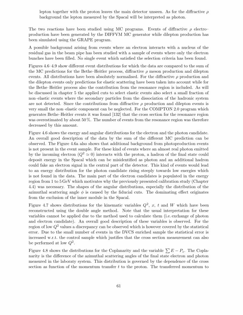
lepton together with the proton leaves the main detector unseen. As for the diffractive ρbackground the lepton measured by the Spacal will be interpreted as photon.

The two reactions have been studied using MC programs. Events of diffractive ρ electro–production have been generated by the DIFFVM MC generator while dilepton production hasbeen simulated using the GRAPE program.

A possible background arising from events where an electron interacts with a nucleus of theresidual gas in the beam pipe has been studied with a sample of events where only the electronbunches have been filled. No single event which satisfied the selection criteria has been found.

Figures 4.6–4.9 show different event distributions for which the data are compared to the sum ofthe MC predictions for the Bethe–Heitler process, diffractive ρ meson production and dileptonevents. All distributions have been absolutely normalised. For the diffractive ρ production andthe dilepton events only predictions for elastic scattering have been taken into account while forthe Bethe–Heitler process also the contribution from the resonance region is included. As willbe discussed in chapter 5 the applied cuts to select elastic events also select a small fraction ofnon–elastic events where the secondary particles from the dissociation of the hadronic systemare not detected. Since the contributions from diffractive ρ production and dilepton events isvery small the non–elastic component can be neglected. For the COMPTON 2.0 program whichgenerates Bethe–Heitler events it was found [132] that the cross section for the resonance regionwas overestimated by about 50%. The number of events from the resonance region was thereforedecreased by this amount.

Figure 4.6 shows the energy and angular distributions for the electron and the photon candidate.An overall good description of the data by the sum of the different MC prediction can beobserved. The Figure 4.6a also shows that additional background from photoproduction eventsis not present in the event sample. For these kind of events where an almost real photon emittedby the incoming electron (Q2 ' 0) interacts with the proton, a hadron of the final state coulddeposit energy in the Spacal which can be misidentified as photon and an additional hadroncould fake an electron signal in the central part of the detector. This kind of events would leadto an energy distribution for the photon candidate rising steeply towards low energies whichis not found in the data. The main part of the electron candidates is populated in the energyregion from 1 to 5GeV which motivates why the previously presented calibration study (Chapter4.4) was necessary. The shapes of the angular distributions, especially the distribution of theazimuthal scattering angle φ is caused by the fiducial cuts. The dominating effect originatesfrom the exclusion of the inner module in the Spacal.

Figure 4.7 shows distributions for the kinematic variables Q2, x, t and W which have beenreconstructed using the double angle method. Note that the usual interpretation for thesevariables cannot be applied due to the method used to calculate them (i.e. exchange of photonand electron candidate). An overall good description of these variables is observed. For theregion of low Q2 values a discrepancy can be observed which is however covered by the statisticalerror. Due to the small number of events in the DVCS enriched sample the statistical error isincreased w.r.t. the control sample which justifies that the cross section measurement can alsobe performed at low Q2.

Figure 4.8 shows the distributions for the Coplanarity and the variable∑E − Pz. The Copla-

narity is the difference of the azimuthal scattering angles of the final state electron and photonmeasured in the laboraty system. This distribution is governed by the dependence of the crosssection as function of the momentum transfer t to the proton. The transferred momentum to

61

0

25

50

75

100

10 15 20 25 30 350

50

100

150

0 2 4 6 8 10

0

25

50

75

100

165 170 175 1800

50

100

0 50 100 150

0

20

40

60

-2 0 20

20

40

60

-2 0 2

Eγ [ GeV ]

# ev

ents H1

Bethe Heitler

dilepton

diff. ρ

a)

Ee [ GeV ]

# ev

ents b)

θγ [ o ]

# ev

ents

c)

θe [ o ]

# ev

ents

d)

φγ [ rad ]

# ev

ents e)

φe [ rad ]

# ev

ents f)

Figure 4.6: Control sample distributions. The data are compared to the sum of predictionsfor the Bethe–Heitler process (elastic and quasi–elastic), elastic dilepton production and elasticρ electro–production. All distributions are absolutely normalised. a) Energy of the photoncandidate (i.e. cluster in the Spacal); b) energy of the electron candidate (i.e. cluster in the LArcalorimeter); c) polar angle of the photon candidate; d) polar angle of the electron candidate;e) azimuthal angle of the photon candidate; f) azimuthal angle of the electron candidate.

the proton is compensated by the final state electron–photon system. For small momentumtransfers the eγ system is balanced and the Coplanarity variable takes a value close to 180◦

whereas for large momentum transfer the eγ system becomes imbalanced leading to a deviationfrom 180◦. The Coplanarity distribution therefore reflects the distribution of the transferredmomentum to the proton. The Bethe–Heitler process is a purely electromagnetic process. The

62

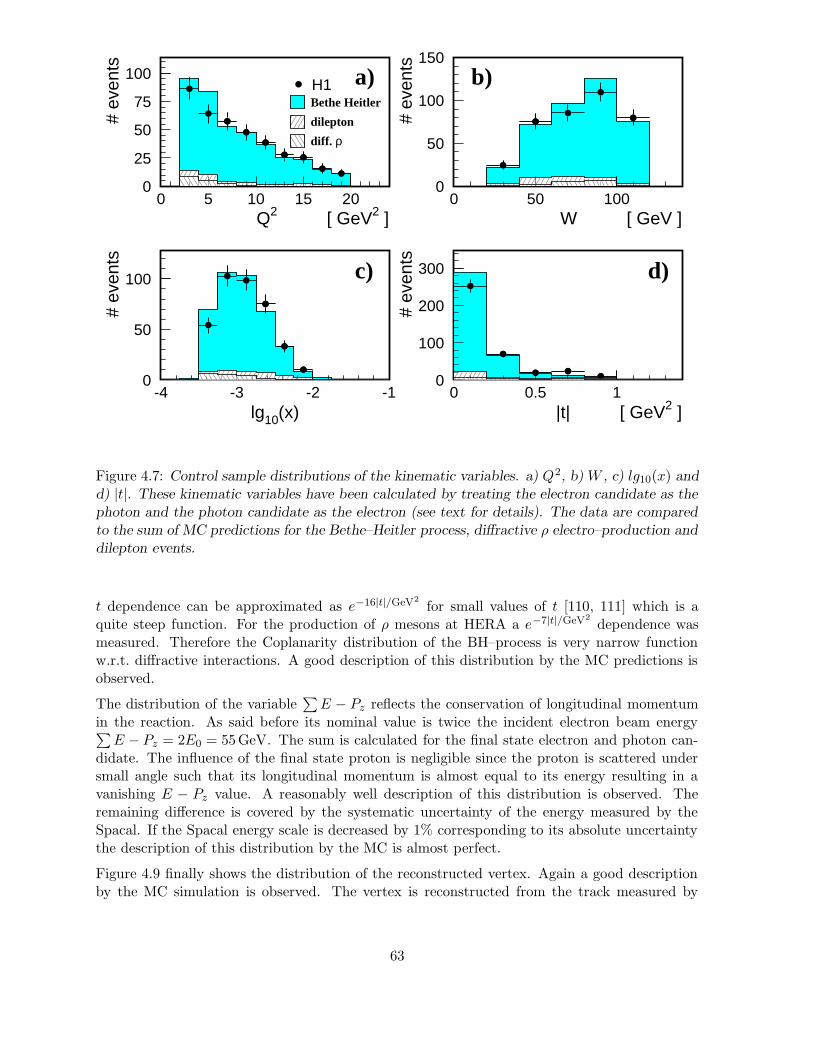
0

25

50

75

100

0 5 10 15 200

50

100

150

0 50 100

0

50

100

-4 -3 -2 -10

100

200

300

0 0.5 1

Q2 [ GeV2 ]

# ev

ents

H1Bethe Heitler

dilepton

diff. ρ

a)

W [ GeV ]

# ev

ents b)

lg10(x)

# ev

ents

c)

|t| [ GeV2 ]#

even

ts

d)

Figure 4.7: Control sample distributions of the kinematic variables. a) Q2, b) W , c) lg10(x) andd) |t|. These kinematic variables have been calculated by treating the electron candidate as thephoton and the photon candidate as the electron (see text for details). The data are comparedto the sum of MC predictions for the Bethe–Heitler process, diffractive ρ electro–production anddilepton events.

t dependence can be approximated as e−16|t|/GeV2

for small values of t [110, 111] which is aquite steep function. For the production of ρ mesons at HERA a e−7|t|/GeV2

dependence wasmeasured. Therefore the Coplanarity distribution of the BH–process is very narrow functionw.r.t. diffractive interactions. A good description of this distribution by the MC predictions isobserved.

The distribution of the variable∑E − Pz reflects the conservation of longitudinal momentum

in the reaction. As said before its nominal value is twice the incident electron beam energy∑E − Pz = 2E0 = 55GeV. The sum is calculated for the final state electron and photon can-

didate. The influence of the final state proton is negligible since the proton is scattered undersmall angle such that its longitudinal momentum is almost equal to its energy resulting in avanishing E − Pz value. A reasonably well description of this distribution is observed. Theremaining difference is covered by the systematic uncertainty of the energy measured by theSpacal. If the Spacal energy scale is decreased by 1% corresponding to its absolute uncertaintythe description of this distribution by the MC is almost perfect.

Figure 4.9 finally shows the distribution of the reconstructed vertex. Again a good descriptionby the MC simulation is observed. The vertex is reconstructed from the track measured by

63

0

100

200

170 180 1900

50

100

150

200

30 40 50 60 70Coplanarity [ o ]

# ev

ents

H1Bethe Heitler

dilepton

diff. ρ

a)

∑E-Pz [ GeV ]

# ev

ents b)

Figure 4.8: Distributions of the Coplanarity and the variable∑E − Pz for the control sample.

The data are compared to the sum of MC predictions for the Bethe–Heitler process and the dif-ferent background contributions. The Coplanarity distribution reflects the momentum transferto the proton while the quantity

∑E − Pz shows the longitudinal momentum conservation.

the CJC by determining the intersection of the track with the beam axis. The mean value ofthe central vertex was estimated to be 1.7 cm by fitting a Gaussian to the data. This value isused for the DVCS enriched sample to reconstruct the event kinematics since no vertex can bereconstructed for these events.

0

20

40

60

80

-40 -20 0 20 40Zvertex [ cm ]

# ev

ents

H1Bethe Heitler

dilepton

diff. ρ

Figure 4.9: Distribution of the z position of the reconstructed vertex. The data are comparedto the sum of the MC predictions for the different contributions.

The Bethe–Heitler process dominating the control sample is known with high accuracy such thatthe MC predictions for this sample are reliable. From the good description of the control sampleby the sum of the different MC predictions it can be concluded that the detector response is wellunderstood. In particular the measurement of low energetic particles with the LAr calorimetercan be trusted which is of paramount importance for the cross section extraction from the DVCSenriched sample.

64

4.7 DVCS Enriched Sample

The DVCS enriched sample has been restricted to the kinematic domain 2 < Q2 < 20GeV2,30 < W < 120GeV and |t| < 1GeV2. The lower limit of the Q2 domain is determined bythe geometrical acceptance of the Spacal whereas the Q2 range is restricted to the upper valuedue to the measured event rate. The variable W is strongly correlated with the scatteringangle of the photon and the cuts have been chosen such that the selected photons lie in theacceptance of the CJC. The lower W cut corresponds to a scattering angle of about 25◦ whereasthe upper cut corresponds to about 160◦ for the main part of the events. The cut on the variable∑E−Pz > 45GeV is imposed to minimise the radiative corrections when extracting the DVCS

cross section.

The DVCS enriched sample consists of 172 events which are expected to comprise contributionsof both the Bethe–Heitler and the DVCS process. In addition it was found that two nonnegligible additional processes contribute to the selected event topology: the diffractive electro–production of ω and φ mesons. In addition the contribution from proton dissociation DeeplyVirtual Compton Scattering has to be taken into account when extracting the cross section forelastic DVCS (see chapter 5).

ω and φ Backgrounds

The diffractive electro–production of ω and φ mesons was found to contribute to the DVCSenriched data sample

• Diffractive ω vector meson production (ep −→ eωp) can contribute to the event topologywhen the produced ω meson decays into a three photon final state, i.e. ω −→ π0γ withthe subsequent decay of the π0 meson in two photons. These events have the same eventtopology as the DVCS enriched sample when the electron is scattered into the backwarddirection and measured in the Spacal (i.e. Q2 > 1GeV2) while only one of the three finalstate photons is detected in the LAr calorimeter and the two remaining photons leavethe main detector either through the beam pipe or their energy is below the noise cut ofEcl < 0.5GeV. The dominating decay channel ω −→ π+π−π0 was found not to contributeto the event sample since one of the charged pions enters very likely the tracking detectorsleading to a rejection of the event.

• Diffractive φ production can contribute to the event topology when the meson decays intokaons, i.e. φ −→ K0

LK0S with the subsequent decay of the K0

S into two neutral pionswhich itself decay into photons. These events contribute to the event topology when thescattered electron is detected in the Spacal and one of the final state photons or the longliving kaon is measured in the LAr calorimeter satisfying the selection criteria while theremaining particles again leave the detector through the beam pipe or have an energybelow the noise threshold.

In order to study these backgrounds, ω and φ events have been generated using the DIFFVMMC program. Note that this event generator does not predict the correct cross sections for theproduction of ω and φ mesons and that hence the generated number of events had to be rescaled[132] such that it corresponds to measured cross sections [68, 63].

65

A possible background arising from events where an electron interacts with a nucleus of theresidual gas in the beam pipe has been studied with a sample of events where only the electronbunches have been filled. No single event which satisfied the selection criteria has been found.

Figure 4.10 shows event distributions for the DVCS enriched sample of the energies and thescattering angles of the final state electron and photon candidate. The data are compared tothe sum of MC predictions for the Bethe–Heitler and DVCS process and the discussed vectormeson backgrounds. The Bethe–Heitler process and the production of ω and φ mesons have beenabsolutely normalised while the contribution from the DVCS process is normalised such thatthe total number of MC events corresponds to the number of selected events in the data sample.This method can be applied since the contribution from the interference term of the DVCS andBH process is expected to cancel (for a detailed discussion see chapter 5.4). The Bethe–Heitlercontribution to the DVCS enriched sample is estimated using the COMPTON program whichgenerates events for the elastic contribution as well as the contribution from the resonance regionto the cross section. The DVCS process has been simulated using the TINTIN MC programdeveloped in this thesis, based on the calculations from Frankfurt, Freund and Strikman, whichgenerates events for the elastic reaction ep −→ eγp. It includes the Bethe–Heitler process, theDVCS process and the interference term.

When comparing the data to the sum of the predictions for the Bethe–Heitler process and thetwo vector meson backgrounds a large excess of events is observed which is very different inshape as well as in normalisation in comparison to the MC predictions. A good descriptionof the data by the sum of the MC predictions is observed when including the DVCS process.This contribution is able to account completely for the missing parts. As discussed earlier thescattered electron has most likely an energy close to the incident electron beam energy (Figure4.10a) which justifies the applied selection criterium Ee > 15GeV. From this distribution it alsocan be concluded that no photoproduction background is present which would show up as risingdistribution towards low energies. Figure 4.10b shows the energy distribution for the photoncandidate where the data again exhibit a quite different shape compared to the predictionof the Bethe–Heitler MC program. As before this difference is completely accounted for byincluding the DVCS prediction. The strongest differences in shape are observed for the polarangle distribution of the electron and photon candidate (Figure 4.10 c) and d)). The reason forthe different shapes of the electron θ–distribution for DVCS and BH lies in the different Q2–dependencies of the two processes. The strong difference in the polar angle distribution of thephoton candidate originates from the different y dependencies of the cross sections. As discussedearlier for the BH–process both the scattered electron and the photon are most likely to be foundin the backward direction whereas the photon in the DVCS process is more frequently expectedin the central or forward direction. The cutoff at about 25◦ for the photon scattering angle isgoverned by the cut on the photon proton centre of mass energy W > 30GeV. Figure 4.10e) and f) show the azimuthal angles of the measured electron and photon. The shape of thesedistributions is governed by the fiducial cuts where the exclusion of the inner part of the Spacalis causing the strongest effect.

The comparison of the distributions shown in Figure 4.10 and Figure 4.6 demonstrates thatindeed for the control sample the same energy and angular ranges are covered as for the DVCSenriched sample which justifies the analysis strategy to prove the understanding of the detectorresponse with the help of the control sample. Since it was shown that the detector response iswell understood it can now be concluded that the observed excess of the data w.r.t. the Bethe–Heitler MC prediction proofs the existence of an up to now unmeasured process the DeeplyVirtual Compton Scattering.

66

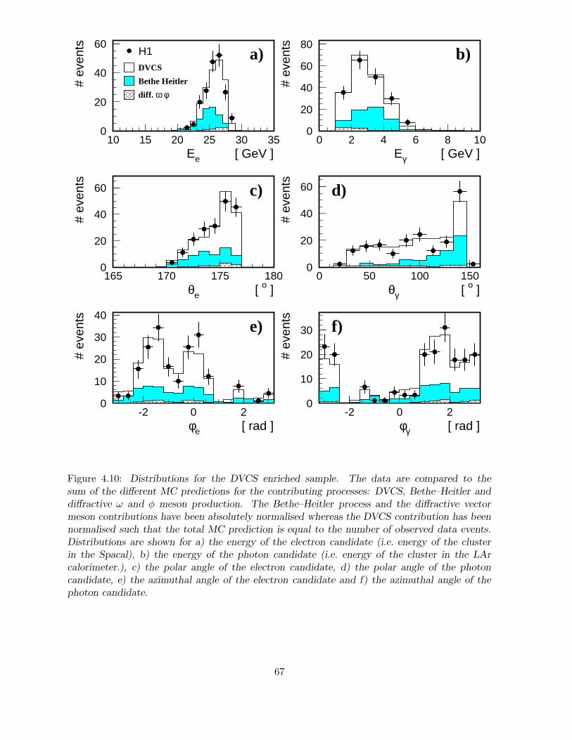
0

20

40

60

10 15 20 25 30 350

20

40

60

80

0 2 4 6 8 10

0

20

40

60

165 170 175 1800

20

40

60

0 50 100 150

0

10

20

30

40

-2 0 20

10

20

30

-2 0 2

Ee [ GeV ]

# ev

ents H1

DVCS

Bethe Heitler

diff. ω φ

a)

Eγ [ GeV ]

# ev

ents b)

θe [ o ]

# ev

ents

c)

θγ [ o ]

# ev

ents

d)

φe [ rad ]

# ev

ents e)

φγ [ rad ]

# ev

ents f)

Figure 4.10: Distributions for the DVCS enriched sample. The data are compared to thesum of the different MC predictions for the contributing processes: DVCS, Bethe–Heitler anddiffractive ω and φ meson production. The Bethe–Heitler process and the diffractive vectormeson contributions have been absolutely normalised whereas the DVCS contribution has beennormalised such that the total MC prediction is equal to the number of observed data events.Distributions are shown for a) the energy of the electron candidate (i.e. energy of the clusterin the Spacal), b) the energy of the photon candidate (i.e. energy of the cluster in the LArcalorimeter.), c) the polar angle of the electron candidate, d) the polar angle of the photoncandidate, e) the azimuthal angle of the electron candidate and f) the azimuthal angle of thephoton candidate.

67

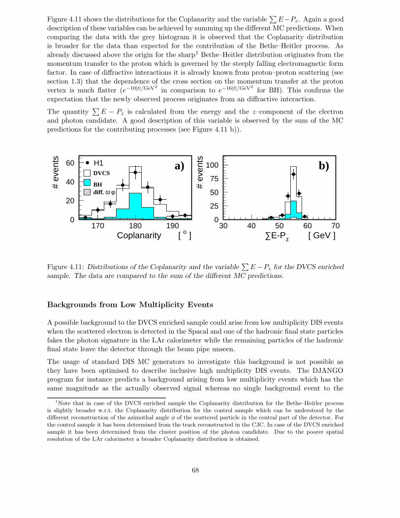
Figure 4.11 shows the distributions for the Coplanarity and the variable∑E−Pz. Again a good

description of these variables can be achieved by summing up the different MC predictions. Whencomparing the data with the grey histogram it is observed that the Coplanarity distributionis broader for the data than expected for the contribution of the Bethe–Heitler process. Asalready discussed above the origin for the sharp1 Bethe–Heitler distribution originates from themomentum transfer to the proton which is governed by the steeply falling electromagnetic formfactor. In case of diffractive interactions it is already known from proton–proton scattering (seesection 1.3) that the dependence of the cross section on the momentum transfer at the protonvertex is much flatter (e−10|t|/GeV2

in comparison to e−16|t|/GeV2

for BH). This confirms theexpectation that the newly observed process originates from an diffractive interaction.

The quantity∑E − Pz is calculated from the energy and the z–component of the electron

and photon candidate. A good description of this variable is observed by the sum of the MCpredictions for the contributing processes (see Figure 4.11 b)).

0

20

40

60

170 180 1900

25

50

75

100

30 40 50 60 70Coplanarity [ o ]

# ev

ents H1

DVCS

BHdiff. ω φ

a)

∑E-Pz [ GeV ]

# ev

ents b)

Figure 4.11: Distributions of the Coplanarity and the variable∑E−Pz for the DVCS enriched

sample. The data are compared to the sum of the different MC predictions.

Backgrounds from Low Multiplicity Events

A possible background to the DVCS enriched sample could arise from low multiplicity DIS eventswhen the scattered electron is detected in the Spacal and one of the hadronic final state particlesfakes the photon signature in the LAr calorimeter while the remaining particles of the hadronicfinal state leave the detector through the beam pipe unseen.

The usage of standard DIS MC generators to investigate this background is not possible asthey have been optimised to describe inclusive high multiplicity DIS events. The DJANGOprogram for instance predicts a background arising from low multiplicity events which has thesame magnitude as the actually observed signal whereas no single background event to the

1Note that in case of the DVCS enriched sample the Coplanarity distribution for the Bethe–Heitler processis slightly broader w.r.t. the Coplanarity distribution for the control sample which can be understood by thedifferent reconstruction of the azimuthal angle φ of the scattered particle in the central part of the detector. Forthe control sample it has been determined from the track reconstructed in the CJC. In case of the DVCS enrichedsample it has been determined from the cluster position of the photon candidate. Due to the poorer spatialresolution of the LAr calorimeter a broader Coplanarity distribution is obtained.

68

DVCS enriched sample is found when using the HERWIG program. The different results of thetwo MC generators originate most probably from the different fragmentation algorithms usedin these programs and is not physical. Therefore a possible background from DIS has to beestimated from the data itself.

If such background events really exist it is most probable that in the majority of cases the neutralparticle which fakes up the photon signature in the LAr calorimeter is the lightest neutral meson,the π0 meson. The background which is predicted by the DJANGO program actually consists ofa fraction of 2/3 of neutral pions and 1/3 of η mesons faking a photon accompanied by additionalneutral pions which escape detection through the beam pipe.

The basic idea for investigation of this kind of background events is to directly reconstruct neutralmesons via their two decay photons. Due to the cut on the transverse momentum for the clusterin LAr calorimeter (PT > 1GeV) the clusters energy is at least 1GeV. For these energies it isexpected that the two decay photons from the pion deposit their energy very close together inthe calorimeter. Depending on the size of the calorimeter cells, which changes with the polarangle θ, only for a small fraction of events two separate clusters are actually reconstructed bythe H1 reconstruction program. For the majority of events only a single cluster is observed.

The minimum opening angle θminγ1γ2

between the two photons originating from π0 decay can becalculated with the formula

cos θminγ1γ2

= 1 − 2 ·m2π0

E2π0

(4.5)

where mπ0 denotes the pion mass and Eπ0 its energy. It turns out that the distribution of theopening angle is a very steeply falling function starting at the minimal opening angle [133] suchthat for most events it is very close to the minimum angle θmin

γ1γ2. For a pion with an energy of

3GeV the opening angle is 7.5◦ which corresponds to a distance of 13 cm between the impactpoints in the LAr calorimeter for a scattering angle θπ = 90◦.

In order to investigate the separation power of the LAr calorimeter a study with simulatedpions has been performed where events with single pions are generated and subjected to theH1 detector simulation and reconstruction program. A selection of events with at least twoelectromagnetic clusters in the LAr calorimeter has been performed and the invariant mass ofthe two photon candidates is reconstructed. The two clusters are required to have an energylarger than 0.5GeV.

In Figure 4.12 a) the reconstructed invariant mass spectrum of these events is shown exhibitinga clear peak around the nominal π0 mass. Background from clusters originating from electronicnoise in the calorimeter, correctly taken into account in the simulation, is not observed. For thisstudy neutral pions have been simulated in the energy range 1.2 < Eπ0 < 5.0GeV uniformlydistributed over the polar angle range 25◦ < θπ0 < 142◦ which corresponds to the region forthe enriched DVCS sample. In Figure 4.12 b) the energy distribution for the generated andreconstructed pions is shown whereas in Figure 4.12 c) these quantities are given as a functionof the polar scattering angle θπ0 . Figure 4.12 d) shows the efficiency of reconstructing π0

mesons as a function of energy. The falling distribution can by understood by the fact that withincreasing energy the opening angle between the two decay photons decreases. The shape of thereconstructed pion distribution as a function of the polar angle (see Figure 4.12 c) is due to thesize of the cells in the electromagnetic LAr calorimeter which is smaller for the central part ofthe LAr calorimeter thus decreasing the separation power. The overall reconstruction efficiencyfor pions is found to be about 20% which makes the investigation of the pion background viathis method feasible.

69

0

100

200

300

400

0 0.1 0.2 0.3 0.4 0.50

250

500

750

1000

0 2 4 6 8 10

0

200

400

0 50 100 1500

0.1

0.2

0 2 4 6 8 10

Constant 355.5Mean .1335

Sigma .2912E-01

Mrec [ GeV ]

# ev

ents a)

Eπ [ GeV ]

# ev

ents

gen.rec.

b)

θrec [ o ]

# ev

ents c)

Eπ [ GeV ]re

c. e

ffici

ency d)

Figure 4.12: The π0 background studied using events with two electromagnetic clusters in theLAr calorimeter. a) the reconstructed invariant mass spectrum for a sample of simulated π0’s, b)the distribution of the generated and reconstructed energy, c) the generated and reconstructedpolar angle of the π0 mesons and d) the reconstruction efficiency in dependence of the generatedpion energy.

Since the described method for investigating the low multiplicity background has been provento be feasible a sample of events has been selected from the data with two clusters in the LArcalorimeter with an energy Ecl > 0.5GeV. In addition an electron candidate is required tobe found in the Spacal using the same cuts as for the DVCS enriched sample. Since pionswith an energy starting at Eπ0 = 1GeV should be studied the cut on the cluster energy hasbeen decreased to Ecl > 0.5GeV because the energy of the pion is shared by two photons. Alladditional cuts which have been applied for the DVCS enriched sample are also imposed for thisselection. In Figure 4.13 a) the reconstructed mass spectrum is shown for the selected events.The data are compared to the sum of the prediction for diffractive ω and φ production. Noprominent peak around the nominal π0 mass can be observed. The mass spectrum is entirelydescribed by the sum of the predictions for vector meson production. When integrating over thefull mass spectrum the data are described by the MC predictions within 1.3 standard deviations.The enhancement of events at about Mrec ∼ 0.7GeV actually originates from the decay of ωmesons into a neutral pion and a photon where the two photons from the π0 decay is detected asone cluster and the photon as the second cluster. When reconstructing the invariant mass of thetwo clusters it is observed to be slightly below the nominal ω mass. To ensure that the separationfrom one to two clusters is adequately described by the H1 detector simulation the distributionsof opening angles are studied. In Figure 4.13 b) and c) the differences of the measured polar

70

angles ∆θ and azimuthal angle ∆φ are shown. A good description of these variables by theMC simulations is found. Figure 4.13 d) and e) show the opening angles for the events with areconstructed mass below Mrec < 0.25GeV again well described by the MC predictions.

0

2

4

6

0 0.1 0.2 0.3 0.4 0.5 0.6 0.7 0.8 0.9 1

0

5

10

15

0 20 40 60 800

5

10

15

0 20 40 60 80

0

2

4

6

0 20 40 60 800

2

4

6

0 20 40 60 80

Mrec [ GeV ]

# ev

ents

H1diff. ω φ

a)

∆θ [ o ]

# ev

ents

b)

Mrec < 1.0 GeV

∆φ [ o ]

# ev

ents

c)

Mrec < 1.0 GeV

∆θ [ o ]

# ev

ents d)

Mrec < 0.25 GeV

∆φ [ o ]

# ev

ents e)

Mrec < 0.25 GeV

Figure 4.13: a) Mass spectrum for reconstructed events with two electromagnetic clusters in theLAr calorimeter. The data are compared to the sum of the predictions for diffractive electro–production of ω and φ mesons. b) Difference of the polar angle θ of the two reconstructedelectromagnetic clusters for a reconstructed mass Mrec < 1GeV. c) Difference of the azimuthalangle φ of the two reconstructed clusters for a reconstructed mass Mrec < 1GeV. d) Differenceof the polar angle θ of the two reconstructed electromagnetic clusters for a reconstructed massMrec < 0.25GeV. e) Difference of the azimuthal angle φ of the two reconstructed clusters for areconstructed mass Mrec < 0.25GeV.

71

From this study it is concluded that the total background from DIS with a neutral pion fakingthe photon in the enriched DVCS sample is accounted for by the predictions for diffractive ωand φ electro–production. Additional backgrounds from low multiplicity DIS events with neutralpions in the final state are not present in the selected data sets.

72

Chapter 5

Cross Section Measurement

In this chapter the determination of the elastic differential cross section for the reaction ep −→eγp as a function of Q2 and W in the kinematic range 2 < Q2 < 20GeV2, 30 < W < 120GeVand |t| < 1GeV will be discussed. After subtraction of the contribution from the Bethe–Heitlerprocess the photon–proton cross section (γ∗p −→ γp) will be extracted which in the next chapterwill then be compared to theoretical predictions.

5.1 Cross Section Determination

The differential electron–proton cross section for the reaction ep −→ eγp is obtained from theDVCS enriched sample by the formula:

dσbin

dQ2=

(Nbin −Nbackg. −Np.dis.)

ε ·A · ∆Q2 · L · (1 + δrad) , (5.1)

dσbin

dW=

(Nbin −Nbackg. −Np.dis.)

ε · A · ∆W · L · (1 + δrad) (5.2)

where dσbin

dQ2 and dσbin

dW denote the differential cross section for a certain bin in Q2 and W ,

respectively. The cross section dσbin

dQ2 is measured in the kinematic range 30 < W < 120GeV

and |t| < 1GeV2 whereas the cross section dσbin

dW is determined for 2 < Q2 < 20GeV2 and|t| < 1GeV2. Nbin is the number of events from the DVCS enriched sample in a certain bin.Nbackg. and Np.dis. are the number of background events (from diffractive electroproduction ofω and φ mesons) in that bin and the number of proton dissociation events, respectively. εis the efficiency of the event selection which decomposes into two terms ε = εTrigger · εNoise

where εTrigger denotes the trigger efficiency and εNoise originates from losses due to noise in theforward detectors leading to a rejection of events. A is the acceptance for reconstructing eventsin a certain bin; it takes the geometrical acceptance of the detector as well as migrations andselection efficiencies into account. ∆Q2 and ∆W are the actual bin sizes. The cross sectionis corrected for higher order QED contributions such that the measurement can be directlycompared to theoretical predictions. This correction is denoted by the term (1 + δrad). L is theintegrated luminosity of the event sample taken into account in this analysis.

73

Definition of Bins

The binning has been chosen such that the number of selected events is almost equal for all binsand that the bin size is larger than the resolution for reconstruction of the kinematic variableswhich have been found to be σ

(Q2

)= 13% and σ (W ) = 5%, respectively. This minimises the

systematic uncertainties as well as migration effects. The cross section is measured in four binsof Q2 over the whole W range and in four bins of W for the entire Q2 regime. The bin definitionand the number of selected events per bin is given in Table 5.1.

Q2–domain # events W–domain # events[GeV2] [GeV]

2.0 - 4.0 58 30 - 60 604.0 - 6.5 44 60 - 80 356.5 - 11.0 43 80 - 100 51

11.0 - 20.0 27 100 - 120 26

Table 5.1: Bin definition for the measurement of the differential cross section as function of Q2

and W and number of events per bin.

Acceptance Correction

The acceptance A has been estimated for each bin using a sample of simulated events generatedwith the TINTIN MC program. It is defined by the formula

A =Nrec

Ngen, (5.3)

whereNrec is the number of events reconstructed in a certain bin andNgen is the number of eventsgenerated in that bin. This procedure takes into account the limited geometrical acceptance ofthe detector induced by the fiducial cuts as well as migration effects due to the limited resolutionof the apparatus. This is however only true if the detector resolution is correctly described bythe detector simulation which is ensured by the observation that the distributions for both,the control sample and the DVCS enriched sample, are correctly described by the sum of thedifferent MC predictions (see Chapter 4). The acceptance calculation must be further modifiedsuch that it accounts for the contribution of events with an interaction vertex at the position ofthe forward satellite vertex. This leads to the relation:

A =NrecNV + f ·NrecSV

NgenNV + f ·Ngen SV, (5.4)

where NrecNV and NrecSV are the number of reconstructed events which originate from thenominal vertex (NV) and satellite vertex (SV), respectively, while NgenNV and Ngen SV are thecorresponding numbers for the generated sample. The fraction f is ratio of events originatingfrom the satellite vertex and the number of events originating from the nominal vertex. In thepresent case f is 3.5% determined by the luminosity system in combination with the Time ofFlight system which was used to study the bunch structure.

For the determination of the acceptance using the TINTIN program an exponential t–dependenceof the cross section has been assumed dσ

dt ∼ e−b|t| where the slope parameter b has been chosento be b = 7GeV−2, a value which has been measured for elastic production of ρ mesons in

74

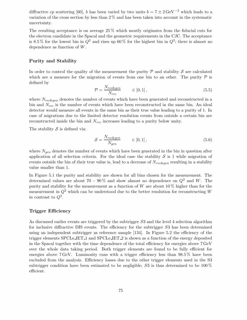
diffractive ep scattering [60], b has been varied by two units b = 7 ± 2GeV−2 which leads to avariation of the cross section by less than 2% and has been taken into account in the systematicuncertainty.

The resulting acceptance is on average 25% which mostly originates from the fiducial cuts forthe electron candidate in the Spacal and the geometric requirements in the CJC. The acceptanceis 8.5% for the lowest bin in Q2 and rises up 60% for the highest bin in Q2; there is almost nodependence as function of W .

Purity and Stability

In order to control the quality of the measurement the purity P and stability S are calculatedwhich are a measure for the migration of events from one bin to an other. The purity P isdefined by

P =Nrec&gen

Nrec∈ [0, 1] , (5.5)

where Nrec&gen denotes the number of events which have been generated and reconstructed in abin and Nrec is the number of events which have been reconstructed in the same bin. An idealdetector would measure all events in the same bin as their true value leading to a purity of 1. Incase of migrations due to the limited detector resolution events from outside a certain bin arereconstructed inside the bin and Nrec increases leading to a purity below unity.

The stability S is defined via:

S =Nrec&gen

Ngen∈ [0, 1] , (5.6)

where Ngen denotes the number of events which have been generated in the bin in question afterapplication of all selection criteria. For the ideal case the stability S is 1 while migration ofevents outside the bin of their true value is, lead to a decrease of Nrec&gen resulting in a stabilityvalue smaller than 1.

In Figure 5.1 the purity and stability are shown for all bins chosen for the measurement. Thedetermined values are about 70 − 90% and show almost no dependence on Q2 and W . Thepurity and stability for the measurement as a function of W are about 10% higher than for themeasurement in Q2 which can be understood due to the better resolution for reconstructing Win contrast to Q2.

Trigger Efficiency

As discussed earlier events are triggered by the subtrigger S3 and the level 4 selection algorithmfor inclusive diffractive DIS events. The efficiency for the subtrigger S3 has been determinedusing an independent subtrigger as reference sample [134]. In Figure 5.2 the efficiency of thetrigger elements SPCLe IET 1 and SPCLe IET 2 is shown as a function of the energy depositedin the Spacal together with the time dependence of the total efficiency for energies above 7GeVover the whole data taking period. Both trigger elements are found to be fully efficient forenergies above 7GeV. Luminosity runs with a trigger efficiency less than 98.5% have beenexcluded from the analysis. Efficiency losses due to the other trigger elements used in the S3subtrigger condition have been estimated to be negligible; S3 is thus determined to be 100%efficient.

75

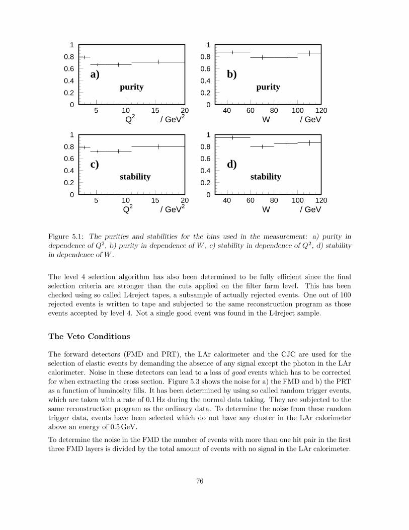
0

0.2

0.4

0.6

0.8

1

5 10 15 200

0.2

0.4

0.6

0.8

1

40 60 80 100 120

0

0.2

0.4

0.6

0.8

1

5 10 15 20

Q2 / GeV2

puritya)

W / GeV

purityb)

Q2 / GeV2

stabilityc)

W / GeV

stabilityd)

0

0.2

0.4

0.6

0.8

1

40 60 80 100 120

Figure 5.1: The purities and stabilities for the bins used in the measurement: a) purity independence of Q2, b) purity in dependence of W , c) stability in dependence of Q2, d) stabilityin dependence of W .

The level 4 selection algorithm has also been determined to be fully efficient since the finalselection criteria are stronger than the cuts applied on the filter farm level. This has beenchecked using so called L4reject tapes, a subsample of actually rejected events. One out of 100rejected events is written to tape and subjected to the same reconstruction program as thoseevents accepted by level 4. Not a single good event was found in the L4reject sample.

The Veto Conditions

The forward detectors (FMD and PRT), the LAr calorimeter and the CJC are used for theselection of elastic events by demanding the absence of any signal except the photon in the LArcalorimeter. Noise in these detectors can lead to a loss of good events which has to be correctedfor when extracting the cross section. Figure 5.3 shows the noise for a) the FMD and b) the PRTas a function of luminosity fills. It has been determined by using so called random trigger events,which are taken with a rate of 0.1Hz during the normal data taking. They are subjected to thesame reconstruction program as the ordinary data. To determine the noise from these randomtrigger data, events have been selected which do not have any cluster in the LAr calorimeterabove an energy of 0.5GeV.

To determine the noise in the FMD the number of events with more than one hit pair in the firstthree FMD layers is divided by the total amount of events with no signal in the LAr calorimeter.

76

a)

b)

Figure 5.2: Efficiency of the trigger elements SPCLe IET 1 (full triangles) and SPCLe IET 2open triangles) [134]: a) Efficiency in dependence of the cluster energy; b) Efficiency of thetrigger element SPCLe IET 1 and SPCLe IET 2 for energies above 4GeV as function of theluminosity run for the complete data taking period. Single runs with an efficiency less than98.5% are excluded from the analysis.

For the PRT the number of events with any hit is divided by the total number of events withno cluster in the LAr calorimeter.

As can be inferred from Figure 5.3 the data taking period 1997 is divided into five periods fromwhich only data of the periods II and IV have been used in the analysis. The noise for theseperiods has been determined to be 5.3 ± 1.5%. The origin of the noise is synchrotron radiationfrom the positron beam which can be investigated in further detail by studying the contributionfrom each layer of the FMD. It turned out that the dominant contribution to the noise comesfrom the most forward layer which is exposed most to the synchrotron radiation. A short phase

77

in period IV with a higher noise level than for the rest of the period. has been traced backto wrong collimator settings upstream the electron beam which were designed to protect thedetector from synchrotron radiation. The noise in the PRT can be savely neglected since it isalways well below 0.5%.

0

10

20

30

40

50

60

1250 1300 1350 1400 1450 1500 1550# lumi fill

FM

D n

oise

/ %

a)

I

II III IV V

# lumi fill

PR

T n

oise

/ %

b)I II III IV V

0

10

20

30

40

50

60

1250 1300 1350 1400 1450 1500 1550

Figure 5.3: Noise in the forward detectors as function of the lumi fill number: a) noise in theforward muon detector (FMD); b) noise in the proton remnant tagger (PRT). The five differentregions correspond to different detector conditions for the data taking. I) Problems in the FMDreadout leading to an abnormal high noise rate; II) normal data taking; III) Problems in thePRT readout; IV) normal data taking; V) change of trigger setup. The solid line in a) indicatesthe fitted noise of 5.3%. The error of 1.5% is shown by the dashed lines.

Period I has been neglected due to severe read out problems in the FMD which led to a mixingof the FMD signals from different events. The effect results in an increase of the noise up to40 − 50%. Period III has not been used in the analysis due to malfunctioning of the PRTleading to an increase of its noise to an abnormal high level. Period V has been excluded from

78

the analysis since no appropriate trigger setup was available for DVCS events.

The noise in the LAr calorimeter has already been taken into account when determining theacceptance A. The H1 detector simulation overlaps randomly triggered events from the LArcalorimeter during the event simulation. These noise events have been recorded in special runsthroughout the data taking.

A further correction of 3.5±2.0% originates from a read out problem in the CJC which consistedin the mixing of signals from different events in the recorded event. Some wire signals wereactually taken from the event triggered directly before the event in question eventually leadingto fake hits. These wrong hits mostly led to a reconstructed track resulting in a rejection ofthe event in this analysis. Since this error happened randomly for different (small) regions ofthe CJC the influence on the analysis was found to be small and could be corrected for. Thecorrection factor of 3.5% has been determined from an event sample of randomly triggeredevents.

Proton Dissociation Background

The selection criteria have been chosen such that the contribution from proton dissociationevents is suppressed. Especially the cuts on the forward detectors (FMD and PRT) have beendesigned for a rejection of inelastic DVCS events. Due to their limited geometrical and kinematicacceptance there is however still a sizable background from this process present.

This has been estimated from the relative amount of untagged (events which survive the cutson the FMD and PRT) and tagged events (events which have signals in the forward detectors)in combination with the efficiency to tag events from elastic and proton dissociation processes.The total number of events Ntot can be written as the sum of untagged and tagged events

Ntot = Nuntagged +Ntagged. (5.7)

At the same time Ntot is also given by the sum of elastic and proton dissociation events

Ntot = Nel. +Ndiss.. (5.8)

Note that Ndiss. denotes only proton dissociation events which leave no signal in the main de-tector, neither the CJC nor the LAr calorimeter. Therefore this method cannot be used todetermine the cross section for the proton dissociation process. When introducing the proba-bilities Pdiss−tag and Pel−tag which denote the probability to tag proton dissociation and elasticevents, respectively, the following formula can be derived

Nel =Nuntagged −Ntot · (1 − Pdiss−tag)

Pdiss−tag − Pel−tag. (5.9)

The numbers Nuntagged and Ntot are derived from data. The tagging efficiencies Pdis−tag andPel−tag have been determined using the DIFFVM MC program in combination with the H1detector simulation. The DIFFVM program offers the possibility to generate the four vectorsof all particles in the hadronic final state which is not possible for the TINTIN program whichgenerates only elastic events. The DIFFVM program has been run in the ρ–meson mode whichshould have no influence on the analysis since it is expected that the cross section for generatingan excited mass MY of the proton has the same shape for ρ meson production as for DVCS. Inchapter 4 it was discussed that the forward detectors are correctly described by the H1 detector

79

simulation (see Figure 4.3). Therefore the simulation can be used to determine the two taggingefficiencies in question. Using this method the following results have been derived

Pdiss−tag = 0.56,

Pel−tag = 0.005.

The uncertainty on the extraction of the proton dissociation background has been estimatedby varying the FMD efficiency by ±4% and the PRT efficiency by ±25% where the value forthe FMD is justified by the differences between the data and the MC prediction. The largevariation for the PRT originates from the large correction which had to be applied to get agood description of the data by the MC simulations. The final result for the proton dissociationbackground which has to be subtracted from the data is 16 ± 8%.

Background from ω and φ Production

It was found (see chapter 4) that background from diffractive electro–production of ω and φmesons contributes to the enriched DVCS sample. This is statistically subtracted bin by bin. Ithas been estimated using the DIFFVM MC program that this background contributes by about3.5% in average being less than 6% for any of the used bins. The prediction from the DIFFVMMC program has been normalised to measured cross sections [132, 63, 68].

Radiative Corrections

The cross section has been corrected for QED initial state radiation (ISR), i.e. for the collinearemission of photons off the incoming electron, which for HERA kinematics represents the mostimportant contribution to the higher order QED corrections. The effect due to photon emissionfrom the outgoing electron can be neglected since such photons are radiated in the outgoingelectron direction and deposit thus their energy in the same cluster of calorimeter cells.

The factor (1 + δrad) (see equations 5.1 and 5.2) has been determined by the MC programTINTIN which was run with and without inclusion of initial state radiation. The earlier discussedcomparisons between data and MC predictions as well as the determination of the acceptancehave been performed with a DVCS MC sample including ISR. The correction factor 1+ δrad cannow be calculated using the relation

1 + δrad =σBorn

DV CS

σBorn+ISRDV CS

(5.10)

where σBornDV CS denotes the cross section on the born level and σBorn+ISR

DV CS the cross section includ-ing ISR as estimated using the MC program. This correction was determined bin wise and foundto be about 3% independent of Q2 and W . This small value justifies the cut

∑E−Pz > 45GeV

since δrad would be about 10% without this requirement.

5.2 The ep Cross Section

All variables of equations 5.1 and 5.2 having estimated, the cross section can be calculated. Themeasured differential cross section of the reaction ep −→ eγp is shown in Figure 5.4 as a function

80

of Q2 and W and compared to the contribution from the Bethe-Heitler process. The data pointsare given with the statistical error (inner error bars) and the statistical and systematic error (seebelow) added in quadrature (outer error bars). The measured cross section is observed to bequite different in shape and normalisation in comparison to the expectation for the Bethe–Heitlerprocess. When fitting the Q2 dependence of the cross section with a function

f(Q2

)= a ·

(1

Q2

)n

. (5.11)

The parameter n was found1 to be n = 2.47 ± 0.14 which significantly differs from n = 2.0expected for the Bethe–Heitler process. For the measured cross section as function of W thedifference in shape is even more evident. For large values of W corresponding to the electron andthe photon being scattered into the backward direction, the Bethe–Heitler process dominatesthe cross section. Its contribution to the cross section decreases rapidly towards small values ofW whereas the measured cross section however tends to be rather constant.

As discussed in chapter 2 the interference term contributing to the cross section is proportional tocosφR where φR is the angle between the electron scattering and photon production plane in thephoton–proton centre of mass system. Since the measurement is performed for all values of φR

(see below for a detailed discussion) the interference term cancels. Hence the observed differencebetween the measured cross section and the contribution from the Bethe–Heitler process can beentirely attributed to the DVCS process. As the cosφR dependence follows from the helicitydependence of the QCD matrix element it is assumed to be true for all models (e.g. dipolemodels) which do not aim to predict the interference term and only provide results for the pureDVCS contribution.

5.3 Systematic Errors

In this section the systematic uncertainties and their influence on the measurement will bediscussed. They are divided into two contributions, one which covers all global systematicuncertainties shared by all data points and one with the bin dependent uncertainties. Theglobal uncertainties taken into account are:

• Luminosity measurement: 1.5%,

• Noise determination for the FMD: 1.5%,

• Noise determination for the CJC noise (event mixing induced): 2%,

• Subtraction of the proton dissociation background: 8%,

• Uncertainty on the acceptance correction (including the change of acceptance by varyingthe t-slope): 4%.

When added in quadrature, they add up to a total global uncertainty of 9.4%.

The bin dependent uncertainties are derived by varying the relevant measurement related quan-tities (e.g. energy scales) within their experimental uncertainties (in positive and negativ di-rection) taking the maximal deviation of the resulting cross section as systematic error. The

1Note that the cross section has not been corrected for the bin centre. It was however found that changingthe centre for single bins does only marginally influence the results of the fit.

81

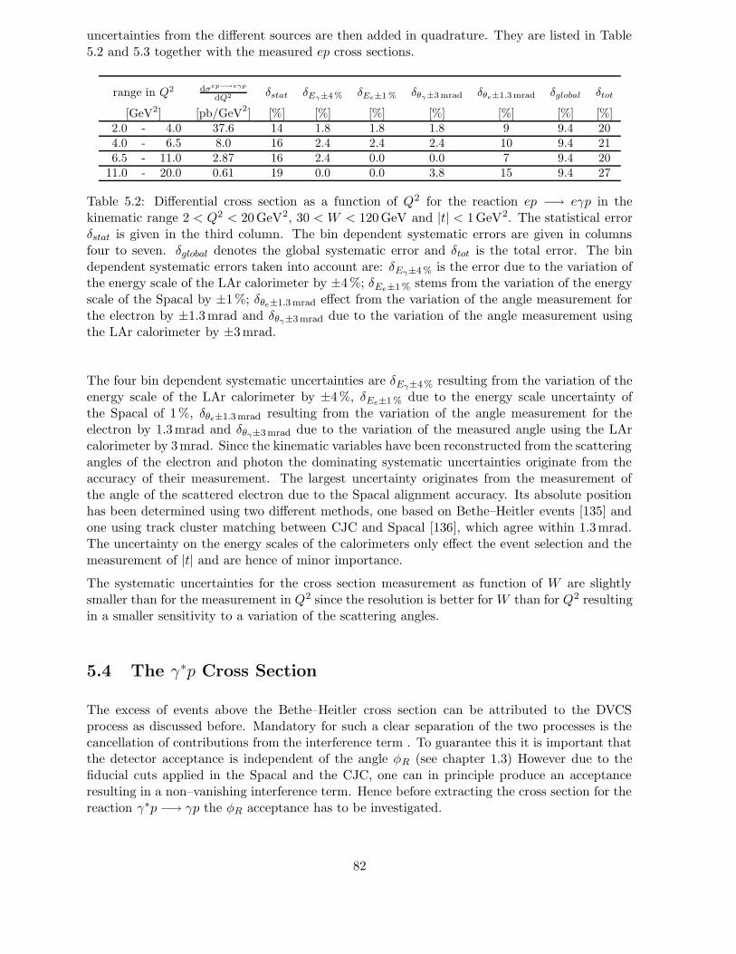
uncertainties from the different sources are then added in quadrature. They are listed in Table5.2 and 5.3 together with the measured ep cross sections.

range in Q2 dσep−→eγp

dQ2 δstat δEγ±4% δEe±1 % δθγ±3mrad δθe±1.3mrad δglobal δtot

[GeV2] [pb/GeV2] [%] [%] [%] [%] [%] [%] [%]

2.0 - 4.0 37.6 14 1.8 1.8 1.8 9 9.4 204.0 - 6.5 8.0 16 2.4 2.4 2.4 10 9.4 216.5 - 11.0 2.87 16 2.4 0.0 0.0 7 9.4 20

11.0 - 20.0 0.61 19 0.0 0.0 3.8 15 9.4 27

Table 5.2: Differential cross section as a function of Q2 for the reaction ep −→ eγp in thekinematic range 2 < Q2 < 20GeV2, 30 < W < 120GeV and |t| < 1GeV2. The statistical errorδstat is given in the third column. The bin dependent systematic errors are given in columnsfour to seven. δglobal denotes the global systematic error and δtot is the total error. The bindependent systematic errors taken into account are: δEγ±4 % is the error due to the variation ofthe energy scale of the LAr calorimeter by ±4%; δEe±1 % stems from the variation of the energyscale of the Spacal by ±1%; δθe±1.3 mrad effect from the variation of the angle measurement forthe electron by ±1.3mrad and δθγ±3 mrad due to the variation of the angle measurement usingthe LAr calorimeter by ±3mrad.

The four bin dependent systematic uncertainties are δEγ±4 % resulting from the variation of theenergy scale of the LAr calorimeter by ±4%, δEe±1 % due to the energy scale uncertainty ofthe Spacal of 1%, δθe±1.3 mrad resulting from the variation of the angle measurement for theelectron by 1.3mrad and δθγ±3 mrad due to the variation of the measured angle using the LArcalorimeter by 3mrad. Since the kinematic variables have been reconstructed from the scatteringangles of the electron and photon the dominating systematic uncertainties originate from theaccuracy of their measurement. The largest uncertainty originates from the measurement ofthe angle of the scattered electron due to the Spacal alignment accuracy. Its absolute positionhas been determined using two different methods, one based on Bethe–Heitler events [135] andone using track cluster matching between CJC and Spacal [136], which agree within 1.3mrad.The uncertainty on the energy scales of the calorimeters only effect the event selection and themeasurement of |t| and are hence of minor importance.

The systematic uncertainties for the cross section measurement as function of W are slightlysmaller than for the measurement in Q2 since the resolution is better for W than for Q2 resultingin a smaller sensitivity to a variation of the scattering angles.

5.4 The γ∗p Cross Section

The excess of events above the Bethe–Heitler cross section can be attributed to the DVCSprocess as discussed before. Mandatory for such a clear separation of the two processes is thecancellation of contributions from the interference term . To guarantee this it is important thatthe detector acceptance is independent of the angle φR (see chapter 1.3) However due to thefiducial cuts applied in the Spacal and the CJC, one can in principle produce an acceptanceresulting in a non–vanishing interference term. Hence before extracting the cross section for thereaction γ∗p −→ γp the φR acceptance has to be investigated.

82

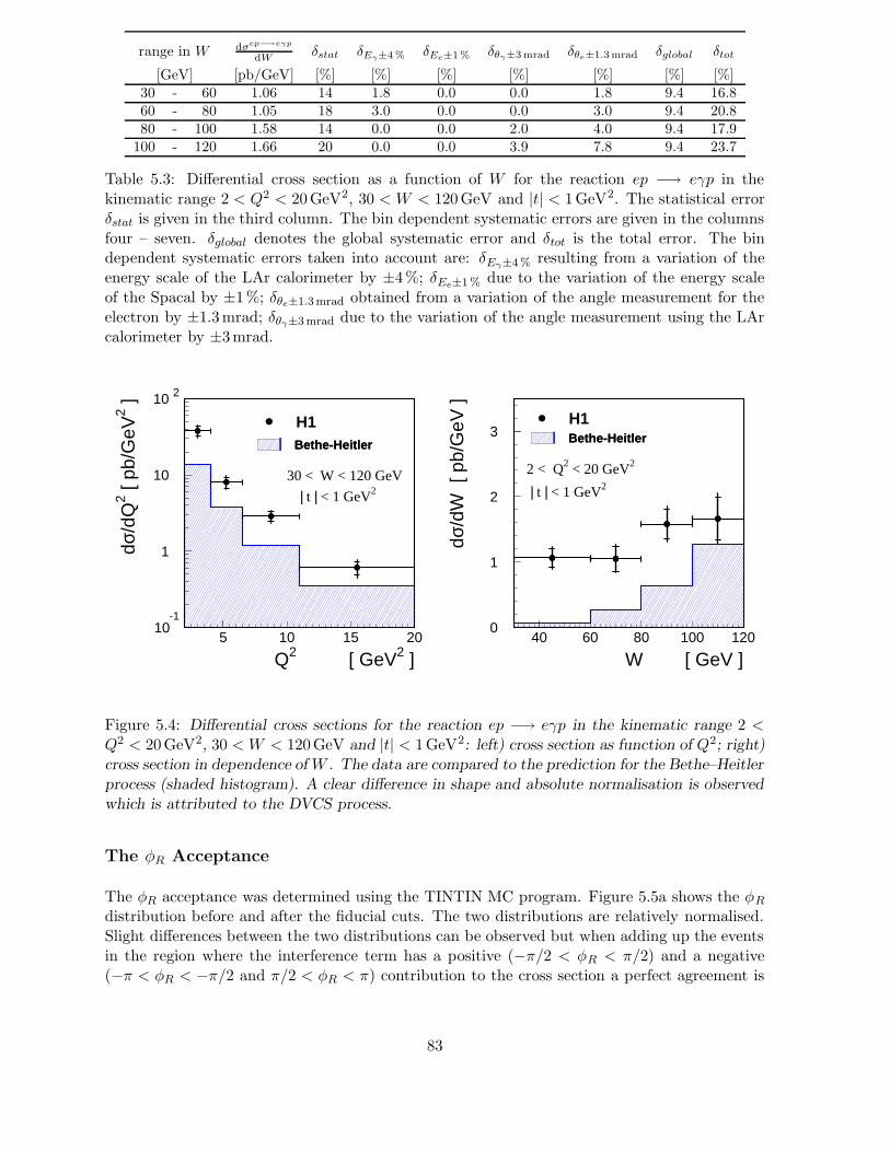
range in W dσep−→eγp

dWδstat δEγ±4 % δEe±1% δθγ±3mrad δθe±1.3mrad δglobal δtot

[GeV] [pb/GeV] [%] [%] [%] [%] [%] [%] [%]30 - 60 1.06 14 1.8 0.0 0.0 1.8 9.4 16.860 - 80 1.05 18 3.0 0.0 0.0 3.0 9.4 20.880 - 100 1.58 14 0.0 0.0 2.0 4.0 9.4 17.9

100 - 120 1.66 20 0.0 0.0 3.9 7.8 9.4 23.7

Table 5.3: Differential cross section as a function of W for the reaction ep −→ eγp in thekinematic range 2 < Q2 < 20GeV2, 30 < W < 120GeV and |t| < 1GeV2. The statistical errorδstat is given in the third column. The bin dependent systematic errors are given in the columnsfour – seven. δglobal denotes the global systematic error and δtot is the total error. The bindependent systematic errors taken into account are: δEγ±4 % resulting from a variation of theenergy scale of the LAr calorimeter by ±4%; δEe±1 % due to the variation of the energy scaleof the Spacal by ±1%; δθe±1.3 mrad obtained from a variation of the angle measurement for theelectron by ±1.3mrad; δθγ±3 mrad due to the variation of the angle measurement using the LArcalorimeter by ±3mrad.

10 -1

1

10

10 2

5 10 15 20

H1 Bethe-Heitler Bethe-Heitler

30 < W < 120 GeV

| t | < 1 GeV 2

Q 2 [ GeV 2 ]

d σ /d

Q 2 [

pb/G

eV 2 ]

0

1

2

3

40 60 80 100 120

H1 Bethe-Heitler Bethe-Heitler

2 < Q 2 < 20 GeV 2

| t | < 1 GeV 2

W [ GeV ]

d σ /d

W [

pb/

GeV

]

Figure 5.4: Differential cross sections for the reaction ep −→ eγp in the kinematic range 2 <Q2 < 20GeV2, 30 < W < 120GeV and |t| < 1GeV2: left) cross section as function of Q2; right)cross section in dependence of W . The data are compared to the prediction for the Bethe–Heitlerprocess (shaded histogram). A clear difference in shape and absolute normalisation is observedwhich is attributed to the DVCS process.

The φR Acceptance

The φR acceptance was determined using the TINTIN MC program. Figure 5.5a shows the φR

distribution before and after the fiducial cuts. The two distributions are relatively normalised.Slight differences between the two distributions can be observed but when adding up the eventsin the region where the interference term has a positive (−π/2 < φR < π/2) and a negative(−π < φR < −π/2 and π/2 < φR < π) contribution to the cross section a perfect agreement is

83

observed (see Figure 5.5 b). Thus the acceptance is such that the contribution of the interferenceterm to the cross section indeed cancels.

0

0.02

0.04

0.06

-2 0 2φr / rad

arb.

uni

ts

II IIIa) before cuts

after cutsI II

b)

Σ

arb.

uni

ts

0

0.2

0.4

0 0.5 1 1.5 2

Figure 5.5: a) Distribution of the angle φR for a MC simulation before and after application ofthe fiducial cuts. Both distributions are relatively normalised. The region I denotes the regionπ/2 < φR < π/2 where the interference term of the Bethe–Heitler and the DVCS process hasa positive contribution to the cross section. In the region II the interference term leads to anegative contribution to the cross section. b) Sum of events for the regions I and II (see text fordiscussion).

Extraction of the γ∗p Cross Section

Before one can extract the cross section for the reaction γ∗p −→ γp the Bethe–Heitler contribu-tion has to be subtracted from the measured electron–proton cross section. This has been doneusing the BH cross section prediction of the COMPTON 2.0 program; the values are listed inTable 5.4.

Q2–domain dσBH

dQ2 W–domain dσBH

dW

[GeV2] [pb/GeV2] [GeV] [pb/GeV]2.0 - 4.0 13.82 30 - 60 0.074.0 - 6.5 3.75 60 - 80 0.276.5 - 11.0 1.20 80 - 100 0.63

11.0 - 20.0 0.35 100 - 120 1.27

Table 5.4: The cross sections for the Bethe–Heitler contribution to the electron–proton crosssection as calculated with the COMPTON 2.0 program as function of Q2 for 30 < W < 120GeVand as function of W for 2 < Q2 < 20GeV2 both for |t| < 1GeV2.

After the subtraction of the Bethe–Heitler contribution the photon–proton cross section can beobtained using the following formula based on the decomposition of the electron–proton crosssection into a photon flux and the photon–proton cross section

dσep−→eγp

dQ2dy

(Q2, y

)= Γ

(Q2, y

)· σγ∗p−→γp

(Q2, y

)(5.12)

84

where Γ is the flux of virtual photons emitted from the incoming electron. It can be approximatedfor low y using the Hand convention [137]

Γ =αem

(1 − y + y2

2

)

πyQ2. (5.13)

Here αem represents the electromagnetic coupling constant. Note that while the electron–protoncross section is differential in Q2 and y, the photon–proton cross section is not.

Using these formulae the photon–proton cross section can be obtained by the following method.When integrating the differential electron–proton cross section one gets

∫ Q2max

Q2min

∫ ymax

ymin

d2σep−→eγp

dQ2dydQ2dy = σep−→eγp =

CtotN

L (5.14)

where Ctot includes all corrections as discussed before (see equations 5.1 and 5.2), N is thenumber of events in the bin under consideration and L is the integrated luminosity of the datasample. Hence σep−→eγp is nothing else but the measured differential electron–proton crosssection multiplied with the bin width. When integrating the right side of equation 5.12 oneobtains the following relation:

σep−→eγp =

∫ Q2max

Q2min

∫ ymax

ymin

Γ(Q2, y

)· σγ∗p−→γp

(Q2, y

)dQ2dy. (5.15)

This relation cannot be simplified further since both Γ(Q2, y

)and σγ∗p−→γp

(Q2, y

)depend on

Q2 and y. Therefore the γ∗p cross section has to be parameterised. In vector meson productionthe following factorised ansatz has been successfully used [60]:

σγ∗p−→γp(Q2, y

)= A · ya ·

(1

Q2

)n

(5.16)

with two free parameters a and n. The normalisation factor A can be obtained using this ansatzand solving equation 5.15. Finally one gets the following expression for the photon–proton crosssection:

σγ∗p−→γp(Q2

0, y0

)=CtotN

L · 1

B· ya

0 ·(

1

Q20

)n

(5.17)

with

B =αem

π

∫ ymax

ymin

dy ya 1 − y + y2

2

y

∫ Q2max

Q2min

dQ2 1

Q2

(1

Q2

)n

. (5.18)

When calculating the photon–proton cross section as function of Q2, the bin boundaries Q2max

and Q2min are chosen as the boundaries of the corresponding bin for the electron–proton cross

section. The y–range is chosen such that it corresponds to the full W–region of the measurement(W 2 ≈ ys

). For the measurement of the photon–proton cross section as function of W the

integration over y corresponds to the bins in W of the electron–proton cross section and theintegration over Q2 is performed for the full range of the measurement. The cross sectionσγ∗p−→γp

(Q2

0, y0

)is the photon–proton cross section at y0 and Q2

0. It is not possible to extractthe photon–proton cross section and the free parameters a and n at the same time. Therefore aniterative method has been chosen with reasonable starting values a0 and n0. By this procedurethe γ∗p cross section has been extracted and the Q2 and y dependences have been fitted to

85

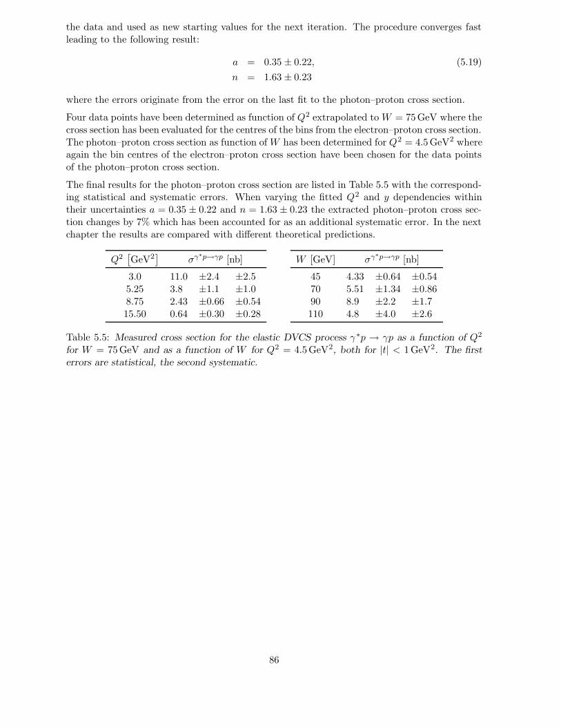
the data and used as new starting values for the next iteration. The procedure converges fastleading to the following result:

a = 0.35 ± 0.22, (5.19)

n = 1.63 ± 0.23

where the errors originate from the error on the last fit to the photon–proton cross section.

Four data points have been determined as function of Q2 extrapolated to W = 75GeV where thecross section has been evaluated for the centres of the bins from the electron–proton cross section.The photon–proton cross section as function of W has been determined for Q2 = 4.5GeV2 whereagain the bin centres of the electron–proton cross section have been chosen for the data pointsof the photon–proton cross section.

The final results for the photon–proton cross section are listed in Table 5.5 with the correspond-ing statistical and systematic errors. When varying the fitted Q2 and y dependencies withintheir uncertainties a = 0.35 ± 0.22 and n = 1.63 ± 0.23 the extracted photon–proton cross sec-tion changes by 7% which has been accounted for as an additional systematic error. In the nextchapter the results are compared with different theoretical predictions.

Q2[GeV2

]σγ∗p→γp [nb] W [GeV] σγ∗p→γp [nb]

3.0 11.0 ±2.4 ±2.5 45 4.33 ±0.64 ±0.545.25 3.8 ±1.1 ±1.0 70 5.51 ±1.34 ±0.868.75 2.43 ±0.66 ±0.54 90 8.9 ±2.2 ±1.715.50 0.64 ±0.30 ±0.28 110 4.8 ±4.0 ±2.6

Table 5.5: Measured cross section for the elastic DVCS process γ∗p → γp as a function of Q2

for W = 75GeV and as a function of W for Q2 = 4.5GeV2, both for |t| < 1GeV2. The firsterrors are statistical, the second systematic.

86

Chapter 6

Discussion of the Results

In this chapter the measured photon–proton cross section of the DVCS process will be comparedto different theoretical predictions of which few exist at present.

In Figure 6.1 the measurement is compared to the calculation of Frankfurt, Freund and Strikman(FFS) [97] and the prediction from Donnachie and Dosch (DD) [100]. The cross section ismeasured as function of Q2 for W = 75GeV and |t| < 1GeV2 and as function of W forQ2 = 4.5GeV2 and |t| < 1GeV2. The data are presented as points with statistical errors (innererror bars) and statistical and systematic uncertainties added in quadrature (outer error bars).Since the calculations are performed for t = tmin an exponential function dσ

dt ∼ e−b|t| for theunknown |t| dependence has been assumed with 5 < b < 9GeV−2 which corresponds to therange measured in vector meson production at HERA and is assumed to be a reasonable rangefor DVCS. This leads to a normalisation uncertainty of the predictions since the cross sectionis integrated over t The upper bound for the predictions corresponds to b = 5GeV−2 whereasthe lower bound is given by b = 9GeV−2. Within this uncertainty the data are well describedby the theoretical calculations. The absolute normalisation is best for large values of b. For amore definite statement on the normalisation a measurement of the t–slope has however to beperformed.

In the model of Frankfurt, Freund and Strikman the cross section was calculated at a normalisa-tion point Q2

0 using the aligned jet model and the evolution to higher values of Q2 was performedusing leading order evolution kernels for generalised parton distributions. Thus at low values ofQ2 effects of the skewedness have been neglected while they are generated at higher values of Q2

by the evolution procedure. Within the present accuracy of the data this method is succesfull,most probably due to the small skewedness expected for low values of Q2 and its effect on thecross section calculation. This observation is in agreement with the measurement of the crosssection for light vector meson production where the data can be explained without includingeffects due to generalised parton distributions.

The model of Donnachie and Dosch is based on the dipole approach where the virtual photon isassumed to fluctuate into a quark antiquark system which subsequently interacts with the protonand then recombines to the real photon. The dipole cross section has been modelled within theframework of the two pomeron approach where small dipoles interact predominantly with thehard pomeron and large dipoles with the soft pomeron. The free parameters of this model havebeen determined from proton–proton scattering experiments and inclusive diffraction data fromHERA measurements. The prediction for DVCS itself has no free parameter.

87

H1DVCS (FFS)

DVCS (DD)

W = 75 GeV

| t | < 1 GeV2

Q2 [ GeV2 ]

10-1

1

10

0 5 10 15 20

σγ∗ p

→ γ

p [n

b]

H1DVCS (FFS)DVCS (DD)

Q2 = 4.5 GeV2

| t | < 1 GeV2

W [ GeV ]

0

5

10

15

20

25 50 75 100 125

σγ∗ p

→ γ

p [n

b]

Figure 6.1: The measurement of the photon–proton cross section of the DVCS process γ ∗p −→ γpin the kinematic range 2 < Q2 < 20GeV2, 30 < W < 120GeV and |t| < 1GeV2 in comparisonto theoretical predictions from Frankfurt, Freund and Strikman (FFS) [97] and Donnachie andDosch (DD) [100]. The error bars denote the statistical error (inner) and the quadratic sum ofthe statistical error and the systematic uncertainty (outer): left) Cross section as a function ofthe photon virtuality Q2 for W = 75GeV; right) cross section as function of the photon–protoncentre of mass energy W for Q2 = 4.5GeV2. An exponential |t| dependence dσ

dt ∼ e−b|t| leadingto a normalisation uncertainty indicated by the band for the predictions, has been assumed with5 < b < 9GeV−2. The upper bound of the prediction corresponds to b = 5GeV−2 and the lowerbound is given by b = 9GeV−2.

The model of Donanchie and Dosch predicts a systematicaly lower cross section for the DVCSprocess in the low Q2 region

(Q2 < 8GeV2

)which leads to an even better agreement with the

data. To further investigate the validity of this model more precise data are needed.

Figure 6.2 shows the measurement in comparison with the predictions based on the dipoleapproach from Forshaw, Kerley and Shaw (FKS) [102, 103] and McDermott, Frankfurt, Guzeyand Strikman (MFGS) [102, 104]. Again the calculations are performed for t = tmin and hencean exponential t–dependence has been assumed with the t–slope b = 7GeV−2. When changingthe t–slope b to smaller or larger values again the normalisation changes. Although both dipolemodels depend on very different assumptions they provide an excellent description of the dataexcept at large values of Q2 where the MFGS prediction tends to be larger than the data. Theparameters of these models have been determined from fits to the diffractive structure function

FD(3)2 and vector meson production cross sections. They exhibit no free parameter for the

DVCS prediction. This can be interpreted as a tight connection existing between the differentdiffractive processes on which these models are based. In order to investigate these models infurther detail again more precise data are needed.

88

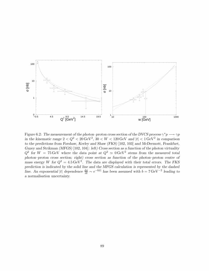
−0.5 4.5 9.5 14.5 19.5Q

2 [GeV

2]

0

1

10

100

σ [n

b]

10 100 1000w [GeV]

1

10

100

σ [n

b]

Figure 6.2: The measurement of the photon–proton cross section of the DVCS process γ ∗p −→ γpin the kinematic range 2 < Q2 < 20GeV2, 30 < W < 120GeV and |t| < 1GeV2 in comparisonto the predictions from Forshaw, Kerley and Shaw (FKS) [102, 103] and McDermott, Frankfurt,Guzey and Strikman (MFGS) [102, 104]: left) Cross section as a function of the photon virtualityQ2 for W = 75GeV where the data point at Q2 ' 0GeV2 stems from the measured totalphoton–proton cross section; right) cross section as function of the photon–proton centre ofmass energy W for Q2 = 4.5GeV2. The data are displayed with their total errors. The FKSprediction is indicated by the solid line and the MFGS calculation is represented by the dashedline. An exponential |t| dependence dσ

dt ∼ e−b|t| has been assumed with b = 7GeV−2 leading toa normalisation uncertainty.

89

Summary

In this thesis the first measurement of the cross section for elastic Deeply Virtual ComptonScattering (DVCS) in ep collisions has been presented. The data have been taken with the H1experiment at the electron–proton collider HERA. For ep scattering the DVCS process representsthe scattering of a virtual photon off a proton (γ∗p −→ γp) where the virtual photon is emitted bythe incoming electron. In a QCD based approach the process can be interpreted as a scatteringof the photon off a quark from the proton and thus delivers a clean tool to investigate the protonstructure. In particular the process resides its interest from the potential access it delivers tothe generalised parton densities. A complication of the measurement is that the Bethe–Heitler(BH) process where the electron scatters elastically off the proton and a photon is emitted bythe electron has the same signature and is thus indistinguishable from the DVCS process underinvestigation. However the BH cross section is calculable to high precision in the framework ofQED and thus can be subtracted statistically.

The DVCS signal has been established by the selection of events with one electron and one photoncandidate measured with the H1 detector in a region of phase space where DVCS is expectedto dominate. The data sample was taken in the 1997 data taking period and corresponds toan integrated luminosity of 8 pb−1. A large excess of events over the prediction for the Bethe–Heitler process is observed. To assure the quality of the measurement the detector response hasbeen controlled with a data sample dominated by Bethe–Heitler events.

Using a newly developed DVCS MC program, within the scope of this thesis, the differentialelectron–proton cross section for the reaction ep −→ eγp has been extracted as a function of thephoton virtuality Q2 and the photon–proton centre of mass energy W in the kinematic range2 < Q2 < 20GeV2, 30 < W < 120GeV and |t| < 1GeV2 where t denotes the squared momentumtransfer at the proton vertex. The cross section has been corrected for several background anddetector effects. After subtraction of the contribution of the Bethe–Heitler process the electron–proton cross section has been converted to a photon–proton cross section as function of Q2 andW . Within the present accuracy QCD based as well as semiclassical models are able to describethe measured cross sections. The main results of this analysis have been published [141].

In order to achieve further progress future measurements with more precise data are needed.This goal can be achieved due to the expected increase of luminosity after the HERA upgradeand the usage of newly installed detectors yielding a decrease of the systematic uncertainties.It is of particular interest to measure the t–dependence of the cross section to overcome thenormalisation problem of the theoretical predictions. In addition a measurement of the azimuthalangle asymmetry would provide access to the real part of the QCD amplitude and informationon the generalised parton densities.

90

Appendix A

TINTIN: A DVCS MC program

The MC program TINTIN developed within the scope of this analysis generates the four vectorsof the final state particles for events of the reaction ep −→ eγp and calculates the cross sectionin a given kinematic range based on the predictions of Frankfurt, Freund and Strikman (seeChapter 2.2). The generated four vectors are interfaced to the H1 detector simulation.

The TINTIN program is based on the Monte Carlo technique (see e.g. [138]) using an acceptance–rejection–method. According to the predicted cross section, the kinematic variables

(Q2, y, t, φ

)

are generated from which the four vectors of the final state particles are reconstructed. Theemission of real photons from the incident lepton which is expected to be the largest higherorder QED correction for HERA kinematics can optionally be chosen. The implemented photonradiation is based on the collinear approximation [139, 140].

The TINTIN program is implemented in the H1 generator software environment and consists of11 subroutines. A steering file provides the input to the program (see Table A.1) and the outputis written to FPACK–files where the events are stored in form of BOS–banks the H1 internaldata format. The basic routines of the program are:

• TINMain routine of the TINTIN program which is called from the H1 generator software.

• TININIInitialisation of all parameters for the event generation.

• TINCHAThe routine reads the steering card and changes the parameters for the event generation.

• TINEVTMain routine of the event loop. It generates the number of events as required in thesteering file.

– QED ISRSubroutine which generates the emission of a real photon from the incoming electronline according to the collinear approximation.

– KINCHARoutine which recalculates the kinematic variables according to the energy of theemitted photon from the incident electron.

91

– KINGENRoutine which generates the variables Q2, y, t and φ taking the boundary values (e.g.tmin) correctly into account.

– CALCSIGCalculation of the cross section for the generated point in phase space according tothe calculations of Frankfurt, Freund and Strikman.

– CALCKINCalculation of the four vectors of the outgoing particles.

At the end of the event loop the decision is taken whether a generated event is acceptedor rejected according to the defined phase space region.

• TINFILLInterface to the H1 generator software for the four vectors of the final state particles.

• TINYENDCalculation of the cross section and final book keeping.

100 ! NEVT ! Number of events to be generated-1 ! SIGN ! lepton beam (+1=electron, -1=positron)1 ! ITYP ! generation type(1=sum, 2=BH, 3=DVCS)1 ! IRAD ! ISR-flag (0=off/1=on)

1.5 ! Q2MIN ! minimum Q2 [GeV**2]1000.0 ! Q2MAX ! maximum Q2 [GeV**2]0.0001 ! YMIN ! minimum y

1.0 ! YMAX ! maximum y1.0E-5 ! XMIN ! minimum x

1.0 ! XMAX ! maximum x2.0 ! TMAX ! max t

27.5 ! ELEP ! lepton energy [GeV]820.0 ! EPROT ! proton energy [GeV]0.55 ! R ! IM A(g*p->g*p)/IM A(g*p->gp)4.5 ! B ! t-slope [GeV**-2]0.0 ! THLMIN ! minimal lepton angle [grad]

178.0 ! THLMAX ! maximal lepton angle [grad]15.0 ! ELMIN ! minimal lepton energy [GeV]0.0 ! THGMIN ! minimal photon angle [grad]

177.0 ! THGMAX ! maximal photon angle [grad]0.3 ! EGMIN ! minimal photon energy [GeV]0.0 ! EIMIN ! minimal ISR photon energy [GeV]

Table A.1: Typical steering file with the list of parameters which have to be chosen for the eventgeneration.

92

Acknowledgements

I would like to thank Prof. Dr.D. Wegener for the opportunity to work on this thesis and hissupport during the last years especially for the stay abroad. Many useful suggestions and criticalquestions lead to improvements of this thesis.

I thank Prof. Dr. J. Sacton for the possibility to work for 1.5 years at the Brussels instituteand Dr. L. Favart for his supervision of the data analysis. I profited very much from the manydiscussions we had about DVCS and other physics topics.

During the last years I enjoyed very much to work in the Dortmund as well as in the Brusselsgroup which both had an excellent spirit leading to a very good working atmosphere and oftenbeyond. In particular I want to thank O. Behrendt, C. Collard, G. Contreras, R. Heremans, G.Herrera, C. Issever (especially for her efforts on the computing system which ensured very stableworking conditions), X. Janssen (for the collaboration when producing the ntuples and manyuseful discussions about proton dissociation), V. Lendermann, D. Luke, P. Marage (who hadalways a good idea for the analysis), M. Mondragon, J. Naumann, R. Poschl (He and Jurgenshared my passion for things which are sometimes almost as important as physics althoughthey follow the wrong ideology.), A. Vargas, K. Wacker and C. Wissing (for his efforts on thecomputing system and his patience when answering many of my computing questions).

Special thanks go to H.C. Schultz-Coulon for the close collaboration over the last years, espe-cially for many motivating discussions during the hard times and for the careful reading of themanuscript.

I thank my colleagues from H1 and in particular the diffractive working group who contributedwith many useful suggestions to this analysis. Among many others I would like to thank J.Gayler and R. Wallny for extensive discussions about the LAr calorimeter and the Spacal electronmeasurement. The help of D. Schmidt was very useful for the calibration study.

During the time when I worked on the trigger I profited from the very intense support of J.C.Bizot who also introduced me to the art of thinking in hexadecimal.

I thank M. Diehl for his patience when explaining me, during many hours, all the details aboutgeneralised parton distributions. He kindly read two chapters of this thesis.

I would like to thank the Graduiertenkolleg “Erzeugung und Zerfalle von Elementarteilchen” fora scholarship and the possibility to attend several Summer Schools and Conferences. The timein Brussels was financed by a scholarship from the Deutscher Akademischer Austauschdienstand subsequently the Martin Schmeißer Stiftung for which I am grateful. The work of theDortmund group was supported by the Bundesministerium fur Bildung, Wissenschaft, Forschungund Technologie (contract number 057DO55 and 05H11PEA).

93

Bibliography

[1] R. G. Roberts, “The Structure Of The Proton”, Cambridge Univ. Pr., 1990.

[2] H. Abramowicz and A. Caldwell, Rev. Mod. Phys. 71 (1999) 1275 [arXiv:hep-ex/9903037].

[3] A. Levy, DESY-97-013 Lectures given at Strong Interaction Study Days, Kloster Banz,Germany, 10-12 Oct 1995.

[4] M. Gockeler, R. Horsley, D. Pleiter, P. E. Rakow and G. Schierholz, arXiv:hep-ph/0108105.

[5] C. Adloff et al. [H1 Collaboration], Eur. Phys. J. C 21 (2001) 33 [arXiv:hep-ex/0012053].



[8] J. Breitweg et al. [ZEUS Collaboration], Eur. Phys. J. C 12 (2000) 411 [arXiv:hep-ex/9907010].

[9] S. Chekanov et al. [ZEUS Collaboration], arXiv:hep-ex/0105090.

[10] A. C. Benvenuti et al. [BCDMS Collaboration], Phys. Lett. B 223 (1989) 485.

[11] M. R. Adams et al. [E665 Collaboration], Phys. Rev. D 54 (1996) 3006.

[12] M. Arneodo et al. [New Muon Collaboration (NMC)], Nucl. Phys. B 483 (1997) 3.

[13] E. D. Bloom et al., Phys. Rev. Lett. 23 (1969) 930.

[14] M. Breidenbach et al., Phys. Rev. Lett. 23 (1969) 935.

[15] J. D. Bjorken, Phys. Rev. 179 (1969) 1547.

[16] J. D. Bjorken and E. A. Paschos, Phys. Rev. 185 (1969) 1975.

[17] R. P. Feynman, Phys. Rev. Lett. 23 (1969) 1415.

[18] R. P. Feynman, Photon Hadron Interactions, Bejamin 1972.

[19] D. J. Fox et al., Phys. Rev. Lett. 33 (1974) 1504.

[20] H. D. Politzer, Phys. Rev. Lett. 30 (1973) 1346.

[21] D. J. Gross and F. Wilczek, Phys. Rev. D 8 (1973) 3633.

[22] D. J. Gross and F. Wilczek, Phys. Rev. Lett. 30 (1973) 1343.

94

[23] D. J. Gross and F. Wilczek, Phys. Rev. D 9 (1974) 980.

[24] M. Gell-Mann, Phys. Lett. 8 (1964) 214.

[25] G. Zweig, CERN-TH-412.

[26] J. C. Collins, D. E. Soper and G. Sterman, Nucl. Phys. B 261 (1985) 104.

[27] J. R. Forshaw and D. A. Ross, “Quantum chromodynamics and the pomeron”, CambridgeUniv. Pr., 1997.

[28] Y. L. Dokshitzer, Sov. Phys. JETP 46 (1977) 641 [Zh. Eksp. Teor. Fiz. 73 (1977) 1216].

[29] V. N. Gribov and L. N. Lipatov, Yad. Fiz. 15 (1972) 781 [Sov. J. Nucl. Phys. 15 (1972)438].

[30] V. N. Gribov and L. N. Lipatov, Yad. Fiz. 15 (1972) 1218 [Sov. J. Nucl. Phys. 15 (1972)675].

[31] G. Altarelli and G. Parisi, Nucl. Phys. B 126 (1977) 298.

[32] K. G. Wilson, Phys. Rev. 179 (1969) 1499.

[33] E. A. Kuraev, L. N. Lipatov and V. S. Fadin, Sov. Phys. JETP 44 (1976) 443 [Zh. Eksp.Teor. Fiz. 71 (1976) 840].

[34] E. A. Kuraev, L. N. Lipatov and V. S. Fadin, Sov. Phys. JETP 45 (1977) 199 [Zh. Eksp.Teor. Fiz. 72 (1977) 377].

[35] I. I. Balitsky and L. N. Lipatov, Sov. J. Nucl. Phys. 28 (1978) 822 [Yad. Fiz. 28 (1978)1597].

[36] M. Ciafaloni, Nucl. Phys. B 296 (1988) 49.

[37] G. Marchesini, Nucl. Phys. B 445 (1995) 49 [arXiv:hep-ph/9412327].

[38] S. Catani, F. Fiorani and G. Marchesini, Nucl. Phys. B 336 (1990) 18.

[39] C. Adloff et al. [H1 Collaboration], Nucl. Phys. B 538 (1999) 3 [arXiv:hep-ex/9809028].

[40] C. Adloff et al. [H1 Collaboration], Phys. Lett. B 462 (1999) 440 [arXiv:hep-ex/9907030].

[41] M. Gluck, E. Reya and A. Vogt, Z. Phys. C 53 (1992) 127.

[42] M. Gluck, E. Reya and A. Vogt, Eur. Phys. J. C 5 (1998) 461 [arXiv:hep-ph/9806404].

[43] M. Botje, arXiv:hep-ph/0110123.

[44] A. B. Kaidalov, Phys. Rept. 50 (1979) 157.

[45] G. Alberi and G. Goggi, Phys. Rept. 74 (1981) 1.

[46] K. Goulianos, Phys. Rept. 101 (1983) 169.

[47] P. D. Collins, “An Introduction To Regge Theory And High-Energy Physics”, CambridgeUniv. Pr., 1977.

95

[48] A. Donnachie and P. V. Landshoff, Phys. Lett. B 296 (1992) 227 [arXiv:hep-ph/9209205].

[49] G. Ingelman and P. E. Schlein, Phys. Lett. B 152 (1985) 256.

[50] R. Bonino et al. [UA8 Collaboration], Phys. Lett. B 211 (1988) 239.

[51] A. Brandt et al. [UA8 Collaboration], Phys. Lett. B 297 (1992) 417.

[52] T. Ahmed et al. [H1 Collaboration], Nucl. Phys. B 429 (1994) 477.

[53] T. Ahmed et al. [H1 Collaboration], Nucl. Phys. B 435 (1995) 3.

[54] M. Derrick et al. [ZEUS Collaboration], Phys. Lett. B 346 (1995) 399 [arXiv:hep-ex/9501011].

[55] M. Derrick et al. [ZEUS Collaboration], Phys. Lett. B 315 (1993) 481.

[56] J. C. Collins, Phys. Rev. D 57 (1998) 3051 [Erratum-ibid. D 61 (1998) 019902] [arXiv:hep-ph/9709499].

[57] C. Adloff et al. [H1 Collaboration], Z. Phys. C 76 (1997) 613 [arXiv:hep-ex/9708016].


[59] C. Adloff et al. [H1 Collaboration], arXiv:hep-ex/0108047.





[64] J. Breitweg et al. [ZEUS Collaboration], Phys. Lett. B 437 (1998) 432 [arXiv:hep-ex/9807020].


[66] J. Breitweg et al. [ZEUS Collaborations], Eur. Phys. J. C 12 (2000) 393 [arXiv:hep-ex/9908026].


[68] J. Breitweg et al. [ZEUS Collaboration], arXiv:hep-ex/0006013.

[69] J. J. Sakurai, Annals Phys. 11 (1960) 1.


[71] M. G. Ryskin, Z. Phys. C 57 (1993) 89.

[72] A. Kreisel, talk at DIS, Bologna, 2001

[73] F. E. Low, Phys. Rev. D 12 (1975) 163.

96

[74] S. Nussinov, Phys. Rev. Lett. 34 (1975) 1286.

[75] J. C. Collins, L. Frankfurt and M. Strikman, Phys. Rev. D 56 (1997) 2982 [arXiv:hep-ph/9611433].

[76] X. Ji, W. Melnitchouk and X. Song, Phys. Rev. D 56 (1997) 5511 [arXiv:hep-ph/9702379].

[77] B. Geyer, D. Robaschik, M. Bordag and J. Horejsi, Z. Phys. C 26 (1985) 591.

[78] T. Braunschweig, B. Geyer, J. Horejsi and D. Robaschik, Z. Phys. C 33 (1986) 275.

[79] F. M. Dittes, D. Muller, D. Robaschik, B. Geyer and J. Horejsi, Phys. Lett. B 209 (1988)325.

[80] D. Muller, D. Robaschik, B. Geyer, F. M. Dittes and J. Horejsi, Fortsch. Phys. 42 (1994)101 [arXiv:hep-ph/9812448].

[81] P. Jain and J. P. Ralston, arXiv:hep-ph/9305250.

[82] X. Ji, Phys. Rev. Lett. 78 (1997) 610 [arXiv:hep-ph/9603249].

[83] X. Ji, Phys. Rev. D 55 (1997) 7114 [arXiv:hep-ph/9609381].

[84] A. V. Radyushkin, Phys. Rev. D 56 (1997) 5524 [arXiv:hep-ph/9704207].

[85] M. Diehl, T. Feldmann, R. Jakob and P. Kroll, Eur. Phys. J. C 8 (1999) 409 [arXiv:hep-ph/9811253].

[86] A. V. Radyushkin, Phys. Lett. B 380 (1996) 417 [arXiv:hep-ph/9604317].

[87] A. V. Radyushkin, arXiv:hep-ph/0101225.

[88] V. Y. Petrov, P. V. Pobylitsa, V. Polyakov, I. Bornig, K. Goeke and C. Weiss, Phys. Rev.D 57 (1998) 4325 [arXiv:hep-ph/9710270].

[89] M. Penttinen, V. Polyakov and K. Goeke, Phys. Rev. D 62 (2000) 014024 [arXiv:hep-ph/9909489].

[90] V. Polyakov and C. Weiss, Phys. Rev. D 60 (1999) 114017 [arXiv:hep-ph/9902451].

[91] A. D. Martin, M. G. Ryskin and T. Teubner, Phys. Lett. B 454 (1999) 339 [arXiv:hep-ph/9901420].

[92] G. P. Lepage and S. J. Brodsky, Phys. Lett. B 87 (1979) 359.

[93] A. V. Efremov and A. V. Radyushkin, Phys. Lett. B 94 (1980) 245.

[94] J. C. Collins and A. Freund, Phys. Rev. D 59 (1999) 074009 [arXiv:hep-ph/9801262].

[95] M. Diehl, T. Gousset, B. Pire and J. P. Ralston, Phys. Lett. B 411 (1997) 193 [arXiv:hep-ph/9706344].

[96] A. Freund, Nucl. Phys. Proc. Suppl. 79 (1999) 368 [arXiv:hep-ph/9905233].

[97] L. L. Frankfurt, A. Freund and M. Strikman, Phys. Rev. D 58 (1998) 114001 [Erratum-ibid.D 59 (1998) 119901] [arXiv:hep-ph/9710356].

97

[98] L. L. Frankfurt and M. I. Strikman, Phys. Rept. 160 (1988) 235.

[99] G. R. Kerley and M. McDermott, J. Phys. G G26 (2000) 683 [arXiv:hep-ph/0001050].

[100] A. Donnachie and H. G. Dosch, Phys. Lett. B 502 (2001) 74 [arXiv:hep-ph/0010227].


[102] M. McDermott, R. Sandapen and G. Shaw, arXiv:hep-ph/0107224.

[103] J. R. Forshaw, G. Kerley and G. Shaw, Phys. Rev. D 60 (1999) 074012 [arXiv:hep-ph/9903341].

[104] M. McDermott, L. Frankfurt, V. Guzey and M. Strikman, Eur. Phys. J. C 16 (2000) 641[arXiv:hep-ph/9912547].

[105] A. Freund and M. F. McDermott, arXiv:hep-ph/0106115.



[108] R. S. Thorne, A. D. Martin, W. J. Stirling and R. G. Roberts, arXiv:hep-ph/0106075.

[109] H. Abramowicz and A. Levy, arXiv:hep-ph/9712415.

[110] T. Carli, A. Courau, S. Kermiche and P. Kessler, In Proceedings, Physics at HERA, vol.3, 1468-1472, Hamburg, 1991.

[111] A. Courau, S. Kermiche, T. Carli and P. Kessler, In Proceedings, Physics at HERA, vol.2, 902-915, Hamburg, 1991.

[112] A. Courau and P. Kessler, Phys. Rev. D 46 (1992) 117.

[113] B. List and A. Mastroberardino, Prepared for Workshop on Monte Carlo Generators forHERA Physics (Plenary Starting Meeting), Hamburg, Germany, 27-30 Apr 1998.

[114] T. Abe, Comput. Phys. Commun. 136 (2001) 126 [arXiv:hep-ph/0012029].

[115] G. A. Schuler and H. Spiesberger, In Proceedings, Physics at HERA, vol. 3, 1419-1432,Hamburg, 1991.

[116] G. Marchesini, B. R. Webber, G. Abbiendi, I. G. Knowles, M. H. Seymour and L. Stanco,Comput. Phys. Commun. 67 (1992) 465.

[117] C. Wissing, “Bestimmung der Charakteristika des Flugzeitsystems des H1–Detektors zurMessung des Strahluntergrundes” (In German), Diploma thesis, Universitat Dortmund,1998.

[118] H1 Collaboration, I. Abt et al., Nucl. Instrum. Methods A 3 86(1997) 310 and 348.

[119] B. Andrieu et al. [H1 Calorimeter Group Collaboration], Nucl. Instrum. Meth. A 336

(1993) 460.

[120] R. D. Appuhn et al. [H1 SPACAL Group Collaboration], Nucl. Instrum. Meth. A 386

(1997) 397.

98

[121] T. Nicholls et al. [H1 SPACAL Group Collaboration], Nucl. Instrum. Meth. A 374 (1996)149.

[122] P. Van Esch et al., Nucl. Instrum. Meth. A 446 (2000) 409 [arXiv:hep-ex/0001046].

[123] M. Dirkmann, “Messung der diffraktiven Strukturfunktion FD(3)2 des Protons bei kleinen

Impulsubertragen mit dem H1-Detektor” (In German), Dissertation, Universitat Dort-mund, 1998.

[124] R. Stamen, talk at DPG, Heidelberg, 1999

[125] R. Stamen, talk at the H1 trigger Workshop, Schloß Ringberg, 2000

[126] R. Brun, R. Hagelberg, M. Hansroul and J. C. Lassalle, CERN-DD-78-2-REV.

[127] M. Dirkmann, “Untersuchungen an einem Spaghetti–Kalorimeter unter besondererBerucksichtigung des inneren Randbereiches und des Nachweises von Pi-Mesonen” (In Ger-man), Diploma thesis, Universitat Dortmund, 1995.

[128] B. Heinemann, “Measurement of charged current and neutral current cross sections inpositron proton collisions at

√s ≈ 300GeV”, Dissertation, Universitat Hamburg, 1999,

DESY-THESIS-1999-046.

[129] D. Schmidt, “Diffractive photoproduction of charmonium in the H1 detector at HERA”(In German), Dissertation, Universitat Hamburg, 2001, DESY-THESIS-2001-029.

[130] P. D. Thompson, “Open Charm Production in Inclusive and Diffractive Deep–InelasticScattering at HERA”, Dissertation, University of Birmingham, 1999.

[131] X. Janssen, private communication.

[132] V. Lendermann, “Measurement of the QED Compton Scattering Cross Section with theH1 Detector at HERA”, Dissertation, Universitat Dortmund, 2001.

[133] G. Kallen, Elementary Particle Physics, Addison–Wesley Publ. Comp.

[134] R. Wallny, “Measurement and QCD analysis of the structure function F2

(x,Q2

)”, Disser-

tation, Universitat Zurich, 2001.

[135] R. Stamen, “Analyse quasireeller QED-Compton–Ereignisse” (In German), Diploma the-sis, Universitat Dortmund, 1998.

[136] A. Glazov, “Measurement of the Proton Structure Functions F2

(x,Q2

)and FL

(X,Q2

)

with H1 Detector at HERA”, Dissertation, Humboldt–Universitat Berlin, 1998.

[137] L. N. Hand, Phys. Rev. 129 (1963) 1834.

[138] R. Y. Rubinstein, “Simulation and the Monte Carlo Method”, John Wiley and Sons, Inc.,New York, 1981.

[139] G. Pancheri, P. Touschek, Nuovo Cim. B 51 (1962) 216.

[140] G. Pancheri, Nuovo Cim. A 60 (1963) 321.


99

Measurement of deeply virtual Compton scattering at HERA

Documents

Transcript of Measurement of deeply virtual Compton scattering at HERA