arX

iv:h

ep-p

h/01

1147

2v2

14

Feb

2002

A detailed next-to-leading order QCD analysis of deeply virtual Compton scattering

observables

Andreas Freund∗

Institut fur Theoretische Physik, Univ. Regensburg, Universitatstr. 31, 93053 Regensburg , Germany

Martin McDermott†

Division of Theoretical Physics, Dept. Math. Sciences, Univ. of Liverpool, Liverpool, L69 3BX, UK

We present a detailed next-to-leading order (NLO) leading twist QCD analysis of deeply virtualCompton scattering (DVCS) observables, for several different input scenarios, in the MS scheme. Wediscuss the size of the NLO effects and the behavior of the observables in skewedness ζ, momentumtransfer, t, and photon virtuality, q2 = −Q2. We present results on the amplitude level for un-polarized and longitudinally polarized lepton probes, and unpolarized and longitudinally polarizedproton targets. We make predictions for various asymmetries and for the DVCS cross section andcompare with the available data.

I. INTRODUCTION

In the quest for understanding the structure of hadrons, hard, exclusive lepton-nucleon processes have emerged asvery promising candidates to further constrain the dynamical degrees of freedom of hadronic matter. Experimentally,such processes are typified by a clear spatial separation of the scattered final state nucleon and the diffractively-produced, exclusive system, X , i.e. by the presence of a large rapidity gap. The hard scale required for a perturbativeanalysis is either provided by the spacelike virtuality, Q2 = −q2 ≫ Λ2

QCD, of the exchanged photon, a heavy quarkmass, or by a large momentum transfer to the hadron in the t-channel, t ≪ 0. Deeply virtual Compton scattering(DVCS) [1–13], γ∗(q) + p(P ) → γ(q′) + p(P ′), is the most promising1 of these processes. One reason for this isthat on the lepton level it interferes with a competing QED process, known as the Bethe-Heitler (BH) process, inwhich the final state photon is radiated from either the initial or final state lepton. The associated interferenceterm offers the unique possibility to directly measure both the imaginary and real parts of QCD amplitudes, viavarious angular asymmetries. A factorization theorem has been proven for the DVCS process [6,7] which relates theexperimentally-accessible amplitudes to a new class of fundamental functions, called generalized parton distributions(GPDs) [1–3,15–17], which encode detailed information about the partonic structure of hadrons.

GPDs are an extension of the well-known parton distribution functions (PDFs) appearing in inclusive processes suchas deep inelastic scattering (DIS), or Drell-Yan, and encode additional information about the partonic structure ofhadrons, above and beyond that of conventional PDFs. They are defined as the Fourier transforms of non-local light-cone operators2 sandwiched between nucleon states of different momenta3, commensurate with a finite momentumtransfer in the t-channel to the final state proton. As such, the GPDs depend on four variables (X, ζ, Q2, t) ratherthan just two (X, Q2) as is the case for regular PDFs. This allows an extended mapping of the dynamical behavior of anucleon in the two extra variables, skewedness ζ, and momentum transfer, t. In fact, knowledge of the behavior of theGPDs in these two extra variables would allow one to obtain, for the first time, a three dimensional map of the protonin terms of its partonic constituents. The GPDs are true two-particle correlation functions, whereas the PDFs areeffectively only one-particle distributions. They contain, in addition to the usual PDF-type information residing in theso-called “DGLAP region” [18] (for which the momentum fraction variable is larger than the skewedness parameter,X > ζ), supplementary information about the distribution amplitudes of virtual “meson-like” states in the nucleonin the so-called “ERBL region” [19] (X < ζ).

∗andreas.freund@physik.uni-regensburg.de†martinmc@amtp.liv.ac.uk1The fact that the produced real photon is an elementary quantum state eliminates the need for further non-perturbative

information, which is required for example in exclusive vector meson production [14]. This simplifies the theoretical treatmentconsiderably.

2compared to local operators in inclusive reactions.3in inclusive reactions the momenta are the same.

1

A good knowledge of GPDs is required to establish the boundary conditions for a large class of exclusive processescalculable in QCD. Unfortunately, reliable perturbative calculations can only be made if t is either small or large,confining a sensible comparison between theory and experiment to restricted kinematical regions where either thet-dependence is a purely nonperturbative function (small t, large Q2) as in DVCS or the Q2-dependence is mainlynon perturbative (small Q2, large t) as in, for example, large-t photoproduction of a real photon (wide angle DVCS)[20]. In light of this observation, one might question the practicality of studying and measuring these exclusivedistributions, given that inclusive PDFs may only be constrained well via a global analysis of a large number of datapoints from numerous experiments.

It turns out that the GPDs are rather more tightly constrained than one might naively assume [21]. Firstly, they areobliged to reproduce the regular PDFs in the forward limit ζ → 0 [1–3]. Secondly, they are each required to be eithersymmetric or antisymmetric about the point X = ζ/2 in the ERBL region, and they have to obey a polynomialityconstraint (see for example [22]). These are properties which need to be preserved under evolution. Lastly, theDVCS amplitudes, and thus certain observables, seem to be very sensitive to the shape of the GPD in the small ζregion, especially the real part of DVCS amplitudes [23,24]. Hence, experimental measurements of DVCS observables,even of only moderate statistics, appear to give a good opportunity to pin-down the GPDs, given these theoreticalrestrictions. Therefore a careful, thorough and accurate theoretical analysis of DVCS is necessary to understand howvarying the input GPDs affects the physical observables and the quantitative and qualitative changes in going fromleading order (LO) to next-to-leading order (NLO) accuracy in perturbation theory. In this paper, we present sucha NLO analysis, in the MS-scheme, for both polarized and unpolarized scattering, and explore some of the necessaryissues required to make an optimal extraction of the GPDs from current and future data.

The physical picture emerging for DVCS is also very interesting in its own right. Several important questionsimmediately arise. What does the energy and Q2-dependence of DVCS reveal about the nature of diffractive exchangeand how does it compare to other diffractive processes ? Why does DVCS appear to have significant probability inthe valance region at larger x, i.e. outside of the region in which generic diffraction usually occurs ? Is the physicalpicture for DVCS the same in both regions ? We will attempt a partial answer to these questions in the following.

This paper gives a comprehensive analysis of DVCS observables at NLO accuracy. Complementary informationmay be found in [21,23,24]. To bring our analysis right up to date, we introduce unpolarized input GPDs based on twoof the most recent PDF sets, CTEQ5M [25] and MRST99 [26] (in addition to GRV98 [27], and the older MRSA’ [28]used in our earlier publications). This allows us to push our input scale for skewed evolution down to Q0 = 1 GeV.For the purposes of comparison we also present the results for DVCS observables obtained using our earlier inputmodels. Various computer codes used in our analysis our available from the HEPDATA website [29].

This paper is structured as follows. In section II we reiterate the kinematics of DVCS and BH and define theDVCS observables, i.e. various measurable angular asymmetries and cross sections. In section III we describe thevarious input GPDs and present numerical results for the NLO evolution [15,30] of the new sets. Section IV discusseshow the various DVCS amplitudes are produced via convolution integrals of GPDs with coefficient functions. Wepresent the Q2 and ζ-dependence of the unpolarized amplitudes for the new sets graphically. In section V we giveour predictions for the DVCS observables in ζ, Q2 and t, for various polarizations of probe and target, as well asdiscussing their implications. We compare our results with the currently available data and with other theoreticalpredictions in section VI. Finally, we briefly conclude in section VII.

N(P )e�(k)

N(P 0) (q0)e�(k0)

�(q)a) N(P )

e�(k)N(P 0) �(�)

e�(k0) (q0)b) N(P )

e�(k)N(P 0)

(q0)e�(k0) �(�) )

FIG. 1. a) DVCS graph, b) BH with photon from final state lepton and c) with photon from initial state lepton.

II. KINEMATICS AND OBSERVABLES FOR DVCS AND BH

2

A. Kinematics and frame definition

The lepton level process, e±(k, κ) N(P, S) → e±(k′, κ′) N(P ′, S′) γ(q′, ǫ′), receives contributions from each of thegraphs shown in Fig. 1. The corresponding differential cross section is given by4:

dσDV CS+BH =1

4k · P|T ±|2(2π)4δ(4)(k + P − k′ − P ′ − q′)

d3k′

2k′0(2π)3d3P′

2P ′0(2π)3d3q′

2q′0(2π)3, (1)

where the square of the amplitude receives contributions from pure DVCS (Fig. 1a), from pure BH (Figs. 1b, 1c) andfrom their interference (with a sign governed by lepton charge),

|T ±|2 =∑

κ′,S′,ǫ′

[|T ±DV CS|

2 + (T ±∗DV CSTBH + T ±DV CST∗

BH) + |TBH |2]. (2)

The DVCS amplitude is given by

T ±DV CS = ±e3

q2ǫ′∗µ T µν u(k′)γνu(k)

{+ for e+

− for e−, (3)

where q = k − k′, ǫ′∗µ is the polarisation vector of the outgoing real photon, and the hadronic tensor, Tµν , is defined

by a time ordered product of two electromagnetic currents:

Tµν(q, P, P ′) = i

∫dxeix·q〈P ′, S′|T jµ(x/2)jν(−x/2)|P, S〉 , (4)

where q = (q + q′)/2. This hadronic tensor contains twelve5 independent kinematical structures [32] for a spin-1/2target. Here, we restrict ourselves to the twist-2 part of Tµν and drop all other terms of either kinematical or dynamicalhigher twist. From the structure of the operator product expansion (OPE) one can immediately conclude that, totwist-2 accuracy6, one has the following form factor decomposition:

Tµν(q, P, ∆) = −gµνq · V1

2P · q− iǫµνρσ

qρAσ1

2P · q, (5)

where P = (P + P ′)/2 and the gauge invariant tensors gµν = PµρgρσPσν and ǫµναβ = PµρǫρσαβPσν are constructedthrough the projection tensor Pµν ≡ gµν − qµq′ν/q · q′. The vector V µ

1 and axial-vector Aν1 are expressed, again to

twist-2 accuracy, through the following form factor decomposition,

V1µ = U(P ′, S′)

(H1γµ − E1

iσµν∆ν

2M

)U(P, S) , (6)

A1µ = U(P ′, S′)

(H1γµγ5 − E1

∆µγ5

2M

)U(P, S) , (7)

where U, U are spinors for the incoming and outgoing hadron state, ∆ = P − P ′ is the momentum transfered fromthe hadron7 and M is the hadron mass. The various Lorentz structures have associated amplitudes: H1, E1 areunpolarized helicity non-flip and helicity flip amplitudes, respectively, and H1, E1 are their polarized counterparts.These amplitudes are expressed, via the DVCS factorization theorem [6,7], as convolutions of a hard scatteringcoefficient function and a GPD. They depend on the following Lorentz-invariant variables:

ξ =Q2

2P · q, Q2 = −q2, t = ∆2 = (P − P ′)2 ,

4In this section we follow closely the notation of [31].512 = 1

2× 3 (virtual photon) × 2 (final photon) × 2 (initial nucleon) × 2 (final nucleon). The reduction factor 1/2 is a result

of parity invariance.6We drop a twist-2 contribution arising from a double helicity flip of the photon, i.e. going from helicity +1 to helicity −1

or vice versa, which is suppressed in αs since this double flip can only be mediated by gluons. Thus when we speak of twist-2contributions we really mean twist-2 modulo this double flip contribution.

7Note that there is a relative minus sign between our definition of ∆ and that of [31] (our definition is the same as r in [22]).

3

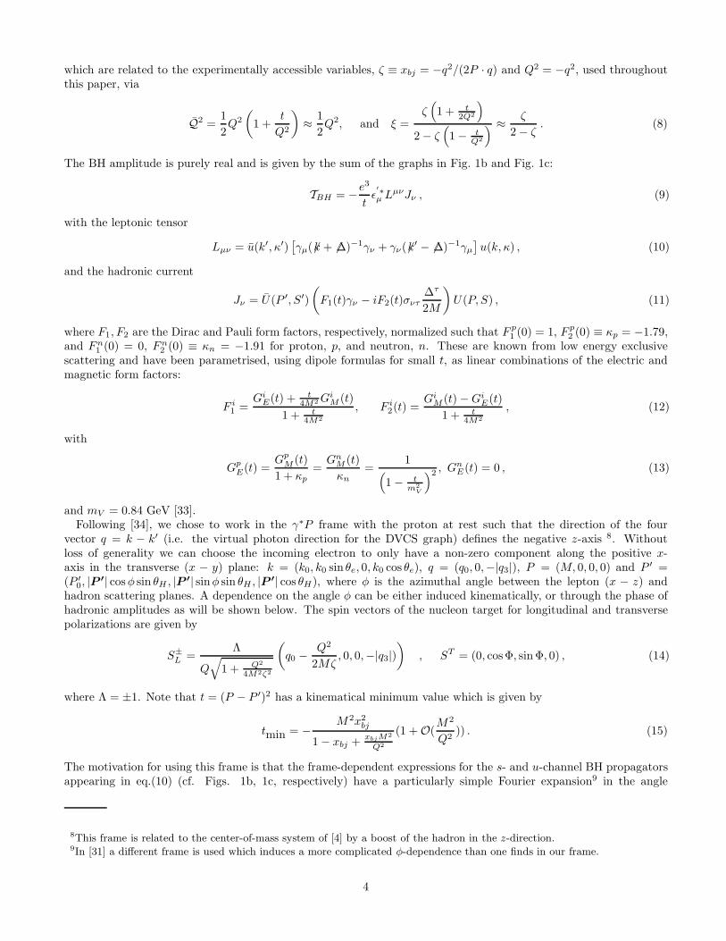
which are related to the experimentally accessible variables, ζ ≡ xbj = −q2/(2P · q) and Q2 = −q2, used throughoutthis paper, via

Q2 =1

2Q2

(1 +

t

Q2

)≈

1

2Q2, and ξ =

ζ(1 + t

2Q2

)

2− ζ(1− t

Q2

) ≈ ζ

2− ζ. (8)

The BH amplitude is purely real and is given by the sum of the graphs in Fig. 1b and Fig. 1c:

TBH = −e3

tǫ′∗µ LµνJν , (9)

with the leptonic tensor

Lµν = u(k′, κ′)[γµ(6k + 6∆)−1γν + γν(6k′ − 6∆)−1γµ

]u(k, κ) , (10)

and the hadronic current

Jν = U(P ′, S′)

(F1(t)γν − iF2(t)σντ

∆τ

2M

)U(P, S) , (11)

where F1, F2 are the Dirac and Pauli form factors, respectively, normalized such that F p1 (0) = 1, F p

2 (0) ≡ κp = −1.79,and Fn

1 (0) = 0, Fn2 (0) ≡ κn = −1.91 for proton, p, and neutron, n. These are known from low energy exclusive

scattering and have been parametrised, using dipole formulas for small t, as linear combinations of the electric andmagnetic form factors:

F i1 =

GiE(t) + t

4M2 GiM (t)

1 + t4M2

, F i2(t) =

GiM (t)−Gi

E(t)

1 + t4M2

, (12)

with

GpE(t) =

GpM (t)

1 + κp=

GnM (t)

κn=

1(1− t

m2V

)2 , GnE(t) = 0 , (13)

and mV = 0.84 GeV [33].Following [34], we chose to work in the γ∗P frame with the proton at rest such that the direction of the four

vector q = k − k′ (i.e. the virtual photon direction for the DVCS graph) defines the negative z-axis 8. Withoutloss of generality we can choose the incoming electron to only have a non-zero component along the positive x-axis in the transverse (x − y) plane: k = (k0, k0 sin θe, 0, k0 cos θe), q = (q0, 0,−|q3|), P = (M, 0, 0, 0) and P ′ =(P ′0, |P

′| cosφ sin θH , |P ′| sinφ sin θH , |P ′| cos θH), where φ is the azimuthal angle between the lepton (x − z) andhadron scattering planes. A dependence on the angle φ can be either induced kinematically, or through the phase ofhadronic amplitudes as will be shown below. The spin vectors of the nucleon target for longitudinal and transversepolarizations are given by

S±L =Λ

Q√

1 + Q2

4M2ζ2

(q0 −

Q2

2Mζ, 0, 0,−|q3|)

), ST = (0, cosΦ, sin Φ, 0) , (14)

where Λ = ±1. Note that t = (P − P ′)2 has a kinematical minimum value which is given by

tmin = −M2x2

bj

1− xbj +xbjM2

Q2

(1 +O(M2

Q2)) . (15)

The motivation for using this frame is that the frame-dependent expressions for the s- and u-channel BH propagatorsappearing in eq.(10) (cf. Figs. 1b, 1c, respectively) have a particularly simple Fourier expansion9 in the angle

8This frame is related to the center-of-mass system of [4] by a boost of the hadron in the z-direction.9In [31] a different frame is used which induces a more complicated φ-dependence than one finds in our frame.

4

φ. The dimensionless forms P1 = (k+∆)2

Q2 = t+2k·∆Q2 and P2 = (k−q′)2

Q2 = 1 − 2k·∆Q2 are (up to corrections of order

O((−t/Q2), (M2/Q2))):

P1 =1

y

{1 + 2

√(tmin − t)(1 − x)(1 − y)

Q2cosφ−

t

Q2(1− y − x(2 − y))− 2

M2x2

Q2(2 − y)

},

P2 = −1

y

{(1 − y) + 2

√(tmin − t)(1− x)(1 − y)

Q2cosφ−

t

Q2(1− x(2 − y))− 2

M2x2

Q2(2− y)

}. (16)

The product P1P2 appears in the BH and interference expressions and thus induces an additional kinematical (ratherthan hadronic) φ-dependence. In certain kinematical regions, this additional φ-dependence can fake certain hadronicφ-dependences [34], it can also lead to unwanted contributions in certain φ-asymmetries, as discussed below. One wayout of this dilemma is to weight DVCS observables with P1P2, leaving only the pure hadronic φ-dependence (exploitingthe orthogonality of cosφ and cosm′φ for integer m′ 6= 1). We will not do this here because such a weighting requiresa good φ resolution not available for the present data and also because the pure twist-2 contributions may well explainmost of the observed data without needing to take twist-3 or higher contributions into account. Nevertheless, studyingweighted DVCS observables should be done as soon as good experimental φ-resolution is available.

B. DVCS observables: differential cross section and asymmetries

After performing the phase space integration in eq.(1), the triple differential cross section on the lepton level isgiven by

dσ(3)(e±p→ e±γp)

dxbjdQ2d|t|=

∫ 2π

0

dφdσ(4)

dxbjdQ2d|t|dφ=

α3e.m.xbjy

2

8πQ4

(1 +

4M2x2bj

Q2

)−1/2 ∫ 2π

0

dφ|T ±|2 . (17)

The twist two expressions for the DVCS squared, interference and BH squared terms, for all probe and targetpolarizations, required for eq.(17) are very similar to eqs.(24-32) of [31] but with the full expressions for the BHpropagators of eq.(16) included to reinstate the correct y- and φ-dependence (a correction factor of −(1−y)/(y2P1P2)should be applied to eqs.(27-32) of [31]).

From the pure DVCS piece (following the usual single photon exchange flux factor convention adopted in [35]),changing variable from xbj to y and integrating over t, one may define the virtual-photon proton cross section via

dσ(2)(e±p→ e±γp)

dydQ2=

αe.m.(1 + (1− y)2)

2πQ2yσ(γ∗P → γP ) . (18)

We give predictions for σ(γ∗P → γP ) and compare with the recent experimental data from the H1 Collab. [10] insection VI.

We will now define various DVCS observables, in terms of a list of asymmetries in the azimuthal angle φ:

• The (unpolarized) azimuthal angle asymmetry (AAA), measured in the scattering of an unpolarized probe onan unpolarized target, is defined by

AAA =

∫ π/2

−π/2dφ(dσDV CS+BH − dσBH)−

∫ 3π/2

π/2dφ(dσDV CS+BH − dσBH)

∫ 2π

0dφdσDV CS+BH

, (19)

where dσBH is the pure BH term.

• The single spin asymmetry (SSA), measured in the scattering of a longitudinally polarized probe on an unpo-larized target, is defined by

SSA =

∫ π

0 dφ∆σDV CS+BH −∫ 2π

π dφ∆σDV CS+BH

∫ 2π

0dφ(dσDV CS+BH,↑ + dσDV CS+BH,↓)

, (20)

where ∆σ = dσ↑−dσ↓ and ↑ and ↓ signify that the lepton is polarized along or against its direction, respectively.

5

• The asymmetry of an unpolarized probe on a longitudinally polarized target (UPLT) is given by:

UPLT =

∫ π

0 dφ∆σDV CS+BHLT −

∫ 2π

π dφ∆σDV CS+BHLT∫ 2π

0 dφ(dσDV CS+BH↑ + dσDV CS+BH

↓ ), (21)

where ∆σLT = dσ↑ − dσ↓ with ↑ and ↓ signifying that the target is polarized along or against the +z-direction,respectively, corresponding to Λ = ∓1 in eq.(14).

• The asymmetry of an unpolarized probe on a transversely polarized target (UPTT) is given by:

UPTT =

∫ π

0 dφ∆σDV CS+BHTT −

∫ 2π

π dφ∆σDV CS+BHTT∫ 2π

0dφ(dσDV CS+BH

→ + dσDV CS+BH← )

, (22)

where ∆σTT = dσ→ − dσ← with → and ← signify that the target transverse polarization vector, ST , pointsalong the +x and −x directions (i.e. Φ = 0, π), respectively.

• The charge asymmetry (CA) in the scattering of an unpolarized probe on an unpolarized target:

CA =

∫ π/2

−π/2 dφ∆dCσDV CS+BH −∫ 3π/2

π/2 dφ∆dCσDV CS+BH

∫ 2π

0dφ(d+σDV CS+BH + d−σDV CS+BH)

, (23)

where ∆dCσ = d+σ− d−σ corresponds to the difference of the scattering with a positron probe and an electronprobe.

• The charge asymmetry with a double spin flip of a longitudinally polarized probe on a longitudinally polarizedtarget (CADSFL):

CADSFL =

∫ π/2

−π/2 dφ∆dCσDV CS+BH,LPLT −

∫ 3π/2

π/2 dφ∆dCσDV CS+BH,LPLT

∫ 2π

0 dφ(d+σDV CS+BH↑ + d−σDV CS+BH

↓ ), (24)

where ∆dCσLPLT = d+σ↑↑ − d−σ↓↓ −∆dCσ with d+σ↑↑ corresponding to a positron beam polarized along its own

direction scattering with a target with its polarization vector having a positive z-component, d−σ↓↓ correspondsto an electron beam polarized against its own direction scattering on target with its polarization vector havinga negative z-component and with ∆dCσ having the same meaning as for CA.

• The charge asymmetry with a double spin flip of a longitudinally polarized probe on a transversally polarizedtarget (CADSFT):

CADSFT =

∫ π/2

−π/2 dφ∆dCσDV CS+BH,LPTT −

∫ 3π/2

π/2 dφ∆dCσDV CS+BH,LPTT

∫ 2π

0 dφ(d+σDV CS+BH→ + d−σDV CS+BH

← ), (25)

where ∆dCσLPTT = d+σ↑→−d−σ↓←−∆dCσ, with d+σ↑→ corresponding to a positron beam polarized along its own

direction scattering on a target with a polarization vector pointing in the +x direction, d−σ↓← corresponds toan electron beam polarized against its own direction scattering on a target with a polarization vector pointingin the −x direction, and ∆dCσ having the same meaning as in CA.

The definitions above make the asymmetries directly proportional to the real part of a combination of DVCSamplitudes, in the case of the AAA, CA, CADSFT and CADSFL, and to the imaginary part of a combination ofDVCS amplitudes for SSA, UPTT and UPLT. If one forms the proper combinations from eqs.(24-32) of [31], withthe correction factor included, one observes that for small-x DVCS observables the information from transversallypolarized targets is redundant to the information from longitudinally polarized targets as far as the information onthe real and imaginary part of DVCS amplitudes is concerned. For large x, this is, strictly speaking, no longertrue! However, higher twist corrections, especially in the normalization of the asymmetries, will make extraction ofinformation on individual amplitudes virtually impossible. For this reason we will focus only on DVCS observables

6

which may be obtained using an unpolarized or longitudinally polarized target. Note that for small x and t, thesecombinations of amplitudes reduce to just the unpolarized (for AAA, CA and SSA) or polarized (for UPLT andCADSFL) helicity non-flip amplitudes [31]. Note also that the definition of the AAA is different from the usual one(see e.g. the first reference of [8]) and is designed to ensure that the numerator contains only the interference termand is thus directly proportional to a DVCS amplitude. This slight change was necessary since, on inspection, it wasrealised that the pure BH contribution to the numerator does not vanish when the φ integrations in the numerator ofeq.(19) are carried out (due to the correction factor, ∝ 1/P1P2, applied to eq.(27) of [31]). Hence the BH contributionneeds to be subtracted from the differential cross section in order to have an asymmetry which is directly proportionalto the real part of a hadronic DVCS amplitude.

Note that in the following we will always assume a positron probe, except in the case of charge asymmetries whereone needs both positron and electron. Thus for the corresponding electron observables the overall sign in the resultswe will quote below has to be reversed.

At this point, we wish to make a few general comments on the φ-behavior of the lepton level expressions given ineqs.(30-32) of [31] (modified by the propagator factors). Firstly, one can cleanly separate the real and imaginary partsof DVCS amplitudes using their different φ behavior either by taking moments with respect to a function in φ (usuallyeither sine or cosine) thereby projecting out the unwanted contributions, or, equivalently, by forming asymmetries inthe angle φ, as we did above. Secondly, as was observed in [4,34], the φ-dependence of the expressions also allows aclean separation into different twist contributions. For example (see [34]), the real and imaginary parts of twist-2 canbe separated from one another by using φ-moments, since the real and imaginary parts of twist-3 amplitudes havea φ-dependence which is very different from that of twist-2: e.g. cosφ (twist-2) and cos 2φ (twist-3) [4,34]. ThusDVCS allows the real and imaginary parts of hadronic twist-2 and twist-3 amplitudes to be isolated for the first timewithin the same experiment, simply by using different moments or asymmetries in the azimuthal angle φ. Therefore,experimental upgrades which enhance the instrumentation in the forward region (see e.g. [36] for a H1 Collaborationproposal) are vital to maximise the physics scope of these experiments. We note the asymmetries as defined abovedo not necessarily require a good resolution in the angle φ, it is sufficient to specify which hemisphere in φ a givenevent corresponds to. A reasonable sample of events will then be sufficient to measure the asymmetries. If one wishesto produce asymmetries weighted for example with a sine or cosine, then a good phi resolution is of course required.This concludes our comments on DVCS/BH kinematics and DVCS observables.

III. GPDS AND INPUT MODELS

A. Symmetries and representations of GPDs

For the definition of our input GPDs we follow precisely the prescription given in [21]. GPDs result from matrixelements for quark and gluon correlators of unequal momentum nucleon states and may be defined in a number ofways. Following [2,3], we initially chose a definition which treated the initial and final state nucleon momentum(P, P ′, respectively) symmetrically by involving parton light-cone fractions with respect to the momentum transfer,∆ = P −P ′, and the average momentum, P = (P +P ′)/2. The inherent symmetries of the matrix elements are clearlymanifest in associated symmetries of the GPDs. We then shifted to a definition [37] based on light-cone fractionsof the incoming hadron, for the purposes of evolution and a direct comparison with conventional PDFs and withexperiment. We discussed the manifestation of the symmetries in this representation and explicitly illustrated theirpreservation under evolution.

Matrix elements of the non-local operators are defined on the light cone and involve a light-like vector zµ (z2 = 0).They can be most generally represented by a double spectral representation with respect to P · z and ∆ · z [1,2,22](see eq.(4) of [21]). In accordance with the associated Lorentz structures, the non-singlet, singlet and gluon matrixelements involve functions corresponding to proton helicity conservation (labelled with F ) and to proton helicity flip(labelled with K) which are collectively known as double distributions. Henceforth, for brevity, we shall only discussthe helicity non-flip parts explicitly. However, the helicity flip case is exactly analogous. The D-terms in eq.(4) of [21]correspond to resonance-like exchange [22,38] and permit non-zero values for the singlet and gluon matrix elementsin the limit P · z → 0 and ∆ · z 6= 0, which is allowed by their evenness in P · z.

By making a particular choice of the light-cone vector, zµ, as a light-ray vector (so that in light-cone variables,z± = z0±z3, only its minus component is non-zero: zµ = (0, z−,~0)) one may reduce the double spectral representationof eq.(4) of [21], defined on the entire light-cone, to a one dimensional spectral representation, defined along a light

7

ray, depending on the skewedness parameter, ξ, defined by

ξ = ∆ · z/2P · z = ∆+/2P+ , (26)

which is equivalent to our definition in Sec. II (cf. eq.(8)). The resultant GPDs are the off-forward parton distributionfunctions (OFPDFs) introduced in [1,4]:

H(v, ξ, t) =

∫ 1

−1

dx′∫ 1−|x′|

−1+|x′|

dy′δ(x′ + ξy′ − v)F (x′, y′, t) , (27)

where v ∈ [−1, 1]. In terms of individual flavor decompositions, the singlet, non-singlet and gluon distributions aregiven through

HS(v, ξ) =∑

a

Hq,a(v, ξ) ∓Hq,a(−v, ξ) ,

HNS,a(v, ξ) = Hq,a(v, ξ)±Hq,a(−v, ξ) ,

HG(v, ξ) = Hg(v, ξ)±Hg(−v, ξ) , (28)

where the upper (lower) signs corresponds to the unpolarized (polarized) case. Note that the symmetries which holdfor the matrix elements can change for the His, due to the influence of the P · z, z factors in eq.(4) of [21]. Inparticular, the unpolarized quark singlet is antisymmetric about v = 0, as are both D-terms, whereas the unpolarizedquark non-singlet and the gluon are symmetric. The opposite symmetries hold for the polarized distributions. Thehelicity flip GPDs, are found analogously (double integrals with respect to the Ks) and similar reasoning establishestheir symmetry properties.

As in [21], we shall make the usual assumption that the t-dependence of all of these functions factorizes into implicitform factors. One should bear in mind that in order to make predictions for physical amplitudes (for t 6= 0) theseform factors must be specified. Note that the assumption of a factorized t-dependence, as a general statement, mustbe justified within the kinematic regime concerned. It appears to be valid at small x and small t, from the HERAdata on a variety of diffractive measurements. However, it appears not to hold for moderate to large t and larger x[39].

For the purposes of comparing to experiment it is natural to define GPDs in terms of momentum fractions, X ∈ [0, 1],of the incoming proton momentum, P , carried by the outgoing parton. To this end we adapt the notation anddefinitions of [37] introducing two non-diagonal parton distribution functions (NDPDFs), Fq and F q, for flavor, a:

Fq,a

(X1 =

v1 + ξ

1 + ξ, ζ

)=

Hq,a(v1, ξ)

(1− ζ/2), F q,a

(X2 =

ξ − v2

1 + ξ, ζ

)= −

Hq,a(v2, ξ)

(1− ζ/2), (29)

where v1 ∈ [−ξ, 1], v2 ∈ [−1, ξ] (see Fig. 4 of [37]), ζ ≡ ∆+/P+ is the skewedness defined on the domain ζ ∈ [0, 1] suchthat ξ ≈ ζ/(2− ζ) and ζ = xbj for DVCS (this definition is equivalent and the relations are the same as those in Sec.II). The transformations between the v1, v2 and X1, X2 are given implicitly in eq.(29), the inverse transformationsare:

v1 =X1 − ζ/2

1− ζ/2, v2 =

ζ/2−X2

1− ζ/2. (30)

For the gluon one may use either transformation, e.g.

Fg(X, ζ) =Hg(v1, ξ)

(1 − ζ/2). (31)

There are two distinct kinematic regions for the GPDs, with different physical interpretations. In the DGLAP [18]region, X > ζ (|v| > ξ), Fq(X, ζ) and F q(X, ζ) are independent functions, corresponding to quark or anti-quarkfields leaving the nucleon with momentum fraction X and returning with positive momentum fraction X− ζ. As suchthey correspond to a generalization of regular DGLAP PDFs (which have equal outgoing and returning fractions).In the ERBL [19] region, X < ζ (|v| < ξ), both quark and anti-quark carry positive momentum fractions (X, ζ −X)away from the nucleon in a meson-like configuration, and the GPDs behave like ERBL [19] distributional amplitudescharacterising mesons. This implies that Fq and F q are not independent in the ERBL region and indeed a symmetry

8

is observed: Fq(ζ −X, ζ) = F q(X, ζ) (which directly reflects the symmetry of Hq(v, ξ) about v = 0). Similarly, thegluon distribution, Fg, is DGLAP-like for X > ζ and ERBL-like for X < ζ. This leads to unpolarized non-singlet,FNS,a = Fq,a − F q,a, and gluon GPDs which are symmetric, and a singlet quark distribution FS =

∑a F

q,a + F q,a

which is antisymmetric, about the point X = ζ/2 in the ERBL region. Again the opposite symmetries hold for thepolarized distributions.

B. GPD input models

For our input models we we follow precisely the procedure given in section III of [21] which is based on Radyushkin’sansatz [40] for GPDs. Here we briefly describe some salient features which are required for the discussion and givevarious technical details not included in [21]. The input distributions, Fq,q,g(X, ζ, Q0), at the input scale, Q0, havethe correct symmetries and properties and are built from conventional PDFs in the DGLAP region, for both theunpolarized and polarized cases. These input NDPDFs then serve as the boundary conditions for our numericalevolution.

Factoring out the overall t-dependence we have the following integral relations between the double distributionsand NDPDFs for the quark and antiquark:

Fq,a(X, ζ) =Hq,a(v1, ξ)

1− ζ/2=

∫ 1

−1

dx′∫ 1−|x′|

−1+|x′|

dy′δ (x′ + ξy′ − v1)F q,a(x′, y′)

(1− ζ/2),

F q,a(X, ζ) = −Hq,a(v2, ξ)

1− ζ/2=

∫ 1

−1

dx′∫ 1−|x′|

−1+|x′|

dy′δ (x′ + ξy′ − v2)F q,a(x′, y′)

(1− ζ/2). (32)

with 1 > v1 > −ξ, −1 < v2 < ξ and a similar relation for the gluon (for which one can use either v1 or v2).Following [31,40] we employ a factorized ansatz for the double distribution where they are given by a product of a

profile function, πi, and a conventional PDF, f i, (i = q, g). The profile functions are chosen to guarantee the correctsymmetry properties in the ERBL region and their normalization is specified by demanding that the conventionaldistributions are reproduced in the forward limit: e.g. Fg(X, ζ → 0) → fg(X). The exact t-dependence will bespecified in Sec. IV, since it depends on whether one is dealing with helicity-flip or helicity non-flip amplitudes,unpolarized or polarized in origin.

In [21] we specified two particular forward input distributions for the GPDs by using two consistent sets of inclusive

unpolarized and polarized PDFs, i.e. GRV98 [27] and GRSV0010 [41] with Λ(4,NLO)QCD = 246 MeV, and MRSA’ [28]

and GS(gluon ’A’) [42] with Λ(4,NLO)QCD = 231 MeV at the common input scale Q2

0 = 4 GeV2 and Λ(4,LO)QCD = 174 MeV

for both sets. These pairs of unpolarized and polarized sets were consistent in the sense that the unpolarized PDFswere used to constrain the respective polarized PDFs and both use the same choices for ΛQCD, etc in the evolution.

In order to bring our analysis more up-to-date11 and to further investigate the input model dependence, we relaxour (rather weak) consistency requirement in this paper and use two additional contemporary MS-scheme unpolarizedsets. We use CTEQ5M [25] and MRST99 [26] in conjunction with the GRSV0012 polarized set at the common input

scale of Q20 = 1 GeV2 (with Λ

(4,NLO)QCD = 326 MeV for CTEQ5M13, and Λ

(4,NLO)QCD = 300 MeV for MRST99). For the

LO evolution of these sets, we have for both models Λ(4,LO)QCD = 192 MeV.

Having defined this particular input model for the double distribution one may then perform the y′-integration ineq.(32) using the delta function. This modifies the limits on the x′ integration according to the region concerned: forthe DGLAP region X > ζ one has:

Fq,a(X, ζ) =2

ζ

∫ v1+ξ

1+ξ

v1−ξ

1−ξ

dx′πq

(x′,

v1 − x′

ξ

)qa(x′) . (33)

10the “standard” scenario with an unbroken flavor sea.11In particular the MRSA’/GS(A) set from 1995 is based on rather old data.12the “valence” or broken flavor sea scenario.13we use the FORTRAN code supplied by Pumplin [43] at the input scale of Q0 = 1 GeV, to feed into our double distribution

code. Despite the fact that this code is not recommended for use at such a low scale we found that the results matched verysmoothly onto the results at higher scales.

9

For the anti-quark, since v2 = −v1 one may use eqs.(29,32) with v2 → −v1, and, exploiting the fact that f q(x) =−q(|x|) for x < 0, one arrives at

F q,a(X, ζ) =2

ζ

∫ −v1+ξ

1−ξ

−v1−ξ

1+ξ

dx′πq

(x′,−v1 − x′

ξ

)qa(|x′|). (34)

In the ERBL region (X < ζ, |v| < ξ) integration over y′ leads to:

Fq,a(X, ζ) =2

ζ

[∫ v1+ξ

1+ξ

0

dx′πq

(x′,

v1 − x′

ξ

)qa(x′)−

∫ 0

−(ξ−v1)1+ξ

dx′πq

(x′,

v1 − x′

ξ

)qa(|x′|)

], (35)

F q,a(X, ζ) = −2

ζ

[∫ ξ−v11+ξ

0

dx′πq

(x′,−v1 − x′

ξ

)qa(x′)−

∫ 0

−(ξ+v1)

1+ξ

dx′πq

(x′,−v1 − x′

ξ

)qa(|x′|)

]. (36)

The non-singlet (valence) and singlet quark combinations are given by:

FNS,a ≡ Fq,a + F q,a ≡[Hq,a(v1, ξ)−Hq,a(−v1, ξ)]

1− ζ/2, (37)

FS ≡∑

a Fq,a −F q,a≡

∑

a

[Hq,a(v1, ξ) + Hq,a(−v1, ξ)]

1− ζ/2. (38)

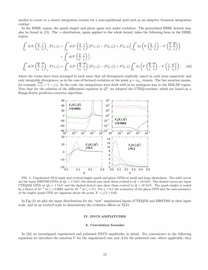
We implemented eqs.(37,38) using eqs.(33,34) and eqs.(35,36) for the DGLAP and ERBL regions respectively,employing an adaptive Gaussian numerical integration routine on a non-equidistant grid 14. We comment further onour usage of grids and integration routines below.

The integration ranges in eqs.(33,34) and eqs.(35,36) sample the input PDFs all the way down to zero in x′.Generally speaking, the providers of PDF sets issue programs that only allow their PDFs to be called for x′ greaterthan some minimum value. This is partly for technical reasons but also partly because the PDFs have not yet beenwell constrained by inclusive data in the very small x region, which corresponds to very high centre-of-mass energies.For the implementation of MRST, MRSA’ and GS we are fortunate to have access to analytic forms themselves atthe input scale15 and we simply extrapolate these into the very small x region. For GRV98 and GRSV00 this is notthe case and it was necessary to perform fits, at the Q0-scale concerned, to the small x behavior of these sets forvalues of x where they are available and then extrapolate these fits into the very small x regime16. In investigatingthis issue we noticed that if PDFs (and the quarks in particular) were too singular the integrals for the individual qand q were divergent (although this divergence is cancelled in forming the singlet, some regulation of the limit x′ → 0was required). This issue is not merely of technical interest. The physics message is clear: the GPDs defined above,using Radyushkin’s ansatz [40], and hence the DVCS observables are very sensitive to the behavior of the PDFs inthe small x region and also to their extrapolation to extremely small x. To the best of our knowledge this has notbeen explicitly pointed out before.

The unpolarized singlet also includes the D-term on the right hand side of eq.(38) (in principle there is also ananalogous term in the unpolarized gluon (DG in eq.(4) of [21]), but we choose to set it to zero, since nothing isknown for the gluon D-term except its symmetry.). We adapt the model introduced in [38] for the unpolarized singletD-term, which is based on the chiral-quark-soliton model. This D-term is antisymmetric in its argument, i. e. aboutthe point X = ζ/2 (in keeping with the anti-symmetry of FS , and HS about v = 0). It is non-zero only in the ERBLregion and hence vanishes entirely in the forward limit. In practice it only assumes numerical significance for large ζ(see Fig. 6 of [21]).

14This uses up most of the computing time for an evolution run.15for CTEQ5M we use Pumplin’s code [43]16Having tried several forms we eventually settled on fits of the type f(x) = f(x1) (x/x1)

a (1 + b log(x/x1) + c (x − x1)),with x1 being the minimum value of x available and with the power a constrained to be greater than zero to allow convergenceas x → 0.

10

C. GPD evolution

The input GPDs must now be evolved in Q2, using renormalization group equations, in order to make predictionsfor DVCS amplitudes at evolved scales. The input GPDs, as previously defined, are continuous functions which spanthe DGLAP and ERBL regions, and evolve in scale appropriately according to generalised versions of the DGLAP orERBL evolution equations. Note that the evolution in the ERBL region depends on the DGLAP region, i.e. there isa convolution integral in the ERBL equations spanning the DGLAP region [ζ, 1], whereas the DGLAP evolution isindependent of the ERBL region. As the scale increases, partons are pushed from the DGLAP into the ERBL regionsimply through momentum degradation, but not vice versa. The ERBL region thus acts as a sink for the partons.Hence, in the asymptotic limit of infinite Q2, we recover the simple asymptotic pion-type distribution amplitude in theERBL region and a completely empty DGLAP region. This will have strong implications for the DVCS amplitudesand cross section. Note that in performing the evolution we assumed that the t-dependences of the quarks and gluons(which mix under evolution) are the same and factorize such that they do not influence the degree of mixing underevolution. Otherwise, any assumed t-dependence will be modified by the QCD evolution, complicating calculations.In fact the t-dependence of quarks and gluons should be different, however, since we study DVCS only at small t, thedifferences in their t-dependence should be small. This unresolved problem of t-dependence mixing will be addressedin another paper.

The renormalization group equations (RGEs), or evolution equations, for the DGLAP region and ERBL regions,involve convolutions of GPDs with generalised kernels. They are implemented in a FORTRAN numerical evolutioncode. In the DGLAP region the quark flavor singlet and the gluon distributions mix under evolution according togeneralized DGLAP kernels17 taken from [15]. The flavor non-singlet (NS) quark combinations do not mix underevolution. Note that in order to do the full evolution and afterwards extract the various quark species separately oneneeds to solve two separate evolution equations. One for a symmetric combination qa

+ = qa + qa − 1/Nf

∑a(qa + qa)

and one for an antisymmetric combination qa− = qa − qa. A single quark species, i.e. quark or anti-quark in the

DGLAP region, or just a singlet or non-singlet quark combination in the ERBL region, can be extracted the followingway:

(qa

qa

)=

1

2(qa

+ ± qa− + qS) , with qS =

1

NF

∑

a

(qa + qa) , (39)

in the DGLAP region and

qS,a = (qa+ + qS) , and qNS,a = qa

− , (40)

in the ERBL region. This procedure was adopted in our FORTRAN code.A numerical implementation of the convolution integrals of the RNG equations involves specifying a treatment of

the integrable endpoint singularities. This is achieved via the following definition of the +-distributions (in this casewe chose to apply it to the “whole kernel”) in the DGLAP region:

∫ 1

y

dz

zP

(y

z,ζ

z

)

+

F(z, ζ) =

∫ 1

y

dz

zP

(y

z,ζ

z

)(F(z, ζ)−F(ζ, ζ)) −F(ζ, ζ)

[∫ 1

ζy

dzP

(z,

ζ

y

)−

∫ 1

y

dzP

(z, z

ζ

y

)],

(41)

and accordingly implemented in our code. Note that the lower limit of the first integral in the last bracket is ζ/y,which is not necessarily a grid point. Since we initially used an equidistant grid in the integration variable18, we

17Note that in the second reference of [15] there was a typographical error in Eq. (188) where the overall sign of the polarizedpure singlet term in the QQ sector should be − so as to be consistent with Eq. (178). In another typographical error, thefactor 3 in the first term of the square bracket in the second line of Eq. (194) of the same reference, i.e. the equation for theunpolarized GQ kernel, should be replaced by 3ζ. These mistakes were properly corrected in the implementation of the kernelsin the GPD evolution code.

18Our method of integration is the following: we first introduce an equidistant grid which we then stretch both in the ERBLand DGLAP regions with particular transformation functions in order to be able to treat the important region around ζ and0 more accurately. We then compute the Jacobian of this transformation for the inverse transformation we need. On thenon-equidistant grid we compute the input distributions and then the kernels. Using the Jacobian we transform back onto theequidistant grid and perform the convolution integrals using an equidistant grid integration routine like a semi-open Simpsonto account for the remaining integrable singularities at y and ζ.

11

needed to resort to a slower integration routine for a non-equidistant grid such as an adaptive Gaussian integrationroutine.

In the ERBL region, the quark singlet and gluon again mix under evolution. The generalized ERBL kernels mayalso be found in [15]. The +-distribution, again applied to the whole kernel, takes the following form in the ERBLregion:

∫ 1

y

dzV

(y

ζ,z

ζ

)

+

F(z, ζ) =

∫ 1

y

dzV

(y

ζ,z

ζ

)[F(z, ζ)−F(ζ, ζ)] + F(ζ, ζ)

[ ∫ ζ

y

dz

(V

(y

ζ,z

ζ

)− V

(z

ζ,y

ζ

))

+

∫ 1

ζ

dzV

(y

ζ,z

ζ

)],

∫ y

0

dzV

(y

ζ,z

ζ

)

+

F(z, ζ) =

∫ y

0

dzV

(y

ζ,z

ζ

)[F(z, ζ)−F(ζ, ζ)] + F(ζ, ζ)

∫ y

0

dz

(V

(y

ζ,z

ζ

)− V

(z

ζ,y

ζ

)), (42)

where the terms have been arranged in such away that all divergences explicitly cancel in each term separately andonly integrable divergences, as in the case of forward evolution at the point y = xbj , remain. The bar notation means,

for example, z/ζ = 1− z/ζ. In the code, the integrations were dealt with in an analogous way to the DGLAP region.Note that for the solution of the differential equation in Q2, we adopted the CTEQ-routines, which are based on aRunge-Kutta predictor-corrector algorithm.

0.0 0.1 0.2 0.3X

−20

−10

0

10

2010

−710

−610

−510

−410

−3−90

−60

−30

0

30

60

90

0.0 0.1 0.2 0.3 0.4 0.5X

0

2

4

6

8

10

12

14

10−7

10−6

10−5

10−4

10−310

−3

10−2

10−1

100

101

102

103

FS(X,ζ,Q2)

Fg(X,ζ,Q2)

Fg(X,ζ,Q2)FS(X,ζ,Q

2)

ζ=0.0001

ζ=0.0001

ζ=0.1 ζ=0.1

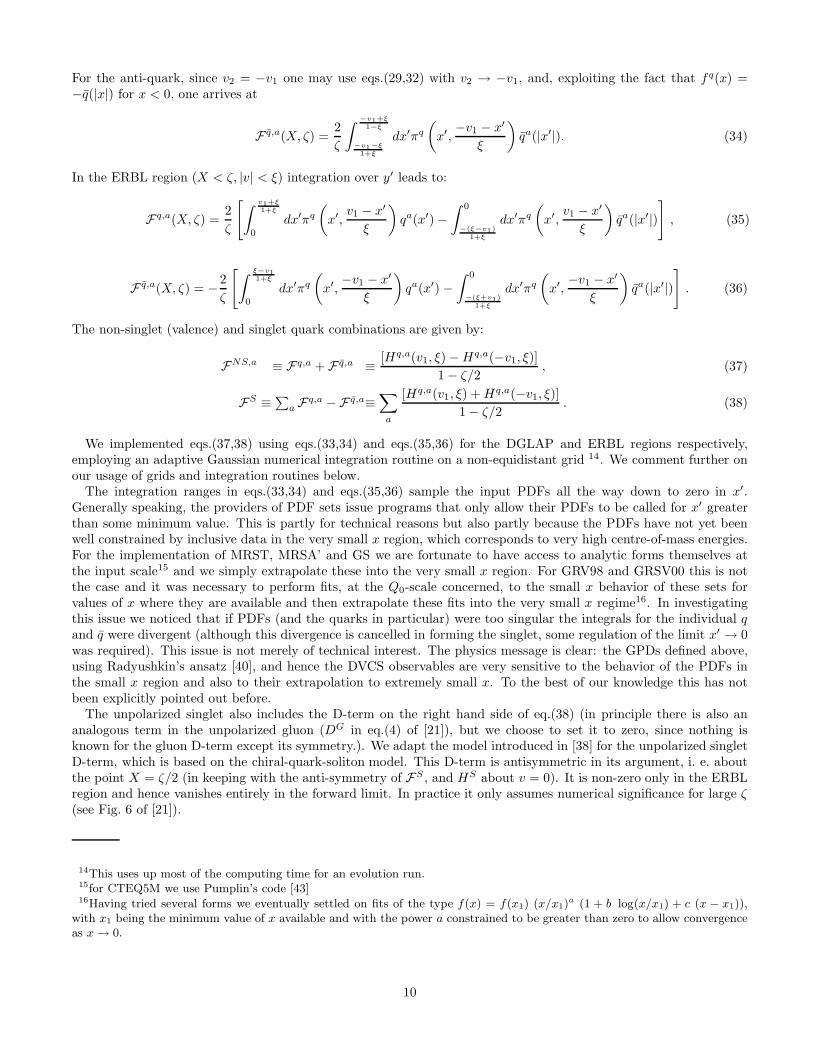
FIG. 2. Unpolarized NLO input and evolved singlet quark and gluon GPDs at small and large skewedness. The solid curvesare the input MRST99 GPDs at Q0 = 1 GeV, the dotted ones show them evolved to Q = 10 GeV. The dashed curves are inputCTEQ5M GPDs at Q0 = 1 GeV and the dashed-dotted ones show them evolved to Q = 10 GeV. The quark singlet is scaledby a factor of 10−4 at ζ = 0.0001 and by 10−2 at ζ = 0.1. For ζ = 0.1 the symmetry of the gluon GPD and the anti-symmetryof the singlet quark GPD are apparent about the point X = ζ/2 = 0.05.

In Fig.(2) we plot the input distributions for the “new” unpolarized inputs (CTEQ5M and MRST99) at their inputscale, and at an evolved scale to demonstrate the evolution effects in NLO.

IV. DVCS AMPLITUDES

A. Convolution formulae

In [24] we investigated unpolarised and polarised DVCS amplitudes in detail. For convenience in the followingequations we introduce the notation V for the unpolarized case and A for the polarized case, where applicable, they

12

take the upper and lower signs, respectively19. The factorization theorem [6,7] for DVCS proves that the amplitudetakes the following factorized form in the non-diagonal representation (up to power-suppressed corrections of O(1/Q)):

TS,V/A

DV CS(ζ, µ2, Q2, t) =∑

a

e2a

(2− ζ

ζ

)[∫ 1

0

dX T S(a),V/A

(2X

ζ− 1 + iǫ,

Q2

µ2

)FS(a),V/A(X, ζ, µ2, t)

∓

∫ 1

ζ

dX T S(a),V/A

(1−

2X

ζ,Q2

µ2

)FS(a),V/A(X, ζ, µ2, t)

],

Tg,V/A

DV CS(ζ, µ2, Q2, t) =1

Nf

(2− ζ

ζ

)2 [ ∫ 1

0

dX T g,V/A

(2X

ζ− 1 + iǫ,

Q2

µ2

)Fg,V/A(X, ζ, µ2, t)

±

∫ 1

ζ

dX T g,V/A

(1−

2X

ζ,Q2

µ2

)Fg,V/A(X, ζ, µ2, t)

]. (43)

Note that the second integral is purely real and does not need a +iǫ prescription since there is no divergence of thecoefficient function in the integration interval. Also note the opposite sign structure in the quark singlet and gluon casedue to opposite symmetries of the quark singlet and gluon. For our numerical calculations, we set the factorizationscale, µ2, equal to the photon virtuality, Q2 (in [24] we studied the effects of its variation and found them to berather mild; the associated uncertainties are less than those due to differences in the input model GPDs so we neglectthem). Henceforth, we suppress the factorized t-dependence and give predictions for t = 0. We will specify it for eachcase later. The LO and NLO coefficient functions, T i,V/A, are taken from eqs.(14-17) of [44] and are summarized inappendix A of [24]. They contain logarithms of the type log(1 −X/ζ)n/(1 −X/ζ)n1 , with n, n1 = 0, 1, 2, 3. Hence,depending on the region of integration, they can have both real and imaginary parts (i.e. if the argument of the logis positive or negative), which in turn generate real and imaginary parts of the DVCS amplitudes.

In eq.(43), we employ the +iǫ prescription through the Cauchy principal value prescription (“P.V.”) which weimplemented through the following algorithm:

P.V.

∫ 1

0

dX T

(2X

ζ− 1

)F(X, ζ, Q2) =

∫ ζ

0

dX T

(2X

ζ− 1

)(F(X, ζ, Q2)−F(ζ, ζ, Q2)

)+

∫ 1

ζ

dX T

(2X

ζ− 1

)(F(X, ζ, Q2)−F(ζ, ζ, Q2)

)+ F(ζ, ζ, Q2)

∫ 1

0

dX T

(2X

ζ− 1

). (44)

Each term in eq. (44) is now either separately finite or only contains an integrable logarithmic singularity. Thisalgorithm closely resembles the implementation of the + regularization in the evolution of PDFs and GPDs. Wenote that the first integral (in the ERBL region) is strictly real. The second and third terms contain both real andimaginary parts (which are generated in the DGLAP region). Explicit expressions for the real and imaginary partsof the DVCS amplitudes are given in Sec.(II) of [24]. They involve integrals over the coefficient functions which maybe calculated explicitly and are given in Appendix B of [24]. The real and imaginary parts of the unpolarized andpolarized DVCS amplitudes were computed using a FORTRAN code based on numerical integration routines. Weimplemented the exact solution to the RNG equation for αs in LO or NLO in our calculation, as appropriate, to beconsistent throughout our analysis.

19refering to vector and axial-vector currents for the quarks

13

B. Numerical results: unpolarized case

1 6 11 16 21Q

2 in GeV

2

−10

0

10

20

30

40

50

60

701 6 11 16 21

−5.0e+04

5.0e+04

1.5e+05

2.5e+05

3.5e+05

4.5e+05

5.5e+05

1 6 11 16 21Q

2 in GeV

2

−10

0

10

20

30

40

50

60

701 6 11 16 21

−5.0e+04

5.0e+04

1.5e+05

2.5e+05

3.5e+05

4.5e+05

5.5e+05

Unpol. Re and Im singlet DVCS Amplitude in LO/NLO

CTEQ5Mζ=0.1

CTEQ5Mζ=0.0001

ζ=0.1MRST

ζ=0.0001MRST

FIG. 3. The Q2-dependence of the real and imaginary parts of the quark singlet DVCS amplitude. The solid (dashed) curveis the real part in LO (NLO) and the dotted (dashed-dotted) curve is the imaginary part in LO (NLO).

In this subsection we illustrate the Q2- and ζ-dependence, as well as the size, of the real and imaginary partsof the unpolarized DVCS amplitudes for the new input distributions (MRST99, CTEQ5M), calculated at LO andNLO accuracy. Fig. 3 shows the Q2-dependence of the real and imaginary parts of the quark singlet contribution,at LO and NLO, for two values of ζ = 0.1, 0.0001, representative of HERMES and HERA kinematics, respectively.Correspondingly, Fig. 4 shows the gluon contributions, which start at NLO. Note the strong Q2-dependence in NLOof the imaginary part of the quark singlet and gluon amplitude at small ζ. This might raise concerns about theconvergence of the perturbative expansion, especially when comparing NLO with LO in the quark singlet, where NLOgrows much stronger with Q2 than LO. This is due to the same type of logarithmic divergences as X → ζ in both theevolution kernels and NLO coefficient functions. These divergences enhance the region around ζ, which is importantfor the value of the imaginary part [23], more quickly in Q2 than αs drops as Q2 increases. However, the quarksinglet amplitude itself is not an observable quantity at NLO but rather the sum of quark singlet and gluon. Whencomparing the physical amplitudes at LO and NLO, the relative NLO corrections decrease as Q2 increases, as theyindeed should [23].

The above figures are complemented by Figs. 5 and Figs. 6, which show the ζ-dependence at fixed Q2 for the quarksinglet and gluon contributions, respectively. Again we would like to point out the remarkable power-like behaviorof the unpolarized amplitudes in ζ for fixed Q2 already remarked upon and explained in [24] (with the exception ofthe NLO real parts of the quark singlet amplitude for CTEQ5M for the Q2 values plotted due to a somewhat strangecombination of small quark input and comparatively large gluon input. At higher Q2, the CTEQ5M distribution alsodisplays the characteristic power-like behavior in ζ).

14

1 6 11 16 21Q

2 in GeV

2

−25

−20

−15

−10

−5

0

1 6 11 16 21−250000

−200000

−150000

−100000

−50000

0

1 6 11 16 21Q

2 in GeV

2

−20

−15

−10

−5

0

1 6 11 16 21−250000

−200000

−150000

−100000

−50000

0

Unpol. Re and Im gluon DVCS Amplitude in NLO

CTEQ5Mζ=0.1

CTEQ5Mζ=0.0001

ζ=0.1MRST

ζ=0.0001MRST

FIG. 4. The Q2-dependence of the real (solid line) and imaginary (dotted line) parts of the unpolarized gluon DVCSamplitude, which starts at NLO, for two representative values of ζ.

10−4

10−3

10−2

10−1

ζ

10−2

10−1

100

101

102

103

104

105

106

10−4

10−3

10−2

10−110

−2

10−1

100

101

102

103

104

105

106

10−4

10−3

10−2

10−1

ζ

10−2

10−1

100

101

102

103

104

105

106

10−4

10−3

10−2

10−110

−2

10−1

100

101

102

103

104

105

106

Unpol. Re and Im singlet DVCS Amplitude in LO/NLO

CTEQ5MQ2=2.25 GeV2

CTEQ5MQ2=4 GeV2

MRSTQ2=2.25 GeV2

MRSTQ2=4 GeV2

FIG. 5. The real and imaginary parts of the unpolarized quark singlet DVCS amplitude, as a function of ζ. The solid(dashed) curve is the real part in LO (NLO) and the dotted (dashed-dotted) curve is the imaginary part in LO (NLO). To beable to plot the NLO real part of the quark singlet amplitude in a viewable manner, we removed the first point for CTEQ5Min the upper left plot (since it was negative and thus not easily handled in a log-log plot) and shifted the NLO curve of the realpart in the upper right plot upward by an amount of O(1), again to avoid negative numbers.

15

10−4

10−3

10−2

10−1

ζ

100

101

102

103

104

105

10−4

10−3

10−2

10−110

0

101

102

103

104

105

10−4

10−3

10−2

10−1

ζ

100

101

102

103

104

105

10−4

10−3

10−2

10−110

0

101

102

103

104

105

Unpol. Re and Im gluon DVCS Amplitude in NLO

CTEQ5MQ2=2.25 GeV2

MRSTQ2=2.25 GeV2

CTEQ5MQ2=4 GeV2

MRSTQ2=4 GeV2

FIG. 6. The real and imaginary parts of the unpolarized gluon DVCS amplitude as functions of ζ, for fixed Q2. The solidcurve is the modulus of the real part (which is actually negative) and the dotted curve is the modulus of the imaginary part ofthe gluon amplitude, which is also negative!

C. Specification of t-dependence and helicity flip amplitudes

In this subsection we specify the t-dependence of the various unpolarized/polarized helicity non-flip/flip DVCS

amplitudes, H1, H1, E1, E1, for each parton species a = S(a = u, d, s), g. These are required in eqs.(5, 6, 7) to fullyspecify TDVCS (our choices follow those of [31] closely) 20. The various form factors are specified as follows:

Ha1(ζ, Q2, t) = F a

1 (t)T a,V (ζ, Q2) , Ha1(ζ, Q2, t) = Ga

1(t)Ta,A(ζ, Q2) ,

Ea1 (ζ, Q2, t) = F a

2 (t)T a,VE1

(ζ, Q2) , Ea1 (ζ, Q2, t) = Ga

2(t)T a,A

E1(ζ, Q2) , (45)

where, in the helicity flip case on the second line, we have introduced additional subscripts, E1, E1, on the right handside to distinguish this case from the helicity non-flip one considered explicitly above. For the up and down quarkflavors we exploit the fact that proton and neutron form an iso-spin doublet to arrive at:

2Fui (t) = 2F p

i (t) + Fni (t), 2F d

i (t) = F pi (t) + 2Fn

i (t) , for i = 1, 2 , (46)

corresponding to the Dirac and Pauli form factors, respectively (see eqs.(12, 13)). For the helicity non-flip polarizedcase we choose [31]:

Gu,d1 (t) =

(1−

t

m2A

)−2

, Gs,g1 (t) = (1−

t

m2A

)−3 , (47)

where mA = 0.9 GeV [33]. The strange quark and the gluon sea-like form factors were chosen in [31] using thecounting rules for elastic form factors which give 1/t3, for large t. Hence, for the unpolarized case the electric and

20In fact the GPDs themselves may already be considered to have a given helicity specification. The assumption of a factorizedt-dependence for the GPDs allows the specification of the t-dependence to be moved to the amplitude level.

16

magnetic form factors were chosen to be

Gs,gE (t) =

Gs,gM (t)

1 + κs,g=

(1−

t

m2V

)−3

, (48)

where we further assume κs,g = 0. This gives (cf. eq.(12))

F s,g1 (t) = Gs,g

E (t) =

(1−

t

m2V

)−3

, F s,g2 (t) = 0 , (49)

with mV = 0.84 GeV.For the helicity-flip case, we still have to specify the polarized and unpolarized GPDs. Unfortunately there are no

inclusive analogs to guide us. However, we do know that the unpolarized helicity flip GPD contains a D-term with arelative minus sign as compared to the helicity non-flip GPD, such that when added they cancel 21. In contrast to [31]we set the GPD equal to this D-term, which is non-zero only in the ERBL region22. We then evolve this distributionin Q2 and use it as an input to calculate T a,V

E1for use in eq.(45), with the F a

2 (t) for various a specified in eqs.(46, 49).For the polarized helicity flip amplitude, TE , it was observed that, in a similar fashion to the effective pseudo scalar

form factors in β-decay [33], one can approximate it at small t by the pion pole (see for example [40]). Thus we chosethe corresponding GPD to only contain the asymptotic pion distribution amplitude given by

φπ(X/ζ) =8

3

2− ζ

ζ

X

ζ

(1−

X

ζ

), (50)

in the ERBL region (and zero for X > ζ). Since we use the asymptotic form we do not evolve the GPD and use it

directly in the computation of the DVCS amplitude, T a,A

E1(ζ, Q2). The t-dependence is given by the pion pole and

thus we find

Ea1 (ζ, Q2, t) = Ga

2(t) Ta,A

E1(ζ, Q2) =

4g(3)A M2

m2π − t

T a,A

E1(ζ, Q2) , for a = u, d , (51)

where g(3)A = 1.267, M is the nucleon mass and T a,A

E1= φπ, for all Q2. For the s-quark and the gluon we set E to

zero. This completes the specification of the t-dependence of DVCS amplitudes, which are then used to compute thevarious DVCS observables defined in Sec. II.

We close this section with a few comments. We note that E1, E1 only have real parts since the GPD is zero forX > ζ. Furthermore, in the asymptotic limit Q2 → ∞ for finite ζ, when all the partons have accumulated in theERBL region, all amplitudes have zero imaginary part and a real part which is given by an asymptotic distributionamplitude in the ERBL region, thus the overall amplitude, and hence the appropriately scaled triple differential crosssection, remain non-zero, in contrast to inclusive DIS.

V. LO AND NLO RESULTS FOR DVCS OBSERVABLES

In this section we present results for the triple differential cross section and for various asymmetries (AAA, SSA, CA,UPLT, CADSFL) defined in subsection II B, in kinematics appropriate for the H1, ZEUS and HERMES experiments.We show the results as functions of t (for fixed ζ, Q2), of ζ (for fixed t, Q2) and of Q2 (for fixed t, ζ) using the variousinput distributions defined in subsection III B. For our predictions in HERA kinematics we assume an e+P scatteringwith a proton energy of 920 GeV and a positron energy of 27.5 GeV (except of course for the charge asymmetries,which also use an electron probe of 27.5 GeV).

21This has to be the case since the n-th. moment in X of the sum is a polynomial of degree n-1 in ζ, whereas the n-th. momentof the non-flip and flip GPDs separately are polynomials of degree n. The highest power of the polynomial in each case isgenerated by the D-term and thus they must cancel.

22Strictly speaking this violates the polynomiality condition since the helicity flip GPD is multiplied by the Pauli form factorrather than the Dirac form factor. However since the helicity flip term is numerically insignificant for DVCS observables thismodel is sufficient for phenomenological purposes.

17

A. The triple differential cross section

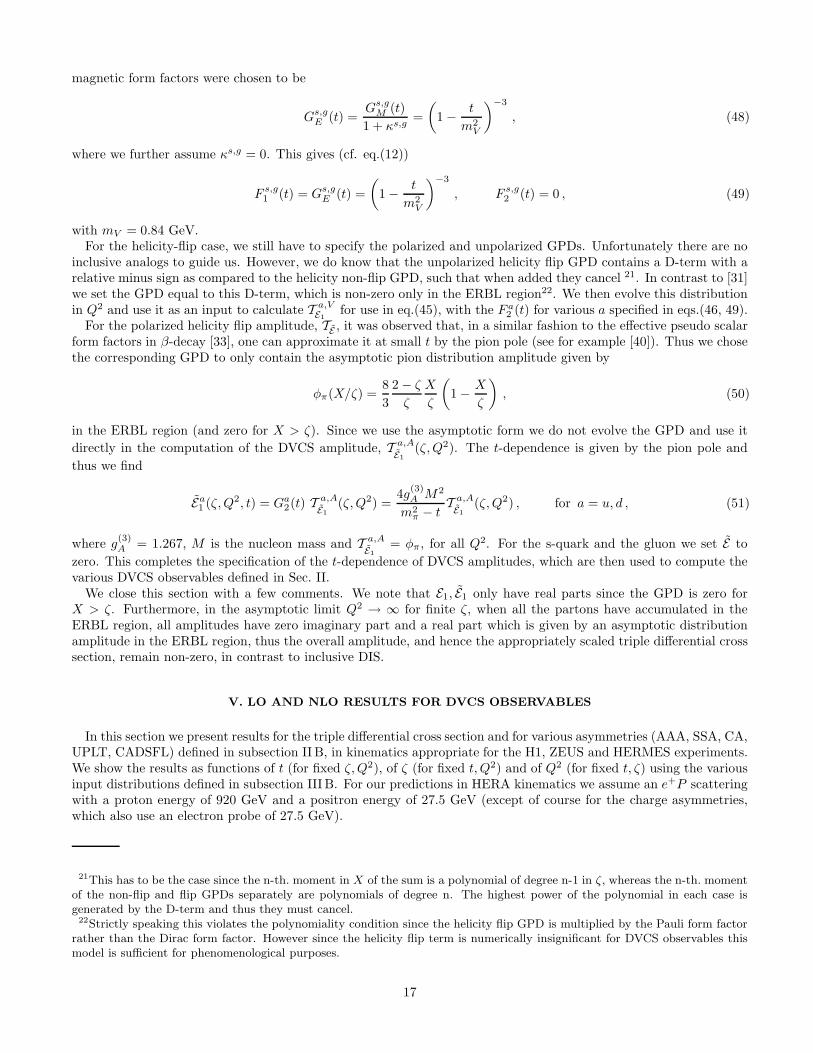
In Fig. 7 and Fig. 8 we show the triple differential cross section of eq.(17), as a function of t at fixed ζ and Q2, forour four input distributions. We note that at the common point Q2 = 4 GeV2, GRV98, MRSA’ and MRST99 are inclose agreement, for small ζ = x. In general CTEQ5M and MRST99 experience only moderate changes in going fromLO to NLO.

At small ζ = x, for GRV98 and MRSA’ input distributions, the NLO corrections are much larger. As Q2 increases,at fixed ζ, the spread of the predictions is seen to decrease. This is partly due to the evolution washing out thedifferences between the various input distributions, and partly due to an increased significance of the BH process.

−0.5−0.4−0.3−0.2−0.1t in GeV

2

0

0.05

0.1

0.15

0.20

1000

2000

3000

4000

5000

6000

−0.5−0.4−0.3−0.2−0.1t in GeV

2

0

0.05

0.1

0.15

0.20

1000

2000

3000

4000

5000

6000

Q2 = 4 GeV

2

x = 0.0001Q

2 = 9 GeV

2

x = 0.0001

Q2 = 4 GeV

2

x = 0.2Q

2 = 9 GeV

2

x = 0.2

dσ/dxdQ 2d|t| in nb/GeV 4

FIG. 7. The triple differential cross section in t for fixed x = ζ and Q2. The solid (dotted) curve is the MRSA′

set in LO(NLO) and the dashed (dashed-dotted) curve is the GRV98 set in LO (NLO).

−0.5−0.4−0.3−0.2−0.1t in GeV

2

00.5

11.5

22.5

33.5

44.5

0

2000

4000

6000

8000

10000

−0.5−0.4−0.3−0.2−0.1t in GeV

2

00.5

11.5

22.5

33.5

44.5

0

500

1000

1500

2000

2500

3000

Q2 = 2.25 GeV2

x = 0.0001Q2 = 4 GeV2

x = 0.0001

Q2 = 2.25 GeV2

x = 0.1Q2 = 4 GeV2

x = 0.1

dσ/dxdQ 2d|t| in nb/GeV 4

18

FIG. 8. The triple differential cross section in t for fixed x = ζ and Q2. The solid (dotted) curve is the CTEQ5M set in LO(NLO) and the dashed (dashed-dotted) curve is the MRST99 set in LO (NLO).

10−4

10−3

10−2

x

10−1

100

101

102

10310

−410

−310

−210−1

100

101

102

103

104

0.15 0.20 0.25 0.30x

0

0.05

0.1

0.15

0.20.15 0.20 0.25 0.300

0.05

0.1

0.15

0.2

dσ/dxdQ2d|t| in nb/GeV

2

Q2 = 4 GeV2t = −0.25 GeV

2

t = −0.25 GeV2

Q2 = 9 GeV2

t = −0.25 GeV2

Q2 = 4 GeV2

t = −0.25 GeV2

Q2 = 6.25 GeV2

FIG. 9. The triple differential cross section in x = ζ for fixed t and Q2. The solid (dotted) curve is the MRSA′

set in LO(NLO) and the dashed (dashed-dotted) curve is the GRV98 set in LO (NLO).

10−4

10−3

10−2

x

100

101

102

10310

−410

−310

−2100

101

102

103

104

0.10 0.15 0.20 0.25 0.30x

0

0.2

0.4

0.6

0.8

10.10 0.15 0.20 0.25 0.300

0.2

0.4

0.6

0.8

1

dσ/dxdQ2d|t| in nb/GeV

2

Q2 = 2.25 GeV2t = −0.25 GeV

2

t = −0.25 GeV2

Q2 = 4 GeV2

t = −0.25 GeV2

Q2 = 2.25 GeV2

t = −0.25 GeV2

Q2 = 4 GeV2

FIG. 10. The triple differential cross section in x = ζ for fixed t and Q2. The solid (dotted) curve is the CTEQ5M set in LO(NLO) and the dashed (dashed-dotted) curve is the MRST99 set in LO (NLO).

In Figs. 9, 10, we employ logarithmic scales for HERA kinematics (x < 10−2) to illustrate the ζ-behavior for fixedQ2 and t. It is interesting to note that we find the same type of power law behavior, ζn, for the triple differentialcross section, which also includes the BH process, as we found previously for the unpolarized DVCS amplitudes (seeFigs. 5 -6). Note that the kink for Q2 = 9 GeV2 is due to going from a BH dominated region at x = 0.0001 (y > 0.8)to a region where DVCS dominates (x > 0.0005 and y < 0.2).

19

The fact that the GRV98 and MRSA’ input scale is Q20 = 4 GeV2, implies that the available Q2-range at small

x is rather limited for these distributions. Hence, in Fig. 11 we show only the Q2-dependence of the MRST99 andCTEQ5M sets, which start at Q2

0 = 1 GeV2. For smaller Q2, where DVCS dominates BH, the cross section fallsquickly with Q2 and one is sensitive to the details of the choice of input distribution. As Q2 increases and BH startsto dominate over DVCS, one observes that the curves begin to converge and one loses sensitivity to the details of theinput GPD.

We would like to point out that at large x all of the distributions produce fairly similar results and that the NLOcorrections are tame. This is expected because each of the distributions have been strongly constrained by global fitsto high statistics data in this region and hence behave similarly. Any observed differences may result in part fromthe holistic nature of the GPDs, which requires a continuous function for all X , both at the input scale and uponevolution. The real part of the amplitude is sensitive to an integral over the ERBL region X < ζ so one may havesome residual sensitivity to the behavior at very small X ≪ ζ, particularly if this behavior is extreme. The imaginarypart is strongly influenced by the behavior at X = ζ which in turn is constrained by a symmetry in the ERBL region.This sensitivity is further enhanced at smaller ζ, where the input PDFs are not yet so well constrained by direct(mainly inclusive) measurements. Hence, we optimistically speculate that a detailed measurement of the differentialcross section, at HERA, for relatively low Q2 ≈ 1 − 4 GeV2, could help to discriminate between different standardinput PDFs.

2.25 3.25 4.25 5.25 6.25Q

2 in GeV

2

0

1000

2000

3000

4000

1.5 2.5 3.5Q

2 in GeV

2

0

0.5

1

1.5

2

dσ/dxdQ 2d|t| in nb per GeV −4

x = 0.0001t = −0.25 GeV

2 t = −0.25 GeV2

x = 0.1

FIG. 11. The triple differential cross section in Q2 for fixed t and x = ζ. The solid (dotted) curve is the CTEQ5M set in LO(NLO) and the dashed (dashed-dotted) curve is the MRST99 set in LO (NLO).

B. The single spin asymmetries (SSA,UPLT)

Having found a large spread of predictions for the triple differential cross section for different input GPDs, we nowturn to two single spin asymmetries which are directly sensitive to the imaginary part of DVCS amplitudes. Let usfirst discuss the SSA, defined in eq.(20), which can be measured using a polarized lepton probe on an unpolarizedtarget. At small x the numerator in eq.(20) is directly proportional to Im H1 (see the second term of eq.(30) of [31]).

In Figs. 12, 13 we illustrate the t-dependence at fixed ζ and Q2, and note that the predictions range from as littleas 5% to as much as 30%. We note that in general the t-dependence is rather flat for t > −0.1 GeV2, indicating that,to a certain extent, the t-dependence cancels in the ratio of eq.(20). This means that an experimental measurement ofthis asymmetry, even with a rather coarse binning in t, would be able to distinguish between different input scenarios,especially at larger Q2 values. At the common scale of Q2 = 4 GeV2, the GRV98 and MRSA’ sets produce verysimilar numbers within LO and NLO, whereas CTEQ5M and MRST99 are more different within LO and NLO, atleast at small x. The NLO to LO corrections are generally speaking small to moderate (5− 30%).

Figs. 14, 15 show that the SSA drops steeply in ζ = x for fixed Q2 and t, suggesting that the HERA experimentswill only be able to measure the SSA in the small ζ regime (ζ ∈ [10−3, 10−4]). We would also like to point out that thedifferences for the different input sets becomes so small on the scale of the actual value of the SSA at larger ζ in HERAkinematics, that only very high statistics would be able to discriminate between them. Thus, for HERA, only a smallζ measurement would gives a reasonable discrimination between the various inputs. For HERMES kinematics, where

20

for fixed ζ = x, Q2 one of course probes a different y = Q2/xS value, the SSA again becomes sizeable. Unfortunately,in this high ζ = x regime, the SSA is proportional to a linear combination of imaginary parts of H1, H1, E1 ratherthan just Im H1 as at small ζ (see second term of eq.(30) of [31]).

−0.5−0.4−0.3−0.2−0.1t in GeV

2

−0.25

−0.225

−0.2

−0.175

−0.15

−0.125

−0.1

−0.075−0.35

−0.3

−0.25

−0.2

−0.15

−0.5−0.4−0.3−0.2−0.1t in GeV

2

−0.25

−0.225

−0.2

−0.175

−0.15

−0.125

−0.1

−0.075−0.35

−0.3

−0.25

−0.2

−0.15

Q2 = 4 GeV

2

x = 0.0001

Q2 = 9 GeV

2

x = 0.0001

Q2 = 4 GeV

2

x = 0.2Q

2 = 9 GeV

2

x = 0.2

Single Spin Asymmetry

FIG. 12. The single spin asymmetry as a function of t, for fixed x = ζ and Q2. The solid (dotted) curve is the MRSA′

setin LO (NLO) and the dashed (dashed-dotted) curve is the GRV98 set in LO (NLO).

−0.5−0.4−0.3−0.2−0.1t in GeV

2

−0.35

−0.3

−0.25

−0.2

−0.15

−0.1

−0.05

0−0.35

−0.3

−0.25

−0.2

−0.15

−0.1

−0.05

0

−0.5−0.4−0.3−0.2−0.1t in GeV

2

−0.35

−0.3

−0.25

−0.2

−0.15

−0.1

−0.05

0−0.35

−0.3

−0.25

−0.2

−0.15

−0.1

−0.05

0

Q2 = 2.25 GeV2

x = 0.0001

Q2 = 4 GeV2

x = 0.0001

Q2 = 2.25 GeV2

x = 0.1Q2 = 4 GeV2

x = 0.1

Single Spin Asymmetry

FIG. 13. The SSA in t for fixed x and Q2. The solid (dotted) curve is the CTEQ5M set in LO (NLO) and the dashed(dashed-dotted) curve is the MRST99 set in LO (NLO).

21

0.15 0.2 0.25 0.3x

−0.3

−0.25

−0.2

−0.15

−0.1

−0.05

010

−410

−310

−2

0.15 0.2 0.25 0.3x

−0.3

−0.25

−0.2

−0.15

−0.1

−0.05

010

−410

−310

−2−0.3

−0.25

−0.2

−0.15

−0.1

−0.05

0

10−4−0.3

−0.25

−0.2

−0.15

−0.1

−0.05

0

Single Spin Asymmetry

Q2 = 4 GeV

2t = −0.25 GeV

2t = −0.25 GeV

2

Q2 = 9 GeV

2

t = −0.25 GeV2

Q2 = 4 GeV

2 t = −0.25 GeV2

Q2 = 6.25 GeV

2

FIG. 14. The SSA in x = ζ for fixed t and Q2. The solid (dotted) curve is the MRSA′

set in LO (NLO) and the dashed(dashed-dotted) curve is the GRV98 set in LO (NLO).

10−4

10−3

10−2

x

−0.3

−0.25

−0.2

−0.15

−0.1

−0.05

0

0.0510

−410

−310

−2−0.3

−0.25

−0.2

−0.15

−0.1

−0.05

0

0.05

0.1 0.15 0.2 0.25 0.3x

−0.3

−0.2

−0.1

00.1 0.15 0.2 0.25 0.3

−0.3

−0.25

−0.2

−0.15

−0.1

−0.05

0

Single Spin Asymmetry

Q2 = 2.25 GeV2t = −0.25 GeV

2

t = −0.25 GeV2

Q2 = 4 GeV2

t = −0.25 GeV2

Q2 = 2.25 GeV2

t = −0.25 GeV2

Q2 = 4 GeV2

FIG. 15. The SSA as a function of x = ζ for fixed t and Q2. The solid (dotted) curve is the CTEQ5M set in LO (NLO) andthe dashed (dashed-dotted) curve is the MRST99 set in LO (NLO).

Finally, in Fig. 16 we plot the Q2-dependence for fixed ζ = x and t. For small ζ we observe that the magnitudeof the SSA increases with Q2, for both distributions. At large ζ, both MRST99 and CTEQ5M have very similar Q2

behavior and the NLO corrections are small. Note that at small ζ the NLO corrections appear to grow in Q2 which atfirst sight looks strange. This is due to the fact that the BH process gains prominence relative to the DVCS process, soany differences between calculations of ImH1 for the interference term in the numerator become enhanced. However,the NLO corrections remain moderate between 15− 30%.

22

2.25 3.25 4.25 5.25 6.25Q

2 in GeV

2

−0.6

−0.5

−0.4

−0.3

−0.2

−0.1

1.5 2.5 3.5Q

2 in GeV

2

−0.6

−0.5

−0.4

−0.3

−0.2

−0.1

Single Spin Asymmetry

x = 0.0001t = −0.25 GeV

2

t = −0.25 GeV2

x = 0.1

FIG. 16. The SSA as a function of Q2, for fixed t and x = ζ. The solid (dotted) curve is the CTEQ5M set in LO (NLO) andthe dashed (dashed-dotted) curve is the MRST99 set in LO (NLO).

If one switches now to a longitudinally polarized proton target as available at HERMES, but not currently plannedfor HERA, and an unpolarized lepton probe, one can form the unpolarized single spin asymmetry UPLT which isdirectly sensitive to the imaginary part of a combination of DVCS amplitudes. Furthermore, for the small ζ regimewithin HERA kinematics, we find on inspection of the first term (proportional to Λ sinφ) of eq.(31) of [31] that theUPLT at small ζ is directly proportional to the imaginary part of the polarized amplitude H1 and that the otheramplitudes like the numerically large H1 are suppressed by x. Hence, even though Im H1 is about a factor of onethousand smaller than Im H at x = 10−4, the suppression factor of x means that Im H1 constitutes only a 10%correction. Hence the UPLT is mainly sensitive to Im H1 at small x. Since this amplitude is numerically small,we found the UPLT asymmetry itself to be very small, at small x = ζ, and thus virtually impossible to measure.Therefore, we do not show plots for HERA kinematics but rather only for HERMES kinematics.

−0.5−0.4−0.3−0.2−0.1t in GeV

2

00.020.040.060.08

0.10.120.140.160.18

0.2

−0.5−0.4−0.3−0.2−0.1t in GeV

2

00.020.040.060.08

0.10.120.140.160.18

0.2

Q2 = 4 GeV

2

x = 0.15

Q2 = 6.9 GeV

2

x = 0.15

The UPLT Asymmetry

FIG. 17. The UPLT as a function of t, for fixed x and Q2. The solid (dotted) curve is the MRSA′

set in LO (NLO) and thedashed (dashed-dotted) curve is the GRV98 set in LO (NLO).

23

−0.5−0.4−0.3−0.2−0.1t in GeV

2

0.10.120.140.160.18

0.20.220.24

−0.5−0.4−0.3−0.2−0.1t in GeV

2

0.10.120.140.160.18

0.20.220.24

Q2 = 2.25 GeV

2

x = 0.15

Q2 = 4 GeV

2

x = 0.15

The UPLT Asymmetry

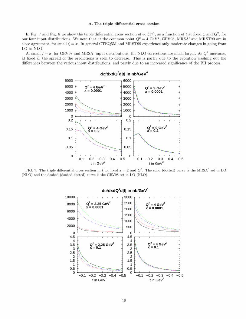
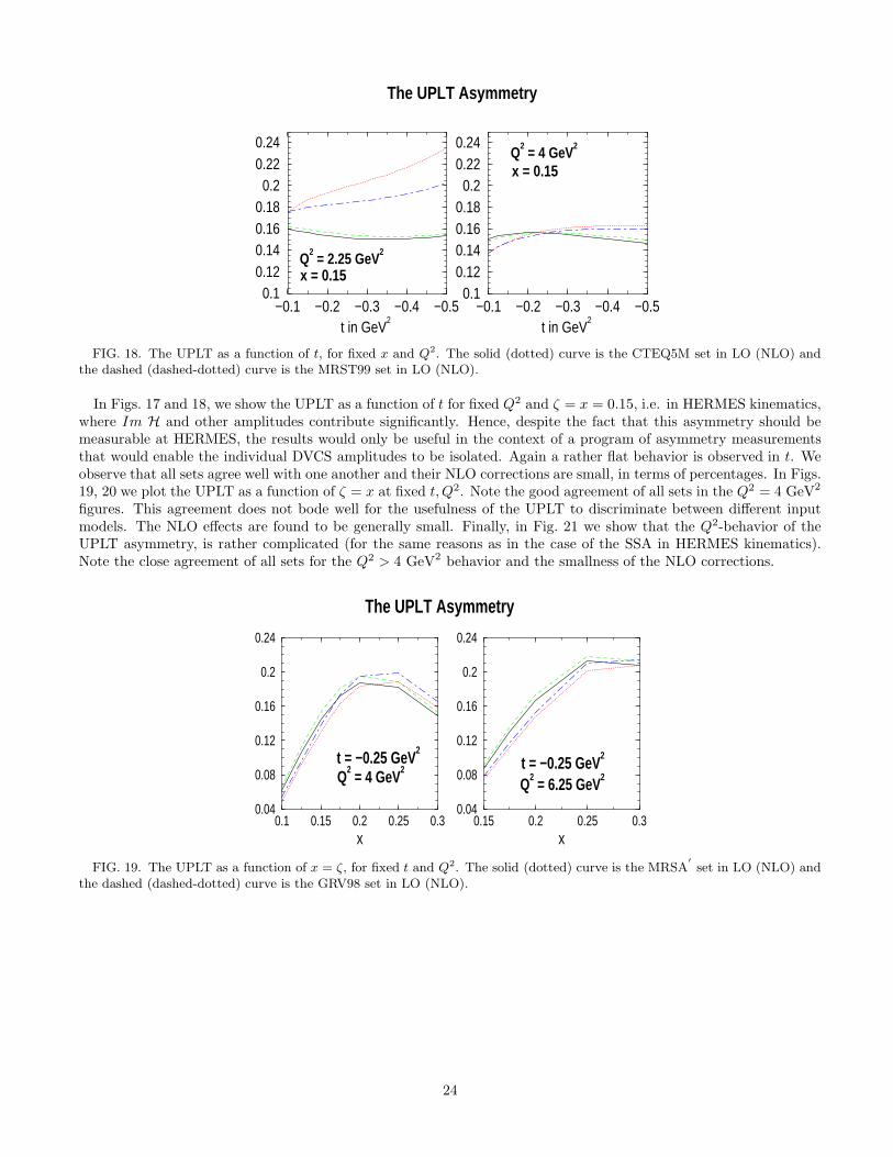
FIG. 18. The UPLT as a function of t, for fixed x and Q2. The solid (dotted) curve is the CTEQ5M set in LO (NLO) andthe dashed (dashed-dotted) curve is the MRST99 set in LO (NLO).

In Figs. 17 and 18, we show the UPLT as a function of t for fixed Q2 and ζ = x = 0.15, i.e. in HERMES kinematics,where Im H and other amplitudes contribute significantly. Hence, despite the fact that this asymmetry should bemeasurable at HERMES, the results would only be useful in the context of a program of asymmetry measurementsthat would enable the individual DVCS amplitudes to be isolated. Again a rather flat behavior is observed in t. Weobserve that all sets agree well with one another and their NLO corrections are small, in terms of percentages. In Figs.19, 20 we plot the UPLT as a function of ζ = x at fixed t, Q2. Note the good agreement of all sets in the Q2 = 4 GeV2

figures. This agreement does not bode well for the usefulness of the UPLT to discriminate between different inputmodels. The NLO effects are found to be generally small. Finally, in Fig. 21 we show that the Q2-behavior of theUPLT asymmetry, is rather complicated (for the same reasons as in the case of the SSA in HERMES kinematics).Note the close agreement of all sets for the Q2 > 4 GeV2 behavior and the smallness of the NLO corrections.

0.1 0.15 0.2 0.25 0.3x

0.04

0.08

0.12

0.16

0.2

0.24

0.15 0.2 0.25 0.3x

0.04

0.08

0.12

0.16

0.2

0.24

The UPLT Asymmetry

Q2 = 4 GeV2t = −0.25 GeV

2

t = −0.25 GeV2

Q2 = 6.25 GeV2

FIG. 19. The UPLT as a function of x = ζ, for fixed t and Q2. The solid (dotted) curve is the MRSA′

set in LO (NLO) andthe dashed (dashed-dotted) curve is the GRV98 set in LO (NLO).

24

0.1 0.15 0.2 0.25 0.3x

0.04

0.08

0.12

0.16

0.2

0.24

0.1 0.15 0.2 0.25 0.3x

0.04

0.08

0.12

0.16

0.2

0.24

The UPLT Asymmetry

Q2 = 2.25 GeV2t = −0.25 GeV

2t = −0.25 GeV

2

Q2 = 4 GeV2

FIG. 20. The UPLT as a function of x = ζ, for fixed t and Q2. The solid (dotted) curve is the CTEQ5M set in LO (NLO)and the dashed (dashed-dotted) curve is the MRST99 set in LO (NLO).

1.5 2.5 3.5 4.5 5.5Q

2 in GeV

2

0.04

0.06

0.08

0.1

0.12

0.14

0.16

0.18

0.2

4 4.5 5 5.5 6 6.5Q

2 in GeV

2

0.04

0.06

0.08

0.1

0.12

0.14

0.16

0.18

0.2

The UPLT Asymmetry

x = 0.15t = −0.25 GeV

2

t = −0.25 GeV2

x = 0.15

FIG. 21. The UPLT as a function of Q2, for fixed t and x = ζ. In the left figure, the solid (dotted) curve is the CTEQ5Mset in LO (NLO) and the dashed (dashed-dotted) curve is the MRST99 set in LO (NLO), and in the right figure, the solid(dotted) curve is the MRSA’ set in LO (NLO) and the dashed (dashed-dotted) curve is the GRV98 set in LO (NLO).

C. The azimuthal angle asymmetry (AAA)

We now discuss the (unpolarized) azimuthal angle asymmetry, defined in eq. (19), which directly probes the realpart of DVCS amplitudes and only Re H1 at small ζ = x where it dominates the other amplitudes (cf. the termproportional to cosφ in eq.(30) of [31]). Again we would like to point out that subtracting the BH contribution isnecessary since it does not cancel in the asymmetry due to the φ-dependence of the propagators P1 and P2.

In general, Figs. 22, 23 reveal a rather flat behavior of the AAA in t, for fixed ζ, Q2. We note that the spreadof predictions coming from different inputs is rather large, indicating a strong sensitivity of the AAA to the inputdistributions and to the order in perturbation theory. The NLO corrections are very large, simply because the gluonenters at NLO for the first time, with a relative minus sign compared to the quarks in the real parts of the amplitudes.The wide spread in results indicates that the AAA is a highly sensitive discriminator between different input models,even those which have, up until now, agreed very well with one another. Hence, measuring the AAA both at HERAand HERMES with high precision is imperative for constraining the GPDs via a global fit. Note also that this strongsensitivity to the details of the shape and size of the GPD both in the ERBL and DGLAP region, as anticipated bythe results in [23,24], indicates that an extraction of the GPDs with reasonable precision may be possible.

25

−0.5−0.4−0.3−0.2−0.1t in GeV

2

−0.15

−0.1

−0.05

0

0.05−0.2

−0.15

−0.1

−0.05

0

−0.5−0.4−0.3−0.2−0.1t in GeV

2

−0.15

−0.1

−0.05

0

0.05−0.2

−0.15

−0.1

−0.05

0Q

2 = 4 GeV

2

x = 0.0001

Q2 = 9 GeV

2

x = 0.0001

Q2 = 4 GeV

2

x = 0.2Q

2 = 9 GeV

2

x = 0.2

Azimuthal Angle Asymmetry

FIG. 22. The AAA in t for fixed x = ζ and Q2. The solid (dotted) curve is the MRSA′

set in LO (NLO) and the dashed(dashed-dotted) curve is the GRV98 set in LO (NLO).

−0.5−0.4−0.3−0.2−0.1t in GeV

2

−0.05

0.1

0.25

0.4

0.55

0.7

−0.25

−0.15

−0.05

0.05

0.15

0.25

0.35

0.45

−0.5−0.4−0.3−0.2−0.1t in GeV

2

−0.05

0.1

0.25

0.4

0.55

0.7

−0.25

−0.15

−0.05

0.05

0.15

0.25

0.35

0.45

Q2 = 2.25 GeV2

x = 0.0001Q2 = 4 GeV2

x = 0.0001

Q2 = 2.25 GeV2

x = 0.1Q

2 = 4 GeV

2

x = 0.1

Azimuthal Angle Asymmetry

FIG. 23. The AAA in t for fixed x = ζ and Q2. The solid (dotted) curve is the CTEQ5M set in LO (NLO) and the dashed(dashed-dotted) curve is the MRST99 set in LO (NLO).

26

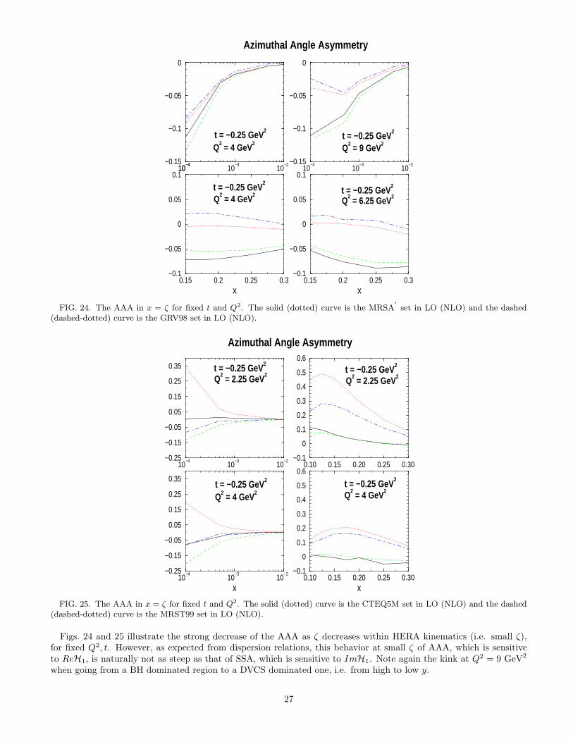
0.15 0.2 0.25 0.3x

−0.1

−0.05

0

0.05

0.110

−410

−310

−2

0.15 0.2 0.25 0.3x

−0.1

−0.05

0

0.05

0.110

−410

−310

−2−0.15

−0.1

−0.05

0

10−4−0.15

−0.1

−0.05

0

Azimuthal Angle Asymmetry

Q2 = 4 GeV

2t = −0.25 GeV

2t = −0.25 GeV

2

Q2 = 9 GeV

2

t = −0.25 GeV2

Q2 = 4 GeV

2 t = −0.25 GeV2

Q2 = 6.25 GeV

2

FIG. 24. The AAA in x = ζ for fixed t and Q2. The solid (dotted) curve is the MRSA′

set in LO (NLO) and the dashed(dashed-dotted) curve is the GRV98 set in LO (NLO).

10−4

10−3

10−2

x

−0.25

−0.15

−0.05

0.05

0.15

0.25

0.35

10−4

10−3

10−2−0.25

−0.15

−0.05

0.05

0.15

0.25

0.35

0.10 0.15 0.20 0.25 0.30x

−0.1

0

0.1

0.2

0.3

0.4

0.5

0.60.10 0.15 0.20 0.25 0.30

−0.1

0

0.1

0.2

0.3

0.4

0.5

0.6

Azimuthal Angle Asymmetry

Q2 = 2.25 GeV2t = −0.25 GeV

2

t = −0.25 GeV2

Q2 = 4 GeV2

t = −0.25 GeV2

Q2 = 2.25 GeV2

t = −0.25 GeV2

Q2 = 4 GeV2

FIG. 25. The AAA in x = ζ for fixed t and Q2. The solid (dotted) curve is the CTEQ5M set in LO (NLO) and the dashed(dashed-dotted) curve is the MRST99 set in LO (NLO).

Figs. 24 and 25 illustrate the strong decrease of the AAA as ζ decreases within HERA kinematics (i.e. small ζ),for fixed Q2, t. However, as expected from dispersion relations, this behavior at small ζ of AAA, which is sensitiveto ReH1, is naturally not as steep as that of SSA, which is sensitive to ImH1. Note again the kink at Q2 = 9 GeV2

when going from a BH dominated region to a DVCS dominated one, i.e. from high to low y.

27

The ζ-dependence of the AAA in the valence region probed at HERMES (where it has already measured the SSA),shows very large NLO effects, consistent within all sets, which make the AAA large and thus measurable at HERMES.The large overall size and spread of predictions is encouraging for measurements of the AAA at large x since evenhere the discriminating power between GPD models is very good.

2.25 3.25 4.25 5.25 6.25Q

2 in GeV

2

−0.25

−0.15

−0.05

0.05

0.15

0.25

0.35

0.45

1.5 2 2.5 3 3.5 4Q

2 in GeV

2

−0.05

0.15

0.35

0.55

0.75

0.95

Azimuthal Angle Asymmetry

x = 0.0001t = −0.25 GeV

2 t = −0.25 GeV2

x = 0.1

FIG. 26. The AAA in Q2 for fixed t and x = ζ. The solid (dotted) curve is the CTEQ5M set in LO (NLO) and the dashed(dashed-dotted) curve is the MRST99 set in LO (NLO).

Finally we show the Q2-dependence of the AAA in Fig. 26 (again only for MRST99 and CTEQ5M, due to theirlower input scale). For small ζ = x we see a fairly flat behavior of the AAA with Q2 with the NLO to LO changesstaying fairly constant in Q2. At large ζ = x, the predictions for the two sets quickly approach one another in bothLO and NLO as Q2 increases. Also the NLO to LO change decreases as Q2 increases in line with the argument thatBH starts dominating at large Q2 due to the associated increase in y.

D. The charge asymmetries (CA,CADSFL)

Other asymmetries which measure the real part of DVCS amplitudes are the charge and charge double spin flipasymmetries (see eqs.(23, 24)). These asymmetries require the measurement of DVCS with both the positron and theelectron and, in the case of the CADSFL, a longitudinally polarized probe and target at the same time. Thus theyare more difficult to measure than the AAA or other observables. The CA isolates the same combination of real partsof DVCS amplitudes as the AAA (i.e. the first term in eq.(30) of [31], which is proportional to cosφ), and wouldtherefore serve as a useful complementary measurement.

The CADSFL isolates the combination of real parts of DVCS amplitudes given in the second term of eq.(31) of [31].The UPLT asymmetry isolates the imaginary part of the same linear combination. Thus a combined measurement ofboth CADSFL and UPLT at small x reveals information about the real and imaginary parts of the polarized helicitynon-flip DVCS amplitude H1.

We discuss the CA first. Figs. 27-31 reveal that the CA is very similar to the AAA in the BH dominated region,and is within 20% of it in the DVCS dominated region for both LO and NLO. It can be easily seen that the t, x andQ2 behavior is very similar for both asymmetries. This behavior can be understood quite easily: in contrast to theAAA case, for CA the interference term drops out in the normalization in eq. (23) due to the sign change of theinterference term in going from a positron to an electron probe. The numerator is the same for both asymmetries.Hence, deviations between the AAA and the CA results show directly the influence of the interference term relativeto the BH and DVCS contributions. The larger the deviation the more important the interference term. Hence, aprecise measurement of the CA and the AAA will serve as a very good consistency check of the experimental analysis,since strong deviations between the CA and AAA are not expected. One caveat here is the possible importance ofhigher twist contributions in the interference term.

28

−0.5−0.4−0.3−0.2−0.1t in GeV

2

−0.1

−0.05

0

0.05−0.2

−0.15

−0.1

−0.05

0

−0.5−0.4−0.3−0.2−0.1t in GeV

2

−0.1

−0.05

0

0.05−0.2

−0.15

−0.1

−0.05

0

Q2 = 4 GeV

2

x = 0.0001

Q2 = 9 GeV

2

x = 0.0001

Q2 = 4 GeV

2

x = 0.2

Q2 = 9 GeV

2

x = 0.2

The Charge Asymmetry

FIG. 27. The CA in t for fixed x = ζ and Q2. The solid (dotted) curve is the MRSA′

set in LO (NLO) and the dashed(dashed-dotted) curve is the GRV98 set in LO (NLO).

−0.5−0.4−0.3−0.2−0.1t in GeV

2

−0.05

0.05

0.15

0.25

0.35

0.45

−0.35

−0.25

−0.15

−0.05

0.05

0.15

0.25

0.35

−0.5−0.4−0.3−0.2−0.1t in GeV

2

−0.05

0.05

0.15

0.25

0.35

0.45

−0.35

−0.25

−0.15

−0.05

0.05

0.15

0.25

0.35

Q2 = 2.25 GeV2

x = 0.0001 Q2 = 4 GeV2

x = 0.0001

Q2 = 2.25 GeV2

x = 0.1Q

2 = 4 GeV

2

x = 0.1

The Charge Asymmetry

FIG. 28. The CA in t for fixed x = ζ and Q2. The solid (dotted) curve is the CTEQ5M set in LO (NLO) and the dashed(dashed-dotted) curve is the MRST99 set in LO (NLO).

29

0.15 0.2 0.25 0.3x

−0.1

−0.05

0

0.05

0.110

−410

−310

−2

0.15 0.2 0.25 0.3x

−0.1

−0.05

0

0.05

0.110

−410

−310

−2−0.15

−0.1

−0.05

0

10−4−0.15

−0.1

−0.05

0

Charge Asymmetry

Q2 = 4 GeV

2t = −0.25 GeV

2t = −0.25 GeV

2

Q2 = 9 GeV

2

t = −0.25 GeV2

Q2 = 4 GeV

2 t = −0.25 GeV2

Q2 = 6.25 GeV

2

FIG. 29. The CA in x = ζ for fixed t and Q2. The solid (dotted) curve is the MRSA′

set in LO (NLO) and the dashed(dashed-dotted) curve is the GRV98 set in LO (NLO).

10−4

10−3

10−2

x

−0.25

−0.15

−0.05

0.05

0.15

0.25

10−4

10−3

10−2−0.25

−0.15

−0.05

0.05

0.15

0.25

0.1 0.15 0.2 0.25 0.3x

−0.1

0

0.1

0.2

0.3

0.4

0.50.1 0.15 0.2 0.25 0.3

−0.1

0

0.1

0.2

0.3

0.4

0.5

The Charge Asymmetry

Q2 = 2.25 GeV2t = −0.25 GeV

2

t = −0.25 GeV2

Q2 = 4 GeV2

t = −0.25 GeV2

Q2 = 2.25 GeV2

t = −0.25 GeV2

Q2 = 4 GeV2

FIG. 30. The CA in x = ζ for fixed t and Q2. The solid (dotted) curve is the CTEQ5M set in LO (NLO) and the dashed(dashed-dotted) curve is the MRST99 set in LO (NLO).

30

2.25 3.25 4.25 5.25 6.25Q

2 in GeV

2

−0.3

−0.2

−0.1

0

0.1

0.2

0.3

1.5 2.5 3.5Q

2 in GeV

2

−0.1

0

0.1

0.2

0.3

0.4

0.5

0.6

The Charge Asymmetry

x = 0.0001t = −0.25 GeV

2

t = −0.25 GeV2

x = 0.1

FIG. 31. The CA in Q2 for fixed t and x = ζ. The solid (dotted) curve is the CTEQ5M set in LO (NLO) and the dashed(dashed-dotted) curve is the MRST99 set in LO (NLO).

Moving now to a longitudinally polarized probe and target, we will study the charge asymmetry in a double spinflip experiment, the CADSFL.

−0.5−0.4−0.3−0.2−0.1t in GeV

2

−0.04−0.02

00.020.040.060.08

0.10.12

−0.5−0.4−0.3−0.2−0.1t in GeV

2

−0.04−0.02

00.020.040.060.08

0.10.12

Q2 = 4 GeV2

x = 0.15Q2 = 6.9 GeV2

x = 0.15

The CADSFL Asymmetry

FIG. 32. The CADSFL in t for fixed x = ζ and Q2. The solid (dotted) curve is the MRSA′

set in LO (NLO) and the dashed(dashed-dotted) curve is the GRV98 set in LO (NLO).

For HERA kinematics the CADSFL turns out to be too small to be measured, i.e. consistent with zero for anypractical purposes, and thus we will not show plots for HERA kinematics. For HERMES kinematics, the asymmetryis of the order of a few percent, so one might hope to be able to measure it. In Figs. 32 and 33 we show the t-dependence for fixed ζ = x and Q2, which turns out to be rather steep. In Figs. 34 and 35 we show the ζ-dependencefor fixed t, Q2. They indicate that although in percentage terms the spread of predictions is large the overall size ofthe CADSFL (only a few percent) would seem to indicate that exploiting this spread of predictions is impractical.

Finally we show the Q2-behavior of CADSFL in Fig. 36, for fixed t, ζ. We see quite a moderate to large differencein going from LO to NLO. Note the sign difference between the GRV98 and MRSA’ sets on the one hand and theCTEQ5M and MRST99 sets on the other hand. This gives some hope to use this asymmetry as a discriminatorbetween different model inputs. Generally speaking, due to its overall smallness, it is not as promising a candidateas the CA asymmetry as a good DVCS observable, even though it is directly sensitive to the real part of a polarizedamplitude at small ζ. This concludes our presentation of DVCS observables in LO and NLO.

31

−0.5−0.4−0.3−0.2−0.1t in GeV

2

−0.1−0.08−0.06−0.04−0.02

00.020.04

−0.5−0.4−0.3−0.2−0.1t in GeV

2

−0.1−0.08−0.06−0.04−0.02

00.020.04

Q2 = 2.25 GeV2

x = 0.15

Q2 = 4 GeV2

x = 0.15

The CADSFL Asymmetry

FIG. 33. The CADSFL in t for fixed x = ζ and Q2. The solid (dotted) curve is the CTEQ5M set in LO (NLO) and thedashed (dashed-dotted) curve is the MRST99 set in LO (NLO).

0.1 0.15 0.2 0.25 0.3x

−0.04

−0.02

0

0.02

0.04

0.06

0.15 0.2 0.25 0.3x

−0.04

−0.02

0

0.02

0.04

0.06

The CADSFL Asymmetry

Q2 = 4 GeV2t = −0.25 GeV

2t = −0.25 GeV

2

Q2 = 6.25 GeV2

FIG. 34. The CADSFL in x = ζ for fixed t and Q2. The solid (dotted) curve is the MRSA′

set in LO (NLO) and the dashed(dashed-dotted) curve is the GRV98 set in LO (NLO).

0.1 0.15 0.2 0.25 0.3x

−0.04

−0.03

−0.02

−0.01

0

0.01

0.02

0.03

0.1 0.15 0.2 0.25 0.3x

−0.04

−0.03

−0.02

−0.01

0

0.01

0.02

0.03

The CADSFL Asymmetry

Q2 = 2.25 GeV2t = −0.25 GeV

2 t = −0.25 GeV2

Q2 = 4 GeV2

FIG. 35. The CADSFL in x = ζ for fixed t and Q2. The solid (dotted) curve is the CTEQ5M set in LO (NLO) and thedashed (dashed-dotted) curve is the MRST99 set in LO (NLO).

32

1.5 2.5 3.5 4.5 5.5Q

2 in GeV

2

−0.03−0.02−0.01

00.010.020.030.040.050.06

4 4.5 5 5.5 6 6.5Q

2 in GeV

2

−0.03−0.02−0.01

00.010.020.030.040.050.06

The CADSFL Asymmetry

x = 0.15t = −0.25 GeV

2

t = −0.25 GeV2

x = 0.15

FIG. 36. The CADSFL in Q2 for fixed t and x = ζ. In the left figure, the solid (dotted) curve is the CTEQ5M set in LO(NLO) and the dashed (dashed-dotted) curve is the MRST99 set in LO (NLO), and in the right figure, the solid (dotted) curveis the MRSA’ set in LO (NLO) and the dashed (dashed-dotted) curve is the GRV98 set in LO (NLO).

E. Summary of optimal DVCS observables

We summarise the results of the previous subsections as follows:

• The triple differential cross section is quite a good discriminator between different GPD models, particularlyat Q2 values close to the input scale (at higher Q2 the BH process dominates). We predict a steep rise withdecreasing ζ reflecting the underlying powerlike behavior in ζ of the DVCS amplitudes.

• The SSA is quite sizable and well behaved in NLO for all the input GPDs concerned, which makes it a verygood candidate to be measured both at HERA and HERMES. For small ζ (HERA kinematics) we predict astrong increase in magnitude as ζ decreases (a feature shared by AAA and CA) and good discriminating powerbetween input models, especially at larger Q2.

• The AAA and CA seem to be very good candidates for discriminating between different input GPDs simplybecause they measure the real part of DVCS amplitudes which are very sensitive to the underlying details ofthe GPDs, in Radyushkin’s ansatz, especially at NLO where the gluon enters with a relative minus sign for thereal part of its amplitude. Practical measurements for both asymmetries appear feasible for both HERMES andHERA kinematics.

• The measurement of UPLT (CADSFL) appears to be practical only at large ζ in HERMES kinematics, where ittests a linear combination of imaginary (real) parts of several DVCS amplitudes. Therefore these measurementshave very limited discriminating power between model GPDs.

In summary it seems that four out of six observables are large enough to make measurements at HERA and HERMESfeasible, and which have good discriminating power between input scenarios. Thus the prospects of unraveling thedetails of the DVCS process experimentally are in principle very good.

VI. COMPARISON WITH EXPERIMENT AND OTHER CALCULATIONS

In this section we compare our LO and NLO results for each of our input sets with the available published experi-mental data from H1 and HERMES. The ZEUS collaboration announced the first measurement of DVCS at HERA[9] (see also [13]), but has yet to publish a cross section.

33

H1 recently published their data [10] on the measured DVCS cross section on both the lepton level and the photonlevel. They use the equivalent photon approach, which relates the pure DVCS cross section on the lepton level (withthe interference neglected23 and the pure BH term subtracted) to the virtual-photon proton cross section:

d2σ(ep→ epγ)

dydQ2= Γ σDV CS(γ∗p→ γp) where Γ =

αe.m.(1 + (1 − y)2)

2πyQ2. (52)

By integrating eq. (17) over t, φ, and changing variables from xbj to y, we can establish the formula for the photon-levelcross section in terms of our amplitudes as

σDV CS(γ∗p→ γp) =α2x2π

Q4B|TDV CS |

2|t=0, (53)

where B stems from the t-integration and, within our model for the t-dependence, B ≈ 6.5 GeV−2 (with a surprisinglysmall spread of about 1 GeV−2 !). We observed that for the kinematical region of the H1 data which is limited tosmall x, i.e. to small ζ, we could write

∫ ttmin

−∞

dt |TDV CS |2 ≈

1

B|TDV CS |

2|t=0 (54)

as if we had assumed a global exponential dependence, eBt, as was used by H1 in their comparison to other [8,46]calculations (dropping all amplitudes except H). On numerical inspection we found that indeed H clearly dominatesall the other amplitudes for HERA kinematics. Therefore, in comparing to the data, we can safely neglect all otheramplitudes (i.e. polarised and helicity-flip) in the DVCS square term.

The same assumption was made in previous LO QCD [8] and two-component dipole model [46,47] calculations,which both reproduce the H1 data quite well. Since ours is a QCD calculation we point out the differences andsimilarities with [8]. The latter was based on a LO input (CTEQ3L) with the assumption that the GPDs are equal tothe PDFs at the input scale. The imaginary part of the unpolarized helicity non-flip amplitude was then computedusing the aligned jet model and the imaginary part, rather than the GPD, was then evolved to higher Q2. This isequivalent to what we did at LO24 since the imaginary part of the DVCS amplitude is simply π times the GPD atζ = xbj , legitimising the approach in [8]. The DVCS triple differential cross section, at small x, was then computedby comparing the imaginary part of DVCS to DIS and thus introducing the structure function F2 through the opticaltheorem. In order to reconstruct the real part of the DVCS amplitude a dispersion relation approach was usedwhich exploited the slope of F2 in ln(1/x) at small x (which was extracted from data to give η = ReADIS/ImADIS)together with the comparative factor R = ImADVCS/ImADIS. The specification was completed with the additionalassumption of a global t-dependence, eBt. In contrast to [8], we computed both parts of the DVCS amplitudes directlyand used them in the unapproximated expressions for the DVCS triple differential cross section, which also containsthe polarized as well as helicity flip amplitudes (however these can be safely neglected in the cross section at smallζ). Furthermore, we assumed a dipole type t-dependence which is close to the exponential behavior at small ζ and t,as well as being correct at larger t (and small ζ).

In Fig. 37 we plot σDV CS(γ∗p) at Q2 = 4.5 GeV2 in W (this is of course similar to a plot in 1/x = W 2/Q2) forGRV and MRST input models at LO and NLO. Also shown is the H1 data, for which they quote <Q2 >= 4.5 GeV2,with systematic and statistical error bars added in quadrature. In Fig. 38, we plot σDV CS(γ∗p) in Q2 for fixedW = 75 GeV. The most obvious observation to make is that all of the the curves lie well above the data. Howeverthey do have the correct shapes (rising with W and falling rapidly with Q2).

23This may be ignored at small y, typical of HERA kinematics, and after integration over φ.24Note however that our LO calculation is based on NLO input PDFs, and a different ansatz for the GPDs, so we don’t

necessarily expect the results to agree closely.

34

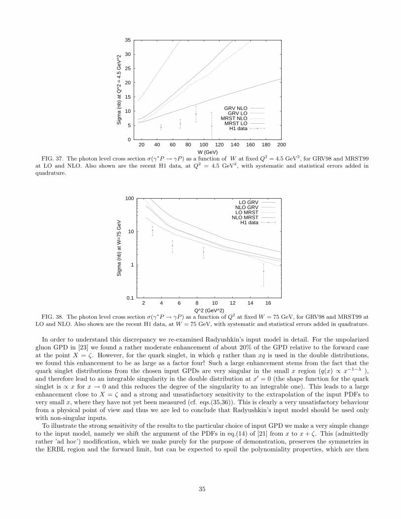
0

5

10

15

20

25

30

35

20 40 60 80 100 120 140 160 180 200

Sig

ma

(nb)

at Q

^2 =

4.5

GeV

^2

W (GeV)

GRV NLOGRV LO

MRST NLOMRST LO

H1 data

FIG. 37. The photon level cross section σ(γ∗P → γP ) as a function of W at fixed Q2 = 4.5 GeV2, for GRV98 and MRST99at LO and NLO. Also shown are the recent H1 data, at Q2 = 4.5 GeV2, with systematic and statistical errors added inquadrature.

0.1

1

10

100

2 4 6 8 10 12 14 16

Sig

ma

(nb)

at W

=75

GeV

Q^2 (GeV^2)

LO GRVNLO GRVLO MRST

NLO MRSTH1 data

FIG. 38. The photon level cross section σ(γ∗P → γP ) as a function of Q2 at fixed W = 75 GeV, for GRV98 and MRST99 atLO and NLO. Also shown are the recent H1 data, at W = 75 GeV, with systematic and statistical errors added in quadrature.

In order to understand this discrepancy we re-examined Radyushkin’s input model in detail. For the unpolarizedgluon GPD in [23] we found a rather moderate enhancement of about 20% of the GPD relative to the forward caseat the point X = ζ. However, for the quark singlet, in which q rather than xq is used in the double distributions,we found this enhancement to be as large as a factor four! Such a large enhancement stems from the fact that thequark singlet distributions from the chosen input GPDs are very singular in the small x region (q(x) ∝ x−1−λ ),and therefore lead to an integrable singularity in the double distribution at x′ = 0 (the shape function for the quarksinglet is ∝ x for x → 0 and this reduces the degree of the singularity to an integrable one). This leads to a largeenhancement close to X = ζ and a strong and unsatisfactory sensitivity to the extrapolation of the input PDFs tovery small x, where they have not yet been measured (cf. eqs.(35,36)). This is clearly a very unsatisfactory behaviourfrom a physical point of view and thus we are led to conclude that Radyushkin’s input model should be used onlywith non-singular inputs.

To illustrate the strong sensitivity of the results to the particular choice of input GPD we make a very simple changeto the input model, namely we shift the argument of the PDFs in eq.(14) of [21] from x to x + ζ. This (admittedlyrather ’ad hoc’) modification, which we make purely for the purpose of demonstration, preserves the symmetries inthe ERBL region and the forward limit, but can be expected to spoil the polynomiality properties, which are then

35

restored25 under evolution [45]. In making this modification we ensure that the PDFs are never sampled below x = ζ(which removes the sensitivity to the very small x region) and can be expected to reduce considerably the enhancementof the GPDs at X = ζ. Figs. 39 and 40 show the very dramatic effect on the cross section. The theory curves for themodified ansatz now undershoot the experimental data by about a factor of two and appear to reproduce the shapein W and Q2 rather well. In summary we claim that this illustrates that the H1 data are already able to begin toconstrain the input GPDs. It seems clear that if one is to use Radyushkin’s ansatz at very small ζ the input PDFsshould be non-singular. Alternatively, one must invent a new parameterization of the GPDs at the input scale thatretains the required features (correct polynomiality and symmetry properties and faithful reproduction of the forwardlimit) without the problem of a strong sensitivity to the very small x region and associated large enhancement of theGPDs relative to the PDFs at the point X = ζ. This might be achieved by choosing a non-singular double distributionat a very low input scale, with the small X behavior generated by perturbative evolution.

0

2

4

6

8

10

12

20 40 60 80 100 120 140 160 180 200

Sig

ma

(nb)

at Q

^2 =

4.5

GeV

^2

W (GeV)

GRV NLOGRV LO

MRST NLOMRST LO

H1 data

FIG. 39. The photon level cross section σ(γ∗P → γP ) as a function of W at Q2 = 4.5 GeV2, for GRV98 and MRST99 atLO and NLO using the shifted ansatz.

0.1

1

10

2 4 6 8 10 12 14 16 18 20

Sig

ma

(nb)

at W

=75

GeV

Q^2 (GeV^2)

LO GRVNLO GRVLO MRST

NLO MRSTH1 data

FIG. 40. The photon level cross section σ(γ∗P → γP ) as a function of Q2 at fixed W = 75 GeV, for GRV98 and MRST99at LO and NLO, using the shifted ansatz.

25In [45], in which the evolution is performed using moments, it is shown that expansion coefficients in an orthogonal basisallow only even powers of ζ in the expansion, in line with the symmetry properties of GPDs. Similarly, in our numericalsolution, which is carried out in x space rather than moment space, the non-polynomial pieces will be killed by the kernelsunder convolution (the kernels encode the GPD symmetries in their structure).

36

We now turn to the SSA as measured by the HERMES collaboration [11]. They define the SSA, weighted withsin φ, as follows:

SSA =2∫ 2π

0 dφ sin φ (dσ↑ − dσ↓)∫ 2π

0(dσ↑ + dσ↓)

. (55)

They quote two values: SSA = −0.18± 0.05± 0.05 and 〈SSA〉 = −0.23± 0.03± 0.04. The first, which assumes thattheir missing mass equals the proton mass, is quoted at the following average values: <x>= 0.11, <Q2>= 2.5 GeV2

and <t>= −0.27 GeV2. The second (average) value is the SSA integrated over the missing mass at the same averagevalues of x, Q2 and t. At this point in x, Q2, t for the HERMES definition we find SSA = −0.365 for CTEQ5M andSSA = −0.35 for MRST99.

Given the fact that the input models used do not describe the data at small ζ, and that we find the same typeof enhancement effect when comparing GPDs with forward PDFs at both small and large ζ, the failure to describethe HERMES data is not surprising. In fact one needs higher statistics over a wide kinematic range in severalDVCS observables to be able to begin to tune the input GPDs using a fitting method. Only then can one startdiscriminating between different choices for the PDFs in input models. Furthermore, for HERMES data one needs toknow the normalizations of numerator and the denominator producing the measured asymmetry to help to constrainthe normalization of the individual amplitudes (in order to be able to make any sensible statements about a comparisonbetween theory and experiment).

In comparing with other calculations we show qualitative agreement with [8,46,47] and quantitative agreement with[31,44] wherever we used the same input distributions (MRSA’ and GS(A) only).

VII. CONCLUSIONS

We have presented a detailed next-to-leading (NLO) QCD analysis of deeply virtual Compton scattering (DVCS)observables. We quantified the NLO corrections and established which observables have the best prospects to bemeasured accurately at HERA and HERMES (the triple differential cross section and the azimuthal angle (AAA),single spin (SSA) and charge (CA) asymmetries). We have demonstrated that such measurements would have gooddiscriminating power between different scenarios for the generalized parton distributions (GPDs), by examining fourcases. It turns out that AAA and CA, which test the real part of unpolarized DVCS amplitude at small x are themost sensitive to the choice of GPD model.

We performed a comparison with presently available DVCS data and showed that within Radyushkin’s ansatz forthe GPDs, all of the models we examined overshoot the H1 data. This is due to their singular nature of the quarksinglet at small x which leads to a strong sensitivity to the PDFs in the extremely small x region, where they have notyet been measured. We illustrated this strong sensitivity by artificially shifting the argument of the PDFs by ζ, whichled to a large reduction in the theoretical predictions for the photon-level cross section (which then undershoots thedata). This illustrates an urgent need for improved input models, which do not rely on a singular double distributionand also for more, high precision data to help constrain them.

ACKNOWLEDGEMENTS

A. F. was supported by the DFG under contract # FR 1524/1-1. M. M. was supported by PPARC. We gladlythank D. Muller for helpful conversations and discussions throughout this project. We also thank R. G. Roberts forproviding the input parameters of the ‘corrected’ MRST parton set.

[1] D. Muller et al., Fortsch. Phys. 42 (1994) 101.[2] A. V. Radyushkin, Phys. Rev. D 56 (1997) 5524.[3] X. Ji, J. Phys. G 24 (1998) 1181.[4] M. Diehl et al., Phys. Lett. B 411 (1997) 193.

37

[5] M. Vanderhaeghen, P. A. M. Guichon and M. Guidal, Phys. Rev. D 60 (1999) 094017.[6] J. C. Collins and A. Freund, Phys. Rev. D 59 (1999) 074009.[7] X. Ji and J. Osborne, Phys. Rev. D58 (1998) 094018[8] L. Frankfurt, A. Freund and M. Strikman, Phys. Rev. D 58 (1998) 114001;

Erratum-ibid. D59 (1999) 119901; Phys. Lett. B 460 (1999) 417,A. Freund and M. Strikman, Phys. Rev. D 60 (1999) 071501.

[9] P. R. Saull, for ZEUS Collab., “Prompt photon production and observation of deeply virtual Compton scattering crosssection at HERA”, Proc. EPS 1999, Tampere, Finland, hep-ex/0003030.

[10] C. Adloff et al., H1 collab., Phys. Lett. B517 (2001) 47.[11] A. Airapetian et al., HERMES Collab., Phys. Rev. Lett. 87 (2001) 182001.[12] S. Stepanyan et al., CLAS Collab., Phys. Rev. Lett. 87 (2001) 182002.[13] ZEUS Collab., “Measurement of the deeply virtual Compton scattering cross section at HERA”, Abstract 564, IECHEP

2001, July 2001, Budapest, Hungary.[14] J. C.Collins, L. Frankfurt and M. Strikman, Phys. Rev. D 56 (1997) 2982.[15] A. V. Belitsky et al., Phys. Lett. B 437 (1998) 160;

A. V. Belitsky, A. Freund and D. Muller, Nucl. Phys. B574 (2000) 347.[16] V. Yu. Petrov et al., Phys. Rev. D 57 (1998) 4325.[17] L. Frankfurt et al., Phys. Lett. B 418 (1998) 345, Erratum-ibid. B429 (1998) 414;

A. Freund and V. Guzey, Phys. Lett. B 462 (1999) 178.[18] V. N. Gribov and L. N. Lipatov, Sov. J. Phys 15 (1972) 438, 675;

Yu. L. Dokshitzer, Sov. Phys. JETP 46 (1977) 641;G. Altarelli. and G. Parisi, Nucl Phys B126 (1977) 298.

[19] A. V. Efremov and A. V. Radyushskin, Theor. Math. Phys. 42 (1980) 97, Phys Lett. B94 (1980) 245;S. J. Brodsky and G. P. Lepage, Phys Lett. B87 (1979) 359; Phys. Rev. D22 (1980) 2157.

[20] A. Radyushkin, Phys. Rev. D58 (1998) 114008.[21] A. Freund and M. McDermott, hep-ph/0106115.[22] M. V. Polyakov and C. Weiss, Phys. Rev. D 60 (1999) 114017.[23] A. Freund and M. McDermott, hep-ph/0106124.[24] A. Freund and M. McDermott, hep-ph/0106319.[25] H.Lai et al., Eur. Phys. J. C 12 (2000) 375.[26] A. Martin et al. , Eur. Phys. J. C14 (2000) 133.[27] M. Gluck, E. Reya and A. Vogt, Eur. Phys. J. C 5 (1998) 461;

we evolve from the low input scales up to Q0 = 2 GeV, using conventional (forward) DGLAP evolution.[28] A. D. Martin, R. G. Roberts and W. J. Stirling, Phys. Lett. B 354 (1995) 155.[29] http://durpdg.dur.ac.uk/hepdata/dvcs.html[30] J. Blumlein, B. Geyer and D. Robaschik, Phys. Lett. B406 (1997) 161;

I. I. Balitsky and A. V. Radyushkin, Phys. Lett. B413 (1997) 114;L. Mankiewicz et al., Phys. Lett. B 425 (1998) 186;A. V. Belitsky and D. Mueller, Phys. Lett. B 417 (1998) 129, Nucl. Phys. B 537 (1999) 397.

[31] A. V. Belitsky et al., Nucl. Phys. B 593 (2001) 289.[32] P. Kroll, M. Schurmann, P. A. M. Guichon, Nucl. Phys. A 598 (1996) 435.[33] L. B. Okun, Leptons and quarks, North-Holland, (Amsterdam, 1982).[34] A. V. Belitsky et al., Phys. Lett. B 510 (2001) 117.[35] S. Aid et al., H1 Collab., Nucl. Phys. B 468 (1996) 3.[36] L. Favart, for H1 Collab., Proposal for a very forward proton spectrometer in H1 after 2000,

Proc. of DIS2000, Liverpool, April 2000, eds. J. A. Gracey and T. Greenshaw (World Scientific (2001), pp 618).[37] K. Golec-Biernat and A. D. Martin, Phys. Rev. D 59 (1999) 014029.[38] N. Kivel, M. V. Polyakov and M. Vanderhaeghen, Phys. Rev. D 63 (2001) 114014.[39] P. Penttinen, M. Polyakov and K. Goeke, Phys. Rev. D 62 (2000) 014024.[40] A. V. Radyushkin, Phys. Rev. D59 (1999) 014030.[41] M. Gluck et al., Phys. Rev. D 63 (2001) 094005.[42] T. Gehrmann and W. J. Stirling, Phys. Rev. D 53 (1996) 6100.[43] http://www.phys.psu.edu∼cteq/fortran/pdfs/Ctq5Par.f[44] A. V. Belitsky et al., Phys. Lett. B 474 (2000) 163.[45] A. V. Belitsky et al., Nucl. Phys. B 546 (1999), 279.[46] A. Donnachie and H.G. Dosch, Phys. Lett. B 502 (2001) 74.[47] M. McDermott, R. Sandapen and G. Shaw, hep-ph/0107224.

38