arX

iv:h

ep-p

h/93

0731

1v1

20

Jul 1

993

July 1993 LBL–34147

Next-to-Leading Order QCD Corrections

to Jet Cross Sections and Jet Rates

in Deeply Inelastic Electron Proton Scattering ∗ †

Dirk Graudenz ‡ § ¶

Theoretical Physics GroupLBL / University of California

1 Cyclotron RoadBerkeley, CA 94720, USA

Abstract

Jet cross sections in deeply inelastic scattering in the case of transverse photon exchangefor the production of (1+1) and (2+1) jets are calculated in next-to-leading order QCD (herethe ‘+1’ stands for the target remnant jet, which is included in the jet definition for reasonsthat will become clear in the main text). The jet definition scheme is based on a modifiedJADE cluster algorithm. The calculation of the (2+1) jet cross section is described in detail.Results for the virtual corrections as well as for the real initial- and final state correctionsare given explicitly. Numerical results are stated for jet cross sections as well as for the ratioσ(2+1) jet/σtot that can be expected at E665 and HERA. Furthermore the scale ambiguity

of the calculated jet cross sections is studied and different parton density parametrizationsare compared.

∗This work was supported by the Director, Office of Energy Research, Office of High Energy and Nuclear

Physics, Division of High Energy Physics of the U.S. Department of Energy under Contract DE-AC03-76SF00098

and the Bundesministerium fur Forschung und Technologie under contract number 05 5AC 91 P.†Revised version.‡supported by Max Kade Foundation, New York§Address after January 1, 1994: CERN, Theoretical Physics Division, CH-1211 Geneva, Switzerland¶E-mail addresses: graudenz @ theorm.lbl.gov, GRAUDENZ @ LBL.bitnet, I02GAU @ DHHDESY3.bitnet

Disclaimer

This document was prepared as an account of work sponsored by the United States Government. Neitherthe United States Government nor any agency thereof, nor The Regents of the University of California, norany of their employees, makes any warranty, express or implied, or assumes any legal liability or responsibilityfor the accuracy, completeness, or usefulness of any information, apparatus, product, or process disclosed, orrepresents that its use would not infringe privately owned rights. Reference herein to any specific commercialproducts process, or service by its trade name, trademark, manufacturer, or otherwise, does not necessarilyconstitute or imply its endorsement, recommendation, or favoring by the United States Government or anyagency thereof, or The Regents of the University of California. The views and opinions of authors expressedherein do not necessarily state or reflect those of the United States Government or any agency thereof ofThe Regents of the University of California and shall not be used for advertising or product endorsementpurposes.

Lawrence Berkeley Laboratory is an equal opportunity employer.

ii

1 Introduction

Recent results from E665 and HERA show that events with a clear jet-like structure are present indeeply inelastic electron proton scattering [1, 2]. With sufficient luminosity it should thereforebe possible to study jet cross sections to use them for a test of QCD and an independentdetermination of its fundamental parameter ΛQCD. Jet cross sections may even be useful toextract some information on the gluon density at small x, because the gluon density is importantin (2+1)1 jet production.

Because of the strong scale dependence of fixed order cross sections calculated in perturbativeQCD, the possibility of a large size of the corrections and because a determination of αs must bebased on a next-to-leading (NLO) order cross section, the calculation of higher order correctionsis well motivated. Since now experimental results are available, it is worthwhile to give a detailedaccount of the technical problems of the calculation of the (2+1) jet cross section. A second goalof the present work is to study the jet cross sections in detail numerically. In deeply inelasticscattering, the O(αs) corrections to the O(α0

s) Born term are well known (see [3, 4, 5, 6, 7, 8, 9]).In addition, the O(α2

s) Born terms for the production of (3+1) jets have been calculated [10, 11].In this paper the calculation of the cross section for the production of (2+1) jets to O(α2

s) inthe case of transverse photon exchange2 is described. For more details of the calculation see[12, 13]. The contributions with a transverse exchanged photon dominate the cross section, as isshown in Section 8. More recently, the other parity-conserving helicity cross sections have beencalculated based on [12], see [14].

One of the main features of hadronic events in high-energy collisions is the pronounced jet-like structure. These jets are attributed to the production of partons in the fundamental QCDprocess [15]. Due to the presence of infrared divergences in QCD, a suitable prescription has tobe given in order to define the finite parts that arise from divergent terms after the singularitiesbetween real and virtual corrections have been cancelled. Such a prescription is related to thejet definition that is used on the parton level to calculate jet cross sections. In Section 2 jetdefinitions in deeply inelastic scattering are discussed and the jet definition scheme based on amodification of the JADE cluster algorithm that is used in this calculation is defined.

In Section 3 the calculation of the (1+1) jet cross section in next-to-leading order is reviewedand the results for the (2+1) jet Born terms are stated. In Section 4 the results for the virtualcorrections to (2+1) jet production are given. In Sections 5 and 6 the calculation of the realcorrections to (2+1) jet production is described (separated according to singularities in the finaland initial state). The sum of virtual and real corrections gives the finite jet cross section afterrenormalisation of the parton densities. The flavour factors are listed in Section 7. In Section8 the numerical results for jet cross sections and for the ratio σ(2+1) jet/σtot are presented.

The dependence of the jet cross sections on the renormalisation and factorization scales, thedependence on the jet definition scheme and the dependence on the parametrization of theparton densities is also studied. The appendix contains explicit results for massless 1-looptensor structure integrals, phase space integrals and the virtual and real corrections.

1The target remnant is counted as a jet, so “2+1” stands for the production of 2 partons in the hard QCDprocess, possibly accompanied by additional soft or collinear partons.

2Here, the cross section for transverse photon exchange is defined by the helicity cross section obtained by acontraction of the hadron tensor with the metric tensor (−gµν).

1

2 Jet Cross Sections

Jets must be defined in terms of experimentally observable quantities. An experimental eventis characterised by the energies and momenta of the outgoing particles. Since at high energiesthe multiplicity of the events is large and since presently there is no practical way (based onQCD) to describe hadron dynamics on the level of observable particles, one has to try to extractinformation from experimental data in a form that can be compared with theoretical resultsfrom perturbative QCD. At e+e−-colliders it has been observed that outgoing hadrons veryoften appear as clusters of particles concentrated in a small cone in momentum space. Theseclusters were called jets. Given an experimental event and a resolution parameter c (the “jetcut”), a suitable algorithm is applied to the event giving the number of jets of the event andthe particles associated with each of the jets. Therefore, the algorithm that is used defines whatis meant by a “jet”. To compare experiment and theory, one must use the same algorithm intheoretical calculations. One should expect that experiment and theory are comparable as longas the same algorithm is used in the experimental analysis and in the theoretical calculation.Of course, the problem is that in realistic events the final state consists of hadrons, whereasin theoretical calculations (based on QCD) the outgoing “particles” are partons. Therefore thecrucial hypothesis is that jets on the hadron level and jets on the parton level can be identified.

The first jet definition that has been given is that of Sterman and Weinberg [15]. It isbased on cones in momentum space defined by an opening angle δ and an energy fraction ǫ.This definition, which is well suited for e+e−-annihilation for a small number of jets becomescomplicated if a larger number of jets is produced. In addition, it is not Lorentz invariant (thisis not a problem in the case of e+e−-annihilation, since here the CM system is a unique frameof reference). Later, another type of algorithm was proposed, the cluster algorithm first usedby the JADE collaboration [16]. This algorithm combines succesively two particles into a jet, iftheir invariant mass squared sij is smaller than a fraction c of a typical mass scale :

sij ≤ cM2. (1)

In e+e−-annihilation, c is of the order of 10−2, and M2 is set to Q2, the total invariant mass ofthe hadronic final state.

For hadron colliders, jet definitions in terms of “cones” in rapidity and azimuthal angle arefavoured (UA1-type algorithms). Such a jet definition singles out a particular axis (namely, thedirection of the two colliding beams). In the case of pp-events the incoming partons are assumedto have only small transverse momentum, and therefore the situation is symmetric with respectto this particular axis.

The situation is quite different for electron-proton colliders. Here the interaction is mediatedby the exchange of a virtual photon with momentum q (and Q2 := −q2 > 0). This photon hitsa proton with momentum P . Therefore, the interaction should be described in the CM systemwith ~P + ~q = ~0. This system varies from event to event, and this is the reason why a Lorentzinvariant jet definition should be used [11].

Before a suggestion for a suitable jet algorithm in eP-scattering is given, one should have acloser look at the target remnant. An interesting question is: “Is it reasonable to include thetarget jet in a jet analysis?”. One should consider the process in fig. 1. This Feynman graph

2

describes initial state radiation of a gluon with momentum p2 from the initial quark line withmomentum p0. It is assumed that the gluon is emitted collinearly with a large energy in thedirection of the incoming quark causing a strong enhancement of the cross section for this processbecause of the pole of the quark propagator. Since all partons are assumed to be massless thegluon will go in the same direction as the target remnant. Under the assumption that “partonjets” roughly correspond to “hadron jets”, there will be no possibility to disentangle the hadronsfrom the debris of the proton and those coming from the fragmentation of the gluon. To beconsistent, one therefore should define “parton jets” in the following way: If an outgoing gluoncan be separated from the remnant by a suitable condition (e.g. invariant mass), the gluon andthe remnant are considered to be two jets with momenta p2 and pr. If the gluon and the remnantcannot be separated, they count as one jet whose momentum p∗ = p2 + pr is the sum of thegluon momentum and the momentum of the remnant. In an experiment, however, one cannotmeasure the momentum of the remnant directly since most of the hadrons from this jet are lostin the beam pipe. The momentum of the target remnant jet must therefore be determined inan indirect way. The jet algorithm should also have the property that all collinear singularitiesare treated in such a way that they factorize the corresponding Born term. This allows for aprocess independent definition of the renormalised scale dependent parton densities.

For the experimental analysis it is proposed to use a modified JADE cluster algorithm(mJADE algorithm) consisting of two steps (see also [11]):(1) Define a precluster of longitudinal momentum (in the direction of the beam pipe) pr that isgiven by the missing longitudinal momentum of the event.(2) Apply the JADE cluster algorithm to the set of momenta

p1, p2, . . . , pn, pr, (2)

where p1, p2, . . . , pn are the momenta of the visible hadrons in the detector and pr is the mo-mentum of the precluster.

It remains to define the order of magnitude of the jet cut and the mass scale M2 to be usedin the mJADE algorithm. The jet cut should be such that it is small enough to ensure properlyseparated jets in the detector (otherwise the jets coming from the real corrections could becometoo broad), but large enough to avoid large logarithms that could spoil a fixed order result inperturbation theory. One can think of cM2 as a new mass scale that is needed to specify thecross section completely. In a deeply inelastic process there are several mass scales given byan event, namely the virtuality Q2 of the exchanged vector boson, the invariant mass W 2 ofthe hadronic final state and, in general, several invariant masses p2

i⊥ from transverse momentaof outgoing particles. Therefore large logarithms are expected if the quotient of any two ofthese scales becomes small (or large). So one should avoid kinematical regions where this couldhappen. Because of the jet cut an additional scale cM2 enters the calculation, where one could,for example, use Q2, W 2 or some p2

i⊥ as M2. Since it is suggested to include the target remnantin the jet analysis, it is natural to use the scale M2 = W 2 in the jet algorithm (analogous tothe situation in e+e−-annihilation). If the scales p2

i⊥ are omitted from the discussion, the scalesQ2 = SHyxB, W 2 = SHy(1−xB) and cW 2 = cSHy(1−xB) are relevant. Here

√SH is the total CM

energy of the collider, xB = Q2/2Pq is the Bjorken variable and y is the usual lepton variabley = Pq/Pk, with P the proton momentum and k the momentum of the incoming electron.

This is not the only reasonable choice for the mass scale used in the the jet definition. In

fact, in Section 3 it is pointed out that a scale like Q2 or(

W αQβ√

SHy1−α−β

))2

with parameters

3

α, β may be reasonable if the parton densities have to be probed at small x. In contrast, theconsiderations here are based on the simple observation that the observable invariants (includingthose with the remnant jet) sum up to W 2, and it is somehow natural to use this particularscale. For another possible jet definition in eP scattering see [17].

In the cross section large logarithms of Q2/W 2 ≈ xB, cW 2/W 2 = c and cW 2/Q2 ≈ c/xB (theapproximation of small xB is made since most events are expected in this region) are expected.For cuts of the order of 0.01 the logarithms in c should be comparable to those encountered ine+e−-annihilation because of a similar structure of the matrix elements.

Berger and Nisius have studied the effect of the inclusion of the target remnant in the jetanalysis [18] by using the Monte Carlo generator LEPTO5.2. They come to the conclusionthat the correlation of the number of jets on the parton level and the number of jets afterfragmentation is much stronger if the remnant jet is included. For more details, see [11].

3 (1+1) and (2+1) Jets: Cross Sections to O(αs)

In this section the calculation of the (1+1) jet cross section in NLO is reviewed. This is donefor two reasons: these results are needed to calculate jet rates, and their calculation serves as anillustration of the more complicated case of the NLO corrections to (2+1) jet production. As abyproduct, one gets the results for the (2+1) jet Born terms. The total cross section to O(αs)for photon exchange has been calculated in [4], and the (1+1) jet cross section to this order forall neutral and charged current processes can be found in [9]. Here the special case of the (1+1)jet cross section for the exchange of a transverse photon is discussed in detail and results for alongitudinally polarised photon are stated. It is safe to focus on the QCD corrections for thetransverse polarization of the virtual photon, since the cross section for longitudinally polarizedphotons contributes only about 20% to the Born term cross section (see Section 8), and this isexpected to be true for the relative contribution of the longitudinal terms to the NLO correctionsas well.

The cross section for eP-scattering differential in xB and y is given by

dσH

dxBdy=

∑

i

∫ 1

xB

dξ

ξfi(ξ)

(4π)ǫ (SHxB)−ǫ (y(1− y))−ǫ µ4ǫ

Γ(1− ǫ)α2 1

2

1

SHxB

· dPS(n)parton

1

e2µ2ǫ(2π)2d

1

Q2

1

N ′

∫

dΩ′ lµν Hµν , (3)

where d = (4 − 2ǫ) is the space-time dimension (ǫ 6= 0 regularises the ultraviolet and infrareddivergences [19, 20, 21]), µ is a mass scale for making the coupling constants dimensionless in d

dimensions, dPS(n)parton is the n-parton phase space

dPS(n)parton = (2π)d

n∏

i=1

ddpiδ(p2i )

(2π)d−1δ(p0 + q −

n∑

i=1

pi), (4)

Ω′ is the volume element of d− 3 angles specifying the direction of the outgoing lepton relativeto the outgoing partons, and

N ′ =

∫

dΩ′ (5)

4

is a normalisation constant. The incoming parton carries a fraction ξ of the proton momentum,the fi(ξ) are the bare parton densities for partons of flavour i,

lµν = kµk′ν + kνk′µ − kk′gµν (6)

is the lepton tensor and Hµν is the hadron tensor (including coupling constants, colour factors,etc.).

The integration over Ω′ can be performed. It can be shown by a direct evaluation of theintegrals in d-dimensional space that

1

Q2

1

N ′

∫

dΩ′ lµν =1 + (1− y)2 − ǫy2

2(1− ǫ)y2(−gµν − ǫµν

q )

+4(1− ǫ)(1− y) + 1 + (1− y)2 − ǫy2

2(1 − ǫ)y2(ǫµν

R + ǫµν0 ), (7)

where

ǫµνq =

1

Q2qµqν ,

ǫµνR =

1

Q2(qµqν + 2xp(p

µ0qν + qµpν

0)),

ǫµν0 =

4x2p

Q2pµ0pν

0 , (8)

and xp := xB/ξ. Because of current conservation qµHµν = 0 one has

ǫαµq Hµν = ǫαµ

R Hµν = 0. (9)

With the definition trH := hg := (−gµν)Hµν , h0 := ǫµν0 Hµν one obtains

1

Q2

1

N ′

∫

dΩ′ lµν Hµν

=1 + (1− y)2 − ǫy2

2(1 − ǫ)y2hg +

4(1− ǫ)(1− y) + 1 + (1− y)2 − ǫy2

2(1 − ǫ)y2h0. (10)

By defining

σλ =∑

i

∫ 1

xB

dξ

ξfi(ξ)

(4π)ǫ (SHxB)−ǫ (y(1− y))−ǫ µ4ǫ

Γ(1− ǫ)α2 1

2

1

SHxB

· dPS(n)parton

1

e2µ2ǫ(2π)2dhλ (11)

with λ ∈ g, 0 one arrives at

dσH

dxBdy=

1 + (1− y)2 − ǫy2

2(1 − ǫ)y2σg

+4(1− ǫ)(1− y) + 1 + (1− y)2 − ǫy2

2(1− ǫ)y2σ0. (12)

5

In the literature cross sections σU , σL for unpolarized and longitudinally polarized photons havebeen defined. They are related to the definitions used in this paper by σg = 2(1−ǫ)σU−σL, σ0 =σL.

Now the special case of (1+1) jet production is considered. Fig. 2 depicts the Feynmandiagram to O(α0

s). The diagram for the 1-loop virtual correction is shown in fig. 3. The resultfor the sum of these diagrams is well known [4]:

dσBorn&virt.H

dxBdy=

∑

i

∫ 1

xB

dxp

xpfren

i

(

xB

xp,M2

f

)

(4π)ǫ (SHxB)−ǫ (y(1− y))−ǫ µ4ǫ

Γ(1− ǫ)α2 1

2

1

SHxB

·1 + (1− y)2 − ǫy2

2(1 − ǫ)y22π 4(1− ǫ) Q2

i

·

δqi

[

1 +

(

4πµ2

Q2

)ǫΓ(1− ǫ)

Γ(1− 2ǫ)

αs

2πCF

(

− 2

ǫ2− 3

ǫ

)

+αs

2πCF (−8− 2 ζ(2))

]

δ(1 − xp)

+

(

4πµ2

M2f

)ǫΓ(1− ǫ)

Γ(1− 2ǫ)

αs

2π

1

ǫPq←i(xp)

+O(ǫ). (13)

The integration over ξ is rewritten in terms of the variable xp = xB/ξ, and the symbol δqi restrictsthe summation to quark initiated terms. ζ(2) = π2/6, and Qi is the charge of the quark withflavour i normalised to e. µ is the renormalisation scale and Mf is the factorization scale. Thepole terms in ǫ proportional to δ(1−xp) are infrared singularities that will cancel against infraredsingularities in the real corrections, and the term proportional to the Altarelli-Parisi splittingfunction Pq←i(xp) will cancel against collinear singularities in the real corrections. Note that thebare parton densities fi(ξ) are already expressed in terms of the renormalised parton densities[4, 22] in the MS-scheme

freni

(

ξ,M2f

)

=

∫ 1

ξ

du

u

[

δijδ(1− u) +αs

2π

(

−1

ǫ

)

Pi←j(u)Γ(1− ǫ)

Γ(1 − 2ǫ)

(

4πµ2

M2f

)ǫ]

fj(ξ

u). (14)

The Altarelli-Parisi kernels are

Pq←q(u) = CF

[

1 + u2

(1− u)++

3

2δ(1 − u)

]

,

Pg←q(u) = CF1 + (1− u)2

u,

Pg←g(u) = 2NC

[

1

(1− u)++

1

u+ u(1− u)− 2

]

+

(

11

6NC −

1

3Nf

)

δ(1 − u),

Pq←g(u) =1

2

[

u2 + (1− u)2]

. (15)

Nf is the number of quark flavours.

Now the real NLO corrections to (1+1) jet production will be calculated. The Born terms ofO(αs) have to be integrated over the phase space region that, by the jet definition, is consideredto be a (1+1) jet region. In a first step, suitable variables are defined, then the (1+1) jet region

6

is determined and finally the integration is performed. The phase space for the production of2 partons is constructed in the following way. As usual, the variable

z =Pp1

Pq, (16)

is defined, where p1 is one of the outgoing partons. By defining t = s12/W2 (p2 is the momentum

of the second outgoing parton) and a = xB + (1− xB)t one obtains

∫

dPS(2) =

∫

dPS∗(2)ξδ(ξ − a),

∫

dPS∗(2) =

∫

(4π)ǫ

Γ(1− ǫ)

(

W 2)−ǫ

t−ǫ (z(1 − z))−ǫ 1

8π

1− xB

adz dt, (17)

where the fact that ξ = a if p0 = ξP is being used. By means of the factor ξδ(ξ−a) the integral∫

dξ/ξ f(ξ) in the cross section formula (3) can be performed trivially. The ranges of integrationare z ∈ [0, 1] and t ∈ [0, 1]. The invariants sij = 2pipj expressed in terms of z and t are

s01 = SHy(xB + (1− xB)t)z,

s02 = SHy(xB + (1− xB)t)(1− z),

s12 = SHy(1− xB)t. (18)

The momentum of the target remnant is pr = (1− ξ)P . The observable momenta are p1, p2 andpr. Invariants for these momenta are defined by uij = 2pipj/W

2. In terms of the variables zand t they read

ur1 = (1− t)z,

ur2 = (1− t)(1− z),

u12 = t. (19)

Let us define the (2+1) jet region by the condition sij > cW 2, with i, j ∈ 1, 2, r. It is easyto see that in the (t, z)-plane where the allowed phase space is the square [0, 1]× [0, 1] the (2+1)jet region is a triangle given by the following conditions:

(a) c < t < 1− 2c,

(b) zc(t) < z < 1− zc(t), where zc(t) = c1− t .

The region within the square surrounding this triangle is therefore the (1+1) jet region. Allregions where the cross section becomes singular are within the (1+1) jet region thus allowingthe factorization of the collinear singularities and their absorption into the renormalised partondensities. It should be noted that for (2+1) jet production the minimal momentum fraction ξ ofthe parton densities that can be probed is ξmin(xB) = xB +(1−xB)c because of the cut conditionon s12. The minimum is ξmin = c for xB → 0 and is therefore of order 0.01. If one wants touse the gluon initiated (2+1) jet events to determine gluon densities at small x a different scale

for the jet definition could be chosen. If the scale is Q2 or(

W αQβ√

SHy1−α−β

)2, the minimal

7

ξ depending on xB turns out to be ξmin(xB) = xB(1 + c) and ξmin(xB) = xB + (1 − xB)αxBβc,

respectively, and for sufficiently small xB and c both give small ξmin. If xB is fixed, thesedefinitions are of course equivalent to the choice of a much smaller cut c in the jet definitionscheme based on W 2, and it is therefore important to check whether the (2+1) jets are stillcalculated in a regime where perturbation theory is still valid, i.e., whether the (2+1) jet rateis small enough compared to the total cross section.

After this short digression the results for the Born cross sections for the production of2 partons are stated. The relevant diagrams are depicted in fig. 4 with the graph G replacedby the diagrams of fig. 5. Of course, in fig. 4 one would have an additional diagram from anincoming antiquark, but since the resulting expressions are (except for the charges) the same asthose for incoming quarks, these diagrams are omitted in the sequel.

The traces of the hadron tensor for quark and gluon initiated processes are

trHBorn, q inc. = L1Q2j8(1 − ǫ)CF Tq,

trHBorn, g inc. = L1Q2j8(1 − ǫ)

1

2Tg (20)

with

Tq = (1− ǫ)

(

s02

s12+

s12

s02

)

+2Q2s01

s02s12+ 2ǫ,

Tg =1

1− ǫ

(1− ǫ)

(

s01

s02+

s02

s01

)

− 2Q2s12

s01s02− 2ǫ

(21)

andL1 = (2π)2dg2e2µ4ǫ. (22)

p0 is always the momentum of the incoming parton, and p1 is the momentum of the outgoingquark.

These formulae are already averaged over the colour degree of freedom of the incomingpartons. The factor of 1/(1 − ǫ) in the expression for Tg comes from the fact that a gluonhas 2(1 − ǫ) helicity states in d = (4 − 2ǫ) dimensions compared to only 2 helicity states in4 dimensions.

Now the integration of the cross sections over the (1+1) jet region of the 2-parton phasespace can be done by subtracting the (2+1) jet cross section from the total cross section toO(αs). The technical reason is that this subtraction makes the explicit universal factorizationof the singular parts in the form of a product of an Altarelli-Parisi splitting function and theBorn term more transparent than the direct integration over the (1+1) jet region.

The total cross section from the real corrections for transverse photons and quark initiatedprocesses is [4]:

dσtot.,t,qH

dxBdy=

∑

i

∫ 1

xB

dxp

xpfren

i

(

xB

xp,M2

f

)

(4π)ǫ (SHxB)−ǫ (y(1− y))−ǫ µ4ǫ

Γ(1− ǫ)α2 1

2

1

SHxB

·1 + (1− y)2 − ǫy2

2(1 − ǫ)y22π 4(1− ǫ) Q2

i

(

4πµ2

Q2

)ǫΓ(1− ǫ)

Γ(1− 2ǫ)

αs

2πCF δqi

8

·

2

ǫ2δ(1 − xp) +

1

ǫ

[

− 1

CFPq←q + 3δ(1 − xp)

]

+2

(

ln(1− xp)

1− xp

)

+

− (1 + xp) ln(1− xp)−3

2

1

(1− xp)+−

1 + x2p

1− xpln xp

+3− xp +7

2δ(1 − xp)

+O(ǫ). (23)

The “+”–prescriptions are defined in [23] (they are implicitly used for functions defined on theinterval [0, 1]) and are the result of the subtraction in the collinear regime. The bare partondensities are expressed in terms of the renormalised ones and terms of O(α2

s) are dropped. Thecorresponding expression for the gluon initiated process is3

dσtot.,t,gH

dxBdy=

2Nf∑

i=1

∫ 1

xB

dxp

xpfren

g

(

xB

xp,M2

f

)

(4π)ǫ (SHxB)−ǫ (y(1− y))−ǫ µ4ǫ

Γ(1− ǫ)α2 1

2

1

SHxB

·1 + (1− y)2 − ǫy2

2(1− ǫ)y22π 4(1 − ǫ) Q2

i

(

4πµ2

Q2

)ǫΓ(1− ǫ)

Γ(1− 2ǫ)

αs

2π

1

2

1

1− ǫ

·

− 21

ǫPq←g(xp) +

(

(1− xp)2 + x2

p

)

ln1− xp

xp

+O(ǫ). (24)

Note that the sum over quark flavours reflects the different flavours that are produced in thisprocess.4

In the sum of (13), (23) and (24) the infrared and collinear singularities cancel, and one isleft with a finite total cross section to O(αs). To obtain the (1+1) jet cross section one has tosubtract the (2+1) jet cross section from the total cross section. Since there are no singularitiesin the (2+1) jet region, ǫ can be set to 0. The integration of (20) over the (2+1) jet region isnot difficult. If all contributions are summed up one arrives at the finite (1+1) jet cross section.The quark initiated part is given by

dσ(1+1),t,qH

dxBdy=

2Nf∑

i=1

∫ 1

xB

dxp

xpQ2

i freni

(

xB

xp,M2

f

)

α2 1

2

1

SHxB

1 + (1− y)2

2y2· 2π · 4

·

1 + CFαs

2π

[

(−8− 2ζ(2)) δ(1 − xp)

+2

(

ln(1− xp)

1− xp

)

+

− (1 + xp) ln(1− xp)−3

2

1

(1− xp)+−

1 + x2p

1− xpln xp

+3− xp +7

2δ(1 − xp) +

1

CFln

Q2

M2f

Pq←q(xp)

−(

[

1

2

1

1− xp− 2

xp

1 − xp

]

(1− 2zc(t(xp)))

+

[

1− xp + 2xp

1− xp

]

ln1− zc(t(xp))

zc(t(xp))

)

Ξc≤t(xp)≤1−2c

]

, (25)

3Compared to [4] there is a difference in the finite parts. It results from the average over the helicities of aninitial gluon. Here it is assumed that the gluon has d − 2 = 2(1 − ǫ) polarization states instead of 2.

4To make the cancellation of the collinear divergence transparent, a “double counting” is included which iscancelled by a factor of 1/2.

9

and the gluon initiated processes contribute

dσ(1+1),t,gH

dxBdy=

2Nf∑

i=1

∫ 1

xB

dxp

xpQ2

i freng

(

xB

xp,M2

f

)

α2 1

2

1

SHxB

1 + (1− y)2

2y2· 2π · 4

· 12

αs

2π

[

(

(1− xp)2 + x2

p

)

(

ln1− xp

xp− 1

)

+ 2 lnQ2

M2f

Pq←g(xp)

−(

− (1− zc(t(xp))) + (1− 2xp(1− xp))

· ln 1− zc(t(xp))

zc(t(xp))

)

Ξc≤t(xp)≤1−2c

]

, (26)

where ΞA is the characteristic function of the set specified in A restricting the integration tothat set and t(xp) is the variable t introduced above given by

t(xp) =xB

1− xB

1− xp

xp. (27)

The logarithms depending on the factorization scale that cancel part of the scale dependenceof the parton densities are indicated explicitly. There are no such terms depending on therenormalisation scale because the Born term is of O(α0

s).

The corresponding terms for a virtual photon with longitudinal polarization arise at O(αs).They are given by

dσ(1+1),l,qH

dxBdy=

2Nf∑

i=1

∫ 1

xB

dxp

xpQ2

i freni

(

xB

xp,M2

f

)

α2 1

2

1

SHxB

4(1 − y) + 1 + (1− y)2

2y2· 2π · 4

·CFαs

2π

[

xp −(

xp (1− 2zc(t(xp)))

)

Ξc≤t(xp)≤1−2c

]

(28)

and

dσ(1+1),l,gH

dxBdy=

2Nf∑

i=1

∫ 1

xB

dxp

xpQ2

i freng

(

xB

xp,M2

f

)

α2 1

2

1

SHxB

4(1 − y) + 1 + (1− y)2

2y2· 2π · 4

· 12

αs

2π

[

2xp(1− xp)−(

2xp(1− xp) (1− 2zc(t(xp)))

)

Ξc≤t(xp)≤1−2c

]

(29)

for incoming quarks and gluons, respectively.

Now the jet recombination scheme ambiguity which arises from the problem of the mappingof a “jet phase space” of massive jets in NLO onto a phase space of massless partons in leadingorder is discussed. The real corrections for the (1+1) jet cross section have been obtained by anintegration of the Born terms for the production of 2 partons over some region of phase spacespecified by the jet cut definition. To cancel the infrared and collinear singularities, one has todefine effective (1+1) jet variables that allow the identification of the corresponding singularitiesin the virtual corrections and in the contribution from the redefinition of the parton densities.This procedure is a map of the (1+1) jet region of the 2-parton phase space onto the (1+1)jet phase space. In principle this map is ambiguous, but fortunately the the difference between

10

different maps is 0 for vanishing jet cut. Here the following scheme is tacitly assumed: If a clusteralgorithm is applied to a 2-parton event that looks like a (1+1) jet event, then the final result ofthis clustering will be two clusters with momenta pA and pB, one of them being massless and oneof them being massive. The (1+1) jet Born term and the virtual correction always result in twomassless clusters pC and pD. The identification is done by mapping (pA + pB)2 onto (pC + pD)2.In this special case both expressions are equal to W 2. This quantity can be determined fromelectron variables alone, so what is essentially done is the identification of processes in which theelectrons have the same momenta. This, however, may correspond to very different situationson the parton level, since e.g. a radiated final state gluon can be collinear to the remnant jetresulting in a remnant with a large momentum or can be collinear to the outgoing quark. Thesituation is similar in the case of the corrections to the (2+1) jet cross section. In that case,however, the identification involves two variables and not only one, and so the identificationusing W 2 is not sufficient.

4 (2+1) Jets: Virtual Corrections

In this section the calculation of the virtual corrections to the production of (2+1) jets isdescribed. The one-loop corrections to the graphs from fig. 5 are given in fig. 6. The one-loopdiagrams from fig. 7 contribute to the wave function renormalisation and are taken into accountin the counter term. To obtain the O(α2

s) corrections the diagrams in fig. 6 must be multipliedby the Born diagrams. The resulting topologies can be divided into three classes:

(I) QED-like graphs with colour factor NCC2F ,

(II) QED-like graphs with colour factor NCCF

(

CF − 12NC

)

,

(III) non-abelian graphs with colour factor −12N2

CCF ,

resulting in terms proportional to the colour factors NCC2F and N2

CCF . The sum of the virtualO(α2

s) corrections averaged over the colour degree of freedom of the incoming parton is

trHv, q inc. = L1L2Q2j8(1− ǫ)C2

F E1,q −1

2NCCF E2,q

+

(

1

ǫ+ log

Q2

µ2

)

(

1

3Nf −

11

6NC

)

CF Tq+O(ǫ), (30)

trHv, g inc. = L1L2Q2j8(1− ǫ)1

2CF E1,g −

1

4NCE2,g

+

(

1

ǫ+ log

Q2

µ2

)

(

1

3Nf −

11

6NC

)

1

2Tg+O(ǫ), (31)

11

where

L2 =αs

2π

(

4πµ2

−q2 − iη

)ǫΓ(1− ǫ)

Γ(1− 2ǫ). (32)

Here Nf is the number of active quark flavours in the fermion loops and µ2 is the renormalisationscale (it is understood that the running αs is always evaluated at the scale µ2). The contributionsE1,q, E2,q, E1,g and E2,g come from the calculation of the matrix elements of the graphs infig. 6. The explicit expressions for the Ei,q and Ei,g are collected in Appendix B. The tracecalculations of the matrix elements were done with the help of REDUCE [24]. Then the loopintegrals were performed by an insertion of one-loop tensor structure integrals (see appendixA). Here one has to be careful with respect to the imaginary parts of Spence functions andlogarithms which are important because q2 < 0. The results obtained here have been checkedagainst those of the e+e−-case [25]. This was possible because all infinitesimal imaginary partsfrom the propagators were kept in the formulae.

In (30), (31) the counter terms (in the MS-scheme) to cancel UV singularities (see [25])is already added. Some 1/ǫ2- and 1/ǫ-poles remain. These divergences are due to the IRsingularities of the loop corrections.

For the processes with an incoming quark the following variables are defined:

zq :=p1p0

p0q, zg :=

p2p0

p0q, xp :=

xB

a. (33)

The divergent parts are

trHv, q inc. = L1L2Q2j8(1− ǫ)CF Tq

·

CF

[

(

− 1

ǫ2+

1

ǫ

(

ln1− zg

xp− 3

2

))

+

(

− 1

ǫ2+

1

ǫ

(

lnzqa

xB

− 3

2

)) ]

−1

2NC

[

(

2

ǫ2+

1

ǫ

(

lnx2

p

(1− xp)(1− zq)+ 2

))

+1

ǫ· 53

+1

ǫln

1− zg

1− xp+

1

ǫln

zq

1− zq

]

+Nf ·1

3· 1ǫ

+O(ǫ0). (34)

For the processes with an incoming gluon the variables are similar:

zq :=p1p0

p0q, zq :=

p2p0

p0q, xp :=

xB

a. (35)

The divergent parts are

trHv, g inc. = L1L2Q2j8(1− ǫ)

1

2Tg

12

·

CF

[

2

(

− 1

ǫ2+

1

ǫ

(

ln1− xp

xp− 3

2

))

]

−1

2NC

[

1

ǫln

1− xp

1− zq+

1

ǫln

1− xp

1− zq

+

(

2

ǫ2+

1

ǫ

(

− lna2zq(1− zq)

xB2

+11

3

))

]

+Nf ·1

3· 1ǫ

+O(ǫ0). (36)

They will cancel against divergent terms from the real corrections.

5 (2+1) Jets: Final State Real Corrections

To O(α2s) one has to consider the contributions from the Born terms in fig. 8 integrated over

the (2+1) jet phase space region in the 3-parton phase space.

Again there are graphs with an incoming quark and an incoming gluon. The generic diagramsare shown in fig. 9. There are, of course, additional contributions with incoming antiquarks;their structure is identical to the quark-initiated processes.

The integrations become singular if the integrand contains a propagator whose denominatorvanishes in the integration region. The method of partial fractions is used to separate initialand final state singularities. This allows the identification of the terms proportional to O(c0),O(ln c) and O(ln2 c) (c is the jet cut). In this section the final state singularities are considered,the initial state singularities are treated in the next section.

For the process

e−(k)+ proton(P )→ e−(k′)+ target remnant(pr)+ parton(p1)+ parton(p2)+ parton(p3) (37)

a parametrization of the phase space of the outgoing partons with momenta pi is needed. Thetarget remnant with momentum pr = (1− ξ)P is described by the variable ξ. The parametriza-tion is chosen such that the integration over the region s12 < c (p1 and p2 being collinear orp1 being soft or p2 being soft) is simple. In close analogy to calculations in e+e−-annihilationit is reasonable to describe the two particle phase space of p1 and p2 in the CM frame of thesemomenta (see fig. 10).

Let p0 be the momentum of the incoming parton. One can define a variable z by

z :=p0p3

p0q(38)

that describes the phase space of p3 (the azimuthal dependence is contained in the lepton phasespace, and the remaining third integration is trivial because of energy conservation). One candefine a polar angle θ given by θ := 6 (~p1, ~p0) in the CM frame of p1 and p2 and an azimuthal

13

angle ϕ by the angle between the planes spanned by ~p0, ~p1 and ~p0, ~p3, respectively. Let χ bedefined by χ := 6 (~p0, ~p3) and

b :=1

2(1− cos θ) (39)

d :=1

2(1− cos χ) (40)

e := b + d− 2bd− 2√

b(1− b)d(1 − d) cos ϕ. (41)

With the normalisation factors

Nϕ :=π4ǫΓ(1− 2ǫ)

Γ2(1− ǫ)=

∫ π

0sin−2ǫ ϕdϕ (42)

Nb :=Γ2(1− ǫ)

Γ(2− 2ǫ)=

∫ 1

0(b(1− b))−ǫ db (43)

the 3-parton phase space in d = 4− 2ǫ dimensions is

∫

dPS(3) =

∫

(16π2)ǫ

128π3Γ(2− 2ǫ)s−ǫ12 ds12z

−ǫ (SHy(ξ − xB)(1 − z)− s12)−ǫ

·dz1

Nϕsin−2ǫ ϕdϕ

1

Nb(b(1− b))−ǫ db

=

∫

dPS∗(2)∫

dPS∗(r). (44)

dPS∗(2) is defined in eq. (17), and

dPS∗(r) = aδ(ξ − a)L22π

αsµ−2ǫ 1

2

1

8π2

Q2

xpxǫ

p

1

1− 2ǫdµF , (45)

dµF =

(

1− s12

SHy(ξ − xB)(1− z)

)−ǫ

r−ǫ12 dr12

1

Nϕsin−2ǫ ϕdϕ

· 1

Nb(b(1− b))−ǫ db, (46)

rij :=sij

SHyξ. (47)

dPS∗(2) contains the variables z and t = s12/W2 that are identified with the corresponding

(2+1) jet variables. The phase space for 3 particles factorizes as a product of a phase spacefor 2 particles dPS∗(r) and an effective phase space for a particle and a cluster dPS∗(2). Theinvariants rij can be expressed in the variables t, z, b, xp = xB/ξ, ϕ and r12:

r01 = (1− z)b,

r02 = (1− z)(1 − b),

r03 = z,

r13 = (1− xp − r12)e,

r23 = (1− xp − r12)(1− e). (48)

14

The variable d in eq. (40) is given by

d =z

1− z

r12

1− xp − r12. (49)

The phase space boundaries are

xB ∈ [0, 1], ξ ∈ [xB, 1], t ∈ [0, 1],

ϕ ∈ [0, π], b ∈ [0, 1], r12 ∈ [0, (1 − xp)(1− z)]. (50)

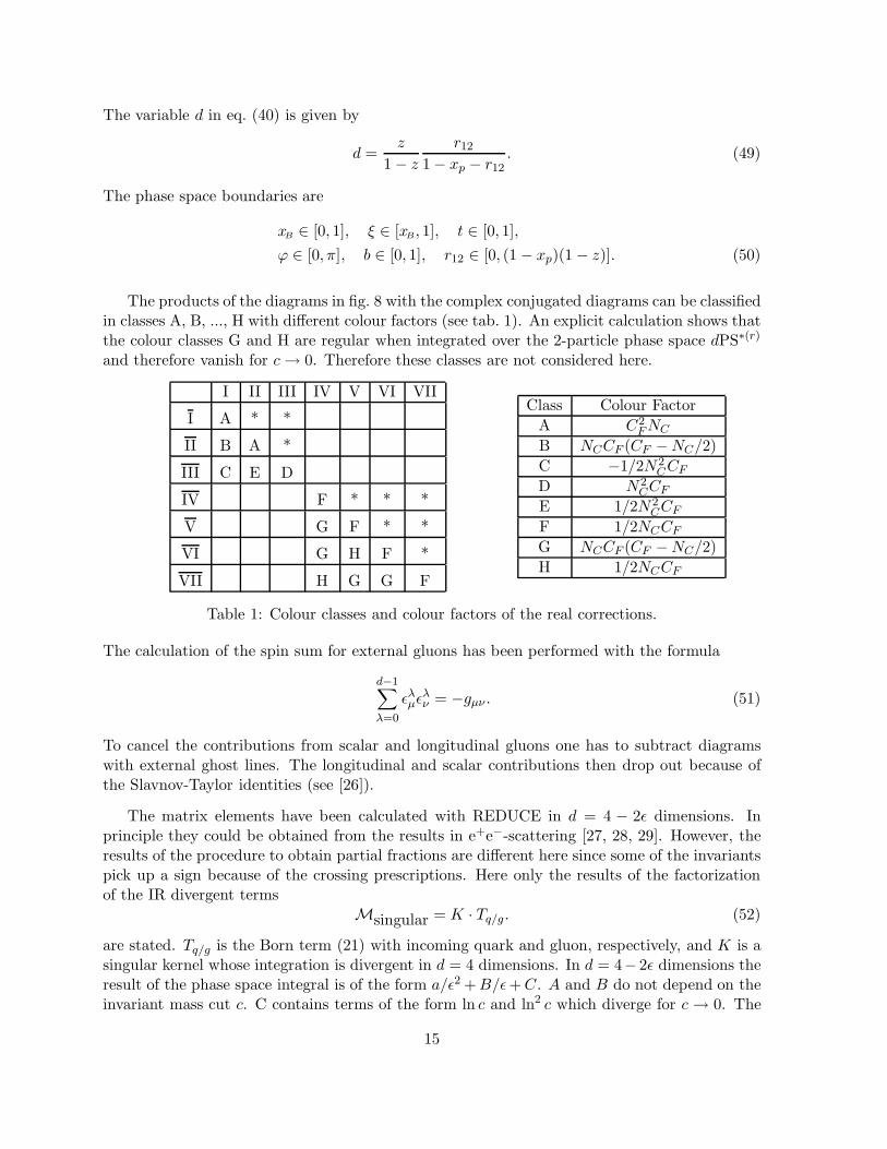
The products of the diagrams in fig. 8 with the complex conjugated diagrams can be classifiedin classes A, B, ..., H with different colour factors (see tab. 1). An explicit calculation shows thatthe colour classes G and H are regular when integrated over the 2-particle phase space dPS∗(r)

and therefore vanish for c→ 0. Therefore these classes are not considered here.

I II III IV V VI VII

I A * *

II B A *

III C E D

IV F * * *

V G F * *

VI G H F *

VII H G G F

Class Colour Factor

A C2F NC

B NCCF (CF −NC/2)

C −1/2N2CCF

D N2CCF

E 1/2N2CCF

F 1/2NCCF

G NCCF (CF −NC/2)

H 1/2NCCF

Table 1: Colour classes and colour factors of the real corrections.

The calculation of the spin sum for external gluons has been performed with the formula

d−1∑

λ=0

ǫλµǫλ

ν = −gµν . (51)

To cancel the contributions from scalar and longitudinal gluons one has to subtract diagramswith external ghost lines. The longitudinal and scalar contributions then drop out because ofthe Slavnov-Taylor identities (see [26]).

The matrix elements have been calculated with REDUCE in d = 4 − 2ǫ dimensions. Inprinciple they could be obtained from the results in e+e−-scattering [27, 28, 29]. However, theresults of the procedure to obtain partial fractions are different here since some of the invariantspick up a sign because of the crossing prescriptions. Here only the results of the factorizationof the IR divergent terms

Msingular = K · Tq/g. (52)

are stated. Tq/g is the Born term (21) with incoming quark and gluon, respectively, and K is asingular kernel whose integration is divergent in d = 4 dimensions. In d = 4− 2ǫ dimensions theresult of the phase space integral is of the form a/ǫ2 + B/ǫ + C. A and B do not depend on theinvariant mass cut c. C contains terms of the form ln c and ln2 c which diverge for c → 0. The

15

Class incoming parton product of diagrams colour factor

F1 quark I·I, II·II, II·I NCC2F /NC

F2 quark II·I, III·I, III·II (−1/2)N2CCF /NC

F3 quark III·I, III·II (−1/2)N2CCF /NC

F4 quark III·III N2CCF /NC

F5 quark IV·IV, V·V, VI·VI, VII·VII (1/2)NCCF /NC

F6 gluon I·I, II·II, II·I NCC2F /(2NCCF )

F7 gluon II·I, III·I, III·II (−1/2)N2CCF /(2NCCF )

Table 2: Colour factors.

contributions from the final state singularities are divided into seven classes (see tab. 2). Theresults for the traces of the hadronic tensor trHFi

for the seven colour classes are given explicitlyin appendix C.

The singular kernels are integrated over the (2+1) jet like region in phase space. Thecondition for partons j, k to form a jet is sjk ≤ cW 2. This condition can be rephrased in termsof the variables

rjk :=sjk

SHyξ(53)

as

rjk ≤ c1− xB

xB

xp. (54)

The phase space boundary is given by rjk ≤ (1− xp)(1− z). So the (2+1) jet region is specifiedby

rjk ≤ α := min

(1− xp)(1− z), c1 − xB

xB

xp

, b ∈ [0, 1], ϕ ∈ [0, π]. (55)

The phase space integrals are listed in appendix D. One obtains∫

(2+1) jetdPS∗(r)trHFi

= aδ(ξ − a)L1L28(1 − ǫ)Fi. (56)

for the corrections from the final state singularities. The explicit expressions are collected inappendix E.

6 (2+1) Jets: Initial State Real Corrections

In this section the contributions from the initial state singularities are described. In the case ofthe final state singularities the momentum fraction ξ of the incoming parton is a fixed parameterin the matrix elements. In the case of the initial state singularities, however, there is theadditional problem that ξ is an integration variable and that ξ is an argument of the partondensities fi(ξ). Although there is no expression for fi(ξ) in a closed form, the problem can besolved [4] by a Taylor expansion around the singular point and the well known “+”-prescriptions[23]

D+(g) :=

∫ 1

0duD(u) (g(u)− g(1)) . (57)

16

A similar parametrization of the phase space as in the case of the final state singularities isused, but the effective (2+1) jet variables are defined in a different way. Let p0 be the momentumof the incoming parton and p3 the momentum of an outgoing parton. For the calculation of thesingularity resulting from s03 → 0 p1 and p2 are the momenta of the partons to be identifiedwith the effective (2+1) jet momenta. Variables z′, z and t are defined by

z′ :=p0p3

p0q, z :=

p0p1

p0q, t :=

s12

W 2. (58)

With the conventions from Section 5 one obtains

b =z

1− z′. (59)

A factor of unity

1 =

∫

dξ′δ(ξ − ξ′) (60)

is inserted in eq. (44) to display a change of variables

σ :=1− t

1−z′ −1−ξ′

1−xB

1− t1−z′

(61)

explicitly. As a result one obtains∫

dPS(3) =

∫

dPS∗(2)∫

dPS∗(r), (62)∫

dPS∗(r) = δ(ξ − ξ′)L22π

αsµ−2ǫ 1

2

1

8π2W 2H(z′)dµI , (63)

H(z′) = (1− z′)−2+2ǫ(

1− z′

1− t

)1−ǫ (

1− z′

1− z

)−ǫ

= 1 +O(z′), (64)

dµI =Γ(1− 2ǫ)

Γ2(1− ǫ)a

(

1− xB

xB

)−ǫ

(1− t)1−ǫσ−ǫdσz′−ǫdz′1

Nϕsin−2ǫ ϕdϕ. (65)

The δ-function δ(ξ − ξ′) can be used to perform the integration over the parton densities. dµI

is the measure for the singular integrations. The invariants tij := sij/W2 can be expressed in

terms of the phase space variables:

t01 = (ν − ζ)z,

t02 = (ν − ζ)(1− z − z′),

t03 = (ν − ζ)z′,

t12 = t,

t13 = (1− ζ − t)e,

t23 = (1− ζ − t)(1− e), (66)

where

ν =1

1− xB

, ζ = (1− σ)

(

1− t

1− z′

)

, (67)

e = b + d + 2bd− 2√

b(1− b)d(1 − d) cos ϕ, (68)

d =z′

1− z′r

1− xB

ξ′ − r. (69)

17

It should be noted thatξ = a + (1− a)σ +O(z′). (70)

The phase space boundaries are given by

xB ∈ [0, 1], ξ, ξ′ ∈ [xB, 1], t ∈ [0, 1], z ∈ [0, 1],

ϕ ∈ [0, π], σ ∈ [0, 1], 0 ≤ z′ ≤ min 1− z, 1 − t. (71)

The factorization of the divergent parts is performed in the form

Msingular = K · Tq/g. (72)

up to terms that vanish for c → 0 after the integration. Therefore one can, for example, setH(z′) identically to 1.

The contributions from the initial state singularities are divided into seven classes (see tab. 3).In the case of the initial state singularities the incoming parton of the (3+1) jet graph is notnecessarily the incoming parton of the (factorized) (2+1) jet process. This is the familiar factthat the quark parton densities modify the evolution of the gluon density and vice versa. Intab. 3 a list of the incoming partons of both processes is added. The explicit expressions of thesingular kernels trHIi

are collected in appendix F.

Class (3+1) (2+1) product of diagrams colour factor

I1 quark quark I·I, II·II, II·I NCC2F /NC

I2 quark quark II·I, III·I, III·II (−1/2)N2CCF /NC

I3 quark gluon IV·IV, V·V, VI·VI, VII·VII (1/2)NCCF /NC

I4 gluon quark I·I, II·II, II·I NCC2F /(2NCCF )

I5 gluon quark II·I, III·I, III·II (−1/2)N2CCF /(2NCCF )

I6 gluon gluon II·I, III·I, III·II (−1/2)N2CCF /(2NCCF )

I7 gluon gluon III·III N2CCF /(2NCCF )

Table 3: Colour factors.

The boundaries of the (2+1) jet phase space region are given by the invariant mass cutcondition. For the initial state singularities, the variable z′ is the crucial variable that determinesthe singularity structure. The matrix elements become singular for z′ = 0. Let “r” be the labelfor the target remnant jet. The invariant trj is given by trj = ((1− ξ)/ξ) t0j. If pr and p3 arethe momenta combined into a jet, then the invariants of the effective (2+1) jet event are t12,t1r3, t2r3. The cut conditions read

tr3 =1− ξ

1− xB

z′ ≤ c, (73)

t12 = t ≥ c, (74)

t1r3 = t13 + t1r + t3r = (1− ζ − t)e +1− ξ

1− xB

(z + z′) ≥ c, (75)

t2r3 = t23 + t2r + t3r = (1− ζ − t)(1− e) +1− ξ

1− xB

(1− z) ≥ c. (76)

18

Especially the last two of these conditions are too complicated to be used in an analyticalcalculation since they involve a restriction of the azimuthal angle integration. Therefore thecontributions from the initial state singularities are integrated up to the phase space boundary(so ϕ ∈ [0, π], z′ ∈ [0,min1−z, 1− t]) by keeping the effective (2+1) jet variables z and t fixed.The (3+1) jet contribution is then subtracted after a numerical integration. Since the integralincluding the parton densities cannot be performed analytically, this is not a serious restriction.The shape of the phase space regions in the (z′, σ)–plane is given in fig. 11.

The poles and double poles in ǫ characterising IR (z′ = σ = 0) and collinear (z′ = 0)singularities can be calculated in the integration over the full (z′, σ)-plane. The phase spaceintegrals are given in appendix G. In the formulae given there the upper limit of the z′-integrationis β = min1 − z, 1 − t. In the integrals σ is used as an integration variable. The integralinvolving the parton densities is of the form

∫ 1

0dσ

f(ξ(σ, z′, . . .), Q2)

ξ(σ, z′, . . .)D(σ). (77)

Here D is a generalized function depending on σ and the other jet variables. f(ξ(σ, z′, . . .), Q2)is expanded in a Taylor series in z′ and all terms of order O(z′) that do not contribute in theapproximation used here are neglected. One obtains

f(ξ(σ, z′, . . .) = f(a + (1− a)σ,Q2) +O(z′). (78)

a is the momentum fraction of the incoming parton of the factorized Born term. With thedefinition

u :=a

ξ=

a

a + (1− a)σ+O(z′) (79)

eq. (77) can be rewritten as

∫ 1

0

du

uf(

a

u,Q2)D (σ(u))

1

1− a. (80)

Since D is a generalized function, one has to take care for the boundary terms of the variabletransformation σ → u.

Finally one obtains for the real corrections from the initial state singularities

∫

(2+1) jet ∪ (3+1) jetdPS∗(r)trHIi

=

∫ 1

a

du

uξδ

(

ξ − a

u

)

L1L28(1 − ǫ)Ii. (81)

The explicit expressions for the Ii are given in appendix H.

7 (2+1) Jets: Finite Cross Sections

In the preceeding sections the calculation of the Born terms O(αs), the virtual corrections O(α2s)

and the real corrections O(α2s) has been described. In the sum of the virtual and real corrections

the IR singularities cancel, and the remaining collinear singularities are absorbed into the partondensities by the redefinition eq. (14). The final cross sections is then free of divergencies. The

19

partonic cross sections must be multiplied with the different flavour factors of the 14 classes ofdiagrams and integrated over the momentum fraction of the incoming parton. Let the chargeof the quark of flavour i be qi = Qie, where i = 1 stands for d-quarks, i = 2 for d, i = 3for u-quarks, and so on. Let fi(ξ,M

2f ) be the parton density of flavour i, fg(ξ,M

2f ) the gluon

density and Nf the number of flavours. Then the flavour factors are

HF1,HF2

,HF3,HF4

,HI1,HI2 :

2Nf∑

i=1

Q2i fi(ξ,M

2f ),

HF5: Nf

2Nf∑

i=1

Q2i fi(ξ,M

2f ),

HF6,HF7

,HI4 ,HI5,HI6,HI7 :

Nf∑

i=1

Q22i−1fg(ξ,M

2f ),

HI3 :

Nf∑

i=1

Q22i−1

2Nf∑

j=1

fj(ξ,M2f ). (82)

Here the factors Q2j are included which are already present in the terms HFi

and HIi.

The Born terms and virtual corrections with incoming quarks are multiplied by

2Nf∑

i=1

Q2i fi(ξ,M

2f ), (83)

those with an incoming gluon byNf∑

i=1

Q22i−1fg(ξ,M

2f ). (84)

8 Numerical Results

In this section the results of the numerical evaluation of the jet cross sections are presented.The finite (1+1) jet cross section has been calculated in Section 3, the (2+1) jet cross sectionin Section 7.

The matrix elements for (1+1) and (2+1) jet production are implemented in the programPROJET 3.3 [30] which uses the multidimensional adaptive integration routine VEGAS [31,32] for the numerical integrations. The parton density parametrizations are from the packagePAKPDF [33]. PROJET 3.3 allows the integration over bins in xB, y, W 2 and Q2. Furthermore,acceptance cuts on the angles of the outgoing lepton and the outgoing jets in the laboratoryframe can be applied.

To be definite, the following parameters are used. In the case of HERA the CM energy isECM = 295 GeV, whereas the CM energy of the E665 experiment is ECM = 31 GeV. In thelatter case the lepton phase space is restricted by 2 GeV < Q < 5 GeV, 20 GeV < W < 40 GeVand 0.05 < y < 0.95. Unless otherwise stated, the renormalisation and the factorization scales

20

are set to µ = Mf = Q, and the parton densities are from the MRS, set D– parametrization[34], which is presently favoured by structure function measurements at HERA. The number offlavours in the final state is set to 5.

The dependence of the jet cross sections on the jet cut c is shown in fig. 12. The jet definitionscheme is sij

><cW 2 (sij

><M2 means that two clusters have to be combined if their invariant mass

is smaller than M2 and have to be considered as two separate clusters if their invariant mass islarger than M2). The phase space of the outgoing lepton for HERA is assumed to be 0.001 <xB < 1, 10 GeV < W < 295 GeV, and 3.16 GeV < Q < 10 GeV (a), 10 GeV < Q < 31.6 GeV(b), 31.6 GeV < Q < 100 GeV (c). The graph in fig. 12 (d) is for E665. The (1+1) jet Borncross section does not depend on the jet cut, because the condition sr1 > cW 2 is always triviallysatisfied for c < 1. The (1+1) jet cross section in NLO decreases with decreasing cut c, becausethe total cross section to O(αs) is independent of c while the (2+1) jet cross section to O(αs)strongly increases with decreasing cut. The (2+1) jet cross section in NLO is comparable to the(2+1) jet cross section on the Born level as long as the jet cut is not too small. At c ≈ 0.007the NLO (2+1) jet cross section starts to decrease, and will go to −∞ for c → 0 because ofdominant terms ∼ − ln2 c in the NLO corrections. If one thinks of cW 2 as a new scale in thecross section, this behaviour (an extremum of the cross section at some value of this scale) canbe interpreted as a stabilsation with respect to a change in this scale. If the difference betweenthe cross section on the Born level and the cross section in NLO is too large this is a sign ofthe breakdown of fixed order perturbation theory. However, if c ≥ 0.01 this does not seem tobe the case, and therefore the region of values for c for phenomenological studies should starthere. The contribution from the longitudinal polarisation of the virtual photon is always small(of the order of 20%) compared to the transverse cross section. Therefore using the transversecontributions in NLO and the longitudinal contributions on the Born level should be accurate(the relative magnitude of the corrections to the longitudinal cross sections are expected tobe of the same order as in the transverse case, see also [14]). The cut dependence of the jetcross sections in all the three regions in Q for HERA studied here is similar, up to the absolutenormalisation.

The jet rates R(2+1) in fig. 13 are defined by R(2+1) = σ(2+1)/σtot. In the case of Born

terms, σtot is given by the total cross section to O(α0s), which is equal to the (1+1) jet cross sec-

tion on the Born level. In the case of the NLO corrections, σtot is given by the total cross sectionto O(αs), which is equal to the sum of the (1+1) and (2+1) jet cross sections to O(αs). This defi-nition has the advantage that the denominator is always independent of the jet cut. R(2+1), Bornis strongly increasing with decreasing jet cut c. R(2+1), NLO is smaller than R(2+1), Born in

the bin of smaller values of Q (a). In the bin of larger values of Q (c), R(2+1), NLO is larger

than R(2+1), Born for c > 0.015 and smaller for c < 0.015.

Now two different jet definition schemes are compared, fig. 14. Here we use the HERA CMenergy. The lepton phase space is given by 3.16 GeV < Q < 20 GeV, 10 GeV < W < 295 GeV.

In (a) the scheme is sij><cW 2, and in (b) the cut condition is sij

><c

(

W αQβ√

SHy1−α−β

)2with

α = 0.8, β = 0.2. The (2+1) jet cross sections on the Born level in the scheme (b) are alwayslarger (for the same value of c) because the absolute scale of the cut in (b) is always smaller.Furthermore, the NLO starts to deviate considerably from the Born level at c ≈ 0.02 in thejet definition scheme (b). Therefore, if this scheme is used, larger values of c are advised. If

21

the parameter β is too small, then the NLO cross sections are frequently negative (for smallabsolute values of the cut scale, fixed order perturbation theory breaks down, this is similar tothe case of small c in the cW 2 scheme, see above).

The results for the scale dependence of the cross sections at HERA energies are shown infig. 15 (a)–(c) (0.001 < xB < 1, 5 GeV < Q < 100 GeV, 10 GeV < W < 295 GeV, c = 0.02).In principle, the renormalisation scale µ and the factorization scale Mf are arbitrary. Thesescales give rise to logarithms of the form ln(µ2/M2) and ln(M2

f /M2) in the cross section, whereM is some mass scale in the process. The logarithms are potentially large and spoil perturbationtheory if the renormalisation and factorization scales are not of the same order of magnitudeas M . In order to study the behaviour of the cross sections for a change of the scale, therenormalisation scale (fig. 15 (a), (c)) and the factorization scale (fig. 15 (b), (c)) are varied inthe form of ρQ, where ρ is a parameter in the range 0.2 to 5. If only the renormalisation scaleis varied (a), the (1+1) jet cross section on the Born level is constant, because it is of O(α0

s).The (2+1) jet cross section on the Born level possesses a large scale dependence of ±40% in therange of ρ given above. The NLO correction to the (2+1) jet cross section reduces this scaledependence considerably, because there is a term logarithmic in µ that cancels a part of thescale dependence of the running coupling in the Born term such that the overall dependence onµ is (formally) of O(α3

s). The (1+1) jet cross section in NLO is scale dependent because of therunning coupling constant, and there is no mechanism (i.e., no explicit logarithmic term in µ)that would cancel this dependence (the reason for this is discussed in Section 3). Fortunately,the total cross section to O(αs) is less scale dependent than the (1+1) jet cross section. Thedependence on the factorization scale is shown in fig. 15 (b). The (1+1) jet Born term is stronglyscale dependent. Because the parton densities are redefined when the NLO contributions arecalculated, there is a term that makes the dependence on Mf formally of O(α2

s) in NLO. Asimilar cancellation takes place for the (2+1) jet cross section. If both the renormalisation andthe factorization scale are varied (c), the overall picture is that, compared to the Born level,the NLO cross sections are less scale dependent. In fig. 16 (a) the scale dependence of thejet rates is shown.5 It is evident that the NLO results have a much smaller scale dependencethan the results on the Born level. The same graphs for HERA for the range of Q given by100 GeV < Q < 200 GeV are shown in fig. 15 (d)–(f), and the corresponding graph for the jetrates is fig. 16 (b). The scale dependent cross sections and jet rates for the kinematical regionof the E665 experiment (for a jet cut c = 0.04) are shown in fig. 15 (g)–(i) and fig. 16 (c).

Finally the dependence on the parton densities at HERA for two different jet definitionschemes (fig. 17) is discussed, with parameters 5 GeV < Q < 295 GeV, 10 GeV < W < 295 GeV,c = 0.02. The parametrizations HMRS set B [35], MT set B1 [36] and the more recent onesMRS sets D0 and D– are chosen for comparison. The two sets of curves in fig. 17 are for thecross sections xBdσ/dxB for (1+1) and (2+1) jets in NLO. The jet definition scheme in (a)is sij

><cW 2. For values of xB smaller than 0.01 the different parametrizations clearly predict

different (1+1) jet cross sections. The (2+1) jet cross section differential in xB is insensitive toa variation of the parametrization. The reason is that in the cW 2 scheme all contributions tothe (2+1) jet cross section come from ξ > c, ξ being the momentum fraction of the incomingparton, as discussed in Section 2. Since c = 0.02, there is very small variation in the (2+1) jet

5The three curves for the NLO corrected terms should intersect at ρ = 1. The small difference at ρ = 1 is dueto small fluctuations from the spline fit to the Monte Carlo results.

22

cross section because there is not much difference in the parametrizations for ξ > 0.02. The

situation is different in the scheme (b) sij><c

(

W αQβ√

SHy1−α−β

)2with α = 0.7, β = 0.3. Here

the (2+1) jet cross section receives contributions from the parton densities at ξ < c as well,and therefore the (2+1) jet cross section depends on the parametrization. Using such a schememight therefore be a possibility to measure the gluon density fg(ξ,M

2f ) for small ξ via (2+1) jet

cross sections by a a subtraction of the quark initiated contribution from the total (quark andgluon initiated) (2+1) jet cross section.

9 Summary and Conclusions

In this paper the calculation of (1+1) and (2+1) jet cross sections in deeply inelastic electronproton scattering has been described. The jet definition includes the target remnant jet and isbased on a modified JADE cluster algorithm. The inclusion of the proton remnant in the jetdefinition scheme is a consistent way to define ’exclusive’ jet cross section for the productionof (n+1) jets because of the possibility of collinear emission of partons in the direction of thetarget remnant jet.

The cross sections are studied for HERA and E665 energies in detail. The jet cut dependencesuggests that, if cW 2 is used as the mass scale in the invariant jet definition, the jet cut cshould be larger than 0.01 to avoid large NLO corrections that could invalidate a fixed orderperturbative expansion. In the cW 2 scheme, the (2+1) jet cross section depends on the partondensities fi(ξ,M

2f ) for ξ > c only, even for very small xB. If one wishes to probe the parton

densities at smaller values of ξ, a different jet definition scheme has to be used. In the proposedregion for c, the NLO corrections are at most of the order of 30%, and even smaller for verylarge Q2.

A set of jet definition schemes that could be useful is given by the cut condition

sij><c

(

W αQβ√

SHy1−α−β

)2, where α and β are some parameters in the range of [0, 1]. By

comparing the results for different parametrizations of parton densities it is explicitly shownthat such a jet definition scheme gives a strong dependence of the (2+1) jet cross section onthe chosen parametrization. However, it must be studied whether such a jet definition is exper-imentally feasible and useful for the determination of the gluon density.

An important point is the scale dependence of the calculated cross section. It is a generalphenomenon that leading order cross sections that depend on the strong coupling constantand scale dependent parton densities are strongly scale dependent. This leads to a theoreticaluncertainty because, in principle, the renormalisation and factorization scales are arbitrary(although they should be chosen to be of the order of some physical scale in the process) andthe variation of the cross section with respect to changes in the scales can be interpreted asbeing due to (unknown) higher order corrections because the cross section to all orders must beindependent of the scales. The NLO corrections usually improve the situation because termsarise that cancel part of the scale dependence of the leading order. This desirable feature ispresent in the calculation described here, as has been shown explicitly by a variation of thescales as multiples of Q2. The scale dependence is significantly reduced. It can be concludedthat the NLO corrections reduce the theoretical uncertainties of the leading order and shouldprovide well defined jet cross sections that could be useful in experimental analyses.

23

10 Acknowledgements

I have benefitted from interesting disscussions with Ch. Berger, Th. Brodkorb, J. Conrad,I. Hinchliffe, G. Ingelman, J.G. Korner, G. Kramer, Z. Kunszt, N. Magnussen, R. Nisius, C. Sal-gado, H. Spiesberger, G. Schuler and P. Zerwas. I would like to thank W. Buchmuller (DESY)and I. Hinchliffe (LBL) for the warm hospitality extended to me at DESY and LBL where partof this work has been done. Moreover I wish to thank I. Hinchliffe and M. Luty for a criticalreading of the manuscript. M. Klasen and D. Michelsen pointed out some typographic errors in[12].

24

A Massless 1-Loop Tensor Structure Integrals

This appendix contains the results for the tensor structure integrals

I20,1µ(r) :=

∫

ddk1, kµ

(k2 + iη)((k − r)2 + iη),

I30,1µ,2µν(r, p) :=

∫

ddk1, kµ, kµkν

(k2 + iη)((k − r)2 + iη)((k − r − p)2 + iη), (85)

I40(p1, p2, p3) :=

∫

ddk1

(k2 + iη)((k + p2)2 + iη)((k − p1)2 + iη)((k − p1 − p3)2 + iη)

needed for the evaluation of the virtual corrections for graphs with massless particles. It isassumed that p2 = p2

1 = p22 = p2

3 = 0, but not necessarily r2 = 0. The integrals are regularizedby dimensional regularisation (d = 4 − 2ǫ) to take care of UV and IR divergences. iη is aninfinitesimal imaginary part, η > 0. It is convenient to define the functions

F (r, p) :=

(

r2 + 2pr + iη

q2 + iη

)−ǫ

−(

r2 + iη

q2 + iη

)−ǫ

, (86)

G(r, p) :=−q2

2pr

(

r2 + 2pr + iη

q2 + iη

)1−ǫ

−(

r2 + iη

q2 + iη

)1−ǫ

, (87)

H(r, p) :=

(

−q2

2pr

)2

(

r2 + 2pr + iη

q2 + iη

)2−ǫ

−(

r2 + iη

q2 + iη

)2−ǫ

. (88)

The calculation with Feynman parametrizations gives (compare [25])

I20(r) =iπ2−ǫΓ(1 + ǫ)Γ2(1− ǫ)

ǫ2Γ(1− 2ǫ)(−q2 − iη)−ǫ(ǫ + 2ǫ2)

(

r2 + iη

q2 + iη

)−ǫ

+O(ǫ), (89)

I21µ(r) =iπ2−ǫΓ(1 + ǫ)Γ2(1− ǫ)

ǫ2Γ(1− 2ǫ)(−q2 − iη)−ǫ(

ǫ

2+ ǫ2)

(

r2 + iη

q2 + iη

)−ǫ

rµ +O(ǫ), (90)

I30(r, p) =iπ2−ǫΓ(1 + ǫ)Γ2(1− ǫ)

ǫ2Γ(1− 2ǫ)(−q2 − iη)−ǫ 1

2prF (r, p) +O(ǫ), (91)

I31µ(r, p) =iπ2−ǫΓ(1 + ǫ)Γ2(1− ǫ)

ǫ2Γ(1− 2ǫ)(−q2 − iη)−ǫ ·

(1 + ǫ + 2ǫ2)1

2prF (r, p)rµ

+(1 + ǫ + 2ǫ2)1

2pr

(

− r2

2prF (r, p) + (ǫ + ǫ2)G(r, p)

)

pµ

+O(ǫ), (92)

I32µν(r, p) =iπ2−ǫΓ(1 + ǫ)Γ2(1− ǫ)

ǫ2Γ(1− 2ǫ)(−q2 − iη)−ǫ

(

1 +3

2ǫ + 3ǫ2

)

1

2pr

·

− 1

4

(

ǫ +3

2ǫ2)

2pr G(r, p)gµν

+F (r, p)rµrν

+

(

r2

2pr

)2

F (r, p) − 2(ǫ + ǫ2)r2

2prG(r, p) − 1

2

(

ǫ +1

2ǫ2)

H(r, p)

pµpν

25

+

[

− r2

2prF (r, p) + (ǫ + ǫ2)G(r, p)

]

(pµrν + pνrµ)

+O(ǫ), (93)

I40(p1, p2, p3) =iπ2−ǫΓ(1 + ǫ)Γ2(1− ǫ)

ǫ2Γ(1− 2ǫ)(−q2 − iη)−ǫ 2

(q2)2y12y13

·

1− ǫ (l(y12) + l(y13))

+ǫ2(

1

2l2(y12) +

1

2l2(y13) + R(y12, y13)

)

+O(ǫ). (94)

In I40 the momentum q is defined by q = p1 + p2 + p3, and the invariants yij are given byyij := 2pipj/q

2. The function R is given by

R(x, y) = l(x) l(y)− l(x) l(1− x)− l(y) l(1− y)− S(x)− S(y) + ζ(2). (95)

l(x) is the natural logarithm with an additional prescription for arguments on the cut [−∞, 0]

l(x) := limηց0

ln(x + sgn(q2)sgn(1− x)iη), (96)

and S is defined byS := lim

ηց0L2(x + sgn(q2)sgn(1− x)iη), (97)

where L2 is the complex dilogarithm

L2(z) = −∫ z

0du

ln(1− u)

u. (98)

It can easily be seen where the iη-prescription is important. For q2 > 0 it fixes the imaginarypart of the factor (−q2 − iη)−ǫ. Expanded up to O(ǫ2) this gives the well known π2-terms (incombination with 1/ǫ2-poles) in e+e−-annihilation and in the Drell-Yan process. In deeplyinelastic scattering (−q2 − iη)−ǫ has no imaginary part. However, the functions F , G and Hgive rise to π2-terms in combination with poles 1/ǫ, 1/ǫ2.

B Virtual Corrections

In this appendix the explicit expressions for the virtual corrections are given. For the processeswith an incoming quark the following invariants are defined:

yqi =zq

xp=

1− zg

xp,

yig =1− zq

xp=

zg

xp,

yqg =1− xp

xp, (99)

26

where the variables zq and zg are defined in eq. (33) and xp = xB/ξ. One then obtains

E1,q =

[

− 2

ǫ2+

1

ǫ(2 ln yqi − 3)

]

· Tq

+(

−2ζ(2)− ln2 yqi − 8)

· Tq

+4 ln(yqi)

(

2yqi

−yqg + yig+

yqi2

(−yqg + yig)2

)

+ ln(yqg)

(

4yqi − 2yqg

yqi + yig+

yqgyig

(yqi + yig)2

)

+ ln(yig)

(

4yqi + 2yig

yqi − yqg+

yqgyig

(yqi − yqg)2

)

+2yqi

2 + (yqi + yig)2

yqgyigR′(yqi,−yqg) + 2

yqi2 + (yqi − yqg)

2

yqgyigR′(yqi, yig)

+yqi

(

4

−yqg + yig+

1

yqi − yqg+

1

yqi + yig

)

+yqi

yqg− yqi

yig+

yqg

yig+

yig

yqg, (100)

E2,q =

[

2

ǫ2+

1

ǫ(2 ln yqi − 2 ln yqg − 2 ln yig)

]

· Tq

+(

2ζ(2)− ln2 yqi +(

ln2 yqg − π2)

+ ln2 yig + 2R′(−yqg, yig))

· Tq

−[

ln(yqg)2yqg

yqi + yig+ ln(yig)

−2yig

yqi − yqg

+4 ln(yqi)

(

yqi2

(−yqg + yig)2+

2yqi

−yqg + yig

)

−2

(

−yqg

yig− yig

yqg− yqi

yqg+

yqi

yig− 2yqi

−yqg + yig

)

+2R′(yqi,−yqg)yqi

2 + (yqi + yig)2

yqgyig

+2R′(yqi, yig)yqi

2 + (yqi − yqg)2

yqgyig

]

. (101)

For the processes with an incoming gluon the following variables are defined:

yqi =zq

xp=

1− zq

xp,

yqi =zq

xp=

1− zq

xp,

yqq =1− xp

xp. (102)

27

The variables zq and zq are defined in eq. (35). For these processes one obtains

E1,g =

[

− 2

ǫ2+

1

ǫ(2 ln yqq − 3)

]

· Tg

+(

−2ζ(2)− (ln2 yqq − π2)− 8)

· Tg

+4 ln(yqq)

(

−2yqq

yqi + yqi+

yqq2

(yqi + yqi)2

)

+ ln(yqi)

(

−4yqq + 2yqi

−yqq + yqi− yqiyqi

(−yqq + yqi)2

)

+ ln(yqi)

(

−4yqq + 2yqi

−yqq + yqi− yqiyqi

(−yqq + yqi)2

)

−2yqq

2 + (−yqq + yqi)2

yqiyqiR′(−yqq, yqi)− 2

yqq2 + (−yqq + yqi)

2

yqiyqiR′(−yqq, yqi)

−yqq

(

4

yqi + yqi+

1

−yqq + yqi+

1

−yqq + yqi

)

+yqq

yqi+

yqq

yqi− yqi

yqi− yqi

yqi, (103)

E2,g =

[

2

ǫ2+

1

ǫ(2 ln yqq − 2 ln yqi − 2 ln yqi)

]

· Tg

+(

2ζ(2) −(

ln2 yqq − π2)

+ ln2 yqi + ln2 yqi + 2R′(yqi, yqi))

· Tg

+ ln(yqi)−2yqi

−yqq + yqi+ ln(yqi)

−2yqi

−yqq + yqi

+4 ln(yqq)

(

yqq2

(yqi + yqi)2− 2yqq

yqi + yqi

)

−2

(

yqi

yqi+

yqi

yqi− yqq

yqi− yqq

yqi+

2yqq

yqi + yqi

)

−2R′(−yqq, yqi)yqq

2 + (−yqq + yqi)2

yqiyqi

−2R′(−yqq, yqi)yqq

2 + (−yqq + yqi)2

yqiyqi. (104)

The function R′ is given by

R′(x, y) = ln |x| ln |y| − ln |x| ln |1− x| − ln |y| ln |1− y|− lim

ηց0Re (L2(x + iη) + L2(y + iη)) + ζ(2). (105)

28

C Factorized Integration Kernels for Final State Singularities

In this appendix the results for the singular kernels from the final state singularities are sum-marised. It is convenient to add additional indices to the integration variables r, z and b. Let

zj :=p0pj

p0q, (106)

where p0 is the momentum of the incoming parton, and

rjk :=sjk

SHyξ. (107)

If the integration variable b is fixed in the (pj, pk) CM system, let

bj :=1

2(1− cos θj), θj := 6 (~pj, ~p0). (108)

Let Tq/g(xp, zj) be the Born term with incoming quark/gluon, expressed in the variables xp =xB/ξ and zj . For the singular matrix elements one obtains (including the average over colourdegrees of freedom for incoming partons and the symmetry factor for identical particles in thefinal state)

trHF1= L18π

2 αs

2πµ2ǫ16(1 − ǫ)C2

F Q2j

xp

Q2

· 1

rqg

[

(1− bq)(1 − ǫ)− 2 + 21− zg

rqg + (1− zq)(1 − bq)

]

Tq(xp, zg), (109)

trHF2= L18π

2 αs

2πµ2ǫ(−16)(1 − ǫ)NCCF Q2

j

xp

Q2

· 1

rqg

[

1− zg

rqg + (1− zg)(1− bq)− 1− xp − rqg

rqg + (1− xp − rqg)(1 − bq)

]

Tq(xp, zg), (110)

trHF3= L18π

2 αs

2πµ2ǫ8(1− ǫ)NCCF Q2

jxp

Q2

· 1

rgg

[

1− xp − rgg

rgg + (1− xp − rgg)bg+

1− zq

rgg + (1− zq)bg

+1− xp − rgg

rgg + (1− xp − rgg)(1− bg)+

1− zq

rgg + (1− zq)(1 − bg)− 2

]

Tq(xp, zq), (111)

trHF4= L18π

2 αs

2πµ2ǫ(−16)(1 − ǫ)NCCF Q2

j

xp

Q2

1

rgg

[

1− bg + b2g

]

Tq(xp, zq)

+terms ∼(

1− 2(1 − ǫ) cos2 ϕ)

, (112)

trHF5= L18π

2 αs

2πµ2ǫ8(1− ǫ)CF Q2

j

xp

Q2

· 1

rqq

[

1− 2bq(1− bq)(1 + ǫ)

]

Tq(xp, zq)

+terms ∼(

1− 2(1 − ǫ) cos2 ϕ)

, (113)

trHF6= L18π

2 αs

2πµ2ǫ8(1− ǫ)CF Q2

j

xp

Q2

29

· 1

rqg

[

(1− bq)(1 − ǫ)− 2 + 21− xp − rqg

rqg + (1− xp − rqg)(1− bq)

]

Tg(xp, zq)

+(q ↔ q), (114)

trHF7= L18π

2 αs

2πµ2ǫ(−8)(1 − ǫ)NCQ2

j

xp

Q2

· 1

rqg

[

1− xp − rqg

rqg + (1− xp − rqg)(1 − bq)− 1− zq

rqg + (1− zq)(1 − bq)

]

Tg(xp, zq)

+(q ↔ q). (115)

In this factorization terms that vanish (after the integration) for c→ 0 are neglected. Thereforethe cut should not be too large in the numerical evaluation. For small values of the cut the cross

section is dominated by terms ∼(

− ln2 c)

.

D Phase Space Integrals for Final State Singularities

In this appendix the results for the real corrections of the terms involving final state singularitiesare collected. A measure dµF is defined by

∫

dµF :=

∫ α

0drr−ǫ

(

1− r

h

)−ǫ ∫ 1

0

db

Nbb−ǫ(1− b)−ǫ

∫ π

o

dϕ

Nϕsin−2ǫ ϕ. (116)

Integrals of terms with singularities for r → 0, b → 0 are needed in the integrations over thesingular region of phase space. Nb and Nϕ are normalisation constants from the phase space,and h is an arbitrary parameter which does not show up in the results up to order O(ǫ0). Theupper limit α of the r-integration has the meaning of a jet cut. The integrals that were neededwere solved by use of [37, 38, 39, 40] and are of the following type:

f1(y) :=

∫

dµF1

r

y

r + yb

=1

2ǫ2+

1

ǫ

(

−1− 1

2ln(y)

)

+ ln y − 1

2ln2 α

y+

1

4ln2 y

− S(

−α

y

)

− ζ(2) +O(ǫ), (117)

f2(y) :=

∫

dµF1

r

y − r

r + (y − r)b

=1

2ǫ2+

1

ǫ

(

−1− 1

2ln(y)

)

+ ln y − 1

2ln2 α

y+

1

4ln2 y − ζ(2) +O(ǫ), (118)

f3 :=

∫

dµF1

r(1− b)(1− ǫ)

= − 1

2ǫ+

1

2+

1

2ln α +O(ǫ), (119)

f4 :=

∫

dµF1

r

= −1

ǫ+ ln α +O(ǫ), (120)

30

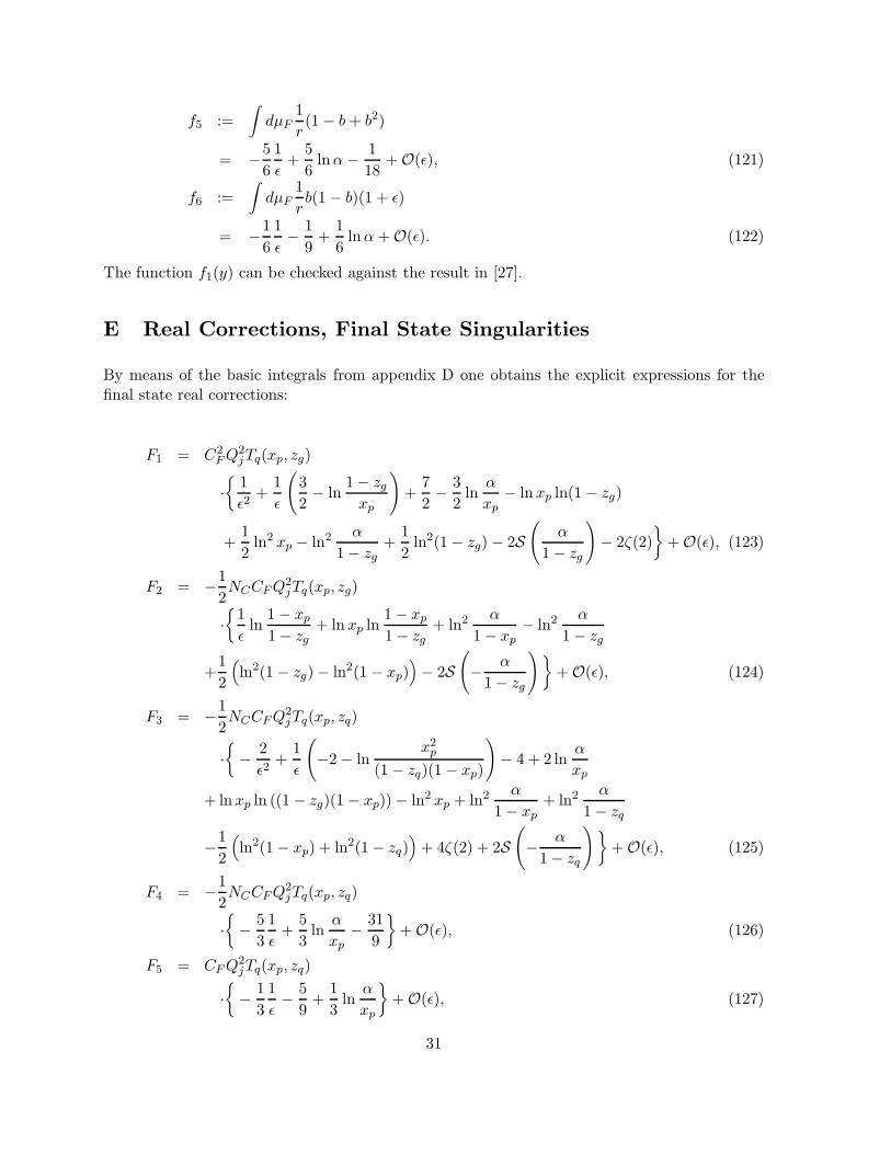
f5 :=

∫

dµF1

r(1− b + b2)

= −5

6

1

ǫ+

5

6ln α− 1

18+O(ǫ), (121)

f6 :=

∫

dµF1

rb(1− b)(1 + ǫ)

= −1

6

1

ǫ− 1

9+

1

6ln α +O(ǫ). (122)

The function f1(y) can be checked against the result in [27].

E Real Corrections, Final State Singularities

By means of the basic integrals from appendix D one obtains the explicit expressions for thefinal state real corrections:

F1 = C2F Q2

jTq(xp, zg)

·

1

ǫ2+

1

ǫ

(

3

2− ln

1− zg

xp

)

+7

2− 3

2ln

α

xp− ln xp ln(1− zg)

+1

2ln2 xp − ln2 α

1− zg+

1

2ln2(1− zg)− 2S

(

α

1− zg

)

− 2ζ(2)

+O(ǫ), (123)

F2 = −1

2NCCF Q2

jTq(xp, zg)

·

1

ǫln

1− xp

1− zg+ ln xp ln

1− xp

1− zg+ ln2 α

1− xp− ln2 α

1− zg

+1

2

(

ln2(1− zg)− ln2(1− xp))

− 2S(

− α

1− zg

)

+O(ǫ), (124)

F3 = −1

2NCCF Q2

jTq(xp, zq)

·

− 2

ǫ2+

1

ǫ

(

−2− lnx2

p

(1− zq)(1− xp)

)

− 4 + 2 lnα

xp

+ ln xp ln ((1− zg)(1 − xp))− ln2 xp + ln2 α

1− xp+ ln2 α

1− zq

−1

2

(

ln2(1− xp) + ln2(1− zq))

+ 4ζ(2) + 2S(

− α

1− zq

)

+O(ǫ), (125)

F4 = −1

2NCCF Q2

jTq(xp, zq)

·

− 5

3

1

ǫ+

5

3ln

α

xp− 31

9

+O(ǫ), (126)

F5 = CF Q2jTq(xp, zq)

·

− 1

3

1

ǫ− 5

9+

1

3ln

α

xp

+O(ǫ), (127)

31

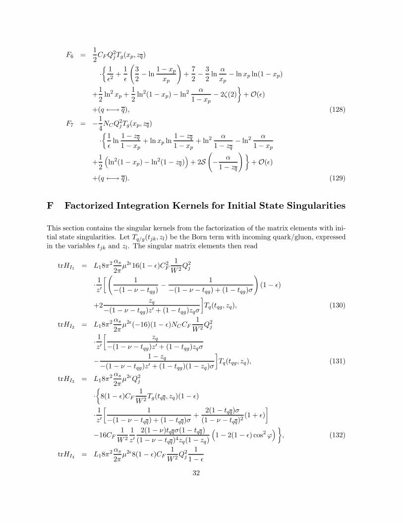
F6 =1

2CF Q2

jTg(xp, zq)

·

1

ǫ2+

1

ǫ

(

3

2− ln

1− xp

xp

)

+7

2− 3

2ln

α

xp− ln xp ln(1− xp)

+1

2ln2 xp +

1

2ln2(1− xp)− ln2 α

1− xp− 2ζ(2)

+O(ǫ)

+(q ←→ q), (128)

F7 = −1

4NCQ2

jTg(xp, zq)

·

1

ǫln

1− zq

1− xp+ ln xp ln

1− zq

1− xp+ ln2 α

1− zq− ln2 α

1− xp

+1

2

(

ln2(1− xp)− ln2(1− zq))

+ 2S(

− α

1− zq

)

+O(ǫ)

+(q ←→ q). (129)

F Factorized Integration Kernels for Initial State Singularities

This section contains the singular kernels from the factorization of the matrix elements with ini-tial state singularities. Let Tq/g(tjk, zl) be the Born term with incoming quark/gluon, expressedin the variables tjk and zl. The singular matrix elements then read

trHI1 = L18π2 αs

2πµ2ǫ16(1 − ǫ)C2

F

1

W 2Q2

j

· 1z′

[

(

1

−(1− ν − tqg)− 1

−(1− ν − tqg) + (1− tqg)σ

)

(1− ǫ)

+2zq

−(1− ν − tqg)z′ + (1− tqg)zqσ

]

Tq(tqg, zq), (130)

trHI2 = L18π2 αs

2πµ2ǫ(−16)(1 − ǫ)NCCF

1

W 2Q2

j

· 1z′

[

zq

−(1− ν − tqg)z′ + (1− tqg)zqσ

− 1− zq

−(1− ν − tqg)z′ + (1− tqg)(1 − zq)σ

]

Tq(tqg, zq), (131)

trHI3 = L18π2 αs

2πµ2ǫQ2

j

·

8(1− ǫ)CF1

W 2Tg(tqq, zq)(1− ǫ)

· 1z′

[

1

−(1− ν − tqq) + (1− tqq)σ+

2(1 − tqq)σ

(1− ν − tqq)2(1 + ǫ)

]

−16CF1

W 2

1

z′2(1− ν)tqqσ(1− tqq)

(1− ν − tqq)4zq(1− zq)

(

1− 2(1 − ǫ) cos2 ϕ)

, (132)

trHI4 = L18π2 αs

2πµ2ǫ8(1− ǫ)CF

1

W 2Q2

j

1

1− ǫ

32

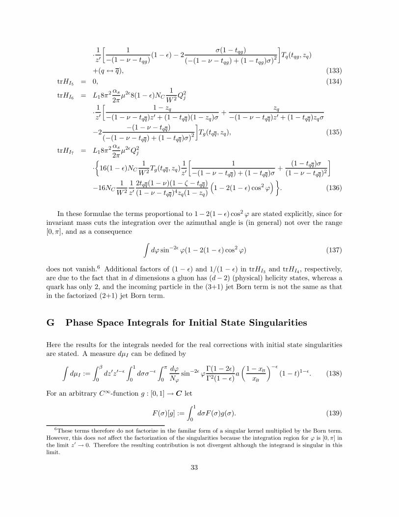
· 1z′

[

1

−(1− ν − tqg)(1− ǫ)− 2

σ(1− tqg)

(−(1− ν − tqg) + (1− tqg)σ)2

]

Tq(tqg, zq)

+(q ↔ q), (133)

trHI5 = 0, (134)

trHI6 = L18π2 αs

2πµ2ǫ8(1− ǫ)NC

1

W 2Q2

j

· 1z′

[

1− zq

−(1− ν − tqq)z′ + (1− tqq)(1− zq)σ+

zq

−(1− ν − tqq)z′ + (1− tqq)zqσ

−2−(1− ν − tqq)

(−(1− ν − tqq) + (1− tqq)σ)2

]

Tg(tqq, zq), (135)

trHI7 = L18π2 αs

2πµ2ǫQ2

j

·

16(1 − ǫ)NC1

W 2Tg(tqq, zq)

1

z′

[

1

−(1− ν − tqq) + (1− tqq)σ+

(1− tqq)σ

(1− ν − tqq)2

]

−16NC1

W 2

1

z′2tqq(1− ν)(1− ζ − tqq)

(1− ν − tqq)4zq(1− zq)

(

1− 2(1− ǫ) cos2 ϕ)

. (136)

In these formulae the terms proportional to 1− 2(1− ǫ) cos2 ϕ are stated explicitly, since forinvariant mass cuts the integration over the azimuthal angle is (in general) not over the range[0, π], and as a consequence

∫

dϕ sin−2ǫ ϕ(1 − 2(1 − ǫ) cos2 ϕ) (137)

does not vanish.6 Additional factors of (1 − ǫ) and 1/(1 − ǫ) in trHI3 and trHI4, respectively,are due to the fact that in d dimensions a gluon has (d− 2) (physical) helicity states, whereas aquark has only 2, and the incoming particle in the (3+1) jet Born term is not the same as thatin the factorized (2+1) jet Born term.

G Phase Space Integrals for Initial State Singularities

Here the results for the integrals needed for the real corrections with initial state singularitiesare stated. A measure dµI can be defined by

∫

dµI :=

∫ β

0dz′z′−ǫ

∫ 1

0dσσ−ǫ

∫ π

0

dϕ

Nϕsin−2ǫ ϕ

Γ(1− 2ǫ)

Γ2(1− ǫ)a

(

1− xB

xB

)−ǫ

(1− t)1−ǫ. (138)

For an arbitrary C∞-function g : [0, 1]→ C let

F (σ)[g] :=

∫ 1

0dσF (σ)g(σ). (139)

6These terms therefore do not factorize in the familar form of a singular kernel multiplied by the Born term.However, this does not affect the factorization of the singularities because the integration region for ϕ is [0, π] inthe limit z′

→ 0. Therefore the resulting contribution is not divergent although the integrand is singular in thislimit.

33

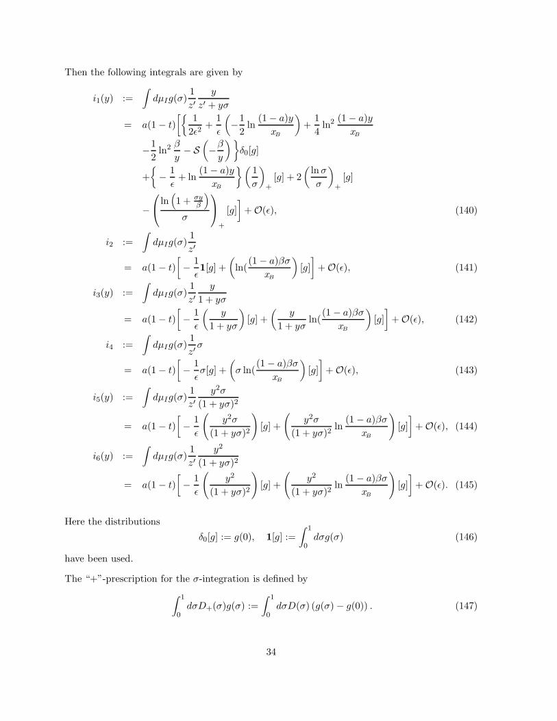
Then the following integrals are given by

i1(y) :=

∫

dµIg(σ)1

z′y

z′ + yσ

= a(1− t)

[

1

2ǫ2+

1

ǫ

(

−1

2ln

(1− a)y

xB

)

+1

4ln2 (1− a)y

xB

−1

2ln2 β

y− S

(

−β

y

)

δ0[g]

+

− 1

ǫ+ ln

(1− a)y

xB

(

1

σ

)

+[g] + 2

(

ln σ

σ

)

+[g]

−

ln(

1 + σyβ

)

σ

+

[g]

]

+O(ǫ), (140)

i2 :=

∫

dµIg(σ)1

z′

= a(1− t)

[

− 1

ǫ1[g] +

(

ln((1− a)βσ

xB

)

[g]

]

+O(ǫ), (141)

i3(y) :=

∫

dµIg(σ)1

z′y

1 + yσ

= a(1− t)

[

− 1

ǫ

(

y

1 + yσ

)

[g] +

(

y

1 + yσln(

(1 − a)βσ

xB

)

[g]

]

+O(ǫ), (142)

i4 :=

∫

dµIg(σ)1

z′σ

= a(1− t)

[

− 1

ǫσ[g] +

(

σ ln((1− a)βσ

xB

)

[g]

]

+O(ǫ), (143)

i5(y) :=

∫

dµIg(σ)1

z′y2σ

(1 + yσ)2

= a(1− t)

[

− 1

ǫ

(

y2σ

(1 + yσ)2

)

[g] +

(

y2σ

(1 + yσ)2ln

(1− a)βσ

xB

)

[g]

]

+O(ǫ), (144)

i6(y) :=

∫

dµIg(σ)1

z′y2

(1 + yσ)2

= a(1− t)

[

− 1

ǫ

(

y2

(1 + yσ)2

)

[g] +

(

y2

(1 + yσ)2ln

(1− a)βσ

xB

)

[g]

]

+O(ǫ). (145)

Here the distributions

δ0[g] := g(0), 1[g] :=

∫ 1

0dσg(σ) (146)

have been used.

The “+”-prescription for the σ-integration is defined by

∫ 1

0dσD+(σ)g(σ) :=

∫ 1

0dσD(σ) (g(σ)− g(0)) . (147)

34

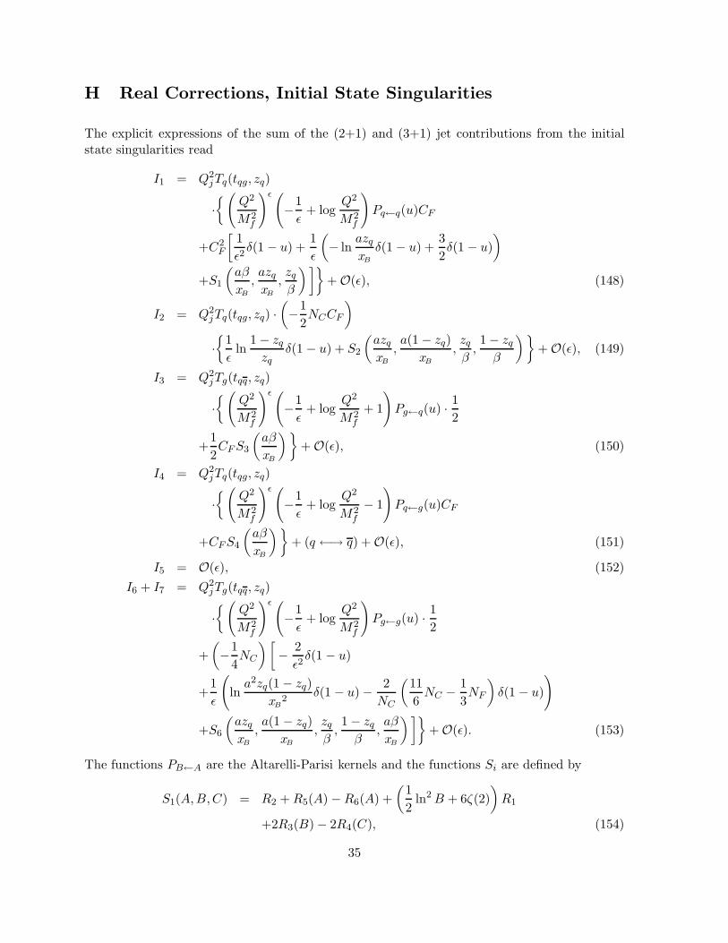
H Real Corrections, Initial State Singularities

The explicit expressions of the sum of the (2+1) and (3+1) jet contributions from the initialstate singularities read

I1 = Q2jTq(tqg, zq)

·

(

Q2

M2f

)ǫ(

−1

ǫ+ log

Q2

M2f

)

Pq←q(u)CF

+C2F

[

1

ǫ2δ(1 − u) +

1

ǫ

(

− lnazq

xB

δ(1 − u) +3

2δ(1 − u)

)

+S1

(

aβ

xB

,azq

xB

,zq

β

)]

+O(ǫ), (148)

I2 = Q2jTq(tqg, zq) ·

(

−1

2NCCF

)

·

1

ǫln

1− zq

zqδ(1 − u) + S2

(

azq

xB

,a(1− zq)

xB

,zq

β,1− zq

β

)

+O(ǫ), (149)

I3 = Q2jTg(tqq, zq)

·

(

Q2

M2f

)ǫ(

−1

ǫ+ log

Q2

M2f

+ 1

)

Pg←q(u) · 12

+1

2CF S3

(

aβ

xB

)

+O(ǫ), (150)

I4 = Q2jTq(tqg, zq)

·

(

Q2

M2f

)ǫ(

−1

ǫ+ log

Q2

M2f

− 1

)

Pq←g(u)CF

+CF S4

(

aβ

xB

)

+ (q ←→ q) +O(ǫ), (151)

I5 = O(ǫ), (152)

I6 + I7 = Q2jTg(tqq, zq)

·

(

Q2

M2f

)ǫ(

−1

ǫ+ log

Q2

M2f

)

Pg←g(u) · 12

+

(

−1

4NC

) [

− 2

ǫ2δ(1 − u)

+1

ǫ

(

lna2zq(1− zq)

xB2

δ(1 − u)− 2

NC

(

11

6NC −

1

3NF

)

δ(1 − u)

)

+S6

(

azq

xB

,a(1− zq)

xB

,zq

β,1− zq

β,aβ

xB

)]

+O(ǫ). (153)

The functions PB←A are the Altarelli-Parisi kernels and the functions Si are defined by

S1(A,B,C) = R2 + R5(A)−R6(A) +

(

1

2ln2 B + 6ζ(2)

)

R1

+2R3(B)− 2R4(C), (154)

35

S2(A,B,C,D) = R1

(

1

2ln2 A− 1

2ln2 B

)

+ 2 (R3(A)−R3(B))

−2 (R4(C)−R4(D)) , (155)

S3(A) = R6(A) + 2R7(A)− 2R10, (156)

S4(A) =1

2R0 +

1

2R5(A)−R8(A), (157)

S6(A,B,C,D,E) = −R1

(

1

2ln2 A +

1

2ln2 B + 12ζ(2)

)

− 2 (R3(A) + R3(B))

+2 (R4(C) + R4(D)) + 4R9(E)− 4R6(E)− 4R7(E), (158)

and the functions Ri are distributions in the variable u given by

R0 = 1, (159)

R1 = δ(1 − u), (160)

R2 = 1− u, (161)

R3(λ) =

ln

[

λ(

1−uu

)2]

1− u

+

− ln

(

λ

(

1− u

u

)2)

, (162)

R4(λ) =u

1− uln

(

1 + λ1− u

u

)

, (163)

R5(λ) = ln

(

λ1− u

u

)

, (164)

R6(λ) = u ln

(

λ1− u

u

)

, (165)

R7(λ) =1− u

uln

(

λ1− u

u

)

, (166)

R8(λ) = u(1 − u) ln

(

λ1− u

u

)

, (167)

R9(λ) = u2 ln

(

λ1− u

u

)

, (168)

R10(λ) =1− u

u. (169)

36

References

[1] E665 Collaboration, Phys. Lett. 69 (1992) 1026

[2] H1 Collaboration, Phys. Lett. B299 (1993) 385, Phys. Lett. B298 (1993) 469ZEUS Collaboration, DESY preprint 92-180, DESY preprint 93-030

[3] G. Altarelli, R.K. Ellis, G. Martinelli, Nucl. Phys. B143 (1978) 521, Erratum Nucl.Phys. B146 (1978) 544

[4] G. Altarelli, R.K. Ellis, G. Martinelli, Nucl. Phys. B157 (1979) 461

[5] A. Mendez, Nucl. Phys. B145 (1978) 199

[6] A. Mendez, T. Weiler, Phys. Lett. B83 (1979) 221

[7] R.D. Peccei, R. Ruckl, Nucl. Phys. B162 (1980) 125

[8] Ch. Rumpf, G. Kramer, J. Willrodt, Z. Phys. C7 (1981) 337

[9] J.G. Korner, E. Mirkes, G.A. Schuler, Int. J. Mod. Phys. A4 (1989) 1781

[10] T. Brodkorb, J.G. Korner, E. Mirkes, G.A. Schuler, Z. Phys. C44 (1989) 415

[11] D. Graudenz, N. Magnussen, in Proceedings of the HERA Workshop 1991, DESY(eds. W. Buchmuller, G. Ingelman)

[12] D. Graudenz, “Der Drei-Jet-Wirkungsquerschnitt zur Ordnung O(α2s) in der tief-

inelastischen Elektron-Proton- Streuung”, DESY-T-90-01

[13] D. Graudenz, Phys. Lett. B256 (1991)

[14] T. Brodkorb, J.G. Korner, Z. Phys. C54 (1992) 519

[15] G. Sterman, S. Weinberg, Phys. Rev. Lett. 39 (1977) 1436

[16] W. Bartel et al., Z. Phys. C33 (1986) 23

[17] S. Catani, Yu.L. Dokshitzer, B.R. Webber, Phys. Lett. B285 (1992) 291

[18] Ch. Berger, R. Nisius, private communication

[19] G. ’t Hooft, M. Veltman, Nucl. Phys. B44 (1972) 189

[20] G. Leibbrandt, Rev. Mod. Phys. 47 (1975) 849

[21] W.J. Marciano, A. Sirlin, Nucl. Phys. B88 (1975) 86

[22] W. Furmanski, R. Petronzio, Z. Phys. C11 (1982) 293

[23] I.M. Gel’fand, G.E. Shilov, Generalized Functions, Vol. I, Academic Press (NewYork, London, 1964)

37

[24] A.C. Hearn, REDUCE User’s Manual, Version 3.2., Rand Publication CP78 (Rev.4/85)

[25] B. Lampe, G. Kramer, Phys. Scr. 28 (1983) 585

[26] Wang-Chuang Kuo, D. Slaven, Bing-Lin Young, Phys. Rev. D37 (1988) 233

[27] R.K. Ellis, D.A. Ross, A.E. Terrano, Nucl. Phys. B178 (1981) 421

[28] K. Fabricius, G. Kramer, G. Schierholz, I. Schmitt, Z. Phys. C11 (1982) 315

[29] G. Kramer, B. Lampe, Fortschr. Phys. 37 (1989) 161

[30] D. Graudenz, PROJET 3.3 manual (May 1993), to be published

[31] G. Peter Lepage, J. Comp. Phys. 27 (1978) 192

[32] G. Peter Lepage, Cornell preprint, CLNS-80/447 (1980)

[33] K. Charchula, Comp. Phys. Comm. 69 (1992) 360

[34] A. Martin, R. Roberts, J. Stirling, Durham University preprints DTP-92-16, DTP-92-80.

[35] P. Harriman, A. Martin, R. Roberts, J. Stirling, Phys. Rev. D42 (1990) 798

[36] J. Morfin, Wu-Ki Tung, Z. Phys. C52 (1991) 13

[37] Gradstein, Ryshik, Tables of Series, Products, and Integrals 1/2, Verlag HarriDeutsch (1981, Thun, Frankfurt/M.)

[38] M. Abramowitz, I.A. Stegun (eds.), Pocketbook of Mathematical Functions, VerlagHarri Deutsch (1984, Thun, Frankfurt/M.)

[39] H. Bateman, Higher Transcendental Functions I-III, R.E. Krieger Publ. (1985,Malabar, Florida)

[40] A. Devoto, D.D. Duke, Riv. Nuov. Cim. 7 (1984) 1

38

Figure Captions:

Fig. 1 Diagram for initial state radiation.

Fig. 2 Diagram for 1-parton production.

Fig. 3 Diagram for the virtual correction to 1-parton production

Fig. 4 Generic diagrams for 2-parton production.

Fig. 5 Born terms for 2-parton production (hadron tensor).

Fig. 6 Virtual corrections to 2-parton production (hadron tensor).

Fig. 7 Diagrams contributing to the wave function renormalisation.

Fig. 8 Born terms of O(α2s) (the roman numbering labels the 7 different colour classes).

Fig. 9 Generic diagrams for 3-parton production.

Fig. 10 CM frame of p1 and p2.

Fig. 11 (2+1) and (3+1) jet regions in phase space.

Fig. 12 Cut dependence of jet cross sections. “tr.” stands for transverse, “long.” for longitu-dinal polarisation of the exchanged virtual photon. Contributions marked as “NLO” aregiven by the sum of the Born term and the next-to-leading order contribution. (a)–(c)HERA kinematics with (a) 3.16 GeV < Q < 10 GeV, (b) 10 GeV < Q < 31.6 GeV, (c)31.6 GeV < Q < 100 GeV. (d) is the graph for the E665 kinematics.

Fig. 13 The ratio σ2+1/σtot. (a)–(c) HERA kinematics with (a) 3.16 GeV < Q < 10 GeV, (b)10 GeV < Q < 31.6 GeV, (c) 31.6 GeV < Q < 100 GeV, (d) E665 kinematics.

Fig. 14 Dependence of the cross section on the jet definition scheme. The jet definition scheme

is (a) sij><cW 2, (b) sij

><c

(

W αQβ√

SHy1−α−β

)2with α = 0.8, β = 0.2.

Fig. 15 Dependence on the renormalisation and factorization scales. (a) renormalisation scaleµ = ρQ, factorization scale Mf = Q; (b) µ = Q, Mf = ρQ; (c) µ = ρQ, Mf = ρQ. (d)–(f)are the same, but for much larger Q. (g)–(i) are the graphs for E665 energies. To avoidscales that are too low for perturbation theory to be valid, the scales are clipped at a lowerbound of 2 GeV (HERA) and 1 GeV (E665).

Fig. 16 Dependence of the jet rate σ2+1/σtot on the renormalisation and factorization scales.The indices (a)–(i) refer to the indices of Fig. 15 (a)–(i), respectively.

Fig. 17 Dependence on the parton densities. The plotted cross section is xB dσ/dxB , the jet

definition scheme is (a) sij><cW 2, (b) sij

><c

(

W αQβ√

SHy1−α−β

)2with α = 0.7, β = 0.3.

39

Figure 1:

Figure 2:

Figure 3:

40

Figure 4:

Figure 5:

Figure 6:

41

Figure 7:

Figure 8:

42

Figure 9:

Figure 10:

Figure 11:

43

Figure 12:

Figure 13:

Figure 14:

Figure 15:

Figure 16:

Figure 17:

44