
Investigation of erbium-doped fiber laser intra-cavity absorption sensor for gas detection
Upload
khangminh22Category
view
3download
0
Inelastic Collisions of Atomic Antimony, Aluminum, Erbium andThulium below 1 K
(Article begins on next page)
The Harvard community has made this article openly available.Please share how this access benefits you. Your story matters.
Citation Connolly, Colin Bryant. 2012. Inelastic Collisions of AtomicAntimony, Aluminum, Erbium and Thulium below 1 K. Doctoraldissertation, Harvard University.
Accessed April 17, 2018 3:48:21 PM EDT
Citable Link http://nrs.harvard.edu/urn-3:HUL.InstRepos:9909637
Terms of Use This article was downloaded from Harvard University's DASHrepository, and is made available under the terms and conditionsapplicable to Other Posted Material, as set forth athttp://nrs.harvard.edu/urn-3:HUL.InstRepos:dash.current.terms-of-use#LAA

c©2012 - Colin Bryant Connolly
All rights reserved.

Dissertation advisor Author
John Morrissey Doyle Colin Bryant Connolly
Inelastic collisions of atomic antimony, aluminum, erbium and
thulium below 1 K
Abstract
Inelastic collision processes driven by anisotropic interactions are investigated below 1 K.
Three distinct experiments are presented. First, for the atomic species antimony (Sb), rapid
relaxation is observed in collisions with 4He. We identify the relatively large spin-orbit
coupling as the primary mechanism which distorts the electrostatic potential to introduce
significant anisotropy to the ground 4S3/2 state. The collisions are too rapid for the experi-
ment to fix a specific value, but an upper bound is determined, with the elastic-to-inelastic
collision ratio γ ≤ 9.1×10². In the second experiment, inelastic mJ -changing and J-changing
transition rates of aluminum (Al) are measured for collisions with 3He. The experiment em-
ploys a clean method using a single pump/probe laser to measure the steady-state magnetic
sublevel population resulting from the competition of optical pumping and inelastic colli-
sions. The collision ratio γ is measured for both mJ - and J-changing processes as a function
of magnetic field and found to be in agreement with the theoretically calculated dependence,
giving support to the theory of suppressed Zeeman relaxation in spherical 2P1/2 states [1].
In the third experiment, very rapid atom–atom relaxation is observed for the trapped lan-
thanide rare-earth atoms erbium (Er) and thulium (Tm). Both are nominally nonspherical
(L 6= 0) atoms that were previously observed to have strongly suppressed electronic interac-
tion anisotropy in collisions with helium (γ > 104–105, [2, 3]). No suppression is observed in
collisions between these atoms (γ . 10), which likely implies that evaporative cooling them
iii
in a magnetic trap will be impossible. Taken together, these studies reveal more of the role
of electrostatic anisotropy in cold atomic collisions.
iv
Contents
Title Page . . . . . . . . . . . . . . . . . . . . . . . . . . . . . . . . . . . . . . . . iAbstract . . . . . . . . . . . . . . . . . . . . . . . . . . . . . . . . . . . . . . . . . iiiTable of Contents . . . . . . . . . . . . . . . . . . . . . . . . . . . . . . . . . . . . vDedication . . . . . . . . . . . . . . . . . . . . . . . . . . . . . . . . . . . . . . . . xiiiCitations to Previously Published Work . . . . . . . . . . . . . . . . . . . . . . . xivAcknowledgements . . . . . . . . . . . . . . . . . . . . . . . . . . . . . . . . . . . xv
1 Introduction 11.1 Physics with cold atoms . . . . . . . . . . . . . . . . . . . . . . . . . . . . . 11.2 Buffer-gas cooling and trapping . . . . . . . . . . . . . . . . . . . . . . . . . 31.3 Inelastic collisions . . . . . . . . . . . . . . . . . . . . . . . . . . . . . . . . . 5
1.3.1 Measuring cold inelastic collisions . . . . . . . . . . . . . . . . . . . . 6
2 Antimony–4He collisions 92.1 Pnictogen collisions . . . . . . . . . . . . . . . . . . . . . . . . . . . . . . . . 9
2.1.1 The importance of antimony . . . . . . . . . . . . . . . . . . . . . . . 102.2 Experimental design . . . . . . . . . . . . . . . . . . . . . . . . . . . . . . . 11
2.2.1 Experimental cell . . . . . . . . . . . . . . . . . . . . . . . . . . . . . 112.2.2 Antimony production and cooling . . . . . . . . . . . . . . . . . . . . 162.2.3 Thermal dynamics of Zeeman relaxation . . . . . . . . . . . . . . . . 182.2.4 Thermal dynamics in G-10 cells . . . . . . . . . . . . . . . . . . . . . 192.2.5 Absorption spectroscopy detection system . . . . . . . . . . . . . . . 22
2.3 Experimental procedure . . . . . . . . . . . . . . . . . . . . . . . . . . . . . 262.3.1 Momentum transfer cross section comparison . . . . . . . . . . . . . . 262.3.2 Zeeman relaxation model . . . . . . . . . . . . . . . . . . . . . . . . . 292.3.3 Lifetime measurements . . . . . . . . . . . . . . . . . . . . . . . . . . 31
2.4 Results and discussion . . . . . . . . . . . . . . . . . . . . . . . . . . . . . . 382.4.1 Upper bound on Zeeman relaxation rate . . . . . . . . . . . . . . . . 382.4.2 Theory of spin-orbit induced Zeeman relaxation . . . . . . . . . . . . 412.4.3 Sb–4He calculations . . . . . . . . . . . . . . . . . . . . . . . . . . . . 422.4.4 Summary and future outlook . . . . . . . . . . . . . . . . . . . . . . 46
v
3 Aluminum–3He collisions 493.1 Properties and prospects of 2P atoms . . . . . . . . . . . . . . . . . . . . . . 49
3.1.1 Improved study of X(2P1/2)–He Zeeman relaxation . . . . . . . . . . 503.2 Theory of Zeeman relaxation in 2P1/2 atoms . . . . . . . . . . . . . . . . . . 533.3 Optical pumping . . . . . . . . . . . . . . . . . . . . . . . . . . . . . . . . . 56
3.3.1 Quantitative model . . . . . . . . . . . . . . . . . . . . . . . . . . . . 593.3.2 Diffusion into and out of the beam . . . . . . . . . . . . . . . . . . . 613.3.3 Doppler broadening . . . . . . . . . . . . . . . . . . . . . . . . . . . . 633.3.4 Zeeman broadening . . . . . . . . . . . . . . . . . . . . . . . . . . . . 64
3.4 Experimental procedure . . . . . . . . . . . . . . . . . . . . . . . . . . . . . 653.4.1 Aluminum production . . . . . . . . . . . . . . . . . . . . . . . . . . 653.4.2 Pump/probe laser system . . . . . . . . . . . . . . . . . . . . . . . . 663.4.3 Pump laser polarization . . . . . . . . . . . . . . . . . . . . . . . . . 703.4.4 Momentum transfer cross section calibration . . . . . . . . . . . . . . 74
3.5 Data analysis . . . . . . . . . . . . . . . . . . . . . . . . . . . . . . . . . . . 753.5.1 Data processing . . . . . . . . . . . . . . . . . . . . . . . . . . . . . . 753.5.2 Numerical simulation of optical pumping . . . . . . . . . . . . . . . . 783.5.3 Results from fitting data to simulation . . . . . . . . . . . . . . . . . 83
3.6 Conclusion . . . . . . . . . . . . . . . . . . . . . . . . . . . . . . . . . . . . . 893.6.1 Comparison of experiment with theory . . . . . . . . . . . . . . . . . 893.6.2 Implications for future work with 2P atoms . . . . . . . . . . . . . . 90
4 Rare-earth atom–atom collisions 914.1 Submerged-shell atoms . . . . . . . . . . . . . . . . . . . . . . . . . . . . . . 914.2 Experimental design . . . . . . . . . . . . . . . . . . . . . . . . . . . . . . . 93
4.2.1 Apparatus . . . . . . . . . . . . . . . . . . . . . . . . . . . . . . . . . 934.2.2 Buffer-gas cold loading of magnetic traps . . . . . . . . . . . . . . . . 944.2.3 Inelastic collisional heating . . . . . . . . . . . . . . . . . . . . . . . . 99
4.3 Results and analysis . . . . . . . . . . . . . . . . . . . . . . . . . . . . . . . 1044.3.1 Measurement of RE–RE Zeeman relaxation . . . . . . . . . . . . . . 1044.3.2 Discussion of systematic errors . . . . . . . . . . . . . . . . . . . . . . 1074.3.3 Simulation of trap dynamics . . . . . . . . . . . . . . . . . . . . . . . 109
4.4 Possible mechanisms of RE–RE Zeeman relaxation . . . . . . . . . . . . . . 1124.4.1 Magnetic dipole-dipole interaction . . . . . . . . . . . . . . . . . . . . 1124.4.2 Electrostatic quadrupole-quadrupole interaction . . . . . . . . . . . . 1154.4.3 Electronic interaction anisotropy . . . . . . . . . . . . . . . . . . . . 116
4.5 Future prospects for RE atoms . . . . . . . . . . . . . . . . . . . . . . . . . 117
5 Conclusion 1205.1 Summary of collision experiments . . . . . . . . . . . . . . . . . . . . . . . . 1205.2 An increasingly complete picture . . . . . . . . . . . . . . . . . . . . . . . . 122
vi

A Cryogenic production of NH 124A.1 Introduction . . . . . . . . . . . . . . . . . . . . . . . . . . . . . . . . . . . . 124
A.1.1 Motivations for the study of ultracold polar molecules . . . . . . . . . 124A.1.2 Direct cooling of molecules . . . . . . . . . . . . . . . . . . . . . . . . 125A.1.3 Previous work with cold NH . . . . . . . . . . . . . . . . . . . . . . . 127A.1.4 The need for a better source . . . . . . . . . . . . . . . . . . . . . . . 129
A.2 Phase I: Discharge production . . . . . . . . . . . . . . . . . . . . . . . . . . 131A.2.1 Finding a cryogenic production technique . . . . . . . . . . . . . . . . 131A.2.2 Production test apparatus . . . . . . . . . . . . . . . . . . . . . . . . 133A.2.3 G-10 composite trapping cell . . . . . . . . . . . . . . . . . . . . . . . 138A.2.4 Phase I failure: No NH nor N2* detected . . . . . . . . . . . . . . . . 140
A.3 Phase II: Production by ablation of nitrides into hydrogen . . . . . . . . . . 143A.3.1 Production test apparatus . . . . . . . . . . . . . . . . . . . . . . . . 143A.3.2 Copper trapping cell . . . . . . . . . . . . . . . . . . . . . . . . . . . 147A.3.3 Observation of cold NH . . . . . . . . . . . . . . . . . . . . . . . . . . 149A.3.4 Limitations of a copper cell . . . . . . . . . . . . . . . . . . . . . . . 151A.3.5 Limitations of detection . . . . . . . . . . . . . . . . . . . . . . . . . 151A.3.6 FM spectroscopy of NH . . . . . . . . . . . . . . . . . . . . . . . . . 153A.3.7 Challenges of fluorescence detection with limited optical access . . . . 157
A.4 Phase III: Modification of G-10 cell from Phase I . . . . . . . . . . . . . . . 160A.4.1 No NH production enhancement with discharge . . . . . . . . . . . . 160A.4.2 Detection limited by fluorescence of G-10 . . . . . . . . . . . . . . . . 162
A.5 Phase IV: Design for maximized production and fluorescence sensitivity . . . 164A.5.1 Building a new cell . . . . . . . . . . . . . . . . . . . . . . . . . . . . 164A.5.2 Leaky G-10 tubing . . . . . . . . . . . . . . . . . . . . . . . . . . . . 168A.5.3 Production performance . . . . . . . . . . . . . . . . . . . . . . . . . 169A.5.4 Detection performance . . . . . . . . . . . . . . . . . . . . . . . . . . 171
A.6 Summary and future prospects . . . . . . . . . . . . . . . . . . . . . . . . . . 172A.6.1 Successful cryogenic production . . . . . . . . . . . . . . . . . . . . . 172A.6.2 Proposed improvements for improved detection sensitivity . . . . . . 173A.6.3 Prospects for sympathetic cooling . . . . . . . . . . . . . . . . . . . . 174
B Calculating absorption for trapped molecules in motion 176B.1 Reconciling Beer’s Law with the Landau-Zener model . . . . . . . . . . . . . 176
B.1.1 Case 1: Stationary atoms . . . . . . . . . . . . . . . . . . . . . . . . 178B.1.2 Case 2: Arbitrarily slow atoms . . . . . . . . . . . . . . . . . . . . . . 178B.1.3 Case 3: Rapid atoms . . . . . . . . . . . . . . . . . . . . . . . . . . . 180B.1.4 Case 4: Intermediate-speed atoms . . . . . . . . . . . . . . . . . . . . 180B.1.5 Conclusions from the comparison . . . . . . . . . . . . . . . . . . . . 181
B.2 Implications for simulations of trapped spectra . . . . . . . . . . . . . . . . . 182
vii

C Polarization-sensitive absorption spectroscopy and “extra light” 184C.1 Observations of “extra light” . . . . . . . . . . . . . . . . . . . . . . . . . . . 184C.2 Absorption spectroscopy with polarization-dependent optics . . . . . . . . . 188
C.2.1 Quantitative model . . . . . . . . . . . . . . . . . . . . . . . . . . . . 192C.2.2 Mitigating the problem . . . . . . . . . . . . . . . . . . . . . . . . . . 197C.2.3 Extensions to the model . . . . . . . . . . . . . . . . . . . . . . . . . 199
viii
List of Figures
2.1 G-10 superfluid-jacketed cell schematic . . . . . . . . . . . . . . . . . . . . . 132.2 Power curve for G-10 cell used in Al and Sb experiments . . . . . . . . . . . 142.3 Helmholtz magnetic field profile and calculated Zeeman-broadened lineshape 152.4 Cooling of the buffer gas after ablation . . . . . . . . . . . . . . . . . . . . . 172.5 Thermal behavior of copper vs. superfluid-jacketed G-10 composite cells . . . 212.6 Energy level diagrams of N and Sb . . . . . . . . . . . . . . . . . . . . . . . 232.7 Sb absorption spectroscopy laser system schematic . . . . . . . . . . . . . . . 242.8 Sb absorption spectroscopy laser system photographs . . . . . . . . . . . . . 252.9 Sb–4He and Mn–4He momentum transfer cross section comparison . . . . . . 282.10 Simulation of Sb relaxation dynamics at finite temperature . . . . . . . . . . 302.11 Comparison of zero-field and in-field Sb diffusion times . . . . . . . . . . . . 322.12 Simulated zero-field hyperfine spectrum of Sb . . . . . . . . . . . . . . . . . 332.13 Simulated spectrum of Sb in B = 0.9-T Helmholtz field . . . . . . . . . . . . 342.14 Measurement of the Sb 4S3/2 → 4P5/2 isotope shift . . . . . . . . . . . . . . 352.15 Sb spectrum calibration via observation of Zeeman-shifted lines crossing . . . 362.16 Determination of Sb LFS diffusion time using HFS diffusion . . . . . . . . . 372.17 Sb LFS decay at B = 0.86 T . . . . . . . . . . . . . . . . . . . . . . . . . . . 382.18 Sb LFS lifetime data vs. diffusion time . . . . . . . . . . . . . . . . . . . . . 392.19 Lowest Sb–He interaction potentials . . . . . . . . . . . . . . . . . . . . . . . 422.20 Anisotropy of lowest Sb–He and Bi–He interaction potentials . . . . . . . . . 432.21 Calculated Sb–He total elastic and momentum transfer cross sections . . . . 442.22 Calculations of Sb–4He elastic-to-inelastic collision rate ratio γ . . . . . . . . 452.23 Effect of scaling the Sb–4He ab initio interaction potentials on the calculated
collision ratio γ . . . . . . . . . . . . . . . . . . . . . . . . . . . . . . . . . . 462.24 Calculated tensor polarizabilities of pnictogen atoms . . . . . . . . . . . . . 47
3.1 Theoretical calculations of Al–3He elastic-to-inelastic collision rate ratios γmand γJ . . . . . . . . . . . . . . . . . . . . . . . . . . . . . . . . . . . . . . . 55
3.2 Energy level diagram of Al . . . . . . . . . . . . . . . . . . . . . . . . . . . . 583.3 Al absorption spectroscopy laser system schematic . . . . . . . . . . . . . . . 673.4 Zero-field hyperfine spectrum of Al . . . . . . . . . . . . . . . . . . . . . . . 683.5 Hyperfine spectrum of Al low-field seeking states at B = 0.5 T . . . . . . . . 69
ix
3.6 Optical pumping beam profiles and diffraction simulations . . . . . . . . . . 703.7 Al absorption at B = 0.5 T with laser power modulation . . . . . . . . . . . 713.8 Birefringence and the Faraday effect in dewar windows . . . . . . . . . . . . 733.9 Al–3He and Mn–3He momentum transfer cross section calibration . . . . . . 753.10 Processing procedure for Al optical pumping data . . . . . . . . . . . . . . . 763.11 Al optical pumping data at B = 4 T showing the process for computation of
2D residuals from simulations . . . . . . . . . . . . . . . . . . . . . . . . . . 793.12 Spatial simulation of Al optical pumping, diffusion and Zeeman relaxation . 813.13 Results of unbounded fitting of optical pumping data to numerical simulation 833.14 Calculated LFS state branching fraction f+ for J-changing Al–3He collisions 853.15 Results of fitting optical pumping data to numerical simulation with fixed
J-changing branching fraction f+ . . . . . . . . . . . . . . . . . . . . . . . . 86
4.1 Experimental cell used for RE–RE collision measurements . . . . . . . . . . 944.2 Trapped spectra of Er and Tm . . . . . . . . . . . . . . . . . . . . . . . . . . 984.3 Equilibrium η as a function of collision ratio γ . . . . . . . . . . . . . . . . . 1024.4 Inelastic heating of trapped Er . . . . . . . . . . . . . . . . . . . . . . . . . . 1034.5 Trapped Tm decay in the presence of helium . . . . . . . . . . . . . . . . . . 1054.6 Decay of trapped erbium and thulium . . . . . . . . . . . . . . . . . . . . . . 1064.7 Spectrum of Er on 415-nm J → J − 1 transition . . . . . . . . . . . . . . . . 1084.8 Simulation of Er–Er Zeeman relaxation . . . . . . . . . . . . . . . . . . . . . 1134.9 Comparison of lanthanide RE–RE Zeeman relaxation to that between dipolar
S-state atoms . . . . . . . . . . . . . . . . . . . . . . . . . . . . . . . . . . . 114
A.1 NH experiment Phase I test cell schematic . . . . . . . . . . . . . . . . . . . 133A.2 Spectra of NH in discharge . . . . . . . . . . . . . . . . . . . . . . . . . . . . 135A.3 Saturated vapor density of H2 and isotopomers . . . . . . . . . . . . . . . . . 136A.4 Discharge production of ND at 7.5 K . . . . . . . . . . . . . . . . . . . . . . 138A.5 NH experiment Phase I G-10 trapping cell schematic . . . . . . . . . . . . . 139A.6 N2* A→ B spectra . . . . . . . . . . . . . . . . . . . . . . . . . . . . . . . . 141A.7 Long-lived discharge flash in G-10 cell . . . . . . . . . . . . . . . . . . . . . . 143A.8 Discharge in NH experiment Phase II test cell . . . . . . . . . . . . . . . . . 144A.9 Yield of NH for ablation of various targets into H2 gas . . . . . . . . . . . . 145A.10 NH experiment Phase II copper trapping cell . . . . . . . . . . . . . . . . . . 148A.11 NH spectrum observed at 1.2 K . . . . . . . . . . . . . . . . . . . . . . . . . 150A.12 FM absorption spectrum of NH near 1 K . . . . . . . . . . . . . . . . . . . . 155A.13 Broadband EOM performance at 336 nm . . . . . . . . . . . . . . . . . . . . 156A.14 PMT afterpulsing measurement . . . . . . . . . . . . . . . . . . . . . . . . . 159A.15 NH experiment Phase IV G-10 trapping cell . . . . . . . . . . . . . . . . . . 165A.16 Defects in the fiberglass fabric of poor-quality G-10 tubes . . . . . . . . . . . 170
x
C.1 Negative absorption observed by Hancox et al. in the scanned spectrum ofHFS states of Ti . . . . . . . . . . . . . . . . . . . . . . . . . . . . . . . . . 185
C.2 Effect of ablation energy on negative absorption observed by Hancox et al. . 186C.3 Negative absorption observed by Hancox et al. in the spectrum of Dy . . . . 187C.4 Negative absorption observed in the scanned spectrum of LFS states of Al . 189C.5 Negative absorption observed in the trapped spectrum of He* . . . . . . . . 190C.6 Optics schematic for the experiments by Hancox et al. with Ti and Dy . . . 191C.7 Simulation of Al absorption spectrum in a Helmholtz field with polarization-
sensitive detection . . . . . . . . . . . . . . . . . . . . . . . . . . . . . . . . . 195C.8 Negative absorption effect eliminated with the use of a polarizer . . . . . . . 197C.9 Nonlinear effects of polarization rotation on Al lineshape at high OD using a
polarizer . . . . . . . . . . . . . . . . . . . . . . . . . . . . . . . . . . . . . . 198
xi

List of Tables
3.1 Fine-structure splittings and calculated γ values for Group 13 and halogenatoms colliding with 3He . . . . . . . . . . . . . . . . . . . . . . . . . . . . . 51
3.2 Results of previous work on Ga–4He and In–4He collisions . . . . . . . . . . 523.3 Thermally-averaged Al–3He J-changing collision branching fractions . . . . . 873.4 Summary of Al–3He inelastic parameter fitting results . . . . . . . . . . . . . 883.5 Summary of Al–3He theoretical calculations with scaled potentials . . . . . . 88
A.1 Fluorescence in UV windows under 336-nm excitation . . . . . . . . . . . . . 167
xii

To my wife, daughter and parents,
whose support has never flickered
xiii
Citations to Previously Published Work
Portions of this thesis have appeared previously in the following paper:
“Large spin relaxation rates in trapped submerged-shell atoms,” Colin B. Con-
nolly, Yat Shan Au, S. Charles Doret, Wolfgang Ketterle, and John M. Doyle,
Phys. Rev. A 81, 010702(R) (2010). [4]
xiv
Acknowledgements
This thesis was completed with a wealth of assistance. I would like to acknowledge some
of those contributions, in no particular order.
First, I thank my thesis advisor John Doyle for his guidance, encouragement and support
through the many phases of my time in his lab. From my arrival at Harvard, I was happy to
have a healthy student-mentor relationship and I have become keenly aware of its benefits
to all. I have also been grateful for his focus on the big picture, which has helped me to view
my work better in relation to the field and to think critically about future directions. On the
practical side, his rational and reliable approach to providing adequate resources to attack
experimental challenges has been not only a benefit to the experiments themselves, but a
relief to his students. I did not leave stones unturned for lack of liquid helium or lasers.
I have been grateful to have a second mentor in Wolfgang Ketterle, the co-PI of this work.
His input has been invaluable, and his distinct approach and experience provides welcome
diversity to our discussions. With John and Wolfgang, I always feel that I have two mentors
rather than two bosses. I also acknowledge the role of the Harvard-MIT Center for Ultracold
Atoms in facilitating this collaboration.
My research partners Charlie Doret, Yat Shan Au and Eunmi Chae have made countless
contributions to this research. Charlie helped to build and/or install much of the apparatus,
and he was a model senior student during the helium BEC work. I learned a great deal
working alongside him and enjoyed his friendship through our years parked in front of twin
computers at the experiment. After Charlie’s departure, Yat was instrumental in all the
work that followed, especially his stellar work with a dizzying array of laser systems that
include all those described in this thesis. I am grateful for his efforts. I also appreciate
Eunmi’s contributions amid her classes and other projects. Her assistance with the aluminum
xv
simulations was especially helpful when we struggled to understand a new experimental
method and atomic system.
The theoretical contributions from Timur Tscherbul and Alexei Buchachenko has greatly
strengthened the science and given me a much clearer view of the physics underlying my
research. That collaboration has been very valuable and enabled the experiments to go
further than they otherwise would have.
The entire Doyle Lab has been a great source of assistance and camaraderie, and it is a joy
to work among its members. Dave Patterson, Amar Vutha, Nathan Brahms and Matthew
Wright have frequently devoted hours to solving problems in my experiment and offered
critical insight. I also appreciate the efforts of Wes Campbell, Edem Tsikata, Matt Hummon
and Hsin-I Lu, not only in blazing the trail with NH and nitrogen, but for leaving excellent
notes, advice, ideas and equipment behind them. I would also like to give credit to those who
wrote excellent and thoroughly useful Ph.D. theses, especially Jonathan Weinstein, Nathan,
Charlie and Wes, to whose work I referred many times and used as a model for my own.
Stan Cotreau in the Physics Machine Shop and Jim MacArthur in the Electronic In-
strument Design Lab have given me a great deal of excellent technical advice and friendly
company while I labored to do the most minor tasks in their respective specialties. They are
priceless and irreplaceable resources at Harvard.
Finally, I am grateful for the enthusiastic support of my wife and family. Nathalie has
given much of herself toward my own success and deserves much of the credit. The support
of my parents, as well, has always been clear. I appreciate their efforts to understand the
esoteric details of my work, including reading my papers dense with jargon such as “electronic
interaction anisotropy.” Last, I am fortunate to have little Chloe in my life, and grateful for
the healthy perspective that her presence gives me—and the demands of efficiency that it
brings.
xvi
Chapter 1
Introduction
1.1 Physics with cold atoms
The last two decades have seen fantastic progress in methods for cooling, trapping and
manipulating atoms, which has fueled an explosion of applications for cold atoms that range
from precision measurement and quantum information processing to quantum simulation of
complex systems.
Early progress with ultracold atoms focused primarily on the alkali metals, which can
be readily produced at high vapor densities with ovens or getters and whose simple single-
electron valence structures lead to the closed electronic transitions and highly elastic col-
lisions that allow laser cooling and evaporative cooling to be very effective. Alkali atom
experiments have now created Bose-Einstein condensates of over 108 atoms [5], reached
equilibrated temperatures of 300 pK [6], observed quantum phase transitions in an optical
lattice with single-atom resolution [7], and constructed atomic clocks with relative frequency
accuracy of ≈10−16 [8].
Indeed, the great achievements with alkali atoms has led researchers to explore the pe-
1
Chapter 1. Introduction 2
riodic table more fully to make use of the wide array of atomic properties available there.
Ultracold alkaline-earth and alkaline-earth-like atoms and ions have been used for improved
clocks operating at optical frequencies [9], and highly magnetic atoms have been used to cre-
ate dipolar quantum gases [10, 11]. This expansion of cold atomic physics into new systems
has been facilitated by the increasing availability of inexpensive and reliable solid-state laser
systems in a widening spectrum of optical, infrared and ultraviolet wavelengths.
More recently, focus has increasingly shifted towards cold molecules. Many diatomic
molecules have significant electric dipole moments and can be fully polarized in laboratory
electric fields, giving rise to a long-range (∝ 1/r3) dipole-dipole interaction. The prospect of
an ultracold ensemble of strongly-interacting dipoles has inspired a number of proposals to
study exotic phase transitions [12–17] and quantum computing schemes [18, 19]. The energy
levels of certain molecules have been shown to be highly sensitive to New Physics beyond
the Standard Model, and several experiments are underway using molecules to measure the
electric dipole moment of the electron [20–22]. The variety of molecules greatly exceeds that
of atoms, and such diversity brings myriad opportunities; however, not all molecules are
currently accessible for low-temperature experiments. There have thus far been only a small
handful of polar molecules cooled to the ultracold regime (.1 mK), limited to alkali dimers.
Since the primary route to producing these ultracold molecules has been magnetoassociation
or photoassociation from ultracold atoms, the desire for new ultracold molecules has driven
interest in expanding the range of atom cooling techniques to widen the available pool of
component species [23–25].
More than half of the naturally-occurring neutral atomic species in the periodic table have
now been cooled to below 5 K in the lab rest frame (see, for example, [26–28] and references
therein), with over a dozen species further cooled to quantum degeneracy. There remain
open questions, however, that continue to fuel study of novel systems. Atomic collisions, in
Chapter 1. Introduction 3
particular, not only provide a tool for probing electronic structure, but also are in many cases
a path to lower temperatures through sympathetic or evaporative cooling. The experiments
described in this thesis expand the boundaries of cold atomic physics to new species, using
collisions to map out some of the diversity of interactions found across the periodic table.
1.2 Buffer-gas cooling and trapping
Over half of the atomic species studied at low temperatures have been cooled using the
technique of buffer-gas cooling, in which a warm or hot source of atoms or molecules is
cooled by elastic collisions with a cold inert buffer gas (usually helium or neon). The success
of the method is in large part due to its simplicity and generality: nearly any atomic species
and a large number of molecular species1 can be cooled with an appropriate buffer gas density
and temperature. Additionally, large volumes (≫1 cm3) and densities (&1012 cm−3) can be
cooled in nearly all degrees of freedom,2 resulting in large phase space densities and high
collision rates for trapped ensembles.
One limitation of buffer-gas cooling is that it is limited to temperatures high enough
for the buffer gas to remain in the gas phase, setting a lower limit of about 200 mK (using
helium-3) [28, 30]. Additional cooling methods are therefore required to reach the ultracold
regime starting from buffer-gas cooled ensembles. Fortunately, the large atom numbers that
can be achieved leave room for losses along the approach to lower temperatures, as was
demonstrated by the creation of a Bose-Einstein condensate of buffer-gas cooled metastable
1Over two dozen molecular species have been cooled below 10 K and there is evidenceto suggest that most small molecules of N . 10 can be buffer-gas cooled without clusterformation [28, 29].
2Vibrational cooling of molecules has been observed to be less efficient using the buffer-gastechnique than cooling of rotational and translational degrees of freedom [28].
Chapter 1. Introduction 4
helium-4 atoms, which were evaporatively cooled by over five orders of magnitude from
∼500 mK [31]. Further cooling of buffer-gas cooled and trapped ensembles has also been
demonstrated with chromium [32], molybdenum [33] and dysprosium [34].
Further cooling requires thermal isolation of the species of interest from the buffer gas.
Without the buffer gas, however, and in the absence of some other confinement, the cooled
species will immediately expand and freeze to the walls of the cryogenic environment. Hence
experiments that seek further collisional cooling below ∼1 K have generally employed very
deep (≈4 T) superconducting magnetic traps, the only technology currently available to
produce kelvin-scale trap depths for neutral species. Alternative methods include the use of
laser cooling to further reduce the temperature to a range where other trapping methods can
be used [35], an approach that uses the phase space density enhancement of the initial buffer-
gas cooling step to relax the requirements of laser cooling—namely, the number of photons
that must be scattered to bring the particles to rest. Nevertheless, as with laser cooling
of hot atoms, this method is limited to species for which narrow-line, high-power lasers are
available. Furthermore, the need to scatter &104 photons makes the method impractical for
species which lack a sufficiently small and closed set of optical transitions, as is the case with
most molecules outside of a special subset [36, 37].
The majority of atomic and molecular species are paramagnetic. As a result, the gener-
ality of magnetic trapping—along with the high trap depth, large trap volume and excellent
stability it can provide—has made the method a workhorse of the field, including for many
non-alkali species [2, 33, 38–41]. It is particularly well-suited to buffer-gas cooled species,
of which over a dozen have been trapped [28]. The fundamental drawback to magnetic
trapping, however, is that only magnetic field minima, and not maxima, can be created in
free space [42], so that only low-field-seeking states can be trapped with static fields. This
leaves the trapped particles vulnerable to inelastic collisions that cause transitions to lower-

Chapter 1. Introduction 5
energy untrapped states. Such collisions impose lifetime and density limits that can hinder
experiments, especially those that rely on collisional processes such as evaporative cooling.
1.3 Inelastic collisions
From a technical perspective, inelastic collisions are more often bane than boon to exper-
iments with cold atoms and molecules. Elastic collisions—those that preserve the internal
state of the colliding particles—are used to thermalize trapped ensembles during evapora-
tive cooling. They are also used to bring two ensembles into equilibrium during sympathetic
cooling, as with buffer-gas cooling. Inelastic collisions, in contrast, act to equilibrate all
degrees of freedom, which is undesirable when the fully-equilibrated state is not the goal
(e.g., magnetic trapping).3 There are important exceptions to this perspective. Collisional
quenching of the rotational state distribution in buffer-gas cooled molecules greatly increases
population in the lowest rotational levels, enhancing phase space density. Looking instead
to higher energies, collisional excitation in discharges is used to rapidly transfer population
to metastable states, such as the 3S1 state of helium. Thus inelastic collisions can also act
as a tool for engineering a desired state distribution.
In addition to technical interest, there is significant scientific interest in inelastic collisions
and what they reveal about the structure and interactions of the colliding partners. During a
collision between two atoms, the energy levels are perturbed by the interparticle interaction.
Inelastic transitions can result from the mixing of different states in the collision, and hence
the collision rates provide a window to the energy levels and their couplings. This can be
3In fact, the fully-equilibrated state is virtually never the goal for experiments with coldatoms, as all ultracold gases are in a metastable phase—in true equilibrium, the atoms forma solid. Inelastic collisions are the only route to equilibrium and determine the window ofmetastability for cold gases.
Chapter 1. Introduction 6
dramatically displayed by resonant behavior, in which the temperature or magnetic field is
tuned such that the collision energy is nearly resonant with a bound molecular state, at
which point the cross section may diverge or vanish [43–45].
The behavior of the inelastic cross section as a function of temperature or applied field can
also reveal a great deal about the mechanism behind inelastic transitions, be it the electric
[46] or magnetic [47] dipole-dipole interaction, or electrostatic interaction anisotropy [48]. A
complete understanding of these processes in a given colliding system allows for improved
predictions in new, more complex systems, and may potentially inspire new methods for
experiments to control or exploit inelastic collisions. For this reason, and because collisions
remain a crucial tool for cooling and state preparation, collision measurements are a critical
element of the expansion of cold atomic and molecular physics into unexplored territory.
1.3.1 Measuring cold inelastic collisions
Inelastic collision rates can be observed and measured in several different ways. Perhaps the
simplest is to bombard a target atom or molecule with a known flux of collision partners
and directly detect the collision product states [47], which in the case of an inelastic collision
will differ from the initial state. Chemical reaction rates were first measured in this manner
several decades ago [49]. For small inelastic rates, however, the product states are limited
in density and may not be observable. Also, molecular beam collision experiments gener-
ally operate far from the ultracold limit, and while the beam may be narrow in its energy
distribution, the forward velocity is often quite high [50].
Another approach to measuring inelastic collisions is to observe a system move towards
equilibrium. This can be done by introducing atoms from a highly energetic distribution,
such as an oven source or an ablation plume, and allowing inelastic collisions to thermalize
the internal state distribution to a low-temperature bath. This method is employed in the
Chapter 1. Introduction 7
experiment with antimony described in Chapter 2 of this thesis, and in the experiment with
erbium and thulium in Chapter 4. Alternatively, an equilibrated ensemble can be driven out
of equilibrium, e.g. by rapidly turning on a trapping field or resonant laser light, and then
allowed to relax. In both cases, the dynamical return to equilibrium can provide a direct
measurement of inelastic collisions.
Yet another method is to apply a continuous perturbation to the system and measure its
steady-state response. The population of an optically pumped ground state, for example,
is determined by the competition between the pumping rate and the rate at which inelastic
collisions repopulate the state. The “stiffness” of the system can be explored by varying the
perturbation strength, and the collision rate determined from this response. This technique
is used in the aluminum experiment described in Chapter 3.
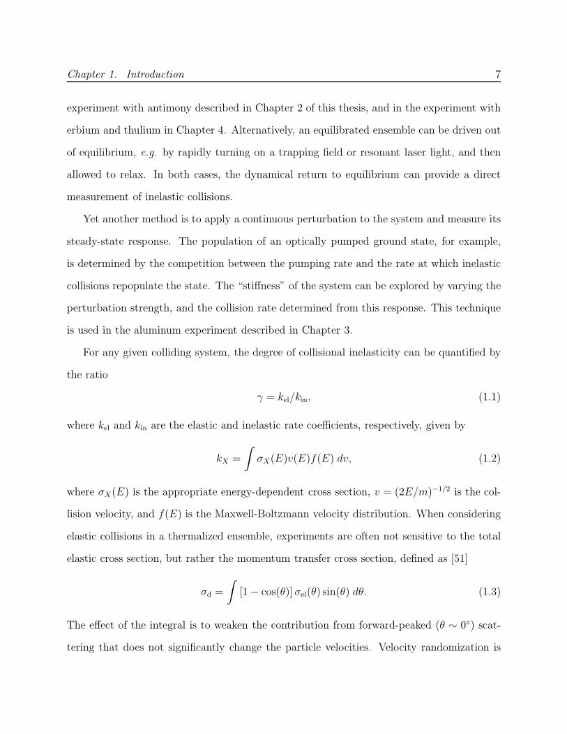
For any given colliding system, the degree of collisional inelasticity can be quantified by
the ratio
γ = kel/kin, (1.1)
where kel and kin are the elastic and inelastic rate coefficients, respectively, given by
kX =
∫
σX(E)v(E)f(E) dv, (1.2)
where σX(E) is the appropriate energy-dependent cross section, v = (2E/m)−1/2 is the col-
lision velocity, and f(E) is the Maxwell-Boltzmann velocity distribution. When considering
elastic collisions in a thermalized ensemble, experiments are often not sensitive to the total
elastic cross section, but rather the momentum transfer cross section, defined as [51]
σd =
∫
[1 − cos(θ)] σel(θ) sin(θ) dθ. (1.3)
The effect of the integral is to weaken the contribution from forward-peaked (θ ∼ 0) scat-
tering that does not significantly change the particle velocities. Velocity randomization is
Chapter 1. Introduction 8
integral to particle diffusion and thermalization, and hence it is the momentum transfer
collision rate kd that is extracted from measurements of those processes. For the remainder
of this thesis, the definition
γ = kd/kin (1.4)
will be used.

Chapter 2
Antimony–4He collisions
2.1 Pnictogen collisions
In addition to their fundamental importance to chemistry and biology, nitrogen and the other
pnictogens (Group 15 atoms) are experimentally promising and theoretically interesting from
the perspective of atomic and molecular physics. Atomic nitrogen, in particular, has a low
polarizability and a highly isotropic electronic distribution, both of which contribute to
robust elasticity in collisions with other atoms and molecules, often limited only by modest
magnetic dipole-dipole interactions [52, 53]. For this reason, nitrogen has been identified
as a promising sympathetic coolant for molecular species, including NH [53–55]. Based on
theoretical calculations, it is also reasonable to expect that evaporative cooling of nitrogen to
the ultracold regime in a magnetic trap will be efficient [52], and hence a quantum degenerate
nitrogen gas may be achievable in a magnetic trap. Such developments would make nitrogen
a potential component of novel and physically unique ultracold diatomic species.
A significant technical drawback to experiments using nitrogen atoms is that the lowest-
energy E1 transition from the ground state is at 121 nm, a difficult vacuum ultraviolet
9
Chapter 2. Antimony–4He collisions 10
(UV) wavelength that precludes the use of traditional laser cooling techniques that have
been so successful in atoms such as the alkali metals. Despite this impediment, very large
trapped ensembles of cold atomic nitrogen have been achieved by means of buffer-gas cooling
[52]; nitrogen has also been co-trapped with NH molecules, a critical first step towards
sympathetic cooling of the molecules [54]. Lacking a 121-nm laser, these experiments have
detected nitrogen using two-photon absorption laser induced fluorescence (TALIF) with a
pulsed 207-nm laser. This method has been satisfactory thus far, but limitations imposed
by the shot-to-shot variation, linewidth, and calibration difficulties inherent to this method
are an impediment to rapid experimental progress.
To this end, the other pnictogens are appealing from a technical perspective as potential
stand-ins for nitrogen. With each step down in the Group 15 column, the optical transition
frequencies are reduced [56], simplifying detection. However, there potentially are significant
challenges to replacing nitrogen with a heavier pnictogen. Atomic polarizability grows with
mass, as does spin-orbit coupling strength. The latter was shown theoretically in the case of
the bismuth to result in severe deformation of the ground 4S3/2 electronic structure, resulting
in rapid inelastic bismuth–helium collisions which were observed experimentally [57]. Since
bismuth is the heaviest stable atom with a half-filled p shell, it is not surprising that its
structure—nominally equivalent to that of nitrogen—is significantly affected by relativistic
distortions.
2.1.1 The importance of antimony
Between the extreme cases of nitrogen and bismuth, cold collisions of the other pnicto-
gens have heretofore not been investigated, and it has remained an open question of how
the strong anisotropy observed in bismuth develops through the group. In fact, even in
the case of bismuth the theoretically calculated inelastic collision rates are well beyond the
Chapter 2. Antimony–4He collisions 11
experimentally accessible parameter space, leaving a wide gap between predictions and ex-
perimental bounds. It has also remained unclear whether there exists a good compromise
between technical feasibility and collisional robustness among the pnictogens, which could
lead to important advancement.
In general, many relativistic effects in atoms are strong functions of the atomic mass.
Hence, it is reasonable to suppose that the inelasticity in bismuth collisions would be sig-
nificantly reduced in collisions instead involving the next-lightest pnictogen, antimony. An-
timony is also the lightest pnictogen for which single-photon excitation is straightforward
with standard narrow-band laser technology, a critical hurdle overcome towards experimental
simplicity. For these reasons, antimony appears well-positioned to be a useful compromise.
This chapter describes experiments investigating Zeeman relaxation of antimony in a
magnetic field due to collisions with helium-4. These inelastic collisions are unfortunately
found to be too rapid to allow for buffer-gas loading of a magnetic trap. However, the
antimony–helium system allows for a more fruitful comparison between experimental and
theoretical results than that which was achievable for the bismuth–helium system. This
comparison supports our understanding of the critical role of spin-orbit coupling in driving
the inelastic transitions [57] and provides a constraint to the antimony–helium interaction
potential. Furthermore, the exploration of this important regime in the pnictogen series
informs the possibilities for future experiments with these atoms.
2.2 Experimental design
2.2.1 Experimental cell
The experiments investigating antimony–helium inelastic collisions were performed in an
experimental cell modeled in part on the cell used to evaporatively cool metastable helium
Chapter 2. Antimony–4He collisions 12
atoms to create a Bose-Einstein condensate [31, 58]. The success of that cell in maintaining
excellent vacuum within seconds of buffer-gas trap loading made it an attractive model for
extending such methods to cool molecular species. The new cell was constructed with the
primary goal of trapping of molecular NH and sympathetic cooling with atomic nitrogen
(see Section A.5). In addition to the antimony experiment described here, it was also used
for the aluminum experiment described in Chapter 3.
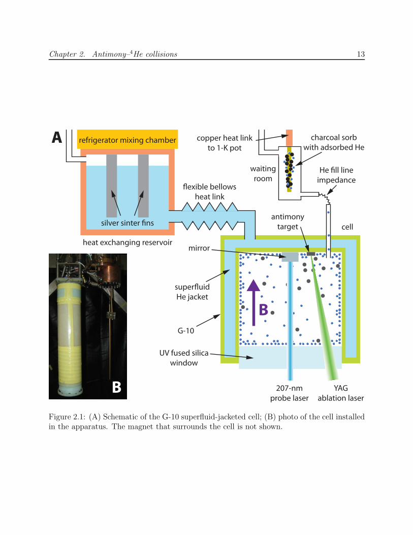
As with the metastable helium cell, the antimony cell consists of two concentric G-
10 CR fiberglass-epoxy composite tubes1 with a jacket of superfluid helium filling the space
between them (Figure 2.1). The superfluid provides excellent thermal conductivity without
electrical conductivity, minimizing eddy current heating when the magnetic field is reduced
to implement evaporative cooling. The superfluid jacket space extends through a flexible
bellows to a copper heat exchanger bolted to the mixing chamber of a dilution refrigerator2.
Sintered silver powder attached to copper fins mounted in the heat exchanger minimize the
Kapitza resistance [59] between metal and superfluid so that the thermal contact between
the refrigerator and cell is limited by the narrow bellows section. The cell’s power curve is
shown in Figure 2.2, from which the flexible link’s thermal conductivity at temperature T is
computed to be κ = (0.47 T 3) W/K4, in good agreement with calculations from Equation 2.13
of [59].
Sealing the cell at its base is a wedged window made of uncoated UV-grade fused silica.
At the top of the cell is a deep-UV aluminum mirror for reflecting a probe laser, as well
as several solid ablation targets attached with Stycast 2850FT black epoxy. There is no
line of sight between the ablation targets and mirror surface to avoid coating the mirror
with ablated material. A small impedance separates the cell from a buffer gas reservoir
1Spaulding Composites, Inc., Rochester, NH.
2Model MNK126-500, Leiden Cryogenics b.v., Leiden, the Netherlands.
Chapter 2. Antimony–4He collisions 13
B
exible bellows
heat link
refrigerator mixing chamber
silver sinter !ns
superuid
He jacket
G-10
UV fused silica
window
heat exchanging reservoir
207-nm
probe laser
YAG
ablation laser
mirror
antimony
target
He !ll line
impedance
charcoal sorb
with adsorbed He
waiting
room
copper heat link
to 1-K pot
cell
AA
B
Figure 2.1: (A) Schematic of the G-10 superfluid-jacketed cell; (B) photo of the cell installedin the apparatus. The magnet that surrounds the cell is not shown.

Chapter 2. Antimony–4He collisions 14
0 100 200 300 400 500 6000
50
100
150
200
250
300
applied power (µW)
Tce
ll (m
K)
0 200 400 600
0
1
2
3
4
5
x 109
Tce
ll4
− T
MC
4 (
mK
4 )
Figure 2.2: Measured power curve of the G-10 superfluid-jacketed cell. The inset shows theconductivity calibration of the flexible thermal link, with the difference of the fourth powersof the cell and mixing chamber temperature plotted against the same horizontal axis. Theinset data are fit to the function expected based upon the T 3 dependence of the superfluidhelium thermal conductivity [59]. Extrapolating the fit to zero thermal gradient and takingthe absolute value yields an estimate of the base heat load on the cell of 66 µW (red triangle).
called the “waiting room” [60]. Inside the waiting room is ≈0.5 cm3 (0.1 g) of activated
coconut charcoal sorb attached to a brass post with Stycast 2850FT black epoxy, which
is thermally anchored to the refrigerator’s 1-K pot. Applying current through a resistive
wire wound on the post rapidly warms the charcoal to >10 K, releasing adsorbed helium
atoms and pressurizing the waiting room. The cell is filled with buffer gas by applying a 1-s
heating pulse of 0.1–0.4 J to the sorb heater, after which it cools below 2 K within 30 s and
cryopumps the waiting room space back to low pressure. The time for buffer gas in the cell
to be pumped back to the waiting room through the impedance is much longer, allowing for
many ablation cycles at relatively constant buffer gas density.
Chapter 2. Antimony–4He collisions 15
−60 −40 −20 0 20 400
0.2
0.4
0.6
0.8
1
1.2
vertical offset from magnet center (mm)
frac
tion
of m
axim
um
−1 −0.5 00
0.2
0.4
detuning (GHz)
σ / σ
0
B = 2 T
magnetic fieldatom density on cell axis
0 K800 mK
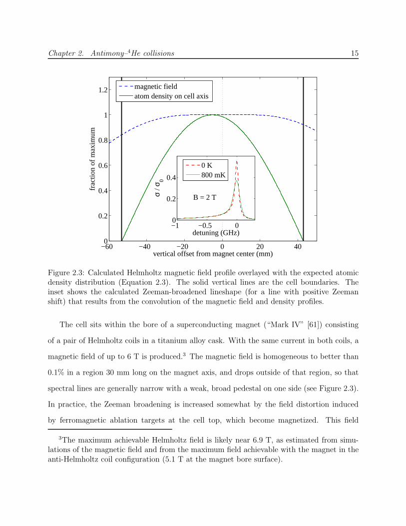
Figure 2.3: Calculated Helmholtz magnetic field profile overlayed with the expected atomicdensity distribution (Equation 2.3). The solid vertical lines are the cell boundaries. Theinset shows the calculated Zeeman-broadened lineshape (for a line with positive Zeemanshift) that results from the convolution of the magnetic field and density profiles.
The cell sits within the bore of a superconducting magnet (“Mark IV” [61]) consisting
of a pair of Helmholtz coils in a titanium alloy cask. With the same current in both coils, a
magnetic field of up to 6 T is produced.3 The magnetic field is homogeneous to better than
0.1% in a region 30 mm long on the magnet axis, and drops outside of that region, so that
spectral lines are generally narrow with a weak, broad pedestal on one side (see Figure 2.3).
In practice, the Zeeman broadening is increased somewhat by the field distortion induced
by ferromagnetic ablation targets at the cell top, which become magnetized. This field
3The maximum achievable Helmholtz field is likely near 6.9 T, as estimated from simu-lations of the magnetic field and from the maximum field achievable with the magnet in theanti-Helmholtz coil configuration (5.1 T at the magnet bore surface).

Chapter 2. Antimony–4He collisions 16
contribution is not known precisely, and may depend on the magnetic field history.
2.2.2 Antimony production and cooling
Atomic antimony is produced by focusing a <10-ns, 1–5-mJ ablation pulse from a 532-nm
doubled Nd:YAG laser onto a ≈3-mm lump of pure antimony metal. Ablation yields are
typically excellent (>1013 atoms), even for low ablation energies, perhaps due in part to a
combination of the moderate melting point and low thermal conductivity of antimony metal
that allows for localized vaporization [62]. Good ablation yield is a boon to the experiment,
not only in terms of detection, but because cold antimony gas can be obtained with minimal
heating of the cryogenic environment.
The cell temperature is held fixed near 800 mK to ensure adequate helium-4 vapor pres-
sure. Lower-temperature buffer-gas cooling is possible with helium-4, however the helium
density is more stable at higher temperatures where the cell heat capacity is larger. Since
ablation heating inevitably causes the cell to heat and cool, it is prudent when the helium
density is critical to the experiment—as is the case when measuring collision rates of atoms
with helium—to operate in a warmer, more density-stable regime whenever possible. After
ablation, the atoms cool to within 0.1 K of the pre-ablation cell temperature within 20 ms
(Figure 2.4).
After ablation and cooling, the atoms diffuse through the buffer gas to the cell walls,
where they freeze. This diffusive transport is governed by the diffusion equation [51],
∂
∂tn(r, t) = D∇2n(r, t), (2.1)
D =3π
32
v
nbσd, (2.2)
where D is the diffusion constant, n and nb are the antimony and buffer gas densities,
respectively, v =√
8kBT/πµ is the mean inter-species velocity with reduced mass µ, and σd
Chapter 2. Antimony–4He collisions 17
0 10 20 30 400
0.2
0.4
0.6
0.8
1
1.2
1.4
1.6
1.8
2
Sb
tem
pera
ture
from
fit t
o V
oigt
pro
file
(K)
time (ms)
A
0 10 20 30 40
10−2
10−1
100
time (ms)
LFS
:HF
S B
oltz
man
n fa
ctor
rat
io
B
EYAG
≈ 4.0 mJ
EYAG
≈ 2.5 mJ
EYAG
≈ 1.5 mJ
cell thermometer
EYAG
≈ 4.0 mJ
EYAG
≈ 2.5 mJ
TZeeman
= Tcell
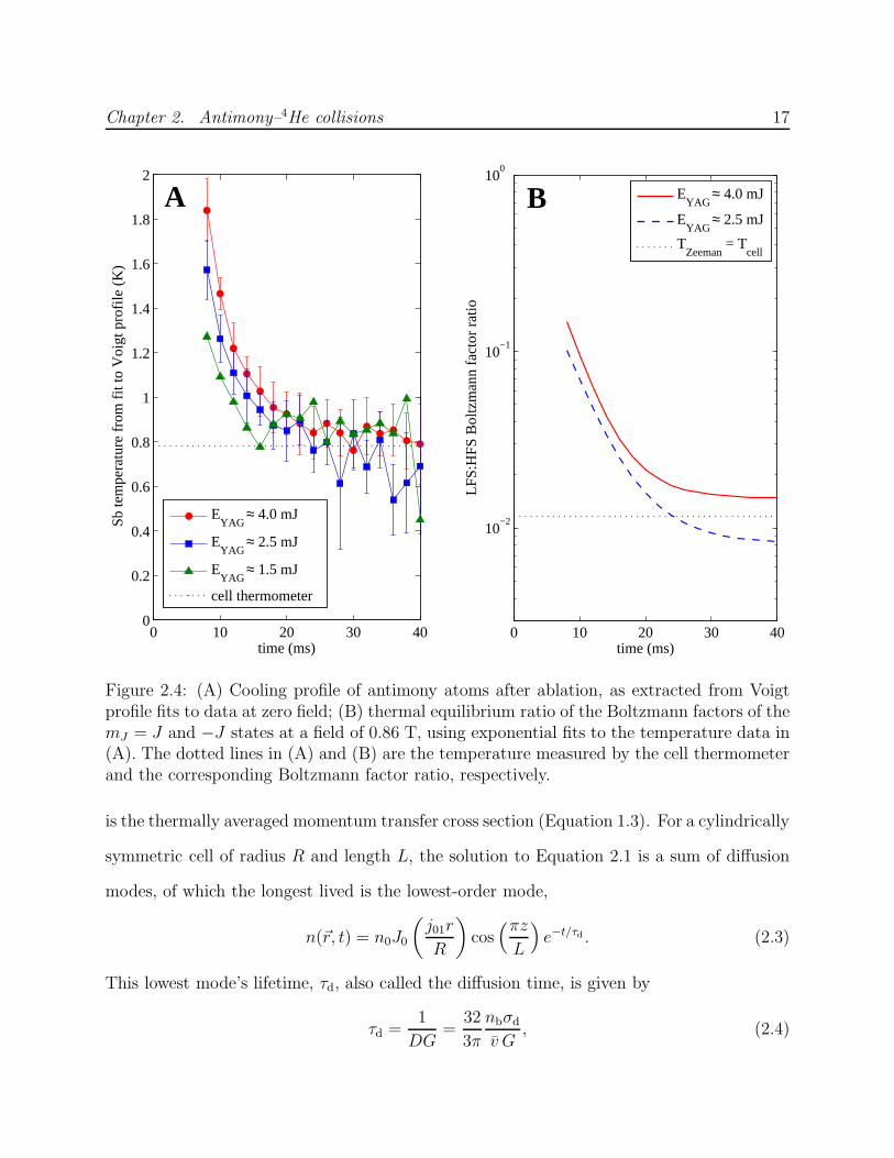
Figure 2.4: (A) Cooling profile of antimony atoms after ablation, as extracted from Voigtprofile fits to data at zero field; (B) thermal equilibrium ratio of the Boltzmann factors of themJ = J and −J states at a field of 0.86 T, using exponential fits to the temperature data in(A). The dotted lines in (A) and (B) are the temperature measured by the cell thermometerand the corresponding Boltzmann factor ratio, respectively.
is the thermally averaged momentum transfer cross section (Equation 1.3). For a cylindrically
symmetric cell of radius R and length L, the solution to Equation 2.1 is a sum of diffusion
modes, of which the longest lived is the lowest-order mode,
n(~r, t) = n0J0
(
j01r
R
)
cos(πz
L
)
e−t/τd . (2.3)
This lowest mode’s lifetime, τd, also called the diffusion time, is given by
τd =1
DG=
32
3π
nbσdv G
, (2.4)

Chapter 2. Antimony–4He collisions 18
G =j201R2
+π2
L2. (2.5)
J0(x) is the zeroth-order Bessel function of the first kind and j01 is its first zero. For L ∼ 2R,
higher-order modes decay at least several times faster than the lowest mode and can be safely
ignored after waiting 1–3 diffusion times. The applied magnetic field is largely homogeneous
across the cell and does not significantly affect the diffusive motion.
2.2.3 Thermal dynamics of Zeeman relaxation
Antimony atoms are produced at a temperature much higher than the energy splitting
∆E = µB/J between magnetic sublevels, where µ = 3µB is the ground state magnetic
moment. Hence, the atoms initially populate all sublevels equally. We define the Zeeman
temperature from the sublevel distribution in a magnetic field B such that the ratio of
populations in the stretched low- and high-field-seeking (LFS and HFS) states are given by
NmJ=J
NmJ=−J= exp
(
−2µB
kBT
)
. (2.6)
As the atoms cool by colliding with the buffer gas, the Zeeman temperature equilibrates
to the translational temperature only via inelastic collisions (Zeeman relaxation). For suffi-
ciently large values of the antimony–helium elastic-to-inelastic collision ratio γ (introduced
in Section 1.3.1, Equation 1.4), the translational temperature will drop and stabilize while
the Zeeman temperature remains high. Under these circumstances, the difference between
the lifetimes of different sublevels reveals the inelastic collision rate.
In the other extreme of γ ≈ 1, where inelastic and elastic collisions occur at similar
rates, the Zeeman distribution remains in equilibrium with the translational temperature.
The lifetimes of the sublevels will then be determined by the temporal and spatial cooling
profile in the first milliseconds after ablation. Measuring low values of γ by watching the
Zeeman temperature fall to equilibrium after ablation is quite difficult, as it requires decon-
Chapter 2. Antimony–4He collisions 19
volving relaxation from the imprecisely-known cooling profile. In general, this presents an
intractable experimental challenge for measuring γ . 1,000 in this manner, and the method
can only produce an upper bound for the inelastic collision rate [57, 63, 64]. As discussed
in Section 1.3.1, there are other ways to measure faster rates of inelastic collisions, such as
the optical pumping method described in Chapter 3. However, other methods may not be
technically feasible in all systems. The discussion here will focus on observing equilibration
of the Zeeman and translational temperatures after ablation into the buffer gas.
The difficulty in observing low values of γ after ablation depends on the ablation energy
and heat capacity of the cell. A large heat capacity—achieved either with a large cell or a high
temperature—will cause the cell temperature to remain stable after ablation. In practice,
the temperature must be kept low enough to achieve a significant Boltzmann factor between
magnetic sublevels with the available magnetic field. In addition, the Zeeman relaxation rate
will in general change with temperature and field, and it is better not to technically constrain
these parameters more than necessary. Using as an example the initial temperature of 1 K
and the measured specific heats [59], one finds that a cell built of 100 cm3 of copper will heat
by approximately 10% and 70% upon absorbing energies of 1 and 10 mJ, respectively. In
comparison, with only 10 cm3 of superfluid helium-4 (the material used to cool the cell for the
antimony experiments described here) the temperature rise is <10% for 10 mJ. The latter’s
heat capacity is sufficient for a stable mean temperature over the entire cell. However, the
thermal conduction time across the cell can place an additional limit on the stability of the
buffer gas temperature, as described in the following section.
2.2.4 Thermal dynamics in G-10 cells
There is reason to expect that the challenge of separating Zeeman relaxation from equili-
brated cooling is particularly acute in experimental cells constructed from G-10 rather than
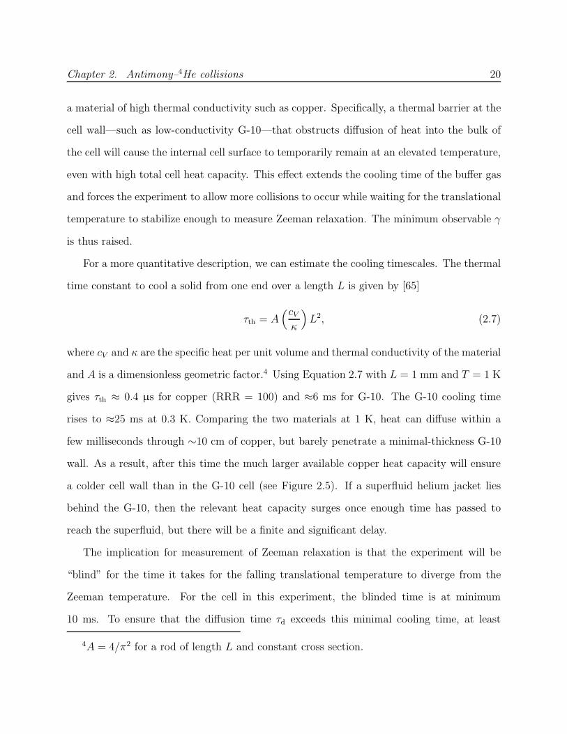
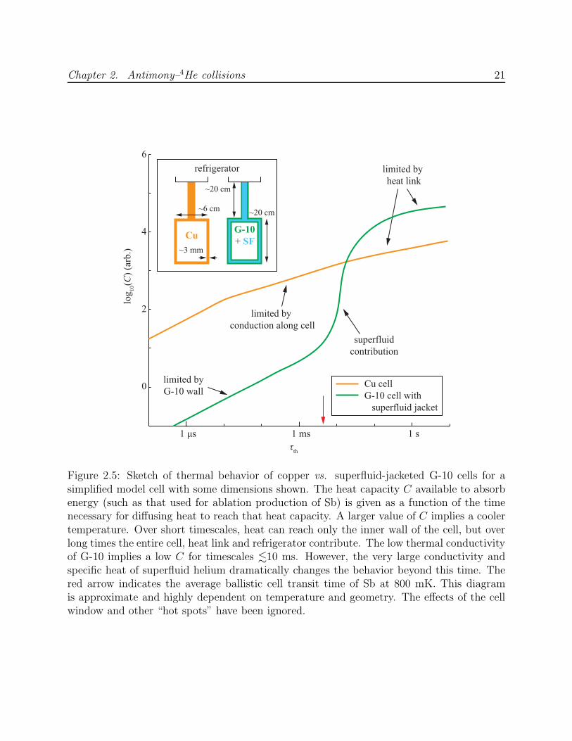
Chapter 2. Antimony–4He collisions 20
a material of high thermal conductivity such as copper. Specifically, a thermal barrier at the
cell wall—such as low-conductivity G-10—that obstructs diffusion of heat into the bulk of
the cell will cause the internal cell surface to temporarily remain at an elevated temperature,
even with high total cell heat capacity. This effect extends the cooling time of the buffer gas
and forces the experiment to allow more collisions to occur while waiting for the translational
temperature to stabilize enough to measure Zeeman relaxation. The minimum observable γ
is thus raised.
For a more quantitative description, we can estimate the cooling timescales. The thermal
time constant to cool a solid from one end over a length L is given by [65]
τth = A(cVκ
)
L2, (2.7)
where cV and κ are the specific heat per unit volume and thermal conductivity of the material
and A is a dimensionless geometric factor.4 Using Equation 2.7 with L = 1 mm and T = 1 K
gives τth ≈ 0.4 µs for copper (RRR = 100) and ≈6 ms for G-10. The G-10 cooling time
rises to ≈25 ms at 0.3 K. Comparing the two materials at 1 K, heat can diffuse within a
few milliseconds through ∼10 cm of copper, but barely penetrate a minimal-thickness G-10
wall. As a result, after this time the much larger available copper heat capacity will ensure
a colder cell wall than in the G-10 cell (see Figure 2.5). If a superfluid helium jacket lies
behind the G-10, then the relevant heat capacity surges once enough time has passed to
reach the superfluid, but there will be a finite and significant delay.
The implication for measurement of Zeeman relaxation is that the experiment will be
“blind” for the time it takes for the falling translational temperature to diverge from the
Zeeman temperature. For the cell in this experiment, the blinded time is at minimum
10 ms. To ensure that the diffusion time τd exceeds this minimal cooling time, at least
4A = 4/π2 for a rod of length L and constant cross section.
Chapter 2. Antimony–4He collisions 21
0
2
4
6
1 μs 1 ms 1 s
τth
log 10
(C)
(arb
.)
Cu cellG-10 cell with superfluid jacket
superfluidcontribution
limited by conduction along cell
limited by heat link
CuG-10
+ SF
~6 cm
~20 cm
~3 mm
refrigerator
~20 cm
limited byG-10 wall
Figure 2.5: Sketch of thermal behavior of copper vs. superfluid-jacketed G-10 cells for asimplified model cell with some dimensions shown. The heat capacity C available to absorbenergy (such as that used for ablation production of Sb) is given as a function of the timenecessary for diffusing heat to reach that heat capacity. A larger value of C implies a coolertemperature. Over short timescales, heat can reach only the inner wall of the cell, but overlong times the entire cell, heat link and refrigerator contribute. The low thermal conductivityof G-10 implies a low C for timescales .10 ms. However, the very large conductivity andspecific heat of superfluid helium dramatically changes the behavior beyond this time. Thered arrow indicates the average ballistic cell transit time of Sb at 800 mK. This diagramis approximate and highly dependent on temperature and geometry. The effects of the cellwindow and other “hot spots” have been ignored.
Chapter 2. Antimony–4He collisions 22
∼1,000 collisions are required, i.e., a minimum observable γ & 1,000. The contrast in
thermal behavior of superfluid-jacketed G-10 cells has further implications for buffer-gas
trapping, especially for marginally-trappable species with γ of 104–105. Sections 4.2.2 and
A.3.4 describe this behavior in relation to specific experiments.
2.2.5 Absorption spectroscopy detection system
Ground state optical detection of the lighter pnictogens is difficult due to the short-wave-
length UV lasers required for single-photon excitation. Antimony is the lightest of the group
for which this wavelength is greater than 205 nm, the lower limit for single harmonic gener-
ation (SHG) in beta barium borate (BBO) nonlinear crystals [66]. Narrow-band continuous
wave (CW) lasers can be created at shorter wavelengths [67, 68], but the process is signif-
icantly more difficult [69], and experimental implementation of such laser systems can be
hindered by limited availability of optical elements such as low-absorption windows.
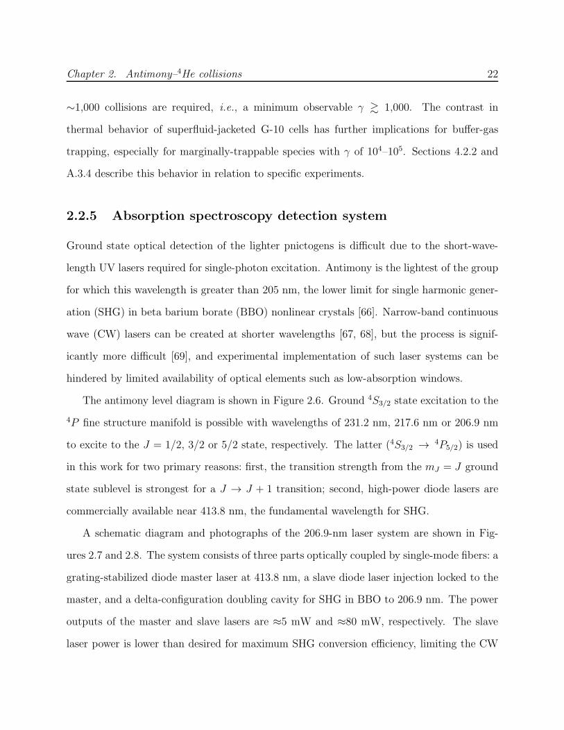
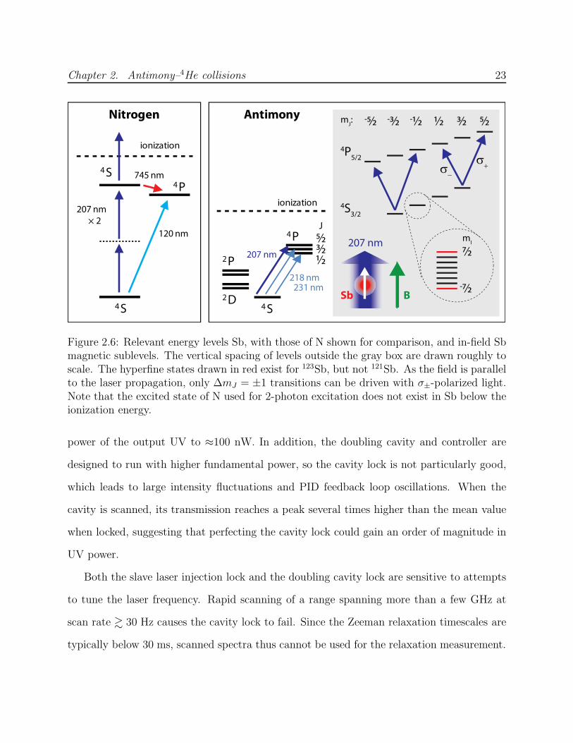
The antimony level diagram is shown in Figure 2.6. Ground 4S3/2 state excitation to the
4P fine structure manifold is possible with wavelengths of 231.2 nm, 217.6 nm or 206.9 nm
to excite to the J = 1/2, 3/2 or 5/2 state, respectively. The latter (4S3/2 → 4P5/2) is used
in this work for two primary reasons: first, the transition strength from the mJ = J ground
state sublevel is strongest for a J → J + 1 transition; second, high-power diode lasers are
commercially available near 413.8 nm, the fundamental wavelength for SHG.
A schematic diagram and photographs of the 206.9-nm laser system are shown in Fig-
ures 2.7 and 2.8. The system consists of three parts optically coupled by single-mode fibers: a
grating-stabilized diode master laser at 413.8 nm, a slave diode laser injection locked to the
master, and a delta-configuration doubling cavity for SHG in BBO to 206.9 nm. The power
outputs of the master and slave lasers are ≈5 mW and ≈80 mW, respectively. The slave
laser power is lower than desired for maximum SHG conversion efficiency, limiting the CW
Chapter 2. Antimony–4He collisions 23
4S4P
4S
120 nm
207 nm
× 2
ionization
745 nm
Nitrogen Antimony
4P
4S
207 nm
ionization
J
5⁄23⁄2½
231 nm218 nm
2P
2D
4P5/2
4S3/2
mJ: 3⁄2-5⁄2 -3⁄2 -½ ½ 5⁄2
σ+σ
−
mI
7⁄2
-7⁄2BSb
207 nm
Figure 2.6: Relevant energy levels Sb, with those of N shown for comparison, and in-field Sbmagnetic sublevels. The vertical spacing of levels outside the gray box are drawn roughly toscale. The hyperfine states drawn in red exist for 123Sb, but not 121Sb. As the field is parallelto the laser propagation, only ∆mJ = ±1 transitions can be driven with σ±-polarized light.Note that the excited state of N used for 2-photon excitation does not exist in Sb below theionization energy.
power of the output UV to ≈100 nW. In addition, the doubling cavity and controller are
designed to run with higher fundamental power, so the cavity lock is not particularly good,
which leads to large intensity fluctuations and PID feedback loop oscillations. When the
cavity is scanned, its transmission reaches a peak several times higher than the mean value
when locked, suggesting that perfecting the cavity lock could gain an order of magnitude in
UV power.
Both the slave laser injection lock and the doubling cavity lock are sensitive to attempts
to tune the laser frequency. Rapid scanning of a range spanning more than a few GHz at
scan rate & 30 Hz causes the cavity lock to fail. Since the Zeeman relaxation timescales are
typically below 30 ms, scanned spectra thus cannot be used for the relaxation measurement.

Chapter 2. Antimony–4He collisions 24
Master
FC
Slave
FC
FC
FC FC
wave meter
FC EOM
Nd:YAG
300 K
77 K
4 Kcell
Optics Table
Dewar
Breadboard
Cryogenic Apparatus
FC
Doubling Cavity
PMTPMT
BBO
!ber
coupler
optical
isolator
mirror 207-nm
mirror
window λ/2 plate #ip
mirror
prism iris lens Fabry-Perot
cavity
single-mode
!ber
multi-mode
!ber
Figure 2.7: Schematic of 414 → 207-nm laser system and optics layout for Sb absorptionspectroscopy. Some steering mirrors are not shown.
Chapter 2. Antimony–4He collisions 25
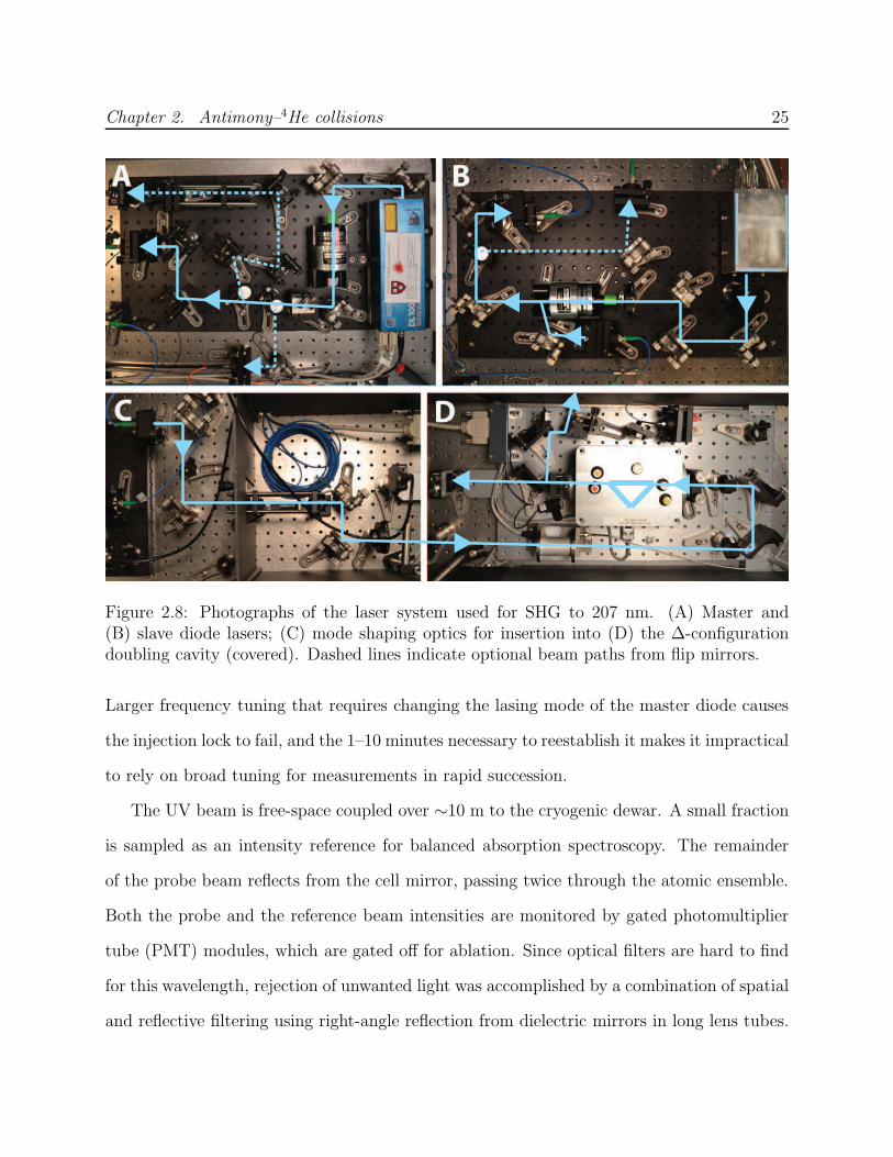
Figure 2.8: Photographs of the laser system used for SHG to 207 nm. (A) Master and(B) slave diode lasers; (C) mode shaping optics for insertion into (D) the ∆-configurationdoubling cavity (covered). Dashed lines indicate optional beam paths from flip mirrors.
Larger frequency tuning that requires changing the lasing mode of the master diode causes
the injection lock to fail, and the 1–10 minutes necessary to reestablish it makes it impractical
to rely on broad tuning for measurements in rapid succession.
The UV beam is free-space coupled over ∼10 m to the cryogenic dewar. A small fraction
is sampled as an intensity reference for balanced absorption spectroscopy. The remainder
of the probe beam reflects from the cell mirror, passing twice through the atomic ensemble.
Both the probe and the reference beam intensities are monitored by gated photomultiplier
tube (PMT) modules, which are gated off for ablation. Since optical filters are hard to find
for this wavelength, rejection of unwanted light was accomplished by a combination of spatial
and reflective filtering using right-angle reflection from dielectric mirrors in long lens tubes.
Chapter 2. Antimony–4He collisions 26
Each mirror, coated for >99% reflectivity at 207 nm, reflects ≈4% of out-of-band light on
average. In addition, the dewar is shrouded in black tarp and the room lights are turned off.
The signal-to-noise of absorption measurements is then limited by beam motion relative to
the cell and to the PMTs, likely caused by vibrations of the dewar and cell relative to the
optics tables that contain the doubling cavity and routing optics.
2.3 Experimental procedure
2.3.1 Momentum transfer cross section comparison
The antimony–helium-4 momentum transfer cross section σd can be determined from Equa-
tion 2.2 by observation of antimony diffusion if the helium density nb is known. In practice,
absolute measurement of nb at low temperatures is complicated by the effects of transpi-
ration and adsorption of helium onto cold surfaces, and it is not directly measured in this
experiment. Under carefully controlled conditions in previous experiments, however, the
density was measured and used to calibrate σd for certain benchmark atoms and molecules
in the range of 1 K [70, 71]. It is thus possible to calibrate the cross sections of other
atoms by comparing their diffusive motion to that of a benchmark species in the same (un-
known) buffer gas density. Manganese is a second-order benchmark species, the cross section
σd,Mn–3He having been calibrated against that of the first-order benchmark species chromium
[58]. In the case of chromium, nb was determined by adding a known quantity of helium-3
in gas phase to a cell of known volume, after saturating the available surface area.
The comparison of σd between antimony and manganese is conducted as follows. The cell
is filled to an unknown but relatively high density of helium-4 buffer gas (σd for manganese
was calibrated using helium-3, and so this is an imperfect comparison). Two separate YAG
lasers of equal pulse energy are aligned to the antimony and manganese targets, respectively.
Chapter 2. Antimony–4He collisions 27
One of the targets is ablated and the atomic diffusion measured, and several repetitions are
made over about 3 min before switching to ablate the other target. The probe lasers are
also interchanged with a flip-mounted mirror, and share the same beam path through the
dewar and to the same PMTs. Manganese is detected on the 6S5/2 → 6P7/2 transition at
403.2 nm using a diode laser. The weak reflections of the manganese probe from the deep
UV optical coatings of the reflective filters described in Section 2.2.5 are sufficient for good
signal-to-noise in measuring absorption.
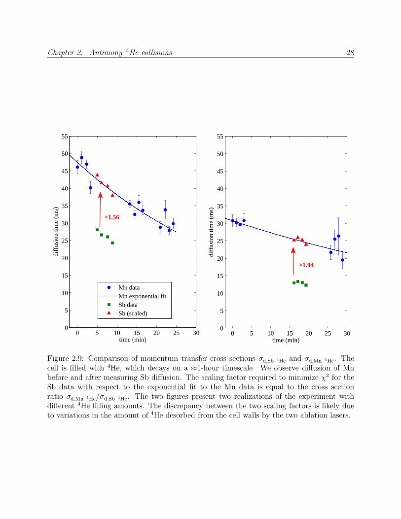
Diffusion lifetime comparisons of manganese and antimony are shown in Figure 2.9. The
helium-4 density decays during the experiment, so that the lifetimes steadily decrease. The
lifetimes for manganese diffusion are fit to a decaying exponential, and then the set of
antimony lifetimes is scaled to minimize the sum of squares of the residuals from this fit.
The resulting scale factor yields the cross section ratio
σd,Mn–4He
σd,Sb–4He
=
√
µSb
µMn
(
τd,Mn
τd,Sb
)
, (2.8)
where µX is the reduced mass of the colliding X–4He system.
The experiment was conducted twice, using two different quantities of filled helium-4.
For the larger fill, the helium density was observed to decay more quickly. The two values
obtained for the cross section ratio are 1.94 after the smaller fill and 1.56 after the larger fill.
The discrepancy may reflect an ablation-induced difference in the buffer gas density, since
the two species are produced using separate YAG beams, only one of which is used at a time.
Helium-4 adsorbed to cell surfaces heated by ablation may temporarily increase the buffer
gas density. For this reason, it is preferable to ablate both targets simultaneously each time,
as is done for the calibration of σd,Al–3He described in Section 3.4.4. Since this was not the
procedure used for the antimony-manganese comparison, the cross section ratio is taken to
be the geometric mean of the two observed ratios, with their discrepancy added as systematic
error in quadrature with measurement error, to yield τd,Sb/τd,Mn = 0.57(7). The resulting
Chapter 2. Antimony–4He collisions 28
0 5 10 15 20 25 300
5
10
15
20
25
30
35
40
45
50
55
time (min)
diffu
sion
tim
e (m
s)
0 5 10 15 20 25 300
5
10
15
20
25
30
35
40
45
50
55
time (min)
diffu
sion
tim
e (m
s)
×1.56
×1.94
Mn dataMn exponential fitSb dataSb (scaled)
Figure 2.9: Comparison of momentum transfer cross sections σd,Sb–4He and σd,Mn–4He. Thecell is filled with 4He, which decays on a ≈1-hour timescale. We observe diffusion of Mnbefore and after measuring Sb diffusion. The scaling factor required to minimize χ2 for theSb data with respect to the exponential fit to the Mn data is equal to the cross sectionratio σd,Mn–4He/σd,Sb–4He. The two figures present two realizations of the experiment withdifferent 4He filling amounts. The discrepancy between the two scaling factors is likely dueto variations in the amount of 4He desorbed from the cell walls by the two ablation lasers.
Chapter 2. Antimony–4He collisions 29
cross section calibration is σd,Sb–4He = 5.7(7) × 10−15 cm2, assuming σd,Mn–4He = σd,Mn–3He.
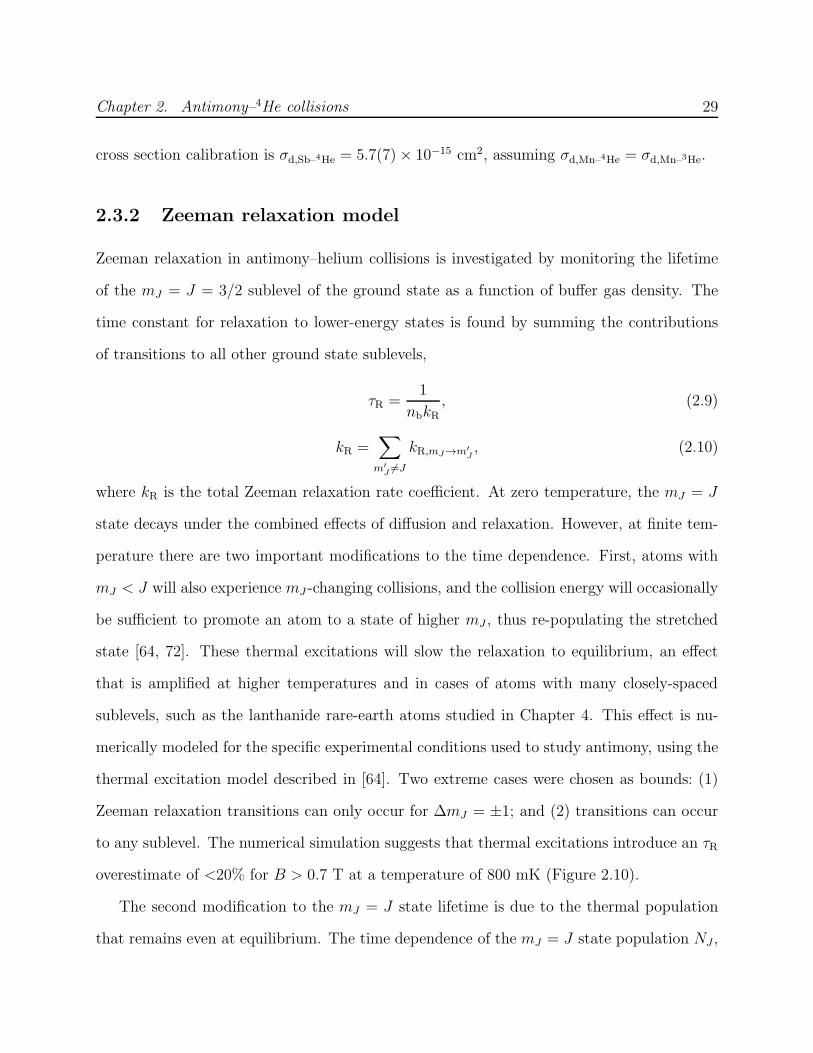
2.3.2 Zeeman relaxation model
Zeeman relaxation in antimony–helium collisions is investigated by monitoring the lifetime
of the mJ = J = 3/2 sublevel of the ground state as a function of buffer gas density. The
time constant for relaxation to lower-energy states is found by summing the contributions
of transitions to all other ground state sublevels,
τR =1
nbkR, (2.9)
kR =∑
m′
J6=J
kR,mJ→m′
J, (2.10)
where kR is the total Zeeman relaxation rate coefficient. At zero temperature, the mJ = J
state decays under the combined effects of diffusion and relaxation. However, at finite tem-
perature there are two important modifications to the time dependence. First, atoms with
mJ < J will also experience mJ -changing collisions, and the collision energy will occasionally
be sufficient to promote an atom to a state of higher mJ , thus re-populating the stretched
state [64, 72]. These thermal excitations will slow the relaxation to equilibrium, an effect
that is amplified at higher temperatures and in cases of atoms with many closely-spaced
sublevels, such as the lanthanide rare-earth atoms studied in Chapter 4. This effect is nu-
merically modeled for the specific experimental conditions used to study antimony, using the
thermal excitation model described in [64]. Two extreme cases were chosen as bounds: (1)
Zeeman relaxation transitions can only occur for ∆mJ = ±1; and (2) transitions can occur
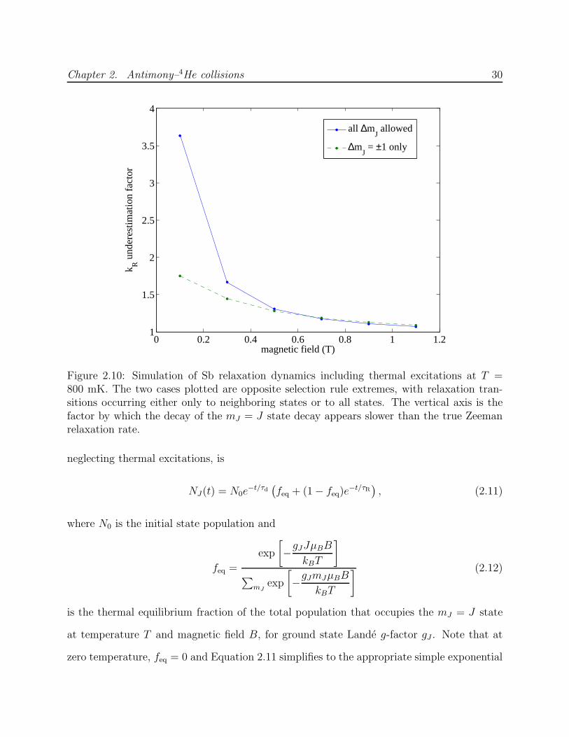
to any sublevel. The numerical simulation suggests that thermal excitations introduce an τR
overestimate of <20% for B > 0.7 T at a temperature of 800 mK (Figure 2.10).
The second modification to the mJ = J state lifetime is due to the thermal population
that remains even at equilibrium. The time dependence of the mJ = J state population NJ ,
Chapter 2. Antimony–4He collisions 30
0 0.2 0.4 0.6 0.8 1 1.21
1.5
2
2.5
3
3.5
4
magnetic field (T)
k R u
nder
estim
atio
n fa
ctor
all ∆mJ allowed
∆mJ = ±1 only
Figure 2.10: Simulation of Sb relaxation dynamics including thermal excitations at T =800 mK. The two cases plotted are opposite selection rule extremes, with relaxation tran-sitions occurring either only to neighboring states or to all states. The vertical axis is thefactor by which the decay of the mJ = J state decay appears slower than the true Zeemanrelaxation rate.
neglecting thermal excitations, is
NJ(t) = N0e−t/τd
(
feq + (1 − feq)e−t/τR
)
, (2.11)
where N0 is the initial state population and
feq =
exp
[
−gJJµBB
kBT
]
∑
mJexp
[
−gJmJµBB
kBT
] (2.12)
is the thermal equilibrium fraction of the total population that occupies the mJ = J state
at temperature T and magnetic field B, for ground state Lande g-factor gJ . Note that at
zero temperature, feq = 0 and Equation 2.11 simplifies to the appropriate simple exponential
Chapter 2. Antimony–4He collisions 31
decay.
Combining Equations 2.4 and 2.9 allows the relaxation lifetime to be expressed as
τR =32
3π
(
1
v2G
) (
1
τd
) (
kdkR
)
=32
3π
( γ
v2G
)
(
1
τd
)
, (2.13)
where v is the mean inter-species velocity and G is a geometric factor defined in Equation 2.5.
The second equality has made use of the elastic-to-inelastic collision ratio γ (Equation 1.4).
Equation 2.13 conveniently has no explicit dependence on the helium density and varies
only with τd. Therefore measurement of both the relaxation and diffusion lifetimes (along
with the cell geometry and temperature) is sufficient to determine γ without the influence
of uncertainty in the buffer gas density or momentum transfer cross section calibration.
While it is in principle possible to extract γ from a single measurement, many measure-
ments are made while varying the helium density in order to confirm that τR varies inversely
proportionally to τd. This provides a check against systematic error. In particular, there
may be other processes contributing to or dominating the decay of the mJ = J state—such
as molecule formation [73]—which will exhibit a different dependence on buffer gas density.
2.3.3 Lifetime measurements
Extracting τR from fits to Equation 2.11 is more reliable if τd can be independently deter-
mined and eliminated as a free parameter, especially at low temperatures where feq is small.
Ideally, the lifetime of the mJ = J state is measured at finite B and at B = 0 under identical
conditions. However, since it takes 10–100 s to ramp the magnetic field, and also since doing
so induces some measure of eddy-current heating, this comparison risks systematic error.
Instead, the lifetimes of the mJ = J and −J states are compared at very similar finite values
of B, which can be switched more rapidly with little heating. The mJ = −J state has the
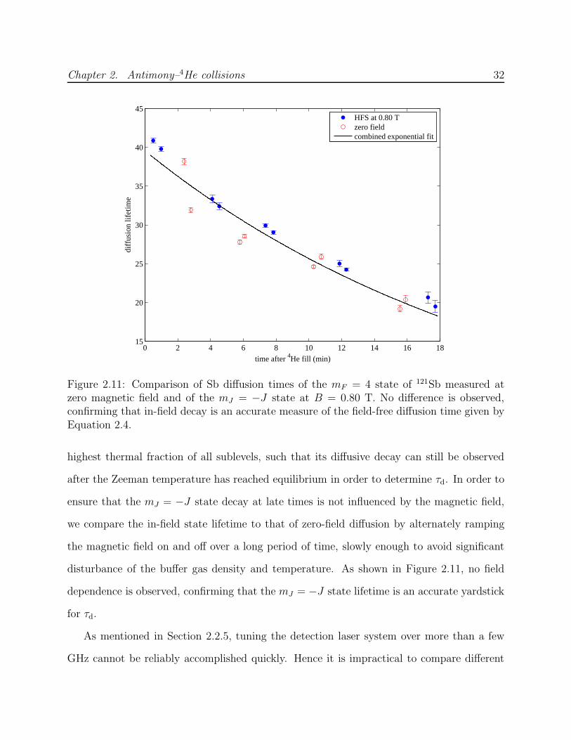
Chapter 2. Antimony–4He collisions 32
0 2 4 6 8 10 12 14 16 1815
20
25
30
35
40
45
time after 4He fill (min)
diffu
sion
life
time
HFS at 0.80 Tzero fieldcombined exponential fit
Figure 2.11: Comparison of Sb diffusion times of the mF = 4 state of 121Sb measured atzero magnetic field and of the mJ = −J state at B = 0.80 T. No difference is observed,confirming that in-field decay is an accurate measure of the field-free diffusion time given byEquation 2.4.
highest thermal fraction of all sublevels, such that its diffusive decay can still be observed
after the Zeeman temperature has reached equilibrium in order to determine τd. In order to
ensure that the mJ = −J state decay at late times is not influenced by the magnetic field,
we compare the in-field state lifetime to that of zero-field diffusion by alternately ramping
the magnetic field on and off over a long period of time, slowly enough to avoid significant
disturbance of the buffer gas density and temperature. As shown in Figure 2.11, no field
dependence is observed, confirming that the mJ = −J state lifetime is an accurate yardstick
for τd.
As mentioned in Section 2.2.5, tuning the detection laser system over more than a few
GHz cannot be reliably accomplished quickly. Hence it is impractical to compare different
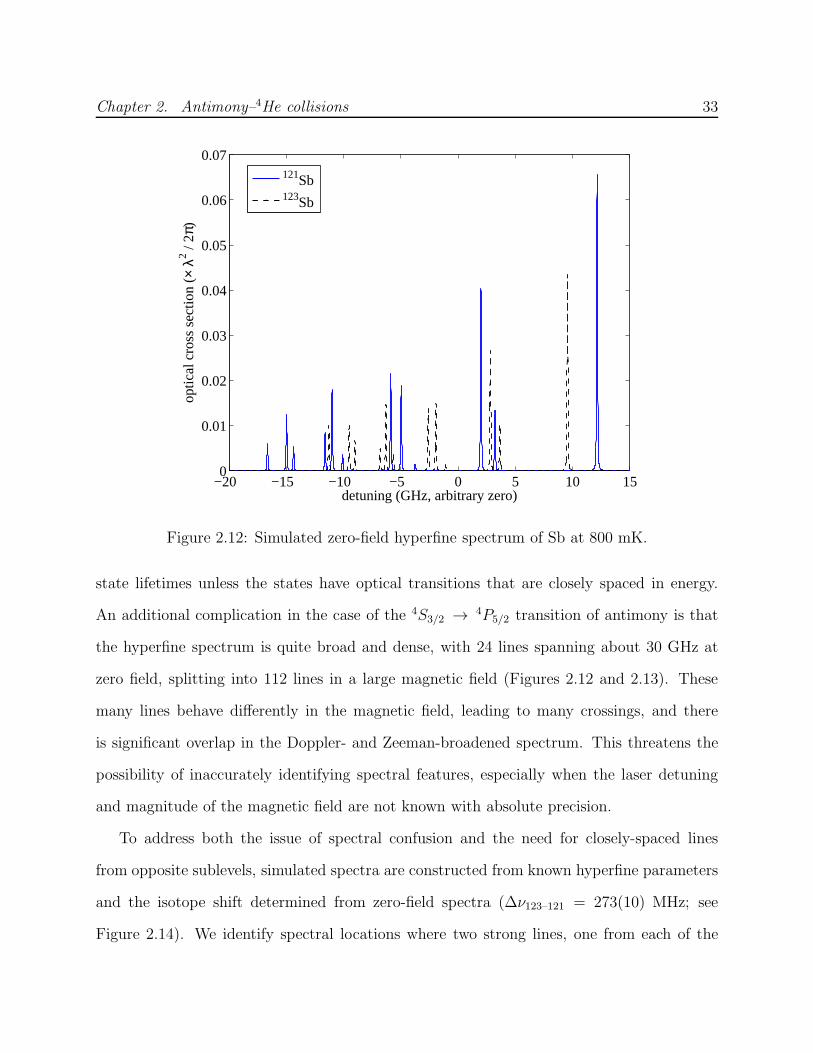
Chapter 2. Antimony–4He collisions 33
−20 −15 −10 −5 0 5 10 150
0.01
0.02
0.03
0.04
0.05
0.06
0.07
detuning (GHz, arbitrary zero)
optic
al c
ross
sec
tion
(× λ2 /
2π)
121Sb123Sb
Figure 2.12: Simulated zero-field hyperfine spectrum of Sb at 800 mK.
state lifetimes unless the states have optical transitions that are closely spaced in energy.
An additional complication in the case of the 4S3/2 → 4P5/2 transition of antimony is that
the hyperfine spectrum is quite broad and dense, with 24 lines spanning about 30 GHz at
zero field, splitting into 112 lines in a large magnetic field (Figures 2.12 and 2.13). These
many lines behave differently in the magnetic field, leading to many crossings, and there
is significant overlap in the Doppler- and Zeeman-broadened spectrum. This threatens the
possibility of inaccurately identifying spectral features, especially when the laser detuning
and magnitude of the magnetic field are not known with absolute precision.
To address both the issue of spectral confusion and the need for closely-spaced lines
from opposite sublevels, simulated spectra are constructed from known hyperfine parameters
and the isotope shift determined from zero-field spectra (∆ν123–121 = 273(10) MHz; see
Figure 2.14). We identify spectral locations where two strong lines, one from each of the
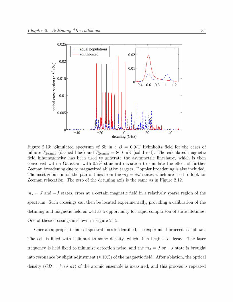
Chapter 2. Antimony–4He collisions 34
−40 −20 0 20 400
0.005
0.01
0.015
0.02
0.025
optic
al c
ross
sec
tion
(× λ2 /
2π)
detuning (GHz)
equal populationsequilibrated
0.4 0.6 0.8 1 1.20
0.01
0.02
Figure 2.13: Simulated spectrum of Sb in a B = 0.9-T Helmholtz field for the cases ofinfinite TZeeman (dashed blue) and TZeeman = 800 mK (solid red). The calculated magneticfield inhomogeneity has been used to generate the asymmetric lineshape, which is thenconvolved with a Gaussian with 0.2% standard deviation to simulate the effect of furtherZeeman broadening due to magnetized ablation targets. Doppler broadening is also included.The inset zooms in on the pair of lines from the mJ = ±J states which are used to look forZeeman relaxation. The zero of the detuning axis is the same as in Figure 2.12.
mJ = J and −J states, cross at a certain magnetic field in a relatively sparse region of the
spectrum. Such crossings can then be located experimentally, providing a calibration of the
detuning and magnetic field as well as a opportunity for rapid comparison of state lifetimes.
One of these crossings is shown in Figure 2.15.
Once an appropriate pair of spectral lines is identified, the experiment proceeds as follows.
The cell is filled with helium-4 to some density, which then begins to decay. The laser
frequency is held fixed to minimize detection noise, and the mJ = J or −J state is brought
into resonance by slight adjustment (≈10%) of the magnetic field. After ablation, the optical
density (OD =∫
nσ dz) of the atomic ensemble is measured, and this process is repeated
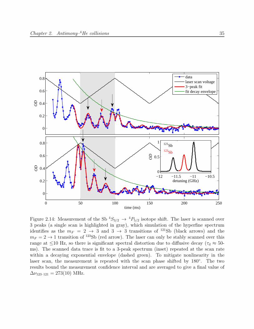
Chapter 2. Antimony–4He collisions 35
0 50 100 150 200 250
0
0.2
0.4
0.6
0.8
time (ms)
OD
−12 −11.5 −11 −10.50
0.5
1
detuning (GHz)
OD
121Sb123Sb
0
0.2
0.4
0.6
0.8
OD
datalaser scan voltage3−peak fitfit decay envelope
Figure 2.14: Measurement of the Sb 4S3/2 → 4P5/2 isotope shift. The laser is scanned over3 peaks (a single scan is highlighted in gray), which simulation of the hyperfine spectrumidentifies as the mF = 2 → 3 and 3 → 3 transitions of 121Sb (black arrows) and themF = 2 → 1 transition of 123Sb (red arrow). The laser can only be stably scanned over thisrange at ≤10 Hz, so there is significant spectral distortion due to diffusive decay (τd ≈ 50-ms). The scanned data trace is fit to a 3-peak spectrum (inset) repeated at the scan ratewithin a decaying exponential envelope (dashed green). To mitigate nonlinearity in thelaser scan, the measurement is repeated with the scan phase shifted by 180. The tworesults bound the measurement confidence interval and are averaged to give a final value of∆ν123–121 = 273(10) MHz.
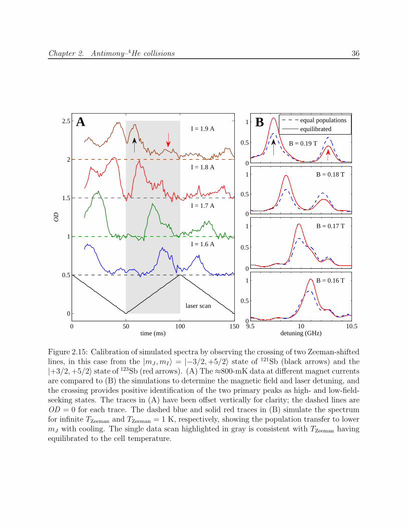
Chapter 2. Antimony–4He collisions 36
0
0.5
1
B
B = 0.19 T
0 50 100 150
0
0.5
1
1.5
2
2.5
time (ms)
OD
AI = 1.9 A
I = 1.8 A
I = 1.7 A
I = 1.6 A
laser scan
0
0.5
1
B = 0.18 T
0
0.5
1
B = 0.17 T
9.5 10 10.50
0.5
1
detuning (GHz)
B = 0.16 T
equal populationsequilibrated
Figure 2.15: Calibration of simulated spectra by observing the crossing of two Zeeman-shiftedlines, in this case from the |mJ , mI〉 = |−3/2,+5/2〉 state of 121Sb (black arrows) and the|+3/2,+5/2〉 state of 123Sb (red arrows). (A) The ≈800-mK data at different magnet currentsare compared to (B) the simulations to determine the magnetic field and laser detuning, andthe crossing provides positive identification of the two primary peaks as high- and low-field-seeking states. The traces in (A) have been offset vertically for clarity; the dashed lines areOD = 0 for each trace. The dashed blue and solid red traces in (B) simulate the spectrumfor infinite TZeeman and TZeeman = 1 K, respectively, showing the population transfer to lowermJ with cooling. The single data scan highlighted in gray is consistent with TZeeman havingequilibrated to the cell temperature.
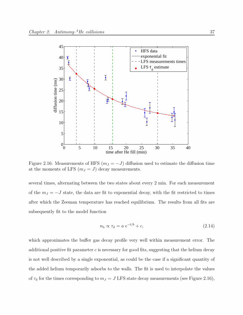
Chapter 2. Antimony–4He collisions 37
0 5 10 15 20 25 30 35 400
5
10
15
20
25
30
35
40
45
time after He fill (min)
diffu
sion
tim
e (m
s)
HFS dataexponential fitLFS measurements timesLFS τ
d estimate
Figure 2.16: Measurements of HFS (mJ = −J) diffusion used to estimate the diffusion timeat the moments of LFS (mJ = J) decay measurements.
several times, alternating between the two states about every 2 min. For each measurement
of the mJ = −J state, the data are fit to exponential decay, with the fit restricted to times
after which the Zeeman temperature has reached equilibrium. The results from all fits are
subsequently fit to the model function
nb ∝ τd = a e−t/b + c, (2.14)
which approximates the buffer gas decay profile very well within measurement error. The
additional positive fit parameter c is necessary for good fits, suggesting that the helium decay
is not well described by a single exponential, as could be the case if a significant quantity of
the added helium temporarily adsorbs to the walls. The fit is used to interpolate the values
of τd for the times corresponding to mJ = J LFS state decay measurements (see Figure 2.16),

Chapter 2. Antimony–4He collisions 38
0 20 40 60 80 10010
−2
10−1
100
101
time (ms)
OD
datadouble−exponential fit
Figure 2.17: Decay of the |mJ , mI〉 = |+3/2,−5/2〉 state of 121Sb at B = 0.86 T andTcell = 800 mK, along with the fit to Equation 2.11. The rapid decay before t = 20 ms islikely influenced by cooling and not a reliable indicator of the Zeeman relaxation rate.
which are then used to constrain the fits of those data to Equation 2.11.
2.4 Results and discussion
2.4.1 Upper bound on Zeeman relaxation rate
An example of mJ = J state decay at B = 0.86 T is shown in Figure 2.17, along with the
bimodal decay fit to Equation 2.11. The results of many such fits over a range of buffer
gas densities are plotted in Figure 2.18. There is no statistically significant dependence of
τR on τd, meaning that the apparent relaxation time is independent of buffer gas density.
Therefore, the decay of the stretched LFS state is not due to spin relaxation.
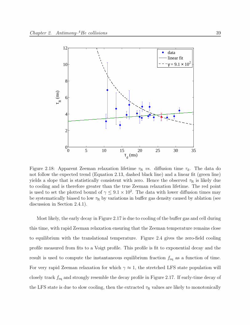
Chapter 2. Antimony–4He collisions 39
0 5 10 15 20 25 30 350
2
4
6
8
10
12
τd (ms)
τ R (
ms)
datalinear fit
γ = 9.1 × 10²
Figure 2.18: Apparent Zeeman relaxation lifetime τR vs. diffusion time τd. The data donot follow the expected trend (Equation 2.13, dashed black line) and a linear fit (green line)yields a slope that is statistically consistent with zero. Hence the observed τR is likely dueto cooling and is therefore greater than the true Zeeman relaxation lifetime. The red pointis used to set the plotted bound of γ ≤ 9.1 × 10². The data with lower diffusion times maybe systematically biased to low τR by variations in buffer gas density caused by ablation (seediscussion in Section 2.4.1).
Most likely, the early decay in Figure 2.17 is due to cooling of the buffer gas and cell during
this time, with rapid Zeeman relaxation ensuring that the Zeeman temperature remains close
to equilibrium with the translational temperature. Figure 2.4 gives the zero-field cooling
profile measured from fits to a Voigt profile. This profile is fit to exponential decay and the
result is used to compute the instantaneous equilibrium fraction feq as a function of time.
For very rapid Zeeman relaxation for which γ ≈ 1, the stretched LFS state population will
closely track feq and strongly resemble the decay profile in Figure 2.17. If early-time decay of
the LFS state is due to slow cooling, then the extracted τR values are likely to monotonically
Chapter 2. Antimony–4He collisions 40
increase with τd at higher buffer gas densities. This behavior is due to slower heat diffusion
in the buffer gas, which increases the cooling time constant. Such a trend is suggested in
Figure 2.18, although it is not statistically significant.
Without complete knowledge of the temporal and spatial cooling profile it is not possible
to extract the Zeeman relaxation rate from the observed decay of the stretched LFS state.
However, the observation of equilibrated Zeeman and translational temperatures allows for
the establishment of an upper bound for γ. To establish this bound, data are selected
from the B = 0.86 T experimental run. At this field, the thermal equilibrium fraction in
the stretched LFS state is minimal, but detectable, which aids in suppression of systematic
errors.
For the data taken at low buffer gas densities, the helium desorbed from the walls by
the ablation pulse may significantly increase the buffer gas density for a short period of
time before being re-adsorbed after the cell walls cool. In such a situation, diffusion times
measured after this period will underestimate the density during the time that Zeeman
relaxation was occurring. This would introduce a systematic bias to lower Zeeman lifetimes,
and hence lower values of γ. To avoid this, spectra in which τd ≈ 25 ms (where the signal
and lifetime are large enough for careful study) are analyzed and the decay after t = 5 ms is
found to be consistent with a constant helium density. Hence only data for which τd > 25 ms
are considered. The strictest bound is found by using the data point highlighted in red in
Figure 2.18 and inverting Equation 2.13 to yield
γ ≤ 3π
32
(
v2GτdτR)
γ ≤ 9.1 × 10². (2.15)
The bound of γ is the most accurate experimental quantity for comparison to theoretical
calculations, since Equation 2.15 is not sensitive to precise knowledge of the buffer gas
density.
Chapter 2. Antimony–4He collisions 41
2.4.2 Theory of spin-orbit induced Zeeman relaxation
The Hamiltonian for the system of antimony or other pnictogen atoms interacting with
helium is
H = − ~2
2µR
∂2
∂R2R +
ℓ2
2µR2+ Vnr + VSO + VB, (2.16)
where µ is the reduced mass, R is the interatomic distance, ℓ is the rotational angular
momentum of the nuclei, and Vnr, VSO and VB are operators describing the nonrelativistic
electrostatic interaction, spin-orbit interaction, and interaction with the magnetic field, re-
spectively. The operator VSO comes about through the relativistic motional magnetic field
generated by electrons moving through the electric field generated by the nucleus. For a
single electron around a nuclear charge Z,
VSO = −µ ·[ v
c2× Enuc
]
= −µ ·[
v
c2×(
Z
4πǫ0r2r
)]
, (2.17)
from which it follows that VSO ∝ Z/c2r3. Using 〈r〉 ∝ a0/Z, where a0 is the Bohr radius, the
approximation can be made that 〈VSO〉 ∝ Z4. Consideration of additional electrons will not
significantly alter this result, both because it is dominated by small-orbit contributions that
are not screened by other electrons, and also because the contributions from the interaction
of µ with the orbits of other electrons will lack the Z-enhancement and in general add
destructively. This strong Z-dependence of VSO leads to a wide variation in spin-orbit induced
anisotropy as one looks from top to bottom in the periodic table.
The spin-orbit interaction couples the 4S3/2 ground state to excited anisotropic 2P and
2D states, through which inelastic transitions occur during collisions with helium. To lowest
nonzero order, the anisotropy is given by [57],
∆E(R) =2
3
B2SP
E2P
[VP Π(R) − VP Σ(R)] , (2.18)
where BSP is the spin-orbit coupling matrix element between the 4S and 2P states, EP is
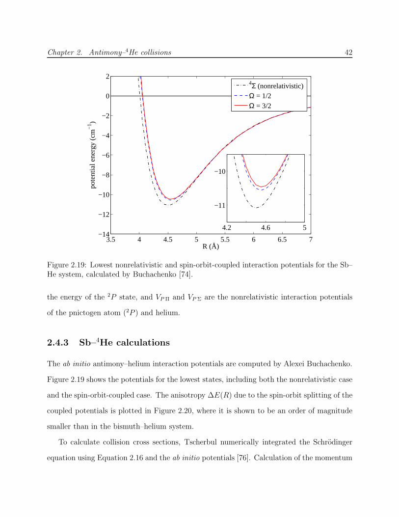
Chapter 2. Antimony–4He collisions 42
3.5 4 4.5 5 5.5 6 6.5 7−14
−12
−10
−8
−6
−4
−2
0
2
R (Å)
pote
ntia
l ene
rgy
(cm−
1 )
4Σ (nonrelativistic)Ω = 1/2Ω = 3/2
4.2 4.6 5
−11
−10
Figure 2.19: Lowest nonrelativistic and spin-orbit-coupled interaction potentials for the Sb–He system, calculated by Buchachenko [74].
the energy of the 2P state, and VP Π and VP Σ are the nonrelativistic interaction potentials
of the pnictogen atom (2P ) and helium.
2.4.3 Sb–4He calculations
The ab initio antimony–helium interaction potentials are computed by Alexei Buchachenko.
Figure 2.19 shows the potentials for the lowest states, including both the nonrelativistic case
and the spin-orbit-coupled case. The anisotropy ∆E(R) due to the spin-orbit splitting of the
coupled potentials is plotted in Figure 2.20, where it is shown to be an order of magnitude
smaller than in the bismuth–helium system.
To calculate collision cross sections, Tscherbul numerically integrated the Schrodinger
equation using Equation 2.16 and the ab initio potentials [76]. Calculation of the momentum
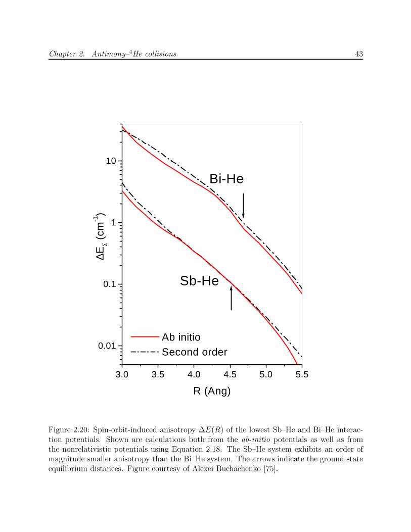
Chapter 2. Antimony–4He collisions 43
3.0 3.5 4.0 4.5 5.0 5.5
0.01
0.1
1
10
Bi-He
Sb-He
Ab initio Second order
∆EΣ
(cm
-1)
R (Ang)
Figure 2.20: Spin-orbit-induced anisotropy ∆E(R) of the lowest Sb–He and Bi–He interac-tion potentials. Shown are calculations both from the ab-initio potentials as well as fromthe nonrelativistic potentials using Equation 2.18. The Sb–He system exhibits an order ofmagnitude smaller anisotropy than the Bi–He system. The arrows indicate the ground stateequilibrium distances. Figure courtesy of Alexei Buchachenko [75].
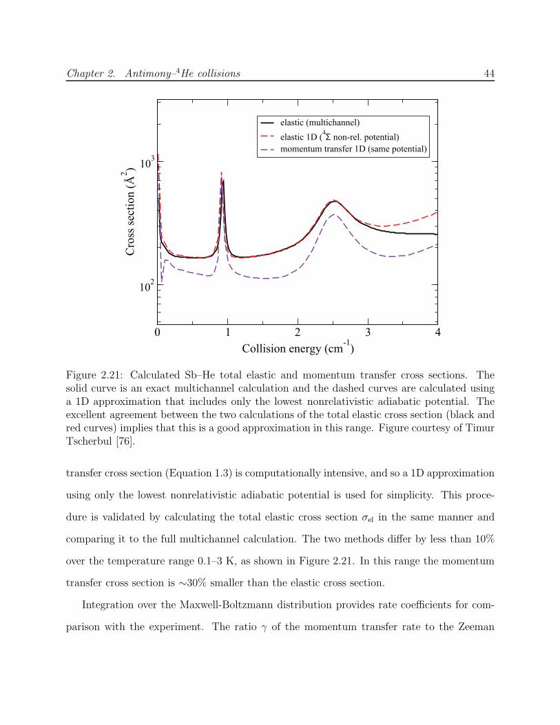
Chapter 2. Antimony–4He collisions 44
0 1 2 3 4
Collision energy (cm-1
)
102
103
Cro
ss s
ecti
on (
Å2 )
elastic (multichannel)
elastic 1D (4Σ non-rel. potential)
momentum transfer 1D (same potential)
Figure 2.21: Calculated Sb–He total elastic and momentum transfer cross sections. Thesolid curve is an exact multichannel calculation and the dashed curves are calculated usinga 1D approximation that includes only the lowest nonrelativistic adiabatic potential. Theexcellent agreement between the two calculations of the total elastic cross section (black andred curves) implies that this is a good approximation in this range. Figure courtesy of TimurTscherbul [76].
transfer cross section (Equation 1.3) is computationally intensive, and so a 1D approximation
using only the lowest nonrelativistic adiabatic potential is used for simplicity. This proce-
dure is validated by calculating the total elastic cross section σel in the same manner and
comparing it to the full multichannel calculation. The two methods differ by less than 10%
over the temperature range 0.1–3 K, as shown in Figure 2.21. In this range the momentum
transfer cross section is ∼30% smaller than the elastic cross section.
Integration over the Maxwell-Boltzmann distribution provides rate coefficients for com-
parison with the experiment. The ratio γ of the momentum transfer rate to the Zeeman
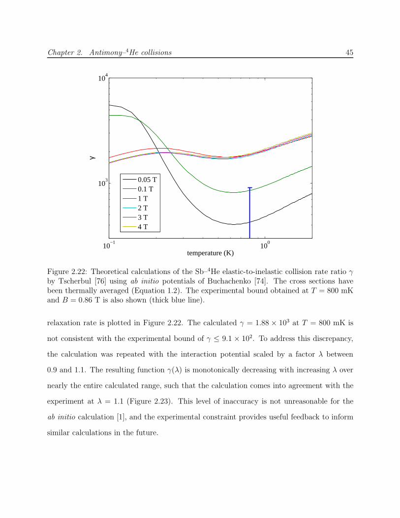
Chapter 2. Antimony–4He collisions 45
10−1
100
103
104
temperature (K)
γ
0.05 T0.1 T1 T2 T3 T4 T
Figure 2.22: Theoretical calculations of the Sb–4He elastic-to-inelastic collision rate ratio γby Tscherbul [76] using ab initio potentials of Buchachenko [74]. The cross sections havebeen thermally averaged (Equation 1.2). The experimental bound obtained at T = 800 mKand B = 0.86 T is also shown (thick blue line).
relaxation rate is plotted in Figure 2.22. The calculated γ = 1.88 × 10³ at T = 800 mK is
not consistent with the experimental bound of γ ≤ 9.1 × 10². To address this discrepancy,
the calculation was repeated with the interaction potential scaled by a factor λ between
0.9 and 1.1. The resulting function γ(λ) is monotonically decreasing with increasing λ over
nearly the entire calculated range, such that the calculation comes into agreement with the
experiment at λ = 1.1 (Figure 2.23). This level of inaccuracy is not unreasonable for the
ab initio calculation [1], and the experimental constraint provides useful feedback to inform
similar calculations in the future.

Chapter 2. Antimony–4He collisions 46
0.9 0.95 1 1.05 1.10
1
2
3
4
5
6
potential scaling factor λ
γ (×
103 )
Sb–4He, B = 0.86 T
Sb–4He, B = 1.50 T
Sb–3He, B = 0.86 Texperimental upper bound
Figure 2.23: Calculations by Tscherbul [76] of the elastic-to-inelastic collision rate ratio γafter scaling the interaction potentials [74] by λ. The blue circles are those corresponding tothe experimental parameters. The experimental bound (dashed line) is in agreement withtheory for λ = 1.1. Also shown (green triangles) are calculated results for the Sb–3He system,for which the inelasticity is reduced due the absence of a collision resonance near 1 K.
2.4.4 Summary and future outlook
The results presented here for Zeeman relaxation of antimony in collisions with helium
provide a valuable window into the onset of spin-orbit induced anisotropy in pnictogen
atoms. The order of magnitude smaller anisotropy in the antimony–helium system compared
to bismuth–helium leads to a similar reduction in the calculated Zeeman relaxation rate.
However, inelastic transitions are still too rapid for the experiment to measure directly,
and γ is far below the value of ∼104 necessary for buffer-gas loading of a magnetic trap.
As a result, buffer-gas loaded antimony does not present an attractive path to ultracold
temperatures, nor is it expected to be a practical alternative to nitrogen as a sympathetic

Chapter 2. Antimony–4He collisions 47
101
102
10−6
10−4
10−2
100
102
nuclear charge Z
tens
or p
olar
izab
ility
|α 2J | (at
omic
uni
ts)
N
P
As
Sb
Biab initio calculation
Z4 scaling
Figure 2.24: Calculated tensor polarizabilities of pnictogen atoms, from [77], along with Z4
scaling predicted for spin-orbit coupling (see Equation 2.17).
coolant for molecules.
A natural extension of this work is to look further up the pnictogen column to arsenic
and phosphorus. The required laser wavelengths are shorter than 200 nm, which is a signif-
icant complication to the experiments. There has, however, recently been theoretical effort
by Buchachenko to build a qualitative understanding of how spin-orbit effects are manifest
from nitrogen to bismuth [77]. Figure 2.24 shows ab initio calculations for all pnictogen
atoms of the anisotropic tensor polarizability αJ2 , one of the simplest expressions of atomic
anisotropy. The calculated values of |αJ2 | closely follow the Z4 spin-orbit scaling implied by
Equation 2.17. Buchachenko specifically cautions against drawing quantitative conclusions
from these values, especially for the high-Z atoms, due to convergence issues with the cal-
culations; however, the trend clearly aligns with the expectation of anisotropy induced by
Chapter 2. Antimony–4He collisions 48
spin-orbit coupling. In addition, the full scattering calculations by Tscherbul et al. [57, 76]
give values of γ for antimony–helium and bismuth–helium that are separated by about an
order of magnitude, similar to the corresponding values of |αJ2 |.
If we extend the comparison, the calculation in Figure 2.24 suggests that arsenic will
relax significantly more slowly than antimony in collisions with helium, but still quickly
enough to make the species marginal for trapping and further cooling. It would then seem
that nitrogen is the best candidate for further efforts toward evaporative cooling and toward
sympathetic cooling of molecules; a conclusion that is based both on its excellent collisional
properties and on the lack of an alternative pnictogen that preserves these properties while
offering a more practical optical transition.
Chapter 3
Aluminum–3He collisions
3.1 Properties and prospects of 2P atoms
The previous chapter described a mechanism for Zeeman relaxation in the pnictogens that
arises from perturbation of the spherical symmetry of the ground S-states by nonspherical
excited states. In that case, the larger the contribution of L 6= 0 states, the larger the
probability of an inelastic transition. Yet while electronic orbital angular momentum can
introduce the anisotropy that drives these transitions, it is not necessarily the case that non-S
state atoms will have rapid inelastic collisions. The next two chapters focus on L 6= 0 atoms
for which inelastic collisions with helium are largely suppressed, although the mechanisms
at play in the two cases are quite distinct.
This chapter describes experiments measuring inelastic collision rates in the aluminum–
helium system. The ground 2P1/2 state of aluminum and other Group 13 atoms is, perhaps
counterintuitively, spherical (see Section 3.2). As a result, Zeeman relaxation is suppressed.
Like S-state atoms, inelastic transitions at low temperature occur through collisional mixing
49
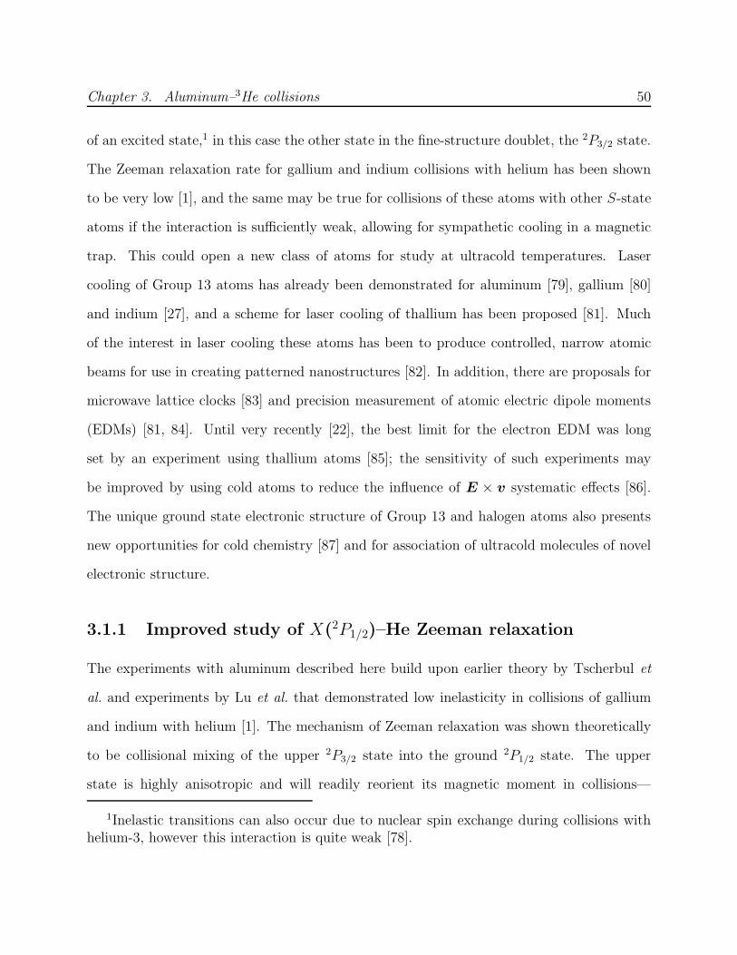
Chapter 3. Aluminum–3He collisions 50
of an excited state,1 in this case the other state in the fine-structure doublet, the 2P3/2 state.
The Zeeman relaxation rate for gallium and indium collisions with helium has been shown
to be very low [1], and the same may be true for collisions of these atoms with other S-state
atoms if the interaction is sufficiently weak, allowing for sympathetic cooling in a magnetic
trap. This could open a new class of atoms for study at ultracold temperatures. Laser
cooling of Group 13 atoms has already been demonstrated for aluminum [79], gallium [80]
and indium [27], and a scheme for laser cooling of thallium has been proposed [81]. Much
of the interest in laser cooling these atoms has been to produce controlled, narrow atomic
beams for use in creating patterned nanostructures [82]. In addition, there are proposals for
microwave lattice clocks [83] and precision measurement of atomic electric dipole moments
(EDMs) [81, 84]. Until very recently [22], the best limit for the electron EDM was long
set by an experiment using thallium atoms [85]; the sensitivity of such experiments may
be improved by using cold atoms to reduce the influence of E × v systematic effects [86].
The unique ground state electronic structure of Group 13 and halogen atoms also presents
new opportunities for cold chemistry [87] and for association of ultracold molecules of novel
electronic structure.
3.1.1 Improved study of X(2P1/2)–He Zeeman relaxation
The experiments with aluminum described here build upon earlier theory by Tscherbul et
al. and experiments by Lu et al. that demonstrated low inelasticity in collisions of gallium
and indium with helium [1]. The mechanism of Zeeman relaxation was shown theoretically
to be collisional mixing of the upper 2P3/2 state into the ground 2P1/2 state. The upper
state is highly anisotropic and will readily reorient its magnetic moment in collisions—
1Inelastic transitions can also occur due to nuclear spin exchange during collisions withhelium-3, however this interaction is quite weak [78].
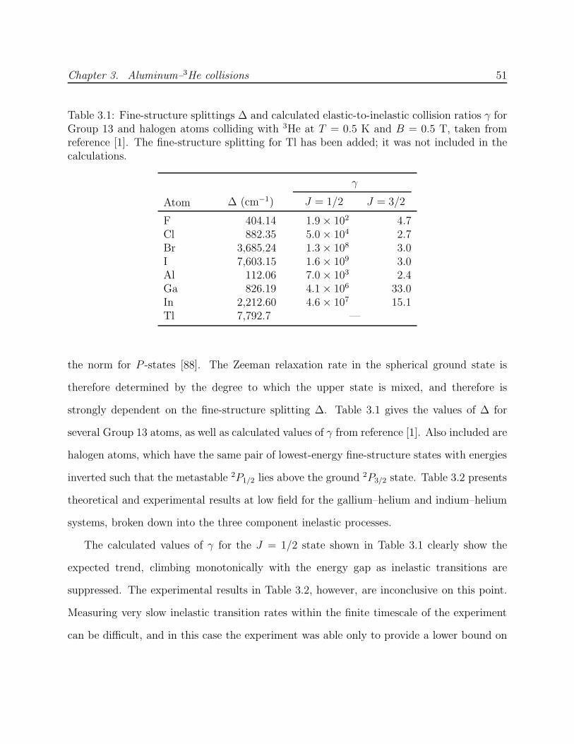
Chapter 3. Aluminum–3He collisions 51
Table 3.1: Fine-structure splittings ∆ and calculated elastic-to-inelastic collision ratios γ forGroup 13 and halogen atoms colliding with 3He at T = 0.5 K and B = 0.5 T, taken fromreference [1]. The fine-structure splitting for Tl has been added; it was not included in thecalculations.
γ
Atom ∆ (cm−1) J = 1/2 J = 3/2
F 404.14 1.9 × 10² 4.7Cl 882.35 5.0 × 10⁴ 2.7Br 3,685.24 1.3 × 10⁸ 3.0I 7,603.15 1.6 × 10⁹ 3.0Al 112.06 7.0 × 10³ 2.4Ga 826.19 4.1 × 10⁶ 33.0In 2,212.60 4.6 × 10⁷ 15.1Tl 7,792.7 —
the norm for P -states [88]. The Zeeman relaxation rate in the spherical ground state is
therefore determined by the degree to which the upper state is mixed, and therefore is
strongly dependent on the fine-structure splitting ∆. Table 3.1 gives the values of ∆ for
several Group 13 atoms, as well as calculated values of γ from reference [1]. Also included are
halogen atoms, which have the same pair of lowest-energy fine-structure states with energies
inverted such that the metastable 2P1/2 lies above the ground 2P3/2 state. Table 3.2 presents
theoretical and experimental results at low field for the gallium–helium and indium–helium
systems, broken down into the three component inelastic processes.
The calculated values of γ for the J = 1/2 state shown in Table 3.1 clearly show the
expected trend, climbing monotonically with the energy gap as inelastic transitions are
suppressed. The experimental results in Table 3.2, however, are inconclusive on this point.
Measuring very slow inelastic transition rates within the finite timescale of the experiment
can be difficult, and in this case the experiment was able only to provide a lower bound on
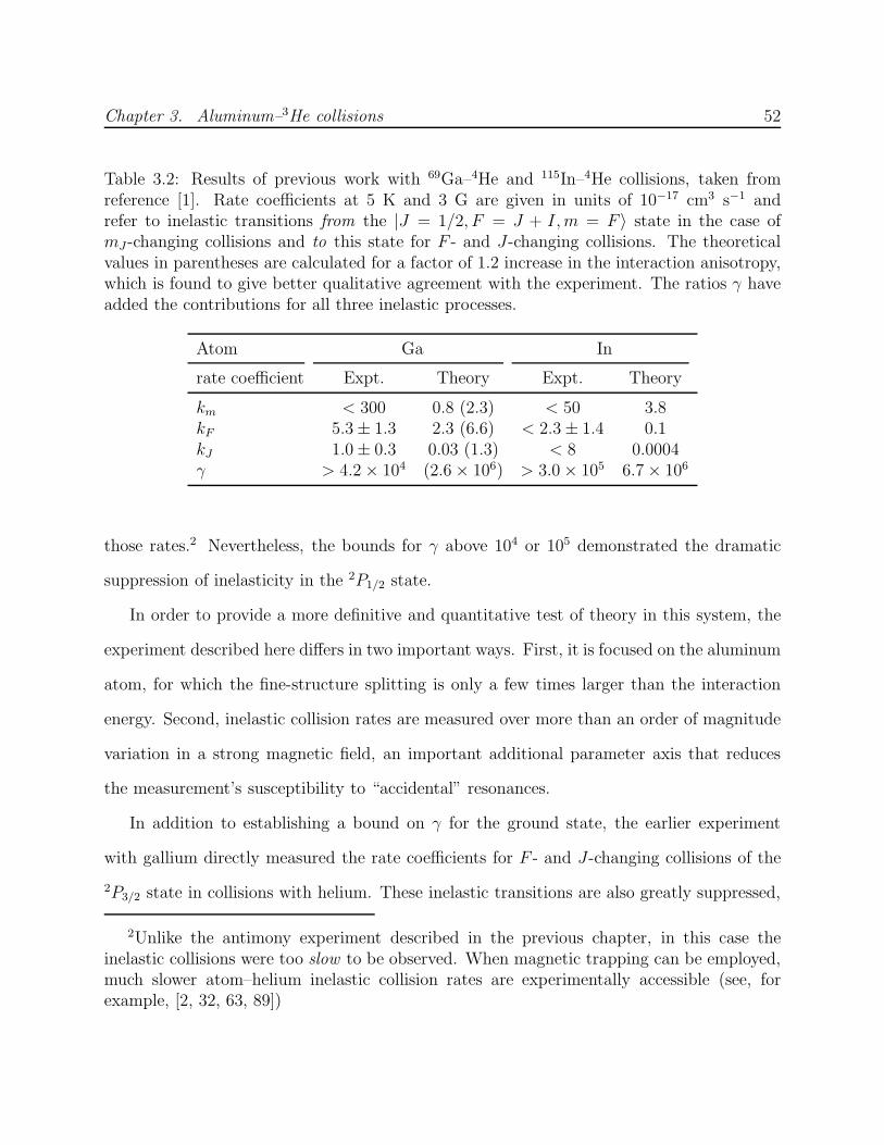
Chapter 3. Aluminum–3He collisions 52
Table 3.2: Results of previous work with 69Ga–4He and 115In–4He collisions, taken fromreference [1]. Rate coefficients at 5 K and 3 G are given in units of 10−17 cm3 s−1 andrefer to inelastic transitions from the |J = 1/2, F = J + I,m = F 〉 state in the case ofmJ -changing collisions and to this state for F - and J-changing collisions. The theoreticalvalues in parentheses are calculated for a factor of 1.2 increase in the interaction anisotropy,which is found to give better qualitative agreement with the experiment. The ratios γ haveadded the contributions for all three inelastic processes.
Atom Ga In
rate coefficient Expt. Theory Expt. Theory
km < 300 0.8 (2.3) < 50 3.8kF 5.3 ± 1.3 2.3 (6.6) < 2.3 ± 1.4 0.1kJ 1.0 ± 0.3 0.03 (1.3) < 8 0.0004γ > 4.2 × 10⁴ (2.6 × 10⁶) > 3.0 × 10⁵ 6.7 × 10⁶
those rates.2 Nevertheless, the bounds for γ above 104 or 105 demonstrated the dramatic
suppression of inelasticity in the 2P1/2 state.
In order to provide a more definitive and quantitative test of theory in this system, the
experiment described here differs in two important ways. First, it is focused on the aluminum
atom, for which the fine-structure splitting is only a few times larger than the interaction
energy. Second, inelastic collision rates are measured over more than an order of magnitude
variation in a strong magnetic field, an important additional parameter axis that reduces
the measurement’s susceptibility to “accidental” resonances.
In addition to establishing a bound on γ for the ground state, the earlier experiment
with gallium directly measured the rate coefficients for F - and J-changing collisions of the
2P3/2 state in collisions with helium. These inelastic transitions are also greatly suppressed,
2Unlike the antimony experiment described in the previous chapter, in this case theinelastic collisions were too slow to be observed. When magnetic trapping can be employed,much slower atom–helium inelastic collision rates are experimentally accessible (see, forexample, [2, 32, 63, 89])
Chapter 3. Aluminum–3He collisions 53
despite the absence of an energy barrier. This is in contrast to rapid fine-structure changing
collision rates (spin-orbit relaxation) in other systems. For example, fine-structure-changing
collisions between ultracold metastable 3P2 ytterbium atoms were observed to be very rapid
[90]; theoretical calculations for 3P0 and 3P1 oxygen atoms colliding with helium at both zero
magnetic field and B = 1 T showed the same below ∼1 K [88, 91].3 The aluminum–helium
system bridges an important gap between these extremes due to its intermediate balance
between fine-structure splitting and interaction energy. Hence it is an important test bed to
explore spin-orbit relaxation in a nontrivial regime.
3.2 Theory of Zeeman relaxation in 2P1/2 atoms
Theoretical calculations of Group 13 and halogen atom collisions with helium were performed
by Tscherbul et al. [1] by expanding the quantum-scattering formalism developed by Krems
and Dalgarno [91] to 2P atoms with nonzero nuclear spin. Their procedure is summarized
here along with new and more detailed calculations for the aluminum–helium system.
The Hamiltonian of the colliding aluminum(2P )–helium complex is written as a modified
version of the parameterization in Equation 2.16:
H = − ~2
2µR
∂2
∂R2R +
ℓ2
2µR2+ V (R, r) + HAl, (3.1)
where again µ is the reduced mass, R is the interatomic distance, r is the electronic coordi-
nates, and ℓ is the rotational angular momentum of the nuclei; the operator V (R, r) is the
aluminum–helium interaction potential and the operator
HAl = ASO L · S + µBB(
Lz + 2Sz
)
+ HI , (3.2)
3Experimental and theoretical work with titanium–helium collisions also observed sup-pression of inelasticity [92, 93], and attributed this to the submerged-shell nature of titanium(see Section 4.1).
Chapter 3. Aluminum–3He collisions 54
is the Hamiltonian of the isolated aluminum atom in a magnetic field B. ASO = 2∆/3 is the
spin-orbit constant of the aluminum atom, Lz and Sz are the projections of the electronic
orbital angular momentum and spin operators L and S onto the field axis, and HI is the
hyperfine Hamiltonian.
The fully uncoupled basis |JmJ〉|ImI〉|ℓmℓ〉 is used, where mJ , mI and mℓ are the projec-
tions of J , I and ℓ onto the field axis. Following [91], the matrix elements of the interaction
potential V (R, r) are
〈JmJ |〈ImI |〈ℓmℓ|V (R, r)|J ′m′J〉|I ′m′
I〉|ℓ′m′ℓ〉
= δmIm′
I(−)S+J+J ′−mJ−m′
ℓ
×[
(2L+ 1)2(2J + 1)(2J ′ + 1)(2ℓ+ 1)(2ℓ′ + 1)]1/2
×∑
λ=0,2
Vλ(R)
L J S
J ′ L λ
J λ J ′
−mJ mJ −m′J m′
J
(3.3)
×
ℓ λ ℓ
−mℓ mℓ −m′ℓ m′
ℓ
L λ L
0 0 0
ℓ λ ℓ′
0 0 0
, (3.4)
where the symbols in parenthesis and curly braces are 3-j and 6-j symbols, respectively. V0
and V2 are the isotropic and anisotropic parts of the interaction potential, respectively.
Highly accurate ab initio aluminum–helium interaction potentials of Σ- and Π-symmetry
are obtained from [94] and fitted to analytic functions with proper long-range behavior.
Expanding the wave function in the uncoupled basis given above and inserting it into the
Schrodinger equation with the Hamiltonian in Equation 2.16 gives a system of close-coupled
differential equations. These equations are solved to yield the probabilities for J- and mJ -
changing transitions during the collision. In addition, the momentum transfer cross section is
calculated from a 1D approximation using the lowest spin-orbit-coupled potential V1/2,1/2(R),
similar to the method described in Section 2.4.3. The calculated values of the collision rate
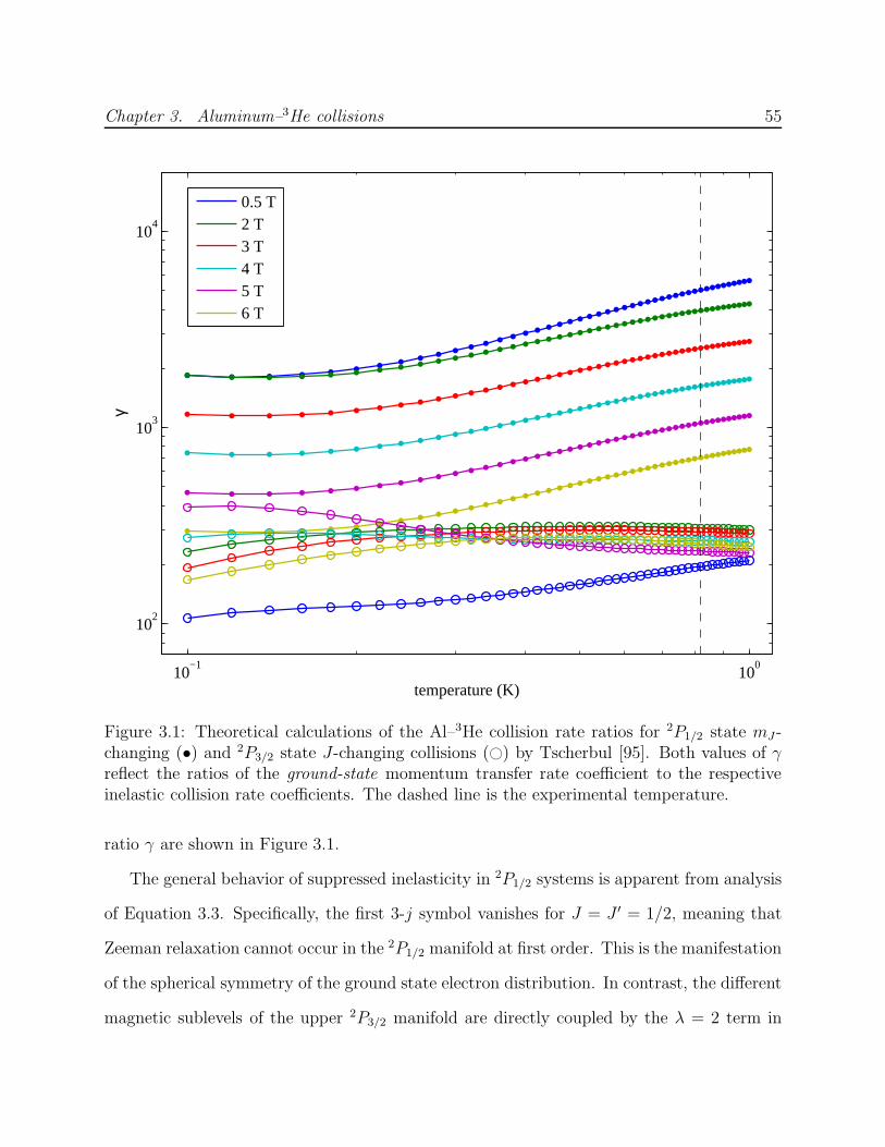
Chapter 3. Aluminum–3He collisions 55
10−1
100
102
103
104
temperature (K)
γ
0.5 T2 T3 T4 T5 T6 T
Figure 3.1: Theoretical calculations of the Al–3He collision rate ratios for 2P1/2 state mJ -changing (•) and 2P3/2 state J-changing collisions (#) by Tscherbul [95]. Both values of γreflect the ratios of the ground-state momentum transfer rate coefficient to the respectiveinelastic collision rate coefficients. The dashed line is the experimental temperature.
ratio γ are shown in Figure 3.1.
The general behavior of suppressed inelasticity in 2P1/2 systems is apparent from analysis
of Equation 3.3. Specifically, the first 3-j symbol vanishes for J = J ′ = 1/2, meaning that
Zeeman relaxation cannot occur in the 2P1/2 manifold at first order. This is the manifestation
of the spherical symmetry of the ground state electron distribution. In contrast, the different
magnetic sublevels of the upper 2P3/2 manifold are directly coupled by the λ = 2 term in
Chapter 3. Aluminum–3He collisions 56
Equation 3.3, hence Zeeman relaxation proceeds rapidly in this state. As such, Zeeman
relaxation of the ground state proceeds through second-order coupling to the 2P3/2 state, at
a rate suppressed by the state splitting.
The spherical symmetry of the 2P1/2 state can be shown directly by expressing the elec-
tronic wave function |ψ〉 = |J = 1/2, mJ = 1/2〉 in the |L,mL〉|S,mS〉 basis:
|ψ〉 =
√
2
3|1, 1〉|1/2,−1/2〉 −
√
1
3|1, 0〉|1/2,+1/2〉 (3.5)
=
√
1
4π
[
sin(θ) eiφ | ↓ 〉 − cos(θ)| ↑ 〉]
, (3.6)
where the second line makes use of the spherical harmonics Y 11 (θ, φ) and Y 0
1 (θ, φ) and defines
| ↑ 〉 and | ↓ 〉 to be the mS = ±1/2 electronic spin wave functions. For any function
f(θ, φ) =∑
ℓmCℓm Ymℓ (θ, φ), the expectation value is equal to
〈ψ|f |ψ〉 =1
4π
∫
dΩ f(θ, φ)[
sin2(θ) + cos2(θ)]
=1
4π
∫
dΩ∑
ℓm
Cℓm Ymℓ (θ, φ)
= C00, (3.7)
i.e., the nonspherical contribution is zero. The nature of the 2P1/2 state demonstrates the
incompleteness of the argument that L 6= 0 atoms are in general not spherical; spin-orbit
coupling can produce spherical P -states. As was demonstrated first in [1] and now further
investigated in the case of aluminum, these states are correspondingly protected by the
spin-orbit splitting from Zeeman relaxation in collisions with helium.
3.3 Optical pumping
Inelastic aluminum–helium collisions are measured by observing the response of the colliding
system to perturbation by optical pumping. Both J-changing andmJ -changing collision rates
Chapter 3. Aluminum–3He collisions 57
can be simultaneously extracted using a clean method that employs a single pump/probe
laser. This method has advantages compared to observing relaxation to equilibrium after
ablation (the method used for antimony in Chapter 2), especially for low-γ systems. First, the
measurement occurs at times well after ablation, when the buffer gas density and temperature
are stable. Second, the experiment is not critically dependent on a large Boltzmann factor,
and so the experimental parameters of magnetic field and temperature are decoupled. For
the aluminum experiment described here, this allows for measurement of inelastic collisions
over a range of magnetic fields at a single temperature.
Briefly, the experimental procedure consists of optical pumping of one ground state mag-
netic sublevel while observing the pump laser absorption to determine the rate of collisional
refilling of the pumped sublevel. The energy level diagram with relevant state-changing pro-
cesses is shown in Figure 3.2. The laser is tuned to the 2P1/2 → 2S1/2 transition at 394.5 nm.
One magnetic sublevel of the ground state 2P1/2 manifold is addressed to pump the system
out of equilibrium. Simultaneously, the sublevel population is probed by monitoring the
fraction of pump light absorbed. Inelastic collisions push the state distribution back towards
equilibrium, competing with optical pumping to produce a steady-state population. This
population is observed as a steady-state OD which varies with pump laser power. The in-
elastic collision rates are revealed by probing this steady-state as a function of pump power
to determine the “stiffness” of the system. Through measurements of this response over
a range of helium densities, and by making separate measurements addressing each mag-
netic sublevel, the effects of J-changing and mJ -changing collisions can be separated and
systematic errors can be controlled.
The finite spatial width of the pump laser beam introduces another process to compete
with optical pumping: diffusion of atoms into and out of the laser beam. At low helium
density, the mean free path is long and atoms pumped to other states will rapidly diffuse
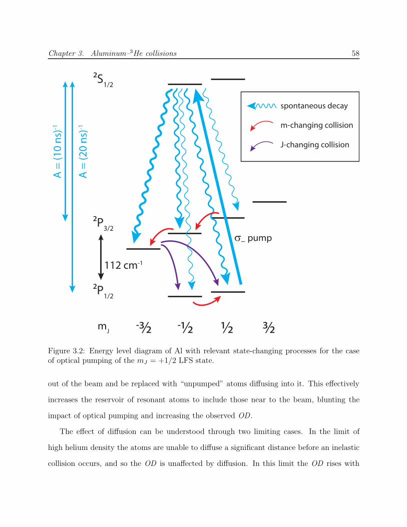
Chapter 3. Aluminum–3He collisions 58
2P3/2
2P1/2
2S1/2
mJ -3⁄2 -½ ½ 3⁄2
112 cm-1
A =
(20
ns)
-1
A =
(10
ns)
-1
spontaneous decay
m-changing collision
J-changing collision
σ– pump
Figure 3.2: Energy level diagram of Al with relevant state-changing processes for the caseof optical pumping of the mJ = +1/2 LFS state.
out of the beam and be replaced with “unpumped” atoms diffusing into it. This effectively
increases the reservoir of resonant atoms to include those near to the beam, blunting the
impact of optical pumping and increasing the observed OD .
The effect of diffusion can be understood through two limiting cases. In the limit of
high helium density the atoms are unable to diffuse a significant distance before an inelastic
collision occurs, and so the OD is unaffected by diffusion. In this limit the OD rises with

Chapter 3. Aluminum–3He collisions 59
increasing helium density as collisions become more rapid. At the other extreme, of low
density, inelastic collisions are rare and the OD is determined by the number of atoms that
can diffuse into the beam to replenish those that are pumped. In this limit the OD rises with
decreasing helium density, as the diffusion becomes more rapid and a larger volume of atoms
participate in the competition between diffusion and optical pumping. The actual behavior
in this limit is somewhat more subtle than this simple description, and will be addressed
more completely in Section 3.3.2.
Between these two limits, which are hereafter referred to as the relaxation regime and the
diffusive regime, respectively, we expect to find a minimum in OD as the helium density is
varied. Since the two regimes behave in fundamentally different ways with respect to many
experimental parameters, this minimum provides a sensitive diagnostic tool.
3.3.1 Quantitative model
As shown in Figure 3.2, optical pumping to the 2S1/2 state results in spontaneous decay
to a number of sublevels of both 2P fine-structure states. The majority (66% [96]) decay
to the upper state, from which they only reach the lower state via J-changing collisions
with helium. The optically pumped 2P1/2 sublevel is replenished by these collisions, as
well as by mJ -changing collisions from the other 2P1/2 sublevel. Atoms in 2P3/2 sublevels
will also undergo mJ -changing transitions; due to the large anisotropy of this state, these
collisions will be very rapid (Table 3.1) compared to other timescales. We therefore assume
thermal equilibrium in the 2P3/2 state. Under this condition &88% of atoms occupy the
lowest mJ = −3/2 sublevel under all experimental conditions except those with the lowest
field (B = 0.5 T), for which the fraction is ≈50%. Possible systematic error due to this
simplification is discussed in Section 3.5.3.
A quantitative model is constructed to predict the state populations N+, N− and N3/2—
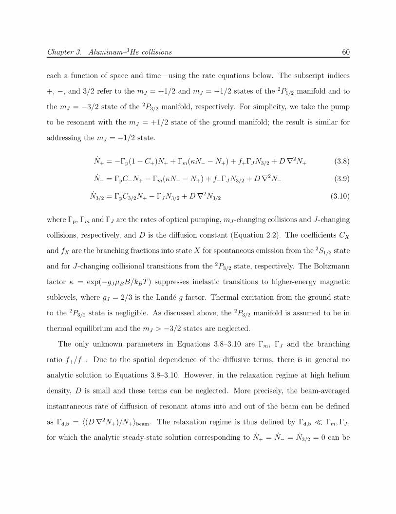
Chapter 3. Aluminum–3He collisions 60
each a function of space and time—using the rate equations below. The subscript indices
+, −, and 3/2 refer to the mJ = +1/2 and mJ = −1/2 states of the 2P1/2 manifold and to
the mJ = −3/2 state of the 2P3/2 manifold, respectively. For simplicity, we take the pump
to be resonant with the mJ = +1/2 state of the ground manifold; the result is similar for
addressing the mJ = −1/2 state.
N+ = −Γp(1 − C+)N+ + Γm(κN− −N+) + f+ΓJN3/2 +D∇2N+ (3.8)
N− = ΓpC−N+ − Γm(κN− −N+) + f−ΓJN3/2 +D∇2N− (3.9)
N3/2 = ΓpC3/2N+ − ΓJN3/2 +D∇2N3/2 (3.10)
where Γp, Γm and ΓJ are the rates of optical pumping, mJ -changing collisions and J-changing
collisions, respectively, and D is the diffusion constant (Equation 2.2). The coefficients CX
and fX are the branching fractions into state X for spontaneous emission from the 2S1/2 state
and for J-changing collisional transitions from the 2P3/2 state, respectively. The Boltzmann
factor κ = exp(−gJµBB/kBT ) suppresses inelastic transitions to higher-energy magnetic
sublevels, where gJ = 2/3 is the Lande g-factor. Thermal excitation from the ground state
to the 2P3/2 state is negligible. As discussed above, the 2P3/2 manifold is assumed to be in
thermal equilibrium and the mJ > −3/2 states are neglected.
The only unknown parameters in Equations 3.8–3.10 are Γm, ΓJ and the branching
ratio f+/f−. Due to the spatial dependence of the diffusive terms, there is in general no
analytic solution to Equations 3.8–3.10. However, in the relaxation regime at high helium
density, D is small and these terms can be neglected. More precisely, the beam-averaged
instantaneous rate of diffusion of resonant atoms into and out of the beam can be defined
as Γd,b = 〈(D∇2N+)/N+〉beam. The relaxation regime is thus defined by Γd,b ≪ Γm,ΓJ ,
for which the analytic steady-state solution corresponding to N+ = N− = N3/2 = 0 can be
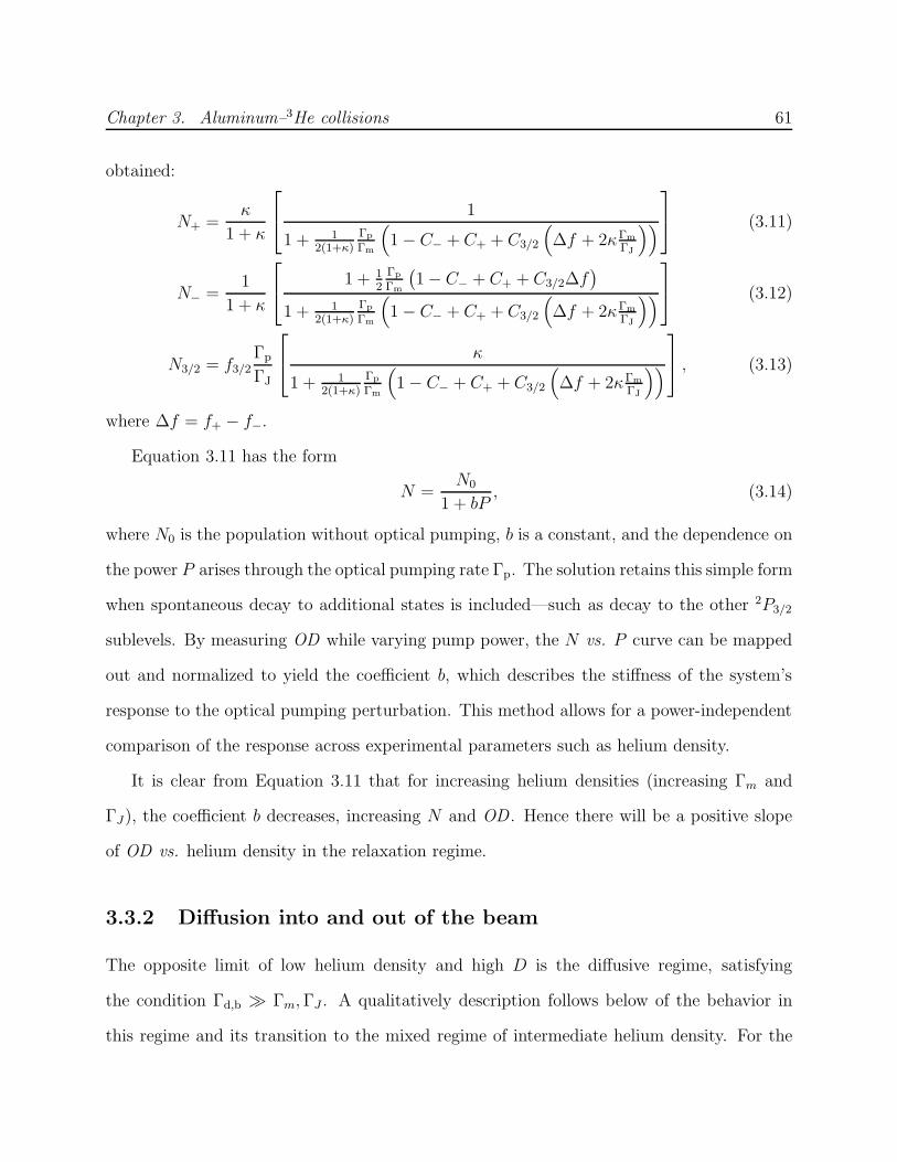
Chapter 3. Aluminum–3He collisions 61
obtained:
N+ =κ
1 + κ
1
1 + 12(1+κ)
Γp
Γm
(
1 − C− + C+ + C3/2
(
∆f + 2κΓm
ΓJ
))
(3.11)
N− =1
1 + κ
1 + 12Γp
Γm
(
1 − C− + C+ + C3/2∆f)
1 + 12(1+κ)
Γp
Γm
(
1 − C− + C+ + C3/2
(
∆f + 2κΓm
ΓJ
))
(3.12)
N3/2 = f3/2Γp
ΓJ
κ
1 + 12(1+κ)
Γp
Γm
(
1 − C− + C+ + C3/2
(
∆f + 2κΓm
ΓJ
))
, (3.13)
where ∆f = f+ − f−.
Equation 3.11 has the form
N =N0
1 + bP, (3.14)
where N0 is the population without optical pumping, b is a constant, and the dependence on
the power P arises through the optical pumping rate Γp. The solution retains this simple form
when spontaneous decay to additional states is included—such as decay to the other 2P3/2
sublevels. By measuring OD while varying pump power, the N vs. P curve can be mapped
out and normalized to yield the coefficient b, which describes the stiffness of the system’s
response to the optical pumping perturbation. This method allows for a power-independent
comparison of the response across experimental parameters such as helium density.
It is clear from Equation 3.11 that for increasing helium densities (increasing Γm and
ΓJ), the coefficient b decreases, increasing N and OD . Hence there will be a positive slope
of OD vs. helium density in the relaxation regime.
3.3.2 Diffusion into and out of the beam
The opposite limit of low helium density and high D is the diffusive regime, satisfying
the condition Γd,b ≫ Γm,ΓJ . A qualitatively description follows below of the behavior in
this regime and its transition to the mixed regime of intermediate helium density. For the
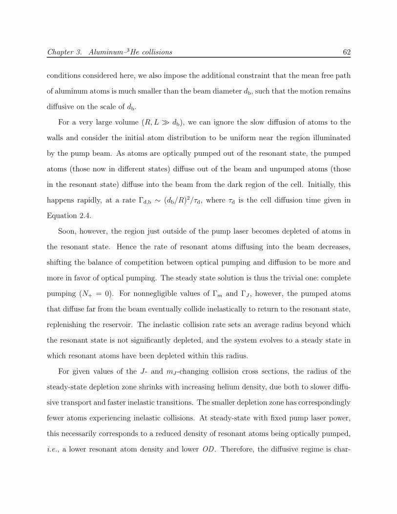
Chapter 3. Aluminum–3He collisions 62
conditions considered here, we also impose the additional constraint that the mean free path
of aluminum atoms is much smaller than the beam diameter db, such that the motion remains
diffusive on the scale of db.
For a very large volume (R,L ≫ db), we can ignore the slow diffusion of atoms to the
walls and consider the initial atom distribution to be uniform near the region illuminated
by the pump beam. As atoms are optically pumped out of the resonant state, the pumped
atoms (those now in different states) diffuse out of the beam and unpumped atoms (those
in the resonant state) diffuse into the beam from the dark region of the cell. Initially, this
happens rapidly, at a rate Γd,b ∼ (db/R)2/τd, where τd is the cell diffusion time given in
Equation 2.4.
Soon, however, the region just outside of the pump laser becomes depleted of atoms in
the resonant state. Hence the rate of resonant atoms diffusing into the beam decreases,
shifting the balance of competition between optical pumping and diffusion to be more and
more in favor of optical pumping. The steady state solution is thus the trivial one: complete
pumping (N+ = 0). For nonnegligible values of Γm and ΓJ , however, the pumped atoms
that diffuse far from the beam eventually collide inelastically to return to the resonant state,
replenishing the reservoir. The inelastic collision rate sets an average radius beyond which
the resonant state is not significantly depleted, and the system evolves to a steady state in
which resonant atoms have been depleted within this radius.
For given values of the J- and mJ -changing collision cross sections, the radius of the
steady-state depletion zone shrinks with increasing helium density, due both to slower diffu-
sive transport and faster inelastic transitions. The smaller depletion zone has correspondingly
fewer atoms experiencing inelastic collisions. At steady-state with fixed pump laser power,
this necessarily corresponds to a reduced density of resonant atoms being optically pumped,
i.e., a lower resonant atom density and lower OD . Therefore, the diffusive regime is char-
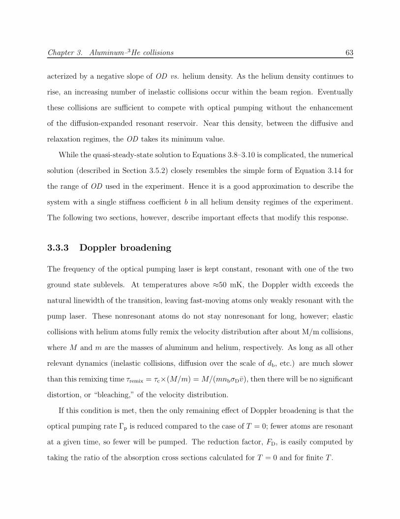
Chapter 3. Aluminum–3He collisions 63
acterized by a negative slope of OD vs. helium density. As the helium density continues to
rise, an increasing number of inelastic collisions occur within the beam region. Eventually
these collisions are sufficient to compete with optical pumping without the enhancement
of the diffusion-expanded resonant reservoir. Near this density, between the diffusive and
relaxation regimes, the OD takes its minimum value.
While the quasi-steady-state solution to Equations 3.8–3.10 is complicated, the numerical
solution (described in Section 3.5.2) closely resembles the simple form of Equation 3.14 for
the range of OD used in the experiment. Hence it is a good approximation to describe the
system with a single stiffness coefficient b in all helium density regimes of the experiment.
The following two sections, however, describe important effects that modify this response.
3.3.3 Doppler broadening
The frequency of the optical pumping laser is kept constant, resonant with one of the two
ground state sublevels. At temperatures above ≈50 mK, the Doppler width exceeds the
natural linewidth of the transition, leaving fast-moving atoms only weakly resonant with the
pump laser. These nonresonant atoms do not stay nonresonant for long, however; elastic
collisions with helium atoms fully remix the velocity distribution after about M/m collisions,
where M and m are the masses of aluminum and helium, respectively. As long as all other
relevant dynamics (inelastic collisions, diffusion over the scale of db, etc.) are much slower
than this remixing time τremix = τc×(M/m) = M/(mnbσDv), then there will be no significant
distortion, or “bleaching,” of the velocity distribution.
If this condition is met, then the only remaining effect of Doppler broadening is that the
optical pumping rate Γp is reduced compared to the case of T = 0; fewer atoms are resonant
at a given time, so fewer will be pumped. The reduction factor, FD, is easily computed by
taking the ratio of the absorption cross sections calculated for T = 0 and for finite T .
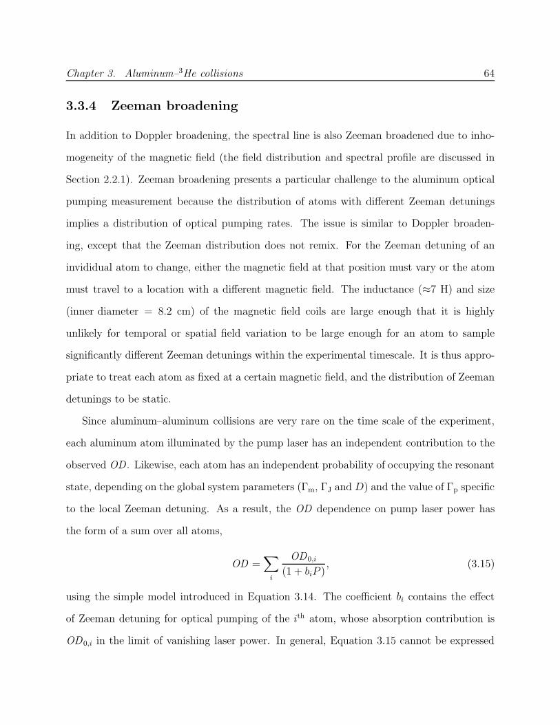
Chapter 3. Aluminum–3He collisions 64
3.3.4 Zeeman broadening
In addition to Doppler broadening, the spectral line is also Zeeman broadened due to inho-
mogeneity of the magnetic field (the field distribution and spectral profile are discussed in
Section 2.2.1). Zeeman broadening presents a particular challenge to the aluminum optical
pumping measurement because the distribution of atoms with different Zeeman detunings
implies a distribution of optical pumping rates. The issue is similar to Doppler broaden-
ing, except that the Zeeman distribution does not remix. For the Zeeman detuning of an
invididual atom to change, either the magnetic field at that position must vary or the atom
must travel to a location with a different magnetic field. The inductance (≈7 H) and size
(inner diameter = 8.2 cm) of the magnetic field coils are large enough that it is highly
unlikely for temporal or spatial field variation to be large enough for an atom to sample
significantly different Zeeman detunings within the experimental timescale. It is thus appro-
priate to treat each atom as fixed at a certain magnetic field, and the distribution of Zeeman
detunings to be static.
Since aluminum–aluminum collisions are very rare on the time scale of the experiment,
each aluminum atom illuminated by the pump laser has an independent contribution to the
observed OD . Likewise, each atom has an independent probability of occupying the resonant
state, depending on the global system parameters (Γm, ΓJ and D) and the value of Γp specific
to the local Zeeman detuning. As a result, the OD dependence on pump laser power has
the form of a sum over all atoms,
OD =∑
i
OD0,i
(1 + biP ), (3.15)
using the simple model introduced in Equation 3.14. The coefficient bi contains the effect
of Zeeman detuning for optical pumping of the ith atom, whose absorption contribution is
OD0,i in the limit of vanishing laser power. In general, Equation 3.15 cannot be expressed

Chapter 3. Aluminum–3He collisions 65
as a single term and the optical pumping effect cannot be simply characterized by a single
b coefficient.
3.4 Experimental procedure
3.4.1 Aluminum production
The same cell is used for the measurement of aluminum–helium inelastic collisions as was used
for the antimony experiment described in Chapter 2. Aluminum is produced by ablating an
aluminum nitride ceramic target into helium-3 buffer gas. Originally intended as a nitrogen
ablation source for NH production, aluminum nitride is likely not the ideal ablation precursor
for atomic aluminum. While the aluminum yield is excellent, since NH production using the
same material was also quite good (see Appendix A), we must assume that atomic nitrogen
is produced in similar or greater quantities. It is possible that aluminum–nitrogen collisions
could cause inelastic transitions that confuse analysis of the aluminum–helium system. For
an interspecies inelastic cross section of 10−14 cm2, such collisions would be likely to occur
within the aluminum diffusion lifetime at nitrogen densities above 1011 cm−3. However, even
with very high ablation yield of >1014 N atoms, such a density would exist only for a short
time before decaying due to diffusion. The aluminum measurement is performed only after
waiting multiple diffusion lifetimes, and so nitrogen–aluminum collisions are unlikely to play
a role.
To increase confidence that these collisions can be ignored, it would be ideal to directly
probe the nitrogen density via 207-nm two-photon absorption laser-induced fluorescence
(see Figure 2.6). Unfortunately, a UV-absorbing film accumulated on the outer surface of
the 77-K window between the antimony and aluminum experiments, precluding this direct
approach. Instead, the nitrogen density was indirectly probed by searching for a dependence

Chapter 3. Aluminum–3He collisions 66
on aluminum density in the system’s response to optical pumping. It is safe to assume
that atomic nitrogen will decay on a timescale not very different from that of aluminum in
the same cell, since momentum transfer cross sections for collisions of different atoms with
helium are generally quite similar [32, 71, 97]. Therefore, a significant change in aluminum
density will be accompanied by a similar change in nitrogen density. By observing no density
variation in the power dependence of OD , we can conclude that neither aluminum–nitrogen
nor aluminum–aluminum inelastic collisions affect the measurement.
3.4.2 Pump/probe laser system
Aluminum is detected by absorption spectroscopy on the 394.5-nm 2P1/2 → 2S1/2 transition
using the diode laser system outlined in Figure 3.3. Aluminum has a single isotope with
nuclear spin I = 5/2 and a simple optical spectrum both at zero (Figure 3.4) and large
(Figure 3.5) magnetic field. For the ≥0.5 T fields used in inelastic collision measurements
described here the states are >99% pure in the J-basis. The zero-field spectrum is fit to a
Voigt profile to confirm that the aluminum temperature is stable and in equilibrium with the
cell walls. A Fabry-Perot cavity is used to calibrate the diode laser scan range and linearity.
Hyperfine a coefficients of the ground and excited states are taken from [98].
The energy level diagram of aluminum is shown in Figure 3.2, along with the relevant
state-changing processes. Atoms are pumped with right(left)-circular polarization from the
mJ = −1/2 (+1/2) state. The lifetime of the excited state is 6.74 ns, with 66% of atoms
decaying to the 2P3/2 manifold, 11% to the opposite sublevel of the ground manifold and
22% back to the original sublevel [96]. The laser intensity used here is far from saturation
(s0 < 0.1%), so the steady-state 2S1/2 population is negligible.
The beam is spatially filtered with an iris after expansion with a telescope, producing
a rather flat, circular intensity profile immediately following the iris. This profile evolves

Chapter 3. Aluminum–3He collisions 67
Diode Laser
AOM
Nd:YAG
300 K
77 K
4 Kcell
Optics
Table
Dewar BreadboardCryogenic Apparatus
FC
!ber
coupler
optical
isolator
mirror beam-
splitter
window wave
plate
"ip
mirror
polarizing
beamsplitter
cube
irislens Fabry-Perot
cavity
multi-mode
!ber
FC
wave meter
transmitted
signal
reference
re"ected
signal
t
V
λ/2λ/4
Figure 3.3: Schematic of 394.5-nm diode laser system and optics layout for Al optical pump-ing experiment. The signal photodiode monitoring the polarizing beamsplitter cube reflectionis the primary signal detector; the transmitted channel is used for diagnostic purposes. Somesteering mirrors are not shown.
due to diffraction as it propagates to the experiment, resulting in the fringed downstream
images shown in Figure 3.6. It is not necessary for the experiment to have a flat intensity
profile at the atoms, however the beam profile there must be known. To that end, the beam

Chapter 3. Aluminum–3He collisions 68
−2 −1.5 −1 −0.5 0 0.5 1 1.5
0
0.5
1
1.5
2
detuning (GHz, arbitrary zero)
OD
F=3→2
F=3→3
F=2→2
F=2→3
data840 mK fit
Figure 3.4: Zero-field hyperfine spectrum of Al at 394.5 nm. The pair of closely-spaced peaksat the center are fit with a Voigt lineshape.
diffraction is simulated by numerically integrating the Green’s function. The simulated
intensity profiles are checked against the images, and then a simulated image is generated
for the point downstream corresponding to the cell mirror location. Since the beam evolves
for 10 cm both before and after this point, all the while interacting with the atoms, this is an
imperfect procedure. The optical pumping measurement is not limited by this uncertainty,
however, and it is sufficient to have approximate knowledge of the fringe period and depth.
To determine the stiffness of the system to the optical pumping perturbation, it is neces-
sary to compare the OD observed while pumping to that of the weak-probe limit of vanishing
laser intensity. Without separate knowledge of the aluminum density distribution, this limit
can only be extrapolated from measurements with low laser power. We measure the steady-
state OD over a range of powers, with each cooled ensemble of aluminum atoms individually
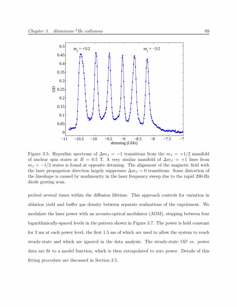
Chapter 3. Aluminum–3He collisions 69
−11 −10.5 −10 −9.5 −9 −8.5 −8 −7.5 −7
0
0.05
0.1
0.15
0.2
0.25
0.3
0.35
0.4
0.45
0.5
detuning (GHz)
OD
mI = +5/2 m
I = −5/2
Figure 3.5: Hyperfine spectrum of ∆mJ = −1 transitions from the mJ = +1/2 manifoldof nuclear spin states at B = 0.5 T. A very similar manifold of ∆mJ = +1 lines frommJ = −1/2 states is found at opposite detuning. The alignment of the magnetic field withthe laser propagation direction largely suppresses ∆mJ = 0 transitions. Some distortion ofthe lineshape is caused by nonlinearity in the laser frequency sweep due to the rapid 200-Hzdiode grating scan.
probed several times within the diffusion lifetime. This approach controls for variation in
ablation yield and buffer gas density between separate realizations of the expeirment. We
modulate the laser power with an acousto-optical modulator (AOM), stepping between four
logarithmically-spaced levels in the pattern shown in Figure 3.7. The power is held constant
for 3 ms at each power level, the first 1.5 ms of which are used to allow the system to reach
steady-state and which are ignored in the data analysis. The steady-state OD vs. power
data are fit to a model function, which is then extrapolated to zero power. Details of this
fitting procedure are discussed in Section 3.5.
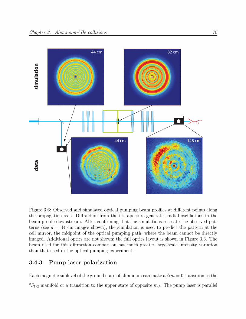
Chapter 3. Aluminum–3He collisions 70
44 cm
44 cm 82 cm
148 cm
sim
ula
tio
nd
ata
Figure 3.6: Observed and simulated optical pumping beam profiles at different points alongthe propagation axis. Diffraction from the iris aperture generates radial oscillations in thebeam profile downstream. After confirming that the simulations recreate the observed pat-terns (see d = 44 cm images shown), the simulation is used to predict the pattern at thecell mirror, the midpoint of the optical pumping path, where the beam cannot be directlyimaged. Additional optics are not shown; the full optics layout is shown in Figure 3.3. Thebeam used for this diffraction comparison has much greater large-scale intensity variationthan that used in the optical pumping experiment.
3.4.3 Pump laser polarization
Each magnetic sublevel of the ground state of aluminum can make a ∆m = 0 transition to the
2S1/2 manifold or a transition to the upper state of opposite mJ . The pump laser is parallel
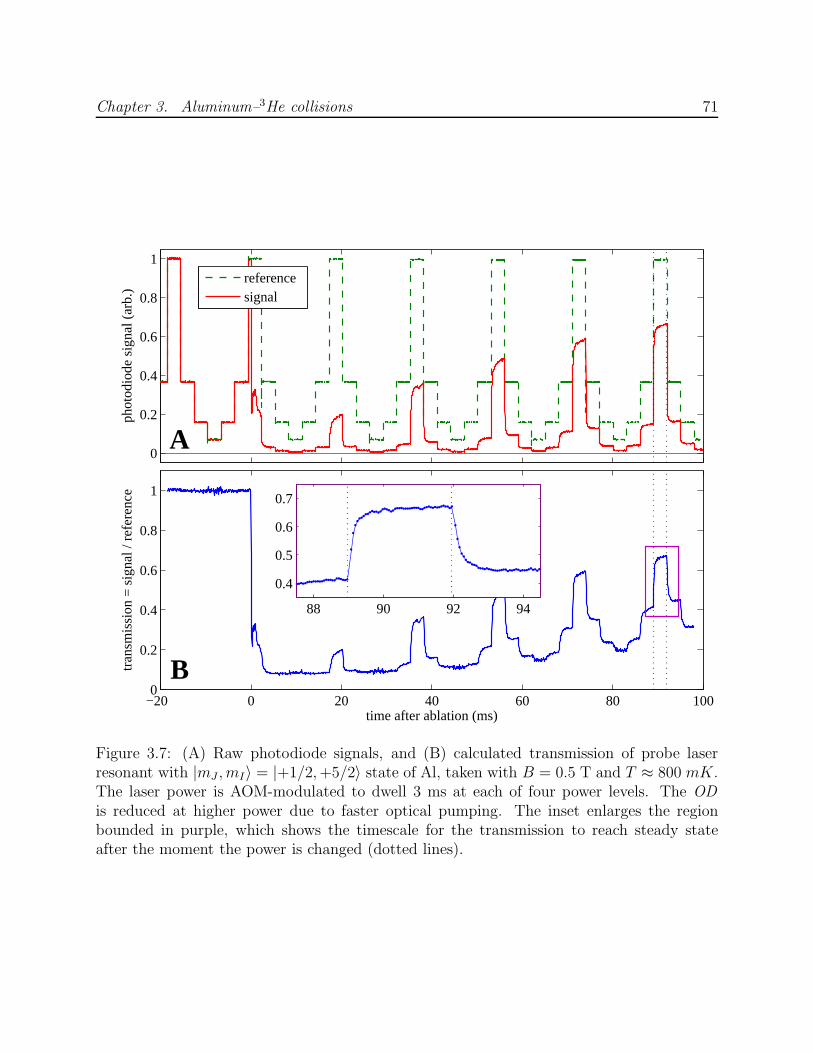
Chapter 3. Aluminum–3He collisions 71
0
0.2
0.4
0.6
0.8
1
phot
odio
de s
igna
l (ar
b.)
A
−20 0 20 40 60 80 1000
0.2
0.4
0.6
0.8
1
time after ablation (ms)
tran
smis
sion
= s
igna
l / r
efer
ence
B
88 90 92 94
0.4
0.5
0.6
0.7
referencesignal
Figure 3.7: (A) Raw photodiode signals, and (B) calculated transmission of probe laserresonant with |mJ , mI〉 = |+1/2,+5/2〉 state of Al, taken with B = 0.5 T and T ≈ 800 mK.The laser power is AOM-modulated to dwell 3 ms at each of four power levels. The OD
is reduced at higher power due to faster optical pumping. The inset enlarges the regionbounded in purple, which shows the timescale for the transmission to reach steady stateafter the moment the power is changed (dotted lines).

Chapter 3. Aluminum–3He collisions 72
to the magnetic field, and so cannot have the appropriate π-polarization to drive ∆m = 0
transitions. Therefore there is only one transition option from each sublevel of the ground
state: mJ = ±1/2 → ∓1/2. As the beam propagates parallel to the field, right-circularly-
polarized light will be σ+-polarized; upon reflection from the cell mirror the polarization
handedness will invert, so that the beam is then propagating antiparallel to the field and
remains σ+-polarized. Similarly, initially left-circularly-polarized light is σ−-polarized. Thus
each ground state sublevel interacts with only one circular polarization.
Engineering the laser polarization to address atoms in the cell is complicated by birefrin-
gence in the multiple windows between the atoms and room temperature optics. The four
fused silica windows are mounted on the cell, the helium bath, the liquid-nitrogen-cooled
radiation shield and the outer dewar, and are referred to as the cell window, 4-K window,
77-K window, and 300-K window, respectively. The cell window4 is epoxied into a close-
fitting G-10 tube; the other three5 are mounted with clamps. Mechanical stresses due to
attachment and thermal contraction are significant, and can cause linear birefringence in
excess of the room-temperature unstressed material specifications. In addition, the Faraday
effect induces circular birefringence in fused silica in high magnetic fields [99], primarily in
the cell window. Measurements of the combined effect are shown in Figure 3.8.
In addition to birefringence in optics, the atomic ensemble itself is birefringent in the mag-
netic field due to its polarization-sensitive absorption. For very high OD , resonant linearly
polarized light will be half absorbed, leaving a single circular polarization. Furthermore, if
the light is detuned from resonance then the dispersive ensemble will phase-shift one circular
polarization with respect to the other, rotating the linear polarization. This nonresonant
effect is especially important when optics between the atoms and detector are polarization
4Glass Fab Inc.: UV fused silica, 1 wedge both sides, 0.5 in thick (thin end).
5CVI Melles-Griot: UV fused silica, 0.5 wedge one side, 0.5 in thick (thick end).
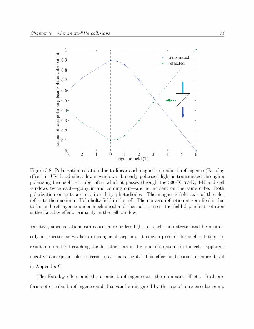
Chapter 3. Aluminum–3He collisions 73
−3 −2 −1 0 1 2 3 4 5 60
0.1
0.2
0.3
0.4
0.5
0.6
0.7
0.8
0.9
1
magnetic field (T)
frac
tion o
f to
tal
pola
rizi
ng b
eam
spli
tter
cube
outp
ut
transmitted
reflected
Figure 3.8: Polarization rotation due to linear and magnetic circular birefringence (Faradayeffect) in UV fused silica dewar windows. Linearly polarized light is transmitted through apolarizing beamsplitter cube, after which it passes through the 300-K, 77-K, 4-K and cellwindows twice each—going in and coming out—and is incident on the same cube. Bothpolarization outputs are monitored by photodiodes. The magnetic field axis of the plotrefers to the maximum Helmholtz field in the cell. The nonzero reflection at zero-field is dueto linear birefringence under mechanical and thermal stresses; the field-dependent rotationis the Faraday effect, primarily in the cell window.
sensitive, since rotations can cause more or less light to reach the detector and be mistak-
enly interpreted as weaker or stronger absorption. It is even possible for such rotations to
result in more light reaching the detector than in the case of no atoms in the cell—apparent
negative absorption, also referred to as “extra light.” This effect is discussed in more detail
in Appendix C.
The Faraday effect and the atomic birefringence are the dominant effects. Both are
forms of circular birefringence and thus can be mitigated by the use of pure circular pump
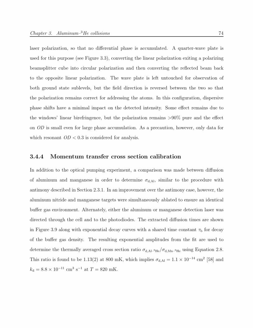
Chapter 3. Aluminum–3He collisions 74
laser polarization, so that no differential phase is accumulated. A quarter-wave plate is
used for this purpose (see Figure 3.3), converting the linear polarization exiting a polarizing
beamsplitter cube into circular polarization and then converting the reflected beam back
to the opposite linear polarization. The wave plate is left untouched for observation of
both ground state sublevels, but the field direction is reversed between the two so that
the polarization remains correct for addressing the atoms. In this configuration, dispersive
phase shifts have a minimal impact on the detected intensity. Some effect remains due to
the windows’ linear birefringence, but the polarization remains >90% pure and the effect
on OD is small even for large phase accumulation. As a precaution, however, only data for
which resonant OD < 0.3 is considered for analysis.
3.4.4 Momentum transfer cross section calibration
In addition to the optical pumping experiment, a comparison was made between diffusion
of aluminum and manganese in order to determine σd,Al, similar to the procedure with
antimony described in Section 2.3.1. In an improvement over the antimony case, however, the
aluminum nitride and manganese targets were simultaneously ablated to ensure an identical
buffer gas environment. Alternately, either the aluminum or manganese detection laser was
directed through the cell and to the photodiodes. The extracted diffusion times are shown
in Figure 3.9 along with exponential decay curves with a shared time constant τb for decay
of the buffer gas density. The resulting exponential amplitudes from the fit are used to
determine the thermally averaged cross section ratio σd,Al–3He/σd,Mn–3He using Equation 2.8.
This ratio is found to be 1.13(2) at 800 mK, which implies σd,Al = 1.1 × 10⁻¹⁴ cm2 [58] and
kd = 8.8 × 10⁻¹¹ cm3 s−1 at T = 820 mK.

Chapter 3. Aluminum–3He collisions 75
0 2 4 6 8 1025
30
35
40
45
50
55
60
time (min)
diffu
sion
tim
e (m
s)
÷1.10
Mn dataMn fitAl dataAl fitAl (scaled)
Figure 3.9: Diffusion time comparison of Al and Mn to determine the momentum transfercross sections ratio σd,Al–3He/σd,Mn–3He. The two fits share the same exponential decay timeconstant. The data are taken with the laser scanning, and the diffusion times plotted arefrom exponential fits to integrated scans. The two data points at each time are separateanalyses considering only one of the two portions of the triangle wave scan—upscans ordownscans. Any scan hysteresis is sufficiently small to not affect the integrated spectra.
3.5 Data analysis
3.5.1 Data processing
For each ablation pulse, the photodiodes shown in Figure 3.3 monitor the intensity of both
the pump laser exiting the cell (the signal beam) and of a reference beam split from the pump
before the dewar. The ratio of the two, normalized to unity in the absence of absorption,
is the transmission of the atomic ensemble (Figure 3.7B). The transmission data is collated
by power level into four separate data sets, which are individually fit over the same time
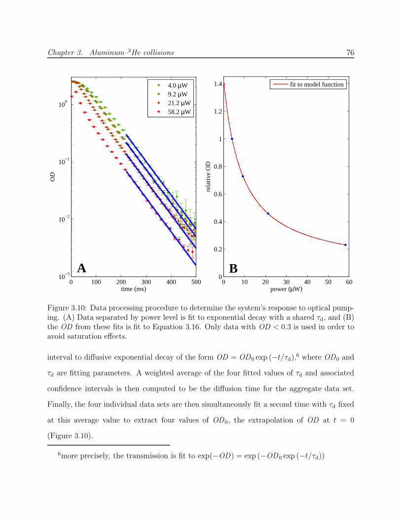
Chapter 3. Aluminum–3He collisions 76
0 10 20 30 40 50 600
0.2
0.4
0.6
0.8
1
1.2
1.4
power (µW)
rela
tive
OD
B0 100 200 300 400 500
10−3
10−2
10−1
100
time (ms)
OD
A
4.0 µW9.2 µW21.2 µW58.2 µW
fit to model function
Figure 3.10: Data processing procedure to determine the system’s response to optical pump-ing. (A) Data separated by power level is fit to exponential decay with a shared τd, and (B)the OD from these fits is fit to Equation 3.16. Only data with OD < 0.3 is used in order toavoid saturation effects.
interval to diffusive exponential decay of the form OD = OD0 exp (−t/τd),6 where OD0 and
τd are fitting parameters. A weighted average of the four fitted values of τd and associated
confidence intervals is then computed to be the diffusion time for the aggregate data set.
Finally, the four individual data sets are then simultaneously fit a second time with τd fixed
at this average value to extract four values of OD0, the extrapolation of OD at t = 0
(Figure 3.10).
6more precisely, the transmission is fit to exp(−OD) = exp (−OD0 exp (−t/τd))
Chapter 3. Aluminum–3He collisions 77
To facilitate comparison of the optical pumping response across varying experimental
parameters, the four values of OD0 from each ablation pulse are fit to a model function:
OD(P ) = a
(
1 − c
bP + 1+ c
)
. (3.16)
The coefficient a is for normalization and is not relevant to the optical pumping analysis.
The model function is a variation of the function in Equation 3.14. The offset c has been
added as a fitting parameter to accommodate deviations from the idealized form (such as
those caused by Zeeman broadening and by spatial variation of pump laser intensity) in
which the system’s response is not described by a single parameter b. The parameterization
in Equation 3.16 is not unique; however, it provides a good approximation. The resulting fits
are generally excellent and give values of c . 0.1. An example fit is shown in Figure 3.10B.
The model function fits are used to predict the ratio OD(Pnorm)/OD(P → 0), which
gives the OD at a certain normalization power Pnorm relative to the weak-probe limit. This
definition allows for comparison across data sets despite pump power fluctuations. OD(P →
0) is extrapolated from the fits, and Pnorm is chosen to be within the range of power levels
used in the experiment. The precise value of Pnorm is not critical; it is chosen such that
OD(Pnorm)/OD(P → 0) ≈ 0.5 to maximize sensitivity to changes in the competing rates in
Equations 3.8–3.10.
Calculating uncertainties for OD(Pnorm) and OD(P → 0) is not trivial due to the trans-
mission noise spectrum. There are significant components to the noise at frequencies ∼ τ−1d
that introduce error in the fit parameters τd and OD0. Since these components cannot be
sufficiently well-sampled during the decay time of a single data set, uncertainties computed
from individual fits systematically underestimate the true uncertainty in these values. Sim-
ply put, the fitting procedure will fit noise features with small residuals even if the fit deviates
greatly from where the noise-free data would lie. More accurate uncertainties are obtained
from the distribution of repeated measurements of the same quantity.
Chapter 3. Aluminum–3He collisions 78
To estimate this distribution, under each set of experimental conditions a null data set is
taken without ablation and the Fourier transform of is computed to obtain a noise spectrum.
That spectrum is then used to generate artificial noise, with identical frequency component
amplitudes to the null data set, but with random phases. The artificial noise is thus a
Fourier-transform-equivalent resampling of the original noise. The original fitted values of
τd and OD0 are used to generate four noise-free OD vs. t curves, which are added to 4×100
independent sets of artificial noise. We fit the resulting simulated data sets in precisely the
same manner as the original data (described above). The standard deviation of the 100 sets
of fit parameters are taken as representative of the actual uncertainty in the original values.
This uncertainty is then propagated for the calculation of OD(Pnorm)/OD(P → 0) and is
used to determine the best-fit parameters for numerical simulation of Equations 3.8–3.10, as
described in the next section. An example data set with error bars is shown in Figure 3.11.
3.5.2 Numerical simulation of optical pumping
To interpret the data, Equations 3.8–3.10 are solved numerically to obtain N+, N− and N3/2
as a function of time and space. Expressed in experimental parameters, the optical pumping
rate is
Γp = 2
(
s0(r)A
2FD
)
, (3.17)
where s0(r) = I(r)/Isat is the spatially-varying saturation parameter of the pump beam
intensity profile I(r), A = 4.99 × 10⁷ s−1 is the Einstein coefficient for the 2P1/2 → 2S1/2
transition, and FD is the reduction factor due to Doppler broadening (Section 3.3). The
factor of 2 is due to the pump beam passing through the atoms twice. Similarly, using
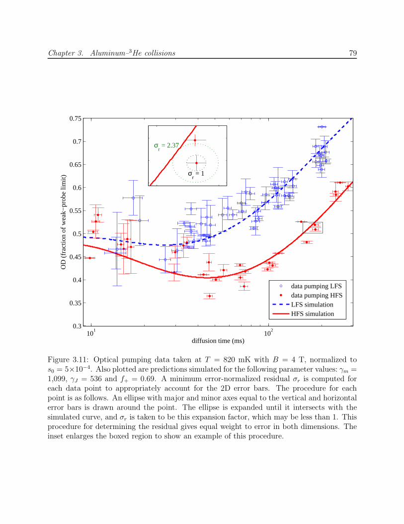
Chapter 3. Aluminum–3He collisions 79
101
102
0.3
0.35
0.4
0.45
0.5
0.55
0.6
0.65
0.7
0.75
diffusion time (ms)
OD
(fr
actio
n of
wea
k−pr
obe
limit)
σr = 1
σr = 2.37
data pumping LFSdata pumping HFSLFS simulationHFS simulation
Figure 3.11: Optical pumping data taken at T = 820 mK with B = 4 T, normalized tos0 = 5×10⁻⁴. Also plotted are predictions simulated for the following parameter values: γm =1,099, γJ = 536 and f+ = 0.69. A minimum error-normalized residual σr is computed foreach data point to appropriately account for the 2D error bars. The procedure for eachpoint is as follows. An ellipse with major and minor axes equal to the vertical and horizontalerror bars is drawn around the point. The ellipse is expanded until it intersects with thesimulated curve, and σr is taken to be this expansion factor, which may be less than 1. Thisprocedure for determining the residual gives equal weight to error in both dimensions. Theinset enlarges the boxed region to show an example of this procedure.

Chapter 3. Aluminum–3He collisions 80
Equations 1.4 and 2.4 the inelastic collision rates can be expressed as
Γm = nbkm =nbkdγm
=3π
32
1
γm(v2G) τd (3.18)
and
ΓJ =3π
32
1
γJ(v2G) τd, (3.19)
where γm and γJ are the ratios of the momentum transfer rate coefficient kd to the inelastic
collision rate coefficients km and kJ for mJ - and J-changing collisions, respectively.
It is important to note that these two rate coefficients refer to collisions of atoms in
different fine-structure states: km refers to mJ -changing collisions of 2P1/2 atoms and km to
J-changing collisions of 2P3/2 atoms. For purposes of analysis, however, the ratios γm and
γJ both express these rate coefficients relative to the same 2P1/2 state momentum transfer
rate coefficient kd. The reason for this is that the experiment has access only to ground
state elastic collisions (through the diffusion time τd) and not those involving 2P3/2 atoms.
The ratios γm and γJ are the quantities determined by the optical pumping experiment.
Calculations of kd for the ground state give a value roughly 40% larger than for the 2P3/2
state due to the presence of a collision resonance in the experimental temperature range.
Separate measurement of kd = 8.8 × 10⁻¹¹ cm3 s−1 (Section 3.4.4) allows the rates km and
kJ to be determined.
Finally, diffusion is included in the numerical simulation using the cylindrically symmetric
diffusion equation [51],
D∇2N(r, t) = D1
r
∂
∂r
(
r∂N(r, t)
∂r
)
= N(r, t), (3.20)
where the diffusion constant D is given in Equation 2.4. The spatial profiles for all three
state populations are evolved forward in time in discrete steps. For each step, the probability

Chapter 3. Aluminum–3He collisions 81
0
0.2
0.4
0.6
0.8
1
A
γm
= γJ = 1,000
0 5 10 15 20 25 300
0.2
0.4
0.6
0.8
1
radial distance from cell axis (mm)
LFS
pop
ulat
ion
(arb
.)
B
γm
= γJ = 100
t = 0 µs
30 µs
90 µs
300 µs
900 µs3 ms9 ms30 ms
Figure 3.12: Spatial simulation of Al optical pumping, diffusion and Zeeman relaxation. Theparameters used are: T = 820 mK, B = 3 T, D = 5 mm2/ms, s0 = 5 × 10⁻⁴, f+ = 0.7,and a uniform pump beam of diameter 3.9 mm (dashed lines). (A) For slower relaxation,diffusion plays a dominant role, and the region beyond the beam is steadily depleted of LFSatoms; (B) rapid relaxation causes the distribution to reach steady state more rapidly, andwith larger LFS population in the beam.
of an atom undergoing an optical or inelastic transition is computed locally. An example
of this spatial evolution is shown in Figure 3.12. The OD is calculated by integrating the
atom density over the beam profile. OD is normalized to 1 when optical pumping begins
at t = 0, at which time the spatial distribution is given by the lowest-order diffusion mode
(Equation 2.3).
Chapter 3. Aluminum–3He collisions 82
The simulated OD vs. time is integrated over the same interval of t = 1.5–2.9 ms that is
used for integrating the OD observed in the experiment. Since OD(t = 0) = 1, this integral
is equal to the ratio OD(P )/OD(P → 0), which is the same quantity extracted from the
data. The simulation is repeated for a range of τd inclusive of the experimental range. This
process is rather computationally intensive, so it would be impractical to employ it in a fitting
routine. Instead, a set of simulations is generated over a matrix of values of the parameters
γm, γJ and the branching ratio f+/f−. For each element of this matrix, a goodness-of-fit
criterion is computed by taking the sum of squares of residuals from the simulation curve.
To appropriately account for the 2D error bars, minimum 2D error-normalized residuals are
computed as shown in Figure 3.11.
One additional free parameter, a scaling factor for the total pump laser power, is included
to account for imperfect knowledge of experimental parameters. The numerical solution to
Equations 3.8–3.10 is sensitive to: pump beam size, intensity profile and detuning from reso-
nance; Doppler and Zeeman broadening; and absorption and birefringence in optical elements
within the cryogenic environment. While each effect is carefully investigated, compounding
measurement uncertainties can cause a vertical offset of the simulated curves to the data.
The additional free parameter, which is generally .2, accounts for such effects, many of
which mimic an adjustment of pump power.
Because there may be several minima of the goodness-of-fit matrix, and since the residuals
from this fitting procedure are not normally distributed (because the problem is nonlinear),
confidence intervals are computed for the fitting parameters using a bootstrapping procedure.
The procedure is as follows: (1) we resample equal-sized data set from the original with
replacement (e.g., the data set 1, 2, 3, 4, 5 might be resampled as 2, 1, 3, 2, 5); (2) we
re-compute the goodness-of-fit matrix using the resampled data and find its minimum (best
fit); (3) we perform steps (1) and (2) 100 times. We take the median and confidence intervals

Chapter 3. Aluminum–3He collisions 83
0 2 4 610
2
103
104
magnetic field (T)
γ m
0 2 4 610
2
103
104
magnetic field (T)
γ J
0 2 4 60
0.1
0.2
0.3
0.4
0.5
0.6
0.7
0.8
0.9
1
magnetic field (T)
f +
fits to data
theoretical calculations
Figure 3.13: Inelastic collision parameters extracted—the mJ -changing collision ratio γm, J-changing collision ratio γJ , and J-changing collision LFS-state branching fraction f+—fromunbounded fitting of optical pumping data to numerical simulation. The parameter f+ ispoorly constrained by the fits, which introduces systematic bias to push γm and γJ towardone another. Also shown are theoretical calculations by Tscherbul (dashed) [95].
of the resulting distribution of 100 best-fit sets of parameter values to be representative of
the true best-fit parameters and their statistical uncertainty.
3.5.3 Results from fitting data to simulation
Best-fit parameters for the collision ratios γm, γJ and the branching fraction f+ = 1 − f−
with bootstrapped confidence intervals are presented in Figure 3.13. It is clear from the
large uncertainty in f+ that this parameter is poorly constrained by the data. This fact

Chapter 3. Aluminum–3He collisions 84
is confirmed by the simulation: if f+ is set to extremes of 0 or 1, the primary effect is to
enhance the distinction between optically pumping the two different ground state sublevels
(the solid red and dashed blue curves in Figure 3.11). Otherwise, there is little effect on the
functional form of the data as a function of diffusion time. Furthermore, variation in f+ is
mimicked by adjustment of the relative contributions of mJ - vs. J-changing collisions (i.e.,
γm vs. γJ). Therefore, allowing f+ to vary freely in the fit from 0 to 1 confuses these effects
in the fitting procedure and introduces a systematic bias forcing γm and γJ toward the same
value.
There is, however, a priori justification for constraining the value of f+. The branching
fraction is determined by the mJ dependence of the interaction Hamiltonian in Equation 3.3.
Specifically, the first 3-j symbol evaluated form′J = ±1/2 gives ratios of f+ = 0.8, 0.6, 0.4 and
0.2 for J-changing transitions from the mJ = +3/2, +1/2, −1/2 and −3/2 sublevels of the
2P3/2 manifold, respectively. The exact calculation of the scattering matrix, however, will be
significantly affected by resonant behavior and higher-order couplings that mix these ratios
(to push f+ toward 0.5, on average). Nevertheless, for decay from the upper mJ = +3/2
state, the value of f+ is expected to be almost 0.8.
This argument is borne out by the calculations of Tscherbul [95]. To test the sensitivity
of the theory to error in the potential, calculations were performed three times with the
interaction potentials scaled by a factor λ of 1, 1.05 and 0.95, respectively. The resulting
values of f+ for collisions of atoms in the mJ = −3/2 sublevel are shown as a function of
magnetic field in Figure 3.14. There is no obvious trend with respect to magnetic field or
λ. Instead, the values appear more or less randomly distributed around a mean of 0.716,
as would be expected from averaging over the contributions from multiple collision reso-
nances. Performing the bootstrapping procedure again with the simulation constrained to
this mean value yields the orange points in Figure 3.15, which are in better agreement with
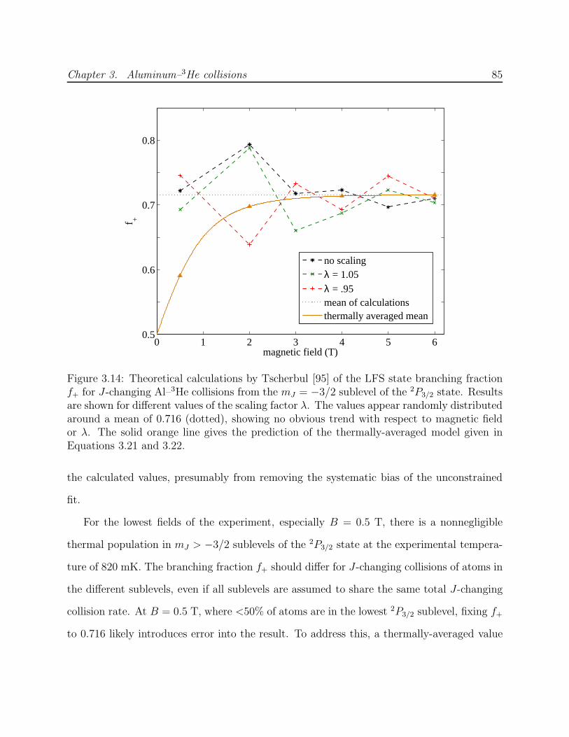
Chapter 3. Aluminum–3He collisions 85
0 1 2 3 4 5 60.5
0.6
0.7
0.8
magnetic field (T)
f +
no scalingλ = 1.05λ = .95mean of calculationsthermally averaged mean
Figure 3.14: Theoretical calculations by Tscherbul [95] of the LFS state branching fractionf+ for J-changing Al–3He collisions from the mJ = −3/2 sublevel of the 2P3/2 state. Resultsare shown for different values of the scaling factor λ. The values appear randomly distributedaround a mean of 0.716 (dotted), showing no obvious trend with respect to magnetic fieldor λ. The solid orange line gives the prediction of the thermally-averaged model given inEquations 3.21 and 3.22.
the calculated values, presumably from removing the systematic bias of the unconstrained
fit.
For the lowest fields of the experiment, especially B = 0.5 T, there is a nonnegligible
thermal population in mJ > −3/2 sublevels of the 2P3/2 state at the experimental tempera-
ture of 820 mK. The branching fraction f+ should differ for J-changing collisions of atoms in
the different sublevels, even if all sublevels are assumed to share the same total J-changing
collision rate. At B = 0.5 T, where <50% of atoms are in the lowest 2P3/2 sublevel, fixing f+
to 0.716 likely introduces error into the result. To address this, a thermally-averaged value

Chapter 3. Aluminum–3He collisions 86
0 2 4 610
2
103
104
magnetic field (T)
γ m
0 2 4 610
2
103
104
magnetic field (T)
γ J
unbounded fitfixed fitthermal fixed fittheory, λ = 1theory, λ = 1.05theory, λ = 0.95
Figure 3.15: Inelastic collision parameters extracted—the mJ -changing collision ratio γm andJ-changing collision ratio γJ—from fitting of optical pumping data to numerical simulationwith the J-changing branching fraction f+ unconstrained (blue circles), fixed at f+ = 0.716(magenta squares), and fixed at f+ = f+ (orange triangles, Equations 3.21 and 3.22). Theo-retical calculations by Tscherbul [95] (dashed lines) are given for Al–3He interaction potentialscaling factor λ = 1, 1.05 and 0.95. Fixing f+ gives better agreement with theory.
f+ was computed for each field using the function
f+ = 0.5 +
(
0.716 − 0.5
0.8 − 0.5
)
× (〈f+〉th − 0.5) (3.21)
〈f+〉th =∑
mJ
NmJ(T ) f+, (3.22)
where f+ is the branching fraction calculated from the first 3-j symbol in Equation 3.3,
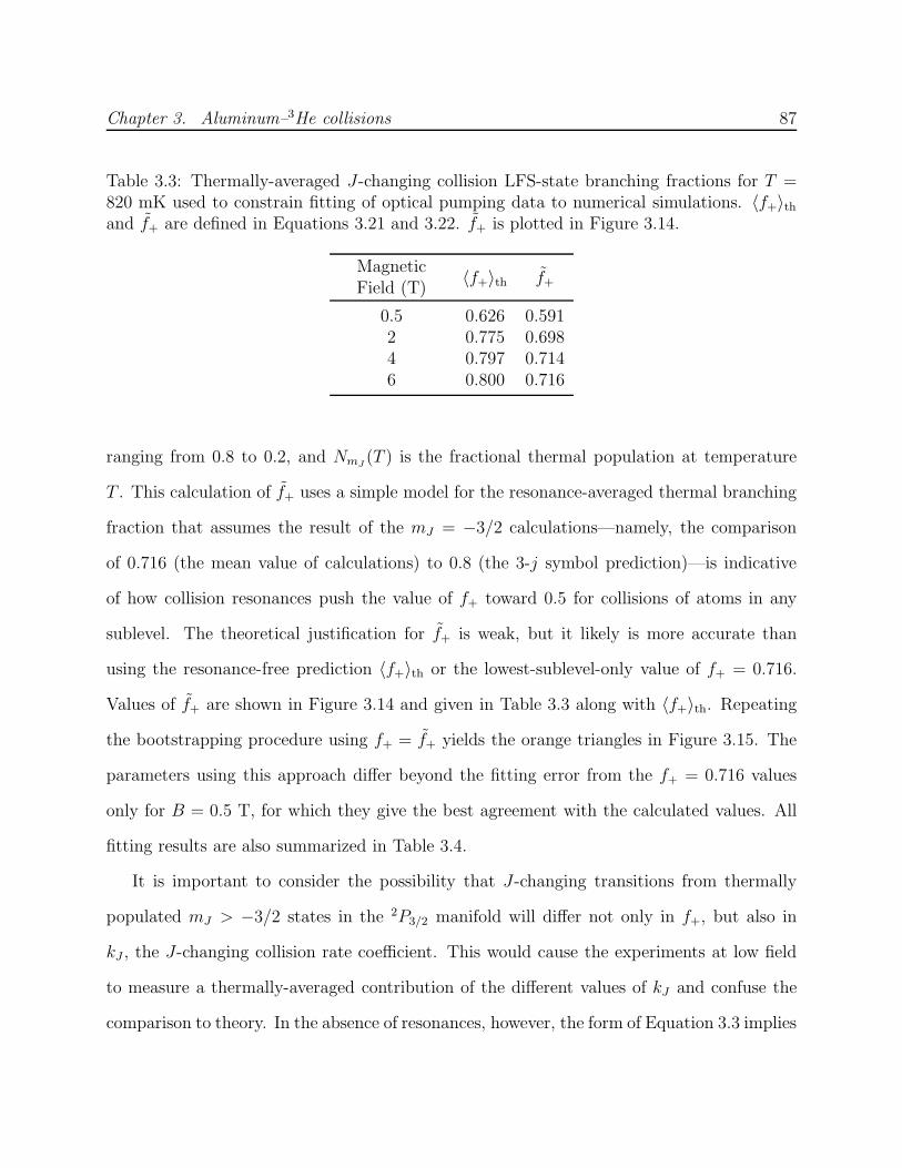
Chapter 3. Aluminum–3He collisions 87
Table 3.3: Thermally-averaged J-changing collision LFS-state branching fractions for T =820 mK used to constrain fitting of optical pumping data to numerical simulations. 〈f+〉thand f+ are defined in Equations 3.21 and 3.22. f+ is plotted in Figure 3.14.
MagneticField (T)
〈f+〉th f+
0.5 0.626 0.5912 0.775 0.6984 0.797 0.7146 0.800 0.716
ranging from 0.8 to 0.2, and NmJ(T ) is the fractional thermal population at temperature
T . This calculation of f+ uses a simple model for the resonance-averaged thermal branching
fraction that assumes the result of the mJ = −3/2 calculations—namely, the comparison
of 0.716 (the mean value of calculations) to 0.8 (the 3-j symbol prediction)—is indicative
of how collision resonances push the value of f+ toward 0.5 for collisions of atoms in any
sublevel. The theoretical justification for f+ is weak, but it likely is more accurate than
using the resonance-free prediction 〈f+〉th or the lowest-sublevel-only value of f+ = 0.716.
Values of f+ are shown in Figure 3.14 and given in Table 3.3 along with 〈f+〉th. Repeating
the bootstrapping procedure using f+ = f+ yields the orange triangles in Figure 3.15. The
parameters using this approach differ beyond the fitting error from the f+ = 0.716 values
only for B = 0.5 T, for which they give the best agreement with the calculated values. All
fitting results are also summarized in Table 3.4.
It is important to consider the possibility that J-changing transitions from thermally
populated mJ > −3/2 states in the 2P3/2 manifold will differ not only in f+, but also in
kJ , the J-changing collision rate coefficient. This would cause the experiments at low field
to measure a thermally-averaged contribution of the different values of kJ and confuse the
comparison to theory. In the absence of resonances, however, the form of Equation 3.3 implies

Chapter 3. Aluminum–3He collisions 88
Table 3.4: Summary of inelastic parameter fitting results at T = 820 mK for the differenttreatments of f+ described in the text, with 68% confidence intervals in parentheses.
f+ unconstrainedMagneticField (T)
γm γJ
0.5 1854 (1589, 2059) 903 ( 736, 1028)2 2028 (1686, 2557) 1337 (1167, 1662)4 911 ( 536, 1491) 799 ( 443, 1240)6 373 ( 256, 519) 549 ( 449, 630)
f+ = 0.716MagneticField (T)
γm γJ
0.5 1563 (1337, 1794) 1162 (1043, 1270)2 2469 (1245, 3015) 654 ( 198, 978)4 1204 ( 983, 1348) 495 ( 277, 692)6 296 ( 241, 334) 611 ( 545, 672)
f+ = f+MagneticField (T)
γm γJ
0.5 2428 (2193, 2643) 511 ( 334, 724)2 2482 (1905, 2921) 1011 ( 836, 1647)
Table 3.5: Summary of theoretical calculations by Tscherbul [95] for T = 820 mK withinteraction potential depths scaled by λ.
γm γJ
MagneticField (T) λ = 1 1.05 0.95 λ = 1 1.05 0.95
0.5 4948 3367 7061 194 163 2532 3905 2823 5377 308 235 3163 2512 1913 3351 295 182 3074 1610 1264 2125 265 159 2525 1042 827 1383 235 201 2496 694 552 932 258 196 268

Chapter 3. Aluminum–3He collisions 89
that the inelastic cross section does not vary dramatically between magnetic sublevels. In
addition, the thermal average over collision energies performed to obtain kJ and γJ will blur
any resonant behavior.
3.6 Conclusion
3.6.1 Comparison of experiment with theory
Theoretical calculations for the unscaled potential and for ±5% scaling are shown in Fig-
ure 3.15 along with the parameters extracted from fitting the data to numerical simulations.
The theory values are also summarized in Table 3.5. The calculated magnetic field depen-
dence of both γm and γJ is in good agreement with the data. The ∼ B−2 dependence of γm
in the range of B = 2–6 T reflects the increased fine-structure state mixing as the magnetic
sublevels are Zeeman-shifted toward one another [95]. In the case of γJ , the J-changing
inelastic collisions are a small contribution to the rapid mJ -changing collisions in the 2P3/2
state (γm < 10 in this state [1]; see Table 3.1). Therefore, there is no simple field dependence
and the form of γJ(B) is more heavily affected by collision resonances that are sensitive to
the exact form of the potential. In general, the result is independent of magnetic field in the
range calculated.
The magnitudes of the measured values of γm and γJ are in better agreement with
theory when the constrained fitting procedure is used. It is likely that the unconstrained fit
is systematically biased toward γm ∼ γJ . For the constrained-fit data, the magnitude of γm
agrees very well with theory, especially for λ = 1.05, however the measured γJ is a factor of
∼3 larger than the calculated value. It is possible that this reflects residual systematic bias
of γJ → γm. For γJ ≪ γm, Equation 3.11 is only weakly dependent on ΓJ (if ∆f = f+ − f−
is not near zero), and hence its value is not as tightly constrained by the data in that case.
Chapter 3. Aluminum–3He collisions 90
3.6.2 Implications for future work with 2P atoms
The comparison of experiment and theory, and specifically the comparison as a function of
magnetic field, gives strong evidence that the mechanism of Zeeman relaxation in the 2P1/2
system is indeed collisional mixing of the excited fine-structure state. This adds confidence to
the predictions of very large values of γ for collisions of gallium and indium (and metastable
halogens chlorine, bromine and iodine) with helium, with predictions ranging ∼104–109. The
theoretical picture applies to other S-state atoms, as well (although for collisions with atoms
with L > 0, Equation 3.3 is modified such that relaxation in the 2P1/2 state is not necessarily
forbidden at first order). In the cases of indium and thallium, where the ground state is
isolated by 2,213 cm−1 and 7,793 cm−1, respectively, the Zeeman relaxation suppression
may extend to collisions of indium or thallium atoms with trapped ultracold alkali atoms if
the strength of the interaction potential does not exceed this splitting. This could allow for
sympathetic cooling of these atoms in a magnetic trap.
The large trap depth and volume available with a magnetic trap could translate into many
more ultracold atoms available for experiments. Species with poor collision properties have
few choices beyond optical dipole traps, which are limited in size and depth by practical
and technical limitations on laser power. The ability to laser cool Group 13 atoms has
already been demonstrated [27, 79, 80], and trapping is a natural next step. For some of
the proposed experiments with these atoms, especially precision measurements [81, 83, 84],
large atom numbers are important. The theory developed by Tscherbul et al. and confirmed
experimentally here and in [1] has provided a potential route to reach that goal. In addition,
the discovery that collisions of these 2P atoms are robustly elastic may inspire future theory
and experiment for new uses for these unique systems.

Chapter 4
Rare-earth atom–atom collisions
4.1 Submerged-shell atoms
The previous two chapters gave examples of systems that run counter to the simple principle
that S-state atoms should uniquely exhibit robustly elastic collisions. In the case of antimony,
a nominally S-state atom was strongly affected by relativistic spin-orbit coupling that rapidly
drove inelastic transitions; in the case of aluminum, a P -state atom, such inelastic transitions
were suppressed to below the case of antimony.
Another important and widespread exception to the uniqueness of S-state elasticity is
the set of so-called “submerged-shell” atoms that account for roughly a third of the periodic
table. Due to nonsequential filling of electronic orbitals, these atoms have valence electrons
that lie closer to the nucleus than do closed outer electron shells (those with higher principle
quantum number) [100]. In many cases, the inner valence electrons are highly anisotropic in
the ground state and the total atomic orbital angular momentum is large. During a collision
with helium, however, the interaction with the spherical outer electron distribution shields
this anisotropy, resulting in a nearly isotropic electrostatic interaction. This shielding was
91

Chapter 4. Rare-earth atom–atom collisions 92
observed in many transition metal [63] and lanthanide rare-earth (RE) [2] atoms during
collisions with helium, demonstrating that electronic anisotropy does not necessarily imply
rapid inelastic collisions.
The shielding effect leads to measured values of γ of 103–105 for many submerged shell
atoms [2, 63, 64]. This is in dramatic contrast to the inelasticity for an interaction domi-
nated by anisotropic valence electrons, as calculations predict for the unshielded 3P2 ground
state of oxygen [91] and the upper fine-structure state of aluminum described in Chapter 3
[1] (see Table 3.1). The mechanism of submerged-shell anisotropy shielding has also been
explored theoretically and shown to indeed arise from the outermost filled s-orbital [3, 101].
Suppression of inelastic collisions in submerged-shell atoms was an exciting development,
particularly for the possibility of extending collisional cooling to a wide array of new atoms.
Elastic collisions with helium allowed for many new species to be buffer-gas cooled and
magnetically trapped [2].
The lanthanide RE atoms, in particular, exhibit very low inelastic collision rates in col-
liding with helium (γ > 104 [2]) and can be trapped in large numbers. The lanthanide series
is of significant technical interest, as well, due to important and sometimes unique attributes
such as narrow transition linewidths useful for precision measurement [102, 103] and sub-
Doppler cooling [104, 105], and large magnetic moments with strong long-range interactions
that can be used to realize unique ultracold states [106–108] or implement quantum com-
puting schemes [109]. The discovery of anisotropy shielding in the RE–helium system laid
open the question of whether similar suppression would exist for RE–RE inelasticity, which
could allow for efficient evaporative cooling and, for example, the creation of large quantum
degenerate ensembles of RE atoms using magnetic traps.
This chapter describes measurements of RE–RE Zeeman relaxation rates in two systems,
collisions between erbium atoms and those between thulium atoms. Both erbium and thulium

Chapter 4. Rare-earth atom–atom collisions 93
have highly anisotropic valence electrons (the ground state terms are [Xe]4f 126s2(3H6) for
erbium and [Xe]4f 136s2(2F7/2) for thulium [110]) and have magnetic moments of µEr =
7 µB and µTm = 3.5 µB. We find that both the erbium–erbium and thulium–thulium
relaxation rates are very large (γ . 10), in striking contrast to the RE–helium systems, and
we see no evidence that electronic interaction anisotropy is suppressed. This discovery helps
to draw boundaries on the submerged-shell model of anisotropy shielding, and implies that
evaporative cooling is likely impossible for L 6= 0 RE atoms in a magnetic trap.
4.2 Experimental design
4.2.1 Apparatus
The experimental cell used to measure RE–RE collisions (Figure 4.1) was originally built for
the creation of a buffer-gas cooled Bose-Einstein condensate of metastable helium-4, and is
described in detail in the thesis of Charlie Doret [111]. It has several features that are not
utilized for trapping RE atoms, including a valve to a pumpout chamber (which is left closed
for the experiments described here) and a radiofrequency (RF) discharge coil wound on the
outer cell surface. The experimental apparatus is otherwise largely similar to that used in
the previous two chapters. Helium-4 buffer gas is added to the cell from the waiting room
in the same manner and the same magnet coils surround the cell, except that in this case
they are configured in an anti-Helmholtz geometry to produce a quadrupole trapping field.
Detection of ground-state erbium and thulium is accomplished by absorption spectrosco-
py with diode lasers. The transitions used are J = 6 → 7 and J = 6 → 5 for erbium at
400.9 nm and 415.2 nm, respectively, and J = 7/2 → 5/2 for thulium at 409.5 nm. A probe
beams is free-space coupled to the experimental dewar and then split to provide an intensity
reference for the absorption measurement. To minimize the noise due to vibration of the cell
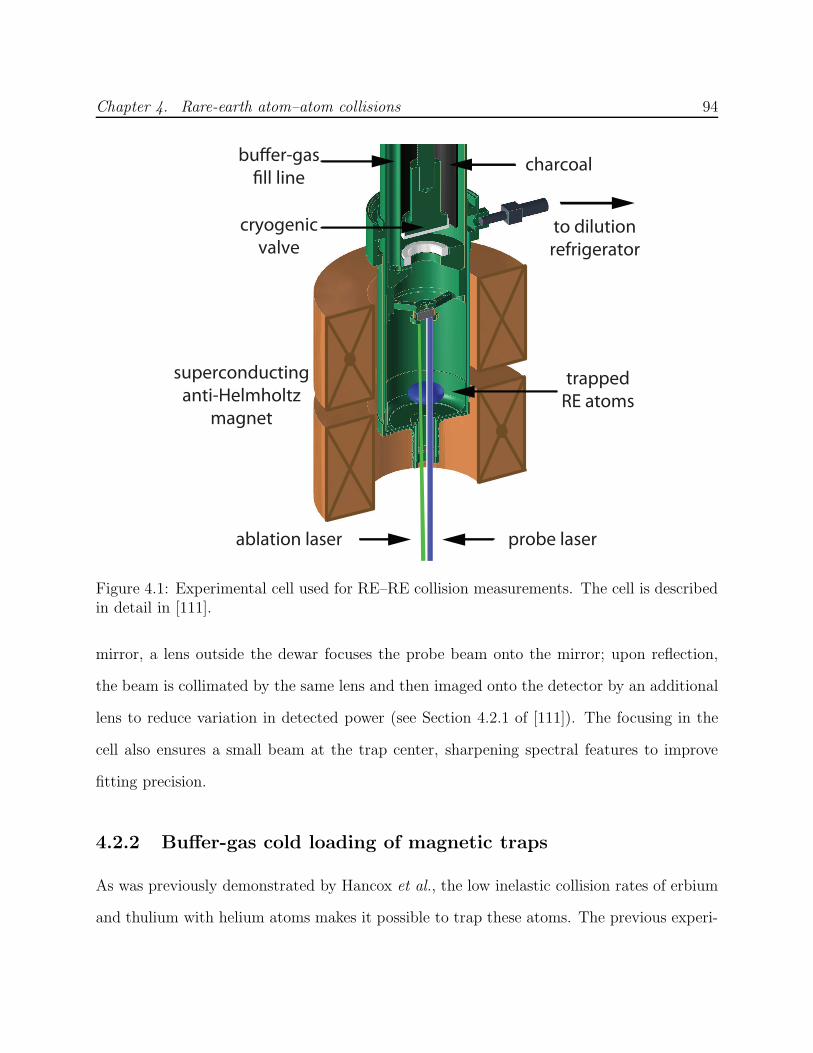
Chapter 4. Rare-earth atom–atom collisions 94
cryogenic
valveto dilution
refrigerator
probe laserablation laser
charcoal
superconducting
anti-Helmholtz
magnet
trapped
RE atoms
bu!er-gas
"ll line
Figure 4.1: Experimental cell used for RE–RE collision measurements. The cell is describedin detail in [111].
mirror, a lens outside the dewar focuses the probe beam onto the mirror; upon reflection,
the beam is collimated by the same lens and then imaged onto the detector by an additional
lens to reduce variation in detected power (see Section 4.2.1 of [111]). The focusing in the
cell also ensures a small beam at the trap center, sharpening spectral features to improve
fitting precision.
4.2.2 Buffer-gas cold loading of magnetic traps
As was previously demonstrated by Hancox et al., the low inelastic collision rates of erbium
and thulium with helium atoms makes it possible to trap these atoms. The previous experi-

Chapter 4. Rare-earth atom–atom collisions 95
ments were performed with helium-3 buffer gas at a density of 8×1015 cm−3 in a copper cell
at ∼800 mK [2]. Under these conditions, the RE–helium collision rate is &7 × 10⁵ s−1 and
lifetimes due to RE–helium Zeeman relaxation are limited to .100 ms, too rapid to observe
collisions between the trapped atoms. By using helium-4 buffer gas, the helium density can
be reduced after trap loading to achieve thermal isolation. This is done by ablating at high
helium density while heating the cell and then allowing the cell to cool to adsorb the buffer
gas onto the cell walls, a process that takes about 1 s due to the thermal response time of the
heat link to the dilution refrigerator (see Section 2.2.4). This method was applied to trap
and thermally isolate dysprosium atoms (µ = 9.93 µB, γ = 4.5 × 10⁵), which were observed
for up to 20 s in the trap [72]. The loss mechanism for trapped dysprosium after cell cooling
was not identified in those experiments, however, and no definite conclusions were drawn
regarding collisions between dysprosium atoms.
An additional method called cold loading has been used in several cases to more rapidly
reduce the buffer gas density after ablation [30, 70, 112–114]. Cold loading consists simply of
ablation (or a YAG pulse in concert with a separate production method [114]) in a cell that is
initially cold enough to ensure a very low initial helium density (nb . 1013 cm−3). Typically,
helium-4 is used. The energy of the ablation laser pulse desorbs a sufficient quantity of
helium to cool the ablated atoms, and the subsequent cell cooling causes this helium to be
readsorbed onto the cell walls. Desorbing with the ablation energy instead of a resistive
heater allows for less total energy to be added to the cell, and hence a faster return to pre-
ablation temperatures. This method was first used for buffer-gas loading of chromium atoms
into a magnetic trap [112], demonstrating significantly less cell heating, but also a reduced
trapped atom yield.
There is an important distinction to be made, however, between different regimes of cold
loading that employ different loading energies and cell construction. As described below, cold

Chapter 4. Rare-earth atom–atom collisions 96
loading in a copper cell relies on a slow (second-scale) thermal connection to the refrigerator.
In contrast, cold loading in superfluid-jacketed G-10 cells can produce a transient buffer gas
density with a shorter lifetime (below 100 ms) while retaining a very large cell heat capacity
in the superfluid. This extension to the cold loading concept, used in the experiments
described here to trap erbium and thulium, is especially suited to moderate-γ species for
which minimizing helium collisions is critical for trapping.
We first consider cold loading in a copper cell, which is not likely to be fundamentally
different from traditional loading with a heating-cooling cycle, and differs only in the total
energy used. Both processes increase the buffer gas density by heating the surfaces to which
helium is adsorbed. The deposited heat immediately begins to diffuse into the solid walls
of the cell by up to 3 mm on a timescale of ≈10 µs (Equation 2.7). This heat diffusion is
extremely rapid, far below the 1-ms timescale of ballistic transport across the cell. Hence
the cell wall surfaces have equilibrated with a large volume of copper (&50 cm3) before the
desorbed helium atoms return to the walls. If the ablation energy deposited is small, then
the heat capacity of this solid volume will ensure that the cell wall will be cold enough
to re-adsorb the helium. In this low-energy situation, buffer-gas cooling is not possible
because the necessary helium density [30] cannot develop. In the other regime of large
ablation energy, the entire cell will warm significantly within the millisecond-scale thermal
diffusion time, and the increased helium density will be temporarily stable. Cooling of the
cell must now occur via conduction to the refrigerator—a situation not much different from
the traditional heating-cooling cycle method of removing buffer gas [97, 112]. Cold loading
aims for the ideal intermediate energy, with just enough helium as necessary for buffer-
gas cooling. However, the large thermal conductivity of copper ensures that the entire cell
must be heated, subsequently requiring &1 s to cool significantly. The trapped atoms will
experience collisions for this duration, which for minimal buffer-gas cooling densities near
Chapter 4. Rare-earth atom–atom collisions 97
nb ≈ 1015 cm−3 implies more than 5 × 10⁴ collisions (assuming σd = 1014 cm2). For species
with γ ∼ 104, this will result in significant losses due to inelastic collisions.
The cold-loading picture is different in a cell constructed from low-thermal-conductivity
materials such as G-10, for which the diffusion of heat into the solid is slowed. As described
in Section 2.2.4, when the energy of ablation heats G-10 surfaces to desorb helium, the heat
will take ≈10 ms to diffuse 1 mm. For ablation energies of 1–10 mJ, the walls will heat
significantly and sustain a high buffer gas density long enough for the ablated atoms to
reach equilibrium. Unlike copper cells, there can then be an additional heat capacity which
provides rapid cooling on the >30-ms time scale, but that does not play a role at shorter
times (Figure 2.5). One example of such a heat capacity is the superfluid helium jacket
surrounding the inner G-10 wall of the composite cells used in this thesis. The superfluid
has a very large heat capacity that exceeds that of the entire mass of G-10, and that of
the entire typical copper cell. Hence a modest ablation energy, after first producing a high
helium density for ∼10 ms, will subsequently be rapidly absorbed into the cell’s heat capacity
to ensure a low cell temperature and good vacuum. We refer to this variation on cold loading
as pulsed-density cold loading.
Pulsed-density cold loading is used here to trap erbium and thulium atoms, which would
otherwise leave the trapped state after an average of γ = 4.3 × 10⁴ and 2.7 × 10⁴ collisions,
respectively [2], i.e., within less than 100 ms at a helium density of 1016 cm−3, assuming
a momentum transfer cross section σd = 1014 cm2. The cell is held at ≈500 mK before
ablation, at which temperature the helium-4 saturated vapor density is <1014 cm−3 [59] and
insufficient for buffer-gas cooling [30]. Erbium or thulium metal is ablated with pulse energy
of ≈5 mJ to fill the trap. Figure 4.2 shows trapped spectra for both species, which are
compared to simulated spectra to determine the peak density in the trap. RE–RE collisional
loss of the trapped atoms is immediately apparent, with no evidence of loss due to RE–helium

Chapter 4. Rare-earth atom–atom collisions 98
0
0.05
0.1
0.15
OD
A
0 2 4 6 8
0
0.02
0.04
0.06
0.08
detuning (GHz, arbitrary zero)
OD
B
datasimulation
170Er
168Er
167Er
166Er
164Er
Figure 4.2: (A) Absorption spectrum of Er on the 400.9-nm (J = 6 → 7) transition in a0.99-T (4.6 K) deep magnetic trap at 530 mK with a peak density of 4.6 × 1010 cm−3. The∆mJ = +1 Zeeman broadened peaks of the dominant isotopes are labeled. The sharperpeaks are ∆mJ = 0 transitions. Hyperfine constants could not be found for 167Er (I = 7/2,23% abundance), and it is ignored in the spectrum simulation. Due to the substantial Zeemanbroadening, this does not significantly affect the implied atom density and temperature. (B)Spectrum of Tm on the 409.5-nm (J = 7/2 → 5/2) transition in a 3.3-T (8.8 K) deep trapat 500 mK with a peak density of 3.8 × 1011 cm−3. Tm has a single isotope with I = 1/2and known hyperfine splitting [115].
Chapter 4. Rare-earth atom–atom collisions 99
Zeeman relaxation.
4.2.3 Inelastic collisional heating
Once the atoms have been loaded into the magnetic trap and the helium density has returned
to low levels (<1012 cm−3), the trapped ensemble is thermally isolated from the cell walls
with a RE–helium Zeeman relaxation lifetime >100 s. The trapped distribution is now free
to evolve on its own via RE–RE collisions: elastic collisions thermalize the trapped ensemble
and drive evaporation and cooling; and inelastic collisions cause trap loss and heating.1
Magnetically trapped systems are well-studied and are known to approach an equilibrium
temperature determined by the competition of evaporative cooling and inelastic heating
[116].
We first consider evaporative cooling, the selective removal of high-energy atoms from an
equilibrating distribution. In the RE trapping cell described in Section 4.2.1, the trap depth
Utrap = µBtrap ≈ µ∂B∂rR is set by the magnetic field at the inner surface of the cell wall of
radius R (the last equality is approximate because the field deviates from a quadrupole near
the magnet coils at the trap edges). Trapped atoms in orbits that intersect the wall will
freeze there. If the trapping parameter η = µBtrap/kBT ≫ 1, then these large-orbit atoms
will carry away an energy Utrap +EK ≫ kBT and reduce the average energy of the remaining
atoms, where EK = 32kBT is the average atomic kinetic energy. Elastic collisions2 continually
thermalize the trapped ensemble to repopulate the tail of the Boltzmann distribution that
contains these high-energy atoms, providing an evaporative loss rate (in a quadrupole trap)
1Three-body collisions may play a role in addition to two-body collisions, but the densitiesof the experiments described here are low enough that they are not observed.
2By convention, the phrase “elastic” is used here instead of “momentum transfer” tomatch the literature on the subject. In this chapter, elastic collisions refer to those thatrandomize the velocity of the two atoms.
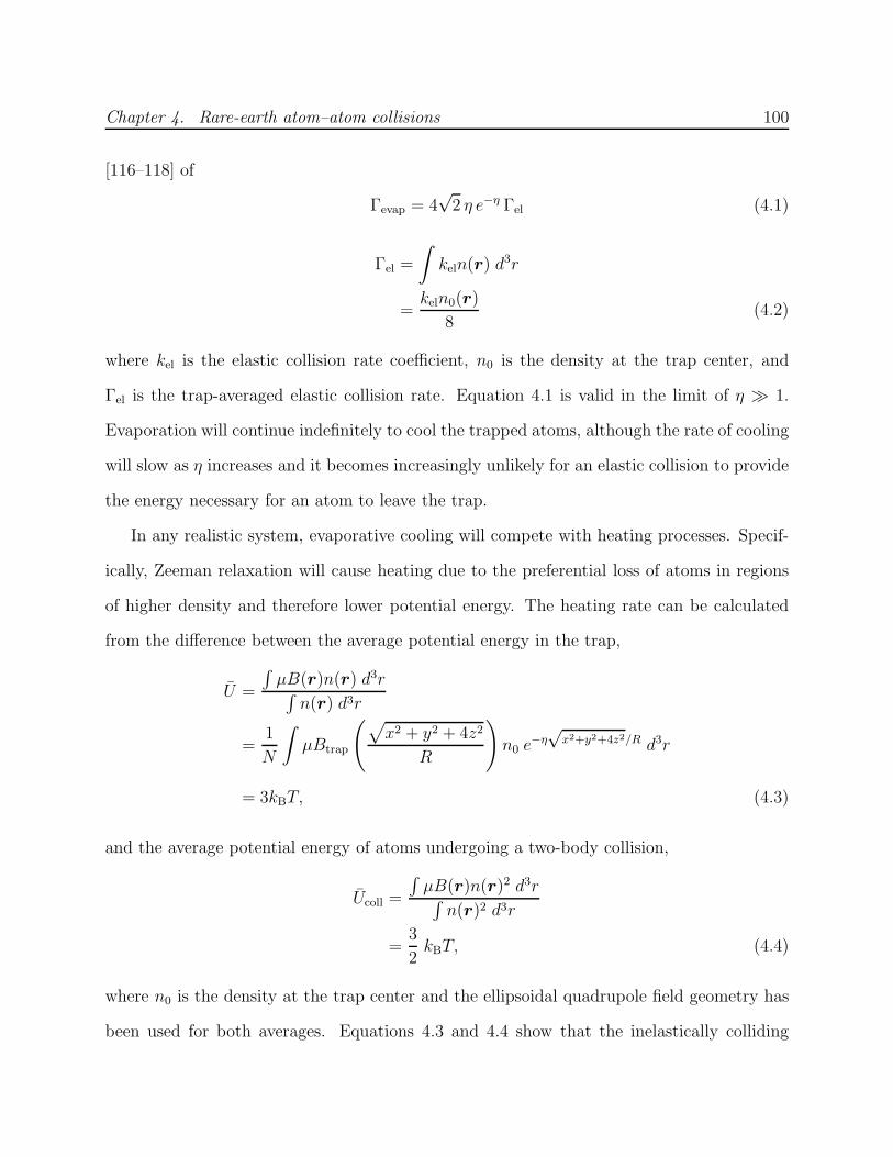
Chapter 4. Rare-earth atom–atom collisions 100
[116–118] of
Γevap = 4√
2 η e−η Γel (4.1)
Γel =
∫
keln(r) d3r
=keln0(r)
8(4.2)
where kel is the elastic collision rate coefficient, n0 is the density at the trap center, and
Γel is the trap-averaged elastic collision rate. Equation 4.1 is valid in the limit of η ≫ 1.
Evaporation will continue indefinitely to cool the trapped atoms, although the rate of cooling
will slow as η increases and it becomes increasingly unlikely for an elastic collision to provide
the energy necessary for an atom to leave the trap.
In any realistic system, evaporative cooling will compete with heating processes. Specif-
ically, Zeeman relaxation will cause heating due to the preferential loss of atoms in regions
of higher density and therefore lower potential energy. The heating rate can be calculated
from the difference between the average potential energy in the trap,
U =
∫
µB(r)n(r) d3r∫
n(r) d3r
=1
N
∫
µBtrap
(
√
x2 + y2 + 4z2
R
)
n0 e−η√
x2+y2+4z2/R d3r
= 3kBT, (4.3)
and the average potential energy of atoms undergoing a two-body collision,
Ucoll =
∫
µB(r)n(r)2 d3r∫
n(r)2 d3r
=3
2kBT, (4.4)
where n0 is the density at the trap center and the ellipsoidal quadrupole field geometry has
been used for both averages. Equations 4.3 and 4.4 show that the inelastically colliding
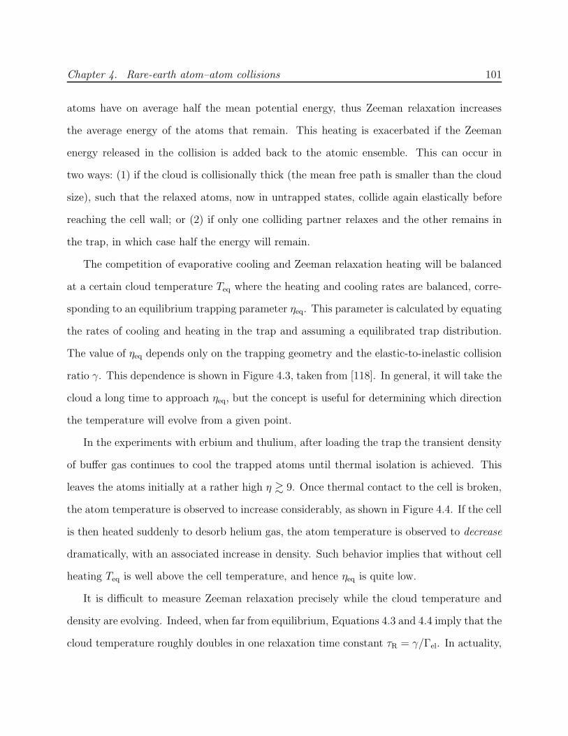
Chapter 4. Rare-earth atom–atom collisions 101
atoms have on average half the mean potential energy, thus Zeeman relaxation increases
the average energy of the atoms that remain. This heating is exacerbated if the Zeeman
energy released in the collision is added back to the atomic ensemble. This can occur in
two ways: (1) if the cloud is collisionally thick (the mean free path is smaller than the cloud
size), such that the relaxed atoms, now in untrapped states, collide again elastically before
reaching the cell wall; or (2) if only one colliding partner relaxes and the other remains in
the trap, in which case half the energy will remain.
The competition of evaporative cooling and Zeeman relaxation heating will be balanced
at a certain cloud temperature Teq where the heating and cooling rates are balanced, corre-
sponding to an equilibrium trapping parameter ηeq. This parameter is calculated by equating
the rates of cooling and heating in the trap and assuming a equilibrated trap distribution.
The value of ηeq depends only on the trapping geometry and the elastic-to-inelastic collision
ratio γ. This dependence is shown in Figure 4.3, taken from [118]. In general, it will take the
cloud a long time to approach ηeq, but the concept is useful for determining which direction
the temperature will evolve from a given point.
In the experiments with erbium and thulium, after loading the trap the transient density
of buffer gas continues to cool the trapped atoms until thermal isolation is achieved. This
leaves the atoms initially at a rather high η & 9. Once thermal contact to the cell is broken,
the atom temperature is observed to increase considerably, as shown in Figure 4.4. If the cell
is then heated suddenly to desorb helium gas, the atom temperature is observed to decrease
dramatically, with an associated increase in density. Such behavior implies that without cell
heating Teq is well above the cell temperature, and hence ηeq is quite low.
It is difficult to measure Zeeman relaxation precisely while the cloud temperature and
density are evolving. Indeed, when far from equilibrium, Equations 4.3 and 4.4 imply that the
cloud temperature roughly doubles in one relaxation time constant τR = γ/Γel. In actuality,
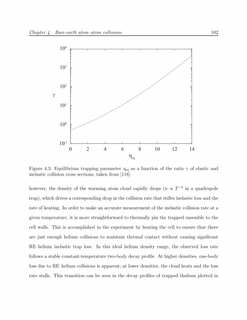
Chapter 4. Rare-earth atom–atom collisions 102
0 2 4 6 8 10 12 14
104
103
102
101
100
10-1
ηeq
γ
Figure 4.3: Equilibrium trapping parameter ηeq as a function of the ratio γ of elastic andinelastic collision cross sections, taken from [118].
however, the density of the warming atom cloud rapidly drops (n ∝ T−3 in a quadrupole
trap), which drives a corresponding drop in the collision rate that stifles inelastic loss and the
rate of heating. In order to make an accurate measurement of the inelastic collision rate at a
given temperature, it is more straightforward to thermally pin the trapped ensemble to the
cell walls. This is accomplished in the experiment by heating the cell to ensure that there
are just enough helium collisions to maintain thermal contact without causing significant
RE–helium inelastic trap loss. In this ideal helium density range, the observed loss rate
follows a stable constant-temperature two-body decay profile. At higher densities, one-body
loss due to RE–helium collisions is apparent; at lower densities, the cloud heats and the loss
rate stalls. This transition can be seen in the decay profiles of trapped thulium plotted in
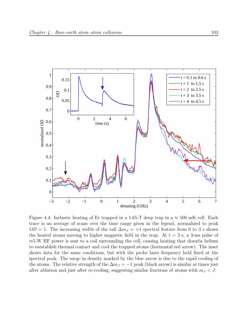
Chapter 4. Rare-earth atom–atom collisions 103
−3 −2 −1 0 1 2 3 4 5 6 7
0
0.1
0.2
0.3
0.4
0.5
0.6
0.7
0.8
0.9
1
detuning (GHz)
norm
aliz
ed O
D
t = 0.1 to 0.6 st = 1 to 1.5 st = 2 to 2.5 st = 3 to 3.5 st = 4 to 4.5 s
0 2 4 6
0
0.05
0.1
0.15
time (s)
OD
Figure 4.4: Inelastic heating of Er trapped in a 1.65-T deep trap in a ≈ 500 mK cell. Eachtrace is an average of scans over the time range given in the legend, normalized to peakOD = 1. The increasing width of the tall ∆mJ = +1 spectral feature from 0 to 3 s showsthe heated atoms moving to higher magnetic field in the trap. At t = 3 s, a 3-ms pulse of≈5-W RF power is sent to a coil surrounding the cell, causing heating that desorbs heliumto reestablish thermal contact and cool the trapped atoms (horizontal red arrow). The insetshows data for the same conditions, but with the probe laser frequency held fixed at thespectral peak. The surge in density marked by the blue arrow is due to the rapid cooling ofthe atoms. The relative strength of the ∆mJ = −1 peak (black arrow) is similar at times justafter ablation and just after re-cooling, suggesting similar fractions of atoms with mJ < J .
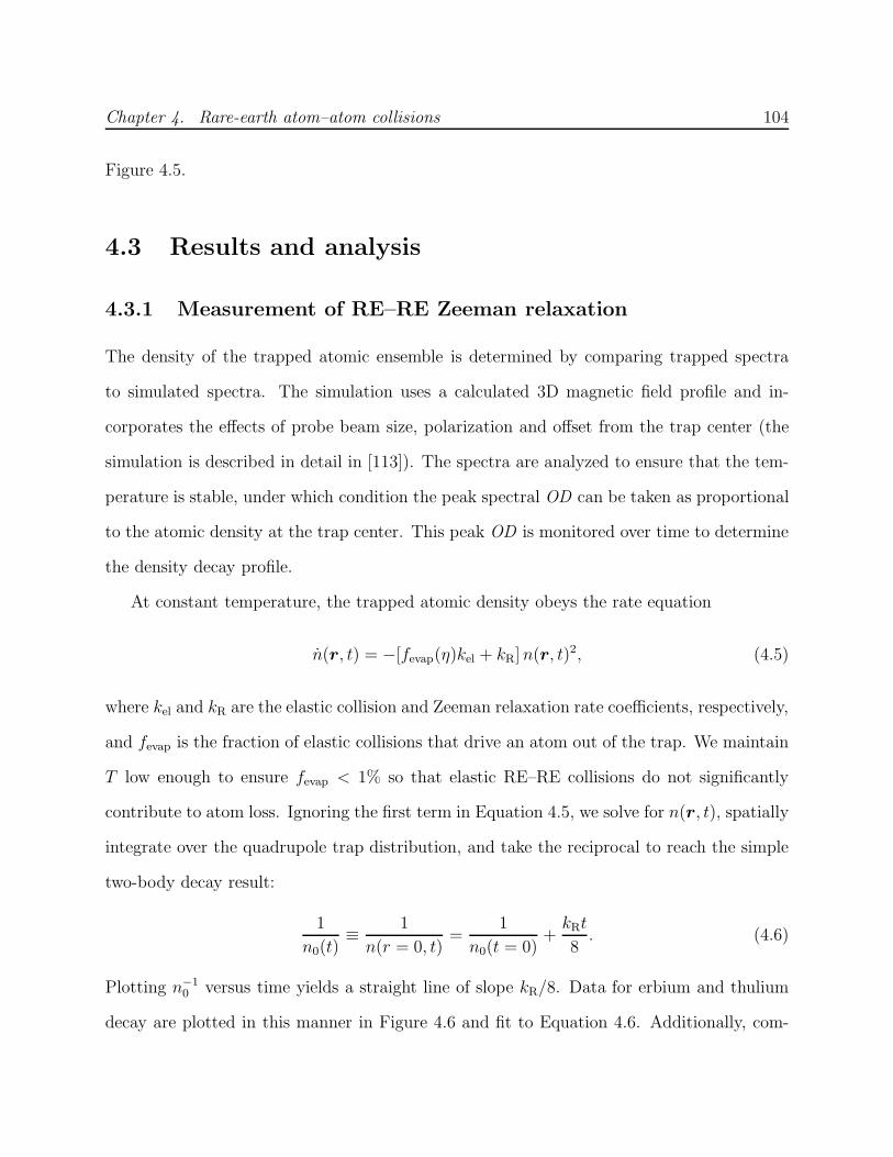
Chapter 4. Rare-earth atom–atom collisions 104
Figure 4.5.
4.3 Results and analysis
4.3.1 Measurement of RE–RE Zeeman relaxation
The density of the trapped atomic ensemble is determined by comparing trapped spectra
to simulated spectra. The simulation uses a calculated 3D magnetic field profile and in-
corporates the effects of probe beam size, polarization and offset from the trap center (the
simulation is described in detail in [113]). The spectra are analyzed to ensure that the tem-
perature is stable, under which condition the peak spectral OD can be taken as proportional
to the atomic density at the trap center. This peak OD is monitored over time to determine
the density decay profile.
At constant temperature, the trapped atomic density obeys the rate equation
n(r, t) = −[fevap(η)kel + kR]n(r, t)2, (4.5)
where kel and kR are the elastic collision and Zeeman relaxation rate coefficients, respectively,
and fevap is the fraction of elastic collisions that drive an atom out of the trap. We maintain
T low enough to ensure fevap < 1% so that elastic RE–RE collisions do not significantly
contribute to atom loss. Ignoring the first term in Equation 4.5, we solve for n(r, t), spatially
integrate over the quadrupole trap distribution, and take the reciprocal to reach the simple
two-body decay result:
1
n0(t)≡ 1
n(r = 0, t)=
1
n0(t = 0)+kRt
8. (4.6)
Plotting n−10 versus time yields a straight line of slope kR/8. Data for erbium and thulium
decay are plotted in this manner in Figure 4.6 and fit to Equation 4.6. Additionally, com-
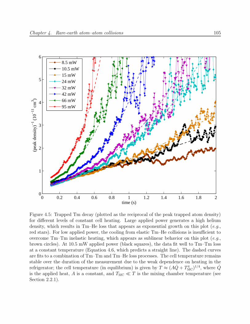
Chapter 4. Rare-earth atom–atom collisions 105
0 0.2 0.4 0.6 0.8 1 1.2 1.4 1.6 1.8 20
1
2
3
4
5
6
time (s)
(pea
k de
nsity
)−1 (
10−
11 c
m3 )
8.5 mW10.5 mW15 mW24 mW32 mW42 mW66 mW95 mW
Figure 4.5: Trapped Tm decay (plotted as the reciprocal of the peak trapped atom density)for different levels of constant cell heating. Large applied power generates a high heliumdensity, which results in Tm–He loss that appears as exponential growth on this plot (e.g.,red stars). For low applied power, the cooling from elastic Tm–He collisions is insufficient toovercome Tm–Tm inelastic heating, which appears as sublinear behavior on this plot (e.g.,brown circles). At 10.5 mW applied power (black squares), the data fit well to Tm–Tm lossat a constant temperature (Equation 4.6, which predicts a straight line). The dashed curvesare fits to a combination of Tm–Tm and Tm–He loss processes. The cell temperature remainsstable over the duration of the measurement due to the weak dependence on heating in therefrigerator; the cell temperature (in equilibrium) is given by T ≈ (AQ + T 4
MC)1/4, where Qis the applied heat, A is a constant, and TMC ≪ T is the mixing chamber temperature (seeSection 2.2.1).

Chapter 4. Rare-earth atom–atom collisions 106
0 0.5 1 1.5 2 2.5 30
1
2
3
4
5
6
time (s)
(pea
k de
nsity
)−1 (
10−
11 c
m3 )
B
0 1 2 3 4 5 6 7 8 90
1
2
3
4
(pea
k de
nsity
)−1 (
10−
10 c
m3 )
time (s)
A datafit to RE–RE loss modelfit to RE–He loss model
Figure 4.6: Decay of trapped (A) erbium and (B) thulium. The vertical axis is the reciprocalof the peak atom density determined from spectra. The solid red line is a fit to Equation 4.6,for decay only from RE–RE collisions. The dashed blue line is a fit to the exponential decayexpected for loss only due to collisions with a constant helium density. The excellent fits toEquation 4.6 indicate that the atom loss is due to RE–RE collisions.
bined fits were made with free parameters for both RE–RE and RE–helium collisional loss
processes. These combined fits yielded RE–helium decay rates consistent with zero, con-
firming that the observed loss is due to Zeeman relaxation collisions between the trapped
atoms. The values of kR given by fits to Equation 4.6 are 1.5(0.2)×10−10 cm3 s−1 for erbium
and 5.7(1.5) × 10−11 cm3 s−1 for thulium, with accuracy limited by the density calibration
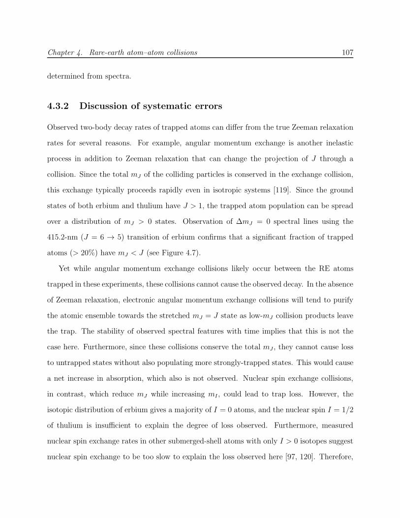
Chapter 4. Rare-earth atom–atom collisions 107
determined from spectra.
4.3.2 Discussion of systematic errors
Observed two-body decay rates of trapped atoms can differ from the true Zeeman relaxation
rates for several reasons. For example, angular momentum exchange is another inelastic
process in addition to Zeeman relaxation that can change the projection of J through a
collision. Since the total mJ of the colliding particles is conserved in the exchange collision,
this exchange typically proceeds rapidly even in isotropic systems [119]. Since the ground
states of both erbium and thulium have J > 1, the trapped atom population can be spread
over a distribution of mJ > 0 states. Observation of ∆mJ = 0 spectral lines using the
415.2-nm (J = 6 → 5) transition of erbium confirms that a significant fraction of trapped
atoms (> 20%) have mJ < J (see Figure 4.7).
Yet while angular momentum exchange collisions likely occur between the RE atoms
trapped in these experiments, these collisions cannot cause the observed decay. In the absence
of Zeeman relaxation, electronic angular momentum exchange collisions will tend to purify
the atomic ensemble towards the stretched mJ = J state as low-mJ collision products leave
the trap. The stability of observed spectral features with time implies that this is not the
case here. Furthermore, since these collisions conserve the total mJ , they cannot cause loss
to untrapped states without also populating more strongly-trapped states. This would cause
a net increase in absorption, which also is not observed. Nuclear spin exchange collisions,
in contrast, which reduce mJ while increasing mI , could lead to trap loss. However, the
isotopic distribution of erbium gives a majority of I = 0 atoms, and the nuclear spin I = 1/2
of thulium is insufficient to explain the degree of loss observed. Furthermore, measured
nuclear spin exchange rates in other submerged-shell atoms with only I > 0 isotopes suggest
nuclear spin exchange to be too slow to explain the loss observed here [97, 120]. Therefore,
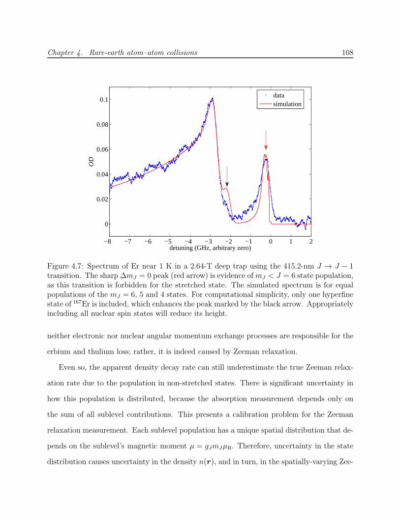
Chapter 4. Rare-earth atom–atom collisions 108
−8 −7 −6 −5 −4 −3 −2 −1 0 1 2
0
0.02
0.04
0.06
0.08
0.1O
D
detuning (GHz, arbitrary zero)
datasimulation
Figure 4.7: Spectrum of Er near 1 K in a 2.64-T deep trap using the 415.2-nm J → J − 1transition. The sharp ∆mJ = 0 peak (red arrow) is evidence of mJ < J = 6 state population,as this transition is forbidden for the stretched state. The simulated spectrum is for equalpopulations of the mJ = 6, 5 and 4 states. For computational simplicity, only one hyperfinestate of 167Er is included, which enhances the peak marked by the black arrow. Appropriatelyincluding all nuclear spin states will reduce its height.
neither electronic nor nuclear angular momentum exchange processes are responsible for the
erbium and thulium loss; rather, it is indeed caused by Zeeman relaxation.
Even so, the apparent density decay rate can still underestimate the true Zeeman relax-
ation rate due to the population in non-stretched states. There is significant uncertainty in
how this population is distributed, because the absorption measurement depends only on
the sum of all sublevel contributions. This presents a calibration problem for the Zeeman
relaxation measurement. Each sublevel population has a unique spatial distribution that de-
pends on the sublevel’s magnetic moment µ = gJmJµB. Therefore, uncertainty in the state
distribution causes uncertainty in the density n(r), and in turn, in the spatially-varying Zee-
Chapter 4. Rare-earth atom–atom collisions 109
man relaxation rate ΓR(r) = kR n(r). Since the observed trap loss is only the trap-averaged
rate, measuring kR requires knowledge of the mJ -state distribution.
This distribution is determined by several factors. Initially, the ablated atoms are equally
distributed over all mJ states. Untrapped states with mJ ≤ 0 are rapidly lost. The states
with the lowest positive values of mJ are only weakly trapped (η < 4.5 at maximum magnetic
field) and evaporate quickly, especially in the presence of thermalizing helium collisions.
Other states, however, will evaporate slowly enough that they remain in the trap throughout
the Zeeman relaxation measurement. Meanwhile, Zeeman relaxation on average causes mJ
to decrease for one or both atoms during an inelastic collision, which repopulates states with
positive mJ < J as they evaporate. At finite temperature, thermal excitations will also
occur, as discussed in Section 2.3.2. Finally, the electronic angular momentum exchange
collisions discussed above will cause mixing of the mJ -state distribution and in general speed
it toward equilibrium. Lacking a definitive measurement of the state distribution, all these
effects combined can introduce significant systematic error to the measurement of kR that
comes from simply applying Equation 4.6.
4.3.3 Simulation of trap dynamics
To study the impact of the effects described in the previous section on the measured Zee-
man relaxation rates, we perform numerical simulations of the trap dynamics. Population in
multiple magnetic sublevels will cause a deviation from Equation 4.6. The three dominant
effects are: (1) the spatial integration of Equation 4.5 depends on the cumulative density
profile n(r) =∑
mJnmJ
(r); (2) thermal excitations occasionally drive relaxation away from
equilibrium; and (3) the so-called “Zeeman cascade” of inelastic transitions to still-trapped
states will require that more than one collision, on average, is necessary for atoms to leave
the trap. The simulation is not intended to be a precise model of these effects—its accuracy
Chapter 4. Rare-earth atom–atom collisions 110
is limited by uncertainty in the state distribution, as well as in the state-specific inelastic
collision rates and helium density. Instead, the simulation is constructed to investigate the
range of simulated parameters that produce trap decay profiles consistent with the experi-
ment. This range is then used to determine an overall estimate of systematic error in the
measurement of kR.
Since there are a large number of particles at high η in the trap, the simulation expresses
the density and collision rates as continuous variables in a series of rate equations. Elastic
collisions with both helium and other trapped atoms are assumed to be rapid enough to
thermalize the distribution, since no significant spectral deformation is observed. Inelastic
collisions, both angular momentum exchange and relaxation, are assumed to proceed with the
same rate coefficients kex and kR for all sublevels. These collisions may, however, prudentially
cause transitions to certain final states. This is accounted for by including selection rules
that vary from 0 (final state not allowed) to 1 (final state maximally allowed). In the case of
Zeeman relaxation, we expect that transitions of |∆mJ | ≤ 2 will be favored for the following
a priori reasons: For relaxation driven by electronic interaction anisotropy, the coupling
to more distant mJ states is a higher-order process, as demonstrated theoretically for the
thulium–helium and oxygen–helium systems [91, 121]. Similarly, the magnetic dipole-dipole
interaction couples states of ∆mJ = ±1 to first order [47]. For either mechanism, such
selection rules would imply that trapped states of high-J atoms like erbium and thulium will
often relax to still-trapped states.
The inelastic collision rates are calculated as follows. First, the rate of electronic angular
Chapter 4. Rare-earth atom–atom collisions 111
momentum exchange, which conserves the total mJ of the colliding partners, is given by
(nmJ)ex =
kex2
∑
m′
J
∑
m′′
J
∑
m′′′
J
[
β|m′′
J−mJ |δ[(mJ +m′
J ) − (m′′J +m′′′
J )]
×(
nm′′
Jnm′′′
J− nmJ
nm′
J
)]
, (4.7)
where kex is the exchange rate coefficient, δ[x] is the Kronecker delta that vanishes for
x 6= 0 and is otherwise unity, and β|∆mJ | is the selection rule for exchange that changes the
projection of J on the field axis by ∆mJ . The factor of 1/2 accounts for double-counting in
the summation. Second, the Zeeman relaxation rate is given by
(nmJ)R = kR nmJ
∑
m′
J<mJ
αmJ ,m′
J
(
nm′
Jexp
(
−(mJ −m′J )gJµBB
kBT
)
− nmJ
)
+∑
m′
J>mJ
αmJ ,m′
J
(
nm′
J− nmJ
exp
(
−(m′J −mJ)gJµBB
kBT
))
, (4.8)
where αmJ ,m′
Jis the selection rule for relaxation mJ → m′
J . Thermal excitations have been
included in Equation 4.8. Inelastic RE–helium collisions occur rarely and are ignored in the
simulation.
Additionally, the simulation calculates the loss rates for evaporation due to elastic colli-
sions. Equation 4.1 is used to determine the evaporation rate from RE–RE collisions, while
RE–helium evaporation is given by
ΓHe evap = ΓRE–He ǫ (M,m) f (η) , (4.9)
where ΓRE–He = nbσdv is the RE–helium collision rate,
ǫ (M,m) =Mm
(M +m)2(4.10)
is the energy transfer efficiency in a collision between two masses M and m [51], and
f (η) ≈(
1
2η3/2 +
1
4η5/2
)
e−η, (4.11)
Chapter 4. Rare-earth atom–atom collisions 112
is the fraction of thermalized trapped atoms with sufficient energy to leave the trap [113].
This expression for f (η) was found by Brahms to be a good approximation at high η of the
more precise result that comes from numerical integration of the Boltzmann distribution.
The elastic and inelastic contributions are added and propagated in time to numerically
simulate the atomic density distribution and calculate the corresponding OD seen by the
probe laser. A range of parameter space is explored to identify conditions under which
it is possible to reproduce the observed data. One such example is shown in Figure 4.8.
As stated above, this process does not provide good constraints to the many underlying
parameters; however, it is useful to demonstrate that simple application of Equation 4.6 to
the observed OD decay—as in Section 4.3.1—will yield a value of kR that underestimates the
true Zeeman relaxation rate by a factor of approximately 2.0 +1.0−0.5. With this correction, the
rate coefficients kR are 3.0(0.4)× 10−10 cm3 s−1 for erbium and 1.1(0.3)× 10−10 cm3 s−1 for
thulium.
4.4 Possible mechanisms of RE–RE Zeeman
relaxation
4.4.1 Magnetic dipole-dipole interaction
The rates of Zeeman relaxation measured for collisions between erbium and between thulium
atoms are significantly higher than inelastic rates observed for other highly magnetic S-state
atoms such as chromium [32, 122], europium [97], manganese [120] and molybdenum [33].
The relaxation rate coefficients for these species were measured in similar magnetic traps at
similar temperatures and found to be . 10−12 cm3 s−1. These S-state atom–atom rates are

Chapter 4. Rare-earth atom–atom collisions 113
108
109
1010
1011
Er
peak
den
sity
(cm−
3 )
A sum of all statesm
J = 6
mJ = 5
mJ = 4
mJ = 3
mJ = 2
mJ = 1
0 1 2 3 4 5 6 7 8 9−0.1
−0.05
0
0.05
0.1
time (s)
resi
dual
from
Er–
Er
fit (
cm−
3 )
B
datasublevel simulation
Figure 4.8: (A) Simulation of Er decay under the conditions of Figure 4.6A, including theeffects of thermal excitations, Zeeman relaxation selection rules, nearest-state electronicangular momentum exchange, and collisions with the helium buffer gas; (B) residuals fromthe fit to Equation 4.6 shown in Figure 4.6A for both the measured data and the simulatedtotal density shown in (A). This simulation is for kR = 3 × 10⁻¹⁰ cm3 s−1, twice the numberextracted from the data. Many simulations are performed to estimate the systematic errorcaused by simply fitting to Equation 4.6.
consistent with the magnetic dipole-dipole interaction [123–125] described by
Vdipole(r) =µ0
4π
µ2
r3[(J1·J2) − 3(J1· r)(J2· r)]. (4.12)
The Zeeman relaxation rate induced by the operator Vdipole is dependent on the specific form
of the interatomic potential. However, in the limit of small inelastic transition probability
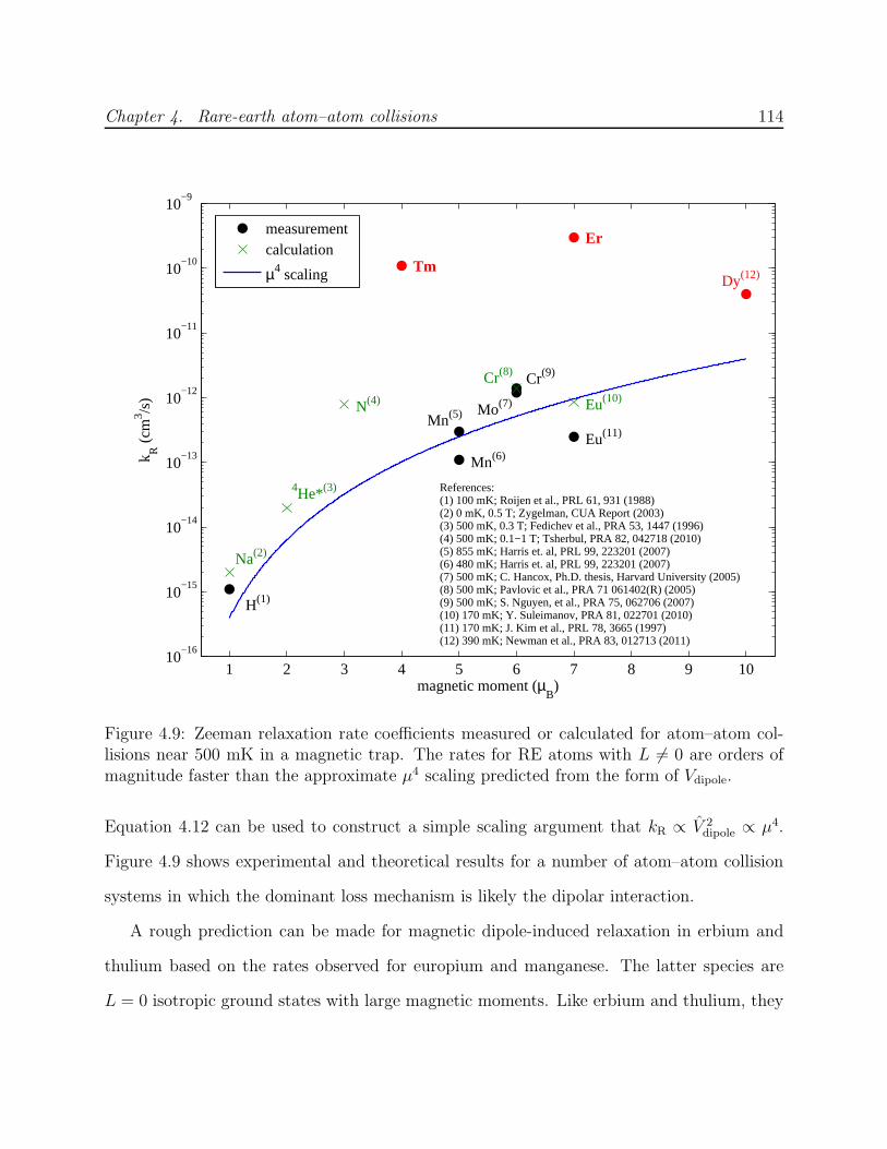
Chapter 4. Rare-earth atom–atom collisions 114
1 2 3 4 5 6 7 8 9 1010
−16
10−15
10−14
10−13
10−12
10−11
10−10
10−9
magnetic moment (µB)
k R (
cm3 /s
)
Cr(9)
Mo(7)
Eu(11)Mn(5)
Mn(6)
H(1)
Na(2)
4He*(3)
N(4) Eu(10)
Cr(8)
Tm
Er
Dy(12)
measurementcalculation
µ4 scaling
References:(1) 100 mK; Roijen et al., PRL 61, 931 (1988)(2) 0 mK, 0.5 T; Zygelman, CUA Report (2003)(3) 500 mK, 0.3 T; Fedichev et al., PRA 53, 1447 (1996)(4) 500 mK; 0.1−1 T; Tsherbul, PRA 82, 042718 (2010)(5) 855 mK; Harris et. al, PRL 99, 223201 (2007)(6) 480 mK; Harris et. al, PRL 99, 223201 (2007)(7) 500 mK; C. Hancox, Ph.D. thesis, Harvard University (2005)(8) 500 mK; Pavlovic et al., PRA 71 061402(R) (2005)(9) 500 mK; S. Nguyen, et al., PRA 75, 062706 (2007)(10) 170 mK; Y. Suleimanov, PRA 81, 022701 (2010)(11) 170 mK; J. Kim et al., PRL 78, 3665 (1997)(12) 390 mK; Newman et al., PRA 83, 012713 (2011)
Figure 4.9: Zeeman relaxation rate coefficients measured or calculated for atom–atom col-lisions near 500 mK in a magnetic trap. The rates for RE atoms with L 6= 0 are orders ofmagnitude faster than the approximate µ4 scaling predicted from the form of Vdipole.
Equation 4.12 can be used to construct a simple scaling argument that kR ∝ V 2dipole ∝ µ4.
Figure 4.9 shows experimental and theoretical results for a number of atom–atom collision
systems in which the dominant loss mechanism is likely the dipolar interaction.
A rough prediction can be made for magnetic dipole-induced relaxation in erbium and
thulium based on the rates observed for europium and manganese. The latter species are
L = 0 isotropic ground states with large magnetic moments. Like erbium and thulium, they
Chapter 4. Rare-earth atom–atom collisions 115
are also submerged-shell atoms. Scaling the cross sections measured for europium [97] and
manganese [33] by µ4 and averaging yields predictions of kR = 3.4 × 10⁻¹³ cm3 s−1 for
erbium and 3.5 × 10⁻¹⁴ cm3 s−1 for thulium. The measured inelastic rate coefficients in
our experiments are 2–3 orders of magnitude larger than these scaled dipolar values. We
therefore conclude that the measured loss is inconsistent with a purely dipolar model.
4.4.2 Electrostatic quadrupole-quadrupole interaction
Another possible loss mechanism is the electrostatic quadrupole-quadrupole interaction. Like
the magnetic dipole-dipole interaction, this interaction is long-range (Vquad ∝ r−5) and thus
should not be shielded by outer electrons. The quadrupole moment tensor operator is defined
as [126]
Q2q =∑
i
r2i
√
4π
5Y 2q (θi, φi), (4.13)
where ri is the electronic coordinate, Y ℓm are the spherical harmonics, and the sum is taken
over all electrons in the atom. The atomic quadrupole moment refers to the Θzz component
of the expectation value of Q2q,
Θzz = 〈LmL| Q20 |LmL〉, (4.14)
which by the Wigner-Eckart theorem has only one truly independent component. Hence the
quadrupole moment is often written simply as Q and taken to be the mL = L component
of Θzz. The quadrupole-quadrupole interaction operator is then proportional to the product
of the quadrupole moments of the colliding partners (Vquad ∝ Q2 for atom–atom collisions).
Since 〈LmL| Y 2m |LmL〉 = 0 for L < 1, this interaction vanishes for collisions of S-state
atoms including all collisions with helium; but it is nonzero for nearly all lanthanide RE–RE
collisions, including those of erbium and thulium.

Chapter 4. Rare-earth atom–atom collisions 116
There is reason to expect, however, that the quadrupole moments of RE atoms are small.
The relativistic collapse of the valence electron shells implies that the electrons are close to
the nucleus—the same reason that the anisotropy is submerged—and hence the moment arm
(ri in Equation 4.13) is small. Calculations for the RE atoms thulium [127] and dysprosium
[128] give values of Q < 0.2 a.u., which corresponds to an interaction energy of .100 mK
(in temperature units) at R = 10 Bohr radii, approximately the inner turning point of the
RE–helium potential. This is similar to the magnetic dipole-dipole interaction energy (at
the same R), ≈200 and ≈50 mK for erbium and thulium, respectively; thus it is unlikely
that the electrostatic quadrupole-quadrupole interaction is responsible for the rapid RE–RE
relaxation.
4.4.3 Electronic interaction anisotropy
The inelasticity in the anisotropic RE–RE systems studied here is comparable to that ob-
served in anisotropic outer-shell (non-submerged) systems. For example, experiments with
metastable 3P2 states of calcium, strontium and ytterbium have observed very rapid inelastic
rate coefficients greater than 10−11 cm3 s−1 [90, 129, 130]. This comparison suggests that
the submerged-shell model of anisotropy shielding that successfully described RE–helium
collisions may not be appropriate to RE–RE systems. A stronger RE–RE interaction poten-
tial may overcome the shielding effect as the atoms approach each other and experience the
valence anisotropy at short range.
In response to recent experiments using laser-cooled dysprosium atoms, Kotochigova and
Petrov [128] performed calculations of dysprosium–dysprosium collisions in the ultracold s-
wave limit using a universal single-channel loss model. Their calculations yield large inelastic
rates at the same order of magnitude as observed experimentally [131], and specifically iden-
tify electrostatic interaction anisotropy as the dominant mechanism with a significant addi-
Chapter 4. Rare-earth atom–atom collisions 117
tional contribution from the magnetic dipole-dipole interaction (dysprosium has the largest
magnetic moment of any atom, µ = 9.93 µB). In contrast, the electrostatic quadrupole-
quadrupole interaction was shown to be a much weaker effect. Collisions in dysprosium
were also experimentally studied at 390 mK by Newman et al. [132], finding large relaxation
rates similar to those of erbium and thulium. Since these three RE atoms have similarly
anisotropic valence shells, there is now strong evidence that the dramatic suppression of elec-
tronic interaction anisotropy observed in the RE–helium systems does not exist for collisions
between RE atoms.
4.5 Future prospects for RE atoms
An unfortunate consequence of the rapid Zeeman relaxation measured in this experiment
is that it is likely that evaporative cooling of these atoms in a magnetic trap is impossible.
Evaporative cooling relies on elastic collisions after losing atoms to evaporation in order to
thermalize the trapped distribution to a lower temperature, requiring γ & 100 for efficient
evaporation [116]. This is not a fundamental limit; cooling can occur for lower values of γ
over small temperature ranges, but significantly increased losses will be sustained.
The value of kel, and hence γ, for erbium and thulium is not measured in this experi-
ment, but an estimate can be obtained from the unitarity limit. For collisions at a finite
temperature, the total collision cross section σ in the absence of resonances is bounded by
[133]
σ <ℓmax∑
ℓ=0
λthπ
(2ℓ+ 1)
<2~2
µkBT
ℓmax∑
ℓ=0
(2ℓ+ 1) (4.15)
where λth =√
2π~2/µkBT is the thermal de Broglie wavelength of the colliding system with
Chapter 4. Rare-earth atom–atom collisions 118
reduced mass µ, and ℓmax is the maximum partial wave involved in the collision. ℓmax is
found by equating the average collision energy EK = 3kBT/2 with the centrifugal barrier in
the approximate Van der Waals potential
V (R) =~2ℓ2
2µR2− C6
r6(4.16)
to yield
ℓmax =
õ
~
[(
3
2kBT
)
√
54C6
]1/3
(4.17)
The C6 coefficient has not been calculated for erbium and thulium and must be estimated.
With the expectation that other lanthanide RE atoms will have similar isotropic parts of the
potential, we take the mean of theoretical calculations for ytterbium [134] and dysprosium
[128] to yield C6 ≈ 1,970 a.u. For erbium and thulium at 500 mK, this corresponds to ≈40
partial waves and a unitarity limit kel ≈ 8× 10⁻¹⁰ cm3 s−1. With this limit, γ . 10 for both
atoms, well below the minimum required for efficient evaporative cooling in a magnetic trap.
Since each non-S-state RE atom studied thus far has exhibited similarly rapid relaxation,
there is little reason to be optimistic for others in the lanthanide series, with the possible
exception of europium (8S7/2).
The inelasticity in these RE–RE systems has been a setback for experimental progress
with these atoms. The earlier success in trapping >1011 of these highly magnetic and
anisotropic atoms held promise that evaporative cooling of buffer-gas trapped RE atoms
could provide a route to very large ultracold ensembles. Such techniques have already been
demonstrated to achieve Bose-Einstein condensation of metastable helium-4 [31]. Instead,
it may be that the RE–helium collisions that allow for buffer-gas trap loading are uniquely
insulated from the interactions that cause trap loss. As a result, cooling RE atoms to the
ultracold regime requires alternate methods.
Great progress has very recently been made using all-optical methods to cool erbium,
thulium and dysprosium. Both dysprosium and erbium atoms have now been laser cooled in
Chapter 4. Rare-earth atom–atom collisions 119
a magneto-optical trap (MOT), loaded directly into an optical dipole trap and evaporatively
cooled to quantum degeneracy [11, 135, 136]. Similar work is underway with thulium [137].
The atom numbers are not large, however (<105 at degeneracy), limited by MOT density
and temperature together with the finite optical dipole trap size and depth. The inelastic
collision rates are found to be large in the ultracold regime, as well [131], so the short
lifetimes of certain states may limit the scope of future experiments. Nevertheless, despite
being constrained to different technologies, progress continues with these interesting systems.

Chapter 5
Conclusion
5.1 Summary of collision experiments
We investigate the role of anisotropic interactions in driving inelastic collisions between
atoms at low temperatures. We explore how relativistic effects and collisional mixing of
energy levels lead to electronic interaction anisotropy that induces Zeeman relaxation. In
addition to developing a more complete model of inelastic atomic collisions, these results are
technically important to experiments. Buffer-gas loading of magnetic traps requires elastic
collisions with helium for cooling, while evaporative cooling requires elastic collisions between
trapped atoms. In both cases, relaxation must be sufficiently rare so that the colliding atoms
remain in the trapped state.
The experiments presented here explore inelastic atomic collisions arising from three
distinct mechanisms. In the first experiment, Zeeman relaxation of antimony occurs in
collisions with helium due to distortion of the ground-state wave function induced by the
spin-orbit interaction. Couplings to excited states introduce anisotropy into the ground
state independent of the collision, so that the interaction with helium is anisotropic. This
120

Chapter 5. Conclusion 121
fundamentally relativistic effect is a strong function of the nuclear charge and is seen to
vary dramatically among the pnictogen atoms, with greatest wave function distortion for
the heavy atoms antimony and bismuth. As a result, the excellent collisional properties of
nitrogen are likely a special case, and no other pnictogen atom exists that could replace
nitrogen in collision experiments while providing more practical detection options.
In the second experiment, inelastic aluminum–helium collisions are suppressed by the
spherical symmetry of the ground 2P1/2 state. In this case, inelastic transitions occur by a
collision-induced admixture of the anisotropic 2P3/2 state. The same is true for the other
Group 13 atoms gallium, indium and thallium, as well as metastable halogen atoms [1], with
the inelastic collision rate suppressed by the fine-structure splitting between the states. For
the heavier species with large splitting, the Zeeman relaxation rate is extremely low, with
calculated values of γ well over 107 for collisions with helium. It may then be possible to
sympathetically cool these atoms with other S-state atoms, provided that the interaction
strength remains sufficiently weaker than the fine-structure splitting.
In the third experiment, we extend earlier work observing suppressed inelasticity in col-
lisions of anisotropic rare-earth (RE) lanthanide atoms with helium [2] to examine RE–RE
collisions, observing no evidence of similar suppression. Indeed, we find inelastic collisions
between RE atoms to be just as rapid as those between anisotropic open-shell atoms such
as metastable 3P states of ytterbium [90] and calcium [129], with relaxation rates similar to
the elastic collision rates. Thus we demonstrate a fundamental difference between these two
systems, along with the limitations of the “submerged-shell” collision model used to describe
them. If the interparticle interaction is sufficiently strong, Zeeman relaxation driven by elec-
trostatic interaction anisotropy proceeds rapidly despite the anisotropic valence electrons
being submerged below spherical closed electron shells. As a result, evaporative cooling in
a magnetic trap is not feasible with these atoms. Instead other technologies, such as optical
Chapter 5. Conclusion 122
dipole traps that can trap the absolute ground state, must be employed, along with their
associated disadvantages of low trap depth and size.
5.2 An increasingly complete picture
The three experiments described here join a wealth of previous work in painting an in-
creasingly complete picture of atomic collisions. The variety of interaction mechanisms and
collisional processes seen across the periodic table is impressive, and has led to an equal or
greater variety of applications for further experiments and technologies. While there remain
unanswered questions—and surely surprises—the landscape has now been rather well ex-
plored. It is increasingly possible for theoreticians to make accurate predictions about novel
systems, and for experimenters to make informed decisions of which collisions to pursue,
exploit or avoid.
In particular, it is clear that elasticity in atomic collisions is not the norm. The majority
of atoms in the periodic table are not S-states, and as a result Zeeman relaxation induced
by collisions between two randomly chosen atoms is likely to be rapid. There are notable
exceptions, such as the suppressed relaxation seen in RE–helium systems and in collisions
of 2P1/2 states with S-states. There are also, however, many S-state atoms that readily
undergo inelastic transitions due to relativistic wave function distortion (i.e., antimony) or
dipolar relaxation (i.e., chromium). Overall, the number of atoms available for evaporative
cooling in magnetic traps is not much more than a dozen, with half being alkali metals. And
even when other methods are used—such as evaporation in an optical dipole trap with atoms
in the absolute ground state—inelastic transitions can still limit state lifetimes to constrain
experiments.
Despite these challenges, there is a wide variety of successful cold atomic physics experi-
Chapter 5. Conclusion 123
ments, both within the limited set of atoms with good collisional properties as well as with
other species for which cooling methods are adapted or invented. Looking to the future,
the field of cold and ultracold collisions has been increasingly focused on molecules and will
likely expand in that direction. Qualitatively more complex than atoms, and with a great
deal more species available to explore, molecules bring with them a number of new challenges
and opportunities. Only a limited set of molecule–molecule collision experiments exist at
very low temperatures, and calculations are significantly more difficult. Nevertheless, the
experience of the past two to three decades of studying cold colliding atoms promises another
fruitful research effort in the years ahead.
Appendix A
Cryogenic production of NH
A.1 Introduction
A.1.1 Motivations for the study of ultracold polar molecules
There is currently great interest in the production of ultracold ensembles of polar molecules.
Unlike atoms, molecules have closely-spaced energy levels of opposite parity, including rota-
tional levels, which can be fully mixed with electric fields available in the laboratory. The
resulting dipole moment leads to an electrostatic dipole-dipole interaction between molecules
with the same range (∝ r−3) as the magnetic dipole-dipole interaction, but stronger by a
factor of α−2, where α ≈ 1/136 is the fine structure constant. Common molecular dipole
moments of order 1 Debye interact over 100 times more strongly than even the largest atomic
magnetic moments (≈10 µB), and these interactions can easily dominate other energy scales
in ultracold experiments [138].
Such strong, long-range interactions have driven a surge of proposals for ways to use these
molecules at low temperatures. These include using polar molecules as qubits to realize a
scalable quantum computer [18, 19]; and creating tunable, low-disorder quantum simulators
124
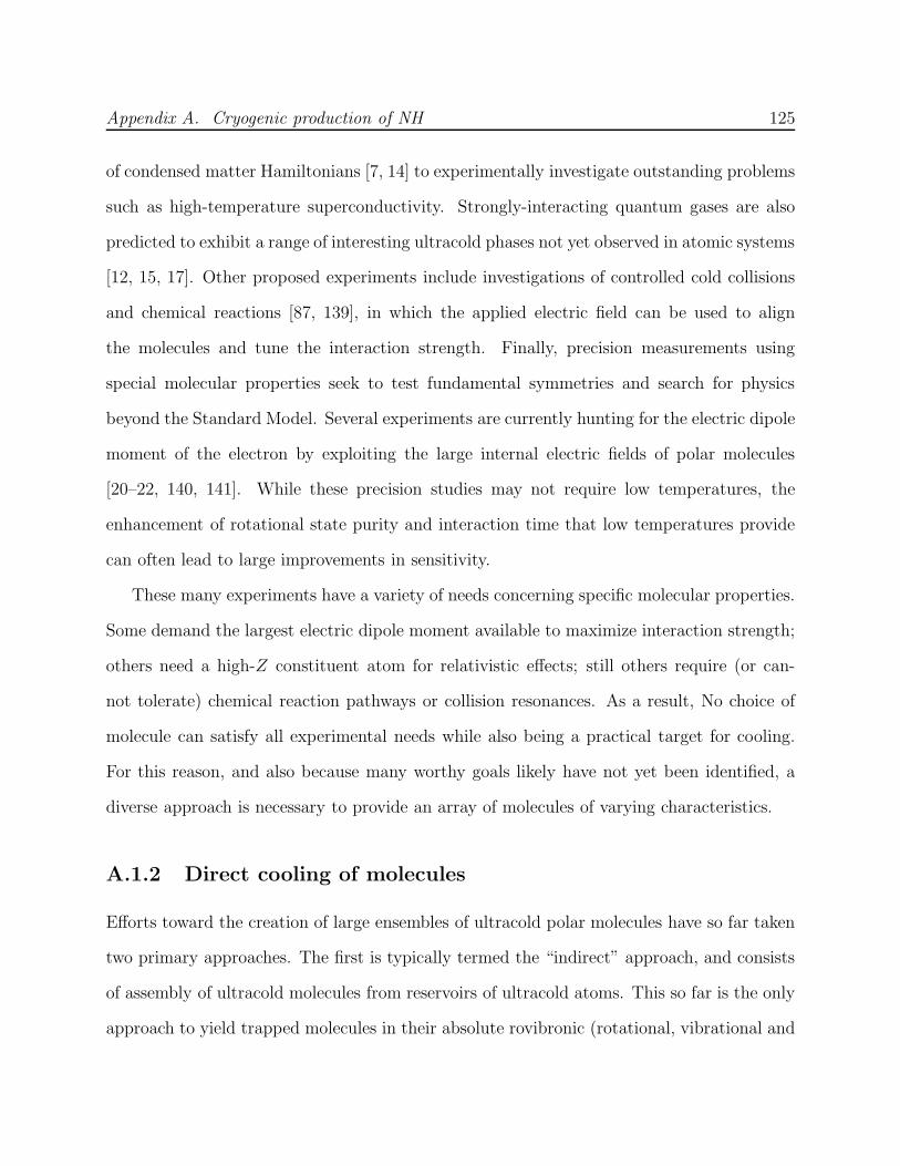
Appendix A. Cryogenic production of NH 125
of condensed matter Hamiltonians [7, 14] to experimentally investigate outstanding problems
such as high-temperature superconductivity. Strongly-interacting quantum gases are also
predicted to exhibit a range of interesting ultracold phases not yet observed in atomic systems
[12, 15, 17]. Other proposed experiments include investigations of controlled cold collisions
and chemical reactions [87, 139], in which the applied electric field can be used to align
the molecules and tune the interaction strength. Finally, precision measurements using
special molecular properties seek to test fundamental symmetries and search for physics
beyond the Standard Model. Several experiments are currently hunting for the electric dipole
moment of the electron by exploiting the large internal electric fields of polar molecules
[20–22, 140, 141]. While these precision studies may not require low temperatures, the
enhancement of rotational state purity and interaction time that low temperatures provide
can often lead to large improvements in sensitivity.
These many experiments have a variety of needs concerning specific molecular properties.
Some demand the largest electric dipole moment available to maximize interaction strength;
others need a high-Z constituent atom for relativistic effects; still others require (or can-
not tolerate) chemical reaction pathways or collision resonances. As a result, No choice of
molecule can satisfy all experimental needs while also being a practical target for cooling.
For this reason, and also because many worthy goals likely have not yet been identified, a
diverse approach is necessary to provide an array of molecules of varying characteristics.
A.1.2 Direct cooling of molecules
Efforts toward the creation of large ensembles of ultracold polar molecules have so far taken
two primary approaches. The first is typically termed the “indirect” approach, and consists
of assembly of ultracold molecules from reservoirs of ultracold atoms. This so far is the only
approach to yield trapped molecules in their absolute rovibronic (rotational, vibrational and
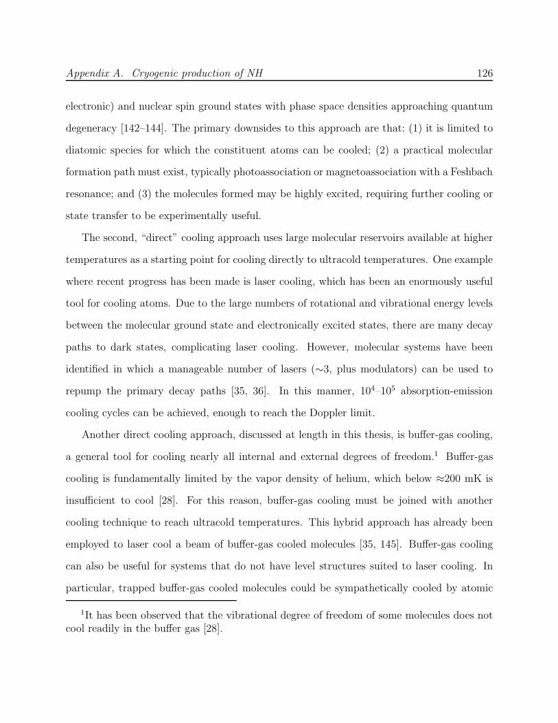
Appendix A. Cryogenic production of NH 126
electronic) and nuclear spin ground states with phase space densities approaching quantum
degeneracy [142–144]. The primary downsides to this approach are that: (1) it is limited to
diatomic species for which the constituent atoms can be cooled; (2) a practical molecular
formation path must exist, typically photoassociation or magnetoassociation with a Feshbach
resonance; and (3) the molecules formed may be highly excited, requiring further cooling or
state transfer to be experimentally useful.
The second, “direct” cooling approach uses large molecular reservoirs available at higher
temperatures as a starting point for cooling directly to ultracold temperatures. One example
where recent progress has been made is laser cooling, which has been an enormously useful
tool for cooling atoms. Due to the large numbers of rotational and vibrational energy levels
between the molecular ground state and electronically excited states, there are many decay
paths to dark states, complicating laser cooling. However, molecular systems have been
identified in which a manageable number of lasers (∼3, plus modulators) can be used to
repump the primary decay paths [35, 36]. In this manner, 104–105 absorption-emission
cooling cycles can be achieved, enough to reach the Doppler limit.
Another direct cooling approach, discussed at length in this thesis, is buffer-gas cooling,
a general tool for cooling nearly all internal and external degrees of freedom.1 Buffer-gas
cooling is fundamentally limited by the vapor density of helium, which below ≈200 mK is
insufficient to cool [28]. For this reason, buffer-gas cooling must be joined with another
cooling technique to reach ultracold temperatures. This hybrid approach has already been
employed to laser cool a beam of buffer-gas cooled molecules [35, 145]. Buffer-gas cooling
can also be useful for systems that do not have level structures suited to laser cooling. In
particular, trapped buffer-gas cooled molecules could be sympathetically cooled by atomic
1It has been observed that the vibrational degree of freedom of some molecules does notcool readily in the buffer gas [28].

Appendix A. Cryogenic production of NH 127
species for which cooling is more straightforward [53, 146, 147]. This final approach has been
the goal of the experiments with cold polar NH described in this appendix.
A.1.3 Previous work with cold NH
The imidogen molecule, especially its most common isotopomer NH, is among the best
diatomic molecular candidates for combining buffer-gas trap loading with the subsequent
thermal isolation required for further cooling in the trap. With a magnetic moment of 2 µB,
NH is readily trapped at temperatures that allow for the use of helium-4 buffer gas, which
can be rapidly removed after cooling and trapping (Section 4.2.2 and [31, 111]).2 The large
rotational splitting of NH prevents the rapid Zeeman relaxation that otherwise can occur
when rotational states are thermally populated in collisions with helium [148]. In addition,
the spin-spin interaction is weak compared to the rotational splitting, reducing the admixture
of the anisotropic N = 2 state into the ground state [149]. Finally, NH has accessible laser
transitions in the near-UV range, in particular the A 3Σ− → X 3Π2 line at 335.9 nm that is
accessible with a frequency-doubled dye or solid state laser.
NH molecules were first buffer-gas cooled below 6 K in 2004 at Harvard from a room-
temperature beam of radicals created in a glow discharge of ammonia (NH3) [150]. The
experiments that followed with the same apparatus successfully trapped the molecules and
measured the elastic and inelastic NH–helium collision rate coefficients [71]. Spin relaxation
in this system was experimentally investigated over a range of isotopomers and determined
by comparison to theory to be driven by rotational state coupling induced by the spin-spin
interaction [151]. In these early experiments NH lifetimes were limited to a maximum of
2Thermal isolation has not yet been demonstrated for species buffer-gas loaded withhelium-3 buffer gas, due to greater cooling requirements. For a thorough discussion ofbuffer-gas cooling of 1-µB species (for which using helium-3 is generally required) see [113].

Appendix A. Cryogenic production of NH 128
≈1 s due to collisions with the buffer gas. Later work extended NH lifetimes to 20 s by
implementing a pulsed buffer gas source to minimize collisions after cooling [114]. Unfortu-
nately, the resulting molecule densities were also lower such that no NH–NH collisions were
observed. The lifetime remained limited by buffer gas collisions due to the residual helium
density created by desorption from helium coating the cell walls.
In 2008 NH molecules and atomic nitrogen (4S3/2, µ = 3 µB) produced in a glow discharge
of a nitrogen-hydrogen gas mixture were simultaneously buffer-gas cooled and co-trapped
[54]. This is a critical first step to sympathetic cooling of the molecules to ultracold temper-
atures. Theoretical calculations show that nitrogen–nitrogen collisions are highly elastic (see
Section 2.1) and should allow for efficient evaporative cooling. A later experiment observed
NH–nitrogen inelastic collisions at a rate sufficient for sympathetic cooling, finding good
agreement with theory that predicts the rate to remain similarly low over the range of 1 K
to 1 mK [53, 55], the second criterion for successful sympathetic cooling of NH using trapped
nitrogen. However, these experiments were performed in the presence of helium gas, and
the NH lifetime was in each case limited by NH–helium collisions. Under such conditions
evaporative cooling is not possible, since the trapped ensemble is not thermally isolated from
the fixed cell temperature.
In the course of the recent NH experiments described in this appendix, it was discovered
that an error was made in the trapped NH density calibration cited in the previous results.
A measurement of probe laser absorption by trapped molecules was used to determine the
trapped NH density via a model using the known experimental conditions and optical tran-
sition properties (see Section 5.2 of [152]). Unfortunately, there were two significant errors in
the calculation. First, the size of the region of resonant magnetic field used in the calculation
was 10 times too large ([152], p. 94). Second, the application of the Landau-Zener model
was found to give a different result from Beer’s Law, which is incorrect (see Appendix B of
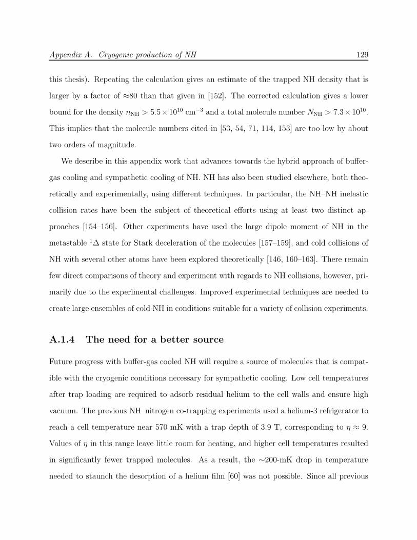
Appendix A. Cryogenic production of NH 129
this thesis). Repeating the calculation gives an estimate of the trapped NH density that is
larger by a factor of ≈80 than that given in [152]. The corrected calculation gives a lower
bound for the density nNH > 5.5×1010 cm−3 and a total molecule number NNH > 7.3×10¹⁰.
This implies that the molecule numbers cited in [53, 54, 71, 114, 153] are too low by about
two orders of magnitude.
We describe in this appendix work that advances towards the hybrid approach of buffer-
gas cooling and sympathetic cooling of NH. NH has also been studied elsewhere, both theo-
retically and experimentally, using different techniques. In particular, the NH–NH inelastic
collision rates have been the subject of theoretical efforts using at least two distinct ap-
proaches [154–156]. Other experiments have used the large dipole moment of NH in the
metastable 1∆ state for Stark deceleration of the molecules [157–159], and cold collisions of
NH with several other atoms have been explored theoretically [146, 160–163]. There remain
few direct comparisons of theory and experiment with regards to NH collisions, however, pri-
marily due to the experimental challenges. Improved experimental techniques are needed to
create large ensembles of cold NH in conditions suitable for a variety of collision experiments.
A.1.4 The need for a better source
Future progress with buffer-gas cooled NH will require a source of molecules that is compat-
ible with the cryogenic conditions necessary for sympathetic cooling. Low cell temperatures
after trap loading are required to adsorb residual helium to the cell walls and ensure high
vacuum. The previous NH–nitrogen co-trapping experiments used a helium-3 refrigerator to
reach a cell temperature near 570 mK with a trap depth of 3.9 T, corresponding to η ≈ 9.
Values of η in this range leave little room for heating, and higher cell temperatures resulted
in significantly fewer trapped molecules. As a result, the ∼200-mK drop in temperature
needed to staunch the desorption of a helium film [60] was not possible. Since all previous
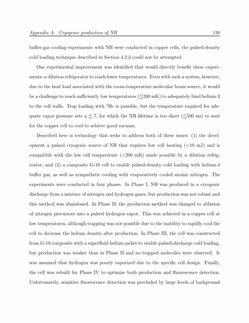
Appendix A. Cryogenic production of NH 130
buffer-gas cooling experiments with NH were conducted in copper cells, the pulsed-density
cold loading technique described in Section 4.2.2 could not be attempted.
One experimental improvement was identified that would directly benefit these experi-
ments: a dilution refrigerator to reach lower temperatures. Even with such a system, however,
due to the heat load associated with the room-temperature molecular beam source, it would
be a challenge to reach sufficiently low temperatures (.200 mK) to adequately bind helium-3
to the cell walls. Trap loading with 4He is possible, but the temperature required for ade-
quate vapor pressure sets η . 7, for which the NH lifetime is too short (.500 ms) to wait
for the copper cell to cool to achieve good vacuum.
Described here is technology that seeks to address both of these issues: (1) the devel-
opment a pulsed cryogenic source of NH that requires low cell heating (<10 mJ) and is
compatible with the low cell temperature (<200 mK) made possible by a dilution refrig-
erator; and (2) a composite G-10 cell to enable pulsed-density cold loading with helium-4
buffer gas, as well as sympathetic cooling with evaporatively cooled atomic nitrogen. The
experiments were conducted in four phases. In Phase I, NH was produced in a cryogenic
discharge from a mixture of nitrogen and hydrogen gases, but production was not robust and
this method was abandoned. In Phase II, the production method was changed to ablation
of nitrogen precursors into a pulsed hydrogen vapor. This was achieved in a copper cell at
low temperatures, although trapping was not possible due to the inability to rapidly cool the
cell to decrease the helium density after production. In Phase III, the cell was constructed
from G-10 composite with a superfluid helium jacket to enable pulsed-discharge cold loading,
but production was weaker than in Phase II and no trapped molecules were observed. It
was assumed that hydrogen was poorly vaporized due to the specific cell design. Finally,
the cell was rebuilt for Phase IV to optimize both production and fluorescence detection.
Unfortunately, sensitive fluorescence detection was precluded by large levels of background
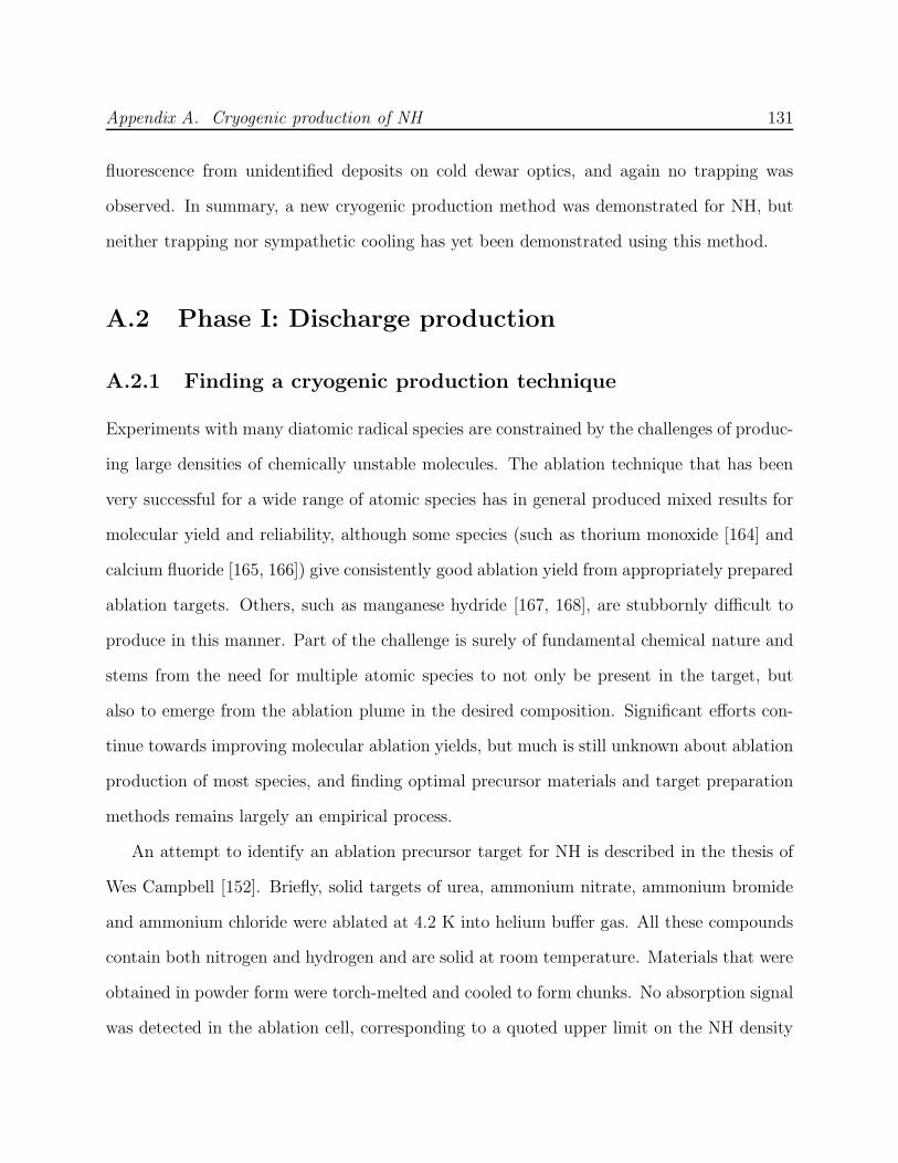
Appendix A. Cryogenic production of NH 131
fluorescence from unidentified deposits on cold dewar optics, and again no trapping was
observed. In summary, a new cryogenic production method was demonstrated for NH, but
neither trapping nor sympathetic cooling has yet been demonstrated using this method.
A.2 Phase I: Discharge production
A.2.1 Finding a cryogenic production technique
Experiments with many diatomic radical species are constrained by the challenges of produc-
ing large densities of chemically unstable molecules. The ablation technique that has been
very successful for a wide range of atomic species has in general produced mixed results for
molecular yield and reliability, although some species (such as thorium monoxide [164] and
calcium fluoride [165, 166]) give consistently good ablation yield from appropriately prepared
ablation targets. Others, such as manganese hydride [167, 168], are stubbornly difficult to
produce in this manner. Part of the challenge is surely of fundamental chemical nature and
stems from the need for multiple atomic species to not only be present in the target, but
also to emerge from the ablation plume in the desired composition. Significant efforts con-
tinue towards improving molecular ablation yields, but much is still unknown about ablation
production of most species, and finding optimal precursor materials and target preparation
methods remains largely an empirical process.
An attempt to identify an ablation precursor target for NH is described in the thesis of
Wes Campbell [152]. Briefly, solid targets of urea, ammonium nitrate, ammonium bromide
and ammonium chloride were ablated at 4.2 K into helium buffer gas. All these compounds
contain both nitrogen and hydrogen and are solid at room temperature. Materials that were
obtained in powder form were torch-melted and cooled to form chunks. No absorption signal
was detected in the ablation cell, corresponding to a quoted upper limit on the NH density
Appendix A. Cryogenic production of NH 132
of 1.8 × 108 cm−3, and the search for an ablation precursor was abandoned.
Due to the success in generating large numbers (≈1012) of metastable helium (He*)
in a pulsed radiofrequency (RF) discharge below 1 K [58], Phase I of a new set of NH
cryogenic production experiments attempted to create NH using RF discharge in a nitrogen-
hydrogen gas mixture. As demonstrated in the He* experiment, the pulsed discharge reached
a saturated He* density within 200 µs at powers below 25 W, meaning that He* discharge
production did not require more energy then a standard ablation laser pulse. Furthermore,
subsequent evaporative cooling of He* to temperatures of order 1 µK [31] showed that the
gas density required to sustain the discharge was compatible with excellent vacuum >10 s
later.
Discharge dynamics are a complicated combination of atoms (and/or molecules), ions and
electrons colliding in the presence of electromagnetic fields, usually also with spontaneous
or collisional state quenching and emission of light. The discharge plasma is often optimized
empirically and is highly sensitive to factors such as conductor geometry, gas density and
gas impurity concentration. As a result, it is very difficult to predict the equilibrium con-
centration of a given species in a molecular discharge at any temperature. The cryogenic
discharge has the additional complication that both nitrogen and hydrogen have negligible
vapor pressure below 1 K [59]. It has been observed, however, that an RF discharge can
etch material from surfaces into the discharging plasma despite the surface and neutral gas
temperature being too low for equilibrium vapor [169]. It is possible that high-energy elec-
trons or electronically excited atoms and ions collide with the surface and eject material.
Such an effect would allow nitrogen and hydrogen to be vaporized for discharge production
at temperatures conducive to trapping NH.
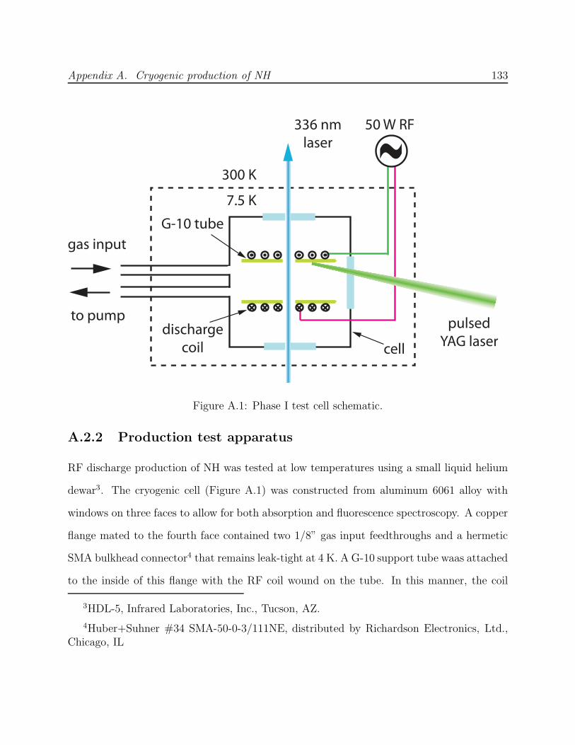
Appendix A. Cryogenic production of NH 133
to pump
gas input
7.5 K
300 K ~50 W RF
cell
discharge
coil
G-10 tube
336 nm
laser
pulsed
YAG laser
Figure A.1: Phase I test cell schematic.
A.2.2 Production test apparatus
RF discharge production of NH was tested at low temperatures using a small liquid helium
dewar3. The cryogenic cell (Figure A.1) was constructed from aluminum 6061 alloy with
windows on three faces to allow for both absorption and fluorescence spectroscopy. A copper
flange mated to the fourth face contained two 1/8” gas input feedthroughs and a hermetic
SMA bulkhead connector4 that remains leak-tight at 4 K. A G-10 support tube waas attached
to the inside of this flange with the RF coil wound on the tube. In this manner, the coil
3HDL-5, Infrared Laboratories, Inc., Tucson, AZ.
4Huber+Suhner #34 SMA-50-0-3/111NE, distributed by Richardson Electronics, Ltd.,Chicago, IL

Appendix A. Cryogenic production of NH 134
spacing from the inner walls of the cell was more than 1 cm. Transverse holes drilled through
the tube allowed for probe laser access.
RF discharge production of NH was first observed at room temperature. The cell was
filled with a 1:1 mixture of nitrogen and hydrogen gases, which was kept slowly flowing
through the cell to purge contaminants and discharge byproducts. RF current at 168 MHz
was chopped at 50-Hz with 50% duty cycle with an RF switch, sent through a 25-W amplifier,
and directed to the discharge coil. The coil impedance-matching was poor and the fraction
of RF power deposited into the discharge was not measured. At pressures of 300–600 mTorr
the discharge glowed brightly, blinking on and off with the RF chop with a lag time of .5 µs.
NH was detected with absorption spectroscopy using the R1 line of the A 3Σ−(v = 0) →
X 3Π2(v = 0) transition at 335.9 nm from the rovibronic ground state. A 2-µW probe beam
was directed through the discharge region and to a photodiode, with a portion of the probe
beam diverted before the cell to another photodiode to serve as an intensity reference. The
differential photodiode signal was monitored with a lock-in amplifier to extract the signal
component at the 50-Hz discharge chopping frequency. The 10 ms that the RF was off in the
chop cycle was several times the diffusion lifetime of NH in the cell, so the RF modulation
was effectively a modulation of the NH density.
The room-temperature absorption spectrum of NH in the discharge is shown in Fig-
ure A.2. The observed Doppler broadening suggests a temperature of 570 K, much hotter
than the cell or coil temperature (the cell was not warm to the touch, and internal compo-
nents would melt or degrade at such a high temperature). It is more likely that the collisional
process that produced NH in the discharge occurs at higher temperatures, and the molecules
do not have time to cool to the cell temperature before chemically reacting. The NH trans-
lational temperature dropped to about 380 K when the experiment was repeated with the
cell cooled to 77 K, at which point both nitrogen and hydrogen remain in gas phase. The

Appendix A. Cryogenic production of NH 135
−4 −3 −2 −1 0 1 2 3 4
0
5
10
15x 10
−4
detuning (GHz)
abso
rptio
n
295−K data (× 5)77−K data
Figure A.2: Absorption spectra of NH produced in an RF discharge of equal parts nitrogenand hydrogen gases. The room temperature and 77 K data are shown with fits (dashedlines) to Doppler temperatures of 570 and 380 K, respectively. The room temperature datahas been magnified by a factor of 5 for clarity. If similar production is assumed at the twotemperatures, then the increased signal at 77 K suggests that the rotational temperature isclose to that of the cell and not in equilibrium with the translational temperature.
population of other rotational levels was not investigated, so it is not known whether the
rotational temperature is also much warmer than the cell. Assuming rotational temperatures
of 77 K and 300 K, the NH density is calculated to be ≈4×1010 cm−3 averaged over the 1 cm
diameter of the coil support tube. This corresponds to a fractional NH density of ∼10−6,
about an order of magnitude lower than observed for cryogenic He* production [58, 111].
When the cell was cooled to its base temperature of ≈7.5 K, a discharge could still be
readily ignited in the cell, suggesting a non-negligible vapor pressure of hydrogen at this
temperature. To ensure an effective test of how the production method would fare below
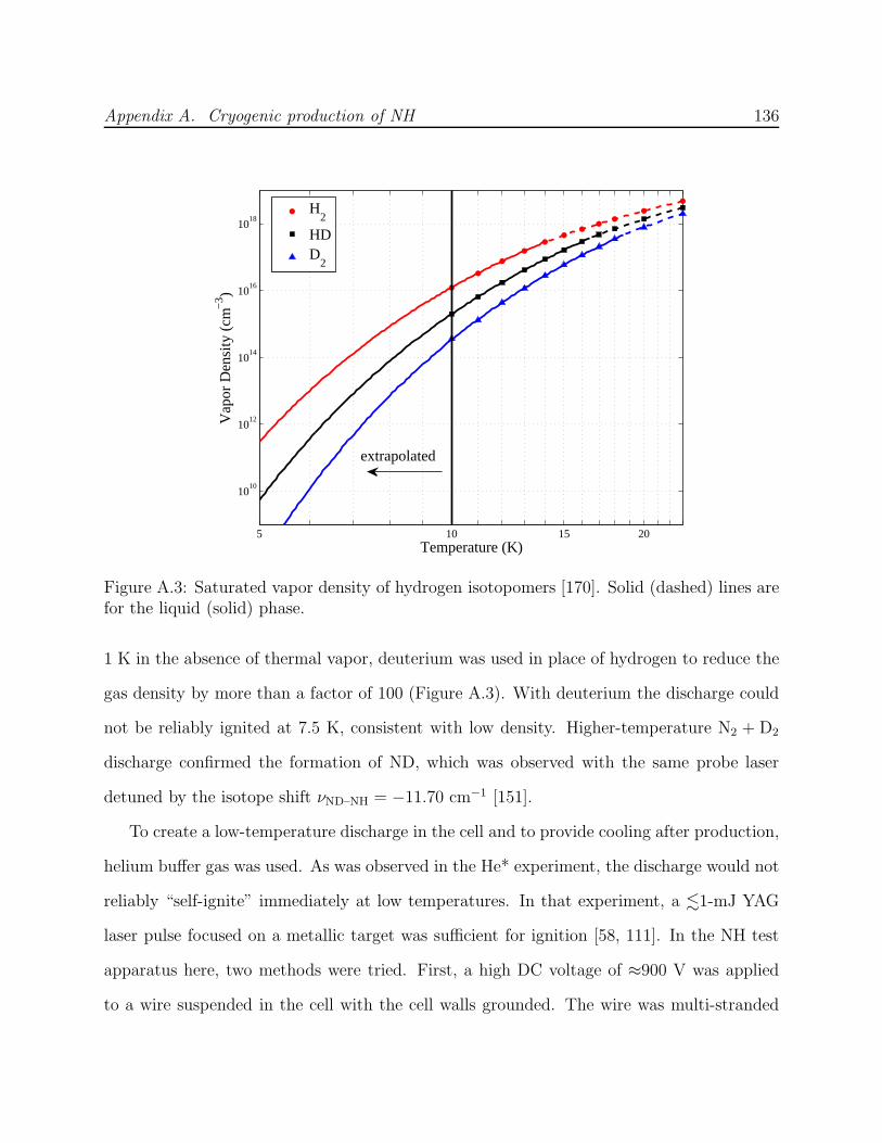
Appendix A. Cryogenic production of NH 136
5 10 15 20
1010
1012
1014
1016
1018
Temperature (K)
Vap
or D
ensi
ty (
cm−
3 )
extrapolated
H2
HDD
2
Figure A.3: Saturated vapor density of hydrogen isotopomers [170]. Solid (dashed) lines arefor the liquid (solid) phase.
1 K in the absence of thermal vapor, deuterium was used in place of hydrogen to reduce the
gas density by more than a factor of 100 (Figure A.3). With deuterium the discharge could
not be reliably ignited at 7.5 K, consistent with low density. Higher-temperature N2 + D2
discharge confirmed the formation of ND, which was observed with the same probe laser
detuned by the isotope shift νND–NH = −11.70 cm−1 [151].
To create a low-temperature discharge in the cell and to provide cooling after production,
helium buffer gas was used. As was observed in the He* experiment, the discharge would not
reliably “self-ignite” immediately at low temperatures. In that experiment, a .1-mJ YAG
laser pulse focused on a metallic target was sufficient for ignition [58, 111]. In the NH test
apparatus here, two methods were tried. First, a high DC voltage of ≈900 V was applied
to a wire suspended in the cell with the cell walls grounded. The wire was multi-stranded
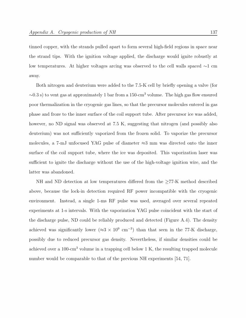
Appendix A. Cryogenic production of NH 137
tinned copper, with the strands pulled apart to form several high-field regions in space near
the strand tips. With the ignition voltage applied, the discharge would ignite robustly at
low temperatures. At higher voltages arcing was observed to the cell walls spaced ∼1 cm
away.
Both nitrogen and deuterium were added to the 7.5-K cell by briefly opening a valve (for
∼0.3 s) to vent gas at approximately 1 bar from a 150-cm3 volume. The high gas flow ensured
poor thermalization in the cryogenic gas lines, so that the precursor molecules entered in gas
phase and froze to the inner surface of the coil support tube. After precursor ice was added,
however, no ND signal was observed at 7.5 K, suggesting that nitrogen (and possibly also
deuterium) was not sufficiently vaporized from the frozen solid. To vaporize the precursor
molecules, a 7-mJ unfocused YAG pulse of diameter ≈3 mm was directed onto the inner
surface of the coil support tube, where the ice was deposited. This vaporization laser was
sufficient to ignite the discharge without the use of the high-voltage ignition wire, and the
latter was abandoned.
NH and ND detection at low temperatures differed from the ≥77-K method described
above, because the lock-in detection required RF power incompatible with the cryogenic
environment. Instead, a single 1-ms RF pulse was used, averaged over several repeated
experiments at 1-s intervals. With the vaporization YAG pulse coincident with the start of
the discharge pulse, ND could be reliably produced and detected (Figure A.4). The density
achieved was significantly lower (≈3 × 109 cm−3) than that seen in the 77-K discharge,
possibly due to reduced precursor gas density. Nevertheless, if similar densities could be
achieved over a 100-cm3 volume in a trapping cell below 1 K, the resulting trapped molecule
number would be comparable to that of the previous NH experiments [54, 71].

Appendix A. Cryogenic production of NH 138
−10 0 10 20 30 40 50 60 70
0
2
4
6x 10
−3
time (ms)
inte
grat
ed a
bsor
ptio
n
−2 −1.5 −1 −0.5 0 0.5 1
0
2
4
x 10−4
detuning (GHz)
abso
rptio
n at
t =
9 m
s
data7.5 K Doppler fit
dataRF TTL control
Figure A.4: ND produced in an RF discharge at T = 7.5 K from nitrogen and deuteriumvaporized into 4He buffer gas by an unfocused YAG laser pulse at t = 0. The discharge glowlags the RF pulse by .50 µs. The temperature of the Doppler fit in this range is poorlyconstrained due to the unresolved hyperfine structure; the actual temperature may be a fewkelvin warmer.
A.2.3 G-10 composite trapping cell
The cell built for NH trapping below 1 K was constructed under several design constraints:
1. Discharge production of NH must be possible. This requires a method for delivery of
precursor ice to the cell in a manner that does not inhibit transmission of dewar optics.
In addition, the ice must be accessible by the vaporization YAG pulse.
2. The cell’s heat capacity must be large enough that energy required for NH production
does not leave the cell too hot for trapping. In addition, regions of the cell with line-
of-sight access to the trap must not take too long to cool, or helium desorbing from
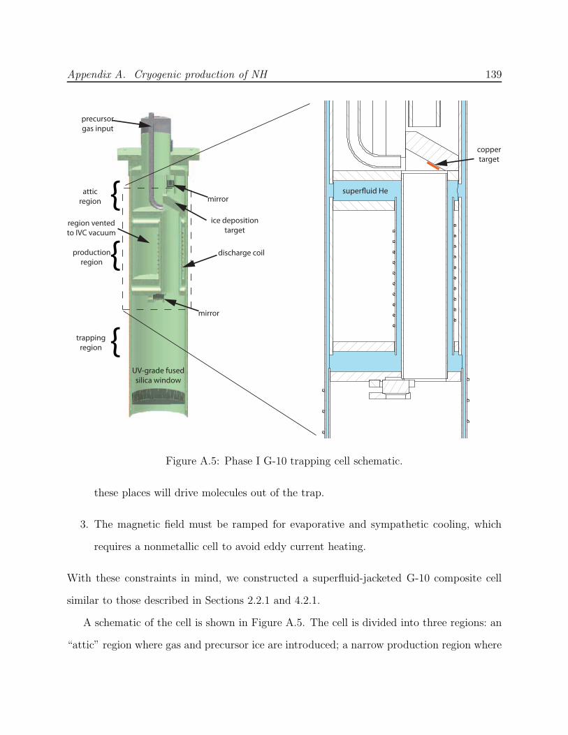
Appendix A. Cryogenic production of NH 139
attic
region
production
region
trapping
region
region vented
to IVC vacuum
precursor
gas input
mirror
mirror
discharge coil
ice deposition
target
UV-grade fused
silica window
copper
target
super!uid He
Figure A.5: Phase I G-10 trapping cell schematic.
these places will drive molecules out of the trap.
3. The magnetic field must be ramped for evaporative and sympathetic cooling, which
requires a nonmetallic cell to avoid eddy current heating.
With these constraints in mind, we constructed a superfluid-jacketed G-10 composite cell
similar to those described in Sections 2.2.1 and 4.2.1.
A schematic of the cell is shown in Figure A.5. The cell is divided into three regions: an
“attic” region where gas and precursor ice are introduced; a narrow production region where
Appendix A. Cryogenic production of NH 140
the discharge is ignited; and the trapping region where the majority of the exposed surface
area is well anchored to the superfluid jacket. A precursor input line deposits ice on an
angled target in the attic region to be vaporized into the production region. In order to
address the second constraint above, the discharge coil is wrapped around the production
region on the outside surface of the superfluid jacket so that the inner cell surface will remain
cold after production. This method was successfully used for the He* evaporative cooling
cell [58, 111]. It was also hoped that by spatially separating NH production and trapping it
might be possible to trap molecules at a higher density than can be achieved in the discharge.
Discharge ignition is accomplished by a weak ablation laser pulse targeting a copper foil in
the production region. Finally, two separate cell mirrors allow for absorption or fluorescence
spectroscopy in both the trapping and production regions.
A.2.4 Phase I failure: No NH nor N2* detected
Despite the success of the cryogenic test apparatus at 7.5 K, no NH was observed in the
trapping cell near 1 K. A range of discharge conditions was tried with a range of vaporization
YAG powers, to no avail. Since nitrogen vapor is the most difficult requirement for the
success of the discharge production method, it was thought that this was the limiting factor.
To investigate the nitrogen gas density, a spectroscopic search was performed for molecular
nitrogen in the metastable A3Πu state (N2*), which has a radiative lifetime of 1.9 s. The
state was probed using the A3Πu(v = 0) → B3Πg(v = 0) transition at 1049.6 nm.
Detection of N2* was first tested in discharges at room temperature and at 70 K.5 The
spectra in Figure A.6 show the observed translational and rotational cooling. The rota-
5In addition, N2* was also detected at room temperature using the A3Πu(v = 0) →B3Πg(v = 3) transition at 687.5 nm and the B3Πg(v = 0) → C3Πu(v = 0) transition near337 nm. Inferior signal-to-noise ratios were achieved on these transitions.

Appendix A. Cryogenic production of NH 141
−2 −1 0 1 2 3−1
0
1
2
3
4
5
6
7
8
9
x 10−3
detuning (GHz)
abso
rptio
n
R12
3
R11
Q12
1370−K trapping cellroom temperature tabletop cell (85% of full scale)
Figure A.6: N2* A → B absorption spectra observed in nitrogen discharge at a detuningnear 9,527.13 cm−1. The Doppler widths fit best to 319 and 107 K, however the rotationaltemperature is consistent with the cell temperature of 295 and 70 K, respectively. The R11line from the ground rotational state is used to search for N2* near 1 K. Rotational lineassignments are based on the (0,0) band analysis in [171].
tional temperatures are more consistent with the cell temperatures than they are with the
translational temperatures, suggesting that these degrees of freedom are not equilibrated.
The 70-K spectrum in Figure A.6 implies a N2* density of ∼1 × 1012 cm−3 in the v = 0
vibrational state (the excited state lifetime is 8 µs [172] and the Franck-Condon factor
is 0.37 [173]). The nitrogen density is not well known, but is likely to be no more than
1016 cm−3, implying a fractional population of N2* of &10−4. Assuming this limit to be the
N2* fraction in the 1-K discharge, as well, and assuming fractional absorption sensitivity of
10−4, this implies sensitivity to molecular nitrogen densities above ∼1012 cm−3 at 1 K, and
perhaps lower.
Appendix A. Cryogenic production of NH 142
Using this spectroscopic tool, no N2* was observed when the apparatus was cooled to near
1 K. The combination of no signature of molecular nitrogen nor of NH suggests that nitrogen
ice is not sufficiently vaporized in the 1-K trapping cell to emulate the performance of the
test cell at 7.5 K. It is possible that the geometry of the trapping cell, with the production
region significantly larger than that of the test cell, limited the nitrogen density—assuming
a similar quantity of molecules vaporized by the YAG laser pulse. It is also possible that the
lower temperature affected the N2* fraction or that the discharge formation of N2* and NH
is significantly altered at 1 K.
Initial tests of fluorescence spectroscopy were performed in the Phase I trapping cell,
although no NH fluorescence was observed. Large photon count rates were observed from
the cell after the end of a discharge pulse in the helium buffer gas (Figure A.7). This
bright source of photons in the first few milliseconds is termed the “discharge flash,” and
its cause is not understood. The discharge may excite long-lived fluorescence in the G-
10 walls surrounding the production region. Alternately, the initial millisecond-scale decay
profile is also consistent with the diffusion time of He*, which is produced in densities over
1011 cm−3; hence it is possible that the flash is short-lived fluorescence at the wall caused
by He* atoms, each depositing 20 eV internal energy. This flash limits the sensitivity to
molecule fluorescence at early times. Fluorescence detection is discussed in more detail in
Section A.3.7.
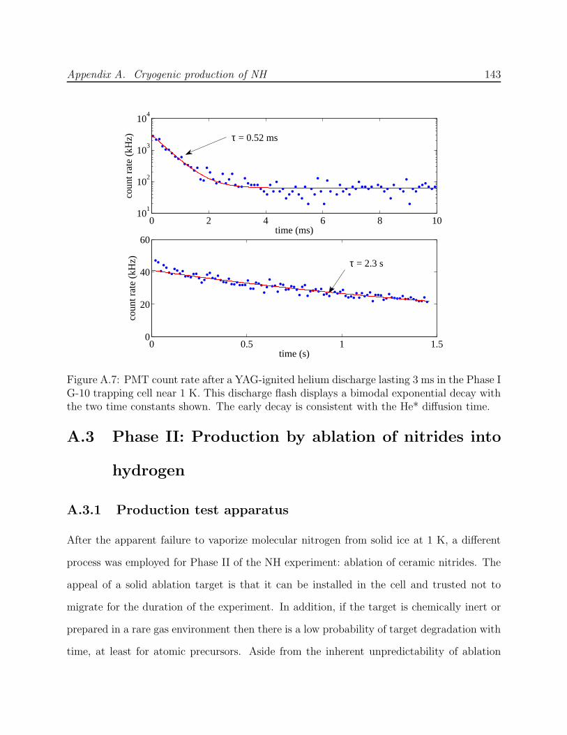
Appendix A. Cryogenic production of NH 143
0 2 4 6 8 1010
1
102
103
104
coun
t rat
e (k
Hz)
time (ms)
0 0.5 1 1.50
20
40
60
coun
t rat
e (k
Hz)
time (s)
τ = 0.52 ms
τ = 2.3 s
Figure A.7: PMT count rate after a YAG-ignited helium discharge lasting 3 ms in the Phase IG-10 trapping cell near 1 K. This discharge flash displays a bimodal exponential decay withthe two time constants shown. The early decay is consistent with the He* diffusion time.
A.3 Phase II: Production by ablation of nitrides into
hydrogen
A.3.1 Production test apparatus
After the apparent failure to vaporize molecular nitrogen from solid ice at 1 K, a different
process was employed for Phase II of the NH experiment: ablation of ceramic nitrides. The
appeal of a solid ablation target is that it can be installed in the cell and trusted not to
migrate for the duration of the experiment. In addition, if the target is chemically inert or
prepared in a rare gas environment then there is a low probability of target degradation with
time, at least for atomic precursors. Aside from the inherent unpredictability of ablation
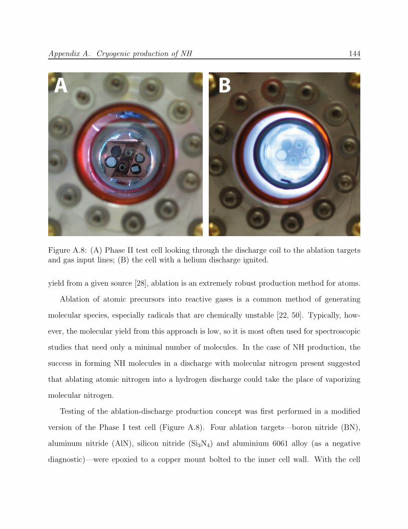
Appendix A. Cryogenic production of NH 144
A B
Figure A.8: (A) Phase II test cell looking through the discharge coil to the ablation targetsand gas input lines; (B) the cell with a helium discharge ignited.
yield from a given source [28], ablation is an extremely robust production method for atoms.
Ablation of atomic precursors into reactive gases is a common method of generating
molecular species, especially radicals that are chemically unstable [22, 50]. Typically, how-
ever, the molecular yield from this approach is low, so it is most often used for spectroscopic
studies that need only a minimal number of molecules. In the case of NH production, the
success in forming NH molecules in a discharge with molecular nitrogen present suggested
that ablating atomic nitrogen into a hydrogen discharge could take the place of vaporizing
molecular nitrogen.
Testing of the ablation-discharge production concept was first performed in a modified
version of the Phase I test cell (Figure A.8). Four ablation targets—boron nitride (BN),
aluminum nitride (AlN), silicon nitride (Si3N4) and aluminium 6061 alloy (as a negative
diagnostic)—were epoxied to a copper mount bolted to the inner cell wall. With the cell

Appendix A. Cryogenic production of NH 145
−2 0 2 4 6 8
0
0.005
0.01
0.015
0.02
0.025
time (ms)
abso
rptio
n
BNSi
3N
4
AlNAl 6061 alloyCu 101
Figure A.9: NH production after ablation of various targets into hydrogen gas in Phase IItest cell at 8.5 K, with probe laser parked on resonance at f = 2 × 14885.31 cm−1. Theablation energy is 6.3 mJ and the H2 pressure, as read with a room-temperature Convectrongauge without correcting for transpiration, is 27 mTorr. The production of NH when ablatingnon-nitrogenous targets is assumed to make use of nitrogen in cell contaminants, such as airice.
cooled to 8.5 K, we ablated the targets into hydrogen, which has significant vapor density
above 1016 cm−3 at this temperature. NH was observed when all materials were ablated,
including the aluminum alloy and the copper target mount (see Figure A.9). Since there
is no significant nitrogen content in the latter two materials, it is assumed that NH was
formed in these cases with nitrogen deposited from ablation of the nitride targets or from
air contamination of the cell while at room temperature. Three rotational lines of NH and
one of ND (using deuterium in place of hydrogen in this case) were independently observed
to confirm that the apparent NH absorption signal was not a coincidental resonance with
another ablation product.

Appendix A. Cryogenic production of NH 146
This performance suggests that the chemistry of ablation into hydrogen gas is favorable
for NH formation. With ablation energy of 6.3 mJ, an average density of ≈3×1010 cm−3 NH
molecules was achieved, corresponding to &1011 total molecules. Atomic ablation yields are
rarely in excess of 1014 atoms at these energies [28], which would imply that at least 0.1%
of the nitrogen atoms produced in ablation are converted to NH molecules, a significantly
higher fraction than that observed in discharge.
The test apparatus was subsequently adapted for lower temperatures and a more open
geometry. The G-10 support tube and coil were replaced with a shorter, free-standing coil
suspended on two nylon rods, allowing for more open area for gas flow transverse to the
coil. The absorption probe laser was directed transverse to the coil just after its end. Better
thermal connections allowed the cell to reach 4.5 K, and deuterium was again used in place
of hydrogen to further limit the thermal vapor (Figure A.3) to simulate the conditions of
a <1 K cell. With deuterium ice added to the cell, we observed ND upon ablation of all
nitride targets. The molecule yield steadily decreased with subsequent ablation pulses, but
would return when the ablation laser was directed to a fresh target. Refilling the cell with
deuterium ice also caused the signal to return. This behavior suggests that ablation alone
(without the discharge) is sufficient to vaporize deuterium ice near to the target, but that the
ice is rapidly depleted as it migrates elsewhere in the cell. The ND yield was more consistent
when a 1-ms discharge was ignited immediately prior to ablation. The discharge likely plays
no role in ND formation other than to provide a significant and repeatable deuterium gas
density. Roughly 1011 ND molecules could be reliably produced at 4.5 K with ≈10 mJ of
combined ablation and RF energy.
Appendix A. Cryogenic production of NH 147
A.3.2 Copper trapping cell
After the Phase I failure to produce NH, the Phase II cell construction was approached with
great caution. Rather than construct a new G-10 composite cell, which would be difficult
to assemble and even more difficult to modify or to fix in the event of leaks, a copper cell
was built. This decision favored a successful test of NH production below 1 K using the
technique of nitride ablation into hydrogen vapor, but precluded the possibility of rapid
magnetic field changes, including evaporative cooling. A schematic of the copper cell is
shown in Figure A.10. The discharge coil sits above the trap center in the cell vacuum,
supported on G-10 posts and sufficiently spaced from the grounded cell walls to allow for
large electric fields inside the coil. Ablation targets are epoxied in a copper mount above the
coil. A 1/4” copper tube for the introduction of hydrogen ice traverses the cell from the top
plate to aim at the inner coil surface. The cell window and top plate are affixed with indium
seals, and the top plate is thermally anchored to the dilution refrigerator mixing chamber
with seven flexible heat links made of braided copper. The bottom of this cell reached a
base temperature of about 130 mK.
With the cell cooled to below 1 K, hydrogen was added in a brief pulse from a ≈150-cm3
room temperature volume, in the same manner as described in Section A.2.4. At first, a
hydrogen-helium filling mixture was used to ensure that the entrained hydrogen would reach
the cell without freezing in the cold fill line. It was discovered, however, that venting a pulse
of pure hydrogen with 1 bar backing pressure was adequate and no helium was necessary.
This suggests that during the filling procedure the inner surfaces of the gas line warmed
momentarily and prevented freezing. Avoiding helium in the fill resulted in a reduced cell
heat load and no need to pump on the cell for a long time afterward.
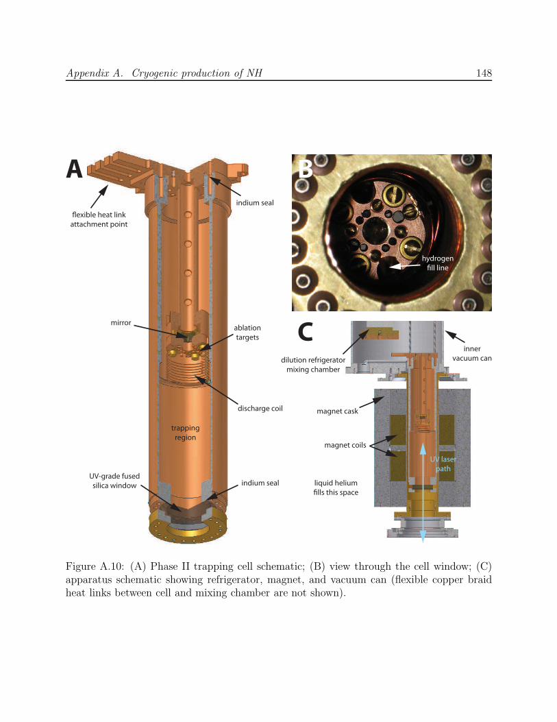
Appendix A. Cryogenic production of NH 148
trapping
region
exible heat link
attachment point
mirror
indium seal
discharge coil
ablation
targets
UV-grade fused
silica window
indium seal
hydrogen
"ll line
inner
vacuum candilution refrigerator
mixing chamber
magnet coils
magnet cask
UV laser
path
BA
C
liquid helium
"lls this space
Figure A.10: (A) Phase II trapping cell schematic; (B) view through the cell window; (C)apparatus schematic showing refrigerator, magnet, and vacuum can (flexible copper braidheat links between cell and mixing chamber are not shown).

Appendix A. Cryogenic production of NH 149
A.3.3 Observation of cold NH
Despite equivalent performance of the nitride ablation targets in the test apparatus, differ-
ences were observed in the trapping cell. Surprisingly, we observed no NH when ablating
the silicon nitride target6. This target was a fragment of a larger piece, which potentially
had different material properties on its outer faces than in the center such that ablation
would differ for outer vs. cleaved surfaces. Next, the boron nitride target7 produced a
∼0.5% “absorption” signal independent of probe laser frequency. Since boron nitride is a
porous and powdery material, this apparent absorption likely was instead just occlusion
of the probe beam by dust particles produced in ablation. The aluminum nitride target8,
however, produced reliable yields of over 1011 NH molecules when ablated into a mixture of
hydrogen and helium-4 gases with the cell temperature held above 6 K. With the cell cooled
to 1 K and no hydrogen in gas phase, the ablation still produced a similar yield, consistent
with the observations of the test apparatus. Also consistent with testing, the yield at 1 K
steadily decreased with additional ablation pulses, likely due to depletion of hydrogen near
the ablation target. NH production consistency was again improved by adding a discharge
pulse that ended coincident with ablation. The discharge was usually ignited with a sepa-
rate, weaker YAG pulse, but this was found to be unnecessary at higher helium densities. It
was not known whether the effect of the discharge was to etch hydrogen from cell surfaces
or whether it rapidly heated the buffer gas near the coil, which then caused hydrogen to
evaporate.
When the cell was cooled below ≈750 mK, NH could no longer be observed. This is likely
because the helium-4 density required to sustain the discharge that produces hydrogen was
699.5% purity, Plasmaterials, Inc., Livermore, CA.
7Part #44838, 99.5% purity, Alfa Aesar, Ward Hill, MA.
8Part #43790, Alfa Aesar, Ward Hill, MA.
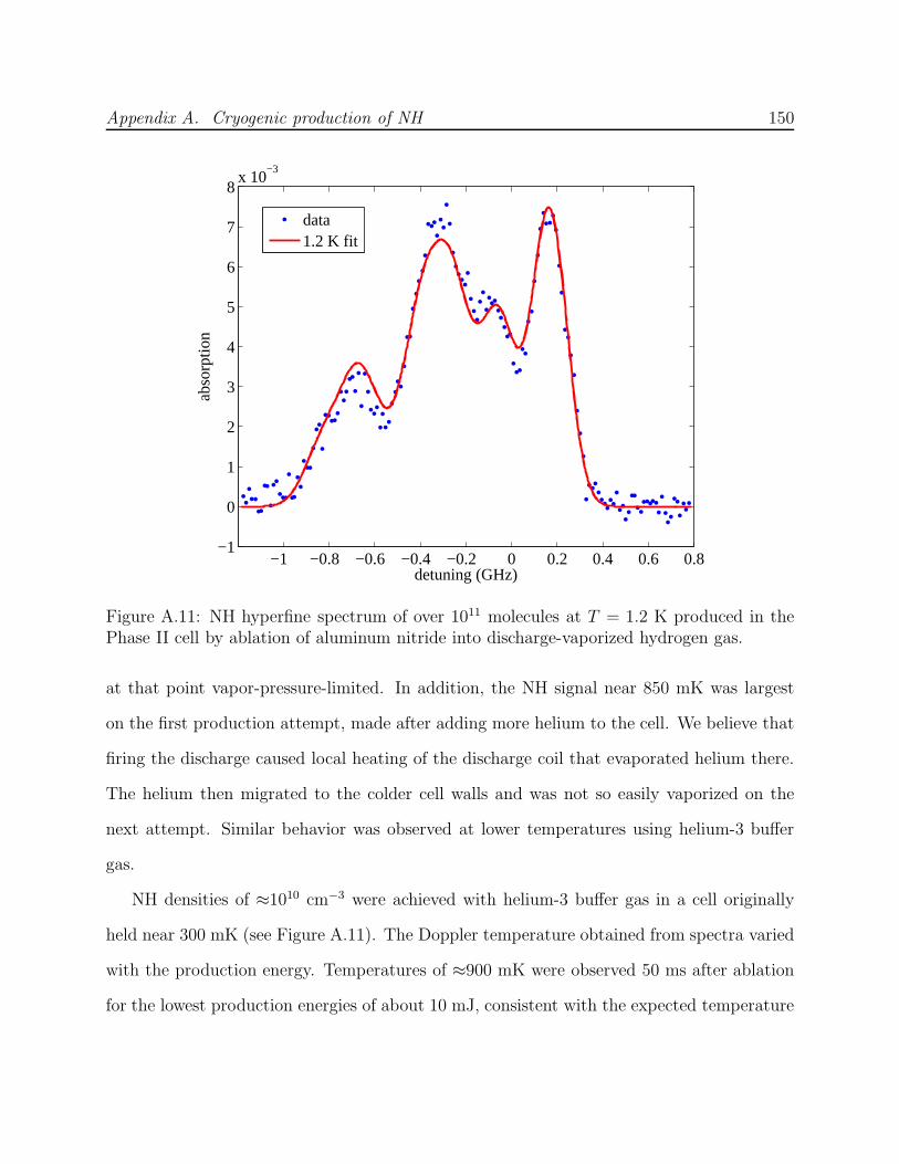
Appendix A. Cryogenic production of NH 150
−1 −0.8 −0.6 −0.4 −0.2 0 0.2 0.4 0.6 0.8−1
0
1
2
3
4
5
6
7
8x 10
−3
detuning (GHz)
abso
rptio
n
data1.2 K fit
Figure A.11: NH hyperfine spectrum of over 1011 molecules at T = 1.2 K produced in thePhase II cell by ablation of aluminum nitride into discharge-vaporized hydrogen gas.
at that point vapor-pressure-limited. In addition, the NH signal near 850 mK was largest
on the first production attempt, made after adding more helium to the cell. We believe that
firing the discharge caused local heating of the discharge coil that evaporated helium there.
The helium then migrated to the colder cell walls and was not so easily vaporized on the
next attempt. Similar behavior was observed at lower temperatures using helium-3 buffer
gas.
NH densities of ≈1010 cm−3 were achieved with helium-3 buffer gas in a cell originally
held near 300 mK (see Figure A.11). The Doppler temperature obtained from spectra varied
with the production energy. Temperatures of ≈900 mK were observed 50 ms after ablation
for the lowest production energies of about 10 mJ, consistent with the expected temperature

Appendix A. Cryogenic production of NH 151
rise from heating the thermal mass of the cell’s ≈300 cm3 of copper.
A.3.4 Limitations of a copper cell
The inability to produce NH using helium-4 buffer gas at temperatures below 750 mK is
consistent with the thermal dynamics of copper described in Section 2.2.4. The high thermal
conductivity of the cell walls rapidly diffuses the energy from RF heating and ablation
throughout the cell’s heat capacity, keeping the walls cool and the helium density too low
to ignite a discharge. Without a discharge, the hydrogen density would be limited to what
could be vaporized by the ablation pulse, and the low helium density would also likely limit
how much of this vaporized hydrogen stayed near to the ablation target.
Unfortunately, the same thermal properties also ensure that the cell temperature, and
hence the helium density (of either isotope), will will not drop rapidly after NH production.
We estimated the lower limit of helium density necessary for NH production from NH dif-
fusion times and helium vapor pressure curves to be ≈1016 cm−3. At this density the NH
Zeeman relaxation lifetime is only ∼30 ms [71], which is too short to allow NH produced in
a magnetic trapping field to equilibrate to a trapped spatial distribution, and also too short
to achieve thermal isolation. NH trapping was not achieved in the Phase II cell.
A.3.5 Limitations of detection
Despite reasonably efficient NH production of over 1011 molecules, detection remains a chal-
lenge with NH, a challenge that is significantly worsened when trapping is attempted. Due
to the long excited state lifetime of 440 µs and the UV wavelength, absorption signals of
cold NH were limited to 2% at zero field. In the presence of a trapping field, two competing
effects modify the absorption. First, the quadrupole trap compresses the molecular ensemble

Appendix A. Cryogenic production of NH 152
to enhance the density from the full trap volume of ≈100 cm3 to the effective volume
Veff = 4π
(
R
η
)3
, (A.1)
which is ≈0.5 cm3 for R = 3 cm and η = 9. This gives a compression factor of about 200
averaged over Veff. Second, however, the large gradient of the trapping field causes significant
Zeeman broadening, reducing resonant absorption. For a fixed laser frequency, there is an
ellipsoidal shell of constant magnetic field which is resonant. The thickness of this resonant
shell, ∆z, can be computed from the Doppler width ωD, the Zeeman shift ∂ω/∂B of the
transition, and the field gradient, giving
∆z =∑
i
fi∆ωD
∂ω∂B
∂B∂z
, (A.2)
where the sum is taken over all hyperfine transitions with relative transition strengths fi
(∑
i fi = 1), which overlap in the Zeeman-broadened spectrum. At 0.5 K, ∆z ∼ 0.5 mm,
which is about 150 times smaller than the effective resonant path length of the spatial
molecule distribution at zero-field, as calculated from the lowest-order diffusion mode.
Assuming no change in production yield, the expected trapped absorption can be es-
timated by combining the ∼200 enhancement in density with ∼150 ÷ 2 decrease in path
length, where the factor of two accounts for the interaction of the trap-centered probe laser
with both halves of the resonant shell. This factor of ∼3 increase, along with the fact that
only a third of the molecules are produced in the mJ = +1 trappable state, implies that
the observed OD will be roughly unchanged with the trap energized only if every one of
these molecules were trapped. In reality, molecules will evaporate from the trap or relax to
untrapped states before coming to equilibrium, thus the OD is almost certain to decrease,
perhaps dramatically.
Balanced absorption regularly yields a noise floor of 10−3 for absorption detection in
the experiments with NH, with an additional factor of .10 obtained from averaging. The
Appendix A. Cryogenic production of NH 153
limiting factor is differential vibrations between the probe laser and cryogenic apparatus.
These are partially compensated by the use of a lens to focus the beam onto the cell mirror
(see Section 4.2.1 of [111]). However, residual noise has significant amplitude in the 1–1,000-
Hz bandwidth of the experimental dynamics. Rapidly scanning the laser over GHz-scale
spectral features cannot be done while maintaining the doubling cavity lock, and so it is
difficult to remove this low-frequency noise.
A.3.6 FM spectroscopy of NH
Frequency modulation (FM) spectroscopy is a powerful method for eliminating low-frequency
noise sources. A probe laser is frequency modulated to add sidebands before interacting with
the molecules. The differential interaction of the sidebands with the molecular spectrum is
extracted with a homodyne measurement that includes only the small components of noise
at the high modulation frequency. Bjorklund et al. [174] calculate the minimum detectable
change in the absorption δ in the shot noise limit to be
∆δmin = 2
[
ηeM2
(
P
~ωc
)
∆f
]−1/2
, (A.3)
where ηe is the detector quantum efficiency, M is the modulation index, P and ωc are the
laser power and carrier frequency, respectively, and ∆f is the measurement bandwidth. The
best detection limit is achieved for long wavelengths and high laser power. In addition, the
sidebands should be as strong as possible.
Unfortunately, several factors conspire against FM detection of NH in a trap. Foremost,
the spectrum is spread over several GHz at temperatures near 0.5 K. Electro-optical modu-
lators (EOMs) in the UV require low-absorption crystals that have high indices of refraction,
which makes it more difficult to produce strong modulation at high frequencies in the GHz
Appendix A. Cryogenic production of NH 154
range.9 As a result, both the carrier frequency and sidebands necessarily interact with the
molecules. Since the FM signal is proportional to the differential absorption and phase shift
between the sidebands, this causes partial common-mode signal rejection. In this regime, the
FM signal resembles the derivative of the spectrum rather the spectrum itself. For the largest
signal, the experiment should therefore seek to sharpen the spectral features, which can be
accomplished by using a small probe beam. On the other hand, the long NH excited state
lifetime ensures a low saturation intensity of 3.6 mW/cm2 and a correspondingly low power
limit for a small beam. Taking these limitations and the short wavelength into account, the
expected noise floor for trapped NH is only somewhat better than AM spectroscopy can
achieve. For a 3-mm beam at saturation intensity and a strong modulation index of 0.3,
∆δmin ≈ 2 × 10⁻⁵ with 1-kHz bandwidth.
Another technical limit enters when the detector is considered. In practice, the 250-µW
beam described above is far in excess of the maximum power observable by the PMTs used
for NH detection, which reduces the sensitivity by more than an order of magnitude. This
limit can be overcome by using photodiodes, although Johnson noise must be accounted for
in this case, since photodiodes have no intrinsic gain. For a room-temperature 50-Ω load,
the Johnson noise amplitude is similar to that of shot noise. This permits observation of
absorption below 10−4 with 1-kHz bandwidth, but only with electronics operating near the
9Since the 336-nm probe laser for NH is produced by frequency doubling a 672-nm dyelaser, it is possible to modulate the red fundamental wavelength at a higher modulationfrequency than is achievable in the UV. The doubling cavity must then be co-resonant forboth the carrier and sideband frequencies (which are likely to be spaced at greater than acavity free spectral range), although this could potentially be avoided by single-pass doublingin a periodically-poled nonlinear crystal [175]. The sidebands and carrier will mix whendoubled to produce additional frequency components, with minimum spacing equal to themodulation frequency. Modulation of the fundamental wavelength was not attempted here,but could in principle provide several GHz separation between the UV carrier and nearestsideband frequencies.
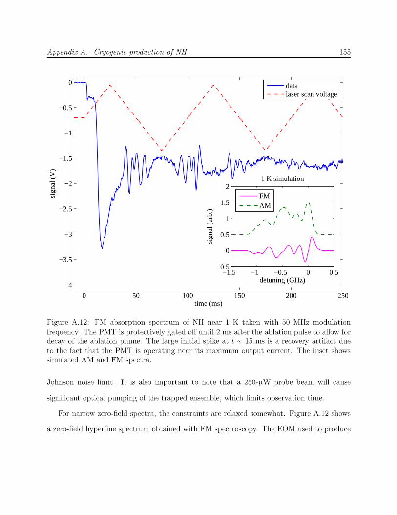
Appendix A. Cryogenic production of NH 155
0 50 100 150 200 250
−4
−3.5
−3
−2.5
−2
−1.5
−1
−0.5
0
time (ms)
sign
al (
V)
−1.5 −1 −0.5 0 0.5−0.5
0
0.5
1
1.5
2
detuning (GHz)
sign
al (
arb.
)
1 K simulation
FMAM
datalaser scan voltage
Figure A.12: FM absorption spectrum of NH near 1 K taken with 50 MHz modulationfrequency. The PMT is protectively gated off until 2 ms after the ablation pulse to allow fordecay of the ablation plume. The large initial spike at t ∼ 15 ms is a recovery artifact dueto the fact that the PMT is operating near its maximum output current. The inset showssimulated AM and FM spectra.
Johnson noise limit. It is also important to note that a 250-µW probe beam will cause
significant optical pumping of the trapped ensemble, which limits observation time.
For narrow zero-field spectra, the constraints are relaxed somewhat. Figure A.12 shows
a zero-field hyperfine spectrum obtained with FM spectroscopy. The EOM used to produce

Appendix A. Cryogenic production of NH 156
−400 −300 −200 −100 0 100 200 300 400
0
0.5
1
1.5
2
2.5
detuning (MHz)
tran
smitt
ed c
avity
pow
er (
arb.
)
50 MHz100 MHz150 MHz200 MHz300 MHz
Figure A.13: Sidebands of 336-nm NH probe beam at different modulation frequencies, asmeasured by transmission of a 8-cm confocal cavity, for use in FM absorption spectroscopy.The EOM is non-resonantly driven with RF signal power of 10 dBm × 45 dB amplification.The individual cavity scans are offset vertically for clarity.
the sidebands10 is broadband to allow for tuning of the modulation frequency, although
the modulation index is stronger at lower frequencies (Figure A.13). The downside of a
nonresonant EOM is that the necessary RF drive power is large (≈300 W is used here11)
and the radiated drive signal is picked up by detection electronics to cause additional noise.
For this technical reason and the fundamental limitations noted above regarding in-trap
detection, FM spectroscopy of NH was abandoned.
10Model 350-50-UV-Phase EOM with potassium dideuterium phosphate (KD*P) crystal,Conoptics, Inc., Danbury, CT.
11Model 550 amplifier, 50–500 MHz, Conoptics, Inc., Danbury, CT.

Appendix A. Cryogenic production of NH 157
A.3.7 Challenges of fluorescence detection with limited
optical access
The dilution refrigerator and magnet used in these experiments were both designed to be
fully or partially immersed in liquid helium for normal operation. Retrofitting the apparatus
to run with these components in vacuum (and using, for example, a pulse tube cooler to
provide cooling to 4 K) would be an extremely expensive and formidable engineering effort.
The alternative—the constraint of maintaining a liquid helium reservoir surrounding the
experiment—makes it very difficult to optically access the trapped ensemble through the
midplane of the magnet. Doing so would require creating several additional cryogenic seals
to provide beam access through the liquid reservoir, magnet, and inner vacuum can. These
seals would complicate the mechanical constraints and assembly procedures of the apparatus.
In addition, the interface with the vacuum can, in particular, would likely require a reduction
in trap depth. Finally, providing superfluid leak-tight optical access through the side of the
superfluid jacket surrounding the cell is an especially complex task.
For these reasons, the experiments in this apparatus have made exclusive use of optical
access via downward-facing windows and a cell mirror. Imaging or fluorescence detection
must therefore collect photons from the same window as lasers used for optical pumping
and ablation, reducing available solid angle. Even worse, unavoidable scatter from these
lasers into collection optics can swamp low signal levels. This is especially true for diagonal
fluorescence spectroscopy, in which the emitted photons are the same wavelength as the
pump photons and scatter cannot be spectrally filtered from the signal.
Diagonal fluorescence detection can still be achieved by temporally filtering the signal
photons from the scattered pump light. As described in Section 2.3.2 of the thesis of Matthew
Hummon [168], the 440-ns excited state lifetime allows enough time to turn off the pump
beam and collect fluorescence light in the absence of scatter. The process is repeated with a

Appendix A. Cryogenic production of NH 158
1-MHz square-wave chop of the pump beam. This temporal filtering reduces the signal level
by about a factor of 6 (including the ≈100-ns dead time to wait for the pump shutoff) while
fully eliminating pump scatter as a source of noise.
Unfortunately, secondary effects of the pump light cause noise that is not eliminated using
this technique. First, fluorescence in cold solid materials may take longer to decay than the
excited molecules, and hence cannot be removed with the pump laser chop. Second, a high
rate of scattered pump photons incident on the detection PMT in the bright phase of the chop
cycle can cause spurious delayed noise pulses called “afterpulses” when the pump laser is off
[176]. Such afterpulsing is sometimes seen when the PMT vacuum becomes contaminated
with helium gas. With the pump laser off the PMT used for these experiments12 generated
afterpulses at a rate of approximately 1% the pump-on count rate (Figure A.14), with a
decay time of roughly 300 ns.13 The afterpulsing can be eliminated by gating the PMT off
when the pump laser is on. However, the repetition rate of the gate is limited to 10 kHz (due
to capacitance in the gating circuit that provides rapid gate speed—higher duty cycle may
be possible with slower gate speed), hence this solution sacrifices two orders of magnitude
in signal photons.
Another detection option is off-diagonal fluorescence using the (0,1) vibrational transition
at 375 nm. The fractional decay to the v = 1 state is only 0.6% [152], hence about 150
photons must be scattered on the (0,0) transition for every 375-nm photon. The bright
pump light can be spectrally filtered, but fluorescence in other materials may be spectrally
12Model H10304 PMT module with gate function, Hamamatsu Corporation, Bridgewater,NJ.
13The afterpulsing of the PMT used for the previous NH work (Model P25A-02, ElectronTubes Limited, now defunct) was also measured and found to be about a factor of 2 worse,although this behavior may have worsened in the intervening months. This suggests thatafterpulsing may be the limiting noise source for the previous chopped-pump experiments ofHummon et al., rather than imperfect AOM extinction, as was thought at the time [168].
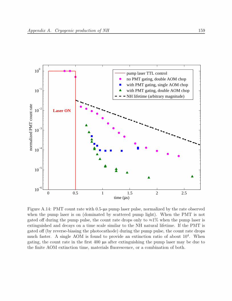
Appendix A. Cryogenic production of NH 159
0 0.5 1 1.5 2 2.510
−6
10−5
10−4
10−3
10−2
10−1
100
Laser ON
time (µs)
norm
aliz
ed P
MT
cou
nt r
ate
pump laser TTL controlno PMT gating, double AOM chopwith PMT gating, single AOM chopwith PMT gating, double AOM chopNH lifetime (arbitrary magnitude)
Figure A.14: PMT count rate with 0.5-µs pump laser pulse, normalized by the rate observedwhen the pump laser is on (dominated by scattered pump light). When the PMT is notgated off during the pump pulse, the count rate drops only to ≈1% when the pump laser isextinguished and decays on a time scale similar to the NH natural lifetime. If the PMT isgated off (by reverse-biasing the photocathode) during the pump pulse, the count rate dropsmuch faster. A single AOM is found to provide an extinction ratio of about 104. Whengating, the count rate in the first 400 µs after extinguishing the pump laser may be due tothe finite AOM extinction time, materials fluorescence, or a combination of both.
Appendix A. Cryogenic production of NH 160
broad and have a significant component in the detection band, especially when that band
is at a longer wavelength than the excitation. The opposite pumping scheme, in which
v = 1 molecules are pumped on the (0,1) line and 336-nm photons are collected, reverses the
wavelength order to reduce materials fluorescence. In this scheme, however, the experiment
will be limited by the 37-ms lifetime of the v = 1 state [153].
Off-diagonal fluorescence detection was attempted in the copper cell by pumping from
the ground (0,0) state and looking for 375-nm photons. With an observed 0.7% pump laser
absorption, no fluorescence signal above background was observed. Based on the measured
fluorescence rate and estimated detection efficiency, a signal-to-noise ratio of ∼8 was ex-
pected. It is difficult to align the fluorescence collection optics to an unobserved signal,
however, and imperfect alignment may be to blame.
A.4 Phase III: Modification of G-10 cell from
Phase I
A.4.1 No NH production enhancement with discharge
After the success of producing NH in the copper Phase II cell using ablation of aluminum
nitride into discharge-vaporized hydrogen gas, the Phase I G-10 cell was modified to insert
ablation targets. The cell walls were cut with a Dremel tool fitted with an abrasive cutting
wheel, with care taken to minimize dust contamination of the interior cell space. With new
ablation targets in place, a new cell window and superfluid jacket patch were epoxied to the
remaining cell wall.
When the modified cell was cooled below 1 K and filled with precursor hydrogen ice,
NH was observed from ablation of aluminum nitride in the production region of the cell.

Appendix A. Cryogenic production of NH 161
Unfortunately, the density was about an order of magnitude lower than that observed in
Phase II. More significantly, while a discharge pulse had served to enhance the hydrogen
density in the copper cell, the discharge had no positive effect on the signal in the G-10 cell.
The maximum NH density was the same as that achieved purely with ablation. As was seen
in the previous cell, the production steadily decreased with repeated ablation pulses after
filling the cell once with hydrogen, and would be replenished upon subsequent filling. Unlike
the previous cell, the discharge appeared to accelerate the production decrease.
One potentially significant difference between the cells is that the Phase III cell had
the discharge coil wrapped external to the superfluid jacket (see Figure A.5), whereas the
Phase II cell coil was in contact with the buffer gas and hydrogen. It is possible that the
dramatic difference in production between the two cells is due to the necessary hydrogen
vaporization being primarily a thermal process: the coil surface heats during the discharge
pulse to evaporate hydrogen. This heating could be caused by resistive heating in the copper
wire or by dissipation of energy into the plasma in the regions of high electric field near
the wire. On the other hand, in contrast to this thermal vaporization, hydrogen could be
vaporized in a process of etching from cold ice by energetic particles produced in the discharge
[169]. The etching process would likely be less dependent on the surface temperature than
the evaporative process, and should not depend strongly on whether or not the coil is in
contact with the hydrogen ice. The contrasting behavior of the Phase II and III cells is
evidence in support of the thermal process being dominant.
A second performance difference between the cells is that the discharge in the Phase III
cell was weaker and less repeatable, due primarily to the twisted-pair cabling leading to the
coil from outside of the cell. The heating observed from the discharge was roughly a factor
of 2 lower than observed in previous cells at similar RF power input, suggesting that power
was being reflected from the coil due to poor coupling.
Appendix A. Cryogenic production of NH 162
A.4.2 Detection limited by fluorescence of G-10
Since off-diagonal fluorescence detection of NH had failed in the copper cell with a clear
simultaneous NH absorption signal, a test experiment was performed to observe (0,1) fluo-
rescence at room temperature. Boron nitride was ablated into hydrogen gas and illuminated
with a 50-µW pump beam resonant with the (0,0) line. Fluorescence was observed separately
at both 336 nm and 375 nm, with a ratio consistent with previous measurements [152]. The
observed collection efficiency was ≈7 times weaker than estimated, which may expose an
flaw in the calculated spatial distribution of fluorescence, and may be related to the failure
to see fluorescence in Phase II. Nevertheless, this observation confirmed the feasibility of
detecting NH using off-diagonal fluorescence.
Due to the weak off-diagonal fluorescence rate, excellent rejection of pump light is nec-
essary. To this end, the PMT aperture was covered by a stack of four filters in the following
order of incidence, as seen by arriving photons: (1) a 6-nm bandwidth interference filter
centered at 375 nm14; (2) a colored glass filter passing 375 nm but not 336 nm15; (3) an
identical copy of (1); and (4) a colored glass filter that passes both 336 and 375 nm16. The
stack is oriented in this way to minimize laser-induced fluorescence in the filters themselves.
The effective rejection factor of this filter stack for the 336-nm pump photons is measured
to be 3 × 108.17 When looking for (0,1) fluorescence in the G-10 Phase III cell, a large noise
background was observed. The noise was correlated with the (0,0) pump laser, but was in-
14Model LD01-37516, Semrock, Inc., Rochester, NY.
15Model B-440, Edmund Optics, Inc., Barrington, NJ.
16Model FGUV11, Thorlabs, Newton, NJ.
17It is not known whether the (3 × 10⁸)−1 photons detected for each 336-nm photonincident on the filter stack is a transmitted photon or whether it is produced by laser-induced fluorescence in the filters. Transmission data the individual filters suggest that thefilter stack transmission should be lower than this value.

Appendix A. Cryogenic production of NH 163
dependent of the pump laser frequency, suggesting that the source was either pump scatter
or unwanted fluorescence in the apparatus. The former was ruled out by the measured filter
stack rejection factor. Visual inspection of the cell revealed visibly fluorescing spots where
stray pump reflections struck G-10, which implied bright, broadband sources of unwanted
light. When the fluorescence detection system was aligned to one of these spots, the noise
level grew dramatically.
Stray reflections are a particular challenge in this apparatus due to the four uncoated
UV fused silica windows between the laser system and molecular ensemble. Each window
surface produces a 3.7% Fresnel reflection of the pump beam. The windows are wedged to
eliminate etalon effects that convert frequency shifts into amplitude noise, and so these stray
reflections propagate in many directions. In principle, the NH experiment could have used
antireflection window coatings for wavelengths of 336 nm, 375 nm and 532 nm to accomodate
the pump, fluorescence and ablation light, respectively. However, other wavelengths are also
often used for diagnostic purposes, especially when other experiments share the apparatus
on the same experimental run. Moreover, the coating is not perfect and the reflections that
remain are still significant.
On the way into the cell, the pump beam produces 8 primary reflections of ≈3.7% power
(some are somewhat weaker due to prior attenuation of the pump beam), and another 8 on
the way out. These primary reflections produce 56 secondary reflections at ≈0.14%, and
240 tertiary reflections. Controlling the directions of all of these reflections is not feasible,
although alignment of the window wedge angles can allow for all the reflections to be con-
tained in a single plane for spatial filtering. Half of these reflections enter the cell, where
many strike a G-10 surface to cause fluorescence. This background light prevented observa-
tion of NH (0,1) fluorescence in the Phase III cell, since even the secondary reflections cause
an unacceptable noise level. Without fluorescence detection, the weaker NH production en-
Appendix A. Cryogenic production of NH 164
sured that no trapped signal could be observed. It was clear from Phase III that fluorescence
detection had to be improved.
A.5 Phase IV: Design for maximized production and
fluorescence sensitivity
A.5.1 Building a new cell
We come now to the final phase of the NH cryogenic production experiments. The Phase IV
cell, a schematic of which is shown in Figure A.15, was designed as the best effort for
trapping, cooling and detection of NH within the constraints of the current apparatus. The
primary improvements are in production and detection. First, in an attempt to recreate the
good production of the Phase II copper cell in a manner consistent with trapping and further
cooling, the discharge coil for the Phase IV cell was anchored to the internal surface of the
cell wall. The calculated time constant necessary to cool this coil after production is similar
to the time for cooling the wall surface itself, consistent with the need to rapidly decrease the
helium density after trap loading. Whether the Phase II cell discharge vaporized hydrogen
by evaporation or by etching, the Phase IV cell mimicked that design for similar results.
Second, to improve the fluorescence detection sensitivity, the cell was engineered to be
dramatically less fluorescent. Rather than the back surface of the cell that is exposed to
stray pump beam reflections being composed entirely of fluorescent G-10, it was covered by
a beam reflector created from polished single-crystal silicon (Figure A.15B). The two halves
of the beam reflector were cut with a waterjet cutter18 from silicon wafer, sandwiching the
wafer between two sheets of 5-mil Kapton and then two 1/4” thick Teflon plates. Piercing
18OMAX Corporation, Kent, WA.
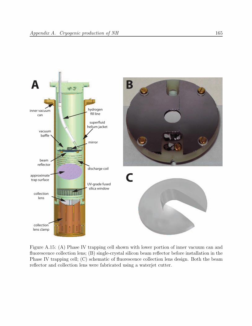
Appendix A. Cryogenic production of NH 165
collection
lens clamp
collection
lens
UV-grade fused
silica window
discharge coil
approximate
trap surface
beam
re!ector
hydrogen
"ll line
vacuum
ba#e
mirror
inner vacuum
can
A B
C
super!uid
helium jacket
Figure A.15: (A) Phase IV trapping cell shown with lower portion of inner vacuum can andfluorescence collection lens; (B) single-crystal silicon beam reflector before installation in thePhase IV trapping cell; (C) schematic of fluorescence collection lens design. Both the beamreflector and collection lens were fabricated using a waterjet cutter.
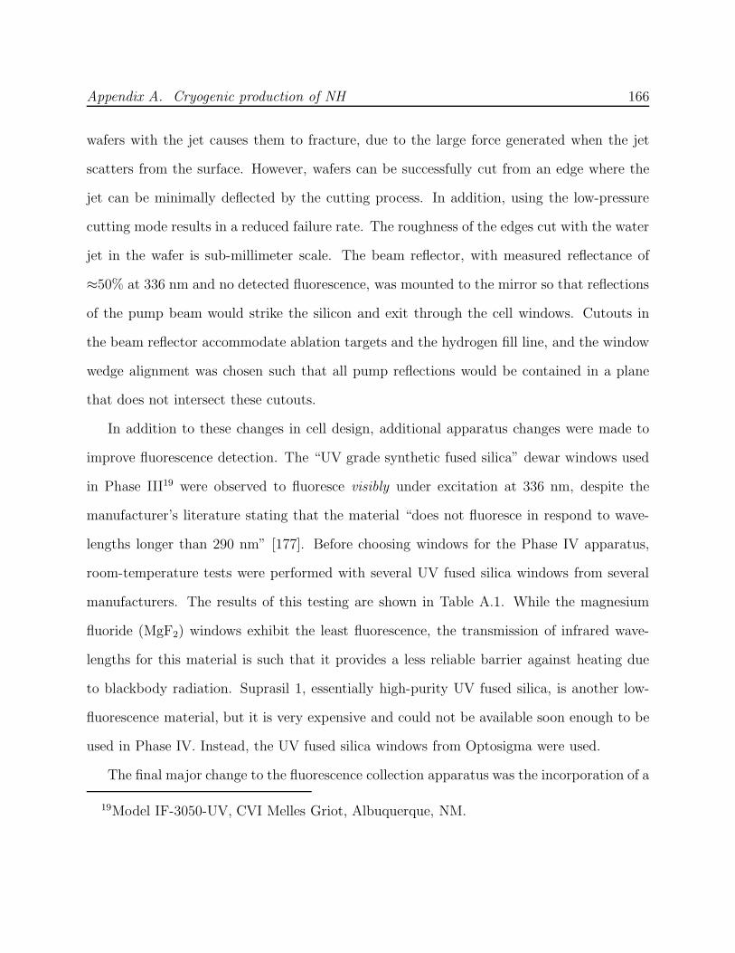
Appendix A. Cryogenic production of NH 166
wafers with the jet causes them to fracture, due to the large force generated when the jet
scatters from the surface. However, wafers can be successfully cut from an edge where the
jet can be minimally deflected by the cutting process. In addition, using the low-pressure
cutting mode results in a reduced failure rate. The roughness of the edges cut with the water
jet in the wafer is sub-millimeter scale. The beam reflector, with measured reflectance of
≈50% at 336 nm and no detected fluorescence, was mounted to the mirror so that reflections
of the pump beam would strike the silicon and exit through the cell windows. Cutouts in
the beam reflector accommodate ablation targets and the hydrogen fill line, and the window
wedge alignment was chosen such that all pump reflections would be contained in a plane
that does not intersect these cutouts.
In addition to these changes in cell design, additional apparatus changes were made to
improve fluorescence detection. The “UV grade synthetic fused silica” dewar windows used
in Phase III19 were observed to fluoresce visibly under excitation at 336 nm, despite the
manufacturer’s literature stating that the material “does not fluoresce in respond to wave-
lengths longer than 290 nm” [177]. Before choosing windows for the Phase IV apparatus,
room-temperature tests were performed with several UV fused silica windows from several
manufacturers. The results of this testing are shown in Table A.1. While the magnesium
fluoride (MgF2) windows exhibit the least fluorescence, the transmission of infrared wave-
lengths for this material is such that it provides a less reliable barrier against heating due
to blackbody radiation. Suprasil 1, essentially high-purity UV fused silica, is another low-
fluorescence material, but it is very expensive and could not be available soon enough to be
used in Phase IV. Instead, the UV fused silica windows from Optosigma were used.
The final major change to the fluorescence collection apparatus was the incorporation of a
19Model IF-3050-UV, CVI Melles Griot, Albuquerque, NM.
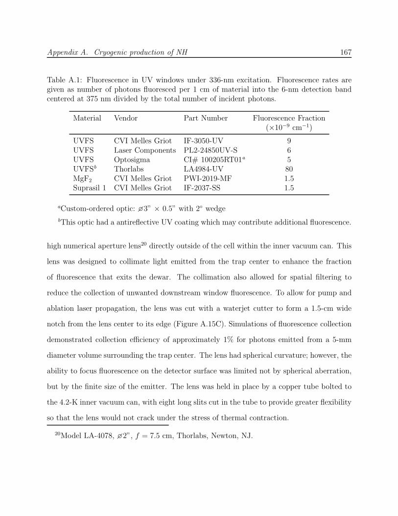
Appendix A. Cryogenic production of NH 167
Table A.1: Fluorescence in UV windows under 336-nm excitation. Fluorescence rates aregiven as number of photons fluoresced per 1 cm of material into the 6-nm detection bandcentered at 375 nm divided by the total number of incident photons.
Material Vendor Part Number Fluorescence Fraction(×10−9 cm−1)
UVFS CVI Melles Griot IF-3050-UV 9UVFS Laser Components PL2-24850UV-S 6UVFS Optosigma CI# 100205RT01a 5UVFSb Thorlabs LA4984-UV 80MgF2 CVI Melles Griot PWI-2019-MF 1.5Suprasil 1 CVI Melles Griot IF-2037-SS 1.5
aCustom-ordered optic: 3” × 0.5” with 2 wedge
bThis optic had a antireflective UV coating which may contribute additional fluorescence.
high numerical aperture lens20 directly outside of the cell within the inner vacuum can. This
lens was designed to collimate light emitted from the trap center to enhance the fraction
of fluorescence that exits the dewar. The collimation also allowed for spatial filtering to
reduce the collection of unwanted downstream window fluorescence. To allow for pump and
ablation laser propagation, the lens was cut with a waterjet cutter to form a 1.5-cm wide
notch from the lens center to its edge (Figure A.15C). Simulations of fluorescence collection
demonstrated collection efficiency of approximately 1% for photons emitted from a 5-mm
diameter volume surrounding the trap center. The lens had spherical curvature; however, the
ability to focus fluorescence on the detector surface was limited not by spherical aberration,
but by the finite size of the emitter. The lens was held in place by a copper tube bolted to
the 4.2-K inner vacuum can, with eight long slits cut in the tube to provide greater flexibility
so that the lens would not crack under the stress of thermal contraction.
20Model LA-4078, 2”, f = 7.5 cm, Thorlabs, Newton, NJ.
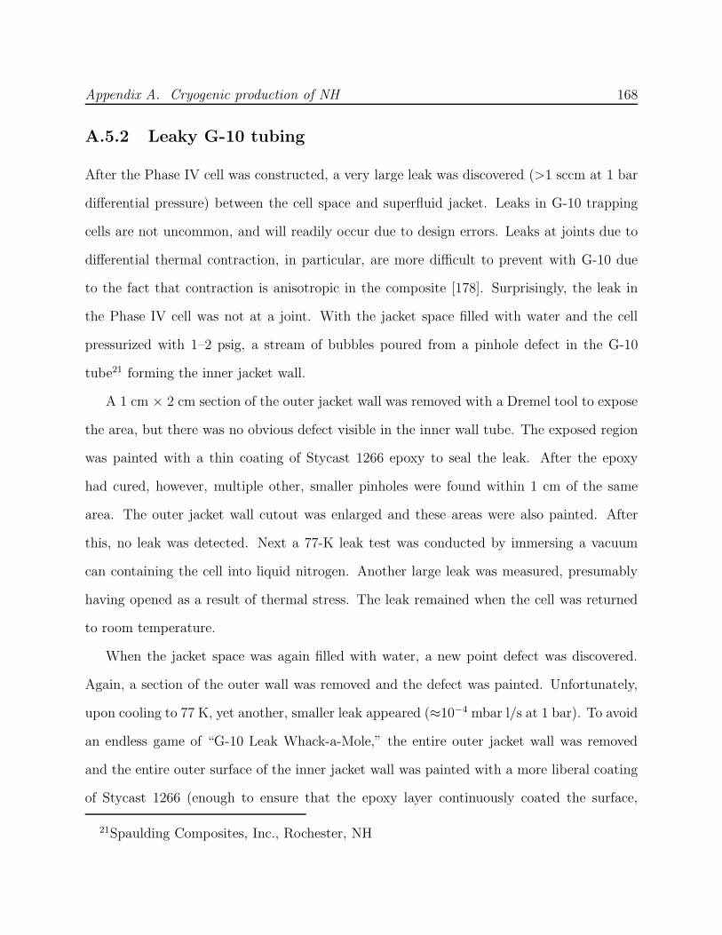
Appendix A. Cryogenic production of NH 168
A.5.2 Leaky G-10 tubing
After the Phase IV cell was constructed, a very large leak was discovered (>1 sccm at 1 bar
differential pressure) between the cell space and superfluid jacket. Leaks in G-10 trapping
cells are not uncommon, and will readily occur due to design errors. Leaks at joints due to
differential thermal contraction, in particular, are more difficult to prevent with G-10 due
to the fact that contraction is anisotropic in the composite [178]. Surprisingly, the leak in
the Phase IV cell was not at a joint. With the jacket space filled with water and the cell
pressurized with 1–2 psig, a stream of bubbles poured from a pinhole defect in the G-10
tube21 forming the inner jacket wall.
A 1 cm × 2 cm section of the outer jacket wall was removed with a Dremel tool to expose
the area, but there was no obvious defect visible in the inner wall tube. The exposed region
was painted with a thin coating of Stycast 1266 epoxy to seal the leak. After the epoxy
had cured, however, multiple other, smaller pinholes were found within 1 cm of the same
area. The outer jacket wall cutout was enlarged and these areas were also painted. After
this, no leak was detected. Next a 77-K leak test was conducted by immersing a vacuum
can containing the cell into liquid nitrogen. Another large leak was measured, presumably
having opened as a result of thermal stress. The leak remained when the cell was returned
to room temperature.
When the jacket space was again filled with water, a new point defect was discovered.
Again, a section of the outer wall was removed and the defect was painted. Unfortunately,
upon cooling to 77 K, yet another, smaller leak appeared (≈10−4 mbar l/s at 1 bar). To avoid
an endless game of “G-10 Leak Whack-a-Mole,” the entire outer jacket wall was removed
and the entire outer surface of the inner jacket wall was painted with a more liberal coating
of Stycast 1266 (enough to ensure that the epoxy layer continuously coated the surface,
21Spaulding Composites, Inc., Rochester, NH
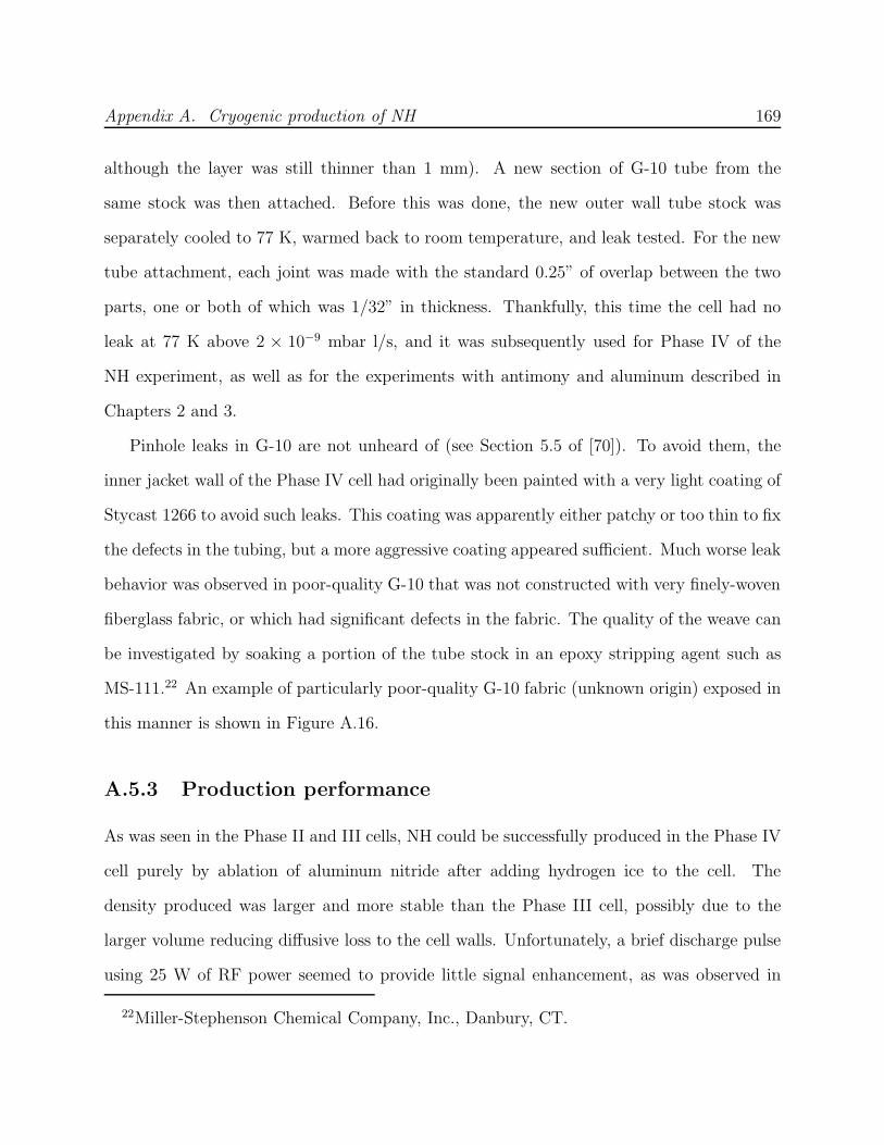
Appendix A. Cryogenic production of NH 169
although the layer was still thinner than 1 mm). A new section of G-10 tube from the
same stock was then attached. Before this was done, the new outer wall tube stock was
separately cooled to 77 K, warmed back to room temperature, and leak tested. For the new
tube attachment, each joint was made with the standard 0.25” of overlap between the two
parts, one or both of which was 1/32” in thickness. Thankfully, this time the cell had no
leak at 77 K above 2 × 10⁻⁹ mbar l/s, and it was subsequently used for Phase IV of the
NH experiment, as well as for the experiments with antimony and aluminum described in
Chapters 2 and 3.
Pinhole leaks in G-10 are not unheard of (see Section 5.5 of [70]). To avoid them, the
inner jacket wall of the Phase IV cell had originally been painted with a very light coating of
Stycast 1266 to avoid such leaks. This coating was apparently either patchy or too thin to fix
the defects in the tubing, but a more aggressive coating appeared sufficient. Much worse leak
behavior was observed in poor-quality G-10 that was not constructed with very finely-woven
fiberglass fabric, or which had significant defects in the fabric. The quality of the weave can
be investigated by soaking a portion of the tube stock in an epoxy stripping agent such as
MS-111.22 An example of particularly poor-quality G-10 fabric (unknown origin) exposed in
this manner is shown in Figure A.16.
A.5.3 Production performance
As was seen in the Phase II and III cells, NH could be successfully produced in the Phase IV
cell purely by ablation of aluminum nitride after adding hydrogen ice to the cell. The
density produced was larger and more stable than the Phase III cell, possibly due to the
larger volume reducing diffusive loss to the cell walls. Unfortunately, a brief discharge pulse
using 25 W of RF power seemed to provide little signal enhancement, as was observed in
22Miller-Stephenson Chemical Company, Inc., Danbury, CT.
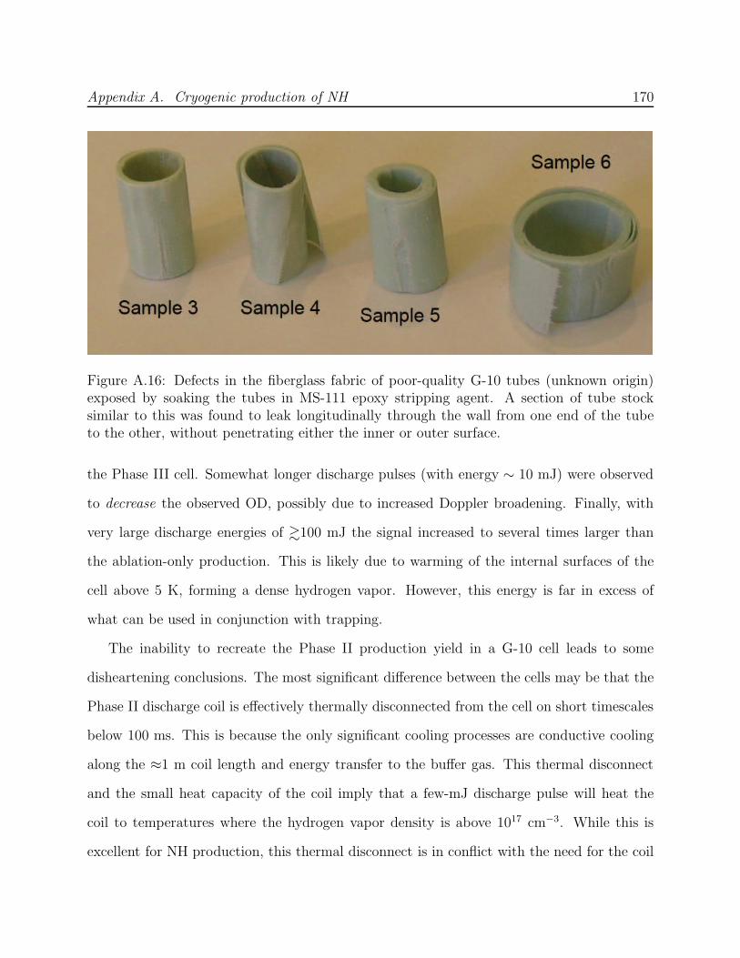
Appendix A. Cryogenic production of NH 170
Figure A.16: Defects in the fiberglass fabric of poor-quality G-10 tubes (unknown origin)exposed by soaking the tubes in MS-111 epoxy stripping agent. A section of tube stocksimilar to this was found to leak longitudinally through the wall from one end of the tubeto the other, without penetrating either the inner or outer surface.
the Phase III cell. Somewhat longer discharge pulses (with energy ∼ 10 mJ) were observed
to decrease the observed OD, possibly due to increased Doppler broadening. Finally, with
very large discharge energies of &100 mJ the signal increased to several times larger than
the ablation-only production. This is likely due to warming of the internal surfaces of the
cell above 5 K, forming a dense hydrogen vapor. However, this energy is far in excess of
what can be used in conjunction with trapping.
The inability to recreate the Phase II production yield in a G-10 cell leads to some
disheartening conclusions. The most significant difference between the cells may be that the
Phase II discharge coil is effectively thermally disconnected from the cell on short timescales
below 100 ms. This is because the only significant cooling processes are conductive cooling
along the ≈1 m coil length and energy transfer to the buffer gas. This thermal disconnect
and the small heat capacity of the coil imply that a few-mJ discharge pulse will heat the
coil to temperatures where the hydrogen vapor density is above 1017 cm−3. While this is
excellent for NH production, this thermal disconnect is in conflict with the need for the coil
Appendix A. Cryogenic production of NH 171
to cool rapidly after production to allow for trapping and thermal isolation. The experience
of Phase III and IV seems to imply that these conflicting requirements cannot be reconciled
to achieve the simultaneous goals of large production yield, trapping, and thermal isolation.
A.5.4 Detection performance
Before the Phase IV cooldown, the room-temperature noise background of unwanted flu-
orescence in the new cell was tested in a tabletop apparatus where full optics positioning
control is possible. These tests confirmed a dramatically reduced fluorescence rate compared
to the Phase III cell, with fluorescence noise at a similarly low level as that caused by pump
beam reflections striking the PMT filter stack. With the pump beam deliberately aligned
poorly to strike the G-10 hydrogen fill line, a somewhat larger, but still acceptable, noise
level was measured, demonstrating the effective spatial filtering of the fluorescence collection
lens. The total noise level with a 50-µW pump beam was measured to be less than 10 kHz,
where a signal of over 1 MHz would be expected for 0.01% of the pump being absorbed and
fluoresced in the collection region.23
Phase IV of the NH experiment was conducted in the cold apparatus after the antimony–
helium collision experiment described in Chapter 2. In the 3–4 weeks of discharge and
production tests after ending the antimony experiment, a film of unknown composition was
deposited on the outer surface of the 77-K window. This film was found to be opaque to
the 207-nm laser used to detect antimony, and hence it cannot have been present for that
experiment. When fluorescence detection of NH was attempted, the film glowed brightly
under excitation with the 336-nm pump beam, with correspondingly terrible background
23This region is about 10% the length of the cell and is overlapped with the trap. Thereforethis 10−4 local fluorescence level would be equal to the in-trap OD , or 10% of the zero fieldOD .
Appendix A. Cryogenic production of NH 172
noise levels at the 375-nm detection band. This background prevented fluorescence detection
of NH in Phase IV, and further testing of the detection improvements could not be performed.
A.6 Summary and future prospects
A.6.1 Successful cryogenic production
The experiments described here demonstrated production of 1011 NH molecules at temper-
atures below 1 K (in the copper Phase II cell) and over 1010 molecules under conditions
compatible with trapping (low production energy in a G-10 cell). The production method
is relatively straightforward to implement, involving only an aluminum nitride target, a gas
line to deposit hydrogen ice, and an ablation laser. This yield is approximately an order of
magnitude smaller than the previous room-temperature discharge source [150], but can be
implemented with under 10 mJ of energy and no additional heat load, such as that associated
with open apertures that pass room-temperature blackbody radiation. Cryogenic discharge
production of NH from nitrogen and hydrogen vapor was also achieved at 7.5 K, but this
could not be replicated in a trapping cell.
Despite this success in production, none of the four phases of the NH work described here
demonstrated NH trapping. The fundamental barrier is poor detection, since a large number
of molecules are produced. As a result, future work with NH could benefit from adopting
the cryogenic production described here in an apparatus better suited to low-background
fluorescence spectroscopy.
Appendix A. Cryogenic production of NH 173
A.6.2 Proposed improvements for improved detection
sensitivity
The apparatus used for this work struggles against a single design constraint: both optical
pumping and fluorescence detection share the same optical path into the cell. Especially be-
cause of the UV wavelengths needed for NH detection, the inevitable scatter and fluorescence
due to the pump beam cannot be adequately filtered from the signal photons. The task of
retrofitting the current experiment for perpendicular optical access would be prohibitively
expensive and difficult, and future experiments would do better to construct a new apparatus
that allows the magnet, refrigerator and cell to occupy the same vacuum space.
Even with perpendicular access, care must still be taken to minimize stray window re-
flections and fluorescence of materials. If pump laser scatter can be adequately reduced,
then diagonal detection is preferable due to the much higher fluorescence rate. Chopping
the pump beam improves the signal-to-noise by a factor of about 12, limited by PMT af-
terpulsing. Afterpulses are not intrinsic to detection with PMTs, so the effect likely can be
greatly reduced if extreme care is taken to avoid helium contamination.24 Alternatively, a
gated detector can be used to remain insensitive to the bright pump, but the gate repetition
rate must be close to 1 MHz to preserve the high signal rate. Likewise, off-diagonal detec-
tion with a perpendicular pump beam could achieve extremely low background noise with
appropriate elimination of line-of-sight between the detector and fluorescing materials along
the pump beam path. Off-diagonal sensitivity would then likely be shot-noise limited due
to the weak Franck-Condon factor.
24Reasonable care was taken with the PMTs used for this work, and the previous NHwork. The PMTs were kept in enclosures either pumped to vacuum or continuously purgedwith nitrogen gas. Nevertheless, both PMTs show similar afterpulsing behavior.
Appendix A. Cryogenic production of NH 174
A.6.3 Prospects for sympathetic cooling
Based on the work outlined in this appendix, one can make modestly optimistic assumptions
about the ability to produce and cool NH in a future G-10 cell. With 1010 molecules produced
under trappable conditions at 0.5 K and a reasonable 10% trapping efficiency, an maximum
initial density of 2 × 1011 cm−3 would be achieved. A significant number of these molecules
would likely undergo spin relaxation in the initial ∼30 ms during which the helium-4 density
drops and thermal isolation is achieved.
Nitrogen is not directly observed in the experiments described here, but the rather ef-
ficient NH production from ablation of aluminum nitride into hydrogen suggests a large
nitrogen yield. Based on previous measurements and calculations of the nitrogen–helium
system, it is safe to assume that nitrogen will be efficiently buffer-gas cooled and trapped
after production and will likely be present in much greater numbers than NH in the trap.
The resulting nitrogen–nitrogen collision rate will be more than rapid enough to proceed
with evaporative cooling.
Sympathetic cooling of NH with evaporatively cooled nitrogen is hampered by the mis-
matched magnetic moments of the two species. The 3-µB nitrogen atoms will form a dense
cloud at the trap center with a more diffuse surrounding cloud of 2-µB NH, precisely the
wrong ordering for efficient sympathetic cooling with the large nitrogen reservoir. As cooling
continues, NH will be consistently at a value of η that is 2/3 that of nitrogen, and thus NH
will be preferentially evaporated. The sympathetic cooling of NH is therefore necessarily less
efficient than evaporative cooling of nitrogen, even neglecting NH–nitrogen inelastic losses.
Evaporative cooling of buffer-gas cooled nitrogen will follow similar constraints as those
outlined in the thesis of Charlie Doret [111] in reference to cooling metastable helium, includ-
ing the rather slow rate at which current can be removed from the superconducting magnet
coils to reduce the trap depth. For this technical reason, and because the values of γ for ni-
Appendix A. Cryogenic production of NH 175
trogen and 4He* are similarly high [52, 179], we take the demonstrated evaporation of 4He*
in that experiment as an efficiency benchmark for predicting the behavior with nitrogen.
Specifically, the two orders of magnitude of atom loss required to reduce the temperature
by two orders of magnitude [180] is a reasonable expectation. As this atom loss would stem
largely from evaporative losses at ηN < 8, the NH loss is likely to be at least an additional
order of magnitude worse (Equation 4.1). Finally, it is important to consider the inelastic
NH–nitrogen losses that will be sustained in addition to this evaporative loss. If ramping the
magnet takes the ∼100 s necessary for the 4He* work, inelastic losses could be significant
even with the interspecies γ being greater than 100. Also, the inelasticity of the interspecies
collisions is calculated to increase at lower temperatures [53]. It will be thus be critical for
the sympathetic cooling experiment not to “waste” any collisions with a suboptimal evap-
oration trajectory. Finally, a large initial molecule reservoir will be necessary—a condition
satisfied by the cryogenic production method described here.

Appendix B
Calculating absorption for trapped
molecules in motion
B.1 Reconciling Beer’s Law with the Landau-
Zener model
Molecules (or atoms) in a magnetic trap will have a distribution of Zeeman shifts corre-
sponding to their spatial distribution superimposed on the trapping field. For a fixed probe
laser frequency, only a certain shell of constant magnetic field will be in resonance. For a
spherical quadrupole field with field along the z-axis given by B = B′0z, the thickness ∆z
of this shell is given by
∆z =Γnat
∂ω∂BB′
0
=1
τnat∂ω∂BB′
0
, (B.1)
where Γnat and τnat are the natural linewidth and lifetime, respectively, and ∂ω/∂B is the
differential magnetic moment between the ground and excited states. For B′0 ∼ 1 T/cm,
∂ω/∂B ∼ µB, and τnat ∼ 100 ns, this resonant shell has ∆z ∼ 1 µm, much smaller than the
trap size. The absorption of the probe laser with initial intensity I0 at the intersection of
176

Appendix B. Calculating absorption for trapped molecules in motion 177
this shell can be calculated from Beer’s Law,
1 − I
I0= 1 − e−OD (B.2)
OD =
∫
n(z) σ(z) dz (B.3)
where n(z) is the molecule density distribution averaged over the laser beam cross section
and σ is the optical cross section.
At temperatures near 500 mK, the molecules are moving at a mean velocity of vz ∼ 1–
2 × 103 cm/s. Doppler broadening inhomogeneously thickens the resonant shell, however
each individual molecule sees the same ∆z ∼ 1 µm at a Doppler-shifted location. The
molecules traverse ∆z on average in a time ∆t < 100 ns (for transitions with longer excited
state lifetimes, transit time broadening will increase ∆z and ∆t). Even for short lifetimes of
10 ns, the molecules will still cross the resonant shell slower than the mean time to excitation
(assuming saturation s0 < 1%, as is typically used to avoid optical pumping out of the trap).
It is then reasonable to ask whether the fact that the molecules are in resonance for a very
brief time affects the absorption rate of photons from the laser beam. Going further, if we
assume a mean collision time longer than ∆t, the molecules will maintain a constant velocity
as they pass through resonance, and hence will experience a linearly-varying detuning
δ =∂ω
∂BB′
0z =∂ω
∂BB′
0vzt. (B.4)
This linear sweep through a resonant interaction is reminiscent of the classic Landau-Zener
treatment of an avoided crossing. It is not obvious that the result of Beer’s Law, obtained
from integrating over a stationary distribution in space, will be the same as that obtained
from applying the Landau-Zener method to each passing molecule. However, through a
series of cases, we show in this appendix that the two approaches are indeed equivalent in
the limit of weak laser power.

Appendix B. Calculating absorption for trapped molecules in motion 178
B.1.1 Case 1: Stationary atoms
For the purposes of all four cases considered here, we will consider a uniform density n of
two-level atoms with excited state lifetime τnat = Γ−1nat. The atoms are moving with constant
uniform velocity v = vz z in a constant-gradient magnetic field B = B′0z. We will first
consider the stationary case of vz = 0. When illuminated with laser light with frequency ω
and saturation parameter s0, the scattering rate of the atoms will be
Γsc =1
2τnat
[
s01 + s0 + (2δ/Γnat)2
]
=s0
2τnat
[
1
1 + (2δτnat)2
]
, (B.5)
where the second equality has used s0 ≪ 1. The total fluorescence rate is given by integrating
Equation B.5 over all space,
Γf =
∫
nΓsc d3r
=s0nA
2τnat
∫
dz
1 + (2τnatδ(z))2
=πs0nA
4τ 2nat∂ω∂BB′
0
, (B.6)
where A is the cross sectional area of the laser beam.
B.1.2 Case 2: Arbitrarily slow atoms
Next we calculate Γf for the case in which the atoms are moving at a constant, very slow
velocity that satisfies vz/∆z ≪ Γsc ≪ Γnat, i.e., the timescale for crossing the resonance is the
slowest in the problem. Each atom will now see a linearly-changing detuning (Equation B.4),
which moves through resonance as t goes from −∞ → ∞. Ignoring the excited state decay,
this is the standard Landau-Zener case. The probability of each atom being found in the

Appendix B. Calculating absorption for trapped molecules in motion 179
excited state after passage is given by [181]
P = 1 − exp
(
−2πΩ2
α
)
. (B.7)
where α = ∂δ/∂t is the detuning sweep rate and ~Ω the interaction matrix element. It is
important to note the relationship between Ω and the Rabi frequency ΩR = −(eE0/~)〈e|(r ·
ε)|g〉 that results from the interaction of the two-level atomic dipole, d = −e r, with the
electric field, E(t) = E0ε cos(kz − ωt), of the laser (with wavevector k and frequency ω).
In the rotating wave approximation, only half of the electric field magnitude drives the
transition with the correct frequency, giving Ω2 = (ΩR/2)2 = s0/8τ2nat [181, 182].
Akulin and Schleich have analyzed the Landau-Zener problem when excited state decay
is taken into account [183]. They find that the number of photons emitted by each atom
passing through resonance is given by
Nph = 2πΩ2
αe−πΩ2/α
∣
∣
∣
∣
WiΩ2/α,−1/2
(
−iΓ2nat
α
)∣
∣
∣
∣
2
, (B.8)
where Wk,m(z) is the Whittaker function [184]. This result is nontrivial and rather opaque,
but useful asymptotic limits are presented in [183]. In the slow-sweep limit considered in
this case (Ω2Γ2nat/α
2 ≫ 1), Equation B.8 simplifies to
Nph = 2πΩ2
α. (B.9)
We then must only multiply by the rate that atoms pass through the resonance to determine
the fluorescence rate
Γf = (nvzA)
[
2πΩ2
α
]
= (nvzA)
[
2π
s08τ2nat
∂ω∂BB′
0vz
]
=πs0nA
4τ 2nat∂ω∂BB′
0
, (B.10)
Appendix B. Calculating absorption for trapped molecules in motion 180
where we have used Ω2 = s0/8τ2nat. Comparison of Equations B.6 and B.10 shows no differ-
ence between the stationary case and the arbitrarily-slow case, which is comforting.
B.1.3 Case 3: Rapid atoms
Next, we consider the case where atoms cross the resonance quickly (vz/∆z ≫ Γnat ≫ Ω).
Akulin and Schleich also consider this limit (α≫ Γ2nat), finding that the number of photons
scattered per atom is given by [183]
Nph = 1 − exp
(
−2πΩ2
α
)
. (B.11)
Note that this is the same as the result that ignores decay (Equation B.7). This makes
sense, since in the case of slow decay the number of photons emitted per atom is at most
one and equal to the probability of reaching the excited state during the crossing. For the
weak-probe limit (s0 ≪ 1), Equation B.11 reduces to Equation B.9 and the fluorescence rate
is the same as in Case 2 (Equation B.10).
B.1.4 Case 4: Intermediate-speed atoms
Finally, we consider the case in which the atoms are moving at a speed such that Ω ≪
vz/∆z ≪ Γnat. This is the case in which the atoms cross the resonance much slower than
the excited state decay, but much faster than the mean time to excitation—so most atoms
cross without scattering a photon. This case (Ω2/α ≪ Ω/Γnat ≪ 1 and Γ2nat ≫ α) is not
specifically addressed in [183]. In this limit, Equation B.8 reduces to
Nph = limΓ2nat/α→∞
2πΩ2
αe−πΩ2/α
∣
∣
∣
∣
WiΩ2/α,−1/2
(
−iΓ2nat
α
)∣
∣
∣
∣
2
= 2πΩ2
αe−πΩ2/α eπΩ
2/α
= 2πΩ2
α, (B.12)

Appendix B. Calculating absorption for trapped molecules in motion 181
which is the same result as found in Case 2. Hence the fluorescence rate is again the same
as Equation B.10.
B.1.5 Conclusions from the comparison
Using the appropriate asymptotic limits of the Landau-Zener problem with decay, compar-
ison of Cases 2–4 gives the same result in all velocity limits, (assuming laser intensity well
below saturation). This shared result is also the same as that of Case 1, the stationary
case. Therefore, we conclude that there is no difference between calculating the fluorescence
rate as a Landau-Zener level crossing or by integrating over a spatially-extended resonance
with a stationary atom distribution. It is safe to assume the atoms to be stationary for the
calculation (except in regards to Doppler shifts), which is a more straightforward calculation.
To determine the OD from the fluorescence rate Γf, we normalize by the incident photon
flux Γph to yield the absorption:
Γf/Γph =
[
πs0nA
4τ 2nat∂ω∂BB′
0
]
[
s0IsatA
~ω
]−1
=π
2nσ
(
1
τnat∂ω∂BB′
0
)
=π
2nσ∆z, (B.13)
where we have used Equation B.1 and the definition of the saturation intensity,
Isat =~ω
2σ0τnat. (B.14)
where σ0 is the resonant optical cross section. We have already made the assumption in
Equation B.5 that absorption of photons does not affect the fluorescence rate (i.e., Γf ≪ Γph)
and so OD ≪ 1 and we can equate it with absorption,
OD =π
2nσ0∆z. (B.15)
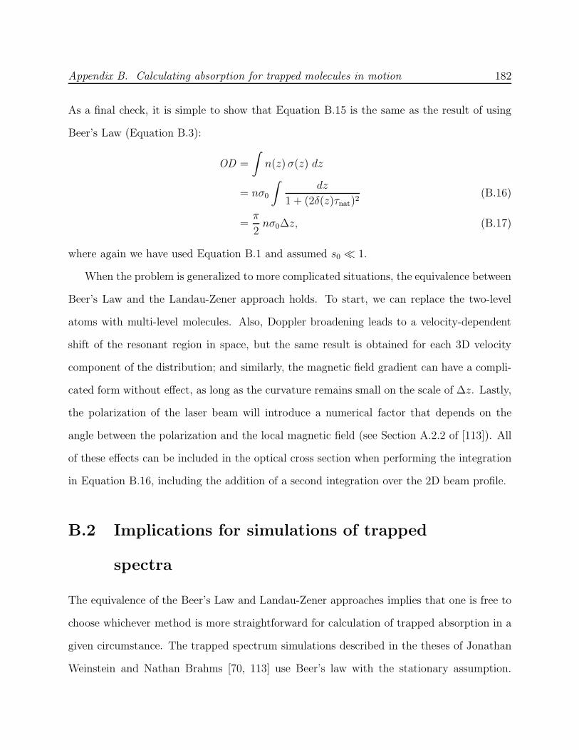
Appendix B. Calculating absorption for trapped molecules in motion 182
As a final check, it is simple to show that Equation B.15 is the same as the result of using
Beer’s Law (Equation B.3):
OD =
∫
n(z) σ(z) dz
= nσ0
∫
dz
1 + (2δ(z)τnat)2(B.16)
=π
2nσ0∆z, (B.17)
where again we have used Equation B.1 and assumed s0 ≪ 1.
When the problem is generalized to more complicated situations, the equivalence between
Beer’s Law and the Landau-Zener approach holds. To start, we can replace the two-level
atoms with multi-level molecules. Also, Doppler broadening leads to a velocity-dependent
shift of the resonant region in space, but the same result is obtained for each 3D velocity
component of the distribution; and similarly, the magnetic field gradient can have a compli-
cated form without effect, as long as the curvature remains small on the scale of ∆z. Lastly,
the polarization of the laser beam will introduce a numerical factor that depends on the
angle between the polarization and the local magnetic field (see Section A.2.2 of [113]). All
of these effects can be included in the optical cross section when performing the integration
in Equation B.16, including the addition of a second integration over the 2D beam profile.
B.2 Implications for simulations of trapped
spectra
The equivalence of the Beer’s Law and Landau-Zener approaches implies that one is free to
choose whichever method is more straightforward for calculation of trapped absorption in a
given circumstance. The trapped spectrum simulations described in the theses of Jonathan
Weinstein and Nathan Brahms [70, 113] use Beer’s law with the stationary assumption.
Appendix B. Calculating absorption for trapped molecules in motion 183
These simulations also go much further than this discussion to appropriately account for the
Zeeman effect in multi-level systems, the finite extent and offset of the beam, and the spatial
integration through the actual trapping geometry.
The thesis of Wes Campbell includes a separate calculation of the fluorescence rate using
the Landau-Zener approach (see Section 5.2 of [152]). He finds a discrepancy compared with
the Beer’s Law result, but this is due to an error in the calculation. The correct result for
trapped absorption is that shown in Equation B.17, along with appropriate consideration of
polarization and spatial integration in the trap.
Appendix C
Polarization-sensitive absorption
spectroscopy and “extra light”
C.1 Observations of “extra light”
Appendix C of the thesis of Cindy Hancox [72] details observations of a confusing phe-
nomenon in which the presence of atoms in a buffer-gas cell led to more light reaching the
signal photodetector, rather than less. This effect gives the impression of negative absorption
and was dubbed “extra light.” Hancox gives her expression for calculating the absorption A
as
A(t) = 1 − D(t)
Dbaseline
(C.1)
D(t) =Vsignal(t)
Vreference(t), (C.2)
where the ratio D(t) of voltages from photodetectors monitoring signal and reference beams
is called the “divide,” and Dbaseline is the divide measured with no atoms in the cell. The
extra light effect was observed purely as an increase in the Vsignal, with no unusual behavior in
Vreference. Examples of extra light given by Hancox in her thesis are reproduced in Figures C.1,
184
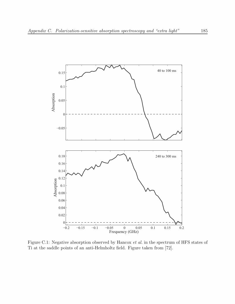
Appendix C. Polarization-sensitive absorption spectroscopy and “extra light” 185
−0.05
0
0.05
0.1
0.15
Abso
rpti
on
40 to 100 ms
−0.2 −0.15 −0.1 −0.05 0 0.05 0.1 0.15 0.2
0
0.02
0.04
0.06
0.08
0.1
0.12
0.14
0.16
0.18
Frequency (GHz)
Abso
rpti
on
240 to 300 ms
Figure C.1: Negative absorption observed by Hancox et al. in the spectrum of HFS states ofTi at the saddle points of an anti-Helmholtz field. Figure taken from [72].
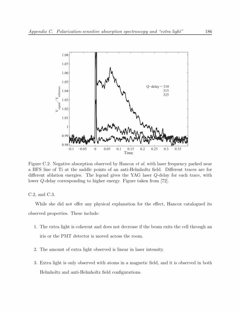
Appendix C. Polarization-sensitive absorption spectroscopy and “extra light” 186
−0.1 −0.05 0 0.05 0.1 0.15 0.2 0.25 0.3 0.350.98
0.99
1
1.01
1.02
1.03
1.04
1.05
1.06
1.07
1.08V
signal
/ V
refe
rence
Time
Q−delay = 310315325
Figure C.2: Negative absorption observed by Hancox et al. with laser frequency parked neara HFS line of Ti at the saddle points of an anti-Helmholtz field. Different traces are fordifferent ablation energies. The legend gives the YAG laser Q-delay for each trace, withlower Q-delay corresponding to higher energy. Figure taken from [72].
C.2, and C.3.
While she did not offer any physical explanation for the effect, Hancox catalogued its
observed properties. These include:
1. The extra light is coherent and does not decrease if the beam exits the cell through an
iris or the PMT detector is moved across the room.
2. The amount of extra light observed is linear in laser intensity.
3. Extra light is only observed with atoms in a magnetic field, and it is observed in both
Helmholtz and anti-Helmholtz field configurations.
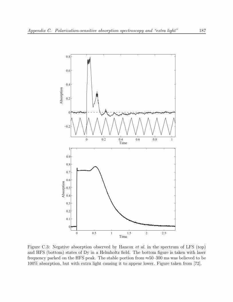
Appendix C. Polarization-sensitive absorption spectroscopy and “extra light” 187
0 0.5 1 1.5 2 2.5
0
0.1
0.2
0.3
0.4
0.5
0.6
0.7
0.8
0.9
1
Abs
orpt
ion
Time
0 0.2 0.4 0.6 0.8 1
−0.2
0
0.2
0.4
0.6
0.8
Absorption
Time
Figure C.3: Negative absorption observed by Hancox et al. in the spectrum of LFS (top)and HFS (bottom) states of Dy in a Helmholtz field. The bottom figure is taken with laserfrequency parked on the HFS peak. The stable portion from ≈50–300 ms was believed to be100% absorption, but with extra light causing it to appear lower. Figure taken from [72].
Appendix C. Polarization-sensitive absorption spectroscopy and “extra light” 188
4. The effect is frequency dependent and strongest near strong spectral features associated
with both low- and high-field-seeking (LFS and HFS) states.
5. The effect is most pronounced at high buffer gas densities.
6. Extra light was observed in experiments with both titanium and dysprosium. No other
species were investigated for the effect.
Since the extra light effect did not interfere with the measurements of Hancox et al., it was
not investigated further. The effect was limited to .5% of Vsignal.
Negative absorption was also observed in the experiments with aluminum described in
Chapter 3 of this thesis. In that case, the effect was much more dramatic (Figure C.4), with
Vsignal increasing by up to 40% when the laser was tuned near resonance at high aluminum
density. In addition, a >10% effect was observed with metastable helium-4 (Figure C.5) in
the same experimental run as the rare-earth atom experiments described in Chapter 4. At
this level, the effect is no longer a small perturbation to the measurement and becomes a
significant concern. This appendix presents a model of apparent negative absorption caused
by the combination of atomic birefringence and polarization-sensitive optical detection.
C.2 Absorption spectroscopy with polarization-
dependent optics
The premise of absorption spectroscopy is straightforward: one laser beam passes through
and interacts with the atomic cloud while a reference beam monitors the laser intensity. Both
beams strike (ideally) matched photodetectors and the ratio of the two signals, normalized to
unity for zero absorption, provides the transmission of the cloud independent of laser intensity
fluctuations to first order. In practice, however, more optics are involved. At minimum,

Appendix C. Polarization-sensitive absorption spectroscopy and “extra light” 189
0 2 4 6 8 10 12 14 16 180.8
0.9
1
1.1
1.2
1.3
time after ablation (ms)
tran
smis
sion
−76 −74 −72 −700
1
OD
detuning (GHz)
Vsignal
/ Vreference
laser scan
Figure C.4: Negative absorption observed in the scanned spectrum of LFS states of Al in a0.5-T Helmholtz magnetic field with T ≈ 850 mK. The inset shows the simulated hyperfinespectrum with asymmetric Helmholtz lineshape (see Figure 2.3).
there are almost always windows on the experimental chamber, and often in multiple layers.
Usually there is also a beamsplitter to separate the signal and reference beams, and mirrors
to steer the beams onto the detectors. The optics schematic for the experiments of Hancox et
al. [72] is shown in Figure C.6. Most buffer-gas trapping experiments with a single half-axis
of optical access have similar layouts (see also Figures 2.7 and 3.3). After the beamsplitter,
the probe beam is overlapped with its reflection from the cell mirror. This overlap ensures
that both beams sample the same region of the cell, simplifying data analysis and minimizing
error. The return beam strikes the same beamsplitter and is partially transmitted to the

Appendix C. Polarization-sensitive absorption spectroscopy and “extra light” 190
0 0.05 0.1 0.15 0.2 0.25 0.30.8
0.9
1
1.1
1.2
tran
smis
sion
time (s)
−0.5 0 0.5 1 1.5 2
1
1.1
Vsignal
/ Vreference
laser scan
Figure C.5: Negative absorption observed in spectrum of trapped He*. The sharp feature isthe ∆m = 0 transition on top of the broader ∆m = +1 feature (see Figure 4.3 of [111] foran undistorted spectrum). The inset (same axis units) shows the signal obtained by holdingthe laser frequency constant where the transmission is maximized.
signal detector.
In the optics layout described above, only a fraction of the laser power exiting the cell
is incident on the signal detector, due to the second pass through the beamsplitter. The
reflected component retraces the beam path back toward the laser and is not monitored. If
some process acts to change the splitting fraction, then more or less light will be seen by
the signal detector, with a corresponding change in Vsignal. An example of such a process
is a polarization rotation. Unless optimized to avoid it, most beamsplitters are polarization
sensitive at 45 incidence, especially beamsplitters with dielectric coatings. Therefore bire-
fringence in the dewar optics or cell can alter the splitting fraction. An extreme example of
this is given in Figure 3.8, which shows the exiting beam polarization rotating as the mag-

Appendix C. Polarization-sensitive absorption spectroscopy and “extra light” 191
Optics table
Verdi Pump Laser Ti:Sa Laser
Wavemeter
Cavity Doubler
Pinhole
Dewar optics plate
Pulsed Doubled YAG
Iris
300K window77K window
4K window
Cell window
Cell mirrorTarget
Iris Filter
Probe Beam
Ablation Beam
Mirror
Beamsplitter
Atom cloud
Cryostat
Neutral density filter
Lens
390 nm diode laser
Wavemeter
Signal PMT
Reference PMT
Ti:Sa laser system
Diode laser system:
may be used in place of Ti:Sa
laser system for Sc detection
Iris Filter
Key:
Figure C.6: Optics schematic for the experiments by Hancox et al. with Ti and Dy, takenfrom [72].
Appendix C. Polarization-sensitive absorption spectroscopy and “extra light” 192
netic field is changed, due to the Faraday effect. In that case, the beamsplitter is a polarizing
beamsplitter cube, and so the splitting fraction is maximally polarization sensitive.
It is easy to see how an atomic cloud in a magnetic field can give rise to frequency- and
atom-density-dependent birefringence. Consider a cell filled with buffer-gas cooled aluminum
atoms at 1 K in a constant magnetic field of 1 T parallel to the laser propagation direction.
From the mJ = +1/2 sublevel of the 2P1/2 ground state, there is only one option for excitation
to the 2S1/2 state: absorbtion of a σ−-polarized photon for a ∆mJ = −1 transition to the
excited state mJ = −1/2 sublevel (the aluminum level diagram is shown in Figure 3.2).
∆m = 0 transitions are forbidden, as they would require polarization along the propagation
direction. Therefore, the atoms only absorb right-circularly polarized light. Upon reflection
from the cell mirror, the beam propagates antiparallel to the field such that σ−-polarization
is equivalent to left-circular polarization. The handedness of the probe light also inverts upon
reflection, and so the interaction is unchanged for the second pass through the atom cloud.
In summary, right-circularly polarized light entering the cell can be entirely absorbed, while
left-circularly polarized light cannot be absorbed at all. If linearly polarized light enters
the cell, half of it will interact and the other half will not, leaving the beam polarization
elliptical.
C.2.1 Quantitative model
It is still not obvious from the argument above why the signal detector should see more light
due to absorption of one circular component. After all, the total beam power is definitely
reduced. For a full picture, it is important to consider both absorption and dispersion caused
by the atomic cloud. When the laser with electric field E0 passes through the atoms, it is
attenuated and phase shifted to yield E = tE0 eiφ. The attenuation coefficient t and phase
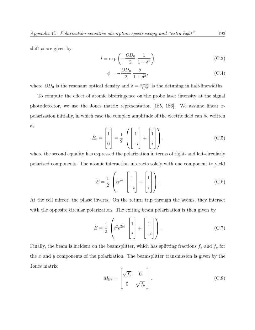
Appendix C. Polarization-sensitive absorption spectroscopy and “extra light” 193
shift φ are given by
t = exp
(
−OD0
2
1
1 + δ2
)
(C.3)
φ = −OD0
2
δ
1 + δ2, (C.4)
where OD0 is the resonant optical density and δ = ω−ω0
Γ/2is the detuning in half-linewidths.
To compute the effect of atomic birefringence on the probe laser intensity at the signal
photodetector, we use the Jones matrix representation [185, 186]. We assume linear x-
polarization initially, in which case the complex amplitude of the electric field can be written
as
E0 =
1
0
=
1
2
1
−i
+
1
i
, (C.5)
where the second equality has expressed the polarization in terms of right- and left-circularly
polarized components. The atomic interaction interacts solely with one component to yield
E =1
2
teiφ
1
−i
+
1
i
. (C.6)
At the cell mirror, the phase inverts. On the return trip through the atoms, they interact
with the opposite circular polarization. The exiting beam polarization is then given by
E =1
2
t2e2iφ
1
i
+
1
−i
. (C.7)
Finally, the beam is incident on the beamsplitter, which has splitting fractions fx and fy for
the x and y components of the polarization. The beamsplitter transmission is given by the
Jones matrix
MBS =
√fx 0
0√
fy
. (C.8)
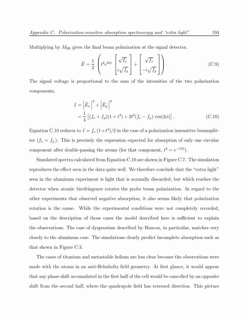
Appendix C. Polarization-sensitive absorption spectroscopy and “extra light” 194
Multiplying by MBS gives the final beam polarization at the signal detector,
E =1
2
t2e2iφ
√fx
i√
fy
+
√fx
−i√
fy
. (C.9)
The signal voltage is proportional to the sum of the intensities of the two polarization
components,
I =∣
∣
∣Ex
∣
∣
∣
2
+∣
∣
∣Ey
∣
∣
∣
2
=1
4
[
(fx + fy)(1 + t4) + 2t2(fx − fy) cos(2φ)]
. (C.10)
Equation C.10 reduces to I = fx (1+t4)/2 in the case of a polarization insensitive beamsplit-
ter (fx = fy ). This is precisely the expression expected for absorption of only one circular
component after double-passing the atoms (for that component, t4 = e−OD).
Simulated spectra calculated from Equation C.10 are shown in Figure C.7. The simulation
reproduces the effect seen in the data quite well. We therefore conclude that the “extra light”
seen in the aluminum experiment is light that is normally discarded, but which reaches the
detector when atomic birefringence rotates the probe beam polarization. In regard to the
other experiments that observed negative absorption, it also seems likely that polarization
rotation is the cause. While the experimental conditions were not completely recorded,
based on the description of those cases the model described here is sufficient to explain
the observations. The case of dysprosium described by Hancox, in particular, matches very
closely to the aluminum case. The simulations clearly predict incomplete absorption such as
that shown in Figure C.3.
The cases of titanium and metastable helium are less clear because the observations were
made with the atoms in an anti-Helmholtz field geometry. At first glance, it would appear
that any phase shift accumulated in the first half of the cell would be cancelled by an opposite
shift from the second half, where the quadrupole field has reversed direction. This picture
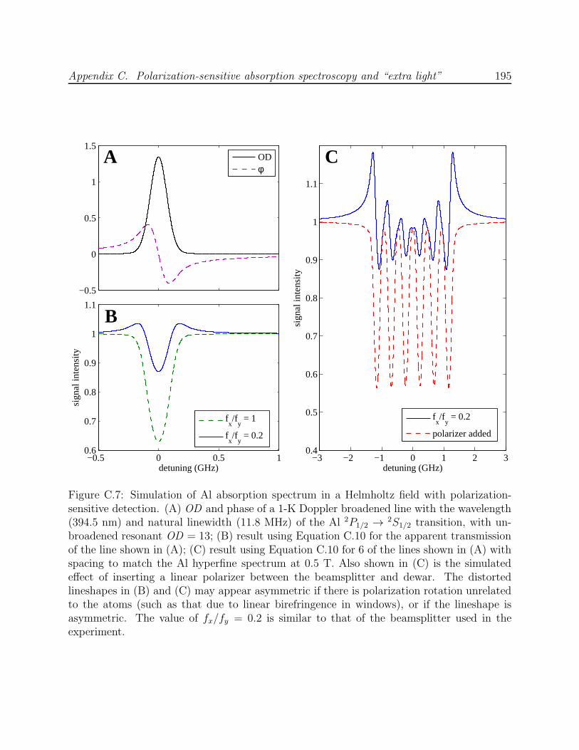
Appendix C. Polarization-sensitive absorption spectroscopy and “extra light” 195
−3 −2 −1 0 1 2 30.4
0.5
0.6
0.7
0.8
0.9
1
1.1
detuning (GHz)
sign
al in
tens
ity
C
−0.5
0
0.5
1
1.5
A
−0.5 0 0.5 10.6
0.7
0.8
0.9
1
1.1
detuning (GHz)
sign
al in
tens
ity
B
fx/f
y = 0.2
polarizer added
ODφ
fx/f
y = 1
fx/f
y = 0.2
Figure C.7: Simulation of Al absorption spectrum in a Helmholtz field with polarization-sensitive detection. (A) OD and phase of a 1-K Doppler broadened line with the wavelength(394.5 nm) and natural linewidth (11.8 MHz) of the Al 2P1/2 → 2S1/2 transition, with un-broadened resonant OD = 13; (B) result using Equation C.10 for the apparent transmissionof the line shown in (A); (C) result using Equation C.10 for 6 of the lines shown in (A) withspacing to match the Al hyperfine spectrum at 0.5 T. Also shown in (C) is the simulatedeffect of inserting a linear polarizer between the beamsplitter and dewar. The distortedlineshapes in (B) and (C) may appear asymmetric if there is polarization rotation unrelatedto the atoms (such as that due to linear birefringence in windows), or if the lineshape isasymmetric. The value of fx/fy = 0.2 is similar to that of the beamsplitter used in theexperiment.

Appendix C. Polarization-sensitive absorption spectroscopy and “extra light” 196
is incomplete, however. When probing high-field-seeking atoms in the saddle points of the
field, the cancellation argument relies on identical densities in the two trap saddles, which
is unlikely to be the case. On the other hand, for low-field-seeking atoms in the trap—the
case of the metastable helium experiment—this cancellation can be very good because the
trapped distribution will rapidly equilibrate.
Cancellation is not expected, however, for polarization rotation caused by absorption of
the π-polarized light that drives ∆m = 0 transitions. The negative absorption seen in the
helium experiment was observed near resonance with such a transition (Figure C.5). This
can be shown quantitatively using the Jones matrices. We assume an infinitesimally-sized
beam. The beam will intersect a resonant ellipsoidal shell in the trap where the magnetic
field has projections on the x- and y-axes of Bx and By, respectively. Only the component of
polarization parallel to the field (π-polarization) will drive the transition. The values of Bx
and By will be the same for the intersection on both sides of the resonant shell (and for the
return pass), so each will constructively add a factor of teiφ to the appropriate polarization
component of the electric field. The resulting light-atom interaction can be expressed by
rotating the polarization by an angle α = − tan−1(By/Bx) before and by −α after the
interaction,
E = MBSR(−α)
t4e4iφ 0
0 1
R(α)
1
0
. (C.11)
The resulting intensity at the detector is then found to be
I = fx[
sin4(α) + t8 cos4(α)]
+ fy sin2(α) cos2(α)(
1 + t8)
+ 2 (fx − fy) t4 sin2(α) cos(4φ). (C.12)
The first two terms are well-behaved partial absorption (t8 = e−OD) for a given value of α.
The third term represents the nonlinear effect, and is zero if α, φ, or (fx− fy) are zero. This
term can cause apparent negative absorption if the total phase accumulation 4φ is greater
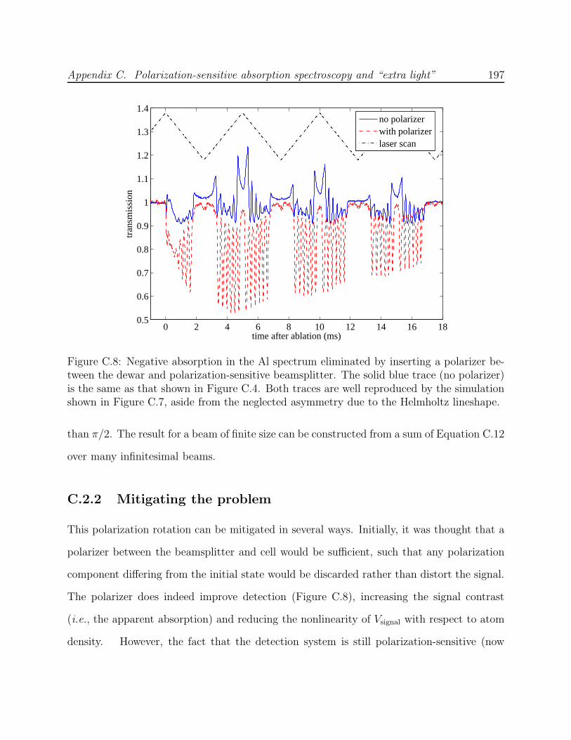
Appendix C. Polarization-sensitive absorption spectroscopy and “extra light” 197
0 2 4 6 8 10 12 14 16 180.5
0.6
0.7
0.8
0.9
1
1.1
1.2
1.3
1.4
time after ablation (ms)
tran
smis
sion
no polarizerwith polarizerlaser scan
Figure C.8: Negative absorption in the Al spectrum eliminated by inserting a polarizer be-tween the dewar and polarization-sensitive beamsplitter. The solid blue trace (no polarizer)is the same as that shown in Figure C.4. Both traces are well reproduced by the simulationshown in Figure C.7, aside from the neglected asymmetry due to the Helmholtz lineshape.
than π/2. The result for a beam of finite size can be constructed from a sum of Equation C.12
over many infinitesimal beams.
C.2.2 Mitigating the problem
This polarization rotation can be mitigated in several ways. Initially, it was thought that a
polarizer between the beamsplitter and cell would be sufficient, such that any polarization
component differing from the initial state would be discarded rather than distort the signal.
The polarizer does indeed improve detection (Figure C.8), increasing the signal contrast
(i.e., the apparent absorption) and reducing the nonlinearity of Vsignal with respect to atom
density. However, the fact that the detection system is still polarization-sensitive (now
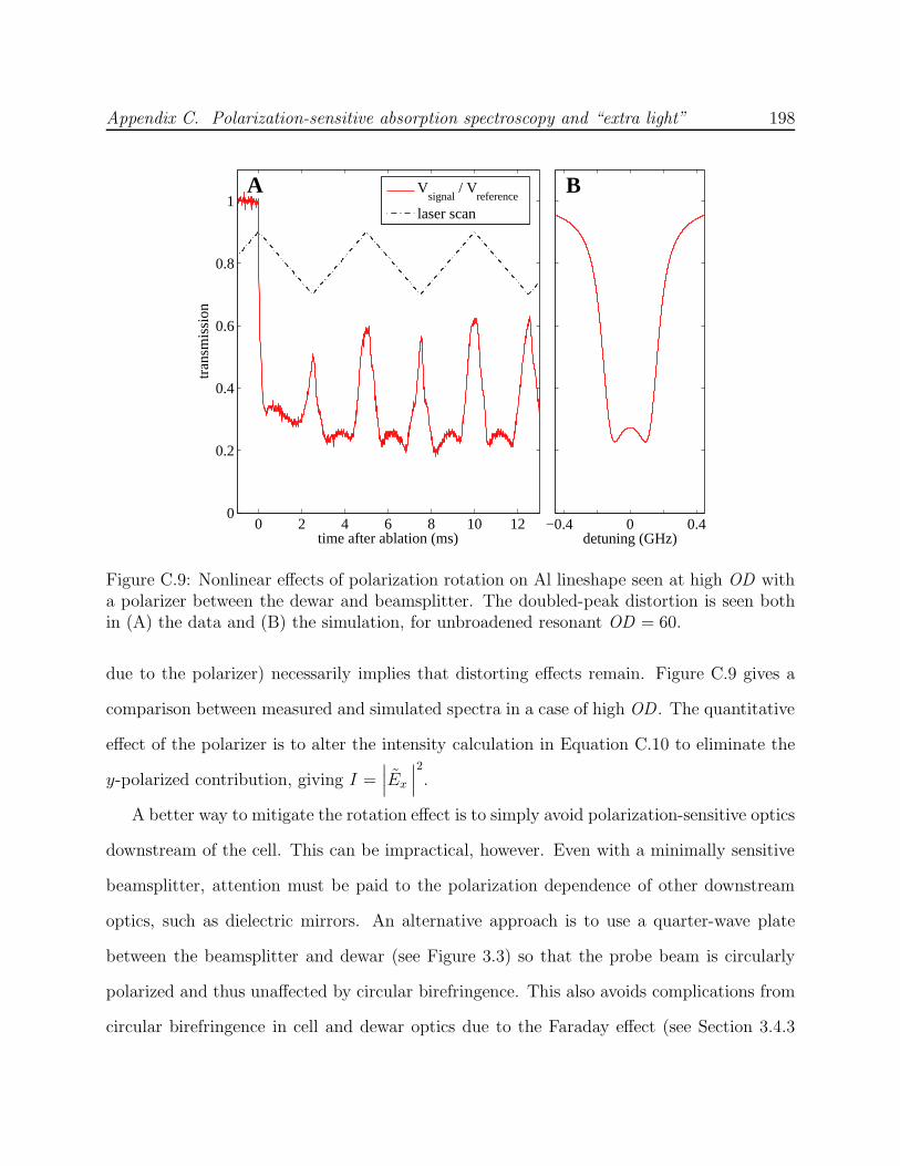
Appendix C. Polarization-sensitive absorption spectroscopy and “extra light” 198
0 2 4 6 8 10 120
0.2
0.4
0.6
0.8
1
time after ablation (ms)
tran
smis
sion
A Vsignal
/ Vreference
laser scan
−0.4 0 0.4detuning (GHz)
B
Figure C.9: Nonlinear effects of polarization rotation on Al lineshape seen at high OD witha polarizer between the dewar and beamsplitter. The doubled-peak distortion is seen bothin (A) the data and (B) the simulation, for unbroadened resonant OD = 60.
due to the polarizer) necessarily implies that distorting effects remain. Figure C.9 gives a
comparison between measured and simulated spectra in a case of high OD . The quantitative
effect of the polarizer is to alter the intensity calculation in Equation C.10 to eliminate the
y-polarized contribution, giving I =∣
∣
∣Ex
∣
∣
∣
2
.
A better way to mitigate the rotation effect is to simply avoid polarization-sensitive optics
downstream of the cell. This can be impractical, however. Even with a minimally sensitive
beamsplitter, attention must be paid to the polarization dependence of other downstream
optics, such as dielectric mirrors. An alternative approach is to use a quarter-wave plate
between the beamsplitter and dewar (see Figure 3.3) so that the probe beam is circularly
polarized and thus unaffected by circular birefringence. This also avoids complications from
circular birefringence in cell and dewar optics due to the Faraday effect (see Section 3.4.3
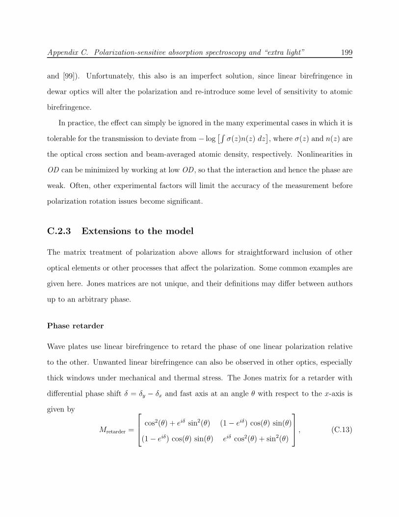
Appendix C. Polarization-sensitive absorption spectroscopy and “extra light” 199
and [99]). Unfortunately, this also is an imperfect solution, since linear birefringence in
dewar optics will alter the polarization and re-introduce some level of sensitivity to atomic
birefringence.
In practice, the effect can simply be ignored in the many experimental cases in which it is
tolerable for the transmission to deviate from − log[∫
σ(z)n(z) dz]
, where σ(z) and n(z) are
the optical cross section and beam-averaged atomic density, respectively. Nonlinearities in
OD can be minimized by working at low OD , so that the interaction and hence the phase are
weak. Often, other experimental factors will limit the accuracy of the measurement before
polarization rotation issues become significant.
C.2.3 Extensions to the model
The matrix treatment of polarization above allows for straightforward inclusion of other
optical elements or other processes that affect the polarization. Some common examples are
given here. Jones matrices are not unique, and their definitions may differ between authors
up to an arbitrary phase.
Phase retarder
Wave plates use linear birefringence to retard the phase of one linear polarization relative
to the other. Unwanted linear birefringence can also be observed in other optics, especially
thick windows under mechanical and thermal stress. The Jones matrix for a retarder with
differential phase shift δ = δy − δx and fast axis at an angle θ with respect to the x-axis is
given by
Mretarder =
cos2(θ) + eiδ sin2(θ) (1 − eiδ) cos(θ) sin(θ)
(1 − eiδ) cos(θ) sin(θ) eiδ cos2(θ) + sin2(θ)
, (C.13)
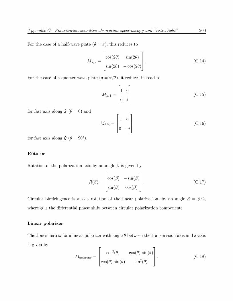
Appendix C. Polarization-sensitive absorption spectroscopy and “extra light” 200
For the case of a half-wave plate (δ = π), this reduces to
Mλ/2 =
cos(2θ) sin(2θ)
sin(2θ) − cos(2θ)
, (C.14)
For the case of a quarter-wave plate (δ = π/2), it reduces instead to
Mλ/4 =
1 0
0 i
(C.15)
for fast axis along x (θ = 0) and
Mλ/4 =
1 0
0 −i
(C.16)
for fast axis along y (θ = 90).
Rotator
Rotation of the polarization axis by an angle β is given by
R(β) =
cos(β) − sin(β)
sin(β) cos(β)
. (C.17)
Circular birefringence is also a rotation of the linear polarization, by an angle β = φ/2,
where φ is the differential phase shift between circular polarization components.
Linear polarizer
The Jones matrix for a linear polarizer with angle θ between the transmission axis and x-axis
is given by
Mpolarizer =
cos2(θ) cos(θ) sin(θ)
cos(θ) sin(θ) sin2(θ)
. (C.18)
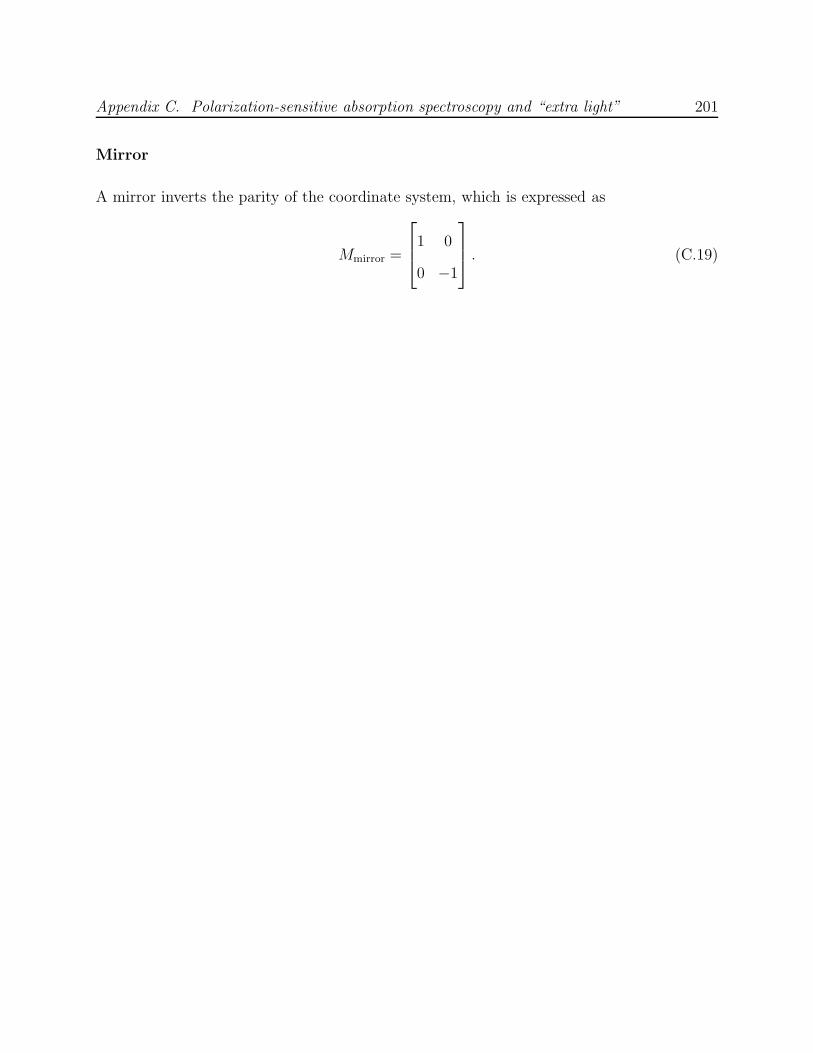
Appendix C. Polarization-sensitive absorption spectroscopy and “extra light” 201
Mirror
A mirror inverts the parity of the coordinate system, which is expressed as
Mmirror =
1 0
0 −1
. (C.19)
Bibliography
[1] T. V. Tscherbul, A. A. Buchachenko, A. Dalgarno, M.-J. Lu, and J. D. Weinstein.Suppression of Zeeman relaxation in cold collisions of 2P 1/2 atoms. Phys. Rev. A 80,040701 (2009).
[2] C. I. Hancox, S. C. Doret, M. T. Hummon, L. Luo, and J. M. Doyle. Magnetictrapping of rare-earth atoms at millikelvin temperatures. Nature 431, 281–284(2004).
[3] R. V. Krems and A. A. Buchachenko. Electronic interaction anisotropy betweenopen-shell lanthanide atoms and helium from cold collision experiment. J. Chem.
Phys. 123, 101101 (2005).
[4] Colin B. Connolly, Yat Shan Au, S. Charles Doret, Wolfgang Ketterle, and John M.Doyle. Large spin relaxation rates in trapped submerged-shell atoms. Phys. Rev. A
81, 010702 (2010).
[5] K. M. R. van der Stam, E. D. van Ooijen, R. Meppelink, J. M. Vogels, and P. van derStraten. Large atom number Bose-Einstein condensate of sodium. Rev. Sci. Instrum.
78, 013102 (2007).
[6] Patrick Medley, David M. Weld, Hirokazu Miyake, David E. Pritchard, and WolfgangKetterle. Spin gradient demagnetization cooling of ultracold atoms. Phys. Rev. Lett.
106, 195301 (2011).
[7] Jonathan Simon, Waseem S. Bakr, Ruichao Ma, M. Eric Tai, Philipp M. Preiss, andMarkus Greiner. Quantum simulation of antiferromagnetic spin chains in an opticallattice. Nature 472, 307–312 (2011).
[8] S. Weyers, V. Gerginov, N. Nemitz, R. Li, and K. Gibble. Distributed cavity phasefrequency shifts of the caesium fountain PTB-CSF2. Metrologia 49, 82 (2012).
[9] Jun Ye, H. J. Kimble, and Hidetoshi Katori. Quantum state engineering and precisionmetrology using state-insensitive light traps. Science 320, 1734–1738 (2008).
202

Bibliography 203
[10] Thierry Lahaye, Tobias Koch, Bernd Frohlich, Marco Fattori, Jonas Metz, AxelGriesmaier, Stefano Giovanazzi, and Tilman Pfau. Strong dipolar effects in aquantum ferrofluid. Nature 448, 672–675 (2007).
[11] Mingwu Lu, Nathaniel Q. Burdick, Seo Ho Youn, and Benjamin L. Lev. Stronglydipolar Bose-Einstein condensate of dysprosium. Phys. Rev. Lett. 107, 190401 (2011).
[12] Haiqing Wei, Rushan Han, and Xiuqing Wei. Quantum phase of induced dipolesmoving in a magnetic field. Phys. Rev. Lett. 75, 2071–2073 (1995).
[13] B. Damski, L. Santos, E. Tiemann, M. Lewenstein, S. Kotochigova, P. Julienne, andP. Zoller. Creation of a dipolar superfluid in optical lattices. Phys. Rev. Lett. 90,110401 (2003).
[14] A. Micheli, G. K. Brennen, and P. Zoller. A toolbox for lattice-spin models withpolar molecules. Nat. Phys. 2, 341–347 (2006).
[15] H. P. Buchler, E. Demler, M. Lukin, A. Micheli, N. Prokof’ev, G. Pupillo, andP. Zoller. Strongly correlated 2D quantum phases with cold polar molecules:Controlling the shape of the interaction potential. Phys. Rev. Lett. 98, 060404 (2007).
[16] Charlotte Gils, Simon Trebst, Alexei Kitaev, Andreas W. W. Ludwig, MatthiasTroyer, and Zhenghan Wang. Topology-driven quantum phase transitions intime-reversal-invariant anyonic quantum liquids. Nat. Phys. 5, 834–839 (2009).
[17] B. Capogrosso-Sansone, C. Trefzger, M. Lewenstein, P. Zoller, and G. Pupillo.Quantum phases of cold polar molecules in 2D optical lattices. Phys. Rev. Lett. 104,125301 (2010).
[18] D. DeMille. Quantum computation with trapped polar molecules. Phys. Rev. Lett.
88, 067901 (2002).
[19] Chaohong Lee and Elena A. Ostrovskaya. Quantum computation with diatomic bitsin optical lattices. Phys. Rev. A 72, 062321 (2005).
[20] J. Lee, E. R. Meyer, R. Paudel, J. L. Bohn, and A. E. Leanhardt. An electronelectric dipole moment search in the X 3∆1 ground state of tungsten carbidemolecules. J. Mod. Opt. 56, 2005–2012 (2009).
[21] A. C. Vutha, W. C. Campbell, Y. V. Gurevich, N. R. Hutzler, M. Parsons,D. Patterson, E. Petrik, B. Spaun, J. M. Doyle, G. Gabrielse, and D. DeMille. Searchfor the electric dipole moment of the electron with thorium monoxide. J. Phys. B 43,074007 (2010).
Bibliography 204
[22] J. J. Hudson, D. M. Kara, I. J. Smallman, B. E. Sauer, M. R. Tarbutt, and E. A.Hinds. Improved measurement of the shape of the electron. Nature 473, 493–496(2011).
[23] Edmund R. Meyer and John L. Bohn. Electron electric-dipole-moment searchesbased on alkali-metal- or alkaline-earth-metal-bearing molecules. Phys. Rev. A 80,042508 (2009).
[24] Lasse Kragh Sørensen, Stefan Knecht, Timo Fleig, and Christel M. Marian.Four-component relativistic coupled cluster and configuration interaction calculationson the ground and excited states of the RbYb molecule. J. Phys. Chem. A 113,12607–12614 (2009).
[25] Hideaki Hara, Yosuke Takasu, Yoshifumi Yamaoka, John M. Doyle, and YoshiroTakahashi. Quantum degenerate mixtures of alkali and alkaline-earth-like atoms.Phys. Rev. Lett. 106, 205304 (2011).
[26] Tino Weber, Jens Herbig, Michael Mark, Hanns-Christoph Ngerl, and Rudolf Grimm.Bose-Einstein condensation of cesium. Science 299, 232–235 (2003).
[27] B. Kloter, C. Weber, D. Haubrich, D. Meschede, and H. Metcalf. Laser cooling of anindium atomic beam enabled by magnetic fields. Phys. Rev. A 77, 033402 (2008).
[28] Wesley C. Campbell and John M. Doyle. Cold Polar Molecules: Creation and
Applications, Chapter 13: Cooling, trap loading, and beam production using acryogenic helium buffer gas, 473–508. CRC, Boca Raton, FL, 2009.
[29] David Patterson, Edem Tsikata, and John M. D. Cooling and collisions of large gasphase molecules. Phys. Chem. Chem. Phys. 12, 9736–9741 (2010).
[30] Robert deCarvalho, John M. Doyle, Bretislav Friedrich, Jinha Kim Thierry Guillet,David Patterson, and Jonathan D. Weinstein. Buffer-gas loaded magnetic traps foratoms and molecules: a primer. Eur. Phys. J. D 7, 289–309 (1999).
[31] S. Charles Doret, Colin B. Connolly, Wolfgang Ketterle, and John M. Doyle.Buffer-gas cooled Bose-Einstein condensate. Phys. Rev. Lett. 103, 103005 (2009).
[32] J. D. Weinstein, R. deCarvalho, C. I. Hancox, and J. M. Doyle. Evaporative coolingof atomic chromium. Phys. Rev. A 65, 021604(R) (2002).
[33] C. I. Hancox, M. T. Hummon, S. V. Nguyen, and J. M. Doyle. Evaporative cooling ofmagnetically trapped atomic molybdenum. Phys. Rev. A 71, 031402(R) (2005).
[34] Bonna K. Newman. Trapped Atom collisions and Evaporative Cooling of non-S State
Atoms. PhD thesis, Massachusetts Institute of Technology, September 2008.
Bibliography 205
[35] E. S. Shuman, J. F. Barry, and D. DeMille. Laser cooling of a diatomic molecule.Nature 467, 820–823 (2010).
[36] M. D. Di Rosa. Laser-cooling molecules. Eur. Phys. J. D 31, 395–402 (2004).
[37] Benjamin K. Stuhl, Brian C. Sawyer, Dajun Wang, and Jun Ye. Magneto-opticaltrap for polar molecules. Phys. Rev. Lett. 101, 243002 (2008).
[38] A. Robert, O. Sirjean, A. Browaeys, J. Poupard, S. Nowak, D. Boiron, C. I.Westbrook, and A. Aspect. A Bose-Einstein condensate of metastable atoms. Science292, 461–464 (2001).
[39] F. Pereira Dos Santos, J. Leonard, Junmin Wang, C. J. Barrelet, F. Perales,E. Rasel, C. S. Unnikrishnan, M. Leduc, and C. Cohen-Tannoudji. Bose-Einsteincondensation of metastable helium. Phys. Rev. Lett. 86, 3459–3462 (2001).
[40] Axel Griesmaier, Jorg Werner, Sven Hensler, Jurgen Stuhler, and Tilman Pfau.Bose-Einstein condensation of chromium. Phys. Rev. Lett. 94, 160401 (2005).
[41] Simon Stellmer, Meng Khoon Tey, Bo Huang, Rudolf Grimm, and Florian Schreck.Bose-Einstein condensation of strontium. Phys. Rev. Lett. 103, 200401 (2009).
[42] William H. Wing. On neutral particle trapping in quasistatic electromagnetic fields.Prog. Quantum Electron. 8, 181–199 (1984).
[43] H. M. J. M. Boesten, C. C. Tsai, J. R. Gardner, D. J. Heinzen, and B. J. Verhaar.Observation of a shape resonance in the collision of two cold 87Rb atoms. Phys. Rev.
A 55, 636–640 (1997).
[44] S. Inouye, M. R. Andrews, J. Stenger, H.-J. Miesner, D. M. Stamper-Kurn, andW. Ketterle. Observation of Feshbach resonances in a Bose-Einstein condensate.Nature 392, 151–154 (1998).
[45] Ph. Courteille, R. S. Freeland, D. J. Heinzen, F. A. van Abeelen, and B. J. Verhaar.Observation of a Feshbach resonance in cold atom scattering. Phys. Rev. Lett. 81,69–72 (1998).
[46] K.-K. Ni, S. Ospelkaus, D. Wang, G. Quemener, B. Neyenhuis, M. H. G. de Miranda,J. L. Bohn, J. Ye, and D. S. Jin. Dipolar collisions of polar molecules in the quantumregime. Nature 464, 1324–1328 (2010).
[47] S. Hensler, J. Werner, A. Griesmaier, P. O. Schmidt, A. Gorlitz, T. Pfau,S. Giovanazzi, and K. Rzazewski. Dipolar relaxation in an ultra-cold gas ofmagnetically trapped chromium atoms. Appl. Phys. B 77, 765–772 (2003).
Bibliography 206
[48] Joop J. Gilijamse, Steven Hoekstra, Sebastiaan Y. T. van de Meerakker, Gerrit C.Groenenboom, and Gerard Meijer. Near-threshold inelastic collisions using molecularbeams with a tunable velocity. Science 313, 1617–1620 (2006).
[49] Ellison H. Taylor and Sheldon Datz. Study of chemical reaction mechanisms withmolecular beams. The reaction of K with HBr. J. Chem. Phys. 23, 1711–1718 (1955).
[50] Giacinto Scoles. Atomic and molecular beam methods. Oxford University Press, NewYork, 1988.
[51] J. B. Hasted. Physics of atomic collisions. American Elsevier, New York, 1972.
[52] T. V. Tscherbul, J. K los, A. Dalgarno, B. Zygelman, Z. Pavlovic, M. T. Hummon,H.-I. Lu, E. Tsikata, and J. M. Doyle. Collisional properties of cold spin-polarizednitrogen gas: Theory, experiment, and prospects as a sympathetic coolant fortrapped atoms and molecules. Phys. Rev. A 82, 042718 (2010).
[53] Matthew T. Hummon, Timur V. Tscherbul, Jacek K los, Hsin-I Lu, Edem Tsikata,Wesley C. Campbell, Alexander Dalgarno, and John M. Doyle. Cold N + NHcollisions in a magnetic trap. Phys. Rev. Lett. 106, 053201 (2011).
[54] Matthew T. Hummon, Wesley C. Campbell, Hsin-I Lu, Edem Tsikata, Yihua Wang,and John M. Doyle. Magnetic trapping of atomic nitrogen (14N) and cotrapping ofNH (X 3Σ−). Phys. Rev. A 78, 050702 (2008).
[55] Piotr S. Zuchowski and Jeremy M. Hutson. Cold collisions of N (4S) atoms and NH(3Σ) molecules in magnetic fields. Phys. Chem. Chem. Phys. 13, 3669–3680 (2011).
[56] J. E. Sansonetti and W. C. Martin. Handbook of basic atomic spectroscopic data. J.
Phys. Chem. Ref. Data 34, 1559–2259 (2005).
[57] S. E. Maxwell, M. T. Hummon, Y. Wang, A. A. Buchachenko, R. V. Krems, andJ. M. Doyle. Spin-orbit interaction and large inelastic rates in bismuth–heliumcollisions. Phys. Rev. A 78, 042706 (2008).
[58] Scott Vinh Nguyen. Buffer gas loading and evaporative cooling in the
multi-partial-wave regime. PhD thesis, Harvard University, May 2006.
[59] Frank Pobell. Matter and Methods at Low Temperatures. 2nd edition. Springer, 1996.
[60] Robert Michniak. Enhanced buffer gas loading: cooling and trapping of atoms with
low effective magnetic moments. PhD thesis, Harvard University, May 2004.
[61] J. G. E. Harris, R. A. Michniak, S. V. Nguyen, W. C. Campbell, D. Egorov, S. E.Maxwell, L. D. van Buuren, and J. M. Doyle. Deep superconducting magnetic trapsfor neutral atoms and molecules. Rev. Sci. Instrum. 75, 17–23 (2004).
Bibliography 207
[62] B. N. Chichkov, C. Momma, S. Nolte, F. von Alvensleben, and A. Tunnermann.Femtosecond, picosecond and nanosecond laser ablation of solids. Appl. Phys. A 63,109–115 (1996).
[63] C. I. Hancox, S. C. Doret, M. T. Hummon, R. V. Krems, and J. M. Doyle.Suppression of angular momentum transfer in cold collisions of transition metalatoms in ground states with nonzero orbital angular momentum. Phys. Rev. Lett. 94,013201 (2005).
[64] Cort Johnson, Bonna Newman, Nathan Brahms, John M. Doyle, Daniel Kleppner,and Thomas J. Greytak. Zeeman relaxation of cold atomic iron and nickel incollisions with 3He. Phys. Rev. A 81, 062706 (2010).
[65] H. S. Carslaw and J. C. Jaeger. Conduction of Heat in Solids. 2nd edition. Oxford,1959. p. 104.
[66] D. N. Nikogosyan. Beta barium borate (BBO): A review of its properties andapplications. App. Phys. A 52, 359–368 (1991).
[67] Chuangtian Chen, Siyang Luo, Xiaoyang Wang, Guiling Wang, Xiaohong Wen,Huaxing Wu, Xin Zhang, and Zuyan Xu. Deep UV nonlinear optical crystal:RbBe2(BO3)F2. J. Opt. Soc. Am. B 26, 1519–1525 (2009).
[68] C. Chen, G. Wang, X. Wang, and Z. Xu. Deep-UV nonlinear optical crystalKBe2BO3F2—discovery, growth, optical properties and applications. Appl. Phys. B
97, 9–25 (2009).
[69] H. Jones-Bey. Deep-UV applications await improved nonlinear optics. Laser Focus
World , 127133 (1998).
[70] Jonathan D. Weinstein. Magnetic trapping of atomic chromium and molecular
calcium monohydride. PhD thesis, Harvard University, December 2001.
[71] Wesley C. Campbell, Edem Tsikata, Hsin-I Lu, Laurens D. van Buuren, and John M.Doyle. Magnetic trapping and Zeeman relaxation of NH (X 3Σ−). Phys. Rev. Lett.
98, 213001 (2007).
[72] C. I. Hancox. Magnetic trapping of transition-metal and rare-earth atoms using
buffer-gas loading. PhD thesis, Harvard University, 2005.
[73] Nathan Brahms, Timur V. Tscherbul, Peng Zhang, Jacek K los, Robert C. Forrey,Yat Shan Au, H. R. Sadeghpour, A. Dalgarno, John M. Doyle, and Thad G. Walker.Formation and dynamics of van der Waals molecules in buffer-gas traps. Phys. Chem.
Chem. Phys. 13, 19125–19141 (2011).
[74] Alexei A. Buchachenko, 2011. Private communication.
Bibliography 208
[75] Alexei A. Buchachenko, 2012. Private communication.
[76] Timur V. Tscherbul, 2011. Private communication.
[77] Alexei A. Buchachenko. Anisotropy of the static dipole polarizability induced by thespin-orbit interaction: the S-state atoms N–Bi, Cr, Mo and Re. Proc. Roy. Soc. A
467, 1310–1328 (2011).
[78] T. V. Tscherbul, P. Zhang, H. R. Sadeghpour, A. Dalgarno, N. Brahms, Y. S. Au,and J. M. Doyle. Collision-induced spin depolarization of alkali-metal atoms in cold3He gas. Phys. Rev. A 78, 060703 (2008).
[79] Roger W. McGowan, David M. Giltner, and Siu Au Lee. Light force cooling, focusing,and nanometer-scale deposition of aluminum atoms. Opt. Lett. 20, 2535–2537 (1995).
[80] Steven J. Rehse, Karen M. Bockel, and Siu Au Lee. Laser collimation of an atomicgallium beam. Phys. Rev. A 69, 063404 (2004).
[81] Isaac Fan, Tzu-Ling Chen, Yu-Sheng Liu, Yu-Hung Lien, Jow-Tsong Shy, and Yi-WeiLiu. Prospects of laser cooling in atomic thallium. Phys. Rev. A 84, 042504 (2011).
[82] Th. Schulze, T. Muther, D. Jurgens, B. Brezger, M. K. Oberthaler, T. Pfau, andJ. Mlynek. Structured doping with light forces. Appl. Phys. Lett. 78, 1781–1783(2001).
[83] K. Beloy, A. Derevianko, V. A. Dzuba, and V. V. Flambaum. Micromagic clock:Microwave clock based on atoms in an engineered optical lattice. Phys. Rev. Lett.
102, 120801 (2009).
[84] B. K. Sahoo, R. Pandey, and B. P. Das. Search for a permanent electric-dipolemoment using atomic indium. Phys. Rev. A 84, 030502 (2011).
[85] B. C. Regan, Eugene D. Commins, Christian J. Schmidt, and David DeMille. Newlimit on the electron electric dipole moment. Phys. Rev. Lett. 88, 071805 (2002).
[86] Eugene D. Commins. Berry’s geometric phase and motional fields. Am. J. Phys. 59,1077–1080 (1991).
[87] R. V. Krems. Cold controlled chemistry. Phys. Chem. Chem. Phys. 10, 4079–4092(2008).
[88] R. V. Krems, G. C. Groenenboom, and A. Dalgarno. Electronic interactionanisotropy between atoms in arbitrary angular momentum states. J. Phys. Chem. A
108, 8941–8948 (2004).
Bibliography 209
[89] Nathan Brahms, Bonna Newman, Cort Johnson, Tom Greytak, Daniel Kleppner, andJohn Doyle. Magnetic trapping of silver and copper, and anomalous spin relaxationin the Ag–He system. Phys. Rev. Lett. 101, 103002 (2008).
[90] A. Yamaguchi, S. Uetake, D. Hashimoto, J. M. Doyle, and Y. Takahashi. Inelasticcollisions in optically trapped ultracold metastable ytterbium. Phys. Rev. Lett. 101,233002 (2008).
[91] R. V. Krems and A. Dalgarno. Disalignment transitions in cold collisions of 3Patoms with structureless targets in a magnetic field. Phys. Rev. A 68, 013406 (2003).
[92] Mei-Ju Lu, Kyle S. Hardman, Jonathan D. Weinstein, and Bernard Zygelman.Fine-structure-changing collisions in atomic titanium. Phys. Rev. A 77, 060701(2008).
[93] Bernard Zygelman and Jonathan D. Weinstein. Theoretical and laboratory study ofsuppression effects in fine-structure-changing collisions of Ti with He. Phys. Rev. A
78, 012705 (2008).
[94] Harry Partridge, James R. Stallcop, and Eugene Levin. Potential energy curves andtransport properties for the interaction of He with other ground-state atoms. J.
Chem. Phys. 115, 6471–6488 (2001).
[95] Timur V. Tscherbul, 2012. Private communication.
[96] D. E. Kelleher and L. I. Podobedova. Atomic transition probabilities of aluminum. acritical compilation. J. Phys. Chem. Ref. Data 37, 709–911 (2008).
[97] J. Kim, B. Friedrich, D. P. Katz, D. Patterson, J. D. Weinstein, R. deCarvalho, andJ. M. Doyle. Buffer-gas loading and magnetic trapping of atomic europium. Phys.
Rev. Lett. 78, 3665–3668 (1997).
[98] Edward S. Chang. Energy levels of atomic aluminum with hyperfine structure. J.
Phys. Chem. Ref. Data 19, 119–125 (1990).
[99] E. Munin, J. A. Roversi, and A. Balbin Villaverde. Faraday effect and energy gap inoptical materials. J. Phys. D 25, 1635 (1992).
[100] Donald C. Griffin, Kenneth L. Andrew, and Robert D. Cowan. Theoreticalcalculations of the d-, f -, and g-electron transition series. Phys. Rev. 177, 62–71(1969).
[101] R. V. Krems, J. K los, M. F. Rode, M. M. Szczesniak, G. Cha lasinski, andA. Dalgarno. Suppression of angular forces in collisions of non-S-state transitionmetal atoms. Phys. Rev. Lett. 94, 013202 (2005).
Bibliography 210
[102] J. L. Hall, M. Zhu, and P. Buch. Prospects for using laser-prepared atomic fountainsfor optical frequency standards applications. J. Opt. Soc. Am. B 6, 2194 (1989).
[103] K. Chebakov, A. Sokolov, A. Akimov, D. Sukachev, S. Kanorsky, N. Kolachevsky,and V. Sorokin. Zeeman slowing of thulium atoms. Opt. Lett. 34, 2955–2957 (2009).
[104] Andrew J. Berglund, James L. Hanssen, and Jabez J. McClelland. Narrow-linemagneto-optical cooling and trapping of strongly magnetic atoms. Phys. Rev. Lett.
100, 113002 (2008).
[105] D. Sukachev, A. Sokolov, K. Chebakov, A. Akimov, N. Kolachevsky, and V. Sorokin.Sub-Doppler laser cooling of thulium atoms in a magneto-optical trap. JETP Lett.
92, 703706 (2010).
[106] M. A. Baranov. Theoretical progress in many-body physics with ultracold dipolargases. Physics Reports 464, 71–111 (2008).
[107] T. Lahaye, C. Menotti, L. Santos, M. Lewenstein, and T. Pfau. The physics ofdipolar bosonic quantum gases. Rep. Prog. Phys. 72, 126401 (2009).
[108] Benjamin M. Fregoso, Kai Sun, Eduardo Fradkin, and Benjamin L. Lev. Biaxialnematic phases in ultracold dipolar Fermi gases. New J. of Phys. 11, 103003 (2009).
[109] M. Saffman and K. Mølmer. Scaling the neutral-atom Rydberg gate quantumcomputer by collective encoding in holmium atoms. Phys. Rev. A 78, 012336 (2008).
[110] W. C. Martin, R. Zalubas, and L. Hagan. Atomic energy levels—The rare-earthelements. Technical report, National Bureau of Standards, 1978. in Nat. Stand. Ref.
Data Ser., NSRDS-NBS 60, 422 pp.
[111] Stephen Charles Doret. A buffer-gas cooled Bose-Einstein condensate. PhD thesis,Harvard University, October 2009.
[112] Jonathan D. Weinstein, Robert deCarvalho, Jinha Kim, David Patterson, BretislavFriedrich, and John M. Doyle. Magnetic trapping of atomic chromium. Phys. Rev. A
57, R3173–R3175 (1998).
[113] Nathaniel Charles Brahms. Trapping of 1 µB atoms using buffer gas loading. PhDthesis, Harvard University, May 2008.
[114] E. Tsikata, W. C. Campbell, M. T. Hummon, H.-I. Lu, and J. M. Doyle. Magnetictrapping of NH molecules with 20 s lifetimes. New J. of Phys. 12, 065028 (2010).
[115] A. V. Akimov, K. Yu. Chebakov, I. Yu. Tolstikhina, A. V. Sokolov, P. B. Rodionov,S. I. Kanorsky, V. N. Sorokin, and N. N. Kolachevsky. Study of transitions inthulium atoms in the 410–420-nm range for laser cooling. Quantum Electron. 38,961–968 (2008).
Bibliography 211
[116] W. Ketterle and N. J. van Druten. Evaporative cooling. Adv. At. Mol. Opt. Phys.
37, 181–236 (1996).
[117] O. J. Luiten, M. W. Reynolds, and J. T. M. Walraven. Kinetic theory of theevaporative cooling of a trapped gas. Phys. Rev. A 53, 381–389 (1996).
[118] Robert deCarvalho and John Doyle. Evaporative cooling at low trap depth. Phys.
Rev. A 70, 053409 (2004).
[119] John L. Bohn, James P. Burke, Chris H. Greene, H. Wang, P. L. Gould, and W. C.Stwalley. Collisional properties of ultracold potassium: Consequences for degenerateBose and Fermi gases. Phys. Rev. A 59, 3660–3664 (1999).
[120] J. G. E. Harris, S. V. Nguyen, S. C. Doret, W. Ketterle, and J. M. Doyle.Spin-exchange collisions of submerged shell atoms below 1 kelvin. Phys. Rev. Lett.
99, 223201 (2007).
[121] A. A. Buchachenko, G. Cha lasinski, M. M. Szczesniak, and R. V. Krems. Ab initio
study of Tm–He interactions and dynamics in a magnetic trap. Phys. Rev. A 74,022705 (2006).
[122] S. V. Nguyen, R. deCarvalho, and J. M. Doyle. Cold 52Cr elastic and inelasticcollision-rate determination using evaporative cooling analysis. Phys. Rev. A 75,062706 (2007).
[123] Z. Pavlovic, R. V. Krems, R. Cote, and H. R. Sadeghpour. Magnetic Feshbachresonances and Zeeman relaxation in bosonic chromium gas with anisotropicinteraction. Phys. Rev. A 71, 061402(R) (2005).
[124] A. A. Buchachenko, Y. V. Suleimanov, G. Cha lasinski, and M. M. Szczesniak.Interactions and collisions of cold metal atoms in magnetic traps. Phys. Scr. 80,048109 (2009).
[125] Yury V. Suleimanov. Zeeman relaxation of magnetically trapped Eu atoms. Phys.
Rev. A 81, 022701 (2010).
[126] Anthony J. Stone. The Theory of Intermolecular Forces, Volume 32. ClarendonPress, Oxford, 1996.
[127] Alexei A. Buchachenko, 2009. Private communication.
[128] Svetlana Kotochigova and Alexander Petrov. Anisotropy in the interaction ofultracold dysprosium. Phys. Chem. Chem. Phys. 13, 19165–19170 (2011).
[129] D. Hansen and A. Hemmerich. Observation of multichannel collisions of coldmetastable calcium atoms. Phys. Rev. Lett. 96, 073003 (2006).

Bibliography 212
[130] A. Traverso, R. Chakraborty, Y. N. Martinez de Escobar, P. G. Mickelson, S. B.Nagel, M. Yan, and T. C. Killian. Inelastic and elastic collision rates for triplet statesof ultracold strontium. Phys. Rev. A 79, 060702 (2009).
[131] Mingwu Lu, Seo Ho Youn, and Benjamin L. Lev. Trapping ultracold dysprosium: Ahighly magnetic gas for dipolar physics. Phys. Rev. Lett. 104, 063001 (2010).
[132] Bonna K. Newman, Nathan Brahms, Yat Shan Au, Cort Johnson, Colin B. Connolly,John M. Doyle, Daniel Kleppner, and Thomas J. Greytak. Magnetic relaxation indysprosium–dysprosium collisions. Phys. Rev. A 83, 012713 (2011).
[133] R. Shankar. Principles of Quantum Mechanics. 2nd edition. Plenum Press, 1994. p.548.
[134] P. Zhang and A. Dalgarno. Static dipole polarizability of ytterbium. J. Phys. Chem.
A 111, 12471–12476 (2007).
[135] Mingwu Lu, Nathaniel Q. Burdick, and Benjamin L. Lev. Quantum degeneratedipolar Fermi gas. Phys. Rev. Lett. 108, 215301 (2012).
[136] K. Aikawa, A. Frisch, M. Mark, S. Baier, A. Rietzler, R. Grimm, and F. Ferlaino.Bose-Einstein condensation of erbium. Phys. Rev. Lett. 108, 210401 (2012).
[137] D. Sukachev, A. Sokolov, K. Chebakov, A. Akimov, S. Kanorsky, N. Kolachevsky, andV. Sorokin. Magneto-optical trap for thulium atoms. Phys. Rev. A 82, 011405 (2010).
[138] S. Ospelkaus, K.-K. Ni, D. Wang, M. H. G. de Miranda, B. Neyenhuis, G. Qumner,P. S. Julienne, J. L. Bohn, D. S. Jin, and J. Ye. Quantum-state controlled chemicalreactions of ultracold potassium-rubidium molecules. Science 327, 853–857 (2010).
[139] Brian C. Sawyer, Benjamin K. Stuhl, Mark Yeo, Timur V. Tscherbul, Matthew T.Hummon, Yong Xia, Jacek K los, David Patterson, John M. Doyle, and Jun Ye. Coldheteromolecular dipolar collisions. Phys. Chem. Chem. Phys. 13, 19059–19066 (2011).
[140] M G Kozlov and L N Labzowsky. Parity violation effects in diatomics. J. Phys. B
28, 1933 (1995).
[141] A. E. Leanhardt, J. L. Bohn, H. Loh, P. Maletinsky, E. R. Meyer, L. C. Sinclair,R. P. Stutz, and E. A. Cornell. High-resolution spectroscopy on trapped molecularions in rotating electric fields: A new approach for measuring the electron electricdipole moment. J. Mol. Spectrosc. 270, 1–25 (2011).
[142] K.-K. Ni, S. Ospelkaus, M. H. G. de Miranda, A. Pe’er, B. Neyenhuis, J. J. Zirbel,S. Kotochigova, P. S. Julienne, D. S. Jin, and J. Ye. A high phase-space-density gasof polar molecules. Science 322, 231–235 (2008).

Bibliography 213
[143] J. Deiglmayr, A. Grochola, M. Repp, K. Mortlbauer, C. Gluck, J. Lange, O. Dulieu,R. Wester, and M. Weidemuller. Formation of ultracold polar molecules in therovibrational ground state. Phys. Rev. Lett. 101, 133004 (2008).
[144] David DeMille. Ultracold molecules: Production techniques and scientificapplications. In Quantum Electronics and Laser Science Conference, QWB1. OpticalSociety of America, 2011.
[145] Matthew Hummon, Mark Yeo, Benjamin Stuhl, Yong Xia, and Jun Ye. Direct lasercooling of yttrium monoxide. In 43rd Annual Meeting of the APS Division of Atomic,
Molecular and Optical Physics, Volume 57. American Physical Society, June 2012.
[146] Pavel Soldan, Piotr S. Zuchowski, and Jeremy M. Hutson. Prospects for sympatheticcooling of polar molecules: NH with alkali-metal and alkaline-earth atoms—a newhope. Faraday Discuss. 142, 191–201 (2009).
[147] T. V. Tscherbul, J. K los, and A. A. Buchachenko. Ultracold spin-polarized mixturesof 2Σ molecules with S-state atoms: Collisional stability and implications forsympathetic cooling. Phys. Rev. A 84, 040701 (2011).
[148] Vijay Singh, Mei-Ju Lu, Kyle Hardman, Muir Morrision, and Jonathan Weinstein.Inelastic collisions of CaH molecules at cryogenic temperatures. In 41st Annual
Meeting of the APS Division of Atomic, Molecular and Optical Physics, Volume 55.American Physical Society, May 2010.
[149] R. V. Krems, H. R. Sadeghpour, A. Dalgarno, D. Zgid, J. K los, and G. Cha lasinski.Low-temperature collisions of NH(X3Σ−) molecules with He atoms in a magneticfield: An ab initio study. Phys. Rev. A 68, 051401 (2003).
[150] D. Egorov, W. C. Campbell, B. Friedrich, S. E. Maxwell, E. Tsikata, L. D. vanBuuren, and J. M. Doyle. Buffer-gas cooling of NH via the beam loaded buffer-gasmethod. Eur. Phys. J. D 31, 307–311 (2004).
[151] Wesley C. Campbell, Timur V. Tscherbul, Hsin-I Lu, Edem Tsikata, Roman V.Krems, and John M. Doyle. Mechanism of collisional spin relaxation in 3Σ molecules.Phys. Rev. Lett. 102, 013003 (2009).
[152] Wesley C. Campbell. Magnetic trapping of imidogen molecules. PhD thesis, HarvardUniversity, February 2008.
[153] Wesley C. Campbell, Gerrit C. Groenenboom, Hsin-I Lu, Edem Tsikata, andJohn M. Doyle. Time-domain measurement of spontaneous vibrational decay ofmagnetically trapped NH. Phys. Rev. Lett. 100, 083003 (2008).

Bibliography 214
[154] Liesbeth M. C. Janssen, Piotr S. Zuchowski, Ad van der Avoird, Gerrit C.Groenenboom, and Jeremy M. Hutson. Cold and ultracold NH–NH collisions inmagnetic fields. Phys. Rev. A 83, 022713 (2011).
[155] Liesbeth M. C. Janssen, Piotr S. Zuchowski, Ad van der Avoird, Jeremy M. Hutson,and Gerrit C. Groenenboom. Cold and ultracold NH–NH collisions: The field-freecase. J. Chem. Phys. 134, 124309 (2011).
[156] Y. V. Suleimanov, T. V. Tscherbul, and R. V. Krems. Efficient method for quantumcalculations of molecule–molecule scattering properties in a magnetic field.Submitted (arXiv:1202.0597).
[157] Sebastiaan Y. T. van de Meerakker, Irena Labazan, Steven Hoekstra, JochenK upper, and Gerard Meijer. Production and deceleration of a pulsed beam ofmetastable NH (a1∆) radicals. J. Phys. B 39, S1077 (2006).
[158] Heather Lewandowski, L. Paul. Parazzoli, and Daniel Lobser. Cold free-radical NHmolecules. In Frontiers in Optics. Optical Society of America, 2006.
[159] Steven Hoekstra, Markus Metsala, Peter C. Zieger, Ludwig Scharfenberg, Joop J.Gilijamse, Gerard Meijer, and Sebastiaan Y. T. van de Meerakker. Electrostatictrapping of metastable NH molecules. Phys. Rev. A 76, 063408 (2007).
[160] Pavel Soldan and Jeremy M. Hutson. Interaction of NH(X 3Σ−) molecules withrubidium atoms: Implications for sympathetic cooling and the formation ofextremely polar molecules. Phys. Rev. Lett. 92, 163202 (2004).
[161] Daniel J. Haxton, Steven A. Wrathmall, H. J. Lewandowski, and Chris H. Greene.Theoretical study of the quenching of NH (1∆) molecules via collisions with Rbatoms. Phys. Rev. A 80, 022708 (2009).
[162] Alisdair O. G. Wallis and Jeremy M. Hutson. Production of ultracold NH moleculesby sympathetic cooling with Mg. Phys. Rev. Lett. 103, 183201 (2009).
[163] Alisdair Wallis, Edward Longdon, Piotr Zuchowski, and Jeremy Hutson. Theprospects of sympathetic cooling of NH molecules with Li atoms. Eur. Phys. J. D
65, 151–160 (2011).
[164] Nicholas R. Hutzler, Maxwell F. Parsons, Yulia V. Gurevich, Paul W. Hess,Elizabeth Petrik, Ben Spaun, Amar C. Vutha, David DeMille, Gerald Gabrielse, andJohn M. Doyle. A cryogenic beam of refractory, chemically reactive molecules withexpansion cooling. Phys. Chem. Chem. Phys. 13, 18976–18985 (2011).
[165] Dimitri Michael Egorov. Buffer-gas cooling of diatomic molecules. PhD thesis,Harvard University, August 2004.
Bibliography 215
[166] Kenneth Maussang, Dima Egorov, Joel S. Helton, Scott V. Nguyen, and John M.Doyle. Zeeman relaxation of CaF in low-temperature collisions with helium. Phys.
Rev. Lett. 94, 123002 (2005).
[167] Michael Stoll, Joost M. Bakker, Timothy C. Steimle, Gerard Meijer, and AchimPeters. Cryogenic buffer-gas loading and magnetic trapping of CrH and MnHmolecules. Phys. Rev. A 78, 032707 (2008).
[168] Matthew Taylor Hummon. Magnetic trapping of atomic nitrogen and cotrapping of
NH. PhD thesis, Harvard University, March 2010.
[169] J. Helffrich, M. Maley, M. Krusius, and J. C. Wheatley. Hydrogen dissociation below1 K. J. Low Temp. Phys. 66, 277–304 (1987).
[170] Russell B. Scott. Cryogenic Engineering. Van Nostrand, Princeton, NJ, 1959.
[171] C. Effantin, C. Amiot, and J. Verges. Analysis of the (0-0), (1-0), and (2-0) bands ofthe B3Πg → A3Σ+
u system of 14N2 and 15N2. J. Mol. Spectrosc. 76, 221–265 (1979).
[172] Thomas A Carlson, Nada Duric, Peter Erman, and Mats Larsson. Collisional transferto the B state in N2. Phys. Scr. 19, 25 (1979).
[173] F. Roux, F. Michaud, and J. Verges. High-resolution Fourier spectrometry of 14N2
infrared emission spectrum: Extensive analysis of the B3Πg–A3Σ+
u system. J. Mol.
Spectrosc. 97, 253–265 (1983).
[174] G. C. Bjorklund, M. D. Levenson, W. Lenth, and C. Ortiz. Frequency modulation(FM) spectroscopy. Appl. Phys. B 32, 145–152 (1983).
[175] M. M. Fejer, G. A. Magel, D. H. Jundt, and R. L. Byer. Quasi-phase-matched secondharmonic generation: Tuning and tolerances. IEEE J. of Quantum Electron. 28, 2631–2654 (1992).
[176] Editorial Committee Hamamatsu Photonics K. K. Photomultiplier Tubes: Basics and
Applications. 3rd edition. Hamamatsu Photonics K. K., Electron Tube Division,February 2006.
[177] CVI Melles Griot. Materials properties. http://www.cvimellesgriot.com, 2009.
[178] L. F. Goodrich, S. L. Bray, and T. C. Stauffer. Nb3Sn critical-current measurementsusing tubular fiberglass-epoxy mandrels. IEEE Trans. on Magn. 25, 2375 –2378(1989).
[179] P. O. Fedichev, M. W. Reynolds, U. M. Rahmanov, and G. V. Shlyapnikov. Inelasticdecay processes in a gas of spin-polarized triplet helium. Phys. Rev. A 53, 1447–1453(1996).

Bibliography 216
[180] Scott V. Nguyen, S. Charles Doret, Colin B. Connolly, Robert A. Michniak,Wolfgang Ketterle, and John M. Doyle. Evaporative cooling of metastable helium inthe multi-partial-wave regime. Phys. Rev. A 72, 060703 (2005).
[181] Jan R. Rubbmark, Michael M. Kash, Michael G. Littman, and Daniel Kleppner.Dynamical effects at avoided level crossings: A study of the Landau-Zener effectusing Rydberg atoms. Phys. Rev. A 23, 3107–3117 (1981).
[182] Harold Metcalf and Peter van der Straten. Laser Cooling and Trapping. Springer,New York, 1999.
[183] V. M. Akulin and W. P. Schleich. Landau-Zener transition to a decaying level. Phys.
Rev. A 46, 4110–4113 (1992).
[184] G. N. Watson E. T. Whittaker. A Course of Modern Analysis. Fourth edition.Cambridge University Press, Cambridge, 1996.
[185] R. Clark Jones. A new calculus for the treatment of optical systems. J. Opt. Soc.
Am. 31, 488–493 (1941).
[186] Frank L. Pedrotti, Leno Matthew. Pedrotti, and Leno S. Pedrotti. Introduction to
Optics. Third edition. Pearson Prentice Hall, Upper Saddle River, N.J., 2007.Chapter 14.
Copyright © 2022 FDOKUMEN