Numerical and analytical modeling of polarization-dependent gain in erbium-doped fiber amplifiers

1942 J. Opt. Soc. Am. B/Vol. 12, No. 10 /October 1995 R. Leners and T. Georges

Numerical and analytical modeling of polarization-dependent gain in erbium-doped fiber amplifiers

R. Leners* and T. Georges

Centre National d’Etudes des Telecommunications, France Telecom,Avenue Pierre Marzin, 22307 Lannion Cedex, France

Received March 6, 1995; revised manuscript received May 22, 1995

We present a rate-equation model that accounts for polarization hole burning in erbium-doped fiber amplifiers.This model yields analytical expressions for the polarization sensitivity of the amplifier for arbitrary signalpolarization states. We investigate the influence of the birefringence properties of the fiber and calculate theaverage polarization properties of an amplifier chain. 1995 Optical Society of America

1. INTRODUCTIONPolarization hole burning (PHB) in rare-earth-dopedglasses is a subject of longstanding interest. Becauseof the disordered structure of the glass host, the dipolesof the ions are characterized by random orientations.Hence a polarized optical field interacts preferentiallywith those ions whose dipoles are parallel to its stateof polarization (SOP). This leads to the partially polar-ized fluorescence emitted by optically pumped rare-earth-doped glasses,1 as evidenced by Hall and Weber2 and Hallet al.3 in neodymium-doped glass amplifiers.

In rare-earth-doped fiber amplifiers these effects hap-pen to be quite small. This probably explains why thefirst investigations were made on fiber lasers for whichPHB effects add up during successive round trips andhave a measurable influence on the laser output.4 – 11

The situation is somewhat similar in long-haul transmis-sion lines with concatenated erbium-doped-fiber ampli-fiers (EDFA’s), in which PHB effects may build up alongthe line and seriously affect the transmission properties,as was first reported by Taylor.12 Because of the selec-tive saturation by the polarized signal field the ampli-fied spontaneous emission (ASE), polarized orthogonallyto the signal, experiences a larger gain than the paral-lel component. This leads to the accumulation of ASEnoise in the orthogonal direction and ultimately to thedegradation of the signal-to-noise ratio at reception.13,14

Further polarization-resolved gain measurements estab-lished the dependence of the EDFA polarization sensitiv-ity on the amplifier gain,15 the relative orientations ofprobe and signal fields,16 and the pump SOP.17,18 Theresponse time of PHB was measured to be of the order of100 ms for typical amplifier conditions,19 and considerableattention has been paid to the suppression of PHB effectsby polarization-scrambling techniques.12,18,20 – 24 For per-fectly circular and isotropic fibers the polarization sensi-tivity is independent of the absolute orientations of thefields and depends only on the relative orientations. Forbirefringent fibers this is not true anymore, as the fieldSOP’s change during propagation, depending on the inputSOP’s. Although such detailed measurements are still

0740-3224/95/101942-13$06.00

lacking, the influence of the birefringence on the polar-ization sensitivity has already been observed.25

The numerical modeling of the polarization propertiesof EDFA’s was first performed by Wysocki,26,27 who parti-tioned the randomly orientated dipoles into a finite num-ber of classes with different orientations. However, thisapproximation seems to converge rather slowly and re-quires a large number of classes to be taken into account.

The purpose of this study is the elaboration of a simpli-fied model, based on a Fourier expansion of the populationdifference.28 The rapid convergence of this expansion en-ables us to truncate it after a few terms. This reducesthe number of equations and considerably simplifies thedescription.

This paper is organized into two major sections. InSection 2 we derive the rate equations of an EDFA withPHB, using a truncated Fourier expansion for the popu-lation difference. In Section 3 we apply these equationsto the calculation of the polarization-resolved gain of anEDFA. We obtain simple expressions for the polariza-tion sensitivity of an EDFA, requiring only the same com-putational effort as for a polarization-insensitive EDFA.In particular, we examine the influence of the fiber bire-fringence and discuss the implications for long-haul trans-mission links with concatenated amplifiers.

2. RATE EQUATIONS ANALYSISWe consider the EDFA a three-level medium, interactingwith a pump field EP sr, td and a signal field ESsr, td(Fig. 1). We assume that the fields may be written as

EQ sr, td 1/2cqsrdP

jx,yEqj sz, tdexpfisvqt 2 kqj zdgej 1 c.c.

; 1/2cqsrdP

jx,yEqj sz, tdUqj szdexpsivqtd 1 c.c.

; 1/2cqsrdEqsz, tdexpsivqtd 1 c.c.

sQ P , S; q p, sd , (1)

where

1995 Optical Society of America

R. Leners and T. Georges Vol. 12, No. 10 /October 1995 /J. Opt. Soc. Am. B 1943

Fig. 1. Three-level system of an EDFA.

Uqj szd exps2ikqj zdej ,

Eqsz, td P

jx,yEqj sz, tdexps2ikqj zdej . (2)

We have assumed that the fiber is characterized by alinear and constant birefringence, i.e., by two linear andorthogonal unit vectors ex and ey that define the two polar-ization modes termed x and y. cqsrd are the radial fielddistributions, and r is the radial coordinate of the fiber.vq are the optical frequencies of the fields, which are as-sumed to be resonant with the transitions. kqj are thepropagation constants of the two polarization modes forfrequency vq. The envelopes Eqj sz, td are slowly vary-ing in time t and along the fiber axis z.

The evolution equations of the field envelopes and ofthe fraction Dsz, t, ad of inverted ions in the upper signallevel are√

≠z 11

Vq≠t

!Eqj

NGq

2Eq ? kSqeD 2 Sqas1 2 Ddl ? Up

qj ,

(3)

dDdt

2Dt

2X

qp,s

12

´0cnqNG0

q

"vq

3 Epq ? fSqeD 2 Sqas1 2 Ddg ? Eq . (4)

The detailed derivation of Eqs. (3) and (4) is given inRef. 29 for the case of a four-level medium. For a three-level medium the calculations are quite similar. We donot reproduce them here but focus on the results of themodel. The only additional features of these equationsin comparison with those of an EDFA without PHB30 are

• The dependence of the population inversion D on anorientational coordinate a and

• The replacement of the scalar cross sections bycross-section ellipses Sqasad and Sqesad for the pump andsignal transitions.28

The subscripts qa and qe indicate the absorption andthe emission cross-section ellipses, respectively. Thesite-to-site variations of the orientations of the absorbingand emitting dipoles, which are at the origin of PHB,may be described by random rotations of the cross-sectionellipses:

Smsad RsadSmR21sad sm qa, qed , (5)

where Sm is the diagonal matrix:

Sm

"ss1d

m 00 ss2d

m

#(6)

and Rsad is the rotation matrix:

Rsad

"cos a 2sin a

sin a cos a

#. (7)

The diagonal elements of Sm are the absorption and emis-sion cross sections for the pump and signal transitions.The angle a defines the orientation of the cross-section el-lipse with respect to the birefringence axes x and y. Theangle brackets k l in Eq. (3) stand for the integration overall the orientations, which we assume to be uniformly dis-tributed, i.e.,

kF sadl Z 2p

0

da

2pF sad . (8)

Finally, in Eqs. (3) and (4), Vq are the group velocitiesof the envelopes where the polarization mode dispersionhas been neglected. Gq and G0

q are transverse overlapintegrals, defined by

Gq

Z `

0dr rjcqsrdj2f srdZ `

0dr rjcqsrdj2

, G0q

Z `

0dr rjcqsrdj2fsrdZ `

0dr rf srd

,

(9)

where f srd is the radial dopant distribution. N is thedopant concentration, and t is the lifetime of the popula-tion inversion. nq are the refractive indices at vq.

The link between Eqs. (3) and (4) and the standarddescription of a polarization-insensitive EDFA may bereadily established. First we rewrite Smsad as

Smsad sm1 11 2 bm

1 1 bm

Ssad , (10)

where sm fss1dm 1 ss2d

m gy2 is the average cross sectionand bm ss2d

m yss1dm is the cross-section anisotropy. For

simplicity we will assume that the absorption and emis-sion cross sections have the same anisotropy, i.e., bqa bqe ; bq.26,28 1 is the unit matrix, and Ssad is given by

Ssad

"cos 2a sin 2a

sin 2a 2cos 2a

#. (11)

In the limit of isotropic dipoles, i.e., for bm ! 1, Sm be-comes independent of a, and Eqs. (3) and (4) reduce tothe equations of a polarization-insensitive EDFA30:√

≠z 11

Vq≠t

!Iq NGqfssqa 1 sqed kDl 2 sqagIq , (12)

dkDldt

2kDlt

2Xq

NG0q

"vqfssqa 1 sqed kDl 2 sqagIq , (13)

where Iq are the intensities of the fields:

Iq 1/2´0cnqjEqj2 . (14)

Because kSsadl 0, the same equations hold if the popu-lation inversion is isotropic, i.e., if D is independent of a.In this case no PHB is present.


Fig. 2. Poincare sphere and Stokes parameters.

To describe the more general situation, it is convenientto factorize the fields into two parts:

Eqsz, td Eqsz, tdfaqsz, tdUqxszd 1 bqsz, tdUqyszdg . (15)

The real amplitudes Eqsz, td describe the scalar proper-ties of the field propagation, and the complex coefficientsaqsz, td and bqsz, td describe the vector properties. Thesecoefficients are normalized as

jaqj2 1 jbqj2 1 . (16)

The three Stokes parameters s1q, s2q, and s3q (Fig. 2) arereadily defined in terms of the coefficients aq and bq:

s1q jaqj2 2 jbqj2 , (17)

s2q aqbpq 1 ap

q bq , (18)

s3q 1i

saqbpq 2 ap

q bqd . (19)

In the stationary case and for a longitudinally uniformfiber, aq and bq are constants, determined by the SOP’sof the fields at the fiber input. If the SOP’s are linear;their values are

aq cos fq , (20)

bq sin fq , (21)

where fq is the angle between the field polarization andthe x axis at the fiber input.

As may be seen from Eq. (3), it is not necessary toknow the population inversion for any orientation a

to compute the polarization-resolved gain. Indeed, thisgain depends only on a limited number of average val-ues of Dsad, weighted by scalar products between thecross-section ellipsoids and the field polarizations. Us-ing expressions (5)–(7), we may rewrite Eq. (3) as√

≠z 11

Vq≠t

!Iq NGqsqsD0 1 c1qD1 1 c2qD2 2 dqdIq

; gqIq , (22)

where

D0 kDl , (23)

D1 kD cos 2al , (24)

D2 kD sin 2al ; (25)

c1q 1 2 bq

1 1 bqsjaqj2 2 jbqj2d

1 2 bq

1 1 bqs1q , (26)

c2q 1 2 bq

1 1 bqfaqbp

q exps2wqd 1 apq bq expsiwqdg

1 2 bq

1 1 bqss2q cos wq 1 s3q sin wqd . (27)

The phase difference wq skqx 2 kqy dz takes into ac-count the birefringence of the fiber. It may equally bewritten as

wq 2pz

Lq,beat

, (28)

where Lq,beat is the beat length of the fiber for the field Eq.sq is the total cross section sq sqa 1 sqe, and dq is theratio between the absorption and the total cross sections:

dq sqa

sqa 1 sqe

. (29)

Equation (22) shows that the gain gq of the fieldsdepends on three averages of the population inversion,Eqs. (23)–(25). It is therefore appropriate to transformEq. (4) for D into a set of equations for the Fourier compo-nents kD cos mal and kD sin mal sm 0, . . . , `d. Thisset divides into two separate hierarchies of equations, onefor the even values of m and one for the odd values of m.As the gain functions gq rely on even Fourier components,we may discard the latter hierarchy. Hence D0, D1, andD2 are the first relevant components of the Fourier expan-sion of D. If this expansion converges rapidly, we maytruncate it without causing a large error. The validity ofthis truncation is discussed in Ref. 29. Thus we assumethat the population inversion may be written as

Dsz, t, ad D0sz, td 1 2D1sz, tdcos 2a 1 2D2sz, tdsin 2a .

(30)

Introducing Eq. (30) into Eq. (4) yields the following setof equations:

tddt

0BB@D0

D1

D2

1CCA 2

0BB@D0

D1

D2

1CCA

2X

qp,s

266666641 c1q c2q

c1q

21 0

c2q

20 1

377777750BB@D0 2 dq

D1

D2

1CCA Pq

P satq

. (31)

Pq is the optical power, defined by

Pq AqIq , (32)

where Aq is the mode areaR

`

0 dr rjcqsrdj2. The satura-tion power P sat

q is given by

P satq

A"vq

Gqsqt, (33)

where A is the doped areaR`

0 dr rf srd. In what follows,we denote the normalized power PqyP sat

q by Jq. The re-mainder of this study concentrates on the polarization


Fig. 3. Absorption and amplification of the pump (solid curve)and the signal (dashed curve) fields along the fiber.

Fig. 4. Longitudinal variation of the average population inver-sion D0.

properties of the EDFA in the stationary regime whereall quantities are time independent. Equation (22) sim-plifies to

dJq

dz gqJq . (34)

The stationary values of D0, D1, and D2 may be readilyevaluated from Eq. (31):

D0 c0d0 2 1/2sc1d1 1 c2d2d

c20 2 1/2sc2

1 1 c22d

, (35)

D1 d1 2 c1D0

2c0

, (36)

D2 d2 2 c2D0

2c0

, (37)

with

c0 1 1Pq

Jq , c1 Pq

c1qJq , c2 Pq

c2qJq ,

d0 Pq

dqJq , d1 Pq

c1qdqJq , d2 Pq

c2qdqJq .

(38)

Let us consider that c0 and d0 are of the order of 1.Then we see that c1, c2, d1, and d2 are of the order of e,where e is s1 2 bpdys1 1 bpd or s1 2 bsdys1 1 bsd. Hencewe deduce from Eqs. (35)–(37) that

D0 d0

c01 0se2d , (39)

D1 0sed , (40)

D2 0sed . (41)

If we introduce these expressions into Eq. (34), we seethat the gain gq separates into two parts:

gq gs0dq 1 gs1d

q , (42)

where gs0dq is the gain of a polarization-insensitive EDFA

and gs1dq is the polarization-dependent contribution of the

order of e2. It is known experimentally that the polar-ization sensitivity of an EDFA is small. This means thate is small, i.e., that the values of bq are close to unity.Hence the evolution of Pp, Ps, and D0 along the ampli-fier is to first approximation insensitive to the SOP’sof the fields. Figures 3 and 4 represent this evolutionfor an amplifier, characterized by the parameters sum-marized in Table 1. The beat length Lq,beat correspondto a fiber with a wavelength-insensitive birefringenceDn 2 3 1026 and are determined by Lq, beat lqyDn.L is the length of the fiber, and P in

q are the input pow-ers. The determination of the values of bq is discussedin Appendix B. For Figs. 3 and 4 the input SOP’s arelinear, with fq 0. The choice of different values of theSOP’s hardly modifies these results. On the other hand,D1 and D2 strongly depend on the SOP’s, and their evolu-tion is given in Figs. 5–8 for different linear input SOP’s.The sign of D1 has an obvious physical meaning. A posi-tive value of D1 corresponds to a high population inversionaround a 0 and a p, i.e., for dipoles aligned withthe x axis, and to a low inversion around a py2 anda 3py2, i.e., for dipoles aligned with the y axis. ForD1 negative we have the opposite situation. For Fig. 5both the pump and the signal fields are injected along thex axis and thus remain linearly polarized during propa-gation. Up to 2.5 m, D1 stays positive because of thepreferential excitation by the pump of those ions that areparallel to x. Beyond that distance the saturation by thesignal is strong enough to render D1 negative. When theinput SOP’s of the fields are not parallel to the birefrin-gence axis the fields undergo periodic variations of theSOP’s along the fiber, passing from linear to elliptical andback to linear states during one beat length. These vari-ations lead to a spatial modulation of the inversion D2, asshown in Figs. 6 and 7. If both fields are launched off

Table 1. Amplifier Parameters

Parameters Pump Signal

lq (nm) 980 1550sqa sm2d 2.5 3 10225 2.8 3 10225

sqe sm2d 0 3.7 3 10225

bq 0.9 0.8t (ms) 10 10

Gq 0.76 0.42A smm2d 7.1 7.1P in

q (mW) 20 0.1N sm23d 5 3 1024 5 3 1024

Lq,beat (cm) 49.0 77.5L (m) 12 12


Fig. 5. Longitudinal variation of D1 (long-dashed curve) and D2(short-dashed curve) for fs 0 and fp 0.

Fig. 6. Longitudinal variation of D1 (long-dashed curve) and D2(short-dashed curve) for fs py4 and fp 0.

Fig. 7. Longitudinal variation of D1 (long-dashed curve) and D2(short-dashed curve) for fs 0 and fp py4.

the birefringence axis, the beating between the two mod-ulations may cause a very irregular pattern of D2 (Fig. 8).

In the framework of our assumptions, Eqs. (34)–(37)constitute the complete description of the stationarypolarization properties of an EDFA. It is, however,possible to use further approximations to obtain morepractical results, which may be easily compared withexperimental data.

3. POLARIZATION SENSITIVITY OF ANERBIUM-DOPED FIBER AMPLIFIERThe main parameter that characterizes the polarizationsensitivity of an EDFA is the gain difference DG between

two probe fields having perpendicular and parallel SOP’swith respect to the signal field. We define a probe fieldEs at the signal frequency vs by

Esszd EsszdfasszdUqxszd 1 bsszdUqyszdg . (43)

The gain Gs experienced by this probe field is given by

Gs Z L

0dz gs

NGsss

Z L

0dzsD0 2 dsd 1 NGsss

1 2 bs

1 1 bs

3Z L

0dzfs1sD1 1 ss2s cos ws 1 s3s sin wsdD2g . (44)

The relations among the Stokes parameters s1s, s2s, s3s,and as, bs are similar to Eqs. (17)–(19). Two mutuallyorthogonal SOP’s correspond to diametrically opposedpoints on the Poincare sphere, i.e., they are characteri-zed by opposite values of the Stokes parameters. Hencethe gains Gk and G' for two probes with parallel andperpendicular SOP’s relative to the signal are given by

Gk NGsss

Z L

0dzsD0 2 dsd

1 NGsss1 2 bs

1 1 bs

3Z L

0dzfs1sD1 1 ss2s cos ws 1 s3s sin wsdD2g , (45)

G' NGsss

Z L

0dzsD0 2 dsd

2 NGsss1 2 bs

1 1 bs

3Z L


Thus

DG G' 2 Gk

2 2NGsss1 2 bs

1 1 bs

3Z L


Fig. 8. Longitudinal variation of D1 (long-dashed curve) and D2(short-dashed curve) for fs py4 and fp py4.


Further, we may rewrite Eqs. (36) and (37) as

D1 12

Xq

c1qsdq 2 D0dJq

1 1X

rJr

, (48)

D2 12

Xq

c2qsdq 2 D0dJq

1 1X

rJr

, (49)

where both sums run over q p, s and r p, s. Aswe pointed out in Section 2, the polarization sensitivityof an EDFA is weak. This enables us to calculate allthe quantities at dominant order of the previously definedparameter e. In particular, the gain gq is given by

gq NGqsqsD0 2 dqd 1 0se2d . (50)

Hence

D1 21

2N

Xq

c1q

Gqsq

gqJq

1 1X

rJr

1 0se3d

21

2N

Xq

1 2 bq

1 1 bq

s1q

Gqsq

J 0q

1 1X

rJr

1 0se3d , (51)

where J 0q dJqydz. Similarly,

D2 21

2N

Xq

1 2 bq

1 1 bq

s2q cos wq 1 s3q sin wq

Gqsq

J 0q

1 1X

rJr

1 0se3d . (52)

Introducing Eqs. (51) and (52) into Eq. (47) yields thefollowing expression for the gain difference DG:

DG Xq

gq

Z L

0fs1ss1qss2s cos ws 1 s3s sin wsd

3 ss2q cos wq 1 s3q sin wqdgJ 0

qdz

1 1X

rJr

1 0se4d , (53)

with

gq

√1 2 bs

1 1 bs

!√1 2 bq

1 1 bq

!Gsss

Gqsq

. (54)

We may easily generalize Eq. (53) to an arbitrary num-ber of signals (e.g., in a wavelength multiplexed system)by letting the sum run over all the channels plus thepump. Further it is important to notice that the evalu-ation of DG at dominant order in e requires only theknowledge of the factor J 0

qs1 1P

r Jrd up to order 0.It may therefore be calculated with the equations of apolarization-insensitive EDFA. Hence Eq. (53) may alsoapply to situations in which a more elaborate model ofthe EDFA has to be considered. Typically this is thecase for high-gain amplifiers in which the saturation byASE plays a significant role. In principle, polarized ASEcould also contribute to PHB in the amplifier. How-ever, the source of polarized ASE is the anisotropy ofthe population inversion, which is created by the sig-nal and pump fields. This implies that the correction tothe polarization-dependent gain that is due to ASE is ofhigher order in e. Hence Eq. (53) remains valid in thepresence of ASE, implicitly taken into account by the fac-tor J 0

qys1 1P

r Jrd.

The gain difference DG depends on the birefringenceproperties of the fiber through the phases wq. We willnow investigate how these properties affect the polariza-tion sensitivity of an EDFA.

A. No BirefringenceObviously the simplest situation consists of a fiber with nobirefringence, i.e., wq 0. In this case Eq. (53) simplifiesto

DG Xq

gqss1ss1q 1 s2ss2qdZ L

0

J 0qdz

1 1X

rJr

, (55)

where we have omitted the higher-order correctionsin e. Equation (55) shows in particular that the gaindifference vanishes for circular SOP’s, which are char-acterized by s1q 0 s2q and s3q 61. Hence, for anamplifier with extremely low birefringence in which thebeat length greatly exceeds the amplifier length, the po-larization insensitivity may be improved if the fields arelaunched with circular SOP’s. However, this does notcorrespond to a realistic situation because of the resid-ual birefringences induced by both the manufacturingprocess and the environmental perturbations of the fiber.Whereas the first type of birefringence may be consideredconstant in time and space, the second one consists ofrandom variations. We analyze the case of a constantbirefringence and discuss how we can use these results tounderstand the more complicated situation with randombirefringence.

B. Constant BirefringenceEven for low birefringences of the order of 1026, the beatlengths are significantly shorter than the amplifier, i.e.,the characteristic length of the amplification and absorp-tion processes of the fields. Hence the longitudinal oscil-lations of the factor ss2s cos ws 1 s3s sin wsdss2q cos wq 1

s3q sin wqd are rapid in comparison with the variations ofJ 0

qys1 1P

r Jrd. We may therefore average these oscilla-tions over the amplifier length and approximate Eq. (53)by

DG øXq

gq

"s1ss1q 1

Z L

0

dzL

ss2s cos ws 1 s3s sin wsd

3 ss2q cos wq 1 s3q sin wqd

# Z L

0

J 0qdz

1 1X

rJr

. (56)

Further, we may useZ L

0

dzL

cos ws sin wq ø 0 øZ L

0

dzL

sin ws cos wq , (57)

Z L

0

dzL

cos ws cos wq ø 1/2dsq øZ L

0

dzL

sin ws sin wq ,

(58)where dsq is the Kronecker symbol. We may now rewriteapproximation (56) as

DG ø gsfs21s 1 1/2ss2

2s 1 s23sdg

Z L

0

J 0sdz

1 1X

rJr

1 gps1ps1s

Z L

0

J 0pdz

1 1X

rJr

Xq

gqs1ss1q 1 dsq

1 1 dsq

Z L

0

J 0qdz

1 1X

rJr

, (59)


where we have used s22s 1 s2

3s 1 2 s21s. Contrary

to Eq. (55), approximation (59) depends only on thefirst Stokes parameters s1q. According to Eq. (17), s1q

is merely the difference between the average powerslaunched along the two birefringence axes but does notdepend on the exact input SOP. In particular, a circularSOP and a linear SOP at 45± off the birefringence axislead to the same gain difference DG. Indeed, a circularSOP becomes linear after half a beat length, and the onlydifference between these two situations is a longitudinalshift of half a beat length of the modulation pattern ofD2 (Figs. 6–8). However, on average this input phaseis irrelevant, and both configurations lead to the samevalue of DG. If the birefringence decreases, the modula-tion period of D2 stretches out and eventually exceeds thelength of the amplifier. In this case the input phase isretained throughout the complete amplifier, and the gaindifference DG becomes sensitive to the second Stokes pa-rameters s2q, as shown in Eq. (55). Hence the validityof approximation (56) essentially depends on the ratiosbetween the beat lengths Lq,beat and the amplifier lengthL. For the amplifier parameters given in Table 1 wehave tested the approximation down to birefringencesof 1026, i.e., for ratios LyLq,beat of the order of 10. Thediscrepancies between approximation (59) and Eq. (53)remain negligible.

Thus, without loss of generality, we may assume inthis subsection that the fields are linearly polarized atthe fiber input. Using Eqs. (17), (20), and (21), we mayexpress DG as

DG Xq

gqcos 2fs cos 2fq 1 dsq

1 1 dsq

Z L

0

J 0qdz

1 1X

rJr

. (60)

To have more practical results, it would be interest-ing to express the remaining integral in Eq. (60) in termsof the normalized input and output powers J in

q and Joutq .

Moreover, it would simplify the computations, as therelationship between the input and output powers canbe found by a simple photon balance equation, with-out any integration along the longitudinal coordinate.30

We did not find an exact way of performing this trans-formation, but we noticed that replacing

RL0 dzJ 0

qys1 1Pr Jrd with sJout

q 2 J inq dys1 1

Pr Jout

r d yields satisfac-tory results over extended power ranges (Appendix A).However, as we are not able to put forward a mathe-matical justification for this crude approximation, oneshould be cautious about using it, without any furthercontrol, for EDFA’s with substantially different param-eters from those of Table 1. The precision of the approxi-mation is, however, sufficient to permit us to discuss themain scaling laws for polarization sensitivity of the EDFAand to make a rough comparison with experimental data(Appendix B). If very accurate quantitative results arerequired, one should resort to a numerical integration.Hence in the remainder of this subsection we will use theapproximate expression for the gain difference:

DG øXq

gqcos 2fs cos 2fq 1 dsq

1 1 dsq

Joutq 2 J in

q

1 1X

rJout

r

. (61)

Figure 9 represents DG as a function of fs for differ-ent values of fp and for the parameters listed in Table 1.We see that, for this particular set of parameters, DGstays positive for any values of fs and fq. The mini-mal value of DG is achieved for fp 0± or fp 90± andfor nontrivial values of fs. It is, however, possible tobalance exactly the effects of the preferential excitationand saturation by the pump and the signal fields, suchas to cancel the overall gain difference. This requiresthe control of the input powers of the fields in additionto their SOP’s. Figure 10 shows that, for fp 0± andfs 0± or fs 22.5±, input signal powers between 225and 220 dBm lead to vanishing gain differences. Moregenerally, DG may be zero for any value of fs between 0±

and 45± and a particular value of the input signal power.On the other hand, it is not possible to have DG 0 whenfp 45±, as shown in Fig. 11. The calculations repre-sented in Figs. 10 and 11 take into account the amplifiedspontaneous emission,30 as it contributes significantly tothe saturation at low input signal powers. The values ofthe fixed parameters are those of Table 1.

These results clearly show that it is possible to ren-der an EDFA polarization insensitive if all the field pa-rameters are carefully adjusted. However, in a long-haultransmission system containing a large number of con-catenated EDFA’s, the signal SOP at the amplifier in-put is not controlled. It may be subjected to slow driftsin time and varies from amplifier to amplifier. In thiscase, only statistical information about the polarizationsensitivity of the amplifier chain may be available. It is

Fig. 9. Gain difference DG as a function of fs for five valuesof fp.

Fig. 10. Gain difference DG as a function of P ins for fp 0±

and five values of fs.


Fig. 11. Gain difference DG as a function of P ins for fp 45±

and three values of fs .

Fig. 12. Gain G (dashed curve) and average gain difference DG(solid curve) as a function of P in

s .

therefore useful to know the average gain difference andthe gain difference fluctuations of an amplifier, assuminga random distribution of signal SOP’s. Using the equa-torial and azimuthal angles cq and xq on the Poincaresphere (Fig. 2), we may rewrite the Stokes parameters as

s1q sin xq cos cq , (62)

s2q sin xq sin cq , (63)

s3q cos xq . (64)

For a uniform distribution of SOP’s on the Poincaresphere the average gain difference DG per amplifier isgiven by

DG 1

4p

Z 2p

0dcs

Z p

0dxs sin xsDG . (65)

Introducing approximation (61) into Eq. (65), we obtain

DG 23

√1 2 bs

1 1 bs

!2Jout

s 2 J ins

1 1X

rJout

r

. (66)

Figure 12 represents the average gain difference DGand the gain G of the amplifier as a function of the signalinput power. As DG and G vary in opposite directionswith increasing signal input power, the relative averagegain difference DGyG decreases uniformly with G, asshown in Fig. 13.

As Eq. (66) is independent of the pump SOP, the control

of the pump polarization is ineffective in reducing theaverage gain difference. On the other hand, the gaindifference fluctuations are influenced by the pump SOP,as may already be anticipated from Fig. 9. Indeed, therelative standard deviation of DG is given by

sDG2 2 DG2d1/2

DG

12p

5

(1 1 15

"√Gsss

Gpsp

!√1 2 bp

1 1 bp

!

3

√1 1 bs

1 2 bs

!cos 2fp

√Jout

p 2 J inp

Jouts 2 J in

s

!# 2) 1/2

. (67)

Figure 14 represents Eq. (67) as a function of signal in-put power for different values of the pump SOP. At highsignal input powers the deviation tends to an asymptoticvalue given by

limJ in

s !`

sDG2 2 DG2d1/2

DG

12p

5

2666642666642666641 1 15

0BBBB@0BBBB@0BBBB@

√1 2 bp

1 1 bp

!

3

√1 1 bs

1 2 bs

!cos 2fp

1 2NGpspLds

J inp h1 2 expf2NGpspLs1 2 dsdgj

1CCCCA1CCCCA1CCCCA

377775377775377775

1/2

.

(68)

Fig. 13. Relative average gain difference DGyG as a functionof G.

Fig. 14. Relative standard deviation of DG as a function of P ins

for six values of fp .


Equation (67) shows that for fp 45± the fluctuationsof DG are minimal and independent of the input powersof the fields. Especially at low signal powers, a slightdeviation from fp 45± can result in a dramatic increaseof the fluctuations.

Hence our analysis leads to quite different conclusionswhether we consider a single EDFA or a chain of EDFA’s.Best performance with respect to polarization insensitiv-ity is achieved in a single EDFA for pump and signalfields launched close to the same birefringence axis andfor relatively low signal input powers. However, the av-erage properties are improved if the pump SOP is 45± offthe birefringence axis. The average gain difference andthe gain difference fluctuations vary in opposite directionswith the input signal power.

C. Random BirefringenceA rigorous description of the influence of random per-turbations on the polarization sensitivity of an EDFAis beyond the scope of this analysis. Indeed, we haveassumed that the fiber is characterized by a time-independent and longitudinally uniform birefringence,which is not valid in a real fiber. However, a simpleranalysis can be made if we assume that the random per-turbations affect not the birefringence properties of thefiber but only the SOP’s of the fields. A convenient wayof quantifying the random evolution of the SOP’s con-sists in describing them as a diffusion on the Poincaresphere.31 Starting from a well-defined SOP at the fiberinput, the SOP becomes less defined during propagationand eventually may be found at any point on the Poincaresphere. The probability distribution fqscq, xq, zd for theSOP of Eq obeys a diffusionlike equation31:

≠fq

≠z

1Lq,scat

"1

sin xq

≠

≠xq

√sin xq

≠fq

≠xq

!

1

√1

sin2 xq2 1

!≠2fq

≠c2q

#. (69)

Lq,scat is the polarization scattering length, i.e., the typi-cal length over which significant changes in the SOP mayoccur. Hence the Stokes parameters s1q, s2q, and s3q arenow random variables, parameterized by the angles cq

and xq on the Poincare sphere. The measurable gain dif-ference is obtained after we take the average of the Stokesparameters over all the SOP’s, weighted by the probabilitydistribution fq. In contrast with those in the precedingsubsection, these average Stokes parameters s1q, s2q, ands3q depend on the longitudinal coordinate. At the fiberinput, fq is sharply peaked at the input SOP’s, and theaverage Stokes parameters are simply the input values:

sjqsz 0d sinjq sj 1, 2, 3d . (70)

At large propagation distances where the SOP’s havecompletely diffused, fq tends toward a uniform distribu-tion. The asymptotic average values of the Stokes pa-rameters and their squares are then given by

limz!`

sjqszd 0 , (71)

limz!`

s2jqszd 1y3 . (72)

If the random evolutions of the pump and signal SOP’sare not correlated, we also have

limz!`

sjqsjs 0 . (73)

The quantitative influence of this diffusion on the gaindifference depends on the exact evolution of the averageStokes parameters along the fiber. The characteristiclength scale is the same as that of the diffusion processitself, i.e., the polarization scattering length Lq,scat. Itis linked to the beat length Lq,beat and the birefringencecorrelation length Lcorr by31

Lq,scat 2L2

q,beat

p2Lcorr

. (74)

The correlation length is associated with the short-length fluctuations of the birefringence properties ofthe fiber, and we will assume that it is significantlyshorter than the beat length. In this case the scatter-ing length exceeds the beat length, and we may useapproximation (56) and (59):

DG øXq

gq

Z L

0dz

s1ss1q 1 dsq

1 1 dsq

J 0q

1 1X

rJr

23

√1 2 bs

1 1 bs

!2 Z L

0

J 0sdz

1 1X

rJr

1Xq

gq

Z L

0dz

s1ss1q 2 1/3dsq

1 1 dsq

J 0q

1 1X

rJr

. (75)

We have separated the gain difference in a polarization-insensitive term plus a polarization-dependent correction.In the limit of a vanishing scattering length the asymp-totic expressions (71)–(73) may be used for the Stokesparameters in approximation (75). In this case the cor-rective term vanishes, and the gain difference becomesindependent of the input SOP’s. Moreover, the value ofDG is identical to the average gain difference found inEq. (66). This result is quite natural, as a rapid dif-fusion is basically the same as a random variation ofthe input SOP’s. In the general case we may thereforeanticipate that the effect of random perturbations resultsin a less pronounced sensitivity of DG to the input SOP’sthan in Eq. (60). A measure of this sensitivity is thepeak-to-peak variation of DG as a function of fs in thecase when we may neglect the influence of the pumpfield. This may be achieved by polarization-scramblingtechniques in which the input pump SOP is varied at ahigh rate compared with the inverse response time of thepopulation inversion.18 For a fiber with constant bire-fringence, i.e., with an infinite scattering length, Eq. (60)yields

DG

√1 2 bs

1 1 bs

!21 1 cos2 2fs

2

Z L

0

J 0sdz

1 1X

rJr

. (76)

This gain difference corresponds to the curve fp 45± inFig. 9. The peak-to-peak variation DGpp between fs 0± and fs 45± is then given by

DGpp 12

√1 2 bs

1 1 bs

!2 Z L

0

J 0sdz

1 1X

rJr

. (77)


When polarization scattering is taken into account weobtain

DG

√1 2 bs

1 1 bs

!2 Z L

0dz

1 1 s21ssfsd2

J 0sdz

1 1X

rJr

. (78)

Hence DGpp is given by

DGpp 12

√1 2 bs

1 1 bs

!2 Z L

0dzfs2

1ss0±d 2 s21ss45±dg

J 0s

1 1X

rJr

.

(79)

During propagation, s21ss0±d decreases from 1 to 1y3,

and s21ss45±d increases from 0 to 1y3. Because in normal

conditions the signal field is amplified all along the EDFA,i.e., J 0

s . 0, we have

12

√1 2 bs

1 1 bs

!2 Z L

0dzfs2

1ss0±d 2 s21ss45±dg

J 0s

1 1X

rJr

,12

√1 2 bs

1 1 bs

!2 Z L

0

J 0sdz

1 1X

rJr

. (80)

Inequality (80) indeed shows that polarization scatteringreduces the peak to peak variation of DG with respect toan unperturbed EDFA.

In conclusion, we have shown that polarization scat-tering decreases the dependence of DG on the inputSOP’s. This is in agreement with experimental observa-tions made on EDFA’s for which the fiber was randomlywound on small-diameter drums.25 Yet random pertur-bations of the fiber birefringence properties are not likelyto reduce the mean polarization sensitivity of an EDFA.However, in a transmission line, where the input SOP’sare not controlled, polarization scattering may be de-sirable because it reduces the fluctuations of DG betweenindividual amplifiers.

4. CONCLUSIONWe have presented a rate-equation model for EDFA’s withPHB, and we have applied it to the calculation of the po-larization sensitivity of an EDFA in the stationary regime.The weakness of the effect enables us to carry out the cal-culation at successive orders of s1 2 bdys1 1 bd, whereb is the cross-section anisotropy. Thus we obtain ex-pressions for the polarization sensitivity of birefringentEDFA’s with an explicit dependence on the SOP’s of thefields. We use these expressions to evaluate the polariza-tion sensitivity of a chain of amplifiers. We obtain quitesimple results, which may provide guidelines in the de-sign of long-haul transmission links, for which PHB is sig-nificant. Because of the clear separation between purepolarization effects and scalar amplification, our resultsrequire the same computational effort as a polarization-insensitive EDFA model. This also means that they canbe adapted to other EDFA models as well as to an arbi-trary number of signals.

Additional progress in the understanding of PHB inEDFA’s could be achieved through the study of the full

dynamical equations. This is particularly important inorder for assessment of the efficiency of polarization-scrambling techniques in reducing PHB effects. Finally,it has been shown that nonlinear polarization rotationis a powerful means for achieving passive mode lockingin erbium-doped fiber lasers.32 – 34 Our model could pro-vide a sound basis for a complete theoretical descriptionof these devices for which a polarization-resolved modelof the gain medium would be required.

APPENDIX A. EVALUATION OFTHE SATURATION FACTORThe purpose of this appendix is to express, at least ap-proximately, the gain difference in terms of the input andoutput powers in the case of an amplifier with constantbirefringence. A first approach consists in the direct in-tegration of

RL0 dzJ 0

qy1 1P

r Jr. This integral may berewritten asZ L

0

J 0qdz

1 1X

rJr

1

1 1 1/2X

rsJ in

r 1 Joutr d

Z L

0

J 0qdz

1 1 j, (A1)

with

j

Pt

Jt 2 1/2sJ int 1 Jout

t d

1 1 1/2Pr

sJ inr 1 Jout

r d. (A2)

In normal conditions the fields are steadily absorbed(pump) or amplified (signal) along the amplifier, i.e., J in

s #

Js # Jouts and Jout

p # Jp # J inp . This implies that jj szdj #

1 at any point in the amplifier. Hence we may use aseries expansion for Eq. (A1):Z L

0

J 0qdz

1 1X

rJr

1

1 1 1/2X

rsJ in

r 1 Joutr d

3Xn0

s21dnZ L

0J 0

qjndz

Jout

q 2 J inq

1 1 1/2X

rsJ in

r 1 Joutr d

11

1 1 1/2X

rsJ in

r 1 Joutr d

3Xn1

s21dnZ L

0J 0

qjndz . (A3)

Because of cross products such asRL

0 J 0pJsdz, the high-

order terms n $ 1 of the expansion cannot be calculatedeasily. If the expansion converges rapidly, the first termalready yields a good approximation, i.e.,Z L

0

J 0qdz

1 1X

rJr

øJout

q 2 J inq

1 1 1/2X

rsJ in

r 1 Joutr d

. (A4)

Hence the gain difference is given by

DG øXq

gqs1ss1q 1 dsq

1 1 dsq

Joutq 2 J in

q

1 1 1/2X

rsJ in

r 1 Joutr d

. (A5)

Alternatively, one can obtain approximate expressionsfor the gain difference by calculating approximate values


for the population differences, integrated over the ampli-fier length. Indeed, Eq. (51) yieldsZ L

0dz

√1 1

Xr

Jr

!s1sD1 2

12N

Xq

1 2 bq

1 1 bq

s1ss1q

Gqsq

3 sJoutq 2 J in

q d . (A6)

We may integrate by parts the left-hand side ofEq. (A6):Z L

0dz

√1 1

Xr

Jr

!D1

√1 1

Xr

Joutr

! Z L

0dzD1

2Z L

0dz

Xr

J 0r

Z L

0dz0D1 . (A7)

As in normal conditions, J 0p and J 0

s have opposite signs,and we might expect that the second term on the right-hand side of Eq. (A7) would remain smaller than the firstone and hence neglect it. By doing so and by combiningequations (A6) and (A7), we obtainZ L

0dzs1sD1 ø

s1s

2N

Xq

1 2 bq

1 1 bq

s1q

Gqsq

Joutq 2 J in

q

1 1X

rJout

r

. (A8)

We may proceed in a similar way, starting fromEq. (52):Z L

0dz

√1 1

Xr

Jr

!ss2s cos ws 1 s3s sin wsdD2

21

2N

Xq

1 2 bq

1 1 bq

dsq

2s2ss2q 1 s3ss3q

GqsqsJout

q 2 J inq d ,

(A9)

where we have used the same approximations as inapproximation (59). UsingZ L

0dz

√1 1

Xr

Jr

!ss2s cos ws 1 s3s sin wsdD2

ø

√1 1

Xr

Joutr

! Z L

0dzss2s cos ws 1 s3s sin wsdD2 ,

(A10)

we obtainZ L

0dzss2s cos ws 1 s3s sin wsdD2

ø 21

2N

Xq

1 2 bq

1 1 bq

dsq

2s2ss2q 1 s3ss3q

Gqsq

Joutq 2 J in

q

1 1X

rJout

r

.

(A11)

Introducing expressions (A8) and (A11) into Eq. (47)yields

DG øXq

gqs1ss1q 1 dsq

1 1 dsq

Jouts 2 J in

s

1 1X

rJout

r

. (A12)

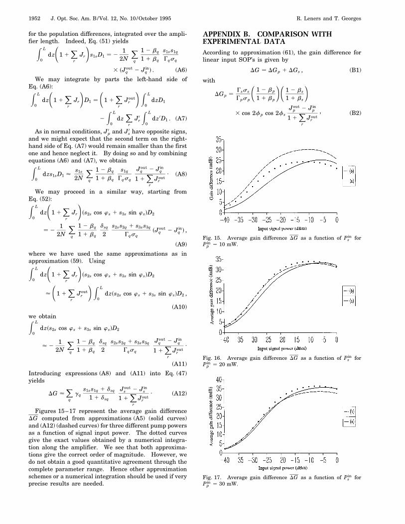
Figures 15–17 represent the average gain differenceDG computed from approximations (A5) (solid curves)and (A12) (dashed curves) for three different pump powersas a function of signal input power. The dotted curvesgive the exact values obtained by a numerical integra-tion along the amplifier. We see that both approxima-tions give the correct order of magnitude. However, wedo not obtain a good quantitative agreement through thecomplete parameter range. Hence other approximationschemes or a numerical integration should be used if veryprecise results are needed.

APPENDIX B. COMPARISON WITHEXPERIMENTAL DATAAccording to approximation (61), the gain difference forlinear input SOP’s is given by

DG DGp 1 DGs , (B1)

with

DGp Gsss

Gpsp

√1 2 bp

1 1 bp

!√1 2 bs

1 1 bs

!

3 cos 2fp cos 2fsJout

p 2 J inp

1 1X

rJout

r

, (B2)

Fig. 15. Average gain difference DG as a function of P ins for

P inp 10 mW.


P inp 20 mW.


P inp 30 mW.


DGs

√1 2 bs

1 1 bs

!21 1 cos2 2fs

2Jout

s 2 J ins

1 1X

rJout

r

. (B3)

Let us denote this gain difference by DG s1d DGp 1

DGs. If we rotate the signal input SOP by 90±, we obtaina second value for DG:

DG s2d 2DGp 1 DGs . (B4)

Finally, if the pump polarization is scrambled at a highrate, we may discard its contribution to DG, i.e.,

DG s3d DGs . (B5)

Experimental values found in Ref. 18 are

DG s1d ø 135 mdB , (B6)

DG s2d ø 0 mdB , (B7)

DG s3d ø 70 mdB , (B8)

The orientations fq of the fields with respect to the bire-fringence axis are not reported. First we have to noticethat these values approximately confirm the relationship

DG s3d 1/2fDG s1d 1 DG s2dg . (B9)

To deduce a value for bs, we use DG s3d DGs 70 mdBwith some additional assumptions. First we assume thatthe remainder of the pump power is negligible comparedwith the signal output power sJout

s .. Joutp d and that the

signal output power is large compared with the saturationpower sJout

s .. 1d. Then

Jouts 2 J in

s

1 1X

rJout

r

øJout

s 2 J ins

Jouts

1 2 exps2Gd ø 1 , (B10)

where G 19 dB is the reported gain of the amplifier.18

The gain difference is then given by

DG s3d

√1 2 bs

1 1 bs

!21 1 cos2 2fs

2. (B11)

Depending on the absolute orientation fs of the signalSOP, the value DG s3d 70 mdB leads to

bs 0.8 for fs 0± , (B12)

bs 0.7 for fs 45± . (B13)

In the absence of information about fs we took the valuesof bs 0.8. The reported measurements were made at apump wavelength of 1480 nm. To the best of our knowl-edge, similar data do not yet exist at 980 nm, and so wechose bp 0.9 rather arbitrarily. Although the magni-tude of the polarization sensitivity of an EDFA depends onthe exact values of bs and bp, the calculations presentedin this paper remain valid as long as the sensitivity isweak, i.e., bs and bp close to unity.

*Present address, Universite Libre de Bruxelles, Op-tique et Acoustique CP 194y5, 50 avenue Roosevelt, 1050Bruxelles, Belgium.

REFERENCES1. V. P. Lebedev and A. K. Przhevuskii, “Polarized lumines-

cence of rare-earth activated glasses,” Sov. Phys. Solid State19, 1389 (1977).

2. D. W. Hall and M. J. Weber, “Polarized fluorescence linenarrowing measurements of Nd laser glasses: evidence ofstimulated emission cross section anisotropy,” Appl. Phys.Lett. 42, 157 (1983).

3. D. W. Hall, R. A. Haas, W. F. Krupke, and M. J. Weber,“Spectral and polarization hole burning in neodymium glasslasers,” IEEE J. Quantum Electron. QE-19, 1704 (1983).

4. J. T. Lin, P. R. Morkel, L. Reekie, and D. N. Payne, “Polar-ization effects in fiber lasers,” in Conference on Lasers andElectro-Optics, Vol. 14 of 1987 OSA Technical Digest Series(Optical Society of America, Washington, D.C., 1987), p. 107.

5. J. T. Lin, L. Reekie, D. N. Payne, and S. B. Poole, “Inten-sity dependent polarization frequency splitting in an Er3+-doped fiber laser,” in Conference on Lasers and Electro-Optics, Vol. 7 of 1988 OSA Technical Digest Series (OpticalSociety of America, Washington, D.C., 1988), paper TuM28.

6. J. T. Lin, W. A. Gambling, and D. N. Payne, “Modeling ofpolarization effects in fiber lasers,” in Conference on Lasersand Electro-Optics, Vol. 11 of 1989 OSA Technical DigestSeries (Optical Society of America, Washington, D.C., 1989),p. 90.

7. J. T. Lin and W. A. Gambling, “Polarisation effects in fi-bre lasers: phenomena, theory and applications,” in FiberLaser Sources and Amplifiers II, M. J. Digonnet and E.Snitzer, eds., Proc. Soc. Photo-Opt. Instrum. Eng. 1373, 42(1990).

8. S. Bielawski, D. Derozier, and P. Glorieux, “Antiphase dy-namics and polarizations effects in the Nd-doped fiber laser,”Phys. Rev. A 46, 2811 (1992).

9. R. Leners, P. L. Francois, and G. Stephan, “Simultaneouseffects of gain and loss anisotropies on the thresholds of abipolarization fiber laser,” Opt. Lett. 19, 275 (1994).

10. R. Leners, P. L. Francois, and G. Stephan, “Polarizationcross-saturation in fiber lasers,” in International QuantumElectronics Conference, Vol. 9 of 1994 OSA Technical DigestSeries (Optical Society of America, Washington, D.C., 1994),p. 212.

11. B. Meziane, F. Sanchez, G. Stephan, and P. L. Francois,“Feedback induced polarization switching in a Nd-dopedfiber laser,” Opt. Lett. 19, 1971 (1994).

12. M. G. Taylor, “Observation of a new polarisation dependenceeffect in long haul optically amplified system,” in OpticalFiber Communication Conference and International Confer-ence on Integrated Optics and Optical Fiber Communication,Vol. 4 of 1993 OSA Technical Digest Series (Optical Societyof America, Washington, D.C., 1993), paper PD5.

13. E. Lichtman, “Limitations imposed by polarization depen-dent gain and loss on all-optical ultralong communicationsystems,” in Optical Fiber Communication Conference, Vol. 4of 1994 OSA Technical Digest Series (Optical Society ofAmerica, Washington, D.C., 1994), p. 257.

14. F. Bruyere and O. Audouin, “Penalties in long-haul opticalamplifier systems due to polarization dependent loss andgain,” IEEE Photon. Technol. Lett. 6, 654 (1994).

15. E. J. Greer, D. J. Lewis, and W. M. Macaulay, “Polarisationdependent gain in erbium doped fibre amplifiers,” Electron.Lett. 30, 46 (1994).

16. R. W. Keys, S. J. Wilson, M. Healy, S. R. Baker, A. Robinson,and J. E. Righton, “Polarization-dependent gain in erbium-doped fibers,” in Optical Fibre Communication Conference,Vol. 4 of 1994 OSA Technical Digest Series (Optical Societyof America, Washington, D.C., 1994), paper FF5.

17. V. J. Mazurczyk and J. L. Zyskind, “Polarization hole burn-ing in erbium doped fiber amplifiers,” in Conference onLasers and Electro-Optics, Vol. 12 of 1993 OSA Technical Di-gest Series (Optical Society of America, Washington, D.C.,1993), paper CPD26.

18. V. J. Mazurczyk and J. L. Zyskind, “Polarisation depen-dent gain in erbium doped fiber amplifiers,” IEEE Photon.Technol. Lett. 6, 616 (1994).

19. N. S. Bergano, “Time dynamics of polarization hole burningin an EDFA,” in Optical Fiber Communication Conference,


Vol. 4 of 1994 OSA Technical Digest Series (Optical Societyof America, Washington, D.C., 1994), paper FF4.

20. Y. Fukada, T. Imai, and A. Mamoru, “BER fluctuation sup-pression in optical in-line amplifier system using polarisa-tion scrambling techniques,” Electron. Lett. 30, 432 (1994).

21. M. G. Taylor and S. J. Penticost, “Improvement in perfor-mance of long haul EDFA link using high frequency polari-sation modulation,” Electron. Lett. 30, 805 (1994).

22. M. G. Taylor, “Improvement in Q with low frequency polar-ization modulation on transoceanic EDFA link,” IEEE Pho-ton. Technol. Lett. 6, 860 (1994).

23. N. S. Bergano, V. J. Mazurczyk, and C. R. Davidson, “Polar-ization scrambling improves SNR performance in a chain ofEDFAs,” in Optical Fiber Communication Conference, Vol. 4of 1994 OSA Technical Digest Series (Optical Society ofAmerica, Washington, D.C., 1994), paper ThR2.

24. V. Letellier, G. Bassier, P. Marmier, R. Morin, R. Uhel,and J. Artur, “Polarisation scrambling in 5 Gbitys 8100 kmEDFA based system,” Electron. Lett. 30, 46 (1994).

25. V. J. Mazurczyk and C. D. Poole, “The effect of birefrin-gence on polarization hole burning in erbium doped fiberamplifiers,” in Optical Amplifiers and Their Applications,Vol. 14 of 1994 OSA Technical Digest Series (Optical Soci-ety of America, Washington, D.C., 1994), paper ThB3.

26. P. F. Wysocki, “Computer modeling of polarization holeburning in EDFAs,” in Optical Fiber Communication Con-ference, Vol. 4 of 1994 OSA Technical Digest Series (OpticalSociety of America, Washington, D.C., 1994), paper FF6.

27. P. F. Wysocki, “Polarization hole-burning in erbium doped

fiber amplifiers with birefringence,” in Optical Amplifiersand Their Applications, Vol. 14 of 1994 OSA Technical Di-gest Series (Optical Society of America, Washington, D.C.,1994), paper ThB4.

28. R. Leners, T. Georges, P. L. Francois, and G. Stephan,“Analytic model of polarization dependent gain in erbiumdoped fibre amplifier,” in Optical Amplifiers and Their Appli-cations, Vol. 14 of 1994 OSA Technical Digest Series (OpticalSociety of America, Washington, D.C., 1994), paper PD1.

29. R. Leners and G. Stephan, “Rate equations analysis of amulti-mode, bipolarization Nd3+-doped fibre laser,” J. Europ.Opt. Soc. (to be published).

30. T. Georges and E. Delevaque, “Analytic modelling of high-gain erbium doped fiber amplifiers,” Opt. Lett. 17, 1113(1992).

31. T. Ueda and W. L. Kath, “Stochastic simulation of pulses innonlinear-optical fibers with random birefringence,” J. Opt.Soc. Am. B 11, 818 (1994).

32. V. J. Matsas, T. P. Newson, D. J. Richardson, and D. N.Payne, “Selfstarting passively mode-locked fibre ring solitonlaser exploiting nonlinear polarisation rotation,” Electron.Lett. 28, 1391 (1992).

33. K. Tamura, H. A. Haus, and E. P. Ippen, “Self-starting ad-ditive pulse mode-locked erbium fibre ring laser,” Electron.Lett. 28, 2226 (1992).

34. M. E. Fermann, M. J. Andrejco, Y. Silberberg, and M. L.Stock, “Passive mode locking by using nonlinear polarizationevolution in a polarization-maintaining erbium-doped fiber,”Opt. Lett. 18, 894 (1993).

Numerical and analytical modeling of polarization-dependent gain in erbium-doped fiber amplifiers

Documents

Transcript of Numerical and analytical modeling of polarization-dependent gain in erbium-doped fiber amplifiers