41st Aerospace Sciences Meeting & Exhibit

6-9 January 2003 / Reno, NV

AIAA 2003-0636

A Jet Formation Criterion for Synthetic Jet Actuators Yogen Utturkar, Ryan Holman, Rajat Mittal, Bruce Carroll, Mark Sheplak, and Louis Cattafesta University of Florida Gainesville, FL The George Washington University Washington, D.C.

For permission to copy or republish, contact the American Institute of Aeronautics and Astronautics, 1801 Alexander Bell Drive, Suite 500, Reston, Virginia 20191-4344.

AIAA-2003-0636

A Jet Formation Criterion for Synthetic Jet Actuators

Yogen Utturkar,1£ Ryan Holman,1£ Rajat Mittal,2¥ Bruce Carroll,1† Mark Sheplak,1§ and Louis Cattafesta1¶

1Department of Mechanical and Aerospace Engineering

University of Florida Gainesville, Florida 32611-6250

(352) 846-3017, (352) 392-7303 (FAX), catman@mae.ufl.edu

2Department of Mechanical and Aerospace Engineering The George Washington University

Washington, D.C. 20052

Abstract This paper proposes and validates a jet formation

criterion for synthetic jet actuators. The synthetic jet is a zero net mass flux device, adding additional momentum but no mass to its surroundings. Jet formation is defined as a mean outward velocity along the jet axis and corresponds to the clear formation of shed vortices. It is shown that the synthetic jet formation is governed by the Strouhal number (or Reynolds number and Stokes number). Numerical simulations and experiments are performed to supplement available two-dimensional and axisymmetric jet formation data in the literature. The data support the jet formation criterion

, where the constant 2Re/ S K> K is approximately 2 and 0.16 for two dimensional and axisymmetric synthetic jets, respectively. This criterion is valid for relatively thick orifice plates with thickness-to-width ratios greater than approximately 2. This result is expected to be useful for the design of flow-control actuators and engine nacelle acoustic liners.

Introduction Synthetic jet actuators have been shown to be a

useful tool for flow control, with applications including mixing enhancement, separation control, and thrust vectoring [1]. Figure 1 shows a schematic of a typical synthetic jet or “zero net mass flux” device. In its most common implementation, a piezoelectric disk is bonded to a metal diaphragm,

which is sealed to form a cavity. As the diaphragm oscillates, fluid is periodically entrained and expelled from the cavity through the orifice (or slot). Under certain operating conditions, a vortex pair (vortex ring in the axisymmetric case) is formed at the orifice edge during the expulsion part of the cycle. This vortex pair is convected away from the orifice. If the self-induced velocity of the vortex pair is strong enough, then the vortex pair is not ingested back into the orifice during the suction part of the cycle. The formation of a vortex pair is defined herein as the onset of jet formation.

t

£ Graduate Student, Student Member AIAA

¥ Associate Professor, Member AIAA

† Associate Professor, Associate Fellow AIAA

§ Assistant Professor, Member AIAA

¶ Assistant Professor, Associate Fellow AIAA

Copyright 2003 by the University of Florida. Published by

the American Institute of Aeronautics and Astronautics, Inc. with permission.

The governing parameters for synthetic jets based on a simple “slug” model [2,3,4] include a dimensionless stroke length and a Reynolds number based on the velocity scale

0 /L d

, (1) ( )/ 2

0 0 00

TU f L f u t d= = ∫

where ( )0u t is the spatial-averaged velocity at the exit, 1T f= is the period, d is the width of the slot (or diameter of the orifice), and is the distance that a “slug” of fluid travels away from the orifice during the ejection portion of the cycle or period. The Reynolds number is then defined as

0L

0Re U d ν= , (2)

where ν µ ρ= is the kinematic viscosity. Alternatively, the Reynolds number can be

defined in terms of a spatial and time-averaged exit velocity during the expulsion stroke [5], Re Ud ν= , where

( )2

0

2 1 ,T

AU u t y

T A= ∫ ∫ dtdA , (3)

A is the exit area, and is the cross-stream coordinate (see Figure 2). It is easily shown that the two velocity scales are related by

y

02=U U .

1

AIAA-2003-0636

Note that ( )0 0/L d U fd= is closely related to the inverse of the Strouhal number, which may be written as

2

1 U UdSt d d S

νω ω ν

= = = 2

Re , (4)

where S is the Stokes number

2dS ω

ν= , (5)

and 2 fω π= is the radian frequency of oscillation of the diaphragm.

The effectiveness of the synthetic jet to impart momentum to its surroundings is highly dependent on these jet formation parameters and on the slot/orifice geometry. It is therefore desirable to define a jet formation criterion in terms of these parameters and validate it through experimental measurements. Similar jet formation criteria have been proposed by Smith and Swift [4] and Utturkar [5] and are described below.

The purpose of this paper is to propose and validate a unified criterion suitable for quasi fully-developed two-dimensional and axisymmetric orifices. First, the jet formation criterion is presented that is based on a simple order-of-magnitude analysis. Next, computational and experimental flow visualization experiments are described that determine the onset of vortex shedding (i.e. jet formation). Detailed Laser Doppler Velocimetry (LDV) measurements are used to determine the jet formation parameters. Finally, available jet formation parameters obtained from various studies are used to validate the criterion.

Order-of-Magnitude Analysis Smith and Swift [4] and Utturkar [5]

independently arrived at a jet formation criterion for two dimensional synthetic jets. Smith and Swift argued that a threshold stroke length exists for jet formation. Utturkar reached a similar conclusion based on the Strouhal number and, using Eq. (4), argued that the ratio of the Reynolds number to the square of the Stokes number must be greater than some constant to ensure jet formation. This criterion is presented here for completeness.

Figure 2 illustrates a vortex pair (or ring) emanating from an orifice. Previous studies [6,7] suggested that under certain circumstances, a vortex pair formed at the orifice lip during the expulsion stroke of the diaphragm can be ingested back into the jet cavity before it can escape due to its self-induced velocity.

The strength of each shed vortex has been shown by Didden [8] to be related to the flux of vorticity through a planar slice of the orifice during the expulsion portion of the cycle

vΩ

/ 2 2

0 0~

T d

v zudydtξΩ ∫ ∫ , (6)

where zξ is the vorticity component of interest, and is the jet velocity. In Figure 2, u sδ is the size of the

viscous flow region characterized by non-zero vorticity. The induced velocity of the dipole IV is proportional to /v dΩ . Performing an order-of-magnitude analysis on Eq. (6) results in

1~vs

U Uδ sδ ωΩ . (7)

If it is assumed that a jet will form when the induced velocity of the dipole IV is somewhat larger than the average jet suction velocity sV , it follows that

2

/ Re~ ~ ~S

vI

s

dV U KV U dω

Ω> , (8)

where K is an unknown constant. The value of this constant varies depending upon

orifice geometry. This is best illustrated by considering again Eq. (6), and assuming a sinusoidally varying velocity profile of the form

, (9) ( ) (0 sinu u t f yω= )

where is the centerline velocity and 0u ( )f y is the shape of the velocity profile defined such that

( )2f y 0d= = due to the no-slip boundary

condition and ( )0 1f y = = . The integral in Eq. (6) then becomes

/ / 2

0 0~

d

vdu udydtdy

π ωΩ ∫ ∫ . (10)

Substituting in Eq. (9) into Eq. (10) results in

( )2

220

1 04 2v

du f fπω

Ω = − +

. (11)

which simplifies to

2

2

4vN Uπ

ωΩ = . (12)

where 0 /N u U= is the ratio of the centerline velocity to the average velocity that has been used.

2

AIAA-2003-0636

Substituting Eq. (12)into Eq. (8) yields the following jet formation criterion:

2

Re2

KS N

′> , (13)

where K ′ is a constant. It should be emphasized that since this is an

order of magnitude analysis, caution must be used when considering Eq. (13). This result merely shows that the jet formation criterion is dependent on the shape of the velocity profile. Also, the velocity profile is assumed to be completely in phase across the orifice. Thus, this approximation is only valid at low Stokes numbers when the velocity profile is parabolic.

For steady flow emanating from an axisymmetric orifice, the average velocity can be expressed as

2

202 0

41 2

2du rU

ddπ

π

= −

∫ rdr . (14)

Evaluating Eq. (14) gives

0 2u

NU

= = . (15)

Similarly, if a two dimensional slot is considered, then

0 1.5u

NU

= = . (16)

The constant N in Eq. (13) is higher for an axisymmetric orifice than for a two-dimensional slot. Hence, the constant K in the jet formation criterion, Eq. (8), is expected to be lower for the axisymmetric jet than for the two dimensional jet. Consequently, a synthetic jet will likely form at a lower Reynolds number for an axisymmetric orifice than for a two dimensional slot.

Computational Studies Numerical simulations have been performed to

characterize the velocity profile of a two-dimensional synthetic jet. A previously developed Cartesian grid solver [9,10,11] is employed in these simulations. Details of the solution procedure can be found in these papers. The solver allows simulation of unsteady viscous incompressible flows with complex immersed moving boundaries on Cartesian grids. This solver employs a second-order accurate central difference scheme for the spatial discretization and a mixed explicit-implicit fractional step scheme for time advancement. An efficient multigrid algorithm is used for solving the pressure Poisson equation.

The key advantage of this solver for the current flow is that the entire geometry of the synthetic jet including the oscillating diaphragm is modeled on a stationary Cartesian mesh. Figure 3 shows a typical mesh used in the simulations. As the diaphragm moves over the underlying Cartesian mesh, the discretization in the cells cut by the solid boundary is modified to account for the presence of the solid boundary. In addition, suitable boundary conditions also need to be prescribed for the external flow. A soft velocity boundary condition is applied on the north, east and west boundaries that allow the conditions at these boundaries to respond freely to the flow created by the jet. All simulations are run until initial transients decay and statistics are accumulated beyond this over a number of cycles.

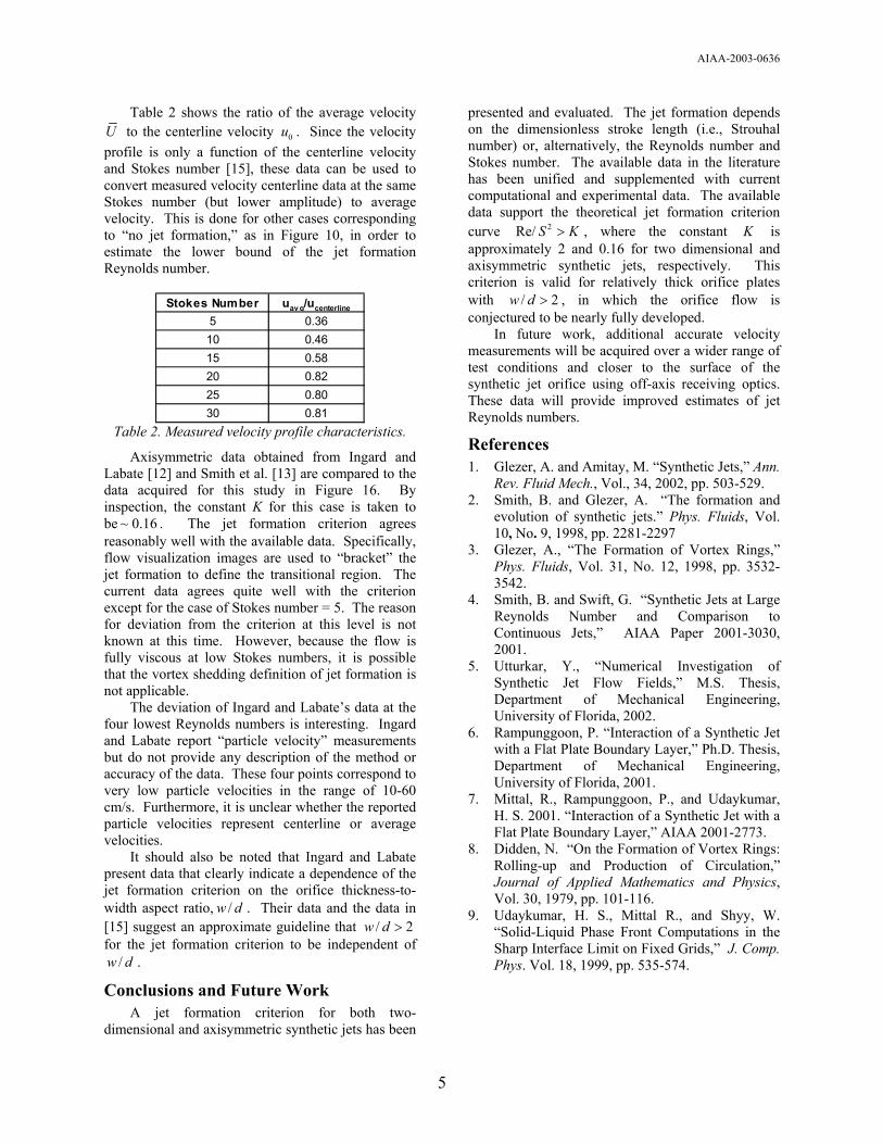
Figure 4 shows a simulation result at four phases in the cycle, for a case of no jet formation. As expected, the vortex structures formed at the orifice during the expulsion part of the cycle are ingested during the suction part. Figure 5 shows a transitional case in which jet formation is not readily apparent. Figure 6 is an example of a case exhibiting a clear jet formation as indicated by the shed vortex pair. A series of numerical simulations over a range of Reynolds and Stokes numbers suggested that the constant 1K ≈ , as shown in Figure 7.

The data of Smith and Swift were converted to Reynolds and Stokes number and are presented in Figure 8. Clearly, the experimental results are in good agreement with the jet formation criterion

2Re 2S > .

Flow Visualization Experimental jet formation data for the

axisymmetric case was published over 50 years ago by Ingard and Labate [12]. More recently, Smith et al. [13] provided additional data that suggests that

>1 for jet formation. However, the Stokes number range covered by these studies is limited to high Stokes numbers. An extension of the experimental data to low Stokes number range is desired and would prove useful in applications involving engine nacelle acoustic liners [14].

0 /L d

Before the jet formation criterion can be validated experimentally, the synthetic jet flowfield device must first be characterized using flow visualization. A piezoelectric-driven synthetic jet is used with an orifice plate of diameter 1.65 mm and a thickness of 1.65 mm. The synthetic jet is mounted inside a large glass tank and operated over a usable range of Stokes numbers from 3-30, and the voltage amplitude was varied to define the envelope of jet formation.

3

AIAA-2003-0636

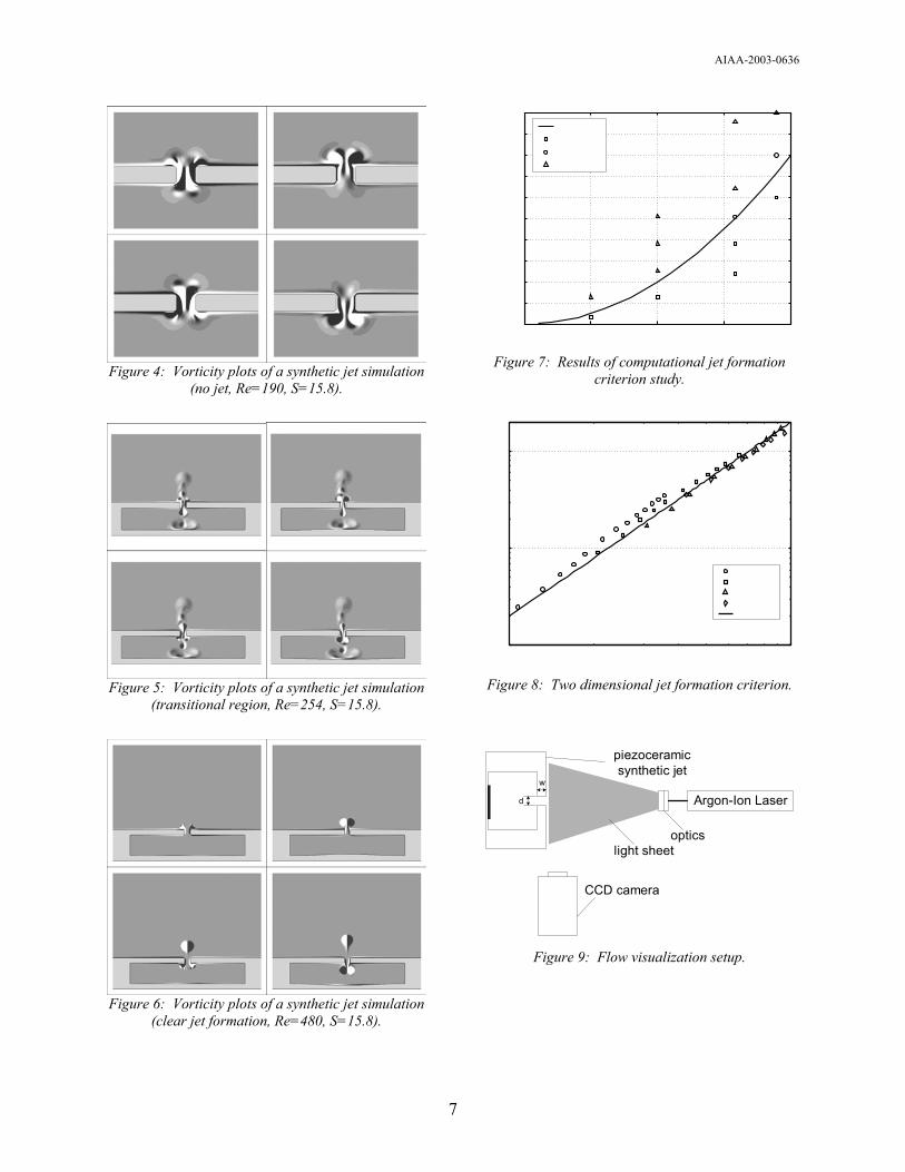
Figure 9 shows a schematic of the flow visualization setup. An argon ion laser is used in conjunction with optical lenses to form a thin light sheet centered on the orifice axis. Atomized fog fluid is introduced into the tank to seed the flow, and a 14-bit cooled CCD camera is employed to acquire detailed, long exposure images to capture the time-averaged behavior of the jet. Figure 10 shows a typical image at low excitation amplitude (V =1 V,

=24), revealing no significant mean axial flow along the jet axis. Stationary recirculation patterns are present on both sides of the orifice, suggesting this flow pattern is characteristic of “Region 1” as defined by Ingard and Labate [12]. In contrast, Figure 11 (V =4.5 V, =24) shows strong mean jet behavior, at a slightly higher amplitude. Therefore, a transitional region is defined as occurring between the case of no mean jet and clear mean jet (which is assumed to correspond to vortex shedding). Images were obtained over a range of amplitudes encompassing the transition region at a given Stokes number. This process was repeated over a Stokes number range of 3-30. The images are in good qualitative agreement with the mean flow regimes described by Ingard and Labate [12].

ac

S

ac S

Velocity Field Measurement In contrast with the Stokes number, estimating

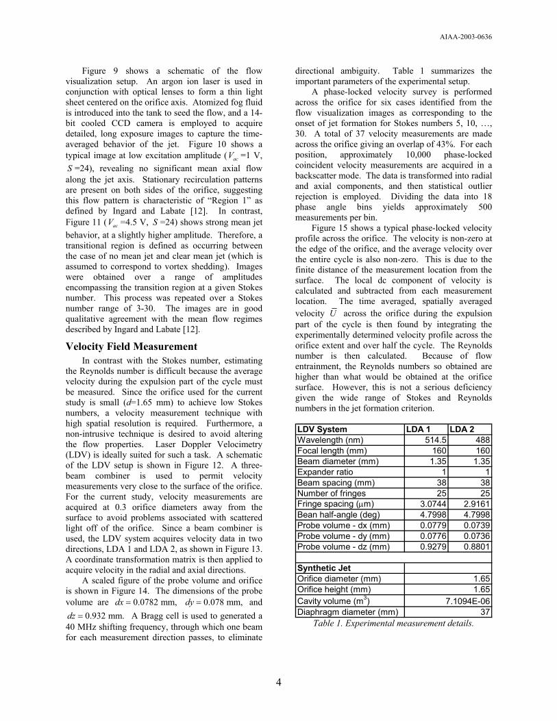
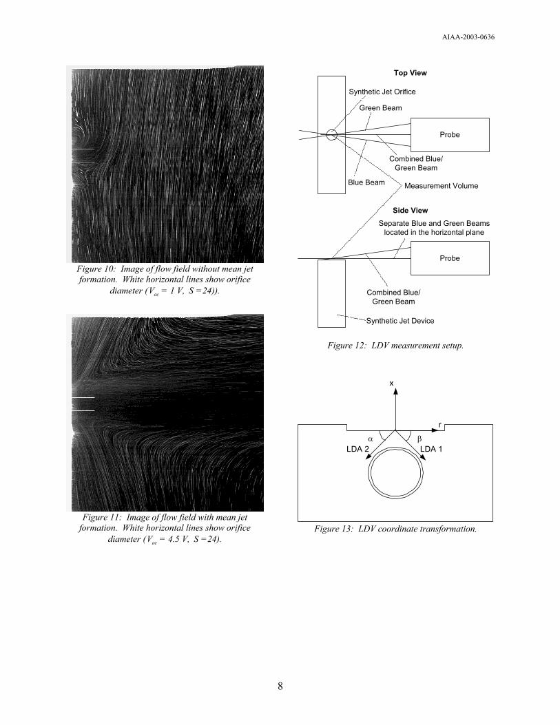
the Reynolds number is difficult because the average velocity during the expulsion part of the cycle must be measured. Since the orifice used for the current study is small (d=1.65 mm) to achieve low Stokes numbers, a velocity measurement technique with high spatial resolution is required. Furthermore, a non-intrusive technique is desired to avoid altering the flow properties. Laser Doppler Velocimetry (LDV) is ideally suited for such a task. A schematic of the LDV setup is shown in Figure 12. A three-beam combiner is used to permit velocity measurements very close to the surface of the orifice. For the current study, velocity measurements are acquired at 0.3 orifice diameters away from the surface to avoid problems associated with scattered light off of the orifice. Since a beam combiner is used, the LDV system acquires velocity data in two directions, LDA 1 and LDA 2, as shown in Figure 13. A coordinate transformation matrix is then applied to acquire velocity in the radial and axial directions.

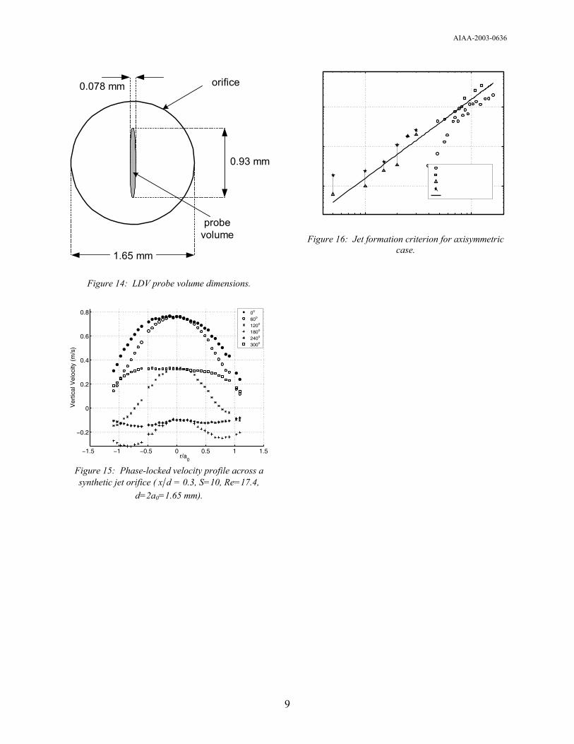
A scaled figure of the probe volume and orifice is shown in Figure 14. The dimensions of the probe volume are and

A Bragg cell is used to generated a 40 MHz shifting frequency, through which one beam for each measurement direction passes, to eliminate

directional ambiguity. Table 1 summarizes the important parameters of the experimental setup.

0.0782 mm,dx =m.

0.078 mm,dy =0.932 mdz =

A phase-locked velocity survey is performed across the orifice for six cases identified from the flow visualization images as corresponding to the onset of jet formation for Stokes numbers 5, 10, …, 30. A total of 37 velocity measurements are made across the orifice giving an overlap of 43%. For each position, approximately 10,000 phase-locked coincident velocity measurements are acquired in a backscatter mode. The data is transformed into radial and axial components, and then statistical outlier rejection is employed. Dividing the data into 18 phase angle bins yields approximately 500 measurements per bin.

Figure 15 shows a typical phase-locked velocity profile across the orifice. The velocity is non-zero at the edge of the orifice, and the average velocity over the entire cycle is also non-zero. This is due to the finite distance of the measurement location from the surface. The local dc component of velocity is calculated and subtracted from each measurement location. The time averaged, spatially averaged velocity U across the orifice during the expulsion part of the cycle is then found by integrating the experimentally determined velocity profile across the orifice extent and over half the cycle. The Reynolds number is then calculated. Because of flow entrainment, the Reynolds numbers so obtained are higher than what would be obtained at the orifice surface. However, this is not a serious deficiency given the wide range of Stokes and Reynolds numbers in the jet formation criterion. LDV System LDA 1 LDA 2Wavelength (nm) 514.5 488Focal length (mm) 160 160Beam diameter (mm) 1.35 1.35Expander ratio 1 1Beam spacing (mm) 38 38Number of fringes 25 25Fringe spacing (µm) 3.0744 2.9161Bean half-angle (deg) 4.7998 4.7998Probe volume - dx (mm) 0.0779 0.0739Probe volume - dy (mm) 0.0776 0.0736Probe volume - dz (mm) 0.9279 0.8801

Synthetic JetOrifice diameter (mm)Orifice height (mm)Cavity volume (m3)Diaphragm diameter (mm)

7.1094E-0637

1.651.65

Table 1. Experimental measurement details.

4

AIAA-2003-0636

Table 2 shows the ratio of the average velocity U to the centerline velocity . Since the velocity profile is only a function of the centerline velocity and Stokes number [15], these data can be used to convert measured velocity centerline data at the same Stokes number (but lower amplitude) to average velocity. This is done for other cases corresponding to “no jet formation,” as in Figure 10, in order to estimate the lower bound of the jet formation Reynolds number.

0u

Stokes Number uav g/ucenterline

5 0.310 0.4615 0.5820 0.8225 0.8030 0.81

6

Table 2. Measured velocity profile characteristics.

Axisymmetric data obtained from Ingard and Labate [12] and Smith et al. [13] are compared to the data acquired for this study in Figure 16. By inspection, the constant K for this case is taken to be . The jet formation criterion agrees reasonably well with the available data. Specifically, flow visualization images are used to “bracket” the jet formation to define the transitional region. The current data agrees quite well with the criterion except for the case of Stokes number = 5. The reason for deviation from the criterion at this level is not known at this time. However, because the flow is fully viscous at low Stokes numbers, it is possible that the vortex shedding definition of jet formation is not applicable.

~ 0.16

The deviation of Ingard and Labate’s data at the four lowest Reynolds numbers is interesting. Ingard and Labate report “particle velocity” measurements but do not provide any description of the method or accuracy of the data. These four points correspond to very low particle velocities in the range of 10-60 cm/s. Furthermore, it is unclear whether the reported particle velocities represent centerline or average velocities.

It should also be noted that Ingard and Labate present data that clearly indicate a dependence of the jet formation criterion on the orifice thickness-to-width aspect ratio, . Their data and the data in [15] suggest an approximate guideline that for the jet formation criterion to be independent of

.

/w d/ 2w d >

/w d

Conclusions and Future Work A jet formation criterion for both two-

dimensional and axisymmetric synthetic jets has been

presented and evaluated. The jet formation depends on the dimensionless stroke length (i.e., Strouhal number) or, alternatively, the Reynolds number and Stokes number. The available data in the literature has been unified and supplemented with current computational and experimental data. The available data support the theoretical jet formation criterion curve , where the constant 2Re/ S K> K is approximately 2 and 0.16 for two dimensional and axisymmetric synthetic jets, respectively. This criterion is valid for relatively thick orifice plates with , in which the orifice flow is conjectured to be nearly fully developed.

/ 2w d >

In future work, additional accurate velocity measurements will be acquired over a wider range of test conditions and closer to the surface of the synthetic jet orifice using off-axis receiving optics. These data will provide improved estimates of jet Reynolds numbers.

References 1. Glezer, A. and Amitay, M. “Synthetic Jets,” Ann.

Rev. Fluid Mech., Vol., 34, 2002, pp. 503-529. 2. Smith, B. and Glezer, A. “The formation and

evolution of synthetic jets.” Phys. Fluids, Vol. 10, No. 9, 1998, pp. 2281-2297

3. Glezer, A., “The Formation of Vortex Rings,” Phys. Fluids, Vol. 31, No. 12, 1998, pp. 3532-3542.

4. Smith, B. and Swift, G. “Synthetic Jets at Large Reynolds Number and Comparison to Continuous Jets,” AIAA Paper 2001-3030, 2001.

5. Utturkar, Y., “Numerical Investigation of Synthetic Jet Flow Fields,” M.S. Thesis, Department of Mechanical Engineering, University of Florida, 2002.

6. Rampunggoon, P. “Interaction of a Synthetic Jet with a Flat Plate Boundary Layer,” Ph.D. Thesis, Department of Mechanical Engineering, University of Florida, 2001.

7. Mittal, R., Rampunggoon, P., and Udaykumar, H. S. 2001. “Interaction of a Synthetic Jet with a Flat Plate Boundary Layer,” AIAA 2001-2773.

8. Didden, N. “On the Formation of Vortex Rings: Rolling-up and Production of Circulation,” Journal of Applied Mathematics and Physics, Vol. 30, 1979, pp. 101-116.

9. Udaykumar, H. S., Mittal R., and Shyy, W. “Solid-Liquid Phase Front Computations in the Sharp Interface Limit on Fixed Grids,” J. Comp. Phys. Vol. 18, 1999, pp. 535-574.

5

AIAA-2003-0636

10. Ye, T., Mittal, R., Udaykumar, H. S., and Shyy, W., “An accurate Cartesian grid method for viscous incompressible flows with complex immersed boundaries,” J. Comp. Phys., Vol. 156, 1999, pp. 209-240.

11. Udaykumar, H.S., Mittal, R., Rampunggoon, P., and Khanna, A. “A Sharp Interface Cartesian Grid Method for Simulating Flow with Complex Moving Boundaries,” J. Comp. Phys. Vol. 174, No. 1, 2001, pp. 345-380.

12. Ingard, U. and Labate, S. “Acoustic Circulation Effects and the Nonlinear Impedance of Orifices,” J. Acous. Soc. Am., Vol. 22, No. 2, 1950, pp. 211-218.

13. Smith, B., Trautman, M., and Glezer, A. “Controlled Interactions of Adjacent Synthetic Jets,” AIAA Paper 99-0669, 1999.

14. Horowitz, S., Nishida, T., Cattafesta, L., and Sheplak, M., “Characterization of Compliant-Backplate Helmholtz Resonators for an Electromechanical Acoustic Liner,” International Journal of Aeroacoustics, Vol. 1, No. 2, 2002, pp. 183-205.

15. Gallas, Q., Holman, R., Nishida, T., Carroll, B., Sheplak, M., and Cattafesta, L. “Lumped Element Modeling of Piezoelectric-Driven Synthetic Jet Actuators.” AIAA Paper 2002-0125, 2002, to appear in AIAA Journal, Vol. 41, No. 2.

oscillating diaphragm

cavity

shed vortex pairs

d

Figure 1: Schematic of a synthetic jet.

d

δs

VI

Vs

Ωv

x

y

Figure 2: Schematic of synthetic jet formation

criterion.

Figure 3: A fixed non-uniform Cartesian grid used in the two-dimensional synthetic jet calculations. Every

third grid point is shown.

6

AIAA-2003-0636

Figure 4: Vorticity plots of a synthetic jet simulation

(no jet, Re=190, S=15.8).

Figure 5: Vorticity plots of a synthetic jet simulation

(transitional region, Re=254, S=15.8).

0 5 10 15 200

50

100

150

200

250

300

350

400

450

500

Stokes Number

Rey

nold

s N

umbe

r

Red/S2=1

No JetTransitionClear Jet

101

102

102

103

104

Stokes Number

Rey

nold

s N

umbe

r

d=0.5 cmd=1.0 cmd=1.5 cmd=2.1 cmRe/S2=2

Figure 6: Vorticity plots of a synthetic jet simulation

(clear jet formation, Re=480, S=15.8).

Figure 7: Results of computational jet formation

criterion study.

Figure 8: Two dimensional jet formation criterion.

Argon-Ion Laser

opticslight sheet

CCD camera

piezoceramicsynthetic jet

d

w

Figure 9: Flow visualization setup.

7

AIAA-2003-0636

Figure 10: Image of flow field without mean jet formation. White horizontal lines show orifice

diameter (V = 1 V, =24)). ac S

Figure 11: Image of flow field with mean jet

formation. White horizontal lines show orifice diameter (V = 4.5 V, =24). ac S

Side View

Top View

Probe

Probe

Synthetic Jet Orifice

Blue Beam

Green Beam

Combined Blue/Green Beam

Combined Blue/Green Beam

Synthetic Jet Device

Separate Blue and Green Beamslocated in the horizontal plane

Measurement Volume

Figure 12: LDV measurement setup.

x

r

LDA 2 LDA 1α β

Figure 13: LDV coordinate transformation.

8

AIAA-2003-0636

orifice

1.65 mm

0.93 mm

0.078 mm

probevolume

Figure 14: LDV probe volume dimensions.

−1.5 −1 −0.5 0 0.5 1 1.5

−0.2

0

0.2

0.4

0.6

0.8

r/a0

Ver

tical

Vel

ocity

(m

/s)

0o

60o

120o

180o

240o

300o

101

102

101

102

103

Stokes Number

Rey

nold

s N

umbe

r

Ingard and LabateSmith et al.Current−No JetCurrent−Clear JetRe/S2=0.16

Figure 15: Phase-locked velocity profile across a synthetic jet orifice ( x d = 0.3, S=10, Re=17.4,

d=2a0=1.65 mm).

Figure 16: Jet formation criterion for axisymmetric

case.

9