Learning canonical correlations

Reprint from SCIA'97

Learning Canonical Correlations

M. Borga, H. Knutsson, T. Landelius

Computer Vision Laboratory

Department of Electrical Engineering

Link�oping University

S-581 83 Link�oping, Sweden

Abstract

This paper presents a novel learning algorithm that �nds the linear combination of one set of multi-

dimensional variates that is the best predictor, and at the same time �nds the linear combination of another set

which is the most predictable. This relation is known as the canonical correlation and has the property of being

invariant with respect to aÆne transformations of the two sets of variates. The algorithm successively �nds all

the canonical correlations beginning with the largest one. It is shown that canonical correlations can be used

in computer vision to �nd feature detectors by giving examples of the desired features. When used on the pixel

level, the method �nds quadrature �lters and when used on a higher level, the method �nds combinations of

�lter output that are less sensitive to noise compared to vector averaging.

1 Introduction

A common problem in neural networks and learning, incapacitating many theoretically promising algorithms, is thehigh dimensionality of the input-output space. As an example, typical dimensionalities for systems having visualinputs far exceed acceptable limits. For this reason, a priori restrictions must be invoked. A common restriction isto use only locally linear models. To obtain eÆcient systems, the dimensionalities of the models should be as lowas possible. The use of locally low-dimensional linear models will in most cases be adequate if the subdivision ofthe input and output spaces are made adaptively [3, 11].An important problem is to �nd the best directions in the input- and output spaces for the local models.

Algorithms like the Kohonen self organizing feature maps [10] and others that work with principal componentanalysis will �nd directions where the signal variances are high. This is, however, of little use in a responsegenerating system. Such a system should �nd directions that eÆciently represents signals that are important

rather than signals that have large energy.In general the input to a system comes from a set of di�erent sensors and it is evident that the range of the

signal values from a given sensor is unrelated to the importance of the received information. The same line ofreasoning holds for the output which may consist of signals to a set of di�erent e�ectuators. For this reason thecorrelation between input and output signals is interesting since this measure of input-output relation is independentof the signal variances. However, correlation alone is not necessarily meaningful. Only input-output pairs that areregarded as relevant should be entered in the correlation analysis.Relating only the projections of the input, x, and output, y, on two vectors, wx and wy, establishes a

one-dimensional linear relation between the input and output. We wish to �nd the vectors that maximizescorr(xTwx ; yTwy), i.e. the correlation between the projections. This relation is known as canonical corre-

lation [6]. It is a statistical method of �nding the linear combination of one set of variables that is the bestpredictor, and at the same time �nding the linear combination of an other set which is the most predictable.It has been shown [7] that �nding the canonical correlations is equivalent to maximizing the mutual information

between the sets X and Y if x and y come from elliptical symmetric random distributions.In section 2, a brief review of the theory of canonical correlation is given. In section 3 we present an iterative

learning rule, equation 7, that �nds the directions and magnitudes of the canonical correlations. To illustrate thealgorithm behaviour, some experiments are presented and discussed in section 4. Finally, in section 5, we discusshow the concept of canonical correlation can be used for �nding representations of local features in computer vision.

1 c 1997 Pattern Recognition Society of Finland


2 Canonical Correlation

Consider two random variables, x and y, from a multi-normal distribution:�x

y

�� N

��x0y0

�;

�Cxx Cxy

Cyx Cyy

��; (1)

where C =�Cxx CxyCyx Cyy

�is the covariance matrix. Cxx and Cyy are nonsingular matrices and Cxy = CT

yx. Consider

the linear combinations, x = wTx (x � x0) and y = wT

y (y � y0), of the two variables respectively. The correlationbetween x and y is given by equation 2, see for example [2]:

� =wTxCxywyq

wTxCxxwxwT

yCyywy

: (2)

The directions of the partial derivatives of � with respect to wx and wy are given by:8><>:

@�@wx

!

= Cxywy �wTxCxywy

wTxCxxwx

Cxxwx

@�@wy

!

= Cyxwx �wTy Cyxwx

wTy Cyywy

Cyywy

(3)

where '^' indicates unit length and '!

=' means that the vectors, left and right, have the same directions. A completedescription of the canonical correlations is given by:�

Cxx [ 0 ][ 0 ] Cyy

��1 �

[ 0 ] Cxy

Cyx [ 0 ]

��wx

wy

�= �

��xwx

�ywy

�(4)

where: �; �x; �y > 0 and �x�y = 1. Equation 4 can be rewritten as:8<:C�1xxCxywy = ��xwx

C�1yyCyxwx = ��ywy

(5)

Solving equation 5 gives N solutions f�n; wxn; wyng; n = f1::Ng. N is the minimum of the input dimensionalityand the output dimensionality. The linear combinations, xn = wT

xnx and yn = wTyny, are termed canonical variates

and the correlations, �n, between these variates are termed the canonical correlations [6]. An important aspect inthis context is that the canonical correlations are invariant to aÆne transformations of x and y. Also note thatthe canonical variates corresponding to the di�erent roots of equation 5 are uncorrelated, implying that:8<

:wTxnCxxwxm = 0

wTynCyywym = 0

if n 6= m (6)

It should be noted that equation 4 is a special case of the generalized eigenproblem [4]:

Aw = �Bw:

The solution to this problem can be found by �nding the vectors w that maximizes the Rayleigh quotient:

r =wTAw

wTBw:

3 Learning Canonical Correlations

We have developed a novel learning algorithm that �nds the canonical correlations and the corresponding canonicalvariates by an iterative method. The update rule for the vectors wx and wy is given by:8<

:wx ( wx + �x x ( yT wy � xTwx )

wy ( wy + �y y ( xT wx � yTwy )(7)



where x and y both have the mean 0. To see that this rule �nds the directions of the canonical correlation we lookat the expected change, in one iteration, of the vectors, wx and wy:8<

:Ef�wxg = �xEfxy

T wy�xxTwxg = �x(Cxywy�kwxkCxxwx)

Ef�wyg = �yEfyxT wx�yy

Twyg = �y(Cyxwx�kwykCyywy)

Identifying with equation 3 gives:

Ef�wxg!

=@�

@wx

and Ef�wyg!

=@�

@wy

(8)

with

kwxk =wTxCxywy

wTxCxxwx

and kwyk =wTyCyxwx

wTyCyywy

This shows that the expected changes of the vectors wx and wy are in the same directions as the gradient of thecanonical correlation, �, which means that the learning rules in equation 7 on average is a gradient search on �.�; �x and �y are found as:

� =qkwxk kwyk; �x = ��1y =

skwxk

kwyk: (9)

3.1 Learning of successive canonical correlations

The learning rule maximizes the correlation and �nds the directions, wx1 and wy1, corresponding to the largestcorrelation, �1. To �nd the second largest canonical correlation and the corresponding canonical variates of equation5 we use the modi�ed learning rule8<

:wx ( wx + �x x ( (y � y1)

T wy � xTwx )

wy ( wy + �y y ( (x� x1)T wx � yTwy )

(10)

where

x1 =xT wx1vx1

wTx1vx1

and y1 =yT wy1vy1

wTy1vy1

:

vx1 and vy1 are estimates of Cxxwx1 and Cyywy1 respectively and are estimated using the iterative rule:8<:vx1 ( vx1 + � ( x xT wx1 � vx1 )

vy1 ( vy1 + � ( y yT wy1 � vy1 )(11)

The expected change of wx and wy is then given by8><>:Ef�wxg = �x

�Cxy

�wy�wy1

wTy1Cyywy

wTy1Cyywy1

��kwxkCxxwx

�

Ef�wyg = �y

�Cyx

hwx�wx1

wTx1Cxxwx

wTx1Cxxwx1

i�kwykCyywy

� (12)

It can be seen that the parts of wx and wy parallel to Cxxwx1 and Cyywy1 respectively will vanish (�wTxwx1 �

0 8 x and �wTywy1 � 0 8 y in equation 10). In the subspaces orthogonal to Cxxwx1 and Cyywy1 the learning

rule will be equivalent to that given by equation 7. In this way the parts of the signals correlated with wTx1x (and

wTy1y) are disregarded leaving the rest unchanged. Consequently the algorithm �nds the second largest correlation

�2 and the corresponding vectors wx2 and wy2. Successive canonical correlations can be found by repeating theprocedure.

4 Performance

In this section, two di�erent experiments are presented to illustrate the eÆciency and performance of the proposedalgorithm.



101

102

103

105

106

107

108

109

1010

1011

dimensions

flops

101

102

103

103

104

105

106

107

dimensions

flops

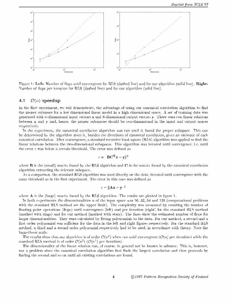
Figure 1: Left: Number of ops until convergence for RLS (dashed line) and for our algorithm (solid line). Right:Number of ops per iteration for RLS (dashed line) and for our algorithm (solid line).

4.1 O(n) speedup

In the �rst experiment, we will demonstrate, the advantage of using our canonical correlation algorithm to �ndthe proper subspace for a low-dimensional linear model in a high dimensional space. A set of training data wasgenerated with n-dimensional input vectors x and 8-dimensional output vectors y. There were two linear relationsbetween x and y and, hence, the proper subspaces should be two-dimensional in the input and output spacesrespectively.In the experiment, the canonical correlation algorithm was run until it found the proper subspace. This can

be determined by the algorithm since it, besides the directions of canonical correlation, gives an estimate of eachcanonical correlation. After convergence, a standard recursive least square (RLS) algorithm was applied to �nd thelinear relations between the two-dimensional subspaces. This algorithm was iterated until convergence, i.e. untilthe error � was below a certain threshold. The error was de�ned as

� = kBCTx� yk2

where B is the (small) matrix found by the RLS algorithm and C is the matrix found by the canonical correlationalgorithm extracting the relevant subspace.As a comparison, the standard RLS algorithm was used directly on the data, iterated until convergence with the

same threshold as in the �rst experiment. The error in this case was de�ned as

� = kAx� yk2

where A is the (large) matrix found by the RLS algorithm. The results are plotted in �gure 1.In both experiments the dimensionalities n of the input space was 16, 32, 64 and 128 (computational problems

with the standard RLS method set the upper limit). The complexity was measured by counting the number of oating point operations ( ops) until convergence (left) and per iteration (right) for the standard RLS method(marked with rings) and for our method (marked with stars). The lines show the estimated number of ops forlarger dimensionalities. They were calculated by �tting polynomials to the data. For our method, a second and a�rst order polynomial was suÆcient for the data in the left and right �gures respectively. For the standard RLSmethod, a third and a second order polynomial respectively had to be used, in accordance with theory. Note thelogarithmic scale.The results show that our algorithm is of order O(n2) when run until convergence (O(n) per iteration) while the

standard RLS method is of order O(n3) (O(n2) per iteration).The dimensionality of the linear relation can, of course, in general not be known in advance. This is, however,

not a problem since the canonical correlation algorithm �rst �nds the largest correlation and then proceeds by�nding the second and so on until all existing correlations are found.



4.2 High dimensional spaces

The second experiment illustrates the algorithms ability to handle high-dimensional spaces. The dimensionality ofx is 800 and the dimensionality of y is 200, so the total dimensionality of the signal space is 1000.Rather than tuning parameters to produce a nice result for a speci�c distribution, we have used adaptive update

factors and parameters producing similar behaviour for di�erent distributions and di�erent number of dimensions.Also note that the adaptability allows a system without a pre-speci�ed time dependent update rate decay. ThecoeÆcients �x and �y were in the experiments calculated according to equation 13:8<

:�x = a�xE

�1x

�y = a�yE�1y

where

8<:Ex ( Ex + b ( kxxTwxk �Ex)

Ey ( Ey + b ( kyyTwyk �Ey)(13)

To get a smooth and yet fast behaviour, an adaptively time averaged set of vectors, wa was calculated. The updatespeed was made dependent on the consistency in the change of the original vectors w according to equation 14.8<

:wax ( wax + c k�xk kwxk

�1 (wx �wax)

way ( way + c k�yk kwyk�1 (wy �way)

where

8<:�x ( �x + d (�wx ��x)

�y ( �y + d (�wy ��y)(14)

This process we call adaptive smoothing.The experiment have been carried out using a randomly chosen distribution of a 800-dimensional x variable and

a 200-dimensional y variable. Two x and two y dimensions were partly correlated. The variances in the 1000dimensions are in the same order of magnitude

0 0.5 1 1.5 2 2.5 3

x 104

0

0.5

1

1.5

iterations

corr

elat

ion

0 0.5 1 1.5 2 2.5 3

x 104

−5

−4

−3

−2

−1

0

1

iterations

Ang

le e

rror

[ l

og(r

ad)

]

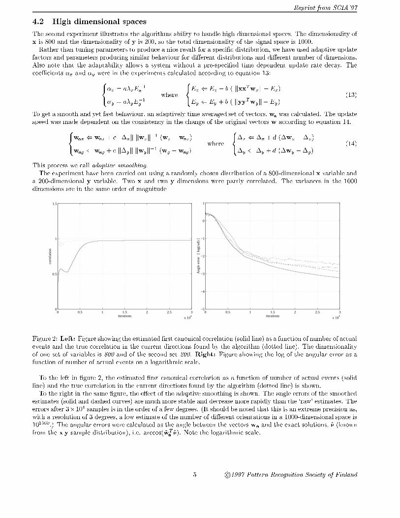
Figure 2: Left: Figure showing the estimated �rst canonical correlation (solid line) as a function of number of actualevents and the true correlation in the current directions found by the algorithm (dotted line). The dimensionalityof one set of variables is 800 and of the second set 200. Right: Figure showing the log of the angular error as afunction of number of actual events on a logarithmic scale.

To the left in �gure 2, the estimated �rst canonical correlation as a function of number of actual events (solidline) and the true correlation in the current directions found by the algorithm (dotted line) is shown.To the right in the same �gure, the e�ect of the adaptive smoothing is shown. The angle errors of the smoothed

estimates (solid and dashed curves) are much more stable and decrease more rapidly than the `raw' estimates. Theerrors after 3�104 samples is in the order of a few degrees. (It should be noted that this is an extreme precision as,with a resolution of 3 degrees, a low estimate of the number of di�erent orientations in a 1000-dimensional space is101500.) The angular errors were calculated as the angle between the vectors wa and the exact solutions, e (knownfrom the x y sample distribution), i.e. arccos(wT

a e). Note the logarithmic scale.



5 Applications in computer vision

At the Computer Vision Laboratory in Link�oping, we have developed a tensor representation of image features (seee.g. [8, 9]) that has received attention in the computer vision society. A possible extension of the tensor concepttowards more robust estimations, representation of certainty, representation of higher order features, etc. involveshigher order �lter combinations.As an example, consider a three-dimensional �ltering with a 7� 7� 7 neighborhood on three scales. This gives

approximately 1000 �lter responses. A complete second order function of this �ltering involves about 106 signals.The selection among all di�erent possible �lter combinations to design a tensor representation is very diÆcult

and a learning system is called for. A standard optimization method, based on mean square error is, however, notvery useful since it is the shape of the tensor that is of interest rather than size. If we, for example, want to have atensor representing the orientation of a signal, we want the tensor to carry as much information as possible aboutthe orientation and not the magnitude of the signal.For this reason, the canonical correlation algorithm is a suitable method, since it is based on mutual information

maximization rather than mean square error [1]. It can also handle high-dimensional signal spaces which is essentialin a further development of the tensor concept in image processing.Experiments show that the canonical correlation algorithm can be used to �nd �lters that describe a particular

feature in an image invariant with respect to other features. The features to be described are learned by givingexamples that are presented in pairs to the algorithm in such a way that the desired feature, e.g. orientation, isequal for each pair while other features, e.g. phase, are presented in an unordered way.

5.1 Learning low level operations

In the �rst experiment, we show that quadrature �lters are found by this method when products of pixel data arepresented to the algorithm. Quadrature �lters can be used to describe lower order features, e.g. local orientation.Let Ix and Iybe a pair of 5� 5 images. Each image consists of a sine wave pattern and additive Gaussian noise.

A sequence of such image pairs is constructed so that, for each pair, the orientation is equal in the two imageswhile the phase di�ers in a random way. The images have independent noise. Each image pair is described byvectors ix and iy.Let X and Y be the outer products of the image vectors, i.e. X = ixi

Tx and Y = iyi

Ty and rearrange the matrices

X and Y into vectors x and y respectively. Now, we have a sequence of pairs of 625-dimensional vectors describingthe products of pixel data from the images.The sequence consist of 6500 examples, i.e. 20 examples per degree of freedom. (The outer product matrices are

symmetric and, hence, the number of free parameters is n2+n2

where n is the dimensionality of the image vector.)For a signal to noise ratio (SNR) of 0 dB, there were 6 signi�cant1 canonical correlations and for an SNR of 10 dBthere were 10 signi�cant canonical correlations. The two most signi�cant correlations for the 0 dB case were both0.7 which corresponds to an SNR2 of 3.7 dB. For the 10 dB case, the two highest correlations were both 0.989,corresponding to an SNR of 19.5 dB.The projections of image signals x for orientations between 0 and � onto the 10 �rst canonical correlation vectors

wx from the 10 dB case are shown to the left in �gure 3. The signals were generated with random phase and withoutnoise. As seen in the �gure, the �rst two canonical correlations are sensitive to the double angle of the orientation ofthe signal and invariant with respect to phase. The two curves are 90Æ out of phase and, hence, form a quadraturepair [5]. The following curves show the lower correlations which are sensitive to the fourth, sixth, eighth, and tenthmultiples of the orientation and they also form quadrature pairs.To be able to interpret the canonical correlation vectors, wx, we can write the vectors as 25 � 25 matrices,

Wx, and then do an eigenvalue decomposition, i.e. Wx =P

�ieieTi . (Note that the data was generated as outer

products, resulting in positive semi de�nite symmetric matrices.) The eigenvectors, ei, can be seen as linear �ltersacting on the image. If the eigenvectors are rearranged into 5� 5 matrices, \eigenimages", they can be interpretedin terms of image features. To the right in �gure 3, the two most signiÆcant eigenimages are shown for the �rst(top) and second (bottom) canonical correlations respectively. We see that these eigenimages form two quadrature�lters sensitive to two perpendicular orientations.

1By signi�cant, we mean that they di�er from the random correlations caused by the limited set of samples. The random correlations,in the case of 20 samples per degree of freedom, is approximately 0.2 (given by experiments).

2The relation between correlation and SNR in this case is de�ned by the correlation between two signals with the same SNR, i.e.corr(s+ �1; s+ �2).



0 π w

x1,

wx2

Projections onto canonical correlation vectors wx1 to w

x8

0 π

wx3

, w

x4

0 π

wx5

, w

x6

0 πorientation

wx7

, w

x8

Eigenimage 1 for wx 1 Eigenimage 2 for w

x 1

Eigenimage 1 for wx 2 Eigenimage 2 for w

x 2

Figure 3: Left: Projections of outer product vectors x onto the 10 �rst canonical correlation vectors. Right:

Eigenvectors of the canonical correlation vectors viewed as images, \eigenimages".

5.2 Learning higher level operations

In this experiment, we use the output from neighboring sets of quadrature �lters rather than pixel values as inputto the algorithm. This can be justi�ed by the fact that we have seen that quadrature �lters can be developed onthe lowest (pixel) level using this algorithm. We will show that canonical correlation can �nd a way of combining�lter output from a local neighborhood to get orientation estimates that is less sensitive to noise than the standardvector averaging method [5].Let qx and qy be 16-dimensional complex vectors of �lter responses from four quadrature �lters from each

position in a 2 � 2 neighborhood. (The content in each position could be calculated using the method in theprevious experiment.) Let X and Y be the real parts3 of the outer products of qx and qy with themselvesrespectively and rearrange X and Y into 256-dimensional vectors x and y. For each pair of vectors, the localorientation was equal while the phase and noise di�ered randomly. The SNR was 0 dB. The two largest canonicalcorrelations were both 0.8. The corresponding vectors detected the double angle of the orientation invariant withrespect to phase.New data were generated using a rotating sine-wave pattern with an SNR of 0 dB and projected onto the two

�rst canonical correlation vectors. The orientation estimates are show to the left in �gure 4 together with estimatesusing vector averaging on the same data. In the right �gure, the angular error is shown for both methods. Themean absolute angular error was 16Æ for the canonical correlation method and 22Æ for the vector averaging method,i.e. an improvement by 27%. Note that the neigborhood is very small (2� 2), but preliminary tests indicate thatthe attainable improvement in noise reduction increase rapidly with neigborhood size.

References

[1] S. Becker and G. E. Hinton. Learning mixture models of spatial coherence. Neural Computation, 5(2):267{277,March 1993.

[2] R. D. Bock. Multivariate Statistical Methods in Behavioral Research. McGraw-Hill series in psychology.McGraw-Hill, 1975.

[3] M. Borga. Hierarchical Reinforcement Learning. In S. Gielen and B. Kappen, editors, ICANN'93, Amsterdam,September 1993. Springer-Verlag.

3It turns out that no correlations are found in the imaginary parts which, hence, can be omitted.



0

π

2πDouble orientation angle

0

π

2πEstimated double angle using canonical correlation

0 π 2π 3π 4π 5π 0

π

2πEstimated double angle using vector averaging

0 200 400 600 800 1000−180

0

180Angular error using canonical correlation (deg)

0 200 400 600 800 1000−180

0

180Angular error using vector averaging (deg)

Figure 4: Left: Orientation estimates for a rotating sine-wave pattern on a 2 � 2 neighborhood with an SNRof 0 dB, using �lter combinations found by canonical correlations (middle) and vector averaging (bottom). Thecorrect double angle is shown as reference (top). Right: Angular errors for 1000 di�erent samples using canonicalcorrelations (middle) and vector averaging (bottom).

[4] M. Borga. Reinforcement Learning Using Local Adaptive Models, August 1995. Thesis No. 507, ISBN 91{7871{590{3.

[5] G. H. Granlund and H. Knutsson. Signal Processing for Computer Vision. Kluwer Academic Publishers, 1995.ISBN 0-7923-9530-1.

[6] H. Hotelling. Relations between two sets of variates. Biometrika, 28:321{377, 1936.

[7] J. Kay. Feature discovery under contextual supervision using mutual information. In International Joint

Conference on Neural Networks, volume 4, pages 79{84. IEEE, 1992.

[8] H. Knutsson. Representing local structure using tensors. In The 6th Scandinavian Conference on Image

Analysis, pages 244{251, Oulu, Finland, June 1989. Report LiTH{ISY{I{1019, Computer Vision Laboratory,Link�oping University, Sweden, 1989.

[9] H. Knutsson. Tensor Based Spatio-temporal Signal Analysis. In J.L. Crowley H.I. Christensen, editor, Visionas Process. Springer, 1995. Basic Research Series.

[10] T. Kohonen. Self-organized formation of topologically correct feature maps. Biological Cybernetics, 43:59{69,1982.

[11] T. Landelius and H. Knutsson. The Learning Tree, A New Concept in Learning. In Proceedings of the 2:nd

Int. Conf. on Adaptive and Learning Systems. SPIE, April 1993.


Learning canonical correlations

Documents

Transcript of Learning canonical correlations