Theoretical study of quantum correlations and nonlinear ...
295
HAL Id: tel-02974737 https://tel.archives-ouvertes.fr/tel-02974737 Submitted on 22 Oct 2020 HAL is a multi-disciplinary open access archive for the deposit and dissemination of sci- entific research documents, whether they are pub- lished or not. The documents may come from teaching and research institutions in France or abroad, or from public or private research centers. L’archive ouverte pluridisciplinaire HAL, est destinée au dépôt et à la diffusion de documents scientifiques de niveau recherche, publiés ou non, émanant des établissements d’enseignement et de recherche français ou étrangers, des laboratoires publics ou privés. Theoretical study of quantum correlations and nonlinear fluctuations in quantum gases Mathieu Isoard To cite this version: Mathieu Isoard. Theoretical study of quantum correlations and nonlinear fluctuations in quantum gases. Pattern Formation and Solitons [nlin.PS]. Université Paris-Saclay, 2020. English. NNT : 2020UPASP004. tel-02974737
-
Upload
khangminh22 -
Category
Documents
-
view
1 -
download
0
Transcript of Theoretical study of quantum correlations and nonlinear ...

HAL Id: tel-02974737https://tel.archives-ouvertes.fr/tel-02974737
Submitted on 22 Oct 2020
HAL is a multi-disciplinary open accessarchive for the deposit and dissemination of sci-entific research documents, whether they are pub-lished or not. The documents may come fromteaching and research institutions in France orabroad, or from public or private research centers.
L’archive ouverte pluridisciplinaire HAL, estdestinée au dépôt et à la diffusion de documentsscientifiques de niveau recherche, publiés ou non,émanant des établissements d’enseignement et derecherche français ou étrangers, des laboratoirespublics ou privés.
Theoretical study of quantum correlations and nonlinearfluctuations in quantum gases
Mathieu Isoard
To cite this version:Mathieu Isoard. Theoretical study of quantum correlations and nonlinear fluctuations in quantumgases. Pattern Formation and Solitons [nlin.PS]. Université Paris-Saclay, 2020. English. NNT :2020UPASP004. tel-02974737

Thès
e de
doc
tora
tN
NT:
2020U
PASP004
Theoretical Study of QuantumCorrelations and Nonlinear
Fluctuations in Quantum Gases
Thèse de doctorat de l’Université Paris-Saclay
École doctorale n 564, Physique en Île-de-France (PIF)Spécialité de doctorat: Physique
Unité de recherche: Université Paris-Saclay, CNRS, LPTMS, 91405,Orsay, France
Référent: : Faculté des sciences d’Orsay
Thèse présentée et soutenue à Orsay, le 10 septembre 2020, par
Mathieu ISOARD
Composition du jury:
Christoph WESTBROOK PrésidentDirecteur de recherche,Institut d’Optique Graduate SchoolLaboratoire Charles FabryMatteo CONFORTI Rapporteur & ExaminateurChargé de recherche (HDR),Université de LilleLaboratoire PhLAMPatrik ÖHBERG Rapporteur & ExaminateurProfesseur,Heriot-Watt UniversityInstitute of Photonics and Quantum SciencesÉlisabeth GIACOBINO ExaminatriceDirectrice de recherche émérite,Université Pierre et Marie CurieLaboratoire Kastler BrosselSandro STRINGARI ExaminateurProfesseur,Università di TrentoINO-CNR BEC Center
Nicolas PAVLOFF DirecteurProfesseur,Université Paris-SaclayLPTMS


As you see, the war treated me kindly enough,in spite of the heavy gunfire,
to allow me to get away from it alland take this walk in the land of your ideas.
— Schwarzschild to Einstein, 22 December 1915


REMERCIEMENTS
Je voudrais tout d’abord remercier mon directeur de thèse, NicolasPavloff, sans qui ce travail n’aurait pas vu le jour. Travailler à ses côtéspendant ces trois dernières années a été un réel plaisir ; sa curiosité sci-entifique m’a permis de découvrir de nouveaux champs de la physiqueet d’acquérir de nouvelles connaissances, sa rigueur et sa ténacité m’ontappris à explorer toutes les pistes possibles d’un sujet pour en saisirtous les contours. Enfin, je retiendrai sa bonne humeur, sa gentillesseet son humour qui en font pour moi le meilleur directeur que j’auraispu espérer.Je remercie tous les membres de mon jury pour avoir pris le temps
de lire ma thèse ; un grand merci à Matteo Conforti et Patrik Öhbergpour avoir été les rapporteurs de ma thèse.Je remercie aussi Nicolas Cherroret d’avoir accepté d’être mon tuteur
pendant mes trois années de doctorat.Je souhaiterais ensuite remercier l’ensemble du LPTMS qui a con-
tribué à rendre ces trois années de doctorat très agréables. Je remercieen particulier Claudine et Karolina pour leur aide et leur réactivité. Jeremercie les permanents et post-docs pour les discussions matinales au-tour du café ; parmi eux, je remercie Christophe, pour l’aide qu’il m’aapportée pendant la préparation de la soutenance, et Guillaume, pouravoir été mon mentor.Il m’est impossible de ne pas mentionner également notre bureau lé-
gendaire que j’ai eu la chance de partager avec mes amis Ivan, Samuel etThibault ; le très fameux tableau d’Ivan rempli d’expressions françaises,Samuel et ses idées lumineuses sur les nombres hyperduaux, Thibaultet ses feuilles volantes, les repas improvisés, les parties de fléchettes etles visites nombreuses de notre cher Aurélien resteront gravés dans mamémoire. Je remercie aussi tous les doctorants que j’ai connus au coursde mes trois années de doctorat et avec lesquels je garderai une affectionparticulière et d’excellents souvenirs ; un merci tout particulier à Ninaet Nadia que j’ai eu la chance de connaître.Je remercie Scott Robertson pour les discussions stimulantes que nous
avons eues sur le rayonnement de Hawking analogue. Je remercie égale-ment mon ami Maxime pour nos nombreuses discussions autour de lagravité analogue, pour m’avoir proposé de préparer un workshop aveclui et donc pour la confiance qu’il m’accorde, enfin pour son soutien.Je voudrais remercier tous mes amis pour leur présence et les nom-
breuses soirées parisiennes que nous avons partagées ensemble; merciThiébaut pour ton aide précieuse à la veille de la soutenance.
Je ne peux terminer ces remerciements sans évoquer ma famille. Ungrand merci à mes proches, à mes parents, à mes grands-parents età ma petite soeur pour m’avoir soutenu dans mes projets depuis tantd’années et qui m’ont permis d’arriver là où j’en suis.
v


CONTENTS
0 introduction générale 11 general introduction 9i acoustic black holes in bose-einstein con-
densates 172 from hawking radiation to analogue gravity 19
2.1 Hawking radiation . . . . . . . . . . . . . . . . . . . . . 212.1.1 Accelerating mirror . . . . . . . . . . . . . . . . . 212.1.2 Penrose diagrams . . . . . . . . . . . . . . . . . . 282.1.3 Gravitational collapse . . . . . . . . . . . . . . . 31
2.2 Analogue gravity . . . . . . . . . . . . . . . . . . . . . . 412.2.1 Sound waves in curved spacetime . . . . . . . . . 412.2.2 Analogue Hawking radiation . . . . . . . . . . . . 46
3 hawking radiation in bose-einstein condensates 493.1 Realization of an acoustic horizon in a Bose-Einstein con-
densate . . . . . . . . . . . . . . . . . . . . . . . . . . . 503.1.1 The Gross-Pitaevskii equation . . . . . . . . . . . 503.1.2 One-dimensional flow of Bose-Einstein condensates 513.1.3 Theoretical configurations . . . . . . . . . . . . . 553.1.4 Experimental realization of an acoustic horizon . 57
3.2 Density correlations in Bose-Einstein condensates . . . . 583.2.1 Bogoliubov approach . . . . . . . . . . . . . . . . 583.2.2 Zero modes . . . . . . . . . . . . . . . . . . . . . 663.2.3 Quantization . . . . . . . . . . . . . . . . . . . . 693.2.4 Density correlations . . . . . . . . . . . . . . . . 713.2.5 Comparison to experiment . . . . . . . . . . . . . 75
3.3 Departing from thermality of analogue Hawking radiation 793.3.1 Hawking temperature . . . . . . . . . . . . . . . 793.3.2 Fourier transform of g(2) . . . . . . . . . . . . . . 813.3.3 Thermality? . . . . . . . . . . . . . . . . . . . . . 84
3.4 M. Isoard, N. Pavloff, Physical Review Letters (2020) . . 894 tripartite entanglement in analogue gravity 101
4.1 Bogoliubov transformations . . . . . . . . . . . . . . . . 1024.1.1 General case . . . . . . . . . . . . . . . . . . . . 1024.1.2 Two-mode squeezed state . . . . . . . . . . . . . 1064.1.3 Bogoliubov transformations in BECs . . . . . . . 109
4.2 Measuring entanglement . . . . . . . . . . . . . . . . . . 1144.2.1 Gaussian states and covariance matrices . . . . . 1144.2.2 Cauchy-Schwarz inequality . . . . . . . . . . . . 1194.2.3 PTT criterion . . . . . . . . . . . . . . . . . . . . 1214.2.4 Degree of entanglement . . . . . . . . . . . . . . 123
4.3 Tripartite entanglement in BECs . . . . . . . . . . . . . 1254.3.1 Tripartite system and parametric down-conversion 1254.3.2 CKW inequality . . . . . . . . . . . . . . . . . . 129
vii

viii contents
4.3.3 Computation of the residual tangle . . . . . . . . 130ii propagation of dispersive shock waves in non-
linear media 1375 fluids of light 139
5.1 Nonlinear Schrödinger equation and hydrodynamic ap-proach . . . . . . . . . . . . . . . . . . . . . . . . . . . . 140
5.2 Characteristics and Riemann invariants . . . . . . . . . 1445.2.1 Hopf equation . . . . . . . . . . . . . . . . . . . . 1445.2.2 Polytropic gas flow . . . . . . . . . . . . . . . . . 146
6 dispersionless evolution of nonlinear pulses 1496.1 Hodograph transformation and Riemann’s method . . . 150
6.1.1 Hodograph transformation . . . . . . . . . . . . . 1516.1.2 Riemann’s method . . . . . . . . . . . . . . . . . 152
6.2 Application of Riemann’s approach . . . . . . . . . . . . 1596.2.1 Polytopic gases and nonlinear optics . . . . . . . 1596.2.2 Example on a non-integrable system . . . . . . . 1636.2.3 Nonlinear optics with specific initial conditions . 166
6.3 M. Isoard, A.M. Kamchatnov, N. Pavloff, RNL (2019) . 1746.4 M. Isoard, A.M. Kamchatnov, N. Pavloff, EPL (2020) . 181
7 formation and propagation of dispersive shockwaves 1897.1 Whitham modulational theory . . . . . . . . . . . . . . . 190
7.1.1 General idea . . . . . . . . . . . . . . . . . . . . 1907.1.2 Whitham equations for NLS equation . . . . . . 194
7.2 Solutions of Whitham equations . . . . . . . . . . . . . . 1987.2.1 Generalized hodograph transform . . . . . . . . . 1997.2.2 Solutions in the shock region . . . . . . . . . . . 2007.2.3 Edges of the shock . . . . . . . . . . . . . . . . . 2047.2.4 Procedure of resolution and results . . . . . . . . 206
7.3 Experimental considerations . . . . . . . . . . . . . . . . 2097.4 M. Isoard, A.M. Kamchatnov, N. Pavloff, Physical Re-
view E (2019) . . . . . . . . . . . . . . . . . . . . . . . . 2167.5 M. Isoard, A.M. Kamchatnov, N. Pavloff, Physical Re-
view A (2019) . . . . . . . . . . . . . . . . . . . . . . . . 2298 conclusion 249iii appendix 253a comparison between different theoretical pa-
rameters for a waterfall configuration 255b zero modes in bose-einstein condensates 257
b.1 Flat profile . . . . . . . . . . . . . . . . . . . . . . . . . 257b.2 Waterfall configuration . . . . . . . . . . . . . . . . . . . 260
c fourier transform of the density correla-tion function 261
d hodograph transform 263e solutions of the euler-poisson equation 265
bibliography 269

0INTRODUCTION GÉNÉRALE
Cette thèse est dédiée à l’étude des phénomènes nonlinéaires dans deuxfluides quantiques qui partagent de nombreuses similitudes : les con-densats de Bose-Einstein [153] et les faisceaux optiques Gaussiens non-linéaires (qui sont aussi considérés comme des “fluides de lumière” [35]).Dans les condensats de Bose-Einstein, les effets nonlinéaires se mani-
festent par les interactions de contact entre bosons et affectent de façonimportante les propriétés du gaz. En 1947, Bogoliubov a été le pre-mier à proposer une nouvelle théorie des perturbations pour prendre encompte les interactions dans un condensat de Bose-Einstein faiblementinteragissant [28] ; cette théorie a été d’une grande importance dansles développements qui ont suivi pour comprendre notamment les liensqui existent entre superfluidité et condensation [78, 144, 145, 152]. Lathéorie de champ moyen developpée par Bogoliubov prédit égalementque des excitations élémentaires sont induites par les fluctuations quan-tiques dans le condensat. Cette propriéte est très importante dans ledomaine de la gravité analogue parce qu’elle permet de créer un fluidetranssonique à l’aide d’un condensat de Bose-Einstein. Dans ce cas, untel fluide pourra être considéré comme l’analogue acoustique d’une trounoir [71].Le domaine de la gravité analogue est né environ sept ans après que
Hawking a prédit que les trous noirs émettent un faible rayonnement[87]. Unruh suggère alors d’utiliser des analogues hydrodynamiques destrous noirs gravitationnels pour étudier leurs propriétés dans le labora-toire[182]. Un fluide transsonique, c’est-à-dire un fluide qui passe d’unerégion subsonique, où les ondes sonores peuvent se propager dans toutesles directions, à une région supersonique, où les ondes sont piégées etentraînées par le fluide en mouvement, joue le même rôle qu’un trounoir. En effet, de même que la lumière reste piégée à l’intérieur d’untrou noir gravitationnel, les ondes sonores, elles, ne peuvent s’échapperde la région supersonique.Pour expliquer simplement ce phénomène, considérons une rivière
au bout de laquelle se trouve une cascade, voir Figure 1. La vitesse ducours d’eau augmente à l’approche de la cascade. Imaginons maintenantque des poissons remontent le courant, tous à la même vitesse. Il estassez intuitif de penser qu’il existe un point de non-retour (“Point ofno return” sur la Figure 1) au-delà duquel les poissons ne sont pluscapables de remonter le courant tant la vitesse de la rivière devientgrande. Dans ce cas, les poissons sont piégés et irrémédiablement en-trainés jusqu’en bas de la cascade qui joue alors le rôle de la singularitéd’un trou noir, comme indiqué sur la Figure 1 ; le point de non-retourest alors l’équivalent d’un horizon des événements pour les poissons.Dans son article de 1981, Unruh n’a pas considéré des poissons dans
une rivière, mais des ondes sonores se propageant dans un fluide en mou-
1

2 introduction générale
Figure 1: Des poissons remontent le cours d’eau d’une rivière. Dessin réal-isé par Nascimbene pour montrer l’analogie entre les trous noirshydrodynamiques et leur équivalent gravitationnel. La rivière sedéplace de la droite vers la gauche et accélère à l’approche d’unecascade. Tous les poissons ont la même vitesse et tente de remon-ter le cours d’eau. Au-delà du panneau marron, dans la partiegauche de la rivière, la vitesse du cours d’eau est si importante queles poissons sont tous entraînés par la rivière vers la cascade. Defaçon équivalente à la lumière qui est piégée à l’intérieur d’un trounoir et se propage jusqu’à sa singularité, les poissons au-delà dupoint de non-retour (indiqué par le panneau marron) sont piégéset tombent jusqu’en bas de la cascade. Cette région joue donc lerôle de l’intérieur du trou noir analogue.
vement. L’idée reste toutefois identique : Si le courant, bien que station-naire, devient supersonique dans une région de l’espace, une onde sonorequi se déplace dans cette région serait alors entrainée par le courant etne pourrait plus atteindre la région subsonique située en amont. L’ondesonore serait dans ce cas piégée dans la partie supersonique, comme lepoisson l’était au-delà du point de non-retour et comme la lumière l’està l’intérieur d’un trou noir gravitationnel. La frontière entre les régionssubsonique et supersonique est alors appelée un horizon acoustique. Detels systèmes transsoniques ont été appelés “trous muets” par Unruh.Toutefois, le lien qui existe entre les trous noirs gravitationnels et les
“trous muets” s’étend au-delà de cette simple analogie cinématique. Eneffet, en linéarisant les équations hydrodynamiques, Unruh a montréque la dynamique des ondes sonores dans le fluide en mouvement estla même que celle d’un champ scalaire dans un espace-temps courbe.Nous reproduirons les calculs qui l’ont mené à cette conclusion dans lepremier chapitre de thèse.
De plus, dans le cas où le champ sonore serait quantifié, il devraithériter des propriétés des champs quantiques qui se propagent dansun espace-temps courbe. En particulier, comme Unruh l’a montré dansson article et comme nous l’expliquerons dans le chapitre 2, l’horizonacoustique “déconnecte” complétement la partie subsonique de la partiesupersonique, et cela doit nécessairement s’accompagner de l’émissionspontanée de particules depuis cet horizon ; ce rayonnement doit no-

introduction générale 3
tamment jouir des mêmes propriétés thermiques que le rayonnement deHawking émis par les trous noirs gravitationnels.L’idée proposée par Unruh a suscité l’intérêt d’une large commu-
nauté ; la gravité analogue connaît en particulier un intérêt importantdepuis les deux dernières décennies, avec de nombreuses expériencesd’analogues acoustiques réalisées dans des écoulements à la surface d’unbassin [59, 159, 192], dans les fibres optiques nonlinéaires [23, 50, 149,184], dans les condensats d’excitons-polaritons [132] et dans les con-densats de Bose-Einstein [102, 105, 131, 163, 170, 175, 177]. Parmi cesdifférentes plateformes, nous nous sommes concentrés au cours de lathèse sur les trous noirs acoustiques réalisés dans les condensats deBose-Einstein transsonique et (quasi) unidimensionnel. Un tel conden-sat en mouvement a été réalisé expérimentalement par J. Steinhauer ily a dix ans [105] ; récemment, l’analogue du rayonnement de Hawkingy a été observé [131, 177].
Dans le chapitre 2, nous revenons tout d’abord sur la découvertede Hawking. Nous soulignons l’universalité du rayonnement de Hawk-ing en considérant tout d’abord le cas d’un miroir en accélération nonuniforme [48, 69]. Ensuite, nous traitons le cas de l’effondrement gravi-tationnel d’une étoile menant à la formation d’un trou noir. La courburede l’espace-temps est si affectée pendant cet effondrement que deux ré-gions déconnectées apparaissent : l’intérieur et l’extérieur du trou noir.Nous montrons que ce processus est très similaire au problème du miroiren mouvement et donne également lieu à l’émission d’un rayonnementthermique [25, 87, 88].Le chapitre 3 est dédié à l’étude du rayonnement de Hawking analogue
dans les condensats de Bose-Einstein. Dans ces systèmes quantiques, lesexcitations sonores entrantes émergent des fluctuations quantiques duvide et donnent naissance aux excitations sortantes après un proces-sus de diffusion à l’horizon acoustique. Ces ondes sonores sortantes sepropagent le long du fluide dans les régions subsonique et superson-ique, situées de part et d’autre de l’horizon acoustique, et induisentdes corrélations de densité. Ainsi, comme suggéré pour la première foisen 2008 par des collaborateurs travaillant à Trente et Bologne [15], ladétection expérimentale de ces corrélations constituerait une signatureindirecte de la présence du rayonnement de Hawking analogue dans lescondensats de Bose-Einstein.Le chapitre 3 présente le travail réalisé pendant la thèse, à savoir
l’étude détaillée des fluctuations quantiques près de l’horizon acoustiqued’une condensat de Bose-Einstein transsonique.Nous démontrons que la prise en compte des modes zéros, relatifs à
la phase du condensat et aux fluctuations du nombre de particules dansce dernier, est nécessaire dans un premier temps pour obtenir une de-scription correcte des corrélations au voisinage de l’horizon acoustique.Cela mène dans un second temps à un excellent accord entre nos résul-tats théoriques et les données expérimentales obtenues par le groupe deJ. Steinhauer en 2019 [131]. Cependant, en raison des effets dispersifsdans notre système, nous prouvons également que le rayonnement de

4 introduction générale
Hawking analogue émis depuis l’horizon acoustique dévie d’un spectretotalement Planckien, comme attendu gravitationnel [87, 88]. Ce car-actère “non-thermique” est inhérent à tout système dispersif. Toutefois,nous montrons dans cette thèse qu’une procédure d’analyse des corréla-tions de densité peut “supprimer” les effets dispersifs et conduire à laconclusion erronée que le spectre de Hawking analogue est compléte-ment thermique. Nous discutons en particulier l’analyse de donnéespubliée par le groupe de J. Steinhauer [131] dans la dernière section duchapitre 3. Ce travail a donné lieu à une publication dans Physical Re-view Letters, cf. fin du chapitre 3. Certains des résultats discutés dansce chapitre mèneront également à la publication d’un plus long articledans le futur.
Dans le chapitre 4, nous étudions l’intrication entre les excitationsqui émergent des fluctuations quantiques de part et d’autre de l’horizonacoustique. En particulier, nous soulignons le lien fondamental qui ex-iste avec le chapitre 2, c’est-à-dire l’existence de deux vides différents,menant alors à l’émission spontanée de particules. Nous montrons queces deux vides sont liés par une transformation de Bogoliubov. De cettemanière, ce que nous définissons comme le vide entrant peut être vudans notre système analogue comme un état Gaussien à trois modes,de sorte que l’intrication est répartie entre ces trois modes.Pour étudier cette intrication tripartite, nous introduisons tout d’abord
la notion de matrice covariante et nous détaillons les différents outilsqui permettent d’étudier la séparabilité d’un état quantique, tels quela violation de l’inégalité de Cauchy-Schwarz ou le critère PPT (Posi-tive Partial Transpose). Ensuite, nous les appliquons au cas particulierde notre système, en suivant la procédure présentée dans la référence[4] pour les états Gaussiens et basée sur l’étude de l’inégalité CKW(Coffman, Kundu, Wootters) [40]. Cela nous permet de calculer le de-gré d’intrication tripartite qui ne dépend que de quantités accessiblesexpérimentalement [131, 176, 177] ; nous pensons donc qu’il serait pos-sible dans le futur d’observer et de mesurer cette intrication tripartitedans les condensats de Bose-Einstein.
En sus de l’étude du rayonnement de Hawking analogue, nous noussommes également intéressés aux liens qui existent entre la condensa-tion de Bose-Einstein et l’optique nonlinéaire. En effet, la lumière qui sepropage dans un milieu nonlinéaire se comporte comme un fluide dont ladynamique est gouvernée par une équation de Gross-Pitaevskii effective[108]. En particulier, les effets nonlinéaires, induits par la lumière dansle milieu dans lequel elle se propage, conduisent à une interaction effec-tive entre photons. Cette analogie avec les condensats de Bose-Einsteina suscité beaucoup d’intérêt dans la communauté scientifique pour ob-server et sonder des phénomènes hydrodynamiques dans le contextede l’optique nonlinéaire, telles que la superfluidité ou les excitationssonores de la lumière [34, 39, 66, 111, 128, 162, 187, 188].Dans la seconde partie de la thèse, nous nous intéressons à un phénomène
qui peut s’observer dans les systèmes non-dissipatifs, nonlinéaires etdispersifs : la formation d’ondes de choc dispersives [100]. La figure 2

introduction générale 5
souligne de nouveau le lien fort qui existe entre les systèmes optiqueset les condensats de Bose-Einstein ; l’image de gauche, extraite de laréférence [22], montre la propagation d’une onde de choc dispersive ra-diale dans un milieu optique nonlinéaire, tandis que l’image de droite,extraite de la référence [91], correspond à la propagation d’une telleonde dans un condensat de Bose-Einstein.
Figure 2: Propagation d’une onde de choc radiale(Gauche) à travers un crystal photoréfractif [22], ©2007, Nature.(Droite) à travers un condensat de Bose-Einstein [91], ©2006,APS.
Les ondes de choc dispersives proviennent des effets nonlinéaires quirendent de plus en plus abrupt le profil d’une perturbation qui sepropage plus vite que son propre front ; elle le rattrape donc inévitable-ment au bout d’un certain temps, appelé temps de déferlement ; Il enrésulte alors un choc qui se traduit par la formation d’un train d’ondes,appelé onde de choc dispersive. L’émergence de telles ondes n’est pasrestreinte aux condensats de Bose-Einstein ou à l’optique nonlinéaire,mais se produit aussi dans de nombreux autres systèmes : la figure 3amontre un mascaret ondulant observé en eaux peu profondes et la figure3b montre une série de nuages enroulés sur eux-mêmes. Dans ce dernierexemple, une telle onde de choc se forme dans l’atmosphère quand deuxmasses d’air de températures différentes se rencontrent ; ce phénomèneest connu sous le nom de Morning Glory. Ces différents exemples révè-lent l’universalité de ce phénomène piloté par la compétition entre effetsnonlinéaires et dispersifs.Dans le chapitre 5, nous montrons tout d’abord que la propagation
d’un faisceau optique (dans l’approximation paraxiale) dans un milieunonlinéaire est gouvernée par une équation de Schrödinger nonlinéaire.Une approche hydrodynamique du problème, proposée en premier parle groupe de Khlokhlov en 1967 [8–11], revient à considérer que le fais-ceau optique se comporte comme un fluide de lumière, caractérisé parune densité et une vitesse. De plus, grâce à cette approche hydrody-namique, la propagation d’un tel fluide peut être étudiée à travers lesinvariants de Riemann et la méthode des caractéristiques. Ces notionssont introduites dans ce chapitre.Dans le chapitre 6, nous étudions avec l’aide de la méthode de Rie-
mann la première étape de l’évolution d’un fluide de lumière en présence

6 introduction générale
(a) Mascaret ondulant observé à TurnagainArm, Alaska (copyright Scott Dickerson, 2013)
(b) Onde de choc dispersive observée dansl’atmosphère – appelée Morning Glory (copyrightMick Petroff, Creative Commons 3.0, 2009)
Figure 3: Exemples d’ondes de choc dispersives observées dans la nature.
d’un fond uniforme, c’est-à-dire avant l’apparition de l’onde de chocdispersive. Cette étape peut être décrite à travers une approche nondispersive qui conduit alors à un excellent accord avec les simulationsnumériques du problème. Nous appliquons en particulier la méthode deRiemann pour des distributions initiales non monotones. Dans ce cas,comme suggéré par Ludford [120], nous avons besoin de déplier le planhodographique. Nous expliquons en détail cette procédure et comparonsnos résultats théoriques avec des simulations numériques. Ce travail aconduit à deux publications : un article de conférence dans lequel nousconsidérons un faisceau optique Gaussien, cf. fin du chapitre 6 ; et lapremière partie d’un article publié dans Physical Review A, cf. fin duchapitre 7.En outre, nous avons remarqué qu’il était possible d’obtenir une so-
lution approximative et simple du problème de Riemann qui est en trèsbon accord avec les simulations. Nous avons généralisé cette approxi-mation au cas des fluides non visqueux, et, en particulier, aux systèmesnon-intégrables. Ce travail a été publié dans EPL (Europhysics Letters),cf. fin du chapitre 6Dans le chapitre 7, nous étudions la seconde étape de l’évolution des
fluides nonlinéaires lorsque les effets dispersifs entrent en jeu. Commementioné plus haut, les effets nonlinéaires couplés aux effets dispersifsconduisent à la formation et la propagation d’une onde de choc dis-persive. Dans ce chapitre, nous décrivons la structure et la dynamiqued’une telle onde dans le cas où le profil de densité initial a la forme d’uneparabole inversée ; une description théorique peut en effet être obtenuepour un tel choix de distribution initiale. Nous montrons que deux in-variants de Riemann varient de façon concomitante dans la région duchoc et que le problème se réduit à la résolution d’une équation d’Euler-Poisson. Nous utilisons les résultats obtenus par Eisenhart [53] et laméthode proposée dans les références [56, 82] pour résoudre analytique-ment cette équation ; nous montrons alors que les résultats théoriquessont en très bon accord avec les simulations numériques.

introduction générale 7
Cette approche est intéressante parce qu’elle permet aussi d’obtenirune description asymptotique de l’onde de choc dispersive. Nous sommesen particulier capables d’extraire des paramètres d’intérêt expérimental,comme le contraste des franges de l’onde de choc.Au cours de la thèse, nous avons tout d’abord commencé par l’étude
de la propagation d’une onde de choc dans le cas de l’équation deKorteweg-De Vries. Ce fut une première étape dans la compréhensionde la méthode décrite dans les références [56, 82]. De plus, l’étape nondispersive de l’étalement peut être facilement étudiée grâce à la méth-ode des caractéristiques. Ce travail a été publié dans Physical ReviewE, cf. fin du chapitre 7.
Ensuite, nous nous sommes intéressés à l’équation de Schrödingernonlinéaire. Dans ce cas, l’étude de l’étalement sans dispersion du flu-ide nonlinéaire est plus complexe et requiert l’utilisation de la méthodede Riemann (voir chapitre 6). Néanmoins, l’analyse de l’onde de chocdispersive est assez similaire à celle utilisée dans le cas de l’équationde Korteweg-De Vries (mais nécessite tout de même un traitementthéorique un peu plus technique) ; ceci montre l’efficacité de la méth-ode suggérée dans les références [56, 82]. Ce travail a été publié dansPhysical Review A et se trouve à la fin du chapitre 7.
Nous reviendrons enfin dans la conclusion sur les similarités entre lescondensats de Bose-Einstein et les fluides de lumière ; nous discuteronsen particulier les perspectives que nous envisageons pour étendre lestravaux présentés dans cette thèse.


1GENERAL INTRODUCTION
This thesis is dedicated to the study of nonlinear-driven phenomenain two quantum gases which bear important similarities: Bose-Einsteincondensates of ultracold atomic vapors [153] and paraxial nonlinearlaser beams (which are sometimes considered as pertaining to the widerclass of “quantum fluid of light” [35])In Bose-Einstein condensates nonlinearity arises from contact inter-
actions between bosons and dramatically affect the properties of thegas. In 1947, Bogoliubov was the first to suggest a new perturbationtheory to take account of interactions in a weakly-interacting Bose gas[28]. Bogoliubov theory is a first-principle mean-field theory of super-fluidity which has been of tremendous importance in the developmentof the field of Bose-Einstein condensates of atomic vapors [78, 144, 145,152]. It predicts the emergence of sound-like excitations from quantumfluctuations in the condensate. This aspect is of particular relevance inthe domain of analogue gravity where a transonic flow is analyzed asan acoustic analogue of a black hole [71].The domain of analogue gravity started around seven years after
Hawking’s prediction in 1974 that black holes emit a faint radiation[87], when Unruh suggested the use of hydrodynamic analogues of grav-itational black holes to study their properties in the laboratory [182]. Atransonic flow, from a subsonic region, where sound waves can propa-gate in all directions, to a supersonic region, where waves are trappedand dragged by the flow, could play the same role as a black hole, notby trapping light but sound excitations.As a simple illustration of the phenomenon, let us consider a river
flowing towards a waterfall. The flow velocity increases when the riverapproaches the waterfall. One also consider fish swinging against thecurrent, with all the same velocity (see Figure 4). One understands thatthere must exist a point of no return beyond which the flow velocitybecomes too important, so that fish are dragged by the flow and boundto fall down to the bottom of the waterfall, playing the role of a blackhole singularity. Then, the point of no return, indicated by the brownpanel in Figure 4, would be the equivalent of the event fish-horizon.In his seminal paper, Unruh did not consider fish in a river, but sound
waves propagating in a fluid flow. The idea is still the same though; ifthe flow, albeit stationary, happens to be supersonic in some region ofspace, a sound wave propagating in this region would be dragged bythe flow and would not be able to reach the subsonic region upstreamthe supersonic one; the boundary between the subsonic and supersonicregions is then the acoustic horizon. One has constructed what Unruhcalled a “dumb hole”.However, this parallel to gravitational black holes extends further
than this simple kinematic analogy; by deriving and linearizing the hy-
9

10 general introduction
Figure 4: Drawing of a river with fish to understand the analogy betweenanalogue black holes and their gravitational counterparts. Theriver flows from the right to the left and accelerates when ap-proaching to the waterfall. All fish have the same velocity andtry to move to the right. Beyond the brown panel, in the left partof the flow, the river velocity is so high that fish are not able to goupstream. Similarly to light which is trapped inside a black holeand propagates down to the black hole singularity, fish are trappedin this part of the flow and are bound to fall down to the waterfall.This region thus plays the role of the interior of the analogue blackhole.
drodynamics equations, Unruh showed that the motion of sound wavesin the fluid flow is equivalent to the one of a scalar field in a curvedspacetime. We will reproduce his calculations in the first chapter of thisthesis.Then, if one quantizes the sound field, one should inherit the prop-
erties of quantum fields propagating in curved spacetime. In particular,as we shall explain in more detail in Chapter 2, the acoustic horizoncompletely disconnects the subsonic part from the supersonic one. Un-ruh showed in his paper that this must lead to spontaneous creation ofparticles from the acoustic horizon, thus to the emission of a radiation,having in principle the same thermal property as the one emitted byblack holes.Unruh’s idea has triggered the interest of a large community; the
analogue gravity field has particularly known a burst of interest in thelast decade, with numerous experimental realizations of acoustic ana-logues in open-channel flows [59, 159, 192], in nonlinear optical fibers[23, 50, 149, 184], in exciton-polariton condensates [132] and in Bose-Einstein condensates [102, 105, 131, 163, 170, 175, 177]. Among them,we will focus on sonic black holes realized in (quasi) one-dimensionaltransonic Bose-Einstein condensates. Such a flow has been experimen-tally achieved by J. Steinhauer ten years ago [105] and, recently, heobserved the analogous Hawking radiation [131, 177].
In Chapter 2 we will come back to Hawking’s breakthrough. We willstress the universality of Hawking radiation by first considering the caseof a non-uniform accelerating mirror; this acceleration will indeed cause

general introduction 11
particle creation from vacuum [48, 69]. Then, we will treat the case ofa gravitational collapse leading to the formation of a black hole. Thespacetime curvature is so much affected during the collapse that twodisconnected regions appear: the interior and the exterior of the blackhole. We will show that this time-dependent process is very similar tothe moving mirror problem and gives rise to the emission of a thermalradiation [25, 87, 88].Chapter 3 is devoted to the study of analogue Hawking radiation in
Bose-Einstein condensates. In these quantum systems, ingoing sound-like excitations will emerge from quantum vacuum fluctuations andscatter into outgoing excitations at the acoustic horizon. These out-going sound waves will then propagate along the flow in both subsonicand supersonic regions and will induce density correlations. Therefore,as first suggested by a collaboration between teams from Trento andBologna [15], the experimental detection of these correlations providesan indirect signature of the analogous Hawking radiation.Chapter 3 presents the part of the original work of this thesis ded-
icated to the detailed analysis of quantum fluctuations close to theacoustic horizon realized in the transonic flow of a BEC.We will first demonstrate that the taking into account of zero modes,
pertaining to the phase of the condensate and the number of particles inthe latter, is necessary to obtain a correct description of the correlationsat the vicinity of the acoustic horizon; this will provide a safely groundedtheory.Then, we will show that, by means of the addition of the zero modes,
our theoretical results compare well with the experimental data ob-tained by the Steinhauer’s group in 2019 [131]. However, we will alsoprove that dispersive effects in our system does not lead to a fully ther-mal analogue Hawking radiation, as predicted by Hawking in the grav-itational case [87, 88], but, on the contrary, presents some departurefrom thermality. This non-thermal feature is inherent to any dispersivesystem. Nevertheless, we show that a self-consistent procedure of dataanalysis “kill” dispersive effects and might lead to the erroneous conclu-sion that the analogue Hawking spectrum is completely thermal, wherein reality it is not. This is the reason why we question the experimentaldata analysis published by J. Steinhauer’s group [131] in the last sectionof Chapter 3. This work resulted in a publication in Physical ReviewLetters, see the article attached at the end of Chapter 3. Some of theresults discussed in this chapter will also lead to a longer article in thefuture.In Chapter 4 we study the entanglement between density waves emerg-
ing from quantum fluctuations on both sides of the acoustic horizon. Inparticular, we stress the fundamental connection with Chapter 2, i.e.,the existence of two different vacua, leading to spontaneous emissionof particles. We show that both vacua are linked through a Bogoli-ubov transformation and that the ingoing vacuum can be seen as athree mode Gaussian state, so that entanglement is shared among threemodes.

12 general introduction
To study this tripartite entanglement, we first introduce the notionof covariance matrix and we detail the different tools to analyze theseparability of a quantum state, such as the violation of Cauchy-Schwarzinequality or the PPT criterion (Positive Partial Transpose). Then, weapply them to the particular case of our system, following the procedurepresented in Ref. [4] for Gaussian states and based on the study of theCKW (Coffman, Kundu, Wootters) inequality [40]. By means of thisprocedure, we are able to compute the degree of tripartite entanglement,which only depends on quantities experimentally accessible [131, 176,177]; thus, we think that it might be possible in the future to observeand measure the tripartite entanglement in Bose-Einstein condensates.
Besides the study of analogue Hawking radiation, we have been alsointerested in the connections that exist between Bose-Einstein conden-sation and nonlinear optics. The propagation of light in a nonlinearmedium behaves as a fluid whose dynamics is governed by an effectiveGross-Pitaevskii equation [108]. In particular, nonlinear effects inducedby light in the medium lead to an effective photon-photon interaction.This analogy with Bose-Einstein condensates has triggered much in-terest in the scientific community to probe hydrodynamics phenomenain the context of nonlinear optics, such as superfluidity or sound-likeexcitations of light [34, 39, 66, 111, 128, 162, 187, 188].In the second part of the thesis, we will be particularly interested in a
specific phenomenon observed in nonlinear, dispersive, non-dissipativesystems: the formation of dispersive shock waves [100]. In this respect,Figure 5 is a clear example of the strong analogy between Bose gas andoptics. The left image extracted from Ref. [22] shows the propagationof a radial dispersive shock wave in a nonlinear optical medium, whilethe right image extracted from Ref. [91] corresponds to the propagationof such a wave in a Bose-Einstein condensate.
Figure 5: Propagation of a radial dispersive shock wave(Left) through a photo-refractive crystal [22], ©2007, Nature.(Right) through a condensate [91], ©2006, APS.
Dispersive shock waves arise from nonlinear effects which induce awave steepening during the propagation of a nonlinear pulse on top ofa background. This is rather intuitive: in the presence of a background,a part of the pulse propagates faster than the front edge and catches

general introduction 13
it up at a certain time, called the wave breaking time; this results in ashock and the formation of a pattern of oscillations, called a dispersiveshock wave. The emergence of such waves is not restricted to the fieldsof Bose-Einstein condensation and nonlinear optics, but also observedin many different systems: Figure 6a shows an example of undular boresin shallow waters and Figure 6b shows morning glory roll clouds in theatmosphere when two air masses of different temperatures collide. Thisundoubtedly reveals the universality of such a phenomenon driven bythe competition between nonlinear and dispersive effects.
(a) Undular bore in Turnagain Arm, Alaska(copyright Scott Dickerson, 2013)
(b) Atmospheric dispersive shock waves – Morningglory roll cloud (copyright Mick Petroff, CreativeCommons 3.0, 2009)
Figure 6: Examples of dispersive shock waves in nature.
In Chapter 5 we will first show that the paraxial propagation of anoptical beam in a nonlinear medium is governed by the nonlinear linearSchrödinger equation. An hydrodynamic approach of the problem, firstproposed by Khlokhlov’s group in 1967 [8–11], amounts to consider thepropagating optical beam as a fluids of light, characterized by a densityand a velocity. Then, by means of this hydrodynamics approach, themotion of the beam can be studied by means of the Riemann invariantsand through the method of characteristics. These notions are introducedin this chapter.In Chapter 6, we study the short-time evolution of a fluid of light in
the presence of a uniform background with the use of Riemann’s method.This first stage of spreading can be described through a dispersionlessapproach and gives an excellent agreement with numerical simulations.We apply Riemann’s method to the case of non-monotonic initial distri-butions. In this case, as proposed by Ludford [120], one needs to unfoldthe hodograph plane. We explain carefully this procedure and we com-pare our theoretical results to numerical simulations. This work led totwo publications: a conference article where we considered a Gaussianoptical beam, see article at the end of Chapter 6; and the first partof an article published in Physical Review A, see article at the end ofChapter 7.In addition, we have noticed that it was possible to obtain a simple
approximate solution of Riemann’s problem which reproduced well the

14 general introduction
simulations. We have generalized this approximation to the case of in-viscid nonlinear pulses, and, in particular, to non-integrable systems.This work has been published in EPL (Europhysics Letters), see articleat the end of Chapter 6.In Chapter 7, we study the long-time evolution of nonlinear pulses
when dispersive effects come into play. As mentioned earlier, nonlineareffects eventually lead to a gradient catastrophe when density gradientsbecome infinite. In this case, a dispersive shock wave appears and startspropagating. In this chapter, we describe such a wave in the case of aninitial density which has the form of an inverted parabola. A theoreti-cal description of the dispersive shock waves can be obtained with suchan initial condition. We show that two Riemann invariants vary con-comitantly in the shock region and that the problem reduces to solvea Euler-Poisson equation. We resort to Eisenhart’s work [53] and themethod proposed in Refs. [56, 82] to solve the problem; we show thatthe theoretical results compare very well with numerical simulations.
An interesting outcome of this approach lies on the possibility toprovide a weak shock theory, i.e., an asymptotic description of the dis-persive shock wave, akin to the one describing the viscous shocks [197].In particular, we are able to extract experimentally relevant parameterssuch as the contrast of the fringes of the dispersive shock waves.We first described the propagation of dispersive shock waves in the
case of the Korteweg-De Vries equation. This was a first step to usethe method developed in Refs. [56, 82] and the dispersionless stage ofspreading is easily treated using the method of characteristics. Thisresulted in a first publication in Physical Review E, attached at the endof Chapter 7.Then, we turned our attention to the nonlinear Schrödinger equation.
In this case, the description of the dispersionless spreading is moreinvolved and requires the use of Riemann’s approach (see Chapter 6).Nevertheless, the analysis of the dispersive shock wave is very similarto the one used in the case of the Korteweg-De Vries equation (butrequires a more involved treatment) and show the effectiveness of themethod suggested in Refs. [56, 82]. This work has been published inPhysical Review A and is also attached at the end of Chapter 7.
We will come back to the similarities between Bose-Einstein conden-sates and fluids of light in the conclusion and we will discuss the futureperspectives to extend the work presented in this thesis.

PUBL ICAT IONS
• Analogue gravity:
→ Departing from thermality of analogue Hawking radiation ina Bose-Einstein condensate
M. Isoard, N. Pavloff, Physical Review Letters 124, 060401(2020)
doi: https://doi.org/10.1103/PhysRevLett.124.060401
Attached to Chapter 3, see Section 3.4.
• Nonlinear hydrodynamics:
→ Short-distance propagation of nonlinear optical pulses
M. Isoard, A.M. Kamchatnov, N. Pavloff, 22e Rencontre duNon-Linéaire, Non-Linéaire Pub (2019)
Attached to Chapter 6, see Section 6.3.
→ Dispersionless evolution of inviscid nonlinear pulses
M. Isoard, A.M. Kamchatnov, N. Pavloff, EPL 129, 64003(2020)
doi: https://doi.org/10.1209/0295-5075/129/64003
Attached to Chapter 6, see Section 6.4.
→ Long-time evolution of pulses in the Korteweg–de Vries equa-tion in the absence of solitons reexamined: Whitham method
M. Isoard, A.M. Kamchatnov, N. Pavloff, Physical ReviewE 99, 012210 (2019)
doi: https://doi.org/10.1103/PhysRevE.99.012210
Attached to Chapter 7, see Section 7.4.
→ Wave breaking and formation of dispersive shock waves in adefocusing nonlinear optical material
M. Isoard, A.M. Kamchatnov, N. Pavloff, Physical ReviewA 99, 053819 (2019)
doi: https://doi.org/10.1103/PhysRevA.99.053819
Attached to Chapter 7, see Section 7.5.
15


Part I
ACOUST IC BLACK HOLES IN BOSE -E INSTE INCONDENSATES


2FROM HAWKING RADIAT ION TO ANALOGUEGRAVITY
An accelerating observer will perceive a black-body radiation wherean inertial observer would observe none. This is the so-called Davies-Fulling-Unruh effect, discovered by Davies, Fullies and Unruh in the70’s [47, 70, 181]. This means that a vacuum state for a inertial ob-server will be regarded as a thermal state for an uniformly acceleratingobserver. But the contrary is also true: an inertial observer will detect athermal flux from a accelerating mirror that recedes from him [48, 69].From a geometrical point of view these two situations are conformallyequivalent [48], so it comes as no surprise to observe a thermal radiationin both cases.However the latter case has a profound physical meaning: acceler-
ation creates particles from vacuum. Let us examine this statementmore precisely and resort to Einstein’s equivalence principle; during itsacceleration period, the moving mirror plays the same role as a time-dependent background geometry. And here is the fundamental issue:a time-dependent geometry, i.e., a time-dependent metric, breaks thetime translation symmetry. Said differently, one cannot define a properconserved energy and the construction of a vacuum state for a givenfield becomes ambiguous.One can decide to expand a quantum field over a certain orthonormal
set a modes and define the corresponding vacuum state with respect tothis decomposition. Yet, in general relativity where spacetime is curved,one could expand this field over another set of modes and find a vacuumstate different from the first one.For instance, let us consider that |0, in〉 was the vacuum in the remote
past, denoted as the in region. We assume that a quantum field wasinitially in this vacuum state. Then, for some reasons, the metric hasevolved in time (for example during a gravitational collapse of a star,an expansion or a contraction of the universe,...), so that the vacuumis now |0, out〉 in the out region (the future of the in region). However,in the Heisenberg picture, the quantum field is still in the state |0, in〉,not considered as the vacuum for an observer living in the out region(for this observer the “true” vacuum would be |0, out〉). In that case,the observer will detect particles. The existence of both vacua will bediscussed in Chapter 4.In other words, this means that any time variation of the spacetime
curvature induces spontaneous emission [142]; and there is one processin the universe which is able to dramatically affect the curvature ofspacetime: the creation of a black hole from a gravitational collapse.When the nuclear energy of the star is not enough to repel the gravi-
tational attraction, the star shrinks and might form a black hole if theremnant mass of the star is sufficiently heavy (it should exceed three or
19

20 from hawking radiation to analogue gravity
four solar masses [137]). All the mass of the star should collapse in onepoint of infinite density, the so-called black hole singularity. This singu-larity is hidden by an event horizon which marks the frontier betweenour universe and a region where nothing can escape, not even light. Anymatter crossing the horizon is trapped and bound to propagate downto the singularity.Intuitively, one can argue that nothing can escape the gravitational
field of such a massive object. However, in 1974, by taking into accountquantum effects at the vicinity of the event horizon, Hawking predictedthat black holes are not black and should emit a faint black-body ra-diation, a flux which is able to elude the strong gravitational field [87,88]; this is the so-called Hawking radiation.Hawking’s prediction in the 70’s has resulted in a burst of studies
around particle creation by black holes [48, 49, 69, 139, 141, 190]. How-ever, as Hawking demonstrated in his paper [87], black holes radiate andloose mass (in other word they evaporate) until they disappear. This isan issue for quantum mechanics. Indeed, black holes are black bodies;thus, they all emit a thermal radiation that carries no information [25].In terms of quantum mechanics, this means that any quantum field in apure quantum state entering the black hole is transformed into a mixedstate, when coming out from the black hole as a thermal radiation. Aslong as the black hole exists there is no issue since the full state is stillpure (inside and outside the black hole), albeit the quantum field out-side the black hole is mixed; this transition from pure to mixed stateswill be discussed in Chapter 4. The situation becomes problematic whenthe black hole has disappeared. Only the mixed state at the exterior ofthe black hole remains; thus, the information about the original quan-tum state has been destroyed and this leads to the so-called informationloss paradox [89, 155]. Is this information really lost? If not, where itis stored? How is information retrieved in our universe? We will brieflydiscuss these issues which are still a matter of debate today1 in theintroduction of Chapter 4.Actually, as indicated by the title of Unruh’s paper in 1981, “Exper-
imental Black-Hole Evaporation?” [182], it is precisely this process ofevaporation that motivates Unruh to suggest the use of hydrodynamicanalogues of black holes to explore this fundamental question.In this chapter, we will first consider an analogy to the Hawking pro-
cess by considering an accelerating mirror. This acceleration will causecreation of particles. We will then turn our attention to the gravita-tional collapse of a star leading to the formation of a black hole and theemission of Hawking radiation.In the second part of this chapter, following Unruh’s findings [182], we
will demonstrate that the motion of sound waves propagating in a fluidflow is equivalent to the one of a massless scalar field in a curved space-time. In particular, we will derive the metric that describes the space-
1 Note for instance that Hawking’s latest paper is precisely about this question ofinformation loss paradox [85], forty years after its discovery.

2.1 hawking radiation 21
time curvature and comment on the emission of an analogue Hawkingradiation, as soon as a sonic horizon exists.
2.1 hawking radiation
Hawking predicts in 1974 that a black hole should emit a thermal ra-diation. We will not enter into all the details of calculations and wewill first consider a simple example to give an overall picture of themain results. In particular, we will focus on the universal process thatgives rise to particle creation from vacuum fluctuations. This will givea first hint to understand how quantum sonic black holes can producea spontaneous radiation from the acoustic horizon.
2.1.1 Accelerating mirror
In this section, following Refs. [25, 48, 69], we will show how a movingmirror can produce particles from vacuum. This example offers the fol-lowing advantage: it gives the same result as for a gravitational collapse,but, here, the problem can be treated within a simpler framework.Therefore, let us consider a mirror moving along the trajectory
x = z(t) < 0, with z(t) = 0, t < 0. (1)
Figure 7 shows this trajectory in the (t, x) plane (pink curve). In thisplane, null rays2 are such that x − t = Constant or x + t = Constant.Note that we choose units where the speed of light is unity: c = 1.
The mirror starts accelerating at t = 0 and reaches asymptoticallythe speed of light, so that its trajectory becomes tangent to the line−t+ v0, where v0 is an arbitrary constant.We now consider a field φ(t, x) satisfying the massless scalar wave
equation
∂2φ
∂t2− ∂2φ
∂x2= 0. (2)
This field propagates to the right of the mirror x > z(t) and will even-tually reflect off the surface of the mirror, such that it also satisfies theboundary condition
φ(z(t), t) = 0. (3)
Such reflections are illustrated in Figure 7 by blue to red straight lines(the choice of colors will become clearer below). The dashed red lineindicates the boundary between regions that we denote by I and II –this is the last reflected ray before the acceleration of the mirror att = 0.
2 A null ray corresponds to a wave propagating at the speed of light.

22 from hawking radiation to analogue gravity
Figure 7: Accelerating mirror in two-dimensional Minkowski spacetime. Thetrajectory of the mirror z(t) corresponds to the pink curve and isasymptotic to the left-moving null ray v = t + x = v0 at latetimes – a null ray is a vector field that propagates at the speed oflight, i.e., whose trajectory is a straight line oriented at 45o to thevertical. Left-moving null rays such that v = t + x < v0 are indi-cated by blue lines and come from the past null infinity denotedas J− (all left-moving null rays come from this hypersurface inthe asymptotic past, see text). These rays reflect off the surfaceof the mirror, thus become right-moving rays and propagate untilthey reach the future null infinity denoted as J +
R (all right-movingnull rays converge to this hypersurface in the asymptotic future).Right-moving rays are colored in red because they undergo a (pos-sibly infinite) redshift when they are reflected. One sees that, whentraced back in time, right-moving rays come from left-moving rayswhich tend to crowd up along the line v = v0. The red dashed line(u = t − x = 0) is the last reflected ray before the accelerationof the mirror. It also corresponds to the boundary between regionI and region II defined in the text. All the left-moving null rayswith v = t+x > v0 (represented by the dark purple straight lines)do not reflect off the surface of the mirror and continue to propa-gate without any disturbance until they reach J +
L (the future nullinfinity for the left-moving null rays). Note that in the absence ofthe mirror all the left-moving rays would have converged to thishypersurface in the asymptotic future. We have also drawn the tra-jectory of an observer (black dashed curve) in region II detectingreflected particles emitted from the surface of the mirror.

2.1 hawking radiation 23
In region I, where the mirror is at rest, nothing surprising happens.The set of positive energy modes3, solutions of equation (2), satisfyingboundary condition (3), are given by
φIω(x, t) =1√π ω
sin(ωx) e−iωt =i√
4π ω
(e−iωv − e−iωu
), (4)
with
v = t+ x, and u = t− x. (5)
We introduce the past null infinity hypersurface4 J −, which correspondsto u = −∞. All the left-moving modes v = Constant come from J −in the asymptotic past t → −∞. Similarly, we also define the futurenull infinity hypersurfaces J +
L , corresponding to u = +∞, and J +R ,
corresponding to v = +∞. These three hypersurfaces are indicated inFigure 7. Any null ray will converge to one of these surfaces (also calledlightlike infinity).
The factor 1√π ω
in expression (4) is a normalization factor. Indeed,the Lagrangian density, from which equation (2) is derived5, is invariantunder phase rotation. For any two solutions φ1 and φ2 of equation (2),this U(1) symmetry implies the conservation of a scalar quantity [133]– the scalar product – of the form
(φ1, φ2) = −i∫
ΣdΣ [φ1 ∂nφ
?2 − ∂nφ1 φ
?2], (6)
where Σ is a spacelike hypersurface and n a future-directed unit vector6
orthogonal to Σ. Actually Σ can be any spacelike hypersurface, sincethe value of (φ1, φ2) is independent of the chosen surface Σ [25, 90]. Onechecks easily that φIω [see equation (4)] is normalized such that7
(φIω, φIω′) = δ(ω − ω′). (7)
In region II, where the mirror accelerates, reflected modes undergo aDoppler shift. Let us consider a solution of equation (2) of the form
φIIω (t, x) = fω(t− x) + gω(t+ x) = fω(u) + gω(v). (8)
3 In the sense that they are eigenfunctions of the operator ∂/∂t: ∂∂tφω = −i ω φω, with
ω > 0.4 A null hypersurface is such that its normal vector field (ct, r) is a null vector, i.e.,its norm equals zero: c2t2 − r2 = 0.
5 This Lagrangian density reads L = 12ηµν∂µφ
? ∂νφ, where η is the usual Minkowskianmetric tensor (+,-,-,-).
6 Let (M, g) be the four-dimensional spacetime, g being the metric. A spacelike hy-persurface Σ ⊂ M is a submanifold of dimension 3 with a timelike normal vectorfield n = (ct, r), i.e., satisfying c2t2 > r2. In our 2-dimensional plane (t, x), a naturalspacelike hypersurface is any curve t = Constant, with normal vector n = (1, 0).
7 The scalar product can be evaluated choosing the spacelike curve t = 0 withn = (1, 0) in expression (6), and remembering that a mode of frequency ω is givenby equation (4) for x > z(t = 0) = 0, 0 otherwise. The scalar product is alsosimply obtained for Σ = J− or J+, whose normal vectors are (1,−1) and (1, 1),respectively.

24 from hawking radiation to analogue gravity
The left-moving modes gω(v) are the same in regions I and II. Therefore,one finds immediately
gω(v) =i√
4π ωe−iωv. (9)
The right-moving modes are reflected modes. The function fω(u) canbe found with the use of boundary condition (3):
0 = fω(t−z(t))+gω(t+z(t))⇒ fω(t−z(t)) =−i√4π ω
e−iω[t+z(t)], (10)
so that
fω(u) =−i√4π ω
e−iω[2τ−u] (11)
where τ is found implicitly through the relation:
τ − z(τ) = u. (12)
The general set of solutions in region I and II is thus
φω(u, v) =i√
4π ω
(e−iωv − e−iωs(u)
), (13)
with
s(u) = 2τ − u, τ − z(τ) = u. (14)
Therefore, if one considers mode decomposition (13), the left-movingmodes assume a simple form, whereas the right-moving modes do not,precisely because of the Doppler distortion when reflecting off the mir-ror.
One could actually find another decomposition, where the right-movingmodes assume the simple form exp(−iωu). Then, these modes, whentraced back in time and reflected off the mirror, will be left-movingmodes with complicated complex exponential exp(iωs−1(v)), where s−1
is the inverse function of s defined in expression (14).In addition, when the trajectory of the mirror approaches the asymp-
tote v = v0 as t→∞ (see the brown straight line in Figure 7), one hasto be careful because left-moving modes are not reflected off the mirrorfor v > v0, see the dark purple lines in Figure 7. In that case, the modedecomposition reads
φω(u, v) =
i√4π ω
(e−iωs
−1(v) − e−iωu), v < v0,
i√4π ω
(e−iωv − e−iωu
), v > v0.
(15)
Despite their similarity, mode decomposition (13) and (15) are funda-mentally different as we will see below.

2.1 hawking radiation 25
Following quantum field theory in curved spacetime [25], one can ex-pand the quantum field φ over a complete set of modes, either choosing(13) or (15):
φ =
∫
ω>0dω [φωaω + φ?ωa
†ω], (16a)
φ =
∫
ω>0dω [φωaω + φ?ωa
†ω], (16b)
where aω and a†ω are annihilation and creation operators pertainingto the mode φω of frequency ω. Then, no mode φω is present in thequantum vacuum state; we can thus define the vacuum |0〉 with respectto the set of modes (13):
aω|0〉 = 0, ∀ω. (17)
Similarly, aω and a†ω are annihilation and creation operators pertainingto the mode φω of frequency ω. The vacuum state |0〉 associated to theset of modes (15) thus reads
aω|0〉 = 0, ∀ω. (18)
We can prove that modes φω and φω are connected through the followingrelations [25]:
φω =
∫
ω>0dω′ [α?ω′ω φω′ − βω′ωφ?ω′ ], (19)
or conversely
φω =
∫
ω>0dω′ [αωω′ φω′ + βωω′ φ
?ω′ ] (20)
with
αωω′ = (φω, φω′), βωω′ = −(φω, φ?ω′), (21)
where (·, ·) corresponds to the scalar product defined by expression (6)and provided (φω, φω′) = δ(ω − ω′), (φω, φω′) = δ(ω − ω′).
In addition, matrices coefficients (21) have the following properties:∫
k>0αωkα
?ω′k − βωkβ?ω′k = δ(ω − ω′), (22a)
∫
k>0αωkβω′k − βωkαω′k = 0. (22b)
Equating equations (16a) and (16b) and using expressions (19) and (20),we can find the relations between the operators aω and aω:
aω =
∫
ω′>0[αω′ωaω′ + β?ω′ωa
†ω′ ] (23a)
aω =
∫
ω′>0[α?ωω′ aω′ − β?ωω′ a†ω′ ] (23b)

26 from hawking radiation to analogue gravity
Transformations (23a) and (23b) between both sets of modes arecalled Bogoliubov transformations. We will introduce them in more de-tail in Section 4.1.Let us now calculate α and β from equations (21) with the use of
expressions (13) and (15). We choose to evaluate the scalar product onthe spacelike hypersurface t = 0. The only non-trivial part for ω, ω′ > 0,i.e., without taking into account the δ(ω − ω′)-terms8, reads
αωω′ ∼i√
4πω′(φIω, e
−iω′s−1(v)), βωω′ ∼−i√4πω′
(φIω, eiω′s−1(v)), (24)
where the integration in expression (6) starts from x = v = 0 to x =v = v0 (x = v since t = 0). One easily obtains [25, 48]αωω′
βωω′∼ ∓ i
2π√ωω′
∫ v0
0ω±ω′[s−1(x)]′ e±iω′ s−1(x) sin(ωx) dx, (25)
where [s−1(x)]′ is the derivative of s−1(x). An integration by parts inthe previous integral yields
αωω′
βωω′∼ ± 1
2π
√ω
ω′
∫ v0
0e±iω
′ s−1(x)−iωxdx. (26)
Therefore, when the function s(x) is such that βωω′ 6= 0, positive modesφω are decomposed into a mixing a positive and negative frequencymodes φω′ and φ?ω′ . In addition annihilation operators aω are a sum ofannihilation and creation operators aω′ and a
†ω′ ; this means necessarily
that |0〉 6= |0〉. In particular, we obtain from expressions (23a)
〈0|Nω|0〉 =
∫
ω′>0|βω′ω|2 dω′ 6= 0, Nω ≡ a†ω aω, (27)
thus leading to spontaneous creation of particles from vacuum.
Let us now consider the following asymptotic mirror trajectory
z(t)→ −t−Ae−2κt + v0, as t→∞. (28)
The trajectory at earlier time is irrelevant because we will only concen-trate our attention to the particle flux emitted by the mirror at latetime. However, for the sake of completeness, we mention that one couldtake a trajectory of the form
z(t) =
− κ−1 ln(coshκt), if t > 0,
0, if t ≤ 0,(29)
8 Indeed, here we are only interested in the non-trivial terms because they lead toparticle creation. For instance, if s = 1 in equations (24), this implies αωω′ =δ(ω − ω′), βωω′ = 0, and thus the set of annihilation operators aω can be expressedin terms of annihilation operators aω only [see, e.g., equation (23a)]. In that caseboth vacua |0〉 and |0〉 are the same and, thus, there is no particle creation. Likewise,positive frequency modes φω are only expanded over positive frequency modes φω,see expression (19). As it will be shown in the following the situation becomes moreinteresting if βωω′ 6= 0, see equation (27).

2.1 hawking radiation 27
whose asymptotic behavior corresponds to expression (28), with A =κ−1 and v0 = κ−1 ln 2. From equations (14) and (28), one obtains theasymptotic form of s(u):
s(u)→ v0 −Ae−κ(v0+u), as u→ +∞. (30)
As one can see from Figure 7, when u→ +∞, all the backward reflectedrays pile up near the asymptotic line v = v0. All the left-moving raysbeyond that line (i.e.,∀ v > v0) are not reflected off the mirror and willnot be detected by an observer whose world line corresponds for instanceto the dashed black line in Figure 7. Thus, the line v = v0 behaves asa kind of horizon and this is precisely what makes this moving mirrorproblem so interesting.As a result, when u → +∞, i.e., v → v0, we expect s−1(v) to be a
rapidly varying function of v. Asymptotically, this yields
s−1(v)→ −κ−1 ln
(v0 − vA
)− v0, v → v0, v < v0. (31)
In particular, one sees from the previous expression that asymptoticright-moving rays u→∞ undergo an infinite blueshift when traced backto J − (this is the reason why we have colored in blue the left-movingrays close to v = v0). In other words, at late time, any mode exp(−iωu)of finite frequency ω and detected by the observer (black dashed curve inFigure 7) originates from a left-moving mode exp[−iωs−1(v)], infinitelyclose to v = v0, with arbitrarily short wavelengths [as s−1(v → v0) →+∞]; it corresponds to the so-called trans-Planckian problem [97, 158].No definite answer to this problem has been yet given in the contextof quantum gravity and, actually, this is an issue we do not encounterin analogue gravity by means of the addition of dispersive effects. Forexample, in Bose-Einstein condensates, there exists a natural cut-off Ωdue to dispersive effects and beyond which analogue Hawking radiationceases to be emitted, see Chapter 3.Let us come back to our moving mirror problem and calculate matri-
ces coefficients αωω′ and βωω′ by inserting expression (31) in equations(26). To make the computation, we first assume that the asymptoticexpression (31) is valid for all x. This is a reasonable assumption sincemost of the contribution to the integral comes from the region v → v0.Then, we let the lower bound of the integral going to −∞; this amountsto consider large frequencies ω, which is valid here because the rapidlyvarying function s−1(v) near v = v0 represents very high frequencies ω[25, 88].By means of the above approximations, expressions (26) are easily
computed and we obtainαωω′
βωω′∼ ± i e
±πω′/2κ
2π√ωω′
e±iω′D−iωv0 ω±iω
′/κ Γ(1∓ iω′/κ), (32)
with D = κ−1 lnA− v0. Then, using the identity
|Γ(1 + ix)|2 =πx
sinhπx, x ∈ R, (33)

28 from hawking radiation to analogue gravity
we obtain the final result
|βωω′ |2 =1
2πκω
(1
eω′/kBT − 1
), with kBT =
κ
2π. (34)
Using expression (27), this leads to
〈0|Nω|0〉 =1
eω/kBT − 1
∫ +∞
0
dω′
2πκω′. (35)
Therefore, an observer, whose world line corresponds to the dashedblack line in Figure 7, will detect spontaneous emission from vacuum,and more precisely, will detect a thermal flux of temperature T ∼ κ.The logarithmic divergence of expression (35) lies in the fact that themirror continues to accelerate during an infinite amount of time, andthus accumulates an infinite number of quanta per mode. Note that thedivergence can be removed by looking instead at the number of quantaemitted per unit time in the frequency range ω to ω + dω [25, 139]:
dNω
dt=
1
eω/kBT − 1
dω2π. (36)
2.1.2 Penrose diagrams
Before deriving Hawking’s famous result in the case of the gravitationalcollapse of a star into a black hole, let us introduce important diagramsin General Relativity, the so-called Penrose diagrams.Such diagrams are very similar to what is drawn in Figure 7. However,
in a Penrose diagram, one is interested in looking at the whole spacetime,i.e., from the asymptotic past to the asymptotic future.There is a simple way to glance at the past and the future at once by
making the following change of variables
u = 2 arctanu, v = 2 arctan v, (37)
where we recall that u = t−x and v = t+x. Note that we still considerhere a two-dimensional Minkowski spacetime ds2 = dt2 − dx2 = du dv.One sees that the coordinate transformations (37) amount to shrink
the asymptotic past and future to finite values. Indeed, the axis x = 0which goes to t = −∞ to t = +∞ now starts from u = v = −π tou = v = π. Similarly the axis t = 0 now goes from v(x = −∞, t = 0) =−u(−∞, 0) = −π to v(∞, 0) = −u(∞, 0) = π, see Figure 8.We denote by i− and i+ the past and future timelike infinities, since
they correspond to t = −∞, ∀x (u = v = −π) and t = +∞, ∀x (u =v = π), respectively. In other words, any timelike vector field9 comesfrom the past timelike infinity and converges to the future timelikeinfinity. The red dashed line drawn in the middle of Figure 8 from i−
to i+ would be the world line of an object at rest in the universe fromits asymptotic past t = −∞ to its asymptotic future t = +∞.
9 A timelike vector field u = (ct, r) has a positive norm uµ uµ if the chosenMinkowskian signature is (+,−,−,−).

2.1 hawking radiation 29
Figure 8: Penrose diagram. The distant past and future t = −∞ and t = +∞become finite by means of the coordinate transformations (37).The past and future null infinities denoted as J−, J +
L and J +R
have been already introduced in Figure 7. All null rays, i.e., withu = t− x = Constant or v = t + x = Constant converge to thesehypersurfaces. As discussed in the text, these null rays are rep-resented as straight lines oriented at 45o from the vertical in aPenrose diagram. The conformal transformation leading to a Pen-rose diagram actually preserves the orientation of the light cone,and thus the notion of causality. Both points i− and i+ are the pastand future timelike infinity, respectively. All timelike vector fieldscome from i− [where u = v = −∞ or u = v = −π, see expressions(37)] and converge to i+ (where u = v = +∞ or u = v = π). Wehave drawn two examples of timelike geodesics, corresponding tox = 0 – red dashed line — and x > 0 – brown curve. The presenceof the green area will become clearer below.
Transformations (37) actually correspond to a conformal transforma-tion to the metric, i.e.,
gµν → gµν = Ω2(x) gµν , (38)
with Ω2(x) =(
14 cos−2 u
2 cos−2 v2
)−1 [25]. The main interest of a confor-mal transformation lies in the fact that it changes lengths but not angles.Therefore, it leaves the light cone invariant: null rays, oriented at 45o tothe vertical in the usual Minkowski spacetime ds2 = dt2 − dx2, remainat 45o after the conformal transformation. Therefore, the causality isthe same as in the usual Minkowski spacetime [25, 117]. In particular,the null hypersurfaces J −, corresponding to u, v = −∞ (u, v = −π),and J +, corresponding to u, v = +∞ (u, v = π), are still at 45o to thevertical, see Figure 8.
moving mirrors Let us now apply what we have learned fromthe previous paragraph to draw the Penrose diagram in the case of an

30 from hawking radiation to analogue gravity
accelerating mirror, as considered in Section 2.1.1. The left graph ofFigure 9 shows such a diagram. The mirror trajectory starts from i−
(t = −∞, x = 0 for the mirror at rest) and becomes asymptotic to thenull ray10 v = v0, reaching eventually the future null infinity denotedas J +
L , see Figure 7. Actually, all the left-moving rays v > v0 will reachthis surface in the asymptotic future. A reflected ray off the mirrorsurface is also depicted in Figure 9; it will reach the asymptotic surfacedenoted as J +
R at t = +∞.
Figure 9: Penrose diagram in the case of the accelerating mirror problem.(Left) This diagram should be compared with Figure 7. Differentreflected rays are depicted, as well as regions I and II. The regionto the left of the mirror is not reachable, and thus not indicatedon the diagram. The trajectory of the mirror becomes tangent tothe line v = v0 asymptotically.(Right) The same situation after a conformal transformation whichamounts to go to the rest frame of the mirror. In this case, the tra-jectory of the mirror is a straight line converging smoothly to J +
L
as it becomes tangent to the left-moving null ray v = v0. Null raysare still straight lines oriented at 45o to the vertical since any con-formal transformation preserves their orientation. The shaded areais not reachable (because it corresponds to a region outside space-time), but is indicated for comparison with Figure 12 obtained inthe case of a gravitational collapse. This shaded area would corre-spond to the interior of the black hole. Any left-moving rays withv > v0 would not be reflected off the surface of the mirror andwould fall inside the gray region. In this case, the hypersurfaceJ +
L would play the role of an event horizon.
However, one can also choose a new system of coordinates associatedto the rest frame of the mirror. This is again a conformal transformation[48] and the resulting Penrose diagram corresponds to the right panel
10 We recall that a null ray corresponds to a wave propagating at the speed of light.

2.1 hawking radiation 31
of Figure 9. One sees that the last reflected rays ending up on J +R
is infinitely close to J +L . The dashed lines delimiting the unreachable
shaded area will become meaningful in the next subsection.At the moment, the connection between a gravitational collapse and
an accelerating mirror in the universe might be still unclear; a firstglance at Figure 12, and a comparison of this figure with the rightgraph of Figure 9, may give a hint!
2.1.3 Gravitational collapse
In this subsection, we will derive the famous result obtained by Hawkingin 1974 [87]. Note that, for simplicity, we will only consider the case of atwo-dimensional spacetime (t, r), whereas Hawking considered the four-dimensional case. Despite this simplification, the final result will besimilar to Hawking’s findings. For a complete derivation we refer thereader to Refs. [25, 88].In the case of a gravitational collapse, spacetime is not Minkowskian
outside the collapsing body, but is rather described by the Schwarzschildmetric introduced in the subsequent paragraph.In addition, we only consider the case of a massless scalar field φ that
propagates in a two-dimensional curved (Schwarzschild) spacetime, i.e.,
∇µ∇µφ =1√−g ∂µ(
√−g gµν ∂νφ) = 0, (39)
where g = (det gµν)−1 and gµν is the curved spacetime metric.
schwarzschild metric This metric describes the spacetime cur-vature in the presence of a spherical object of mass m; it correspondsto an exact solution of Einstein’s equations derived by Schwarzschild11
[165] in 1915. It reads
ds2 =
(1− 2m
r
)dt2 −
(1− 2m
r
)−1
dr2 − r2(dθ2 + sin2 θ dϕ2)
= gµνdxµ dxν ,(40)
gµν being the matrix coefficients of the four-dimensional Schwarzschildmetric. One sees that r = 0 and r = 2m (called Schwarzschild radius)are singular.First, let us notice that if r > 2m, g00 = 1 − 2m/r > 0 (where
the subscript “0” stands for the time coordinate) and g11 = −(1 −2m/r)−1 < 0 (where “1” is for the radial coordinate). However, whenr < 2m, g00 and g11 switch signs; it means that the radial coordinater becomes timelike and the time coordinate t becomes spacelike for
11 “As you see, the war treated me kindly enough, in spite of the heavy gunfire, to allowme to get away from it all and take this walk in the land of your ideas” – Letterexcerpt from Schwarzschild to Einstein, 22 December 1915.Schwarzschild derived the first exact solution of Einstein equations on the Russianfront, the so-called Schwarzschild metric.
32 from hawking radiation to analogue gravity
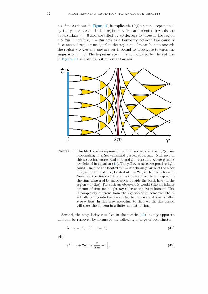
r < 2m. As shown in Figure 10, it implies that light cones – representedby the yellow areas – in the region r < 2m are oriented towards thehypersurface r = 0 and are tilted by 90 degrees to those in the regionr > 2m. Therefore, r = 2m acts as a boundary between two causallydisconnected regions; no signal in the region r < 2m can be sent towardsthe region r > 2m and any matter is bound to propagate towards thesingularity r = 0. The hypersurface r = 2m, indicated by the red linein Figure 10, is nothing but an event horizon.
r
t
0 2m
Figure 10: The black curves represent the null geodesics in the (r, t)-planepropagating in a Schwarzschild curved spacetime. Null rays inthis spacetime correspond to u and v = constant, where u and vare defined in equation (41). The yellow areas correspond to lightcones. The blue line located at r = 0 is the singularity of the blackhole, while the red line, located at r = 2m, is the event horizon.Note that the time coordinate t in this graph would correspond tothe time measured by an observer outside the black hole (in theregion r > 2m). For such an observer, it would take an infiniteamount of time for a light ray to cross the event horizon. Thisis completely different from the experience of someone who isactually falling into the black hole; their measure of time is calledproper time. In this case, according to their watch, this personwill cross the horizon in a finite amount of time.
Second, the singularity r = 2m in the metric (40) is only apparentand can be removed by means of the following change of coordinates:
u = t− r?, v = t+ r?, (41)
with
r? = r + 2m ln∣∣∣ r2m− 1∣∣∣ . (42)
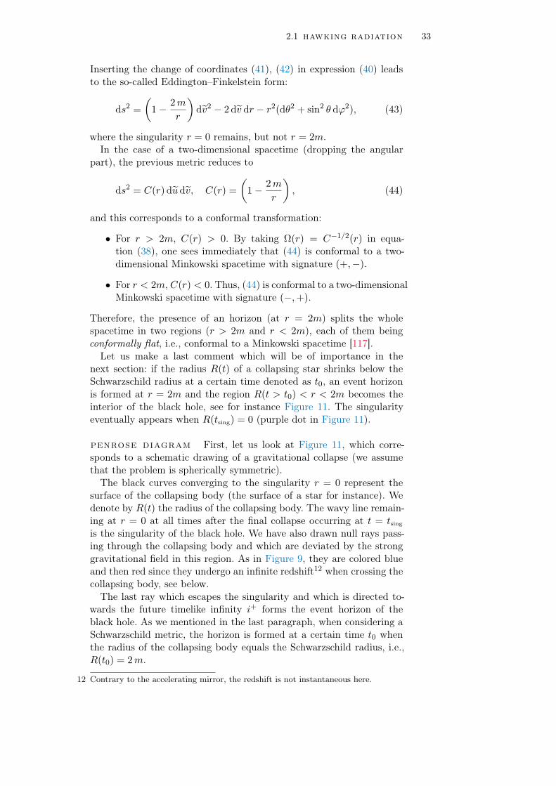
2.1 hawking radiation 33
Inserting the change of coordinates (41), (42) in expression (40) leadsto the so-called Eddington–Finkelstein form:
ds2 =
(1− 2m
r
)dv2 − 2 dv dr − r2(dθ2 + sin2 θ dϕ2), (43)
where the singularity r = 0 remains, but not r = 2m.In the case of a two-dimensional spacetime (dropping the angular
part), the previous metric reduces to
ds2 = C(r) du dv, C(r) =
(1− 2m
r
), (44)
and this corresponds to a conformal transformation:
• For r > 2m, C(r) > 0. By taking Ω(r) = C−1/2(r) in equa-tion (38), one sees immediately that (44) is conformal to a two-dimensional Minkowski spacetime with signature (+,−).
• For r < 2m, C(r) < 0. Thus, (44) is conformal to a two-dimensionalMinkowski spacetime with signature (−,+).
Therefore, the presence of an horizon (at r = 2m) splits the wholespacetime in two regions (r > 2m and r < 2m), each of them beingconformally flat, i.e., conformal to a Minkowski spacetime [117].
Let us make a last comment which will be of importance in thenext section: if the radius R(t) of a collapsing star shrinks below theSchwarzschild radius at a certain time denoted as t0, an event horizonis formed at r = 2m and the region R(t > t0) < r < 2m becomes theinterior of the black hole, see for instance Figure 11. The singularityeventually appears when R(tsing) = 0 (purple dot in Figure 11).
penrose diagram First, let us look at Figure 11, which corre-sponds to a schematic drawing of a gravitational collapse (we assumethat the problem is spherically symmetric).The black curves converging to the singularity r = 0 represent the
surface of the collapsing body (the surface of a star for instance). Wedenote by R(t) the radius of the collapsing body. The wavy line remain-ing at r = 0 at all times after the final collapse occurring at t = tsing
is the singularity of the black hole. We have also drawn null rays pass-ing through the collapsing body and which are deviated by the stronggravitational field in this region. As in Figure 9, they are colored blueand then red since they undergo an infinite redshift12 when crossing thecollapsing body, see below.The last ray which escapes the singularity and which is directed to-
wards the future timelike infinity i+ forms the event horizon of theblack hole. As we mentioned in the last paragraph, when considering aSchwarzschild metric, the horizon is formed at a certain time t0 whenthe radius of the collapsing body equals the Schwarzschild radius, i.e.,R(t0) = 2m.
12 Contrary to the accelerating mirror, the redshift is not instantaneous here.

34 from hawking radiation to analogue gravity
Figure 11: Schematic drawing of a gravitational collapse leading to the for-mation of a black hole. The surface of the collapsing body (assum-ing spherical and of mass m) is indicated by the black curves. Wedenote by R(t) the object radius at time t, eventually shrinkingto zero at a time denoted as tsing and pinpointed by the purpledot. An infinite density point is then formed and called black holesingularity. Null rays, depicted as blue to red curves (since theyundergo a – possibly infinite – redshift), come from J−, thenpass though the collapsing body. They are distorted due to thestrong gravitational field in the vicinity of the black hole region.The null ray going out from the collapsing body when its surfaceradius is R(t0) = 2m (i.e., the Schwarzschild radius in the caseof a Schwarzschild spacetime, see text) is so distorted that it be-comes a vertical straight line; it corresponds to the last ray thatescapes the singularity and converges to the intersection betweenthe future timelike infinity i+ and the future null infinity J +,see Figure 12. The surface delimited by these two null rays (bysymmetry, the second null ray goes out from the collapsing bodywhen R(t0) = −2m) forms the so-called event horizon. We havealso indicated that these null rays correspond to u = ∞, withu defined in expression (41). Any ray crossing the surface of thecollapsing body at a later time t > t0, such as the dark purplecurve in the graph, is bound to propagate down to the singular-ity. We have also drawn the world line of an observer outside theblack hole and able to detect null rays after they passed throughthe collapsing body.
Beyond that point, we enter the interior of the black hole; anythingthat propagates here is bound to fall down to the singularity13 (see thedark purple null ray in Figure 11).
13 Note that the singularity is hidden by the event horizon delimiting the mysteriousinterior of the black hole – In the absence of an event horizon, the singularity is said

2.1 hawking radiation 35
Now, we will draw the Penrose diagram of such a collapse. To modelthe spherical symmetry of the four-dimensional situation, we can re-strict the problem to r ≥ 0 and reflect the null rays at r = 0; thiswill reproduce the trajectory of incoming null rays inside the collapsingbody through the center at r = 0, and then out of the body [25], seeFigure 13 for instance. Such reflections will be achieved by imposingthe boundary condition φ(r = 0, t) = 0 for the field φ, exactly as wedid in Section 2.1.1, see equation (3).Figure 12 shows the two-dimensional Penrose diagram associated to
the gravitational collapse of a spherical body. The center of the bodyr = 0 is a vertical line until it reaches the purple dot; this dot indicatesthe moment when the surface has shrunk to the the singularity. Thesurface of the body corresponds to the black curve; initially this curvecomes from the past timelike infinity i− and converges to the purple dot.The line appears distorted as a result of the coordinates transformation(37), where u and v should be replaced by the Kruskal coordinates14.
The last left-moving null ray v = v0 that escapes the singularityis reflected from the center r = 0, and then moves to the right untilit reaches the intersection between the future timelike infinity i+ andthe null hypersurface J +
R . This ray goes out from the collapsing bodyjust before the formation of the event horizon when R(t ' t0) ' 2m,where we recall that R(t) is the decreasing radius of the spherical body.Looking at equations (41) and (42), we find that this outgoing and right-moving ray thus corresponds to the null ray u = +∞ and is tangent tothe hypersurface J +
L , see Figure 12.Then, all the left-moving rays such that v > v0 reflect off the center at
a point located beyond the purple dot and thus propagate down to thesingularity (see for instance the dark purple null ray in Figure 12). Thefact that the singularity (corresponding to r = 0) is perpendicular tothe black dashed vertical line r = 0 is a bit subtle: in fact, the Penrosediagram shown in Figure 12 hides two Penrose diagrams glued togetheralong the curve R(t)! The green area corresponds to the interior of thecollapsing body, whose spacetime is described by the conformally flatmetric (46). Thus, the associated Penrose diagram simply looks like thegreen area in Figure 8. The other part of the diagram represents theexterior of the collapsing body, whose spacetime is described by theSchwarzschild metric (40). In this case, the associated Penrose diagramis a bit more complicated to draw and is a portion of the so-calledmaximally extended Kruskal manifold [25, 129].
Besides this subtle point, the gray area in Figure 12 is located beyondthe event horizon and corresponds to the interior of the black hole. Thisregion is equivalent to the shaded region in the right plot of Figure 9.
to be naked. R. Penrose postulated in 1969 that no naked singularity exists in ouruniverse; this is known as the cosmic censorship hypothesis [146].
14 The Kruskal coordinates are defined by [25, 129]
u = ∓4me−u/4m, v = 4mev/4m, (45)
with the minus (plus) sign for u if r > 2m (r < 2m).

36 from hawking radiation to analogue gravity
Figure 12: Penrose diagram of the gravitational collapse. To model thespherical symmetry of the four-dimensional situation, we haverestricted the problem to r ≥ 0 and reflected the null rays atr = 0. This procedure of reflection is better illustrated in Fig-ure 13. Then, the problem becomes very similar to the case ofthe accelerating mirror, see the right diagram of Figure 9. Themain difference lies in the fact that the redshift accumulated bynull rays when crossing the collapsing body is not instantaneous,contrary to the case of the moving mirror. The surface of thecollapsing body is represented by the black curve R(t) and theinterior corresponds to the green area. When the surface radiusreaches r = 0 at t = tsing, a singularity is formed. This eventis indicated by the purple dot. The last reflected ray escapingfrom the singularity corresponds to u = ∞ and comes from aleft-moving null ray with v = v0. Thus, the event horizon is noth-ing but the null hypersurface J +
L . All the left-moving rays withv > v0 enter the interior of the black hole and propagate downto the singularity, as illustrated for instance with the dark purplenull ray.
As in Figure 7, the dashed black curve in Figure 12 would correspondto the world line of an observer in our universe, outside the black hole,converging to the asymptotic future i+ and observing the right-movingnull rays passing through. In full analogy with the accelerating mirror,all the right-moving rays converge to J +
R . When traced back in theasymptotic past, they all converge to J − and crowd up around v = v0.
hawking radiation Let us now compute the expected sponta-neous emission due to the gravitational collapse. This amounts to calcu-

2.1 hawking radiation 37
late the relationship between the left-moving waves propagating fromJ − to the center of the collapsing body, then come out and propagateto J +
R , see the left graph of Figure 13. Equivalently, one can model thespherical symmetry of the four-dimensional situation by reflecting nullrays from r = 0, see the right graph of Figure 13.
Figure 13: Portions of the graphs depicted in Figure 11 and Figure 12.(Left) A null ray with v = Constant enters the collapsing body.In the interior of the body, we define new coordinates U and V ,see expressions (46).(Right) Portion of the Penrose diagram illustrated in Figure 12.The null ray is reflected at the center r = 0 of the collapsingbody.
Inside the collapsing body, we introduce a new time coordinate τ andwe assume that the spacetime is conformal to Minkowski spacetime [25,87] with line element
ds2 = A(U, V ) dU dV, where
U = τ − r,V = τ + r.
(46)
We have introduced in the previous equation a new time coordinate τinside the collapsing body. The coordinates U and V are indicated inFigure 13.Outside the spherical body, we use the two-dimensional Schwarzschild
metric given by expression (44), where u and v are defined in equations(41) and (42).
Then, the transformations between the interior and the exterior coor-dinates are given in terms of two functions denoted as α and β – Thesefunctions will be determined later:
U = α(u), v = β(V ). (47)
Now, let us consider an outgoing null ray going out from the collapsingbody and propagating towards J +
R with u = Constant. When tracedback in time, such a ray had coordinate U = α(u) = Constant in theinterior of the body, after passing through r = 0, see Figure 13. At the

38 from hawking radiation to analogue gravity
center of the body r = 0, expressions (46) show that V (τ, 0) = U(τ, 0)= Constant. Then, we can use the function β that connects V and v toobtain the full connection between v and u:
v = β(V ) = β(U) = β α(u) = Constant. (48)
Similarly to the case of the accelerating mirror, an ingoing wave exp(−iωv)will be converted into an outgoing wave exp[−iωβα(u)] when going outfrom the collapsing body; comparing with expression (13), this wouldcorrespond to s = β α.We shall now find explicitly the functions α and β. To that end, we
have to match the exterior and interior metrics (44) and (46) across thecollapsing surface r = R(t) = R(τ), i.e.,
C[R(τ)] du dv = A(U, V )dU dV, (49)
with
u = τ −R(τ)− 2m ln
∣∣∣∣R(τ)
2m− 1
∣∣∣∣ ,
v = τ +R(τ) + 2m ln
∣∣∣∣R(τ)
2m− 1
∣∣∣∣ ,and
U = τ −R(τ),
V = τ +R(τ).(50)
One finds easily from expression (49) both differential equations15
α′ =dUdu
= C (1− R)
[R2 +AC (1− R2)]1/2 − R−1
,
β′ =dVdv
= C−1 (1 + R)−1R2 − [AC (1− R2)]1/2 + R
,
(51)
where R = dR/dτ and (R2)1/2 = −R because R < 0.To solve these differential equations let us make a comment related to
what we have learned from the accelerating mirror problem: we noticedthat the most redshifted right-moving rays were those coming from theregion at the vicinity of v = v0. In addition, due to this significantredshift, the major contribution to the integral (26) [which gives even-tually the total number of emitted quanta from vacuum, see equation(27)] corresponds to v ' v0.
In the gravitational case and by similarity with the mirror problem,we expect this strong redshift to occur close to v = v0, i.e., for null rayscoming out from the collapsing body at R(t0) ' 2m when the surfaceof the spherical body approaches the event horizon, see Figure 11.Therefore, let us assume that C(R) = (1 − 2m/R) ' 0, so that
equations (51) simplify to
dUdu
=R− 1
2 RC(R), (52a)
dVdv
=A (R− 1)
2 R. (52b)
15 Note that r? =∫C−1 dr, where r? and C(r) are defined in equations (42) and (44),
respectively.

2.1 hawking radiation 39
Then, we expand R(t) around t = t0, where we recall that t0 is themoment corresponding to the formation of the event horizon:
R(t) ' R(t0) + R(t0)(t− t0). (53)
This leads to16
C
2 R(t0)' κ (t− t0), 1− R(t0) ' U +R(t0)− t0
t− t0, (54)
where we have introduced
κ =1
2
dCdR
∣∣∣∣R(t0)
=our case
1
4m. (55)
Actually, κ, called the surface gravity, measures how curved is the met-ric at the vicinity of the horizon. One sees that in the case of theSchwarzschild metric, the surface gravity is inversely proportional tothe mass of the black hole.Finally, by integrating equation (52a) with the use of (54), we obtain
κ u = − ln |U +R(t0)− t0|+ Const., as u→ +∞. (56)
Therefore, inverting the previous expression gives
U = e−κ u + t0 −R(t0), as u→ +∞. (57)
At late times, i.e., for large values of u, one sees from (56) and (57)that U does not really depend on u and equals t0 − R(t0). Likewise,outgoing waves with such large values of u all pile up at the vicinity ofv = v0 when traced back in time. This implies that a narrow range ofvalues for V and v covers a large area of J +
R . Therefore, if U and Vdo not vary too much when u → +∞, we can assume that A(U, V ) isapproximately constant in equation (52b) and integrate it:
V =A[R(t0)− 1]
2 R(t0)(v0 − v) + t0 −R(t0). (58)
The integration constant in the previous expression has been found bytaking the limit v → v0, which should correspond to u→ +∞. Insertingexpression (58) in equation (56), then using the continuity conditionU = V at r = 0, we obtain
u = −κ−1 ln
(v0 − vA
), as v → v0, v < v0, (59)
with A = A[R(t0)− 1]/(2 R(t0)).A glance at equation (31) confirms the high similarity between the
gravitational collapse and the moving mirror problem. This lies on the
16 Using U = t − R(t) at the surface of the collapsing body and making a Taylorexpansion of C around t0.

40 from hawking radiation to analogue gravity
fact that the above analysis is based on geometric optics. Therefore, theDoppler shift acquired after the reflection on the surface of the mirroris equivalent to the effects of distortion in the background geometryduring the gravitational collapse.In addition, we have treated the case of a massless scalar field prop-
agating in the Schwarzschild spacetime, but the above results can bederived in a more general framework for any quantum field in a blackhole spacetime [25].Then, from expression (59), we find that natural outgoing positive
modes of energy ~ω > 0 for an observer whose world line would be theblack dashed curve in Figure 12 are
φω =i√
4πω
(eiω κ
−1 ln[(v0−v)/A] − e−iωu), v < v0. (60)
This positive mode is actually a superposition of ingoing positive andnegative energy modes φω and φ?ω [see expression (19)] given by
φω =i√
4πω
(e−iωv − e−iω (v0−A e−κ u)
). (61)
Again, this is precisely this mixing of positive and negative energieswhich will lead to spontaneous emission. Indeed, using directly the re-sults found in Section 2.1.1, we can compute the matrices coefficients(21) and arrive to the expected number of particles spontaneously emit-ted from vacuum [see equation (35), and also (34)]:
〈0|Nω|0〉 ∝1
e~ω/kBTH − 1, (62)
where TH is the so-called Hawking temperature,
TH =~κ
kB 2π c, κ =
c4
4Gm. (with the right units) (63)
Expression (62) is nothing but the the so-called Hawking radiation emit-ted by black holes.
Let us conclude this section with some remarks. In the above calcula-tions we assume that u→ +∞. This means that we have computed theexpected flux of particles at late time. For an observer outside the blackhole, this steady flux would be seen as emerging from the event horizonand would correspond to a thermal radiation of temperature TH. Wenote that the Hawking temperature is proportional to the surface grav-ity κ, and thus depends on the spacetime curvature at the vicinity ofthe horizon [see expression (55)]. As we will show below, the analogueHawking temperature in the context of analogue gravity will be alsoproportional to a quantity that measures the “curvature” of the fluidflow near the acoustic horizon.Moreover, it was proved that this positive energy flux converging toJ +R should be balanced by a negative energy flux entering the black
hole [88, 190]. Wald actually showed that particles are created by pair,

2.2 analogue gravity 41
one of positive energy should travel towards J +R (and corresponds to
a null ray vpos < v0), and the other one, of negative energy, should beabsorbed by the black hole (and actually correspond to the symmetricof vpos with respect to v0, i.e., vneg = 2 v0 − vpos > v0) [190]; Bothparticles of opposite energy form what we call a Hawking pair.As a last comment, we can estimate the expected Hawking tempera-
ture for typical black holes of mass M ' 10M, where M is the massof the sun. Expression (63) can be indeed approximated to
TH ' 10−6 MM
K, (64)
meaning that the Hawking temperature is about a µK, thus completelylost in the Cosmological Microwave Background.
2.2 analogue gravity
The event horizon of a black hole can be seen as a point of no return:anything that crosses the horizon is trapped inside the black hole, can-not come back to our universe and is bound to propagate until it reachesthe singularity.In the general introduction we have compared a black hole to a river
flowing towards a waterfall. Imagine that some fish are traveling in theriver trying to go upstream the flow. Fish close to the waterfall are notable to swim up the river and are bound to fall down to the bottom ofthe waterfall, playing here the role of the black hole singularity. There-fore, the point where the flow velocity equals the velocity of the fishcould be seen as the equivalent of the event horizon: beyond that pointfish are trapped, see Figure 4 of the general introduction.This idea of comparing black holes to hydrodynamic systems might
seem rather naive at this stage; however, as we will see in this section,the similarity between analogue systems and black holes goes beyondthe kinematic analogy discussed in the previous paragraph.In the following, we will not consider fish in a river but rather sound
waves propagating in a transonic flow, see Figure 14. We will first provethat the hydrodynamic equations for sound waves correspond to thewave equation of a massless scalar field in a curved spacetime. Then,using the seminal result obtained by Unruh in 1981 [182], we will showthat an analogous Hawking radiation can be defined in analogue sys-tems.
2.2.1 Sound waves in curved spacetime
Let us start with the usual inviscid hydrodynamic equations
∂tρ+∇(ρv) = 0, (65a)
∂tv + (v · ∇)v = −1
ρ∇p, (65b)
p = p(ρ), (65c)

42 from hawking radiation to analogue gravity
Figure 14: Different configurations of transonic flows.(Left) One-dimensional flow such as considered in Chapter 3. Thefluid moves from the left to the right. The subsonic region cor-responds to the left part where v < c; then, the flow becomessupersonic (v > c) in the right region. The boundary betweenthese two regions corresponds the blue dashed line (at x = xH)and plays the role of an acoustic horizon for sound waves. Indeed,a sound wave propagating in the supersonic region is dragged bythe flow and forms a Cerenkov cone as shown in the figure. Thesupersonic region is the analogue of the interior of a black hole.On the contrary, a sound wave in the subsonic region can propa-gate in all directions.(Right) Two-dimensional case with a spherical symmetry andwhere the flow velocity is only radial – this is the situation con-sidered in Unruh’s paper [182] and in this subsection. The bluedashed line located at a radius rH corresponds to the acoustichorizon, beyond which sound waves are trapped.
where ρ(r, t) is the fluid density, v(r, t) the flow velocity and p(r, t)the pressure. We also assume that the flow is irrotational; we can thusdefine a scalar field ψ(r, t) such that
v = ∇ψ. (66)
We are interested in the small fluctuations around the background flow.We thus expand the physical quantities up to first order:
ψ(r, t)
ρ(r, t)
p(r, t)
=
ψ0(r, t)
ρ0(r, t)
p0(r, t)
+ ε
ψ1(r, t)
ρ1(r, t)
p1(r, t)
, (67)
where (ψ0, ρ0, p0) is an exact solution of the set of equations (65) andε is a small parameter. Then, we linearize the hydrodynamic equationsat first order17. We find for equation (65a):
∂tρ1 +∇ · (ρ0∇ψ1 + ρ1∇ρ0) = 0 (68)
17 Note that this is exactly what we will do in Chapter 3 in the context of Bose-Einsteincondensates, see in particular the hydrodynamic equations (121) and the linearizedversion (123).

2.2 analogue gravity 43
A linearization of equation (65c) leads to
p1 = c2(ρ0) ρ1, with c2(ρ0) =dpdρ
(ρ0), (69)
with c(ρ0) the background sound velocity. Moreover, equation (65b)becomes at first order [109]
ρ0(∂tψ1 +∇ψ0 · ∇ψ1) = −p1. (70)
Then, using together expressions (68), (69) and (70), we obtain
∂t
[ρ0
c2(∂tψ1 + v0 · ∇ψ1)
]= ∇·
[ρ0∇ψ1 −
ρ0
c2(∂tψ1 + v0 · ∇ψ1)v0
],
(71)
where we have introduced v0 = ∇ψ0. Note that if v0 = 0, providedthat the background density ρ0 is constant (which leads to a constantsound velocity c(ρ0) along the fluid flow), expression (71) reduces tothe wave equation (2), i.e., the wave equation for a massless scalar fieldin Minkowski spacetime.
curved spacetime metric The situation is more interestingwhen v0 6= 0. Let us write expression (71) with Einstein notations,such that for example
∂t
(ρ0
c2v0 · ∇ψ1
)= ∂0
(ρ0
c2vj0 ∂jψ1
), (72)
where the subscript 0 corresponds to the time coordinate t and j ∈1, 2, 3 stands for space coordinates x, y, z. Equation (71) then reads
∂0
(ρ0
c2∂0ψ1
)+ ∂0
(ρ0
c2vj0 ∂jψ1
)
+ ∂j
(ρ0
c2vj0∂0ψ1
)+ ∂i
(ρ0v
i0 v
j0 − ρ0 c
2δijc2
∂jψ1
)= 0.
(73)
We would like now to identify the previous expression with the waveequation in curved spacetime (39). By defining
gµν =1
c ρ0
(1 vj0vi0 vi0 v
j0 − c2δij
),√−g = (−det gµν)−1 =
ρ20
c, (74)
Expression (73) becomes
∂µ(√−g gµν∂νψ1) = 0. (75)
Then, by multiplying the last equation by 1/√−g, we obtain the ex-
pected wave equation of a massless scalar field in a curved spacetime
∇µ∇µψ1 =1√−g ∂µ(
√−g gµν ∂νψ1) = 0, (76)

44 from hawking radiation to analogue gravity
whose metric tensor is
gµν =ρ
c
(c2 − v2
0 (v0)j
(v0)i −δij
). (77)
The inverse metric tensor is given by expression (74). From equation(77), it is easy to prove that the line element in this spacetime is givenby
ds2 = gµν dxµ dxν
=ρ0
c[c2 dt2 − (vi0dt− dxi)δij(v
j0dt− dxj)].
(78)
We can already guess from the form of the metric tensor (77) the intrin-sic connection between black holes and transonic flows. First, if v0 = 0,we find the metric associated to a Minkowski spacetime (+,−,−,−);this is what we already noticed in the last paragraph.Now, if v0 6= 0 and the flow becomes supersonic (|v0| > c) in a certain
region, g00 becomes negative, exactly as it occurs for a Schwarzschildmetric when r becomes lower than the Schwarzschild radius 2m, seeequation (40).Thus, let us take the math a step further and show the full analogy
between the metric (77) and the Schwarzschild metric (40). In polarcoordinates (r, θ, ϕ) the metric (77) becomes
gµν =ρ
c
c2 − v20 v0,r v0,θ v0,ϕ
v0,r −1 0 0
v0,θ 0 −r2 0
v0,ϕ 0 0 −r2 sin θ
. (79)
Then, if v0 is only radial (see e.g., the right drawing of Figure 14), i.e.,v0,θ = v0,ϕ = 0, the line element (78) becomes
ds2 =ρ0
c[c2dt2 − (v0,rdt− dr)2 − r2(dθ2 + sin2 θdϕ2)]. (80)
In this coordinates system, this line element exactly corresponds to theso-called Painlevé -Gullstrand line element [80, 140]. By making thefollowing change of variable18
τ = t+
∫ r v0,r
c2 − v20,r
dr′, (81)
we obtain
ds2 =ρ0
c
(
1−v2
0,r
c2
)c2dτ2 −
(1−
v20,r
c2
)−1
dr2 − r2 dΩ2
, (82)
with dΩ2 = dθ2 + sin2 θdϕ2. We can already see the similarity with theSchwarzschild line element here. Let us now consider a transonic flowwith radial velocity
v0,r = −c√rH
r, (83)
18 Note that τ can be understood as a time coordinate only if |v0,r| c.

2.2 analogue gravity 45
where we assume that c is constant. Since c > 0, the minus sign inthe previous expression ensures that the velocity is directed towardsthe center r = 0. Such a velocity splits the flow in two regions: forr > rH the flow is subsonic (|v0,r| < c); for r < rH the flow is supersonic(|v0,r| > c). The line element (82) becomes
ds2 =ρ0
c
[(1− r2
H
r2
)c2dτ2 −
(1− r2
H
r2
)−1
dr2 − r2 dΩ2
], (84)
and is conformally equivalent to the Schwarzschild metric (40), whererH plays the role of the Schwarzschild radius. In our case, rH is calledacoustic horizon. In addition, if we define
C(r) =c2 − v2
0,r
c2, r? =
∫ r
[C(r′)]−1 dr′, (85)
and
u = τ − r?/c, v = τ + r?/c, (86)
equation (82) becomes
ds2 = ρ0(r) (c2 − v20,r) du dv, (87)
where we dropped the angular part. Note the similarity between ex-pressions (87) and (44). The structure of spacetime is exactly the same:the acoustic horizon splits the spacetime in two regions (subsonic andsupersonic), each of them being conformally flat, but disconnected atthe horizon [117, 158].Note that using expression (81) in equations (86), we obtain
u = t−∫ r dr′
c+ v0,r(r′), v = t+
∫ r dr′
c− v0,r(r′), (88)
in agreement with Ref. [158]. Note also that here we assume that thesound velocity c is constant and absolute19 – the latter assumption willnot be true in the presence of dispersion, see e.g., Chapter 3.Then, one can prove that the field ψ1, solution of the wave equation
(76), is also solution of [25]
∂2ψ1
∂u ∂v= 0. (89)
In addition, if we define
ku =ω
c+ v0,r, kv = − ω
c− v0,r, (90)
one findsψ1 ∝ e±iωu = e±i(ωt−
∫ r ku(r′)dr′),
ψ1 ∝ e±iωv = e±i(ωt−∫ r kv(r′)dr′),
(91)
19 In the sense that any sound wave propagates at the sound velocity, independentlyof its frequency or wavenumber; in other words we consider here a dispersionlesstheory.

46 from hawking radiation to analogue gravity
with
ω − v0,r ku = c ku, ω − v0,r kv = −c kv. (92)
Therefore, a fixed frequency ω in the laboratory frame is related to theco-moving frequency ωcm = ω − v0,r k via a Doppler shift. Then, theu-modes correspond to ωcm = ck and the v-modes to ωcm = −ck. Wealso introduce the scalar product [158] [similar to expression (6)]:
(ψ1, ψ2) = −i∫
R[ψ1 ∂ηψ
?2 − ∂ηψ1 ψ
?2] dr, (93)
where ∂η = ∂t + v0,r∂r is the partial derivative with respect to time inthe co-moving frame.
2.2.2 Analogue Hawking radiation
Let us now turn our attention to the existence of an analogous Hawkingradiation using what we have learned from the previous subsection.Suppose first that the flow is subsonic or supersonic everywhere –
in this case, the radial velocity is not given by expression (83). Forsimplicity, we assume that the radial velocity is constant v0,r = Vr,with |Vr| < c in a subsonic flow and |Vr| > c in a supersonic flow.Solutions of the wave equation (89) are
ψω1 ∝ e±iω(t− r−rHc+Vr
), or ψω1 ∝ e±iω(t+r−rHc−Vr ), (94)
where rH is just for the moment an integration constant used to computeintegrals (88). Let us introduce the coordinates pertaining to the co-moving frame
η = t, ξ = r − rH − Vr t. (95)
Solutions (94) can be then recast in the form
ψω1,→ ∝ e±iωcm(η−ξ/c), or ψω1,← ∝ e±iωcm(η+ξ/c), (96)
and correspond to the right- (with the subscript →) and left-movingmodes (with the subscript←) with respect to the co-moving frame. Werecall that ωcm is the co-moving frequency. Using the scalar product(93), it is easy to prove that the positive frequency modes in the subsonicregion correspond to exp[−iωcm(η±ξ/c)], while in the supersonic regionthey are exp[iωcm(η ± ξ/c)].
On the contrary, if the flow now becomes transonic20 at a certainposition rH, the subsonic and the supersonic regions are disconnected.Indeed, one sees from equations (88) that the variable u is ill-defined at
20 Note that the radial velocity is not necessarily given by (83) – the only requirementlies in the existence of a position rH dividing the flow in a subsonic and a supersonicregion.
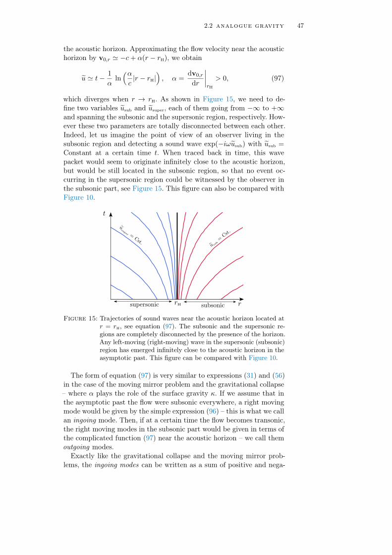
2.2 analogue gravity 47
the acoustic horizon. Approximating the flow velocity near the acoustichorizon by v0,r ' −c+ α(r − rH), we obtain
u ' t− 1
αln(αc|r − rH|
), α =
dv0,r
dr
∣∣∣∣rH
> 0, (97)
which diverges when r → rH. As shown in Figure 15, we need to de-fine two variables usub and usuper, each of them going from −∞ to +∞and spanning the subsonic and the supersonic region, respectively. How-ever these two parameters are totally disconnected between each other.Indeed, let us imagine the point of view of an observer living in thesubsonic region and detecting a sound wave exp(−iωusub) with usub =Constant at a certain time t. When traced back in time, this wavepacket would seem to originate infinitely close to the acoustic horizon,but would be still located in the subsonic region, so that no event oc-curring in the supersonic region could be witnessed by the observer inthe subsonic part, see Figure 15. This figure can also be compared withFigure 10.
Figure 15: Trajectories of sound waves near the acoustic horizon located atr = rH, see equation (97). The subsonic and the supersonic re-gions are completely disconnected by the presence of the horizon.Any left-moving (right-moving) wave in the supersonic (subsonic)region has emerged infinitely close to the acoustic horizon in theasymptotic past. This figure can be compared with Figure 10.
The form of equation (97) is very similar to expressions (31) and (56)in the case of the moving mirror problem and the gravitational collapse– where α plays the role of the surface gravity κ. If we assume that inthe asymptotic past the flow were subsonic everywhere, a right movingmode would be given by the simple expression (96) – this is what we callan ingoing mode. Then, if at a certain time the flow becomes transonic,the right moving modes in the subsonic part would be given in terms ofthe complicated function (97) near the acoustic horizon – we call themoutgoing modes.
Exactly like the gravitational collapse and the moving mirror prob-lems, the ingoing modes can be written as a sum of positive and nega-

48 from hawking radiation to analogue gravity
tive frequency outgoing modes through a Bogoliubov transformation21
of the form (19). Therefore, this mixing of positive and negative energymodes will lead to spontaneous creation of particles from vacuum if onequantizes the sound field as done by Unruh in 1981 [182]. He found thata thermal spectrum should be emitted from the acoustic horizon withtemperature
T analogueH =
~α2πkB
, α =dv0,r
dr
∣∣∣∣rH
, (98)
i.e., the analogous version of expression (63). In the case of analoguegravity, the analogous Hawking temperature depends on how fast isthe transition from the subsonic to the supersonic region through theparameter α. In analogy to the surface gravity, this measures the “cur-vature” of the flow near the sonic horizon.
To conclude, we hope that we convinced the reader of the stronganalogy between transonic flows and black holes. Unruh proved thatanalogue systems indeed give rise to spontaneous emission of particles.However, quantum fluctuations leading to analogue Hawking radiationare too small to be detected in classical platforms22. This is the reasonwhy we will now turn our attention to quantum fluids – one-dimensionalflow of Bose-Einstein condensates, where the (analogue) spontaneousHawking radiation can be explored. This is what we discuss in the nextchapter.
21 We do not detail this transformation here because we will discuss them later in thecontext of analogue gravity, see Chapter 4. Let us just mention that this mixing ofpositive and negative frequencies results from a problem of analyticity of expression(97) when crossing the acoustic horizon rH from the subsonic to the supersonic region.This is similar to the problem encountered in Rindler space [25] where two regionsof spacetime are also disconnected. Likewise, this is nicely discussed and detailed inthe context of analogue gravity in Ref. [158].
22 Despite this fact, classical systems such as surface water experiments [59, 61, 159,192] are still very exciting; for instance, one can use an external perturbation tocreate stimulated Hawking radiation.

3HAWKING RADIAT ION IN BOSE -E INSTE INCONDENSATES
Garay et al [71] were the first to propose the use of Bose-Einstein con-densates (BECs) as acoustic analogues, followed by many others [18–21, 63, 76, 104, 164, 199, 202] in the last two decades. BECs are indeedexcellent candidates to explore Hawking radiation in analogue systemsfor the following reasons:
First, the theory of Bose-Einstein condensation is well-established[148, 153]. This is an uncontested advantage for studying quantum fluc-tuations emerging in the condensate. Based on a Bogoliubov approach,a theoretical treatment of these fluctuations for one-dimensional flowsof BECs was first suggested by Leonhardt et al in Refs. [115, 116].In addition, BECs provide an excellent platform to explore the effect
of these fluctuations on the condensate itself, the so-called backreaction.This might bring new perspectives in General Relativity, a theory whichis not unequivocal when quantum effects are taken into account. Thisprogram exceeds the scope of this thesis, but we hope that a theoreticalanalysis of the backreaction problem for sonic black holes in BECs willbe proposed in the future.
Second, BECs are quantum systems. Contrary to classical analogues,for which Hawking radiation can only result from a disturbance externalto the system [59, 60, 159, 160], here, the analogous Hawking radiationmay originate from quantum fluctuations in the system. Quasiparticlesare spontaneously emitted from the acoustic horizon and propagatein opposite direction, exactly as it would occur at the vicinity of agravitational black hole event horizon (see Section 3.2.1 and Figure 21).This gives rise to correlated and entangled currents emitted outside andinside the acoustic black hole.This correlated signals can be identified and measured by means of
the density-density correlation function. This was first proposed in 2008by a collaboration between teams from Bologna and Trento [15]. Con-trary to gravitational black holes, information can be extracted fromthe interior of a sonic black hole; it is then possible to measure exper-imentally the density correlations in the supersonic region. Likewise,density correlations are much less affected by thermal noise than a di-rect measurement of the Hawking effect (see, for instance, Section 3.2.5and [156]).
Motivated by this promising idea, theoretical predictions for specificconfigurations of one-dimensional acoustic black holes in BECs havebeen obtained in Refs. [110, 124, 156]. One of these configurationswas realistic enough to be implemented experimentally in 2010 by the
49

50 hawking radiation in bose-einstein condensates
Technion Group [105]. A first measurement of density correlations wasachieved in 2016 [177]. After several technical improvements of the ex-perimental setup, a much less noisy measurement was performed in2019 [131]. The theoretical results obtained during this PhD comparevery well with experimental data of Ref. [131]. Therefore, we are able toconclude from this analysis that the Technion Group obtained a clearsignature of Hawking radiation in a Bose-Einstein condensate, almostforty years after Unruh’s suggestion to use hydrodynamic analogues ofblack holes [182].
In this chapter, we will first explain how a sonic horizon can be re-alized in a Bose-Einstein condensate. We will also discuss two specificconfigurations and the experimental realization of one of them. Thiswill conclude Section 3.1.
Then, in Section 3.2, we will provide a detailed theoretical analysisof quantum fluctuations, within a Bogoliubov approach. The specificityof this thesis is to improve the theoretical treatment previously used inthe field by taking into account the zero modes.By means of this well-founded theory, we are able to reproduce with a
nice accuracy the experimental results recently published by the Tech-nion Group in Ref. [131]. Finally, although we confirm that the ex-perimental determination of the Hawking temperature is reliable, wechallenge some claims of Refs. [131, 177] in Section 3.3.
3.1 realization of an acoustic horizon in a bose-einsteincondensate
3.1.1 The Gross-Pitaevskii equation
The many body Hamiltonian describing N interacting bosons in thepresence of an external potential Vext is given, in second quantization,by [45, 106, 153]
H =
∫dr Φ†
[− ~2
2m∇2 + Vext +
g3D n
2
]Φ, (99)
where Φ(r, t) = exp(i H t/~)Φ(r) exp(−i H t/~) is the field operator inthe Heisenberg representation, m the mass of the bosons, n = Φ†Φ thedensity operator and g3D is the coupling constant.The time evolution of the field operator Φ(r, t) is
i ~∂tΦ(r, t) = [Φ, H]
= − ~2
2m∇2Φ(r, t) + [Vext(r) + g3D n] Φ(r, t).
(100)
We recall that the form of the Hamiltonian (99) corresponds to aneffective interaction between the particles Veff(r − r′) = g3D δ(r − r′)characterized by a single parameter g3D. The coupling constant g3D and

3.1 realization of an acoustic horizon in a bose-einstein condensate 51
the s-wave scattering length a are related through the relation [148, 153]
g3D =4π ~2 a
m. (101)
This means that the details of the interaction potential, i.e., at the mi-croscopic level, are ignored; only the scattering length a characterizesthe effects of the interaction on the gas on a macroscopic scale1. There-fore, if we denote n3D the density of the gas and d the interparticledistance, the use of this effective potential will be legitimate only if thecondition For 87Rb, a =
5.77 nm [27]. Withn3D ∼ 1014 cm−3,a3 n3D < 10−3.
a d = n−1/33D (102)
is fulfilled [153]. In this case, the system is said to be dilute or weaklyinteracting. We will always consider this mean-field regime in the fol-lowing.
Bose-Einstein condensation occurs when the temperature is low enoughand when there is a macroscopic occupation of the lowest energy state,i.e., when the number of atoms in this state becomes very large. In thiscase, the Bogoliubov approach [28] consists in writing
Φ(r, t) = Φ(r, t) + δφ(r, t), (103)
where Φ(r, t) is a classical field, called the order parameter of the con-densate and δφ(r, t) is a quantum correction which describes the quan-tum fluctuations of the interacting Bose gas. The condensate densityis given by n(r, t) = |Φ(r, t)|2, while the density operator still readsn = |Φ|2.Within this Bogoliubov approach, one needs to work in the grand
canonical ensemble since the number of particles in the condensate fluc-tuates [37]. We will explain this point in more detail in Section 3.2 withthe addition of zero modes in the theory. Therefore, in the following, in-stead of the Hamiltonian (99), we shall consider HGC = H−µ N , whereµ is the chemical potential and N =
∫dr n is the number of particles.
Inserting decomposition (103) in equation (100) leads, at zero order, tothe well-known time-dependent Gross-Pitaevskii equation [78, 152]:
i ~∂tΨ(r, t) = − ~2
2m∇2Ψ(r, t) + [Vext(r) + g3D n− µ] Ψ(r, t), (104)
with Ψ(r, t) = Φ(r, t) exp(i µ t/~).
3.1.2 One-dimensional flow of Bose-Einstein condensates
We consider a quasi one-dimensional Bose-Einstein condensate: the gasis elongated in the longitudinal direction x and radially confined by
1 In this thesis, we will only consider repulsive interactions, i.e., when a > 0 andg3D > 0.

52 hawking radiation in bose-einstein condensates
a strong harmonic potential V⊥(r⊥) = mω2⊥ r
2⊥/2 of frequency ω⊥. A
schematic view and an experimental realization of a quasi-1D Bose-Einstein condensate are shown in Figure 16.We consider the possibility of adding a longitudinal external poten-
tial U(x). Its importance and its precise form will be discussed in Sec-tion 3.1.3.
xr⊥
Radial confinement with frequency ω⊥
Figure 16: (Left) Experimental realization of an elongated Bose-Einsteincondensate [79]. (Right) Schematic view of a quasi one-dimensional Bose-Einstein condensate, whith x the longitudinalcoordinate and r⊥ the radial coordinate.
One uses the following Ansatz to describe the condensate wave func-tion: Ψ(r, t) = ψ(x, t)ϕ⊥(r⊥; n), where n(x, t) =
∫dr⊥|Ψ|2 = |ψ(x, t)|2
[95, 113]. The Gross-Pitaevskii equation (104) becomes [153]
i ~∂tψ(x, t) = − ~2
2m∂xxψ(x, t)+
[U(x) + g |ψ(x, t)|2 − µ
]ψ(x, t), (105)
where g = 2 ~ω⊥ a [135] is an effective one-dimensional nonlinear cou-pling constant.
1d mean-field regime The validity of equation (105) relies onseveral conditions. As mentioned in the previous section, the total num-ber of atoms should be large and the temperature low enough to reachthe condensed phase. Moreover, even at zero temperature, one needs torespect the following inequalities
(a
a⊥
)2
na 1, (106)
where a is the scattering length and a⊥ =√
~/ω⊥m is the harmonicoscillator length.The left inequality ensures that the transverse dimension of the cloud
should be sufficiently large with respect to the scattering length a toavoid the Tonks-Girardeau regime. This condition is equivalent to requir-ing ξ d [153], where d = n−1 is the one-dimensional inter-particledistance and ξ = ~/√mg n is the healing length [45], i.e., the typicallength scale on which the interaction energy balances quantum pressure[the kinetic term in equation (105)]. Say differently, if this condition isnot satisfied, the mean-field regime is no longer valid.
The right inequality ensures that the 1D dynamics does not triggersexcitations of the transverse degrees of freedom to avoid the 3D-liketransverse Thomas-Fermi regime.

3.1 realization of an acoustic horizon in a bose-einstein condensate 53
A last important remark at this point: note that a one-dimensionalBose-Einstein condensate cannot exist due to the absence of long-rangeorder2 [130, 154]. However, a quasi-condensed phase can be reachedwith a large occupation number of the ground state.
stationary and transonic flow Let us now consider a quasione-dimensional condensate moving from the left to right (in the pos-itive x direction) at some velocity V . Moreover, the flow is taken sta-tionary, meaning that the condensate wave function ψ does not dependon time. Thus, in the following, we will only consider the stationaryGross-Pitaevskii equation
µψ(x) = − ~2
2m∂xxψ(x) + [U(x) + g n(x)]ψ(x), (108)
The previous equation describes the background density. Then, den-sity fluctuations around this background may appear in the condensate.These elementary excitations emerge from quantum fluctuations [see thesecond term of the right-hand side of the Bogoliubov expansion (103)]and behave as sound waves at low energy (i.e., in the long-wavelengthlimit, see Figure 20).In Bose-Einstein condensate, the sound velocity at which these exci-
tations propagate is given by
c =
√g n
m. (109)
Note that the sound velocity is well-defined when the density n(x) inthe previous expression is constant. The local sound velocity is indeedan approximate concept, only rigorously valid where the condensatedensity varies over typical length scales much larger than the healinglength.To realize a sonic black hole configuration, one should modulate the
sound velocity and the flow velocity along the condensate to create asubsonic region, where V < c, and a supersonic region, where V > c.One may achieve such a dissymmetry along the flow by a proper chosenexternal potential U(x) in equation (108). Indeed, in the presence ofsuch a potential, the density profile changes along the condensate, andso does the sound velocity through the relation (109). Then, using the
2 If Ψ is the field operator which describes the one-dimensional system, the one-bodydensity matrix is n(1)(x, x′) =
⟨Ψ(x) Ψ(x′)
⟩. In this case, a long-range order exists
if
n(1)(x, x′) −−−−−−−−→|x−x′|/ξ→∞
n0, (107)
where ξ is the healing length and n0 the condensate density.One shows that this limit diverges when using the Bogoliubov approach. However,an exact derivation [130, 154] demonstrates that off-diagonal terms of the the one-body density matrix tends to zero. This proves that no long-range order exists, andhence, neither does a one-dimensional condensed phase [92, 127]. A nice discussionabout this problem can be found in Ref. [109].

54 hawking radiation in bose-einstein condensates
stationarity of the flow, one has (when the density does not vary toomuch to ensure the validity of the sound velocity)
nV = Cst⇒ c2 V = Cst. (110)
This means that the flow velocity is also modulated. Therefore, one cantune the parameters to obtain a region of higher density (and thus ofslower flow velocity) and an other region of lower density (and thusof faster flow velocity), such that the first region is subsonic and thesecond one is supersonic. In this case, the flow becomes transonic.
notations and conservation laws The external potentialU(x) in equation (108) plays the role of an obstacle. Furthermore, wewill consider cases where U(x) is discontinuous at x = 0, and definethe subscripts u for upstream (x < 0) and d for downstream (x > 0)this obstacle. We also introduce the Mach numbers mu,d = Vu,d/cu,d,where Vu (Vd) is the upstream (downstream) flow velocity and cu (cd)the upstream (downstream) local sound velocity. The analogous blackhole is realized in a situation where the far upstream (x→ −∞) flow issubsonic (mu < 1), and the far downstream one (x→ +∞) is supersonic(md > 1). Here, the condensate wave function, solution of equation(108), is
ψ(x) =
√nu exp(ikux)φu(x) for x < 0 ,√nd exp(ikdx)φd(x) for x > 0 .
(111)
In expression (111) we have separated the upstream and downstream ex-pressions of ψ(x) because U(x) is discontinuous at x = 0. The quantitiesφu(x) and φd(x) will be determined later; we demand that limx→−∞ φu(x)and limx→+∞ φd(x) are constant complex numbers of modulus unity, sothat nu and ~ku/m = Vu > 0 (nd and ~kd/m = Vd > 0) are the up-stream (downstream) asymptotic density and velocity. The asymptotichealing lengths and sound velocities are ξu,d and cu,d, with ~2/(mξ2
α) =mc2
α = gαnα (α = u or d) where gu,d = limx→∓∞ g(x). We allow fora position-dependent effective atomic interaction g(x) for being ableto consider the model configuration introduced in Refs. [15, 36] and inSection 3.1.3, which we denote as “flat profile” below.Inserting the asymptotic limits of (111) (when x → ∓∞) in the
stationary Gross-Pitaevskii equation (108) gives the conservation laws
nuVu = ndVd ,~k2
u
2m+ Uu + gunu =
~k2d
2m+ Ud + gdnd , (112)
where Uu,d = limx→∓∞ U(x). The first of these equations is the currentconservation relation and the second one can be considered as a con-servation of the local chemical potential (one can indeed define such alocal quantity in regions where the density varies weakly over a distanceof the order of the healing length).

3.1 realization of an acoustic horizon in a bose-einstein condensate 55
3.1.3 Theoretical configurations
flat profile configuration This configuration has been in-troduced in Refs. [15, 36], as an idealized structure in which the back-ground density profile is a plane wave of constant amplitude and veloc-ity: nu = nd ≡ n0, ku = kd ≡ k0 and φu(x) = φd(x) ≡ 1. A transonicconfiguration is achievable in such a set-up when
U(x) =
Uu for x < 0 ,
Ud for x > 0 ,g(x) =
gu for x < 0 ,
gd for x > 0 ,
and gun0 + Uu = gdn0 + Ud .
(113)
In this case one has a constant flow velocity V0 = ~k0/m and
cdcu
=mu
md=ξuξd< 1 . (114)
An experimental realization of this idealized configuration seems dif-ficult. First, the coupling constant g(x) varies along the condensate;obtaining such a local monitoring of g(x) is certainly a great challenge.Second, one needs to control very precisely the external potential U(x)to compensate the variations of the coupling constant and to keep con-stant the chemical potential µ = ~2 k2
0/(2m) + U(x) + g(x)n0.This is why another configuration, called “waterfall profile” or “step-
like profile”, has been suggested in Ref. [110] and has been realizedexperimentally [102, 105, 131, 175, 177] (see next paragraph and Sec-tion 3.1.4).
waterfall configuration The condensate is accelerated inthe downstream region x > 0 by an attractive step-like potential U(x) =−U0Θ(x), where Θ is the Heaviside function and U0 > 0 (see Fig-ure 17). The nonlinear parameter g is constant throughout the system.In this transonic configuration the order parameter [equation (111)]corresponds upstream to half a grey soliton and downstream to a planewave [114]:
φu(x) = cos θ tanh (x cos θ/ξu)− i sin θ , and φd(x) = −i , (115)
where sin θ = mu.Contrary to the flat profile configuration in which the upstream and
downstream Mach numbers can be chosen independently, here, oncemu
is fixed all the other dimensionless parameters of the flow are determinedby equations (112) and by imposing continuity of ψ at x = 0. This yields
VdVu
=nund
=1
m2u
= md =
(ξdξu
)2
=
(cucd
)2
,
U0
gnu=m2u
2+
1
2m2u
− 1.
(116)

56 hawking radiation in bose-einstein condensates
0
x
ξu
U(x)
U0= −Θ(x)
−1
1
Vu < cu
Vu Vd
Vd > cd
n(x)
Figure 17: Waterfall configuration. The red curve is a step-like potentialwhose discontinuity is located at x = 0. The blue curve is thecondensate density profile, corresponding to half a grey solitonin the upstream region (see equation (115)) and constant in thedownstream region. The sound velocity can be found from thebackground density profile through equation (109) and is shownin Figure 18. Asymptotic upstream and downstream sound ve-locities are denoted cu and cd, respectively. The flow moves fromthe left to to right in the lab frame as indicated on the graphby brown arrows. Upstream and downstream flow velocities aredenoted Vu and Vd, respectively. The interior of the sonic blackhole, i.e., the supersonic region corresponds to the gray shadedregion.
−4 −2 0 2 4
x/ξu
0.5
1.0
1.5
2.0
v(x
),c(
x) v(x)
Vu
Vd
c(x)
cu
cd
v=
c
v > cv < c
Figure 18: Flow velocity v(x) and sound velocity c(x) along the condensate.Asymptotic upstream and downstream values are mentioned onthe graph. The dashed red line indicates the boundary betweenthe subsonic and supersonic regions where v = c. The light grayshaded region (upstream the obstacle located at x = 0) corre-sponds to a region where the condensate density varies over typ-ical length scales much larger than the healing length. Thus, thelocal sound velocity c cannot be properly defined in this shadedarea and the concept of sonic horizon becomes ill defined. Thedark gray shaded region is the interior of the sonic black hole.
location of the acoustic horizon As noticed in Refs. [109,110], the acoustic horizon, which is at the boundary between the sub-sonic and the supersonic regions (i.e., where v = c), is not exactlylocated at x = 0 but slightly upstream the obstacle (see Figure 18).

3.1 realization of an acoustic horizon in a bose-einstein condensate 57
In addition, as already discussed in the last paragraph, the sound ve-locity is only well-defined when the density varies over typical lengthscales much larger than the healing length. Therefore, the concept ofsonic horizon is ill defined, and this is the reason why the region at thevicinity of x = 0 is shaded in Figure 18.
However, it will not be a problem in the following: we just needto remember that the position x = 0 is the location of the potentialdiscontinuity, where one has to be careful with matching conditionsbetween the upstream and the downstream regions (see Section 3.2).
3.1.4 Experimental realization of an acoustic horizon
In this subsection, we discuss the experimental realization by the Tech-nion group of an acoustic black hole in a Bose-Einstein condensate us-ing a step-like external potential [131, 177]. The one-dimensional Bose-Einstein condensate consists of 8.000 87Rb atoms. The region x < 0is illuminated with an additional laser beam that creates a positivepotential as shown in Figure 19. Thus, a step-like potential whose dis-continuity is located at x = 0 is formed: this is a waterfall configuration.Then, the potential is put in motion at a constant speed to the left, cre-ating a subsonic and a supersonic region as explained in the previoussubsection. Figure 19 shows the experimental density profiles of thecondensate obtained in 2016 [177] and 2019 [131]. The resulting densityprofiles fit quite well with the theoretical and expected profile (115), asshown in Figure 19 where the green curves correspond to half a greysoliton3.We now optimize our theoretical parameters such that they are the
closest from the experimental configuration. This will be useful in thefollowing to compare our theoretical results with experimental ones (seeSection 3.2.5 and Section 3.3). First, we know from continuity equations(116) that, in a waterfall configuration, once one of the parameters isfixed (for instance the upstream Mach numbermu) all the others are setas well. Second, the experiment is not a ‘true’ waterfall configuration,in the sense that experimental parameters do not exactly respect theequalities imposed by conditions (116).Thus, we should fix the right parameter to obtain the best configura-
tion with respect to the experimental setup. A table with experimentaland theoretical parameters can be found in Appendix A. In this table,we compare different configurations, whose parameters are fixed by oneof the equalities of (116). For instance, the experimental downstreamMach number is mexp
d = 2.9 [131]. If we choose the same value for thetheoretical downstream Mach number, then, all the other theoretical pa-rameters can be calculated with conditions (116). Actually, this choice(fixing md = 2.9) leads to the best agreement between experimentaland theoretical parameters.
3 The agreement is slightly less good in 2019 (graph (c) in Figure 19) than in 2016(inset of graph (b) in Figure 19). Notwithstanding this point, we will nicely reproducethe experimental density correlations signal showing the robustness of the theoreticaldescription, see below.

58 hawking radiation in bose-einstein condensates
50
100
n (µ
m-1
)
x/ξ
0
flow
-30 -20 -10 0 10 20 30
a
b
c
Figure 19: (a) Image of the experimental one-dimensional Bose-Einstein con-densate obtained in the presence of a step-like external potential[177]. The step-like function is shown on top of the figure andmoves to the left. The image is obtained by absorption of light:the brightest region is the outside of the sonic black hole (high-density area), while the darkest region is the inside (low-densityarea).(b) Density profile obtained from (a). The green curve in the insetis half a grey soliton.(c) Density profile obtained in Ref. [131]. The green curve cor-responds to the expected theoretical background density for awaterfall configuration with mu = 0.59 (see the text). The insetshows the step-like potential which moves to the left in the free-falling frame, implying that the flow moves to the right in the labframe.
3.2 density correlations in bose-einstein condensates
We have seen hitherto how to construct an acoustic black hole in aBose-Einstein condensate. The questions we would like to address inthis section are:
• How could we define an analogue of Hawking radiation in Bose-Einstein condensate?
• How to detect such a signal?
3.2.1 Bogoliubov approach
First, the analogue of Hawking radiation originates from quantum fluc-tuations emerging from the condensate.To describe these fluctuations, let us start by decomposing the total
field operator Ψ(x) using a Bogoliubov approach, as done in (103):
Ψ(x) = ψ(x) + δψ(x, t), (117)
where δ ˆψ(x, t) is as small quantum perturbation. For the moment, weconsider δψ(x, t) as a small classical field, denoted as δψ, with ψ + δψsolution of the time-dependent Gross-Pitaevskii equation (105).Linearizing this equation (see, e.g., Ref. [65]) leads to the well-known
Bogoliubov-De Gennes equations
i ~∂t
(δψ
δψ?
)=
(H g ψ2
−g (ψ?)2 −H
) (δψ
δψ?
), (118)

3.2 density correlations in bose-einstein condensates 59
where H = − ~2
2m∂2x + 2 g |ψ|2 + U(x)− µ.
dispersive hydrodynamics equations It is interesting atthis point to establish the connection with Chapter 2. To this end, wedescribe the condensate wave function in terms of number density andphase by means of the Madelung representation: For the moment
we do not assumestationarity of theflow.
ψ(x, t) =√n0(x, t) ei θ0(x,t), (119)
where n0 is the condensate density and θ0 its phase; the phase beingconnected to the flow velocity V by the formula
V (x, t) ≡ ~m∂x θ0. (120)
From the Gross-Pitaevskii equation (105) one finds two equations forn0 and θ0:
∂t n0 + ∂x (n0 V ) = 0 ,
∂t V + V ∂x V +g
mρ0∂x P +
~2
2m2∂x Π +
1
m∂xU(x) = 0,
P =n2
0
2, and Π = − 1√
n0∂xx√n0,
(121)
where P is an effective pressure induced by nonlinearities and Π is thequantum pressure [153].The set of equations (121) are the hydrodynamics equations: the first
one is the continuity equation, the second one is the Euler equation.However, one sees a main (and dramatic) difference with the hydrody-namics equations introduced in Chapter 2: the addition of dispersiveeffects in the system through the quantum pressure term in the secondequation of (121) will prevent us to define a proper metric4 (see below).
lagrangian density and metric Let us now imagine thatthe density and the phase slightly fluctuate, such that the total classicalfield which describes the system becomes This is nothing
but the Bogoliubovdecomposition(117)
Ψ =√n0 + n1 e
i (θ0+θ1) =√n0e
i θ0 + δψ,
with δψ =√n0e
i θ0
(n1
2n0+ i θ1
) (122)
Using the linearized version of the time-dependent Gross-Pitaevskiiequation, namely the Bogoliubov-De Gennes equations [see equation(118)], one finds [119]
(∂t + v0 ∂x) θ1 = −mc2(−i ∂x)
~n0n1, (123a)
(∂t + ∂x v0) (∂t + v0 ∂x)θ1 − c2(−i ∂x) ∂2x θ1 = 0, (123b)
4 As we already mentioned in Chapter 2, dispersive effects are totally absent in generalrelativity. For massless fields, the speed of light c is the speed of waves, regardlessof their frequency or wavevector. The wave speed is absolutely fixed.

60 hawking radiation in bose-einstein condensates
where c2(−i ∂x) is an operator which takes into account the dispersionin the system:
c2(−i ∂x) = c2 − ~2
4m2∂2x, (124)
with c =√n0 g/m, the usual sound velocity.
Note that the set of equations (123) are obtained assuming that n0
is constant. Albeit this is true for the flat profile configuration, thisassumption is incorrect for the waterfall configuration in the subsonicregion at the vicinity of the horizon (see Figure 17). However the densitytends reasonably fast to its constant value nu (for a specific case ofexperimental interest where n(x) ' nu for x < −3 ξu). In any case,as we already mentioned in Section 3.1.3, one is not able to define aproper sound velocity when the density varies on scales of the order ofthe healing length5.Despite this assumption, equations (123) are very instructive and
meaningful. The field θ1(x, t) is solution of a (massless) wave equation incurved spacetime. Indeed, when c2(−i∂x) = c2, i.e., in the dispersionlessregime, equation (123b) can be written in terms of a metric gµν :
1√−G ∂µ(
√−G gµ ν∂νθ1) = 0, (125)
with G = det gµν . One finds in this case
gµν =n0
mc
(c2 − v2
0 v0
v0 −1
), (126)
which is equivalent to the metric derived in Chapter 2 [see equation (77)].Equivalently, the field θ1(x, t) can be seen as a massless field propagatingin a 1+1D curved spacetime whose metric is given by equation (126).
In presence of dispersion, we are forced to abandon the concept ofmetric, which is strictly valid in a dispersionless regime. However onecan still write a Lagrangian density from which equation (123b) is de-rived [158]. We introduce a complex field θ(x, t) solution of the masslesswave equation (125), such that θ1 = θ+θ?. This ensures that θ1 definedin expression (122) is real and solution of equation (123b). Then, theLagrangian density reads
L =1
2|(∂t + v ∂x) θ|2 − 1
2|c(−i ∂x) ∂x θ|2. (127)
Similarly, we also introduce n(x, t), a solution of equation (123a) suchthat n1 = n + n?.This field is related to the canonical momentum πassociated to θ through the relation
π =∂L
∂(∂t θ?)= (∂t + v ∂x) θ =
(123a)−mc2(−i ∂x)
~n0n. (128)
5 Equations (123) are derived in Ref [119] with a varying density, but neglectingdispersive effects. The derivation also leads to a generalized Klein-Gordon equation.

3.2 density correlations in bose-einstein condensates 61
scalar product From the Lagrangian density (127) we can alsoderived a conserved current [133]
Ji = i
[∂L
∂(∂i θ?)θ? − ∂L
∂(∂i θ)θ
], where i ∈ t, x. (129)
The current Jt can be understood as a density of charge and is asso-ciated to a conserved quantity – the scalar product – defined as [158]
〈θk|θl〉 = i
∫
RJt dx = i
∫
Rdx (θ?k πl − θl π?k) , (130)
where θk,l are two solutions of equation (123) and πk,l are derived fromequation (128). Introducing Λk = (−πk + i θk, −πk − i θk)T, the scalarproduct (130) becomes
〈Λk|Λl〉 =
∫
RdxΛ†k σz Λl, (131)
with σz = diag(1, −1). This scalar product will be of importance in thefollowing to normalize correctly the excitation modes emerging fromquantum fluctuations. Indeed, from this scalar product, one can definethe norm N of an excitation mode: N = 〈θ|θ〉 = −〈θ?|θ?〉, or equiva-lently N = 〈Λ|Λ〉 = −〈σx Λ?|σx Λ?〉, where σx is the Pauli matrix.
dispersion relation Let us now consider a plane wave θ(x, t) =A exp[−i (ω t − q x)], solution of equation (123b). We obtain immedi-ately the corresponding dispersion relation
(ω − V q)2 = ω2B(q), with ωB(q) =
√c2 q2 +
(~ q2
2m
)2
, (132)
ωB(q) being the so-called Bogoliubov dispersion relation6.If the condensate were at rest, i.e., V = 0, the elementary excitations
would have frequency ω = ωB, as expected in Bose-Einstein condensa-tion theory using a Bogoliubov approach. Yet, when the condensate ismoving, dispersion relation (132) implies that the frequency undergoesa Doppler shift, which is in some sense a very intuitive result. Therefore,in the free-falling frame (where the condensate is at rest) the emitted ex-citation has frequency ωB, while in the lab frame (where the condensateis moving), it has frequency ω, related to ωB via equation (132).
6 Let us add a brief comment on the Bogoliubov dispersion relation. This expressioncan be rewritten in terms of dimensionless parameters and reads in this case [148,153]
~ωB(Q)/(mc2) = Q
√1 +
Q2
4, (133)
with Q = ξ q. Low energy excitations (when Q 1) travel at the sound velocitywith energy ~ωB = c p (p = ~ q). These quasiparticles are sound waves and arecalled phonons. When Q 1, excitations become free particles with energy ~ωB =p2/(2m) +mc2.Denoting λ the wavelength of the excitation, one sees that the turning point betweenthe phonon (where interactions dominate) and the free particles regimes (wherequantum pressure dominates) takes place around λ ∼ ξ, which corresponds to theproper definition of the healing length [45, 148, 153] introduced in Section 3.1.2.
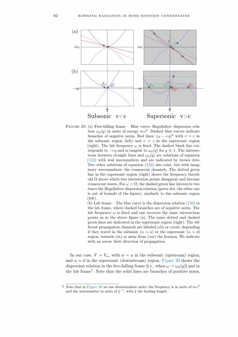
62 hawking radiation in bose-einstein condensates
(a)
(b)
Ω
Ω
Figure 20: (a) Free-falling frame – Blue curve: Bogoliubov dispersion rela-tion ωB(q) in units of energy mc2. Dashed blue curves indicatebranches of negative norm. Red lines: (ω − v q)2 with v < c inthe subsonic region (left) and v > c in the supersonic region(right). The lab frequency ω is fixed. The dashed black line cor-responds to −c q and is tangent to ωB(q) for q 1. The intersec-tions between straight lines and ωB(q) are solutions of equation(132) with real wavenumbers and are indicated by brown dots.Two other solutions of equation (132) also exist, but with imag-inary wavenumbers: the evanescent channels. The dotted greenline in the supersonic region (right) shows the frequency thresh-old Ω above which two intersection points disappear and becomeevanescent waves. For ω > Ω, the dashed green line intersects twotimes the Bogoliubov dispersion relation (green dot, the other oneis out of bounds of the figure), similarly to the subsonic region(left).(b) Lab frame – The blue curve is the dispersion relation (132) inthe lab frame, where dashed branches are of negative norm. Thelab frequency ω is fixed and one recovers the same intersectionpoints as in the above figure (a). The same dotted and dashedgreen lines are indicated in the supersonic region (right). The dif-ferent propagation channels are labeled α|in or α|out, dependingif they travel in the subsonic (α = u) or the supersonic (α = d)region, towards (in) or away from (out) the horizon. We indicatewith an arrow their direction of propagation.
In our case, V = Vα, with α = u in the subsonic (upstream) region,and α = d in the supersonic (downstream) region. Figure 20 shows thedispersion relation in the free-falling frame [i.e., when ω = ωB(q)] and inthe lab frame7. Note that the solid lines are branches of positive norm,
7 Note that in Figure 20 we use dimensionless units: the frequency is in units of mc2
and the wavenumber in units of ξ−1, with ξ the healing length.

3.2 density correlations in bose-einstein condensates 63
i.e., when 〈θ|θ〉 > 0, while dashed curves are branches of negative norm[〈θ|θ〉 < 0].
By means of equation (132), one sees that the possible modes of emis-sion in each region (subsonic or supersonic), can be found graphically asthe intersections between straight lines ω(q)−Vα q and the Bogoliubovdispersion relation ωB(p). This is what is outlined Figure 20. For a fixedfrequency ω, since the tangent of ωB(q) equals cq in the long-wavelengthlimit (ξ q 1, with ξ the healing length), one finds two possible modesof excitation in the subsonic region (because, here, Vu < c). In thesupersonic region (Vd > c) the situation is more complex: below a cer-tain threshold Ω there are four modes of excitations; when ω > Ω, twomodes become evanescent and the line ω(q)−Vd q intersects ωB(q) onlytwo times.
scattering channels As one can see from Figure 20, theseexcitation modes are labeled ` = α|in or ` = α|out, with α = u, d,depending if the excitation travels in the upstream or the downstreamregion, towards (ingoing-modes) or away (outgoing-modes) from theobstacle located at x = 0. Each of them takes part of three differentscattering processes induced by a ingoing-mode. For example, a ingo-ing-mode emitted in the upstream region and propagating to the right(` = u|in) will scatter at the horizon and be converted in outgoing-modes, either propagating in the upstream region against the flow orin the downstream region in the direction of the flow. This process ofmode conversion is schematically represented in Figure 21. Two otherscattering processes can be induced by ` = d1|in or ` = d2|in. Note thatthe evanescent modes, characterized by a complex wavenumber q, arealso mentioned in Figure 21.
Figure 21: Sketch of the different channels contributing to the incomingquantum modes U , D1 and D2. In each plot the backgroundcondensate propagates from left to right, the white region corre-sponds to the upstream subsonic flow, the gray one to the interiorof the analogous black hole (downstream supersonic flow) and theregion of the horizon is represented by the dark gray shaded inter-face (see also Figure 18). The labels indicate the different modesof emission shown in Figure 20. Each mode (U , D1 and D2) isseeded by a ingoing channel (u|in, d1|in and d2|in) propagatingtowards the horizon.
basis set for expanding the elementary excitationsWe learned from the aforementioned paragraphs that quantum fluctu-ations in a moving condensate result in the emission of quasiparticles.

64 hawking radiation in bose-einstein condensates
These excitations are plane waves characterized by their frequency ω(ωB in the free-falling frame), their wavenumber q, and also their norm.They can be emitted in different modes, whose notations are detailed inthe previous paragraph. Positive (negative) norm modes carry a positive(negative) charge, i.e., a positive (negative) scalar product.
We shall now expand the small classical field δψ (see Equation 117)over a complete set of eigenvectors. We look for stationary modes8 ofthe form
(δ ψω
δ ψ?ω
)= Ξ e−i ω t =
(u(x)
v(x)
)e−i ω t, (134)
where u(x) and v(x) are the Bogoliubov amplitudes. Inserting (134) inthe Bogoliubov-De Gennes equations (118) leads to well-known diago-nalization problem of the Bogoliubov-De Gennes Hamiltonian
~ω Ξ = LBG Ξ , with LBG =
(H g ψ2
−g (ψ?)2 −H
), (135)
where we recall that H = − ~2
2m∂2x + 2 g |ψ|2 + U(x) − µ. Thus, Ξ is an
eigenvector with eigenvalue ~ω. Note that the symmetry property ofthe Bogoliubov-De Gennes equations [65] implies that for each solutionΞ = (u, v)T of energy ε = ~ω of equation (135), the quantity Υ =(v?, u?)T = σx Ξ∗ is also a solution of energy −ε = −~ω.
From equation (131), one checks that the norm
〈Ξ|Ξ〉 =
∫
RdxΞ† σz Ξ (136)
is conserved. Moreover, if 〈Ξ|Ξ〉 > 0, then 〈Υ|Υ〉 < 0. For a certain modeΞ emitted with frequency ω and wavenumber q, it is worth noticingthat the sign of its norm only depends on the sign of ωB(|q|), i.e., thefrequency of this mode in the free-falling frame9. Therefore, looking atFigure 20, we notice that the D2-mode has a negative norm, or saydifferently, carries a negative charge, while the U and D1-modes arepositive norm modes.This last remark is very important. Indeed, we can already guess
where the analogous Hawking radiation in BECs comes from: each scat-tering processes shown in Figure 21 gives birth to a positive norm modeu|out propagating away from the horizon outside the acoustic blackhole, and a negative norm mode d2|out also propagating away from thehorizon inside the black hole. These two modes are nothing but theanalogous Hawking pair in our system. The specificity of acoustic blackholes in BECs lies in the fact that an other outgoing positive norm
8 The existence of stationary modes is ensured by the time invariance of the La-grangian density (127) [133].
9 Indeed, this directly comes from equation (131). Going to the free-falling frame,one sees that π = ∂t′θ, with t′ = t, x′ = x − v0 t, and ∂t′ = ∂t + v0 ∂x. Then,by considering a stationary mode θ(x′, t′) = θ(x′) exp[−i ωB(|q|) t′], the norm is〈θ|θ〉 = 2ωB(|q|)
∫R dx |θ|
2.

3.2 density correlations in bose-einstein condensates 65
mode d1|out is also emitted during the scattering process, leading totripartite entanglement (see Chapter 4).Then, combining the different channels with appropriate matching
conditions at x = 0 one can build modes defined on all the real axiswhich form a basis set for expanding the elementary excitations. Wechoose to build solutions on well defined ingoing channels u|in, d1|in,and d2|in, as shown in Figure 21. The corresponding wave-functions aredenoted as ΞU , ΞD1 and ΞD2, with ΞL(x) = (uL(x), vL(x))T . They havethe form,
for x < 0 : ΞU(x) = Su,u Ξu|out(x) + Sevau,u Ξu|eva(x) + Ξu|in(x) ,
ΞD1(x) = Su,d1 Ξu|out(x) + Sevau,d1 Ξu|eva(x) ,
ΞD2(x) = Su,d2 Ξu|out(x) + Sevau,d2 Ξu|eva(x) ;
for x > 0 : ΞU(x) = Sd1,u Ξd1|out(x) + Sd2,u Ξd2|out(x) ,
ΞD1(x) = Sd1,d1 Ξd1|out(x) + Sd2,d1 Ξd2|out(x) + Ξd1|in(x) ,
ΞD2(x) = Sd1,d2 Ξd1|out(x) + Sd2,d2 Ξd2|out(x) + Ξd2|in(x) ,
(137)
with
Ξ`(x) ≡(u`(x)
v`(x)
)= ei q` x
(eimVα x/~ U`(x)
e−imVα x/~ V`(x)
), (138)
where the labels ` refer to the possible modes of emission (` = α|inor ` = α|out), and Vα is the flow velocity in the subsonic (α = u) orthe supersonic (α = d) region. In the flat profile configuration, andalso in the downstream region of the waterfall configuration (where φα,defined in equation (111), is constant) the solution of equation (135) areplane waves. In the upstream region of the waterfall configuration thesolutions are also known, see, e.g., Ref. [24] and the explicit expressionsof U`(x) and V`(x) are given in Ref. [110]. In equation (138) q`’s arethe wave vector of the Bogoliubov modes, solutions of the dispersionrelation (132). The S’s in equation (137) are reflection and transmissioncoefficients: for instance Su,d1(ω) describes how the amplitude of a waveof angular frequency ω initiated in the d1|in channel is scattered ontothe u|out one. Note that in the above expressions all quantities dependon ω.The classical field δψ can be now expanded over the basis formed by
eigenvectors ΞL and ΥL:
δψ(x, t) =
(δψ(x, t)
δψ?(x, t)
)
=
∫ +∞
0dω
∑
L∈U,D1ΞL(ω, x) e−i ω t bL(ω) + ΥL(ω, x) ei ω t b?L(ω)
+
∫ Ω
0dωΥD2(ω, x) ei ω t bD2(ω) + ΞD2(ω, x) e−i ω t b?D2(ω) ,
(139)

66 hawking radiation in bose-einstein condensates
withbL(ω) = 〈ΞL|δψ〉 , and b?L(ω) = −〈ΥL|δψ〉 , if L ∈ U, D1,bD2(ω) = 〈ΥD2|δψ〉 , and b?D2(ω) = −〈ΞD2|δψ〉 .
(140)
In equation (139), Ω is the threshold above which the mode D2 disap-pears. Note that in the case of the D2-mode the positive norm mode isΥD2(ω, x) ei ω t for ω > 010. The validity of equation (139) is based on acorrect normalization of ΞL, i.e.,
⟨ΞL′(ω)|ΞL(ω′)
⟩= νLδL,L′δ(ω − ω′) , (141)
with νU = νD1 = 1 and νD2 = −1. Using expansion (137), one seesthat this normalization imposes the following relation between the S-coefficients:
S†ηS = η , where S =
Su,u Su,d1 Su,d2
Sd1,u Sd1,d1 Sd1,d2
Sd2,u Sd2,d1 Sd2,d2
, (142)
and with η = diag(1, 1,−1). Note that the evanescent are not involvedin equation (142) because they do not carry any current [110].
3.2.2 Zero modes
The decomposition (139) does not form a complete basis. Indeed, thelinear operator LBG [see equation (135)] is not self-adjoint and one can-not build a priori a complete basis set from the eigenfunctions ΞL. Ageneral technique has been exposed in Ref. [26] for building a Jordanrepresentation of LBG which, besides its normalized eigenvalues, admitsalso solutions of zero energy and zero norm.
Indeed, within the Bogoliubov approach, the phase of the condensatewave function is fixed, implying that the global U(1) symmetry is bro-ken. This symmetry breaking is actually associated to a zero energy solu-tion of equation (135): for any fixed θ, the quantity ψθ(x) = ψ(x) exp(iθ)is also solution of the stationary Gross-Pitaevskii (108). Since one canwrite ψθ ' ψ + iθ ψ it follows that i θ ψ is a solution of the linearizedGross-Pitaevskii equation with ω = 0.The corresponding solution of equation (135) reads (the term i θ has
been factorized out)
P =
(ψ
−ψ?
), with LBG P = 0 . (143)
10 For completeness we mention that another possible expansion for the D2-modewould have been
... +
∫ 0
−Ω
dω ΞD2(ω, x) e−i ω t 〈ΞD2|∆〉 −ΥD2(ω, x) ei ω t 〈ΥD2|∆〉 .

3.2 density correlations in bose-einstein condensates 67
We recall that ψ(x) is the condensate wave function and takes a differentform in the upstream and the downstream regions, see expressions (111).This is the reason why we introduce
Pα(x) =
( √nα e
i kα x φα(x)
−√nα e−i kα x φ?α(x)
), with LBG Pα = 0 , (144)
where kα = mVα/~ and, as usual, P = Pu for negative x and P = Pdfor positive x. These modes have zero norm: 〈Pα|Pα〉 = 0.
As we noticed earlier, for each solution of the Bogoliubov-De Gennesequations (118) with ε = ~ω > 0, one solution of negative energy−ε also exists. Thus, we expect that an another mode of zero energyshould be associated to the mode Pα. This mode of excitation actuallycorresponds to addition of particles to the system [148]. Indeed, if thenumber of particles varies, so does the chemical potential µ. Thus, letus consider a family of solutions of the Gross-Pitaevskii equation (105)parameterised by µ:
ψµ,α(x, t) = ψstµ,α(x) e−i(µ−µ0) t , (145)
with α ∈ u, d and where ψstµ=µ0,α(x) =
√nα exp(i kα x)φα(x) is a
stationary solution of equation (108) with µ = µ0. If the chemical po-tential varies around µ0, δψ = ψµ0+δµ−ψµ0 is a solution of the linearisedGross-Pitaevskii equation (118) when δµ→ 0:
i ~ ∂t
(∂µψµ,α|µ=µ0
∂µψ?µ,α|µ=µ0
)= LBG
(∂µψµ,α|µ=µ0
∂µψ?µ,α|µ=µ0
), (146)
with ∂µψµ,α|µ=µ0 = ∂µψstµ,α|µ=µ0 − i t~ ψst
µ0,α. One finds
LBG Qα =i
Meff
Pα, with Qα =
(qα(x)
−q?α(x)
), (147)
where qα(x) = i ∂Nψstµ,α|µ=µ0 and where 1/Meff = dµ/dN [26, 148, 157]
plays the role of an effective mass (N being the number of particles inthe system). One has also 〈Qα|Qα〉 = 0.In our case, the system is infinite and, thus, Meff → ∞. Indeed, if
we slightly anticipate on Section 3.2.3, the phase of the condensatedeviates from its initial value and this is known as the phenomenon ofphase diffusion [118]. However, the inertia associated to the change ofthe global phase of a system of infinite number of particles is infinite andthis imposes Meff →∞ [see equation (161) of Section 3.2.3]. Therefore,the mode Qα is also solution of Qα LBG = 0.In the following, we only explicit the expressions of Qα for the flat
profile and the waterfall configurations. The details of calculations canbe found in Appendix B.

68 hawking radiation in bose-einstein condensates
flat profile
Qu = DeΛuXu
(−i Λu
2 −mu
−i Λu2 +mu
),
Qd = A
(1
−1
)
+DE eiK0 Xd
(K02 −md
K02 +md
)+DE? e−iK0 Xd
(−K0
2 −md
−K02 +md
),
(148)
with
Qα =
(ei kα x 0
0 e−i kα x
)Qα
Xα = x/ξα, K0 = 2√m2d − 1, and Λu = 2
√1−m2
u ,
A = D [md (E + E?)−mu] ,
E = − Λu2mdK
20
ξdξu
(Λumd + imuK0) .
(149)
The parameterD in equations (148) and (149) can be found numericallyfor different configurations mu = Vu/c and md = Vd/c, see Appendix B.This gives an approximate expression for D:
D =m2uK
20
8 (1 +mu) (m2d −m2
u)⇒ A = − mu
2 (1 +mu). (150)
waterfall configuration
Qu = D
[χ(Xu)− Λ
2
]2
eΛuXu
(1
1
),
Qd = A
(φd
−φ?d
)
+ E eiK0Xd
([K0
2 −md]φd
[K02 +md]φ
?d
)+ E e−iK0Xd
([−K0
2 −md]φd
[−K02 +md]φ
?d
),
(151)
with
Qα =
(ei kα x 0
0 e−i kα x
)Qα
χ(X) =√
1−m2u tanh
(√1−m2
uX)
A = iD(1−m2
u) (1 + 2m2u)
2 (1 +m2u)
, and E = iDm2u (m2
u − 1)
4 (1 +m2u)
.
(152)
The parameter D in equations (151) and (152) can be also found nu-merically. In this case,
D = iamu + b
1−mu, (153)

3.2 density correlations in bose-einstein condensates 69
with a = 0.175 and b = −4.56 10−3. Note that for the waterfall config-uration, md = 1/m2
u.
Once the zero modes have been derived with the correct matchingconditions at x = 0, the basis is complete and the small classical fieldδψ(x, t) is decomposed as follows
δψ(x, t) =
(δψ(x, t)
δψ?(x, t)
)= −i P 〈Q|∆〉+ iQ 〈P |∆〉
+
∫ +∞
0dω
∑
L∈U,D1ΞL(ω, x) e−i ω t bL(ω) + ΥL(ω, x) ei ω t b?L(ω)
+
∫ Ω
0dωΥD2(ω, x) ei ω t bD2(ω) + ΞD2(ω, x) e−i ω t b?L(ω) ,
(154)
with the correct normalization between P and Q, i.e., 〈Q|P 〉 = i.
3.2.3 Quantization
The quantization is directly obtained from expression (154): the fieldoperator δψ associated to the elementary excitations is expanded overthe scattering modes and reads
δψ(x, t) =
(δψ
δψ†
)= −i P Q+ iQ P
+
∫ +∞
0dω
∑
L∈U,D1ΞL(ω, x) e−i ω t bL(ω) + ΥL(ω, x) ei ω t b†L(ω)
+
∫ Ω
0dωΥD2(ω, x) ei ω t bD2(ω) + ΞD2(ω, x) e−i ω t b†D2(ω) ,
(155)
where bL(ω) and b†L(ω) are respectively the annihilation and creationoperators pertaining to a scattering process induced by an ingoing modeL|in, L ∈ u, d1, d2. They are the quantized version of bL(ω) and b?L(ω)defined in equation (140):
bL(ω) =⟨
ΞL|δψ⟩
=
∫
Rdxu?L δψ(x, t)− v?L δψ†(x, t), if L ∈ U, D1,
bD2(ω) =⟨
ΥD2|δψ⟩
=
∫
Rdx vD2 δψ(x, t)− uD2 δψ
†(x, t),
(156)
Zero modes operators P and Q are given by
Q =⟨Q|δψ
⟩=
∫
Rdx[q?(x) ψ(x, t) + q(x) ψ†(x, t)
],
P =⟨P |δψ
⟩=
∫
Rdx[ψ?(x) ψ(x, t) + ψ(x) ψ†(x, t)
],
(157)

70 hawking radiation in bose-einstein condensates
where ψ(x) =√nα e
i kα x φα(x) [see equation (111)]. The operator Q
is the phase operator of the condensate, while P corresponds to thefluctuations of the number of particles.
This quantization yields the correct commutation relations[bL(ω), b†
L′(ω′)]
= δL,L′δ(ω−ω′), and [Q, P] = 〈Q|P 〉 = i. (158)
The taking into account of the zero modes, with the proper normaliza-tion of mode Q ensures that the field operator δψ verifies the correctcommutation relation
[δψ(x, t), δψ†(x′, t)
]= δ(x− x′) . (159)
The importance of the zero modes to obtain a correct normalization isstressed in Figure 22. One sees that the zero modes cannot be neglectedto have a well-founded theory based on a proper normalization.
Once the zero modes have been included, the quadratic Hamiltonianwhich describes the quantum fluctuations is [26]
Hquad =1
2
∫
Rdx ∆† σz LBG ∆
=P2
2Meff
+∑
L∈U,D1,D2νL
∫ ΩL
0dω ~ω b†L(ω) bL(ω),
(160)
with ΩU = ΩD1 = ∞ and ΩD2 = Ω, νU = νD1 = 1, and νD2 = −1.The first term of equation (160) has the form of a free kinetic energy,with no restoring force and is associated with the zero eigenvalue of theBogoliubov-De Gennes Hamiltonian LBG [26]. Thus, the operator P canbe identified with a momentum operator and the parameter Meff maybe indeed interpreted as an effective mass. The second contribution toequation (160) is a system of independent oscillators of energies ~ω.Then, the ground state |0〉 of the Hamiltonian (160) consists of anoscillator ground state such that bL |0〉 = 0, L ∈ U,D1, D2, andof a zero-momentum plane wave state such that P |0〉 = 0 [26].In addition one has also[Q, Hquad
]= i
P
Meff
. (161)
Equation (161) implies that the phase operator Q(t) is not stationaryand deviates from its initial value Q(t = 0). This is the phenomenonof phase diffusion (see, e.g, Ref. [118]). In our case, Meff → ∞ and nophase diffusion occurs. The physical interpretation of this phenomenonwas already mentioned in Section 3.2.2 and corresponds to the inertiaassociated to the change of the global phase of a system with infinitenumber of particles.Let us conclude this subsection with a last remark: the decomposition
(154) is not unique. Indeed, one would be tempted to define outgoingoperators cL and c†L, the annihilation and creation operators for out-going modes L|out, with L ∈ u, d1, d2, i.e., which destroy or create

3.2 density correlations in bose-einstein condensates 71
10 20 30 40 50
−1
0
1
2
3
∫ [ψ(x
),ψ
† ()]
x′/ξu
x′
Figure 22: Commutation relation[ψ(x, t), ψ†(x′, t)
]calculated with or with-
out the zero modes and integrated over x′/ξu, for x = 30 ξu. Thesolid red curve corresponds to the real part of the resulting in-tegration, while the dashed red curve refers to as the imaginarypart. When the zero modes are taken into account, one obtainsthe blue curves: a Heaviside function for the real part (solid blue)and zero for the imaginary part (dashed blue), thus yielding thecorrect normalization (159).
a quasiparticle in one of the outgoing channels u, d1 or d2. Insertingexpressions (137) in equation (154), one would find another decompo-sition in terms of this new operators c’s. This would also provide therelation between ingoing operators11 bL and outgoing operators cL,
cU
cD1
c†D2
=
Su,u Su,d1 Su,d2
Sd1,u Sd1,d1 Sd1,d2
Sd2,u Sd2,d1 Sd2,d2
bU
bD1
b†D2
, (162)
known as a Bogoliubov transformation. We will discuss this importantpoint in Chapter 4.
3.2.4 Density correlations
The study of density correlations to explore the analogous Hawking radi-ation has been first proposed in 2008 by a collaboration between teamsfrom Trento and Bologna [15]. We already discussed in the introductionof this chapter the numerous interests of studying the density-densitycorrelation function G(2); among them the possible experimental detec-tion of the analogous Hawking signal, weakly affected by experimentalnoises.
11 Note here the subtle sense of ingoing : this does not correspond to an ingoing wavel|in, but instead refers to as the whole scattering process induced by one of theingoing channel l|in, l ∈ u, d1, d2.

72 hawking radiation in bose-einstein condensates
The density correlation function is defined by
G(2)(x, x′) =〈: n(x, t)n(x′, t) :〉 − 〈n(x, t)〉 〈n(x′, t)〉'ψ(x)ψ?(x′)〈δψ†(x, t) δψ(x′, t)〉
+ ψ(x)ψ(x′)〈δψ†(x, t) δψ†(x′, t)〉+ c.c.
(163)
In this equation, the symbol “:” denotes normal ordering and the finalexpression is obtained within the Bogoliubov approach, encompassingthe effects of quantum fluctuations at leading order. The function ψ(x)corresponds to the condensate wave function defined in equation (111).At zero temperature, the average 〈· · · 〉 in equation (163) is taken overthe state |0〉, the vacuum state12 for the ingoing operators bL. Althoughthis state is thermodynamically unstable and cannot support a thermaldistribution, finite temperature effects can still be included as explainedfor instance in Refs. [62, 124, 156].Using the results derived in Ref. [156] and adding the contribution
from the zero modes, equation (163) can be rewritten
G(2)(x1, x2) = G(2)ZM(x1, x2) +
√n1 n2
∫ +∞
0
dω
2πγ(x1, x2, ω), (164)
where G(2)ZM(x1, x2) accounts for the zero modes contribution, ni = nu
(nd) if xi < 0 (xi > 0), i ∈ 1, 2 and γ(x1, x2, ω) is split in a zero-temperature contribution γ0 and a thermal term γT:
γ(x1, x2, ω) = γ0(x1, x2, ω) + γT(x1, x2, ω). (165)
The zero-temperature term is [110]
γ0(x1, x2, ω) =∑
L∈U,D1v?L(x1) rL(x2)
+ Θ(Ω− ω) u?D2(x1) rD2(x2) + c.c.,
(166)
with uL(xi) = e−i ki xi φ?i (xi)uL(xi), vL(xi) = ei kα xi φi(xi) vL(xi), andrL(xi) = uL(xi) + vL(xi). In these expressions, φi = φu (= φd) andki = ku (= kd) if xi < 0 (xi > 0)13.The other contribution to equation (165) reads [110]
γT(x1, x2, ω) =∑
L∈U,D1,D2r?L(x1) rL(x2)nL(ω) + c.c., (167)
where nL(ω) is the occupation number for each of the scattering mode L.For instance nU(ω) = nth[ωB(qu|in)], with ωB the Bogoliubov dispersionrelation and nth(ω) = (exp(ω/T ) − 1)−1 the thermal Bose occupationfactor (the condensate is initially at thermal equilibrium at temperatureT ).
12 Here, vacuum means no elementary excitations, i.e., bL |0〉 = 0, L ∈ U,D1, D2[see also the discussion below the quadratic Hamiltonian (160) of Section 3.2.3].
13 we recall that φi = 1 for the flat profile configuration, while for the waterfall config-uration the expression is given in equation (115). We also recall that kα = mVα/~.

3.2 density correlations in bose-einstein condensates 73
We now turn our attention to the first contribution to equation (164):the two-body density matrix of the zero modes G(2)
ZM. Inserting the zeromodes contribution to the quantum operator (154) in equation (163)gives
G(2)ZM(x1, x2) = 2 i ψ(x1)Q?(x1) Im[ψ?(x2)Q(x2)]
⟨P2⟩
− 2 i ψ(x1)P ?(x1) Im[ψ?(x2)Q(x2)]⟨Q P
⟩
− 2 i ψ(x1)Q?(x1) Im[ψ?(x2)P (x2)]⟨P Q
⟩
+ 2 i ψ(x1)P ?(x1) Im[ψ?(x2)P (x2)]⟨Q2⟩
+ c.c,
(168)
with ψ(xi) the condensate wave function defined in equation (111). Us-ing the fact that P |0〉 = 0 (see Section 3.2.3) and ψ?(xi)P (xi) =|ψ(xi)|2, equation (168) reduces to the simple expression:
G(2)ZM(x1, x2) = 2 |ψ(x1)|2 Im[ψ?(x2)Q(x2)]. (169)
Finally, in order to compare our results with the experimental dataobtained by the Technion group [131, 177], we shall normalize the cor-relation function (163) in the same way:
g(2)(x, x′) =
√ξu ξdnu nd
G(2)(x, x′). (170)
This normalization will become meaningful later when we compute theFourier transform of the density-density correlation function (see Sec-tion 3.3.2).Figure 23 shows the normalized density-density correlation function
(170) computed at zero temperature for a waterfall configuration. Wemention that we also take into account the position dependence of thebackground density ψ(x) in the upstream region [see equation (115)],as well as the evanescent channels close to the horizon.Three dashed straight lines have been added in this figure: each of
them corresponds to the correlation lines where a large correlated signalis expected. Indeed, to understand this point let us consider the follow-ing simple picture: correlated outgoing waves (induced by the samescattering process) are emitted from the horizon at a certain time t0.These waves propagate either in the upstream subsonic region (thiswould correspond to a u|out mode) or in the downstream supersonicregion (this would correspond to a d1|out or a d2|out mode) at theirgroup velocity, denoted here Vg(q) = ∂ω/∂q, with ω their frequency andq their wavenumber. For simplicity, we assume that these quasiparticlesare phonons (i.e., low energy excitations). Therefore, using the disper-sion relation (132) and neglecting the dispersive contribution, we findtheir respective positions at equal propagation time t:
xu|out = (Vu − cu) t < 0, xd1|out = (Vd + cd) t > 0,
and xd2|out = (Vd − cd) t > 0.(171)

74 hawking radiation in bose-einstein condensates
−150−100 −50 0 50 100 150
x/ξu
−150
−100
−50
0
50
100
150
x′ /
ξ u
−0.010
−0.008
−0.006
−0.004
−0.002
0.000
0.002
0.004
0.006
0.008
0.010
Figure 23: Intensity plot of the density-density correlation functiong(2)(x, x′) at zero temperature for a waterfall configuration withmu = 0.42 and taking into account all contributions to equation(164). The parameter ξu is the healing length in the upstream re-gion. The dashed straight lines correspond to the correlation lineswhere a large correlated signal is expected: Hawking-Partner cor-relations (blue dashed), u|out-d1|out correlations (green dashed),and d1|out-d2|out correlations (pink dashed).
Thus, we expect a high correlation signal along their trajectories, i.e.,lines of slopes
xu|out
xd2|out=Vu − cuVd − cd
< 0,xu|out
xd1|out=Vu − cuVd + cd
< 0,
andxd2|out
xd1|out=Vd − cdVd + cd
> 0.
(172)
The three dashed lines in Figure 23 correspond to lines whose slopesare given by expressions (172). We are particularly interested in theblue dashed line of slope (Vu − cu)/(Vd − cd). This line indicates alarge correlation signal induced by a u|out − d2|out pair. This exactlycorresponds to the emission of a correlated Hawking-Partner pair, as itwould occur at the vicinity of a gravitational black hole: an excitationemitted in the u|out mode propagates in the subsonic region, outsidethe acoustic black hole and has a positive charge (in the sense of positivenorm), while an excitation emitted in the d2|out mode propagates insidethe black hole, in the supersonic region, and carries a negative charge.Therefore, this correlation line is the signature of the analogous Hawk-
ing effect in Bose-Einstein condensates induced by quantum fluctua-tions.

3.2 density correlations in bose-einstein condensates 75
It is also worth noticing that the correlation lines u|out− d1|out andu|out−d2|out, which separate at large distance from the horizon, mergeclose to the horizon (this is clear from Figure 24).
To conclude this subsection, we would like to emphasize the impor-tance of the zero modes in the calculation. The correlation signal com-puted along a longitudinal cut (this cut is drawn in the left plot ofFigure 24) clearly shows that the zero modes cannot be neglected togive a correct description of the correlations. Indeed, as we can noticefrom the right plot of the same figure, zero modes ‘kill’ the spuriousoscillations of the blue curve (obtained when the zero modes are ne-glected).
−20 −10 0 10 20
x/ξu
−1.0
−0.5
0.0
0.5g
(2) (x,x
′ =10
ξ u)
without zero modes
with zero modes
−20 −10 0 10 20
x/ξu
−20
−10
0
10
20
x′ /
ξ u
Figure 24: (Left) Intensity plot of density correlations for x/ξu and x′/ξuclose to the horizon for a waterfall configuration with mu = 0.59(this value is of experimental interest – see Section 3.1.4). Asin Figure 23, all contributions to equation (164) are included inthe calculation. The blue dashed line indicates a longitudinal cutalong x/ξu for x′ = 10 ξu.(Right) Correlation signal along this cut computed either by tak-ing into account the zero modes (red curve) or neglecting them(blue curve).
3.2.5 Comparison to experiment
We shall now compare our theoretical results with experimental data ob-tained recently by the Technion group [131], whose experimental setuphas been already presented in Section 3.1.4. So far, such a comparisonbetween the experiment and the theory was not possible: the experi-mental correlations have been acquired close to the horizon, a regionwhere the correlations are difficult to be obtained theoretically becauseone cannot neglect the position dependence of the condensate densityand the evanescent channels. However, by means of the addition of thezero modes, we are now able to obtain a correct theoretical descriptionof the correlations at the vicinity of the horizon. This enables us tosafely compare experimental and theoretical results.

76 hawking radiation in bose-einstein condensates
Figure 25 shows a 2D plot of the density correlation pattern. Thefunction g(2)(x, x′) has been computed at zero temperature for a wa-terfall configuration with Mach numbers mu = Vu/cu = 0.59 andmd = Vd/cd = 2.9. The downstream Mach number md is chosen toreproduce the experimental configuration studied in Ref. [131], as dis-cussed in Section 3.1.4. In this figure, the correlation line of the Hawking-Partner pair is visible in both theoretical and experimental plots andis indicated by a green dashed line. We can first compare the slope ofthese lines, denoted pth (theoretical) and pexp (experimental). We find
|pth| = 0.45− 0.55, and |pexp| = 0.57− 0.62. (173)
The theoretical slope pth ranges from −0.55 to −0.45 because this slopetends to increase at the vicinity of the horizon (see Figure 26).The slightdiscrepancy between experimental and theoretical slopes might comefrom several causes: albeit our theoretical value for the downstreamMach number md coincides with the experimental one, it is not thecase for the upstream Mach number mu (the experimental value is 0.44,while the continuity relations (116) impose mu = 0.59 for md = 2.9).This could indicate that the experimental setup is not a perfect waterfallconfiguration. Therefore, the slope could be slightly shifted with respectto an ideal situation where the external potential is a perfect step-likefunction. It is also possible that the experiment is not completely sta-tionary which makes the slope shift. Indeed, in a recent publication ofthe Technion group [102] the time evolution of an analogue black holeis studied in a configuration close to that of Ref. [131] (mexp
u = 0.37 andmexp
d = 3.3). Several 2D plots of the density-density correlation functionare shown at different times after the formation of the horizon. In theseplots, the slope of the Hawking-Partner correlation line varies between-0.79 and -0.58 with an average of -0.62 in agreement with Ref. [131].
Besides this point, a similar feature is observed in experimental andtheoretical results: the slopes of the Hawking-Partner correlation linesextracted from Figure 25 deviate by an angle of '-9 from the pre-dicted slopes given by (172) and obtained in a dispersionless regime forphonon-like excitations. This deviation is a first indication that elemen-tary excitations are not emitted with the same group velocity due tothe presence of dispersive effects in Bose-Einstein condensates.
hawking-partner correlations A more precise comparisonbetween experimental and theoretical results can be achieved by follow-ing the procedure used in Ref. [131], which consists in averaging g(2)
over the region inside the green rectangle represented in Figure 25. Asshown in the left plot of Figure 26, one defines a local coordinate x′′
which is orthogonal to the locus of the minima of g(2) (indicated byblack dots), and one plots the averaged g(2) (denoted as g(2)
av ) as a func-tion of the variable x′′. This is done in the right plot of Figure 26. Ourtheoretical approach (red and green curves) is in good agreement withexperimental data (blue dots with error bars extracted from Ref. [131]).We recall that theoretical results are obtained for a configuration whosedownstream Mach number md = 2.9 leads to theoretical parameters

3.2 density correlations in bose-einstein condensates 77
x''
-15 -10 -5 0 5 10 15
-15
-10
-5
0
5
10
15
-0.1
-0.05
0
0.05
0.1
0.15
x/ξ
x′ /
ξ
x/ξ
x′ /
ξ
Figure 25: (Left) Theoretical density correlation pattern obtained close tothe horizon at zero temperature for a waterfall configuration withMach numbers mu ≡ Vu/cu = 0.59 and md = Vd/cd = 2.9.The parameter ξ =
√ξu ξd is the geometrical mean of the heal-
ing lengths ξu and ξd, where ξ(u/d) = ~(mgn(u,d))−1/2. The line
of anti-correlation in the upper left and lower right quadrantscorresponds to the merging close to the horizon of the Hawking-partner (u|out−d2|out) and Hawking-companion (u|out−d1|out)correlations. The green rectangle delimits the region where we av-erage g(2) for comparison with experimental data (see Figure 26).(Right) Experimental density correlation pattern taken from Ref.[131]. A line of anti-correlation is visible in the upper left andlower right quadrants. Here also, the Hawking-partner correla-tions merge with those of the Hawking-companion close to thehorizon. The green rectangle also delimits the region where ex-perimental correlations have been averaged (see Figure 26).
closest from experimental ones (see Section 3.1.4). If one fixes an otherparameter (for instance mu = 0.44) to determine the others throughrelations (116), the theoretical configuration is further away from theexperimental one, and that yields a less good agreement between theexperimental and theoretical Hawking-Partner correlated signals14. Weinsist that the good agreement between our approach and experimentalresults can only be achieved through a correct description of the quan-tum fluctuations – equation (155) – including the contribution of zeromodes and of evanescent channels.
Let us notice that the analogue Hawking temperature TH appears inthe legend of the right plot of Figure 26. However, we did not explainso far how we could define such an analogue Hawking temperature ina Bose-Einstein condensate. We call the reader to be patient until thefirst subsection of Section 3.3, where the definition of this mysterioustemperature is unveiled.
14 Hence, we computed the density-density correlation function for mu = 0.44 andmu = 0.51 and we observed a less good agreement with experimental data than formu = 0.59. These results are not shown in Figure 26 for a better readability.

78 hawking radiation in bose-einstein condensates
To conclude this section, our theoretical results (which could not havebeen obtained without the strong theoretical background provided byprevious studies [15, 36, 62, 110, 113, 156, 158]) confirms the exper-imental observation of the spontaneous analogue Hawking effect in aBose-Einstein condensate. We hope that we convinced the reader of theimportance (the necessity) of the zero modes to obtain a well-foundedtheory that correctly describes the quantum fluctuations in an acousticblack hole formed in a Bose-Einstein condensate. As we mentioned inthe introduction of this chapter, the description of density correlationsat the vicinity of the acoustic horizon is a further step towards possi-ble studies on the backreaction problem, i.e., the influence of quantumfluctuations on the background density profile.
0 5 10 12 15−15
−10
−5
0
=-0.55
=-0.45
= 3
x′ /
ξ u
x′′/ξ
x′′/ξ
x/ξu
pth
pth
= -3x′′/ξ
−3 −2 −1 0 1 2 3
x′′/ξ
−0.03
−0.02
−0.01
0.00
0.01g(2
)av
Theory, T = 0Theory, T = 1.9 TH
Experiment
Figure 26: (Left) 2D plot of the density-density correlation signal overex-posed to enhance the Hawking-Partner correlation line. Blackdots indicate the locus of the minima of g(2). The pink line istangent to the black dots in the near-horizon region, while thelight blue line is tangent to the black dots a little further fromthe horizon. The slopes of these lines are denoted pth and theircorresponding values are written on the graph and in equation(173). Two perpendicular cuts to the Hawking-Partner correla-tion line at x = 5 ξu and x = 12 ξu are also shown. We define alocal coordinate denoted x′′ which varies along these cuts.(Right) Intensity of the averaged g(2) (denoted as g(2)av ) as a func-tion of the variable x′′/ξ computed over the region inside thegreen rectangle shown in Figure 25 (or say differently, the cor-relation signal g(2) is averaged over perpendicular cuts to theHawking-Partner correlation line). We recall that ξ =
√ξu ξd is
the geometrical mean of the healing lengths ξu and ξd. The redcurve exemplifies the theoretical results obtained at zero tem-perature, while the green one shows the result for a non-zerotemperature T = 1.9TH, with TH the analogue Hawking tempera-ture. The computation of this Hawking temperature is explainedin Section 3.3.1. The blue dots are experimental data extractedfrom Ref. [131].

3.3 departing from thermality of analogue hawking radiation 79
3.3 departing from thermality of analogue hawk-ing radiation
We learned from the last section that the study of density correlationswas an efficient way to detect the signature of the Hawking effect inBose-Einstein condensates. Thus, such quantum systems are promisingcandidates to explore the spontaneous Hawking radiation in more detail.However, are there some limitations to the analogy between the spon-taneous emission of quasiparticles in BECs and the predicted Hawkingradiation emitted by gravitational black holes? How far can we pushthe analogy further?In this section we discuss these questions. We show in particular that
dispersive effects affect significantly the Hawking spectrum and leadto a departure from the thermal radiation predicted by Hawking forgravitational black holes (see the discussion in Chapter 2 and Refs. [87,88]).Actually we have already mentioned some effects of dispersion in
BECs. First, we are not able to properly define a metric such as (126) inthe presence of dispersion. This is the most dramatic issue of the analogybetween dispersive acoustic black holes and general relativity. Second,density correlations are affected by dispersive effects, in particular theslope of the Hawking-Partner correlation line which deviates from thedispersionless prediction. In addition, the asymmetry of the Hawking-Partner correlation signal shown in the right plot of Figure 26 is anotherhint of the presence of dispersion [156].Therefore, in line with the aforementioned comments, it is not sur-
prising that dispersion dramatically affects the Hawking signal.In the following, we first define the analogous Hawking temperature
in our system and explain how this value can be obtained. Then, weshow that the Hawking spectrum can be found from the Fourier trans-form of the density-density correlation function. We also show that thewindowing to compute the Fourier transform should be chosen verycarefully and might lead to the erroneous conclusion that the Hawkingspectrum in BECs is thermal. We finally draw conclusions about thethermality of acoustic black holes in BECs.
3.3.1 Hawking temperature
For gravitational black holes, the Hawking radiation is the signal emit-ted outside the black hole propagating away from the horizon. In ourcase, as mentioned in the previous section, the analogue of a Hawkingparticle is a quasiparticle emitted in the u|out mode (see for instanceFigure 21). Thus, the Hawking radiation spectrum, i.e., the number ofemitted quanta in the u|out mode at frequency ω, is
NH(ω) =⟨c†U(ω) cU(ω)
⟩, (174)
where c†U (cU) is the creation (annihilation) operator for the outgoingmode u|out [this operator has been already defined at the end of Sec-

80 hawking radiation in bose-einstein condensates
tion 3.2.3 and is related to the ingoing operators bL and b†L throughrelation (162)]. As in equation (163), the average 〈· · · 〉 in equation (174)is taken over the state |0〉, the vacuum state for the ingoing operatorsbL. Using equation (162), one finds
NH(ω) = |Su,u(ω)|2⟨b†U bU
⟩+ |Su,d1(ω)|2
⟨b†D1 bD1
⟩
+ |Su,d2(ω)|2⟨bD2 b
†D2
⟩
=T= 0|Su,d2(ω)|2,
(175)
for T = 0. Equation (175) should be compared with equation (62) ofChapter 2. In both equations, NH is given in terms of the transmissioncoefficient associated to the scattering process induced by the ingoingnegative norm mode [in Chapter 2 this coefficient would correspondto βωω′ , see expressions (19) and (21)]. The left plot of Figure 27 ex-emplifies the Hawking radiation spectrum for a waterfall configurationwith upstream Mach number mu = 0.59. In the long-wavelength limit(dispersionless regime) NH can be approximated by a thermal radiationnTH
of temperature TH:
NH(ω) = |Su,d2|2 '1
e~ω/kBTH − 1≡ nTH
(ω), (176)
where TH plays the role of the analogue Hawking temperature. The redcurve in the left plot of Figure 27 shows the approximated thermalradiation nTH
leading to TH = 0.102 gnu in this particular case (withµ the chemical potential). In fact, the analogue Hawking temperaturecan be calculated analytically from the low-ω behavior of the scatteringmatrix coefficient Su,d2 (see, e.g, Ref. [110] where the analytic formulafor TH is given).
Another measure of the analogue Hawking temperature can be ob-tained through the correlation spectrum of the Hawking radiation, i.e.,the Hawking-Partner correlations measured in k-space: 〈cU(ω) cD2(ω)〉,with cD2 the outgoing annihilation operator pertaining to the d2|outmode. Let us assume that, in the scattering process schematically il-lustrated in Figure 21 for the D2-mode, the companion d1|out channelplays a negligible role, so that the |Sd1,d2|2 term can be omitted in thenormalization condition |Sd2,d2|2 = 1+|Su,d2|2+|Sd1,d2|2 of the S-matrix(see, e.g., Ref. [156]). Then one obtains in the long-wavelength limit
| 〈cU(ω) cD2(ω)〉 |2 = |Su,d2|2 |Sd2,d2|2 ' nTH(ω) [1 + nTH
(ω)] . (177)
The right plot of Figure 27 shows the correlation spectrum for a wa-terfall configuration with mu = 0.59. Similarly to the left graph of thesame figure, the red curve is obtained from equation (177) by approxi-mating the Hawking radiation by a thermal radiation nTH
. In this case,the best fit between the blue and the red curves leads to TH = 0.106 gnu,slightly different from the result obtained from the Hawking radiationspectrum
⟨c†U cU
⟩. This discrepancy results from the fact that we ne-
glect the d1|out channel in the calculation of (177).

3.3 departing from thermality of analogue hawking radiation 81
In the following we choose to use equation (177) to determine theHawking temperature to be in agreement with the choice made by theexperimental group [131, 177].
0.0 0.2 0.4 0.6 0.8 1.0 1.2
h ω (units of mc2u)
0.0
0.5
1.0
1.5
⟨ c† Uc U
⟩
0.00 0.05 0.100
5
10
Ω
0.0 0.2 0.4 0.6 0.8 1.0 1.2
h ω (units of mc2u)
0.0
0.5
1.5
|〈cUc D
2〉|2 1.0
Ω
0.00 0.05 0.100
5
10
Figure 27: Here, we consider a waterfall configuration whose upstream Machnumber is mu = 0.59.(Left) The blue curve is the Hawking radiation spectrum NH asa function of the energy ~ω in units of mc2u. The red curve corre-sponds to a thermal radiation nTH
of temperature TH = 0.102 gnu[see equation (176)]. The inset shows a zoom on the low energysector. We recall that Ω is the threshold frequency above whichthe d2 modes disappear.(Right) The blue curve corresponds to the correlation spectrum(177) as a function of the energy ~ω in units of mc2u, whilethe red curve is obtained from equation (177) by approximat-ing the Hawking radiation by a thermal radiation nTH
, withTH = 0.106 gnu. The inset shows a zoom on the low energy sector.The dashed red curve drawn in this inset is obtained from a ther-mal radiation with TH = 0.102 gnu, i.e., the Hawking temperaturedetermined from the Hawking radiation spectrum NH.
3.3.2 Fourier transform of g(2)
It is actually possible to obtain the correlation spectrum (177) fromthe Fourier transform of density correlations. Indeed, Figure 28 showsthe result of the Fourier transform of g(2) computed over the upperleft region of Figure 23. One can observe a more pronounced signal forcertain pairs (k, k′). For instance, the brightest signal corresponds toHawking-Partner pairs (u|out-d2|out). Indeed, for each frequency ω onecan calculate wavevectors k = kH(ω) and k′ = kP(ω), the momenta rel-ative to the condensate of a Hawking quantum (H) and its Partner (P)obtained from the dispersion relation (132). This calculation leads tothe green curve in Figure 28 that fits perfectly with the bright signalobtained from the computation of the Fourier transform. Another sig-nal is much less bright and corresponds to Hawking-Companion pairs(u|out-d1|out). The red curve corresponds to k′ = kd1|out(ω) as a func-

82 hawking radiation in bose-einstein condensates
tion of k = kH(ω), and indeed follows the signal computed from theFourier transform (this signal is more visible in the inset of Figure 28).
0 1 2 3 4
k
0.0
0.5
1.0
1.5
2.0
2.5
3.0
k′
0 1 2
k
0
1
k′
Figure 28: Fourier transform of g(2) computed over the upper left region ofFigure 23. The green curve corresponds to k = kH and k′ = kP,the momenta relative to the condensate of a Hawking quantumand its partner obtained from the dispersion relation (132). Thered curve corresponds to k = kH and k′ = kd1|out. The insetshows the same plot, but overexposed to enhance the Hawking-Companion (u|out-d1|out) correlation signal.
Figure 29 illustrates the computation of the Fourier transform of g(2)
computed over the green rectangle of Figure 25 for both theoretical andexperimental results. One sees a clear damping of the signal comparedto Figure 28 when the region of integration of the Fourier transformbecomes relatively narrow: this is a first hint of the importance of thewindowing of the Fourier transform. The signal pertaining to Hawking-Companion pairs (u|out-d1|out) has completely disappear. This mightlead us to believe that no quasiparticles are emitted in the mode d1|out,while this is not the case since a signal is clearly visible in k-space (seeFigure 28) and in real space (see Figure 23).Let us go further in the analysis: if we perform the Fourier transform
of g(2) at fixed ω, for wavevectors kH(ω) and kP(ω) (u|out-d2|out chan-nels) having an energy ~ω in the laboratory frame, one obtains (seeAppendix C)
S−10√
nundLuLd
∫ 0
−Ludx
∫ Ld
0dx′ e−i(kHx+kPx
′) g(2)(x, x′)
= d(ω) 〈cU(ω)cD2(ω)〉 = d(ω)Su,d2 S?d2,d2.
(178)
In equation (178) d(ω) is a damping factor which depends on the win-dowing of the Fourier transform [see below, equation (179)]. S0(ω) =(ukH
+ vkH)(ukP
+ vkP) is the static structure factor, where the uk’s
and the vk’s are the standard Bogoliubov amplitudes of excitationsof momentum k (see, e.g., Refs. [148, 153]). The integration region

3.3 departing from thermality of analogue hawking radiation 83
Figure 29: Fourier transform of g(2) computed over the green rectangle ofFigure 25 – (Left) Theoretical result (Right) Experimental resultextracted from Ref. [131]. The green curve corresponds to k =kH and k′ = kP, the momenta relative to the condensate of aHawking quantum and its partner obtained from the dispersionrelation (132). The red curve corresponds to k = kH and k′ =kd1|out.
[−Lu, 0] × [0, Ld] lies in the upper left quadrant of Figure 23. Equa-tion (178) remains valid as long as kH Lu 1 and kP Ld 1 (seeAppendix C).
The damping factor d(ω) in equation (178) can be calculated (seeAppendix C) and is
d(ω) =1√a(ω)
, if a(ω) ≥ 1, and d(ω) =√a(ω), if a(ω) ≤ 1,
with a(ω) =Ld |Vg(kH)|Lu Vg(kP)
.
(179)
In equation (179) Vg,H(ω) = ∂ω/∂q|q=kH[Vg,P(ω)] is the group velocity
of a Hawking quantum [of a partner] of energy ~ω. One sees that thereis no damping (d(ω) = 1) if and only if
Lu|Vg,H(ω)| =
LdVg,P(ω)
, (180)
We recover exactly the same condition as the one mentioned in Refs.[62, 134]. Therefore, it is clear from equation (180) that the integrationregion [−Lu, 0] × [0, Ld] should be adapted for each value of ω. Thisresult will be of paramount importance in the following: if one doesnot adapt the integration region, the Fourier transform (178) is auto-matically damped and, thus, one does not obtain the true correlationspectrum (177). This could lead to the erroneous conclusion that theanalogous Hawking radiation is thermal (see Section 3.3.3).The red curve of Figure 30 shows the correlation spectrum (177)
normalized by the static structure factor S0(ω). The green dots areobtained from the numerical computation of the Fourier transform ofg(2) [equation (178)] and, in this case, the windowing [−Lu, 0]× [0, Ld]is adapted for each frequency ω using relation (180). One observes a

84 hawking radiation in bose-einstein condensates
nice agreement between the theoretical prediction and numerical results,except for low energies where conditions kH Lu 1 and kP Ld 1 areviolated. The blue curve is obtained for an other choice of windowingthat does not respect condition (180): here, we choose Lu Vg,P(0) =Ld |Vg,H(0)|, i.e., the long-wavelength limit of equation (180). Thus, Luand Ld are the same for all frequencies. The brown stars are obtainedfrom the numerical computation of the Fourier transform of g(2) andagree well with the damped correlation spectrum predicted by equation(178).
0.0 0.2 0.4 0.6 0.8 1.0 1.2
h ω (units of mc2u)
0.000
0.005
0.010
|d(ω
)S0<c Uc D
2>|2 No damping – d(ω) = 1
Damping – d(ω) 6= 1
Figure 30: Hawking-Partner correlation signal. The red curve is the cor-relation spectrum obtained from the right hand side of equa-tion (178) with d(ω) = 1,∀ω. The green dots corresponds tothe numerical computation of the Fourier transform of g(2) [seethe left hand side of equation (178)], where the integration re-gion [−Lu, 0] × [0, Ld] is adapted for each frequency ω to re-spect condition (180). The blue curve also corresponds to theright hand side of equation (178), but with d(ω) 6= 1. In thisparticular case, we choose Lu Vg,P(0) = Ld |Vg,H(0)| leading to[d(ω)]2 = |Vg,H(0)|Vg,P(ω)/[Vg,P(0) |Vg,H(ω)|] < 1. The brownstars are obtained from the numerical computation of the Fouriertransform of g(2) with Lu Vg,P(0) = Ld |Vg,H(0)|.
3.3.3 Thermality?
Hawking predicted that black holes should emit a thermal radiation,characterized by an effective temperature, the Hawking temperature [87,88]. This important property comes from the fact that dispersive effectsare totally absent in General Relativity: a massless field propagates atthe speed of light regardless of its frequency or wavevector. The wavespeed is absolutely fixed.The thermality of Hawking radiation is crucial because it ensures the
correctness of the analogy between analogue gravity and General Rel-ativity. However, we argued several times in the previous subsectionsthat dispersion does play an important role in Bose-Einstein conden-sates. However, it is commonly accepted that the spectrum of analo-

3.3 departing from thermality of analogue hawking radiation 85
gous Hawking radiation only weakly departs from thermality [41, 42,183]. This general consensus has been recently reinforced by the ex-perimental results obtained by the Technion group, claiming that theexperimental analogous Hawking radiation is thermal [102, 131].In this subsection we demonstrate that dispersive effects lead to a
significant departure from thermality, at least from a theoretical pointof view. We also use the findings of Section 3.3.2 to show that a self-consistent procedure might lead to the unfounded conclusion that theanalogous Hawking radiation is fully thermal.
dispersionless and thermal model To explain this claim,let us first consider a simple dispersionless and thermal model: we onlytake into account correlations between Hawking-Partner pairs and weapproximate all the coefficients of the scattering matrix by their long-wavelength limit; one has in particular |Su,d2|2 = nTH
(ω), ∀ω, with nTH
a Bose thermal distribution of temperature TH [see Section 3.3.1 andequation (177)]. In this case we obtain the following result for g(2) in awaterfall configuration [156]:
g(2)(x, x′) =c2u
|Vu|out|Vd2|outmu
∫ Σ
0
dε
2πf(ε, x, x′) ,
f(ε, x, x′) =ε eε/(2TH)
eε/TH − 1cos
[cu ε
ξu
(x
Vd2|out− x′
Vu|out
)].
(181)
In equation (181), Vu|out = cu (mu−1) and Vd2|out = cd (md−1) are thegroup velocity of the Hawking and partner quanta in the dispersionlessregime. The parameter Σ = ~Ω/(mc2
u) is the usual cut-off above whichd2-modes cease to exist. Expression (181) can be re-written in terms ofthe local coordinate x′′, orthogonal to the locus of the minima of g(2),defined in Section 3.2.5 and indicated in Figure 25 and Figure 26. Onefinds
x′′ =x− x′/γ√
1 + γ2,
g(2)(x′′) =c2u
|Vu|out|Vd2|outmu
∫ Σ
0
dε
2π
ε eε/(2TH)
eε/TH − 1cos(εlx′′),
(182)
with γ = Vu|out/Vd2|out and l =√mu (1 −mu)/
√γ2 − 1. The density-
density correlation function (182) is shown in the left plot of Figure 31(brown curve, with mu = 0.59 and TH = 0.106 gnu). We also displayfor comparison the theoretical correlation signal in the presence of dis-persion (red curve) and experimental data (blue dots) already shownin Figure 26. We recall that g(2)
av means that the experimental blue dotsand the theoretical red curve have been obtained after averaging thecorrelation signal over cuts perpendicular to the Hawking-Partner cor-relation line.The symmetry of the dispersionless profile in Figure 31 is a feature
of the absence of dispersion [156]. However, one sees that neither thesymmetry nor the width and the depth of the dispersionless profilematch well with the red curve or the experimental blue dots.

86 hawking radiation in bose-einstein condensates
−3 −2 −1 0 1 2 3
x′′/ξ
−0.03
−0.02
−0.01
0.00
0.01
g(2
)av
Dispersive model
Dispersionless model
Experiment
0.0 0.2 0.4 0.6 0.8 1.0 1.2
h ω (units of mc2u)
0.000
0.005
0.010
|S0<
c Uc D
2>
|2
FT – dispersive
Thermal spectrum
FT – dispersionless
Experiment
Figure 31: Here we consider a waterfall configuration with mu = 0.59.(Left) Experimental blue dots and the theoretical red curve havebeen obtained after averaging the correlation signal over cutsperpendicular to the Hawking-Partner correlation line (see forinstance Figure 26). The brown curve corresponds to the dis-persionless model, whose density-density correlation function ismade explicit in equation (182).(Right) The red curve corresponds to the Fourier transform of g(2)in the presence of dispersion, while the brown dots are obtainedfrom the Fourier transform of the dispersionless profile (181). Thedashed green curve is a thermal spectrum with effective tempera-ture TH = 0.106 gnu. The blue dots with error bars are from Ref.[131]. They are obtained after processing the experimental resultfor g(2).
Therefore, we would not expect a priori that the Hawking correlationspectrum | 〈cU(ω) cD2(ω)〉 |2 of the dispersionless model coincides withthose obtained from the dispersive model and experimental results; andthis is indeed the case for the theoretical result: the red curve in theright plot of Figure 31 corresponds to the Fourier transform of g(2) inthe presence of dispersion, while the brown dots are obtained from theFourier transform of the dispersionless profile (181). By virtue of equa-tions (178) and (177), the brown dots should match with a thermal cor-relation spectrum of temperature TH
15. This is indeed the case as shownin the right plot of Figure 31 where the dashed green curve correspondsto a thermal spectrum with an effective temperature TH = 0.106 gnu.Moreover, as expected, the red curve and the brown dots coincide in thedispersionless regime, i.e., in the long-wavelength limit (~ω → 0). Then,the red curve deviates from the thermal spectrum due to dispersive ef-fects. Thus, we can conclude that the analogous Hawking radiationsignificantly departs from thermality in a Bose-Einstein condensate.It is clear from the left plot of Figure 31 that the experimental blue
dots are closer from the dispersive red curve than the dispersionlessbrown curve. Therefore, the natural question that arises from this com-ment is: why the experimental correlation spectrum shown in the right
15 Note that here the windowing of the Fourier transform does not need to be adapted,since condition (180) does not depend on the frequency in the dispersionless regime.

3.3 departing from thermality of analogue hawking radiation 87
plot of Figure 31 does not follow the theoretical (dispersive) expectation,but, on the contrary, seems to coincide with a thermal spectrum?To answer this question or, at least, suggest a procedure which might
lead to this outcome, we need to keep in mind the results obtained inthe previous subsection. Indeed, we noticed in Section 3.3.2 that thewindowing of the Fourier transform of g(2) plays a significant role inthe result: if the region of integration is not adapted for each frequencyω, the correlation spectrum is automatically damped by a factor d(ω)made explicit in equation (179). Figure 32 illustrates the consequenceof this remark: the left plot of this figure shows the expected (‘true’)correlation spectrum (177) for a waterfall configuration with mu = 0.59(red curve), as well as the damped correlation spectrum obtained witha region of integration fixed by the long-wavelength limit of equation(180) with mu = 0.59 (blue curve)16. The dashed gray curve representsa thermal spectrum with an effective temperature TH = 0.106 gnu. Onesees that the blue curve is very close to the thermal spectrum and thiswould make us think that analogous Hawking radiation is thermal. Wehope to convince the reader of the importance of the windowing of theFourier transform (178) here.
0.2 0.4 0.6 0.8 1.0
h ω (units of mc2u)
0.0
0.2
0.4
0.6
0.8
1.0
|d(ω
)<
c Uc D
2>
|2
0.2 0.4 0.6 0.8 1.00.00
0.02
0.04
0.06
0.08
0.10
0.2 0.4 0.6 0.8 1.0
h ω (units of mc2u)
0.00
0.02
0.04
0.06
0.08
0.10
|d(ω
)<
c Uc D
2>
|2
Figure 32: (Left) Red curve: true correlation spectrum with no damp-ing. Blue curve: damped correlation spectrum, computed from(178) with a region of integration that corresponds to the long-wavelength limit of condition (180). The dashed gray curve isa thermal spectrum with effective temperature TH = 0.106 gnu.The inset is a zoom on the dashed green rectangle region. Here,we consider a waterfall configuration with mu = 0.59.(Right) The light red (light blue) region is the expected (damped)correlation spectrum obtained in a waterfall configuration for dif-ferent upstream Mach numbers, ranging from mu = 0.51 (dasheddotted red and blue curves) to mu = 0.59 (solid red and bluecurves). The blue dots are extracted from Ref. [131]. The dashedgray and the dashed borwn curves correspond to thermal spec-tra whose temperatures are TH = 0.106 gnu and TH = 0.124 gnu,respectively.
16 This figure actually corresponds to Figure 30 without the normalization factor S0.

88 hawking radiation in bose-einstein condensates
The right plot of Figure 32 corresponds to the inset of the left graph.Blue dots are obtained after processing the experimental data for g(2)
and are extracted from Ref. [131]. The light red (light blue) region isthe true (damped) correlation spectrum obtained for different upstreamMach numbers, ranging from mu = 0.51 (dashed dotted red and bluecurves) tomu = 0.59 (solid red and blue curves). In the long-wavelengthlimit, experimental points belong to the light red and the light blueregions. Then, they slightly deviate to the lower bound of the blueregion and they stay there up to the cut-off frequency Ω. The browncurve is a thermal spectrum of effective temperature TH = 0.124 gnu,corresponding to the experimental value found in Ref. [131].Therefore, several conclusions can be drawn from the above com-
ments. It is quite possible that dispersive effects only play a negligiblerole in the experiment and, in this case, it is not surprising to find anice agreement with a thermal spectrum17. However, it is clear fromthe procedure described and used in Ref. [131] to analyze experimentaldata that the windowing has not been adapted for each frequency. Thus,the analysis of experimental data could have been dramatically affectedby the windowing of the Fourier transform, leading to a damping of thecorrelation spectrum. Results shown in Figure 32 are totally consistentwith this explanation.
In conclusion, from a theoretical point of view, the analogous Hawk-ing radiation is not fully thermal, except in the long-wavelength limit.We also explained that a data analysis procedure might lead to theerroneous conclusion that the Hawking radiation spectrum is thermal:the only manner to obtain the true correlation spectrum is to adaptthe window of the Fourier transform such as prescribed by condition(180). Despite this fact, the agreement between the thermal spectrumand the true spectrum in the dispersionless regime leads to the correctdetermination of the Hawking temperature.
17 The angle of the Hawking-Partner correlation line shown in Figure 25 (which devi-ates from the dispersionless result) and the asymmetry of the experimental profileshown in Figure 26 would let us think that dispersion does have an effect in theexperiment.

3.4 m. isoard, n. pavloff, physical review letters (2020) 89
3.4 article: departing from thermality of analoguehawking radiation in a bose-einstein condensate
→ Departing from thermality of analogue Hawking radiation in a Bose-Einstein condensate
M. Isoard, N. Pavloff, Physical Review Letters 124, 060401 (2020)
doi: https://doi.org/10.1103/PhysRevLett.124.060401
We study the quantum fluctuations in a one dimensional Bose-Einsteincondensate realizing an analogous acoustic black hole. The taking intoaccount of evanescent channels and of zero modes makes it possible toaccurately reproduce recent experimental measurements of the densitycorrelation function. We discuss the determination of Hawking tempera-ture and show that in our model the analogous radiation presents somesignificant departure from thermality.

Departing from Thermality of Analogue Hawking Radiationin a Bose-Einstein Condensate
M. Isoard and N. PavloffUniversite Paris-Saclay, CNRS, LPTMS, 91405 Orsay
(Received 5 September 2019; accepted 9 January 2020; published 10 February 2020)
We study the quantum fluctuations in a one-dimensional Bose-Einstein condensate realizing ananalogous acoustic black hole. The taking into account of evanescent channels and of zero modes makes itpossible to accurately reproduce recent experimental measurements of the density correlation function. Wediscuss the determination of Hawking temperature and show that in our model the analogous radiationpresents some significant departure from thermality.
DOI: 10.1103/PhysRevLett.124.060401
The Hawking effect [1] being of kinematic origin [2] canbe transposed to analogue systems, as first proposed byUnruh [3]. Among the various platforms that have beenproposed for observing induced or spontaneous analogousHawking radiation and related phenomena, the ones forwhich the experimental activity is currently the mostintense are surface water waves [4–10], nonlinear light[11–17], excitonic polaritons [18], and Bose-Einstein con-densed atomic vapors [19–22].Because of their low temperature, their intrinsic quantum
nature, and the high experimental control achieved inthese systems, Bose-Einstein condensates (BECs) seemparticularly suitable for studying analogue Hawking effect.Steinhauer and colleagues have undertaken several studiesof quasiunidimensional configurations, making it possibleto realize analogue black hole horizons in BEC systems, andmade claims of observation of Hawking radiation [20–22].Their results have triggered the interest of the community[23–33] and generated a vivid debate [34,35]. One of thegoals of the present Letter is to contribute to this debate, andto partially close it, at least in what concerns densitycorrelations around an analogue black hole horizon. Adefinite theoretical answer can be obtained thanks to aremark that had been overlooked in previous works: oneneeds to develop the quasiparticle operator on a completebasis set for properly describing the density fluctuations.This is achieved in the first part of this Letter, and we applythis theoretical approach to the analysis of the experimentalresults of Ref. [22].While in general relativity the thermality of the Hawking
radiation is constrained by the laws of black hole thermo-dynamics, no such general principle is expected to hold foranalogue systems [2]. It is nonetheless commonly acceptedthat the spectrum of analogous Hawking radiation onlyweakly departs from thermality [36–38], and that allrelevant features of an analogue system can be understoodon the basis of a hydrodynamical, long wavelengthdescription. However, the phenomenology of analogous
systems provides mechanisms supporting the impossibilityof a perfectly thermal analogue Hawking radiation [39]. Inthe second part of this Letter we argue that in the BEC casewe are considering, it is legitimate to determine a Hawkingtemperature from the information encoded in the densitycorrelation function, but we show that some features of theradiative process at hand significantly depart from thermal-ity and propose a procedure for confirming our view.We consider a one-dimensional configuration in which
the quantum field Ψðx; tÞ is a solution of the Gross-Pitaevskii equation
iℏ∂tΨ ¼ −ℏ2
2m∂2xΨþ ½gnþUðxÞΨ: ð1Þ
In this equation m is the mass of the atoms, n ¼ Ψ†Ψ, andthe term gn describes the effective repulsive atomicinteraction (g > 0). We have studied several externalpotentials UðxÞ making it possible to engineer a sonichorizon, but we only present here the results for a stepfunction: UðxÞ ¼ −U0ΘðxÞ with U0 > 0. The reason forthis choice is twofold: (i) This potential has been realizedexperimentally in Refs. [21,22]; (ii) from the three con-figurations analyzed in Ref. [31], this is the one that leads tothe signal of quantum nonseparability which is the largestand the most resilient to temperature effects.In the spirit of Bogoliubov’s approach, we write the
quantum field as
Ψðx; tÞ ¼ expð−iμt=ℏÞ½ΦðxÞ þ ψðx; tÞ; ð2Þ
where μ is the chemical potential. ΦðxÞ is a classical fielddescribing the stationary condensate and ψðx; tÞ accountsfor small quantum fluctuations. Although such a separationis not strictly valid in one dimension, it has been argued inRef. [31] that it constitutes a valid approximation over alarge range of one-dimensional densities. In the case we
PHYSICAL REVIEW LETTERS 124, 060401 (2020)
0031-9007=20=124(6)=060401(6) 060401-1 © 2020 American Physical Society
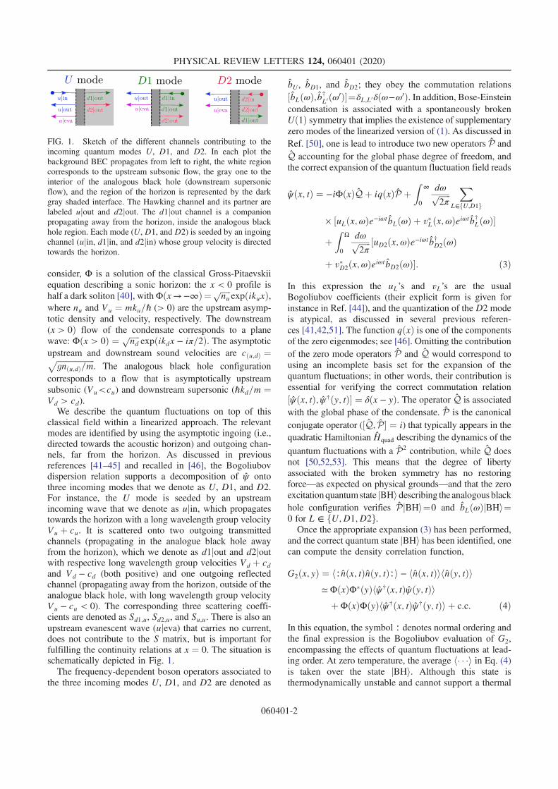
consider, Φ is a solution of the classical Gross-Pitaevskiiequation describing a sonic horizon: the x < 0 profile ishalf a dark soliton [40], withΦðx→−∞Þ¼ ffiffiffiffiffi
nup
expðikuxÞ,where nu and Vu ¼ mku=ℏ (> 0) are the upstream asymp-totic density and velocity, respectively. The downstream(x > 0Þ flow of the condensate corresponds to a planewave: Φðx > 0Þ ¼ ffiffiffiffiffi
ndp
expðikdx − iπ=2Þ. The asymptoticupstream and downstream sound velocities are cðu;dÞ ¼ffiffiffiffiffiffiffiffiffiffiffiffiffiffiffiffiffiffiffignðu;dÞ=m
p. The analogous black hole configuration
corresponds to a flow that is asymptotically upstreamsubsonic (Vu<cu) and downstream supersonic (ℏkd=m ¼Vd > cd).We describe the quantum fluctuations on top of this
classical field within a linearized approach. The relevantmodes are identified by using the asymptotic ingoing (i.e.,directed towards the acoustic horizon) and outgoing chan-nels, far from the horizon. As discussed in previousreferences [41–45] and recalled in [46], the Bogoliubovdispersion relation supports a decomposition of ψ ontothree incoming modes that we denote as U, D1, and D2.For instance, the U mode is seeded by an upstreamincoming wave that we denote as ujin, which propagatestowards the horizon with a long wavelength group velocityVu þ cu. It is scattered onto two outgoing transmittedchannels (propagating in the analogue black hole awayfrom the horizon), which we denote as d1jout and d2joutwith respective long wavelength group velocities Vd þ cdand Vd − cd (both positive) and one outgoing reflectedchannel (propagating away from the horizon, outside of theanalogue black hole, with long wavelength group velocityVu − cu < 0). The corresponding three scattering coeffi-cients are denoted as Sd1;u, Sd2;u, and Su;u. There is also anupstream evanescent wave (ujeva) that carries no current,does not contribute to the S matrix, but is important forfulfilling the continuity relations at x ¼ 0. The situation isschematically depicted in Fig. 1.The frequency-dependent boson operators associated to
the three incoming modes U, D1, and D2 are denoted as
bU, bD1, and bD2; they obey the commutation relations½bLðωÞ;b†L0 ðω0Þ¼δL;L0δðω−ω0Þ. In addition, Bose-Einsteincondensation is associated with a spontaneously brokenUð1Þ symmetry that implies the existence of supplementaryzero modes of the linearized version of (1). As discussed inRef. [50], one is lead to introduce two new operators P andQ accounting for the global phase degree of freedom, andthe correct expansion of the quantum fluctuation field reads
ψðx; tÞ ¼ −iΦðxÞQþ iqðxÞP þZ
∞
0
dωffiffiffiffiffiffi2π
pX
L∈fU;D1g
× ½uLðx;ωÞe−iωtbLðωÞ þ vLðx;ωÞeiωtb†LðωÞ
þZ
Ω
0
dωffiffiffiffiffiffi2π
p ½uD2ðx;ωÞe−iωtb†D2ðωÞ
þ vD2ðx;ωÞeiωtbD2ðωÞ: ð3Þ
In this expression the uL’s and vL’s are the usualBogoliubov coefficients (their explicit form is given forinstance in Ref. [44]), and the quantization of the D2 modeis atypical, as discussed in several previous referen-ces [41,42,51]. The function qðxÞ is one of the componentsof the zero eigenmodes; see [46]. Omitting the contributionof the zero mode operators P and Q would correspond tousing an incomplete basis set for the expansion of thequantum fluctuations; in other words, their contribution isessential for verifying the correct commutation relation½ψðx; tÞ; ψ†ðy; tÞ ¼ δðx − yÞ. The operator Q is associatedwith the global phase of the condensate. P is the canonicalconjugate operator (½Q; P ¼ i) that typically appears in thequadratic Hamiltonian Hquad describing the dynamics of the
quantum fluctuations with a P2 contribution, while Q doesnot [50,52,53]. This means that the degree of libertyassociated with the broken symmetry has no restoringforce—as expected on physical grounds—and that the zeroexcitationquantumstate jBHidescribing the analogous blackhole configuration verifies PjBHi¼0 and bLðωÞjBHi¼0 for L ∈ fU;D1; D2g.Once the appropriate expansion (3) has been performed,
and the correct quantum state jBHi has been identified, onecan compute the density correlation function,
G2ðx; yÞ ¼ h∶nðx; tÞnðy; tÞ∶i − hnðx; tÞihnðy; tÞi≃ΦðxÞΦðyÞhψ†ðx; tÞψðy; tÞi
þΦðxÞΦðyÞhψ†ðx; tÞψ†ðy; tÞi þ c:c: ð4Þ
In this equation, the symbol ∶ denotes normal ordering andthe final expression is the Bogoliubov evaluation of G2,encompassing the effects of quantum fluctuations at lead-ing order. At zero temperature, the average h i in Eq. (4)is taken over the state jBHi. Although this state isthermodynamically unstable and cannot support a thermal
FIG. 1. Sketch of the different channels contributing to theincoming quantum modes U, D1, and D2. In each plot thebackground BEC propagates from left to right, the white regioncorresponds to the upstream subsonic flow, the gray one to theinterior of the analogous black hole (downstream supersonicflow), and the region of the horizon is represented by the darkgray shaded interface. The Hawking channel and its partner arelabeled ujout and d2jout. The d1jout channel is a companionpropagating away from the horizon, inside the analogous blackhole region. Each mode (U, D1, and D2) is seeded by an ingoingchannel (ujin, d1jin, and d2jin) whose group velocity is directedtowards the horizon.
PHYSICAL REVIEW LETTERS 124, 060401 (2020)
060401-2

distribution, finite temperature effects can still be includedas explained for instance in Refs. [31,41,42].In 2008 a collaboration between teams from Bologna
and Trento [54,55] pointed out that, in the presence of ahorizon, G2 should exhibit nonlocal features resultingfrom correlations between the different outgoing chan-nels, in particular, between the Hawking quantum and itspartner (ujout − d2jout correlation in our terminology).The importance of this remark lies in the fact that, due tothe weak Hawking temperature TH (at best one fourthof the chemical potential [44]), the direct Hawkingradiation is expected to be hidden by thermal fluctua-tions, whereas density correlations should survive temper-ature effects in typical settings [42]. This idea has beenused to analyze the Hawking signal in Ref. [22], where astationary correlation pattern was measured in the vicinityof the horizon. In this region, it is important for atheoretical treatment to account for the position depend-ence of the background density and to include thecontribution of the evanescent channels in the expansion(3). We also checked that it is essential to take intoaccount the contribution of the zero modes to obtain asensible global description of the quantum fluctuations.The corresponding two-dimensional plot of the densitycorrelation pattern is represented in Fig. 2. G2 has beencomputed at zero temperature, for Vd=cd ¼ 2.90, whichimposes Vu=cu ¼ 0.59 [44,46]. This value is chosen toreproduce the experimental configuration studied in
Ref. [22]. The dotted line in the upper left quadrantof Fig. 2 marks the anticorrelation curve that resultsfrom the Hawking-partner (ujout−d2jout) and Hawking-companion (ujout − d1jout) correlations. We find thatthese two correlation lines, which separate at largedistance from the horizon [42,44,55], merge close tothe horizon, as also observed experimentally.A precise comparison of our results with experiment
can be achieved by following the procedure used inRef. [22], which consists in averaging G2 over the regioninside the green rectangle represented in Fig. 2. One definesa local coordinate x00 that is orthogonal to the locus of theminima of G2, and one plots the averaged G2 (denoted asGav
2 ) as a function of the variable x00. This is done in Fig. 3.
We insist that the good agreement between our approachand the experimental results can only be achieved through acorrect description of the quantum fluctuations—Eq. (3)—including the contribution of zero modes and evanescentchannels.It has been noticed by Steinhauer [56] that the determi-
nation of G2ðx; x0Þ in the upper left (or lower right)quadrant of the ðx; x0Þ plane makes it possible to evaluatethe Hawking temperature thanks to the relation
Su;d2ðωÞSd2;d2ðωÞ ¼ hcUðωÞcD2ðωÞi
¼ S−10ffiffiffiffiffiffiffiffiffiffiffiffiffiffiffiffiffiffiffiffi
nundLuLdp
Z0
−Lu
dxZ
Ld
0
dx0e−iðkHxþkPx0ÞG2ðx; x0Þ:
ð5Þ
In this expression S is the matrix that describes thescattering of the different channels onto each other, andS0ðωÞ ¼ ðukH þ vkHÞðukP þ vkPÞ is the static structurefactor, where the uk’s and the vk’s are the standardBogoliubov amplitudes of excitations of momentum k(see, e.g., Refs. [57,58]). The cL’s are outgoing modesrelated to the incoming ones by the S matrix [42]
FIG. 2. Intensity plot of the dimensionless correlation functionξðnundÞ−1=2G2ðx; x0Þ for x and x0 close to the horizon. Theparameter ξ ¼ ffiffiffiffiffiffiffiffiffi
ξuξdp
is the geometrical mean of the healinglengths ξu and ξd, where ξðu=dÞ ¼ ℏðmgnðu;dÞÞ−1=2. The line ofanticorrelation in the upper left and lower right quadrantscorresponds to the merging close to the horizon of theHawking-partner (ujout − d2jout) and Hawking-companion(ujout − d1jout) correlations. The green rectangle delimits theregion where we average G2 for comparison with experimentaldata (see Fig. 3).
FIG. 3. Red solid line: zero temperature density correlationfunction Gav
2 ðx; x0Þ plotted as a function of x00. The blue dots witherror bars are the results of Ref. [22]. The orange solid line is thefinite temperature result for kBT ¼ 0.2gnu, i.e., T ≃ 1.9TH .
PHYSICAL REVIEW LETTERS 124, 060401 (2020)
060401-3

0B@
cUcD1
c†D2
1CA ¼
0B@
Su;u Su;d1 Su;d2Sd1;u Sd1;d1 Sd1;d2Sd2;u Sd2;d1 Sd2;d2
1CA
0B@
bU
bD1
b†D2
1CA: ð6Þ
The Fourier transform of G2 in Eq. (5) is performed atfixed ω, for wave vectors kHðωÞ and kPðωÞ, which are themomenta relative to the condensate of a Hawking quantumand its partner (ujout and d2jout channels in our terminol-ogy) having an energy ℏω in the laboratory frame. Theintegration region ½−Lu; 0 × ½0; Ld lies in the upper leftquadrant of Fig. 2, and should be adapted for each value ofω in such a way that [31,59]
Lu
jVg;HðωÞj¼ Ld
Vg;PðωÞ; ð7Þ
where Vg;HðωÞ [Vg;PðωÞ] is the group velocity of aHawking quantum (of a partner) of energy ℏω. We havechecked that once the prescription (7) is fulfilled, for-mula (5) is very well verified [46]. It is then intriguing toobserve that, while theory and experiment both agree onthe value of G2 in real space (Fig. 3), they do not for thecorrelation hcUðωÞcD2ðωÞi: as can bee seen in Fig. 4, theagreement is restricted to the low energy regime. This isthe bluish region in the figure, which corresponds to adomain where the ratio kHðωÞ=kPðωÞ is equal to its longwavelength value ðcu − VuÞ=ðcd − VdÞ with an error lessthat 10%.Let us discuss this discrepancy in some detail. The
interest of Eq. (5) lies in the fact that the scattering matrix
coefficient Su;d2 is the equivalent of the Hawking βparameter: its squared modulus is expected to behave asa Bose thermal distribution nTHðωÞ with an effectivetemperature TH, the Hawking temperature [1]. In ananalogous system such as ours, because of dispersiveeffects, this equivalence is only valid in the long wave-length limit, typically in the blue region of Fig. 4. Thissuggests a possible manner to reconcile theory and experi-ment: we assume that the ratio kHðωÞ=kPðωÞ is ω inde-pendent and equal to its low energy value, ðcu − VuÞ=ðcd − VdÞ (this value is denoted as tan θ in Refs. [21,22]).We also assume that, in the scattering process schematicallyillustrated in Fig. 1 for theD2mode, the companion d1joutchannel plays a negligible role, so that the jSd1;d2j2 term canbe omitted in the normalization condition jSd2;d2j2 ¼ 1þjSu;d2j2 þ jSd1;d2j2 of the S matrix (see, e.g., Ref. [42]).Then one obtains
jSu;d2j2jSd2;d2j2 ≃ nTHðωÞ½1þ nTHðωÞ: ð8Þ
Using the experimental values from Ref. [22] for Vα and cα(α ∈ fu; dg) and for the Hawking temperature TH leads,within approximation (8), to the blue curve of Fig. 4 thatagrees with the results published in Ref. [22] (blue dotswith error bars). It is important to note that this procedure isself-consistent in the following sense: If one performsnumerically the Fourier transform (5) over a domain that,instead of fulfilling the relation (7), verifies the ω-inde-pendent condition Lu=jVu − cuj ¼ Ld=ðVd − cdÞ, appro-priate in a nondispersive, long wavelength approximation,one obtains a result (not shown for legibility, but see [46])close to a thermal spectrum, i.e., to the blue curve in Fig. 4.Although this procedure is self-consistent, it is not fullycorrect, as can be checked by the fact that the resultingvalue of hcUðωÞcD2ðωÞi only agrees with the exact one (redcurve in Fig. 4) in the long wavelength limit. Stateddifferently: this procedure leads to the erroneous conclu-sion that the radiation is fully thermal. However, since allapproaches coincide in the long wavelength regime (bluecolored region of Fig. 4), they all lead to the correctdetermination of the Hawking temperature. For a flow withVd=cd¼2.9, our theoretical treatment yields kBTH=ðgnuÞ¼0.106, whereas the experimental value reported for thisquantity in Ref. [22] is 0.124 (corresponding to a Hawkingtemperature TH ¼ 0.35 nK).In conclusion, our work sheds a new light on the study of
quantum correlations around an analogous black holehorizon, and on the corresponding Hawking temperature.From a theoretical point of view, we argue that thecontribution of zero modes is essential for constructing acomplete basis set necessary to obtain an accurate descrip-tion of the quantum fluctuations. This claim is supported bythe excellent agreement we obtain when comparing ourresults with recent experimental ones. On the experimentalside, we substantiate the determination of the Hawking
FIG. 4. Hawking-partner correlation signal represented as afunction of the dimensionless energy. The red solid curve is thetheoretical result from Eq. (5). The dots with error bars are fromRef. [22]. They are obtained after processing the experimentalresult for G2 by means of the Fourier transform (5). The blueregion corresponds to a domain where the ratio of Hawking andpartner wave vectors is equal to its long wavelength value withina 10% accuracy. The blue solid curve is the theoretical resultobtained by neglecting dispersive effects in Eq. (5) and discardingthe contribution of the companion d1jout channel (see the text).
PHYSICAL REVIEW LETTERS 124, 060401 (2020)
060401-4

temperature presented in Ref. [22], although we find thatthe Hawking spectrum is not thermal for all wavelengths.We identify a natural but unfounded procedure for analyz-ing the information encoded in G2ðx; x0Þ that leads to theopposite conclusion; we show that, within our approach, analternative analysis of the correlation pattern accuratelyaccounts for nonhydrodynamical effects. It would thus beinteresting to reanalyze the data published in Ref. [22] toinvestigate if the windowing (7) we propose for Eq. (5)modifies the experimental conclusion for the Hawking-partner correlation signal and confirms the departure fromthermality we predict.
We acknowledge fruitful discussions with I. Carusotto,M. Lewenstein, and J. Steinhauer, whom we also thank forproviding us with experimental data.
[1] S. W. Hawking, Nature (London) 248, 30 (1974); Commun.Math. Phys. 43, 199 (1975).
[2] M. Visser, Phys. Rev. Lett. 80, 3436 (1998).[3] W. G. Unruh, Phys. Rev. Lett. 46, 1351 (1981).[4] G. Rousseaux, C. Mathis, P. Maïssa, T. G. Philbin, and U.
Leonhardt, New J. Phys. 10, 053015 (2008).[5] S. Weinfurtner, E. W. Tedford, M. C. J. Penrice, W. G.
Unruh, and G. A. Lawrence, Phys. Rev. Lett. 106,021302 (2011).
[6] L.-P. Euve, F. Michel, R. Parentani, T. G. Philbin, and G.Rousseaux, Phys. Rev. Lett. 117, 121301 (2016).
[7] V. Cardoso, A. Coutant, M. Richartz, and S. Weinfurtner,Phys. Rev. Lett. 117, 271101 (2016).
[8] T. Torres, S. Patrick, A. Coutant, M. Richartz, E. W.Tedford, and S. Weinfurtner, Nat. Phys. 13, 833 (2017).
[9] L.-P. Euve, S. Robertson, N. James, A. Fabbri, and G.Rousseaux, arXiv:1806.05539.
[10] H. Goodhew, S. Patrick, C. Gooding, and S. Weinfurtner,arXiv:1905.03045.
[11] T. G. Philbin, C. Kuklewicz, S. Robertson, S. Hill, F. König,and U. Leonhardt, Science 319, 1367 (2008).
[12] F. Belgiorno, S. L. Cacciatori, M. Clerici, V. Gorini, G.Ortenzi, L. Rizzi, E. Rubino, V. G. Sala, and D. Faccio,Phys. Rev. Lett. 105, 203901 (2010).
[13] E. Rubino, F. Belgiorno, S. L. Cacciatori, M. Clerici, V.Gorini, G. Ortenzi, L. Rizzi, V. G. Sala, M. Kolesik, and D.Faccio, New J. Phys. 13, 085005 (2011).
[14] M. Elazar, V. Fleurov, and S. Bar-Ad, Phys. Rev. A 86,063821 (2012).
[15] K. E. Webb, M. Erkintalo, Y. Xu, N. G. R. Broderick, J. M.Dudley, G. Genty, and S. G. Murdoch, Nat. Commun. 5,4969 (2014).
[16] D.Vocke, C.Maitland, A. Prain, K. E.Wilson, F. Biancalana,E. M. Wright, F. Marino, and D. Faccio, Optica 5, 1099(2018).
[17] J. Drori, Y. Rosenberg, D. Bermudez, Y. Silberberg, and U.Leonhardt, Phys. Rev. Lett. 122, 010404 (2019).
[18] H. S. Nguyen, D. Gerace, I. Carusotto, D. Sanvitto, E.Galopin, A. Lemaître, I. Sagnes, J. Bloch, and A. Amo,Phys. Rev. Lett. 114, 036402 (2015).
[19] O. Lahav, A. Itah, A. Blumkin, C. Gordon, S. Rinott, A.Zayats, and J. Steinhauer, Phys. Rev. Lett. 105, 240401(2010).
[20] J. Steinhauer, Nat. Phys. 10, 864 (2014).[21] J. Steinhauer, Nat. Phys. 12, 959 (2016).[22] J. R. M. de Nova, K. Golubkov, V. I. Kolobov, and J.
Steinhauer, Nature (London) 569, 688 (2019).[23] F. Michel and R. Parentani, Phys. Rev. A 91, 053603 (2015).[24] F. Michel, J.-F. Coupechoux, and R. Parentani, Phys. Rev. D
94, 084027 (2016).[25] M. Tettamanti, S. L. Cacciatori, A. Parola, and I. Carusotto,
Europhys. Lett. 114, 60011 (2016).[26] J. R. M. de Nova, S. Finazzi, and I. Carusotto, Phys. Rev. A
94, 043616 (2016).[27] A. Finke, P. Jain, and S. Weinfurtner, New J. Phys. 18,
113017 (2016).[28] Y.-H. Wang, T. Jacobson, M. Edwards, and C.W. Clark,
SciPost Phys. 3, 022 (2017).[29] A. Parola, M. Tettamanti, and S. L. Cacciator, Europhys.
Lett. 119, 50002 (2017).[30] S. Robertson, F. Michel, and R. Parentani, Phys. Rev. D 96,
045012 (2017).[31] A. Fabbri and N. Pavloff, SciPost Phys. 4, 019 (2018).[32] A. Coutant and S. Weinfurtner, Phys. Rev. D 97, 025006
(2018).[33] J. M. Gomez Llorente and J. Plata, J. Phys. B 52, 075004
(2019).[34] U. Leonhardt, Ann. Phys. (Berlin) 530, 1700114 (2018).[35] J. Steinhauer, Ann. Phys. (Berlin) 530, 1700459 (2018).[36] W. G. Unruh, Phys. Rev. D 51, 2827 (1995).[37] S. Corley and T. Jacobson, Phys. Rev. D 54, 1568 (1996).[38] S. Corley, Phys. Rev. D 55, 6155 (1997).[39] T. Jacobson, Phys. Rev. D 44, 1731 (1991).[40] P. Leboeuf, N. Pavloff, and S. Sinha, Phys. Rev. A 68,
063608 (2003).[41] J. Macher and R. Parentani, Phys. Rev. A 80, 043601 (2009).[42] A. Recati, N. Pavloff, and I. Carusotto, Phys. Rev. A 80,
043603 (2009).[43] A. Coutant, R. Parentani, and S. Finazzi, Phys. Rev. D 85,
024021 (2012).[44] P.-É. Larre, A. Recati, I. Carusotto, and N. Pavloff, Phys.
Rev. A 85, 013621 (2012).[45] D.Boiron,A. Fabbri, P.-É. Larre, N. Pavloff, C. I.Westbrook,
and P. Ziń, Phys. Rev. Lett. 115, 025301 (2015).[46] See Supplemental Material at http://link.aps.org/
supplemental/10.1103/PhysRevLett.124.060401 which re-calls previous results, details some characteristics of the zeromodes and of the analysis of the Hawking spectrum andincludes Refs. [47–49].
[47] P. Villain, M. Lewenstein, R. Dum, Y. Castin, L. You, A.Imamoğlu, and T. A. B. Kennedy, J. Mod. Opt. 44, 1775(1997).
[48] N. Bilas and N. Pavloff, Phys. Rev. A 72, 033618 (2005).[49] P. Deuar, A. G. Sykes, D. M. Gangardt, M. J. Davis, P. D.
Drummond, and K. V. Kheruntsyan, Phys. Rev. A 79,043619 (2009).
[50] M. Lewenstein and L. You, Phys. Rev. Lett. 77, 3489(1996).
[51] U. Leonhardt, T. Kiss, and P. Öhberg, J. Opt. B 5, S42(2003).
PHYSICAL REVIEW LETTERS 124, 060401 (2020)
060401-5

[52] P. Ring and P. Shuck, The Nuclear Many-Body Problem(Springer-Verlag, Berlin, 1980).
[53] J. P. Blaizot and G. Ripka, Quantum Theory of FiniteSystems (MIT Press, Cambridge, MA, 1986).
[54] R. Balbinot, A. Fabbri, S. Fagnocchi, A. Recati, and I.Carusotto, Phys. Rev. A 78, 021603(R) (2008).
[55] I. Carusotto, S. Fagnocchi, A. Recati, R. Balbinot, and A.Fabbri, New J. Phys. 10, 103001 (2008).
[56] J. Steinhauer, Phys. Rev. D 92, 024043 (2015).
[57] C. J. Pethick and H. Smith, Bose-Einstein Condensation inDilute Gases (Cambridge University Press, Cambridge,England, 2002).
[58] L. P. Pitaevskii and S. Stringari, Bose-Einstein Conde-nsation, International Series of Monographs on Physics(Oxford University Press, Oxford, United Kingdom,2016).
[59] J. R. M. de Nova, F. Sols, and I. Zapata, New J. Phys. 17,105003 (2015).
PHYSICAL REVIEW LETTERS 124, 060401 (2020)
060401-6

Supplemental material to:Departing from thermality of analogue Hawking radiation in a Bose-Einstein
condensate
M. Isoard1 and N. Pavloff1
1Universite Paris-Saclay, CNRS, LPTMS, 91405 Orsay, France
THE BACKGROUND FLOW AND DENSITYPROFILES
We recall here the properties of the background tran-sonic flow Φ(x) realizing an analogue black hole horizon[1]. Φ(x) is solution of the classical stationary Gross-Pitaevskii equation
µΦ = − ~2
2m∂2xΦ + [g n(x) + U(x)] Φ , (S1)
with n(x) = |Φ(x)|2 and U(x) = −U0Θ(x), where Θ isthe Heaviside step function and U0 > 0. There exists astationary solution of this equation which is half a darksoliton glued at x = 0 to a plane wave [2]:
Φ(x) =
√nu exp(ikux)χu(x) ≡ Φu(x) for x ≤ 0,√nd exp(ikdx− iπ/2) ≡ Φd(x) for x ≥ 0.
(S2)where
χu(x) = cos θ tanh(x cos θ/ξu)− i sin θ. (S3)
In these equations nu and nd are the asymptotic up-stream and downstream densities, ξu = ~(mgnu)−1/2 isthe upstream healing length and sin θ = Vu/cu where Vuand cu = ~/(mξu) are the asymptotic flow and soundvelocities. The downstream flow and sound velocity areVd = ~kd/m and cd =
√gnd/m. The chemical potential
µ in Eq. (S1) verifies
µ = 12mV
2u + gnu = 1
2mV2d + gnd − U0. (S4)
The matching conditions at x = 0 impose
VdVu
=nund
=
(cuVu
)2
=Vdcd. (S5)
Hence, in this configuration, which we denote as “wa-terfall”, the upstream and downstream Mach numbers(Vu/cu and Vd/cd) are not independent. We chose totake the same downstream Mach number than in theexperiment [3]: Vd/cd = 2.9. From (S5) this imposesVu/cu = 0.59, different from the experimental value(Vu/cu|exp = 0.44). This difference indicates that theexperiment is not exactly in a waterfall configuration.This is probably due to the fact that the experimentalexternal potential is not exactly a Heaviside function.It could also be that the experimental flow has not yet
reached a fully stationary state. This difference does notpreclude a very good agreement with the experimentaldensity correlation pattern (as observed in Fig. 3 of themain text); however, it explains why we cannot repro-duce with the same accuracy the behavior of the densitycorrelation function G2(x, x′) in all the quadrants of Fig.2 of the main text: the d1|out − d2|out correlation line(upper right quadrant of Fig. 2 of the main text) doesnot exactly superimposes with the experimental one. Wetake the same value of Vd/cd as in the experiment, be-cause this is the choice which gives the better account ofexperiment in the upper left quadrant of Fig. 2 of themain text, which is the core of the discussion of Ref. [3].
THE BOGOLIUBOV-DE GENNES EQUATIONS
In this section we present the construction of expan-sion (3) of the main text. The first part of the section isdevoted to the definition of the usual Bogoliubov modes,and is an abridged version of a discussion which can befound in Ref. [1]; the second part concerns the construc-tion of the zero modes and comprises a general discus-sion (from Refs. [4–6]) followed by the explicit form ofthese modes in the situation we consider [Eqs. (S14) and(S15)].
The simplest way to set up an eigen-basis set for ex-panding the quantum fluctuation operator is to treatψ as a small classical field, denoted as ψ, withexp(−iµt/~)(Φ + ψ) solution of the classical version ofEq. (1) of the main text. One then looks for a normalmode of the form
ψ(x, t) = u(x, ω)e−iωt + v∗(x, ω)eiωt (S6)
For such a normal mode, the linearization of the Gross-Pitaevskii equation leads to the so-called Bogoliubov-de Gennes equation which reads LΞ = ~ω Ξ, whereΞ(x, ω) = (u(x, ω) , v(x, ω))T and
L =
(H Φ2(x)
−(Φ∗(x))2 −H
), (S7)
with H = ~2
2m∂2x + U(x) − 2gn(x) − µ. Far upstream,
the background density being constant, the eigen-modesbehave as plane waves of the form
Ξ(x, ω) =
(u(x, ω)v(x, ω)
)−→
x→−∞eiqx
(exp(ikux)Uω
exp(−ikux)Vω
)
(S8)

2
where Uω and Vω are complex constants, their explicitexpression can be found in Ref. [1], together with thegeneral expression of u(x, ω) and v(x, ω). The same typeof behavior is observed downstream. The correspondingdispersion relations are of the form
(ω − Vαq)2= ω2
B(q), (S9)
where α = u far upstream and α = d downstream and
ωB(q) = cαq√
1 + q2ξ2α/4 (S10)
is the Bogoliubov dispersion relation. The asymptoticupstream and downstream dispersion relations are rep-resented in Fig. SF1. One sees in this figure that, foreach value of ω, there exists three incoming channels,i.e., three plane waves which group velocity is directedtowards the horizon. One of these plane waves lies in theupstream region, we denote it as u|in, the two others liein the downstream region: d1|in and d2|in.
Once the eigen-modes Ξ has been found for all non-zero frequencies, the eigen-basis needs to be completedwith the addition of zero modes for which ω = 0. First,it is clear that L admits a simple zero mode:
LP = 0 , where P =
(Φ(x)−Φ∗(x)
). (S11)
The physical interpretation of the existence of this zeromode is the following: it results from the U(1) symmetrybreaking of the condensate wave function and it is a col-lective mode with no restoring force, which is sometimesdenoted as a spurious mode [4, 5]. Indeed, if Φ is a sta-tionary solution of the Gross-Pitaevskii equation, for anyarbitrary constant θ, Φθ(x) = Φ(x) eiθ is also a station-ary solution. Φθ tends continuously to Φ when θ → 0,hence δΦ = Φθ −Φ ' i θΦ is a solution of the linearizedGross-Pitaevskii equation. This immediately translatesinto the fact that (δΦ, δΦ∗)T = i θP is a zero mode of L.
Another mode of excitation corresponds to addition ofparticles to the system [6]. By differentiating the Gross-Pitaevskii equation with respect to the number of parti-cles N , we find the mode Q associated to P:
Q =
(q(x)−q∗(x)
), with LQ = −i d µ
dNP, (S12)
where µ is the chemical potential of the condensate. Thetwo modes Q and P complete the eigen-basis of L, or,more precisely, make it possible to write L in a Jordannormal form. The field operator ψ which describes thequantum fluctuations can be now expanded over the scat-
FIG. SF1: Graphical representation of the dispersion rela-tion, i.e., of the solutions of Eq. (S9) in the far upstream(upper plot) and far downstream (lower plot) regions. In theupstream region, for a given ω (represented by a horizontaldashed line) one finds two real solutions of Eq. (S9) whichwe denote as qu|in and qu|out. The intercept of the horizon-tal dashed line with the corresponding dispersion relation ismarked with a colored dot labeled u|in or u|out, as appro-priate. The situation is different downstream: there exists athreshold energy below which Eq. (S9) admits 4 real solutionswhich we denote as qd1|in, qd1|out, qd2|in and qd2|out. Both d2solutions disappear above the threshold. All these solutionscorrespond to the channels identified in the main text. Theyare denoted as “in” (“out”) is their group velocity – schemat-ically represented by an arrow – is directed towards (awayfrom) the horizon.
tering modes and the zero modes:
ψ(x, t) =− iΦ(x)Q+ iq(x)P +
∫ ∞
0
dω√2π
∑
L∈U,D1
[uL(x, ω)e−iωt bL(ω) + v∗L(x, ω)eiωt b†L(ω)]
+
∫ Ω
0
dω√2π
[uD2(x, ω)e−iωt b†D2(ω)
+ v∗D2(x, ω)eiωt bD2(ω)].
(S13)

3
In this expression the uL’s and the vL’s are linear combi-nations of terms of the form (S8) involving the S-matrix(see Refs. [1, 7]), and Q is the phase operator of the con-densate, while P corresponds to the fluctuations of thenumber of particles. The quadratic Hamiltonian Hquad
describing the linear dynamics of the elementary exci-tations of the system contains a term P2/2Meff , where1/Meff = dµ/dN [4–6]. Thus, the operator P can beidentified with a momentum operator and Meff with aneffective mass. In addition, the commutation relation[Q, Hquad] = i P/Meff indicates that the phase operator
Q(t) is not stationary and deviates from its initial valueQ(t = 0). This is the phenomenon of phase diffusion,see, e.g, Ref. [8].
In our case, the system is infinite: no phase diffusioncan occur and Meff → ∞. The physical interpretationof this phenomenon is that the inertia associated to thechange of the global phase of a system of infinite num-
ber of particles is infinite. Therefore, the mode Q is alsosolution of LQ = 0 [see Eq. (S12) with dµ/dN → 0].Moreover, the operator L has a different expression forx < 0 and x > 0, just because Φ does [see Eq. (S2)]. Asa result, L admits zero energy eigen-states (ω = 0) whichhave different forms in the upstream and the downstreamregion. The modes P and Q should be written as linearcombinations of these zero modes. In particular, in theupstream region the density profile is a portion of darksoliton [see Eq. (S2)], and the expression of the corre-sponding zero modes can be found, e.g., in Ref. [9]. Oneobtains
P(x < 0) =
(Φu(x)−Φ∗u(x)
)and P(x > 0) =
(Φd(x)−Φ∗d(x)
),
(S14)while
Q(x < 0) = i√nuA
[cos θ tanh(x cos θ/ξu)− Λu
2
]2
eΛu x/ξu
(ei ku x
e−i ku x
)and
Q(x > 0) = B
(Φd(x)−Φ∗d(x)
)+ C eiK0 x/ξd
([K0/2−Md] Φd(x)[K0/2 +Md] Φ∗d(x)
)+ C e−iK0 x/ξd
([−K0/2−Md] Φd(x)[−K0/2 +Md] Φ∗d(x)
),
(S15)
with Λu = 2√
1−M2u = 2 cos θ and K0 = 2
√M2d − 1,
where Mu and Md are the upstream and downstreamMach numbers (Mα = Vα/cα). In expression (S15), thenormalization factors A, B and C are dimensionless realnumbers which are determined by imposing the matchingconditions at x = 0 and the commutation relation be-tween Q and P: [Q, P] = i, or equivalently, Q† σz P = i,where σz is the third Pauli matrix.
FOURIER TRANSFORM OF THE DENSITYCORRELATION FUNCTION
The computation of the Fourier transform of the G2
function gives access to the correlation signal betweenthe Hawking pair [kH(ω), kP(ω)] in momentum space fora fixed energy ~ω in the lab frame, see Eq. (5) ofthe main text. The wave vectors kH = qu|out(ω) andkP = −qd2|out(ω) are the momenta relative to the con-densate of the Hawking quantum and of its partner (seethe discussion in Ref. [7]). We define
I(ω) =1√
nu nd Lu Ld×
∫ 0
−Lu
dx
∫ Ld
0
dx′ e−i(kH(ω) x+kP(ω) x′)G2(x, x′),
(S16)
where G2 is the density correlation function [Eq. (4)of the main text]. The quantities nu and nd are theasymptotic densities in both regions (when x→ −∞ andx′ → +∞).
As proved in Refs. [7, 10], the integration in Eq. (S16)should be performed over a domain [−Lu, 0] × [0, Ld]which is adapted to each Hawking pair [kH(ω), kP(ω)]:one should verify
Lu Vg,P(ω) = Ld |Vg,H(ω)| , (S17)
where
Vg,I(ω) ≡ ∂ω
∂k
∣∣∣∣kI
, I ∈ H, P. (S18)
This condition has a physical interpretation: the timetaken by an elementary excitation pertaining to theHawking channel to go from the horizon to the centerof the upstream window [−Lu, 0] has to be the sameas the time taken by its partner to go from the hori-zon to the center of the downstream window [0, Ld].The Fourier transform can be calculated theoretically forLu, Ld → +∞ [still verifying (S17)] and this leads to Eq.(5) of the main text, i.e.:
I(ω) = S0 Sud2(ω)S∗d2d2(ω). (S19)
Fig. SF2 compares the numerical computation of theFourier transform (S16) (black dots), when the choice of

4
the window [−Lu, 0] × [0, Ld] respects condition (S17),with the theoretical expectation [left hand side of Eq.(S19), red curve in the figure]. We observe a nice agree-ment, except, of course, for long wavelengths where thevalidity condition of Eq. (S19): kHLu and kPLd 1 isviolated.
The choice of the window is crucial; for example, theorange triangles in Fig. SF2 are obtained for anotherprescription which corresponds to the long wavelengthlimit of Eq. (S17):
Lu Vg,H(0) = Ld |Vg,P(0)| , (S20)
where Vg,H(0) = Vu − cu and Vg,P(0) = Vd − cd are thegroup velocities of the Hawking quantum kH and its part-ner kP in the long wavelength limit. As expected, the re-sult deviates from the evaluation which uses the correctcondition (S17).
To recover the numerical result obtained by using theprescription (S20), we use the following approximations:(i) we assume that kH(ω) = ω/(Vu − cu) and kP(ω) =ω/(Vd− cd), as if we were in the dispersionless regime forall frequencies ω, and (ii) we also assume that Sud2(ω) 'nTH(ω), with nTH(ω) (the Bose thermal distribution atthe Hawking temperature) and that |Sud2|2 |S∗d2d2|2 'nTH
(ω)(1 + nTH(ω)) [Eq. (8) of the main text]. Then,
we compute expression (S19) using both approximations(i) and (ii): we obtain the dark blue curve in Fig. SF2which agrees well with the orange triangles.
In conclusion, one may numerically analyse the infor-mation contained in the density distribution G2 by usingEq. (S16) within the oversimplified long wavelength pre-scription (S20) and still get an equality between the twoterms of Eq. (S19). However, this approach could leadto the erroneous conclusion that the analogous Hawkingradiation is thermal for all frequencies ω. In our sys-tem, where dispersion plays an important role, only theresult represented by the red curve in Fig. SF2 shouldbe considered as correct, and it clearly deviates from thethermal result (dark blue curve in Fig. SF2).
EFFECT OF TEMPERATURE ON THEDENSITY CORRELATION FUNCTION
In this section, we discuss how to account for temper-ature effects in our system. We first note that the sta-tionary configuration we consider is thermodynamicallyunstable, and cannot support a thermal state. However,a thermal-like occupation of the states can be definedas detailed for instance in Ref. [7]. Previous studies[11] have already highlighted the robustness of the cor-relation signal, even if the temperature of the system isgreater than the Hawking temperature. Our results con-firm this point, as shown in Fig. 3 of the main text(the orange solid line is the finite temperature result forkB T = 0.2 gnu ' 1.9TH). At finite temperature, the
0.0 0.5 1.0h ω/g nu
0.00
0.01
|I(ω
)|2
FIG. SF2: Fourier transform of the G2 function, denoted asI(ω) and given by expression (S16), plotted as a function ofω. The red curve indicates the theoretical expectation: righthand side of Eq. (S19). The black dots are obtained by thenumerical computation of the Fourier transform (S16) withcondition (S17). The orange triangles are also obtained nu-merically, but for a different choice of window correspondingto prescription (S20). The dark blue curve is obtained from(S19) but in the long wavelength approximation, where theanalogous Hawking signal is thermal.
density correlation function G2(x, x′) splits in two parts[1, 11]:
G2(x, x′) = G02(x, x′) +GT2 (x, x′), (S21)
where G02 is the zero temperature contribution and GT2
accounts for the additional temperature effects. As al-ready mentioned in Refs. [11, 12], GT2 contains a termwhich corresponds to a thermal enhancement of zero tem-perature correlations, together with additional contribu-tions involving scattering processes specific to the T 6= 0case. This results in a practical disappearance of theu|out − d1|out correlation for kB T ' 0.2 gnu, while theu|out−d2|out Hawking signal is robust up to kB T ' gnu,see the discussion in Ref. [11]. This confirms the interestof using analog system to investigate analog Hawking ra-diation: the non-local correlation pattern in G2 is weaklyaffected by temperature and a noticeable signal can berecorded even if T is larger than TH.
The finite T result presented in the main text is ob-tained by computing the two contributions in (S21) sepa-rately, in a regime which has been denoted as the “weaklyinteracting quasicondensate regime” in Ref. [13], andwhich holds when the following conditions are met:
4 τ2α
(ξα nα)4 1
(ξα nα)2 1, (S22)
where α ∈ u, d and τα = kB T/(g nα) is the reducedtemperature. We use typical experimental parametersof Ref. [3] to evaluate the order of magnitude of the

5
different terms in the inequalities (S22): ξu = 1.4µm,ξd = 2.38µm, nu ' 70−90µm−1 and nd ' 20µm−1. Weobtain (ξu nu)−2 ' 6.3 × 10⁻⁵ − 10−4 1, (ξd nd)
−2 '4.4 × 10⁻⁴ 1. By computing the left hand part of(S22) in the upstream and downstream regions, we findthat the more stringent condition reads kB T 8.3 gnu,i.e., our approach is valid up to kB T ' 0.8−1 gnu TH.
[1] P.-E. Larre, A. Recati, I. Carusotto, and N. Pavloff, Phys.Rev. A 85, 013621 (2012).
[2] P. Leboeuf, N. Pavloff and S. Sinha, Phys. Rev. A 68,063608 (2003).
[3] J. R. M. de Nova, K. Golubkov, V. I. Kolobov, and J.Steinhauer, Nature (London) 569, 688 (2019).
[4] P. Ring and P. Shuck, The Nuclear Many-Body Problem(Springer-Verlag, Berlin, 1980).
[5] J. P. Blaizot and G. Ripka, Quantum Theory of FiniteSystems (MIT Press, Cambridge, MA, 1986).
[6] C. J. Pethick and H. Smith, Bose-Einstein Condensa-tion in Dilute Gases, (Cambridge University Press, Cam-bridge, England, 2002).
[7] A. Fabbri and N. Pavloff, SciPost Phys. 4, 019 (2018).[8] P. Villain, M. Lewenstein, R. Dum, Y. Castin, L. You,
A. Imamoglu, and T. A. B. Kennedy, J. Mod. Optics 44,1775 (1997).
[9] N. Bilas and N. Pavloff Phys. Rev. A 72, 033618 (2005).[10] J. R. M. de Nova, F. Sols and I. Zapata, New. J. Phys.
17, 105003 (2015).[11] A. Recati, N. Pavloff and I. Carusotto, Phys. Rev. A 80,
043603 (2009).[12] J. Macher and R. Parentani, Phys. Rev. A 80, 043601
(2009).[13] P. Deuar, A. G. Sykes, D. M. Gangardt, M. J. Davis, P.
D. Drummond and K. V. Kheruntsyan, Phys. Rev. A 79,043619 (2009).

4TRIPARTITE ENTANGLEMENT IN ANALOGUEGRAVITY
Hawking pairs emitted at the vicinity of a gravitational black hole areentangled. This peculiar property of quantum systems has triggeredmuch interest in general relativity [48, 49, 69, 139, 141, 190] in connec-tion to the so-called information loss paradox [12, 85, 89, 96, 122, 125,126, 155, 181, 185, 203] and the vivid debate around it [178] . Indeed,if black holes radiate a thermal radiation, as predicted by Hawking in1974 [87], they slowly evaporate and should disappear in a finite amountof time. As long as the black hole exists, the Hawking particle and its“Partner” emitted from each side of the event horizon are entangled.From an observer outside the black hole (and thus only able to detectthe presence of Hawking particles) the quantum state is perceived asa mixed state, but the full state (Hawking + partner) remains a pureentangled state. However, after the evaporation process, the quantumfield will remain entangled with the quantum field observables insidethe past black hole – even though the black hole has evaporated com-pletely. This means that any quantum field in a pure state evolves toa mixed state and the knowledge of the final state is not sufficient todetermine the initial state; in other words, there is a violation of unitar-ity [185] and information has been lost during this evaporation process;in particular, one can wonder what happens for the entangled Hawkingpair when the black hole has disappeared?These questions are still debated today and several suggestions have
been proposed to overcome this paradox [185]: no complete evaporationof the black hole, information coming out in a final burst, a firewallformed on the horizon – a barrier significantly diminishing entanglementacross the horizon, but requiring the quantum field to be singular onthe horizon.However, no theory is known today to solve unambiguously the prob-
lem. A natural question we might ask ourselves in this thesis: is analoguegravity able to give some insights on this fundamental issue of informa-tion loss paradox? A recent publication indeed suggested to use a plasmalaser to mimic an accelerating relativistic mirror1, giving rise to emis-sion of Hawking pairs from vacuum fluctuations [38]. Partner particlesare trapped beyond an horizon, while Hawking particles, reflected fromthe mirror, can be detected. Then, in the proposed experiment, theplasma mirror is suddenly stopped to imitate the final evaporation of ablack hole and to observe how trapped partner particles are released.In our case, acoustic analogues in Bose-Einstein condensates (BECs)
do not evaporate. However, quanta emitted spontaneously from vacuumfluctuations, i.e., elementary excitations on top of the condensate, share
1 see Section 2.1.1 for more details about particle creation by accelerating mirrors.
101

102 tripartite entanglement in analogue gravity
entanglement with each other. The study of entanglement in BECs isa first step to explore the peculiar quantum properties emerging fromthe presence of an horizon. It might be interesting in the future tosuggest new experimental setups in BECs to delve into the informationloss paradox; and our theoretical studies addressing several possibletools for evaluating the amount of bipartite (or tripartite) entanglementconstitute a preliminary step in this direction.This chapter is entirely dedicated to the study of entanglement emerg-
ing in sonic analogues in BECs. We show in particular that our systemgives rise to tripartite entanglement and we are able to determine thedegree of entanglement between the three outgoing modes emitted spon-taneously from the acoustic horizon.First, we need to introduce Bogoliubov transformations and precise
their specific properties in the case we consider. Then, we present sometools to quantify and measure entanglement. In a third part, we studytripartite entanglement.
4.1 bogoliubov transformations
In this section, we consider linear transformations that preserve canon-ical commutation rules for boson operators. We will restrict ourselvesto the case of unitary transformations.
4.1.1 General case
Let us consider N creation and annihilation boson operatorsb = (b1, . . . , bN , b
†1, . . . , b
†N)T, with the usual commutation relation
[bi, bj ] = Ωij , (183)
where
Ω =
(0 1N
−1N 0
). (184)
Consider now the following transformation acting on the b’s operators:
ci =2N∑
j=1
Tij bj , or equivalently c = T b, (185)
with c = (c1, . . . , cN , c†1, . . . , c
†N)T the transformed operators, and
T =
(α∗ −β∗−β α
). (186)
In expression (186), α and β are N × N matrices. Written in a moreexplicit form, the transformation reads
c1...cN
= α∗
b1...bN
− β
∗
b†1...b†N
, (187)

4.1 bogoliubov transformations 103
andc†1...c†N
= −β
b1...bN
+ α
b†1...b†N
. (188)
One sees that, if β 6= 0, the transformation mixes creation and annihi-lation operators.In addition, as mentioned in the introduction of this section, we con-
sider here linear transformations that preserve the bosonic commutationrule, i.e., the set of transformed operators c must respect the commu-tation relation (183). This leads to the condition
T Ω T T = Ω, (189)
meaning that T belongs to the symplectic group2 Sp(2N,K), whereK = R or C . Condition (189) imposes the following relations betweenthe matrices α and β:
αα† − β β† = 1N , α βT − β αT = 0
α† α− βT β∗ = 1N , αT β∗ − β† α = 0.(190)
Moreover, since T is a symplectic matrix, one finds immediately
T −1 = −Ω T T Ω =
(αT β†
βT α†
). (191)
To the canonical transformation (185) there corresponds in general aunitary scalar operator T acting in Fock space such that:
c = T † bT. (192)
Equation (192) should be understood as
c1 =T † b1 T,...
cN =T † bN T,
c†1 =T † b†1 T,...
c†N =T † b†N T,
(193)
and similarly for the inverse transformation (using the fact that T is aunitary operator, i.e., T−1 = T †):
b = T cT †. (194)
Then, one shows that in our case this operator should be of the form[26]
T = e12bT Qb, (195)
2 We recall that the symplectic group is the set of linear transformations of a 2N -dimensional vector space over K (= R or C) which preserve a non-singular skew-symmetric bilinear form, here represented by the skew-symmetric matrix Ω.

104 tripartite entanglement in analogue gravity
with Q a 2N×2N matrix, assumed symmetric without loss of generality.Such a quadratic operator gives rise to linear transformations3. Indeed,it is not difficult to show that the unitary operator defined in (195)leads to4
ci = T−1 bi T =2N∑
j=1
T ′ij bj , or equivalently c = T ′ b, (197)
with
T ′ =
(T ′11 T ′12
T ′21 T ′22
)= eΩQ (198)
a symplectic matrix, thus respecting condition (189), but a priori notequal to T defined in equation (186). In expression (198), T ′ij are N×Nmatrices. In addition to the symplectic property of T ′, the unitarity ofT adds another constraint. Indeed, let us define the matrix γ = Σz Ω,with Σz = diag(1N ,−1N). By noticing that c† = cT γ, one finds
c† = b† γ (T ′)T γ,
c† = b† (T ′)†.(199)
Thus, we obtain another condition on T ′:
(T ′)∗ = γT ′ γ, (200)
leading to (T ′11)∗ = T ′22 ≡ α and (T ′12)∗ = T ′21 ≡ −β. Therefore wefind T ′ = T , where T is defined in (186).
We also define vacua with respect to each set of annihilation operators:
bi |0〉b = 0, and ci |0〉c = 0, i ∈ 1, . . . , N. (201)
Note that both vacua are identical if β = 0, i.e., when ci does notcontain any creation operators b†i [see equation (187)]. Actually, Bothvacua are linked through the relation
|0〉b = T |0〉c, and |0〉c = T † |0〉b. (202)
Indeed, bi |0〉b = T ci T† T |0〉c = T ci |0〉c = 0, where we used the inverse
transformation (194) and ci |0〉c = 0.
3 We precise that the transformation is linear at the level of the operators: c’s opera-tors are linear combinations of b’s and b†’s operators.
4 One can use the well know operator identity
eA B e−A = B + [A, B] +1
2![A, [A, B]] + · · · . (196)

4.1 bogoliubov transformations 105
canonical decomposition Let us consider three special typesof transformation.• The first type is
T (1) = e12bTQ(1) b, with Q(1) =
(0 0
0 X
), (203)
the N × N matrix X being symmetric. Expressions (197) and (198),applied to a unitary operator of the form (203), lead to
T (1) = eΩQ(1)=
(1N X
0 1N
), (204)
and thus,
ci = bi +
N∑
j=1
Xij b†j , and c†i = b†i , ∀i ∈ 1, . . . , N. (205)
The creation operators are left invariant under this transformation.
• The second type does not mix the creation and the annihilationoperators. The matrix Q ≡ Q(2) defined in (195) has the form
Q(2) =
(0 Y T
Y 0
). (206)
Expressions (197) and (198), with Q given by the matrix (206), gives
T (2) =
(eY 0
0 e−YT
). (207)
• The third type is similar to the first one, but leaves invariant theannihilation operators:
Q(3) =
(Z 0
0 0
), with ZT = Z ⇒ T (3) =
(1N 0
−Z 1N
), (208)
that is to say, under the effect of T (3) one has:
ci = bi, and c†i = b†i −N∑
j=1
Zij bj , ∀i ∈ 1, . . . , N. (209)
These three transformations actually generate the most general unitaryBogoliubov transformation since any matrix T can be decomposed asfollows:
T = T (1) T (2) T (3) =
(1N X
0 1N
) (eY 0
0 e−YT
) (1N 0
−Z 1N
)
=
(eY −X e−Y
TZ X e−Y
T
−e−Y TZ e−Y
T
).
(210)

106 tripartite entanglement in analogue gravity
Indeed, provided det(α) 6= 0, and by means of the symmetry of X andZ, as well as the group law property (189), matrices X, Y , and Z canbe found in terms of the T -coefficients. One obtains [16, 123]
X = −β∗ α−1, Z = α−1 β, e−YT
= α. (211)
Then, we can use the following property for product of bosons transfor-mations:This property
follows fromequations (197)
and (186).e
12bTQ(1) b . . . e
12bTQ(n) b = e
12bTQb, (212)
where Q(1), . . . , Q(n) and Q are all symmetric, and satisfy
eΩQ(1). . . eΩQ(n)
= eΩQ, i.e., T (1) . . .T (n) = T . (213)
This shows that the operator T can be uniquely decomposed into theproduct [16, 123]
T = T (1) T (2) T (3), where T (i) = e12bTQ(i) b, i ∈ 1, 2, 3, (214)
with Q(1),(2),(3) given in equations (203), (206), and (208). Expression(214) can be written explicitly as
T = (detα)−1/2 exp
1
2
N∑
i,j=1
Xi,j c†i c†j
× exp
N∑
i,j=1
Yi,j c†i cj
exp
1
2
N∑
i,j=1
Zi,j ci cj
,
(215)
where we used the fact that5 bT Qb = cT Q c, for any symmetric matrixQ.The interest of the previous expression lies in the fact that all anni-
hilation operators have been put to the right. Therefore, when actingon the vacuum |0〉c, we obtain
|0〉b = (detα)−1/2 exp
1
2
∑
i,j
Xi,j c†i c†j
|0〉c, (216)
with X = −β∗ α−1.
4.1.2 Two-mode squeezed state
Let us apply the results derived in the last section to a simple example.We consider here a two-mode squeezed operator, that is to say
Tsq2(φω) = exp[φω
(b†1 b†2 − b1 b2
)], (217)
5 Indeed, using equation (197), one has bTQb = cT (T −1)TQT −1 c. Equation (186)and symplectic properties of the matrix T (189) and (191) lead to bTQb = cTQ c.Note that we used Ω2 = −12N .

4.1 bogoliubov transformations 107
with tanh rω = exp(−c πω/κ). The meaning of c, κ and ω will becomeclearer below. Equation (217) can be written in the form used in theprevious section:
Tsq2(rω) = e12bTQsq2 b = e
12cTQsq2 c, (218)
where here
b =
b1
b2
b†1b†2
, c =
c1
c2
c†1c†2
, (219)
are the creation and annihilation operators linked by the Bogoliubovtransformation
c = T †sq2(rω)bTsq2(rω). (220)
In equation (218), Qsq2 is given by
and Qsq2 =
0 −rω 0 0
−rω 0 0 0
0 0 0 rω
0 0 rω 0
. (221)
One finds from equation (186)
Tsq2 =
(αsq2 −βsq2
−βsq2 αsq2
), (222)
with
αsq2 =
(cosh rω 0
0 cosh rω
), βsq2 = −
(0 sinh rω
sinh rω 0
). (223)
The Bogoliubov transformation associated to the unitary operator (217)between two vectors b and c is
c1 (2) = cosh rω b1 (2) + sinh rω b†2 (1), (224)
i.e.,(c1
c2
)= αsq2
(b1
b2
)− βsq2
(b†1b†2
). (225)
Equation (216) becomes in this case
|0〉b = (cosh rω)−1etanh rω c†1 c†2 |0〉c. (226)

108 tripartite entanglement in analogue gravity
physical interpretation Let us expand equation (226) overa Fock space associated to the c’s operators6,
|0〉b = (cosh rω)−1∞∑
n=0
e−n c π ω/κ|n〉1 |n〉2, (227)
where |n〉i is a state with n particles in mode i (i ∈ 1, 2), and wherewe used tanh rω = exp(−cπω/κ). One sees that |0〉b is a pure state. Onthe contrary the reduced density matrix with respect to mode 1 [in thesense that we trace out over mode 2] is
ρ(1) =
∞∑
n′=0
2〈n′|0〉b b〈0|n′〉2
= (cosh rω)−2∞∑
n=0
(tanh rω)2n |n〉1 1〈n|.
= (1− e−2 c π ω/κ)∞∑
n=0
e−2n c π ω/κ |n〉1 1〈n|.
(228)
The density matrix (228) describes a mixed state.Let us go further in the interpretation: imagine an observer restricted
to a region where he can only have access to mode 1. If this observermeasures an observable O, with associated operator O, in the quantumstate |0〉b, then the measure is given by
b〈0|O|0〉b = Tr(O ρ(1)). (229)
Therefore, if one takes the particle number operator for mode 1, N1 =c†1 c1, the observer will measure
b〈0|N1|0〉b =1
(coth rω)2 − 1=
1
e~ω/kBTeff − 1, (230)
with
Teff ≡~ω
2 kB ln(coth rω). (231)
Note that, in equation (230), the parameter ω plays the role of a fre-quency. Using coth rω = exp(c πω/κ), one finds
Teff =~κ2πc≡ TH (232)
Thus, this observer perceives a thermal radiation emitted from a certainsource with an effective temperature TH, independent of the frequencyω. From equation (232), one sees that this temperature is nothing butthe Hawking temperature derived in Chapter 2.What can we learn from this paragraph? A pure state appears as
a mixed state for an observer confined in a certain region, where he
6 One has in particular (c†i )n |0〉c =
√n! |n〉i, i ∈ 1, 2.

4.1 bogoliubov transformations 109
has only access to modes emitted in this subsystem. This is exactlythe situation that occurs after a gravitational collapse leading to theformation of a black hole. The event horizon hides the information insidethe black hole and this entails a loss of information [25] (this is clearsince we obtain a mixed state and not a pure state).Thus, a quantum field in a pure state will be seen in a mixed state
for an observer located outside the black hole. Said differently, the vac- A mixed state isassociated to anon-zero entropy,i.e., a loss ofinformation (seeSection 4.2.4).
uum |0〉b is no longer the physical vacuum for an outside observer tothe black hole, since the ‘true’ vacuum would be now |0〉c; any detectorpositioned outside the black hole will register the presence of a thermalradiation given by the Planck spectrum (230), i.e., the so-called Hawk-ing radiation. A similar result can be found for an expanding universewhere the acceleration is responsible from the emission of quanta [25].
generalization The results derived in this section can be gener-alized to a n mode squeezed operator given by
Tsqn(z) = e12bTQsqn b, (233)
with
b =
b1...bN
b†1...b†N
, and Qsqn =
(−z† 0
0 z
), (234)
where z is a N × N symmetric matrix. This matrix can be decom-posed into a product of an Hermitian matrix and a unitary matrixz = r exp(i φ), with r (positive semi-definite) and φ two Hermitian ma-trices. This is called a polar decomposition. In this case, the Bogoliubovtransformation associated to the operator Tsqn(z) between two sets ofcreation and annihilation operators b and c reads [123]
c = T †sqn(z)bTsqn(z) = Tsqn b, (235)
with
Tsqn =
(cosh(r) sinh(r) ei φ
sinh(rT) ei φT
cosh(rT)
). (236)
The matrix (236) is the generalized version of expression (222).
4.1.3 Bogoliubov transformations in BECs
Let us now apply the previous results to the case of Bogoliubov trans-formations in our BEC system. Actually, we have already mentioned

110 tripartite entanglement in analogue gravity
the presence of a Bogoliubov transformation in Chapter 3 [given byequation (162)]:
cU
cD1
c†D2
=
Su,u Su,d1 Su,d2
Sd1,u Sd1,d1 Sd1,d2
Sd2,u Sd2,d1 Sd2,d2
bU
bD1
b†D2
, (237)
where cI (bI), I ∈ U,D1, D2 are the annihilation operators associatedto outgoing (ingoing) modes. In equation (237), Si,j , i, j ∈ u, d1, d2are the coefficients of the scattering matrix introduced in Chapter 3.Note that in expression (237) all coefficients depend on the energy ~ω.Let us now define the sets of ingoing and outgoing operators b =
(bU , bD1, bD2, b†U , b†D1, b
†D2)
T and c = (cU , cD1, cD2, c†U , c†D1, c
†D2)
T. Equation(237) can be re-written in the form used in this chapter
c = T b =
(α∗ −β∗−β α
)b, (238)
with
α =
S∗u,u S∗u,d1 0
S∗d1,u S∗d1,d1 0
0 0 Sd2,d2
, β = −
0 0 S∗u,d2
0 0 S∗d1,d2
Sd2,u Sd2,d1 0
. (239)
Applying expression (216) to our case gives immediately
|0〉b = |Sd2,d2|−1 exp
[1
2
∑
I,J
XI,J c†I c†J
]|0〉c, (240)
with |0〉b and |0〉c both vacua associated to the b’s ans c’s operators,respectively, and
X =
0 0Su,d2Sd2,d2
0 0Sd1,d2Sd2,d2
Su,d2Sd2,d2
Sd1,d2Sd2,d2
0
, with X = −β∗ α−1. (241)
Expression (240) takes the simple form
|0〉b = |Sd2,d2|−1e
(XU,D2 c
†U+XD1,D2 c
†D1
)c†D2 |0〉c. (242)
Expanding expression (242) over a Fock space gives7
|0〉b =1
|Sd2,d2|+∞∑
n=0
+∞∑
n′=0
√√√√(n+ n′
n′
)Xn′U,D2 X
nD1,D2
× |n′〉(U) |n〉(D1) |n+ n′〉(D2).
(243)
7 Where |n〉(I) = 1√n!
(c†I)n |0〉c

4.1 bogoliubov transformations 111
Expression (243) shows that the state we consider is a three-mode purestate8 (since ρb = |0〉b b〈0| is a pure state). Then, the reduced densitymatrix with respect to mode I, I ∈ U,D1, D2 is
ρ(I) = (cosh rI)−2∞∑
n=0
(tanh rI)2n |n〉(I) (I)〈n|, (244)
where we introduced a parameter rI for each mode U , D1, and D2:
tanh[rU(ω)] =|Su,d2(ω)|√
1 + |Su,d2(ω)|2,
tanh[rD1(ω)] =|Sd1,d2(ω)|√
1 + |Sd1,d2(ω)|2,
tanh[rD2(ω)] =
√|Sd2,d2(ω)|2 − 1
|Sd2,d2(ω)| .
(245)
In particular, one has sinh rU = |Su,d2|, sinh rD1 = |Sd1,d2|, and sinh rD2 =√|Sd2,d2|2 − 1. By virtue of the scattering matrix normalization (142),
the three parameters rU , rD1, and rD2 are linked through the relation
(sinh rU)2 + (sinh rD1)2 = (sinh rD2)
2. (246)
thermality Expression (244) is exactly the same as equation (228).The reduced density matrix ρ(I) is associated to a thermal state [see be-low, equation (284)] and describes a two mode squeezed vacuum stateTsq2(rI) |0〉c [see equations (217) and (226)]. Therefore, using equation(230), one immediately obtains the number of emitted quanta in theu|out mode at frequency ω, i.e., the Hawking radiation spectrum al-ready defined in Section 3.3.1,
NH(ω) =⟨c†U(ω) cU(ω)
⟩=
1
e~ω/kBTeff − 1, (247)
with
Teff(ω) =~ω
2 kB ln[coth rU(ω)]. (248)
Thus, we obtain a thermal radiation of effective temperature Teff(ω),compare with expression (62) obtained in Chapter 2. In this sense, theanalogue Hawking radiation in BECs is indistinguishable from a radi-ation emitted by a thermal source at the same temperature [74]. How-ever, this thermality is different from the one discussed in Section 3.3.3.Indeed, Hawking radiation emitted by black holes is a black-body radia-tion with an effective temperature which does not depend on the energy
8 This state can be also seen as a two-mode squeezed vacuum state, formed by themode D2 and a superposition of the modes U and D1 [see below, starting fromequation (250), and, in particular, equations (256) and (258)].

112 tripartite entanglement in analogue gravity
~ω [see expression (63) of Chapter 2], at variance with the temperaturedetermined in expression (248). In this sense, the analogue Hawkingspectrum is clearly not thermal, albeit one naturally recovers the def-inition of analogue Hawking temperature in the long-wavelength limit[110]
Teff(ω) −−−→ω→0
TH. (249)
The effective temperature Teff , as well as the analogue Hawking tem-perature TH, are shown in Figure 33 for a waterfall configuration9 withupstream Mach number mu = Vu/cu = 0.59.
0.0 0.2 0.4 0.6 0.8 1.0 1.2h ω [in units of mc2
u]
0.00
0.05
0.10
0.15
Teff
TH
Figure 33: Effective temperature Teff computed from equation (248) for a wa-terfall configuration with upstream Mach number mu = Vu/cu =0.59 (see Section 3.1.3). The red dashed line indicates the long-wavelength limit, for which the effective temperature matcheswith the definition of the analogue Hawking radiation TH definedin equation (176) in Section 3.3.1. Note also that the tempera-ture decreases to zero at ω = Ω, where Ω is the cut-off frequencydefined in Figure 20 of Chapter 3.
two mode squeezed vacuum state We conclude this sectionwith a last remark: it is in fact possible to show that expression (242)corresponds to a two mode squeezed vacuum state. This comes fromthe fact that one can factor out the creation operator c†D2 in equation(242).
To demonstrate this point, let us first introduce some notations: thecoefficients of the scattering matrix are complex, and thus we definethe phase ϕi,j , such that Si,j = |Si,j | exp(i ϕi,j), ∀i, j ∈ u, d1, d2.Then we introduce new annihilation and creation operators eI , I ∈U, D1, D2:
eU = e−i ϕu,d2 cU , eD1 = e−i ϕd1,d2 cD1, eD2 = ei ϕd2,d2 cD2. (250)
9 The definition of a waterfall configuration is given in Section 3.1.3.

4.1 bogoliubov transformations 113
The transformation between operators eI and cI is unitary and corre-sponds to a rotation operator
R(ϕ) = exp
(i∑
IJ
c†I ϕi,j cJ
), (251)
with ϕ = diag(−ϕu,d2,−ϕd1,d2, ϕd2,d2). One has indeed
e = R†(ϕ) cR(ϕ) = Φ c, (252)
with e = (eU , eD1, eD2, e†U , e†D1, e
†D2)
T, and
Φ =
(Φd 0
0 Φ†d
). (253)
In expression (253), Φd = diag(e−i ϕu,d2 , e−i ϕd1,d2 , ei ϕd2,d2). Note thatexpression (253) is a peculiar form of the matrix T defined in equation(186), which does not mix annihilation and creation operators.
Then, one can write the full transformation from the set of operatorsb to the set e:
e = R†(ϕ)T †bT R(ϕ) = Φ T b, (254)
where T corresponds to the unitary Bogoliubov transformation betweenb and c, and T is given by equations (238) and (239).Then, we also define an angle θ(ω) such that:
cos(θ) ≡ |XU,D2|tanh rD2
and sin(θ) ≡ |XD1,D2|tanh rD2
, (255)
where we recall thatXI,J are the coefficients of the matrixX [see expres-sion (241)]. This enables us to introduce a new annihilation operator
eθ = cos(θ) eU + sin(θ) eD1. (256)
Note that sinh rU = cos(θ) sinh rD2 and sinh rD1 = sin(θ) sinh rD2.By means of these new notations, expression (242) becomes
|0〉b = (cosh rD2)−1etanh rD2 e
†θ e†D2 |0〉c
= Tsq2(rD2) |0〉c,(257)
with
Tsq2(rD2) = exp[rD2
(e†θ e†D2 − eθ eD2
)]. (258)
Therefore, |0〉b is indeed a two mode squeezed vacuum state. This willmake it possible to write the covariance matrix (280) in a standard form(see Section 4.2.1). Moreover, note that the change of basis (256) couldbe seen as the equivalent of the action of beamsplitter in a quantumoptics setup; we will come back to this analogy in Section 4.3.1.

114 tripartite entanglement in analogue gravity
4.2 measuring entanglement
In this section we discuss the different possibilities for measuring entan-glement. The first subsection is devoted to the definition of the so-calledcovariance matrices. These matrices provide a powerful tool for charac-terizing entanglement through symplectic eigenvalues, and we will usethem throughout the following sections.Then, we define Cauchy-Schwarz inequality or, equivalently in our
case, the DGCZ criterion [52] (where DGCZ are the co-authors of Ref.[52]). A violation of this inequality ensures the non-separability of abipartite state. Several studies in the field of acoustic black holes [32,33, 62] used this criterion to study entanglement properties of pairs ofquanta emitted in BECs from vacuum fluctuations.In this thesis, as mentioned in the introduction of this chapter, we
wish to study tripartite entanglement. Previous works pertaining toquantum information theory [3–6, 166, 167, 169] developed numeroustools to explore entanglement of multipartite states. In particular, Peres-Horodecki (PPT) criterion is used in this community to study non-PPT means
‘Positive PartialTranspose’.
separability, and this is the reason why one subsection is dedicated toits analysis. However, this criterion does not measure the degree of en-tanglement. Since our aim is to characterize the degree of entanglementof a tripartite state, we need to use a computable measure that is ableto quantify entanglement sharing, such as the Von-Neuman entropy orthe logarithmic negativity. Therefore, we end this section by their defi-nition.
4.2.1 Gaussian states and covariance matrices
gaussian states By definition, a quantum state10
ρ =∑
i
pi |ψi〉 〈ψi| (259)
is Gaussian if and only if its associated characteristic Wigner function
χW(λ) = Tr[ρ D(λ)
](260)
is a Gaussian function [72].In equation (260), λ = (λ1, . . . , λN ,−λ∗1, . . . ,−λ∗N)T, with λi ∈ C,
and D(λ) is a displacement operator defined as
D(λ) = eλT b, with b = (b1, . . . , bN , b
†1, . . . , b
†N)T. (261)
Consider a pure Gaussian state ρG = |ψG〉 〈ψG| and a unitary Bogoli-ubov transformation
|ψ〉 = T |ψG〉. (262)
10 The density matrix ρ is also referred to as the quantum state in the quantum infor-mation community.

4.2 measuring entanglement 115
We define for convenience
χGW(λ) ≡ Tr
[ρG D(λ)
]. (263)
Then, ρ = |ψ〉 〈ψ| is also a Gaussian state. Indeed, first we notice that
ρ = T ρG T†. (264)
Therefore, by using the cyclicity of the trace and equation (197),
χW(λ) = Tr[ρ D(λ)
]
Tr[T ρG T
† D(λ)]
= Tr[ρG T
† D(λ)T]
= Tr[ρG e
λT T † bT]Tr[ρG e
λT T b]
= Tr[ρG D(T T λ)
],
(265)
and thus
χW(λ) = χGW(T T λ). (266)
Equation (266) proves that the Wigner characteristic function χW(λ),associated to the quantum state ρ, is a Gaussian function, meaning thatρ is indeed a Gaussian state.
In our case, since we consider a Bogoliubov transformation |0〉c =T † |0〉b, the Gaussian character of the vacuum |0〉b is preserved throughthis transformation, and thus |0〉c is also a Gaussian state; and thisresult is expected: |0〉c is an oscillator ground state such that cI |0〉c =0, I ∈ U,D1, D2, thus necessarily Gaussian. Recalling expression(243), the Bogoliubov transformation associated to the scattering pro-cess (237) leads to a three-mode Gaussian pure state.
covariance matrices Let us now introduce the vector of quadra-ture operators
ξ =√
2 (q1, p1, . . . , qN , pN)T, (267)
with qi and pi the position and momentum operators related to modei, and defined in terms of the creation and annihilation operators as11
qi =bi + b†i√
2, and pi =
bi − b†i√2 i
, ∀ i ∈ 1, . . . , N. (268)
Therefore we can define a (unitary) matrix U such that
ξ = U b, b = U † ξ. (269)
Using equation (269), one sees that the vector ξ must respect the com-mutation relation
[ξi, ξj ] = 2 iΩij , ∀ i, j ∈ 1, . . . 2N, (270)
11 The factor√
2 in the definition of ξ in equation (267) seems useless, since it cancelswith the factor 1/
√2 in the definition of the position and momentum operators
[expressions (268)]. However, we decided to keep this factor in expression (267) tofollow the conventions used in Ref. [4], in particular for the normalization of thecovariance matrix and the symplectic eigenvalues (see below).

116 tripartite entanglement in analogue gravity
with
Ω = − i2U ΩUT =
N
⊕1ω, ω =
(0 1
−1 0
). (271)
We define the covariance matrix σ, a real symmetric positive-definitematrix, such that:
σi,j ≡1
2〈ξi ξj + ξj ξi〉 − 〈ξi〉 〈ξj〉. (272)
Let us consider now a unitary transformation, decomposed into aBogoliubov transformation (we denote the corresponding operator Tto respect the notations used in the previous sections) and a rotationtransformation [the corresponding operator is denoted R(ϕ)].
In the Heisenberg picture, the quadrature operators ξ are transformedby this unitary transformation. Indeed, it is easy to prove that in thiscase
R†(ϕ)T † ξ T R(ϕ) = UΦ T U †ξ ≡J (U) ξ, (273)
where J (U) = U Φ T U † ∈ Sp(2N,R) [172]. Denoting Φ(U) = U ΦU †
and T (U) = U T U †, one might prefer to write J (U) = Φ(U) T (U).The covariance matrix (272) associated to this transformation is
σ′i,j =1
2〈ξ′i ξ′j + ξ′j ξ
′i〉 − 〈ξ′i〉 〈ξ′j〉, (274)
where we have introduced the transformed vector
ξ′ = (ξ′1, . . . , ξ′N) = J (U) ξ. (275)
Thus expression (274) becomes
σ′i,j =1
2
∑
kl
[J (U)]ik 〈ξk ξl + ξl ξk〉 − 〈ξk〉 〈ξl〉 [J (U)T]lj , (276)
showing that
σ′ = J (U)σJ (U)T. (277)
We could also write it in the form
σ′ = Φ(U) T (U)σT (U)T Φ(U)T, (278)
where the decomposition into a Bogoliubov transformation and a rota-tion becomes clearer.
Note that, if Φ = diag(Φd,Φ†d), with Φd = diag[exp(i ϕ1), . . . , exp(i ϕN)],
Φ(U) =
Rϕ1
. . .
RϕN
, Rϕi =
(cos(ϕi) sin(ϕi)
− sin(ϕi) cos(ϕi)
). (279)

4.2 measuring entanglement 117
In this case, the matrix Φ(U) is diagonal and corresponds for each modei ∈ 1, . . . , N to a rotation of angle ϕi. One sees from equation (253)that we are exactly in this case.
Let us summarize the action of a Bogoliubov transformation followedby a rotation on an initial covariance matrix σG. Using expression (272),the covariance matrix can be written explicitly in terms of the positionand the momentum operators
σG =
σ1 ε12 · · · ε1N
εT12
. . . . . ....
.... . . . . . εN−1N
εT1N · · · εT
N−1N σN
, (280)
with
σi = 2
( ⟨q2i
⟩〈qi, pi〉
〈qi, pi〉⟨p2i
⟩), εij = 2
(〈qi qj〉 〈qi pj〉〈pi qj〉 〈pi pj〉
), (281)
where 〈qi, pi〉 = 12 (〈qi pi〉+ 〈pi qi〉) , i ∈ 1, . . . , N.
In equations (280) and (281) the position and momentum operatorsqi and pi, i ∈ 1, . . . , N are linked to the initial set of annihilationand creation operators b through relation (269), or explicitly throughrelation (268). After the unitary transformation, using equations (272)and (277) one finds that the covariance matrix σ has the same form asequation (280), but now
qi → q′i =ei + e†i√
2, and pi → p′i =
ei − e†i√2 i
, (282)
where ei (e†i ) are the transformed annihilation (creation) operators [see,
e.g., expression (254)].
simple cases In this paragraph we just mention some simple co-variance matrices, which will be useful in the following:
• Vacuum state – The covariance matrix associated to a vacuum state|0〉 is
σ0 = 1. (283)
This result is immediate from equation (281).
• Thermal state – A thermal state is described by a density matrixof the form
ρth(n) =1
n+ 1
∞∑
n=0
(n
n+ 1
)n|n〉 〈n|. (284)
Note that, as mentioned earlier, the reduced density matrices ρ(I) de-rived in equation (244) are thermal states with n = sinh2(rI), ∀ I ∈

118 tripartite entanglement in analogue gravity
U,D1, D2. One checks that n is indeed the mean occupation numberfor each mode I, since sinh2(rI) = 〈c†I cI〉.
Here also, one finds from equation (281) that the covariance matrixσth associated to the density matrix (284) is
σth = (2 n+ 1)12. (285)
wick theorem Gaussian states are fully characterized by the firstand second moments of the vector ξ. One can always impose 〈ξ〉 = 0by using some local displacement operations. Therefore, the covariancematrix reduces to σi,j = 1
2 〈ξi ξj + ξj ξi〉 and entirely describes the cor-responding Gaussian state of density operator ρ. This is an importantremark: the covariance matrix σ characterizes the entanglement of thecorresponding Gaussian state.We mention for completeness that higher order moments can be eval-
uated by using the Wick theorem
〈O1 . . . ON〉 =∑〈Oi1Oi2〉 . . . 〈OiN−1
OiN 〉, (286)
where the sum is taken over all different manners to associate the initialoperators Oi, and with ij < ij+1, j ∈ 1, . . . , N − 1.
williamson’s theorem For any real symmetric positive-definite2N × 2N matrix σ there exists S ∈ Sp(2N,R) such that the so-calledsymplectic transform of σ by S has the canonical diagonal form, uniqueup to the ordering of the νj ,
ν = S σ ST = diag(ν1, ν1, ..., νN , νN), with νj ∈ R+. (287)
The quantities νj are called the symplectic eigenvalues of σ and theycan be computed as the eigenvalues of the matrix |iΩσ|, where Ω hasbeen defined in equation (271) 12.In addition, one sees from equation (285) that the diagonal form ν of
any covariance matrix σ is associated to a density matrix
ρν =N
⊗j=1
ρth(νj), (289)
where ρth(νj) is defined in equation (284). Therefore Williamson’s the-orem proves that any Gaussian states can be decomposed into thermalstates, whose mean occupation number n are the symplectic eigenvaluesνj .
uncertainty relation A bona fide covariance matrix σ has tosatisfy the uncertainty relation [172]
σ + iΩ ≥ 0. (290)
12 This statement can be proven on the canonical diagonal form [166]. Indeed, one hasΩ−1 = ΩT = −Ω, Ω2 = −11 and S−1 = Ω−1 ST Ω leading to
Ω ν = ΩS σ ST = (ST)−1 Ωσ ST. (288)

4.2 measuring entanglement 119
Let us prove this property. Using the Williamson’s theorem, we knowthat there exists a symplectic matrix S such that ν = S σ ST. Thus,
ν + iΩ = S (σ + iΩ)ST, (291)
where we used S ΩST = Ω. The explicit expression of ν + iΩ is easilyobtained and reads
ν + iΩ =N
⊕i=1$i, where $i =
(νi 1
−1 νi
). (292)
Thus, since the eigenvalues of $i are νi ± 1, ν + iΩ ≥ 0 if and onlyif νi ≥ 1, i ∈ 1, . . . , N. By noticing that νi = 2 〈q2
i 〉 = 2 〈p2i 〉 =
Tr(ρν p2i ), where ρν is given by expression (284), one obtains
νi ≥ 1⇒ (∆qi)2 (∆pi)
2 ≥ 1
4, (293)
which corresponds exactly to the Heisenberg uncertainty relation, andwhich is always verified for a pair of canonical operators qi, pi. Thisensures that ν+iΩ ≥ 0. Then, since the transformation (291) preservesthe positive-semi-definiteness, σ + iΩ ≥ 0.
4.2.2 Cauchy-Schwarz inequality
duan et al. criterion (also called the DGCZ criterion) As dis-cussed in Ref. [52], there exists a general inequality for Gaussian states,which is a sufficient and necessary condition for two modes to be entan-gled. The covariance matrix associated to two modes, say 1 and 2, isexplicitly
σ12 =
(σ1 ε12
εT12 σ2
), (294)
where σ1, σ2 and ε12 are 2× 2 matrices given by (281). This covariancematrix is said to be in its standard form when it is of the form
σ12 =
n1 0 `1 0
0 n2 0 `2
`1 0 m1 0
0 `2 0 m2
, (295)
where n1, n2, m1, m2 ≥ 1, and `1, `2 ∈ R. In this case, Duan et al. [52]proved that a sufficient and necessary condition for these two modes tobe entangled is
|`1| >
√(n1 − 1) (m1 − 1)
|`2| >√
(n2 − 1) (m2 − 1)(296)
In our case, we consider two modes I and J among U , D1, andD2. As explained in the previous subsection, the corresponding two

120 tripartite entanglement in analogue gravity
mode covariance matrix can be calculated in terms of the transformedannihilation and creation operators eI and e
†I defined in expression (254):
σI = (1 + 2 〈e†I eI〉)12 = (1 + 2 〈c†I cI〉)12, ∀I ∈ U,D1, D2, (297)
and
εIJ =
2|〈cI cJ〉|σz, if I ∈ U,D1, J = D2,
2|〈cI c†J〉|12, if I, J ∈ U,D1,(298)
where we recall that c’s operators annihilate or create an excitation inone of the outgoing modes u|out, d1|out, or d2|out [see equation (237)].Note that in equation (298), the result is written in terms of cI (c
†I) and
not eI (e†I). This will be indeed more convenient for future discussions,
since c’s operators have a real physical meaning and are linked to e’soperators just by a phase factor [see equation (250)].We immediately see that the covariance matrix described by matrices
(297) and (298) is in its standard form, with
n1 = n2 = (1 + 2 〈c†I cI〉),m1 = m2 = (1 + 2 〈c†J cJ〉),
`1 =
−`2 = 2|〈cI cJ〉|, if I ∈ U,D1, J = D2,
`2 = 2|〈cI c†J〉|, if I, J ∈ U,D1.
(299)
Thus, using the DGCZ criterion (296), we state that two modes I andJ are entangled if and only if
|〈cI cJ〉|2 > 〈c†I cI〉 〈c†J cJ〉, if I ∈ U,D1, J = D2,
|〈cI c†J〉|2 > 〈c†I cI〉 〈c†J cJ〉, if I, J ∈ U,D1.(300)
The set of inequalities (300) exactly corresponds to a violation of theCauchy-Schwarz inequality [75, 174].
entanglement Let us now use inequalities (300) to determineif there is entanglement in our system. First, we write the covariancematrix in terms of the parameters rI introduced in equation (245):
σI = cosh(2 rI)12, ∀I ∈ U,D1, D2, (301)
and
εIJ =
2 sinh(rI) cosh(rJ)σz, if I ∈ U,D1, J = D2,
2 sinh(rI) sinh(rJ)12, if I, J ∈ U,D1. (302)
Therefore, we obtain
〈c†I cI〉 〈c†J cJ〉|〈cI cJ〉|2
= [tanh(rD2)]2, if I ∈ U,D1, J = D2,
〈c†I cI〉 〈c†J cJ〉|〈cI c†J〉|2
= 1, if I, J ∈ U,D1.(303)

4.2 measuring entanglement 121
One sees that the first inequality of (300) is always verified [tanh(rD2) <1], meaning that the Cauchy-Schwarz inequality is violated. This meansthat pairs of quanta U −D2 and D1−D2 are entangled.However, the second inequality of (300) is not true: indeed, according
to equation (303), 〈c†U cU〉 〈c†D1 cD1〉 = |〈cU c†D1〉|2. This means that a pairof quanta U −D1 is not entangled, but instead separable.
Therefore, one guesses how tripartite entanglement emerges. Threeoutgoing quanta, emitted from the acoustic horizon in the mode U , D1,andD2, respectively, share entanglement with each other in a particularmanner: positive energy modes U and D1 are not entangled, but each ofthem is entangled with the negative mode D2. This renders the wholesystem entangled.
4.2.3 PTT criterion
Another important criterion is the PPT (‘Positive Partial Transpose’)criterion which will reveal more useful than the DGCZ criterion forstudying tripartite entanglement. Consider a density matrix ρ whichacts on a Hilbert space of the form HA ⊗ HB. The partial transposewith respect to subsystem A is defined as13
ρTA = (T⊗ 1)(ρ), (304)
where T is the transposition map applied to A and 1 is the identity mapapplied to B.
The Peres-Horodecki (or PPT) criterion states that a necessary andsufficient condition [171, 193] for a state ρ to be separable is that ρTA (orρTB) must be positive semidefinite, i.e., all its eigenvalues are positive.Therefore, if one of the eigenvalues is negative after the partial transposeoperation14, the state is entangled. Therefore, PTT criterion helps todecide if two subsystems are entangled or not.The covariance matrix appears to be a very powerful tool to use PPT
criterion. Indeed, it has been proven that the covariance matrix σTA ofthe partially transposed state ρTA with respect to subsystem A is [171]
σTA = Tσ T, with T =m
⊕1σz ⊕ 12n, (305)
where m is the dimension of subsystem A, n is the dimension of subsys-tem B, σz is the usual 2×2 Pauli matrix, and 12n is the 2n-dimensionalidentity matrix.If we consider now a [1 + (n − 1)]-mode Gaussian state (in the
sense that subsystem A is one-dimensional and subsystem B is (n− 1)-dimensional), in analogy with condition (293), the PPT criterion can
13 Such a density matrix can be written as ρ =∑ρijkl |iA jB〉〈kA lB|. Then the trans-
position map applied to subsystem A leads to ρTA =∑ρkjil |iA jB〉〈kA lB|.
14 One does not need to partial transpose with respect to A, and then to B to concludeon the separability or not of the state. Indeed, it suffices to partial transpose withrespect to one of both subsystems, say A for example. Then, because ρTB = (ρTA)T,the spectrum of ρTB is the same as the spectrum of ρTA .

122 tripartite entanglement in analogue gravity
be expressed as a condition of the symplectic eigenvalues15 νTAj of
σTA . The [1 + (n− 1)]-mode Gaussian state is separable
if and only if νTAj ≥ 1, ∀ j ∈ 1, . . . , n. (306)
A violation of the previous inequality by one of the symplectic eigenval-ues νTA
j ensures the non-separability of the state. This condition canbe also written
σTA + iΩ ≥ 0, (307)
in full analogy with inequality (290).
determination of the symplectic eigenvalues We givehere the explicit expression of the symplectic eigenvalues in the case ofa two-mode Gaussian state.We denote ν± the symplectic eigenvalues associated to the density
matrix ρ, which describes the two-mode Gaussian state. The symplecticeigenvalues of the partially transposed density matrix ρT1 with respectto the first mode16 is denoted νT1
± .Then, as in expression (294), we define the two-mode covariance ma-
trix as
σ12 =
(σ1 ε12
εT12 σ2
), (308)
where the 2× 2 matrices σ1,2 and ε12 are defined in (281).One can find easily the symplectic eigenvalues associated to σ12 [169,
186]. First, using the Williamson’s theorem, which states that any co-variance matrix σ can be put into a diagonal form ν through a sym-plectic transform, we can find a symplectic matrix S such that ν12 =S σ12 ST, with ν12 = diag(ν−, ν−, ν+, ν+).Then, to find the explicit expressions of ν− and ν+, we use the fact
that detσ12 and the quantity defined by ∆12 = detσ1+detσ2+2 det ε12
are symplectic invariant, i.e., invariant under a symplectic transform[169]. This means that det ν12 = ν− ν+ = detσ12 and ∆12(ν12) = ν2
− +ν2
+ = ∆12(σ12), thus leading to
2 ν2± = ∆12 ±
√∆2
12 − 4 det σ12. (309)
In addition, one can prove easily that partial transpose operation changesthe sign in front of det ε12 in the expression of ∆12 [171]. Therefore, thesymplectic eigenvalues associated to σT1
12 are given by
2 (νT1± )2 = ∆
T112 ±
√(∆
T112 )2 − 4 detσ12, (310)
15 We recall that the symplectic eigenvalues ν are the eigenvalues of |iΩσ|, withΩ defined in equation (271) and σ is the covariance matrix associated to a densitymatrix ρ. The existence of the symplectic eigenvalues is ensured by the Williamson’stheorem (see Section 4.2.1).
16 We changed the notation ρTA to ρT1 for simplicity.

4.2 measuring entanglement 123
with ∆T112 = detσ1 + detσ2 − 2 det ε12.
For a two-mode state, PPT criterion reduces to whether or not νT1−
is greater than one. Indeed, if the bipartite state is separable, it fol-lows immediately that νT1
+ ≥ 1; if the bipartite state is entangled, onecan prove that necessarily det ε12 < 0 [171], meaning that ∆
T112 > ∆12,
and thus, νT1+ > ν−. Using the uncertainty principle (293), one obtains
νT1+ ≥ ν− ≥ 1. In all cases (separable or entangled), νT1
+ ≥ 1. Therefore,condition (306) can only be violated by νT1
− and the necessary and suffi-cient condition PPT condition for the separability of the state reducesto
νT1− ≥ 1. (311)
In our case, it is simple to show that the symplectic eigenvalue νTU−
(where the notation TU means that we partial transpose with respectto mode U) of the reduced covariance matrix σUD1 is greater than one,meaning that a pair of quanta U−D1 is separable. On the contrary, theeigenvalues νTD2
− of the reduced covariance matrix σUD2 and σD1D2 arelower than one. This implies that pairs of quanta U −D2 or D1−D2are entangled, thus leading to the same results as those obtained withthe Cauchy-Schwarz inequality in Section 4.2.2.
The use of PPT criterion, and in particular of the symplectic eigen-values νTA
j (or equivalently νT1j ) will become clear in the next sub-
section, where we introduce the logarithmic negativity as a measure ofthe degree of entanglement.
4.2.4 Degree of entanglement
We introduced two criteria heretofore to determine the separability ofa bipartite state. We would like now to measure the degree of entangle-ment, provided by the negativity N .
logarithmic negativity The negativity of a quantum state ρis defined as [204]
N (ρ) ≡ ‖ρTA‖1 − 1
2, (312)
where ‖O‖1 = Tr√O† O is the trace norm, and ρTA is the partially
transposed density matrix with respect to subsystem A; for instance,with respect to mode 1 for a [1+(n−1)]-mode Gaussian state. One canhave an intuition of this measure: equation (312) quantifies the extentto which ρTA fails to be positive. Indeed, since ‖ρ‖1 = 1 by definitionof a density matrix, if one eigenvalue of ρTA is negative, ‖ρTA‖1 < 1and N (ρ) < 0; the more ρTA has negative eigenvalues the more N (ρ)becomes negative.Let us now introduce the logarithmic negativity
EN (ρ) ≡ ln ‖ρTA‖1 . (313)

124 tripartite entanglement in analogue gravity
Identically to condition (312),the logarithmic negativity also measuresthe extent to which ρTA fails to be positive, and equals zero if thebipartite state is separable.Here again, the covariance matrix represents a powerful tool. For a
two-mode Gaussian state, one can prove that [5, 186]
E1|2N (ρ) = max[0,−ln νT1
− ], (314)
where νT1− is the lowest symplectic eigenvalues of the partially trans-
posed density matrix ρT1 with respect to mode 1 defined in equation(310). Note that, in (314), the notation 1|2 means that we consider thestate of the bipartition composed of mode 1 and mode 2.
Since the explicit expression of νT1− is given in (310), we can calculate
expression (314) for a two-mode Gaussian pure state. Here, we presentthe approach for a pure state because (i) the calculation of expression(314) for a mixed state is more tedious, (ii) our system is a pure state,(iii) the generalization from a two-mode Gaussian pure state to a [1 +(N−1)]-mode Gaussian pure state (in our case N = 3) has been studiedin Ref. [6] and is given below [see equation (318), which will be usefullater for the computation of the degree of tripartite entanglement, seeequation (338)]. First, we use the fact that any covariance matrix can beput into its standard form (295) through local linear unitary Bogoliubovtransformations17 (LLUBO) [52].
For a pure state the standard form of the covariance matrix reducesto [3]
σp12 =
a 0√a2 − 1 0
0 a 0 −√a2 − 1√
a2 − 1 0 a 0
0 −√a2 − 1 0 a
, (316)
17 Consider a covariance matrix σ12 of the form (308); A local linear Bogoliubov trans-formation is such that the transformed covariance matrix reads
σ′12 = S σ12 ST, (315)
with S = diag (S1, S2) ∈ Sp(2,R) ⊗ Sp(2,R), S1 and S2 being 2 × 2 symplecticmatrices [52, 171]. Equation (315), together with the form of the symplectic matrixS, imply that locally σ′1 = S1 σ1 S
T1 , σ′2 = S2 σ2 S
T2 , ε′12 = S1 ε12 S
T2 . Since detS1 =
detS2 = ±1 (recall that S1 and S2 are symplectic), detσ′1 = detσ1, detσ′2 = detσ2,and det ε′12 = det ε12. Thus, ∆12, ∆
T112 , and det σ12 are also symplectic invariants.
This property can be extended straightforwardly to any 2N × 2N covariance matrixσ1...N by defining S = diag (S1, . . . , SN) ∈ Sp(2,R) ⊗ . . . ⊗ Sp(2,R). In this case,detσi and det εij , ∀ i, j ∈ 1, . . . , N are symplectic invariants – for instance, notethat Φ(U) defined in equation (279) is such a LLUBO transformation applied to aN -mode Gaussian state.In our case, the covariance matrix is already in its standard form [see the set ofequations (297), (298), and (299)]. Indeed, we considered the covariance matrixassociated to the full transformation (254), i.e., the transformation from the set ofoperators b to the set e. If we have considered instead the transformation between band c only, the covariance matrix would not have been in its standard form. One seesfrom equations (278) and (279) that we used a LLUBO transformation [expression(279)] between the set of operators c and e.

4.3 tripartite entanglement in becs 125
where a =√
detσ1 is called the local mixedness; the notation σp meansthat we consider here a pure state. Using expression (316), one computeseasily ∆
T112 defined below (310). We obtain ∆
T112 = 4 a2 − 1, and thus,
νT1± = a±
√a2 − 1. This leads to
E1|2N (ρ) = −arcsinh (
√a2 − 1). (317)
Actually, inasmuch as νT1+ ≥ ν− ≥ 1, this implies a ≥ 1.
• if a = 1, νT1+ = ν
T1− = 1, thus the state is separable by virtue of the
PPT criterion (311).
• If a > 1, νT1+ > 1, leading to νT1
− < 1. Therefore, the PPT criterion(311) affirms that the state is entangled, and, indeed, E1|2
N (ρ) 6= 0 inthis case.Expressions (314) and (317) can be generalized to [1 + (N − 1)]-
mode Gaussian pure states, i.e., to each bipartite state i|i1 . . . iN , wherei ∈ 1, . . . N and ij 6= i, ∀ j ∈ 1, . . . , N − 1. Indeed, in this case, itwas proven in Ref. [6] that
Ei|i1...iNN (ρ) = −arcsinh
(√a2i − 1
), (318)
with ai =√
detσi the local mixedness pertaining to mode i, σi beingdefined in expression (280).
In the following, we will use the squared logarithmic negativity, i.e.,
Eτ (ρ) ≡ ln2 ‖ρT1‖1 , (319)
where ρT1 means that the density matrix ρ has been partial transposedwith respect to mode 1. One finds from equation (318) that
Ei|i1...iNτ (ρ) = arcsinh2
(√a2i − 1
). (320)
4.3 tripartite entanglement in becs
In this section, we use the results derived previously to study tripartiteentanglement emerging in an acoustic black hole. It is worth recallingthat these results apply to Gaussian states only. We can safely usethem here, since we proved in Section 4.1.3, together with the resultsderived in Section 4.2.1, that the Bogoliubov transformation associatedto the scattering process (237) led to expression (243), i.e., a three-modeGaussian pure state. ρb = |0〉b b〈0| is a
pure state.
4.3.1 Tripartite system and parametric down-conversion
Before computing the degree of tripartite entanglement in our system,let us write the 6×6 covariance matrix σ associated to the three-modeGaussian pure state (243). We already computed the submatrices σI ,
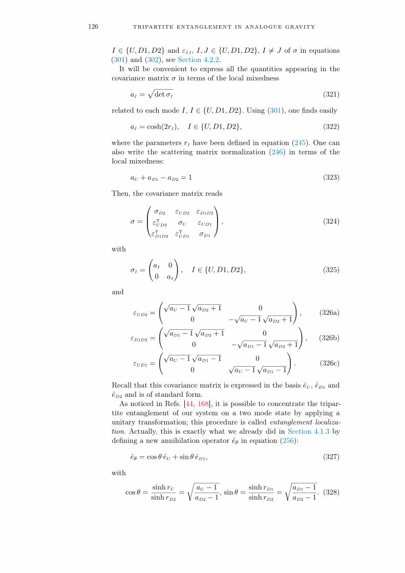
126 tripartite entanglement in analogue gravity
I ∈ U,D1, D2 and εIJ , I, J ∈ U,D1, D2, I 6= J of σ in equations(301) and (302), see Section 4.2.2.
It will be convenient to express all the quantities appearing in thecovariance matrix σ in terms of the local mixedness
aI =√
detσI (321)
related to each mode I, I ∈ U,D1, D2. Using (301), one finds easily
aI = cosh(2rI), I ∈ U,D1, D2, (322)
where the parameters rI have been defined in equation (245). One canalso write the scattering matrix normalization (246) in terms of thelocal mixedness:
aU + aD1 − aD2 = 1 (323)
Then, the covariance matrix reads
σ =
σD2 εUD2 εD1D2
εTUD2 σU εUD1
εTD1D2 εT
UD1 σD1
, (324)
with
σI =
(aI 0
0 aI
), I ∈ U,D1, D2, (325)
and
εUD2 =
(√aU − 1
√aD2 + 1 0
0 −√aU − 1√aD2 + 1
), (326a)
εD1D2 =
(√aD1 − 1
√aD2 + 1 0
0 −√aD1 − 1√aD2 + 1
), (326b)
εUD1 =
(√aU − 1
√aD1 − 1 0
0√aU − 1
√aD1 − 1
). (326c)
Recall that this covariance matrix is expressed in the basis eU , eD1 andeD2 and is of standard form.
As noticed in Refs. [44, 168], it is possible to concentrate the tripar-tite entanglement of our system on a two mode state by applying aunitary transformation; this procedure is called entanglement localiza-tion. Actually, this is exactly what we already did in Section 4.1.3 bydefining a new annihilation operator eθ in equation (256):
eθ = cos θ eU + sin θ eD1, (327)
with
cos θ =sinh rUsinh rD2
=
√aU − 1
aD2 − 1, sin θ =
sinh rD1
sinh rD2
=
√aD1 − 1
aD2 − 1. (328)

4.3 tripartite entanglement in becs 127
Therefore, the unitary transformation associated to this change of basis,from eD2, eU , eD1 to eD2, eθ, eθ+π
2, is
Uθ =
1 0 0 0 0 0
0 1 0 0 0 0
0 0 cos θ 0 sin θ 0
0 0 0 cos θ 0 sin θ
0 0 − sin θ 0 cos θ 0
0 0 0 − sin θ 0 cos θ
. (329)
Then, using the fact that under any local linear Bogoliubov transforma-tion U the covariance matrix transforms as σ′ = UσUT [52, 171], wefind here
σθ = Uθ σ UTθ =
(σsq 0
0 12
), (330)
with
σsq ≡
cosh(2rD2) 0 sinh(2rD2) 0
0 cosh(2rD2) 0 − sinh(2rD2)
sinh(2rD2) 0 cosh(2rD2) 0
0 − sinh(2rD2) 0 cosh(2rD2)
, (331)
i.e., σsq is the covariance matrix associated to a two mode squeezedstate with squeezing parameter rD2. This was expected: the covariancematrix σθ corresponds to the two mode squeezed vacuum state (258).The tripartite entanglement between the three modes U , D1 and D2is equivalent to the one of a two mode squeezed state between D2 andU −D1, where the mode U −D1 [the mode “θ”, see equation (327)] isin fact a linear combination of U and D1.Likewise, one can draw a nice analogy with a quantum optics system:
parametric down-conversion generates a two modes squeezed state (hereeθ). This mode directed to a beamsplitter generates a linear combinationbetween the two outgoing channels (here, eU and eD1), see Figure 34.Note that the pair U −D1 is indeed separable and each of these modesshare entanglement with the remaining mode D2. Such a setup withparametric down-conversion was suggested for instance in Ref. [44].The interest of the system we consider is to generate such a com-
bination of states through the Bogoliubov transform (237): tripartiteentanglement naturally emerges from quantum fluctuations around asonic horizon.
Besides this analogy, one can compute very easily the symplecticeigenvalues associated to the covariance matrix σ
TD2θ of the partially
transposed state ρTD2 from (330). Indeed, two of them are trivially 1,and the remaining ones are those of a two mode squeezed state with

128 tripartite entanglement in analogue gravity
Figure 34: Example of a tripartite entangled system generated by paramet-ric down-conversion and the use of a beamsplitter to create alinear combination between two separable modes. The modes D2(the partner), and ‘θ’ form a squeezed state, see expression (258).Then the mode ‘θ’ splits in two modes by means of a beamsplit-ter, see equation (327); They correspond to the Hawking (modeU) and the companion (mode D1) quanta.
covariance matrix (331); they can be easily computed from (310). There-fore, we obtain18
νTD2j = e2 rD2 , e2 rD2 , e−2 rD2 , e−2 rD2 , 1, 1. (332)
One sees in particular that the PPT criterion (306) is always violated forall rD2 > 0. We can also use expression (314) to compute the logarithmicnegativity between the bipartite system formed by the modeD2 and themode U−D1 (corresponding to a two mode squeezed state of parameterrD2). This gives the squared logarithmic negativity:
ED2|UD1τ = 4 r2
D2 = arcsinh2(√
a2D2 − 1
), (333)
in agreement with expression (320).A local unitary transformation also exists for the modes U and D1.
In that case, the transformed covariance matrix will be of the form(330), with σsq a covariance matrix associated to a two mode squeezedstate with squeezing parameter rU or rD1. Indeed, by computing theeigenvalues of the matrix |iΩσTI |, with I ∈ U,D1, one finds easilythat
νTUj = e2 rU , e2 rU , e−2 rU , e−2 rU , 1, 1,
νTD1j = e2 rD1 , e2 rD1 , e−2 rD1 , e−2 rD1 , 1, 1.
(334)
Then, the uniqueness of these eigenvalues, which correspond to those ofa covariance matrix of the form σ = diag(σsq,12), indicates that such alocal unitary transformation also exists for U and D1.
18 Note that these symplectic eigenvalues are also those associated to the covariancematrix σTD2 of the partially transposed state ρTD2 , where σ is given by (324), withsubmatrices (325) and (326). This property lies in the uniqueness of the symplecticeigenvalues, see Williamson’s theorem, Section 4.2.1.

4.3 tripartite entanglement in becs 129
Therefore, similarly to (333), expression (314) leads to
ED1|UD2τ = 4 r2
D1 = arcsinh2(√
a2D1 − 1
),
EU|D1D2τ = 4 r2
U = arcsinh2(√
a2U − 1
),
(335)
in agreement with (320). The above results will be useful in the followingsection to compute the degree of entanglement of the tripartite system.More generally, note that any bisymmetric (m + n)-mode Gaussian
state with a covariance matrix σ can be brought, by means of a localunitary operation, with respect to the m × n-mode bipartition, to atensor product of single mode uncorrelated states and of a two modeGaussian state [168].
4.3.2 CKW inequality
Entanglement is usually shared between a pair of objects, forming abipartite state; in this sense, entanglement is monogamous: it cannotbe freely shared among many objects. Indeed, if a pair of particles ismaximally entangled19, then, these two particles cannot share entangle-ment with a third one. Consequently, several inequalities to study howentanglement is shared among multipartite states have been derived inthe past and are known as CKW inequalities (Coffman, Kundu andWootters) [40]. In Ref. [40], Coffman, Kundu and Wootters consideredthe case of pure states of three qubits. Later, these results have beenextended for three-mode Gaussian states and all symmetric Gaussianstates20 with an arbitrary number of modes [4]. We are particularly in-terested in the latter achievement since we consider here a three-modeGaussian state. The CKW inequality for a tripartite system reads
τres ≥ 0, with τres = τ (1|23) − τ (1|2) − τ (1|3), (336)
where τ , called the tangle, is a proper measure of bipartite entanglementfor continuous variables, e.g., the squared logarithmic negativity definedin Section 4.2.4; for instance, τ (1|23) measures the bipartite entangle-ment between 1 and the composite subsystem 2 − 3. In expression(336), τres is called the residual tangle and quantifies the tripartite en-tanglement between 1, 2 and 3.The inequality (336) means that the entanglement shared between 1
and 2, tracing out 3, in addition to the entanglement shared between 1and 3, tracing out 2, cannot exceed the total entanglement shared be-tween 1 and the pair 2, 3. Figure 35 shows a qualitative sketch of theCKW monogamy inequality with Borromean rings. On the left-handside of the picture rings are all entangled with each other: this exempli-fies the tripartite entanglement (≡ τres). Then, one might consider theblue and green rings as one subsystem. In this case, one study how the
19 A state is maximally entangled when the degree of entanglement is maximized – thiscan be measured through the logarithmic negativity for example.
20 A symmetric N -mode Gaussian state is such that all local mixedness ai, i ∈1, . . . , N, defined below equation (318), are all equal to each other.

130 tripartite entanglement in analogue gravity
red ring is entangled with the ‘blue-green’ ring (≡ τ (1|23)). The otherconfigurations in Figure 35 consist of tracing out one of the ring tostudy the entanglement between each bipartite systems (red and bluerings – τ (1|2) – or red and green rings – τ (1|3)).
Figure 35: Borromean rings extracted from Ref. [58] to illustrate the tripar-tite entanglement. The CKW inequality states that the entangle-ment shared between 1 and 2 (red and blue rings), tracing out3, in addition to the entanglement shared between 1 and 3 (redand green rings), tracing out 2, cannot exceed the total entan-glement shared between 1 (red ring) and the pair 2, 3 (greenand blue rings). The positive difference between these quantitiescorresponds to the left-hand side of the equality and is called theresidual tangle; it measures the tripartite entanglement sharedamong all the three modes and is represented by the three entan-gled rings.
However, expression (336) depends on which mode (among the three)is mode 1, then mode 2 and mode 3. To encompass all possible cases,we consider instead
τres ≡ mini,j,k
[τ (i|jk) − τ (i|j) − τ (i|k)], (337)
where i, j, k ∈ 1, 2, 3. Equation (337) ensures that, if τres > 0, thesystem does exhibit tripartite entanglement.
4.3.3 Computation of the residual tangle
To calculate the residual tangle τres defined in expression (336), we useas it was shown in Ref. [4] the squared logarithmic negativity Eτ as ameasure of entanglement.We already know from Section 4.2.4 that
τ (1|23) = E1|23τ (ρ) = arcsinh2
(√a2
1 − 1
), (338)
where ρ is the density matrix associated to the three-mode Gaussianstate and a1 ≡
√detσ1 is the local mixedness related to mode 1 [see
equation (320)]. We also recall that σ1 is one of the submatrices of thematrix (280).The computation of E1|2
τ (ρ) and E1|3τ (ρ) is more difficult since the
density matrices of composite subsystems 1−2 and 1−3 correspondto mixed states21.
21 Indeed, while the whole system is a three-mode pure state, the restrictions to twomodes (tracing out the remaining mode) are described by mixed states.

4.3 tripartite entanglement in becs 131
For such mixed states, it was proven in Ref. [3] that
Q(1) def= E1|2
τ (ρ) + E1|3τ (ρ)
= arcsinh2 [√m2(a1, s, d)− 1]
+ arcsinh2 [√m2(a1, s,−d)− 1],
(339)
with
s =a2 + a3
2, and d =
a2 − a3
2, (340)
m = m− (m = m+) if D ≤ 0 (D > 0) [4]:
k± = a21 ± (s+ d)2,
D = 2 (s− d)−√
2 [k2− + 2 k+ + |k−| (k2
− + 8 k+)1/2)]/k+,
m− =|k−|
(s− d)2 − 1,
m+√2
=
√2 a2
1 (1 + 2 s2 + 2 d2)− (4 s2 − 1) (4 d2 − 1)− a41 −√δ
4 (s− d),
δ = (a1 − 2 d− 1) (a1 − 2 d+ 1) (a1 + 2 d− 1) (a1 + 2 d+ 1)
× (a1 − 2 s− 1) (a1 − 2 s+ 1) (a1 + 2 s− 1) (a1 + 2 s+ 1).
(341)
In our case, there are some simplifications in equations (341). Indeed,using equation (323), we have immediately δ = 0.
We now specify two different cases:
1. a1 = aU (or a1 = aD1), a2 = aD1 (or a2 = aU), and a3 = aD2.
We obtain
m−(a1, s, d) =|a1 − a2|a3 − 1
, and m−(a1, s,−d) =a1 + a3
1 + a2
m+(a1, s, d) =
√a1 a2
a3, and m+(a1, s,−d) =
√a1 a3
a2,
(342)
and D ≥ 0, ∀ a1, a2, with of course a1,2 ≥ 1 [with D defined in(341)]. Therefore, we shall choose m = m+ in equation (339).
Besides, we also know that state 1|2 = U |D1 is separable (or wecan just check easily that d < −(a2
1− 1)/(4s) [4]). Thus, E1|2τ = 0
and we have at the end
Q(1) = E1|3τ = arcsinh2
(√a1 a3 − a2
a2
)(343)
2. a1 = aD2, a2 = aU (or a2 = aD1), and a3 = aD1 (or a3 = aU).
In this case,
s =aU + aD1
2=aD2 + 1
2= smin, (344)

132 tripartite entanglement in analogue gravity
which is the minimum value of s and this is expected: s reachesits minimal value when the reduced bipartition 2|3 = U |D1 isseparable [4]; and we know from the Cauchy-Schwartz inequalitythat U and D1 are not entangled.
The parameter D is always negative and we obtain [4]
m−(a1, smin,±d) =
1 + 3 a1 ± 2 d
3 + a1 ∓ 2 d, (345)
which leads to the corresponding Q(1) computed from (339):
Q(1) = E1|2τ + E1|3
τ
= arcsinh2
(2
1 + a2
√(a2 + a3) (a3 − 1)
)
+ arcsinh2
(2
1 + a3
√(a2 + a3) (a2 − 1)
).
(346)
At the end we obtain for the tripartite entanglement:
τres = min(1)=U,D1,D2
[arcsinh2(√
a2(1) − 1
)−Q(1)], (347)
where Q(1) is computed from equation (343) or equation (346) depend-ing on the chosen case. Actually, it was proven by Adesso et al. that theminimum in equation (347) is reached for the lowest local mixedness [4].Figure 36 shows the curves associated to the three local mixedness aU ,aD1 and aD2 as functions of the frequency22 ω. The results are obtainedfor a waterfall configuration with upstream Mach number mu = 0.59(see Section 3.1.3 for the definition of this specific configuration). Wecan identify two regimes: below a frequency denoted as ωthr (=0.56for mu = 0.59) the lowest local mixedness is aD1; above this frequencythreshold23, the minimum value becomes aU . We also note that all localmixedness tend to 1 when ω → Ω, where Ω corresponds to the vanish-ing of the D2 mode, see Figure 20 for the definition of Ω; this means inparticular that the population in the different modes vanish:
〈c†U(Ω) cU(Ω)〉 = 〈c†D1(Ω) cD1(Ω)〉 = 〈c†D2(Ω) cD2(Ω)〉 = 0, (348)
since aI = 1 + sinh2(rI) = 1 + 〈c†I cI〉, I ∈ U,D1, D2.We decided to compute the residual tangle (347) in the three cases
(1) = U,D1, D2 to check a posteriori that the minimum tangle wasindeed reached for the lowest local mixedness. We denote by τ (I)
res theresidual tangle such that (1) = I in equation (347), I ∈ U,D1, D2.The result is shown in Figure 37 for the same configuration (mu = 0.59).One sees that the system exhibits tripartite entanglement, which di-verges when the energy tends to zero. Then, the residual tangle de-creases rapidly to zero and completely vanishes at the upper boundfrequency Ω.
As shown in Figure 38, one has indeed τ (U)res < τ (D1)
res for ω > ωthr, i.e.,when aU < aD1; the difference between both tangles is very tiny though.

4.3 tripartite entanglement in becs 133
Figure 36: Local mixedness defined in equation (322) for each mode U , D1and D2 as functions of the parameters rI . These parameters de-pend on the frequency ω and their explicit expressions are givenin terms of the scattering matrix coefficients in equations (245).The scattering matrix coefficients are computed for a waterfallconfiguration with upstream Mach number mu = 0.59, see Sec-tion 3.1.3 for the definition of this specific configuration. The fre-quency ωthr indicates the turning point above which aU becomeslower than aD1. The upper bound frequency Ω corresponds to thevanishing of the D2 mode, see Figure 20.
Figure 37: Residual tangle calculated from equations (338), (343) and (346),where the subscript “1” is replaced by either U , D1 – case 1,equation (343) – or D2 – case 2, equation (346). We denote byτ (I)res, I ∈ U,D1, D2 the corresponding tangle. The inset of thefigure corresponds to a zoom over the low energy sector. Theupper bound frequency Ω corresponds to the vanishing of the D2mode, see Figure 20. We recall that this result is obtained for awaterfall configuration with upstream Mach number mu = 0.59,see Section 3.1.3 for the definition of this specific configuration.

134 tripartite entanglement in analogue gravity
Figure 38: Difference between the residual tangles τ (U)res and τ (D1)
res , computedfrom equations (338) and (343). The frequency ωthr indicates theturning point above which aU becomes lower than aD1, see Fig-ure 36.
In conclusion, the presence of negative energy modes renders theacoustic black hole energetically unstable [71]; this leads to creationof entangled quanta of positive and negative energies emerging at theacoustic horizon from quantum vacuum fluctuation and propagating inthe subsonic and the supersonic regions.Said differently, the total absence of ingoing modes in the system
does not mean that no outgoing modes are emitted from the scatteringprocess occurring at the acoustic horizon. In that sense, one can per-ceive the analogue Hawking radiation (and also the Hawking radiationin the gravitational case) as an amplification process [158]: the modeconversion of ingoing modes into negative energy outgoing modes mustresult in an increase of positive energy outgoing modes.This also means that the in-vacuum associated to the ingoing modes
is different from the out-vacuum associated to the outgoing modes. Inthe gravitational case, the in-vacuum is seen as a thermal state for anobserver outside a black hole [25, 87, 88]. Therefore, this observer willperceive a thermal radiation emitted from the event horizon of the blackhole, the so-called Hawking radiation, see Chapter 2.In this chapter, we proved that the same process occurs in sonic black
hole, the mode conversion at the acoustic horizon and the ‘mixing’ ofpositive and negative energy modes corresponds to a Bogoliubov trans-formation. In particular, the in-vacuum in our analogue system can beseen as an effective two mode squeezed vacuum state between a nega-tive energy mode – D2 – and a linear combination of positive energymodes – U and D1. We showed that an observer in the subsonic regionwill then perceive a ‘thermal’ radiation, whose effective temperaturedepends on the energy of the mode. From this point of view, the ana-logue Hawking spectrum is thermal, but it is not Planckian since thetemperature depends on the energy.
22 Recall that the local mixedness defined in equations (322) depend on the parametersrI , I ∈ U,D1, D2, which depend themselves on the energy ~ω, see equations (245).
23 We have noticed that this threshold decreases when mu decreases.
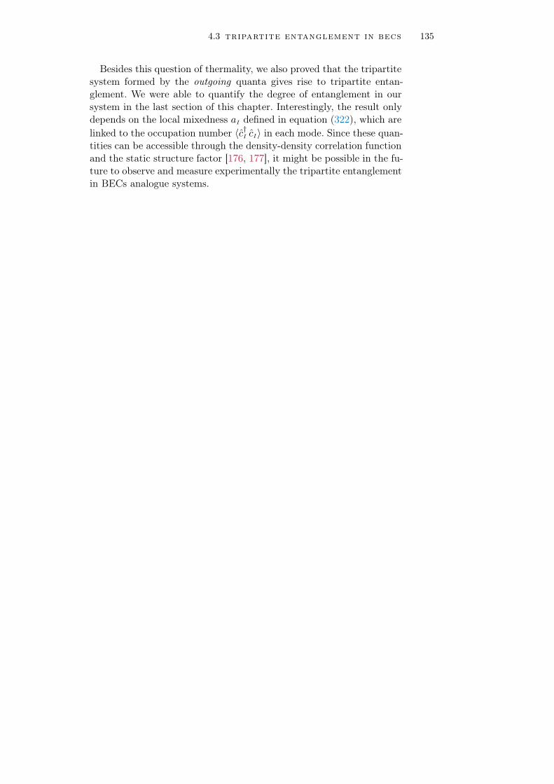
4.3 tripartite entanglement in becs 135
Besides this question of thermality, we also proved that the tripartitesystem formed by the outgoing quanta gives rise to tripartite entan-glement. We were able to quantify the degree of entanglement in oursystem in the last section of this chapter. Interestingly, the result onlydepends on the local mixedness aI defined in equation (322), which arelinked to the occupation number 〈c†I cI〉 in each mode. Since these quan-tities can be accessible through the density-density correlation functionand the static structure factor [176, 177], it might be possible in the fu-ture to observe and measure experimentally the tripartite entanglementin BECs analogue systems.


Part II
PROPAGATION OF DISPERS IVE SHOCKWAVES IN NONL INEAR MEDIA


5FLU IDS OF L IGHT
The propagation of light in a nonlinear material is amenable to a hydro-dynamic treatment [8–11, 179]. This approach amounts to consider thepropagating optical beam as a fluid of light. In fact, nonlinear effectsinduced by light in the medium lead to an effective photon-photon in-teraction, similarly to atomic Bose gases where nonlinearity arises fromcontact interactions between bosons. This rich analogy suggests thatmany hydrodynamic phenomena studied in the context of Bose-Einsteincondensation can be also explored in nonlinear optics. In particular, thestudy of fluids of light resulted in a burst of interest for probing many-body physics quantum phenomena, such as superfluidity or sound-likeexcitations of light [34, 39, 66, 111, 128, 162, 187, 188].In addition, we mention that this analogy to hydrodynamics can be
also used to explore analogue gravity, such as optical event horizons[57], ergo regions [189], stimulated Hawking radiation [50]; as alreadydiscussed in the first part of this thesis, this confirms the universalityof Hawking radiation as soon as an horizon is present.Another phenomenon of interest for us (which will be studied in de-
tail in the next chapters) is the formation of dispersive shock waves innonlinear media. Many studies have been carried out in nonlinear opticsto observe and describe the propagation of such waves [22, 43, 64, 191,200, 201]. In this thesis, we will analyze more specifically the nonlinearspreading of a region of increased light intensity in the presence of auniform constant background, leading eventually to the formation of adispersive shock wave.
In the absence of background and for a smooth initial intensity pat-tern, the spreading is mainly driven by the nonlinear defocusing andcan be treated analytically in some simple cases [179].The situation is more interesting in the presence of a constant back-
ground: The pulse splits in two parts, each eventually experiencing non-linear wave breaking, leading to the formation of a dispersive shock wavewhich cannot be described within the framework of perturbation theory,even if the region of increased intensity corresponds to a perturbationof the flat pedestal. This scenario indeed fits with the hydrodynamicapproach of nonlinear light propagation and is nicely confirmed by theexperimental observations of Refs. [191, 200].
In this chapter, we show that a propagating optical beam can be seenas a fluid of light. We also introduce the notion of characteristics andRiemann invariants, before applying them in simple cases. Then, in thenext chapter, we use and generalize these important mathematical toolsto describe the dispersionless evolution of nonlinear pulses, such as theshort-time evolution of the fluid of light in the presence of a uniform
139

140 fluids of light
background light intensity. Indeed, during this first stage of spreading,the pulse can be described within a nondispersive approximation bymeans of Riemann’s approach.Eventually, at later times, nonlinear effects induce wave steepening,
which results in a gradient catastrophe and wave breaking. After thewave breaking time, dispersive effects can no longer be omitted and ashock is formed; in this case we resort to Whitham modulation theory[197] to describe the time evolution of the pulse. The theoretical studyof the propagation of the dispersive shock wave is addressed in thelast chapter. The difficulty, here, lies in the fact that two Riemanninvariants vary concomitantly. In addition, an interesting outcome of ourtheoretical treatment is an asymptotic determination of experimentallyrelevant parameters of the dispersive shock, such as a simple estimateof the contrast of the fringes of the dispersive shock waves.
5.1 nonlinear schrödinger equation and hydrodynamicapproach
Let us consider the propagation of a monochromatic optical beam ina nonlinear dielectric medium, such as a hot Rubidium atomic vapor[66]. The propagation of the beam induces local electric dipole moments,leading to a polarization of the dielectric material. The electric displace-ment field is defined as
D(r, t) = ε0 E(r, t) + P(r, t), (349)
where ε0 is the vacuum permittivity, andP(r, t) is the density of inducedelectric dipole moments in the material, called the polarization density.Here, we consider a nonlinear medium in which P depends nonlinearlyon E:
P(r, t) = PL(r, t) + PNL(r, t), (350)
where PL is the linear polarization and PNL is the nonlinear polarization.Their components are1
PLµ(r, t) = ε0 [χ˜ (1)]µν Eν
PNLµ (r, t) = ε0 [χ˜ (3)]µναβ Eν EαEβ
, with µ ∈ x, y, z, (351)
where χ˜ (1) is the linear susceptibility and the fourth rank tensor χ˜ (3) is
the third-order susceptibility. We discarded the second-order χ˜ (2) con-
tribution to the nonlinear polarization because we consider an inversioninvariant medium in which the response is not affected when E→ −E.
In a non magnetic dielectric material Maxwell equations read [108]
∇×E = −∂tB, ∇×B =1
ε0 c2∂tD, ∇ ·D = 0, ∇ ·B = 0, (352)
1 Note that we use Einstein notations in equation (351), i.e., [χ˜(1)]µν Eν = [χ˜
(1)]µxEx+
[χ˜(1)]µyEy + [χ˜
(1)]µzEz.

5.1 nonlinear schrödinger equation and hydrodynamic approach 141
leading to
∆E−∇ (∇ ·E) =1
c2∂2tE +
1
ε0 c2∂2tP. (353)
Assuming that ∇·E = 0 (this will be justified a posteriori), one obtains
∆E =1
c2∂2tE +
1
ε0 c2∂2tP. (354)
We consider now a linearly polarized beam, of the form
E(r, t) =1
2(E(r) e−iω0t + c.c.) ~x, (355)
where E(r) is a complex function, which does not depend on time. Thiswill be denoted as a stationary beam. In this case, one has in particular
P(r, t) = ε0
[χ(1) +
3
4χ(3) |E(r)|2
]E(r, t), (356)
where it is customary to simply write χ(1) ≡ [χ˜ (1)]xx, χ(3) ≡ [χ˜ (3)]xxxx
in an isotropic medium, and where terms ∝ exp(−3iω0t), correspondingto third harmonic generation, have been discarded.Therefore, using equation (354), we obtain
∆E− 1
c2
[1 + χ(1) +
3
4χ(3) |E(r)|2
]∂2tE = 0 (357)
In the following, one considers a slowly modulated plane wave in theparaxial approximation
E(r) = A(~r⊥, z) eiβ0z, where |∂zA| ≤ β0 |A|. (358)
Inserting the previous expression in equation (357) yields2
i∂zA = − 1
2β0∇2⊥A− k0 n2 |A|2A, (360)
where ∇⊥ is the transverse Laplacian, and
k0 =ω0
c, β0 = n0 k0, n2 =
3
8n0χ(3), n0 = (1 +χ(1))1/2. (361)
We also define the optical beam intensity I ≡ |A|2 and the nonlinearrefractive index ∆n ≡ n2 I = n2 |A|2.
2 First, note that in the paraxial approximation one neglects ∂zzA, leading to a first-order differential equation with respect to z:
2 i β0 ∂zA+ ∇2⊥A = −ω
20
c2
(1 + χ(1) − c2
ω20
β20 +
3
4χ(3) |A|2
)A. (359)
Second, by discarding nonlinear effects for a perfect plane wave, i.e., constant A, onefinds β0 = n0 k0, where n0 = (1 + χ(1))1/2 is the linear index refraction.

142 fluids of light
We can already notice the similarity between equation (360) and thenonlinear Schrödinger equation. The nonlinear term, which containedthe nonlinear refractive index, is interpreted as an effective photon-photon interaction induced by the Kerr nonlinearity, i.e., the nonlinearpolarization of the dielectric material where the optical beam propa-gates.If χ(3) > 0, the process is said self-focusing3 and corresponds to
an effective attractive interaction between photons. On the contrary, ifχ(3) < 0, the process is said self-defocusing and leads to an effectiverepulsive interaction between photons [31, 66, 162].Let us now justify that ∇ · E can be indeed neglected in equation
(353). One finds easily that
∇ ·E = − 2n0 n2
1 + χ(1) + 2n0n2|E(r)|2 E(r) ∂x|E(r)|2. (362)
The previous expression is non zero only through the transverse deriva-tive of the slowly varying envelope A. It is additionally small becausethe nonlinear contribution is small4 (n2|E|2 ≤ 1): thus, it can be safelyneglected.
In the following, we consider the case of a defocusing nonlinearity (n2 < 0, χ(3) < 0); that is, as shown in the paragraph below, one finds anequation analogous to the Gross-Pitaevskii equation, where the nonlin-earity is mediated by repulsive interactions between bosons. Therefore,as mentioned in the introduction of this chapter, one understands thestrong analogy with weakly interacting Bose gases; within an hydrody-namic approach [9, 10, 179], the propagation of the optical beam in thenonlinear material can be seen as a fluid of light where fundamentalphenomena, such as superfluidity [128], can be explored.
nonlinear schrödinger equation We define dimensionlessunits by choosing a reference intensity Iref and introducing the non-linear length5 zNL = (k0|n2|Iref)
−1 and the transverse healing lengthξ⊥ = (zNL/n0k0)1/2. We consider a geometry where the transverse pro-file is translationally invariant and depends on a single Cartesian co-ordinate (see Figure 39). One thus writes ~∇2
⊥ = ξ−2⊥ ∂2
x where x is thedimensionless transverse coordinate and we define an effective “time”t = z/zNL. The quantity ψ(x, t) = A/
√Iref is then a solution of the
dimensionless nonlinear Schrödinger equation equation
i ∂tψ = −12∂xxψ + |ψ|2ψ , (363)
which can be compared with equation (105) of Chapter 3 (removingthe external potential U(x) and the chemical potential µ). Therefore,
3 The Kerr nonlinearity induces a change in refractive index n of the material: n =n0 + ∆n, with ∆n = n2 I. When n2 > 0, i.e., χ(3) > 0, the refractive index becomeslarger in the areas where the intensity is higher, usually at the center of a beam,creating a focusing density profile.
4 In typical experiments, one has indeed |A|2 ' 105 W.m−2 and n2 ' 10−10 W.m−2.5 The nonlinear length is the typical length above which nonlinear effects become
predominant.

5.1 nonlinear schrödinger equation and hydrodynamic approach 143
the propagation of an optical beam in a nonlinear dielectric material isentirely described by equation (363), where the longitudinal directionz plays the role of an effective time t.
Figure 39: Evolution of an optical beam propagating in a nonlinear dielec-tric material. It propagates along the z axis, as indicated by theblue arrow. The propagation direction plays the role of an effec-tive “time” t = z/zNL, where we introduced the nonlinear lengthzNL = (k0|n2|Iref)−1. In the last expression, n2 is proportional tothe third-order Kerr nonlinearity χ(3) [see equations (361)], andIref is a reference intensity [see the text above equation (363)].The vertical axis corresponds to the quantity |ψ|2 = I/Iref , whereI is the intensity of the beam. The parameter |ψ0|2 correspondsto the background intensity. As mentioned in the introduction ofthis chapter, this leads eventually to the formation of a dispersiveshock wave, which will be studied in Chapter 7. The transverseprofile is translationally invariant and depends on a single Carte-sian coordinate x.
hydrodynamic approach Our objectives in this thesis lies inthe theoretical description of the propagation of such a fluid of light.The derivation of hydrodynamic equations which govern its evolutionwill enable us to efficiently use powerful tools, such as the Riemann in-variants, the Riemann method, or the Whitham modulational theory, tocompletely characterize its short and long-time propagation. As we havealready proceeded in Chapter 3, let us use a Madelung transformationsuch that6
ψ(x, t) =√ρ(x, t) ei S(x,t), (364)
where the phase S(x, t) is connected to the fluid velocity u(x, t) throughthe relation
u(x, t) ≡ ∂xS. (365)
6 We consider here the case of a one-dimensional fluid flow, but the results of thisparagraph can be generalized straightforwardly to two dimensions.

144 fluids of light
In full analogy with the set of equations (121) obtained in Chapter 3,one obtains from the nonlinear Schrödinger equation (363) the system
∂tρ+ ∂x(ρ u) = 0,
∂tu+ u ∂xu+1
ρ∂xP +
1
2∂xΠ = 0,
(366)
with
P =ρ2
2, and Π = − 1√
ρ∂xx√ρ. (367)
In expression (367), P is an effective pressure due to nonlinear effects,and Π is associated to a quantum pressure term (also called quantumpotential) due to dispersive effects in the system. The first equation ofthe system (366) is the continuity equation, while the second one is theEuler equation. In the dispersionless approach, when density gradientsof the initial density ρ(x, t = 0) are weak, one can neglect the quantumpressure. In this case, the set of hydrodynamic equations becomes
∂tρ+ ∂x(ρ u) = 0,
∂tu+ u ∂xu+ ∂xρ = 0.(368)
5.2 characteristics and riemann invariants
In this section we introduce the concept of characteristics and Riemanninvariants. There are indeed powerful tools to solve partial differentialequations (PDE) and we will use them throughout this and the subse-quent chapters.
Characteristics are curves on which certain quantities, the Riemanninvariants are conserved. We first introduce them with a simple example,the Hopf equation, before considering the case of a polytropic gas flow,characterized by a density ρ, a pressure P (ρ) = ργ/γ and a soundvelocity c(ρ) = ρ(γ−1)/2, up to normalization constants; for adiabaticflow of an ideal gas, the adiabatic index γ is equal to the ratio γ =CP/CV of the specific heat capacities at constant pressure (CP) and atconstant volume (CV).A fluid of light, as considered in the previous section, whose evolution
is governed by the nonlinear Schrödinger equation (363) (or equivalentlya Bose gas described by the Gross-Pitaevskii equation) corresponds toγ = 2 [P (ρ) = ρ2/2, see equation (367)].
5.2.1 Hopf equation
Consider a function u(x, t) solution of the Hopf equation
∂tu+ u ∂xu = 0. (369)
In the plane (t, x) there exists a vector field
a ≡ (1, u), (370)

5.2 characteristics and riemann invariants 145
such that equation (369) can be rewritten
(a∇)u = 0, (371)
where ∇ = (∂t, ∂x). The previous expression implies that u is constantalong integral curves Γ generated by the vector field a. If the point(t = 0, x = x0) in the plane (t, x) corresponds to an initial value u = u0,then equation (371) implies that u(x, t) is constant along the curve Γ0
generated by a0 ≡ (1, u0).Let us introduce a parameter s along Γ0, such that
` = (t(s), x(s)), and a0 =d`
ds. (372)
The notations are summarized in Figure 40.
Figure 40: Sketch of the curve Γ0 in the plane (t, x). This curve is definedparametrically by (t = t(s), x = x(s)), with s a parameter movingalong Γ0. The brown arrow corresponds to the tangent vector tothe point of coordinates (t(s), x(s)); this vector is denoted a0.
This yields the following equationsdtds
= 1, anddxds
= u0, (373)
leading to
t = s, and x = u0 s+ x0. (374)
Therefore, given an initial point (t = 0, x = x0, u = u0) in the threedimensional Cartesian coordinate system (t, x, u), the value u0 corre-sponding to the initial coordinate x0 is carried after time t to thepoint x given by equation (374). In this case, the curves Γ are straightlines, called characteristics, and generate a surface from the initial curve(0, x, u(x, t = 0)).
In addition, in the exceptional case where the initial conditions wouldbe defined on a characteristic curve Γ, one would not be able to use aTaylor series expansion to calculate u(x, t) in the vicinity of Γ, i.e., theCauchy Problem for equation (369) cannot be solved. Indeed, we can-not calculate from equation (369) the derivatives of u(x, t) along anydirection intersecting the characteristic curve Γ, precisely because ex-pression (371) shows that information only propagates along this curve.We will use this important remark in the following to derive the Rie-mann invariants.

146 fluids of light
5.2.2 Polytropic gas flow
We have introduced the main idea of the method of characteristics inthe previous subsection: given the initial data, one finds a set of curves,the characteristics, along which a quantity is conserved. In the case ofHopf equation, the conserved quantity is directly given by u(x, t) andthe characteristics are straight lines [see equation (374)].Let us now generalize this method to the case of polytropic gas flow
described by a density ρ(x, t) and a velocity u(x, t), solutions of the setof equations7
∂tρ+ ρ ∂xu+ u ∂xρ = 0,
∂tu+ u ∂xu+c2
ρ∂xρ = 0,
(375)
with c2 = ργ−1.As mentioned in Section 5.2.1, if the initial data are given on a char-
acteristic curve, one is not able to solve the Cauchy problem associatedto the system (375). We will use this remark to find the characteristics.Indeed, let us consider in the plane (t, x) such a characteristic curve,
denoted Γ and defined parametrically by (t = f(s), x = g(s)), with sa parameter along the curve. We introduce an angle φ such that thecomponents of the vector tangent to Γ read
dxds
= cosφ, anddtds
= sinφ, (376)
Assuming that the initial data for ρ(x, t) and u(x, t) are given on thecurve Γ, one can calculate their derivatives along Γ:
dρds
= ∂xρ cosφ+ ∂tρ sinφ,
duds
= ∂xu cosφ+ ∂tu sinφ.
(377)
The set of equations (375), together with equations (377), is a systemof four equations of four unknown functions ∂tρ, ∂xρ, ∂tu, ∂xu. SinceΓ is a characteristic curve, this system does not have a solution8 and,thus, its determinant ∆Γ equals 0:
∆Γ =
∣∣∣∣∣∣∣∣∣∣
1 u 0 ρ
0 c2
ρ 1 u
sinφ cosφ 0 0
0 0 sinφ cosφ
∣∣∣∣∣∣∣∣∣∣
= 0
⇔ ∆Γ = (cosφ− u sinφ)2 − c2 sin2 φ = 0.
(378)
7 We will follow the method presented by A. Kamchatnov in his book [100].8 Otherwise the derivatives of ρ and u would be known along directions intersectingthe characteristic curve Γ and the Cauchy problem would be solved.

5.2 characteristics and riemann invariants 147
The previous equation has two solutions
cotφ± = u± c. (379)
Therefore, there exists two characteristic curves Γ± defined paramet-rically by (t = f(s±), x = g(s±)), whose tangent vectors are aΓ± =(sinφ±, cosφ±).
In addition, it is worth noticing that solutions of equation (378) arereal here: the system is called hyperbolic. When the solutions are com-plex, the system is called elliptic; for instance, such a configuration canbe encountered in mean-field game theory [29, 30].Now, we will find the conserved quantities along Γ±, namely the Rie-
mann invariants, denoted λ±. Multiplying the first equation of the sys-tem (375) by (cosφ±−u sinφ±) and the second equation by−c2/ρ sinφ±,then using equations (377) and (378), yields
duds±
± c
ρ
dρds±
= 0. (380)
We define two functions λ±(ρ, u) such that
∂λ±
∂u=
1
2, and
∂λ±
∂ρ= ± c
2 ρ. (381)
In this case, equations (380) and (381) lead to
dλ±
ds±= 0, (382)
meaning that λ+ (λ−) is a conserved quantity along Γ+ (Γ−). Solvingequations (381) gives
λ±(ρ, u) =u
2± 1
2
∫ ρ c(ρ′)ρ′
dρ′. (383)
For a polytropic gas flow, where c2(ρ) = ργ−1, we obtain the explicitexpressions
λ±(ρ, u) =u
2± c(ρ)
γ − 1. (384)
In particular, when γ = 2 [which corresponds to the hydrodynamicequations (368)], λ± = u
2 ±√ρ.
We end this section with a last comment: the determination of theRiemann invariant makes it possible to put the system in an effectivelydiagonal form. Indeed, one may also consider λ± as functions of t andx. Equation (382) would give in this case
∂tλ± + v± ∂xλ± = 0, where v± ≡ cotφ±. (385)
Therefore, one sees that solving the initial system of equations (375)reduces to find both Riemann invariants λ±(x, t), solutions of equations

148 fluids of light
(385). Writing v± = u ± c [see equation (379)] in terms of λ±, in thecase of a polytropic flow, differential equations (385) become
∂tλ+ +
1
2
[(1 + γ)λ+ + (3− γ)λ−
]∂xλ
+ = 0,
∂tλ− +
1
2
[(3− γ)λ+ + (1 + γ)λ−
]∂xλ
− = 0.
(386)
If one of the Riemann invariants is always constant in some regionof space x ∈ I ⊂ R, say for instance λ+(x, t) = λ+
0 , ∀x ∈ I, thisregion is called a simple-wave region. The problem is then automaticallysolved: the first equation of (386) is trivially satisfied, and the secondone reduces to a Hopf equation
∂tv− + v−∂xv− = 0. (387)
Solutions of the previous equation have been already discussed in Sec-tion 5.2.1. Therefore, the characteristic curves in a simple-wave regionare straight lines in the plane (t, x), along which v− and λ− are constant.Therefore, in turn, one is able to find λ−(x, t) for each position x andtime t.The second set of characteristic curves Γ+, with tangent vector aΓ =
(sinφ+, cosφ+) and v+ = cotφ+, can be found with equation
dx
dt= v+(x, t) =
1
2
[(1 + γ)λ+(x, t) + (3− γ)λ−(x, t)
], (388)
where λ+(x, t) and λ−(x, t) are known in the simple-wave region. Thus,Integrating the differential equation (388) yields the trajectories of thecharacteristic curves Γ+. This problem is discussed in more detail inRef. [100], where the simple wave approach is applied to a polytropicgas in expansion into an empty half-space.
Solving the system of partial differential equations (385), when bothRiemann invariants vary concomitantly in some regions, is a more dif-ficult problem and requires more involved mathematical tools, such asRiemann’s method, a generalization of the method of characteristics.The different situations of interest for us necessitate the use of sucha method; this is the reason why the next chapter is dedicated to itsstudy.

6DISPERS IONLESS EVOLUTION OF NONL INEARPULSES
As we showed in Chapter 3 and Chapter 5, Bose-Einstein condensatesand their photonic counterparts, the fluids of light, are described by thesame type of nonlinear equations. In both cases, the problem can bemapped onto dispersive hydrodynamic equations, through a Madelungtransformation [see, e.g., equations (121) and (366)]. This hydrody-namic approach has triggered much interest experimentally, as we al-ready mentioned in the previous chapter. However, this analogy is alsoa powerful tool to address numerous theoretical problems. Indeed, inChapter 3, we used the mapping to hydrodynamic equations to showthat the motion of excitations emerging in a flowing Bose-Einstein con-densate was the one of a massless scalar field in a curved spacetime. InChapter 5, we noticed that the dynamics of Bose gases and fluids oflight, in the absence of dispersion, was described by the same hydrody-namic equations as those governing the inviscid gas dynamics:
∂tρ+ ρ ∂xu+ u ∂xρ = 0,
∂tu+ u ∂xu+c2(ρ)
ρ∂xρ = 0,
(389)
where c(ρ) =√ρ is the sound velocity. In fact, this is a particular case
of polytropic gases, for which
c(ρ) = ργ−1
2 (390)
where γ is the adiabatic index (γ > 1). However, even in this apparentlysimple case for which a number of exact solutions have been obtained forvarious problems [107], solving the system of equations (389) becomesquite complicated if the parameter
β =3− γ
2 (γ − 1)(391)
is not an integer number (which is the case for Bose gases and fluids oflight where γ = 2 and β = 1
2).
The aim of this chapter is to present a theoretical method to de-scribe the dispersionless evolution of nonlinear pulses, whose dynamicsis governed by hydrodynamic equations (389).Many physical models lead to this one-dimensional hydrodynamic
description and can be addressed by this method. We first consider thegeneral case of polytropic gases. Then, we particularize the solutions tothe case of nonlinear optical pulses in the presence of a uniform constantbackground, when density gradients of the density ρ are sufficiently
149

150 dispersionless evolution of nonlinear pulses
weak to neglect dispersive effects1. A last example illustrates the case ofa non-integrable system: a zero temperature Bose-Einstein condensatetransversely confined in an atomic wave guide.
6.1 hodograph transformation and riemann’s method
We introduced the Riemann invariants λ+(x, t) and λ−(x, t) in Chap-ter 5. These invariants are conserved along characteristic curves andthey “diagonalize” the system of hydrodynamic equations (389). Weproved that they were given by
λ±(x, t) =u(x, t)
2± 1
2
∫ ρ(x,t) c(ρ′)ρ′
dρ′, (392)
and solutions of the partial differential equations
∂tλ± + v±(λ+, λ−) ∂xλ
± = 0, v±(λ+, λ−) = u± c(ρ). (393)
If one solves the nonlinear equations given by (393) and finds the cor-responding Riemann invariants λ+(x, t) and λ−(x, t), one immediatelyknows the density and velocity distributions for each position x and atany time t:
λ+(x, t) + λ−(x, t) = u(x, t),
λ+(x, t)− λ−(x, t) =
∫ ρ(x,t) c(ρ′)ρ′
dρ′.(394)
Therefore, the problem consists of solving equations (393). In addition,we can notice from equations (394) that c(ρ) is a function of λ+ − λ−.Thus, we obtain
v±(λ+, λ−) = λ+ + λ− ± c(λ+ − λ−). (395)
In the first subsection, we show that these equations can be linearizedby considering x and t as functions of the Riemann invariants:
x = x(λ+, λ−), t = t(λ+, λ−). (396)
This is known as a hodograph transformation [100, 107]. This procedureleads to a Euler-Poisson equation2, whose solutions can be found bymeans of the Riemann’s method [173]. This method is discussed in thesecond subsection.
1 The formation of a dispersive shock wave resulting from a gradient catastrophe willbe studied in Chapter 7.
2 In the case of complex Riemann invariants, one finds a Laplace equation and a nicemapping to an electrostatic problem [29].

6.1 hodograph transformation and riemann’s method 151
6.1.1 Hodograph transformation
This transformation consists in considering x and t as functions of theindependent variables λ± [see equation (396)] and leads to the followingsystem of linear equations (see Appendix D):
∂x
∂λ+− v−(λ+, λ−)
∂t
∂λ+= 0,
∂x
∂λ−− v+(λ+, λ−)
∂t
∂λ−= 0.
(397)
We look for the solutions of these equations in the form
x− v+(λ+, λ−)t = w+(λ+, λ−),
x− v−(λ+, λ−)t = w−(λ+, λ−).(398)
A simple test of consistency shows that the unknown functions w±(λ+, λ−)should verify the Tsarev equations [180]
1
w+ − w−∂w+
∂λ−=
1
v+ − v−∂v+
∂λ−,
1
w+ − w−∂w−∂λ+
=1
v+ − v−∂v−∂λ+
.
(399)
Now we notice that since the velocities v± are given by expressions(395), the right-hand sides of both equations (399) are equal to eachother:
1
v+ − v−∂v+
∂λ−=
1
v+ − v−∂v−∂λ+
=1− c′(λ+ − λ−)
2 c(λ+ − λ−), (400)
where c′(λ) ≡ dc(λ)/dλ, λ = λ+ − λ−. Consequently ∂w+/∂λ− =
∂w−/∂λ+ and w± can be sought in the form
w± =∂W
∂λ±. (401)
Substitution of equations (400) and (401) into equations (399) showsthat the function W obeys the Euler-Poisson equation
∂2W
∂λ+∂λ−− 1− c′(λ+ − λ−)
2c(λ+ − λ−)
(∂W
∂λ+− ∂W
∂λ−
)= 0. (402)
A formal solution of equation (402) in the (λ+, λ−) plane (the so-calledhodograph plane) can be obtained with the use of the Riemann method(see subsection below and Ref. [173]).
In conclusion, the system of hydrodynamic equations (389) can bemapped onto an Euler-Poisson equation (402), where W plays the roleof a potential. The knowledge of this potential determines the functionsw± through expression (401). Then, the Riemann invariants λ+(x, t)and λ−(x, t) can be obtained as functions of x and t by inverting thesystem of equations (398). Ultimately, the density ρ(x, t) and the veloc-ity u(x, t) can be determined with equations (394).

152 dispersionless evolution of nonlinear pulses
The above procedure might give the impression to be cumbersomeand unnecessary. However, it constitutes a powerful tool to addresshydrodynamic problems: indeed, we started from nonlinear equations(389) and we arrived to a linear equation (402), whose solutions arewell know in numerous cases. Besides, in certain problems, one caneven obtain a physical interpretation of the potentialW , which appearsnaturally from the hodograph transformation [29, 30].
6.1.2 Riemann’s method
Let us consider a linear differential equation of second order of the form3
L (W ) ≡ ∂2W
∂λ+ ∂λ−+ a(λ+, λ−)
∂W
∂λ++ b(λ+, λ−)
∂W
∂λ−= 0, (403)
where L is a differential operator. We define the so-called adjoint dif-ferential operator
M (R) ≡ ∂2R
∂λ+ ∂λ−− ∂ (aR)
∂λ+− ∂ (bR)
∂λ−, (404)
where R, called the Riemann function, needs to be determined [seebelow, equations (412)]. One shows easily that
RL (W )−WM (R) =∂U
∂λ+− ∂V
∂λ−, (405)
with
U =1
2
(R∂W
∂λ−−W ∂R
∂λ−
)+ aRW,
V =1
2
(W
∂R
∂λ+−R ∂W
∂λ+
)− bRW.
(406)
We now assume that the initial data λ+(x, t = 0) and λ−(x, t = 0)are known. This corresponds to the schematic curve C0 represented inthe hodograph plane (λ+, λ−) and shown in Figure 41 for two cases:λ−(x, 0) is a decreasing (or increasing) function of λ+(x, 0). Therefore,using equations (398) and (401), one can determine W along the curveC0:
∂W
∂λ+
∣∣∣∣C0
=∂W
∂λ−
∣∣∣∣C0
= x(λ+, λ−). (407)
Then, we show below that, from the knowledge of the values of λ+ andλ− on the initial curve C0, one is able to calculate the potential W atany point P (λ+ = ξ, λ− = η) in the hodograph plane. As illustrated inFigure 41, we denotes A (B) the intersection point between the straightline λ− = η (λ+ = ξ) and C0. The dark green region in Figure 41
3 In this subsection, we mainly follow the procedure presented in Sommerfeld’s book[173]
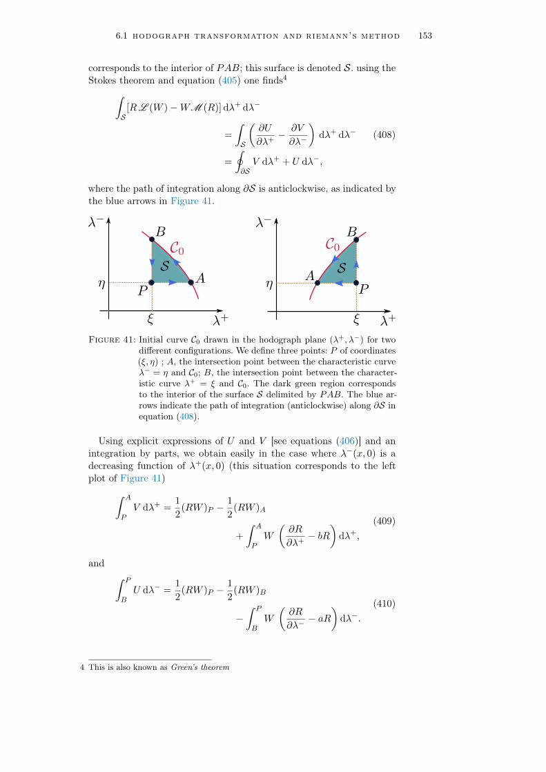
6.1 hodograph transformation and riemann’s method 153
corresponds to the interior of PAB; this surface is denoted S. using theStokes theorem and equation (405) one finds4
∫
S[RL (W )−WM (R)] dλ+ dλ−
=
∫
S
(∂U
∂λ+− ∂V
∂λ−
)dλ+ dλ−
=
∮
∂SV dλ+ + U dλ−,
(408)
where the path of integration along ∂S is anticlockwise, as indicated bythe blue arrows in Figure 41.
Figure 41: Initial curve C0 drawn in the hodograph plane (λ+, λ−) for twodifferent configurations. We define three points: P of coordinates(ξ, η) ; A, the intersection point between the characteristic curveλ− = η and C0; B, the intersection point between the character-istic curve λ+ = ξ and C0. The dark green region correspondsto the interior of the surface S delimited by PAB. The blue ar-rows indicate the path of integration (anticlockwise) along ∂S inequation (408).
Using explicit expressions of U and V [see equations (406)] and anintegration by parts, we obtain easily in the case where λ−(x, 0) is adecreasing function of λ+(x, 0) (this situation corresponds to the leftplot of Figure 41)
∫ A
PV dλ+ =
1
2(RW )P −
1
2(RW )A
+
∫ A
PW
(∂R
∂λ+− bR
)dλ+,
(409)
and∫ P
BU dλ− =
1
2(RW )P −
1
2(RW )B
−∫ P
BW
(∂R
∂λ−− aR
)dλ−.
(410)
4 This is also known as Green’s theorem

154 dispersionless evolution of nonlinear pulses
Therefore, one finds∫
S[RL (W )−WM (R)] dλ+ dλ−
= (RW )P −1
2(RW )A −
1
2(RW )B +
∫
C0V dλ+ + U dλ−
+
∫ A
PW
(∂R
∂λ+− bR
)dλ+ −
∫ P
BW
(∂R
∂λ−− aR
)dλ−.
(411)
We know from equation (403) that L (W ) = 0 anywhere in the interiorof S. Moreover, we can choose the Riemann function R(λ+, λ−; ξ, η)in a convenient way for us; we demand that this function respects thefollowing conditions:
M (R) = 0 in S, (412a)R(P ) = R(ξ, η; ξ, η) = 1, (412b)∂R
∂λ+− bR = 0, on the characteristic λ− = η,
∂R
∂λ−− aR = 0, on the characteristic λ+ = ξ.
(412c)
In this case, conditions (412) and expression (411) lead to
W (P ) =1
2(RW )A +
1
2(RW )B ∓
∫ B
AV dλ+ + U dλ−, (413)
with the ‘minus’ sign if one considers the case depicted in the left plotof Figure 41, and the ‘plus’ sign in the case exemplified in the right plotof the same figure.Consequently, the knowledge of initial data suffices to determine the
function W for any point P in the hodograph plane, provided the Rie-mann function R is known [computed from equations (412)].
riemann function In the case of the Euler-Poisson equation(402) [and comparing with the differential equation (403)], one obtains
a(λ+, λ−) =c′(λ+ − λ−)− 1
2c(λ+ − λ−)= −b(λ+, λ−). (414)
Then, conditions (412c) and (412b) yield
R(λ+, η; ξ, η) =
√c(ξ − η)
c(λ+ − η)exp
(∫ λ+−η
ξ−η
dλ2 c(λ)
),
R(ξ, λ−; ξ, η) =
√c(ξ − η)
c(ξ − λ−)exp
(∫ ξ−λ−
ξ−η
dλ2 c(λ)
),
(415)
where R(λ+, η; ξ, η) is the Riemann function along the characteristicλ− = η (i.e., along PA, see Figure 41), and R(ξ, λ−; ξ, η) is the Riemannfunction along the characteristic λ+ = ξ (i.e., along PB). Expressions(415) suggest that R can be sought in the form
R(λ+, λ−; ξ, η) = R(λ+ − λ−, ξ − η)F (λ+, λ−; ξ, η), (416)

6.1 hodograph transformation and riemann’s method 155
where F (λ+, η; ξ, η) = 1 = F (ξ, λ−; ξ, η) and
R(λ1, λ2) =
√c(λ2)
c(λ1)exp
(∫ λ1
λ2
dλ2 c(λ)
)
=
√c(λ2)ρ(λ1)
c(λ1)ρ(λ2).
(417)
The final expression in the above formula has been obtained by meansof a change of variable ρ = ρ(λ) in the integral, where the function ρ(λ)is the reciprocal function of λ(ρ) given in (394)
λ(ρ) =
∫ ρ c(ρ′)dρ′
ρ′, (418)
and c(λ) = c(ρ(λ)), so that dλ/c(λ) = dρ/ρ.
initial conditions We now consider the case where initial den-sity and velocity distributions are given by
ρ(x, 0) = ρ(x), and u(x, 0) = 0. (419)
The density ρ(x) can be non-monotonic, as illustrated in the right mar-gin. For simplicity, we assumed the existence of one global maximumreached at x = 0; we also assume that the density distribution is sym-metric. The generalization to non-symmetric distributions is straight-forward. We denote the regions x < 0 and x > 0 as regions 1 and 3,respectively. Since u(x, 0) = 0, one deducts from equations (394) that
λ+(x, 0) = −λ−(x, 0), λ+(x, 0) =
∫ ρ(x)
0
c(ρ)
ρdρ. (420)
Thus, in this case, the initial curve C0 is a straight line in the hodo-graph plane (λ+, λ−). We introduce the monotonous functions λ(1)(x) ≡λ+(x < 0, 0) and λ(3)(x) ≡ λ+(x ≥ 0, 0). Their reciprocal functions aredenoted x(1)(λ) and x(3)(λ), respectively. Here, since the initial densitydistribution is symmetric, we define
λ(x) ≡ λ(3)(x) = λ(1)(−x), x(λ) ≡ x(3)(λ) = −x(1)(λ). (421)
We obtain for the value of x on the curve C0:
x =
x(λ) if x ≥ 0,
−x(λ) if x < 0.(422)
The functions λ(x) and x(λ) are illustrated in the schematic graphs ofFigure 42.Besides that, since at t = 0 the values λ+ = λ and λ− = −λ cor-
respond to the same value of x, we find that x(λ) is an even function,x(−λ) = x(λ). All these notations are summarized in Figure 42, where,in particular, the minimum and the maximum of λ+(x, t = 0) are de-noted λ0 and λm, respectively.

156 dispersionless evolution of nonlinear pulses
Figure 42: (Left) Sketch of λ+(x, t = 0) and, in particular, λ(x) ≡ λ+(x ≥0, 0). This curve can be obtained from the initial density distribu-tion ρ(x) through expression (420). Since we consider a symmet-ric density distribution here, the dashed part of the red curve isthe symmetric of the solid curve and thus corresponds to λ(−x).The minimum and the maximum of λ(x) are denoted λ0 and λm,respectively.(Right) Reciprocal function of λ(x), denoted x(λ) [see equation(422)].
For the specific initial conditions (419), since λ+(x, 0) = −λ−(x, 0),equation (407) shows thatW is constant along the initial curve C0. Thevalue of this constant is immaterial, we take W |C0 = 0 for simplicity.
However, the non-monotonicity of ρ adds a slight difficulty here. In-deed, depending on which region we are, x = x(λ) – region 3 – orx = −x(λ) – region 1 – [see equation (422)]; this leads for instance toan ambiguity about the choice of x in (407), and so does for expressionsof U and V [see equations (406)].An elegant way to solve this problem has been proposed by Ludford
and consists in unfolding the hodograph plane [120], as shown in Fig-ure 44. The red curve in both graphs corresponds to C0 and a sketchof the initial Riemann invariants λ+(x, 0) = −λ−(x, 0), for a specificnon-monotonic density distribution ρ(x), is depicted in the left plot ofFigure 43. Region 1 then corresponds to the upper left domain of theright plot of Figure 44, while region 3 corresponds to the bottom rightdomain: this amounts to define a distinct hodograph plane for eachmonotonous part of the initial distribution.For t > 0, the initial hump of density ρ(x) splits in two parts and
both Riemann invariants λ+ and λ− propagate in opposite direction,as illustrated by the green arrows in the right plot of Figure 43. A newregion appears: it corresponds to the domain where λ+ and λ− have thesame monotonicity. We denote this region as region 2. Then, one is ableto extract from this graph λ+(x, t > 0) as a function of λ−(x, t > 0)in order to draw the corresponding curve in the hodograph plane; weobtain the blue curve shown in Figure 44, either when the hodograph
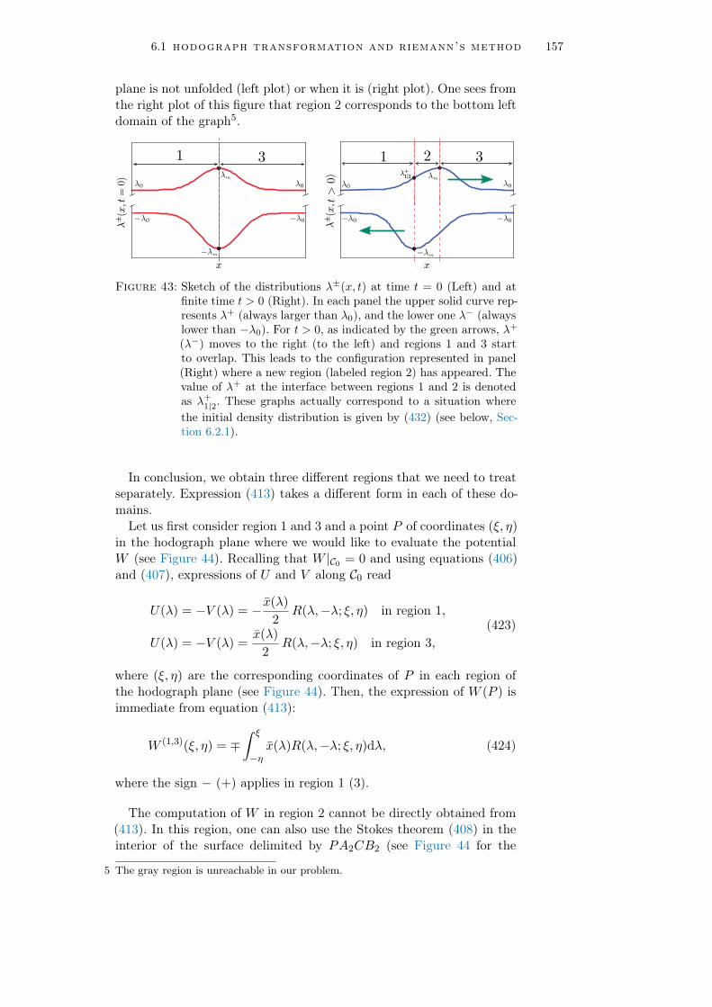
6.1 hodograph transformation and riemann’s method 157
plane is not unfolded (left plot) or when it is (right plot). One sees fromthe right plot of this figure that region 2 corresponds to the bottom leftdomain of the graph5.
Figure 43: Sketch of the distributions λ±(x, t) at time t = 0 (Left) and atfinite time t > 0 (Right). In each panel the upper solid curve rep-resents λ+ (always larger than λ0), and the lower one λ− (alwayslower than −λ0). For t > 0, as indicated by the green arrows, λ+(λ−) moves to the right (to the left) and regions 1 and 3 startto overlap. This leads to the configuration represented in panel(Right) where a new region (labeled region 2) has appeared. Thevalue of λ+ at the interface between regions 1 and 2 is denotedas λ+1|2. These graphs actually correspond to a situation wherethe initial density distribution is given by (432) (see below, Sec-tion 6.2.1).
In conclusion, we obtain three different regions that we need to treatseparately. Expression (413) takes a different form in each of these do-mains.Let us first consider region 1 and 3 and a point P of coordinates (ξ, η)
in the hodograph plane where we would like to evaluate the potentialW (see Figure 44). Recalling that W |C0 = 0 and using equations (406)and (407), expressions of U and V along C0 read
U(λ) = −V (λ) = − x(λ)
2R(λ,−λ; ξ, η) in region 1,
U(λ) = −V (λ) =x(λ)
2R(λ,−λ; ξ, η) in region 3,
(423)
where (ξ, η) are the corresponding coordinates of P in each region ofthe hodograph plane (see Figure 44). Then, the expression of W (P ) isimmediate from equation (413):
W (1,3)(ξ, η) = ∓∫ ξ
−ηx(λ)R(λ,−λ; ξ, η)dλ, (424)
where the sign − (+) applies in region 1 (3).
The computation of W in region 2 cannot be directly obtained from(413). In this region, one can also use the Stokes theorem (408) in theinterior of the surface delimited by PA2CB2 (see Figure 44 for the
5 The gray region is unreachable in our problem.

158 dispersionless evolution of nonlinear pulses
notations). Similarly to equation (413), we can split the integral overthe different segments and we easily obtain
W (2)(ξ, η) = [RW (1)]B2 + [RW (3)]A2
+
∫ C
A2
(∂R
∂λ−− aR
)
λ+=λm
W (3)(λm, λ−) dλ−
−∫ B2
C
(∂R
∂λ+− bR
)
λ−=−λmW (1)(λ+,−λm) dλ+.
(425)
Therefore, equations (424) and (425) solve the problem. Using equation(401) one finds the expressions of w± in each region. Inverting the systemof equations (398) gives λ± as functions of x and t.
Figure 44: (Left) Behavior of the Riemann invariants in the hodographplane at a given time t. The red straight line is the curveC0. The blue solid line is the curve with parametric equation(λ+(x, t > 0), λ−(x, t > 0)). The corresponding Riemann invari-ants λ±(x, t > 0) (as functions of x) are shown in the right plotof Figure 43.(Right) The same curves on the four-sheeted unfolded surface.The regions 1, 2 and 3 correspond to the different regimes ofmonotonicity identified in Figure 43. In our problem, the wholegray shaded domain above C0 is unreachable. A generic point Phas coordinates (ξ, η), as indicated for instance in region 3, andpoints A1, B1, A3, B3 and C lie on the initial curve C0. PointsA2 and B2 lie on a boundary between two regions. The arrowsindicate the direction of integration in equations (413) and (425).
approximate solutions We would like to simplify expressions(424) and (425). First, in region 2, we notice that, at short time, thecoordinates ξ and η of point P are close to λm and −λm, respectively(see Figure 44). This leads to the approximation
(∂R
∂λ−− aR
)
λ+=λm
'(∂R
∂λ+− bR
)
λ−=−λm' 0, (426)
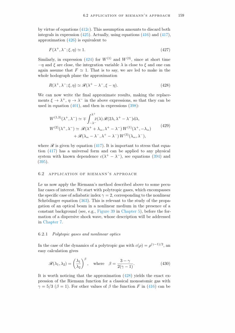
6.2 application of riemann’s approach 159
by virtue of equations (412c). This assumption amounts to discard bothintegrals in expression (425). Actually, using equations (416) and (417),approximation (426) is equivalent to
F (λ+, λ−; ξ, η) ' 1. (427)
Similarly, in expression (424) for W (1) and W (3), since at short time−η and ξ are close, the integration variable λ is close to ξ and one canagain assume that F ' 1. That is to say, we are led to make in thewhole hodograph plane the approximation
R(λ+, λ−; ξ, η) ' R(λ+ − λ−, ξ − η). (428)
We can now write the final approximate results, making the replace-ments ξ → λ+, η → λ− in the above expressions, so that they can beused in equation (401), and then in expressions (398):
W (1,3)(λ+, λ−) ' ∓∫ λ+
−λ−x(λ) R(2λ, λ+ − λ−)dλ,
W (2)(λ+, λ−) ' R(λ+ + λm, λ+ − λ−)W (1)(λ+,−λm)
+ R(λm − λ−, λ+ − λ−)W (3)(λm, λ−),
(429)
where R is given by equation (417). It is important to stress that equa-tion (417) has a universal form and can be applied to any physicalsystem with known dependence c(λ+ − λ−), see equations (394) and(395).
6.2 application of riemann’s approach
Le us now apply the Riemann’s method described above to some pecu-liar cases of interest. We start with polytropic gases, which encompassesthe specific case of adiabatic index γ = 2, corresponding to the nonlinearSchrödinger equation (363). This is relevant to the study of the propa-gation of an optical beam in a nonlinear medium in the presence of aconstant background (see, e.g., Figure 39 in Chapter 5), before the for-mation of a dispersive shock wave, whose description will be addressedin Chapter 7.
6.2.1 Polytopic gases and nonlinear optics
In the case of the dynamics of a polytropic gas with c(ρ) = ρ(γ−1)/2, aneasy calculation gives
R(λ1, λ2) =
(λ1
λ2
)β, where β =
3− γ2(γ − 1)
. (430)
It is worth noticing that the approximation (428) yields the exact ex-pression of the Riemann function for a classical monoatomic gas withγ = 5/3 (β = 1). For other values of β the function F in (416) can be

160 dispersionless evolution of nonlinear pulses
shown to obey the hypergeometric equation (see, e.g., Ref. [173]) andour approximation corresponds to the first term in its series expansion.Thus, we obtain
W (1,3)(λ+, λ−) ' ∓(
2
λ+ − λ−)β ∫ λ+
−λ−λβ x(λ)dλ,
W (2)(λ+, λ−) '(
2
λ+ − λ−)β
×∫ λm
−λ−λβ x(λ)dλ+
∫ λm
λ+
λβ x(λ)dλ.
(431)
The case β = 1/2 corresponds to the propagation of an optical beamin a nonlinear dielectric material and the dynamics of a Bose-Einsteincondensed system [94].
initial conditions One sees that expressions (431) are given interms of x(λ), the reciprocal function of λ(x) ≡ λ+(x ≥ 0, 0), whereλ+(x ≥ 0, 0) can be calculated from (420). Here, we take an initialprofile of the form6
ρ(x) = ρ0 + ρ1 exp(−x2/x20) , (432)
with ρ0 and ρ1 > 0. One obtains from (420),
x(λ) = x0
√ln ρ1 − ln
[|(γ − 1)λ|
2γ−1 − ρ0
]. (433)
For such a “single-bump” type of initial conditions, there exist two valuesλm = λ(0) and λ0 = λ(x → ∞) (λm > λ0 > 0) such that λ+(x, t) ∈[λ0, λm] and λ−(x, t) ∈ [−λm,−λ0]. This situation corresponds exactlyto the graphs shown in Figure 42.
procedure OnceW (λ+, λ−) is known in all three regions 1, 2 and3 by means of equations (431), it is possible to compute λ+(x, t) andλ−(x, t), and then ρ(x, t) and u(x, t), following the procedure below:
• One first determines the value λ+1|2(t) reached by λ+ at the bound-
ary between regions 1 and 2, see the right panel of Figure 43. Thisboundary corresponds to the point where λ− = −λm at time t.From equations (398), λ+
1|2(t) is thus determined by solving
w(1)+ (λ+
1|2,−λm)− w(1)− (λ+
1|2,−λm)
v+(λ+1|2,−λm)− v−(λ+
1|2,−λm)+ t = 0 , (434)
where w(1)+ = ∂W (1)/∂λ+. We then know that, in region 1 at time
t, λ+ takes all possible values between λ0 and λ+1|2(t) (cf. Figure 43
and Figure 44).
6 In the case of nonlinear optics this initial profile corresponds to a Gaussian beam,which can be easily set up experimentally.
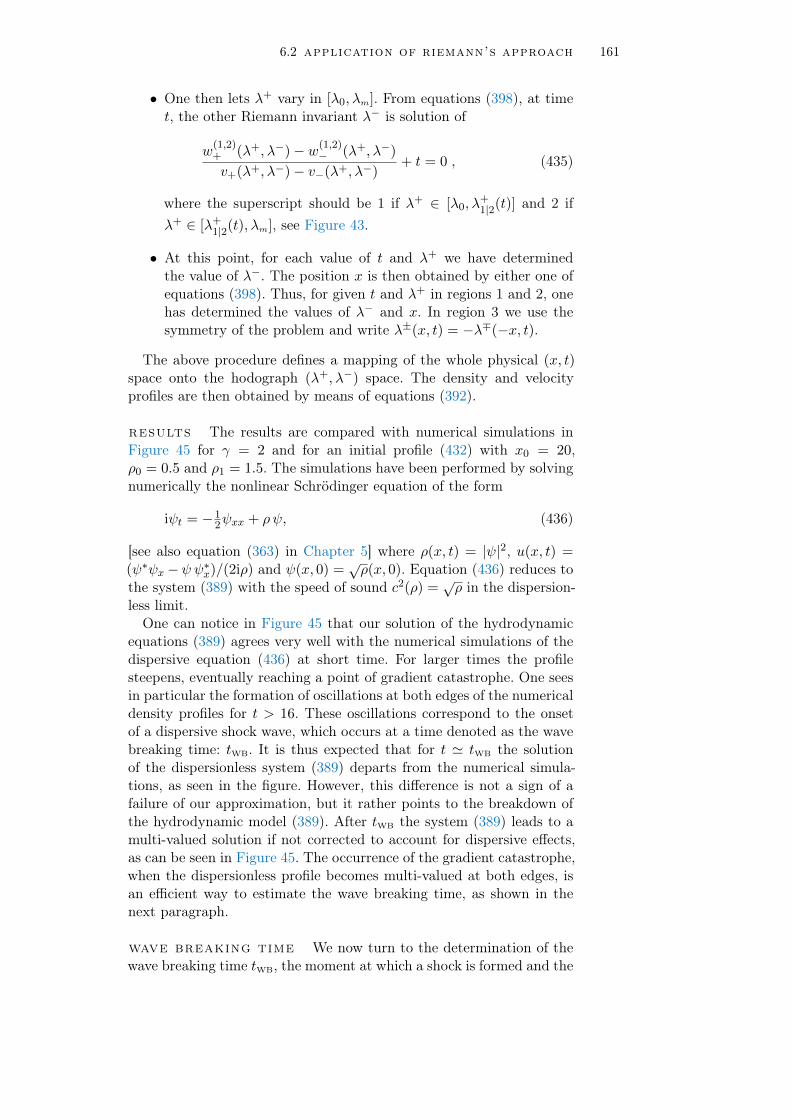
6.2 application of riemann’s approach 161
• One then lets λ+ vary in [λ0, λm]. From equations (398), at timet, the other Riemann invariant λ− is solution of
w(1,2)+ (λ+, λ−)− w(1,2)
− (λ+, λ−)
v+(λ+, λ−)− v−(λ+, λ−)+ t = 0 , (435)
where the superscript should be 1 if λ+ ∈ [λ0, λ+1|2(t)] and 2 if
λ+ ∈ [λ+1|2(t), λm], see Figure 43.
• At this point, for each value of t and λ+ we have determinedthe value of λ−. The position x is then obtained by either one ofequations (398). Thus, for given t and λ+ in regions 1 and 2, onehas determined the values of λ− and x. In region 3 we use thesymmetry of the problem and write λ±(x, t) = −λ∓(−x, t).
The above procedure defines a mapping of the whole physical (x, t)space onto the hodograph (λ+, λ−) space. The density and velocityprofiles are then obtained by means of equations (392).
results The results are compared with numerical simulations inFigure 45 for γ = 2 and for an initial profile (432) with x0 = 20,ρ0 = 0.5 and ρ1 = 1.5. The simulations have been performed by solvingnumerically the nonlinear Schrödinger equation of the form
iψt = −12ψxx + ρψ, (436)
[see also equation (363) in Chapter 5] where ρ(x, t) = |ψ|2, u(x, t) =(ψ∗ψx −ψ ψ∗x)/(2iρ) and ψ(x, 0) =
√ρ(x, 0). Equation (436) reduces to
the system (389) with the speed of sound c2(ρ) =√ρ in the dispersion-
less limit.One can notice in Figure 45 that our solution of the hydrodynamic
equations (389) agrees very well with the numerical simulations of thedispersive equation (436) at short time. For larger times the profilesteepens, eventually reaching a point of gradient catastrophe. One seesin particular the formation of oscillations at both edges of the numericaldensity profiles for t > 16. These oscillations correspond to the onsetof a dispersive shock wave, which occurs at a time denoted as the wavebreaking time: tWB. It is thus expected that for t ' tWB the solutionof the dispersionless system (389) departs from the numerical simula-tions, as seen in the figure. However, this difference is not a sign of afailure of our approximation, but it rather points to the breakdown ofthe hydrodynamic model (389). After tWB the system (389) leads to amulti-valued solution if not corrected to account for dispersive effects,as can be seen in Figure 45. The occurrence of the gradient catastrophe,when the dispersionless profile becomes multi-valued at both edges, isan efficient way to estimate the wave breaking time, as shown in thenext paragraph.
wave breaking time We now turn to the determination of thewave breaking time tWB, the moment at which a shock is formed and the

162 dispersionless evolution of nonlinear pulses
Figure 45: Density profile ρ(x, t) for different times of propagation t. Theinitial density distribution ρ(x) is Gaussian, with x0 = 20, ρ0 =0.5 and ρ1 = 1.5 [see equations (419) and (432)]. The blue curvescorrespond to the theoretical results obtained from expressions(431), with β = 1
2 (γ = 2). For this specific value of the adiabaticindex γ, the nonlinear Schrödinger equation (436) can be indeedmapped onto hydrodynamic equations (389) in the dispersionlesslimit [or equation (366) when dispersion is taken into account].The red curves are obtained with numerical simulations of thedispersive equation (436). The formation of oscillations aroundt ' 20 correspond to the birth of a dispersive shock wave.
dispersionless approach fails. As mentioned in the above paragraph, thiscorresponds to a gradient catastrophe, i.e., a point of infinite gradient∂λ±/∂x =∞. If one considers for instance the right part of the profile(region 3), from equations (398), this occurs at a time t such that
t = − ∂w(3)+ /∂λ+
1 + c′(λ+ − λ−)= − ∂w
(3)+ /∂λ+
1 + d ln cd ln ρ
∣∣∣λ+−λ−
, (437)
and tWB is the smallest of the times7 (437).One can easily compute tWB approximately when the point of largest
gradient in ρ(x) lies in a region where ρ ' ρ0. This occurs for somespecific initial distributions (such as the inverted parabola consideredin Section 6.2.3) or when the initial bump is only a small perturbation
7 It is worth noticing that this formula yields an expression for the breaking timeobtained from our approximate solution of the initial value problem and in thissense it provides less general but more definite result than the upper estimate of thebreaking time obtained by Lax in Ref. [112].

6.2 application of riemann’s approach 163
of the background. In this case, it is legitimate to assume that wavebreaking is reached for λ− ' −λ0 and this yields
λ+ − λ− ' 12
∫ ρ
0
c(ρ′)ρ′
dρ′ + 12
∫ ρ0
0
c(ρ′)ρ′
dρ′. (438)
Equations (401) and (429) then lead to w(3)+ ' x(λ+) and (437) becomes
t ' − 2
1 + d ln cd ln ρ
∣∣∣ρ
× ρ
c(ρ)dρdx
, (439)
where ρ stands for ρ(x(λ+)). Within our hypothesis, it is legitimate toassume that the shortest of times t is reached close to the point x(λ+)for which |dρ/dx| is maximal8. We note x∗ the coordinate of this pointand ρ∗ = ρ(x∗). One thus obtains
tWB '2
1 + d ln cd ln ρ
∣∣∣ρ∗
× ρ∗
c(ρ∗) · max∣∣∣dρdx
∣∣∣. (440)
For an initial density distribution of the form (432) with c(ρ) =√ρ
(γ = 2), one obtains
tWB '4
3
√e
2x0
√ρ0 + e−1/2ρ1
ρ1. (441)
For the specific initial conditions of Figure 45: x0 = 20, ρ0 = 0.5, andρ1 = 1.5, expression (441) yields tWB ' 17.4, in good agreement withnumerical simulations.
6.2.2 Example on a non-integrable system
We now study in some details a case where the dependence of c onρ is less simple than the one of equation (390): this is the case of azero temperature Bose-Einstein condensate transversely confined in anatomic wave guide. For a harmonic trapping, the transverse averagedchemical potential can be represented by the interpolating formula [73]
µ⊥(ρ) = ~ω⊥√
1 + 4aρ, (442)
where ω⊥ is the angular frequency of the transverse harmonic potential,a > 0 is the s-wave scattering length, ρ(x, t) = |ψ(x, t)|2 is the lineardensity of the condensate, and ψ(x, t) is the one-dimensional condensatewave function9. In this case, the dynamics of the condensate is governedby an effective one-dimensional Gross-Pitaevskii equation
i~∂t ψ = − ~2
2m∂xxψ + µ⊥(|ψ|2)ψ, (443)
8 Indeed, the gradient catastrophe is likely to occur at the point where the initialdensity gradient is maximal.
9 We note that other expressions for µ⊥ have also been proposed in the literature [101,161].

164 dispersionless evolution of nonlinear pulses
with m the mass of the atoms in the Bose gas. When aρ 1, one recov-ers the transverse Gaussian regime with µ⊥(ρ) ' ~ω⊥ + g|ψ|2, whereg = 2~ω⊥a [135] is an effective one-dimensional nonlinear coupling con-stant (see Section 3.1.2 where the 1D mean-field regime is discussed inmore detail).Expression (442) yields the correct sound velocity mc2 = ρ dµ⊥/dρ
both in the low (aρ 1) and in the high (aρ 1) density regimes.In these two limiting cases the dispersionless dynamics of the system isthus correctly described by the hydrodynamic equations (389) with, inappropriate dimensionless units10
c2(ρ) =ρ√
1 + ρ, (444)
where one has made the changes of variables 4aρ → ρ, u/u0 → u,x/x0 → x and t/t0 → t, where 2mu2
0 = ~ω⊥ and t0 = x0/u0. Thelength x0 used to non-dimensionalize the dispersionless equations is afree parameter: we will chose it equal to the parameter x0 appearing inthe initial condition11 (432). Note that in dimensionless units equation(443) becomes
iψt = −12ψxx + 2ψ
√1 + |ψ|2, (445)
which is a non-integrable equation.
Let us now apply the Riemann’s method. In the case characterizedby equations (442) and (444), expressions (417) and (418) yield
R(λ1, λ2) =
(ρ2(λ1) + ρ3(λ1)
ρ2(λ2) + ρ3(λ2)
)1/8
, (446)
where ρ(λ) is the reciprocal function of
λ(ρ) = 2
∫ √ρ
0
du(1 + u2)1/4
. (447)
We can now insert the above expressions in equations (429) and usethe procedure described in Section 6.2.1 to obtained theoretically thedensity and velocity distributions ρ(x, t) and u(x, t). The results areshown and compared with numerical simulations in Figure 46 for aninitial profile (432) with ρ0 = 1 and ρ1 = 1. The simulations have beenperformed by solving numerically a generalized nonlinear Schrödingerequation (445).Once again, as already observed in Figure 45, the approximate expres-
sions (429) give an excellent agreement with the numerical simulations
10 This can be easily proven using a Madelung transformation ψ =√ρ exp(i S), with
∂xS(x, t) = u(x, t), ρ(x, t) and u(x, t) being the density and the velocity distributionsof the gas.
11 We note here that the initial condition (432) can be realized by several means inthe context of BEC physics. One can for instance suddenly switch on at t = 0 ablue detuned focused laser beam [13]. An alternative method has been demonstratedin Ref. [86]: by monitoring the relative phase of a two species condensate, one canimplement a bump (or a through) in one of the components.

6.2 application of riemann’s approach 165
and confirm the efficiency of Riemann’s method to describe the propa-gation of nonlinear pulses.
We can also estimate the wave breaking time using expression (440);for a sound velocity of the form (444), we find
tWB '√e
2
8(1 + ρ∗)6 + 5ρ∗
x0
c(ρ∗)ρ∗
ρ1. (448)
The location xWB of the wave breaking event can be obtained from (398).Within our approximation scheme, this yields, for the right part of theprofile:
xWB ' x∗ + c(ρ∗)tWB. (449)
These results are compared in Figure 47 with the values determinedfrom the Riemann approach. The overall agreement is excellent. Wealso note that replacing ρ∗ by ρ0 in equations (448) and (449) gives aresult which is less accurate, but still quite reasonable, see Figure 47.
Figure 46: Density and velocity plotted as a function of x/x0 for dimension-less times t/t0 = 0.5, 1, 1.5, 2, 3 and 4 respectively. The initialconditions are given by equations (419) and (432) with ρ0 = 1and ρ1 = 1, they are represented by the gray solid lines. Theblue solid lines are the results of the hydrodynamic system (389)obtained from the approximate Riemann’s approach describedin Section 6.1.2. The red curves are the results of the numericalsimulations of equations (445).

166 dispersionless evolution of nonlinear pulses
Figure 47: Wave breaking time tWB and position of the wave breaking eventxWB for different values of ρ1/ρ0. The system considered is aquasi-1D Bose-Einstein condensate for which the speed of soundis given by (444). The initial distributions given by equation (432)and u(x, t = 0) = 0. The blue solid lines are the approximate re-sults (448) and (449). The red dots are the results obtained fromRiemann’s approach. The brown solid lines are obtained by re-placing ρ∗ by ρ0 in equations (448) and (449), see the paragraph‘Wave breaking time’ of Section 6.2.1, and, in particular, expres-sions (439) and (440).
6.2.3 Nonlinear optics with specific initial conditions
We conclude this chapter with a last example, when the initial densitydistribution is not Gaussian, as in equation (432), but has the form ofan inverted parabola:
ρ(x) ≡ ρ(x, 0) =
ρ0 + ρ1(1− x2/x2
0) if |x| < x0,
ρ0 if |x| ≥ x0,(450)
and
u(x, 0) = 0. (451)
We still consider the propagation of an optical beam in a nonlinearmaterial. Therefore, the dynamics of the fluid of light is governed by thenonlinear Schrödinger equation (436), i.e., a specific case of polytropicgases with adiabatic index γ = 2. The sound velocity is thus c(ρ) =
√ρ
and the Riemann invariants are given by λ± = 12u+
√ρ.
Equations (421) and (422) are in the considered case:
x =
x(3)(λ) if x > 0,
x(1)(λ) if x < 0,(452)
with
x(3)(λ) = −x(1)(λ) = x0
√1− λ2 − ρ0
ρ1. (453)
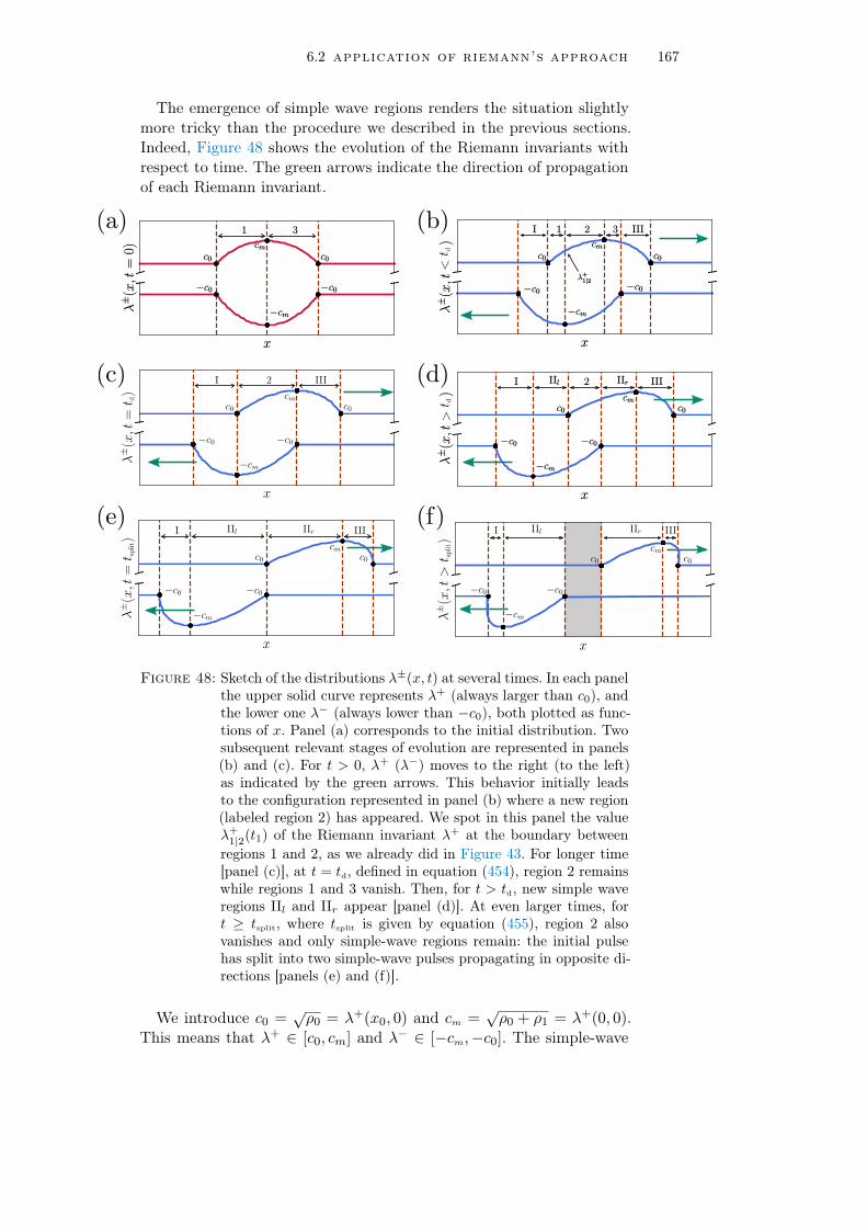
6.2 application of riemann’s approach 167
The emergence of simple wave regions renders the situation slightlymore tricky than the procedure we described in the previous sections.Indeed, Figure 48 shows the evolution of the Riemann invariants withrespect to time. The green arrows indicate the direction of propagationof each Riemann invariant.
Figure 48: Sketch of the distributions λ±(x, t) at several times. In each panelthe upper solid curve represents λ+ (always larger than c0), andthe lower one λ− (always lower than −c0), both plotted as func-tions of x. Panel (a) corresponds to the initial distribution. Twosubsequent relevant stages of evolution are represented in panels(b) and (c). For t > 0, λ+ (λ−) moves to the right (to the left)as indicated by the green arrows. This behavior initially leadsto the configuration represented in panel (b) where a new region(labeled region 2) has appeared. We spot in this panel the valueλ+1|2(t1) of the Riemann invariant λ+ at the boundary betweenregions 1 and 2, as we already did in Figure 43. For longer time[panel (c)], at t = td, defined in equation (454), region 2 remainswhile regions 1 and 3 vanish. Then, for t > td, new simple waveregions IIl and IIr appear [panel (d)]. At even larger times, fort ≥ tsplit, where tsplit is given by equation (455), region 2 alsovanishes and only simple-wave regions remain: the initial pulsehas split into two simple-wave pulses propagating in opposite di-rections [panels (e) and (f)].
We introduce c0 =√ρ0 = λ+(x0, 0) and cm =
√ρ0 + ρ1 = λ+(0, 0).
This means that λ+ ∈ [c0, cm] and λ− ∈ [−cm,−c0]. The simple-wave

168 dispersionless evolution of nonlinear pulses
regions, where one of the Riemann invariants is constant, are denotedI, IIl, IIr and III (see Figure 48).Before entering into the details, we introduce two important times td
and tsplit which define three stages during the propagation of the pulse:
• Time td corresponds to the vanishing of regions 1 and 3 [see graph(c) of Figure 48]. At this precise moment, λ+ = cm and λ− = −c0.Thus, using equation (435), we obtain
td = −w(2)+ (cm,−c0)− w(2)
− (cm,−c0)
v+(cm,−c0)− v−(cm,−c0), (454)
with w(2)± = ∂W (2)/∂λ± and v±(λ+, λ−) given by expression (395).
In the case a polytropic gas with adiabatic index γ = 2, v+−v− =λ+ − λ−.
• Time tsplit defines the moment for which the pulse splits into twosimple-wave pulses propagating in opposite directions. This situ-ation corresponds to the graph (e) of Figure 48. Likewise, this isalso the exact point in time for which region 2 disappears andλ± = ±c0 at the position where the pulse splits (in our case, thisoccurs exactly at x = 0, see graph (e) of Figure 48). Therefore,
tsplit = −w(2)+ (c0,−c0)− w(2)
− (c0,−c0)
v+(c0,−c0)− v−(c0,−c0). (455)
This gives
tsplit =x0
c0+
1
4 c5/20
∫ cm
c0
√λ [x(3)(λ)− x(1)(λ)]dλ . (456)
For an initial profile of the form (450), x(1,3)(λ) are given by ex-pressions (453), and this leads to
tsplit =x0
c0
(1 +G(ρ1/ρ0)
), (457)
where
G(X) =X
4
∫ 1
0
√1− u
(1 +Xu)1/4du . (458)
The three stages thus corresponds to:
• 0 ≤ t ≤ tdThis stage of the propagation is illustrated in the graphs (a), (b)and (c) of Figure 48. The simple-wave regions, where one of theRiemann invariants is constant, are denoted I and III. As shownin graph (b) of Figure 48, region I corresponds to λ+(x ∈ I, t) =c0, and region III to λ−(x ∈ III, t) = −c0. Region 2 appears,exactly as it occurred in the previous section for a Gaussian pulse.Therefore, in regions 1, 2 and 3, one can safely apply the procedure

6.2 application of riemann’s approach 169
described in Section 6.2.1 where the potential W (n), n ∈ 1, 2, 3is given by expressions (431), with β = 1
2 .
For any time t, such that 0 ≤ t ≤ td, the boundary betweenregion I and 1 located at a position denoted xI−1 can be foundas follows: one fixes λ+ = c0. Then, one finds the correspondingvalue of λ− = λ−c0 , solving equation (435) with the superscript 1.Ultimately, using equations (398), we obtain
xI−1 = v−(c0, λ−c0) t+ w
(1)− (c0, λ
−c0), (459)
where w(1)− = ∂W (1)/∂λ−.
Once xI−1 is determined, region I corresponds to x ≤ xI−1, with
x = v−(c0, λ−) t+ w
(1)− (c0, λ
−), x ∈ I, (460)
for λ− ∈ [λ−c0 ,−c0]. The Riemann invariants in the area locatedat the left of region I are simply λ± = ±c0, see graph (b) ofFigure 48.
The boundary between regions 3 and III is simply determined bysymmetry of the problem12: x3−III = −xI−1, λ+(3−III, t) = −λ−c0 ,and λ− = −c0 (see graph (b) of Figure 48). Then, region IIIcorresponds to x ≥ x3−III, with
x = v+(λ+,−c0) t+ w(3)+ (λ+,−c0), x ∈ III, (461)
for λ+ ∈ [c0,−λ−c0 ].
At the precise time td, when regions 1 and 3 vanish (see graph (c)of Figure 48), the boundary between I and 2, denoted xI−2, andbetween 2 and III, denoted x2−III, are given by
xI−2 = v−(c0,−cm) t+ w(2)− (c0,−cm),
x2−III = v+(cm,−c0) t+ w(2)+ (cm,−c0),
(462)
that is to say λ−c0 = −cm in equation (459), see graph (c) ofFigure 48.
• td < t < tsplit
This stage corresponds to the graph (d) of Figure 48. Regions Iand 2 become disconnected, as well as regions 2 and III. Two newsimple-wave regions denoted IIl and IIr emerge and fill the gapbetween the disconnected regions (see graph (d) of Figure 48).
First, in region I and III, the determination of xI−2 and x2−III
still holds [see equations (462)]. We denote these positions xI−IIl
12 In the case of a non-symmetric problem – corresponding to u(x, 0) 6= 0, i.e.,λ+(x, 0) 6= −λ−(x, 0)–, one can still use equation (435) with λ− = −c0 and findthe corresponding value of λ+.

170 dispersionless evolution of nonlinear pulses
and xIIr−III, since they locate now the boundaries between I andIIl and between IIr and III, respectively:
xI−IIl = v−(c0,−cm) t+ w(2)− (c0,−cm),
xIIr−III = v+(cm,−c0) t+ w(2)+ (cm,−c0),
(463)
Then, one can use equations (460) and (461), to determine thepositions associated to λ+ = c0, λ− ∈ [−cm,−c0] (region I) orλ+ ∈ [c0, cm], λ− = −c0 (region III).
Second, the boundaries between regions IIl and 2 and between 2and IIr are determined exactly as explained above equation (459):one fixes λ+ = c0. Then, one finds the corresponding value ofλ− = λ−c0 , solving equation (435), now with the superscript 2.Using equations (398), we obtain
xIIl−2 = v−(c0, λ−c0) t+ w
(2)− (c0, λ
−c0),
x2−IIr = −xIIl−2.(464)
Then, for xI−IIl ≤ x ≤ xIIl−2 (region IIl),
x = v−(c0, λ−) t+ w
(2)− (c0, λ
−), λ− ∈ [−cm, λ−c0 ], (465)
and, for x2−IIr ≤ x ≤ xIIr−III (region IIr),
x = v+(λ+,−c0) t+w(2)+ (λ+,−c0), λ+ ∈ [−λ−c0 , cm]. (466)
• t ≥ tsplit
This stage corresponds to graphs (e) and (f) of Figure 48. Whent = tsplit, region 2 vanishes, see graph (e). The boundary be-tween regions IIl and IIr amounts to take t = tsplit and the limitλ−c0 → −c0 in equation (464). The other boundaries (between Iand IIl and between IIr and III) are determined as explained inthe previous point [see equations (463)]. Note that now all regionsare simple-wave regions.
For t > tsplit [see graph (f)], one determines easily the bound-aries between the different regions; the only change with respectto graph (e) is the separation between regions IIl and IIr andthe emergence of the grey area where λ± = ±c0. The bound-ary between this grey region and IIl still corresponds to the limitλ−c0 → −c0 in equation (464).
Note the multi-valued regions at the left edge of λ− and the rightedge of λ+ in graph (f) of Figure 48. This indicates that this graphis obtained after the wave breaking time. Here, the wake breakingthus occurs after the splitting of the initial pulse into two pulses,i.e., tWB > tsplit; this is not always the case, see below and, inparticular, Figure 50.

6.2 application of riemann’s approach 171
One obtains an excellent description of the initial dispersionless stageof evolution of the pulse, as demonstrated by the very good agreementbetween theory and numerical simulations illustrated in Figure 49. Thegraphs in this figure compare at different times the theoretical densityprofile ρ(x, t) with the one obtained by numerical integration of equation(436), taking the initial condition u(x, 0) = 0 and ρ(x, 0) given by (450)with x0 = 20, ρ0 = 0.5 and ρ1 = 1.5. One sees that the profile is multi-valued at both edges for t = 10 and t = 15; this means that the gradientcatastrophe already occurred, and thus tWB < 10. An exact calculationwill yield tWB ' 6.3 (see next paragraph), confirming this observation.
wave breaking time The wave breaking exactly occurs at theposition xWB = x0, since this position corresponds to the highest densitygradient [see equation (450)]. Using (437) and the expression of w(3)
+ ,obtained from W (3) [see equations (431)], an easy computation leads tothe exact result Remember that
γ = 2 and β = 12.
tWB =2
3
∣∣∣∣∣dx(3)
dλ
∣∣∣∣∣λ=c0
=2 c0 x0
3 ρ1, (467)
where we used the expression of x(3)(λ) given by (453).Taking x0 = 20, ρ0 = 0.5 and ρ1 = 1.5, one obtains tWB ' 6.3 in
excellent agreement with the emergence of a multi-valued profile whenusing the Riemann’s method.
Figure 49: Comparison between theoretical results obtained from Riemann’smethod (blue curves) and numerical simulations of equation (436)(red curves) for different times of propagation t = 0, 5, 10 and 15.The initial density distribution ρ(x) is given by expression (450).
Figure 50 displays several typical density profiles in a “phase space”with coordinates ρ1/ρ0 and t. The curves tsplit(ρ1/ρ0) [as given by equa-tions (457) and (458)] and tWB(ρ1/ρ0) [equation (467)] separate this

172 dispersionless evolution of nonlinear pulses
plane in four regions, labeled as (a), (b), (c) and (d) in the figure.These two curves cross at a point represented by a white dot whosecoordinates we determined numerically as being ρ1/ρ0 = 0.60814 andc0 t/x0 = 1.09623. These coordinates are universal in the sense thatthey have the same value for any initial profile of inverted parabolatype, such as given by equation (450), with u(x, 0) = 0. Other types ofinitial profile would yield different precise arrangements of these curvesin phase space, but the qualitative behavior illustrated by Figure 50 isgeneric. For instance, when tWB < t < tsplit, the wave breaking has al-ready occurred while the profile is not yet split in two separated humps.This situation is represented by the inset (b). This is the situation whichhas been considered in Refs. [191] and [200].
The physical situation depicted in Figure 50 corresponds to physi-cal intuition: a larger initial hump (larger ρ1/ρ0) experiences earlierwave breaking, and needs a longer time to be separated in two contra-propagating pulses. On the contrary, a small perturbation, with ρ1 ρ0,will split much before experiencing a wave breaking. Moreover, we canlearn from Figure 50 that perturbation theory always fails in describingcorrectly the propagation of a nonlinear pulse at large times. Indeed,any hump on top of a background (ρ1 > 0), no matter how small it is,will lead to the formation of a dispersive shock wave at some finite time;this time can be very large (tWB → +∞, when ρ1 → 0, see Figure 50),but is never infinite.
Figure 50: Behavior of the light intensity profile ρ = |ψ|2 [see equation (436)]in the plane (ρ1/ρ0, t). The plane is separated in four regionsby the curves t = tWB [see equation (467)] and t = tsplit [seeequations (457) and (458)]. These curves cross at the point rep-resented by a white dot (of coordinates ρ1/ρ0 = 0.60814 andc0 t/x0 = 1.09623). Typical profiles obtained numerically are dis-played in the insets (a), (b), (c) and (d) which represent ρ(x, t)plotted as a function of x for fixed t.

6.2 application of riemann’s approach 173
We conclude this chapter by stressing that Riemann’s method is apowerful tool to describe the propagation of a pulse within a disper-sionless approximation. In the case of an optical beam propagating in amedium, we have used Riemann’s approach for two different initial con-ditions: an inverted parabola and a Gaussian beam. The latter is morerealistic experimentally, but the description of the dispersive shock waveis a bit more difficult than for the inverted parabola. Indeed, as we willsee in the next chapter, if one takes a Gaussian beam initially, fourRiemann invariants vary concomitantly in the region of the dispersiveshock wave, which renders the study quite involved. Moreover, in thiscase, the determination of the breaking time and of the boundary of theDSW can only be determined approximately. On the contrary, in thecase of an inverted parabola, the description of the short-time propaga-tion using Riemann’s method is more tedious, since one has to worryabout the emergence of simple wave regions (which do not exist for aGaussian beam). However, the wave breaking time and the position ofthe dispersive shock wave can be determined exactly. In addition, onlytwo Riemann invariants vary in the region of the dispersive shock wave.In this case, as we will see in Chapter 7, we know how to describe thedispersive shock wave using both Whitham modulational theory andthe method presented in Refs. [56, 82].

174 dispersionless evolution of nonlinear pulses
6.3 article: short-distance propagation of nonlin-ear optical pulses
→ Short-distance propagation of nonlinear optical pulses
M. Isoard, A.M. Kamchatnov, N. Pavloff, 22e Rencontre du Non-Linéaire, Non-Linéaire Pub (2019)
We theoretically describe the quasi one-dimensional transverse spread-ing of a light pulse propagating in a defocusing nonlinear optical mate-rial in the presence of a uniform background light intensity. For shortpropagation distances the pulse can be described within a nondisper-sive approximation by means of Riemann’s approach. The theoreticalresults are in excellent agreement with numerical simulations.

rencontre du non-lineaire 2019 1
Short-distance propagation of nonlinear optical pulses
Mathieu Isoard1, A. M. Kamchatnov2,3 & N. Pavloff1
1 LPTMS, UMR 8626, CNRS, Univ. Paris-Sud, Universite Paris-Saclay, 91405 Orsay, France2 Institute of Spectroscopy, Russian Academy of Sciences, Troitsk, Moscow, 108840, Russia3 Moscow Institute of Physics and Technology, Institutsky lane 9, Dolgoprudny, Moscow region, 141701, Russia
Resume. Nous etudions la propagation transverse d’un pulse lumineux quasi-unidimensionnel dans un milieuoptique non-lineaire, en presence d’un fond d’intensite lumineuse constante. Dans un premier temps, le signalinitial se divise en deux parties qui se propagent dans des directions opposees. Ce phenomene peut etre decrittheoriquement a l’aide d’une approche non dispersive en utilisant une modification de la methode de Riemannproposee par Ludford. Les resultats sont en excellent accord avec les simulations numeriques.
Abstract. We theoretically describe the quasi one-dimensional transverse spreading of a light pulse propagatingin a defocusing nonlinear optical material in the presence of a uniform background light intensity. For shortpropagation distances the pulse can be described within a nondispersive approximation by means of Riemann’sapproach. The theoretical results are in excellent agreement with numerical simulations.
1 Introduction
It has long been realized that light propagating in a nonlinear medium was amenable to a hydrodynamictreatment [1,2]. In the present work we use such an approach to study a model configuration whichhas been realized experimentally in a one-dimensional situation in the defocusing regime in Ref. [3]:the nonlinear spreading of a region of increased light intensity in the presence of a uniform constantbackground. In the absence of background, and for a smooth initial intensity pattern, the spreading ismainly driven by the nonlinear defocusing and can be treated analytically in some simple cases [1]. Thesituation is more interesting in the presence of a constant background: the pulse splits in two parts,each eventually experiencing nonlinear wave breaking, leading to the formation of dispersive shock wavesat both extremities of the split pulse. In the present work we concentrate on the pre-shock period anddemonstrate that it can be very accurately described within a non-dispersive nonlinear approximation.
The paper is organized as follows: In Sec. 2 we present the model and the set-up we aim at studying.The spreading and the splitting stage of evolution is accounted for in Sec. 3 within a dispersionlessapproximation which holds when the pulse region initially presents no large intensity gradient. Theproblem is first mapped onto an Euler-Poisson equation in Sec. 3.1. This equation is solved in Sec. 3.2by using Riemann-Ludford method. In Sec. 3.3 the theoretical results are compared with numericalsimulations. Our conclusions are presented in Sec. 4.
2 The model
In the paraxial approximation, the stationary propagation of the complex amplitude A(r) of the electricfield of a monochromatic beam is described by the equation (see, e.g., Ref. [4])
i∂zA = − 1
2n0k0∇2⊥A− k0δnA .
In this equation, n0 is the linear refractive index, k0 = 2π/λ0 is the carrier wave vector, z is the longitu-dinal coordinate along the beam, ∇2
⊥ the transverse Laplacian and δn is a nonlinear contribution to theindex. In a non absorbing defocusing Kerr nonlinear medium one can write δn = −n2|A|2, with n2 > 0.
c© Non Lineaire Publications, Avenue de l’Universite, BP 12, 76801 Saint-Etienne du Rouvray cedex

2 M. Isoard et al.
We consider a system with a uniform background light intensity, denoted as I0, on top of which aninitial pulse is added at the entrance of the nonlinear cell. To study the propagation of this pulse alongthe beam (direction z), we introduce the following characteristic quantities: the nonlinear length zNL =(k0n2I0)−1 and the transverse healing length β⊥ = (zNL/n0k0)1/2. Since the transverse profile depends ona single Cartesian coordinate, we write ∇2
⊥ = β−2⊥ ∂2
x where x is the dimensionless transverse coordinate,and also define an effective “time” t = z/zNL. In this framework, the quantity ψ(x, t) = A(x, t)/
√I0 is
solution of the dimensionless nonlinear Schrodinger (NLS) equation
iψt = − 12ψxx + |ψ|2ψ . (1)
The initial ψ(x, t = 0) is real (i.e., no transverse velocity or, in optical context, no focusing of the lightbeam at the input plane), with a dimensionless intensity ρ(x, t) = |ψ|2 which departs from the constantbackground value (which we denote as ρ0) only in the region near the origin where it forms a bump. Tobe specific, we consider the typical case where
ρ(x, 0) = ρ0 + ρ1 exp (−2x2/x20) , and u(x, 0) = 0 . (2)
The maximal density of the initial profile is ρ(0, 0) = ρ0 + ρ1 ≡ ρm.
3 The dispersionless stage of evolution
The initial pulse splits into two signals propagating in opposite directions of x axis. The aim of thissection is to theoretically describe this splitting within a dispersionless approximation.
3.1 Riemann variables and Euler-Poisson equation
By means of the Madelung substitution ψ(x, t) =√ρ(x, t) exp
(i∫ x
u(x′, t) dx′), the NLS equation (1)
can be cast into a hydrodynamic-like form for the density ρ(x, t) and the flow velocity u(x, t):
ρt + (ρu)x = 0 , ut + uux + ρx +
(ρ2x
8ρ2− ρxx
4ρ
)
x
= 0 . (3)
These equations are to be solved with the initial conditions (2). The last term of the left hand-side of thesecond of Eqs. (3) accounts for the dispersive character of the fluid of light. In the first stage of spreading
of the bump, if the density gradients of the initial density are weak (i.e., if x0 minρ−1/20 , ρ
−1/21 ), the
effects of dispersion can be neglected, and the system (3) simplifies to
ρt + (ρu)x = 0 , ut + uux + ρx = 0 . (4)
The above equations can be written in a more symmetric form by introducing the Riemann invariants
λ±(x, t) = 12u(x, t)±
√ρ(x, t) , (5)
which evolve according to the system [equivalent to (4)]:
∂tλ± + v±(λ−, λ+) ∂xλ
± = 0 , with v±(λ−, λ+) = 12 (3λ± + λ∓) = u±√ρ . (6)
The Riemann velocities v± in (6) have a simple physical interpretation for a smooth velocity and densitydistribution: v+ (v−) corresponds to a signal which propagates downstream (upstream) at the localvelocity of sound c =
√ρ and which is dragged by the background flow u.
The system (6) can be linearized by means of the hodograph transform (see, e.g., Ref. [5]) whichconsists in considering x and t as functions of λ+ and λ−. One readily obtains
∂±x− v∓∂±t = 0, (7)

Propagation of nonlinear optical pulses 3
where ∂± ≡ ∂/∂λ±. One introduces two auxiliary (yet unknown) functions W±(λ−, λ+) such that
x− v±(λ−, λ+) t = W±(λ−, λ+). (8)
Inserting the above expressions in (7) shows that the W±’s are solution of Tsarev equations [6]
∂−W+
W+ −W−=
∂−v+
v+ − v−, and
∂+W−W+ −W−
=∂+v−v+ − v−
. (9)
From Eqs. (6) and (9) one can verify that ∂−W+ = ∂+W−, which shows that W+ and W− can be soughtin the form
W± = ∂±χ, (10)
where χ(λ−, λ+) plays the role of a potential. Substituting expressions (10) in one of the Tsarev equationsshows that χ is a solution of the following Euler-Poisson equation
∂2χ
∂λ+∂λ−− 1
2 (λ+ − λ−)
(∂χ
∂λ+− ∂χ
∂λ−
)= 0 . (11)
3.2 Solution of the Euler-Poisson equation
We use Riemann’s method (see, e.g., Ref. [7]) to solve the Euler-Poisson equation (11) in the (λ+, λ−)–plane which we denote below as the “characteristic plane”. We follow here the procedure exposed inRef. [8] which applies to non-monotonous initial distributions, such as the one corresponding to Eq. (2).
We first schematically depict in Fig. 1(a) the initial spatial distributions λ±(x, 0) of the Riemanninvariants (left panel). The initial condition (2) yields λ±(x, 0) = ±
√ρ(x, 0). A later stage of evolution
is shown in the right panel of Fig. 1. We introduce notations for some remarkable values of the Riemanninvariants: λ±(−∞, t) = λ±(∞, t) = ±√ρ0 ≡ ±c0 and λ±(0, 0) = ±√ρm ≡ ±cm. We also define as partA (part B) the branch of the distribution of the λ±’s which is at the right (at the left) of the extremum±cm. These notations are summarized in Fig. 1(a).
λ±(x,t
=0)
cm
31
B A
(a)
x
−cm
B A λ±(x,t
=t 1) cmλ+
1|2
321(b)
x
−cm
Figure 1. Sketch of the distributions λ±(x, t) at time t = 0 (left panel) and at finite time t > 0 (right panel). Ineach panel the upper solid curve represent λ+ (always larger than c0), and the lower one λ− (always lower than−c0). Panel (a) corresponds to the initial distribution, in which part B corresponds to region 1 and part A toregion 3 (see the text). For t > 0, λ+ (λ−) moves to the right (to the left) and part B of λ+ starts to overlap withpart A of λ−. This leads to the configuration represented in panel (b) where a new region (labeled region 2) hasappeared. For later convenience, the value λ+
1|2(t1) is added in this panel. It corresponds to the value of λ+ at the
boundary between regions 1 and 2 (see the discussion in Sec. 3.3).
At a given finite time, the x axis can be considered as divided in three domains, each requiring aspecific treatment. Each domain is characterized by the behavior of the Riemann invariants. In domain

4 M. Isoard et al.
3 (domain 1 respectively), λ+ is decreasing (increasing) while λ− is increasing (decreasing); in domain2 both are increasing, see Fig. 1(b). The theoretical description of this nonlinear wave is challengingbecause in each regions both Riemann invariants (λ+ and λ−) depend on position (i.e., there is no simplewave region).
The values of the Riemann invariants corresponding to Fig. 1(b) are represented in the characteristicplane in Fig. 2(a). The red curve C 0 in Figs. 2(a) and (b) corresponds to the initial conditions depictedin Fig. 1(a). Since λ+(x, 0) = −λ−(x, 0), the curve C 0 lies along the anti-diagonal in the characteristicplane. The (blue) curvy lines correspond to regions where both Riemann invariants depend on position:the domains 1, 2 and 3. In each of these three domains the solution χ of the Euler-Poisson equationhas a different expression. In order to describe these three branches, following Ludford [8], we introduceseveral sheets in the characteristic plane by unfolding the domain [c0, cm]× [−cm,−c0] into a four timeslarger region as illustrated in Fig. 2(b). We remark here that the whole region above C 0 — shaded inFig. 2(b) — is unreachable for the initial distribution we consider: for instance, the upper shaded trianglein region 1 would correspond to a configuration in which λ+
region1(x, t) > |λ−region1(x, t)|, which does not
occur in our case, see Fig. 1(b). The potential χ(λ−, λ+) can now take a different form in each of theregions labeled as 1, 2 and 3 in Fig. 2(b) and still be considered as single-valued. In each of the threedomains, we use Riemann-Ludford method to solve Eq. (11). This yields, to a very good approximation(a thorough analysis can be found in Ref. [9])
χ(n)(λ−, λ+) =
√2√
λ+ − λ−∫ λ+
−λ−
√r wA/B(r) dr , (12)
for regions n = 1 and 3. In the above formula, the superscript A should be used when n = 3, and thesuperscript B when n = 1, and wA ( wB) is the inverse function of the initial λ profiles in part A (partB). For the initial condition (2) one has
x = wA/B(λ) = ±x0
√−1
2lnλ2 − ρ0
ρ1if x ≷ 0 .
In region 2, the formulae (12) are replaced by
χ(2)(λ−, λ+) =
√2√
λ+ − λ−
(∫ λ+
cm
√r wB(r) dr +
∫ cm
−λ−
√r wA(r) dr
). (13)
3.3 Results and comparison with numerical simulations
Once χ(n)(λ−, λ+) has been determined in each of the three regions (n = 1, 2 or 3), the problem is solved.
One first computes W(n)± (λ−, λ+) in each region from Eqs. (10), (12) and (13). Then, the procedure to
obtain the values of λ+ and λ− as functions of x and t is the following:
• One starts by determining the value of λ+ for which λ− = −cm at time t. This value of λ+ definesthe boundary between regions 1 and 2. We denoted it as λ+
1|2(t); it is represented in Fig. 1(b). From
Eqs. (8), λ+1|2(t) is a solution of
W(1)+ (−cm, λ+
1|2)−W (1)− (−cm, λ+
1|2)
v+(−cm, λ+1|2)− v−(−cm, λ+
1|2)+ t = 0 . (14)
We then know that, in region 1 at time t, λ+ takes all possible values between c0 and λ+1|2(t).
• One picks a value of λ+ in [c0, cm]. From Eqs. (8), λ− is then solution of
W(n)+ (λ−, λ+)−W (n)
− (λ−, λ+)
v+(λ−, λ+)− v−(λ−, λ+)+ t = 0 , (15)

Propagation of nonlinear optical pulses 5
−c0
−cm
c0 cm λ+λ−
C0
1
2
3
(a)
C0
−c0
−cm
−c0
c0 cm c0 λ+λ−
1
2
3
λ+ increases λ+ decreases
λ−
decr
ease
sλ−
incr
ease
s
(b)
Figure 2. (a) Behavior of the Riemann invariants in the characteristic plane at a given time t (blue curve). Thered curve C 0 corresponds to the initial condition [λ−(x, 0) = −λ+(x, 0)]. (b) The same curves in the four-sheetedunfolded surface. In our problem, the whole gray shaded domain above C0 is unreachable.
with n = 1 if λ+ ∈ [c0, λ+1|2(t)] and n = 2 if λ+ ∈ [λ+
1|2(t), cm]. This determines the value of the
Riemann invariants in regions 1 and 2. In region 3 one uses the symmetry of the problem and writesλ±(x, t) = −λ∓(−x, t), see Fig. 1(b).• At this point, for each value of t and λ+ we know the value of the other Riemann invariant λ−. The
position x is then simply obtained by either one of Eqs. (8). So, for given t and λ+ in region n, one hasdetermined the values of λ− and x. In practice, this makes it possible to associate a couple (λ−, λ+) toeach (x, t). The density and velocity profiles are then obtained through Eqs. (5).
The results of the above approach are compared in Fig. 3 with the numerical solution of Eq. (1), takingthe initial condition given by Eq. (2) with ρ0 = 0.5, ρ1 = 1.5 and x0 = 20. One reaches an excellentagreement for the density profile and also for the velocity profile (not shown in the figure) up to t ' 20.As time increases, the profile steepens and oscillations become visible at both ends of the pulse at t & 16.There exists a certain time, the wave breaking time tWB, at which nonlinear nondispersive spreading leadsto a gradient catastrophe; our approximation subsequently predicts a nonphysical multivalued profile, ascan be seen in Fig. 3 (for t > 20). The time tWB can be computed by noticing that the wave breakingoccurs for the value λ+
WB = (ρ0 + ρ1/√e )1/2 which is associated in the initial profile with the largest
gradient in ∂xρ. At the wave-breaking time the profile of λ+ in region 3 has a vertical tangent line:∂x/∂λ+ = 0. For simplicity we also assume that the wave breaking occurs in a region where one cansafely approximate λ− = −c0. Differentiation of (7) then yields
tWB =2
3
∣∣∣∣∣dW
(3)+ (−c0, λ+)
dλ+
∣∣∣∣∣λ+WB
=
∣∣∣∣∣∣
∫ λ+
c0
√rwA(r)dr
√2(λ+ + c0)5/2
+
√2(c0 − λ+)wA(λ+)
3√λ+(λ+ + c0)3/2
+2
3
√2λ+
λ+ + c0
dwA
dλ+
∣∣∣∣∣∣λ+WB
. (16)
The numerical value of tWB is found to be ' 19.15 for our choice of initial condition, in good agreementwith numerical simulations. Note also that for a small bump (ρ1 ρ0) the wave breaking time becomesvery large. From (16), and for an initial profile of type (2), one gets at leading order in ρ1/ρ0:
tWB '2√e
3
x0
c0
(ρ0
ρ1
). (17)
This means that the breaking time is much greater than the time ∼ x0/c0 of propagation of sound alongthe pulse profile. In our optical system the wave breaking is regularized by the formation of a dispersive

6 M. Isoard et al.
x−80
−60−40
−200
2040
6080
t
04
812
1620
2428
32
ρ(x,t)
0.0
0.5
1.0
1.5
2.0
t=0
t=4
t=8
t=12
t=16
t=20
t=24
t=28
t=32
Figure 3. Density pro-file ρ(x, t) correspond-ing to the initial con-ditions (2) with ρ0 =0.5, ρ1 = 1.5 and x0 =20. The red dashed linecorresponds to the ex-act solution of the dis-persionless system (6)(see the text), while theblack curve displays thedensity obtained fromthe numerical solutionof Eq. (1).
shock wave which is a region with large oscillations of intensity and phase, whose extend increases withtime, as can be seen in Fig. 3. Its description requires a nonlinear treatment able to account for dispersiveeffects and this goes beyond te scope of the present letter (see, e.g., Ref. [9]).
4 Conclusion
In this work we demonstrate that a nondispersive hydrodynamic approach to the spreading and splittingof an optical pulse compares extremely well with the results of numerical simulations up to the wavebreaking time. At larger time, one observes the formation of an optical dispersive shock wave, which canbe studied within Whitham modulation theory. In the case of the initial distribution given by Eq. (2), theshock should be described by four varying Riemann invariants and this requires a thorough investigation.Work in this direction is in progress.
References
1. V. I. Talanov, Radiophys. 9, 138 (1965).2. S. A. Akhmanov, A. P. Sukhorukov and R. V. Khokhlov, Usp. Fiz. Nauk 93, 19 (1967).3. W. Wan, S. Jia, and J. W. Fleischer, Nature Phys. 3, 46 (2007).4. L. D. Landau and E. M. Lifshitz, Electrodynamics of Continuous Media, Course of Theoretical Physics
vol. 8 (Elsevier Butterworth-Heinemann, Oxford, 2006).5. A. M. Kamchatnov, Nonlinear Periodic Waves and Their Modulations—An Introductory Course, (World
Scientific, Singapore, 2000).6. S. P. Tsarev, Math. USSR Izv. 37, 397 (1991).7. A. Sommerfeld, Partial Differential Equations in Physics, (Lectures on Theoretical Physics volume VI)
(Academic Press, New York, 1964).8. G. S. S. Ludford, Proc. Camb. Phil. Soc. 48, 499 (1952).9. M. Isoard, A.M. Kamchatnov, N. Pavloff, arXiv:1902.06975 [nlin.PS] (2019).

6.4 m. isoard, a.m. kamchatnov, n. pavloff, epl (2020) 181
6.4 article: dispersionless evolution of inviscid non-linear pulses
→ Dispersionless evolution of inviscid nonlinear pulses
M. Isoard, A.M. Kamchatnov, N. Pavloff, EPL 129, 64003 (2020)
doi: https://doi.org/10.1209/0295-5075/129/64003
We consider the one-dimensional dynamics of nonlinear non-dispersivewaves. The problem can be mapped onto a linear one by means of thehodograph transform. We propose an approximate scheme for solvingthe corresponding Euler-Poisson equation which is valid for any kind ofnonlinearity. The approach is exact for monoatomic classical gas andagrees very well with exact results and numerical simulations for othersystems. We also provide a simple and accurate determination of thewave breaking time for typical initial conditions.

March 2020
EPL, 129 (2020) 64003 www.epljournal.org
doi: 10.1209/0295-5075/129/64003
Dispersionless evolution of inviscid nonlinear pulses
M. Isoard1, A. M. Kamchatnov2,3 and N. Pavloff1
1 Universite Paris-Saclay, CNRS, LPTMS - 91405 Orsay, France2 Institute of Spectroscopy, Russian Academy of Sciences - Troitsk, Moscow, 108840, Russia3 Moscow Institute of Physics and Technology - Institutsky lane 9, Dolgoprudny, Moscow region, 141701, Russia
received 8 December 2019; accepted in final form 13 April 2020published online 27 April 2020
PACS 47.40.-x – Compressible flows; shock wavesPACS 42.65.Sf – Dynamics of nonlinear optical systems; optical instabilities, optical chaos
and complexity, and optical spatio-temporal dynamicsPACS 02.30.Jr – Partial differential equations
Abstract – We consider the one-dimensional dynamics of nonlinear non-dispersive waves. Theproblem can be mapped onto a linear one by means of the hodograph transform. We propose anapproximate scheme for solving the corresponding Euler-Poisson equation which is valid for anykind of nonlinearity. The approach is exact for monoatomic classical gas and agrees very well withexact results and numerical simulations for other systems. We also provide a simple and accuratedetermination of the wave breaking time for typical initial conditions.
Copyright c© EPLA, 2020
Introduction. – In the long wavelength limit, manyphysical models lead, in the one-dimensional regime, toequations of wave propagation equivalent to the equationsof inviscid gas dynamics
ρt + (ρu)x = 0, ut + uux +c2
ρρx = 0, (1)
where u is interpreted as a local “flow velocity”, andc = c(ρ) has a meaning of a local “sound velocity” whichdepends on a local “density” ρ. These nonlinear equationswere studied very intensively in the framework of gas dy-namics (see, e.g., ref. [1]) and a number of exact solutionshave been obtained for various problems in the particularcase of polytropic gases for which, up to a normalizationconstant which can be rescaled to unity,
c(ρ) = ρ(γ−1)/2, (2)
where γ is the adiabatic index (γ > 1). However, evenin this apparently simple case, the solutions become quitecomplicated if the parameter
β =3 − γ
2(γ − 1)(3)
is not an integer number. This difficulty is encounteredfor instance in the study of the evolution of a nonlinearpulse with initial density and velocity distributions
ρ(x, 0) = ρ(x), u(x, 0) = 0, (4)
where ρ is a specified function of x; see, e.g., the solution ofthe problems pulse evolution in optical systems with Kerrnonlinearity [2] or of collision of two rarefaction waves inthe dynamics of a Bose-Einstein condensed system [3], forwhich γ = 2 (and β = 1/2).
In refs. [4,5] it was noticed that for the case γ = 2 onecan obtain a very accurate and simple approximate solu-tion of the problem of evolution of the pulse (4). Theaim of the present paper is to generalize this approach toarbitrary dependence c = c(ρ). We first present the hodo-graph transform which maps the nonlinear system ontoa linear Euler-Poisson equation which can be solved byRiemann’s method. We then propose an approximate ex-pression for the Riemann function which leads to a simplesolution of the problem. The approach is discussed andcompared with numerical simulations. We also discuss anapproximate determination of the time of shock formationin the system.
Hodograph transform and Riemann method. –The term in ρx in (1) being positive, the system is hyper-bolic. It can be cast to a diagonal form by introducing theRiemann invariants
r±(x, t) =1
2u(x, t) ± 1
2
∫ ρ(x,t)
0
c(ρ′)dρ′
ρ′. (5)
64003-p1
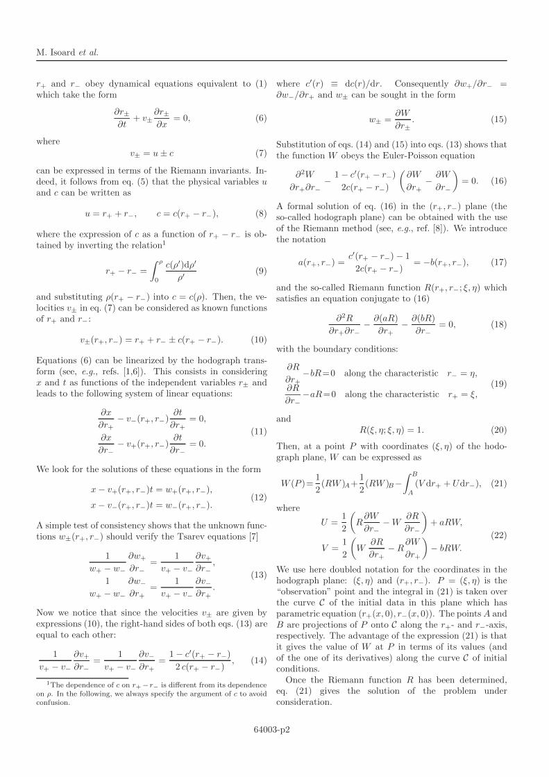
M. Isoard et al.
r+ and r− obey dynamical equations equivalent to (1)which take the form
∂r±∂t
+ v±∂r±∂x
= 0, (6)
where
v± = u ± c (7)
can be expressed in terms of the Riemann invariants. In-deed, it follows from eq. (5) that the physical variables uand c can be written as
u = r+ + r−, c = c(r+ − r−), (8)
where the expression of c as a function of r+ − r− is ob-tained by inverting the relation1
r+ − r− =
∫ ρ
0
c(ρ′)dρ′
ρ′(9)
and substituting ρ(r+ − r−) into c = c(ρ). Then, the ve-locities v± in eq. (7) can be considered as known functionsof r+ and r−:
v±(r+, r−) = r+ + r− ± c(r+ − r−). (10)
Equations (6) can be linearized by the hodograph trans-form (see, e.g., refs. [1,6]). This consists in consideringx and t as functions of the independent variables r± andleads to the following system of linear equations:
∂x
∂r+− v−(r+, r−)
∂t
∂r+= 0,
∂x
∂r−− v+(r+, r−)
∂t
∂r−= 0.
(11)
We look for the solutions of these equations in the form
x − v+(r+, r−)t = w+(r+, r−),
x − v−(r+, r−)t = w−(r+, r−).(12)
A simple test of consistency shows that the unknown func-tions w±(r+, r−) should verify the Tsarev equations [7]
1
w+ − w−
∂w+
∂r−=
1
v+ − v−
∂v+∂r−
,
1
w+ − w−
∂w−∂r+
=1
v+ − v−
∂v−∂r+
.
(13)
Now we notice that since the velocities v± are given byexpressions (10), the right-hand sides of both eqs. (13) areequal to each other:
1
v+ − v−
∂v+∂r−
=1
v+ − v−
∂v−∂r+
=1 − c′(r+ − r−)
2 c(r+ − r−), (14)
1The dependence of c on r+ −r− is different from its dependenceon ρ. In the following, we always specify the argument of c to avoidconfusion.
where c′(r) ≡ dc(r)/dr. Consequently ∂w+/∂r− =∂w−/∂r+ and w± can be sought in the form
w± =∂W
∂r±. (15)
Substitution of eqs. (14) and (15) into eqs. (13) shows thatthe function W obeys the Euler-Poisson equation
∂2W
∂r+∂r−− 1 − c′(r+ − r−)
2c(r+ − r−)
(∂W
∂r+− ∂W
∂r−
)= 0. (16)
A formal solution of eq. (16) in the (r+, r−) plane (theso-called hodograph plane) can be obtained with the useof the Riemann method (see, e.g., ref. [8]). We introducethe notation
a(r+, r−) =c′(r+ − r−) − 1
2c(r+ − r−)= −b(r+, r−), (17)
and the so-called Riemann function R(r+, r−; ξ, η) whichsatisfies an equation conjugate to (16)
∂2R
∂r+∂r−− ∂(aR)
∂r+− ∂(bR)
∂r−= 0, (18)
with the boundary conditions:
∂R
∂r+−bR=0 along the characteristic r− = η,
∂R
∂r−−aR=0 along the characteristic r+ = ξ,
(19)
andR(ξ, η; ξ, η) = 1. (20)
Then, at a point P with coordinates (ξ, η) of the hodo-graph plane, W can be expressed as
W (P )=1
2(RW )A+
1
2(RW )B−
∫ B
A
(V dr+ + Udr−), (21)
where
U =1
2
(R
∂W
∂r−− W
∂R
∂r−
)+ aRW,
V =1
2
(W
∂R
∂r+− R
∂W
∂r+
)− bRW.
(22)
We use here doubled notation for the coordinates in thehodograph plane: (ξ, η) and (r+, r−). P = (ξ, η) is the“observation” point and the integral in (21) is taken overthe curve C of the initial data in this plane which hasparametric equation (r+(x, 0), r−(x, 0)). The points A andB are projections of P onto C along the r+- and r−-axis,respectively. The advantage of the expression (21) is thatit gives the value of W at P in terms of its values (andof the one of its derivatives) along the curve C of initialconditions.
Once the Riemann function R has been determined,eq. (21) gives the solution of the problem underconsideration.
64003-p2

Dispersionless evolution of inviscid nonlinear pulses
Approximate solution. – We now proceed and con-sider the specific problem formulated in the introduction.To simplify the discussion we assume that the initial dis-tribution ρ(x) reaches an extremum at x = 0 and is aneven function of x: ρ(−x) = ρ(x). The generalization tonon-symmetric distributions is straightforward.
First of all, we have to understand how the initial profile(4) fixes the boundary conditions for W on curve C in thehodograph plane. To this end, we compute the initialdistribution of the Riemann invariant r+ for positive x att = 0:
r(x) ≡ r+(x > 0, t = 0) =1
2
∫ ρ(x)
0
c(ρ)dρ
ρ. (23)
Denoting as x(r) the reciprocal function, we obtain for thevalue of x on the curve C:
x =
x(r), if x > 0,
−x(r), if x < 0.(24)
Besides that, since at t = 0 the values r+ = r and r− = −rcorrespond to the same value of x, we find that x(r) is aneven function, x(−r) = x(r). As an illustration, for aninitial profile of the form
ρ(x) = ρ0 + ρ1 exp(−x2/x20) (25)
(with ρ0 and ρ1 > 0), one obtains in the case of a poly-tropic gas (2):
x(r) = x0
√ln ρ1 − ln
[|(γ − 1) r| 2
γ−1 − ρ0
]. (26)
For such a “single-bump” type of initial conditionswhich we consider, there exist two values rm = r(0) andr0 = r(x → ∞) (rm > r0 > 0) such that r+(x, t) ∈ [r0, rm]and r−(x, t) ∈ [−rm, −r0]. At a given time t, the space canbe separated in three different regions 1, 2 and 3, depend-ing on the values of ∂r±/∂x, as illustrated in fig. 1. In eachregion both r+ and r− vary concomitantly, and this is thereason why we have to resort to Riemann’s method2. Fordetermining the value of W in each of the three regions 1,2 and 3, we follow Ludford [9] and unfold the hodographplane into three sheets as illustrated in fig. 2(b).
For the specific initial condition (4), the curve C is repre-sented by the anti-diagonal (r− = −r+) and the points Aand B of eq. (21) have coordinates A(−η, η) and B(ξ,−ξ).Equations (12) with t = 0 give
∂W
∂r+
∣∣∣∣C
=∂W
∂r−
∣∣∣∣C
= x.
This implies that W keeps a constant value along C. Thevalue of this constant is immaterial, we take W |C = 0 for
2We note that for some initial conditions there might also ex-ist simple-wave regions which cannot be tackled by the Riemannmethod. The density and velocity profiles in such regions are easilydescribed (see the case studied in ref. [4]) and we do not considerhere their possible occurrence so as not to burden the discussion.
r±(x
,t=
0) rm
31
−rm
0 x −→(a)
r±(x
,t>
0) rmr+1|2
321
−rm
x −→(b)
Fig. 1: Sketch of the distributions r±(x, t) at time t = 0 (a) andat finite time t > 0 (b). In each panel the upper solid curverepresents r+ (always larger than r0), and the lower one r−
(always lower than −r0). For t > 0, r+ (r−) moves to theright (to the left) and regions 1 and 3 start to overlap. Thisleads to the configuration represented in panel (b) where a newregion (labeled region 2) has appeared. The value of r+ at theinterface between regions 1 and 2 is denoted as r+1|2.
simplicity, and eqs. (22) then reduce to
U =x
2R(r, −r; ξ, η), V = −x
2R(r, −r; ξ, η). (27)
We thus obtain from (21) W =∫ ξ
−η xRdr which gives inregions 1 and 3 the explicit expressions
W (1,3)(ξ, η) = ∓∫ ξ
−η
x(r)R(r, −r; ξ, η)dr, (28)
where the sign − (+) applies in region 1 (3). The differencein signs comes from the fact that x = ∓ x(r) dependingon if one is in region 1 or 3 (see eq. (24)).
When P is in region 2 one applies formula (21) withan integration path different from the one used in re-gions 1 and 3, see fig. 2. Upon integrating by parts oneobtains
W (2)(P ) =(RW (1)
)B2
+(RW (3)
)A2
+
∫ C
A2
(∂R
∂r−− aR
)
r+=rm
W (3)dr−
−∫ B2
C
(∂R
∂r+− bR
)
r−=−rm
W (1)dr+, (29)
where the coordinates of the relevant points are:A2(rm, η), B2(ξ,−rm) and C(rm, −rm) (see fig. 2).
64003-p3

M. Isoard et al.
12
1
2
3
3
B1
A1
B3
B2
A2
C
C
P
P
P
C
A3
12
1
2
3
3
B1
A1
B3
B2
A2
C
C
P
P
P
C
A3
++
+ +
+
0
decreasesincreases
decre
ase
sin
cre
ase
s
(a)
(b)
Fig. 2: (a) Behavior of the Riemann invariants in the character-istic plane at a given time t. The red straight line is the curveC. The black solid line is the curve with parametric equation(r+(x, t), r−(x, t)). (b) The same curves on the four-sheetedunfolded surface. The colored regions 1, 2 and 3 are the sameas the ones identified in fig. 1. In our problem, the whole grayshaded domain above C is unreachable. A generic point P ofhas coordinates (ξ, η) and points A1, B1, A3, B3 and C lie onthe initial curve C. Points A2 and B2 lie on a boundary betweentwo regions. The arrows indicate the direction of integrationin eqs. (21) and (29).
For small enough time of evolution, ξ is close to rm andη is close to −rm, the integrand functions in eq. (29) arethen small by virtue of eqs. (19). A simple approximationthus consists in keeping only the two first terms in theright-hand side of (29).
It now remains to determine the Riemann function Rfor computing expression (28) of W in regions 1 and 3and completely solving the problem. One first remarks
that the conditions (19) and (20) yield
R(r+, η; ξ, η) =
√c(ξ − η)
c(r+ − η)exp
(∫ r+−η
ξ−η
dr
2 c(r)
),
R(ξ, r−; ξ, η) =
√c(ξ − η)
c(ξ − r−)exp
(∫ ξ−r−
ξ−η
dr
2 c(r)
).
(30)
These expressions suggest that R can be sought in theform
R(r+, r−; ξ, η) = R(r+ − r−, ξ − η)F (r+, r−; ξ, η), (31)
where F (r+, η; ξ, η) = 1 = F (ξ, r−; ξ, η) and
R(r1, r2) =
√c(r2)
c(r1)exp
(∫ r1r2
dr
2 c(r)
)
=
√c(r2)ρ(r1)
c(r1)ρ(r2).
(32)
The final expression in the above formula has been ob-tained by means of a change of variable ρ = ρ(r) in theintegral, where the function ρ(r) is the reciprocal functionof r(ρ) given in (9)
r(ρ) =
∫ ρ
0
c(ρ′)dρ′
ρ′, (33)
and c(r) = c(ρ(r)), so that dr/c(r) = dρ/ρ.
We note here that the approximation previously usedfor discarding the integrated terms in the right-hand sideof eq. (29) amounts to assume that F ≃ 1. Similarly, inexpression (28) for W (1) and W (3), since at short time−η and ξ are close, the integration variable r is closeto ξ and one can again assume that F ≃ 1. That is tosay, we are led to make in the whole hodograph plane theapproximation
R(r+, r−; ξ, η) ≃ R(r+ − r−, ξ − η). (34)
We can now write the final approximate results, makingthe replacements ξ → r+, η → r− in the above expres-sions, so that they can be used in eqs. (12) and (15):
W (1,3)(r+, r−) ≃ ∓∫ r+
−r−
x(r)R(2r, r+ − r−)dr,
W (2)(r+, r−) ≃ R(r+ + rm, r+ − r−)W (1)(r+, −rm)
+R(rm − r−, r+ − r−)W (3)(rm, r−),
(35)
where R is given by eq. (32). Formulae (34) and (35) arethe main results of the present work. It is important tostress that eq. (32) has a universal form and can be appliedto any physical system with known dependence c(r+−r−),see eqs. (8) and (9).
64003-p4

Dispersionless evolution of inviscid nonlinear pulses
Examples. – In the case of the dynamics of a poly-tropic gas with c(ρ) = ρ(γ−1)/2, an easy calculation gives
R(r1, r2) =
(r1r2
)β
, where β =3 − γ
2(γ − 1). (36)
It is worth noticing that the approximation (34) yieldsthe exact expression of the Riemann function for a clas-sical monoatomic gas with γ = 5/3 (β = 1). For othervalues of β the function F in (31) can be shown to obeythe hypergeometric equation (see, e.g., ref. [8]) and ourapproximation corresponds to the first term in its seriesexpansion. Thus, we obtain
W (1,3)(r+, r−) ≃ ∓(
2
r+ − r−
)β ∫ r+
−r−
rβ x(r)dr,
W (2)(r+, r−) ≃(
2
r+ − r−
)β
×∫ rm
−r−
rβ x(r)dr +
∫ rm
r+
rβ x(r)dr
.
(37)
For the case of “shallow water” equations with γ = 2 (β =1/2) these formulae reproduce the results of refs. [4,5].The approximation (37) cannot be distinguished from theexact result of Riemann’s approach for the type of initialcondition considered in ref. [4].
We now study in some details a case where the depen-dence of c on ρ is less simple than the one of eq. (2): thisis the case of a zero temperature Bose-Einstein conden-sate transversely confined in an atomic wave guide. For aharmonic trapping, the transverse averaged chemical po-tential can be represented by the interpolating formula [10]
µ⊥(ρ) = ω⊥√
1 + 4aρ, (38)
where ω⊥ is the angular frequency of the transverse har-monic potential, a > 0 is the s-wave scattering length, andρ(x, t) is the linear density of the condensate. We note thatother expressions for µ⊥ have also been proposed in theliterature [11,12]. Expression (38) yields the correct soundvelocity mc2 = ρ dµ⊥/dρ both in the low (aρ ≪ 1) andin the high (aρ ≫ 1) density regimes. In these two limit-ing cases the long wave length dynamics of the system isthus correctly described by the hydrodynamic equations(2) with, in appropriate dimensionless units:
c2(ρ) =ρ√
1 + ρ, (39)
where one has made the changes of variables 4aρ → ρ,u/u0 → u, x/x0 → x and t/t0 → t, where 2mu2
0 = ω⊥and t0 = x0/u0. The length x0 used to non-dimensionalizethe dispersionless equations is a free parameter: we willchose it equal to the parameter x0 appearing in the initialcondition (25). We note here that the initial condition(25) can be realized by several means in the context ofBEC physics. One can for instance suddenly switch on
at t = 0 a blue detuned focused laser beam [13]. Analternative method has been demonstrated in ref. [14]: bymonitoring the relative phase of a two species condensate,one can implement a bump (or a through) in one of thecomponents.
In the case characterized by eqs. (38) and (39), expres-sions (32) and (33) yield
R(r1, r2) =
(ρ2(r1) + ρ3(r1)
ρ2(r2) + ρ3(r2)
)1/8
, (40)
where ρ(r) is the reciprocal function of
r(ρ) = 2
∫ √ρ
0
du
(1 + u2)1/4. (41)
In order to evaluate W it then suffices to determine x(r)by inverting the relation (23) and to compute the appro-priate integrals (35). Once W (r+, r−) is known in allthree regions 1, 2 and 3, it is possible to compute r+(x, t)and r−(x, t), and then ρ(x, t) and u(x, t) as explained inrefs. [4,5]:
– One first determines the value r+1|2(t) reached by
r+ at the boundary between regions 1 and 2, seefig. 1(b). This boundary corresponds to the pointwhere r− = −rm at time t. From eqs. (12), r+1|2(t) is
thus determined by solving
w(1)+ (r+1|2, −rm) − w
(1)− (r+1|2, −rm)
v+(r+1|2, −rm) − v−(r+1|2, −rm)+ t = 0, (42)
where w(1)+ = ∂W (1)/∂r+. We then know that, in
region 1 at time t, r+ takes all possible values betweenr0 and r+1|2(t) (cf. figs. 1 and 2).
– One then let r+ vary in [r0, rm]. From eqs. (12), attime t, the other Riemann invariant r− is solution of
w(1,2)+ (r+, r−) − w
(1,2)− (r+, r−)
v+(r+, r−) − v−(r+, r−)+ t = 0 , (43)
where the superscript should be (1) if r+ ∈ [r0, r+1|2(t)]
and (2) if r+ ∈ [r+1|2(t), rm].
– At this point, for each value of t and r+ we havedetermined the value of r−. The position x is thenobtained by either one of eqs. (12). So, for given tand r+ in regions 1 and 2, one has determined thevalues of r− and x. In region 3 we use the symmetryof the problem and write r±(x, t) = −r∓(−x, t).
The above procedure defines a mapping of the wholephysical (x, t) space onto the hodograph (r+, r−) space.The density and velocity profiles are then obtained bymeans of eqs. (5). The results are compared with nu-merical simulations in fig. 3 for an initial profile (25) with
64003-p5

M. Isoard et al.
−6 −4 −2 0 2 4 6
1.00
1.25
1.50
1.75
2.00
ρ(x
,t)
−6 −4 −2 0 2 4 6
x/x0
−0.2
0.0
0.2
u(x
,t)
Fig. 3: Density and velocity plotted as a function of x/x0 fordimensionless times t/t0 = 0.5, 1, 1.5, 2, 3 and 4, respectively.The initial conditions are given by eqs. (4) and (25) with ρ0 = 1and ρ1 = 1, they are represented by the gray solid lines. Theblue solid lines are the results of the hydrodynamic system (1)obtained from the approximate Riemann’s approach describedin the text. The dashed lines are the results of the numericalsimulations of eq. (44).
ρ0 = 1 and ρ1 = 1. The simulations have been performedby solving numerically a generalized nonlinear Schrodingerequation of the form
iψt = −1
2ψxx + 2 ψ
√1 + ρ, (44)
where ρ(x, t) = |ψ|2, u(x, t) = (ψ∗ψx − ψ ψ∗x)/(2iρ) and
ψ(x, 0) =√
ρ(x, 0). This effective Gross-Pitaevskii equa-tion reduces to the system (1) with the speed of sound (39)in the dispersionless limit3. It yields an excitation spec-trum always of Bogoliubov type, which is incorrect in thelarge density limit (ρ ≫ 1). However, one can show thateq. (44) is acceptable even in this limit provided one re-mains in the long wavelength, hydrodynamic regime. Itis not appropriate when rapid oscillations appear in thedensity and velocity (if ρ ≫ 1) such as observed in fig. 3for t/t0 = 3. These oscillations correspond to the onset ofa dispersive shock wave, which occurs at a time denotedas the wave breaking time: tWB. For t > tWB the numeri-cal simulations can be considered as accurately describingthe physical system only when ρ ≪ 1. But for t > tWB
our dispersionless approach also fails (see below): we arethus safe when comparing our results with numerical sim-ulations at earlier times.
One sees in fig. 3 that our solution of the hydrodynamicequations (1) agrees very well with the numerical simula-tions of the dispersive equation (44) at short time. Forlarger times the profile steepens, eventually reaching a
3It would be easier and more natural to compare our approximateRiemann approach with the numerical solution of eqs. (1). However,the difference between the two results is so small that the discussionof this comparison has little interest.
point of gradient catastrophe at time tWB. It is thus ex-pected that for t ≃ tWB the solution of the dispersionlesssystem (1) departs from the numerical simulations, as seenin the figure. However, this difference is not a sign of afailure of our approximation, but it rather points to thebreakdown of the hydrodynamic model (1). After tWB thesystem (1) leads to a multi-valued solution if not correctedto account for dispersive effects, as can be seen in fig. 3.
Wave breaking time. – We now turn to the determi-nation of the wave breaking time tWB at which a shockis formed. After tWB the system (1) has to be modifiedin order to account for viscous and/or dispersive effects,depending on the physical situation under consideration.
We treat the case of an initial profile roughly of thetype (25): a bump over a uniform background. Wavebreaking corresponds to the occurrence of a gradient catas-trophe for which ∂r±/∂x = ∞. If one considers for in-stance the right part of the profile (region 3), from eq. (12),this occurs at a time t such that
t = − ∂w(3)+ /∂r+
1 + c′(r+ − r−)= − ∂w
(3)+ /∂r+
1 + d ln cd ln ρ
∣∣∣r+−r−
, (45)
and tWB is the smallest of the times (45). It is worth notic-ing that this formula yields an expression for the breakingtime obtained from our approximate solution of the initialvalue problem and in this sense it provides less generalbut more definite result than the upper estimate of thebreaking time obtained by Lax in ref. [15].
One can easily compute tWB approximately when thepoint of largest gradient in ρ(x) lies in a region whereρ ≃ ρ0. This occurs for some specific initial distributions(such as the inverted parabola considered in ref. [4]) orwhen the initial bump is only a small perturbation of thebackground. In this case, it is legitimate to assume thatwave breaking is reached for r− ≃ −r0 and that
r+ − r− ≃ 1
2
∫ ρ
0
c(ρ′)
ρ′dρ′ +
1
2
∫ ρ0
0
c(ρ′)
ρ′dρ′. (46)
Equations (15) and (35) then lead to w(3)+ ≃ x(r+)
and (45) becomes
t ≃ − 2
1 + d ln cd ln ρ
∣∣∣ρ
× ρ
c(ρ)dρdx
, (47)
where ρ stands for ρ(x(r+)). Within our hypothesis, it islegitimate to assume that the shortest of times t is reachedclose to the point x(r+) for which |dρ/dx| is maximal. Wenote x∗ the coordinate of this point and ρ∗ = ρ(x∗). Onethus obtains
tWB ≃ 2
1 + d ln cd ln ρ
∣∣∣ρ∗
× ρ∗
c(ρ∗) · max∣∣∣dρdx
∣∣∣. (48)
In a “shallow water” case with γ = 1/2 and for an initialprofile where the bump is an inverted parabola, such asconsidered in ref. [4], the above formula is exact.
64003-p6

Dispersionless evolution of inviscid nonlinear pulses
0.0 0.2 0.4 0.6 0.8 1.00
5
10
15
20
c(ρ
0)t W
B/x
0
0.0 0.2 0.4 0.6 0.8 1.0
ρ1/ρ0
0
10
20
xW
B/x
0
Fig. 4: Wave breaking time tWB and position of the wave break-ing event xWB for different values of ρ1/ρ0. The system consid-ered is a quasi-1D BEC for which the speed of sound in givenby (39). The initial profile is given by eqs. (4) and (25). Theblue solid lines are the approximate results (49) and (50). Thered dots are the results obtained from Riemann’s approach.The black solid lines are obtained by replacing ρ∗ by ρ0 ineqs. (49) and (50), see the text.
For the initial profile (25), in the case where the speedof sound is given by (39), formula (48) yields
tWB ≃√
e
2
8(1 + ρ∗)6 + 5ρ∗
x0
c(ρ∗)ρ∗
ρ1. (49)
The location xWB of the wave breaking event can be ob-tained from (12). Within our approximation scheme, thisyields, for the right part of the profile:
xWB ≃ x∗ + c(ρ∗)tWB. (50)
These results are compared in fig. 4 with the values de-termined from the Riemann approach. The overall agree-ment is excellent. We also note that replacing ρ∗ by ρ0 ineqs. (49) and (50) gives a result which is less accurate, butstill quite reasonable, see fig. 4.
Conclusion. – We have presented an approximatemethod for describing the hydrodynamic evolution of anonlinear pulse. The method is quite general and appliesfor any type of nonlinearity. It has been tested for cases ofexperimental interest in the context of nonlinear optics inref. [4] and here for studying the spreading of a nonlinearpulse in a guided atomic Bose-Einstein condensate. Thislast example is of particular interest for bench-markingthe approach because the nonlinearity at hand has a non-trivial density dependence.
One could imagine to extend the present study inseveral directions. A possible track would be to solve thedispersionless shallow water equations (eqs. (1) and (2)with γ = 2) for more general initial conditions than dis-cussed in the present work, as considered for instance in
refs. [16,17] in the context of the initial stage of formationof a tsunami. Future studies could also test the presentapproach in the optical context for pulses propagating in anonlinear photo-refractive material, where, up to now, notheoretical method was known for dealing with the disper-sionless stage of evolution. In this context we note that thesimple and accurate approximate analytic results obtainedfor tWB and xWB (eqs. (49) and (50)) should be helpfulfor determining the best parameters for an experimentalobservation of the wave breaking phenomenon.
We finally stress that the approximate scheme presentedin this work, providing an accurate account of the stageof non-dispersive propagation of a pulse, is an importantand necessary step for studying the post wave breaking dy-namics, and particularly the formation of dispersive shockwaves in non-integrable systems.
REFERENCES
[1] Landau L. D. and Lifshitz E. M., Fluid Mechanics(Pergamon, Oxford) 1987.
[2] Forest M. G., Rosenberg C.-J. and Wright IIIO. C., Nonlinearity, 22 (2009) 2287.
[3] Ivanov S. K. and Kamchatnov A. M., Phys. Rev. A,99 (2019) 013609.
[4] Isoard M., Kamchatnov A. M. and Pavloff N., Phys.Rev. A, 99 (2019) 053819.
[5] Isoard M., Kamchatnov A. M. and Pavloff N.,in Compte-rendus de la 22e rencontre du Non Lineaire,edited by Falcon E., Lefranc M., Petrelis F. andPham C.-T. (Non-Lineaire Publications, Saint-Etiennedu Rouvray) 2019, p. 33.
[6] Kamchatnov A. M., Nonlinear Periodic Waves andTheir Modulations—An Introductory Course (World Sci-entific, Singapore) 2000.
[7] Tsarev S. P., Math. USSR Izv., 37 (1991) 397.[8] Sommerfeld A., Partial Differential Equations in
Physics (Academic Press, New York) 1964.[9] Ludford G. S. S., Proc. Cambridge Philos. Soc., 48
(1952) 499.[10] Gerbier F., Europhys. Lett., 66 (2004) 771.[11] Salasnich L., Parola A. and Reatto L., Phys. Rev.
A, 65 (2002) 043614.[12] Kamchatnov A. M. and Shchesnovich V. S., Phys.
Rev. A, 70 (2004) 023604.[13] Andrews M. R., Kurn D. M., Miesner H.-J., Durfee
D. S., Townsend C. G., Inouye S. and Ketterle W.,Phys. Rev. Lett., 79 (1998) 553.
[14] Hall D. S., Matthews M. R., Wieman C. E. andCornell E. A., Phys. Rev. Lett., 81 (1998) 1543.
[15] Lax P. D., J. Math. Phys., 5 (1964) 611.[16] Pelinovsky E. N. and Rodin A. A., Izv. Atmos. Ocean.
Phys., 49 (2013) 548.[17] Rodin A. A., Rodina N. A., Kurkin A. A. and
Pelinovsky E. N., Izv. Atmos. Ocean. Phys., 55 (2019)374.
64003-p7

7FORMATION AND PROPAGATION OF DISPERS IVESHOCK WAVES
This chapter is devoted to the study of dispersive shock waves. Anoptical beam propagating in a nonlinear dielectric material might expe-rience a gradient catastrophe leading to the formation of a dispersiveshock wave (DSW).It has been shown by Talanov [179] that a smooth localized light
pulse sent in a nonlinear medium, spreads smoothly and can be de-scribed through the dispersionless hydrodynamic equations. However,the situation becomes quite different for a hump on top of a uniformbackground light intensity: the hump splits in two parts which propa-gate in opposite directions. The front and the rear edge of the humphave the same intensity as the background and accordingly propagateat the background sound velocity c0, while the points of larger intensitypropagate at larger velocity. When these points catch up the front edge(see Figure 51), this leads to the formation of a shock. In other words,when this situation occurs, density gradients at the front edge of the leftan right-moving humps become infinite: this is a gradient catastrophe.
Figure 51: Evolution of a hump on top of a background. The initial bumpsplits in two parts, each of them propagating in opposite direction,as indicated by the arrows. The front and the rear edge of thehump have the same intensity as the background and accordinglypropagate at the background sound velocity. On the contrary,all the points of larger intensity move at a higher velocity; thisis illustrated by the arrows attached to each pulse and longerthan those located at each edge. Therefore, at a certain time,called wave breaking time, the points of larger intensity catch upthe front edge (for the left and right-moving bumps), leading toinfinite density gradients: this is a gradient catastrophe. The wavebreaking is indicated by the vertical dashed lines at both edgesof each pulse.
189

190 formation and propagation of dispersive shock waves
As we discussed in the previous chapter, no matter how small isthe hump on top of the background, a DSW is formed at each edge ofeach pulse moving away from each other. Therefore, perturbation theoryalways fails at describing such a situation, whereas the dispersionlessapproach leads to a non-physical multi-valued density distribution. Thisis the reason why we shall turn our attention to a theory which is ableto encompass dispersive effects after the shock has formed. This theorydoes exist and has been developed by Whitham [194–197], then used byGurevich and Pitaevskii [84] to describe a DSW as a slowly modulatednonlinear wave. The existence of two scales between fast oscillationsin the shock and slow evolution of certain parameters along the shock,such as its wavelength or its amplitude, led them to the idea of usingWhitham modulational theory for DSW; this is what we discuss in thefirst section of this chapter.Then, we apply the Gurevich-Pitaevskii approach to the nonlinear
Schrodinger equation (NLS). We show in particular that the theoreti-cal treatment compares very well with numerical simulations. This ap-proach also provides an asymptotic description of the DSW, namely aweak shock theory, from which we can extract experimentally relevantparameters such as the contrast of the fringes of the DSW.
7.1 whitham modulational theory
7.1.1 General idea
The main idea of Whitham modulational theory consists of describingmodulations of nonlinear periodic waves which cannot be approximatedby linear waves. The approach is based on the existence of two scales.We consider fast oscillations with wavelength L(x, t), which slowly de-pends on space and time, and thus change little in one wavelength. Wealso assume that the amplitude of the wave does not vary too muchin one wavelength. An example of such a slowly modulated wave is il-lustrated in Figure 52. The red dashed inset represents a portion ofthe fast oscillating wave. One sees that the wavelength, denoted L, andthe amplitude of the wave, denoted A, do not vary much over severalwavelengths.
Consequently, we can average the equations of motion which governthe variations of these parameters (wavelength, amplitude,...) along thenonlinear wave over fast oscillations; these averaged modulation equa-tions are called the Whitham equations.
Let us consider a differential equation in the form
φ(u, ∂tu, ∂xu, ∂ttu, ∂txu, ∂xxu, . . .) = 0, (468)
where ∂i1...in = ∂n/∂i1 . . . ∂in, with i1, . . . , in ∈ t, x. Now we supposethat the wave variable u(x, t) depends on x and t only through ξ =x−V t. Thus, multiplying equation (468) by ∂ξu and integrating it, oneobtains
u2ξ = F (u, V,Ai), (469)

7.1 whitham modulational theory 191
where Ai are a set of parameters, such as the amplitude or the wave-length of the wave packet, which arise from the integration of (468).Periodic solutions correspond to oscillations of u between two zeros1 ofF , denoted as u1(V,Ai) and u2(V,Ai), with u1 < u2. Let us introduceξ1 and ξ2 such that
u(ξ1, V, Ai) = u1(V,Ai), u(ξ2, V, Ai) = u2(V,Ai). (470)
Then, the wavelength corresponding to this periodic solution reads
L = L(V,Ai) = 2
∫ ξ2
ξ1
dξ = 2
∫ u2
u1
du√F (u, V,Ai)
, (471)
where we used a change of variable and expression (469). The wavectork and the frequency ω are equal to
k = k(V,Ai) =2π
L(V,Ai), ω = ω(V,Ai) = V k(V,Ai). (472)
Since we consider here a slowly modulated wave u(ξ, V,Ai), the param-eters V and Ai are slow functions of x and t, and thus change little inone wavelength L. We would like to average these parameters over fastoscillations of the wave according to the rule
F(ξ, V,Ai) =1
2∆
∫ ξ+∆
ξ−∆F(ξ′, V, Ai) dξ′, (473)
where the interval ∆ should be much longer than the wavelength L andmuch shorter that any characteristic size ` in the problem, see Figure 52.Thus, one considers here
L ∆ `. (474)
Following Whitham approach, it is more convenient to average con-servation laws, such as for example
∂tP + ∂xQ = 0, (475)
where P(ξ, V,Ai) andQ(ξ, V,Ai) are two functions which can be derivedfrom (468). By averaging over fast oscillations according to (473), wefind that the averaged conservation law can be written as
∂tP(ξ, V,Ai) + ∂xQ(ξ, V,Ai) = 0. (476)
As one can see from the inset of Figure 52 and from the difference ofscales (474), the wavelength remains constant up to small correctionsin the interval 2∆. Therefore, we can replace the average over 2∆ inexpression (473) by the average over the wavelength, i.e.,
F(V,Ai) =1
L
∫ ξ+L
ξF(ξ, V,Ai) dξ, (477)
1 Think about F as the opposite of the potential energy and u2ξ as proportional to an
effective kinetic energy.

192 formation and propagation of dispersive shock waves
Figure 52: Different scales along the dispersive shock wave. The amplitude Aand the wavelength L vary over a length `, but can be consideredalmost constant along the interval ∆, as illustrated in the inset ofthe figure. In addition, ∆ is much longer than the wavelength L.The existence of these two scales, between fast oscillations andslowly modulated parameters (wavelength, amplitude,...) alongthe DSW, is at the heart of Whitham modulational theory.
where the explicit dependence of F on x and t disappears by means ofthe periodicity of F . As a result, equation (476) becomes
∂tP(V,Ai) + ∂xQ(V,Ai) = 0, (478)
where the dependence of x and t only appear through the slowly varyingparameters V and Ai. The averaged conservation laws of the form (478)are the Whitham equations. One should find as many Whitham equa-tions as there are parameters (V,Ai) to describe the evolution of eachof them. Then, we know the evolution of the nonlinear wave variableu(x− V t, V,Ai), since it only depends on the set of parameters (V,Ai).
illustrative example Even though we will consider nonlinearwaves in the following, let us first examine an instructive example ofmodulation of a linear wave governed by equation
∂ttu− ∂xxu+1
4∂xxxxu = 0, (479)
This differential equation actually corresponds to a linearized versionof the Gross-Pitaevskii equation [see equation (123b) with v0 = 0]. Weseek periodic solutions of equation (479) in the form u(ξ) = u(x− V t).They are given by
u(x− V t, V, a) = a sin[2√V 2 − 1(ξ − ξ0)], (480)
where a plays the role of the wave amplitude. In the following we takeξ0 = 0; this initial phase will indeed disappear after the averaging pro-cess (477).
Then, the wavenumber and the frequency are given by
k = 2√V 2 − 1, ω = 2V
√V 2 − 1. (481)
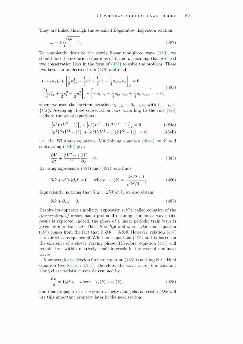
7.1 whitham modulational theory 193
They are linked through the so-called Bogoliubov dispersion relation
ω = k
√k2
4+ 1. (482)
To completely describe the slowly linear modulated wave (480), weshould find the evolution equations of V and a, meaning that we needtwo conservation laws in the form of (475) to solve the problem. Thesetwo laws can be derived from (479) and read
(−ut ux)t +
[1
8u2xx +
1
2u2t +
1
2u2x −
1
4uxxx ux
]
x
= 0,
[1
8u2xx +
1
2u2t +
1
2u2x
]
t
+
[−ut ux −
1
4utx uxx +
1
4ut uxxx
]
x
= 0,
(483)
where we used the shortcut notation ui1...in ≡ ∂i1...inu, with i1 . . . in ∈t, x. Averaging these conservation laws according to the rule (478)leads to the set of equations
[a2V (V 2 − 1)
]t+[a2(V 2 − 1)(2V 2 − 1)
]x
= 0, (484a)[a2V 2(V 2 − 1)
]t+[a2V (V 2 − 1)(2V 2 − 1)
]x
= 0, (484b)
i.e., the Whitham equations. Multiplying equation (484a) by V andsubtracting (484b) gives
∂V
∂t+
2V 2 − 1
V
∂V
∂x= 0. (485)
By using expressions (481) and (482), one finds
∂tk + ω′(k)∂xk = 0, where ω′(k) =k2/2 + 1√k2/4 + 1
. (486)
Equivalently, noticing that ∂xω = ω′(k)∂xk, we also obtain
∂tk + ∂xω = 0. (487)
Despite its apparent simplicity, expression (487), called equation of theconservation of waves, has a profound meaning. For linear waves thisresult is expected: indeed, the phase of a linear periodic train wave isgiven by θ = kx − ωt. Thus, k = ∂xθ and ω = −∂tθ, and equation(487) comes from the fact that ∂x∂tθ = ∂t∂xθ. However, relation (487)is a direct consequence of Whitham equations (478) and is based onthe existence of a slowly varying phase. Therefore, equation (487) willremain true within relatively small intervals in the case of nonlinearwaves.
Moreover, let us develop further: equation (486) is nothing but a Hopfequation (see Section 5.2.1). Therefore, the wave vector k is constantalong characteristic curves determined by
dxdt
= Vg(k), where Vg(k) ≡ ω′(k), (488)
and thus propagates at the group velocity along characteristics. We willuse this important property later in the next section.

194 formation and propagation of dispersive shock waves
7.1.2 Whitham equations for NLS equation
In the case of the defocusing nonlinear Schrödinger equation
i ∂tψ = −1
2∂xxψ + |ψ|2 ψ, (489)
which can be mapped onto hydrodynamic equations [see equation (366)]through a Madelung transformation ψ =
√ρ exp(i
∫u dx), nonlinear
periodic solutions can be written in terms of four parameters λ1 ≤λ2 ≤ λ3 ≤ λ4 in the form [100]
ρ(x, t) = 14(λ4 − λ3 − λ2 + λ1)2 + (λ4 − λ3)(λ2 − λ1)
× sn2(√
(λ4 − λ2)(λ3 − λ1) (x− V t),m),
u(x, t) = V − C
ρ(x, t),
(490)
where sn is the Jacobi elliptic sine function (see. e.g., Ref. [2]),
V = 12
4∑
i=1
λi , m =(λ2 − λ1)(λ4 − λ3)
(λ4 − λ2)(λ3 − λ1), (491)
and
C = 18(−λ1 − λ2 + λ3 + λ4)× (−λ1 + λ2 − λ3 + λ4)
× (λ1 − λ2 − λ3 + λ4) .(492)
For constant λi’s, expressions (490), (491) and (492) correspond to anexact (single phase) solution of the NLS equation, periodic in time andspace, where oscillations have the amplitude
a = (λ2 − λ1)(λ4 − λ3) , (493)
and the spatial wavelength
L =2 K(m)√
(λ4 − λ2)(λ3 − λ1). (494)
As explained in the previous section, the great insight of Gurevich andPitaevskii [84] has been to describe a dispersive shock wave as a slowlymodulated nonlinear wave of type (490). Solution (490) being entirelycharacterized by the knowledge of the four slowly varying parametersλi(x, t), one needs four Witham equations (478) to solve the problem.They read [100, 197]
∂tλi + vi(λ1, λ2, λ3, λ4) ∂xλi = 0, i = 1, 2, 3, 4. (495)
One sees immediately that the λi’s are the Riemann invariants of theWhitham equations [compare for instance with equations (385)]. Equa-tions (495) were first found in Refs. [67, 143]. The vi’s are the associated

7.1 whitham modulational theory 195
characteristic velocities; their explicit expressions can be obtained fromthe relation2 [82, 100]
vi = V − 1
2
L
∂iL, i = 1, 2, 3, 4 , (496)
where ∂i = ∂/∂λi. This yields
v1 = V − (λ4 − λ1)(λ2 − λ1)K(m)
(λ4 − λ1)K(m)− (λ4 − λ2)E(m),
v2 = V +(λ3 − λ2)(λ2 − λ1)K(m)
(λ3 − λ2)K(m)− (λ3 − λ1)E(m),
v3 = V − (λ4 − λ3)(λ3 − λ2)K(m)
(λ3 − λ2)K(m)− (λ4 − λ2)E(m),
v4 = V +(λ4 − λ3)(λ4 − λ1)K(m)
(λ4 − λ1)K(m)− (λ3 − λ1)E(m),
(497)
where m is given by equation (491) and E(m) is the complete ellipticintegrals of the second kind.In our case, as shown in Figure 53, for x > 0, the left edge of the DSW,
connected to the dispersionless part of the profile, is called solitonic edgeand corresponds to the limitm→ 1; the first oscillation is indeed a darksoliton, see equation (498). The right edge, glued to the background,is called small amplitude edge or harmonic edge and corresponds tom → 0, see equation (500). We detail these two limiting cases in thesubsequent paragraphs.
solitonic edge In this case, m → 1 (λ2 = λ3), sn(x,m) →tanh(x) and expression (490) describes a dark soliton (for which L →∞):
ρ(x, t) =1
4(λ4 − λ1)2 − (λ2 − λ1)(λ4 − λ2)
cosh2[√
(λ2 − λ1)(λ4 − λ2)ξ](498)
with ξ = x− 12(λ1 + 2λ2 + λ3)t.
The Whitham velocities reduce to
v1 = 12(3λ1 + λ4), v2 = v3 = 1
2(λ1 + 2λ2 + λ4),
v4 = 12(λ1 + 3λ4).
(499)
harmonic edge In the limit m → 0 (λ1 = λ2 or λ3 = λ4),sn(x,m)→ sin(x), and equation (490) describes a small amplitude sinu-soidal wave oscillating around a constant density background ρ0. Thespecific example shown in Figure 53 corresponds to λ3 → λH, where
2 The fact that one can write the Whitham velocities in the form of (496) is a gen-eral property of Whitham equations; this was indeed indicated independently byGurevich et al. [81] and Kudashev [103] for the Korteweg-De Vries equation and byKamchatnov [99] for the derivative nonlinear Schrödinger equation.

196 formation and propagation of dispersive shock waves
Figure 53: The inset shows the full density distribution after the formationof dispersive shock waves at the left (right) edge of the pulsepropagating to the left (right). The green arrows indicate thepropagation direction of each pulse.The red rectangle represents a zoom over the dispersive shockwave (DSW) formed by the pulse propagating in the region x > 0.The DSW is connected to the dispersionless (smooth) profile atthe left edge, corresponding to the limit m→ 1 in equation (490);this edge is called solitonic edge because the first oscillation isdescribed by a dark soliton, see equation (498). The right edgeof the DSW is often called small amplitude edge or harmonicedge and corresponds to m→ 0; this edge is indeed described bysmall linear oscillations over a constant background, see equation(500).
we have introduced λH ≡ λ4(m → 0), see Figure 54. In this case, thesolution (490) reduces to
ρ(x, t) ' ρ0 + a2(x, t) sin2
(πξ
L
), (500)
where ρ0 = 14(λ1 − λ2)2, and where a2(x, t) = 2 c0(λH − λ3) is a small
amplitude (λH − λ3 → 0 because at this edge λ3 → λH ≡ λ4). Inaddition, one has
L =2π
k=
π√(λH − λ1)(λH − λ2)
, (501)
and ξ = x− V t, with V = 12(λ1 + λ2) + λH [computed from (491)].
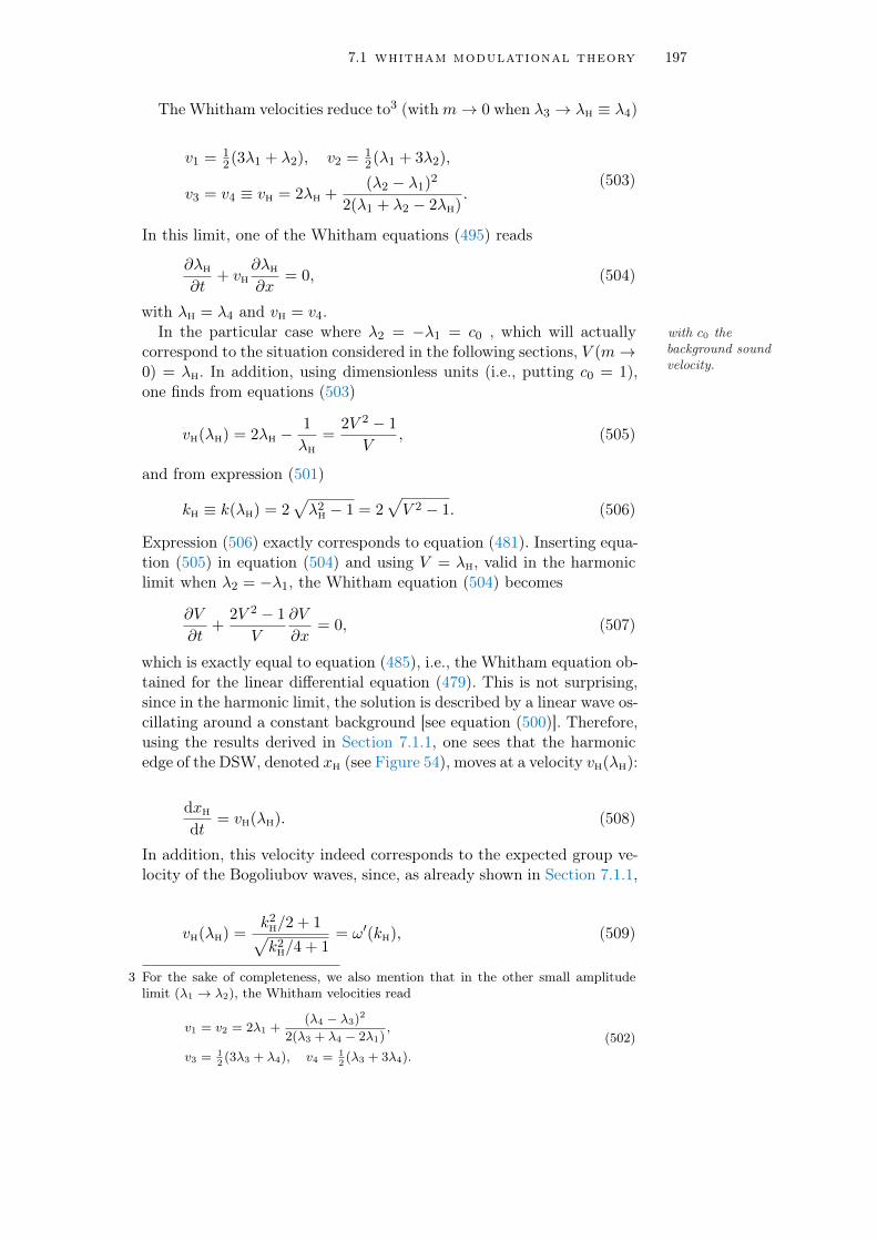
7.1 whitham modulational theory 197
The Whitham velocities reduce to3 (withm→ 0 when λ3 → λH ≡ λ4)
v1 = 12(3λ1 + λ2), v2 = 1
2(λ1 + 3λ2),
v3 = v4 ≡ vH = 2λH +(λ2 − λ1)2
2(λ1 + λ2 − 2λH).
(503)
In this limit, one of the Whitham equations (495) reads
∂λH
∂t+ vH
∂λH
∂x= 0, (504)
with λH = λ4 and vH = v4.In the particular case where λ2 = −λ1 = c0 , which will actually with c0 the
background soundvelocity.
correspond to the situation considered in the following sections, V (m→0) = λH. In addition, using dimensionless units (i.e., putting c0 = 1),one finds from equations (503)
vH(λH) = 2λH −1
λH
=2V 2 − 1
V, (505)
and from expression (501)
kH ≡ k(λH) = 2√λ2
H − 1 = 2√V 2 − 1. (506)
Expression (506) exactly corresponds to equation (481). Inserting equa-tion (505) in equation (504) and using V = λH, valid in the harmoniclimit when λ2 = −λ1, the Whitham equation (504) becomes
∂V
∂t+
2V 2 − 1
V
∂V
∂x= 0, (507)
which is exactly equal to equation (485), i.e., the Whitham equation ob-tained for the linear differential equation (479). This is not surprising,since in the harmonic limit, the solution is described by a linear wave os-cillating around a constant background [see equation (500)]. Therefore,using the results derived in Section 7.1.1, one sees that the harmonicedge of the DSW, denoted xH (see Figure 54), moves at a velocity vH(λH):
dxH
dt= vH(λH). (508)
In addition, this velocity indeed corresponds to the expected group ve-locity of the Bogoliubov waves, since, as already shown in Section 7.1.1,
vH(λH) =k2
H/2 + 1√k2
H/4 + 1= ω′(kH), (509)
3 For the sake of completeness, we also mention that in the other small amplitudelimit (λ1 → λ2), the Whitham velocities read
v1 = v2 = 2λ1 +(λ4 − λ3)2
2(λ3 + λ4 − 2λ1),
v3 = 12(3λ3 + λ4), v4 = 1
2(λ3 + 3λ4).
(502)

198 formation and propagation of dispersive shock waves
with ω(k) = k√
k2
4 + 1, and where we used equations (505) and (506).This property of the small-amplitude edge is especially important in
the theory of DSWs for non-integrable equations (see, e.g., Refs. [54,55]).
To conclude this section, if one is able to find the solutions of Whithamequations (495), by inserting the corresponding Riemann invariantsλi(x, t), i = 1, 2, 3, 4 in expressions (490), one knows the evolution ofthe density and velocity profiles along the DSW; this is exactly whatwe intend to do in the following section.
Figure 54: Sketch of the Riemann invariants λ1, λ2, λ3, λ4 along the DSWregion, represented in blue. The dispersionless part of the pro-file, described by the Riemann invariants λ+ and λ−, is depictedin pink. As explained in Section 7.2, in our specific case, twoRiemann invariants (λ1 and λ2) remain constant in the shockregion. They are connected to the dispersionless Riemann invari-ants λ+ = c0 and λ− = −c0 at the right edge (harmonic edge,m = 0). Furthermore, λ3 → λH ≡ λ4 at this edge. At the left andsolitonic edge (m = 1), λ1 is still connected to λ−, while λ+ isnow glued to λ4. In the other hand, λ2 = λ3 = c0 at this edge.The position of the left edge (right edge) is denoted as xS (xH).
7.2 solutions of whitham equations
In this section, we present the solutions of Whitham equations (495),in the case where two Riemann invariants remain constant along theDSW. This situation arises when considering an initial density profileof the form of an inverted parabola, see expression (450).First, as explained in the introduction of this chapter, the initial
hump on top of a background splits in two parts; later, each of themexperiences a wave breaking and this leads to the formation of a DSWat both edges. This exactly corresponds to the situation depicted in theinset (d) of Figure 50.

7.2 solutions of whitham equations 199
The Riemann invariants λ±, which describe the dispersionless evolu-tion of the nonlinear pulse, propagate in opposite direction, as shownin Figure 48.Then, if we concentrate our attention to the region x > 0 (the region
x < 0 can be obtained by symmetry of the problem), the right edge ofλ+, glued to the background, becomes multi-valued at a certain time,as illustrated in the graph (f) of Figure 48; this indicates a sign ofthe failure of the dispersionless approach after the wave breaking. Theform of λ+ in this multi-valued region, and the fact that λ− = −c0
there, suggests to take λ1 = λ− = −c0 and λ2 = λ+ = c0. Then, onlyλ3(x, t) and λ4(x, t) vary along the DSW and must match with thedispersionless profile at both edges of the DSW, see Figure 54.Therefore, in the following, we consider in the shock region
λ1(x, t) = −c0, λ2(x, t) = c0, (510)
which trivially satisfy the Whitham equations (495), and the remainingWhitham equations for λ3(x, t) and λ4(x, t):
∂λ3,4
∂t+ v3,4(−c0, c0, λ3, λ4)
∂λ3,4
∂x= 0. (511)
7.2.1 Generalized hodograph transform
The nonlinear Whitham equations (511) are very similar to equations(393). This suggests to use the same trick to ‘linearize’ the Whithamequations by means of a hodograph transform (see Section 6.1.1). Thisprocedure consists of writing x and t as functions of the Riemann in-variants:
x = x(λ3, λ4), t = t(λ3, λ4). (512)
By introducing two functions w3(λ3, λ4) and w4(λ3, λ4) such that
x− v3,4(−c0, c0, λ3, λ4)t = w3,4(λ3, λ4), (513)
and by using the results of Section 6.1.1, this leads to the Tsarev equa-tions (399), where the superscripts + and − should be replaced by 3and 4, respectively.By means of expressions (496), one can prove easily that w3 and w4
verify the Tsarev equations if and only if
∂4[(∂3k)w3] = ∂3[(∂4k)w4], (514)
with ∂i = ∂/∂λi and k = 2π/L. The previous equation suggests that(∂3k)w3 and (∂4k)w4 may be expressed in terms of a potentialW , suchthat [82]
(∂ik)wi = ∂i(kW ), with i ∈ 3, 4. (515)
This yields
wi(λ3, λ4) =
(1− L
∂iL∂i
)W
= W + 2(vi − V )∂iW, i ∈ 3, 4,(516)

200 formation and propagation of dispersive shock waves
where we used k/∂ik = −L/∂iL = 2(vi − V ) [see equation (496)]. In-serting (516) in the Tsarev equations, together with expressions of theWhitham velocities given by (496), shows that the potential W is solu-tion of the following Euler-Poisson equation:
∂2W
∂λ3∂λ4− 1
2(λ3 − λ4)
(∂W
∂λ3− ∂W
∂λ4
)= 0. (517)
Exactly as it already occurs in Chapter 6, we have transformed the setof nonlinear equations (511) into a linear differential equation (517).We could certainly solve the problem using Riemann’s method, as weproceeded in Chapter 6. However, we found it more convenient to followthe method described in Refs. [56, 82]. In these works, the authors useda general solution of (517) derived by Eisenhart in 1918 [53].
7.2.2 Solutions in the shock region
A general solution of (517) is given by [53]
W (λ3, λ4) =
∫ λ3
c0
ψ(µ) dµ√λ3 − µ
√λ4 − µ
+
∫ λ4
c0
ϕ(µ) dµ√|λ3 − µ|
√λ4 − µ
, (518)
where ψ(µ) and ϕ(µ) are two functions determined by boundary condi-tions.
In our case, as it was first understood in Ref. [83], the propagationof the DSW occurs in two steps after the wave breaking. Indeed, if theinitial density distribution is non monotonous, as illustrated for instancein Figure 48, the first parts which become multi-valued are the left edgeof λ−(x, t) and the right edge of λ+(x, t) (see for instance graph (f) ofFigure 48).
To clarify the discussion, let us assume that we aim at describing theDSW long time after the wave breaking when the initial pulse has splitin two parts4, i.e., t > tsplit, see for instance the inset of Figure 53. Inthis case, as shown in graph (f) of Figure 48, λ+ is made of two simplewave regions: IIr and III; the latter being glued to the background.
Since for λ+ the wave breaking occurs at the boundary between re-gion III and the background, region III is the first which is graduallyabsorbed in the DSW. The part of region III absorbed in the DSW ata given time t is denoted as region A, see Figure 55. In that case, theleft edge of region A, corresponding to the solitonic edge, is connectedto the remaining dispersionless part of the simple wave region III5.Then, at a time that denoted as tA|B, region III is completely absorbed;
it is now the turn of region IIr to be swallowed by the DSW, see graph (f)of Figure 48. The shock region is now divided in two domains A and B,whose boundary corresponds to λ4 = cm, with cm = max [λ+(x, t = 0)],and is indicated by the green solid curve in Figure 55.
4 This is actually a reasonable assumption since Whitham modulational theory iscorrect at large enough values of time, when the DSW is well formed with a largenumber of oscillations [84].
5 Indeed, one may glance at graph (f) of Figure 48 to be convinced that region A isindeed connected to region III in the first few moments after the shock has formed.

7.2 solutions of whitham equations 201
Therefore, we need to treat separately both regions. The solution ofthe Euler-Poisson equation (517) in region A (B) is denoted as WA
(WB). The matching condition between these two solutions reads
WA(λ3, cm) = WB(λ3, cm), (519)
and is realized at a position that we denote by xm. We also denote by xS
and xH the positions of the solitonic edge [m→ 1 in expressions (490)]and of the harmonic edge [m → 0 in expressions (490)], see Figure 55where all these notations are summarized.
Figure 55: Schematic plots of the position dependence of the Riemann in-variants inside (blue solid curves) and outside (pink solid curves)the DSW (colored region).(a) For t < tA/B, the DSW is connected to the simple wave regionIII of the smooth dispersionless profile, see graph (f) of Figure 48.At t = tA/B, region III is completely absorbed by the DSW. Thus,for this time, the shock wave connects to the smooth profile ex-actly at λ+(xS(t), t) = cm.(b) For t > tA/B, the DSW is connected at its left edge at a pointbelonging to region IIr of the smooth dispersionless profile, seegraph (f) of Figure 48. In this case the shock wave is divided intwo regions A and B, separated by the green vertical line in theplot. The continuity along the separation line between the tworegions (i.e., at x = xm(t)) is ensured by equation (519).In both plots we introduce λS = λ4(xS(t), t), the value of λ4 atthe solitonic edge of the DSW. The position x? locates the leftboundary of the simple wave region IIr, where λ+ equals c0. As inFigure 54, positions xS and xH locate the solitonic and harmonicedges of the DSW, respectively.
boundary conditions The general solution of the Euler-Poissonequation is made explicit in equation (518). We define two functions ψA
and ϕA, such that
WA(λ3, λ4) =
∫ λ3
c0
ψA(µ) dµ√λ3 − µ
√λ4 − µ
+
∫ λ4
c0
ϕA(µ) dµ√|λ3 − µ|
√λ4 − µ
(520)
is the solution of equation (517) in region A. Then, we can use theboundary conditions of the problem to find the expressions of bothfunctions ψA and ϕA.

202 formation and propagation of dispersive shock waves
• The solitonic edge, located at position xS, connects region A (ift < tA|B) or region B (if t ≥ tA|B) and the dispersionless profile(region III or IIr). Thus, one has at this edge
λ1 = −c0, λ2 = λ3 = c0, λ4 = λ+(xS, t) ≡ λS(t), (521)
see Figure 55. The precise determination of λS(t) is given in Sec-tion 7.2.3.
Then, using equations (513), (499), (461) and (466), one obtains6
xS −1
2(3λS − c0)t = w4(c0, λS),
xS −1
2(3λS − c0)t = w
(i)+ (λS,−c0),
(522)
with the superscript (i) = (3) if t < tA|B or (i) = (2) if t ≥ tA|B.In the second equation of (522), the function w
(i)+ (λS,−c0) has
been defined in Chapter 6 [see equation (398)], and correspondsto ∂W (i)/∂λ+(λS,−c0), where W (i) is given by (431).
The set of equations (522) shows that w4(c0, λS) = w(i)+ (λS,−c0).
Using expression (516), this leads to
WA,B(c0, λS)+(2λS−c0)∂WA,B
∂λ4(c0, λS) = w
(i)+ (λS,−c0), (523)
where the superscript A corresponds to the superscript (i) = (1),and B to (i) = (2). Differential equation (523) can be easily solvedand we arrive to the first boundary condition:
WA(c0, λS) =1
2√λS − c0
∫ λS
c0
w(3)+ (r,−c0)√r − c0
dr, (524a)
WB(c0, λS) =− 1
2√λS − c0
∫ cm
λS
w(2)+ (r,−c0)√r − c0
dr
+1
2√λS − c0
∫ cm
c0
w(3)+ (r,−c0)√r − c0
dr ,
(524b)
where the second term of equation (524b) ensures that condition(519) is fulfilled.
• For the harmonic edge, at the right boundary of the DSW, onesees from Figure 54 and Figure 55 that λ3 → λH ≡ λ4. The secondboundary equation consists of requiring that
WA(λ3 = λH, λ4 = λH) does not diverge. (525)
• Lastly, For t ≥ tA|B, one needs to respect the boundary condition(519) connecting WA and WB.
• The expression of tA|B is determined in Section 7.2.3, see equation(534).
6 we also used v+(λ+, λ−) = 12(3λ+ + λ−), see equation (395) with c(λ+ − λ−) =
12(λ+ − λ−) for an adiabatic index γ = 2.

7.2 solutions of whitham equations 203
solution in region A Expression (520) with λ3 = c0 and thefirst boundary condition (524a) yield7
ϕA(µ) =1
2π√µ − c0
∫ µ
c0
w(3)+ (r, −c0 ) dr√
µ − r. (526)
Then, the second boundary condition (525) imposes More details canbe found inAppendix E.ψA(µ) = −ϕA(µ), (527)
leading to the solution
WA(λ3, λ4) =
∫ λ4
λ3
ϕA(µ) dµ√µ− λ3
√λ4 − µ
, (528)
where ϕA is given by formula (526).
solution in region B We look for a solution in this region inthe form
W B(λ3 , λ4) = W A(λ3 , λ4) +
∫ cm
λ4
ϕB(µ) dµ√µ − λ3
√µ − λ4
, (529)
The above expression ensures that W B, (i) being the sum of two solu-tions of the Euler-Poisson equation, is also a solution of this equationand (ii) verifies the boundary condition (519) since the second term ofthe right-hand side of (529) vanishes when λ4 = cm.
Using the boundary condition (524b) for region B leads to the deter-mination of ϕB(µ): See also
Appendix E
ϕB(µ) =1
2π√µ − c0
∫ cm
µ
w(3)+ (r, −c0) − w
(2)+ (r, −c0 )√
r − µdr . (530)
Inserting expression (530) in equation (529) gives the solution of theEuler-Poisson equation in region B .
Consequently, equation (528) together with equation (529) solve theproblem in the shock region8. Before detailing the procedure to obtainthe Riemann invariants λ3 and λ4 as functions of x and t (see Sec-tion 7.2.4), let us analyze more carefully the edges of the shock. Thiswill determine the position of each edge xS(t) and xH(t) for any giventime t, the value λ4(xS, t) = λS(t), and also the time tA|B when regionB start arising.
7 To demonstrate this expression, we used the inverse Abel transformation [1], seeAppendix E.
8 Expressions of WA and WB in term of a single integral can be found in Appendix E,see equations (625) and (627).

204 formation and propagation of dispersive shock waves
7.2.3 Edges of the shock
solitonic edge We recall that the solitonic edge is located in ourcase at the left edge of the DSW (for the part of the pulse propagating tothe right), see Figure 53. At this edge, the Riemann invariants are madeexplicit (521). The corresponding Whitham velocities are v3 = (λS +c0)/2 and v4 = (3λS − c0)/2 [see equations (499)], and both equations(513) read9
xS −1
2(3λS − c0)t = wα4 (c0, λS) = w
(i)+ (λS,−c0),
xS −1
2(λS + c0)t = wα3 (c0, λS) = Wα(c0, λS),
(531)
where we have introduced wα4 and wα3 :
wαi (λ3, λ4) = Wα + 2(vi − V )∂iWα, i ∈ 3, 4, (532)
with α = A (α = B) in region A (in region B). In the set of equations(531) the superscripts are α = A and (i) = (3) if t < tA|B or α = B and(i) = (2) if t ≥ tA|B. This gives at once
t(λS) =1
λS − c0
[Wα(c0, λS)− w(i)
+ (λS,−c0)], (533a)
xS(λS) = c0 t+1
2
[3Wα(c0, λS)− w(i)
+ (λS,−c0)], (533b)
where Wα(c0, λS), α = A,B are given by expressions (524). In particu-lar, one can determine from equation (533a) the explicit expression oftA|B = t(λS = cm):
tA|B =−1
(cm − c0)3/2
∫ cm
c0
√r − c0
dw(3)+ (r,−c0)
drdr, (534)
where we used an integration by parts in equation (524a).In addition, for a given time t, the expression of λS(t) is given implic-
itly by expression (533a). Once λS(t) is determined, the position of theleft edge xS(t) can be computed from equation (533b).
harmonic edge This edge corresponds to the right edge of theDSW in our case. For any given time t, this boundary is located atx = xH(t), where λ2 = −λ1 = c0 and λ3 → λH(t) ≡ λ4(t), see Figure 54and Figure 55. Note that this edge is always at the border with regionA. Therefore, we obtain from (516):
xH − vHt = wA4 (λH, λH), (535)
where wA4 is given by expression (532) and vH = 2λH− c20
λH[see equation
(503)]. Using the fact that vH = dxH/dt [see equation (508)], differenti-ation of (535) with respect to time gives
t = − 1
dvH/dλH
dwA4 (λH, λH)
dλH
. (536)
9 Note that wα3 (c0, λS) = Wα(c0, λS) since [v3 − V ](−c0, c0, c0, λS) = 0 and∂3W
α(c0, λS) remains finite, see equation (532).

7.2 solutions of whitham equations 205
Then, using together equations (532) and (528) leads to
wA4 (λH, λH) = π ϕA(λH) + π
(λH −
c20
λH
)dϕA
dµ(λH) , (537)
and
dwA4 (λH, λH)
dλH
= π
(2 +
c20
λ2H
)dϕA
dµ(λH)
+ π
(λH −
c20
λH
)d2ϕA
dµ2(λH) ,
(538)
where ϕA is given by expression (526). Inserting equation (538) in equa-tion (536) yields
t = −π dϕA
dµ(λH)− π λ2
H − c20
2λ2H + c2
0
d2ϕA
dµ2(λH). (539)
Thus, for a fixed time t, the value of λH(t) is determined implicitly bymeans of the previous equation. Then, the position of the harmonic edgexH(t) can be obtained from equation (535) with the use of expression(537).
weak shock theory Let us examine the asymptotic behaviourof the shock at large time t → ∞. In this case, t > tA|B and λS → c0;using expression (533a) with α = B and performing an integration byparts for each integral of equation (524b), leads to
t(λS → c0) ' A(λS − c0)3/2
, (540)
with
A =−(∫ c0
cm
√r − c0
dw(2)+ (r,−c0)
drdr
+
∫ cm
c0
√r − c0
dw(3)+ (r,−c0)
drdr
).
(541)
We thus obtain the asymptotic expressions
λS(t→∞) ' c0 +
(At
)2/3
, xS(t→∞) ' c0 t+3A2/3
2t1/3 . (542)
At large enough time, the dispersionless profile between x? and xS
(corresponding to the simple-wave region IIr, see Figure 55) dependsonly on the self-similar variable10 (x − x?)/t, and so does λ+. In addi-tion, one sees from graph (e) of Figure 48 that x?(tsplit) = 0, and thusx?(t) = c0(t − tsplit); at large time, one can consider that x?(t) ' c0 t.
10 Indeed, asymptotically, as one can guess from expressions (542), the details of theinitial distribution are lost; it is thus reasonable to consider that the dispersionlessprofile only depends on a self-similar variable of type x/t.

206 formation and propagation of dispersive shock waves
This approximation and the self-similarity of the profile in region IIr,together with the use of equation (393), lead to
λ+ = c0 +2
3
x− x?t
, λ+ ∈ IIr, t tWB. (543)
Then, one can extract from the second equation of (394) the correspond-ing density profile in this simple-wave region:
ρ(x, t) =
(c0 +
1
3
x− x?t
)2
, x ∈ [x?, xS], t tWB. (544)
Using the second equation of (542), we obtain∫ xS
x?
(√ρ(x, t)− c0
)1/2=A√
2, (545)
where A is given by expression (541) and is thus associated to a con-served quantity during the propagation of the dispersive nonlinear pulse.First, it is worth noticing that we found the same type of conservedquantity in the case of the Korteweg-de Vries equation [93]. Second,our results obtained for dispersive shock waves provide the counterpartof the weak viscous shock theory [197] : (i) a nonlinear pattern of tri-angular shape (see the dispersionless profile depicted in Figure 53) mayalso appear at the rear edge of a (viscous) shock, (ii) the details of theinitial distribution are lost at large time (as in the present case) and(iii) a conserved quantity of the type (545) also exists.
7.2.4 Procedure of resolution and results
procedure of resolution It is now possible to completelydescribe the evolution of the DSW during its propagation using theresults obtained in Section 7.2.2 and in Section 7.2.3.First, one needs to compute the time tA|B from expression (534).
Then,
• for t ≤ tA|B (see graph (a) of Figure 55),
One starts to calculate λS(t) by inverting expression (533a) andλH(t) by solving equation (539). Then, one picks λ4 ∈ [λH, λS] andfinds the corresponding value for λ3 by solving
t = −wA4 (λ3, λ4)− wA
3 (λ3, λ4)
v4(λ3, λ4)− v3(λ3, λ4), (546)
where we used the shortcut notation vi(λ3, λ4) = vi(−c0, c0, λ3, λ4),i ∈ 3, 4, and where wA
i , i ∈ 3, 4 are determined11 from equa-tions (532). Once λ3 is determined, all the Riemann invariantsare known and can be inserted in equations (490) to find the cor-responding density and velocity distributions ρ(x, t) and u(x, t).The position x associated to a set of Riemann invariants λ3, λ4can be computed from one of the equations (513).
11 The potential WA(λ3, λ4) (and its first derivative with respect to λ3 or to λ4) canbe easily computed numerically from expression (625).

7.2 solutions of whitham equations 207
• for t ≥ tA|B, (see graph (b) of Figure 55)
The situation is not much more difficult than the previous point.One also determines λS(t) and λH(t) from equations (533a) and(539). Then, the procedure is divided in two steps:
– For λ4 ∈ [λS, cm], one finds the corresponding value for λ3
by solving12
t = −wB4 (λ3, λ4)− wB
3 (λ3, λ4)
v4(λ3, λ4)− v3(λ3, λ4). (547)
– For λ4 ∈ [λH, cm], one finds the corresponding value for λ3
by solving equation (546).
Then, the problem is solved: one computes the density and veloc-ity distributions by means of equations (490), and the position xassociated to a set of Riemann invariants λ3, λ4 from one of theequations (513).
0 50 100 150 200 250 300 350
t
0
50
100
150
200
250
300
350
xS,x
H,xm
x H x m
xS
Region A
Region B
Figure 56: (Left) Black solid curves: time evolution of xS(t) and xH(t) calcu-lated from equations (533b) and (535). Green solid curve: timeevolution of xm(t) computed from equation (548), for whichλ4(xm(t), t) = cm. This position delimits region A from regionB. Red dashed line: asymptotic behavior of xS(t), from the sec-ond equation of (542). The green points indicate the positionxS(t) extracted from simulations, for an initial condition (450)with ρ0 = 0.5, ρ1 = 1.5 and x0 = 20 [we also take initiallyu(x, t = 0) = 0]. The red dot marks the birth of the DSW [attime tWB ' 6.3, see equation (467)], while the blue one initiatesregion B [at time tA|B ' 25.9, computed from equation (534)].(Right) Blue solid curve: time evolution of λS(t) from equation(533a). Red dashed line: asymptotic behavior, from the first equa-tion of (542). The green points are extracted from simulations fordifferent times, for the initial profile (450) with ρ0 = 0.5, ρ1 = 1.5and x0 = 20 [and u(x, t = 0) = 0].
12 The potential WB(λ3, λ4) (and its first derivative with respect to λ3 or to λ4) canbe easily computed numerically from expression (627).

208 formation and propagation of dispersive shock waves
results The position xm(t) at the boundary between region A andB is computed as follows: one determines the value of λm3 associated toλ4(xm(t), t) = cm by solving equation (546). Once λm3 is found, one canuse equation (513) to compute xm(t):
xm(t) = v4(λm3 , cm) t+ wA4 (λm3 , cm). (548)
The left plot of Figure 56 shows xS(t), xm(t) and xH(t) computedfrom equations (533b), (548) and (535), respectively. The blue and greendots are extracted from simulations and match well with the theoreticalresults. The red dashed line corresponds to the asymptotic behaviourof xS(t), see equation (542).The blue curve in the right plot of Figure 56 corresponds to λ4(xS(t), t) =
λS(t) [computed from (533a)], while the red dashed curve represents itsasymptotic behaviour, extracted from (542). The green dots are ob-tained from simulations and nicely agree with the theoretical expecta-tion.
Figure 57: Comparison between theory and numerical simulations for thedensity profile ρ(x, t) at t = 50 (upper plot) and t = 200(lower plot). The initial profile is given by expression (450), withρ0 = 0.5, ρ1 = 1.5 and x0 = 20 [and u(x, t = 0) = 0]. The bluecurves are the numerical results. The red solid lines are the en-velopes of the density (490) where the λi’s are calculated by theprocedure described at the beginning of this section. The dashedbrown lines correspond to the the dispersionless part of the pro-file, determined using Riemann’s method exposed in Chapter 6.

7.3 experimental considerations 209
The results for the density profile using Whitham modulational the-ory are shown in Figure 57 at different values of time for the initialdistributions (450) (with ρ0 = 0.5, ρ1 = 1.5, x0 = 20) and (451). Theagreement with numerical simulations is excellent. Note that Whitham’stheory leads to a correct determination of the envelopes but not of thephase along the DSW. This parameter indeed vary too fast in the shockregion to be properly described by the Whitham equations13.In Figure 58 we also compare the wavelength of the nonlinear oscilla-
tions within the DSW as determined by Whitham approach [see equa-tion (494)] with the results of numerical simulations, and the agreementis again very good.
Figure 58: Wavelength of the nonlinear oscillations within the DSW for t =200. The theoretical red curve is calculated from equation (494).The blue points are extracted from simulations.
7.3 experimental considerations
In Section 7.2.4, and more generally in this chapter and the previousone, we proved that Riemann’s method and Whitham modulationaltheory are powerful tools to describe the propagation of nonlinear pulsesgoverned by the nonlinear Schrödinger equation. However, the resultsderived above require a good grasp of these methods.This is the reason why we would like to show in this section that
some parameters can be extracted from our theoretical results, and, inparticular, from the weak shock theory described in Section 7.2.3. Thiswill give accurate, albeit approximate, analytic expressions.
The contrast of the fringes in the DSW is an example of an experimen-tally relevant parameter. Indeed, if one wish to observe experimentallythe formation of a dispersive shock wave, it might be interesting to tunecarefully the initial parameters of the pulse to maximize the visibility
13 Some studies have been conducted by T. Grava to describe the phase along the DSWin the case of the Korteweg-de Vries equation, see, e.g., [136].

210 formation and propagation of dispersive shock waves
of the oscillations in the shock region. This question has been actuallystudied in Ref. [200] by Xu et al. in a nonlinear optical fiber, by vary-ing the intensity of the background. In this case, the dynamics in theoptical fiber is governed by the following equation [7]:
−i∂zA = −β2
2∂2tA+ γ|A|2A+ i
α
2A, (549)
where A is the envelope amplitude [as in equation (358)], β2 encom-passes dispersive effects, γ the nonlinear coefficient and α accounts forthe linear loss. Therefore, one sees immediately that equation (549) is aone-dimensional nonlinear Schrödinger equation, where time is playedby the variable x in equation (489).
In Ref. [200], the fiber has a fixed length L = 3 km and the initialprofile is a Gaussian bump — i.e., different from (450) — on top of abackground:14
|A(t, z = 0)|2 = P0 + P1 e−2 t2/t20 , (550)
with t0 = 18.3 ps, P1 = 5.9 W and P0 is the background power,which varies in the experiment. In addition, in this experiment [200],γ = 3 (W.km)−1 > 0 and β2 = 2.5 10−26 s2/m > 0, leading to a self-defocusing behavior of equation (549).
As we proceeded in Section 5.1, we can work with dimensionless quan-tities. We choose a reference power Pref = 1 W and define an effec-tive time τ = γ Prefz, an effective transverse length x = t
√γPrefβ2
andthe quantity ψ = A/
√Pref , solution of the one-dimensional nonlinear
Schrödinger equation
−i ∂τψ = −1
2∂2xψ + |ψ|2ψ + i αeffψ, (551)
where αeff = α2γP eff
is the dimensionless absorption coefficient.
The initial ‘density’ profile then reads
ρ(x, τ = 0) = |ψ(x, 0)|2 = ρ0 + ρ1 e−2x2/x2
0 , (552)
with ρ0 = P0/Pref , ρ1 = P1/Pref = 5.9 and x0 = t0
√γPrefβ2
= 6.3.The final ‘density’ profile is imaged at the output of the fiber of length
L = 3 km; this corresponds to an effective time τ out = γPrefL = 9.
A quantitative evaluation of the visibility of the oscillations near thesolitonic edge of the DSW has been obtained in Ref. [200] by measuringthe contrast defined as follows
Cont =ρmax − ρmin
ρmax + ρmin, (553)
14 We recall that t plays the role of the transverse length x and z corresponds to aneffective time.

7.3 experimental considerations 211
where ρmax and ρmin are defined in graph (b) of Figure 59 (this figurehas been extracted from Ref. [200]). The contrast was measured exper-imentally for different initial configurations (552) by keeping ρ1 and x0
fixed and varying ρ0. The experimental result agreed very well withnumerical simulations taking into account absorption in the fiber, asillustrated in Figure 59.
Figure 59: (a) Contrast of the fringes of a dispersive shock wave formed bya nonlinear pulse propagating in an optical fiber. The contrast isdefined by expression (553), where ρmax and ρmin are shown ingraph (b). The blue curve corresponds to the numerical results,while the red bars (with error bars) are obtained experimentally.Different experimental profiles are shown in figures (e), (f) and(g) for different relative background level P0/P1; these quantitiescorrespond to the initial powers of the background and the bump,see equation (550). Graphs (b), (c) and (d) are the correspond-ing profiles obtained from simulations for the same set of initialparameters. Note that here, P1 is left fixed, while P0 varies.
In our case, we do not consider exactly the same initial profile and donot take damping into account, but we show that our approach gives avery reasonable analytic account of the behavior of Cont considered asa function of ρ0/ρ1.In addition, we do not choose exactly the same definition of ρmax
[appearing in equation (553)] as in Ref. [200]: we decided to take ρmax
as being located at the solitonic edge (see the inset of Figure 62) becauseit has a simple analytic expression there. Indeed, from equation (498)(i.e., when m→ 1, which is the relevant regime near the solitonic edgeof the DSW), we obtain
ρmax = 14(λS + c0)2 , and ρmin = 1
4(λS − 3c0)2 , (554)
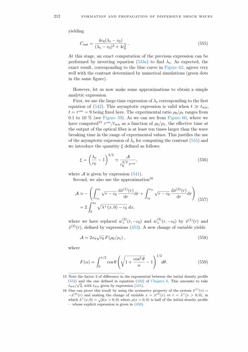
212 formation and propagation of dispersive shock waves
yielding
Cont =4c0(λS − c0)
(λS − c0)2 + 4c20
. (555)
At this stage, an exact computation of the previous expression can beperformed by inverting equation (533a) to find λS. As expected, theexact result, corresponding to the blue curve in Figure 62, agrees verywell with the contrast determined by numerical simulations (green dotsin the same figure).
However, let us now make some approximations to obtain a simpleanalytic expression.First, we use the large-time expression of λS corresponding to the first
equation of (542). This asymptotic expression is valid when t tWB,t = τ out = 9 being fixed here. The experimental ratio ρ0/ρ1 ranges from0.1 to 10 % (see Figure 59). As we can see from Figure 60, where wehave computed15 τ out/tWB as a function of ρ0/ρ1, the effective time atthe output of the optical fiber is at least ten times larger than the wavebreaking time in the range of experimental values. This justifies the useof the asymptotic expression of λS for computing the contrast (555) andwe introduce the quantity ξ defined as follows:
ξ =
(λS
c0− 1
)3/2
' Ac
3/20 τ out
, (556)
where A is given by expression (541).Second, we also use the approximation16
A '−(∫ c0
cm
√r − c0
dx(1)(r)
drdr +
∫ cm
c0
√r − c0
dx(3)(r)
drdr
)
= 2
∫ x0
0
√λ+(x, 0)− c0 dx,
(557)
where we have replaced w(2)+ (r,−c0) and w
(3)+ (r,−c0) by x(1)(r) and
x(3)(r), defined by expressions (453). A new change of variable yields
A ' 2x0√c0 F (ρ0/ρ1) , (558)
where
F (α) =
∫ π/2
0cos θ
(√1 +
cos2 θ
α− 1
)1/2
dθ. (559)
15 Note the factor 2 of difference in the exponential between the initial density profile(552) and the one defined in equation (432) of Chapter 6. This amounts to taketWB/
√2, with tWB given by expression (441).
16 One can prove this result by using the symmetry property of the system x(1)(r) =−x(3)(r) and making the change of variable x = x(3)(r) ⇔ r = λ+(x > 0, 0), inwhich λ+(x, 0) =
√ρ(x > 0, 0) where ρ(x > 0, 0) is half of the initial density profile
— whose explicit expression is given in (450).

7.3 experimental considerations 213
τout /t
WB τout/t
WB
Figure 60: (Left) Blue curve : ratio of the effective time at the output ofthe fiber τ out = 9 by the wave breaking time tWB, computedfrom expression (441) and for an initial Gaussian beam (552),as a function of the initial ratio ρ0/ρ1. The red dashed curvecorresponds to tWB = τ out, i.e., in the considered case, tWB = 9.The inset shows the same curves for higher density background(we recall that in the experiment ρ1 = 5.9 is fixed and only ρ0varies).
A simple analytic expression of F (α) cannot be obtained, but we checkedthat one can devise an accurate approximation by expanding the termin the above integrand around θ = 0 up to second order in θ. This yields
F (α) ' (√α+ 1−√α)1/2
α1/4−
14(π2/4− 2)
α1/4√
1 + α(√α+ 1−√α)1/2
. (560)
A comparison between the exact result (559) and the approximate ex-pression (560) is shown in Figure 61. The maximal relative error in therange of experimental values α ∈ [0, 0.1], i.e., ρ0/ρ1 between 0 and 10%, is less than 2 %. Thus, we can safely use the approximate result(560), which is also valid for much larger values of α, see the inset ofFigure 61.Therefore, we arrive to a simple analytic equation for the contrast
(555) in terms of the parameter ξ defined in (556):
Cont =4 ξ2/3
4 + ξ4/3, with ξ ' 2x0√
ρ1 τ out
√ρ1
ρ0F
(ρ0
ρ1
), (561)
where we used the approximate expression (558) to evaluate ξ. Theresult is represented as a red curve in Figure 62. As one can see, it com-pares quite well with the value of Cont extracted from the numericalsimulations. The better agreement with the numerical result is reachedfor small ρ0/ρ1; this was expected: in this regime the wave breakingoccurs rapidly (τ out/tWB →∞, see Figure 60), and one easily fulfills the

214 formation and propagation of dispersive shock waves
Figure 61: Blue curve: F (α) computed from the exact result (559). Dashedred curve: approximate result evaluated from expression (560).The inset shows F (α) for a wider range of possible values α.
condition τ out tWB where the approximation (542) holds. Moreover,one sees that experimental data extracted from Ref. [200] and repre-sented as brown bars in Figure 62 match well with the analytic resultgiven by (561), despite the approximations we made and the fact thatthe form of the initial profile considered in this reference is not exactlythe same as ours.
Figure 62: Contrast Cont represented as a function of ρ0/ρ1. In order to fol-low the procedure used in Ref. [200], we fixed here the values ofρ1, x0 and τ out [ρ1 = 2, x0 = 20 and τ out = 49 – which give thesame contrast as ρ1 = 5.9, x0 = 6.3 and τ out = 9, see the textbelow equation (562)] and varied the value of ρ0. The green dotscorrespond to the numerically determined value of the contrast,obtained from equation (553) where ρmin and ρmax are definedas illustrated in the inset. The yellow triangle pinpoints the den-sity ratio ρ0/ρ1 for which the contrast is unity, see in particularequation (562). The red curve corresponds to the contrast com-puted from the approximate expression (561). The brown barsare experimental data extracted from Ref. [200].

7.3 experimental considerations 215
In addition, there is a special value of ρ0/ρ1 for which the contrastis unity, meaning that the quantity ρmin cancels. One sees from (554)that this is obtained for ξ = 3, i.e., 2c0 ' (A/τ out)2/3. Using expression(558), the contrast is thus unity when
c0 τout
x0=
1√2F (ρ0/ρ1) . (562)
A numerical solution of this equation gives, for the parameters of Fig-ure 62, a contrast unity when ρ0/ρ1 = 7.7%, while the exact equation(555) predicts a maximum contrast when ρ0/ρ1 = 8.3% instead (indi-cated by a yellow triangle in Figure 62).Besides, one sees from equation (561) that different sets of parameters
x0, ρ1 and τ out (the effective time being fixed by the length of the fiberin this specific case) such that
√ρ1 τ
out
x0= Constant (563)
all lead to the same contrast Cont. For instance, taking ρ1 = 5.9, x0 =6.3 and τ out = 9 ( √ρ1 τ
out/x0 = 3.47) yields the same result for thecontrast as taking ρ1 = 2, x0 = 20 and τ out = 49 (which correspondsto the red dashed curve in Figure 62). We did not plot both curves forthese two different configurations for legibility of the figure.
To conclude, we have demonstrated that our approach successfullydescribes the propagation of a dispersive shock wave in a system whosedynamics is governed by the nonlinear Schrödinger equation. Similarresults have been also obtained for the Korteweg-de Vries equation [93],but are not reproduced in this thesis. In both cases, we were able tofind the evolution of the Riemann invariants in the shock region, whentwo of them were varying.However, the solutions of the problem are often implicit and require
the use of numerical computations to extract, for instance, the envelopesof the DSW at a certain time t.
Nevertheless, we also proved that it was possible to extract from ourapproach a weak shock theory for these dispersive systems, exactly asit was done for viscous shocks [197]. This asymptotic description of theDSW can be used in some physical systems as soon as t tWB; whenthis condition is fulfilled, one can compute certain experimental quanti-ties, such as the contrast of the fringes in the DSW, from simple analyticexpressions derived from the weak shock theory. Therefore, beyond themathematical description and the richness of Whitham modulationaltheory to describe nonlinear systems, one can also predict the behav-ior of parameters of experimental relevance: determining for instancethe best configuration for visualizing the fringes of the DSW should beuseful for future studies.

216 formation and propagation of dispersive shock waves
7.4 article: long-time evolution of pulses in thekorteweg–de vries equation in the absence ofsolitons reexamined: whitham method
This work, albeit not discussed in this thesis, was an important step inour understanding of the problem, before considering the more compli-cated case of the nonlinear Schrödinger equation.
→ Long-time evolution of pulses in the Korteweg–de Vries equationin the absence of solitons reexamined: Whitham method
M. Isoard, A.M. Kamchatnov, N. Pavloff, Physical Review E 99,012210 (2019)
doi: https://doi.org/10.1103/PhysRevE.99.012210
We consider the long-time evolution of pulses in the Korteweg–deVries equation theory for initial distributions which produce no solitonbut instead lead to the formation of a dispersive shock wave and of ararefaction wave. An approach based on Whitham modulation theorymakes it possible to obtain an analytic description of the structure andto describe its self-similar behavior near the soliton edge of the shock.The results are compared with numerical simulations.

PHYSICAL REVIEW E 99, 012210 (2019)
Long-time evolution of pulses in the Korteweg–de Vries equation in the absence of solitonsreexamined: Whitham method
M. Isoard,1 A. M. Kamchatnov,2,3 and N. Pavloff1
1LPTMS, CNRS, Univ. Paris-Sud, Université Paris-Saclay, 91405 Orsay, France2Institute of Spectroscopy, Russian Academy of Sciences, Troitsk, Moscow, 108840, Russia
3Moscow Institute of Physics and Technology, Institutsky lane 9, Dolgoprudny, Moscow region, 141701, Russia
(Received 12 October 2018; published 16 January 2019)
We consider the long-time evolution of pulses in the Korteweg–de Vries equation theory for initial distribu-tions which produce no soliton but instead lead to the formation of a dispersive shock wave and of a rarefactionwave. An approach based on Whitham modulation theory makes it possible to obtain an analytic description ofthe structure and to describe its self-similar behavior near the soliton edge of the shock. The results are comparedwith numerical simulations.
DOI: 10.1103/PhysRevE.99.012210
I. INTRODUCTION
It is well known that pulses propagating through a nonlin-ear medium typically experience wave breaking. Their long-time evolution depends on which effect—in addition to thenonlinearity—dominates after the wave breaking moment:viscosity or dispersion. If viscosity dominates, then the shockcorresponds to a region of localized extend in which the slowvariables display a sharp transition. A typical small-amplitudeviscous shock can be modeled by the Burgers’ equation
ut + uux = νuxx, (1)
for which a full analytic theory has been developed (see, e.g.,Ref. [1]). For a positive initial profile u(x, t = 0) ≡ u0(x) >
0 which is well-enough localized [i.e., u0(x) → 0 fast enoughfor |x| → ∞] the time-evolved pulse acquires a triangle-likeshape at its front edge [or at its rear edge if u0(x) < 01],gradually spreading out with decreasing amplitude.
The situation changes drastically if dispersive effects dom-inate rather than viscosity. In this case the typical evolutioncan be described by the celebrated Korteweg–de Vries (KdV)equation
ut + 6uux + uxxx = 0, (2)
which admits oscillating solutions ranging from linear wavesto bright solitons. A positive localized initial pulse u0(x) > 0,after an intermediate stage of wave breaking and complicateddeformation, eventually evolves into a sequence of solitonswith some amount of linear dispersive waves. The character-istics of the solitons are determined by the initial distributionu0(x). If this initial pulse is intense enough—so that thenumber of solitons is large—one may determine the param-eters of these solitons by means of the asymptotic formulaof Karpman [2] which is obtained in the framework of theinverse scattering transform method discovered by Gardner,
1A so-called N -wave appears if u0(x ) has both polarities; see, e.g.,Ref. [1].
Green, Kruskal, and Miura [3]. However, if u0(x) < 0, sinceEq. (2) does not admit dark (i.e., “negative”) solitons, thenwave breaking does not result in the production of solitons,but it rather leads to the formation of a dispersive shock wave(DSW) connected to a triangle-like rarefaction wave whichis the remnant of the initial trough. The shape and the timeevolution of this oscillatory structure are highly nontrivial andconsiderable efforts have been invested in their study.
In an early investigation of Berezin and Karpman [4] it wasshown that the KdV equation admits solutions of the form
u(x, t ) = 1
t2/3f
( x
t1/3
), (3)
and numerical simulations of these authors demonstrated thatsome region of the evolving wave structure is indeed de-scribed by solutions of type (3). The existence of such a regionwas confirmed by the inverse scattering transform method inRefs. [5,6] and its “quasi-linear” part was studied in Ref. [7].An extensive study of the asymptotic evolution of the pulsein the absence of solitons was performed in Ref. [8] wheredifferent characteristic parts of the wave structure were distin-guished and their main parameters were calculated. However,in this reference, Ablowitz and Segur—who first explicitlypoint to the formation of a dispersive shock wave—confinedthemselves to the analytic study of typical limiting cases andexplicit formulas for the whole dispersive shock wave regionwere found much later [9] with the use of a quite involvedanalysis of the associated Riemann-Hilbert problem. Thisapproach was developed further in Refs. [10–12] and otherpapers.
Although the above-mentioned approaches are mathemati-cally strict, the methods used are difficult and the theory devel-oped has not found applications to concrete problems relatedwith other integrable evolution equations. Since the questionof evolution of pulses in the absence of solitons is related withexperiments in physics of water waves [13,14], Bose-Einsteincondensates [15,16], and nonlinear optics [17,18], the devel-opment of a simpler and more transparent physically approachis desirable. Such an approach, based on the Whitham theory
2470-0045/2019/99(1)/012210(12) 012210-1 ©2019 American Physical Society

M. ISOARD, A. M. KAMCHATNOV, AND N. PAVLOFF PHYSICAL REVIEW E 99, 012210 (2019)
of modulations of nonlinear waves [19], was suggested longago by Gurevich and Pitaevskii [20] and since that time it hasdeveloped into a powerful method with numerous applications(see, e.g., the review article [21]). Despite the facts that someelements of the Whitham theory were used in Refs. [6,8] andthat the general solution of the solitonless initial value prob-lem has been obtained in Ref. [22], no asymptotic analysishas been performed within Whitham’s formalism, so that itsrelationship with the previous results remained unclear.
The main goal of the present paper is to fill this gap and toapply the Whitham theory to the description of the asymptoticevolution of initial pulses in the small dispersion limit (or forwide pulses) under the condition of absence of solitons. Weshow that the combination of two ideas—self-similarity ofthe solution and quasisimple character [23] of the dispersiveshock wave—permits an asymptotic analysis of the solution.The relatively simple theory developed in the present workshould be useful in the analysis of experiments devoted to theevolution of pulses of this type.
The paper is organized as follows. In Sec. II we presentthe main aspects of Whitham theory and of the generalizedhodograph method applying to quasisimple waves (followingRefs. [22–28]). In Sec. III, the application of the ideas ofRef. [23] to the soliton edge of the DSW makes it possibleto find the law of motion of this edge and suggests a self-similar asymptotic behavior consistent with Eq. (3). In Sec. IVwe perform the large-time asymptotic analysis of the rear(soliton) part of the dispersive shock wave by the Whithammethod within this self-similarity assumption. This yields asurprisingly simple derivation of the solution first explicitlyobtained in Ref. [9]. The description of the DSW in its fullrange by the method of El and Khodorovskii [22] is presentedin a self-contained manner in Sec. V. In this section weconsider the time evolution of several initial profiles illustrat-ing the possible different behaviors in the shock region andcompare the theoretical results with numerical simulations.We present our conclusions in Sec. VI.
II. WHITHAM THEORY AND THE GENERALIZEDHODOGRAPH METHOD
A. The smooth part of the profile
We consider an initial pulse with nonpositive profileu(x, t = 0) = u0(x) defined on finite interval of x and havinga single minimum minx∈Ru0(x) = −1 (this value can bechanged by an appropriate rescaling on u, x, and t). Weconsider a initial profile of finite extend x0, and assume thatx0 1, so that in a first stage of evolution one can neglectdispersive effects. This amounts to replace the KdV dynamicsby the Hopf equation,
rt + 6 r rx = 0. (4)
We changed notation here to mark the difference betweenr (x, t ), solution of the approximate equation (4), and u(x, t ),which is the exact solution of the KdV equation (2). The solu-tion of the Hopf equation is well known (see, e.g., Ref. [29])and it is given in implicit form in terms of functions inverse tou0(x), as explained now.
In the case we consider, u0(x) has a single minimum andits inverse function is two valued. We denote its two branches
FIG. 1. The solid black, solid pink, and dashed red lines repre-sent r (x, t ) solution of (4) for times t = 0, t = tWB, and t = 2.5 tWB
for an initial condition r (x, 0) given by the parabolic profile u0(x )defined in Eq. (6) with x0 = 40. The dots represent the position ofthe minimum min x∈Rr (x, t ) which separates parts A (at the left)and B (at the right) of the profile.
as wA(r ) and wB(r ), where the first function refers to the partof the pulse to the left of its minimum and the second one toits right. Then the solution of the Hopf equation is given bythe formulas
x − 6 r t = wA(r ), (5a)
x − 6 r t = wB(r ). (5b)
For example, in case of a parabolic initial pulse
u0(x) =
4 x(x + x0)/x20 for − x0 x 0,
0 elsewhere,(6)
the inverse functions are equal to
wA(r ) = x02 (−1 − √
1 + r ),
wB(r ) = x02 (−1 + √
1 + r ),where r ∈ [−1, 0]. (7)
Figure 1 represents the initial profile (6) and its time evolutionas computed from Eqs. (5), i.e., without taking dispersiveeffects into account. Figure 2 represents the correspondingfunctions wA(r ) and wB(r ). In the following we shall performthe explicit computations using this initial profile. Other types
FIG. 2. The two branches wA(r ) and wB(r ) of the reciprocalfunction of u0(x ). The figure is drawn for the initial parabolicprofile (6) [the corresponding expressions of wA(r ) and wB(r ) aregiven in Eq. (7)] but the behavior is the generic one.
012210-2

LONG-TIME EVOLUTION OF PULSES IN THE … PHYSICAL REVIEW E 99, 012210 (2019)
of profiles, with less generic behaviors, will be presented anddiscussed in Sec. V.
The wave-breaking time is the time tWB =1/max(−6 du0/dx) at which the solution of (4) becomesinfinitely steep (see, e.g., Ref. [1]). In the present workwe consider initial profiles for which the largest slopemax(−du0/dx) is reached at x = −x0 for r = 0 and thus
tWB = −1
6
(dwA
dr
)r=0
. (8)
For the initial profile (6) we get tWB = x0/24. For t tWB thedispersionless approximation fails (the corresponding formalsolution of the Hopf equation is multivalued), and a DSW isformed, initially around x = −x0, which then expands towardthe negative x direction. We now explain how it can bedescribed within Whitham modulational theory.
B. Periodic solutions and their modulations
The KdV equation (2) admits nonlinear periodic solutionswhich can be written in terms of three parameters r1 r2 r3 as (see, e.g., Ref. [29])
u(x, t ) = r3 + r2 − r1 − 2(r2 − r1)
× sn2(√
r3 − r1(x − V t ),m), (9)
where
V = 2(r1 + r2 + r3) (10)
and
m = r2 − r1
r3 − r1. (11)
The notation “sn” in formula (9) refers to the Jacobi sinefunction (see, e.g., Ref. [30]). For constant parameters ri
expression (9) is an exact (single phase) solution of the KdVequation, periodic in time and space with wavelength
L = 2K (m)√r3 − r1
, (12)
where K (m) is the complete elliptic integral of the first kind.According to the Gurevich-Pitaevskii scheme, a DSW may
be described as a modulated nonlinear periodic wave oftype (9) for which the ri’s slowly depend on time and positionand evolve according to the Whitham equations (see, e.g,Refs. [21,29])
∂t ri + vi (r1, r2, r3)∂xri = 0, i = 1, 2, 3. (13)
The quantities vi in these equations are the Whitham veloc-ities. Their explicit expressions have first been derived byWhitham [19] and can also be obtained from the relation
vi =(
1 − L
∂iL∂i
)V = V − 2
L
∂iL, (14)
where L is the wavelength (12), V the phase velocity (10)of the nonlinear periodic solution (9), and ∂i stands for ∂ri
.
One gets
v1 = 2(r1 + r2 + r3) + 4(r2 − r1)K (m)
E(m) − K (m),
v2 = 2(r1 + r2 + r3) − 4(r2 − r1)(1 − m)K (m)
E(m) − (1 − m)K (m),
v3 = 2(r1 + r2 + r3) + 4(r3 − r1)(1 − m)K (m)
E(m),
(15)
where E(m) is the complete elliptic integral of the secondkind.
Since Eqs. (13) have a diagonal form (that is, they includederivatives of a single parameter ri in each equation), thevariables ri are called Riemann invariants of the Whithamequations—Riemann was the first who introduced such vari-ables in the theory of nonlinear waves.
The two edges of the DSW are denoted as xL(t ) and xR(t ).The first one is the small-amplitude edge; it is at the leftof the DSW in the case we consider. Within the Whithamapproximation, it makes contact between the DSW and theundisturbed profile: u(x, t ) = 0 for x xL(t ). The small-amplitude version of (9) corresponds to the limit m 1 andtakes the form
u(x, t ) = r3 + (r2 − r1) cos[2√
r3 − r1(x − V t )]. (16)
In this harmonic linear limit, r2 → r1 (m → 0) and theWhitham velocities (15) reduce to
v1|r2=r1 = v2|r2=r1 = 12 r1 − 6 r3,
v3|r2=r1 = 6 r3. (17)
Around the left boundary of the DSW, the amplitude 2(r2 −r1) of the oscillations is small and since this edge propagatesalong a zero background, we arrive at the conclusion that r3 =0 and r1 = r2 for x = xL(t ).
The other edge, at the right side of the DSW, is thelarge-amplitude soliton edge, with m = 1. Therefore we musthave here r2 = r3 and in this limit the nonlinear pattern (9)degenerates into a soliton solution of the form
u(x, t ) = r1 + 2(r2 − r1)
cosh2[√
r2 − r1(x − V t )]. (18)
This implies that the right of the DSW is bounded by a solitonfor which the Whitham velocities are given by
v1|r2=r3 = 6 r1,
v2|r2=r3 = v3|r2=r3 = 2 r1 + 4 r3. (19)
C. Generalized hodograph method
The dispersionless approach of Sec. II A leads, after thewave-breaking time, to an nonphysical, multivalued solution.The form, displayed in Fig. 1, of r (x, t tWB) in the regionof multivaluedness suggests that the DSW accounting forthe post wave-breaking dynamics should be described byWhitham-Riemann invariants arranged in a configuration suchthat r3 = 0 (thus ensuring matching with the unperturbedprofile at the left), whereas r2 and r1 both depend on x andt , with always r3 r2 r1.
The contact of the DSW with the smooth pro-file which prevails for x xR(t ) imposes the condition
012210-3

M. ISOARD, A. M. KAMCHATNOV, AND N. PAVLOFF PHYSICAL REVIEW E 99, 012210 (2019)
r1(xR(t ), t ) = r (xR(t ), t ), where r (x, t ) is a solution of theHopf equation (4) with initially r (x, 0) = u0(x). Thereforethe description of the DSW for x ∈ [xL(t ), xR(t )] imposes theboundary conditions
r1(xR(t ), t ) = r (xR(t ), t ) ≡ rR(t ), r2(xR(t ), t ) = 0,
(20a)
r1(xL(t ), t ) = r2(xL(t ), t ) ≡ rL(t ). (20b)
Note that all the above functions are only defined after thewave breaking time, i.e., for t tWB.
This type of structure, in which two Riemann invariants (r1
and r2) change along the DSW, is not a simple wave solution;it belongs to the class of “quasisimple waves” introduced inRef. [23]. In this case, Eq. (13) with i = 3 is trivially satisfiedand for solving the remaining two Whitham equations we usethe so-called generalized hodograph method of Tsarev [31].To this end, one introduces two functions Wi (r1, r2) (i = 1or 2), making it possible to write a vector generalization ofEq. (5) for the Whitham system:
x − vi (r1, r2)t = Wi (r1, r2), i = 1, 2. (21)
For the sake of brevity we have noted in the above equationvi (r1, r2) = vi (r1, r2, r3 = 0) for i ∈ 1, 2; we will keep thisnotation henceforth. The Wi’s must satisfy the compatibilityequation found by substituting (21) into (13). This leads tothe Tsarev equations:
∂jWi
Wi − Wj
= ∂jvi
vi − vj
, for i = j. (22)
One can show (see, e.g., Refs. [25,27,28]) that (22) is solvedfor Wi’s of the form
Wi =(
1 − L
∂iL∂i
)W = W +
(1
2vi − r1 − r2
)∂iW , (23)
where W (r1, r2) is solution of the Euler-Poisson equation
∂12W = ∂1W − ∂2W
2(r1 − r2). (24)
There is, however, a subtle point here, which was first under-stood in Ref. [23] (see also Ref. [22]). After the wave breakingtime, the development of the dispersive shock wave occurs intwo steps:
(A) Initially (when t is close to tWB), the DSW is con-nected at its right edge to the smooth profile coming from thetime evolution of part A of the initial profile. In this case, fora given time t , the lower value of u(x, t ) is reached within thesmooth part of the profile and keeps its initial values (−1).
(B) Then, after a while, the left part of the initial profile(part A) has been “swallowed” by the DSW which is thenconnected at its right to the smooth profile coming from thetime evolution of part B of u0(x). In this case, the minimumminx∈Ru(x, t ) is reached inside the DSW (or at its bound-ary), is negative and larger than −1 (i.e., less pronounced thanin the previous case A), and asymptotically tends to 0 for largetime.
We denote the region of the DSW [and of the (x, t ) plane]in which r1 is a decreasing function of x as region A, the partwhere it increases as region B. In region A of the (x, t ) plane,
we denote by W A(r1, r2) the solution of the Euler-Poissonequation; in region B we denote it instead as W B(r1, r2). Thesetwo forms are joined by the line r1 = −1 (cf. the upper plotsof Fig. 5) along which
W A(−1, r2) = W B(−1, r2). (25)
Since the general solution of the Euler-Poisson equation withthe appropriate boundary conditions, and the construction ofthe resulting nonlinear pattern are quite involved, we shall firstconsider some particular—but useful—results which followfrom general principles of the Whitham theory.
III. MOTION OF THE SOLITON EDGE OF THE SHOCK
During the first stage of evolution of the DSW, its right(solitonic) edge is connected to the smooth dispersionlesssolution described by formula (5a), that is we have here
xR − 6rRt = wA(rR ). (26)
On the side of the DSW, in vicinity of this boundary, theWhitham equations (13) with the limiting expressions (19)(where r3 = 0) for the velocities vi are given by
∂t r1 + 6r1∂xr1 = 0, ∂t r2 + 2r1∂xr2 = 0. (27)
For solving these equations one can perform a classical hodo-graph transformation (see, e.g., Ref. [29]), that is, one assumethat x and t are functions of the independent variables r1 andr2: t = t (r1, r2), x = x(r1, r2). We find from Eqs. (27) thatthese functions must satisfy the linear system
∂x
∂r1− 2r1
∂t
∂r1= 0,
∂x
∂r2− 6r1
∂t
∂r2= 0.
At the boundary with the dispersionless solution [where r1 =rR, see (20a)] the first equation reads
∂xR
∂rR
− 2 rR
∂t
∂rR
= 0, (28)
and this must be compatible with Eq. (26). Differentiation ofEq. (26) with respect to rR and elimination of ∂xR/∂rR with theuse of Eq. (28) yield the differential equation for the functiont (rR ) ≡ t (rR, 0):
4 rR
dt
drR
+ 6 t = −dwA(rR )
drR
. (29)
At the wave-breaking time, rR = 0, and (29) gives the correctdefinition (8) of the wave-breaking time: tWB = t (0). Elemen-tary integration then yields
t (rR ) = 1
4(−rR )3/2
∫ rR
0
√−rdwA(r )
drdr
= 1
8(−rR )3/2
∫ rR
0
wA(r )√−rdr − wA(rR )
4 rR
. (30)
Substituting this into (26) we get the following expression forthe function xR(rR ) ≡ x(rR, 0):
xR(rR ) = − 3
2√−rR
∫ rR
0
√−rdwA(r )
drdr + wA(rR )
= − 3
4√−rR
∫ rR
0
wA(r )√−rdr − 1
2wA(rR ). (31)
012210-4

LONG-TIME EVOLUTION OF PULSES IN THE … PHYSICAL REVIEW E 99, 012210 (2019)
The two formulas (30) and (31) define in an implicit way thelaw of motion x = xR(t ) of the soliton edge of the DSW.
The above expressions are correct as long as the solitonedge is located inside region A, that is up to the moment
tA/B = t (−1) = 1
4
∫ −1
0
√−rdwA(r )
drdr, (32)
after which the soliton edge connects with part B of thesmooth profile. Concretely, for a time t > tA/B, we have tosolve the differential equation
4 rR
dt
drR
+ 6 t = −dwB(rR )
drR
with the initial condition t (−1) = tA/B. This yields
t (rR ) = 1
4(−rR )3/2
[ ∫ −1
0
√−rdwA(r )
drdr
+∫ rR
−1
√−rdwB(r )
drdr
](33)
and
xR(rR ) = − 3
2(−rR )1/2
[ ∫ −1
0
√−rdwA(r )
drdr
+∫ rR
−1
√−rdwB(r )
drdr
]+ wB(rR ). (34)
At asymptotically large time t → ∞ one is at stage B ofevolution, with furthermore rR → 0. Hence the upper limit ofintegration in the second integrals of formulas (33) and (34)can be put equal to zero. Integration over r in the resultingexpressions can be replaced by integration over x with accountof the fact that wA,B(r ) represent two branches of the inversefunction of r = u0(x), so we get
t (rR ) A4(−rR )3/2
, where A =∫R
√−u0(x) dx
is a measure of the amplitude of the initial trough. Conse-quently, we obtain
rR(t ) = −(A
4t
)2/3
, xR(t ) = −3A2/3
21/3t1/3, (35)
where we have neglected a term of order x0 which is smallcompared to the infinitely increasing time-dependent ones.
At large time, the dispersionless part of the profile be-tween x = 0 and xR(t ) is stretched to a quasilinear behavioru(x, t ) = x rR(t )/xR(t ), and one thus has∫ 0
xR (t )dx
√−u(x, t ) = −2
3xR(t )
√−rR(t ) = A, (36)
which means that the quantity A is conserved, at least atthe level of the present asymptotic analysis. This situationis reminiscent of—but different from—the dissipative casewhere nonlinear patterns of triangular shape may also appearat the rear edge of a (viscous) shock. In the dissipative casethere also exists a conserved quantity. For Burgers’ equation,for instance, with an initial condition of type (6), a singleviscous shock appears which is followed by an asymptoticallytriangular wave. This means that the details of the initial
distribution are lost (as in the present case), but for Burgers’equation the conserved quantity is not the quantity A definedin Eq. (36), but the integral
∫I (t )dx u(x, t ), where I (t ) is the
support of the triangular wave (equivalent to our segment[xR(t ), 0]).
Formulas (35) suggest that in the vicinity of the solitonedge, the behavior of the DSW must be self-similar, andwe now turn to the investigation of this possibility in theframework of Whitham theory.
IV. SIMILARITY SOLUTION AT THE SOLITON EDGE OFTHE SHOCK
In this section we use the Whitham approach to obtain thelong-time asymptotic behavior of the shock close to xR(t ),valid up to x ∼ −t1/3(ln t )3/2 (see Refs. [8,9]).
Equations (35) suggest that, close to the soliton edge ofthe DSW, the Riemann invariants r1 and r2 have the followingscaling form:
ri = 1
t2/3Ri
( x
t1/3
). (37)
Here x < 0 and since r1 < r2 < 0, we have R1 < R2 < 0.The scaling (37) agrees with the scaling (3) of the full KdVequation first noticed in Refs. [4–6]. Written in terms of therescaled Riemann parameters R1 and R2 and of the self-similar variable z = x/t1/3, the Whitham equations (13) read
dRi
dz= − 2Ri
z − 3R1Vi (m), i = 1, 2, (38)
where
m = 1 − R2/R1, (39)
and the velocities V1(m) and V2(m) are given by
V1(m) = 2(2 − m) − 4mK (m)
E(m) − K (m),
V2(m) = 2(2 − m) + 4m(1 − m)K (m)
E(m) − (1 − m)K (m).
(40)
The two equations (38) can be reduced to a single one if weintroduce the variable
ζ = z/R1 (41)
and look for the dependence of ζ on m. A simple calculationyields the differential equation
dζ
dm= [ζ − V1(m)][ζ − 3V2(m)]
2(1 − m)[V2(m) − V1(m)], (42)
whose basic properties can be studied in the phase plane(m, ζ ). The phase portrait in this plane is displayed in Fig. 3.It admits the singular points
(0, 12), (0, 36) for m = 0;(1, 6), (1, 6) for m = 1.
(43)
As is clear from Fig. 3, the point (0,12) is a node and the point(0,36) is a saddle. At m = 1 the two singular points merge intoone (1,6) of a mixed saddle-node type. Numerical solution of
012210-5

M. ISOARD, A. M. KAMCHATNOV, AND N. PAVLOFF PHYSICAL REVIEW E 99, 012210 (2019)
m
ζ
0 0.2 0.4 0.6 0.8 1
10
20
30
40
FIG. 3. Integral curves of Eq. (42). The separatices are depictedas solid thick lines. The dots are the singular points (43).
Eq. (42) suggests that the separatrix joining the singular points(0,12) and (1,6) is a straight line
ζ = 6(2 − m), (44)
which, after returning to the variables R1, R2, and z, leadsto the assumption that the system (38) admits the followingintegral:
R1 + R2 = 16z. (45)
A direct check shows that indeed d(R1 + R2)/dz = 1/6 un-der the condition (45), so that this assumption is proved. Theintegral curves beginning in vicinity of this separatrix areattracted to it when m decreases, so one can expect that justthis separatrix realizes the self-similar regime of the DSWnear its soliton edge.
To determine the dependence of m on z, we find, with theuse of Eqs. (38),
dm
dz= 6ζ (m)(1 − m)(V2(m) − V1(m))
z[ζ (m) − 3V1(m)][ζ (m) − 3V2(m)]. (46)
Substituting Eq. (44) and the expressions (40) in the above,we get the following equation:
dm
dz= − 2 − m
zmK (m)F (m), (47)
where
F (m) = (2 − m)E(m) − 2(1 − m)K (m). (48)
The solution of this equation determines m = m(z) along theseparatrix.
The form of expression (48) suggests that it can be obtainedas a result of the calculation of some elliptic integral in whichthe integration limits may play the role of more convenientvariables. Inspection of tables of such integrals shows that theformula 3.155.9 in Ref. [30] (which we write down here withnotations slightly different from the original reference),
I = 3∫ q1
q2
√(q2
1 − y2)(
y2 − q22
)dy
= q1[(
q21 + q2
2
)E(m) − 2q2
2K (m)], (49)
has the necessary structure. In Eq. (49) one has q1 > q2 > 0and m = 1 − (q2/q1)2.
To establish the link between the two expressions (48)and (49), it is enough to take
q21 + q2
2 = 1, (50)
so that 1 − m = q22/q2
1 , 2 − m = 1/q21 . Assuming that the
variables q1, q2 satisfy (50), we obtain
q21 = 1
2 − m, q2
2 = 1 − m2 − m
, (51)
and then, imposing m = m, we get F (m) = (2 − m)3/2I .Since dq1/dm = q3
1/2, Eq. (47) can be cast under the form
dq1
d ln(−z)= − q1
2mK (m)F (m), (52)
which is more convenient for further calculations. On theother hand, the integral (49) with account of Eqs. (51) sim-plifies to
I = q1[E(m) − 2
(1 − q2
1
)K (m)
],
and its differentiation with respect to q1 gives
dI
dq1= 3q2
1mK (m). (53)
With the help of the formulas obtained we transformEq. (52) to
dI
I= −3
2d ln(−z).
Then, integration of this equation with the boundary conditionz = z1 at m = 1 yields z as a function of m:
z = z1 I−2/3(m) = z12 − m
F 2/3(m), (54)
where
z1 = xR(t )
t1/3= −6(A/4)2/3 (55)
is the value of z for m = 1 (at the soliton edge of the DSW,see Sec. III).
From the formulas (39) and (51) we find the relationshipbetween the Ri’s and the qi’s:
R1 = q21
6z, R2 = q2
2
6z, (56)
so that for the dependence of the Riemann invariants on m weobtain:
R1(m) = z1
6(2 − m)I 3/2,
R2(m) = (1 − m)z1
6(2 − m)I 3/2.
(57)
Formulas (54), (55), and (57), together with Eq. (37), com-pletely determine the self-similar solution of the Whithamequations: For fixed t we have x(m) = t1/3z(m), so that allfunctions are defined parametrically, with m playing the roleof the parameter. Up to notations, this solution coincides withthe one obtained in Ref. [9] by means of an asymptotic studyof a Riemann-Hilbert problem in the framework of the inversescattering transform method.
012210-6

LONG-TIME EVOLUTION OF PULSES IN THE … PHYSICAL REVIEW E 99, 012210 (2019)
In the harmonic limit m 1, the relation (54) reads
m = m1z−3/4, where m1 = 211/4
√3π
(−z1)3/4, (58)
which leads to the expressions
r1 = x
12t− m1
24
(−x)1/4
t3/4, r2 = x
12t+ m1
24
(−x)1/4
t3/4. (59)
It is important to notice that the difference r2 − r1, that is,the amplitude of the oscillations in the “quasilinear” region ofZakharov and Manakov [7], increases with growing distancefrom the soliton edge [as (−x)1/4] but r2/r1 → 1 and m →0 here. Hence, this limit is not a small-amplitude one andtherefore the self-similar regime cannot be realized along thewhole DSW; it takes place close enough to the soliton edgeonly; see Figs. 6(e), 6(f), and 8. Consequently, we have to turnto the general solution of the Whitham equations to obtain afull description of the DSW.
V. GENERAL SOLUTION
In this section, following Ref. [22], we turn to the generalsolution of the Whitham equations given by the formulas ofSec. II C. Our task now is to express the functions Wi (r1, r2),i = 1, 2, in terms of the initial form u0(x) of the pulse. Aswas indicated above, at the first stage of evolution the DSWis located inside the region A and after the moment tA/B [seeEq. (32)] a second stage begins where it also reaches regionB. Correspondingly, the expressions for Wi and W are givenby different formulas and should be considered separately.
A. Solution in region A
In region A one can follow the procedure explained inRef. [25]. One imposes the matching of the right edge of theDSW with the dispersionless solution (5): Just at x = xR(t ),we have r1 = r (x, t ), where r (x, t ) is the solution of (4), andv1(r1, 0) = 6 r1 [this follows from Eq. (19)]. Comparing inthis case Eqs. (5) and (21) one obtains
W A1 (r1, 0) = wA(r1), (60)
which embodies the same information as Eq. (20a). In termsof W this corresponds to the equation
W A(r1, 0) + 2 r1 ∂1WA(r1, 0) = wA(r1), (61)
whose solution is
W A(r1, 0) = 1
2√−r1
∫ 0
r1
wA(ρ) dρ√−ρ. (62)
This will serve as a boundary condition for the Euler-Poissonequation (24) whose general solution has been given byEisenhart [32] in the form
W A(r1, r2) =∫ 0
r1
ϕA(μ) dμ√(μ − r1)|r2 − μ|
+∫ 0
r2
ψA(μ) dμ√(μ − r1)(μ − r2)
, (63)
where the functions ϕA and ψA are arbitrary functions tobe determined from the appropriate boundary conditions. By
taking r2 = 0 in this expression one sees that ϕA(μ)/√−μ
is the Abel transform of W A(r1, 0). The inverse transformreads [33]
ϕA(μ)√−μ= − 1
π
d
dμ
∫ 0
μ
W A(r, 0) dr√r − μ
. (64)
Plugging expression (62) for W A(r, 0) in this formula andchanging the order of integration, one obtains
ϕA(μ) = 1
2 π√−μ
∫ 0
μ
wA(ρ) dρ√ρ − μ
. (65)
For the initial profile (6), wA is given in Eq. (7) and one getsexplicitly
ϕA(μ) = − x0
4π
(3 + 1 + μ√−μ
tanh−1 √−μ
).
In order to determine the function ψA, one considers the leftboundary of the DSW where, according to (20b), r1 and r2
are asymptotically close to each other. Let us write r1 = r
and r2 = r + ε with r ∈ [−1, 0] and ε small and positive. Onegets from (63)
W A(r, r + ε) =∫ 0
r+ε
dμϕA(μ) + ψA(μ)√
(μ − r )(μ − r − ε)
+∫ r+ε
r
ϕA(μ) dμ√(μ − r )(r + ε − μ)
. (66)
In the right-hand side of the above equality, the second termconverges when ε tends to 0 [toward πϕA(r )], whereas the firstone diverges unless ϕA(r ) + ψA(r ) = 0, this being true for allr ∈ [−1, 0]. This imposes that the functions ϕA and ψA shouldbe opposite one the other and the final form of the Eisenhartsolution in case A thus reads
W A(r1, r2) =∫ r2
r1
ϕA(μ) dμ√(μ − r1)(r2 − μ)
, (67)
where ϕA is given by formula (65).
B. Solution in region B
One looks for a solution of the Euler-Poisson equation inregion B of the form
W B(r1, r2) = W A(r1, r2) +∫ r1
−1
ϕB(μ) dμ√(r1 − μ)(r2 − μ)
. (68)
Indeed, this ensures that W B, (i) being the sum of two solu-tions of the Euler-Poisson equation is also a solution of thisequation and (ii) verifies the boundary condition (25) sincethe second term of the right-hand side of (68) vanishes whenr1 = −1.
At the right boundary of the DSW, W B(r1, 0) verifiesthe same equation (61) as W A(r1, 0) does, where all thesuperscripts A should be replaced by B. The solution with theappropriate integration constant reads
W B(r1, 0) = 1
2√−r1
∫ −1
r1
wB(ρ) dρ√−ρ
+ 1
2√−r1
∫ 0
−1
wA(ρ) dρ√−ρ. (69)
012210-7

M. ISOARD, A. M. KAMCHATNOV, AND N. PAVLOFF PHYSICAL REVIEW E 99, 012210 (2019)
The same procedure than the one previously used in part A ofthe DSW leads here to
ϕB(μ) = 1
2 π√−μ
∫ μ
−1dρ
wA(ρ) − wB(ρ)√μ − ρ
. (70)
For the initial profile (6) one gets explicitly
ϕB(μ) = −x0
4
1 + μ√−μ.
In the generic case, Eqs. (68) and (70) give the solution of theEuler-Poisson equation in region B.
C. Characteristics of the DSW at its edges
It is important to determine the boundaries xR(t ) and xL(t )of the DSW, as well as the values of the Riemann invariants r1
and r2 at these points. The law of motion of the soliton edgewas already found in Sec. III and it is instructive to show howthis result can be obtained from the general solution.
At the soliton edge we have r2 = r3 = 0 and r1 = rR(t ).The corresponding Whitham velocities are v1 = 6 rR and v2 =2 rR [see Eqs. (19)], and the two equations (21) read
xR − 6rRt = W1(rR, 0) = w(rR ),
xR − 2rRt = W2(rR, 0) = W (rR, 0). (71)
These formulas apply to both stages of evolution and thereforethe superscripts A and B are dropped out. They give at once
t (rR ) = 1
4rR
[W (rR, 0) − w(rR )],
xR(rR ) = 1
2[3W (rR, 0) − w(rR )]. (72)
Let us consider the stage A, for instance. Equation (62) yields
W A(rR, 0) = − 1
2√
rR
∫ rR
0
wA(ρ)dρ√−ρ,
which, inserted into Eqs. (72), gives immediately the re-sults (30) and (31). For instance, for the initial profile (6),when the right boundary is still in region A, one obtainsexplicitly
t (rR ) = x0
16 rR
(√1 + rR − arcsin
√−rR√−rR
). (73)
At the wave-breaking time, rR = 0 and this yields tWB =t (rR = 0) = x0/24 as already obtained [cf. Eq. (8)]. Stage Aends at time tA/B at which the minimum (−1) of the smoothpart of the profile enters the DSW. This corresponds to tA/B =t (rR = −1) and yields, for the initial parabolic profile (6),tA/B = π x0/32.
Let us now turn to the determination of the location xL(t )of the left boundary of the DSW and of the common valuerL(t ) of r1 and r2 at this point. In the typical situation the leftboundary is located in region A. In this case the equations (21)for i = 1 and 2 are equivalent and read
xL − 12 rLt = W A1 (rL, rL ). (74)
An equation for rL alone is obtained by demanding that thevelocity dxL/dt of the left boundary is equal to the common
FIG. 4. Dispersionless evolution of the initial triangular pro-file (77) with x0 = 40. The solid black, solid pink, and dashed redlines represent r (x, t ) solution of (4) for times t = 0, t = tWB andt = 2 tWB.
value 12 rL of v1 and v2 at this point [cf. Eqs. (17)]. The timederivative of Eq. (74) then yields
t = − 1
12
dW A1 (rL, rL )
drL
. (75)
Once rL(t ) has been determined by solving this equation, xL(t )is given by Eq. (74).
Note that the relation dxL/dt = 12 rL is a consequence ofthe general statement that the small-amplitude edge of theDSW propagates with the group velocity corresponding tothe wave number determined by the solution of the Whithamequations. Indeed, the KdV group velocity of a linear wavewith wave-vector k moving over a zero background is vg =−3k2, and here k = 2π/L = 2
√−rL [cf. Eq. (12)], hencevg = 12 rL = dxL/dt , as it should. This property of the small-amplitude edge is especially important in the theory of DSWsfor nonintegrable equations (see Refs. [34,35]).
We also study below a case different from (6) for whichthe left boundary of the DSW belongs to region B andcorresponds to r1 = r2 = −1 [in the so-called triangular casecorresponding to u0(x) given by Eq. (77)]. Then, at the small-amplitude edge v1 = v2 = −12 and Eqs. (21) yield xL + 12 ·t = Cst, the constant being the common value of W B
1 (−1,−1)and W B
2 (−1,−1). It can be determined at t = tWB, leading inthis case to
xL = −x0 − 12(t − tWB). (76)
It is worth noticing that the velocity dxL/dt = −12 agreeswith the leading term in Eq. (59) for r1 = −1 in spite ofa nonvanishing amplitude of the self-similar solution in thislimit. For a more detailed study of the small-amplitude regionbeyond the Whitham approximation, see, e.g., Ref. [12].
D. The global picture
We now compare the results of the Whitham approach withthe numerical solution of the KdV equation for the initialprofile (6) and also for a profile
u0(x) =
−1 +∣∣∣2xx0
+ 1∣∣∣ for − x0 x 0,
0 elsewhere.(77)
012210-8

LONG-TIME EVOLUTION OF PULSES IN THE … PHYSICAL REVIEW E 99, 012210 (2019)
−140 −120 −100 −80 −60 −40 −20 0
x
0
2
4
6
8
10
12
ttA/B
tWB
t = 10
−120 −110 −100 −90 −80 −70 −60
x
−1.0
−0.8
−0.6
−0.4
−0.2
0.0
r 1,r
2
r2
r1Region A
Region B
xL(t)xR(t)
Region A Region B
= 10t
xLxR
r1 =
-1
−200 −150 −100 −50 0
x
0
2
4
6
8
10
12
14
16
t
tWB
t = 10
r1 = r2 = −1
r2
=0
Region B
−120 −110 −100 −90 −80 −70 −60 −50
x
−1.0
−0.8
−0.6
−0.4
−0.2
0.0
r 1,r
2
r2
r1
= 10t
xL(t) xR(t) xL
xR
(a) (b)
(c) (d)
FIG. 5. The upper plots (a) and (b) refer to the parabolic initial profile, and the lower ones (c) and (d) to the triangular initial profile. Leftcolumn: Different regions in the (x, t ) plane. The DSW occurs in the colored regions. The characteristics of the dispersionless evolution arerepresented as gray lines. In plot (a) the time tA/B is the time where part A of the initial profile has been completely absorbed by the DSW.For the triangular profile in plot (c) one has tA/B = tWB. Right column: Plot of the two varying Riemann invariants r1(x, t ) and r2(x, t ) at fixedt = 10 for xL(t ) x xR(t ). In plots (a) and (b) the green dashed line marks the separation between regions A and B.
This profile is represented in Fig. 4 at t = 0, at wave-breakingtime, which in the present case is equal to tWB = x0/12 andalso at t = 2 tWB (using the dispersionless approximation pre-sented in Sec. II A).
We henceforth denote the initial profile (6) as “parabolic”and the initial profile (77) as “triangular.” As was indicatedabove, the triangular profile has the particularity of having aDSW within the region B only. This is clear from Fig. 4: PartA of the initial profile does not penetrate into the DSW regionbefore part B does. Or, phrasing this differently, accordingto the dispersionless evolution, at t = tWB both parts A andB penetrate into the region of multivaluedness at x −x0.
The DSW is described by Whitham method as explainedin Secs. II B and II C. For this purpose one needs to determiner1 and r2 as functions of x and t (r3 ≡ 0). This is performedas follows:
(i) First, we pick up a given r1 ∈ [−1, rR], where rR is thevalue of r1 at the soliton edge, the point where the DSW isconnected to the rarefaction wave (how to compute it has beenexplained in Sec. V C).
(ii) Second, at fixed t and r1, we find the correspondingvalue r2 as a solution of the difference equation obtained fromEqs. (21),
(v1 − v2) · t = W2(r1, r2) − W1(r1, r2) , (78)
where W1 and W2 are computed from Eq. (23).(iii) Last, the corresponding value of x is determined by
x = W1 + v1t (or, equivalently, x = W2 + v2t).This procedure gives, for each r1 ∈ [−1, rR] and t , the
value of r2 and x. In practice, it makes it possible to associate
to each (x, t ) a couple (r1, r2). The result is shown in Figs. 5for the two initial profiles (6) and (77).
Note that the characteristics of the DSW are different forthe initial profiles (6) and (77): For the parabolic profile, inFig. 5(a), the edge point of the DSW—at (x0, tWB)—pertains toregion A and corresponds to r1 = 0, while for the triangularprofile, in Fig. 5(b), the edge point of the DSW belongs toregion B, with r1 = −1. For the parabolic profile, the valuer1 = −1 defines a line which separates the regions A and B ofthe plane (x, t ), see Fig. 5(a). This line reaches a boundary ofthe DSW only at xR(tA/B), where tA/B is the time where part A ofthe initial profile has just been completely absorbed within theDSW. On the other hand, for the triangular profile, the wholeleft boundary of the DSW corresponds to the line r1 = −1,see Fig. 5(c).
The knowledge of r1(x, t ) and r2(x, t ) makes it possibleto determine, for each time t > tWB, u(x, t ) as given by theWhitham approach, for all x ∈ R:
(i) In the regions x 0 and x xL(t ), we haveu(x, t ) = 0.
(ii) In the region [xR(t ), 0], one has u(x, t ) = r (x, t )which is solution of the Hopf equation (obtained by themethod of characteristics, as explained in Sec. II A).
(iii) Inside the DSW, for x ∈ [xL(t ), xR(t )], the functionu(x, t ) is given by expression (9), with r3 = 0 and r1 andr2 determined as functions of x and t by the procedure justexplained.
The corresponding profiles are shown in Fig. 6 for theparabolic and triangular initial distributions. The agreementwith the numerical solution of Eq. (2) is excellent in bothcases. The numerical simulations are performed using a
012210-9

M. ISOARD, A. M. KAMCHATNOV, AND N. PAVLOFF PHYSICAL REVIEW E 99, 012210 (2019)
−80 −60 −40 −20 0 20
x
−1.0
−0.8
−0.6
−0.4
−0.2
0.0
0.2
u(x
,t=
t WB)
−70 −60 −50 −40 −30 −20 −10 0 10 20
x
−1.0
−0.8
−0.6
−0.4
−0.2
0.0
0.2
u(x
,t=
t WB)
−140 −120 −100 −80 −60 −40 −20 0 20
x
−0.8−0.6−0.4−0.2
0.00.20.40.60.8
u(x
,t=
10)
−140 −120 −100 −80 −60 −40 −20 0
x
−0.6
−0.4
−0.2
0.0
0.2
0.4
0.6
u(x
,t=
10)
−1200 −1000 −800 −600 −400 −200 0
x
−0.2
−0.1
0.0
0.1
0.2
u(x
,t=
100)
−1200 −1000 −800 −600 −400 −200 0
x
−0.2
−0.1
0.0
0.1
0.2
u(x
,t=
100)
(a) (b)
(c) (d)
(e) (f)
FIG. 6. u(x, t ) as a function of x for fixed t . The left column refers to the parabolic initial profile and the right one to the triangular initialprofile. The upper row [(a) and (b)] corresponds to the wave-breaking time tWB, the central row [(c) and (d)] to t = 10, and the lower one[(e) and (f)] to t = 100. The blue solid line corresponds to the numerical solution of Eq. (2). The thick envelopes correspond to the results ofWhitham modulation theory. The dashed red lines represent the dispersionless profile r (x, t ) and also, in (c)–(f), the Whitham result for thesoliton at the large-amplitude boundary of the DSW. The green dashed envelopes in (e) and (f) are the asymptotic self-similar results obtainedin Sec. IV.
spatial mesh h = 0.1, evaluating the spatial derivatives ux anduxxx by means of, respectively, two- and four-point formulas(i.e., with an accuracy h2), and time propagated using a fourth-order Runge-Kutta method with a time step t = 10−3.
In Fig. 7 we also compare the wavelength of the nonlin-ear oscillations within the DSW as determined by Whithamapproach [Eq. (12)] with the results of numerical simulations,and the agreement is again very good.
E. The initial square profile
In this section we discuss another type of initial condition,which we denote as a “square profile”:
u0(x) =−1 for − x0 x 0,
0 elsewhere. (79)
El and Grimshaw already theoretically studied the same ini-tial condition by using the method just explained [36]. Wewill here compare the theory with numerical simulations toindicate some limitations of the one-phase Whitham methodwhich we use in the present work.
For this initial profile, wave breaking occurs instanta-neously (i.e., tWB = 0), and until t = x0/4 a plateau (i.e., asegment with constant u(x, t ) = −1) separates the DSW (atthe right) from a rarefaction wave (at the left). In this con-figuration, the DSW corresponds to the standard Gurevich-Pitaevskii scheme for a steplike initial profile with a singlevarying Riemann invariant (r2 in this case). This DSW can bedescribed using the self-similar variable ζ = (x + x0)/t ; inthis case Eq. (13) for i = 2 reads ζ = v2(−1, r2). One alsoobtains xL(t ) = −x0 − 2 t , xR(t ) = −6 t and the rarefactionwave corresponds to r (x, t ) = x/6t for x ∈ [xR(t ), 0].
It is interesting to remark that the Gurevich-PitaevskiiDSW can also be described within the approach exposed inSecs. II C and V D by solving Eq. (21) for i = 2. Here W A
2should be computed from
W A(r1, r2) = −x0 (80)
by means of Eq. (23). The form (80) of W A comes from (67)with wA(r ) = −x0.
At t = x0/4 the plateau disappears, and one enters intoregion B with now, as usual, two varying Riemann invariants.
012210-10

LONG-TIME EVOLUTION OF PULSES IN THE … PHYSICAL REVIEW E 99, 012210 (2019)
−1000 −800 −600 −400 −200
x
0
2
4
6
8
10
L
FIG. 7. Evolution of the wavelength of the nonlinear oscillationswithin the DSW as a function of position x. The figure correspondsto the time evolution of the parabolic initial profile represented in thelower left plot of Fig. 6 (t = 100). The continuous line representsthe results of Whitham theory and the points are the value of thewavelength extracted from the numerical simulations.
Formulas (68) and (70) lead here to
W B(r1, r2) = −x0 − x0
π
∫ r1
−1
√μ + 1 dμ√−μ(r1 − μ)(r2 − μ)
,
= −x0 + 2 x0/π√−r1(1 + r2)
×
(1 + r1
r1,m
)− K (m)
, (81)
where m = (1 + 1/r1)/(1 + 1/r2) and is the completeelliptic integral of the third kind.
The predictions of Whitham theory are compared in Fig. 8with numerical simulations. Surprisingly enough, the agree-ment between simulation and theory decreases at large time:At t = 100 one can notice oscillations in the envelope of thefront part of the DSW (Gurevich-Pitaevskii part). Inspectionof the dynamics of formation of the nonlinear structure revealsthat, during the formation of the rear rarefaction wave, oscil-lations appear due to dispersive effects associated with thediscontinuity of the initial condition (79): Their interferencewith the oscillations of the DSW leads to the modulatedstructure which can be observed in the lower plot of Fig. 8.Such a behavior requires a two-phase approach for a correctdescription. Note also that for numerical purposes the initialcondition is smoothed2 and that the beating phenomenonincreases for sharper initial condition (or for lower valuesof x0).
The predictions of the self-similar solution of Sec. IV arealso displayed in Fig. 8. In this figure, the envelopes of theDSW expected from Eqs. (37) and (57) are represented byred dashed lines. In the vicinity of its soliton edge, the DSWis accurately described by the similarity solution. Howeverthis approach is not able to tackle the other, small-amplitude,
2In the numerical simulations presented in Fig. 8 we take u0(x ) =14 [tanh(x/) − 1] × 1 + tanh[(x + x0 )/] with = 2. This pro-file tends to (79) when → 0.
−700 −600 −500 −400 −300 −200 −100 0
−0.5
0.0
0.5
u(x
,t=
50)
−1200 −1000 −800 −600 −400 −200 0
−0.4
−0.2
0.0
0.2
0.4
u(x
,t=
100)
x
(a)
(b)
FIG. 8. Evolution of an initial square profile of type (79) withx0 = 80 after a time t = 50 (a) and t = 100 (b). The blue solid linesare the results of numerical simulations. The orange envelopes aredetermined by Whitham method. The green dashed envelopes arethe asymptotic self-similar results obtained in Sec. IV. The dashedred lines represent the Whitham result for the soliton at the large-amplitude boundary of the DSW. Note the change of scale in the axisof the two plots.
boundary of the shock. This is expected since—as discussedabove—in the small-amplitude region a scaling different fromthe one of Eq. (3) holds, with the relevant self-similar param-eter ζ = (x + x0)/t ; see Refs. [9,37] for a general discussion.
VI. CONCLUSION
In the present work we have studied asymptotic solutionsof the KdV equation for which no soliton is formed. Weused the Whitham modulation theory combined with thegeneralized hodograph method for describing the DSW whichis formed after wave breaking. The results typically comparevery well with numerical simulations (see Sec. V D), exceptin the case of a initial square distribution (Sec. V E) where weargue that a two-phase approach would be needed for a correctdescription of the shock region.
A simple similarity description has been also obtained nearthe large-amplitude region of the shock, still within the frame-work of Whitham’s approach. Our results confirm, simplify,and extend in some respects the previous works on this subject(see Sec. IV). We also showed in Sec. III that this theoryprovides a practical tool for the description of the nonlinearevolution of pulses and can be used for comparison withexperimental data, since it yields simple analytic formulasfor some characteristic features of DSWs. In particular ourwork reveals the existence of a conserved quantity which hasremained unnoticed until now, see Eq. (36).
Extensions of the present approach to noncompletely inte-grable equations [35] and to other systems of physical interestare under study.
012210-11
M. ISOARD, A. M. KAMCHATNOV, AND N. PAVLOFF PHYSICAL REVIEW E 99, 012210 (2019)
ACKNOWLEDGMENTS
A.M.K. thanks Laboratoire de Physique Théorique et Mod-èles Statistiques (Université Paris-Saclay), where this work
was started, for kind hospitality. This work was supportedby the French ANR under Grant No. ANR-15-CE30-0017(Haralab project).
[1] G. B. Whitham, Linear and Nonlinear Waves (Wiley Inter-science, New York, 1974).
[2] V. I. Karpman, Phys. Lett. A 25, 708 (1967).[3] C. S. Gardner, J. M. Green, M. D. Kruskal, and R. M. Miura,
Phys. Rev. Lett. 19, 1095 (1967).[4] I. A. Berezin and V. I. Karpman, Zh. Eksp. Teor. Fiz. 46, 1880
(1964) [Sov. Phys. JETP 19, 1265 (1964)].[5] A. B. Shabat, Doklady AN SSSR 211, 1310 (1973) [Sov.
Mathem. Dokl. 14, 1266 (1973)].[6] M. J. Ablowitz and A. C. Newell, J. Math. Phys. 14, 1277
(1973).[7] V. E. Zakharov and S. V. Manakov, Zh. Eksp. Teor. Fiz. 71, 203
(1976) [Sov. Phys. JETP 44, 106 (1976)].[8] M. J. Ablowitz and H. Segur, Stud. Appl. Math. 57, 13
(1977).[9] P. Deift, S. Venakides, and Z. Zhou, Commun. Pure Appl. Math.
47, 199 (1994).[10] G. A. El, A. L. Krylov, and S. Venakides, Commun. Pure Appl.
Math. 54, 1243 (2001).[11] T. Claeys and T. Grava, Commun. Math. Phys. 286, 979 (2009).[12] T. Claeys and T. Grava, Commun. Pure Appl. Math. 63, 203
(2010).[13] J. L. Hammack and H. Segur, J. Fluid Mech. 65, 289 (1974);
84, 337 (1978).[14] S. Trillo, M. Klein, G. F. Clauss, and M. Onorato, Physica D
333, 276 (2016).[15] A. M. Kamchatnov, A. Gammal, and R. A. Kraenkel, Phys. Rev.
A 69, 063605 (2004).[16] M. A. Hoefer, M. J. Ablowitz, I. Coddington, E. A. Cornell,
P. Engels, and V. Schweikhard, Phys. Rev. A 74, 023623(2006).
[17] W. Wan, S. Jia, and J. W. Fleischer, Nat. Phys. 3, 46 (2007).[18] G. Xu, M. Conforti, A. Kudlinski, A. Mussot, and S. Trillo,
Phys. Rev. Lett. 118, 254101 (2017).[19] G. B. Whitham, Proc. R. Soc. A 283, 238 (1965).[20] A. V. Gurevich and L. P. Pitaevskii, Zh. Eksp. Teor. Fiz. 65, 590
(1973) [Sov. Phys. JETP 38, 291 (1974)].[21] G. A. El and M. A. Hoefer, Physica D 333, 11 (2016).[22] G. A. El and V. V. Khodorovsky, Phys. Lett. A 182, 49 (1993).[23] A. V. Gurevich, A. L. Krylov, and N. G. Mazur, Zh. Eksp. Teor.
Fiz. 95, 1674 (1989) [Sov. Phys. JETP 68, 966 (1989)].[24] A. V. Gurevich, A. L. Krylov, and G. A. El, Pis’ma Zh. Eksp.
Teor. Fiz. 54, 104 (1991) [JETP Lett. 54, 102 (1991)].[25] A. V. Gurevich, A. L. Krylov, and G. A. El, Zh. Eksp. Teor. Fiz.
101, 1797 (1992) [Sov. Phys. JETP 74, 957 (1992)].[26] A. L. Krylov, V. V. Khodorovskii, and G. A. El, Pis’ma Zh.
Eksp. Teor. Fiz. 56, 325 (1992) [JETP Lett. 56, 323 (1992)].[27] O. C. Wright, Commun. Pure Appl. Math. 46, 423 (1993).[28] F. R. Tian, Commun. Pure Appl. Math. 46, 1093 (1993).[29] A. M. Kamchatnov, Nonlinear Periodic Waves and Their
Modulations—An Introductory Course (World Scientific,Singapore, 2000).
[30] I. S. Gradshteyn and I. M. Ryzhik, Table of Integrals, Series,and Products (Academic Press, New York, 1966).
[31] S. P. Tsarev, Math. USSR Izv. 37, 397 (1991).[32] L. P. Eisenhart, Ann. Math. 120, 262 (1918).[33] G. Arfken and H. J. Weber, Mathematical Methods for Physi-
cists (Academic Press, Orlando, FL, 2005).[34] G. A. El, Chaos 15, 037103 (2005); 16, 029901 (2006).[35] A. M. Kamchatnov, Phys. Rev. E 99, 012203 (2019).[36] G. A. El and R. H. J. Grimshaw, Chaos 12, 1015 (2002).[37] H. Segur and M. J. Ablowitz, Physica D 3, 165 (1981).
012210-12

7.5 m. isoard, a.m. kamchatnov, n. pavloff, physical review a (2019) 229
7.5 article: wave breaking and formation of disper-sive shock waves in a defocusing nonlinear opti-cal material
→ Wave breaking and formation of dispersive shock waves in a defo-cusing nonlinear optical material
M. Isoard, A.M. Kamchatnov, N. Pavloff, Physical Review A 99,053819 (2019)
doi: https://doi.org/10.1103/PhysRevA.99.053819
We describe theoretically the quasi-one-dimensional transverse spread-ing of a light beam propagating in a nonlinear optical material in thepresence of a uniform background light intensity. For short propagationdistances the pulse can be described within a nondispersive (geomet-ric optics) approximation by means of Riemann’s approach. For largerdistances, wave breaking occurs, leading to the formation of dispersiveshocks at both edges of the beam. We describe this phenomenon withinWhitham modulation theory, which yields excellent agreement with nu-merical simulations. Our analytic approach makes it possible to extractthe leading asymptotic behavior of the parameters of the shock, settingup the basis for a theory of nondissipative weak shocks.

PHYSICAL REVIEW A 99, 053819 (2019)
Wave breaking and formation of dispersive shock waves in a defocusing nonlinear optical material
M. Isoard,1 A. M. Kamchatnov,2,3 and N. Pavloff1
1LPTMS, UMR 8626, CNRS, Univ. Paris–Sud, Université Paris–Saclay, 91405 Orsay, France2Institute of Spectroscopy, Russian Academy of Sciences, Troitsk, Moscow 108840, Russia
3Moscow Institute of Physics and Technology, Institutsky Lane 9, Dolgoprudny, Moscow Region 141701, Russia
(Received 19 February 2019; published 14 May 2019)
We describe theoretically the quasi-one-dimensional transverse spreading of a light beam propagating in anonlinear optical material in the presence of a uniform background light intensity. For short propagation distancesthe pulse can be described within a nondispersive (geometric optics) approximation by means of Riemann’sapproach. For larger distances, wave breaking occurs, leading to the formation of dispersive shocks at both edgesof the beam. We describe this phenomenon within Whitham modulation theory, which yields excellent agreementwith numerical simulations. Our analytic approach makes it possible to extract the leading asymptotic behaviorof the parameters of the shock, setting up the basis for a theory of nondissipative weak shocks.
DOI: 10.1103/PhysRevA.99.053819
I. INTRODUCTION
It has long been known that light propagating in a nonlinearmedium is amenable to a hydrodynamic treatment (see, e.g.,Refs. [1–3]). In the case of a defocusing nonlinearity, thisrich analogy has not only triggered experimental research,but also made it possible to get an intuitive understandingof observations of, e.g., the formation of rings in the farfield beyond a nonlinear slab [4,5], dark solitons [6–8], vor-tices [9–11], wave breaking [12,13], dispersive shock waves[14–19], spontaneously self-accelerated Airy beams [20], anoptical event horizon [21], ergo regions [22], stimulatedHawking radiation [23], soniclike dispersion relations [24,25],and superfluid motion [26]. Very similar phenomena have alsobeen observed in the neighboring fields of cavity polaritonsand Bose-Einstein condensation of atomic vapors. They allresult from the interplay between nonlinearity and dispersion,whose effects become prominent near a gradient catastropheregion.
In this work we present a theoretical treatment of a modelconfiguration which has been realized experimentally in aone-dimensional situation in Refs. [15,18]: the nonlinearspreading of a region of increased light intensity in thepresence of a uniform constant background. In the absenceof background and for a smooth initial intensity pattern, thespreading is mainly driven by the nonlinear defocusing andcan be treated analytically in some simple cases [1]. Thesituation is more interesting in the presence of a constantbackground: The pulse splits in two parts, each eventuallyexperiencing nonlinear wave breaking, leading to the for-mation of a dispersive shock wave (DSW) which cannot bedescribed within the framework of perturbation theory, evenif the region of increased intensity corresponds to a weakperturbation of the flat pedestal. This scenario indeed fits withthe hydrodynamic approach of nonlinear light propagationand is nicely confirmed by the experimental observationsof Refs. [15,18]. Although the numerical treatment of theproblem is relatively simple [27–29], a theoretical approach toboth the initial splitting of the pulse and the subsequent shock
formation requires a careful analysis. The goal of this article isto present such an analysis. A most significant outcome of ourdetailed treatment is a simple asymptotic description of someimportant shock parameters. This provides a nondissipativecounterpart of the usual weak viscous shock theory (see, e.g.,Ref. [30]) and paves the way for a quantitative experimentaltest of our predictions.
The paper is organized as follows. In Sec. II we present themodel and the setup we study. After a brief discussion of theshortcomings of the linearized approach, the spreading andsplitting stage of evolution is accounted for in Sec. III withina dispersionless approximation which holds when the pulseregion initially presents no large intensity gradient. It is wellknown that in such a situation the light flow can be describedby hydrodynamiclike equations which can be cast into a diag-onal form for two new position and time-dependent variables:the so-called Riemann invariants. The difficulty here lies inthe fact that the splitting involves simultaneous variations ofboth of them: One does not have an initial simple wave withinwhich one of the Riemann invariants remains constant, asoccurs, for instance, in a similar unidirectional propagationcase modeled by the Korteweg–de Vries equation (see, e.g.,Ref. [31]). We treat the problem in Secs. III A and III B usingan extension of the Riemann method due to Ludford [32] (alsoused in Ref. [33]) and compare the results with numericalsimulations in Sec. III C. During the spreading of the pulse,nonlinear effects induce wave steepening, which results ina gradient catastrophe and wave breaking. After the wavebreaking time, dispersive effects can no longer be omittedand a shock is formed; in this case we resort to Whithammodulation theory [30] to describe the time evolution of thepulse. Such a treatment was initiated long ago by Gurevichand Pitaevskii [34], and since that time it has developed intoa powerful method with numerous applications (see, e.g., thereview article in [35]). Here there is an additional complexitywhich lies, as for the initial nondispersive stage of evolution,in the fact that two of the (now four) Riemann invariantswhich describe the modulated nonlinear oscillations vary in
2469-9926/2019/99(5)/053819(18) 053819-1 ©2019 American Physical Society

ISOARD, KAMCHATNOV, AND PAVLOFF PHYSICAL REVIEW A 99, 053819 (2019)
the shock region. Such a wave has been termed quasisim-ple in Ref. [36], and a thorough treatment within Whithamtheory has been achieved in the Korteweg–de Vries case inRefs. [37–40]. In Sec. IV we generalize this approach to thenonlinear Schrödinger equation (NLS), which describes lightpropagation in the nonlinear Kerr medium (see also Ref. [41]).An interesting outcome of our theoretical treatment is theasymptotic determination of experimentally relevant param-eters of the dispersive shock (Sec. V). In Sec. VI we presentthe full Whitham treatment of the after-shock evolution andcompare the theoretical results with numerical simulations.We present in Sec. VII a panorama of the different regimes wehave identified and discuss how our approach can be used toget a simple estimate of the contrast of the fringes of the DSW.This should be helpful in determining the best experimentalconfiguration for studying the wave breaking phenomenonand the subsequent dispersive shock. Our conclusions and asummary of our results are presented in Sec. VIII.
II. MODEL AND LINEAR APPROXIMATION
In the paraxial approximation, the stationary propagationof the complex amplitude A(r ) of the electric field of amonochromatic beam is described by the equation (see, e.g.,Ref. [42])
i∂zA = − 1
2n0k0∇2
⊥A − k0δnA. (1)
In this equation, n0 is the linear refractive index, k0 = 2π/λ0
is the carrier wave vector, z is the coordinate along thebeam, ∇2
⊥ is the transverse Laplacian, and δn is a nonlinearcontribution to the index. In a nonabsorbing defocusing Kerrnonlinear medium we can write δn = −n2|A|2, with n2 > 0.
We define dimensionless units by choosing a refer-ence intensity Iref and introducing the nonlinear lengthzNL = (k0n2Iref )−1 and the transverse healing length ξ⊥ =(zNL/n0k0)1/2. We consider a geometry where the transverseprofile is translationally invariant and depends on a singleCartesian coordinate. We thus write ∇2
⊥ = ξ−2⊥ ∂2
x , where xis the dimensionless transverse coordinate and we define aneffective time t = z/zNL. The quantity ψ (x, t ) = A/
√Iref is
then a solution of the dimensionless NLS equation
iψt = − 12ψxx + |ψ |2ψ. (2)
In the following we consider a system with a uniform back-ground light intensity, on top of which an initial pulse is addedat the entrance of the nonlinear cell. The initial ψ (x, t = 0)is real (i.e., no transverse velocity or, in an optical context,no focusing of the light beam at the input plane), with adimensionless intensity ρ(x, t ) = |ψ |2 which departs from theconstant background value (which we denote by ρ0) onlyin the region near the origin where it forms a bump. To bespecific, we consider the typical case where
ρ(x, 0) =ρ0 + ρ1
(1 − x2/x2
0
)if |x| < x0
ρ0 if |x| x0.(3)
The maximal density of the initial profile is defined as ρm =ρ0 + ρ1. It would be natural to choose the reference lightintensity Iref to be equal to the background one; in this case
(a)
(b)
FIG. 1. Density profiles ρ(x, t ) for an initial condition u(x, 0) =0 and ρ(x, 0) given by (3) with ρ0 = 1, ρ1 = 0.15, and x0 = 20.Results are shown for (a) the numerical solution of Eq. (2) and (b) thelinearized version (4). The profiles are plotted from time t = 0 tot = 360 with a time step equal to 40.
we would have ρ0 = 1. However, we prefer to be more generaland to allow for values of ρ0 different from unity.
We stress here the paramount importance of nonlineareffects for large time, i.e., for large propagation distance inthe nonlinear medium. Even for a bump which weakly departsfrom the background density, a perturbative approach failsafter the wave breaking time. This is illustrated in Fig. 1,which compares numerical simulations of the full Eq. (2) withits linearized version. The linearized treatment is obtained bywriting ψ (x, t ) = exp(−iρ0t )[
√ρ0 + δψ (x, t )] and assuming
that |δψ |2 ρ0, which yields the evolution equation
i∂tδψ = − 12∂2
x δψ + ρ0(δψ + δψ∗) (4)
and then ρ(x, t ) ρ0 + √ρ0(δψ + δψ∗). In the case illus-
trated in Fig. 1, the initial profile has, at its maximum, aweak 15% density increase with respect to the background.The initial splitting of the bump is correctly described bythe linearized approach, but after the wave breaking timethe linearized evolution goes on predicting a roughly globaldisplacement of the two humps at constant velocity (withadditional small dispersive corrections) and clearly fails toreproduce both the formation of DSWs and the stretchingof the dispersionless part of the profile (which reaches aquasitriangular shape).
053819-2

WAVE BREAKING AND FORMATION OF DISPERSIVE … PHYSICAL REVIEW A 99, 053819 (2019)
III. DISPERSIONLESS STAGE OF EVOLUTION
In view of the shortcomings of the linearized approxima-tion illustrated in Fig. 1, we include nonlinear effects at allstages of the dynamical study of the model. By means of theMadelung substitution
ψ (x, t ) =√
ρ(x, t ) exp
(i∫ x
u(x′, t )dx′)
, (5)
the NLS equation (2) can be cast into a hydrodynamiclikeform for the density ρ(x, t ) and the flow velocity u(x, t ):
ρt + (ρu)x = 0,
ut + uux + ρx +(
ρ2x
8ρ2− ρxx
4ρ
)x
= 0.(6)
These equations are to be solved with the initial conditions (3)and u(x, 0) = 0.
The last term on the left-hand side of the second of Eqs. (6)accounts for the dispersive character of the fluid of light. In thefirst stage of spreading of the bump, if the density gradients ofthe initial density are weak, i.e., if x0 maxρ−1/2
0 , ρ−1/21 ,
the effects of dispersion can be neglected and the system (6)then simplifies to
ρt + (ρu)x = 0, ut + uux + ρx = 0. (7)
These equations can be written in a more symmetric form byintroducing the Riemann invariants
λ±(x, t ) = u(x, t )
2±
√ρ(x, t ), (8)
which evolve according to the system [equivalent to (7)]
∂tλ± + v±(λ−, λ+)∂xλ
± = 0, (9)
with
v±(λ−, λ+) = 12 (3λ± + λ∓) = u ± √
ρ. (10)
The Riemann velocities (10) have a simple physical inter-pretation for a smooth velocity and density distribution: v+(v−) corresponds to a signal which propagates downstream(upstream) at the local velocity of sound c = √
ρ and whichis dragged by the background flow u.
The system (9) can be linearized by means of the hodo-graph transform (see, e.g., Ref. [43]), which consists in con-sidering x and t as functions of λ+ and λ−. We readily obtain
∂±x − v∓∂±t = 0, (11)
where ∂± ≡ ∂/∂λ±. We introduce two auxiliary (yet un-known) functions W±(λ+, λ−) such that
x − v±(λ−, λ+)t = W±(λ−, λ+). (12)
Inserting the above expressions in (11) shows that the W ± aresolutions of Tsarev equations [44]
∂−W+W+ − W−
= ∂−v+v+ − v−
,∂+W−
W+ − W−= ∂+v−
v+ − v−. (13)
From Eqs. (10) and (13) we can verify that ∂−W+ = ∂+W−,which shows that W+ and W− can be sought in the form
W± = ∂±χ, (14)
where χ (λ−, λ+) plays the role of a potential. Substitutingexpressions (14) in one of the Tsarev equations shows that χ
is a solution of the Euler-Poisson equation
∂2χ
∂λ+∂λ− − 1
2(λ+ − λ−)
(∂χ
∂λ+ − ∂χ
∂λ−
)= 0, (15)
which can be written under the standard form
∂2χ
∂λ+∂λ− + a(λ−, λ+)∂χ
∂λ+ + b(λ−, λ+)∂χ
∂λ− = 0, (16)
with
a(λ−, λ+) = −b(λ−, λ+) = − 1
2(λ+ − λ−). (17)
A. Solution of the Euler-Poisson equation
We can use Riemann’s method to solve Eq. (16) in the(λ+, λ−) plane, which we refer to below as the characteristicplane. We follow here the procedure given in Refs. [32,33],which applies to nonmonotonic initial distributions, such asthe one corresponding to Eq. (3).
We first schematically depict in Fig. 2 the initial spatialdistributions λ±(x, 0) of the Riemann invariants [Fig. 2(a)]and their later typical time evolution [Figs. 2(b) and 2(c)].We introduce notation for several special initial values of theRiemann invariants: λ±(−x0, 0) = λ±(x0, 0) = ±√
ρ0 = ±c0
and λ±(0, 0) = ±√ρm = ±cm. We also define as part A (B)
the branch of the distribution of the λ± which is at the right(left) of the extremum. All the notation is summarized inFig. 2(a).
At a given time, the x axis can be considered as divided intofive domains, each requiring a specific treatment. Each regionis characterized by the behavior of the Riemann invariant andis identified in Figs. 2(b) and 2(c). The domains in whichboth Riemann invariants depend on position are labeled byarabic numbers and the ones in which only one Riemanninvariant depends on x are labeled by roman numbers. Forinstance, in region III, λ+ is a decreasing function of x whileλ− = −c0 is a constant; in region 3, λ+ is decreasing whileλ− is increasing; in region 2 both are increasing; etc.
The values of the Riemann invariants at time correspondingto Fig. 2(b) are represented in the characteristic plane inFig. 3(a). In this plot the straight solid lines correspond tothe simple-wave regions (I and III) while the curvy linescorresponds to regions where both Riemann invariants de-pend on position: domains 1, 2, and 3. In each of thesethree domains the solution χ of the Euler-Poisson equationhas a different expression. In order to describe these threebranches, following Ludford [32], we introduce several sheetsin the characteristic plane by unfolding the domain [c0, cm] ×[−cm,−c0] into a four times larger region as illustrated inFig. 3(b). The potential χ (λ−, λ+) can now take a differentform in each of the regions labeled 1, 2, and 3 in Fig. 3(b) andstill be considered as single valued.
We consider a flow where initially u(x, 0) = 0, whichimplies that λ+(x, 0) = −λ−(x, 0). This condition defines the
053819-3

ISOARD, KAMCHATNOV, AND PAVLOFF PHYSICAL REVIEW A 99, 053819 (2019)
FIG. 2. Sketch of the distributions λ±(x, t ) at several times. Ineach panel the top solid curve represent λ+ (always larger than c0)and the bottom one λ− (always lower than −c0), both plotted asfunctions of x. (a) Initial distribution, in which part B correspondsto region 1 and part A to region 3 (see the text). Two subsequentrelevant stages of evolution are represented in (b) and (c). Theycorrespond to times t1 < tSW(cm ) < t2, where tSW(cm ) is defined inSec. III B (see also Fig. 4). For t > 0, λ+ (λ−) moves to the right (tothe left) and part B of λ+ starts to overlap with part A of λ−. Thisbehavior initially leads to the configuration represented in (b), wherea new region (labeled region 2) has appeared. For later convenience,we spot in this panel the value λ+
1|2(t1) of the Riemann invariantλ+ at the boundary between regions 1 and 2 (see the discussion inSec. III C). For longer time [in (c)], region 2 remains while regions1 and 3 vanish and new simple-wave regions IIl and IIr appear.At even larger times (not represented), region 2 also vanishes andonly simple-wave regions remain: The initial pulse has split into twosimple-wave pulses propagating in opposite directions.
curve of initial conditions of our problem in the characteristicplane. It is represented by a red solid curve labeled C0 inFig. 3. We remark here that the whole region above C0 [shadedin Fig. 3(b)] is unreachable for the initial distribution weconsider: For instance, the upper shaded triangle in region 1would correspond to a configuration in which λ+
region1(x, t ) >
|λ−region1(x, t )|, which does not occur in our case [see
Fig. 2(b)].Before establishing that the expression for χ is the three
relevant regions of Fig. 3, it is convenient to define the inverse
FIG. 3. (a) Behavior of the Riemann invariants in the character-istic plane at a given time t . (b) Same curve on the four-sheeted un-folded surface. The red curve C0 corresponds to the initial condition[λ−(x, 0) = −λ+(x, 0)]. At later time, the relation between λ+(x, t )and λ−(x, t ) is given by the black solid curve, which is denoted byCt in the text. A generic point P of Ct has coordinates (λ+, λ−) andpoints C1, A1, B2, C3, and A3 lie on the initial curve C0. Points A2
and C2 lie on a boundary between two regions. The arrows indicatethe direction of integration in Eqs. (21) and (28). In our problem, thewhole gray shaded domain above C0 is unreachable.
functions of the initial λ profiles in both parts A and B ofFig. 2(a). The symmetry of the initial conditions makes itpossible to use the same functions for λ+ ∈ [c0, cm] and λ− ∈[−cm,−c0]:
x =
⎧⎪⎨⎪⎩
wA(λ±) = x0
√1 − (λ± )2−ρ0
ρm−ρ0if x > 0
wB(λ±) = −x0
√1 − (λ± )2−ρ0
ρm−ρ0if x < 0.
(18)
053819-4

WAVE BREAKING AND FORMATION OF DISPERSIVE … PHYSICAL REVIEW A 99, 053819 (2019)
For t = 0, using Eqs. (12) and (14), the boundary conditionsread
∂χ
∂λ±
∣∣∣∣λ±(x,t=0)
= x = wA(B)(λ±), (19)
where the superscript B holds in region 1 (when x < 0) andA holds in region 3 (x > 0). Formula (19) requires someexplanation: Its left-hand side is a function of two variablesλ+ and λ− which is evaluated for λ− = −λ+; its right-handside is expressed by the same function in terms of λ+ or λ−since the functions wA and wB depend only on the square oftheir argument. The boundary conditions (19) correspond to apotential χ which takes the form along C0,
χ (n)(λ− = −λ+, λ+)
=∫ λ+
c0
wA(B)(r)dr +∫ λ−
−c0
wA(B)(r)dr, (20)
where n = 1 or 3 and, on the right-hand side, the superscriptA (B) holds when n = 3 (n = 1). For the specific initial con-dition we consider [u(x, 0) ≡ 0 and ρ(x, 0) an even functionof x], wA and wB are even functions and thus our choice ofintegration constants yields χ = 0 along C0.
Let us now consider a point P, lying in either region 1 or3 (the case of region 2 is considered later), with coordinates(λ+, λ−) in the characteristic plane. We introduce points A1,A3, C1, and C3 which are located on the curve C0, with geo-metrical definitions obvious from Fig. 3(b). Note the differentsubscripts for C and A: Subscript 1 (3) is to be used if P is inregion 1 (3). We can obtain the value of χ at the point P fromRiemann’s method (see, e.g., Ref. [45]); the general solutionreads
χ (n)(P) = 1
2χ (Cn)R(Cn) + 1
2χ (An)R(An)
−∫ Cn
An
V dr + U ds, (21)
with
U (s, r) = 1
2
(R
∂χ
∂s− χ
∂R
∂s
)+ aRχ,
V (s, r) = 1
2
(χ
∂R
∂r− R
∂χ
∂r
)− bRχ,
(22)
where
R(s, r) = 2
π
√r − s
λ+ − λ− K[m(s, r)], (23)
with K the complete elliptic integral of the first kind and
m(s, r) = (λ+ − r)(λ− − s)
(r − s)(λ+ − λ−)(24)
the associated parameter (we follow here the convention ofRef. [46]). In our case, the symmetries of the initial profilelead to many simplifications in formulas (21) and (22). Alongthe curve C0 we have χ = 0. This implies that χ (n)(An) =χ (n)(Cn) = 0, and along the integration path going from An
to Cn we have
U = 12wA(B)(r)R(s = −r, r) = −V, (25)
where the superscript A (B) holds when P is in region 3(region 1). Explicit evaluation of expression (21) then yields
χ (n)(P) = 2√
2
π√
λ+ − λ−
∫ λ+
−λ−
√rK[m(r)]wA(B)(r)dr, (26)
where
m(r) ≡ m(−r, r) = (λ+ − r)(λ− + r)
2r(λ+ − λ−). (27)
To calculate χ (P) in region 2 we define three points: A2,B2, and C2 [see Fig. 3(b)]. Point B2 is on the curve C0, atthe junction between regions 1, 2, and 3. Point A2 lies onthe characteristic curve λ+ = cm, on the boundary betweenregions 2 and 3, whereas point C2 lies on the characteristicλ− = −cm, on the boundary between regions 1 and 2. Then,from Eqs. (21)–(24), we can easily find that in region 2,
χ (2)(P) = χ (B2)R(B2) +∫ C2
B2
(∂χ
∂r+ bχ
)R1(r)dr
−∫ B2
A2
(∂χ
∂s+ aχ
)R2(s)ds, (28)
where
R1(r) ≡ 2
π
√r + cm
λ+ − λ− K[m1(r)],
m1(r) = (r − λ+)(cm + λ−)
(r − λ−)(λ+ + cm)(29)
and
R2(s) = 2
π
√cm − s
λ+ − λ− K[m2(s)],
m2(s) = (cm − λ+)(λ− − s)
(cm − λ−)(λ+ − s). (30)
Note that in formula (28) we have χ (B2) = 0 and the value ofχ along the integration lines B2C2 and A2B2 is known from theprevious result (26). After some computation we eventuallyget the expression for χ (P) in region 2,
χ (2)(P) = 2√
2
π√
λ+ − λ−
[ ∫ λ+
cm
√rK[m0(r; λ+)]wB(r)dr
+∫ cm
−λ−
√rK[m0(r; −λ−)]wA(r)dr
]
+ 4√
2
π2√
λ+ − λ−
[ ∫ λ+
cm
√rwB(r) f1(r)dr
+∫ cm
−λ−
√rwA(r) f2(r)dr
], (31)
where we have introduced the notation
f1(r) =∫ r
λ+K[m0(r; u)]
∂K[m1(u)]
∂udu,
f2(r) =∫ r
−λ−K[m0(r; u)]
∂K[m2(−u)]
∂udu,
(32)
with
m0(r; u) = (r − u)(cm − r)
2r(u + cm). (33)
053819-5

ISOARD, KAMCHATNOV, AND PAVLOFF PHYSICAL REVIEW A 99, 053819 (2019)
In many instances we can actually simplify the expressions(26) and (31): for reasonable values of cm (chosen to be ofsame order as c0 in our simulations) the elliptic integral K(m)turns out to be approximately equal to π/2 for all points Pin the three regions. In this case, the exact expressions (26)and (31) can be replaced by a simple approximation χ (P) χapp(P) which reads, when P is in region n = 1 or 3,
χ (n)app(λ−, λ+) =
√2√
λ+ − λ−
∫ λ+
−λ−
√rwA(B)(r)dr, (34)
where the superscript A (B) holds when n = 3 (n = 1). WhenP is in region 2 we get
χ (2)app(λ−, λ+) =
√2√
λ+ − λ−
∫ λ+
cm
√rwB(r)dr
+√
2√λ+ − λ−
∫ cm
−λ−
√rwA(r)dr. (35)
This approximation greatly simplifies the numerical determi-nation of the integrals involved in the solution of the problem.We have checked that it is very accurate in all the configura-tions we study in the present work. The reason for its validityis easy to understand in regions 1 and 3: The argument of theelliptic integral K in Eq. (26) is zero at the two boundaries ofthe integration domain (r = −λ− and r = λ+) and reaches amaximum when r = √−λ−λ+, taking the value
0 mmax = 1
2
(1 − 2
√−λ−λ+
λ+ − λ−
) 1
2. (36)
As time varies, the largest value of mmax is reached at the pointwhere region 3 disappears, when λ+ = cm and λ− = −c0.For cm/c0 ∼ 1 this value is typically much lower than theupper bound 1
2 of Eq. (36). For instance, in the numericalsimulations below, we take ρ0 = 0.5 and ρm = 2 and we getaccordingly c0 = √
0.5 and cm = √2 and the corresponding
largest value of mmax is 2.9 × 10⁻².
B. Simple-wave regions
Once χ has been computed in the domains 1, 2, and 3where two Riemann invariants depend on position, it remainsto determine the values of λ+ and λ− in the simple-waveregions. Let us focus on, for instance, region III, in whichλ− = −c0 and λ+ depends on x and t . The behavior of thecharacteristics in the (x, t ) plane is sketched in Fig. 4. Wesee in this figure that the characteristic of a given value ofλ+ enters the simple-wave region III at a given time, whichwe denote by tSW(λ+), and a given position xSW(λ+). Beyondthis point the characteristic becomes a straight line and thegeneral solution of Eq. (9) for λ+ is known to be of the form
x − v+(−c0, λ+)t = h(λ+), (37)
where the unknown function h is determined by boundaryconditions. From Eq. (12) we see that just at the boundarybetween regions 3 and III we have
xSW(λ+) − v+(−c0, λ+)tSW(λ+) = W (3)
+ (−c0, λ+), (38)
where W (3)+ = ∂+χ (3). This shows that in Eq. (37) the
unknown function h(λ+) is equal to W (3)+ (−c0, λ
+). The
const
FIG. 4. Sketch of the characteristics in the (x, t ) plane. The black(red) solid lines are specific characteristics for λ+ (λ−) stemmingfrom the edges of the hump and from its maximum. The thick dashedline is a generic characteristic of λ+. In the hatched regions bothRiemann invariants are constant [λ±(x, t ) = ±c0] and the profileis flat. In the colored regions both Riemann invariants depend onposition (the color code is the same as in Fig. 3: region 1 is pink,region 2 is yellow, and region 3 is cyan). In the white regions onlyone Riemann invariant depends on position: We have a simple wave.The notation is explained in the text.
equation of the characteristic in region III thus reads
x − v+(−c0, λ+)t = W (3)
+ (−c0, λ+). (39)
Similar reasoning shows that in region I we have
x − v−(λ−, c0)t = W (1)− (λ−, c0). (40)
For time larger than tSW(cm), regions 1 and 3 disappear andtwo new simple-wave regions appear, which we denote by IIl
and IIr [see Fig. 4 and also Fig. 2(c)]. The same reasoningas above shows that in these regions the characteristics aredetermined by
x − v+(−c0, λ+)t = W (2)
+ (−c0, λ+) in IIr (41)
and
x − v−(λ−, c0)t = W (2)− (λ−, c0) in IIl . (42)
C. Solution of the dispersionless problem and comparisonwith numerical simulations
The problem is now solved: Having determined χ inregions 1, 2, and 3 (see Sec. III A), we obtain W± in theseregions from Eqs. (14).
(i) It is then particularly easy to find the values of λ+ andλ− in the simple-wave regions. For instance, in region III, wehave λ− = −c0, and for given x and t , λ+ is obtained fromEq. (39). The same procedure is to be employed in the simple-wave regions I, IIr , and IIl , where the relevant equations arethen Eqs. (40), (41), and (42), respectively.
(ii) To determine the values of λ+ and λ− as functions ofx and t in regions 1, 2, and 3 we follow a different procedurewhich is detailed below, but which essentially consists in thefollowing: For a given time t and a given region n (n = 1, 2,
053819-6

WAVE BREAKING AND FORMATION OF DISPERSIVE … PHYSICAL REVIEW A 99, 053819 (2019)
FIG. 5. Theoretical curves Ct representing λ− as a function ofλ+ at a given time in the characteristic plane. The curves are plottedfor t = 0 (C0, in red), t = 2 (blue), t = 5 (orange), and t = 20 >
tSW(cm ) (green). The corresponding initial distribution λ±(x, 0) isschematically represented in Fig. 2(a). We take here c0 = 1/
√2 and
cm = √2.
or 3) we pick one of the possible values of λ+. From Eqs. (12)λ− is then solution of
W (n)+ (λ−, λ+) − W (n)
− (λ−, λ+)
v+(λ−, λ+) − v−(λ−, λ+)+ t = 0 (43)
and x is determined by either one of Eqs. (12). So, for givent and λ+ in region n, we have determined the values of λ−and x. In practice, this makes it possible to associate a couple(λ−, λ+) in region n to each (x, t ).
The procedure for determining the profile in regions 1, 2,and 3 which has just been explained has to be implementedwith care, because the relevant regions to be considered andtheir boundaries change with time; for instance, regions 1 and3 disappear when t > tSW(cm). It would be tedious to list hereall the possible cases so instead we explain the specifics of theprocedure by means of an example: the determination of λ+and λ− in region 1 when t < tSW(cm).
We start by determining the value of λ+ along the char-acteristic λ− = −cm at time t (see Fig. 4). This value ofλ+ defines the boundary between regions 1 and 2 and weaccordingly denote it by λ+
1|2(t ); it is represented in Fig. 2(b).From Eqs. (12) it is a solution of
W (1)+ (−cm, λ+
1|2) − W (1)− (−cm, λ+
1|2)
v+(−cm, λ+1|2) − v−(−cm, λ+
1|2)+ t = 0. (44)
We then know that, in region 1, at time t , λ+ takes all possiblevalues between c0 and λ+
1|2(t ). Having determined the preciserange of variation of λ+ we can now, for each possible λ+,determine λ− from Eq. (43) (with n = 1) and follow theabove-explained procedure.
(iii) The approach described in the present section makes itpossible to determine the curve Ct representing, at time t , theprofile in the unfolded characteristic plane. A sketch of Ct wasgiven in Fig. 3(b); it is now precisely represented in Fig. 5 forseveral values of t , along with the initial curve C0.
Once λ+ and λ− have been determined as functions of xand t , the density and velocity profiles are obtained throughEqs. (8). We obtain an excellent description of the initialdispersionless stage of evolution of the pulse, as demonstrated
−60 −40 −20 0 20 40 600.0
0.5
1.0
1.5
2.0
ρ(x
,t=
5)
FIG. 6. Comparison between theory and simulations for t = 5.The red dashed curve is extracted from the exact solution of thedispersionless system (9) (see the text), while the blue curve displaysthe numerical solution of Eq. (2) with the initial conditions u(x, 0) =0 and ρ(x, 0) given by Eq. (3) taking ρ0 = 0.5, ρ1 = 1.5 (i.e., ρm =2), and x0 = 20. The corresponding initial distributions λ±(x, 0) aredrawn schematically in Fig. 2(a), here with c0 = √
ρ0 = √0.5 and
cm = √ρm = √
2.
by the very good agreement between theory and numericalsimulations illustrated in Figs. 6 and 7. These figures, togetherwith Fig. 8, compare at different times the theoretical densityprofile ρ(x, t ) with the one obtained by numerical integrationof Eq. (2), taking the initial condition u(x, 0) = 0 and ρ(x, 0)given by (3) with ρ0 = 0.5, ρm = 2, and x0 = 20. Similaragreement is obtained for the velocity profile u(x, t ). Notethat for time t = 5, some small diffractive contributions atthe left and right boundaries of the pulse are not accountedfor by our dispersionless treatment (see Fig. 6). At largertime, the density profile at both ends of the pulse steepensand the amplitude of these oscillations accordingly increases.There exists a certain time, the wave breaking time tWB, atwhich nonlinear spreading leads to a gradient catastrophe;the dispersionless approximation subsequently predicts a non-physical multivalued profile, as can be seen in Fig. 7 and moreclearly in Fig. 8. The time tWB can be easily computed if thewave breaking occurs at the simple-wave edges of the pulse(see, e.g., [47]) as it happens in our case, when the simple
−60 −40 −20 0 20 40 600.0
0.5
1.0
1.5
2.0
ρ(x
,t=
10)
FIG. 7. Same as Fig. 6 but with t = 10. Notice that the disper-sionless treatment leads to small regions of multivalued profile atboth edges of the pulse.
053819-7

ISOARD, KAMCHATNOV, AND PAVLOFF PHYSICAL REVIEW A 99, 053819 (2019)
−60 −40 −20 0 20 40 600.0
0.5
1.0
1.5
2.0
ρ(x
,t=
15)
FIG. 8. Same as Figs. 6 and 7 but with t = 15. The multivalued-ness of the theoretical profile is obvious here. It is associated withthe formation of dispersive shocks at both edges of the pulse.
waves I and III break. These edges propagate with the soundvelocity c0 over a flat background and, at the wave breakingmoment, the profile of λ+ in region III (or λ− in region I)has a vertical tangent line in the limit λ+ → c0 (λ− → −c0),that is, ∂x/∂λ± → 0 as λ± → ±c0. Then differentiation of thesimple-wave solution (39) or (40) gives at once
tWB = 2
3
∣∣∣∣∣dW (3)+ (−c0, λ
+)
dλ+
∣∣∣∣∣λ+=c0
(45)
(for definiteness we consider the simple wave in the regionIII). Substitution of the expression for W (3)
+ (−c0, λ+) in the
relation (45) yields, after simple calculations [48],
tWB = 2
3
∣∣∣∣dwA
dλ+
∣∣∣∣λ+=c0
. (46)
The numerical value of tWB is 6.3 for our choice of initialcondition, in excellent agreement with the onset of doublevaluedness of the solution of the Euler-Poisson equation. Indispersive nonlinear systems the wave breaking is regularizedby formation of regions with large oscillations of density andflow velocity, whose extent increases with time. This situationis typical for the formation of dispersive shock waves andrequires a nonlinear treatment able to account for dispersiveeffects. Such an approach is introduced in the next section, butbefore turning to this aspect, we now compute an importantcharacteristics time: the time tsplit at which the initial bump hasexactly split into two separated parts. For t > tsplit a plateauof constant density ρ0 develops between the two separatedhumps, as illustrated, for instance, in Fig. 1. We can see fromFig. 4 that tsplit = tSW(c0) and can thus be computed fromEqs. (12) as
tsplit = W (2)− (−c0, c0) − W (2)
+ (−c0, c0)
v+(−c0, c0) − v−(−c0, c0). (47)
On the right-hand side of this equation we have W (2)± =
∂±χ (2), where it is legitimate to use the expression (35) sincewe are in the limiting case where λ+ = −λ−. This yields atonce
tsplit = x0
c0+ 1
4c5/20
∫ cm
c0
√r[wA(r) − wB(r)]dr. (48)
In the limit of a very small initial bump, cm is very close toc0 and the second term on the right-hand side of Eq. (48) isnegligible. In this case a linear approach is valid: The twosubparts of the bump move, one to the right, the other to theleft, at velocities ±c0 and a time tsplit x0/c0 is needed fortheir complete separation. The second term on the right-handside of Eq. (48) describes the nonlinear correction to thisresult. For the initial profile (3) the expressions of wA and wB
are given in Eq. (18) and we directly obtain, from Eq. (48),
tsplit = x0
c0[1 + G(ρ1/ρ0)], (49)
where
G(X ) = X
4
∫ 1
0
√1 − u
(1 + Xu)1/4du. (50)
In the simulations, we took x0 = 20, c0 = √0.5, and ρ1/ρ0 =
3 and formula (49) then yields tsplit 40.1. Note that in thiscase the simple linear estimate would be x0/c0 28.3. Theaccuracy of the result (49) can be checked against numericalsimulations by plotting the numerically determined centraldensity of the hump ρ(x = 0, t ) as a function of time andchecking that it just reaches the background value at t = tsplit .This is indeed the case: For the case we consider here ρ(x =0, t = 40.1) departs from ρ0 by only 3%.
For a small bump with ρ1 ρ0, the weak nonlinear correc-tion to the linear result is obtained by evaluating the small-Xbehavior of the function G in (50). This yields
tsplit x0
c0
[1 + 1
6
ρ1
ρ0− 1
60
(ρ1
ρ0
)2
+ · · ·]. (51)
For the numerical values for which we performed the simula-tions, stopping expansion (51) at first order in ρ1/ρ0 yieldstsplit 42.4. At the next order we get tsplit 38.2. Thesevalues are reasonable upper and lower bounds for the exactresult. Of course, the expansion is more efficient for lowervalues of ρ1/ρ0: Even for the relatively large value ρ1/ρ0 = 1,expansion (51) gives an estimate which is off the exact result(49) by only 0.3%.
IV. WHITHAM THEORY AND GENERALIZEDHODOGRAPH METHOD
In this section we first give a general presentation ofWhitham modulational theory (Sec. IV A) and then discussspecific features of its implementation for the case in whichwe are interested (Sec. IV B).
A. Periodic solutions and their modulations
The NLS equation (2) is equivalent to the system (6) whichadmits nonlinear periodic solutions that can be written interms of four parameters λ1 λ2 λ3 λ4 in the form (see,e.g., Ref. [43])
ρ(x, t ) = 1
4(λ4 − λ3 − λ2 + λ1)2 + (λ4 − λ3)(λ2 − λ1)
× sn2(√
(λ4 − λ2)(λ3 − λ1)(x − V t ), m),
u(x, t ) = V − C
ρ(x, t ), (52)
053819-8

WAVE BREAKING AND FORMATION OF DISPERSIVE … PHYSICAL REVIEW A 99, 053819 (2019)
where sn is the Jacobi elliptic sine function (see, e.g.,Ref. [46]),
V = 12
4∑i=1
λi, m = (λ2 − λ1)(λ4 − λ3)
(λ4 − λ2)(λ3 − λ1), (53)
and
C = 18 (−λ1 − λ2 + λ3 + λ4)(−λ1 + λ2 − λ3 + λ4)
× (λ1 − λ2 − λ3 + λ4). (54)
For constant λi, expressions (52)–(54) correspond to an exact(single-phase) solution of the NLS equation, periodic in timeand space, where oscillations have the amplitude
a = (λ2 − λ1)(λ4 − λ3) (55)
and the spatial wavelength
L = 2K(m)√(λ4 − λ2)(λ3 − λ1)
. (56)
In the limit m → 0 (λ1 = λ2 or λ3 = λ4), sn(x, m) → sin(x)and Eq. (52) describes a small-amplitude sinusoidal waveoscillating around a constant background. In the other lim-iting case m → 1 (λ2 = λ3), sn(x, m) → tanh(x) and Eq. (52)describes a dark soliton (for which L → ∞).
The great insight of Gurevich and Pitaevskii [34] wasto describe a dispersive shock wave as a slowly modulatednonlinear wave, of type (52), for which the λi are functionsof x and t which vary weakly over one wavelength and oneperiod. Their slow evolution is governed by the Whithamequations [30,43]
∂tλi + vi(λ1, λ2, λ3, λ4)∂xλi = 0, i = 1, 2, 3, 4. (57)
Comparing with Eqs. (9), we see that the λi are the Rie-mann invariants of the Whitham equations first found inRefs. [49,50]. The vi are the associated characteristic ve-locities; their explicit expressions can be obtained from therelation [38,43]
vi = V − 1
2
L
∂iL, i = 1, 2, 3, 4, (58)
where ∂i = ∂/∂λi. This yields
v1 = V − (λ4 − λ1)(λ2 − λ1)K(m)
(λ4 − λ1)K(m) − (λ4 − λ2)E(m),
v2 = V + (λ3 − λ2)(λ2 − λ1)K(m)
(λ3 − λ2)K(m) − (λ3 − λ1)E(m),
v3 = V − (λ4 − λ3)(λ3 − λ2)K(m)
(λ3 − λ2)K(m) − (λ4 − λ2)E(m),
v4 = V + (λ4 − λ3)(λ4 − λ1)K(m)
(λ4 − λ1)K(m) − (λ3 − λ1)E(m),
(59)
where m is given by Eq. (53) and E(m) is the complete ellipticintegrals of the second kind.
In the soliton limit m → 1, i.e., λ3 → λ2, the Whithamvelocities reduce to
v1 = 12 (3λ1 + λ4), v2 = v3 = 1
2 (λ1 + 2λ2 + λ4),
v4 = 12 (λ1 + 3λ4).
(60)
In a similar way, in the small-amplitude limit m → 0, i.e.,λ2 → λ1, we obtain
v1 = v2 = 2λ1 + (λ4 − λ3)2
2(λ3 + λ4 − 2λ1),
v3 = 1
2(3λ3 + λ4), v4 = 1
2(λ3 + 3λ4),
(61)
and in another small-amplitude limit (m → 0 when λ3 → λ4),we have
v1 = 1
2(3λ1 + λ2), v2 = 1
2(λ1 + 3λ2),
v3 = v4 = 2λ4 + (λ2 − λ1)2
2(λ1 + λ2 − 2λ4). (62)
B. Generalized hodograph method
In Sec. III we have provided a nondispersive description ofthe spreading and splitting of the initial pulse in two parts (onepropagating to the left and the other to the right). During thisnonlinear process the leading wavefront steepens and leads towave breaking. This occurs at a certain time tWB after whichthe approach of Sec. III predicts a nonphysical multivaluedprofile (see, e.g., Fig. 8), since it does not take into accountdispersive effects. The process of dispersive regularization ofthe gradient catastrophe leads to the formation of a dispersiveshock wave, as first predicted by Sagdeev in the context ofcollisionless plasma physics (see, e.g., Ref. [51]).
For the specific case we are interested in, the Gurevich-Pitaevskii approach, which consists in using Whitham theoryfor describing the DSW as a slowly modulated nonlinearwave, holds, but it is complicated by the fact that two of thefour Riemann invariants vary in the shock region. As alreadyexplained in the Introduction, we adapt here the methoddeveloped in Refs. [37–40] for treating a similar situation forthe Korteweg–de Vries equation. The general case of NLSdispersive shock with all four Riemann invariants varying wasconsidered in Ref. [52].
In all the following we concentrate our attention on theshock formed at the right edge of the pulse propagating tothe right. Due to the symmetry of the problem, the sametreatment can be employed for the left pulse. The prediction ofmultivalued λ+ resulting from the dispersionless approach ofSec. III suggests that after wave breaking of the simple-wavesolution, the correct Whitham-Riemann invariant should besought in a configuration such that λ1 = λ− = −c0, λ2 =λ+(x → ∞) = c0, and λ3 and λ4 both depend on x and t . Inthis case the Whitham equations (57) with i = 1, 2 are triviallysatisfied, and to solve them for i = 3 and 4, we introduce twofunctions Wi(λ3, λ4) (i = 3 or 4), exactly as we did in Sec. IIIwith W±(λ−, λ+):
x − vi(λ3, λ4)t = Wi(λ3, λ4), i = 3, 4. (63)
For the sake of brevity we have defined in this equationvi(λ3, λ4) = vi(λ1 = −c0, λ2 = c0, λ3, λ4) for i ∈ 3, 4; wewill keep this notation henceforth.
Then we can derive Tsarev equations for Wi(λ3, λ4) [re-placing the subscripts + and − by 4 and 3 in (13)] and we canshow (see, e.g., Refs. [38,52–54]) that these are solved for Wi
053819-9

ISOARD, KAMCHATNOV, AND PAVLOFF PHYSICAL REVIEW A 99, 053819 (2019)
of the form
Wi =(
1 − L
∂iL∂i
)W = W + 2(vi − V )∂iW , (64)
where W (λ3, λ4) is solution of the Euler-Poisson equation
∂34W = ∂3W − ∂4W
2(λ3 − λ4). (65)
As was first understood in Ref. [36], after the wave breakingtime, the development of the dispersive shock wave occursin two steps. Initially (when t is close to tWB), the DSW isconnected at its left edge to the smooth profile coming fromthe time evolution of the right part of the initial profile ofλ+ (part A), which is gradually absorbed in the DSW. Thisprocess of absorption is complete at a time we denote bytA|B. Then, for t > tA|B, the DSW is connected to the smoothprofile coming from the time evolution of part B of λ+ [this iscase B, region B of the (x, t ) plane]. During the initial step(for t < tA|B), for a given time t , the highest value of thelargest Riemann invariant is reached within the smooth partof the profile and keeps the constant value cm. Then, in thesubsequent time evolution, this highest value is reached withinthe DSW (or at its right boundary) where there exists a pointwhere λ4 takes its maximal value (cm). We illustrate these twosteps of development of the DSW in Fig. 9. We refer to theregion of the DSW where λ4 is a decreasing function of x asregion A and the part where it increases as region B.
In region A of the (x, t ) plane, we denote by W A(λ3, λ4)the solution of the Euler-Poisson equation and in region B wedenote it instead by W B(λ3, λ4). These two forms are joinedby the line λ4 = cm, where
W A(λ3, cm) = W B(λ3, cm). (66)
We denote the position where this matching condition isrealized by xm(t ) [see Fig. 9(b)]. The corresponding boundaryin the (x, t ) plane is represented as a green solid curve inFig. 10.
Since the general solution of the Euler-Poisson equationwith the appropriate boundary conditions and the constructionof the resulting nonlinear pattern are quite involved, we willfirst consider some particular but useful results which followfrom general principles of the Whitham theory.
V. MOTION OF THE SOLITON EDGE OF THE SHOCK
During the first stage of evolution of the DSW, its left(solitonic) edge is connected to the smooth dispersionlesssolution whose dynamics is described by formula (39), thatis, we have here
xS − v+(−c0, λS)t = W (3)+ (−c0, λS), (67)
where xS(t ) is the position of the left edge of the DSW andλS(t ) ≡ λ+(xS(t ), t ). We recall that in all the following wefocus on the DSW formed in the right part of the pulse. HenceEq. (67) concerns the right part of the nondispersive part ofthe profile. According to the terminology of Sec. III, thiscorresponds to region III.
On the other hand, in vicinity of this boundary, theWhitham equations (57) with the limiting expressions (60)
FIG. 9. Schematic plots of the position dependence of the Rie-mann invariants inside (blue solid curves) and outside (yellow solidcurves) the DSW (colored region). (a) For t < tA|B, the DSW isconnected to the smooth profile coming from the time evolution ofpart A of the initial pulse. At t = tA|B, part A is completely absorbedby the DSW. Thus, for this time, the shock wave connects to thesmooth profile exactly at λ+(xS(t ), t ) = cm. (b) For t > tA|B, theDSW is connected at its left edge at a point belonging to part B of thedispersionless profile. In this case the shock wave is divided into tworegions A and B, separated by the green vertical line in the plot. Thecontinuity along the separation line between the two regions, i.e., atx = xm(t ), is ensured by Eq. (66).
(where λ2 = λ3 = c0) for the velocities vi are given by
∂tλ3 + 12 (λ4 + c0)∂xλ3 = 0,
∂tλ4 + 12 (3λ4 − c0)∂xλ4 = 0. (68)
To solve these equations we can perform a classical hodo-graph transform, that is, we assume that x and t are functionsof the independent variables λ3 and λ4: t = t (λ3, λ4) andx = x(λ3, λ4). We find from Eqs. (68) that these functionsmust satisfy the linear system
∂x
∂λ3− 1
2(3λ4 − c0)
∂t
∂λ3= 0,
∂x
∂λ4− 1
2(λ4 + c0)
∂t
∂λ4= 0.
At the left edge of the DSW, the second equation reads
∂xS
∂λS− 1
2(λS + c0)
∂t
∂λS= 0, (69)
053819-10

WAVE BREAKING AND FORMATION OF DISPERSIVE … PHYSICAL REVIEW A 99, 053819 (2019)
FIG. 10. Black solid curves show the time evolution of xS(t )and xH(t ) calculated from Eqs. (96) and (99), respectively. Thegreen solid curve shows the time evolution of xm(t ), for whichλ4(xm(t ), t ) = cm, which marks the separation between regions Aand B. The red dashed curve shows the asymptotic behavior ofxS(t ), from Eq. (81). The green points indicate the positions xS(t )extracted from simulations, for an initial condition (3) with ρ0 = 0.5,ρm = 2, and x0 = 20. The red point marks the birth of the DSW(at time tWB 6.3), while the blue one initiates region B (at timetA|B 25.9).
which must be compatible with Eq. (67). Differentiation ofEq. (67) with respect to λS and elimination of ∂xS/∂λS withthe use of Eq. (69) yields a differential equation for thefunction t (λS) ≡ t (c0, λS):
(λS − c0)dt
dλS+ 3
2t = −dW (3)
+ (−c0, λS)
dλS. (70)
At the wave breaking time, λS = c0, which corresponds to thedefinition tWB = t (c0), and Eq. (70) then yields
tWB = −2
3
dW (3)+ (−c0, λS)
dλS
∣∣∣∣∣λS=c0
, (71)
in agreement with Eq. (46), which should be expected since atthe wave breaking moment the DSW reduces to a point in theWhitham approximation. For the concrete case of our initialdistribution we can get a simple explicit expression for tWB
which reads [see Eq. (46) and note [48]]
tWB = −2
3
dwA(λS)
dλS
∣∣∣∣λS=c0
= 2c0x0
3ρ1, (72)
where the right-hand side is the form of the central formulacorresponding to the initial profile (3). Taking ρ0 = 0.5, ρm =2, and x0 = 20, we find tWB 6.3, in excellent agreementwith the numerical simulations.
The solution of Eq. (70) reads
t (λS) = −1
(λS − c0)3/2
∫ λS
c0
√r − c0
dW (3)+ (−c0, r)
drdr
= 1
2(λS − c0)3/2
∫ λS
c0
W (3)+ (−c0, r)√
r − c0dr
− W (3)+ (−c0, λS)
λS − c0. (73)
Substituting this expression into (67), we obtain the functionxS(λS) ≡ x(c0, λS):
xS(λS) = 12 (3λS − c0)t (λS) + W (3)
+ (−c0, λS). (74)
The two formulas (73) and (74) define, in an implicit way, thelaw of motion x = xS(t ) of the soliton edge of the DSW.
The above expressions are correct as long as the solitonedge is located inside region A of the DSW, that is, up tothe moment tA|B = t (cm). From (73) we obtain the explicitexpression
tA|B = −1
(cm − c0)3/2
∫ cm
c0
√r − c0
dW (3)+ (−c0, r)
drdr. (75)
In the case we consider, this yields tA|B = 25.9. For timelarger than tA|B the soliton edge connects with region B ofthe dispersionless profile, which corresponds to region IIr (seeFig. 4). Concretely, for a time t > tA|B, instead of Eq. (70) wehave to solve the differential equation
(λS − c0)dt
dλS+ 3
2t = −dW (2)
+ (−c0, λS)
dλS, (76)
with the initial condition t (cm) = tA|B. The solution ofEq. (76) reads
t (λS) = −1
(λS − c0)3/2
( ∫ λS
cm
√r − c0
dW (2)+ (−c0, r)
drdr
+∫ cm
c0
√r − c0
dW (3)+ (−c0, r)
drdr
)(77)
and xS(λS) is determined by Eq. (41):
xS(λS) = 12 (3λS − c0)t (λS) + W (2)
+ (−c0, λS). (78)
At asymptotically large time t → ∞ we are in stage B ofevolution of the DSW with furthermore λS → c0. In this casethe upper limit of integration in the first integral of formula(77) can be set equal to c0. Thus, we get in this limit
t (λS) A(λS − c0)3/2
, (79)
where the expression for the constant A is
A = −( ∫ c0
cm
√r − c0
dW (2)+ (−c0, r)
drdr
+∫ cm
c0
√r − c0
dW (3)+ (−c0, r)
drdr
). (80)
Consequently, we obtain the asymptotic expressions
λS(t ) = c0 +(A
t
)2/3
, xS(t ) = c0t + 3A2/3
2t1/3. (81)
We denote the position of the rear point of the simple wave byx∗(t ) (see Fig. 9). It is clear from Fig. 4 that x∗ = 0 at timet = tSW(c0), i.e., just when region 2 disappears, whereafterthe dispersionless approach of Sec. III predicts a profile withonly simple waves and plateau regions. The rear edge ofthe simple wave then propagates over a flat background atconstant velocity c0; we thus have
x∗(t ) = c0[t − tSW(c0)]. (82)
053819-11

ISOARD, KAMCHATNOV, AND PAVLOFF PHYSICAL REVIEW A 99, 053819 (2019)
Asymptotically, i.e., at time much larger than tSW(c0), we havex∗(t ) c0t and, in the simple-wave profile between x∗(t ) andxS(t ), λ+ depends on the self-similar variable [x − x∗(t )]/twhile λ− is constant. Then Eqs. (9) readily yield
λ+ = c0 + 2
3
x − x∗(t )
t, λ− = −c0 for x ∈ [x∗(t ), xS(t )].
(83)
Equation (8) then yields the explicit expression of ρ in thisregion (which was roughly described at the end of Sec. II ashaving a quasitriangular shape), and using (81) we obtain∫ xS(t )
x∗(t )[√
ρ(x, t ) − c0]1/2dx = 1√2
A. (84)
The asymptotic situation at the rear of the DSW is reminiscentof what occurs in the theory of weak dissipative shocks where(i) a nonlinear pattern of triangular shape may also appearat the rear edge of a (viscous) shock, (ii) the details of theinitial distribution are lost at large time (as in the presentcase), and (iii) a conserved quantity of the type (84) alsoexists. Hence the above results provide, for a conservativesystem, the counterpart of the weak viscous shock theory(presented, for instance, in Ref. [30]). Note, however, that theboundary conditions at the large-amplitude edge of the shockare different depending on whether we consider a dissipativeor a conservative system and that the corresponding velocityand conserved quantity are accordingly also different. Notealso that equivalent relations for the behavior of a rarefactionwave in the rear of a dispersive shock in the similar situationfor the Korteweg–de Vries equation have been obtained inRef. [31].
Formulas (81) and (84) are important because they provideindirect evidence making it possible to assert if a givenexperiment has indeed reached the point where a bona fidedispersive shock wave should be expected.
In the next section we give an explicit theoretical descrip-tion of the whole region of the dispersive shock.
VI. SOLUTION IN THE SHOCK REGION
In this section we turn to the general solution of theWhitham equations given by the formulas of Sec. IV B. Ourtask is to express the functions W3 and W4 in terms of theinitial distribution of the light pulse. As was indicated above,we need to distinguish two regions, A and B, in which Wtakes different values.
A. Solution in region A
In region A we can straightforwardly adapt the proce-dure explained in Ref. [38]. We impose the matching of theleft edge of the DSW with the dispersionless solution (seeSec. III B): Just at x = xS(t ), we have λ4 = λ+, λ3 = λ2 = c0,and λ1 = −c0 (see Fig. 9) and Eq. (60) yields v4(λ3, λ4) =(3λ4 − c0)/2 = v+(−c0, λ
+). Then, at this point, the condi-tions (39) and (63) with i = 4 are simultaneously satisfied,which implies
W A4 (λ3 = c0, λ4 = λ+) = W (3)
+ (−c0, λ+), (85)
where W (3)+ is the form of W+ corresponding to region 3.
Note that here the first argument of the function W (3)+ is
λ− = −c0 for all times. Indeed, the boundary condition (85)corresponds to the matching in physical space at xS(t ). Whenthe DSW starts to form at time tWB, the edge xS(tWB) lies onthe characteristic issued from x0 [x0 defines the initial extent ofthe pulse; see Eq. (3)]. The Riemann invariant λ− is constantand equal to −c0 along this characteristic (cf. Fig. 4). Then,because the characteristics of λ− in the dispersionless regionclose to xS are oriented to the left whereas xS moves to theright, it is clear that λ−(xS(t ), t ) = −c0 for t tWB.
In terms of W the relation (85) corresponds to the equation
W A(c0, λ4) + 2(λ4 − c0)∂4WA(c0, λ4) = W (3)
+ (−c0, λ4),(86)
whose solution is
W A(c0, λ4) = 1
2√
λ4 − c0
∫ λ4
c0
W (3)+ (−c0, r)dr√
r − c0. (87)
This will serve as a boundary condition for the Euler-Poissonequation (65) whose general solution has been given byEisenhart [55] in the form
W A(λ3, λ4) =∫ λ3
c0
ψA(μ)dμ√λ3 − μ
√λ4 − μ
+∫ λ4
c0
ϕA(μ)dμ√|λ3 − μ|√λ4 − μ, (88)
where ϕA(μ) and ψA(μ) are arbitrary functions to be deter-mined from the appropriate boundary conditions. By takingλ3 = c0 in this expression we see that ϕA(μ)/
√μ − c0 is the
Abel transform of W A(c0, λ4). Using the inverse transforma-tion [56] and expression (87) we can show that
ϕA(μ) = 1
2π√
μ − c0
∫ μ
c0
W (3)+ (−c0, r)dr√
μ − r, (89)
where we recall that W (3)+ = ∂+χ (3). In order to determine the
other unknown function ψA, we consider the right boundaryof the DSW where λ3 and λ4 are asymptotically close toeach other. We can show (see, e.g., equivalent reasoning inRef. [31]) that in order to avoid divergence of W A(λ3, λ4 =λ3), we need to impose ψA(λ) = −ϕA(λ). The final form ofthe Eisenhart solution in region A thus reads
W A(λ3, λ4) =∫ λ4
λ3
ϕA(μ)dμ√μ − λ3
√λ4 − μ
, (90)
where ϕA is given by formula (89).
B. Solution in region B
We look for a solution of the Euler-Poisson equation inregion B in the form
W B(λ3, λ4) = W A(λ3, λ4) +∫ cm
λ4
ϕB(μ)dμ√μ − λ3
√μ − λ4
,
(91)
where cm is the maximum value for λ4. This expressionensures that W B, (i) being the sum of two solutions of the
053819-12

WAVE BREAKING AND FORMATION OF DISPERSIVE … PHYSICAL REVIEW A 99, 053819 (2019)
Euler-Poisson equation, is also a solution of this equation and(ii) verifies the boundary condition (66) since the second termon the right-hand side of (91) vanishes when λ4 = cm.
At the left boundary of the DSW, W B(c0, λ4) verifies anequation similar to (86):
W B(c0, λ4) + 2(λ4 − c0)∂4WB(c0, λ4) = W (2)
+ (−c0, λ4).(92)
The solution with the appropriate integration constant reads
W B(r1, 0) = 1
2√
λ4 − c0
∫ cm
λ4
W (2)+ (−c0, r)√
r − c0dr
+ 1
2√
λ4 − c0
∫ cm
c0
W (3)+ (−c0, r)√
r − c0dr, (93)
where W (2)+ is the form of W+ corresponding to region 2. The
same procedure as the one previously used for region A of theDSW leads here to
ϕB(μ) = 1
2π√
μ − c0
∫ cm
μ
W (3)+ (−c0, r) − W (2)
+ (−c0, r)√μ − r
dr.
(94)
Equations (91) and (94) give the solution of the Euler-Poissonequation in region B.
C. Characteristics of the DSW at its edges
It is important to determine the boundaries xS(t ) and xH(t )of the DSW, as well as the values of the Riemann invariants λ3
and λ4 at these points. The law of motion of the soliton edgewas already found in Sec. V and it is instructive to show howthis result can be obtained from the general solution.
At the soliton edge we have λ2 = λ3 = c0 and λ4 = λS(t ).The corresponding Whitham velocities are v3 = (λS + c0)/2and v4 = (3λS − c0)/2 [see Eqs. (60)], and Eqs. (63) read
xS − 12 (3λS − c0)t = W α
4 (c0, λS) = W (n)+ (−c0, λS),
xS − 12 (λS + c0)t = W α
3 (c0, λS) = W α (c0, λS),(95)
where, in order to have formulas applying to both stages ofevolution of the DSW, we have introduced dummy indices α
and n with α = A or B and n = 3 or 2, respectively. This givesat once
t (λS) = 1
λS − c0[W α (c0, λS) − W (n)
+ (−c0, λS)],
xS(λS) = c0t + 1
2[3W α (c0, λS) − W (n)
+ (−c0, λS)]. (96)
Let us consider stage A, for instance. Equation (87) yields
W A(c0, λS) = 1
2√
λS − c0
∫ λS
c0
W (3)+ (−c0, r)dr√
r − c0,
which inserted into Eqs. (96) gives immediately the results(73) and (74).
Figure 10 shows the time evolution of xS(t ). The blackcurve is calculated from Eqs. (96), while the red dashedcurve corresponds to the asymptotic behavior of xS, givenby Eq. (81). The green points are extracted from simulationsand exhibit very good agreement with the theory. The same
0 50 100 150 200 250 300 3500.8
0.9
1.0
1.1
1.2
1.3
1.4
λS
FIG. 11. The black solid curve shows the time evolution of λS(t )from Eq. (96), or equivalently from Eq. (73) and then (77). Thered dashed curve shows the asymptotic behavior from Eq. (81). Thegreen points are extracted from simulations for different times, forthe initial profile (3) with ρ0 = 0.5, ρm = 2, and x0 = 20. The bluesolid curve is an approximation obtained by schematically describingthe initial splitting by assuming λ− const for all t during theevolution of the right pulse (see the text).
excellent agreement is obtained for the time evolution of λS,as shown in Fig. 11.
We demonstrated in Sec. III the accuracy of the Riemannmethod for describing the spreading and splitting of the initialpulse into two parts. The matching between the left edge of theDSW and the dispersionless profile at the point of coordinates(xS, λS) is given in Eq. (67). Since the splitting occurs rapidly,a simpler approach would be to make the approximationλ−(x, t ) = −c0 = const for the dispersionless right part of theprofile. In this case, the Riemann equation (9) for λ+ reducesto
∂λ+
∂t+
(3
2λ+ − 1
2c0
)∂λ+
∂x= 0. (97)
This equation can be solved by the method of characteristics,which yields the implicit solution for λ+(x, t ),
x − (32λ+ − 1
2 c0)t = wA(B)(λ+), (98)
where wA(B) is the inverse function of the initial λ+(x) profilein part A (B) [in our case the explicit expressions are given inEqs. (18)].
Within this approximation the DSW is described throughW by the same equations (89)–(91) and (94) as before,replacing W (3/2)
+ (−c0, r) by wA(B)(r) everywhere. Further, λS
computed using this approximation is represented in Fig. 11as a function of t (blue solid curve), where it is also comparedwith the results obtained using the full Riemann method(black solid curve) and the results extracted from numericalsimulations (green points). As we can see, an accurate descrip-tion of the spreading and splitting stage is important since theblue curve does not precisely agree with the results of the sim-ulations, mainly at large times. However, this approximationgives a correct description of the initial formation of the DSW:This is discussed in Ref. [48], where it is argued that, closeto the wave breaking time, the approximation W (3)
+ (−c0, r) wA(r) is very accurate.
Let us now turn to the determination of the location xH(t )of the small-amplitude harmonic boundary of the DSW and of
053819-13

ISOARD, KAMCHATNOV, AND PAVLOFF PHYSICAL REVIEW A 99, 053819 (2019)
the common value λH(t ) of λ3 and λ4 at this point (see Fig. 9).In the typical situation the left boundary is located in region A.In this case the equations (63) for i = 3 and 4 are equivalentand read
xH − vHt = W Ai (λH, λH), i = 3 or 4, (99)
where vH = vi(λH, λH) = 2λH − c20/λH [cf. Eqs. (62)]. An
equation for λH alone is obtained by demanding that thevelocity dxH/dt of the left boundary is equal to the commonvalue vH of v3 and v4. The differentiation of Eq. (99) withrespect to time then yields
t = − 1
dvH/dλH
dW A4 (λH, λH)
dλH. (100)
Note that the relation dxH/dt = vH is a consequence ofthe general statement that the small-amplitude edge of theDSW propagates with the group velocity corresponding tothe wave number determined by the solution of the Whithamequations. Indeed, the NLS group velocity of a linear wavewith wave vector k moving over a background ρ0 = c2
0 is thegroup velocity of the so-called Bogoliubov waves
vg(k) = k2/2 + c20√
k2/4 + c20
, (101)
where k = 2π/L = 2√
λ2H − c2
0 [L is computed from
Eq. (56)]. This yields vg = 2λH − c20/λH = vH, as it should.
This property of the small-amplitude edge is especiallyimportant in the theory of DSWs for nonintegrable equations(see, e.g., Refs. [57,58]).
The value of W A4 (λH, λH) in Eq. (99) is computed through
(63) and (90). We get
W A4 (λH, λH) = πϕA(λH) + π
(λH − c2
0
λH
)dϕA
dμ(λH) (102)
and
dW A4 (λH, λH)
dλH= π
(2 + c2
0
λ2H
)dϕA
dμ(λH)
+ π
(λH − c2
0
λH
)d2ϕA
dμ2(λH), (103)
where ϕA is given by Eq. (89). Once expression (103) has beenused to obtain λH(t ) by solving Eq. (100), the position xH(t )of the harmonic edge of the DSW is determined by (99). Thetime evolution of xH(t ) is displayed in Fig. 10.
The position of the point xm(t ) where λ4 = cm (cf. Fig. 9)can be obtained from Eqs. (63). First, for a given time t , weneed to find the corresponding value λ3, the solution of theequation
t = W3(λ3, cm) − W4(λ3, cm)
v4(λ3, cm) − v3(λ3, cm). (104)
Note that in this equation we did not write the superscript Aor B, because this formula equally holds in both cases since itis to be determined at the boundary between the two regionsA and B of the DSW [cf. Eq. (66) and Fig. 9]. Then xm(t ) isdetermined using either of Eqs. (63). The result is shown in
Fig. 10, where the curve xm(t ) represents the position of theboundary between the two regions A and B at time t .
D. Global picture
We now compare the results of the Whitham approach withthe numerical solution of the NLS equation (2) for the initialprofile (3). The DSW is described by Whitham method asexplained in Secs. IV A and IV B. For this purpose we needto determine λ3 and λ4 as functions of x and t (whereasλ1 = −c0 and λ2 = c0). This is performed as follows. First,we pick up a given λ4 ∈ [c0, λS], where λS is the value of λ4
at the soliton edge, the point where the DSW is connectedto the rarefaction wave (it has been explained in Secs. Vand VI C how to compute it). Second, at fixed t and λ4, wefind the corresponding value λ3 as a solution of the differenceof Eqs. (63),
(v4 − v3)t = W3(λ3, λ4) − W4(λ3, λ4), (105)
where W3 and W4 are computed from Eq. (64), with a su-perscript A or B, as appropriate. Finally, the correspondingvalue of x is determined by x = W3 + v3t (or equivalentlyx = W4 + v4t). This procedure gives, for each λ4 ∈ [c0, λS]and t , the values of λ3 and x. In practice, it makes it possibleto associate with each (x, t ) a couple (λ3, λ4). The resultsconfirm the schematic behavior depicted in Fig. 9.
The knowledge of λ3(x, t ) and λ4(x, t ) completes our studyand enable us to determine, for each time t > tWB, ρ(x, t ) andu(x, t ) as given by the Whitham approach, for all x ∈ R+.Denoting by x∗(t ) the left boundary of the hump [recall thatwe concentrate on the right part of the light intensity profile(see Fig. 9)], we have the following.
(i) In the two regions x xH(t ) and 0 x x∗(t ), wehave u(x, t ) = 0 and ρ(x, t ) = ρ0.
(ii) In the dispersionless region [x∗(t ), xS(t )], u(x, t ) andρ(x, t ) are computed from (7) in terms of λ+ and λ−, whichare computed as explained in Sec. III. The profile in thisregion rapidly evolves to a rarefaction wave [with λ− = −c0
(see Fig. 9)] of triangular shape.(iii) Inside the DSW, for x ∈ [xS(t ), xH(t )], the functions
ρ(x, t ) and u(x, t ) are given by the expression (52), with λ1 =−c0 = −λ2 and λ3 and λ4 determined as functions of x and tby the procedure just explained.
The corresponding density profiles are shown in Fig. 12 atdifferent values of time for the initial distribution (3) (withρ0 = 0.5, ρ1 = 1.5, and x0 = 20). The agreement with thenumerical simulation is excellent. The same level of accuracyis reached for the velocity profile u(x, t ).
In Fig. 13 we also compare the wavelength of the nonlin-ear oscillations within the DSW as determined by Whithamapproach [Eq. (56)] with the results of numerical simulations.The agreement is again very good.
VII. DISCUSSION AND EXPERIMENTALCONSIDERATIONS
The different situations we have identified are summarizedin Fig. 14, which displays several typical density profilesin a phase space with coordinates ρ1/ρ0 and t . The curvestsplit (ρ1/ρ0) [as given by Eq. (49)] and tWB(ρ1/ρ0) [Eq. (72)]
053819-14

WAVE BREAKING AND FORMATION OF DISPERSIVE … PHYSICAL REVIEW A 99, 053819 (2019)
(a)
(b)
FIG. 12. Comparison between theory and numerical simulationsfor the density profile ρ(x, t ) at (a) t = 50 and (b) t = 200. Theinitial profile is the same as that used in all the previous figures.The blue curves are the numerical results. The red solid curves arethe envelopes of the density (52) where the λi are calculated bythe procedure described in Sec. VI D. The dashed orange curvescorrespond to the dispersionless part of the profile, determined usingthe method given in Sec. III.
separate this plane into four regions, labeled as (a), (b), (c),and (d) in the figure. These two curves cross at a point repre-sented by an open circle whose coordinates we determined nu-merically as being ρ1/ρ0 = 0.608 14 and c0t/x0 = 1.096 23.These coordinates are universal in the sense that they have thesame value for any initial profile of inverted parabola type,such as given by Eq. (3), with u(x, 0) = 0. Other types ofinitial profile would yield different precise arrangements ofthese curves in phase space, but we expect the qualitativebehavior illustrated by Fig. 14 to be generic, because thedifferent regimes depicted in this figure correspond to physicalintuition: A larger initial hump (larger ρ1/ρ0) experiences
200 225 250 275 300 325 350 375 4002
3
4
5
6
7
8
9
10
L(x
,t=
200)
FIG. 13. Wavelength of the nonlinear oscillations within theDSW for t = 200. The theoretical red curve is calculated fromEq. (56). The blue points are extracted from simulations.
FIG. 14. Behavior of the light intensity profile in the plane(ρ1/ρ0, t ). The plane is separated into four regions by the curvest = tWB and t = tsplit . These curves cross at the point representedby an open circle (of coordinates ρ1/ρ0 = 0.608 14 and c0 t/x0 =1.096 23). Typical profiles are displayed in the insets (a)–(d), whichrepresent ρ(x, t ) plotted as a function of x for fixed t .
earlier wave breaking and needs a longer time to be separatedinto two counterpropagating pulses. Also, the evolution of asmall initial pulse can initially be described by perturbationtheory and first splits into two humps which experience wavebreaking in a later stage (as illustrated in Fig. 1): This isthe reason why tsplit < tWB for small ρ1/ρ0. In the oppositesituation where tWB < t < tsplit , the wave breaking has alreadyoccurred while the profile has not yet split into two separatehumps. This is the situation represented by inset (b) and whichhas been considered in Refs. [15,18].
In Ref. [18], Xu et al. studied the formation of a DSW in anonlinear optic fiber1 varying the intensity of the background.In particular, they quantitatively evaluated the visibility of theoscillations near the solitonic edge of the DSW by measuringthe contrast
Cont = ρmax − ρmin
ρmax + ρmin, (106)
where ρmax and ρmin are defined in the inset of Fig. 15. InRef. [18], the contrast was studied for a fiber of fixed length,for an initial Gaussian bump, i.e., different from (3), keepingthe quantities analogous to ρ1 and x0 fixed and varying ρ0.The experimental results agreed very well with numericalsimulations taking into account absorption in the fiber. Herewe do not consider exactly the same initial profile and do nottake damping into account, but we show that our approachgives a very reasonable analytic account of the behavior ofCont considered as a function of ρ0/ρ1.
From Eq. (52) in the limit m → 1 (which is the relevantregime near the solitonic edge of the DSW) we get
ρmax = 14 (λS + c0)2, ρmin = 1
4 (λS − 3c0)2, (107)
1In this case the role of variable x in Eq. (2) is played by time,but the phenomenology is very similar to the one we describe in thepresent work (see, e.g., [59]).
053819-15

ISOARD, KAMCHATNOV, AND PAVLOFF PHYSICAL REVIEW A 99, 053819 (2019)
FIG. 15. Contrast Cont represented as a function of ρ0/ρ1. Wefollow here the procedure of Ref. [18] and use the same dimension-less parameters: The value of ρ0 varies while ρ1 = 5.9, x0 = 6.3,and t = 9 are fixed. The green circles correspond to the numericallydetermined value of the contrast, obtained from Eq. (106), where ρmin
and ρmax are defined as illustrated in the inset. The black solid curvecorresponds to expression (108), where λS is obtained from (77). Thered dashed curve is the approximate result obtained from the samealign (108), but evaluating λS from Eqs. (81), (110), and (112). Thetriangle marks the point of contrast unity.
yielding
Cont = 4c0(λS − c0)
(λS − c0)2 + 4c20
. (108)
The results presented in Fig. 15 demonstrate that, as expected,this expression (black solid curve in the figure) agrees verywell with the contrast determined from the numerical solutionof Eq. (2) (green points).
At this point, the computation of Cont through (108) relieson the determination of λS by means of (77), a task whichrequires a good grasp of the Riemann approach. However,we can get an accurate, though approximate, analytic deter-mination of Cont in a simpler way: by using the large-timeexpression (81) for λS, together with the approximation
A −(∫ c0
cm
√r − c0
dwB(r)
drdr +
∫ cm
c0
√r − c0
dwA(r)
drdr
)
= 2∫ x0
0
√λ+(x, 0) − c0dx. (109)
In the above, we approximated in expression (80)W (3/2)
+ (−c0, r) by wA(B)(r), used the symmetry ofthese functions, and made the change of variablex = wA(r) ⇔ r = λ+(x, 0), in which λ+(x, 0) = √
ρ(x, 0),where ρ(x, 0) is the initial density profile (3). A new changeof variable yields
A 2x0√
c0F (ρ0/ρ1), (110)
where
F (α) =∫ π/2
0cos θ
(√1 + cos2 θ
α− 1
)1/2
dθ. (111)
A simple analytic expression of F (α) cannot be obtained, butwe checked that one can devise an accurate approximationby expanding the term in parentheses in the above integrand
around θ = 0 up to second order in θ . This yields
F (α) (√
α + 1 − √α)1/2
α1/4
−14 (π2/4 − 2)
α1/4√
1 + α(√
α + 1 − √α)1/2
. (112)
In the domain 10−3 α 50, F (α) varies over two orders ofmagnitude (from 4.8 to 7.8 × 10⁻²) and the approximation(112) gives an absolute error ranging from 5.8 × 10⁻² to1.8 × 10−3 and a relative one ranging from 1.1% to 2.4%.
Combining Eqs. (108), (81), (110), and (112) yields ananalytic expression for the contrast Cont. This expression isrepresented as a dashed red curve in Fig. 15. As we can see,it compares quite well with the value of Cont extracted fromthe numerical simulations.2 The better agreement with thenumerical result is reached for small ρ0/ρ1; this was expected:In this regime the wave breaking occurs rapidly and we easilyfulfill the condition t tWB where the approximation (81)holds. We note here that the behavior of the contrast illustratedin Fig. 15 is very similar to the one obtained in Ref. [18].In both cases there is a special value of ρ0/ρ1 for which thecontrast is unity, meaning that the quantity ρmin cancels. From(107) and (81) this is obtained for 2c0 (A/t )2/3, i.e., using(110), for
c0t
x0= 1√
2F (ρ0/ρ1). (113)
A numerical solution of this equation gives, for the parametersof Fig. 15, a contrast unity when ρ0/ρ1 = 7.9%, while theexact Eq. (108) predicts a maximum contrast when ρ0/ρ1 =8.3% instead (the exact result at ρ0/ρ1 = 7.9% is Cont =0.999). These two values are marked with a single trianglein Fig. 15 because they cannot be distinguished on the scaleof the figure. This shows that the solution of Eq. (113) gives asimple way to determine the best configuration for visualizingthe fringes of the DSW; this should be useful for futureexperimental studies.
Note that formula (108) demonstrates that the contrast de-pends only on λS/c0 and using the approximate relations (81)and (113) leads to the conclusion that Cont can be consideredas a function of the single variable
X = x0
t√
ρ1
√ρ1
ρ0F (ρ0/ρ1). (114)
Hence, for a configuration different from the one considered inFig. 15 but for which the combination of parameters t
√ρ1/x0
takes the same value (namely, 3.47), the curve Cont (ρ0/ρ1)should superimpose on the one displayed in Fig. 15. Wechecked that this is indeed the case by taking ρ1 = 2, x0 = 20,and t = 49, but did not plot the corresponding contrast inFig. 15 for legibility.
Figure 15 and the discussion of this section illustrate theversatility of our approach which not only gives an excellent
2Computing the contrast using expression (111) instead of theapproximation (112) yields a result which is barely distinguishablefrom the dashed curve in Fig. 15.
053819-16

WAVE BREAKING AND FORMATION OF DISPERSIVE … PHYSICAL REVIEW A 99, 053819 (2019)
account of the numerical simulations at the prize of an elabo-rate mathematical treatment, but also provides simple limitingexpressions, such as Eq. (81), which make it possible to obtainan analytic and quantitative description of experimentallyrelevant parameters such as the contrast of the fringes of theDSW.
VIII. CONCLUSION
In this work we presented a detailed theoretical treatmentof the spreading of a light pulse propagating in a nonlinearmedium. A hydrodynamic approach to both the initial nondis-persive spreading and the subsequent formation of an opticaldispersive shock compares extremely well with the resultsof numerical simulations. Although in reality the transitionbetween these two regimes is gradual, it is sharp within theWhitham approximation. An exact expression has been ob-tained for the theoretical wave breaking time which separatesthese two regimes [Eq. (72)], which may be used to evaluatethe experimental parameters necessary to observe a DSW ina realistic setting (see Fig. 14). In addition, our theoreticaltreatment provides valuable insight into simple features of theshocks which are relevant to future experimental studies, suchas the coordinates of its trailing edge xS, the large-time nondis-persive intensity profile which follows it (Sec. V), and thebest regime for visualizing the fringes of the DSW (Sec. VII).We note also that our treatment reveals the existence of anasymptotically conserved quantity, see Eq. (84).
A possible extension of the present work would be toconsider an initial configuration for which, at variance withthe situation we study here, the largest intensity gradient is notreached exactly at the extremity of the initial hump. In thiscase, wave breaking occurs within a simple wave (not at itsboundary) and the DSW has to be described by four position-and time-dependent Riemann invariants [52]. In the vicinityof the wave breaking moment, one of the Riemann invariantscan be considered as constant and a generic dispersionlesssolution can be represented by a cubic parabola; a detailedtheory was developed in Ref. [60] for this simpler case. InRefs. [61,62] the general situation was considered for theKorteweg–de Vries equation.
We conclude by stressing that the present treatment fo-cused on quasi-one-dimensional spreading; future develop-ments should consider non-exactly-integrable systems, forinstance, light propagation in a photorefractive medium, in abidimensional situation with cylindrical symmetry.
ACKNOWLEDGMENTS
We thank T. Bienaimé, Q. Fontaine, and Q. Glorieux forfruitful discussions. We also thank an anonymous refereefor suggestions that improved the manuscript. A.M.K. thanksLaboratoire de Physique Théorique et Modèles Statistiques(Université Paris–Saclay), where this work started, for kindhospitality. This work was supported by the French ANRunder Grant No. ANR-15-CE30-0017 (Haralab project).
[1] V. I. Talanov, Radiophys. 9, 138 (1965).[2] S. A. Akhmanov, A. P. Sukhorukov, and R. V. Khokhlov, Zh.
Eksp. Teor. Fiz. 50, 1537 (1966) [Sov. Phys. JETP 23, 1025(1966)].
[3] S. A. Akhmanov, A. P. Sukhorukov, and R. V. Khokhlov,Usp. Fiz. Nauk 93, 19 (1967) [Sov. Phys. Usp. 10, 609 (1968)].
[4] S. A. Akhmanov, D. P. Krindach, A. P. Sukhorukov, and R. V.Khokhlov, Pis’ma Zh. Eksp. Teor. Fiz. 6, 509 (1967) [JETPLett. 6, 38 (1967)].
[5] R. G. Harrison, L. Dambly, D. Yu, and W. Lu, Opt. Commun.139, 69 (1997).
[6] P. Emplit, J. P. Hamaide, F. Reynaud, C. Froehly, and A.Barthelemy, Opt. Commun. 62, 374 (1987).
[7] D. Krökel, N. J. Halas, G. Giuliani, and D. Grischkowsky, Phys.Rev. Lett. 60, 29 (1988).
[8] A. M. Weiner, J. P. Heritage, R. J. Hawkins, R. N. Thurston,E. M. Kirschner, D. E. Leaird, and W. J. Tomlinson, Phys. Rev.Lett. 61, 2445 (1988).
[9] F. T. Arecchi, G. Giacomelli, P. L. Ramazza, and S. Residori,Phys. Rev. Lett. 67, 3749 (1991).
[10] M. Vaupel, K. Staliunas, and C. O. Weiss, Phys. Rev. A 54, 880(1996).
[11] D. Vocke, K. Wilson, F. Marino, I. Carusotto, E. M. Wright, T.Roger, B. P. Anderson, P. Öhberg, and D. Faccio, Phys. Rev. A94, 013849 (2016).
[12] J. E. Rothenberg and D. Grischkowsky, Phys. Rev. Lett. 62, 531(1989).
[13] N. Ghofraniha, C. Conti, G. Ruocco, and S. Trillo, Phys. Rev.Lett. 99, 043903 (2007).
[14] G. Couton, H. Maillotte, and M. Chauvet, J. Opt. B 6, S223(2004).
[15] W. Wan, S. Jia, and J. W. Fleischer, Nat. Phys. 3, 46 (2007).[16] C. Barsi, W. Wan, C. Sun, and J. W. Fleischer, Opt. Lett. 32,
2930 (2007).[17] J. Fatome, C. Finot, G. Millot, A. Armaroli, and S. Trillo, Phys.
Rev. X 4, 021022 (2014).[18] G. Xu, A. Mussot, A. Kudlinski, S. Trillo, F. Copie, and M.
Conforti, Opt. Lett. 41, 2656 (2016).[19] G. Xu, M. Conforti, A. Kudlinski, A. Mussot, and S. Trillo,
Phys. Rev. Lett. 118, 254101 (2017).[20] M. Karpov, T. Congy, Y. Sivan, V. Fleurov, N. Pavloff, and S.
Bar-Ad, Optica 2, 1053 (2015).[21] M. Elazar, V. Fleurov, and S. Bar-Ad, Phys. Rev. A 86, 063821
(2012).[22] D. Vocke, C. Maitland, A. Prain, F. Biancalana, F. Marino, E. M.
Wright, and D. Faccio, Optica 5, 1099 (2018).[23] J. Drori, Y. Rosenberg, D. Bermudez, Y. Silberberg, and U.
Leonhardt, Phys. Rev. Lett. 122, 010404 (2019).[24] D. Vocke, T. Roger, F. Marino, E. M. Wright, I. Carusotto, M.
Clerici, and D. Faccio, Optica 2, 484 (2015).[25] Q. Fontaine, T. Bienaimé, S. Pigeon, E. Giacobino, A. Bramati,
and Q. Glorieux, Phys. Rev. Lett. 121, 183604 (2018).[26] C. Michel, O. Boughdad, M. Albert, P.-É. Larré, and M. Bellec,
Nat. Commun. 9, 2108 (2018).[27] A. M. Kamchatnov, A. Gammal, and R. A. Kraenkel, Phys. Rev.
A 69, 063605 (2004).[28] G. A. El, A. Gammal, E. G. Khamis, R. A. Kraenkel, and A. M.
Kamchatnov, Phys. Rev. A 76, 053813 (2007).
053819-17
ISOARD, KAMCHATNOV, AND PAVLOFF PHYSICAL REVIEW A 99, 053819 (2019)
[29] M. Conforti and S. Trillo, in Rogue and Shock Waves inNonlinear Dispersive Media, edited by M. Onorato, S. Residori,and F. Baronio, Lecture Notes in Physics Vol. 926 (SpringerInternational, Cham, 2016).
[30] G. B. Whitham, Linear and Nonlinear Waves (Wiley Inter-science, New York, 1974).
[31] M. Isoard, A. M. Kamchatnov, and N. Pavloff, Phys. Rev. E 99,012210 (2019).
[32] G. S. S. Ludford, Proc. Cambridge Philos. Soc. 48, 499 (1952).[33] M. G. Forest, C.-J. Rosenberg, and O. C. Wright III,
Nonlinearity 22, 2287 (2009).[34] A. V. Gurevich and L. P. Pitaevskii, Zh. Eksp. Teor. Fiz. 65, 590
(1973) [Sov. Phys. JETP 38, 291 (1974)].[35] G. A. El and M. A. Hoefer, Physica D 333, 11 (2016).[36] A. V. Gurevich, A. L. Krylov, and N. G. Mazur, Zh. Eksp. Teor.
Fiz. 95, 1674 (1989) [Sov. Phys. JETP 68, 966 (1989)].[37] A. V. Gurevich, A. L. Krylov, and G. A. El, Pis’ma Zh. Eksp.
Teor. Fiz. 54, 104 (1991) [JETP Lett. 54, 102 (1991)].[38] A. V. Gurevich, A. L. Krylov, and G. A. El, Zh. Eksp. Teor. Fiz.
101, 1797 (1992) [Sov. Phys. JETP 74, 957 (1992)].[39] A. L. Krylov, V. V. Khodorovskii, and G. A. El, Pis’ma Zh.
Eksp. Teor. Fiz. 56, 325 (1992) [JETP Lett. 56, 323 (1992)].[40] G. A. El and V. V. Khodorovsky, Phys. Lett. A 182, 49 (1993).[41] G. A. El, A. M. Kamchatnov, V. V. Khodorovskii, E. S.
Annibale, and A. Gammal, Phys. Rev. E 80, 046317 (2009).[42] L. D. Landau, E. M. Lifshitz, and L. P. Pitaevskii, Electrody-
namics of Continuous Media, Landau and Lifshitz Course ofTheoretical Physics Vol. 8 (Elsevier Butterworth-Heinemann,Oxford, 2006).
[43] A. M. Kamchatnov, Nonlinear Periodic Waves and Their Mod-ulations: An Introductory Course (World Scientific, Singapore,2000).
[44] S. P. Tsarev, Math. USSR Izv. 37, 397 (1991).[45] A. Sommerfeld, Partial Differential Equations in Physics, Lec-
tures on Theoretical Physics Vol. VI (Academic, New York,1964).
[46] Handbook of Mathematical Functions: With Formulas, Graphs,and Mathematical Tables, edited by M. Abramowitz and I. A.Stegun (Dover, New York, 1970).
[47] L. D. Landau and E. M. Lifshitz, Fluid Mechanics (Pergamon,Oxford, 1987).
[48] It should not be a surprise that, to determine the wave breakingtime, it is legitimate to replace W (3)
+ (−c0, λ+) by wA(λ+) in
Eq. (45). Indeed, the wave breaking phenomenon occurs whenseveral characteristics issued from the right region of the edgeof the bump cross (in region III for the case considered). For allthese characteristics, we intuitively expect that we can neglectthe weak dependence of λ− on x. This is indeed the case: Wecan rigorously show that W (3)
+ (−c0, λ+) and wA(λ+) coincide
in the limit λ+ = c0, which is the relevant one for evaluating(45).
[49] M. G. Forest and J. E. Lee, in Oscillation Theory, Computation,and Methods of Compensated Compactness, edited by C. Dafer-mos, J. L. Ericksen, D. Kinderlehrer, and M. Slemrod, IMAVolumes on Mathematics and its Applications Vol. 2 (Springer,New York, 1986), p. 35.
[50] M. V. Pavlov, Teor. Mat. Fiz. 71, 351 (1987) [Theor. Math.Phys. 71, 584 (1987)].
[51] R. Z. Sagdeev, in Reviews of Plasma Physics, edited by M. A.Leontovich (Consultants Bureau, New York, 1966), Vol. 4,p. 23.
[52] G. A. El and A. L. Krylov, Phys. Lett. 203, 77 (1995).[53] O. C. Wright, Commun. Pure Appl. Math. 46, 423
(1993).[54] F. R. Tian, Commun. Pure Appl. Math. 46, 1093 (1993).[55] L. P. Eisenhart, Ann. Math. 120, 262 (1918).[56] G. Arfken and H. J. Weber, Mathematical Methods for Physi-
cists (Academic, Orlando, 2005).[57] G. A. El, Chaos 15, 037103 (2005); 16, 029901 (2006).[58] A. M. Kamchatnov, Phys. Rev. E 99, 012203 (2019).[59] Y. S. Kivshar and G. P. Agrawal, Optical Solitons (Academic,
San Diego, 2003).[60] A. M. Kamchatnov, R. A. Kraenkel, and B. A. Umarov, Phys.
Rev. E 66, 036609 (2002).[61] G. A. El, A. L. Krylov, and S. Venakides, Commun. Pure Appl.
Math. 54, 1243 (2001).[62] T. Grava and C. Klein, Commun. Pure Appl. Math. 60, 1623
(2007).
053819-18


8CONCLUS ION
Analogue gravity has been initially proposed by Unruh as a tool mak-ing it possible to observe “experimental black hole evaporation” [182].Today, analogue gravity has become an active field of research thatrepresents a new source of inspiration to deepen our understanding offundamental processes at the interface of general relativity, condensedmatter, hydrodynamics and optics.In this thesis, we have shown that analogue systems in Bose-Einstein
condensates were excellent candidates to explore the analogous Hawkingradiation. By taking into account zero modes whose contribution hadbeen overlooked in previous studies, we have obtained a self-groundedtheory and we have been able to compare successfully our theoreticalresults with experimental data obtained by J. Steinhauer’s group in2019 [131]. The observation of such a signal in an analogue quantumsystem is undoubtedly the result of strong experimental improvementsand theoretical developments in the last years.We have also revealed that the expected Hawking signal in Bose-
Einstein condensates was not thermal due to dispersive effects. In partic-ular, we have questioned the data analysis performed by J. Steinhauer’sgroup [131] and we have conjectured that a self-consistent proceduremight have led them to the erroneous conclusion that the analogueHawking radiation is fully thermal. This departure from the predictedthermal radiation emitted by black holes [87] shows the significant roleplayed by dispersion in analogue systems. Interestingly, this importanteffect does not kill the spontaneous emission from the sonic horizon, but,instead, enhances it, see e.g., the right graph of Figure 31. We think thatthe role of dispersion that leads to a departure from thermality shouldbe explored in more detail in the future; in addition, the fact that com-plete dispersive systems in optics, i.e., without sonic branches in thedispersion relation, also reveal the existence of an analogue Hawkingradiation is an intriguing path to scrutinize [97, 98].The correct theoretical description of density correlations at the vicin-
ity of the acoustic black hole is also an important step towards the explo-ration of backreaction: the objective in the future will be to understandwhat is the effect of the analogous Hawking radiation on the densitybackground1. Our recent results should make it possible to quantifythis backreaction effect and this is one of the directions we would liketo follow in the near future.In Chapter 4, we have proved that sonic black holes in Bose-Einstein
condensates reveal tripartite entanglement shared among quanta emit-ted from the sonic horizon. We showed in particular that the process
1 Backreaction in general relativity is the effect of Hawking radiation to the space-time geometry near the event horizon; this is one possible path to delve into theinformation loss paradox.
249

250 conclusion
behind these entanglement properties was a Bogoliubov transformation,i.e., a mixing of positive and negative energy modes, leading to the ex-istence of two different vacua. This has confirmed the fundamental roleplayed by Bogoliubov transformations in effective curved spacetimesgenerated by analogue systems, in close connection with the resultsdiscussed in Chapter 2.The existence of tripartite entanglement is a novel aspect, not yet
explored, in the context of Bose-Einstein analogue systems. A lot ofwork remains to be done: we would like to analyze the effect of temper-ature on the entanglement and propose a measurement procedure ableto experimentally reveal tripartite entanglement in these systems.
In the second part of this thesis, we have been interested in nonlineareffects leading to a gradient catastrophe and to the formation of disper-sive shock waves. We stressed in particular the universality of hydrody-namics equations to describe many physical models in various physicsfields; for instance, the non-dispersive approximation of the nonlinearSchrödinger equation, which describes the dynamics of Bose-Einsteincondensates or optical beams in nonlinear media, is a particular case ofthe equations governing the dynamics of polytropic gases, themselvesbeing a particular case of inviscid nonlinear hydrodynamics equations.Therefore, a better grasp of this type of equations will be certainly a fur-ther step in the theoretical description and comprehension of numerousphysical phenomena.In Chapter 6, we considered the general case of inviscid nonlinear
pulses. We described the first stage of spreading of a bump on top ofa uniform background by means of Riemann’s method. Then, we ap-plied our results in the case of the nonlinear Schrödinger equation. Fur-thermore, we showed that approximate solutions of Riemann’s methodwere accurate to describe correctly the dynamics of nonlinear pulses.Likewise, this approach was also effective in the case of non-integrableequations; we took the specific example of a Bose-Einstein condensatetransversely confined in an atomic wave guide.In Chapter 7, we studied in more detail the propagation of dispersive
shock waves in the case of the nonlinear Schrödinger equation. Our theo-retical approach, based on a hodograph transform and the resolution ofan Euler-Poisson equation with the use of the method proposed in Refs.[56, 82], compared very well with numerical simulations. We have beenable in particular to extract a weak shock theory and have obtainedsimple analytic expressions to describe some experimental parameters,such as the contrast of the fringes of a dispersive shock wave.
In the near future, we hope to compare the theoretical results ob-tained during this PhD with experimental data. Indeed, dispersive shockwaves have been recently observed experimentally by a group at LKB.They sent an optical pulse in the presence of a background light inten-sity through a vapour of rubidium atoms and noticed the formation ofoscillations at both edges of the bump, see Figure 63. The dynamicsof such a fluid of light is governed by a non-integrable equation, which

conclusion 251
Figure 63: (Left) Initial optical beam. (Right) After propagation throughthe vapour of Rubidium atoms. The franges at both edges ofthe pulse correspond to the formation of dispersive shock waves,courtesy of Tom Bienaimé, LKB, for providing these experimen-tal images.
reduces to the nonlinear Schrödinger equation when there is no satu-ration of the nonlinearity nor absorption [162]. However, it seems thatthe effects of saturation and absorption might play an important rolein these systems. In this case, it would be very interesting to extendthe theoretical description of dispersive shock waves to non-integrableequations in order to take into account these effects and to consider 2Ddynamics.
The work presented in this manuscript illustrates how the fields ofquantum and nonlinear fluctuations in quantum fluids can dialog onewith the other. This corresponds to a vivid domain of research in whichthe fields of nonlinear optics and of quantum matter waves benefit fromthe cross fertilization of many body physics and quantum optics [51]to explore emerging areas, such as quantum information science [17, 46,68, 121, 138, 147, 150, 198], and even probe the foundations of quantumphysics [151].


Part III
APPENDIX


ACOMPARISON BETWEEN DIFFERENTTHEORETICAL PARAMETERS FOR A WATERFALLCONF IGURATION
Theoretically, we need to impose the following conditions:
VdVu
=nund
=1
m2u
= md =
(ξdξu
)2
=
(cucd
)2
, (564)
see (116), Section 3.1.3.The experiment performed by J. Steinhauer’s group is not in a true
waterfall configuration. We should fix the right parameter(s) to obtainthe best configuration with respect to the experimental setup [131]. Ta-ble 1 shows the different experimental and theoretical parameters; wecompare different configurations, whose parameters are fixed by oneof the equalities of (564). For instance, the experimental downstreamMach number is mexp
d = 2.9 [131]. If we choose the same value forthe theoretical downstream Mach number (column 5 of Table 1), then,all the other theoretical parameters can be calculated with conditions(564). Actually, this choice (fixingmd = 2.9) leads to the best agreementbetween experimental and theoretical parameters, see Table 1.
Parameters Exp. val. (cu/cd)2 (ξd/ξu)2 md 1/m2
u Vd/Vu
cu 0.52 0.52 0.52 0.52 0.52 0.52cd 0.31 0.31 0.31 0.31 0.23 0.26ξu 1.4 1.4 1.4 1.39 1.4 1.4ξd 2.36 2.34 2.36 2.36 3.16 2.77
ξ =√ξuξd 1.82 1.81 1.82 1.81 2.1 1.97
md 2.9 2.81 2.84 2.9 5.11 3.91mu 0.44 0.6 0.59 0.59 0.44 0.51Vu 0.23 0.23 0.23 0.31 0.23 0.23Vd 0.9 0.65 0.65 0.9 1.18 0.9
Table 1: The experimental values are extracted from Ref. [131] and written inthe second column. Then, the theoretical parameters in each column(from column 3 to column 7) are obtained by fixing one of conditions(564). The condition that we decide to fix is indicated on top of eachcolumn and the corresponding parameter(s) is(are) colored in red.The bold numbers can be chosen freely (indeed, in most cases, onlythe ratio is fixed – for example, conditions (564) only fixes the ratiocu/cd; thus, one can choose either cu or cd equal to the experimentalvalue, and then fix the other parameter by means of cu/cd).
255


BZERO MODES IN BOSE -E INSTE IN CONDENSATES
In this appendix, we detail the determination of the zero modes intro-duced in Section 3.2.2.
The zero modes are given by
P =
(ψ(x)
−ψ?(x)
), and Q =
(q(x)
−q?(x)
), (565)
and satisfy
LBG P = 0, LBG Q = 0, (566)
where ψ(x) is the condensate wave function and LBG is the Bogoliubov-De Gennes Hamiltonian defined in equation (135). The fact that Qis also an eigenvector of LBG, with eigenvalue zero, comes from theabsence of phase diffusion in our system, i.e., Meff in equation (147),see the discussion in Section 3.2.3 for more details.
b.1 flat profile
For the flat profile configuration
ψ(x) =√n0 exp(ik0x), (567)
see Section 3.1.3. We look for the most general solutions of equations(566):
Pα = APα
(eik0x
−e−ik0x
), (568)
and
Qd = A
(eik0x
−e−ik0x
)+B eiK0 Xd
( (K02 −md
)eik0x
(K02 +md
)e−ik0x
)
+B ei αe−iK0 Xd
( (−K0
2 −md
)eik0x
(−K0
2 +md
)e−ik0x
) (569a)
Qu = C
(eik0x
−e−ik0x
)+DeΛuXu
( (−i Λu
2 −mu
)eik0x
(−i Λu
2 +mu
)e−ik0x
), (569b)
with K0 = 2√m2d − 1 and Λu = 2
√1−m2
u, and where the subscriptshold for the upstream (u) or the downstream (d) region.
257

258 zero modes in bose-einstein condensates
The matching conditions at the horizon read
Pu(x = 0) = Pd(x = 0),
∂x Pu(x = 0) = ∂x Pd(x = 0),(570)
and
Qu(x = 0) = Qd(x = 0, )
∂xQu(x = 0) = ∂xQd(x = 0).(571)
We see immediately that APu = APd and can be fixed arbitrarily to 1.
For Qα the conditions are
A+B
(K0
2−md
)+B ei α
(−K0
2−md
)= C +D
(−i Λu
2−mu
)
−A+B
(K0
2+md
)+B ei α
(−K0
2+md
)= −C +D
(−i Λu
2+mu
)
iBK0 ξ−1d
[(K0
2−md
)− ei α
(−K0
2−md
)]= DΛu ξ
−1u
(−i Λu
2−mu
)
iBK0 ξ−1d
[(K0
2+md
)− ei α
(−K0
2+md
)]= DΛu ξ
−1u
(−i Λu
2+mu
)
(572)
After solving this system of equations we find that
B = DE and B ei α = DE∗,
A = C +D [md (E + E∗)−mu]
with E = − Λu2mdK
20
ξdξu
(Λumd + imuK0)
(573)
Then, the zero modes have zero norm, that is to say
Q†α σz Qα = 0 and P †α σz Pα = 0, (574)
where σz is the Pauli matrix. The norm of Pα is immediately zero fromexpression (568). For Qu, equation (574) leads to
iΛuC∗DeΛuXu + c.c = 0. (575)
We can take C = 0 without loss of generality.Then, the value of D is determined numerically. The procedure is
the following: we know that the field operator δψ should be correctlynormalized, see equation (159):
[δψ(x, t), δψ†(x′, t)
]= δ(x− x′) . (576)
Then, we can extract the zero modes contribution to the expansion ofthe quantum field operator (155), denoted as
ψZM = iQP − i P Q. (577)

B.1 flat profile 259
If δψ is correctly normalized, one should have
[ψ1(x, t), ψ†1(x′, t)]− δ(x− x′) = −[ψZM (x, t), ψ†ZM (x′, t)], (578)
where we have introduced ψ1 = δψ−ψZM , i.e., the operator δψ withouttaking into account the zero modes contribution. The solid blue andgreen curves (real and imaginary parts, respectively) in the left graphof Figure 64 show the numerical computation of [ψ1(x, t), ψ†1(x′, t)] −δ(x−x′) in the downstream region for a specific configuration (mu = 0.5,md = 4, with x = 75 ξu and x′ ranging from x′ = 60 ξu to x′ = 90 ξu).One sees that, indeed, the absence of zero modes in expansion (155)leads to an incorrect normalization; one observes spurious oscillations.The dashed red and pink curves (real and imaginary parts, respectively)are obtained from the calculation of −[ψZM (x, t), ψ†ZM (x′, t)] with theuse of expressions (568) and (569a) and by fixing D such that bothcurves agree. Therefore, by choosing a correct value of D (here D =0.079), one can remove the spurious oscillations and obtain a correctnormalization of the total field operator δψ, see, e.g., Figure 22. In fact,these oscillations are nothing but the contribution of the zero modes inexpression (155).
Figure 64: Numerical determination of D for the flat profile configuration.(Left) Downstream region: x > 0, x′ > 0, with x =75 ξu. Solid blue and green curve: real and imaginaryparts of [ψ1(x, t), ψ†1(x′, t)] − δ(x − x′), respectively; dashedred and pink curve: real part and imaginary parts of−[ψZM (xa, t), ψ
†ZM (xb, t)].
(Right) Upstream region: x < 0, x′ < 0, with x = −20. Samecolor code as the left plot.
A final check consists of performing the same calculation in the up-stream region. The value of D found in the downstream region shouldbe the same as the one in the upstream region. The solid blue and greencurves (real and imaginary parts, respectively) in the right graph of Fig-ure 64 show the numerical computation of [ψ1(x, t), ψ†1(x′, t)]−δ(x−x′)in the upstream region for the same configuration (mu = 0.5, md = 4,with x = −20 ξu and x′ ranging from x′ = −25 ξu to x′ = 0). Thedashed red and pink curves (real and imaginary parts, respectively) are
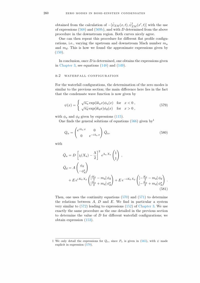
260 zero modes in bose-einstein condensates
obtained from the calculation of −[ψZM (x, t), ψ†ZM (x′, t)] with the useof expressions (568) and (569b), and with D determined from the aboveprocedure in the downstream region. Both curves nicely agree.
One can then repeat this procedure for different flat profile configu-rations, i.e., varying the upstream and downstream Mach number mu
and md. This is how we found the approximate expressions given by(150).
In conclusion, onceD is determined, one obtains the expressions givenin Chapter 3, see equations (148) and (149).
b.2 waterfall configuration
For the waterfall configurations, the determination of the zero modes issimilar to the previous section; the main difference here lies in the factthat the condensate wave function is now given by
ψ(x) =
√nu exp(ikux)φu(x) for x < 0 ,√nd exp(ikdx)φd(x) for x > 0 ,
(579)
with φu and φd given by expressions (115).One finds the general solutions of equations (566) given by1
Qα =
(ei kα x 0
0 e−i kα x
)Qα, (580)
with
Qu = D
[χ(Xu)− Λ
2
]2
eΛuXu
(1
1
),
Qd = A
(φd
−φ?d
)
+ E eiK0Xd
([K0
2 −md]φd
[K02 +md]φ
?d
)+ E e−iK0Xd
([−K0
2 −md]φd
[−K02 +md]φ
?d
).
(581)
Then, one uses the continuity equations (570) and (571) to determinethe relations between A, D and E. We find in particular a systemvery similar to (572) leading to expressions (152) of Chapter 3. We useexactly the same procedure as the one detailed in the previous sectionto determine the value of D for different waterfall configurations; weobtain expression (153).
1 We only detail the expressions for Qα, since Pα is given in (565), with ψ madeexplicit in expression (579).

CFOURIER TRANSFORM OF THE DENS ITYCORRELATION FUNCTION
In this appendix we detail the calculation leading to expression (178)of Chapter 3.
Let us introduce
I(ω) =1√
nundLuLd
∫ 0
−Ludx
∫ Ld
0dx′ e−i(kHx+kPx
′) g(2)(x, x′)
=1√
nu nd Lu Ld
∫ +∞
−∞dx
∫ +∞
−∞dx′e−i(kHx+kPx
′) g(2)(x, x′) Πu(x) Πd(x),
(582)
where kH(ω) and kP(ω) are the momenta relative to the condensate ofthe Hawking quantum and of its partner at a frequency ω, and where
Πu(x) = Θ(x+Lu)−Θ(x), and Πd(x) = Θ(x)−Θ(x−Ld). (583)
In the previous expression Θ is the Heaviside function. By expandingthe g(2) function with the use of expressions (170), (163), (164) and(166), it is not difficult to show that
I(kH, kP) =
∫dω′
2πA(ω′)Πu[kH(ω)−qu|out(ω
′)] Πd[kP(ω)+qd2|out(ω′)],
(584)
with
A(ω) =1√Lu Ld
(UkH+ VkH
) (UkP+ VkP
) Sud2(ω)S∗d2d2(ω). (585)
In expression (584), qα|out(ω′), α ∈ u, d, are the wave vectors as-
sociated to the u|out and d2|out modes, calculated from the disper-sion relation, see in particular Figure 20. Note that, with this notation,kH = qu|out(ω) < 0 and kP = −qd2|out(ω) < 0.
In equation (585), UkH≡ Uu|out (VkH
≡ Vu|out) and UkP≡ Ud2|out
(VkP≡ Vd2|out), where Uα|out and Vα|out are defined in equation (138).
The Fourier transforms of Πα are
Πα(q) = Lα ei q Lα/2 sinc(q Lα/2). (586)
In the following, we consider the case where Lu, Ld → +∞; in this limitthe windows Πα are well peaked around zero. This means that the onlysignificant contribution in the integral arises when ω′ ' ω. In this case,one has
qu|out(ω
′) ' qu|out(ω) + q′u|out(ω) (ω′ − ω),
qd2|out(ω′) = qd2|out(ω) + q′d2|out(ω) (ω′ − ω),
(587)
261

262 fourier transform of the density correlation function
where q′α|out =dqα|out
dω . Expressions (587) can be rewritten in the form
qu|out(ω′)− qu|out(ω) ' ω′ − ω
Vg(kH),
qd2|out(ω′)− qd2|out(ω) ' ω′ − ω
Vg(kP),
(588)
where we noticed that q′u|out(ω) = 1/Vg(kH) and q′d2|out(ω) = 1/Vg(kP).Then, we make the following change of variable in (584):
s = |Vg(kH)| [kH − qu|out(ω′)]. (589)
Using relations (588), we see immediately that
s = Vg(kP)[kP + qd2|out(ω′)]. (590)
Integral (584) becomes
I(ω) = A(ω)
∫ds
2πΠu
(s
|Vg(kH)|
)Πd
(s
Vg(kP)
). (591)
With a new change of variable
I(ω) = A(ω)|Vg(kH)|Ld
π
∫dt sinc(t) sinc
(tLd |Vg(kH)|Lu Vg(kP)
)
× exp
[i
(Ld |Vg(kH)|Lu Vg(kP)
− 1
)t
].
(592)
The previous integral can be rewritten
I(ω) = A(ω)√Lu Ld
√|Vg(kH)|Vg(kP) d(ω), (593)
with
d(ω) =
√a(ω)
π
∫dt sinc(t) sinc [a(ω) t] ei [a(ω)−1] t, (594)
and
a(ω) =Ld |Vg(kH)|Lu Vg(kP)
. (595)
The explicit computation of integral (594) gives
d(ω) =
√a(ω), if a(ω) ≤ 1
1√a(ω)
, if a(ω) ≥ 1.(596)
One can recast expression (593) in the form
I(ω) = S0 d(ω)Sud2(ω)S∗d2d2(ω) = S0 d(ω) 〈cU(ω) cD2(ω)〉, (597)
where S0 =√∣∣Vu|out
∣∣ Vd2|out (UkH+ VkH
) (UkP+ VkP
).
Note that ukH,kP=√∣∣Vα|out
∣∣UkH,kPand vkH,kP
=√∣∣Vα|out
∣∣VkH,kP
(α = u if k = kH, α = d2 if k = kP), where the uk’s and the vk’s arethe standard Bogoliubov amplitudes of excitations of momentum k (see,e.g., Refs. [148, 153]).The final expression (597) is exactly the same as equation (178) of
Chapter 3.

DHODOGRAPH TRANSFORM
The goal of this appendix is to prove expressions (397) of Chapter 6.We start from the partial differential equations
∂tλ± + v±(λ+, λ−) ∂xλ
± = 0, (598)
and we consider x and t as functions of the Riemann invariants λ+ andλ−:
x = x(λ+, λ−), t = t(λ+, λ−). (599)
Let us now introduce an unknown function Φ(x, t) = Φ[x(λ+, λ−), t(λ+, λ−)].By differentiating with respect to λ+ and λ−, we obtain the system:
Φx xλ+ + Φt tλ+ = Φλ+ ,
Φx xλ− + Φt tλ− = Φλ− ,(600)
where we used the shortcut notations Φx = ∂Φ/∂x, xλ+ = ∂x/∂λ+, ...The solutions of the set of equations (600) are given by
Φx = D−1 (Φλ+ tλ− − Φλ− tλ+),
Φt = D−1 (Φλ− xλ+ − Φλ+ xλ−),(601)
with D = xλ+ tλ− − xλ− tλ+ . Then, taking Φ = λ+ or Φ = λ− leads to
λ+x = D−1 tλ− , λ+
t = −D−1 xλ− ,
λ−x = −D−1 tλ+ , λ−t = D−1 xλ+ ,(602)
Inserting the previous expressions in equations (598) yields immediatelythe set of linear equations (397).
263


ESOLUTIONS OF THE EULER -PO ISSON EQUATION
We consider the Euler-Poisson equation
∂2W
∂λ3∂λ4− 1
2(λ3 − λ4)
(∂W
∂λ3− ∂W
∂λ4
)= 0. (603)
A general solution of equation (603) has been found by Eisenhart in1918 [53] in the form
W (λ3, λ4) =
∫ λ3
c0
ψ(µ) dµ√λ3 − µ
√λ4 − µ
+
∫ λ4
c0
ϕ(µ) dµ√|λ3 − µ|
√λ4 − µ
, (604)
where c0 is a constant and plays the role of the sound velocity in ourcase.
In this appendix, we detail the calculations to obtain the explicitexpressions of ψ and ϕ in both regions A and B [see Section 7.2.2, fromequation (526) to equation (530)].
region a We seek for a solution of (603) in the form
WA(λ3, λ4) =
∫ λ3
c0
ψA(µ) dµ√λ3 − µ
√λ4 − µ
+
∫ λ4
c0
ϕA(µ) dµ√|λ3 − µ|
√λ4 − µ
. (605)
we know two boundary conditions for WA, given by (524a) and (525):
WA(c0, λS) =1
2√λS − c0
∫ λS
c0
w(3)+ (r,−c0)√r − c0
dr, (606a)
WA(λ3 = λH, λ4 = λH) does not diverge. (606b)
Taking the limit λ3 → c0 in equation (605) and using expression (606a),yields
∫ λ4
c0
ϕA(µ) dµ√µ− c0
√λ4 − µ
=1
2√λS − c0
∫ λS
c0
w(3)+ (r,−c0)√r − c0
dr. (607)
The inverse Abel transformation amounts to perform the following trans-formation: given two functions φ and w such that
∫ λ φ(µ)√λ− µ dµ = w(r), (608)
one obtains after transformation [1, 14]
φ(µ) =1
π
ddµ
∫ µ w(r)√µ− r dr. (609)
265

266 solutions of the euler-poisson equation
Therefore, using this transformation in the case of expression (607) leadsto
ϕA(µ)√µ− c0
=1
2π
ddµ
∫ µ
c0
dr√µ− r√r − c0
∫ r
c0
w(3)+ (x,−c0)√x− c0
dx. (610)
Inverting both integrals gives
ϕA(µ)√µ− c0
=1
2π
ddµ
∫ µ
c0
dxw
(3)+ (x,−c0)√x− c0
∫ µ
x
dr√µ− r√r − c0
. (611)
Then, we compute the second integral over r:∫ µ
x
dr√µ− r√r − c0
= 2 arctan
(√x− µc0 − x
), (612)
and thus,
ϕA(µ) dµ√µ− c0
=1
π
ddµ
∫ µ
c0
dxw
(3)+ (x,−c0)√x− c0
arctan
(√µ− xx− c0
). (613)
The last step consists of taking the derivative with respect to µ to obtainexactly equation (526):
ϕA(µ) =1
2π√µ− c0
∫ µ
c0
w(3)+ (r,−c0) dr√
µ− r . (614)
Then, we use the second boundary condition (606b) when λ3 → λ4 ≡ λH.We introduce a small parameter ε such that
λ3 = λH − ε, λ4 = λH. (615)
In this case, equation (605) can be written as
WA(λH − ε, λH) =
∫ λH−ε
c0
dµψA(µ) + ϕA(µ)√λH − ε− µ
√λH − µ
+
∫ ε
0
ϕA(λH + µ− ε) dµ√µ(ε− µ)
.
(616)
When ε→ 0, the second integral of equation (616) converges to πϕA(λH).However, if ψA+ϕA 6= 0, the first integral clearly diverges. Consequently,WA converges when λ3 → λ4 = λH if and only if
ψA(µ) = −ϕA(µ), (617)
and, in this case,
WA(λH, λH) = πϕA(λH). (618)
This value exactly coincides with the first term of expression (537). Theexplicit expression of ϕA given by (614), as well as condition (617), leadto the solution of the Euler-Poisson equation (603) in region A [seeequation (528)]

solutions of the euler-poisson equation 267
region b In this region, we seek for a solution of (603) in the form
WB(λ3, λ4) = WA(λ3, λ4) +
∫ cm
λ4
ϕB(µ) dµ√µ− λ3
√µ− λ4
. (619)
This expression ensures the continuity betweenWA andWB, when λ4 →cm [see condition (519)]. The boundary condition in region B reads
WB(c0, λS) =− 1
2√λS − c0
∫ cm
λS
w(2)+ (r,−c0)√r − c0
dr
+1
2√λS − c0
∫ cm
c0
w(3)+ (r,−c0)√r − c0
dr .
(620)
Inserting expressions (606a) and (620) in equation (627) yields∫ cm
λS
ϕB(µ) dµ√µ− c0
√µ− λS
=
∫ cm
λS
wdiff+ (r) dr√r − c0
, (621)
with wdiff+ (r) = w
(3)+ (r,−c0)−w(2)
+ (r,−c0). Similarly to region A, we canperform an inverse Abel transform to obtain in this case
ϕB(µ)√µ− c0
= − 1
π
ddµ
∫ cm
µdx
wdiff+ (x)√x− c0
arcsinh(√
x− µµ− c0
). (622)
Taking the derivative with respect to µ leads immediately to the result(530):
ϕB(µ) =1
2π√µ− c0
∫ cm
µ
w(3)+ (r,−c0)− w(2)
+ (r,−c0)√r − µ dr . (623)
complete elliptic integrals The solutions of the Euler-Poisson equation WA and WB can be expressed in terms of a singleintegral by means of the complete elliptic integrals of the first kind1.Indeed,
WA(λ3, λ4) =1
2π
∫ λ4
λ3
dµ∫ µ
c0
w(3)+ (r,−c0) dr√
µ− λ3√λ4 − µ
√µ− c0
√µ− r
=1
2π
∫ λ3
c0
dr∫ λ4
λ3
w(3)+ (r,−c0) dµ√
µ− λ3√λ4 − µ
√µ− c0
√µ− r
+1
2π
∫ λ4
λ3
dr∫ λ4
r
w(3)+ (r,−c0) dµ√
µ− λ3√λ4 − µ
√µ− c0
√µ− r ,
(624)
where we have inserted expression (614) in equation (528) and haveinverted both integrals. Both integrals over µ on the right-hand sideof equation (624) are complete elliptic integrals of the first kind [77].Therefore,
WA(λ3, λ4) =1
π
∫ λ3
c0
w(3)+ (r,−c0) fA(λ3, r) dr
+1
π
∫ λ4
λ3
w(3)+ (r,−c0) fA(r, λ3) dr,
(625)
1 The formulae below are easier to compute numerically.

268 solutions of the euler-poisson equation
with
fA(x1, x2) =K [mA(x1, x2)]√x1 − c0
√λ4 − x2
,
mA(x1, x2) =(λ4 − x1) (x2 − c0)
(λ4 − x2) (x1 − c0),
(626)
K(mA) being a complete elliptic integral of the first kind. The sameprocedure gives in region B:
WB(λ3, λ4) = WA(λ3, λ4) +1
π
∫ cm
λ4
wdiff+ (r) fB(r) dr, (627)
with
fB(r) =1√
r − λ3
√λ4 − c0
K[
(λ3 − c0) (r − λ4)
(λ4 − c0) (r − λ3)
]. (628)

BIBL IOGRAPHY
[1] N.H. Abel. “Auflösung Einer Mechanischen Aufgabe.” In: Jour-nal für die reine und angewandte Mathematik (Crelles Journal)1826 (1826), pp. 153–157. doi: 10.1515/crll.1826.1.153.
[2] M. Abramowitz and I. A. Stegun. Handbook of MethematicalFunctions. New-York: Dover Publications, 1970.
[3] Gerardo Adesso and Fabrizio Illuminati. “Gaussian Measures ofEntanglement versus Negativities: Ordering of Two-Mode Gaus-sian States.” In: Physical Review A 72 (2005), p. 032334. doi:10.1103/PhysRevA.72.032334.
[4] Gerardo Adesso and Fabrizio Illuminati. “Continuous VariableTangle, Monogamy Inequality, and Entanglement Sharing in Gaus-sian States of Continuous Variable Systems.” In: New Journal ofPhysics 8 (2006), pp. 15–15. doi: 10.1088/1367-2630/8/1/015.
[5] Gerardo Adesso, Alessio Serafini, and Fabrizio Illuminati. “Ex-tremal Entanglement and Mixedness in Continuous Variable Sys-tems.” In: Physical Review A 70 (2004), p. 022318. doi: 10.1103/PhysRevA.70.022318.
[6] Gerardo Adesso, Alessio Serafini, and Fabrizio Illuminati. “Quan-tification and Scaling of Multipartite Entanglement in Continu-ous Variable Systems.” In: Physical Review Letters 93 (2004),p. 220504. doi: 10.1103/PhysRevLett.93.220504.
[7] G. Agrawal. Nonlinear Fiber Optics. Elsevier, 2013. doi: 10 .
1016/C2011-0-00045-5.
[8] S. A. Akhmanov, A. P. Sukhorukov, and R. V. Khokhlov. “Self-Focusing and Self-Trapping of Intense Light Beams in a Nonlin-ear Medium.” In: Sov. Phys. JETP 23 (1966), p. 1025.
[9] S. A. Akhmanov, A. P. Sukhorukov, and R. V. Khokhlov. “Self-Focusing and Self-Trapping of Intense Light Beams in a Nonlin-ear Medium.” In: Zh. Eksp. Teor. Fiz 50 (1966), p. 1537.
[10] S. A. Akhmanov, A. P. Sukhorukov, and R. V. Khokhlov. “Self-Focusing and Diffraction of Light in a Nonlinear Medium.” In:Usp. Fiz. Nauk 93 (1967), p. 19.
[11] S. A. Akhmanov, A. P. Sukhorukov, and R. V. Khokhlov. “Self-Focusing and Diffraction of Light in a Nonlinear Medium.” In:Sov. Phys. Usp. 10 (1968), p. 609.
[12] Ahmed Almheiri, Donald Marolf, Joseph Polchinski, and JamesSully. “Black Holes: Complementarity or Firewalls?” In: Jour-nal of High Energy Physics 2013 (2013), p. 62. doi: 10.1007/JHEP02(2013)062.
269

270 Bibliography
[13] M. R. Andrews, D. M. Kurn, H.-J. Miesner, D. S. Durfee, C. G.Townsend, S. Inouye, and W. Ketterle. “Propagation of Soundin a Bose-Einstein Condensate.” In: Physical Review Letters 79(1997), pp. 553–556. doi: 10.1103/PhysRevLett.79.553.
[14] G. Arfken and H. J. Weber.Mathematical Methods for Physicists.Orlando: Academic Press, 2005.
[15] Roberto Balbinot, Alessandro Fabbri, Serena Fagnocchi, AlessioRecati, and Iacopo Carusotto. “Nonlocal Density Correlations asa Signature of Hawking Radiation from Acoustic Black Holes.”In: Physical Review A 78 (2008), p. 021603. doi: 10 . 1103 /
PhysRevA.78.021603.[16] R. Balian and E. Brezin. “Nonunitary Bogoliubov Transforma-
tions and Extension of Wick’s Theorem.” In: Il Nuovo CimentoB Series 10 64 (1969), pp. 37–55. doi: 10.1007/BF02710281.
[17] Luca Barbiero, Christian Schweizer, Monika Aidelsburger, Eu-gene Demler, Nathan Goldman, and Fabian Grusdt. “CouplingUltracold Matter to Dynamical Gauge Fields in Optical Lattices:From Flux Attachment to Z 2 Lattice Gauge Theories.” In: Sci-ence Advances 5 (2019). doi: 10.1126/sciadv.aav7444.
[18] Carlos Barceló, S. Liberati, and Matt Visser. “Probing Semiclas-sical Analog Gravity in Bose-Einstein Condensates with WidelyTunable Interactions.” In: Physical Review A 68 (2003), p. 053613.doi: 10.1103/PhysRevA.68.053613.
[19] Carlos Barceló, Stefano Liberati, and Matt Visser. “Towardsthe Observation of Hawking Radiation in Bose–Einstein Conden-sates.” In: International Journal of Modern Physics A 18 (2003),pp. 3735–3745. doi: 10.1142/S0217751X0301615X.
[20] Carlos Barceló, Stefano Liberati, and Matt Visser. “AnalogueGravity.” In: Living Reviews in Relativity 8 (2005), p. 12. doi:10.12942/lrr-2005-12.
[21] Carlos Barceló, Stefano Liberati, and Matt Visser. “AnalogueGravity.” In: Living Reviews in Relativity 14 (2011), p. 3. doi:10.12942/lrr-2011-3.
[22] Christopher Barsi, Wenjie Wan, Can Sun, and Jason W. Fleis-cher. “Dispersive Shock Waves with Nonlocal Nonlinearity.” In:Optics Letters 32 (2007), p. 2930. doi: 10.1364/OL.32.002930.
[23] F. Belgiorno, S. L. Cacciatori, M. Clerici, V. Gorini, G. Ortenzi,L. Rizzi, E. Rubino, V. G. Sala, and D. Faccio. “Hawking Radia-tion from Ultrashort Laser Pulse Filaments.” In: Physical ReviewLetters 105 (2010), p. 203901. doi: 10.1103/PhysRevLett.105.203901.
[24] Nicolas Bilas and Nicolas Pavloff. “Dark Soliton Past a Finite-Size Obstacle.” In: Physical Review A 72 (2005), p. 033618. doi:10.1103/PhysRevA.72.033618.
[25] N. D. Birrell and P. C. W. Davies. Quantum Fields in CurvedSpace. Cambridge University Press, 1982. doi: 10.1017/CBO9780511622632.

Bibliography 271
[26] Jean-Paul Blaizot and Georges Ripka. Quantum Theory of FiniteSystems. Cambridge, Mass: MIT Press, 1986.
[27] H. M. J. M. Boesten, C. C. Tsai, J. R. Gardner, D. J. Heinzen,and B. J. Verhaar. “Observation of a Shape Resonance in theCollision of Two Cold Rb 87 Atoms.” In: Physical Review A 55(1997), pp. 636–640. doi: 10.1103/PhysRevA.55.636.
[28] N.N. Bogoliubov. “On the Theory of Superfluidity.” In: Jour-nal of Physics (Union of Soviet Socialist Republics) 11 (1947),pp. 23–32.
[29] T. Bonnemain. “Quadratic Mean Field Games with NegativeCoordination.” PhD thesis. Université Cergy-Pointoise, 2020.
[30] T. Bonnemain, T. Gobron, and D. Ullmo. “Universal Behavior inNon Stationary Mean Field Games.” In: arXiv:1907.05374 [cond-mat, physics:physics] (2019). arXiv: 1907.05374 [cond-mat, physics:physics].
[31] R. Boyd. Nonlinear Optics. Academic Press, 2008.
[32] Xavier Busch and Renaud Parentani. “Dynamical Casimir Effectin Dissipative Media: When Is the Final State Nonseparable?” In:Physical Review D 88 (2013), p. 045023. doi: 10.1103/PhysRevD.88.045023.
[33] Xavier Busch, Renaud Parentani, and Scott Robertson. “Quan-tum Entanglement Due to a Modulated Dynamical Casimir Ef-fect.” In: Physical Review A 89 (2014), p. 063606. doi: 10.1103/PhysRevA.89.063606.
[34] Iacopo Carusotto. “Superfluid Light in Bulk Nonlinear Media.”In: Proceedings of the Royal Society A: Mathematical, Physicaland Engineering Sciences 470 (2014), p. 20140320. doi: 10.1098/rspa.2014.0320.
[35] Iacopo Carusotto and Cristiano Ciuti. “Quantum Fluids of Light.”In: Reviews of Modern Physics 85 (2013), pp. 299–366. doi: 10.1103/RevModPhys.85.299.
[36] Iacopo Carusotto, Serena Fagnocchi, Alessio Recati, RobertoBalbinot, and Alessandro Fabbri. “Numerical Observation of Hawk-ing Radiation from Acoustic Black Holes in Atomic Bose–EinsteinCondensates.” In: New Journal of Physics 10 (2008), p. 103001.doi: 10.1088/1367-2630/10/10/103001.
[37] Yvan Castin. Mécanique Quantique : Seconde Quantification etRésolvante; Master 2ème Année : Concepts Fondamentaux de LaPhysique. 2011.
[38] Pisin Chen and Gerard Mourou. “Accelerating Plasma Mirrorsto Investigate the Black Hole Information Loss Paradox.” In:Physical Review Letters 118 (2017), p. 045001. doi: 10.1103/PhysRevLett.118.045001.
[39] R. Y. Chiao. “Bogoliubov Dispersion Relation for a Photon Fluid:Is This a Superfluid?” In: Optics Communications 179 (2000),p. 157.

272 Bibliography
[40] Valerie Coffman, Joydip Kundu, and William K. Wootters. “Dis-tributed Entanglement.” In: Physical Review A 61 (2000), p. 052306.doi: 10.1103/PhysRevA.61.052306.
[41] Steven Corley. “Particle Creation via High Frequency Disper-sion.” In: Physical Review D 55 (1997), pp. 6155–6161. doi: 10.1103/PhysRevD.55.6155.
[42] Steven Corley and Ted Jacobson. “Hawking Spectrum and HighFrequency Dispersion.” In: Physical Review D 54 (1996), pp. 1568–1586. doi: 10.1103/PhysRevD.54.1568.
[43] Gilles Couton, Hervé Maillotte, and Mathieu Chauvet. “Self-Formation of Multiple Spatial Photovoltaic Solitons.” In: Journalof Optics B: Quantum and Semiclassical Optics 6 (2004), S223–S230. doi: 10.1088/1464-4266/6/5/009.
[44] D. Daems, F. Bernard, N. J. Cerf, and M. I. Kolobov. “Tri-partite Entanglement in Parametric Down-Conversion with Spa-tially Structured Pump.” In: Journal of the Optical Society ofAmerica B 27 (2010), p. 447. doi: 10.1364/JOSAB.27.000447.
[45] Franco Dalfovo, Stefano Giorgini, Lev P. Pitaevskii, and SandroStringari. “Theory of Bose-Einstein Condensation in TrappedGases.” In: Reviews of Modern Physics 71 (1999), pp. 463–512.doi: 10.1103/RevModPhys.71.463.
[46] Jean Dalibard, Fabrice Gerbier, Gediminas Juzeliunas, and Pa-trik Öhberg. “Colloquium : Artificial Gauge Potentials for Neu-tral Atoms.” In: Reviews of Modern Physics 83 (2011), pp. 1523–1543. doi: 10.1103/RevModPhys.83.1523.
[47] P C W Davies. “Scalar Production in Schwarzschild and RindlerMetrics.” In: Journal of Physics A: Mathematical and General 8(1975), pp. 609–616. doi: 10.1088/0305-4470/8/4/022.
[48] P. C. W. Davies and S. A. Fulling. “Radiation from Moving Mir-rors and from Black Holes.” In: Proceedings of the Royal Societyof London. A. Mathematical and Physical Sciences 356 (1977),pp. 237–257. doi: 10.1098/rspa.1977.0130.
[49] Bryce S. DeWitt. “Quantum Field Theory in Curved Spacetime.”In: Physics Reports 19 (1975), pp. 295–357. doi: 10.1016/0370-1573(75)90051-4.
[50] Jonathan Drori, Yuval Rosenberg, David Bermudez, Yaron Sil-berberg, and Ulf Leonhardt. “Observation of Stimulated Hawk-ing Radiation in an Optical Analogue.” In: Physical Review Let-ters 122 (2019), p. 010404. doi: 10.1103/PhysRevLett.122.010404.
[51] Peter D. Drummond and Mark Hillery. The Quantum Theory ofNonlinear Optics. Cambridge: Cambridge University Press, 2014.doi: 10.1017/CBO9780511783616.

Bibliography 273
[52] Lu-Ming Duan, G. Giedke, J. I. Cirac, and P. Zoller. “Insepa-rability Criterion for Continuous Variable Systems.” In: Phys-ical Review Letters 84 (2000), pp. 2722–2725. doi: 10.1103/PhysRevLett.84.2722.
[53] Luther Pfahler Eisenhart. “Triply Conjugate Systems with EqualPoint Invariants.” In: The Annals of Mathematics 20 (1919),p. 262. doi: 10.2307/1967119.
[54] G. A. El. “Resolution of a Shock in Hyperbolic Systems Modifiedby Weak Dispersion.” In: Chaos: An Interdisciplinary Journalof Nonlinear Science 15 (2005), p. 037103. doi: 10.1063/1.1947120.
[55] G. A. El. “Erratum: “Resolution of a Shock in Hyperbolic Sys-tems Modified by Weak Dispersion” [Chaos 15, 037103 (2005)].”In: Chaos: An Interdisciplinary Journal of Nonlinear Science 16(2006), p. 029901. doi: 10.1063/1.2186766.
[56] G.A. El’ and V.V. Khodorovsky. “Evolution of a SolitonlessLarge-Scale Perturbation in Korteweg-de Vries Hydrodynamics.”In: Physics Letters A 182 (1993), pp. 49–52. doi: 10.1016/0375-9601(93)90051-Z.
[57] M. Elazar, V. Fleurov, and S. Bar-Ad. “All-Optical Event Hori-zon in an Optical Analog of a Laval Nozzle.” In: Physical ReviewA 86 (2012), p. 063821. doi: 10.1103/PhysRevA.86.063821.
[58] Christopher Eltschka and Jens Siewert. “Monogamy Equalitiesfor Qubit Entanglement from Lorentz Invariance.” In: PhysicalReview Letters 114 (2015), p. 140402. doi: 10.1103/PhysRevLett.114.140402.
[59] L.-P. Euvé, F. Michel, R. Parentani, T. G. Philbin, and G. Rousseaux.“Observation of Noise Correlated by the Hawking Effect in a Wa-ter Tank.” In: Physical Review Letters 117 (2016), p. 121301. doi:10.1103/PhysRevLett.117.121301.
[60] Léo-Paul Euvé, Scott Robertson, Nicolas James, Alessandro Fab-bri, and Germain Rousseaux. “Scattering of Co-Current SurfaceWaves on an Analogue Black Hole.” In: arXiv:1806.05539 [gr-qc,physics:physics] (2018). arXiv: 1806.05539 [gr-qc, physics:physics].
[61] Léo-Paul Euvé, Scott Robertson, Nicolas James, Alessandro Fab-bri, and Germain Rousseaux. “Scattering of Co-Current SurfaceWaves on an Analogue Black Hole.” In: Physical Review Letters124 (2020), p. 141101. doi: 10.1103/PhysRevLett.124.141101.
[62] Alessandro Fabbri and Nicolas Pavloff. “Momentum Correlationsas Signature of Sonic Hawking Radiation in Bose-Einstein Con-densates.” In: SciPost Physics 4 (2018), p. 019. doi: 10.21468/SciPostPhys.4.4.019.

274 Bibliography
[63] Daniele Faccio, Francesco Belgiorno, Sergio Cacciatori, Vitto-rio Gorini, Stefano Liberati, and Ugo Moschella, eds. AnalogueGravity Phenomenology. Vol. 870. Lecture Notes in Physics. Cham:Springer International Publishing, 2013. doi: 10.1007/978-3-319-00266-8.
[64] J. Fatome, C. Finot, G. Millot, A. Armaroli, and S. Trillo. “Ob-servation of Optical Undular Bores in Multiple Four-Wave Mix-ing.” In: Physical Review X 4 (2014), p. 021022. doi: 10.1103/PhysRevX.4.021022.
[65] Alexander L Fetter. “Nonuniform States of an Imperfect BoseGas.” In: Annals of Physics 70 (1972), pp. 67–101. doi: 10.1016/0003-4916(72)90330-2.
[66] Q. Fontaine, T. Bienaimé, S. Pigeon, E. Giacobino, A. Bramati,and Q. Glorieux. “Observation of the Bogoliubov Dispersion in aFluid of Light.” In: Physical Review Letters 121 (2018), p. 183604.doi: 10.1103/PhysRevLett.121.183604.
[67] M. Gregory Forest and Jong-Eao Lee. “Geometry and Modula-tion Theory for the Periodic Nonlinear Schrodinger Equation.”In: Oscillation Theory, Computation, and Methods of Compen-sated Compactness. Ed. by George R. Sell, Hans Weinberger,Constantine Dafermos, J. L. Ericksen, David Kinderlehrer, andMarshall Slemrod. Vol. 2. New York, NY: Springer New York,1986, pp. 35–69. doi: 10.1007/978-1-4613-8689-6_3.
[68] Kieran A. Fraser and Francesco Piazza. “Topological Soliton-Polaritons in 1D Systems of Light and Fermionic Matter.” In:Communications Physics 2 (2019), p. 48. doi: 10.1038/s42005-019-0149-1.
[69] S. A. Fulling and P. C. W. Davies. “Radiation from a MovingMirror in Two Dimensional Space-Time: Conformal Anomaly.”In: Proceedings of the Royal Society of London. A. Mathematicaland Physical Sciences 348 (1976), pp. 393–414. doi: 10.1098/rspa.1976.0045.
[70] Stephen A. Fulling. “Nonuniqueness of Canonical Field Quan-tization in Riemannian Space-Time.” In: Physical Review D 7(1973), pp. 2850–2862. doi: 10.1103/PhysRevD.7.2850.
[71] L. J. Garay, J. R. Anglin, J. I. Cirac, and P. Zoller. “Sonic Analogof Gravitational Black Holes in Bose-Einstein Condensates.” In:Physical Review Letters 85 (2000), pp. 4643–4647. doi: 10.1103/PhysRevLett.85.4643.
[72] C. Gardiner and P. Zoller.Quantun Noise. Berlin: Springer-Verlag,1999.
[73] F Gerbier. “Quasi-1D Bose-Einstein Condensates in the Dimen-sional Crossover Regime.” In: Europhysics Letters (EPL) 66 (2004),pp. 771–777. doi: 10.1209/epl/i2004-10035-7.
[74] Christopher Gerry and Peter Knight. Introductory Quantum Op-tics. Cambridge University Press, 2004. doi: 10.1017/CBO9780511791239.

Bibliography 275
[75] S. Gilbert. Linear Algebra and Its Applications. Stamford, CT:Cengage Learning, 2005.
[76] S. Giovanazzi, C. Farrell, T. Kiss, and U. Leonhardt. “Conditionsfor One-Dimensional Supersonic Flow of Quantum Gases.” In:Physical Review A 70 (2004), p. 063602. doi: 10.1103/PhysRevA.70.063602.
[77] I.S. Gradshteyn and I.M. Ryzhik. Table of Integrals, Series, andProducts. Elsevier, 1980. doi: 10.1016/C2013-0-10754-4.
[78] E. P. Gross. “Structure of a Quantized Vortex in Boson Systems.”In: Il Nuovo Cimento 20 (1961), pp. 454–477. doi: 10.1007/BF02731494.
[79] W. Guerin. “Source Atomique Cohérente Dans Des Pièges Op-tique et Magnétique: Réalisation d’un Laser à Atomes Guidé.”PhD thesis. Université Paris-Sud - Paris XI, 2007.
[80] A. Gullstrand. Allgemeine Lösung Des Statischen Einkörperprob-lems in Der Einsteinschen Gravitationstheorie. Vol. 16. ArkivFör Matematik, Astronomi Och Fysik. Stockholm: Almqvist &Wiksell, 1922.
[81] A.V. Gurevich, A.L. Krylov, and G.A. El. “Breaking of a Rie-mann Wave in Dispersive Hydrodynamics.” In: Pis’ma Zh. Exp.Teor. Fiz. 54 (1991), p. 104.
[82] A.V. Gurevich, A.L. Krylov, and G.A. El. “Evolution of a Rie-mann Wave in Dispersive Hydrodynamics.” In: Zh. Eksp. Teor.Fiz 101 (1992), p. 1797.
[83] A.V. Gurevich, A.L. Krylov, and N.G. Mazur. “Quasi-SimpleWaves in Korteweg-De Vries Hydrdynamics.” In: Zh. Eksp. Teor.Fiz 95 (1989), p. 1674.
[84] A.V. Gurevich and L. Pitaevskii. “Nonstationary Structure ofa Collisionless Shock Wave.” In: Zh. Eksp. Teor. Fiz 65 (1973),p. 590.
[85] Sasha Haco, Stephen W. Hawking, Malcolm J. Perry, and An-drew Strominger. “Black Hole Entropy and Soft Hair.” In: Jour-nal of High Energy Physics 2018 (2018), p. 98. doi: 10.1007/JHEP12(2018)098.
[86] D. S. Hall, M. R. Matthews, J. R. Ensher, C. E. Wieman, andE. A. Cornell. “Dynamics of Component Separation in a BinaryMixture of Bose-Einstein Condensates.” In: Physical Review Let-ters 81 (1998), pp. 1539–1542. doi: 10.1103/PhysRevLett.81.1539.
[87] S. W. Hawking. “Black Hole Explosions?” In: Nature 248 (1974),p. 30. doi: 10.1038/248030a0.
[88] S. W. Hawking. “Particle Creation by Black Holes.” In: Com-munications In Mathematical Physics 43 (1975), p. 199. doi:10.1007/BF02345020.
276 Bibliography
[89] S. W. Hawking. “Loss of Information in Black Holes.” In: TheGeometric Universe. Oxford University Press, 1998, p. 125.
[90] S. W. Hawking and G. F. R. Ellis. The Large Scale Structure ofSpace-Time. Cambridge University Press, 1973. doi: 10.1017/CBO9780511524646.
[91] M. A. Hoefer, M. J. Ablowitz, I. Coddington, E. A. Cornell, P.Engels, and V. Schweikhard. “Dispersive and Classical ShockWaves in Bose-Einstein Condensates and Gas Dynamics.” In:Physical Review A 74 (2006), p. 023623. doi: 10.1103/PhysRevA.74.023623.
[92] P. C. Hohenberg. “Existence of Long-Range Order in One andTwo Dimensions.” In: Physical Review 158 (1967), pp. 383–386.doi: 10.1103/PhysRev.158.383.
[93] M. Isoard, A. M. Kamchatnov, and N. Pavloff. “Long-Time Evo-lution of Pulses in the Korteweg–de Vries Equation in the Ab-sence of Solitons Reexamined: Whitham Method.” In: PhysicalReview E 99 (2019), p. 012210. doi: 10.1103/PhysRevE.99.012210.
[94] S. K. Ivanov and A. M. Kamchatnov. “Collision of RarefactionWaves in Bose-Einstein Condensates.” In: Physical Review A 99(2019), p. 013609. doi: 10.1103/PhysRevA.99.013609.
[95] A. D. Jackson, G. M. Kavoulakis, and C. J. Pethick. “SolitaryWaves in Clouds of Bose-Einstein Condensed Atoms.” In: Physi-cal Review A 58 (1998), pp. 2417–2422. doi: 10.1103/PhysRevA.58.2417.
[96] Ted Jacobson. Introductory Lectures on Black Hole Thermody-namics. 1996.
[97] Maxime J. Jacquet. Negative Frequency at the Horizon. SpringerTheses. Cham: Springer International Publishing, 2018. doi: 10.1007/978-3-319-91071-0.
[98] Maxime J. Jacquet and Friedrich Koenig. “The Influence of Space-time Curvature on Quantum Emission in Optical Analogues toGravity.” In: arXiv:2001.05807 [cond-mat, physics:gr-qc, physics:quant-ph] (2020). arXiv: 2001.05807 [cond-mat, physics:gr-qc, physics:quant-ph].
[99] A. M. Kamchatnov. “Propagation of Ultrashort Periodic Pulsesin Nonlinear Fiber Light Guides.” In: Zh. Eksp. Teor. Fiz 97(1990), p. 144.
[100] A. M. Kamchatnov. Nonlinear Periodic Waves and Their Mod-ulations: An Introductory Course. World Scientific, 2000.
[101] A. Kamchatnov and V. Shchesnovich. “Dynamics of Bose-EinsteinCondensates in Cigar-Shaped Traps.” In: Physical Review A 70(2004), p. 023604. doi: 10.1103/PhysRevA.70.023604.

Bibliography 277
[102] Victor I. Kolobov, Katrine Golubkov, Juan Ramón Muñoz deNova, and Jeff Steinhauer. “Spontaneous Hawking Radiation andbeyond: Observing the Time Evolution of an Analogue BlackHole.” In: arXiv:1910.09363 [gr-qc] (2019). arXiv: 1910.09363[gr-qc].
[103] V.R. Kudashev. “Conservation of Number of Waves and Inheri-tance of Simmetries under Whitham Averaging.” In: Pis’ma Zh.Exp. Teor. Fiz. 54 (1991), p. 179.
[104] Yasunari Kurita and Takao Morinari. “Formation of a Sonic Hori-zon in Isotropically Expanding Bose-Einstein Condensates.” In:Physical Review A 76 (2007), p. 053603. doi: 10.1103/PhysRevA.76.053603.
[105] Oren Lahav, Amir Itah, Alex Blumkin, Carmit Gordon, Sha-har Rinott, Alona Zayats, and Jeff Steinhauer. “Realization ofa Sonic Black Hole Analog in a Bose-Einstein Condensate.” In:Physical Review Letters 105 (2010), p. 240401. doi: 10.1103/PhysRevLett.105.240401.
[106] L. D. Landau and E. M. Lifshitz.Mécanique Quantique — ThéorieNon-Relativiste. Vol. 3. Union soviétique, 1967.
[107] L. D. Landau and E. M. Lifshitz. Fluids Mechanics. Oxford: Perg-amon, 1987.
[108] L. D. Landau, E. M. Lifshitz, and L. P. Pitaevskii. Electrodynam-ics of Continuous Media. Vol. 8. Landau and Lifshitz Course ofTheoretical Physics. Elsevier Butterworth-Heinemann, Oxford,2006.
[109] P.-É. Larré. “Fluctuations Quantiques et Effets Non-LinéairesDans Les Condensats de Bose-Einstein. Des Ondes de Choc Dis-persives Au Rayonnement de Hawking Acoustique.” PhD thesis.Université Paris-Sud, 2013.
[110] P.-É. Larré, A. Recati, I. Carusotto, and N. Pavloff. “QuantumFluctuations around Black Hole Horizons in Bose-Einstein Con-densates.” In: Physical Review A 85 (2012), p. 013621. doi: 10.1103/PhysRevA.85.013621.
[111] Pierre-Élie Larré and Iacopo Carusotto. “Optomechanical Sig-nature of a Frictionless Flow of Superfluid Light.” In: PhysicalReview A 91 (2015), p. 053809. doi: 10.1103/PhysRevA.91.053809.
[112] P.D. Lax. “Development of Singularities of Solutions of NonlinearHyperbolic Partial Differential Equations.” In: J. Math. Phys. 5(1964), pp. 611–613.
[113] P. Leboeuf and N. Pavloff. “Bose-Einstein Beams: Coherent Prop-agation through a Guide.” In: Physical Review A 64 (2001),p. 033602. doi: 10.1103/PhysRevA.64.033602.
[114] P. Leboeuf, N. Pavloff, and S. Sinha. “Solitonic Transmission ofBose-Einstein Matter Waves.” In: Physical Review A 68 (2003),p. 063608. doi: 10.1103/PhysRevA.68.063608.

278 Bibliography
[115] U. Leonhardt, T. Kiss, and P. Öhberg. “Theory of ElementaryExcitations in Unstable Bose-Einstein Condensates and the In-stability of Sonic Horizons.” In: Physical Review A 67 (2003),p. 033602. doi: 10.1103/PhysRevA.67.033602.
[116] U Leonhardt, T Kiss, and P hberg. “Bogoliubov Theory of theHawking Effect in Bose Einstein Condensates.” In: Journal ofOptics B: Quantum and Semiclassical Optics 5 (2003), S42–S49.doi: 10.1088/1464-4266/5/2/357.
[117] U. Leonhardt and T. G. Philbin. Geometry and Light: The Sci-ence of Invisibility. New-York: Dover Publications, 2010.
[118] M. Lewenstein and L. You. “Quantum Phase Diffusion of a Bose-Einstein Condensate.” In: Physical Review Letters 77 (1996),pp. 3489–3493. doi: 10.1103/PhysRevLett.77.3489.
[119] Stefano Liberati, Giovanni Tricella, and Andrea Trombettoni.“The Information Loss Problem: An Analogue Gravity Perspec-tive.” In: Entropy 21 (2019), p. 940. doi: 10.3390/e21100940.
[120] Geoffrey S. S. Ludford. “On an Extension of Riemann’s Methodof Integration, with Applications to One-Dimensional Gas Dy-namics.” In: Mathematical Proceedings of the Cambridge Philo-sophical Society 48 (1952), pp. 499–510. doi: 10.1017/S0305004100027900.
[121] M. D. Lukin. “Colloquium : Trapping and Manipulating PhotonStates in Atomic Ensembles.” In: Reviews of Modern Physics 75(2003), pp. 457–472. doi: 10.1103/RevModPhys.75.457.
[122] Dieter Lüst and Ward Vleeshouwers. Black Hole Informationand Thermodynamics. SpringerBriefs in Physics. Cham: SpringerInternational Publishing, 2019. doi: 10 . 1007 / 978 - 3 - 030 -
10919-6.
[123] Xin Ma and William Rhodes. “Multimode Squeeze Operatorsand Squeezed States.” In: Physical Review A 41 (1990), pp. 4625–4631. doi: 10.1103/PhysRevA.41.4625.
[124] Jean Macher and Renaud Parentani. “Black-Hole Radiation inBose-Einstein Condensates.” In: Physical Review A 80 (2009),p. 043601. doi: 10.1103/PhysRevA.80.043601.
[125] Juan Maldacena. “The Large-N Limit of Superconformal FieldTheories and Supergravity.” In: International Journal of The-oretical Physics 38 (1999), pp. 1113–1133. doi: 10 . 1023 / A :
1026654312961.
[126] Samir D Mathur. “The Information Paradox: A Pedagogical In-troduction.” In: Classical and Quantum Gravity 26 (2009), p. 224001.doi: 10.1088/0264-9381/26/22/224001.
[127] N. D. Mermin and H. Wagner. “Absence of Ferromagnetismor Antiferromagnetism in One- or Two-Dimensional IsotropicHeisenberg Models.” In: Physical Review Letters 17 (1966), pp. 1133–1136. doi: 10.1103/PhysRevLett.17.1133.
Bibliography 279
[128] Claire Michel, Omar Boughdad, Mathias Albert, Pierre-Élie Larré,and Matthieu Bellec. “Superfluid Motion and Drag-Force Cancel-lation in a Fluid of Light.” In: Nature Communications 9 (2018),p. 2108. doi: 10.1038/s41467-018-04534-9.
[129] C. W. Misner, K. S. Thorne, and J. A. Wheeler. Gravitation. W.H. Freeman, Princeton University Press, 1973.
[130] Christophe Mora and Yvan Castin. “Extension of BogoliubovTheory to Quasicondensates.” In: Physical Review A 67 (2003),p. 053615. doi: 10.1103/PhysRevA.67.053615.
[131] Juan RamónMuñoz de Nova, Katrine Golubkov, Victor I. Kolobov,and Jeff Steinhauer. “Observation of Thermal Hawking Radia-tion and Its Temperature in an Analogue Black Hole.” In: Nature569 (2019), pp. 688–691. doi: 10.1038/s41586-019-1241-0.
[132] H. S. Nguyen, D. Gerace, I. Carusotto, D. Sanvitto, E. Galopin,A. Lemaître, I. Sagnes, J. Bloch, and A. Amo. “Acoustic BlackHole in a Stationary Hydrodynamic Flow of Microcavity Polari-tons.” In: Physical Review Letters 114 (2015), p. 036402. doi:10.1103/PhysRevLett.114.036402.
[133] E. Noether. “Invariante Variationsprobleme.” In: Nachr. König.Gesellsch. Wiss. Göttingen, Math.-Phys. Klasse (1918), pp. 235–237.
[134] J R M de Nova, F Sols, and I Zapata. “Entanglement and Viola-tion of Classical Inequalities in the Hawking Radiation of Flow-ing Atom Condensates.” In: New Journal of Physics 17 (2015),p. 105003. doi: 10.1088/1367-2630/17/10/105003.
[135] M. Olshanii. “Atomic Scattering in the Presence of an ExternalConfinement and a Gas of Impenetrable Bosons.” In: PhysicalReview Letters 81 (1998), pp. 938–941. doi: 10.1103/PhysRevLett.81.938.
[136] Miguel Onorato, Stefania Resitori, and Fabio Baronio, eds. Rogueand Shock Waves in Nonlinear Dispersive Media. Vol. 926. Lec-ture Notes in Physics. Cham: Springer International Publishing,2016. doi: 10.1007/978-3-319-39214-1.
[137] J. R. Oppenheimer and G. M. Volkoff. “On Massive NeutronCores.” In: Physical Review 55 (1939), pp. 374–381. doi: 10.1103/PhysRev.55.374.
[138] Tomoki Ozawa et al. “Topological Photonics.” In: Reviews ofModern Physics 91 (2019), p. 015006. doi: 10.1103/RevModPhys.91.015006.
[139] Don N. Page. “Particle Emission Rates from a Black Hole: Mass-less Particles from an Uncharged, Nonrotating Hole.” In: Phys-ical Review D 13 (1976), pp. 198–206. doi: 10.1103/PhysRevD.13.198.
[140] P. Painlevé. “La Mécanique Classique et La Théorie de La Rel-ativité.” In: Les Comptes Rendus de l’Académie des Sciences deParis 173 (1921), p. 677.

280 Bibliography
[141] Leonard Parker. “Probability Distribution of Particles Createdby a Black Hole.” In: Physical Review D 12 (1975), pp. 1519–1525. doi: 10.1103/PhysRevD.12.1519.
[142] Leonard Parker. “The Production of Elementary Particles byStrong Gravitational Fields.” In: Asymptotic Structure of Space-Time. Ed. by F. Paul Esposito and Louis Witten. Boston, MA:Springer US, 1977, pp. 107–226. doi: 10.1007/978-1-4684-2343-3_2.
[143] M. V. Pavlov. “Nonlinear Schrodinger Equation and the Bogolyubov-Whitham Method of Averaging.” In: Theoretical and Mathemat-ical Physics 71 (1987), pp. 584–588. doi: 10.1007/BF01017090.
[144] O. Penrose. “CXXXVI. On the Quantum Mechanics of HeliumII.” In: The London, Edinburgh, and Dublin Philosophical Mag-azine and Journal of Science 42 (1951), pp. 1373–1377. doi:10.1080/14786445108560954.
[145] Oliver Penrose and Lars Onsager. “Bose-Einstein Condensationand Liquid Helium.” In: Physical Review 104 (1956), pp. 576–584. doi: 10.1103/PhysRev.104.576.
[146] R. Penrose. “Gravitational Collapse: The Role of General Rela-tivity.” In: Rivista del Nuovo Cimento, Numero Speziale 1 (1969),p. 252.
[147] J. Perczel, J. Borregaard, D. E. Chang, S. F. Yelin, and M. D.Lukin. “Topological Quantum Optics Using Atomlike EmitterArrays Coupled to Photonic Crystals.” In: Physical Review Let-ters 124 (2020), p. 083603. doi: 10.1103/PhysRevLett.124.083603.
[148] Christopher Pethick and Henrik Smith. Bose-Einstein Conden-sation in Dilute Gases. Cambridge ; New York: Cambridge Uni-versity Press, 2008.
[149] T. G. Philbin, C. Kuklewicz, S. Robertson, S. Hill, F. Konig, andU. Leonhardt. “Fiber-Optical Analog of the Event Horizon.” In:Science 319 (2008), p. 1367. doi: 10.1126/science.1153625.
[150] Francesco Piazza and Philipp Strack. “Umklapp Superradiancewith a Collisionless Quantum Degenerate Fermi Gas.” In: Physi-cal Review Letters 112 (2014), p. 143003. doi: 10.1103/PhysRevLett.112.143003.
[151] Igor Pikovski, Michael R. Vanner, Markus Aspelmeyer, M. S.Kim, and Časlav Brukner. “Probing Planck-Scale Physics withQuantum Optics.” In: Nature Physics 8 (2012), pp. 393–397. doi:10.1038/nphys2262.
[152] L. P. Pitaevskiı. “Vortex Lines in an Imperfect Bose Gas.” In: So-viet Physics — Journal of Experimental and Theoretical Physics13 (1961), p. 451.
[153] L. P. Pitaevskiı and S. Stringari. Bose-Einstein Condensationand Superfluidity. International Series of Monographs on Physics.Oxford, United Kingdom: Oxford University Press, 2016.

Bibliography 281
[154] V. N. Popov. “Functional Integrals in Quantum Field Theoryand Statistical Physics.” In: D. Reidel Pub., Dordrecht (1983).
[155] John Preskill. “Do Black Holes Destroy Information?” In: arXiv:hep-th/9209058 (1992). arXiv: hep-th/9209058.
[156] A. Recati, N. Pavloff, and I. Carusotto. “Bogoliubov Theory ofAcoustic Hawking Radiation in Bose-Einstein Condensates.” In:Physical Review A 80 (2009), p. 043603. doi: 10.1103/PhysRevA.80.043603.
[157] Peter Ring and Peter Schuck. The Nuclear Many Body Problem.Texts and Monographs in Physics. Berlin: Springer, 2004.
[158] Scott J Robertson. “The Theory of Hawking Radiation in Labo-ratory Analogues.” In: Journal of Physics B: Atomic, Molecularand Optical Physics 45 (2012), p. 163001. doi: 10.1088/0953-4075/45/16/163001.
[159] Germain Rousseaux, Christian Mathis, Philippe Maïssa, ThomasG Philbin, and Ulf Leonhardt. “Observation of Negative-FrequencyWaves in a Water Tank: A Classical Analogue to the HawkingEffect?” In: New Journal of Physics 10 (2008), p. 053015. doi:10.1088/1367-2630/10/5/053015.
[160] Germain Rousseaux, Philippe Maïssa, Christian Mathis, PierreCoullet, Thomas G Philbin, and Ulf Leonhardt. “Horizon Ef-fects with Surface Waves on Moving Water.” In: New Journal ofPhysics 12 (2010), p. 095018. doi: 10.1088/1367-2630/12/9/095018.
[161] L. Salasnich, A. Parola, and L. Reatto. “Effective Wave Equa-tions for the Dynamics of Cigar-Shaped and Disk-Shaped BoseCondensates.” In: Physical Review A 65 (2002), p. 043614. doi:10.1103/PhysRevA.65.043614.
[162] Neven Šantić, Adrien Fusaro, Sabeur Salem, Josselin Garnier,Antonio Picozzi, and Robin Kaiser. “Nonequilibrium Preconden-sation of Classical Waves in Two Dimensions Propagating throughAtomic Vapors.” In: Physical Review Letters 120 (2018), p. 055301.doi: 10.1103/PhysRevLett.120.055301.
[163] R. Schley, A. Berkovitz, S. Rinott, I. Shammass, A. Blumkin,and J. Steinhauer. “Planck Distribution of Phonons in a Bose-Einstein Condensate.” In: Physical Review Letters 111 (2013),p. 055301. doi: 10.1103/PhysRevLett.111.055301.
[164] Ralf Schützhold. “Detection Scheme for Acoustic Quantum Radi-ation in Bose-Einstein Condensates.” In: Physical Review Letters97 (2006), p. 190405. doi: 10.1103/PhysRevLett.97.190405.
[165] K. Schwarzschild. “Uber Das Gravitationsfeld Eines Massenpunk-tes Nach Der Einsteinschen Theorie.” In: Sitz. der K. Preuss.Akad. der Wiss. 7 (1916), pp. 189–196.
[166] Alessio Serafini. “Multimode Uncertainty Relations and Separa-bility of Continuous Variable States.” In: Physical Review Letters96 (2006), p. 110402. doi: 10.1103/PhysRevLett.96.110402.

282 Bibliography
[167] Alessio Serafini. “Detecting Entanglement by Symplectic Uncer-tainty Relations.” In: Journal of the Optical Society of AmericaB 24 (2007), p. 347. doi: 10.1364/JOSAB.24.000347.
[168] Alessio Serafini, Gerardo Adesso, and Fabrizio Illuminati. “Uni-tarily Localizable Entanglement of Gaussian States.” In: Physi-cal Review A 71 (2005), p. 032349. doi: 10.1103/PhysRevA.71.032349.
[169] Alessio Serafini, Fabrizio Illuminati, and Silvio De Siena. “Sym-plectic Invariants, Entropic Measures and Correlations of Gaus-sian States.” In: Journal of Physics B: Atomic, Molecular andOptical Physics 37 (2004), pp. L21–L28. doi: 10.1088/0953-4075/37/2/L02.
[170] I. Shammass, S. Rinott, A. Berkovitz, R. Schley, and J. Stein-hauer. “Phonon Dispersion Relation of an Atomic Bose-EinsteinCondensate.” In: Physical Review Letters 109 (2012), p. 195301.doi: 10.1103/PhysRevLett.109.195301.
[171] R. Simon. “Peres-Horodecki Separability Criterion for Continu-ous Variable Systems.” In: Physical Review Letters 84 (2000),pp. 2726–2729. doi: 10.1103/PhysRevLett.84.2726.
[172] R. Simon, N. Mukunda, and Biswadeb Dutta. “Quantum-NoiseMatrix for Multimode Systems: U( n ) Invariance, Squeezing,and Normal Forms.” In: Physical Review A 49 (1994), pp. 1567–1583. doi: 10.1103/PhysRevA.49.1567.
[173] A. Sommerfeld. Partial Differential Equations in Physics. New-York: Academic Press, 1964.
[174] J. Michael Steele. The Cauchy-Schwarz Master Class: An In-troduction to the Art of Mathematical Inequalities. CambridgeUniversity Press, 2004. doi: 10.1017/CBO9780511817106.
[175] Jeff Steinhauer. “Observation of Self-Amplifying Hawking Radi-ation in an Analogue Black-Hole Laser.” In: Nature Physics 10(2014), pp. 864–869. doi: 10.1038/nphys3104.
[176] Jeff Steinhauer. “Measuring the Entanglement of Analogue Hawk-ing Radiation by the Density-Density Correlation Function.” In:Physical Review D 92 (2015), p. 024043. doi: 10.1103/PhysRevD.92.024043.
[177] Jeff Steinhauer. “Observation of Quantum Hawking Radiationand Its Entanglement in an Analogue Black Hole.” In: NaturePhysics 12 (2016), pp. 959–965. doi: 10.1038/nphys3863.
[178] L. Susskind. The Black Hole War: My Battle with Stephen Hawk-ing to Make the World Safe for Quantum Mechanics. UnitedStates: Little, Brown and Company, 2008.
[179] V. I. Talanov. “Self Focusing of Wave Beams in Nonlinear Me-dia.” In: ZhETF Pisma Redaktsiiu 2 9 (1965), p. 218.

Bibliography 283
[180] S P Tsarëv. “The Geometry of Hamiltonian Systems and Hydro-dynamic Type. The Generalized Hodograph Method.” In: Math-ematics of the USSR-Izvestiya 37 (1991), pp. 397–419. doi: 10.1070/IM1991v037n02ABEH002069.
[181] W. G. Unruh. “Notes on Black-Hole Evaporation.” In: PhysicalReview D 14 (1976), pp. 870–892. doi: 10.1103/PhysRevD.14.870.
[182] W. G. Unruh. “Experimental Black-Hole Evaporation?” In: Phys-ical Review Letters 46 (1981), p. 1351. doi: 10.1103/PhysRevLett.46.1351.
[183] W. G. Unruh. “Sonic Analogue of Black Holes and the Effectsof High Frequencies on Black Hole Evaporation.” In: PhysicalReview D 51 (1995), pp. 2827–2838. doi: 10.1103/PhysRevD.51.2827.
[184] W. G. Unruh and R. Schützhold. “Hawking Radiation from “PhaseHorizons” in Laser Filaments?” In: Physical Review D 86 (2012),p. 064006. doi: 10.1103/PhysRevD.86.064006.
[185] William G Unruh and Robert M Wald. “Information Loss.” In:Reports on Progress in Physics 80 (2017), p. 092002. doi: 10.1088/1361-6633/aa778e.
[186] G. Vidal and R. F. Werner. “Computable Measure of Entan-glement.” In: Physical Review A 65 (2002), p. 032314. doi: 10.1103/PhysRevA.65.032314.
[187] David Vocke, Thomas Roger, Francesco Marino, Ewan M.Wright,Iacopo Carusotto, Matteo Clerici, and Daniele Faccio. “Experi-mental Characterization of Nonlocal Photon Fluids.” In: Optica2 (2015), p. 484. doi: 10.1364/OPTICA.2.000484.
[188] David Vocke, Kali Wilson, Francesco Marino, Iacopo Carusotto,Ewan M. Wright, Thomas Roger, Brian P. Anderson, PatrikÖhberg, and Daniele Faccio. “Role of Geometry in the Super-fluid Flow of Nonlocal Photon Fluids.” In: Physical Review A 94(2016), p. 013849. doi: 10.1103/PhysRevA.94.013849.
[189] David Vocke, Calum Maitland, Angus Prain, Kali E. Wilson,Fabio Biancalana, Ewan M.Wright, Francesco Marino, and DanieleFaccio. “Rotating Black Hole Geometries in a Two-DimensionalPhoton Superfluid.” In: Optica 5 (2018), p. 1099. doi: 10.1364/OPTICA.5.001099.
[190] Robert M. Wald. “On Particle Creation by Black Holes.” In:Communications in Mathematical Physics 45 (1975), pp. 9–34.doi: 10.1007/BF01609863.
[191] Wenjie Wan, Shu Jia, and JasonW. Fleischer. “Dispersive Superfluid-like Shock Waves in Nonlinear Optics.” In: Nature Physics 3(2007), pp. 46–51. doi: 10.1038/nphys486.

284 Bibliography
[192] Silke Weinfurtner, Edmund W. Tedford, Matthew C. J. Penrice,and William G. Unruh. “Measurement of Stimulated HawkingEmission in an Analogue System.” In: Physical Review Letters106 (2011), p. 021302. doi: 10.1103/PhysRevLett.106.021302.
[193] R. F. Werner and M. M. Wolf. “Bound Entangled GaussianStates.” In: Physical Review Letters 86 (2001), pp. 3658–3661.doi: 10.1103/PhysRevLett.86.3658.
[194] G. B. Whitham. “A General Approach to Linear and Non-LinearDispersive Waves Using a Lagrangian.” In: Journal of Fluid Me-chanics 22 (1965), pp. 273–283. doi: 10.1017/S0022112065000745.
[195] G. B. Whitham. “Non-Linear Dispersive Waves.” In: Proceed-ings of the Royal Society of London. Series A. Mathematical andPhysical Sciences 283 (1965), pp. 238–261. doi: 10.1098/rspa.1965.0019.
[196] G. B. Whitham. “Two-Timing, Variational Principles andWaves.”In: Journal of Fluid Mechanics 44 (1970), p. 373. doi: 10.1017/S002211207000188X.
[197] G. B. Whitham. Linear and Nonlinear Waves. New-York: Wiley-Interscience, 1974.
[198] K. Wintersperger, M. Bukov, J. Näger, S. Lellouch, E. Demler,U. Schneider, I. Bloch, N. Goldman, and M. Aidelsburger. “Para-metric Instabilities of Interacting Bosons in Periodically Driven1D Optical Lattices.” In: Physical Review X 10 (2020), p. 011030.doi: 10.1103/PhysRevX.10.011030.
[199] S. Wüster and C. M. Savage. “Limits to the Analog HawkingTemperature in a Bose-Einstein Condensate.” In: Physical Re-view A 76 (2007), p. 013608. doi: 10 . 1103 / PhysRevA . 76 .
013608.[200] G. Xu, A. Mussot, A. Kudlinski, S. Trillo, F. Copie, and M.
Conforti. “Shock Wave Generation Triggered by a Weak Back-ground in Optical Fibers.” In: Optics Letters 41 (2016), p. 2656.doi: 10.1364/OL.41.002656.
[201] Gang Xu, Matteo Conforti, Alexandre Kudlinski, Arnaud Mus-sot, and Stefano Trillo. “Dispersive Dam-Break Flow of a PhotonFluid.” In: Physical Review Letters 118 (2017), p. 254101. doi:10.1103/PhysRevLett.118.254101.
[202] I Zapata, M Albert, R Parentani, and F Sols. “Resonant HawkingRadiation in Bose–Einstein Condensates.” In: New Journal ofPhysics 13 (2011), p. 063048. doi: 10.1088/1367-2630/13/6/063048.
[203] B. Zwiebach. A First Course in String Theory. New-York: Cam-bridge University Press, 2004.
[204] Karol Życzkowski, Paweł Horodecki, Anna Sanpera, and MaciejLewenstein. “Volume of the Set of Separable States.” In: PhysicalReview A 58 (1998), pp. 883–892. doi: 10.1103/PhysRevA.58.883.

colophon
This document was typeset using the typographical look-and-feel classicthesisdeveloped by André Miede. The style was inspired by Robert Bringhurst’sseminal book on typography “The Elements of Typographic Style”. classicthesisis available for both LATEX and LYX:
https://bitbucket.org/amiede/classicthesis/
Happy users of classicthesis usually send a real postcard to the au-thor, a collection of postcards received so far is featured here:
http://postcards.miede.de/

Titre: Étude Théorique des Corrélations Quantiques et des Fluctuations Non-linéairesdans les Gaz QuantiquesMots clés: Gravité analogue, Rayonnement de Hawking, Condensats de Bose-Einstein, Fluides non-linéaires, Ondes de chocs dispersives
Résumé: Cette thèse est dédiée à l’étude desphénomènes nonlinéaires dans deux fluides quan-tiques qui partagent de nombreuses similitudes : lescondensats de Bose-Einstein et les “fluides de lu-mière”.
Dans une première partie, nous étudions les ana-logues soniques des trous noirs. Il est possible decréer une configuration stationnaire d’un condensatde Bose-Einstein en écoulement d’une région sub-sonique vers une région supersonique. Ce fluidetranssonique joue alors le rôle d’un trou noir puisqueles ondes sonores ne peuvent s’échapper de la régionsupersonique. En outre, en quantifiant le champsonore, il est possible de montrer qu’un rayonnementde Hawking analogue émerge des fluctuations quan-tiques du vide. Dans cette thèse, nous montronsque la prise en compte des “modes zéros” – omisjusqu’alors dans le contexte de la gravité analogue
– est essentielle pour obtenir une description précisedu processus de Hawking, menant alors à un excel-lent accord avec les résultats expérimentaux. Enfin,nous étudions l’intrication entre les différentes exci-tations quantiques et montrons que notre systèmecrée de l’intrication tripartite.
Dans une second temps, nous étudions la propa-gation des fluides nonlinéaires grâce à une approchehydrodynamique et à des méthodes mathématiquesdéveloppées par Riemann et Whitham. Nous étu-dions la structure oscillante et la dynamique des on-des de chocs dispersives qui se forment à la suited’un déferlement. Notre approche permet de trouverdes expressions analytiques simples qui décrivent lespropriétés asymptotiques du choc. Cela donne accèsà des paramètres d’intérêt expérimental, comme letemps de déferlement, la vitesse de l’onde de chocou encore le contraste de ses franges.
Title: Theoretical Study of Quantum Correlations and Nonlinear Fluctuations in Quan-tum GasesKeywords: Analogue Gravity, Hawking radiation, Bose-Einstein condensates, Nonlinear fluids ,Dis-persive shock waves
Abstract: This thesis is dedicated to the studyof nonlinear-driven phenomena in two quantumgases which bear important similarities: Bose-Einstein condensates of ultracold atomic vapors and“fluids of light”.
In a first part, we study sonic analogues of blackholes. In a Bose-Einstein condensate, it is possibleto implement a stationary configuration with a cur-rent flowing from a subsonic region to a supersonicone. This mimics a black hole, since sonic excita-tions cannot escape the supersonic region. Besides,quantizing the phonon field leads to a sonic analogueof Hawking radiation. In this thesis, we show that acorrect account of “zero modes” – overlooked so farin the context of analogue gravity – is essential foran accurate description of the Hawking process, and
results in a excellent comparison with recent exper-imental data. In addition, we characterize the en-tanglement shared among quantum excitations andshow that they exhibit tripartite entanglement.
In a second part, we investigate the shortand long time propagation of nonlinear fluidswithin a hydrodynamic framework and by meansof mathematical methods developed by Riemannand Whitham. In particular, we study the oscillat-ing structure and the dynamics of dispersive shockwaves which arise after a wave breaking event. Weobtain a weak shock theory, from which we can ex-tract a quantitative description of experimentallyrelevant parameters, such as the wave breaking time,the velocity of the solitonic edge of the shock or thecontrast of its fringes.
Université Paris-SaclayEspace Technologique / Immeuble DiscoveryRoute de l’Orme aux Merisiers RD 128 / 91190 Saint-Aubin, France