Quantifying meta-correlations in financial markets

This article has been downloaded from IOPscience. Please scroll down to see the full text article.

2012 EPL 99 38001

(http://iopscience.iop.org/0295-5075/99/3/38001)

Download details:

IP Address: 132.66.128.152

The article was downloaded on 13/08/2013 at 11:04

Please note that terms and conditions apply.

View the table of contents for this issue, or go to the journal homepage for more

Home Search Collections Journals About Contact us My IOPscience

August 2012

EPL, 99 (2012) 38001 www.epljournal.org

doi: 10.1209/0295-5075/99/38001

Quantifying meta-correlations in financial markets

Dror Y. Kenett1,2(a)

, Tobias Preis2,3,4,5

, Gitit Gur-Gershgoren6,7 and Eshel Ben-Jacob1

1 School of Physics and Astronomy, Tel-Aviv University - Ramat Aviv 69978, Tel-Aviv, Israel2 Center for Polymer Studies, Department of Physics, Boston University - 590 Commonwealth Avenue,Boston, MA 02215, USA3Department of Mathematics, UCL - Gower St, London, WC1E 6BT, UK, EU4 Chair of Sociology, in particular of Modeling and Simulation, CLU E 5 - Clausiusstr. 50, 8092 Zurich, Switzerland5Artemis Capital Asset Management GmbH - Gartenstr. 14, D-65558 Holzheim, Germany, EU6 Faculty of Business Administration, Ono Academic College - Tzahal 104, Kiryat Ono, Israel7Department of Economic Research, Israel Securities Authority - 22 Kanfei Nesharim St., Jerusalem 95464, Israel

received 28 April 2012; accepted in final form 6 July 2012published online 7 August 2012

PACS 89.65.Gh – Economics; econophysics, financial markets, business and managementPACS 89.65.-s – Social and economic systemsPACS 89.75.-k – Complex systems

Abstract – Financial markets are modular multi-level systems, in which the relationships betweenthe individual components are not constant in time. Sudden changes in these relationshipssignificantly affect the stability of the entire system, and vice versa. Our analysis is basedon historical daily closing prices of the 30 components of the Dow Jones Industrial Average(DJIA) from March 15th, 1939 until December 31st, 2010. We quantify the correlation amongthese components by determining Pearson correlation coefficients, to investigate whether meancorrelation of the entire portfolio can be used as a precursor for changes in the index return.To this end, we quantify the meta-correlation – the correlation of mean correlation and indexreturn. We find that changes in index returns are significantly correlated with changes in meancorrelation. Furthermore, we study the relationship between the index return and correlationvolatility – the standard deviation of correlations for a given time interval. This parameter providesfurther evidence of the effect of the index on market correlations and their fluctuations. Ourempirical findings provide new information and quantification of the index leverage effect, andhave implications to risk management, portfolio optimization, and to the increased stability offinancial markets.

Copyright c© EPLA, 2012

Introduction. – The formation of bubbles in finan-cial markets is followed by a strong herding phenom-enon amongst traders [1], and the burst of these bubblesis accompanied by strong synchrony in the markets; forexample, as shown by Lillo et al. [2] following crashes,and more recently investigated by Petersen et al. [3].Such synchrony in financial markets can be used as apredictive measure for the formation of bubbles, and moreimportantly, for the burst of such bubbles. As such, itis crucial to develop new quantitative measures to fullycapture, characterize and understand the market dynam-ical states, stability and transition between economicstates. Currently, in this regard, much work is focused onthe analysis of zero lagged [4–7] or higher-order laggedcorrelations [8], a detrending approach to the study of

(a)E-mail: drorkenett@gmail.com

cross-correlations [9,10], and other measures to study co-movement and synchronization in stock markets [11–16].Recent studies building on the availability of huge and

detailed data sets of financial markets have analyzedand modeled the static and dynamic behavior of thisvery complex system [14,17–26] suggesting that financialmarkets are governed by systemic shifts and feature non-equilibrium properties. Due to recent events, the interestin the dynamics of stock correlations has exponentiallyincreased, with new tools to perform such investigationsbecoming ever steadily more available [13,14,27,28].Recently, it has been suggested that aggregate risk

should be a source of interdependence among observablestock returns [29]. It is proposed that as such, an increasein aggregate risk is partially reflected in an increase inthe average correlation between stock returns, wheneverthe stock market as a whole has a positive sensitivity to

38001-p1

Dror Y. Kenett et al.

aggregate market shocks. The focus of the work by Polletet al. was on whether the average correlation of dailystock prices can be used to forecast quarterly changes ofthe market index, while the question of how the averagestock correlation —as a proxy for the market risk— isrelated to changes of the market index. The absence of aneasily detectable relationship between stock market riskand subsequent stock market returns poses difficulties formainstream asset pricing models. This critical issue is wellknown in finance, and the term “leverage effect” wascoined by Black in 1976 [30]. In light of recent events, thiseffect has regained center stage, and much work is focusedon uncovering its true nature [11,31–34]. Very recently,Reigneron et al. have reported on the concept of theindex correlation leverage effect [11]. The authors uncov-ered new information on the parameters contributing tothis effect, and analytically quantified the relationshipbetween stock average correlations and past returns of theindex.Here, we make use of a unique dataset to empirically

explore the functional relationship between the averagemarket correlation and the stock index return, and inves-tigate whether the average correlation can be used asprecursor to changes in the stock market index. This isfollowing the work of Muchnik et al. [35], who have inves-tigated the issue of memory in stock market index returntime series. The findings reported here present informa-tion, new insights and understandings on this phenomenonin financial markets.

Time-dependent average correlation. – Weanalyze historical daily closing prices of the N ≡ 30components of the Dow Jones Industrial Average (DJIA)from 15th March 1939 until 31st December 2010, obtainedfrom the Center for Research in Security Prices (CRSP).During these T ≡ 18596 trading days, various adjustmentsof the DJIA occurred. We explicitly consider the adjust-ment of the index when one of the 30 stocks is removedfrom the index and replaced by a new stock in order toensure that we accurately reproduce the index value ateach trading day.To quantify the time-dependent average correlation, we

calculate the mean of Pearson product-moment correlationcoefficients [36] among the DJIA components in time inter-vals comprising ∆t trading days each. In each ∆t tradingday interval, first we determine correlation coefficients forall possible N = 30 stock pairs. Secondly, we calculate themean value of these correlation coefficients for each timeinterval.We begin by calculating the index return for the given

∆t time interval,

rD(t,∆t) =ln(pD(t+∆t))

ln(pD(t)), (1)

where pD(t) is the price of the DJIA index at day t.We normalize the time series of returns, rD(t,∆t), by its

standard deviation, σD(∆t), defined as

σD(∆t) =

√√√√ 1T

T∑t=1

rD(t,∆t)2−(1

T

T∑t=1

rD(t,∆t)

)2. (2)

The normalized time series of returns, R(t,∆t), is givenby

R(t,∆t) =rD(t,∆t)− 1

T

∑Tt=1 rD(t,∆t)

σD(∆t). (3)

In each time interval comprising ∆t trading days, wecalculate the correlation matrix, between the time seriesof the individual stock returns. Time-dependent returns ofstock i are given by the difference of log(pi), where pi(t)is the price of stock i at day t :

ri(t) =log(pi(t+1))

log(pi(t)). (4)

The correlation coefficient between return time series ofstock i and return time series of stock j are calculated ina ∆t trading day interval by

ci,j(t,∆t) =∆t · γi,j − ηi · ηj

∆t2σi(t,∆t)σj(t,∆t), (5)

γi,j(t,∆t) =

t+∆t−1∑τ=t

ri(τ)rj(τ), (6)

ηi(t,∆t) =t+∆t−1∑τ=t

ri(τ), (7)

with the standard deviation of return time series i calcu-lated in the corresponding time interval comprising ∆ttrading days

σi(t,∆t) =

√√√√ 1

∆t

t+∆t−1∑τ=t

ri(τ)2−(1

∆t

t+∆t−1∑τ=t

ri(τ)

)2.

(8)The average correlation coefficient of all DJIA componentsis given by the average of all matrix elements of ci,j . Weneglect non-diagonal elements:

C(t,∆t) =1

N(N − 1)∑i,j,i �=j

ci,j(t,∆t). (9)

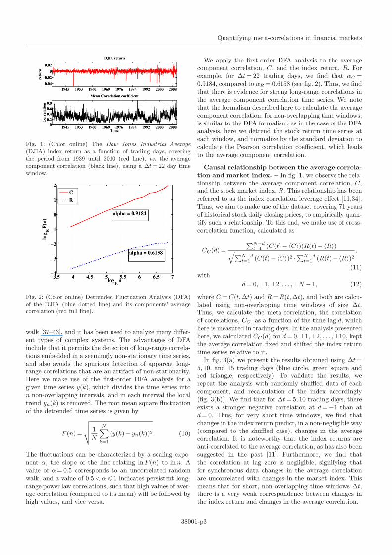
Investigating the dynamics of the average correlationover a long period, we observe non-random patterns. Infig. 1 we present an example, plotting R, the return of theDJIA index, vs. C, the average correlation between DJIAcomponents, calculated using a ∆t= 22 time window, withfull overlap.

Evidence of memory in the average correla-tion time series. – The Detrended Fluctuation Analy-sis (DFA) method has been introduced in the late 1990s,as a modified root mean square analysis of a random

38001-p2

Quantifying meta-correlations in financial markets

Fig. 1: (Color online) The Dow Jones Industrial Average(DJIA) index return as a function of trading days, coveringthe period from 1939 until 2010 (red line), vs. the averagecomponent correlation (black line), using a ∆t= 22 day timewindow.

Fig. 2: (Color online) Detrended Fluctuation Analysis (DFA)of the DJIA (blue dotted line) and its components’ averagecorrelation (red full line).

walk [37–43], and it has been used to analyze many differ-ent types of complex systems. The advantages of DFAinclude that it permits the detection of long-range correla-tions embedded in a seemingly non-stationary time series,and also avoids the spurious detection of apparent long-range correlations that are an artifact of non-stationarity.Here we make use of the first-order DFA analysis for agiven time series y(k), which divides the time series inton non-overlapping intervals, and in each interval the localtrend yn(k) is removed. The root mean square fluctuationof the detrended time series is given by

F (n) =

√√√√ 1N

N∑k=1

(y(k)− yn(k))2. (10)

The fluctuations can be characterized by a scaling expo-nent α, the slope of the line relating lnF (n) to lnn. Avalue of α= 0.5 corresponds to an uncorrelated randomwalk, and a value of 0.5<α� 1 indicates persistent long-range power law correlations, such that high values of aver-age correlation (compared to its mean) will be followed byhigh values, and vice versa.

We apply the first-order DFA analysis to the averagecomponent correlation, C, and the index return, R. Forexample, for ∆t= 22 trading days, we find that αC =0.9184, compared to αR = 0.6158 (see fig. 2). Thus, we findthat there is evidence for strong long-range correlations inthe average component correlation time series. We notethat the formalism described here to calculate the averagecomponent correlation, for non-overlapping time windows,is similar to the DFA formalism; as in the case of the DFAanalysis, here we detrend the stock return time series ateach window, and normalize by the standard deviation tocalculate the Pearson correlation coefficient, which leadsto the average component correlation.

Causal relationship between the average correla-tion and market index. – In fig. 1, we observe the rela-tionship between the average component correlation, C,and the stock market index, R. This relationship has beenreferred to as the index correlation leverage effect [11,34].Thus, we aim to make use of the dataset covering 71 yearsof historical stock daily closing prices, to empirically quan-tify such a relationship. To this end, we make use of cross-correlation function, calculated as

CC(d) =

∑N−dt=1 (C(t)−〈C〉)(R(t)−〈R〉)√∑N−d

t=1 (C(t)−〈C〉)2 ·∑N−dt=1 (R(t)−〈R〉)2

,

(11)with

d= 0,±1,±2, . . . ,±N − 1, (12)

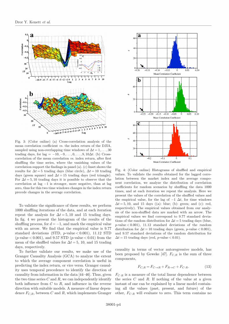
where C =C(t,∆t) and R=R(t,∆t), and both are calcu-lated using non-overlapping time windows of size ∆t.Thus, we calculate the meta-correlation, the correlationof correlations, CC , as a function of the time lag d, whichhere is measured in trading days. In the analysis presentedhere, we calculated CC(d) for d= 0,±1,±2, . . . ,±10, keptthe average correlation fixed and shifted the index returntime series relative to it.In fig. 3(a) we present the results obtained using ∆t=

5, 10, and 15 trading days (blue circle, green square andred triangle, respectively). To validate the results, werepeat the analysis with randomly shuffled data of eachcomponent, and recalculation of the index accordingly(fig. 3(b)). We find that for ∆t= 5, 10 trading days, thereexists a stronger negative correlation at d=−1 than atd= 0. Thus, for very short time windows, we find thatchanges in the index return predict, in a non-negligible way(compared to the shuffled case), changes in the averagecorrelation. It is noteworthy that the index returns areanti-correlated to the average correlation, as has also beensuggested in the past [11]. Furthermore, we find thatthe correlation at lag zero is negligible, signifying thatfor synchronous data changes in the average correlationare uncorrelated with changes in the market index. Thismeans that for short, non-overlapping time windows ∆t,there is a very weak correspondence between changes inthe index return and changes in the average correlation.

38001-p3

Dror Y. Kenett et al.

Fig. 3: (Color online) (a) Cross-correlation analysis of themean correlation coefficient vs. the index return of the DJIA,sampled using non-overlapping time windows of ∆t= 1, . . . , 30trading days, for lag = −10,−9, . . . , 0, . . . , 9, 10∆t. (b) Cross-correlation of the mean correlation vs. index return, after firstshuffling the time series, where the vanishing values of thecorrelation support the findings in panel (a). (c) Inset shows theresults for ∆t= 5 trading days (blue circle), ∆t= 10 tradingdays (green square) and ∆t= 15 trading days (red triangle).For ∆t= 5, 10 trading days it is possible to observe that thecorrelation at lag −1 is stronger, more negative, than at lagzero, thus for this two time windows changes in the index returnprecede changes in the average correlation.

To validate the significance of these results, we perform1000 shuffling iterations of the data, and at each iterationrepeat the analysis for ∆t= 5, 10 and 15 trading days.In fig. 4 we present the histogram of the results of theshuffling process, for d=−1, and mark the empirical valuewith an arrow. We find that the empirical value is 9.77standard deviations (STD, p-value< 0.001), 11.12 STD(p-value< 0.001), and 9.57 STD (p-value< 0.01) from themean of the shuffled values for ∆t= 5, 10, and 15 tradingdays, respectively.To further validate our results, we make use of the

Granger Causality Analysis (GCA) to analyze the extentto which the average component correlation is useful inpredicting the index return, or vice versa. Granger causal-ity uses temporal precedence to identify the direction ofcausality from information in the data [44–46]. Thus, giventhe two time series C and R, we can independently identifyboth influence from C to R, and influence in the reversedirection with suitable models. A measure of linear depen-dence FC,R, between C and R, which implements Granger

Fig. 4: (Color online) Histograms of shuffled and empiricalvalues. To validate the results obtained for the lagged corre-lation between the market index and the average compo-nent correlation, we analyze the distribution of correlationcoefficients for random scenarios by shuffling the data 1000times, and at each iteration we repeat the analysis. Here wepresent the values of the correlation of the shuffled values andthe empirical value, for the lag of −1 ∆t, for time windows∆t= 5, 10, and 15 days ((a): blue; (b): green; and (c): red,respectively). The empirical values obtained from our analy-sis of the non-shuffled data are marked with an arrow. Theempirical values we find correspond to 9.77 standard devia-tions of the random distribution for ∆t= 5 trading days (blue,p-value< 0.001), 11.12 standard deviations of the randomdistribution for ∆t= 10 trading days (green, p-value< 0.001),and 9.57 standard deviations of the random distribution for∆t= 15 trading days (red, p-value< 0.01).

causality in terms of vector autoregressive models, hasbeen proposed by Geweke [47]. FC,R is the sum of threecomponents,

FC,R = FC→R+FR→C +FC·R. (13)

FC·R is a measure of the total linear dependence betweenthe series C and R. If nothing of the value at a giveninstant of one can be explained by a linear model contain-ing all the values (past, present, and future) of theother, FC·R will evaluate to zero. This term contains no

38001-p4

Quantifying meta-correlations in financial markets

Fig. 5: (Color online) (a) Cross-correlation analysis of thecorrelation volatility coefficient, ΣC, vs. the index return of theDJIA, sampled using non-overlapping time windows of ∆t= 5trading days (blue circle), ∆t= 10 trading days (green square)and ∆t= 15 trading days (red triangle). For ∆t= 5 and 10trading days it is possible to observe that the correlation at lag−1 is stronger, more negative, than at lag zero, thus for thistwo time windows changes in the index return precede changesin the correlation volatility. Error bars were calculated usingthe standard deviation of the correlation volatility.

directional information, and represents residual correla-tions in the data that cannot be assigned to causallydirected influence based on the information in the data.FC→R is a measure of linear directed influence from C toR. If past values of C improve the prediction of the currentvalue of R, then FC→R > 0. For all investigated values of∆t= 5, 10, 15 trading days, we only find significant valuesfor FR→C , with F∆t=5R→C = 0.041 (p-value = 0), F

∆t=10R→C =

0.078 (p-value = 0), and F∆t=15R→C = 0.068 (p-value < 0.001).

Correlation volatility. – Whereas the relationshipbetween the average correlation and index return havebeen investigated in the past [11,31,32], much less atten-tion has been given on such a possible relationship betweenthe STD of correlations and the index return. First, wedefine the correlation volatility, which is the STD ofcomponent correlations calculated for a given time window∆t as

ΣC(t,∆t) =1

N(N − 1)

√√√√√ ∑i,j,i�=j

c2i,j(t,∆t)− ∑i,j,i�=j

ci,j(t,∆t)

2

.

(14)

Next, we repeat the procedure used to calculate themeta-correlation, CC , to investigate the cross-correlationrelationship between the correlation volatility, ΣC, andthe index return. As for the case of the average correlation,we focus on ∆t = 5, 10, and 15 trading days, and theresults are presented in fig. 5.Here we observe a positive meta-correlation between the

correlation volatility and index return. As in the case ofthe average correlation, we observe that for ∆t= 5 and10 trading days, the meta-correlation at lag −1 is largerthan at lag 0, which provides the information that changesin the index return in these time intervals will precedechanges in the correlation volatility.

Summary. – In summary, the empirical findingspresented here shed new light on the relationship betweenstock correlations and the return of the market index.The average correlation is negatively correlated with theindex return, where the correlation at lag zero becomesmore negative, and the correlation at lag minus one lessnegative, as function of ∆t. Using such methods as DFAand Granger causality analysis, we show further quantita-tive empirical evidence to this relationship. Furthermore,whereas the correlation volatility is positively correlatedwith it. In addition, the correlation volatility is found tobe positively correlated with the index return, displayingsimilar qualitative behavior as the average correlation. Itis important to note that both the average correlationand correlation volatility have a larger absolute value ofthe correlation with the index at lag of minus one timewindow for ∆t smaller than 15.

∗ ∗ ∗

This work was partially supported by the Tauber familyFoundation and the Maguy-Glass Chair in the Physics ofComplex Systems at Tel Aviv University (to DYK andEBJ), and the German Research Foundation Grant PR1305/1-1 (to TP).

REFERENCES

[1] Lux T., Econ. J., 105 (1995) 881.[2] Lillo F. andMantegna R. N., Phys. Rev. E, 68 (2003)016119.

[3] Petersen A. M., Wang F., Havlin S. and StanleyH. E., Phys. Rev. E, 82 (2010) 036114.

[4] Plerou V., Gopikrishnan P., Rosenow B., AmaralL. A. N., Guhr T. and Stanley H. E., Phys. Rev. E,65 (2002) 55125.

[5] Tumminelo M., Aste T., Di Matteo T. andMantegna R. N., Proc. Natl. Acad. Sci. U.S.A., 102(2005) 10421.

[6] Tumminello M., Di Matteo T., Aste T. andMantegna R. N., Eur. Phys. J. B, 55 (2007) 209.

[7] Tumminello M., Lillo F. and Mantegna R. N.,J. Econ. Behav. Organ., 75 (2010) 40.

[8] Podobnik B., Wang D., Horvatic D., Grosse I. andStanley H. E., EPL, 90 (2010) 68001.

[9] Podobnik B., Horvatic D., Petersen A. M. andStanley H. E., Proc. Natl. Acad. Sci. U.S.A., 106 (2009)22079.

[10] Xu L., Ivanov P. C., Hu K., Chen Z., Carbone A.and Stanley H. E., Phys. Rev. E, 71 (2005) 05110.

[11] Reigneron P. A., Allez R. and Bouchaud J. P.,Physica A, 390 (2011) 3026.

[12] Preis T., Paul W. and Schneider J. J., EPL, 82 (2008)68005.

[13] Preis T., Schneider J. J. and Stanley H. E., Proc.Natl. Acad. Sci. U.S.A., 108 (2011) 7674.

[14] Kenett D. Y., Shapira Y., Madi A., Bransburg-Zabary B., Gur-Gershgoren G. and Ben-Jacob E.,PLoS ONE, 6 (2011) e19378.

38001-p5

Dror Y. Kenett et al.

[15] Kenett D. Y., Raddant M., Lux T. and Ben-JacobE., PLoS ONE, 7 (2012) e31144.

[16] Kenett D. Y., Shapira Y., Gur-Gershgoren G. andBen-Jacob E., J. Eng. Sci. Technol. Rev., 4 (2012) 218.

[17] Mantegna R. N. and Stanley H. E., An Introductionto Econophysics: Correlation and Complexity in Finance(Cambridge University Press, Cambridge, UK) 2000.

[18] Preis T., Reith D. and Stanley H. E., Philos. Trans.R. Soc. A, 368 (2010) 5707.

[19] Preis T., Moat H. S., Stanley H. E. andBishop S. R.,Sci. Rep., 2 (2012) 350.

[20] Gabaix X., Gopikrishnan P., Plerou V. and StanleyH. E., Nature, 423 (2003) 267.

[21] Lillo F., Farmer J. D. and Mantegna R. N., Nature,421 (2003) 129.

[22] Plerou V., Gopikrishnan P., Gabaix X. and StanleyH. E., Phys. Rev. E, 66 (2002) 027104.

[23] Cont R. and Bouchaud J. P., Macroecon. Dyn., 4(2000) 170.

[24] Takayasu H. (Editor), Practical Fruits of Econophysics(Springer, Berlin) 2006.

[25] Preis T., Eur. Phys. J. ST, 194 (2011) 5.[26] Feng L., Li B., Podobnik B., Preis T. and Stanley

H. E., Proc. Natl. Acad. Sci. U.S.A., 109 (2012) 8388.[27] Onnela J. P., Chakraborti A. and Kask K., Phys.

Rev. E, 68 (2003) 1.[28] Kenett D. Y., Shapira Y., Madi A., Bransburg-

Zabary S., Gur-Gershgoren G. and Ben-Jacob E.,AUCO Czech Econ. Rev., 4 (2010) 330.

[29] Pollet J. M. andWilson M., J. Fin. Econ., 96 (2010)364.

[30] Black F., in Proceedings of the 1976 Meetings of theAmerican Statistical Association, Business and Econom-ics Section (American Statistical Association) 1976,pp. 177–181.

[31] Bouchaud J. P. and Potters M., Physica A, 299(2001) 60.

[32] Bouchaud J. P., Matacz A. and Potters M., Phys.Rev. Lett., 87 (2001) 228701.

[33] Balogh E., Simonsen I., Nagy B. and Neda Z., Phys.Rev. E, 82 (2010) 066113.

[34] Borland L. and Hassid Y., ArXiv e-prints, arXiv:1010.4917 (2010).

[35] Muchnik L., Bunde A. and Havlin S., Physica A, 388(2009) 4145.

[36] Pearson K., Philos. Trans. R. Soc. London A, 186(1895) 343.

[37] Peng C. K., Havlin S., Stanley H. E. and Gold-berger A. L., Chaos, 5 (1995) 82.

[38] Bunde A., Havlin S., Kantelhardt J. W., PenzelT., Peter J.-H. and Voigt K., Phys. Rev. Lett., 85(2000) 3736.

[39] Kantelhardt J. W., Koscielny-Bunde E., Rego H.H. A., Havlin S. and Bunde A., Physica A, 295 (2001)441.

[40] Bunde A., Schelinhuber H. J. and Kropp J., TheScience of Disasters: Climate Disruptions, Heart Attacksand Market Crashes (Springer-Verlag, Berlin) 2002.

[41] Carbone A., Catello G. and Stanley H. E., PhysicaA, 344 (2004) 267.

[42] Xu L., Ivanov P. C., Hu K., Chen Z., Carbone A.and Stanley H. E., Phys. Rev. E, 71 (2005) 051101.

[43] Bashan A., Bartsch R., Kantelhardt J. W. andHavlin S., Physica A, 387 (2008) 5080.

[44] Granger C. W. J, Econometrica, 37 (1969) 424.[45] Granger C. W. J., J. Econ. Dyn. Control, 2 (1980)

329.[46] Roebroeck A., Formisano E. and Goebel R.,

Neuroimage, 25 (2005) 230.[47] Geweke J. F., J. Am. Stat. Assoc., 77 (1982) 304.

38001-p6