Review of Dynamometer Correlations - National Environment ...
102
Proposed Diesel Vehicle Emissions National Environment Protection Measure Preparatory Work A R A R A R A R A Revie vie vie vie view of w of w of w of w of Dynamometer Dynamometer Dynamometer Dynamometer Dynamometer Cor Cor Cor Cor Correla ela ela ela elations tions tions tions tions, In-Ser , In-Ser , In-Ser , In-Ser , In-Service vice vice vice vice Str Str Str Str Strate te te te tegies and gies and gies and gies and gies and Engine Deterior Engine Deterior Engine Deterior Engine Deterior Engine Deterioration tion tion tion tion March 2000
-
Upload
khangminh22 -
Category
Documents
-
view
1 -
download
0
Transcript of Review of Dynamometer Correlations - National Environment ...
Proposed Diesel Vehicle EmissionsNational Environment Protection MeasurePreparatory Work
A RA RA RA RA Reeeeevievievievieview ofw ofw ofw ofw of Dynamometer Dynamometer Dynamometer Dynamometer DynamometerCorCorCorCorCorrrrrrelaelaelaelaelationstionstionstionstions, In-Ser, In-Ser, In-Ser, In-Ser, In-ServiceviceviceviceviceStrStrStrStrStraaaaatetetetetegies andgies andgies andgies andgies andEngine DeteriorEngine DeteriorEngine DeteriorEngine DeteriorEngine DeterioraaaaationtiontiontiontionMarch 2000

Prepared for the
National Environment Protection Council
by
td.NELSON ENGLISH, LOXTON & ANDREWS Pty. LMANAGEMENT, TRANSPORTATION & PLANNING CONSULTANTS
Vic., Australia, 32325289 2895 +613 Fax 2700 5289 +613 Tel. Lorne, 323, P.O. Box
Email: [email protected] 005 065 903
in association with
Energy and Environmental Analysis Inc.
ISBN 0 64232 322 4
© National Environment Protection Council Service Corporation 2000
This work is copyright. It may be reproduced in part subject to the inclusion ofacknowledgement of the source and no commercial sale.
A suite of projects have been developed during the preparatory work for a proposed DieselVehicle Emissions National Environment Protection Measure. These projects are:
The Australian Diesel Fleet Existing Vehicle Characteristics and theModelling of Transport Demand, Vehicle Populations and Emissions
In-Service Emissions Performance - Phase 1: Urban Drive CycleDevelopment
In-Service Emissions Performance - Phase 2: Vehicle Testing
In-Service Certification Correlation Studies
A Review of Dynamometer Correlations, In-Service Emissions and EngineDeterioration
In-Service Emissions Testing – Pilot Study, Fault Identification and Effect ofMaintenance
Major funding for these projects has been provided by Environment Australia. The othercontributing agencies are the Department of Transport and Regional Services, NSW RoadsTraffic Authority and the National Road Transport Commission.
Electronic copies of these documents are available from:
National Environment Protection Council Service CorporationLevel 5, 81 Flinders StreetAdelaide, SA 5000
Telephone: (08) 8419 1200Facsimile: (08) 8224 0912
These documents are also available online: http://www.nepc.gov.au

CONTENTSEXECUTIVE SUMMARY............................................................................................................ 1
Introduction.......................................................................................................................................... 1Background on Emission Standards and Test Procedures ............................................................ 1NEPC Project 5..................................................................................................................................... 2
Types of Cycles ................................................................................................................................. 2Correlations Between Engine and Chassis Tests ......................................................................... 3Establishing Correlations in Australia .......................................................................................... 4
NEPC Project 6..................................................................................................................................... 5Emissions Deterioration .................................................................................................................. 5Control of In-service Emissions...................................................................................................... 6Retrofit and Rebuild Related Programs ........................................................................................ 8Recommendations for Australia .................................................................................................. 10
1 INTRODUCTION............................................................................................................... 111.1 Objectives ................................................................................................................................. 111.2 Report Outline ......................................................................................................................... 11
2 EMISSION STANDARDS AND TEST PROCEDURES FOR HEAVY-DUTYDIESEL ENGINES .............................................................................................................. 122.1 Overview .................................................................................................................................. 122.2 U.S. Heavy Duty Diesel Engine Emissions Standards....................................................... 13
2.2.1 U.S. Federal HDD Emission Standards .......................................................................... 132.2.2 California HDD Emissions Standards ............................................................................ 15
2.3 European Regulations ............................................................................................................ 182.4 Japanese Standards ................................................................................................................. 202.5 Steady State Certification Test............................................................................................... 202.6 Transient Tests......................................................................................................................... 23
3 CHASSIS TEST CYCLES .................................................................................................. 283.1 Overview .................................................................................................................................. 283.2 Steady-State 13-Mode Test..................................................................................................... 283.3 Geometric Test Cycles ............................................................................................................ 303.4 Realistic Test Cycles ................................................................................................................ 413.5 Summary of Heavy Duty Testing Options .......................................................................... 47
4 EMISSIONS CORRELATION BETWEEN DIFFERENT TESTS .............................. 524.1 Issues ......................................................................................................................................... 524.2 Comparison Between Engine Based 13-Mode And Transient Tests................................ 534.3 Correlation of Engine Based Steady State Tests to Chassis Based Steady-State Tests .. 544.4 Correlations Between Chassis Dynamometer and Engine Dynamometer Tests:
Transient Emissions........................................................................................................ 57
5 METHODOLOGIES FOR TESTING IN AUSTRALIA .............................................. 625.1 Overview .................................................................................................................................. 625.2 Cycle Selection ......................................................................................................................... 625.3 Effect of Vehicle Size/Weight................................................................................................ 635.4 Effect of Certification Standards and Country of Origin................................................... 635.5 Effect of Age/State-of-Maintenance..................................................................................... 64
5.6 Levels of Correlation Achievable .......................................................................................... 645.7 Checklist of Key Issues for Testing ....................................................................................... 65
6 EMISSIONS DETERIORATION UNDER IN-SERVICE CONDITIONS ...............676.1 Overview .................................................................................................................................. 676.2 European Emission Factor Programs ................................................................................... 68
6.2.1 Testing in Netherlands......................................................................................................686.2.2 Testing in the U.K. .............................................................................................................696.2.3 Testing in Germany ...........................................................................................................706.2.4 Other Tests ..........................................................................................................................706.2.5 Light-Duty Diesel Testing.................................................................................................71
6.3 Emission Factor Testing in the U.S. ...................................................................................... 716.4 Hddv Emission Factors Derived from Models.................................................................... 74
7 EMISSIONS CONTROL STRATEGIES.........................................................................817.1 Types of Strategies................................................................................................................... 817.2 Inspection/Maintenance Programs ...................................................................................... 817.3 Retrofit and Rebuild Related Programs ............................................................................... 85
7.3.1 European Developments...................................................................................................857.3.2 U.S. Developments.............................................................................................................87
8 POTENTIAL CONTROL PROGRAMS FOR AUSTRALIA .......................................908.1 Context ...................................................................................................................................... 908.2 Deterioration of Emissions Under In-Service Conditions ................................................. 908.3 Maintenance of In-Service Emissions ................................................................................... 918.4 Retrofit and Rebuild Control Programs ............................................................................... 92
BIBLIOGRAPHY.........................................................................................................................95
Diesel Vehicle Emissions – A Review of Dynamometer Correlations, In-Service Strategies and Engine Deterioration Page 1
EXECUTIVE SUMMARY
INTRODUCTIONThe National Environment Protection Council (NEPC) is undertaking a critical examination andassessment of emission from diesel engine powered vehicles in Australia. There is worldwideinterest in the methods to test heavy-duty diesels for emissions, and in the emissions from dieselin-service vehicles. The NEPC has issued two projects to study these issues. The first (Project 5)is to conduct a critical examination of the literature and on-going efforts to establish a correlationbetween measured emissions on a chassis dynamometer and on an engine dynamometer forheavy-duty vehicles. The second (Project 6) requires an examination of the emissiondeterioration under in-service conditions for both light-duty and heavy-duty diesel vehicles.This project also requires an examination of regulatory and non-regulatory programs to maintainemissions at certification levels.
Since both projects require an understanding of emission standards and test methods, thesetopics are covered under a common background section. Details specific to each project arecovered in separate sections.
BACKGROUND ON EMISSION STANDARDS AND TEST PROCEDURESAustralia imports all of its heavy-duty diesel engines from three sources: Japan, Europe or theU.S. Japanese engines are used in most of the lighter vehicles (around five tons GVM) and inabout half the vehicles in the ten to 15 GVM range. European diesels account for the other half ofthis range, while European and U.S. diesels engines power the larger vehicles over 15 tons GVM.Australia did not require these engines to meet any criteria pollutant emission standards until1996, and has adopted European ECE R49/02 standards since that time. The Australianregulation also allows alternative certification to U.S. 1991 and later standards or Japanese 1994and later standards.
Since the Australian heavy-duty engine market is not large, it is unlikely that engines wereespecially designed for Australia. Most Australian engines are likely to have technologyequivalent to the country of origin model, but some may be recalibrated for increased fuelefficiency and, hence, increased NOx emissions.
For a variety of reasons, heavy-duty emissions regulations are based on testing engines asopposed to entire vehicles. A detailed survey of emission standards and test procedures showedthat U.S. heavy-duty diesel engine emission standards have been and are the most stringent inthe world, while European and Japanese standards have lagged U.S. standards by about fiveyears. However, by 2008 the U.S., Japanese and European standards are likely to be harmonisedand achieve near parity.
It should be noted that even the U.S. standards were relatively lax until 1988, and even thehighest emitting engines could meet pre-1988 standards with modest technological changes.This is also true for European and Japanese standards to the early to mid-1990s. Hence, mostengines certified to these standards had emissions far below the standards, and the standardswere not binding.
Engine test procedures also varied between the U.S., Europe and Japan. Until 1984, all threeutilised a steady-state engine test called the 13-mode test, although the individual modedefinitions varied between the three. Since 1984, the U.S. has used a more complicated transientcycle based test that more closely replicates the engine’s duty cycle during typical driving.
Diesel Vehicle Emissions – A Review of Dynamometer Correlations, In-Service Strategies and Engine Deterioration Page 2
European and Japan have continued to use the 13-mode test. Starting in model year 2005,European regulations will require both a transient test (different from the U.S. transient test) anda revised 13-mode test. The U.S. has also proposed re-incorporating the 13-mode test along withthe existing transient test starting in model year 2004.
The need for a transient cycle based test procedure has been debated extensively, but it is nowacknowledged that at very low emission levels, the transient test provides a significantly betterindication of on-road emissions than any steady-state test. At higher emission levels moretypical of engines built until the late 1980’s in the U.S. or early 1990s in Europe, the steady-statetest procedure could be used to provide a reasonable indication of criteria pollutant emissions,with the possible exception of particulate mater (PM). However, PM standards for heavy-dutyengines were not effective until the late-1980s or early 1990s.
Light –duty diesel vehicles are currently popular in Europe but not in the U.S. or Japan. Thesevehicles have been certified using procedures and standards that were and are similar to thosefor light-duty gasoline vehicles. As with heavy-duty diesels, the emission standards applicable todiesel vehicles were relatively lax and standards to 1992 were easily met by most vehicles. Since1992, the introduction of PM standards has resulted in some difficulty in meeting thesestandards, but standards for gaseous emissions continue to be not binding. However, it shouldbe noted that diesel car sales are very low in Australia, and most light-duty diesels sold are inlight commercial vehicles or in four-wheel drive utility vehicles. Commercial vehicles generallyemploy smaller or derated versions of heavy-duty engines used in trucks of 3.5 to 7 tons GVM.Four wheel drive utility vehicles use unique large displacement light duty engines.
The findings of the background analysis that are important to the two NEPC projects are:
• Australia had no emission standards for criteria pollutant emissions from heavy-duty engineuntil 1996, so that emissions of heavy-duty engines imported prior to 1996 is not wellunderstood.
• Most engines imported from Europe or Japan until the early to mid-1990s had emission levelsthat were well below applicable standards in those countries.
• The steady state engine based 13-mode test is the reference emissions test for the majority ofheavy-duty engines imported to Australia. Only engines imported from the U.S. (which arenot a sizeable fraction of the Australian heavy-duty fleet) were certified based on a transienttest.
• In the future, as emissions standard are increased in stringency, certification will require useof both the 13-mode steady-state test and transient test in Europe and the U.S.
• The light duty diesel fleet in Australia is not similar to the light-duty diesel fleet in Europe. Itconsists of larger displacement light-duty engines or smaller versions of heavy-duty engines.
NEPC PROJECT 5This project had two objectives. The first was to conduct a critical examination of the literatureand on-going efforts to establish a correlation between measured emissions on a chassis (vehicle)dynamometer and on an engine dynamometer. The second was to provide advice onmethodologies for establishing such correlation in Australia, with an assessment of the level ofconfidence that can be applied to such correlations.
Types of CyclesA comprehensive review of the available chassis test cycles was performed. Until the early1990s, there was virtually no interest in replicating the engine based 13-mode steady-state test ona chassis dynamometer. The 13-mode test consists of a series of engine RPM and torque

Diesel Vehicle Emissions – A Review of Dynamometer Correlations, In-Service Strategies and Engine Deterioration Page 3
operating points (or modes) over which emissions are measured. Since about 1992, thereplication of this test has been extensively investigated in Europe. In principle, this replicationis very straightforward, but the major difficulty is in determining engine torque output when theengine is in the vehicle. Two methods were developed, one based on engine fuel consumption,and the second based on calculation of power loses in the vehicle transmission, driveline andtyres. Both methods have been successfully developed in Europe.
Transient test cycles have been for more widely used in chassis dynamometer based testing.Two types of cycles exist that we have labelled as “geometric” and “realistic”. Geometric, orstylised, test cycles obtain their name from the fact that the speed versus time trace appears as aseries of straight lines that reflect constant acceleration rates, constant speed cruise and constantdeceleration rates. Realistic cycles are derived from actual driving traces where speed andacceleration rates vary continuously over time. Several geometric cycles have been widely usedhistorically, and these include the Society of Automotive Engineers J1376 test procedures and theWest Virginia ‘Five Peak’ cycle. Realistic cycles have been historically limited to the U.S. EPATransient Test (derived from the same data as the engine based transient test) but other cycles areunder development. In this context, the newly developed Australian Composite Urban EmissionDrive Cycles (CUEDC) are classified as “realistic”.
The major drawback to most chassis based transient cycles is the fact that the cycles are invariantwith engine characteristics, whereas engine based cycles are defined in terms of the engine’smaximum torque and RPM ratings. Hence, a truck of a given weight (GVM) with a powerfulengine is not subjected to accelerations requiring full engine power during a chassis test, whilean underpowered truck may have difficulty keeping up with the specified driving trace. Thelack of scaling is a major drawback and this problem could also effect the newly developedCUEDC. There are research programs in the U.S. to develop a cycle whose specification scaleswith the test vehicle’s power-to-weight ratio. Preliminary results from such efforts arepromising, but more work is required before such cycles can be universally adopted.
Correlations Between Engine and Chassis TestsThe topic of correlations between engine and chassis based tests is complex because of the manysources of variability in emissions. The sources include:
• engine cycle-to-cycle variability;• engine-to-engine production variability;• emissions measurement instrument variability;• drive cycle variability;• driver variability.
When comparing results from two different engines of the same model type, all of the abovesources of variability come into play and total variability can be large.
Manufacturers have attempted to measure the correlation of emission from different test cyclesconducted on engine dynamometers. In general, there is agreement that NOx emissions can becorrelated between transient tests and steady-state tests, but the correlation for PM emissions ispoor at low emission levels. The coefficient of variation (COV) for NOx emissions across the twocycles is in the order of ten percent, for the same engine and laboratory.
European testing to compare results from the engine based 13-mode test with the chassis based13-mode test show that very good correlations have been established. Experienced testlaboratories have obtained average emission correlations with a COV of two percent, and amaximum error for any pollutant of less than five percent. However, engines with very low
Diesel Vehicle Emissions – A Review of Dynamometer Correlations, In-Service Strategies and Engine Deterioration Page 4
emissions have not been examined, and it is possible that the COV could be higher due to thedifficulty in measuring low concentrations of pollutants. More limited testing in Japan has alsoachieved good correlations of the Japanese 13-mode test (which is different from the European13-mode test).
U.S. testing to compare the results from the engine based transient test and the chassis basedEPA transient test have had mixed success so far. Reasonable correlations have been achieved ifthe chassis test forces acceleration at near full power and the truck can follow the specifiedspeed/time trace with limited error. However, underpowered or overpowered trucks result inrelatively poor correlations. As noted, these has been some recent progress in developing achassis based test that “scales” with the truck power-to-weight ratio. However, testing is toolimited to date to provide meaningful COV values. Moreover, there are numerous transient testspecifications that are currently undefined and set by each laboratory in an ad hoc manner. Itshould be noted that the Australian CUEDC would have similar problems in the field unless itcan be scaled to truck characteristics.
There has also been some attempt to reproduce the engine based transient cycle on a chassis testby hooking up a dynamometer to the axles and conducting the entire test in one e gear. The axledynamometer arrangement is similar to the engine dynamometer arrangement except that itcannot provide motoring torque (i.e., use the engine in a braking mode). Limited results to datehave been disappointing because of poor PM emissions correlation.
Establishing Correlations in AustraliaThe survey of the state-of-the-art for establishing correlations shows that:• good correlations between engine and chassis based emission test results can be obtained for
the 13-mode test except, possibly at very low emission levels;• correlations on transient tests are far more difficult to obtain, largely due to the way chassis
transient tests have been specified (or not specified).
In general, the steady-state procedure can be reproduced on either a roll based chassisdynamometer or an axle dynamometer, but we do not wish to imply that achieving a highdegree of correlation is easy. There are many issues that Australia will need to resolve forimplementing the steady-state test, including:
(1) The test points (in terms of engine RPM and torque) must be obtained from the type approvalcertificate. Such certificates are not available for U.S. engines (since there is no 13-mode testrequirement) and may not be available for Japanese engines;
(2) The determination of engine torque using the fuel consumption method requires an enginemap that may not be readily available. Moreover, some assumption must be made on thestate-of-tune of the engine, and this can lead to significant error.
(3) Determination of engine torque using the power loss estimation method must rely onempirical formulae to estimate drivetrain losses. European formulae may not be applicableto Australian vehicles.
(4) There may be no easy way to check the correlation because even engine test facilities are verylimited in Australia, and such facilities have not been audited by any experienced agency.
(5) In the absence of any simple method to resolve these issues, correlations in Australia may notachieve the levels attained in Europe.
Diesel Vehicle Emissions – A Review of Dynamometer Correlations, In-Service Strategies and Engine Deterioration Page 5
Correlation issues for transient tests are substantially more complex, and Australia should beprepared to address the “scaling” issues in terms of adapting the drive cycle to truckspecifications. It is also believed that axle dynamometer based measurements where the systemcannot simulate motoring of the engine may result in very inaccurate results for PM emissions.It is recommended that Australia monitors U.S. developments in transient cycle specificationsand addresses these issues in the context of the CUEDC in the future.
NEPC PROJECT 6This project had three main objectives. First, the in-service emissions deterioration rates for bothlight-duty and heavy-duty diesels were critically examined. Second, we examined worldwideemission control programs that are designed to maintain engine emission performance atoriginal levels over its useful life. Third, programs that are related to improving the emissionperformance of in-service vehicles (through retrofit of control technology or upgrade at the timeof engine rebuild) were examined. The applicability of both types of programs to Australia wasassessed, based on the data from existing programs.
Emissions DeteriorationThe emissions deterioration of heavy-duty diesels has not been studied extensively largely dueto the lack of adequate test facilities, and the expense involved in recruiting and testing a sampleof in-use trucks. There is also a widespread belief that the emissions of heavy-duty diesel enginesare relatively stable over their useful life.
Since the late-1980s, there has been a growing realisation that in-service diesels do not maintaincertification level emissions over their useful life. There are several components to the in-serviceemissions deterioration, or “excess” emissions that occurs. First, even in the certification process,emissions are assigned a deterioration factor based on an idealised durability cycle, and the realworld duty cycles imparts somewhat larger deterioration in emissions relative to the certificationdurability test. Second, the levels of maintenance recommended by the manufacturers areusually not strictly followed, causing additional deterioration. Third, there may be mal-maintenance (either intentional or unintentional) due to mechanic inexperience. Fourth, theremay be intentional tampering, usually to increase horsepower or fuel economy. Lastly, theremay be design defects in the emission control system that causes high emissions.
Emissions deterioration is also defined in several ways. One definition is the emissions of in-service diesels with respect to the emissions standard to which a particular engine is certified.The second defines deterioration with respect to the increase in emissions relative to emissionswhen an engine is new and properly tuned. These definitions can cause substantial differences inthe findings on deterioration largely because many engines have been certified at emission levelswell below standards, and even a significant increase in emissions will not cause an exceedanceof standards. Indeed, this is the situation with many of the study results from Europe.
Significant testing of in-service trucks has been conducted in the Netherlands, Germany and theUK, with some limited testing in Sweden. Most of these tests have been conducted on vehicleswith engines certified to the 88/77/EEC standard or the Euro I standard, with a few certified tothe Euro II standard. Vehicles were typically 4 to 5 years old at the time of testing (except for theengines certified to the Euro II standard). No vehicles were found to exceed the 88/77/EECstandard partly because the standard was not very stringent. Analysis of the data on vehicleswith engines certified to the Euro I or II standard showed about 5 to 10 percent of vehiclesexceeding standards for one pollutant, and up to 15 percent exceeding standards for anypollutant. Observers in Europe believe that tampering and mal-maintenance are low in Europe,
Diesel Vehicle Emissions – A Review of Dynamometer Correlations, In-Service Strategies and Engine Deterioration Page 6
but the sampling process for the in-service emissions testing conducted is potentially biased infavour of clean well-maintained trucks.
There has been some testing of in-use diesels in Germany and Netherlands in the 1980s. As withheavy-duty diesels, applicable standards prior to 1992 were not very stringent and virtually novehicles were found to exceed standards. There has been only limited testing in the 1990s, and atest of 28 diesel light-duty vehicles in Germany that were certified to Euro I levels found thatthree vehicles exceeded PM standards and only one of the three exceeded the standards by alarge amount. Gaseous emission standards were met by all vehicles. However, the relevance ofthese findings for Australia is limited because the light-duty fleet is not similar to the one inEurope.
Little testing has been done in the US, with only one major program on heavy-duty enginesconducted in the 1980s. Statistical analysis of the data showed that at the end of an engine’suseful life of about 500,000km, HC emissions increase by over 70 percent and PM emissionsincrease by over 80 percent, on average, relative to emissions when new. ( This does not compareemissions with standards and is a different measure of deterioration then the one discussed forEurope). A completely different approach to estimating emissions deterioration has also beenused in the US. This method relies on finding the mal-performance rates of emission controls bydiagnosing a large number of in-service vehicles, and modelling the emissions deterioration byassociating each mal-performance with an incremental emissions impact. Interestingly, thisapproach resulted in a similar finding as the statistical approach for engines manufactured in thelate 1970s to early 1980s. For newer engines, especially those featuring electronic controls, themal-performance rates are lower, but the percentage increase in emissions due to mal-performance is larger. This is partly because of the low absolute emission rates and partlybecause modern engines are so highly tuned for best emissions that mal-performances cause alarger percent increase in emissions than for older engine designs.
Some observers believe that the European tampering and mal-maintenance rates are much lowerthan American rates and that in-service emissions deterioration is a bigger problem for the USthan for Europe. It is not clear what the situation in Australia is, and we could find no objectiveevidence of the situation being closer to Europe or the US. Nevertheless, the modelling approachallows an assessment of the situation at reasonable cost, and is recommended for Australia.
Control of In-service EmissionsThe maintenance of emissions by inspecting in-service vehicles is used widely, although manyprograms are using test methods that may be not be effective, or are completely ineffective atworst. Much of the motivation for subjecting heavy-duty vehicles to inspection/maintenanceprograms is the public perception of diesel smoke, as well as the real threat of the carcinogenietyof smoke particulates. Virtually all of the ongoing programs to control in-service emissions havefocused on smoke emissions, and the accompanying reduction (or increase) in gaseous emissionsas a result of reducing smoke has not received any attention except in isolated cases. Indeed,outside of analyses conducted by California in the early-1990s, we have not been able to find anyattempt to characterise the other benefits of smoke reduction programs that are now in place inmost OECD countries.
Seven states in the U.S. currently have active heavy-duty I/M programs with two othersoperating pilot programs. All EC countries and Japan have truck inspection programs althoughthe quality varies widely between European countries. Virtually all programs are based onsmoke emissions as an indicator of pass/fail status.
Diesel Vehicle Emissions – A Review of Dynamometer Correlations, In-Service Strategies and Engine Deterioration Page 7
Light-duty diesel vehicles are also subject to inspection and maintenance programs in mostOECD countries. In the US and Japan, many local jurisdictions use tests similar to thoseemployed for petrol vehicles, even though the tests are irrelevant to a diesel. In some states in theUS and in most locations in Japan and Europe, light duty diesels are also subjected to a smoketest.
A typical I/M program consists of standardised test and measurement procedures, a set ofpass/fail cutpoints, and an enforcement mechanism. Smoke tests can be loosely categorised intotwo types: transient and steady-state. Transient tests measure smoke over a changing enginespeed and load cycle, while steady-state tests measure smoke during a constant speed and loadcondition. Each can be effective in detecting certain typical engine mal-performances althoughtransient tests are generally more robust in terms of the scope of mal-performances identified.
The most common test procedure currently applied in the U.S. to heavy-diesels is the SAE J1667snap acceleration test procedure, recently promulgated by the Society of Automotive Engineers.This test procedure was jointly developed by the regulatory and trucking communities andspecifically addresses industry concerns with its predecessor J1243 test procedures. Light-dutydiesels have not been of much concern in the US due to the small population.
In general, transient testing provides an effective means of identifying the short duration smokeevents that characterise a variety of common mal-performances. On the other hand, steady-statetests at wide-open throttle (i.e., lug down) do not identify several common mal-performances,but identify some mal-performances that the transient tests do not. These mal-performances arenot as common, but can have a significant emissions impact. The idle and cruise mode tests arelargely ineffective in detecting most mal-performances, since they are conducted at part throttle.
Most EC countries also use the snap acceleration test (sometimes call free acceleration test) forboth light-duty and heavy-duty diesels though some regional jurisdictions in Germany requireboth the snap acceleration test and the lug-down test. The European snap acceleration test is notidentical to the J1667 in terms of meter response time and technical criteria to determine a validtest, and these specifications also very from country-to-country. For example, Germany has atime specification for the RPM increase on the free acceleration test, while France does not.
The largest difference between the U.S. and Europe is that the smoke opacity standards in manythe EC countries are type specific and vary from engine model to engine model. The standardsare actually suggested by the engine manufacturer, leading to considerable complexity inadministration. Moreover, the engine manufacturers have an incentive to make the standardsrelatively lax, so that so engines with marginal mal-performances are not failed.
In Japan, the free acceleration test is also used, but the smoke measurement is based on a longaveraging time instrument so the results are not comparable to the SEA J1667 test. However,Japan implements a standard of 40 percent opacity for pre-1999 trucks, and 25 percent opacity for1999 and later vehicles.
While detailed failure rates for EC countries and Japan are not available, several leadingresearchers confirmed to EEA that only about one percent of vehicles (light or heavy) testedactually fail the test. Hence, the primary value of the test appears to be as a deterrent totampering in Europe and Japan. Failure rates are somewhat greater in the U.S., but still quite lowgiven the number of smoky trucks observed usually on the road. Only the California RoadsideProgram has addressed the issue of targeting likely failure for the test, and is hence moreeffective. Since high smoke emitters can be usually identified, to targeting of potential failures isquite easy.

Diesel Vehicle Emissions – A Review of Dynamometer Correlations, In-Service Strategies and Engine Deterioration Page 8
Analysis for California shows that the I/M program is capable of identifying at least half of all“excess” emissions of HC and PM on older mechanically controlled engines. No recent analysishas been done on the benefits for newer electronically controlled engines, but the absolutequantity of excess emissions as well as the percent identified have undoubtedly declined relativeto older engines. The high level of excess emission may be a phenomenon that is U.S. specific,since the rates of tampering and mal-maintenance are potentially much higher in the U.S.,relative to European levels.
Retrofit and Rebuild Related ProgramsThe potential to decrease emissions of in-service diesels through retrofit of new technologies toolder vehicles or by rebuilding engines to new standards has received considerable attention inEurope and the U.S. over the last five to seven years.
To date, there are no regulations in Europe requiring the retrofit of technologies or the rebuildingof engines to more stringent emissions standards. The EC regulation only requires that rebuiltengines meet the original specification that the engine was designed to; the same regulationapplies to re-engined vehicles. However, in the case of re-engined vehicles, we understand thatmost operators in Europe simply buy a current model engine of the same make, so that anupgrade occurs ‘defacto’ simply due to convenience.
While there are no requirements that legally enforce retrofit or upgrade, there are manyorganisations in Europe that are voluntarily retrofitting engines with newer technology, mostlytrap oxidisers or oxidation catalysts. The vast majority of these voluntary retrofits have been bythe Metropolitan Transport Organisations (state-owned) for the bus fleet.
The retrofit devices are commercially offered by catalyst manufacturers, such as Engelhard andJohnson-Matthey. Each country is certifying retrofit devices to meet a minimum performancerequirement that requires a reduction in PM of at least 20 to 25 percent and HC by a similaramount, without increasing NOx emissions or noise.
Virtually no assessment of programs that aim at reducing NOx emissions from in-servicevehicles has occurred in Europe. NOx can be reduced from in-service engines by a number ofactions ranging from injection pump and injection timing recalibration to the addition of an air-to-air intercooler in non-intercooled or jacket water intercooled engines. We are unaware of anyEuropean program that has focused on these aspects, although there is a white paper to bereleased shortly in England that may discuss such issues.
Sweden is using a novel method to encourage the retrofit or upgrade of engines. It has createdenvironmental zones in its three largest cities: Stockholm, Goteburg and Malmo. The zoneessentially covers the entire central business district of the cities. Within these zones, municipalcouncils have the right to restrict heavy-duty diesel vehicles that do not meet stringent emissionstandards or are retrofitted with approved devices. Conversations with environmentalauthorities of Stockholm and Goteberg confirmed that many older buses are now fitted withLevel A devices and a few with Level B devices. There has been a redirection of newer trucks tothe environmental zones, but authorities believe that several hundred private trucks haveadopted retrofit devices in all of Sweden. Hence, it is regarded as a relatively successful local airpollution control strategy.
The U.S. has moved ahead on some specific retrofit and rebuild requirements that are now partof the regulations. There are four major actions that now affect retrofit and rebuild in the U.S.:
Diesel Vehicle Emissions – A Review of Dynamometer Correlations, In-Service Strategies and Engine Deterioration Page 9
1. retrofit and rebuild requirements for 1993 and earlier urban bus engines;
2. the California Low Emission Vehicle Emissions Credit Program;3. the North-Eastern States Voluntary Heavy-Duty Retrofit Program;4. the Low NOx Emissions Rebuild Program.
Of these, the first and last programs are driven by regulatory requirements, while the Californiaand North-Eastern State Program are market driven approaches.
In early 1993, EPA published final Retrofit/Rebuild Regulations for 1993 and Earlier Model YearUrban Buses. The regulations require affected urban bus operators to comply with one of twoprogram options, beginning January 1, 1995. Option 1 established particulate matter (PM)emission requirements for each urban bus in an operator’s fleet when the engine is rebuilt orreplaced. Option 2 is a fleet averaging program that sets out specific annual target levels foraverage PM emissions from urban buses in an operator’s fleet. The two compliance options aredesigned to yield equivalent emissions reductions for approximately the same cost.
Certification activity under the retrofit program has lagged substantially behind the scheduleanticipated by EPA when the final rule was promulgated. No equipment was certified whenEPA revised the post-rebuild levels based on equipment. EPA’s assumption that certificationactivity would begin early was incorrect and more importantly, EPA’s assumption thatcertification activity would be complete by mid-1996 was incorrect. For example, EPA onlyrecently certified equipment manufactured by Engelhard Corporation that triggers the 0.10g/bhp-hr (0.13 g/kWh) standard for 1979 though 1989 model year Detroit Diesel Corporation(DDC) 6V92TA MUI engines. Additionally, Johnson Matthey Incorporated has been certified tosupply equipment to the same standard, and applicable to these, and other, DDC engines. Thereare other plans for certifying equipment to the 0.10 g/bhp-hr (0.13 g/kWh) standard for a largesegment of the bus engine population. Hence, the program has little impact to date
The California and North Eastern States programs are similar in that they involve the use ofemission credits that can be generated by retrofitting a diesel engine. In the U.S., most majormetropolitan areas are not yet in compliance with the air quality requirements for ozone and aredesignated as non-attainment areas. In these areas, businesses that generate more emissions thansome allowable level are required to offset the increase by purchasing credits or helping reduceemission elsewhere, making emission reductions a marketable commodity. Hence, there is valueto a private firm reducing emission by retrofit, and selling these credits can (in theory) offset thecost of retrofit either partially or entirely. To date, however, the number of voluntary retrofits hasbeen very small (a few hundred vehicles nationally) largely because the cost of retrofit is verymuch higher than the market value of the credits.
The newest program is one that has come about from a settlement of a regulatory action by EPAagainst the diesel engine manufacturers. The US EPA believed that modern diesel enginesemployed “cycle beating” techniques to met current emission standards, and initiated legalactions against engine manufacturers. As part of the settlement, the manufacturers have agreedto develop low NOx rebuild kits for a range of popular engine models manufactured between1993 and 1998. These kits will essentially bring the NOx levels of affected engines down by about25 percent. The kit is to be available at no extra cost to rebuilders and owners, and all engineswithin the model year range that are selected by manufacturers must be rebuilt using this kit.Such kits are expected to be available in the marketplace shortly.

Diesel Vehicle Emissions – A Review of Dynamometer Correlations, In-Service Strategies and Engine Deterioration Page 10
As noted, only the two regulatory programs are expected to have a significant influence onrebuild and retrofit. The U.S. EPA is considering other rebuild and retrofit requirements forheavy-duty diesels but no actions are expected in the near future.
Recommendations for AustraliaThe need for control strategies to address heavy-duty is very much dependent on the rates ofmal-performance and tampering found in Australia. Anecdotal evidence from industry sourcesvaries, and a survey would be required to obtain an objective estimation.
If these rates are quite low, then the programs may not be cost effective and will lead to asituation as in Europe, where almost no one fails the inspection for emissions. At present, theonly type of control program in existence is based on smoke emissions. Such programs to controlsmoke emissions have popular public support, and analysis by California has shown a randomroadside program ( where potential failures are visually identified and tested)can be very costeffective and result in reductions to HC and PM emissions , in addition to being a deterrent totampering. This type of program may be the only one suitable for Australia, since Australia hashad a smoke emissions standard that engines must meet since the 1970s.
Retrofit of technology to reduce emissions has focused primarily on reducing particulateemissions, and a number of commercial products are available for the European market that aresuitable for Australian engines imported from Europe. Similar products are being developed forsome US and Japanese engines, especially those fitted to buses. While the performance of theseproducts is good, costs are still very high and most sales have been to Metropolitan busoperators. It is not clear that such devices are cost effective for Australia.
Upgrade at engine rebuild to a lower emissions specification is also possible, but a rebuild kitmust be developed with assistance from the engine manufacturer. Such kits are available forsome engines, but certainly not for all engines. As a result, it will not be possible to impose aregulatory requirement to upgrade all engines at rebuild. A market based approach offeringincentives to manufacturers may result in such kits becoming available for at least some of themore popular high sales volume engine lines in Australia.
Diesel Vehicle Emissions – A Review of Dynamometer Correlations, In-Service Strategies and Engine Deterioration Page 11
1 INTRODUCTION
The National Environmental Protection Council (NEPC) is undertaking a critical examinationand assessment of emission from diesel engine powered vehicles in Australia. Diesel engines areextensively used in heavy-duty trucks and buses, but have little penetration in the light-dutyvehicle fleet. For a number of reasons unique to heavy-duty vehicles, the emissions from dieselengines used in this application have been traditionally quantified using an engine dynamometerbased test. The correlation of measured emissions between such tests and vehicle-based testsconducted on a chassis dynamometer has been of much interest recently, since more focus hasbeen placed on the in-use (as opposed to certification) emissions of diesel-powered vehicles.
The interest in the in-use emissions of heavy-duty diesels has grown as light-duty vehicles havebeen controlled to increasingly stringent standards. Heavy-duty diesel vehicles are now asignificant contributor to the total NOx and combustion derived particulate matter (PM)inventory in Australia. In-use emissions of diesels have also been historically assumed to be nearcertification levels, but recent testing has shown that this assumption may not be valid, and in-use deterioration may be significant. As a result, programs are being developed in OECDcountries to control in-use heavy-duty diesel vehicle emissions, and to further reduce theiremissions by retrofitting advanced emission control technologies to older vehicles in service.
1.1 OBJECTIVESThe NEPC has issued two projects to study these issues. The first (NEPC Project 5) is to conducta critical examination of the literature and on-going efforts to establish a correlation betweenmeasured emissions on a chassis dynamometer and on an engine dynamometer. The second(NEPC Project 6) requires an examination of the emissions deterioration that takes place underin-service conditions. The project also requires an examination of regulatory and non-regulatoryprograms to maintain original emissions performance over the useful life, as well as reducing in-service emissions though retrofit of advanced emission control technology.
1.2 REPORT OUTLINEProjects 5 and 6 rely on a common set of data that includes emissions from in-use vehicle enginesmeasured using both chassis based and engine based tests. The analyses for the two projects alsorely on a common understanding of test cycles and certification levels. As a result, the reports forthe two projects are combined, with Section 2 providing the overview of engine based test cyclesand certification standards, while Section 3 detailing the chassis based test procedures and theirdevelopment.
Sections 4 and 5 address the issues related to Project 5, and provide details on emissioncorrelation issues. Section 5 addresses these issues in the Australian context, and discusses theimplications of testing vehicles encompassing a wide range of sizes and engine output, countryof origin, certification standards, age and condition.
Sections 6, 7, 8 address issues raised in Project 6. Section 6 examines the literature ondeterioration of diesel emissions under in-service conditions. Though the data is limited, thereare some conclusions of interest to Australia. Section 7 provides an overview of controlprograms both in terms of maintaining original emission levels and in terms of retrofit oftechnologies. An evaluation of the emission reduction benefits, cost-effectiveness andpracticality of these control programs for Australia is provided in Section 8.
Diesel Vehicle Emissions – A Review of Dynamometer Correlations, In-Service Strategies and Engine Deterioration Page 12
2 EMISSION STANDARDS AND TEST PROCEDURES FORHEAVY-DUTY DIESEL ENGINES
2.1 OVERVIEWAlthough Australia had only a smoke opacity standard for heavy-duty diesel engines until 1996,engines imported into Australia have generally employed most of the technologicalimprovements brought about as a result of emission standards applicable in the country ofmanufacture. While these engines need not necessarily be calibrated to meet the same standardsas engines sold in Australia, there is the potential that some of the diesel engines imported intoAustralia have largely similar emission characteristics as the same model sold in the country oforigin. However, many engines imported from Japan may have been certified to UN based ECErequirements.
Since 1995 (for new design engines) and 1996 for all engines, the relevant Australian Design Rule,ADR 70, has referenced the European ECE R49/02 standards for compression ignition engines asthe appropriate regulation for heavy-duty diesel engines (HDDE) sold in Australia. However,the ADR also allows engines to be certified to two alternative standards for heavy-duty engines:
• The USA standards applicable to either 1991 to 1993 heavy-duty engines or 1994 and laterheavy-duty engines;
• The 1994 Japanese exhaust emission standards for heavy-duty vehicles.
Hence, it is likely that engines sourced from Europe, Japan and the USA (which constitute theoverwhelming majority of all engines sold in Australia) since 1996 are certified to standards intheir country of origin, largely because development of a special Australian version would not begenerally cost-effective.
The three standards that ADR 70 refers to are quite different in stringency, and different testprocedures are used to certify these engines as well, so that the numerical emission standards arenot directly comparable. This section details the historical standards and certification testprocedures used to serve as a reference or a benchmark for the analysis. Standards and testprocedures are detailed below.
Heavy-duty vehicle certification emissions testing is performed on an engine rather than vehiclespecific basis due to several issues unique to the heavy-duty vehicle sector. For example, thesame heavy-duty engine can be used across a number of vehicle classes of widely differingweight characteristics. In addition, the same engine can be coupled with several differentdrivetrains. In fact, the same vehicle may be offered with several independent engine anddrivetrain options. Thus, the number of vehicle/engine/drivetrain combinations, each of whichwould have to demonstrate compliance individually if emissions certification was vehiclespecific, is substantially greater in the heavy-duty sector than is the case in the light duty sector.
Compounding this complexity are several other issues. Heavy-duty vehicle manufacturers oftenuse engines manufactured by others. Therefore, targeting responsible parties for compliancepurposes on a vehicle specific basis would necessarily involve the resolution of applicable crossmanufacturer issues. Vehicle specific test equipment demands are also of concern. Chassisdynamometer capabilities required to test the full range of heavy-duty vehicles are substantiallymore demanding (and expensive) than those required for light duty vehicle testing. Heavy-dutyvehicles can have inertial weights ranging from 3,000 to 40,000 kg or more, whereas light dutyvehicle inertial weights of 1,000 to 5,000 kg are typical.
Diesel Vehicle Emissions – A Review of Dynamometer Correlations, In-Service Strategies and Engine Deterioration Page 13
A 4,000 kg dynamometer inertia capacity is sufficient to test almost any light duty vehicleproduced. Even in use vehicle emissions inspection and maintenance programs have moved todynamometer-based inspections in the U.S. given the relative cost effectiveness of light duty testequipment. Conversely, there remain only a handful of facilities in the U.S. with chassisdynamometers capable of testing at heavy-duty vehicle inertial weights of even 10,000 kg. As aresult, certification testing in all OECD countries is currently engine based.
2.2 U.S. HEAVY DUTY DIESEL ENGINE EMISSIONS STANDARDSThe U.S. EPA sets emission standards for new non-California heavy-duty diesel (HDD) engines.The California Air Resources Board (ARB) is responsible for setting emission standards for HDDengines that are sold as new in California. Federally certified heavy-duty diesel vehicles(HDDV) may be registered in California as a result of relocation by the vehicle’s owner or as aresult of sale of the vehicle to an in-state operator.
This section discusses both U.S. Federal and California emission certification standards andprocedures for new heavy-duty diesel engines. All of the historical standards, as well as currentand future standards, are presented, since some HDD engines typically remain in serviceconsiderably longer than light duty engines and many older HDD engines are still in service. Infact, HDD engines are designed to be rebuilt and are typically rebuilt more than once throughouttheir lives.
2.2.1 U.S. Federal HDD Emission StandardsThe U.S. EPA has set standards for emissions from heavy-duty diesel engines since 1974.Emission standards for hydrocarbons (HC), carbon monoxide (CO), oxides of nitrogen (NOx),and particulate have been periodically revised during the intervening years, and the emissiontest procedure itself was changed in 1985. The U.S. EPA has recently proposed emissionstandards for 2004 and subsequent model year HDD engines, and is in the process of settingstandards for post-2007 engines. U.S. standards are expressed in g/bhp-hr, and to convert to theEuropean g/kWh basis, they should be multiplied by 1.341. The U.S. standards cover dieselengines used in all vehicles over 8,500 lb GVW, or 3.86 tonnes GVW.
Table 2-1 lists the emission standards for new Federal heavy-duty diesel engines.1 All of thecertification tests are performed on an engine dynamometer, but prior to 1985 the test consistedof measuring the emissions at thirteen steady-state test points. Since 1985, the test procedure hasbeen a transient procedure with starts, stops and speed/load changes. The transient test is morerepresentative of actual engine operating conditions than the steady-state test procedure, and isdiscussed in Section 2.6.
The proposed 2004 standards2 will allow the manufacturers to meet standards of 0.5/2.0 g/bhp-hr or 0.67/2.68 g/kWh for HC/NOx respectively and a standard of 2.4 HC+ NOx g/bhp-hr or3.22 g/kWh. These standards are based on the existing transient test used since 1984. However,the U.S. EPA recognises that the existing test does not cover a range of in-use operatingconditions. Hence, the U.S. EPA has proposed reintroducing the 13-mode test, as modified forthe European stationary test cycle described below (not all aspects of the U.S. EPA proposedcycle may be identical to the ESC). The EPA has also proposed that it be allowed to select threeadditional test points in the emission control range of the engine to assure itself that emissions donot peak outside the test envelope, and has introduced a maximum allowable emissions limit(MAEL) based on these three test points. Separately, the U.S. EPA has also proposed Not-to-Exceed emission limits that involves testing under any feasible driving condition including-coldstart, and is intended to ensure that no defeat device is used to allow high emissions in some partof the operating range.

Diesel Vehicle Emissions – A Review of Dynamometer Correlations, In-Service Strategies and Engine Deterioration Page 14
Table 2-1: US Federal Exhaust Emission Standards for Heavy Duty Diesel Engines (g/kWh)
Model Year[1] Hydrocarbons Carbon Monoxide Oxides of Nitrogen HC +NOx ParticulatesAccel. 40%Lug 20%Accel. 20%Lug 15%Peak 50%
2.01 33.53 -- 13.41 ---- 33.53 -- 6.71 --
1.74 20.79 14.35 -- --0.67 20.79 12.07 -- --
1985-1987 1.74 20.79 14.35 -- -- Same1988-1990 1.74 20.79 8.05 -- -- Same1991-1993 1.74 20.79 6.71 -- 0.34[3] Same1994-1997 1.74 20.79 6.71 -- 0.14 Same1998-2003 1.74 20.79 5.36 -- 0.14 Same2004 and Subsequent
0.67 20.79 2.68 3.22 0.14 Same
[1] The steady-state procedures were used through 1984 and the transient procedure has been used since 1985.[2]
[3] See text for discussion of urban bus emission standards.Source: US.40 Code of Federal Regulations (CFR) Part 86, Appendix 1, Section (f)Note: Original standards expressed in gm/bhp-hr
Manufacturers had the option of using the 1983 procedure and standards, or standards of 1.74 HC, 20.78 CO and 14.35 NOx on the transient procedure or standards of 0.67 HC, 20.78 CO and 12.07 NOx on the steady-state procedures.
1984[2] Same
21.46 --
1979-1983 Same
1974-1978 -- 53.64 --
Smoke Opacity1970-1973 -- -- -- -- --
Diesel Vehicle Emissions – A Review of Dynamometer Correlations, In-Service Strategies and Engine Deterioration Page 15
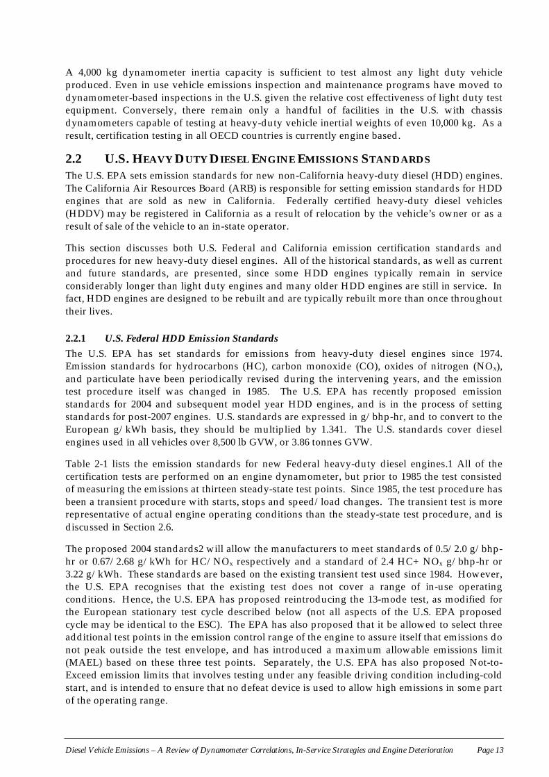
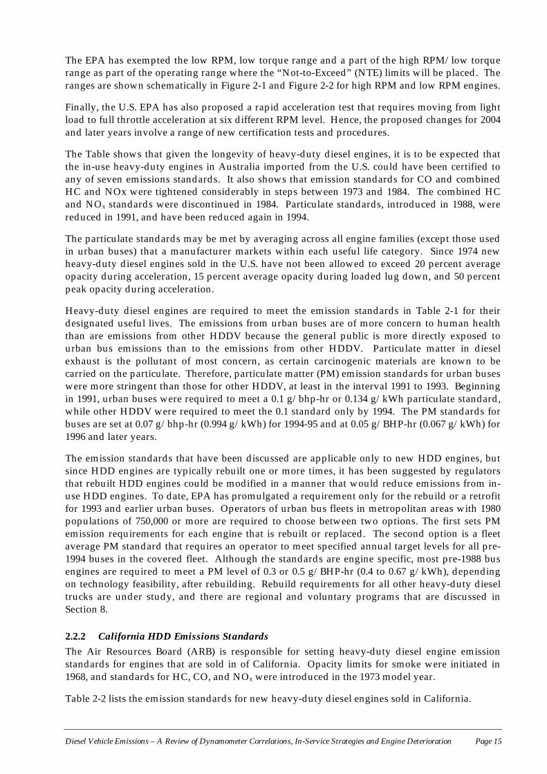
The EPA has exempted the low RPM, low torque range and a part of the high RPM/low torquerange as part of the operating range where the “Not-to-Exceed” (NTE) limits will be placed. Theranges are shown schematically in Figure 2-1 and Figure 2-2 for high RPM and low RPM engines.
Finally, the U.S. EPA has also proposed a rapid acceleration test that requires moving from lightload to full throttle acceleration at six different RPM level. Hence, the proposed changes for 2004and later years involve a range of new certification tests and procedures.
The Table shows that given the longevity of heavy-duty diesel engines, it is to be expected thatthe in-use heavy-duty engines in Australia imported from the U.S. could have been certified toany of seven emissions standards. It also shows that emission standards for CO and combinedHC and NOx were tightened considerably in steps between 1973 and 1984. The combined HCand NOx standards were discontinued in 1984. Particulate standards, introduced in 1988, werereduced in 1991, and have been reduced again in 1994.
The particulate standards may be met by averaging across all engine families (except those usedin urban buses) that a manufacturer markets within each useful life category. Since 1974 newheavy-duty diesel engines sold in the U.S. have not been allowed to exceed 20 percent averageopacity during acceleration, 15 percent average opacity during loaded lug down, and 50 percentpeak opacity during acceleration.
Heavy-duty diesel engines are required to meet the emission standards in Table 2-1 for theirdesignated useful lives. The emissions from urban buses are of more concern to human healththan are emissions from other HDDV because the general public is more directly exposed tourban bus emissions than to the emissions from other HDDV. Particulate matter in dieselexhaust is the pollutant of most concern, as certain carcinogenic materials are known to becarried on the particulate. Therefore, particulate matter (PM) emission standards for urban buseswere more stringent than those for other HDDV, at least in the interval 1991 to 1993. Beginningin 1991, urban buses were required to meet a 0.1 g/bhp-hr or 0.134 g/kWh particulate standard,while other HDDV were required to meet the 0.1 standard only by 1994. The PM standards forbuses are set at 0.07 g/bhp-hr (0.994 g/kWh) for 1994-95 and at 0.05 g/BHP-hr (0.067 g/kWh) for1996 and later years.
The emission standards that have been discussed are applicable only to new HDD engines, butsince HDD engines are typically rebuilt one or more times, it has been suggested by regulatorsthat rebuilt HDD engines could be modified in a manner that would reduce emissions from in-use HDD engines. To date, EPA has promulgated a requirement only for the rebuild or a retrofitfor 1993 and earlier urban buses. Operators of urban bus fleets in metropolitan areas with 1980populations of 750,000 or more are required to choose between two options. The first sets PMemission requirements for each engine that is rebuilt or replaced. The second option is a fleetaverage PM standard that requires an operator to meet specified annual target levels for all pre-1994 buses in the covered fleet. Although the standards are engine specific, most pre-1988 busengines are required to meet a PM level of 0.3 or 0.5 g/BHP-hr (0.4 to 0.67 g/kWh), dependingon technology feasibility, after rebuilding. Rebuild requirements for all other heavy-duty dieseltrucks are under study, and there are regional and voluntary programs that are discussed inSection 8.
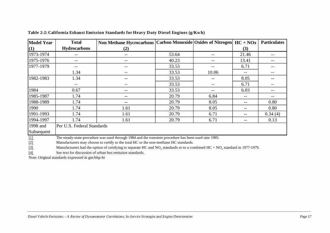
2.2.2 California HDD Emissions StandardsThe Air Resources Board (ARB) is responsible for setting heavy-duty diesel engine emissionstandards for engines that are sold in of California. Opacity limits for smoke were initiated in1968, and standards for HC, CO, and NOx were introduced in the 1973 model year.
Table 2-2 lists the emission standards for new heavy-duty diesel engines sold in California.
Diesel Vehicle Emissions – A Review of Dynamometer Correlations, In-Service Strategies and Engine Deterioration Page 16
Figure 2-1: Proposed NTE Zone for Heavy-Duty Diesel Engines – C Speed < 2400 rpm
Figure 2-2: Proposed NTE Zone for Heavy-Duty Diesel Engines – C Speed > 2400 rpm
Diesel Vehicle Emissions – A Review of Dynamometer Correlations, In-Service Strategies and Engine Deterioration Page 17
Table 2-2: California Exhaust Emission Standards for Heavy Duty Diesel Engines (g/Kwh)
Model Year (1)
Total Hydrocarbons
Non Methane Hycrocarbons (2)
Carbon Monoxide Oxides of Nitrogen HC + NOx (3)
Particulates
1973-1974 -- -- 53.64 -- 21.46 --1975-1976 -- -- 40.23 -- 13.41 --
-- -- 33.53 -- 6.71 --1.34 -- 33.53 10.06 -- --1.34 -- 33.53 -- 8.05 --
-- -- 33.53 -- 6.71 --1984 0.67 -- 33.53 -- 6.03 --1985-1987 1.74 -- 20.79 6.84 -- --1988-1989 1.74 -- 20.79 8.05 -- 0.801990 1.74 1.61 20.79 8.05 -- 0.801991-1993 1.74 1.61 20.79 6.71 -- 0.34 (4)1994-1997 1.74 1.61 20.79 6.71 -- 0.131998 and Subsequent [1] The steady-state procedure was used through 1984 and the transient procedure has been used sine 1985.[2] Manufacturers may choose to certify to the total HC or the non-methane HC standards.[3] Manufacturers had the option of certifying to separate HC and NOx standards or to a combined HC + NOx standard in 1977-1979.[4] See text for discussion of urban bus emission standards.Note: Original standards expressed in gm/bhp-hr
1982-1983
Per U.S. Federal Standards
1977-1979
Diesel Vehicle Emissions – A Review of Dynamometer Correlations, In-Service Strategies and Engine Deterioration Page 18
The exhaust emissions are measured using the same test procedure that EPA uses, the onlydifference being that manufacturers had the option of using the transient test procedurebeginning in 1983 in California. The Table shows that the California standards were generally ayear or more ahead of the Federal standards, but that the Federal and California standards for allpollutants are essentially the same after 1988, and identical after 1998.
The ARB was also directed by the legislature to consider emission control technology, cleanerburning diesel fuels, and alternative fuels as methods that may be used to meet any newemission standards. One technology that has the potential for reduced emissions at relatively lowcost is positive crankcase ventilation (PCV). ARB required that all transit bus engines havepositive crankcase ventilation systems beginning in 1996. In addition, ARB has adopted theFederal transit bus standards for particulate and NOx emissions.
ARB has responded to the legislative requirements for low emission vehicles by adopting aprogram that generates emission reduction credits for low emission retrofits of existing vehiclesor the purchase of low emission transit buses (ARB:1996). Hence, market mechanisms are beingemployed to spur the sales of low emission buses and to rebuild engines to lower emissionstandards. “Low emission” engines can be certified to a range of “credit standards” which are atleast 30 percent lower than the ceiling standard. The ceiling standard is the standard for whichthe engine was originally certified to when first placed in service, or a standard indicated by ARBfor pollutants where no standard existed at the time the engine was placed in service. Forexample, a retrofit of 1987 Heavy Duty Diesel Engine originally certified to a 6.0 g/BHP-hr (8.04g/kWh) NOx standard would have to be at 4.0 g/BHP-hr (5.36 g/kWh) or lower to obtainemission credits. California has specified a credit certification procedure and a calculationprocedure to derive the amount of credit generated by a single retrofit or purchase of a lowemission engine.
California HDT customers would not be required to use engines that meet these low emissionsstandards, but would be encouraged to do so by the existence of NOx emission credit programsthat would be administered by the air quality districts. Bus manufacturers have expressedconcern that few customers will be willing to pay the premium for low emission bus engines thatmanufacturers must charge for low sales volume engines, and consequently, little benefit may begained from the standards.
2.3 EUROPEAN REGULATIONSThe ECE regulations (www.dieselnet.com/standards.html) have been in force since 1982, and theoriginal regulation is referred to as the ECE R49 standard. Europe has always utilised the 13-mode test, a steady-state test conducted on an engine dynamometer, which is very similar to theU.S. 13-mode test utilised for certification before 1984. The 13-mode test continues to be used tothis day. The standard (officially) between 1982 and 1990 was 18.0 g/kWh for NOx, which wassignificantly higher than any U.S. standards in the 1980s.
Although the standards were modified officially in 1990 as part of the 88/77/EEC regulation,German manufacturers had voluntarily undertaken to keep emission levels at least 20 percentbelow ECE R49 from 1987, which compared closely to the 88/77/EEC requirements. It is notclear if other non-German manufacturers participated in the voluntary program. The so-calledEuro I and Euro II standards were introduced in calendar year 1992 and 1996 respectively, withthe Euro III and Euro IV standards planned for 2000 and 2005, respectively. As these standardscome into force in October of the years mentioned, they really apply to model years 1993, 1997,2001 and 2006. There is also a Euro V standard for 2008 and beyond that has been recentlypromulgated.
Diesel Vehicle Emissions – A Review of Dynamometer Correlations, In-Service Strategies and Engine Deterioration Page 19
In addition to the numerical change in emission standards, the ECE R-49 13 mode test cycle (alsodescribed in Section 2.5 and 2.6) is to be changed with the Euro III and later standards. The newprocedure requires two test cycles, one a steady-state cycle called the European Stationary Cycle(ESC), and the second, a transient test called the European Transient Cycle (ETC). These newtests have resulted in standards being more stringent than implied by the numerical valuereduction relative to the Euro II standard. In addition, the Euro III and later standards alsorequire compliance with a smoke test that involves a transient short cycle, called the EuropeanLoad Response cycle. Maximum smoke opacity on this cycle is restricted to 0.7/m for Euro IIIand 0.5/m for Euro IV and V standards.
Table 2-3 shows the European standards through the proposed Euro IV standard for both steadystate and transient (for Euro III and later) tests.
Table 2-3: European Heavy-Duty Engine Emission Standards (g/kWh)
(a) Steady State Cycle
(b) Transient Test
The Euro II standard has a NOx stringency that is approximately similar to the U.S. 1994-1997standard, but the particulate standards are not comparable due to the differences in testprocedure. The Euro III standard is comparable to the U.S. 1988-2003 standard in stringency forthe transient test, while the Euro IV standards are somewhat less stringent for NOx but morestringent for PM relative to the U.S. 2004 standard. Note that both the Euro II and Euro IIIstandards have less stringent PM standards for small diesel engines. The U.S. is planning toimplement a 2007+ standard that may be equal to the Euro V standard, in the interest ofharmonisation.
Regulation HC CO NOx PMECE R49 (15-4-1982) 3.5 14 18 None88/77/EEC (1-10-90)* 2.4 11.2 14.4 None
Euro I (1-10-93) 1.1 4.5 80.61(<85 kw) 0.36 (>85 kw)
Euro II (1-10-96) 1.1 4 7 0.15Euro III (1-10-00)** 0.66 2.1 5 0.10(0.13)a/Euro IV (1-10-05) 0.46 1.5 3.5 0.02Euro V 0.46 1.5 2 0.02
Regulation HC CO NOx PMEuro III 0.78 5.45 5 0.16(0.21)a/Euro IV 0.55 4 3.5 0.03Euro V 0.55 4 2 0.03* Voluntary compliance by German manufacturers since 1987.** Special standards for “environmentally friendly vehicles” of 0.25/1.5/2.0/0.02.a/ For high speed engines with cylinder displacement of <0.75 dm3.
Diesel Vehicle Emissions – A Review of Dynamometer Correlations, In-Service Strategies and Engine Deterioration Page 20
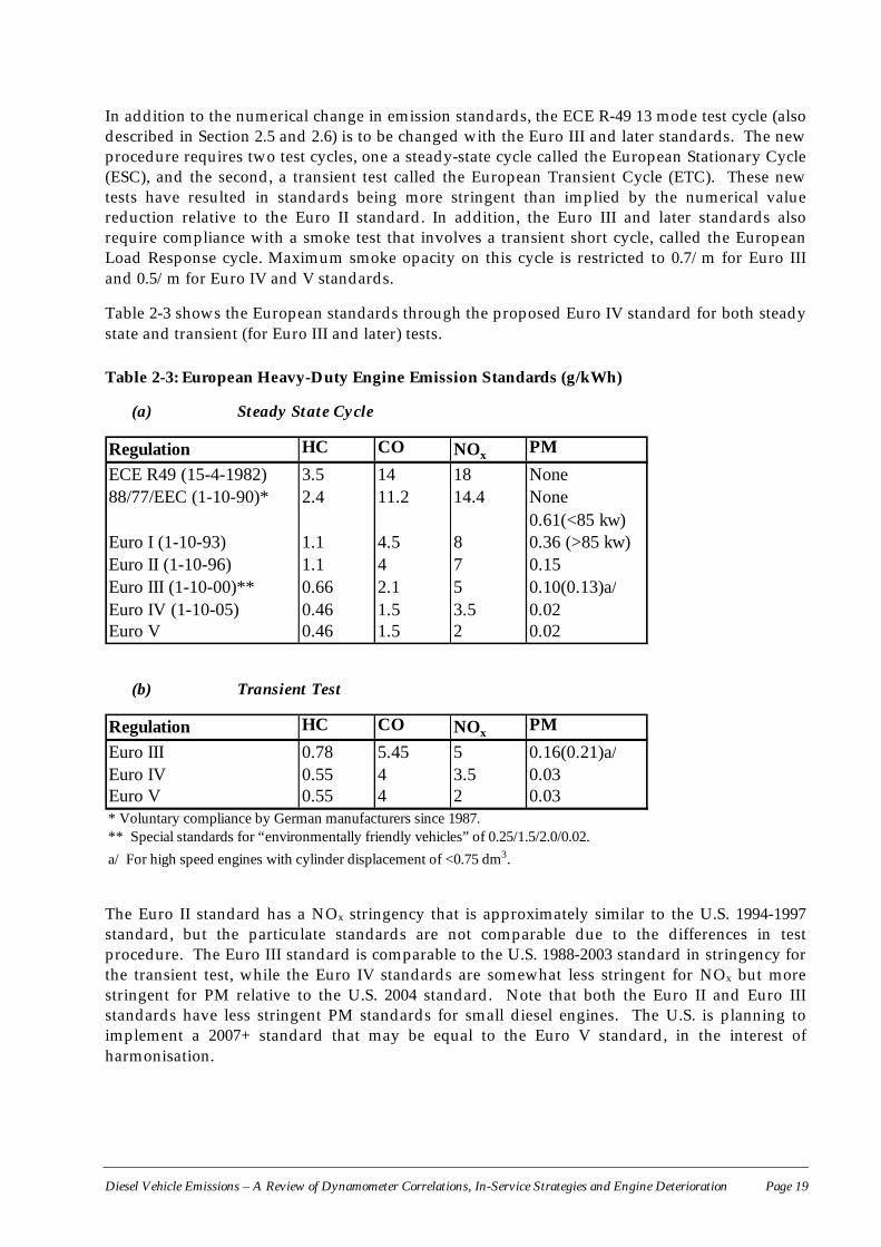
2.4 JAPANESE STANDARDSThe Japanese standards for heavy-duty diesel engines are also based on a 13-mode test cycle,although the modes are defined differently relative to the ECE-R49 test. However, Japanesestandards applicable for the last ten years are quite similar to the Euro II standard for NOx, butare considerably less stringent for PM in numerical terms (SAE:1973).
Since model year 1999, the NOx and PM standards have been reduced considerably, with theNOx standard being somewhat lower numerically than Euro II and the PM standard beingsomewhat higher. However, the Japanese 13-mode cycle has a considerably higher weighting ofthe idle mode (41 percent) so that the numerical values are not readily comparable, especially forPM. It may be that the stringency adjusted for test cycle differences make the current standardsimilar in stringency for NOx and PM to Euro III, since the idle mode contributes to PM but notto NOx. The Japanese standards are shown in Table 2-4. Note the special exemption for lowsales volume engines, as well as the interpretation of standards as a production mean. It shouldalso be noted that Japan is considering reducing standards for all pollutants by 50 percent formodel year 2007 or 2008.
Table 2-4: Japanese Standards For Heavy –Duty Diesel Vehicles (g/kWh, maximum/mean)
Standards prior to this model year (1999) differed between direct injection (DI) and indirectinjection (IDI) diesels. Typically, IDI diesels were used only in relatively small vehicles, (3.5 to 8tons GVW) but since these vehicles are popular in Australia, it may be an issue for consideration.
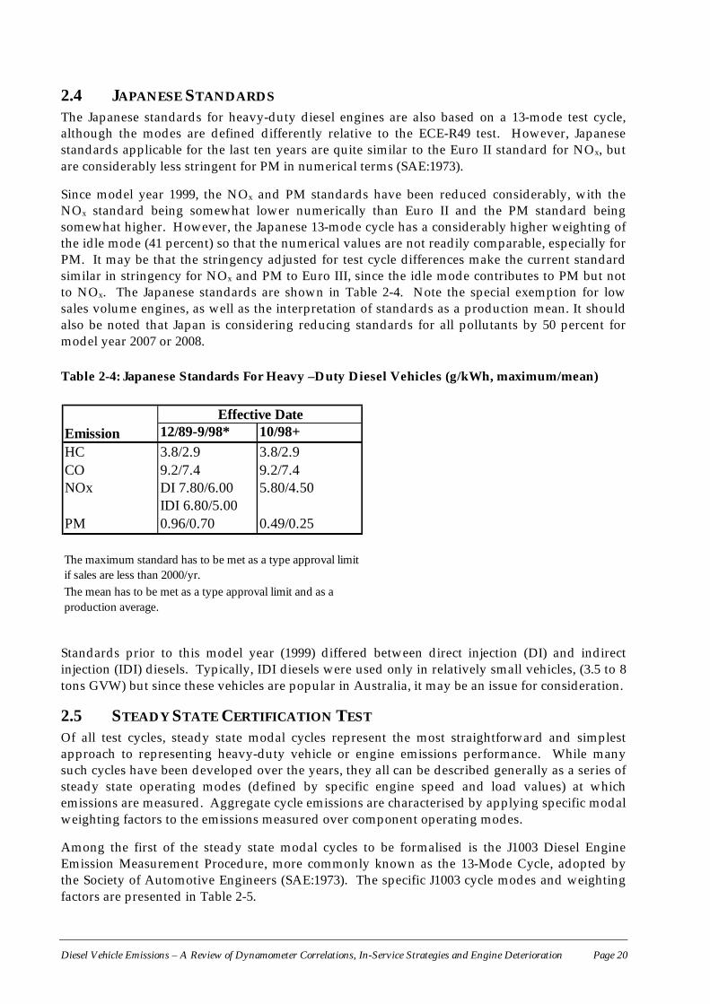
2.5 STEADY STATE CERTIFICATION TESTOf all test cycles, steady state modal cycles represent the most straightforward and simplestapproach to representing heavy-duty vehicle or engine emissions performance. While manysuch cycles have been developed over the years, they all can be described generally as a series ofsteady state operating modes (defined by specific engine speed and load values) at whichemissions are measured. Aggregate cycle emissions are characterised by applying specific modalweighting factors to the emissions measured over component operating modes.
Among the first of the steady state modal cycles to be formalised is the J1003 Diesel EngineEmission Measurement Procedure, more commonly known as the 13-Mode Cycle, adopted bythe Society of Automotive Engineers (SAE:1973). The specific J1003 cycle modes and weightingfactors are presented in Table 2-5.
12/89-9/98* 10/98+HC 3.8/2.9 3.8/2.9CO 9.2/7.4 9.2/7.4NOx DI 7.80/6.00
IDI 6.80/5.005.80/4.50
PM 0.96/0.70 0.49/0.25
Effective DateEmission
The maximum standard has to be met as a type approval limit if sales are less than 2000/yr.The mean has to be met as a type approval limit and as a production average.
Diesel Vehicle Emissions – A Review of Dynamometer Correlations, In-Service Strategies and Engine Deterioration Page 21
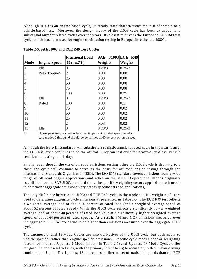
Although J1003 is an engine-based cycle, its steady state characteristics make it adaptable to avehicle-based test. Moreover, the design theory of the J1003 cycle has been extended to asubstantial number related cycles over the years. Its closest relative is the European ECE R49 testcycle, which has been used for engine certification testing in Europe since the late 1980’s.
Table 2-5: SAE J1003 and ECE R49 Test Cycles
Although the Euro III standards will substitute a realistic transient based cycle in the near future,the ECE R49 cycle continues to be the official European test cycle for heavy-duty diesel vehiclecertification testing to this day.
Finally, even though the era of on road emissions testing using the J1003 cycle is drawing to aclose, the cycle will continue to serve as the basis for off road engine testing through theInternational Standards Organisation (ISO). The ISO 8178 standard covers emissions from a widerange of off road engine applications and relies on the same 13 operational modes originallyestablished for the SAE J1003 standard (only the specific weighting factors applied to each modeto determine aggregate emissions vary across specific off road applications).
The only difference between the J1003 and ECE R49 cycles is the mode specific weighting factorsused to determine aggregate cycle emissions as presented in Table 2-5. The ECE R49 test reflectsa weighted average load of about 50 percent of rated load (and a weighted average speed ofabout 52 percent of rated speed). While the J1003 cycle reflects a significantly lower weightedaverage load of about 40 percent of rated load (but at a significantly higher weighted averagespeed of about 64 percent of rated speed). As a result, PM and NOx emissions measured overthe aggregate ECE R49 cycle tend to be higher than emissions measured over the aggregate J1003cycle.
The Japanese 6- and 13-Mode Cycles are also derivatives of the J1003 cycle, but both apply tovehicle specific, rather than engine specific emissions. Specific cycle modes and/or weightingfactors for both the Japanese 6-Mode (shown in Table 2-7) and Japanese 13-Mode Cycles differfor gasoline and diesel vehicles, with the primary intent being to accurately reflect urban drivingconditions in Japan. The Japanese 13-mode uses a different set of loads and speeds than the ECE
Mode Engine SpeedFractional Load (%, ±2%)
SAE J1003Weights
ECE R49Weights
1 Idle 0 0.20/3 0.25/32 Peak Torque* 2 0.08 0.083 25 0.08 0.084 50 0.08 0.085 75 0.08 0.086 100 0.08 0.257 Idle 0 0.20/3 0.25/38 Rated 100 0.08 0.19 75 0.08 0.0210 50 0.08 0.0211 25 0.08 0.0212 2 0.08 0.0213 Idle 0 0.20/3 0.25/3* Unless peak torque speed is less than 60 percent of rated speed, in which
case modes 2 through 6 should be performed at 60 percent of rated speed.
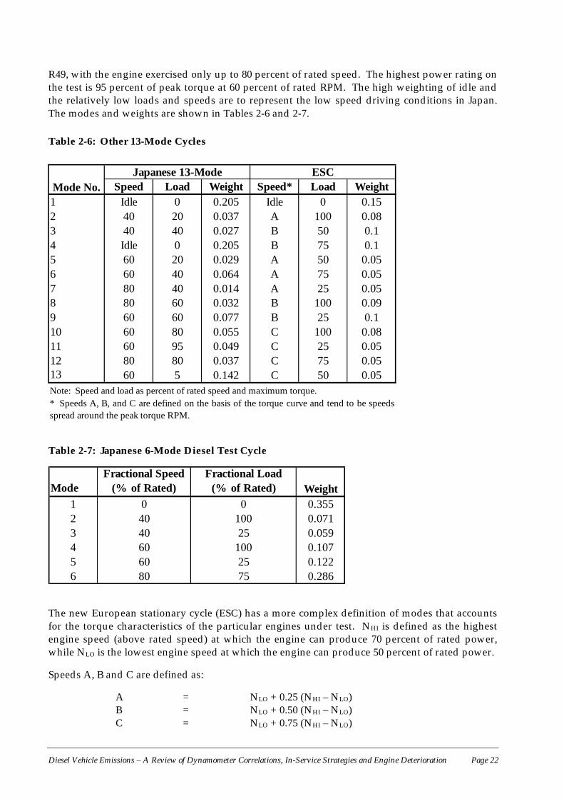
Diesel Vehicle Emissions – A Review of Dynamometer Correlations, In-Service Strategies and Engine Deterioration Page 22
R49, with the engine exercised only up to 80 percent of rated speed. The highest power rating onthe test is 95 percent of peak torque at 60 percent of rated RPM. The high weighting of idle andthe relatively low loads and speeds are to represent the low speed driving conditions in Japan.The modes and weights are shown in Tables 2-6 and 2-7.
Table 2-6: Other 13-Mode Cycles
Table 2-7: Japanese 6-Mode Diesel Test Cycle
The new European stationary cycle (ESC) has a more complex definition of modes that accountsfor the torque characteristics of the particular engines under test. NHI is defined as the highestengine speed (above rated speed) at which the engine can produce 70 percent of rated power,while NLO is the lowest engine speed at which the engine can produce 50 percent of rated power.
Speeds A, B and C are defined as:
A = NLO + 0.25 (NHI – NLO)B = NLO + 0.50 (NHI – NLO)C = NLO + 0.75 (NHI – NLO)
ModeFractional Speed
(% of Rated)Fractional Load
(% of Rated) Weight1 0 0 0.3552 40 100 0.0713 40 25 0.0594 60 100 0.1075 60 25 0.1226 80 75 0.286
Speed Load Weight Speed* Load Weight1 Idle 0 0.205 Idle 0 0.152 40 20 0.037 A 100 0.083 40 40 0.027 B 50 0.14 Idle 0 0.205 B 75 0.15 60 20 0.029 A 50 0.056 60 40 0.064 A 75 0.057 80 40 0.014 A 25 0.058 80 60 0.032 B 100 0.099 60 60 0.077 B 25 0.110 60 80 0.055 C 100 0.0811 60 95 0.049 C 25 0.0512 80 80 0.037 C 75 0.0513 60 5 0.142 C 50 0.05Note: Speed and load as percent of rated speed and maximum torque.* Speeds A, B, and C are defined on the basis of the torque curve and tend to be speedsspread around the peak torque RPM.
Japanese 13-Mode ESCMode No.
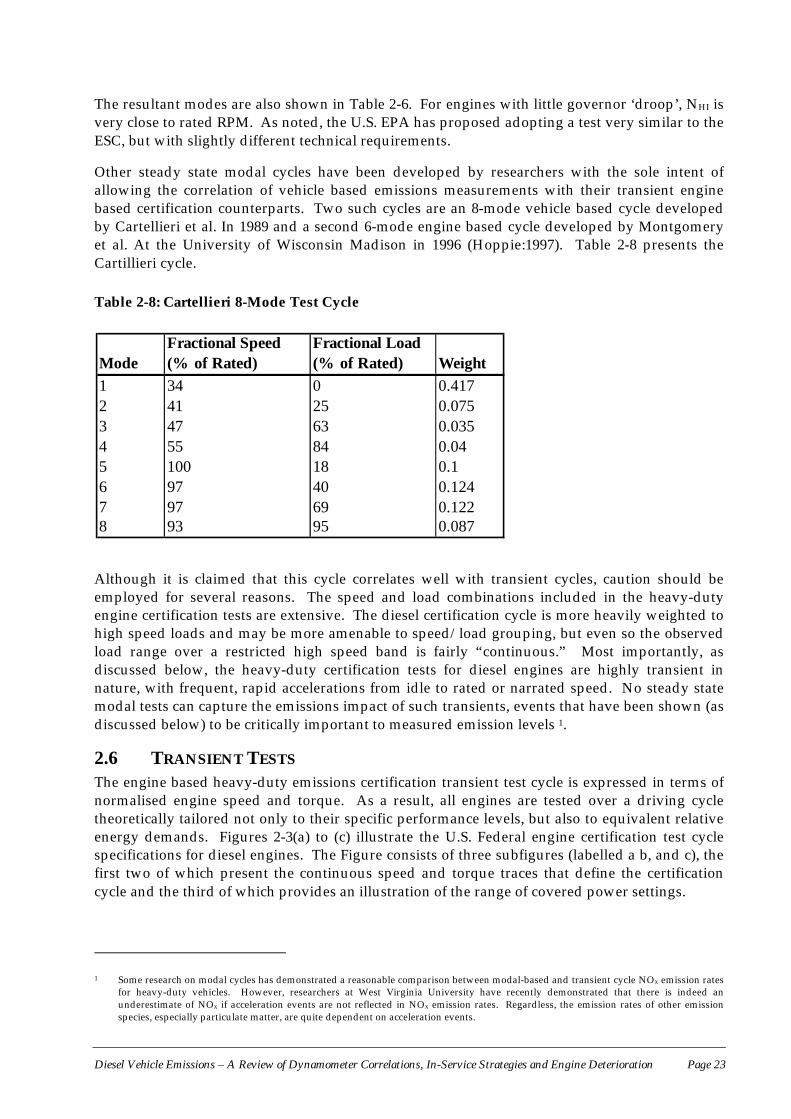
Diesel Vehicle Emissions – A Review of Dynamometer Correlations, In-Service Strategies and Engine Deterioration Page 23
The resultant modes are also shown in Table 2-6. For engines with little governor ‘droop’, NHI isvery close to rated RPM. As noted, the U.S. EPA has proposed adopting a test very similar to theESC, but with slightly different technical requirements.
Other steady state modal cycles have been developed by researchers with the sole intent ofallowing the correlation of vehicle based emissions measurements with their transient enginebased certification counterparts. Two such cycles are an 8-mode vehicle based cycle developedby Cartellieri et al. In 1989 and a second 6-mode engine based cycle developed by Montgomeryet al. At the University of Wisconsin Madison in 1996 (Hoppie:1997). Table 2-8 presents theCartillieri cycle.
Table 2-8: Cartellieri 8-Mode Test Cycle
Although it is claimed that this cycle correlates well with transient cycles, caution should beemployed for several reasons. The speed and load combinations included in the heavy-dutyengine certification tests are extensive. The diesel certification cycle is more heavily weighted tohigh speed loads and may be more amenable to speed/load grouping, but even so the observedload range over a restricted high speed band is fairly “continuous.” Most importantly, asdiscussed below, the heavy-duty certification tests for diesel engines are highly transient innature, with frequent, rapid accelerations from idle to rated or narrated speed. No steady statemodal tests can capture the emissions impact of such transients, events that have been shown (asdiscussed below) to be critically important to measured emission levels 1.
2.6 TRANSIENT TESTSThe engine based heavy-duty emissions certification transient test cycle is expressed in terms ofnormalised engine speed and torque. As a result, all engines are tested over a driving cycletheoretically tailored not only to their specific performance levels, but also to equivalent relativeenergy demands. Figures 2-3(a) to (c) illustrate the U.S. Federal engine certification test cyclespecifications for diesel engines. The Figure consists of three subfigures (labelled a b, and c), thefirst two of which present the continuous speed and torque traces that define the certificationcycle and the third of which provides an illustration of the range of covered power settings.
1 Some research on modal cycles has demonstrated a reasonable comparison between modal-based and transient cycle NOx emission rates
for heavy-duty vehicles. However, researchers at West Virginia University have recently demonstrated that there is indeed anunderestimate of NOx if acceleration events are not reflected in NOx emission rates. Regardless, the emission rates of other emissionspecies, especially particulate matter, are quite dependent on acceleration events.
ModeFractional Speed(% of Rated)
Fractional Load(% of Rated) Weight
1 34 0 0.4172 41 25 0.0753 47 63 0.0354 55 84 0.045 100 18 0.16 97 40 0.1247 97 69 0.1228 93 95 0.087

Diesel Vehicle Emissions – A Review of Dynamometer Correlations, In-Service Strategies and Engine Deterioration Page 24
The Federal certification cycle is actually defined in discrete one second intervals. In subfigures(a) and (b), these one second intervals have simply been linearly connected to produce acontinuous trace (as is common practice for all driving cycle development), while subfigures (c)present only the discrete one second power settings which actually define the certification cycle.Therefore, each of the power setting markers depicted in subfigure (c ) represents an equal timeperiod of one second. The total cycle time spent at any restricted range of power settings isindicated by the clustering of discrete one second markers.
The EPA engine transient cycle was derived from a detailed study of actual truck driving habitsusing instrumented trucks operating in New York and Los Angeles. The data collected wasanalysed statistically, and a cycle was derived that captures the most common drivingcharacteristics. The U.S. transient cycle has three segments:
• the New York city cycle with an average speed of 11.74 km/hr;• the Los Angeles non-freeway cycle with a speed of 27.0 km/hr;• the Los Angeles freeway cycle with a speed 75.34 km/hr.
Engine manufacturers have complained that the statistical analysis combined data fromdissimilar vehicles and some of the transients in the cycle cannot be observed in real life.
Figure 2-4(a) and (b) show the density plots for the new European Transient Cycle (ETC) versusthe U.S. cycle (TUV:1995), and it seems that this cycle has a wider representation of loads andengine speeds than the U.S. Transient Cycle. The ETC also has three segments:
• a city segment with an average speed of 50 km/hr, and frequent stops;• a rural driving segment with hard accelerations and average speeds of 72 km/hr;• a highway segment with an average speed of 88 km/hr.
Broadly speaking, the ETC is quite similar in concept to the U.S. Transient Cycle. Recent testinghas shown that emission results from the two tests are correlated, and the wider speed/loadranges encountered in the ETC typically increase HC, CO and PM emission relative to thosemeasured on the U.S. cycle.
Because the certification cycles are defined on the basis of maximum test engine speed andtorque, a larger engine will be “exercised” to the same extent over the certification test cycle as asmaller engine (i.e., the load factor for the certification test is constant across test engines).However, both engines may be used in vehicles with similar in-use duty cycles.

Diesel Vehicle Emissions – A Review of Dynamometer Correlations, In-Service Strategies and Engine Deterioration Page 25
Figure 2-3: Federal Test Procedure for Heavy-Duty Diesel Engines
a)
b)
c)
-10
0
10
20
30
40
50
60
70
80
90
100
110
120
0 120 240 360 480 600 720 840 960 1080Time (Seconds)
Perc
ent o
f Max
Tor
que
Negative torque values indicate periods of closed rack motoring.
-10
0
1020
3040
5060
70
80
90100
110120
-10 0 10 20 30 40 50 60 70 80 90 100 110 120
Percent of Rated Speed
Perc
ent o
f Max
Tor
que
Negative torque values indicate periods of closed rack motoring.
-100
102030405060708090
100110120
0 120 240 360 480 600 720 840 960 1080
Time (Seconds)
Perc
ent o
f Rat
ed E
ngin
e Sp
eed
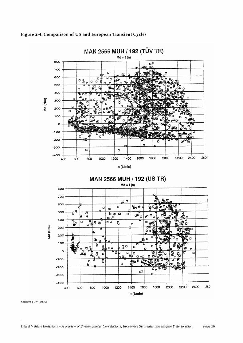
Diesel
Figure 2-4: Comparison of US and European Transient Cycles
Source
Vehicle Emissions – A Review of Dynamometer Correlations, In-Service Strategies and Engine Deterioration Page 26
: TUV (1995)
Diesel Vehicle Emissions – A Review of Dynamometer Correlations, In-Service Strategies and Engine Deterioration Page 27
In such a case, the smaller engine may indeed experience in-use operational characteristicssimilar to those of the certification test, while the larger engine typically operates at substantiallylower power demands (and, all other factors being equal, at emission rates lower than implied bythe engine certification test). In contrast, light duty vehicles are certified over a transient drivingcycle that is the same for all test vehicles. Overpowered vehicles will work less over the testcycle than “underpowered” vehicles and, as long as the cycle itself is representative of in-useoperations, the real world emission rates of the two engines (ignoring such issues asdeterioration, mal-maintenance, and tampering) will be described in a proper relative sense.
Further confounding the translation of engine specific to vehicle specific emission rates is theneed to consider such issues as gearing ratios and power losses between the vehicle engine andits drive wheels. Engine specific emission rates, unaffected by drivetrain issues, are expressed inmass per unit of engine work (typically grams per brake horsepower-hour or per kWh). Avehicle specific conversion factor which considers drivetrain impacts in expressing engine workrequired per unit distance travelled (typically brake horsepower-hour or kWh per mile) cantheoretically be developed to generate the mass per unit distance (typically grams per mile)emission rate commonly used to assess vehicle specific emissions performance. However, whilesuch a conversion factor can be developed from brake specific fuel consumption (BSFC), fueldensity, and fuel economy measurements, research has shown (not surprisingly) that two ofthese vehicles related parameters vary with operating mode. The issues are discussed in Section4 of this report.
Diesel Vehicle Emissions – A Review of Dynamometer Correlations, In-Service Strategies and Engine Deterioration Page 28
3 CHASSIS TEST CYCLES
3.1 OVERVIEWTesting of heavy-duty trucks, as opposed to engines, has been very limited around the world,largely because chassis dynamometers capable of handing trucks in excess of 5,000 kg loadedweight are quite rare. For example, even in the U.S. where there has been truck testingconducted for over 30 years, there are currently only four facilities capable of conductingtransient cycle tests on trucks with an inertia weight of over 8,000 kg. The number in Europe issimilarly small, and only two of the facilities have the capability of conducting full scale transienttests. Japan has only one such facility and there are none in Australia. As a result, the test cyclesand test procedures are in a state of infancy relative to the highly developed test procedures forlight-duty vehicles, whose inertia weights are typically in the 1,000 to 2,000 kg range. In thiscontext, the same issues are not present for light-duty vehicles since the certification test isspecified as a chassis dynamometer test, and the certification test can be performed by numerouslaboratories in Australia. Moreover, the test is identical for light-duty diesel and gasolinevehicles, although diesels must also certify to a smoke test in EU countries.
There has been virtually no interest in the U.S. in replicating the 13-mode engine steady state teston a chassis dynamometer in the U.S. since it was known since the late 1970s that the test wouldnot be used for certification after 1984. Hence, virtually all of the data on tests conducted usingthe 13-mode cycle on a chassis dynamometer has been from Europe.
Transient test cycles are of two types: first the “geometric” cycles that have been used historicallyto test trucks and buses, and second, the “realistic” cycles that are now in use in the U.S. Thesecycles are discussed below in the context of a chassis dynamometer based test.
3.2 STEADY-STATE 13-MODE TESTSubstantial work towards the development of a chassis version of the 13-mode enginecertification test has been conducted in Europe. In principle, the steady state test is relativelysimple to perform, as the engine speed and load must be held steady at ten specified speed/loadpoints, and three idle points. While engine speed can be easily measured off the tachometer, thedetermination of engine load other than rated maximum is difficult on a chassis dynamometer.
In the European project “Diesel-controle methode” (Van Gompel and Verbech:1993), ameasuring method was developed to carry out a 13-mode test with heavy-duty diesel engines ona chassis dynamometer. A description of this optimised measuring method follows, and theactivities for this measuring method must be carried out in the order described below.
Vehicle Instrumentation
The vehicle must be instrumented to measure:
• engine speed;• exhaust gas back pressure;• inlet depression;• fuel, oil and constant temperature;• exhaust gas temperature.
The test also requires use of certification quality diesel fuel if the results are to be compared tocertification tests.
Diesel Vehicle Emissions – A Review of Dynamometer Correlations, In-Service Strategies and Engine Deterioration Page 29
Adjustment of Rear Axle Weight
After completion of the instrumentation, the vehicle is placed on the chassis dynamometer, andthe optimum axle weight is set. By means of a lifter or a pull-down device, the unloaded wheelpressure is lowered or raised, in order to achieve the optimum axle weight. This optimum axleweight ensures that the sum of rolling resistance losses and slippage losses is minimal, so thatheat development in the tyres is limited during the 13-mode test.
Determination of Dynamic Wheel Radius
After the optimum axle weight has been established, the average dynamic wheel radius isdetermined. This is done by driving without any load in all gears at an engine speedcorresponding to the intermediate speed. The speed of the rollers is used to determine thedynamic wheel radius for each separate gear. The average dynamic wheel radius is thencompared with the static wheel radius. In this way, the specified ratios of the transmission andrear axle are checked whether they match the actual transmission ratios.
Power Measurement/Lambda Check
After the complete vehicle has been warmed up on the chassis dynamometer, a powermeasurement and Lambda check are carried out. At three RPM test-points of the 13-mode test(idle, MT-100 and MR-100) all the parameters are measured which are also measured in the 13-mode test. (The test RPM of these three test points can be obtained from the type-approvalcertificate). Using the measured values, the Lambda is calculated at each test point on the basisof air/fuel consumption and from the composition of the exhaust gas emission. If the Lambdavalues between the two full-load test points deviate by more than five percent, this points to apossible leak in the inlet or exhaust sections. After any fault has been rectified, a new checkmeasurement is carried out. If the differences between the Lambda values are below fivepercent, the calculated engine power is compared with the type-approval documentation. For anengine power which is too low in MR-100 (difference less than five percent), the full-load curve isredefined in order to determine the test speeds for the 13-mode test. By means of the calculatedengine power at MT-100 and MR-100, the test settings for the individual modes are determined.
During the course of the European in use compliance program (1994-1995) the number of testpoints for the values measured was increased. On the one hand, these steps were taken to makea more precise determination of any deviations or malfunctions in engine behaviour possible soas to facilitate discovery of the cause of the deviations. On the other hand, the Lambda checkwas used to permit comparison with the type-approval test. In this way conditions identical tothe type-approval test has been achieved in practically all cases.
Chassis Dynamometer Setting
From the measured engine power at MT-100 and MR-100, the settings are determined for the 13-mode test. For each mode-point the optimum gear ratio is determined, at which heatdevelopment in the tyres is minimal. In order to avoid damage to the truck’s own tyres, butmore specifically since the rolling resistance of these tyres is unknown, separate wheels with testtyres are mounted. The test tyres should have known rolling resistance coefficients measuredfrom tests. Subsequently, the optimum gear ratio is approached by selecting the correct gear.Using this transmission ratio the driving speed is calculated, as well as the corresponding brakeforce per mode-point. Due to the technical limitations of a specific chassis dynamometer, insome cases a different transmission ratio must be chosen. The driving speed and thecorresponding brake force are then re-determined. For trucks provided with a low and a highgearing, all the chosen speeds must be in the same gear.
Diesel Vehicle Emissions – A Review of Dynamometer Correlations, In-Service Strategies and Engine Deterioration Page 30
Emissions Measurement
Emissions measurements are carried out in accordance with the procedures for the engine based13-mode test. This involves adjusting the exhaust back pressure and exhaust split into thedilution tunnel for PM sampling. The load for each mode is adjusted to match specificationswithin one minute, and each test point is held for at least five minutes. Particulate emissions aremeasured towards the end of the five minute period, with the sampling time proportional to theweighting of each mode. Final results for gaseous emission are calculated based on each modesresults, weighted by the appropriate factors.
These methods have been found to yield results that correspond well with engine based 13-modetests.
3.3 GEOMETRIC TEST CYCLESGeometric (or stylised) test cycles for heavy duty vehicle testing have been in existence for twodecades or more. Generally these cycles are characterised by a one or more series of idle,acceleration, steady state cruise, and deceleration events that when presented in terms of speedversus cycle time or speed versus cycle distance produce cycle traces that are basically geometric(often sawtooth like) in shape. In effect, these cycles do include a treatment of transient (i.e.,acceleration based) emissions events that are omitted from the steady state modal cyclesdiscussed above, but such treatment is most often simplistic in nature and cannot really beviewed as reflective of anything but a very general representation of in-use operationalcharacteristics.
The primary rationale for this simplistic treatment can be traced to the fact that these cycles weredesigned for either test track or on road application (heavy duty chassis dynamometer setupswere not common when most of these cycles were developed and neither are they today).Nevertheless, a substantial number of geometric cycles have been developed for a wide range ofheavy-duty vehicle applications and the majority of in use emissions research conducted over thelast several years has been based on the use of one or more of these cycles.
Perhaps the best place to begin a review of geometric test cycles is, as was the case for modalcycles, with the handbook of SAE standards. SAE standard J1376 includes a series of cyclesdesigned to determine heavy-duty truck and bus fuel economy. While emissions measurementwas not a central focus of J1376 development, the J1376 cycles have probably been used moreoften in support of in use heavy-duty vehicle emissions testing than any other emissions testcycle. In fact, one component of SAE J1376, the Central Business District (CBD) portion of theTransit Coach Design Operating Cycle (TCDOC) is probably the most widely used in use heavyduty vehicle emissions test of the last 15 years (excluding simplified smoke measurement tests).The fact that these cycles were not explicitly designed for emissions evaluation is not significant.The issues of importance to emissions researchers were ones of cycle standardisation and aperception of reasonable, if not absolute, consistency between the test cycle and actual vehicleoperating cycles. While this latter presumption is certainly not accurate given the generalisednature of the geometric cycles and even the former presumption is questionable for reasonswhich are discussed in more detail below, the perceived standardisation and lack of betteralternative cycles has led to widespread use of (at least some of) the J1376 cycles.
Figure 3-1 presents the SAE J1376 Long Haul Test Cycle. As is obvious, this cycle is intended toreflect interstate highway operation and is composed of two repetitions of a sub cycle consistingof wide-open throttle (WOT) acceleration from zero to 55 miles per hour (mph), immediatelyfollowed by a steady state cruise at 55 mph through a distance of 14.79 miles and acoasting/braking deceleration applied to bring the vehicle back to a speed of zero mph at a
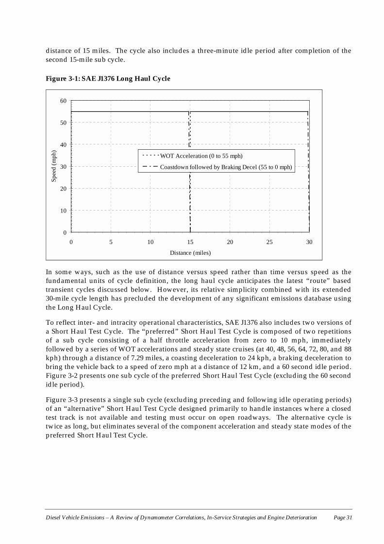
Diesel Vehicle Emissions – A Review of Dynamometer Correlations, In-Service Strategies and Engine Deterioration Page 31
distance of 15 miles. The cycle also includes a three-minute idle period after completion of thesecond 15-mile sub cycle.
Figure 3-1: SAE J1376 Long Haul Cycle
0
10
20
30
40
50
60
0 5 10 15 20 25 30
Distance (miles)
Spee
d (m
ph)
WOT Acceleration (0 to 55 mph)
Coastdown followed by Braking Decel (55 to 0 mph)
In some ways, such as the use of distance versus speed rather than time versus speed as thefundamental units of cycle definition, the long haul cycle anticipates the latest “route” basedtransient cycles discussed below. However, its relative simplicity combined with its extended30-mile cycle length has precluded the development of any significant emissions database usingthe Long Haul Cycle.
To reflect inter- and intracity operational characteristics, SAE J1376 also includes two versions ofa Short Haul Test Cycle. The “preferred” Short Haul Test Cycle is composed of two repetitionsof a sub cycle consisting of a half throttle acceleration from zero to 10 mph, immediatelyfollowed by a series of WOT accelerations and steady state cruises (at 40, 48, 56, 64, 72, 80, and 88kph) through a distance of 7.29 miles, a coasting deceleration to 24 kph, a braking deceleration tobring the vehicle back to a speed of zero mph at a distance of 12 km, and a 60 second idle period.Figure 3-2 presents one sub cycle of the preferred Short Haul Test Cycle (excluding the 60 secondidle period).
Figure 3-3 presents a single sub cycle (excluding preceding and following idle operating periods)of an “alternative” Short Haul Test Cycle designed primarily to handle instances where a closedtest track is not available and testing must occur on open roadways. The alternative cycle istwice as long, but eliminates several of the component acceleration and steady state modes of thepreferred Short Haul Test Cycle.
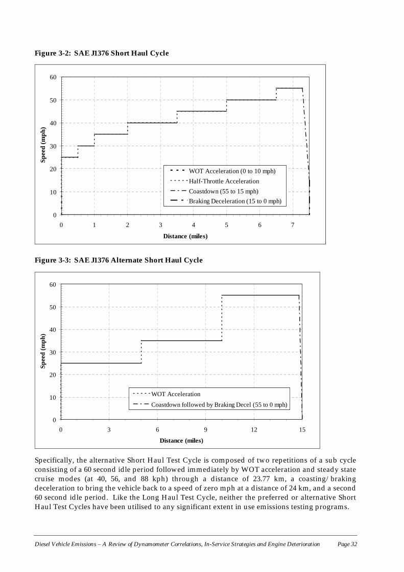
Diesel Vehicle Emissions – A Review of Dynamometer Correlations, In-Service Strategies and Engine Deterioration Page 32
Figure 3-2: SAE J1376 Short Haul Cycle
0
10
20
30
40
50
60
0 1 2 3 4 5 6 7
Distance (miles)
Spee
d (m
ph)
WOT Acceleration (0 to 10 mph)Half-Throttle AccelerationCoastdown (55 to 15 mph)Braking Deceleration (15 to 0 mph)
Figure 3-3: SAE J1376 Alternate Short Haul Cycle
0
10
20
30
40
50
60
0 3 6 9 12 15
Distance (miles)
Spee
d (m
ph)
WOT Acceleration
Coastdown followed by Braking Decel (55 to 0 mph)
Specifically, the alternative Short Haul Test Cycle is composed of two repetitions of a sub cycleconsisting of a 60 second idle period followed immediately by WOT acceleration and steady statecruise modes (at 40, 56, and 88 kph) through a distance of 23.77 km, a coasting/brakingdeceleration to bring the vehicle back to a speed of zero mph at a distance of 24 km, and a second60 second idle period. Like the Long Haul Test Cycle, neither the preferred or alternative ShortHaul Test Cycles have been utilised to any significant extent in use emissions testing programs.
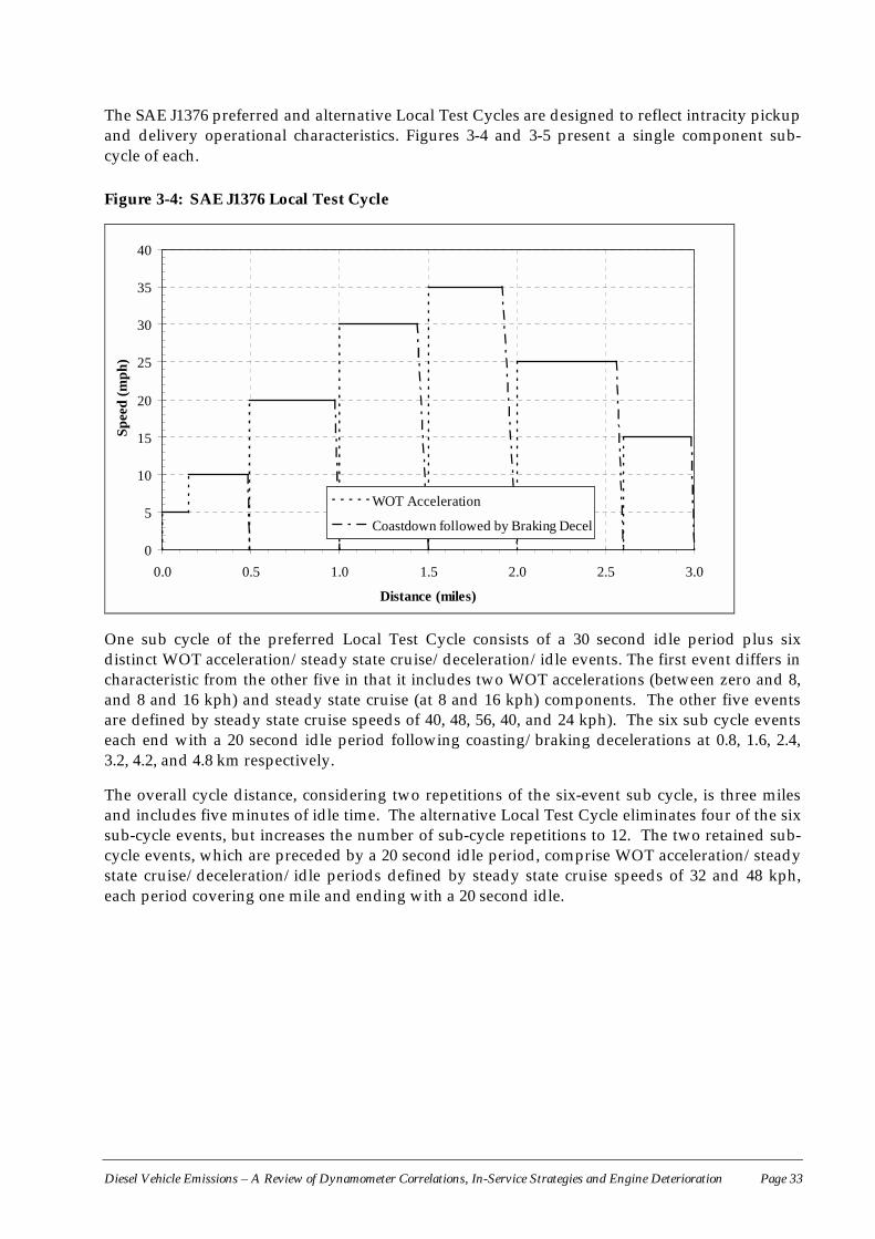
Diesel Vehicle Emissions – A Review of Dynamometer Correlations, In-Service Strategies and Engine Deterioration Page 33
The SAE J1376 preferred and alternative Local Test Cycles are designed to reflect intracity pickupand delivery operational characteristics. Figures 3-4 and 3-5 present a single component sub-cycle of each.
Figure 3-4: SAE J1376 Local Test Cycle
0
5
10
15
20
25
30
35
40
0.0 0.5 1.0 1.5 2.0 2.5 3.0
Distance (miles)
Spee
d (m
ph)
WOT Acceleration
Coastdown followed by Braking Decel
One sub cycle of the preferred Local Test Cycle consists of a 30 second idle period plus sixdistinct WOT acceleration/steady state cruise/deceleration/idle events. The first event differs incharacteristic from the other five in that it includes two WOT accelerations (between zero and 8,and 8 and 16 kph) and steady state cruise (at 8 and 16 kph) components. The other five eventsare defined by steady state cruise speeds of 40, 48, 56, 40, and 24 kph). The six sub cycle eventseach end with a 20 second idle period following coasting/braking decelerations at 0.8, 1.6, 2.4,3.2, 4.2, and 4.8 km respectively.
The overall cycle distance, considering two repetitions of the six-event sub cycle, is three milesand includes five minutes of idle time. The alternative Local Test Cycle eliminates four of the sixsub-cycle events, but increases the number of sub-cycle repetitions to 12. The two retained sub-cycle events, which are preceded by a 20 second idle period, comprise WOT acceleration/steadystate cruise/deceleration/idle periods defined by steady state cruise speeds of 32 and 48 kph,each period covering one mile and ending with a 20 second idle.
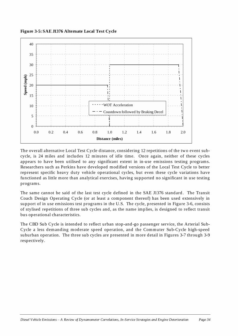
Diesel Vehicle Emissions – A Review of Dynamometer Correlations, In-Service Strategies and Engine Deterioration Page 34
Figure 3-5: SAE J1376 Alternate Local Test Cycle
0
5
10
15
20
25
30
35
40
0.0 0.2 0.4 0.6 0.8 1.0 1.2 1.4 1.6 1.8 2.0
Distance (miles)
Spee
d (m
ph)
WOT Acceleration
Coastdown followed by Braking Decel
The overall alternative Local Test Cycle distance, considering 12 repetitions of the two event sub-cycle, is 24 miles and includes 12 minutes of idle time. Once again, neither of these cyclesappears to have been utilised to any significant extent in in-use emissions testing programs.Researchers such as Perkins have developed modified versions of the Local Test Cycle to betterrepresent specific heavy duty vehicle operational cycles, but even these cycle variations havefunctioned as little more than analytical exercises, having supported no significant in use testingprograms.
The same cannot be said of the last test cycle defined in the SAE J1376 standard. The TransitCoach Design Operating Cycle (or at least a component thereof) has been used extensively insupport of in use emissions test programs in the U.S. The cycle, presented in Figure 3-6, consistsof stylised repetitions of three sub cycles and, as the name implies, is designed to reflect transitbus operational characteristics.
The CBD Sub Cycle is intended to reflect urban stop-and-go passenger service, the Arterial Sub-Cycle a less demanding moderate speed operation, and the Commuter Sub-Cycle high-speedsuburban operation. The three sub cycles are presented in more detail in Figures 3-7 through 3-9respectively.
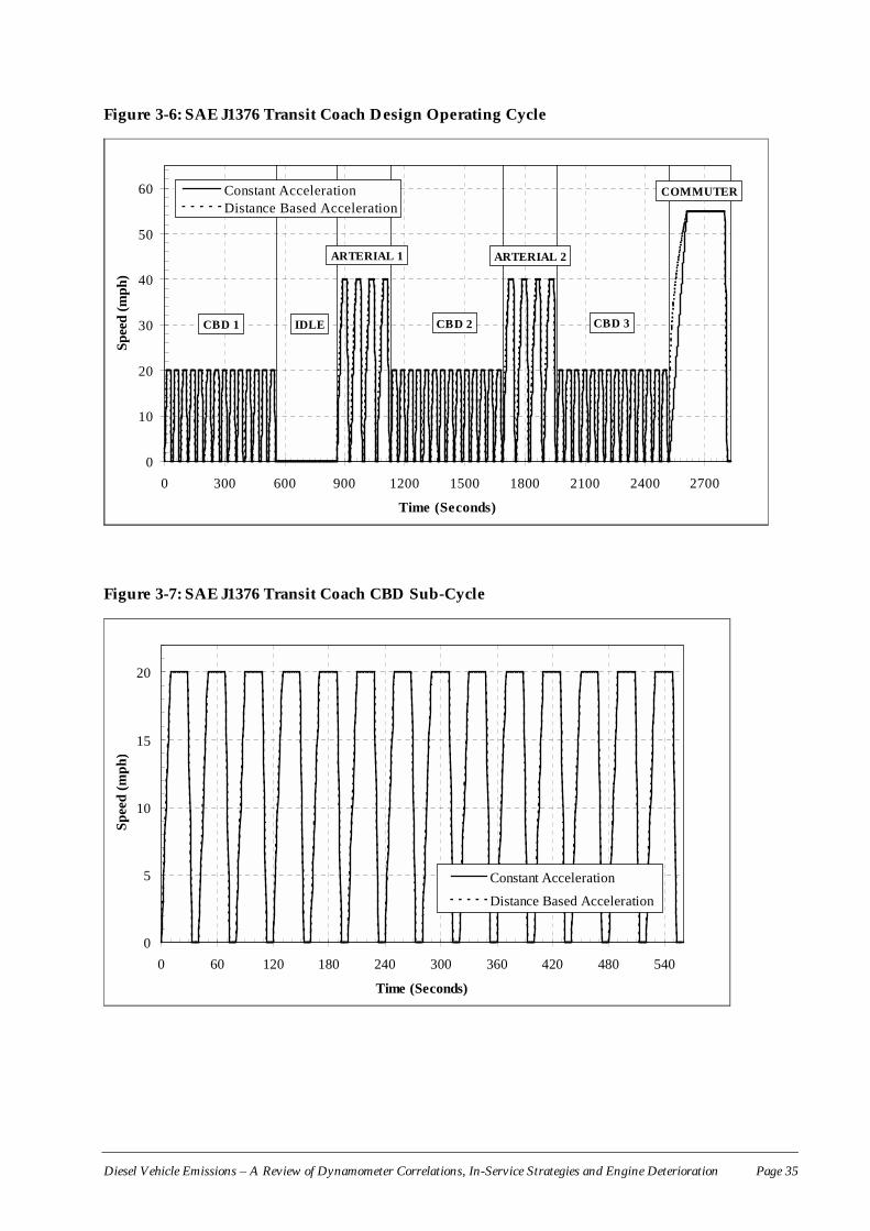
Diesel Vehicle Emissions – A Review of Dynamometer Correlations, In-Service Strategies and Engine Deterioration Page 35
Figure 3-6: SAE J1376 Transit Coach Design Operating Cycle
0
10
20
30
40
50
60
0 300 600 900 1200 1500 1800 2100 2400 2700
Time (Seconds)
Spee
d (m
ph)
Constant AccelerationDistance Based Acceleration
CBD 1 CBD 2 CBD 3IDLE
ARTERIAL 1 ARTERIAL 2
COMMUTER
Figure 3-7: SAE J1376 Transit Coach CBD Sub-Cycle
0
5
10
15
20
0 60 120 180 240 300 360 420 480 540
Time (Seconds)
Spee
d (m
ph)
Constant Acceleration
Distance Based Acceleration
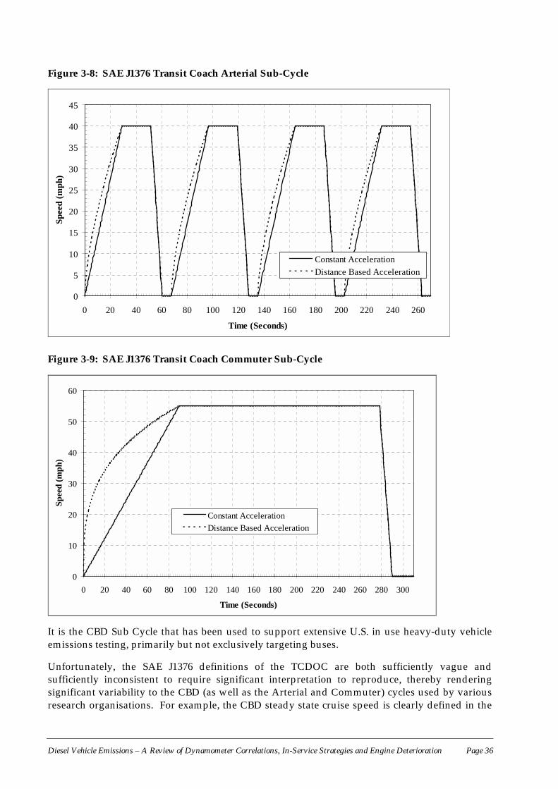
Diesel Vehicle Emissions – A Review of Dynamometer Correlations, In-Service Strategies and Engine Deterioration Page 36
Figure 3-8: SAE J1376 Transit Coach Arterial Sub-Cycle
0
5
10
15
20
25
30
35
40
45
0 20 40 60 80 100 120 140 160 180 200 220 240 260
Time (Seconds)
Spee
d (m
ph)
Constant AccelerationDistance Based Acceleration
Figure 3-9: SAE J1376 Transit Coach Commuter Sub-Cycle
0
10
20
30
40
50
60
0 20 40 60 80 100 120 140 160 180 200 220 240 260 280 300
Time (Seconds)
Spee
d (m
ph)
Constant AccelerationDistance Based Acceleration
It is the CBD Sub Cycle that has been used to support extensive U.S. in use heavy-duty vehicleemissions testing, primarily but not exclusively targeting buses.
Unfortunately, the SAE J1376 definitions of the TCDOC are both sufficiently vague andsufficiently inconsistent to require significant interpretation to reproduce, thereby renderingsignificant variability to the CBD (as well as the Arterial and Commuter) cycles used by variousresearch organisations. For example, the CBD steady state cruise speed is clearly defined in the

Diesel Vehicle Emissions – A Review of Dynamometer Correlations, In-Service Strategies and Engine Deterioration Page 37
J1376 standards as 20 mph, but the defined cruise distance of 540 feet is not completely consistentwith the defined cruise time of 18.5 seconds. Simple calculations demonstrate that a 540 footcruise at 20 mph will take 18.41 seconds whereas an 18.5 second cruise at 20 mph will cover542.67 feet. Similar (and often larger) inconsistencies plague the acceleration and decelerationportions of the sub cycle as well as corresponding portions of the Arterial and Commuter subcycles. Unfortunately, these inconsistencies are often larger than simple round off errors wouldallow.
Nevertheless, to a large extent, these inconsistencies can be dismissed if the cycle times (asopposed to cycle distances) are taken as correct since, when totalled, the indicated componentevent times do sum to the indicated sub cycle times while similar agreement between indicatedcomponent distances does not exist.
Unfortunately, the simplicity of such an approach to actual TCDOC sub cycle constructionbreaks down for the acceleration portions of the sub cycles. The figures included in the SAEJ1376 standard clearly depict the TCDOC acceleration events as non-linear 2, with accelerationrates declining over time, while a simple cycle construction treatment based on statedacceleration times yields constant acceleration rates. Various researchers have respondeddifferently, some relying on constant accelerations, others constructing declining accelerationcurves using typically undocumented techniques. For this reason, cycles initially portrayed asidentical have been found to differ from research organisation to research organisation.
Unfortunately, the unintended side effect is that emissions portrayed as measured over the samecycle are subject to uncertain levels of variation due to cycle specific, rather than vehicle specific,influences. For example, West Virginia University (WVU), a primary researcher of in use heavyduty vehicle emissions, uses a straight-line acceleration “curve” in their interpretation of theCBD cycle, while Environment Canada, having also performed extensive heavy duty vehicletesting over the CBD cycle, uses a declining acceleration approach.
Using the information incorporated in the SAE J1376 standard, there is only one obvious meansof constructing a viable declining acceleration curve for the acceleration portions of the CBD,Arterial, and Commuter Sub Cycles. If both the stated acceleration distance and the statedacceleration time are assumed to be correct (despite the obvious inconsistencies in these sameparameters for the steady state cruise and deceleration portions of the cycles), and it is alsoassumed that the velocity curve produced during the declining acceleration period is continuousthroughout the acceleration event, then there is only one acceleration solution which yields the“correct” distance travelled given the design acceleration period time (e.g., 10 seconds for theCBD Sub Cycle acceleration events) and post acceleration travel speed (e.g., 20 mph for the CBD).
The sub cycle speed versus time traces presented in Figures 3-7 through 3-9 incorporate bothconstant acceleration curves (as unbroken lines) and travel distance limited acceleration curves(as dashed lines) to illustrate the sensitivity of constructed cycles to researcher interpretation.Unfortunately, there is no way of knowing exactly what acceleration assumptions variousresearchers have utilised short of obtaining the actual speed versus time traces for the actual testcycles. This uncertainty combined with the general uncertainties created by the inconsistent
2 Depicted cycle traces in the SAE J1376 standard are also not entirely reliable and clearly include undesirable artistic liberties. For
example, the WOT and half-cycle acceleration events of the Long Haul, Short Haul, and Local Test Cycles are all depicted as“consuming” discrete, fixed travel distances when clearly individual vehicles will travel varying distances during such events dependingon available engine power. Nevertheless, only the TCDOC depicts non-linear acceleration events. The figures presented in this paperattempt to minimize the impact of artistic license by depicting available power-controlled accelerations as instantaneous rather than ascomprising a discrete travel distance (although clearly some variable distance will be traveled during the acceleration event).
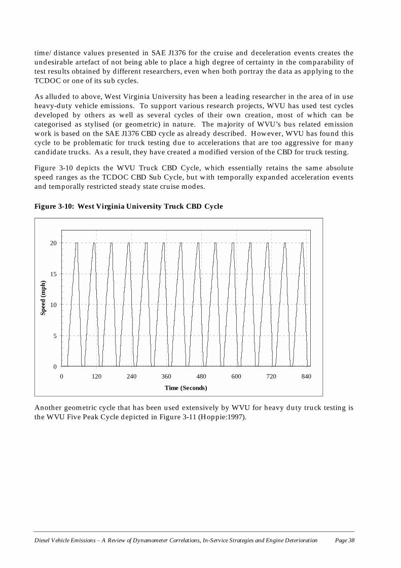
Diesel Vehicle Emissions – A Review of Dynamometer Correlations, In-Service Strategies and Engine Deterioration Page 38
time/distance values presented in SAE J1376 for the cruise and deceleration events creates theundesirable artefact of not being able to place a high degree of certainty in the comparability oftest results obtained by different researchers, even when both portray the data as applying to theTCDOC or one of its sub cycles.
As alluded to above, West Virginia University has been a leading researcher in the area of in useheavy-duty vehicle emissions. To support various research projects, WVU has used test cyclesdeveloped by others as well as several cycles of their own creation, most of which can becategorised as stylised (or geometric) in nature. The majority of WVU’s bus related emissionwork is based on the SAE J1376 CBD cycle as already described. However, WVU has found thiscycle to be problematic for truck testing due to accelerations that are too aggressive for manycandidate trucks. As a result, they have created a modified version of the CBD for truck testing.
Figure 3-10 depicts the WVU Truck CBD Cycle, which essentially retains the same absolutespeed ranges as the TCDOC CBD Sub Cycle, but with temporally expanded acceleration eventsand temporally restricted steady state cruise modes.
Figure 3-10: West Virginia University Truck CBD Cycle
0
5
10
15
20
0 120 240 360 480 600 720 840
Time (Seconds)
Spee
d (m
ph)
Another geometric cycle that has been used extensively by WVU for heavy duty truck testing isthe WVU Five Peak Cycle depicted in Figure 3-11 (Hoppie:1997).
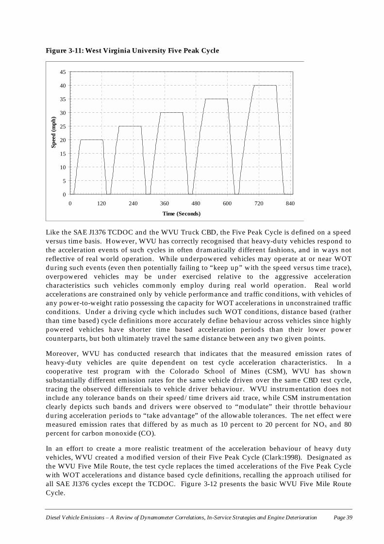
Diesel Vehicle Emissions – A Review of Dynamometer Correlations, In-Service Strategies and Engine Deterioration Page 39
Figure 3-11: West Virginia University Five Peak Cycle
0
5
10
15
20
25
30
35
40
45
0 120 240 360 480 600 720 840
Time (Seconds)
Spee
d (m
ph)
Like the SAE J1376 TCDOC and the WVU Truck CBD, the Five Peak Cycle is defined on a speedversus time basis. However, WVU has correctly recognised that heavy-duty vehicles respond tothe acceleration events of such cycles in often dramatically different fashions, and in ways notreflective of real world operation. While underpowered vehicles may operate at or near WOTduring such events (even then potentially failing to “keep up” with the speed versus time trace),overpowered vehicles may be under exercised relative to the aggressive accelerationcharacteristics such vehicles commonly employ during real world operation. Real worldaccelerations are constrained only by vehicle performance and traffic conditions, with vehicles ofany power-to-weight ratio possessing the capacity for WOT accelerations in unconstrained trafficconditions. Under a driving cycle which includes such WOT conditions, distance based (ratherthan time based) cycle definitions more accurately define behaviour across vehicles since highlypowered vehicles have shorter time based acceleration periods than their lower powercounterparts, but both ultimately travel the same distance between any two given points.
Moreover, WVU has conducted research that indicates that the measured emission rates ofheavy-duty vehicles are quite dependent on test cycle acceleration characteristics. In acooperative test program with the Colorado School of Mines (CSM), WVU has shownsubstantially different emission rates for the same vehicle driven over the same CBD test cycle,tracing the observed differentials to vehicle driver behaviour. WVU instrumentation does notinclude any tolerance bands on their speed/time drivers aid trace, while CSM instrumentationclearly depicts such bands and drivers were observed to “modulate” their throttle behaviourduring acceleration periods to “take advantage” of the allowable tolerances. The net effect weremeasured emission rates that differed by as much as 10 percent to 20 percent for NOx and 80percent for carbon monoxide (CO).
In an effort to create a more realistic treatment of the acceleration behaviour of heavy dutyvehicles, WVU created a modified version of their Five Peak Cycle (Clark:1998). Designated asthe WVU Five Mile Route, the test cycle replaces the timed accelerations of the Five Peak Cyclewith WOT accelerations and distance based cycle definitions, recalling the approach utilised forall SAE J1376 cycles except the TCDOC. Figure 3-12 presents the basic WVU Five Mile RouteCycle.

Diesel Vehicle Emissions – A Review of Dynamometer Correlations, In-Service Strategies and Engine Deterioration Page 40
The cycle clearly continues to be geometric in design. The solid speed versus distance trace ofFigure 3-12 is nothing more than a re-expression of the Figure 3-11 speed versus time trace forthe WVU Five Peak Cycle. However, the dashed line speed versus distance trace is what vehicledrivers actually follow during the test cycle. During acceleration events, the vehicle always lagsthe instantaneous speed change employed in the cycle trace, “forcing” the driver into a WOTacceleration mode until such time as the steady state cruise speed is attained. Total cycle timewill vary in accordance with available engine power, but all test vehicles will travel the samefive-mile distance regardless of overall cycle time.
Intuitively, the distance based cycle (or route) is more reflective of actual vehicle behaviour sinceall vehicles are allowed to “arrive at their destination” in accordance with their respective powercharacteristics. WVU demonstrated that a 350 horsepower truck run over both the time basedFive Peak Cycle and the corresponding distance based Five Mile Route Cycle emitted about 6percent more NOx and 40 percent more CO over the distance based cycle. Although thiscomparison clearly demonstrates the sensitivity of heavy-duty vehicle emissions to theacceleration characteristics of the test cycle, absolute emission differences will vary across trucksin accordance with truck power-to-weight ratios.
Figure 3-12: West Virginia University Five Mile Route Cycle
0
5
10
15
20
25
30
35
40
45
0 1 2 3 4 5
Distance (miles)
Spee
d (m
ph)
The WVU Five Mile Route Cycle is representative of the most recent examples of geometricallyconstructed heavy-duty vehicle driving cycles. Several of the cycles described above have beenused to support in use heavy duty vehicle emissions testing, most notably the CBD, Arterial, andCommuter Sub Cycles of the TCDOC (primarily, but not exclusively, for testing programstargeting buses), the WVU Truck CBD Cycle, the WVU Five Peak Cycle, and the WVU Five MileRoute Cycle. The only additional geometric cycle that appears with any significant frequency inheavy duty testing programs is the New York City Garbage Truck Cycle (NYGTC). As depictedin Figure 3-13, the NYGTC is a very low speed cycle that includes nine shortacceleration/cruise/deceleration events interrupted by substantial periods of idle.
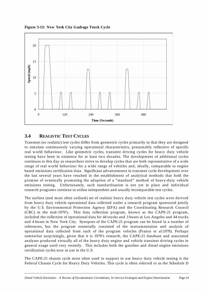
Diesel Vehicle Emissions – A Review of Dynamometer Correlations, In-Service Strategies and Engine Deterioration Page 41
Figure 3-13: New York City Garbage Truck Cycle
0
5
10
15
20
0 120 240 360 480
Time (Seconds)
Spee
d (m
ph)
3.4 REALISTIC TEST CYCLESTransient (or realistic) test cycles differ from geometric cycles primarily in that they are designedto simulate continuously varying operational characteristics, presumably reflective of specificreal world behaviour. Like geometric cycles, transient driving cycles for heavy duty vehicletesting have been in existence for at least two decades. The development of additional cyclescontinues to this day as researchers strive to develop cycles that are both representative of a widerange of real world behaviour for a wide range of vehicles and, ideally, comparable to enginebased emissions certification data. Significant advancements in transient cycle development overthe last several years have resulted in the establishment of analytical methods that hold thepromise of eventually promoting the adoption of a “standard” method of heavy-duty vehicleemissions testing. Unfortunately, such standardisation is not yet in place and individualresearch programs continue to utilise independent and usually incomparable test cycles.
The earliest (and most often utilised) set of realistic heavy duty vehicle test cycles were derivedfrom heavy duty vehicle operational data collected under a research program sponsored jointlyby the U.S. Environmental Protection Agency (EPA) and the Coordinating Research Council(CRC) in the mid-1970’s. This data collection program, known as the CAPE-21 program,included the collection of operational data for 44 trucks and 3 buses in Los Angeles and 44 trucksand 4 buses in New York City. Synopses of the CAPE-21 program can be found in a number ofreferences, but the program essentially consisted of the instrumentation and analysis ofoperational data collected from each of the program vehicles (France et al:1978). Perhapssomewhat surprisingly, given that it is 1970’s research, the CAPE-21 database and associatedanalyses produced virtually all of the heavy duty engine and vehicle transient driving cycles ingeneral usage until very recently. This includes both the gasoline and diesel engine emissionscertification cycles now in use in the U.S.
The CAPE-21 chassis cycle most often used to support in use heavy duty vehicle testing is theFederal Chassis Cycle for Heavy Duty Vehicles. This cycle is often referred to as the Schedule D
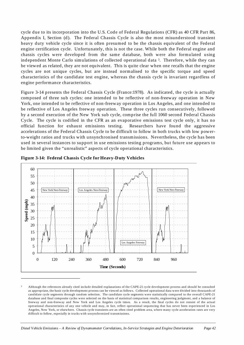
Diesel Vehicle Emissions – A Review of Dynamometer Correlations, In-Service Strategies and Engine Deterioration Page 42
cycle due to its incorporation into the U.S. Code of Federal Regulations (CFR) as 40 CFR Part 86,Appendix I, Section (d). The Federal Chassis Cycle is also the most misunderstood transientheavy duty vehicle cycle since it is often presumed to be the chassis equivalent of the Federalengine certification cycle. Unfortunately, this is not the case. While both the Federal engine andchassis cycles were developed from the same database, both were also formulated usingindependent Monte Carlo simulations of collected operational data 3. Therefore, while they canbe viewed as related, they are not equivalent. This is quite clear when one recalls that the enginecycles are not unique cycles, but are instead normalised to the specific torque and speedcharacteristics of the candidate test engine, whereas the chassis cycle is invariant regardless ofengine performance characteristics.
Figure 3-14 presents the Federal Chassis Cycle (France:1978). As indicated, the cycle is actuallycomposed of three sub cycles: one intended to be reflective of non-freeway operation in NewYork, one intended to be reflective of non-freeway operation in Los Angeles, and one intended tobe reflective of Los Angeles freeway operation. These three cycles run consecutively, followedby a second execution of the New York sub cycle, comprise the full 1060 second Federal ChassisCycle. The cycle is codified in the CFR as an evaporative emissions test cycle only, it has noofficial function for exhaust emissions testing. Researchers have found the aggressiveaccelerations of the Federal Chassis Cycle to be difficult to follow in both trucks with low power-to-weight ratios and trucks with unsynchronised transmissions. Nevertheless, the cycle has beenused in several instances to support in use emissions testing programs, but future use appears tobe limited given the “unrealistic” aspects of cycle operational characteristics.
Figure 3-14: Federal Chassis Cycle for Heavy-Duty Vehicles
0
5
10
15
20
25
30
35
40
45
50
55
60
0 120 240 360 480 600 720 840 960
Time (Seconds)
Spee
d (m
ph)
New York Non-Freeway New York Non-FreewayLos Angeles Non-Freeway
Los Angeles Freeway
3 Although the references already cited include detailed explanations of the CAPE-21 cycle development process and should be consulted
as appropriate, the basic cycle development process can be viewed as follows. Collected operational data were divided into thousands ofcandidate cycle segments through random selection. The candidate cycle segments were statistically compared to the overall CAPE-21database and final composite cycles were selected on the basis of statistical comparison results, engineering judgment, and a balance offreeway and non-freeway and New York and Los Angeles cycle times. As a result, the final cycles do not consist of the actualoperational characteristics of any one vehicle and may, in fact, reflect operational sequencing that has never been experienced in LosAngeles, New York, or elsewhere. Chassis cycle transients are an often cited problem area, where many cycle acceleration rates are verydifficult to follow, especially in trucks with unsynchronized transmissions.
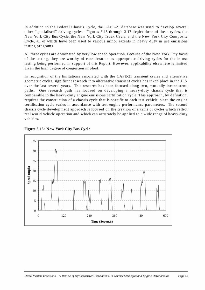
Diesel Vehicle Emissions – A Review of Dynamometer Correlations, In-Service Strategies and Engine Deterioration Page 43
In addition to the Federal Chassis Cycle, the CAPE-21 database was used to develop severalother “specialised” driving cycles. Figures 3-15 through 3-17 depict three of these cycles, theNew York City Bus Cycle, the New York City Truck Cycle, and the New York City CompositeCycle, all of which have been used to various minor extents in heavy duty in use emissionstesting programs.
All three cycles are dominated by very low speed operation. Because of the New York City focusof the testing, they are worthy of consideration as appropriate driving cycles for the in-usetesting being performed in support of this Report. However, applicability elsewhere is limitedgiven the high degree of congestion implied.
In recognition of the limitations associated with the CAPE-21 transient cycles and alternativegeometric cycles, significant research into alternative transient cycles has taken place in the U.S.over the last several years. This research has been focused along two, mutually inconsistent,paths. One research path has focused on developing a heavy-duty chassis cycle that iscomparable to the heavy-duty engine emissions certification cycle. This approach, by definition,requires the construction of a chassis cycle that is specific to each test vehicle, since the enginecertification cycle varies in accordance with test engine performance parameters. The secondchassis cycle development approach is focused on the creation of a cycle or cycles which reflectreal world vehicle operation and which can accurately be applied to a wide range of heavy-dutyvehicles.
Figure 3-15: New York City Bus Cycle
0
5
10
15
20
25
30
35
0 120 240 360 480 600
Time (Seconds)
Spee
d (m
ph)
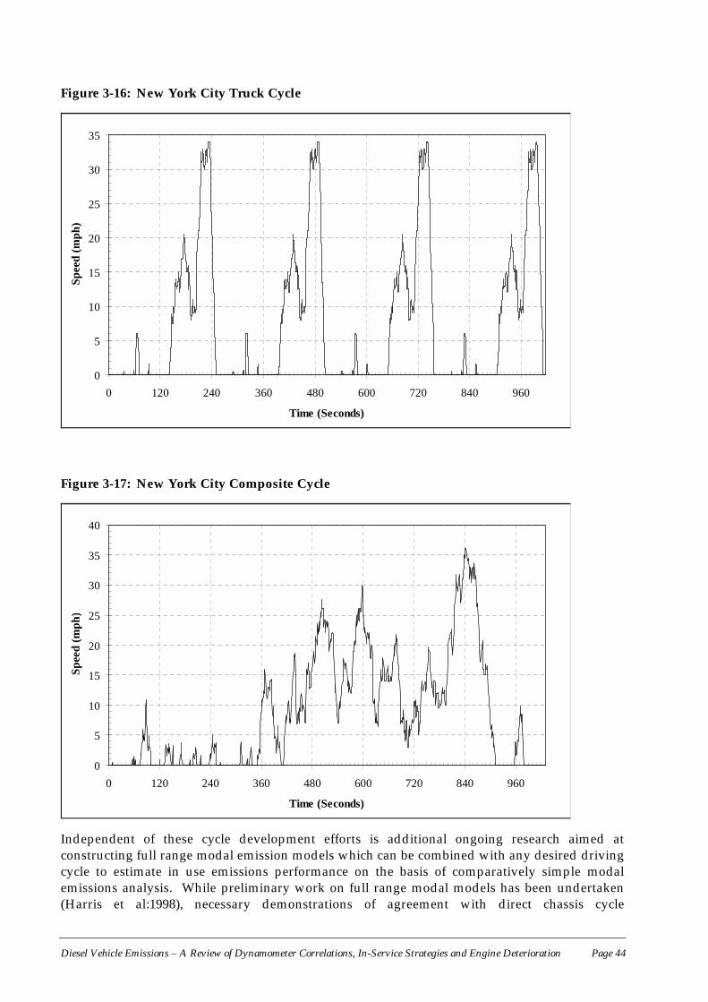
Diesel Vehicle Emissions – A Review of Dynamometer Correlations, In-Service Strategies and Engine Deterioration Page 44
Figure 3-16: New York City Truck Cycle
0
5
10
15
20
25
30
35
0 120 240 360 480 600 720 840 960
Time (Seconds)
Spee
d (m
ph)
Figure 3-17: New York City Composite Cycle
0
5
10
15
20
25
30
35
40
0 120 240 360 480 600 720 840 960
Time (Seconds)
Spee
d (m
ph)
Independent of these cycle development efforts is additional ongoing research aimed atconstructing full range modal emission models which can be combined with any desired drivingcycle to estimate in use emissions performance on the basis of comparatively simple modalemissions analysis. While preliminary work on full range modal models has been undertaken(Harris et al:1998), necessary demonstrations of agreement with direct chassis cycle
Diesel Vehicle Emissions – A Review of Dynamometer Correlations, In-Service Strategies and Engine Deterioration Page 45
measurements or correlation with engine cycle data have yet to be accomplished. Hence, theseU.S. research efforts are not discussed in detail in this report. However, European (mostlyGerman) efforts have focused on the development of modal emission models.
Significant progress has been made in developing a procedure for heavy-duty vehicle chassisbased testing that is comparable to the engine based certification test. The current approach isbased on developing a chassis cycle that approximates the energy demands of the enginecertification cycle. This “conservation of energy” approach was originally suggested byresearchers at WVU, with recent enhancements suggested by researchers with the U.S. EPA(Harris et al:1995).
Since energy demands are conserved across the engine and chassis cycles, the Heavy-DutyVehicle FTP Energy Conservation Cycle 4 is vehicle specific, just like the engine cycle upon whichit is based. The cycle construction process for a specific vehicle/test weight combination is quiteintensive, but easily adaptable to software automation.
While the specific calculations necessary to create a chassis cycle with equivalent certificationcycle energy demands are somewhat complex, the basic process can be summarised as follows:
1) Engine cycle torque and speed values are translated to horsepower,
2) Instances of positive torque at idle are eliminated as unrealistic (causing a decrease in totalcycle energy of about 0.5 percent),
3) Thermal horsepower losses (drivetrain losses, aerodynamic drag, rolling resistance) arecalculated and subtracted from engine horsepower to determine net motive power,
4) Vehicle speed is calculated as a function of mass and net motive power,
5) Based on certification cycle speed profiles, deceleration periods are assigned as eithercoasting or braking decelerations, and
6) Shift delays are added for manual transmission vehicles (these delays prolong the chassiscycle, but do not alter cycle energy).
7) Throughout cycle construction, gearing ratios are used to check available torque againsttorque required to meet vehicle speed demands. In instances where insufficient torque isavailable, cycle speeds based on maximum torque are substituted for successively calculatedspeeds until cycle energy demands equilibrate.
Figure 3-18 presents an example Heavy-Duty Vehicle FTP Energy Conservation Cycle drivingtrace.
This cycle was developed for a 1990 Freightliner tractor with a 325 horsepower Caterpillar 3176engine towing a 45-foot cargo trailer. The gross combined weight was 45,800 pounds and theassumed inertial weight was 48,500 pounds. Road load forces were calculated as 277.12 + 0.1287(velocity). It is important to recognise that, while not presented in Figure 3-18, a schedule of shift
4 This cycle naming convention is not extracted from the literature, but instead designed specifically for this Report. Reference
terminology, such as “Second Generation Modified Energy Conservation Cycle (MEC/FTP2) (SAE:1982)” are not sufficiently descriptivefor a general report such as this.
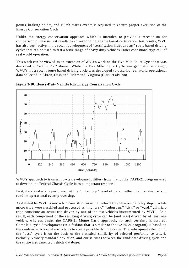
Diesel Vehicle Emissions – A Review of Dynamometer Correlations, In-Service Strategies and Engine Deterioration Page 46
points, braking points, and clutch status events is required to ensure proper execution of theEnergy Conservation Cycle.
Unlike the energy conservation approach which is intended to provide a mechanism forcomparison of chassis test results to corresponding engine based certification test results, WVUhas also been active in the recent development of “certification independent” route based drivingcycles that can be used to test a wide range of heavy duty vehicles under conditions “typical” ofreal world operation.
This work can be viewed as an extension of WVU’s work on the Five Mile Route Cycle that wasdescribed in Section 2.2.2 above. While the Five Mile Route Cycle was geometric in design,WVU’s most recent route based driving cycle was developed to describe real world operationaldata collected in Akron, Ohio and Richmond, Virginia (Clark et al:1998).
Figure 3-18: Heavy-Duty Vehicle FTP Energy Conservation Cycle
0
10
20
30
40
50
60
70
0 120 240 360 480 600 720 840 960 1080 1200
Time (Seconds)
Spee
d (m
ph)
WVU’s approach to transient cycle development differs from that of the CAPE-21 program usedto develop the Federal Chassis Cycle in two important respects.
First, data analysis is performed at the “micro trip” level of detail rather than on the basis ofrandom operational event processing.
As defined by WVU, a micro trip consists of an actual vehicle trip between delivery stops. Whilemicro trips were classified and processed as “highway,” “suburban,” “city,” or “yard,” all microtrips constitute an actual trip driven by one of the test vehicles instrumented by WVU. As aresult, each component of the resulting driving cycle can be (and was) driven by at least onevehicle, whereas under the CAPE-21 Monte Carlo approach, no such certainty is assured.Complete cycle development (in a fashion that is similar to the CAPE-21 program) is based onthe random selection of micro trips to create possible driving cycles. The subsequent selection ofthe “best” cycle is on the basis of the statistical similarity of selected performance criteria(velocity, velocity standard deviation, and cruise time) between the candidate driving cycle andthe entire instrumented vehicle database.
Diesel Vehicle Emissions – A Review of Dynamometer Correlations, In-Service Strategies and Engine Deterioration Page 47
Figure 3-19(a) presents a speed versus time trace for the WVU transient City/Suburban HeavyVehicle Route Cycle (CSHVR).
The cycle is comprised of four micro trips from the Akron/Richmond database. However, as aspeed versus time cycle, the CSHVR cycle presented in Figure 3-19(a) suffers from the sameweakness which plagues many of the geometric cycles discussed in Section 3.3 and the FederalChassis Cycle discussed above. Namely, the cycle is based on specific acceleration characteristicsthat may be too aggressive for some vehicles and not aggressive enough for others.
In actual real world situations, vehicles with more available power than the vehicle that drovethe applicable micro trip will accelerate faster in free flow conditions and encounter speedrestrictions (e.g., posted limits, traffic constraints) quicker than the micro trip vehicle. Forunderpowered vehicles, exactly the opposite will be true. As a result, WVU researchersundertook the additional step of converting the CSHVR to a speed versus distance format thatbetter describes real world driving behaviour.
Figure 3-19(b) presents the CSHVR Cycle in its final speed versus distance format. The solidtrace is simply a re-expression of the solid speed versus time trace of Figure 3-19(a). However,during actual WOT accelerations, the vehicle driver would actually be instructed to accelerate inaccordance with the instantaneous acceleration characteristics indicated by the dashed portionsof the trace.
While these instantaneous accelerations certainly cannot be attained in practice, the vehicledriver will maintain WOT until the post-free acceleration speed in attained, and willsubsequently “rejoin” the ideal cycle at the point where the ideal cycle distance equals the actualtravelled distance. In this manner all vehicles drive the same distance, mimicking the behaviourthat vehicles of differing power-to-weight ratios would exhibit had they actually driven thehypothetical route between the two terminus points. For illustrative purposes, the WOTacceleration points are also marked in Figure 3-19(a) as dashed traces, but it should berecognised that these traces are nonsensical in the context of speed versus time as thesubstitution of vehicle specific acceleration performance would either constrict or extend thetime axis.
3.5 SUMMARY OF HEAVY DUTY TESTING OPTIONSAs discussed in the previous sections, myriad heavy-duty vehicle driving cycles have beendeveloped over the last 25 or so years. Table 3-1(a) to (c) presents summary descriptive statisticsfor the various cycles discussed. The 13-mode cycle in its chassis variant is of interest in testingvehicles from the perspective of conformity with engine-based regulations. Since both Europeand the U.S. are likely to have a 13-mode certification test in the future (the ESC), development of13-mode test capability is likely to be useful for some time to come. The major advantage of the13-mode test is that no inertia weight simulation is required. Cycle statistics do not have anyspecific meaning in the context of the 13-mode, as it is used to provide a map of engine emissionsunder varied operating conditions.

Diesel Vehicle Emissions – A Review of Dynamometer Correlations, In-Service Strategies and Engine Deterioration Page 48
Figure 3-19: West Virginia University City/Suburban Heavy Vehicle Cycles
(a) Speed Cycle
0
10
20
30
40
50
60
70
0 120 240 360 480 600 720 840 960 1080 1200
Time (Seconds)
Spee
d (m
ph)
(b) Route Cycle
0
5
10
15
20
25
30
35
40
45
0 1 2 3 4 5 6
Distance (Miles)
Spee
d (m
ph)

Diesel Vehicle Emissions – A Review of Dynamometer Correlations, In-Service Strategies and Engine Deterioration Page 49
Table 3-1: Selected Statistics of Various Heavy-Duty Engine and Vehicle Driving Cycles
Explanatory Notes:1. Cycle distance statistics are not relevant for an engine-based cycle. Even if engine speeds were converted to vehicle speeds for a given vehicle/load combination, corresponding
distance statistics would only be applicable to the specific vehicle/load combination as cycle absolute engine speeds vary across test engines.2. Cycle engine speed and acceleration statistics vary in accordance with the rated speed of the test engine.
3. For distance-based cycles with wide-open throttle (WOT) accelerations, absolute cycle time duration, average speed, average acceleration, and maximum acceleration statisticsare dependent on the available power of the test engine. Maximum deceleration statistics are indeterminate due to the combination of coastdown and braking decelerations incycle definition and the dependency of the former on test vehicle mass.
Duration DistanceAverage Speed
Maximum Speed
Average (Absolute)
AccelerationMaximum
AccelerationMaximum
Deceleration Idle Time(sec) (miles) (mph) (mph) (mph/sec) (mph/sec) (mph/sec) (sec)
Federal HDGE Certification Cycle 1167 (see note 1) (see note 2) (see note 2) (see note 2) (see note 2) (see note 2) 325Federal HDDE Certification Cycle 1199 (see note 1) (see note 2) (see note 2) (see note 2) (see note 2) (see note 2) 477Alternate Federal HDGE Certification Cycle 1167 (see note 1) (see note 2) (see note 2) (see note 2) (see note 2) (see note 2) 363Federal Heavy Duty Chassis Cycle 1060 5.552 18.86 58 0.585 4.38 -4.63 338New York Non-Freeway Segment of the Federal Chassis Cycle 254 0.5335 7.56 34 0.594 4.38 -4.18 127Los Angeles Non-Freeway Segment of the Federal Chassis Cycle 285 1.1523 14.55 42 0.643 3.97 -4.18 79Los Angeles Freeway Segment of the Federal Chassis Cycle 267 3.3327 44.94 58 0.505 2.95 -4.63 5SAE J1376 Long Haul Cycle (see note 3) 30 (see note 3) 55 (see note 3) WOT (see note 3) 180SAE J1376 Short Haul Cycle (see note 3) 7.5 (see note 3) 55 (see note 3) WOT (see note 3) 120SAE J1376 Alternate Short Haul Cycle (see note 3) 15 (see note 3) 55 (see note 3) WOT (see note 3) 240SAE J1376 Local Test Cycle (see note 3) 3 (see note 3) 35 (see note 3) WOT (see note 3) 300SAE J1376 Alternate Local Test Cycle (see note 3) 2 (see note 3) 30 (see note 3) WOT (see note 3) 720SAE J1376 Transit Coach Design Operating Cycle (see note 4) 2830 14.0471 17.87 55 0.859 13.03 -4.58 670CBD Segment of the SAE J1376 TCDOC (see note 4) 560 2.0247 13.02 20 1 2.56 -4.44 98Arterial Segment of the SAE J1376 TCDOC (see note 4) 270 1.9838 26.45 40 1.185 4.58 -4.44 28Commuter Segment of the SAE J1376 TCDOC (see note 4) 310 4.0051 46.51 55 0.355 13.03 -4.58 20West Virginia University Truck CBD Cycle 854 2.1831 9.2 20 0.656 0.8 -1.4 159.6West Virginia University Five Peak Cycle 850 5.0068 21.21 40 0.353 0.9 -1.4 104West Virginia University Five Mile Route Cycle (see note 5) 5.0068 (see note 5) 40 (see note 5) WOT -1.4 104New York City Garbage Truck Cycle 585 0.3788 2.33 20 0.263 2.8 -1.4 404New York CityBus Cycle 600 0.6148 3.69 30.8 0.662 6.2 -4.6 392New York City Truck Cycle 1016 2.1343 7.56 34 0.594 4.4 -4.1 511.2New York City Composite Cycle 1030 2.5053 8.76 36 0.699 4.63 -4.38 322Heavy Duty Vehicle FTP Energy Conservation Cycle (see note 6) 1283 8.3122 23.34 68.33 0.589 5.15 -2.43 281West Virginia University City/Suburban Heavy Vehicle Route Cycle (see note 7) 6.6807 (see note 7) 43.8 (see note 7) WOT -4 386.5
Cycle
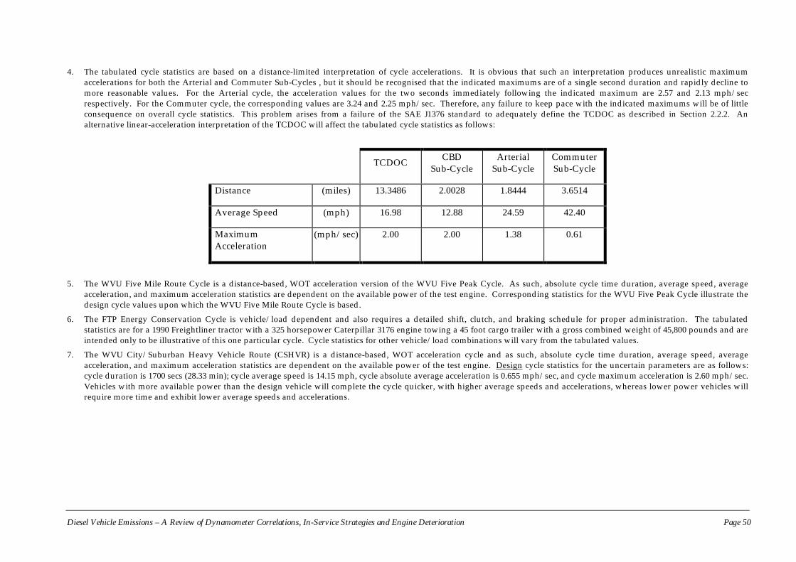
Diesel Vehicle Emissions – A Review of Dynamometer Correlations, In-Service Strategies and Engine Deterioration Page 50
4. The tabulated cycle statistics are based on a distance-limited interpretation of cycle accelerations. It is obvious that such an interpretation produces unrealistic maximumaccelerations for both the Arterial and Commuter Sub-Cycles , but it should be recognised that the indicated maximums are of a single second duration and rapidly decline tomore reasonable values. For the Arterial cycle, the acceleration values for the two seconds immediately following the indicated maximum are 2.57 and 2.13 mph/secrespectively. For the Commuter cycle, the corresponding values are 3.24 and 2.25 mph/sec. Therefore, any failure to keep pace with the indicated maximums will be of littleconsequence on overall cycle statistics. This problem arises from a failure of the SAE J1376 standard to adequately define the TCDOC as described in Section 2.2.2. Analternative linear-acceleration interpretation of the TCDOC will affect the tabulated cycle statistics as follows:
TCDOC CBDSub-Cycle
ArterialSub-Cycle
CommuterSub-Cycle
Distance (miles) 13.3486 2.0028 1.8444 3.6514
Average Speed (mph) 16.98 12.88 24.59 42.40
MaximumAcceleration
(mph/sec) 2.00 2.00 1.38 0.61
5. The WVU Five Mile Route Cycle is a distance-based, WOT acceleration version of the WVU Five Peak Cycle. As such, absolute cycle time duration, average speed, averageacceleration, and maximum acceleration statistics are dependent on the available power of the test engine. Corresponding statistics for the WVU Five Peak Cycle illustrate thedesign cycle values upon which the WVU Five Mile Route Cycle is based.
6. The FTP Energy Conservation Cycle is vehicle/load dependent and also requires a detailed shift, clutch, and braking schedule for proper administration. The tabulatedstatistics are for a 1990 Freightliner tractor with a 325 horsepower Caterpillar 3176 engine towing a 45 foot cargo trailer with a gross combined weight of 45,800 pounds and areintended only to be illustrative of this one particular cycle. Cycle statistics for other vehicle/load combinations will vary from the tabulated values.
7. The WVU City/Suburban Heavy Vehicle Route (CSHVR) is a distance-based, WOT acceleration cycle and as such, absolute cycle time duration, average speed, averageacceleration, and maximum acceleration statistics are dependent on the available power of the test engine. Design cycle statistics for the uncertain parameters are as follows:cycle duration is 1700 secs (28.33 min); cycle average speed is 14.15 mph, cycle absolute average acceleration is 0.655 mph/sec, and cycle maximum acceleration is 2.60 mph/sec.Vehicles with more available power than the design vehicle will complete the cycle quicker, with higher average speeds and accelerations, whereas lower power vehicles willrequire more time and exhibit lower average speeds and accelerations.
Diesel Vehicle Emissions – A Review of Dynamometer Correlations, In-Service Strategies and Engine Deterioration Page 51
While the various geometric cycles examined have definitive weaknesses relative to their abilityto represent actual in use vehicle emission rates (no vehicles operate in the stylised modescomprising these cycles), the inclusion of one or more of these cycles in any future test programin Australia may be advantageous for two reasons. First, while the detailed cycle characteristicsare certainly not reflective of real world operation, average cycle statistics may be reasonableapproximations of aggregate real world behaviour. Second, use of one or more of these cycleswill provide a potential linkage to in use emissions data collected in other test programs.
Geometric cycles dominate previous heavy-duty vehicle testing programs. In this regard, theSAE J1376 CBD Sub Cycle, the WVU Five Peak Cycle, the WVU Five Mile Route Cycle, the WVUTruck CBD Cycle, and the New York City Garbage Truck Cycle all have been used to supportrecent heavy-duty vehicle emissions test programs. Of these, the SAE J1376 CBD Sub Cycleappears to the most common link to multiple test programs (although as described in Section2.2.2 above, required researcher interpretation during cycle implementation as well as WVU’sdemonstration of institution specific acceleration dependencies renders this linkage somewhattenuous).
All of the various transient cycles presented are worthy of consideration. In most locations, thevarious New York City cycles would probably be inappropriate due to their very low speeddistributions, but it may be useful for “inner city” simulation. Without question, the transientcycle that has been used most often in previous heavy-duty vehicle test programs is the FederalChassis Cycle. While many of these programs erroneously assumed that the cycle was correlatedto the federal engine certification cycle, they nevertheless collected in use emissions data usingthe chassis cycle. The New York Non-Freeway Sub Cycle of the Federal Chassis Cycle is anequally viable candidate. The major weakness of all these transient cycles is their speed versustime design basis, which is unlikely to accurately reflect the real world behaviour of vehicleswith substantially different power-to-weight ratios. The WVU CSHVR Cycle is currently theonly viable candidate cycle that overcomes this weakness, but its speed and accelerationperformance characteristics are probably not reflective of the operational constraints imposed byNew York City traffic.
Finally, the Heavy-Duty Vehicle FTP Energy Conservation Cycle approach is a viable candidatefor testing program inclusion if correlation with the engine certification cycles can bedemonstrated (which has not yet been accomplished). However, it would be beneficial tocalculate emissions (should the cycle be selected for testing program inclusion) separately for theaggregate cycle and the portion of the cycle that corresponds to the portions of the enginecertification cycle.
Diesel Vehicle Emissions – A Review of Dynamometer Correlations, In-Service Strategies and Engine Deterioration Page 52
4 EMISSIONS CORRELATION BETWEEN DIFFERENT TESTS
4.1 ISSUESThere has been considerable interest recently between the emission correlations not only betweendifferent test procedures but also between engine dynamometer and chassis dynamometer basedtests. The obvious area of interest for engine manufacturers has been correlation of 13-modeengine based test results with U.S. transient cycle engine based test results, and studies havebeen conducted in both the U.S. and Europe on this question. As noted in Section 3 of thisreport, correlation’s between engine based steady-state test (mostly 13-mode) and chassisdynamometer based 13-mode test has been conducted almost exclusively in Europe withvirtually no testing in the U.S. In contrast, correlation of engine dynamometer transient cycleemissions with chassis dynamometer transient cycle emissions has been conducted exclusively inthe U.S. There has been some limited study of geometric cycles and their relationship to thecertification transient cycle in Europe, and these connections have been established in studies inGermany.
The correlation issues raised by the comparisons are quite complex as there are many sources ofvariability that can affect the correlation between any pair of unique tests.
First, any given engine has some cycle-to-cycle variability even on a very accurate andreproducible test cycle conducted on an engine dynamometer. Although the level of variabilitycannot be separated from the measurement error of the emissions measuring instruments, mostmodern diesels are believed to have cycle-to-cycle variability of much less than five percent, andit is potentially in the two percent range for most pollutants.
Second, identical engines of a given engine family can have different emission due to differentproduction tolerances in the emission critical parts. Engine-to-engine variability can be quitehigh, and the net emission distribution is often modelled as a lognormal or Weibull distribution.The coefficient of variation (σ/x) can be around 15 percent, so that engines at either end of thedistribution can differ in emissions by a factor of two, or more. In this context, it should be notedthat emission regulations do not require all engines to meet emission standards, but rather, it beestablished with a high level of confidence that the average emission are well below standards.
Measurement variability arises from random and systematic errors in the emissionsmeasurement train. While guidelines for repeatability vary among laboratories, a typical COVfor engine tests that includes engine variability is around three to five percent. Of course,instrument error is often defined at full scale and, at very low emission levels, COV can increasedramatically. This is particularly true for particulate measurements, where particulate iscollected and weighed on a filter. Particulate weights of less than a milligram are difficult tomeasure accurately.
Driver variability is a separate issue that applies to chassis dynamometer tests. Drivers have tofollow a cycle trace and shift the transmission at specific points, and the speed errors and shifterrors can be significant. Trained and expert drivers can reduce the variability to levelsapproaching an engine dynamometer test, but even between expert drivers, there are differencesin how “aggressively” the trace is followed. In addition, there can be significant error whenspecific engines or transmissions do not allow the driver to keep up with the driving trace evenat full throttle. Such issues are, of course, relevant only for transient tests.
The significance of the above discussion arises when attempting to correlate results from achassis dynamometer based test of a particular engine to the certification test result of an engine
Diesel Vehicle Emissions – A Review of Dynamometer Correlations, In-Service Strategies and Engine Deterioration Page 53
tested on an engine dynamometer. All of the above sources of variability are included, makingthe interpretation of results very difficult.
The following subsections discuss the correlation between (1) engine based 13-mode andtransient tests, (2) chassis based 13-mode and engine based 13-mode tests and (3) betweenchassis based transient tests and engine based transient tests.
4.2 COMPARISON BETWEEN ENGINE BASED 13-MODE AND TRANSIENTTESTS
As noted earlier, diesel engine manufacturers did not wish to incur the expense of installingtransient cycle dynamometers in the 1980s and U.S. manufacturers and European manufacturersattempted to develop correlations between the 13-mode test and the U.S. transient test. In eachcase, the same engine was tested on both cycles on the same laboratory, so that comparisonerrors were minimised.
In the early 1980s, approximately 50 engines were tested in the U.S. on both test procedures, butsome of the data was not available publicly. EEA (1985) obtained data for 33 engines andestimated the relationship between steady state and transient emissions. It was discovered thatCummins engines behaved uniquely and differently from all other engine types due to theirunique fuel systems. Hence the 15 Cummins engines and 18 “other” engines were separated intotwo groups for the regression analysis 5.
For the non-Cummins engines, EEA found that:
HCT = 0.167 + 1.05 HCSS (r2 = 0.70)(0.184)
NOxT = 1.70 + 0.75 NOxSS (r2 = 0.82)(0.13)
Where subscript T is for transient test and SS for steady state test.
For the Cummins engines, EEA found
HCT = 0.31 + 1.77 HCSS (r2 = 0.79)(0.25)
NOxT = 1.03 + 0.81 NOxSS (r2 = 0.84)(0.13)
While the NOx relationships are similar, the HC relationships are quite different between the twogroups of engines. Nevertheless, it is important to note that reasonable correlation was obtainedbetween two very different test methods over a very broad range of emissions performance (HCranging from 0.4 to 3 g/kWh and NOx from 4.5 to 14 g/kWh on the transient test).
It is particularly significant that the correlation was obtained between two tests, one using a coldstart and the other starting with an engine that is fully warmed up. Many in the industrybelieved that these correlations could be further improved by reweighting the different modes onthe steady state test.
5 Numbers in parentheses are standard errors of coefficients.

Diesel Vehicle Emissions – A Review of Dynamometer Correlations, In-Service Strategies and Engine Deterioration Page 54
No data on particulates were available from the U.S. steady state tests, but EPA believed that thecorrelation between steady state and transient test particulate emissions is poor. Manufacturersadvanced a number of engineering reasons that suggest it may be possible to obtain goodcorrelations for all emissions of concern between steady state engine “maps” and transient cycleemissions because:
• Diesel engines do not require acceleration enrichment, and the air fuel ratio during atransient acceleration/deceleration is more carefully controlled than in a gasoline engine.
• Diesel engines require very little cold start enrichment, and the effect of cold starts onemissions is small.
• Diesel engines do not (yet) use any exhaust aftertreatment, and modelling their emissions donot, therefore, require the difficult prediction of catalyst efficiency.
European manufacturers have actively investigated the particulate question, and developed aparticulate measurement system suited to the 13-mode test that did not require the weighting of26 filters (two for each mode). Test results were obtained for 29 engines the spanned the range of100 to 200 kW output (Cornetti et al:1988). Both linear and quadratic fits were attempted and theregression results are:
PMT = 0.25 + 75 PMSS (r2 = 0.67)
and PMT = -0.10 + 2.04 PMSS –1.04 PMSS2 (r2 = 0.77)
The coefficients were significant at the 95 percent level, and the standard error of the estimatewas 0.12 for the linear fit and 0.10 for the quadratic fit. However, visual observation of the dataplotted in Figure 4-1 shows that one data point in particular (with relatively low transient cycleemissions but high steady-state emissions) is responsible for the quadratic fit, and the regressionis not very robust.
In both the NOx and PM regressions, the intercept term is quite large, and would invalidate anycomparison at low NOx or PM emission levels. For example, the US PM emission standard isnow at 0.10 g/bhp-hr (0.13 g/kWh), which is less than half the intercept term in the PMequation. Hence there is now widespread acceptance of the fact that at low emission levels, thereis little correlation between the two test procedures. Nevertheless, Australia could be interestedin these correlations as they apply to older, higher emitting engines.
More recently, the TUV-Rheinland (1995) in Germany conducted emission factor testing on 34engines certified to the Euro I, 88/77/EEC and R49 standards using both the U.S. transient testand the new European transient test. EEA obtained only aggregate data on emission averages bycertification level for the two cycles. Emissions for all pollutants are higher on the Europeantransient test, HC and PM by about 15 percent and NOx by about six percent. The 13-mode R49test had the highest NOx level on average.
4.3 CORRELATION OF ENGINE BASED STEADY STATE TESTS TO CHASSISBASED STEADY-STATE TESTS
The work on correlation between engine based tests and chassis dynamometer tests has beencontinuing since the early 1990s, and the original Van Gompel and Verbech (1993) publication onthe “Diesel Controle Methode” (in Dutch) served as the basis for testing accuracy according to88/77/EEC and 72/306/EEC.
Diesel Vehicle Emissions – A Review of Dynamometer Correlations, In-Service Strategies and Engine Deterioration Page 55
Figure 4-1: Correlation of PM Emissions Measured by Transient and Steady-State Tests(g/bhp-hr)
Source: Cornetti et al (1988)
As noted in Section 3, the correlations’ principal concern is the error associated with powermeasurement at each of the 13-modes, since RPM can be measured with great accuracy andsteady- state emission measurements are not a significant source of error (typical measurementerrors are less than one percent, unless the emission are at the threshold of the instrumentsensitivity). PM emission measurement can have a COV of five percent or higher duet to thedifficulty of measuring PM on the light loads of the 13- mode test.
The calculation of engine power delivered to the chassis dynamometer is obtained from thefollowing equation:
Pengine = Pwheel + Ptrans + Paux + Proll
where subscript: engine is the engine power outputwheel is the measured power at the wheelstrans is the power loss in the transmissionaux is the power to auxiliary driversroll is the rolling resistance loss
The ‘Diesel Controle Methode’ project10 recommended the formula:
Paux = Prated x [0.0139 (n/nr) + 0.032 (n/nr)3]
where: n is the test RPM
nr is the rated RPM
Diesel Vehicle Emissions – A Review of Dynamometer Correlations, In-Service Strategies and Engine Deterioration Page 56
The formula is empirically derived and may not hold true for Australia. The project also deriveddetailed tyre rolling resistance power (Proll) as a function of tyre temperature and rollingresistance coefficient, while a similar empirical formula was derived for transmission loses. Sincethe first correlation project, two more recent projects have been conducted, one in 1994-1995 andone in 1996-1997. In the 1994/1995 project, five engine were tested on the engine and chassisbased cycles, and the empirical power loss formulae were revised. In the most recent project,four additional engines were tested with some slight readjustment to the formulae to derivepower losses (Rikjeboer et al:1998).
The power delivered can also be calculated on the basis of fuel consumption, if the engine brakespecific fuel consumption is available at the test point or measured from the enginedynamometer. Results from the two methods to estimate engine power are compared in Table4-1, using the formulas for power losses derived in the original study and the most recentupdates.
It should be noted that the most recent update shows that the average error in calculated powerhas been reduced to less than 0.5 percent. The maximum positive error observed for any modehas been reduced from 10.2 percent using the 1992 formulae to 4.2 percent using the latest (1997)method, while the largest negative deviation is increased slightly from –2.9 percent using the1992 formula, to –3.4 percent.
Table 4-1: Steady State 13-Mode Test Error in Power Loss Calculation
The deviations plus the error in measurement of emissions contributes to total error. The datapresented imply that maximum error for all gaseous pollutants is less than six percent, whileaverage error is probable in the range of ±2 percent.
The emissions data, however, showed larger variations than expected. EEA obtained data on sixengines tested on both the engine and chassis tests, and the data are shown in Table 4-2. NOxemissions indicated an average error of ±4 percent but maximum error was almost ten percent.
Engine Make Model 1992* Method
1996*
Update1997*
Update
DAF RS108L 1.003 0.974 0.978Mercedes OM 366 LA 1.021 1 1.007Renault MIDR 06.35 1.018 0.984 0.991Scania DTC 1101 1.059 0.997 1.009Volvo D12A-380 1.076 1.016 1.029Average 1.035 0.994 1.003
DAF RS222L -- 0.973 0.98MAN D 0826 LF08 -- 0.995 0.999Mercedes OM 366A -- 1.033 1.03Scania DSC1201 -- 0.975 0.988Average 0.993 1.001Source: Rijkeboer(1998)* Values are ratios of engine power calculated using empirical formula versus power calculated using fuel consumption.
1995 Tests
1996-1997 Tests
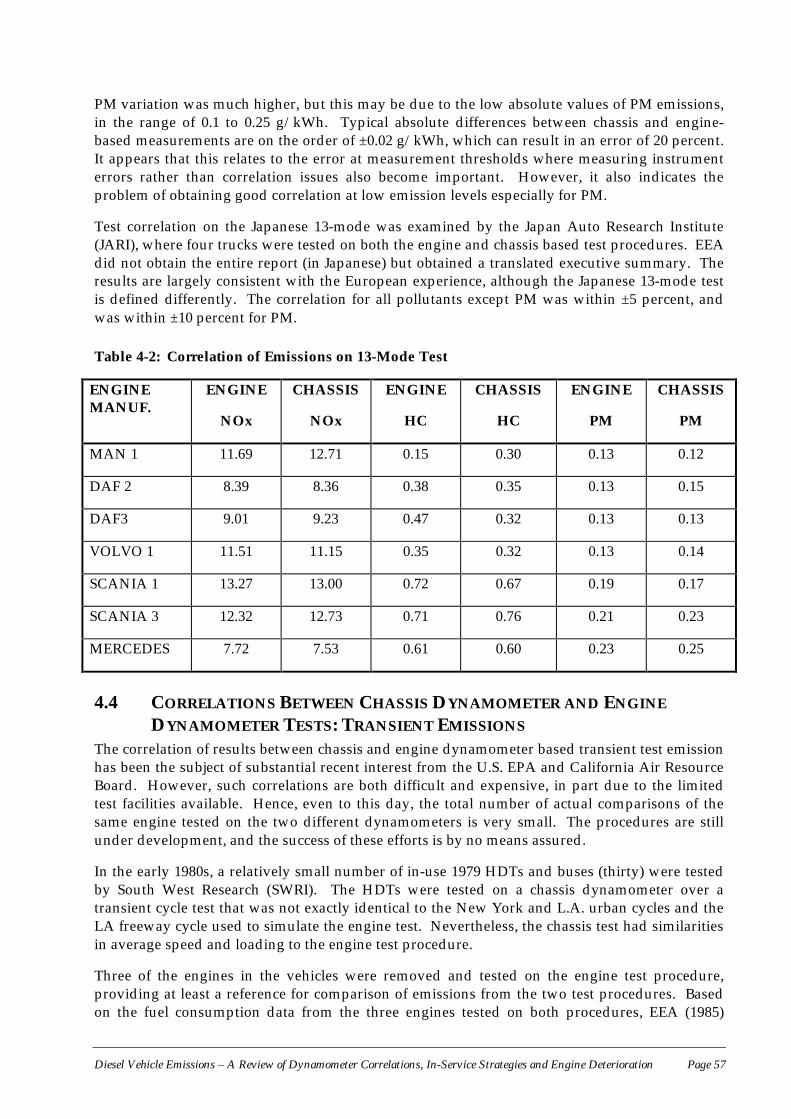
Diesel Vehicle Emissions – A Review of Dynamometer Correlations, In-Service Strategies and Engine Deterioration Page 57
PM variation was much higher, but this may be due to the low absolute values of PM emissions,in the range of 0.1 to 0.25 g/kWh. Typical absolute differences between chassis and engine-based measurements are on the order of ±0.02 g/kWh, which can result in an error of 20 percent.It appears that this relates to the error at measurement thresholds where measuring instrumenterrors rather than correlation issues also become important. However, it also indicates theproblem of obtaining good correlation at low emission levels especially for PM.
Test correlation on the Japanese 13-mode was examined by the Japan Auto Research Institute(JARI), where four trucks were tested on both the engine and chassis based test procedures. EEAdid not obtain the entire report (in Japanese) but obtained a translated executive summary. Theresults are largely consistent with the European experience, although the Japanese 13-mode testis defined differently. The correlation for all pollutants except PM was within ±5 percent, andwas within ±10 percent for PM.
Table 4-2: Correlation of Emissions on 13-Mode Test
ENGINEMANUF.
ENGINE
NOx
CHASSIS
NOx
ENGINE
HC
CHASSIS
HC
ENGINE
PM
CHASSIS
PM
MAN 1 11.69 12.71 0.15 0.30 0.13 0.12
DAF 2 8.39 8.36 0.38 0.35 0.13 0.15
DAF3 9.01 9.23 0.47 0.32 0.13 0.13
VOLVO 1 11.51 11.15 0.35 0.32 0.13 0.14
SCANIA 1 13.27 13.00 0.72 0.67 0.19 0.17
SCANIA 3 12.32 12.73 0.71 0.76 0.21 0.23
MERCEDES 7.72 7.53 0.61 0.60 0.23 0.25
4.4 CORRELATIONS BETWEEN CHASSIS DYNAMOMETER AND ENGINEDYNAMOMETER TESTS: TRANSIENT EMISSIONS
The correlation of results between chassis and engine dynamometer based transient test emissionhas been the subject of substantial recent interest from the U.S. EPA and California Air ResourceBoard. However, such correlations are both difficult and expensive, in part due to the limitedtest facilities available. Hence, even to this day, the total number of actual comparisons of thesame engine tested on the two different dynamometers is very small. The procedures are stillunder development, and the success of these efforts is by no means assured.
In the early 1980s, a relatively small number of in-use 1979 HDTs and buses (thirty) were testedby South West Research (SWRI). The HDTs were tested on a chassis dynamometer over atransient cycle test that was not exactly identical to the New York and L.A. urban cycles and theLA freeway cycle used to simulate the engine test. Nevertheless, the chassis test had similaritiesin average speed and loading to the engine test procedure.
Three of the engines in the vehicles were removed and tested on the engine test procedure,providing at least a reference for comparison of emissions from the two test procedures. Basedon the fuel consumption data from the three engines tested on both procedures, EEA (1985)
Diesel Vehicle Emissions – A Review of Dynamometer Correlations, In-Service Strategies and Engine Deterioration Page 58
developed a method to calculate the work done, in kWh, for an engine driven over the chassisdynamometer cycle given the dynamometer settings of inertia weight and absorptionhorsepower. In two of the three cases, the match between emissions in g/kWh and g/km wasextremely close, within ±5 percent. In the third case, the match was much poorer (+20%) due tothe fact the vehicle was equipped with a high horsepower engine, which was very lightly loadedon the chassis dynamometer test but loaded normally on the engine test.
The fuel consumption based methodology can be simply derived from the conversion of g/kWhto g/km of vehicle travel, using the equation:
g/km = g/kWh x kWh/km
= g/kWh x kWh x g-fuel g-fuel km
The g-fuel/kWh is the engine brake specific fuel consumption (bsfc) and the term g-fuel/km isthe vehicle fuel consumption. In the particular case of the SWRI tests both terms were availableas measured quantities from the same engine but such data is not universally available for anyrandom chassis test, so that typically on “official” or specification value must be used for bsfc.
The above equation is an identity that must hold true for all pollutants. Yet, on broader samplesof vehicles using “official” bsfc values, the conversion factors were found to vary by pollutant. A1992 U.S. EPA report suggested conversion factors (in bhp-hr/mile) ranging from 1.6 for HC to4.3 for CO, indicating significant cycle specific variation.
Very little research was conducted from the mid-1980’s to the mid-1990s on this topic in the U.S.More recently, there have been three significant studies aimed at establishing correlationsbetween the chassis and engine based transient cycles.
One analysis by the Colorado School of Mines (McCormick et al:1998) examined the correlationbetween the engine based U.S. FTP test and the U.S. Federal chassis cycle, for three heavy-dutyengines, all of 1993 model year. The engine-based test included both cold and hot cycles, andinvolved three repeats of the hot cycle for each engine. In all cases, the measured THC emissionswere very low; the two Detroit Diesel Series 50 engines had THC emissions below 0.05 g/bhp-hror less than five percent of the applicable standard, while the Navistar DTA-466 has emissions of0.16 g/bhp-hr, still substantially below standards.
As a result of the very low THC level, the coefficient of variation (COV) for the THC emissionsmeasured was quite high, ranging from 16.5% for one DDC Series 50, to about six percent for theDTA-466. The COV for PM measurements was under seven percent, and less than one percentfor NOx, for all three engines on the engine test. All three engines easily met the emissionstandards for 1993. The chassis dynamometer tests also revealed very high levels of COV forthree repeat tests for HC emissions. The COV was at 33 percent for one DDC Series 50, and at 20percent for the other two engines. COV levels for NOx on the chassis test was quite low, at lessthan four percent for all engines.
The comparison between engine and chassis based results can be best shown as the calculatedconversion factor for each pollutant in bhp-hr/mile. Ideally, the conversion factor should beidentical for all pollutants. However, the calculated conversion factors are relatively low for HC,and reasonably similar of PM, NOx, and CO, as shown in Table 4-3.

Diesel Vehicle Emissions – A Review of Dynamometer Correlations, In-Service Strategies and Engine Deterioration Page 59
Table 4-3: Calculated Conversion Factors – Engine to Chassis Dynamometer Results (bhp-hr/mile)
For these latter three pollutants, the average conversion factor is 6.90 + 0.34 for the first engine, aCOV of about five percent. For vehicle 2, it is 6.16 + 1.27, so that the COV is about 20 percent.For vehicle 3, the conversion factor is 3.09 + 0.66, so that the COV is about 22 percent. THCmeasurements are excluded from this analysis due to the very low emission levels wheremeasurement instrument errors could be quite significant.
The 20 percent COV is broadly indicative of the type of correlation that is possible between theengine and chassis test for emissions when emission levels are not at measurement thresholds.
The reasons and sources for this error are discussed in Section 3, and it is largely because:
1. the engine test is scaled to the torque and RPM characteristics of the engine under test,whereas the driving cycle is invariant for all engines;
2. many parameters in the chassis test are not well specified and depend on individuallaboratory practices or project specific practices.
A more recent study was funded by the California Air Resources Board (1998) and conducted byWest Virginia to improve the chassis test procedures. The test program utilised two trucks aNavistar T 444 E engine in a six speed single axle International chassis truck, and a CumminsN14 engine in a ten speed over-the-road tractor that was configured to operate either withtandem driven axles or a single drive axle. Both engine and chassis emission tests wereemployed. Each engine was subjected to mapping and to hot and cold engine certification tests.The levels of carbon dioxide (CO2), CO, NOx, HC, and (PM) were recorded. In addition, theengines were operated in various tampering modes to raise emission levels with a view tocorrelating these elevated levels with the behaviour when the engine was later tested on thechassis dynamometer. The Navistar was tested with an alternate stock controller and threetemperature sensor tampering modes that caused the engine to employ a cold start mode andelevated NOx levels. For example, with the sensor input falsely set to correspond to 39 degreesFahrenheit (four degrees Centigrade), the hot test NOx level was 15.25 g/bhp-hr (20.45g/kWh)compared to 4.98 g/bhp-hr (5.2 g/kWh) for the stock case. The Cummins engine wasalso operated with a disabled manifold air pressure sensor and a false manifold air pressuresensor signal that raised the level the level of PM measured.
Each engine was installed in a truck, and emissions testing was conducted using the WestVirginia University Transportable Heavy-Duty Emissions Testing Laboratory, which employs afull-scale exhaust dilution tunnel and analysers similar to those in the engine emissionscertification test cell. Power was withdrawn directly from the vehicles hubs while the tyres ran
Test Number 1 2 3Vehicle Type Bus Bus TruckEngine DDC S50 DDC S50 DTA-466THC 3.6 9.67 1.81NOx 7.27 5.32 2.78CO 6.59 5.53 2.65PM 6.83 7.63 3.85Source: McCormick et al: 1998
Diesel Vehicle Emissions – A Review of Dynamometer Correlations, In-Service Strategies and Engine Deterioration Page 60
on rollers. Axle torque was measured using torque cells in the driveline and power wasabsorbed using eddy current dynamometers installed on the laboratory chassis dynamometertest bed. Motoring was not possible, so that some deviation between the engine behaviourduring the chassis and engine testing did occur. Each vehicle was mapped to yield a curve offull power axle torque, with one gear selected, though the engine speed range. The axle torquewas referenced back to engine speed and was used to construct the target axle torque scheduleduring the subsequent emissions testing. Resulting data provided for the development of adrivetrain and rolling tyre loss model: efficiency was typically less than 80 percent. Emissionlevels were measured for both trucks using stock and tampering modes, and the tractor wasoperated in three different gears and with tandem and single axle drive.
The chassis test (in grams/axle-power hour) and the engine test (in grams per brake kWh) basedNOx levels correlated well, for both the Navistar and Cummins engines, for the combination ofdata from both engines. A regression of the data indicated:
Engine NOx (g/bkWh) = 0.775 x Chassis NOx (g/akWh) (r2 = 0.95)
The excellence of this correlation can be attributed to the near linearity of NOx with respect toengine power. A good correlation between chassis and engine tests was also found forNOx/CO2 ratios:
Engine NOx/CO2 = 0.98 x Chassis NOx/CO2
Particulate matter was less well correlated, with the best fit as
Engine PM (g/kWh) = 0.776 x chassis PM (g/akWh) (r2 = 0.39)
Particulate matter emissions are non-linear with respect to engine load and escalate significantlyas full power operation is approached. Hence, throttle control differences between engine andchassis tests may have had a major effect on measured PM emissions, especially since PMemissions are also sensitive to the transient operation of turbocharged diesel engines.
WVU researchers believed that PM measurements are marred by dilution tunnel behaviour,where factors such as thermophoresis, soot deposition on the tunnel wall and wall depositshedding lead to variations between runs. The variations of PM measurements of + 10 percentbetween certification laboratories using engine dynamometers during “round robin” tests arecommon. All of these factors appeared to have contributed to the poor PM correlation observed.
The results of the project indicate that the proposed test method is far too complex for a field test,and that significant improvements to evaluating PM emission were not realised (NOx is mucheasier to predict, as discussed in Section 4-1).
As implied in Section 3, there are now new efforts by the U.S. EPA and WVU that are focusingon the “energy conservation cycle “ as a possible means of improving the correlation. Theseefforts are still in the preliminary stages, and no data is publicly available to assess theimprovements in correlation yet. However, data could become available within the next year.
A brief summary of the levels of correlation achievable when emissions are well abovemeasurement thresholds is provided below.
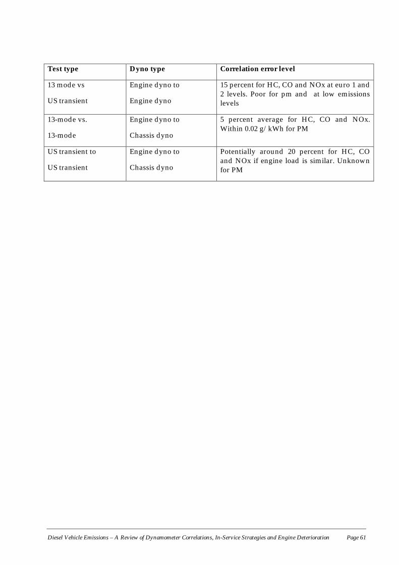
Diesel Vehicle Emissions – A Review of Dynamometer Correlations, In-Service Strategies and Engine Deterioration Page 61
Test type Dyno type Correlation error level
13 mode vs
US transient
Engine dyno to
Engine dyno
15 percent for HC, CO and NOx at euro 1 and2 levels. Poor for pm and at low emissionslevels
13-mode vs.
13-mode
Engine dyno to
Chassis dyno
5 percent average for HC, CO and NOx.Within 0.02 g/kWh for PM
US transient to
US transient
Engine dyno to
Chassis dyno
Potentially around 20 percent for HC, COand NOx if engine load is similar. Unknownfor PM
Diesel Vehicle Emissions – A Review of Dynamometer Correlations, In-Service Strategies and Engine Deterioration Page 62
5 METHODOLOGIES FOR TESTING IN AUSTRALIA
5.1 OVERVIEWThe analyses presented in Sections 3 and 4 provide a number of insights into the methodologiesto establish a correlation between chassis dynamometer emissions tests and enginedynamometer emissions tests. The recommendations presented here combine the insights fromearlier analyses as well as insights obtained by EEA in discussion with researchers in the field.The recommendations are presented in the context of the current situation in Australia, whichhas limited heavy-duty vehicle test facilities, as well as the recent development of an Australianheavy-duty vehicle driving cycle.
5.2 CYCLE SELECTIONAs noted in Section 3, the three most important chassis based test cycles for consideration are:• The steady-state 13-mode test• The SAE J1376 CBD cycle• The U.S. Federal cycle
The steady-state 13-mode test has a number of advantages. The test equipment is relatively lowcost, as no inertia weight simulation is required and no CVS system with bag sampling isrequired for emission measurement. Since most heavy-duty diesels sold in Australia are sourcedfrom Japan and Europe, replication of the certification test is possible with good relativeaccuracy, in principle.
The J1376 CBD cycle is one of the most widely used tests around the world historically and isrelatively simple to perform. Its possible uses for Australia are (1) it is capable of providingmodal emission data if emission are measured on a continuous basis and (2) it can permitcomparisons of Australian data to worldwide data. The CBD cycle is of particular interest forbus emissions, which is often the focus of emission control activity.
The U.S. Federal chassis cycle or its modified versions, may be of future importance to Australia.This may be the only chassis test available that can provide reasonable estimates of emissions onthe European or U.S. transient emissions cycle at the very stringent standards proposed for NOxand PM in the next decade. As Australia moves to standards such as Euro IV and Euro V in thefuture, the Federal cycle may be required to test these vehicles for compliance. However, thereare significant aspects of the cycle and test procedure still under development. It is an optionwhere Australia should monitor developments but not adopt the cycle immediately.
In this context, the Australian Driving cycle that is under development should be reviewed byinternational testing experts to identify significant areas of concern for implementation. Ourinvolvement in heavy-duty testing and the review presented in Section 3 and 4 show that theimplementation details can have a major effect on measured emissions and should not be left forad hoc interpretation by the laboratories concerned. The details include:
• determination of test weight (inertia) and dynamometer power absorption unit settings;• specification of gear shifts;• speed trace allowable error;• total distance allowable error;• acceleration specifications for different vehicle power-to-weight ratios.

Diesel Vehicle Emissions – A Review of Dynamometer Correlations, In-Service Strategies and Engine Deterioration Page 63
It is our understanding that such implementation details have not yet been developed by theNEPC, and should be addressed in the development effort.
5.3 EFFECT OF VEHICLE SIZE/WEIGHTBroadly speaking, the above procedures have been utilised to test trucks over a very wide inertiaweight range from 7,000 kg to 30,000+ kg. Hence, the specification of the cycle is not necessarilyaffected by vehicle weight and size although the size of the dynamometer is affected due to theneed for twin-roller dynamometers for vehicles over 18,000 kg GVW with twin drive axles. Inaddition, the dilution air requirements increase in proportion to engine rated HP, so that theemissions measurement system flow rate capability is an issue for large vehicles or large engines.
While the above issues are obvious, there are secondary issues that can cause testing problems.First, the power-to-loaded weight ratio decreases as a function of truck size, and large trucks ofover 20 tons GVW have great difficulty in following a driving trace with a high degree oftransient behaviour, leading to significant speed and distance errors over a chassis cycle.Secondly, large trucks feature multi-speed gearboxes, and many transient cycles do not allowenough time in the trace for manually shifting a nine or ten-speed gearbox. In contrast, manylighter models especially around 3.5 to five tons GVW are equipped with automatictransmissions which are easier to use in following a transient driving cycle, but could causeproblems in the 13-mode due to the potential inability to hold the same gear for some subset ofmodes, and due to potential difficulty in maintain torque converter loss constant during aparticular mode.
Third, most of the smaller trucks in-use in Australia are sourced from Japan, so that there is somecorrelation between truck weight and test type. Methods developed for larger European sourcedengines may not be applicable to smaller trucks.
5.4 EFFECT OF CERTIFICATION STANDARDS AND COUNTRY OF ORIGINDuring the 1980 to 1995 period, there have been significant differences in the stringency ofemissions standards between the U.S., Europe and Japan. As discussed in Section 6 of thisreport, typical average emissions for a modern diesel engine design that is largely“uncontrolled” is about 11 to 12 g/kWh for NOx and 0.5 to 0.6 g/kWh for PM based on the U.S.transient test. These are averages, with emissions distributed widely around these values.Hence, most engines were significantly below applicable standards prior to the Euro I standards.The pre-1999 Japanese standard, based on their own speed 13-mode test, is also believed to benot very stringent on NOx, and most engines are well below certification limits.
If Australia intends to test pre-Euro I or pre-1999 Japanese diesels for compliance with thestandards in the country of origin, it is anticipated that few vehicles will fail to comply, and mostwill be well below standards.
On the other hand, post-1994 U.S. engines certified to very stringent NOx and PM standards willbe difficult to test on the 13-mode, since measured PM on any contemplated 13-mode or steadystate tests will be close to measurement thresholds. Hence, the levels of measurement error forPM may be unacceptable for well-maintained diesel engines calibrated to 1994+ U.S. emissionstandards.
Separately, the issue of the Japanese 6-mode test, which applied to all 1994 and earlier vehiclesfrom 3.5 to 12 tons indicates that the need to develop expertise in the steady-state 6-mode cycle,if compliance issues for these vehicles are of interest in Australia. If compliance with original six-mode standards is not an issue, than the specific issues with the six-mode test may not needinvestigation.
Diesel Vehicle Emissions – A Review of Dynamometer Correlations, In-Service Strategies and Engine Deterioration Page 64
With the introduction of Euro III standards in Europe and the further tightening of standards in2004 in the U.S. and 2005 in Europe, Australian testing capabilities must improve significantly sothat it is possible to run a complete transient cycle with inertia weight simulation. We are awarethat simpler test facilities are likely to be used in the near term due to the lack of test facilities inAustralia, but caution that the usefulness of these facilities will be time limited.
There are also some special issues on data availability to conduct correlation testing. The 13-mode test requires knowledge of the test RPM values that can be obtained from the typeapproval certificate in Europe. No such equivalent is available in the U.S. and it is not clear if thetype approval details are publicly available for Japanese certification. Using the fuelconsumption based power setting determination on the 13-mode test could also result inproblems if the engine bsfc maps are not readily available; such maps are difficult to obtain forAustralian models of U.S. or Japanese engines.
5.5 EFFECT OF AGE/STATE-OF-MAINTENANCEMost of the difficulties encountered with testing older vehicles are operational in nature. First,many older vehicles can be in poor mechanical state, and tyre and axle bearing failures can occurdriving the test, causing damage or safety problems. Most facilities perform a detailedmechanical check of the drivetrain, brakes and tyres prior to acceptance for testing to ensuremechanical safety. Tyres are especially prone to damage at high load test points on the chassisdynamometer, and older vehicles must have good tyres, or else test tyres must be fitted to thevehicle.
Second, the availability of all required data to conduct the test may be a problem on oldervehicles, especially if the engine sticker is missing or contains ambiguous data. Even in Europe,recent test programs on older trucks had difficulty in resolving engine certification states onabout five percent of all trucks. The problem may be far more severe in Australia where therewere no emission requirements prior to 1996.
Third, the fuel consumption based method may not yield correct results if the engine calibrationis incorrectly set (either intentionally or due to component wear). For example, turbochargerwear would result in lower boost pressure at a given RPM/throttle setting, leading tosignificantly lower power than calculated based on fuel consumption. Hence, on test cycles suchas the 13-mode where engine output must be estimated, the problems with older or mal-maintained engines could give rise to significant emission measurement errors if emissions aremeasured in g/kWh.
5.6 LEVELS OF CORRELATION ACHIEVABLEThe issues regarding correlation of emission measurements are relatively complex, and dependon the type of chassis test employed, the type and age of the vehicle tested, and the experienceand expertise of the laboratory conducting the tests.
Successful correlation of chassis test based emission results with engine test based emissionresults have been achieved on the 13-mode test in Europe. Average emission error relative to theofficial certification test should be within ±5 percent but maximum error can be much largerespecially for low emissions engines.
However, it should be noted that these tests have access to the type approval certificate thatspecifies engine RPM and fuel consumption at the different test modes. It also relies on the useof special tyres with known (measured) rolling resistance coefficients and empirical formulaederived for accessory and transmission power losses for European trucks. Since Australiandiesel engines are sourced from a variety of countries, it is not clear that all of the required data
Diesel Vehicle Emissions – A Review of Dynamometer Correlations, In-Service Strategies and Engine Deterioration Page 65
inputs are available to achieve this level of correlation. In the more general case where the datainputs must rely on a combination of available data and engineering analyses, the correlationcould be significantly worse.
In addition, there will be an initial phase where new laboratories in Australia will gainexperience with the procedure. It is likely that once some experience is gained, a COV of tenpercent maybe a reasonable expectation for correlation, for all pollutants except PM. For PM, theCOV may be larger. However, for all pollutants, the COV will increase for tests on modernengines with very low emission levels.
Repeat tests of the 13-mode or any transient cycle on the chassis dynamometer should achieve arepeatability level with a COV of five percent or less for all pollutants except PM. The absoluteemission level of PM and the repeatability of the PM measurement system may lead to highervariances, in the range of 20 percent.
Geometric cycles that can be used to generate modal data are typically very repeatable, and inter-lab comparisons have shown that cycle emissions can be reproduced with a COV of five percentor less, except in the case of PM emissions. Data from modal emissions profiles can be utilised toestimate emission factors for any driving condition.
“Realistic” driving cycles such as the chassis based U.S. transient test or the Australian DrivingCycle have a number of open issues regarding cycle specifications and test protocol that make itdifficult to provide an estimate of correlation. If the cycle is defined as a speed/time trace that isinvariant for all trucks, correlation with engine tests can be very poor. New developments toscale cycle characteristics to truck capability and to define testing protocol more carefully maylead to significant improvements in the correlation between measured emission on the chassistest and the engine test in the near future, but success is not assured. Data from limited testingsuggests that a COV of 20 percent or so may be possible with well-specified test procedures.
5.7 CHECKLIST OF KEY ISSUES FOR TESTINGBased on recent considerations of the types of laboratories available in Australia, the NEPC couldutilise the following points as a checklist for deciding testing capability.
• Dynamometer configuration – a twin roll dynamometer with inertia weights and a powerabsorption unit capable of simulating loads up to 300 HP and weights to 40,000 kg can beused for all types of tests. Axle or hub attached dynamometers can be used for steady statetests. If these dynamometers are not capable of motoring the engine during decelerations,emissions measured on transient tests may not be accurate, especially for PM and HCemissions.
• Emission measurement – gaseous emissions measurement is generally not a major problem.Measurement of PM emissions using a flow splitter/dilution tunnel approach is difficult forlow PM emissions engines. Flow rates in the tunnel and filter weight measurementthresholds should be carefully considered for accuracy.
• Steady-state tests – reproduction of the 13-mode requires the ability to measure power outputof the engine. If the power loss method is proposed, special tyres with known rollingresistance will need to be used. The adequacy of European formulae to predict transmissionand axle power loss should be checked for a sample of Australian trucks. If fuelconsumption is used as a power indicator, the availability of fuel consumption maps fortested engines from the manufacturer is essential.
• Transient cycle – detailed specifications need to be developed for all transient cyclesincluding the CUEDC to enable correct setting of (1) inertia weight (2) power absorption (3)allowable speed trace error (4) allowable total distance error and (5) gear shift requirements
Diesel Vehicle Emissions – A Review of Dynamometer Correlations, In-Service Strategies and Engine Deterioration Page 66
for any arbitrary transmission. Driver training will be required to follow the specified cycletrace with any arbitrary engine/transmission. Cycles will need to be “scaled” to each truck’spower-to-weight ratio.
• Country of origin of test truck – a comprehensive library of the type approval certificates willbe required to determine the steady-state test modes for all engines. No such data isavailable on Japanese engines certified on the 6-mode test or U.S. engines certified since 1984.An alternative 13-mode test specification must be derived for such engines
• Older/Poorly maintained vehicles – apart from the usual safety issues, such vehicles maypose problems if 13-mode test power determination is fuel consumption based. Mal-performance in the engine can raise (or even lower) fuel consumption by as much as tenpercent for a given setting. Hence, some procedure must be specified to determine the stateof tune of a tested engine.
The levels of correlation achievable relative to an engine test are dependent on a detailed andsuccessful resolution of all the issues raised above.
Diesel Vehicle Emissions – A Review of Dynamometer Correlations, In-Service Strategies and Engine Deterioration Page 67
6 EMISSIONS DETERIORATION UNDER IN-SERVICECONDITIONS
6.1 OVERVIEWProject 6 as defined by the NEPC requires an examination of the emissions deterioration of bothlight and heavy-duty diesel vehicles under in-service conditions. However, the diesel fleet inAustralia has few “light-duty” vehicles if one uses consistent definitions across countries. Dieselpenetration in cars is very low, in the order of 2.5 percent, in Australia. Light commercialvehicles are not consistently defined in all the Australian states, but the broadest definitionincluded passenger and cargo vans, sport utility (4 wheel drive) vehicles, small pickup trucks, aswell as small delivery trucks in the 2.5 to 3.5 ton GVM range. Reports for the NEPC haveidentified the diesel penetration for the LCV fleet to be over 20 percent, but this may apply to amore narrow definition of LCV. For example, VFACTS reported sales of about 166,000 LCVs in1997, of which small cargo vans were 20,000, pickup trucks were about 73,000, sport utilityvehicles were about 71,000 and small commercial trucks were about 2000. Other LCV definitionsdo not include the sport utility vehicles, and we believe that the diesel penetration for LCV relieson this type of definition, and indicates sales of about 20,000 diesel LCVs per year in the recentpast.
Typical diesel engines used in LCVs fall largely into two categories. One category includessmaller versions of heavy-duty engines used in vehicles in the 3.5 to 7 ton GVM range, such as afour cylinder version of a 6 litre displacement, 6 cylinder engine. This type of engine is popularfor the 2.5 to 3.5 ton GVM class and in some pickup style vehicles and cargo vans. The secondtype are unique prechamber diesels that are relatively large displacement (about 4 litres) lightduty engines. Such engines are used in several popular sport utility vehicles and pickup trucks,such as the Toyota Land Cruiser and Nissan Patrol. The emission characteristics of the first typeare likely to be quite similar to the larger versions employed in heavy-duty trucks. The emissioncharacteristics of the second group are largely unknown as no studies have been done of their in-use emissions. More conventional light-duty passenger car diesels have been largely of Europeanorigin, with VW, Mercedes and Peugeot accounting for the majority of such vehicles in Australia.There are few European studies of their emissions behaviour. Hence the focus of this report is onheavy-duty diesels, as this is most relevant to Australia.
The emissions of in-service heavy-duty diesel engines relative to certification levels have also notbeen studied extensively due to two reasons. First, diesel engine test facilities are quite limitedand no good chassis test procedures exist, as is evident from the discussion in Sections 3 and 4.Second, diesel engines were widely believed to have stable emissions over their useful life; theU.S. EPA assumed emission factors essentially equal to certification standards, as an example.
Since the late-1980s, there has been a growing realisation that in-service diesels do not maintaincertification level emissions over their useful life. There are several components to the in-serviceemissions deterioration, or “excess” emissions that occurs. First, even in the certification process,emissions are assigned a deterioration factor based on an idealised durability cycle, and the realworld duty cycles imparts somewhat larger deterioration in emissions relative to the certificationdurability test. Second, the levels of maintenance recommended by the manufacturers areusually not strictly followed, causing additional deterioration. Third, there may be mal-maintenance (either intentional or unintentional) due to mechanic inexperience. Fourth, theremay be intentional tampering, usually to increase horsepower or fuel economy. Lastly, theremay be design defects in the emission control system that cause high emissions.
Diesel Vehicle Emissions – A Review of Dynamometer Correlations, In-Service Strategies and Engine Deterioration Page 68
In general, the severity of the emission deterioration increases from the first reason to the fifth.However, tampering and design defects usually affect only a small portion of the fleet, except insome usual circumstances. Such a circumstance occurred recently in the U.S., where the EPAdetermined that heavy-duty engine manufacturers had employed ‘cycle beating’ devices thatresulted in low certification test emissions but high in-service emissions.
The typical methodology used to determine the in-service emissions of a group or class ofvehicles is to obtain a random sample of these vehicles that is a snapshot of their representationin the fleet and test them for emissions. The emission results are regressed against odometer(VKT) or vintage to obtain an average deterioration rate for the fleet. This method only works ifthe sample size is relatively large and the incidents of mal-maintenance and tampering in thesample are similar to the fleet wide rate. Typically, sample sizes of several hundred vehicles arenecessary to capture those incidents (which occur at rates of a few percent, typically) and toprovide reasonable confidence in the estimates.
Unfortunately, in the case of heavy-duty trucks, the samples range from a few vehicles to a fewtens of vehicles, making statistical approaches of limited value. Hence, there have been attemptsto model the emission deterioration on a semi-theoretical basis, using observed rates of mal-performance and tampering from larger samples with engineering estimates of the effects of thethese defects on emissions.
Both the test data based approach and the modelling approach are described here, with theresults compared.
6.2 EUROPEAN EMISSION FACTOR PROGRAMSSignificant testing in-service heavy-duty trucks has been conducted in Europe by twoorganisations in particular: the TNO in Netherlands, the Transportation Research Laboratory inthe U.K. and TUV-Rheinland in Germany. More limited testing of trucks has been conducted inSweden.
6.2.1 Testing in NetherlandsThe TNO in Netherlands has conducted tests on the largest sample of heavy-duty trucks inEurope. Data from a November 1998 report19 indicates that total of 128 heavy-duty vehicles hadbeen tested through early 1998, with the sample broken out as follows:
• 88/77EEC standard - 26• Euro I standard - 76• Euro II standard - 26
Virtually all of these trucks were tested on the R49 based 13-mode test conducted on a chassisdynamometer.
As noted in the discussion in Section 2 that Euro O (88/77/EEC) and Euro I standards were notvery stringent, and most engines were certified at levels well below applicable standards. Hence,the prospect of failing the standards is quite unlikely, as it would require significant tampering.
For the 26 Euro O certification vehicles, there were no failures of NOx or HC standards (No PMstandards were in force). The highest observed NOx was 10.2 g/kWh, which is well below the14.4 g/kWh standard. Average levels for most engines were in the 7 to 8 g/kWh range with thelowest at 5.6 g/kWh. Typical PM level were 0.4 to 0.6 g/kWh, with the highest at 0.8 g/kWh.

Diesel Vehicle Emissions – A Review of Dynamometer Correlations, In-Service Strategies and Engine Deterioration Page 69
Data on 64 of the 76 Euro I vehicles tested was available. There were several engines close to the9 g/kWh production standard, and since measurement error and production tolerances cancause minor exceedances of the standard, we evaluated emission failures at a level about tenpercent above the standards. Only four of the 64 engines exceeded the 10 g/kWh NOx level, andthree of the 64 exceeded the 0.44 g/kWh PM level. The highest observed NOx level was 14.2g/kWh and the highest PM level was 0.6 g/kWh.
Data on the 26 Euro II certification vehicles showed one vehicle with NOx higher than ten percentabove the certification limit of 7.0 g/kWh (i.e., over 7.7 g/kWh) and two vehicles exceeding the0.15 g/kWh PM standard by over ten percent.
Both the Euro I and Euro II standard samples indicate a failure rate for each pollutant in therange of five to eight percent. Conversations with TNO indicated that is about the correctobserved failure rate in Europe. It should be noted that few vehicles fail both NOx and PMstandards simultaneously.
The TNO also conducted detailed checks on a subset of engines were checked for calibration.The defects found and the observed rates are as follows:
• Incorrect maximum fuel setting - 11 percent• Incorrect governor RPM setting - 5.5 percent• Injection timing (early) - 8 percent• Injection timing (late) - 13 percent• Injector worn - 13 percent
Typically, early injection timing leads to high NOx, while injector wear and incorrect fuel pumpsettings can lead to high PM and HC, if severe enough.
6.2.2 Testing in the U.K.The Transportation Research Laboratory (TRL) conducted tests in 1998/1999 on 20 heavy-dutyvehicles, ten of which were certified to Euro I standards and ten to Euro II standards. Allvehicles were tested on a chassis dynamometer on both the 13-mode test and the European FIGEtransient test. Fourteen vehicles had inertia weights between 12,500 and 15,000 kg, while sixwere lighter with the lightest at 5800 kg.
Consistent with the experience of the other European countries, only one vehicle of ten failed theEuro I standards, with NOx emissions at 11.5 g/kW-h. None of these vehicles exceeded the HC,CO or PM standards. Similarly, only one of the ten vehicles failed the Euro II standard, withNOx emission at 7.98 g/kW-h, while a second exceeded the NOx standards by a small amount(two percent) so that it cannot be classified as a failure with high confidence.
Mean emission levels for the two groups of vehicles are as follows:
Euro I - 0.43 HC/1.34 CO/7.45 NOx/0.09 PM g/kW-h
Euro II - 0.30 HC/1.60 CO/6.37 NOx/0.05 PM g/kW-h
This shows that most Euro I engines were well below applicable production standards for allpollutants. The Euro II engine mean NOx emissions were relatively close to standards, but allother pollutant emissions were well below standards.
Diesel Vehicle Emissions – A Review of Dynamometer Correlations, In-Service Strategies and Engine Deterioration Page 70
The same engines tested on the FIGE transient cycle had NOx emission that was about fivepercent lower on average, but HC emissions that were 30 percent higher, relative to the 13-modetest. PM emissions on the FIGE cycle were 0.24 g/kW-h for Euro I engines and 0.17 g/kW-h forEuro II engines. These values are much higher than those on the 13-mode test but still quite lowin comparison even to Euro III standards.
6.2.3 Testing in GermanyThe TUV-Rheinland has also tested a variety of engines, although there is no recent report ontheir test activities. One major emission factor program conducted in 1995 tested 34 engines9with the sample breakdown as follows:
• ECE R49 - 20• 88/77/EEC - 12• Euro I - 2
In contrast to the TNO tests, the TUV tests were performed on an engine dynamometer. Inaddition to the 13-mode test, the U.S. transient test and a more detailed mapping of emissions at35 steady-state test points were performed to develop a modal emissions model.
As expected, none of the engines exceeded the ECE R49-01 standards for NOx and CO, althoughthere were two engines with very high gaseous HC emissions and particulate emissions. Theaverage HC emissions was 1.8 g/kWh, but the two ‘high” engines exceeded 4 g/kWh. AverageNOx emission was 11.2 g/kWh, while the highest was at 17.3 g/kWh, slightly below the 18.0standard. The two “high” HC emitters also had very high particulate emissions at over threetimes the average of 0.7 g/kWh.
The 88/77/EEC certified (Euro O) engines showed significantly lower emissions. HC and COemissions were far below standards but one of the 12 engines tested exceeded the NOx emissionsstandard of 14.4 g/kWh by less than ten percent. Particulate emissions were in the same rangeas in the TNO tests, but all engines had PM emissions below 0.6 g/kWh. The NOx failure rate isstatistically similar to the observed failure rate in the TNO tests.
The two Euro I certified engines were relatively new at the time of testing and had NOx
emissions of about 7 g/kWh and PM emissions of 0.3 g/kWh. HC and CO levels were at lessthan half the applicable standards.
6.2.4 Other TestsSweden has also recently conducted some testing of heavy-duty vehicles by its Motor TestCentre (MTC: the Swedish testing organisation) but the sample is very small. MTC has testedfive heavy-duty trucks and two truck engines on the chassis and engine dynamometerrespectively (MTC:1995). Sweden had optional certification to Euro II standards even prior to1996 and two of the vehicles tested had apparently been certified to this optional standard. Allvehicles met Euro I limits, but the two vehicles certified to the Euro II limits exceed the PMstandard by small amounts. One vehicle tested was a Scania bus with an oxidation catalyst. Itwas tested twice, once when new and the second time at 142,000 km. Although there wereemission increases with use, the absolute values of CO and HC emissions were very low (wellbelow Euro II standards) due to the catalyst. The Swedish data has too small a sample to makebroad judgements about emission failure rates or in-use deterioration in Sweden.
Diesel Vehicle Emissions – A Review of Dynamometer Correlations, In-Service Strategies and Engine Deterioration Page 71
6.2.5 Light-Duty Diesel TestingThere have been tests of in-use light duty diesels by the TNO in Netherlands and by the TUV inGermany as part of broader emission factor programs for all light duty vehicles in the 1980s, butthe overall sample of diesel vehicles tested in that era is still quite small. However, the issue withthe European testing is that emission standards for light duty vehicles prior to the Euro Istandard introduced in 1992 were quite lax, and the standards were above the near uncontrolledrate for light duty diesel vehicles for HC, CO and NOx. (Typically, HC and CO emissions fromlight duty diesels are at extremely low levels in comparison to gasoline engine emissions). Therewere no particulate emission requirements in the 1980s, and it was broadly concluded thatemissions from in-use diesels did not suggest any large-scale violations of standards. The Euro Istandard of 1992 imposed a HC+NOx standard of 0.97 g/km and a PM standard of 0.14 g/kmwhile the Euro II standard of 1996 resulted in further reductions to 0.7 g/km and 0.08 g/kmrespectively. Even the Euro I standard for HC+NOx is still above the near uncontrolled emissionlevel for most modern light-duty diesels and only the PM standard was a serious constraint. Atesting program conducted during 1995-1997 in support of an Inspection test developmentprogram tested 28 diesels certified to Euro I levels. Not surprisingly, no vehicles failed to meetthe standards for gaseous pollutants. Several vehicles failed to meet particulate emissionstandards, although only 3 of 28 vehicles exceeded the limit by more than 25 percent. Only one ofthe 28 vehicles was a “gross” emitter with PM emissions slightly in excess of 1 g/km, over 7times the standard. As a result, much of the focus in Europe is on identifying and repairing highPM emitters.
6.3 EMISSION FACTOR TESTING IN THE U.S.There has been remarkably little testing in the U.S. on broad samples of in-use trucks. Arelatively small number of in-use diesel 1979 HDTs and buses (thirty) were tested by South WestResearch (SWRI) in the early 1980’s. The HDTs were tested on a chassis dynamometer over atransient cycle test that was not exactly identical to the New York and L.A. urban cycles and theLA freeway cycle used to simulate the engine test. Nevertheless, the chassis test had similaritiesin average speed and loading to the engine test procedure. The tests covered 23 heavy-dutytrucks and seven buses.
A comprehensive analysis of the dependence of emissions on odometer from the chassisdynamometer data was attempted by converting the emissions to units of g/bhp-hr using acalculation derived from the dynamometer HP and weight setting (EEA:1985). It was obviousthat the emissions (in g/kWh) were radically different for buses in comparison to trucks, andwere typically two to three times higher on average. Therefore, it was decided to treat the twovehicle types separately. For the 23 trucks, inspection of the emission data revealed that therewas a strong trade-off between HC and NOx emissions. This trade-off is well known inengineering circles, and since the 1979 emissions requirements specified only a HC + NOx
standard, manufacturers often set different goals for HC and NOx. Only one vehicle had bothvery high NOx and very high HC emissions, and was removed from the analysis.
The remaining emissions data on 22 trucks were then analysed to provide emission factors as afunction of use, i.e., a zero mile rate and an odometer dependent rate of the form:
Brake-Specific Emissions = C + D x ODOMETER
The results for HC, CO, NOx, particulates and HC + NOx are summarised in Table 6-1. Usingdata on the 22 trucks, it can be seen the odometer dependence of the emission factor (i.e.deterioration rate) is not statistically significant at the 90 percent confidence level for HC, NOx
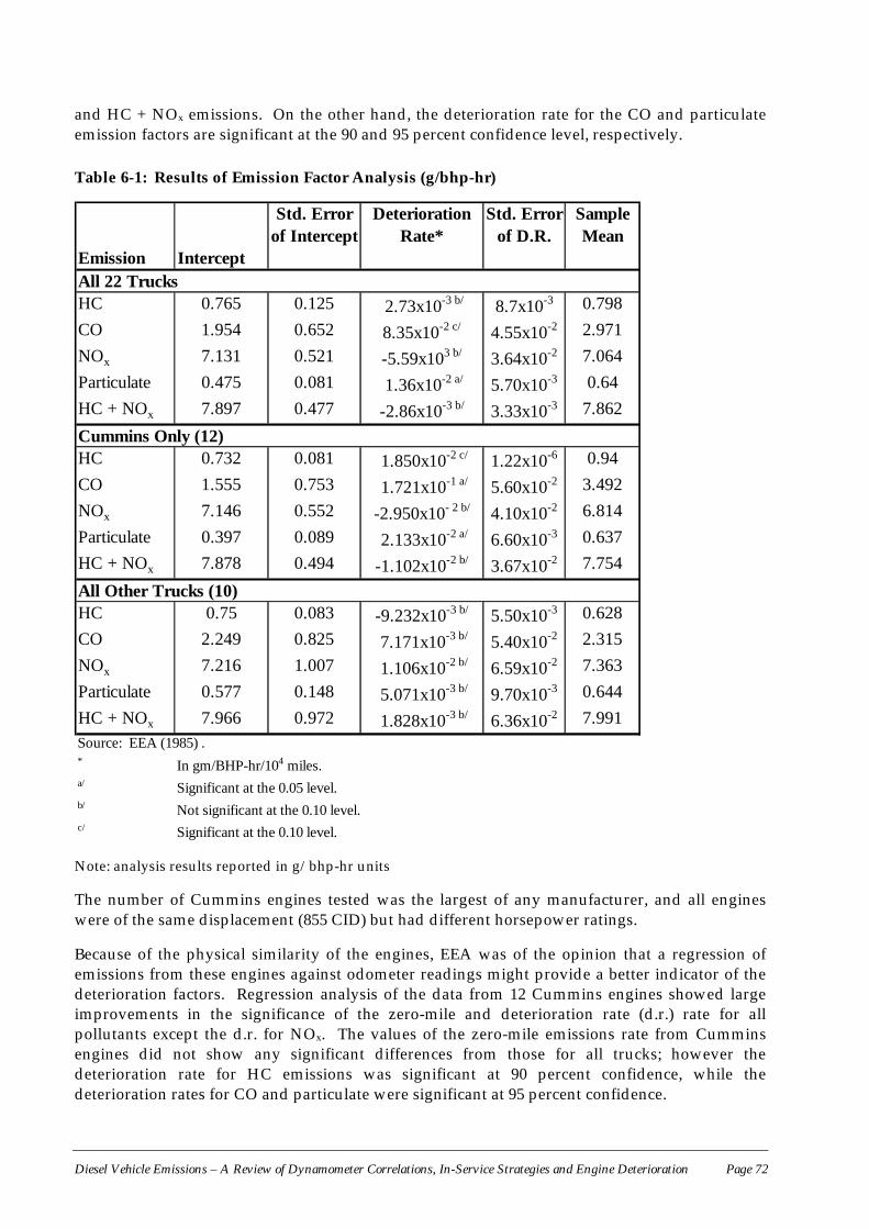
Diesel Vehicle Emissions – A Review of Dynamometer Correlations, In-Service Strategies and Engine Deterioration Page 72
and HC + NOx emissions. On the other hand, the deterioration rate for the CO and particulateemission factors are significant at the 90 and 95 percent confidence level, respectively.
Table 6-1: Results of Emission Factor Analysis (g/bhp-hr)
Emission Intercept
Std. Error of Intercept
Deterioration Rate*
Std. Error of D.R.
Sample Mean
HC 0.765 0.125 2.73x10⁻³ b/ 8.7x10⁻³ 0.798CO 1.954 0.652 8.35x10⁻² c/ 4.55x10⁻² 2.971NOx 7.131 0.521 -5.59x10³ b/ 3.64x10⁻² 7.064Particulate 0.475 0.081 1.36x10⁻² a/ 5.70x10⁻³ 0.64HC + NOx 7.897 0.477 -2.86x10⁻³ b/ 3.33x10⁻³ 7.862
HC 0.732 0.081 1.850x10⁻² c/ 1.22x10⁻⁶ 0.94CO 1.555 0.753 1.721x10⁻¹ a/ 5.60x10⁻² 3.492NOx 7.146 0.552 -2.950x10- 2 b/ 4.10x10⁻² 6.814Particulate 0.397 0.089 2.133x10⁻² a/ 6.60x10⁻³ 0.637HC + NOx 7.878 0.494 -1.102x10⁻² b/ 3.67x10⁻² 7.754
HC 0.75 0.083 -9.232x10⁻³ b/ 5.50x10⁻³ 0.628CO 2.249 0.825 7.171x10⁻³ b/ 5.40x10⁻² 2.315NOx 7.216 1.007 1.106x10⁻² b/ 6.59x10⁻² 7.363Particulate 0.577 0.148 5.071x10⁻³ b/ 9.70x10⁻³ 0.644HC + NOx 7.966 0.972 1.828x10⁻³ b/ 6.36x10⁻² 7.991
* In gm/BHP-hr/104 miles.a/ Significant at the 0.05 level.b/ Not significant at the 0.10 level.c/ Significant at the 0.10 level.
All Other Trucks (10)
Source: EEA (1985) .
All 22 Trucks
Cummins Only (12)
Note: analysis results reported in g/bhp-hr units
The number of Cummins engines tested was the largest of any manufacturer, and all engineswere of the same displacement (855 CID) but had different horsepower ratings.
Because of the physical similarity of the engines, EEA was of the opinion that a regression ofemissions from these engines against odometer readings might provide a better indicator of thedeterioration factors. Regression analysis of the data from 12 Cummins engines showed largeimprovements in the significance of the zero-mile and deterioration rate (d.r.) rate for allpollutants except the d.r. for NOx. The values of the zero-mile emissions rate from Cumminsengines did not show any significant differences from those for all trucks; however thedeterioration rate for HC emissions was significant at 90 percent confidence, while thedeterioration rates for CO and particulate were significant at 95 percent confidence.
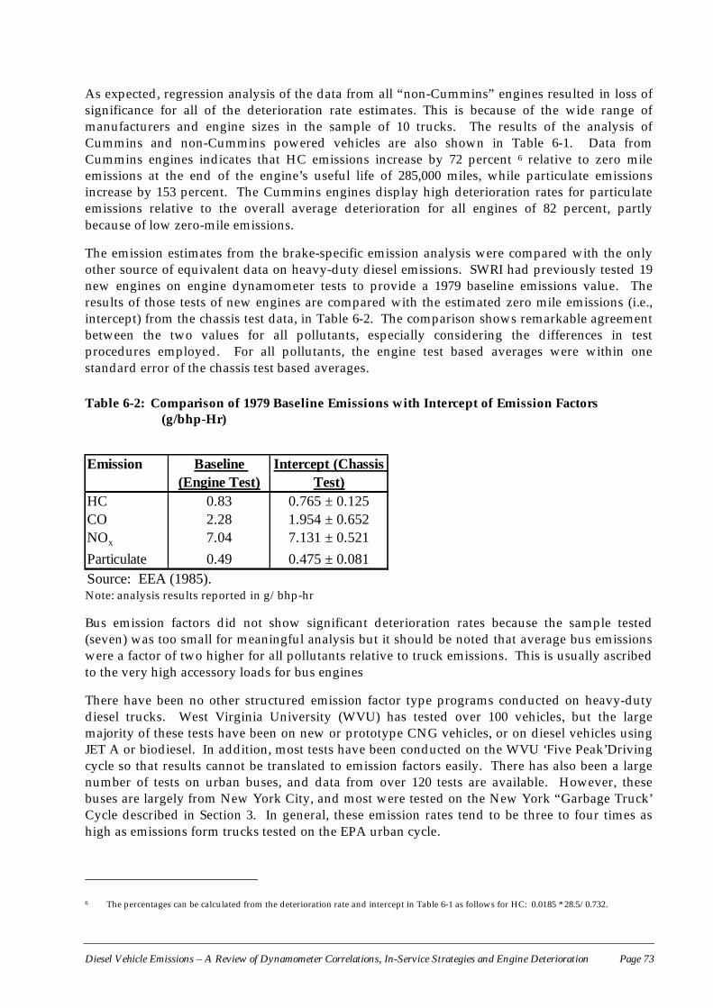
Diesel Vehicle Emissions – A Review of Dynamometer Correlations, In-Service Strategies and Engine Deterioration Page 73
As expected, regression analysis of the data from all “non-Cummins” engines resulted in loss ofsignificance for all of the deterioration rate estimates. This is because of the wide range ofmanufacturers and engine sizes in the sample of 10 trucks. The results of the analysis ofCummins and non-Cummins powered vehicles are also shown in Table 6-1. Data fromCummins engines indicates that HC emissions increase by 72 percent 6 relative to zero mileemissions at the end of the engine’s useful life of 285,000 miles, while particulate emissionsincrease by 153 percent. The Cummins engines display high deterioration rates for particulateemissions relative to the overall average deterioration for all engines of 82 percent, partlybecause of low zero-mile emissions.
The emission estimates from the brake-specific emission analysis were compared with the onlyother source of equivalent data on heavy-duty diesel emissions. SWRI had previously tested 19new engines on engine dynamometer tests to provide a 1979 baseline emissions value. Theresults of those tests of new engines are compared with the estimated zero mile emissions (i.e.,intercept) from the chassis test data, in Table 6-2. The comparison shows remarkable agreementbetween the two values for all pollutants, especially considering the differences in testprocedures employed. For all pollutants, the engine test based averages were within onestandard error of the chassis test based averages.
Table 6-2: Comparison of 1979 Baseline Emissions with Intercept of Emission Factors(g/bhp-Hr)
Note: analysis results reported in g/bhp-hr
Bus emission factors did not show significant deterioration rates because the sample tested(seven) was too small for meaningful analysis but it should be noted that average bus emissionswere a factor of two higher for all pollutants relative to truck emissions. This is usually ascribedto the very high accessory loads for bus engines
There have been no other structured emission factor type programs conducted on heavy-dutydiesel trucks. West Virginia University (WVU) has tested over 100 vehicles, but the largemajority of these tests have been on new or prototype CNG vehicles, or on diesel vehicles usingJET A or biodiesel. In addition, most tests have been conducted on the WVU ‘Five Peak’Drivingcycle so that results cannot be translated to emission factors easily. There has also been a largenumber of tests on urban buses, and data from over 120 tests are available. However, thesebuses are largely from New York City, and most were tested on the New York “Garbage Truck’Cycle described in Section 3. In general, these emission rates tend to be three to four times ashigh as emissions form trucks tested on the EPA urban cycle.
6 The percentages can be calculated from the deterioration rate and intercept in Table 6-1 as follows for HC: 0.0185 * 28.5/0.732.
Emission Baseline (Engine Test)
Intercept (Chassis Test)
HC 0.83 0.765 ± 0.125CO 2.28 1.954 ± 0.652NOx 7.04 7.131 ± 0.521Particulate 0.49 0.475 ± 0.081Source: EEA (1985).
Diesel Vehicle Emissions – A Review of Dynamometer Correlations, In-Service Strategies and Engine Deterioration Page 74
There has been virtually no emission factor of light duty diesels in the US, largely because ofvery low light-duty diesel penetration in the US market. Diesels enjoyed a brief burst ofpopularity in the US light-duty market in the 1979 to 1983 time frame, with the GM 5.7 litre V8diesel and the VW 1.6 litre 4-cylinder diesel accounting for the vast majority of sales. These firstgeneration passenger car diesels suffered from several mechanical problems, with the GM diesel,in particular, having such severe problems that it was withdrawn from production. A smallnumber of these diesels were tested by the EPA and California in the mid-1980s and found tohave high particulate and HC emissions, but these conclusions are probably specific to thesemodels, and not generally applicable to better established diesels from Mercedes or Peugeot.Since that time, there has been no emission factor testing of light duty diesels in the US
6.4 HDDV EMISSION FACTORS DERIVED FROM MODELSDue to the very limited testing of in-use HDDVs, the U.S. EPA has largely assumed the emissionfactors from certification standards. MOBILE5, the EPA Mobile Source emission inventory modelincorporates emission factors for all HDDV’s but treats all HDDVs as a single group, so thatdifferences between light-heavy, medium-heavy and heavy-heavy duty vehicles cannot beobserved from the emission factors. More importantly, the emission factors for HC and NOx arebased solely on certification standards and have zero deterioration rates for all diesel trucks since1984. While detailed documentation of the EPA emission factor derivation was not provided, itis apparent that the emission factor is set approximately equal to an assumed certification level,which is 20 to 30 percent below the certification standard, for 1984 and later HDDVs. The U.S.EPA does not have separate emission factors for buses, and the available data suggests that busemissions are significantly higher than truck emissions.
Surveys conducted by California have established that diesel truck HC emissions increase withuse due to component deterioration, mal-maintenance or intentional maladjustment (tampering)in the field. Many types of mal-performances give rise to high smoke levels, and smoky trucksare widely observed on-the-road. Random samples of HDDVs from surveys conducted in1990/1991 have indicated that about one-third of the HDDV population had smoke well inexcess of certification standards, especially during acceleration. Hence, EPA’s assumption ofzero deterioration seems unjustifiable for HC and particulate emissions. However, the inverserelationship between NOx and HC suggest that NOx emissions deterioration with age or use maybe zero or even negative.
Surveys of diesel engines in the field, and the expertise of the manufacturers’ serviceorganisations has allowed a comprehensive compilation of the typical mal-performances thatoccur in diesels which lead to high smoke or gaseous emissions. In general, mal-performances inthe intake air system or the fuel system are the most common causes of high smoke and HCemissions, although an engine in very poor mechanical condition can have sufficient loss oflubricating oil or compression to cause high smoke and gaseous emissions.
Based on discussions with manufacturers, the data developed by EEA23 in Table 6-3 is acomprehensive listing of mal-performance in diesel engines, and their frequency of occurrence asmeasured in a qualitative form. In the air intake system, dusty air filters and leaky turbochargeroil seals are relatively common, while more serious turbocharger damage or problems with theintercoolers are quite rare. Valve system timing and valve leaks are also less frequentlyobserved; if a valve leak is significant, then the cylinder can stop functioning completely due toloss of compression and the resulting vibration will make the engine undriveable in short order.
On the fuel system side, governor tampering and tampering with the “air-fuel ratio control” (alsoknown as throttle delay) are widely acknowledged as the most common forms of tampering,
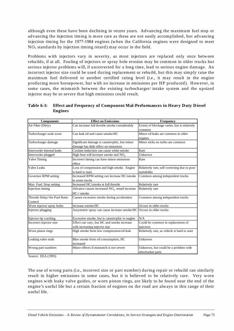
Diesel Vehicle Emissions – A Review of Dynamometer Correlations, In-Service Strategies and Engine Deterioration Page 75
although even these have been declining in recent years. Advancing the maximum fuel stop oradvancing the injection timing is more rare as these are not easily accomplished, but advancinginjection timing for the 1977-1984 engines (when the California engines were designed to meetNOx standards by injection timing retard) may occur in the field.
Problems with injectors vary in severity, as most injectors are replaced only once betweenrebuilds, if at all. Fouling of injectors or spray hole erosion may be common in older trucks butserious injector problems will, if uncorrected for a long time, lead to serious engine damage. Anincorrect injector size could be used during replacement or rebuild, but this may simply raise themaximum fuel delivered to another certified rating level (i.e., it may result in the engineproducing more horsepower, but with no increase in emissions per HP produced). However, insome cases, the mismatch between the existing turbocharger/intake system and the upsizedinjector may be so severe that high emissions could result.
Table 6-3: Effect and Frequency of Component Mal-Performances in Heavy Duty DieselEngines
The use of wrong parts (i.e., incorrect size or part number) during repair or rebuild can similarlyresult in higher emissions in some cases, but it is believed to be relatively rare. Very wornengines with leaky valve guides, or worn piston rings, are likely to be found near the end of theengine’s useful life but a certain fraction of engines on the road are always in this range of theiruseful life.
Components Effect on Emissions FrequencyAir Filter (Dirty) Can increase full throttle smoke considerably Extent of blockage varies, but is relatively
commonTurbocharger seals worn Can leak oil and cause smoke/HC Minor oil leaks are common in older
enginesTurbocharger damage Significant damage is catastrophic, but minor
damage has little effect on emissionsMinor nicks on turbo are common
Intercooler internal leaks Coolant induction can cause white smoke RareIntercooler plugged High heat will increase smoke and NOx UnknownValve Timing Incorrect timing can have minor emissions
effectRare
Valve Leaks Loss of compression and high smoke. Engine is hard to start.
Relatively rare, self correcting due to poor startability
Governor RPM setting Increased RPM setting can increase HC/smoke in some trucks
Common among independent trucks
Max. Fuel. Stop setting Increased HC/smoke at full throttle Relatively rareInjection timing Advance causes increased NOx, retard increase
HC-/ smokeRelatively rare
Throttle Delay/Air-Fuel Ratio Control
Causes excessive smoke during acceleration Common among independent trucks
Worn injector spray holes Increase smoke/HC Occurs in older trucksInjector plugging Assymetric spray can cause increase smoke/HC Occurs in older trucks
Injector tip cracking Excessive smoke, but is catastrophic to engine N/AIncorrect injector size Effect can vary, but HC and smoke increase
with increasing injector sizeCould be common in replacement of injectors
Worn piston rings High smoke from low compression/oil leak Relatively rare, as vehicle is hard to start
Leaking valve seals Blue smoke from oil consumption, HC increased
Unknown
Wrong part numbers Minor effects if mismatch is not severe Unknown, but could be a problem with aftermarket parts
Source: EEA (1993)
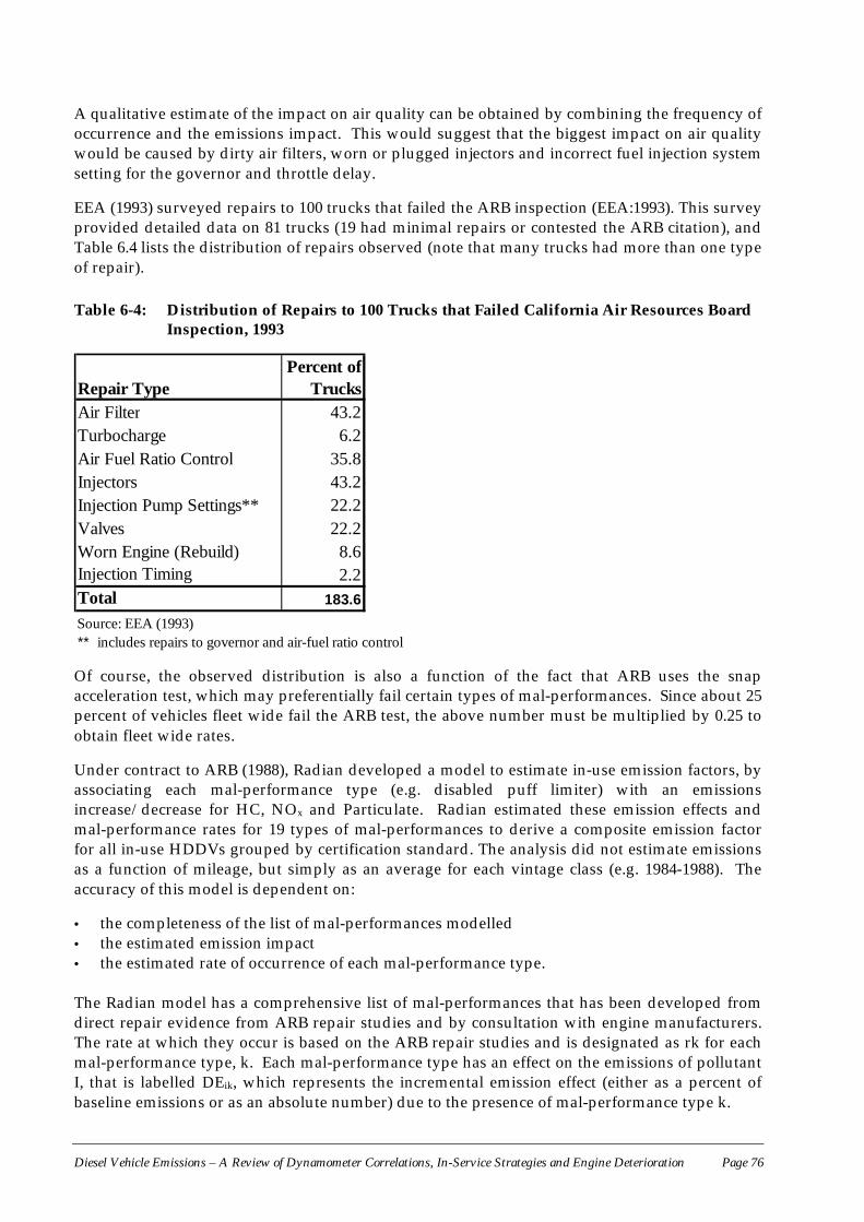
Diesel Vehicle Emissions – A Review of Dynamometer Correlations, In-Service Strategies and Engine Deterioration Page 76
A qualitative estimate of the impact on air quality can be obtained by combining the frequency ofoccurrence and the emissions impact. This would suggest that the biggest impact on air qualitywould be caused by dirty air filters, worn or plugged injectors and incorrect fuel injection systemsetting for the governor and throttle delay.
EEA (1993) surveyed repairs to 100 trucks that failed the ARB inspection (EEA:1993). This surveyprovided detailed data on 81 trucks (19 had minimal repairs or contested the ARB citation), andTable 6.4 lists the distribution of repairs observed (note that many trucks had more than one typeof repair).
Table 6-4: Distribution of Repairs to 100 Trucks that Failed California Air Resources BoardInspection, 1993
Repair TypePercent of
TrucksAir Filter 43.2Turbocharge 6.2Air Fuel Ratio Control 35.8Injectors 43.2Injection Pump Settings** 22.2Valves 22.2Worn Engine (Rebuild) 8.6Injection Timing 2.2Total 183.6
** includes repairs to governor and air-fuel ratio controlSource: EEA (1993)
Of course, the observed distribution is also a function of the fact that ARB uses the snapacceleration test, which may preferentially fail certain types of mal-performances. Since about 25percent of vehicles fleet wide fail the ARB test, the above number must be multiplied by 0.25 toobtain fleet wide rates.
Under contract to ARB (1988), Radian developed a model to estimate in-use emission factors, byassociating each mal-performance type (e.g. disabled puff limiter) with an emissionsincrease/decrease for HC, NOx and Particulate. Radian estimated these emission effects andmal-performance rates for 19 types of mal-performances to derive a composite emission factorfor all in-use HDDVs grouped by certification standard. The analysis did not estimate emissionsas a function of mileage, but simply as an average for each vintage class (e.g. 1984-1988). Theaccuracy of this model is dependent on:
• the completeness of the list of mal-performances modelled• the estimated emission impact• the estimated rate of occurrence of each mal-performance type.
The Radian model has a comprehensive list of mal-performances that has been developed fromdirect repair evidence from ARB repair studies and by consultation with engine manufacturers.The rate at which they occur is based on the ARB repair studies and is designated as rk for eachmal-performance type, k. Each mal-performance type has an effect on the emissions of pollutantI, that is labelled DEik, which represents the incremental emission effect (either as a percent ofbaseline emissions or as an absolute number) due to the presence of mal-performance type k.
Diesel Vehicle Emissions – A Review of Dynamometer Correlations, In-Service Strategies and Engine Deterioration Page 77
Hence the excess emissions are given by
DEI = Srk × DEik.
The Radian model data on mal-performance types, rates of occurrence and emission increases isdocumented in Appendix A as a series of three spreadsheets, for light-heavy, medium-heavy andheavy-heavy-duty engines, and DEI is reported as a percent increase in emissions from the zero-mile level. Here, the rates (rk) of mal-performance are fleet averages, and are associated with therate at the mid-point of a vehicle’s useful life. The useful life estimates are about 180,000 milesfor light-heavy engines, 300,000 miles for medium-heavy engines, and 500,000 miles for heavy-heavy-duty engines. Using the VMT weights implied from registration statistics, the averagemid-point of the useful life is 190,000 miles for the fleet.
The Radian model directly indicates the percentage increase in emissions at the mid-point ofHDDV useful life, and it is assumed that the deterioration occurs linearly with mileage, as iscommon in all EPA emission inventory models. The impact of inspection and repair is modelledas a reduction in the rate of occurrence (rk) of mal-performances. This reduction is calculatedfrom the mal-performance identification rate, which is a function of the test and standard used,and a repair rate that represents the percent of properly repaired vehicles. The Radian model’spredictions of increases in emissions from initial levels, for HC, NOx, and PM, are provided inTable 6-5.
Available limited data on these issues suggest that the Radian model is reasonable, and it hassince been updated by EEA (1993) with more recent and complete data on mal-performancesrates. Based on this updated version, the “average” emissions increases over the useful life bypollutant type for the California fleet in 1995 are:
• HC: - 34.0 percent• NOx: - 6.6 percent• Particulate: - 43.7 percent
These above percentages indicate the fraction of total emissions associated with trucks emittingabove the certification level.
Interestingly, the analysis of the 22 trucks from MY1979 described in the previous subsectionleads to similar estimates of increased emissions. The analysis of the Cummins engine dataprovided statistically significant coefficients of deterioration for each pollutant. Estimating thedeterioration at the mid-point of a HDDV’s life (150,000 miles) leads to the following increases inemission estimates from the regressions shown in Table 6-1.
• HC - 36 percent (based on Cummins engines)• NOx - ~ 0 percent• Particulate- 41 percent (based on all engines)• These data suggests that the Radian models’ predictions of excess emissions are correct at least inthe order of magnitude sense. Based on these data one can conclude that the in-use deteriorationof HC and PM from component mal-performance is very significant.
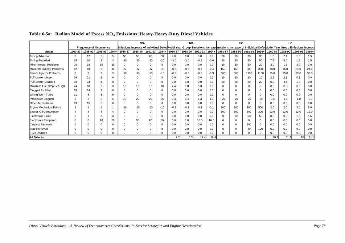
Diesel Vehicle Emissions – A Review of Dynamometer Correlations, In-Service Strategies and Engine Deterioration Page 78
Table 6-5a: Radian Model of Excess NOX Emissions; Heavy-Heavy-Duty Diesel Vehicles
1960-87 1988-90 1991-93 1994+ 1960-87 1988-90 1991-93 1994+ 1960-87 1988-90 1991-93 1994+ 1960-87 1988-90 1991-93 1994+ 1960-87 1988-90 1991-93 1994+Timing Advanced 8 12 5 5 50 50 60 60 4.0 6.0 3.0 3.0 20 20 30 30 1.6 2.4 1.5 1.5Timing Retarded 15 10 3 3 -20 -20 -20 -20 -3.0 -2.0 -0.6 -0.6 50 50 50 50 7.5 5.0 1.5 1.5Minor Injector Problems 20 18 15 15 0 0 0 0 0.0 0.0 0.0 0.0 10 10 20 20 2.0 1.8 3.0 3.0Moderate Injector Problems 12 10 8 8 -5 -5 -5 -5 -0.6 -0.5 -0.4 -0.4 150 150 300 300 18.0 15.0 24.0 24.0Severe Injector Problems 3 3 3 3 -10 -10 -10 -10 -0.3 -0.3 -0.3 -0.3 500 500 1100 1100 15.0 15.0 33.0 33.0Puff Limiter Misset 29 21 2 0 0 0 0 0 0.0 0.0 0.0 0.0 10 10 10 10 2.9 2.1 0.2 0.0Puff Limiter Disabled 30 23 5 0 0 0 0 0 0.0 0.0 0.0 0.0 20 20 20 20 6.0 4.6 1.0 0.0Maximum Fuel Stop Set High 24 18 3 3 10 10 10 10 2.4 1.8 0.3 0.3 0 0 0 0 0.0 0.0 0.0 0.0Clogged Air Filter 18 14 8 8 0 0 0 0 0.0 0.0 0.0 0.0 0 0 0 0 0.0 0.0 0.0 0.0Wrong/Worn Turbo 11 8 5 5 0 0 0 0 0.0 0.0 0.0 0.0 0 0 0 0 0.0 0.0 0.0 0.0Intercooler Clogged 3 7 5 5 10 20 25 25 0.3 1.4 1.3 1.3 -20 -20 -20 -20 -0.6 -1.4 -1.0 -1.0Other Air Problems 13 15 8 8 0 0 0 0 0.0 0.0 0.0 0.0 0 0 0 0 0.0 0.0 0.0 0.0Engine Mechanical Failure 1 1 1 1 -10 -10 -10 -10 -0.1 -0.1 -0.1 -0.1 200 200 300 500 2.0 2.0 3.0 5.0Excess Oil Consumption 4 4 4 4 0 0 0 0 0.0 0.0 0.0 0.0 300 300 300 300 12.0 12.0 12.0 12.0Electronics Failed 0 1 3 3 0 0 0 0 0.0 0.0 0.0 0.0 0 30 50 50 0.0 0.3 1.5 1.5Electronics Tampered 0 6 20 20 0 30 80 80 0.0 1.8 16.0 16.0 0 0 0 0 0.0 0.0 0.0 0.0Catalyst Removed 0 0 0 0 0 0 0 0 0.0 0.0 0.0 0.0 0 0 100 0 0.0 0.0 0.0 0.0Trap Removed 0 0 0 0 0 0 0 0 0.0 0.0 0.0 0.0 0 0 40 100 0.0 0.0 0.0 0.0EGR Disabled 0 0 0 0 0 0 0 0 0.0 0.0 0.0 0.0 0 0 0 0 0.0 0.0 0.0 0.0All Defects 2.7 8.3 19.4 19.4 70.7 61.3 81 81.4
DefectFrequency of Occurrence
HCModel Year Group Emissions Increase
NOxEmissions Increase of Individual DefecModel Year Group Emissions IncreaseEmissions Increase of Individual Defec
NOx HC
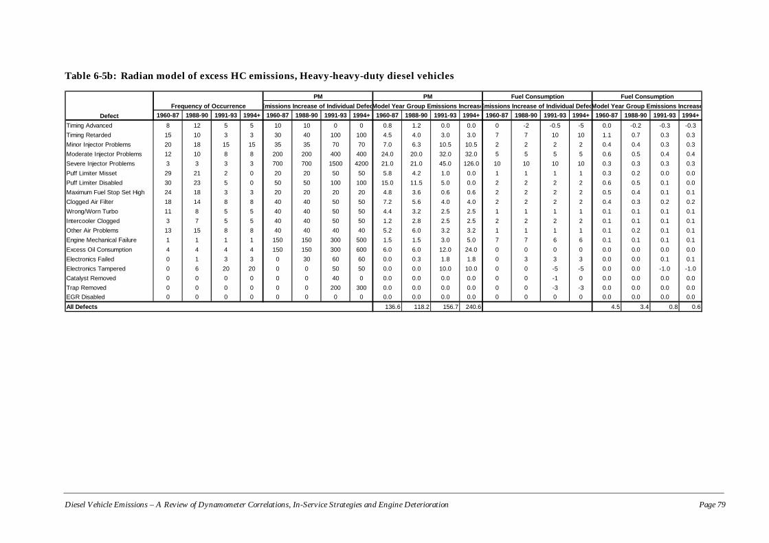
Diesel Vehicle Emissions – A Review of Dynamometer Correlations, In-Service Strategies and Engine Deterioration Page 79
Table 6-5b: Radian model of excess HC emissions, Heavy-heavy-duty diesel vehicles
1960-87 1988-90 1991-93 1994+ 1960-87 1988-90 1991-93 1994+ 1960-87 1988-90 1991-93 1994+ 1960-87 1988-90 1991-93 1994+ 1960-87 1988-90 1991-93 1994+Timing Advanced 8 12 5 5 10 10 0 0 0.8 1.2 0.0 0.0 0 -2 -0.5 -5 0.0 -0.2 -0.3 -0.3Timing Retarded 15 10 3 3 30 40 100 100 4.5 4.0 3.0 3.0 7 7 10 10 1.1 0.7 0.3 0.3Minor Injector Problems 20 18 15 15 35 35 70 70 7.0 6.3 10.5 10.5 2 2 2 2 0.4 0.4 0.3 0.3Moderate Injector Problems 12 10 8 8 200 200 400 400 24.0 20.0 32.0 32.0 5 5 5 5 0.6 0.5 0.4 0.4Severe Injector Problems 3 3 3 3 700 700 1500 4200 21.0 21.0 45.0 126.0 10 10 10 10 0.3 0.3 0.3 0.3Puff Limiter Misset 29 21 2 0 20 20 50 50 5.8 4.2 1.0 0.0 1 1 1 1 0.3 0.2 0.0 0.0Puff Limiter Disabled 30 23 5 0 50 50 100 100 15.0 11.5 5.0 0.0 2 2 2 2 0.6 0.5 0.1 0.0Maximum Fuel Stop Set High 24 18 3 3 20 20 20 20 4.8 3.6 0.6 0.6 2 2 2 2 0.5 0.4 0.1 0.1Clogged Air Filter 18 14 8 8 40 40 50 50 7.2 5.6 4.0 4.0 2 2 2 2 0.4 0.3 0.2 0.2Wrong/Worn Turbo 11 8 5 5 40 40 50 50 4.4 3.2 2.5 2.5 1 1 1 1 0.1 0.1 0.1 0.1Intercooler Clogged 3 7 5 5 40 40 50 50 1.2 2.8 2.5 2.5 2 2 2 2 0.1 0.1 0.1 0.1Other Air Problems 13 15 8 8 40 40 40 40 5.2 6.0 3.2 3.2 1 1 1 1 0.1 0.2 0.1 0.1Engine Mechanical Failure 1 1 1 1 150 150 300 500 1.5 1.5 3.0 5.0 7 7 6 6 0.1 0.1 0.1 0.1Excess Oil Consumption 4 4 4 4 150 150 300 600 6.0 6.0 12.0 24.0 0 0 0 0 0.0 0.0 0.0 0.0Electronics Failed 0 1 3 3 0 30 60 60 0.0 0.3 1.8 1.8 0 3 3 3 0.0 0.0 0.1 0.1Electronics Tampered 0 6 20 20 0 0 50 50 0.0 0.0 10.0 10.0 0 0 -5 -5 0.0 0.0 -1.0 -1.0Catalyst Removed 0 0 0 0 0 0 40 0 0.0 0.0 0.0 0.0 0 0 -1 0 0.0 0.0 0.0 0.0Trap Removed 0 0 0 0 0 0 200 300 0.0 0.0 0.0 0.0 0 0 -3 -3 0.0 0.0 0.0 0.0EGR Disabled 0 0 0 0 0 0 0 0 0.0 0.0 0.0 0.0 0 0 0 0 0.0 0.0 0.0 0.0All Defects 136.6 118.2 156.7 240.6 4.5 3.4 0.8 0.6
Emissions Increase of Individual DefecModel Year Group Emissions IncreaseEmissions Increase of Individual DefecModel Year Group Emissions IncreaseDefect
Frequency of OccurrencePM PM Fuel Consumption Fuel Consumption

Diesel Vehicle Emissions – A Review of Dynamometer Correlations, In-Service Strategies and Engine Deterioration Page 80
The advent of particulate standards in 1988 and 1991, and improvements to engine technologyhave brought about dramatic reductions in certification HC emissions levels even though the HCemission standards are unchanged since 1984, at 1.74 g/kWh. In the early and mid-1980’s, actualcertification HC levels were in the 0.94 to 1.21 g/kWh range. Certification levels declined to the0.4 to 0.67 g/kWh range in 1991, indicating a 50 percent reduction in emissions. In 1998, manyengines have certification HC levels of less than 0.27 g/kWh, i.e. at levels approaching tenpercent of the standard!
These reductions have not been taken into account in the EPA emission factors or into the Radianmodel, and both models are probably overestimating HC emissions from HDDV’s by as much asa factor of 2 for 1991 and later engines.
In contrast to the U.S. models that emphasise the role of component mal-performance, Europeanmodels have tended to assume that the test sample reflects the performance of the fleet as awhole. It is possible that truck owners are more law abiding in Europe relative to the U.S. andtampering may be relatively rare, especially in Germany and Switzerland. However,conversations with researchers revealed that European test vehicles are usually obtained fromlarge fleets on a voluntary basis, so that tampered or mal-performing vehicles are unlikely to besubmitted for testing.
The TUV has, however, developed a ‘modal’ model that is capable of forecasting emissions ofany truck (engine/transmission) over an arbitrary driving cycle. One major finding of the modelis that mountainous terrains (gradients) have very large effects on NOx emissions (TUV-Rheinland:1995). A two percent gradient results in a near doubling of NOx relative to level road,while a six percent gradient results in NOx levels four times as high. This effect has not beenstudied widely in the U.S.
Diesel Vehicle Emissions – A Review of Dynamometer Correlations, In-Service Strategies and Engine Deterioration Page 81
7 EMISSIONS CONTROL STRATEGIES
7.1 TYPES OF STRATEGIESStrategies to control emissions from in-service vehicles have followed two distinctly differentpaths. The first method attempts to maintain emissions from in-service vehicles relatively closeto certification and design levels. The second method attempts to reduce emissions from in-service vehicles by retrofit of new technology or upgrading of engines during rebuild. Bothstrategies have been attempted with varying degrees of success in the U.S. and Europe. Japanhas only an annual inspection program for diesel vehicles as part of their program to maintainemissions at certification levels. Even in the U.S. and Europe, retrofit and rebuild controlprograms are just emerging as a potential option, and these strategies are not yet well proven inpractice.
The maintenance of emissions by inspecting in-service vehicles is used widely, although manyprograms are using test methods that may be not be effective, or are completely ineffective atworst. Programs to retrofit technology have largely focused on public use vehicles such as busesor government owned trucks, although there are some innovative market based approachesencouraging owners retrofit technology to obtain emission credits. These strategies arediscussed below.
7.2 INSPECTION/MAINTENANCE PROGRAMSMuch of the motivation for subjecting heavy-duty vehicles to inspection/maintenance programsis the public perception of diesel smoke, as well as the real threat of the carcinogeniety of smokeparticulate. Virtually all of the ongoing programs to control in-service have focused on smokeemissions, and the accompanying reduction (or increase) in gaseous emissions as a result ofreducing smoke has not received any attention except in isolated cases. Indeed, outside ofanalyses conducted by California in the early-1990s, we have not been able to find any attempt tocharacterise the other benefits of smoke reduction programs that are now in place in most OECDcountries.
However, there are a number of inspection maintenance programs in Europe for light-dutydiesel vehicles, and there have been some recent programs to develop more sophisticated testsfor diesel inspections. Currently, most European diesel car and light-truck inspection programstest only for diesel smoke, and there are no broad conclusions for reductions of emissions ofcriteria pollutants. A 1998 study sponsored by the EU attempted to quantify the cost-benefit oflight duty diesel inspections using two alternative smoke tests. All EC countries and Japan havetruck inspection programs although the quality varies widely between European countries.Virtually all programs are based on smoke emissions as an indicator of pass/fail status.
Seven states in the U.S. currently have active heavy-duty I/M programs with two othersoperating pilot programs. Light-duty diesel vehicles are included in many state I/M programs(they are exempt in some states), but generally use the same test as for gasoline vehicles; the testis usually irrelevant to the diesel. Since there are so few light-duty diesels in the US, there hasbeen insufficient attention to this fact.
Smoke emissions are generally measured in terms of opacity, which is simply the percentage oflight blocked by the smoke plume. Opacity is measured with an opacimeter (or smoke meter), aninstrument that measures the amount of light that can be transmitted though an exhaust plume(and, by extension, the amount of light scattered or absorbed by an exhaust plume). There are
Diesel Vehicle Emissions – A Review of Dynamometer Correlations, In-Service Strategies and Engine Deterioration Page 82
basically two kinds of opacimeters: Full flow, end of line opacimeters and partial flowopacimeters.
Full flow opacimeters measure the opacity of a cross section of the full exhaust plume just as theplume exits a vehicle exhaust pipe. Because exhaust pipes are not of standard size and shape,the length across which the transmitted light must pass (i.e., the path length) and therefore, thenumber of smoke particles available for scattering and absorption can very across test vehicles.For this reason, all opacity readings from full flow opacimeters must be corrected to a standardpath length to avoid testing inconsistencies. Partial flow opacimeters take a sample of theexhaust gas from inside the exhaust pipe and measure opacity within a cell of fixed path length.Thus, all readings taken with a given partial flow opacimeter are consistent (and independent ofthe exhaust stack diameter), but generally are still corrected to a standard stack diameter forconsistency with full flow smoke meter readings.
A typical I/M program consists of standardised test and measurement procedures, a set ofpass/fail cut points, and an enforcement mechanism. Smoke tests can be loosely classified intotwo types: transient and steady state. Transient tests measure smoke over a changing enginespeed and load cycle, while steady-state tests measure smoke during a constant speed and loadcondition. Each can be effective in detecting certain typical engine mal-performances althoughtransient tests are generally more robust in terms of the scope of mal-performances identified.
There are two common transient tests:
• The On-Road Acceleration Test, where the vehicle is either started from a standstill or isrolling at low speed, following which the accelerator is depressed to the maximum (or wide-open throttle) position and held there for six to tem seconds or more.
• The Snap Acceleration (or Snap Idle) Test, which requires, with the transmission in neutraland the engine at normal idle, the accelerator pedal be depressed to the maximum, or wide-open throttle, position. The pedal is held at this position for five seconds or until the enginereaches governed speed. The pedal is then released and the engine allowed to return tonormal idle.
There are four common steady-state tests currently in use:
• The Stall Test, where the vehicle engine is operated at wide-open throttle, with the automatictransmission engaged in drive, and the brakes engaged to prevent vehicle motion.
• The Lug-Down Test, where the engine is operated at wide-open throttle with the vehiclemounted on a dynamometer. Dynamometer load is increased to reduce engine speed (i.e.,“lug-down”) from rated RPM to some fraction (generally around 70 percent) of rated RPM.In the absence of a dynamometer, the vehicle can be “lugged” down by the carefulapplication of the vehicle brakes
• The Idle Test where the vehicle’s exhaust smoke opacity is measured at normal curb idle orhigh idle.
• The Cruise Mode (i.e., Clayton Key Mode) Test, where the vehicle is tested by applying asingle load, while being operated at a constant speed.
The most common test procedure currently applied in the U.S. to heavy-diesels is the SAEJ166725 snap acceleration test procedure, recently promulgated by the Society of AutomotiveEngineers. This test procedure was jointly developed by the regulatory and truckingcommunities and specifically addresses industry concerns with its predecessor J1243 testprocedures.

Diesel Vehicle Emissions – A Review of Dynamometer Correlations, In-Service Strategies and Engine Deterioration Page 83
The SAE J1667 test incorporates:
• a specific method of performing the snap-acceleration test;• correction factors for normalising measured smoke opacity when measurements are made at
alternative optical path lengths and non-standard ambient conditions;• specifications for the smoke meter, and especially for overall instrument response time.
In general, transient testing provides an effective means of identifying the short duration smokeevents that characterise a variety of common mal-performances. On the other hand, steady-statetests at wide-open throttle (i.e., lug down) do not identify several common mal-performances,but identify some mal-performances that the transient tests do not. These mal-performances arenot as common, but can have a significant emissions impact. The idle and cruise mode tests arelargely ineffective in detecting most mal-performances, since they are conducted at part throttle.
A summary of state specific U.S. Test programs is as follows:
The failure rate is a function of both the test used and the pass/fail standards. In most states inthe U.S., J1667 test standards are usually 40 percent opacity for 1991 and later vehicles, and 55percent opacity for 1990 and older vehicles, but is up to 70 percent opacity in some states. Thestandard for 1990 and older vehicles of 55 percent opacity appears to fail a significant portion ofmal-performing vehicles. On the other hand, the 40 percent standard appears to be almostcompletely ineffective with modern engines, especially those with electronic controls. Electroniccontrols can easily disable fuel systems if the vehicle is not in gear, making the J1667 procedureuseless. Failure rates for modern (post-1994) U.S. engines are extremely low, typically less thanthree percent.
Most EC countries also use the snap acceleration test (sometimes call free acceleration test)though some regional jurisdictions in Germany require both the snap acceleration test and thelug-down test. The European snap acceleration test is not identical to the J1667 in terms of meterresponse time and technical criteria to determine a valid test, and these specifications also veryfrom country-to-country. For example, Germany has a time specification for the RPM increaseon the free acceleration test, while France does not.26
The largest difference between the U.S. and Europe is that the smoke opacity standards in manythe EC countries are type specific and vary from engine model to engine model. The standardsare actually suggested by the engine manufacturer, leading to considerable complexity inadministration. Moreover, the engine manufacturers have an incentive to make the standardsrelatively lax, so that so engines with marginal mal-performances are not failed.
State Test Failure RateArizona Lug-Down 4.50%
California SAE J1667Roadside Test of
Potential Failures OnlyColorado Lug Down < 1%
Nevada SAE J1667Roadside Test of
Potential Failures Only
New JerseyRolling Acceleration
or Stall-Test Not AvailableWashington SAE J1667 2 to 3 percentSource: EEA (1999)

Diesel Vehicle Emissions – A Review of Dynamometer Correlations, In-Service Strategies and Engine Deterioration Page 84
Most European countries also use the free-acceleration test for light-duty vehicles, with opacitystandards that are either model specific or equivalent to about 40 to 50 percent opacity (peak). Ina recent (1998) study by the European Commission, a number of inspection type short tests wereinvestigated by European Research laboratories. The first type of test involved a dynamometerbased short transient cycle over which only smoke emissions were monitored. The second wasthe free acceleration test. Although the report concluded that the first type of test showedpromise, it is not well supported by the data. Indeed, the correlation between smokemeasurements over the short test and PM emissions on the certification type test was verydependent on one data point for a gross PM emitter. Removal of this one data point resulted inthe correlations becoming substantially worse, to the point where the benefit over the freeacceleration test was not large. At this point in time, it can be stated that there is no good test forinspection of diesel light duty vehicles, but it should be noted that the free-acceleration test canspot gross emitters of PM (of course, such vehicles can be spotted by the unaided eye easily)
In Japan, the free acceleration test is also used, but the smoke measurement is based on a longaveraging time instrument so the results are not comparable to the SAE J1667 test. However,Japan implements a standard of 40 percent opacity for pre-1999 trucks, and 25 percent opacity for1999 and later vehicles.
While detailed failure rates for EC countries and Japan are not available, several leadingresearchers confirmed to EEA that only about one percent of both light-duty and heavy-dutyvehicles tested actually fail the test. Hence, the primary value of the test appears to be as adeterrent to tampering in Europe and Japan.
Failure rates are somewhat greater in the U.S., but still quite low given the number of smokytrucks observed usually on the road. Only the California Roadside Program has addressed theissue of targeting likely failures for the test, and is hence more effective. Since high smokeemitters can be visually identified, targeting of potential failures is quite easy.
As noted, only California has attempted to estimate the benefits of the heavy-duty vehicle smokeopacity reduction program. Many researchers have claimed that the free acceleration test basedsmoke opacity has no correlation with HC or PM emissions measured on the 13-mode ortransient test. While this is an accurate statement, high smoke on the free acceleration test (at lestfor older mechanically controlled engines) is indicative of a defect in the air-fuel ratio controlsystem. Depending on the defect, this can have a large or small effect on emissions measured ona certification type test. Hence, the free acceleration test is a mal-performance indicator ratherthan an emissions indicator.
The mal-performance model described in Section 6 provides an appropriate tool to estimate thebenefits of an I/M program. Analysis for California shows that the I/M program is capable ofidentifying at least half of all “excess” emissions of HC and PM on older mechanically controlledengines. No recent analysis has been done on the benefits for newer electronically controlledengines, but the absolute quantity of excess emissions as well as the percent identified haveundoubtedly declined relative to older engines. The high level of excess emission may be aphenomenon that is U.S. specific, since the rates of tampering and mal-maintenance arepotentially much higher in the U.S., relative to European levels.
As noted, virtually no analysis of inspection program cost-effectiveness has been performedoutside of the U.S., with most existing analysis from California of their roadside smokeinspection program. In a recent study for Denver (Colorado), data from the California programand the existing Colorado program (which uses a lug down test) was utilised to estimate the
Diesel Vehicle Emissions – A Review of Dynamometer Correlations, In-Service Strategies and Engine Deterioration Page 85
cost-effectiveness of different types of programs: centralised annual inspection vs. randomroadside, SAEJ1667 test vs. lug down.
Based on actual administrative and test costs, and estimated repair costs and emissionreductions, the analysis developed the cost-effectiveness in terms of U.S. dollars per ton of (HC +PM + NOx) reduced. They are as follows:
• Centralised Program, Lug Down test - $3260/ton• Centralised Program, J1667 test - $3030/ton• Centralised Program, J1667 + lug down test - $3430/ton• Roadside Program, J1667 test - $2430/ton
One of the major findings is that program type has a major impact on costs. In centralisedprograms, all vehicles are inspected and only ten percent or so may fail. The large cost ofinspecting the other 90 percent makes such programs significantly more expensive than roadsideprograms that target likely failures by visually identifying potential failures. The similarity of allof the cost per ton figures is driven partly by the deterrent effect of having any program, whichreduces tampering.
The 1998 EC report referred to earlier also attempted to calculate the cost effectiveness of diesellight-duty vehicle inspection using the (admittedly) low quality tests. Repair costs for vehiclesfailing the tests appear to have been assumed, and also appear quite low, at Euro 200 to 300. Inspite of this relatively low cost assumed, the cost effectiveness per ton of PM reduction wascalculated at Euro 34,000. This cost is an order of magnitude higher than the cost-effectiveness ofheavy-duty vehicle inspection calculated in Denver. Although the methodologies are not thesame, the costs provide at least an order of magnitude sense but may also be influenced by therelatively low rates of mal-performance in Northern Europe.
It is not clear if Australian cost effectiveness figures will be similar since the benefits are quitedependent on mal-performance rates in the fleet. If the mal-performance rates are quite low (asis potentially the case in Europe), the costs per ton will be much higher.
7.3 RETROFIT AND REBUILD RELATED PROGRAMSThe potential to decrease emissions of in-service diesels through retrofit of new technologies toolder vehicles or by rebuilding engines to new standards has received considerable attention inEurope and the U.S. over the last five to seven years.
7.3.1 European DevelopmentsTo date, there are no regulations in Europe requiring the retrofit of technologies or the rebuildingof engines to more stringent emissions standards, for either light- or heavy-duty vehicles. TheEC regulation only requires that rebuilt engines meet the original specification that the enginewas designed to; the same regulation applies to re-engined vehicles. However, in the case of re-engined vehicles, we understand that most operators in Europe simply buy a current modelengine of the same make, so that an upgrade occurs ‘defacto’ simply due to convenience.
While there are no requirements that legally enforce retrofit or upgrade, there are manyorganisations in Europe that are voluntarily retrofitting engines with newer technology, mostlytrap oxidisers or oxidation catalysts. The vast majority of these voluntary retrofits have been bythe Metropolitan Transport Organisations (state-owned) for the bus fleet. Both Germany and theU.K. confirmed that these are probably several hundred buses in each country that have beenretrofitted with trap oxidisers. A few large transport companies have retrofitted a handful of
Diesel Vehicle Emissions – A Review of Dynamometer Correlations, In-Service Strategies and Engine Deterioration Page 86
trucks (the total in the EC is a few hundred) as a public relations measure or as a demonstrationprogram. Virtually all of the retrofit has been with trap oxidisers that primarily affect PMemissions, and to a lesser extent, HC emissions. There have been some retrofit of oxidationcatalysts to light-duty vehicles in Sweden and Germany, but these have largely been asdemonstration programs in Europe.
The retrofit devices for heavy-duty vehicles are commercially offered by catalyst manufacturerssuch as Engelhard and Johnson-Matthey. Each country is certifying retrofit devices to meet aminimum performance requirement that requires a reduction in PM of at least 20 to 25 percentand HC by a similar amount, without increasing NOx emissions or noise. Newer regulations inGermany now require a minimum performance of 70 percent reduction in PM from Euro I orearlier certification engines, and a number of devices are new available commercially. Thecertification is by a publicly owned laboratory; as an example, TUV-Essen is responsible forcertifying such devices for Germany.
Virtually no assessment of programs that aim at reducing NOx emissions from in-service vehicleshas occurred in Europe. NOx can be reduced from in-service engines by a number of actionsranging from injection pump and injection timing recalibration to the addition of an air-to-airintercooler in non-intercooled or jacket water intercooled engines. We are unaware of anyEuropean program that has focused on these aspects, although there is a white paper to bereleased shortly in England that may discuss such issues.
The principal reason for the lack of any major activity in retrofitting new technology is the veryhigh cost of retrofit. Typical costs for a trap oxidiser or oxidation catalyst are around U.S. $1000per litre of engine displacement. Hence, retrofitting a typical heavy-duty truck powered by an11-litre engine with a trap oxidiser could cost U.S. $11,000 (over A$16,000) or more, which isprohibitive for a commercial truck owner. Light-duty vehicle retrofit costs are also on the sameorder, and a typical small car engine must be retrofitted with a catalyst that can easily exceedUS$1000, or A$ 1500. Costs are coming down with increased sales and learning, but the costdecline in quite slow.
Sweden is using a novel method to encourage the retrofit or upgrade of heavy-duty engines. Ithas created environmental zones in its three largest cities: Stockholm, Goteburg and Malmo.The zone essentially covers the entire central business district of the cities. Within these zones,municipal councils have the right to restrict heavy-duty diesel vehicles that do not meet stringentemission standards. The current regulation (due to be revised next year) prohibits diesel heavy-duty vehicles that do not meet the Euro II requirements from these areas, but provides generaldispensations to two categories of vehicles:
• vehicles less than eight years old;• vehicles retrofitted with exhaust devices that meet specific emissions reduction criteria.
Two levels of performance have been set up for retrofit technologies. Level A requirement a PMreduction of 25 percent and an HC reduction of 60 percent relative to untreated exhaust. Level Brequires a PM reduction of 80 percent and an HC reduction of 60 percent. Vehicles less than tenyears old must be fitted with devices meeting the Level A requirements, while vehicles olderthan ten years must utilise devices certified to Level B.
Conversations with environmental authorities of Stockholm and Goteberg confirmed that manyolder buses are now fitted with Level A devices and a few with Level B devices. There has beena redirection of newer trucks to the environmental zones, but authorities believe that several
Diesel Vehicle Emissions – A Review of Dynamometer Correlations, In-Service Strategies and Engine Deterioration Page 87
hundred private trucks have adopted Level A and Level B rated retrofit devices in all of Sweden.Hence, it is regarded as a relatively successful local air pollution control strategy.
While other countries in Europe have restricted traffic zones for older vehicles, these regulationsare not directed especially at retrofit devices.
7.3.2 U.S. DevelopmentsThe U.S. has moved ahead on some specific retrofit and rebuild requirements for heavy-dutyvehicles only, that are now part of the regulations. There are four major actions that now affectretrofit and rebuild in the U.S.:
• retrofit and rebuild requirements for 1993 and earlier urban bus engines;• the California Low Emission Vehicle Emissions Credit Program;• the North-Eastern States Voluntary Heavy-Duty Retrofit Program;• the Low NOx Emissions Rebuild Program.
Of these, the first and last program are driven by regulatory requirements, while the Californiaand North-Eastern State Program are market driven approaches. Separately, there are specialfinancial incentives available for conversion to alternative fuels, but those are not consideredhere.
The Clean Air Act (as amended in 1990) required EPA to promulgate regulations affecting thereplacement or rebuilding of 1993 and earlier model year urban buses. Engines replaced orrebuilt after January 1, 1995, are required to comply with an emission standard or controltechnology reflecting the best retrofit technology and maintenance practices achievable. The actrestricts this requirement to 1993 and earlier model year urban buses operating in MetropolitanStatistical Areas and Consolidated Metropolitan Statistical Areas with 1980 populations of750,000 or more.
In early 1993, EPA published final Retrofit/Rebuild Regulations for 1993 and Earlier Model YearUrban Buses. The regulations require affected urban bus operators to comply with one of twoprogram options, beginning January 1, 1995. Option 1 established particulate matter (PM)emission requirements for each urban bus in an operator’s fleet when the engine is rebuilt orreplaced. Option 2 is a fleet averaging program that sets out specific annual target levels foraverage PM emissions from urban buses in an operator’s fleet. The two compliance options aredesigned to yield equivalent emissions reductions for approximately the same cost.
Option 1 requires affected urban buses to meet a 0.10 g/bhp-hr (0.13 g/kWh) PM standard at thetime of engine rebuild or replacement. This option is effective only if equipment had beencertified by EPA for at least six months as meeting the 0.10 g/bhp-hr standard for less than a lifecycle cost limits of $7,940 (in 1992 U.S. dollars). The regulation allows transit operators to plantheir budgeting and procurement activities, and to help ensure an adequate supply of parts areavailable from equipment manufacturers. If certified equipment is available, then affected busesmust use equipment which reduce PM emissions by 25 percent, if such equipment has beencertified by EPA for less than a life cycle cost limit of $2,000 (in 1992 U.S. dollars).
Option 2 is an averaging-based program that requires bus operators to meet an annual averagefleet PM level, instead of requiring each individual rebuilt engine to meet a specific PM level. Onan annual basis, an operator must reduce its “actual” PM emissions from its buses to a level nogreater than its annual target level for the fleet (TLF). The operator calculates the TLF for eachyear of the program, beginning calendar year 1996, based on actual fleet composition, anassumed engine rebuild and retirement schedule, and EPA’s determination of expected PM
Diesel Vehicle Emissions – A Review of Dynamometer Correlations, In-Service Strategies and Engine Deterioration Page 88
levels for each engine model. As each engine in a fleet is assumed to be rebuilt in a particularcalendar year, the TLF calculations “switch” from a “pre-rebuild” PM emission level to a lower“post-rebuild” level that reflects the assumed use of lower-emitting, certified equipment. Overthe years of the program, as the engines in a fleet are assumed to be rebuilt, this “switching”results in numerically lower TLF values.
Certification activity under the retrofit program has lagged substantially behind the scheduleanticipated by EPA when the final rule was promulgated. No equipment was certified whenEPA revised the post-rebuild levels based on equipment. The first certification for the programoccurred on May 31, 1995, almost a year after the post-rebuild levels were revised the first time.Several rebuild/retrofit kits were certified by 1996, but none were certified to the 0.10 g/bhp-hrPM standard. EPA’s assumption that certification activity would begin early was incorrect andmore importantly, EPA’s assumption that certification activity would be complete by mid-1996was incorrect. For example, EPA only recently certified equipment manufactured by EngelhardCorporation that triggers the 0.10 g/bhp-hr standard for 1979 though 1989 model year DetroitDiesel Corporation (DDC) 6V92TA MUI engines. Additionally, Johnson Matthey Incorporatedhas been certified to supply equipment to the same standard, and applicable to these, and other,DDC engines. There are other plans for certifying equipment to the 0.10 g/bhp-hr standard for alarge segment of the bus engine population.
The California and North Eastern States programs are similar in that they involve the use ofemission credits that can be generated by retrofitting a heavy-duty diesel engine. In the U.S.,most major metropolitan areas are not yet in compliance with the air quality requirements forozone and are designated as non-attainment areas. In these areas, businesses that generate moreemissions than some allowable level are required to offset the increase by purchasing credits orhelping reduce emission elsewhere, making emission reductions a marketable commodity.Hence, there is value to a private firm reducing emission by retrofit, and selling these credits can(in theory) offset the cost of retrofit either partially or entirely.
The California and North-Eastern States programs certify specific control technologies and havedeveloped specifications on how the credits are to be calculated. In the case of diesel engines,low emission retrofits can be specific to a range of “credit” standards that are at least 30 percentlower than the “ceiling” standard. The ceiling standard is the original certification standard.The administration of these credit programs is at the local air quality control authority. To date,however, the number of voluntary retrofits has been very small (a few hundred vehiclesnationally) largely because the cost of retrofit is very much higher than the market value of thecredits.
The newest program is one that has come about from a settlement of a regulatory action by EPAagainst the diesel engine manufacturers. As referred to in Section 7, the EPA believed thatmodern diesel engines employed “cycle beating” techniques to met current emission standards,and initiated legal actions against engine manufacturers. As part of the settlement, themanufacturers have agreed to develop low NOx rebuild kits for a range of popular enginemodels manufactured between 1993 and 1998. These kits will essentially bring the NOx levels ofaffected engines down by about 25 percent. The kit is to be available at no extra cost torebuilders and owners, and all engines within the model year range that are selected bymanufacturers must be rebuilt using this kit. Such kits are expected to be available in themarketplace shortly.
As noted, only the two regulatory programs are expected to have a significant influence onrebuild and retrofit. The U.S. EPA is considering other rebuild and retrofit requirements forheavy-duty diesels but no actions are expected in the near future.
Diesel Vehicle Emissions – A Review of Dynamometer Correlations, In-Service Strategies and Engine Deterioration Page 89
No good estimates on cost-effectiveness of either a retrofit or rebuilt or rebuild program isavailable. However, the cost of retrofit ranges from A$15,00 to A$20,000 for a typical diesel truckwith engines ranging from six to ten litres displacement. Over the typically lifetime of the retrofitdevice of 400,000 to 500,000 km, computed reductions in particulate emissions (for a typical 15ton rigid truck) is on the order of 0.5 ton. Hence the cost-effectiveness in terms of dollars per tonis not very good at $30,000 to $40,000 per ton, without even including administrative cost anddevice maintenance cost. On the other hand, rebuild upgrade kits cold be very cost effective, butno cost data on such kits are available yet. It is widely expected that a rebuild kit could reduceNOx by 20 to 30 percent but have an incremental cost of A$1000 or less.
Diesel Vehicle Emissions – A Review of Dynamometer Correlations, In-Service Strategies and Engine Deterioration Page 90
8 POTENTIAL CONTROL PROGRAMS FOR AUSTRALIA
8.1 CONTEXTStrategies to control diesel emissions in Australia must be developed in the context of the dieselfleet in Australia. A large fraction of the Australian fleet is imported from Europe and Japan,with European makes mostly in the 12 to 25 ton gross weight categories and Japanese trucksdominating the 3.5 to 12 ton category. Makes imported from the U.S. are typically in the largesttrucks, those over 25 tons gross weight. Our contacts with Australian staff of major importers ofdiesel engines suggested that most engines imported from Europe potentially meet the Euro Istandard since 1999/1994. As noted the ‘Euro O’ standards was not very stringent and mostEuropean engines sold in Australia prior to 1993 probably met ‘Euro 0’ standards. In addition,Japanese standards (relative to the Japanese test requirements on the six-mode) for lighter truckengines were not very stringent, so that on average, most Direct Injection diesels met the Euro Oor even Euro I standards. Some of the trucks around five tons GVM employ IDI diesels, whichhave very low NOx emissions (capable of meeting Euro III levels). Hence, strategies need to besensitive to the Australian fleet composition.
Buses are a special case, and a majority of buses in Australia use engines from Germany orSweden. Hence, this segment offers the possibility of harmonising control strategies withGermany or Sweden.
The Australian light-duty diesel fleet consists primarily of smaller versions of heavy-duty dieselengines, or large displacement special purpose light-duty diesel engines, most of which aresourced from Japan. While the former type of diesel has much in common with heavy-dutyengines used in trucks in the 3.5 to 6 ton GVM range, the latter category is somewhat unique andthere is no good understanding of their emission characteristics and control strategies for theiremissions. Passenger car type diesels imported from Western Europe or Japan (of 1.5 to 2.5 litresdisplacement) are a relatively small contributor to total diesel emissions due to their smallpopulation, and the relevance of Western Europe’s light-duty diesel emission control programsto Australia is limited.
8.2 DETERIORATION OF EMISSIONS UNDER IN-SERVICE CONDITIONSAlthough there are only a limited number of studies on the topic of in-service deterioration ofemissions, there are a number of findings of potential interest to Australia.
Since the Euro 0 and Japanese standards to 1998 were not very stringent, the potential of older in-service engines exceeding these standards is quite small. Most engines will have emissions wellbelow applicable standards, and only severe tampering or mal-maintenance will cause engines toexceed the standards appreciably. This finding is likely to affect a significant portion of theAustralian fleet.
The findings from Europe indicate that about five to ten percent of the heavy-duty fleet willlikely exceed the Euro I and Euro II standards (plus a margin of safety of ten percent of thestandard). This represents a fleet wide average failure rate, and actual failure rates will likelyincrease with truck age or use. In contrast, a much larger portion of the engines (20 to 25percent) certified to standards in the U.S. prior to 1991 (approximately equivalent to Euro I orEuro II ) are likely to be exceeding standards in the U.S. There is a widespread belief (unprovento date) that tampering and mal-maintenance rates are higher in the U.S. than in Europe. It is notclear from available data where Australia is in terms of mal-performance rates.

Diesel Vehicle Emissions – A Review of Dynamometer Correlations, In-Service Strategies and Engine Deterioration Page 91
Since emission tests of heavy-duty trucks are expensive, only a limited sample of in-use truckscan be tested. However, the engineering model developed for California may be a useful tool tocombine survey-based data on mal-performance rates in Australia with available emissions datato develop in-use emission factors. This method has been used with some success in the U.S. Thesurvey of mal-performance rates in the in-service Australian truck fleet needs to be established inorder to develop an appropriate control strategy for in-use emissions as well.
The European experience with light-duty diesels is similar, in that few vehicles exceed standards.Even the Euro I and II standards applicable to this category of vehicles are not very stringentrelative to near uncontrolled rates, so that few vehicles fail gaseous emission standards. Failureof PM standards is more common, but gross emitters (emitting over 5 times the standard) may berelatively rare. It is also not clear wether data from old mechanically controlled IDI diesels willbe representative of the new breed of turbocharged, electronically controlled DI diesels that willdominate the market in the future.
8.3 MAINTENANCE OF IN-SERVICE EMISSIONSVirtually all of the programs around the world for inspection of in-service light and heavy-dutyvehicle emissions have focused on smoke, and by extension, PM emissions. The snap accelerationtest also appears to be the test of choice for most inspection programs, although test cycle detailsand the specifications of the smoke meter vary between countries. The recently published SAEJ1667 procedure provides a high degree of standardisation of test details and is a possible optionfor Australia if it is decided that the snap acceleration test is useful under Australian conditions.
The snap acceleration test should not be thought of as a predictor of PM emissions for anyvehicle, but rather as a diagnostic test to identify mal-performances present in the engine thatcould lead to high emissions. The actual types of mal-performances identified by the test and therelative excess emissions reduction that occurs from repair of these defects depends both on thesmoke opacity pass/fail standard and the type of engine. The test works reasonably well inidentifying defects on older engine models with mechanically controlled fuel systems, but doesnot work well with more recent electronically controlled engines. Anecdotal evidence suggeststhe bulk of the heavy-duty engines currently operating in Australia is of the mechanicallycontrolled type, although the electronically controlled engines will eventually become dominant.Hence, there is a time window where the snap acceleration test could be useful to Australia.Second, and more importantly, the snap acceleration test is particularly useful in identifyingdefects that arise from tampering to increase power by overfuelling the engine. These types oftampering are not uncommon on mechanically controlled engines in the U.S., but this is not thecase in Europe. Hence, the applicability and usefulness of the test in Australia depends to somedegree on the types and rates of mal-performances present in the in-use fleet. Finally, it shouldbe noted that the programs in the U.S. using this test have set relatively lax pass/ fail cut pointsso that its primary use has been has been as a method to identify “gross” emitters. The U.S.standards have also been influenced by the threat of lawsuits in the case of false failures.
Smoke measurement on the “lug down” test is also sometimes used as an adjunct or as analternative to the snap acceleration test. Available data suggests that the lug down test doesidentify different mal-performances than the snap acceleration test, but the test is more difficultto conduct and is preferably performed on a dynamometer, which is expensive. The marginalbenefit of this test as an adjunct to the snap acceleration test is dependent on the rate of mal-performance in the fleet of those mal-performances recognised by the lug down test.
All tests focusing on smoke emissions identification and reduction also provide reductions in PMemissions and in gaseous HC emissions but the actual reductions provided are a function of both
Diesel Vehicle Emissions – A Review of Dynamometer Correlations, In-Service Strategies and Engine Deterioration Page 92
the test employed and the rates and types of mal-performances in the fleet. It is difficult toprovide a general estimate of benefits in Australia as there are no data to support any of themodelling conducted in the US. However, smoky trucks are regarded as a public nuisance andcontrol programs can be justified on the basis of smoke reductions alone. Moreover, suchprograms have a deterrent effect on tampering, which can be of significant benefit to emissions.At this time, there are no developed procedures to identify high NOx emitters, and much of thedevelopment of chassis based procedures described in Sections 3 and 4 of this report is tosupport the development of a short test that would allow direct measurement of all gaseouspollutants.
Manufacturers of engines have suggested direct interface with on-board diagnostics forelectronically controlled engines as one method to identify emission control system defects.There have also been suggestions to inspect emission critical components by a performancecheck. At present, these methods are difficult to incorporate into any common inspectionprogram due to the lack of standardised on-board diagnostics, or due to the time required toconduct performance checks of emission critical components. However, the on-board diagnosticinterface may become possible in the future as the systems are harmonised around the world.
8.4 RETROFIT AND REBUILD CONTROL PROGRAMSRetrofit programs around the world have, to date, focused on the retrofit of trap oxidisers oroxidation catalysts for the control of PM emissions and HC emissions from heavy-duty dieselengines. Programs for light–duty diesel vehicles are limited to a handful of voluntary catalystretrofit programs. Other than the urban bus program in the US, all other approaches arevoluntary or market based. The programs have been largely restricted to the urban bus market inmost countries because costs of these devices are currently in the range of US $10,000 to 15,000for a typical heavy-duty installation for the parts alone (labour costs to install the system willvary by body type). Many newer systems are capable of reducing PM emissions by 70 percent ormore from a Euro I or earlier certification engine, which typically emits PM at a rate of 0.5g/kWh. Hence, a reduction of 0.35 g/kWh is possible. For a typical urban bus, the conversionfactor from g/kWh to g/km is about 2, implying a reduction of PM emissions of 0.7 g/km. Overthe life of the trap oxidiser or catalyst (estimated at around 600,000 km), the lifetime emissionsare reduced by 0.42 tonnes, implying an undiscounted cost effectiveness of A$38,000 per tonne (the costs could be higher).
These current cost numbers indicate why policies using market measures have had only limitedappeal to date. Although the costs could decline significantly in the future, the current costsmake the retrofit option a very expensive form of emission control. The main advantage withthese systems is that they are 1) commercially available 2) are performance certified by anunbiased organisation and 3) have after sales support in the marketplace. Australia has theadvantage that its buses use engines from Germany and Sweden, which have active retrofitdevice approval and performance certification programs. By accepting these certifications,Australia could adopt retrofit requirements for buses with very low administrative burdens.
No retrofit devices to reduce NOx emissions are commercially available, although there areprototypes of reduction catalysts that are being demonstrated now. One example is the ureabased SCR catalyst being developed by Siemens that can reduce NOx emissions by 70 percent.However, these systems are still a few years from commercialisation and may also requireinfrastructure changes such as the need to provide urea at filling stations. System costs are veryuncertain at this time, but could be in the same range as trap oxidisers. Since NOx emissions areten times higher in mass than PM emissions, cost per ton will be about one-tenth those citedabove for PM, making these devices more cost effective.

Diesel Vehicle Emissions – A Review of Dynamometer Correlations, In-Service Strategies and Engine Deterioration Page 93
Rebuild requirements in most EC countries have focused on maintaining the certification levelsof emissions for the original engine. Rebuild requirements to reduce emissions from originallevels have, to date, been implemented only in the US and one focuses on urban bus PMemissions, while the second focuses on low-NOx rebuild kits. The bus requirements force eitherthe re-engining of buses at rebuild with a current model engine or the retrofit of a trap oxidiseror catalysts covered in the discussion above. The low-NOx rebuild kit is of great interest as the kitcosts will be low and it could provide a 20 to 25 percent reduction in NOx with relatively smalleffects on fuel consumption. The main disadvantage to Australia is that such kits will beavailable for only a relatively small portion of the fleet that consists of engines imported from theUS between 1993 and 1998.
In the absence of manufacturer-developed kits for a low emissions rebuild, it may be possible torebuild engines to a more recent specification. Most manufacturers often use the same basicengine block for decades and upgrade the heads, pistons and fuel injection system that can thenbe utilised by older versions of the engine. In some instances, the exhaust and intake pipes arerelocated to accommodate an intercooler so that the upgrade may not be possible due to layoutrestrictions. However, the introduction of very stringent emission standards for heavy-dutydiesels in recent years has resulted in manufacturers introducing many new engine models withnew blocks and phasing out production of older models. As a result, this approach can only beimplemented on a case-by-case basis in Australia.
One possible option for Australia is to work with the EC and Japan to encourage manufacturersto develop low emission rebuild kits for high sales volume engines. Without manufacturerintervention and assistance, it will be difficult for Australia to develop a rebuild requirement thatcalls for any reduction in emissions relative to the original specification. Another disincentive forAustralia is that the original specification is itself unknown in terms of emissions for many pre-1996 engines, and a standard rebuild requirement for all engines will certainly involvesubstantial equity concerns. While reductions from certification or original levels are possiblethrough upgrade at rebuild, research is required for identifying candidate models that arerelatively common in the Australian fleet, and for identifying the type and cost of the upgradepossible.
It is possible that upgrades at rebuild can provide NOx reductions of 2 to 3 g/kWh for pre-1996engine that translates to 4 to 6 g/km emission reduction. Over a truck engine lifetime afterrebuild of 500,000 km, a total NOx reduction of two to three tons is possible. Costs for such kits(as an increment of the standard rebuild kit) are expected to be very low, certainly under A$1000and possibly less than half that amount. Hence the cost-effectiveness is very good at less than$500/ton.
Table 8-1 summarises the various options for Australia. Since actual mal-performance rates inAustralia are unknown, a study or survey to determine these rates would be most useful.
At present, we can comment only on the portion of the light vehicle fleet in Australia, withengines similar to the light end of the heavy-duty fleet. For these vehicles, we anticipate that theoptions are quite similar to those for heavy-duty vehicles. Vehicles equipped with light-dutydiesel engines can have similar options, but European studies suggest that costs of emissionreduction per ton are much higher. In addition, there appears to be no good method to test light-duty diesels in an inspection type situation, although development work is continuing on thistopic in Europe.
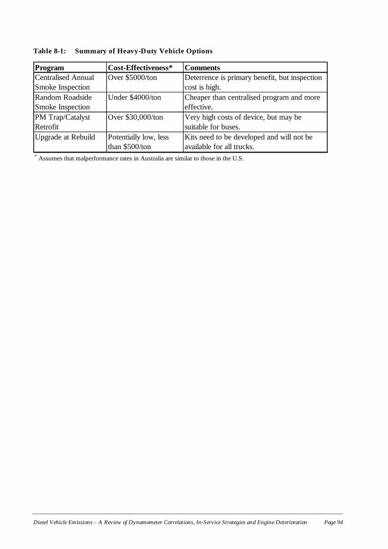
Diesel Vehicle Emissions – A Review of Dynamometer Correlations, In-Service Strategies and Engine Deterioration Page 94
Table 8-1: Summary of Heavy-Duty Vehicle Options
Program Cost-Effectiveness* CommentsCentralised Annual Smoke Inspection
Over $5000/ton Deterrence is primary benefit, but inspection cost is high.
Random Roadside Smoke Inspection
Under $4000/ton Cheaper than centralised program and more effective.
PM Trap/Catalyst Retrofit
Over $30,000/ton Very high costs of device, but may be suitable for buses.
Upgrade at Rebuild Potentially low, less than $500/ton
Kits need to be developed and will not be available for all trucks.
* Assumes that malperformance rates in Australia are similar to those in the U.S.
Diesel Vehicle Emissions – A Review of Dynamometer Correlations, In-Service Strategies and Engine Deterioration Page 95
BIBLIOGRAPHY
1. U.S. 40 Code of Federal Regulations (CFR) Part 86, Appendix I, Section (f).
2. U.S. EPA (1999), Notice of Proposed Rulemaking, Control of Emissions of Air Pollutionfrom Highway Heavy-Duty Engines, August.
3. ARB (1996), , Mobil Source Emissions Reduction Credits, California Air Resource BoardReport, February.
4. Diesel net, Diesel Emissions Online, Emission Standards (site:www.dieselnet.com/standards.html).
5. SAE (1973), Diesel Engine Emissions Measurement Procedure – SAE J1003, SAERecommended Practice, approved March 1973.
6. Hoppie, J.A. (1997), “Defining Drivetrain Losses in Developing a Cycle for Engine andChassis Dynamometer Test Compliance,” Masters These, West Virginia University.
7. TUV-Rheinland (1995), Exhaust Emission Factors for Heavy-Duty Vehicles in the FederalRepublic of Germany for Reference Year; 1990, Final report, UFO Pan No. 104 05 151/02,March.
8. Van Gompel, P. and Verbech, R. (1993), “Eindrapport Diesel-Controle Methode”, TNOReport 93.OR.VM.023.1/PVG/RV, Netherlands.
9. SAE (1982), Fuel Economy Measurement Test for Trucks and Buses – SAE J1376, SAERecommended Practice, approved July 1982.
10. Clark, N.N., et al (1998), Development of a Heavy-Duty Chassis Dynamometer DrivingRoute: Phase I report; prepared for the Midwest Research Institute and National EnergyResearch Laboratory, West Virginia University, May 27.
11. France, C.J. and Wysor, T. (1978), Selection of Transient Cycles for Heavy-Duty Vehicles,Report HDV-78-02, U.S. EPA, June.
12. France, C.J. (1978), Transient Cycle Arrangement for Heavy-Duty Engine and ChassisEmissions Testing, Report HDV-78-04, U.S. EPA, August.
13. Harris, D.B, King, F.G., Brown, J.E. (1995), Development of On-Road Emission Factors forHeavy-Duty Diesel Vehicles Using a Continuous Sampling System, presented to theAWMA Conference on Emissions Inventory, Research Triangle Park, October.
14. Harris, D.B, King, F.G., Brown, J.E. (1998), Heavy-Duty Truck Test Cycles: Driveabilityversus Realistic Engine Exercises, draft EPA report.
15. EEA (1985), Mobile Source Emissions Analysis for California, Report to the California AirResources Board, June.
16. Cornetti, G.M., et. Al. (1988), U.S. Transient Cycle versus ECE R.49 13-Mode Cycle, SAEPaper 880715, March.
17. Rijkeboer, R.C., et al. (1998), Final Report In-Use Compliance Program: Trucks 1996-1997,TNO Report No. 99.OR.VM.040.1/RR, November.

Diesel Vehicle Emissions – A Review of Dynamometer Correlations, In-Service Strategies and Engine Deterioration Page 96
18. McCormick, R.L., et. Al. (1998), Comparison of Chassis Dynamometer In-Use Emissionswith Engine Dynamometer FTP Emissions for Three Heavy-Duty Diesel Vehicles, SAEPaper 982653, October.
19. ARB (1998), Demonstration of a Heavy-Duty Vehicle Chassis Screening Test forCompliance Testing Heavy-Duty Engine, Final Report, California Air Resources BoardContract No. 94-347, July 1998.
20. MTC (1995), Emission for Four Heavy-Duty Vehicles, Motor Test Centre Report No. MTC9406A, October 1995 (Sweden).
21. EEA (1993), Feasibility Study for an I/M Program for Heavy-Duty Vehicles, Report to theCalifornia Bureau of Automotive Repair, January.
22. ARB (1988), Heavy-Duty Vehicle I/M Study, California Air Resources Board Contractorreport from Radian, May 1988.
23. EEA (1999), personal communication between Mr. D. Hassel of TUV-Rheinland and Mr.K.G. Duleep. Table 2-2 .