Quantifying Uncertainty In Reserve Estimates

Casualty Actuarial Society E-Forum, Spring 2009 1

Quantifying Uncertainty In Reserve Estimates

Zia Rehman, FCAS, MAAA, and Stuart Klugman, Ph.D., FSA ________________________________________________________________________ Abstract

Property/casualty reserves are estimates of losses and loss development and as such will not match the ultimate results. Sources of error include model error (the methodology used does not accurately reflect the development process), parameter error (model parameters are calibrated from the data), and process error (future development is random). This paper provides a comprehensive and practical methodology for quantifying risk that includes all three sources. The key feature is that variability is captured by examining historical changes in ultimate values rather than examining the underlying claim distribution. We present both the conceptual framework as well as practical examples.

________________________________________________________________________

1. THE VARIABILITY PROBLEM

The Challenge of Reserving

The Property/Casualty business model relies on the accurate measurement of risk. Of relevance to this paper is the measurement of reserving risk. Accurate actuarial loss reserving is one of the regulatory requirements in measuring solvency. Consequently, one of the most important tasks for an actuary is to estimate the proper amount of reserves to be set aside to meet future liabilities of current in-force business.

Because the stated reserve is an estimate and not the true number, there is error and it is important to measure this error. Quantifying the potential error allows for setting ranges around a best estimate, allows for measures of risk, and can assist in the setting of risk based capital requirements. Recent papers such as Hayne [8] and Shapland [11] make the importance of this issue clear.

In this paper we propose a method for measuring the total risk involved in reserve estimates. It is simple to apply and uses data that is almost always available from the reserve setting process. A key feature is that our measure of reserve variability does not depend on the method used to determine the reserves.

Literature Review

There are many papers regarding different loss reserving techniques, some deterministic, some stochastic. For a comprehensive review of existing deterministic methods the reader is referred to Wiser [17] and Brown and Gottlieb [2]. For an excellent overview of a wide range of stochastic reserving methods in general insurance, the reader is referred to England and Verrall [5]. Other references of interest include Bornhuetter and Ferguson [1], Finger [6], and Taylor



[12].

While the traditional chain ladder technique provides only a point estimate of the total reserve, it has become evident recently that actuaries also need a measure of variability in loss reserving estimation. Sound methodologies that quantify risks related to the balance sheet are important for attracting and retaining capital in the firm. Standard and Poor’s ratings as well as investors are very interested in the value at risk (VaR) measurements. The NAIC and state regulators are interested in monitoring the reserve variability in the form of reserve ranges. Variability and sometimes the entire distribution of the loss reserving estimation are important for risk management purposes. Questions such as what is the 95th percentile of losses or the cost of loss portfolio transfer are important in managing and assessing risk. These questions can be properly addressed with a thorough analysis of the variability of the reserve estimate.

Over the last thirty years many researchers have made significant contributions to the study of the variability of reserving methods. The 2005 CAS working party paper [3] presents a comprehensive review that brings all of the important historical research together. A representative, but not exhaustive, list would include the following: Taylor and Ashe [13] introduced the second moment of estimates of outstanding claims. Hayne [7] provided an estimate of statistical variation in development factor methods when a lognormal distribution is assumed for these factors. Verrall [15] derived unbiased estimates of total outstanding claims as well as the standard errors of these estimates. Mack [10] used a distribution-free formula to calculate the standard errors of chain ladder reserve estimates. England and Verrall [5] presented analytic and bootstrap estimates of prediction errors in claims reserving. De Alba [4] gave a Bayesian approach to obtain predictive distribution of the total reserves. Taylor and McGuire [14] applied general linear model techniques to obtain an alternative method in cases where the chain ladder method performs poorly. Verrall [16] implemented Bayesian models within the framework of generalized linear models that led to posterior predictive distributions of quantities of interest.

However, the CAS 2005 working party [3] ultimately concluded, “there is no clear preferred method within the actuarial community.” Actuaries need to select one or several methods that are considered appropriate for the specific situation. When it comes to the final decision, judgment still overrules.

The Risk Measurement Problem

The 2005 CAS working party report [3] notes that the sources of uncertainty in the reserve estimate come from three types of risk: process risk, parameter risk and model risk. Model risk is the uncertainty in the choice of model. Parameter risk is the uncertainty in the estimates. Process



risk is the uncertainty in the observations given the model and its parameters.

Shapland [11, p.124] highlights the importance of all the risks:

Returning to the earlier definition of loss liabilities … all three types or risk … should be included as part of the calculated expected value. Alternatively, some or all of these types of risk could be included in a ‘risk margin’ as defined under ASOP No. 36.

These three risks are intertwined and thus hard to separate. In particular, process risk is usually calculated as if the model and parameters were correct and parameter risk is calculated as if the model were correct.

In this paper the three risks will not be separately measured nor directly treated1. Often, when model risk is discussed it is in the context of the chosen model versus the true model or in the context of the chosen model versus alternative models. Rather, we capture the total risk from all three sources underlying the reserve estimate. The reserving model (or ultimate loss selection if no specific method is used) will be considered fixed and any errors measured will be a consequence of that choice.

From a risk management perspective this is appropriate. Now that the reserves have been established, what is the potential error that may result, given the current reserve review?

A Summary of Our Approach

Most approaches to risk measurement rely on the statistical properties of the data as reflected by the model selected for calculating the reserve. Those approaches attempt to capture the underlying distribution of losses. This will capture process error, but not model or estimation error. That is because any calculations will be done assuming the model and its estimated parameters are correct. In this setting, process error can be estimated using statistical measures such as Fisher information. We choose to look at the reserves (as reflected in the estimated ultimate losses) themselves as they evolve over time. This provides a way to reflect all the sources of error. Each reserve set in the past is an estimate of its distribution and thus its errors can be estimated from the historical errors made in the estimations. Because the ultimates will converge to the true value, the errors made along the way reflect all sources of error.

Our methodology will be introduced within a stable context. In particular, we assume that the underlying loss development processes have not changed over time and that the same reserving methodology has also not changed. Further, we assume we are working with indicated reserves that are the result of a specific methodology. Our method does not depend on the particular 1 The model presented will capture the parameter and model risk in the actuary’s estimate but will not measure the parameter uncertainty due to its own estimate.



methodology selected, just that it be consistently applied. After working through this situation we will discuss modifications that can allow our methods to be applied in more general settings.

Note that we model indicated reserves instead of held reserves. This is because indicated reserves do not have management or other ad hoc adjustments. Therefore, indicated reserves are more stable and thus easier to model. What is interesting about held reserves is where they fall within the probability distribution of the unknown true reserve. This can provide an indication of the degree to which held reserves are conservative or aggressive.

Because the method presented here is free of the choice of the reserving method used, it is not necessary to even have a specific method. The only requirement is a history of ultimate loss selections. Thus we rely on the actual error history of the reserving department.

We make a theoretical and practical case for the lognormal distribution for the errors in aggregate reserves, line or total. The focus on the aggregate distribution also removes the need to choose individual size of loss distributions.

Each of the following sections will take one step through the development of the risk measure. An example will be followed throughout to illustrate the formulas.

2. RESERVING PROCESS AND DATA

The reserve review process generates reserves based on raw data analysis. The indicated ultimate losses are selected by line using perhaps several methods as well as judgment. These line ultimates are then added to yield total indicated reserve.

Management adjustments called margins may be applied to the total reserve. These margins may then allocated by line and by accident year to the indicated ultimate losses and reported in Schedule P Part2. As noted earlier, our method does not work with these reserves.

There are three issues of interest relating to measuring reserve variability:

• The distribution of the true (but unknown) ultimate losses by line and in aggregate. This shows the volatility and the bias in the actuarial selections.

• The held reserves that are reported in Schedule P Part2 as a percentile on the distribution of reserves.

• A procedure to allocate the margin by line & accident year such that ultimate losses for all years are at a constant percentile.

It is instructive to understand several aspects of indicated reserves:



Indicated reserves are the actuary’s best estimates based on the data and exclude management adjustments. Therefore errors are due only to actuarial selections, methods, or randomness in the data.

Data triangles used for reserve reviews can be quarterly or annual. Generally most companies like to have consistency in the indicated reviews as it is easier to update spreadsheets for each review if they are the same size. Also most companies like to track development to ultimate and prefer complete triangles if data is available.

Reserve reviews are done on a net and or direct basis and the underlying triangles are based on the relevant data. They are definitely conducted annually to report Annual Statement reserves but many companies do them quarterly.

Reserving actuaries refer to lines of business as “segments” as they can be custom defined by the actuary for reserve reviews. These can be different than the usual lines of business such as those defined in Schedule P. For consistency of notation in this paper, we will call reserve segments as lines of business. The methodology will be the same in both cases.

Generally the DCC (Defense & Cost Containment) reserve review (indicated reserves) is done using data where they are either a part of the loss triangle (loss + DCC) or are treated separately (DCC only). In the first case we treat DCC as part of the losses and in the latter case as another data segment (if broken out separately). In this paper loss shall mean whatever appears in the analysis being evaluated.

The variability for ULAE reserves is outside the scope of the paper and will not be discussed. For most companies ULAE reserves are a relatively small part of the total reserves.

Scope of Model

The approach presented in this paper is generic and applies to any type of triangle such as

Paid or incurred

Count or Severity

Accident year, policy year, or report year

Quarterly or annual.

Each of these triangles eventually leads to the appropriate ultimate losses. Depending on the choices made above and the selected reserve methodology, the distribution of errors will differ. For example if only the paid loss development method is used and we track its history of ultimate losses over time then the resulting reserve distribution will pertain to the paid loss development method. If several methods are used and the actuary finally selects reserves based



on several indications (typically this is the case) then the triangle history of final selected ultimate losses will provide the distribution of the selected reserves.

An interesting point is that the method can even be applied to the raw data. This is equivalent to treating the data as the selected ultimate loss. In this case the resulting distribution will pertain to the data itself (paid or incurred losses etc). This essentially creates a new reserving method. However, the purpose of this paper is not to promote a new way of calculating reserves, rather to develop a method for determining the distribution of the indicated reserves resulting from actuarial selections.

Reasonable estimates

A standard assumption that is in line with Actuarial Standards of practice (ASOP) on reserves is that the reserve ranges are set around reasonable estimates. This is partly achieved by using indicated ultimate reserves instead of held reserves as these do not have management adjustments.

Cases where the indicated ultimate losses are unreasonable are outside the scope of this paper. This does not necessarily mean that the model will not apply but rather that the authors have not given consideration for such cases in this paper.

3. A MODEL FOR ERRORS

Measuring the error from the data

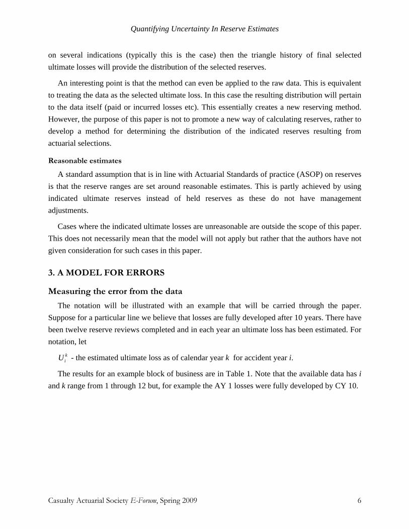
The notation will be illustrated with an example that will be carried through the paper. Suppose for a particular line we believe that losses are fully developed after 10 years. There have been twelve reserve reviews completed and in each year an ultimate loss has been estimated. For notation, let

kiU - the estimated ultimate loss as of calendar year k for accident year i.

The results for an example block of business are in Table 1. Note that the available data has i and k range from 1 through 12 but, for example the AY 1 losses were fully developed by CY 10.



AY(i)

/CY(k)

1 2 3 4 5 6 7 8 9 10 11 12

1 148,741 103,058 100,010 98,001 96,280 95,579 95,176 95,161 95,150 95,113

2 186,087 120,444 113,083 109,097 108,443 107,934 107,836 107,814 107,907 107,860

3 139,092 94,318 89,032 86,552 85,584 85,532 85,557 85,655 85,626 85,650

4 58,441 52,585 52,136 51,375 51,501 51,799 51,870 51,914 51,933

5 22,738 30,670 32,948 33,986 34,363 34,329 34,467 34,642

6 24,134 37,035 42,981 42,688 42,894 43,052 43,533

7 26,695 51,849 57,143 57,817 58,200 58,647

8 57,397 67,688 74,995 75,793 76,736

9 94,537 94,281 98,453 98,055

10 93,784 104,539 100,257

11 116,443 124,781

12 172,224

Table 1 – Indicated ultimate losses from 12 calendar year valuations.



For example, the value 42,894 is the indicated ultimate loss estimated at the end of calendar year 10 for losses incurred in accident year 6. We are interested in the errors made in the estimates of the ultimate losses. Some of those errors can be determined from Table 1. We will use the logarithm of the ratio for the errors, for reasons to be explained later.

For example, the ultimate value for accident year 3 was estimated at the end of calendar year 11 (development year 8) to be 85,626. A year later, the actual value of 85,650 was known. The error is ln(85,650/85,626) = 0.00028. We cannot calculate the error for later accident years because they have not yet been fully developed. The errors we care about are 9ln( / )k i k

i i ie U U+= where i + 9 > k. The numerator is the fully developed ultimate loss and the denominator is the estimate as of CY k. For our example we are currently at k = 12 and so are concerned with the errors made in estimates from AY 4 onward.

In order to gather more information about errors from this information, begin with an error that is not immediately useful. Consider * 1ln( / )j j j

i i ie U U+= where available. This represents the error realized as the estimated ultimate value is updated one calendar year later. Here is one reason for using logarithms – the errors are additive. In fact,

9

1 2 9

1 8

81

0

8*

ln( / )

ln

ln( / )

.

k i ki i i

k k ii i i

k k ii i i

i kk g k gi i

g

ij

ij k

e U U

U U UU U U

U U

e

+

+ + +

+ +

+ −+ + +

=

+

=

=

⎛ ⎞= ⎜ ⎟

⎝ ⎠

=

=

∑

∑

L

In this notation, the development year of the denominator value is d = j – i + 1. The advantage of this approach is that the available data in our example provides many estimated values as presented in Table 2.



AY(i)\DY(d) 1 2 3 4 5 6 7 8 9

1 ‐0.36691 ‐0.03003 ‐0.02029 ‐0.01772 ‐0.00731 ‐0.00423 ‐0.00016 ‐0.00012 ‐0.00039

2 ‐0.43503 ‐0.06306 ‐0.03589 ‐0.00601 ‐0.00471 ‐0.00090 ‐0.00021 0.00086 ‐0.00044

3 ‐0.38846 ‐0.05768 ‐0.02825 ‐0.01125 ‐0.00061 0.00029 0.00114 ‐0.00034 0.00028

4 ‐0.10559 ‐0.00858 ‐0.01470 0.00245 0.00577 0.00137 0.00085 0.00037

5 0.29925 0.07165 0.03102 0.01103 ‐0.00099 0.00401 0.00506

6 0.42824 0.14889 ‐0.00684 0.00481 0.00368 0.01111

7 0.66386 0.09722 0.01173 0.00660 0.00765

8 0.16492 0.10251 0.01058 0.01237

9 ‐0.00271 0.04330 ‐0.00405

10 0.10857 ‐0.04182

11 0.06916

Table 2 – year-to-year error values, *jie



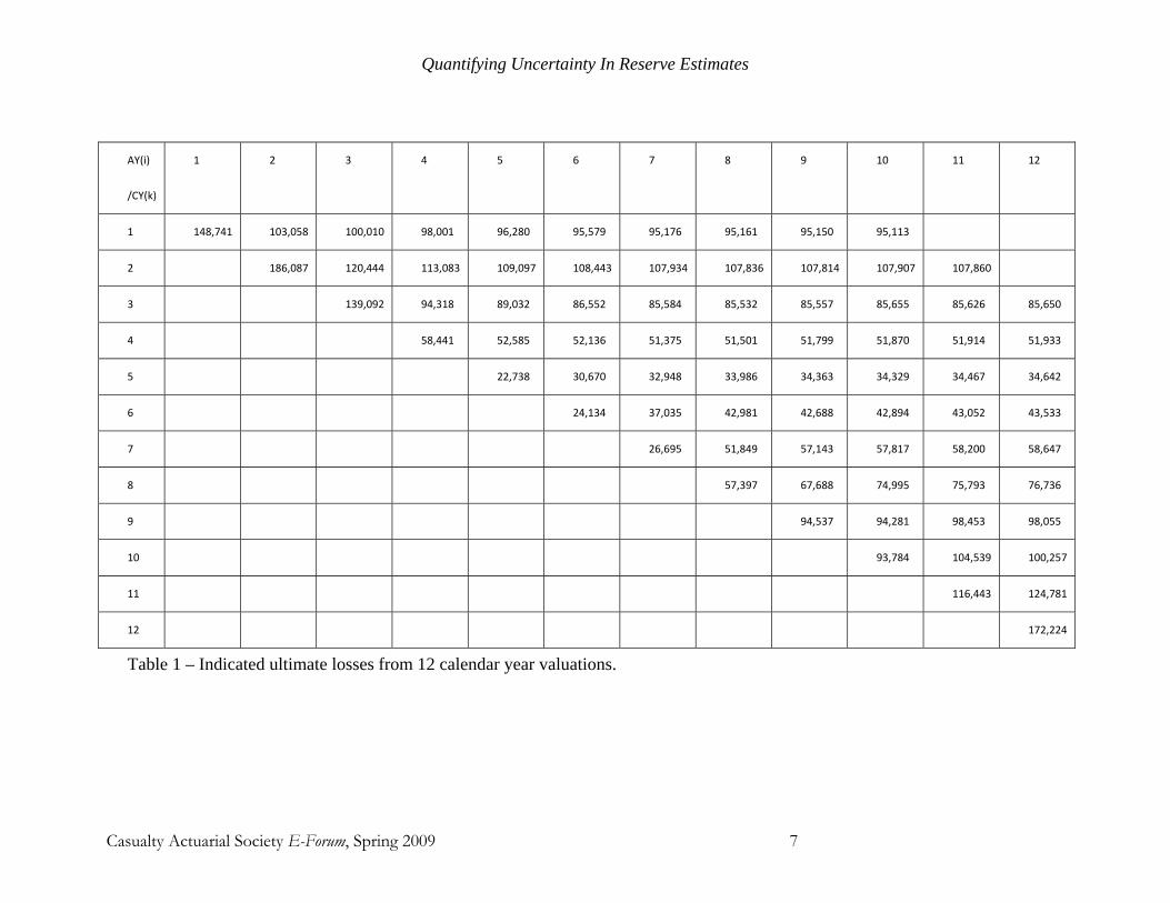
There is another interpretation of these errors. Regardless of the reserving method, a factor representing the ultimate development can be inferred. Suppose we are looking at accident year i and calendar year j. The factor is /j j j

i i iu U L= where jiL is the paid loss for that accident year at

the end of year j. One year later the factor is 1 1 1/j j ji i iu U L+ + += . These represent age to ultimate for

two different development years. The ratio, 1/j ji iu u + represents how losses were expected to

develop while 1 /j ji iL L+ is how they actually developed. The ratio of actual to expected is

1 /j ji iU U+ which is the error measurement we have been using.

Now that the key data values have been calculated it is time to construct a model.

The Model

We propose that the error random variables have the normal distribution, and in particular,

( ).,~ 2*1

*1

*+−+− ijij

ji Ne σμ

Note that the mean and variance are constant for a given development year. The rest of this section is devoted to justifying these assumptions. It should be noted that justifying the assumptions through data analysis is not sufficient. If this method is to be useful regardless of the loss reserving method used, the justification must be based on our beliefs about the loss development and reserving processes and not any particular models or empirical evidence.

Normal distribution

After the ultimate loss is estimated at a particular time, what factors will cause it to change when it is re-estimated one year later? Day by day during that year a variety of events may take place. Among them are2:

Economic forces such as inflation and changes in the legal environment will alter the amounts paid on open claims or those newly reported.

The rate at which claims develop may change.

Purely random events may affect individual open claims.

Actuary’s opinion on IBNR may change depending on the adequacy of case reserves.

These factors will tend to act proportionally on the current estimate of the ultimate loss. Because there are many such factors happening many times in the course of a year, it is reasonable to assume we are looking at the product of a variety of random variables, most with values near 1. The Central Limit Theorem indicates that the result is a lognormal distribution and

2 At this point in the paper we focus on lognormality as a consequence of unchanging development processes. We relax this assumption later in the paper.



thus measuring the error in the logarithm will produce values with a normal distribution.

Normal approximation

The above arguments relating to the central limit theorem apply to a fictitious accident year with infinite claims. This accident year need not be evaluated infinitely many times but the changes at each valuation should be driven by infinite reasons underlying infinite claims.

In practice a finite subset of this hypothetical accident year is available. The reasons causing the change in the ultimate loss are finite and not infinite and thus the distribution is approximately normal3. The approximation can be improved by increasing the number of reasons driving the change in ultimate losses. This can be done in the following ways:

Increase the valuation time (example once a year rather than four times a year)

Increase the claim count (large volume line)

The claim count required for a good normal approximation in turn depends on the skewness of the underlying size of loss distribution. As a practical matter the model will work well even for a modest claim count.

Reserve valuations conducted less frequently (example once a year rather than four times a year) will allow greater “reasons” for changes and thus help with the normal approximation. The tradeoff is the loss of accuracy in ultimate loss estimation and consequential bias. Also note that both the parameters of the distribution and its shape (to which extent it is lognormal) will change depending on the frequency of reserve review.

A subtle point concerns the later development intervals. In these intervals the changes are usually driven by a handful of claims (few reasons) and thus violate the normality assumption. However at those valuations the aggregate errors are often close to zero with small volatility (constants) and thus departure from the normality has little impact on the total distribution for the entire accident year.

Mean

At first it may seem that the mean should be zero. There are two reasons that is not so. First, consider the expected revised ultimate loss given the current estimate:

* *21 1 / 21( / ) j i j ij j

i iE U U eμ σ− + − +++ = .

For the reserve estimate to be unbiased, it is necessary that * *21 10.5j i j iμ σ− + − += − and not zero.

3 Technically, the distribution remains approximately normal even for the infinite claim accident year but the distribution is closer to normal than in the finite case.



In addition, it is possible that the reserving method is biased. This may be a property of the method selected and may even be a deliberate attempt by the reserving actuary to adjust the reserves based on knowledge that is outside the data.

Having the mean be constant from one accident year to the next is a consequence of the assumptions that were made at the beginning. That is, there is no change in the underlying development process or reserving method.

Having the mean depend on the development year seems reasonable. As the development year increases any systematic bias is likely to be reduced in the expectation that the ultimate value will not be much different from the current value. In addition, we expect the variance of the errors to decrease and if the ultimate loss estimates are unbiased, the means will then also decrease (in absolute value).

Complete Triangle of Errors

For at least one accident year we need the losses to be fully developed. Even better would be to have a few fully developed years so there would be more data available for computing covariances and variances. There is a tradeoff in that older fully developed accident years that are not part of the in-force book may be less predictive and may not reflect the current prevailing business environment.

The opposite concern is when there are not enough accident years available to obtain fully developed losses. This can happen for relatively new companies or lines of business. Note that tail errors generally result from estimation errors of pending court cases or simply absence of data due to a new line. Since we are dealing with a year in aggregate, these errors are usually close to zero and therefore contribute less to the variance than earlier development intervals.

4. PARAMETER ESTIMATION

Return to the continuing example and recall Table 2. The numbers in this table are percentage changes (errors) of the estimated ultimate losses and have been assumed to have been drawn from six normal distributions. The upper half of the triangle is fixed and known and our goal is to obtain the normal means and variances for the yet-to-be observed errors in the lower right part of the table.



Estimation of the mean

We choose to calculate an initial estimate of the mean by calculating the sample mean,

12( 1)*

* 1ˆ12

di d

ii

d

e

dμ

−+ −

==−

∑

where d is the development year, the sum is taken over all accident years for which errors were available.4

The results for our example are in Table 3.

DY(d) 1 2 3 4 5 6 7 8 9

mu‐hat 0.0396 0.0262 0.0063 0.0003 0.0005 0.0019 0.0013 0.0002 0.0002

mu‐hat

(Selected)

0.0396 0.0262 0.0063 0.0003 0.0005 0.0019 0.0013 0.0002 0.0002

Table 3 – Estimated means by development year

However, there are reasons why the sample mean may not be the appropriate choice. The results may be biased due to model risk. The estimate of the mean affects the estimate of the expected ultimate loss.

For example if 2

2σμ −< then the estimated ultimate loss will be less than the indicated ultimate showing redundancy in resulting reserves. The opposite is true if the inequality is reversed. Thus any value of mean that is different than

2

2σ− should be justified.

The estimation of the mean can effectively result in taking a position that the actuarial estimate is biased. This is not trivial and there should be careful analysis before making that assertion. We discuss the mean selection in greater detail under distribution reviews later in the paper.

Estimation of the Variance

The variance parameter measures the risk historically faced by the book in force. For very long tailed lines this would mean that it will capture the changes in reserving methods and other changes that have taken place.

The variance estimate is the usual unbiased estimate. The equation is,

4 An alternative is to use a weighted average where the weights are the indicated ultimate values for that accident year. This allows more weight to be placed on those accident years in which there is more data.



212( 1)*

*2 1

ˆˆ

11

di d

i di

d

e

d

μσ

−+ −

=

⎡ ⎤−⎣ ⎦=

−

∑.

Note that the estimated mean must be the sample mean.

For our data the estimated standard deviations by development year are given in Table 4. As expected, for the most part, the standard deviations decrease by lag.

DY(d) 1 2 3 4 5 6 7 8 9

sd‐hat 0.3502 0.0762 0.0213 0.0108 0.0055 0.0052 0.0022 0.0005 0.0004

Table 4 – Standard deviations by development year

Correlations

For a given accident year, it is likely that the errors for one development year are correlated with those from other development years. These must be estimated. A formula for the covariance is

12( 1)* ( ' 1)*

'*

, '

ˆ ˆˆ

11

di d i d

i d i di

d d

e e

d

μ μσ

−+ − + −⎡ ⎤ ⎡ ⎤− −⎣ ⎦ ⎣ ⎦

=−

∑

Where d > d’ represent two different development years and each sample mean is based only on the first 10 – d observations.

The matrix of covariances is given in Table 5.



d 1 2 3 4 5 6 7 8 9

1 0.12261 0.02379 0.00664 0.00356 0.00178 0.00175 0.00062 0.00000 0.00000

2 0.02379 0.00581 0.00122 0.00070 0.00027 0.00040 0.00011 0.00000 0.00000

3 0.00664 0.00122 0.00045 0.00020 0.00005 0.00006 0.00005 0.00000 0.00000

4 0.00356 0.00070 0.00020 0.00012 0.00004 0.00004 0.00002 0.00000 0.00000

5 0.00178 0.00027 0.00005 0.00004 0.00003 0.00002 0.00000 0.00000 0.00000

6 0.00175 0.00040 0.00006 0.00004 0.00002 0.00003 0.00001 0.00000 0.00000

7 0.00062 0.00011 0.00005 0.00002 0.00000 0.00001 0.00000 0.00000 0.00000

8 0.00000 0.00000 0.00000 0.00000 0.00000 0.00000 0.00000 0.00000 0.00000

9 0.00000 0.00000 0.00000 0.00000 0.00000 0.00000 0.00000 0.00000 0.00000

Table 5 – Covariances

The total variance for any given accident year can now be calculated from Table 5. For example the variance for AY 12 will be the sum of the values in the table (shown as 0.46129 in the table 6 below).

5. THE ERROR DISTRIBUTION FOR A GIVEN ACCIDENT YEAR

Now that we have a model for the errors from one calendar year to the next, we need to return to the error we care about. Recall that

8*

ik ji i

j k

e e+

=

= ∑ .

From the assumptions made previously, this error has a normal distribution and its mean depends only on the latest development year, k – i + 1.

( )211,~ +−+− ikik

ki Ne σμ 8

*1 1

8 82 *2 *

1 1 1, ' 11 '

2

i

k i j ij k

ji i

k i j i j i j ij k j k j k

μ μ

σ σ σ

+

− + − +=

+ +

− + − + − + − += = + =

=

= +

∑

∑ ∑ ∑

These quantities can be estimated by adding the respective mean, variance, and covariance



estimates.

For our example, we now have estimates of the distribution of the error in the ultimate loss as estimated from the data available at the end of calendar year 12. They are given in Table 6.

AY mean sd

4 ‐0.000181 0.000401

5 0.000013 0.000303

6 0.001352 0.002243

7 0.003294 0.006727

8 0.003791 0.010914

9 0.004077 0.021106

10 ‐0.002222 0.040233

11 0.024019 0.113210

12 0.063590 0.460129

Table 6 – Means and standard deviations by accident year

6. THE ERROR DISTRIBUTION FOR ALL ACCIDENT YEARS COMBINED

While we have been using logarithms to measure the error, when all is done we are interested in the ultimate losses themselves. To make the formulas easier to follow, rather than allow arbitrary values, we will follow the example and assume we are at the end of CY 12 and losses are fully developed after 10 years. In particular, we care about

13 214 12 .U U U= + +L

Recall from the notation that the terms on the right hand side represent the fully developed losses at a time in the future when the ultimate results are known. Rewrite this expression as



12 12 12 124 4 12 1212

12

412

12 124 1212 124 12

exp( ) exp( )

exp( )

.

i ii

ii

U U e U e

V r e

UrU U

V U U

=

= + +

=

=+ +

= + +

∑

L

L

L

Here V is the estimated ultimate loss as of CY 12 for all open years and the weights are the relative proportion in each accident year. This indicates that the ultimate loss is a weighted average of lognormal random variables. This can be painful to work with (though not hard to simulate). Because the error random variables are usually close to zero and will vary about their mean, consider the following Taylor series approximations.

1212

4

1212

4

1212

4

1212

4

ln ln exp( )

ln (1 )

ln 1

.

i ii

i ii

i ii

i ii

UX r eV

r e

re

re

=

=

=

=

⎡ ⎤= = ⎢ ⎥⎣ ⎦⎡ ⎤

≈ +⎢ ⎥⎣ ⎦⎛ ⎞= +⎜ ⎟⎝ ⎠

≈

∑

∑

∑

∑

The approximate log-ratio has a normal distribution and thus U has an approximate lognormal distribution. The moments of the normal distribution are:

1212

4

12

134

ln i ii

i ii

UE E reV

rμ

μ

=

−=

⎛ ⎞⎛ ⎞=⎜ ⎟ ⎜ ⎟⎝ ⎠ ⎝ ⎠

=

=

∑

∑

1212

4

122 2

134

2

ln

.

i ii

i ii

UVar Var reV

r σ

σ

=

−=

⎛ ⎞⎛ ⎞ ≈⎜ ⎟ ⎜ ⎟⎝ ⎠ ⎝ ⎠

=

=

∑

∑



For the example, V = 760,808, μ = 0.01927, σ2 = 0.01123, and then the expected ultimate loss is 779,978 and the standard deviation is 82,892.

7. EXTENSION TO MULTIPLE LINES OF BUSINESS

Suppose there are two lines of business. Each can be analyzed separately using the method previously outlined. However, it is likely that the results for the lines are not independent. One approach would be to model the correlation structure between error values from the two lines. The problem with that approach is that there may not be corresponding cells to match and also the number of parameters may become prohibitive5.

An alternative is to combine the data from the two lines into a single triangle and analyze it using the methods of this paper. When finished, there will be a distribution for each line separately and for the combined lines. Usually, only the total reserve is of importance and thus only the combined results are needed. The individual line results will be useful for internal analyses and also if it is desired to allocate the reserves back to the lines.

To illustrate this idea, we add a second line of business. The same analysis gives: V = 244,537, μ = -030759, σ2 = 0.008933, and then the expected ultimate loss is 180,593 and the standard deviation is 17,107.

Combining the two lines creates a single table with the totals from each. An analysis of these tables produces V = 1,005,376, μ = -0.02674, σ2 = 0.009582, and then the expected ultimate loss is 983,520 and the standard deviation is 96,506.

8. ALLOCATION OF ULTIMATE LOSSES

From the previous examples there is an interesting situation. If the two lines were independent, the standard deviation of the total would be

2 282,892 17,107 84,638+ =

Which is less than the standard deviation from the combined lines, which was 96,506. There is thus a positive correlation between the lines and when setting reserves and then allocating them to the lines, something needs to be done.

5 Combining distributions also requires the multivariate normality assumption. This is hard to test but is often made in practice.



Allocation of reserves

Suppose we set reserves with a margin for conservatism based on the results of the previous section. For example, suppose we set ultimate losses to be at the 95th percentile. That is,

1,005,376exp( 0.02674 1.645 0.009582) 1,149,833.− + =

where the mean and standard deviation are for the corresponding normal distribution.

We also want to set ultimate losses for each line of business such that they add to 1,149,833. However, this cannot be achieved by setting each line at its 95th percentile. A reasonable approach is set each line at the same percentile, using the percentile that makes the sum work out. It turns out that if each line is set at the 96.28th percentile, the ultimate estimates will be 937,025 and 212,808.

9. MODEL EXTENTION TO PRACTICAL SETTINGS

Distribution reviews

Once the reserving actuary has completed the reserve review the distribution review should follow. The actuary will remember the considerations for selecting the ultimate losses. These include data considerations, coverage changes, mix changes etc. All of these can now be factored in the bias (mean parameter) estimation of resulting reserve distribution.

The distribution review allows the actuary to consider the possibility of estimation bias in the current reserve estimate. For example if the historical errors of the selected ultimate losses for a line are positive and the actuary has not changed the selection approach then the current estimate will likely have a positive error (too low an estimate).

The reserve diagnostics are particularly important in evaluating such errors as the past is not always indicative of the future. For example a sign of case reserve weakening should lead to a higher IBNR all else being equal.

These mechanisms of monitoring errors allow early warning signs for future potential reserve deficiencies.

Finally note that changes in conditions do not invalidate the lognormal property. However, changes in conditions will change the lognormal parameters, thereby increasing the degree of difficulty for projection accuracy.

Volatility measurement under changing conditions

While the distribution reviews and the resulting mean parameter will account for changes in



reserve adequacy, the volatility parameter reflects historical data and is therefore slow to respond to changes in the errors. Thus if the reserving methods change abruptly or the reserving actuary is replaced, the volatility will change slowly as the data emerges. Such cases are handled in the following ways:

In many cases it is wise to let data lead the way as it may be pre-emptive to conclude about the volatility of the new process. This is especially relevant in light of the fact that processes themselves usually change slowly over time (such as experience of reserving actuary etc).

In rare cases, the change in reserve methodology is driven by an abrupt decision such as outsourcing the reserve review to a consultant. In that case, the historical error data will have to be restated with the new process.

10. APPLICATIONS

We now present a few applications of the previous results.

Loss estimation method

The chain ladder estimate is biased for long tailed lines partly due to the fact that the covariance by development intervals is not incorporated in its estimate. Using the parameter estimation technique presented in this paper (including the variance covariance matrix of a triangle) the expected ultimate loss for an accident year

( ) ⎟⎟⎠

⎞⎜⎜⎝

⎛+=

2exp

2σμoUUE

U = Ultimate loss, oU = Incurred or paid loss, 2σ = sum of variance covariance matrix (the number of terms depend on the age of the accident year).

Claim Commutations

Claim commutations involve transfer of reserves from a ceding carrier to an acquiring carrier. The risk to the acquiring company is that the indicated reserves may not be sufficient to pay all claims. One complication is that the agreed to reserve value may not be the same as that used in the determination of the reserve distribution. Let H be this arbitrary reserve value. A reasonable fair transaction price is this reserve plus the value of expected excess reserve cost above H. Let C be this cost. The total price is then given by H C+ . The formula for C is:

( ) ( )RHC x H f x dx

∞= −∫

where, R is the random true reserve. Let P be the amount paid and as before U is the random,



true, ultimate loss. Then, R U P= − and so

22

( ) ( )

( ) ( )

( ) ( )

( ) ( )

ln( ) ln( )exp[ ln( ) / 2] 1

ln( ) ln( )( ) 1

RH

UH

UP H

C x H f x dx

x H f x P dx

y P H f y dy

E U E U P H

H P VV

H P VH P

μ σμ σσ

μσ

∞

∞

∞

+

= −

= − +

= − −

= − ∧ +

⎡ ⎤⎛ ⎞+ − − −= + + −Φ⎢ ⎥⎜ ⎟

⎝ ⎠⎣ ⎦⎡ + − − ⎤⎛ ⎞− + −Φ⎜ ⎟⎢ ⎥⎝ ⎠⎣ ⎦

∫∫∫

The second line is a change of variable using .R U P= −

The same concept applies in situations where one company acquires or merges with another company or a re-insurer acquires the reserve of the ceding carrier (Loss Portfolio Transfer).

Insurance market segmentation

The expected excess cost formula gives an insight into insurance economics. The assuming carrier will pool the assumed reserves into existing homogenous reserve segments. If the pooling decreases the total risk, captured in the estimated 2σ for the line, the assuming carrier’s expected excess cost will be lower than ceding carrier’s. This assumes that the reserve adequacy of the reserve segment is estimated identically by both parties.

The above argument explains insurance market segmentation. Companies grow their business in a given line and continue to acquire business from smaller companies in the same line because they face different total risks. Unlike other businesses, the volatility of losses underlying estimates drives decisions to acquire and grow an existing business segment. This is also the reason why low risk (short tailed, fast developing) lines are seldom ceded to other companies.

Net and Direct Reserve Distributions

We can quantify the reserve distribution net of reinsurance and/or recoveries using the method explained in the paper. This is possible because we are following the net reserve reviews and simply measuring the uncertainty in the estimates.

One caveat when dealing with net distributions is that the true mean can be harder to estimate especially if treaties have changed recently. As stated earlier quarterly error triangles are more helpful in such cases as they are more responsive to changes. In other cases, the current actuary’s



estimate can be taken to be unbiased until further history is developed under the new treaty.

In many where reinsurance has a relatively small impact on total reserve a change in treaty provisions will not change the resulting net error distribution significantly. For examples quota share reinsurance on a loss occurring basis on a line with large claim count per accident year will not necessarily lead to a lower variability of the net aggregate error distribution (emphasis added). The reserving actuary will see proportionally lower losses for new accident years but this may not impact net error distribution.

Another example is casualty excess of loss coverage that attaches at a high layer. If the ground up claim count is large enough the change of reinsurance treaty many have very little impact on the net error distribution as few losses out of the total will be ceded in that layer.

In some cases especially for low frequency & high severity lines such as personal umbrella excess of loss coverage, the impact of a change in treaty can be significant and the error history will not be relevant to the current treaty. This will require the actuary to conduct net historical reserve reviews based on the new treaty. This can be time consuming should be done if the line forms a significant part of the total reserve.

Net distributions result in net reserve ranges and net reserving capital. These are relevant from a solvency, regulatory and company rating standpoint.

Regulatory & Rating Agency Applications

Regulators and rating agencies are interested in quantifying reserve ranges, percentiles, and reserving capital in order to monitor the solvency of the company. The regulator, in particular is interested in measuring the performance of the held reserve, shown in Schedule P.

Once the distribution of the reserves is known we can state the percentile of the held reserves. Note that the management bias will now make a difference as it will position the held reserves to the right or left of the true mean.

We can also calculate the reserving risk capital as the difference between a selected cutoff value (say 95th percentile) of the indicated reserves and the held reserves. The resulting reserving risk capital can be used to modify the RBC reserving risk charge. Note that the NAIC tests of reserve development to surplus ratios suggest comparing dollar ultimate loss errors to company surplus. This is very similar to our approach of measuring reserve uncertainty. Thus, the reserving risk charge measured using the method outlined in this paper would be consistent with the current annual statement and NAIC practices.



11. CONCLUSION

The paper presents a shift in paradigm from loss distributions of the underlying losses to distributions of the company’s estimates. This represents a new way of measuring reserving risk. By being able to quantify risk both by line and for the company, effective management of capital, reinsurance, and other company functions becomes feasible.

We provide a framework for assessing reserve review accuracy as well as measuring the distribution of the current reserve review. This is done using a “distribution review” immediately after a reserve review using the same segments and models currently used by the reserving department.

Given the current complex reserving environment where reserving is both an art and a science there is no statistical formula to set reserves or its distribution. Rather we present a rigorous framework that involves the same considerations and process as the underlying reserve review itself.

Acknowledgement We are indebted to Zhongzian Han (Statistics & Actuarial Science department of the University of Central

Florida) for his furnishing the literature review. The authors would also like to thank William J Gerhardt (Nationwide Insurance) for being a great sounding board and providing invaluable feedback.

The authors are also grateful to an anonymous reviewer for extensive data testing and feedback.

REFERENCES

[1] Bornhuetter, R.L. and R.E. Ferguson, 1972. “The Actuary and IBNR,” Proceedings of the Casualty Actuarial Society, LIX, pp. 181-195.

[2] Brown, R.L., Gottlieb, L.R., 2001. Introduction to ratemaking and loss reserving for property and casualty insurance, second ed. Winsted, CT: ACTEX.

[3] CAS Working Party on Quantifying Variability in Reserve Estimates, 2005. “The Analysis and Estimation of Loss & ALAE Variability: A Summary Report,” Casualty Actuarial Society Forum, Fall 2005, pp. 29-146.

[4] De Alba, E., 2002. “Bayesian Estimation of Outstanding Claims Reserve,”. North American Actuarial Journal, 6, pp. 1-20.

[5] England, P. D. and Verrall, R.J., 2002. “Stochastic Claims Reserving in General Insurance,” British Actuarial Journal 8, pp.443-544.

[6] Finger, R, J.,1976. “Modeling Loss Reserve Developments.,” Proceedings of the Casualty Actuarial Society, LXIII, pp. 90-105.

[7] Hayne, R.M., 1985. “An Estimate of Statistical Variation in Development Factor Methods,” Proceedings of the Casualty Actuarial Society, LXXII, pp. 25-43.

[8] Hayne, R.M., 2004. “Estimating and Incorporating Correlation in Reserve Variability,” Casualty Actuarial Society Forum, Fall 2004, pp. 53-72.

[9] Kreps, R.E., 2005. “Riskiness Leverage Models,” Proceedings of the Casualty Actuarial Society, XCII, pp. 31-60.

[10] Mack, T., 1993. “Distribution-Free Calculation of the Standard Error of Chain Ladder Reserve Estimates,” ASTIN Bulletin 23, pp. 213-25.

[11] Shapland, Mark, 2007. “Loss Reserve Estimates: A Statistical Approach for Determining Reasonableness,” Variance, 1, pp. 120-148.

[12] Taylor, G.C., 2000. Loss Reserving: An Actuarial Perspective. Dordrecht, Netherlands: Kluwer Academic Publishers.



[13] Taylor, G.C., and Ashe, F.R., 1983. “Second moments of estimates of outstanding claims,” Journal of Econometric,s 23 (1), pp.37-61.

[14] Taylor, G. C., and McGuire, G., 2004. “Loss Reserving with GLMs: A Case Study,”. Casualty Actuarial Society Discussion Paper Program, Applying and Evaluating Generalized Linear Model, pp. 327-92.

[15] Verrall, R.J., 1991. “On the Estimation of Reserves from Loglinear Models,” Insurance: Mathematics and Economics, 10 (1), pp. 75-80.

[16] Verrall, R. J., 2004. “A Bayesian Generalized Linear Model for the Bornhuetter-Ferguson Method of Claims Reserving,” North American Actuarial Journal 8, no. 3:67-89.

[17] Wiser, R.F., 2001. Foundations of Casualty Actuarial Science, Alexandria, VA: Casualty Actuarial Society (Chapter 5), pp. 197-285.

Biographies of the Authors

Zia Rehman is Director of Actuarial Analysis at Ohio Bureau of Workers Compensation in Columbus, OH. He has a Masters degree in mathematics from the University of Louisville. He is a Fellow of the CAS and a Member of the American Academy of Actuaries.

Stuart Klugman is Principal Financial Group Professor of Actuarial Science at Drake University in Des Moines, IA. He is a Fellow of the SOA and has a PhD in Statistics from the University of Minnesota. He has published in several actuarial journals and is a co-author of Loss Models.

[email protected] Ph: 515-865-3952 [email protected]

Quantifying Uncertainty In Reserve Estimates

Documents

Transcript of Quantifying Uncertainty In Reserve Estimates