Quantifying the uncertainty in estimates of surface–atmosphere fluxes through joint evaluation of...

HESSD8, 2861–2893, 2011

Quantifying theuncertainty in

estimates

J. Timmermans et al.

Title Page

Abstract Introduction

Conclusions References

Tables Figures

J I

J I

Back Close

Full Screen / Esc

Printer-friendly Version

Interactive Discussion

Discussion

Paper

|D

iscussionP

aper|

Discussion

Paper

|D

iscussionP

aper|

Hydrol. Earth Syst. Sci. Discuss., 8, 2861–2893, 2011www.hydrol-earth-syst-sci-discuss.net/8/2861/2011/doi:10.5194/hessd-8-2861-2011© Author(s) 2011. CC Attribution 3.0 License.

Hydrology andEarth System

SciencesDiscussions

This discussion paper is/has been under review for the journal Hydrology and EarthSystem Sciences (HESS). Please refer to the corresponding final paper in HESSif available.

Quantifying the uncertainty in estimatesof surface- atmosphere fluxes throughjoint evaluation of the SEBS and SCOPEmodelsJ. Timmermans1, C. van der Tol1, A. Verhoef2, W. Verhoef1, Z. Su1,M. van Helvoirt1, and L. Wang1

1University of Twente, Faculty for Geoinformation Sciences and Earth Observation (ITC),The Netherlands2Soil Research Centre, Department of Geography and Environmental Science, The Universityof Reading, UK

Received: 2 March 2011 – Accepted: 3 March 2011 – Published: 16 March 2011

Correspondence to: J. Timmermans (j [email protected])

Published by Copernicus Publications on behalf of the European Geosciences Union.

2861

http://www.hydrol-earth-syst-sci-discuss.net

http://www.hydrol-earth-syst-sci-discuss.net/8/2861/2011/hessd-8-2861-2011-print.pdf

http://www.hydrol-earth-syst-sci-discuss.net/8/2861/2011/hessd-8-2861-2011-discussion.html

http://creativecommons.org/licenses/by/3.0/

HESSD8, 2861–2893, 2011


estimates


Title Page



Tables Figures

J I

J I

Back Close

Full Screen / Esc



Discussion

Paper

|D

iscussionP

aper|

Discussion

Paper

|D

iscussionP

aper|

Abstract

Accurate estimation of global evapotranspiration is considered of great importance dueto its key role in the terrestrial and atmospheric water budget. Global estimation ofevapotranspiration on the basis of observational data can only be achieved by usingremote sensing. Several algorithms have been developed that are capable of esti-5

mating the daily evapotranspiration from remote sensing data. Evaluation of remotesensing algorithms in general is problematic because of differences in spatial and tem-poral resolutions between remote sensing observations and field measurements. Thisproblem can be solved by using Soil Vegetation Atmosphere Transfer (SVAT) models,because on the one hand these models provide evapotranspiration estimations also10

under cloudy conditions and on the other hand can scale between different spatialresolutions.

In this paper, the Soil Canopy Observation, Photochemistry and Energy fluxes(SCOPE) model is used for the evaluation of the Surface Energy Balance System(SEBS) model. SCOPE was employed to simulate remote sensing observations and to15

act as a validation tool. The advantages of the SCOPE model in this validation are (a)the temporal continuity of the data, and (b) the possibility of comparing different com-ponents of the energy balance. The SCOPE model was run using data from a wholegrowth season of a maize crop.

It is shown that the original SEBS algorithm produces significant uncertainties in the20

turbulent flux estimations due to the misparameterizations of the ground heat flux andsensible heat flux. In the original SEBS formulation the fractional vegetation cover isused to calculate the ground heat flux. As this variable saturates very fast for increasingLAI, the ground heat flux is underestimated. It is shown that a parameterization basedon LAI greatly reduces the estimation error over the season from RMSE=25 W m−2 to25

RMSE=18 W m−2. The uncertainties in the sensible heat flux arise due to a misparam-eterization of the roughness height for heat. In the original SEBS formulation the rough-ness height for heat is only valid for short vegetation. An additional parameterization

2862





HESSD8, 2861–2893, 2011


estimates


Title Page



Tables Figures

J I

J I

Back Close

Full Screen / Esc



Discussion

Paper

|D

iscussionP

aper|

Discussion

Paper

|D

iscussionP

aper|

for tall vegetation was implemented in the SEBS algorithm to correct for this. Thisimproved the correlation between the latent heat flux predicted by the SEBS and theSCOPE algorithm from −0.05 to 0.69, and led to a decrease in error from 123 W m−2

to 94 W m−2 for the latent heat, with SEBS latent heat being consistently lower than theSCOPE reference. In addition the stability of the evaporative fraction was investigated.5

1 Introduction

Accurate estimation of evapotranspiration, ET, is considered of great importance dueto its key role in hydrology and meteorology. It is involved in many feedback mech-anisms, for example between the water and the energy balance, and those betweenthe land surface and the atmosphere. Accurate estimation of ET is of importance for10

applications such as irrigation management, weather forecasting and climate modelsimulations. Despite the importance of accurate estimates of ET, no validated globalevapotranspiration product exists that meets all spatial and temporal requirements fora comprehensive water cycle analysis. In response to the demand for such a product,the Water Cycle Multi-mission Observation Strategy (WACMOS), launched by the Eu-15

ropean Space Agency (ESA), aims at developing a daily evapotranspiration product ona global scale with a 1km resolution

It is challenging to find an algorithm suitable for the global scale with such high spatialand temporal resolution. The algorithm should include the most important exchangeprocesses while retaining a minimum of input parameters. Remote sensing based20

evapotranspiration algorithms, such as TSEB and SEBAL, cannot be used for esti-mating global evapotranspiration because they either require local calibration (SEBAL)(Bastiaanssen et al., 1998) or too many input parameters (TSEB) (Kustas and Norman,2000; Timmermans et al., 2007). The Surface Energy Balance System SEBS (Su,2002) circumvents the calibration problem by using a more physically based parame-25

terization of the turbulent heat fluxes for different states of the land surface and the at-mosphere (Su et al., 2001), through implementation of the similarity theory (Brutsaert,

2863





HESSD8, 2861–2893, 2011


estimates


Title Page



Tables Figures

J I

J I

Back Close

Full Screen / Esc



Discussion

Paper

|D

iscussionP

aper|

Discussion

Paper

|D

iscussionP

aper|

1999; Obukhov, 1971; Monin and Obukhov, 1954), while keeping the number of re-quired input variables to a feasible minimum. Of the different available models, SEBSprovides the best compromise between the detail levels of the model description onthe one hand, and the input requirements for the purpose of the WACMOS project onthe other hand.5

Because ET cannot be detected directly from space, most remote sensing algorithms(including SEBS) estimate ET from latent heat flux (Kalma et al., 2008; Glenn et al.,2007). This latent heat flux is calculated as the residual of the energy balance. Theaccuracy of the product thus depends on the accuracy of the other components ofthe energy balance: net radiation, ground heat flux and sensible heat flux. These10

components are calculated for the overpass time of the satellite. To scale the estimatesup to a daily (24-hour) value, an assumption about the diurnal cycle of the fluxes isneeded (Rauwerda et al., 2002; Shan et al., 2008).

Validation of ET products is problematic, because spatially distributed data for vali-dation are not available. The SEBS algorithm has been validated locally for many low15

vegetation types (Shan et al., 2008; Timmermans et al., 2005; Jia et al., 2003; McCabeand Wood, 2006; Su et al., 2005). Extra uncertainty enters the validation process dueto differences in spatial and temporal resolution between the remote sensing observa-tions and the ground measurements (Kite and Droogers, 2000).

Footprints of ground measurements range between 100 m2 and 250 m2 for Bowen20

ratio stations (Pauwels and Samson, 2006; Pauwels et al., 2008) to around 0.1–0.3 km2

for scintillometer stations (Hartogensis, 2006). These scales are much lower than thedesired spatial resolution of the WACMOS project of 1 km2. The required temporalresolution (daily) is difficult to obtain using a single satellite sensor. Combining ob-servations from the Moderate Resolution Imaging Spectroradiometer (MODIS) and the25

Advanced Along-Track Scanning Radiometer (AATSR), and the MEdium ResolutionImaging Spectrometer (MERIS) can enhance this temporal resolution, although cloudcontamination still is present. Validation of the various heat fluxes using long timeseries of remote sensing imagery is therefore very difficult.

2864





HESSD8, 2861–2893, 2011


estimates


Title Page



Tables Figures

J I

J I

Back Close

Full Screen / Esc



Discussion

Paper

|D

iscussionP

aper|

Discussion

Paper

|D

iscussionP

aper|

The objective of the research described in this paper is to create a methodologyfor evaluating the suitability of the SEBS model (or any other remote sensing-basedevapotranspiration algorithms for that matter) in providing the spatial and temporalresolutions required by the WACMOS project. The application of a Soil VegetationAtmosphere Transfer (SVAT) model (Olioso et al., 1999) would be ideal for such an5

evaluation. In order to create long time series, the input for this SVAT model should bebased mostly on meteorological parameters and other field data.

The recently developed Soil Canopy Observation of Photochemistry and Energyfluxes model, SCOPE, (van der Tol et al., 2009) presents us with the possibility ofestimating turbulent heat fluxes and radiative transfer using only a limited amount of10

data. This SVAT model combines accurate estimates of optical and thermal radia-tion, (Verhoef et al., 2007), with a detailed representation of the biophysical processesthrough an extensive aerodynamic resistance model (Verhoef et al., 1999) and en-ergy balance modeling at the leaf level. This SCOPE model was used to calculate theturbulent heat fluxes and the hyperspectral outgoing radiances. These radiances are15

converted into sensor bands using a sensor simulator (Timmermans, 2009). Theseband observations were then fed through the SEBS preprocessor for the calculationof land surface temperature (LST), albedo and emissivity (Sobrino et al., 2004). Fi-nally turbulent heat fluxes estimated by the SEBS algorithm was compared to thoseestimated by the SCOPE model.20

In Sect. 2.1 the SEBS and SCOPE model are explained in more detail, as well as themethod for coupling the two models together. In Sect. 2.2 the field site and data col-lection is described, and in Sect. 2.3 the investigations into the LAI retrieval algorithmand the parameterizations of the different fluxes (ground heat flux, sensible heat fluxand daily evapotranspiration) are discussed. The discussion and conclusions follow in25

the final two sections.

2865





HESSD8, 2861–2893, 2011


estimates


Title Page



Tables Figures

J I

J I

Back Close

Full Screen / Esc



Discussion

Paper

|D

iscussionP

aper|

Discussion

Paper

|D

iscussionP

aper|

2 Methodology

In this investigation the SCOPE model is coupled to the SEBS model. SCOPE esti-mates both the turbulent fluxes and hyperspectral radiative transfer. Through a sensorsimulator and the SEBS preprocessor the input variables for the SEBS algorithm arecalculated using these “observations”. This way the SCOPE model acts as a forcing5

and validation tool for the SEBS algorithm. This methodology is illustrated in Fig. 1.The advantage of simulating band radiances enables estimation of evapotranspira-

tion for dates when there is no remote sensing observation (for example when there areclouds) and is therefore suitable for creating long time series. This capability, in combi-nation with a sensor simulator, enables the model also to reproduce past, current and10

future satellite sensor observations (Timmermans et al., 2009; Verhoef, 2008), and tocombine several sensors in a synergistic manner. This synergistic use however fallsoutside the scope of the presented investigation.

The investigation into the uncertainties in SEBS flux estimates focuses mainly on theeffect of high vegetation types on the daily evapotranspiration, because SEBS has so15

far been validated only for low vegetation types (Shan et al., 2008; Timmermans et al.,2005; Jia et al., 2003; McCabe and Wood, 2006; Su et al., 2005). For high vegetationtypes some of the parameterizations in SEBS might fail due to the complex nature ofthe turbulent heat exchange. Focus of this paper will be on the height dependence ofthe LAI retrieval, the ground heat flux parameterization, the aerodynamic resistance es-20

timation and its dependence on the roughness height for heat, and the diurnal stabilityof the evaporative fraction.

2.1 SEBS

The Surface Energy Balance System, SEBS, makes use of the energy balance (Eq. 1)to estimate the latent heat flux at the time of overpass. In order to scale from the25

instantaneous to the daily time scale, it is assumed that the evaporative fraction (Eq. 2)

2866





HESSD8, 2861–2893, 2011


estimates


Title Page



Tables Figures

J I

J I

Back Close

Full Screen / Esc



Discussion

Paper

|D

iscussionP

aper|

Discussion

Paper

|D

iscussionP

aper|

remains constant over the day.

Rn =G0+H+λE, (1)

Λ=λE

Rn−G=Λr ·λEwet

Rn−G, (2)

Λr =1−H−Hwet

Hdry−Hwet(3)

Here, Rn is the net radiation [W m−2]; G0 the soil heat flux [W m−2]; H , Hdry, and Hwet are5

the actual, dry limit and wet limit sensible heat flux [W m−2], respectively; λE and λEwet

are the actual latent heat fluxes [W m−2] at overpass and the hypothetical wet limit; andΛ and Λr are the evaporative fraction (λE )/(Rn–G) [−] and relative evaporation [−].

SEBS was developed by (Su, 2002) for the estimation of atmospheric turbulent fluxesusing satellite earth observation data. SEBS is a remote sensing algorithm for estimat-10

ing (daily) evapotranspiration. It consists of a set of algorithms for the determinationof the land surface physical parameters and variables, such as albedo, emissivity, landsurface temperature, and vegetation coverage, from spectral reflectance and radiancedata (Su, 1996; Su et al., 1999). It includes an extended model for the determinationof the roughness height for heat transfer (Su et al., 2001) and a formulation for the15

estimation of the evaporative fraction on the basis of the energy balance at limitingcases.

In the original formulation, SEBS calculates evapotranspiration based on the netradiation, the ground heat flux and the evaporative fraction. The net radiation is cal-culated using incoming shortwave radiation, albedo, air and land surface temperature20

and emissivity. The ground heat flux is estimated based on the weighted average ofground heat flux over vegetated (Monteith, 1973) and bare soil (Kustas and Daughtry,1989). The evaporative fraction is estimated throught the relative evaporation usingthe sensible heat fluxes (Eqs. 2 and 3). This sensible heat flux is calculated iteratively

2867





HESSD8, 2861–2893, 2011


estimates


Title Page



Tables Figures

J I

J I

Back Close

Full Screen / Esc



Discussion

Paper

|D

iscussionP

aper|

Discussion

Paper

|D

iscussionP

aper|

through use of the Obukhov length and the friction velocity. The equations required tocalculate the evapotranspiration, ground heat flux and the sensible heat flux are shownin Eqs. (4)–(7).

λE =Λ(Rn−G0) (4)

G0 =Rn (Γc+ (1− fc)(Γs−Γc)) (5)5

H =ρaCp(θo−θa)

ra(6)

ra =

[ln(hc

/z0h

)−Cw

]ku∗

(7)

Here fc is the fractional vegetation cover [−]; Γc and Γs are the values [−] of the ratio ofthe net radiation to ground heat flux ratio for the full canopy limit and the bare soil limit;ρa is the density of air [kg m−3]; Cp is the specific heat coefficient of air [J Kg−1 K−1]; ra10

is the aerodynamic resistance [s m−1]; u∗ is the friction velocity [s m−1]; k is the von Kar-man constant [−]; θo and θa are the potential temperatures of the land surface and air[K]; hc is the height of the vegetation [m]; Cw is the correction term for atmospheric (in)stability correction term [−], and z0h is the roughness height for heat [m]. The correc-tion for the atmospheric stability depends on the state of the atmosphere and the mea-15

surement height. In SEBS Cw is calculated using the Monin-Obukhov Similarity theory(MOS) if the measurements were performed within the atmospheric surface layer, andBulk Atmospheric Similarity theory (BAS) if the measurements were performed abovethis surface layer. The roughness height for heat is calculated based on the roughnessheight for momentum, z0m, through the relationship given by kB−1 = ln

(z0m

/z0h

). This20

kB−1 (Massman, 1999; Su et al., 2001) is calculated based on the weighted averagebetween limiting values of soil and full canopy (Eq. 8).

kB−1 =kB−1c f 2

c +kB−1m fsfc+ f 2

c kB−1s (8)

2868





HESSD8, 2861–2893, 2011


estimates


Title Page



Tables Figures

J I

J I

Back Close

Full Screen / Esc



Discussion

Paper

|D

iscussionP

aper|

Discussion

Paper

|D

iscussionP

aper|

Here, fs is the fractional soil coverage [−]. The bare soil contribution is calculated

as kB−1s = 2.46(Re∗)

1/4 − ln(7.4), with Re∗ the roughness Reynolds number. The full

canopy contribution is given by kB−1c = kCd

/[4Ctβ

(1−e−n/2

)], with Cd the drag co-

efficient of the leaves, Ct the heat transfer coefficient of the leaves, β the ratio be-tween the friction velocity and the wind speed at canopy height, and n the cumula-5

tive leaf drag area. Finally, the soil-canopy interaction contribution is calculated usingkB−1

m =kβz0m/(

C∗thc

), with C∗

t the heat transfer coefficient of the soil.The errors in the final estimation of evapotranspiration can be contributed to either

propagation of input errors, or errors induced by poor parameterizations of the surfaceprocesses in the model. Uncertainties in the input data usually originate from the10

atmospheric correction of the remote sensing imagery, or from the difference in surfaceparameter retrieval algorithms. Using the SCOPE model to simulate these variables,this uncertainty is removed in the analysis.

2.2 SCOPE model

The Soil Canopy Observation of Photochemistry and Energy fluxes, SCOPE, model15

is used to circumvent these problems as it is able to simultaneously simulate top-of-canopy satellite imagery and estimate the evapotranspiration. This enables the separa-tion of uncertainties in the input parameters and the errors induced by parameterizationerrors.

The SCOPE model is a soil-vegetation-atmosphere-transfer (SVAT) model that cou-20

ples radiative transfer of optical and thermal radiation with leaf biochemistry processes(van der Tol et al., 2009). This coupling is performed, similar to the CUPID model (Nor-man, 1979), at the leaf level using an energy balance approach model. It calculatesthe aerodynamic resistances (Verhoef et al., 1999), the within-canopy canopy heat fluxvertical distribution, the hyperspectral outgoing radiances (Verhoef et al., 2007) over25

the whole spectrum, the photosynthesis of C3 (Farquhar et al., 1980) or C4 vegetation,and stomatal resistance (Cowan, 1977).

2869





HESSD8, 2861–2893, 2011


estimates


Title Page



Tables Figures

J I

J I

Back Close

Full Screen / Esc



Discussion

Paper

|D

iscussionP

aper|

Discussion

Paper

|D

iscussionP

aper|

The radiative transfer of outgoing and internal optical and thermal radiation inSCOPE is based on FluorSAIL with added analytical parts from the unified 4SAILmodel (Verhoef et al., 2007). This model calculates the directional outgoing radianceof the land surface at specific wavelengths, taking into account the spectra of incomingsolar and diffuse radiation, canopy structure and the component temperatures of the5

soil and canopy. The SCOPE model uses a discrete version of the directional radianceequation because the leaf energy balance is solved for different layers (x). In addition,the radiation depends on the sun-canopy-observer geometry and on leaf orientation,because the biophysical processes are different for sunlit and shaded components.The FluorSAIL model originally was intended to compute only canopy reflectance and10

fluorescence, but the addition of thermal radiation and considering the energy balanceon the individual leaf level allowed the construction of an SVAT model like SCOPE.

Recently, a sensor simulator has been added to the SCOPE model (Timmermanset al., 2009) for estimating thermal bands of different satellites. This sensor simulatorhas been modified in this research to cover the optical part of the spectrum and extra15

sensors (MODIS, AATSR)., (Timmermans, 2009). This sensor simulator integrates themeasured radiances with the sensor band sensitivity to calculate the “measured” bandradiances. Using the optical and thermal radiation from the radiative transfer model,SCOPE is now able to reproduce past, current and future satellite sensor data (Verhoefand Bach, 2007; Verhoef, 2008; Timmermans et al., 2009). At the moment SCOPE20

does not simulate the path of the radiation through the atmosphere, and consequentlysimulates the observed radiances like the sensor is situated at the top of the canopy.

3 Experimental setup

The meteorological data used for the forcing of the SCOPE model was obtained atThe University of Reading Crops Research Unit experimental site (Sonning, United25

Kingdom). The data set used comprises micrometeorological variables, such as airtemperature, Ta, wind speed, Ua, and actual vapor pressure, ea. In addition the energy

2870





HESSD8, 2861–2893, 2011


estimates


Title Page



Tables Figures

J I

J I

Back Close

Full Screen / Esc



Discussion

Paper

|D

iscussionP

aper|

Discussion

Paper

|D

iscussionP

aper|

balance fluxes were measured for a complete growth cycle of maize during the summerof 2002 (see van der Tol et al., 2009b, for a detailed overview of the site, and sensorsused). A unique feature of this particular dataset is that after the maximum canopyheight and LAI (3.7 m2 m−2) was achieved the canopy was thinned out. The LAI valuesobtained after this thinning were approximately 2.0, 1.0, 0.5 and 0.25 m2 m−2). Leaves5

were systematically removed from the canopy, without modifying the height of the crop.This abrupt change is clearly seen in the different surface parameters (LAI and canopyheight) measured, as shown in Fig. 2. The stepwise change in leaf area density pro-vides a perfect dataset for testing the variability of the LAI retrieval methods and theeffect on the surface energy balance.10

4 Results

4.1 Leaf area index

Although not part of the original SEBS formulation, LAI in many SEBS-based investi-gations is calculated from NDVI using the parameterization presented in Eq. (10) (Su,1996). However this parameterization is only valid for sparse vegetation types; for15

denser vegetation types it produces values of LAI that are unrealistically high. Author,like (Song et al., 2008), couple LAI to NDVI using a logarithmic expression (Eq. 10).These two retrieval algorithms are shown in Eqs. (9 and 10).

LAI=NDVI

√1+NDVI1−NDVI

(9)

LAI=A ln(

1− NDVIB

)(10)20

Here, the values of A and B depend on the vegetation type, which for maize is given asA= (−2.11)−1 and B= 0.9. However, this method cannot be implemented into SEBS

2871





HESSD8, 2861–2893, 2011


estimates


Title Page



Tables Figures

J I

J I

Back Close

Full Screen / Esc



Discussion

Paper

|D

iscussionP

aper|

Discussion

Paper

|D

iscussionP

aper|

as NDVI values higher than 0.9 are found, and therefore this parameterization shouldbe modified. As proof of the validity of the methodological concept the NDVI values cal-culated from the SCOPE simulations are compared to the LAI values measured in thefield. The results of this comparison are shown in Fig. 3. Here, the original parameteri-zation by Su, the new parameterization by Song et al. (2008) and the parameterization5

based on Song et al. (2008) but with optimized A and B values, are shown.It is clear that the parameterization of (Song et al., 2008) with the optimized values,

produces more accurate values of LAI than the other two methods. Both relationshipsbetween LAI and NDVI given in (Su, 1996) and the original by (Song et al., 2008)produce too high results. With the original values of Song et al. (2008) the maximum10

value of NDVI is assumed to be 0.9, while here we find NDVI values as high as 0.92.This causes the relationship to produce non-realistic values. The optimized relation-ship was set for higher maximum NDVI values, and although it produces slightly lowerLAI values, the values of LAI do not become infinite for NDVI>0.92. Using these op-timized coefficients the difference between measured and estimated LAI resulted in a15

RMSE=0.3 m2 m−2.

4.2 Ground heat flux

The original ground heat flux in SEBS uses the fractional vegetation cover to performa weighted average between bare soil coverage and the full canopy ground heat flux(Kustas and Daughtry, 1989). As the fractional vegetation cover saturates much faster20

than the height of the vegetation or the LAI, this causes an underestimation of theground heat flux for medium to high leaf area indices. (Kustas et al., 1993) proposed touse the LAI instead of the fractional vegetation cover, see Eq. (11). They argued thatthis parameterization is more physical than the approach used in (Kustas and Daughtry,1989) as it represents the extinction of the incoming solar radiation more realistically.25

Values for Cr0 and the extinction coefficient a depend on the vegetation type, and ingeneral can be assumed to be 0.34 and 0.46, respectively (Brutsaert, 2005).

2872





HESSD8, 2861–2893, 2011


estimates


Title Page



Tables Figures

J I

J I

Back Close

Full Screen / Esc



Discussion

Paper

|D

iscussionP

aper|

Discussion

Paper

|D

iscussionP

aper|

G0

Rn=Cr0exp(−aLAI) (11)

The values of Cr0 and a in the current paper are retrieved by using the incoming opticalradiation from SCOPE, the land surface temperature obtained through the simulatedAATSR sensor and the ground heat flux obtained trough measurements. In the SCOPEmodel the ground heat flux is calculated using a slab model for the ground. Although5

the soil temperatures found from the model are consistent with the observations, theground heat fluxes are too high compared to the measured values. Therefore for thisinvestigation the in-situ measurements are used, instead of the simulated values.

The first step is to sort the observations based on the LAI of the vegetation. In orderto achieve a high accuracy, a long time series of both net radiation and ground heat flux10

is needed, during which LAI does not change. The different classes are filtered, basedon the number of values found in the histogram; occurrences below 50 observationsare filtered out. The field in Sonning is therefore well suited for this investigation as themaize was thinned in steps, from very high LAI (3.7 m2 m−2) to very low leaf area index(0.25 m2 m−2). Note that only daytime values between 10:00 and 16:00 h are used.15

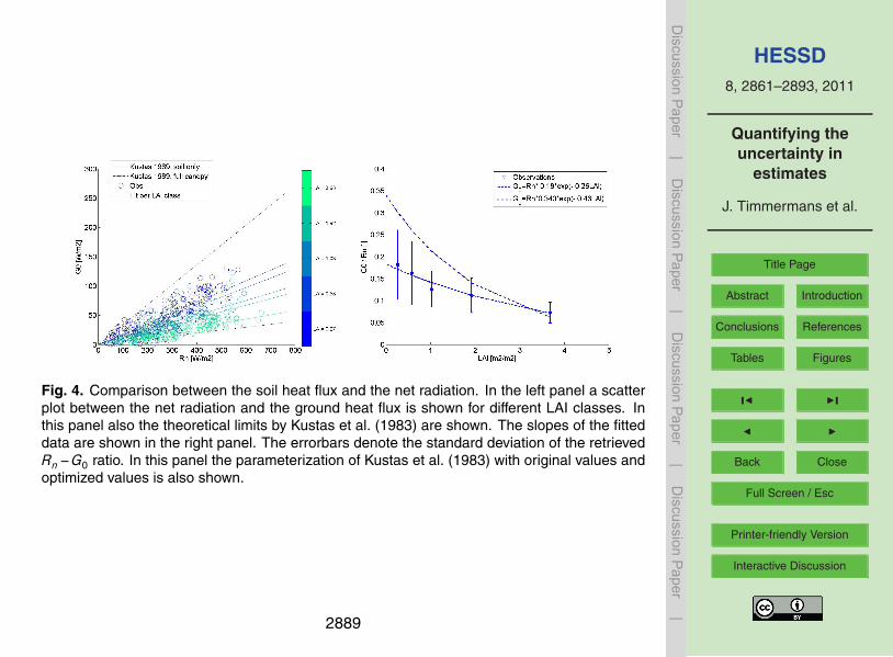
After filtering the coefficients in Eq. (11) are retrieved. The results are shown in Fig. 4.The ratio between the ground heat flux and net radiation behaves exactly as pre-

dicted; the observations fall well within the theoretically predicted values set by thebare soil and full canopy limits. In addition it is observed that the ratio of net radia-tion and ground heat flux correlates very well with LAI. However, lower values of both20

the extinction coefficient (a= 0.26) and the amplitude (Cr0 = 0.18) are found than thevalues advised by (Kustas et al., 1993; Brutsaert, 2005).

These low values for the amplitude and the extinction coefficient originate from thehigh variation in the Rn−G0 ratio for classes with a low LAI. This high variation iscaused by non-uniform shading affects of the soil due to the low fractional vegetation25

cover. When dealing with sparse vegetation the amount of radiation reaching the soilis highly dependent on the geometry of the sun and the leaf orientations.

2873





HESSD8, 2861–2893, 2011


estimates


Title Page



Tables Figures

J I

J I

Back Close

Full Screen / Esc



Discussion

Paper

|D

iscussionP

aper|

Discussion

Paper

|D

iscussionP

aper|

The high values of the ratio between ground heat flux and net radiation originate forparticular sun-leaf geometries. For these cases the sun-beam directly strike the soil,without being attenuated by the vegetation. Low values for the ratio between groundheat flux and net radiation originate from low solar zenith angles. For these cases thecanopy appears to be dense and closed. These deviations need to be investigated in5

more detail; therefore the original values of Cr0 and a given by (Kustas et al., 1993)have been used, instead of the values found in this paragraph. Using the parameteri-zation of (Kustas et al., 1993) the difference between observed and measured groundheat flux was 18 W m−2 which is a decrease when compared original SEBS parame-terization with a RMSE=25 W m−2.10

4.3 Roughness heights

The sensible heat flux in SEBS is calculated from the aerodynamic resistance and thedifference in potential temperature between the land surface and the atmosphere atmeasurement height (Eqs. 6 and 7). This resistance has been shown in the previoussection to depend on the roughness height for heat, the friction velocity and the log-15

arithmic windspeed profile of the wind speed. (Jacobs et al., 1989; Liu et al., 2007)found that the value of aerodynamic resistance for maize ranged from 20 to 50 s m−1.However, when using the original SEBS parameterizations we found it to vary between80 and 200 s m−1, resulting in a unrealistically low sensible heat flux, compared to themeasured maize H-values.20

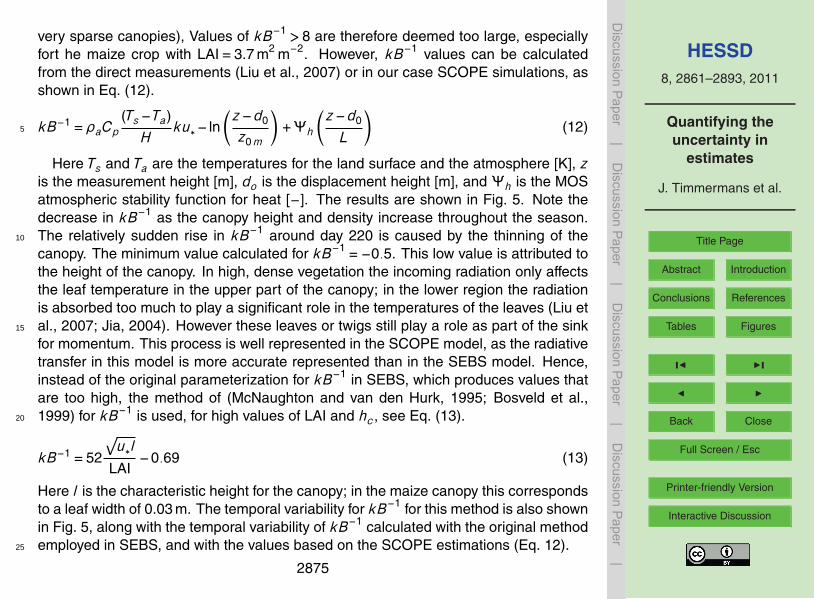
The error in the aerodynamic resistance appears to be caused by the parameter-ization of the roughness height for heat. In the original SEBS parameterization thisroughness height is estimated based on the kB−1. In SEBS this variable is usuallyhigher than 8.0; the roughness height for momentum is always higher than the rough-ness height for heat (i.e. kB−1 > 0), except for bare soils for which negative values25

of kB−1 have been found (see Verhoef et al., 1997b). Small negative values havealso been found for tall, dense canopies (Liu et al., 2007; Jia, 2004).Values for closedcanopies are usually around 2, but kB−1 increases for sparse canopies (up to 15 for

2874





HESSD8, 2861–2893, 2011


estimates


Title Page



Tables Figures

J I

J I

Back Close

Full Screen / Esc



Discussion

Paper

|D

iscussionP

aper|

Discussion

Paper

|D

iscussionP

aper|

very sparse canopies), Values of kB−1 > 8 are therefore deemed too large, especiallyfort he maize crop with LAI=3.7 m2 m−2. However, kB−1 values can be calculatedfrom the direct measurements (Liu et al., 2007) or in our case SCOPE simulations, asshown in Eq. (12).

kB−1 =ρaCp(Ts−Ta)

Hku∗− ln

(z−d0

z0m

)+Ψh

(z−d0

L

)(12)5

Here Ts and Ta are the temperatures for the land surface and the atmosphere [K], zis the measurement height [m], do is the displacement height [m], and Ψh is the MOSatmospheric stability function for heat [−]. The results are shown in Fig. 5. Note thedecrease in kB−1 as the canopy height and density increase throughout the season.The relatively sudden rise in kB−1 around day 220 is caused by the thinning of the10

canopy. The minimum value calculated for kB−1 =−0.5. This low value is attributed tothe height of the canopy. In high, dense vegetation the incoming radiation only affectsthe leaf temperature in the upper part of the canopy; in the lower region the radiationis absorbed too much to play a significant role in the temperatures of the leaves (Liu etal., 2007; Jia, 2004). However these leaves or twigs still play a role as part of the sink15

for momentum. This process is well represented in the SCOPE model, as the radiativetransfer in this model is more accurate represented than in the SEBS model. Hence,instead of the original parameterization for kB−1 in SEBS, which produces values thatare too high, the method of (McNaughton and van den Hurk, 1995; Bosveld et al.,1999) for kB−1 is used, for high values of LAI and hc, see Eq. (13).20

kB−1 =52

√u∗l

LAI−0.69 (13)

Here l is the characteristic height for the canopy; in the maize canopy this correspondsto a leaf width of 0.03 m. The temporal variability for kB−1 for this method is also shownin Fig. 5, along with the temporal variability of kB−1 calculated with the original methodemployed in SEBS, and with the values based on the SCOPE estimations (Eq. 12).25

2875





HESSD8, 2861–2893, 2011


estimates


Title Page



Tables Figures

J I

J I

Back Close

Full Screen / Esc



Discussion

Paper

|D

iscussionP

aper|

Discussion

Paper

|D

iscussionP

aper|

It is obvious that the new parameterization of kB−1 correlates much better with ob-served values than the original SEBS parameterization. Even the thinning of the LAIisclearly characterized using this method, illustrated by the good correspondence ofkB−1 at the end of the measurement period. However the method only applies forclosed canopies, and is less accurate for low vegetation. Therefore it is opted to use5

this method only when the LAI is above the threshold value of 1.5 and only whenhc >1 m.

4.4 Instantaneous heat fluxes

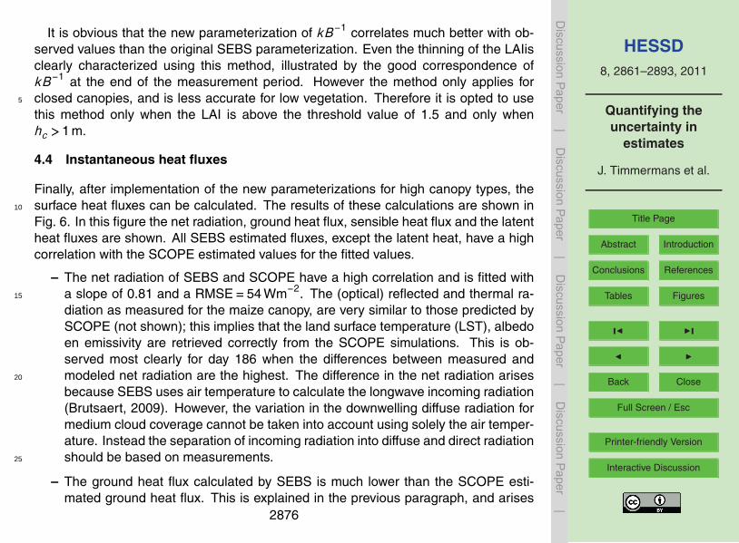
Finally, after implementation of the new parameterizations for high canopy types, thesurface heat fluxes can be calculated. The results of these calculations are shown in10

Fig. 6. In this figure the net radiation, ground heat flux, sensible heat flux and the latentheat fluxes are shown. All SEBS estimated fluxes, except the latent heat, have a highcorrelation with the SCOPE estimated values for the fitted values.

– The net radiation of SEBS and SCOPE have a high correlation and is fitted witha slope of 0.81 and a RMSE=54 Wm−2. The (optical) reflected and thermal ra-15

diation as measured for the maize canopy, are very similar to those predicted bySCOPE (not shown); this implies that the land surface temperature (LST), albedoen emissivity are retrieved correctly from the SCOPE simulations. This is ob-served most clearly for day 186 when the differences between measured andmodeled net radiation are the highest. The difference in the net radiation arises20

because SEBS uses air temperature to calculate the longwave incoming radiation(Brutsaert, 2009). However, the variation in the downwelling diffuse radiation formedium cloud coverage cannot be taken into account using solely the air temper-ature. Instead the separation of incoming radiation into diffuse and direct radiationshould be based on measurements.25

– The ground heat flux calculated by SEBS is much lower than the SCOPE esti-mated ground heat flux. This is explained in the previous paragraph, and arises

2876





HESSD8, 2861–2893, 2011


estimates


Title Page



Tables Figures

J I

J I

Back Close

Full Screen / Esc



Discussion

Paper

|D

iscussionP

aper|

Discussion

Paper

|D

iscussionP

aper|

because SCOPE estimates the ground heat flux using the Force-Restore method,which in this case overestimated the ground heat flux. The differences be-tween the measurements and the SEBS derived ground heat flux decreased fromRMSE=21 Wm−2 to RMSE=18 Wm−2 using the new parameterization. The newSEBS formulation for G0 (Brutsaert, 2005; Kustas et al., 1993) clearly follows the5

measurements of the ground heat flux.

– The SEBS sensible heat flux has improved a lot using the new parameteriza-tion for the roughness height of heat. The differences (expressed as RMSE) be-tween SEBS and SCOPE decreased when using the new parameterization, from100 Wm−2 to 56 Wm−2; the correlation increased from −0.07 to 0.68. Only for10

high LAI values is SEBS underestimating the sensible heat. This indicates thatadditional processes play a role in the sensible heat flux for high LAI values, otherthan those already estimated using the new parameterization.

– The latent heat flux calculated by SEBS is considerably higher then the latent heatflux predicted by SCOPE. The new parameterizations improved the estimation of15

λE , as illustrated by the reduction in RMSE from 123 Wm−2 to 94 Wm−2. Thisdifference originates mainly due to the overestimation of the evaporative fractionfor very high LAI. In Fig. 6 this can be clearly observed because the slope for thesensible heat flux deviates as much from the 1:1 line as the slope of the latentheat flux (but in opposite directions). This will be investigated further in the next20

section.

4.5 Evaporative fraction

The evaporative fraction, EF, in SEBS is to be calculated based on Λ =ΛrλEwet

/(Rn−G), but in SCOPE is calculated as λE

/(H+λE ). In SEBS, EF therefore

depends on the actual sensible heat flux, and the sensible heat flux at the hypotheti-25

cal dry and wet limit. The sensible heat flux at these limits is calculated respectivelyas the maximum available energy, for the dry scenario, while for the wet scenario H

2877





HESSD8, 2861–2893, 2011


estimates


Title Page



Tables Figures

J I

J I

Back Close

Full Screen / Esc



Discussion

Paper

|D

iscussionP

aper|

Discussion

Paper

|D

iscussionP

aper|

is calculated from Rn−G0−λE , with λE derived from the Penman Monteith equation.The evaporative fraction is calculated by SEBS at the time of overpass and consideredconstant during the rest of the day. However several researchers have reported a diur-nal dependence of the evaporative fraction (Li et al., 2008; Farah et al., 2004; Lu andZhuang, 2010).5

Combining SCOPE and SEBS allows us to investigate not only the diurnal patternof EF, but also the uncertainties of EF at overpass time and the daily average of EF.The results of the comparison are shown in Fig. 7. Here, the diurnal pattern of theevaporative fraction is shown for the complete growing season, for all individual days(the left panel), and for a 10-day average.10

As expected, the evaporative fraction at night is much lower than the evaporativefraction during the day, as the nighttime latent heat is close to zero. During day timethe evaporative fraction varies for most days, except from those with low LAI values.This is shown most clearly when studying the diurnal variation of the 10-day averageEF values. The 10-day average EF remains stable for the days 170–180, 240–250 and15

250–260. These days correspond to low LAI values of 0.25, 0.5 and 0.25, respectively.For days 230–240, (LAI=1.0) the evaporative fraction starts to vary diurnally. For allother days (i.e. those with LAI>1.0) EF has a pronounced diurnal pattern. For LAI>2.0EF has the same pattern: with EF lower in the morning than later in the day. Thereforethe average evaporative fraction is higher than the instantaneous evaporative fraction.20

This is confirmed in Fig. 7.Figure 8 shows both the instantaneous evaporative fractions at overpass time cal-

culated by SEBS and SCOPE and the daily average values of the evaporative fractioncalculated by SCOPE. The daily evaporative fraction is in all cases higher than theinstantaneous EF by SCOPE, except for the low LAI classes (at the very start and25

end of the experimental period). The comparison between instantaneous/daily aver-age evaporative fractions by SEBS and SCOPE is hampered due to the large variationin the SEBS evaporative fraction. This variation occurs when net radiation is very low.In these cases the evaporative fraction predicted by SEBS becomes very low. The

2878





HESSD8, 2861–2893, 2011


estimates


Title Page



Tables Figures

J I

J I

Back Close

Full Screen / Esc



Discussion

Paper

|D

iscussionP

aper|

Discussion

Paper

|D

iscussionP

aper|

explanation of this low net radiation was given in the previous paragraph. When onlytaking into account the moderate and high values the instantaneous evaporative frac-tion by SEBS is much higher than the instantaneous evaporative fraction of SCOPE.This is due to an underestimation of the sensible heat for high LAI values, which shouldbe explored in future investigations. Fortunately, when comparing the instantaneous5

evaporative fraction values with the daily averaged ones they are of the same order.

5 Conclusions

In this paper a method was successfully presented for the validation/ investigation ofthe SEBS model, or any other remote sensing model that calculates energy balancefluxes and surface temperatures. This method uses the SCOPE model to estimate10

simultaneously the turbulent heat fluxes from a canopy as well as band observationsfrom a satellite sensor. These radiances were then fed through the SEBS preprocessorin order to obtain surface variables like LST, albedo and emissivity. The data usedfor this comparison comprised micrometeorological driving and verification data for acomplete growing season of maize.15

Parameterizations that were investigated were the LAI retrieval algorithm, the groundheat flux parameterization and the estimation of the roughness height for heat (thisplays a role in the aerodynamic resistance). For each of these parameterizations therewere problems at high values of LAI. It was found that the original LAI parameteriza-tion in SEBS overestimated LAI.The method proposed by Song et al. (2008) was used20

instead, as this fitted very well with the observations for most LAI classes. This algo-rithm was slightly altered to incorporate the high NDVI values estimated for the maizecanopy under study. The new algorithm showed lower errors (RMSE=0.3 m2 m−2)than the parameterization currently implemented in the SEBS algorithm.

The original parameterization of the ground heat flux used the fractional vegeta-25

tion cover in a weighted average approach. As fractional vegetation cover saturatesmore quickly than the maximum canopy height and LAI, it was decided to change this

2879





HESSD8, 2861–2893, 2011


estimates


Title Page



Tables Figures

J I

J I

Back Close

Full Screen / Esc



Discussion

Paper

|D

iscussionP

aper|

Discussion

Paper

|D

iscussionP

aper|

parameterization. Because currently SCOPE is overestimating the ground heat flux,the ground heat flux from measurements was used to calibrate an alternative, morephysical, parameterization (Kustas and Daughtry, 1989); it characterizes the extinc-tion of radiation through a dense canopy. Values for the different coefficients wereobtained through investigation of the ratio of soil heat flux and net radiation for differ-5

ent LAI classes. Variations in the coefficients originated because the measured valuesfor low LAI values showed high variation. Therefore, instead of using the optimizedcoefficients, it was decided to use the original Kustas parameter values.

The last parameterization modified was that describing the relative magnitude ofthe roughness height for momentum and heat, as expressed by the parameter kB−1 =10

ln(z0m

/z0h

). In high dense canopies most of the radiation is absorbed by the leaves at

the top of the canopy. Therefore the position of the virtual source of the sensible heat,as expressed by z0h, is relatively higher in the canopy than for low vegetation. Thisphysical process was not characterized correctly in the original parameterization takenfrom Su. Hence, to take this effect into account, a simple parameterization by Bosveld15

based on LAI and the friction velocity was used. This change in parameterizationresulted in an improvement of the correlation between SEBS and SCOPE modelledsensible heat flux from −0.07 to 0.68.

After implementing all the new parameterizations, the various energy balance fluxesand the evaporative fraction were calculated. Even though the roughness height for20

heat was improved greatly using a new parameterization, SEBS still underestimatedthe sensible heat flux for high LAI values. This means that some processes are stillnot characterized well enough and further investigation is required. Using the instan-taneous, wet and dry limit sensible heat fluxes, the evaporative fraction, EF, was cal-culated in SEBS. This EF was compared to the instantaneous and daily averaged EF25

simulated by SCOPE. SCOPE calculated a diurnal pattern in the evaporative fractioncausing the daily average to be higher than the SCOPE-obtained instantaneous EF atoverpass time. EF from SEBS however was of the same order as the SCOPE daily av-eraged evaporative fraction. This originates from the low values of the SEBS estimated

2880





HESSD8, 2861–2893, 2011


estimates


Title Page



Tables Figures

J I

J I

Back Close

Full Screen / Esc



Discussion

Paper

|D

iscussionP

aper|

Discussion

Paper

|D

iscussionP

aper|

instantaneous sensible heat. Although the new parameterization for kB−1 over tall veg-etation can still be improved further, estimations by SEBS can already be used for dailyevapotranspiration estimations because the obtained valued for the evaporative frac-tion appears to represent correctly the daily average.

In conclusion, the methodology presented in this paper enabled a thorough investi-5

gation in the different parameterizations of SEBS. The advantage of the method pre-sented in this paper, i.e. combining SEBS with SCOPE, is mainly that for days wherethere are no acquisitions we can still continue the investigation. Although no actualremote sensing imagery was used, the methodology, through the use of the sensorsimulator, proved the viability of using the AATSR sensor for calculating the different10

land surface fluxes. The SCOPE model at the moment overestimates the ground heatflux; this should be addressed in the next version of the SCOPE model. A version ofSCOPE that incorporates a detailed multi-layer below-ground parameterization of heat,water and gas fluxes will be developed in the context of the UK (NERC) funded FUSEproject (NE/I007288/1).15

Acknowledgements. We would like to thank the ESA for contributing to our research in the formof the WACMOS project. In addition we would also like to thank Kitsiri Weligepolage for his helpwith the parameterization of the roughness height for heat. Furthermore, various people wereinvolved during the fieldwork at Sonning farm. Special thanks are due to Caroline Houldcroftand Bruce Main.20

References

Bastiaanssen, W. G. M., Menenti, M., Feddes, R. A., and Holtslag, A. A. M.: A remote sensingsurface energy balance algorithm for land (SEBAL), 1. Formulation, J. Hydrol., 212–213,198–212, 1998.

Bosveld, F., Holtslag, A. A. M., and Van den Hurk, B.: Interpretation of crown radiation tempera-25

tures of a dense douglas fir forest with similarity theory, Bound.-Layer Meteor., 92, 429–451,1999.

2881





HESSD8, 2861–2893, 2011


estimates


Title Page



Tables Figures

J I

J I

Back Close

Full Screen / Esc



Discussion

Paper

|D

iscussionP

aper|

Discussion

Paper

|D

iscussionP

aper|

Brutsaert, W.: Aspects of bulk atmospheric boundary layer similarity under free-convectiveconditions, Rev. Geophys., 37(4), 439–451, doi:10.1029/1999RG900013, 1999.

Brutsaert, W.: Hydrology, Cambridge University Press, New York, 605 pp., 2005.Brutsaert, W.: Hydrology, an Introduction, fourth printing ed., Cambridge University Press,

Cambridge, UK, 605 pp., 2009.5

Farah, H. O., Bastiaanssen, W. G. M., and Feddes, R. A.: Evaluation of the temporal variabilityof the evaporative fraction in a tropical watershed, Int. J. Appl. Earth Obs., 5, 129–140, 2004.

Glenn, E. P., Huete, A. R., Nagler, P. L., Hirschboeck, K. K., and Brown, P.: Integrating remotesensing and ground methods to estimate evapotranspiration, CRC Cr. Rev. Plant Sci., 26,139–168, doi:10.1080/07352680701402503, 2007.10

Hartogensis, O.: Exploring Scintillometry in the Stable Atmospheric Surface Layer, PhD, Mete-orologie en Luchtkwaliteit, Wageningen Universiteit, Wageningen, 240 pp., 2006.

Jacobs, A. F. G., Halbersma, J., and Przybula, C.: Behaviour of crop resistance of maize duringa growing season, Estimation of Areal Evapotranspiration, Vancouver, Canada, 1989, 165–175, 1989.15

Jacquemoud, S., Verhoef, W., Baret, F., Bacour, C., Zarco-Tejada, P. J., Asner, G. P., Francois,C., and Ustin, S. L.: PROSPECT plus SAIL models: A review of use for vegetation charac-terization, Remote Sens. Environ., 113, S56–S66, doi:10.1016/j.rse.2008.01.026, 2009.

Jia, L., Su, Z. B., van den Hurk, B., Menenti, M., Moene, A., De Bruin, H. A. R., Yrisarry,J. J. B., Ibanez, M., and Cuesta, A.: Estimation of sensible heat flux using the Surface20

Energy Balance System (SEBS) and ATSR measurements, Phys. Chem. Earth, 28, 75–88,doi:10.1016/s1474-7065(03)00009-3, 2003.

Jia, L.: Modeling heat exchanges at the land-atmosphere interface using multi-angular thermalinfrared measurements, PhD, Wageningen University, Wageningen, 199 pp., 2004.

Kalma, J. D., McVicar, T. R., and McCabe, M. F.: Estimating Land Surface Evaporation: A25

Review of Methods Using Remotely Sensed Surface Temperature Data, Surv. Geophys., 29,421–469, doi:10.1007/s10712-008-9037-z, 2008.

Kite, G. W. and Droogers, P.: Comparing evapotranspiration estimates from satellites, hydro-logical models and field data, J. Hydrol., 229, 3–18, 2000.

Kustas, W. P. and Daughtry, C. S. T.: Estimation of the soil heat flux/net radiation ratio from30

spectral data., Agr. Forest Meteorol., 49, 205–223, 1989.Kustas, W. P., Daughtry, C. S. T., and Van Oevelen, P. J.: Analytical treatment of the relation-

ships between soil heat flux/net radiation and vegetation indices, Remote Sens. Environ., 46,

2882





http://dx.doi.org/10.1029/1999RG900013

http://dx.doi.org/10.1080/07352680701402503

http://dx.doi.org/10.1016/j.rse.2008.01.026

http://dx.doi.org/10.1016/s1474-7065(03)00009-3

http://dx.doi.org/10.1007/s10712-008-9037-z

HESSD8, 2861–2893, 2011


estimates


Title Page



Tables Figures

J I

J I

Back Close

Full Screen / Esc



Discussion

Paper

|D

iscussionP

aper|

Discussion

Paper

|D

iscussionP

aper|

319–330, 1993.Kustas, W. P. and Norman, J. M.: A Two-Source Energy Balance Approach Using Directional

Radiometric Temperature Observations for Sparse Canopy Covered Surfaces, Agron. J., 92,847–854, 2000.

Li, S., Kang, S., Li, F., Zhang, L., and Zhang, B.: Vineyard evaporative fraction based on eddy5

covariance in an arid desert region of Northwest China, Agr. Water Manage., 95, 937–948,2008.

Liu, Shaomin, Lu, L., Mao, D., and Jia, L.: Evaluating parameterizations of aerodynamic re-sistance to heat transfer using field measurements, Hydrol. Earth Syst. Sci., 11, 769–783,doi:10.5194/hess-11-769-2007, 2007.10

Lu, X. L. and Zhuang, Q. L.: Evaluating evapotranspiration and water-use efficiency of ter-restrial ecosystems in the conterminous United States using MODIS and AmeriFlux data,Remote Sens. Environ., 114, 1924–1939, doi:10.1016/j.rse.2010.04.001, 2010.

Massman, W. J.: A model study of kBH-1 for vegetated surfaces using [“]localized near-field”Lagrangian theory, J. Hydrol., 223, 27–43, 1999.15

McCabe, M. F. and Wood, E. F.: Scale influences on the remote estimation of evap-otranspiration using multiple satellite sensors, Remote Sens. Environ., 105, 271–285,doi:10.1016/j.rse.2006.07.006, 2006.

McNaughton, K. G. and van den Hurk, B. J. J. M.: A “lagrangian” revision of the resistors in thetwo-layer model for calculating the energy budget of a plant canopy, Bound.-Layer Meteor.,20

74, 17, 261–288, 1995.Monin, A. S. and Obukhov, A. M.: Osnovnye zakonomernosti turbulentnogo peremesivanija v

prizemnom sloe atmosfery, Trudy geofiz. inst. AN SSSR, 24 (151), 163–187, citeulike-article-id:3716139, 1954.

Monteith, J. L.: Principles of enviromental physics, Edward Arnold Press, 241 pp., 1973.25

Norman, J. M.: Modeling the complete crop canopy., in: Modification of the aerial environmentof plants, edited by: Barfield, B. J. and Gerber, J. F., ASAE Monogr. Am. Soc. Agric. Eng.,St. Joseph, MI., 249–277, 1979.

Obukhov, A. M.: Turbulence in an atmosphere with a non-uniform temperature, Bound.-LayerMeteor., 2, 7–29, citeulike-article-id:6100935, 1971.30

Olioso, A., Chauki, H., Wigneron, J., Bergaoui, K., Bertuzzi, P., Chanzy, A., Bessemoulin, P.,and Clavet, J. C.: Estimation of energy fluxes from thermal infrared, spectral reflectances,microwave data and SVAT modeling, Phys. Chem. Earth, Part B: Hydrology, Oceans and

2883





http://dx.doi.org/10.5194/hess-11-769-2007



HESSD8, 2861–2893, 2011


estimates


Title Page



Tables Figures

J I

J I

Back Close

Full Screen / Esc



Discussion

Paper

|D

iscussionP

aper|

Discussion

Paper

|D

iscussionP

aper|

Atmosphere, 24, 829–836, 1999.Pauwels, V. R. N. and Samson, R.: Comparison of different methods to measure and model

actual evapotranspiration rates for a wet sloping grassland, Agr. Water Manage., 82, 1–24,doi:10.1016/j.agwat.2005.06.001, 2006.

Pauwels, V. R. N., Timmermans, W., and Loew, A.: Comparison of the estimated water and5

energy budgets of a large winter wheat field during AgriSAR 2006 by multiple sensors andmodels, J. Hydrol., 349, 425–440, doi:10.1016/j.jhydrol.2007.11.016, 2008.

Shan, X., van de Velde, R., Wen, J., He, Y., Verhoef, W., and Su, Z.: Regional Evapotranspi-ration over the arid inland heihe river basin in northwest China, Dragon 1 Programme FinalResults, Beijing, 2008.10

Sobrino, J. A., Soria, G., and Prata, A. J.: Surface temperature retrieval from Along TrackScanning Radiometer 2 data: Algorithms and validation, J. Geophys. Res.-Atmos., 109,D11101, doi:10.1029/2003jd004212, 2004.

Song, J., Wang, J., Xiao, Y., Shuai, Y., and Huawei, W.: The method on generating lai produc-tion by fusing BJ-1 remote sensing data and modis LAI product, The International Archives of15

the Photogrammetry, Remote Sensing and Spatial Information Sciences, Vol. XXXVII. PartB1., Beijing, 949–956, 2008.

Su, H., McCABE, M. F., and Wood, E. F.: Modeling Evapotranspiration during SMACEX: Com-paring Two Approaches for Local- and Regional-Scale Prediction, J. Hydrometeorol., 6, 910–922, 2005.20

Su, Z.: Remote sensing applied to hydrology: the Sauer river Basin Study, Phd, Hydrol-ogy/Wasserwirtschaft, Faculty of Civil Engineering, Ruhr University, Bochum, 1996.

Su, Z., Pelgrum, H., and Menenti, M.: Aggregation effects of surface heterogeneity in land sur-face processes, Hydrol. Earth Syst. Sci., 3, 549–563, doi:10.5194/hess-3-549-1999, 1999.

Su, Z., Schmugge, T., Kustas, W. P., and Massman, W. J.: An evaluation of two models for25

estimation of the roughness height for heat transfer between the land surface and the atmo-sphere, J. Appl. Meteorol., 40, 1933–1951, 2001.

Su, Z.: The Surface Energy Balance System (SEBS) for estimation of turbulent heat fluxes,Hydrol. Earth Syst. Sci., 6, 85–100, doi:10.5194/hess-6-85-2002, 2002.

Timmermans, J., Verhoef, W., van der Tol, C., and Su, Z.: Retrieval of canopy component30

temperatures through Bayesian inversion of directional thermal measurements, Hydrol. EarthSyst. Sci., 13, 1249–1260, doi:10.5194/hess-13-1249-2009, 2009.

Timmermans, J., van der Tol, C., Verhoef, A., Wang, L., van Helvoirt, M.D., Verhoef, W. and

2884





http://dx.doi.org/10.1016/j.agwat.2005.06.001

http://dx.doi.org/10.1016/j.jhydrol.2007.11.016

http://dx.doi.org/10.1029/2003jd004212




HESSD8, 2861–2893, 2011


estimates


Title Page



Tables Figures

J I

J I

Back Close

Full Screen / Esc



Discussion

Paper

|D

iscussionP

aper|

Discussion

Paper

|D

iscussionP

aper|

Su, Z.: Quantifying the uncertainty in estimates of surface atmosphere fluxes by evaluationof sebs and scope models. : Quantifying the uncertainty in estimates of surface atmospherefluxes by evaluation of sebs and scope models, in: Proceedings of the symposium earthobservation and water cycle science, Proceedings of the symposium earth observation andwater cycle science, Frascati, Italy 2009, 2010.5

Timmermans, W. J., van der Kwast, J., Gieske, A. S. M., Su, Z., Olioso, A., Jia, L., and Elbers,J. A.: Intercomparison of Energy Flux Models using Aster Imagery at the SPARC 2004 site(Barrax, Spain), SPARC final workshop, Enschede, 2005.

Timmermans, W. J., Kustas, W. P., Anderson, M. C., and French, A. N.: An intercom-parison of the surface energy balance algorithm for land (SEBAL) and the two-source10

energy balance (TSEB) modeling schemes, Remote Sens. Environ., 108, 369–384,doi:10.1016/j.rse.2006.11.028, 2007.

van der Tol, C., Verhoef, W., Timmermans, J., Verhoef, A., and Su, Z.: An integrated modelof soil-canopy spectral radiances, photosynthesis, fluorescence, temperature and energybalance, Biogeosciences, 6, 3109–3129, doi:10.5194/bg-6-3109-2009, 2009.15

Verhoef, A., McNaughton, K. G., and Jacobs, A. F. G.: A parameterization of momentum rough-ness length and displacement height for a wide range of canopy densities, Hydrol. Earth Syst.Sci., 1, 81–91, doi:10.5194/hess-1-81-1997, 1997.

Verhoef, W. and Bach, H.: Coupled soil-leaf-canopy and atmosphere radiative transfier mod-eling to simulate hyperspectral multi-angular surface reflectance and TOA radiance data,20

Remote Sens. Environ., 109, 166–182, doi:10.1016/j.rse.2006.12.013, 2007.Verhoef, W., Jia, L., Xiao, Q., and Su, Z.: Unified optical-thermal four-stream radiative transfer

theory for homogeneous vegetation canopies, IEEE Trans. Geosci. Remote Sensing, 45,1808–1822, doi:10.1109/tgrs.2007.895844, 2007.

Verhoef, W.: A Bayesian optimisation approach for model inversion of hyperspectral – multidi-25

rectional observations : the balance with A Priori information, 10th international symposiumon physical measurements and spectral signatures in remote sensing, Davos, Switserland,208–213, 2008.

2885






http://dx.doi.org/10.5194/bg-6-3109-2009



http://dx.doi.org/10.1109/tgrs.2007.895844

HESSD8, 2861–2893, 2011


estimates


Title Page



Tables Figures

J I

J I

Back Close

Full Screen / Esc



Discussion

Paper

|D

iscussionP

aper|

Discussion

Paper

|D

iscussionP

aper|

Fig. 1. Methodology flowchart for comparing SEBS with SCOPE.

2886





HESSD8, 2861–2893, 2011


estimates


Title Page



Tables Figures

J I

J I

Back Close

Full Screen / Esc



Discussion

Paper

|D

iscussionP

aper|

Discussion

Paper

|D

iscussionP

aper|

Fig. 2. SCOPE input parameters and variables measured at the experimental site during 2002.In the top left panel the surface parameters are shown. In the bottom left panel the atmosphericdriving variables. In the right panel the incoming optical and thermal radiance data are shown.The red lines depict half hourly in situ measured data, and the blue lines depict the values atAATSR overpass time (Taatsr).

2887





HESSD8, 2861–2893, 2011


estimates


Title Page



Tables Figures

J I

J I

Back Close

Full Screen / Esc



Discussion

Paper

|D

iscussionP

aper|

Discussion

Paper

|D

iscussionP

aper|

Fig. 3. NDVI – LAI relationships. The LAI values obtained by measurements (open circles) andthe Su (line with closed circles) and Song parameterizations are shown. The Song parameteri-zation is shown with its original values (the green dotted) for A and B and also for the optimizedvalues (solid red line).

2888





HESSD8, 2861–2893, 2011


estimates


Title Page



Tables Figures

J I

J I

Back Close

Full Screen / Esc



Discussion

Paper

|D

iscussionP

aper|

Discussion

Paper

|D

iscussionP

aper|

Fig. 4. Comparison between the soil heat flux and the net radiation. In the left panel a scatterplot between the net radiation and the ground heat flux is shown for different LAI classes. Inthis panel also the theoretical limits by Kustas et al. (1983) are shown. The slopes of the fitteddata are shown in the right panel. The errorbars denote the standard deviation of the retrievedRn−G0 ratio. In this panel the parameterization of Kustas et al. (1983) with original values andoptimized values is also shown.

2889





HESSD8, 2861–2893, 2011


estimates


Title Page



Tables Figures

J I

J I

Back Close

Full Screen / Esc



Discussion

Paper

|D

iscussionP

aper|

Discussion

Paper

|D

iscussionP

aper|

Fig. 5. Top panel: Seasonal variation in the daily kB−1 values for the maize canopy, calculatedfrom observations, the parameterizations from Su (2001) and Bosveld et al. (1999). In thebottom panel the roughness length for heat and momentum is shown for Su (2001) and for thenew kB−1 parameterization. The new values of the roughness length for heat, are calculatedusing the kB−1 parameterization of Bosveld (1999), and the roughness length for momentumby Su (2001).

2890





HESSD8, 2861–2893, 2011


estimates


Title Page



Tables Figures

J I

J I

Back Close

Full Screen / Esc



Discussion

Paper

|D

iscussionP

aper|

Discussion

Paper

|D

iscussionP

aper|

Fig. 6. Comparison of instantaneous surface heat fluxes predicted by SEBS and SCOPE. In theleft panel the diurnal measurements and estimations are shown. There were no measurementsof sensible heat and latent heat over the thinned maize field. In the right panel a scatterplotbetween SEBS and SCOPE estimated heat fluxes is shown. The instantaneous surface heatfluxes from SEBS show a high correlation with the SCOPE estimated surface heat fluxes. SEBSunderestimates the sensible heat flux for a fully developed maize canopy (between day 200 and220).

2891





HESSD8, 2861–2893, 2011


estimates


Title Page



Tables Figures

J I

J I

Back Close

Full Screen / Esc



Discussion

Paper

|D

iscussionP

aper|

Discussion

Paper

|D

iscussionP

aper|

Fig. 7. Diurnal variation of the evaporative fraction during the maize growing season. In the leftpanel the diurnal evaporative fraction as calculated by the SCOPE model for each separate dayis shown. In the right panel the 10-day average of the diurnal evaporative fraction as calculatedwith SCOPE is shown. The dotted line represents the overpass time of AATSR.

2892





HESSD8, 2861–2893, 2011


estimates


Title Page



Tables Figures

J I

J I

Back Close

Full Screen / Esc



Discussion

Paper

|D

iscussionP

aper|

Discussion

Paper

|D

iscussionP

aper|

Fig. 8. Variation in evaporative fraction during the maize growing season. Evaporative fractionsat overpass time calculated by SEBS and SCOPE are shown, as well as the daily averagevalues of the evaporative fraction by SCOPE.

2893





Quantifying the uncertainty in estimates of surface–atmosphere fluxes through joint evaluation of...

Documents

Transcript of Quantifying the uncertainty in estimates of surface–atmosphere fluxes through joint evaluation of...