Impacts of Land-Atmosphere Interactions on Regional ...

Purdue UniversityPurdue e-Pubs

Open Access Dissertations Theses and Dissertations

January 2015

Impacts of Land-Atmosphere Interactions onRegional Convection and RainfallYue ZhengPurdue University

Follow this and additional works at: https://docs.lib.purdue.edu/open_access_dissertations

This document has been made available through Purdue e-Pubs, a service of the Purdue University Libraries. Please contact [email protected] foradditional information.

Recommended CitationZheng, Yue, "Impacts of Land-Atmosphere Interactions on Regional Convection and Rainfall" (2015). Open Access Dissertations. 1491.https://docs.lib.purdue.edu/open_access_dissertations/1491

https://docs.lib.purdue.edu?utm_source=docs.lib.purdue.edu%2Fopen_access_dissertations%2F1491&utm_medium=PDF&utm_campaign=PDFCoverPages

https://docs.lib.purdue.edu/open_access_dissertations?utm_source=docs.lib.purdue.edu%2Fopen_access_dissertations%2F1491&utm_medium=PDF&utm_campaign=PDFCoverPages

https://docs.lib.purdue.edu/etd?utm_source=docs.lib.purdue.edu%2Fopen_access_dissertations%2F1491&utm_medium=PDF&utm_campaign=PDFCoverPages

https://docs.lib.purdue.edu/open_access_dissertations?utm_source=docs.lib.purdue.edu%2Fopen_access_dissertations%2F1491&utm_medium=PDF&utm_campaign=PDFCoverPages

https://docs.lib.purdue.edu/open_access_dissertations/1491?utm_source=docs.lib.purdue.edu%2Fopen_access_dissertations%2F1491&utm_medium=PDF&utm_campaign=PDFCoverPages

Graduate School Form 30Updated 1/15/2015

PURDUE UNIVERSITYGRADUATE SCHOOL

Thesis/Dissertation Acceptance

This is to certify that the thesis/dissertation prepared

By

Entitled

For the degree of

Is approved by the final examining committee:

To the best of my knowledge and as understood by the student in the Thesis/Dissertation Agreement, Publication Delay, and Certification Disclaimer (Graduate School Form 32), this thesis/dissertation adheres to the provisions of Purdue University’s “Policy of Integrity in Research” and the use of copyright material.

Approved by Major Professor(s):

Approved by: Head of the Departmental Graduate Program Date

Yue Zheng

Impacts of Land-Atmosphere Interactions on Regional Convection and Rainfall

Doctor of Philosophy

Jon Harbor Kiran AlapatyChair

Nathanial Brunsell

Qianlai Zhuang

Dev Niyogi

Dev Niyogi

Indrajeet Chaubey 11/5/2015

i

IMPACTS OF LAND-ATMOSPHERE INTERACTIONS ON REGIONAL

CONVECTION AND RAINFALL

A Dissertation

Submitted to the Faculty

of

Purdue University

by

Yue Zheng

In Partial Fulfillment of the

Requirements for the Degree

of

Doctor of Philosophy

December 2015

Purdue University

West Lafayette, Indiana

ii

To my beloved daughters Yuyi Sophia Han and Xiaoniuniu Liliya Han, my husband

Tianhe Han, my mother Zhi Wang, my father Linkui Zheng, and my grandparents, for

their endless inspiration, support, and love.

iii

ACKNOWLEDGEMENTS

This study benefitted in part through support of National Science Foundation (NSF)

CAREER (AGS-0847472), NSF Hydrology Community-based Data Interoperability

Networks (INTEROP), NSF CISE 1250232 Strong City Program, USDA National

Institute of Food and Agriculture (NIFA) Drought Trigger projects through Texas A&M

at Purdue (2011-67019-20042), USDA NIFA Hatch project 1007699, US EPA’s Air,

Climate, and Energy (ACE) Program, Department of Energy’s Atmospheric Radiation

Measurement Program (DOE-ARM), U.S. Department of Energy Atmospheric System

Research Program. Additional support for the KON Ameriflux site was provided through

a subcontract to the NSF Long Term Ecological Research Program at the Konza Prairie

Biological Station (DEB-0823341; subcontract: SS1093) and subcontract number

7114774 from the Lawrence Berkeley National Laboratory under DOE contract DE-

AC02-05CH11231. Financial support given by the Earth System Science Organization,

Ministry of Earth Sciences, Government of India (Grant/Project no.

MM/SERP/CNRS/2013/INT-10/002) to conduct this research under Monsoon Mission,

and computational resources by Purdue Rosen Center for Advanced Computing and US

EPA/ORD supercomputing are also gratefully acknowledged.

iv

The graduate committee comprising of Drs. Jon Harbor, Kiran Alapaty, Nathanial

Brunsell, Qianlai Zhuang, and Dev Niyogi is also gratefully acknowledged for their role

as true mentors.

Special thanks to Drs. Anil Kumar, Joseph Alfieri at USDA/ARS, Anthony Del Genio at

NASA Goddard Institute for Space Studies, John Kain of NOAA, Megan Mallard of

UNC, and Mr. Russell Bullock, Drs. Jerold Herwehe and Christopher Nolte, and Ms.

Tanya Spero at US EPA, for their help in many ways facilitating the research. My

appreciation also goes to Mr. John Halley Gotway at NCAR/RAL for the help on MET,

and Mrs. Dan Dietz and Lev Gorenstein at ITaP Research Computing (RCAC) for their

help on the WRF runs. Thanks to Ms. Dallas Staley for her usual outstanding editing.

The land surface lab and Indiana State Climate Office consist of the major part of my

Purdue research life and will continue to have positive influence on my life ahead.

Thanks to all the group members!

Most importantly, I am deeply thankful to my family. Thanks to my parents for their

endless love, support, and sacrifices. Thanks to my daughter Sophia and my upcoming

baby daughter Liliya, your love makes it worth it all. Finally, thanks to my loving and

dearest husband, Tianhe Han, for always being my side, loving, encouraging, supporting,

and believing me.

Yue Zheng

West Lafayette, Indiana, 2015

v

TABLE OF CONTENTS

Page

LIST OF TABLES ........................................................................................................... viii

LIST OF FIGURES ........................................................................................................... ix

ABSTRACT .................................................................................................................... xvii

CHAPTER 1. INTRODUCTION .................................................................................... 1

1.1 Background ............................................................................................................... 1

1.2 Study Objectives ....................................................................................................... 7

1.3 Case Studies and Observational Data ...................................................................... 10

1.4 Model Configurations ............................................................................................. 12

1.5 Dissertation Layout ................................................................................................. 15

CHAPTER 2. IMPACTS OF HETEROGENEOUS LAND COVER AND LAND

SURFACE PARAMETERIZATIONS ON TURBULENT FLOW AND MESOSCALE

SIMULATIONS IN THE WRF MODEL......................................................................... 16

2.1 Introduction ............................................................................................................. 16

2.2 Numerical experiments ........................................................................................... 18

2.2.1 A brief description of the land-surface parameterizations ............................. 19

2.2.2 Numerical model configuration ..................................................................... 20

2.2.3 Model experiments ........................................................................................ 23

2.3 Results and discussion ............................................................................................. 24

2.3.1 Impacts of LSMs affected by land-surface heterogeneity on surface heat

fluxes ....................................................................................................................... 25

2.3.2 Impact of land-surface heterogeneity on modeling bias ................................ 31

2.3.3 Impacts on turbulent characteristics .............................................................. 33

2.3.4 Impacts on surface-atmosphere interactions .................................................. 41

vi

Page

2.4 Summary and conclusions ....................................................................................... 48

CHAPTER 3. IMPACTS OF LAND-ATMOPSHERE COUPLING ON REGIONAL

RAINFALL AND CONVECTION .................................................................................. 51

3.1 Introduction ............................................................................................................. 51

3.2 Numerical modeling framework and study domain ................................................ 54

3.2.1 Offline modeling system ................................................................................ 54

3.2.2 WRF Model and domain configurations ....................................................... 56

3.2.3 Data for model case studies ........................................................................... 60

3.3 Land-atmosphere coupling method and Czil experiments ....................................... 61

3.4 Model verification and comparisons ....................................................................... 64

3.4.1 Impact of the “Czil” on the offline Noah LSM ............................................... 64

3.4.2 The impacts of the Czil coupling parameter on the WRF-Noah model .......... 72

3.5 Conclusions and discussions ................................................................................... 94

CHAPTER 4. IMPROVING HIGH-RESOLUTION WEATHER FORECASTS USING

THE WEATHER RESEARCH AND FORECASTING (WRF) MODEL WITH AN

UPDATED KAIN-FRITSCH SCHEME .......................................................................... 98

4.1 Introduction ............................................................................................................. 98

4.2 Methodology ......................................................................................................... 103

4.2.1 The KF CPS ................................................................................................. 104

4.2.2 A brief description of subgrid-scale cloud-radiation interactions ............... 105

4.2.3 A dynamic formulation for the adjustment timescale .................................. 105

4.2.4 Enhancement of grid-scale vertical velocity using subgrid-scale updraft mass

fluxes ..................................................................................................................... 109

4.2.5 Entrainment methodology based on LCL .................................................... 110

4.3 Design of Simulations ........................................................................................... 113

4.4 Results and Discussions ........................................................................................ 117

4.4.1 Simulation period 0000 UTC 4 June – 0000 UTC 6 June 2002: Experiments

1-6: ..................................................................................................................... 117

vii

Page

4.4.2 Simulation period 0000 UTC 28 July – 0000 UTC 30 July 2010: Experiments

19-24: ..................................................................................................................... 126

4.4.3 Simulation period 0000 UTC 5 July – 0000 UTC 7 July 2010: Experiments

13-18: ..................................................................................................................... 132

4.4.4 Sensitivity to microphysics schemes: Experiments 7-12 and 31-36: .......... 136

4.4.5 Sensitivity to each science update: Experiments 25-30: .............................. 139

4.5 Summary and conclusions ..................................................................................... 144

CHAPTER 5. IMPACT OF LAND-ATMOSPHERE-CONVECTION INTERACTIONS

ON REGIONAL PRECIPITATION INTENSITY AND VARIATION IN WRF ......... 147

5.1 Introduction ........................................................................................................... 147

5.2 Methodology ......................................................................................................... 149

5.3 Numerical simulations design ............................................................................... 152

5.4 Results ................................................................................................................... 154

5.4.1 Precipitation ................................................................................................. 154

5.4.2 Soundings .................................................................................................... 159

5.4.3 Vertical velocity ........................................................................................... 161

5.4.4 Horizontal wind speeds and mixing ratio .................................................... 163

5.4.5 Surface fluxes .............................................................................................. 165

5.4.6 CAPE/CIN ................................................................................................... 167

5.5 Discussion ............................................................................................................. 169

CHAPTER 6. CONCLUSIONS ................................................................................... 170

REFERENCES ............................................................................................................... 180

APPENDIX: ACRONYMS ............................................................................................ 208

VITA ............................................................................................................................... 211

PUBLICATIONS ............................................................................................................ 216

viii

LIST OF TABLES

Table .............................................................................................................................. Page

2.1 Summary of the numerical experiments ..................................................................... 24

2.2 Mean values of diurnal averaged of area-averaged surface heat fluxes ..................... 28

2.3 Summary of the land-cover type selection.................................................................. 29

2.4 Diurnal averaged RMSE of 2 m temperature (T2m) and moisture (q2m), and 10 m wind

speed (U10m) for model forecasts over the domain ........................................................... 33

3.1 The characteristics of study regions ............................................................................ 56

3.2 Summary of the coupling experiments ....................................................................... 64

3.3 Comparisons of surface exchange coefficient of heat (Ch) between observation and

model runs with different Czil values over three vegetation types in U.S. SGP. The results

are temporally averaged for June 2002 ............................................................................. 67

3.4 Biases and RMSE of 2 m temperature (T), 2 m moisture (Q), and 10 m wind speed

(WSPD) for 0-48 hr model forecasts over U.S. SGP at 3-km grid spacing ...................... 74

3.5 Area-averaged accumulated precipitation (mm) over U.S. SGP at 3-km grid spacing

........................................................................................................................................... 75

3.6 Biases of 2 m temperature (T), 2 m moisture (Q), and surface wind speed (WSPD) for

0-24 hr model forecasts over India domain at 3-km grid spacing .................................... 86

4.1 Summary of the numerical experiments ................................................................... 116

4.2 48-hour averaged root mean square error (RMSE) of area-averaged precipitation

over a 3-km grid spacing domain.................................................................................... 132

5.1 Summary of the numerical experiments ................................................................... 154

ix

LIST OF FIGURES

Figure ............................................................................................................................. Page

1.1 The experimental design flowchart ............................................................................. 10

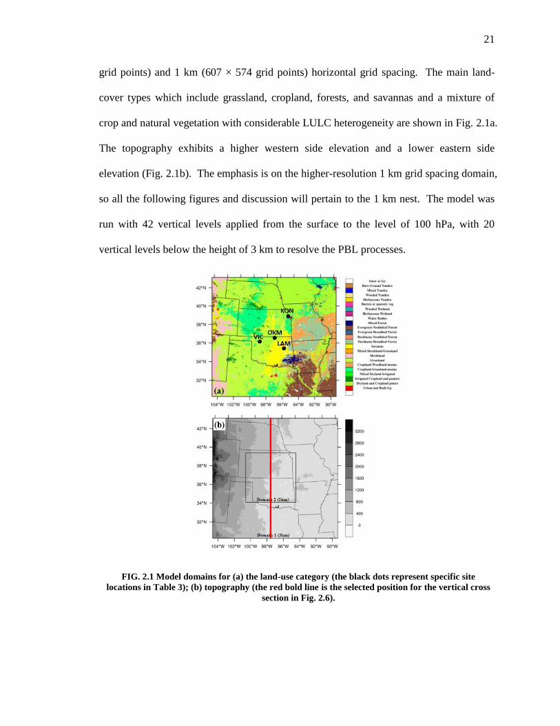
2.1 Model domains for (a) the land-use category (the black dots represent specific site

locations in Table 3); (b) topography (the red bold line is the selected position for the

vertical cross section in Fig. 2.6). ..................................................................................... 21

2.2 Spatial variations in surface latent heat flux (W m-2

) at 2100 UTC (1500 CST) 7 July

2007 in (a-c) WS01, WN01, WH01, (d-f) WS03, WN03, WH03, and (g-i) WS09, WN09,

WH09. ............................................................................................................................... 26

2.3 Spatial variations in surface sensible heat flux (W m-2

) at 2100 UTC (1500 CST) 7

July 2007 in (a-c) WS01, WN01, WH01, (d-f) WS03, WN03, WH03, and (g-i) WS09,

WN09, WH09. .................................................................................................................. 27

2.4 Comparisons of diurnal variations in surface latent heat flux (W m-2

) between the

model runs at 1 km length scale initiated at 1200 UTC (0600 CST) 7 July 2007, and the

observations over (a) grassland (KON), (b) forest (OKM), (c) wet cropland (LAM), and

(d) dry cropland (VIC). Details of the land-cover types are in Table 2.3 ......................... 30

2.5 Comparisons of diurnal variations of surface sensible heat flux (W m-2

) between the


observations over (a) grassland (KON), (b) forest (OKM), (c) wet cropland (LAM), and

(d) dry cropland (VIC). Details of the land-cover types are in Table 2.3 ......................... 30

2.6 Vertical cross section in the north-south direction through the middle of the domain

(as seen in Fig 1b) for temperature (K) and relative humidity (%) at 2100 UTC (1500

CST) 7 July 2007 in (a-c) WS01, WN01, WH01, (d-f) WS03, WN03, WH03, and (g-i)

WS09, WN09, WH09. ...................................................................................................... 32

file:///C:/Users/apark/Desktop/2007%20Word%20Template%20-0412/Multiple%20Appendix/TimesNewRoman%20Word%202010%20ma%20111812.docx%23_Toc341019727



x

Figure ............................................................................................................................. Page

2.7 Maps of (A) mid-PBL vertical velocity and (B) the wind fields at 2100 UTC 7 July

2007 with 1-km grid spacing ............................................................................................ 35

2.8 Energy spectra (m2 s

-3) multiplied by frequency (s

-1) computed from coupled WRF

simulations compared to observations at 2100 UTC (1500 CST) on 7 July 2007 for (a)

temperature at 2 m, (b) specific humidity at 2 m, (c) U-wind at 10 m, (d) V-wind at 10 m,

and (e) vertical velocity .................................................................................................... 38

2.9 Energy spectra (m2 s



forecasts at 1, 3, and 9 km length scales at 2100 UTC (1500 CST) compared to

observations on 7 July 2007 for temperature at 2 m (top), specific humidity at 2 m

(middle), and vertical velocity (bottom) in WS (a, d, g), WN (b, e, h), and WH (c, f, i) . 40

2.10 Sounding profile at 0000 UTC (1800 CST) 8 July 2007 of specific humidity (g kg-1

)

(a, d), potential temperature (K) (b, e), and wind speed (m s-1

) (c, f), valid at Norman, OK

(OUN, 35.18°N, 97.44°W) (top) and Topeka, KS (TOP, 39.07°N, 95.62°W) (bottom) .. 42

2.11 Vertical profiles of normalized (a) turbulent thermal flux (W m-2

), (b) turbulent

moisture flux (W m-2

), (c) buoyancy flux (m K s-2

), and (d) TKE (m2 s

-2) averaged from

2100 UTC (1500 CST) to 2130 UTC (1530 CST) 7 July 2007 for wet cropland (LAM)

and dry cropland (VIC) ..................................................................................................... 44

2.12 Vertical profiles of vertical velocity averaged from 2100 UTC (1500 CST) to 2130

UTC (1530 CST) 7 July 2007 for grassland (KON) (a), forest (OKM) (b), wet cropland

(LAM) (c), and dry cropland (VIC) (d). Details of the land-cover types are in Table 2.3 46

2.13 Vertical profiles of normalized TKE (m2 s

-2) averaged from 2100 UTC (1500 CST)

to 2130 UTC (1530 CST) 7 July 2007 with 1, 3, and 9 km length scales in WN (a, d), WS

(b, e), and WH (c, f) over wet cropland (LAM) and dry cropland (VIC) ......................... 47

3.1 Topography maps of the nested model domains over the (a) U.S. southern Great

Plains (SGP), (b) Europe, (c) India, and (d) West Africa ................................................. 57

3.2 A snapshot of cases (UN0.1, UN0.5, and UN0.8) with three different Czil values and

resulting impacts on latent heat flux (W m-2

) (upper row) and sensible heat flux (W m-2

)

(bottom row) at 1800 UTC for 2 June 2002. .................................................................... 66

xi

Figure ............................................................................................................................. Page

3.3 Comparisons of 25 day-averaged surface latent heat flux (W m-2

) and sensible heat

flux (W m-2

) between observation and offline experiments over (a) grassland, (b)

cropland, and (c) forest in U.S. SGP. ................................................................................ 68

3.4 Variations of averaged-daily simulated surface variables: (a-c) precipitation forcing

(mm day-1

), (d-f) surface soil moisture (m3 m

-3), (g-i) surface soil temperature (K), (j-l)

latent heat flux (W m-2

), and (m-o) sensible heat flux (W m-2

) from offline Noah

experiments over grassland (left column), cropland (middle column), and forest (right

column). ............................................................................................................................ 69

3.5 Comparisons of midday values of Ch (m s-1

) averaged from 1700 UTC to 2100 UTC

in June 2002 between observation and offline experiments: (a) BG, (b) BC, and (c) BF. 71

3.6 Comparisons of surface heat fluxes (W m-2

) between the 24-48 hr CS experiments

initialized at 1200 UTC 12 June 2002 and the observation over (a-b) grassland (Elmwood,

OK, 36.62°N, 100.62°W) and (c-d) cropland (Lamont, OK, 36.61°N, 97.49°W). .......... 73

3.7 Vertical profiles of area-averaged bias over the U.S. SGP 3-km grid spacing domain

at 1800 UTC 12 June 2002 (a) temperature (K), (b) specific humidity (10-3

× kg kg-1

), and

(c) wind speed (m s-1

). ...................................................................................................... 76

3.8 Comparisons of the 3 hrs accumulated precipitation (0000 – 0300 UTC) on 13 June

2002 over the U.S. SGP 3-km grid spacing domain between the model forecasts with (a)

Czil = 0.01, (b) Czil = 0.05, (c) Czil = 0.1, (d) Czil = 0.3, (e) Czil = 0.5, (f) Czil = 0.8, (g)

dynamic Czil-var, and (h) the STAGE-IV observed precipitation. ...................................... 78

3.9 Comparisons between the 0-24 hr CE experiments initialized at 0600 UTC 21 July

2007 and the observation of (a) latent heat flux (W m-2

), (b) sensible heat flux (W m-2

), (c)

surface temperature (K), and (d) wind speed (m s-1

), at Black Forest, Germany (48.54°N,

8.397°E). ........................................................................................................................... 80

3.10 0-24 hr model forecast, initialized at 0600 UTC 21 July 2007, area-averaged bias

over Europe 3-km grid spacing domain of (a) 2 m specific humidity (10-3

× kg kg-1

), (b) 2

m temperature (K), (c) 10 m wind speed (m s-1

), and (d) ETS of 3 hrs accumulated

precipitation from 0600 UTC 21 July to 0600 UTC 22 July 2007 over the European 9-km

grid spacing domain .......................................................................................................... 82

xii

Figure ............................................................................................................................. Page

3.11 Comparisons of reflectivity at 1200 UTC 12 May 2012 over India 3-km grid spacing

domain between model forecasts with (a) Czil = 0.01, (b) Czil = 0.05, (c) Czil = 0.1, (d) Czil

= 0.3, (e) Czil = 0.5, (f) Czil = 0.8, (g) dynamic Czil-var, and (h) the observation................. 83

3.12 Comparison of accumulated precipitation initiated at 0000 UTC 12 May 2012 over

India 3-km grid spacing domain between model forecasts and the observation .............. 84

3.13 0-24 hr model forecast initialized at 0000 UTC 12 May 2012, area-averaged bias

over the Indian 3-km grid spacing domain of (a) 2 m specific humidity (10-3

× kg kg-1

), (b)

2 m temperature (K), (c) 10 m wind speed (m s-1

), and (d) ETS of 3 hrs accumulated

precipitation from 0000 UTC 12 July to 0000 UTC 13 May 2012 over the Indian 9-km

grid spacing domain .......................................................................................................... 86

3.14 Vertical profiles of area-averaged bias over the Indian 3-km grid spacing domain at

1200 UTC 12 May 2012 for (a) temperature (K), (b) specific humidity (10-3

× kg kg-1

),

and (c) wind speed (m s-1

) ................................................................................................. 87

3.15 147 points histograms of the observation and the WRF model forecasts for 2 m

temperature (K): (a) Observations, (b) Czil = 0.01, (c) Czil = 0.05, (d) Czil = 0.1, (e) Czil =

0.3, (f) Czil = 0.5, (g) Czil = 0.8, and (h) dynamic Czil-var ................................................... 88

3.16 147 points histograms of the observation and the WRF model forecasts for 2 m

specific humidity (kg kg-1

): (a) Observation, (b) Czil = 0.01, (c) Czil = 0.05, (d) Czil = 0.1,

(e) Czil = 0.3, (f) Czil = 0.5, (g) Czil = 0.8, and (h) dynamic Czil-var .................................... 89

3.17 Comparisons between the 0-24 hr CA experiments and the observation of (a) latent

heat flux (W m-2


), (c) 2 m temperature (K), and (d) friction

velocity (m s-1

), initialized at 0600 UTC 10 August 2006 for Niamey (13.478°N,

2.174°E), Niger, Africa ..................................................................................................... 91

3.18 0-24 hr model forecast, initialized at 0600 UTC 10 August 2006, area-averaged bias

over the West African 3-km grid spacing domain of (a) 2 m specific humidity (10-3

× kg

kg-1

), (b) 2 m temperature (K); Vertical profiles of domain averaged bias over a 3-km

grid spacing domain for (c) temperature (K), (d) specific humidity (10-3

× kg kg-1

), and (e)

wind speed (m s-1

) at 1200 UTC 10 August 2006 ............................................................ 92

xiii

Figure ............................................................................................................................. Page

3.19 Comparisons of the 3 hrs accumulated precipitation (0300 – 0600 UTC) on 11

August 2006 over the West African 3-km grid spacing domain between model forecasts

with (a) Czil = 0.01, (b) Czil = 0.05, (c) Czil = 0.1, (d) Czil = 0.3, (e) Czil = 0.5, (f) Czil = 0.8,

(g) dynamic Czil-var, and (h) the TRMM-based precipitation ........................................... 93

4.1 (a) Topography map of the nested model domain over the U.S. SGP, and (b) the

IHOP_2002 domain and fixed deployment locations

(https://www.eol.ucar.edu/field_projects/ihop2002). ..................................................... 115

4.2 Comparative example of simulated 12-hour (0000 UTC – 1200 UTC 5 June 2002)

accumulated precipitation (mm) over a 9-km grid spacing domain with GFS (top), CFSR

(middle) for EXP (a, d), BASE (b, e), and UKF (c, f), and (g) Stage IV observed

precipitation .................................................................................................................... 119


accumulated precipitation (mm) over a 3-km grid spacing domain with GFS (top), CFSR

(middle) for EXP (a, d), BASE (b, e), and UKF (c, f), and (g) Stage IV observed

precipitation .................................................................................................................... 120

4.4 Outgoing longwave radiation (W m-2

) with GFS at 1800 UTC (1 pm CDT) 5 June

2002 over a 9-km grid spacing domain (top) and 3-km grid spacing domain (bottom) for

EXP (b, f), BASE (c, g), and UKF (d, h) ........................................................................ 123

4.5 Surface shortwave radiation (W m-2

) with GFS at 1800 UTC (1 pm CDT) 5 June

2002 over a 9-km grid spacing domain (top) and 3-km grid spacing domain (bottom) for

EXP (b, f), BASE (c, g), and UKF (d, h) ........................................................................ 123

4.6 48-hour variation (0000 UTC 4 June – 0000 UTC 6 June 2002) of (a) downward

longwave flux at ground surface (W m-2

), (b) downward shortwave flux at ground surface

(W m-2

), (c) temperature at 2 m (°C), and (d) specific humidity at 2 m (g kg-1

), at New

Salem (37.31°N, 98.94°W), KS, from IHOP_2002 site 7 measurements (solid line) and

corresponding simulations in EXP (dotted line), BASE (dot-dash line), and UKF (dash

line) with GFS at 3-km grid spacing ............................................................................... 124

xiv

Figure ............................................................................................................................. Page

4.7 Sounding profile at 0000 UTC 6 July 2002 of specific humidity (g kg-1

) (a, d),

potential temperature (K) (b, e), and wind speed (m s-1

) (c, f), valid at Norman, OK

(OUN, 35.18°N, 97.44°W) (top) and Topeka, KS (TOP, 39.07°N, 95.62°W) (bottom) 125

4.8 Comparative example of simulated 6-hour (1800 UTC 29 July – 0000 UTC 30 July

2010) accumulated precipitation (mm) over a 9-km grid spacing domain with GFS (top),

CFSR (middle) for EXP (a, d), BASE (b, e), and UKF (c, f), and (g) Stage IV observed

precipitation .................................................................................................................... 127




precipitation and (h) visible satellite image valid at 2132 UTC 29 July 2010. The satellite

image is obtained from http://aviationweather.gov/adds/ managed by NOAA’s Aviation

Digital Data Services ...................................................................................................... 128

4.10 48-hour (0000 UTC 28 July – 0000 UTC 30 July 2010) area-averaged over 3-km

grid spacing precipitation (mm) from Stage IV observations (solid line) and

corresponding simulations of EXP (dotted line), BASE (dot-dash line), and UKF (dashed

line) with GFS (a-d) and CFSR (e-h) .............................................................................. 131

4.11 Vertical profile of virtual potential temperature (K) at 0000 UTC 29 July 2010 at 9-

km grid spacing domain (a,c) and 3-km grid spacing domain (b,d) valid at Amarillo, TX

(AMA, 35.23°N, -101.7°W) (top) and Topeka, KS (TOP, 39.07°N, 95.62°W) (bottom)

......................................................................................................................................... 133




precipitation .................................................................................................................... 134




precipitation .................................................................................................................... 135

xv

Figure ............................................................................................................................. Page

4.14 The subgrid-scale rain rate (mm hr-1

) simulated at 9- and 3-km grid spacings from

the UKF scheme with GFS at 2000 UTC 5 July ............................................................. 136


accumulated precipitation (mm) over a 9-km grid spacing domain with the CFSR and

Goddard microphysics scheme (top), WRF Double-Moment 6-class scheme (middle) for

the EXP (a, d), BASE (b, e), and UKF (c, f), and (g) Stage IV observed precipitation . 137


accumulated precipitation (mm) over a 3-km grid spacing domain with the CFSR and

Goddard microphysics scheme (top), WRF Double-Moment 6-class scheme (middle) for

EXP (a, d), BASE (b, e), and UKF (c, f), and (g) Stage IV observed precipitation ....... 138


grid spacing (a) accumulated total precipitation (mm) with GFS and (b) accumulated

subgrid-scale precipitation (mm) with GFS: Stage IV observations (black solid) and

corresponding simulations of DYNTAU (blue dot-dash), WUP (orange dashed), ENT

(green dotted), UKF (red long-dashed), and BASE (purple double dash)...................... 140


grid spacing total precipitation (mm) from Stage IV observations (black solid) and

corresponding simulations of DYNTAU (blue dot-dash), WUP (orange dashed), ENT

(green dotted), UKF (red long-dashed), and BASE (purple double dash) with GFS ..... 143

4.19 48-hour (0000 UTC 28 – 0000 UTC 30 July 2010) area-averaged over 3-km grid

spacing subgrid-scale precipitation (mm) from simulations of DYNTAU (blue dot-dash),

WUP (orange dashed), ENT (green dotted), UKF (red long-dashed), and BASE (purple

double dash) with GFS.................................................................................................... 143

5.1 (a) WRF nested domain with topography height (meters), and (b) map of the MC3E

study domain.. ................................................................................................................. 153

5.2 6-hour accumulated precipitation (1200 UTC – 1800 UTC on 20 May 2011) over the

outer domain with 9 km grid spacing compared with the Stage IV observation. ........... 156

5.3 6-hour accumulated precipitation (1200 UTC – 1800 UTC on 20 May 2011) over the

inner domain with 3 km grid spacing compared with the Stage IV observation. ........... 157

xvi

Figure ............................................................................................................................. Page

5.4 48-hour (0000 UTC 19 – 0000 UTC 21 May 2011) time series of area-averaged

precipitation (mm) from Stage IV observations (solid black line) and simulations with

different rain rate thresholds ........................................................................................... 159

5.5 Vertical profiles of model-simulated potential temperature (a, d), specific humidity (b,

e), and wind speed (c, f) at the sites of Dodge City, KS (DDC; 37.46°N, -99.58°W) and

Amarillo, TX (AMA; 35.13°N, -101.43°W) at 1200 UTC on 20 May 2011 compared

with observations ............................................................................................................ 160

5.6 Simulated large-scale vertical velocity (m s-1

) at Dodge City, KS (DDC; 37.46°N, -

99.58°W) ......................................................................................................................... 162

5.7 Simulated horizontal wind fields (wind vectors) and hydrometeor mixing ratio (white-

blue shaded) at 1 km height at 12:00 UTC on 20 May 2011 over the inner domain with 3

km grid spacing ............................................................................................................... 164

5.8 24-hour (0000 UTC 20 May – 0000 UTC 21 May 2011) time series of (a)

temperature at 2 m (°C), (b) relative humidity at 2 m (%) at ARM site E11 (36.88°N, -

98.29°W), and (c) surface sensible flux (W m-2

) and (d) surface latent heat flux (W m-2

)

at ARM site E4 (37.95°N, -98.33°W) over the 3 km grid spacing domain compared with

observations (solid black line). ....................................................................................... 166

5.9 24-hour (0000 UTC 20 May – 0000 UTC 21 May 2011) time series of (a) CAPE (J

kg-1

), (b) CIN (J kg-1

) at Dodge City, KS (DDC; 37.46°N, -99.58°W), and (c) the skew-T

plot at 0000 UTC 20 May 2011. ..................................................................................... 168

xvii

ABSTRACT

Zheng, Yue. Ph.D., Purdue University, December 2015. Impacts of Land-Atmosphere

Interactions on Regional Convection and Rainfall. Major Professor: Dev Niyogi.

High resolution (1-10 km) numerical weather prediction (NWP) models face major

challenges trying to improve representation of moist processes. In particular, simulating

the interaction between the land surface and regional convection and rainfall is a source

of uncertainties and presents three main barriers: (i) NWP models generally have simple

land surface schemes, (ii) land-atmosphere coupling is not properly represented in models,

and (iii) many assumptions made in deriving the theory of convective parameterizations

are no longer valid at “gray scales” (e.g., 1-10 km). In this dissertation, interactions

between land-surface heterogeneities, land-atmosphere coupling, and moist convection

and related mesoscale circulations were investigated in four major studies to improve and

advance the understanding of high-resolution model simulations of regional convection

and precipitation. A number of short-term (i.e., 24-48 hours) retrospective numerical

experiments were conducted over a variety of land-atmosphere coupling hotspot regions

across the globe.

First, impacts of heterogeneous land surface on turbulent flow and mesoscale simulations

were assessed. Experiments were conducted using the Weather Research and Forecasting

xviii

(WRF) model coupled with a simple (slab) land surface model (LSM), a modestly

complex Noah LSM, and a land data assimilation system (LDAS) with detailed surface

fields. Three heterogeneity length scales: 1, 3, and 9 km, were employed to alter land

cover and land use. The response of high-resolution model simulations’ to spatial scales

changes of land-surface heterogeneity by modification of land-surface properties and

changes in land-surface representation were investigated. Results indicate that both land-

surface parameterizations and surface heterogeneity affect model simulations, and the

impact of land-surface parameterizations is found to be more important, particularly for

low frequency (𝑓 < 10−4 hz) eddies and mesoscale circulations. Replacing a simple slab

land model with more detailed land surface models (LSMs) (e.g., Noah or High-

Resolution Land Data Assimilation System) can help reduce uncertainties in the

simulation of surface fluxes which may be greatly affected by land-surface heterogeneity

via improved turbulent characteristics over heterogeneous landscapes. An important

result that emerges from the analysis is that the impact of land-surface heterogeneity on

atmospheric feedbacks can be detected in mesoscale circulations that are roughly four

times the heterogeneity spatial scale. It follows that the heterogeneity length scale that

can influence mesoscale circulations would be a function of grid spacing in the model.

Second, the role of land-atmosphere coupling over regions with relatively strong coupling

between land-surface conditions and moist convection were assessed. The need for

adopting a dynamic coupling strength within the land surface model was assessed by

analyzing rainfall events and impacts of land-atmosphere coupling using the Noah land

model and WRF model simulations over the U.S. southern Great Plains (SGP), Europe,

xix

northern India, and West Africa. Land-atmosphere coupling strength impacts on model

parameterizations (i.e., land surface processes, PBL dynamics, and moist convection)

were quantified and the range of regional variation in the coupling coefficient for model

simulations was documented. Results indicate that the adoption of a dynamic land-

atmosphere coupling formulation helps improve the simulation of surface fluxes and the

resulting atmospheric state, thus dynamic coupling shows promise in modulating model

results and improving convective system simulation and precipitation forecasts. For the

four regions, the surface coupling coefficient does not affect the general location but

could improve the intensity of simulated precipitation. Results highlight that there is high

uncertainty in land-atmosphere coupling and the results from this and prior studies need

to be considered with caution. In particular, zones identified as coupling hotspots in

climate studies and their coupling strength would likely change depending on the model

formulations and coupling coefficient assigned.

Third, impacts of an updated convection scheme on high-resolution precipitation

forecasts were assessed. At high resolution spatial scales, precipitation biases and errors

can occur due to uncertainties in initial meteorological conditions, grid-scale cloud

microphysics schemes, and/or subgrid-scale convection schemes. To reduce precipitation

biases and uncertainties, scale-aware parameterized cloud dynamics were introduced to

high-resolution forecasts by making several changes to the Kain-Fritsch (KF) convection

parameterization scheme (CPS) in the WRF model. These changes include subgrid-scale

cloud radiation interactions, a convective adjustment timescale, the cloud updraft mass

flux impacting grid-scale vertical velocity, and a LCL-based methodology for

xx

parameterizing entrainment. This updated KF (UKF) CPS allows the convection scheme

to facilitate a smooth transition from parameterized cloud physics to resolved grid-scale

cloud physics across different grid resolutions. Results indicate that (1) high-resolution

precipitation forecasting is more sensitive to the source of initial conditions than to grid-

scale microphysics or convective parameterizations, and (2) the UKF CPS greatly

alleviates excessive precipitation at 9 km grid spacing and improves results at 3 km grid

spacing as well.

In the last part of this dissertation, impacts of land-atmosphere-convection interactions on

regional precipitation intensity and variation in the WRF model were assessed.

Sensitivity experiments including effects of LSM, land-atmosphere coupling strength,

and CPS on the fields of precipitation, surface scalars, and convection reveal that

including a more detailed land surface parameterization, a dynamical surface coupling

strength coefficient, and UKF CPS together, improves mesoscale simulations of several

meteorological and convection parameters in the short-term high-resolution WRF model,

increasing accuracy about 40% for precipitation intensity forecasts.

Overall, results highlight the persistent role of land-surface heterogeneity for turbulent

flow and mesoscale circulation, the essential role of land-atmosphere coupling for

regional convection and precipitation formation over hotspot regions, and in particular,

the important role of a scale-dependent subgrid-scale convection scheme on convective

precipitation at intermediate scales. Together the improvements in land-surface

representation, land atmosphere coupling, and convection parameterization can yield

xxi

positive impacts on the model performance for short-term regional rainfall predictions,

and therefore land-atmosphere-convection feedbacks can be well represented.

Key words: Convection parameterization, High-resolution, Land-atmosphere interaction,

Land-atmosphere coupling, Land-surface heterogeneity, LSM, Mesoscale convection,

PBL, Precipitation, Subgrid-scale, Surface coupling strength, Surface fluxes, WRF-ARW

1

CHAPTER 1. INTRODUCTION

1.1 Background

Many of the central problems in meteorology and climate science involve moist

(atmospheric) convection. The deep, precipitating moist convection contributes to severe

weather, such as excessive rainfall and flash floods, straight-line winds, hail, lightning,

and tornadoes (Stevens 2005). There is growing evidence that changes in land-surface

properties can significantly influence convective rainfall on regional and global scales

through dynamic processes (Pielke et al. 2001).

The land surface consists of different features; the heterogeneous land surfaces behave as

sources and sinks of heat and moisture, and the spatial structure of the surface

characteristics are shown to influence heat and moisture fluxes within the planetary

boundary layer (PBL) (e.g., Zhong and Doran 1995; Baldi et al. 2005; Holt et al. 2006;

Niyogi et al. 2006; Zhang et al. 2010; Niu et al. 2011). Additionally, the different scales

of land surface heterogeneity, ranging from meters to kilometers, could generate different

sizes and strengths of turbulent eddies, which in turn influence the atmospheric

convection resulting in enhanced cloud formation and associated precipitation due to

higher surface evapotranspiration (e.g., Hadfield et al. 1992; Pielke and Uliasz 1993;

Avissar and Liu 1996; Avissar et al. 1998; Weaver and Avissar 2001; Koster et al. 2003;

2

Weaver 2004a, b; Kang 2007; LeMone et al. 2007a; Huang and Margulis 2009; Niyogi et

al. 2009a; Alfieri and Blanken 2012). Avissar and Chen (1993) pointed out that correctly

representing turbulent fluxes over heterogeneous surfaces is important to improve

parameterizations in atmospheric models. Most current land surface models (LSMs)

characterize land surface properties, such as surface exchange coefficients of heat and

moisture, roughness length, and albedo, by effective parameters, and the mechanism of

coupled different LSMs in representing impacts of land-surface heterogeneity is therefore

also necessary for improved simulations of land-atmospheric interactions. Thus, it is

necessary to understand both the statistical properties of turbulent flow and mesoscale

predictions by different land surface parameterizations coupled to mesoscale weather

forecasting models over a heterogeneous land surface.

Literature suggests that the overlying air properties are influenced to some extent by the

underlying land surface heterogeneity through land-atmosphere feedback which may be

linked to the land-atmosphere coupling strength through exchange coefficients of heat

and momentum (e.g., Niyogi et al. 1999; Pielke 2001; Trier et al. 2004; Holt et al. 2006;

Koster et al. 2003, 2004, 2006; LeMone et al. 2008, 2010; Seneviratne et al. 2010; Hirsch

et al. 2014). The surface heating strongly depends on the land-atmosphere coupling, as

lesser (or more) precipitation results in dryer (or wetter) soil, which contributes to a

decrease (or increase) in the cooling effects from latent heat flux and thus amplifies (or

reduces) summertime temperatures (Koster et al. 2004; Fischer et al. 2007). These kinds

of global regions were identified as “hot spot” areas of strong coupling between summer

rainfall and land-surface conditions (Koster et al. 2004). A number of atmospheric

3

models [(e.g., 12 participating atmospheric general circulation models (AGCM) in the

Global Land-Atmosphere Coupling Experiment (GLACE)] have been studied to see if

the land-atmospheric coupling effect can be well represented. However, the hot spots

land-atmosphere coupling effect could be incorrectly captured due to a lack of knowledge

of the model-prescribed coupling strength (Koster et al. 2003; Ruiz-Barradas and Nigam

2005; Dirmeyer et al. 2006; Hirsch et al. 2014; Lorenz and Pitman 2014).

Recently the role of the coefficient C in the Zilitinkevich (1995) equation (Czil) for the

coupling strength between land and atmosphere has been examined (e.g., LeMone et al.

2008, 2010; Chen and Zhang, 2009; Trier et al. 2011). The parameter of Czil describes

the influence of surface turbulence on surface heat transfer and has been identified as the

only parameter that could bring the Noah land surface model-based HRLDAS and

observations into agreement (LeMone et al. 2008). Most importantly, the parameter of

Czil has a significant impact on model response to surface and boundary layer feedback

which can affect predictions of weather/climate and more specifically convection and

associated cloud-radiation-precipitation. Thus, it is necessary to explore model

sensitivity to Czil and its coupling capabilities over the hotspot regions.

Atmospheric moist convection is a result of parcel-environment instability, and the moist

processes play an important role in accurately predicting severe weather, air pollution,

climate, and the hydrological cycle. Convectively active clouds play a central role in the

interaction of radiative, dynamical, and hydrological processes in the atmosphere.

4

Cloud microphysics schemes have been widely used in Numerical Weather Prediction

(NWP) forecast models (e.g., Done et al. 2004; Deng and Stauffer 2006; Wulfmeyer et al.

2006; Case et al. 2008; Niyogi et al. 2011). However, at finer spatial and temporal scales,

cloud microphysics schemes have limitations in representing moist convection due to two

primary facts: 1) cloud grid-scale dynamics are separated from cloud physics; and 2) the

subgrid-scale cloud effects need to be accounted for in high spatial resolution forecasts

(e.g., ~1 to 10 km grid spacing; Arakawa and Jung 2011; Gustafson Jr. et al. 2013;

Molinari and Dudek 1992).

The convective parameterization (CP) has always been a key factor to improve numerical

modeling of the atmosphere (Arakawa and Jung 2011). Particularly, the subgrid-scale

cumulus cloudiness in many high-resolution NWP models can influence simulations of

atmospheric radiation and the resulting precipitation. However, the subgrid-scale

convective parametrization scheme (CPS) has been greatly neglected outside of global

climate models. Therefore many CPSs could not work properly at intermediate-scales

(e.g., ~1 to 10 km grid spacing) due to the many assumptions tied to scales around 25 km.

To improve the representation of subgrid-scale clouds for higher resolutions, there is a

need to relax some of the assumptions towards achieving scale independence in the CPSs

[e.g., the Kain-Fritsch (KF) CPS].

Along with increasing resolution, the impact of parameterized convection is expected to

become less and less significant. However, the tendencies produced by parameterized

convection would dominate over resolved convection at higher resolutions, resulting in

5

improper simulation of moist convection and precipitation. To address these issues, the

scale-aware parameterized cloud dynamics will be introduced to the KF scheme for high-

resolution forecasts by making several changes.

One of the many key parameters to modify in the CPS is the convective adjustment

timescale. It is the time over which the convective available potential energy (CAPE) is

“removed” to stabilize the atmosphere. It determines the duration of convective heating,

drying, precipitation, and radiative fluxes, and is set as a constant value in many regional

and global models. Another key parameter is the entrainment rate which is often

specified in many global models. For high-resolution simulations, the assumptions made

in the formulations for adjustment timescale and entrainment of the KF scheme should be

reconsidered to make CPSs seamless across the spatial scales. Additionally, the

importance of including subgrid-scale convective momentum transport on grid-scale

vertical motions deserves attention. One potential benefit is that adding the subgrid-scale

vertical velocity could help reduce model spin-up time.

Based on the above considerations, a few changes have been made to the KF CPS in this

dissertation. These changes include subgrid-scale cloud-radiation interactions, a dynamic

adjustment timescale, impacts of cloud updraft mass fluxes on grid-scale vertical velocity,

and lifting condensation level-based entrainment methodology that includes scale

dependency.

6

Thus, the premise of this Ph.D. dissertation research is that accurate representations of the

heterogeneous land surface, land-atmosphere coupling, and cloud convection at high

resolutions are of vital importance for regional and global numerical models to accurately

simulate mesoscale convection and forecast precipitation. This study will assess the

land-atmosphere interactions associated with regional convection and precipitation over

the U.S. southern Great Plains (SGP), and in particular, assess the land-atmosphere

coupling impacts over four hotspot regions (U.S. SGP, Europe, northern India, and West

Africa) across the globe.

The Weather Research and Forecasting (WRF) model (Skamarock and Klemp 2008) is

the main modeling tool used in this research. The WRF model has been commonly used

around the world for a wide range of meteorological studies and operational purposes

across spatial scales ranging from meters to thousands of kilometers and timescales from

days to decades. It is a fully compressible non-hydrostatic, primitive-equation model

with multiple-nesting capabilities to enhance resolution over the areas of interest.

Therefore, this dissertation research is specifically guided by the following four questions:

i) how does land-surface heterogeneity affect LSM/WRF simulations and the differences

arising from different LSMs impact the turbulent flow and mesoscale predictions? ii)

How do current meteorological models represent land-atmosphere surface coupling

strength and what is the impact of surface-atmosphere coupling strength on regional (and

though not considered here, global) model performance? iii) To what extent can a

subgrid-scale convection scheme be modified to bring in scale-awareness for improving

7

high-resolution short-term precipitation forecasts in the WRF model? And iv) How could

the land-atmosphere-cloud connection linkage be improved in a coupled model

framework?

1.2 Study Objectives

The main objective of this dissertation is to improve the understanding and model

forecast ability for regional convection and precipitation. The main hypothesis is that

accurate representation of fine-scale heterogeneous land surfaces and land-atmosphere

coupling strength in conjunction with an improved CPS within the high-resolution (1-10

km) WRF model, can significantly improve mesoscale convection and precipitation

forecasts. The unique focus of this research is to investigate NWP model performance at

multi-scale processes involving turbulent processes, mesoscale circulations, subgrid-scale

convective clouds, and the interactions between them.

A variety of techniques including numerical modeling, field and satellite observations,

and data assimilation were used in this study. Sensitivity analysis and statistical-

dynamical approaches for improving high-resolution weather forecasts were also

employed to assess the simulations of regional convection and rainfall.

A four-pronged strategy was undertaken as shown below.

i. Examined the role of land use and land cover variability on boundary layer

dynamics and assessed the importance of the turbulent processes for mass and

8

energy transfer between the heterogeneous land surface and boundary layer in the

NWP model.

- Coupled model simulations were conducted utilizing observations (e.g.,

eddy covariance data and surface fluxes from AmeriFlux and ARM, and

radiosonde data).

- Spectral characteristics of landscape heterogeneity and observed turbulent

data were analyzed.

- Reduced uncertainty of surface flux simulations over heterogeneous

landscapes.

- Improved boundary layer and mesoscale process simulations via turbulent

processes by using detailed land surface models coupled to the WRF model.

ii. Investigated the impact of land-atmosphere coupling on different hotspot regions

across the globe and assessed the impacts on mesoscale convection and rainfall.

- Analyzed rainfall events over four land-atmosphere coupling hotspot

regions (U.S. SGP, Europe, northern India, and West Africa) by conducting

offline model and coupled Noah-WRF modeling experiments.

- Improved simulations of surface fluxes, atmospheric state, and

precipitation intensity by using a dynamic land-atmosphere coupling coefficient.

- Processed and utilized precipitation observations (e.g., MPE and TRMM

data).

iii. Improved the prediction accuracy of fine scale (1-10 km) short-term precipitation

by incorporating a subgrid-scale cloud convection effect in the WRF model.

9

- Implemented improved methodologies to update the KF CPS in the WRF

model by introducing scale-aware parameterized cloud dynamics for high-

resolution forecasts.

- Evaluated the impact of physics, dynamics, and initial conditions on high-

resolution short-term precipitation forecasts based on the updated KF (UKF)

scheme.

iv. Explored the impact of interaction between land-surface and cloud on mesoscale

convection and precipitation intensity and distribution.

- Improved model forecast capabilities for convection and precipitation at

mesoscale and convection permitting scales.

- Explored the impact of land-atmosphere-cloud interactions on

precipitation for heavy rainfall events.

- Examined the performance of PBL schemes, land surface schemes, and

CPSs for severe thunderstorm events.

A flowchart of the research experimental design is shown in Fig. 1.1.

10

1.3 Case Studies and Observational Data

A number of short-term (24- or 48-hour) retrospective numerical experiments over four

different land-atmosphere coupling hotspot regions across the globe (U.S. SGP, Europe,

northern India, and West Africa) were chosen for study. The main study domain is

centered on the U.S. SGP due to its importance as a land-atmosphere coupling hotspot

Fig. 1.1 The experimental design flowchart

11

and the availability of various high quality observations. The four different sets of

mesoscale events designed and studied are:

1) Pre-convective environment: A wet “few clouds” day without precipitation over the

U.S. SGP in summer 2007 was selected so that the cloud influence bias could be

avoided. The wet land-surface has a larger latent heat flux which leads to relatively

high atmospheric water vapor content in the PBL enhancing surface net radiation.

Heterogeneous landscape under wet conditions is important to improve the

understanding of land-atmosphere coupling processes and mesoscale convection.

2) Precipitation over regions with strong coupling between land-surface conditions and

moist convection: The four regions, U.S. SGP, Europe, India, and West Africa, were

selected since each region was identified as a land-atmosphere coupling hotspot in

different global studies. These hotpots are also diverse in landscape with intense

mesoscale convection and heavy precipitation events. As stated previously, the U.S.

SGP has been a popular domain of many land-atmosphere coupling studies with high

quality observational data. Europe is a region with large amounts of orographic

precipitation due to its various mountainous terrains. Northern India is selected

because of its monsoon region where heavy rainfall events and mesoscale convection

are primarily associated with monsoon rainfall. The concentrated rainfall in West

Africa has revealed the critical importance of studying the interactions between land

surface and atmosphere.

3) Precipitation, cloud dynamics, and microphysics: four representative regional rainfall

cases with different patterns and time periods over the U.S. SGP were selected and

four sets of (thirty-six runs as total) 48-hour WRF experiments were conducted. Case

12

1: 0000 UTC 4 June – 0000 UTC 6 June 2002; Case 2: 0000 UTC 28 July – 0000

UTC 30 July 2010; Case 3: 0000 UTC 5 July – 0000 UTC 7 July 2010; and Case 4:

0600 UTC 14 June – 0600 UTC 16 June 2002. The purpose is to assess the high-

resolution model’s ability with the UKF scheme to forecast regional precipitation

intensity and distribution.

4) Mesoscale convective system: A convective event was selected where there was a

squall line with extended trailing stratiform over the U.S. SGP from the MC3E field

campaign in May 2011.

1.4 Model Configurations

The WRF model (Skamarock and Klemp 2008) is a useful tool to understand earth

system processes across spatial scales ranging from meters to thousands of kilometers

and timescales from days to decades. It is the main modeling tool used in this

dissertation. Numerical model simulations were designed and conducted with multiple

nested domains according to the research tasks. The model configurations were based on

previous studies (e.g., Krishnan et al. 2003; Venkata Ratnam and Cox 2006; Bukovsky

and Karoly 2009; Flaounas et al. 2011). The lateral boundary and initial conditions were

provided by NCEP Global Final Analysis (FNL) data derived from the Global Forecast

System (GFS) and Climate Forecast System Reanalysis (CFSR) data.

A number of short-term retrospective numerical experiments were performed over a

variety of land-atmosphere coupling hotspot regions across the globe to study the

improvements in heterogeneous land surface representation, land-atmosphere surface

13

coupling effect, and CPSs. It is hypothesized that together, these improvements can

provide a positive impact on predictions of high-resolution regional convection and

rainfall.

One of the key aspects for simulating regional convection and rainfall is the

representation of fine-scale heterogeneity land surface. To address the roles of land-

surface heterogeneity in affecting land-surface processes and the corresponding PBL

responses, the WRF model was coupled to a simple LSM (slab), a detailed LSM (Noah),

and a fine-scale heterogeneous field analyses as provided by the High-Resolution land

data assimilation system (HRLDAS).

Slab model calculates ground temperature from a five-layer soil thermal diffusion option

without explicit representation of vegetation effects (Blackadar 1976, 1979). In the slab

model, the ground wetness (as soil moisture availability) is set at a constant value during

the WRF-ARW simulations, and this constant soil moisture value may result in difficulty

in modeling latent heat flux due to the vegetation-process interactive complexity.

In addition to the slab scheme, the other LSM used was the Noah model originated by

Pan and Mahrt (1987), has and was significantly modified later (see Koren et al. 1999; Ek

et al. 2003; Chen and Dudhia 2001). The Noah model has explicit representation of

vegetation effects and time-varying soil moisture/temperature, and has been used in the

WRF model for a variety of mesoscale applications (e.g., Leung et al. 2003; Trier et al.

14

2004; Niyogi et al. 2006; Weisman et al. 2008; Chen et al. 2011; Otte et al. 2012; Bullock

et al. 2015).

HRLDAS runs in an uncoupled, offline mode at 1 km resolution with 30 months of spin-

up initialization using a variety of atmospheric forcings and surface conditions (Chen et

al. 2007) and was also used in this study. HRLDAS integrates static fields of land use

and soil texture and prognostic vegetation and meteorology based on Noah LSM. In

addition to running offline, HRLDAS is then run in a coupled mode with WRF using the

Noah LSM on the same WRF nested grids. It is capable of providing a more realistic

mesoscale environment and captures fine-scale land-surface heterogeneity (Holt et al.

2006; Case et al. 2008; Charusombat et al. 2012).

In addition to land-surface parameterization changes, WRF runs were also conducted for

sensitivity analysis of the Czil values by using the same physical options over the four

selected hot spot regions to constrain the confounding variables. Along with studies

involving land-atmosphere coupling, high-resolution experiments to determine the role of

convection schemes were also performed. Three convective treatments were designed

with a combination of two cloud microphysics schemes [the Goddard microphysics

scheme and the WRF double-moment 6-class scheme (WDM6)] and two types of initial

conditions (as discussed above): (1) no CPS; (2) the latest KF scheme; and (3) the UKF

scheme.

15

WRF is a state-of-the-art atmospheric modeling system and has been largely developed

and maintained over the past years. This dissertation is based on research that has

spanned several years during which a few of the model versions were released. In each

of the model simulations, the latest available WRF version at the time of the study (WRF

3.4.1) was used. More details about the current and previous WRF releases can be found

at http://www2.mmm.ucar.edu/wrf/users/download/get_source.html.

1.5 Dissertation Layout

This dissertation is organized as follows. The following four chapters deal with the four

research strategies undertaken in this dissertation. Chapter 2 discusses the role of

landscape heterogeneity on atmospheric mesoscale predictions and turbulent flow.

Chapter 3 assesses the role of land-atmosphere coupling strength over regions with strong

coupling between land-surface conditions and moist convection. Chapter 4 improves the

prediction of precipitation distribution and variability by introducing scale-aware

parameterized cloud dynamics for high-resolution forecasts. Chapter 5 summarizes and

assesses the impact of the improvements in land-surface representation, land atmosphere

coupling strength, and CP on high-resolution precipitation forecasts. The overall

conclusions from the dissertation are summarized in Chapter 6.

16

CHAPTER 2. IMPACTS OF HETEROGENEOUS LAND COVER AND LAND

SURFACE PARAMETERIZATIONS ON TURBULENT FLOW AND

MESOSCALE SIMULATIONS IN THE WRF MODEL1

2.1 Introduction

Land surface models (LSMs) parameterize energy and water exchanges and their

coupling between the terrestrial biosphere and atmosphere (Henderson-Sellers et al. 1995,

1996; Niyogi et al. 1999; Pitman 2003). Recent progress in LSMs in NWP models has

demonstrated their utility in providing accurate and high-resolution representations of

surface properties (e.g., LeMone et al. 2008; Niyogi et al. 2009a; Niu et al. 2011; Wei et

al. 2013; Cai et al. 2014). Many studies have employed different LSMs to represent land

heat and water storage and their relationships with fluxes (Dirmeyer et al. 2006), and the

overall mesoscale model forecasts are influenced by the representation of land-surface

heterogeneity (Avissar and Pielke 1989).

Land-surface heterogeneity has been primarily represented in LSMs as horizontal

changes in surface properties, such as land use/land cover (LULC), topography, and soil

moisture (e.g., Chen and Avissar 1994; Eastman et al. 1998; Trier et al. 2004; Holt et al

2006). The land-surface heterogeneity also results in a mosaic of spatial gradients in

surface energy and water budgets (e.g., Pielke and Uliasz 1993; LeMone et al. 2007;

1 Zheng, Y., N. A. Brunsell, J. G. Alfieri, D. Niyogi, 2015: Impacts of land surface coupling on Boundary

Layer simulation over heterogeneous landscapes. Earth Interact., Land Use Land Cover Change Special

Issue.

17

Niyogi et al. 2009a; Alfieri and Blanken 2012). The differential heating of the

atmosphere caused by land-surface heterogeneity can lead to mesoscale atmospheric

circulations and convective weather processes in the PBL over a broad range of spatial

and temporal scales (Hadfield et al. 1992; Avissar and Liu 1996; Avissar et al. 1998;

Koster et al. 2003; Niyogi et al. 2006; Kang et al. 2007; Weaver 2004a, b).

The coupled simulated mesoscale features can be influenced by the scale of the

heterogeneity. For example, Wang et al. (1996) showed that in the lower atmosphere,

fine scale thermal variability of the landscape influenced convection initiation in a three-

dimensional stochastic linear model of the mesoscale circulation. Baidya Roy and

Avissar (2000) found notable turbulent thermals were developed when the length scale of

the surface heterogeneity exceeded 5-10 km, highlighting that subgrid-scale

parameterization needs to include mesoscale processes instead of only accounting for

turbulence. Yates et al. (2003) showed that the effect of scale changes of land-surface

heterogeneity is evident in modeled estimates of the domain mean flux. While for larger

length scales of land-surface heterogeneity, which could be regarded as relatively

homogeneous conditions, the modeled latent heat flux became increasingly important

(Brunsell et al. 2011). As a result, the increasing heterogeneity scale may change the

subgrid heterogeneity effects, and lead to significant changes in modeled surface energy

partitioning which in turn affects the vertical fluxes of heat and moisture in the planetary

boundary layer (PBL) and the simulation of mesoscale circulations (Zhong and Doran

1995; Baldi et al. 2005; Zhang et al. 2010).

18

Understanding the mechanisms of coupled LSMs/WRF in representing impacts of land-

surface heterogeneity is necessary for improving simulation of land-atmospheric

interactions. While a number of LSMs coupled to atmospheric models have been used to

investigate the impacts of heterogeneous surface forcings on the PBL and the resulting

mesoscale circulations, there has been limited attempt to quantify how changes in length

scales of land-surface heterogeneity affect the development of mesoscale circulations and

turbulent flow in high-resolution (1~10 km) mesoscale models (Holt et al. 2006; Niyogi

et al. 2006; Trier et al. 2008; Niu et al. 2011). Therefore, in this study we conduct a

number of numerical experiments to address the roles of land-surface heterogeneity in

affecting land-surface processes and the corresponding mesoscale responses. Our

objectives include two primary aspects: 1) to understand to what extent land-surface

heterogeneity impacts high-resolution (1~10 km) coupled LSMs/WRF simulations; and 2)

to investigate how the differences arising from different land-surface parameterizations

impact turbulent flow and mesoscale circulations.

2.2 Numerical experiments

A series of numerical experiments were conducted using the WRF model (version 3.4.1;

Skamarock et al. 2008) coupled to a simple LSM (slab), a relatively detailed LSM (Noah),

and a fine-scale heterogeneous field analyses as provided by a High-Resolution land data

assimilation system (HRLDAS).

19

2.2.1 A brief description of the land-surface parameterizations

The slab model is a simple but effective land model which prognostically calculates

ground temperature from a five-layer soil thermal diffusion option (with layer thickness

from top to bottom of 0.01, 0.02, 0.04, 0.08, and 0.16 m) without explicit representation

of vegetation effects (Blackadar 1976, 1979). The soil moisture availability in the slab

model is a spatially varying but temporally constant parameter which is defined as a

function of land use type in the WRF-ARW simulation. The constant soil moisture

availability values can introduce difficulty in modeling latent heat flux due to the

complex interactions among vegetation and evapotranspiration process (Chen and Dudhia

2001).

The other LSM model used is the Noah model, which was developed with the

consideration of the sensitivity of boundary layer development to surface moisture and

vegetation (Chen and Dudhia 2001). The Noah LSM has explicit representation of

vegetation effects and time-varying soil moisture. It has been used in WRF by including

simplified approaches of canopy resistance, surface evaporation, vegetation transpiration,

surface and sub-surface runoff scheme, and treatment of soil thermal and hydraulic

properties. One canopy layer and four soil layers with thickness of 0.1, 0.3, 0.6, and 1.0

m from the ground surface to the bottom of the soil depth are used in the Noah LSM.

In addition, HRLDAS which runs in an uncoupled, offline mode at higher resolution with

30 months of spinup initialization using a variety of atmospheric forcings and surface

20

conditions (Chen et al. 2007), is employed to provide a more realistic mesoscale

environment (Holt et al. 2006). In addition to running offline, HRLDAS is then

employed in a coupled analysis with WRF using the Noah LSM on the same WRF nested

grids. HRLDAS integrates static fields of land use and soil texture with four soil layers

as well as time-varying fields of vegetation and meteorology based on Noah LSM. It is

capable of capturing land-surface heterogeneity at a spatial scale ranging from 1 to 10 km,

which is a typical magnitude for mesoscale applications (Holt et al. 2006; Charusombat et

al. 2012). Details of the spinup period and model configuration of HRLDAS will be

provided in the next section.

Thus, this study employed the slab model which has constant soil moisture but prognostic

soil temperature; the Noah model which has time-varying soil moisture and soil

temperature with explicit representation of vegetation effects; and, the HRLDAS which

provides more detailed land surface conditions, coupled to the WRF model separately.

The purpose of using these different LSMs is to confine the land-surface heterogeneity as

much as realistically possible to (i) only soil temperature varying (i.e., slab LSM), (ii)

both soil temperature and moisture varying (i.e., Noah LSM), and (iii) finer length scale

of heterogeneity (i.e., HRLDAS).

2.2.2 Numerical model configuration

The study domain is centered on the U.S. SGP due to its importance as a land-atmosphere

coupling “hotspot” (Koster et al. 2004; Zheng et al. 2015) and the availability of various

observations. The WRF model is configured with 2 two-way nests of 3 km (490 × 470

21

grid points) and 1 km (607 × 574 grid points) horizontal grid spacing. The main land-

cover types which include grassland, cropland, forests, and savannas and a mixture of

crop and natural vegetation with considerable LULC heterogeneity are shown in Fig. 2.1a.

The topography exhibits a higher western side elevation and a lower eastern side

elevation (Fig. 2.1b). The emphasis is on the higher-resolution 1 km grid spacing domain,

so all the following figures and discussion will pertain to the 1 km nest. The model was

run with 42 vertical levels applied from the surface to the level of 100 hPa, with 20

vertical levels below the height of 3 km to resolve the PBL processes.

FIG. 2.1 Model domains for (a) the land-use category (the black dots represent specific site

locations in Table 3); (b) topography (the red bold line is the selected position for the vertical cross

section in Fig. 2.6).

22

A one degree, 6-hourly National Centers for Environmental Prediction (NCEP) Global

Final Analysis (FNL) dataset derived from the Global Forecast System (GFS) was used

to set the boundary and initial conditions for the large-scale atmospheric fields, soil

parameters (i.e., soil moisture and temperature), and sea surface temperature (SST).

Additionally, a long-term (30-months) offline high-resolution spinup and a variety of

atmospheric forcing and surface conditions, including NCEP Stage-IV Rainfall Analysis

at 4 km grid spacing, 50 km Geostationary Operational Environmental Satellite (GOES)

solar downward radiation, other atmospheric forcing conditions from model-based

analysis, and the United States Geological Survey (USGS) land-use and land-cover map

with 24 vegetation types, were used in HRLDAS to initialize surface and soil fields.

The major physical options used for this study included the Kain-Fritsch CPS (Janjic

1994, 2000), the Morrison double-moment microphysics scheme (Hong and Pan 1996),

the Mellor-Yamada-Janjic (MYJ) PBL scheme (Janjic 2001), and the Rapid Radiative

Transfer Model (RRTM) for longwave and shortwave radiation (Mlawer et al. 1997).

For model comparisons, data from the AmeriFlux network and the Atmospheric

Radiation Measurement (ARM) (Stokes and Schwartz 1994) observations over U.S. SGP

were used. The data includes surface fluxes averaged every 30 minutes, air temperature

at 1.5 m, specific humidity at 1.5 m, and wind speed at 1.5 m measured every 5 seconds.

To study the model performance over the study region, the operational observed vertical

sounding profiles from the NOAA/National Weather Service as archived at the

University of Wyoming (http://weather.uwyo.edu/upperair/sounding.html) were also

employed.

23

2.2.3 Model experiments

A number of short-term numerical experiments using the WRF model coupled with three

different land-surface parameterizations were conducted and compared. A relatively

calm day with few scattered clouds and no precipitation [from 1200 UTC on 7 July (i.e.,

0600 CST on 7 July) to 1200 UTC on 8 July (i.e., 0600 CST on 8 July)] was selected to

capture the PBL processes. The study region exhibits a relatively wet condition in which

the surface net radiation would tend to be enhanced along with a larger latent heat flux

and relatively high atmospheric water vapor content in the PBL. The coupling between

the land-surface processes and the PBL is expected to be important under such conditions

(Eltahir 1998; Findell et al. 2011; Santanello 2013a,b).

The WRF Preprocessing System (WPS) was used to initialize USGS soil texture map,

terrain height, land-water mask, and land use/land cover. To represent the continuous

land-surface heterogeneity in this study for simulations of the coupled models, three

different surface heterogeneity length scales (1, 3, and 9 km) of LULC are generated (or

upscaled) from the 30 s resolution USGS 24-class LULC datasets using 4-point

interpolation. Note that the length scales are only used to filter LULC but not change the

actual grid spacing of the model runs. The land surface becomes more homogenous as

the length scale increases, resulting in substantially altered LULC type information for

the coupled modeling.

24

A total of nine coupled mesoscale numerical experiments have been conducted and the

summary of these experiments is shown in Table 2.1. Each set of numerical simulations

has been assigned an experiment name and these are referred to as WS (slab/WRF), WN

(Noah/WRF), and WH (HRLDAS/WRF). Each of the LSM/WRF run includes three sets

of experiments corresponding to the heterogeneity length scale. For example, the WS

case has three numerical simulations including WS01, WS03, and WS09, as identified

under Case name in Table 2.1, referring to the 1, 3, and 9 km length scales respectively.

Table 2.1 Summary of the numerical experiments

Case

name

Land-surface

initialization

Land-surface grid

spacing (km)

WS01

slab

1

WS03 3

WS09 9

WN01

Noah

1

WN03 3

WN09 9

WH01

HRLDAS

1

WH03 3

WH09 9

2.3 Results and discussion

The analyses of the simulation results are undertaken to understand to what extent the

change in surface heterogeneity due to increased LULC length scales affects the

mesoscale model fields. The assessments are primarily centered on the impact of LSMs

and the land-surface heterogeneity on WRF simulated surface heat fluxes, surface

parameters, turbulent characteristics and vertical turbulent fluxes, and mesoscale

circulations.

25

2.3.1 Impacts of LSMs affected by land-surface heterogeneity on surface heat fluxes

To investigate the impacts of the scale issue caused by land-surface heterogeneity on

LSMs, we compared the surface latent and sensible heat fluxes over the domain (Figs. 2.2

and 2.3). As the length scale of LULC type increases, the spatial variations of surface

heat fluxes for WS and WN become more homogenous while WH results show

insignificant changes. This is because the decreased resolution of the LULC in WS and

WN affect the simulations of surface albedo, soil moisture, and surface skin temperature,

thereby changing the surface radiation components resulting in the spatial changes of

surface fluxes. However, since the land-surface initialization of WH is based on a high-

resolution (1 km) uncoupled land-surface modeling system, the grid cells in WH retain

the land-surface details of different surface types in the following coupled runs with 1, 3,

and 9 km length scales. As a result, the surface heat fluxes for WH do not show any

notable differences. The surface heat fluxes for WS show similar spatial patterns to those

for WH. However, the LE fluxes for WS for the different length scales at 2100 UTC

(1500 CST), 7 July 2007 are significantly higher than WH with a maximum difference of

about 300 W m-2

on the west side of Kansas where the main land-surface type is mixed

dry-land-irrigated. In such wet conditions, the constant soil moisture values prescribed in

the slab model becomes the important cause of such differences. Although HRLDAS is

built upon the Noah LSM, WN has a larger range of surface heat fluxes and different heat

flux patterns compared to WH. More interestingly, it is found that over the domain in

WN, LE on the east side is much lower than that on the west side, and this may be related

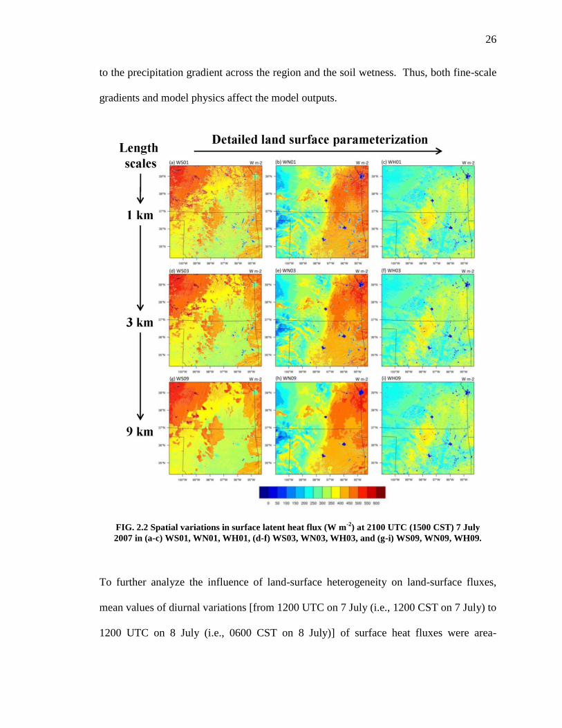
26

to the precipitation gradient across the region and the soil wetness. Thus, both fine-scale

gradients and model physics affect the model outputs.

To further analyze the influence of land-surface heterogeneity on land-surface fluxes,

mean values of diurnal variations [from 1200 UTC on 7 July (i.e., 1200 CST on 7 July) to

1200 UTC on 8 July (i.e., 0600 CST on 8 July)] of surface heat fluxes were area-

FIG. 2.2 Spatial variations in surface latent heat flux (W m-2

) at 2100 UTC (1500 CST) 7 July

2007 in (a-c) WS01, WN01, WH01, (d-f) WS03, WN03, WH03, and (g-i) WS09, WN09, WH09.

27

averaged over the domain and shown in Table 2.2. The WS shows the largest area-

averaged LE (the smallest area-averaged H), whereas the WN results in the smallest area-

averaged LE which is about 30 W m-2

less than that for WS. Results show that LE

decreases with increasing length scales for the three coupled cases where the impact of

smoothing land-surface heterogeneity from 1 to 9 km on LE for WS is the largest (2.3 W

FIG. 2.3 Spatial variations in surface sensible heat flux (W m-2

) at 2100 UTC (1500 CST) 7 July


28

m-2

). This shows that the slab model is more sensitive to land-surface heterogeneity

impacts. The area-averaged H for WS increases when the land-surface becomes more

homogeneous. The changing length scale modifies the amount of surface energy, and for

WS the impact of the length scale changing from 1 to 9 km on H (6.8%) is more

significant than on LE (1.6%). Thus, the increased length scales weaken the

heterogeneity effects in the slab/WRF simulations, and this can result in significant

changes of surface energy partitioning simulated in the slab model. This in turn affects

the simulated heat and moisture within the PBL. The Noah and HRLDAS runs show less

sensitivity to the land-surface heterogeneity length scale changes, indicating that a more

detailed land-surface parameterization can help reduce the uncertainty in surface

representation.

Table 2.2 Mean values of diurnal averaged of area-averaged surface heat fluxes

Case name H (W m-2

) LE (W m-2

)

WS01 32.12 144.78

WS03 33.64 143.10

WS09 34.30 142.48

WN01 45.09 138.43

WN03 45.64 138.29

WN09 44.02 138.02

WH01 56.87 113.63

WH03 56.87 113.63

WH09 57.15 112.92

Four typical land-surface types (grassland, forest, wet cropland, and dry cropland) in the

domain were selected to study the responses of LSMs in the high-resolution coupled

model (Table 2.3). Comparisons of diurnal variations of surface heat fluxes between the

model runs over the domain and the measurements over four specific locations with

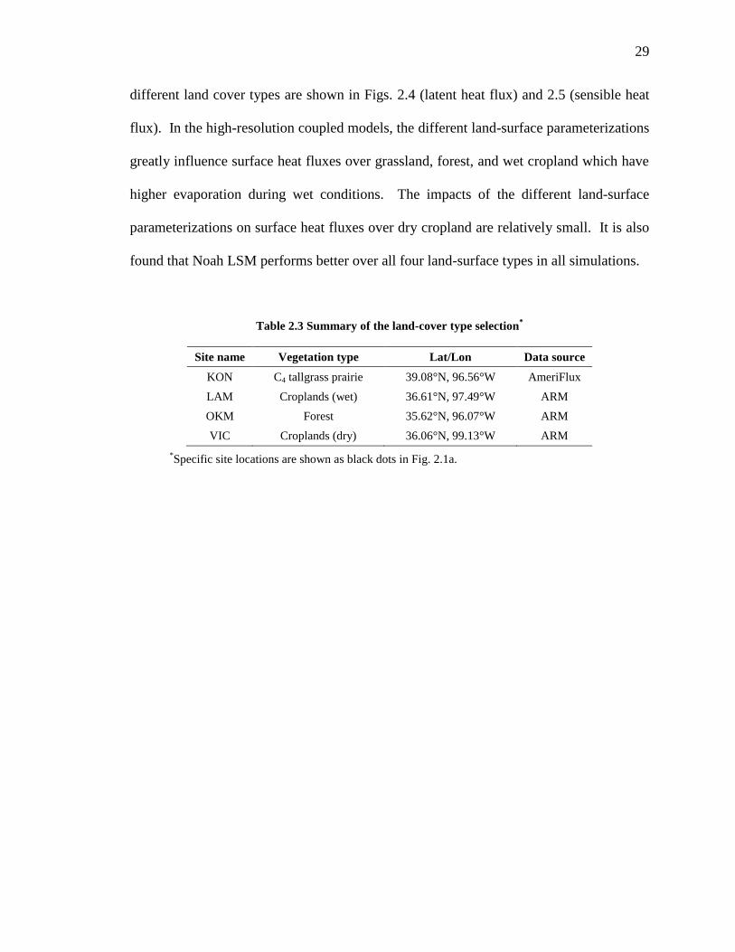
29

different land cover types are shown in Figs. 2.4 (latent heat flux) and 2.5 (sensible heat

flux). In the high-resolution coupled models, the different land-surface parameterizations

greatly influence surface heat fluxes over grassland, forest, and wet cropland which have

higher evaporation during wet conditions. The impacts of the different land-surface

parameterizations on surface heat fluxes over dry cropland are relatively small. It is also

found that Noah LSM performs better over all four land-surface types in all simulations.

Table 2.3 Summary of the land-cover type selection*

Site name Vegetation type Lat/Lon Data source

KON C4 tallgrass prairie 39.08°N, 96.56°W AmeriFlux

LAM Croplands (wet) 36.61°N, 97.49°W ARM

OKM Forest 35.62°N, 96.07°W ARM

VIC Croplands (dry) 36.06°N, 99.13°W ARM

*Specific site locations are shown as black dots in Fig. 2.1a.

30

FIG. 2.4 Comparisons of diurnal variations in surface latent heat flux (W m-2

) between the model

runs at 1 km length scale initiated at 1200 UTC (0600 CST) 7 July 2007, and the observations over

(a) grassland (KON), (b) forest (OKM), (c) wet cropland (LAM), and (d) dry cropland (VIC).

Details of the land-cover types are in Table 2.3.

FIG. 2.5 Comparisons of diurnal variations of surface sensible heat flux (W m-2

) between the


observations over (a) grassland (KON), (b) forest (OKM), (c) wet cropland (LAM), and (d) dry

cropland (VIC). Details of the land-cover types are in Table 2.3.

31

2.3.2 Impact of land-surface heterogeneity on modeling bias

A vertical cross section in the north-south direction through the middle of the domain was

analyzed for temperature and relative humidity at 2100 UTC (1500 CST) 7 July 2007

(Fig. 2.6). Similar patterns are noted for the three schemes in the 1-km length scale

simulations. As the heterogeneity length scale increases the cross sections of relative

humidity show differences compared to those at the 1 km length scale. The PBL depth

for WS and WN runs at the 9 km length scale are much lower compared to that at the 1

km length scale. This may be related to the eddies growing faster in the simulations with

1 km length scale than those with 9 km length scale, and that the MYJ PBL scheme in the

1-km-heterogeneity simulation aids the vertical transport of energy flux (Ching et al.

2014; LeMone et al. 2013; Zhou et al. 2014). The cross section for WH at the 9 km

length scale shows very different patterns for temperature and relative humidity when

compared to those for WS and WN. Consistent to the results noted for surface fluxes, the

land-surface heterogeneity has less impact on the HRLDAS/WRF runs. Thus, the land-

surface parameterization impacts the high-resolution coupled LSMs/WRF simulations

more significantly than land-surface heterogeneity. This is not surprising considering

that to some extent the land-surface heterogeneity is dictated by the land-surface model.

Additionally, the PBL depth for WH is less dependent on the spatial heterogeneity scale,

and stays similarly high for increasing heterogeneous length scale. This may be caused

by the larger surface sensible heat flux in the WH simulations which leads to stronger

resolved eddy motions and a deeper boundary layer.

32

Surface heat fluxes would eventually account for the difference in PBL processes and

affect mesoscale simulations, modeling biases and the model’s ability to simulate mass

and energy exchanges at the microscale (e.g., Bukovsky and Karoly 2009; Weaver et al.

2002; LeMone et al. 2013, 2014; Reen et al. 2013). To assess the impacts of land-surface

heterogeneity on coupled model biases, the simulated atmospheric variables were

analyzed further.

FIG. 2.6 Vertical cross section in the north-south direction through the middle of the domain (as

seen in Fig 1b) for temperature (K) and relative humidity (%) at 2100 UTC (1500 CST) 7 July


The red bold marker “cross” in Fig 1a is the selected position for the cross section.

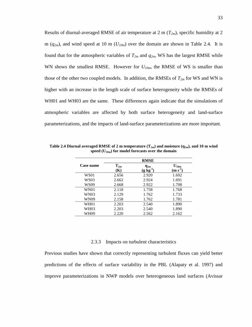
33

Results of diurnal-averaged RMSE of air temperature at 2 m (T2m), specific humidity at 2

m (q2m), and wind speed at 10 m (U10m) over the domain are shown in Table 2.4. It is

found that for the atmospheric variables of T2m and q2m, WS has the largest RMSE while

WN shows the smallest RMSE. However for U10m, the RMSE of WS is smaller than

those of the other two coupled models. In addition, the RMSEs of T2m for WS and WN is

higher with an increase in the length scale of surface heterogeneity while the RMSEs of

WH01 and WH03 are the same. These differences again indicate that the simulations of

atmospheric variables are affected by both surface heterogeneity and land-surface

parameterizations, and the impacts of land-surface parameterizations are more important.

Table 2.4 Diurnal averaged RMSE of 2 m temperature (T2m) and moisture (q2m), and 10 m wind

speed (U10m) for model forecasts over the domain

Case name

RMSE

T2m

(K)

q2m

(g kg-1

)

U10m

(m s-1

)

WS01 2.656 2.920 1.692

WS03 2.662 2.924 1.691

WS09 2.668 2.922 1.708

WN01 2.118 1.758 1.768

WN03 2.129 1.762 1.733

WN09 2.158 1.762 1.781

WH01 2.203 2.540 1.890

WH03 2.203 2.540 1.890

WH09 2.220 2.562 2.162

2.3.3 Impacts on turbulent characteristics

Previous studies have shown that correctly representing turbulent fluxes can yield better

predictions of the effects of surface variability in the PBL (Alapaty et al. 1997) and

improve parameterizations in NWP models over heterogeneous land surfaces (Avissar

34

and Pielke 1989; Avissar and Chen 1993; Weaver 2004a, b; Alfieri et al. 2009; Case

2011). Additionally, a model’s ability to reproduce observed energy spectra can help

indicate whether the model has correct energy transfer and if it can reliably reproduce

multiscale forecasts within the atmosphere (Skamarock 2004). The improved

representation of small-scale phenomena therefore may contribute to improving

mesoscale forecasts. We hypothesize that the land-surface heterogeneity affects turbulent

flow and mesoscale circulations which can be represented by LSMs coupled to WRF

model; and the turbulent representations are important for improving the coupled model

simulations when replacing a simple slab model to a more detailed LSM. This

hypothesis builds off prior results of Skamarock and Dempsey (2005) that showed that

WRF-ARW forecasts produced kinetic energy spectra that bear close resemblance to

climatologically observed spectra.

The maps of the vertical velocity and wind fields at the middle of the PBL height (~ 1 km)

have shown the convective structure of the PBL at 2100 UTC 7 July 2007 (Fig. 2.7). The

domain averaged turbulent vertical velocities are as expected close to zero and are

negative (downward) for all the simulations. The vertical velocity fields show pockets of

updrafts or downdrafts notably in the northwestern part of the domain (Fig. 2.7A), and

these patterns are more apparent in the HRLDAS runs [Figs. 2.7A (c,f,i)]. A reason for

this might be related to the land-surface heterogeneity induced in the high-resolution

HRLDAS/WRF experiment. Since the convective eddies have positively correlated to

the vertical velocity, these eddies provide a source of turbulent kinetic energy and

positive heat flux. For the runs with 9-km land-use heterogeneity length scale, slab/WRF

35

and Noah/WRF runs show stronger downward vertical velocity over the domain. This

might indicate there are some eddies in these two runs that are tightly coupled to the

landscape. However, the HRLDAS/WRF runs have insignificant changes in the vertical

velocities and wind speeds due to the high-resolution (1 km) uncoupled land-surface

modeling system initialization. The averaged wind speed at the mid-PBL level height is

about 5 m s-1

, and show stronger gradients. Thus, the spatial averaged energy spectra

could be reasonably representing the impacts of spatial heterogeneity and different land-

surface parameterizations.

Fast Fourier Transform (FFT) analysis was conducted and the WRF model kinetic energy

spectra were developed to understand how the characteristics of the mesoscale energy

spectra simulated by different LSMs/WRF are influenced by land-surface heterogeneity.

FIG. 2.7 Maps of (A) mid-PBL vertical velocity and (B) the wind fields at 2100 UTC 7 July 2007

with 1-km grid spacing.

36

For short periods and the condition that the advection velocity of the turbulence is much

greater than the turbulent vertical scale, Taylor’s hypothesis of frozen turbulence can be

invoked so that the spectrum of the time series data can be assumed to be representative

of the spatial turbulent structure (Stull 1988). To satisfy Taylor’s hypothesis, the

simulated data over the domain were processed according to the condition that the

standard deviation of wind speed is smaller than half of the mean wind speed (Willis and

Deardorff 1976). A total of 558 × 591 data points were produced in the domain. To

minimize the effects of the lateral boundary conditions, the energy densities were

spatially averaged from grids beginning 15 points away from all the boundaries

(Skamarock 2004). The energy densities were horizontally averaged using a one-

dimensional spectral decomposition of the related scalars along the west-east direction.

The kinetic energy spectra for the three different coupled models over the heterogeneous

land surface were then computed at the height of each model’s surface layer using data

from these selected points.

The energy densities were calculated correspondingly to intense turbulent activity at 2100

UTC (1500 CST) 7 July 2007. The model results were compared against turbulence

observations obtained using the eddy covariance (EC) technique which employed a

Campbell Scientific CR1000 datalogger to sample velocities and virtual temperatures at

20 Hz. The EC tower in our research is from the AmeriFlux network and located at KON

(39.08°N, 96.56°W; Fig. 2.1a).

37

The direct forcing from the flow interaction with topography and convection, the

downscale cascade from lower frequencies, and upscale cascade from higher frequencies,

are three substantial processes in the build-up of energy in the mesoscale portion of the

spectrum (Skamarock 2004). Fig. 2.8 shows the energy spectra with standard deviation

log-log plots of simulated T2m, q2m (Figs. 2.8 a and b), and the log-log plots of horizontal

wind velocities at 10 m (U10m, V10m), and vertical velocity (W) [Figs. 2.8 (c-e)] at the

model’s lowest layer for the three different coupled models at the 1 km length scale.

Note that since variations in variables such as temperature and humidity can persist as

“footprints” of former turbulent flow, the resulting spectra of these variables cannot be

associated with eddy motions (Stull 1988; Schmid 2002). It is noted that the energy

spectra show similar trends of curves. This is likely because the initial and lateral

boundary conditions for all the models are derived from the same 1 degree FNL analysis

data. However, the spectra can be sensitive to the different land-surface features. The

spectra of simulated T2m and q2m for WS depart from those for WN and WH and are much

stronger (Fig. 2.8a), while the spectra for WN are the smallest but very close to the

observations (Figs. 2.8 a and b). A large portion of the turbulent observations are found

when the frequency is larger than 10-4

hz, indicating that the large eddies that are resolved

in WRF model contribute essentially to the turbulence state. Additionally, the surface

turbulence is a mix of some low-level frequencies related directly to the surface wind and

some related to the PBL wind. By analyzing the spectra for temperature and humidity,

we concluded that the LSMs/WRF can capture most of the turbulent eddies that

contribute to turbulence variances.

38

By decomposing a series of measurements into frequency, the contributions from eddies

of different time and space scales to the overall turbulence can be quantified. Impacts of

LSMs on the spectra of U10m and V10m are noted to be more significant at lower

frequencies (𝑓 < 10−4 hz) where the mesoscale circulations may be created as a result of

land-surface heterogeneity (Fig. 2.9c and d). The spectral amplitude of U10m for WH is

larger than those of WN and WS (Fig. 2.9c). WS shows stronger spectral amplitude for

V10m (Fig. 2.8d), but all the simulated energy spectra of V10m are much smaller than the

observations, indicating that although the energy from large size eddies for V10m of WS is

FIG. 2.8 Energy spectra (m2 s



simulations compared to observations at 2100 UTC (1500 CST) on 7 July 2007 for (a)

temperature at 2 m, (b) specific humidity at 2 m, (c) U-wind at 10 m, (d) V-wind at 10 m, and (e)

vertical velocity.

39

stronger than those for WN and WH, the coupled models still underestimate the energy

spectra of V10m that are contributed to by large eddies. All spectra of vertical velocity

collapse to a series of close curves in the middle and higher frequencies (Fig. 2.8e).

The spectra have also been analyzed to estimate heterogeneity influences. Fig. 2.9 shows

log-log plots of energy spectra (m2 s


-1) at 2100 UTC (1500

CST) over the domain at 1, 3, and 9 km length scales for T2m, q2m, and vertical velocity in

WS, WN, and WH. It is noted that the spectral amplitude of T2m for all the experiments

decreases as the length scale increases [Figs. 2.9 (a-c)]. At higher frequencies with 3 km

length scale, an upturn occurs at the end of tail from the energy spectra of T2m. The

slopes of WS01 and WS03 for T2m and q2m are larger than the corresponding slopes of the

observations, indicating that slab/WRF cannot well represent the energy spectra of T2m

and q2m and underestimates the energy cascade. The spectra of q2m for WN03 are smaller

than those for WN01 and WN09, and in the inertial subrange and higher frequencies,

WS01 and WN01 show the largest spectral magnitudes while at lower frequencies, the

spectra of q2m for WS09 and WN09 are the strongest (Figs. 2.9 d and e). For

HRLDAS/WRF runs, non-linear changes in the log value of the energy spectra with the

increase of the heterogeneous length scale have been noticed. The T2m and q2m show the

largest energy over the 9 km heterogeneity spatial scale, whereas the energy spectra for

the 3 km length scale experiments are the smallest (Fig. 2.9e and f). Thus under

abundant soil moisture availability conditions, the impacts of surface heterogeneity on the

spectra of simulated surface temperature and moisture can be noted at all frequencies.

The more detailed LSM/WRF at the 1 km length scale simulates a better energy spectrum.

40

FIG. 2.9 Energy spectra (m2 s



forecasts at 1, 3, and 9 km length scales at 2100 UTC (1500 CST) compared to observations on 7

July 2007 for temperature at 2 m (top), specific humidity at 2 m (middle), and vertical velocity

(bottom) in WS (a, d, g), WN (b, e, h), and WH (c, f, i).

41

For W simulated by WS and WN at lower frequencies, the spectral energy amplitude

increases as the length scale increases (Figs. 2.9 g and h), indicating the large size of

eddies over the land surface with a 9 km length scale contain more energy than those with

a 1 and 3 km length scale. In the inertial subrange, the energy spectra amplitudes are

largest at the 1 km length scale, thus all the coupled models are able to represent land-

surface heterogeneity impacts on the vertical velocity which is much stronger over a

more heterogeneous land surface. WH01 and WH09 show close curves for the energy

spectra of the vertical velocity. Additionally, as seen in Figs. 2.9(g-i) W is less sensitive

to the different land-surface parameterizations, especially at the 1 km length scale.

Thus, in response to land-surface heterogeneity and LSMs, the impact of horizontal

spatial scale of land-surface heterogeneity on mesoscale coupled model’s energy spectra

can be better captured at the 1 km length scale by a more detailed land-surface

parameterization.

2.3.4 Impacts on surface-atmosphere interactions

Sounding profiles (Fig. 2.10) at 0000 UTC (1800 CST) 8 July 2007 for specific humidity,

potential temperature, and wind speed at Norman, OK (OUN, 35.18°N, 97.44°W) and

Topeka, KS (TOP, 39.07°N, 95.62°W) were simulated and compared to observations.

We only show sounding profiles simulated at the 1 km length scale as an example of the

responses of sounding profiles to changes in the land-surface parameterizations. The

profiles of temperature, moisture, and wind speed in the WS model soundings are well

simulated for the TOP site. Simulated potential temperature, wind speed, and surface and

42

upper-level specific humidity by WS are also in good agreement with observations from

the OUN site. From the surface to the 900 hPa level, WH shows cold biases for surface

potential temperature while WN over-predicts temperature for both sites. Surprisingly,

the slab model simulates the profiles of temperature, moisture, and wind speed better at

the 1 km length scale.

FIG. 2.10 Sounding profile at 0000 UTC (1800 CST) 8 July 2007 of specific humidity (g kg-1

) (a,

d), potential temperature (K) (b, e), and wind speed (m s-1

) (c, f), valid at Norman, OK (OUN,

35.18°N, 97.44°W) (top) and Topeka, KS (TOP, 39.07°N, 95.62°W) (bottom).

43

The dimensionless vertical profiles of the turbulent moisture flux, turbulent thermal flux,

buoyancy flux, turbulent kinetic energy (TKE), and wind velocities were averaged from

2100 UTC (1500 CST) to 2130 UTC (1530 CST) 7 July 2007 at specific site locations

(Table 2.3) for each experiment and scaled using boundary layer heights. Since the

modeled PBL top is very irregular and not a good parameter to compare with PBL depth,

we used actual sounding profiles to estimate the PBL heights (Cheng et al. 2002). Fig.

2.11 shows the impacts of different land-surface schemes on turbulent processes in the

PBL over wet/dry croplands. Results confirm that the turbulent characteristics vary over

different land-surface properties, and the turbulence is stronger above the higher surface

heat flux which agrees to the findings of Hadfield et al. (1992). As seen in Figs. 2.11 a

and e, the difference among the vertical profiles of normalized turbulent thermal flux

between WS01 and WH01 is positive toward the entrainment zone. This is because the

stronger spectrum of T2m for WS (Fig. 2.8a) leads to larger eddies and more energy

vertically transported into the PBL. WN shows the largest normalized turbulent thermal

flux over the wet cropland (Fig. 2.11a), however, the spectrum of T2m for WN did not

show the largest amplitude (Fig. 2.8a). Additionally, the higher surface sensible heat flux

(e.g., Fig. 2.5) does not necessarily provide a higher averaged vertical turbulent thermal

flux. In Fig. 2.11b and f, stronger gradients at the surface where water vapor is

evaporated into the boundary layer and the entrainment zone where a cap on the mixed

layer exists, are noted for all the land-surface parameterizations over wet cropland. This

result further supports the findings of previous surface heterogeneity impact studies

(Avissar and Schmidt 1998; Huang and Margulis 2009). However WN fails to simulate

this phenomenon over dry cropland. WH shows the largest moisture flux in the near-

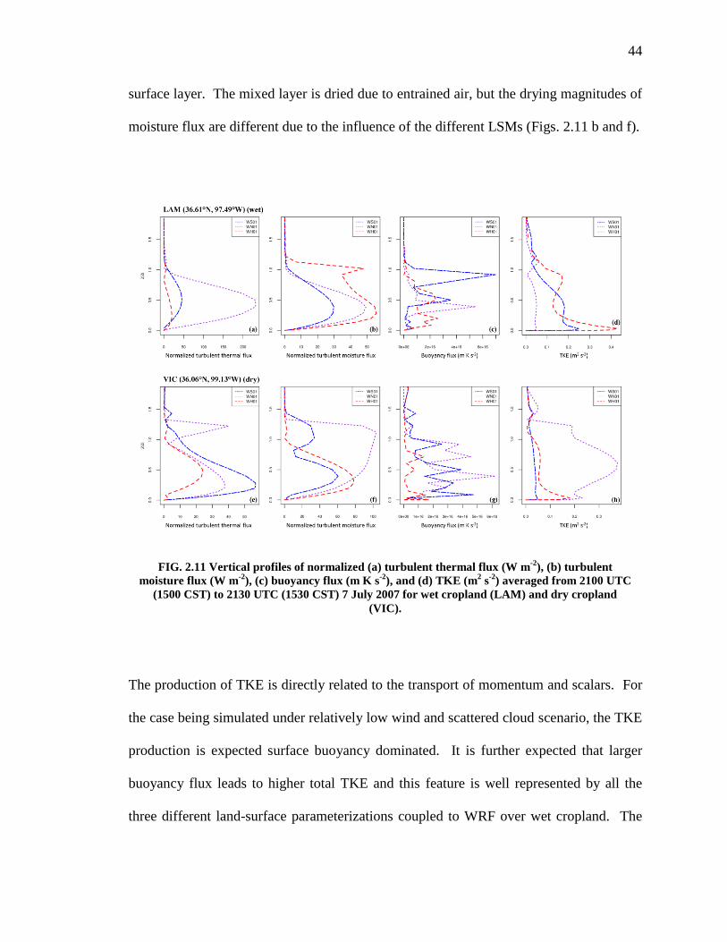
44

surface layer. The mixed layer is dried due to entrained air, but the drying magnitudes of

moisture flux are different due to the influence of the different LSMs (Figs. 2.11 b and f).

The production of TKE is directly related to the transport of momentum and scalars. For

the case being simulated under relatively low wind and scattered cloud scenario, the TKE

production is expected surface buoyancy dominated. It is further expected that larger

buoyancy flux leads to higher total TKE and this feature is well represented by all the

three different land-surface parameterizations coupled to WRF over wet cropland. The

FIG. 2.11 Vertical profiles of normalized (a) turbulent thermal flux (W m-2

), (b) turbulent

moisture flux (W m-2

), (c) buoyancy flux (m K s-2

), and (d) TKE (m2 s

-2) averaged from 2100 UTC

(1500 CST) to 2130 UTC (1530 CST) 7 July 2007 for wet cropland (LAM) and dry cropland

(VIC).

45

simulated total TKE profiles for all land-surface parameterizations approach the

maximum values at the surface and by definition decrease along with the height below

the boundary layer height (Fig. 2.11d). However, over dry cropland the total TKE for

WN increases with height from the land surface to half of the boundary layer height and

decreases when the normalized height is larger than 0.5 (Fig. 2.11h). Among all the three

simulations over dry cropland, the buoyancy flux in the PBL for WH is smaller than that

for WS (Fig. 2.11g), and the total TKE simulated by WS is the smallest (Fig. 2.11h). For

WN, the vertical turbulent moisture flux and total TKE are not well simulated.

Fig. 2.12 shows vertical profiles of normalized vertical velocity (taken as the ratio of

vertical velocity and convective velocity; Deardorff and Willis 1982) averaged from 2100

UTC (1500 CST) to 2130 UTC (1530 CST) 7 July 2007 over different land surfaces

(Table 2.3). The vertical velocity is a key parameter which is associated with turbulent

parameters. In general, the simulations differ with different land-surface

parameterizations. The profiles of normalized vertical velocity are simulated differently

by different land-surface parameterizations, but are identical in shape (Fig. 2.12). As

shown in Fig. 2.12, over tall grass prairie, the magnitude of normalized vertical velocity

for WS is much larger than those for WN and WH. The vertical velocity profiles for WN

and WH show close curves over the tall grass prairie, but WS and WH show similar

velocities below 500 m height above the land surface. The simulated vertical velocity

show larger difference over the cropland, and is impacted significantly over dry cropland.

The vertical profiles of horizontal velocity variance were also been studied. Results show

over tall grass prairie and cropland, larger horizontal velocities occur near the land

46

surface due to association with stronger wind shears during the daytime. Over forest, the

near-surface horizontal velocity is small because of the larger surface roughness. Near

the boundary layer height, all simulated horizontal velocities show a large gradient over

tall grass prairie, but the magnitudes of the variations are different. Note that while these

results reveal that there are differences in the turbulent structure simulated by the

different land-surface parameterizations coupled to WRF model in response to the

surface heterogeneity, they cannot be used to evaluate whether one land-surface scheme

surpasses the other in representing turbulent characteristics.

The vertical profiles of normalized TKE with 1, 3, and 9 km length scales in WS, WN,

and WH are shown in Fig. 2.13. TKE is a measure of turbulent intensity that can also be

influenced by the heterogeneity induced atmospheric motions. The variation of TKE

profile for WS is found to be the most significant at the 3 km length scale (Figs. 2.13 a

and d). Large gradients of TKE for WN are noted near the boundary layer height over

the wet cropland, indicating vigorous turbulence occurs in Noah/WRF simulations over

FIG. 2.12 Vertical profiles of vertical velocity averaged from 2100 UTC (1500 CST) to 2130 UTC

(1530 CST) 7 July 2007 for grassland (KON) (a), forest (OKM) (b), wet cropland (LAM) (c), and

dry cropland (VIC) (d). Details of the land-cover types are in Table 2.3.

47

wet cropland (Fig. 2.13b). For WH the TKE profiles have close curves for the 3 km and

9 km length scales, but the boundary layer is much more turbulent at the 1 km length

scale (Figs. 2.13 c and f). However, the simulated boundary layers are much more

turbulent for WS03 and WN01 over dry cropland, indicating that the different land-

surface parameterization can result in significant difference in boundary layer simulations,

particularly over the heterogeneous dry cropland.

FIG. 2.13 Vertical profiles of normalized TKE (m2 s

-2) averaged from 2100 UTC (1500 CST) to

2130 UTC (1530 CST) 7 July 2007 with 1, 3, and 9 km length scales in WN (a, d), WS (b, e), and

WH (c, f) over wet cropland (LAM) and dry cropland (VIC).

48

2.4 Summary and conclusions

We conducted a series of numerical experiments (slab/WRF, Noah/WRF, and

HRLDAS/WRF) to study the role of land-surface heterogeneity on the turbulent flow and

mesoscale processes in the WRF model coupled within different land-surface

parameterizations. Results show that the more detailed land-surface parameterizations

over heterogeneous land surface typically help improve turbulent processes, leading to

improved simulations of land-atmosphere interactions over heterogeneous land surface.

Changes of length scales of land-surface heterogeneity affect high-resolution model

simulations through modification of land-surface properties. Typically the spatial

variation of surface heat flux decreases as the length scale of land-surface heterogeneity

increases. The slab model is found to be more sensitive to land-surface heterogeneity

impacts, whereas the Noah and HRLDAS runs show less sensitivity to the land-surface

heterogeneity length scale changes, indicating that the more detailed land-surface

parameterizations (e.g., Noah LSM and HRLDAS) can help reduce the uncertainty of

surface flux simulations over heterogeneous landscapes.

Land-surface heterogeneity and changes in land-surface initialization also result in

impacts on modeling biases, and the impacts of changes in land-surface parameterizations

are more significant. Nonlinear impacts are found in simulated surface temperature,

moisture, and wind speeds due to landscape heterogeneity. Larger biases have been

noted in the slab/WRF run.

49

The responses of turbulent spectra to land-surface heterogeneity indicate that the more

detailed LSMs/WRF simulate more correct turbulent spectra over the heterogeneous land

surface. The energy spectra response nonlinearly to changes in the heterogeneous length

scales. The impacts of LSMs on turbulent energy spectra are more significant at lower

frequencies of the spectra with 1 km heterogeneity length scale. Results of the spectral

analysis provide an important finding that the atmospheric feedbacks that are roughly

four times of the land heterogeneity spatial scale can be adequately resolved in the

coupled mesoscale model. For example, for the 1 km heterogeneity length scale, the

circulation larger than 4 km would be resolved; it would be larger than 12 km to be

resolved for the 3 km length scale, and larger than 36 km for the 9 km length scale. This

highlights the question such as “what is the minimum land heterogeneity required to

trigger atmospheric circulation?”. The effect would be a function of the degree of spatial

heterogeneity represented in the land surface model, which is often a function of the grid

spacing. This emergent feature needs to be studied further.

Results also identify substantial variations in turbulent spectra and provide one piece of

evidence showing the nonlinear influence of spatial length scales and the use of different

land-surface parameterizations on turbulent energy spectra. However, the turbulent

characteristics obtained at the surface may not be in equilibrium with the flow at height

over a heterogeneous land surface (Schmid 1994), and it is possible to examine the

change in the spatial energy spectra in relation to the length scale of heterogeneity.

Results indicate that there are differences in the heterogeneity length scales represented

by the model runs with different land-surface parameterizations.

50

The spatial heterogeneity represented by different land-surface parameterizations would

resolve the atmospheric circulation which is at least four times of the spatial

heterogeneity length scale. The vertical profiles of the turbulent fluxes and TKE can also

be used to represent LSM influences and land-surface heterogeneity impacts. Our results

agree with prior studies (e.g., Holt et al. 2006; Niyogi et al. 2006; Niyogi et al. 2009b;

Niu et al. 2011) that showed a positive impact of the improved land-surface

parameterization on model responses in terms of surface fluxes and mesoscale dynamical

features. Additionally, this study has addressed the issue of how the detailed land surface

representation affects the boundary layer and mesoscale processes via turbulent processes.

51

CHAPTER 3. IMPACTS OF LAND-ATMOPSHERE COUPLING ON REGIONAL

RAINFALL AND CONVECTION2

3.1 Introduction

The coupling between the atmosphere and the land surface can play an important role in

regional convection and precipitation (i.e., Trier et al. 2004; Holt et al. 2006; LeMone et

al. 2010) and is one of the important components of any given weather and climate model

(Pielke et al. 2011). The importance of land-atmosphere coupling has been emphasized

in many observational and modeling studies (e.g., Dirmeyer 2000; Koster et al. 2003,

2004, 2006; Seneviratne et al. 2010). Wetter soils can cause higher evaporation, and

higher latent heat flux, which in turn enhances the moisture availability within the

planetary boundary layer (PBL), affects the atmospheric heating rates and cloud

formation, and can impact local and regional precipitation (Niyogi et al. 1999; Pielke

2001; Kang et al. 2007; LeMone et al. 2008). The impacts of land-atmosphere coupling

on regional temperature through a negative correlation between soil moisture and surface

temperature also have been noted (Fischer et al. 2007; Hirsch et al. 2014).

It is expected that land-surface feedbacks can have a more dominant impact on regional

precipitation in some regions of the globe as compared to others. Koster et al. (2004)

identified global "hot spot" regions as areas of strong coupling between summer rainfall

2 Zheng, Y., A. Kumar, and D. Niyogi, 2015: Impacts of land-atmosphere coupling on regional rainfall and

convection. Clim. Dyn., 44, 2383–2409, doi: 10.1007/s00382-014-2442-8.

52

and land-surface conditions, and concluded that there was a significant impact on cloud

formation, which was sensitive to the land-surface forcings such as soil moisture, land

use, and topography (Koster et al. 2003; LeMone et al. 2008; Houze 2012). It has been

noted that the coupling hot spots identified in the Global Land-Atmosphere Coupling

Experiment (GLACE) study could be incorrectly capturing land-atmosphere coupling

(Dirmeyer et al. 2006). In particular, the land surface models (LSM) may represent

incorrect coupling in climate models, leading to too much evaporation and incorrect soil

moisture-precipitation feedback (Ruiz-Barradas and Nigam 2005). As a result, models

can overestimate moisture in summer due to a lack of knowledge in reference to the

model-prescribed land-atmosphere coupling strength (Koster et al. 2003; Hirsch et al.

2014; Lorenz and Pitman 2014). Similarly, Zhang et al. (2008) for example, concluded

that the U.S. SGP does not show up as a strong land-atmosphere coupling region in their

regional model runs. This raises broad questions such as how do the current

meteorological models represent land-atmosphere surface coupling strength? What

would be the impact of surface-atmosphere coupling strength on regional (and though not

considered here, global) model performance?

One way of representing the coupling strength between land and atmosphere is through

the surface exchange coefficient. Recent studies such as LeMone et al. (2008) and Chen

and Zhang (2009) concluded that the surface exchange coefficient is responsible for

transferring surface energy into the lower atmosphere and that the land-atmosphere

coupling strength depends on this coefficient for different land-cover types and climate

regimes. Trier et al. (2011) explored the impacts of the coupling coefficient “C” based

53

on the Zilitinkevich (1995) equation (thereafter Czil) on the mesoscale warm rain

processes over the U.S. SGP locale. Their results indicated that the representation of Czil

significantly affected precipitation and convection via a stronger surface exchange

simulation, but the implication and possible advantages of dynamically changing Czil in

regional scenarios over different regions are not yet clear. Therefore, we investigated the

coupling impact using an offline Noah land model and a coupled WRF model over U.S.

SGP, Europe, India, and West African regions. These four regions were selected because

of the diversity in landscape, and the preponderance of intense mesoscale convection and

heavy precipitation cases. Further, each of these regions was identified as a land-

atmosphere coupling hotspot in different global studies (Koster et al. 2004 and 2006; Xue

et al. 2004; Seneviratne et al. 2006).

Thus, the objective of this study is to assess the role of coupling strength over regions

with strong coupling between land-surface conditions and moist convection. We

hypothesize that a better understanding of the coupling effect will benefit numerical

weather prediction (NWP) and the parameterizations used for land surface

representations, and could potentially lead to improved simulation of severe weather

events. The main tasks undertaken are 1) to quantify the land-atmosphere coupling

strength impacts on model parameterizations (i.e., land surface processes, PBL dynamics,

and moist convection), 2) to document the range of the regional variations in Czil for

model simulations, and, 3) to identify if the dynamically changing Czil could help

improve the NWP model’s summer convection simulations over the different coupling

hotspot regions.

54

This paper is organized as follows. Section 2 summarizes the experimental setup using

the uncoupled Noah LSM and the coupled WRF mesoscale model as well as the study

domain. Section 3 discusses the methodology adopted to assess the effects of the land-

atmosphere coupling strength. Section 4 evaluates the different case studies and

simulations. The study conclusions and discussions are provided in Section 5.

3.2 Numerical modeling framework and study domain

This section describes the model setup and the experimental study domain. The

methodology first tests the impacts of the coupling coefficients within an offline model in

order to study the impacts of surface coupling strength on energy partitioning and surface

heat exchanges. This analysis is conducted over the U.S. SGP. Following the uncoupled

diagnostics, the remainder of the experiments uses a coupled Noah-WRF modeling

framework for regional coupling analysis across the four different regions.

3.2.1 Offline modeling system

The coupling strength needs to be studied in association with the land cover

characteristics (Hirsch et al. 2014). As a result, a number of numerical experiments over

three different land surfaces (grassland, cropland, and forest) are undertaken using a 1-D

offline (uncoupled) Noah LSM within the High Resolution Land Data Assimilation

System (HRLDAS; Chen et al 2007). The land model is forced by analysis fields or

meteorological observations rather than coupled to an atmospheric model. HRLDAS

integrates static fields of land use and soil texture as well as time-varying fields of

vegetation and meteorology. The primary reason for using HRLDAS is that this

55

framework is capable of capturing the land-surface heterogeneity at multiple scales that

are important for resolving microscale to regional features (Holt et al. 2006; Charusombat

et al. 2012).

As stated, the U.S. SGP domain has been a subject of recent land-atmosphere coupling

studies (e.g., Koster et al. 2006; Zhang et al. 2008; Trier et al. 2011) and has a number of

high quality observations. A 188 × 170 × 31 grid domain was set up with 4 km

horizontal grid spacing (Fig. 3.1). An eighteen month spinup initialization was run from

December 2000 to June 2002 following Chen et al. (2007). The atmospheric forcing and

surface conditions used in HRLDAS were: i) National Centers for Environmental

Prediction (NCEP) Stage-IV Rainfall Analysis at 4 km horizontal grid spacing; ii) 50 km

GOES solar downward radiation; iii) other atmospheric forcing conditions from model-

based analysis; and iv) the USGS land-use and land-cover map with 24 vegetation types.

The domain was initialized using the USGS soil texture map, terrain height, land-water

mask and land use through the WRF Pre-processing System (WPS). These data were

interpolated to a regular 0.01 degree geographic projection according to the respective

WRF grids. The offline (uncoupled) HRLDAS model is grid-based, and uses 1-D

column version of Noah to execute single-site land-surface simulations. The soil

conditions at four soil depth layers and the vegetation were initialized as model input

parameters, and the physical processes were identical to that of the Noah LSM described

by Chen et al. (1997, 2007). Surface heat flux observations were used to evaluate the

model results.

56

3.2.2 WRF Model and domain configurations

WRF 3.4.1 (Skamarock et al. 2008) was used to conduct coupled simulations with Noah

LSM. One degree 6-hourly NCEP Global Final Analysis (FNL) dataset, which was

derived from the Global Forecast System (GFS), was used to set the boundary and initial

conditions for the large-scale atmospheric fields, soil parameters (i.e., soil moisture and

temperature), and sea surface temperature (SST). The WRF model was run with 28

vertical levels applied from the surface to 50 hPa level. The model was setup over four

different regions, the U.S. SGP, Europe, northern India, and West Africa. Each region

has unique land-surface characteristics, and the cases being simulated are typical for the

regions and employed to study the coupling impacts on atmospheric convection

simulations. A summary of the four regions is shown in Table 3.1 and discussed next.

Table 3.1 The characteristics of study regions

Model grid points

Land-cover type Geographic feature 9-km grid

spacing

3-km grid

spacing

U.S. SGP 290 × 280 307 × 274

Grassland, cropland,

savannas and a mixture of

crop and natural vegetation

Modestly higher elevation

on the western side,

synoptic and mesoscale

weather events

Europe 250 × 240 307 × 274

Forest, arable land with

permanent crops, and

pastures and mixed mosaics

Mountainous terrain;

Dominant orographic

precipitation

India 250 × 240 307 × 274 Forest and agricultural land

A typical monsoon region

with trough and associated

weather patterns

West Africa 433 × 433 631 × 631

Forest, cropland, woodland

and shrub land, grassland,

and bare soil

Large flat area

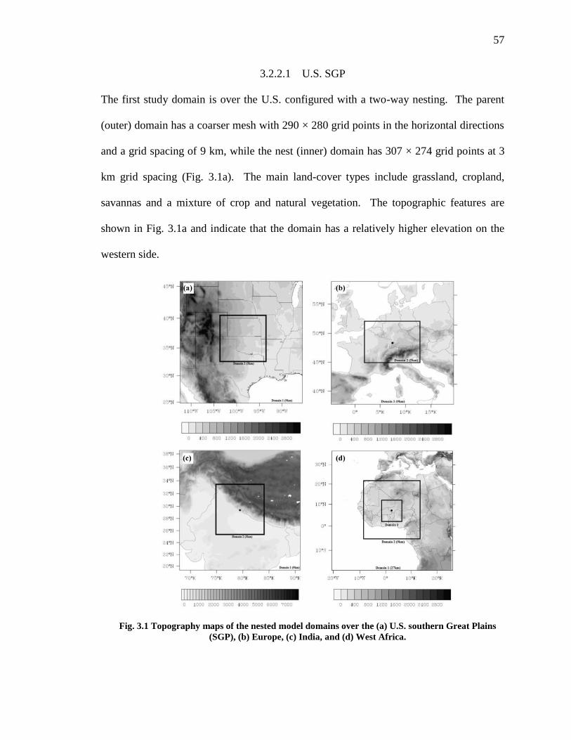
57

3.2.2.1 U.S. SGP

The first study domain is over the U.S. configured with a two-way nesting. The parent

(outer) domain has a coarser mesh with 290 × 280 grid points in the horizontal directions

and a grid spacing of 9 km, while the nest (inner) domain has 307 × 274 grid points at 3

km grid spacing (Fig. 3.1a). The main land-cover types include grassland, cropland,

savannas and a mixture of crop and natural vegetation. The topographic features are

shown in Fig. 3.1a and indicate that the domain has a relatively higher elevation on the

western side.

Fig. 3.1 Topography maps of the nested model domains over the (a) U.S. southern Great Plains

(SGP), (b) Europe, (c) India, and (d) West Africa.

58

3.2.2.2 Europe

The second study region is over Europe and also has two-way nested domains of 9 km

(250 × 240 grid points) and 3 km (307 × 274 grid points) grid spacing that cover most of

Germany (Fig. 3.1b). The three dominant land types in the European domain are forest,

arable land and permanent crops, and pastures and mixed mosaics. This region is

complex with various mountainous terrains that affect regional circulation patterns and

result in large amounts of orographic precipitation, particularly in the summertime.

Because of the complex link between convective processes and orography, this domain is

relatively difficult to simulate (Wulfmeyer et al. 2008).

3.2.2.3 Northern India

The third domain is set up over India using the two-way nesting with 250 × 240 grid

points at 9 km horizontal grid spacing for the outer domain and 307 × 274 grid points

with 3 km horizontal grid spacing for the inner domain (Fig. 3.1c). India is a typical

monsoon region where heavy rain events and mesoscale convection are predominantly

associated with monsoon rainfall. The major land-cover types over the Northern India

domain are forest and agricultural land.

3.2.2.4 West Africa

The fourth domain covers West Africa (Fig. 3.1d). As this region is much larger than the

previous three regions, we configure the model with two nested domains: a coarse mesh

of 300 × 300 grid points with 27 km horizontal grid spacing, and 2, two-way nested

59

domains of 433 × 433 grid points with 9 km, and 631 × 631 grid points with 3 km,

respectively. The primary land-cover types are forest, cropland, woodland and shrubland,

grassland, and bare soil.

3.2.2.5 Model configuration

We recognize that different model schemes and physical options may perform differently

over different regions. For example, Bukovsky and Karoly (2009) found that the Kain-

Fritsch (KF) scheme performed better over the U.S. in terms of mean precipitation, while

Flaounas et al. (2011) pointed out that the combination of the KF scheme and the Mellor-

Yamada-Janjic (MYJ) PBL scheme provided the best simulation of the West Africa

monsoon. Similarly Venkata Ratnam and Cox (2006) reported that the KF scheme

simulated more realistic moisture profile and rainfall distribution over India. To

constrain the confounding variables in understanding the model response to study the

regional sensitivity of the Czil values, we use the same physical options to conduct model

simulations over the four selected regions. The predominant physical options in the 9

and 3 km nests included: (a) The Goddard microphysics scheme which includes ice, snow

and graupel processes and is suitable for high-resolution simulations (Tao, Simpson and

McCumber 1989). (b) The KF scheme, which is a deep and shallow convection sub-grid

scheme using a mass flux approach with downdrafts and CAPE removal time scale

(Janjic 1994, 2000). (c) The MYJ PBL scheme (Janjic 2002), which is used together with

the Eta similarity theory surface layer. The ability to represent moisture entrainment into

the lower atmosphere within this local-closure PBL scheme provides more realistic

convection triggering with the KF scheme. (d) The Noah LSM (Chen and Dudhia 2001),

60

which has a single vegetation canopy layer and simulates soil moisture and temperature

for four soil layers with the depth of 0.1, 0.3, 0.6, and 1.0 m respectively. Longwave

radiation is based on the Rapid Radiative Transfer Model (Mlawer et al. 1997), while the

shortwave radiation only considers a downward beam (Dudhia 1989). The surface layer

scheme is used to determine the exchange coefficient which links surface heat and

moisture fluxes to the LSM and the PBL.

3.2.3 Data for model case studies

We employed AmeriFlux data and the International H2O Project 2002 (IHOP_2002) field

campaign data as verification datasets. The AmeriFlux sites produce a full suite of

relatively long-term measurements of the meteorological variables and exchange rates of

surface heat fluxes, with the knowledge of ecosystem and the history of land use and land

cover changes. The IHOP_2002 field campaign was conducted with an objective of

improving convective initiation predictions and quantitative precipitation forecasts in

NWP models. The field data provide continuous complete measurement of surface

fluxes, near-surface meteorological variables, and soil conditions during the late spring

and early summer of 2002 (Weckwerth and Parsons 2006; LeMone et al. 2008).

The experiments over Europe were carried out with data gathered during the Convective

and Orographically-induced Precipitation Study (COPS) field campaign for the time

period from 21 to 23 July 2007. The locations of the COPS field experiment are between

southern Germany and eastern France. The Atmospheric Radiation Measurement (ARM)

Mobile Facility (AMF) was deployed in the Black Forest region of Germany to capture

61

the convection and orographic rainfall processes in the complex mountainous terrain.

More details about the COPS field campaign can be found in Wulfmeyer et al. (2008).

Unlike the U.S. and European domains, the Indian domain has limited publicly available

observations and conspicuously lacks flux measurements. There are only 15 observations

within the inner domain. Therefore, we resort to using the radar reflectivity, atmospheric

soundings, and the area-averaged bias of temperature, moisture, and wind speed to

evaluate the model results. Similarly, there are limited surface sites, instrumentation, or

spatial and temporal sampling as part of in situ field experiments over the region of West

Africa. However, because of the ARM Mobile Facility (AMF) deployment in Niamey,

Niger, West Africa as part of the African Monsoon Multidisciplinary Analysis (AMMA)

field phases and observing periods (Redelsperger et al. 2006), there is an accessible

meteorological dataset. Data from the Tropical Rainfall Measuring Mission (TRMM)

precipitation [3B42 and TRMM Multi-satellite Precipitation Analysis (TMPA)] are also

used for both the Indian and African model studies. All observed atmospheric soundings

from selected weather stations over these four study regions are obtained from the

University of Wyoming (http://weather.uwyo.edu/upperair/sounding.html).

3.3 Land-atmosphere coupling method and Czil experiments

Detailed land-surface representation is essential for realistic model forecasts (Holt et al.

2006; Niyogi et al. 2006). The key parameters associated with a LSM include sensible

and latent heat fluxes which control the diurnal evolution and development of the PBL

(Trier et al. 2011). In the Noah LSM (Chen and Dudhia, 2001; Ek et al. 2003) the surface

62

sensible (H) and latent (LE) heat fluxes are determined through the bulk aerodynamic

method as:

(3.1)

(3.2)

where is the air density, is the specific heat of air at constant pressure, is the

wind speed, and are the air potential temperature and the air specific humidity at the

lowest model level or at a specific measurement height above the ground (i.e., 2 m), and

and are the surface potential temperature and the surface specific humidity. The

parameters and are the surface exchange coefficients of sensible heat and latent

heat fluxes, and in the surface layer parameterization is assumed to equal to which

controls the total heat flux inputs into the models’ lower atmospheric layer.

Within the Noah LSM, the roughness length for moisture and heat, zot, is calculated

according to Zilitinkevich (1995) and expressed as

(3.3)

where zom is the roughness length for momentum, Re is the roughness Reynolds number,

k = 0.4 is the von kármán constant, ʋ is the kinematic molecular viscosity, is the

surface friction velocity, and C (thereafter Czil) is an empirical constant, which is set to

0.1 by default in the existing Noah LSM.

ashp UCCH

asq qqUCLE

pC U

a aq

s sq

hCqC

qC hC

)exp( eomot RkCzz

om

e

zuR

*

0

*

0u

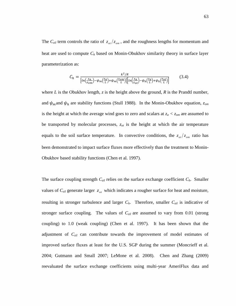
63

The Czil term controls the ratio of , and the roughness lengths for momentum and

heat are used to compute Ch based on Monin-Obukhov similarity theory in surface layer

parameterization as:

𝐶ℎ =𝑘2/𝑅

[𝑙𝑛(𝑧𝑎

𝑧𝑜𝑚)−𝜓𝑚(

𝑧𝑎𝐿

)+𝜓𝑚(𝑧𝑜𝑚

𝐿)][𝑙𝑛(

𝑧𝑎𝑧𝑜𝑡

)−𝜓ℎ(𝑧𝑎𝐿

)+𝜓ℎ(𝑧𝑜𝑡

𝐿)]

(3.4)

where L is the Obukhov length, z is the height above the ground, R is the Prandtl number,

and 𝜓𝑚and 𝜓ℎ are stability functions (Stull 1988). In the Monin-Obukhov equation, zom

is the height at which the average wind goes to zero and scalars at za < zom are assumed to

be transported by molecular processes, zot is the height at which the air temperature

equals to the soil surface temperature. In convective conditions, the ratio has

been demonstrated to impact surface fluxes more effectively than the treatment to Monin-

Obukhov based stability functions (Chen et al. 1997).

The surface coupling strength Czil relies on the surface exchange coefficient Ch. Smaller

values of Czil generate larger which indicates a rougher surface for heat and moisture,

resulting in stronger turbulence and larger Ch. Therefore, smaller Czil is indicative of

stronger surface coupling. The values of Czil are assumed to vary from 0.01 (strong

coupling) to 1.0 (weak coupling) (Chen et al. 1997). It has been shown that the

adjustment of Czil can contribute towards the improvement of model estimates of

improved surface fluxes at least for the U.S. SGP during the summer (Moncrieff et al.

2004; Gutmann and Small 2007; LeMone et al. 2008). Chen and Zhang (2009)

reevaluated the surface exchange coefficients using multi-year AmeriFlux data and

omot zz

omot zz

otz

64

obtained Czil values that are vegetation type dependent. They dynamically linked Czil as a

function of canopy height h (m) and represented it as:

Czil = 10(-0.4h)

(3.5)

These results motivate the need for investigating the impacts of Czil on mesoscale land-

atmospheric convection simulations over typical vegetation types and different regions.

Experimental details of all experiments and related Czil values are shown in Table 3.2.

Table 3.2 Summary of the coupling experiments

Case

name

Coupling coefficient

(Czil) Experimental focus Regions

UN 0.1, 0.5, 0.8 Uncoupled Noah LSM based

simulated surface heat fluxes U.S. SGP

BG

0.1, 0.3, 0.5, 0.8, 1.0 Bulk aerodynamic coefficient

of heat (Ch ) over U.S. SGP

Grassland

BC Cropland

BF Forest

CS

0.01, 0.05, 0.1, 0.3,

0.5, 0.8, var

Surface fluxes, 2 m temperature

and moisture, vertical profiles of

temperature, moisture, and wind

speed, etc.

U.S. SGP

CE Europe

CI India

CA West Africa

UN refers to uncoupled runs; B refers to uncoupled experiments for bulk Ch for grass (BG), cropland (BC),

and Forest (BF). C refers to coupled runs over U.S. SGP (CS), Europe (CE), India (CI), and West Africa

(CA).

3.4 Model verification and comparisons

3.4.1 Impact of the “Czil” on the offline Noah LSM

We first analyze impacts of the surface coupling strength coefficient on surface heat

fluxes within the offline or uncoupled experiments (UN). To obtain better surface fluxes

and equilibrium soil conditions at small scales, 18-month-long HRLDAS runs with three

65

different Czil values (0.1, 0.5, and 0.8) were conducted as spinup for offline Noah land

model experiments.

Fig. 3.2 shows a snapshot of the model output for the three different Czil values (referred

to as runs UN0.1, UN0.5, and UN0.8) and the impact on surface heat fluxes at the very

end day of the HRLDAS 18-month-long simulations (1800 UTC on 2 June 2002). The

area-averaged value of H decreases from 334 W m-2

to 205 W m-2

when the surface

coupling strength changes from 0.1 to 0.8. However, the area-averaged LE has small

variations, which are 2 W m-2

differences between UN0.1 and UN0.5 and 25 W m-2

differences between UN0.5 and UN0.8. It is noted that the influence of Czil on LE is

small compared to that on H. This is possibly due to the manner in which LE is

computed as the residual of the energy balance, suggesting that the offsets between

decreased net radiation and increased ground heat flux due to increasing Czil and the

decrease in H are small. Results also indicate that with increasing Czil, the coupling

strength becomes weak, resulting in less rough surface for heat/moisture, and the

simulated surface fluxes are less spatially heterogeneous.

66

The diurnal surface heat fluxes are averaged from 1 to 25 June 2002 over three different

land covers (grassland, cropland, and forest) in the U.S. SGP. As seen in Fig. 3.3, there

are small differences between the observed and modeled temporal-averaged LE over

grassland and cropland, but large impacts have been found on H. This may be caused by

drier soils in these locations which allow greater H changes in the simulations (Trier et al.

2011). The observed H lies between the model experiments of UN0.1 and UN0.5 over

grassland and cropland. The surface coupling strength has a notable effect on estimating

heat fluxes over the forest land cover, where the maximum difference between the

averaged observed and modeled surface fluxes is about 96.9 W m-2

for LE and 66.5W m-2

Fig. 3.2 A snapshot of cases (UN0.1, UN0.5, and UN0.8) with three different Czil values and resulting

impacts on latent heat flux (W m-2

) (upper row) and sensible heat flux (W m-2

) (bottom row) at 1800

UTC for 2 June 2002.

67

for H. In spite of these relatively large impacts on heat fluxes over forest, the observed

and modeled LE of UN0.1 are comparable, while H from UN0.8 is in better agreement

with the observed data, indicating that only over a forest land cover the surface coupling

strength of LE is stronger than that of H.

To further analyze the land-atmosphere coupling strength over the three different land-

cover types, experiments were conducted with a broader range of Czil values. These

experiments are labeled as BG, BC, and BF. As seen in Fig. 3.4, Czil values lead to

different soil temperature and soil moisture fields. Higher soil moisture and warmer

surface leads to higher LE due to more surface evaporation and transpiration. The

impacts of soil moisture on surface heat fluxes are more significant on grassland and

cropland when the soils are drier and not saturated. Smaller differences caused by

coupling strength can be seen in soil moisture in the forest region, but the soil

temperature differences are significant and affect LE. For example, the higher soil

temperature leads to smaller LE and less surface evaporation into atmosphere.

Table 3.3 Comparisons of surface exchange coefficient of heat (Ch) between observation and model

runs with different Czil values over three vegetation types in U.S. SGP. The results are temporally

averaged for June 2002.

Veg Types/

Observational Site Observation Czil=0.1 Czil=0.3 Czil=0.5 Czil=0.8 Czil=1.0

Grassland (h < 1m) 0.0025 0.058 0.030 0.020 0.013 0.011

Cropland (h = 3m) 0.019 0.040 0.022 0.017 0.011 0.009

Forest (h = 25m) 0.037 0.042 0.016 0.010 0.003 0.001

68

Fig. 3.3 Comparisons of 25 day-averaged surface latent heat flux (W m-2

) and sensible heat flux (W

m-2

) between observation and offline experiments over (a) grassland, (b) cropland, and (c) forest in

U.S. SGP.

Forest

Forest

69

Fig. 3.4 Variations of averaged-daily simulated surface variables: (a-c) precipitation forcing (mm day-1

), (d-

f) surface soil moisture (m3 m

-3), (g-i) surface soil temperature (K), (j-l) latent heat flux (W m

-2), and (m-o)

sensible heat flux (W m-2

) from offline Noah experiments over grassland (left column), cropland (middle

column), and forest (right column).

(a)

(d)

(g)

(j)

(m)

(b)

(e)

(h)

(k)

(n)

(c)

(f)

(i)

(l)

(o)

70

The Ch, which is directly related to the coupling strength and controls the total energy

flux, is evaluated to explore the land-atmosphere coupling strength. Using Eq. 3.1, the

surface exchange coefficient, Ch, can be written as

(3.6)

The IHOP_2002 experiment provided 30-minute observed surface data, including

sensible heat flux, wind speed at 10 m, surface temperature, air temperature, downward

solar radiation, and outgoing longwave radiation. Using observed air temperature and

outgoing longwave radiation, θa and θs are calculated. These 30-minute data are then

used to compute Ch which is referred to as observed Ch. The observed and offline Noah

modeled Ch are then averaged from 1700 UTC to 2100 UTC in June 2002 to obtain

midday values, the results of which are shown in Table 3.3 and Fig. 3.5. It can be seen

that BG0.1, BC0.1, and BF0.1 have large averaged-daily variations of Ch. The modeled

Ch of BG1.0 over the grass site located at Elmwood, OK (36.62°N, 100.62°W) is in better

agreement with the observations. Over the Bondville, IL, a cropland site (40.00°N,

88.29°W, Table 3.3), the averaged value of Ch for BC0.5 is the closest to the observed Ch.

The primary vegetation type in the Ozark, MO site (38.74°N, 92.20°W) is deciduous

broadleaf forest land cover with typical plant height at 25 m. Tall vegetation sites, such

as forest, have rougher surfaces and results in stronger turbulence and the observed Ch

has large variability over the forest. The differences between air and surface

temperatures which have effects on limiting the flux of net radiative heat transfer from

the atmosphere to the soil are larger. Since the calculation of observed Ch is affected by

the differences between potential surface and air temperatures, the observed Ch has large

variability over the forest. The larger roughness also leads to larger Ch, indicating that

asph UCHC /

71

the surface coupling effects in forest area are stronger. The result shown in Fig. 3.5c

suggests a relatively good agreement between the modeled Ch of BF0.1 and the

observation corresponds well. Thus, consistent with prior results, it is concluded that a

constant value of Czil cannot provide good agreement across different land-cover types in

the version of the Noah LSM being used in WRF.

Fig. 3.5 Comparisons of midday values of Ch (m s-1

) averaged from 1700 UTC to 2100 UTC in June

2002 between observation and offline experiments: (a) BG, (b) BC, and (c) BF.

72

3.4.2 The impacts of the Czil coupling parameter on the WRF-Noah model

The impacts of the coupling strength, especially the dynamic vegetation type-dependent

coupling strength (Czil-var) (Table 3.2), on convective WRF-Noah model simulations are

investigated next. The experiments are over different hotspot regions (U.S. SGP, Europe,

northern India, and West Africa) with different surface coupling strength. Impacts of

surface coupling strength on surface and boundary layer variables such as surface heat

fluxes, 2 m temperature and moisture, 10 m wind speed, precipitation, PBL soundings,

are then analyzed and discussed.

3.4.2.1 U.S. SGP

(a) Surface flux analysis

Model simulations covering a 48-hr period were conducted with a variety of Czil values

initialized at 1200 UTC 12 June 2002. To study atmospheric feedback to surface

coupling strength following spinup, the results in Fig. 3.6 show the second day runs over

grassland and cropland simulated 24 hrs after the initial condition. The experiments with

the weak coupling strength (CS0.8) have better match with the observations (Fig. 3.6),

but the coupling strength once again modestly affects LE values over cropland. The runs

CS0.8 over both grassland and cropland match the observed H. Rainfall modifies soil

moisture and leads to higher LE. The increased LE is accompanied with a decreased H

from the surface, indicating a smaller Ch, and hence weaker coupling strength of H. In

response to the weak coupling strength the surface air temperature is increased as less H

is transported from the surface, resulting in an increase in ground heat flux. As a result,

the weak coupling strength runs overestimate the soil surface temperature and the

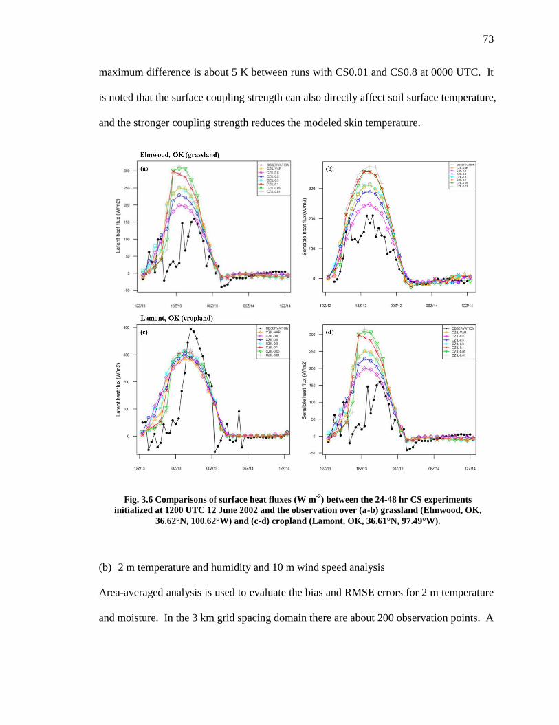
73

maximum difference is about 5 K between runs with CS0.01 and CS0.8 at 0000 UTC. It

is noted that the surface coupling strength can also directly affect soil surface temperature,

and the stronger coupling strength reduces the modeled skin temperature.

(b) 2 m temperature and humidity and 10 m wind speed analysis

Area-averaged analysis is used to evaluate the bias and RMSE errors for 2 m temperature

and moisture. In the 3 km grid spacing domain there are about 200 observation points. A

Fig. 3.6 Comparisons of surface heat fluxes (W m-2

) between the 24-48 hr CS experiments

initialized at 1200 UTC 12 June 2002 and the observation over (a-b) grassland (Elmwood, OK,

36.62°N, 100.62°W) and (c-d) cropland (Lamont, OK, 36.61°N, 97.49°W).

74

majority of the observed data is from NCEP Automated Data Processing (ADP) Global

Upper Air and Surface Weather Observations and obtained from meteorological sites

with 6 hrs temporal resolution. The satellite wind data is obtained from the National

Environmental Satellite Data and Information Service (NESDIS).

Table 3.4 Biases and RMSE of 2 m temperature (T), 2 m moisture (Q), and 10 m wind speed (WSPD)

for 0-48 hr model forecasts over U.S. SGP at 3-km grid spacing

Coupling

coefficient

(Czil) case

Bias RMSE

2 m T

(K)

2 m Q

(10-3

×kg kg-1

)

WSPD

(m s-1

)

2 m T

(K)

2 m Q

(10-3

×kg kg-1

)

WSPD

(m s-1

)

CS0.01 -3.27 0.41 1.49 4.09 2.13 3.49

CS0.05 -3.16 0.30 1.63 4.01 2.08 3.47

CS0.1 -3.01 0.22 1.40 3.90 2.05 3.48

CS0.3 -2.67 -0.02 1.43 3.69 2.03 3.47

CS0.5 -2.47 -0.18 1.35 3.62 2.05 3.35

CS0.8 -2.36 -0.37 1.29 3.65 2.12 3.20

CSvar -3.04 0.20 1.53 3.93 2.09 3.38

Table 3.4 shows the mean bias and RMSE of 2 m temperature and moisture, and 10 m

wind speed for the 0-48 hr model forecasts. All model runs show cold biases, with

CS0.01 and CSvar show the largest cold biases in the surface layer. This is a result of

strong surface coupling strength causing more H being lost from the surface leading to a

cooler surface. The bias and RMSE of 2 m temperature increase as the coupling strength

became stronger, and the 2 m moisture of CS0.01, CS0.05, and CS0.1 show wet biases.

The coupling coefficients in CS0.3, CS0.5, and CS0.8 lead to dry biases and the smallest

bias of the 2 m moisture occurs in CS0.3. The impact of the surface coupling strength on

the 10 m winds is relatively small.

(c) Planetary Boundary Layer: Temperature, Humidity and Wind speed profile

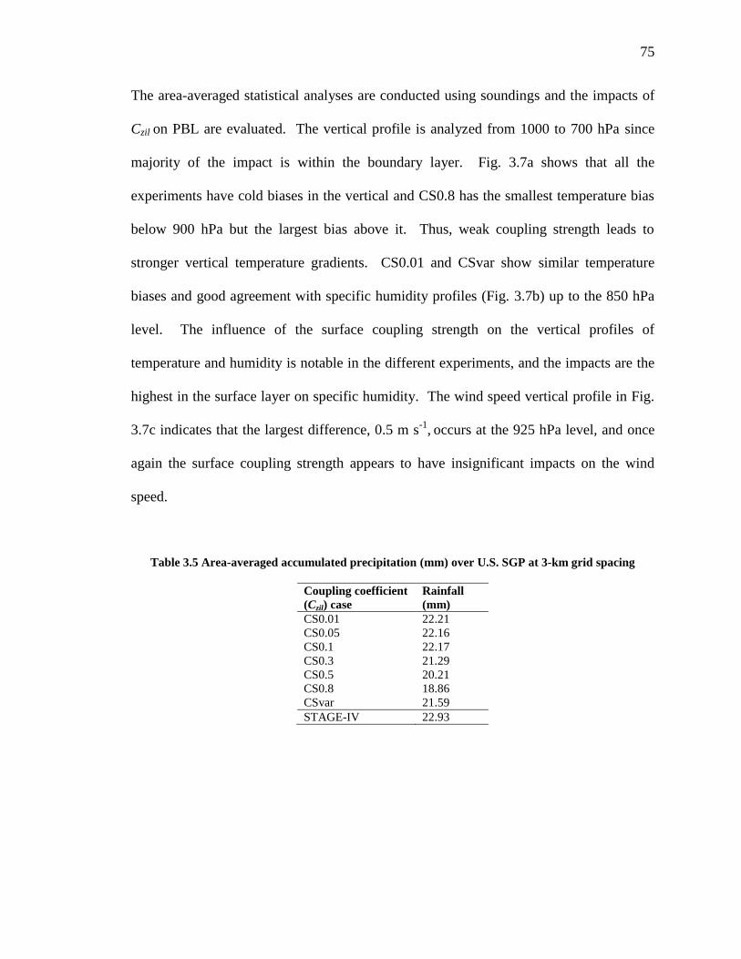
75

The area-averaged statistical analyses are conducted using soundings and the impacts of

Czil on PBL are evaluated. The vertical profile is analyzed from 1000 to 700 hPa since

majority of the impact is within the boundary layer. Fig. 3.7a shows that all the

experiments have cold biases in the vertical and CS0.8 has the smallest temperature bias

below 900 hPa but the largest bias above it. Thus, weak coupling strength leads to

stronger vertical temperature gradients. CS0.01 and CSvar show similar temperature

biases and good agreement with specific humidity profiles (Fig. 3.7b) up to the 850 hPa

level. The influence of the surface coupling strength on the vertical profiles of

temperature and humidity is notable in the different experiments, and the impacts are the

highest in the surface layer on specific humidity. The wind speed vertical profile in Fig.

3.7c indicates that the largest difference, 0.5 m s-1

, occurs at the 925 hPa level, and once

again the surface coupling strength appears to have insignificant impacts on the wind

speed.

Table 3.5 Area-averaged accumulated precipitation (mm) over U.S. SGP at 3-km grid spacing


(Czil) case Rainfall

(mm)

CS0.01 22.21

CS0.05 22.16

CS0.1 22.17

CS0.3 21.29

CS0.5 20.21

CS0.8 18.86

CSvar 21.59

STAGE-IV 22.93

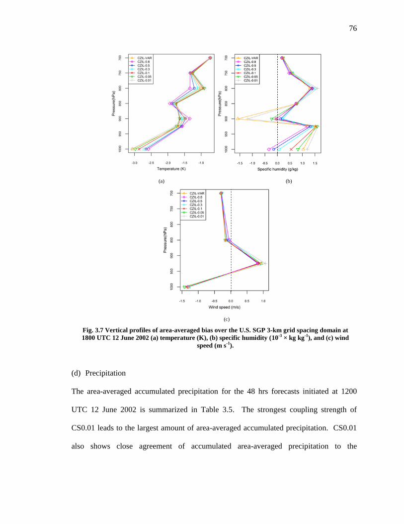
76

(d) Precipitation

The area-averaged accumulated precipitation for the 48 hrs forecasts initiated at 1200

UTC 12 June 2002 is summarized in Table 3.5. The strongest coupling strength of

CS0.01 leads to the largest amount of area-averaged accumulated precipitation. CS0.01

also shows close agreement of accumulated area-averaged precipitation to the

(a) (b)

(c)

Fig. 3.7 Vertical profiles of area-averaged bias over the U.S. SGP 3-km grid spacing domain at

1800 UTC 12 June 2002 (a) temperature (K), (b) specific humidity (10-3

× kg kg-1

), and (c) wind

speed (m s-1

).

77

observation, and the amount of rainfall for CSvar and CS0.3 are similar to each other.

Since heavier rainfall is obtained by increasing the coupling strength through decreased

values of Czil, it is possible that the model’s ability to correctly simulate rainfall can be

tuned through surface coupling coefficient, particularly in areas where there is a known

bias with convection triggering and rainfall under prediction. The weak coupling tends to

produce weak convective system with less precipitation whereas the strong coupling

results in more water vapor into the atmosphere and ultimately more precipitation.

Interestingly, the coupling strength does not appear to affect the timing of the peak rains,

and only alters the amount of the precipitation. These results need to be examined with a

larger ensemble of CP experiments, but are consistent to those reported in Trier et al.

(2011) for the U.S. SGP.

To further explore the impact of Czil on precipitation, 3 hr (0000 UTC - 0300 UTC 13

June 2002) accumulated precipitation (Fig. 3.8) was analyzed. The experiments with

constant Czil values have similar precipitation patterns in the U.S. SGP domain. Results

again highlight that the constant surface coupling strength does not affect the general

location but only the magnitude of the simulated precipitation. However, the dynamic

Czil improves both the pattern and location of the simulated precipitation in our

experiments. For instance, results show that the 3 hr accumulated precipitation of Czil-var

has a better spatial agreement to the STAGE-IV observed precipitation than those of the

constant values in the northern part of Texas. Therefore, the dynamic Czil shows

promising potential for improving the simulation of warm rain quantitative forecast over

the U.S. SGP.

78

Fig. 3.8 Comparisons of the 3 hrs accumulated precipitation (0000 – 0300 UTC) on 13 June 2002

over the U.S. SGP 3-km grid spacing domain between the model forecasts with (a) Czil = 0.01, (b) Czil

= 0.05, (c) Czil = 0.1, (d) Czil = 0.3, (e) Czil = 0.5, (f) Czil = 0.8, (g) dynamic Czil-var, and (h) the STAGE-

IV observed precipitation.

79

3.4.2.2 Europe

(a) Analysis of surface flux, 2 m temperature, and friction velocity

The surface flux observations used for the European domain correspond to Black Forest,

Germany (48.54°N, 8.397°E) and are centered in the 3 km grid spacing model domain

(Fig. 3.1b). The study region is characterized by significant amounts of orographic

rainfall in summer. The flux analysis shows that CE0.1 and CEvar have similar LE (Fig.

3.9a), but the simulated LE with the weak coupling strength of CE0.8 leads to about 22

Wm-2

reduction than that with the strong coupling strength of CE0.05. The mean of the

24 hrs observed LE is 50.77 W m-2

, and CE0.3 (52.50 W m-2

for LE) is found to be close

to the observation. The mean of LE for the dynamic Czil experiment (58.66 W m-2

) shows

better agreement with the observation than that for CE0.8 (38.26 W m-2

), but the dynamic

Czil experiments do not improve the simulated LE. Majority of the model simulations

overestimated H before evening (1800 UTC, 7 pm local time). During the night time

after 1800 UTC, model forecasts of LE have good agreement with the observations, and

H for CE0.3, CE0.5, and CE0.8 agree well with observations. The overestimation of LE

from the model leads to more moisture in the surface layer and decreases the 2 m

temperature. As a result, the 2 m temperature is underestimated by 2-5 K in all Czil

experiments (Fig. 3.9c). The 10 m wind speed again indicates that surface coupling

strength has little impact on the surface wind speed.

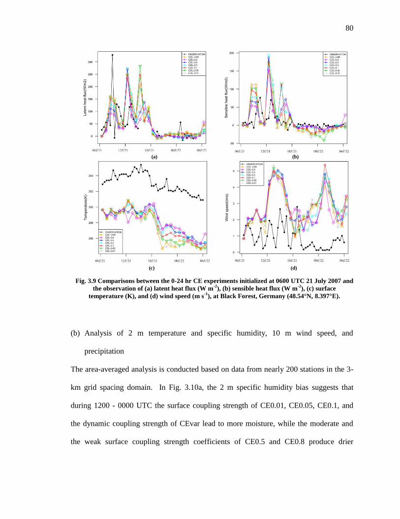
80

(b) Analysis of 2 m temperature and specific humidity, 10 m wind speed, and

precipitation

The area-averaged analysis is conducted based on data from nearly 200 stations in the 3-

km grid spacing domain. In Fig. 3.10a, the 2 m specific humidity bias suggests that

during 1200 - 0000 UTC the surface coupling strength of CE0.01, CE0.05, CE0.1, and

the dynamic coupling strength of CEvar lead to more moisture, while the moderate and

the weak surface coupling strength coefficients of CE0.5 and CE0.8 produce drier

(a) (b)

(c) (d)

Fig. 3.9 Comparisons between the 0-24 hr CE experiments initialized at 0600 UTC 21 July 2007 and

the observation of (a) latent heat flux (W m-2


), (c) surface

temperature (K), and (d) wind speed (m s-1

), at Black Forest, Germany (48.54°N, 8.397°E).

81

boundary layer. The model simulated moisture is improved for CE0.3. Fig. 3.10b shows

that there is about a 1-4 K 2 m temperature cold biases in all the experiments. Reductions

in the temperature bias are noted for the moderate and the weak coupling strength of

CE0.5 and CE0.8. CE0.1 which is the default coupling coefficient in current WRF model

shows similar 2 m temperature and moisture biases to CEvar, but both of them fail to

improve surface temperature and moisture. The 10 m wind speed was also analyzed and

the biases of the different coupling strength increased before 1800 UTC when a heavy

rainfall occurred and then the biases decreased in the evening. The similarity of patterns

in Fig. 3.10c corresponds well to our previously stated conclusion for other regions that

the surface coupling appears to have insignificant impact on surface wind speeds. The

higher winds contribute to the low temperature bias through increased mechanical

mixing.

The Equitable Threat Score (ETS) of 3 hrs accumulated precipitation over the 9 km grid

spacing domain in Europe are assessed to analyze the coupling strength influence. The

Experimental Real-Time TRMM Multi-Satellite Precipitation Analysis (TMPA) data are

used for comparisons. As seen in Fig. 3.10d, the runs show limited skill, but the impacts

of the coupling strength is still evident. A more reasonable precipitation simulation is

found with the weak coupling strength coefficient of CE0.8. Results indicate that the

dynamic Czil, and weak coupling strength may be helpful to improve summer convection

simulations over Europe.

82

3.4.2.3 North India

(a) Reflectivity

A series of X-band Doppler weather radars (DWRs) are operated by India Meteorological

Department (IMD) in weather mode for detection of localized weather phenomenon

(Routray et al. 2010). The reflectivity product from the New Delhi DWR is used for

model comparisons. Fig. 3.11 presents the radar reflectivity field from all the

experiments and the observation corresponding to 1200 UTC 12 May 2012. CI0.5 and

CI0.8 show wider regions of stratiform precipitation (25-40 dBZ) which are closer to the

observation. Strong coupling strength leads to lighter rain and smaller areas of

precipitation, but the dynamic Czil modestly improved the precipitation intensity and

Fig. 3.10 0-24 hr model forecast, initialized at 0600 UTC 21 July 2007, area-averaged bias over

Europe 3-km grid spacing domain of (a) 2 m specific humidity (10-3

× kg kg-1

), (b) 2 m temperature

(K), (c) 10 m wind speed (m s-1

), and (d) ETS of 3 hrs accumulated precipitation from 0600 UTC

21 July to 0600 UTC 22 July 2007 over the European 9-km grid spacing domain.

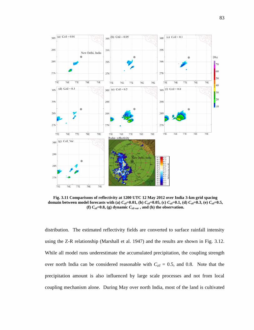
83

distribution. The estimated reflectivity fields are converted to surface rainfall intensity

using the Z-R relationship (Marshall et al. 1947) and the results are shown in Fig. 3.12.

While all model runs underestimate the accumulated precipitation, the coupling strength

over north India can be considered reasonable with Czil = 0.5, and 0.8. Note that the

precipitation amount is also influenced by large scale processes and not from local

coupling mechanism alone. During May over north India, most of the land is cultivated

Fig. 3.11 Comparisons of reflectivity at 1200 UTC 12 May 2012 over India 3-km grid spacing

domain between model forecasts with (a) Czil=0.01, (b) Czil=0.05, (c) Czil=0.1, (d) Czil=0.3, (e) Czil=0.5,

(f) Czil=0.8, (g) dynamic Czil-var , and (h) the observation.

84

and the dry parched surface produces thermals into the atmosphere. These thermals when

interacting with larger moisture source often lead to regional precipitation events. The

model appears to capture these feedbacks as the weak coupling is dominant over

cultivated but parched land surface.

(b) Statistical analysis

The 0-24 hr area-averaged 2 m temperature and moisture, and 925 mb wind speed biases

are shown in Fig. 3.13 and the mean values of the bias are presented in Table 3.6. All the

runs show cold biases but a better response in simulating 2 m temperature is achieved

with the weak coupling strength of CI0.8. CIvar and CI0.5 show similar feedbacks on

temperature, while the strong coupling strength of CI0.01 produces the largest

temperature bias. All the coupling runs show dry biases, and a slightly better response

occurs with the strong coupling coefficient of CI0.01. Since the strong coupling strength

Fig. 3.12 Comparison of accumulated precipitation initiated at 0000 UTC 12 May 2012 over India

3-km grid spacing domain between model forecasts and the observation.

85

leads to relatively more moisture than the other runs, as a feedback the LE of the strong

coupling run is higher. As the surface coupling strength is linked to the evolution of

moisture in the model (Trier et al. 2011), the weak coupling strength produces drier

environment for the PBL, resulting in reduced moisture (Fig. 3.14b). The wind speeds at

925 hPa of all experiments show similar biases before 1200 UTC, but large differences

are noted between 1200 UTC 11 May and 0000 UTC 13 May 2012 and CIvar has the

least bias. The vertical profiles of the area-averaged bias from the surface to 700 hPa

levels in the PBL are shown in Fig. 3.14. Significant impacts of the coupling strength are

found below 925 hPa, where all the simulations show lower temperature, less moisture,

and larger wind speed biases. The wind speed profile shows mixed results, whereas the

CIvar indicates an improved response.

TRMM data are used to assess the ETS of 3 hrs accumulated precipitation over the 9 km

grid spacing India domain (Fig. 3.13d). All model runs show similar precipitation results

though the weak coupling strength leads to higher ETS scores and a better precipitation

forecast. The observation and model based histograms of 147 stations (grid) based WRF

2 m temperature and 2 m specific humidity are generated in Figs. 3.15 and 3.16. The

histogram of CI0.8 shows similar distribution as compared to the range of 305-310 K in

the 2 m temperature observation histogram. All of the other coupling strengths produce

lower frequencies of 305-310 K range but higher frequencies are observed within the

range of 300-305 K. The histograms correspond well with the results of area-averaged

biases, emphasizing that the weak coupling strength has the best results for simulating the

2 m temperature. On the contrary, the 2 m specific humidity histogram of CI0.8 has the

86

largest difference compared to observations indicating that the weak coupling strength is

not able to capture the 2 m specific humidity over the northern Indian region. So, “what

is an optimum coupling strength for the Indian monsoon region?” is still an open question.

Our results do indicate that the constant value used in the default Noah/WRF model is not

the optimal value.

Table 3.6 Biases of 2 m temperature (T), 2 m moisture (Q), and surface wind speed (WSPD) for 0-24

hr model forecasts over India domain at 3-km grid spacing


(Czil) case 2 m T

(K)

2 m Q

(10-3

×kg kg-1

)

WSPD

(m s-1

)

CI0.01 -2.95 -1.59 0.11

CI0.05 -2.84 -1.66 0.04

CI0.1 -2.69 -1.68 -0.06

CI0.3 -2.38 -1.76 -0.26

CI0.5 -2.27 -1.83 -0.37

CI0.8 -2.19 -1.87 -0.49

CIvar -2.33 -1.79 -0.06

Fig. 3.13 0-24 hr model forecast initialized at 0000 UTC 12 May 2012, area-averaged bias over the

Indian 3-km grid spacing domain of (a) 2 m specific humidity (10-3

× kg kg-1

), (b) 2 m temperature

(K), (c) 10 m wind speed (m s-1

), and (d) ETS of 3 hrs accumulated precipitation from 0000 UTC

12 July to 0000 UTC 13 May 2012 over the Indian 9-km grid spacing domain.

87

(a) (b)

(c)

Fig. 3.14 Vertical profiles of area-averaged bias over the Indian 3-km grid spacing domain at 1200

UTC 12 May 2012 for (a) temperature (K), (b) specific humidity (10-3

× kg kg-1

), and (c) wind

speed (m s-1

).

88

Fig. 3.15 147 points histograms of the observation and the WRF model forecasts for 2 m temperature

(K): (a) Observation, (b) Czil = 0.01, (c) Czil = 0.05, (d) Czil = 0.1, (e) Czil = 0.3, (f) Czil = 0.5, (g) Czil = 0.8,

and (h) dynamic Czil-var.

(a) Observation (b) Czil = 0.01

(c) Czil = 0.05 (d) Czil = 0.1

(e) Czil = 0.3 (f) Czil = 0.5

(g) Czil = 0.8 (h) Czil_var

89

Fig. 3.16 147 points histograms of the observation and the WRF model forecasts for 2 m specific

humidity (kg kg-1

): (a) Observation, (b) Czil = 0.01, (c) Czil = 0.05, (d) Czil = 0.1, (e) Czil = 0.3,

(f) Czil = 0.5, (g) Czil = 0.8, and (h) dynamic Czil-var.

(a) Observation (b) Czil = 0.01

(c) Czil = 0.05 (d) Czil = 0.1

(e) Czil = 0.3 (f) Czil = 0.5

(g) Czil = 0.8 (h) Czil_var

90

3.4.2.4 West Africa

(a) Surface flux analysis

The impact of different coupling strengths on surface heat fluxes over the West African

domain is shown in Figs. 3.17 a and b. CAvar results in a better estimation of LE but

overestimates H. The H for CA0.3 has a good agreement with the observation, but the

bias increases with stronger coupling when the coupling coefficient is decreased from 0.3

to 0.01. Since the LE of CA0.3 also matches well to the observations, the coupling

strength of CA0.3 could be able to modify the surface fluxes over West Africa. The

surface air temperature is affected by H and is expected to be sensitive to surface

coupling strength. The runs with strong coupling strength show good agreement between

the 2 m temperature and observations (Fig. 3.17c), but CAvar results in about 1-3 K

lower temperature before 0300 UTC and higher temperatures after that. The constant

coupling coefficients have little impacts on the 10 m wind speed, but the impact of Czil on

friction velocity is significant over West Africa. Since the smaller Czil leads to larger

roughness length for heat which means rougher surface for heat and moisture, the surface

turbulence is stronger and results in larger friction velocity. Although the temporal

patterns of the friction velocity are similar among the different coupling runs, the strong

coupling strength and the dynamic Czil lead to relatively poor simulations of the friction

velocity (Fig. 3.17d).

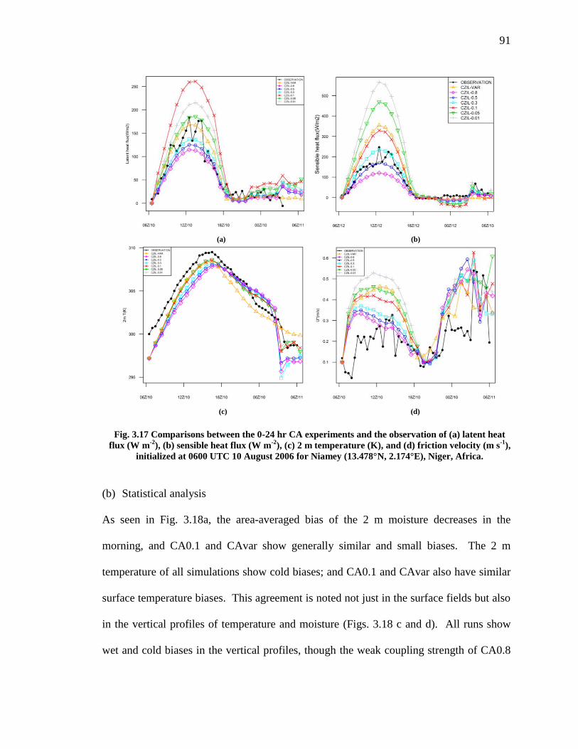
91

(b) Statistical analysis

As seen in Fig. 3.18a, the area-averaged bias of the 2 m moisture decreases in the

morning, and CA0.1 and CAvar show generally similar and small biases. The 2 m

temperature of all simulations show cold biases; and CA0.1 and CAvar also have similar

surface temperature biases. This agreement is noted not just in the surface fields but also

in the vertical profiles of temperature and moisture (Figs. 3.18 c and d). All runs show

wet and cold biases in the vertical profiles, though the weak coupling strength of CA0.8

(a) (b)

(c) (d)

Fig. 3.17 Comparisons between the 0-24 hr CA experiments and the observation of (a) latent heat

flux (W m-2


), (c) 2 m temperature (K), and (d) friction velocity (m s-1

),

initialized at 0600 UTC 10 August 2006 for Niamey (13.478°N, 2.174°E), Niger, Africa.

92

results in the best performance. The impacts of the coupling strength are more significant

at the surface. All the model runs have generally similar humidity biases around 925 hPa,

but the different responses caused by the surface coupling strength show up again around

900 hPa. The wind speed forecast is improved by strong coupling strength in the surface

layer, but the weak surface coupling strength run shows a smaller bias between the levels

of 925 hPa and 850 hPa (Fig. 3.18e). The impact noted on wind speed for this case is not

entirely apparent and is likely a result of the larger domain considered in this experiment.

(a) (b)

(c) (d) (e)

Fig. 3.18 0-24 hr model forecast, initialized at 0600 UTC 10 August 2006, area-averaged bias over

the West African 3-km grid spacing domain of (a) 2 m specific humidity (10-3

× kg kg-1

), (b) 2 m

temperature (K); Vertical profiles of domain averaged bias over a 3-km grid spacing domain for

(c) temperature (K), (d) specific humidity (10-3

× kg kg-1

), and (e) wind speed (m s-1

) at 1200 UTC

10 August 2006.

93

(c) Precipitation

The 3 hrs accumulated precipitation over the West African region is simulated by all Czil

experiments and again the TRMM-based precipitation estimates are used for comparisons.

Fig. 3.19 Comparisons of the 3 hrs accumulated precipitation (0300 – 0600 UTC) on 11 August

2006 over west Africa 3-km grid spacing domain between model forecasts with (a) Czil=0.01, (b)

Czil=0.05, (c) Czil=0.1, (d) Czil=0.3, (e) Czil=0.5, (f) Czil=0.8, (g) dynamic Czil-var , and (h) the TRMM-

based precipitation.

94

Again the results show consistency in that the surface coupling strength affects

precipitation intensity and not the location. The dynamic Czil experiment (Fig. 3.19g)

successfully simulates one of the heavy rainfall systems identified in the TRMM-based

precipitation estimates, but was missed in other experiments (Fig. 3.19h).

3.5 Conclusions and discussions

In this study, the impact of land-atmosphere coupling was assessed using an offline Noah

LSM and the coupled Noah/WRF model for select summer time mesoscale convection

and heavy rainfall cases over the U.S. SGP, Europe, northern India, and West Africa

regions. The potential benefit of using the dynamic formulation for representing the land

atmosphere coupling was studied over the four different coupling “hotspot” regions. The

area-averaged statistical analysis of 2 m temperature and moisture and 10 m wind speeds

were conducted and the impacts of surface coupling strength on precipitation were

evaluated. The Czil is found to have good potential to modulate the model results and

particularly improve the simulation of the convective systems. The dynamic coupling

strength helps improve the precipitation forecasts in terms of intensity but not necessarily

its location.

The impacts of the coupling effect on the convection vary across different land-cover

types and over different regions. Over the different regions, the model biases response

varies with the changes in coupling strength. Significant impacts from surface coupling

strength are found between the surface layer and the 925 hPa level. In summer, over the

U.S. SGP the strong coupling leads to cold and wet boundary layer, resulting in strong

95

convective system and heavier rainfall, whereas the coupling over northern India is

relatively weak and produces lighter rain and smaller areas of precipitation due to the

cultivated parched land surface. However, because of the unavailability of observed

surface fluxes in India, the coupling impacts on surface energy and surface variables need

further analysis when additional data become available. The model performance with

different Czil values may vary with different PBL schemes or CPs. Thus, additional

ensemble experiments are needed in future studies.

Surface heat fluxes show the largest impact in terms of the coupling strengths assigned

over different regions. Results indicate that the constant surface coupling coefficient

adopted in the current coupled Noah/WRF model has deficiency in producing correct

surface fluxes. Over the U.S. SGP, H is better simulated by the weak coupling

coefficient (Czil = 0.8), while LE from runs with the strong coupling coefficients (Czil =

0.01 and 0.05) and the dynamic Czil-var match the observations better. In addition, the

strong coupling strength overestimates the surface temperature and is able to modify the

surface and atmospheric characteristics. The surface heat fluxes are overestimated during

the daytime in all the model runs over the European domain. The runs with Czil = 0.5 and

the dynamic Czil-var have a similar LE evolution, and the coupling strength Czil = 0.3 leads

to an improvement of LE. Over West Africa, the current WRF model leads to coupling

effects that are too strong and could be improved by decreasing the coupling coefficient

to 0.3 in the land model. The dynamic Czil_var is able to improve the simulations of the

surface fluxes over West Africa.

96

The model over predicts the sensible heat flux in the convective PBL with all coupling

strengths and this may be due to errors in the different boundary layer formulations

within the model (Hacker and Angevine 2013) and not just a coupling coefficient based

problem. The weak coupling strength also potentially acts to buffer or reduce the biases.

A strong vertical moisture gradient is a sign of the weak coupling effects. Excess

moisture is reduced by the weak coupling strength which produces a drier environment

for the PBL due to the linkage between the surface coupling strength and the evolution of

moisture in the model. Over prediction of the 10 m wind speed produces too large

momentum fluxes over the four regions, and the momentum fluxes are generally

insensitive to the coupling strength (except in the case of West Africa region).

One important and consistent result that emerged from analysis over the different regions

is that the precipitation locations are not affected by the coupling strength in all the

experiments, but the coupling strength does have impacts on the magnitude of the

precipitation and changes the local spatial and temporal patterns of the rainfall. Our

investigation also reveals that improvements made to the existing surface and atmosphere

coupling strength by adopting the dynamic coupling coefficient are helpful in improving

precipitation predictions.

There is high uncertainty in land-atmosphere coupling findings and the results from this

and prior studies need to be considered with caution. Zones identified as coupling

hotspots in climate studies, and the associated coupling strength would likely change

depending on the model roughness/coupling coefficient assigned. Thus the “actual”

97

coupling itself is perhaps a model artifact-albeit a useful one to study different processes

including improving predictability. As a result, the zone of “high” or “low” coupling

strength should be considered in the context of the model and parameterizations used.

More efforts need to be directed toward adopting the dynamic Czil rather than a constant

value that is currently used in the Noah/WRF like models. Model results are consistently

though modestly improved and encouraging when a dynamic Czil is used. Therefore, the

dynamic Czil formulation is recommended for use in future studies but with a caution for

use over complex terrains. Evaluating the impact of coupling coefficient in a coupled

model is highlighted as the results may be different than in the offline mode. Our results

indicate that identifying the correct coupling is a challenge as it can improve one variable

and deteriorate another. The coupling coefficient has significant control on the model

performance particularly the quantitative precipitation forecasts and is thus an important

feature for studying hydrometeorological extremes such as droughts and heavy rain

events.

98

CHAPTER 4. IMPROVING HIGH-RESOLUTION WEATHER FORECASTS USING

THE WEATHER RESEARCH AND FORECASTING (WRF) MODEL WITH AN

UPDATED KAIN-FRITSCH SCHEME3

4.1 Introduction

Numerical weather prediction (NWP) forecast models have been greatly improved,

motivated by the role of providing accurate forecasts about severe weather events to

mitigate the loss of life and property. Furthermore, credibility of climate change

simulations at urban-scales can be increased by first improving the accuracy of high-

resolution model simulations at weather prediction timescales (Chen et al. 2011). In

particular, moist processes play an important role in properly simulating weather, air

pollution, climate and the hydrological cycle. Clouds and precipitation formed in these

processes are important forecast products, thus accurate prediction of precipitation is one

of the most beneficial areas of NWP improvement. For this reason, key processes

occurring within clouds, including microphysical and dynamical processes, need to be

well understood and modeled.

Cloud microphysics schemes have been used in NWP models, but those microphysical

processes may not be accurately represented due to the lack of supporting measurements

for many processes occurring at finer spatial and temporal scales. For example, the

3 Zheng, Y., K. Alapaty, J. A. Herwehe, A. D. Del Genio, D. Niyogi, 2015: Improving high-resolution

weather forecasts using the Weather Research and Forecasting (WRF) model with an updated Kain-Fritsch

scheme. Mon. Wea. Rev., doi: 10.1175/MWR-D-15-0005.1 (In press).

99

formulation described in Kain et al. (2008) has been found to be appropriate for WRF

Single Moment 6-class (WSM6) microphysics (Hong et al. 2004) and has been

successfully used in some numerical studies (e.g., Done et al. 2004; Deng and Stauffer

2006; Wulfmeyer et al. 2006; Case et al. 2008; Niyogi et al. 2011). However, according

to Clark et al. (2012), many such studies are not able to accurately clarify unique

precipitation particle and other physical parameters in different microphysical processes

using regional models such as the WRF model (Skamarock and Klemp 2008). This

problem revealed that many characteristics of the model results were quite sensitive to

the choice of microphysics scheme (Weisman et al. 2008; Dawson et al. 2010; Bryan and

Morrison 2012). Clark et al. (2012) also found that no single microphysics scheme could

surpass the others in performance during the 2010 National Oceanic and Atmospheric

Administration’s (NOAA’s) Hazardous Weather Testbed (HWT) Spring Forecasting

Experiment. There is also much debate on whether more complex microphysics schemes

provide value for precipitation forecasts (e.g., Luo et al. 2010; Seifert and Stevens 2010;

van Lier-Walqui et al. 2012; Van Weverberg et al. 2013). Based on the microphysics

scheme sensitivity study of Blossey et al. (2007), microphysics was found to have little

impact on decreasing a model’s apparently excessive precipitation efficiency.

Additionally, Cintineo et al. (2014) pointed out that large uncertainties remain in how

various microphysics schemes represent subgrid-scale microphysical processes. Thus, as

grid spacing decreases, cloud microphysics schemes have limitations in representing

moist convection (Arakawa and Jung 2011; Gustafson Jr. et al. 2013; Molinari and

Dudek 1992).

100

One reason for the partial failure of cloud microphysics schemes can be attributed to the

fact that grid-scale dynamics is separated from cloud physics. Additionally, there will be

clouds that are unresolved by high spatial resolutions (e.g., ~1 to 10 km grid spacings)

and their effects need to be accounted for to improve predictability (e.g., Molinari and

Dudek, 1992; Seaman et al. 1998). Thus, from these studies it can be inferred that, at

high spatial resolutions, usage of a cloud microphysics scheme alone (without an active

parameterized convection scheme) may not be sufficient to represent moist convection

and precipitation for warmer periods in weather forecasts.

The dynamic cloud processes that describe cloud formation and growth can impact the

timing, location, and intensity of precipitation. In many NWP models, the fractional

cloudiness can influence atmospheric radiation budgets as well as the dynamics and

thermodynamics, but in the past, subgrid-scale cumulus cloudiness and the associated

radiative impacts have been largely neglected outside of global climate models. Alapaty

et al. (2012) and Herwehe et al. (2014) emphasized and documented the importance of

incorporating such subgrid-scale cloud-radiation interactions using the Kain-Fritsch (KF)

CPS (Kain 2004) and the Rapid Radiation Transfer Model, Global (RRTMG) schemes

(Iacono et al. 2008). In order to represent subgrid-scale clouds at higher resolutions, it

will be shown that there is a need to relax some of the assumptions used in CPs (e.g., the

KF scheme). We address some of these issues that cause CPSs to degrade progressively

as resolution is increased, in particular for high-resolution modeling (for grid spacings on

the order of 1-10 km).

101

One of the many key parameters in CPSs is the convective adjustment timescale, a

characteristic time scale with which convective available potential energy (CAPE) is

reduced at an exponential rate by convection. This parameter is set as a constant value in

many regional and global models with the exception of a very few models (e.g., the

European Centre for Medium-Range Weather Forecasts model, Bechtold et al. 2008).

Literature indicated that there is some uncertainty in the specification of this parameter.

For example, Mishra and Srinivasan (2010) improved the simulation of the seasonal

mean precipitation significantly by increasing the adjustment time scale value from 1

hour to 8 hours, while Done et al. (2006) found that varying the adjustment timescale

from minutes to one day resulted in changing all CP-generated subgrid-scale rainfall to

only grid-scale precipitation. In addition, the magnitude of convective heating and drying

rates has been found to correlate with local CAPE more strongly at finer scales when grid

spacing is on the order of 1-10 km (Kain 2004). Another key cloud process is the

interaction between convection and its environment through entrainment and detrainment.

These processes are quite complex and are of vital importance in regional and global

models (e.g., Tokioka et al. 1988; Kain and Fritsch 1990; Kang et al. 2009). In many

global models (e.g., Neale et al. 2010), the entrainment rate is specified and is a

parameter often adjusted to improve results; however, there are very few regional and

global models in which the entrainment rate is empirically estimated (e.g., Kain 2004;

Chikira and Sugiyama 2010; Del Genio et al. 2012). But for high-resolution simulations,

assumptions made in the entrainment formulation of the KF scheme need to be

reconsidered. The convective momentum transport by cumulus convection is not

included in many regional models, but for high-resolution modeling the importance of

102

including such subgrid-scale transport on grid-scale vertical motions deserves attention

since it could help reduce model spin up time.

Based on the above considerations, a few updates that were explored using the KF

convection scheme are: inclusion of subgrid-scale cloud radiation interactions, a dynamic

adjustment timescale, impact of subgrid-scale cloud updraft mass fluxes on grid-scale

vertical velocity, and an entrainment methodology based on the lifting condensation level

(LCL). These changes introduce scale dependency for some of these key parameters in

the KF scheme with an expectation that they will improve weather forecasts at 9- and 3-

km grid spacings.

Since forecasts are sensitive to the initial conditions and small changes in the initial

conditions can lead to big changes farther out in time (Rabier et al. 1996; Stensrud et al.

2000), an accurate specification of the initial model state (i.e., the analysis of the

atmospheric state) can make a significant improvement in high-resolution NWP model

forecasts (Ehrendorfer 1997; Simmons and Hollingsworth 2002). In this study, we also

explore impacts of initial conditions on short-term high-resolution forecasts, as well as

the sensitivity to different initial conditions of a high-resolution NWP model that includes

an updated parameterized cloud dynamics. For that reason, we have made an attempt to

study the impacts of introducing scale-aware convective parameterized cloud dynamics

for high-resolution forecasts using two different initial analyses.

103

To improve the prediction of precipitation distribution and variability, this study

introduces several changes to the KF CPS in the WRF model and evaluates their impacts

on high-resolution short-term forecasts. Since high-resolution models can have varying

degrees of sensitivities to physics, dynamics, and initial conditions, the objectives of this

study are limited to understanding of the impacts of using (1) initial conditions obtained

from two different analysis fields, and (2) a scale-dependent UKF scheme on high-

resolution precipitation forecasts using WRF version 3.4.1 (Skamarock and Klemp 2008).

This paper is organized as follows: Section 2 presents methods for updating the KF

scheme; Section 3 describes the design of the numerical simulations; Section 4 evaluates

the WRF model performance; and summary and conclusions are provided in Section 5.

4.2 Methodology

For the purpose of improving high-resolution precipitation forecasts, we developed an

updated KF scheme based on the study of subgrid-scale cloud-radiation interactions by

Alapaty et al. (2012) by introducing grid resolution dependency and modifying the

adjustment timescale and entrainment processes which influence surface precipitation.

To help mitigate model spin up issues in short-range weather forecasts and associated

precipitation, we also considered the impacts of subgrid-scale cloud updraft mass fluxes

on grid-scale vertical velocity.

Multisensor Precipitation Estimates (MPE, also known as Stage IV Next-Generation

Radar) hourly rainfall products and the satellite infrared cloud observations were used for

validation of the model forecasts. MPE Stage IV is a national precipitation analysis

104

obtained from consideration of Next-Generation Radar data and precipitation gauges (Lin

and Mitchell 2005). MPE data at 4-km spatial resolution were obtained at hourly

intervals and interpolated for a 3 km grid spacing in our study. The high spatial

resolution of MPE data makes it possible to evaluate high-resolution NWP model

precipitation forecasts.

4.2.1 The KF CPS

The KF CPS (Kain and Fritsch 1990, 1993; Kain 2004) has been used successfully over

the years, incorporated in the Pennsylvania State University–National Center for

Atmospheric Research Mesoscale Model (Wang and Seaman 1997), the National Centers

for Environmental Prediction (NCEP) Eta Model (Black 1994), the WRF model

(Skamarock and Klemp 2008), and the new Model for Prediction Across Scales (MPAS)

(Skamarock et al. 2012). The KF scheme is a mass flux parameterization and uses the

Lagrangian parcel method, and it can be generally grouped into three parts: 1) the

convective trigger function, 2) the mass flux formulation, and 3) the closure assumptions.

The early version of the KF scheme (Kain and Fritsch 1990, 1993) utilized a simple cloud

model with moist updrafts and downdrafts, and has been modified for use by NWP

models. Several components of that KF scheme have been changed (Kain, 2004) to

include an updraft formulation (i.e., imposing a minimum entrainment rate, specified

cloud radius to vary as a function of subcloud-layer convergence, allowing a minimum

cloud depth to vary as a function of cloud-base temperature, and allowing shallow

convection), a downdraft formulation (i.e., introducing a new downdraft algorithm), and a

closure assumption (i.e., calculating CAPE based on the path of an entraining parcel). In

105

this study, we have used that latest version of the KF scheme (i.e., Kain, 2004) to

introduce several new science updates which are described in the following section.

4.2.2 A brief description of subgrid-scale cloud-radiation interactions

In most NWP models, subgrid-scale CPs do not consider cumulus cloud feedbacks to

radiation due to a lack of knowledge on how to estimate fractional cloudiness as a

function of parameterized clouds, resulting in biases in both regional weather and climate

simulations (Herwehe et al. 2014). Alapaty et al. (2012) introduced a subgrid-scale

cumulus cloudiness formulation to the KF CPS (Kain 2004) and the RRTMG models

(Iacono et al. 2008). The inclusion of subgrid-scale cloud-radiation interactions created

more realistic longwave and shortwave radiation variability, leading to the improvement

of several meteorological parameters at both the weather and climate timescales. Here,

we extend the study of subgrid-scale cloud-radiation interactions by relaxing some of the

assumptions used in the KF scheme and hypothesize that our UKF scheme will reduce

excessive precipitation in weather forecasts for short-term high-resolution modeling

studies.

4.2.3 A dynamic formulation for the adjustment timescale

The adjustment timescale (τ) is the time over which CAPE is reduced to stabilize the

atmosphere, originally introduced by Frisch and Chappell (1980). In the default

configuration of many NWP models, a constant value of τ is specified as a global

constant. The KF scheme uses a technique that was proposed by Fritsch and Chappell

(1980) for the estimation of τ based on the mean tropospheric horizontal wind speed and

106

grid resolution. However, as noted by Stensrud (2007), this formulation may approach its

limitation either for high resolution grids or for environments with strong winds, such as

hurricane simulations. Because of this limitation, τ was found to be one of the parameters

that caused wet biases in simulated precipitation amounts at 12-km grid spacing (Bullock

et al. 2015). As we move from coarser (~15 km) to high resolution (~1 km) grids, one

would expect the impacts of parameterized convection to gradually become less

significant. However, many CPSs cannot work properly at these finer scales because the

tendencies produced by parameterized convection dominate over resolved convection

(Arakawa and Jung 2011; Molinari and Dudek 1992). To make CPSs (such as KF)

seamless across these spatial scales, τ should increase with increased grid resolution such

that atmospheric stability restoration is gradually taken over by the resolved convective

processes. However, it does not occur with the existing τ methodology used in the KF

scheme as demonstrated by Bullock et al. (2015). To that effect, a formulation for τ is

developed by using cloud macrophysical parameters following the notion used by

Bechtold et al. (2008).

Considering the fact that many KF parameters are tied to grid spacing of around 25 km

(Kain 2004), we derive a new grid resolution-dependent dynamic formulation of the

adjustment timescale based on Bechtold et al. (2008):

𝜏 =𝐷𝑒𝑝𝑡ℎ 𝑆𝑐𝑎𝑙𝑒

𝑉𝑒𝑙𝑜𝑐𝑖𝑡𝑦 𝑆𝑐𝑎𝑙𝑒𝐹𝑛(𝐷𝑥) (4.1)

𝜏 =𝐻

𝑊𝛽 (4.2)

𝛽 = [1 + 𝑙𝑛 (25

𝐷𝑥)] (4.3)

107

where H is cloud depth (m), and W is cloud averaged vertical velocity (m s-1

). 𝐷𝑥 is the

horizontal grid-spacing (km), and 𝛽 is a scaling parameter dependent on the model’s

horizontal grid spacing 𝐷𝑥 (km), analogous to but different from that of Bechtold et al.

(2008).

For a spectrum of grid resolutions, the adjustment timescale τ from Eq. 4.1 without the

scaling parameter 𝛽 would be of the same order. Thus, as argued earlier, the scaling

parameter helps the scheme represent a smooth transition from parameterized cloud

physics to resolved grid-scale cloud physics. For a 25 km grid, the scaling parameter 𝛽

will become 1.0, while for a 1 km grid it would be about four times larger. Proposed

spatial variation of the scaling parameter closely follows the logarithmic-bimodal

distribution of cloud fraction dependency on horizontal grid resolution derived from a

cloud resolving modeling study (Arakawa and Wu 2013). In our study, as resolution

increases, τ increases and thus reduces the number of parameterized updrafts, which

conforms to the main theme of Arakawa and Wu (2013) that subgrid-scale cloud fraction

should cover only a small portion of a grid cell. Since the cloud depth (H) is readily

available from the KF, cloud averaged vertical velocity scale (W) is the only unknown in

the Eq. 4.2 and it is estimated as follows.

We extend the shallow convection study of Grant and Lock (2004) that used large eddy

simulations (LES) and observations of the Barbados Oceanographic and Meteorological

Experiment (BOMEX; Holland and Rasmusson 1973) to relate cloud depth-averaged

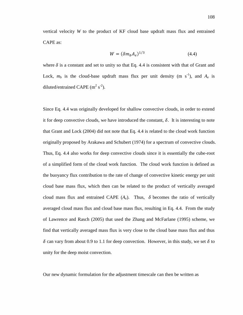
108

vertical velocity W to the product of KF cloud base updraft mass flux and entrained

CAPE as:

𝑊 = (𝛿𝑚𝑏𝐴𝑒)1 3⁄ (4.4)

where 𝛿 is a constant and set to unity so that Eq. 4.4 is consistent with that of Grant and

Lock, mb is the cloud-base updraft mass flux per unit density (m s-1

), and Ae is

diluted/entrained CAPE (m2 s

-2).

Since Eq. 4.4 was originally developed for shallow convective clouds, in order to extend

it for deep convective clouds, we have introduced the constant, 𝛿. It is interesting to note

that Grant and Lock (2004) did not note that Eq. 4.4 is related to the cloud work function

originally proposed by Arakawa and Schubert (1974) for a spectrum of convective clouds.

Thus, Eq. 4.4 also works for deep convective clouds since it is essentially the cube-root

of a simplified form of the cloud work function. The cloud work function is defined as

the buoyancy flux contribution to the rate of change of convective kinetic energy per unit

cloud base mass flux, which then can be related to the product of vertically averaged

cloud mass flux and entrained CAPE (Ae). Thus, 𝛿 becomes the ratio of vertically

averaged cloud mass flux and cloud base mass flux, resulting in Eq. 4.4. From the study

of Lawrence and Rasch (2005) that used the Zhang and McFarlane (1995) scheme, we

find that vertically averaged mass flux is very close to the cloud base mass flux and thus

𝛿 can vary from about 0.9 to 1.1 for deep convection. However, in this study, we set 𝛿 to

unity for the deep moist convection.

Our new dynamic formulation for the adjustment timescale can then be written as

109

𝜏 =𝐻

(𝛿𝑚𝑏𝐴𝑒)1 3⁄ 𝛽 = 𝐻

(𝛿𝑚𝑏𝐴𝑒)1 3⁄ [1 + 𝑙𝑛 (25

𝐷𝑥)] (4.5)

Thus, the adjustment timescale in Eq. 4.5 increases as resolution increases, resulting in

longer time allowed for CAPE consumption by parameterized cloud physics and, hence,

stabilization of the atmosphere by the KF scheme, facilitating a gradual transition of the

stability restoration by the KF scheme to the grid-scale cloud physics.

4.2.4 Enhancement of grid-scale vertical velocity using subgrid-scale updraft mass

fluxes

Many studies (e.g., Han and Pan 2011; Richter and Rasch 2008; Mallard et al. 2013) cite

the need for inclusion of convective momentum transport into the KF scheme for proper

simulation of hurricanes. But, for high-resolution convective precipitation forecasts, it is

not clear whether subgrid-scale updraft mass flux plays an important role on grid-scale

momentum, mass, and energy transport. To address an aspect of this issue, we

considered impacts of subgrid-scale updraft mass fluxes on grid-scale vertical velocity

using a simple linear methodology. One potential benefit is that it can help reduce model

spin up time over convectively active regions by increasing the grid-scale vertical

velocity. The proposed simple linear mixing methodology for enhancing grid-scale

vertical velocity is expressed as

𝑊𝑢𝑝 =𝑀𝑢𝑝

𝜌=

𝑀 𝐷𝑥2⁄

𝜌 (4.6)

𝑊𝑛 = 𝑊𝑔 + 𝑊𝑢𝑝 (4.7)

110

where 𝑊𝑢𝑝 is the effective vertical velocity of subgrid-scale updraft (m s-1

), 𝑀𝑢𝑝 is the

subgrid-scale updraft mass flux (kg m-2

s-1

), ρ is the convective plume density (kg m-3

), 𝑀

is the updraft mass rate (kg s-1

), 𝑊𝑛 is the reformulated grid-scale vertical velocity (m s-1

),

and 𝑊𝑔 is the grid-scale vertical velocity (m s-1

).

4.2.5 Entrainment methodology based on LCL

From Kain (2004) the equation of the minimum entrainment rate for convective plumes is

given by

∆𝑀𝑒 = 𝑀𝑏𝐶

𝑅∆𝑃 (4.8)

where ∆𝑀𝑒 is the mixing rate (kg s-1

), 𝑀𝑏 is the updraft mass rate at cloud base (kg s-1

),

C=0.03 is a constant (m Pa-1

) which controls the overall magnitude of the entrainment

rate for convective plumes, R is the radius of cloud base and dependent on the magnitude

of vertical velocity at the lifting condensation level (LCL) (m), and ∆𝑃 is the pressure

depth of a model layer (Pa).

The magnitude of the constant C used in the Eq. 4.8 is the same as that of the non-

dimensional Tokioka parameter, α = 0.03, (Tokioka et al. 1988) used in global climate

studies (e.g., Kang et al. 2009; Kim et al. 2011; Lin et al. 2013) for entrainment rate

estimation. These global studies showed that the hyperactivity of a subgrid-scale

convection scheme can be largely modulated by tuning the Tokioka parameter, which

allows grid-scale processes to perform the needed moisture conditioning of the large-

scale atmosphere. These studies also showed that the subgrid-scale precipitation

111

decreases as the Tokioka parameter increases, resulting in an increase of grid-scale

precipitation for improved climate simulations. Dependence of the entrainment on

horizontal grid resolution for radiatively driven shallow (stratocumulus) clouds was

studied by Stevens and Bretherton (1999) using a large-eddy simulation model. Their

study found that when the horizontal spacing is coarsened, the entrainment rate decreased

without any noticeable changes in the overall structure of the subcloud layer and cloud

layer. The role of entrainment for continental deep convective clouds was extensively

studied by Del Genio and Wu (2010). One of their findings was that at finer spatial

resolutions, their inferred entrainment rate was greater because turbulence was more

resolved. They also used the WRF model at different grid resolutions and found the

inferred entrainment rate at 125 m grid spacing to be stronger than that inferred at 600 m

grid spacing. Entrainment in deep convective clouds was also studied by Romps and

Kuang (2010) using a LES model. It was shown that the purity of convection decreases

with finer grids (ranging from 3200 to 100 m spacings), suggesting increased entrainment

with finer grid spacing. Finally, in a recent cloud resolving modeling study, Bryan and

Morrison (2012) concluded that changes in the simulated squall line intensity differences

between two model grid resolutions (1 and 0.25 km) were primarily attributed to the

increased entrainment. Thus, all these studies clearly highlighted the dependency of

entrainment on the horizontal grid resolution (i.e., entrainment increases as grid

resolution increases). de Rooy et al. (2013) provides a detailed review of entrainment in

cumulus convection and highlights the study of Houghton and Cramer (1951) that

entrainment needs to be partitioned into two parts: (1) entrainment due to large-scale

processes; and (2) entrainment due to turbulence at cloud edges. Since the first type of

112

entrainment is being represented by the Eq. 4.8, we have included the second type of

entrainment through the usage of Tokioka parameter. Thus, we considered all of these

findings when reformulating the entrainment rate (Eq. 4.8) in the KF scheme to make it

more adaptable to high-resolution model forecasts and to work seamlessly across spatial

scales. We introduce this feature via a dynamic Tokioka parameter that increases as

model resolution increases. Thus, the resolution dependent Tokioka parameter helps to

represent grid spacing effects on convective cloud-entrainment interactions similar to that

documented in the literature. Hence, consistent with the above global climate and large-

eddy simulation studies, we have introduced a scale dependency for the Tokioka

parameter by multiplying it with the β shown in Eq. 4.3, and also replaced R by ZLCL (m)

– subcloud layer depth – which is the height of the LCL above the ground. The main

advantage of using ZLCL instead of R is that at higher resolutions, R generally approaches

the upper limit of 2 km used in the KF scheme, thus, it is not consistent with the

assumption that subgrid-scale cloud fraction covers only a small area of a grid cell (e.g.,

Arakawa and Wu, 2013). In such situations, the diameter of the KF cloud will become 4

km and thus, at the 3 km grid spacing used in this study, usage of R is inappropriate as

the assumed subgrid cloud diameter exceeds the grid size.

Then, the new minimum entrainment equation can be written as:

∆𝑀𝑒 = 𝑀𝑏𝛼𝛽

𝑍𝐿𝐶𝐿∆𝑃 (4.9)

Thus, Eq. 4.9 attempts to include both the types of entrainment consistent with the

descriptions of de Rooy et al. (2013).

113

4.3 Design of Simulations

The WRF model (Skamarock and Klemp 2008) is commonly used for a wide range of

meteorological studies across scales ranging from meters to thousands of kilometers and

timescales from days to decades. An increasing number of researchers are employing it

to study regional weather (e.g., Chen et al. 2011) and historic and future climate (e.g.,

Otte et al. 2012). However, recent regional climate research noted that WRF often

produced excessive precipitation within highly energetic convective systems (Done et al.

2004; Hong et al. 2010; Alapaty et al. 2012; Herwehe et al. 2014). We hypothesize that

including the effects of parameterized scale-aware cloud dynamics into a high-resolution

WRF simulation will reduce the excessive rainfall biases by properly representing

convective timescale, grid-scale vertical velocity, and entrainment effects.

The WRF model version 3.4.1 was used to conduct all weather forecast simulations over

the U.S. SGP due to its importance as a land-atmosphere coupling “hotspot” (Koster et al.

2004; Zheng et al. 2014) and the availability of various observations. The main land-

cover types include grassland, cropland, savannas, and a mixture of crop and natural

vegetation. To understand the effects of using parameterized cloud dynamics for high-

resolution forecasts, we tested three WRF model configurations with two-way interacting

nests for the SGP. In our model simulations we used two choices [the Goddard

microphysics scheme and the WRF double-moment 6-class scheme (WDM6)] for grid-

scale cloud processes for both grid spacings (9 and 3 km). However, for subgrid-scale

cloud representation, we used three approaches: (1) disabled subgrid-scale convection,

allowing only explicit convection; (2) the latest KF scheme (Kain, 2004); and (3) our

114

UKF scheme. Details on the cloud formulations used in this study are described in the

Table 4.1, showing a total of 36 numerical experiments. We have assigned a unique

experiment name for each set of numerical simulation and these are referred to as EXP

(explicit convection only), BASE [with the Kain (2004) KF], and UKF (with the update

KF). For example, for each simulation period, EXP case has two numerical simulations,

as identified under Experiment Number in the Table 4.1, referring to two types of initial

conditions. To study impacts due to the choice of microphysics representation with the

UKF scheme and its effects on regional weather simulations, we performed another set of

six numerical experiments. These experiments were designed to compare the

performance of the Goddard microphysics scheme with the WDM6. Note that no

nudging or data assimilation was used in any of the simulations.

One degree 6-hourly NCEP Global Final Analysis (FNL) data derived from the Global

Forecast System (GFS) and 0.5 degree 6-hourly Climate Forecast System Reanalysis

(CFSR) data were used separately to develop lateral boundary and initial conditions for

the large-scale atmospheric fields, soil parameters (i.e., soil moisture and temperature),

and sea surface temperature (SST). The WRF model was configured with two-way

interactive nested domains using horizontal grid spacing of 9 km (290 × 280 grid points;

Domain 1 in Fig. 4.1a) and 3 km (307 × 274 grid points; Domain 2 in Fig. 4.1a).

Locations of observational sites in Domain 2 are shown in Fig. 4.1b. In the vertical, the

model was configured with 28 eta levels with a model top at 50 hPa. Prominent physics

options in the WRF model configuration included the RRTMG radiation models (Iacono

et al. 2008), the Goddard microphysics scheme (Tao et al. 1989), the Mellor-Yamada-

115

Janjic (MYJ) planetary boundary layer (PBL) scheme (Janjic 2002), and the Noah land-

surface model (Chen and Dudhia 2001). We focus our evaluation on assessing the

updated model’s ability to forecast the location and intensity of surface precipitation,

surface longwave and shortwave radiation, and surface temperature fields.

Fig. 4.1 (a) Topography map of the nested model domain over the U.S. SGP, and (b) the

IHOP_2002 domain and fixed deployment locations

(https://www.eol.ucar.edu/field_projects/ihop2002).

116


Simulation

period

Experi

ment

No.

Experi

ment

name

Initial

conditions

Microphysics

scheme

9-km grid

spacing

3-km grid

spacing

0000 UTC 4

June – 0000

UTC 6 June

2002

1 EXP

GFS

Goddard

microphysics

scheme

KF scheme No cumulus

parameterization 2 CFSR

3 BASE

GFS KF scheme KF scheme

4 CFSR

5 UKF

GFS UKF scheme UKF scheme

6 CFSR

0000 UTC 16

June – 0000

UTC 18 June

2002

7 EXP

GFS

Goddard

microphysics

scheme



9 BASE


10 CFSR

11 UKF


12 CFSR

0000 UTC 5

July – 0000

UTC 7 July

2010

13 EXP

GFS

Goddard

microphysics

scheme



15 BASE


16 CFSR

17 UKF


18 CFSR

0000 UTC 28

July – 0000

UTC 30 July

2010

19 EXP

GFS

Goddard

microphysics

scheme



21 BASE


22 CFSR

23 UKF


24 CFSR

25 DYNT

AU

GFS KF scheme with only

dynamic τ update 26 CFSR

27 WUP


updraft mass flux update 28 CFSR

29 ENT


entrainment update 30 CFSR

0600 UTC 14

June – 0600

UTC 16 June

2002

31 EXP

GFS

WDM6

scheme



33 BASE


34 CFSR

35 UKF


36 CFSR

117

4.4 Results and Discussions

The primary goal of this study is to investigate the suitability of the UKF scheme for

high-resolution simulations representing and forecasting surface precipitation. Another

goal is to study the impacts of two types of initial conditions obtained from different

analyses on high-resolution model simulations. For this purpose, WRF simulations using

the 1.0 degree 6-hourly FNL datasets derived from GFS (denoted as GFS) to specify the

initial states as well as boundary conditions are compared to those which used the 0.5

degree 6-hourly CFSR data (denoted as CFSR) as initial and boundary conditions. Four

different regional precipitation patterns and time periods were selected for this

experiment. An additional microphysics scheme sensitivity study (using the Goddard and

WDM6 microphysics schemes) was designed to explore whether various microphysics

schemes accompanied with the UKF scheme are able to produce appropriate precipitation

forecasts for these high-resolution simulations.

4.4.1 Simulation period 0000 UTC 4 June – 0000 UTC 6 June 2002: Experiments 1-6:

Representative examples of observed and simulated 12-hour accumulated precipitation at

9-km grid spacing and 6-hour accumulated precipitation at 3-km grid spacing starting at

0000 UTC 5 June 2002 are shown in Figs. 4.2 and 4.3. It is apparent that the model

forecasts with GFS contain precipitation at appropriate general locations and with a

similar spatial structure when compared to the Stage IV observed precipitation (Figs. 4.2g

and 4.3g). However, the precipitation forecasts over the central to eastern regions of the

domains using CFSR as initial and boundary conditions [Fig. 4.2 (d-f) and Fig. 4.3 (d-f)]

are shifted to the north, while in Figs. 4.2 (d-f) the precipitation patterns over central

118

Mexico and Gulf of Mexico (based on observed cloud cover) seem to be reasonably

simulated. Such precipitation location offset indicates that the reanalysis systems may be

impacted by interactions between the observational data and the assimilation system and

can create unrealistic precipitation distributions shortly after the model is initialized. It

also indicates that some forecasts are more sensitive to initialization than to convective

parameterization or physics. The 6-hour accumulated precipitation from the 3-km grid

spacing UKF GFS forecast (Fig. 4.3c) depicts a broad area of heavy precipitation over the

western parts of the domain similar to that seen in the observations (Fig. 4.3g). It is also

noted that the high-resolution UKF model simulations show improvement in the

precipitation distribution. For instance, in Figs. 4.2 and 4.3 the heavy precipitation which

occurred along the border of Oklahoma and Texas is shifted to the north and east in the

BASE run (Figs. 4.2b and 4.3b), but is well simulated by the UKF run (Figs. 4.2c and

4.3c). In addition, around Lake Michigan the 12-hour accumulated precipitation from the

9-km grid spacing forecast from UKF (Fig. 4.2c) has less coverage than that in the other

two model runs using EXP and BASE (Figs. 4.2 a and b), again making UKF’s

precipitation coverage more similar to the observations. Note that the MPE observations

are only limited to land areas and thus no observational data exists over the ocean. Thus,

large precipitation over the ocean [lower right corner in the Figs. 4.2 (a-f)] simulated by

the model cannot be verified.

119

Fig. 4.2 Comparative example of simulated 12-hour (0000 UTC – 1200 UTC 5 June 2002)

accumulated precipitation (mm) over a 9-km grid spacing domain with GFS (top), CFSR (middle)

for EXP (a, d), BASE (b, e), and UKF (c, f), and (g) Stage IV observed precipitation.

120

For cloudy skies, outgoing longwave radiation (OLR) is reduced as opposed to clear skies

and thus intercomparison of modeled OLR (W m-2

) can point out differences in

simulations of cloud placement and depth. The OLR at 1800 UTC (1pm CDT) 5 June

2002 for WRF simulations with GFS for the 9- and 3-km grid spacing domains




121

(Experiments 1, 3, and 5 in Table 4.1) are shown in Fig. 4.4. The time shown is for the

42nd

forecast hour of the 48-hour simulations when convection is active. Satellite cloud

coverage images available from the NOAA’s Aviation Digital Data Services

[http://aviationweather.gov/adds/] are used for comparison to the EXP, BASE, and UKF

runs. The OLR over the 9-km grid spacing domain [Figs. 4.4(a-d)] indicates that the

southwest to northeast orientation of a band of low OLR for the UKF is more comparable

to the satellite observation and contains more detailed information due to the subgrid-

scale effects that are included here but not present in the BASE and EXP runs. It also

shows less OLR for the UKF due to subgrid clouds (i.e., Michigan, Alabama, Mississippi,

and Texas) and more OLR under less cloudy regions (i.e., Indiana, Ohio, and Kentucky)

compared with those for EXP and BASE. In addition, as one of the key components of

the surface energy budget, the representation of downward shortwave radiation (DSR) is

also used for the comparison. Fig. 4.5 shows DSR for 1800 UTC (1pm CDT) 5 June

2002 along with satellite cloud coverage showing widespread cloudiness throughout

Texas, Oklahoma, Missouri, Tennessee, Kentucky, Indiana, and Illinois. The DSR for

the 9-km grid spacing over Tennessee, Kentucky, Mississippi and Alabama in EXP and

BASE indicates clear sky conditions (Figs. 4.5 b and c). However, in UKF, the DSR

indicates more cloud coverage (Fig. 4.5d) similar to that seen in the observations (Fig.

4.5a). Further, the DSR for the 3-km grid spacing simulations [Figs. 4.5 (f-h)] indicate

that the cloud coverage for UKF is larger and in better agreement with the observations

(Fig. 4.5e). This result is primarily because of the UKF scheme where the radiative

effects of subgrid-scale clouds can be realistically represented even in grid spacing

smaller than 4 km. Thus, the UKF configuration improves the cloud cover simulation,

122

producing more realistic simulated radiation which could contribute to a better

precipitation forecast.

Improved representation of cloudiness also affects the temporal variations of surface

radiation in UKF for high-resolution model forecasts. For example, the measured 48-

hour variations of downward longwave and shortwave fluxes and the corresponding

simulations at New Salem (37.31°N, 98.94°W), KS (IHOP_2002 site 7) at 3-km grid

spacing (Figs. 4.6 a and b) indicate that UKF modulates the radiative impacts in the

model, particularly during the second day of the forecast. Both the EXP and BASE show

large biases in shortwave fluxes with more than 600 W m-2

overestimations in the second

day. The UKF simulation decreases the downward shortwave flux while increasing the

downward longwave flux with the help of improved representation of cloudiness (Figs.

4.6 a and b), leading to an overall improvement in the temporal variability of the surface

fluxes. The increased cloudiness from UKF also reduces the surface temperature (Fig.

4.6c) by about 5°C. The UKF also shows a better simulation than the others in terms of

variability, especially for the last 6 hours of the run. However, the impact on the 2-m

specific humidity (Fig. 4.6d) is not significantly different among runs because it depends

on several land surface parameters such as soil moisture.

123

Fig. 4.4 Outgoing longwave radiation (W m-2

) with GFS at 1800 UTC (1 pm CDT) 5 June 2002

over a 9-km grid spacing domain (top) and 3-km grid spacing domain (bottom) for EXP (b, f),

BASE (c, g), and UKF (d, h).

Fig. 4.5 Surface shortwave radiation (W m-2

) with GFS at 1800 UTC (1 pm CDT) 5 June 2002 over

a 9-km grid spacing domain (top) and 3-km grid spacing domain (bottom) for EXP (b, f), BASE (c,

g), and UKF (d, h).

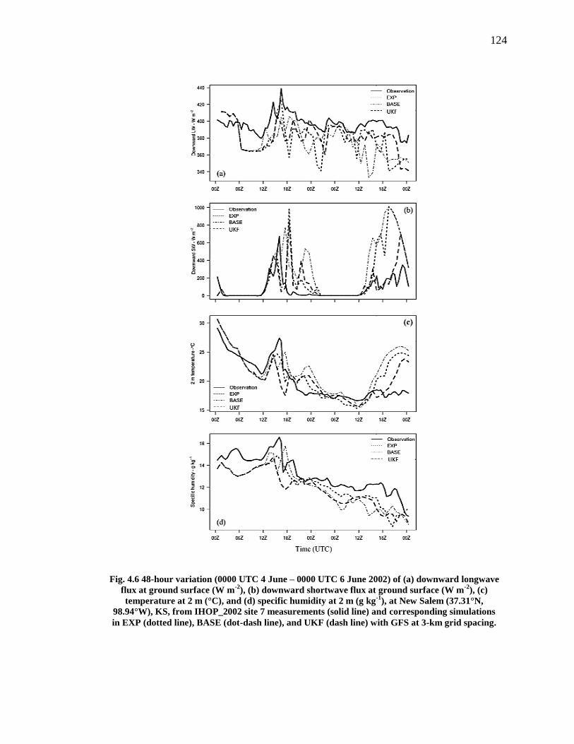
124

Fig. 4.6 48-hour variation (0000 UTC 4 June – 0000 UTC 6 June 2002) of (a) downward longwave

flux at ground surface (W m-2

), (b) downward shortwave flux at ground surface (W m-2

), (c)

temperature at 2 m (°C), and (d) specific humidity at 2 m (g kg-1

), at New Salem (37.31°N,

98.94°W), KS, from IHOP_2002 site 7 measurements (solid line) and corresponding simulations

in EXP (dotted line), BASE (dot-dash line), and UKF (dash line) with GFS at 3-km grid spacing.

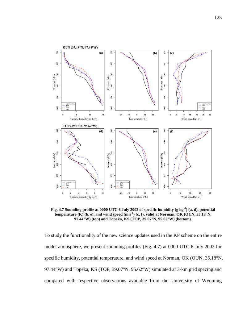
125

To study the functionality of the new science updates used in the KF scheme on the entire

model atmosphere, we present sounding profiles (Fig. 4.7) at 0000 UTC 6 July 2002 for

specific humidity, potential temperature, and wind speed at Norman, OK (OUN, 35.18°N,

97.44°W) and Topeka, KS (TOP, 39.07°N, 95.62°W) simulated at 3-km grid spacing and

compared with respective observations available from the University of Wyoming

Fig. 4.7 Sounding profile at 0000 UTC 6 July 2002 of specific humidity (g kg-1

) (a, d), potential

temperature (K) (b, e), and wind speed (m s-1

) (c, f), valid at Norman, OK (OUN, 35.18°N,

97.44°W) (top) and Topeka, KS (TOP, 39.07°N, 95.62°W) (bottom).

126

(http://weather.uwyo.edu/upperair/sounding.html). For both observation sites, there is

no clear indication of which simulation is outperforming the others, indicating that the

UKF has only minor differences with the other simulations for this observational time.

However, tropospheric wind speeds and surface specific humidity simulated by the UKF

seem to be closer to the observations. A detailed comparison of lower tropospheric

profiles is presented in the following section.

4.4.2 Simulation period 0000 UTC 28 July – 0000 UTC 30 July 2010: Experiments 19-

24:

To extend this case study, a second set of 48-hour simulations was initialized at 0000

UTC 28 July 2010 (Experiments 19-24). Comparative examples of simulated 6-hour

accumulated precipitation on the second day over 9- and 3-km grid spacings are shown in

Figs. 4.8 and 4.9. It is noted that the initial conditions still play an important role in the

model simulation, but the precipitation forecast with CFSR has no spatial shift in this

case, relative to observations. The general rainfall locations of UKF with GFS and CFSR

are similar and close to the observations. The KF scheme in the EXP and the BASE runs

with 9-km grid spacing again result in heavier amounts of rainfall (Figs. 4.8 a-b and d-e),

while UKF reduces the excessive precipitation and leads to a much better simulation. In

the 3-km grid spacing precipitation forecast (Fig. 4.9), excessive precipitation occurs with

the BASE run, but better forecasts are evident in EXP and UKF. Since the high-

resolution MPE (Stage IV) hourly rainfall products have some biases (e.g., Wang et al.

2008; Westcott et al. 2008; Westcott 2009), the visible satellite cloud observation is

127

Fig. 4.8 Comparative example of simulated 6-hour (1800 UTC 29 July – 0000 UTC 30 July 2010)



128



for EXP (a, d), BASE (b, e), and UKF (c, f), and (g) Stage IV observed precipitation and (h) visible

satellite image valid at 2132 UTC 29 July 2010. The satellite image is obtained from

http://aviationweather.gov/adds/ managed by NOAA’s Aviation Digital Data Services.

129

included in the analysis to provide additional information. For the 9- and 3-km grid

spacing runs, the observed 6-hour accumulated precipitation does not exceed 1 mm in

most of the northern Texas panhandle, however, cloudiness (which is taken as a key input

parameter in our research) can be seen in Texas in the visible satellite image (Fig. 4.9h).

The observed cloudiness indicates that the precipitation fields simulated in the high

resolution grid by EXP and UKF in Figs. 4.9 (a, c, d, and f) are comparable to each other.

Furthermore, it is demonstrated that the explicit treatment of convection (no cumulus

parameterization) with a 3-km grid spacing at times can adequately predict convective

systems and precipitation, consistent with the results of Done et al. (2004). For this case

study, the UKF results successfully demonstrate that it does not decrease the accuracy of

precipitation forecasts, relative to the EXP (explicit treatment of convection). However,

Done et al. (2004) also pointed out that for some cases, explicit precipitation treatments

suffered with an increasing propagated bias in the forecasts which may be mitigated

using UKF treatment.

Three rain rate thresholds (5, 15, and 25 mm h-1

) were used to separate out light, medium,

and heavy precipitation for the experiments. Within the thresholds, precipitation, which

was accumulated over time, was area-averaged over the 3-km grid spacing domain. Fig.

4.10 shows the 48-hour (0000 UTC 28 July – 0000 UTC 30 July 2010) period area-

averaged accumulated precipitation for simulations in EXP, BASE, and UKF, reflecting

dynamic changes in modeling of convective events, and for forecasts with GFS and

CFSR, reflecting the change in initial and boundary conditions. As expected, results

130

show that the area-averaged precipitation rates from the high-resolution simulation with

UKF are closer to the corresponding Stage IV observations in precipitation intensity and

the timing of convection initiation for both GFS and CFSR. It can be seen that

improvements of the area-averaged precipitation are made by UKF with GFS for the very

light rain rates (0-5 mm h-1

), the moderate rain rates (15-25 mm h-1

), and the heavier rain

rates (greater than 25 mm h-1

), while the BASE run performs poorest for all the rates.

The difference in the light rain rates (5-15 mm h-1

) with GFS between EXP and UKF is

very small. The area-averaged rainfall simulated using CFSR is found to be heavier

compared to the GFS results. In addition, the 48-hour averaged root mean square error

(RMSE) for the 3-km domain is shown in Table 4.2. In general, the 48-hour averaged

RMSE of the area-averaged precipitation is greatly decreased by UKF for all rainfall

rates. It indicates that UKF outperforms the other two simulations at every threshold,

regardless of the dataset used for initial and boundary conditions. The differences in the

area-averaged RMSE between GFS and CFSR for EXP are small (less than or equal to

0.10 mm h-1

at every threshold) for all but greater than 25 mm h-1

cases, while the

differences for BASE are obviously larger (~ 0.16 to 0.33 mm h-1

). Although a

negligibly small difference is seen for UKF for the very light rain rate, the differences in

RMSE between GFS and CFSR for the other rates are larger. In the heavier rainfall

threshold, differences in the 48-hour averaged RMSE are significant for all the

experiments (i.e., 0.29 mm h-1

for EXP, 0.26 mm h-1

for BASE, and 0.25 mm h-1

for UKF).

These differences reflect the influence of model initial conditions on the convection

scheme’s contribution to the precipitation forecast, suggesting that changes in the model

131

initial conditions can have a direct effect on the simulation of precipitation through the

CP used in NWP models.

Fig. 4.10 48-hour (0000 UTC 28 July – 0000 UTC 30 July 2010) area-averaged over 3-km grid

spacing precipitation (mm) from Stage IV observations (solid line) and corresponding

simulations of EXP (dotted line), BASE (dot-dash line), and UKF (dashed line) with GFS (a-d)

and CFSR (e-h).

132

Table 4.2 48-hour averaged root mean square error (RMSE) of area-averaged precipitation

over a 3-km grid spacing domain

RMSE

GFS CFSR

0-5

mm h-1

5-15

mm h-1

15-25

mm h-1

greater

than 25

mm h-1

0-5

mm h-1

5-15

mm h-1

15-25

mm h-1

greater

than 25

mm h-1

EXP 0.74 1.09 0.60 0.55 0.70 1.00 0.50 0.26

BASE 1.68 1.29 0.77 0.71 1.35 1.07 0.61 0.45

UKF 0.47 1.06 0.55 0.43 0.45 0.87 0.37 0.18

Fig. 4.11 shows the vertical profile of virtual potential temperature for two grid cells for

the 9- and 3-km grid spacings at 0000 UTC 29 July 2010. Note that all three simulations

miss the shallow surface inversion at Topeka, KS (TOP, 39.07°N, 95.62°W) (Figs. 4.11 c

and d) and EXP and UKF underestimate the surface temperature (Figs. 4.11 a and b). It

is difficult to pick out whether EXP or UKF performed better at Amarillo, TX (AMA,

35.23°N, -101.7°W) since EXP looks slightly better in the lower levels and UKF

performs best in the upper portion of the profile (Figs. 4. 11 a and b). Also note that the

virtual potential temperatures for UKF are almost constant with height in the PBL and

close to the observations from the International H2O Project (IHOP), indicating that the

MYJ scheme used in the WRF simulations with the UKF scheme is capable of simulating

improved well-mixed boundary layers.

4.4.3 Simulation period 0000 UTC 5 July – 0000 UTC 7 July 2010: Experiments 13-18:

A distinct widespread northeast to southwest rainfall was observed in Oklahoma during

the local afternoon hours of 6 July 2010 (Figs. 4.12 and 4.13). Estimated 6-hour (1800

UTC 5 July – 0000 UTC 7 July 2010) accumulated precipitation for the EXP, BASE, and

UKF simulations and the Stage IV observed precipitation are compared and shown in

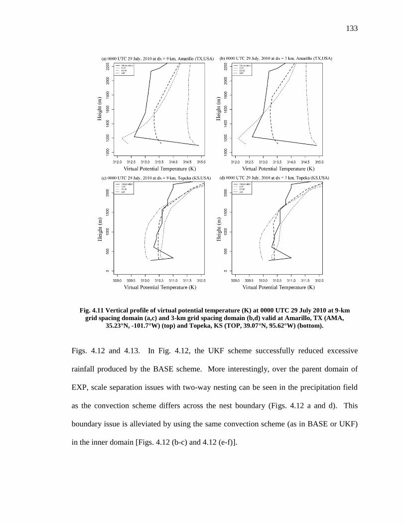
133

Figs. 4.12 and 4.13. In Fig. 4.12, the UKF scheme successfully reduced excessive

rainfall produced by the BASE scheme. More interestingly, over the parent domain of

EXP, scale separation issues with two-way nesting can be seen in the precipitation field

as the convection scheme differs across the nest boundary (Figs. 4.12 a and d). This

boundary issue is alleviated by using the same convection scheme (as in BASE or UKF)

in the inner domain [Figs. 4.12 (b-c) and 4.12 (e-f)].

Fig. 4.11 Vertical profile of virtual potential temperature (K) at 0000 UTC 29 July 2010 at 9-km

grid spacing domain (a,c) and 3-km grid spacing domain (b,d) valid at Amarillo, TX (AMA,

35.23°N, -101.7°W) (top) and Topeka, KS (TOP, 39.07°N, 95.62°W) (bottom).

134

In the 3-km grid spacing simulations (Fig. 4.13), EXP forecasts more precipitation in

northeast Kansas, while producing less precipitation than observed in Oklahoma. The

improvement of using better initial conditions on high-resolution rainfall predictions can

be seen in EXP and UKF, and at 3-km grid spacing, the precipitation simulated by UKF




135

with GFS is similar to the Stage IV observation. However, the BASE run simulates more

rainfall than observed and there are no obvious improvements when changing initial

conditions. Since the UKF is able to improve the high-resolution precipitation forecast

by introducing subgrid-scale effects, an instantaneous east-west oriented transect of the




136

subgrid-scale rain rate simulated at 9- and 3-km grid spacings is taken across Oklahoma

and northern Texas at 2000 UTC 5 July 2010 (Fig. 4.14). It is found that the simulated

convective rain rate for the finer resolution model (i.e., 3-km grid spacing) is generally

less than that for the coarser resolution model (i.e., 9-km grid spacing) and confirms that

subgrid-scale precipitation decreases when the model resolution increases.

4.4.4 Sensitivity to microphysics schemes: Experiments 7-12 and 31-36:

Sensitivity analysis is useful for diagnosing the impacts of interactions of convective

treatment and microphysics on regional forecasts of rainfall. A 48-hour period starting at

0600 UTC 14 June 2002 during IHOP_2002 is examined due to significant convective

activity and a large regional event that occurred over the most of the Oklahoma and

larger regions of Kansas and north Texas (Wilson and Roberts 2006). Sensitivity

experiments (Experiments 7-12 and 31-36 in Table 4.1) were conducted by varying

model convective and microphysics schemes. Six-hour accumulated precipitation

Fig. 4.14 The subgrid-scale rain rate (mm hr-1

) simulated at 9- and 3-km grid spacings from the

UKF scheme with GFS at 2000 UTC 5 July.

137

forecasts from all the experiments are compared to Stage IV precipitation analyses. Fig.

4.15 provides an example of 9-km grid spacing forecasts of 6-hour accumulated

precipitation with the two microphysical parameterizations and three convective

treatments. Since the outer domain is large compared to the inner domain, it mitigates


accumulated precipitation (mm) over a 9-km grid spacing domain with the CFSR and Goddard

microphysics scheme (top), WRF Double-Moment 6-class scheme (middle) for the EXP (a, d),

BASE (b, e), and UKF (c, f), and (g) Stage IV observed precipitation.

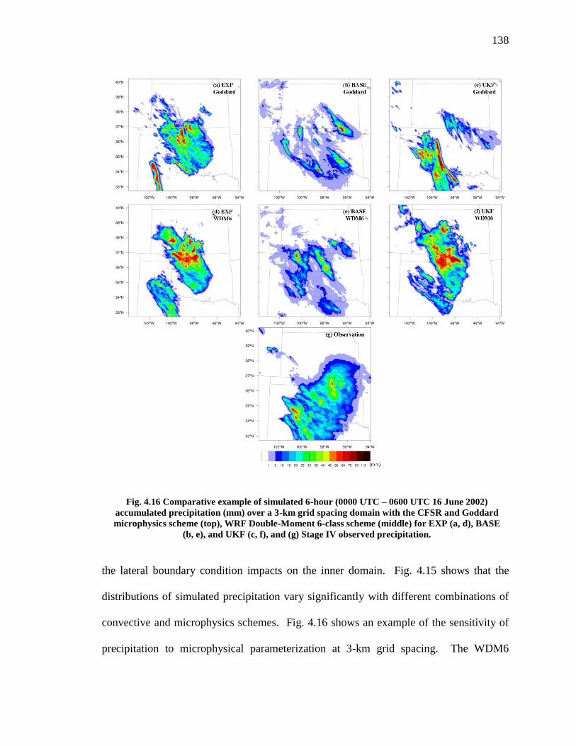
138

the lateral boundary condition impacts on the inner domain. Fig. 4.15 shows that the

distributions of simulated precipitation vary significantly with different combinations of

convective and microphysics schemes. Fig. 4.16 shows an example of the sensitivity of

precipitation to microphysical parameterization at 3-km grid spacing. The WDM6


accumulated precipitation (mm) over a 3-km grid spacing domain with the CFSR and Goddard

microphysics scheme (top), WRF Double-Moment 6-class scheme (middle) for EXP (a, d), BASE

(b, e), and UKF (c, f), and (g) Stage IV observed precipitation.

139

scheme produces a large swath of precipitation with high values in the center. The

Goddard scheme with UKF is not able to provide a large area of precipitation, although

the orientation of the precipitation distribution is similar to observed rainfall. These

results demonstrate that the impact of using the UKF scheme will vary from case to case

and improvements may not be consistent with differing microphysics schemes.

Therefore, for the cases where good initial conditions are not present, the microphysics

scheme and the UKF scheme have limitations on improving the precipitation forecast.

4.4.5 Sensitivity to each science update: Experiments 25-30:

We recall that the three updates which include properly representing timescale

(DYNTAU), grid-scale vertical velocity (WUP), and entrainment effect (ENT), have

been employed to modify the original KF scheme, and as a result, the UKF scheme has

substantially reduced the excessive precipitation biases for NWP high-resolution

forecasts. To find out which update is dominating the precipitation differences, six

additional simulations (Experiments 25-30 in Table 4.1) using each update separately

initialized by GFS and CFSR were conducted for simulation period 0000 UTC 28 July –

0000 UTC 30 July 2010. Fig. 4.17 shows 48-hour (0000 UTC 28 July – 0000 UTC 30

July 2010) 3-km grid spacing area-averaged accumulated precipitation (mm) from Stage

IV observations (black solid) and corresponding simulations in DYNTAU, WUP, ENT,

UKF, and BASE using GFS (Fig. 4.17a) reanalysis data.

140

Since BASE produced more precipitation over wide areas as compared to the observation

at 3-km grid spacing (Fig. 4.9), the simple area-averaged precipitation for BASE

compensates its low precipitation intensity with an overprediction of areal rainfall

coverage, resulting in better agreement of the area-averaged accumulated total

precipitation with the observation. WUP slightly reduces the area-averaged total

precipitation compared to BASE, indicating that the update with subgrid-scale updraft


spacing (a) accumulated total precipitation (mm) with GFS and (b) accumulated subgrid-scale

precipitation (mm) with GFS: Stage IV observations (black solid) and corresponding simulations

of DYNTAU (blue dot-dash), WUP (orange dashed), ENT (green dotted), UKF (red long-dashed),

and BASE (purple double dash).

141

mass flux impacts on grid-scale vertical velocity helps to slightly increase saturation

levels of the environment, thereby leading to a minor increase in subgrid-scale

precipitation. DYNTAU is found to contribute more to decreasing the simulated rainfall

amount. One modeling fact of many CPSs is that as model resolution increases, impacts

from a standard subgrid-scale parameterization become more significant. However, with

the adjustment timescale (τ) update, the value of τ increases and results in longer time to

remove CAPE for atmospheric stabilization, resulting in the simulated precipitation by

DYNTAU being reduced, a desired feature. In the update of the entrainment effects, the

introduced scale-dependent Tokioka parameter, as well as the LCL-based methodology,

in the high-resolution simulation helps to achieve the proper representation of convective

clouds through increased entrainment. As a result, the hyperactivity of the subgrid-scale

convection scheme is alleviated, leading to a decrease of subgrid-scale precipitation.

Consistently, ENT reduces the precipitation from BASE, and it shows the minimum area-

averaged precipitation among all of the simulations with a separated update. To

summarize, the three different updates contribute differently to the precipitation changes

and show non-linear impacts. We also found similar results using the CFSR reanalysis

data (not shown). To further assess the relative contribution of each of the updates on

precipitation components, i.e., subgrid-scale versus grid-scale, Fig. 4.17b shows 48-hour

accumulated subgrid-scale precipitation obtained from using each of the updates. In the

literature, a few studies (e.g., Wang et al. 2009; Snively and Gallus 2014; Van Weverberg

et al. 2013) use the term “cloud-permitting” scale (quasi-convective resolution) for grid

spacings which are smaller than 4 km. These studies demonstrate that grid-scale

microphysics schemes are adequate to produce reasonable precipitation in model

142

forecasts/simulations at cloud-permitting scales, implying that the subgrid-scale

convective component is either weak or absent. As shown by comparisons of Figs. 4.17 a

and b, the total precipitation in the UKF simulation is dominated by grid-scale

precipitation, with the amount of subgrid rainfall below 1 mm for the entire forecast. To

further examine relative intensity of precipitation with each of the updates, in Fig. 4.18

we present the accumulated value of 48-hour (0000 UTC 28 July – 0000 UTC 30 July

2010) 3-km grid spacing area-averaged precipitation (mm) from Stage IV and

corresponding simulations in DYNTAU, WUP, ENT, UKF, and BASE with GFS for

certain thresholds of hourly rates. For the rate less than 5 mm h-1

, UKF slightly under

predicts while ENT is on average closest to the observations. Simulations with the other

updates overpredict the observed rate. Results indicate that too much drizzle has been

simulated by BASE and modifying the grid-scale vertical velocity alone cannot

significantly improve the precipitation forecast. DYNTAU and ENT contribute to reduce

the drizzle, and UKF, which includes all three updates, shows good improvement for the

forecast of drizzle. But, for the rest of the hourly rates, UKF outperforms the other

simulations. However, UKF still tends to underpredict precipitation values at rates

greater than 5 mm h-1

. Fig. 4.19 shows the accumulated 48-hour (0000 UTC 28 July –

0000 UTC 30 July 2010) area-averaged subgrid-scale precipitation (mm) for 3-km grid

spacing from simulations in DYNTAU, WUP, ENT, UKF, and BASE with GFS when

the hourly rates are in the same thresholds as shown in Fig. 4.18. It can be seen that UKF

primarily contributes to the precipitation forecast when rate is less than 5 mm h-1

, but

negligibly improves the simulation when the rate is greater than 5 mm h-1

and less than

15 mm h-1

, and has zero contribution with higher hourly rain rates.

143


spacing total precipitation (mm) from Stage IV observations (black solid) and corresponding

simulations of DYNTAU (blue dot-dash), WUP (orange dashed), ENT (green dotted), UKF (red

long-dashed), and BASE (purple double dash) with GFS.

Fig. 4.19 48-hour (0000 UTC 28 – 0000 UTC 30 July 2010) area-averaged over 3-km grid spacing

subgrid-scale precipitation (mm) from simulations of DYNTAU (blue dot-dash), WUP (orange

dashed), ENT (green dotted), UKF (red long-dashed), and BASE (purple double dash) with GFS.

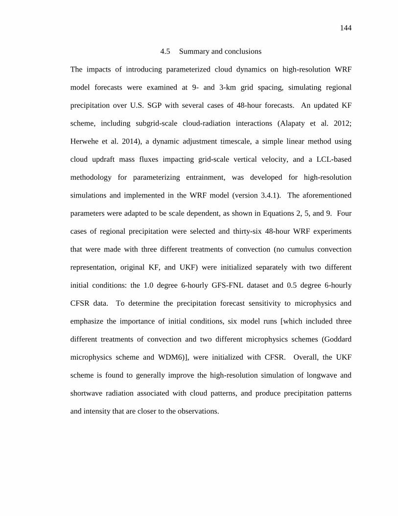
144

4.5 Summary and conclusions

The impacts of introducing parameterized cloud dynamics on high-resolution WRF

model forecasts were examined at 9- and 3-km grid spacing, simulating regional

precipitation over U.S. SGP with several cases of 48-hour forecasts. An updated KF

scheme, including subgrid-scale cloud-radiation interactions (Alapaty et al. 2012;

Herwehe et al. 2014), a dynamic adjustment timescale, a simple linear method using

cloud updraft mass fluxes impacting grid-scale vertical velocity, and a LCL-based

methodology for parameterizing entrainment, was developed for high-resolution

simulations and implemented in the WRF model (version 3.4.1). The aforementioned

parameters were adapted to be scale dependent, as shown in Equations 2, 5, and 9. Four

cases of regional precipitation were selected and thirty-six 48-hour WRF experiments

that were made with three different treatments of convection (no cumulus convection

representation, original KF, and UKF) were initialized separately with two different

initial conditions: the 1.0 degree 6-hourly GFS-FNL dataset and 0.5 degree 6-hourly

CFSR data. To determine the precipitation forecast sensitivity to microphysics and

emphasize the importance of initial conditions, six model runs [which included three

different treatments of convection and two different microphysics schemes (Goddard

microphysics scheme and WDM6)], were initialized with CFSR. Overall, the UKF

scheme is found to generally improve the high-resolution simulation of longwave and

shortwave radiation associated with cloud patterns, and produce precipitation patterns

and intensity that are closer to the observations.

145

Experiments using GFS and CFSR for initialization were conducted to assess how the

initial condition dataset impacts forecasts. These studies show that the general

distribution and intensity of precipitation forecasts are significantly influenced by initial

conditions obtained from different analysis fields. The area-averaged precipitation

simulated using CFSR is found to be heavier compared to the GFS results. Simulations

using the UKF scheme outperform the other simulations at light, medium, and heavy

precipitation rates, regardless of the dataset used for initial conditions. The larger

differences in the area-averaged RMSE between the two initial conditions are found with

the original KF scheme, but for heavy precipitation rates (greater than 25 mm h-1

),

significant differences due to changes in initial conditions are noted in all of the

convective treatments (Table 4.2). Sensitivity analysis demonstrates that the precipitation

forecasts are more sensitive to the type of initialization than to grid-scale microphysics or

convective treatments in our case studies. Therefore, a good initial condition dataset is

necessary for a good NWP model forecast, consistent with that documented in the

literature (Rabier et al. 1996; Stensrud et al. 2000).

In this study we find that grid resolution-dependent parameterized convective physics in

the KF scheme results in improvement of high-resolution forecasts. Thus, the UKF

scheme in the WRF model at high-resolution scales produces more accurate surface

radiation values and results in the improvement of simulated cloudiness. The UKF

scheme not only reduces excessive rainfall amounts, but also improves both the location

and intensity of precipitation in high-resolution (3 and 9 km) forecasts. Regional climate

simulations that are being performed by our group do indicate that each of the science

146

updates presented in this paper results in a large reduction in monthly precipitation biases,

which will be reported in a follow up paper.

147

CHAPTER 5. IMPACT OF LAND-ATMOSPHERE-CONVECTION INTERACTIONS

ON REGIONAL PRECIPITATION INTENSITY AND VARIATION IN WRF4

5.1 Introduction

Accurate and site-specific forecasts of short-term precipitation are of key importance for

predicting extreme weather events such as excessive rainfall and flash flood. A variety of

mesoscale processes are involved in affecting the regional convection and precipitation,

ranging from land processes, boundary layer processes, and convective cloud processes.

The land surface heterogeneity can influence the exchanges of radiative, moisture, heat,

and momentum fluxes with the atmosphere, and can lead to critical impacts on the

development of convective and rainfall events (Hadfield et al. 1992; Avissar et al. 1998;

Niyogi et al. 2006; LeMone et al. 2008). Many land-surface parametrization schemes

have been developed, in particular, to represent the water and energy budgets at the land

surface, water storage in the ground, and evapotranspiration to the atmosphere (Niyogi et

al. 1999; Pitman 2003; Dirmeyer et al. 2006). Thus, an essential role of the land-surface

parameterization is to provide accurate inputs to boundary layer and convective processes

to properly represent hydrology cycling.

4 Zheng, Y., K. Alapaty, D. Niyogi, 2015: Impact of land-atmosphere-convection interactions on regional

precipitation intensity and variation in WRF (In submission).

148

However, several parameters employed in the land-surface parametrization schemes are

very uncertain, leading to too much evaporation and precipitation (Pitman 1994;

Henderson-Sellers et al. 1995, 1996; Niyogi et al. 1999; Pitman et al. 1999; Betts 2007;

Abramowitz 2008; Fischer et al. 2010; Niu et al. 2011; Han et al. 2014). For example,

the surface latent heat fluxes do not solely depend on the land surface processes but also

on the land-atmosphere coupling, affecting regional convection and precipitation (Pielke

2001; Findell and Eltahir 2003; Koster et al. 2004, 2006; Santanello et al. 2011; Trier et

al. 2011; Taylor et al. 2012).

Areas with strong coupling between soil moisture and summer rainfall are generally

identified as “hot spots” (Koster et al. 2004), where wetter-than-usual soil moisture may

lead to higher-than-usual evapotranspiration, and result in stronger potential impact on

convection and increased precipitation. The strength of the coupling between land and

atmosphere varies from place to place and from time to time. For example, Zheng et al.

(2015a) have pointed out that the adoption of a dynamic coupling coefficient helped

improving simulation of surface fluxes and the resulting atmospheric state, and in turn

improved the intensity of the simulated precipitation. Therefore, the improvements in

land-atmosphere coupling will help reduce uncertainties in land-atmosphere feedbacks.

The role of a convective parameterization in a numerical model is often thought as

primary contributor to the simulated precipitation locations and amounts. However, these

convection schemes that are capable of generating different patterns of precipitation and

driving mesoscale circulations need to be well understood and improved. Particularly, at

149

the intermediate-scales (i.e., for horizontal grid spacings between ~1 and ~10 km) many

CPS do not work properly. When an explicit convection scheme has been employed in

most of these high resolution studies, many times precipitation forecasts were found to be

unsatisfactory. Based on the considerations of unresolved clouds and their effects in

simulating moist convection and precipitation for warmer periods, some of the

assumptions used in the convective parameterizations have been relaxed to make a CPS

suitable for high resolution grids (Alapaty et al. 2012; Herwehe et al. 2014; Bullock et al.

2015; Zheng et al. 2015b). Thus, a CPS can be seamlessly adaptable to the intermediate-

scales and work properly for high-resolution model forecasts.

Therefore, based on our previous studies (Zheng et al. 2015a and b), we study the impacts

of different representations of land surface processes, land-atmosphere coupling strength,

and a convective parameterization scheme on short-term regional precipitation forecasts.

We also explore to what extent the improvements in land-atmosphere-convection

interactions in the Weather Research and Forecasting (WRF) model benefit the short-

term regional precipitation intensity and variation. This paper is organized as follows:

Section 2 presents methods including the three aspects of improvements and the design of

numerical simulations; Section 3 evaluates the model results; and discussions are in

Section 4.

5.2 Methodology

Eight different representations of the three processes (land surface processes

representation, coupling strength, and subgrid-scale convection processes) are used in this

150

study. The Noah LSM has prognostic land states, including surface skin temperature, soil

moisture and soil temperature at four soil layers (0.1, 0.3, 0.6, and 1.0 m thickness),

canopy water content, snowpack water equivalent content and depth. The soil moisture

prognostic calculation in the Noah LSM is based on Richard’s equation:

𝜕𝜃

𝜕𝑡=

𝜕

𝜕𝑧(𝐷

𝜕𝜃

𝜕𝑧) +

𝜕𝐾

𝜕𝑧+ 𝐹𝜃 (5.1)

where θ is the soil water content, z is the elevation, t is time, 𝐹𝜃 represents the sources

(i.e., rainfall) and sinks (i.e., evaporation) of soil moisture, K is the hydraulic conductivity,

and D is the soil water diffusivity. Both D and K are functions of soil texture.

The soil temperature prognostic equation is:

𝐶(𝜃)𝜕𝑇

𝜕𝑡=

𝜕

𝜕𝑧(𝐾𝑡(𝜃)

𝜕𝑇

𝜕𝑧) (5.2)

where C and Kt are functions of soil texture and soil moisture. The surface energy

balance and water balance in the Noah LSM are:

𝑅𝑛𝑒𝑡 = 𝐻 + 𝐿𝐸 + 𝐺 + 𝑆𝑃𝐺𝐻 (5.3)

∆𝑆 = 𝑃 − 𝑅 − 𝐸 (5.4)

where 𝑅𝑛𝑒𝑡 is the net radiation, H is the sensible heat flux, LE is the latent heat flux, G is

the ground heat flux, and SPGH the snow phase-change heat flux. Additionally, ∆𝑆 is the

change in soil moisture content, P is the precipitation, R is the runoff, and E is the

evaporation.

Within the Noah LSM, the surface coupling strength controls the ratio of the roughness

lengths for momentum and heat which more effectively impact surface fluxes. It has

151

been demonstrated that the coupling strength coefficient which is dynamically linked as a

function of canopy height can help improve regional precipitation intensities, compared

to using the default constant coefficient (Chen and Zhang 2009; Zheng et al. 2015a). The

dynamical coupling strength is represented as:

𝐶𝑧𝑖𝑙 = 10(−0.4ℎ) (5.5)

where 𝐶𝑧𝑖𝑙 is the surface coupling strength, and h is the canopy height (meter).

For the convective parameterization, one of the crucial improvements in the UKF CPS is

its scale dependency with the scaling parameter 𝛽, which makes the scheme a smooth

transition from parameterized cloud physics to resolved grid-scale cloud physics:

𝛽 = [1 + ln (25

𝐷𝑥)] (5.6)

where 𝐷𝑥 (km) is the model’s horizontal grid spacing. Additionally, the UKF CPS

includes the subgrid-scale cloud-radiation interactions, a dynamic adjustment timescale,

impacts of cloud updraft mass fluxes on grid-scale vertical velocity, and lifting

condensation level (LCL) l-based entrainment methodology. The primary formulations

in the UKF CPS are:

𝜏 =𝐻

(𝛿𝑚𝑏𝐴𝑒)1 3⁄ 𝛽 (5.7)

𝑊𝑛 = 𝑊𝑔 + 𝑊𝑢𝑝 = 𝑊𝑔 +𝑀 𝐷𝑥2⁄

𝜌 (5.8)

∆𝑀𝑒 = 𝑀𝑏𝛼𝛽

𝑍𝐿𝐶𝐿∆𝑃 (5.9)

where τ is the adjustment timescale, H is cloud depth (m), 𝛿 is a constant and set to unity,

mb is the cloud-base updraft mass flux per unit density (m s-1

), and Ae is diluted/entrained

152

convective available potential energy (CAPE; m2 s

-2); 𝑊𝑛 is the reformulated grid-scale

vertical velocity (m s-1

), 𝑊𝑔 is the grid-scale vertical velocity (m s-1

), 𝑊𝑢𝑝 is the effective

vertical velocity of subgrid-scale updraft (m s-1

), ρ is the convective plume density (kg m-

3), and 𝑀 is the updraft mass rate (kg s

-1); ∆𝑀𝑒 is the mixing rate (kg s

-1), 𝑀𝑏 is the

updraft mass rate at cloud base (kg s-1

), α=0.03 is a constant (m Pa-1

) which controls the

overall magnitude of the entrainment rate for convective plumes, ZLCL is the height of the

LCL above the ground (m), and ∆𝑃 is the pressure depth of a model layer (Pa).

5.3 Numerical simulations design

The WRF model (WRF 3.4.1; Skamarock et al. 2008) is configured with 2 two-way nests

of 9 km (290 × 280 grid points) and 3 km (307 × 274 grid points) horizontal grid spacing,

and 28 eta vertical levels with a model top at 50 hPa over the U.S. SGP domain (Fig. 5.1).

The research domain was selected due to its importance as one of the land-atmosphere

coupling hotspot regions and the availability of various observations. One degree 6-

hourly NCEP Global Final Analysis (FNL) data derived from the Global Forecast System

(GFS) was used as initial conditions for the atmospheric fields, soil states, and sea surface

temperature. The major physics options in the WRF model included the RRTMG

radiation models (Iacono et al. 2008), the Goddard microphysics scheme (Tao et al. 1989),

and the Mellor-Yamada-Janjic (MYJ) planetary boundary layer (PBL) scheme (Janjic

2002).

153

A convection case [from 0000 UTC on 19 May (i.e., 1800 CST on 7 July) to 0000 UTC

on 21 May (i.e., 1800 CST on 8 July), 2011] of squall line with extended trailing

stratiform observed during a major joint field campaign [the Midlatitude Continental

Convective Clouds Experiment, also known as MC3E (Jensen et al. 2010) was selected to

examine the enhanced coupled WRF model’s ability to simulate the variation and

intensity of rainfall. A total of eight WRF configurations were tested with two LSM

models (slab model and Noah LSM), with/without dynamic land-atmosphere coupling

strength, and two treatments for the CPS [the latest KF scheme (Kain 2004), and the UKF

scheme (Zheng et al. 2015b). The summary of the experiments is shown in Table 5.1.

Observations from the MC3E at the Atmospheric Radiation Measurement (ARM) SGP

facilities, and the high spatial resolution Multisensor Precipitation Estimates (MPE, also

Fig. 5.1 (a) WRF nested domain with topography height (meters), and (b) map of the MC3E study

domain.

154

known as Stage IV Next-Generation Radar) hourly rainfall products (Lin and Mitchell

2005), were used for model comparisons.


Experiment Land surface

model

Land-

atmosphere

coupling strength

Convective

parameterization

scheme

S_KF Slab 0.1 KF

S_V_KF Slab Varying KF

S_UKF Slab 0.1 UKF

S_V_UKF Slab Varying UKF

N_KF Noah 0.1 KF

N_V_KF Noah Varying KF

N_UKF Noah 0.1 UKF

N_V_UKF Noah Varying UKF

* S: slab model, N: Noah LSM, V: dynamical Czil, KF: the latest KF scheme,

UKF, the updated KF scheme.

5.4 Results

5.4.1 Precipitation

The operational WRF model 6-hour total precipitation forecasts valid from 1200 to 1800

UTC on 20 May 2011 are shown in Figs. 5.2 (for the outer domain with 9 km grid

spacing) and 5.3 (for the inner domain with 3 km grid spacing). For the 9 km grid

spacing forecasting, an observed area of heavy rainfall is clearly evident across the

central domain and in a northeast orientation (Fig. 5.2i). Forecasts (retrospective) with

155

the slab model produce a smaller area of heavy rain, and the precipitation is located

further to the southeast [as seen in the red circle in Figs. 5.2 (a-d)]. Forecasts with the

Noah LSM and KF show less intense precipitation in the red circle area (Figs. 5.2 e and f)

but the spatial patterns, though displaced, are closer to observations. It can be seen that

the dynamical coupling strength only slightly improves the precipitation intensity (Fig.

5.2f). The heavier rainfall simulated in the Noah/WRF UKF runs (i.e., N_UKF and

N_V_UKF runs) is further to the north across Oklahoma, which is closer to the

observation (Figs. 5.2 g and h) but with an underprediction of light precipitation in the

northern regions in the highlighted area. For the 3 km grid spacing (for the inner domain),

the slab/WRF runs cannot well simulate the precipitation (Figs. 5.3 a and b), even with

the help of the dynamical coupling strength and the UKF scheme (Figs. 5.3 c and d). In

these forecasts, heavy precipitation is predicted in wrong locations. Thus, the LSM has a

more dominate role in rainfall forecasting and the simple LSM may produce incorrect

precipitation patterns and intensities due to obvious limitations in the slab land surface

parameterization. The Noah/WRF KF runs (i.e., N_KF and N_V_KF runs) show a

widespread area of precipitation distribution with much of the rainfall predicted to

receive between 1 and 25 mm, and these runs miss the observed heavier rainfall across

the eastern part of Oklahoma (Figs. 5.3 e and f). The UKF scheme significantly improves

the precipitation forecast for the 3 km grid spacing Noah/WRF simulation (Fig. 5.3g),

and the dynamical coupling strength helps yield a positive impact on the high-resolution

simulated precipitation intensity (Fig. 5.3h). Thus, the high-resolution WRF model

coupled to the Noah LSM, the dynamical coupling strength, and the UKF CPS, can lead

to more accurate forecasting for precipitation amounts and locations.

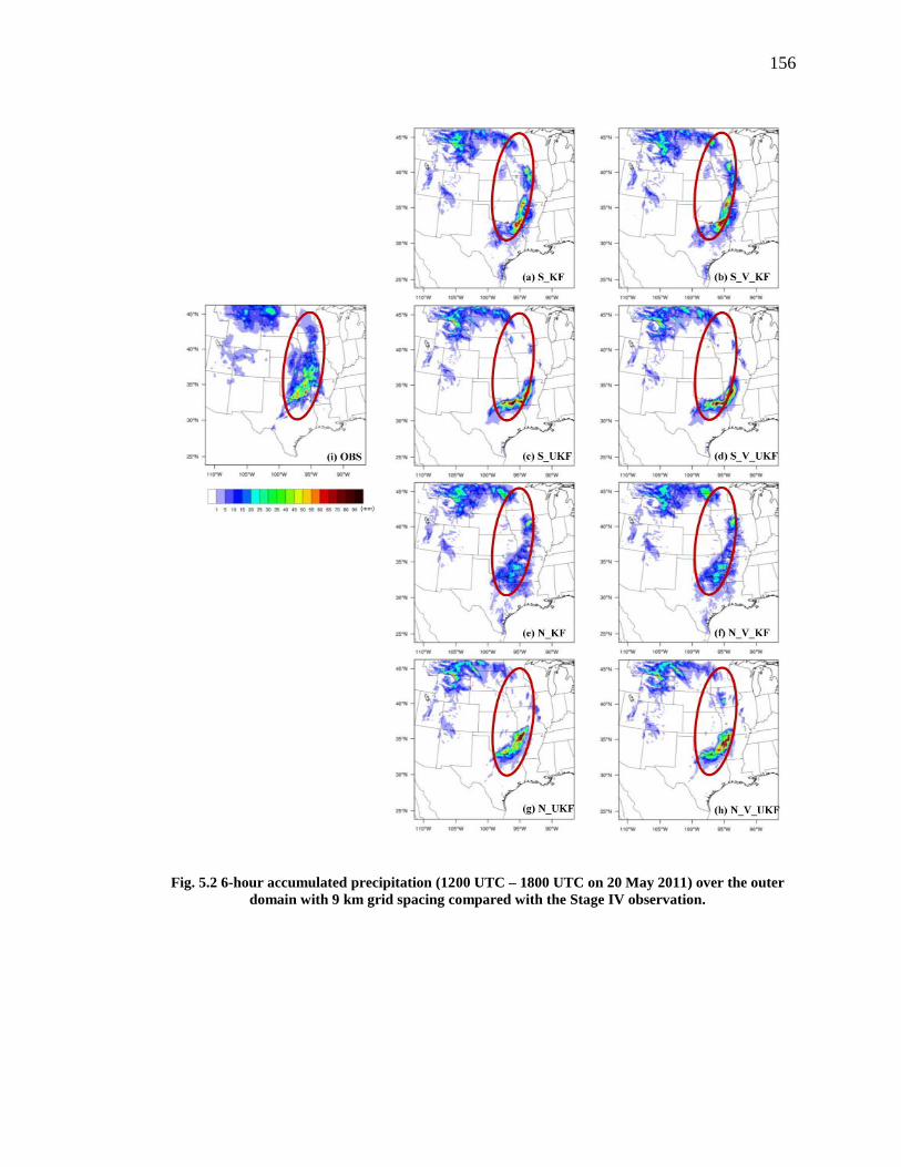
156

Fig. 5.2 6-hour accumulated precipitation (1200 UTC – 1800 UTC on 20 May 2011) over the outer

domain with 9 km grid spacing compared with the Stage IV observation.

157

Fig. 5.3 6-hour accumulated precipitation (1200 UTC – 1800 UTC on 20 May 2011) over the inner

domain with 3 km grid spacing compared with the Stage IV observation.

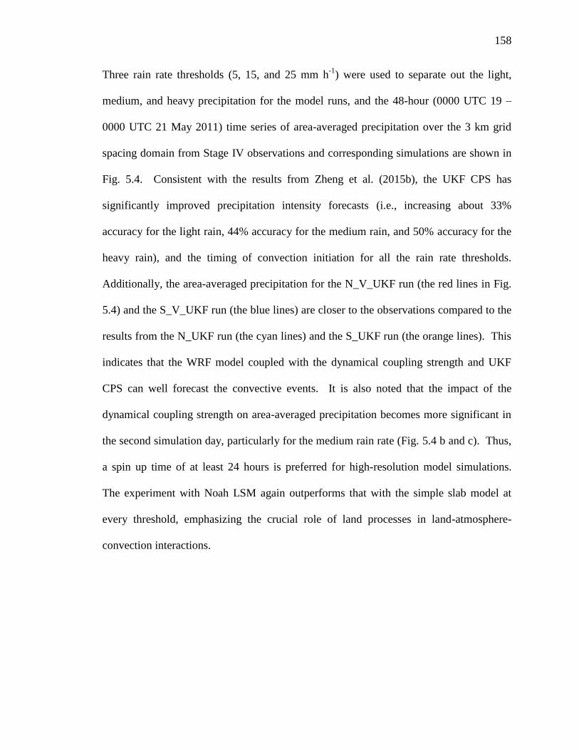
158

Three rain rate thresholds (5, 15, and 25 mm h-1

) were used to separate out the light,

medium, and heavy precipitation for the model runs, and the 48-hour (0000 UTC 19 –

0000 UTC 21 May 2011) time series of area-averaged precipitation over the 3 km grid

spacing domain from Stage IV observations and corresponding simulations are shown in

Fig. 5.4. Consistent with the results from Zheng et al. (2015b), the UKF CPS has

significantly improved precipitation intensity forecasts (i.e., increasing about 33%

accuracy for the light rain, 44% accuracy for the medium rain, and 50% accuracy for the

heavy rain), and the timing of convection initiation for all the rain rate thresholds.

Additionally, the area-averaged precipitation for the N_V_UKF run (the red lines in Fig.

5.4) and the S_V_UKF run (the blue lines) are closer to the observations compared to the

results from the N_UKF run (the cyan lines) and the S_UKF run (the orange lines). This

indicates that the WRF model coupled with the dynamical coupling strength and UKF

CPS can well forecast the convective events. It is also noted that the impact of the

dynamical coupling strength on area-averaged precipitation becomes more significant in

the second simulation day, particularly for the medium rain rate (Fig. 5.4 b and c). Thus,

a spin up time of at least 24 hours is preferred for high-resolution model simulations.

The experiment with Noah LSM again outperforms that with the simple slab model at

every threshold, emphasizing the crucial role of land processes in land-atmosphere-

convection interactions.

159

5.4.2 Soundings

A squall line was observed at midnight on 20 May (0600 UTC) confirming that the

convective storm occurred in a rather stable environment. Soundings over two different

sites were examined [Dodge City, KS (DDC; 37.46° N, -99.58° W) and Amarillo, TX

(AMA; 35.13° N, -101.43° W)] at 1200 UTC 20 May (6 hours after convection initiation),

to study the coupled mesoscale models’ performance (Fig. 5.5). The soundings

observations are available from the University of Wyoming

(http://weather.uwyo.edu/upperair/sounding.html). In the lower boundary layer the

soundings for N_V_UKF are much warmer, while the potential temperatures for

S_V_UKF are closer to the observations. All runs show moister and stronger wind

Fig. 5.4 48-hour (0000 UTC 19 – 0000 UTC 21 May 2011) time series of area-averaged

precipitation (mm) from Stage IV observations (solid black line) and simulations with different

rain rate thresholds.

160

soundings above the 925 hPa pressure level in the PBL. The specific humidity profile for

N_V_UKF is closer to observations over the DDC site, but S_V_UKF shows a better

simulated specific humidity profile over the AMA site. There is no clear indication that

the dynamical coupling strength could lead to better soundings and convection simulation

when coupled with the UKF CPS, however, the comparison between the 3 km grid

spacing runs with UKF and KF CPS clearly indicates that the UKF scheme outperforms

the KF scheme in simulating the vertical moisture and wind speed profiles.

Fig. 5.5 Vertical profiles of model-simulated potential temperature (a, d), specific humidity (b, e),

and wind speed (c, f) at the sites of Dodge City, KS (DDC; 37.46°N, -99.58°W) and Amarillo, TX

(AMA; 35.13°N, -101.43°W) at 1200 UTC on 20 May 2011 compared with observations.

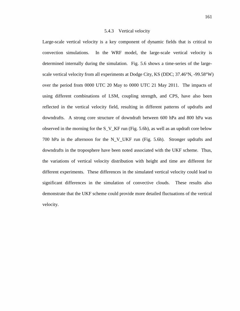
161

5.4.3 Vertical velocity

Large-scale vertical velocity is a key component of dynamic fields that is critical to

convection simulations. In the WRF model, the large-scale vertical velocity is

determined internally during the simulation. Fig. 5.6 shows a time-series of the large-

scale vertical velocity from all experiments at Dodge City, KS (DDC; 37.46°N, -99.58°W)

over the period from 0000 UTC 20 May to 0000 UTC 21 May 2011. The impacts of

using different combinations of LSM, coupling strength, and CPS, have also been

reflected in the vertical velocity field, resulting in different patterns of updrafts and

downdrafts. A strong core structure of downdraft between 600 hPa and 800 hPa was

observed in the morning for the S_V_KF run (Fig. 5.6b), as well as an updraft core below

700 hPa in the afternoon for the N_V_UKF run (Fig. 5.6h). Stronger updrafts and

downdrafts in the troposphere have been noted associated with the UKF scheme. Thus,

the variations of vertical velocity distribution with height and time are different for

different experiments. These differences in the simulated vertical velocity could lead to

significant differences in the simulation of convective clouds. These results also

demonstrate that the UKF scheme could provide more detailed fluctuations of the vertical

velocity.

162

Fig. 5.6 Simulated large-scale vertical velocity (m s-1

) at Dodge City, KS

(DDC; 37.46°N, -99.58°W).

163

5.4.4 Horizontal wind speeds and mixing ratio

Given the assumption that differences in land-surface parameterizations and land-

atmosphere coupling strength are the primary roles in leading to the differences in wind

and moisture fields, Fig. 5.7 shows the instantaneous high horizontal wind vectors and

mixing ratio at the middle of the PBL height (~ 1 km) at 1200 UTC 20 May 2011 from

different experiments. The differences in the wind field and moisture field lead to

changes in the distribution and intensity of moisture convergence. The coupling strength

and the convection scheme have a greater impact on the wind field density and wind

direction. The change in wind direction reflects the changes in dynamics during the

convective simulation. The water vapor mixing ratio is much higher in the southeastern

part of the domain, and these patterns are also notable in the 6-hour precipitation over the

inner domain in Fig. 5.3. Thus, the moisture field has a close positive relationship to the

precipitation, indicating that the correct simulation of the water vapor mixing ratio in the

PBL is crucial in precipitation forecasting. The different representations of soil moisture

in the two LSMs (i.e., the slab model has constant soil moisture while the Noah model

has time-varying soil moisture) can lead to the different patterns of water vapor mixing

ratio, and it is concluded that the primary reason for the unrealistic precipitation

simulated by slab/WRF (Figs. 5.2 and 5.3) is due to the constant value of the soil

moisture availability in the bucket slab model. The dynamical coupling strength

coefficient has a more significant impact on the moisture field and wind vector field

when the UKF is employed for the WRF simulations. Therefore, the WRF model

coupled with the more detailed LSM, the dynamical coupling strength coefficient, and the

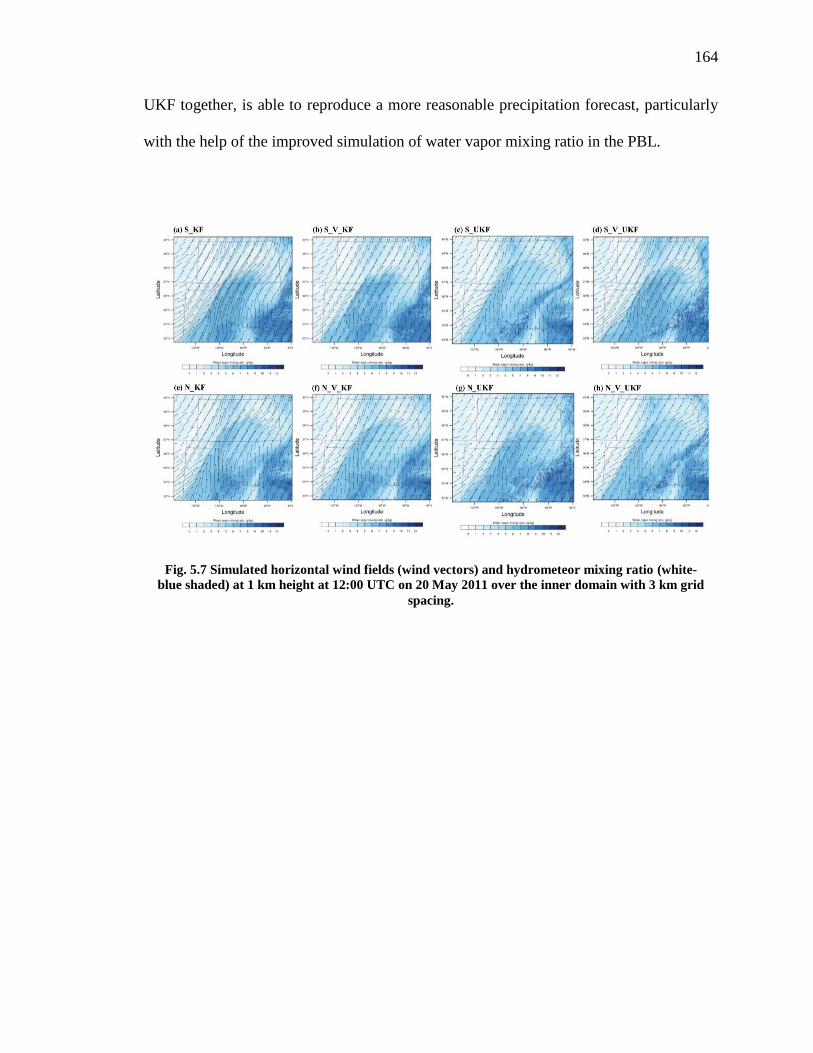
164

UKF together, is able to reproduce a more reasonable precipitation forecast, particularly

with the help of the improved simulation of water vapor mixing ratio in the PBL.

Fig. 5.7 Simulated horizontal wind fields (wind vectors) and hydrometeor mixing ratio (white-

blue shaded) at 1 km height at 12:00 UTC on 20 May 2011 over the inner domain with 3 km grid

spacing.

165

5.4.5 Surface fluxes

The impact of the land-atmosphere-convection interactions on the important near-surface

variables was also assessed (Fig. 5.8). The simulations using 3 km grid spacing were

compared to minute observations of 2 m temperature and 2 m relative humidity data, and

half-hourly observations of surface sensible heat flux and latent heat flux data. All these

data are from the ARM measurements located over the MC3E study domain. The near-

surface variables are more sensitive to the parameterizations during the daytime. For 2 m

temperature, all WRF model runs show a warm bias in the morning after 1500 UTC 20

May. The 2 m temperature for the S_KF run shows a curve very similar to observations

during the nighttime (before 0900 UTC 20 May), while the results from other simulations

are also in a reasonable range and close to observations (Fig. 5.8a). For 2 m relative

humidity, the WRF model runs show a wet bias in the nighttime but strong dry biases

during the daytime (Fig. 5.8b). The N_V_UKF increases instead of reducing the dry bias

for the daytime simulation. It is found that the choice of LSM plays a crucial role in

these bias magnitude differences, and the WRF model coupled with the three-aspect

improvements is not able to significantly reduce the bias primarily due to soil moisture

impacts in the model. However, it is not evident that the WRF model coupled with the

simple slab model could lead to accurate regional convection and rainfall. Additionally,

it was determined that the cause is internal to the WRF model itself. The surface sensible

and latent heat fluxes indicate that the WRF configuration with a dynamical coupling

strength coefficient could greatly help reduce surface flux bias (Figs. 5.8 c and d), leading

to improved heat and moisture transfer simulations in the PBL. Therefore, the effect of

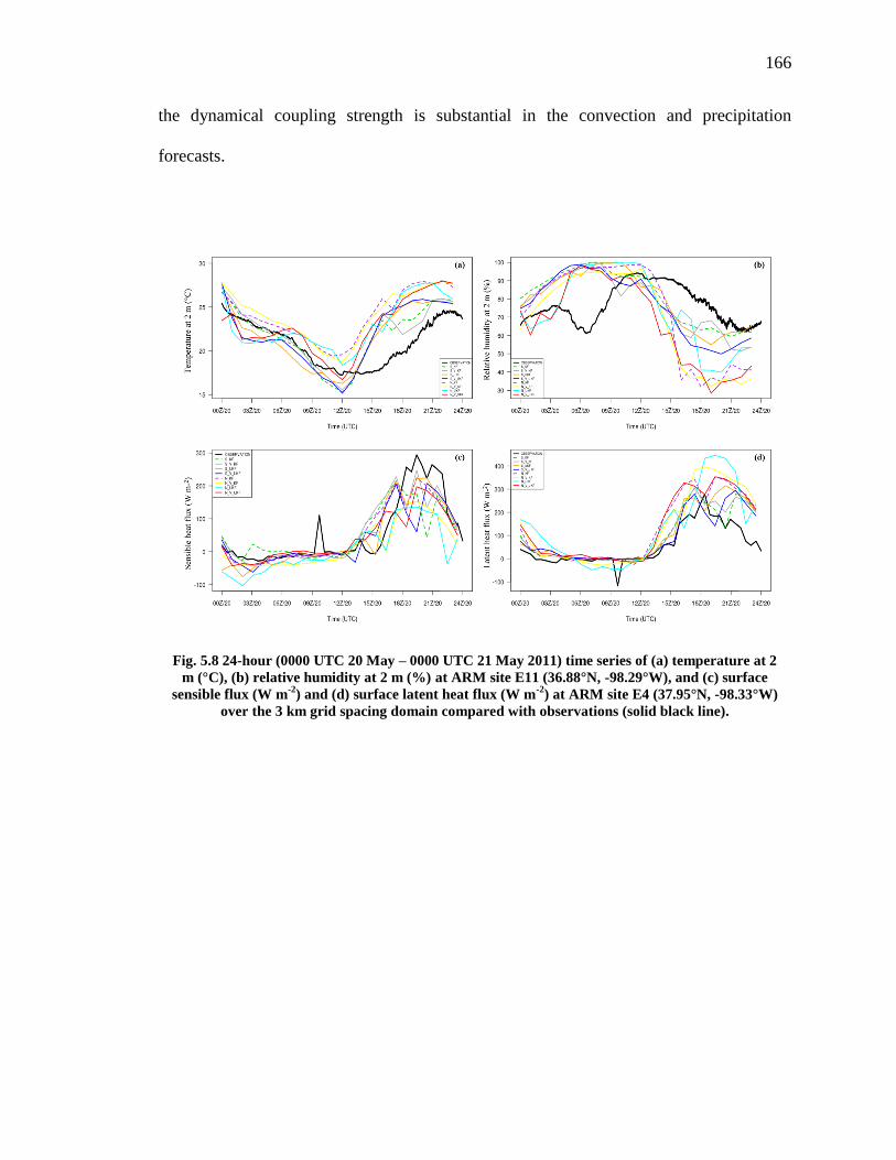
166

the dynamical coupling strength is substantial in the convection and precipitation

forecasts.

Fig. 5.8 24-hour (0000 UTC 20 May – 0000 UTC 21 May 2011) time series of (a) temperature at 2

m (°C), (b) relative humidity at 2 m (%) at ARM site E11 (36.88°N, -98.29°W), and (c) surface

sensible flux (W m-2

) and (d) surface latent heat flux (W m-2

) at ARM site E4 (37.95°N, -98.33°W)

over the 3 km grid spacing domain compared with observations (solid black line).

167

5.4.6 CAPE/CIN

Fig. 5.9 shows the time series of the CAPE and convection inhibition (CIN) calculated

from observed soundings at Dodge City, KS (DDC; 37.46°N, -99.58°W), and the Skew-T

at 0000 UTC 20 May 2011. CAPE is calculated as the vertical sum of the buoyancy

which raises an air parcel along a reversible moist adiabatic from the level of free

convection (LFC) to the equilibrium level (EL) (Moncrieff and Miller 1976). CIN is the

negative value of CAPE below LFC, and can be thought of as a measure of the work that

an air parcel must do to reach the LFC where it will finally become positively buoyant.

The magnitude of CAPE is strongly dependent on the environmental soundings profile.

Since the elevated convective storms occurred with a strong squall line that was observed

on 20 May 2011, and the convection had near saturated soundings in the unstable PBL,

large CAPE with strong diurnal variation had been diagnosed by Xie et al. (2014). As

seen in Fig. 5.9a and b, both CAPE and CIN are sensitive to the influence of LSM,

coupling strength, and CPS. The simulated magnitude peaks of CAPE occurred around

midnight (from 0400 UTC to 0500 UTC 20 May). The large magnitudes of CAPE for

the Noah/WRF simulations are earlier and larger than those for the slab/WRF simulations.

The simulations with the UKF scheme significantly reduced the CAPE value, possibly

leading to a decrease in the simulated precipitation rate under such unstable and saturated

conditions. However, to investigate if convection could be well captured (or improved)

by the mesoscale WRF model coupled with the improved scheme/parameterizations, a

longer simulation period or another case for deep convection should be conducted. Most

CIN values are distributed in the range from -400 to 0 J kg-1

. The small absolute values

of CIN for the slab/WRF simulations suggest the higher precipitation rates that are seen

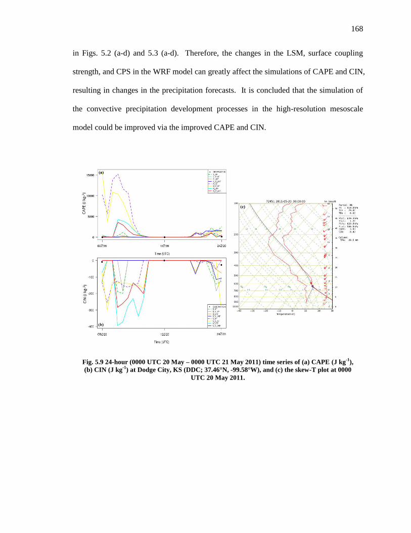
168

in Figs. 5.2 (a-d) and 5.3 (a-d). Therefore, the changes in the LSM, surface coupling

strength, and CPS in the WRF model can greatly affect the simulations of CAPE and CIN,

resulting in changes in the precipitation forecasts. It is concluded that the simulation of

the convective precipitation development processes in the high-resolution mesoscale

model could be improved via the improved CAPE and CIN.

Fig. 5.9 24-hour (0000 UTC 20 May – 0000 UTC 21 May 2011) time series of (a) CAPE (J kg-1

),

(b) CIN (J kg-1

) at Dodge City, KS (DDC; 37.46°N, -99.58°W), and (c) the skew-T plot at 0000

UTC 20 May 2011.

169

5.5 Discussion

The impact of including the effects of LSM, land-atmosphere coupling strength, and CPS

on the fields of precipitation, surface scalars, and convection were examined for 48-hour

weather simulations over the U.S. SGP domain. From the experiments conducted with an

observed squall line during the summertime, it was found that including a more detailed

land surface parameterization, a dynamical surface coupling strength coefficient, and the

UKF scheme together, improves the mesoscale simulations of several meteorological and

convection parameters in the high-resolution WRF model. The land-atmosphere-

convection feedbacks therefore can be well represented. Generally, the LSM plays a

dominate role in the short-term convection and rainfall forecasts, the dynamical coupling

strength helps improve precipitation intensity, and the UKF scheme helps create more

realistic moist convective process parameters and precipitation variability. By studying

the parameterized schemes in the land-atmosphere-convection interactions, the close

relationship between the land surface, PBL processes, and convective activities is

examined. This research will directly benefit the regional climate and hydrological

modeling communities by providing more accurate prediction of high-resolution regional

convection and rainfall. This research will also help improve the understanding and

parameterization of moist processes in regional meteorological models, particularly over

the regions that have close feedback between soil moisture and precipitation.

170

CHAPTER 6. CONCLUSIONS

The interactions between land-surface variability and cloud dynamics and their impacts

on regional convection and rainfall have been studied based on the synthesis of numerical

modeling analyses and field observations. A number of numerical experiments were

conducted over a variety of land-atmosphere coupling hotspot regions across the globe.

Model simulations of regional convection and rainfall were improved by studying the

impacts of the heterogeneous land surface, the land-atmosphere surface coupling strength,

and improving the KF CPS for regional short-term weather forecasts.

Land-surface heterogeneity in LULC plays a key role in influencing the simulation of

surface fluxes and PBL dynamics. Land heat and water storages and their relationship

with fluxes can be changed to some extent by land-surface heterogeneity. Nonlinear

impacts are found in simulated surface temperature, moisture, and wind speeds along

with heterogeneity length scale changes. Spatial variations of the surface heat flux are

found to decrease nonlinearly as the length scale of land-surface heterogeneity increases

(becoming more homogeneous). The different land-surface parameterizations represent

the impact of land-surface heterogeneity in different manners and show a variety of

modeling biases. The simple slab soil model is found to be more sensitive to land-surface

171

heterogeneity impacts, whereas the more detailed land-surface parameterizations (e.g.,

Noah LSM and HRLDAS) are less sensitive to heterogeneity length scale changes.

Larger biases have been noted in the coupled slab/WRF runs. Results also indicate that

in wet conditions, the surface heat fluxes over land which contains higher evaporation

and stronger coupling strength (e.g., grassland, forest, and wet cropland) are greatly

impacted by land-surface parameterizations. The Noah LSM performs better over

different types of LULC. Vertical fluxes of heat and moisture in the PBL are affected by

surface energy partitioning and the turbulent parameterization for mass and energy

transfer between the heterogeneous land surface and the PBL within the coupled

LSM/WRF models are explored to show the substantial impacts. The impact of land-

surface parameterizations on turbulent energy spectra is found to be more significant at

lower frequencies in the spectra where larger eddies dominate. The slab/WRF

overpredicts the energy spectra of surface temperature and moisture and underestimates

the energy cascade. The response of turbulent spectra to the length scales of land-surface

heterogeneity indicate that the energy spectra respond nonlinearly to heterogeneous

length scale changes and the simulated vertical velocity is less sensitive to land-surface

parameterizations at finer-scale heterogeneous land surfaces. Additionally, the WRF

model coupled with a more detailed land-surface parameterization can more accurately

simulate turbulent spectra over a heterogeneous land surface. An important finding from

the spectral analysis is that the atmospheric circulation, which is roughly four times the

spatial heterogeneity length scale, can be adequately resolved in the coupled mesoscale

WRF model. This result shows that the land-surface heterogeneity effect would be a

function of the degree of the heterogeneity spatial scales represented in the LSM.

172

Vertical fluxes of heat and moisture in the PBL are affected by the impact of land-surface

heterogeneity and LSMs on surface energy partitioning, influencing simulations of

mesoscale atmospheric circulations and regional convective weather processes. Results

show that vertical profiles of turbulent flux and TKE can also be used to represent

impacts of the land-surface parameterization and land-surface heterogeneity. Results

indicate that HRLDAS/WRF well simulates the vertical turbulent moisture flux and total

TKE in the PBL, and is able to capture the stronger gradients of the moisture flux at the

surface and entrainment zone. Thus, the more detailed land-surface representation can

not only improve the mean fields of surface flux simulations but also turbulent processes,

leading to improved simulations of land-atmosphere interactions over heterogeneous land

surfaces. Therefore, a positive impact of the improved land-surface parameterization

over a fine-scale heterogeneous land surface has been identified via the simulated

turbulent processes and mesoscale simulations.

The coupling between the atmosphere and the land surface plays an important role in

regional convection and precipitation. The potential benefit of examining the land

atmosphere coupling over four different coupling “hotspot” regions indicates that the

land surface coupling strength coefficient Czil has the potential to modulate mesoscale

model results and improve the simulation of convective systems. Additionally, the

dynamic formulation for representing land atmosphere coupling helps improve

precipitation forecasts in terms of intensity but not necessarily in its location.

173

Impacts of the coupling effect on regional convection vary across different land-cover

types and over different areas. Surface heat fluxes have the largest impact in terms of the

coupling strength assigned over the different regions. Results indicate that the constant

surface coupling coefficient used in the current coupled Noah/WRF model is deficient in

producing correct surface fluxes. Model biases respond differently along with changes in

surface coupling strength. The current WRF model in use over West Africa leads to

coupling effects that are too strong and could be improved by using the coupling

coefficient of 0.3 or the dynamic Czil. It is also noted that in summer over the U.S. SGP,

strong coupling leads to a cold and wet boundary layer resulting in a strong convective

system and heavier rainfall, but due to the cultivated parched land surface over northern

India, the coupling is found to be relatively weak, leading to lighter rain and smaller areas

of precipitation.

Thus the high uncertainty in land-atmosphere coupling findings indicates that the

coupling strength for the “hotspot” regions needs to be carefully considered and the zone

of “high” or “low” coupling strength should be evaluated in the context of the model and

parameterizations used. Since the modestly improved and encouraging model results are

associated with using a dynamic Czil, more efforts need to be directed toward adopting the

dynamic coupling coefficient rather than the constant value currently used in the

Noah/WRF models. It is a challenge to identify the correct coupling for land-atmosphere

interactions as it can improve one variable and deteriorate another. In addition, the

coupling coefficient has significant control on model performance particularly the

quantitative precipitation forecasts and is therefore an important feature in the study of

174

hydrometeorological extremes such as droughts and heavy rain events. The results

highlight that evaluating and improving land-atmosphere coupling could potentially

improve model performance across the globe.

Moist processes, especially the representation of clouds and their microphysical

processes, are of vital importance in forecasting convection and precipitation. However

at high spatial resolutions, the use of cloud microphysics alone may not be sufficient to

represent moist convection and precipitation for warmer periods in weather forecasts

(Clark et al. 2012). To reduce precipitation bias and errors occurring at high resolution

scales due to uncertainties in the initial meteorological conditions and/or in grid-scale

cloud microphysics schemes, in this research dissertation the scale-aware parameterized

cloud dynamics for high-resolution forecasts were introduced to the KF CPS in the WRF

model. The UKF scheme includes subgrid-scale cloud-radiation interactions (Alapaty et

al. 2012; Herwehe et al. 2014), a dynamic adjustment timescale, cloud updraft mass

fluxes impacting grid-scale vertical velocity, and an LCL-based methodology to

parameterize entrainment. The UKF scheme is found to generally improve high-

resolution simulation of longwave and shortwave radiation associated with cloud patterns,

and produce precipitation patterns and intensity that are closer to the observations.

Results from experiments using two different initial conditions (GFS and CFSR) indicate

that the general distribution and intensity of precipitation forecasts are significantly

influenced by initial conditions obtained from different analysis fields. The simulated

area-averaged precipitation initiated by CFSR is found to be heavier than forecasts using

175

GFS. The larger differences in the area-averaged RMSE between the two initial

conditions are found in the original KF scheme, but significant differences are noted in

all of the convective treatments for very heavy precipitation rates (greater than 25 mm h-

1). From the sensitivity analysis, results indicate that precipitation forecasts are more

sensitive to initialization than to grid-scale microphysics or convective treatments, thus a

good initial condition dataset is necessary for NWP model forecasts.

The UKF scheme in the WRF model at high-resolution scales is found to produce more

accurate surface radiation values and results in the improvement of simulated cloudiness.

Three different updates to the KF scheme which include properly representing timescale,

grid-scale vertical velocity, and the entrainment effect are found to contribute differently

to the precipitation changes and show nonlinear impacts. Results show that the UKF

primarily contributes to precipitation forecasts when the rain rate is less than 5 mm h-1

,

negligibly improving the simulation when the rate is greater than 5 mm h-1

and less than

15 mm h-1

, and has no contribution with higher hourly rain rates. Additionally, results

show that the UKF scheme not only reduces excessive rainfall amounts, but improves

both the location and intensity of precipitation in high-resolution forecasts.

A series of retrospective 48-hour experiments were conducted to explore how the land-

atmosphere-convection interactions affect the WRF model based on the above results.

The impacts of using different combinations of (i) LSM, (ii) land-atmosphere surface

coupling strength, and (iii) UKF CPS on short-term moist processes in the WRF model

were assessed accordingly. Results show that the LSM has a more dominate role in

176

simulating surface and near-surface temperature, boundary layer water vapor mixing ratio,

and regional rainfall. The simple LSM could produce an inappropriate water vapor

mixing ratio and latent heat flux due to its simple parameterizations, resulting in incorrect

precipitation intensity and variability. The dynamic coupling strength coefficient could

significantly reduce surface flux uncertainties and positively impact precipitation

intensity emphasizing its substantial role in convection and precipitation forecasting. The

UKF improves the high-resolution precipitation intensity forecast by about 43%. The

precipitation simulation for the WRF model coupled with the dynamical coupling

strength and the UKF CPS has good agreement with observations indicating that the

representation of moist processes could be improved by improving the interactions

between land-atmosphere coupling and convective parameterization. Particularly, for the

3 km grid spacing simulation, the UKF scheme can lead to better simulated sounding

profiles compared to the KF scheme. Results also show that the UKF scheme could

provide more detailed fluctuation of vertical velocity which needs to be considered

critically in the simulation of convective clouds. Thus, the interactions between the land

surface, PBL processes, and convective activities have been assessed by examining the

parameterized schemes in LSM, land-atmosphere coupling strength, and CPS. The land-

atmosphere-convection interactions could be well represented by employing a more

detailed land surface parameterization, a dynamical surface coupling strength coefficient,

and the UKF scheme, together.

However, there are some important aspects of the research limitation that should be

aware. For example, the data limitation over certain regions needs further analysis when

177

additional data become available, and the current study addresses diurnal convection and

precipitation situations in summertime only. Additional ensemble experiments related to

different sets of parameterization schemes are needed for further sensitivity analysis, and

additional sets of simulations with different ranges of relative soil moisture saturation are

needed to gain further insights into the longer-term behavior of the land-atmosphere-

convection system. Thus, further insights to the sensitivity of model parameters and

precipitation predictability would lead to a better understanding of land-atmosphere

feedback and moist process mechanism. Additionally, some open questions such as, "At

what spatial scale would the land surface heterogeneity trigger mesoscale circulations

that can affect the moist convection in climate models and may result in changes or

missing in large-scale circulations? How would the land-atmosphere coupling strength

be influenced due to the climate change and what would be the resulting impacts on

cloud formation and moist convection? For the climate system and climate sensitivity, to

what extent (e.g., initial condition, model resolution, and parameterization) to improve

the global/regional climate models for a better understanding and more appropriate

representation of clouds and moist convection, rather than obtaining more expensive

models?" would be of great interest to explore.

Overall, through the study of the impacts of land surface heterogeneity on turbulent flow

and mesoscale simulations, the land-atmosphere coupling strength over certain regions

across the globe with strong feedbacks between soil moisture and precipitation, and the

dynamical scale-awareness UKF convection scheme, this research dissertation has

examined the nature and magnitude of land surface, land-atmosphere coupling,

178

convection, and the interactions and feedbacks affecting and controlling regional moist

processes. Three substantial results were identified that help to explain the numerical

modeling for convection and land surface interactions: 1) Atmospheric feedbacks that are

roughly four times of the land heterogeneity spatial scale can be adequately resolved in

the coupled mesoscale model; 2) Evaluating and using a dynamic land-atmosphere

coupling strength could potentially improve convective model performance over areas

where there is a known bias with convection triggering and rainfall; and 3) A grid

resolution-dependent parameterized convective physics in the convection scheme reduces

fine scale precipitation biases and could work properly at grey scales. These results offer

a strategy to obtain information related to land surface, appropriate land-atmosphere

coupling strength, and grey scale convective parameterization, and also have significantly

improved the accuracy of the WRF model at high-resolutions for short-term convective

weather forecasting.

This research is essential for regional climate and hydrological modeling communities.

The understanding and improvements developed in this dissertation may also lead to

methodologies to implement new processes in land surface schemes, find sensitivities in

moist convection, and diagnose uncertainties and errors in mesoscale and large-scale

circulations. The scientific strategies in this research dissertation could greatly enhance

high-resolution mesoscale model performance and benefit moist process representation

for both regional and global meteorological models. This improved understanding of

regional convection and rainfall could essentially contribute to severe weather

179

exploration, tropical cyclone post-landfall risk estimation, and other convection-related

phenomenon.

REFERENCES

180

REFERENCES

Abramowitz, G., R. Leuning, M. Clark, and A. Pitman, 2008: Evaluating the performance

of land surface models, J. Clim., 21(21), 5468-5481, doi:

10.1175/2008JCLI2378.1.

Alapaty, K., S. Raman, and D. Niyogi, 1997: Uncertainty in the specification of surface

characteristics: A study of prediction errors in the Boundary Layer. Bound-Lay.

Meteorol., 82: 475-502, doi: 10.1023/A:1017166907476.

Alapaty, K., J. A. Herwehe, T. L. Otte, C. G. Nolte, O. R. Bullock, M. S. Mallard, J. S.

Kain, and J. Dudhia, 2012: Introducing subgrid-scale cloud feedbacks to radiation

for regional meteorological and climate modeling, Geophys. Res. Lett., 39, L24809,

doi: 10.1029/2012GL054031.

Alfieri, J. G., and P. D. Blanken, 2012: How representative is a point? The spatial

variability of surface energy fluxes across short distances in a sand-sagebrush

ecosystem. J. Arid. Environ., 48: 42-49, doi: 10.1016/j.jaridenv.2012.04.010.

Alfieri, J. G., D. Niyogi, H. Zhang, M. A. LeMone, and F. Chen, 2009: Quantifying the

spatial variability of surface fluxes using data from the 2002 International H2O

Project. Bound-Lay. Meteorol., 133: 323-341, doi: 10.1007/s10546-009-9406-2.

Arakawa, A., and W. H. Schubert, 1974: Interaction of a cumulus cloud ensemble with

the large-scale environment, Part I. J. Atmos. Sci., 31, 674–701.

http://dx.doi.org/10.1029/2012GL054031

181

Arakawa, A., and J.-H. Jung, 2011: Multiscale modeling of the moist-convective

atmosphere — A review. Atmos. Res., 102, 263-285.

Arakawa, A., and C.-M. Wu, 2013: A Unified Representation of Deep Moist Convection

in Numerical Modeling of the Atmosphere. Part I. J. Atmos. Sci., 70, 1977–1992.

Avissar R., and R. A. Pielke, 1989: A parameterization of heterogeneous land surfaces

for atmospheric numerical models and its impact on regional meteorology. Mon.

Wea. Rev., 117, 2113-2136, doi: 10.1175/1520-

0493(1989)117<2113:APOHLS>2.0.CO;2.

Avissar, R., and F. Chen, 1993: Development and analysis of prognostic equations for

mesoscale kinetic energy and mesoscale (subgrid scale) fluxes for large-scale

atmospheric models. J. Atmos. Sci., 50: 3751-3774, doi: 10.1175/1520-

0469(1993)050<3751:DAAOPE>2.0.CO;2.

Avissar, R., and Y. Liu, 1996: Three‐dimensional numerical study of shallow convective

clouds and precipitation induced by land surface forcing. J. Geophys. Res., 101(D3):

7499-7518, doi: 10.1029/95JD03031.

Avissar, R., E. W. Eloranta, K. Gürer, and G. J. Tripoli, 1998: An evaluation of the large-

eddy simulation option of the regional atmospheric modeling system in simulating a

convective boundary layer: A FIFE Case Study. J. Atmos. Sci., 55, 1109-1130.

Avissar, R., and T. Schmidt, 1998: An evaluation of the scale at which ground-surface

heat flux patchiness affects the convective boundary layer using large-eddy

simulations. J. Atmos. Sci., 55: 2666-2689, doi: 10.1175/1520-

0469(1998)055<2666:AEOTSA>2.0.CO;2.

182

Baidya Roy, S., and R. Avissar, 2000: Scales of response of the convective boundary

layer to surface heterogeneity. Geophys. Res. Lett., 27: 533-536,

doi: 10.1029/1999GL010971.

Baldi M., G. A. Dalu, R. A. Pielke, and F. Meneguzzo, 2005: Analytical evaluation of

mesoscale fluxes and pressure field. Environ. Fluid Mech., 5, 1-2, doi:

10.1007/s10652-005-8089-6, 3-33.

Bechtold, P., M. Köhler, T. Jung, F. Doblas-Reyes, M. Leutbecher, M. J. Rodwell, F.

Vitart, and G. Balsamo, 2008: Advances in simulating atmospheric variability with

the ECMWF model: From synoptic to decadal time-scales. Q.J.R. Meteorol. Soc.,

134, 1337–1351, doi: 10.1002/qj.289.

Betts, A. K., 2007: Coupling of water vapor convergence, clouds, precipitation, and land‐

surface processes. J. Geophys. Res.: Atmos., 112 (D10), doi:

10.1029/2006JD008191.

Black, T. L., 1994: The New NMC Mesoscale Eta Model: Description and Forecast

Examples. Wea. Forecasting, 9, 265–278, doi: 10.1175/1520-

0434(1994)009<0265:TNNMEM>2.0.CO;2.

Blackadar, A. K., 1979: High resolution models of the planetary boundary layer. Adv.

Environ. Sci. Eng., Vol. 1, No. 1, J. Pfafflin and E. Ziegler, Eds., Gordon and

Breach, 50-85.

Blanken, P. D., 1998: Turbulent flux measurements above and below the overstory of a

boreal aspen forest. Bound-Lay. Meteorol., 89: 109-140, doi:

10.1023/A:1001557022310.

183

Blossey, P. N., C. S. Bretherton, J. Cetrone, and M. Kharoutdinov, 2007: Cloud-

Resolving model simulations of KWAJEX: Model sensitivities and comparisons

with satellite and radar observations. J. Atmos. Sci., 64, 1488–1508, doi:

10.1175/JAS3982.1.

Brunsell, N. A., D. B. Mechem, and M. C. Anderson, 2011: Surface heterogeneity

impacts on boundary layer dynamics via energy balance partitioning. Atmos. Chem.

Phys., 11: 3403-3416, doi:10.5194/acp-11-3403-2011.

Bryan, G. H., and H. Morrison, 2012: Sensitivity of a simulated squall line to horizontal

resolution and parameterization of microphysics. Mon. Wea. Rev., 140, 202–225.

Bukovsky, M. S., and D. J. Karoly, 2009: Precipitation simulations using WRF as a

nested regional climate model. J. Appl. Meteor. Climatol., 48.10, 2152-2159, doi:

10.1175/2009JAMC2186.1.

Bullock, O. R. Jr., K. Alapaty, G. A. Herwehe, T. L. Spero, and C. G. Nolte, 2015: A

dynamically computed convective time scale for the Kain-Fritsch convective

parameterization scheme. Mon. Wea. Rev., 143, 2105–2120, doi: 10.1175/MWR-D-

14-00251.1.

Cai, X., Z.-L. Yang, Y. Xia, M. Huang, H. Wei, L.R. Leung, and M.B. Ek, 2014:

Assessment of simulated water balance from Noah, Noah-MP, CLM, and VIC

over CONUS using the NLDAS test bed. J. Geophys. Res. Atmos., 119 (24):

13751–13770, doi: 10.1002/2014JD022113.

http://dx.doi.org/10.1175/JAS3982.1

184

Case, J. L., W. L. Crosson, S. V. Kumar, W. M. Lapenta, and C. D. Peters-Lidard, 2008:

Impacts of high-resolution land surface initialization on regional sensible weather

forecasts from the WRF Model. J. Hydrometeor, 9, 1249–1266, doi:

10.1175/2008JHM990.1.

Case, J. L., S. V. Kumar, J. Srikishen, and G. J. Jedlovec, 2011: Improving numerical

weather predictions of summertime precipitation over the southeastern United

States through a high-resolution initialization of the surface state. Wea. Forecasting.,

26: 785–807, doi: 10.1175/2011WAF2222455.1.

Charusombat, U., D. Niyogi, S. Garrigues, A. Olioso, O. Marloie, M. Barlage, F. Chen,

M. Ek, X. Wang, and Z. Wu, 2012: Noah-GEM and Land Data Assimilation

System (LDAS) based downscaling of Global Reanalysis surface fields:

Evaluations using observations from a CarboEurope agricultural site, COMPAG.

Comput. Electron. Agr., 86, 55-74, doi: 10.1016/j.compag.2011.12.001.

Chen, F., and R. Avissar, 1994: Impact of land-surface moisture variability on local

shallow convective cumulus and precipitation in large-scale models. J. Appl.

Meteor., 33: 1382-1401, doi: 10.1175/1520-

0450(1994)033<1382:IOLSMV>2.0.CO;2.

Chen, F., Z. Janjic, and K. Mitchell, 1997: Impact of atmospheric surface-layer

parameterizations in the new land-surface scheme of the NCEP mesoscale Eta

model. Bound.-Layer. Meteor., 85.3, 391-421, doi: 10.1023/A:1000531001463.

Chen, F., and J. Dudhia, 2001: Coupling an advanced land surface hydrology model with

the Penn State–NCAR MM5 modeling system. Part I: Model implementation and

sensitivity. Mon. Wea. Rev., 129, 569–585.

185

Chen, F., K. W. Manning, M. A. LeMone, S. B. Trier, J. G. Alfieri, R. Roberts, M.

Tewari, and Coauthors, 2007: Description and evaluation of the characteristics of

the NCAR High-Resolution Land Data Assimilation System. J. Appl. Meteor.

Climatol., 46.6, 694-713, doi: 10.1175/JAM2463.1.

Chen, F., and Y. Zhang, 2009: On the coupling strength between the land surface and the

atmosphere: From viewpoint of surface exchange coefficients. Geophys. Res. Lett.

36.10, L10404, doi: 10.1029/2009GL037980.

Chen, F., and Coauthors, 2011: The integrated WRF/urban modelling system:

development, evaluation, and applications to urban environmental problems. Int. J.

Climatol., 31, 273–288, doi: 10.1002/joc.2158.

Cheng, Y., V. M. Canuto, and A. M. Howard, 2002: An improved model for the turbulent

PBL. J. Atmos. Sci., 59: 1550-1565.

Chikira, M., and M. Sugiyama, 2010: A cumulus parameterization with state-dependent

entrainment rate. Part I: Description and sensitivity to temperature and humidity

profiles. J. Atmos. Sci., 67, 2171–2193.

Ching, J., R. Rotunno, M. LeMone, A. Martilli, B. Kosovic, P. A. Jimenez, and J. Dudhia,

2014: Convectively induced secondary circulations in fine-grid mesoscale

numerical weather prediction models. Mon. Wea. Rev., 142, 3284–3302, doi:

10.1175/MWR-D-13-00318.1.

Cintineo, R., J. A. Otkin, M. Xue, and F. Kong, 2014: Evaluating the performance of

planetary boundary layer and cloud microphysical parameterization schemes in

convection-permitting ensemble forecasts using synthetic GOES-13 satellite

observations. Mon. Wea. Rev., 142, 163–182, doi: 10.1175/MWR-D-13-00143.1.

http://dx.doi.org/10.1175/MWR-D-13-00143.1

186

Clark, A. J., and Coauthors, 2012: An overview of the 2010 Hazardous Weather Testbed

Experimental Forecast Program Spring Experiment. Bull. Amer. Meteor. Soc., 93,

55–74, doi: 10.1175/BAMS-D-11-00040.1.

Dawson, D. T., M. Xue, J. A. Milbrandt, and M. K. Yau, 2010: Comparison of

evaporation and cold pool development between single-moment and multimoment

bulk microphysics schemes in idealized simulations of tornadic thunderstorms. Mon.

Wea. Rev., 138, 1152–1171, doi: 10.1175/2009MWR2956.1.

Deardorff, J. W., and G.E. Willis, 1982: Investigation of the frozen-turbulence hypothesis

for temperature spectra in a convectively mixed layer. Phy. Fluids, 25, 21-28.

Del Genio, A. D., and J. Wu, 2010: The role of entrainment in the diurnal cycle of

continental convection. J. Climate, 23, 2722-2738.

Del Genio, A. D., Y. Chen, D. Kim, and M.-S. Yao, 2012: The MJO transition from

shallow to deep convection in CloudSat/CALIPSO data and GISS GCM

simulations. J. Climate, 25, 3755-3770, doi:10.1175/JCLI-D-11-00384.1.

de Rooy, W. C., P. Bechtold, K. Frohlich, C. Hoehnegger, H.Jonker, D. Mironov, A.P.

Siebesma, J. Teixeira, and J. Yano, 2013: Entraiment and detrainment in cumulus

convection: An overview. Q. J. R. Meteorol. Soc., 129, 1-19.

Deng, A., and D. R. Stauffer, 2006: On improving 4-km mesoscale model simulations. J.

Appl. Meteor. Climatol., 45, 361–381, doi: 10.1175/JAM2341.1.

Dirmeyer, P. A., 2000: Using a global soil wetness dataset to improve seasonal climate

simulation. J. Climate., 13, 2900–2922.

http://dx.doi.org/10.1175/BAMS-D-11-00040.1

187

Dirmeyer, P. A., R. D. Koster, and Z. Guo, 2006: Do global models properly represent

the feedback between land and atmosphere?. J. Hydrometeorol., 7.6, 1177-1198,

doi: 10.1175/JHM532.1.

Dirmeyer, P. A., X. Gao, M. Zhao, Z. Guo, T. Oki, and H. Naota, 2006: GSWP-2:

Multimodel analysis and implications for our perception of the land surface. Bull.

Amer. Meteor. Soc., 87: 1381-1397, doi: 10.1175/BAMS-87-10-1381.

Done, J. M., G. C. Craig, S. L. Gray, P. A. Clark, and M. E. B. Gray, 2006: Mesoscale

simulations of organized convection: Importance of convective equilibrium. Q. J. R.

Meteorol. Soc., 132, 737–756, doi: 10.1256/qj.04.84.

Dudhia, J., 1989: Numerical study of convection observed during the winter monsoon

experiment using a mesoscale two-dimensional model. J. Atmos. Sci., 46.20,

3077-3107, doi: 10.1175/1520-0469(1989)046<3077:NSOCOD>2.0.CO;2.

Eastman, J. L., R. A. Pielke, and D. J. McDonald, 1998: Calibration of soil moisture for

large eddy simulations over the FIFE area. J. Atmos. Sci., 55, 1131-1140.

Ehrendorfer, M., 1997: Predicting the uncertainty of numerical weather forecasts: a

review. Meteor. Z., 6, 147-183.

Ek, M. B., K. E. Mitchell, Y. Lin, E. Rogers, P. Grunmann, V. Koren, G. Gayno, and J. D.

Tarpley, 2003: Implementation of Noah land surface model advances in the

National Centers for Environmental Prediction operational mesoscale Eta model.

J. Geophys. Res., 108.D22, 8851, doi: 10.1029/2002JD003296.

Eltahir, E. A. B., 1998: A soil moisture-rainfall feedback mechanism: 1. Theory and

observations. Water. Resour. Res., 34(4): 765-776, doi: 10.1029/97WR03499.

http://dx.doi.org/10.1029/97WR03499

188

Findell K. L, and E. A. B. Eltahir, 2003: Atmospheric controls on soil moisture-boundary

layer interactions: Part I: Framework development. J. Hydrometeorol., 4: 552–

569, doi: 10.1029/2001JD001515.

Findell, K. L., P. Gentine, B. R. Lintner, and C. Kerr, 2011: Probability of afternoon

precipitation in eastern United States and Mexico enhanced by high evaporation.

Nat. Geosci., 4: 434-439, doi: 10.1038/ngeo1174.

Fritsch, J. M., and C. F. Chappell, 1980: Numerical prediction of convectively driven

mesoscale pressure systems. Part I: Convective parameterization. J. Atmos. Sci.,

37, 1722-1733.

Fischer, E. M., S. I. Seneviratne, D. Lüthi, and C. Schär, 2007: Contribution of land-

atmosphere coupling to recent European summer heat waves. Geophys. Res. Lett.,

34.6, L06707, doi: 10.1029/2006GL029068.

Flaounas, E., S. Bastin, and S. Janicot, 2011: Regional climate modelling of the 2006

West African monsoon: sensitivity to convection and planetary boundary layer

parameterisation using WRF. Climate Dyn., 36.5-6, 1083-1105, doi:

10.1007/s00382-010-0785-3.

Grant, A. L. M. and A. P. Lock, 2004: The turbulent kinetic energy budget for shallow

cumulus convection. Q. J. R. Meteorol. Soc., 130, 401–422, doi: 10.1256/qj.03.50.

Gustafson Jr., W. I., P.-L. Ma, H. Xiao, B. Singh, P. J. Rasch, and J. D. Fast, 2013, The

Separate Physics and Dynamics Experiment (SPADE) framework for determining

resolution awareness: A case study of microphysics, J. Geophys. Res. Atmos., 118,

9258–9276, doi: 10.1002/jgrd.50711.

189

Gutmann, E. D., and E. E. Small, 2007: A comparison of land surface model soil

hydraulic properties estimated by inverse modeling and pedotransfer functions.

Water Resour. Res., 43.5, W05418, doi: 10.1029/2006WR005135.

Hacker, J. P., and W. M. Angevine, 2013: Ensemble data assimilation to characterize

surface-layer errors in numerical weather prediction models. Mon. Wea. Rev.,

141.6, 1804-1821, doi: 10.1175/MWR-D-12-00280.1.

Hadfield, M. G., W. R. Cotton, and R. A. Pielke, 1992: Large-eddy simulations of

thermally forced circulations in the convective boundary layer. Part II: The effect of

changes in wavelength and wind speed. Bound.-Layer Meteor., 58, 307-328.

Han, J., and H.-L. Pan, 2011: Revision of convection and vertical diffusion schemes in

the NCEP Global Forecast System. Wea. Forecasting, 26, 520–533, doi:

10.1175/WAF-D-10-05038.1.

Han, X., H.-J. Hendricks Franssen, C. Montzka, and H. Vereecken, 2014: Soil moisture

and soil properties estimation in the Community Land Model with synthetic

brightness temperature observations. Water Resour. Res., 50, 6081–6105, doi:

10.1002/2013WR014586.

Henderson-Sellers, A., A. J. Pitman, P. K. Love, P. Irannejad, and T. H. Chen, 1995: The

Project for Intercomparison of Land Surface Parameterization Schemes (PILPS):

Phases 2 and 3. Bull. Amer. Meteor. Soc., 76: 489-503, doi: 10.1175/1520-

0477(1995)076<0489:TPFIOL>2.0.CO;2

Henderson-Sellers, A., K. McGuffie, and A. J. Pitman, 1996: The Project for

Intercomparison of Land-surface Parametrization Schemes (PILPS): 1992 to 1995.

Clim. Dyn., 12(12): 849-859, doi: 10.1007/s003820050147.

190

Herwehe, J. A., K. Alapaty, T. L. Spero, and C. G. Nolte, 2014: Increasing the credibility

of regional climate simulations by introducing subgrid-scale cloud – radiation

interactions. J. Geophys. Res., 119, 5317-5330, doi: 10.1002/2014JD021504.

Hirsch, A. L., A. J. Pitman, and J. Kala, 2014: The role of land cover change in

modulating the soil moisture-temperature land-atmosphere coupling strength over

Australia. Geophys. Res. Lett., 41, doi: 10.1002/2014GL061179.

Holland, J. Z., and E. M. Rasmusson, 1973: Measurement of atmospheric mass, energy,

and momentum budgets over a 500-kilometer square of tropical ocean. Mon. Wea.

Rev., 101, 44–55.

Holt, T. R., D. Niyogi, F. Chen, K. Manning, M. A. LeMone, and A. Qureshi, 2006:

Effect of Land-Atmosphere Interactions on the IHOP 24-25 May 2002

Convection Case. Mon. Wea. Rev., 134.1, 113-133, doi: 10.1175/MWR3057.1.

Hong, S.-Y., and H. L. Pan, 1996: Nonlocal boundary layer vertical diffusion in a

medium-range forecast model. Mon. Wea. Rev., 124: 2322–2339, doi:

10.1175/1520-0493(1996)124<2322:NBLVDI>2.0.CO;2.

Hong, S.-Y., J. Dudhia, and S.-H. Chen, 2004: A revised approach to ice microphysical

processes for the bulk parameterization of clouds and precipitation. Mon. Wea. Rev.,

132, 103–120, doi: 10.1175/1520-0493(2004)132<0103:ARATIM>2.0.CO;2.

Hong, S.-Y., K.-S. Sunny Lim, Y.-H. Lee, J.-C. Ha, H.-W. Kim, S.-J. Ham, and J.

Dudhia, 2010: Evaluation of the WRF double-moment 6-class microphysics scheme

for precipitating convection. Adv. Meteor., 2010, 707253, doi:10.1155/2010/707253.

Houghton, H., and H. Cramer, 1951: A theory of entrainment in convective currents. J.

Meteorol., 8, 95-102.

http://dx.doi.org/10.1175/1520-0493%282004%29132%3C0103:ARATIM%3E2.0.CO;2

191

Houze, R. A. Jr, 2012: Orographic effects on precipitating clouds. Rev. Geophys., 50,

RG1001, doi: 10.1029/2011RG000365.

Huang, H. Y., and S. A. Margulis, 2009: On the impact of surface heterogeneity on a

realistic convective boundary layer. Water. Resour. Res., 45: W04425, doi:

10.1029/2008WR007175.

Iacono, M. J., J. S. Delamere, E. J. Mlawer, M. W. Shepard, S. A. Clough, and W. D.

Collins, 2008: Radiative forcing by long-lived greenhouse gases: Calculations with

the AER radiative transfer models. J. Geophys. Res., 113, D13103, doi:

10.1029/2008JD009944.

Janjic, Z. I., 1994: The step-mountain eta coordinate model: Further developments of the

convection, viscous sublayer, and turbulence closure schemes. Mon. Wea. Rev.,

122.5, 927-945, doi: 10.1175/1520-0493(1994)122<0927:TSMECM>2.0.CO;2.

Janjic, Z. I., 2000: Comments on “Development and evaluation of a convection scheme

for use in climate models”. J. Atmos. Sci., 57.21, 3686, doi: 10.1175/1520-

0469(2000)057<3686:CODAEO>2.0.CO;2.

Janjic, Z. I., 2001: Nonsingular implementation of the Mellor-Yamada level 2.5 scheme

in the NCEP Meso model. NOAA/NWS/NCEP Office Note 437, 61 pp.

Janjic, Z. I., 2002: Nonsingular Implementation of the Mellor-Yamada Level 2.5 Scheme

in the NCEP Meso model. NCEP Office Note No. 437, 61pp.

Jensen, M. P., et al., 2010: Midlatitude Continental Convective Clouds Experiment

(MC3E), DOE/SC-ARM/10-0004.

192

Kain, J. S., and J. M. Fritsch, 1990: A one-dimensional entraining/detraining plume

model and its application in convective parameterization. J. Atmos. Sci., 47, 2784–

2802, doi: 10.1175/1520-0469(1990)047<2784:AODEPM>2.0.CO;2.

Kain, J. S., and J. M. Fritsch, 1993: Convective parameterization for mesoscale models:

The Kain–Fritsch scheme. The Representation of Cumulus Convection in Numerical

Models, Meteor. Monogr., No. 24, Amer. Meteor. Soc., 165–170.

Kain, J. S., 2004: The Kain–Fritsch convective parameterization: An Update. J. Appl.

Meteor., 43, 170–181, doi: 10.1175/1520-

0450(2004)043<0170:TKCPAU>2.0.CO;2.

Kain, J. S., and Coauthors, 2008: Some practical considerations regarding horizontal

resolution in the first generation of operational convection-allowing NWP. Wea.

Forecasting, 23, 931–952, doi: 10.1175/WAF2007106.1.

Kang, S. L., K. J. Davis, and M. A. LeMone, 2007: Observations of the ABL structures

over a heterogeneous land surface during IHOP_2002. J. Hydrometeor., 8.2, 221-

244, doi: 10.1175/JHM567.1.

Kang, S. M., D. M. W. Frierson, and I. M. Held, 2009: The tropical response to

extratropical thermal forcing in an idealized GCM: the importance of radiative

feedbacks and convective parameterization. J. Atmos. Sci., 66, 2812–2827, doi:

10.1175/2009JAS2924.1.

Kim, D., A. H. Sobel, E. D. Maloney, D. M. W. Frierson, and I.-S. Kang, 2011: A

Systematic Relationship between Intraseasonal Variability and Mean State Bias in

AGCM Simulations. J. Climate, 24, 5506–5520, doi: 10.1175/2011JCLI4177.1.

http://dx.doi.org/10.1175/1520-0469%281990%29047%3C2784:AODEPM%3E2.0.CO;2

http://dx.doi.org/10.1175/1520-0450%282004%29043%3C0170:TKCPAU%3E2.0.CO;2

http://dx.doi.org/10.1175/1520-0450%282004%29043%3C0170:TKCPAU%3E2.0.CO;2

http://dx.doi.org/10.1175/2009JAS2924.1

http://dx.doi.org/10.1175/2011JCLI4177.1

193

Koster, R. D., M. J. Suarez, R. W. Higgins, and H. M. Van den Dool, 2003:

Observational evidence that soil moisture variations affect precipitation. Geophys.

Res. Lett., 30.5, 1241, doi: 10.1029/2002GL016571.

Koster, R. D., and Coauthors, 2004: Regions of strong coupling between soil moisture

and precipitation, Science, 305: 1138-1140, doi: 10.1126/science.1100217.

Koster, R. D., Y. C. Sud, Z. Guo, P. A. Dirmeyer, G. Bonan, K. W. Oleson, E. Chan, and

Coauthors, 2006: GLACE: the global land-atmosphere coupling experiment. Part

I: overview. J. Hydrometeorol., 7.4, 590-610, doi: 10.1175/JHM510.1.

Lawrence, M. G., and P. J. Rasch, 2005: Tracer transport in deep convective updrafts:

Plume ensemble versus bulk formulations. J. Atmos. Sci., 62, 2880–2894.

LeMone, M. A., F. Chen, J. G. Alfieri, M. Tewari, B. Geerts, Q. Miao, R. L. Grossman,

and R. L. Coulter, 2007: Influence of land cover and soil moisture on the horizontal

distribution of sensible and latent heat fluxes in southeast Kansas during

IHOP_2002 and CASES-97, J. Hydrometeorol., 8: 68-87, doi: 10.1175/JHM554.1.

LeMone, M. A., M. Tewari, F. Chen, J. G. Alfieri, and D. Niyogi, 2008: Evaluation of

the Noah land surface model using data from a fair-weather IHOP_2002 day with

heterogeneous surface fluxes. Mon. Wea. Rev., 136.12, 4915-4941, doi:

10.1175/2008MWR2354.1.

LeMone, M. A., F. Chen, M. Tewari, J. Dudhia, B. Geerts, Q. Miao, R. Coulter, and R.

Grossman, 2010: Simulating the IHOP_2002 fair-weather CBL with the WRF-

ARW-Noah modeling system. Part I: Surface fluxes and CBL structure and

evolution along the eastern track. Mon. Wea. Rev., 138.3, 722-744, doi:

10.1175/2009MWR3003.1.

194

LeMone, M. A., M. Tewari, F. Chen, and J. Dudhia, 2013: Objectively determined fair-

weather CBL depths in the ARW-WRF model and their comparison to CASES-97

observations. Mon. Wea. Rev., 141: 30-54, doi: 10.1175/MWR-D-12-00106.1.

LeMone M. A., M. Tewari, F. Chen, and J. Dudhia, 2014: Objectively determined fair-

weather NBL features in ARW-WRF and their comparison to CASES-97

Observations. Mon. Wea. Rev., 142: 2709–2732, doi: 10.1175/MWR-D-13-00358.1.

Lin, Y., and K. E. Mitchell, 2005: The NCEP Stage II/IV hourly precipitation analyses:

Development and applications. Preprints, 19th Conf. on Hydrology, San Diego, CA,

Amer. Meteor. Soc., 1.2.

Lin, Y., M. Zhao, Y. Ming, J.-C. Golaz, L. J. Donner, S. A. Klein, V. Ramaswamy, and S.

Xie, 2013: Precipitation partitioning, tropical clouds, and intraseasonal variability in

GFDL AM2. J. Climate, 26, 5453–5466, doi: 10.1175/JCLI-D-12-00442.1.

Lorenz, R., and A. J. Pitman, 2014: Effect of land-atmosphere coupling strength on

impacts from Amazonian deforestation. Geophys. Res. Lett., 41, doi:

10.1002/2014GL061017.

Luo, Y., Y. Wang, H. Wang, Y. Zheng, and H. Morrison, 2010: Modeling convective-

stratiform precipitation processes on a Mei-Yu front with the Weather Research and

Forecasting model: Comparison with observations and sensitivity to cloud

microphysics parameterizations. J. Geophys. Res., 115, D18117, doi:

10.1029/2010JD013873.

Mallard, M. S., G. M. Lackmann, A. Aiyyer, and K. Hill, 2013: Atlantic hurricanes and

climate change. Part I: Experimental design and isolation of thermodynamic effects.

J. Climate, 26, 4876–4893.

http://dx.doi.org/10.1175/JCLI-D-12-00442.1

195

Marshall, J. S., R. Langille, and W. Palmer, 1947: Measurement of rainfall by radar. J.

Meteor., 4, 186-192, doi: 1520-0469(1947)004<0186:MORBR>2.0.CO;2.

Mishra, S. K., and J. Srinivasan, 2010: Sensitivity of the simulated precipitation to

changes in convective relaxation time scale. Ann. Geophys., 28, 1827–1846, doi:

10.5194/angeo-28-1827-2010.

Molinari, J., and M. Dudek, 1992: Parameterization of convective precipitation in

mesoscale numerical models: A critical review. Mon. Wea. Rev., 120, 326–344.

Moncrieff, M. W., and M. J. Miller, 1976: The dynamics and simulation of tropical

cumulonimbus and squall lines. Q.J.R. Meteorol. Soc., 102: 373-394, doi:

10.1002/qj.49710243208.

Moncrieff, M. W., 2004: Analytic representation of the large-scale organization of

tropical convection. J. Atmos. Sci., 61.13, 1521-1538, doi: 10.1175/1520-

0469(2004)061<1521:AROTLO>2.0.CO;2.

Mlawer, E. J., S. J. Taubman, P. D. Brown, M. J. Iacono, and S. A. Cough, 1997:

Radiative transfer for inhomogeneous atmosphere: RRTM, a validated correlated-

k model for the longwave. J. Geophys. Res., 102.D14, 16663-16682, doi:

10.1029/97JD00237.

Neale, R. B., and Coauthors, 2010: Description of the NCAR Community Atmospheric

Model (CAM5.0), NCAR Tech. Note NCAR/TN-486+STR, 268 pp.

Niyogi, D., S. Raman, and K. Alapaty, 1999: Uncertainty in specification of surface

characteristics, Part ii: Hierarchy of interaction explicit statistical analysis.

Bound.-Lay. Meteorol., 91.3, 341-366, doi: 10.1023/A:1002023724201.

196

Niyogi, D., T. Holt, S. Zhong, P. C. Pyle, and J. Basara, 2006: Urban and land surface

effects on the 30 July 2003 mesoscale convective system event observed in the

southern Great Plains. J. Geophys. Res., 111, D19107, doi:

10.1029/2005JD006746.

Niyogi, D., R. Mahmood, and J. O. Adegoke, 2009a: Land-use/land-cover change and its

impacts on weather and climate. Bound-Lay. Meteorol., 133: 297-298, doi:

10.1007/s10546-009-9437-8.

Niyogi, D., K. Alapaty, S. Raman, and F. Chen, 2009b: Development and evaluation of a

coupled photosynthesis-based gas exchange evapotranspiration model (GEM) for

mesoscale weather forecasting applications. J. Appl. Meteorol. Climatol., 48: 349-

368, doi:10.1175/2008JAMC1662.1.

Niyogi, D., P. Pyle, M. Lei, S. P. Arya, C. M. Kishtawal, M. Shepherd, F. Chen, and B.

Wolfe, 2011: Urban modification of thunderstorms: An observational storm

climatology and model case study for the Indianapolis urban region. J. Appl. Meteor.

Climatol., 50, 1129–1144, doi: 10.1175/2010JAMC1836.1.

Niu, G. Y., and Coauthors, 2011: The community Noah land surface model with

multiparameterization options (Noah-MP): 1. Model description and evaluation

with local-scale measurements. J. Geophys. Res., 116: D12109, doi:

10.1029/2010JD015139.

Otte, T. L., C. G. Nolte, M. J. Otte, and J. H. Bowden, 2012: Does nudging squelch the

extremes in regional climate modeling?. J. Climate, 25, 7046–7066, doi:

10.1175/JCLI-D-12-00048.1.

http://dx.doi.org/10.1175/JCLI-D-12-00048.1

197

Pielke, R. A., and M. Uliasz, 1993: Influence of landscape variability on atmospheric

dispersion. J. Air Waste Mgt., 43, 989-994.

Pielke, R. A., 2001: Influence of the spatial distribution of vegetation and soils on the

prediction of cumulus convective rainfall. Rev. Geophys., 39.2, 151-177, doi:

10.1029/1999RG000072.

Pielke, R. A., A. Pitman, D. Niyogi, R. Mahmood, C. McAlpine, F. Hossain, K. K.

Goldewijk, U. Nair, R. Betts, S. Fall, M. Reichstei, P. Kabat, and N. de Noblet,

2011: Land use/land cover changes and climate: modeling analysis and

observational evidence. WIREs. Clim. Change., 2.6, 828-850, doi:

10.1002/wcc.144.

Pitman, A. J., 1994: Assessing the sensitivity of a land-surface scheme to the parameter

values using a single column model. J. Clim., 7(12), 1856-1869, doi:

10.1175/1520-0442(1994)007<1856:ATSOAL>2.0.CO;2.

Pitman, A. J. et al., 1999: Key results and implications from phase 1 (c) of the project for

intercomparison of land-surface parametrization schemes. Clim. Dyn., 15(9), 673-

684, doi: 10.1007/s003820050309.

Pitman, A. J., 2003: The evolution of, and revolution in, land surface schemes designed

for climate models. Int. J. Climatol., 23: 479-510, doi: 10.1002/joc.893.

Rabier, F., E. Klinker, P. Courtier, and A. Hollingsworth, 1996: Sensitivity of forecast

errors to initial conditions. Q.J.R. Meteorol. Soc., 122, 121–150, doi:

10.1002/qj.49712252906.

198

Redelsperger, J. L., C. D. Thorncroft, A. Diedhiou, T. Lebel, D. J. Parker, and J. Polcher,

2006: African Monsoon Multidisciplinary Analysis: An international research

project and field campaign. Bull. Amer. Meteor. Soc., 87.12, 1739-1746, doi:

10.1175/BAMS-87-12-1739.

Reen, B. P., D. R. Stauffer, and K. J. Davis, 2014: Land-surface heterogeneity effects in

the planetary boundary layer. Bound-Lay. Meteorol., 150.1: 1-31, doi: s10546-013-

9860-8.

Richter, J. H., and P. J. Rasch, 2008: Effects of convective momentum transport on the

atmospheric circulation in the community atmosphere model, Version 3. J. Climate,

21, 1487–1499, doi: 10.1175/2007JCLI1789.1.

Romps, D. M., and Z. Kuang, 2010: Do undiluted convective plumes exist in the upper

tropical troposphere? J. Atmos. Sci., 67, 468-484.

Routray, A., U. C. Mohanty, S. R. H. Rizvi, D. Niyogi, K. K. Osuri, and D. Pradhan,

2010: Impact of Doppler weather radar data on numerical forecast of Indian

monsoon depressions. Q. J. R. Meteorol. Soc., 136, 1836–1850, doi:

10.1002/qj.678.

Ruiz-Barradas, A., and S. Nigam, 2005: Warm season rainfall variability over the US

Great Plains in observations, NCEP and ERA-40 reanalyses, and NCAR and

NASA atmospheric model simulations. J. Climate., 18.11, 1808-1830, doi:

10.1175/JCLI3343.1.

Santanello, J. A., C. D. Peters-Lidard, and S. V. Kumar, 2011: Diagnosing the Sensitivity

of Local Land–Atmosphere Coupling via the Soil Moisture–Boundary Layer

Interaction. J. Hydrometeor, 12, 766–786, doi: 10.1175/JHM-D-10-05014.1.

199

Santanello Jr., J. A., C. D. Peters-Lidard, A. Kennedy, and S. V. Kumar, 2013a:

Diagnosing the nature of land-atmosphere coupling: A case study of dry/wet

extremes in the U.S. Southern Great Plains. J. Hydrometeor, 14: 3–24, doi:

10.1175/JHM-D-12-023.1.

Santanello Jr., J. A., S. V. Kumar, C. D. Peters-Lidard, K. Harrison, and S. Zhou, 2013b:

Impact of land model calibration on coupled land–atmosphere prediction. J.

Hydrometeor, 14, 1373–1400, doi: 10.1175/JHM-D-12-0127.1.

Schmid, H. P., 1994: Source areas for scalars and scalar fluxes. Bound-Lay. Meteorol.,

67(3): 293-318, doi: 10.1007/BF00713146.

Schmid, H. P., 2002: Footprint modeling for vegetation atmosphere exchange studies: a

review and perspective. Agr. Forest. Meteorol., 113:159-183, doi: 10.1016/S0168-

1923(02)00107-7.

Seaman, N. L., S. A. Michelson, P. C. Shafran, and D. R. Stauffer, 1998: Forecast of a

severe squall line development in MM5 using explicit moist physics at 4-km

resolution. 12th Conf. on Numerical Weather Prediction, Phoenix, AZ, Amer.

Meteor. Soc., J1–J4.

Seifert, A., and B. Stevens, 2010: Microphysical Scaling Relations in a Kinematic Model

of Isolated Shallow Cumulus Clouds. J. Atmos. Sci., 67, 1575–1590, doi:

10.1175/2009JAS3319.1.

Seneviratne, S. I., D. Lüthi, M. Litschi, and C. Schär, 2006: Land-atmosphere coupling

and climate change in Europe. Nature, 443, 205-209, doi: 10.1038/nature05095.

http://dx.doi.org/10.1175/2009JAS3319.1

200

Seneviratne, S. I., T. Corti, E. L. Davin, M. Hirschi, E. B. Jaeger, I. Lehner, B. Orlowsky,

and A. J. Teuling, 2010: Investigating soil moisture–climate interactions in a

changing climate: A review. Earth Sci. Rev., 99, 125–161.

Simmons, A. J., and A. Hollingsworth, 2002: Some aspects of the improvement in skill of

numerical weather prediction. Q. J. R. Meteor. Soc., 128, 647–677.

Skamarock, W. C., 2004: Evaluating mesoscale NWP models using kinetic energy

spectra. Mon. Weather. Rev., 132 (12): 3019-3032, doi:10.1175/MWR2830.1.

Skamarock, W. C., and D. Dempsey, 2005: High resolution winter season NWP:

Preliminary evaluation of the WRF-ARW and WRF-NMM models in the DWFE

forecast experiment. Preprints, 17th Conf. on Numerical Weather Prediction,

Washington, DC, Amer. Meteor. Soc., 16A.3.

Skamarock, W. C., J. B. Klemp, J. Dudhia, D.O. Gill, D. Barker, M. G. Duda, X. Huang,

and W. Wang, 2008: A description of the Advanced Research WRF version 3.

NCAR/TN–4751 STR, 113 pp.

Skamarock, W. C., and J. B. Klemp, 2008: A time-split nonhydrostatic atmospheric

model for weather research and forecasting applications. J. Comput. Phys., 227,

3465-3485.

Skamarock, W. C., J. B. Klemp, M. G. Duda, L. D. Fowler, S.-H. Park, and T. D. Ringler,

2012: A Multiscale Nonhydrostatic Atmospheric Model Using Centroidal Voronoi

Tesselations and C-Grid Staggering. Mon. Wea. Rev., 140, 3090–3105.

Snively, D. V., and W. A. Gallus Jr., 2014: Prediction of Convective Morphology in

Near-Cloud-Permitting WRF Model Simulations. Wea. Forecasting, 29, 130–149,

doi: 10.1175/WAF-D-13-00047.1

201

Stensrud, D. J., J. Bao, and T. T. Warner, 2000: Using initial condition and model physics

perturbations in short-range ensemble simulations of mesoscale convective systems.

Mon. Wea. Rev., 128, 2077–2107.

Stensrud, D. J., 2007: Parameterization Schemes: Keys to Understanding Numerical

Weather Prediction Models. Cambridge publication, 462 pp.

Steven, D. E., and C. S. Bretherton, 1999: Effects of resolution on the simulation of

stratocumulus entrainment. Q. J. R. Meteorol. Soc., 125, 425-439.

Stokes, G. M., and S. E. Schwartz, 1994: The Atmospheric Radiation Measurement

(ARM) program: Programmatic background and design of the cloud and radiation

test bed. Bull. Amer. Meteor. Soc., 75: 1201–1221, doi: 10.1175/1520-

0477(1994)075<1201:TARMPP>2.0.CO;2.

Stull, R. B., 1988: An Introduction to Boundary Layer Meteorology. Kluwer Academic

Publishers, 666pp.

Tao, W. K., J. Simpson, and M. McCumber, 1989: An ice-water saturation adjustment.

Mon. Wea. Rev., 117, 231-235, doi: 10.1175/1520-

0493(1989)117<0231:AIWSA>2.0.CO;2.

Taylor, C. M., R. A. M. De Jeu, F. Guichard, P. P. Harris, and W. A. Dorigo, 2012:

Afternoon rain more likely over drier soils, Nature, 489, 423-426, doi:

10.1038/nature11377.

Tokioka, T., K. Yamazaki, A. Kotoh, and T. Ose, 1988: The equatorial 30-60 day

oscillation and the Arakawa–Schubert penetrative cumulus parameterization. J.

Meteor. Soc. Japan, 66, 883–900.

202

Trier, S. B., F. Chen, and K. W. Manning, 2004: A study of convection initiation in a

mesoscale model using high-resolution land surface initial conditions. Mon. Wea.

Rev., 132.12, 2954-2976, doi: 10.1175/MWR2839.1.

Trier, S. B., F. Chen, K. W. Manning, M. A. LeMone, and C. A. Davis, 2008: Sensitivity

of the PBL and precipitation in 12-Day simulations of warm-season convection

using different land surface models and soil wetness conditions. Mon. Wea. Rev.,

136, 2321–2343. doi: 10.1175/2007MWR2289.1

Trier, S. B., M. A. LeMone, F. Chen, and K. W. Manning, 2011: Effects of surface heat

and moisture exchange on ARW-WRF warm-season precipitation forecasts over

the central United States. Wea. Forecasting., 26.1, 3-25, doi:

10.1175/2010WAF2222426.1.

van Lier-Walqui, M., T. Vukicevic, and D. J. Posselt, 2012: Quantification of Cloud

Microphysical Parameterization Uncertainty Using Radar Reflectivity. Mon. Wea.

Rev., 140, 3442–3466, doi: 10.1175/MWR-D-11-00216.1.

Van Weverberg, K., and Coauthors, 2013: The Role of Cloud Microphysics

Parameterization in the Simulation of Mesoscale Convective System Clouds and

Precipitation in the Tropical Western Pacific. J. Atmos. Sci., 70, 1104–1128, doi:

10.1175/JAS-D-12-0104.1.

Venkata Ratnam, J., and E. A. Cox, 2006: Simulation of monsoon depressions using

MM5: sensitivity to cumulus parameterization schemes. Meteorol. Atmos. Phys.,

93.1-2, 53-78, doi: 10.1007/s00703-005-0160-9.

http://dx.doi.org/10.1175/MWR-D-11-00216.1

http://dx.doi.org/10.1175/JAS-D-12-0104.1

203

Wang, J., R. L. Bras, and E. A. B. Eltahir, 1996: A stochastic linear theory of mesoscale

circulation induced by the thermal heterogeneity of the land surface. J. Atmos. Sci.,

53: 3349-3366, doi: 10.1175/1520-0469(1996)053<3349:ASLTOM>2.0.CO;2.

Wang, X., H. Xie, H. Sharif, and J. Zeitler, 2008: Validating NEXRAD MPE and stage

III precipitation products for uniform rainfall on the Upper Guadalupe River Basin

of the Texas Hill Country. J. Hydrol., 348, 73–86, doi:

10.1016/j.jhydrol.2007.09.057.

Wang, Y., C. N. Long, L. R. Leung, J. Dudhia, S. A. McFarlane, J. H. Mather, S. J. Ghan,

and X. Liu, 2009: Evaluating regional cloud-permitting simulations of the WRF

model for the Tropical Warm Pool International Cloud Experiment (TWP-ICE,

Darwin 2006). J. Geophys. Res. 114, 1-21, DOI: 10.1029/2009JD012729.

Wang, W., and N. L. Seaman, 1997: A comparison of convective parameterization

schemes in a mesoscale model. Mon. Wea. Rev., 125:252-278.

Weaver, C. P., 2004a: Coupling between large-scale atmospheric processes and

mesoscale land-atmosphere interactions in the U.S. Southern Great Plains during

summer. Part I: Case studies. J. Hydrometeorol., 5: 1223-1246, doi: 10.1175/JHM-

396.1.

Weaver, C. P., 2004b: Coupling between large-scale atmospheric processes and

mesoscale land-atmosphere interactions in the U.S. Southern Great Plains during

summer. Part II: Mean Impacts of the Mesoscale. J. Hydrometeorol., 5: 1247-1258,

doi: 10.1175/JHM-397.1.

http://dx.doi.org/10.1029/2009JD012729

204

Weaver, C. P., S. Baidya Roy, and R. Avissar, 2002: Sensitivity of simulated mesoscale

atmospheric circulations resulting from landscape heterogeneity to aspects of model

configuration. J. Geophys. Res., 107(0), doi: 10.1029/2001JD000376.

Weckwerth, T. M., and D. B. Parsons, 2006: A Review of Convection Initiation and

Motivation for IHOP_2002. Mon. Wea. Rev., 134, 5-22, doi:

10.1175/MWR3067.1.

Wei, H. L., Y. L. Xia, K. E. Mitchell, and M. B. Ek, 2013: Improvement of the Noah land

surface model for warm season processes: Evaluation of water and energy flux

simulation, Hydrol. Processes, 27(2), 297–303.

Weisman, M. L., C. Davis, W. Wang, K. W. Manning, and J. B. Klemp, 2008:

Experiences with 0–36-h explicit convective forecasts with the WRF-ARW model.

Wea. Forecasting, 23, 407–437, doi: 10.1175/2007WAF2007005.1.

Westcott, N. E., H. V. Knapp, and S. D. Hilberg, 2008: Comparison of gage and multi-

sensor precipitation estimates over a range of spatial and temporal scales in the

Midwestern United States. J. Hydrol., 351, 1–12, doi:

10.1016/j.jhydrol.2007.10.057.

Westcott, N. E., 2009: Differences in multi-sensor and rain-gauge precipitation amounts.

Water Mgt., 162, 73–81, doi: 10.1680/wama.2009.162.2.73.

Willis, G. E., and J. W. Deardorff, 1976: On the use of Taylor’s translation hypothesis for

diffusion in the mixed layer. Q. J. R. Meteorol. Soc., 102(434): 817-822, doi:

10.1002/qj.49710243411.

205

Wilson, J. W., and R. D. Roberts, 2006: Summary of convective storm initiation and

evolution during IHOP: Observational and modeling perspective. Mon. Wea. Rev.,

134, 23–47.

Wulfmeyer, V., and Coauthors, 2006: Four-Dimensional variational assimilation of water

vapor differential absorption lidar data: The first case study within IHOP_2002.

Mon. Wea. Rev., 134, 209–230, doi: 10.1175/MWR3070.1.

Wulfmeyer, V, A. Behrendt, H. Bauer, C. Kottmeier, U. Corsmeier, A. Blyth, G. Craig,

and Coauthors, 2008: The convective and orographically induced precipitation

study: a research and development project of the world weather research program

for improving quantitative precipitation forecasting in low-mountain regions. Bull.

Amer. Meteor. Soc., 89.10, 1477-1486, doi: 10.1175/2008BAMS2367.1.

Xie, S., Y. Zhang, S. E. Giangrande, M. P. Jensen, R. McCoy, and M. Zhang, 2014:

Interactions between cumulus convection and its environment as revealed by the

MC3E sounding array. J. Geophys. Res. Atmos., 119, 11,784-11,808, doi:

10.1002/2014JD022011.

Xue ,Y., H.-M. H. Juang, W.-P. Li, S. Prince, R. DeFries, Y. Jiao, and R. Vasic, 2004:

Role of land surface processes in monsoon development: East Asia and West

Africa. J. Geophys. Res., 109, D03105, doi: 10.1029/2003JD003556.

Yates, D. N., F. Chen, and H. Nagai, 2003: Land surface heterogeneity in the Cooperative

Atmosphere Surface Exchange Study (CASES-97). Part II: Analysis of spatial

heterogeneity and its scaling. J. Hydrometeorol., 4: 219-234, doi: 10.1175/1525-

7541(2003)4%3C219:LSHITC%3E2.0.CO;2.

206

Zilitinkevich, S. S., 1995: Non-local turbulent transport: Pollution dispersion aspects of

coherent structure of convective flows. Air Pollution III, 1, 53-60, doi:

10.2495/AIR950071.

Zhang, G. J., and N. A. McFarlane, 1995: Sensitivity of climate simulations to the

parameterization of cumulus convection in the Canadian Climate Center general

circulation model. Atmos.–Ocean, 33, 407–446.

Zhang, J., W. C. Wang, and L. R. Leung, 2008: Contribution of land-atmosphere

coupling to summer climate variability over the contiguous United States. J.

Geophys. Res., 113, D22109, doi: 10.1029/2008JD010136.

Zhang, N., Q. L. Williams, and H. Liu, 2010: Effects of land-surface heterogeneity on

numerical simulations of mesoscale atmospheric boundary layer processes. Theor.

Appl. Climatol., 102: 307-317, doi: 10.1007/s00704-010-0268-9.

Zheng, Y., A. Kumar, and D. Niyogi, 2015a: Impacts of land-atmosphere coupling on

regional rainfall and convection. Climate Dyn., 44, 2383–2409, doi:

10.1007/s00382-014-2442-8.

Zheng, Y., K. Alapaty, J. A. Herwehe, A. D. Del Genio, and D. Niyogi, 2015b:

Improving high-resolution weather forecasts using the Weather Research and

Forecasting (WRF) model with an updated Kain-Fritsch scheme. Mon. Wea. Rev.,

in press, doi: 10.1175/MWR-D-15-0005.1.

Zhong, S., and J. C. Doran, 1995: A modeling study of the effects of inhomogeneous

surface fluxes on boundary-layer properties. J. Atmos. Sci., 52, 3129–3142, doi:

10.1175/1520-0469(1995)052<3129:AMSOTE>2.0.CO;2.

207

Zhou, B., J. S. Simon, and F. K. Chow, 2014: The convective boundary layer in the Terra

Incognita. J. Atmos. Sci., 71, 2545–2563, doi: 10.1175/JAS-D-13-0356.1.

APPENDIX

208

Appendix: Acronyms

ADP – Automated Data Processing

AGCM – Atmospheric General Circulation Model

AMMA – African Monsoon Multidisciplinary Analysis

AMF – ARM Mobile Facility

ARM – Atmospheric Radiation Measurement

BASE – Original KF Scheme

BOMEX – Barbados Oceanographic and Meteorological Experiment

CAPE – Convective Available Potential Energy

CFSR – Climate Forecast System Reanalysis

COPS – Convective and Orographically-induced Precipitation Study

CP – Convective Parameterization

CPS – Convective Parametrization Scheme

Czil – Zilitinkevich Coefficient C

DWR – Doppler Weather Radar

EC – Eddy Covariance

EL – Equilibrium Level

ETS – Equitable Threat Score

EXP – Explicit Treatment of Convection

FFT – Fast Fourier Transform

FNL – NCEP Global Final Analysis

GFS – Global Forecast System

209

GLACE – Global Land-Atmosphere Coupling Experiment

GOES – Geostationary Operational Environmental Satellites

HRLDAS – High Resolution Land Data Assimilation System

HWT – Hazardous Weather Testbed

IHOP_2002 – International H2O Project 2002

IMD – India Meteorological Department

KF – Kain-Fritsch

LCL – Lifting Condensation Level

LES – Large Eddy Simulations

LFC – Level of Free Convection

LSM – Land Surface Model

LULC – Land Use and Land Cove

MPAS – Model for Prediction across Scales

MPE – Multisensor Precipitation Estimates

MYJ – Mellor-Yamada-Janjic

NCEP – National Centers for Environmental Prediction

NESDIS – National Environmental Satellite Data and Information Service

NOAA – National Oceanic and Atmospheric Administration

NWP – Numerical Weather Prediction

PBL – Planetary Boundary Layer

RMSE – Root Mean Square Error

RRTM – Rapid Radiative Transfer Model

RRTMG – Rapid Radiation Transfer Model, Global

210

SGP – Southern Great Plains

SST – Sea Surface Temperature

TKE – Turbulent Kinetic Energy

TMPA – TRMM Multi-satellite Precipitation Analysis

TRMM – Tropical Rainfall Measuring Mission

UKF – Updated KF Scheme

USGS – United States Geological Survey

WDM6 – WRF double-moment 6-class scheme

WSM6 – WRF Single Moment 6-class

WPS – WRF Preprocessing System

WRF-ARW – Advanced Research Weather Research and Forecasting

211

VITA

YUE ZHENG

Department of Earth, Atmospheric, and Planetary Sciences and Indiana State Climate Office

LILY 2-420, 915 W. State Street, Purdue University, West Lafayette, IN 47907

EDUCATION

Purdue University West Lafayette, IN

Ph.D., Atmospheric Sciences 2011-present

Dissertation: Impacts of Land-Atmosphere Interactions on Regional Rainfall and Convection

Expected graduation 2015

University of Kansas Lawrence, KS

Ph.D. student, transferred to Purdue University 2009-2011

Beijing Normal University Beijing, China

M.S., Cartography and Geography Information System 2006-2009

Thesis: Modeling Microwave Emission from Vegetated Surface Based on L-system Simulation

Beijing Forestry University Beijing, China

B.S., Resources Environment and the Management of Urban and Rural Planning 2002-2006

Thesis: Analysis of the impacts of Spatial Heterogeneity on Urban Heat Island effects

RESEARCH EXPERIENCE

Purdue University West Lafayette, IN

211

Indiana State Climate Office and Land Surface Lab

Graduate Researcher; Advisor: Dr. Dev Niyogi 2011-present

• Explored impact of interactions between land-surface and cloud on mesoscale convection

and precipitation

• Examined the role of fine-scale surface heterogeneity on boundary layer dynamics

• Assessed the impact of land-atmosphere coupling strength on mesoscale convection and

rainfall

US Environmental Protection Agency Research Triangle Park, NC

Student Researcher; Mentor: Dr. Kiran Alapaty Summer 2013

• Improved the prediction accuracy of high-resolution (1~10 km) short-term precipitation

by incorporating scale-aware cloud dynamics in WRF model

University of Kansas Lawrence, KS

Graduate Researcher; Advisor: Dr. Nathanial Brunsell 2009-2011

• Scaling surface observations with Eddy Covariance and examined the role of land cover

variability on boundary layer dynamics

• Water survey in Canon City, Colorado

Beijing Normal University Beijing, China

State Key Laboratory of Remote Sensing Science

Graduate Research Assistant; Advisor: Lixin Zhang 2006-2009

• Improved simulation of microwave radiation for vegetated surface based on radiometer

field experiments, models, and computer graphics

• Participation in and support for Watershed Allied Telemetry Experimental Research

remote sensing field campaign

ADDITIONAL ACADEMIC EXPERIENCE

212

Purdue University (Teaching Assistant) West Lafayette, IN

EAPS 221 Survey of Atmospheric Science Spring 2014

EAPS 591 Climate Time Series Analysis Fall 2013

Tecumseh Jr. High School Lafayette, IN

Co-Teach Science Fall 2012

• Worked with teachers to integrate research and new approaches into local middle school

classrooms

• Taught lessons as the primary teacher

Beijing Normal University (Teaching Assistant) Beijing, China

Microwave Remote Sensing Fall 2007, 2008

• Taught undergraduates radiometer field experiment

PUBLICATIONS

Zheng, Y., A. Kumar, D. Niyogi (2015) Impacts of land-atmosphere coupling on regional rainfall

and convection. Climate Dynamics 44: 2383-2409, doi: s00382-014-2442-8.

Zheng, Y., K. Alapaty, J. A. Herwehe, A. D. Del Genio, D. Niyogi (2015) Improving high-

resolution weather forecasts using the Weather Research and Forecasting (WRF) model with an

updated Kain-Fritsch scheme. Monthly Weather Review, doi: 10.1175/MWR-D-15-0005.1.

Zheng, Y., N. A. Brunsell, J. G. Alfieri, D. Niyogi (2015) Impacts of land surface coupling on

Boundary Layer simulation over heterogeneous landscapes. Earth Interactions, Land Use Land

Cover Change Special Issue. (Under revisions)

Zheng, Y., K. Alapaty, D. Niyogi (2015) Impact of land-atmosphere-convection interactions on

regional precipitation intensity and variation in WRF. (In submission)

Han, T., Y. Zheng, G. Gong (2015) Energy and exergy analysis of building thermal load in

different climate zones in China. Energy and Buildings. (In press)

213

A. Chevuturi, A. P. Dimri, S. Das, Y. Zheng, A. Kumar, D. Niyogi (2015) Numerical simulation

of an intense precipitation event over Rudraprayag in the Central Himalayas during 13-14

September 2012. Earth Interactions. (In submission)

Zheng, Y., L. Zhang (2009) Study of the Effects of Vegetation on Microwave Radiation of

Frozen Soil in Cold Regions. Journal of Glaciology and Geocryology 31(2): 214-219.

Zheng, Y., G. Sun (2008) The Animation of Tree Development Based on Timed L-system. The

16th International Conference on Geoinformatics and Joint Conference on GIS and Built

Environment.

Zheng, Y., L. Zhang, G. Sun (2008) Understanding the Vegetation Effects at Frozen

Environment by Theory and Field Experiment. IEEE International Geoscience & Remote Sensing

Symposium.

CONFERENCE PRESENTATIONS

Y. Zheng, K. Alapaty, J. A. Herwehe, A. Del Genio, D. Niyogi, Improving High-Resolution

Weather Forecasts using the Weather Research and Forecasting (WRF) Model with an Improved

Kain-Fritsch Scheme, 27th Conference on Weather Analysis and Forecasting (WAF), Chicago, IL,

19 Jun. - 3 Jul. 2015

K. Alapaty, J. Herwehe, R. Bullock, Y. Zheng, A. Sims, M. Mallard, L. Fowler, Testing of multi-

scale Kain-Fritsch scheme using regional and global Models, the 16th Annual WRF Users

Workshop, Boulder, CO, Jun. 15-19, 201

Y. Zheng, K. Alapaty, D. Niyogi, A. Kumar, Improving high-resolution weather forecasts using

the Weather Research and Forecasting (WRF) model with updated Kain-Fritsch scheme, AGU

Fall Meeting, San Francisco, CA, Dec. 8-12, 2013

214

K. Alapaty, R. Bullock, Y. Zheng, J. Herwehe, D. Niyogi, J. Kain, Precipitation biases in high-

resolution regional weather and climate simulations: What are the causes?, UC Davis, CA, Sep.

10-12, 2013

Y. Zheng, N. A. Brunsell, D. Niyogi, Explore the Impacts of Soil Moisture/Temperature

Variation on ABL from a Turbulent Mechanism Perspective, 20th Symposium on Boundary

Layer Turbulence, Boston, MA, Jul. 9-13, 2012

SKILLS

WRF and related pre/post-processing (WPS, ARW-post, UPP)

Linux and high performance computing environment

C and FORTRAN

Data analysis and visualization packages (NCL and GrADS)

Statistical analysis and software (R, Matlab, and MET)

Geographic Information Systems and related software (ArcGIS and MapInfo)

Remote Sensing and related software (ENVI and ERDAS)

GRANTS AND AWARDS

Incentive Grant, Purdue University 2013

Community Service Learning Grant 2012

Graduate Academic Excellence Award, Beijing Normal University 2008-2009

Second Prize, the 2nd Symposium of Geography Graduate Academia, Beijing 2006

Outstanding Student Award four years in a row, Beijing Forestry University 2002-2006

PUBLICATIONS

216

PUBLICATIONS

Zheng, Y., A. Kumar, D. Niyogi (2015) Impacts of land-atmosphere coupling on regional rainfall and convection. Climate Dynamics 44: 2383-2409, doi: s00382-014-2442-8.

Zheng, Y., K. Alapaty, J. A. Herwehe, A. D. Del Genio, D. Niyogi (2015) Improving high-resolution weather forecasts using the Weather Research and Forecasting (WRF) model with an updated Kain-Fritsch scheme. Monthly Weather Review, doi: 10.1175/MWR-D-15-0005.1.

Zheng, Y., N. A. Brunsell, J. G. Alfieri, D. Niyogi (2015) Impacts of land surface coupling on Boundary Layer simulation over heterogeneous landscapes. Earth Interactions, Land Use Land Cover Change Special Issue. (Under revisions)

Zheng, Y., K. Alapaty, D. Niyogi (2015) Impact of land-atmosphere-convection interactions on regional precipitation intensity and variation in WRF. (In submission)

Impacts of Land-Atmosphere Interactions on Regional ...

Documents

Transcript of Impacts of Land-Atmosphere Interactions on Regional ...