1

PRACTICAL ELEMENTS OF THEORETICAL PHYSICS

Version Y-4, in process of correction and improvement

Summary of Infinitesimal Calculus

Vector and Tensor Calculus

Maxwell's Theory and Electrodynamics

Special Relativity

Calculus of Variations

Lagrangian and Hamiltonian Formalisms

by Jacques Chauveheid

Copyright © 2005 by same author. Parts of this bookmay be reproduced if indicating their origin This is,however, a free book.1st edition 1996: ISBN 9977-12-203-22nd edition 1998: ISBN 9977-12-337-3

The intention is adding two chapters about quantummechanics and general relativity in a rathersynthesized and "usable" form (depending on timeavailable).

Abstract The dominant problems in field unification, thereforein theoretical physics in general, arise in

2

Lagrangian formulations of field theories, besidesequations of motion defining forces, both subjectsintroduced in the last chapter. The main intention ispresenting theoretical physics in an accessiblemanner, concise although somewhat detailed - perhapsa bit too much regarding extensions of the Faraday-Maxwell theory ?

New Edition, with the collaboration of MSc JorgePoveda.

3

CONTENTS

Chapter I: HISTORICAL SURVEY.....p. 3

Chapter II: MATHEMATICAL TOOLS.....p. 9II-1 Infinitesimal CalculusII-2 Vector CalculusII-3 Application to the Mechanics of Motion

Chapter III: MAXWELL'S ELECTROMAGNETISM.....p. 14III-1 ElectrostaticsIII-2 Permanent CurrentsIII-3 Variable CurrentsIII-4 Uniform FieldsIII-5 Magnetic and Dipole Moments

Chapter IV: ELECTROMAGNETIC ENERGY.....p. 25IV-1 Energy Density-Energy FluxIV-2 Electrostatic CaseIV-3 Electromagnetic RadiationIV-4 Joule's Effect- Magnetic Hysteresis

Chapter V: SPECIAL RELATIVITY.....p. 38V-1 Theoretical BackgroundV-2 The Lorentz TransformationsV-3 Transformation and Addition of VelocitiesV-4 Length Contraction-Time DilationV-5 Geometrical InterpretationV-6 Vectors and TensorsV-7 Electric Current and Four-Momentum

Chapter VI: FOUR-DIMENSIONAL ELECTROMAGNETISM.....p. 55VI-1 Electromagnetism before RelativityVI-2 Maxwell's Equations

4

VI-3 Invariants and TransformationsVI-4 Energy Tensors

Chapter VII: SPECIAL RELATIVITY - COMPLEMENTS.....p. 71VII-1 Macroscopic BodiesVII-2 Relativistic Hydrodynamics-Perfect FluidsVII-3 Mass Defect–Energy Definition and Problem

Chapter VIII: LAGRANGIAN AND HAMILTONIAN.....p. 80VIII-1 Calculus of Variations and Lagrange's EquationVIII-2 Non-relativistic Case without MagnetismVIII-3 Hamilton's Equation

CHAPTER IX: LAGRANGIAN ELECTRODYNAMICS....p. 85IX-1 Motion in an Electromagnetic FieldIX-2 Lagrangian Formulation of MotionIX-3 Hamiltonian FormulationIX-4 Non-relativistic Case with MagnetismIX-5 Hamilton-Jacobi EquationIX-6 Equations of Motion and Field EquationsIX-7 From Faraday-Maxwell to Einstein’s General Relativity

Chapter I: Historical survey

The definition of kinetic energy W emerged from theworks of Lagrange and de Coriolis during the 18th and19th centuries [refs. 1a, 1b]:

W = (1/2)mv2

(1)

5

We recall that the resulting force F acting on a bodyof mass m and velocity v is given by

F = m.dv/dt, (2)

this seems the only acceptable definition (not anequation) for it. The infinitesimal work dW producedby this force along an infinitesimal displacement dris given by the scalar product

dW = F.dr = m(dv/dt).dr = mdv.v (3)

since v ≡ dr/dt.

By integration one finds the energy ΔW (notnecessarily positive) communicated by this force tothe massive body along the finite trajectory AB(generally a curved line):

B B BΔW = ∫ dW = ∫ mv.dv = ∫ d(mv2/2) A A A

= (m/2)(vB)2 - (m/2)(vA)2 , (4)

because v.v = v2 , which retrieves (1) for vA = 0 .

The fundamental relation (1) led to the discovery ofthe equivalence between the kinetic energy ofmolecules of a gas and heat, which made possible thesubsequent development of the theory of thermodynamicsin which the temperature is a measure of this energy

6

per unit volume. Thermodynamics led to the developmentof internal combustion engines, which shows that anynew expression for the energy invariably leads tomajor technological advances.

Around 1865, Maxwell found the differential equationsof the electromagnetic field that bear his name.Maxwell's theory used the field concept previouslypioneered by Faraday and uncovered the soughtexpression of electromagnetic energy in vacuum but notinside massive matter, which still remains a "mystery"[2].

In 1905, Einstein and Poincaré discovered, at the sametime, the theory of special relativity, which also ledto a new expression of the energy En of a massivebody:

En = mc2/γ , with γ ≡ (1 - v2/c2)1/2 , (5)

where c is the speed of light. The non-relativisticapproximation is characterized by a small velocity ofmatter according to

v/c << 1 . (6)

Applying Taylor's formula to 1/γ until the firstorder of v2/c2 gives

1/γ ≈ 1 + v2/2c2. (7)

One finds therefore

7

En ≈ mc2 + (1/2)mv2 (8)

in which figures the kinetic energy, besidesEinstein's rest energy mc2.

The same year, Einstein explained the photoelectriceffect by proposing that the energy of electromagneticradiation or light was conveyed by discrete quanta.This confirmed a previous result of Planck in 1900based on the study of the blackbody radiation,according to which e-m radiation was emitted andabsorbed in quanta. Einstein's originality was thatlight is always constituted by quanta, not only duringemission or absorption processes. The energy Wph of alight quantum or photon is given by

Wph = hν

(9)

where h is Planck's constant and ν is the frequencyof radiation.

In 1913, Bohr postulated that the hydrogen atom onlyhad one electron following round orbits and proposed amodel. His work was not entirely new [1b] but Bohrintroduced the factor n (n = 1, 2, ...) in quantizingthe electron angular momentum according to thefollowing equation (it is the modern way to explainwhat he did in a different but equivalent way):

mvr = nħ , (ħ ≡ h/2π) (10)

8

(r is the radius of a round orbit).

The Coulomb attraction, between the proton and theelectron, gives a second equation for the centripetalforce

mv2/r = e2/r2 , (11)

or, mv2r = e2 .(12)

Dividing (12) by (10) gives

v = e2/nħ . (13)

Therefore, Eq. (10) leads to

r = nħ/mv = n2ħ2/me2. (14)

Since an electron has the charge -e , its energy Wis

W = mv2/2 - eΦ (15)

where Φ is the electric potential. Since Φ = e/r ,one gets, using Eq. (12),

-eΦ = -e2/r = -mv2. (16)

With (13), Eq. (15) becomes

W = -(1/2)mv2 = -me4/2n2ħ2,(17)

9

or,

W = - R/n2 , (18)

where Rydberg's constant R reads

R = me4/2ħ2. (19)

The negative energy levels of the electron of thehydrogen atom, given by Eq. (18), were in very closeagreement with observations in 1913.

In 1924, de Broglie associated a wave to a freeelectron (going in a straight line). He took thePlanck-Einstein ideas for Eq. (9) and wrote for theelectron, which is a massive particle:

En = mc2/γ = h ν. (20)

Eq. (20) works according to the frequency ν of a planewave ψ of constant unit amplitude:

ψ = exp[i(p.r - Ent)/ħ] , (i ≡√-1) , (21)

where the momentum p is given by

p ≡ mv/γ , (22)

and whose wave length λ obeys therefore the relation

λ = h/p. (23)

10

The validity of (23) has been tested with a highdegree of accuracy in experiments of diffraction ofelectrons, which proved the physical character of deBroglie's waves.

In 1926, Schrödinger proposed a wave equation based onde Broglie's mathematics whose simple wave solution(21) verifies the equation

pxψ = -iħ∂xψ (224)

implying

(px)2ψ = -ħ2∂x∂xψ (25)

(∂x is the partial derivative to the variable x).

So, the square of momentum p2 ≡ (px)2 + (py)2 + (pz)2

enters the second order equation

(1/2m)p2ψ = -(ħ2/2m)Δψ , (26)

where Δ is the Laplacian operator (see next chapter).At the non-relativistic approximation (6), thisequation becomes

(1/2)mv2ψ = - (ħ2/2m)Δψ . (27)

Adding - eΦψ to each member gives

[-(h2/2m)Δ - eΦ]ψ = Weψ

11

(28)

which is the time-independent Schrödinger equation fora particle of electric charge -e , retrieving theenergy levels found in Bohr's theory of the hydrogenatom.

The year 1927 was marked by the Solvay Congress ofPhysics in Brussels, during which Bohr's ideas werewell received. His probabilistic vision of quantum,based on Heisenberg's uncertainty relations, rejectedthe concept of strict causality so dear to Einsteinand even put in doubt the existence of physicalreality. Such views became known under the name ofCopenhagen interpretation. On this occasion, Einsteinwas alone in raising a public objection to Bohr'sassertions. Later, Schrödinger and de Broglie alsodisagreed with Bohr's position and even Dirac becamehighly critical of quantum theories to which hecontributed so much [1b]. Nevertheless, Heisenberg andPauli seemed to agree with the way quantum physics hadbeen presented in 1927.

In fact, Bohr's concepts were based on theprobabilistic interpretation we owe to Max Born. Thishas worked consistently through experiments and inquantum chemistry, and has therefore been verysuccessful. Nevertheless, objections to the Copenhageninterpretation have not vanished until now [3,4].

In Volume II, the subject of quantum will be touched.The reader might then accept the idea that, ifabsolute causality in the sense of 18th century Euler-

12

Lagrange mechanics seems to be gone for good, nobodyhas demonstrated that a reasonable extension ofclassical physics could not be compatible with quantummechanics.

REFERENCES

[1a] W. Yourgrau and S. Mandelstam: Variational principles indynamics and quantum theory, Dover, NY 1968, p. 30.

[1b] A. Pais: Inward Bound: of matter and forces in the physicalworld, Oxford University Press 1986.

[2] A. Einstein: The meaning of relativity, PrincetonUniversity Press, 5th Ed. 1955, p. 49.

[3] L. de Broglie: Ondes électromagnétiques et photons,Gauthier-Villars, Paris 1968, p. 1.

[4] D. Bohm and B.J. Hiley: The undivided universe,Routledge, London 1991.

Chapter II: Mathematical tools

II-1. Infinitesimal calculus In what follows, the reader will find integrals offunctions and their first derivatives, which will be

13

assumed continuous. Otherwise, integrals would not bevalid.

The function y of the variable x is symbolized byy(x). Two values xA and xB of x are considered and thefollowing notation is used:

y(xA) = yA ; y(xB) = yB . (29)

The interval (xA, xB) is then divided into n intervalsΔxk corresponding to n intervals Δyk. Therefore,

yB - yA = Σk Δyk = Σ (Δy/Δx)Δx .(30)

One defines

dy/dx = limit(Δy/Δx) (31)

for an infinite value of n .

So, for an infinite number of vanishing intervals, therelation (30) reads ByB - yA = ∫ y'dx ; with y' ≡ dy/dx . (32) A

The function y' is called derivative of y , and yis the primitive of y'. The relation (32) defines adefinite integral from A to B. Omitting the boundariesA and B , one writes

y = ∫y'dx , (33)

14

and this integral, whose meaning remains evident, iscalled indefinite. To visualize this, one can draw agraphic of y' on a plane, using the rectangularcoordinates x and y, which provides the conventionalinterpretation according to which a definite integralrepresents an area. One can also consider definiteintegrals along a closed curve in the plane Oxy,defining a positive orientation according to theconvention used in trigonometry. In two dimensions,this allows the calculation of the area S inside thecurve. One recalls

S = ∮-y.dx = ∮x.dy (34), with = ∫∫ dx.dy = ∫∫ dx1.dx2

Green's theorem then reads

∮E1.dx1 + E2.dx2 = ∫∫ (∂1E2 - ∂2E1)dx1.dx2 , (35)

easy to demonstrate, whose generalization in threedimensions gives Stokes' theorem of identical form(see further).

II-2. Vector calculus In what follows, the rectangular coordinates x, y, zwill indifferently be named x1, x2 and x3. Therefore,the partial derivative ∂x may be written ∂1 , etc...

One now expresses any vector a in terms of itscomponents ak and the unit vectors 1k :

15

a = a111 + a212 + a313 = Σ k ak1k . (36)

Due to orthogonality, the scalar product of unitvectors verifies

1j.1k = δjk ; (j, k = 1, 2, 3) , (37)

where δjk is the symbol of Kronecker, worth 1 when j= k , and 0 when j and k differ. It is thereforeeasy to verify the following equality about thecommutative scalar product of two arbitrary vectors aand b:

a.b = a1b1 + a2b2 + a3b3 = Σ akbk . (38)

Regarding the anti-commutative vector product, onerecalls the following relations between the unitvectors of a right-handed coordinate system:

11^12 = - 12^11 = 13 ,

12^13 = - 13^12 = 11 ,

13^11 = - 11^13 = 12 , (39)

and

11^11 = 12^12 = 13^13 = 0. (40)

In these formulas the terms coming from cyclicpermutations of the three numbers 1, 2 and 3 give non-

16

vanishing contributions with the same sign. Oneverifies

a^b = (a2b3 - a3b2)11 + (a3b1 - a1b3)12 + (a1b2 - a2b1)13.(41)

The gradient of the scalar Φ is now defined (a scalaris a pure number, real or complex):

gradΦ = 11∂1Φ + 12∂2Φ + 13∂3Φ = Σ 1k.∂kΦ . (42)

The differential operator ∂ is defined by

∂ ≡ 11∂1 + 12∂2 + 13∂3 = Σ 1k∂k . (43)

So,

gradΦ ≡ ∂Φ . (44)

The curl of the vector B is defined by

curlB ≡ ∂^B , (45)

whose components will be calculated, using therelations (39) and (40). The right member of (45)gives

(11∂1 + 12∂2 + 13∂3)^(b111 + b212 + b313)

= ∂1b2(11^12) + ∂1b3(11^13) + ∂2b1(12^11)

+ ∂2b3(12^13) + ∂3b1(13^11) + ∂3b2(13^12)

17

= (∂2b3 - ∂3b2)11 + (∂3b1 - ∂1b3)12 + (∂1b2 - ∂2b1)13 ,(46)

whose structure is the same as in (41), where a hasbeen replaced by ∂. The divergence operator is thendefined by

diva = ∂.a , (47)

which, by using (37), gives

diva = (Σ j 1j∂j).(Σ k ak1k) = = Σj Σk ∂jakδjk

= ∂1a1 + ∂2a2 + ∂3a3. (48)

So, the gradient of a scalar is a vector, the curl ofa vector is a vector and the divergence of a vector isa scalar.

Replacing a by ∂ in (47) gives the Laplacianoperator Δ [5]:

Δ ≡ . = (∂x)2 + (∂y)2 + (∂z)2 . (49)

One recalls Stokes' theorem [5]

∮E.ds = ∫∫ curlE.dS (50)

(ds ≡ dx.1x + dy.1y + dz.1z) whose form is identical to(35).

In three dimensions, Gauss' theorem reads∫∫∫divD.d3x = ∯D.dS (51)

18

∫∫ refers to a surface integral over an open surfacelimited by a closed curve along which the line-integral ∮is calculated; ∯ refers to an integralover a closed surface, and dS is an orientedinfinitesimal element of surface and d3x is theinfinitesimal 3-volume defined by

d3x ≡ dx.dy.dz. (52)

The integral in the right member of (51) is calculatedon a closed surface containing the volume ofintegration. Next, Stokes' and Gauss' theorems willnot be difficult to demonstrate and the reader willrealize how intuitive all these integrals are, whenderiving Maxwell's equations for electromagnetism,.

II-3. Application to the mechanics of motion The location of a moving body is determined by thevector r, function of the time t . The velocityvector v is defined by

v ≡ dr/dt (53)

One writes v = v.1t , (54)

where 1t is the unit tangential vector to thetrajectory, which, has intrinsic geometrical meaning.The acceleration a is defined by

a ≡ dv/dt = (dv/dt)1t + v(d1t/dt), (55)

19

where

d1t/dt = (ds/dt)(d1t/ds) = v(d1t/ds) , (56)

because s is the length of the trajectory, implying

v = ds/dt. (57)

Since 1t has a constant length, the curvature radiusR is defined by

d1t/ds = (1/R)1n , (58)

where 1n is the normal unit vector perpendicular to 1t

(no torsion considered here). Due to (56) and (58),(55) reads

a = (dv/dt)1t + (v2/R)1n

(59)

In the case of a constant value of v (v is thenorm of v), Eq. (59) reduces to

a = (v2/R)1n , (60)

which gives the centripetal acceleration v2/R for roundorbits.

REFERENCE

20

[5] M.R. Spiegel: Vector analysis, Mc Graw Hill, Schaum,1987.

Chapter III: Maxwell's electromagnetism

Section III-1 treats the subject of electrostatics.Permanent currents are described in section III-2 andvariable currents in section III-3. Maxwell's theorywill receive a more modern treatment in chapter V withthe four-dimensional formalism of special relativity.We follow Lorentz' electron theory in which charges invacuum are the physical sources of the electromagneticfield, which limits most of what follows to themicrophysical electrodynamics of point charges invacuum.

Electromagnetism is the phenomenon based on theelectric and magnetic fields E and B found in theexpression of the Lorentz force F acting on a particleof electric charge e:

F = e(E + v^B)(61)

III-1. Electrostatics The electric displacement vector D is defined by

21

D = εoE , (62)

where εo is a constant called dielectric induction ofvacuum. It has been found through observations thatthe total charge e of a system is given by

∯D.dS = e. (63)

According to Gauss' theorem, the left member reads

∯∫∫∫D.dS = ∫∫∫divD.d3x. (64)

(d3x ≡ dxdydz). Since ρ is the density of electriccharge, one then writes

∫∫∫ρ.d3x = e. (65)

Therefore, equations (63) and (64) imply the firstMaxwell equation

divD = ρ. (66)

Electrostatics is characterized by the second integral

∮E.ds = 0 (67)

implying that E is the gradient of the scalar -Φ ; Φbeing the electric, or electrodtastic, potential.Therefore,

E = - gradΦ. (68)

22

One verifies

ΔΦ = div(gradΦ), (69)

so that Eq. (66) implies the important equation

ΔΦ = -ρ/εo

(70)

These equations are now applied to the case of apoint-charge in vacuum, around which fields arecalculated with (63) at the distance r from thecharge. One thus writes

εoE4πr2 = e , or, (71)

E = (e/4πεor2)1r ; (1r ≡ r/r) .(72)

In the cgs system, εo = 1/4π and (72) reduces to

E = (e/r2)1r . (73)

One shows that the solution

Φ = e/4πεor (74)

verifies (68) by calculating grad(1/r). From

r ≡ (x2 + y2 + z2)1/2 , (75)

one finds ∂x(1/r) = - (1/r2)∂xr = - x/r3 , (76)

23

since (75) implies ∂xr = x/r . (77)

Therefore,

-∂x(e/4πεor) = ex/4πεor3 . (78)

So, - gradΦ = er/4πεor3 = (e/4πεor2)1r = E. (79)

For a system of particles, (74) reads

Φ = (1/4πεo)Σ ek/r k . (80)

If the sources of the electric field are not point-like, the solutions for Φ and E are:

Φ = (1/4πεo) ∫∫∫(ρ/r)d3x (81)

E = (1/4πεo) ∫∫∫(ρ1r/r2)d3x (82)

III-2. Permanent currents This section treats the problem of stationary electriccurrents whose equations are independent of time.Besides a time-independent electric field E. Thesecurrents also generate a time-independent magneticfield B, according to a first integral based onexperiment:

∯B.dS = 0 (82)

24

Following Gauss' theorem, (82) thus implies the secondMaxwell equation

divB = 0 . (83)

B is the curl of a vector, because

div(curlB) = 0 (84)

is an identity. Eq. (83) implies the solution

B = curlA , (85)

where the vector A is defined as the magneticpotential. Based on Faradays’s observations,stationary magnetism is also characterized by theintegral

∫∫J.dS = ∮H.ds , (86)

where the vector H is defined by

B = μoH , (87)

where μo is the magnetic permeability of vacuum. Theelectric current density J is defined by

J = ρv . (88)

Due to (86), Stokes' theorem then implies

curlH = J , (89)

25

which is the third Maxwell equation for permanent, orconstant, distributions of currents.

Eqs. (85) and (89) imply

curl(curlA) = μoJ . (90)

The following identity is easily verified:

curl(curlA) = - ΔA + grad(divA) . (91)

So, assuming the validity of the condition divA = 0 ,to be justified further, Eq. (90) becomes

ΔA = -μoJ(92)

Eq. (92) has the same structure as Eq. (70). Accordingto the Φ-solution (81), this leads to the next vectorsolution (93) to both solutions

ΔΦ = - ρ/εo → Φ = (1/4πεo) ∫∫∫ (ρ/r)d3x (93-a),

and

ΔA = - μoJ → A = (μo/4π) ∫∫∫(J/r)d3x (93-b)

26

In agreement with the previous Φ-solution (74) for oneparticle, one could, for a single moving particle,introduce the solution

A = (μo/4π)ev/r , (94)

which, at first sight, does not seem acceptablebecause a moving charge does not produce permanentfields, the subject of this section. However, whentreating the problem of the field produced by onemoving charge [6], one finds that Eq. (94) is correctat the non-relativistic approximation. In this case,time-dependence produces relativistic effects, highlynegligible in most situations.

For a system of particles, (94) reads

A = (μo/4π)Σ ekvk/r k . (95)

One now calculates the magnetic field from (94), itsgeneralization (95) no raising problem. Consider thesimplest case of one particle acting on a second one.First, an operation of differentiation (derivative)cannot apply to the vector v whose origin is a point Owhere the first particle acts as unique source of thefield exerted on the second one located at the pointP. One therefore writes r = OP , the origin Orepresenting the location of the first particle, thesecond particle being located at P. Using (76), the z-component of curl(v/r) is therefore calculated at thepoint P where the second particle is acted upon by thefirst one. One remarks that, for this purpose, v and

27

the charge e of the source look like having beentransported to P by parallel displacement but this isonly a picture of the the dynamics of an interactionat a distance. Accordingly, one calculates

[curl(v/r)]3 = ∂1(v2/r) - ∂2(v1/r)

= v2∂1(1/r) - v1∂2(1/r) = (v^r/r 3)3 , (96)

which gives the Biot-Savart law in the three forms

B = (μo/4π)ev^1r/r2 ; (1r ≡ r/r) , (97)

B = (μo/4π)Σ ekvk^rk/(rk)3 , (98)

B = (μo/4π)∫∫∫d3x(J^1r)/r2 (99)

III-3. Variable currents Variable currents are by definition time-dependent.These represent the general case where the equationsfor electromagnetism contain the partial derivative tot (t is the time). In fact, one gets from observations(Faraday) a first equation

∮E.ds = - (d/dt)∫∫ B.dS(100)

With Stokes' theorem, the left member of (100) becomes

∮E.ds = ∫∫ curlE.dS (101)

28

which leads to the fourth Maxwell equation

curlE = - ∂tB . (102)

Through (85), the magnetic field has been defined asthe curl of the magnetic potential. This is assumed toremain valid in the general case, so that Eq. (102)reads

curl(E + ∂tA) = 0 . (103)

One recalls the identity curl(gradX) = 0 (easy toverify), implying through (103) that the vector E+ ∂tA is the gradient of -Φ , generalizing (68).One therefore writes

E = - gradΦ - ∂tA . (104)

There exists an equation expressing the experimentallaw of conservation of electricity:

(d/dt) ∫∫∫ ρ.d3x + ∯J.dS = 0 (105)

The first integral measures the change of chargeinside a volume per unit of time. The second integralrepresents the charge leaving this volume per timeunit. Using Gauss' theorem transforms (105) into

∫∫∫(divJ + ∂tρ)d3x = 0 , (106)

29

which implies the equation of conservation ofelectricity, also called equation of continuity:

divJ + ∂tρ = 0 . (107)

Assuming validity of the first Maxwell equation (66),Eq. (107) reads

div(J + ∂tD) = 0 . (108)

Due to the identity div(curlX) = 0 , easy to verify,(108) leads to the third Maxwell equation,generalizing Eq. (89):

curlH = J + ∂tD . (109)

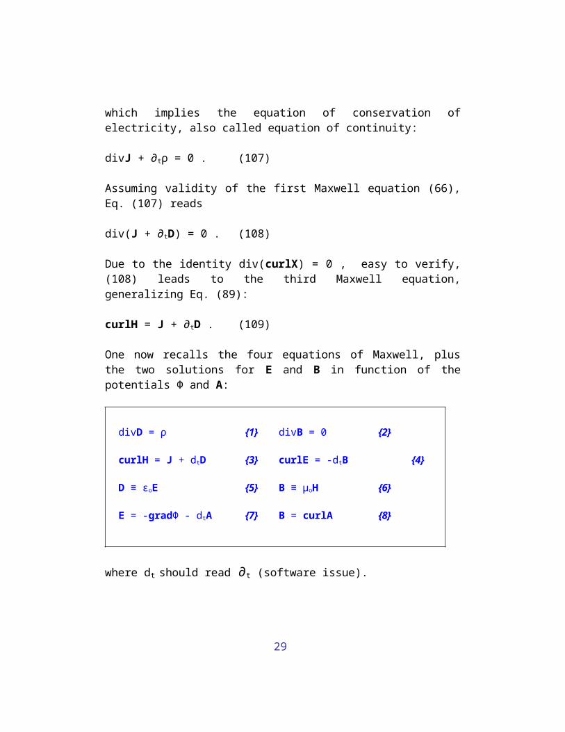
One now recalls the four equations of Maxwell, plusthe two solutions for E and B in function of thepotentials Φ and A:

divD = ρ {1} divB = 0 {2}

curlH = J + dtD {3} curlE = -dtB {4}

D ≡ εoE {5} B ≡ μoH {6}

E = -gradΦ - dtA {7} B = curlA {8}

where dt should read ∂t (software issue).

30

To generalize (92), one derives time-dependentequations of the magnetic potential, using {8}, {5} and{6}. Eq. {3} then reads

curl(curlA) = μoJ + εoμo∂tE . (110)

One uses the identity (91) to get the Laplacianoperator. Through {7}, one then finds

[Δ - c-2(∂t)2]A = - μoJ + grad(divA + c-2∂tΦ) , (111)

(c2 ≡ 1/εoμo),

which gives the electromagnetic value of the speed oflight c.

Eq. (111) can be written in the simple form

□A = - μoJ (112)

where the Dalembertian operator □ is defined by

□ ≡ Δ - (1/c2)(∂t)2, (113)

according to the Lorentz gauge

divA + (1/c2)∂tΦ = 0 (114)

One now looks for a time-dependent equation for theelectric potential Φ, which would generalize (70).Using {7} and {5}, Eq. {1} reads

31

div(- gradΦ - ∂tA) = ρ/εo , (115)

or,

[Δ - c-2(∂t)2]Φ = - ρ/εo - ∂t(divA + c-2∂tΦ) , (116)

which reduces to

□Φ = - ρ/εo

(117)

with the Lorentz gauge.

Solutions of (112) and (117) are outgoing and ingoingwaves. We only give here particular solutions of Φ andA in the form of outgoing waves called retardedpotentials, which shows that the electromagneticinteraction travels at the speed of light. Thisimplies that the effect from a source located at thepoint O at the time t is felt at the point P , wherefields are calculated, at the time t + r/c. Forcontinuous distributions of charges, the solutions forthe potentials are

Φ(r,t) = (1/4πεo)∫∫∫d3x.ρ(0,t-r/c)/r ,

A(r,t) = (μo/4π)∫∫∫d3x.ρ(0,t-r/c)v/r . (118)

According to (111-b), μo/4π = 1/4πεoc2 reads

μo/4π = 1/c2 , (119)

32

in the cgs system where εo = 1/4π.

With these formulas, approximate calculations offields at great distances from moving sources [6], infact at infinity where light will never arrive, led tothe dubious supposition that accelerated chargesalways radiate energy in the form of electromagneticwaves. [7], which cannot be so with Bohr’s circularorbits where the electric force is perpendicular tothe electron velocity, producing therefore no work (noenergy), Moreover, physical results should be derivedfrom calculations as exact as possible, as close aspossible to the radiating matter. In this somewhatconfuse situation, the solution is thereforeEinstein’s hypothesis about emission of light quanta(photons 1905). However, in the particular case ofBohr’s round orbits, there subsists the possibility ofelectronic transitions on basis of Heisenberg’suncertainty products of indeterminations alsoreferring to “deviations” (terminology) duringelectronic transitions [8].

Besides, Hermann Weyl realized that one could notsustain a physically acceptable conclusion, only onbasis of approximate calculations. He then developedthe adverse thesis quite indirectly [8b]. In thisview, his judgment perhaps implied a suggestion ofthe type "verify calculations”.

III-4. Uniform Fields A uniform field is not only constant in time (time-independent), but is also characterized by a constant

33

intensity over a definite region. This implies thatthe space derivatives of the field vanish in thatregion. A first example is given by the uniformelectric field satisfying

Φ = - E.r , (120)

which is checked as follows:

E = - gradΦ = grad(E.r) = Σ c 1c∂c(Σ k Ekxk)

= Σ c 1c(Σ k Ekδck) = Σ c 1cEc = E .

A uniform magnetic field verifies

A = B^r/2, (121)

which is easily checked by calculating a component ofB , for example B1.

III-5. Magnetic and dipole moments The magnetic moment M of a system formed by discretecharges is defined by

M = (1/2)Σ k ekrk^vk . (122)

If particles are characterized by the same ratio e/m,(122) gives

M = (e/2m)Σ k mkrk^vk ,

which also reads

34

M = (e/2m)L , (123)

where L is the angular momentum of the system.

The electric dipole moment d of a system of charges isdefined by

d = Σk ekrk. (124)

If the total charge of the system is zero, the dipolemoment is independent from the origin of thecoordinate system (easily demonstrated). The dipoleand magnetic moments are used in approximate estimatesof the fields at great distance from systems ofcharges [6], which act as sources of the field.

REFERENCES

[6] L. Landau and E. Lifshitz: The classical theory of fields,Addison Wesley, Ma 1961, pp. 171, 186, 103.

[7] R.L. Liboff: Introductory quantum mechanics, HoldenDay, San Francisco 1980, p. 29.

[8] J. Chauveheid and F.X. Vacanti: Toward a visualization ofelectronic transition, Physics Essays, vol. 15, p. 253(2002).

[8b] H. Weyl: Space-Time-Matter, Dover, NY 1952, p. 303.

35

Chapter IV: Electromagnetic energy

IV-1. Energy density and energy flux Maxwell's electromagnetism is a dualistic theory inwhich electrically charged particles moving in vacuumare the sources of the field. This electromagneticfield has its own energy, but electromagnetic energyis only known in vacuum. In what follows, it will beshown that Maxwell's theory is not concerned withenergy inside massive matter, which commonly lookslike a mystery [9].

Maxwell’s equations allow to clarify basic issuesregarding the transformation of electromagnetic energyinto kinetic energy of matter, and conversely. To seethis, one recalls Eqs. {3} and {4}:

εo∂tE = curlH - J , (125)

μo∂tH = - curlE . (126)

One multiplies (125) by E , (126) by H and sums theresults, which gives

εoE.∂tE + μoH.∂tH = - (H.curlE - E.curlH) - E.J . (127)

One recalls the identity

div(E^H) = H.curlE - E.curlH . (128)

36

Therefore, (127) reads

divY + ∂twem = - E.J , (129)

where the density of electromagnetic energy in vacuumwem and the Poynting vector Y are defined by

wem = (εoE2 + μoH2)/2

Y = E^H(130) and 131)

Y is the flux density of electromagnetic energy(amount of electromagnetic energy through unit area inunit time - flux means current). This is easily seenin vacuum (J = 0) where (129) becomes

divY + ∂twem = 0 , (132)

which is the equation of conservation ofelectromagnetic energy in vacuum, analogous to Eq.(107) expressing the conservation of electricity.

In the presence of material sources, electromagneticenergy transforms into kinetic energy of matter andconversely. One shows this by a volume-integration of(129) giving

(d/dt)∫∫∫ wem.d3x + ∫∫∫ ρ(v.E)d3x = - ∯Y.dS (133)

37

In the case of discrete charges (really continuousdistributions of charge are in fact never realizedoutside particles), the second integral reads

∫∫∫ρ(v.E)d3x = Σ k ek(E.vk) = Σ k Fk.vk ,(134)

where Fk is the Lorentz force acting on a particle ofcharge ek. Since perpendicular to velocity, the workproduced by the magnetic component of the Lorentzforce is zero. Therefore, (133) gives for the sum ofelectromagnetic energy Wem and kinetic energy W:

(d/dt)(Wem + W) + ∯Y.dS = 0 (135)

which expresses the conservation of the total energyof an isolated system. One remarks that, through(130), electromagnetic energy is positive definite.But, for an hydrogen atom, the potential energy of theelectron -e2/r, representing the electromagnetic energyof the system, is negative [Eqs. (15) and (28)]. Thisis so because a constant is missing [see Eq. (383)].According to (134) and (135), it seems thatelectromagnetic energy in vacuum, therefore inphotons, cannot be confused with the inertia ofcharged matter (detailed further).

IV-2. Electrostatic case Applying the equations to simple cases shows theimplications of a theory. For example, one can

38

calculate the total electrostatic energy U outside around particle of charge e and radius R:

∞ ∞U = (εo/2) ∫ E2dτ = (εo/2) ∫ (e/4πεor2)24πr2dr R R ∞= (e2/8πεo)[-1/r] , (136) R

or U = e2/8πεoR, which reduces to

U = e2/2R(137)

in the cgs system (εo = 1/4π).

The vanishing radius of an isolated particle wouldthus make this electromagnetic energy greater than theenergy of a finite universe. This is why particlesmust be finite. One can put (137) in the form

U = eΦ/2 , with Φ = e/4πεoR, (138)

Φ being the potential at the surface of the particle.

For a system of point-like charges, theelectromagnetic energy U of vacuum is given by theintegral ∞ ∞U = (εo/2) ∫ E2d3x = -(1/2) ∫ D.gradΦ)d3x. (139)

39

0 0

Integrating by parts gives

∞ ∞2U = ∫ (Φ.divD)d3x - ∫ div(D.Φ)d3x. (140) 0 0

In (140), the second integral on the surface of asphere S, with radius R reaching infinity, gives

-∯Φ(D.dS) = [- 4πR2Φ(D.1r)]∞ (141)

clearly vanishing for a finite system of charges.Therefore, with the first equation of Maxwell, (139)gives

U = (1/2) ∫Φde (142)

(de = ρd3x) which defines the electrostatic energy ofa finite system of charges, in agreement with (138) ifthe charge is concentrated at the boundary betweenmatter and vacuum.

So, Maxwell's theory is a macroscopic theory that doesnot penetrate particles. Its equations in matter suchas {1} and {3} are restricted to theoreticaldistributions of charged matter and might not be validinside elementary particles, which would be thesubject of another theory.

40

IV-3. Electromagnetic radiation We recall the particular outgoing wave-solutions (118)of d'Alembert's equations (112) and (117), from whichthe electric and magnetic fields can be calculated byusing Eqs. {7} and {8}. These solutions describe theelectromagnetic interaction in a system of generallymoving charges. Far from the sources, these solutionscan be made as small as one wishes by increasing thedistance, due to the presence of a negative power of runder the sign of integration (ρ/r and J/r).

Therefore, the intensity of these solutions diminishesat least by half (see ref. [9]) when the distance fromthe sources doubles. Therefore, although thesesolutions are sometimes treated asymptotically asplane waves of electromagnetic radiation, they cannever be assimilated to plane waves with constantintensity. Since the decrease of intensity is due tothe presence of source terms in the right members of(112) and (117), one must, for a model ofelectromagnetic radiation with constant intensity,look at the source-free equations:

□A = 0 , (143)

□Φ = 0 , (144)

which describe a particular form of matter calledphotons, γ-rays, electromagnetic radiation, light (allsomewhat synonyms). One now considers solutions f(u)of (143) and (144) that indifferently represent A orΦ. The variable u is then defined by

41

u = k.r - Ωt , (145)

where Ω and k are constant. This linear dependencein x, y, z, t is what makes f(u) a plane wave-solution, which is detailed further; k is the wave-vector and one recalls

Ω = 2πν , (146)

ν being the wave frequency. For du = 0,

k.dr = Ω.dt , (147)

implying for the absolute value v of the wavevelocity:

v = dr/dt = Ω/k(148)

which characterizes the progression of the wave alongits wave-vector. One recalls that the wave-length λ isdefined by

λ = v/ ; ( is the frequency). (149)

To simplify the calculations, one takes

k = k1z . (150)

Therefore, u reduces to

42

u = kz - Ωt

(151)

(k and Ω are assumed > 0), and f(u) is functionz and t only, which shows even more clearly that thelinear structure of u characterizes a plane wavesolution. The operator □ then reads

□ = (∂z)2 - (1/c2)(∂t)2. (152)

Calculations based on the expression of u in relationto the magnetic potential Aα (α = 1, 2, 3) give

A'α ≡ ∂u(Aα) and A''α ≡ (∂u)2Aα . (153)

So,

∂3Aα = A'α.k ; ∂1Aα = ∂2Aα = 0 ; ∂tAα = - A'α.Ω ;

(∂3)2Aα = A''α.k2 ; (∂t)2Aα = A''α.Ω2 . (154)

Therefore, Eq. (143) in the form □Aα = 0 gives

k2 = Ω2/c2

(155)

equivalent to (148) with c = Ω/k . One gets the sameresult with Φ(u) , which indicates that the speed oflight c is the speed of propagation of the planeelectromagnetic wave represented by the solutionsA(u) and Φ(u). Since the potentials are, through u,

43

functions of z and t only, one sees that the non-vanishing components of B are B1 and B2. Using Eq. {8}and remembering that k = k3 , one gets

B1 = - ∂3A2 = - A'2.k3 = (k^A')1 ,

B2 = ∂3A1 = A'1.k3 = (k^A')2 , (156) or,

B = k^A'(157)

which implies

k.B = A'.B = 0.(158)

One calculates the electric field given by Eq. {7}. Inanalogy with (153), the following notation is used:

Φ' ≡ ∂uΦ . (159)

So,

∂3Φ = Φ'k ; ∂1Φ = 0 ; ∂2Φ = 0 ; ∂tΦ = - ΩΦ',

recalling ∂tAα = - ΩA'α . (160)

Therefore,

E1 = - ∂1Φ - ∂tA1 = 0 + ΩA'1 ,

E2 = - ∂2Φ - ∂tA2 = 0 + ΩA'2 ,

E3 = - ∂3Φ - ∂tA3 = - kΦ' + ΩA'3 , (161)

44

or,

E = - Φ'.k + ΩA'. (162)

From (157) and (162), one finds

B.E = 0(163)

Equations (143) and (144) were conditioned by theLorentz gauge (114). This condition reads

A'3k3 - (1/c2)ΩΦ' = 0 , or (164)

k.A' = (Ω/c2)Φ'. (165)

The scalar product of k and E is calculated, using(162) and (165):

k.E = - Φ'k2 + ΩA'.k = Φ'(- k2 + Ω2/c2). (166)

Eq. (155) implies

k.E = 0(167)

The three vectors E, B, k are therefore perpendicularto each other. One now shows that the system formed bythem is right-handed, by finding the expression ofPoynting's vector Y, first writing (162) in the form

45

A' = (E + Φ'k)/Ω. (168)

Eq. (157) then becomes

B = k^(E + Φ'k)/Ω, (169)

reducing to

B = k^E/Ω. (170)

This, through k = Ω/c, gives the important relationbetween the electric and magnetic intensities:

B = E/c(171)

which, through (111), implies

εoE2 = μoH2. (172)

Therefore, the electromagnetic energy densitytransported by the wave reads

wem = εoE2 = μoH2

(173)

and the Poynting vector reads

Y = E^(k^E)/μoΩ . (174)

46

It is easy to demonstrate the vector identity

a^(b^c) = (a.c)b - (a.b)c , (175)

so, Eq. (174) becomes

Y = (1/μoΩ)[(E.E)k - (E.k)E] . (176)

Using (167), this reduces to

Y = E2k/μoΩ. (177)

With (111), (173) and k = Ω/c, one finally gets

Y = c.wem1k

(178)

The flux density of energy (flux means current) isthus the product of the energy density wem by the wavevelocity c. One had a similar result with electricity,since the electric current density is the product ofthe density of electricity by the velocity of electriccurrent.

Monochromatic radiation is represented by simpletrigonometric functions of u, giving sinusoidal wavesand others, or is represented by the real part of acomplex exponential of the same variable. On smallintervals, albeit greater than the wave-length, theaverage intensity can be regarded as constant, whichbrings us back to the beginning of this section wherepart of the concern was a lack of dispersion of a

47

radiating electromagnetic wave, so that it could beregarded as a beam of constant intensity. Besides itsemission from transitions to lower electronic energylevels in atoms (see Bohr's model), electromagneticradiation can also be caused by non-elastic collisionsof moving charges. For the treatment of non-chromaticwaves, one expands in series of Fourier [9].

The previous physical results can be derived in asimpler manner by considering the wave propagationalong the x-axis and making Φ = 0 and Ax = 0 (?) [9],invoking the principle of gauge invariance (seesection VI-2). However, the method followed here hasthe advantage of presenting a greater generality.Moreover, the fact that a simplification of methodleads to equivalent results supports gauge invariancefor photons, which might be a bit difficult to showotherwise.

IV-4. Joule's effect and magnetic hysteresis According to Lorentz' interpretation, Maxwell's theoryhas until now been developed in the vacuumcharacterized by the two constants εo and μo. If onewishes to use the theory in another medium such as aconductor crossed by an electric current and siege ofelectromagnetic phenomena, one must use differentvalues of these parameters now referred to as ε andμ. These will no longer remain constant since, inagreement with experiment, their value will alsodepend on the intensity of the field, as seen in thecase of magnetic hysteresis. These two parameters,respectively called dielectric induction and magnetic

48

permeability of the medium, describe the electric andmagnetic fields E and B in the form

E = D/ε , and B = μH . (179)

So, the equations of Maxwell {1} to {4}, with theirsolutions {7} and {8}, will remain unchanged, Eqs. {5}and {6} are replaced by (179). Since ε and μ are notconstant, their derivatives do not vanish and thetreatment of energy in section IV-1 has to changeaccordingly, which is done below. One writes Eqs. {3}and {4}:

∂tD = curlH - J , (180)

∂t B = - curlE. (181)

One multiplies (180) by E and (181) by H, sums theresults using the identity (128). So,

E. ∂tD + H. ∂tB + div(E^H) + E.J = 0 , (182)

where E^H is the Poynting vector Y. The energydensity wem is then redefined by

wem = (1/2)(E.D + H.B) . (183)

Therefore,

∂twem = (E.∂tD + H.∂tB) - (1/2)(E.∂tD + H.∂tB)

+ (1/2)(∂tE.D + ∂tH.B) , or (184)

49

E.∂tD + H.∂tB = ∂twem + (1/2)(H.∂tB - B.∂tH)

+ (1/2)(E.∂tD - D.∂tE). (185)

Eq. (182) then becomes

divY + ∂twem + E.J + (1/2)(H.∂tB - B.∂tH)

+ (1/2)(E.∂tD - D.∂tE) = 0 . (186)

If the first three terms were alone, the situationwould look the same as in Eq. (129). However, herethird term expresses the dissipation of energy due tonon-elastic collisions inside the medium, called Jouleeffect. The fourth and fifth terms refer respectivelyto the magnetic and electric hysteresis. Now,regarding the Joule effect in a conductor, one recallsthat the electric current density is proportional tothe electric field, which reads

J = E/α(187)

where α is the resistivity of the medium.

One considers a transverse section of area S, crossedby a current of intensity i, and writes

i = JS = ES/α . (188)

Multiplying this by the length dx of the conductorgives

50

idx = ESdx/α . (189)

Neglecting magnetic effects, Eq. {7} reads

E = - dΦ/dx. (190)

Therefore, (189) becomes

idx = - SdΦ/α , (191)

which gives Ohm's law

dΦ = -ri ; with r = αdx/S

(192)

where r is the resistance of the conductor.

The term E.J in (186) permits to calculate the thermaldissipation dW/dt per unit time along the length dx.One remarks that the dimension of dW/dt is the same asthat of ∂twem multiplied by a volume. So, onemultiplies E.J by the volume Sdx, using (190):

dW/dt = EJ(Sdx) = Eidx = - idΦ . (193)

With (192), (193) then gives Joule's law

dW/dt = ri2

(194)

51

The loss of energy by unit volume wmh through magnetichysteresis is calculated over the time T:

T Twmh = ∫ 1/2)(H.∂tB-B.∂tH)dt = ∫ HdB-BdH)/2 . (195) 0 0

One draws a diagram with the rectangular coordinates x= H, y = B, and integrates over a closed cycle ofperiod T, which gives\\

Wmh = (1/2)∮H.dB - B.dH (196)

as the dissipated energy by unit volume in the form ofthe area of the hysteresis cycle [see (34)].

REFERENCES

[9] A. Einstein: The Meaning of relativity, PrincetonUniversity Press, 5th ed. 1955, p. 50; L. Landau andE. Lifshitz: The classical theory of fields, Addison Wesley, Ma1961, pp. 104, 111, 117, 123.

Chapter V: Special relativity

V-1. Theoretical background

52

According to what follows, special relativity is notan independent theory since being strictly aconjunction of direct applications of Maxwell'sequations (previously pioneered by Faraday), withtherefore no need to invent anything new, or bringing“new ideas”. All this is explicitly and sufficientlydetailed in the title of Einstein’s 1905 paper: “On theElectrodynamics of Moving Bodies”. However, this is not all,since will be used Galileo’s relativity principle,following which the equations of physics are the samefor two observers in relative motion of constantvelocity, which, for example, is synonymous to “thelaws of mechanics are not affected by a uniformrectilinear motion of the system(s)”.

The Faraday-Maxwell theory, in the final form ofMaxell’s equations, also provides a satisfactoryexplanation of electromagnetism in vacuum, and givesthe correct relationship between the kinetic energy ofcharged (massive) matter and the electromagneticenergy of vacuum, in the form of a law of energyconservation (Eq. 135). Moreover, Maxwell's equationsin vacuum provide a rational explanation of theconstitution of light, although this theory isincomplete without its corpuscular character(photons). The fundamental feature is thedetermination of light velocity c in empty space, infunction of the electric induction and magneticpermeability of vacuum (c2 = 1/εoμo in Eq. 111-b),which, with next Eq. 198, integrally constitutes thecomplete basis of special relativity, the rest beingentirely deduced from these two relations.

53

This first theory of relativity was presented inachieved form and quite simultaneously by Einstein andPoincaré in 1905, succeeding to a rather long list ofprevious contributors such as FitzGerald, Larmor,Lorentz and others. Special relativity assumesaccordingly in its second postulate that the velocityof light is the same for two inertial observerscharacterized by a uniform relative velocity, theadjective "inertial" meaning "in the absence of agravitational field". In an inertial reference system,a body not acted upon by external forces maintains arectilinear trajectory with constant velocity, whichrecalls Galileo and roughly tells the same as 1915general relativity where "inertial" means "not subjectto an external gravitational field".

The two postulates of special relativity can beexpressed as follows:

(1) Same physical laws are valid for inertialobservers in uniform relative motion. This relativitypostulate implies particular changes of 4-coordinates,called Lorentz transformations, which do not affectthe equations when passing from one inertial system toanother one.

(2) Common physical properties of vacuum arefound by such observers, therefore same values for εo,μo and c. This postulate presents Special Relativityas a theory not requiring a purely kinematicalinterpretation that would obscure the electromagneticcharacter of c in vacuum.

54

Ratifying the physical properties of vacuum derivedfrom Maxwell's theory, Special Relativity marked thehistoric end of the mechanical concept of ether, amaterial massless medium whose stresses were imaginedto represent the electromagnetic field in vacuum.

However, vacuum electromagnetism is representablewithout ether but this did not seem well understoodbefore 1905. The ether was supposed to fill theuniverse, endowed with mysterious properties such asfrictionless, not subject to gravitation, omnipresentand penetrating all forms of matter, etc.

The observational evidences of special relativity,having crushed the belief in the ether, for a specificexplanation of vacuum electromagnetism, come from theexperiments of Michelson-Morley, Fizeau and theaberration of fixed stars (detailed discussions figurein ref. [10]). Moreover, according to Einstein’s words(?), remains some possibility for gravitational ether,besides the Englert-Higgs field as second candidate -eventually both, why not ?

V-2.The Lorentz transformation Lorentz’ transformations were discovered in (very)incomplete form by Woldemar Voigt in 1887 (Göttingen)[11], but Lorentz, who might have found themindependently besides Larmor (Cambridge) had the greatmerit to realize their fundamental importance.Einstein reinterpreted Lorentz' ideas and considered asource of light at the origin of an arbitrary inertialcoordinate system xyzt. An observer in this

55

referential can write the following equation of motionof a spherical light-wave emitted at the origin O atthe time zero:

r = ct ; (with r2 ≡ x2 + y2 + z2), (197)

which is equivalent to

c2t2 - x2 - y2 - z2 = 0. (198)

According to the second postulate, a second inertialobserver will write in his coordinate system x'y'z't':

c2t'2 - x'2 - y'2 - z'2 = 0 . (199)

If Eq. (198) is satisfied, this will also be the casefor Eq. (199) if the quadratic form

c2t2 - x2 - y2 - z2 (200)

is invariant through a particular change of 4-coordinates: x, y, z, t → x', y', z', t' , calledLorentz transformation. Four-coordinates include thethree space coordinates plus the time. A point orevent of the four-dimensional space-time continuum ischaracterized by four coordinates.

The invariance of this quadratic form is therefore thegeneral condition following which (198) and (199) areboth satisfied. In (200), the variables x, y, z, trepresent the respective 4-coordinate differences

56

xP - xQ , yP - yQ , zP - zQ and tP - tQ , P and Qbeing two arbitrary points of the four-dimensionalcontinuum.

To keep things simple, one then assumes that thereferential x'y'z't' is moving relative to xyzt at thevelocity V, and that the x-axis and x'-axis ofcoordinates coincide. In this case, the Lorentztransformation, implying the invariance of (200), isfound to be:

x = (1/γ)(x' + Vt')y = y'z = z't = (1/γ)[t' + (V/c2)x']

(201) with

γ = (1 - V2/c2)1/2

(202)

The inverse Lorentz transformation x'y'z't' → xyzt isfound by changing V into -V, substituting xyzt byx'y'z't' and conversely. The reader will findderivations of the Lorentz transformation in mostbooks on special relativity (see ref. [10] for asimple derivation). The reader is invited to memorizethese formulas and check their validity by verifyingthe invariance of the quadratic form (200) through thetransformation (201).

57

With special relativity, the concepts of absolutespace and absolute time seem definitively gone andreplaced by the concept of absolute space-time. Thereis no radical division between three-dimensional spaceand one-dimensional time, because coordinates mixthrough Lorentz transformations. This does not meanthat space and time can be confused since the squareof their respective coordinates appear with oppositesign in (200).

Absolute simultaneity loses its meaning sincesimultaneous events in one coordinate system will notbe simultaneous in another. Instantaneous action at adistance has therefore no place in this theory, inagreement with Maxwell's theory of electromagnetism(see Eqs. 118).

A peculiarity of Lorentz transformations is that 1/γis infinite for V = c, which indicates that theprinciple of relativity only works for inertialobservers whose relative velocity is inferior to thespeed of light. Velocities greater than c areprohibited because leading to imaginary values of γ.

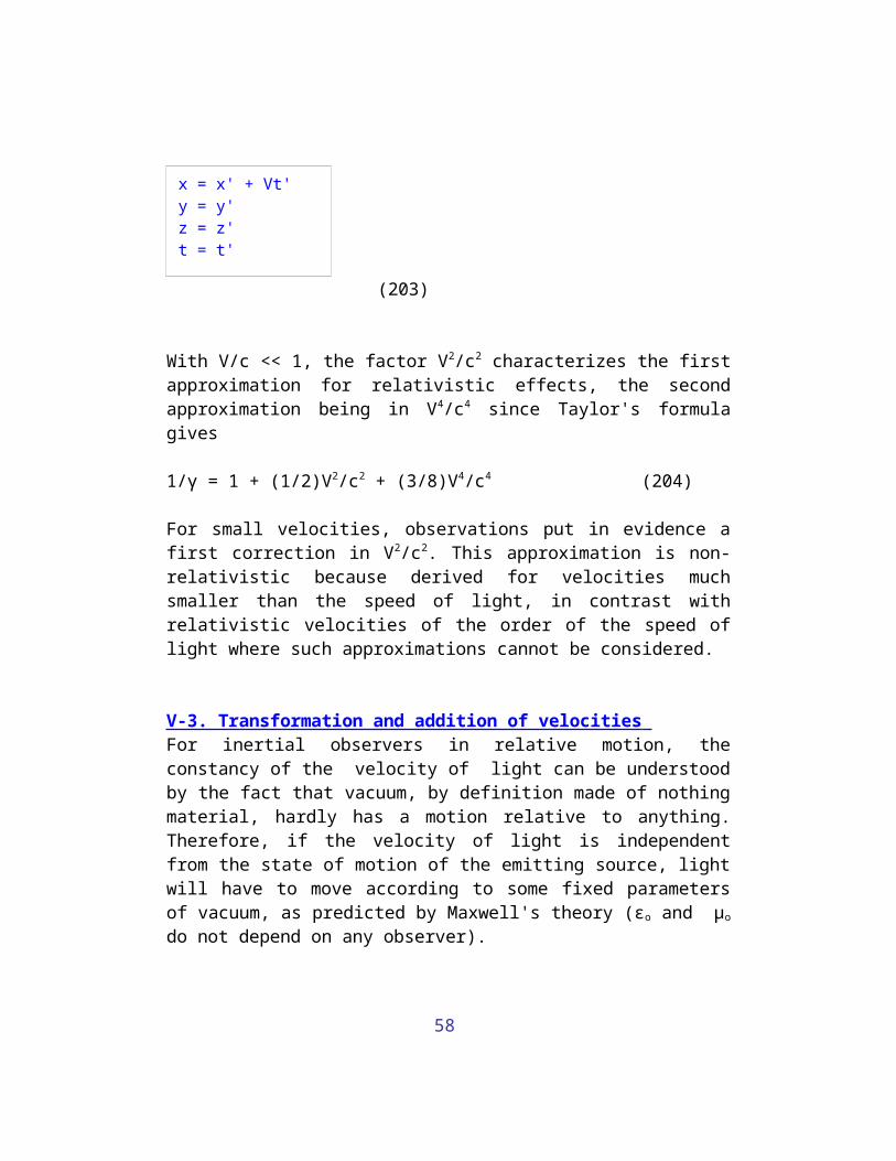
Making V/c = 0 in (201) retrieves Newtonian, Galileanor non-relativistic physics (all synonyms) with theGalileo transformation

58

x = x' + Vt'y = y'z = z't = t'

(203)

With V/c << 1, the factor V2/c2 characterizes the firstapproximation for relativistic effects, the secondapproximation being in V4/c4 since Taylor's formulagives

1/γ = 1 + (1/2)V2/c2 + (3/8)V4/c4 (204)

For small velocities, observations put in evidence afirst correction in V2/c2. This approximation is non-relativistic because derived for velocities muchsmaller than the speed of light, in contrast withrelativistic velocities of the order of the speed oflight where such approximations cannot be considered.

V-3. Transformation and addition of velocities For inertial observers in relative motion, theconstancy of the velocity of light can be understoodby the fact that vacuum, by definition made of nothingmaterial, hardly has a motion relative to anything.Therefore, if the velocity of light is independentfrom the state of motion of the emitting source, lightwill have to move according to some fixed parametersof vacuum, as predicted by Maxwell's theory (εo and μo

do not depend on any observer).

59

Secondly, Maxwell's equations in vacuum imply theequation of motion of light (197) and also give adefinite energy density to electromagnetic radiation,independently of initial conditions such as the sourcevelocity [see Eq. (178)]. This explains why thevelocity of light must be independent from thevelocity of its source(s).

In fact, these two arguments are nothing but thecontent of the two postulates of the theory, insertedinto the equation of motion (197) and the invariancecondition (200) implying the Lorentz transformation(201). In what follows, (201) will be used to derive atheorem of addition of velocities, presentingdifferently (perhaps more understandably), thepostulated independence of the velocity of light fromthe motion of its sources.

One differentiates (201), with V constant:

dx = (1/γ)(dx'+ Vdt') ,

dy = dy' ,

dz = dz' ,

dt = (1/γ)[dt' + (V/c2)dx'] . (205)

Dividing dx by dt leads to

dx/dt = (dx' + Vdt')/[dt' + (V/c2)dx'] . (206)

60

Dividing the numerator and denominator by dt' in theright member, one finds

vx = (V + v'x)/(1 + Vv'x/c2) , (207)

where v'x ≡ dx'/dt' . (208)

Dividing dy and dz by dt then gives

vy = v'y.γ/(1 + Vv'x/c2) , (209)

vy = v'z.γ/(1 + Vv'x/c2) . (210)

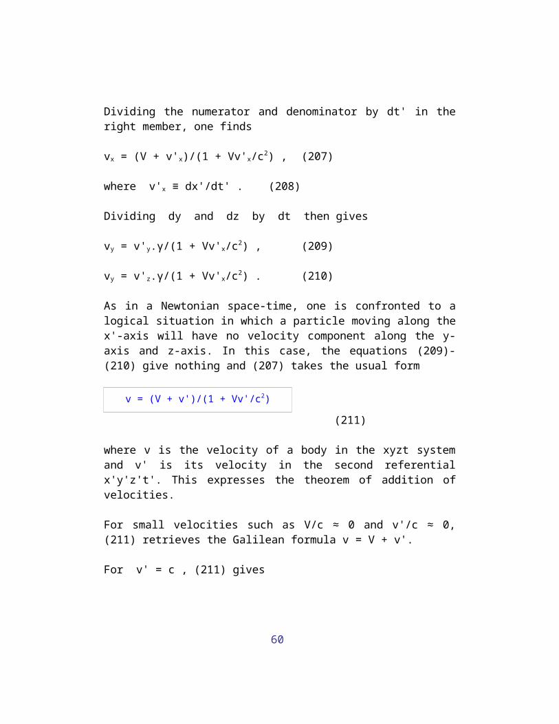
As in a Newtonian space-time, one is confronted to alogical situation in which a particle moving along thex'-axis will have no velocity component along the y-axis and z-axis. In this case, the equations (209)-(210) give nothing and (207) takes the usual form

v = (V + v')/(1 + Vv'/c2)

(211)

where v is the velocity of a body in the xyzt systemand v' is its velocity in the second referentialx'y'z't'. This expresses the theorem of addition ofvelocities.

For small velocities such as V/c ≈ 0 and v'/c ≈ 0,(211) retrieves the Galilean formula v = V + v'.

For v' = c , (211) gives

61

v = (V + c)/(1 + V/c) = c , (212)

which shows that the light has the same velocity c inboth referentials. Moreover, an emitting source withvelocity V produces the same light velocity c in thetwo 4-coordinate systems. This demonstrates that thevelocity of light does not depend on the velocity ofits source.

V-4. Length contraction and time dilation One considers a rigid rod at rest in the movingreferential x'y'z't'. This rod is located along thex'-axis. In this system, the so-called proper length,or length at rest, lo of the rod is defined by

lo = x'2 - x'1 , (213)

where x'1 and x'2 are the coordinates of itsextremities, and the proper length is always definedin a system in which the rod is at rest. The measuringof the rod length l = x2 - x1 in another system xyztwill be realized at a definite time t (measurementtime in the referential xyzt). One now writes theinverse Lorentz transformation of (201):

x' = (1/γ)(x - Vt) , (214)

t' = (1/γ)[t - (V/c2)x] . (215)

At a determined time t, Eq. (214) implies

x'2 - x'1 = (1/γ)(x2 - x1).(216) or,

62

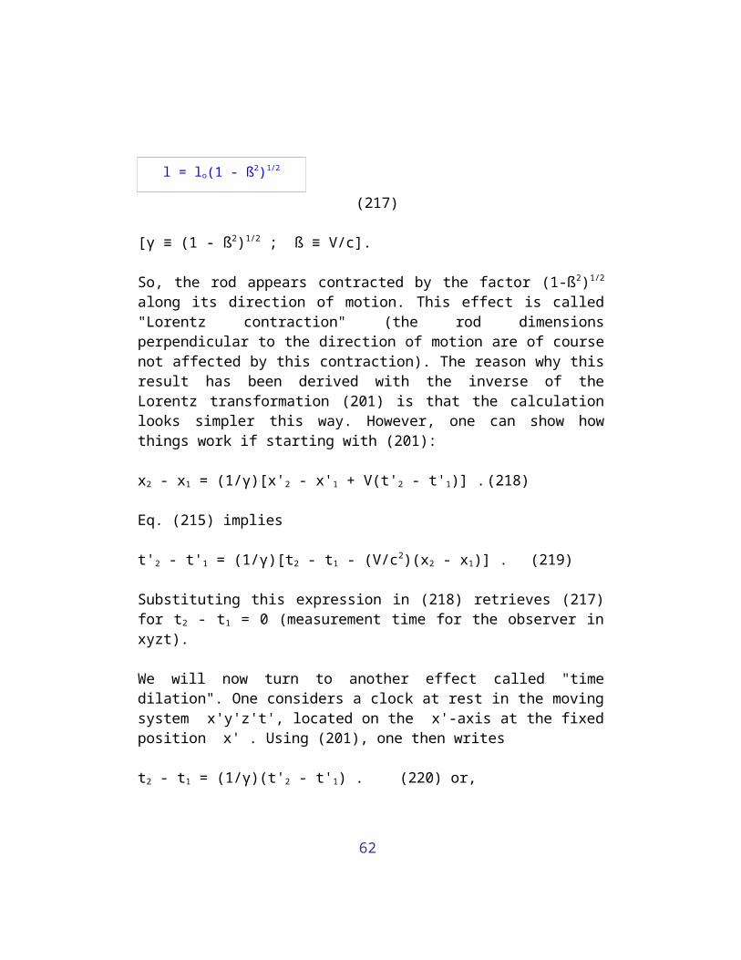
l = lo(1 - ß2)1/2

(217)

[γ ≡ (1 - ß2)1/2 ; ß ≡ V/c].

So, the rod appears contracted by the factor (1-ß2)1/2

along its direction of motion. This effect is called"Lorentz contraction" (the rod dimensionsperpendicular to the direction of motion are of coursenot affected by this contraction). The reason why thisresult has been derived with the inverse of theLorentz transformation (201) is that the calculationlooks simpler this way. However, one can show howthings work if starting with (201):

x2 - x1 = (1/γ)[x'2 - x'1 + V(t'2 - t'1)] .(218)

Eq. (215) implies

t'2 - t'1 = (1/γ)[t2 - t1 - (V/c2)(x2 - x1)] . (219)

Substituting this expression in (218) retrieves (217)for t2 - t1 = 0 (measurement time for the observer inxyzt).

We will now turn to another effect called "timedilation". One considers a clock at rest in the movingsystem x'y'z't', located on the x'-axis at the fixedposition x' . Using (201), one then writes

t2 - t1 = (1/γ)(t'2 - t'1) . (220) or,

63

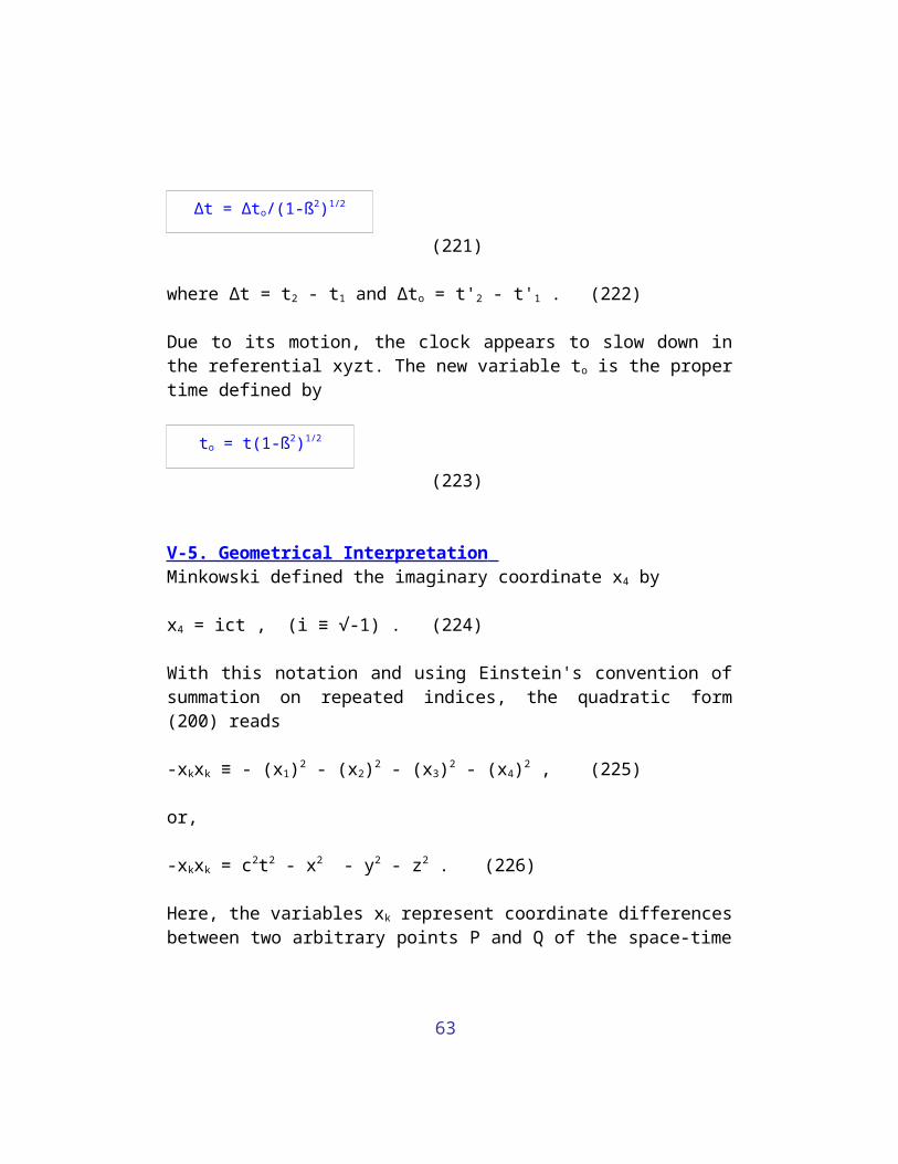
Δt = Δto/(1-ß2)1/2

(221)

where Δt = t2 - t1 and Δto = t'2 - t'1 . (222)

Due to its motion, the clock appears to slow down inthe referential xyzt. The new variable to is the propertime defined by

to = t(1-ß2)1/2

(223)

V-5. Geometrical Interpretation Minkowski defined the imaginary coordinate x4 by

x4 = ict , (i ≡ √-1) . (224)

With this notation and using Einstein's convention ofsummation on repeated indices, the quadratic form(200) reads

-xkxk ≡ - (x1)2 - (x2)2 - (x3)2 - (x4)2 , (225)

or,

-xkxk = c2t2 - x2 - y2 - z2 . (226)

Here, the variables xk represent coordinate differencesbetween two arbitrary points P and Q of the space-time

64

continuum in which, in analogy with Euclideangeometry, the four-dimensional distance or interval Δsis defined by

(Δs)2 = - ΔxkΔxk = c2Δt2 - Δx2 - Δy2 - Δz2

(227)

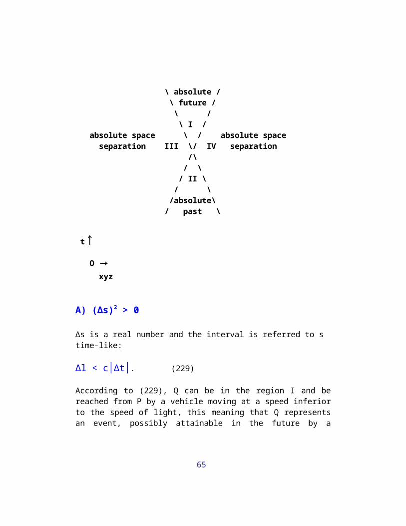
Due to the hyperbolic character of (227), thevanishing of Δs does not imply the identity of twopoints, but gives the following condition according towhich two points P and Q can be connected by a lightsignal upon a light-cone (see the two interruptedlines representing a light-cone on next figure.

Δl = ± cΔt

with (Δl)2 ≡ (Δx)2 + (Δy)2 + (Δz)2. (228)

If Q is located on the upper half of the cone, thus onone of the interrupted lines above P, a light signalcan be sent from P and received at Q. Conversely, if Qis located on the lower half of the cone, a lightsignal can be sent from Q to P. The vanishing of Δs,constituting an invariant feature, no Lorentztransformation can modify the situation of P and Qbeing located on a light-cone, which characterizesnull-distance events in the sense of the theory ofrelativity.

65

\ absolute / \ future / \ / \ I / absolute space \ / absolute space separation III \/ IV separation /\ / \ / II \ / \ /absolute\ / past \

t↑ O → xyz

A) (Δs)2 > 0

Δs is a real number and the interval is referred to s time-like:

Δl < c│Δt│. (229)

According to (229), Q can be in the region I and bereached from P by a vehicle moving at a speed inferiorto the speed of light, this meaning that Q representsan event, possibly attainable in the future by a

66

moving body located at P. Conversely, if Q is locatedin the region II, P represents a possible future eventfor a moving body from Q. The space interval Δl can bemade to vanish according to a Lorentz transformation,leaving an absolute time separation between two eventsat a same place, one representing the past and theother the future. Past and future thus have anabsolute meaning for events separated by a time-likeinterval. This explains why, according to Minkowski,physical events can only be related causally in thiscase.

B) (Δs)2 < 0

Δs is an imaginary number and the interval is referredto as space-like:

Δl > c│Δt│ (230)

Q is located in one of the regions III and IV. Theevents P and Q cannot be joined by a vehicle moving ata speed smaller than the speed of light. Through anadequate Lorentz transformation, Δt can be made tovanish but the two events would remain separated inspace. Being located at distinct places thus has anabsolute meaning for events separated by a space-likeinterval. Finally, the conditions (229) and (230) areinvariant and are therefore unaffected by Lorentztransformations.

V-6. Vectors and tensors

67

We will consider general Lorentz transformations inwhich the four coordinate-axes and the relativevelocity between referentials can be orientedarbitrarily. We write such general lineartransformations (first using the primes in the leftmember):

x'k = aknxn , (231)

where the coefficients akn are constant. So,differentiating (231) leads to

dx'k = akndxn . (232)

According to (227), an infinitesimal 4-dimensionalinterval ds between two neighboring points satisfiesthe relation

(ds)2 = - dxkdxk ≡ - δkndxkdxn . (233)

The dxk are the components of a 4-vector and,according to the second postulate, the interval dsis invariant through Lorentz transformations. With theuse of the Minkowski notation (224), the Lorentztransformations simply reduce to linear orthogonal 4-transformations whose properties will be studied next.One remarks that infinitesimal dx can be replaced bythe finite Δx, since these are vector components aswell, but the infinitesimal notation will be kept forconvenience. Therefore,

ds2 = -dx'kdx'k = -akmakndxmdxn . (234)

68

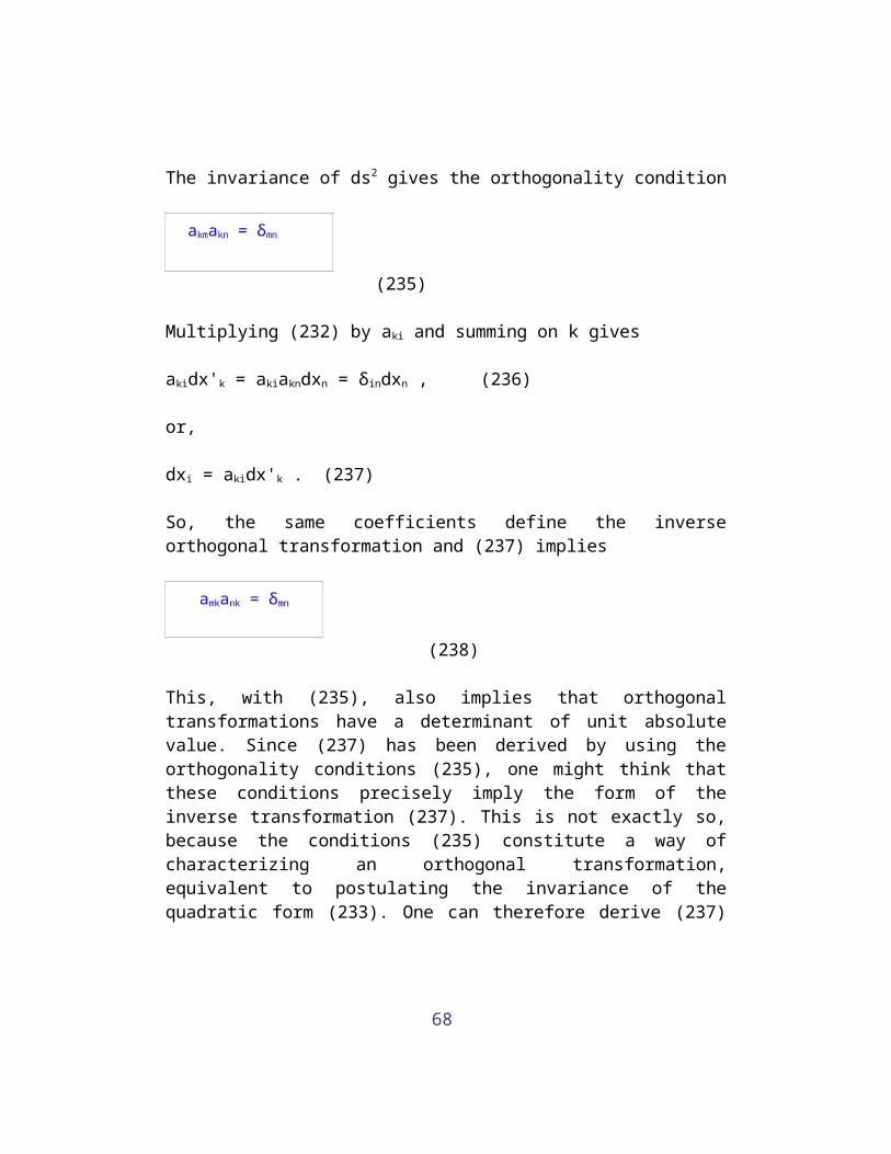
The invariance of ds2 gives the orthogonality condition

akmakn = δmn

(235)

Multiplying (232) by aki and summing on k gives

akidx'k = akiakndxn = δindxn , (236)

or,

dxi = akidx'k . (237)

So, the same coefficients define the inverseorthogonal transformation and (237) implies

amkank = δmn

(238)

This, with (235), also implies that orthogonaltransformations have a determinant of unit absolutevalue. Since (237) has been derived by using theorthogonality conditions (235), one might think thatthese conditions precisely imply the form of theinverse transformation (237). This is not exactly so,because the conditions (235) constitute a way ofcharacterizing an orthogonal transformation,equivalent to postulating the invariance of thequadratic form (233). One can therefore derive (237)

69

by simply assuming the invariance of (233), which isseen in

ds2 = -dx'kdx'k = -(akndxn)dx'k

= -dxn(akndx'k) = -dxndxn (239)

From vectors such as dxk , one can form the tensor ofsecond rank dxkdxj , whose components transform like

dx'kdx'j = akmajndxmdxn. (240)

Accordingly, a vector is a tensor of rank one. Sincetensor transformations are linear, one can form newtensors by addition or subtraction of tensors of samerank. A tensor of rank zero can be found bycontracting the two indices of a tensor of secondrank, which in the case of dxkdxj amounts to make k= j , then retrieving the quadratic form (233) whichis a scalar (one component only).

Regarding Lorentz transformations of determinant -1,the simplest ones are time-inversion and space-reflection. Time-inversion is defined by

x' = x ; y' = y ; z' = z ; t' = - t , (241)

and space-reflection by

x' = - x ; y'= - y ; z' = - z ; t' = t . (242)

These particular orthogonal transformations belong tothe sub-group of inversions and cannot be confusedwith rotations, since not arising from continuous

70

variations of a coordinate system [12]. If Lorentztransformations are restricted to those withdeterminant +1, the volume-element dx1^dx2^dx3^dx4 is aninvariant. One shows this by considering 2-dimensionalorthogonal transformations, which simplifies thecalculations. In this case, the surface-element dx1^dx2

transforms as follows:

dx'1^dx'2 = (a11dx1 + a12dx2)^(a21dx1 + a22dx2)

= (a11a22 - a21a12)dx1^dx2 = (detakn)dx1^dx2

= dx1^dx2 . (243)

One can say that the invariance of the infinitesimal4-volume element, through Lorentz transformations withdeterminant +1, is due to the fact that the Lorentzcontraction of its 3-volume part is exactlycompensated by the time dilatation of dt.

There exist special tensors [12], such as the secondrank Kronecker tensor δjk. This tensor is characterizedby diagonal unit components. One verifies that thedefinition of δjk is preserved through the tensortransformation

δ'mn = amjankδjk , (244)

which reduces to

δ'mn = amkank = δmn , (245)

retrieving (238). According to Einstein's conventionfor summation, one notes that

71

δjj = 4 . (246)

A tensor Ankl is symmetric in the k and l indices if Ankl

= Anlk. The Kronecker tensor δjk is therefore symmetric.Similarly, Bnkl is antisymmetric in the indices k andl if Bnkl = - Bnlk . This implies that the diagonalelements of an antisymmetric tensor of second rank,such as Fjk , vanish: F11 = F22 = F33 = F44 = 0.

A second special tensor is the totally antisymmetricfourth rank tensor εjkmn, whose components of unitabsolute value are determined according to even andodd permutations of indices:

є1234 = + 1 ; - 1 = ε1243 = ε1324 , etc... (247)

Its tensor character is easily proven throughtransformations in the simple 2-dimensional case. Thistensor is peculiar in the way that its components arenot affected by inversions, contrary to usual tensors.This is why it is called a pseudo-tensor. If thetensor Fjk is antisymmetric, the pseudo-tensor(1/2)εjkmnFmn is called its dual. The pseudo-tensor εjkmn

finds a practical use in the mathematical theory ofsurface and volume integrals [13]. The fact that itscomponents are not affected when passing from a right-handed to a left-handed system shows some lack ofphysical character.

Importantly, tensors of higher rank are derived bydifferentiation of tensors. To see this, one uses theformula

72

∂jf = (∂f/∂x'k)(∂x'k/∂xj) (248)

(noting that ∂if ≡ ∂f/∂xi). Since (231) implies ∂x'k/∂xj = akj, (248) reads

∂jf= akj(∂f/∂x'k) = akj∂'kf . (249)

Therefore, ∂j transforms according to thetransformation (237), inverse of (231). Accordingly,∂'j verifies

∂'j = ajk∂k (250)

The ∂k are therefore the components of a 4-vector, andone can write the transformation law of the tensor∂jAk:

(∂jAk)' = ajmakn∂mAn , ∂jAk = amjank(∂mAn)' (251)

In the next chapter, the reader will see, in theparticular case of electromagnetism, how physical lawscan be formulated through tensor equations in whichpartial derivatives are vectors.

V-7. Electric current and 4-momentum Contrary to Newtonian physics, the velocity dxk/dt of amoving body is not a vector because dt is not aninvariant. So, a new 4-velocity uk ≡ dxk/dto will bedefined. From (223) and (233), one writes

73

dto ≡ γdt = ds/c (252)

[γ ≡ (1-ß2)1/2 ; ß ≡ v/c], where dto clearly is aninvariant. Therefore,

uk = cdxk/ds = dxk/dto = dxk/γdt

(253)

The three space-components uß thus provide a simplegeneralization for dxß/dt (here, Greek indicesexclusively refer to space). The fourth componentreads

u4 = ic/γ (254)

(i ≡ √-1). The 4-momentum vector pk is muk , whose 4-component reads

p4 = imc/γ , (255) or,

p4 = iEn/c

(256), recalling

En = mc2/γ

(257)

where En is the energy of a massive body. Regarding theelectric current density Jk, its 4-dimensionaldefinition is

74

Jk ≡ ρouk = ρocdxk/ds , (258)

where ρo is the rest electric charge density (expressedin a system in which the particle velocity is zero); ρo

is an invariant and the definition (258) implies

Jβ = ρodxβ/γdt = ρovβ/γ (259)

which retrieves the previous definition (88):

Jβ ≡ ρvβ , (260) if

ρ = ρo/γ

(261)

ρ differs from the rest charge density, since it isthe charge density of a moving particle, as seen by anobserver in his coordinate system. ρ is thus greaterthan ρo , due to the volume contraction in thedirection of the particle motion (Lorentz' lengthcontraction). The component J4 reads

J4 = icρ . (262)

Results are summarized below:

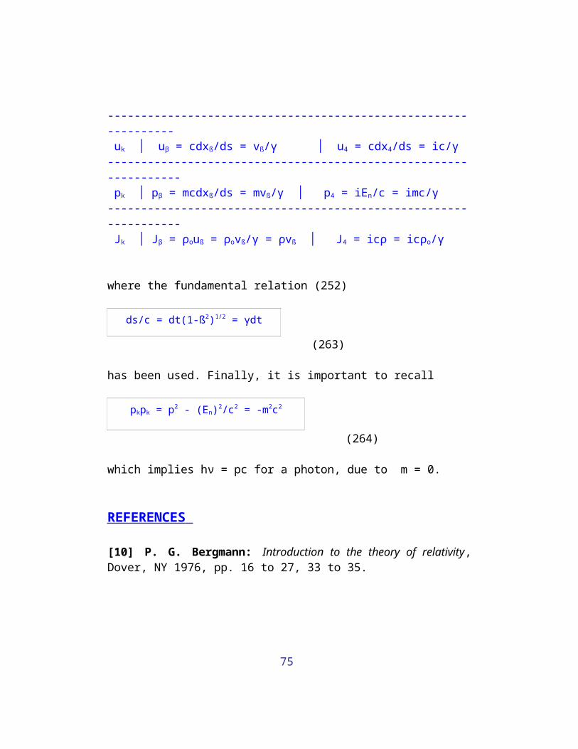
space components │ time components─────────────────────────────────── dxk │ dxß │ dx4 = icdt

75

---------------------------------------------------------------- uk │ uβ = cdxß/ds = vß/γ │ u4 = cdx4/ds = ic/γ----------------------------------------------------------------- pk │ pβ = mcdxß/ds = mvß/γ │ p4 = iEn/c = imc/γ----------------------------------------------------------------- Jk │ Jβ = ρouß = ρovß/γ = ρvß │ J4 = icρ = icρo/γ

where the fundamental relation (252)

ds/c = dt(1-ß2)1/2 = γdt

(263)

has been used. Finally, it is important to recall

pkpk = p2 - (En)2/c2 = -m2c2

(264)

which implies hν = pc for a photon, due to m = 0.

REFERENCES

[10] P. G. Bergmann: Introduction to the theory of relativity,Dover, NY 1976, pp. 16 to 27, 33 to 35.

76

[11] A. Pais: "Subtle is the Lord...", the science and the life of AlbertEinstein, Oxford University Press, 1982.

[12] A. Einstein: The meaning of relativity, PrincetonUniversity Press, 5th ed. 1955, pp. 10, 15.

[13] L. Landau and E. Lifshitz: The classical theory of fields,Addison Wesley, Ma 1961, p. 20.

Chapter VI: 4-dimensional electromagnetism

VI-1. Electromagnetism before relativity We will follow Lorentz' viewpoint following which thephysical sources of electromagnetism are smallelectric charges in vacuum [14]. For a microphysicaltheory, one cannot consider the electrodynamics of acontinuous material medium, useful however at themacroscopic level (see section IV-4). At Lorentz'fundamental level, the dielectric constant and themagnetic permeability are the constants in vacuum εo

and μo. Accordingly, one writes Maxwell's equations interms of the electric and magnetic fields E and B:

divE = ρ/εo (265)

curlE = - ∂tB (266)

curlB = μoJ + (1/c2)∂tE (267)

77

divB = 0 (268)

In a Newtonian framework, orthogonal spacetransformations will be used because relatingCartesian 3-coordinate systems, which are thesimplest. A good reason for considering suchtransformations is due to space derivatives acting asvectors in the equations. The derivative ∂t is aninvariant because time is absolute in this framework.

Since there is no length contraction, contrary tospecial relativity, one writes ρ = ρo. The right memberof (265) is an invariant. Its left member ∂ßEß is aninvariant as well if Eß is a vector, which will beassumed. Eq. (265) reads

∂ßEß = ρ/εo , (265-b)

where Greek indices refer to space. One now looks atEq. (266), whose x-component is

∂2E3 - ∂3E2 = -∂tB1. (269)

To interpret this, the magnetic field has to berepresented by the three components of anantisymmetric tensor of second rank Fαß:

B1 = F23, B2 = F31 , B3 = F12 , (270)

With this notation, (266) gives the second rankequation

∂αEß - ∂ßEα = -∂tFαß . (266-b)

78

Eq. (267) then becomes

∂αFßα = μoJß + (1/c2)∂tEß . (267-b)

Finally, Eq. (268) is the third rank equation

∂αFßδ + ∂δFαß + ∂ßFδα = 0 , (268-b)

characterized by the cyclic permutation of the threeindices α, ß, δ. It is easy to verify that, due to theantisymmetry of Fαß, the left member of (268-b) is atotally antisymmetric tensor (so, in any pair of thethree indices) of the third rank, with only fourcomponents (easy to verify). The solution of (268-b)is

Fαß = ∂αAß - ∂ßAα , (271)

where Aß is a 3-vector called magnetic potential. Eq.(268-b) is solved and one looks now at the otherequations, substituting in them Fαß by its expression(271). Eq. (266-b) then reads

∂αEß - ∂ßEα = ∂α(-∂tAß) - ∂ß(-∂tAα) , (272)

whose solution is

Eß = - ∂ßΦ - ∂tAß , (273)

where Φ is the electric potential. With this, (265-b)gives

79

□Φ + ∂t[∂ßAß + (1/c2)∂tΦ] = -ρ/εo (274)

according to the definition (113) of the Dalembertianoperator □.

With (271) and (273), Eq. (267-b) then becomes

□Aβ - ∂β[∂αAα + (1/c2)∂tΦ] = - μoJß (275)

The terms between brackets vanish according to theLorentz gauge (see next section).

VI-2. Maxwell's equations The use of orthogonal 3-transformations helped clarifyMaxwell's equations. But Maxwell's theory is invariantthrough more general transformations constituting aninvariance group [15]: the Lorentz group. Eqs. (274)and (275) include the Dalembertian operator

□ ≡ ∂k∂k , (276)

which is an invariant in special relativity where ∂k

is a vector. So, Maxwell's theory seems, at firstsight, to be Lorentz-invariant, which will beconfirmed further. Maxwell's electromagnetism was notinvariant through Galileo's transformations and thispresented a major problem before relativity wasdiscovered.

80

To put (273) in a relativistic form, one notes that x4

= ict implies

∂t = ic∂4 ; or, ∂4 = -(i/c)∂t , (277)

which shows the equivalence between (276) and (113).Using the notation

A4 = iΦ/c , (278)

(273) reads therefore

Eß = -∂ßΦ - ∂tAß = -∂ß(-icA4) - ic∂4Aß

= ic(∂ßA4 - ∂4Aß) , (279)

or,

Eß = icFß4 , with Fß4 ≡ ∂ßA4 - ∂4Aß . (280)

With (270) and (271), (280) establishes the tensorcharacter of the electric and magnetic field, eachrepresented by three of the six components of theantisymmetric tensor Fjk. This tensor is defined by

Fjk ≡ ∂jAk - ∂kAj. (281)

Fjk is the electromagnetic field. So, the system offour Maxwell equations reduces to a much simplersystem of two Lorentz-covariant equations inMinkowski's space-time:

μoJk = ∂jFkj (282)

81

∂aFbc + ∂cFab + ∂bFca = 0 (283)

If a, b, c are space indices, Eq. (283) retrieves(268). If one of these indices is 4, the same equationleads to (266). If, in Eq. (282), k is spatial Eq.(267) is retrieved. Finally, if k = 4, Eq. (265) isrecovered.

The equations (274) and (275) for the 4-vectorpotential Ak condense into one equation:

□Ak - ∂k(∂jAj) = - μoJk , (284)

which is implied by (282):

μoJk = ∂j(∂kAj - ∂jAk) = ∂k(∂jAj) - □Ak (285)

Regarding the electric current density Jk, applying thedifferential operator ∂k to (282) (and summing) gives

∂kJk = 0 , (285-b)

because the contraction of a symmetric tensor with anantisymmetric tensor vanishes identically:

∂k∂jFkj = - ∂k∂jFjk = - ∂j∂kFjk = - ∂k∂jFkj ≡ 0. (286)

Since ∂4J4 = - (i/c) ∂t(icρ) = ∂tρ , (286-b)

is the equation of continuity (107).

82

Lorentz-invariance is not the only invariance inMaxwell's theory since the equations (282) and (283)are characterized by gauge invariance, based on theindetermination of potentials. This indetermination isdue to the fact that the four equations (284) do notdetermine the potentials Ak uniquely. One sees this byapplying the differential operator ∂k to Eq. (284) (andsumming), which gives

∂k(□Ak) - □(∂kAk) = - μo∂kJk = 0 , (287)

and shows that the equations (284) are connectedthrough the identity (287). This amounts to say thatthese four equations really correspond to threeindependent equations [15]. In Maxwell's theory,electricity conservation, in the form of (285),appears as a consequence of this indeterminationthrough the identical vanishing of the left member of(287).

A gauge transformation (A' → A) is defined by

A'k = Ak + ∂kf (288)

(f is an arbitrary scalar). This transformation doesnot affect the equations not containing thepotentials, such as Maxwell's equations. The scalar f,being arbitrary, can be adjusted so that the followingcondition is fulfilled:

∂kAk = 0. (289)

For example, if ∂kAk differs from zero, the equation

83

∂kAk = - □f (290)

determines f for the verification of (289) by A'k.

The condition (289), called Lorentz gauge, is used tosimplify Eq. (284), which leads to the solutions (118)for the 4-potential. The physical character of gaugeinvariance regarding Maxwell's equations is thereforeestablished. But there exists a controversy about itsadequacy in extensions of traditionalelectromagnetism, such as theories of massive photons[16]. In these cases, systems of equations are notgauge-invariant (for that, one equation wouldsuffice). Moreover, one could hardly restrictMaxwell's theory to Maxwell's equations, forgettingtheir implications, since the electromagnetic energyof the simplest system is not gauge-invariant [see Eq.(142)].

One may define Maxwell's theory by the system ofMaxwell's equations (282) and (283), of which Eq.(281) is the unique solution of (283). Considering thesystem of (281) and (282) renders Eq. (283)superfluous and one can even look at (281) as a strictdefinition, not an equation, so that the theory wouldbe built on Eq. (282) only. Finally, one could seeMaxwell's theory as based on the manifestly non gauge-invariant Eq. (284) for the potentials, plus the fielddefinition (281). Gauge freedom in Eq. (281) (notreally an equation but a definition) would be used forgetting the simple solutions (118) through (289).

84

This illustrates that what is gauge-invariant inMaxwell's electromagnetism is Fjk only, therefore notnecessarily all the equations expressing the truephysics of the theory, if one admits that the energyof a finite system is well defined.

VI-3. Invariants and transformations Due to the relativity of motion, the electric andmagnetic fields have no absolute individuality becausetheir components mix through Lorentz transformations.Accordingly, an electric field will acquire magneticcomponents and, conversely, a magnetic field will gainelectric components. There exist two invariants thatwill not be affected by such transformations, thefirst one is FjkFjk. The second invariant, really apseudoscalar, is εjkmnFjkFmn. Expressing these invariantsin terms of the electric and magnetic fields,according to (270) and (280), gives

FjkFjk = FαßFαß + 2Fα4Fα4 = 2(B2 - E2/c2) , (291)

εjkmnFjkFmn = - (8i/c)E.B . (292)

One draws conclusions:

(1) If the first invariant is < 0 , the electric fieldis always greater than the magnetic field which can bemade to vanish in a particular referential if (292)vanishes. If the invariant (291) is > 0, the magneticfield is greater than the electric field which can bemade to vanish if the second invariant also vanishes.If the invariant (291) vanishes, the electric and

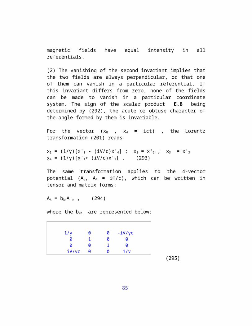
85

magnetic fields have equal intensity in allreferentials.

(2) The vanishing of the second invariant implies thatthe two fields are always perpendicular, or that oneof them can vanish in a particular referential. Ifthis invariant differs from zero, none of the fieldscan be made to vanish in a particular coordinatesystem. The sign of the scalar product E.B beingdetermined by (292), the acute or obtuse character ofthe angle formed by them is invariable.

For the vector (xß , x4 = ict) , the Lorentztransformation (201) reads

x1 = (1/γ)[x'1 - (iV/c)x'4] ; x2 = x'2 ; x3 = x'3

x4 = (1/γ)[x'4+ (iV/c)x'1] . (293)

The same transformation applies to the 4-vectorpotential (Aα, A4 = iΦ/c), which can be written intensor and matrix forms:

Ak = bknA'n , (294)

where the bkn are represented below:

1/γ 0 0 -iV/γc0 1 0 00 0 1 0iV/γc 0 0 1/γ

(295)

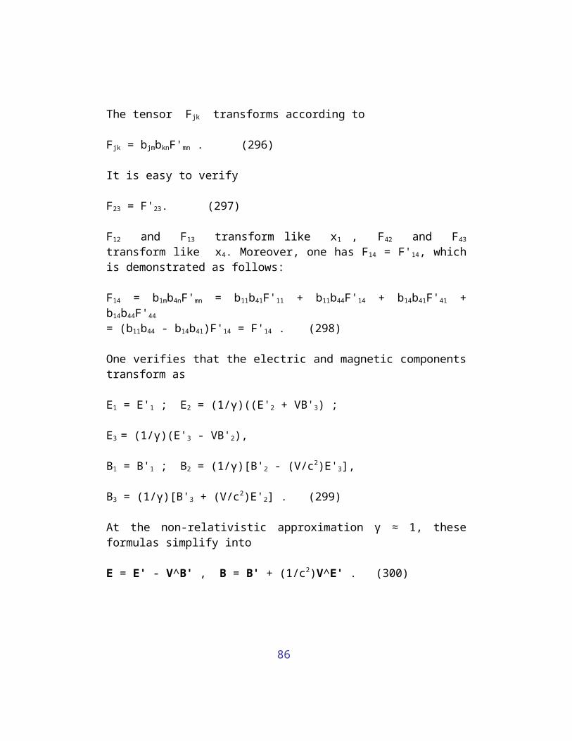
86

The tensor Fjk transforms according to

Fjk = bjmbknF'mn . (296)

It is easy to verify

F23 = F'23. (297)

F12 and F13 transform like x1 , F42 and F43

transform like x4. Moreover, one has F14 = F'14, whichis demonstrated as follows:

F14 = b1mb4nF'mn = b11b41F'11 + b11b44F'14 + b14b41F'41 +b14b44F'44

= (b11b44 - b14b41)F'14 = F'14 . (298)

One verifies that the electric and magnetic componentstransform as

E1 = E'1 ; E2 = (1/γ)((E'2 + VB'3) ;

E3 = (1/γ)(E'3 - VB'2),

B1 = B'1 ; B2 = (1/γ)[B'2 - (V/c2)E'3],

B3 = (1/γ)[B'3 + (V/c2)E'2] . (299)

At the non-relativistic approximation γ ≈ 1, theseformulas simplify into

E = E' - V^B' , B = B' + (1/c2)V^E' . (300)

87

VI-4. Energy Tensors In special relativity one can represent distributionsof matter by using the Dirac δ-functions [15], whichwill be considered in the next chapter. Here, adifferent method pioneered by Einstein is followed[17] and could be qualified as "partly hydrodynamic".This approach, aimed at detailing the relationshipbetween charged matter and the electromagnetic field,is not concerned by collisions of particles and doesnot therefore introduce the concept of pressure. So,the energy-tensor of massive matter Pab is simplydefined by

Pab = σouaub , (301)

where σo is the rest mass density of matter. One nextdefines the relativistic force fk per unit volume:

fk ≡ ∂jPjk (302)

The 4-volume integration of fk over the particle volumeand during a short time Δt, gives

∫∫∫fk.d3x.dx4 = icΔt∫∫∫fk.d3x = ic.Δt.Fk (303)

where Fk is the force acting on the particle:

Fk ≡ ∫∫∫fk.d3x ≈ fkV. (304)

(V is now the particle volume) since here σo keeps auniform value in matter. Using Gauss' theorem, onefinds

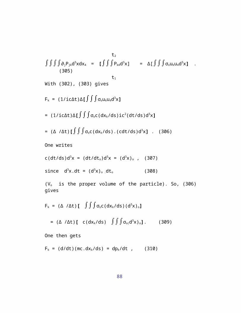
88

t2

∫∫∫∫∂jPjkd3xdx4 = [∫∫∫Pk4d3x] = Δ[∫∫∫σouku4d3x] .(305)

t1

With (302), (303) gives

Fk = (1/icΔt)Δ[∫∫∫σouku4d3x]

= (1/icΔt)Δ[∫∫∫σoc(dxk/ds)ic2(dt/ds)d3x]

= (Δ /Δt)[∫∫∫σoc(dxk/ds).(cdt/ds)d3x] . (306)

One writes

c(dt/ds)d3x = (dt/dto)d3x = (d3x)o , (307)

since d3x.dt = (d3x)o .dto (308)

(Vo is the proper volume of the particle). So, (306)gives

Fk = (Δ /Δt)[ ∫∫∫σoc(dxk/ds)(d3x)o]

= (Δ /Δt)[ c(dxk/ds) ∫∫∫σo(d3x)o]. (309)

One then gets

Fk = (d/dt)(mc.dxk/ds) = dpk/dt , (310)

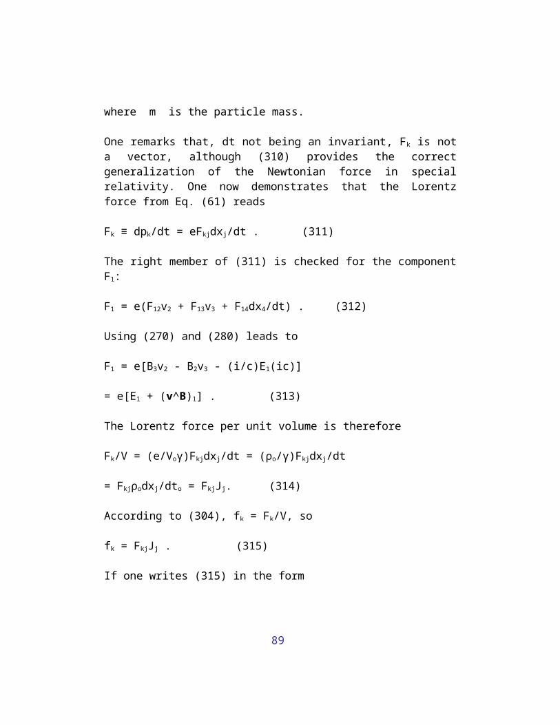
89

where m is the particle mass.

One remarks that, dt not being an invariant, Fk is nota vector, although (310) provides the correctgeneralization of the Newtonian force in specialrelativity. One now demonstrates that the Lorentzforce from Eq. (61) reads

Fk ≡ dpk/dt = eFkjdxj/dt . (311)

The right member of (311) is checked for the componentF1:

F1 = e(F12v2 + F13v3 + F14dx4/dt) . (312)

Using (270) and (280) leads to

F1 = e[B3v2 - B2v3 - (i/c)E1(ic)]

= e[E1 + (v^B)1] . (313)

The Lorentz force per unit volume is therefore

Fk/V = (e/Voγ)Fkjdxj/dt = (ρo/γ)Fkjdxj/dt

= Fkjρodxj/dto = FkjJj. (314)

According to (304), fk = Fk/V, so

fk = FkjJj . (315)

If one writes (315) in the form

90

fk = FkjJj = - ∂jEjk, (with fk = ∂jPjk) , (316)

Ejk would be the energy-tensor of vacuumelectromagnetism per unit volume, and (316) wouldimply

∂j(Pjk + Ejk) = 0 (317)

which expresses the law of conservation of energy-momentum, which shall be detailed further. To find theexpression of Ejk, (315) is developed according toMaxwell's equation (282):

fk = FkjJj = (1/μo)Fkj∂nFjn . (318)

Integrating by parts gives

μofk = - ∂n(FkjFnj) - Fjn∂nFkj . (319)

Applying (283) leads to

μofk = - ∂j(FknFjn) + Fjn(∂jFnk + ∂kFjn) . (320)

The second term of (320) reads

(1/2)∂k(FjnFjn) - Fjn∂jFkn

= (1/2)∂k(FjnFjn) - ∂j(FjnFkn) + Fkn∂jFjn , (321)

whose third term gives

- Fkn∂jFnj = - μoFknJn = - μofk . (322)

91

Therefore, (320) becomes

μofk = - 2∂j(FjnFkn) + (1/2)∂k(FmnFmn) - μofk (323), or

2μofk = - 2∂j[FjnFkn - (1/4)δjk(Fmn)2] , (324)

where (Fmn)2 ≡ FmnFmn.

One then summarizes:

∂jPjk = fk = FkjJj = -∂jEjk

Eab = (1/μo)[FajFbj - (1/4)δab(Fjk)2](325)

Like Pab , Eab is symmetric, its trace vanishes since

Ejj ≡ 0. (326)

One completes the results of (325) by writing (317) inthe form

∂jTjk = 0 , (327)

and

Tab = Pab + Eab , (328)

where Tab is the symmetric energy tensor of matterand electromagnetic field.

For k = 4 , (327) gives

92

∂ßT4ß - (i/c)∂tT44 = 0 (329)

(Greek indices always refer to space), which isequivalent to

∂ß(- icT4ß) + ∂t(- T44) = 0 (330), equivalent tothe three

relations

∂ßεß + ∂tw = 0, (331) and

εß ≡ -icT4ß and w ≡ -T44. (332)

where w is the energy density and εß is the densityof energy flux (current). To visualize this, oneconsiders the particular case withoutelectromagnetism, so that Tab reduces to Pab. In analogywith (261), the mass density σ is defined in theobserver's coordinate system or referential:

σ = σo/γ . (333)

One then finds

(εm)ß = σc2uß , (334)

and

wm = σc2/γ , (335)

93

where wm is the energy density of matter and (εm)ß isthe matter energy flux density. As seen through (334),the density of matter momentum (Pm)ß is related to(εm)ß by

(Pm)ß = (εm)ß/c2 , (336)

the momentum density Pß being defined by

Pß = -(i/c)T4ß . (337)

In the case of free electromagnetism (no matter), themass density σ vanishes, w becomes wem and εß isPoynting's vector:

wem = - E44 , (338)

Yß = - icE4ß. (339)

Demonstration of (338):

-E44 = - (1/μo)[F4jF4j - (1/4)δ44(Fjk)2] . (340)

Eqs. (291), (270) and (280) imply

- E44 = - (1/μo)[F4ßF4ß - (B2 - E2/c2)/2]

= (1/μoc2)EßEß + (1/2μo)B2 - (1/2μoc2)E2 . (341)

Using (111), (341) reduces to

-E44 = (εo/2)E2 + (μo/2)H2 = wem. (342)

94

Demonstration of (339):

- icE41 = - (ic/μo)[F4ßF1ß - (1/4)δ41(Fjk)2]

= - (ic/μo)(F42F12 + F43F13) = (1/μo)(E2B3 - E3B2)

= (E^H)1 = Y1 . (343)

One now details Eq. (330):

∂ß(- icP4ß - icE4ß) + ∂t(- P44 - E44) = 0 , (344)

or,

∂ß[Yß + (εm)ß] + ∂t(wm + wem) = 0 . (345)

One recalls Eq. (129)

∂ßYß + EßJß + ∂twem = 0. (346)

Therefore,

∂ß[(εm)ß] + ∂twm = EßJß . (347)

One recalls that, due to the corpuscular character ofmatter, the present approach could be referred to as"partly hydrodynamical". Also, the complete equationsof electromagnetism, together with the expression oftheir corresponding energy tensor, are not knowninside massive matter. One is therefore limited to amechanical description [17] of charged particles

95

interacting only through the Lorentz force. Thisrepresentation is found by volume integration of theequations, as seen in the derivation of Eq. (310). Oneshall therefore integrate (347) in a volume thatincludes the system of charges, which gives

∯εm.dS + (d/dt)∫∫∫wm.d3x = ∫∫∫E.J.d3x (348)

Since no matter crosses the border of the volume ofintegration, the first integral vanishes. The secondintegral reads

(d /dt)∫∫∫σ(c2/γ)d3x = (d/dt)(Σ mc2/γ). (349)

The right member of (348) gives

∫∫∫ρ(v.E)d3x = Σ eE.v = Σ (v.dp/dt) . (350)

Eq. (348) is therefore implied by

dEn/dt = (dp/dt).v , (351)

which is easily verified.

Until now, only the time-component (k = 4) of thedivergence equation (327) has been considered. Oneshould therefore have a look at its space-component:

∂jTßj = 0 ; or ∂αTßα + ∂t[-(i/c)Tß4] = 0 .(352)

96

The components of Tßk with k = 1, 2, 3 define thedensity of momentum flux along the ß-axis,corresponding to the momentum density per unit timepassing through a unit surface perpendicular to thex, y and z-axis (tensor character). According to(337), -(i/c)Tß4 is the momentum density along the ß-axis.

From the viewpoint of equations of conservation, theequations (330) and (352) are entirely analogous tothe charge conservation implied by the vanishingdivergence of the electric current density. This is soaccording to Gauss' theorem in four dimensions wherethe 4-volume integration of ∂kJk between the twohyperplanes t1 and t2, each of them determined by asingle value of x4 (the time) contains the whole 3-dimensional space. During the time-interval t2–t1, onedetails this vanishing contribution:

t2 t2

∫∂kJkd4x = ∫J4d3x] = ic∫ρd3x] = 0 (353) t1 t1

(d4x ≡ d3x.dx4)

where both 3-dimensional volumes refer respectively tothe two times t1 and t2 , again Eq. (353) expressesthe law of charge conservation. One therefore gets theentirely analogous result with the previous three Tßkplus T4k , because the vanishing divergence of thetensor Tab expresses both conservations of total

97

momentum and total energy in any system of chargedmatter and electromagnetic field.

REFERENCES

[14] M.-A. Tonnelat: Les théories unitaires de l'électromagnétismeet de la gravitation, Gauthier-Villars, Paris 1965, p. 66.

[15] S. Weinberg: Gravitation and cosmology, Wiley, NY1972, pp. 92, 161, 39.

[16] L. de Broglie: Ondes électromagnétiques et photons,Gauthier-Villars, Paris 1968, p. 14.

[17] A. Einstein: The meaning of relativity, PrincetonUniversity Press, 5th ed. 1955, p. 51.

Chapter VII: Special relativity -Complements

The first theory of relativity, now called specialrelativity, was simultaneously discovered by Einsteinand Poincaré in 1905 and provided the basis forgeneral relativity (1915) and quantum mechanics(1925). Now, this theory is verified on a daily basisin the many experiments performed in particleaccelerators and is certainly the most productive andsuccessful theory of all times. Moreover, special

98

relativity has evolved into the basic framework forall interactions besides gravity.

Curiously, ten years after its discovery, the validityof special relativity could not be convincinglyconfirmed by experiments, mainly by Kaufmann. It seemsthat part of the scientific community got tired ofthis situation and finally accepted special relativityon the basis of its explicative power and its innerconsistency. Its generalization in the form of atheory of gravitation in 1915 helped establishrelativity as a viable theory. But the strikinglyprecise prediction for the motion of Mercury'sperihelion (excess precession) was not even consideredfor Einstein's Nobel prize.

VII-1. Macroscopic bodies Macroscopic systems are seen as fluids when theirdescription includes the pressure caused by collisionsbetween the particles constituting these systems.However, one may briefly ignore this pressure, as ifnon-interacting particles were not colliding during abrief moment. In this case, the energy tensor ofmassive matter Tab reads

Tab = σouaub , (354)

where σo is the rest mass density and uk is the 4-velocity of massive matter. One recalls

uk ≡ cdxk/ds , with ds2 = - dxkdxk , (355)

99

where c is the speed of light. For an observer, themass density σ is given by

σ = σo/(1 - ß2)1/2 , with ß ≡ v/c , (356)

where v is the particle velocity. One also recalls

ds = cdt(1 - ß2)1/2 = cdto (357)

(to is the proper time). Using the concept of energy-tensor, one finds the energy of a particle by putting(354) in the form

Tab = [σ(1 - ß2)1/2]uaub . (358)

Based on the convention x4 = ict , the energy densityof this particle is -T44 and its energy istherefore given by -T44V , V being the particlevolume. Since the particle mass m ≡ σV , the particleenergy is obtained by detailing -T44V:

-T44V = mc2/(1 - ß2)1/2 ≈ mc2 + (1/2)mv2 + ... (359)

One can represent σ by using Dirac's δ-function inthree dimensions and write for the particle A ofrest mass mA:

σA(x)= mA(x)δ3(x - xA) , (360)

because mA(x) = mA for x = xA, or

mA(xA) = mA . (361)

10

According to the definition of Dirac's function, onecan thus write

∫σA(x)d3x = ∫mA(x)δ3(x - xA)d3x = mA(xA) = mA .(362)

For the total mass density σ of the system, one gets

σ = ΣA mAδ3(x - xA) , (363)

and

∫σd3x = ΣA mA . (364)

VII-2. Relativistic hydrodynamics - perfect fluids The concept of a fluid is introduced by consideringaverage values for physical parameters, whenidentifying a system of particles to a fictitiouscontinuous medium called fluid. So, in a fluid, massdensity and velocity are statistical values thatcharacterize the matter distribution. It is clear thatsuch an approximation only makes sense at a scale muchgreater than the size of the particles and their meanfree path (between collisions), at which the number ofparticles is seen as enormous. Also, the shocksbetween the particles constituting the fluid generateanother physical parameter called pressure.

The introduction of a fluid considerably reduces thestructure of the energy tensor by restricting it toits average value. This process eliminates the needfor summing individual energy tensors such as (354),

10

for all the particles, and noting their changes at anymoment, following the exact path of every particle,etc...

By definition, a fluid is perfect when isotropic (thesame in any direction) for an observer moving with thefluid. In this case, the observer is called"comoving". This condition of isotropy furthersimplifies the structure of the energy tensor so thatfor any observer this tensor can be written [18] inthe form

Tab = (η + P)wawb + Pδab , (365)

where

wa ≡ dxa/ds , (366)

η is the fluid energy density and P is the pressure.Due to (365), the trace of Tab is an invariant reading

Tii = - η + 3P , (367)

since

wbwb = -1 and δii = 4 , (368)

following Einstein's convention of summing on repeatedindices. According to (354) and (356), Tab can bewritten

Tab = σc2wawb(1 - ß2)1/2 . (369)

10

Therefore, for a non-comoving observer, one finds

Tii = - ΣA mAc2(1 - ß2)1/2δ(x - xA) . (370)

So, Tii is negative which, through (367), implies thecondition

P ≤ η/3 . (371)

noting that the pressure is evidently positive.

For a system of relativistic particles such as a gasof photons, the rest mass of particles vanishes,together with Tii. In this case, (371) implies that thepressure of a relativistic gas equals a third of itsenergy density, an important result.

The results (370) and (371) remain valid for anysystem of electrically charged particles interactingthrough the Lorentz force. This is due to the factthat the energy tensor of free electromagnetism has avanishing trace. So, its addition to Tab given by (354)will not affect (370).

With regard to the kinetic theory of gases, one writesthe average value of the energy tensor (354) in areferential in which the gas is at rest:

(Tab)Av = [nmuaub(1 - ß2)1/2]Av (372)

10

(Av means average), where n is the number of particlesper unit volume (σ = nm). In this coordinate system,the matrix form of Tab (365) is

P 0 0 0 0 p 0 0 0 0 p 0 0 0 0 -η

(373)

because the fluid velocity vanishes in this case (ß =0 for the fluid). One equals the 4-4 components from(372) and (373), which gives

n = [nmc2/(1 - ß2)1/2]Av . (374)

Equaling any of the space-components, one finds

P = [(nm/3)v2/(1 - ß2)1/2]Av . (375)

due to [(v1)2]Av = (v2/3)Av . (376)

At the non-relativistic approximation, one thusretrieves the result that pressure equals two-thirdsof the average kinetic energy per unit volume.

VII-3. Mass defect - energy definition and problem Neutral and non-interacting molecules are present ingases usually treated as perfect fluids (unboundsystems in a first approximation). Their number of

10

constituents is very high since it is meaningless tospeak of stable unbound systems with only a fewconstituents.

Consider a two-body system formed by two neutralmasses m1 and m2. According to mass-energyconservation, the mass-energy Mc2 of this system reads

Mc2 = m1c2/[1 - (v1/c)2]1/2 + m2c2/[1 - (v2/c)2]1/2 , (377)

implying M > m1 + m2 and the fact that the massdefect

ΔM = M - m1 - m2(377-b)

should be positive. However, this is more intuitive atthe non-relativistic approximation where the totalenergy W reads

W = m1c2 + m2c2 + ΔM.c2, (377-c)

with ΔM positive for a disintegration by definitionemitting the positive energy ΔM.c2. According to this,binary systems and others would be unstable if ΔM isnegative [does not work according to the threeequations (377)], so that no disintegration couldoccur without a supply of enough energy compensatingthe mass defect [19].

In the case of electromagnetism, one can look at thesimplest two-body system united by the Lorentz force,the hydrogen atom. One recalls that the energy densityof the electromagnetic field in vacuum wem reads

10

wem = (1/2)(εoE2 + μoH2) (378)

[see Eq. (130)]. The volume integration of theelectrostatic part of this energy in the whole 3-dimensional space gives the total electrostatic energyof vacuum U, in function of the electric potential Φand the electric charge e of the sources:

U = (1/2) ∫ Φde , (379)

where the electric charge of any particle of thesystem is supposed to be uniformly distributed on itsboundary between matter and vacuum (equipotentialsurface, see Eq.142). The fact that such charges arein reality not concentrated on these surfaces does notmatter here, since it is simply the way Maxwell'stheory works for calculating U in vacuum from volumeintegrals. Mass-energy of particles is not be confusedwith U in the dualistic Maxwell theory where sourcesand fields are fundamentally distinct entities.

According to (379), if particles are spherical, Ureduces to

U = e2/2R ; (cgs system: 4πεo = 1), (380)

R being the particle radius.

Therefore, neglecting magnetic effects in a systemformed by a proton and an electron at a very great distance from each other, one can express the

10

electromagnetic energy of vacuum Uo in terms of theproton radius Rp and the electron radius Re :

Uo ≈ e2(1/2Rp + 1/2Re) . (381)

Chapter IV evidences the validity of energyconservation for a system of charged particles andelectromagnetism in vacuum. One now uses thisprinciple to calculate U for a distance proton-electron of the order of the hydrogen atom radius(written r in this case). Accordingly, the workproduced by the Lorentz force acting on the electron,brought from infinity to the distance r , representsthe corresponding loss of electromagnetic energy -ΔWin vacuum (ΔW is the work). One thus writes

r rΔW = ∫(- e2/x2)dx = [e2/x] = e2/r . (382) ∞ ∞

Therefore,

U ≈ Uo - e2/r. (383)

Due the positivity of electromagnetic energy (see Eq.378), U is positive definite. Quite evidently,

e2/2Re > e2/r , or r > 2Re . (384)

which equally applies to Rp. One verifies that (383)is consistent with (379) for the energy of the

10

hydrogen atom, since expressing Φ at the surface ofthe proton and the electron as if their charges wereuniformly distributed on such equipotentials. AsMaxwell's theory is linear, the effect from differentsources is the sum of individual effects from eachsource. The potential on the equipotential of theproton is the sum of the potential from its own chargeand the potential caused by the distant electroncharge (conversely for the equipotential on theelectron). About the electromagnetic energy of thesystem proton-electron, one thus writes

(1/2) ∫ Φde = (1/2)[(e/Rp - e/r)e + (-e/Re + e/r)(-e)]

= - e2/r + e2(1/2Rp + 1/2Re) (385)

(-e is the electron charge), confirming (383). TheMaxwell-Lorentz theory thus characterizes boundsystems of charged particles with negative mass-energybinding whose total electromagnetic energy is,however, always positive. Here, the negativeelectrostatic energy of interaction, or negativeenergy binding, is given by (1/2)Σ eA.eB/rAB (A ≠ B)[19].

Therefore, Uo is a blocked energy, not usable andpartly similar to the missing “dark” mass in galaxiesand the missing “dark” energy in cosmology, bothseemingly not yet accounted for in publishedcalculations, evidencing conceptual identity betweenboth items in spite of dissimilar respective

10

percentages (viewpoint not detailed here). However, asmall part of global missing mass-energy has to comefrom vacuum electromagnetism entering in full aspositive source of gravitational mass-energy in theright member of Einstein’s equation of gravitationaccording to Eq. (130). This positive energy source isinexistent in traditional classical physics andquantum mechanics discarding gravity since onlyevidencing negative binding energies intuitivelyconsistent with their production. Although thisquestion here looks like “another story”, additionalresults should come from field unification, althoughwithout firm guarantee for satisfactory estimates ofthe missing mass-energy in galaxies and cosmology.

All this, besides the binding energy, built on -e2/rfiguring in Schrödinger's equation, representing anegative contribution to inertial-gravitational massof systems of particles. One thus draws theconclusion:

- The inertial part of field energy in a boundsystem is the difference between the total fieldenergy and the extended value of Uo. Positivevacuum electromagnetic energy such as Uo fromparticles in vacuum may be insufficientlyaccounted as inertial mass-energy of a system ofparticles. However, the true problem seems quitebigger than that.

In conclusion, electrically charged matter is thesource of electromagnetic fields in vacuum, referredto as free electromagnetism, but Maxwell's theory is

10

imprecise about the sources of its own fields, so thatelectric charges look uniformly distributed onequipotentials at all borders between matter andvacuum, although apparently not affecting energycalculations.

In contrast, electric charges quite logically existinside volumes of elementary particles such aselectrons and quarks. Otherwise, electromagneticenergy in the vacuum surrounding one very smallisolated charged particle could become greater thanthe energy of the whole universe if its radius issufficiently small, which evidently does not makesense.

Note: This section will be revised for greater clarityand precision.

REFERENCES

[18] S. Weinberg: Gravitation and cosmology, Wiley, NY1972, p. 48.

[19] L. Landau and E. Lifshitz: The classical theory of fields,Addison Wesley, Ma 1961, pp. 33, 97.

Chapter VIII: Lagrangian and Hamiltonian

11

VIII-1. Calculus of variations and Lagrange's equation Consider the Lagrangian L , function of the space coordinates xß and the space-components of velocity vß (Greek indices exclusively refer to space). One writes

L ≡ L(xß, vß) , (386)

where L is time-independent. At first sight, thisdistinction between space and time components ofvelocity seems against the spirit of the theory ofrelativity. However, the 4-momentum component p4 reads

p4 = mcdx4/ds = imc/(1 - ß2)1/2 ,(387)

which shows that p4 is a function of v2. In the non-relativistic case, it will be shown that L is thedifference between the kinetic energy and thepotential energy, which rules out a direct dependenceof L with respect to time. Here, time-dependence isonly found after integration of the equations ofmotion.

The action S is defined by the integral

S = ∫L.dt .(388)

This integral is taken over a definite pathrepresenting the trajectory of a particle moving in afield acting on it. For simplicity, one ignores theintegral sign and writes (388) in the differentialform

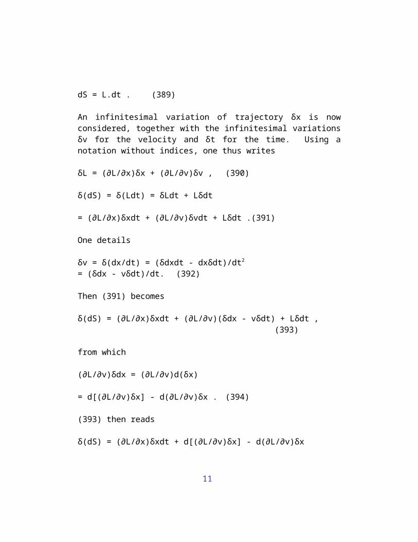
11

dS = L.dt . (389)

An infinitesimal variation of trajectory δx is nowconsidered, together with the infinitesimal variationsδv for the velocity and δt for the time. Using anotation without indices, one thus writes

δL = (∂L/∂x)δx + (∂L/∂v)δv , (390)

δ(dS) = δ(Ldt) = δLdt + Lδdt

= (∂L/∂x)δxdt + (∂L/∂v)δvdt + Lδdt .(391)

One details

δv = δ(dx/dt) = (δdxdt - dxδdt)/dt2

= (δdx - vδdt)/dt. (392)

Then (391) becomes

δ(dS) = (∂L/∂x)δxdt + (∂L/∂v)(δdx - vδdt) + Lδdt ,(393)

from which

(∂L/∂v)δdx = (∂L/∂v)d(δx)

= d[(∂L/∂v)δx] - d(∂L/∂v)δx . (394)

(393) then reads

δ(dS) = (∂L/∂x)δxdt + d[(∂L/∂v)δx] - d(∂L/∂v)δx

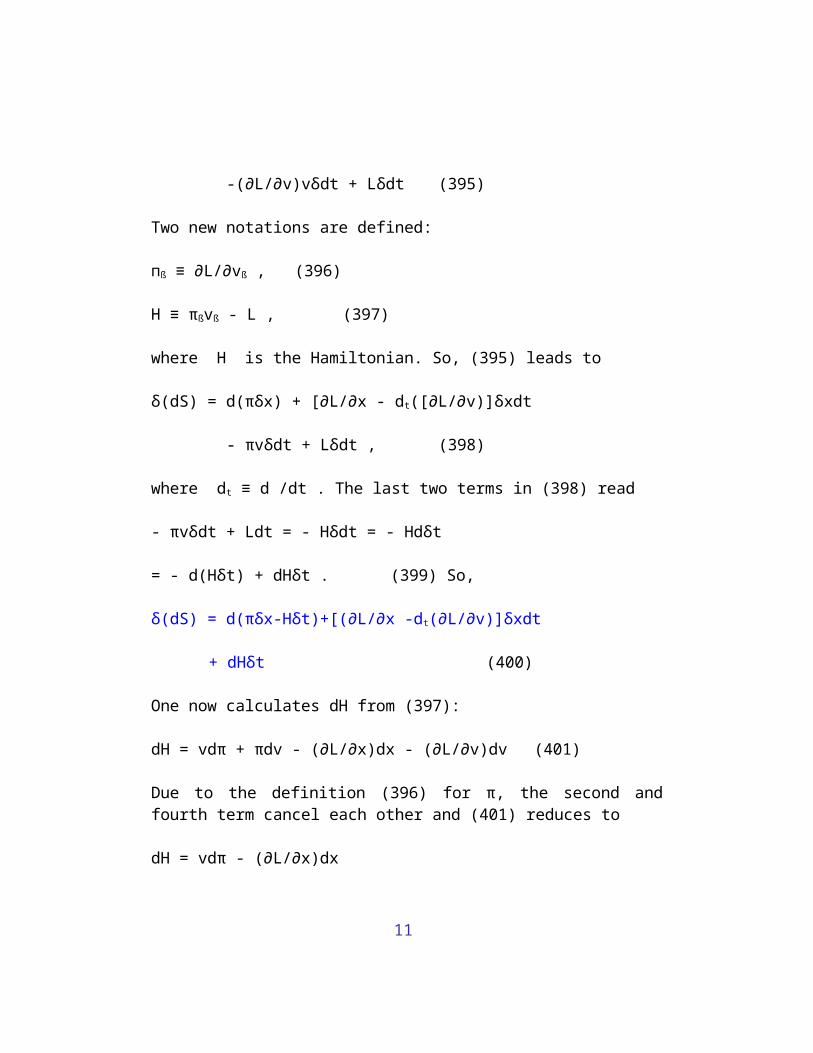
11

-(∂L/∂v)vδdt + Lδdt (395)

Two new notations are defined:

пß ≡ ∂L/∂vß , (396)

H ≡ πßvß - L , (397)

where H is the Hamiltonian. So, (395) leads to

δ(dS) = d(πδx) + [∂L/∂x - dt([∂L/∂v)]δxdt

- πvδdt + Lδdt , (398)

where dt ≡ d /dt . The last two terms in (398) read

- πvδdt + Ldt = - Hδdt = - Hdδt

= - d(Hδt) + dHδt . (399) So,

δ(dS) = d(πδx-Hδt)+[(∂L/∂x -dt(∂L/∂v)]δxdt

+ dHδt (400)

One now calculates dH from (397):

dH = vdπ + πdv - (∂L/∂x)dx - (∂L/∂v)dv (401)

Due to the definition (396) for π, the second andfourth term cancel each other and (401) reduces to

dH = vdπ - (∂L/∂x)dx

11

= [(dπ/dt)v - (∂L/∂x)dx/dt]dt

= [(dπ/dt) - (∂L/∂x)]vdt . (402)

Therefore, the Hamiltonian is a constant of motion (dH= 0) if the equation

∂L/∂x - dt((∂L/∂v) = 0 (403)

is satisfied. Besides (396) and (397), which are twodefinitions, the previous equalities (388) to (402)are in fact identities. So, the imposition of aconstant Hamiltonian gives the equation (403). Puttingindices, Eq. (403) reads

∂L/∂xβ - dt(∂L/∂vβ) = 0, (404)

which is the usual Lagrange equation.

Adding an equation to an identity gives an equation,not an identity. It is remarkable that the equation ofmotion (404), implying dH = 0, simplifies considerablythe identity (400) into the equation

δ(dS) = d(πßδxß - Hδt) (405)

Integrating (405) gives

B BδΔS = ∫ d(πßδxß - Hδt) = [πßδxß - Hδt] (406) A A

11

(ΔS ≡ SB - SA.

If the variations δx and δt vanish at the points A andB, the variation of ΔS also vanishes. The equationof motion (404) thus implies an extremal or stationaryvalue to the integral (388).

VIII-2. Non-relativistic case without magnetism In Newtonian physics, the Lagrangian L is defined bythe difference between the kinetic energy and thepotential energy Z:

L = (1/2)mv2 - Z . (407)

The momentum π1 is given by

π1 = ∂[(m/2)vßvß]/∂v1 = mv1 , (408) or,

πß = mvß (409)

The Hamiltonian H reads

H = πßvß - L = mvßvß - [(1/2)mv2 - Z] , (410)

giving

H = (1/2)mv2 + Z , (411)

for the total energy. Finally, Eq. (404) recovers thewell known equation of motion

11

m(dvß/dt) = - ∂ßZ . (412)

VIII-3. Hamilton's equations Eq. (410) shows that πß is the momentum. Accordingly,it seems natural to consider two kinds of variables:the coordinates xß and the momentum πß, eliminating thevß. The equations of this new representation will bebased on partial derivatives of the Hamiltonianrelative to this new system of variables. From (397)and (404), one writes

∂H/∂x = - (∂L/∂x) = - dπ/dt. (413), and

∂H/∂π = dx/dt (414)

These equations are called Hamilton equations and areusually written in the form

dx/dt = ∂H/∂π (415)

dπ/dt = - ∂H/∂x (416)

(recalling the definition H ≡ πv - L).

In the non-relativistic case, due to (410), theHamiltonian H reads

H = π2/2m + Z (417),

(π2 ≡ πßπß).

11

So,

∂H/∂π = π/m. (418)

(415) then reads

dx/dt = π/m , (419)

which retrieves (410). Eq. (416) gives

dπ/dt = - ∂Z/∂x , (420)

which is Eq. (412).

In the previous section, the Lagrange equation hasimplied the constancy of the Hamiltonian. Now, thisconstancy will be demonstrated on the basis of theHamilton equations:

dH/dt = (∂H/∂x)dx/dt + (∂H/∂π)(dπ/dt) . (421)

With (415) and (416), (421) becomes

dH/dt = = (∂H/∂x )(∂H/∂π) + (∂H/∂π)(-∂H/∂x)

= (∂H/∂xβ)(∂H/∂πβ) - (∂H/∂πβ)(∂H/∂xβ) = 0. (422)

which defines Poisson's brackets.

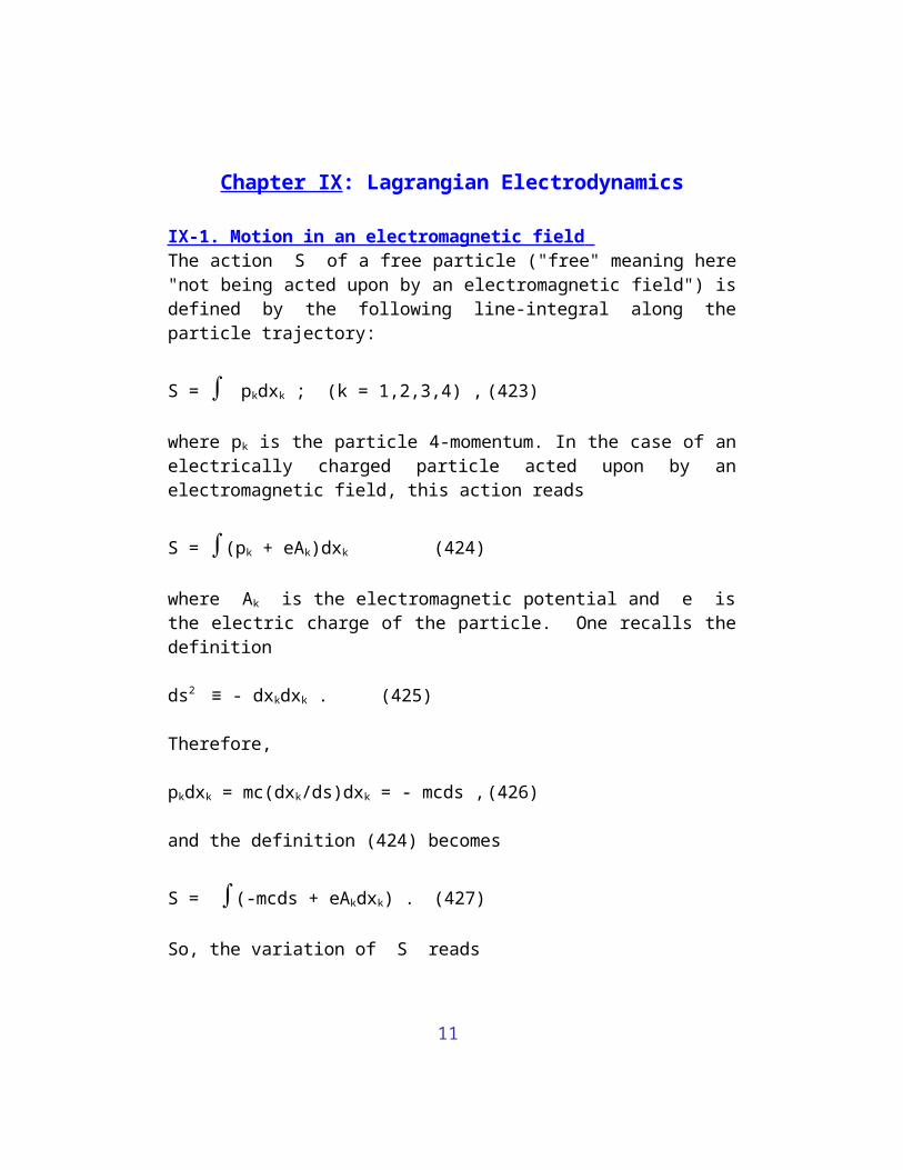
11

Chapter IX: Lagrangian Electrodynamics

IX-1. Motion in an electromagnetic field The action S of a free particle ("free" meaning here"not being acted upon by an electromagnetic field") isdefined by the following line-integral along theparticle trajectory:

S = ∫ pkdxk ; (k = 1,2,3,4) , (423)

where pk is the particle 4-momentum. In the case of anelectrically charged particle acted upon by anelectromagnetic field, this action reads

S = ∫(pk + eAk)dxk (424)

where Ak is the electromagnetic potential and e isthe electric charge of the particle. One recalls thedefinition

ds2 ≡ - dxkdxk . (425)

Therefore,

pkdxk = mc(dxk/ds)dxk = - mcds ,(426)

and the definition (424) becomes

S = ∫(-mcds + eAkdxk) . (427)

So, the variation of S reads

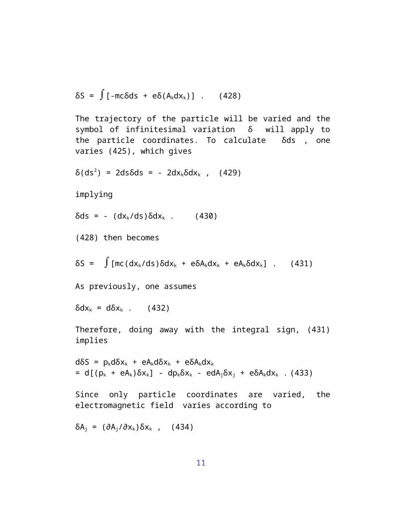
11

δS = ∫[-mcδds + eδ(Akdxk)] . (428)

The trajectory of the particle will be varied and thesymbol of infinitesimal variation δ will apply tothe particle coordinates. To calculate δds , onevaries (425), which gives

δ(ds2) = 2dsδds = - 2dxkδdxk , (429)

implying

δds = - (dxk/ds)δdxk . (430)

(428) then becomes

δS = ∫[mc(dxk/ds)δdxk + eδAkdxk + eAkδdxk] . (431)

As previously, one assumes

δdxk = dδxk . (432)

Therefore, doing away with the integral sign, (431)implies

dδS = pkdδxk + eAkdδxk + eδAkdxk

= d[(pk + eAk)δxk] - dpkδxk - edAjδxj + eδAkdxk . (433)

Since only particle coordinates are varied, theelectromagnetic field varies according to

δAj = (∂Aj/∂xk)δxk , (434)

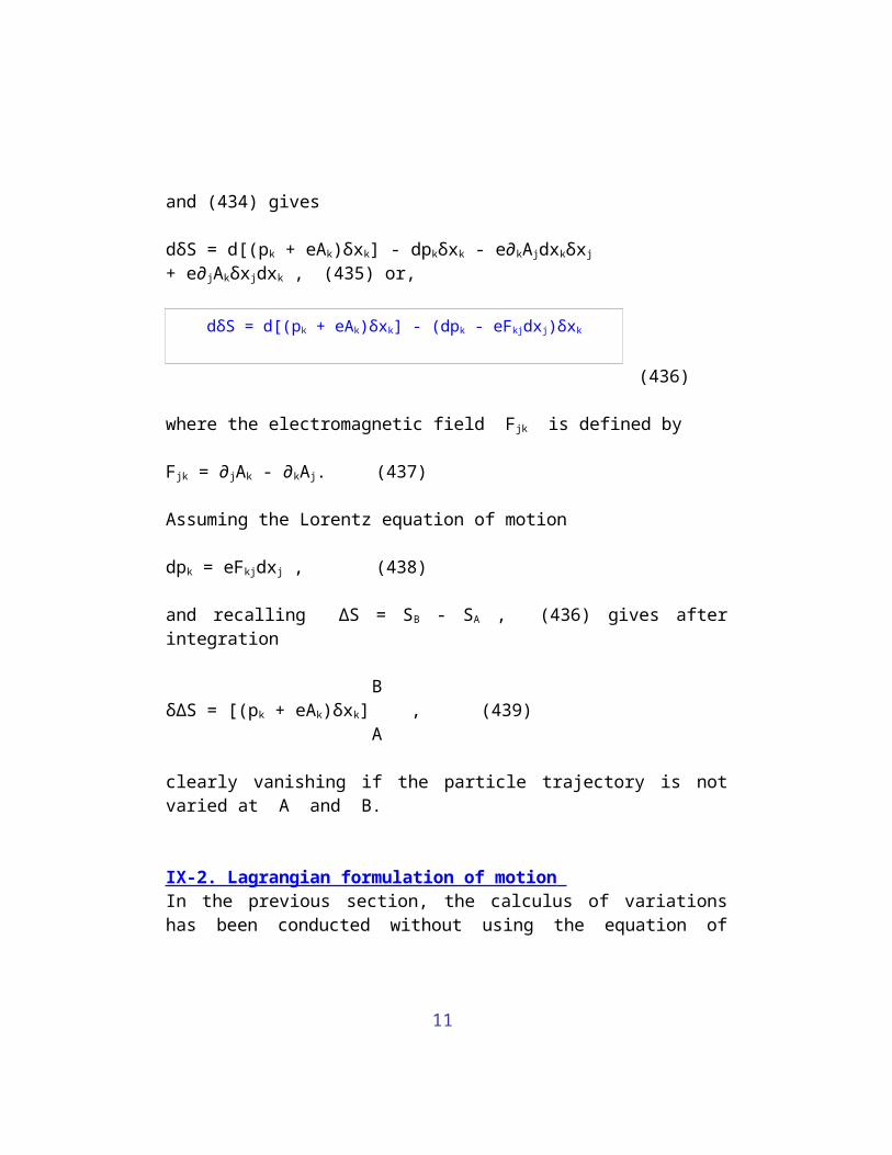
11

and (434) gives

dδS = d[(pk + eAk)δxk] - dpkδxk - e∂kAjdxkδxj

+ e∂jAkδxjdxk , (435) or,

dδS = d[(pk + eAk)δxk] - (dpk - eFkjdxj)δxk

(436)

where the electromagnetic field Fjk is defined by

Fjk = ∂jAk - ∂kAj. (437)

Assuming the Lorentz equation of motion

dpk = eFkjdxj , (438)

and recalling ΔS = SB - SA , (436) gives afterintegration

BδΔS = [(pk + eAk)δxk] , (439) A

clearly vanishing if the particle trajectory is notvaried at A and B.

IX-2. Lagrangian formulation of motion In the previous section, the calculus of variationshas been conducted without using the equation of

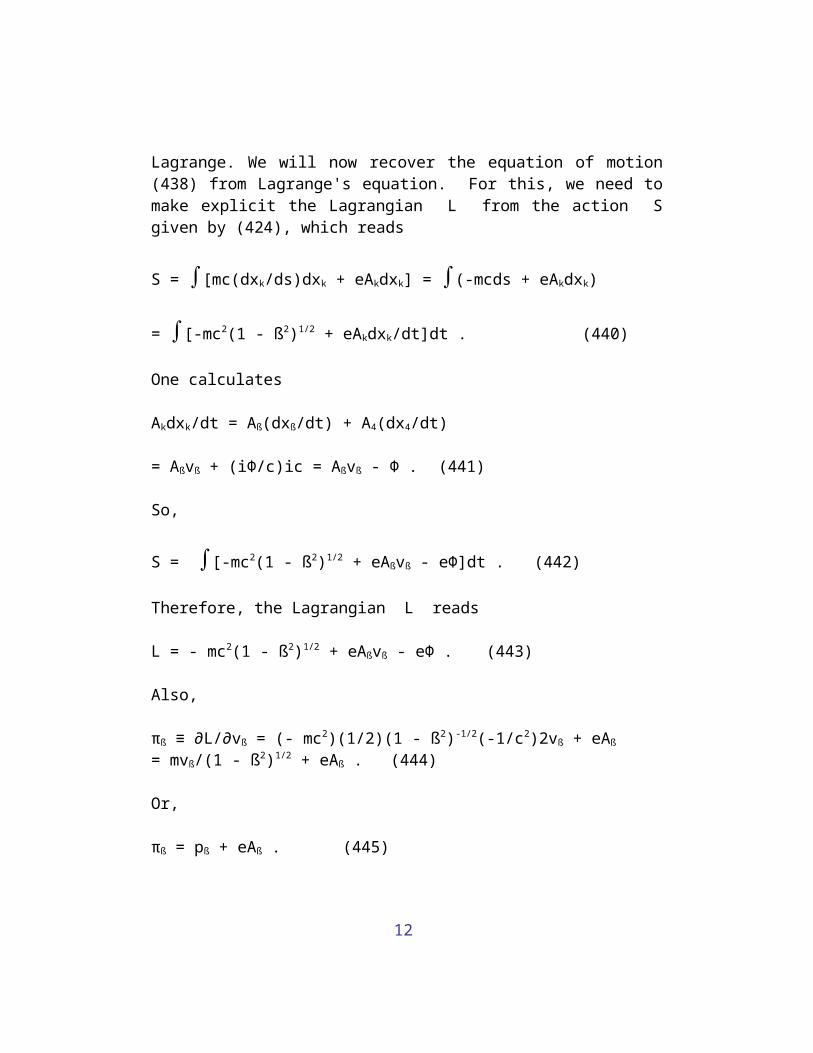
12

Lagrange. We will now recover the equation of motion(438) from Lagrange's equation. For this, we need tomake explicit the Lagrangian L from the action Sgiven by (424), which reads

S = ∫[mc(dxk/ds)dxk + eAkdxk] = ∫(-mcds + eAkdxk)

= ∫[-mc2(1 - ß2)1/2 + eAkdxk/dt]dt . (440)

One calculates

Akdxk/dt = Aß(dxß/dt) + A4(dx4/dt)

= Aßvß + (iΦ/c)ic = Aßvß - Φ . (441)

So,

S = ∫[-mc2(1 - ß2)1/2 + eAßvß - eΦ]dt . (442)

Therefore, the Lagrangian L reads

L = - mc2(1 - ß2)1/2 + eAßvß - eΦ . (443)

Also,

πß ≡ ∂L/∂vß = (- mc2)(1/2)(1 - ß2)-1/2(-1/c2)2vß + eAß

= mvß/(1 - ß2)1/2 + eAß . (444)

Or,

πß = pß + eAß . (445)

12

Therefore, the Hamiltonian H reads

H = (pß + eAß)vß + mc2(1 - ß2)1/2 - eAßvß + eΦ

= pßvß + mc2(1 - ß2)1/2 + eΦ . (446)

Since p and v have the same direction, theirscalar product is

pßvß = pv = mv2/(1 - ß2)1/2 , (447)

and (446) becomes

H = [mv2 + mc2.(1 - ß2)]/(1 - ß2)1/2 + eΦ , (448)

or,

H = En + eΦ, (449)

recalling the definition (5) En ≡ mc2/(1 - v2/c2)1/2.

One notes that

dtAß = ∂tAß + ∂αAßvα . (450)

Therefore, using (450), the Lagrange equation (404)reads

dpß/dt+ e(∂tAß + ∂αAßvα) = e∂ß(Aαvα - Φ)

dpß/dt = e(-∂tAß - vα∂αAß + vα∂ßAα - ∂ßΦ)

12

= e[(- ∂ßΦ - ∂tAß) + vα(∂ßAα - ∂αAß)] , (451)

or,

dpß/dt= e(Eß + Fßαvα) . (452)

This equation gives the Lorentz force, retrieving thespace-components of Eq. (438).

IX-3. Hamiltonian formulation The concept of a constant energy or Hamiltonian isrelated to the very definition of energy, andconversely. This is the basic philosophy of theHamiltonian formalism in which the equations of motionassure the constancy of energy, in agreement with theresults of Maxwell's theory. Here, (448) gives theHamiltonian but the velocity needs to be replaced bythe generalized momentum π (change of variables).For this, one recalls (264):

pßpß - (En/c)2 = - m2c2 . (453)

Using (445) and (449), the elimination of pß and En

leads to

(H - eΦ)2/c2 = m2c2 + (πß - eAß)(πß - eAß) , (454)

or,

H = [m2c4 + c2(πß - eAß)2]1/2 + eΦ (455)

12

So, En will provide a simplified notation for thesquare root in (455), when verifying Hamilton'sequations. According to (455), one writes

∂H/∂πβ = (1/2En)(- 2ec2Aß + 2c2πß) = (c2/En)(πß - eAß)

= (c2pß/En) = vß = dxß/dt . (456)

which retrieves the first Hamilton equation (415). Onenow checks that the second Hamilton equation (416)recovers the Lagrange equation of motion:

∂H/∂xß = (1/2En)(-2ec2∂ßAαπα + 2e2c2Aα∂ßAα) + e∂ßΦ

= (ec2/En)(- ∂ßAαπα + eAα∂ßAα) + e∂ßΦ

= (e/m)(1 - ß2)1/2(πα - eAα)(-∂ßAα) + e∂ßΦ

= (e/m)(1 - ß2)1/2pα(-∂ßAα) + e∂ßΦ

= -evα∂ßAα + e∂ßΦ , (457)

or,

-∂H/∂xß = evα∂ßAα - e∂ßΦ . (458)

Using (450), one calculates dπ/dt:

dπß/dt = dt(pß + eAß) = dpß/dt+ e(∂tAß + ∂αAßvα). (459)

Equaling (458) and (459) gives

12

dpß/dt = e(-∂tAß - ∂ßΦ) + eFßαvα , (460)

or,

dpß/dt= e(Eß + Fßαvα) , (461)

which is Lagrange's equation of motion (452).

IX-4. Non-relativistic cse with magnetism A non-relativistic approximation is characterized by v2

<< c2 , or p2 << m2c2 . According to Taylor's formula, one usesthe approximation

(1 + x)1/2 ≈ 1 + x/2 , for x << 1 . (462)

Then, (455) gives

H ≈ mc2[1 + (1/2m2c2)(πß - eAß)2] + eΦ , (463)

or,

H ≈ mc2 + (1/2m)(πß - eAß)2 + eΦ , (464)

which, besides Einstein's rest energy, recovers theresult from pre-relativity physics.

IX-5. The Hamilton-Jacobi equation

12

One looks back at the identity (400), assuming thatLagrange's equation of motion is satisfied, whichimplies a constant Hamiltonian. Since

δ(dS) = dδS , (465)

one writes

dδS = d(πßδxß - Hδt) , (466)

which yields

δS = πßδxß - Hδt . (467)

One thus derives Jacobi's equations

πß = ∂S/∂xß , and H = - ∂S/∂t (468)

Accordingly, (454) gives the Hamilton-Jacobi equation

(∂ßS - eAß)2 - (∂tS + eΦ)2/c2 = - m2c2

(469)

IX-6. Equations of motion and field equations Maxwell's equations are field equations that allow tocalculate the electromagnetic field acting on chargedmatter, together with the field energy in vacuum. ButMaxwell's equations do not imply the Lorentz forceacting on that matter. However, as seen in thederivation of equations. (135) and (351), energy

12

conservation in systems of charged matter implies theLorentz force and conversely.

So, in electrodynamics, field equations and equationsof motion (that give the forces) are differentobjects. The Lagrangian formulation of motionretrieves the Lorentz force, which implies theconstancy of energy represented by the Hamiltonian, inagreement with the paragraph above. It would be usefulto enlarge the formalism of motion so that Maxwell'sfield equations could also be included, which wouldestablish the relationship between field equations andequations of motion. For this purpose, the followingaction S is proposed:

S = ∫pkdxk + ∫eAkdxk - ∫(1/4μo)FjkFjkd3x.dt (470)

The second and third integrals are based upon theelectromagnetic potential, since Fjk is seen here asthe notation for ∂jAk - ∂kAj. The second integral willbe transformed into a 4-volume integral, so that thesecond and third integrals will produce fieldequations for electromagnetism by variation of theLagrange field variable Ak. This is the main differencebetween field equations, derived by field variation,and the equations of motion found by variation of thecoordinates representing the location of the fieldsources, electrically charged matter in this case.

One develops the second integral

∫eAkdxk = ∫(ρodVo)Ak(cdxk/ds)(ds/c)

12

= ∫(ρodVo)Akukdto = ∫ρoukAkdVodto

= ∫AkJkd3xdt. (471)

For equations of electromagnetism, one joins thesecond and third integrals to form the action forelectromagnetism Sem:

Sem = ∫£emd3xdt = ∫[AkJk - (1/4μo)FjkFjk]d3xdt , (472)

where the Lagrangian density £em for electromagnetismis thus defined by

£em ≡ AkJk - (1/4μo)FjkFjk . (473)

Since only the fields are varied to derive fieldequations, one writes

δ∫£emd3xdt = ∫δ£emd3xdt . (474)

The vanishing variation of Sem then implies theequation

δ£em = 0 . (475)

One calculates

δFjk = ∂jδAk - ∂kδAj , (476)

according to the definition (281) for Fjk . So,

12

δ£em = JkδAk - (1/4μo)2Fjk(∂jδAk - ∂kδAj)

= JkδAk - (1/2μo)Fjk2∂jδAk

= JkδAk - (1/μo)Fjk∂jδAk . (477)

Integrating the second term by parts gives

δ£em = JkδAk + (1/μo)∂jFjkδAk - (1/μo)∂j(FjkδAk) . (478)

The third term in the right member is a divergencethat, according to Gauss' theorem, gives acontribution in the form of a 3-volume integral overthe hypersurface bounding the region of integration(space-time is four-dimensional). According to thevariational principle followed here, the fieldvariations δAk and the variations of the field firstderivatives δ(∂jAk), and therefore δFjk , vanish atthe limit of the region of integration, making thiscontribution to vanish (although variations of firstderivatives play no role in this particular case).So, neglecting this divergence, (478) gives, for δ£em =0 ,

[Jk + (1/μo)∂jFjk]δAk = 0 , (479)

or,

Jk = (1/μo)∂jFkj . (480)

Maxwell's equation (282) is so retrieved, togetherwith eq. (283) implied by the definition (281) for Fjk.

12

According to the philosophy of Lagrangian formalism,all fields must be varied (no discrimination). Theconcept of field should therefore cover everythingthat is not a constant; otherwise the very definitionof a field would be arbitrary. In this view, theelectric current density has also to be varied. This,with a Lagrangian such as (473), would imply theunacceptable vanishing of the electromagneticpotential, which leads to think that (473) isincomplete. Moreover, if one realizes that only thefirst two integrals of (470) give the equations ofmotion because these are line-integrals, one wonderswhy the first integral cannot be converted into a 4-volume integral and contribute to the field equations.An answer to these questions has been proposed [20,21].

IX-7. From Faraday-Maxwell to Einstein’s generalrelativity

A. About de Broglie and Schrödinger In 1924, de Broglie associated a wave to a freeelectron going in a straight line; he took the Planck-Einstein ideas and wrote its relativistic energy E:

E ≡ mc2/(1 - v2/c2)1/2 = hν, (1-1)

which works according to the frequency ν of a planewave ψ of constant unit amplitude:

ψ = exp[i(p.r - Et)/ħ] , (i ≡ √-1) , (1-2)

13

with the momentum p defined by

p ≡ mv/(1 - v2/c2)1/2 , (1-3)

whose wavelength λ obeys therefore the relation

λ = h/p. (1-4)

The validity of (1-4) has been tested with a highdegree of accuracy in diffraction of electrons,evidencing the physical character of de Broglie'swave.

In 1926, Schrödinger proposed a wave equation based onde Broglie's mathematics, whose wave-solution (1-2)verifies the equation

pxψ = -iħ∂xψ, (1-5)

implying

(px)2ψ = -ħ2∂x∂xψ (1-6)

(∂x is the partial derivative to the variable x).

The square of momentum p2 ≡ (px)2 + (py)2 + (pz)2 thusenters the second order equation

(1/2m)p2ψ = -(ħ2/2m)Δψ , (1-7)

where Δ is the Laplacian operator. At the non-relativistic approximation, this equation reads

13

(1/2)mv2ψ = -(ħ2/2m)Δψ . (1-8)

Adding -eΦψ to each member then gives

[-(h2/2m)Δ - eΦ]ψ = Wψ, (1-9)

where W is the total energy and this equation is thetime-independent Schrödinger equation for a particleof electric charge -e, which retrieves Bohr’s energylevels of his theory of the hydrogen atom (1913).

B. Significant points of Jacobi's workDuring the 1828-1838 period, Carl-Gustav Jacobi usedfour coordinates for space and time for any particleor body, exactly as in relativity theory (three spacecoordinates plus the time t). This is exemplified inthe infinitesimal variation δS of the action S:

δS = pδx - Wδt (2-1)

where p is the momentum (p = mv). From this, the twoequations

p = ∂S/∂x ; W = -∂S/∂t (2-2)

are immediate, particularly if one writes thesimplest solution for S:

S = p.x - Et. (2-3)

13

In some disagreement with Hamilton, Jacobi arguedthat the system (2-2) i sufficient for distinguishingfinal conditions from initial ones, both formulations(2-1) and (2-2) being equivalent. The system (2-2),formed by two equations among the simplestimaginable, constitutes the complete basis for wavemechanics and classical mechanics.

Equations (2-1) and (2-2) do not result fromequations of motion. On the contrary, the vanishingvariation (2-1) implies them, which establishes the“logical” pre-eminence of wave mechanics over theNewtonian mechanics of trajectories, often confusedwith classical mechanics whose determination oftrajectories only was its preliminary formulation.

The importance of (2-2) is verified by its trivialimplication in the form of the Hamilton-Jacobiequation from which celestial mechanics is said toderive. With Planck's constant, the Hamilton-Jacobiequation [22] constituted the starting point forSchrödinger’s discovery of his famous equation in1926. This fact seems somewhat overlooked intreatises of quantum mechanics, when Schrödinger’sequation is presently the most used equation alongwith Einstein's relation E = mc2, the generalizedindustrial use of both relations characterizing thepresent epoch.

Due to (2-3), Eq. (1-2) also reads

ψ = exp[iS/ħ). (2-4)

13

The novelty was the introduction of the constant ħfrom Planck's constant h, in 1905 ratified byEinstein for the photon, subsequently used bySchrödinger in 1926 (ħ ≡ h/2π).

Discarding for a while the direct relationshipbetween relativity theory and Maxwell'selectromagnetism, Eq. (2-1) implies the theory ofspecial relativity if δS is an invariant. This remarkleads to Einstein's general relativity (1915) ifcurvilinear coordinates are used, accepting that thespace-time curvature has no reason to vanisheverywhere. In contrast, the discovery of Einstein'sequation for gravitation was a less obviousoperation. Moreover, Bohr’s principle of wave-particle complementarity is trivially implied by Eqs.(2-1) and (2-2). In other words, all this looks likethe old sentence ”the more things change, the morethey stay the same”.

REFERENCES [20] J. Chauveheid: A proposal for a quadratic electromagneticcoupling based on the underlying philosophy of Einstein-Maxwell theory,Physics Essays, vol. 10, p. 474 (1997).

[21] J. Chauveheid: On the connection between classical andquantum fields, Physics Essays, vol. 12, p. 146 (1999).

[22] J. Chauveheid and F.X. Vacanti: Schrödinger and the Hamilton-Jacobi equation, Physics Essays, vol. 15, p. 5 (2002).

13