Estimating immigration in neutral communities: theoretical and practical insights into the sampling...
20
Estimating immigration in neutral communities: theoretical and practical insights into the sampling properties Franc¸ois Munoz 1 * and Pierre Couteron 2 1 UM2 – UMR AMAP (botAnique et bioinforMatique de l’Architecture des Plantes), Boulevard de la Lironde, TA A-51 ⁄ PS2, F-34398 Montpellier Cedex 5, France; and 2 IRD – UMR AMAP (botAnique et bioinforMatique de l’Architecture des Plantes), Boulevard de la Lironde, TA A-51 ⁄ PS2, F-34398 Montpellier Cedex 5, France Summary 1. Widening applications of neutral models of communities necessitates mastering the process of inferring parameters from species composition data. In a previous paper, we introduced the novel conditional G ST (k) statistic based on community composition. We showed that it is a reliable basis for assessing migrant fluxes into local communities under a generalized version of the spatially implicit neutral model of SP Hubbell, which can accommodate non-neutral patterns at scales broader than the communities. 2. We provide here new insights into the sampling properties of the G ST (k) statistic and on the derived immigration number, I(k). The analytical formulas for bias and variance are useful to assess estimation accuracy and investigate the variation of I(k) across communities. 3. Immigration estimation is asymptotically unbiased as sample size increases. We confirm the validity of our analytical results on the basis of simulated neutral communities. 4. We also underline the potential of using I(k) as a descriptive index of community isolation, without reference to any model of community dynamics. 5. We further propose a practical application of the bias and variance analysis for defining sampling designs for immigration quantification by efficiently balancing the number and size of community samples. Key-words: bias, community isolation, G ST (k) statistic, immigration, spatially implicit neu- tral model, unified neutral theory of biodiversity and biogeography, variance Introduction Since the seminal work of Hubbell (2001), the neutral theory of biodiversity has raised much interest by providing a nontrivial null hypothesis against which the nature of real-world bio- diversity patterns may be tested and discussed (McGill 2003; Nee & Stone 2003; Volkov et al. 2003; Leigh 2007). Under the key assumption of ‘ecological equivalence’, namely that indi- viduals have equal fitness whatever their species or habitat, Hubbell (2001) and followers (Etienne 2005) proposed a two- level spatially implicit neutral model (so-called 2L-SINM by Munoz, Couteron, & Ramesh 2008; see a synthesis in Beera- volu et al. 2009 and present Fig. 1a left) to decouple the dynamics of the large biogeographical background (i.e. the metacommunity), in which the effect of infrequent speciation and extinction events is quantified via the biodiversity parame- ter h (speciation-drift balance), from local community dynam- ics, which is controlled by the immigration parameter, I (migration-drift balance, Etienne & Olff 2004). The theory has found some support from the investigation of very rich tree communities in wet evergreen tropical forests, where alterna- tive models were not satisfactory for explaining some observed diversity patterns, such as the overrepresentation of rare spe- cies in the species abundance distributions (SAD) (Hubbell 2001; Chave, Alonso, & Etienne 2006). From a theoretical standpoint, neutral models can help us grasp how the interac- tion between limited immigration and local ‘ecological drift’ (Hubbell 2001) may influence taxonomic composition. Munoz, Couteron, & Ramesh (2008) have further proposed to relax the assumptions made by Hubbell (2001) at the upper level (i.e. the metacommunity) and to generalize the initial 2L- SINM into a 3L-SINM, by introducing an intermediate level, the regional pool of migrants, which may be shaped by *Correspondence author. E-mail: [email protected] Correspondence site: http://www.respond2articles.com/MEE/ Methods in Ecology and Evolution doi: 10.1111/j.2041-210X.2011.00133.x Ó 2011 The Authors. Methods in Ecology and Evolution Ó 2011 British Ecological Society
Transcript of Estimating immigration in neutral communities: theoretical and practical insights into the sampling...

Estimating immigration in neutral communities:
theoretical and practical insights into the sampling
properties
Francois Munoz1* and Pierre Couteron2
1UM2 – UMR AMAP (botAnique et bioinforMatique de l’Architecture des Plantes), Boulevard de la Lironde,
TA A-51 ⁄PS2, F-34398 Montpellier Cedex 5, France; and 2IRD – UMR AMAP (botAnique et bioinforMatique de
l’Architecture des Plantes), Boulevard de la Lironde, TA A-51 ⁄PS2, F-34398 Montpellier Cedex 5, France
Summary
1. Widening applications of neutral models of communities necessitates mastering the process of
inferring parameters from species composition data. In a previous paper, we introduced the novel
conditional GST(k) statistic based on community composition. We showed that it is a reliable basis
for assessing migrant fluxes into local communities under a generalized version of the spatially
implicit neutral model of SP Hubbell, which can accommodate non-neutral patterns at scales
broader than the communities.
2. We provide here new insights into the sampling properties of the GST(k) statistic and on the
derived immigration number, I(k). The analytical formulas for bias and variance are useful to assess
estimation accuracy and investigate the variation of I(k) across communities.
3. Immigration estimation is asymptotically unbiased as sample size increases. We confirm the
validity of our analytical results on the basis of simulated neutral communities.
4. We also underline the potential of using I(k) as a descriptive index of community isolation,
without reference to anymodel of community dynamics.
5. We further propose a practical application of the bias and variance analysis for defining
sampling designs for immigration quantification by efficiently balancing the number and size of
community samples.
Key-words: bias, community isolation, GST(k) statistic, immigration, spatially implicit neu-
tral model, unified neutral theory of biodiversity and biogeography, variance
Introduction
Since the seminal work ofHubbell (2001), the neutral theory of
biodiversity has raised much interest by providing a nontrivial
null hypothesis against which the nature of real-world bio-
diversity patterns may be tested and discussed (McGill 2003;
Nee & Stone 2003; Volkov et al. 2003; Leigh 2007). Under the
key assumption of ‘ecological equivalence’, namely that indi-
viduals have equal fitness whatever their species or habitat,
Hubbell (2001) and followers (Etienne 2005) proposed a two-
level spatially implicit neutral model (so-called 2L-SINM by
Munoz, Couteron, & Ramesh 2008; see a synthesis in Beera-
volu et al. 2009 and present Fig. 1a left) to decouple the
dynamics of the large biogeographical background (i.e. the
metacommunity), in which the effect of infrequent speciation
and extinction events is quantified via the biodiversity parame-
ter h (speciation-drift balance), from local community dynam-
ics, which is controlled by the immigration parameter, I
(migration-drift balance, Etienne & Olff 2004). The theory has
found some support from the investigation of very rich tree
communities in wet evergreen tropical forests, where alterna-
tive models were not satisfactory for explaining some observed
diversity patterns, such as the overrepresentation of rare spe-
cies in the species abundance distributions (SAD) (Hubbell
2001; Chave, Alonso, & Etienne 2006). From a theoretical
standpoint, neutral models can help us grasp how the interac-
tion between limited immigration and local ‘ecological drift’
(Hubbell 2001) may influence taxonomic composition.
Munoz, Couteron, & Ramesh (2008) have further proposed to
relax the assumptions made by Hubbell (2001) at the upper
level (i.e. the metacommunity) and to generalize the initial 2L-
SINM into a 3L-SINM, by introducing an intermediate level,
the regional pool of migrants, which may be shaped by*Correspondence author. E-mail: [email protected]
Correspondence site: http://www.respond2articles.com/MEE/
Methods in Ecology and Evolution doi: 10.1111/j.2041-210X.2011.00133.x
� 2011 The Authors. Methods in Ecology and Evolution � 2011 British Ecological Society

non-neutral influences (Fig. 1a right). Under the 3L-SINM,
the study of the local migration-drift equilibrium can be dis-
connected from non-neutral influences occurring at larger
scales, via the estimation of the immigration parameter I.
Although inferring Hubbell’s parameters motivated a great
deal of research in recent years leading to several estimation
methods (Volkov et al. 2003; Etienne 2005, 2009;Munoz et al.
2007;Munoz, Couteron, &Ramesh 2008), the rapidly growing
number of applications to real-world data sets has raised ques-
tions about how to assess the reliability of the inference, even
in the strictly neutral case. Furthermore, published methods
have frequently led to substantially differing parameter esti-
mates when applied to the same data sets (see for instance Lati-
mer, Silander, & Cowling 2005; Etienne et al. 2006; Etienne
2009, Table 1). The lack of knowledge on confidence limits has
discouraged wider andmore systematic applications of neutral
theory through meta-analyses on parameter values. It is also
hindering the development and application of more realistic
models of community assemblages. Our aim is to provide such
a statistically informed perspective on the estimation of the
immigration parameter under the 3L-SINM.
The immigration parameter I is here central and represents
the number of potential migrants competing with resident off-
spring at each mortality event within the community, and as
such, it is closely related to Hubbell’s (2001) migration proba-
bility, m ¼ IIþN�1 (N notes the size of a local community). The
neutral theory basically invokes ‘dispersal limitation’ from the
metacommunity to the local community to define I and m
(Hubbell 2001; Etienne 2005). But when these parameters are
estimated from real-world data, they may also include the
effects of many processes that altogether determine the relative
isolation and differentiation of the local community from its
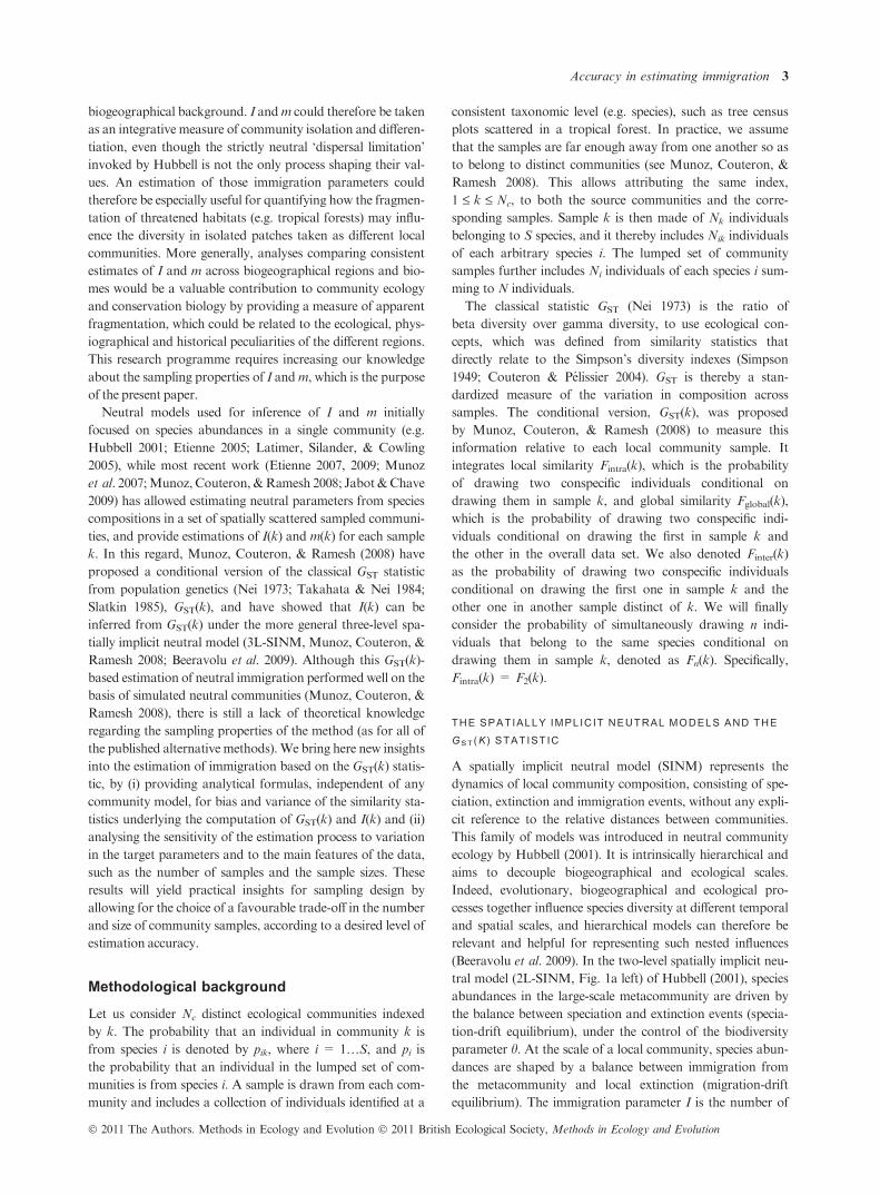
The spatially-implicit neutral models (SINM) with two levels (2L-SINM, left) and three levels (3L-SINM, right).
2L-SINM 3L-SINM
Estimation context
ˆ(k) is to be estimated for a sample k from the Iobserved species abundances. Sampling error occurs from uncontrolled random variation in species abundances (issue addressed in the present paper).
I(k) controls the probability of drawing a new individual that belongs to a lineage not represented in the sample (Etienne 2005, Munoz et al. 2008), but which may be already present in the community.
I(k) controls the probability that a dead individual is replaced by a migrant from outside the community.
Immigration Immigration
Metacommunity
Community i
Community j Community k
I(i) I(j) I(k)
Pool of migrants
Community i
Community j Community k
I(i) I(j) I(k)
Biogeographical scale
Estimation
Theo
ryD
ata
Community k I(k), equation (1)
Sample k I(k), equation (1)
Sample k (k), equation (2) I
Pool of migrants
(a)
(b)
Fig. 1. Immigration theory and estimation in a network of communities. (a) Two versions of a spatially implicit neutral model are considered,
including two levels (2L-SINM, conforming to Hubbell 2001; left) and three levels (3L-SINM,Munoz, Couteron, & Ramesh 2008; right). In the
2L-SINM, the migrants are randomly drawn from a large biogeographical source and the model is neutral at all scales, while in the 3L-SINM,
the local community dynamics is neutral but the model allows for non-neutral sources of variation within the pool of immigrants (the third level).
(b) summarizes the sampling and estimation issues addressed in the paper. All of the sampled communities k (e.g. forest plots) are assumed to be
independent to allow the application of equation 1 as in Munoz, Couteron, & Ramesh (2008), and the immigration numbers are estimated from
equation 2 (the hat notation represents estimated values).
2 F. Munoz & P. Couteron
� 2011 The Authors. Methods in Ecology and Evolution � 2011 British Ecological Society, Methods in Ecology and Evolution
biogeographical background. I andm could therefore be taken
as an integrative measure of community isolation and differen-
tiation, even though the strictly neutral ‘dispersal limitation’
invoked by Hubbell is not the only process shaping their val-
ues. An estimation of those immigration parameters could
therefore be especially useful for quantifying how the fragmen-
tation of threatened habitats (e.g. tropical forests) may influ-
ence the diversity in isolated patches taken as different local
communities. More generally, analyses comparing consistent
estimates of I and m across biogeographical regions and bio-
mes would be a valuable contribution to community ecology
and conservation biology by providing a measure of apparent
fragmentation, which could be related to the ecological, phys-
iographical and historical peculiarities of the different regions.
This research programme requires increasing our knowledge
about the sampling properties of I andm, which is the purpose
of the present paper.
Neutral models used for inference of I and m initially
focused on species abundances in a single community (e.g.
Hubbell 2001; Etienne 2005; Latimer, Silander, & Cowling
2005), while most recent work (Etienne 2007, 2009; Munoz
et al. 2007;Munoz, Couteron, &Ramesh 2008; Jabot&Chave
2009) has allowed estimating neutral parameters from species
compositions in a set of spatially scattered sampled communi-
ties, and provide estimations of I(k) and m(k) for each sample
k. In this regard, Munoz, Couteron, & Ramesh (2008) have
proposed a conditional version of the classical GST statistic
from population genetics (Nei 1973; Takahata & Nei 1984;
Slatkin 1985), GST(k), and have showed that I(k) can be
inferred from GST(k) under the more general three-level spa-
tially implicit neutral model (3L-SINM, Munoz, Couteron, &
Ramesh 2008; Beeravolu et al. 2009). Although this GST(k)-
based estimation of neutral immigration performedwell on the
basis of simulated neutral communities (Munoz, Couteron, &
Ramesh 2008), there is still a lack of theoretical knowledge
regarding the sampling properties of the method (as for all of
the published alternative methods).We bring here new insights
into the estimation of immigration based on the GST(k) statis-
tic, by (i) providing analytical formulas, independent of any
community model, for bias and variance of the similarity sta-
tistics underlying the computation of GST(k) and I(k) and (ii)
analysing the sensitivity of the estimation process to variation
in the target parameters and to the main features of the data,
such as the number of samples and the sample sizes. These
results will yield practical insights for sampling design by
allowing for the choice of a favourable trade-off in the number
and size of community samples, according to a desired level of
estimation accuracy.
Methodological background
Let us consider Nc distinct ecological communities indexed
by k. The probability that an individual in community k is
from species i is denoted by pik, where i = 1…S, and pi is
the probability that an individual in the lumped set of com-
munities is from species i. A sample is drawn from each com-
munity and includes a collection of individuals identified at a
consistent taxonomic level (e.g. species), such as tree census
plots scattered in a tropical forest. In practice, we assume
that the samples are far enough away from one another so as
to belong to distinct communities (see Munoz, Couteron, &
Ramesh 2008). This allows attributing the same index,
1 £ k £ Nc, to both the source communities and the corre-
sponding samples. Sample k is then made of Nk individuals
belonging to S species, and it thereby includes Nik individuals
of each arbitrary species i. The lumped set of community
samples further includes Ni individuals of each species i sum-
ming to N individuals.
The classical statistic GST (Nei 1973) is the ratio of
beta diversity over gamma diversity, to use ecological con-
cepts, which was defined from similarity statistics that
directly relate to the Simpson’s diversity indexes (Simpson
1949; Couteron & Pelissier 2004). GST is thereby a stan-
dardized measure of the variation in composition across
samples. The conditional version, GST(k), was proposed
by Munoz, Couteron, & Ramesh (2008) to measure this
information relative to each local community sample. It
integrates local similarity Fintra(k), which is the probability
of drawing two conspecific individuals conditional on
drawing them in sample k, and global similarity Fglobal(k),
which is the probability of drawing two conspecific indi-
viduals conditional on drawing the first in sample k and
the other in the overall data set. We also denoted Finter(k)
as the probability of drawing two conspecific individuals
conditional on drawing the first one in sample k and the
other one in another sample distinct of k. We will finally
consider the probability of simultaneously drawing n indi-
viduals that belong to the same species conditional on
drawing them in sample k, denoted as Fn(k). Specifically,
Fintra(k) = F2(k).
THE SPATIALLY IMPLIC IT NEUTRAL MODELS AND THE
GST (K ) STATIST IC
A spatially implicit neutral model (SINM) represents the
dynamics of local community composition, consisting of spe-
ciation, extinction and immigration events, without any expli-
cit reference to the relative distances between communities.
This family of models was introduced in neutral community
ecology by Hubbell (2001). It is intrinsically hierarchical and
aims to decouple biogeographical and ecological scales.
Indeed, evolutionary, biogeographical and ecological pro-
cesses together influence species diversity at different temporal
and spatial scales, and hierarchical models can therefore be
relevant and helpful for representing such nested influences
(Beeravolu et al. 2009). In the two-level spatially implicit neu-
tral model (2L-SINM, Fig. 1a left) of Hubbell (2001), species
abundances in the large-scale metacommunity are driven by
the balance between speciation and extinction events (specia-
tion-drift equilibrium), under the control of the biodiversity
parameter h. At the scale of a local community, species abun-
dances are shaped by a balance between immigration from
the metacommunity and local extinction (migration-drift
equilibrium). The immigration parameter I is the number of
Accuracy in estimating immigration 3
� 2011 The Authors. Methods in Ecology and Evolution � 2011 British Ecological Society, Methods in Ecology and Evolution
immigrants that compete with local offspring when an indi-
vidual dies in the local community. This important parameter
was first named the ‘fundamental dispersal number’ (Etienne
& Alonso 2005), but the concept can be enlarged to include
other sources of immigration limitation from the background
region (Munoz, Couteron, & Ramesh 2008). Munoz et al.
(2007) showed that the 2L-SINM of Hubbell can accommo-
date varying immigration conditions across local communities
k, by allowing varying values of I(k), and several recent
approaches have been proposed to estimate I(k) in the pres-
ence of this variation (Etienne 2007, 2009; Munoz, Couteron,
& Ramesh 2008; Jabot & Chave 2009).
In the three-level spatially implicit neutralmodel (3L-SINM,
Fig. 1a right) of Munoz, Couteron, & Ramesh (2008), the lar-
ger-scale source of immigrants is not necessarily considered to
be a metacommunity at speciation-drift equilibrium because
the model allows for various processes to occur at an interme-
diate scale, thereby providing greater flexibility for represent-
ing real-world patterns and migration pathways (Fig. 1 in
Munoz, Couteron, & Ramesh 2008). In this case, contrary to
the 2L-SINM, there is no assumption about the SAD of the
immigrants. In the context of the 3L-SINM, Munoz, Couter-
on, & Ramesh (2008) introduced the computation of
GSTðkÞ ¼ FintraðkÞ�FglobalðkÞ1�FglobalðkÞ and showed that GST(k) directly
relates to the immigration parameter, I(k), of the source com-
munity k, through the relationship:
GSTðkÞ ¼1
1þ IðkÞ= 1� Pðk=kÞð Þ ; eqn 1
Here, P(k ⁄k) is the probability of drawing an individual
in sample k conditional on first drawing an individual in
k, which is measured as Pðk=kÞ ¼ Nk�1N�1 . Applications to
simulated neutral communities showed that exact estima-
tors of the similarities,
FintraðkÞ ¼XSi¼1
Nik
Nk
� �Nik � 1
Nk � 1
� �and
FglobalðkÞ ¼XSi¼1
Nik
Nk
� �Ni � 1
N� 1
� �;
are to be used to get unbiased estimates of the immigra-
tion parameters on the basis of equation 1 (Munoz, Cou-
teron, & Ramesh 2008):
IðkÞ ¼ 1� Pðk=kÞð Þ 1
GSTðI; kÞ� 1
!
¼ 1� Pðk=kÞð Þ 1� FintraðkÞFintraðkÞ � FglobalðkÞ
!;
eqn 2
The corresponding immigration rates (i.e. the migration
probability of Hubbell 2001) can be estimated using
mðkÞ ¼ IðkÞIðkÞþNk�1
.
SAMPLING PROPERTIES
Akey issue is to investigate inmore detail the sampling proper-
ties of IðkÞ (equation 2) so as to gain insights about its bias and
variance and to formally assess the degree of confidence in its
estimation. The word ‘sampling’ here conceptually encom-
passes two distinct sources of variation.
First, the neutral theory of Hubbell (2001) allows for ran-
domfluctuations in species abundances owing to the finite sizes
of the community (local drift) and of the metacommunity (glo-
bal drift). Influxes of new species (speciation) in the metacom-
munity and of immigrants in local communities are necessary
to avoid species fixation andmonodominance, and tomaintain
species diversity. The stochastic nature of the replacement of
dead individuals was shown to be strictly analogous to a sam-
pling process (Etienne & Alonso 2005), so that Etienne (2005)
and followers could derive exact sampling formulas for species
abundances in local community samples k (Etienne 2005,
2007; Munoz, Couteron, & Ramesh 2008; Noble et al. 2010).
The relationship between GST(k) and I(k) in equation 1 holds
for any sample taken in a given community (Fig. 1b, part
above the dashed line; see also Munoz, Couteron, & Ramesh
2008).
Second, although equation 1 is exact for any sample in com-
munity k, it only provides an estimate of I(k), denoted IðkÞ,which is marked by random fluctuations in the constitutive
similarity statistics within GST(k), because the species frequen-
cies in samples are themselves random variables. Thus, the I(k)
notation embodies the sampling variation because of ecologi-
cal drift in neutral theory (equation 1 and Fig. 1b, above
the line), while IðkÞ further includes the sampling variation
because of estimation error of similarity statistics (equation 2
and Fig. 1b, below the dashed line). The latter source of
sampling error is characterized by the ‘hat’ notation and is
the focus of the present work. We intend to gain insights into
this sampling variation by applying a multinomial model of
sample draws from the corresponding source community. This
model requires assuming, as a first approximation, that the
communities are large enough compared to the samples to
allow the drawing of samples from the communities with
replacement.
Analytical results
We investigated the sampling properties of GSTðkÞ and IðkÞ,using a delta method for calculating approximate sampling
means and variances (Davison 2003). We then provided fur-
ther analytical results for IðkÞ in the particular case of the two-
level version (2L-SINM). We used Mathematica � (Wolfram,
2003) for Taylor series expansions and investigation of the
limit cases.
SAMPLING VARIAT ION IN SIMILARITY STATIST ICS
We investigated the variation among many samples succes-
sively drawn in a given community to predict the error in esti-
mating similarities from a single sample. As mentioned above,
we assumed each community sample to be small enough com-
pared to the source community, so that the individuals making
up a sample are drawn from the source community with
replacement. Species abundances in a sample made of Nk
individuals follow a multinomial distribution with parameters
4 F. Munoz & P. Couteron
� 2011 The Authors. Methods in Ecology and Evolution � 2011 British Ecological Society, Methods in Ecology and Evolution

pik, the species probabilities in the reference community. We
therefore investigated the influence of multinomial variation
on the sampling properties of IðkÞ.We used binary indicator
functions (Cormen et al. 2001) of species identity to explore
the variations of the similarities, as Lande (1996) did for inves-
tigating Simpson’s diversity.
Specifically, for FintraðkÞ ¼PSi¼1
nikNk
� �nik�1Nk�1
� �, we established
(Appendix S1) that
E FintraðkÞ� �
¼ FintraðkÞ; eqn 3A
and
Var FintraðkÞ� �
� 4
NkF3ðkÞ � FintraðkÞ2� �
þO1
N2k
� �;
eqn 3B
as in Lande (1996).
Appendix S1 further shows that the two other similarity
statistics, FinterðkÞ ¼PS
i¼1Nik
Nk
� �Ni�Nik
N�Nk
� �and FglobalðkÞ ¼PS
i¼1Nik
Nk
� �Ni�1N�1� �
, are also unbiased:
E FinterðkÞ� �
¼ FinterðkÞ eqn 3C
E FglobalðkÞ� �
¼ FglobalðkÞ eqn 3D
The sampling properties of the similarity statistics here hold
irrespective of any underlyingmodel of species dynamics.
SAMPLING ERROR ON IðkÞ AND mðkÞ
From this premise, we turned to investigate the sampling error
in the parameters IðkÞ and mðkÞ from their relationships
with GSTðkÞ and the constitutive similarity statistics FintraðkÞand FglobalðkÞ, such as IðkÞ ¼ g FintraðkÞ; FglobalðkÞ
� �, with
g x; yð Þ ¼ 1� Pðk=kÞð Þ 1�xx�y (from equation 2) and mðkÞ ¼f IðkÞ� �
, with f zð Þ ¼ zzþNk�1.
We denote the derivatives g0xðxÞ ¼@gðxÞ@x , g00
x2ðxÞ ¼ @2gðxÞ
@x2,
g00xyðxÞ ¼@2gðxÞ@x@y , and so on. Using a delta method based on Tay-
lor series expansions (Davison 2003; see Appendix S2), we
could obtain approximate expected values and sampling vari-
ances of IðkÞ:
EðIðkÞÞ � gð �X; �YÞ þ CovðX;YÞg00xyð �X; �YÞ
þ 1
2VarðXÞg00x2 ð �X; �YÞ þ 1
2VarðYÞg00y2ð �X; �YÞ
eqn 4A
VarðIðkÞÞ � g0xð �X; �YÞ2VarðXÞ þ g0yð �X; �YÞ2VarðYÞþ 2CovðX;YÞg0yð �X; �YÞg0xð �X; �YÞ
eqn 4B
with X ¼ FintraðkÞ, Y ¼ FglobalðkÞ, �X ¼ E FintraðkÞ� �
and�Y ¼ E FglobalðkÞ
� �.
We assumed the sampling variance of FglobalðkÞ and the
covariance of FglobalðkÞ and FintraðkÞ to be negligible com-
pared with the variance of FintraðkÞ. The assumption is fairly
reasonable, insofar as FglobalðkÞ depends on the sampling
variation in the large overall data set (lumped samples),
which is automatically an order of magnitude smaller than
the sampling variation in each community sample k, as far
as there are many samples. Thus, under the assumptions of
a network of many small community samples, equations 4A
and 4B simplify into EðIðkÞÞ � gð �X; �YÞ þ 12 VarðXÞg00x2 ð �X; �YÞ
and VarðIðkÞÞ � g0xð �X; �YÞ2VarðXÞ, with g0xðx; yÞ ¼� 1� Pðk=kÞð Þ 1�y
x�yð Þ2 and g00x2 ðx; yÞ ¼ 2 1� Pðk=kÞð Þ 1�yx�yð Þ3.
Replacing �X and �Y with the corresponding expected values
of the similarity statistics (equations 4A and 4B) yielded the
following relationship:
EðIðkÞÞ � 1� Pðk=kÞð Þ 1� FintraðkÞFintraðkÞ � FglobalðkÞ
1þ 1� FglobalðkÞ1� FintraðkÞ
VarðFintraðkÞÞFintraðkÞ � FglobalðkÞ� �2
!
Using equation 1, this simplified into
EðIðkÞÞ� IðkÞþ IðkÞþ1�P k=kð Þð Þ VarðFintraðkÞÞFintraðkÞ�FglobalðkÞ� �2 :
Likewise,
VarðIðkÞÞ� 1�Pðk=kÞð Þ 1�FintraðkÞFintraðkÞ�FglobalðkÞ
� �2
1�FglobalðkÞ1�FintraðkÞ
� �2 VarðFintraÞFintraðkÞ�FglobalðkÞ� �2 :
By denoting TðkÞ¼ VarðFintraðkÞÞFintraðkÞ�FglobalðkÞð Þ2, we finally got
VarðIðkÞÞ � IðkÞ þ 1� P k=kð Þð Þ2TðkÞ eqn 5A
and the estimation of bias
Bias IðkÞ� �
¼ EðIðkÞÞ � IðkÞ ¼ IðkÞ þ 1� P k=kð Þð ÞTðkÞeqn 5B
The quantities IðkÞ þ 1� P k=kð Þð ÞandT(k) are central herefor characterizing the sampling error because they control both
the bias and the variance in estimation of IðkÞ. Using a least-
square loss function, the best bias-variance trade-off is
obtained byminimizing themean square error
MSE ¼ Bias2 þ Var ¼ EðIðkÞÞ � IðkÞ� �2þVarðIðkÞÞ
¼ IðkÞ þ 1� P k=kð Þð Þ2TðkÞ TðkÞ þ 1ð Þ:
Recall that Var FintraðkÞ� �
� 4Nk
F3ðkÞ � FintraðkÞ2� �
to
getTðkÞ ¼ 4Nk
F3ðkÞ�FintraðkÞ2
FintraðkÞ�FglobalðkÞð Þ2. Let us consider thatP(k ⁄k)=
(Nk ) 1) ⁄ (N ) 1) primarily depends on the fixed number of
sites sampled, Nc = N ⁄Nk, so that P k=kð Þ � 1=Nc. I(k) and
the actual similarity statistics (without ‘hats’) are independent
fromNk, so that both the estimation bias and variance decrease
as 1 ⁄Nk; hence,
EðIðkÞÞ � IðkÞ þO1
Nk
� �; biasðIðkÞÞ2 � O
1
N2k
� �
andVarðIðkÞÞ � O 1Nk
� �.
Accuracy in estimating immigration 5
� 2011 The Authors. Methods in Ecology and Evolution � 2011 British Ecological Society, Methods in Ecology and Evolution

As a consequence,MSE = O(1 ⁄Nk), and the sampling vari-
ance is here more constraining for optimization. We further
investigated the sampling properties of
mðkÞ ¼ f IðkÞ� �
¼ IðkÞIðkÞ þNk � 1
;
by using the deltamethod, so that
E mðkÞð Þ � f E IðkÞ� �� �
þ 1
2VarðIðkÞÞf00x E IðkÞ
� �� �¼ mðkÞ
þ 1
NkTðkÞ IðkÞ þ 1� Pðk=kÞð Þ þO
1
N3k
� �
andVar mðkÞð Þ � Var IðkÞ� �
f0x E IðkÞ� �� �2
with
f0x E IðkÞ� �� �
¼ Nk � 1
IðkÞ � 1þNk þ TðkÞ 1þ IðkÞ � Pðk=kÞð Þð Þ2
¼ O1
Nk
� �:
Therefore, BiasðmðkÞÞ � O 1N2
k
� �and VarðmðkÞÞ � O 1
N3k
� �.
In this case, MSE = O(1 ⁄Nk3), and the faster decrease in esti-
mation error when community samples get large may have
been a reason for preferring investigatingm(k) in earlier appli-
cations of neutral theory (Hubbell 2001; Etienne 2005; Munoz
et al. 2007).
The sampling results here are not dependent on any assump-
tion on the nature of species assembly, as we have only analy-
sed nonlinear functions of similarity statistics. At this stage,
IðkÞ and mðkÞ can be used as heuristic indexes of community
isolation from their common background (similarly to using
diversity indexes). But one may also want to further interpret
and discuss their nature as immigration parameters in the con-
text of the 3L-SINM,where there is still no a priori expectation
for Fintra(k), F3(k) and Fglobal(k). The derivations below are
given for the particular case of the 2L-SINM, where we can
further specify the nature of the migrant pool and the species
abundance distributions therein to predict these values.
SAMPLING ERROR FOR THE TWO-LEVEL SPATIALLY
IMPLIC IT NEUTRAL MODEL (2L-S INM)
Let us now consider the well-known case of the 2L-SINM of
Hubbell (2001), which is a particular case of the 3L-SINM.We
analytically derived the expected probabilities Fn(k) in a given
community sample k as explicit functions of the parameters hand I(k) (Appendix S3). The analytical formulas for the first
values of n are
F2ðkÞ ¼ FintraðkÞ ¼ 1� hhþ 1
IðkÞIðkÞ þ 1
eqn 6A
as presented by Etienne (2005),
F3ðkÞ¼2IðkÞ2þ3IðkÞðhþ2Þþ2ðhþ1Þðhþ2Þ
IðkÞþ1ð Þ IðkÞþ2ð ÞCðhþ1ÞCðhþ3Þ ;and
eqn6B
whereC is theGamma function.
The three similarity statistics, Fintra(k), Fglobal(k) and
Finter(k), defined above, are linked through the relationship
FglobalðkÞ ¼ Pðk=kÞFintraðkÞ þ 1� Pðk=kÞð ÞFinterðkÞ(Munoz,
Couteron, & Ramesh 2008). Here, we recall that Finter(k)
is the probability that two individuals, one drawn in k and
the other in another community, are conspecific. Individu-
als drawn from distinct communities are descendants of
distinct immigrants from the common pool of migrants
(Etienne & Olff 2004), and hence, Finter(k) is the probabil-
ity that two individuals are conspecific in the pool of
migrants (Munoz, Couteron, & Ramesh 2008: equation 3).
In the context of the 2L-SINM, the pool of migrants is
directly the metacommunity (Hubbell 2001); hence,
FinterðkÞ ¼ 1� hhþ1 (Ewens 1972) and then
FglobalðkÞ ¼ Pðk=kÞFintraðkÞ þ 1� Pðk=kÞð ÞFinterðkÞ
¼ 1
hþ 1þ Pðk=kÞ h
IðkÞ þ 1ð Þ hþ 1ð Þ :
eqn 6D
Under the 2L-SINM, the expected values of Fintra(k),
F3(k) and Fglobal(k) are therefore functions of the two fun-
damental parameters I(k) and h, and we can derive
EðIðkÞÞ and VarðIðkÞÞ by calculating the exact expression
of T(k) as a function of I(k) and h:
TRADE-OFF BETWEEN SAMPLE SIZE AND NUMBER OF
SAMPLES
The above results allow for the assessment of sampling designs
and for delineating a domain of efficient parameter inference.
Let us consider, for instance, forest plots in wet evergreen trop-
ical forests, which are a classical field of application of neutral
models. Different sampling strategies are possible with sample
sizes ranging, for illustration purposes, from 0,1 ha plots
including Nk = 50 individuals on average to 1 ha plots
including 500 individuals or more (Munoz, Couteron, &
Ramesh 2008). The mean square error MSE = Bias2 + Var
can be used as an accuracy index measuring the performance
F4ðkÞ ¼6IðkÞ3Cðhþ 3Þ þ ð12IðkÞ2 þ 11IðkÞðhþ 2Þ þ 6ðhþ 1Þðhþ 2ÞÞCðhþ 4Þ
IðkÞ þ 1ð Þ IðkÞ þ 2ð Þ IðkÞ þ 3ð Þh:CðhÞ
Cðhþ 3ÞCðhþ 4Þ eqn 6C
TðkÞ ¼ 2IðkÞ 2 Nk � 1ð Þ hþ 1ð Þ hþ 2ð Þ þ IðkÞ hþ 2Nk � 2ð Þ IðkÞ þ hþ 3ð Þð ÞIðkÞ þ 2ð Þ Nk � 1ð ÞNk 1� Pðk=kÞð Þ2h hþ 2ð Þ
¼ O1
Nk
� �eqn 7
6 F. Munoz & P. Couteron
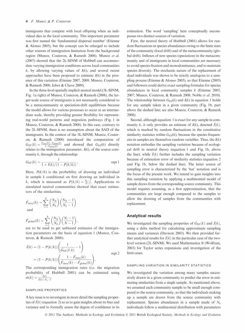
� 2011 The Authors. Methods in Ecology and Evolution � 2011 British Ecological Society, Methods in Ecology and Evolution
of a given sampling design. The smaller is MSE, the better is
the estimation of immigration.
In an application of the 2L-SINM of Hubbell (2001),
Fig. 2A shows contours of constant MSE when the sample
size Nk (abscissa) and the number of samples Nc (ordinate)
are varying in a case where I = 10 and h = 50, which are
fairly realistic values for tropical forests in South India
(Munoz et al. 2007; Munoz, Couteron, & Ramesh 2008).
The log10 values of MSE are shown along with the
contours. This figure shows that one cannot improve MSE
over a certain limit for a given sample size because increas-
ing the number of samples leads to an asymptote in MSE.
Specifically, for 0,1-ha forest plots of about Nk = 50,
log10(MSE) cannot go below 1,09, while for 1-ha forest
plots of about Nk = 500, it can go down to 0,016, and the
asymptotic difference in accuracy is a factor of about 12 in
absolute scale. Hence, one cannot expect good estimation
from community samples that are too small, even if there
are many samples. For illustration, consider a fixed overall
sampling effort of N = 5000 individuals, which can be
achieved for different sample sizes Nk and sample numbers
Nc such as, for instance, Nc = 50 samples of size Nk = 100
(Fig. 2A, point a), or Nc = 10 samples of size Nk = 500
(Fig. 2A, point b). In the former case, log10(MSE) = 0,8,
while in the latter case, log10(MSE) = 0,1, so that the
MSE is improved by a factor 4,6 with fewer large samples.
Furthermore, the arrow in Fig. 2A indicates that sampling
10 samples of 500 individuals is as accurate as sampling 30
samples of 440 individuals because both designs stand on
the same isoline of log10(MSE) = 0,1. In the former case,
only 5000 individuals are to be sampled, compared with
13 200 in the latter case. Therefore, it is better for estima-
tion performance to rely on fewer large samples, as long as
the assumption that the samples are smaller than the corre-
sponding communities is correct.
It is also possible to use the derivatives of MSE to investi-
gate the gain in performance when increasing sampling pres-
sure. Let us fix, for instance, a qualitative limit atdMSE
dNc¼ �0; 05, above which the gain is arbitrarily judged
no longer worth it. Fig. 2B (solid line) shows the correspond-
ing number of samples as a function of Nk. For instance, 24
samples of 50 individuals or seven samples of 500 individuals
are located at the same level of dMSEdNc
¼ �0; 05, and this
illustrates again that the advantage of getting additional
samples closely depends on sample size. One may use other
isoclines of dMSEdNc
(e.g. in Fig. 2B, isoclines at )0,01 repre-
sented by the dashed line and at )0,005 represented by the
dotted line) to reach a desired limit in estimation perfor-
mance when increasing the sample number. Information on
sampling properties is therefore useful for establishing a sam-
pling strategy prior to field work. The approach is analo-
gous, in principle, with using saturation curves and
exploratory statistics to fix the size of sampling plots for the
assessment of diversity in a local community (Gimaret-Car-
pentier et al. 1998).
Simulation application
SIMULATED NEUTRAL COMMUNITY SAMPLES
We used the two-step simulation algorithm of Munoz et al.
(2007, Appendix) in Matlab�(Mathworks, 2004) to simulate
neutral community samples complying with the 2L-SINM
of Hubbell (2001). First, we used the sequential algorithm of
Etienne (2005) to generate a pool of migrant ancestors
(migrant pool) as a very large metacommunity sample. The
0
0,1
0,2 0,3 0,4 0,5 0,6
0,7
0,8
0,9
1
1,1
100 200 300 400 500 600
510
2040 (a)
(b)
(A) Isolines of MSE N
umbe
r of s
ampl
es N
c
100 200 300 400 500
1030
5070
−0,005−0,01−0,05
dMSEdNc
=
(B) dMSE
dNc
Num
ber o
f sam
ples
Nc
Sample size Nk
Sample size Nk
Isolines of
Fig. 2. Trade-off between sample size (Nk) and number of samples
(Nc) for estimating immigration, as measured using the MSE statistic
of squared bias plus variance. In (A), isolines of constant MSE value
are shown with 0Æ1 increments on log10 scale. (a) and (b) are cases
where 5000 individuals are sampled overall using, respectively, 10
samples of 500 individuals and 50 samples of 100 individuals. The
arrow shows that 10 samples of 500 individuals (5000 individuals
overall) and 30 samples of 440 individuals (13 200 individuals overall)
are at the same level of MSE = 0Æ1. In these cases, it is less expensive
to use larger samples. (B) shows the value of Nc on ordinates such asdMSE
dNcis equal to )0,05 (solid line), )0,01 (dashed line) and )0,005
(dotted line) for a range of local sample sizes on abscissa. For these
examples, the statistics were calculated in the context of the 2L-SINM
ofHubbell (2001) with I(k) = 10 and h = 50.
Accuracy in estimating immigration 7
� 2011 The Authors. Methods in Ecology and Evolution � 2011 British Ecological Society, Methods in Ecology and Evolution

pool was characterized by the biodiversity parameter h,which controls the speciation-drift equilibrium. We repeated
the procedure for two values of h, 50 and 100, which illus-
trates a range of biodiversity figures of tree communities in
semi-evergreen and evergreen tropical forests (Hubbell 2001;
Munoz et al. 2007). For each migrant pool representing a
shared biogeographical background (metacommunity), we
generated 50 local community samples k with constant local
immigration numbers I(k) (see Munoz et al. 2007 for more
details). We repeated the procedure to generate 50 indepen-
dent migrant pools as replicates, for each of which we simu-
lated 50 community samples, so as to get a total of 2500
community samples for each value of I(k). We varied I(k)
from 10 to 200 with increments of 10, and we considered
two sample sizes: Nk = 400 and 800 (wet evergreen tropical
forest plots of about 1 ha usually fall within this range). We
ensured that the migrant pools included a significantly larger
number of individuals than the derived local community
samples, namely 50Nk, and ensured that the results remained
consistent when sizes ranging from 25Nk to 1000Nk were
used.
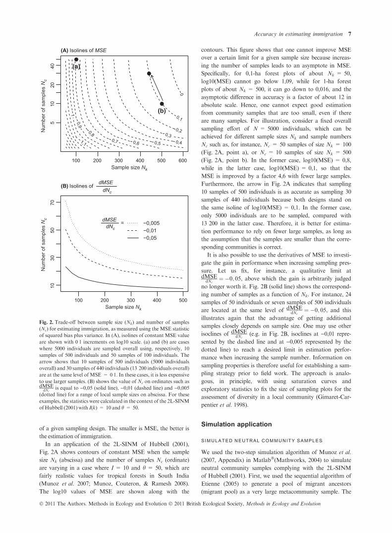
SIMULATED VS. PREDICTED SAMPLING
CHARACTERISTICS
For given values of I(k),Nk and h, we calculated the mean and
standard deviation of IðkÞ using equations (5A), (5B) and (7)
on the basis of 50 simulated community samples associated
with amigrant pool. To avoid spurious effects because of some
rare outliers, we calculated 95% trimmed statistics by exclud-
ing 2,5% of observations from each side. We repeated the pro-
cedure for each of the fifty replicate migrant pools and for each
of the 20 values of I(k). Figure 3 shows the departures of
observed bias and variance from our theoretical predictions.
The results are presented for three combinations of parame-
ters: h = 50, Nk = 400 (a and b); h = 50, Nk = 800 (c and
d); and h = 100,Nk = 400 (e and f).
We conducted extensive simulation experiments (results not
shown) to verify that the sampling properties remained consis-
tent for varying sizes of the pool of migrants (from 25Nk to
1000Nk) and for varying numbers of community samples
(from 50 to 250 samples) associated with a migrant pool. In
spite of the approximationsmade, our analytical predictions of
0 50 100 150 200
−0·6
−0·2
0·2
0·6(a)
ΔMea
n/I (
k)ΔM
ean/
I (k)
ΔMea
n/I (
k)
0 50 100 150 200
−1·0
0·0
0·5
1·0(b)
0 50 100 150 200
−0·6
−0·2
0·2
0·6(c)
0 50 100 150 200
−1·0
0·0
0·5
1·0(d)
0 50 100 150 200
−0·6
−0·2
0·2
0·6(e)
I (k)0 50 100 150 200
−1·0
0·0
0·5
1·0(f)
ΔSTD
/I (k
)ΔS
TD/I
(k)
ΔSTD
/I (k
)
I (k)
Fig. 3. The differences divided by I(k) between simulated and analytical values of themean (DMean; a, c, e) and standard deviation (DSTD; b,d,f)
of IðkÞ, as a function of I(k) (abscissa). The results are provided for three simulated data sets that comply with the 2L-SINM of Hubbell (2001),
with parameters h = 50,Nk = 400 (a, b); h = 50,Nk = 800 (c, d) and h = 100,Nk = 400 (e, f). There are 50 replicate values for each theoreti-
cal I(k).
8 F. Munoz & P. Couteron
� 2011 The Authors. Methods in Ecology and Evolution � 2011 British Ecological Society, Methods in Ecology and Evolution

sampling variance and mean of the immigration parameter
were globally consistent with simulation results (Fig. 3). The
relative difference between simulated and analytical EðIðkÞÞ(i.e. DMean ⁄ I(k)) wavered around 0 over the range of I(k) val-
ues, showing good agreement for varying configurations of handNk (Fig. 3a,c,e).We still noted that the width of the scatter
increased at values of I(k) above 75–100. On the other hand,
despite a good overall fit, the sampling standard deviation was
slightly underestimated at small I(k) (ca. under 75; Fig. 3b,d,f;
DSTD ⁄ I(k)>0). We found quite similar results for mðkÞ(results not shown).
Discussion
Our central result here is that estimating immigration parame-
ters I(k) and m(k) is asymptotically unbiased for large enough
samples, and it is an important and original result as far as the
novel conditional version GST(k) of GST is concerned. The
unconditionalFST and related statistics, such asGST, have been
widely investigated and debated in population genetics, espe-
cially about getting reliable enough estimates (Rottenstreich
et al., 2007; Guillot, 2010) and subsequently getting a correct
inference of migration (Whitlock and McCauley, 1999). A
major interest of using the conditional formGST(k) to estimate
immigration parameters I(k) is that it overcomes the problem
of averaging immigration effects across all the communities,
which Whitlock and McCauley (1999) pointed out for the
unconditional FST-based approach.
BecauseGST(k) and I(k) are nonlinear functions of similarity
statistics of analytically established sampling variances, we per-
formed the statistical analysis of their sampling accuracy using
appropriate Taylor series expansions (delta method) to avoid
cumbersome formulas and computation (Appendix S2). The
delta method basically assumes that the sampling statistics are
dominated by lower-order terms of the Taylor series (variances
and covariances), and we further neglected the variance of
Fglobal(k) and the covariance of Fglobal(k) and Fintra(k) against
the variance of Fintra(k). The simulation application for com-
munity samples complying with Hubbell’s model confirmed
that the analytical results based on these approximations were
reliable enough for a range of realistic parameters (sample size
and values of I(k) as from surveys in wet evergreen tropical for-
ests). To such extent, the variance of the estimation is mostly
sensitive to the variation in local similarity, Fintra(k). This result
may be robust against departures from Hubbell’s model, and
to verify it, simulations studies are still needed, but these are
beyond the scope of this paper.
In a broad perspective, the bias and variance formulas of
equations 4 and 5 are independent from any underlying model
of community dynamics, and notably, their applicability is not
restricted to neutral models. As such, I(k) andm(k) can be used
as descriptive indexes of community isolation, complementary
to diversity statistics. We may also note that our results (equa-
tions 4 and 5) are straightforwardly applicable to theD statistic
proposed by Jost (2008) as an alternative to GST. In practice,
the variation of I(k) values over a set of sampling sites can be
compared to external environmental information (e.g. geol-
ogy, climate) as to detect possible environmental filtering of
community composition. For this, the analytical results on the
sampling variance of I(k) will become useful to design tests of
departures from a regional mean. In this regard, a perspective
will be to investigate in greater details the distribution of IðkÞto provide further insights into the confidence limits.
Furthermore, the mean square error formula (MSE) based
on sampling bias and variance offers a synthetic measure of
estimation performance, which is of practical interest for
designing efficient sampling schemes (illustration in Fig. 2). In
our application, estimation performance as measured byMSE
reaches a plateau when the size and ⁄or the number of commu-
nity samples is increased. The isolines of MSE in Fig. 2A can
be used to select the appropriate sample number and size for a
desired level of accuracy, which can provide guidance in the
design and evaluation of sampling schemes. It is quite similar
to designing sampling schemes to correctly estimate species
alpha and beta diversities in communities (Gimaret-Carpentier
et al. 1998).
A further important message for community ecologists is
that sampling issues are central to the analysis of community
composition, when stochastic processes and estimation error
are intertwined. Therefore, one should take into account both
(i) the sampling nature of the neutral theory (Etienne&Alonso
2005), and more generally of the fundamental concept of com-
position drift (a process that is likely to be pervasive even when
interacting with non-neutral processes); and (ii) the sampling
error in parameter estimation as in any inference process.
Finally, the strict dichotomy of neutral vs. non-neutral mod-
els is progressively vanishing and recent works have suggested
that the scope of neutral models should be enlarged and that
the predictions on relative species abundances are robust
(Allouche&Kadmon 2009;Noble et al. 2010). Several authors
(Hubbell 2006; Zillio & Condit 2007) argued that the assump-
tion of ecological equivalence of individuals is realistic insofar
as the trade-off between life traits in a group of trophically sim-
ilar species (a guild) may produce comparable levels of fitness.
Furthermore, the three-level spatially implicit neutral model of
Munoz, Couteron, & Ramesh (2008) illustrates how non-neu-
tral processes at regional scale can be incorporated in the tradi-
tional neutral approach. Hence, this 3L-SINM framework
may be applied to a variety of contexts that have to do with
community isolation, including anthropogenic fragmentation
in tropical forests, and it may become a useful approach for
conservation issues (Pearse &Crandall 2004).
Acknowledgements
We warmly thank the editor and an anonymous reviewer for their valuable
comments and suggestions.
References
Allouche, O. & Kadmon, R. (2009) A general framework for neutral models of
community dynamics.Ecology Letters, 12, 1287–1297.
Beeravolu, C.R., Couteron, P., Pelissier, R. & Munoz, F. (2009) Studying eco-
logical communities from a neutral standpoint: a review of models’ structure
and parameter estimation.EcologicalModelling, 220, 2603–2610.
Accuracy in estimating immigration 9
� 2011 The Authors. Methods in Ecology and Evolution � 2011 British Ecological Society, Methods in Ecology and Evolution

Chave, J., Alonso, D. & Etienne, R.S. (2006) Comparing models of species
abundance.Nature, 441, E1.
Cormen, T.H., Leiserson, C.E., Rivest, R.L. & Stein, C. (2001) Indicator ran-
dom variables. Introduction to Algorithms, 2nd edn, pp. 94–99. MIT Press
andMcGraw-Hill, Cambridge.
Couteron, P. & Pelissier, R. (2004) Additive apportioning of species diversity:
towards more sophisticated models and analyses.Oikos, 107, 215–221.
Davison, A.C. (2003) Statistical Models. Cambridge University Press, Cam-
bridge, UK.
Etienne, R.S. (2005) A new sampling formula for neutral biodiversity. Ecology
Letters, 8, 253–260.
Etienne, R.S. (2007) A neutral sampling formula for multiple samples and an
‘‘exact’’ test of neutrality.Ecology Letters, 10, 608–618.
Etienne, R.S. (2009)Maximum likelihood estimation of neutral model parame-
ters for multiple samples with different degrees of dispersal limitation. Jour-
nal of Theoretical Biology, 257, 510–514.
Etienne, R.S. & Alonso, D. (2005) A dispersal-limited sampling theory for spe-
cies and alleles.Ecology Letters, 8, 1147–1156.
Etienne, R.S. & Olff, H. (2004) A novel genealogical approach to neutral biodi-
versity theory.Ecology Letters, 7, 170–175.
Etienne, R.S., Latimer, A.M., Silander. Jr, J.A. & Cowling, R.M. (2006) Com-
ment on ‘‘Neutral Ecological Theory Reveals Isolation and Rapid Specia-
tion in a BiodiversityHot Spot’’.Science, 311, 610b.
Ewens, W.J. (1972) The sampling theory of selectively neutral alleles. Theoreti-
cal Population Biology, 3, 87–112.
Gimaret-Carpentier, C., Pelissier, R., Pascal, J.-P. & Houiller, F. (1998) Sam-
pling strategies for the assessment of the tree species diversity. Journal of
Vegetation Science, 9, 161–172.
Guillot, G. (2010) Splendor and misery of indirect measures of migration and
gene flow.Heredity, 106, 11–12.
Hubbell, S.P. (2001) The Unified Neutral Theory of Biodiversity and Biogeogra-
phy. PrincetonUniversity Press, Princeton andOxford.
Hubbell, S.P. (2006) Neutral theory and the evolution of ecological equiva-
lence.Ecology, 87, 1387–1398.
Jabot, F. & Chave, J. (2009) Inferring the parameters of the neutral theory of
biodiversity using phylogenetic information and implications for tropical
forests.Ecology Letters, 12, 239–248.
Jost, L. (2008) GST and its relatives do not measure differentiation.Molecular
Ecology, 17, 4015–4026.
Lande, R. (1996) Statistics and partitioning of species diversity, and similarity
amongmultiple communities.Oikos, 76, 5–13.
Latimer, A.M., Silander Jr, J.A. & Cowling, R.M. (2005) Neutral Ecological
Theory Reveals Isolation and Rapid Speciation in a Biodiversity Hot Spot.
Science, 309, 1722–1725.
Leigh, E.G. (2007) Neutral theory: a historical perspective. Journal of Evolu-
tionary Biology, 20, 2075–2091.
Mathworks (2004)Matlab 7.0.Mathworks Inc., Natwick,MA.
McGill, B.J. (2003) A test of the unified neutral theory of biodiversity. Nature,
422, 881–885.
Munoz, F., Couteron, P. & Ramesh, B. (2008) Beta-diversity in spatially impli-
cit neutral models: a new way to assess species migration.The American Nat-
uralist, 172, 116–127.
Munoz, F., Couteron, P., Ramesh, B.R. & Etienne, R.S. (2007) Estimating
parameters of neutral communities: from one Single Large to Several Small
samples.Ecology, 88, 2482–2488.
Nee, S. & Stone, G. (2003) The end of the beginning for neutral theory. Trends
in Ecology & Evolution, 18, 433–434.
Nei,M. (1973) Analysis of Gene Diversity in Subdivided Populations. Proceed-
ings of the National Academy of Sciences of the United States of America, 70,
3321–3323.
Noble, A.E., Temme, N.M., Fagana, W.F. & Keitt, T.H. (2011) A sampling
theory for asymmetric communities, Journal of Theoretical Biology, 273, 1–
14.
Pearse, D.E. & Crandall, K.A. (2004) Beyond F-ST: analysis of population
genetic data for conservation.Conservation Genetics, 5, 585–602.
Rottenstreich, S., Miller, J.R. & Hamilton, M.B. (2007) Steady state of homo-
zygosity and Gst for the island model. Theoretical Population Biology, 72,
231–244.
Rottenstreich, S., Hamilton, M.B. & Miller, J.R. (2007) Dynamics of Fst for
the islandmodel.Theoretical Population Biology, 72, 485–503.
Simpson, E.H. (1949)Measurement of diversity.Nature, 163, 688.
Slatkin, M. (1985) Gene flow in natural populations. Annual Review of Ecology
and Systematics, 16, 393–430.
Takahata, N. & Nei, M. (1984) FST and GST statistics in the finite island
model.Genetics, 107, 501–504.
Volkov, I., Banavar, J.R., Hubbell, S.P. & Maritan, A. (2003) Neutral theory
and relative species abundance in ecology.Nature, 424, 1035–1037.
Whitlock, M.C. & McCauley, D.E. (1999) Indirect measures of gene flow and
migration: FST!=1 ⁄ (4Nm+1).Heredity, 82, 117–125.
Wolfram (2003)Mathematica 5.2. WolframResearch, Inc., Champaign, IL.
Zillio, T. & Condit, R. (2007) The impact of neutrality, niche differentiation
and species input on diversity and abundance distributions.Oikos, 116, 931–
940.
Received 20October 2010; accepted 22May 2011
Handling Editor: Robert Freckleton
Supporting Information
Additional Supporting Information may be found in the online ver-
sion of this article.
Appendix S1. Sampling properties of the similarities.
Appendix S2.Deltamethod to assess the samplingmean and variance
of twice differentiable functions.
Appendix S3. Raw moments of the local species abundance distribu-
tion (SAD) in the context of the two-level spatially implicit neutral
model (2L-SINM) ofHubbell (2001).
As a service to our authors and readers, this journal provides support-
ing information supplied by the authors. Such materials may be
re-organised for online delivery, but are not copy-edited or typeset.
Technical support issues arising from supporting information (other
thanmissing files) should be addressed to the authors.
10 F. Munoz & P. Couteron
� 2011 The Authors. Methods in Ecology and Evolution � 2011 British Ecological Society, Methods in Ecology and Evolution

Appendix A: Sampling properties of the similarities
In a network of community samples k (1 ≤ k ≤ Nc), such that each of them belongs to a
distinct source community, we assumed the community samples k to be multinomial draws
from the corresponding source communities, in which the species probabilities are denoted
pik, respectively. We used Bernouilli indicator variables Giz to investigate the sampling
variation in such multinomial draws. The global indicator variable, Giz, was used to represent
a set of N individuals drawn from the overall set of communities (G is for “global”). Giz = 1 if
an individual z within this draw is of species i, and Giz = 0 otherwise, so that ∑=z
izi GN and
izi z
N G= ∑∑ . Likewise, Kiz are the local indicator variables for the multinomial draws of Nk
individuals from local communities, so that ∑=z
izik KN .
If two distinct individuals z and z’ from sample k belong to the same species, then KizKiz’
= 1, otherwise KizKiz’ = 0. Because of the binary 0/1 values, Kiz = Kizn. These properties are the
same for Giz. In the subsequent analysis, we will derive expected values over an infinite
number of draws using symbol E(). In this regard, E(Kizn) = pik and E(Giz) = E(Giz
n) = pi in the
context of multinomial draws. Furthermore, E(Kiz Kiz’ …Kizn) denotes the probability of
drawing n different individuals in sample k that belong to the same species, which is, by
definition, the raw moment Fn(k) (see Appendix C).
Fintra(k) is the probability of drawing two individuals that belong to the same species
conditional on drawing them in community sample k, while Finter(k) is the probability of
drawing two conspecific individuals conditional on the first being in k and the other in another
sample, and Fglobal(k) is the probability of drawing two conspecific individuals conditional on
the first being in k and the other being in any of the samples.
The theoretical relationship between these probabilities is (Munoz et al. 2008):

( ) )()(1)()()( kFkkPkFkkPkF interintraglobal −+= (B1)
Where P(k/k) is the probability of drawing a second individual from sample k when the first
has been already drawn from k.
Exact estimators of Fintra(k), Finter(k) and Fglobal(k) are:
∑ −−
=i k
ik
k
ikintra N
NNN
kF11
)(ˆ , ∑ −−
=i k
iki
k
ikinter NN
NNNN
kF )(ˆ and ∑ −−
=i
i
k
ikglobal N
NNN
kF11
)(ˆ
where Nk and N are the number of individuals in sample k and in the overall dataset,
respectively, while Nik and Ni are the numbers of individuals belonging to species i in sample
k and in the overall dataset, respectively, such as ∑=i
iNN and ∑=i
ikk NN . These statistics
comply with equation (B1).
Using indicator variables, the probability of drawing in sample k two different
individuals, z and z’, belonging to the same species is: ∑=i
izizintra KKEkF )()( ' and
∑≠
=−ji
jzizintra KKEkF )()(1 ' . Likewise, ∑=i
izizinter KGEkF )()( ' is the probability for z taken in
k and z’ in a different sample, and ∑=i
izizglobal KGEkF )()( ' is the probability for any pair of
distinct z in k and z’ in the overall dataset. In the subsequent analysis, we will investigate the
sampling properties of the similarity statistics in detail using the properties of Giz and Kiz.
Expected value of )(ˆ kFintra
( )∑ ∑∑∑ ⎟⎠
⎞⎜⎝
⎛−
−=
−−
=i z
izz
izkki k
ik
k
ikintra KK
NNNN
NN
kF 11
111
)(ˆ is defined for a given multinomial draw
from the source community.
( ) ( ) ( ) ( ) ( )∑ ∑∑∑ ⎟⎠
⎞⎜⎝
⎛−+
−=
≠i ziz
zziziz
ziz
kkintra KEKKEKE
NNkFE
''
2
11)(ˆ

In the context of multinomial draws, we have: ( ) ( ) ( ) ikkizkz
izz
iz pNKENKEKE === ∑∑ 2
and ( ) )()1(' kFNNKKE intrakkz
iziz −=∑ for z ≠ z’.
Although there is replacement, Kiz and Kiz’ are not independent because Cov(Kiz,Kiz’)=
( ) ( ) ( ) 0)('' ≠−=− kFNKEKEKKE intrakiziziziz .
This yields: ( ) ( ) ( )( )1ˆ ( ) 1 ( ) ( )1intra k ik k k intra k ik intra
k k
E F k N p N N F k N p F kN N
= + − − =−
. (B2)
∑ −−
=i k
ik
k
ikintra N
NNN
kF11
)(ˆ is thus an unbiased estimator of Fintra(k), while the approximated
version 2
)(ˆ ∑ ⎟⎟⎠
⎞⎜⎜⎝
⎛=
i k
ikintra N
NkF is biased (see Lande 1996).
Variance of )(ˆ kFintra
( )( )
( ) 22
22
2
11
111
)(ˆintra
iikik
kkintra
i k
ik
k
ikintra FNNE
NNF
NN
NN
EkFVar −⎟⎟⎠
⎞⎜⎜⎝
⎛⎟⎠
⎞⎜⎝
⎛−
−=⎟
⎟
⎠
⎞
⎜⎜
⎝
⎛⎟⎟⎠
⎞⎜⎜⎝
⎛−
−−
= ∑∑
( ) ( ) ( ) ( )∑∑∑≠
−−+−=⎟⎠
⎞⎜⎝
⎛−
jijkjkikik
iikik
ikiki NNNNNNNN 1111 22
2
( ) ( ) ( )∑∑∑≠
+−++−=⎟⎠
⎞⎜⎝
⎛−
jijkikjkikjkik
iikikik
ikiki NNNNNNNNNNN 222234
2
221
In the following calculations, we will use the indicator variables Kiz linked to species
abundances through ∑=z
izik KN .
• Terms that sum over species i:
(i) ∑ ∑∑∑ ⎟⎠
⎞⎜⎝
⎛ +=≠i zz
izizz
izi
ik KKKN'
'22 and thus )()1( int
2 kFNNNNE rakkki
ik −+=⎟⎠
⎞⎜⎝
⎛∑ )
(ii) ∑ ∑∑∑∑ ∑∑ ⎟⎠
⎞⎜⎝
⎛++=⎟
⎠
⎞⎜⎝
⎛=
≠≠≠i zzziziziz
zziziz
ziz
i ziz
iik KKKKKKKN
''''''
'
2'
33
3 3
Hence, )()2)(1()()1(3 33 kFNNNkFNNNNE kkkintrakkk
iik −−+−+=⎟⎠
⎞⎜⎝
⎛∑
(iii)
∑ ∑∑∑∑∑∑ ⎟⎠
⎞⎜⎝
⎛ ++++=≠≠≠≠≠≠≠i zzzz
izizizizzzz
izizizzz
izizzz
izizz
izi
ik KKKKKKKKKKKKN'''"'
'''''''''
2'''
'
3'
'
2'
244 643
Hence,
( ) ( )( ) ( )( )( ) )(321)(216)(17 434 kFNNNNkFNNNkFNNNNE kkkkkkkintrakkk
iik −−−+−−+−+=⎟⎠
⎞⎜⎝
⎛∑
• Terms that sum over different species i and j:
(i) ∑ ∑∑ ∑∑∑ ∑∑∑≠ ≠≠ ≠≠≠
⎟⎠
⎞⎜⎝
⎛=⎟⎠
⎞⎜⎝
⎛ +=⎟⎠
⎞⎜⎝
⎛⎟⎠
⎞⎜⎝
⎛=ji zz
jzizji zz
jzizz
jzizji z
jzz
izji
jkik KKKKKKKKNN'
''
' , and
hence )1)(1( intrakkji
jkik FNNNNE −−=⎟⎟⎠
⎞⎜⎜⎝
⎛∑≠
(ii) ∑ ∑∑∑ ∑∑∑≠ ≠≠≠≠≠
⎟⎠
⎞⎜⎝
⎛+=⎟
⎠
⎞⎜⎝
⎛⎟⎠
⎞⎜⎝
⎛=
ji zzzjzjziz
zzjziz
ji zjz
ziz
jijkik KKKKKKKNN
''''''
'
2'
22
)( ''' jzjziz KKKE is the probability of drawing three distinct individuals that belong to two
species. F3(k) is the probability of drawing three individuals that belong to the same species
and Fintra(k) is the probability of drawing two individuals that belong to the same species, so
that )()()( 3''' kFkFKKKE intrajzjziz −= .
Hence, ( ) ( ))()()2)(1()(1)1( 32 kFkFNNNkFNNNNE intrakkkintrakk
jijkik −−−+−−=⎟⎟⎠
⎞⎜⎜⎝
⎛∑≠
(iii) ∑ ∑∑∑≠≠
⎟⎠
⎞⎜⎝
⎛⎟⎠
⎞⎜⎝
⎛=
ji zjz
ziz
jijkik KKNN
2222
∑ ∑∑∑∑∑≠ ≠≠≠≠≠≠≠≠≠
⎟⎠
⎞⎜⎝
⎛ +++=ji zzzz
jzjzizizzzz
izjzjzzzz
jzizizzz
jzizji
jkik KKKKKKKKKKKKNN''''''
''''''"'
2'''
"'
2"'
'
2'
222

)( '''''' jzjziziz KKKKE is the probability of drawing four distinct individuals falling into two
conspecific pairs of different species. F4(k) is the probability of drawing four individuals that
belong to the same species and (Fintra(k))² is the probability of drawing two conspecific pairs,
and hence ( ) )()()( 42
'''''' kFkFKKKKE intrajzjziziz −= .
This yields: ( ) ( )( ) ⎟⎟
⎠
⎞⎜⎜⎝
⎛
−−−−+
−−−+−−=⎟⎟
⎠
⎞⎜⎜⎝
⎛∑≠ )()()3)(2)(1(
)()()2)(1(2)(1)1(
42
intra
3intraintra22
kFkFNNNN
kFkFNNNkFNNNNE
kkkk
kkkkk
jijkik
In summary, the exact variance of )(ˆ kFintra simplifies to:
( ) ( ) ( ) ( )( )23
1ˆ ( ) 2 ( ) 6 4 ( ) 4 2 ( )1intra intra k intra k
k k
Var F k F k N F k N F kN N
= + − + −−
(B3)
The first order series expansion according to 1/Nk reads:
( ) ( ) ⎟⎟⎠
⎞⎜⎜⎝
⎛+−≈ 2
2int3
1)()(4)(ˆk
rak
intra NOkFkF
NkFVar .
This first order expansion also holds for the approximate statistic 2
)(ˆ ∑ ⎟⎟⎠
⎞⎜⎜⎝
⎛=
i k
ikintra N
NkF (see
Lande 1996).
Expected value of )(ˆ kFglobal and )(int kF er
( )1 1ˆ ( ) 11 1
ik iglobal iz iz
i i z zk k
N NF k K GN N N N
− ⎛ ⎞= = −⎜ ⎟− − ⎝ ⎠∑ ∑∑ ∑
The indicator function Giz here enlarges the sampling context to the overall dataset.
( ) ( ) ( ) ( ) ( )''
1ˆ ( )1global iz iz iz iz iz
i z z z zk
E F k E K G E K G E KN N ≠
⎛ ⎞= + −⎜ ⎟− ⎝ ⎠
∑ ∑ ∑ ∑
( ) ( ) ( )''
1ˆ ( )1global iz iz
i z zk
E F k E K GN N ≠
=− ∑∑

When summing over z ≠ z’, z being an individual in plot k, we need to distinguish two
cases, namely that z’ can be either an individual of plot k or of another sample, hence:
( )''
( 1) ( ) ( ) ( )iz iz k k intra k k interi z z
E K G N N F k N N N F k≠
= − + −∑∑ .
This yields: ( ) ( 1) ( ) ( ) ( )ˆ ( ) ( )1
k intra k interglobal global
N F k N N F kE F k F kN
− + −= =
−.
Thus, )(ˆ kFglobal is an unbiased estimator of Fglobal(k).
On the other hand, ( )
1ˆ ( ) ik i ikinter iz iz iz
i i z z zk k k k
N N NF k K G KN N N N N N
− ⎛ ⎞= = −⎜ ⎟− − ⎝ ⎠∑ ∑∑ ∑ ∑
( ) ( ) ( ) ( ) ( ) ( )2' '
' '
1ˆ ( )inter iz iz iz iz iz iz izi z z z z z zk k
E F k E K G E K G E K E K KN N N ≠ ≠
⎛ ⎞= + − −⎜ ⎟− ⎝ ⎠
∑ ∑ ∑ ∑ ∑
( ) ( ) ( ) ( ) ( ) ( )int ' ' '' ' '
, '
1 1ˆ ( )er iz iz iz iz iz izi z z z z i z zk k k k
z k z k
E F k E K G E K K E K GN N N N N N≠ ≠ ≠
∈ ∉
⎛ ⎞⎛ ⎞ ⎜ ⎟= − =⎜ ⎟ ⎜ ⎟− −⎝ ⎠ ⎜ ⎟
⎝ ⎠∑ ∑ ∑ ∑ ∑ , which
simplifies to ( ) )()(int kFkFE interer = .
Hence, )(int kF er is conversely an unbiased estimator of Finter(k).

Appendix B: Delta method to assess the sampling mean and variance of twice
differentiable functions
The one-variable case
Let )(XfZ = be a function of the random variable X, of which expectation X and
variance Var(X) are known. The derivative functions of f are:
xxfxf x ∂
∂=
)()(' , 2
2'' )()(2 x
xfxfx ∂
∂= ,
yxxfxf xy ∂∂
∂=
)()(2
'' ,yxxfxf yx ∂∂
∂= 2
3)3( )()(2 , and so on.
Assuming that X takes values x around X , the second order Taylor series expansion of
f(X) in the neighborhood of X is: ( ) ( ) )(21)()( "2' XfXxXfXxXfZ xx −+−+≈ .
This implies:
)()(21)( " XfxVarXfZ x+≈ (C1)
and ( ) ( )( ))()(21)( 2"' XVarXxXfXfXxZZ xx −−+−≈− .
Finally, ( ) ( ) 2'22 )(XfXxZZ x−≈− at the second order around X and hence
2' )()()( XfXVarYVar x≈ . (C2)
The two-variable case
Now let Z = g(X, Y) be a differentiable function of two random variables X and Y. Its
second order series expansion around ( X ,Y ) is:
( ) ( ) ( )( )( ) ( )2 2
' ' "
2 2" "
( , ) ( , ) ( , ) ( , )
1 1( , ) ( , )2 2
x y xy
x y
Z g X Y x X g X Y y Y g X Y x X y Y g X Y
x X g X Y y Y g X Y
≈ + − + − + − −
+ − + −
and thereby

),()(21),()(
21),(),(),( """
22 YXgYVarYXgXVarYXgYXCovYXgZyxxy +++≈ (C3)
Furthermore,
( ) ( ) ( )( ) ( ) ( )
⎟⎟⎟⎟
⎠
⎞
⎜⎜⎜⎜
⎝
⎛
−−−
−+−+−−+−+−≈−
),()(21),()(
21),(),(
),(21),(
21),(),(),(
"""
"2"2"''
2
22
YXgYVarYXgXVarYXgYXCov
YXgYyYXgXxYXgYyXxYXgYyYXgXxZZ
yxxy
yxxyyx
é
( ) ( ) ( ) ( )( ) ),(),(2),(),( ''2'22'22 YXgYXgYyXxYXgYyYXgXxZZ yxyx −−+−+−≈−
and finally,
( ) ),()(),(),(2),()(),()()( ''2'2' YXgYEyYXgYXCovYXgYVarYXgXVarZVar xyyx −++≈ (C4)

Appendix C: Raw moments of the local species abundance distribution (SAD) in the
context of the two-level spatially implicit neutral model (2L-SINM) of Hubbell (2001)
The raw moment Fn(k) associated with the species abundance distribution (SAD) in a
local community sample k is the probability of drawing n individuals that belong to the same
species in k, and as such it can be written down as: 1
( ) (1 ) ( )n
n meta commj
F k p j p j n=
= ∑
where )( njpcomm is the probability of drawing n individuals in sample k that belong to j
different lineages, that is, which are the descendants of j independent migrant ancestors.
)1( jpmeta is the probability that the j independent migrant ancestors belong to the same
species.
I(k) is the immigration number of community k, that is, the number of immigrants
available for replacement in the community when an individual dies. We consider the
coalescent-type reasoning of Etienne and Olff (2004) and Etienne (2005), that is, when we
draw a new individual in a local community k, increasing the sample size from n to n+1, the
probability that the (n+1)th individual is the descendant of a lineage not represented in the
initial sample is nkI
kI+)()( , while the probability that the (n+1)th individual is the descendant
of a lineage already represented is conversely nkI
n+)(
.
Hence,
nkIkInjp
nkInnjpnjp commcommcomm +
−++
=+)(
)()1()(
)()1(
According to Ewens (1972), ( )s
j
jsmeta
ljsp θ
θ,)( = in Hubbell’s metacommunity undergoing
speciation-drift equilibrium, and, likewise, ( )j
n
njcomm kI
kIl
njp )()(
)( ,= in the local
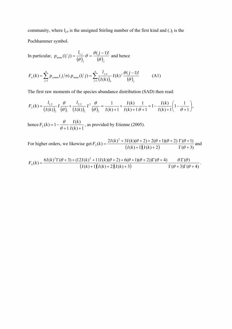
community, where lj,n is the unsigned Stirling number of the first kind and (.)j is the
Pochhammer symbol.
In particular, ( ) ( ) jj
jmeta
jljp
θθθ
θ)!1()1( ,1 −
== and hence
( ) ( )∑∑==
−==
n
j j
j
n
njmeta
n
jcommn
jkIkI
ljpnjpkF
1
,
1
)!1()()(
)1(.)()(θ
θ (A1)
The first raw moments of the species abundance distribution (SAD) then read:
( ) ( ) ( ) ( ) ⎟⎠⎞
⎜⎝⎛
+−
+−=
+++
+=+=
111
1)()(1
11
1)()(
1)(1
)()()(
2
2
2
2,2
12
2,12 θθθ
θθθ
kIkI
kIkI
kII
kIl
IkI
lkF ,
hence1)(
)(1
1)(2 ++−=
kIkIkF
θθ , as provided by Etienne (2005).
For higher orders, we likewise get ( )( ) )3()1(
2)(1)()2)(1(2)2)((3)(2)(
2
3 +Γ+Γ
+++++++
=θθθθθ
kIkIkIkIkF and
( )( )( ) )4()3()(.
3)(2)(1)()4())2)(1(6)2)((11)(12()3()(6)(
23
4 +Γ+ΓΓ
++++Γ+++++++Γ
=θθθθθθθθθ
kIkIkIkIkIkIkF .