The sampling theory of neutral alleles and an urn model in population genetics
37
J. Math. Biol. (1987) 25:123-159 dournalof Mathematical Biology t~) Springer-Verlag 1987 The sampling theory of neutral alleles and an urn model in population genetics* Fred M. Hoppe Departments of Mathematics and Statistics, The University of Michigan, Ann Arbor, MI 48109-1027, USA Abstract. The behaviour of a P61ya-like urn which generates Ewens' sampling formula in population genetics is investigated. Connections are made with work of Watterson and Kingman and to the Poisson-Dirichlet distribution. The order in which novel types occur in the urn is shown to parallel the age distribution of the infinitely many alleles diffusion model and consequences of this property are explored. Finally the urn process is related to Kingman's coalescent with mutation to provide a rigorous basis for this parallel. Key words: Ages of alleles--Coalescent--Ewens' sampling formula-- Genealogy -- Mutation -- Poisson-Dirichlet -- P61ya urn -- Population genetics -- Size-biased sampling I. Introduction The following P61ya-like urn process ~ was described in Hoppe (1984). An urn contains one black ball whose mass is 0 > 0 and various numbers of other balls having assorted colours (non-black) each of mass one. At each instant of discrete time a ball is drawn at random (that is in proportion to its mass). If the selected ball is black then it is returned together with one additional ball of a previously unused colour. Otherwise it is returned together with one additional ball of the same colour. All new balls have unit mass and for definiteness the natural numbers will be used sequentially to label the colours as the need arises. At the outset there is a single black ball and no others in the urn. The random variable Xn is defined to be the label of the additional ball returned after the nth drawing. K is the random number of distinct labels present after the nth return and &(n), 1 ~< i ~ < K, is the number of balls labelled i. Also a = (al, aa, .., an) denotes, in the terminology of genetics, the allelic partition (Kingman (1978)) aj being the number of times the integer j appears in the set {Sa(n),..., SK(n)}. * This research was partially supported by the Sloan Foundation under Grant 85-6-14 and by the National Science Foundation
Transcript of The sampling theory of neutral alleles and an urn model in population genetics

J. Math. Biol. (1987) 25:123-159 dournalof
Mathematical Biology
t~) Springer-Verlag 1987
The sampling theory of neutral alleles and an urn model in population genetics*
Fred M. Hoppe
Departments of Mathematics and Statistics, The University of Michigan, Ann Arbor, MI 48109-1027, USA
Abstract. The behaviour of a P61ya-like urn which generates Ewens' sampling formula in population genetics is investigated. Connections are made with work of Watterson and Kingman and to the Poisson-Dirichlet distribution. The order in which novel types occur in the urn is shown to parallel the age distribution of the infinitely many alleles diffusion model and consequences of this property are explored. Finally the urn process is related to Kingman's coalescent with mutation to provide a rigorous basis for this parallel.
Key words: Ages of a l l e l e s - - C o a l e s c e n t - - E w e n s ' sampling f o r m u l a - - Genealogy - - Mutation - - Poisson-Dirichlet - - P61ya urn - - Population genetics - - Size-biased sampling
I. Introduction
The following P61ya-like urn process ~ was described in Hoppe (1984). An urn contains one black ball whose mass is 0 > 0 and various numbers of other balls having assorted colours (non-black) each of mass one. At each instant of discrete time a ball is drawn at random (that is in proportion to its mass). I f the selected ball is black then it is returned together with one additional ball of a previously unused colour. Otherwise it is returned together with one additional ball of the same colour. All new balls have unit mass and for definiteness the natural numbers will be used sequentially to label the colours as the need arises. At the outset there is a single black ball and no others in the urn. The random variable Xn is defined to be the label of the additional ball returned after the nth drawing. K is the random number of distinct labels present after the nth return and &(n), 1 ~< i ~ < K, is the number of balls labelled i. Also a = (al, aa, �9 . . , an) denotes, in the terminology of genetics, the allelic partition (Kingman (1978)) aj being the number of times the integer j appears in the set {Sa(n) , . . . , SK(n)}.
* This research was partially supported by the Sloan Foundation under Grant 85-6-14 and by the National Science Foundation

124 F . M . H o p p e
The use of allelic partitions is convenient in those genetic applications where no biological significance is to be attached to the actual labels which merely represent distinct allelic forms of a gene and aj becomes the number of alleles having j copies in a sample. The sequence { X 1 , . . . , X , } determines a random allelic partition Hn pertaining to which the following was established.
Theorem A. {Hn} is a M a r k o v process h a v i n g m a r g i n a l d i s t r ibu t ions
n! 012i P r [ I I . : a ] : ~ - g ~
i=l ia ia i [ (1.1)
where [ 0 ]" = 0 ( 0 + 1) �9 �9 �9 ( 0 + n - 1) is the a s c e n d i n g f a c t o r i a l a n d a = ( al , . . . , a , ) wi th Y, iai = n.
The right-hand side of (1.1), known as Ewens' sampling formula, was derived (Ewens (1972), see also Karlin and McGregor (1972)) as the limiting distribution of allelic numbers in a random sample, first for a discrete Wright-Fisher model with mutation and then later by various authors for other models displaying infinitely many selectively neutral alleles. The goal of this paper is to understand why (1.1) occurs in the present context where there appears neither a genetic nor a population structure.
The paper is a mixture of theorems and discussion and it is organized as follows. In Sect. 2 we present our first two theorems describing the limiting behaviour of q/. The distributions which emerge relate intimately to work of Watterson and Kingman, connections which are explored in Sects. 3 and 4 dealing with size-biased relabelling of P61ya urns and the Poisson-Dirichlet distribution, respectively. Section 4 also addresses modelling issues associated with samples from a population. In Sect. 5 we draw upon a remarkable equivalence between the order that alleles are sampled and their age distribution in order to derive various age properties in an entirely new and simple fashion. In Sect. 6 we develop a representation for Ewens' partition as a residual allocation model. Section 7 describes affinities between the Markovian property of / /n and partition structures, while Sect. 8 establishes the relationship between the urn model in reverse time and the genealogy of the coalescent (Kingman (1982), Tavar6 (1984), Watterson (1984)) with mutation. The final section summarizes the main results.
2. Limit behaviour of the urn
Theorem 1.
l i m S i ( n ) = P i and ~ P~= I n--> co n i=1
Theorem 2. The propor t ions
z . = P,, i
n ~ l
a . s .

T h e s a m p l i n g t h e o r y o f n e u t r a l a l l e l e s 125
are independent and identically distributed each with a Beta (1, 0) density 0 ( 1 - z) ~ ~ l ( 0 < z < 1).
Corollary.
n - 1
P I = Z 1 and P n = Z n 1~ ( 1 - Z i ) f o rn>~2. (2.1) i=1
To prepare for the proofs we need to establish some facts concerning multivari- ate P61ya urns for which we refer to Blackwell and MacQueen (1973) whose elegant treatment motivated our approach.
At time t = 0 an urn contains cq balls of type i(1 ~< i <~ K). I f ai is non-integer we interpret the fractional part as being represented by a ball having the fractional part as mass. At each instant of discrete time a ball is drawn at random (with probabili ty proport ional to its mass). The ball is then returned to the urn together with one additional ball of the same type and unit mass. The random variable X~ is the type of the nth additional ball placed into the urn. It is possible to formulate this process without using physics concepts such as mass and we may equivalently consider a fixed array of K cells labelled 1, 2 , . . . , K and associated non-negative reals ai, 1 ~< i ~< K, with Y~ oei = 0. Tokens are sequentially thrown at this array in such a way that if Xn denotes the cell into which the nth token lands then
Pr[Xn+~ = i[ X~, X2, . . . , Xn] - - OIl ~- v~(n) (2.2) O+n
where vi(n) equals the number of tokens in cell i after n throws. The process {X1, X2 , . . . } is endowed with the following properties:
~i(n) lim =P~ and Y~Pg=I a.s.; (2.3) n~oo n
_P-= (PI, P2, �9 �9 �9 PK) (2.4)
has a Dirichlet distribution with parameter ( a ~ , . . . , aK) which we denote by D ( o q , . . . , a K ) ;
Conditional on P, {X1, X2 , . . . } are independent and identically distributed with distribution Pr[X1 = i l P] = P~. (2.5)
The Dirichlet D ( a l , . . . , a K ) is defined as the joint distribution of a random . . . ~ X K vector of proportions -P=-(PI ,P2 PK) where P i= JY.j=iXj and
X~, X 2 , . . . , XK are independent G a m m a random variables having respective densities
1 - - e 'x,, l ( x ~ > 0 ) . V(o~,)
(It is convenient to regard the X~ as rePresenting on some scale the abundances of different resources so that 3~ Xj is the total abundance and P represents the relative proportions.) The distribution is singular with respect to Lebesgue

126 F.M. Hoppe
measure in K dimensions , but the K - 1 d imensional distr ibution of (P~, P 2 , . . . , PK-I ) is absolute ly cont inuous with density
1~(~[ K O/i) ( K~I ~aK--1 K-lpTi__ 1 [I~ F(O/i) 1- Pi] i=,[I (2.6)
over the s implex {(Pl, �9 . . , PK-~): Pi I> 0 and L~ pi ~ 1}. We record here for later recall the fact that the marginals P~ have Beta(O/i, Yj~;i O/J) densities
F(E O/j) pT,-~(1 - - p i ) ( E J ~ ' % ) - l l ( O <p~ < 1) r(O/,)r(E.~, O/s)
with E(Pi) = O/i/~S~l O/j. A detai led discussion of the Dirichlet distr ibution may be found in Wilks (1962, Sect. 7.7). For nota t ional convenience we denote the symmetr ic Dirichlet in which all O/i ~ O/ by the symbol D(O/; K).
Proof of Theorem 1. Between selections of the b lack ball {Xn} behaves like a P61ya urn, the types being represented by the currently used colours. In t roduce {h~}~%1 an independen t family of Bernoulli r a n d o m variables such that Pr[hi -- 1] = 0 / ( 0 + i - 1) and Pr[hi = 0] = (i - 1)/( 0 + i - !) . Define s topping t imes { ti} by t 1 = 1 a.s. and, for i/> 2, ti = min { j > ti_l: Aj = 1} or oo if no such j exists. These times herald the in t roduct ion of new colours.
Fix an integer k/> 1 and set for each n/> 1
U(k) ~J i f l ~ < j ~ < k , A s = l a n d X , + k = X j
" \ 0 else.
tr(k)V ~ takes values in { 0 , 1 , 2 , . . . , k } and condi t ional on The process { . . . . . 1 {X1, �9 �9 Xk} it behaves like a (k + 1) colour P61ya urn where the types have been labelled according to the occurrence t ime of their initial appea rance if that t ime was prior to k or zero (otherwise). The initial urn compos i t ion for the {U(f )} process is the relabelled configurat ion of the {X~} process after k draws and is given by (O/(0k),..., O/(k k)) where
O/,k)=(~iSx,(k) i=o.l<~i<~k'
Also, let
Si(n,k)=#{j: u)k)=i,l<~j<~n} i f0~<i<~k
denote the relabelled configurat ion of observed types at t ime n + k (where all types first observed after t ime k have been labelled zero, as noted previously) . Most o f the k + 1 colours are of course absent.
Let n ~ o o and app ly (2.3) to deduce the existence of r a n d o m quantit ies (k). 0 ~< i <~ k} such that Ti ,
Pr[lim Si(n,k)+O/Ik) (k)lX 1 X k ] = l L n~oo n+k+O --'Yi , ' ' ' ,
and take expecta t ions to obta in (k)
lirfl Si(n'k)+ai -311 k) a.s. .-~ n+k+O

The sampling theory of neutral alleles 127
Observe that S~(n, k ) + oil k ) = oil n+k) for 1 ~ i ~ k by definition so that
- (n+k) lim ,~i = 71k) ,,~oo n + k
implying that y~k) does not depend on k and giving
C t ( n ) i
lim =y~ a.s. l < ~ i < o o n ~ o o n
where yl k) =- yi for 1 ~< i < co. Next, note that
0 E['y(ok) I X , , X2 , . . . , Xk] =
O + k
because condi t ional on (X~, X 2 , . . . , X k ) the r andom variable y(0 k) has a Beta- (0, k) distr ibution being a marginal o f the Dirichlet distribution o(G ,?) , . . . , Thus
I I ~ E 1 - ~ y~ - O ~ - k " i=l
Since
co k
1 - ~, Yi = lim 1 - Z 3'~ i = 1 k ~ o o i ~ l
we use domina ted convergence to force
0 ~=1 k-~o~ 0 + k = 0
1 oo / > 0 Y9 and because -Y~=I 7~ this assures i=~ "y~ = 1. With the limit behaviour in hand for the relabelled process we return to the
original sequence {X,}. The colour i first appears at time 6 and thus S~(n) = a ~') ti
for n/> 6. We conclude that
S,(n) lim = %, =- Pi a.s. n -->(x) I"~
By our const ruct ion the only positive terms in the sequence (71(w), T2(w) , . . . ) are (7~,(w), y,2(oJ),. . . ) and thus Y~_, Pi = Y.~=~ %, = 1 because Pr[6 <oo finitely often] = l im ,_~ Pr[h~ = 0, Vi/> n] = l im ,_~ rI~=, (i - 1) / (0 + i - 1) = 0.
P r o o f o f Theorem 2. I f ( Y 1 , . . . , Y,+I) have a joint D ( a ~ , a 2 , . . . , a ,+ l ) distribution ] ~ n + l
then the r a n d o m variables { U1, �9 �9 �9 U, }, where Uk = Y k / ~ ~= k Y~, are independent n + l
with Beta(ak, ~ = k + l a~) densities respectively (Connor and Mos imann (1969)). We will use this fact to verify that Z , and the family { Z ~ , . . . , Z,_a} are indepen- dent for all n/>2. Thus fixing n denote by ~ ( ' ) the o--algebra generated by {XI, X 2 , . . . } up to the time t,; let ak = S k ( t , ) , 1<~ k<~ n, represent the number o f balls labelled k in the urn just after the first ball with label n is added and define a , + l = 0. By coalescing into one group all types with labels > ~ n + l we obtain a process whose probabilist ic behaviour f rom time t, onwards is that o f

128 F.M. Hoppe
a P61ya urn with initial composition ( a l , . . , , a,+,)~ Accordingly, given ~(n) the joint distribution of ( P , , . . . P . , ~ = , + I P i ) is D(a, , a2 , . . . , a,+,) and con- sequently given if( ') the random variables {Z~, l<~i<~n} are independent Beta(o~,/3~) where/3~ = ~i"__++~+1%. The definition of t, requires a , = 1 a.s. forcing th~ joint density given ~('> to factor into a product of two terms,
"([' F(a~+fli) z'~ ' ( l - z~ ) ~ ' - ' ] and O(1-z.) ~ i = 1 r(o~,)r(~,)
The unconditional joint density likewise factors as cb(z, , . . . , z ,_,)O(1-z,) ~ for some function 43. This displays 0(1 - z , ) ~ as the marginal density of Z, and shows Z, and { Z 1 , . . . , Z,-1} to be independent. Since n is arbitrary the proof is complete.
Proof of Corollary.
P.=z.~ ei i = r l
= Z,(1 - P1 . . . . . P, 1)
l - P , . . . . . P, ] = Z . f : E - : p---~_2 ( l - P , . . . . . P.-2)
= Z . ( 1 - Z . _ , ) ( 1 - P1 . . . . . P.-2) .
Induction finishes up the proof.
3. Connection with Watterson's k-al le le model
The genetics underlying (1.1) is obscured by the above formulation. In the original context (Ewens (1972)) a population of 2 N genes with an infinite number of possible alleles at a locus with no selective differences is reproducing according to a discrete t ime Wright-Fisher process. The 2 N genes of each generation are formed by sampling with replacement from the gene pool o f the previous gener- ation. Additionally as each gene is selected there is a probability u that a (non-recurrent) mutation occurs to a novel allele. The process tracking the allele numbers is transient since each allele is eventually lost, but the partition of the population forms a finite state irreducible Markov chain which approaches an equilibrium distribution under mutation and genetic drift from which a sample of size n is taken whose partition distribution (in the limit N --> oc, u --> 0, 4Nu --> O) is then shown to be described by (t.1).
Strictly speaking, if a sample is taken then there must be a well-defined population (probability model), namely the equilibrium distribution. Unfortu- nately (Ewens (1979)) this distribution is not tractable and Karlin and McGregor (1972) bypass it to derive (1.1) instead analysing the line of descent from one generation to the next to derive a recursion which simplifies in the limit 4Nu --) O.
A variety of different models for selectively neutral mutation lead, in the limit of increasing population size to (1.1). Kingman (1978) has described three broad features linking the models and Watterson (1976) and Kingman (1977) have
The sampling theory of neutral alleles 129
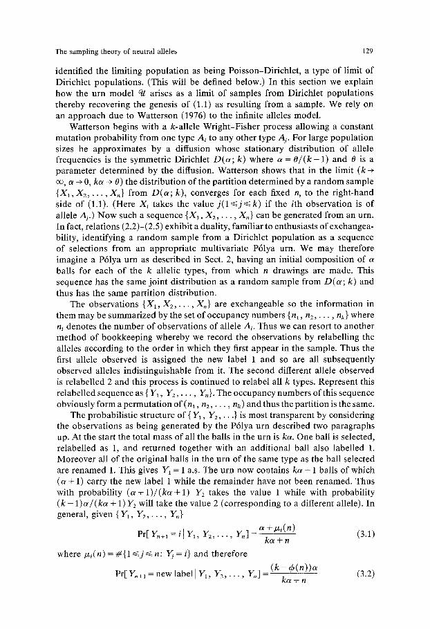
identified the limiting populat ion as being Poisson-Dirichlet, a type of limit of Dirichlet populations. (This will be defined below.) In this section we explain how the urn model ~ arises as a limit of samples from Dirichlet populations thereby recovering the genesis of (1.1) as resulting from a sample. We rely on an approach due to Watterson (1976) to the infinite alleles model.
Watterson begins with a k-allele Wright-Fisher process allowing a constant mutation probabili ty from one type Ai to any other type Aj. For large population sizes he approximates by a diffusion whose stationary distribution of allele frequencies is the symmetric Dirichlet D(a; k) where a = O / ( k - 1) and 0 is a parameter determined by the diffusion. Watterson shows that in the limit (k-~ 00, ~ -+ 0, k~ -+ 0) the distribution of the partition determined by a random sample {X1, X 2 , . . . , X~} from D ( ~ ; k), converges for each fixed n, to the right-hand side of (1A). (Here Xi takes the value j(l<~j<~k) if the ith observation is of allele Aj.) Now such a sequence {X1, X2, �9 �9 �9 Xn} can be generated from an urn. In fact, relations (2.2)-(2.5) exhibit a duality, familiar to enthusiasts of exchangea- bility, identifying a random sample from a Dirichlet population as a sequence of selections from an appropriate multivariate P61ya urn. We may therefore imagine a P61ya urn as described in Sect. 2, having an initial composition of balls for each of the k allelic types, from which n drawings are made. This sequence has the same joint distribution as a random sample from D ( ~ ; k) and thus has the same partition distribution.
The observations {X1, X 2 , . . . , X,} are exchangeable so the information in them may be summarized by the set of occupancy numbers {nl, n2, . . �9 n k } where ni denotes the number of observations of allele A~. Thus we can resort to another method of bookkeeping whereby we record the observations by relabelling the alleles according to the order in which they first appear in the sample. Thus the first allele observed is assigned the new label 1 and so are all subsequently observed alleles indistinguishable from it. The second different allele observed is relabelled 2 and this process is continued to relabel all k types. Represent this relabelled sequence as { I11, Y2, . . - , Yn}. The occupancy numbers of this sequence obviously form a permutat ion of (n 1,/'/2, �9 - �9 , nk) and thus the partition is the same.
The probabilistic structure of { Y1, Y2, �9 �9 .} is most transparent by considering the observations as being generated by the P61ya urn described two paragraphs up. At the start the total mass of all the balls in the urn is km One ball is selected, relabelled as 1, and returned together with an additional ball also labelled 1. Moreover all of the original balls in the urn of the same type as the ball selected are renamed 1. This gives Y1 = 1 a.s. The urn now contains k~ + 1 balls of which (a + 1) carry the new label 1 while the remainder have not been renamed. Thus with probabili ty (t~ + 1) / (ka+ 1) I/2 takes the value 1 while with probability (k - 1)c~/(kc~ + 1) Y2 will take the value 2 (corresponding to a different allele). In general, given { Y1, Y 2 , . . . , Y~}
Pr[ Y,+, = i[ II1, Y 2 , . . . , Yn]
where/x , (n) = #{1 ~<j~< n: Yj = i} and therefore
Pr[ Y,+I = new label I Y1, Y 2 , . . . , Y n ] -
a + Izi(n) (3.1)
k a + n
( k - r
ko~ + n (3.2)

130 F.M. Hoppe
where ~b(n) is the number of distinct values among { Y1, �9 . . , Y,}. Equations (3.1) and (3.2) describe an urn model which, for large k and small t~ with ka-> 0, closely approximates ~// and we refer to it as a/l(a; k).
We interpret these equations as follows. Each time an allele type is first drawn from the urn, the mass of alleles not yet observed decreases by an amount a. Ultimately the source of new alleles is exhausted since k < oo. But when k is large and a small, the effective mass of unobserved alleles remains nearly constant, for moderate sample sizes, at the nominal value ka. Since in the limit (k-~ oo, ot -~ 0 and ko~-> 0), the probabilities in (3.1) and (3.2) converge, respectively, to I~i (n) / (O + n) and 0/ (0 + n) precisely their counterparts defining a//, we would expect that the corresponding partition distributions converge to the partition distribution of the urn a//, which, by Watterson's (1976) result is given by (1.1). This can be made rigorous using weak convergence as for example in the proof of the theorem in Kingman (1977). However, the truth of this assertion is already known by the direct, although non-intuitive combinatorial argument in Hoppe (1984) and our goal here is merely to provide some insight into Theorem A. The urn model ~ thus represents a limiting case of sampling from a Dirichlet population, by maintaining a constant source 0 of novel alleles regardless of the number of distinct alleles already present in the sample.
In a similar fashion we can provide illumination for Theorems 1 and 2. Observe that (2.3) is a strong law of large numbers recovering the Dirichlet distribution from the limiting frequencies. Equally there is a limit for the relative frequencies in the relabelled { Y~, Y2,.-.} and we proceed to show this limiting population to be the size-biased permutation of D ( a ; k). We first define this concept.
Let P = (P~, P2, �9 �9 .) be a random probability distribution on the integers,
Pi~>0 and Y.P~=I a.s. i
P may be supported (as with D(~ ; k)) on a finite subset of the integers and this subset may be random. For concreteness of terminology we will continue to call P~ the frequency of some allele A~ in a hypothetical population. The size-biased permutation ps _= (p~, p~ , . . . ) randomly rearranges the frequencies {Pi} in pro- portion to their values, that is for any i~>1 and distinct subscripts o-(1), ~r(2) . . . . , o-(i),
Pr[P] = P~(j): 1 ~ j ~< i l _P]= P~o)j__II 2 P=(J) 1 k = l Po-(k) �9 (3.3)
This equation has a simple interpretation. We imagine that an individual is randomly selected from the population and we denote the frequency of its (random) allelic type for P~. All such alleles are then removed from the population after which another random selection is made. The frequency (in the entire population) of this second randomly chosen allele is P~ and this process is repeated indefinitely or until all alleles have been exhausted.
If the population is finite, then each random selection is made using a uniform distribution over all remaining individuals. This means that an allele is selected in direct proportion to its numbers in the population. On the other hand, when the type space is countably infinite, as there is no uniform distribution over such

The sampling theory of neutral alleles 131
a set, the selection procedure is interpreted as meaning directly that an allele type is chosen in proportion to its frequency. Hence the name size-biased permu- tation.
There is an equivalent mechanism for generating _ps from a random sample (with replacement) {X1, X2 , . . . } from _P. (Here again Xi is directed to take the value j if the ith observation is allele Aj.) Denote by Qj the relative frequency in the population of the j th distinct allele in the sample. Clearly if or(l) and (r(2) are any distinct positive integers
Pr[Q1 = P~(1)[-P] = P~(1)
and
Pr[Q1 = P~(1), Q2= P~(2)I-P] -- E k P~(1)P~(2) P~(1)P,r(2) = k=l 1 -- P~(1)
These are just (3.3) for i = 1, 2, and it can be shown more generally (by induction) that Q = (Q1, Q2, . . - ) is a version of _ps.
In a correspondingly natural way, mimicking an earlier construction, the sample {X1, X2 , . . . } determines a sequence { Y1, Y2,. . .} which relabels the alleles suc- cessively with the positive integers according to the order they first appear in the sample.
Let o ! ' ) = ( i / n ) # {1 ~< i ~< n: Y~ =j} be the empirical probability function " < j
for the relabelled observations. The strong law for exchangeable variables (2.3) asserts that
1 lim - # {1 ~< i ~< n: Xi = k} exists for each k. n ---) or) n
Hence for almost all realizations {Xl(W), X2(w), . . .} the proportions of all the different types converge. The labelling is irrelevant for the convergence along each sample path. Therefore
lim o! ") exists for each j. - ~ : j t l --) c o
But by definition, Qj is the relative frequency in the population of the j th distinct allele in the sample and thus
!irn Q~')= Qj. (3.4)
When _P is the symmetric Dirichlet D ( a ; k) then this method of generating the size-biased permutation _P" is by its construction equivalent to the urn o//(a; k) and (3.4) thus describes the limiting proportions of the k types in @(a; k). Since ag(a; k) approximates 0-//, we would therefore expect _W to be close to the population defined by (2.1). This is confirmed by the representation (Patil and Taillie (1977))
i - - 1
PSi=U1, P~= Ui I~ ( 1 - Uj), 2<~i<~k-i (3.5) j = l
of the size-biased permutation of the symmetric Dirichlet, where { U~} are indepen- dent random variables having Beta(1 + a, ( k - i ) a ) distributions respectively (_P~

132 F.M. Hoppe
is an example of a completely neutral vector, in the terminology of Connor and Mosimann (1969), or a residual allocation model, in the terminology of Patil and Taillie (1977). The nomenclature in the first instance is striking because the genetics underlying this paper is called the neutral theory). Observe that in the limit k ~ oe, a ~ O, ka ~ O, the Beta(1 + a, ( k - i )a ) random variables become Beta(l, 0) and (3.5) formally merges with (2.1).
The partition distribution of a sample from a population depends only on the unordered population frequencies and thus the partition distribution of a sample from D(a; k) is the same as that obtained from the urn ~//(a; k). This indicates that the partition (1.1) of the limiting urn 0//should be the same as that obtained from the limiting population (2.1) (modulo some continuity arguments). This conclusion is correct and while the heuristic development leading to it is original the result is not new since it is known from the cited work of Watterson (1976) together with Kingman (1977) that the Ewens formula (1.1) describes a random sample taken from a Poisson-Dirichlet population with parameter 0 (denoted by PD(O) and described in the following paragraph). The size-biased permutation of PD(O) is given by (2.1) (see McCloskey (1965), Engen (1975), Patil and Taillie (1977)) while the non-increasing order statistics of (2.1) are PD(O). Both of them describe the same stochastic abundance structure and therefore give rise to the same partition distributions (1.1).
There are a number of characterizations of a Poisson-Dirichlet population (see Kingman (1978, Appendix)). The original definition and existence proof was given by Kingman (1975). He begins with a symmetric Dirichlet D(a; k) in which the population frequencies are re-arranged in decreasing order
P(,)/> P(:)~>' '" I> P(k)
and he shows that for each fixed j, (P(I), P (2) , . . . , P(j)) converge jointly to a vector (P~*,. . . , P~) as k-) co, a - ) 0, ka - ) 0, and this vector is the j th joint mar- ginal of a random probability _P* for which he coined the term Poisson-Dirichlet.
We note, finally, that D ( a ; k) does not converge to a proper random probability as ka -) 0. Each finite joint distribution tends to the zero vector since large k and small a realizes a population in which all alleles are present only in small proportions. Kingman's use of a permutation (descending order statistics) prior to passage to the limit overcomes this degeneracy. Similarly by first taking another (the size-biased) permutation we are again able to derive an appropriate limit. In fact, what the urn ~ is doing is directly generating the size-biased permutation of the Poisson-Dirichlet. We take this up in careful detail in the next section.
4. Relation to the Poisson-Dir ich le t distribution
Watterson (1976) was the first to associate the Ewens sampling formula with a Poisson-Dirichlet population. His approach required the integration of a mixture of multin0mials with a symmetric Dirichlet. Since the representation of the Poisson-Dirichlet as defined by Kingman loses the nice structure of the Dirichlet, which allowed the integration to be carried out, a similar calculation is not analytically feasible if the mixing distribution is Poisson-Dirichlet, and in fact

The sampling theory of neutral alleles 133
Watterson conjectures, "I t is presumably the case, but not easy to prove, that [the Ewens formula] could be arrived at by directly sampling from the population described by D ( a ; k) rather than proceeding indirectly as we have done, letting k[the number of alleles] ~ oe".
A proof of this conjecture was provided by Kingman (1977) using weak convergence theory to graft limits of partitions and limits of populations. We sketch his arguments. Suppose given a sequence of populations {p(k)} (Kingman assumes that the populations are finite and that samples are taken without replacement, but his argument is valid, and simplifies slightly, if sampling is with replacement, in which case the populations could be infinite, as is required here). Such a sequence is said to have the Poisson-Dirichlet limit if the population frequencies arranged in decreasing order converge in the sense of finite dimensional distributions to a Poisson-Dirichlet for some 0. This is shown to imply weak convergence of the corresponding induced distributions regarded as measures on an appropriate compact metric space. The partition distribution of a random sample is expressible as the expectation of a bounded continuous function on this space and hence if {_p(k)} have a PD(O) limit then the partitions converge to the partition from a PD(O) population. (We note in passing that Kingman also proves the converse assertion.) Watterson (1976) contains an explicit calculation that the partitions from D(c~; k) converge to (1.1) as a ~ 0, k-* co with ks ~ 0, and (Kingman (1975)) by the very definition of PD(O), the sequence {D(a ; k)} has the PD(O) limit. This identifies the Ewens formula as describing the partition from a Poisson-Dirichlet population.
This technical and indirect approach contrasts with the concreteness of Watterson's integrations for the symmetric Dirichlet.
A direct proof would be appropriate to exhibit for a result so basic but we have not seen one and we therefore provide such here. Our approach does not require determining the partition distribution, rather we compute the conditional probabilities of observing any particular type in the future given the current sample. This exposes the prominent role played by the Poisson-Dirichlet and its characteristic property which Ewens exploited, and which is a consequence of the representation (2.1).
Theorem 3 (Watterson, Kingman). The partition distribution of a random sample { X ~ , . . . , X~} from a Poisson-Dirichlet population _P is given by Ewens' sampling formula.
Proof In view of Theorem A it suffices to establish that {X1, X2, �9 �9 .} behaves sequentially (with appropriate relabelling) like the urn ~/. We therefore need to evaluate the posterior probabilities, given the sample {X1, X2, �9 . . , Xn}, that the next observation will be novel or one of the types already observed (I thank Bruce Hill for a Bayesian interpretation which led to the step of conditioning on _P below). Consider then Pr[Xn+I=Xj[Xa,X2,. . . ,X~] where l<~j<-n. By exchangeability of the sample it suffices to determine Pr[Xn+~ = XI]X~, . . . , Xn]. We thus evaluate
Pr[X,+~ = X, l X l , . . . , X, ] = E[Pr[X,+~ = X, [ X ~ , . . . , Xn, _P] I X ~ , . . . , X, ]
= E[Px, I X l , , , , , Xn].

134 F . M . H o p p e
The random variable Pxl is the first component in the size-biased permutation of P and is therefore Beta(l, 0). I claim that, more generally, the posterior distribution of Pxl given {X1 ,X2 , . . . ,X , } is Beta(T,O+n-T) where T = #{l~<j~<n: Xj=Xi}. The argument for this, though quite straightforward, requires some extensive preparation. The key is the remarkable property of (2.1) that it defines a population which is invariant (in distribution) under size-biased permutation (Engen (1975)), from which ensues this implication (Hoppe (1986), Theorem l(a)):
If a category if randomly (in proportion to its frequency) deleted from a PD( O) population then the resealed (to sum to unity) residual population is again PD( O ) and is independent of the frequency of the deleted category. (4.1)
The first observation 321 by definition selects a category in proportion to its frequency. Give this category the new label # 1. Its frequency Pxl in the population will be denoted by both P~ and by Z1 e. The remaining categories are then relabelled #2, # , . . . with corresponding frequencies P~, P3~, . . . in such a way that
i--1 # #
P2 =Z2 and P~=Z~ II ( 1 - Z ~ ) fori~>2 (4.2) j - - 2
# co where {Z~ }i=a are independent and identically distributed Beta(l, 0) random variables. That this is possible is a direct consequence of (4.1) and the fact that (2.1) gives a representation of a PD(O) population. The random sample is thus relabelled as {X~, X~ , . # �9 . , Xn }. Evidently Xl ~ ~ # 1. For j/> 2 either X~ = X1, in which case X 7 = # 1, with
Pr[Xj = X1 [_P] = P1 ~
or Xj # X1 in which case X; ~ = # i with (by (4.1) and (4.2))
Pr[X~ = # i[ X~ # Xl, _P] = e~
and thus i--1
Pr[XT=#i[_P]=P~(1-P[)=Z~ II ( 1 - Z f ) for i~>2. j = l
(Notice that the lower index in the product is now 1 in contrast with the 2 of {X2, X3 , . . .} are still conditionally (4.2).) Moreover the random variables # #
independent (given P#) since relabelling does not alter their exchangeability, and represent a random sample from the same PD(O) population. The posterior distribution Pxl given {X1, X 2 , . . . , X,} is in the relabelled # context, the same as the posterior distribution of P~ given a random sample { X ~ , . . . , X , ~} of size n - 1 from P#.
Thus assume that {X1, X 2 , . . . , X , _ I } is a random sample from a PD(O) population _P (the symbol # has been deleted for notational ease). For the evaluation of the posterior distribution Pa given {X1, X2 . . . . , X,-1} we refer to Connor and Mosimann (1969) who have defined a generalized Dirichlet distribu- tion Q = (Q1, Q 2 , . . . , Qm) by Qx= U1, Q~ = U~ I~11 (1 - Uj), for 2 ~ < i<~ m -1 ,
1 __,~, m--1 and t~,, = ,-,j=l QJ where { Ui} are independent Beta(a, b~) random variables. The m - 1 dimensional vector (Q~ , . . . , Qm-1) has a joint density with respect to

The sampling theory of neutral alleles 135
Lebesgue measure given by
m-1 F ( a i + b i ) a-1 . . . . q~m ,-1 ~ F(a~)C(b~) q~' qJ
i = 1 j = i
on the simplex qi/> 0 and ql +" " "+ qm = 1. Just as the posterior o f a Dirichlet remains a Dirichlet with a change in the parameters the same is true o f the general ized Dirichlet. In part icular if a r andom sample is taken f rom Q and if ni denotes the number o f observations o f type i (represented by f requency Q/) then the poster ior density o f (Q1, Q 2 , . . . , Q m - 1 ) is propor t ional to
i ~ l j = i i = 1
which is a generalized Dirichlet with poster ior U~ being Beta(~i~,/~) where ~ = ai + ni, bin-1 = bm-t + nm and then recursively/~-1 =/~ + ni + bi-1 - bi. Note that b0 is arbitrary, entering as a power 1 bo.
Cons ider now our r a n d o m sample {XI, X 2 , . . . , X~ 1} f rom _P (described in the form (2.1)). The joint distribution is for fixed (Xl, x 2 , . . . , X,_l)
P r [ X l = x l , X 2 = x 2 , . . . , X , _ l = x n _ l , _ P ~ A ] = tx (dp) I I P~' i = 1
where A is a Borel set in [0, 1] ~176 is the measure induced through the r andom mapp ing _P on the Borel sets o f [0, 1] ~, and n~ is the number of 1 ~ j<~ n - 1 such that Xj = i. (The p roduc t is only infinite in notation.) The poster ior distribution o f P is
P r [ _ P e a l X l = X l , . . . , X , 1=x,_1] = t x (dp) [I P~' t x (dp) pT'. i = 1 / d [0,1] m i = 1
(4.3)
Those categories not represented among {Xl, x2, �9 . . , x, 1} are integrated out in the numera tor (if A is suitable) and (4.3) for the specified {x~, X e , . . . , X~-l} is then identical to the cor responding expression for the posterior o f a r andom sample f rom the popula t ion
P 1 , P 2 , . . . , P m 1 , 1 - j = l
where m is large enough to include all the observed categories (that is m - 1 1> max{x1, x2, �9 �9 �9 x ,_ l } . The first m - 1 dimensional marginal o f this popula t ion is just the first m - 1 dimensional marginal o f (2.1) and is thus a generalized Dirichlet with parameters given by a~-= 1 for all i and b~ ~ 0 for all i. The posterior distr ibution is therefore a generalized Dirichlet with 5~ = a~ + n~ = 1 + ni and solv- ing r e c u r s i v e l y bi--1 = hi "~- ni -~- b i -1 - bi = bi -k- n i =- brn-1 + nrn ~- rim--1 + " " " + hi . I n
part icular ti 1 = nl + 1 and bl = 0 + nm +" �9 �9 + n2 = 0 + (n - 1 - nl). But recall that T = nl + 1. Thus we identify the posterior o f P1 as being Beta(t~l, 0 + n - 1 - nl) = Beta(T, n + 0 - T ) as claimed above and hence, with a return to the original notat ion in the statement o f the theorem we are proving,
T E [ P x 1 I X 1 , . . . , X ~ ] = E[Beta ( T, 0 + n - T)] - 0 + n" (4.4)
136 F.M. Hoppe
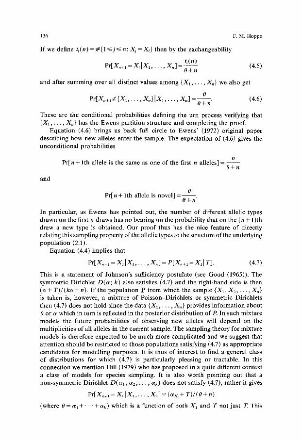
I f we define h(n) = #{1 <~j ~< n: X~ = Xi} then by the exchangeability
Pr[X,+l = X i l X , , . . . , X,] = ti(n__~) (4.5) O+n
and after summing over all distinct values among { X , , . . . , X,} we also get
0 Pr[Xn+~ ~ { S l , . . . , X n } l X l , . . . , X n ] -- 0 -t- n" (4.6)
These are the conditional probabilities defining the urn process verifying that {X1, . . . , X,} has the Ewens partition structure and completing the proof.
Equation (4.6) brings us back full circle to Ewens' (1972) original paper describing how new alleles enter the sample. The expectation of (4.6) gives the unconditional probabilities
and
Pr[n + l th allele is the same as one of the first n alleles] = - - n
O+n
Pr[n + l th allele is novel] = 0
O+n"
In particular, as Ewens has pointed out, the number of different allelic types drawn on the first n draws has no bearing on the probabili ty that on the (n + 1)th draw a new type is obtained. Our proof thus has the nice feature of directly relating this sampling property of the allelic types to the structure of the underlying population (2.1).
Equation (4.4) implies that
Pr[Xn+l = X1 IX1, �9 �9 �9 Xn] = P[X,+I = X1 [ T]. (4.7)
This is a statement of Johnson's sufficiency postulate (see Good (1965)). The symmetric Dirichlet D(a; k) also satisfies (4.7) and the right-hand side is then (a + T)/(ka + n). I f the population P from which the sample {X,, X 2 , . . . , X,} is taken is, however, a mixture of Poisson-Dirichlets or symmetric Dirichlets then (4.7) does not hold since the data { X , , . . . , X,} provides information about 0 or a which in turn is reflected in the posterior distribution of P. In such mixture models the future probabilities of observing new alleles will depend on the multiplicities of all alleles in the current sample. The sampling theory for mixture models is therefore expected to be much more complicated and we suggest that attention should be restricted to those populations satisfying (4.7) as appropriate candidates for modelling purposes. It is thus of interest to find a general class of distributions for which (4.7) is particularly pleasing or tractable. In this connection we mention Hill (1979) who has proposed in a quite different context a class of models for species sampling. It is also worth pointing out that a non-symmetric Dirichlet D(a, , a2 , . . . , ak) does not satisfy (4.7), rather it gives
Pr[X,+, = X l ] X l , . . . r, X n ] = (OIx,"]- T)/( O+ n)
(where 0 = OL 1 "q-" " " -1- O ~ k ) which is a function of both X1 and T not just T. This

The sampling theory of neutral alleles 137
consideration may be useful in the development of a sampling theory incorporat- ing selection.
Both the Poisson-Dirichlet and the symmetric Dirichlet represent infinite populations satisfying Johnson's sufficiency postulate. To derive a class of finite populations satisfying (4.7) we can proceed as follows (although we use the Poisson-Dirichlet the same construction works for the symmetric Dirichlet). Let {X1, X2, �9 �9 XM} represent a random sample from a Poisson-Dirichlet popula- tion P. This sample determines a population P ( M ) of size M (use any convenient labelling, the actual choice being irrelevant for the discussion at hand).
Let {~ , ~ 2 , . . . , ~,}, n ~< M be a random sample without replacement taken from P ( M ) . Since P(M) is itself determined by a random sample from P then by exchangeability {~1, ~ 2 , . . . , ~,} may be considered as a random sample from P (labels not withstanding). Consequently (4.5) and (4.6) are in force which in turn imply Ewens' formula, proving that a random sample of size n chosen without replacement from a population of size M whose partition is described by (1.1) also has the partition (1.1) (Theorem 7.1 of Kelly (1979) and Trajstman (1974)). The Poisson-Dirichlet can thus be interpreted as the infinite population analogue of finite populations which are described by Ewens' formula.
Actually if P is any population with a family of partition distributions induced by sampling and if a finite population P(M) is constructed from P, as in the previous paragraph, then samples from P ( M ) also have the same partition distribution. Kingman (1978) uses this "consistency" condition to define partition structures but he deals with properties of samples while we are concerned with properties of populations. As is evident the two are hardly distinguishable.
5. Ages of alleles
In this section we establish a new methodology, based on the urn ~ for questions involving the ages of alleles in the infinite alleles models. We defer to Sect. 8 a rigorous validation based on mutation in the coalescent.
Recall that we have shown the following. If {X1, X2, �9 �9 .} represents a sequence of observations from a Poisson-Dirichlet population with parameter 0 then the limiting proportions of the alleles indexed by their order of occurrence is given by (2.1). But Griffiths (unpublished) has shown that (2.1) also describes the proportions of the oldest, second o ldes t , . . , alleles in the infinite alleles diffusion limit. Thus the distribution of types according to ages in the population is the same as the distribution of types according to order in the sample. One explanation for this has to do with size-biased sampling and reversibility. Using arguments based on the latter Kelly (1977) for the Moran model, and Watterson and Guess (1977) for the diffusion limit of the Wright-Fisher process show that the probabil- ity an allele is oldest in the population is its frequency. But this is also the probability of observing any particular, and hence the first allele (size-biased sampling). Thus the frequency in the population of the first observed allele is the same as the frequency of the oldest allele. Analogous arguments can be made for the second oldest, third oldest, etc. The use of size-biased sampling (permuta- tion of labels) was also invoked by Hoppe (1986) to give an alternate proof of Kingman's (1978) sampling characterization of the Ewens formula. Another explanation based on genealogy will be given in Sect. 8.

138 F.M. Hoppe
This parallel between ages in the population and order in the sample will now be exploited to derive very readily results previouly determined by more laborious methods, as well as to shed some insight into why these are obtained. We have selected twelve examples for illustration below. Where there is both an (a) and (b) part, the former gives the known result while the latter presents the order approach and proof (where necessary). These show that the urn model provides a unified framework and powerful approach to diverse issues.
Let {X1, X2,...} be a sequence of observations from a Poisson-Dirichlet population _P. In order to obtain joint probabilities involving both the sample and the population, we make the identifications:
{ X 1 , . . . , Xn} represents the observed sample;
{X,+~, X~+2,.. .} represents the population.
(What we mean by the latter is that we can recover the population by the strong law of large numbers applied to {Xn+l, X,+2, . . .} .) In the sequel e represents the type of a randomly selected allele from the sample, S ~ #{1 ~<j~< n: Xj = e} is the number of alleles in the sample which are type e, and Si = #{1 ~<j ~< n: Xj -- Xi} is the number of alleles of the same type as the ith observa- tion in the sample. Observe that exchangeability forces S and Si to be identically distributed.
1. (a) Watterson and Guess (1977). If an allele has frequency Y in the population then it is the oldest with probability Y (conditional on the population).
(b) If an allele has frequency Y in the population then it will be observed first in the sample with probability Y (conditional on the population).
2. (a) Watterson and Guess (1977); Kelly (1977). If an allele is represented by i individuals in a sample of size n then it is the oldest in the population with probability i /( O + n).
(b) Pr[X,+, = e IS = i] = i/(O + n).
Proof By (4.5) Pr[Xn+l = Xj]Sj = i] = i/(O + n). Hence
�9 1 Pr[Sj = i] Pr[X~+l=e lS=i] = ~. 1pr [X~+I=Xj IS~= zJ p - - ~ - ~
j=~n
=i / (O+n) .
3. (a) Watterson and Guess (1977); Kelly (1977). If an allele is represented by i individuals in a sample of size n, then it is the oldest in the sample with probability i/ n.
(b) Pr[X1 = e l S = i] = i/n.
This is immediate from exchangeability.
4. (a) Kelly (1977). In a sample of size n the oldest allele has i representatives with probability
O ( n ~ / ( O + n - 1 ) . n \ i / / \ i

The sampling theory of neutral alleles 139
n i
Proof. From the urn model ~ the first allele observed carries the label 1. Its future occurrence in the sample can thus be described by a two-type Pdlya urn indicating that Pr[S1 = i] is a mixture.
Pr[S1 = i] = xi-l(1 _ x ) , - i 0 ( 1 _x)O a dx (5.1) = 0
of binomials with success probabili ty having Beta(l , 0) distribution (by (2.4) and (2.5)). This integrates to
o(,,-1] V(i)I"(n+O-i) \ i - l l l '(n+O)
which is another way of expressing the desired probability. 5. (a) Saunders, Tavard, and Watterson (1984). I f N~ is the number of types
in the populat ion which are older than the oldest allele in a sample of size n then
PrfNn=k]=0--~nnn 0-77n ' k - -0 ,1 , . . . .
(b) Let ~,~ denote the number of types observed in the sequence {Xn+l, Xn+2,. . .} before a type in {X1, X 2 , . . . , Xn} is observed for the first time again. Then
Pr[un = k] = 0 ~ n , k = 0 , 1 , . . . .
Proof. Let { 7"1, T2, . . .} denote those times i/> n + 1 for which Xi is either novel (not in the preceding set {X1, X 2 , . . . , Xi-1}) or in {X1, X2, . . . , X,,}.
Pr[vn ~> k] = Pr[i_~ 1 {Xr, is novel}]
k
= [I Pr [Xr, is novellX~ is novel(l<~j~< i - 1 ) ] i - -1
k
= H E[Pr[Xr, novellXrj novel(1 <~j~< i - 1), i - -1
rd I novel(1 ~<j ~< i - 1)].
Think of the {X1, X2 , . . . } as generated by the urn ~. The conditioning specifies that the urn contains n "o ld" balls (representing the {X1, X2, �9 �9 �9 Xn}), one black ball (novel) and T ~ - n - 1 "recent" balls (the colours added subsequent to the nth drawing) just before the T~th drawing and the T~th drawing results in either an old ball or a black ball. Since old balls have unit mass while the black ball has mass 0 it is apparent that the conditional probabili ty of drawing a black ball, given that either a black ball or an old ball has been drawn, is 0 /0 + n. Notice that T~ disappears and that this argument generalizes (4.6).
140 F. M. Hoppe
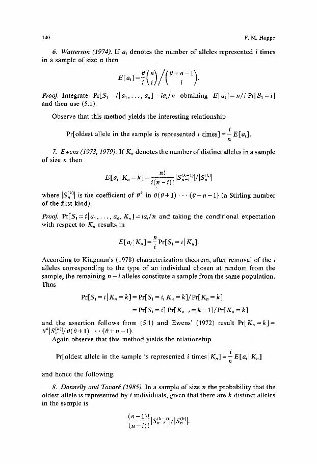
6. Wat terson (1974). I f a~ denotes the n u m b e r o f alleles represented i t imes in a sample of size n then
E [ a i ] = O ( n ] / ( O + n - 1 ) \ill\ i
P r o o f In tegra te Pr[S~ = i[ al , . . . , a ,] = iai/ n obtaining E [ ai] = n / i Pr[S1 = i[ and then use (5.1).
Observe that this me thod yields the interesting rela t ionship
Pr[oldest allele in the sample is represented i t imes] = / E[a~]. n
7. E w e n s (1973, 1979). I f K , denotes the n u m b e r o f distinct alleles in a sample of size n then
n! E [ a~ [ K , = k] - - - I
i ( n - i ) !
where Is~k)l is the coefficient o f O k in 0(0 + 1) �9 �9 �9 (0 + n - 1) (a Stirling n u m b e r of the first kind).
P r o o f Pr[S1 = i I a l , . . . , an, Kn] = i a J n and taking the condi t ional expecta t ion with respect to K , results in
E[a, ]K.] =-n. Pr[S1 = i I K , ] . 1
According to K i n g m a n ' s (1978) character izat ion theorem, after removal of the i alleles cor responding to the type of an individual chosen at r a n d o m f rom the sample , the remaining n - i alleles consti tute a sample f rom the same popula t ion . Thus
Pr[S~ = i[ K . = k[ = Pr[S, = i, K . = k ] / P r [ K . = k[
= Pr[Sa = i[ Pr[Kn_i = k - 1 ] / P r [ K . = k[
and the assert ion follows f rom (5.1) and Ewens ' (1972) result Pr[Kn = k ] = okls(.k>[/ O( O + l ) . . . ( O + n - 1 ) .
Again observe that this me thod yields the re la t ionship
Pr[oldest allele in the sample is represented i times[ K . ] = i E[a~lg.] n
and hence the following.
8. Donne l l y and Tavard (1985). In a sample of size n the probabi l i ty that the oldest allele is represented by i individuals, given that there are k distinct alleles in the sample is
(n - 1)! l s ~ , l / i s ( % ( n - i ) ]

The sampling theory of neutral alleles 141
9. Ewens (1972).
Pr[two alleles d rawn at r a n d o m are of the same type] -= E [ ~ P~] - 1+0"
Proof Evalua te as Pr[X1 = X2] leading immedia te ly to 1/(1 + 0).
10. Watterson and Guess (1977). Let P(a)= max P~. Then for 0.5 ~< x ~< 1 the densi ty of P(a) is 0x- l (1 - x ) ~
Proof We use the no ta t ion in the p r o o f of T h e o r e m 1.
Pr[P(1) > x] = ~ Pr[Pj > x and P(1) = P j ] j= l
oo
= Y~ Pr[T~ > x and P(1) -- ~/j] j = l
oo
= ~ P r [ , / j > x ] j = l
: ~ P r [ ~ ' j > x l , X j : 1] P r [ ,~ j= l ] . j = l
Given Aj = 1 then the limit p ropor t ion yj is Beta( l , 0 + j - 1 ) so the sum becomes
_ (1 d t o + j _ ~ - 0 (1 - t ) ~ dt
j = l j 1
= 0 f ] t - l ( 1 -- t) ~ dt.
11. Ewens (1972). I f K, = # distinct alleles in a sample of size n then
P r [ K , = k] = okls~k)]/[O] ".
Proof The p.g.f, o f 1,2, is (using the independence of the {hi} in Theo rem 1)
E[SKn] : [~ ( . i- l+Os~ i = i \ i + O - - 1 ]
the n u m e r a t o r of which generates the Stirling numbers above. As a corollary, if ti is the t ime of appea rance of the ith novel allele then
Pr[h = n] = P r [K,_ I = i - 1 and An = 1]
o'-lls(~'2~) I 0 [0] "-1 n+O-1
[0]"
The f requency spec t rum ~b(x) for the Poisson-Dir ich le t 12. Ewens (1972). popula t ion _P is
~)(x)=Ox 1(1 -- X ) ~ O < X < I .

142 F.M. Hoppe
Proof L e t f be a bounded measurable function on [0, 1] and let Qa = P~ be the first component in the size-biased permutation of _P. Then clearly
~ f ( P~)P~ = E[f( QO I P]
and since Q~ has a Beta(l , O) density
E[Z f ( P~)P,] = E[f( Q,) ]
Ix = f(x)O(1-x) ~ dx. = 0
Choose for f the function
f(x)={lo/X ifx>tifx<~ t
to derive
I: E[number of types whose frequency exceeds t] = Ox-l(1-x) ~ dx = t
showing that O x - l ( 1 - x ) ~ is the frequency spectrum. By setting g(x)= xf(x) we can write
Ix E[Z g(P~)] = g(x)C(x) dx. = 0
This was obtained (for continuous f ) by Kingman (1980), Eq. (3.4.2) by resorting to the Riesz representation theorem for positive linear functionals. Our argument seems more direct and relates the frequency spectrum to the size-biased permu- tation.
The multivariate frequency spectrum (Watterson (1974, 1976)) can also be derived using (in the bivariate case, for instance)
~f(Pi, 5) PiPj 1 - P, = E [ f ( p , , Q2)]P]
where Q2 = P~ the second component in the size-biased permutation of P.
6. A representation for Ewens' partition
A residual allocation model Q = (Q1, Q2,...) (see Connor and Mosimann (1969), Patil and Taillie (1977)) is described in terms of an independent family { Ui} of random variables called residual fractions. We may think of Q as defining how resources are assigned to a region or types (alleles, colours) are assigned to a population. The first colour is assigned to a proportion U1 ~ Q1 of the population, the second colour to a proportion U2 of the remaining (or residual) fraction 1 - U1 of the population and in general the ith colour is assigned to a proportion Ui of the residual fraction I]~-1~ (1 - Uj) left after the first i - 1 colours have been assigned. In equation form
i 1
Q~ = Ua, Qi = Ui H ( 1 - Uj), i~>2. (6.1) j = l

The sampling theory of neutral alleles 143
When there are but a finite number k of colours to be assigned (6.1) is defined only for i ~ k - 1 and then Qk = I]j~-] (1 - Ufl. This can be succinctly obtained by demanding that Uk be identically 1. From (2.1) we see that the size-biased permutation of the Poisson-Dirichlet PD(O) is a residual allocation model with the residual fractions being identically distributed Beta(l, 0). Also the size-biased permutation (3.5) of the symmetric Dirichlet D ( a ; k) is a residual allocation model with the residual fractions U~ being Beta(1 § a, ( k - i ) a ) .
It was observed at the end of Sect. 4 that the Poisson-Dirichlet is the infinite population analogue of finite populations described" by Ewens' partition. This raises the natural question of whether a corresponding representation holds for Ewens' partition.
Thus let _F be a finite population of size M representing alleles whose unordered frequencies are distributed as in (1.1), but with M replacing n. For instance _F might represent the Moran model in discrete time (Watterson (1974), Trajstman (1974)) at stationarity. Form the size-biased permutation y by selecting one individual at random and removing all V1 alleles of the same type, then selecting another individual at random from the residual M - V1 and removing all V2 alleles of the same type, then continuing in this fashion until the entire population has been depleted (after K selections) and finally defining V ~- ( V I , V 2 , . . . , V K ) .
Theorem 4. _V has the representation
VI = 1 ~- Bin(M - 1, Z1) (6.2)
V~ = 1 + B i n ( M - 1 - V~ . . . . . V~_I, Zi), 2 ~ i ~ K
where {Zi} are i.i.d. Beta(l, 0) random variables and K is the first integer such that Vl..~- V2 ~- . . . + VK = M.
The notation Bin(r, Z) refers to a binomial random variable on r trials and success probability Z, both of which may be random.
Proof. According to Theorem 3, F may be realized as a random sample {X~ , . . . , XM } from a Poisson-Dirichlet population _P. Because of exchangeability, selecting one observation at random from the set { X 1 , . . . , XM) is probabilistically equivalent to selecting the first observation XI. The proof of Theorem 3 shows tha the urn ~ automatically generates the size-biased permutation of the partition determined by {X~ , . . . , X~} and therefore ( V 1 , . . . , VK) is equal in distribution to (S~(M) , . . . , SK ( M ) ) , using the notation of Sect. 2. But SI(M) can be described by a two-type P61ya urn with initial composition (1, 0) and then Eqs. (2.4) and (2.5) show that S i ( M ) is a Beta-binomial random variable of the specified form, verifying (6.2) for Vi. To get V2 we then remove all {Xj: Xj = X1} before selecting another allele for the second component in the size-biased permutation. But those Xj # X1 remaining after the first deletion represent a random sample from a population _Q which is obtained by removal of one category at random from _P. Now P is invariant under this operation (size-biased permutation), meaning that Q is also Poisson-Dirichlet, and moreover Q is independent of the frequency of the deleted category (see Hoppe (1986)). Thus S2(M) is also a Beta-binomial with the mixing variable Z2 independent of Z1. This argument works for S i ( M ) in general establishing (6.2).

144 F.M. Hoppe
Corollary. The population _V described by (6.2) is invariant under size-biased permutation.
It is implicit in the description of a residual allocation model that the popula- tion be a continuum. To come up with an analogous concept for discrete popula- tions it is necessary to rethink the independence structure of the residual fractions. Using (6.2) as our guide we therefore focus not on the proportions assigned to the ith type but rather the actual amount assigned, which, for the model (6.1) is Ui[Ij-ll ( 1 - U j). This quantity depends on {U1, U 2 , . . . , U/_I} only through
i - - 1 . .
II~=1 (1 - Uj), which is the remaining portion of the population. This observation suggests an appropriate reformulation of the residual allocation model for a discrete population.
Suppose a discrete population of size M < co is to be painted with colours 1, 2 , . . . , C where C may be finite or infinite. We present a method for assigning the colours sequentially in such a way that once the first i - 1 colours have been assigned then the ith is assigned by a randomized procedure which depends on the previous assignments only through their cumulative total. Specifically let {Ri(n): 0<~ n ~< M} for each 1 ~ i<~ C be a family of integer-valued random variables where 0 ~ < Ri(n)<~ n. The families are independent but we make no assumptions about dependence within a family. If colours 1, 2 , . . . , i - 1 have been assigned to nl, n 2 , . . . , n~_l individuals respectively then
ni= Ri M - ~, nj j = l
of the remaining individuals are assigned colour i. This process is continued until the population is exhausted with colour K (random) and the vector (nl, n 2 , . . . , nK) is said to be a discrete residual allocation model.
Comparing with (6.2) we see that the Ewens partition has a representation as a discrete residual allocation model with residual functions
R~(n) = 1 + Bin(n - 1, Zi)
where {Z~} are independent Beta(l, 0), thereby providing affirmation of the question raised in the second paragraph above.
The construction typified by Theorem 4 works for samples from any (con- tinuous) residual allocation model _Q as described by (6.1). Suppose a random sample (with replacement) of size M is drawn from Q. Let ni be the number of observations in category (colour) i while K is the first index such that n l+ n2+" �9 "+nK =M.
Theorem 5. (nl, n2 , . . . , nr) is a discrete residual allocation model with residual functions Ri(n) = Bin(n, U~).
Proof The assertion of this theorem is that
" /M i-1 Ui). (6.3) ni = Bln~ - j~lnj ,
Now by definition, for arbitrary non-negative integers Xl, x2 , . . . , xr summing to M
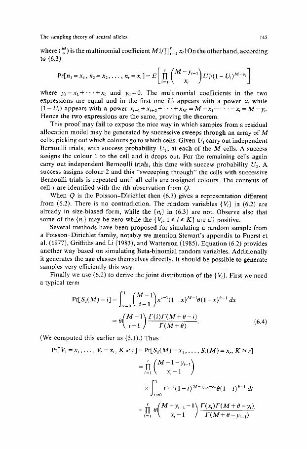
The sampling theory of neutral alleles 145
r where (~ ) is the multinomial coefficient M !/l~ ;= 1 xi ! On the other hand, according to (6.3)
P r [ n l = x l ' n 2 = x 2 ' " " n r = x r ] = E [ ~ = ~ ( xi /
where y~ = x l + . . . + x ~ and yo=0. The multinomial coefficients in the two expressions are equal and in the first one U~ appears with a power xi while ( 1 - U;) appears with a power x~+~ +xi+2+" �9 �9 +xM = M - x a . . . . . . xi = M - y i . Hence the two expressions are the same, proving the theorem.
This p roof may fail to expose the nice way in which samples from a residual allocation model may be generated by successive sweeps through an array of M cells, picking out which colours go to which cells. Given U1 carry out independent Bernoulli trials, with success probabili ty Ua, at each of the M cells. A success assigns the colour 1 to the cell and it drops out. For the remaining cells again carry out independent Bernoulli trials, this time with success probabili ty U2. A success assigns colour 2 and this "sweeeping through" the cells with successive Bernoulli trials is repeated until all cells are assigned colours. The contents of cell i are identified with the ith observation from Q.
When Q is the Poisson-Dirichlet then (6.3) gives a representation different from (6.2). There is no contradiction. The random variables {V~} in (6.2) are already in size-biased form, while the {n~} in (6.3) are not. Observe also that some of the {n~} may be zero while the { V/: 1 ~< i ~ < K} are all positive.
Several methods have been proposed for simulating a random sample from a Poisson-Dirichlet family, notably we mention Stewart's appendix to Fuerst et al. (1977), Griffiths and Li (1983), and Watterson (1985). Equation (6.2) provides another way based on simulating Beta-binomial random variables. Additionally it generates the age classes themselves directly. It should be possible to generate samples very efficiently this way.
Finally we use (6.2) to derive the joint distribution of the { V~}. First we need a typical term
Ix Pr[St (M) = i] = 1 xi_l( 1 _x)M_,0(1 __x)O_l dx = 0
=o(M-1] r(i)r(M+O-i) \ i - 1 / F(M+O) (6.4)
(We computed this earlier as (5.1).) Thus
Pr[V1 = X l , . . . , Vr =xr , K f> r] = Pr[S~(M) = X l , . . . , St(M) =xr, K >! r]
= (i ( M - I - Y i - I ] i=1 \ x i -1 /
• tx'-~(1 - t)M-Y'-l-x'O(1 -- t) ~ dt t=O
=rI O ( M x Y ~ - I - 1 ) f'(x~)F(M+O-y~)" i=l F ( M + 0 -Yi-l)

146 F. M. Hoppe
b y ( 6 . 4 ) w h e r e y~ = x l + " �9 �9 + x~ a n d Yo = 0. This expression simplifies to
O~M!F(M+O-y~) ~[ 1 ( M - y ~ ) ! F ( M +O) ~=~ M-y,_1"
The evaluation of
(6.5)
P r [ V l = X l , . . . , Vr=xr, K = r ]
proceeds identically but with the side constraint Yr = M giving
OrM!F(O) (I 1 (6.6) F ( M + O) i=1 ti
where t~ = M-Yi -1 = x~ + x~+l + ' ' " + xM. Equations (6.5) and (6.6) have recently been derived by Donnelly and Tavar6 (1985), by entirely different methods based on a coalescent, as the joint distribution of the age partition in a sample from the infinite alleles model, thus providing another manifestation of the iden- tification of order with age. (We proved a special case r = 1 in Sect. 5.)
We close by observing that if the equations in (6.2) are divided by M and then M ~ 0o it follows immediately by the strong law of large numbers for binomial random variables that
--M' M' " "" '
converges almost surely for each fixed r as M ~ o o to (Z1 ,Z2(1 - Z1), �9 �9 �9 Zr [[~-11 (1 -Z~)). This is not really a proof of Theorems 1 and 2 because (6.2) depended on these theorems, but the derivation is very suggestive that (6.2) can be used to model a multitude of finite populations whose sampling properties in the limit of large population size are described by the Ewens sampling formula (Kingman (1977)).
7 . T h e r e v e r s e d c h a i n a s a p a r t i t i o n s t r u c t u r e
According to Kingman (1978) a partition structure is a family {P,} of distributions on partitions satisfying the following consistency relation: If a sample of size n has allelic partition distribution P, then the distribution of a random subsample of size m taken from this sample is P,,.
The relationship between P,, and P, is expressed by
P,,,=o'.,,,P,, (7.1)
where {O'mn} is a family of linear transformations satisfying
O't,=~l,,O-mn ( l < m < n ) (7.2)
which in the special case n = m + 1 reduces to
a l + l Pm(al , . . . , am)= Pm+l(al+ 1, a2 , . . . , am, O)
m + l
,,+1 i (a i+ 1) + E - - P m + l ( a l , . . . , a~-l-1, a ~ + l , . . . ) . (7.3)
~=2 m + l

T h e s a m p l i n g t h e o r y o f n e u t r a l a l l e l e s 147
The Ewens distribution is a part i t ion structure arising natural ly th rough a process {H,} thus directing us to examine (7.1) and (7.2) in the context o f Markov chains.
The process {/-/n} o f Theorem A begins at Ho = 0, the empty partition. This is a consequence o f the initial composi t ion o f the urn ~ . We can, however, impose an initial composi t ion prescribed by a measure Ho to define a more general Markov chain with one-step transit ion probabilit ies
P(a, b) = Pr[H,+ 1 = b I/7, = a]
f rom part i t ion a ------ (a l , �9 �9 a~) o f the integer r to part i t ion b (necessarily o f the integer r + 1), and arbitrary initial distribution Ho, where
0 if b = ( a l + 1, a 2 , . . . , ar, O)
O+r iai
P(a,b)= O+r i fb=(a~, . . . ,a i - l ,a~+l+l , . . . ,ar , O) (7.4)
rar i f b = ( a l , . . . , a t - l , 1).
,O+r
We next consider the t ime-reversed probabilit ies
P r [H. = a ] H n + 1 = b] = Pr[H~+I = b [H. = a ] Pr[Hn = a]/Pr[H.+~ = b]. These will depend on the initial state Ho but when Ho = 0 it may be verified using (1.1) that
[ a l + l i fb=(a l+l , a2, / . + 1 .. , a , , 0 )
~(r+ l)(ar+l + l) pr[II"=al/7"+~=b]={7 n - ~ i f b=(a l , . . . , a r - l , ar+a+l,...,a,,O)
i f b = ( a l , . . . , a , - 1, 1). (7.5)
Denote the matrix o f reversed transit ion probabilit ies by Z,n+a. In t roduce the notat ion T,(a) = Pr [ / / , = a 117o = ~] and compute T,(a) = Zb Pr[ / / , = a I //,+1 = b] T,+l(b) which simplifies to
a a + l T~(al,.. . ,a~)= T~+l(al+l, a2,...,a~,O)
n + l n - - -~ ' ' ' ,
+ ~ r ( a ~ + l ) Tn+l(aa , . . a~_l-l, ar+l, an, O) r=2 n + l
+ Tn+l(al, . . . , an - 1, 1).
This is (7.3). We may in the same fashion for I < m < n compute Pr[// t = a [/Tn = b] by a decomposi t ion based on // , , . I f Z, , , is the matrix with components Zm,,(a, b) = Pr[/Tm = a]H,, = b] then we find
T m =Z,,,T, and
Zln = ZlmZmn.
This shows that (7.1) and (7.2) are the C h a p m a n - K o l m o g o r o v equations for the t ime-reversed Markov chain o f partitions. This reversed chain begins in some

148 F.M. Hoppe
partition a and passes through partitions of decreasing integers. Further elucida- tion and interpretation of the reverse process will be made in the next section using the coalescent with mutation where it will be shown that the reverse process follows the lines of descent back in time through successive generations thereby describing the genealogy.
8. The urn and genealogy of the coalescent with mutation
Kingman (1982a, b, c) has introduced a continuous time Markov chain ~t , the n-coalescent, taking values in ~n, the set of all equivalence relations on {1, 2 , . . . , n}, to describe the common ancestry among n individuals randomly selected from a haploid population. Two individuals are in the same equivalence class at time t if and only if they share a common ancestor t time units in the past. The coalescent traces back the genealogy of a sample of individuals and provides a richer sample space structure than the classical methods (such as diffusion approximation) which keep track only of the numbers of each type in successive generations.
A sample path may be visualized as an inverted tree rooted in n vertices, each corresponding to one individual and numbered with the integers {1, 2 , . . . , n}, from which emanate vertical branches (lines of descent) passing backward through genealogical time (but forward in the coalescent). At random times, two branches meet at a vertex (representing a common ancestor) and then continue as one branch up the line of descent. The rules governing the times and choices of branch meetings guarantee that ~t is Markov. Specifically, in the infinitesimal time interval (t, t+ h) the probability is h + o(h) that any two branches will meet. If there are i branches then the overall probability of a change in state is �89 + o(h) and the selection of branches to coalesce is made completely at random. The process ~t is then obtained from a horizontal cross-section through the tree at time t by identifying those individuals descending from each intersected branch as belonging to the same equivalence class. There is associated with ~t a pure death process Dt where D~ = I~l , I" I denoting the number of equivalence classes. Dt is the number of intersected lines of descent at time t and therefore also equals the number of distinct ancestors, at time t in the past, of the sample (taken at time 0).
~t passes through a sequence
R., R n _ l , . . . , R1 (8.1)
of equivalence relations on {1, 2 , . . . , n} spending an exponential amount of time with mean 2 / k ( k - 1 ) in state Rk. Here R,={( i , i ) : l<- i<~n} and R1 = {(i,j): 1 ~< i,j<~ n}. The sequence (8.1) has the property that Ri-~ is obtained by combining two equivalence classes in Ri and thus the number of equivalence classes is IRil = i.
Kingman (1982c) derives Ewens formula as a consequence of mutation in the coalescent. In particular suppose that each equivalence class in ~t is subject to a mutation in the interval ( t, t + h) with probability (0/2) h + o (h). Then define a random equivalence relation ~ on {1, 2 , . . . , n} by grouping individuals as follows. Two individuals are in the same random equivalence class if no mutation occurs up either's line of descent to their first common ancestor. Kingman (1982c,
The sampling theory of neutral alleles 149
Theorem 4) shows that if ~ c g , has k equivalence classes with sizes hi, h2, �9 �9 �9 hk then
k 0 k ]7I ( A j - 1 ) !
Pr[~ = ~:] - J=' (8.2) E0] o
If (8.2) is multiplied by the combinatorial term counting the number of equivalence relations with a given partition then (1.1) arises.
Now (8.2) also occurs in Hoppe (1984, Eq. (2)) with reference to the urn process {X1, X ~ , . . . , X,} described in Sect. 1 above. Specifically
k o k 11 ( S j ( n ) - l ) !
Pr[X1 = x l , . . . , X , = x,] - j=l (8.3) [0 ]"
In fact there is a one-to-one correspondence which we now describe, between sequences {xl, x2, �9 �9 �9 x,} of urn paths and equivalence relations r ~ g,. In one direction, given {xl, x 2 , . . . , x,} define an equivalence relation r by placing i and j in the same class iff xi = xj. Conversely given r set xi -= xi(r = 1 if and only if (1, i) c ~:. Let j(2) = rain{i: & ~ 1} and put x~ = 2 if and only if (j(2), i) ~ ~c. Then let j(3) = min{i: xi # 1 or 2} and continue in the obvious way to construct a path { x l , . . . , x,}. The urn process {X~, . . . , X,} is associated in this fashion with a random equivalence relation and by (8.2) and (8.3) this random equivalence relation has the same distribution as the Y~ of Kingman.
There is a deep connection between the urn process 0//and the genealogy of the sample, to which we now turn, to explain why (8.2) and (8.3) are identical. Recall that ~t tracks the genealogy of afixed sample of size n, and (8.2) describes the distribution at time 0 of the random equivalence relation ~ obtained from ~,. This is a probability on the set g, of all equivalence relations defined on {1, 2 , . . . , n}. ~ however defines a process of partitions on sets whose sizes are changing. In particular H, defines a partition of the integer n, / / . - 1 a partition of the integer n - 1, . . . , HI a partition of one. The equivalence relation ~ induces a partition a = ( a l , a 2 , . . . , a,) of the integer n where a~ is the number of equivalence classes in ~ having size i. In view of Kingman's result that this partition has the Ewens sampling distribution, n a m e l y / / , , this suggests that we construct a process of random equivalence relations on sets of decreasing sizes whose induced partition process has the same distribution as the reverse chain {H,,, H,_I , . . . , / /1} . For this construction we need candidates for the sets upon which these random equivalence relations will be defined. While ~ is defined on the original sample of size n it will ensue that the appropriate sets to use comprise decreasing lines of descents which have not undergone mutation from a given time in the past to the present.
I f a time t is fixed then each member of the sample traces back to one of the D, ancestors alive at time t in the past. Some are mutations from these D, ancestors while others are not. Denote by L, the number of ancestors at time t who have non-mutated descendents in the sample. These we call non-mutant ancestors and a line of descent from such an ancestor to the present is called an original line of descent. (We tacitly assume that mutations are therefore not included in the

150 F.M. Hoppe
line of descent o f their parents but are cons idered to begin new lines of descent (Griffiths (1980)).)
Observe that L, is a pure death process, changes of state resulting f rom either coalescence or mutat ion. Coalescence occurs at unit rate to each pa i r o f original lines of descent giving an overall rate i ( i - 1)/2 when Lt = i. Muta t ions occur at rate 0 /2 along each line and thus the overall muta t ion rate is i0 /2 . Combin ing we find that L, changes f rom i to i - 1 in t ime (t, t + h) with probabi l i ty ( i(0 + i - 1) /2)h + o ( h ) . Denote by T, < T, 1 < " �9 �9 < ?'1 the t imes at which Lt changes state and for definiteness set Lt = i - 1 at T~ making L~ r ight-cont inuous.
Each m e m b e r of the sample either traces back without muta t ion to one of the L t non-mutan t ancestors , or else is a muta t ion f rom one of the D~ ancestors. Those descending without muta t ion are the same type as their ances tor and it is natural then to trace back far ther in t ime the history of these L, non-mutan t ancestors to define an equivalence relat ion (akin to ~ ) on the L, original lines of descent which will g roup into equivalence classes non-mutan t ancestors of the same type. I f this is done for each t then the resulting process should trace the changing genealogy of the sample into the past.
These considerat ions mot ivate the definit ion of a process b ~ of equivalence relations on the Lt original lines of descent which places any two lines into the same equivalence class of O~ if and only if u p o n fol lowing the ancestors they represent far ther up their lines of descent (that is far ther into the past) there is no muta t ion to either before their first c o m m o n ances tor (that is in (t, T) where T is the m o m e n t they first coalesce). This specification mimics that o f ~ but respective the L, non-muta t ed ancestors at each t ime t ra ther than the individuals in the sample (who are the non-muta ted ancestors at t ime t = 0).
As does Yt~ so does 5 p, pass through a sequence
S , , S,_1 . . . . , S l
of equivalence relations. In contrast , though, Si is an equivalence relat ion on a set of cardinal i ty i, not on the same fixed set {1, 2 , . . . , n}, and of course, it is general ly not the case that ISi[ = i.
When Lt decreases by one .9~ changes state. I f by muta t ion then 6e t loses one equivalence class of cardinal i ty one and I b~ decreases by one. Else, a coalescence results in an equivalence class, o f cardinal i ty greater than one, losing a m e m b e r but 15etl then of course stays the same. Whether by muta t ion or coalescence the transi t ions f rom Si to Si_l are caused by the loss of an original line of descent.
The process {S~}~=, provides a sequence of r a n d o m equivalence relat ions on sets o f decreasing size n, n - 1 , . . , 1 paral lel ing the reverse par t i t ion chain deter- mined by ~/. The margina l distr ibution of each S~ is easy to find. Just as K i n g m a n de termined the distr ibution (8.2) o f ~2 (which is just our S, ) we can use a backward K o l m o g o r o v a rgument to prove that
k
O k 1-[ ( A j - 1 ) !
Pr[S, = ~:] - J=l (8.4) [o]'
where {)t~, A2,. �9 �9 ~tk} are the sizes of the equivalence classes of ~. After all, in view of the Poisson nature of coalescence and muta t ion the i original lines of

The sampling theory of neutral alleles 151
descent may be looked upon as representing a sample of size i defining an /-coalescent from which (8.4) is a recontexted version of (8.2).
While the changes of state in 5~, consequent from the joining of two equivalence classes the behaviour of 0 ~ is determined somewhat differently. Kingman (1982c, Theorem 1) shows that the death process D, and the jump chain {Rk; k = n, n - 1 , . . . , 1} are independent and by definition 5~t = RD,. In the case at hand we have a death process Lt and a jump chain {Sk; k = n, n - 1 , . . . , 1} with 5 ~, = SL,. However Lt and {Sk} are not independent since Sk "looks into the future" by tracing lines of descent until their coalescence and searching for mutations. For example if L, = i
Pr[L,+At = i - l [ L t = i] = �89 + 0 - 1)At + o(At)
but if we were to, additionally, condition 0~ and for simplicity let 5r t be the equivalence relation {(I, m); 1 <~ 1, m <~ i}---~ corresponding to the event that all of the i original lines of descent at time t trace back without mutation to a single ancestor, then given L, = i and 0~ = ~ the next original line of descent must be lost by coalescence since the event {5~ = ~:} forbids mutations. In view of the "compet ing Poissons" (coalescence versus mutation)
Pr[L,+a, = i - 1] Lt = i, ~t = ~:3 =�89 1)At+ o(k t )
displaying the lack of independence between L, and {Sk}. We have deliberately ignored numbering the lines of descent in the process
L,. Members of the original sample of size n can be numbered in some fashion (usually random) using the integers {1, 2 , . . . , n}, but when two lines of descent join there is no natural or best number for the line emerging from their common ancestor. More importantly the probabilistic structure is not dependent on the choice (which may also obscure the simplicity of the process). In particular while the marginal distributions of {S~} do not depend on the choice (the distribution of Si depends only on the sizes of its equivalence classes) the joint and hence conditional distributions do.
To demonstrate this dependence of the joint distributions, consider the case where n = 3 and members of the initial sample of size 3 are numbered in some fashion with the integers 1, 2, 3. Suppose the backward genealogy has a coales- cence at T3 between 1 and 2, then a mutation at T2 to the line 3 (numbered in the initial sample) and finally a mutation at 7"1 to the line resulting from the joining of 1 and 2. Suppose the numbering rule is as follows. A mutation event occurring to an original line of descent eliminates its number. I f a coalescence event occurs between two original lines of descent then the choice for the line emanating from their joining will be the smaller of the two numbers. In this example the equivalence classes in $3 are {1, 2} and {3}, the equivalence classes in $2 are {1} and {3} and the equivalence class in $1 is {1}.
Let ~7 be the equivalence relation with classes {1} and {3}. Suppose given $2 = ~7. Observe that there are only two choices for $3:
s with equivalence classes {1}, {2}, and {3} corresponding to a mutation at T3;
(2 with equivalence classes {1, 2} and {3} corresponding to a coalescence at T3.

152 F.M. Hoppe
The relation ~ with equivalence classes (1} and {2, 3} is not permitted since the joint event {$2 = ~ and $3 = ~} would require a coalescence between lines 2 and 3 in ~ in which case the line emerging from their coalescence would be numbered with 2 (being the lesser of 2 and 3) forcing $2 to have classes {1} and (2}, a contradiction. Hence
Pr[S3 = ~[$2 = ~7] = 0.
It is evident that a different numbering can be used to violate this equation for the same choices of ~ and 7.
Accordingly it is preferable to let Sa, (resp. Si, 1 ~ i ~< n) prescribe a partition process M, (resp. Ai) which is the partition of the integer Lt (resp. i) determined by the sizes of the equivalence classes in 5r (resp. Si). Thus M, is a continuous time process passing through the states
A n , A n - l , �9 �9 �9 , A I .
Theorem 6. {Mr} is a Markov process whose embedded reverse jump process {A1, A 2 , . . . , An} is equivalent to the partition chain {II~, II2, . . . , Fin} of Sect 1.
Proof The process {Mr} looks into the future of the coalescent and to verify the Markov property it is convenient to reverse time turning the future into the past. "Thus fix a reference time s > 0 and define the reverse process
M~=M~_t, O<~t<~s.
The past o--algebra o-{M~: 0<~ u ~ < to} at time to is o-{M~ :s-to<<-v<~s}, which depends only on the number of original lines of descent at time s - to and the mutation-coalescence beyond s - to. Now let ta > to and consider the conditional distribution of zd~ given o-{M~: 0<~ u ~< to}. This is the same as the conditional distribution of S~s_ti given or{My: s - to ~< v <~ s}. Ms-,l is determined by the muta- tion-coalescence in ( s - t l , s - t o ) together with the mutation-coalescence sub- sequent to s - to the latter of which is completely captured by Ms_~. Hence the conditional distribution of Ms_,~ given o-{Mv: S - t o ~ v<~s} is the same as the conditional distribution of ~r given Ms-to which shows that {MT} is Markov on O<~t<~s. Since the Markov property is preserved under time reversal (a symmetric version of the Markov property asserts that the future and the past are conditionally independent given the present) it follows that {Mt} is Markov on 0 <~ t ~< s, and s being arbitrary the first part of the theorem follows.
Because {Mr} is Markov so is the embedded jump process {A,, A , -1 , . �9 A1} and then also its time reversal {A~, A 2 , . . . , A,} whose one-step transition prob- abilities we now calculate. First we consider Pr[A, = b IA,_~ = a] for partitions a and b of n - 1 and n respectively. There are two cases.
(1) a~_ l=b~_l+ l , a ~ = b r - 1 , the remaining aj=bj ( j ~ < n - 1 ) : This occurs when one of the equivalence classes in Sn necessarily having cardinality r t> 2 is reduced by one because of a coalescence at T, involving two of the n original lines of descent. The joint probability
Pr[A, = b, A,_I = a]

The sampling theory of neutral alleles 153
may be expressed as
P r [A ._ I = a, a coa lescence occur red at T., and resul t ing or iginal l ine of descent lies in one o f the ar ~ equ iva lence classes o f size r - 1 in a]
which m a y be fur ther d e c o m p o s e d as
ar - 1
E A B C i--1
where
A = P r [ A n l = a ] B = Pr [coa lescence at Tn IAn_l = a] C = Pr[ resul t ing or ig ina l l ine o f descent lies in the class Ci o f size r - 1 in
a]A._l = a and a coa lescence at Tn].
Here {C; ~ C i (a ) ; 1 <~ i ~< ar 1} enumera tes all the equ iva lence classes o f size r - 1 in a.
The r a n d o m par t i t ion A ._ I involves only mu ta t i on and coa lescence subsequen t to T. and by the Poisson na ture o f these events An-1 is i n d e p e n d e n t o f the type o f event which occur red at Tn. Consequen t l y
B = Pr [coa lescence at T.]
n ( n - 1 ) / n ( O + n - 1 ) n - 1
2 2 O + n - 1
in view of the compe t ing Poissons. F ina l ly , the event C specifies r - 1 o f the n - 1 l ines o f descent involving a.
In view of the exchangeab i l i ty presen t forc ing l ines o f descent to be lost comple t e ly at r a n d o m each o f the n - 1 or ig inal l ines o f descent has the same chance o f represen t ing the pa i r which coa lesced at Tn. Thus
r - 1 C -
n - l "
This gives
ar--1 n - 1 r - 1 P r [ A . = b, A . -1 = a] = ~ P r [A ._ I = a] - - - -
i=1 O + n - 1 n - 1
( r -1 )ar_ i - P r [A ._ I = a] .
O + n - 1
The second case is (2) a l = bl - 1, the r ema in ing aj = bj ( j ~< n - 1): This co r r e sponds to a muta-
t ion at 7". causing one o f the equ iva lence classes in S . , having ca rd ina l i ty one, to be e l imina ted . The eva lua t ion o f P r [ A . = b, An 1 = a] p roceeds as in case (1), t hough s l ight ly s implif ied.
P r [ A . = b, A n_ 1 = a] = Pr[An 1 = a and a mu ta t i on occur red at Tn]
= P r [A ._ I = a] P r [muta t ion at T. ] a . - 1 = a ]
0 = Pr[A._x = a] O + n - l "

154 F.M. Hoppe
If we divide by Pr[A, 1 = a] we arrive at
( r - 1)at 1 in (1),
P r [ a , = b i a , _ l = a ] = O + n - 1
0 in (2). O + n - 1
The computat ion of the general one-step transition probabilities Pr [Ai= b ]Ai-~ = a], 1 ~< i ~< n - 1 proceeds identically because in the evaluation of the joint probability Pr[Ai = b, A;_1 = a] in view of the Poisson nature of coalescence and mutation, the i original lines of descent may be looked upon as representing a sample of size i defining an/-coalescent upon which mutation is superimposed so that the previous arguments carry through with i replacing n, giving
[ ( r -1 ) a~_ l in (1)
Pr [A;= blA,_l=a]= t O o i - 1 (8.5)
in (2).
These equations are identical with (7.4) the transition probabilities for the urn 0//. Since A1 and H~ both begin with the partition of one our proof is complete.
Corollary. The jump chain {An, A n - i , . . . , A1} of the backward genealogieal process M, is equivalent to the reverse partition chain {H,, H,-1, �9 �9 HI} of the urn ~
Among the { Tn, T, 1 , . . . , T1} will be k (random) times T, k < T,k_ , < . �9 �9 < T,, -= T~ at which an original line of descent is created by a mutation. Denote these corresponding ancestors by J~k, ~k-~, �9 �9 J l . By construction each individual in the sample must be descended without mutation from some J~ (because lines of descent are eliminated in chronological order beginning with the present). At time 7"1 a single (the first) line of descent is created corresponding to J l . (We are running backwards through the coalescent, that is forward in genealogical time.) Label it one. At T2 a second line is created. I f it arose from the splitting of the first line then it (remains part of the first line and) keeps the label one. I f it arose by mutation (of some other line, unspecified) then it must correspond to ~2 and is so labelled two. In general, if the line of descent created at time T~ resulted from the splitting of an existing line, then it keeps the label of that line, else it is a mutation corresponding to some J j and it is assigned the (previously unused) label j. All individuals which descend without mutation from J j inherit label j. This results in a classification of the alleles by ages, in which the oldest is assigned 1, the second oldest 2 , . . . and so on. Since individuals are assigned the same age if and only if they trace back without mutation to a common ancestor the partition by ages gives, by definition, the same partition as the random equivalence relation ~ of Kingman.
Introduce marker variables { Y1, Y2 , - . . , Y,} where Y~ is the label assigned at time T,.
Theorem 7. The process { Y1, II2, . . . , Yn} is equal in distribution to the urn process {x,, x~ , . . . , x~}.

The sampling theory of neutral alleles 155
Proof This is essentially a restatement of Theorem 6. The process { Y1, Y2 , . . . , Yn} bears the same relationship to {A1, A 2 , . . . , A,} as {X1, X 2 , . . . , Xn} bears to {H1, FI2,.. . , 1I,} in view of (8.5).
We are now in a position to explain the one-to-one correspondence between urn paths and equivalence relations described after (8.3). Each original line of descent acquires an age category based on Y~. By construction there is no mutation along any line from the time it is created until the present. At time t = 0 there are n original lines of descent corresponding to the n members of the initial sample. Each will have an age label I1/ (a label as an allele) and a time number (the subscript i on Y~) indicating its chronological order of occurrence. Earlier we pointed out that numbering the lines of descent in the process L, disturbs the simplicity of the structure. But suppose we number the members of the sample by their chronological number as just described. This will give a specific joint distribution to (Sn, S n - 1 , . . . , $1). In fact, if Sn = ~: where ~: is an equivalence relation on ~n then automatically Sn-1 is deterministically forced to be r /where ~7 is the equivalence relation induced on ~n-1 from ( by the deletion of n from {1, 2 , . . . , n} because the last line created (numbered n) is lost first going back in real time. The same deterministic structure holds going through Sn 1, S, 2 , - . - , $1. But in the other direction, in view of (8.4)
O k k ]~ ( h , - 1)!
[0]i i=l Pr[S~ = ~:l S,_1 = ~/] - �9 PES,_~ = rllS, = ~]
0 m m
E o--~'j~, (m-l)!
where {ai: 1 ~< i <~ k} are the sizes of the equivalence classes of s ~ and {/xj: 1 <~j <~ m} are the sizes of the equivalence classes in r/. For any consistent pair (~7, s ~) with the above numbering Pr[Si_I = ~7 [S~ = ~:] = 1. Consequently
o r - 1 if coalescence at 7]/ Pr[Sg = selS,_l = ,7] = + i - 1 (8.6)
_ 0 if mutation at T~ + i - 1
where r - 1 is the size of the equivalence class of ~7 involved in the coalescence. Equation (8.6) is a restatment of (4.5) and (4.6). The former describes the
probabilistic mechanism by which new lines of descent are created (either by the splitting of an existing line or by mutation), while the latter, describing the urn, gives the probabilities that each allele entering the sample is previously observed or novel. Watterson (1984, Sect. 3.6) and Donnelly and Tavar6 (1986, Sect. 5) also give case (2) of (8.6) although only for the unconditioned probabilities Pr[mutation at T~].
The thrust of Theorems 6 and 7 is that the urn process in the forward direction looks like the jump chain of the coalescent with mutation run backwards to the present from the birth time of the oldest allele in the sample. The labelling of alleles by the order in which they appear in the sample is probabilistically equivalent to labelling them by the order in which their ancestors appeared in

156 F.M. Hoppe
genealogical time, and thus by their age. This justifies the methodology developed in Sect. 5 and we formalize this assertion as a corollary.
Corollary 1. The distribution of allele numbers in the sample labelled by age is the same as the distribution of allele numbers labelled by the order in which they arise in the sample.
The coalescent was introduced by Kingman as a robust approximation to the genealogy of a sample of individuals taken from a large population evolving according to one of a number of similar models. Suppose given a hypothetical infinite population to which the coalescent applies exactly and let Oi denote the proportion in the population of the ith oldest allele. Take a sample of size n and for fixed r let E~,r be the event that the oldest, second o ld e s t , . . . , rth oldest alleles in the population are contained in the sample. By definition the oldest allele is always present in the population meaning that Pr[O1 > 0] = 1 and thus
c o o o
Pr[~j=r+ 1 0 s < 1] = 1. Therefore (~j=r+l OJ) n -'> 0 with probability one as n --> E and since Pr[E,,r] = 1 - [(Y.j=r+l Oj)"]
~irn Pr[E,,r] = 1. (8.7)
Denote by Ni(n; S) the number of individuals in the sample of the ith oldest allele in the sample and let N~(n; P) be the number of individuals in the sample of the ith oldest allele in the population. As n increases, the oldest allele in the sample changes so that Ni(n; S) fluctuates, but Ni(n; P) of course grows monotonically. For each sample path eventually (by (8.7)) the first r oldest alleles in the population lie in the sample and N~(n;S)=N~(n;P), l<~i<~r, n~no (random).
Corollary 2. The proportions ( 01, 02, . . . ) in the population of the alleles ordered by decreasing age have the same representation (2.1) as the alleles relabelled by their order of observation in the sample.
Proof According to Theorem 7 and Corollary 1 the random vector 1/n(Nl(n; S ) , . . . , Nr(n; S)) has the same joint distribution as 1/n(S t (n) , . . . , S~(n)) which by Theorem 1 converges a.s. to the residual alloca- tion model described by (2.1). Therefore 1/n(Nl(n; P ) , . . . , Nr(n; P)) has the same limiting distribution. But it converges to (O1, 02, .. �9 Or) by the strong law of large numbers for exchangeable random variables (namely the sample from the population Q).
This corollary implies Griffiths' result mentioned in Sect. 5. Our proof, based on the coalescent, should remain valid in the limit for any model in the domain of attraction of the coalescent. We will not pursue the appropriate limiting operations and weak convergence needed for a precise interpretation, since Corollary 1 is of primary importance. Incidentally, Corollary 1 does not follow from Corollary 2. Just because a population is described by (2.1) this does not imply that the first observation, for instance, will be from the category labelled one.
It is remarkable that Theorems 6 and 7 should hold. After all, the urn process {X1 ,X2 , . . . ,Xn} is (by Theorem 3) a sample from a population, while { Y1, Y2, �9 �9 �9 Y,} is the jumpchain of a stochastic process. The latter takes place

The sampling theory of neutral alleles 157
in continuous (and in reverse) time while the former involves no temporal structure, the subscripts on the X merely marking the different alleles in the sample.
We close this section by touching base with recent work of Watterson (1984), Ethier and Griffiths (1987), and Donnelly and Tavar6 (1986), all exploring the terrain of the coalescent. The last paper in particular derives joint distributions for age partitions and obtains Griffiths' representation for the age-class propor- tions. Our continuous time process ~ of random equivalence relations is novel and gives a genealogical interpretation of the urn by automatically tracing the ancestry of a sample back in time according to the ages (resulting in Theorem 6). The points of contact between 5r and the papers cited above deserve further study. It also seems appropriate to investigate the connection between the genea- logical approach and reversibility, perhaps by way of an infinite dimensional diffusion whose sample paths are not delabelled order statistics (Ethier and Kurtz (1981, 1986)) but are refined enough to track the changing genealogy. We have some preliminary results in this direction.
9. Final remarks
There are numerous interwoven ideas in this paper which we briefly summarize. This paper has analyzed the behaviour of a P61ya-like urn model which
generates a Markov chain of partitions having the Ewens sampling formula as the marginal distributions and which imposes a labelling of alleles according to their order of occurrence in the sample. This is identical in distribution to that specified by the ages, a beautiful duality which we have shown ensues because the urn partition process is equivalent to the discrete skeleton representing the jumps in the time-reversed coalescent with mutation. This genealogical interpreta- tion explains Griffiths' result that the age distribution of alleles in the population is the size-biased permutation of the Poisson-Dirichlet distribution.
The sequential nature of the urn often obviates the need to compute joint probabilities involving the Poisson-Dirichlet (or its size-biased sibling) and provides a simple basis for computing age and copy number distributions of alleles, both in a sample and the population, as manifested by the numerous examples above. In the spirit of this technique, we have built, on the urn, a direct proof that a random sample from a Poisson-Dirichlet population has the Ewens sampling structure. Previously this has been verified by passage to the limit from a Dirichlet distribution because of the difficulties of integration with respect to the Poisson-Dirichlet. Furthermore this approach illuminates Ewens' original prescription of the appearance of alleles in the sample.
The Poisson-Dirichlet has a representation as an infinite residual allocation model when described in size-biased form. We have formulated a concept of residual allocation model appropriate for discrete populations and have shown that the size-biased version of Ewens' partition is such a model which is addi- tionally invariant under size-biased permutation (analogously to the Poisson- Dirichlet) and is equivalent to partition by ages of alleles. The representation provides a new method for efficient simulation from a Poisson-Dirichlet popula- tion as well as from any other residual allocation model.

158 F . M . Hoppe
Acknowledgments. It is a pleasure to thank Warren Ewens for kindly giving me his comments on an earlier version o~ this paper, Simon Tavar6 for a number of useful discussions, Geoff Watterson for providing historical information, and a referee for a splendid job in reviewing the manuscript. His careful reading uncovered a number of errors and his insistence on detail caused me to rethink some proofs, resulting in a vastly improved exposition, for which I am most grateful.
References
Blackwell, D., MacQueen, J. B.: Ferguson distributions via Prlya urn schemes. Ann. Statist. 1, 353-355 (1973)
Connor, R. J., Mosimann, J. E.: Concepts of independence for proportions with a generalization of the Dirichlet distribution. J. Am. Statist. Assoc. 64, 194-206 (1969)
Donnelly, P., Tavarr, S.: The ages of alleles and a coalescent. Adv. Appl. Probab. 18, 1-19 (1986) Engen, S.: A note on the geometric series as a species frequency model. Biometrica 62, 694-699 (1975) Ethier, S. N., Griffiths, R. C.: The infinitely-many-sites model as a measure-valued diffusion. Ann.
Probab., to appear (1987) Ethier, S. N., Kurtz, T. G.: The infintely-many-neutral-alleles diffusion model. Adv. Appl. Probab.
13, 429-452 (1981) Ethier, S. N., Kurtz, T. G.: Markov processes; characterization and convergence. New York: Wiley
1986 Ewens, W. J.: The sampling theory of selectively neutral alleles. Theor. Popul. Biol. 3, 87-112 (1972) Ewens, W. J.: Testing for increased mutation rate for neutral alleles. Theor. Popul. Biol. 4, 251-258
(1973) Ewens, W. J.: Mathematical population genetics.' New York Heidelberg Berlin: Springer 1979 Fuerst, P. A., Chakraborty, R., Nei, M.: Statistical studies on protein polymorphism in natural
populations. I. Distribution of single locus heterozygosity. Genetics 86, 455-483 (1977) Good, I. J.: The estimation of probabilities. Cambridge: MIT Press 1965 Griffiths, R. C.: Lines of descent in the diffusion approximation of neutral Wright-Fisher models.
Theor. Popul. Biol. 17, 37-50 (1980) Griffiths, R. C., Li, W.-H.: Simulating allele frequencies in a population and the genetic differentiation
of populations under mutation pressure. Theor. Popul. Biol. 23, 19-33 (1983) Hill, B. M.: Posterior moments of the number of species in a finite population and the posterior
probability of finding a new species. J. Am. Statist. Assoc. 74, 668-673 (1979) Hoppe, F. M.: Prlya-like urns and the Ewens sampling formula. J. Math. Biol. 20, 91-99 (1984) Hoppe, F. M.: Size-biased filtering of Poisson-Dirichlet samples with an application to partition
structures in genetics. J. Appl. Probab. 23, 1008-1012 (1986) Karlin, S., McGregor, J.: The number of mutant forms maintained in a population. Proc. Fifth. Berk.
Symp. Math. Stat. and Prob. II, 415-438 (1967) Karlin, S., McGregor, J.: Addendum to a paper of W. Ewens. Theor. Popul. Biol. 3, 113-116 (1972) Kelly, F. P.: Exact results for the Moran neutral allele model. Adv. Appl. Probab. 9, 197-201 (1977) Kingman, J. F. C.: Random discrete distributions. J. Roy. Statist. Soc. B. 37, 1-22 (1975) Kingman, J. F. C.: The population structure associated with Ewens' sampling formula. Theor. Popul
Biol. 11, 274-283 (1977) Kingman, J. F. C.: Random partitions in population genetics. Proc. R. Soc. Lond. A. 361, 1-20 (1978) I(ingman, J. F. C.: The mathematics of genetic diversity. CBMS-NSF Regional Conference Series in
Applied Mathematics, Vol. 34. Philadelphia, PA S.I.A.M. 1980 Kingman, J. F. C.: On the genealogy of large populations. J. Appl. Prob. 19A, 27-43 (1982a) Kingman, J. F. C.: The coalescent. Stoch. Proc. Applic. 13, 235-248 (1982b) Kingman, J. F. C.: Exchangeability and the evolution of large populations. In: Koch, G., Spizzichino,
F. (eds.) Exchangeability in probability and statistics. Amsterdam: North Holland 1982c McCloskey, J.W.: A model for the distribution of individuals by species in an environment. Ph.D.
thesis, Michigan State University (1965) Patil, G. P., Taillie, C.: Diversity as a concept and its implications for random communities. Bull.
Int. Stat. Inst. XLVII, 497-515 (1977) Saunders, I. W., Tavarr, S., Watterson, G. A.: On the genealogy of nested subsamples from a haploid
population. Adv. Appl. Prob. 16, 471-491 (1984)

The sampling theory of neutral alleles 159
Tavar6, S.: Line-of-descent and genealogical processes, and their applications in population genetics models. Theor. Popul. Biol. 26, 119-164 (1984)
Trajstman, A. C.: On a conjecture of G. A. Watterson. Adv. Appl. Prob. 6, 489-493 (1974) Watterson, G. A.: Models for logarithmic species abundance distributions. Theor. Popul. Biol. 6,
217-250 (1974) Watterson, G. A.: The sampling theory of selectively neutral alleles. Adv. Appl. Prob. 6, 463-488 (1974) Watterson, G. A.: The stationary distribution of the infinitely-many neutral alleles diffusion model.
J. Appl. Probab. 13, 639-651 (1976) Watterson, G. A.: Reversibility and the age of an allele. I. Moran's infinitely-many neutral alleles
model. Theor. Popul. Biol. 10, 239-253 (1976) Watterson, G. A.: Lines of descent and the coalescent. Theor. Popul. Biol. 26, 72-92 Watterson, G. A.: Estimating the divergence time of two species, to appear (1985) Watterson, G. A., Guess, H. A.: Is the most frequent allele the oldest? Theor. Popul. Biol. 11, 1.41-160
(1977) Wilks, S. S.: Mathematical statistics. New York: Wiley 1962
Received September 2, 1985/Revised July 16 and November 11, 1986
Note added in proof. P. Donnelly (Theor. Popul. Biol. 30, 271 288) has, meanwhile, also discussed the above urn model and its relation to the ages of alleles.