A dispersal-limited sampling theory forspecies and allelesRAMPAL S. ETIENNE1,∗ & DAVID ALONSO2

1Community and Conservation Ecology Group, University of Groningen, PO Box 14, 9750 AA Haren, The Nether-

lands.

2Ecology and Evolutionary Biology, University of Michigan, 830 North University Av, Ann Arbor MI 48109-1048,

USA.

∗Email for correspondence: r.s.etienne@rug.nl

Keywords: biodiversity, community, neutral model, Ewens sampling formula, random sampling, binomial sam-

pling, hypergeometric sampling, dispersal-limited sampling

Running Head: A dispersal-limited sampling theory

Words in abstract: 222

Words in main text: approx. 4500

Number of references: 44

1

Abstract

The importance of dispersal for biodiversity has long been recognized. However, it was never advertised as vig-1

orously as Stephen Hubbell did in the context of his neutral community theory. After his book appeared in 2001,2

several scientists have sought and found analytical expressions for the effect of dispersal limitation on community3

composition, still in the neutral context. This has been done along two relatively independent lines of research that4

have a different mathematical approach and focus on different, yet related, types of results. Here we study both5

types in a new framework that makes use of the sampling nature of the theory. We present sampling distributions6

that contain binomial or hypergeometric sampling on the one hand and dispersal limitation on the other, and thus7

views dispersal limitation as ubiquitous as sampling effects. Further we express the results of one line of research8

in terms of the other and vice versa, using the concept of subsamples. A consequence of our findings is that meta-9

community size does not independently affect the outcome of neutral models in contrast to a previous assertion10

(Ecol. Lett. 7, p. 904) based on an incorrect formula (Phys. Rev. E 68: 061902, Eqs. 11-14). Our framework11

provides the basis for development of a dispersal-limited non-neutral community theory and applies in population12

genetics as well, where alleles and mutation play the roles of species and speciation respectively.13

Introduction

The importance of dispersal in ecology has long been recognized (e.g. Grinnell 1922, MacArthur & Wilson 1967,14

Levins & Culver 1971, Brown & Kodric-Brown 1977, Hanski 1983, Tilman 1994, Loreau & Mouquet 1999).15

Yet, seldom has a more vigorous (quantitative) case been made than by Hubbell (1997, 2001) who presented a16

comprehensible suite of stochastic neutral models of community structure based on the fundamental processes of17

speciation, extinction and dispersal. In the most often cited model of these, the local community consists of J18

individuals of different species whose off-spring compete for sites that are left open after an individual dies. They19

do not only compete with one another, but they also compete with immigrants from outside the local community:20

there is a probability m that an open site is colonized by an immigrant. If m < 1 the local community is called21

dispersal-limited. With probability 1 − m, the open site is colonized by off-spring of a local individual. Each22

individual in the local community, regardless of species, has an equal chance of colonizing the open site (the neu-23

trality assumption). Each open site is immediately recolonized so community size remains constant (the zero-sum24

2

assumption). The immigrants come from a regional species pool (the metacommunity, Hubbell 2001) that is in a1

stochastic balance between speciation and extinction. This balance is characterized by the parameter θ, a compos-2

ite of the speciation rate ν and metacommunity size JM. Speciation in this model occurs by “point mutation” (in3

other models Hubbell uses “random fission” speciation which is a first step towards modelling allopatric specia-4

tion). This model resembles the continent-island infinite alleles model with Moran-like reproduction in population5

genetics (Wright 1931, Moran 1962, Ewens 1972); the difference with Moran reproduction is that the individual6

that dies does not produce any offspring that could replace it. We note that the terminology “continent-island” is7

only historical; the theory also applies to a local sample from a continuous landscape.8

Hubbell’s (2001) model has been heavily criticized, mostly because of its neutrality assumption. But even if9

this assumption turns out to be untenable, we should not reject the theory completely, as this would be throwing10

out the baby with the bath water. It is now realized that the neutral model is the appropriate null model with which11

other models containing more processes should be compared. Hubbell thus effectively introduced Ockham’s razor12

to community ecology, i.e. the maxim that science should aim at finding the minimal set of processes that can13

satisfactorily explain observed phenomena. However, less attention has been given to the fact that Hubbell put14

dispersal at the top of this minimal set. In this paper we argue that dispersal is just as ubiquitous as sampling15

effects and can even be framed in the same mathematical setting.16

While Hubbell (2001) presented analytical results for his model without dispersal limitation (m = 1) because17

these were already known in population genetics (Ewens 1972, Karlin & McGregor 1972), he provided only18

simulation results for the biologically more interesting case with dispersal limitation (m < 1). This made it19

difficult to test accurately whether the neutral model can explain observed diversity patterns, such as the species-20

abundance distribution, better or worse than other community models (McGill 2003). Recently, however, analytical21

results for the case m < 1 have been found, along two distinct lines of research. These lines of research study the22

problem from the two perspectives that result from the duality of the theory (Etienne & Olff 2004b) with respect23

to time: forwards and backwards in time.24

The forwards-in-time perspective uses a master equation approach with a Markovian description of states and25

transitions (McKane et al. 2000, Volkov et al. 2003, Vallade & Houchmandzadeh 2003, McKane et al. 2004,26

Alonso & McKane 2004). This has resulted in exact analytical expressions and various approximations for the27

expected number of species with a certain abundance in a sample of J individuals from a dispersal-limited local28

community: if n is the abundance, then E [Sn|θ,m, J ] denotes the expected number of species with this abundance29

3

in this sample. Vallade & Houchmandzadeh (2003) and subsequent studies used the shorthand notation of hφni or1

S (n) for this expectation, but we employ the longer notation to emphasize that this is an expectation that follows2

from the model in contrast to the actually observed number of species with abundance n, which we will denote3

by Φn as in Etienne (2005). The expected number of species with a certain abundance is the classical approach4

to study commonness and rarity in community ecology and also a very useful tool in exploring the behavior of5

community models. However, it cannot be used to obtain accurate estimates of the model parameters.6

The backwards-in-time perspective takes a genealogical, coalescent-type approach where community members7

are traced back to the ancestors that once immigrated into the community (Etienne & Olff 2004a,b; Etienne 2005).8

This line has resulted in an analytical expression for the joint multivariate probability of observing S species with9

abundances n1, n2, ..., nS in a sample of J individuals from the local community. Let us denote this collection10

by−→D , that is,

−→D = (n1, n2, ..., nS). The joint multivariate probability is thus the likelihood P [

−→D |θ,m, J ] which11

can be used in maximum likelihood estimation of model parameters from species-abundance data (Etienne 2005)12

or other methods based on the likelihood (Etienne & Olff 2005), but is less useful for studying the behavior of the13

model.14

Because both lines of research work on the same model and have provided exact analytical results, they must15

somehow be related, but until now the common framework has not been made explicit. In this paper, after pre-16

senting the basic results of the two lines of research, we build such a framework. Its most important property is17

the sampling nature of the theory and the role that dispersal plays in it. We introduce new distributions, called the18

dispersal-limited binomial and dispersal-limited hypergeometric distributions by which the results of both lines of19

research arise naturally. As a result we find that the expression for E [Sn|θ,m, J ] for finite metacommunity size, as20

reported by Vallade & Houchmandzadeh (2003) is incorrect. An important consequence is that it is not possible to21

estimate metacommunity size and hence the speciation rate from species-abundance data, as was suggested based22

on this formula (Alonso & McKane 2004, p. 904). Next, we link the two lines of research by expressing results of23

one line of research in terms of the other and vice versa, by making use of the concept of subsamples. Most of our24

results are summarized in Table I. We end with a discussion of our results that tries to open new doors to further25

development of neutral as well as non-neutral theories in community ecology and population genetics.26

Results of the two lines of research4

No dispersal limitation

Without dispersal limitation (m = 1), E [Sn|θ, J ] is given by (Moran 1958, Watterson 1974, Vallade & Houch-1

mandzadeh 2003)2

E [Sn|θ, J ] =θ

n

Γ(J + 1)

Γ (J + 1− n)

Γ (J + θ − n)

Γ (J + θ)(1)

The multivariate probability distribution is given by the Ewens sampling formula (Ewens 1972)3

P [−→D |θ, J ] = J !QS

i=1 niQJ

j=1Φj !

θS

(θ)J(2)

where Φj is the observed number of species with abundance j, as we noted above, and (θ)J is the Pochhammer4

symbol defined as5

(θ)J :=JYi=1

(θ + i− 1) = Γ (θ + J)

Γ (θ)=

JXj=1

s(J, j)θj (3)

where Γ(x) is the Gamma function and s (j, k) is the so-called unsigned Stirling number of the first kind. We will6

frequently use the last two equalities in our formulas below. We also note that s (j, 1) = Γ (j) = (j − 1)! . Below7

we will also frequently use the definition of the beta function:8

B(a, b) :=Γ (a)Γ (b)

Γ (a+ b)=

Z 1

0

xa−1 (1− x)b−1

dx (4)

In Pochhammer notation, (1) becomes even more compact:9

E [Sn|θ, J ] =θ

n

(J + 1− n)n(J + θ − n)n

(5)

Note that JM does not enter equations (1) and (2), except by its role in θ. Below, we make this more explicit.10

Dispersal limitation

With dispersal limitation (m < 1) and metacommunity size JM tending to infinity, E [Sn|θ,m, J ] is given by11

(Vallade & Houchmandzadeh 2003, Alonso & McKane 2004):12

E [Sn|θ,m, J ] =θ

(I)J

µJ

n

¶Z 1

0

(Ix)n (I (1− x))J−n(1− x)

θ−1

xdx (6)

where we used notation of Etienne (2005) for later comparison. Here¡Jn

¢is the usual binomial coefficient,13 µ

J

n

¶=

J !

n! (J − n)!(7)

and I is a transformed immigration parameter,14

I :=m

1−m(J − 1) (8)

5

The parameter I is called µ in Vallade & Houchmandzadeh 2003 and γ in Alonso & McKane 2004, while Ix is1

called λ in Volkov et al. 2003. I is related to the immigration probability m and local community size J as the2

fundamental biodiversity number θ is related to the speciation probability ν and metacommunity size JM (Vallade3

& Houchmandzadeh 2003, Alonso & McKane 2004, Etienne 2005),4

θ :=ν

1− ν(JM − 1) (9)

In analogy to θ, we will call I the fundamental dispersal number.5

Vallade & Houchmandzadeh (2003) derived a different expression for E [Sn|θ,m, JM, J ] for finite metacom-6

munity JM:7

F E [Sn|θ,m, JM, J ] =

µJ

n

¶ JMXj=1

³I jJM

´n

³I³1− j

JM

´´J−n

(I)JE [Sj |θ, JM] F (10)

We will show below that this expression is incorrect (hence theF), and that the expression for E [Sn|θ,m, JM, J ]8

for finite JM is also given by (6). This important finding that JM only enters the formulae through θ, see (9), will9

be discussed later.10

The joint multivariate probability distribution for m < 1 is given by a new sampling formula (Etienne 2005)11

P−→[D|θ,m, J ] =

J !QSi=1 ni

QJj=1 Φj!

θS

(I)J

JXA=S

K(−→D,A)

IA

(θ)A(11)

Here, the K(−→D,A) for A = S, ..., J are coefficients fully determined by the data, being defined as12

K(−→D,A) :=

Xa1,...,aS| S

i=1 ai=A

SYi=1

s (ni, ai) s (ai, 1)

s (ni, 1)(12)

In appendix A we show that (11) can also be written in integral notation13

P [−→D |θ,m, J ] =

J !QSi=1 ni

QJj=1Φj !

θS

(I)J

Z 1

0

...

Z 1

0

SYi=1

Ã(Iixi)ni

(1− xi)θ−1

xi

!dx1...dxS (13)

where14

Ii = Ii−1Yk=1

(1− xk) (14)

Equation (13) provides a way to avoid Stirling numbers in computing the multivariate probability, e.g. by Monte15

Carlo integration. This will, however, be very computationally intensive for a large number of species S.16

We also note that (2) and (11) must be multiplied byJj=1 Φj !

S! if the species are labelled in some way because17

their identity matters (Johnson et al. 1997, Chapter 41).18

6

The sampling nature of the neutral theory

The essential difference between the actual distribution of species abundances in the whole community and the1

observed abundance distribution in samples was already recognized by Fisher et al. (1943), and addressed by2

using Poisson random sampling (Pielou 1969, Bulmer 1974) and, more recently and in a fully exact way, by using3

hypergeometric random sampling (Dewdney 1998). In population genetics, it was immediately acknowledged4

that the Ewens sampling formula represents a theory where such sampling effects are fully taken into account5

(hence the name). However, it has not been emphasized enough in community ecology that this is also true for6

Hubbell’s (2001) extension of the theory that includes dispersal limitation. In this section we emphasize this by7

building a single sampling framework that contains the previous expressions that come from the two separate lines8

of research.9

A particular property of our model formulation is the invariance of the formulae under hypergeometric sampling10

(drawing without replacement), that is, if we take a subsample of size J2 from a sample of size J1 (J1 > J2), then11

the formulae for the subsample are identical to those for the sample when we simply substitute J2 for J1. The12

mathematical formulation is as follows. We first define the hypergeometric distribution as13

Phyp[n|j, J1, J2] :=¡jn

¢¡J1−jJ2−n

¢¡J1J2

¢ (15)

which is the probability of sampling n individuals of a species in a subsample of size J2 given that there are j14

individuals of this species in the sample of size J1. More generally, given a sample of size J1 that contains S115

species with abundances j1, ..., jS1 , the probability of drawing a subsample of size J2 with abundances n1, ..., nS116

(some of which may equal 0) is given by17

Phyp[−→D2|−→D1, J1, J2] :=

QS1i=1

¡jini

¢¡J1J2

¢ (16)

where−→D1 = (j1, ..., jS1) and

−→D2 = (n1, ..., nS1) with some of the ni equalling 0 if S2 < S1.18

Invariance under sampling then means19

E [Sn|θ,m, J2] =

J1Xj=n

Phyp[n|j, J1, J2]E [Sj |θ,m, J1] (17a)

P [−→D2|θ,m, J2] =

X−→D1

Phyp[−→D2|−→D1, J1, J2]P [

−→D1|θ,m, J1] (17b)

where the sum in the second line is over all distinct datasets−→D1 that have size J1.20

7

No dispersal limitation

When there is no dispersal limitation, a local community is a simple sample from the metacommunity. We then1

have (17a) with J1 = JM and J2 = J ; hence2

E [Sn|θ, J ] =JMXj=1

Phyp[n|j, JM, J ]E [Sj |θ, JM] (18)

For infinite metacommunity size JM this can also be written as3

E [Sn|θ, J ] =1Z0

Pbin[n|x, J ]Ω(x)dx (19)

where Pbin[n|x, J ] is the binomial distribution (drawing with replacement),4

Pbin[n|x, J ] :=µJ

n

¶xn (1− x)J−n (20)

and5

Ω(x) :=θ(1− x)θ−1

x(21)

is the abundance distribution in the infinite metacommunity (Ewens 1972, Alonso & McKane 2004); see also Table6

I. We remark that the binomial distribution is the limit of the hypergeometric distribution for infinite metacommu-7

nity size (in which case there is no difference between sampling with and without replacement).8

Equations (18) and (19) are identical for finite JM as well: they both lead to (1), the former due to the sampling9

nature of the theory expressed in (17a), the latter by recognizing the beta distribution in the integrand and writing10

factorials as gamma functions:11

E [Sn|θ, J ] =

µJ

n

¶Z 1

0

xn (1− x)J−nθ(1− x)θ−1

xdx =

= θΓ (J + 1)

Γ (n+ 1)Γ (J − n+ 1)

Γ (n)Γ (θ + J − n)

Γ (θ + J)=

=θ

n

Γ (J + 1)

Γ (J − n+ 1)

Γ (θ + J − n)

Γ (θ + J)(22)

Dispersal limitation

With dispersal limitation, the local community is no longer a simple hypergeometric sample from the metacom-12

munity. It is a dispersal-limited hypergeometric sample (which is dispersal-limited binomial for infinite JM). We13

will derive an expression for the corresponding distribution.14

8

We first consider a metacommunity of infinite size. Let us write (6) as (see also Table I)1

E [Sn|θ,m, J ] =

1Z0

PDLbin [n|m,x, J ]Ω(x)dx (23)

where2

PDLbin [n|m,x, J ] =

µJ

n

¶(Ix)n (I (1− x))J−n

(I)J(24)

and Ω(x) is given by (21). Equation (24) was first calculated in the context of a stochastic model of community3

dynamics based on the community matrix (Solé et al. 2000, McKane et al. 2000), and then applied to the context4

of neutral community ecology (Volkov et al. 2003; McKane et al. 2004). It also appears in a similar model in5

population genetics (Wakeley & Takahashi 2004). Mathematically, it is known as the negative hypergeometric6

distribution which is a special case of the Pólya-Eggenberger distribution which in turn is a special case of the7

unified hypergeometric distribution (Johnson et al. 1997, Chapters 39 and 40). In (23), PDLbin [n|m,x, J ] must be8

interpreted as the probability for a dispersal-limited species of relative abundance x in the metacommunity (with9

infinite size) to be represented by exactly n individuals in a sample of size J (McKane et al. 2004). Our notation10

of PDLbin [n|m,x, J ] refers to the fact that (24) is the dispersal-limited binomial distribution; it becomes the binomial11

distribution (20) as m→ 1 (Alonso & McKane 2004). We can generalize (24) to12

PDLbin [−→D1|m,

−→D2, J ] =

J !

n1!...nS !

QSi=1 (Iixi)ni(I)J

(25)

where Ii is given by (14) and−→D2 is a vector of relative abundances xi. This provides an alternative derivation of13

(13); this is most easily done with the “labelled-species” form of (11).14

For finite metacommunity size the analog of the dispersal-limited binomial distribution PDLbin will be called the15

dispersal-limited hypergeometric distribution PDLhyp. Here we derive an expression for this distribution. We follow16

the second line of research in tracing back individuals in a sample from the local community to their ancestors that17

once immigrated into that local community (Etienne & Olff 2004). These ancestors represent a sample from the18

metacommunity and thus obey all the formula we have presented for the case m = 1. We only need to establish19

the link between the current sample and this sample of ancestors. Let the sample of ancestors contain A ancestors.20

Its probability distribution is also governed by the Ewens sampling formula, with parameter I (Etienne & Olff21

2004):22

P [A|m(I), J ] = s (J,A)IA

(I)J(26)

(See Wakeley 1998 for similar equation in population genetics). Let there be a ancestors of the species under23

consideration. The probability of finding a ancestors of this species, given that there are j individuals of this24

9

species in the metacommunity, is the hypergeometric distribution Phyp[a|j, JM, A] of (15). The probability that1

a ancestors have n descendants among the J individuals in our dispersal-limited sample is computed as follows.2

From combinatorics it is known that there are s (J,A) partitions of J individuals into A groups (each group3

containing at least one individual). For example, if J = 4 and A = 3, the possible partitions are (a, b, cd),4

(a, bc, d), (ab, c, d), (ac, b, d), (ad, b, c), (a, bd, c). Likewise there are s (n, a) partitions of n individuals into a5

groups and s (J − n,A− a) partitions of the remaining J − n individuals into A − a groups. There are¡Jn

¢6

ways of choosing n out of J individuals. Likewise, there are¡Aa

¢ways of choosing a out of A ancestors. The7

probability P [n|a,A, J ] that n individuals in our local community sample descend from exactly a ancestors in our8

metacommunity sample is given by (see also Wakeley 1999)9

P [n|a,A, J ] =¡Jn

¢¡Aa

¢ s (n, a) s (J − n,A− a)

s (J,A)(27)

The dispersal-limited hypergeometric distribution is therefore a sum of the product of the three probabilities given10

in (15), (26) and (27) over all possible values of A and a:11

PDLhyp [n|m, j, JM, J ] =

JXA=1

nXa=1

P [n|a,A, J ]Phyp[a|j, JM, A]P [A|m(I), J ] =

=

µJ

n

¶ JXA=1

nXa=1

s (n, a) s (J − n,A− a)IA

(I)J

1¡Aa

¢Phyp[a|j, JM, A] (28)

For m → 1, I becomes infinite and only the term A = J and a = n contribute to the sum, so (28) becomes12

Phyp. [n|j, JM, J ], because s (n, n) = 1. For JM → ∞, the hypergeometric distribution Phyp[a|j, JM, A] becomes13

the binomial with parameter x = j

JMand the remaining sums in terms of Stirling numbers and powers of x can be14

written as Pochhammer symbols resulting in (24). So, the new dispersal-limited hypergeometric distribution has15

the right limit behavior. For any value of JM, when m tends to 1, it tends to the random hypergeometric sampling.16

When JM tends to infinity, for any value of m, it tends to the dispersal-limited binomial distribution.17

With the new distribution (28), we can write the analog of (23) for finite JM (see also Table I):18

E [Sn|θ,m, JM, J ] =

JMXj=1

PDLhyp [n|m, j, JM, J ]E [Sj |θ, JM] (29)

When we compare this to the result of Vallade & Houchmandzadeh (2003) given in (10), we see that these expres-19

sions are different in general, being only equal for infinite JM for which we have (23). The expression of Vallade &20

Houchmandzadeh (2003) given in (10) is incorrect, because it is not invariant under hypergeometric sampling. In21

fact, it corresponds to an approximate discretization of the exact integral result (6) and only converges to (6) when22

JM tends to infinity (see Appendix B). In Figure 1 we show that (10) converges to the exact result (6) when JM is23

10

large enough, but substantially deviates from it for lower values of JM. As in the case without dispersal limitation,1

the expressions (23) and (29) for infinite and finite metacommunity size JM are identical, as we show in Appendix2

C (see also Table I).3

The dispersal-limited hypergeometric distribution can be generalized to4

PDLhyp

h−→D1|m,

−→D2, JM, J

i= (30)

J !

n1!...nS !

JXA=1

n1Xa1=1

...

nS−1XaS−1=1

ÃS−1Yi=1

s (ni, ai)

!s

ÃJ −

S−1Xi=1

ni, A−S−1Xi=1

ai

!IA

(I)J

a1!...aS !

A!Phyp[

−→a |−→j , JM, A]

which leads to (11) when applied to a sample from the metacommunity (which is governed by the (“labelled-5

species” form of the) Ewens sampling formula (2)). While (28) has a parallel expression in population genetics6

(Wakeley 1999), its generalization (30) is, to our knowledge, entirely new.7

The subsample approach

In this section we relate the expected number of species, equations (1) and (6), to the corresponding multivariate8

probability distributions, equations (2) and (11). First, we examine whether (2) and (11) can be expressed in9

terms of equations (1) and (6), respectively, for the observed values n1, ..., nS . This does not only show the link10

between the two types of expressions (from two lines of research), but it has practical importance as well, because11

the expected number of species with a particular abundance is usually easier to obtain (using the master equation12

approach) than the multivariate probability distribution.13

We need the concept of subsamples. First we note that P [−→D |Θ, J ] = P [n1, ..., nS |Θ, J ] can, like every14

multivariate probability, be written as15

P [−→D |Θ, J ] = P [n1, ..., nS |Θ, J ] = P [n1|Θ, J ]P [n2|n1,Θ, J ] ...P [nS |n1, ..., nS−1,Θ, J ] (31)

where Θ represents the model parameters (θ or (θ,m)). Equation (31) just follows from the definition of condi-16

tional probabilities.17

The first term in (31), P [n1|Θ, J ], is the probability of a species in a sample of size J to have exactly abundance18

n1. The second term in (31), P [n2|n1,Θ, J ], is the probability of a species in sample size of size J to have exactly19

abundance n2 given that another species in the sample has abundance n1. This probability is equivalent to the20

probability of a species in sample of size J − n1 to have exactly abundance n2. It can therefore be expressed as21

P [n2|n1,Θ, J ] = P [n2|Θ, J − n1] (32)11

We call the sample size J − n1 the effective sample size for species 2. More generally, we can define the effective1

sample size Ji for species i as2

Ji := J −i−1Xk=1

nk (33)

This definition implies, for instance, that J1 = J , JS = nS and JS+1 = 0. For later convenience, we define the3

partial datasets−→D i:4

−→D i = (ni, ..., nS) (34)

entailing−→D1 =

−→D and

−→DS = nS . We further define Φni as the number of species with abundance ni in the5

subsample−→D i.6

With definition (33), (31) becomes7

P [−→D |Θ, J ] =

SYi=1

P [ni|Θ, Ji] (35)

In Appendix D we show that this leads to the following expressions (see also Table I):8

P [−→D |θ, J ] =

QSi=1E [Sni |θ, Ji]QJ

j=1Φj !(36)

and9

P [−→D |θ,m, J ] =

QSi=1

bE [Sni |θ,m, Ji]QJj=1Φj !

(37)

with10

bE [Sni |θ,m, Ji] =

1Z0

PDLbin [ni|m,x, Ji] bΩ(x|θ,m,

−→D i+1)dx (38)

where PDLbin [ni|m,x, Ji] is defined in (24) and bΩ(x|θ,m,

−→D i+1) is defined by11

bΩ(x|θ,m,−→D i+1) = Ω (x)F

³x|θ,m,

−→D i+1

´(39)

with Ω (x) given by (21) and F³x|θ,m,

−→D i+1

´defined in equation (D-6) in Appendix D. Comparing (23) and12

(38) we can interpret (38) as having an abundance distribution Ω(x) that is modified by a factor that takes into13

account the subsample−→D i+1. We further note that (36) and (37) are even simpler when species are labelled: then14

there is only S! in the denominator.15

We also note that equations (1) and (6) can be derived from the multivariate probability distributions (2) and16

(11) using the equality17

E [Sn|Θ, J ] =JX

Φn=0

ΦnP [Φn|Θ, J ] (40)

12

where P [Φn|θ, J ] is the probability that exactly Φn species with abundance n are observed. This is a sum over all1

possible datasets that have Φn species with abundance n:2

E [Sn|Θ, J ] =JX

Φn=0

ΦnX−→D|Φn

P [−→D |Θ, J ] (41)

In Appendix E we show that with help of the subsample concept this indeed leads to (1) and (6).3

Watterson (1974) already provided alternative derivations for the mathematically identical model in population4

genetics when m = 1. However, no such derivations have been given for the case with dispersal limitation.5

Discussion

We have presented previously obtained results of neutral community theory in a general framework where the6

dispersal-limited sampling nature of the theory plays a central role. We have summarized our results in Table I.7

For the first time in neutral community ecology, the main results of two lines of research - E [Sn|θ,m, J ], the8

expected number of species with abundance n in a sample of size J , and P−→[D|θ,m, J ], the joint multivariate prob-9

ability of observing S species with abundances n1, n2, ..., nS in a sample of size J - have been presented together10

and related to one another. In the case without dispersal limitation (m = 1), P−→[D|θ, J ] can even be expressed in11

terms of E [Sni |θ, Ji] using subsamples−→D i, whereas in the case with dispersal limitation, this expression must12

be somewhat modified, but has a similar form. Also, we have derived E [Sn|θ,m, J ] and E [S|θ,m, J ] from13

P [−→D |θ,m, J ]. Although this has been derived in the mathematically identical theory in population genetics for14

the case without dispersal limitation, the derivation for the case with dispersal limitation is given here for the first15

time. Relating expected values to multivariate distributions is important because it is much easier to write and16

solve for stationarity dynamical one-dimensional models involving expected values (McKane et al. 2000, Val-17

lade & Houchmandzadeh 2003, McKane et al. 2004) than it is for their corresponding multivariate distributions.18

However, we emphasize that precisely these exact multivariate sampling distributions taken as likelihood functions19

are actually needed to perform maximum likelihood estimation of model parameters (Etienne 2005) and sound20

statistical model comparisons (Etienne & Olff 2005).21

Moreover, our sampling framework has enabled us to show that the sampling distributions are valid for a meta-22

community of any size JM. In other words, two samples of equal size from two metacommunities of different23

sizes JM,1 and JM,2 are characterized by exactly the same sampling distributions, as long as both metacommuni-24

13

ties are described by the same biodiversity number (θ1 = θ2). This has not been emphasized in previous work.1

This is important for two reasons. First, an already existing expression E [Sn|θ,m, JM, J ] when JM is finite2

(Vallade & Houchmandzadeh 2003) turns out to be incorrect. Alonso & McKane (2004), assuming Vallade &3

Houchmandzadeh (2003) to be correct, suggested that species-abundance data can be used to estimate the meta-4

community size and hence the speciation rate ν because θ := ν(JM−1)1−ν (Vallade & Houchmandzadeh 2003, Alonso5

& McKane 2004, Etienne 2005). The independence of metacommunity size that we have shown in this paper,6

however, implies that this is not possible. Second, since metacommunity size does not matter, we can safely as-7

sume infinite metacommunity size which simplifies our formulae, because we can use binomial sampling instead8

of hypergeometric sampling. We want to stress, however, that it is invariance under hypergeometric sampling that9

provided the basis for our sampling theory.10

Thus, mathematically, our formulas are valid for any JM. Nevertheless, we need to remember the model11

assumption of separation of spatiotemporal scales: a local scale with immigration as the source of new species12

versus a regional metacommunity scale with speciation as the source of new species. We cannot, therefore, choose13

any size JM we want; we need to require that JM À J . This assumption allows us to safely ignore speciation at14

the local level, and to assume that local dynamics are much faster than regional dynamics, so the metacommunity15

composition does not change appreciably when the ancestors are sampled (which occurs at different instances).16

The assumption JM À J is biologically very realistic, because, within our framework, J is the sample size that is17

in practice much lower than the metacommunity size.18

We already noted that sampling effects have been recognized since Fisher et al. (1943). However, other19

stochastic models of communities do not (fully) take this into account (Volkov et al. 2003, He 2005), or impose20

Poisson sampling afterwards (Engen & Lande 1996ab, Dewdney 2000, Diserud & Engen 2000). This makes21

comparison of different models difficult, even in the latter case, because the expressions may be conditioned22

differently. Some (implicitly) assume the number of sampled species S and others assume the number of sampled23

individuals J , as do our formulas. For a correct comparison, we need to condition on both (Etienne & Olff 2005).24

Neutral community theory as formulated by Hubbell (2001) can be seen as an extension of Ewens’ (1972)25

theory into the ecological arena. This extension is far from trivial because Hubbell’s main intuition is that, in26

addition to neutral (or ecological) drift, it is dispersal limitation that is the leading factor structuring ecological27

communities. All recent theoretical advances in neutral community theory based on Hubbell’s (2001) formulation28

can now be translated back to population genetics to extend Ewens’ work as “a dispersal-limited sampling theory29

14

of selectively neutral alleles”. With the dispersal-limited sampling distributions introduced in this work, we can1

not only examine whether a certain allelic polymorphism is maintained neutrally, but we can also easily estimate2

the amount of dispersal limitation (or degree of isolation) of the locality where this allelic polymorphism comes3

from. It also enables computation of the ages of alleles in dispersal-limited populations.4

Concerning the evolutionary age of species (or, equivalently, species time-to-extinction), the neutral theory5

has been strongly criticized for yielding unrealistically old species (Lande et al. 2003, Nee 2005). However, this6

finding may depend more on other model assumptions than on the assumption of neutrality. For instance, Nee’s7

(2005) estimates of species ages are based on Ewens’ equilibrium model for fixed community size with θ → 0 and8

m = 1. Griffiths & Lessard (2005) recently presented a formula for any value of θ that makes species ages already9

a few orders of magnitude smaller. Species ages might also be appreciably different if dispersal limitation is taken10

into account. Furthermore, non-equilibrium dynamics and fluctuations in community size may substantially affect11

effective community size and thereby the times scales of species origination. Also, even if species ages are better12

explained by non-neutral processes at evolutionary times scales, such as ecological succession (a process involving13

ecologically non-equivalent species interacting through non-neutral processes such as facilitation and hierarchical14

competition), the final mature community that we observe today may still be consistent with neutral dynamics. In15

sum, the use of species ages to falsify the neutral theory is rather premature.16

A stronger test of neutrality than the goodness of fit of a single species abundance distribution is a test whether17

two local communities that are both dispersal-limited hypergeometric samples from the same metacommunity, but18

are separated by a known distance have the (dis)similarity in their species abundance distributions that one would19

expect from neutrality. We believe that our sampling framework is able to provide such a test in principle. As the20

distance between the local communities obviously matters, a spatially explicit model seems to be unavoidable, but21

perhaps the spatially implicit model with appropriately chosen parameters may be used as a proxy that captures the22

essence. In any case, this is a difficult task mathematically, but one that merits further study. Ideas in population23

genetics involving “isolation by distance” (e.g. Wakeley & Aliacar 2001) may provide fruitful starting points.24

We have expressed the local community as a sample from the larger regional metacommunity, a sample which25

may or may not be affected by dispersal limitation. In our expressions the metacommunity is purely regulated26

by speciation and extinction, and thus governed by the Ewens sampling formula, but this is not necessary. Our27

dispersal-limited hypergeometric distribution can also be applied to metacommunities that are structured according28

to other, even non-neutral, rules. Although at the local community level the dynamics are neutral, any differences29

15

in species abundances due to (non-neutral) metacommunity structure propagate to this local level. This allows for1

a dispersal-limited sampling theory for non-neutral communities. A more exact but more challenging approach2

would be to replace the dispersal-limited hypergeometric distribution of equations (28) and (30) that assume local3

neutrality by a new dispersal-limited distribution that takes into account, at the local level, the same non-neutral4

factors controlling abundances in the metacommunity. This can potentially be done in essentially the same formal-5

ism we have presented here (possibly following suggestions in the population genetics literature (e.g. Wakeley &6

Takahashi 2004 and Slade & Wakeley 2005). Our expressions are however good approximations that are fully in7

line with the model assumptions on the time scale discussed above.8

The picture that emerges is thus: species and niche assembly originate through evolutionary time shaping9

species abundances on the regional, long temporal scale. The very spatially extended nature of ecological systems10

involves dispersal limitation on the local and short temporal scale. So, if a particular locality is sampled, we will11

always have some degree of dispersal limitation in addition to other factors determining species abundances at12

the metacommunity level. The current challenge is to develop a dynamic community theory that can quantify13

the relative importance of dispersal limitation versus other, neutral or non-neutral, factors determining species14

abundances through evolutionary time. We strongly believe that our dispersal-limited sampling theory provides15

the basis for such a unifying theoretical framework.16

Acknowledgements

We thank three anonymous reviewers, John Wakeley, Jérôme Chave and Han Olff for very constructive comments.17

D.A. thanks the support of the James S. McDonnell Foundation through a Centennial Fellowship to Mercedes18

Pascual.19

Supplementary material

The following material is available from http://www.blackwellpublishing.com/products/journals/suppmat/ELE/???.20

Appendix S1.pdf. A pdf-file containing the following four appendices:21

Appendix A. Derivation of equation (13).22

Appendix B. The relation of the approximation (10) to the exact result (6).23

16

Appendix C. Proof of the equality of (23) and (29).1

Appendix D. Derivation of (36) and (37).2

Appendix E. Derivation of (1) and (6) from (2) and (11).3

Appendix F. A historical note on the origins of the binomial and hypergeometric distributions.4

References

Alonso, D. & A.J. McKane (2004). Sampling Hubbell’s neutral theory of biodiversity. Ecology Letters 7: 901-910.5

Brown, J.H. & A. Kodric-Brown (1977). Turnover rate in insular biogeography: effect of immigration on extinc-6

tion. Ecology 58: 445-449.7

Bulmer, M.G. (1974). On fitting the Poisson lognormal distribution to species-abundance data. Biometrics 30:8

101-110.9

Dewdney, A.K. (1998). A general theory of the sampling process with applications to the “veil line”. Theoretical10

Population Biology 54: 294-302.11

Dewdney, A.K. (2000). A dynamical model of communities and a new species-abundance distribution. Biological12

Bulletin 35: 152-165.13

Diserud, O.H. & S. Engen (2000). A general and dynamic species abundance model, embracing the lognormal and14

the gamma models. American Naturalist 155: 497-511.15

Engen, S. & R. Lande (1996a). Population dynamic models generating the lognormal species abundance distribu-16

tion. Mathematical Biosciences 132: 169-183.17

Engen, S. & R. Lande (1996b). Population dynamic models generating the species abundance distributions of the18

Gamma type. Journal of theoretical Biology 178: 325-331.19

Etienne, R.S. (2005). A new sampling formula for neutral biodiversity. Ecology Letters 8: 253-260.20

Etienne, R.S. & H. Olff (2004a). How dispersal limitation shapes species - body size distributions in local commu-21

nities. American Naturalist 163: 69-83.22

Etienne, R.S. & H. Olff (2004b). A novel genealogical approach to neutral biodiversity theory. Ecology Letters 7:23

170-175.24

Etienne, R.S. & H. Olff (2005). Bayesian analysis of species-abundance data: assessing the relative importance of25

dispersal and niche-partitioning for the maintenance of biodiversity. Ecology Letters 8: 493-504.26

17

Ewens, W.J. (1972). The sampling theory of selectively neutral alleles. Theoretical Population Biology 3: 87-112.1

Fisher, R.A., A.S. Corbet & C.B. Williams (1943). The relation between the number of species and the number of2

individuals in a random sample of an animal population. Journal of Animal Ecology 12: 42-58.3

Griffiths, R.C. & S. Lessard (2005). Ewens’ sampling formula and related formulae: Combinatorial proofs, exten-4

sions to variable population size and applications to ages of alleles. Theoretical Population Biology. In press.5

Grinnell, J. (1922). On the role of the accidental. Auk 39: 373-380.6

Hanski, I. (1983). Coexistence of competitors in patchy environment. Ecology 64: 493-500.7

He, F.L. (2005). Deriving a neutral model of species abundance from fundamental mechanisms of population8

dynamics Functional Ecology 19: 187-193.9

Hubbell, S.P. (1997). A unified theory of biogeography and relative species abundance and its application to tropi-10

cal rain forests and coral reefs. Coral Reefs 16: S9-S21.11

Hubbell, S.P. (2001). The unified neutral theory of biodiversity and biogeography. Princeton, NJ: Princeton Uni-12

versity Press.13

Johnson, N.L., S. Kotz & N. Balakrishnan (1997). Discrete multivariate distributions. New York, NY: Wiley.14

Karlin, S. & J. McGregor (1972). Addendum to a paper of W. Ewens. Theoretical Population Biology 3: 113-116.15

Lande, R., S. Engen & B.-E. Saether (2003). Stochastic population dynamics in ecology and conservation. Oxford16

Series in Ecology and Evolution. Oxford, U.K.: Oxford University Press.17

Levins, R. & D. Culver. 1971. Regional coexistence of species and competition between rare species. Proceedings18

of the National Academy of Science of the USA 68: 1246-1248.19

Loreau, M. & N. Mouquet (1999). Immigration and the maintenance of local species diversity. American Naturalist20

154: 427-440.21

MacArhur, R.H. & E.O. Wilson (1967). Island biogeography. Princeton, NJ: Princeton University Press.22

McGill, B.J. (2003). A test of the unified neutral theory of biodiversity. Nature 422: 881-885.23

McKane, A.J., D. Alonso & R.V. Solé (2000). A mean field stochastic theory for species rich assembled commu-24

nities. Physical Review E 62: 8466–8484.25

McKane, A.J., D. Alonso & R.V. Solé (2004). Analytic solution of Hubbell’s model of local community dynamics.26

Theoretical Population Biology 65: 67-73.27

Moran, P.A.P. (1958). Random processes in genetics. Proceedings of the Cambridge Philosophical Society 54:28

60-71.29

18

Moran, P.A.P. (1962). Statistical processes of evolutionary theory. Oxford, U.K.: Clarendon Press.1

Nee, S. (2005). The neutral theory of biodiversity: do the numbers add up? Functional Ecology 19: 173-176.2

Pielou, E.C. (1969). An introduction to mathematical ecology. New York, N.Y.: Wiley.3

Slade, P.F. & J. Wakeley (2005). The structured ancestral selection graph and the many-demes limit. Genetics 169:4

1117–1131.5

Solé, R.V., D. Alonso & A.J. McKane (2000). Scaling in a network model of multispecies communities. Physica6

A 286: 337–344.7

Tilman, D. (1994). Competition and biodiversity in spatially structured habitats. Ecology 75: 2-16.8

Vallade, M. & B. Houchmandzadeh (2003). Analytical solution of a neutral model of biodiversity. Physical Review9

E 68: 061902.10

Volkov, I., J.R. Banavar, S.P. Hubbell & A. Maritan (2003). Neutral theory and relative species abundance in11

ecology. Nature 424: 1035-1037.12

Wakeley, J. (1998). Segregating sites in Wright’s island model. Theoretical Population Biology 53: 166-175.13

Wakeley, J. (1999). Non-equilibrium migration in human history. Genetics 153: 1863–1871.14

Wakeley, J. & N. Aliacar (2001). Gene genealogies in a metapopulation. Genetics 159: 893-905. Corrigendum in15

Genetics 160:1263 (2002).16

Wakeley, J. & T. Takahashi (2004). The many-demes limit for selection and drift in a subdivided population,17

Theoretical Population Biology 66: 83–91.18

Watterson, G.A. (1974). Models for the logarithmic species abundance distribution. Theoretical Population Biology19

6: 217-250.20

Wright, S. (1931). Evolution in Mendelian populations. Genetics 16: 97-159.21

19

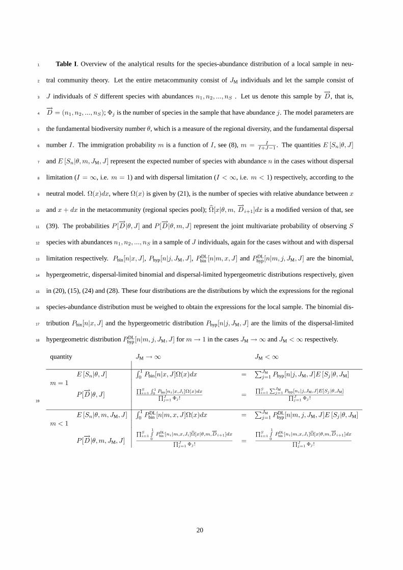
Table I. Overview of the analytical results for the species-abundance distribution of a local sample in neu-1

tral community theory. Let the entire metacommunity consist of JM individuals and let the sample consist of2

J individuals of S different species with abundances n1, n2, ..., nS . Let us denote this sample by−→D , that is,3

−→D = (n1, n2, ..., nS); Φj is the number of species in the sample that have abundance j. The model parameters are4

the fundamental biodiversity number θ, which is a measure of the regional diversity, and the fundamental dispersal5

number I . The immigration probability m is a function of I , see (8), m = II+J−1 . The quantities E [Sn|θ, J ]6

and E [Sn|θ,m, JM, J ] represent the expected number of species with abundance n in the cases without dispersal7

limitation (I = ∞, i.e. m = 1) and with dispersal limitation (I < ∞, i.e. m < 1) respectively, according to the8

neutral model. Ω(x)dx, where Ω(x) is given by (21), is the number of species with relative abundance between x9

and x + dx in the metacommunity (regional species pool); bΩ[x|θ,m,−→D i+1]dx is a modified version of that, see10

(39). The probabilities P [−→D |θ, J ] and P [

−→D |θ,m, J ] represent the joint multivariate probability of observing S11

species with abundances n1, n2, ..., nS in a sample of J individuals, again for the cases without and with dispersal12

limitation respectively. Pbin[n|x, J ], Phyp[n|j, JM, J ], PDLbin [n|m,x, J ] and PDL

hyp[n|m, j, JM, J ] are the binomial,13

hypergeometric, dispersal-limited binomial and dispersal-limited hypergeometric distributions respectively, given14

in (20), (15), (24) and (28). These four distributions are the distributions by which the expressions for the regional15

species-abundance distribution must be weighed to obtain the expressions for the local sample. The binomial dis-16

tribution Pbin[n|x, J ] and the hypergeometric distribution Phyp[n|j, JM, J ] are the limits of the dispersal-limited17

hypergeometric distribution PDLhyp[n|m, j, JM, J ] for m→ 1 in the cases JM →∞ and JM <∞ respectively.18

quantity JM →∞ JM <∞

E [Sn|θ, J ]R 10Pbin[n|x, J ]Ω(x)dx =

PJMj=1 Phyp[n|j, JM, J ]E [Sj |θ, JM]

m = 1

P [−→D |θ, J ]

Si=1

10Pbin[ni|x,Ji]Ω(x)dx

Jj=1 Φj !

=Si=1

JMj=1 Phyp[ni|j,JM,J]E[Sj |θ,JM]

Jj=1 Φj !

E [Sn|θ,m, JM, J ]R 10PDL

bin [n|m,x, J ]Ω(x)dx =PJM

j=1 PDLhyp[n|m, j, JM, J ]E [Sj |θ, JM]

m < 1

P [−→D |θ,m, JM, J ]

Si=1

1

0

PDLbin [ni|m,x,Ji]Ω[x|θ,m,

−→Di+1]dx

Jj=1 Φj !

=

Si=1

1

0

PDLbin [ni|m,x,Ji]Ω[x|θ,m,

−→Di+1]dx

Jj=1 Φj !

19

20

Figure captions

Figure 1. Example of the difference in expected number of species between the exact result (6) and the approxima-1

tion (10) by Vallade & Houchmandzadeh (2003) for two different values of metacommunity size. The parameter2

values used are θ = 50 and m = 0.5. Local community size is J = 20, 000. Particularly the diversity of species3

with low abundances are underestimated with (10). The lower and upper boundaries of the abundance classes are4

such that abundance class i contains all abundances n for which 2i−1 ≤ n < 2i.5

21

Figures

100 101 102 103 104

Abundance

0

10

20

30

40

E[S

| m

, ,

J]

Eq. 6Eq. 10 ( = 10 )

100 101 102 103 1040

10

20

30

40

E[S

| m

, ,

J]

Eq. 6Eq. 10 ( = 10 )M

6

M4

θθ

nn

J

J

1

Figure 1.2

22

Appendix A. Derivation of equation (13)

Here we derive the integral notation of (11). We first note that s (ni, ai) = 0 for ai > ni. Therefore, (11) can be1

written as2

Ph−→D |θ,m, J

i=

J !QSi=1 ni

QJj=1Φj !

θS

(I)J

JXA=S

K(−→D,A)

IA

(θ)A=

=J !QS

i=1 niQJ

j=1Φj !

θS

(I)J

ÃSYi=1

niXai=1

s (ni, ai)s (ai, 1)

s (ni, 1)

!IA

(θ)A=

=J !QS

i=1 niQJ

j=1Φj !

θS

(I)J

n1Xa1=1

...

nSXaS=1

P1IA1

(θ)A1

(A-1)

where3

Ai :=SXj=i

ai (A-2)

(so A1 = A) and4

Pi :=SYj=i

s (nj , aj)s (ai, 1)

s (ni, 1)=

SYj=i

s (nj , aj)Γ (aj)

Γ (nj)(A-3)

We write the first summation of (A-1) in terms of P2, A2 and a1:5

n1Xa1=1

P1IA1

(θ)A1

=

n1Xa1=1

P1IA2+a1

(θ)A2+a1

= P2

n1Xa1=1

s (n1, a1)Γ (a1)

Γ (n1)

IA2+a1

(θ)A2+a1

(A-4)

Expressing (θ)A2+a1in terms of Gamma functions and noting that Γ (n1) = (n1 − 1)!, we obtain after rearranging6

terms7

n1Xa1=1

P1IA1

(θ)A1

= P2IA2

1

(n1 − 1)!Γ (θ)

Γ (θ +A2)

n1Xa1=1

s (n1, a1) Ia1Γ (a1)Γ (θ +A2)

Γ (θ +A2 + a1)(A-5)

The last quotient is the Beta function that can be written in its integral form:8

n1Xa1=1

P1IA1

(θ)Ai1= P2I

A21

(n1 − 1)!Γ (θ)

Γ (θ +A2)

n1Xa1=1

s (n1, a1) Ia1

Z 1

0

xa11 (1− x1)A2(1− x1)

θ−1

x1dx1 (A-6)

Changing the order of summation and integration and using Pochhammer notation leads to:9

n1Xa1=1

P1IA1

(θ)A1

=

Z 1

0

1

(n1 − 1)!P2

IA2

(θ)A2

(1− x1)A2(1− x1)

θ−1

x1

n1Xa1=1

s (n1, a1) (Ix1)a1 dx1 =

=1

(n1 − 1)!

Z 1

0

P2(I (1− x1))

A2

(θ)A2

(1− x1)θ−1

x1(Ix1)n1 dx1 (A-7)

This means that the summation of P1 IA1

(θ)A1over a1 is written in terms of an integral over P2 (I(1−x1))

A2

(θ)A2and some10

additional terms that do not depend on any ai. More generally,11

niXai=1

Pi

³IQi−1

k=1 (1− xk)´Ai

(θ)Ai=

1

(ni − 1)!

Z 1

0

Pi+1

³IQi

k=1 (1− xk)´Ai+1

(θ)Ai+1

ÃIxi

i−1Yk=1

(1− xk)

!ni

(1− xi)θ−1

xidxi

(A-8)1

for i = 1...S. The S summations in (A-1) require repeated application of (A-8), from i = 1 to i = S, which1

yields2

Ph−→D |θ,m, J

i=

J !QSi=1 ni!

QJj=1Φj !

θS

(I)J

Z 1

0

...

Z 1

0

SYi=1

ÃIxi

i−1Yk=1

(1− xk)

!ni

(1− xi)θ−1

xidx1...dxS (A-9)

which is (13) with (14).1

2

Appendix B. The relation of the approximation (10) to the exactresult (6)

A rigorous expansion of the approximate result (10) in Vallade & Houchmandzadeh (2003) in terms of (1/JM)2

powers can be written after some algebra (Alonso & McKane, unpublished):3

S (n) = S0(n) +Oµ1

JM

¶(B-1)

where S(n) is given by (10) and S0(n) is given by (6). This expansion confirms that Vallade & Houchmandzadeh’s4

result (10) converges to (6) when JM tends to infinity. The existence of this expansion suggested a quantitative5

path to independently estimate metacommunity sizes and biodiversity numbers (and hence also speciation rates)6

from species-abundance data. In the main text we have shown that expected sampling abundances do not depend7

on metacommunity size. Therefore, that initial hope of independent estimation must be abandoned. In addition,8

Vallade & Houchmandzadeh’s approximation is not very useful anyway, because the integral in 6 can be evaluated9

much faster and more robustly than the sum in (10).10

The complete proof for the expansion given in (B-1) will be given elsewhere, but an easy argument to show to11

what extent (10) and (6) converge to each other as JM increases goes as follows. The sum in (10) corresponds to12

an approximate discretization of the exact integral result given by (6). Let us write (6) as13

S0(n) =

Z 1

0

G(x) dx (B-2)

where G(x) = PDLbin [n|m,x, J ]Ω(x). We divide the interval (0, 1) in JM points to obtain14

S0(n) ≈JMXj=1

G(xj)∆x (B-3)

where∆x = 1/JM, xj = j∆x and15

G(xj) = PDLbin [n|m,

j

JM, J ]Ω(

j

JM) (B-4)

Hence S0(n) can be approximated by the following sum:16

S0(n) ≈JMXj=1

PDLbin [n|m,j

JM, J ]

θ

j

µ1− j

JM

¶θ−1(B-5)

Compare this to Vallade & Houchmandzadeh’s (2003) formula, given by (10) but repeated here for easier compar-17

ison:1

S(n) =

JMXj=1

PDLbin [n|m,j

JM, J ]E[Sj |θ, JM] (B-6)

3

Because each term E[Sj |θ, JM] can be approximated by (Alonso & McKane 2004)2

E[Sj |θ, JM] =θ

j

µ1− j

JM

¶θ−1+O

µ1

J2M

¶, (B-7)

we conclude that (10), apart from vanishingly small terms, corresponds to the discretization (B-5) in JM points,3

which by definition converges to the integral in the limit of an infinite number of points.1

4

Appendix C. Proof of the equality of (23) and (29)

Here we show that equations (23) and (29) are identical:2

E [Sn|θ,m, J ] =θ

(I)J

µJ

n

¶ 1Z0

(Ix)n (I (1− x))J−n(1− x)θ−1

xdx =

=θ

(I)J

µJ

n

¶ nXj=1

J−nXk=1

s (n, j) s (J − n, k) Ij+kΓ (j)Γ (k + θ)

Γ (j + k + θ)=

=θ

(I)J

µJ

n

¶ JXA=1

nXa=1

s (n, a) s (J − n,A− a) IAΓ (a)Γ (A− a+ θ)

Γ (A+ θ)=

=

µJ

n

¶ JXA=1

nXa=1

s (n, a) s (J − n,A− a)IA

(I)J

Γ (A+ 1− a)

Γ (A+ 1)aΓ (a)

θ

a

Γ (A+ 1)

Γ (A+ 1− a)

Γ (A+ θ − a)

Γ (A+ θ)=

=

µJ

n

¶ JXA=1

nXa=1

s (n, a) s (J − n,A− a)IA

(I)J

1¡Aa

¢E [Sa|θ,A] ==

JMXj=1

JXA=1

nXa=1

¡Jn

¢¡Aa

¢s (n, a) s (J − n,A− a)IA

(I)JPhyp[a|j, JM, A]E [Sj |θ, JM] =

=

JMXj=1

PDLhyp [n|m, j, JM, J ]E [Sj |θ, JM] (C-1)

where in the first line we have used the polynomial form of the Pochhammer symbol (3) and the definition of the3

beta function (4).1

5

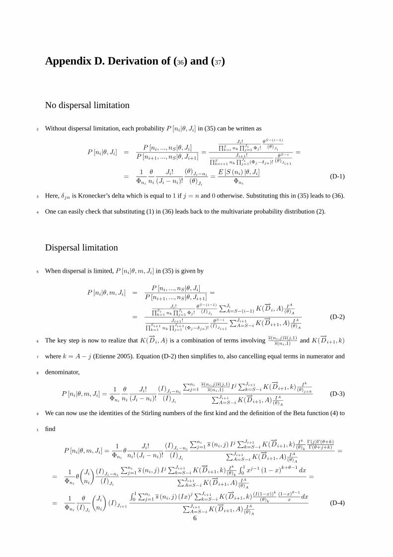
Appendix D. Derivation of (36) and (37)

No dispersal limitation

Without dispersal limitation, each probability P [ni|θ, Ji] in (35) can be written as2

P [ni|θ, Ji] =P [ni, ..., nS |θ, Ji]

P [ni+1, ..., nS |θ, Ji+1]=

Ji!Sk=i nk

Jij=1 Φj !

θS−(i−1)

(θ)Ji

Ji+1!Sk=i+1 nk

Jij=1(Φj−δjn)!

θS−i

(θ)Ji+1

=

=1

Φni

θ

ni

Ji!

(Ji − ni)!

(θ)Ji−ni(θ)Ji

=E [S (ni) |θ, Ji]

Φni(D-1)

Here, δjn is Kronecker’s delta which is equal to 1 if j = n and 0 otherwise. Substituting this in (35) leads to (36).3

One can easily check that substituting (1) in (36) leads back to the multivariate probability distribution (2).4

Dispersal limitation

When dispersal is limited, P [ni|θ,m, Ji] in (35) is given by5

P [ni|θ,m, Ji] =P [ni, ..., nS |θ, Ji]

P [ni+1, ..., nS |θ, Ji+1]=

=

Ji!Sik=1 nk

Jij=1 Φj !

θS−(i−1)

(I)Ji

PJiA=S−(i−1)K(

−→D i, A)

IA

(θ)A

Ji+1!Si+1k=1 nk

Ji+1j=1 (Φj−δjn)!

θS−i

(I)Ji+1

PJi+1A=S−iK(

−→D i+1, A)

IA

(θ)A

(D-2)

The key step is now to realize that K(−→D i, A) is a combination of terms involving s(ni,j)s(j,1)

s(ni,1)and K(

−→D i+1, k)6

where k = A− j (Etienne 2005). Equation (D-2) then simplifies to, also cancelling equal terms in numerator and7

denominator,8

P [ni|θ,m, Ji] =1

Φni

θ

ni

Ji!

(Ji − ni)!

(I)Ji−ni(I)Ji

Pnij=1

s(ni,j)s(j,1)s(ni,1)

IjPJi+1

k=S−iK(−→D i+1, k)

Ik

(θ)j+kPJi+1A=S−iK(

−→D i+1, A)

IA

(θ)A

(D-3)

We can now use the identities of the Stirling numbers of the first kind and the definition of the Beta function (4) to9

find1

P [ni|θ,m, Ji] =1

Φniθ

Ji!

ni! (Ji − ni)!

(I)Ji−ni(I)Ji

Pnij=1 s (ni, j) I

jPJi+1

k=S−iK(−→D i+1, k)

Ik

(θ)k

Γ(j)Γ(θ+k)Γ(θ+j+k)PJi+1

A=S−iK(−→D i+1, A)

IA

(θ)A

=

=1

Φniθ

µJini

¶(I)Ji−ni(I)Ji

Pnij=1 s (ni, j) I

jPJi+1

k=S−iK(−→D i+1, k)

Ik

(θ)k

R 10xj−1 (1− x)

k+θ−1dxPJi+1

A=S−iK(−→D i+1, A)

IA

(θ)A

=

=1

Φni

θ

(I)Ji

µJini

¶(I)Ji+1

R 10

Pnij=1 s (ni, j) (Ix)

jPJi+1k=S−iK(

−→D i+1, k)

(I(1−x))k(θ)k

(1−x)θ−1x dxPJi+1

A=S−iK(−→D i+1, A)

IA

(θ)A

(D-4)

6

Using (3), multiplying the integrand by(I(1−x))Ji+1(I(1−x))Ji+1

and rearranging terms then leads to2

P [ni|θ,m, Ji] =1

Φni

θ

(I)Ji

µJini

¶Z 1

0

(Ix)ni (I (1− x))Ji−ni(1− x)θ−1

x

PJi+1k=S−i

K(−→Di+1,k)(θ)k

(I(1−x))k(I(1−x))Ji+1PJi+1

A=S−iK(−→Di+1,A)(θ)A

IA

(I)Ji+1

dx

(D-5)

Defining3

F³x|θ,m,

−→D i+1

´:=

PJi+1k=S−i

K(−→Di+1,k)(θ)k

(I(1−x))k(I(1−x))Ji+1PJi+1

A=S−iK(−→Di+1,A)(θ)A

IA

(I)Ji+1

(D-6)

and using (39) and (21), we obtain our end result (37).1

7

Appendix E. Derivation of (1) and (6) from (2) and (11)

No dispersal limitation

Equation (1) can be derived from (2) as follows. From (41) we get2

E [Sn|θ, J ] =JX

Φn=1

X−→D |Φn

ΦnJ !QS

i=1 niQJ

j=1 Φj !

θS

(θ)J=

=JX

Φn=1

X−→D |Φn

J !QSi=1 ni

QJj=1 (Φj − δjn)!

θS

(θ)J(E-1)

Defining Φ0j := Φj − δjn where δjn is Kronecker’s delta (which is equal to 1 if j = n and 0 otherwise), we can3

rewrite this as a sum of probabilities of observing exactly Φn − 1 species with abundance n in a subsample of size4

J − n,5

E [Sn|θ, J ] =θ

n

J !

(J − n)!

(θ)J−n(θ)J

J−nXΦ0n=0

X−→D|Φ0n

(J − n)!QS−1i=1 ni

QJ−nj=1 Φ

0j !

θS−1

(θ)J−n=

θ

n

J !

(J − n)!

(θ)J−n(θ)J

X−→D

(J − n)!QS−1i=1 ni

QJ−nj=1 Φ

0j !

θS−1

(θ)J−n(E-2)

The sum on the right hand side is the sum of the probabilities of over all possible datasets with sample size J − n,6

which, evidently, equals unity, and after expressing Pochhammer symbols as quotients of gamma functions, we7

obtain (1).8

Also, the expected number of species (of any abundance) can be calculated as follows:9

E [S|θ, J ] =JX

S=1

SP [S|θ, J ] =JX

S=1

Ss (J, S)θS

(θ)J=

= θJX

S=1

s (J, S)SθS−1

(θ)J= θ

JXS=1

s (J, S)1

(θ)J

d

dθθS =

= θd

dθ

ÃJX

S=1

s (J, S)θS

(θ)J

!− θ

JXS=1

s (J, S) θSd

dθ

1

(θ)J= − (θ)J

d

dθ

1

(θ)J=

= θ (Ψ (θ + J)−Ψ (θ)) =JXi=1

θ

θ + i− 1 (E-3)

where Ψ(x) is the digamma function or psi function, Ψ(x) = ddx lnΓ(x) =

1Γ(x)

ddxΓ(x) and we have used the10

identityPJ

S=1 s (J, S)θS

(θ)J= 1.1

8

Dispersal limitation

When dispersal is limited, with (41) we can derive (6) from (11):2

E [Sn|θ,m, J ] =SX

Φn=0

ΦnX−→D|Φn

P [−→D |θ,m, J ] =

=SX

Φn=1

X−→D|Φn

ΦnJ !QS

i=1 niQJ

j=1Φj !

θS

(I)J

JXA=S

K(−→D,A)

IA

(θ)A=

=SX

Φn=1

X−→D|Φn

J !QSi=1 ni

QJj=1 (Φj − δjn)!

θS

(I)J

JXA=S

K(−→D,A)

IA

(θ)A(E-4)

As in the case without dispersal limitation, we define Φ0j := Φj − δjn and we work towards a sum of probabilities3

of observing exactly Φn − 1 species with abundance n in a sample of size J − n (the corresponding dataset is4

called−→D 0),5

E [Sn|θ,m, J ] =θ

n

J !

(J − n)!

1

(I)J

S−1XΦ0n=0

X−→D|Φ0n

(J − n)!QS−1i=1 ni

QJj=1Φ

0j !θS−1

JXA=S

K(−→D,A)

IA

(θ)A=

=θ

n

J !

(J − n)!

1

(I)J

S−1XΦ0n=0

X−→D 0|Φ0n

(J − n)!QS−1i=1 ni

QJj=1Φ

0j !θS−1

nXj=1

s (n, j) s (j, 1)

s (n, 1)Ij

J−nXk=S−1

K(−→D 0, k)

Ik

(θ)j+k=

=θ

n

J !

(J − n)!

1

(I)J

X−→D 0

(J − n)!QS−1i=1 ni

QJj=1Φ

0j !θS−1

nXj=1

s (n, j) s (j, 1)

s (n, 1)Ij

J−nXk=S−1

K(−→D 0, k)

Ik

(θ)k

(θ)k(θ)j+k

=

=θ

n

J !

(J − n)!

1

(I)J

X−→D 0

(J − n)!QS−1i=1 ni

QJj=1Φ

0j !θS−1

nXj=1

s (n, j)

s (n, 1)Ij

J−nXk=S−1

K(−→D 0, k)

Ik

(θ)k

Γ (j)Γ (θ + k)

Γ (θ + j + k)(E-5)

The term with Gamma functions can be written as a Beta function, and the Beta function can be written in its6

integral notation:1

E [Sn|θ,m, J ] =θ

n

J !

(J − n)!

1

(I)J×

×X−→D 0

(J − n)!QS−1i=1 ni

QJj=1Φ

0j !θS−1

nXj=1

s (n, j)

s (n, 1)Ij

J−nXk=S−1

K(−→D 0, k)

Ik

(θ)k

Z 1

0

xj−1 (1− x)k+θ−1

dx (E-6)

9

Changing the order of integration and summation, and using (3), we obtain2

E [Sn|θ,m, J ] =θ

n!

J !

(J − n)!

1

(I)J×

×Z 1

0

X−→D 0

(J − n)!QS−1i=1 ni

QJj=1Φ

0j !θS−1

nXj=1

s (n, j) (Ix)j

J−nXk=S−1

K(−→D 0, k)

(I (1− x))k

(θ)k

(1− x)θ−1

xdx

= θ

µJ

n

¶1

(I)J×

×Z 1

0

(Ix)n (I (1− x))J−n(1− x)θ−1

x

X−→D 0

(J − n)!QS−1i=1 ni

QJj=1Φ

0j !

θS−1

(I (1− x))J−n

J−nXk=S−1

K(−→D 0, k)

(I (1− x))k

(θ)kdx

= θ

µJ

n

¶1

(I)J

Z 1

0

(Ix)n (I (1− x))J−n(1− x)

θ−1

xdx (E-7)

where in the last line we have used the fact that the sum of the probabilities of all possible datasets equals unity.3

Also, the expected number of species (of any abundance) can be calculated as follows:1

E [S|θ,m, J ] =JX

S=1

SP [S|θ,mJ ] =JX

S=1

SJX

A=S

s(J,A)IA

(I)Js(A,S)

θS

(θ)A=

=JX

A=1

s(J,A)IA

(I)J

AXS=1

Ss(A,S)θS

(θ)A=

=JX

A=1

s(J,A)IA

(I)J

AXi=1

θ

θ + i− 1 =

=JXi=1

θ

θ + i− 1

JXA=i

s(J,A)IA

(I)J=

=J−1Xi=0

θ

(θ + i) (I)J

JXA=i+1

s(J,A)IA (E-8)

10

Appendix F. A historical note on the origins of the binomialand hypergeometric distributions

The first occurrence of “binomial distribution” is found in Yule (1911) on p. 305: “The binomial distribution only2

becomes approximately normal when n is large, and this limitation must be remembered in applying the table3

to cases in which the distribution is strictly binomial”. Fisher (1925) adopted the distribution (part III, section4

18). Although, the name for the distribution relatively new, the distribution itself has been studied since Bernoulli5

(1713, part 1.)6

The earliest use of “hypergeometric distribution” appears in the title of Gonin (1936). Again, the name is7

relatively recent but the distribution itself is already suggested in Problem IV of Huygens (1657, p. 12). He and8

several other mathematicians solved the problem, whereas Bernoulli and de Moivre gave solutions for the general9

case (Hald 2003). At the end of the 19th. century Pearson (1899) wrote a paper in which he considered fitting the10

distribution (given by the ”hypergeometrical series”) to data.11

This brief historical note is based on http://members.aol.com/jeff570/mathword.html.12

References

Bernoulli, J. (1713). Ars Conjectandi. Basel, Switzerland. English translation available at http://cerebro.xu.edu/13

math/Sources/JakobBernoulli/ars_sung/ars_sung.html.14

Fisher, R.A. (1925). Statistical methods for research workers. London, U.K.: Oliver & Boyd. Available at http://15

psychclassics.yorku.ca/Fisher/Methods/index.htm16

Gonin, H.T. (1936). The use of factorial moments in the treatment of the hypergeometric distribution and in tests17

for regression. Philosophical Magazine 7: 215-226.18

Hald (2003). A history of probability and statistics and their applications before 1750. New York, N.Y.: Wiley-19

Interscience.20

Huygens, C. (1657). De ratiociniis in ludo aleae. Reprint of an English translation available at http://www.leidenuniv.21

nl/fsw/verduin/stathist/huygens/huyg1714p.pdf22

Pearson, K. (1899). On certain properties of the hypergeometrical series, and on the fitting of such series to obser-23

vation polygons in the theory of chance. Philosophical Magazine 47: 236-246.24

Yule, G.U. (1911). An introduction to the theory of statistics. London, U.K.: Charles Griffin & Co. Ltd.529

11