Maximum a posteriori CMB lensing reconstruction

Maximum a posteriori CMB lensing reconstruction

Article (Published Version)

http://sro.sussex.ac.uk

Carron, Julien and Lewis, Antony (2017) Maximum a posteriori CMB lensing reconstruction. Physical Review D, 96 (6). 063510-1-063510-19. ISSN 2470-0010

This version is available from Sussex Research Online: http://sro.sussex.ac.uk/id/eprint/72815/

This document is made available in accordance with publisher policies and may differ from the published version or from the version of record. If you wish to cite this item you are advised to consult the publisher’s version. Please see the URL above for details on accessing the published version.

Copyright and reuse: Sussex Research Online is a digital repository of the research output of the University.

Copyright and all moral rights to the version of the paper presented here belong to the individual author(s) and/or other copyright owners. To the extent reasonable and practicable, the material made available in SRO has been checked for eligibility before being made available.

Copies of full text items generally can be reproduced, displayed or performed and given to third parties in any format or medium for personal research or study, educational, or not-for-profit purposes without prior permission or charge, provided that the authors, title and full bibliographic details are credited, a hyperlink and/or URL is given for the original metadata page and the content is not changed in any way.

http://sro.sussex.ac.uk/

Maximum a posteriori CMB lensing reconstruction

Julien Carron and Antony LewisDepartment of Physics and Astronomy, University of Sussex, Brighton BN1 9QH, United Kingdom

(Received 29 April 2017; published 14 September 2017)

Gravitational lensing of the cosmic microwave background (CMB) is a valuable cosmological signal thatcorrelates to tracers of large-scale structure and acts as a important source of confusion for primordialB-mode polarization. State-of-the-art lensing reconstruction analyses use quadratic estimators, which areeasily applicable to data. However, these estimators are known to be suboptimal, in particular forpolarization, and large improvements are expected to be possible for high signal-to-noise polarizationexperiments. We develop a method and numerical code, LensIt, that is able to find efficiently the mostprobable lensing map, introducing no significant approximations to the lensed CMB likelihood, andapplicable to beamed and masked data with inhomogeneous noise. It works by iteratively reconstructingthe primordial unlensed CMB using a deflection estimate and its inverse, and removing residual lensingfrom these maps with quadratic estimator techniques. Roughly linear computational cost is maintained dueto fast convergence of iterative searches, combined with the local nature of lensing. The method achievesthe maximal improvement in signal to noise expected from analytical considerations on the unmasked partsof the sky. Delensing with this optimal map leads to forecast tensor-to-scalar ratio parameter errorsimproved by a factor ≃2 compared to the quadratic estimator in a CMB stage IV configuration.

DOI: 10.1103/PhysRevD.96.063510

I. INTRODUCTION

The large-scale structure of the Universe deflects cosmicmicrowave background (CMB) photons by a few arcmi-nutes, introducing a characteristic signature in the fluctua-tions in the CMB temperature and polarization [1]. Thestatistical homogeneity and isotropy of the CMB getsdistorted locally, and sizeable higher-order statistics areproduced. Lensing estimators use these higher-order sta-tistics to construct an integrated measure of the linear massfluctuations in the Universe that cross-correlates to alltraditional large-scale structure tracers. After the first directdetection of lensing in the CMB by the ACT team [2], theSPT [3], POLARBEAR [4], SPTpol [5], BICEP2-KECK[6] and Planck [7] collaborations have also reported thedetection of the lensing signal and published band-powers.The most decisive detection yet was by the Planck satellite[8]: its full-sky coverage comes with a statistical power thatsimply cannot be matched at the present time.Current measurements all use quadratic estimator tech-

niques, first devised in optimized form by Refs. [9,10]. Thequadratic estimator uses optimally-weighted two-pointstatistics of the data maps to reconstruct the deflectionfield. At current noise levels, this estimator is nearlyoptimal. The science returns from the use of more sophis-ticated techniques are expected to be small, and no othertype of estimator has been applied to data so far. However,the situation will have changed by the time of CMB stageIV (CMB-S4) [11], if not before. At this point thepolarization instrumental noise is expected to becomesmaller than the ∼5 μK arcmin lensing B mode. Barringwelcome detections, lensing will become the most relevant

cosmological source of confusion in the search for pri-mordial B modes [12], and more optimal delensingmethods will become critical.If the noise and primordial polarization B mode is

negligible, a well-known variable-counting argument [13]suggests that as long as the lensing is fully described by agradient deflection remapping of the unlensed fields, theobserved lensed E and B fields should contain enoughinformation to reconstruct essentially perfectly both thelensing potential and the unlensed E field. Fundamentallimits are well below near-future sensitivities, includingcorrections to the remapping approximation from emissionangle, time delay and polarization rotation [14,15], lensingcurl modes from second order post-Born lens-lens couplings[13,16], intrinsic nonlinearities of the CMB at recombination[17,18], and second-order sourced vector and tensor modes[17,19–21]. With the last science release from the Planckteam in sight, it therefore seems timely to revisit alternative,more optimal CMB lensing estimation. This paper presentsand discusses a new implementation of a maximum a pos-teriori estimate of the lensing potential from CMB data.Motivation for this work is not limited to primordial B

modes. The CMB lensing kernel peaks at z ∼ 2 andoverlaps the galaxy and weak lensing surveys targetingthe dark sector of the Universe. The correlated informationis expected to contribute to breaking important degener-acies and to help with systematics, so optimal CMB lensingmass maps will also be useful for use with large-scalestructure observations. Iterative estimates may also beuseful even at higher noise levels, in particular in thepresence of sky cuts or wildly inhomogeneous noise mapswhere the analytic response of the quadratic estimator is

PHYSICAL REVIEW D 96, 063510 (2017)

2470-0010=2017=96(6)=063510(19) 063510-1 © 2017 American Physical Society

https://doi.org/10.1103/PhysRevD.96.063510




inaccurate. An optimal estimate of the potential map mightprove better than the current simpler practice of sweepingthese deviations into Monte-Carlo (MC) corrections to thespectrum estimate. Finally, also looking a bit ahead,successful exploration of the lensed CMB likelihoodmay prove useful more generally, opening a path towardsoptimal joint estimation of the primary CMB and lensingpotential.It is clear how iterative estimates should work in practice,

at least intuitively: delens the data using the quadraticdeflection estimate, then again apply a quadratic estimatoron the resulting maps, with possibly modified weights, anditerate until convergence [22]. Of course, a world ofpotential complications lurks in the details, and no canoni-cally best approach is known at present. Formally, the codewe present finds a maximum of the posterior probabilitydensity function (PDF) of the lensing potential. As such, itis similar in spirit to the first iterative estimator proposed fortemperature reconstruction [23] and polarization [13].A maximum likelihood approach to lensing reconstructionis also discussed, without implementation, in the reviewarticle Ref. [24]. In contrast to Refs. [13,23], our imple-mentation can be considered exact, in the sense that itmaximizes the relevant functions without introducingapproximations, under the assumption of Gaussianunlensed CMB, noise and deflection fields. It can alsoaccount for beams, sky cuts and other nonideal effects.The quadratic estimator has the convenient property of

being relatively straightforward. It can be implementedusing a small number of harmonic transforms [8,25],keeping the overall numerical cost under control (dominatedin the Planck analysis by the cost of the inverse-variancefiltering step). It seems unavoidable that alternative moreoptimal approaches must be substantially more costly, andour implementation is no exception. At each iteration step,maximum a posteriori unlensed CMB maps are produced,under the assumption that the current deflection estimate isthe correct one. This operation in effect solves a largeNpix × Npix set of linear equations, and must be itselfperformed via an iterative method, each step involving afair number of lensing operations, even in the absence of skycuts or other nonideal effects.Nevertheless, lensing and lensing reconstruction have

the advantage of being very local in position space. Alloperations scale linearly with the number of resolutionelements, or follow the cost of an harmonic transform, andthe good convergence properties of the iterative searchesproposed here keep the total computational burden undercontrol. We also provide GPU implementations of the mostexpensive steps.We use the flat sky approximation throughout the main

text. Appendix A describes the implementation on thecurved sky, using the machinery of spin-weight sphericalharmonics. The implementation is otherwise identical in allrespects, though we have so far only thoroughly tested

everything on the flat sky where the numerical implemen-tation is faster. We expect the same convergence propertiesof iterative estimator on the curved sky: empirically, theonly effect we observe increasing the area is to rescale thetotal execution time, which is reasonable given that lensingdistortions are very much localized. Furthermore, iterativedelensing will probably initially be most useful on deepobservations of a small patch of sky where the flat skyapproximation is accurate [11].Sections II and III describe the algorithm and details of

its implementation respectively. Section IV provides testsand applications. We summarize and conclude in Sec. V.

II. DESCRIPTION

Let us first establish some notation. Let x, y be points ona patch of the flat sky of area V, and r ¼ x − y be theseparation vector. The primary, unlensed Stokes CMBfields T, E or B are written as XðxÞ, and Xdat denotesthe observed Stokes data T, Q and U on the data pixels,inclusive of noise and transfer function. We use a, b in (0,1)to denote the two cartesian axes of the flat sky, and use thesymmetric Fourier convention, which is closest to thetraditional curved sky normalization. We use the notationl for multipoles of the CMB maps and L for thelensing maps.We denote the primordial, unlensed CMB modes

fT; E; Bg as a column matrix X, with primordial spectralmatrix Cunl

l

hXlX†l0 i ¼ δll0Cunl

l : ð2:1Þ

This matrix is diagonal with respect to multipole index, butnot necessarily across T, E, B indices. Also let D be thedeflection operation that maps these unlensed CMB modesto the real space, lensed, Stokes parameters. For instance, intemperature we may write explicitly on the flat sky

DTTl ðxÞ≡ 1ffiffiffiffi

Vp eil·ðxþαðxÞÞ;

DTEl ðxÞ ¼ DTB

l ðxÞ ¼ 0: ð2:2Þ

The polarization components are similar but involves thespin-2 flat-sky harmonics. Here, and throughout, we use theapproximation that the lensed fields are entirely defined bya remapping of the unlensed fields, where αðxÞ is thelensing deflection angle that relates the observed lensedfield at x to the unlensed fields at xþ αðxÞ.

A. Model

The model for the CMB data Xdat on the observed pixelsis given by a linear response matrix B operating on thelensed sky (which includes, for example, the effect of theinstrumental beam and pixel window function), plusindependent noise ni, so that

JULIEN CARRON and ANTONY LEWIS PHYSICAL REVIEW D 96, 063510 (2017)

063510-2

Xdat ¼ BDX þ n: ð2:3Þ

The pixel-pixel covariance can be written in compactnotation using a series of linear operators as follows:

Covα ≡ hXdatXdat;†i ¼ BDCunlD†B† þ N; ð2:4Þ

whereN is the noise covariance matrix, which we assume isdiagonal in pixel space. Unlensed CMB fields and the noiseon each pixel are assumed to obey Gaussian statistics, sothe likelihood is also Gaussian. The log-likelihood is then

lnpðXdatjαÞ ¼ −1

2Xdat · Cov−1α Xdat −

1

2ln det Covα: ð2:5Þ

We need to use a prior on the statistics of the deflectionfield to regularize the large number of poorly constrainedsmall-scale modes. The ΛCDMCMB lensing potential ϕ isexpected to be nearly linear, so choosing Gaussian fieldstatistics for ϕ is a natural choice, and will likely remainaccurate in the foreseeable future on the scales wherethe lensing potential can accurately be reconstructed.Using a Gaussian prior on the signal does not preventreconstruction of any non-Gaussian signal that mayactually be present (as expected from nonlinear structuregrowth and post-Born lensing [16,26]).We assume pure gradient lensing deflections, in which

case the log-posterior becomes, up to irrelevant constants,

lnpðϕjXdatÞ ¼ lnpðXdatjϕÞ − 1

2

XL

ϕ2L

CϕϕL

; ð2:6Þ

where the likelihood is given by Eq. (2.5) with α ¼ ∇ϕ.Curl and joint curl/gradient reconstruction is very analo-gous, but should be of limited physical relevance in theforeseeable future, mainly serving as a consistency checkon the gradient reconstruction analysis. An interesting firstprospect would be the detection of the post-Born curlsignal, forecast to be marginally detectable in the bispec-trum with CMB-S4 [16], to which this methodology couldalso be applied.

B. Gradients

To maximize the log-posterior we consider the derivativeof the log-posterior with respect to the deflection. The totalgradient, g, splits naturally into three pieces:

gtota ≡ δ lnpðαjXdatÞδαaðnÞ

¼ gQDa − gMFa þ gPRa ; ð2:7Þ

one from the quadratic part of the likelihood (gQD), onefrom the likelihood covariance determinant (gMF, the mean-field), and one (gPR) from the prior. The choice of the oddsign of gMF is more natural and becomes clear later on. The

prior gradient is straightforward to evaluate assumingGaussian statistics.The gradients of the likelihood are first calculated in real

space, with the gradients with respect to the two cartesiancomponents of the deflection giving

δ lnpðXdatjαÞδαaðnÞ

¼ gQDa ðnÞ − gMFa ðnÞ: ð2:8Þ

These are then rotated to harmonic space to give thegradient and curl components. The piece quadratic in thedata

gQDa ðnÞ ¼ ½VαXdat�iðnÞ½Waα Xdat�iðnÞ; ð2:9Þ

is made up of two legs with data weights

Vα¼B†Cov−1α ; Waα¼D∇aCunlD†B†Cov−1α : ð2:10Þ

The gradient matrix ∇aCunl is block diagonal in harmonicspace with blocks ilaCunl

l . These weights are identical, inthe absence of deflection, to the (unnormalized) traditionalminimum variance (MV) lensing quadratic estimatorsevaluated with unlensed spectra.Both legs of the quadratic estimator [the two terms in

Eq. (2.9)] can be written in terms of reconstructed unlensedCMB modes, as follows. Consider the most probableprimordial CMB modes XWF

α given the data, under theassumption that α is the true deflection field, and that theyare Gaussian fields with power Cunl

l . The maximuma posteriori (MAP) unlensed CMB maps are formallygiven by the Wiener-filtered data.1

XWFα ≡ CunlD†B†Cov−1α Xdat: ð2:11Þ

The leg WaαSdat of the quadratic piece is then simply the

deflected gradient of these maps

Waα XdatðxÞ ¼ D∇aXWF

α ðxÞ: ð2:12Þ

The other leg can be written as the inverse-noise-weightedresidual between the data and how the inferred primordialmodes are predicted to appear:

VαXdat ¼ B†Cov−1α Xdat

¼ B†N−1ðCovα − BDCunlD†B†ÞCov−1α Xdat

¼ B†N−1½Xdat − BDXWFα �: ð2:13Þ

1For a signal seen under a linear response sdat ¼ Rstrue þ n themaximum a posteriori reconstructed signal s is given assumingGaussian statistics by sWF ¼ ðS−1 þ RtN−1RÞ−1RtN−1sdat ¼SRtðSþ NÞ−1sdat

MAXIMUM A POSTERIORI CMB LENSING RECONSTRUCTION PHYSICAL REVIEW D 96, 063510 (2017)

063510-3

The calculation of these two terms is simple once the mapsXWF are reconstructed. Our implementation is discussed inSec. III A.The second part of the likelihood gradient is the

contribution from the mean field

gMFa ðnÞ ¼ 1

2

δ ln det CovαδαaðxÞ

¼ hgQDa ðnÞi: ð2:14Þ

The average here is over realizations of the data, withdisplacementα held fixed. The second equality follows fromobserving that the first variation of a log-likelihood alwaysvanish in the mean, and that gMF

a ðnÞ itself is independent ofthe data (and hence is equal to its expectation). The meanfield serves the same purpose here as for the traditionalquadratic estimator: to subtract the known sources ofanisotropy from the quadratic estimate. It depends on thecurrent estimate of the deflection, because α at this iterationacts as a known source of anisotropy when measuringresidual lensing at the next iteration. Implementations arediscussed in Sec. III C and Appendix B.

III. IMPLEMENTATION

This section presents some details of our implementa-tion. The main numerical difficulty lies in the calculation ofthe Wiener-filtered modes XWF

α in the presence of thedeflection α (and anisotropic noise, masks, etc.). This isdiscussed in Sec. III A. The Wiener-filtering operationrequires the inversion of the deflection field, describedin Sec. III B, and the mean-field evaluation is discussed inSec. III C. We also make use of curvature information toimprove convergence, as discussed in Sec. III D. Finally,we describe our choice of starting point in Sec. III E, andsummarize the workflow of the method in Sec. III F.

A. Reconstruction of the unlensed CMB

The MAP estimate of the unlensed CMB given adeflection field α is formally given by Eq. (2.11), andtypically requires solving a large system of linear equa-tions. This is not straightforward even in the absence of skycuts or other nonideal effects, since the deflection fieldbreaks isotropy so that the harmonic transforms do notdiagonalize the system. However, for all realistic situationswe have investigated, we found that the additional com-plication of the deflection field was minor in comparison to(typically highly anisotropic) sky cuts.Our implementation is as follows. We first transform

Eq. (2.11) to the following form

XWFα ¼ ½ðCunlÞ−1 þD†B†N−1BD�−1D†B†N−1Xdat; ð3:1Þ

and solve for the large inverse in brackets with conjugategradient descent. Here one should understand the bracketedmatrix to act on the space of nonzero unlensed CMB

modes. There is no ambiguity regarding the unlensedspectra ðCunlÞ−1, since all modes in XWF are exactly zerowhen they correspond to fiducial Cunl

l that are zero: theWiener filter builds the maximum a posteriori X maps,hence these vanish whenever the prior variance Cunl does.We found Eq. (3.1) to be more efficient than other possibleways to perform the mask deconvolution, and it also ismore efficient when the lensing operations are the onlysource of complications.For the noise matrix N we use an input variance map that

is diagonal in pixel space. The noise can be inhomo-geneous, and we can also add to the noise matrix a set oftemplates which are projected out. This is useful forinstance to account for poorly understood low-l noise,or to project out any templates for galactic dust. Usingconjugate gradient descent requires a reasonably fast wayto apply ðCunlÞ−1 þD†B†N−1BD to vectors X. The firstterm is diagonal in harmonic space and poses no problem.The second term requires application of the lensingoperators D and D†, and of the inverse noise matrix.From Eq. (3.2), applying the lensing operator to a map issimply achieved by harmonic transforms followed bylensing of the resulting map. As discussed in more detailin Sec. III B, D† also involves the inverse harmonictransform and a delensing operation (lensing with theinverse deflection field). It therefore has the same complex-ity as forward lensing, provided the inverse deflection fieldhas been precomputed. The inverse noise matrix is simpleunder the assumption that it is diagonal in pixel space. Theinclusion of templates is only a minor complication as longas there are only a reasonable number of them. Finally,assuming isotropic beams, the beam operations are fast inharmonic space.All in all, application of the bracketed matrix in

Eq. (3.1) requires 4 harmonic transform and 2 lensingoperations, multiplied by 1, 2 or 3 for temperature only,polarization only or joint reconstruction respectively.Lensing of maps (or the displacement inversion) is nota cheap operation, but the cost scales linearly with thenumber of pixels and can easily be parallelized. Ourimplementations, including a GPU implementation, arediscussed in Sec. III B.The use of a good preconditioner is mandatory for

convergence in acceptable time, especially when dealingwith masked maps. We use a multigrid preconditionerfollowing Ref. [27], where a set of working resolutions isset up so that lower-resolution inverses are used toprecondition those at higher resolution. Specifically, weextend the qcinv package2 by Duncan Hanson to includethe lensing operations. At the lowest resolution stage, weuse a dense preconditioner. We offer no unique recipe of agood multigrid chain as performance appears to dependsubstantially on the specific configuration. The solution

2https://github.com/dhanson/qcinv


063510-4

https://github.com/dhanson/qcinv

https://github.com/dhanson/qcinv

XWFαN obtained at iteration αN can however be used as

starting point for iteration N þ 1, which significantlyspeeds whole process as αN settles down to the convergedestimate.Finally, we note that in ideal situations where α is the

only source of anisotropy, the use of a simple diagonalpreconditioner is much faster, with no need to resort to amultigrid solution, at least up to noise levels of a CMB-S4configuration we have been testing.

B. Lensing and delensing operations

Lensing of maps is done at a resolution of 0.7 arcminutes,using a standard bicubic spline interpolation. Lensing is anexpensive operation, even if easily computed in parallel,and there are a large number of maps to process untilconvergence is reached, and this can dominate the overallcomputational cost in typical runs. We found that portingthe lensing on GPU, using a GPU-optimized implementa-tion [28,29] can provide substantial speed-up. This is one ofthe implementations that we provide.In addition to the forward lensing operation, the filtering

step also requires applying D†. This is equivalent toapplying the inverse deflection together with multiplicationby the magnification. To see this, consider the temperaturepart only. From the explicit form of the operator D inEq. (3.2) we have

½D†T�l ¼1ffiffiffiffiV

pZ

d2xe−il·ðxþαðxÞÞTðxÞ

¼ 1ffiffiffiffiV

pZ

d2xe−il·xjMα−1 jðxÞTðxþα−1ðxÞÞ: ð3:2Þ

The second line follows from the first after the obviouschange of variable x → xþ αðxÞ, where jMj is themagnification matrix determinant that accounts for thechange of volume element in these new coordinates:

½Mα�abðxÞ ¼∂αa∂xb ðxÞ: ð3:3Þ

The inverse deflection α−1 is defined by the condition thatpoints deflected by α are remapped to themselves

xþ α−1ðxþ αðxÞÞ≡ x: ð3:4Þ

Equation (3.2) has the simple form of the harmonictransform of the delensed temperature map, multipliedby the magnification of the inverse deflection. The gener-alization to polarization is immediate.We therefore need to obtain the inverse deflection field.

While some approximation to the inverse deflection ispossible given the noise levels of current data [30,31], wefound the exact inversion is always well-behaved for aΛCDM displacement, is always in the weak-lensingregime, and is not a bottleneck for our reconstruction.

The inversion is a very localized operation which iseasily parallelized, for which we use a simple real spaceNewton-Raphson scheme on a high-resolution grid.Specifically, following Ref. [31], we solve iteratively forα−1ðnÞ using

α−1Nþ1ðnÞ ¼ α−1

NðnÞ −M−1α ðnþ α−1

NðnÞÞ· ðα−1

NðnÞ þ αðnþ α−1NðnÞÞÞ: ð3:5Þ

In practice, we use the same 0.7 arcmin grid spacing that weuse for the lensing operations, in which case 3 iterationsstarting from α−1 ¼ 0 are enough for essentially exactinversion of a typical ΛCDM deflection field. Typicalresulting r.m.s. fractional residuals on the deflection ampli-tude are as low as 2 × 10−5. For lensing reconstruction in arealistic situation, the forward deflection is much smootherin comparison to a typical ΛCDM deflection owing to theprior effectively filtering out many small-scale modes, andcoarser resolutions may also be used.

C. Mean field evaluation

Provided with a large number of data simulations, themean field may be evaluated using

gMFðnÞ ¼ hgQDðnÞi; ð3:6Þ

i.e., by repeating the quadratic estimate on a number NMCof independent simulations of the data maps and averagingto get the mean field. In practice, each of these naiveestimates of gMF has spectrum jgQDj2 and a large resultingMonte-Carlo (MC) noise, containing the signal and noiseparts of gQD. On small scales this noise is typically muchlarger than gMF, so for a reasonable number of MCsimulations the mean field subtraction would effectivelybe adding noise with power jgQDj2=NMC to the estimationof the gradient on these scales. It is therefore desirable toobtain better ways to estimate the mean field. We suggesttwo types of trick to accelerate convergence of the mean-field estimation.The first simply subtracts some of the Monte Carlo noise

by subtracting a mean field calculated using an isotropicapproximation to the data likelihood, using the samerandom phases for the simulations. This introduces nobias, since by isotropy the correction vanishes in the mean,but has the virtue of cancelling part of the MC noise wherethe anisotropy is mild. For example, the isotropic approxi-mation could consist of recalculating the same quadraticestimate but setting α to zero in the weights (in the absenceof other non-ideal effects), or using a simulation extendedto full sky in the presence of sky cuts.The second trick is to modify the weights of the quadratic

estimator, in a way that keeps its expectation value (i.e., themean field) constant. This is discussed in more detail inAppendix B. Combined, these tricks can lead to orders of


063510-5

magnitude decrease of the MC noise on the mean-fieldestimator, drastically reducing the number of simulationsrequired for the same target accuracy.In principle, different random phases must be used for

the simulations at each iteration step: usage of the samephases at each step causes artificial convergence of theiteration towards what is an approximation to the trueposterior. This approximation might still be fairly good,however, if enough simulations are used. At any given scaleit is the mean field MC noise that sets the accuracy at whichthe true maximum a posteriori deflection solution can bedetermined. We refer to this later on as the MC noise floor.

D. Curvature

Finally, to perform an efficient search for the optimalpoint we need the curvature of the likelihood as well as thegradient. Specifically, to perform efficient Newton-typeiteration across parameter space, the inverse curvature isneeded. Curvature matrices such as

½H−1�abLL0 ≡ −δ2 lnpðXdatjαÞ

δαaL δαb;�L0

ð3:7Þ

can never be evaluated exactly in reasonable time. Weproceed as follows: starting with an initial isotropic guess,H0, we perform a rank two update toH every time we moveacross parameter space. At each iteration, two maps aresaved to disk and can be used to apply recursively theinverse curvature matrix to any vector. We use the limitedmemory Broyden-Fletcher-Goldfarb-Shanno (L-BFGS)update [32], for which

HNþ1 ¼ ð1þ ρsytÞHNð1þ ρystÞ − ρsst; ð3:8Þwith

sðnÞ ¼ ϕNþ1ðnÞ − ϕNðnÞ;yðnÞ ¼ gtotNþ1ðnÞ − gtotN ðnÞ; ð3:9Þ

and ρ ¼ 1=yts. Built in this way, the inverse curvature takesinto account non-Gaussian and realization-dependentaspects of the likelihood, and we found can dramaticallyimprove the convergence properties of the iterative search.Since the inverse curvature approximates the covariance, itcan also be used to assess the width of the posterior densityfunction, giving us approximate confidence regions for freeat the end of the iterative process.

E. Starting point

If the posterior density were exactly Gaussian, a singleNewton step starting from α≡ 0 would bring us directly tothe optimal solution. This solution matches (neglecting thedifference between the realization-dependent curvature andits average) the Wiener-filtered quadratic estimator calcu-lated with unlensed weights [33]. However, we use lensed

weights since they provide a better quadratic reconstruction[34], especially on large scales. Explicitly, we use

α0ðLÞ ¼ CϕϕL

CϕϕL þ N0;len

L

iL ϕqestðLÞ; ð3:10Þ

where N0;lenL is the Gaussian reconstruction noise of the

quadratic estimator, calculated with the lensed CMBspectra. N0;len

L is calculated using its real space flat-skyrepresentation (see Appendix B). The quadratic estimator isthe minimum variance (MV) estimator built with the set ofmaps considered: T alone, Q and U polarization alone, orthe three Stokes maps in combination. The filtering step isdescribed in Sec. III A, with the ðα ¼ 0; Clen

l Þ Wiener filterusing an input noise variance map and fiducial beamtransfer function. In temperature, there are known waysto optimize the weights further [35], but Eq. (3.10) workswell for our purposes.

F. Summary of the workflow

We are now in position to summarize and describe theworkflow of the iterative search for the maximum a pos-teriori point. Initially, the displacement α0 is set at theWiener-filtered quadratic estimator as described in Sec. IIIE. To get the optimal reconstruction we apply the followingsteps recursively until satisfactory convergence is reached:(1) The displacement αN is inverted to give α−1

N andcached.

(2) With the deflection and its inverse, the delensedmaps XWF

α are obtained with the ðαN; Cunll Þ Wiener

filter using multigrid-preconditioned conjugate gra-dient inversion. This is the most expensive step ofthe whole process by some margin.

(3) With the delensed CMB at hand, the quadratic part ofgradients are calculated from Eqs. (2.12) and (2.13).

(4) In parallel (unless neglected, or some other approxi-mation scheme is used), the mean field contributionsto the gradient are calculated by repeating steps 2-3on a number of simulated maps, using the tricksdiscussed in Sec. B.

(5) The total gradient gN is then obtained, the inversecurvature updated according to the BFGS scheme of(3.8), and the displacement αNþ1 is found along theNewton descent direction:

αNþ1 ¼ αN þ λHNgN: ð3:11ÞThe parameter λ helps improve convergence. ForCMB-S4-like configurations, we picked λ ¼ 1=2 atall steps, whereas the full Newton step λ ¼ 1 cansafely be used at higher noise levels.

IV. RESULTS

For this preliminary investigation we report three tests ofour reconstruction method. First, using a simulated lensed


063510-6

map similar current Planck public data, we demonstrate useof the Wiener-filtering procedure to extract the maximuma posteriori estimate of the unlensed CMB. Second, wesimulate a lensing reconstruction from polarization on amasked field, with noise levels of next-generation CMBexperiments. In its simplest incarnation, the algorithm doesnot directly provide a delensed primordial B-mode map,but the iteratively reconstructed potential map can still beused to delens the observed B modes. Third and finally,while explicit delensing of B-modes with these improvedlensing maps will be demonstrated in upcoming work, wediscuss the increase in correlation coefficient (and hencedelensing efficiency) that the method can achieve withupcoming CMB data.

A. Wiener filtering

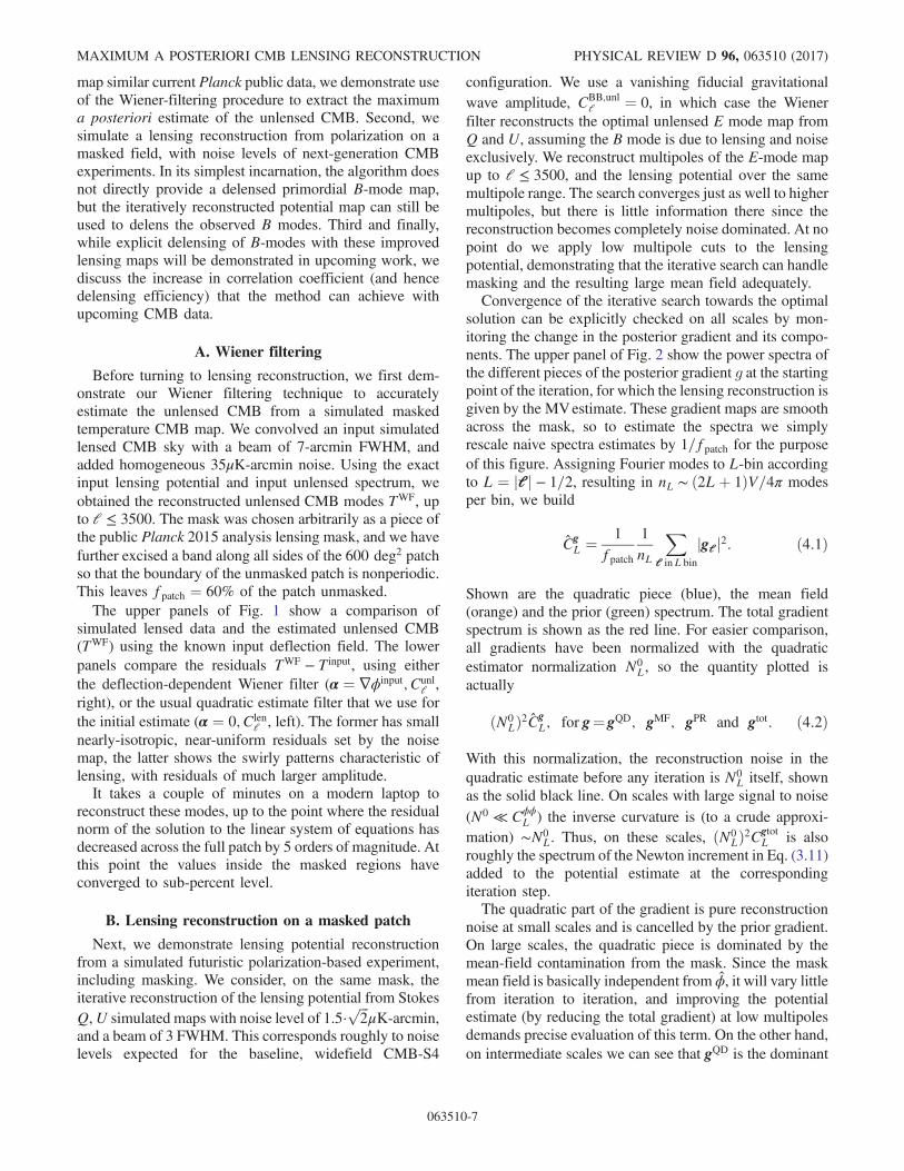
Before turning to lensing reconstruction, we first dem-onstrate our Wiener filtering technique to accuratelyestimate the unlensed CMB from a simulated maskedtemperature CMB map. We convolved an input simulatedlensed CMB sky with a beam of 7-arcmin FWHM, andadded homogeneous 35μK-arcmin noise. Using the exactinput lensing potential and input unlensed spectrum, weobtained the reconstructed unlensed CMB modes TWF, upto l ≤ 3500. The mask was chosen arbitrarily as a piece ofthe public Planck 2015 analysis lensing mask, and we havefurther excised a band along all sides of the 600 deg2 patchso that the boundary of the unmasked patch is nonperiodic.This leaves fpatch ¼ 60% of the patch unmasked.The upper panels of Fig. 1 show a comparison of

simulated lensed data and the estimated unlensed CMB(TWF) using the known input deflection field. The lowerpanels compare the residuals TWF − T input, using eitherthe deflection-dependent Wiener filter (α ¼ ∇ϕinput; Cunl

l ,right), or the usual quadratic estimate filter that we use forthe initial estimate (α ¼ 0; Clen

l , left). The former has smallnearly-isotropic, near-uniform residuals set by the noisemap, the latter shows the swirly patterns characteristic oflensing, with residuals of much larger amplitude.It takes a couple of minutes on a modern laptop to

reconstruct these modes, up to the point where the residualnorm of the solution to the linear system of equations hasdecreased across the full patch by 5 orders of magnitude. Atthis point the values inside the masked regions haveconverged to sub-percent level.

B. Lensing reconstruction on a masked patch

Next, we demonstrate lensing potential reconstructionfrom a simulated futuristic polarization-based experiment,including masking. We consider, on the same mask, theiterative reconstruction of the lensing potential from StokesQ,U simulated maps with noise level of 1.5·

ffiffiffi2

pμK-arcmin,

and a beam of 3 FWHM. This corresponds roughly to noiselevels expected for the baseline, widefield CMB-S4

configuration. We use a vanishing fiducial gravitationalwave amplitude, CBB;unl

l ¼ 0, in which case the Wienerfilter reconstructs the optimal unlensed E mode map fromQ and U, assuming the B mode is due to lensing and noiseexclusively. We reconstruct multipoles of the E-mode mapup to l ≤ 3500, and the lensing potential over the samemultipole range. The search converges just as well to highermultipoles, but there is little information there since thereconstruction becomes completely noise dominated. At nopoint do we apply low multipole cuts to the lensingpotential, demonstrating that the iterative search can handlemasking and the resulting large mean field adequately.Convergence of the iterative search towards the optimal

solution can be explicitly checked on all scales by mon-itoring the change in the posterior gradient and its compo-nents. The upper panel of Fig. 2 show the power spectra ofthe different pieces of the posterior gradient g at the startingpoint of the iteration, for which the lensing reconstruction isgiven by the MVestimate. These gradient maps are smoothacross the mask, so to estimate the spectra we simplyrescale naive spectra estimates by 1=fpatch for the purposeof this figure. Assigning Fourier modes to L-bin accordingto L ¼ jlj − 1=2, resulting in nL ∼ ð2Lþ 1ÞV=4π modesper bin, we build

CgL ¼ 1

fpatch

1

nL

Xl inL bin

jglj2: ð4:1Þ

Shown are the quadratic piece (blue), the mean field(orange) and the prior (green) spectrum. The total gradientspectrum is shown as the red line. For easier comparison,all gradients have been normalized with the quadraticestimator normalization N0

L, so the quantity plotted isactually

ðN0LÞ2Cg

L; for g¼ gQD; gMF; gPR and gtot: ð4:2Þ

With this normalization, the reconstruction noise in thequadratic estimate before any iteration is N0

L itself, shownas the solid black line. On scales with large signal to noise(N0 ≪ Cϕϕ

L ) the inverse curvature is (to a crude approxi-mation) ∼N0

L. Thus, on these scales, ðN0LÞ2Cgtot

L is alsoroughly the spectrum of the Newton increment in Eq. (3.11)added to the potential estimate at the correspondingiteration step.The quadratic part of the gradient is pure reconstruction

noise at small scales and is cancelled by the prior gradient.On large scales, the quadratic piece is dominated by themean-field contamination from the mask. Since the maskmean field is basically independent from ϕ, it will vary littlefrom iteration to iteration, and improving the potentialestimate (by reducing the total gradient) at low multipolesdemands precise evaluation of this term. On the other hand,on intermediate scales we can see that gQD is the dominant


063510-7

contribution to the total gradient at the start of the iterations.Hence, on these scales the lensing map can be improvedwithout relying on cancellation of the mean field.We used 511 simulations at each step to estimate the

mean field. The upturn of the orange curve at L≃ 1000shows the onset of the MC noise dominated regime, wherethe mean-field estimate becomes pure MC noise. Thedot-dashed black line shows an analytic prediction forthe expected MC noise neglecting sky cuts, calculated with

the tools from Appendix B. The MC noise spectrum issmaller than N0

L by four orders of magnitude, so iterationsshould be able to reduce the gradient amplitude by a similaramount. On large scales, the MC noise stays smaller thanthe prior gradient, and thus the iterative procedure will haveexhausted information from the data before it hits the MCnoise floor. However, we will see below that the isotropicprediction for the MC noise is inaccurate on large scales,where there is a substantial contribution from sky cuts.

FIG. 1. A demonstration of how our Wiener filter produces optimal (maximum a posteriori) estimates on the unlensed CMB mapsfrom masked data. The simulated temperature map is comparable to a Planck configuration, and we use the exact input simulateddeflection and exact input unlensed CTT

l spectrum in the filter. The upper-left panel shows the simulated masked temperature data map,with a homogeneous noise level of 35 μK-arcmin and a beam FWHM of 7-arcmin. The (unapodized) mask is built out of a portion of thepublic Planck lensing mask, to which we have added a band surrounding the patch on all sides. The upper right panel shows thereconstructed unlensed map TWF. The residual to the true input CMB map (TWF − T input) is shown on the lower-right panel. The lower-left panel shows the residual (on the unmasked pixels) of the result obtained when the Wiener filter instead uses no deflection but thelensed CMB spectrum in place of the unlensed spectrum (as in the standard quadratic estimator). These residuals are several times largerin magnitude (the same color scale is sometimes saturated), and display the anisotropic swirly patterns generated by the pure gradientdeflection field.


063510-8

A small contribution also comes from the deflection field.It is possible to predict this contribution perturbatively,since the mean field just follows the spatial distribution ofthe deflection field at each step: see Appendix B. Thiscontribution from the deflection is comparatively larger for

temperature reconstruction, and also for temperature incombination with polarization.We start the posterior inverse curvature H0 with the

isotropic estimate

H0L ¼

�1

N0;unlL

þ 1

CϕϕL

�−1: ð4:3Þ

The second term is the prior curvature, and for the first term(the likelihood curvature) we used the unlensed weights.The choice of initial curvature is not critical as long as theBFGS scheme is used to update it. However, using thelensed weights can lead to the algorithm taking steps thatare too large and hence give poor convergence, so we useunlensed weights instead (which gives a curvature that isslightly too large, but works well): steps that are too largeshould be avoided, as the search relies on the displacementbeing invertible at each step. More optimal curvatureestimates might be built using partially lensed weights.Convergence is acceptably quick, and after ∼9 iterations

the bulk of the improvement has been gained, with thegradient spectrum reduced by 2–3 orders of magnitude.Only small variations on the large-scale modes are visiblein the deflection maps after this point. The lower panel ofFig. 2 shows the spectra after 20 iterations. The purplecurve show an empirical estimate of the mean-field MCnoise. This is calculated by splitting our set of simulationsinto two independent sets of size N1 and N2 withcorresponding mean-field prediction gMF1 and gMF2 , andbuilding

CMFL ¼ N1N2

ðN1 þ N2Þ2CMF1−MF2L : ð4:4Þ

This is much larger than the analytic isotropic prediction onlarge scales because of the mask contribution to the MCnoise. The total gradient closely follows the MC noisecurve, and no further improvement can be achieved afterthe 20 iterations. At intermediate scales, the quadraticgradient is visibly much reduced and is now in equilibriumwith the prior.Finally, we show the reconstructed lensing map in Fig. 3.

From left to right in the top row we show the input lensingmap, the quadratic estimate, and the converged iterativesolution. Here we plot the displacement-like but isotropicspin-0 transforms

dðxÞ≡ 1ffiffiffiffiV

pXL

LϕLeiL·x: ð4:5Þ

The reconstruction is visibly improved, both by large-scalemodes filling in the masked regions and by the presence offiner-grained structure well inside the patch. The bottomrow of Fig. 3 shows a zoom in of the central area, showing

FIG. 2. Power spectra of the three gradients gQD (blue), gMF

(orange) and gPR (green) for lensing reconstruction from polari-zation on a masked patch, together with the total gradientspectrum (red). The algorithm works by reducing the red curveas much possible to find the most probable lensing map. Themask is shown in Fig. 1, and causes the large contribution fromthe mean field at low multipoles. All curves are normalized to thequadratic estimator normalization N0

L. The upper panel shows thegradient spectra at the first iteration step, where the deflection isthe Wiener-filtered quadratic estimator, and the lower panelshows the result after 20 iterations. At this point, the gradienthas hit the mean-field MC noise floor (purple on the lower panel)on all scales and the solution cannot be improved by moreiterations. The MC noise floor is mean-field estimator dependentand inversely proportional to the number of simulations used(here 511 per iteration). The dot-dashed line shows predictionsfor the MC noise floor built from an isotropic likelihood, whichare inaccurate at low multipoles because of the sky cuts. At lowmultipoles, the improved reconstruction relies on accuratelycancelling the mean field contribution, but on intermediate scalesthe decrease in the quadratic estimate is immediately visible.


063510-9

instead the lensing convergence where the improvement onsmall scales is more clearly visible.

C. Delensing efficiency

How can our lensing reconstruction method help withmeasurement of primordial tensor modes? In the absence ofa fiducial nonvanishing CBB

l , for which there is at presentno preferred choice, no delensed B-mode map is directlyproduced by the algorithm as the prior sets it to zero.However, it is well known that the lensing map can be usedto remove some of the lensing signal in the observed B-

mode map. Reduction of lensing signal in the B-mode mapwill result in some degree of improvement on tensorconstraints, since the lensing B modes act as a source ofnoise for any primordial signal.Delensing of B-mode polarization has recently been

demonstrated on Planck data by remapping the Stokesmaps [31], and by the SPT team [36] using a templatesubtraction method. In both cases, the expected reductionof lensing-like power is approximately set by the squaredcross-correlation coefficient of the measured lensing mapto the true lensing map, which we call the delensingefficiency:

FIG. 3. The top-left panel shows a simulated lensing field used as input to a lensing reconstruction analysis. The input StokesQ andUmaps are masked with the same mask shown on Fig. 1, and we assume a polarization-sensitive experiment having polarization noiselevel of 1.5 ·

ffiffiffi2

pμK-arcmin and 3 arcmin FWHM beam. The middle panel shows on the same color scale the Wiener-filtered quadratic

estimate, which is the starting point of the iterative solution for the maximum a posteriori solution, Eq. (3.10). The top-right panel showsthe converged solution. The top three panels show the displacement-like scalar field with transform jljϕl, Eq. (4.5). The lower twopanels show the convergence maps κðlÞ ¼ − 1

2l2ϕðlÞ (only the central regions covering one fourth of the map) for the quadratic

estimator (left) and iterative solution (right). The iterative solution can resolve structure down to smaller scales, and improvement canalso be seen in the masked regions.


063510-10

ϵL ≡ ðCϕϕL Þ2

CϕϕL Cϕ ϕ

L

: ð4:6Þ

Figure 4 shows this cross-correlation coefficient for simu-lated reconstructions. We built these curves using 128idealized simulations, with homogeneous input noise mapsand no sky cuts. In this case, the deflection field is the onlysource of mean field at each step, which is sufficiently welldescribed by the perturbative predictions derived anddiscussed in the Appendix B. In all cases, we haveconsidered joint temperature and polarization (MV)reconstruction, with sharp multipole cuts 10 < l ≤ 3000.For the Planck curve, we cut at 2048, following the publicanalysis [37]. Shown are the delensing efficienciesexpected for the MV quadratic estimator (dashed color)and the iterated, converged solution (solid). BesidesPlanck, we also show curves for the Simons

Observatory,3 and two distinct CMB-S4-like configura-tions: one for a wide but shallow coverage, and one for adeep survey with sensitivity increased by a factor of aboutfour. The assumed beam and noise levels are shown inTable I, ignoring all experimental complications, and arenot meant to be necessarily very accurate representations ofthe experiment label. We have used Gaussian beams of3 arcmin FWHM in all cases, again with the exception ofPlanck where we used 6.5 arcmin. The S4-wide configu-ration is identical to those of the optimal reconstructionperformed on the masked sky in Sec. IV B. We show anestimate of the efficiency of this reconstruction as the greendata points. The points are obtained from Eq. (4.6), usingpseudo-CL estimates after enlarging the mask conserva-tively near the mask boundaries, leaving fpatch ∼ 35%, inorder to avoid any edge effects. The points stand in verygood agreement to expectations, demonstrating that mask-ing does not substantially affect the reconstruction qualityaway from the mask boundaries.

FIG. 4. The delensing efficiencies as function of lensing Lmultipole with either the quadratic estimator (dashed coloredlines) or the iterative solution (solid colored lines), for current andfuturistic noise levels. The curves were obtained from 128simulated spectra and cross-spectra of the input lensing withidealized quadratic and iterative reconstructions. The green pointsshow for comparison an estimate of the efficiency from thereconstruction on the masked sky described in Sec. IV B, whichhas identical noise level to the corresponding green curve. Onlydata far away from the mask edges were used to produce thesepoints. Also shown are estimates of the efficiency using CIBmaps, obtained as discussed in the main text from the publicPlanck GNILC maps at 545 GHz. The brown points show theefficiency obtained from 60% of the sky, while the purple pointswere obtained on the cleanest (according to the GNILC dust map)4% of the sky. The black line shows the contribution per log-multipole bin of Cϕϕ

L to the total B-mode power on the scalesrelevant for a primordial B-mode measurement, see Eq. (4.8). Theaverage of the colored curves weighted by the black line gives theapproximate delensing efficiency relevant to each observation.The residual lensing B power is listed in Table I together with thenoise levels and expected improvement on tensor-to-scalar ratioconstraints.

TABLE I. The first three rows give the temperature andpolarization noise levels and beam width input to the simulationsused in Sec. IV C to obtain the delensing efficiencies shown onFig. 4. The next two rows show the effective B-mode lensingpower achievable on the scales relevant for primordial B-modemeasurement, using the quadratic (MV) estimator and the iteratedsolution respectively. The latter results accurately match predic-tions using an iterated Gaussian noise level as described in themain text, shown on the sixth row. The last two rows show thefractional improvement on the error bar of the tensor to scalar ratior (compared to the case of no delensing, assuming r ¼ 0). Theseresults are for the idealized case of no foreground or mean-fieldcontamination, and show some sensitivity to the largest multipoleL that can be delensed. Ratios calculated using a lensmultipole cutat Lmin ¼ 100 instead of Lmin ¼ 40 are shown in parentheses.

PlanckSimons

observatory S4-wide S4-deep

NTlev=ðμKarcminÞ 35 3.0 1.5 0.38

NPlev=ðμKarcminÞ 55 4.2 2.1 0.53

BeamFWHM=ðarcminÞ

6.5 3.0 3.0 3.0

Blen=ðμKarcminÞ(quadratic)

4.5 3.2 2.8 2.3

Blen=ðμKarcminÞ(iterative)

4.5 3.0 2.4 1.4

Prediction(iterative N0

L)4.5 3.0 2.4 1.4

σðrÞ improvement(quadratic)

1.0 1.7(1.5) 2.5(2.2) 4.1(3.3)

σðrÞ improvement(iterative)

1.0 1.8(1.6) 3.1(2.6) 10.6(6.3)

3www.simonsobservatory.org.


063510-11

www.simonsobservatory.org



Figure 4 also shows the delensing efficiency reachableusing the publicly available4 GNILC Cosmic InfraredBackground (CIB) map [38] as an external tracer of thelensing map (purple points). We used the GNILCreconstruction at 545 GHz, covering 60% of the sky,and Planck 2015 lensing potential map to build thesepoints. We estimated the CIB auto spectrum and thelensing-CIB cross-spectrum on the union of their releasedmasks after apodization on a scale of 12 arcmin, decon-volving the pseudo-Cl estimates from the mask couplingmatrix. We show the CIB efficiency estimate

ϵCIBL ≡ ðCCIBϕL Þ2

CCIBCIBL Cϕϕ; fid

L

ð4:7Þ

as the brown data points. The fiducial lensing spectrum isbased on the Planck 2015 cosmology. This estimate isjustified in so far as the lensing map is an unbiased tracer ofthe true lensing, and in the absence of spurious cross-correlation between the two maps. Comparison to previousworks on CIB delensing (Fig. 2 of Ref. [39], using Planckcleaned 545 GHz map, and Fig. 1 of Ref. [36] from the SPTteam, using Herschel 500 μm map) shows good consis-tency5 over the relevant scales.On this large sky fraction (60%), contamination by

galactic dust may reduce somewhat the cross-correlationto the lensing in the GNILC CIB map, and the brown pointsare slightly lower than expected for clean maps [40,41].Larger CIB efficiencies might be possible on cleanerregions of the sky, or with improved dust cleaning fromfuture observations. For comparison we also show as thepurple data points the efficiency on a smaller but cleanerarea, using a mask built by thresholding the GNILC dustmap at 545 GHz, keeping only 4% of the sky unmasked.Not all multipoles are equally important for the purpose

of B-mode delensing. To a good approximation, the Bpower CB

l depends linearly on the lensing deflectionspectrum, hence we may write the delensed B-modepower as

CB;delensl ∼

XL

ð1 − ϵLÞ∂CB

l

∂ lnCϕϕL

: ð4:8Þ

If the very-low l reionization peak cannot be probedor is discarded, the tensor-mode recombination peak (atroughly 40 ≤ l ≤ 100) determines the scale where dele-nsing is most important. The black line on Fig. 4 showsLdCBB

l =d lnCϕϕL , after averaging over this l-multipole

range, and normalized such that it L-integrates to unity.By construction, weighting the efficiency curves on thisfigure against this line gives the delensing efficiencyrelevant for primordial B modes around the recombinationpeak.

Effective residual delensed B-mode noise amplitudes arelisted on the second set of rows of Table I. The delensedB-mode lensing power is calculated from the unlensed Espectrum and a reduced lensing spectrum given by

Cϕϕ; delensL ¼ ð1 − ϵLÞCϕϕ

L ; ð4:9Þwhere the efficiencies are those shown in Fig. 4. Thenumbers in the table are the mean power over40 ≤ l ≤ 100. The partially lensed spectra as well as thecoupling matrix dCBB

l =d lnCϕϕL are obtained with the

PYTHON CAMB package.6 The Planck number matcheswell the result of the B-mode delensing analysis performedby Ref. [31] on data. We also give predictions for theiterated solution. These predictions are obtained followingRef. [22] by iteratively producing delensed power spectraand MV reconstruction noises N0

L, using at each step thereduced lensing power in Eq. (4.9) with efficiencies

ϵL ¼ CϕϕL

CϕϕL þ N0

L

ð4:10Þ

to calculate the partially delensed B-mode power usedwhen calculating N0

L for the next step. The predictionsstand in excellent agreement with our simulatedreconstructions.Table I also shows the expected delensing improvement

of constraints on the tensor-to-scalar ratio r, comparingresults using the iterative lensing estimator to those usingthe quadratic estimator. These are calculated from a toy restimator variance estimate, assuming r ¼ 0,

1

σ2ðrÞ ¼fsky2

Xl≥40

ð2lþ 1Þ�

CB tensor;r¼1l

CB delensl þ CB noise

l

�2

: ð4:11Þ

The delensed B power is the one calculated according toEq. (4.9). More realistic forecasts, for example includingforeground cleaning, are well beyond the scope of thispaper, but we note that these ratios stand in agreement withexpectations [11].

V. SUMMARY

We presented an iterative method for CMB lensingreconstruction, and showed that for future high-sensitivityobservations it can produce substantially better results thanthe quadratic estimator. Even with nontrivial masking, themethod remains numerically tractable and produces resultsin agreement with naive expectations. For low noise levelsthe large-scale lensing modes are all reconstructed withhigh signal to noise, even by the quadratic estimator, so thecosmological information is limited by cosmic variance.The main information gain from the iterative estimatorcomes on smaller scales where the quadratic estimator4http://pla.esac.esa.int.

5Note that both references show the cross-correlation coef-ficient ρL, while we show the efficiency ρ2L.

6camb.readthedocs.io.


063510-12

http://pla.esac.esa.int




camb.readthedocs.io

camb.readthedocs.io

camb.readthedocs.io

reconstruction noise starts to be substantial. However, forB-mode delensing, even small errors on the reconstructionof the large-scale lensing realization can lead to residuallensing B-mode power, so the improvement in signal tonoise is important on all scales.The algorithm works by extracting residual lensing from

optimally reconstructed unlensed CMB maps. As such, itproduces both estimates of the lensing potential and thedelensed CMB maps. Note, however, that the method doesnot directly produce a delensed B-mode map, unless a priorspectrum is adopted for the unlensed B-mode spectrum.Nevertheless, the resulting deflection estimate, alone or incombination with the delensed E map, may be used todelens the observed polarization map, giving improveddelensing efficiency compared to using a quadratic esti-mator reconstruction.The algorithm maximizes the posterior probability for

the lensing potential, assuming Gaussianity of the unlensedmaps and noise. A solution to this same problem was firstattempted in Refs. [13,23]. These references, working inthe absence of nonideal effects, introduced several approx-imations to reduce the computational burden, avoiding inparticular the anisotropic inverse variance filtering step. Forsimilar reasons involving the difficulty of a global analysis,Ref. [42] introduced a local likelihood reconstructionmethod, where the lensing map is approximated as quad-ratic in small neighborhoods, and large wavelengths areignored. We have demonstrated how a conjugate gradientinversion can handle the global inversion very efficiently,and, crucially, can also successfully be applied in thepresence of sky cuts and other realistic nonidealities.Our solution is the first that does not rely on approxima-tions once the fiducial ingredients of the likelihood andprior have been chosen. This means that, given enoughcomputational resources, the resulting lensing potentialmap is optimal and cannot be improved upon.In practice, one limiting factor is the mean-field calcu-

lation. Unless some approximation is used, the mean fieldis calculated with a finite number of simulations, and thissets a Monte-Carlo noise floor that cannot be improvedupon by further iterations. However, we demonstrated thatfor realistic situations reconstructions can be successfullyperformed on masked data for current and next-generationCMB experiments. We also showed how a perturbativeapproximation to the mean field is adequate in the absenceof nonideal effects, allowing very fast iterative reconstruc-tions in this case. We expect the methods and codesdescribed and tested here to be useful for the planningand execution of future CMB lensing analyses.The modular, fully parallelized pipeline (using MPI) is

written in Python, internally calling parts written in C,and/or sending these to a GPU device using the pyCUDAinterface [43]. The flat-sky code is publicly available.7

We also described the curved-sky algorithm; this will betested on data and reported elsewhere.Our successful exploration of the lensed CMB likelihood

suggests several interesting possibilities for future inves-tigation and improvement. The iterative estimate takes as aninput the fiducial unlensed CMB spectra, which we havetaken to include no primordial B modes so that ourposterior (MAP) estimate of the unlensed B modes isexactly zero. This prevents us directly obtaining an optimalmeasurement of a delensed gravitational wave signal,which must be obtained afterwards using a more standardtemplate subtraction or point remapping method. Byallowing for nonzero unlensed B modes in the prior, wecould also allow direct joint estimation of the lensingtogether with the primordial signal. Exactly how best to dothis, given the unknown amplitude of the primordial signaland complications with delensing biases, is worth carefulfuture consideration. Another important future direction isto go beyond estimation of the lensing map to also provideoptimal lensing power spectrum estimates (and estimates ofthe delensed CMB power spectra). Within the maximumposterior density framework, building a posterior densityfor the lensing power spectrum formally requires anintractable marginalization over the deflection field, thoughapproximations can certainly be built [13] and are worthfurther study. Finally, this also opens exciting prospects forcluster CMB lensing [44,45], by allowing nonparametriccluster mass profile measurements from the full likelihood.

ACKNOWLEDGMENTS

We thank Duncan Hanson for making his qcinv codepublicly available, on which our filtering code is partlybased. The research leading to these results has receivedfunding from the European Research Council under theEuropean Union’s Seventh Framework Programme (FP/2007-2013)/ERC Grant Agreement No. 616170. Thisresearch used resources of the National Energy ResearchScientific Computing Center, a DOE Office of ScienceUser Facility supported by the Office of Science of the U.S.Department of Energy under Contract No. DE-AC02-05CH11231. Part of this paper is based observationsobtained with Planck, an ESA science mission with instru-ments and contributions directly funded by ESA MemberStates, NASA, and Canada.

APPENDIX A: CURVED SKY GRADIENTS

We give here the curved sky likelihood gradients,analogous to the flat sky version given in the main text.We first state the results and describe the implementation,and then provide a derivation. This requires only repeateduse of the gradient and curl decomposition of a complexspin s field, which are readily available in widespreadpackages. With real part R and imaginary part I , we maywrite �jsjf as7https://github.com/carronj/LensIt.


063510-13

https://github.com/carronj/LensIt

https://github.com/carronj/LensIt

�jsjfðnÞ ¼ ðRðnÞ � iIðnÞÞ: ðA1Þ

Then the gradient curl component are defined as (jsj > 0)Zd2n�jsjY

�lmðnÞ�jsjfðnÞ≡−ð�1ÞjsjðGlm� iClmÞ;

↔ �jsjfðnÞ¼−ð�1ÞjsjXlm

ðGlm� iClmÞ�jsjYlmðnÞ: ðA2Þ

We follow here for convenience the sign conventionsadopted, e.g., by the relevant spin harmonic transformroutines of the widespread HEALpix package [46]. Thedefinitions of the spin harmonics follow, e.g., Ref. [47].The E, B decomposition of the spin-2 polarization field is

�2PðnÞ≡QðnÞ � iUðnÞ¼ −

Xlm

ðElm � iBlmÞ�2YlmðnÞ: ðA3Þ

We give the results for the joint T, Q, U analysis, therestriction to temperature only or polarization only isstraightforward.We aim to obtain the likelihood gradients with respect to

the displacement modes, in analogy to the flat skyderivation in the main text. We only need to derive thequadratic part of the gradient: the mean field is, as before,its average, and the Gaussian prior is straightforward. Wedefine it by projecting the gradient vector onto the spinbasis e�. This basis is associated to the cartesian ortho-normal frame e1, e2 orthogonal to n, given by e�≡ e1� ie2.The spin �1 quadratic gradient is then defined as

�1gQDðnÞ≡ ea�

δ

δαaðnÞ�1

2Xdat · Cov−1α Xdat

�: ðA4Þ

The unnormalized potential (ϕ) and curl potential (Ω)quadratic estimators (as could have been obtained directlyby taking gradients with respect to ϕ andΩ) are then simplygiven by the harmonic expansion of �1g:

�1gQDðnÞ ¼ −ð�1Þ

XLM

�ϕQDLM � iΩQD

LMffiffiffiffiffiffiffiffiffiffiffiffiffiffiffiffiffiffiffiLðLþ 1Þp �

�1YLMðnÞ: ðA5Þ

Postponing the derivation, the end result is as follows:with n and n0 the undeflected and deflected points,

1gQDðnÞ ¼ −

Xs¼0;�2

−sResðnÞ½ðsXWF�ðn0Þ: ðA6Þ

In this equation, the left leg of the quadratic product is theinverse noise weighted residual

ResðnÞ≡ ½B†Cov−1α Xdat�ðnÞ¼ ½B†N−1ðXdat − BDXWFÞ�ðnÞ; ðA7Þ

and the right leg is given by deflected gradients of theWiener-filtered maps. Explicitly,

½ð0XWF�ðn0Þ¼Xlm

ffiffiffiffiffiffiffiffiffiffiffiffiffiffilðlþ1Þ

pTWFlm 1Ylmðn0Þ

½ð−2XWF�ðn0Þ¼−Xlm

ffiffiffiffiffiffiffiffiffiffiffiffiffiffiffiffiffiffiffiffiffiffiffiffiðlþ2Þðl−1Þ

p½EWF

lm −iBWFlm �−1Ylmðn0Þ

½ð2XWF�ðn0Þ¼−Xlm

ffiffiffiffiffiffiffiffiffiffiffiffiffiffiffiffiffiffiffiffiffiffiffiffiðl−2Þðlþ3Þ

p½EWF

lm þiBWFlm �3Ylmðn0Þ:

ðA8Þ

The only difference between Eq. (A6) and traditionalposition-space curved-sky implementation of the quadraticestimator (as stated above, without the N0 normalization)are the use of the unlensed spectra instead of the lensedspectra in producing XWF, together with the presence of thedeflection operations, both in the filter and explicitlyin Eq. (A6).We now justify Eq. (A6). The model for the observed

signal with noise n is

Xdat ¼ BDXunl þ n; ðA9Þ

where on the curved sky the operator D sends the unlensedT, E and B CMB modes to the deflected Stokes map withdefinite spin 0, �2 (i.e., �2P and not Q, U):

DlmðnÞ ¼

0B@ 0Ylm 0 0

0 −2Ylm −i−2Ylm

0 −−2Ylm i−2Ylm

1CAðn0Þ: ðA10Þ

Similarly, B projects the spin maps T, �2P to the observedXdat ¼ Tdat, Qdat and Udat. From the definitions given inEqs. (A4) and (A7), we have

1gQDðnÞ¼Xdat†Cov−1α B

�−eaþ

δDδαaðnÞ

�CunlD†B†Cov−1α Xdat

¼Zd2n0

Xs¼0;�2

−sResðn0Þ�−eaþ

δDδαaðnÞX

WF

�sþ1

ðn0Þ:

ðA11Þ

On the second line we used the spin s as the index for thedifferent components of the residual and gradient maps.How to make sense of and evaluate the variations of D?From Eq. (A10), all elements are spin-weighted harmonicsat the deflected position, hence we need to understand howthis position changes under a variation of the deflection.The geometry is sketched on Fig. 5. On the curved sky, thenotation n → nþ αðnÞ indicates displacement of lengthjαðnÞj from n along the geodesic in direction α. Thepolarization axes are parallel transported along the geo-desic, leading to some small change in Q, U from the


063510-14

resulting misalignment with the coordinate vectors at thenew point [48,49]. Varying αðnÞ by a small amount δαðnÞgive rises to a slightly different geodesic. On the flat sky,the end separation vector between the points will be δαðnÞ,but this is not so on the curved sphere. Since α is typically afew arcminutes, the difference is very small, and we willneglect it. We now justify this, by deriving the exact but lesspractical result.On any Riemannian manifold, the separation between

the geodesics is described by the Jacobi vector J. J isinitially zero, has initial velocity δαðnÞ, and its accel-eration is set by the Riemann curvature tensor throughthe Jacobi equations. The positive curvature of the spherewill reduce the separation vector compared to the flat sky.The covariant, first order change in a tensor T on themanifold is

ðδT Þðn0Þ ¼ ðJa∇aT Þðn0Þ ðA12Þ

On the sphere, using a parallel orthonormal frame, withone vector e∥ initially aligned with αðnÞ, J is given by

Jðn0Þ ¼ δα∥ðnÞe∥ðn0Þ þsin αðnÞαðnÞ δα⊥ðnÞe⊥ðn0Þ; ðA13Þ

Hence, in this frame,

ðδT Þðn0Þ ¼ δα∥ðnÞ∇∥T ðn0Þ þ sin αðnÞαðnÞ δα⊥ðnÞ∇⊥T ðn0Þ:

ðA14Þ

This differs by sin α=α in the perpendicular componentfrom the approximation that we use, where instead we usethe parallel-transported δαðnÞ (and not δαðn0Þ),

δT ðn0ÞδαaðnÞ ≈ δDðnþ αðnÞ − n0Þ∇aT ðn0Þ: ðA15Þ

This is extremely accurate, since 1 − sin α=α ∼ 10−7 for ∼2arcminutes deflections. With this approximation, we canmake use of the spin lowering and raising form of covariantderivatives for spin weighted functions [47,48]. The equiv-alent of Eq. (A14) for spin-weight quantities sT is

eaþδsT ðn0ÞδαaðnÞ ¼ 2

δsT ðn0Þδ−1αðnÞ

≈ −δDðnþ αðnÞ − n0ÞðsTðn0Þ: ðA16Þ

Using repeatedly

ðsYlm ¼ffiffiffiffiffiffiffiffiffiffiffiffiffiffiffiffiffiffiffiffiffiffiffiffiffiffiffiffiffiffiffiffiffiffiffiffiffilðlþ 1Þ − sðsþ 1Þ

psþ1Ylm ðA17Þ

on all the D matrix entries of Eq. (A10) gives the result inEqs. (A6) and (A8).

APPENDIX B: MEAN FIELD

In this appendix we first discuss a perturbative analyticexpression for the deflection-induced contribution to themean field and then the tricks we used to reduce the numberof simulations needed to calculate the mean field. We usethe ⋆ operator for multiplication of infinite dimensionalmatrices across the survey area (continuous sky indices). Inthe isotropic limit this multiplication reduces to a standardconvolution. Sums over discrete indices (CMB pixels, orStoke fields) are indicated by juxtaposition. In particular,the weight matrices W of the quadratic estimators act withfield and pixel indices on the right, and with field and skyindices on the left. The beam operation B maps the Stokessky onto the data Stokes pixelization. Hence it acts on fieldand sky indices on the right, and field and pixel indices onthe left.

1. Deflection-induced mean-field contribution

A good handle on the deflection-induced contributionto the mean field can be obtained perturbatively. Westart from

gMFa ðxÞ ¼ 1

2

δ ln det CovαδαaðxÞ

; ðB1Þ

FIG. 5. Schematic aid to the curved-sky lensed CMB likelihoodgradient calculation. The variation of a lensed tensor T ðnþαðnÞÞwith respect to the deflection must be calculated at the deflectedposition nþ αðnÞ. This point is defined by following thegeodesic from n in the direction α for length jαj. A variationδαðnÞ in the deflection vector at n shifts the geodesic slightly. Theexact first order change in position is given by the vector field J(solid arrows), proportional to δα infinitesimally close to n andevolving along the original geodesic according to the Jacobiequations set by the curvature tensor. For simplicity, we insteadevaluate the variation using the parallel-transported δα (dashedarrows) instead of J. This neglects the focusing effect of thesphere curvature, slightly overestimating the geodesic deviation.The relative error in the gradient normal component is quadraticin the deflection angle and equal to ð1 − sin α=αÞ ∼ 6 × 10−8 for2 arcmin deflections. This is completely negligible and of similarorder as the small-angle approximation and neglected physicaleffects such as polarization rotation [15]: it is safe to neglect skycurvature on the scale of the deflection angles.


063510-15

where unlike the previous appendix, we do not need todistinguish between upper and lower indices on the flat sky.Recall that x refers to an arbitrary point on the sky,

unrelated to the pixelization: we view each element of thecovariance matrix as a functional of the deflection field.The linear response of the mean field is the second variationof the log-determinant functional. Hence,

δgMFa ðxÞ

δαbðyÞ¼ −

1

2TrCov−1α

δCovαδαaðxÞ

Cov−1αδCovαδαbðyÞ

þ 1

2TrCov−1α

δ2CovαδαaðxÞδαbðyÞ

: ðB2Þ

The first term (identical to the likelihood Fisher matrix),when evaluated at zero displacement, is simply minus theinverse N0

L lensing quadratic estimator response (evaluatedwith unlensed weights). It is convenient to introduce ξ, thereal-space two-point function of the unlensed CMB fields,and ξ;a, its derivative with respect to coordinate axis a. Foreach element of the covariance matrix, we may then write

δCovαδαaðxÞ

��α¼0

¼BðxÞðξ;a⋆B†ÞðxÞ− ðB⋆ξ;aÞðxÞB†ðxÞ: ðB3Þ

In this equation a sum over Stokes-field indices is implicit,and the pixel and further field indices are omitted on bothsides in order to prevent visual cluttering. The secondvariation becomes

δ2CovαδαaðxÞδαbðyÞ

��α¼0

¼ δDðrÞ½BðxÞðξ;ab⋆B†ÞðyÞ þ ðB⋆ξ;abÞðyÞB†ðxÞ�− BðxÞξ;abðrÞB†ðyÞ − BðyÞξ;abðrÞB†ðxÞ; ðB4Þ

where δD is the Dirac delta function. Introducing theisotropic operator

Kðx − yÞ≡ ½B†Cov−1α¼0B�ðx − yÞ; ðB5Þ

all explicit dependence on the pixelization has disappeared,and a short calculation gives

RabðrÞ≡δgMFa ðxÞ

δαbðyÞ��α¼0

¼þTr½ðξ;a⋆KÞðrÞðξ;b⋆KÞðrÞþKðrÞðξ;a⋆K⋆ξ;bÞðrÞ−KðrÞξ;abðrÞþδDðrÞðK⋆ξ;abÞðrÞ�: ðB6Þ

In harmonic space, the last term is a constant, and ensuresthe response to the unobservable deflection monopoleRabðl ¼ 0Þ vanishes as it should. The inverse of minusthe first two terms is the usual N0 lensing bias (heredisplayed with unlensed weights, and before projection

onto gradient and curl components). For low noise experi-ments, ξKξ ∼ ξ on most scales, causing large cancellationsbetween the second and third terms.By design, we have thus

gMFa ðLÞ ¼

Xb

RabðLÞαbðLÞ þOðα2Þ; ðB7Þ

where all terms can easily be calculated with a series ofFourier transforms.Figure 6 shows the expected contribution of the deflec-

tion mean field for the polarization reconstruction consid-ered in Sec. IV B, but with no sky cuts so that the deflectionis the only mean-field source. The blue line shows themean-field spectrum estimate obtained by averaging 500simulations. As a test case we used an input deflection field∇ϕ0, with spectrum

Cϕ0ϕ0

L ¼ ðCϕϕL Þ2

CϕϕL þ N0

L

; ðB8Þ

FIG. 6. The expected contribution of the deflection-inducedmean field for the first step of iterative reconstruction frompolarization with noise level of 1.5 ·

ffiffiffi2

pμK-arcmin and no sky

cut. The prediction (orange line) is calculated using an inputdeflection with spectrum equal to that expected for the firstiteration estimate of the maximum a posteriori solution [i.e., thespectrum of the Wiener-filtered deflection, Eq. (B8)]. Also shownas the (barely visible) blue curve is the measured mean field, withMC noise visible on small scales. The accuracy of the predictionis at least percent-level. Both curves were normalized by N0, asthe gradients on Fig 2, and can be directly compared. This showsthat the ϕ-induced mean field plays very little role in thisconfiguration on the first iteration, where the bulk of thereconstruction improvement is performed. The dotted-dashedblack line shows (with the same normalization) the single-simulation Monte-Carlo noise of the mean-field estimator usedin this work, Eq. (B12). For this configuration, it improves uponthe naive N0 noise (solid black) by more than an order ofmagnitude.


063510-16

equivalent, from Eq. (3.10), to the spectrum of thereconstruction expected at the first iteration step. The orangecurve shows the predicted spectrum from Eq. (B6), which isin very good agreement given the MC noise of the mean-field estimation, visible at high multipoles.

2. Mean field tricks

To improve the calculation of the mean field, weintroduce two tricks that together can reduce the MC noisepower in the mean-field estimate by orders of magnitude.The first, and often the most powerful, is to modify theweights used in the quadratic estimator that is averaged tocalculate the mean field from the simulations. The useful-ness of this trick, however, depends on the adequacy ofCovα to represent the true covariance of the data.Specifically, it makes use of

gCov−1α ≡Cov−1α hXdatXdat;†iCov−1α ¼ Cov−1α : ðB9Þ

In practice, Covα input to the likelihood is always going tobe only an approximation to the true unknown datacovariance. Accurate timestream simulations Xdat cansometimes be used to quantify the mean field (and otherbiases) for the standard quadratic estimator. But moderatenumbers of simulations do not directly provide the meansto accurately calculate Covα or apply its inverse. Thesimulations themselves may of course also only captureonly parts of the complexity entering the relevant system-atics and the data processing. These are difficulties affect-ing the quadratic estimator as well, not specifically theiterative scheme proposed in this paper, that requires someamount of testing in a realistic situation.From Eq. (2.14), the mean field satisfies

gMFa ðnÞ ¼ hgQDa ðnÞi

¼ h½ðVαXdatÞ�iðnÞ½WaαXdat�iðnÞi: ðB10Þ

Performing the average using the normal weights ofEq. (2.10) and assuming we can use Eq. (B9) results in

gMFa ðnÞ¼TrHa

αðn;nÞ with Haα≡B†Cov−1α B⋆D∇aCunlD†;

ðB11Þ

where the trace is over field indices. Only the diagonal ofHa

α is relevant for the mean field, both in respect to sky andfield indices, and since Ha is a vector it vanishes forisotropic fields where there is no mean field.It is possible to construct mean-field estimators with

modified weights, or acting on different maps: as long asthe expectation of the quadratic estimator remains the samethey will produce unbiased estimates of the mean field.We choose weights to apply to independent unit varianceGaussian variables s, with hss†i¼ diagð1Þ on the unmaskedpixels, and use the following pair of weights

W1 ¼ B† Wa2 ¼ D∇aCunl

l D†⋆B†Cov−1α : ðB12Þ

The matrix inverse can be performed in the same way as theusual filtering. We now proceed to justify this choice andexplain why it has lower variance (though is not exactlyminimum variance).Ideally, we would like to choose a pair of weightsW1,Wa

2

to minimize the Gaussian MC noise on the mean fieldestimatewhile keeping the constraint ½W1hss†iWa

2†�ðx;xÞ ¼

TrHaαðx;xÞ. The real-space MC noise covariance is

N0ðrÞ ¼ ðW1W†1ÞðrÞðWa

2Wa2†ÞðrÞ

þ ðW1Wa2†ÞðrÞðWa

2W†1ÞðrÞ: ðB13Þ

For simplicity, we use the constraint W1hss†iWa2† ¼

W1Wa2† ¼ Ha, which is much more stringent than only

matching the diagonal but makes things more tractable. Wethen consider minimizing the variance in the isotropic limit,in which case W1Wa

2† becomes a real-space convolution

and hence the constraint means that in harmonic spaceWa

2ðlÞ ¼ HaαðlÞ=W1ðlÞ, where W1ðlÞ is a free function

of multipole. A natural measure to minimize is theintegrated variance from the above equation

1

V

XL

N0L ¼ N0ðr ¼ 0Þ: ðB14Þ

Using the constraint equation, minimizing N0ðr ¼ 0Þgives

W1ðlÞ ∝ Wa2ðlÞHa

αðr ¼ 0Þ;Wa

2ðlÞ ∝ W1ðlÞHaαðr ¼ 0Þ; ðB15Þ

so the two weight functions are proportional. From theconstraint this implies that W1ðlÞ ∝

ffiffiffiffiffiffiffiffiffiffiffiffiffiffiffiffiffiffiffiffiffiffiffiffiffiffiffiffiffiffiffiffiffiffiHa

αðlÞHaαðr ¼ 0Þp

.The key message of this calculation is that to get lowMC

noise the scale dependence of the weight functions shouldbe similar, though once isotropy is broken by the deflectionin practice it is never possible to obtain exact square rootseven in the absence of non-ideal effects. Other aspectsmatter as well, such as how well the unavoidable matrixinversion behaves with the chosen weights, and the con-tribution of the nonideal effects to the final MC-noise floor.The form given in Eq. (B12) is an empirical compromisebetween these considerations, that we found works well inpractice. It equilibrates the weights in a very crude way,simply by having the same powers of the signal on each leg(though not the exact scale dependence). Despite beingcrude, it reduces the MC noise floor by more than one orderof magnitude for the polarization reconstruction performedin the main text. This is shown on Fig. 6. The dash-dottedblack line the MC noise of the estimator given byEq. (B12), and should be compared to the naive estimateMC noise given by the N0 curve (black, solid). Both curves


063510-17

were calculated with the lensed spectra weights, which is aslightly conservative estimate choice as the iterative searchconverges towards the optimal solution. We found empiri-cally that further modifying the weights to make theirscale-dependence closer (for example multiplying W1 byffiffiffil

pand W2 by 1=

ffiffiffil

pto equilibrate power in the no-beam,

no-lensing, no-noise limit) did not give substantial furtherimprovements.The second trick is to subtract from each MC estimate

the same estimate but based on an isotropic approximationto the posterior that is a close as possible to the true one, asdescribed in Sec. III C.

[1] A. Lewis and A. Challinor, Weak gravitational lensing of theCMB, Phys. Rep. 429, 1 (2006).

[2] S. Das et al., Detection of the Power Spectrum ofCosmic Microwave Background Lensing by the AtacamaCosmology Telescope, Phys. Rev. Lett. 107, 021301(2011).

[3] A. van Engelen et al., A measurement of gravitationallensing of the microwave background using South PoleTelescope data, Astrophys. J. 756, 142 (2012).

[4] P. A. R. Ade et al. (POLARBEAR Collaboration), Meas-urement of the Cosmic Microwave Background PolarizationLensing Power Spectrum with the POLARBEAR experi-ment, Phys. Rev. Lett. 113, 021301 (2014).

[5] K. T. Story et al. (SPT Collaboration), A measurement ofthe cosmic microwave background gravitational lensingpotential from 100 square degrees of SPTpol data,Astrophys. J. 810, 50 (2015).

[6] P. A. R. Ade et al. (BICEP2 Collaboration, Keck ArrayCollaboration), BICEP2/Keck Array VIII: Measurement ofgravitational lensing from large-scale B-mode polarization,Astrophys. J. 833, 228 (2016).

[7] P. A. R. Ade et al. (Planck Collaboration), Planck 2013results. XVII. Gravitational lensing by large-scale structure,Astron. Astrophys. 571, A17 (2014).

[8] P. A. R. Ade, N. Aghanim, M. Arnaud, M. Ashdown, J.Aumont, C. Baccigalupi, A. J. Banday, R. B. Barreiro, J. G.Bartlett et al. (Planck Collaboration), Planck 2015 results.XV. Gravitational lensing, Astron. Astrophys. 594, A15(2016).

[9] W. Hu and T. Okamoto, Mass reconstruction with cosmicmicrowave background polarization, Astrophys. J. 574, 566(2002).

[10] T. Okamoto and W. Hu, Cosmic microwave backgroundlensing reconstruction on the full sky, Phys. Rev. D 67,083002 (2003).

[11] K. N. Abazajian et al. (CMB-S4 Collaboration), CMB-S4Science Book, First Edition, arXiv:1610.02743.

[12] U. Seljak and C. M. Hirata, Gravitational lensing as acontaminant of the gravity wave signal in CMB, Phys.Rev. D 69, 043005 (2004).

[13] C. M. Hirata and U. Seljak, Reconstruction of lensing fromthe cosmic microwave background polarization, Phys. Rev.D 68, 083002 (2003).

[14] W. Hu and A. Cooray, Gravitational time delay effects oncosmic microwave background anisotropies, Phys. Rev. D63, 023504 (2000).

[15] A. Lewis, A. Hall, and A. Challinor, Emission-angle andpolarization-rotation effects in the lensed CMB, J. Cosmol.Astropart. Phys. 08 (2017) 023.

[16] G. Pratten and A. Lewis, Impact of post-Born lensing on theCMB, J. Cosmol. Astropart. Phys. 08 (2016) 047.

[17] S. Mollerach, D. Harari, and S. Matarrese, CMB polariza-tion from secondary vector and tensor modes, Phys. Rev. D69, 063002 (2004).

[18] C. Fidler, G. W. Pettinari, M. Beneke, R. Crittenden, K.Koyama, and D. Wands, The intrinsic B-mode polarisationof the cosmic microwave background, J. Cosmol. Astropart.Phys. 07 (2014) 011.

[19] D. Baumann, P. J. Steinhardt, K. Takahashi, and K. Ichiki,Gravitational wave spectrum induced by primordial scalarperturbations, Phys. Rev. D 76, 084019 (2007).

[20] D. Sarkar, P. Serra, A. Cooray, K. Ichiki, and D. Baumann,Cosmic shear from scalar-induced gravitational waves,Phys. Rev. D 77, 103515 (2008).

[21] J. Adamek, R. Durrer, and V. Tansella, Lensing signals fromSpin-2 perturbations, J. Cosmol. Astropart. Phys. 01 (2016)024.

[22] K. M. Smith, D. Hanson, M. LoVerde, C. M. Hirata, and O.Zahn, Delensing CMB polarization with external datasets,J. Cosmol. Astropart. Phys. 06 (2012) 014.

[23] C. M. Hirata and U. Seljak, Analyzing weak lensing of thecosmic microwave background using the likelihood func-tion, Phys. Rev. D 67, 043001 (2003).

[24] D. Hanson, A. Challinor, and A. Lewis, Weak lensing of theCMB, Gen. Relativ. Gravit. 42, 2197 (2010).

[25] C. Dvorkin and K.M. Smith, Reconstructing patchy reio-nization from the cosmic microwave background, Phys.Rev. D 79, 043003 (2009).

[26] T. Namikawa, CMB lensing bispectrum from nonlineargrowth of the large scale structure, Phys. Rev. D 93, 121301(2016).

[27] K. M. Smith, O. Zahn, and O. Dore, Detection of gravita-tional lensing in the cosmic microwave background, Phys.Rev. D 76, 043510 (2007).

[28] D. Ruijters, B. M. ter Haar Romeny, and P. Suetens,Efficient GPU-based texture interpolation using uniformB-splines, J. Graph. Tools 13, 61 (2008).

[29] D. Ruijters and P. Thévenaz, GPU prefilter for accuratecubic B-spline interpolation, Comput. J. 55, 15 (2012).

[30] E. Anderes, B. Wandelt, and G. Lavaux, Bayesian inferenceof CMB gravitational lensing, Astrophys. J. 808, 152(2015).


063510-18

https://doi.org/10.1016/j.physrep.2006.03.002

https://doi.org/10.1103/PhysRevLett.107.021301


https://doi.org/10.1088/0004-637X/756/2/142


https://doi.org/10.1088/0004-637X/810/1/50

https://doi.org/10.3847/1538-4357/833/2/228

https://doi.org/10.1051/0004-6361/201321543

https://doi.org/10.1051/0004-6361/201525941

https://doi.org/10.1051/0004-6361/201525941

https://doi.org/10.1086/341110

https://doi.org/10.1086/341110



http://arXiv.org/abs/1610.02743







https://doi.org/10.1088/1475-7516/2017/08/023

https://doi.org/10.1088/1475-7516/2017/08/023

https://doi.org/10.1088/1475-7516/2016/08/047



https://doi.org/10.1088/1475-7516/2014/07/011

https://doi.org/10.1088/1475-7516/2014/07/011



https://doi.org/10.1088/1475-7516/2016/01/024

https://doi.org/10.1088/1475-7516/2016/01/024

https://doi.org/10.1088/1475-7516/2012/06/014


https://doi.org/10.1007/s10714-010-1036-y







https://doi.org/10.1080/2151237X.2008.10129269

https://doi.org/10.1093/comjnl/bxq086

https://doi.org/10.1088/0004-637X/808/2/152

https://doi.org/10.1088/0004-637X/808/2/152

[31] J. Carron, A. Lewis, and A. Challinor, Internal delensing ofPlanck CMB temperature and polarization, J. Cosmol.Astropart. Phys. 05 (2017) 035.

[32] J. Nocedal, Updating quasi-newton matrices with limitedstorage, Math. Comput. 35, 773 (1980).

[33] T. Okamoto and W. Hu, CMB lensing reconstruction on thefull sky, Phys. Rev. D 67, 083002 (2003).

[34] D. Hanson, A. Challinor, G. Efstathiou, and P. Bielewicz,CMB temperature lensing power reconstruction, Phys. Rev.D 83, 043005 (2011).

[35] J. Peloton, M. Schmittfull, A. Lewis, J. Carron, and O.Zahn, Full covariance of CMB and lensing reconstructionpower spectra, Phys. Rev. D 95, 043508 (2017).

[36] A. Manzotti et al. (Herschel Collaboration, SPT Collabo-ration), CMB Polarization B-mode Delensing with SPTpoland Herschel, arXiv:1701.04396.

[37] P. A. R. Ade et al. (Planck Collaboration), Planck 2015results. XV. Gravitational lensing, Astron. Astrophys. 594,A15 (2016).

[38] N. Aghanim et al. (Planck Collaboration), Planck inter-mediate results. XLVIII. Disentangling Galactic dust emis-sion and cosmic infrared background anisotropies, Astron.Astrophys. 596, A109 (2016).

[39] P. Larsen, A. Challinor, B. D. Sherwin, and D. Mak,Demonstration of Cosmic Microwave BackgroundDelensing Using the Cosmic Infrared Background, Phys.Rev. Lett. 117, 151102 (2016).

[40] P. A. R. Ade et al. (Planck Collaboration), Planck 2013results. XVIII. The gravitational lensing-infrared back-ground correlation, Astron. Astrophys. 571, A18 (2014).

[41] B. D. Sherwin and M. Schmittfull, Delensing the CMB withthe cosmic infrared background, Phys. Rev. D 92, 043005(2015).

[42] E. Anderes, L. Knox, and A. van Engelen, Mappinggravitational lensing of the CMB using local likelihoods,Phys. Rev. D 83, 043523 (2011).

[43] A. Klöckner, N. Pinto, Y. Lee, B. Catanzaro, P. Ivanov, andA. Fasih, PyCUDA and PyOpenCL: A scripting-basedapproach to GPU run-time code generation, Parallel Com-put. 38, 157 (2012).

[44] E. J. Baxter et al., A measurement of gravitational lensing ofthe cosmic microwave background by galaxy clusters usingdata from the South Pole Telescope, Astrophys. J. 806, 247(2015).

[45] M. Madhavacheril et al. (ACT Collaboration), Evidence ofLensing of the Cosmic Microwave Background by DarkMatter Halos, Phys. Rev. Lett. 114, 151302 (2015);Publisher’s Note, Phys. Rev. Lett. 114, 189901 (2015).

[46] K. M. Gorski, E. Hivon, A. J. Banday, B. D. Wandelt, F. K.Hansen, M. Reinecke, and M. Bartelman, HEALPix—A framework for high resolution discretization, and fastanalysis of data distributed on the sphere, Astrophys. J. 622,759 (2005).

[47] A. Lewis, A. Challinor, and N. Turok, Analysis of CMBpolarization on an incomplete sky, Phys. Rev. D 65, 023505(2001).

[48] A. Challinor and G. Chon, Geometry of weak lensing ofCMB polarization, Phys. Rev. D 66, 127301 (2002).

[49] A. Lewis, Lensed CMB simulation and parameter estimation,Phys. Rev. D 71, 083008 (2005).


063510-19

https://doi.org/10.1088/1475-7516/2017/05/035

https://doi.org/10.1088/1475-7516/2017/05/035

https://doi.org/10.1090/S0025-5718-1980-0572855-7





http://arXiv.org/abs/1701.04396

https://doi.org/10.1051/0004-6361/201525941

https://doi.org/10.1051/0004-6361/201525941

https://doi.org/10.1051/0004-6361/201629022

https://doi.org/10.1051/0004-6361/201629022



https://doi.org/10.1051/0004-6361/201321540




https://doi.org/10.1016/j.parco.2011.09.001

https://doi.org/10.1016/j.parco.2011.09.001

https://doi.org/10.1088/0004-637X/806/2/247

https://doi.org/10.1088/0004-637X/806/2/247



https://doi.org/10.1086/427976

https://doi.org/10.1086/427976





Maximum a posteriori CMB lensing reconstruction

Documents

Transcript of Maximum a posteriori CMB lensing reconstruction