arX

iv:1

012.

2652

v1 [

astr

o-ph

.CO

] 13

Dec

201

0

CMB spectra and bispectra calculations: making the flat-sky approximation rigorous

Francis Bernardeau1,∗ Cyril Pitrou2,† and Jean-Philippe Uzan3,4,5‡1 Institut de Physique Theorique, CEA, IPhT, F-91191 Gif-sur-Yvette,

France CNRS, URA 2306, F-91191 Gif-sur-Yvette, France2Institute of Cosmology and Gravitation, Dennis Sciama Building,

Burnaby Road, Portsmouth, PO1 3FX, United Kingdom,3Institut d’Astrophysique de Paris, UMR-7095 du CNRS,

Universite Pierre et Marie Curie, 98 bis bd Arago, 75014 Paris, France4Department of Mathematics and Applied Mathematics,Cape Town University, Rondebosch 7701, South Africa

5National Institute for Theoretical Physics (NITheP), Stellenbosch 7600, South Africa.(Dated: December 14, 2010)

This article constructs flat-sky approximations in a controlled way in the context of the cosmicmicrowave background observations for the computation of both spectra and bispectra. For angularspectra, it is explicitly shown that there exists a whole family of flat-sky approximations of similaraccuracy for which the expression and amplitude of next to leading order terms can be explicitlycomputed. It is noted that in this context two limiting cases can be encountered for which theexpressions can be further simplified. They correspond to cases where either the sources are localizedin a narrow region (thin-shell approximation) or are slowly varying over a large distance (which leadsto the so-called Limber approximation).

Applying this to the calculation of the spectra it is shown that, as long as the late integratedSachs-Wolfe contribution is neglected, the flat-sky approximation at leading order is accurate at 1%level for any multipole.

Generalization of this construction scheme to the bispectra led to the introduction of an alternativedescription of the bispectra for which the flat-sky approximation is well controlled. This is not thecase for the usual description of the bispectrum in terms of reduced bispectrum for which a flat-skyapproximation is proposed but the next-to-leading order terms of which remain obscure.

PACS numbers: 98.80.-k

I. INTRODUCTION

Cosmological surveys in general and the cosmic mi-crowave background (CMB) in particular are naturallyconstructed on our celestial sphere. Because of the sta-tistical isotropy of such observations, cosmological statis-tical properties, such as the angular power spectra or thebispectra, are better captured in reciprocal space, that isin harmonic space. In general however, most of the phys-ical mechanisms at play take place at small scale and aretherefore not expected to affect the whole sky properties.For instance, the physics of the CMB is, to a large extent,determined by sub-Hubble interactions corrsponding tosub-degree scale on our observed sky. Decomposition inspherical harmonics, while introducing a lot of compli-cation of the calculations, does not carry much physicalinsight into these mechanisms so rather blurs the physicsat play.In this respect, a flat-sky approximation, in which the

sky is approximated by a 2-dimensional plane tangentialto the celestial sphere, hence allowing the use of simpleCartesian Fourier transforms, drastically simplifies CMBcomputations. Such an approximation is intuitively ex-

∗Electronic address: francis.bernardeau@cea.fr†Electronic address: cyril.pitrou@port.ac.uk‡Electronic address: uzan@iap.fr

pected to be accurate at small scales. So far this approx-imation is mostly based on an heuristic correspondencebetween the two sets of harmonic basis (spherical andEuclidean) which can be summarized for a scalar valuedobservable by [1, 2]

Θ(n) =∑

aΘℓmYmℓ (n) →

∫

d2lΘ(l)eil.θ . (1)

In the context of CMB computation, the relations be-tween the flat-sky and the full-sky expansions have beenobtained at leading order in Ref. [2]. However, its valid-ity for the angular power spectrum and the bispectrumis not yet understood in the general case and the expres-sion and order of magnitude of the next to leading orderterms are still to be computed.The goal of this article is to provide such a system-

atic construction. In particular, we will show that thereexists a two-parameter family of flat-sky approximationsfor which well-controlled expansions can be built. Thatallows us to discuss in details their accuracy by perform-ing the computation up to next-to-leading order. In thenew route we propose here, we derive the flat-sky expan-sion directly on the 2-point angular correlation function,instead of relying on the correspondence (1). One of thetechnical key step is to expand the eigenfunctions of thespherical Laplacian onto the eigenfunctions of the cylin-drical Laplacian in order to relate the (true) sphericalcoordinates on the sky expansion to the cylindrical coor-dinates of the flat-sky expansion. This approach proves

2

very powerful since it enables to obtain the full series ofcorrective terms to the flat-sky expansion.

Once the method has been developed, it can be gen-eralized to the polarisation and also to the computationof the bispectrum. In this latter case, depending on theway one chooses to describe the bispectrum, the exactform of the corrective terms has not been obtained butwe can still provide an approximation whose validity canbe checked numerically.

Before we enter the details of our investigations, andas the literature can be very confusing regarding the flat-sky approximations, let us present the different levels ofapproximations we are going to use. The reason thereexist at all a flat-sky approximation is that the phys-ical processes at play have a finite angular range. Incase of the CMB, most of physical processes take placeat sub-horizon scales and within the last scattering sur-face (LSS) (to the exception of the late integrated Sachs-Wolfe effect) and therefore within 1 degree scale on thesky. Let us denote ℓ0 the scale, in harmonic space asso-ciated with this angular scale. While using the flat skyapproximation, the physical processes will be computedin a slightly deformed geometry (changing a conical re-gion into a cylindrical one) introducing a priori an error ofthe order of 1/ℓ0 (actually in 1/ℓ20 depending on the typeof source terms as it will be discussed in details below).Another part of the approximation is related to the pro-jection effects which determine the link between physicalquantities and observables. It introduces another layerof approximation of purely geometrical origin. For thatpart the errors behave a priori as 1/ℓ if ℓ is the scale ofobservation in harmonic space.

The resulting integrals do not lead to factorizable prop-erties as it is the case for exact computations, while a fac-torization property can be recovered taking advantage oftwo possible limiting situations. First, for most of thesmall scale physical processes, one can use the fact thatthe radial extension of the source is much smaller thanits distance from the observer. It is then possible to per-form a thin-shell approximation effectively assuming thatall sources are at the same distance from the observer.

Another limit case corresponds to the situation inwhich the source terms are slowly varying and spreadover a wide range of distances, as e.g. for galaxy dis-tribution or weak-lensing field. In this case the sourcessupport appears very elongated and it is then possibleto use the Limber approximation [3–5] which takes ad-vantage of the fact that contributing wave modes in theradial direction should be much smaller that the modesin the transverse direction (but as such the Limber ap-proximation can be used in conjunction of the flat-skyapproximation or not).

These different layers of approximations proved to beuseful to compute efficiently the effects of secondariessuch as lensing, but also of great help for computing theeffects of non-linearities at the LSS contributing to thebispectrum, either analytically [6, 7] or numerically [8](see Ref. [9] to compare to the full-sky expressions)

as well as for the angular power spectrum; see e.g.Ref. [10] for a review and for the relation between theflat-sky and the full-sky expansions in both real andharmonic space. We shall thus detail the expressionsand corrective terms of the flat-sky approximation inthese two approximations. In particular, we recover theresult by Ref. [5] with a different method in the case ofthe Limber approximation. This is a consistency checkof our new method.

First, we consider the computation of the angularpower spectrum in Section II starting with an exampleof such a construction in order to show explicitly how toconstruct next to leading order terms whose correction isfound to be of the order of 1/ℓ2. We then show that thisconstruction is not unique and present the construction ofa whole family of approximations whose relationship canbe explicitly uncovered. In Section III we present furthercomputation approximations, e.g. the Limber (§ III A)and thin-shell (§ III B) approximations. While in Sec-tions II and III we have assumed, for clarity but alsobecause it changes the result only at next-to-leading or-der, that the transfer function was scalar, in Section IVwe provide the general case of the flat-sky approximationup to next-to-leading order corrections in 1/ℓ includingall physical effects. Eventually Section V considers thecase of higher spin quantities to describe the CMB po-larization.We explore the case of the bispectrum construction

in Section VI. One issue we encountered here is thatdifferent equivalent parameterizations can be used to de-scribe bispectra (amplitudes of bispectra depend on boththe scale and shape of the triangle formed by three ℓmodes that can be described in different manners). Wethus present an alternative description of the bispectrumfor which the flat-sky approximation can be done in acontrolled way. Although we did not do the calculationexplicitly, next-to-leading order terms can be then ob-tained. This is not the case for the reduced bispectrumfor which we could nonetheless propose a general flat-skyapproximation. Similarly to the case of spectra practicalcomputations can then be done in the thin-shell approx-imation or the Limber approximation.

II. POWER SPECTRUM IN THE FLAT-SKY

LIMIT

A. General definitions

In the line of sight approach, the temperature Θ(n)observed in a direction n is expressed as the sum of allemitting sources along the line of sight in direction n,

Θ(n) =

∫

dr

∫

d3k

(2π)3/2w(k, n, r)Φ(k) exp(ik.x) , (2)

where x is the position at distance r and angular posi-tion (θ, ϕ) and Φ is the primordial gravitational potential

3

from which all initial conditions can be constructed [11].w(k, n, r) is a transfer function that depends on both thewave-number k and the direction of observation n. Inparticular, it incorporates altogether the visibility func-tion, τ ′e−τ , where τ is the optical depth, and the timeand momentum dependencies of the sources. It can al-ways be expanded as

w(k, n, r) =∑

j,m

wjm(k, r)(i)j√

4π

2j + 1Y jmk

(n) (3)

where the Y jmk

are the spherical harmonics with azimu-tal direction aligned with k. The source multipoles aredefined using the same conventions as in Refs. [12, 13]except that the multipoles are defined here using the di-rection of observation whereas in these references it isdefined with the direction of propagation [23]. As longas we consider only scalar type perturbations in the per-turbation theory, the source term will only contain wjmterms with m = 0. For instance, the Doppler term of thescalar perturbation introduces a term w10 etc.In order to focus our attention to the geometrical prop-

erties of the flat-sky expansion, we first assume for sim-plicity that the temperature fluctuations do not dependon n and are thus only scalar valued functions. The sta-tistical isotropy of the primordial fluctuations then im-plies that the k-dependency reduces to a k-dependency,so that the transfer function is of the form w(k, r) = w00.The general case is postponed to Section IV.The two-point angular correlation function of the tem-

perature anisotropies, defined by

ξ(θ) = 〈Θ(n)Θ(n′)〉n.n′=cos θ , (4)

is related to the angular power spectrum Cℓ by

Cℓ = 2π

∫

sin θdθ Pℓ(cos θ) ξ(θ), (5)

where Pℓ are the Legendre polynomials of order ℓ. The 3-dimensional power spectrum of the primordial potentialbeing defined by

〈Φ(k)Φ(k′)〉 = δ(k + k′)P (k) , (6)

we can easily invert this relation to get a one-parameterfamily of correlation functions ξv(θ) as

ξv(θ) =

∫

dkr(2π)2

k⊥dk⊥w(k, r)w⋆(k, r′)drdr′

× P (k)J0 [k⊥ (r′ sin vθ + r sin(1− v)θ)]

× exp [ikr (r cos(1 − v)θ − r′ cos vθ)] (7)

where J0 is the Bessel function of the first kind of order0 and where the star denotes the complex conjugation.The index v refers to the parametrization according tothe two line-of-sight

x = r[sin((1− v)θ)n⊥, cos((1− v)θ)] (8)

x′ = r′[sin(vθ)n′

⊥, cos(vθ)] ,

where we have defined the two-dimensional vectors n⊥ ≡(cosϕ, sinϕ) and n

′⊥ ≡ (cos(ϕ + ψ), sin(ϕ + ψ)) with

ψ = π so that n′⊥ = −n⊥. Note that the relation (7) has

been obtained for a fixed value of ψ, the relative anglebetween n

′⊥ and n⊥, although it could have been left as

a free parameter. As we will see in the following, flat-sky approximations can indeed be obtained for any fixedvalue of v and ψ provided n and n′ are close enough tothe azimuthal direction. In the last part of II C we willbriefly comment on the effect of considering ψ.Any Fourier mode k can then be decomposed into a

component kr orthogonal to n⊥ and a component k⊥

parallel to n⊥. Its modulus k is thus to be considered asa function of kr and k⊥ since

k =√

k2r + k2⊥ . (9)

To finish, we parameterize k⊥ as

k = (k⊥ cosβ, k⊥ sinβ, kr) . (10)

Note that the Bessel function in the expression (7) arisesfrom the integration over the angle between k⊥ and n⊥,i.e. β − ϕ. This requires to assume that the transfer

function depends neither on k = k/k nor on n and isthus independent of the angle between k⊥ and n⊥. Notethat for simplicity we could have chosen to set ϕ = 0since only the relative angle between k⊥ and n⊥ mattersin the derivation of the result.

B. A construction case: the v = 0 case

Before investigating the full family ξv in the flat-skylimit, let us concentrate on the particular case v = 0.The flat-sky approximation is obtained as a small anglelimit, i.e. θ ≪ 1 while letting αℓ = ℓθ fixed. In order toexpand the Legendre polynomials Pℓ(cos θ) in that limit,we start from their integral representation as

Pℓ(cos θ) =1

π

∫ π

0

exp [ℓ log (cos θ + i sin θ cosϕ)] dϕ.

(11)In the above mentioned limit, it gives the integral repre-sentation of J0(ℓθ),

J0(ℓθ) =1

π

∫ π

0

exp [iℓθ cosϕ] dϕ . (12)

Furthermore, it allows to obtain the subsequent terms ofthe expansion as

Pℓ(cos θ) = J0(αℓ) (13)

− θ

2J1(αℓ)−

θ2

24J0(αℓ) +

θ2

12αℓJ1(αℓ) + . . . ,

again for a fixed αℓ ≡ ℓθ. The existence of such an ex-pansion, and its simplicity, is central in the constructionwe present here. It shows that the eigenfunctions of the

4

Laplacian on the 2-sphere converge toward eigenfunctionsof the Laplacian on the Euclidean plane.This expansion is however not optimal. It was already

pointed out in Refs. [5, 14, 15] that it can be improvedby choosing the argument of the Bessel functions to beαL = Lθ with

L ≡ ℓ+1

2, (14)

instead of ℓθ. The novel expansion can easily be obtainedby shifting the argument of the Bessel function in theright hand side of the relation (13). It then reads tosecond order,

Pℓ(cos θ) = J0(αL)

+

(

θ

2

)2 [J0(αL)

3− J1(αL)

6αL

]

+ . . . (15)

The correction term in ∼ θ of the expansion (13) hasindeed disappeared and, as a consequence, the first cor-rection to the lowest order of the flat-sky expansion isexpected to scale as ℓ−2, (in the sense discussed below).The accuracy of this mapping is numerically illustratedin Fig. 1 for ℓ = 4 and ℓ = 20, and shown to be bet-ter than the percent level. As can be appreciated from

this expression, from this figure and Fig. 3 later on, thischange of expansion point is a very important step thateventually justifies the use of the flat-sky approximationin the context of precision calculations. Finally it is to benoticed that in order to use correctly the orthogonalityrelations of the Bessel functions, it is necessary to use thevariable

Z ≡ 2 tan (θ/2) (16)

instead of θ since Z runs to infinity when θ → π. Theexpansion of Pℓ(cos θ) in function of αL = LZ reads

Pℓ(cos θ) = J0(αL) (17)

+

(

αL2L

)2 [J0(αL)

3− J1(αL)

6αL+αLJ1(αL)

3

]

+ . . .

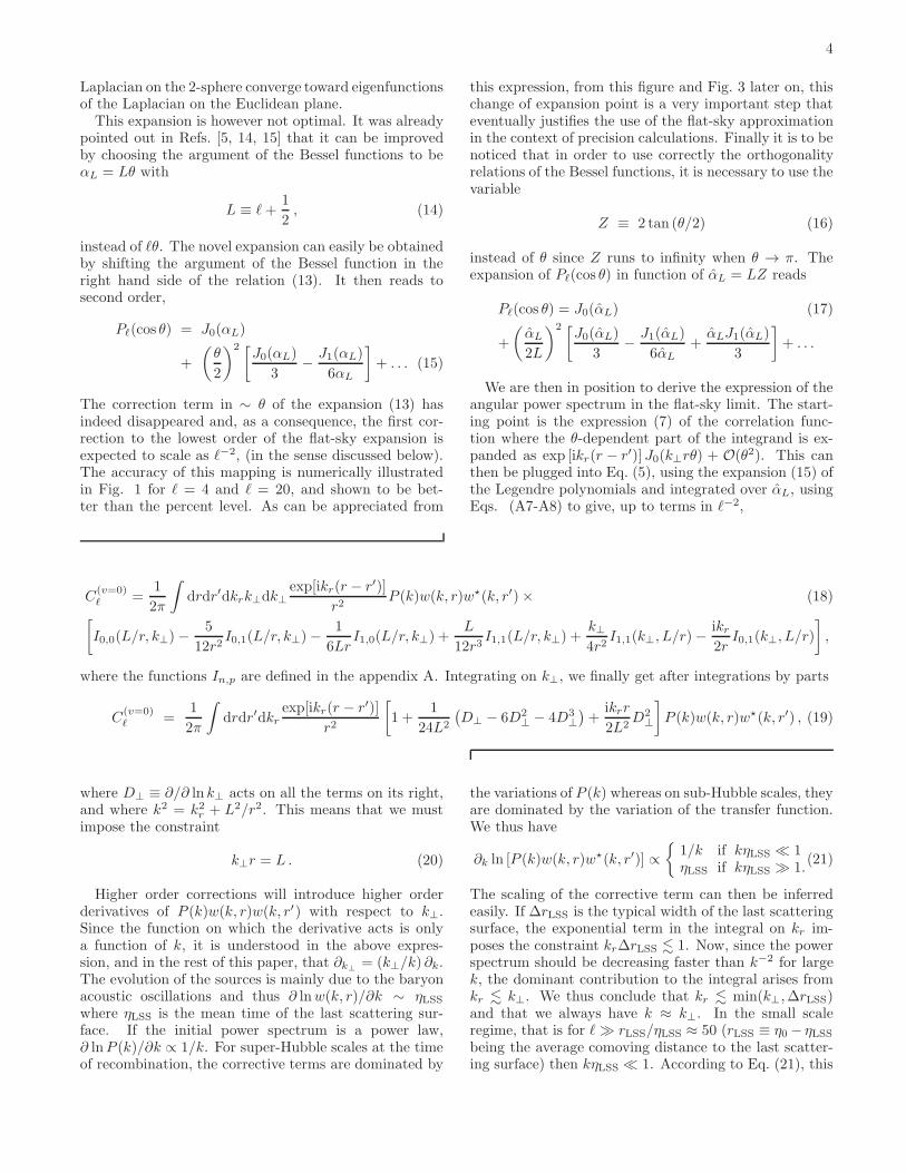
We are then in position to derive the expression of theangular power spectrum in the flat-sky limit. The start-ing point is the expression (7) of the correlation func-tion where the θ-dependent part of the integrand is ex-panded as exp [ikr(r − r′)] J0(k⊥rθ) + O(θ2). This canthen be plugged into Eq. (5), using the expansion (15) ofthe Legendre polynomials and integrated over αL, usingEqs. (A7-A8) to give, up to terms in ℓ−2,

C(v=0)ℓ =

1

2π

∫

drdr′dkrk⊥dk⊥exp[ikr(r − r′)]

r2P (k)w(k, r)w⋆(k, r′)× (18)

[

I0,0(L/r, k⊥)−5

12r2I0,1(L/r, k⊥)−

1

6LrI1,0(L/r, k⊥) +

L

12r3I1,1(L/r, k⊥) +

k⊥4r2

I1,1(k⊥, L/r)−ikr2rI0,1(k⊥, L/r)

]

,

where the functions In,p are defined in the appendix A. Integrating on k⊥, we finally get after integrations by parts

C(v=0)ℓ =

1

2π

∫

drdr′dkrexp[ikr(r − r′)]

r2

[

1 +1

24L2

(

D⊥ − 6D2⊥ − 4D3

⊥

)

+ikrr

2L2D2

⊥

]

P (k)w(k, r)w⋆(k, r′) , (19)

where D⊥ ≡ ∂/∂ ln k⊥ acts on all the terms on its right,and where k2 = k2r + L2/r2. This means that we mustimpose the constraint

k⊥r = L . (20)

Higher order corrections will introduce higher orderderivatives of P (k)w(k, r)w(k, r′) with respect to k⊥.Since the function on which the derivative acts is onlya function of k, it is understood in the above expres-sion, and in the rest of this paper, that ∂k⊥ = (k⊥/k) ∂k.The evolution of the sources is mainly due to the baryonacoustic oscillations and thus ∂ lnw(k, r)/∂k ∼ ηLSSwhere ηLSS is the mean time of the last scattering sur-face. If the initial power spectrum is a power law,∂ lnP (k)/∂k ∝ 1/k. For super-Hubble scales at the timeof recombination, the corrective terms are dominated by

the variations of P (k) whereas on sub-Hubble scales, theyare dominated by the variation of the transfer function.We thus have

∂k ln [P (k)w(k, r)w⋆(k, r′)] ∝

{

1/k if kηLSS ≪ 1ηLSS if kηLSS ≫ 1.

(21)

The scaling of the corrective term can then be inferredeasily. If ∆rLSS is the typical width of the last scatteringsurface, the exponential term in the integral on kr im-poses the constraint kr∆rLSS . 1. Now, since the powerspectrum should be decreasing faster than k−2 for largek, the dominant contribution to the integral arises fromkr . k⊥. We thus conclude that kr . min(k⊥,∆rLSS)and that we always have k ≈ k⊥. In the small scaleregime, that is for ℓ≫ rLSS/ηLSS ≈ 50 (rLSS ≡ η0 − ηLSSbeing the average comoving distance to the last scatter-ing surface) then kηLSS ≪ 1. According to Eq. (21), this

5

0.0 0.5 1.0 1.5

-0.05

0.00

0.05

Θ

P{Hc

osΘL-

Exp

ansi

on

0.0 0.5 1.0 1.5

-0.05

0.00

0.05

Θ

P{Hc

osΘL-

Exp

ansi

on

FIG. 1: Accuracy of the expansions (13) in thin lines and (15) in thick lines. We plot the difference between Pl(cos θ) and itsapproximate forms, at leading order in θ (i.e. J0(lθ), solid lines), first order (long dashed lines), second order (short dashedlines) for ℓ = 4 and as a function of θ (left) and ℓ = 20 (right).

means that the first corrective term is, in this regime, oforder (ηLSS/rLSS)

2 ∼ O(10−4). In the large scale regime,ℓ ≪ rLSS/∆rLSS, and thus k ≈ kr ≈ k⊥. Since for thesemodes ℓ ≪ rLSS/ηLSS, then kηLSS ≪ 1, and this im-plies that the first corrective term scales approximatelyas 1/ℓ2.Concerning the higher order expansion of Eq. (19), we

see that a corrective term of order 1/Ln will involve theoperator Dp

⊥/Ln where p can be any integer, which gives

formally a systematic way of organizing the expansion toany order.To summarize, the precision of the lowest order flat-

sky approximation in the context of CMB calculationsis of order 1/ℓ2 for ℓ . 50 and limited to 10−4 level forℓ & 50, i.e. they are of order max(ℓ−2, ℓ−2

0 ) with ℓ0 = 50.We refer to this first correction as being the correction oforder 1/ℓ2, even if it is limited for small scales becauseof the sub-horizon physics [24].We finally note that in some cases the results can ac-

tually be further improved by choosing the argument ofthe Bessel functions to be αL ≡ Lθ ≡

√

l(l+ 1)θ, sincethen

Pℓ(cos θ) = J0(αL) (22)

+

(

αL2L

)2 [J0(αL)

3− 2J1(αL)

3αL

]

+ . . . .

Indeed, this expansion also removes the corrections scal-ing as ℓ−1 in Eq. (19) since it also does not contain termslinear in θ. Now, the flat-sky constraint reads

k⊥r = L =√

ℓ(ℓ+ 1) . (23)

With this choice, it appears that for any transfer functionw(k, r) that is constant and sharply peaked, i.e. that issuch as w(k, r) = δ(r − rLSS), and for a scale invariantpower spectrum, i.e. P (k) = 2π2A2

sk−3, the lowest order

in the flat-sky expansion takes the form

Cℓ =

∫

dkr2π

1

r2LSSP (k) =

2πA2s

ℓ(ℓ+ 1). (24)

This is precisely the result that one would have obtainedwith the exact (or full spherical sky) calculation since

Cℓ =2

π

∫

dkk2P (k) [jℓ(krLSS)]2=

2πA2s

ℓ(ℓ+ 1).

In other words, with this choice, the leading term of theflat-sky expansion is exact. For CMB on large scales, thisis precisely the case since super-Hubble perturbations arefrozen, leading to the Sachs-Wolfe plateau. Given thatthe initial power spectrum is expected to be almost scale-invariant, we conclude that this expansion of Pℓ(cos θ) isthe best one in the context of CMB computations and weusually adopt it. We can argue that the choice kr = Lis more compact while the choice kr = L gives a bet-ter formula only in the thin-shell approximation. In ap-pendix B we explain how to change the constraint insidethe expressions obtained. In general however, one cannotstate which is the best choice and in the following, unlessstated otherwise, we will use only L.

C. Generalized flat-sky expansions

The derivation of the previous section was limited tothe case v = 0 but, as it appears clearly from the pa-rameterizations (8), it is actually possible to build a two-parameter family of flat-sky approximations, the relationbetween which should be examined.

1. A one-parameter family of flat-sky approximations

The aim of this subsection is to explore the conse-quence of the use of a more general parameterization (8)introducing v as a free parameter. Note that we still keepψ = π although it could be reintroduced at this stage too.Calculations for arbitrary values of ψ are however signifi-cantly more complicated and do not lead to any improved

6

scheme. Then, again, the particular cases v = 0 or v = 1correspond to nz ≡ (0, 0, 1) aligned either with n or n

′

and the case v = 1/2 to nz aligned with (n+ n′)/

√2.

We can now follow the same approach as in section II B.The expansion in powers of Z (instead of θ) can be per-formed with the variables ∆ ≡ r − r′ and

R ≡ r′v + (1− v)r. (25)

Plugging the expansion (17) into Eq. (5) with the defini-tion (7) of the correlation function, one can perform anexpansion in Z and ∆, and then, using the orthonormal-ity relations of appendix A we can compute the integralon αL in function of the In,p(k⊥, L/R). Eventually theresult reads

C(v)ℓ =

∫

drdr′dkr2π

exp(ikr∆)

R2O(v)k⊥P (k)w(k, r)w⋆(k, r′) ,

(26)

where O(v)k⊥

is an operator that applies on the right partof the previous expression with

O(v)k⊥

= 1 +D⊥

24L2− [(4 − 3f1/2)R + f1/2f0∆]

D3⊥

24RL2

−[f1/2f0∆+ 3Rf20 ]

D2⊥

12RL2+ ikr(4f0R+ f1/2∆)

D2⊥

8L2(27)

where f1/2 ≡ 4v(1− v), f0 = 1− 2v and

D⊥ ≡ k⊥∂

∂k⊥=k2⊥k

∂

∂k=

L2

kR2

∂

∂k. (28)

Besides the v = 0 case for which this expression sim-plifies, this is also the case for the symmetric choice,v = 1/2, for which it leads to,

C(v=1/2)ℓ =

∫

drdr′dkr2π

exp(ikr∆)

R2

[

1 +1

24L2

(

D⊥ −D3⊥

)

+ikr∆

8L2D2

⊥

]

P (k)w(k, r)w⋆(k, r′) . (29)

The lowest order of this expression matches the onederived in Ref. [14]. We remind that the constraintk⊥R = L must be satisfied and that this expression isvalid only up to order L−2. In the general case for whichv 6= 1/2, at lowest order in the flat-sky expansion, theexpression would remain formally the same, consideringthat R would then be given by R = r′v+(1−v)r. We willcompare these different parameterizations in the follow-ing paragraph. However, if we also take into account thecorrections, the choice of v would change the expressionof the flat-sky expansion. In appendix B we detail howthe different corrections obtained are consistent with oneanother.

2. Breaking of statistical isotropy and off diagonalcontributions

The existence of mathematically equivalent flat-sky ap-proximations may appear surprising at first view (at leastit surprised the authors) but it can be fully understoodwhen one addresses the construction of the correlators inharmonic space not assuming the statistical isotropy of

the sky.

Indeed an important consequence of the flat-sky ap-proximation is, because a particular direction has beensingled out, to break the statistical isotropy of the sky.There is therefore no reason to have, Cℓ1m1ℓ2m2

=Cℓ1δℓ1ℓ2δm1m2

at any order in flat-sky approximationwhere Cℓ1m1ℓ2m2

is the ensemble average of the productof two spherical harmonics coefficients.

In terms of the two-point angular correlation functionswe have in general,

Cℓ1m1ℓ2m2≡

∫

dn1dn2ξ(n1, n2)Ym1

ℓ1(n1)Y

⋆m2

ℓ2(n2) ,

(30)where ξ(n1, n2) is the correlation function of two givendirections. The difference with Eq. (4) is that we havenot assumed isotropy. If we choose these two directionsto be close to a common direction n, then we can expandthe spherical harmonics of Eq. (30) around that directionwhich is chosen to be aligned with the azimuthal direc-tion and this step breaks explicitly the isotropy of theproblem. At lowest order, this gives (see appendix C)

Y mℓ (n) ≃√

2ℓ+ 1

4π(−1)mJm(ℓθ)eimϕ.

It implies that

Cℓ1m1ℓ2m2≃ δm1m2

Cℓ1ℓ2 , (31)

as a consequence of the preservation of the statisticalrotational invariance around the particular direction n.The term Cℓ1ℓ2 is explicitely given by

Cℓ1ℓ2 ≡ 1

2π

∫

dr1dr2dk⊥k⊥dkrP (k)w(k, r1)w⋆(k,r2)

× exp[ikr(r1 − r2)]δ(k⊥r1 − L1)δ(k⊥r2 − L2)√

L1L2

(32)

where we remind that L ≡ ℓ + 1/2 (or =√

ℓ(ℓ+ 1)).

7

Performing the integrals on r1 and r2 leads to

Cℓ1ℓ2 ≡ 1

2π

∫

dk⊥k⊥

dkrP (k) exp

[

i(L1 − L2)krk⊥

]

×w(

k, L1

k⊥

)

w⋆(

k, L2

k⊥

)

√L1L2

. (33)

In Fig 2 we present Cℓ1ℓ2 in the space of (ℓ1 + ℓ2)/2 and(ℓ1−ℓ2)/2. The main power is carried by multipoles suchthat ℓ1 ≈ ℓ2. The difference between the different possi-ble flat-sky approximations lies precisely in the existenceof (small) off-diagonal terms.

0.1

0.2

0.40.6 0.7

0.8 0.90.95

50 100 150 200 250 300 350 400

0.0

0.2

0.4

0.6

0.8

H{1+{2L�2

H{1-{ 2L�

2

C{1 {2, normalized to unity on{1={2

FIG. 2: Cℓ1ℓ2/Cℓ+ℓ+

with ℓ+ = (L1 + L2)/2 − 1. Most ofthe signal is localized on the diagonal L1 = L2. The choice ofthe path of integration in this space leads to different flat-skyexpansions, that is to different choices of the flat-sky directionn or equivalently of the parameter v. For v = 0 or v = 1, thelowest order of Eq. (19) can be recovered by integrating onan horizontal or a vertical line in the (L1, L2) plane. As forv = 1/2, the lowest order of the expression (29) is recoveredby integrating on the line L1 +L2 =const. The vertical blackline(s) is the superposition of those various integration pathsfor L = 280. On the plot they are hardly distinguishable.

3. Recovering the different flat-sky approximations

Interestingly, each C(v)ℓ can be recovered by a proper

integration of Cℓ1ℓ2 , given by Eq. (32), in the (ℓ1, ℓ2)-plane. Each path of integration corresponds to a way torelate the correlation function ξ(n1, n2) to ξ(θ) definedin Eq. (4).For instance, when v = 0, the expression (19), which is

then the lowest order part of the expression (29), can be

recovered by integrating along the path L1=const., i.e.as

L1Cℓ1 =

∫

dL2

√

L1L2Cℓ1ℓ2 . (34)

The integration along L2=const. corresponds to the casev = 1 and gives by symmetry the same result, which wasexpected since it corresponds to exchanging n1 and n2.The symmetric case v = 1/2 can be recovered by inte-

grating on the path L1 + L2=const. Making the changeof variables

L+ =L1 + L2

2, L− =

L1 − L2

2, (35)

we thus obtain

Cℓ1 =

∫

dL−

2

√L1L2

L+Cℓ1ℓ2

=

∫

dL−

2

√

(

1− L2−

L2+

)

Cℓ1ℓ2 . (36)

Actually, for a general v, the lowest order of the ex-pression (29) is recovered by integrating on the path ofequation

L2/L1 = (v − 1)/v (37)

in this plane. The case of ψ 6= π in Eq. (8) leads tosimilar constructions but with slightly more complicatedintegration paths. To show it let us reintroduce ψ inEq. (8). Then the angular separation θ of the directionsn and n′ reads

θ2 = (v2 + (1− v)2 − 2v(1− v) cosψ)θ2 (38)

and the effective radius R (as it appears in the argumentof J0) is

R2 = (r2v2 + r′2(1 − v)2 − 2rr′v(1 − v) cosψ)θ2 (39)

with the relation

Lθ = k⊥R. (40)

The relation between L, L1 and L2 then follows from therelations L1 = rk⊥ and L2 = r′k⊥. It reads,

L2 =v2L2

1 + (1− v)2L22 − 2v(1− v) cosψL1L2

v2 + (1− v)2 − 2v(1− v) cosψ(41)

which describes the arc of an ellipse in the (L1, L2) plane.All these approximations are a priori of similar precision.Note however that when ψ is small, θ should be large inorder to keep θ fixed making the various expansions lessprecise. It then corresponds to a very squeezed ellipse inthe (L1, L2) plane.

8

III. TWO LIMIT CASES

It is worth remarking that in either Eq. (19) or moregenerally in Eq. (29), the computation of power spectraat leading order involves a genuine 3D numerical integra-tion. It is therefore numerically less favorable than exactcalculations (which involves only two integrals [12, 16][25].) It is just more transparent since it does not re-quire the computation of spherical Bessel functions, andgeometrically more transparent since the results are pre-sented in a Cartesian form.Depending on the physical situation, it is however pos-

sible to introduce simplifications that will make the com-putations faster.

A. The Limber approximation

Let us first consider the situation in which the sourcesstretch in a wide range of distances ∆r and varysmoothly. As long as ℓ/r × ∆r ≫ 1, it implies thatk⊥∆r ≫ 1. As a consequence, the contributions in theintegral on kr are approximately ranging from −1/∆r to

1/∆r, that is in a range of values where k =√

k2⊥ + k2r ≃k⊥ and all functions except the exponential in the inte-grand can be considered constant.The Limber approximation then consists in replacing

∫

dkr exp[ikr(r − r′)]

by 2πδ(r − r′) so that the integral on r′ can then beperformed trivially. We finally obtain, at lowest orderin powers of ℓ−1

Cℓ =

∫

dr

∣

∣

∣

∣

w(k, r)

r

∣

∣

∣

∣

2

P (k) , (42)

with the Limber constraint kr = L. The first correctionsscale as L−2 and have been computed in Ref. [5]. Wecan recover this result from Eq. (29), by expanding allfunctions of k around k⊥ as

f(k) = f(k⊥) +k2r2k⊥

∂f(k)

∂k

∣

∣

∣

∣

k=k⊥

+ . . .

This will result in a term proportional to k2r which canbe handled using

∫

dkr(ikr)n exp[ikr∆] = 2πδ{n}(∆) , (43)

where δ{n} is the n-th derivative of the Dirac distribution.The term proportional to kr in Eq. (29) can be handledin the same way and gives δ′(∆). Integrating by partsin ∆ removes the derivatives of the Dirac distributions,using that ∂R/∂r = 1 − v and ∂R/∂r′ = v. Then, theintegral on r′ is trivial, because of the Dirac distributions,and one can then perform an integration by parts in r inorder to reshape the result. We finally obtain

C(v=1/2)ℓ =

∫

dr

r2

{

P (k) |w(k, r)|2 + D

2L2

[

r

∣

∣

∣

∣

∂ [w(k, r)/√r]

∂ ln r

∣

∣

∣

∣

2

P (k)

]

− D2

2L2[w(k, r)2P (k)]− D3

6L2[w(k, r)2P (k)]

}

(44)

where Dn ≡ kn∂/∂kn and we recover the result ofRef. [5]. The Limber approximation is not well suitedfor CMB computation since its hypothesis is not satis-fied during recombination. However, when it comes tothe contributions of the reionization era, sources stretchin a wide range of distances and the Limber approxi-mation can be used. Special care must be taken thoughbecause the source have a directional dependence and arenot simple scalar valued sources. The main sources are(i) the Sachs-Wolfe contribution δr/4+Φ where δr is thedensity contrast of the radiation (ii) the late variation Φ′

of the gravitational potential, and (iii) the Doppler con-tribution ni∂iv, where v is the scalar part of the baryonvelocity. A naive estimation would lead to think that theDoppler effect is the most significant contribution sincev ∼ (rLSS − r) while the intrinsic Sachs-Wolfe term re-mains of order one. However, in Fourier space this leadsto a term proportional to krv, and it cannot be dealtwith the naive replacement kr → 0 since this would van-

ish. Instead, it should be treated using Eq. (43) andit leads to replace the Doppler source by idv/dr (if weignore the derivatives of 1/r) before taking the lowestorder of the Limber approximation, and this then givesa contribution of order unity as well. Physically, thismeans that the modes which favor the Doppler effect arethose aligned with the line-of-sight ni, but the contribu-tion of these modes is further suppressed in the Limberapproximation for sources stretching in a wide range ofdistances. See Section IV below for a discussion on theflat-sky expansion in general in the case of sources withintrinsic directional dependence. Furthermore, if we de-cide to consider the late Integrated Sachs-Wolfe (ISW)effect which is due to the variation of the gravitationalpotentials, the Limber approximation is satisfactory aswell. We shall not consider any of these in this articleand focus our attention to the effects that occur duringthe recombination.

9

B. The thin-shell approximation

A useful approximation can be derived when thesources are contributing only in a thin range of distances.

Indeed, in such a case the factors 1/r2 or 1/R2 can bereplaced by 1/r2LSS, where rLSS is the mean distance ofthe sources each time one has to compute k (e.g. k =√

k2r + L2/R2 is replaced by kLSS ≡√

k2r + L2/r2LSS).The integrals on r and r′ in the lowest order term ofexpression (29) can be factorized and we obtain the thin-shell flat-sky approximation

Cℓ =1

r2LSS

∫

dkr2π

∣

∣

∣

∣

∫

dr exp(ikrr)w(kLSS, r)

∣

∣

∣

∣

2

P (kLSS) .

(45)In the full-sky computation, this factorization is auto-matic since there is also an integral over r, which is thensquared, and another integral over k. In general, the flat-sky expansion breaks this property, and it is recovered inthe thin-shell approximation.

Estimating the error introduced by the thin-shell ap-proximation is actually difficult and quite model de-pendent. First the error introduced by replacing thefactor 1/R2 by 1/r2LSS will be very limited if rLSS istaken in the middle of the LSS and should be muchless than ∆rLSS/rLSS. However we also need to esti-mate the error introduced by the approximation of theflat-sky constraint. Depending on the k dependence ofS(k, r) ≡ w(k, r)w(k, r′)⋆P (k), this will lead to two ex-treme cases. If it is a pure power law and depends onlyon k, then S(k) ≃ S(kLSS)− (R− rLSS)/rLSSD⊥S(kLSS)and again if rLSS is chosen in the middle of the LSS, af-ter integration on r and r′, the error would be muchsmaller than ∆rLSS/rLSS. However if the sources arepurely oscillatory with frequency k, which is the casefor the small scales, that is if S(k, r) ∝ cos(kr) for in-stance, the relative error introduced would be of order∆rLSS/rLSS. So for small scales, this is much larger thanthe first corrections in the expression (19) which scaleas max(ℓ−2, ℓ−2

0 ) with ℓ0 ≡ rLSS/ηLSS ≃ 50. We shallsee in the next section that it is in principle comparableon small scales to the larger corrections introduced whenwe consider the non-scalar nature of the sources whichare of order max(ℓ−1, ℓ−1

0 ). However, in practice the er-ror introduced in the thin-shell approximation is smallersince ∆rLSS < ηLSS and also because the sources are notpurely oscillatory and converge to a power-law on smallscales thanks to viscous effects, thus reducing further theerror made.

We can also try to compute corrective terms to thethin-shell approximation. This correction is obtained byexpanding R around rLSS but also k around kLSS and isgiven at lowest order of this expansion by

δCthin shellℓ = (46)

∫

drdr′dkr2π

exp(ikr∆)

r2LSSδOP (kLSS)w(kLSS, r)w⋆(kLSS, r′) ,

with

δO ≡[

1− (R− rLSS)

rLSS(2 +D⊥)

]

. (47)

Since R− rLSS = v[r′ − rLSS] + (1− v)[r− rLSS] the inte-grals on r and r′ in the expression of this correction canalso be expressed as a sum of factorized integrals, whichmeans that numerically it corresponds effectively to sumsof two-dimensional integrals. On large scales the operatorD⊥ acts mainly on P (kLSS) since it contains the domi-nant k dependence (see the discussion in section II B).However on small scales the dependence in k is domi-nated by the source terms w(kLSS, r) and w⋆(kLSS, r

′),and this lowest order correction is not valid given the nu-merous oscillations of the sources. However for a sourcewhich depends purely on kr, as is roughly the case forthe baryon acoustic oscillations, then on small scales itdepends nearly on k⊥r since k ≃ k⊥, and the error intro-duced by replacing k with kLSS can be seen as an errorin the placement of the distance r at which the sourceis emitting. In that limit case, everything happens as ifthe visibility function contained in the expression of thesource w(k, r) was slighlty distorted when performing thethin-shell approximation. In practice, we shall not cor-rect for this since the source is not purely depending onkr on small scales. This means that we should make theoperatorD⊥ contained in δO act only on P (kLSS) for ourpractical purposes when using Eq. (46) to correct for thethin-shell approximation that we take.In the context of CMB, the use of the thin-shell approx-

imation requires to rewrite the source in order to localizethe physical effects on the LSS. In practice, the termsinvolving the gravitational potential Φ, i.e. of the typeni∂iΦ [11, 12], whose contribution would stretch fromthe LSS up to now, are replaced by dΦ/dr − ∂Φ/∂r.This clearly splits the effect into an effect on the LSS(dΦ/dr), the Einstein effect, and an integrated effect(∂Φ/∂r) which is negligible for a matter dominated uni-verse since the potential is then constant. Should weconsider the effect of the cosmological constant on thevariation of the gravitational potential, then we coulduse the Limber approximation discussed in the previousparagraph, and sum the resulting Cℓ to the contributionof the LSS.In Fig. 3, we present the flat-sky approximation for

an instantaneous recombination, including only the in-trinsic Sachs-Wolfe effect in order for the source to bepurely scalar. The corrections in the thin-shell approx-imation can be read from the expression (29). Howeverfor practical purposes, the derivatives with respect to k⊥need to be converted into derivatives with respect to k sothat their action on w(k, r)w(k, r′)⋆P (k) is clearer. How-ever, as we shall see in Section IV, for realistic purposes,the sources are not a pure scalar and have an intrinsicgeometric dependence so that the first correction will ac-tually scale as L−1.It is interesting to remark that all flat-sky expansions

will lead to the same expressions at lowest order in the

10

2 5 10 50 100 500 10000

1000

2000

3000

4000

5000

600090° 45° 10° 2° 0.5° 0.2°

{

HT0L2{H{+1L C{

QQ�H2ΠL ΜK2

2 5 10 50 100 500 1000

-4

-2

0

2

4

90° 45° 10° 2° 0.5° 0.2°

{

Relative error in%

FIG. 3: Left: Comparison of the flat-sky approximations (with k⊥r = ℓ in dashed line and with k⊥r =√

ℓ(ℓ+ 1) in dotted line)to the exact computation (solid line). We consider the standard cosmology with an instantaneous recombination and ignore alleffects but the intrinsic Sachs-Wolfe effect (Θ = δr/4+Φ). Right: The relative errors of these two flat-sky approximations withrespect to the exact computation. The first method is limited to a 1% relative error above ℓ = 100, as discussed in Section IIB,whereas the second one is much better since the first corrections scale as ℓ−2.

thin-shell approximation and in the Limber approxima-tion, since then, as we have already seen, the lowest orderdoes not depend on the choice of v (nor ψ). In the caseof the thin-shell this can be understood from Fig. 2. Thethiner the shell, the more the function Cℓ1ℓ2 is peaked onthe diagonal L1 = L2 and the less the integral dependson the line of integration in the (L1, L2) plane. On Fig. 2,we plot two contours of integration corresponding respec-tively to v = 0 and v = 1, and it can be understood thatthe integrals obtained on these contours cannot be verydifferent. The Limber case is similar since the factor

∫

dkr exp

[

i(L1 − L2)krk⊥

]

(48)

in Eq. (33) is approximated to be 2πk⊥δ(L1 − L2).

IV. EFFECT OF NON-SCALAR SOURCE

TERMS

So far, we have assumed that the transer function wasscalar, in the sense that it was a function w(k, r) that

does not depend on k and n, that is the expansion (3)contained only a term w00. In general, this is not thecase since scalar perturbations involve m = 0 terms withℓ = 1 (Doppler effect) while vector perturbations andgravity waves generates terms with m = 1 and m = 2respectively.In order to take this dependence into account in the

flat-sky analysis, one needs to compute Eq. (7) with thesource (3). From the parameterization (8) with the choiceϕ = 0, we deduce that

k.n =1

k

[

kr + k⊥θ

2cos(β) +O(θ2)

]

(49)

on small scales, where we remind that β is defined in theparameterization (10) of k.

A. Lowest order flat-sky expansion

As long as we consider only scalar perturbations, thesource term will contain wjm terms with m = 0. Notethat this is different from our previous assumption thatonly w00 was not vanishing.The expansion (3) contains only terms in Y j0

k(n) which

are proportional to Pj(k.n). At lowest order in θ,

Pmj (k.n) depends only on kr/k so that the flat-sky ex-pansion remains unchanged as long as we make the re-placement

w(k, r) →∑

j

ijwj0(k, r)Pj(kr/k) . (50)

In conclusion, the formal expression of the flat-sky ap-proximation at lowest order remains unchanged for cos-mological scalar perturbations (which are the dominantsources of CMB anisotropies).

B. First correction

We have seen that for scalar field sources, the firstcorrection scale as ℓ−2. However, for the general case, thefirst correction arises from the first correction in (49) andscales as ℓ−1. Since the dominant effects come from j = 0and j = 1, we can ignore the contribution coming fromj = 2 in the computation and there is no contribution

11

for j ≥ 3. Thus, we restrict to

w(k, n, r) = [w00(k, r) + ikrkw10(k, r)]

+θ

2

[

ik⊥kw10(k, r) cos β

]

+O(θ2) .(51)

In the two-point correlation function, the first correctionwill arise from the product of the first order of w(k, n, r)with its lowest order term. Using the symmetry of theintegral in kr the first corrective term due to the geometryof the sources is thus

w(k, n, r)w⋆(k, n′, r′) ≃ (52)[

w00(k, r) + ikrkw10(k, r)

] [

w00(k, r′) + i

krkw10(k, r

′)

]⋆

+θ

2i cosβ

k⊥k

[w00(k, r)w⋆10(k, r

′) + w10(k, r)w⋆00(k, r

′)]

≡ ww⋆(k, r, r′) + θi cosβ (ww⋆)(1)

(k, r, r′) .

In order to go from Eq. (2) to Eq. (7), the integral overβ will give a term −J1[k⊥RZ] instead of the previousterm J0[k⊥RZ] (due to the factor i cosβ). Following theexactly same method as in Section II C, we obtain theflat-sky expression with the first correction included

Cℓ =

∫

drdr′dkr2π

exp[ikr(r − r′)]

R2

{

P (k)ww⋆(k, r, r′)

−D⊥

k2⊥r

[

k⊥P (k) (ww⋆)

(1)(k, r, r′)

] }

, (53)

where we can take either the flat-sky constraint k⊥R = Lor k⊥R = L given that the corrections to this expressionare of order ℓ−2. This expression can be further sim-plified in the thin-shell approximation and can then befurther improved by including the corrections due to thisthin-shell approximation given in Eq. (46). Similarly toour discussion at the end of Section II B, the first cor-rective term which comes from the second term in thecurly brackets in the expression above, is of order 1/ℓ upto ℓ ≃ 100 and then of the order of 1% beyond. Includ-ing this first correction to the lowest order of the flat-skyexpansion (the first term in the curly brackets in the ex-pression above) considerably improves the precision ofthe flat-sky expansion. Note that the corrective termsin the expression (29) were at least of order 1/ℓ2, andthus the corrective term in the expression (53), whichcomes from the directional dependence of the sources, isthe dominant one. To compare with Eq. (29), one wouldneed to derive the corrections of order 1/ℓ2 in Eq. (53),which seems an unneeded academic sophistication. Fig. 4depicts the relative error with respect to the exact calcu-lation, with and without including the first correction oforder 1/ℓ given in Eq. (53), using the thin-shell approx-imation and taking into account all effects but the lateintegrated Sachs-Wolfe effect.

V. FLAT-SKY EXPANSION OF HIGHER SPIN

QUANTITIES

The CMB radiation is not described entirely by itstemperature, since it is polarized by the Compton scat-tering of photons on free electrons. Only the linear po-larization is generated through this process and it is de-scribed by the spin ±2 fields defined from the Stokesparameters

±2X(n) ≡ Q(n)± iU(n) . (54)

±2X(n) is dependent on the choice of the basis used todefined the linear polarization. Any rotation of this basisby an angle γ around the direction n transforms it as

±2X(n) →±2 X(n)e±2iγ .In order to define the correlation function of two

spinned quantities, s1X and s2Y , one shall use the spinraising and lowering operators, respectively ′∂+ and ′∂−

which are defined for a spin s quantity by [1, 17]

′∂±sX = − sin±s (∂θ ± i csc θ∂ϕ) sin∓s

sX (55)

in order to relate them to a spin-0 field. We thus define

sX ≡ (−1)s ′∂−ssX, sX ≡ ′∂−ssX (56)

respectively for s > 0 and s < 0. The expansion of sXon spinned spherical harmonics according to

sX(n) =∑

ℓm

sXℓm sYmℓ (n) (57)

can then be related to its expansion on spherical harmon-ics as

sX(n) =∑

ℓm

sXℓm

√

(ℓ+ |s|)!(ℓ− |s|)!Y

mℓ (n) . (58)

The two sets of spherical harmonics are related by

(−1)s ′∂−ssYmℓ =

√

(ℓ+ s)!

(ℓ− s)!Y mℓ if s > 0, (59)

′∂−ssYmℓ =

√

(ℓ− s)!

(ℓ+ s)!Y mℓ if s < 0.

We further define the electric and magnetic parts as

E(X)(n) ≡ 1

2

[

sX(n) + −sX(n)]

, (60)

B(X)(n) ≡ 1

2i

[

sX(n)− −sX(n)]

, (61)

where here we choose the convention s ≥ 0. For a spin0 quantity such as the temperature, E(0X) = 0X = 0Xand B(0X) = 0. Due to parity invariance, the correlationbetween an electric type quantity and a magnetic type

12

2 5 10 50 100 500 10000

1000

2000

3000

4000

5000

6000

700090° 45° 10° 2° 0.5° 0.2°

{

HT0L2{H{+1L C{

QQ�H2ΠL ΜK2

5 10 50 100 500 1000

-4

-2

0

2

4

45° 10° 2° 0.5° 0.2°

{

Relative error in%

FIG. 4: Left: Comparison of the flat-sky approximations with the constraint k⊥r =√

ℓ(ℓ+ 1) while including only the lowestorder in the expression (53) (dashed line) or adding its correction of order ℓ−1 (dotted line) to the exact computation (solidline, standard cosmology, ignoring only the late time ISW effect). The calculations in the flat-sky approximations have beendone using the thin-shell approximation.Right: The relative errors of these two approximations with respect to the exact computation in respectively continuous forthe lowest order expression and dashed line when including the first correction in ℓ−1. In dotted line we also compute the errorwhen adding on top of the order ℓ−1 correction, the correction of Eq. (46) due to the thin-shell approximation. The lowestorder is limited to a 1% relative error beyond ℓ = 100 whereas the first correction increases substantially the presicion on smallscales and the correction for the thin-shell approximation improves also the largest scales.

quantity always vanishes. We then define the correlationfunction as

ξE(X)E(Y )(θ) = 〈E(X)(n)E(Y )(n′)⋆〉n.n′=cos θ (62)

≡∑

ℓ

2ℓ+ 1

4π

√

(ℓ+ s1)!

(ℓ− s1)!

(ℓ + s2)!

(ℓ − s2)!CE(X)E(Y )ℓ Pℓ(cos θ) ,

with similar definitions for magnetic type multipoles.The angular power spectra are then extracted through

CE(X)E(Y )ℓ = 2π

√

(ℓ− s1)!

(ℓ+ s1)!

(ℓ − s2)!

(ℓ + s2)!(63)

×∫

sin θdθ Pℓ(cos θ)ξE(X)E(Y )(θ) .

The emitting sources for a spin s quantity are expandedsimilarly to Eq. (3) but with a decomposition on spinnedspherical harmonics

w[sX ](x) =

∫

d3k

(2π)3/2w[sX ](k, n, r) exp(ik.x) (64)

with

w[sX ](k, n, r) =∑

ℓ,m

wℓm[−sX ](k, r)(iℓ)

√

4π

2ℓ+ 1

×sY ℓmk (n)eisϕ(k,n) , (65)

where ϕ(k, n) is the azimuthal angle of k with respect ton [1]. The source multipoles for spinned quantities are

defined using the same conventions as in Refs. [12, 13]except that the multipoles here refer to the direction ofobservation whereas in these references it refers to the di-rection of propagation. We have thus made the replace-ment s→ −s additionally to the extra factor (−1)ℓ whichwas already considered for spin 0 quantities in Eq. (3),in order to take this fact into account by using the trans-formation properties under parity of the multipoles.At the lowest order of the flat-sky expansion, we can

approximate ϕ(k, n) by β. In particular, this impliesthat the spin raising and lowering operators applied onw[sX ] will act only on exp(ik.x) and we find that atlowest order in the flat-sky expansion

′∂±s exp(ik.x) ≃ (−ikr)se∓is(ϕ−β) exp(ik.x), (66)

for s > 0. We thus deduce that the sources for E(sX)and B(sX) are given by

w[(E/B)(sX)](k, n, r) =∑

ℓ,m

(ikr)s(i)ℓ√

4π

2ℓ+ 1(67)

{

±1

2wℓm[(E/B)(X)](k, r)

×[

(−1)se−isϕ−sY

ℓmk

(n) + eisϕsYℓmk

(n)]

+i

2wℓm[(B/E)(X)](k, r)

×[

(−1)se−isϕ−sY

ℓmk (n)− eisϕsY

ℓmk (n)

]}

,

with the + sign for E and the − sign for B.

13

In the case where there are only scalar sources (m = 0),this simplifies substantially. From the parameterization(8), that is with the choice ϕ = 0 and using that sY

ℓ0 =(−1)sY ℓs, we obtain

w[E(X)](k, n, r) = (68)

∑

ℓ

(−ikr)s(i)ℓwℓ[E(X)](k, r)

√

(ℓ− s)!

(ℓ+ s)!P sℓ (kr/k)

and a vanishing w[B(X)]. Following the same methodas in section II B, the factors (kr)(s1+s2) are going tobe approximately canceled by the prefactor of Eq. (64)which is behaving as ℓ−(s1+s2). A more careful derivationwould require to use k =

√

k2⊥ + k2r and the exact formof the prefactor in Eq. (64). However, we are here inter-ested in the most simple expression for the lowest orderof the flat-sky expansion and we drop these extra com-plications. Since polarization is not generated on largescales, this will be sufficient to obtain an excellent flat-sky expansion. In the end of the computation, for scalarperturbations the multipoles associated with the corre-lation of spinned quantities is obtained just by replacingthe sources according to

w(k, r) →∑

ℓ

(−1)siℓ+swℓ0[E](k, r)

√

(ℓ − s)!

(ℓ + s)!P sℓ

(

krk

)

.

We use this expression for the computation of the sourcesof linear polarization (s = 2, and only ℓ = 2 in the sumabove since there are only quadrupolar sources), and wecompare the full-sky computation of CEEℓ and CΘE

ℓ withthe flat-sky result in Fig. 5

VI. THE BISPECTRUM

We shall now investigate the flat-sky expansion of thebispectrum. We shall assume that it arises from pri-mordial non-Gaussian initial conditions described by aprimordial bispectrum for the metric fluctuation, e.g.,

〈Φ(k1)Φ(k2)Φ(k3)〉 = δ3(k1 + k2 + k3)B(k1,k2) . (69)

As we shall see the derivation of the temperature bis-pectrum is much more subtle and we only partially suc-ceeded in a sense we explain below. The reason lies in thefact that there are actually many ways of representing abispectrum the properties of which in the flat-sky limitmight be different.

A. Two different representations of the bispectrum

in harmonic space

1. Definitions

We are interested in the expectation values of〈aℓ1m1

aℓ2m2aℓ3m3

〉 of the aℓm coefficients of the CMB

temperature. Because of the statistical isotropy of thesky, theirm-dependence is bound to be that of the Gauntintegral Gℓ1ℓ2ℓ3m1m2m3

so that it is more fruitful to introducethe reduced bispectrum bℓ1ℓ2ℓ3 (see Ref. [18] for instance)defined as

〈aℓ1m1aℓ2m2

aℓ3m3〉 ≡ Gℓ1ℓ2ℓ3m1m2m3

bℓ1ℓ2ℓ3 . (70)

The a priori purpose of the following is to propose a con-trolled approximation for bℓ1ℓ2ℓ3 in the flat-sky limit. Itturns out however, as we shall see later, that in orderto have a controlled limit expression of that quantity,strong regularity conditions should be imposed on theinitial metric perturbation B(k1,k2).The bispectrum can actually be equally characterized

by the following quantities (reminding L ≡ ℓ+ 1/2),

ξℓ1ℓ2M =∑

ℓ3

2L3

(

ℓ1 ℓ2 ℓ3M −M 0

)(

ℓ1 ℓ2 ℓ30 0 0

)

bℓ1ℓ2ℓ3 ,

(71)that contains the same information as bℓ1ℓ2ℓ3 since it canbe inverted as

bℓ1ℓ2ℓ3 =∑

M

(

ℓ1 ℓ2 ℓ3M −M 0

)

(

ℓ1 ℓ2 ℓ30 0 0

) ξℓ1ℓ2M . (72)

ξℓ1ℓ2M is a real-valued quantity that obeys the followingsymmetry properties

ξℓ1ℓ2M = ξℓ1ℓ2−M = ξℓ2ℓ1M . (73)

As we shall see, ξℓ1ℓ2M actually enjoys a better-controlledasymptotic expression than bℓ1ℓ2ℓ3 in the large ℓ limit,similar to what was achieved for the angular power spec-trum in the previous sections.

2. Properties of ξℓ1ℓ2M

Let us first relate ξℓ1ℓ2M to the angular three-pointfunction. We introduce three unit vectors on the celestialsphere, n1, n2 and n3, by

ni = (sin θi cosϕi, sin θi sinϕi, cos θi), (74)

where θi and ϕi are the Euler angles and i = 1..3. Tak-ing advantage of the statistical isotropy of the sky, thethree-point temperature correlation function can alwaysbe expressed as a function of the relative angle with re-spect to say n3, setting θ3 = 0, so as a function of thefour angles, (θ1, ϕ1, θ2, ϕ2). These dependencies can thenbe expanded on spherical harmonics as

〈Θ(n1)Θ(n2)Θ(n3)〉 ≡ ξ(θ1, ϕ1, θ2, ϕ2) (75)

=∑

ℓi,mi

ξℓ1ℓ2m1m2

√

2L1

4π

2L2

4πY m1

ℓ1(θ1, ϕ1)Y

m2

ℓ2(θ2, ϕ2) .

14

2 5 10 50 100 500 1000-150

-100

-50

0

50

100

15090° 45° 10° 2° 0.5° 0.2°

{

HT0L2{H{+1L C{

QE�H2ΠL ΜK2

2 5 10 50 100 500 1000-6

-5

-4

-3

-2

-1

0

1

90° 45° 10° 2° 0.5° 0.2°

{

Log10@HT0L2{H{+1L C{

EE�H2ΠLD ΜK2

FIG. 5: Comparison of the flat-sky approximation (dashed line) to the exact computation (solid line) for CΘE

ℓ (left) and CEE

ℓ

(right) ignoring the effect of reionization. Since they only disagree on very large scales, in the regime where the polarizationfails to be generated, both curves are hardly distinguishible. We assume standard cosmology.

Rotational invariance further implies that ξ depends onlyon ϕ21 ≡ ϕ2−ϕ1 so that ξℓ′

1ℓ′2m′

1m′

2vanishes ifm′

1 6= −m′2.

We conclude that

ξ(θ1, ϕ1, θ2, ϕ2) = (76)

∑

ℓ1,ℓ2,M

ξℓ1ℓ2M−M

√

2L1

4π

2L2

4πYMℓ′

1(θ1, ϕ1)Y

−Mℓ′2

(θ2, ϕ2) .

This expression generalizes the expansion of the two-point correlation function in terms of Pℓ(θ).

3. Relation between ξℓ1ℓ2M and the bispectrum

To obtain such a relation, we need to express ξ in termsof directions n1, n2, n3 instead of relative angles. Thiscan be achieved by performing a rotationR, under whichthe sperical harmonics transform as

Y mℓ (R−1n) =∑

m′

Y m′

ℓ (n)Dℓm′m(R) (77)

where Dℓm′m are the rotation matrices and can be ex-

pressed in terms of spin-weighted spherical harmonics as

Dℓ−ms(ϕ, θ, ψ) = (−1)m

√

4π

2LsY

mℓ (θ, ϕ) e−isψ . (78)

It follows that

ξ(n1, n2, n3) =∑

ℓ1,ℓ2,M,m1,m2

ξℓ1ℓ2M−M (79)

×Y m1∗ℓ1

(n1) MYm1

ℓ1(n3) Y

m2∗ℓ2

(n2) −MYm2

ℓ2(n3).

Using∫

d2n s1Ym1

ℓ1(n) s2Y

m2

ℓ2(n) s3Y

m3

ℓ3(n) = (80)

√

8L1L2L3

4π

(

ℓ1 ℓ2 ℓ3s1 s2 s3

) (

ℓ1 ℓ2 ℓ3m1 m2 m3

)

when s1 + s2 + s3 = 0, we obtain

bℓ1,ℓ2,ℓ3 =∑

M

(

ℓ1 ℓ2 ℓ3M −M 0

)

(

ℓ1 ℓ2 ℓ30 0 0

) ξℓ1ℓ2M−M . (81)

This shows that the coefficients ξℓ1ℓ2M−M are nothingbut the parameters ξℓ1ℓ2M that we introduced earlier asan alternative description of the bispectrum,

ξℓ1ℓ2M = ξℓ1ℓ2M−M . (82)

They can therefore be expressed in terms of the real spacecorrelation function,

ξℓ1ℓ2M =4π√

2L12L2

∫

d2n1d2n2ξ(θ1, ϕ1, θ2, ϕ2)

×YMℓ1 (θ1, ϕ1)Y−Mℓ2

(θ2, ϕ2) (83)

=8π2

√2L12L2

∫

sin θ1dθ1

∫

sin θ2dθ2

∫

dϕ21

×YMℓ1 (θ1, 0)Y−Mℓ2

(θ2, ϕ21) ξ(θ1, 0, θ2, ϕ21).

This is the generalisation of Eq. (5) for the bispectrum.

B. Flat-sky limit of ξℓ1ℓ2M

We follow the same path as for the power spectrum.The first step is then to provide a formal expression of

15

the three-point correlation function in real space. Setting

xi = rini, (84)

for i = 1...3 and

k1 = (k1 sinα1 cosβ1, k1 sinα1 sinβ1, k1 cosα1)

= (k⊥1 cosβ1, k⊥1 sinβ1, k

z1), (85)

k2 = (k⊥2 cosβ2, k⊥2 sinβ2, k

z2) . (86)

Formally the three-point temperature correlation func-tion then reads

ξ(θ1, ϕ1, θ2, ϕ2) =

∫

d3k1d3k2 dr1 dr2 dr3B(k1,k2) exp [ik

z1(r1 cos θ1 − r3) + ikz2(r2 cos θ2 − r3)]

×w(k1, r1)w(k2, r2)w(|k3|, r3) exp[

ik⊥1 r1 sin θ1 cos(β1 − ϕ1) + ik⊥2 r2 sin θ2 cos(β2 − ϕ2)]

,(87)

where the Dirac distribution of Eq. (69) has been takeninto account. We are left with a function of the relativeangles (θ1, ϕ1) and (θ2, ϕ2).For a fixed value of M , YMℓ (θ, ϕ) has a well con-

trolled limit in the flat-sky approximation. It is givenby Eq. (8.722) of Ref. [19]

YMℓ (θ, ϕ) →(

2L

4π

)1/2

(−1)MJM [Lθ]eiMϕ . (88)

In appendix C, we show how the next to leading orderterms of this expression can be obtained. The expan-sion parameter is M/ℓ or Mθ. The completion of thecalculation then relies on the relation,

∫ ∞

0

xJM (ax)JM (bx)dx =δ(a− b)

b. (89)

We can now proceed to the evaluation of (83) in theflat-sky limit, as it is now straightforward. Defin-ing ρ1 = k⊥1 r1θ1 and ρ2 = k⊥2 r2θ2 the expression ofξ(θ1, ϕ1, θ2, ϕ2) at leading order is

ξ(θ1, 0, θ2, ϕ21) = (90)∫

d3k1d3k2 dr1 dr2 dr3 B(k1,k2)

[

∏

a=1,2,3

w(ka, ra)

]

exp

[

i∑

a=1,2

kzara3

]

exp [iρ1 cosβ1 + iρ2 cos(β2 − ϕ21)] ,

with ri3 ≡ ri − r3, and k3 ≡ |k3|. Then the subse-quent angular integrations that appear in the expressionof ξℓ1ℓ2M in Eq. (83) lead to the following transforms:

• the integration over ϕ21 ofexp [iρ2 cos(β2 − ϕ1)− iMϕ21] gives a termiMJM (ρ2) e

iMβ2 ;

• the integration over β1, fixing the relativeangle β12 between the wave vectors k1 and

k2, of exp [iρ1 cosβ1 + iMβ2] gives a term(−i)MJM (ρ1) e

iMβ12 ;

• the integration over θ1 of JM (ρ1)JM (L1θ1) gives aterm δ(L1 − k⊥1 r1)/L1;

• the integration over θ2 of JM (ρ2)JM (L2θ2) gives aterm δ(L2 − k⊥2 r2)/L2.

Then, the integration over k⊥1 and k⊥2 can be performedexplicitly and we are left with

ξℓ1ℓ2M =

∫ 2π

0

dβ{k}

2πeiMβ{k} bfsℓ1ℓ2(β{k}) (91)

where

bfsℓ1ℓ2(β{k}) =

∫

dkz1 dkz2 dr1 dr2 dr3

w(k1, r1)

r21

w(k2, r2)

r22×w(k3, r3)B(k1,k2) exp [ik

z1r13 + ikz2r23] .(92)

In this expression,

k21 = kz12 + L2

1/r21 , k22 = kz2

2 + L22/r

22, (93)

and B(k1,k2) is an implicit relation of kz1 , kz2 and of the

relative angle of their transverse parts, β{k} since

k23 = (kz1 + kz2)2 + L2

1/r21 + L2

2/r22

+2 cos(β{k})L1L2/(r1r2). (94)

It can further be noted that because bfsℓ1ℓ2(β{k}) is invari-ant under β{k} → −β{k}, the expression of ξℓ1ℓ2M alsoreads

ξℓ1ℓ2M =

∫ 2π

0

dβ{k}

2πcos(Mβ{k}) b

fsℓ1ℓ2(β{k}). (95)

The M -dependence in this expression is the one of theFourier transform of the β{k}-dependence, that is thatof the relative angle between the wave numbers in thetransverse direction. The equations (92) and (95) repre-sent the flat-sky approximation of ξℓ1ℓ2M .

16

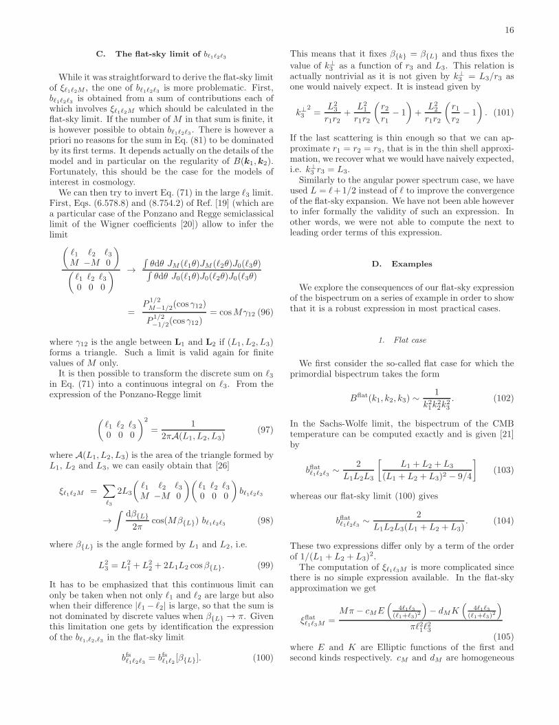
C. The flat-sky limit of bℓ1ℓ2ℓ3

While it was straightforward to derive the flat-sky limitof ξℓ1ℓ2M , the one of bℓ1ℓ2ℓ3 is more problematic. First,bℓ1ℓ2ℓ3 is obtained from a sum of contributions each ofwhich involves ξℓ1ℓ2M which should be calculated in theflat-sky limit. If the number ofM in that sum is finite, itis however possible to obtain bℓ1ℓ2ℓ3 . There is however apriori no reasons for the sum in Eq. (81) to be dominatedby its first terms. It depends actually on the details of themodel and in particular on the regularity of B(k1,k2).Fortunately, this should be the case for the models ofinterest in cosmology.We can then try to invert Eq. (71) in the large ℓ3 limit.

First, Eqs. (6.578.8) and (8.754.2) of Ref. [19] (which area particular case of the Ponzano and Regge semiclassicallimit of the Wigner coefficients [20]) allow to infer thelimit

(

ℓ1 ℓ2 ℓ3M −M 0

)

(

ℓ1 ℓ2 ℓ30 0 0

) →∫

θdθ JM (ℓ1θ)JM (ℓ2θ)J0(ℓ3θ)∫

θdθ J0(ℓ1θ)J0(ℓ2θ)J0(ℓ3θ)

=P

1/2M−1/2(cos γ12)

P1/2−1/2(cos γ12)

= cosMγ12 (96)

where γ12 is the angle between L1 and L2 if (L1, L2, L3)forms a triangle. Such a limit is valid again for finitevalues of M only.It is then possible to transform the discrete sum on ℓ3

in Eq. (71) into a continuous integral on ℓ3. From theexpression of the Ponzano-Regge limit

(

ℓ1 ℓ2 ℓ30 0 0

)2

=1

2πA(L1, L2, L3)(97)

where A(L1, L2, L3) is the area of the triangle formed byL1, L2 and L3, we can easily obtain that [26]

ξℓ1ℓ2M =∑

ℓ3

2L3

(

ℓ1 ℓ2 ℓ3M −M 0

)(

ℓ1 ℓ2 ℓ30 0 0

)

bℓ1ℓ2ℓ3

→∫

dβ{L}

2πcos(Mβ{L}) bℓ1ℓ2ℓ3 (98)

where β{L} is the angle formed by L1 and L2, i.e.

L23 = L2

1 + L22 + 2L1L2 cosβ{L}. (99)

It has to be emphasized that this continuous limit canonly be taken when not only ℓ1 and ℓ2 are large but alsowhen their difference |ℓ1 − ℓ2| is large, so that the sum isnot dominated by discrete values when β{L} → π. Giventhis limitation one gets by identification the expressionof the bℓ1,ℓ2,ℓ3 in the flat-sky limit

bfsℓ1ℓ2ℓ3 = bfsℓ1ℓ2 [β{L}]. (100)

This means that it fixes β{k} = β{L} and thus fixes the

value of k⊥3 as a function of r3 and L3. This relation isactually nontrivial as it is not given by k⊥3 = L3/r3 asone would naively expect. It is instead given by

k⊥32=

L23

r1r2+

L21

r1r2

(

r2r1

− 1

)

+L22

r1r2

(

r1r2

− 1

)

. (101)

If the last scattering is thin enough so that we can ap-proximate r1 = r2 = r3, that is in the thin shell approxi-mation, we recover what we would have naively expected,i.e. k⊥3 r3 = L3.Similarly to the angular power spectrum case, we have

used L = ℓ+1/2 instead of ℓ to improve the convergenceof the flat-sky expansion. We have not been able howeverto infer formally the validity of such an expression. Inother words, we were not able to compute the next toleading order terms of this expression.

D. Examples

We explore the consequences of our flat-sky expressionof the bispectrum on a series of example in order to showthat it is a robust expression in most practical cases.

1. Flat case

We first consider the so-called flat case for which theprimordial bispectrum takes the form

Bflat(k1, k2, k3) ∼1

k21k22k

23

. (102)

In the Sachs-Wolfe limit, the bispectrum of the CMBtemperature can be computed exactly and is given [21]by

bflatℓ1ℓ2ℓ3 ∼ 2

L1L2L3

[

L1 + L2 + L3

(L1 + L2 + L3)2 − 9/4

]

(103)

whereas our flat-sky limit (100) gives

bflatℓ1ℓ2ℓ3 ∼ 2

L1L2L3(L1 + L2 + L3). (104)

These two expressions differ only by a term of the orderof 1/(L1 + L2 + L3)

2.The computation of ξℓ1ℓ3M is more complicated since

there is no simple expression available. In the flat-skyapproximation we get

ξflatℓ1ℓ3M =Mπ − cME

(

4ℓ1ℓ3(ℓ1+ℓ3)

2

)

− dMK(

4ℓ1ℓ3(ℓ1+ℓ3)

2

)

πℓ21ℓ23

(105)where E and K are Elliptic functions of the first andsecond kinds respectively. cM and dM are homogeneous

17

0 10 20 30 40 50-4.0

-3.5

-3.0

-2.5

-2.0

-1.5

{

Log 1

0H{2Ξ 1

0{ML

0 20 40 60 80 100

-26

-25

-24

-23

-22

-21

-20

{

Log 1

0H{2Ξ 1

0{

ML

FIG. 6: Left: ξflatℓ1ℓMfor ℓ1 = 10, M = 0, 1, 2 (top to bottom) from exact computations (dots) and flat-sky approximation (solid

line) in the Sachs-Wolfe plateau limit. Right: ξlocalℓ1ℓMfor ℓ1 = 10, M = 0, 1, 2, 3 (from thick to thin dots) computed exactly from

Eq. (71).

functions of ℓ3/ℓ1 that are such that the numerator inEq. (105) scales like (ℓ3/ℓ1)

−1−M when ℓ3/ℓ1 is large,

c0 = 1 = −d0 (106)

c1 = 1 = d1 (107)

c2 =(2ℓ3/ℓ1 + 1)(ℓ3/ℓ1 + 2)

ℓ3/ℓ1(108)

d2 = − (2(ℓ3/ℓ1)2 − 3ℓ3/ℓ1 + 2)

ℓ3/ℓ1. (109)

The result formally diverges for ℓ1 → ℓ3, due to the factthat some configurations are IR divergent when k2 → 0.It implies that for the flat case in the Sachs-Wolfe plateaulimit, the set ofM ’s contributing in the sum (81) remainsfinite and this validates the flat-sky approximation for thebispectrum given by Eq. (100). The result is depicted onFig. 6.

2. Local case

In the local case, the bispectrum is defined [21] by

Blocal(k1, k2, k3) ∼1

k31k32

+1

k32k33

+1

k33k31

. (110)

The bispectra can be computed by splitting B in 3 termsnone of which has pathological IR divergences (in otherwords, bℓ1ℓ2ℓ3 can be symmetrized only at the end) andwe shall not encounter the divergence problems we hadin the flat case. In its thin-shell approximation, a similarmethod consisting in splitting the computation in threeterms was also of particular interest for the numericalcomputation of the bispectrum generated by non-lineareffects around the LSS that we performed in Ref. [8].Furthermore, in the Sachs-Wolfe regime, the only non-

zero contribution for each term is for M = 0. This leadsto the flat-sky limit of the bispectrum

blocalℓ1ℓ2ℓ3 =(

ξlocalℓ1ℓ30 + ξlocalℓ2ℓ10 + ξlocalℓ3ℓ20

)

(111)

with

ξlocalℓ1ℓ20 ∼ 1

(L1L2)2. (112)

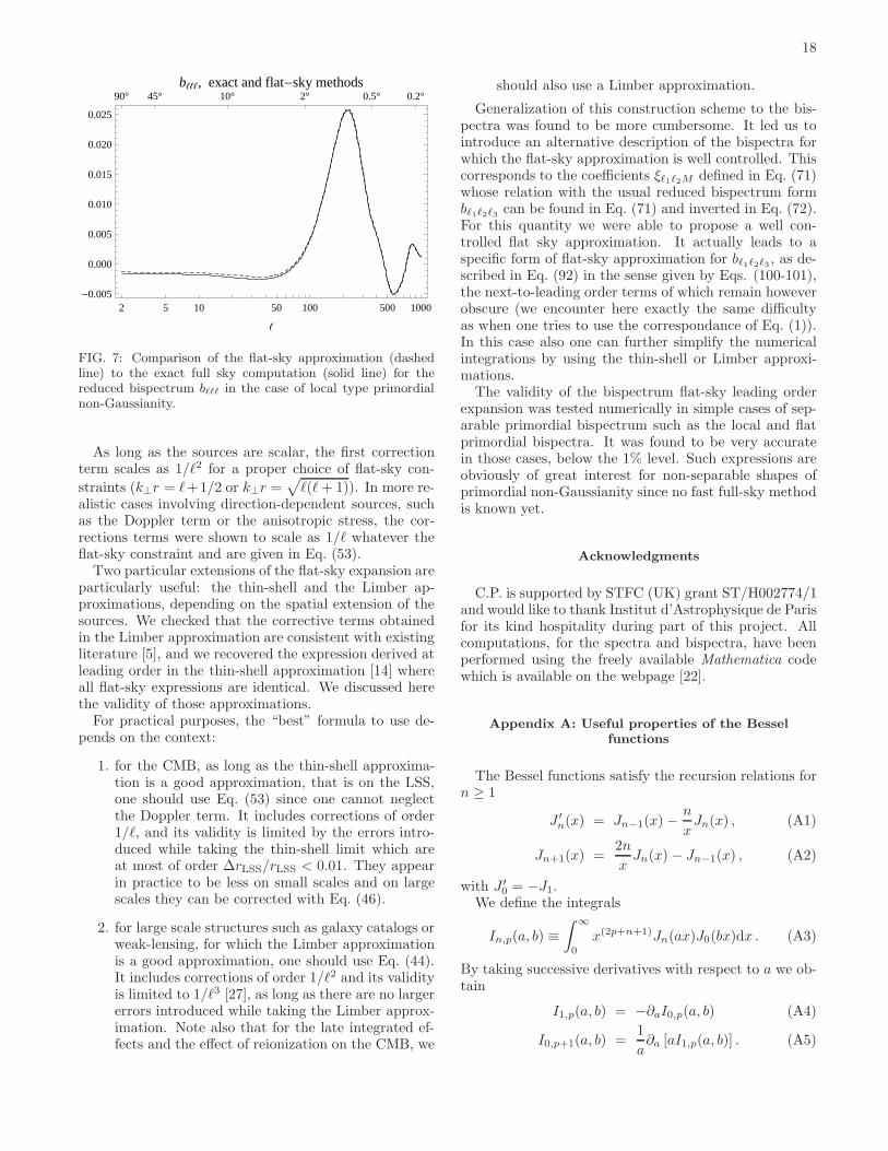
Had we chosen the flat constraint L = k⊥r instead ofL = k⊥r, we would have obtained a similar expressionwith L→ L. It would thus have matched the full-sky ex-pression, similarly to what was obtained in Section II C.Again, we conclude that for the local case, in the Sachs-Wolfe plateau limit, only M = 0 is contributing and thisvalidates the assumption that the number of M ’s con-tributing in the sum (81) is finite. Beyond the Sachs-Wolfe regime we can estimate numerically the differentterms in the sum on M in order to validate the assump-tion that only a finite number of M is required to es-timate the bispectrum out of the ξℓ1ℓ2M . Similarly tothe Sachs-Wolfe plateau, we split in three terms the pri-mordial bispectrum (110), and for each of these termswe plot ξℓ1ℓ2M on Fig. 6 for different values of M . Itis clear that the contribution of each M is exponentiallysupressed when M increases.To finish, we compare in Fig. 7 the flat-sky limit to

the exact full-sky calculation for the bispectrum of localtype and for equilateral configurations (i.e. such thatℓ1 = ℓ2 = ℓ3 = ℓ). The agreement is excellent.

VII. CONCLUSION

This article provides a systematic construction of theflat-sky approximation of the angular power spectrumboth for the temperature and polarization, in particularit shows that the expansion can be performed to anyorder. Additionally, we showed that this construction isnot unique and that there exists a two-parameter familyof flat-sky expansions, depending on the arbitrary choiceof the flat-sky directions with respect to the azimuthalangle.

18

2 5 10 50 100 500 1000-0.005

0.000

0.005

0.010

0.015

0.020

0.025

90° 45° 10° 2° 0.5° 0.2°

{

b{{{, exact and flat-sky methods

FIG. 7: Comparison of the flat-sky approximation (dashedline) to the exact full sky computation (solid line) for thereduced bispectrum bℓℓℓ in the case of local type primordialnon-Gaussianity.

As long as the sources are scalar, the first correctionterm scales as 1/ℓ2 for a proper choice of flat-sky con-

straints (k⊥r = ℓ+1/2 or k⊥r =√

ℓ(ℓ+ 1)). In more re-alistic cases involving direction-dependent sources, suchas the Doppler term or the anisotropic stress, the cor-rections terms were shown to scale as 1/ℓ whatever theflat-sky constraint and are given in Eq. (53).Two particular extensions of the flat-sky expansion are

particularly useful: the thin-shell and the Limber ap-proximations, depending on the spatial extension of thesources. We checked that the corrective terms obtainedin the Limber approximation are consistent with existingliterature [5], and we recovered the expression derived atleading order in the thin-shell approximation [14] whereall flat-sky expressions are identical. We discussed herethe validity of those approximations.For practical purposes, the “best” formula to use de-

pends on the context:

1. for the CMB, as long as the thin-shell approxima-tion is a good approximation, that is on the LSS,one should use Eq. (53) since one cannot neglectthe Doppler term. It includes corrections of order1/ℓ, and its validity is limited by the errors intro-duced while taking the thin-shell limit which areat most of order ∆rLSS/rLSS < 0.01. They appearin practice to be less on small scales and on largescales they can be corrected with Eq. (46).

2. for large scale structures such as galaxy catalogs orweak-lensing, for which the Limber approximationis a good approximation, one should use Eq. (44).It includes corrections of order 1/ℓ2 and its validityis limited to 1/ℓ3 [27], as long as there are no largererrors introduced while taking the Limber approx-imation. Note also that for the late integrated ef-fects and the effect of reionization on the CMB, we

should also use a Limber approximation.

Generalization of this construction scheme to the bis-pectra was found to be more cumbersome. It led us tointroduce an alternative description of the bispectra forwhich the flat-sky approximation is well controlled. Thiscorresponds to the coefficients ξℓ1ℓ2M defined in Eq. (71)whose relation with the usual reduced bispectrum formbℓ1ℓ2ℓ3 can be found in Eq. (71) and inverted in Eq. (72).For this quantity we were able to propose a well con-trolled flat sky approximation. It actually leads to aspecific form of flat-sky approximation for bℓ1ℓ2ℓ3 , as de-scribed in Eq. (92) in the sense given by Eqs. (100-101),the next-to-leading order terms of which remain howeverobscure (we encounter here exactly the same difficultyas when one tries to use the correspondance of Eq. (1)).In this case also one can further simplify the numericalintegrations by using the thin-shell or Limber approxi-mations.The validity of the bispectrum flat-sky leading order

expansion was tested numerically in simple cases of sep-arable primordial bispectrum such as the local and flatprimordial bispectra. It was found to be very accuratein those cases, below the 1% level. Such expressions areobviously of great interest for non-separable shapes ofprimordial non-Gaussianity since no fast full-sky methodis known yet.

Acknowledgments

C.P. is supported by STFC (UK) grant ST/H002774/1and would like to thank Institut d’Astrophysique de Parisfor its kind hospitality during part of this project. Allcomputations, for the spectra and bispectra, have beenperformed using the freely available Mathematica codewhich is available on the webpage [22].

Appendix A: Useful properties of the Bessel

functions

The Bessel functions satisfy the recursion relations forn ≥ 1

J ′n(x) = Jn−1(x) −

n

xJn(x) , (A1)

Jn+1(x) =2n

xJn(x)− Jn−1(x) , (A2)

with J ′0 = −J1.

We define the integrals

In,p(a, b) ≡∫ ∞

0

x(2p+n+1)Jn(ax)J0(bx)dx . (A3)

By taking successive derivatives with respect to a we ob-tain

I1,p(a, b) = −∂aI0,p(a, b) (A4)

I0,p+1(a, b) =1

a∂a [aI1,p(a, b)] . (A5)

19

Using the orthonormality relation

∫ ∞

0

xJ0(ax)J0(bx)dx =δ(a− b)

b, (A6)

we obtain the expression of the main integrals of interestfor this paper

I0,0(a, b) =δ(b− a)

b(A7)

I1,0(a, b) =δ′(b − a)

b(A8)

I0,1(a, b) =δ′(b − a)

ab− δ′′(b− a)

b(A9)

I1,1(a, b) =δ′(b − a)

ba2+δ′′(b− a)

ab− δ′′′(b − a)

b.(A10)

Appendix B: Relating the corrections in the

different flat-sky expansions

In the expansion (22), had we chosen the constraint

k⊥R = L, then the expression of the corrective terms inthe square brackets would have been modified by the re-placement of L by L and an extra operator −1/(8L2)D⊥

would have been added in the brackets since for any func-tion Q, Q(L/r) ≃ Q(L/r)− 1/(8L2)kQ′(k). This meansthat the numerical factor in front of the operator D⊥

would be 1/6 instead of 1/24. For a scale-invariant powerspectrum and a sharply peaked constant transfer func-tion, i.e. w(k, r) ∝ δ(r − rLSS), the correction terms arethus proportional to

(4D⊥ −D3⊥)

1

k3= 15k4⊥

(k2⊥ − 6k2r)

k9,

and the integral on kr of this function is zero. This is agood check of our expansion. Indeed, in Section II C wehave seen that in this particular case, the leading order ofthe flat-sky expansion is equal to the exact result so thatit was expected that the corrections vanish. Actually, thisproperty should not depend on v since the v-dependencein the lowest order term of the expansion coming fromthe fact that R is a function of v, disappears when thesources are located only at a given distance rLSS. Forall choices of v and for a scale invariant power spectrumand a peaked transfer function, the lowest order of theflat-sky expansion is equal to the exact result. We cancheck indeed that in that case the corrective terms inthe expression (19) where v = 0 once expressed with the

constraint k⊥R = L, vanish as well. The v-dependentcorrections need to be consistent, and though they areformally different as v is varied, they should lead to thesame result, at least in that case where the transfer func-tion is sharply peaked. We now show that the correctiveterms for different choices of v can be related by integra-tion by parts in that case.We assume that w(k, r) ∝ δ(r − rLSS) so that we can

also assume that all the k dependence is located in P (k)

so that we can drop the factors w(k, rLSS) for simplicityand set rLSS = 1. Expanding the correlation (7) in Z weobtain

ξv = ξ1/2 +

∫

dkr(2π)2

k⊥dk⊥P (k) (B1)

× (1− 2u)Z3

8

[

−Zk2rJ0(k⊥Z) + k⊥J1(k⊥Z)]

and thus we can relate the corresponding multipoles

Cvℓ = C(v=1/2)ℓ +∆Cℓ , (B2)

with

∆Cℓ =(1− 2v)

8

∫

dkr(2π)

dk⊥P (k) (B3)

×[

k2⊥I1,1(k⊥, L)− k⊥k2rI0,2(k⊥, L)

]

=(1− 2v)

8

∫

dkr(2π)

dk⊥P (k)

×{

k2⊥I1,1(k⊥, L)− k2r∂

∂k⊥

[

k⊥I1,1(k⊥, L)]

}

.

Integrating by parts we obtain

∆Cℓ =(1− 2v)

8

∫

dkr(2π)

dk⊥ (B4)

×k2⊥{

P (k)I1,1(k⊥, L) +k2rkP ′(k)I1,1(k⊥, L)

}

.

Another integration by parts in kr is sufficient to obtainthat ∆Cℓ = 0. This proves that even if the expressionof the corrections is formally different for a different v,the corrective term remains the same in the thin-shellapproximation.

Appendix C: Asymptotic forms for the spherical

harmonics

The spherical harmonics can be expressed in terms ofthe Legendre polynomials as

Y mℓ (u, ϕ) =

(

2ℓ+ 1

4π

)1/2 [(ℓ −m)!

(ℓ +m)!

]1/2

Pmℓ (u) eimϕ

(C1)where u = cos θ. The construction of the spherical har-monics for non-zero values of m are obtained from therecursion relation

Pmℓ (u) = (−1)m(1 − u2)m/2dm

dumPℓ(u) . (C2)

Each of these operators can then be evaluated in the flat-sky limit, with u ≈ 1− θ2/2,

(1− u2)m

2

(−d

du

)m

= θm(

d

θdθ

)m

(C3)

+m(m− 1)

6θm

(

d

θdθ

)m−1

+ . . . .

20

Taking advantage that for finite values of m

[

(ℓ −m)!

(ℓ +m)!

]1/2

=1

(ℓ + 1/2)m

×[

1 +m(2m+ 1)(2m− 1)

24 ℓ2+ . . .

]

, (C4)

we can use the relation (15) to get the expression of Y mℓ ,and its next to leading order corrections to an arbitraryorder, in the flat-sky approximation. The final result canbe written in terms of Bessel functions of the first kindthanks to the relation,

Jm(θ) = (−θ)m(

d

θdθ

)m

J0(θ). (C5)

We then recover the known large ℓ expression of the

spherical harmonics,

Y mℓ (θ, ϕ) →(

2L

4π

)1/2

(−1)mJm[Lθ]eimϕ, (C6)

where the first correction term is in 1/ℓ2 or in θ2. Itcomes from the sub-leading terms in Eq. (15), the sub-leading operators in (C4) and the subleading terms in(C4). All these corrective terms make the flat-sky ex-pansions controllable when m is finite but clearly notwhen it is of the order of ℓ. The corrective terms areexpected to involve Bessel functions Jm′ where m′ differsto m by at most 2. Subleading terms in the final resultsof flat-sky expressions can then be obtained in principleusing relations (or similar to those) given in appendix A.

[1] M. Zaldarriaga and U. Seljak, Phys. Rev. D 55, 1830(1997), astro-ph/9609170.

[2] W. Hu, Phys. Rev. D 62, 043007 (2000), astro-ph/0001303.

[3] D. N. Limber, Astrophys. J. 117, 134 (1953).[4] P. J. E. Peebles, The large-scale structure of the universe

(Princeton: Princeton Univ. Press, 1980).[5] M. Loverde and N. Afshordi, Phys. Rev. D 78, 123506

(2008), 0809.5112.[6] L. Boubekeur, P. Creminelli, G. D’Amico, J. Norena, and

F. Vernizzi, JCAP 0908, 029 (2009), 0906.0980.[7] C. Pitrou, J.-P. Uzan, and F. Bernardeau, Phys. Rev. D

78, 063526 (2008), 0807.0341.[8] C. Pitrou, J.-P. Uzan, and F. Bernardeau, JCAP 1007,

003 (2010), 1003.0481.[9] D. Nitta, E. Komatsu, N. Bartolo, S. Matarrese, and

A. Riotto, JCAP 5, 14 (2009), 0903.0894.[10] A. Lewis and A. Challinor, Physics. Rep. 429, 1 (2006),

arXiv:astro-ph/0601594.[11] C. Ma and E. Bertschinger, Astrophys. J. 455, 7 (1995),

astro-ph/9506072.[12] W. Hu and M. White, Phys. Rev. D 56, 596 (1997),

astro-ph/9702170.[13] C. Pitrou, Class. Quant. Grav. 26, 065006 (2009),

0809.3036.[14] J. R. Bond, in Cosmology and Large Scale Structure,

edited by R. Schaeffer, J. Silk, M. Spiro, & J. Zinn-Justin(1996), pp. 469–+.

[15] U. Seljak, Astrophys. J. 482, 6 (1997), astro-ph/9608131.

[16] U. Seljak and M. Zaldarriaga, Astrophys. J. 469, 437

(1996), astro-ph/9603033.[17] J. N. Goldberg, A. J. Macfarlane, E. T. Newman,

F. Rohrlich, and E. C. G. Sudarshan, J. Math. Phys.8, 2155 (1967).

[18] E. Komatsu (2002), astro-ph/0206039.[19] I. S. Gradstein and I. M. Ryzik, Tables of Integrals, Series

and Products (New York: Academic, 1966).[20] G. Ponzano and T. Regge, in Spectroscopy and group the-

oretical methods in Physics, edited by F. Bloch (Amster-dam: North-Holland, 1968).

[21] N. Bartolo, E. Komatsu, S. Matarrese, and A. Riotto,Phys. Rept. 402, 103 (2004), astro-ph/0406398.

[22] URL http://icg.port.ac.uk/~pitrouc/cmbquick.htm.[23] The direction of observation is opposite to the direction

of propagation, and the transformation properties underparity bring an extra (−1)ℓ in the above formula whencompared to Eq. (7.1) of Ref. [13] or Eq. (10) of Ref. [12].

[24] In particular for any other observable or physical mecha-nisms for which the variations of w(k, r) can be neglected,the corrective term would indeed scale as 1/ℓ2 also onsmall scales, and this justifies our choice of denomina-tion.

[25] More precisely, the exact result has three integrals aswell, but the integral on r is squared and numerically wehave effectively only two integrals.

[26] Note that because ℓ1+ℓ2+ℓ3 should be even, subsequentvalues of ℓ2 in this sum are separated by 2 units.

[27] Note that this differs from the conclusion of Ref. [5] whereit is claimed without proof that the next order is only atℓ−4.