Flat tax reform: A quantitative exploration

1This paper was one of the winners of the 1996}1997 Graduate Student Paper Contest of TheSociety for Computational Economics.

*Tel.: (519) 679 2111 (ext. 5303); fax: (519) 6613666 ; e-mail: [email protected].

Journal of Economic Dynamics & Control23 (1999) 1425}1458

Flat tax reform: A quantitative exploration1

Gustavo Ventura*

Department of Economics, University of Western Ontario, London, Ont., Canada N6A 5C2

Abstract

This paper explores quantitatively the general equilibrium implications of a revenueneutral tax reform in which the current income and capital income tax structure in theU.S. is replaced by a #at tax, as proposed by Hall and Rabushka (1995), (The Flat Tax,2nd ed. Hoover). The central aspects of such reform, the impact of tax reform on capitalaccumulation and labor supply, as well as its distributional consequences, are analyzed ina dynamic general equilibrium model. Main results are that, (i) the elimination of theactual taxation of capital income has an important and positive e!ect on capitalaccumulation; (ii) mean labor hours are relatively constant across tax systems, butaggregate labor in e$ciency units increases; (iii) in all circumstances analyzed, thedistributions of earnings, income and especially wealth become more concen-trated. ( 1999 Elsevier Science B.V. All rights reserved.

JEL classixcation: E62; H20

Keywords: Flat tax; Distribution

1. Introduction

Recently, various proposals to drastically reformulate the tax code have beenadvanced in the United States. One such proposal for fundamental tax reform,the so called yat tax, has received considerable attention. In a nutshell, the

0165-1889/99/$ - see front matter ( 1999 Elsevier Science B.V. All rights reserved.PII: S 0 1 6 5 - 1 8 8 9 ( 9 8 ) 0 0 0 7 9 - 7

2See Hall and Rabushka (1995) for the seminal reference on the #at tax.

proposed reform consists of the replacement of existing federal income andcorporation income taxes by a single tax rate applied to labor income abovea given threshold, and all (gross) capital income after full investment deductibil-ity. What are, in quantitative terms, the consequences of such drastic reform? Itis clear that a careful assessment of the changes generated by a #at tax is ofparticular importance given that the impact of such drastic reform is expected tobe widespread. For instance, recent debates have emphasized issues such as thegreater simplicity and fairness of the resulting tax code after the reform, de-creased compliance costs of a #at tax as compared to the actual tax structure,the removal of deadweight losses implied by the current progressive income tax,growth e!ects, distributional considerations, etc.2

This paper focuses on two central and con#icting issues of the #at tax debate.Since a #at tax is a form of consumption taxation that removes distortionsassociated with the existence of a progressive income tax and the (double)taxation of capital income, #at tax proponents argue that its positive e!ects onaggregate capital accumulation, labor supply and welfare are expected to be ofconsiderable magnitude. On these grounds, the shift towards a #at tax is viewedas highly desirable. However, as some critics point out, a #at tax reform mayadversedly a!ect the cross-sectional income and wealth distribution. Theseconsiderations together dictate that the quantitative exploration of a #at taxreform is an important subject. Addressing these issues simultaneously with thediscipline imposed by general equilibrium modelling is, nevertheless, not an easytask, since such analysis invariably involves the construction of models capableof matching up to some degree distributional features of actual economies. Thepresent paper constitutes an attempt in this direction.

As discussed above, the replacement of the actual forms of income and capitalincome taxation by a #at tax is expected to impact on the levels of aggregatelabor hours and capital accumulation, the corresponding factor prices, welfare,and the distribution of income and wealth among households. This observationprovokes in turn a multitude of specixc questions regarding the overall e!ects ofsuch reform:

1. What is the impact of the #at tax reform on capital accumulation?2. How is aggregate labor supply a!ected? What is the impact of a #at tax

reform on the distribution of labor hours?3. Does the pre-tax income distribution change substantially with the reform?

In particular, how do the earnings, income and wealth Gini coe$cients undera #at tax code compare to the Gini coe$cients under the current structure?How do the percentages of income earned by agents at di!erent percentiles ofthe income distribution compare between the two tax systems?

4. Does the after-tax income distribution become more unequal?

1426 G. Ventura / Journal of Economic Dynamics & Control 23 (1999) 1425}1458

3See Elmendorf (1996) for an extensive survey of the interest rate elasticity of savings in life cyclemodels.

4Fullerton and Rogers (1993) and Altig et al. (1997) are life cycle models that incorporateheterogeneity at birth in labor productivity, but no idiosyncratic shocks.

5See Quadrini and Rios Rull (1997) for an overview of the distributional implications ofeconomies with heterogeneous agents in terms of the distribution of wealth. See Huggett (1996) andHuggett and Ventura (1998) for the distributional implications of life cycle economies with hetero-geneous agents.

The aim of this paper is thus to explore the general equilibrium consequencesof a revenue neutral tax reform, in which an income and capital income taxstructure designed to mimic the prevailing structure in the U.S. is replaced bya #at tax. In order to properly attack this problem, the model economiesconsidered in this paper are populated by complex forms of heterogeneousagents. I study life cycle economies in which agents live for a realistic number ofperiods, face uncertain lifetimes, have preferences over consumption and leisure,and di!er in terms of their age as well as in their earnings histories. In particular,earnings histories are di!erent for agents within a given cohort due to di!erencesat birth in labor productivities and uninsurable variation of such productivitiesover time. Furthermore, agents can accumulate a single risk-free asset to providefor retirement income and insure themselves against lifetime uncertainty and#uctuations experienced in the market return to labor. Finally, there existsa pay-as-you-go Social Security scheme, with similar features to the one actuallyin place in the U.S.

It is important to point out that model economies with the features outlinedabove are particularly useful in the study of a #at tax reform. Three reasons forthis are mentioned here. First, as recently Engen and Gale (1996) have observed,the presence of uninsurable idiosyncratic risk is potentially important for thestudy of tax reforms, since in such an environment the response of savings to theelimination of distortions is likely to be smaller.3 The key reason for this is thatasset holdings are used to smooth out idiosyncratic shocks, and as a result, assetaccumulation is less responsive to changes in the rate of return. Second,di!erences at birth in labor productivities and over the life cycle,4 together withthe uninsurable shocks to such productivities just mentioned, create stationarydistributions of labor earnings, income and wealth that are able to approximatereasonably well actual distributional statistics.5 This point is fundamental, asa key objective of the present paper is to understand the e!ects of a #at tax onthe distributions of earnings, income and wealth. Finally, the presence ofendogenous labor in a context of agent heterogeneity is important for tworeasons. First, it permits to study movements in labor hours due to the change inthe tax system at both the aggregate level, as well as across people. And second,it tempers the e!ect on asset accumulation of idiosyncratic shocks discussed

G. Ventura / Journal of Economic Dynamics & Control 23 (1999) 1425}1458 1427

6Summers (1981), Auerbach et al. (1983), Auerbach and Kotliko! (1983)Auerbach and Kotliko!(1987), Fullerton and Rogers (1993) and several other authors found a substantial response of capitalaccumulation in life cycle models to the elimination of intertemporal distortions. For example,Auerbach and Kotliko! (1987), (Table 5.6, p. 73) found that a revenue neutral shift from a #at rateincome tax of 20% to a consumption tax, boosts capital formation in the long run by about 34%.Large responses are also a well known feature of in"nitely-lived agent models. For instance, in thecontext of a real business cycle model, Hu!man and Greenwood (1991) found that a capital incometax reduction from 35% to 25% increases average capital and output by about 34.3% and 9.0%respectively. See Engen et al. (1997) for a comparison of the results yielded by competing appliedgeneral equilibrium models of tax reform.

above. A reason for this is that in the current setup, as individual agents areallowed to vary labor hours supplied, they have an aditional element to insurethemselves against such shocks. To my knowledge, this non-trivial role for laboris a novel feature in the analysis of tax reforms.

Several "ndings emerge from this study. First, the e!ects of the #at tax reformon capital accumulation appear to be substantial. Consequently, the e!ects onthe wage and the interest rate are of considerable magnitude. As pointed out inthe text, this is a consequence of the replacement of current capital income andincome taxes by a consumption based form of taxation. In this regard, this resultparallels quantitative "ndings provided by the vast applied general equilibriumliterature that studied the impact of consumption taxes against other forms oftaxation.6 Second, the potential impact on labor supply so emphasized byproponents of the #at tax can be divided into two parts. On the one hand, afterthe tax reform, mean labor hours are relatively constant in the benchmarkcalculations. On the other hand, signi"cant changes in the distribution of laborhours are observed. Labor hours supplied by agents at the top of the incomedistribution substantially increase: households in the upper income quintileincrease labor hours by no less than 9% in the cases considered. Sincethese agents are highly productive, this latter e!ect is the factor behind theoverall increase in the value of the aggregate labor input in e$ciency units thatis observed, which in turn reinforces the e!ect of higher capital levels onoutput. Finally, the cross-sectional distributions of earnings, income and inparticular wealth become more concentrated in all cases analyzed. This is a key"nding, as one of the objections to a #at tax is its potential negative distribu-tional impact.

The paper proceeds as follows. Section 2 describes the basic #at tax reformproposal. Section 3 describes in detail the model economies. Section 4 discussesthe details of the calibration process. Section 5 presents the main "ndings of thepaper in terms of the aggregate impact of a #at tax and its distributional e!ects.Section 6 brie#y studies the role of accidental bequests in the results. Finally,Section 7 concludes.


2. Flat tax reform

As originally conceived by Robert Hall and Alvin Rabushka in the earlyeighties, the main objective of the so called #at tax is to create a form ofprogressive consumption taxation to replace the actual personal income tax andthe corporation income tax in the U.S. The tax system proposed by Hall andRabushka (1995) comprises two di!erent, but consistent forms of taxation. The"rst one is called &wage tax'. This part of the #at tax plan taxes the sum of allwages, salaries and pensions above a given labor income threshold. The mar-ginal tax rate is yat (constant) above the threshold, which implies, of course, thataverage taxes paid are increasing in the amount of labor income. It is here, in thewage tax, where the progressive part of the proposal lies. In this regard,the notion of progressivity embodied in the #at tax is di!erent from the one inthe actual income tax, in which both marginal and average tax rates areincreasing.

The second part of the #at tax plan is the &business tax'. Since the objective isan integrated consumption-based tax, this new instrument is designed to tax allincome which is not labor income or investment. Consequently, the business taximposes a #at rate (the same rate as the wage tax) on all corporate andnon-corporate business income less wages and employer's pension contribu-tions, purchases of inputs from other "rms, and investment. In other words, inthe aggregate, the business tax imposes a #at rate on all capital income after netcapital accumulation.

Some remarks about the nature and possible implications of a #at tax are nowin order. As just described in the above paragraphs, with a proposed #at tax rateset around 20%, and an actual income tax with graduated rates at 15%, 28%,31%, 36% and 39.6%, this new form of taxation reduces quite substantiallymarginal tax rates on labor income for upper-middle and upper income house-holds. However, depending upon the exemption levels chosen, the marginal taxrate for households previously in the 15% tax bracket may or may not increase.Even though the "nal impact on labor supply is unknown, there is room forpotential increases in hours worked, in particular for households in the uppertax brackets. Furthermore, since it fully removes the income tax and thecorporate income tax, the #at tax proposal eliminates the present doubletaxation of capital income, and it does it in a crucial way. Due to the fact that the#at tax is a form of consumption taxation, it does not a!ect the asset accumula-tion decision on the margin. That is, in the simplest case, the marginal rate ofsubstitution between consumption today and consumption tomorrow is nota!ected by the tax rate. This suggests that an important general equilibriume!ect is possible on capital accumulation and factor prices. Finally, the com-bined e!ects of the change in the degree of progressivity and the removal ofdistortions hint that important distributional changes are likely to occur.Consider, for example, the intuitive case of the distribution of labor earnings.


7The modelling framework used here is similar to that used by Imrohoroglu et al. (1995), Huggett(1996), and Huggett and Ventura (1998). Also similar frameworks appear in Hubbard and Judd(1987), Rios-Rull (1996) and Imrohoroglu (1997) among others. For a general discussion of econo-mies with heterogeneous agents, see Rios-Rull (1995).

8Auerbach and Kotliko! (1987), (Chapter 8) and others introduced progressive income taxes intheir work. The framework studied here, however, is richer in the sense that progressive taxes inmodel economies are imposed over brackets of income or labor income, as it is actually the case inthe U.S. and in the Hall}Rabushka proposal. This realistic modelling of progressive taxes has alsobeen implemented recently by Engen and Gale (1996).

9The weights kj

are normalized to sum to 1, and are given by the recursionkj`1

"(sj`1

/(1#n))kj.

Here, the #at tax proposal contains the ingredients to make this distributionmore concentrated. If the exemption level on labor income is set not too high,the #at tax may reduce the labor supply of agents at the bottom of the earningsdistribution. Simultaneously, if substitution e!ects prevail, the adoption of the#at tax will increase the labor hours supplied of households at the top percen-tiles of such distribution. These considerations together dictate that the distribu-tion of labor earnings is likely to become more concentrated.

3. Model economies

I study a general equilibrium } life cycle economy populated by heterogen-eous agents.7 The novelty in the present formulation is the introduction ofendogeneous labor supply together with realistic (progressive) forms of taxation,capable of approximating the actual tax structure as well as the #at tax proposaladvanced by Hall and Rabushka (1995).8

Demographics: Each period a continuum of agents are born. Agents livea maximum of N periods and face a probability s

jof surviving up to age

j conditional upon being alive at age j!1. Population at time t is denoted by Nt,

and grows at a constant rate n. The demographic structure is stationary, suchthat age j agents always constitute a fraction k

jof the population at any point

in time.9Preferences: All agents have preferences over streams of consumption and

leisure, represented by the following utility function:

ECN+j/1

bjAj

<i/1

siBu(c

j,t,1!l

j,t)D (1)

where cj,t

and lj,t

denote consumption and labor supplied at age j and period t,respectively. Agents are endowed with one unit of time at each age. The periodutility function u(c,1!l ) belongs to the constant relative risk aversion class.


Furthermore, the period utility function displays intratemporal elasticity ofsubstitution between consumption and leisure equal to 1,l being the coe$cientof consumption in the composite good and p the coe$cient of relative riskaversion. Hence, the utility function has the form

u(c, l )"[cl(1!l )1~l](1~p)

(1!p). (2)

Technology: At any time period t there is a constant returns to scale produc-tion technology that transforms capital K and labor ¸ into output >. Thistechnology is represented by a Cobb}Douglas production function. The techno-logy improves over time because of labor augmenting technological change. Thetechnology level X

tgrows at a constant rate, g. Therefore,

>"F(K,¸X)"AKa(¸X)1~a (3)

The capital stock depreciates at the constant rate d.Individual constraints: The market return per hour of labor supplied of an age

j agent at time t is given by wte(z, j), where w

tis a wage rate common to all agents,

and e(z, j) is a function that summarizes the combined productivity e!ects of ageand of an idiosyncratic productivity shock z. The shock z lies in the bounded setZLR and follows a Markov process, with transition probabilities p(z@,z).Shocks received by age 1 agents are distributed according to the probabilitymeasure q(z). Productivity shocks are assumed to be independently distributedacross agents, and the law of large numbers is assumed to hold. This determinesthat no uncertainty will exist in the aggregate, even though uncertainty over themarket return to labor supplied will prevail at the individual level.

All agents are born with no assets, and face mandatory retirement at agej"R#1. This determines that agents are allowed to work only up to ageR (inclusive). An age j agent with idiosyncratic shock z chooses consumption c

j,t,

labor hours lj,t

and risk-free asset holdings aj`1,t`1

. The budget constraint forsuch an agent is then

cj,t#a

j`1,t`14a

j,t(1#r

t)#(1!h)w

te(z, j)l

j,t#¹R

t#b

j,t!¹

j,t(4)

cj,t50, a

j,t5a

tand a

j`1,t`150 if j"N

where aj,t

are asset holdings at age j and time t, ¹Rtis an (age independent)

lump-sum transfer of accidental bequests, ¹j,t

are taxes paid, h is the (#at)payroll social security tax and b

j,tis the social security transfer. Asset holdings

pay a risk-free return rt. The constraint a

j,t5a

timplies that agents face a bor-

rowing constraint. In addition, if an agent survives up to the terminal period(j"N), then next period asset holdings must be non-negative. In other words,agents are not allowed to borrow when the probability of surviving up to the


10Technical progress determines that in steady state the bene"t level will grow over time at rate g.Thus, cohorts that retire later receive a higher bene"t level. In the present formulation, socialsecurity transfers are completely independent of earnings histories, and thus equal the same amountfor all cohort members after retirement. This is not the case under the U.S. system, in spite of thehighly redistributive nature of the social security payments. See Huggett and Ventura (1998) forexamples on how to proceed with a more realistic formulation.

11Savings are de"ned as the change in asset holdings of households (aj`1,t`1

!aj,t

).

next period equals zero. The social security bene"t bj,t

is zero before theretirement age R and equals a xxed bene"t level for an agent after retirement.10

Taxes and government consumption: In the model economies considered, thegovernment consumes in every period the amount G

t, which is "nanced only

through taxation. Since the purpose of the paper is to analyze the impact of a #attax reform, I consider two generic tax regimes in the model economies. In the"rst one, labelled from now on as baseline and designed to mimic the current taxstructure in the U.S., there is a progressive income tax, as well as a #at capitalincome tax at rate q

kthat will later be identi"ed with the actual corporation

income tax (see Section 3). The income tax is comprised of M di!erent brackets,de"ned by thresholds I

0, I

1, I

2,2, I

M, with corresponding marginal tax rates

qm, m"1,2, M. An agent's income subject to taxation is de"ned to be labor

plus asset income. Consequently, an age j agent with an incomeI,w

te(z, j)l

j,t#r

taj,t

, with I3(Im~1

, Im], pays the amount

¹j,t"q

1(I

1!I

0)#q

2(I

2!I

1)#2#q

m(I!I

m~1)#q

k[r

taj,t

]. (5)

It is worth noting that as an agent's income subject to taxation includes capital(asset) income, capital income is taxed through the income tax as well as throughthe speci"c tax on capital income. It follows that an individual with incomeI3(I

m~1,Im] faces a tax rate on capital income equal to (q

k#q

m).

In the second tax regime, labeled yat tax, designed to replicate the &business'and labor income taxes embodied in the #at tax proposal, agents pay rate q

"on

capital income after full deductibility of savings made,11 and rate q-over all

labor income above a threshold IH. Therefore, total taxes paid by an age j agentreceiving a shock z amount to

¹j,t"G

q-[w

te(z, j)l

j,t!IH]#q

"[r

taj,t!(a

j`1,t`1!a

j,t)] if w

te(z, j)l

j,t5IH,

q"[r

taj,t!(a

j`1,t`1!a

j,t)] otherwise.

(6)

Observe that since in equilibrium the interest rate will equate the rental priceof capital after subtracting depreciation (see Section 3.2), in both tax regimesdepreciation allowances will be tax deductible.


12Once a(x, j) and l(x, j) are found, the optimal decision rule for consumption c(x, j) is triviallydetermined from the budget constraint.

3.1. Recursive formulation

From now on, time subscripts are dropped since I focus on stationaryequilibria. For computational purposes I transform variables in order to removethe consequences of growth. The transformations are standard: aggregate vari-ables G,K and > are divided by NX, aggregate labor is divided by N, andindividual variables and factor prices that grow over time in steady state at therate g, are divided by the technology level. The transformations proceed asfollows:

a("a/X, a("a /X, c("c/X, ¹RK "¹R/X, bKj"b

j/X, lK"l,

¹K "¹/X, GK "G/(NX), KK "K/(NX), K "¸/N, w("w/X, r("r.

With these transformations, an agent's decision problem can be described instandard recursive fashion. An agent's state is denoted by the pairx"(a( , z), x3X, where a( are current (transformed) asset holdings and z is theidiosyncratic productivity shock. The setX isX"[a( ,R)]Z. With some abuseof notation, I denote total taxes at state (x, j) (income taxes plus capital incometaxes in the baseline case or wage plus business taxes in the #at tax case) by¹(x, j). Consequently, optimal decision rules are functions for consumptionc(x, j), labor l(x, j), and next period asset holdings a(x,j) that solve the followingdynamic programming problem:12

<(x, j)"max(lK ,a( {)

u(c( ,1!lK )#b(1#g)*l(1~p)+sj`1

E[<(a( @, z@, j#1)Dx] (7)

subject to

c(#a( @(1#g)4a( (1#r( )#(1!h)w( e(z, j)l#¹RK #bLj!¹(x, j),

c(50, a( @5a( , a( @50 if j"N,

<(x,N#1),0.

(8)

3.2. Equilibrium

In the model economies, agents are heterogeneous with respect to the realiz-ation of their idiosyncratic labor productivity shock, their asset holdings, andtheir age. To specify the notion of equilibrium, a probability measure t

jde"ned

on subsets of the individual state space will describe the heterogeneity in assetsand productivity shocks within a particular cohort. Let (X,B(X),t

j) be a prob-

ability space where B(X) is the Borel p-algebra on X. The probability measure


tjmust be consistent with individual decision rules that determine the asset

position of individual agents at a given age, given the asset history and thehistory of labor productivity shocks. Therefore, it is generated by the law ofmotion of the productivity shock z and the asset decision rule a(x, j). Thedistribution of individual states across age 1 agents is determined by theexogenous initial distribution of labor productivity shocks q(z), since agents areborn with zero assets. For agents j'1 periods old, the probability measure isgiven by the recursion:

tj`1

(B)"PX

P(x, j,B)dtj

(9)

where

P(x, j,B)"p(z@, z) if (a(x, j), z@)3B,

P(x, j,B)"0 otherwise.

It is possible now to state the de"nition of steady-state equilibrium:

Dexnition. A steady state equilibrium is a collection of decision rulesc(x, j), a(x, j), l(x, j), factor prices w( and r( , taxes paid ¹(x, j), a lump sum transfer ofaccidental bequests ¹RK , social security transfers bK

j, aggregate capital KK , aggreg-

ate labor K , government consumption GK , a payroll tax h, a tax regime 3Mbase-line, -at taxN and distributions (t

1, t

2,2,t

N) such that

1. c(x, j), a(x, j) and l (x, j) are optimal decision rules.2. Factor prices are determined competitively: w("F

2(KK , K ) and

r("F1(KK , K )!d

3. Markets clear:1. 3.1. +

jkj:X(c(x, j)#a(x, j)(1#g)) dt

j#GK "F(KK , K )#(1!d)KK ,

1. 3.2. +jkj:Xa(x, j)dt

j"(1#n)KK ,

1. 3.3. +jkj:Xl(x, j)e(z, j) dt

j" K .

4. Distributions are consistent with individual behavior:

tj`1

(B)"PX

P(x, j, B) dtj

for j"1,2, N!1 and for all B3B(X).5. Government budget constraint is satis"ed:

GK "+j

kjP

X

¹(x, j) dtj.

6. Social security bene"ts equal taxes: hw( K "+Nj/R

kjbjK .


13The data for equipment and structures, residences, and consumer durables is taken fromMusgrave (1992a,b), (pp. 136, Table 2). The stock of inventories is from the Economic Report of thePresident (1993), (Table B16). Estimates of the stock of land are from the Flow of Funds Accounts.

7. Transfers equal accidental bequests:

¹RK "C+j

kj(1!s

j`1)P

X

(a(x, j)(1#r( )) dtjDN(1#n).

Conditions 1}5 above are standard. Conditions 6 and 7, however, requiresome explanation. Condition 6 implies budget balance for the social securitysystem, and that such a system is funded on a pay-as-you-go basis. Condition7 states that lump sum transfers ¹RK equal per-capita accidental bequests. Thisformulation is obviously not a realistic feature of the U.S. economy. However, itis made in order to introduce lifetime uncertainty, and therefore realistic demo-graphic patterns, in the simplest possible way.

4. Calibration

4.1. Model parameters

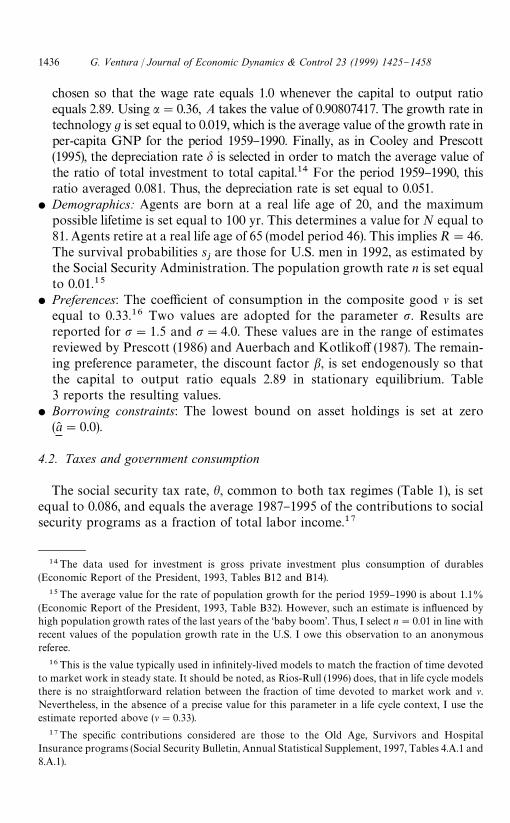
As a "rst step in the calibration process, the model period considered is setequal to one year. As a second step it is necessary to adopt a notion of the capitalstock, so that the targets for the model economies to match under the baselinetax case can be de"ned. In recent work, Cooley and Prescott (1995) de"nea broad notion of capital, and propose a detailed methodology of calibration.Cooley and Prescott de"ne as capital equipment and structures, residences,inventories, consumer durables, the stock of land and government ownedcapital. For the purposes of this paper, I exclude from the notion of capitalgovernment owned capital since in the model economies the government onlyconsumes, and services received from government owned capital are excludedfrom taxation in practice. Following the Cooley and Prescott methodology,I calculate that for the period 1959}1990, the capital to output ratio averaged2.89.13 This is the target value that the model economies under income pluscorporation income taxes are obliged to match. Based upon these choices,model parameters are selected as follows:

f Technology: The capital share a is set equal to the average value of the ratio ofcapital income to total income, where capital income and income are com-puted as in Cooley and Prescott (1995) (excluding services from governmentcapital). This ratio averaged 0.36 for the period 1959}1990, in line with theestimate of Prescott (1986). Since the constant A is a free parameter, it is


14The data used for investment is gross private investment plus consumption of durables(Economic Report of the President, 1993, Tables B12 and B14).

15The average value for the rate of population growth for the period 1959}1990 is about 1.1%(Economic Report of the President, 1993, Table B32). However, such an estimate is in#uenced byhigh population growth rates of the last years of the &baby boom'. Thus, I select n"0.01 in line withrecent values of the population growth rate in the U.S. I owe this observation to an anonymousreferee.

16This is the value typically used in in"nitely-lived models to match the fraction of time devotedto market work in steady state. It should be noted, as Rios-Rull (1996) does, that in life cycle modelsthere is no straightforward relation between the fraction of time devoted to market work and l.Nevertheless, in the absence of a precise value for this parameter in a life cycle context, I use theestimate reported above (l"0.33).

17The speci"c contributions considered are those to the Old Age, Survivors and HospitalInsurance programs (Social Security Bulletin, Annual Statistical Supplement, 1997, Tables 4.A.1 and8.A.1).

chosen so that the wage rate equals 1.0 whenever the capital to output ratioequals 2.89. Using a"0.36, A takes the value of 0.90807417. The growth rate intechnology g is set equal to 0.019, which is the average value of the growth rate inper-capita GNP for the period 1959}1990. Finally, as in Cooley and Prescott(1995), the depreciation rate d is selected in order to match the average value ofthe ratio of total investment to total capital.14 For the period 1959}1990, thisratio averaged 0.081. Thus, the depreciation rate is set equal to 0.051.

f Demographics: Agents are born at a real life age of 20, and the maximumpossible lifetime is set equal to 100 yr. This determines a value for N equal to81. Agents retire at a real life age of 65 (model period 46). This implies R"46.The survival probabilities s

jare those for U.S. men in 1992, as estimated by

the Social Security Administration. The population growth rate n is set equalto 0.01.15

f Preferences: The coe$cient of consumption in the composite good l is setequal to 0.33.16 Two values are adopted for the parameter p. Results arereported for p"1.5 and p"4.0. These values are in the range of estimatesreviewed by Prescott (1986) and Auerbach and Kotliko! (1987). The remain-ing preference parameter, the discount factor b, is set endogenously so thatthe capital to output ratio equals 2.89 in stationary equilibrium. Table3 reports the resulting values.

f Borrowing constraints: The lowest bound on asset holdings is set at zero(a("0.0).

4.2. Taxes and government consumption

The social security tax rate, h, common to both tax regimes (Table 1), is setequal to 0.086, and equals the average 1987}1995 of the contributions to socialsecurity programs as a fraction of total labor income.17


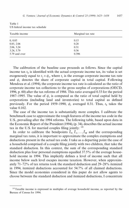
Table 1US federal income tax schedule

Taxable income Marginal tax rate

0, 0.85 0.150.85, 2.06 0.282.06, 3.24 0.313.24, 5.79 0.365.79 and over 0.396

18Taxable income is expressed in multiples of average household income, as reported by theBureau of Census for 1994.

The calibration of the baseline case proceeds as follows. Since the capitalincome tax t

kis identi"ed with the actual corporate income tax, its value is set

exogenously equal to tc]/

c, where t

cis the average corporate income tax rate

and /c

denotes the share of corporate capital in total capital. FollowingMendoza et al. (1994), the corporate income tax rate is calculated as the ratio ofcorporate income tax collections to the gross surplus of corporations (OECD,1996, p. 60) after the tax reforms of 1986. This ratio averaged 0.33 for the period1987}1995. The value of /

cis computed as the ratio of total capital held by

corporations (including land and inventories) to total capital as de"nedpreviously. For the period 1959}1990, /

caveraged 0.31. Thus, t

ktakes the

value 0.102.The case of the income tax is substantially more complex. I calibrate the

benchmark case to approximate the rough features of the income tax code in theU.S., prevailing after the 1994 reforms. The following table, based upon data inthe Economic Report of the President (1994), (p. 34), describes the actual incometax in the U.S. for married couples "ling jointly: 18

In order to calibrate the bendpoints IK0, IK

1,2, IK

Mand the corresponding

marginal tax rates, it is important to approximate the complex exemptions anddeductions present in the actual tax code. I take as a departing point the case ofa household comprised of a couple "ling jointly with two children, that take thestandard deduction. In this context, the sum of the corresponding standarddeduction plus four personal exemptions equalled 37.5% of the average house-hold income in 1994. This implicitly de"nes a level of income such that allincome below such level escapes income taxation. However, when approxim-ately 71}72% of tax returns took the standard deduction and 29}28% itemizedin 1994, itemized deductions accounted for 54.7% of all claimed deductions.Since the model economies considered in this paper do not allow agents tochoose between the standard deduction and itemized deductions, I concentrate


19The concept of income utilized in the computation of (IK ) is labor plus asset income before taxesplus all transfers.

Table 2Income tax schedule in model economies

w( e(z, j)l(x, j)#r( a(j

Marginal tax rate

0, 0.5IK 0.00.5 IK , 1.35IK 0.151.35 IK , 2.56IK 0.282.56 IK , 3.74IK 0.313.74 IK , 6.29IK 0.366.29 IK and over 0.396

on the case in which the lowest level of income subject to taxation is equal to50% of the mean household income of the model economy considered.

Once the lowest income level subject to income taxation is set, I use theprevious table as a benchmark for the calibration of the bendpoints and themarginal tax rates, expressed in terms of the multiples of mean householdincome (IK ) (Table 2).19

Hence, IK0"0, IK

1"0.5IK , IK

2"1.35IK , IK

3"2.56IK , IK

4"3.74IK , and IK

5"

6.29IK . Once the two sources of tax collections have been parametrized, thevalue of government consumption is determined endogenously by the equilib-rium condition 5. As a consequence, the interpretation of GK in the modeleconomies under the baseline tax case is the size of tax collections out of capitalincome and income taxes. Since the purpose of the paper is to consider a revenueneutral tax reform, the #at tax case is parametrized using the value of GK from thecorresponding calculations for the baseline tax regime. Notice that tax collec-tions in the case of a #at tax equal

+j

kjCqlPAw( e(z, j)l(x, j)dt

j(x)#q

"PX

(r( a(!(a(x, j)(1#g)!a( ))dtj(x)D

(10)

with A"Mx3X: w( e(z, j)l(x, j)5IK HN.In order to satisfy the above government budget constraint, values for IK H must

be speci"ed. To preserve comparability across model economies and tax re-gimes, results are reported for di!erent exemption values as multiples of themean income (IK ) of the corresponding model economy under the baseline taxregime. With IK H and GK at hand, provided that in the baseline Hall and Rabushka(1995) proposal the #at tax rate is q

""q

-,q, the #at tax rate is obtained by

updating its value after an initial guess at every iteration in the computation ofequilibria, until the government budget constraint is satis"ed.


20Hubbard et al. (1995), Huggett (1996) and Storesletten et al. (1998) are examples.

21Linear interpolations are used to obtain the pro"le for all possible ages.

4.3. The stochastic structure of wages

Recently, some models with heterogeneous agents and no labor supplydecision have been calibrated using a regression to the mean process forlog-labor earnings.20 The calibration adopted by these papers cannot immedi-ately be extended to the model economies analyzed here, because labor supplyis endogenous in the current setup. I proceed to calibrate the market return perunit of labor time supplied, described by the function e(z, j), under theassumption that the underlying stochastic structure also follows a regression tothe mean process. Notice that since w( is a constant at all ages and states, thecalibration of the function e(z, j) is equivalent to the calibration of a wage processover an agent's working life. Let y

jand y6

jdenote the log market return and the

mean log market return of an agent j periods old. Thus, the labor productivityshock is de"ned as z,y

j!y6

j, which implies that the function e(z, j) takes the

form e(z, j)"e(z`y6 j). Then, the market return to labor follows the regression tothe mean process for all 1(j4R:

yj!y6

j"c(y

j~1!y6

j~1)#e

j(11)

with e&N(0,p2e ). For j"1, y1&N(y6

1, p2

y1).

The calibration of the wage process proceeds as follows. First, the age speci"cpattern of mean log wages y6

1,2, y6

Ris chosen. I approximate this by using the

wage pro"le computed by Hansen (1993).21 The pro"le is displayed in Fig. 1.Second, I need to set values for the remaining parameters of the wage process

(c,p2e , p2y1). The natural avenue to select values for these parameters would be

using (i) data on the magnitude and persistence of idiosyncratic wage shocks and(ii) data on the concentration of wages. Unfortunately, no data is available onthe magnitude and persistence of shocks to log wages even though there is datameasuring the concentration of wages. Thus, I proceed to select parametervalues so that the implied wage distribution matches some recent estimates ofthe concentration of wages. In this regard, Ryscavage (1994) "nds that the wageGini coe$cient for all earners was 0.35 in 1989. This previous estimate can betaken as a lower bound since it understates the true degree of wage inequality(see Ryscavage (1994) for details). Based upon these considerations, I setc"0.985, p2

y1"0.29, and p2e"0.02 as the baseline parameter values. This

choice determines that the Gini coe$cient for wages equals 0.38. This calibratedprocess for wages generates an earnings distribution in stationary equilibriumwhose concentration statistics come close to recent estimates for the actualdistribution in the U.S. Furthermore, the endogenous earnings process also


Fig. 1. Wage pro"le (ratio to the overall mean).

22The value for mean hours represents the mean fraction of discretionary time spent working byagents who are 65 yr old or younger. Therefore, it equals

CR+j/1

kjP

X

l(x,j)dtjDN

R+j/1

kj.

approximates recent parameter estimates of regression to the mean for log-laborearnings (see Section 4.1).

The wage process described above is discretized for computational purposes.The shock z takes 21 possible values, evenly spaced in the log scale, ranging from!5p

y1to 5p

y1. Probabilities q(z) of receiving a particular shock for age 1 agents

are computed by simple numerical integration of the normal distributionN(0,p2

y1). Transition probabilities p(z@, z) are obtained in a similar fashion.

5. Results

This section reports the basic quantitative "ndings for both tax regimes.Details on how equilibria are computed are described in the Appendix.

5.1. Baseline taxes

Table 3 below shows basic statistics for the model economies.22 These resultsare important, in the sense that they will be compared afterwards with the


Table 3Descriptive statistics

Modeleconomy

KK />K Saving rate(%)

K Meanhours

>K w( r( (%) Discountfactor (b)

p"1.5 2.89 8.4 0.320 0.275 0.500 1.0 7.4 0.985p"4.0 2.89 8.4 0.318 0.273 0.496 1.0 7.4 1.013

23 It should be pointed out that a discount factor higher than one (i.e. a negative time preferencerate), as the one obtained for p"4.0, is not a problem in life cycle economies with or withoutuncertain lifetimes, since such a possibility is theoretically admissible. It is also worth noting that inan economy with secular growth and preferences as the ones speci"ed here, agents discount at therate bI s

j`1, bI ,b(1#g)l(1~p), as Eq. (7) indicates. Given the calibrated values of l, b and g,bI is lower

than one and equal to 0.9941 for p"4.0. Lifetime uncertainty through conditional survivalprobabilities implies that the age dependent discount factor is lower than bI for all ages(bI s

j`1(bI (1 for all j).

24These measures tend to understate the true degree of earnings concentration, due to severaldata problems. See Henle and Ryscavage (1990) for details.

equivalent statistics for the model economies under a #at tax. Observe that thediscount factor required to match the target capital to output ratio underp"4.0 is substantially higher than in the case of p"1.5, as in the formersituation, households accumulate a lower amount of capital for a given discountfactor. Thus, the discount factor is increased in order to induce higher levels ofcapital accumulation.23

In order to take seriously the distributional impact of #at tax reform to becomputed later, it is key to check some statistics on the stationary distributionsof income, labor earnings and wealth under the baseline taxes against actualdata. These statistics are displayed in Tables 4}6. In terms of the distribution oflabor earnings, the model economies are sucessful in approximating recentestimates for the U.S. In this regard, Henle and Ryscavage (1990) report that theearnings Gini coe$cient for all earners in the period 1985 to 1988 averaged 0.47,and that in 1988 the percent share in aggregate earnings of the lowest, second,third, fourth and upper quintiles was 2.1, 8.3, 15.8, 25.2, and 48.6 respectively.24Notice that both model economies match the earnings Gini. The model econo-mies also generate similar values for the share of aggregate earnings earned bydi!erent quantiles. For example, in the case of p"1.5, the percent share inaggregate earnings of the lowest to the highest quintiles is 3.2, 8.9, 14.0, 23.0, and50.9, respectively.

Finally, the arti"cial sample created by the model economies (see Appendix)can be used to estimate the coe$cient (c( ) of a regression to the mean for


Table 4Earnings distribution statistics

Modeleconomy

Quintile EarningsGini

Earnings

1st 2nd 3rd 4th 5thc(

U.S. 2.1 8.3 15.8 25.2 48.6 0.47 0.95p"1.5 3.2 8.9 14.0 23.0 50.9 0.47 0.95p"4.0 3.5 9.0 13.9 22.8 50.8 0.47 0.96

Table 5Distributional features

Modeleconomy

EarningsGini

Wealth Gini Income Gini Median}meanincome ratio

Median}meanwealth ratio

U.S. 0.47 0.72}0.84 0.43 0.65 0.23p"1.5 0.47 0.60 0.43 0.671 0.586p"4.0 0.47 0.60 0.42 0.689 0.565

Table 6Percent share of income earned by quantiles

Modeleconomy

Top1%

Top5%

Top10%

Quintile

1st 2nd 3rd 4th 5th

p"1.5 6.7 20.9 32.6 5.7 9.8 13.5 22.7 48.3p"4.0 6.7 20.8 32.4 5.7 9.9 13.8 22.3 48.2

25The regression coe$cient is estimated for agents 20}64 yr old. Agents with zero earnings areexcluded from the sample.

26Hubbard et al. (1995) estimate coe$cients equal to 0.96, 0.95 and 0.96 for households with lessthan 12 yr of education, 12}15 yr of education and 16 or more years of education, respectively.

log-labor earnings.25 On this topic, Hubbard et al. (1995) recently estimateda coe$cient that averages 0.95 for households with di!erent education levelsusing annual data.26 As Table 4 demonstrates, the model economies performquite well along this dimension.


27The concept of income used for the reported distributional calculations is labor plus assetincome before taxes, plus all transfers. The data for mean and median income and wealth data inTable 5 is from Wol! (1994), (Table 3).

28For instance, Avery and Kennickell (1993) using data from the Survey of Consumer Financesreport that the top 1% of U.S. households earned 12.9% in 1986.

29For 1983 and 1989, Wol! (1987), (1994) reports wealth Gini coe$cients ranging from 0.72 to0.84, depending upon the de"nition of wealth holdings employed.

30See Huggett (1996) for a study of the implications of heterogenous agents-life cycle modelswithout labor supply in terms of the wealth distribution. See Hubbard et al. (1995) for the role ofmeans-tested transfers and uninsurable risk on the wealth holdings of low income U.S. households.

The model economies also perform reasonably in terms of the implied incomedistribution along di!erent dimensions.27 In this regard, recent studies havedocumented extensively several features of the income distribution in the U.S.,and its time path. Using data from the Consumer Population Survey for the caseof income after transfers and before taxes, Ryscavage (1995) reports that theincome Gini was 0.428, 0.428, 0.433, 0.434 and 0.447 for 1990, 1991, 1992 and1993 respectively. He also reports that in 1993, the share received by eachquintile was 3.6, 9.0, 15.1, 23.5, and 48.9, and that the top 5% of householdsearned approximately 20% of aggregate income. Table 6 shows that resultsobtained for the share of income of the di!erent quantiles resemble the actualones mentioned above. The match is particularly good for the share of incomeearned by the upper 20% of the distribution. Likewise, as Table 5 demonstrates,the model economies generate reasonable values for the income Gini. The modeleconomies, nonetheless, do not concentrate enough income in the extreme uppertail (top 1%) of the income distribution, as other studied have documented.28

The results obtained for the case of the wealth distribution, however, are notas satisfactory as for the case of income and earnings. The model economiesgenerate substantially more concentration of wealth than income, as it is thecase in the actual data. Nevertheless, the implied wealth distribution is not asconcentrated as the actual one. As a consequence, the model economies generateGini coe$cients of about 0.60, that fall short of estimates for the U.S.29 30

How are labor hours supplied distributed across households in the baselinecase? This question is interesting from a quantitative standpoint, since a #at taxis likely to have a signi"cant impact on labor hours for households with di!erentearnings abilities. Table 7 shows the results for mean labor hours at di!erentpercentiles of the income distribution.

Observe that mean labor hours increase as the quintiles of income increase,with the exception of the third quintile. Also notice the important degree ofheterogeneity in labor hours supplied. Households in the 5th income quintilework 31}32% and 30}31% more than households in the lowest quintile, forp"1.5 and p"4.0, respectively.


Table 7Mean labor hours at di!erent income quintiles

Modeleconomy

Top Top Top 80}90% Quintile1% 5% 10%

1st 2nd 3rd 4th 5th

p"1.5 0.341 0.332 0.322 0.285 0.229 0.277 0.253 0.299 0.301p"4.0 0.344 0.333 0.322 0.283 0.231 0.269 0.255 0.297 0.301

31The results in this section are a!ected by the magnitude of the calibrated rate of technicalprogress, which is above some estimates. For instance the Congressional Budget O$ce (1998)estimates an average real growth rate of output of about 2.14% for the next ten years. Undera population growth rate of about 1.0%, this implies a value for g of about 1.2%. It is reasonable toconjecture, however, that the main results of the paper will not change substantially if the rate oftechnical progress is reduced. A key reason for this is that in order to match the target capital tooutput ratio under the baseline taxes, a reduction in g requires a reduction in the b } recall p'1 } soas to induce a reduction in the degree of capital accumulation.

One of the functions frequently attributed to a tax code is its capacity toreduce inequality among households. Thus, it is important to know howe!ective the baseline tax regime is in reducing the degree of income inequality, inorder to compare these results later with those under a #at tax. Table 8 showsthe distribution of income after income and capital income taxes.

The "ndings displayed in Table 8 show that the progressive structure of theincome tax built into the baseline tax regime is indeed capable of reducingincome inequality in an important way. Notice that the after tax income Ginicoe$cients are reduced from 0.43}0.42 to about 0.38. Notice also that thepercentage shares of income are all adjusted, so that the after tax incomedistribution becomes less concentrated. For instance, observe that the share ofthe 5th quintile is reduced by 3.9 and 3.8 percentage points for the cases ofp"1.5 and p"4.0, respectively.

5.2. Flat tax reform

Results for the revenue neutral tax reform are displayed for two exemptionlevels, 20% and 40% of the mean income (IK ) of the corresponding modeleconomy under income and corporation income taxes.31

5.2.1. AggregatesTable 9 shows descriptive statistics for the model economies under a #at tax.A key quantitative "nding here is that the #at tax has a signi"cant impact on

capital accumulation. As shown in Table 9, capital income ratios, net saving


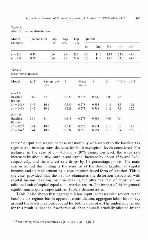
Table 8After tax income distribution

Modeleconomy

Income Gini Top Top Top Quintile1% 5% 10%

1st 2nd 3rd 4th 5th

p"1.5 0.38 5.6 18.0 28.8 6.4 11.1 14.7 23.4 44.4p"4.0 0.38 5.6 17.8 28.6 6.5 11.1 15.0 23.0 44.4


Model KK />K Saving rate(%)

K Meanhours

>K w( r( (%) q (%)

p"1.5Baseline#at tax

2.89 8.4 0.320 0.275 0.500 1.00 7.4 *

IK H"0.2IK 3.45 10.1 0.339 0.278 0.585 1.11 5.3 19.1IK H"0.4IK 3.45 10.1 0.328 0.273 0.566 1.11 5.3 25.2


2.89 8.4 0.318 0.273 0.496 1.00 7.4 *

IK H"0.2IK 3.41 10.0 0.335 0.275 0.574 1.10 5.5 19.4IK H"0.4IK 3.44 10.0 0.324 0.270 0.559 1.10 5.4 25.7

32Net saving rates are computed as [(1#n)(1#g)!1]KK />K .

rates32 output and wages increase substantially with respect to the baseline taxregime, and interest rates decrease for both exemption levels considered. Forinstance, in the case of p"4.0 and a 20% exemption level, the wage rateincreases by about 10%, output and capital increase by about 15% and 34%,respectively, and the interest rate drops by 1.9 percentage points. The mainreason behind this "nding is the removal of the double taxation of capitalincome, and its replacement by a consumption-based form of taxation. This isthe case, provided that the #at tax eliminates the distortion associated withcapital income taxation, by now making the after tax rate of return on anaditional unit of capital equal to its market return. The impact of this in generalequilibrium is quite important, as Table 9 demonstrates.

Table 9 also shows that aggregate labor input increases with respect to thebaseline tax regime, but in apparent contradiction, aggregate labor hours stayaround the levels previously found for both values of p. The underlying reasonfor this result is that the distribution of labor hours is crucially a!ected by the


33That is, an increase in the marginal tax rate on labor income for households who previouslyfaced a marginal tax rate of 15%, reductions in such tax rates for others, as well as the elimination ofintertemporal distortions created by the taxation of capital income through the income tax as well asthrough the capital income tax at rate q

k.

34For example, the reader should note that in the case of p"4.0 and a 20% exemption level, thehighest marginal tax rate on labor income (including social security taxes) falls from 48.2% to about28% after the reform.

35Several factors interact in the model economies after the reform that a!ect the age pro"le ofhours worked. Among them are (i) the reduction of marginal tax rates on labor income }which leadsagents to shift labor hours to middle age and old years with previously high marginal tax rates; (ii)the elimination of the distortions created by the taxation of capital income under the baseline taxes} which implies a shift of hours to younger years; and (iii) the fall in the interest rate } with the e!ectof shifting labor hours to middle age and old years.

fundamental changes in the tax structure,33 and the induced income andsubstitution e!ects implied by changes in factor prices and changes in the lumpsum transfer of accidental bequests. As in the case of the previous tax regime, it ispossible to calculate the structure of labor hours at income percentiles. Table 10shows the results.

It is worth noting that under the #at tax, households situated at low incomequintiles work more hours with the high exemption level (IK H"0.4IK ) than withthe low exemption level (IK H"0.2IK ), meanwhile the opposite pattern is true forhouseholds at upper quintiles, a "nding that re#ects the interaction betweenexemption levels and tax rates dictated by the revenue neutrality requirement, asshown in Table 9. Nevertheless, the impact of the #at tax on hours of householdsin the highest quintile is always positive, re#ecting the e!ects of sharp reductionsin marginal tax rates on labor income.34 A related perspective on the conse-quences of the reform on hours worked is yielded by observing the e!ects of thereform on hours worked over the life cycle. The quantitative magnitude of suchintertemporal reallocation is displayed in Table 11, which shows average laborhours for di!erent age groups. It is clear from these results that the net e!ect ofthe #at tax reform is to reallocate labor hours to relatively high productivityyears (middle age), and away from younger ages.35

The increase in labor hours of high income households mentioned previouslyis quite important, ranging from about 15}16% to 11}12% for p"1.5, andfrom 13}14% to 9}10% for p"4.0. These positive changes in the labor supplyof relatively richer households, groups that contain both an important fractionof households at the peak of their age-productivity cycle and a high fraction ofhouseholds receiving high shocks, are the key factors behind the increase in totallabor input in the model economies. Therefore, the key reason for the increase inlabor input together with relatively unchanged average labor hours, is simplythat additional hours of highly productive agents, are in all cases more thansu$cient to compensate for the negative e!ects on aggregate labor input ofrelatively low productivity households.


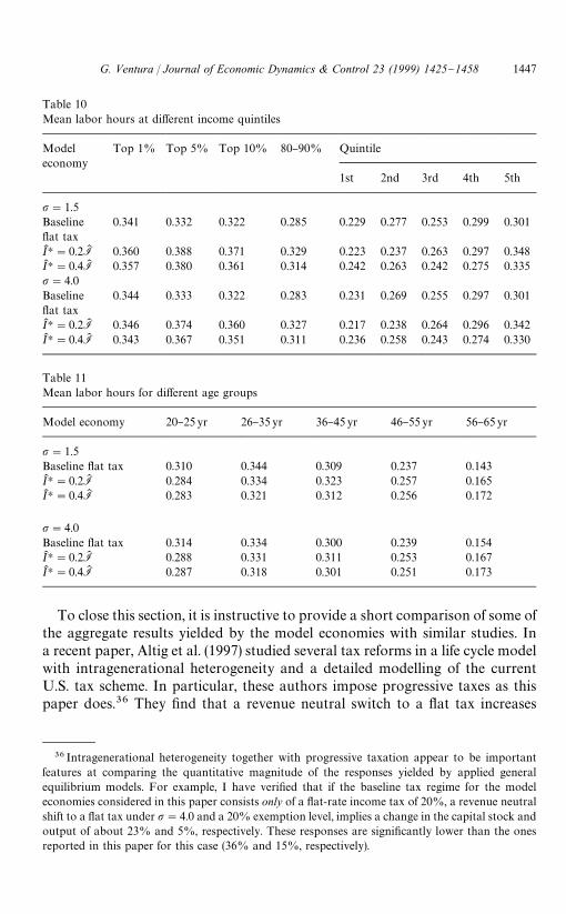
Table 10Mean labor hours at di!erent income quintiles

Modeleconomy

Top 1% Top 5% Top 10% 80}90% Quintile

1st 2nd 3rd 4th 5th


0.341 0.332 0.322 0.285 0.229 0.277 0.253 0.299 0.301

IK H"0.2IK 0.360 0.388 0.371 0.329 0.223 0.237 0.263 0.297 0.348IK H"0.4IK 0.357 0.380 0.361 0.314 0.242 0.263 0.242 0.275 0.335p"4.0Baseline#at tax

0.344 0.333 0.322 0.283 0.231 0.269 0.255 0.297 0.301

IK H"0.2IK 0.346 0.374 0.360 0.327 0.217 0.238 0.264 0.296 0.342IK H"0.4IK 0.343 0.367 0.351 0.311 0.236 0.258 0.243 0.274 0.330

Table 11Mean labor hours for di!erent age groups

Model economy 20}25yr 26}35yr 36}45yr 46}55yr 56}65yr

p"1.5Baseline #at tax 0.310 0.344 0.309 0.237 0.143IK H"0.2IK 0.284 0.334 0.323 0.257 0.165IK H"0.4IK 0.283 0.321 0.312 0.256 0.172


36 Intragenerational heterogeneity together with progressive taxation appear to be importantfeatures at comparing the quantitative magnitude of the responses yielded by applied generalequilibrium models. For example, I have veri"ed that if the baseline tax regime for the modeleconomies considered in this paper consists only of a #at-rate income tax of 20%, a revenue neutralshift to a #at tax under p"4.0 and a 20% exemption level, implies a change in the capital stock andoutput of about 23% and 5%, respectively. These responses are signi"cantly lower than the onesreported in this paper for this case (36% and 15%, respectively).

To close this section, it is instructive to provide a short comparison of some ofthe aggregate results yielded by the model economies with similar studies. Ina recent paper, Altig et al. (1997) studied several tax reforms in a life cycle modelwith intragenerational heterogeneity and a detailed modelling of the currentU.S. tax scheme. In particular, these authors impose progressive taxes as thispaper does.36 They "nd that a revenue neutral switch to a #at tax increases


37The #at tax system considered by Altig et al. (1997) taxes labor income only above a giventhreshold, as this paper does. However, unlike this paper, Altig et al. (1997) exempt housing wealthfrom taxation, which accounts for about half of the capital stock. As these authors point out, thisparticular feature of the #at tax they consider yields a lower increase in the overall labor input afterthe reform.

38 It should be stressed that the study of annual income and earnings is investigated here, ratherthan the distribution of lifetime income or of tax incidence from a lifetime perspective. There are tworeasons for this. First, there is large literature that documents distributional statistics, using data thatmainly comes in annual form, that are useful to test the performance of the model economies.Second, a study of the distribution of lifetime income or of lifetime tax incidence under alternativetax schemes, as carried out in some studies, cannot be undertaken here due to the presence ofincomplete markets in the current setup. That is, (i) lack of Arrow}Debreu markets to insure againstuninsurable #uctuations in labor productivity, and (ii) borrowing constraints. Unfortunately, in thiscontext, the present value calculations required to calculate lifetime distributional statistics are notfeasible. An alternative is to study the distribution of welfare at birth, in the spirit of Fullerton andRogers (1993), Altig et al. (1997) and other studies, where welfare for every shock level at birth isde"ned as <(0, z,1). I perform such an analysis in Ventura (1998).

output in the long run by about 6.1%, while in the case of a pure consumptiontax the increase is in the order of 11%.37 In this paper the response of output isof about 15% and 12% for p"4.0 and exemption levels of 20% and 40%. Whataccounts for this discrepancy in results? Aside from di!erences in calibration,I list here two di!erences between the models that lead to a larger response ofoutput in the present paper. First and more importantly, Altig et al. applya progressive tax only to labor income, while capital income is taxed at a #atrate. In contrast, in this paper capital income is taxed progressively through theincome tax, and also at a #at rate t

k. As a result, in this paper the highest

marginal tax rate on capital income is 50.4%, while in Altig et al. &new' capitalfaces a #at rate of 19.7% and &old' capital faces a #at rate of 23.7%. Hence, in theinitial steady state, capital accumulation is clearly more distorted in the presentpaper, and thus, the quantitative e!ects of the elimination of the taxation ofcapital income are higher. Second, all labor income is subject to the earningspayroll tax in this paper. In Altig et al., only labor earnings below a thresholdlevel (i.e. maximum taxable earnings set by the Social Security Administration)are subject to the payroll tax. This implies that for a given tax schedule on laborearnings, individuals with high labor earnings face a lower marginal tax rate inthe Altig et al. model. Since the impact of tax reform on hours worked depend onthe pre-reform marginal tax rates, this feature is potentially key in explaining thedi!erences between the quantitative implications of the two models.

5.2.2. Distributional ewectsTable 12 shows distributional aspects of the model economies under the #at

tax. The results clearly show that the cross-sectional distributions of earnings,wealth and income are adversedly a!ected in all circumstances.38


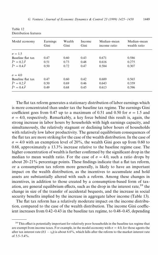
Table 12Distribution features

Model economy EarningsGini

WealthGini

IncomeGini

Median}meanincome ratio




39This e!ect is potentially important for relatively poor households in the baseline tax regime thatare exempt from income taxes. For example, in the model economy with p"4.0, for those agents theafter tax interest rate (r( (1!t

k)) is about 6.6%, which falls after the reform to the market interest rate

of 5.5}5.4%.

The #at tax reform generates a stationary distribution of labor earnings whichis more concentrated than under tax the baseline tax regime. The earnings Ginicoe$cient goes from 0.47 up to a maximum of 0.51 and 0.50 for p"1.5 andp"4.0, respectively. Remarkably, a key force behind this result is, again, thestrong increase in labor hours by households with high earnings capacity, andsimultaneously, the relatively stagnant or declining labor hours of householdswith relatively low labor productivity. The general equilibrium consequences ofthe #at tax are more striking for the case of the wealth distribution. In the case ofp"4.0 with an exemption level of 20%, the wealth Gini goes up from 0.60 to0.68, approximately a 13.3% increase relative to the baseline regime case. Thehigher concentration of wealth is further con"rmed by the signi"cant drop in themedian to mean wealth ratio. For the case of p"4.0, such a ratio drops byabout 20}21% percentage points. These "ndings indicate that a #at tax reform,or a consumption tax reform more generally, is likely to have an importantimpact on the wealth distribution, as the incentives to accumulate and holdassets are substantially altered with such a reform. Among these changes inincentives, in addition to those created by a consumption-based form of tax-ation, are general equilibrium e!ects, such as the drop in the interest rate,39 thechange in size of the transfer of accidental bequests, and the increase in socialsecurity bene"ts implied by the increase in aggregate labor income (Table 13).

The #at tax reform has a relatively moderate impact on the income distribu-tion, compared to the case of the wealth distribution. The income Gini coe$c-ient increases from 0.42}0.43 in the baseline tax regime, to 0.48}0.45, depending


Table 13Percent share of income earned by quintiles

Modeleconomy

Top 1% Top 5% Top 10% Quintile

1st 2nd 3rd 4th 5th


6.7 20.9 32.6 5.7 9.8 13.5 22.7 48.3

IK H"0.2IK 7.5 23.5 36.3 4.9 8.3 12.4 20.9 53.5IK H"0.4IK 7.7 23.8 36.7 5.5 8.7 11.9 20.2 53.7


6.7 20.8 32.4 5.7 9.9 13.8 22.3 48.2

IK H"0.2IK 7.3 22.7 35.1 5.1 8.6 12.9 21.0 52.3IK H"0.4IK 7.4 23.0 35.4 5.7 9.0 12.5 20.4 52.4

40Despite its relative small magnitude in both tax regimes, movements in the size of the lump sumtransfer of accidental bequests a!ect not only the income distribution, but also the distribution oflabor hours. This problem is explored in Section 6.

on the model economy considered. Both median and mean income increase withthe reform, but changes in mean income dominate so that the ratio of median tomean decreases, as Table 11 demonstrates. Most of the changes occur in thepercent share of the upper 20% of households, which increases after the taxreform by about 5.2}5.4 percentage points for p"1.5, and 4.1}4.2 percentagepoints for the case of p"4.0.

It is important to point out the presence of two elements in the modeleconomies that contribute to moderate the impact on the income distribution ofthe #at tax reform. First, as the #at tax increases both the wage rate and in mostcases the size of aggregate labor input, tax collections out of social security taxesincrease. Consequently, social security payments increase equally for all house-holds compared to the case of the baseline tax regime. This increase in socialsecurity transfers, with clear implications on the wealth and income distribution,is an interesting general equilibrium e!ect that has not been emphasized in thedebate on fundamental tax reform. Second, since the size of accidental bequestsincreases roughly proportional with aggregate wealth, the corresponding lumpsum transfer to all households increases also. This latter e!ect is a consequenceof the particular form used here to handle accidental bequests, so it is likely thatmore realistic ways of handling bequests will not display such an equalizingimpact on the income distribution40 (Table 14).


Table 14After tax income distribution

Modeleconomy

IncomeGini

Top1%

Top5%

Top10%

Quintile

1st 2nd 3rd 4th 5th


0.38 5.6 18.0 28.8 6.4 11.1 14.7 23.4 44.4

IK H"0.2IK 0.47 7.7 23.7 36.4 5.2 8.6 12.3 20.5 53.4IK H"0.4IK 0.45 7.6 23.5 35.9 5.8 9.6 12.1 19.9 52.6


0.38 5.6 17.8 28.6 6.5 11.1 15.0 23.0 44.4

IK H"0.2IK 0.45 7.3 22.6 34.9 5.4 9.1 12.9 20.8 51.8IK H"0.4IK 0.43 7.2 22.2 34.2 6.0 9.9 13.0 20.3 50.7

41All results in this section are reported for the case of p"4.0.

This section is closed with the examination of the capacity of the #at tax toreduce income inequality. As Table 12 demonstrates, the progressive features ofthe #at tax regime do not reduce the concentration of income in the magnitudethat the features of the baseline tax regime did. Indeed, the reduction in incomeinequality under the #at tax is relatively small, measured by the changes in Ginicoe$cients and shares of income earned by di!erent percentiles. The implicationof this "nding is straightforward: for the model economies investigated, both thebefore tax and after tax income distributions become more concentrated withthe adoption of the #at tax.

6. The role of accidental bequests

One potential concern about the computational experiments studied in thispaper is that, despite its small magnitude, the lump sum transfer of accidentalbequests varies with the change in tax regimes as its value is roughly propor-tional to the size of aggregate wealth. It increases with the adoption of a #at tax,and its value is further decreased with a higher exemption level. In this section,I brie#y explore quantitatively the role played by this particular way of handlingaccidental bequests in the context of tax reform.41 All transfers of accidentalbequests are now eliminated, allowing the government to tax all accidental


42This implies a change in condition 5 in the de"nition of equilibrium that now becomes

GK "+j

kjP

X

¹(x, j) dtj#¹RK .

There are other ways of attacking this problem without a careful modelling of the family.Rios-Rull (1996) eliminates accidental bequests by imposing the existence of a market for one-periodannuities, where agents can perfectly insure themselves against lifetime uncertainty. In Hubbard andJudd (1987), agents receive accidental bequests only once, at a pre-determined age. Yet anotheravenue would be to model the receipt of a bequest as an uncertain event, in which the size of thebequest received is random.

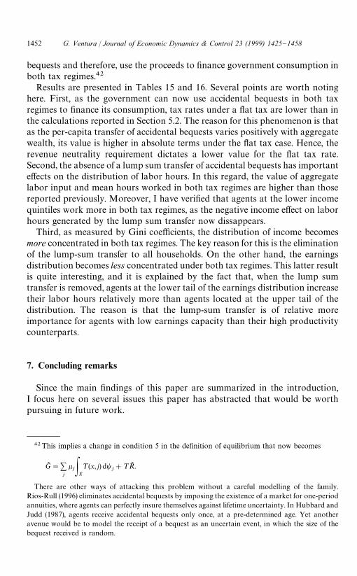
bequests and therefore, use the proceeds to "nance government consumption inboth tax regimes.42

Results are presented in Tables 15 and 16. Several points are worth notinghere. First, as the government can now use accidental bequests in both taxregimes to "nance its consumption, tax rates under a #at tax are lower than inthe calculations reported in Section 5.2. The reason for this phenomenon is thatas the per-capita transfer of accidental bequests varies positively with aggregatewealth, its value is higher in absolute terms under the #at tax case. Hence, therevenue neutrality requirement dictates a lower value for the #at tax rate.Second, the absence of a lump sum transfer of accidental bequests has importante!ects on the distribution of labor hours. In this regard, the value of aggregatelabor input and mean hours worked in both tax regimes are higher than thosereported previously. Moreover, I have veri"ed that agents at the lower incomequintiles work more in both tax regimes, as the negative income e!ect on laborhours generated by the lump sum transfer now dissappears.

Third, as measured by Gini coe$cients, the distribution of income becomesmore concentrated in both tax regimes. The key reason for this is the eliminationof the lump-sum transfer to all households. On the other hand, the earningsdistribution becomes less concentrated under both tax regimes. This latter resultis quite interesting, and it is explained by the fact that, when the lump sumtransfer is removed, agents at the lower tail of the earnings distribution increasetheir labor hours relatively more than agents located at the upper tail of thedistribution. The reason is that the lump-sum transfer is of relative moreimportance for agents with low earnings capacity than their high productivitycounterparts.

7. Concluding remarks

Since the main "ndings of this paper are summarized in the introduction,I focus here on several issues this paper has abstracted that would be worthpursuing in future work.



Modeleconomy

KK />K K Mean hour >K w( r( (%) q (%)

Baseline#at tax

2.89 0.336 0.297 0.522 1.00 7.4 *

IK H"0.2IK 3.44 0.357 0.306 0.615 1.11 5.4 0.167IK H"0.4IK 3.46 0.347 0.300 0.601 1.11 5.3 0.219

Table 16Distributional features

Model economy EarningsGini

WealthGini

IncomeGini

Median}meanincome ratio


Baseline #at tax 0.46 0.59 0.43 0.690 0.570IK H"0.2IK 0.48 0.68 0.47 0.649 0.389IK H"0.4IK 0.47 0.67 0.46 0.624 0.404

First, as Engen and Gale (1996) and other authors have stressed, the currentU.S. tax code contains some of the features of a consumption tax, provided thatcontributions to several pension plans are tax deductible and that earnings onthese accounts are taxed only upon withdrawal. Since assets held in theseaccounts represent a substantial fraction of total "nancial assets held by U.S.households (approximately 35%), these considerations indicate that some of thequantitative "ndings of this paper would require further study under suchcircumstances. In particular, it is likely that (i) the positive quantitative impact ofa #at tax reform on capital formation and output will be reduced, as in Engenand Gale (1996), and (ii) the negative distributional impact of a #at tax oncross-sectional distributions will be reduced as well.

Second, as Gentry and Hubbard (1997) have recently pointed out, a #at tax ora consumption tax di!ers from a standard income tax in the sense that thetreatment of capital income di!ers only for one component of what is usuallyde"ned as capital income } the opportunity cost of capital or return to waiting.Other components of capital income not considered in the model economies ofthis paper, such as inframarginal returns to investing (pure economic pro"ts), orthe return to risk taking are similarly treated under both an income tax and anconsumption tax. This implies that if these components of capital income areproperly incorporated in a general equilibrium model, the impact of a #at tax oncapital accumulation and output is likely to be reduced. Moreover, sinceentepreneurial income and holdings of risky assets are concentrated in upper


43See Gravelle (1994), (Chapter 4) for a comprehensive survey of the distortionary e!ects ofcorporate income taxation.

44See Slemrod (1996) for a recent estimation of compliance costs of the U.S. Federal tax code andfor a projection of the compliance costs of a #at tax.

45The quantitative magnitude of the potential increase in the growth rate is subject to debate. Onthe one hand, Cassou and Lansing (1997) obtain an increase in the growth rate from implementinga #at tax ranging from 0.18 to 0.75 percentage points. On the other hand, Lucas (1990) showed thatthe complete elimination of capital income taxes, and their replacement by taxes on labor, has aninsigni"cant e!ect on the long run growth rate. Stokey and Rebelo (1995) con"rmed this "nding fora variety of endogeneous growth models.

percentiles of the income distribution in actual data, the negative distributionale!ect of a #at tax reform will be moderated as well.

Third, this paper has explored and compared the aggregate as well as thecross-sectional properties of steady states under a representation of the actualU.S. federal tax code and a #at tax. However, a complete analysis of the taxreform demands an analysis of the transition between steady states. In the con-text of the model economies studied in this paper, such a study of thetransitional dynamics would permit a careful and meaningful analysis ofthe welfare gains or losses associated with the #at tax reform as well asthe distribution of such welfare gains or losses for agents born with di!erentlabor productivity levels, both during the transition as well as at the "nal steadystate.

Fourth, as an integrated consumption-based form of taxation, the #at taxeliminates the distortion in the allocation of capital between corporate andnon-corporate sectors, as well as other distortions induced by the currentcorporate income tax.43 As there is a single sector in the economies studied inthis paper, only the e!ects emerging from the replacement of a tax systemincluding a #at-rate tax on all capital income by a #at tax could be considered. Itis then clear that there are potential welfare gains arising from a #at tax, inaddition to those that could be derived from the model economies investigatedhere.

Fifth, some authors have pointed out that the current federal tax code mayinvolve high compliance costs not modelled here. The relative simplicity em-bodied in the Hall}Rabushka proposal (&tax forms really can "t on post-cards')suggests that the #at tax may well represent an improvement over the existingsituation.44 Finally, a #at tax reform may increase permanently the growth rate,as suggested by authors who studied tax reforms in the context of endogenousgrowth models.45 As in the case of the elimination of the corporate income taxdiscussed above, the two previous remarks suggest that there are additionalwelfare gains associated with a #at tax on top of those that could be implied bythe model economies studied in this paper.


46The asset grid is constructed according to the equation ak("a(#b(k!1)2., k3M1, 401N,

b"a(6 /4002.

Acknowledgements

I would like to thank to Mark Huggett for continuous advice and comments,and to two anonymous referees whose comments have improved this papersubstantially. I would also like to thank Anne Villamil, Bart Taub, AndreH sErosa, Kent Smetters, Kevin Lansing, John Whalley and seminar participants atIllinois, Western Ontario, Centro de InvestigacioH n EconoH mica (I.T.A.M.),C.I.D.E., the 1997 North American Meetings and Latin American Meetings ofthe Econometric Society, the 1997 Meetings of the Society for ComputationalEconomics and the 1997 Meetings of the Society of Economic Dynamics forcomments, and the Econometrics Lab at the University of Illinois for computerfacilities. All errors are mine.

Appendix A. Computation

Equilibria are computed using the following algortithm:

1. Guess the value for capital KK , labor K , and transfers of accidental bequests,¹RK . In the case of the #at tax, guess also a value for the common tax rate q.

2. Compute factor prices: w("F2(KK , K ) and r("F

1(KK , K )!d. Obtain the social

security transfers, from condition 6 in the de"nition of equilibrium. In thebaseline tax regime, compute mean income, the capital income tax q

k, and the

income tax bendpoints.3. Calculate optimal decision rules: a(x, j), l (x, j), and c(x, j).4. Calculate values of KK , K , transfers ¹RK and tax collections that are implied by

a(x, j) and l(x, j).5. If the guessed values from step 1 equal the implied values in step 4, then this is

a steady-state equilibrium. Otherwise, guess new values and repeat the abovesteps.

Steps 3 and 4 above need to be explained. To carry out step 3, the space ofasset holdings is discretized. The asset space takes 401 possible values, rangingfrom a( , to an upper bound a(6 . The distance between gridpoints increases withasset levels.46 Provided that for all x3X, a(x,N)"0 since <(x,N#1),0,decision rules for assets at every gridpoint are computed by solving the age-speci"c Bellman equations backwards from j"N!1. From j"N!1 toj"R#1, only asset decision rules need to be computed, since labor hourssupplied are zero. The asset decision rule is obtained by "rst bracketing themaximum over the asset grid using a bisection procedure. Once the maximum


47Higher numbers of agents turned out to be irrelevant, in the sense that they do not a!ectdescriptive statistics of the model economies.

has been bracketed, the asset decision is obtained by applying a Golden Searchmethod, as implemented by Press et al. (1994). To undertake this process, valuefunctions o! gridpoints are given by linear interpolation of value functions atgridpoints.

For ages j"1 through j"R, the problem is relatively more complex due tothe presence of the labor supply decision and further complications created byprogressive taxation. Notice that at every j3M1,2,RN and x3X, for everydesired a( @, the labor decision is a well de"ned intratemporal optimization prob-lem. Furthermore, the agent's budget constraint is di!erentiable with respect tolabor hours except at the non-di!erentiable points lK

i"(IK

i!r( a( )/we(z, j),

i"1,2,M in the baseline tax regime, and lK"(IK H)/we(z, j) in the #at tax regime.Labor supply is then obtained by guessing a bracket of income or labor income(depending upon the tax regime considered), obtaining desired labor hours byusing the closed form solution determined by "rst order conditions, and thenchecking if the implied income or labor income falls within the guessed bracket.For the case of the baseline tax regime, if when the guessed bracket is (IK

i~1, IK

i],

the implied income belongs to (IKi, IK

i`1], and whenever the selected bracket is

(IKi, IK

i`1], the implied income falls into (IK

i~1, IK

i], labor hours are those de"ned by

the corresponding non-di!erentiable point. The same reasoning applies to thecase of the #at tax regime. The process just described yields for every choice of a( @,desired labor hours and taxes paid for all j3M1,2, RN and x3X. Therefore, withthe information on labor hours and taxes paid, the asset decision rule iscomputed as in the previous case.

Theoretically, step 4 requires the computation of the probability measurest1, t

2,2,t

N. I circumvent this problem by instead performing an equivalent

aggregation process by simulating the behavior of a large number of agents.Equilibria are computed by simulating shock histories and consequent decisionrules and taxes paid for 20,000 agents per cohort in a stationary equilibrium.47Whenever current assets fall outside gridpoints, decision rules and taxes paid areobtained by linear interpolation of values at gridpoints. All the distributionalfeatures of the model economies analyzed in the text, are further computed byusing the simulated shock histories and implied decision rules obtained for thesteady state under consideration.

References

Altig, D., Auerbach, A., Kotliko!, L., Smetters, K., Walliser, J., 1997. Simulating US tax reform.NBER Working Paper 6248.


Auerbach, A., Kotliko!, L., Skinner, J., 1983. The e$ciency gains of dynamic tax reform. Interna-tional Economic Review 24, 81}100.

Auerbach, A., Kotliko!, L., 1983. National savings, economic welfare and the sructure of taxation.In: Feldstein, M. (Ed.), Behavioral Simulation Methods in Tax Policy Analysis. The University ofChicago Press, Chicago.

Auerbach, A., Kotliko!, L., 1987. Dynamic Fiscal Policy. Cambridge University Press, Cambridge.Avery, R., Kennickell, A., 1993. US household wealth: changes from 1983 to 1986. Research in

Economic Inequality 4, 27}68.Cassou, S., Lansing, K., 1997. Growth e!ects of a #at tax. Mimeo.Congressional Budget O$ce, 1998. The Economic and Budget Outlook: Fiscal Years 1999}2008.

Washington, DC.Cooley, T., Prescott, E., 1995. Economic growth and business cycles. In: Cooley, T. (Ed.), Frontiers of

Business Cycle Research. Princeton University Press, Princeton, NJ.Elmendorf, D., 1996. The e!ects of interest rate changes on household saving and consumption:

a survey. Federal Reserve Board, mimeo.Engen, E., Gale, W., 1996. The e!ects of fundamental tax reform on saving. In: Aaron, H., Gale, W.

(Eds.), Economic E!ects of Fundamental Tax Reform. Brookings Institution Press, Washington,DC.

Engen, E., Gravelle, J., Smetters, K., 1997. Dynamic tax models: why they do the things they do?.National Tax Journal L 3, 657}682.

Fullerton, D., Rogers, L., 1993. Who Bears the Lifetime Tax Burden? Brookings Institution,Washington, DC.

Gentry, W., Hubbard, G., 1997. Distributional implications of introducing a broad based consump-tion tax. Tax Policy and the Economy 11, pp. 1}48.

Gravelle, J., 1994. The Economic E!ects of Taxing Capital Income. MIT Press, Cambridge, MA.Hall, R., Rabushka, A., 1995. The Flat Tax, 2nd ed. Hoover Institution Press.Hansen, G., 1993. The cyclical and secular behavior of the labor input: comparing e$ciency units

and hours worked. Journal of Applied Econometrics 8, 71}80.Henle, P., Ryscavage, P., 1990. Earnings inequality accelerates in the 1980's. Monthly Labor Review

3}17.Hubbard, G., Judd, K., 1987. Social security and individual welfare: precautionary saving, liquidity

constraints and the payroll tax. American Economic Review 77, 630}646.Hubbard, G., Skinner, J., Zeldes, S., 1995. Precautionary savings and social insurance. Journal of

Political Economy 103, 360}399.Hu!man, G., Greenwood, J., 1991. Tax analysis in a real business cycle model: on measuring

harberger triangles and okun gaps. Journal of Monetary Economics 27 (2), 167}190.Huggett, M., 1996. Wealth distribution in life-cycle economies. Journal of Monetary Economics 38,

469}494.Huggett, M., Ventura, G., 1998. On the distributional implications of social security reform. Mimeo,

University of Western Ontario.Imrohoroglu, S., 1997. A quantitative analysis of capital income taxation. Mimeo, University of

Southern California.Imrohoroglu, A., Imrohoroglu, S., Joines, D., 1995. A life cycle analysis of social security. Economic

Theory 6, 83}114.Lucas, R., 1990. Supply side economics: an analytical review. Oxford Economic Papers 42,

293}316.Mendoza, E., Razin, A., Tesar, L., 1994. E!ective tax rates in macroeconomics: cross country

estimates of tax rates on factor prices and consumption. Journal of Monetary Economics 34 (3),297}324.

Musgrave, J., 1992a. Fixed reproducible tangible wealth in the United States: revised estimates.Survey of Current Business 72, 106}107.


Musgrave, J., 1992b. Organization for Economic Cooperation and Development, 1990. NationalAccounts Detailed Tables 1983}1995. Organization for Economic Cooperation and Develop-ment, Paris.

Prescott, E., 1986. Theory ahead of business cycle measurement. Federal Reserve Bank of Min-neapolis Quarterly Review 9}22.

Press, W., Teukolsky, S., Vetterling, W., Flannery, B., 1994. Numerical Recipes in Fortran: The Artof Scienti"c Computing, 2nd ed. Cambridge University Press, Cambridge.

Quadrini, V., Rios Rull, J.V., 1997. Understanding the U.S. distribution of wealth. Federal ReserveBank of Minneapolis Quaterly Review 21 (2), 22}36.

Rios-Rull, J.V., 1995. Models with heterogeneous agents. In: Cooley, T. (Ed.), Frontiers of BusinessCycle Research. Princeton University Press, Princeton, NJ.

Rios-Rull, J.V., 1996. Life cycle economies and aggregate #uctuations. Review of Economic Studies63, 465}489.

Ryscavage, P., 1994. Gender related shifts in the distribution of wages. Monthly Labor Review 3}16.Ryscavage, P., 1995. A surge in growing income inequality? Monthly Labor Review 51}61.Slemrod, J., 1996. Which is the simplest tax system of them all? In: Aaron, H., Gale, W. (Eds.),

Economic E!ects of Fundamental Tax Reform. Brookings Institution Press, Washington, DC.Stokey, N., Rebelo, S., 1995. Growth e!ects of #at-rate taxes. Journal of Political Economy 103,

519}550.Storesletten, K., Telmer, C., Yaron, A., 1998. Persistent idiosyncratic shocks and incomplete

markets. mimeo.Summers, L., 1981. Capital income taxation and accumulation in a life cycle model. American

Economic Review 71, 533}544.Ventura, G., 1998. Flat tax reform: a quantitative exploration. Research Report 9706, University of

Western Ontario.Wol!, E., 1987. Estimates of household wealth inequality in the US, 1962}1983. Review of Income

and Wealth, 231}57.Wol!, E., 1994. Trends in household wealth in the United States: 1962}1983 and 1983}1989. Review

of Income and Wealth 4 (2), 143}174.


Flat tax reform: A quantitative exploration

Documents

Transcript of Flat tax reform: A quantitative exploration