arX

iv:a

stro

-ph/

0501

504v

3 2

0 S

ep 2

005

Astronomy & Astrophysicsmanuscript no. ctp˙maps˙v5 February 2, 2008(DOI: will be inserted by hand later)

Comparison of map-making algorithms for CMB experiments

T. Poutanen1,2, G. de Gasperis3, E. Hivon4, H. Kurki-Suonio2, A. Balbi3,5, J. Borrill6,7, C. Cantalupo7,6, O. Dore8, E.Keihanen1,2, C. Lawrence9, D. Maino10, P. Natoli3,5, S. Prunet11, R. Stompor6,7, and R. Teyssier12

1 Helsinki Institute of Physics, P.O. Box 64, FIN-00014 Helsinki, Finland2 University of Helsinki, Department of Physical Sciences, P.O. Box 64, FIN-00014, Helsinki, Finland3 Dipartimento di Fisica, Universita di Roma “Tor Vergata”,via della Ricerca Scientifica 1, I-00133 Roma, Italy4 IPAC, MS 100-22, Caltech, Pasadena, CA 91125, U.S.A5 INFN, Sezione di Roma II, via della Ricerca Scientifica 1, I-00133 Roma, Italy6 Computational Research Division, Lawrence Berkeley National Laboratory, Berkeley CA 94720, U.S.A.7 Space Sciences Laboratory, University of California Berkeley, Berkeley CA 94720, U.S.A.8 Department of Astrophysical Sciences, Princeton University, Princeton, NJ 08540, U.S.A.9 Jet Propulsion Laboratory, 4800 Oak Grove Drive, Mailstop 169-327, Pasadena CA 91109, U.S.A.

10 Dipartimento di Fisica, Universita di Milano, Via Celoria16, I-20131 Milano, Italy11 Institut d’Astrophysique de Paris, 98 bis Boulevard Arago,F-75104 Paris, France12 Service d’Astrophysique, DAPNIA, Centre d’Etudes de Saclay, F-91191 Gif-sur-Yvette, France

September 20, 2005

Abstract. We have compared the cosmic microwave background (CMB) temperature anisotropy maps made from one-yeartime ordered data (TOD) streams that simulated observations of the originally planned 100 GHz P Low FrequencyInstrument (LFI). The maps were made with three different codes. Two of these, ROMA and MapCUMBA, were implemen-tations of maximum-likelihood (ML) map-making, whereas the third was an implementation of the destriping algorithm. Thepurpose of this paper is to compare these two methods, ML and destriping, in terms of the maps they produce and the angularpower spectrum estimates derived from these maps. The difference in the maps produced by the two ML codes was found tobe negligible. As expected, ML was found to produce maps withlower residual noise than destriping. In addition to residualnoise, the maps also contain an error which is due to the effect of subpixel structure in the signal on the map-making method.This error is larger for ML than for destriping. If this erroris not corrected a bias will be introduced in the power spectrumestimates. This study is related to P activities.

Key words. methods: data analysis – cosmology: cosmic microwave background

1. Introduction

Map-making from an observed time ordered data (TOD) streamis an important step in the data processing pipeline of a cosmicmicrowave background (CMB) experiment. A number of map-making algorithms which, under the assumption of Gaussiandistributed and stationary noise, aim at finding the optimalminimum variance map have been proposed (Wright 1996;Borrill 1999; Dore et al. 2001; Natoli et al. 2001). The de-striping technique (Burigana et al. 1997; Delabrouille 1998;Maino et al. 1999, 2002; Revenu et al. 2000a, 2000b; Keihanenet al. 2004) is a simpler map-making method.

For this study we utilized simulated one-year TOD streams,that had been produced in the course of the work of the CTP(Cℓ for Temperature and Polarisation) Working Group of theP Consortia. These TODs represent the output of a sin-gle detector of the originally planned 100 GHz LFI (Low

Send offprint requests to: T. Poutanen, e-mail:torsti.poutanen@helsinki.fi

Frequency Instrument) channel of the P satellite. Thissimulated data contains contributions from CMB and fore-ground emissions, as well as from the instrumental noise. Thenoise was assumed Gaussian distributed and stationary overtheentire mission, containing a 1/ f and a white noise component.We considered temperature anisotropies only; no polarisation.

Output maps were generated from the TODs using threedistinct map-making codes. The output maps and their angu-lar power spectra were critically compared. The map-makingcodes were ROMA (Roma Optimal Mapmaking Algorithm;Natoli et al. 2001; de Gasperis et al. 2005), MapCUMBA (orig-inally introduced by Dore et al. 2001, current version based onthe preconditioned conjugate gradient method) and destriping(Keihanen et al. 2004). All methods have been developed totreat P-like data.

A minimum variance map maximizes the likelihood func-tion involving the full noise covariance. The ROMA andMapCUMBA algorithms aim at producing the minimum vari-

2 Poutanen et al.: Comparison of map-making algorithms for CMB experiments

ance map. To accomplish this, the algorithms require knowl-edge on the characteristics of the instrument noise. Both iter-ative (Dore et al. 2001) and non-iterative (Natoli et al. 2002)methods to estimate the noise properties directly from the datahave been proposed. In this paper ROMA and MapCUMBA arereferred to with a common name maximum likelihood (ML)map-making.

Destriping does not employ the noise covariance matrixand does not aim at producing a minimum variance map inthis sense. Thus it does not require prior knowledge on thecharacteristics of the instrument noise. This simplifies the al-gorithm considerably as compared to the ML map-making.In spite of this, destriping is able to provide an estimate ofthe low-frequency part of the instrument noise and to returna TOD where these noise components have been removed.Destriping can also be applied to estimate various systematiceffects and drifts, remove them and return a cleaned TOD (seee.g. Mennella et al. 2002).

The aim of this paper is to compare these two methods,ML (ROMA and MapCUMBA) and destriping, in terms of themaps they produce and the angular power spectrum (Cℓ) esti-mates derived from these maps.

This paper is organized as follows. In Sect. 2 we describethe map-making and power spectrum estimation methods ap-plied in this study. The simulated one-year TOD streams areintroduced in Sect. 3. The output maps are compared in Sect. 4and the power spectrum estimates produced from the simulatedTODs are examined in Sect. 5. The conclusions are given inSect. 6. In Appendix A we describe how the output map is splitin the (wanted) binned noiseless map and in the (unwanted) re-construction error map. These quantities were considered in thecomparison of the output maps in Sect. 4. In Appendix B wediscuss some details about how theCℓ of the maps are relatedto the inputCℓ used to generate the TODs.

2. Methods

Let us denote by a column vectory the samples of the observedTOD. The length ofy is Nt, the number of samples in the to-tal mission. In the map-making problem we assume that thesignal samples are scanned from a pixelized temperature map(m). (This assumption of course represents an approximationto reality, and thus contributes to error in the final maps.) Thelength of the column vectorm is Npix, the number of pixels inthe map.

The scanning is implemented by a pointing matrixP. Thesize of the pointing matrix is [P] = (Nt,Npix). Each row con-tains zeros except for one element with value one, indicatingthe pixel at which the detector beam centre was pointing whenthe sample was measured. The map-making methods discussedhere utilize pointing information only to the accuracy given bythe pixel size. If the instrument beam response is sphericallysymmetric (and as we are neglecting polarisation), informationabout the rotation angle of the detector around the line of sightis not needed, and such a simple pointing matrix is sufficient.The pixel temperature of the output map will then represent aconvolution of the sky and the beam. We have used in this studysimulated TODs corresponding to both spherically symmetric

and elliptic beams; but a study of the effects of beam shape ispostponed to a future detailed study by the CTP group.

For an asymmetric beam every pixel will be smoothed witha different response that is the mean of the beam orientationsof the observations falling in that pixel. Recently a deconvo-lution map-making algorithm was introduced that can providean output map where the smoothing of the instrument beam(symmetric or asymmetric) is deconvolved leading to a mapthat is an estimate of the true sky (Armitage & Wandelt 2004).Deconvolution map-making is beyond the scope of this study.

2.1. ROMA and MapCUMBA

The output map (m) is solved by minimizing the log-likelihoodformula (Natoli et al. 2001)

χ2 = (y − Pm)TN−1(y − Pm). (1)

HereN is the noise covariance matrixN = 〈nnT〉, wheren isthe instrument noise component of the TOD and〈·〉 denotesexpectation value. A set of linear equations is obtained fortheoutput map

PTN−1Pm = PTN−1y. (2)

Eq. (2) is a general result for the minimum variance map.Usually ML map-making assumes the noise to be stationary

throughout the mission. It is further assumed that the elementsof the covariance matrix (Ni j ) vanish when|i − j| is larger thansomeNη andNη ≪ Nt. This means that the correlation is signif-icant only across a number of samples that is a tiny fraction ofthe total length of the TOD. Thus the noise correlation matrix Ncan be approximated by a circulant matrix (Natoli et al. 2001).Note that the matrixN−1 is approximately circulant as well.The multiplicationN−1y can be carried out more easily in thefrequency domain whereN−1 is diagonal (Natoli et al. 2001).Both in the ROMA and in the MapCUMBA algorithms the out-put map is solved from Eq. (2) with an iterative preconditionedconjugate gradient method. The iterations are repeated until thefractional difference has reached a low enough value (Natoli etal. 2001). This limit is typically on the order of 10−6.

Due to the circulant matrix approximation each row of thematrix N−1 contains the same element values with a differentcyclic permutation. It is assumed that only the elements of arow with |i − j| ≤ Nξ (Nξ ≪ Nt) have non-zero values. The restof the elements are zero. The collection of the non-zero ele-ments (of a row) is called thenoise filter. The lag of an elementis the difference of its indices (i− j). The choice of the valueNξis a significant decision for the quality of the output maps andfor the computation time of the algorithm (Natoli et al. 2001).

Natoli et al. (2001) have shown how ML map-making canbe applied when the instrument noise is only piece-wise sta-tionary.

2.2. Destriping technique

The destriping technique for map-making has been derivedfrom the COBRAS/SAMBA Phase-A study (Bersanelli etal. 1996). It has been implemented by several groups (Burigana

Poutanen et al.: Comparison of map-making algorithms for CMB experiments 3

et al. 1997; Delabrouille 1998; Maino et al. 1999, 2002; Revenuet al. 2000a, 2000b; Keihanen et al. 2004; Efstathiou 2005).The implementation studied in this paper (Keihanen etal. 2004) makes use of the fact that P is a spinning space-craft. Detector beams are drawing almost great circles on thesky. Each scan circle is observed several times before the spinaxis is repointed. In order to reduce the level of instrumentalnoise, the signal can be averaged (“coadded”) over these scancircles. In the following we call this averaged scan circle aring.This coadding shortens the TOD by a factor given by the num-ber of circles between repointings.

Janssen et al. (1996) has pointed out that the effect of theinstrumental noise, in particular 1/ f noise, on the ring can beapproximated by a uniform offset or “baseline”. The key prob-lem in destriping is to find the amplitudes of these baselines.The destriping technique uses the redundancy of the observingstrategy by considering the intersections (crossing points) be-tween the scan circles to obtain these amplitudes. A crossingpoint is defined as two samples from different rings falling onthe same pixel. According to this definition, two closely spacedrings may have a crossing point (or a sequence of them, whenthe rings run parallel) without actually crossing each other, ifthe distance between the rings is smaller than the pixel size.

The correlated noise component of the TOD is modelled asncorr = Fa (Keihanen et al. 2004). Here vectora contains theamplitudes of the baselines and matrixF unfolds them into aTOD. That is,Fa is a piecewise constant TOD, where the con-stants are given by the elements ofa. Once the amplitudes havebeen solved,Fa is subtracted from the original TOD to pro-duce a cleaned TOD. Finally the output map is binned from thecleaned TOD. This procedure is formally described by min-imizing the following likelihood function with respect to theoutput mapm and the amplitudesa (Keihanen et al. 2004)

χ2 = (y − Pm − Fa)T(y − Pm − Fa)/σ2. (3)

It is assumed here that the variance (σ2) of the non-correlatedcomponent of the noise is constant throughout the TOD. Theamplitudes (a) can be solved from the equation

FTZFa = FTZy (4)

and the output map is given by

m = (PTP)−1PT(y − Fa). (5)

In Eq. (4) Z ≡ It − P(PTP)−1PT , whereIt is a unit matrixwith dimensionNt. The matrixZ is determined by the cross-ing points of the scan circles. WhenZ is acting on the TOD itsubtracts from each sample the average of the samples hittingthe same pixel.

It turns out that the matrixFTZF is singular and additionalconditions are required before the amplitudes can be solvedfrom Eq. (4). To accomplish this, we require that the sum ofthe baseline amplitudes is zero.

The destriping method, as given by Eqs. (4) and (5) requiresno knowledge of the noise power spectrum. (If it is known thatσ2 varies between different parts of the TOD, this informationcan of course be incorporated to improve the accuracy of themethod.)

The dimension of the matrixFTZF equals the number ofthe fitted baselines. A typical number of baselines for a oneyear TOD (number of rings) is of the order of several thou-sands. This is a less complex problem than solving the map inthe ML method (cf. Eq. (2)), because the number of pixels inthe output map is typically between 106 . . .108.

Generalized approaches to destriping method have beenimplemented (but not used in the present study) which are ableto fit different sets of base functions (in addition to the uniformbaseline) and may better remove the contributions of differentsystematic effects from the TODs (Delabrouille 1998; Mainoet al. 2002; Keihanen et al. 2004, 2005).

2.3. Estimation of the angular power spectrum

We studied the CMB angular power spectrum estimates ob-tained from the output maps. For the power spectrum estima-tion we used the MASTER approach (Monte carlo ApodisedSpherical Transform EstimatoR) described by Hivon et al.(2002). MASTER has been adapted to operate both withROMA (Balbi et al. 2002) and with destriping (Poutanen etal. 2004).

The angular power spectrum of the CMB skyCinℓ

is derivedfrom the spherical harmonic expansion coefficients (aℓm) of thesky

Cinℓ =

12ℓ + 1

ℓ∑

m=−ℓ|aℓm|2. (6)

The simulated TODs are generated from such a spectrum, sup-posed to represent the “real sky”. We call it theinput spec-trum for our simulation+map-making problem. Theaℓm coef-ficients are a realisation of the underlying “theoretical” angularpower spectrumCth

ℓ. The ensemble mean (of many realisations)

equals the theoretical spectrum,〈Cinℓ〉 = Cth

ℓ. The angular power

spectrum (pseudo spectrum) of an output map is denotedCℓ.We further defineCB

ℓ, which is the angular power spectrum of

the binned noiseless map. That map is obtained by binning thesamples of the noiseless signal-only TOD to map pixels.

The ensemble mean of the CMB pseudo spectrum dependson the ensemble mean of the spectrum of the sky. Hivon etal. 2002 express this relation as

〈Cℓ〉 =∑

ℓ′

Mℓℓ′Fℓ′B2ℓ′D

2ℓ′〈C

inℓ′ 〉 + 〈Nℓ〉. (7)

The matrixMℓℓ′ is the mode coupling matrix (kernel matrix)determined by the applied sky cut (Hivon et al. 2002). Asymmetric instrument beam is assumed and its smoothing ismodelled byB2

ℓ. Pixelisation introduces additional smoothing,

which is represented by the pixel window factorD2ℓ. The fil-

ter functionFℓ represents a possible distorting effect of map-making and the noise bias〈Nℓ〉 the remaining noise.

There are a number of complications in the relation be-tween the spectrum of the output mapCℓ and that of the skyCinℓ′ , not fully captured by Eq. (7). These are related to the ex-

perimental setup, and, in the case of simulated data, to imper-fections in how the simulation models the experiment. Some ofthese are discussed in Appendix B. The purpose of this study

4 Poutanen et al.: Comparison of map-making algorithms for CMB experiments

is to compare map-making algorithms. We want to isolate themap-making errors from these other effects. Thus we will nottry to estimate the angular power spectrum of the sky (Cin

ℓ) but

instead we compare the spectra of the output maps to the spec-trum of the binned noiseless map (CB

ℓ). The map-making meth-

ods compared here are derived from assumptions (see begin-ning of Sect. 2) which correspond to the binned noiseless mapbeing equal to the true sky (or the covered part of it), and thusit is effectively the object the map-making methods are tryingto estimate.

The spectra of the output map and the binned noiseless mapcan be related by

〈Cℓ〉 = Fℓ〈CBℓ 〉 + 〈Nℓ〉. (8)

HereFℓ accounts for the map-making errors only, and we shalluse this definition for the filter function. It can be determinedby e.g. signal-only MC simulations. We expect that its devi-ation from one should be small. We have dropped the modecoupling matrix because the sky coverage of the output mapand the binned noiseless map are identical. Likewise, the beam(symmetric or not) and pixel window have the same effect onboth maps, and therefore do not appear in Eq. (8). The esti-mate of the spectrum of the binned noiseless map (CB

ℓ) can be

obtained by inverting the equation

Cℓ = FℓCBℓ + 〈Nℓ〉 . (9)

The influence of the instrument noise is modelled by thenoise bias term〈Nℓ〉. For destriping an analytic method hasbeen proposed (Efstathiou 2005) that can provide an estimatefor the noise bias. However, in this study we used Monte Carlo(MC) simulations to obtain an estimate for it. A number ofnoise only TODs were generated from the power spectral den-sity (PSD) of the instrument noise. Maps were made from theseTODs and a mean of their pseudo spectra was derived. Thismean is an estimate of the noise bias.

3. Time ordered data

The “observed” TOD streams used in this study were gener-ated by computer simulations that used the Level S software(Reinecke et al. 2005). The correspondence between the sam-ple sequence of the TOD and locations on the sky is determinedby the scanning strategy. The P satellite will be placed inan orbit around the 2nd Lagrangian point (L2) of the Earth-Sunsystem (Dupac & Tauber 2005). A satellite placed around L2will stay near the ecliptic plane and will follow the Earth whenit is orbiting the Sun.

The P satellite rotates around its spin axis and the an-gle between the spin axis and the optical axis of the telescopeis 85. While the satellite is spinning (at nominal rate 1 rpm)the beam draws nearly great circles in the sky. The satellitespinaxis is repointed at one-hour intervals. The different scanningstrategies considered for P (Dupac & Tauber 2005) dif-fer in what path these repointings follow on the sky. Betweenthe repointings the spin axis remains fixed. We applied a “cy-cloidal” scanning strategy where the spin axis followed a cir-cular path around the anti-solar direction. The angle between

Fig. 1. Number of hits per pixel for the scanning strat-egy applied in this study. The map is in the eclip-tic coordinate system. The scale is log10(nhit), wherenhit is the number of hits in a pixel. (A version ofthe paper with a better-quality figure can be found athttp://www.physics.helsinki.fi/∼tfo cosm/tfo planck.html.)

the spin axis and the Sun–Earth axis was 10, and the spinaxis completed a full circle around the Sun–Earth axis every6 months (while the Sun–Earth axis itself of course made a fullcircle along the ecliptic in one year).

The simulated TODs were generated for the originallyplanned 100 GHz LFI detector number 9. The length of theTODs was 12 months. They consisted of 525 960 scanning cir-cles with 6498 samples on each circle, corresponding to a sam-pling frequency offs = 108.3 Hz. Since we assumed idealizedsatellite motion, where the 60 scan circles between repointingsfell exactly on each other, sample by sample, these circles couldeasily be averaged into a single ring. This coadding of the TODwas performed before destriping was applied, but it was notdone for the ML codes.

In this study we utilized the HEALPix1 pixelisationscheme. Its pixel dimension is set by theNside resolution pa-rameter. A map of the full sky contains 12N2

side pixels.The number of hits per pixel (Nside = 512) of the applied

scanning strategy is shown in Fig. 1. At this resolution the skycoverage was 100 % (every pixel was hit).

The instrument noise was a sum of white and 1/ f noise.The PSD of the noise was

P( f ) =

(1+

fkf

)σ2

fs, ( f > fmin). (10)

Here fk is the knee frequency where the spectral powers of the1/ f and white noise are equal. The nominal white noise stan-dard deviation (std) per integration time (t = 1/ fs) is σ andfmin is the minimum frequency below which the noise spec-trum becomes flat. The values of the noise parameters are givenin Table 1. They represented a realistic expected noise perfor-mance of the instrument hardware. We used the stochastic dif-ferential equation (SDE) algorithm (from Level S) to gener-ate the TODs of the instrumental noise. Perfect knowledge of

1 http://healpix.jpl.nasa.gov

Poutanen et al.: Comparison of map-making algorithms for CMB experiments 5

the noise parameter values was assumed both in the ML map-making and in the power spectrum estimation.

Table 1. Simulation parameters used in the TOD generation. TwoTODs (signal-only and signal+noise) were generated for all 4 sim-ulation cases leading to 8 TODs in total. The TODs were generatedusing Level S software (Reinecke et al. 2005). The TODs are sums ofCMB (C), foreground (F), and/or noise (N) as indicated in the table.The CMB and foreground TODs were made using totalconvolver andinterpolation algorithms (cases 1, 2 and 4) or they were scanned froma high resolution map (case 3). This is also indicated in the table.

Parameters common to all casesDetector LFI 100 GHzNumber of detectors 1Mission time 12 monthsScanning (a) CycloidalNoise

σ (b) 3957.26µKfmin 10−4 Hzfs 108.3 Hz

Parameters for Case 1 Case 2 Case 3 Case 4TOD (S only) C+F (c) C+F (c) C (d) C (c)TOD (S+N) C+F+N C+F+N C+N C+NBeam (e,f) Symmetric Elliptic Symmetric EllipticNoise - fk 0.03 Hz 0.03 Hz 0.1 Hz 0.1 Hz

(a) 10 amplitude and 6 months period.(b) White noise std of the detector TOD (in antenna temp. units).(c) Signal made using totalconvolver and interpolation.(d) Signal scanned from a high resolution map.(e) Symmetric Gaussian beam:Full width half maximum (FWHM)= 10.6551 arcmin.(f) Elliptic Gaussian beam:FWHMmajor= 11.8652 arcmin, FWHMminor = 9.5684 arcmin.

We used 8 distinct TODs for this study. They were split infour cases (2 TODs in a case). The simulation parameters forthe TODs are shown in Table 1. The differences between thecases were the knee frequencies of the instrument noise, thetelescope beams, whether the foreground2 was included, andthe ways how the TODs were generated. The sky containedCMB and foreground emissions in cases 1 and 2 but only CMBin cases 3 and 4. Four TODs contained signal+noise and fourTODs had signal only. The TODs were convolved with either asymmetric or an elliptic instrument beam (see Table 1).

The CMB signal was derived from a set ofaℓm expansioncoefficients that was a realisation from a theoretical CMB an-gular power spectrumCth

ℓ. This Cth

ℓwas computed using the

CMBFAST code3 (Seljak & Zaldarriaga 1996), and it cor-responds to aΛCDM (cosmological constant+ Cold DarkMatter) model.

For the cases 1, 2 and 4, the expansion coefficients of thesky were convolved with the beam using the total convolu-

2 P foreground template maps were applied in the TOD gen-eration. The templates are available for the P collaboration athttp://planck.mpa-garching.mpg.de

3 http://www.cmbfast.org

tion technique (Wandelt & Gorski 2001). The totalconvolveralgorithm (part of Level S) outputs a discrete temperature fieldwhich is tabulated in an equally spaced three dimensional grid(two dimensions for the pointing of the beam centre and onedimension for the beam orientation). The TOD samples wereinterpolated from the tabulated temperature grid. For the case3, the signal TOD was scanned from a high resolution map gen-erated from theaℓm that had been convolved with the beam. Themap hadNside= 1024 and it was generated with the SYNFASTcode of the HEALPix package.

4. Output maps

We had 8 TODs available for map-making comprising 4 cases(a signal+noise TOD and a signal-only TOD for each case).Output maps were made from these TODs using three map-making codes, leading to 24 output maps in total.

The 4 cases differed in a number of ways: in whether fore-ground was included, in noise, in beam shape, and in howTODs were generated. These differences represent both real ef-fects and imperfections (e.g., interpolation errors) in TOD gen-eration. They result in variations of map-making performancefrom case to case. However, these variations are not the ob-ject of this paper. (The TODs differed in too many ways for astudy of the effect of these differences to be conducted from just4 cases). Instead, the object is to compare map-making meth-ods. We have included all 4 cases available to us, mainly to seewhether the results of comparison between methods stay con-sistent from case to case. They do. Some conclusions regardingthe effect of foregrounds on the different map-making methodscan also be drawn.

All output maps were made with pixel resolutionNside =

512. The noise in the signal+noise TODs resembled the noiseof a single LFI 100 GHz detector. Thus the maps are muchnoisier than they would be if they were made from a full set of24 detectors, by a factor of about

√24.

Before the ROMA and MapCUMBA output maps could bemade the noise filters had to be produced (see Sect. 2.1). Theywere determined from the analytical model of the noise PSD(see Eq. (10)) and its known parameter values. The noise fil-ters were symmetric and hadNξ = 65537 elements at non-negative lags (lag≥ 0). The applied noise filters were iden-tical in ROMA and in MapCUMBA. The conjugate gradientiterations were continued until the fractional difference had de-creased to< 10−6.

For destriping the amount of TOD was reduced by averag-ing 60 scan circles between the repointings. The baseline am-plitudes were solved exactly (no iterations) from Eq. (4) usingas an additional condition that their sum is zero.

The output maps of ML map-making and destriping canbe divided into abinned noiseless mapand areconstructionerror map(Tegmark 1997a). The binned noiseless map is thesignal-only TOD binned to map pixels. The reconstruction er-ror map (ε) is the (unwanted) deviation of the output map fromthe binned noiseless map. A goal of map-making is to minimizethis error. The reconstruction error map can be further split intothe signal (εp) and noise (εn) components:ε = εp + εn. Theseare discussed in detail in Appendix A. As shown there, the sig-

6 Poutanen et al.: Comparison of map-making algorithms for CMB experiments

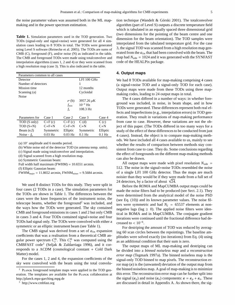
Fig. 2. The ROMA output map for case 1. The units are antennaKelvins at 100 GHz. The maps for MapCUMBA and destrip-ing look similar. This map is an output from one detector. Forthis plot the map resolution was degraded toNside = 256. Themonopole was removed from the map.

Fig. 3. The ROMA reconstruction error map for case 1. Theunits are antenna Kelvins. The maps for MapCUMBA and de-striping look similar. The map is an output from one detector.For this plot the map resolution was degraded toNside = 256.(A version of the paper with a better-quality figure can be foundat http://www.physics.helsinki.fi/∼tfo cosm/tfo planck.html.)

nal component arises from pixelisation noise (Dore et al. 2001).The noise component (εn) is the output map from the noise partof the TOD.

Note that the map-making methods are linear (up to numer-ical accuracy effects), so that these components can be obtainedseparately and studied independently, by applying the codes tothe noise and signal parts of the simulated TODs (see e.g. deGasperis et al. 2005).

Our maps express the temperature fluctuations in the an-tenna temperature. The ratio of the thermodynamic tempera-ture fluctuation to the antenna temperature fluctuation is (ex −1)2/x2ex, wherex = hν/kT0, h is the Planck constant,ν is thefrequency,k is the Boltzmann constant andT0 = 2.725 K isthe CMB temperature. For this study the ratio is 1.287 (ν =

100 GHz).

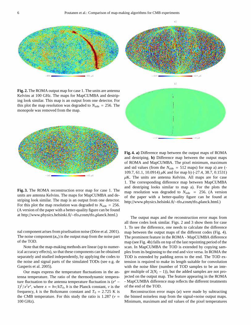
Fig. 4. a) Difference map between the output maps of ROMAand destriping.b) Difference map between the output mapsof ROMA and MapCUMBA. The pixel minimum, maximumand std values (from theNside = 512 maps) for map a) are (-109.7, 61.1, 10.0914)µK and for map b) (-27.4, 38.7, 0.1531)µK. The units are antenna Kelvins. All maps are for case1. The corresponding difference map between MapCUMBAand destriping looks similar to map a). For the plots themap resolution was degraded toNside = 256. (A versionof the paper with a better-quality figure can be found athttp://www.physics.helsinki.fi/∼tfo cosm/tfo planck.html.)

The output maps and the reconstruction error maps fromall three codes look similar. Figs. 2 and 3 show them for case1. To see the difference, one needs to calculate the differencemap between the output maps of the different codes (Fig. 4).The prominent feature in the ROMA - MapCUMBA differencemap (see Fig. 4b) falls on top of the last repointing period ofthescan. In MapCUMBA the TOD is extended by copying sam-ples from its beginning to the end and vice versa. In ROMA theTOD is extended by padding zeros to the end. The TOD ex-tension is required to make its length suitable for convolutionwith the noise filter (number of TOD samples to be an inte-ger multiple of 2(Nξ − 1)), but the added samples are not pro-jected on the output map. The feature appearing in the ROMA- MapCUMBA difference map reflects the different treatmentsof the end of the TOD.

Reconstruction error maps (ε) were made by subtractingthe binned noiseless map from the signal+noise output maps.Minimum, maximum and std values of the pixel temperatures

Poutanen et al.: Comparison of map-making algorithms for CMB experiments 7

Table 2. The std, minimum and maximum values (all inµK at100 GHz antenna scale) of the pixel temperatures of the reconstruc-tion error maps (ε = εp + εn). The numbers were calculated fromNside = 512 maps. They can be compared to the std of a white noisemap, calculated as

√〈1/n〉σ, where〈1/n〉 is the mean (taken over the

hit pixels) of the inverse of the number of hits in a pixel. Theval-ues are 137.219µK for cases 1 and 2 and 137.400µK for cases 3and 4. The values are different between the cases due to small differ-ences in the cycloidal scannings.This white noise std represents thelevel below which one cannot get. The difference between ROMAand MapCUMBA is negligible. We give the numbers in the table withmany digits just to show at what level this difference is. The numbersin this table and the next one should be compared in the horizontaldirection, to see the difference between the codes. The differences inthe vertical direction reflect the effect of several differences in how theTODs were generated, but these effects are not the object of this paper.

std forε(min, max) ROMA MapCUMBA DestripingCase 1 138.2497 138.2496 138.455

(-825.3, 876.0) (-825.3, 876.0) (-822.5, 891.1)Case 2 138.2475 138.2474 138.454

(-825.0, 876.7) (-825.0, 876.7) (-822.5, 891.2)Case 3 138.9109 138.9110 139.397

(-838.4, 938.2) (-838.1, 938.1) (-851.2, 952.3)Case 4 138.9114 138.9114 139.398

(-838.1, 937.9) (-838.1, 937.9) (-851.2, 952.2)

Table 3. Same as Table 2 but now the values are for the signal com-ponent of the reconstruction error map (εp). The units are antennaµK(at 100 GHz).

std forεp

(min, max) ROMA MapCUMBA DestripingCase 1 0.8794 0.8796 0.281

(-100.7, 53.8) (-100.7, 53.8) (-3.0, 2.1)Case 2 0.6140 0.6142 0.252

(-62.2, 37.8) (-62.2, 37.8) (-2.3, 1.8)Case 3 0.3130 0.3130 0.120

(-2.0, 1.9) (-2.0, 1.9) (-0.6, 0.7)Case 4 0.4064 0.4064 0.169

(-2.8, 3.1) (-2.8, 3.1) (-0.9, 0.8)

of the reconstruction error maps are given in Table 2. In termsof the map variance ML map-making is slightly better than de-striping. Table 2 also shows that the ML std is higher than thestd of the white noise indicating that excess noise remains in themap. The cases 3 and 4 have higher map std’s than the cases1 and 2. This is mainly caused by the higher knee frequencyof the instrument noise in the cases 3 and 4. The map vari-ances of ROMA and MapCUMBA are practically equal show-ing that their performances are similar. The results shown inTable 2 represent the performance of a single LFI detector. Forfrequency maps made from the observations of multiple LFIdetectors the noise levels would be correspondingly lower.Forcomparison it can be noted that the noise level of a one-year

W-band (94 GHz) frequency map (Nside= 512) of the WMAP4

experiment (from a total of eight W-band detectors making up4 differencing assemblies) is slightly higher (∼142 µK) thanthe noise levels of Table 2, which represents just a single LFIdetector.

Pixel statistics for the signal components of the reconstruc-tion error maps (εp) are given in Table 3. These maps were pro-duced by subtracting the binned noiseless map from the noise-less signal-only output maps. In ML map-making the TOD wasconvolved with the noise filter. As an example, the signal com-ponents of the reconstruction error maps for case 1 are shownin Fig. 5. The maps contained CMB and foreground signals.The error magnitudes are larger for the ML map-making thanfor the destriping. Additionally, the largest errors in theMLmap tend to locate where the foreground signal (actually, itsgradient) is strongest. For destriping this error appears as (er-roneous) baselines corresponding to offsetting an entire ring.Therefore a similar correlation between the errors and the fore-ground signal is not visible in the destriped maps, althoughweexpect that the largest errors still originate from where the fore-ground signal is strong.

The methods that were used to generate the signal partsof the TODs were not uniform (total convolution vs. scanningof a high resolution map, see Sect. 3). That complicates thecomparison of the results of Table 3 between the beams. Thiscomparison was not attempted in this study. However, the re-sults can well be compared (at a given beam) between differentmap-making algorithms which was the main purpose of thisstudy.

Table 3 shows that the signal-only ML maps deviate morefrom the binned noiseless map than what happens in destriping.Foreground increases this error and large errors may occur insome pixels of the ML maps. The std ofεp is small comparedto the std of the overall reconstruction error map (see Table2)which is an indication that the total error is dominated by theinstrument noise.

The source ofεp is the pixelisation noise (as shown inAppendix A). In ML map-making the pixelisation noise spec-trum up to the knee frequency of the instrument noise con-tributes toεp. In destriping, however, only a lower frequencypart contributes leading to a smallerεp. This is addressed inmore detail in Appendix A. The galactic foreground signal hasa stronger spatial variation than CMB. This results in higherpixelisation noise, which explains the higherεp magnitudes inthe cases 1 and 2 than in the cases 3 and 4 (see Table 3).

We calculated the angular power spectra of the recon-struction error maps (ε) (Fig. 6). The spectra of ROMA andMapCUMBA were very similar and could not be distinguishedin the plot. The ratio of the power spectra between destripingand ROMA is shown in Fig. 7. It seems that in destripingε hashigher power in most multipoles.

To examine this further, 100 MC noise-only TODs wereproduced from the known PSD of the instrument noise (see Eq.(10)). The MC noise TODs were generated by the SDE methodusing a different seed value for every realisation. To have a rea-sonable calculation time for this MC study, multiple 35 hour

4 http://map.gsfc.nasa.gov

8 Poutanen et al.: Comparison of map-making algorithms for CMB experiments

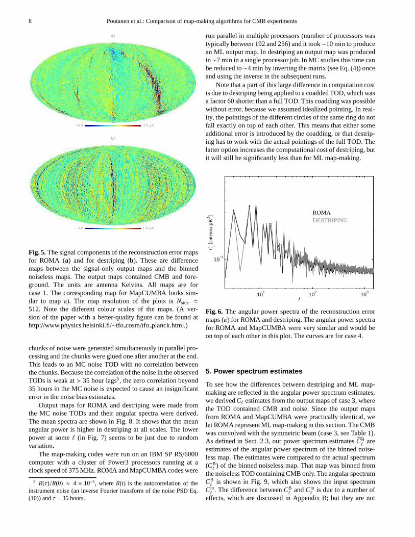
Fig. 5. The signal components of the reconstruction error mapsfor ROMA (a) and for destriping (b). These are differencemaps between the signal-only output maps and the binnednoiseless maps. The output maps contained CMB and fore-ground. The units are antenna Kelvins. All maps are forcase 1. The corresponding map for MapCUMBA looks sim-ilar to map a). The map resolution of the plots isNside =

512. Note the different colour scales of the maps. (A ver-sion of the paper with a better-quality figure can be found athttp://www.physics.helsinki.fi/∼tfo cosm/tfo planck.html.)

chunks of noise were generated simultaneously in parallel pro-cessing and the chunks were glued one after another at the end.This leads to an MC noise TOD with no correlation betweenthe chunks. Because the correlation of the noise in the observedTODs is weak at> 35 hour lags5, the zero correlation beyond35 hours in the MC noise is expected to cause an insignificanterror in the noise bias estimates.

Output maps for ROMA and destriping were made fromthe MC noise TODs and their angular spectra were derived.The mean spectra are shown in Fig. 8. It shows that the meanangular power is higher in destriping at all scales. The lowerpower at someℓ (in Fig. 7) seems to be just due to randomvariation.

The map-making codes were run on an IBM SP RS/6000computer with a cluster of Power3 processors running at aclock speed of 375 MHz. ROMA and MapCUMBA codes were

5 R(τ)/R(0) ≈ 4 × 10−5, whereR(t) is the autocorrelation of theinstrument noise (an inverse Fourier transform of the noisePSD Eq.(10)) andτ = 35 hours.

run parallel in multiple processors (number of processors wastypically between 192 and 256) and it took∼10 min to producean ML output map. In destriping an output map was producedin ∼7 min in a single processor job. In MC studies this time canbe reduced to∼4 min by inverting the matrix (see Eq. (4)) onceand using the inverse in the subsequent runs.

Note that a part of this large difference in computation costis due to destriping being applied to a coadded TOD, which wasa factor 60 shorter than a full TOD. This coadding was possiblewithout error, because we assumed idealized pointing. In real-ity, the pointings of the different circles of the same ring do notfall exactly on top of each other. This means that either someadditional error is introduced by the coadding, or that destrip-ing has to work with the actual pointings of the full TOD. Thelatter option increases the computational cost of destriping, butit will still be significantly less than for ML map-making.

101

102

103

10−1

l

Cl [a

nten

na µK

2 ] ROMADESTRIPING

Fig. 6. The angular power spectra of the reconstruction errormaps (ε) for ROMA and destriping. The angular power spectrafor ROMA and MapCUMBA were very similar and would beon top of each other in this plot. The curves are for case 4.

5. Power spectrum estimates

To see how the differences between destriping and ML map-making are reflected in the angular power spectrum estimates,we derivedCℓ estimates from the output maps of case 3, wherethe TOD contained CMB and noise. Since the output mapsfrom ROMA and MapCUMBA were practically identical, welet ROMA represent ML map-making in this section. The CMBwas convolved with the symmetric beam (case 3, see Table 1).As defined in Sect. 2.3, our power spectrum estimatesCB

ℓare

estimates of the angular power spectrum of the binned noise-less map. The estimates were compared to the actual spectrum(CBℓ) of the binned noiseless map. That map was binned from

the noiseless TOD containing CMB only. The angular spectrumCBℓ

is shown in Fig. 9, which also shows the input spectrumCinℓ

. The difference betweenCBℓ

andCinℓ

is due to a number ofeffects, which are discussed in Appendix B; but they are not

Poutanen et al.: Comparison of map-making algorithms for CMB experiments 9

200 400 600 800 1000 1200 14000.90

0.95

1.00

1.05

1.10S

PE

CT

RU

M R

AT

IO

DESTRIPING / ROMA

a)

5 10 15 20 25 30 35 40 45 500.40

0.60

0.80

1.00

1.20

1.40

l

SP

EC

TR

UM

RA

TIO

b)

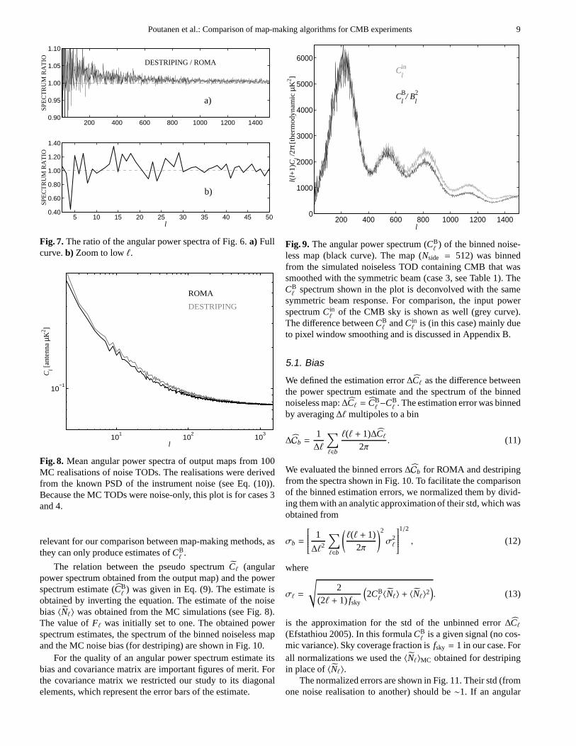
Fig. 7. The ratio of the angular power spectra of Fig. 6.a) Fullcurve.b) Zoom to lowℓ.

101

102

103

10−1

l

Cl [a

nten

na µK

2 ]

ROMA

DESTRIPING

Fig. 8. Mean angular power spectra of output maps from 100MC realisations of noise TODs. The realisations were derivedfrom the known PSD of the instrument noise (see Eq. (10)).Because the MC TODs were noise-only, this plot is for cases 3and 4.

relevant for our comparison between map-making methods, asthey can only produce estimates ofCB

ℓ.

The relation between the pseudo spectrumCℓ (angularpower spectrum obtained from the output map) and the powerspectrum estimate (CB

ℓ) was given in Eq. (9). The estimate is

obtained by inverting the equation. The estimate of the noisebias〈Nℓ〉 was obtained from the MC simulations (see Fig. 8).The value ofFℓ was initially set to one. The obtained powerspectrum estimates, the spectrum of the binned noiseless mapand the MC noise bias (for destriping) are shown in Fig. 10.

For the quality of an angular power spectrum estimate itsbias and covariance matrix are important figures of merit. Forthe covariance matrix we restricted our study to its diagonalelements, which represent the error bars of the estimate.

200 400 600 800 1000 1200 14000

1000

2000

3000

4000

5000

6000

l

l(l+

1)C

l /2π

[th

erm

od

yna

mic

µK2 ]

Clin

ClB/ B

l2

Fig. 9. The angular power spectrum (CBℓ) of the binned noise-

less map (black curve). The map (Nside = 512) was binnedfrom the simulated noiseless TOD containing CMB that wassmoothed with the symmetric beam (case 3, see Table 1). TheCBℓ

spectrum shown in the plot is deconvolved with the samesymmetric beam response. For comparison, the input powerspectrumCin

ℓof the CMB sky is shown as well (grey curve).

The difference betweenCBℓ

andCinℓ

is (in this case) mainly dueto pixel window smoothing and is discussed in Appendix B.

5.1. Bias

We defined the estimation error∆Cℓ as the difference betweenthe power spectrum estimate and the spectrum of the binnednoiseless map:∆Cℓ = CB

ℓ−CBℓ. The estimation error was binned

by averaging∆ℓ multipoles to a bin

∆Cb =1∆ℓ

∑

ℓ∈b

ℓ(ℓ + 1)∆Cℓ2π

. (11)

We evaluated the binned errors∆Cb for ROMA and destripingfrom the spectra shown in Fig. 10. To facilitate the comparisonof the binned estimation errors, we normalized them by divid-ing them with an analytic approximation of their std, which wasobtained from

σb =

1

∆ℓ2

∑

ℓ∈b

(ℓ(ℓ + 1)

2π

)2

σ2ℓ

1/2

, (12)

where

σℓ =

√2

(2ℓ + 1) fsky

(2CBℓ〈Nℓ〉 + 〈Nℓ〉2

). (13)

is the approximation for the std of the unbinned error∆Cℓ(Efstathiou 2005). In this formulaCB

ℓis a given signal (no cos-

mic variance). Sky coverage fraction isfsky = 1 in our case. Forall normalizations we used the〈Nℓ〉MC obtained for destripingin place of〈Nℓ〉.

The normalized errors are shown in Fig. 11. Their std (fromone noise realisation to another) should be∼1. If an angular

10 Poutanen et al.: Comparison of map-making algorithms forCMB experiments

200 400 600 800 1000 1200 1400−1000

0

1000

2000

3000

4000

5000

6000

l(l+

1)C

l /2π

[th

erm

od

yna

mic

µK2 ]

DESTRIPING

ClB/ B

l2 (black)

<Nl>

MC/ B

l2

a)

200 400 600 800 1000 1200 1400−1000

0

1000

2000

3000

4000

5000

6000

l

l(l+

1)C

l /2π

[th

erm

od

yna

mic

µK2 ]

ROMA

DESTRIPING

ClB/ B

l2 (thin black)

b)

Fig. 10. a) Angular power spectrum estimateCBℓ

for destriping(grey curve). The ROMA estimate would fall nearly on top ofthe destriping estimate and would not distinguish in this plot.The estimates were derived from a single sky realisation (case3). The output maps covered the full sky and contained CMBand instrument noise. Since just a single detector was consid-ered, the noise becomes dominant already at aroundℓ ≃ 350.CBℓ

is the angular spectrum of the binned noiseless map and〈Nℓ〉MC is the MC noise bias (for destriping). Note that theyhave been deconvolved with a symmetric beam that was iden-tical to the instrument beam. The filter functionFℓ was set toone for both estimates.b) Same as a) but the spectra have beenℓ binned to∆ℓ = 25. The difference between the ROMA anddestriping estimates is visible atℓ > 1000.

power spectrum estimate has a non-zero bias the mean of thefluctuations of the normalized error will have a positive or neg-ative trend. In the case of zero bias the mean will be close tozero. We can note that the normalized errors are different forROMA and destriping, the largest differences being atℓ < 800.The differences are, however, smaller than the std of the errors.

200 400 600 800 1000 1200 1400

−3

−2

−1

0

1

2

3

l

NO

RM

ALI

ZE

D E

RR

OR

ROMA

DESTRIPING

Fig. 11. The normalized power spectrum estimation errors forROMA and destriping. The normalized error was obtained bydividing the binned estimation error (Eq. (11),∆ℓ = 25) withthe analytic approximation of its std (Eq. (12)). The std ofdestriping was used in all normalizations. The filter functionhad value 1.0 for both curves. The bin-to-bin fluctuations aremainly caused by the instrument noise.

200 400 600 800 1000 1200 14000.992

0.993

0.994

0.995

0.996

0.997

0.998

0.999

1

1.001

1.002

l

Fl

ROMA

DESTRIPING

Fig. 12. Filter functionsFℓ for ROMA and destriping. Theywere obtained from Eq. (9) (with〈Nℓ〉 = 0) by dividing thepseudo spectra of the output maps of the noiseless CMB-onlyTOD with the spectrum of the binned noiseless map. The fil-ter function for MapCUMBA was nearly identical to the filterfunction of ROMA and would not distinguish from the ROMAfilter function in this plot.

We could expect that some bias could be introduced to ourpower spectrum estimates because we neglected (by settingFℓ= 1 in Eq. (9)) the error that the map-making causes to theCMB signal. This is a reflection of the signal componentεp

of the reconstruction error that we found in the map domain(see Sect. 4). To assess the level of the bias we estimatedFℓ forROMA and for destriping. We carried out no MC simulations toestimate them, but we determined them from Eq. (9) using the

Poutanen et al.: Comparison of map-making algorithms for CMB experiments 11

200 400 600 800 1000 1200 1400

−3

−2

−1

0

1

2

3

l

NO

RM

ALI

ZE

D E

RR

OR

ROMA

DESTRIPING

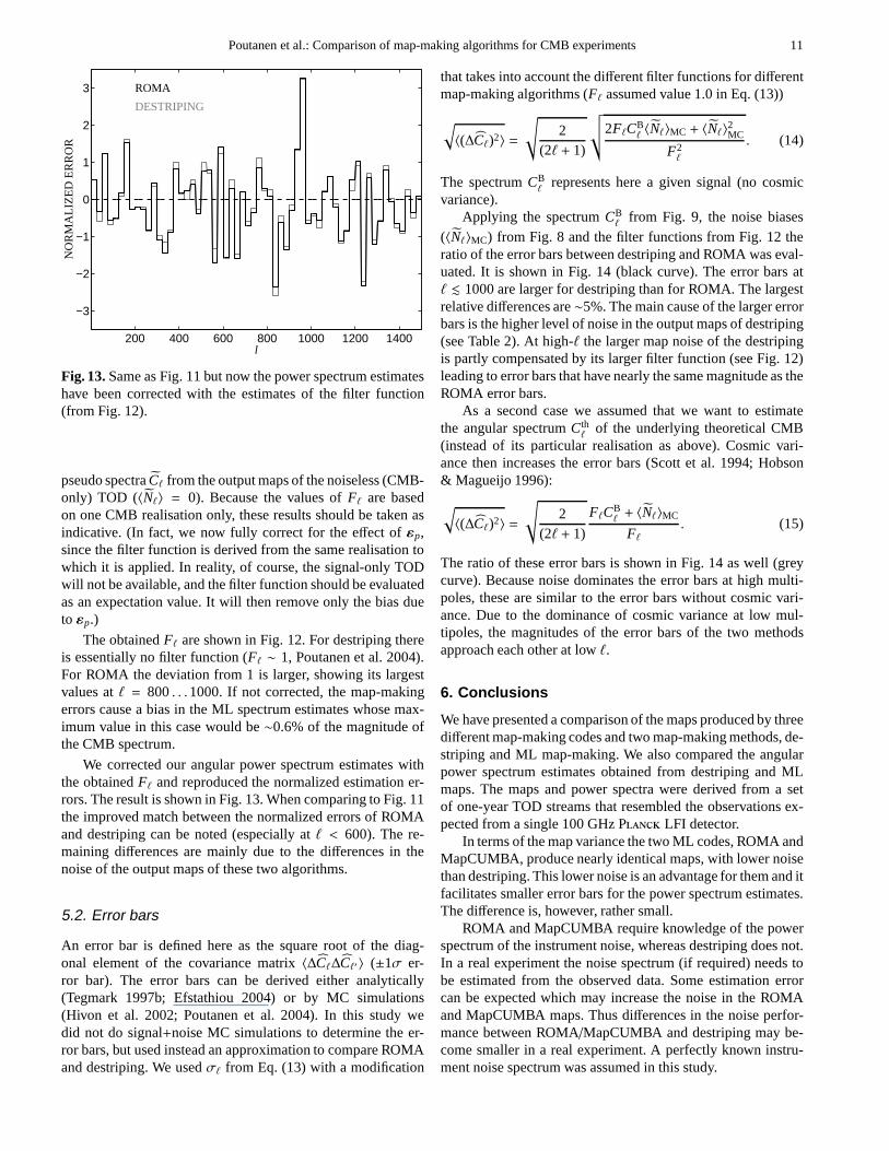
Fig. 13. Same as Fig. 11 but now the power spectrum estimateshave been corrected with the estimates of the filter function(from Fig. 12).

pseudo spectraCℓ from the output maps of the noiseless (CMB-only) TOD (〈Nℓ〉 = 0). Because the values ofFℓ are basedon one CMB realisation only, these results should be taken asindicative. (In fact, we now fully correct for the effect of εp,since the filter function is derived from the same realisation towhich it is applied. In reality, of course, the signal-only TODwill not be available, and the filter function should be evaluatedas an expectation value. It will then remove only the bias dueto εp.)

The obtainedFℓ are shown in Fig. 12. For destriping thereis essentially no filter function (Fℓ ∼ 1, Poutanen et al. 2004).For ROMA the deviation from 1 is larger, showing its largestvalues atℓ = 800. . .1000. If not corrected, the map-makingerrors cause a bias in the ML spectrum estimates whose max-imum value in this case would be∼0.6% of the magnitude ofthe CMB spectrum.

We corrected our angular power spectrum estimates withthe obtainedFℓ and reproduced the normalized estimation er-rors. The result is shown in Fig. 13. When comparing to Fig. 11the improved match between the normalized errors of ROMAand destriping can be noted (especially atℓ < 600). The re-maining differences are mainly due to the differences in thenoise of the output maps of these two algorithms.

5.2. Error bars

An error bar is defined here as the square root of the diag-onal element of the covariance matrix〈∆Cℓ∆Cℓ′〉 (±1σ er-ror bar). The error bars can be derived either analytically(Tegmark 1997b; Efstathiou 2004) or by MC simulations(Hivon et al. 2002; Poutanen et al. 2004). In this study wedid not do signal+noise MC simulations to determine the er-ror bars, but used instead an approximation to compare ROMAand destriping. We usedσℓ from Eq. (13) with a modification

that takes into account the different filter functions for differentmap-making algorithms (Fℓ assumed value 1.0 in Eq. (13))

√〈(∆Cℓ)2〉 =

√2

(2ℓ + 1)

√√2FℓCB

ℓ〈Nℓ〉MC + 〈Nℓ〉2MC

F2ℓ

. (14)

The spectrumCBℓ

represents here a given signal (no cosmicvariance).

Applying the spectrumCBℓ

from Fig. 9, the noise biases(〈Nℓ〉MC) from Fig. 8 and the filter functions from Fig. 12 theratio of the error bars between destriping and ROMA was eval-uated. It is shown in Fig. 14 (black curve). The error bars atℓ . 1000 are larger for destriping than for ROMA. The largestrelative differences are∼5%. The main cause of the larger errorbars is the higher level of noise in the output maps of destriping(see Table 2). At high-ℓ the larger map noise of the destripingis partly compensated by its larger filter function (see Fig.12)leading to error bars that have nearly the same magnitude as theROMA error bars.

As a second case we assumed that we want to estimatethe angular spectrumCth

ℓof the underlying theoretical CMB

(instead of its particular realisation as above). Cosmic vari-ance then increases the error bars (Scott et al. 1994; Hobson& Magueijo 1996):

√〈(∆Cℓ)2〉 =

√2

(2ℓ + 1)

FℓCBℓ+ 〈Nℓ〉MC

Fℓ. (15)

The ratio of these error bars is shown in Fig. 14 as well (greycurve). Because noise dominates the error bars at high multi-poles, these are similar to the error bars without cosmic vari-ance. Due to the dominance of cosmic variance at low mul-tipoles, the magnitudes of the error bars of the two methodsapproach each other at lowℓ.

6. Conclusions

We have presented a comparison of the maps produced by threedifferent map-making codes and two map-making methods, de-striping and ML map-making. We also compared the angularpower spectrum estimates obtained from destriping and MLmaps. The maps and power spectra were derived from a setof one-year TOD streams that resembled the observations ex-pected from a single 100 GHz P LFI detector.

In terms of the map variance the two ML codes, ROMA andMapCUMBA, produce nearly identical maps, with lower noisethan destriping. This lower noise is an advantage for them and itfacilitates smaller error bars for the power spectrum estimates.The difference is, however, rather small.

ROMA and MapCUMBA require knowledge of the powerspectrum of the instrument noise, whereas destriping does not.In a real experiment the noise spectrum (if required) needs tobe estimated from the observed data. Some estimation errorcan be expected which may increase the noise in the ROMAand MapCUMBA maps. Thus differences in the noise perfor-mance between ROMA/MapCUMBA and destriping may be-come smaller in a real experiment. A perfectly known instru-ment noise spectrum was assumed in this study.

12 Poutanen et al.: Comparison of map-making algorithms forCMB experiments

200 400 600 800 1000 1200 1400

1

1.01

1.02

1.03

1.04

1.05E

RR

OR

BA

R R

AT

IO

l

ERROR BAR RATIO (DESTRIPING / ROMA)

COSMIC VARIANCE

NO COSMIC VARIANCE

Fig. 14. An estimate for the ratio of the error bars between de-striping and ROMA. Black curve is for the estimation of a par-ticular CMB realisation of the sky (no cosmic variance, errorbars from Eq. (14)) and the grey curve is for the estimationof the underlying theoretical CMB spectrum (cosmic varianceincluded, error bars from Eq. (15)).

The map-making methods caused errors (exhibited in thesignal component of the reconstruction error map) in the signalpart of the output maps. The origin of these errors is the sub-pixel structure of the signal (pixelisation noise). It was shownthat these errors were smaller in destriping than in ROMA andMapCUMBA. It was further shown that, if a proper correctionis not applied, these errors may show up as an extra bias in thepower spectrum estimates. The extra bias would be larger forROMA and MapCUMBA than for destriping.

In terms of CPU resources destriping is less demanding.This is an advantage in e.g. MC simulations.

Acknowledgements.The work reported in this paper was done by theCTP Working Group of the P Consortia. P is a missionof the European Space Agency. Some of this work was carried outin June 2002 and in January 2003 during two CTP meetings hostedby the Institute of Astronomy (University of Cambridge). Wethanktheir hospitality during these meetings. This research used resourcesof the National Energy Research Scientific Computing Center, whichis supported by the Office of Science of the U.S. Department of Energyunder Contract No. DE-AC03-76SF00098. This work has made use ofthe P satellite simulation package (Level S), which is assembledby the Max Planck Institute for Astrophysics P Analysis Centre(MPAC). We acknowledge the use of the CMBFAST code for thecomputation of the theoretical CMB angular power spectrum.Someof the results in this paper have been derived using the HEALPixpackage (Gorski et al. 1999, 2005a). This work was supported by theAcademy of Finland grant no. 75065. TP wishes to thank the VaisalaFoundation for financial support. The US P Project is supportedby the NASA Science Mission Directorate.

Appendix A: Reconstruction error map

In this Appendix we discuss in more detail the reconstructionerror map and how its signal and noise components arise.

The output map of the ML map-making can be solved fromEq. (2). That equation is reproduced here

PTN−1Pm = PTN−1y. (A.1)

The noise covariance matrixN can be freely normalizedby a constant without affecting the output map. Let us assumethat each element ofN has been divided by the variance (σ2)of the non-correlated noise component of the observed TOD(vectory). By replacingN−1 with an identityIt − (It −N−1) andrearranging some of the terms one obtains for the output map

m = (PTP)−1B−1PTN−1y, (A.2)

where

B = Im − PT(It − N−1)P(PTP)−1. (A.3)

HereIt andIm are unit matrices with dimensions equal to thenumber of samplesNt of the TOD and the number of pixelsNpix in the map, respectively. We can apply a geometric seriestrick (Tegmark 1997a) to prove the following identity

[Im − PT(It − N−1)P(PTP)−1]−1PT =

= PT [It − (It − N−1)P(PTP)−1PT ]−1. (A.4)

Applying this in Eqs. (A.2) and (A.3) and noting the definitionof the matrixZ (see Sect. 2.2) one obtains for the output map

m = (PTP)−1PT [It + (N − It)Z]−1y. (A.5)

By adding and subtractingy on the right hand side and carry-ing out some arithmetic manipulations the output map can beexpressed in the following form

m = (PTP)−1PT [y − ∆]. (A.6)

Vector∆ is solved from the linear equation

[Z + (N − It)−1]∆ = Zy. (A.7)

Let the complex valued matrixH ([H] = (Nt,Nt)) be an in-verse DFT (Discrete Fourier Transform) operator that convertsfrequency domain vectors to time domain (to TOD domain):y = Hy, wherey is the frequency domain counterpart ofy. Theinverse operator toH is its Hermitian conjugateH†. We canassume that the matrixH is normalized toHH† = H†H = It.A square matrixA ([A] = (Nt,Nt)) in the TOD domain can beconverted to a matrixA in the frequency domain:A = H†AH.

After converting both sides of Eq. (A.7) into frequency do-main, the vector∆ (frequency domain counterpart of∆) can besolved from the equation

[H†ZH + (N − It)−1]∆ = H†Zy. (A.8)

The solution for the output map becomes then

m = (PTP)−1PT [y −H∆]. (A.9)

Comparing Eqs. (A.8) and (A.9) to the corresponding Eqs. (4)and (5) of destriping the similarity of the output map solutionsbetween ML and destriping can be clearly seen.

Poutanen et al.: Comparison of map-making algorithms for CMB experiments 13

The observed TOD (y) contains two components: signals and instrument noisen (see Sect. 3). The termZy (see Eq.(A.8)) can now be split in two components

Zy = Zs + Zn. (A.10)

Writing out the first term on the right hand side we obtain

Zs = s − P(PTP)−1PTs. (A.11)

Apart from the sign,Zs is the pixelisation noise introduced byDore et al. (2001). Pixelisation noise represents error that iscaused by the discretization of the sky into pixels. FollowingDore et al. (2001) we define pixelisation noisep = −Zs.

The split ofZy in two components means that∆ is split intwo components as well:∆ = ∆p+ ∆n. They can be solved from

[H†ZH + (N − It)−1]∆p = −H†p (A.12)

and

[H†ZH + (N − It)−1]∆n = H†Zn. (A.13)

In destriping the amplitudes of the base functions are splitanal-ogously:a = ap+ an. The first component is determined by thepixelisation noise and the second one by the instrument noise.

Next we inserty = s + n into Eqs. (A.6) and (A.7). Weobtain for the output map

m = (PTP)−1PTs − (PTP)−1PTH∆p +

+(PTP)−1PT [n −H∆n]. (A.14)

Ideally, we would like the output map of the map-making algo-rithm to be equal to the first term on the right hand side. It iscalledbinned noiseless mapin this study. The rest of the termsbring error. They are represented by thereconstruction errormap(Tegmark 1997a)

ε = m − (PTP)−1PTs. (A.15)

The reconstruction error map is comprised of a signal compo-nent (εp) and a noise component (εn).

ε = εp + εn. (A.16)

εp = −(PTP)−1PTH∆p (A.17)

εn = (PTP)−1PT [n −H∆n] (A.18)

For destriping we can write analogously

εp = −(PTP)−1PTFap (A.19)

εn = (PTP)−1PT [n − Fan]. (A.20)

The signal and noise components of the reconstructionerror map were used extensively when the map-making al-gorithms were compared in Sect. 4. We studied the mini-mum, maximum and std values of their pixel temperatures.Additionally, we produced their angular power spectra andcompared them as well.

A.1. Map-making errors and pixelisation noise

The purpose of this section is to give a qualitative explanationto the fact that the magnitude of the signal component of thereconstruction error map is larger for the ML map-making thanfor the destriping. The signal component of the reconstructionerror depends on∆p in the ML map-making and onap in thedestriping (see Eqs. (A.17) and (A.19)). The source of bothquantities is the pixelisation noisep.

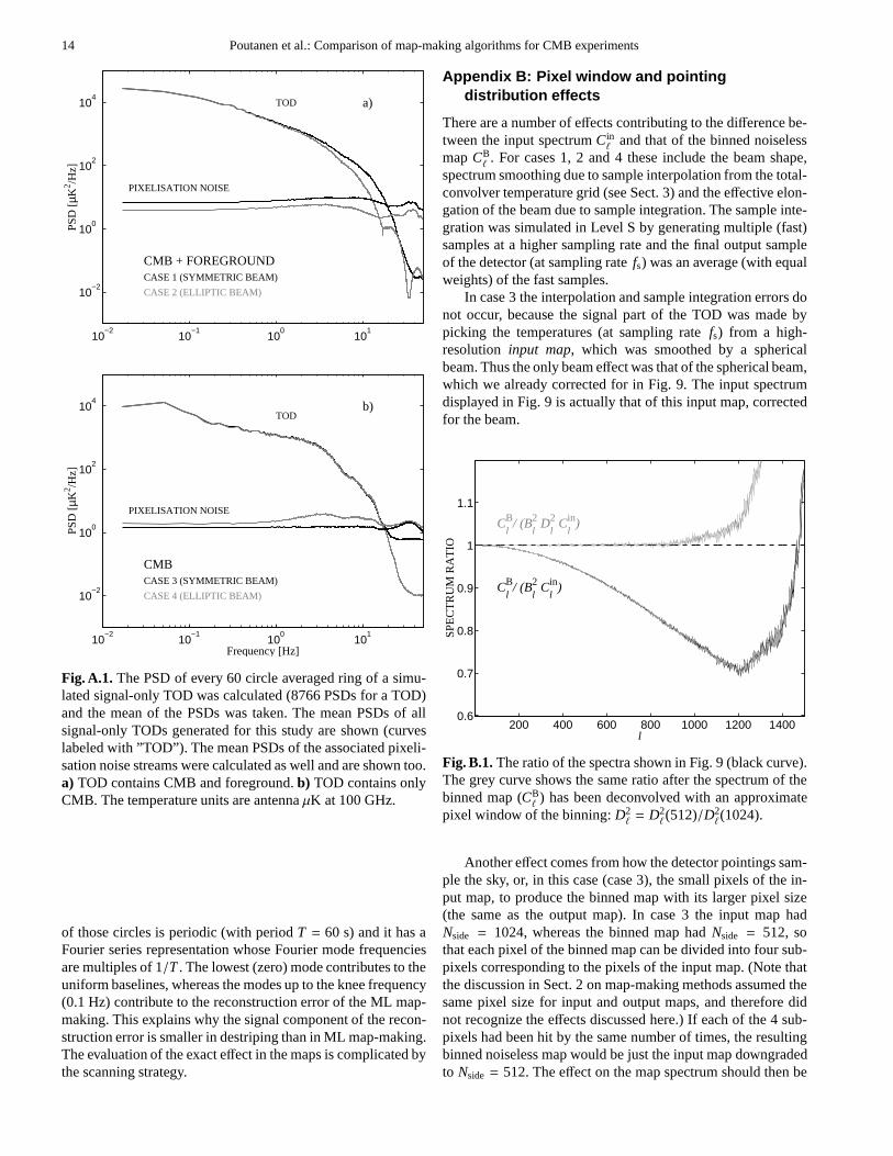
We will first examine the spectrum of the pixelisation noise(p = H†p). The PSD of every 60 circle averaged ring of a sim-ulated signal-only TOD was calculated and the mean of thesePSDs was taken over the full one year TOD. The mean PSDs ofall four simulated signal-only TODs and their associated pix-elisation noise streams (p = −Zs, s = TOD) were determined.They are shown in Fig. A.1.

The level of the pixelisation noise is higher for the TODscontaining CMB and foreground than for the TODs of CMBonly. This explains why the signal component of the recon-struction error increases when the foreground emissions are in-cluded in the simulations.

The samplepk of the pixelisation noise stream (k indexesthe sample) is

pk =

1Nk

∑

i∈ksi

− sk =1Nk

∑

i∈k(si − sk), (A.21)

wheresk is the kth sample of the TOD,i ∈ k refers to those TODsamples (includingsk) that hit the same pixel assk andNk is thenumber of hits in that pixel. We can assume that the magnitudesof the pixel-to-pixel correlations are smaller for the tempera-ture differences (si − sk) than for the temperatures themselves.This means that notable correlation exists betweenpk and pk′

only if they are samples from the same pixel. Only the frac-tion Npix/Nt ≪ 1 of the TOD samples are observations fromthe same pixel leading to, in average, a weak correlation be-tween the samples of the pixelisation noise. This explains the”white noise” type nearly flat spectra of the pixelisation noises(see Fig. A.1). The fact that in Fig. A.1a the pixelisation noiseis larger for the symmetric beam than for the elliptic beam andopposite in Fig. A.1b reflects the different methods that wereused in generating the symmetric beam TODs (total convolu-tion in case 1 vs. scanning a high resolution map in case 3, seeSect. 3).

Vector∆p is a solution to Eq. (A.12). The matrixN is diag-onal with samples (bins) of 1+ fk/ f (cf. Eq. (10)) in its diago-nals. The diagonal elements of (N − It)−1 are≫ 1 for frequen-cies higher than the knee frequency. Fig. A.1 suggests that thepower ofH†ZH∆p is considerably smaller than the power of∆p leading to an approximation where we can ignoreH†ZH inEq. (A.12). This indicates that in the ML map-making the sig-nal component of the reconstruction error is mainly determinedby that part of the pixelisation noise spectrum that falls belowthe knee frequency (Hivon et al. 2005).

By looking at Eqs. (4) and (A.19) we can expect that indestriping the uniform baselines of the pixelisation noisecon-tribute to this error. Because we assumed an exact repetition ofthe pointings of the 60 circles of a ring, the pixelisation noise

14 Poutanen et al.: Comparison of map-making algorithms forCMB experiments

10−2

10−1

100

101

10−2

100

102

104

PS

D [µ

K2 /H

z]

CMB + FOREGROUND

a)

CASE 1 (SYMMETRIC BEAM)

CASE 2 (ELLIPTIC BEAM)

TOD

PIXELISATION NOISE

10−2

10−1

100

101

10−2

100

102

104

Frequency [Hz]

PS

D [µ

K2 /H

z]

CMB

b)

CASE 3 (SYMMETRIC BEAM)

CASE 4 (ELLIPTIC BEAM)

TOD

PIXELISATION NOISE

Fig. A.1. The PSD of every 60 circle averaged ring of a simu-lated signal-only TOD was calculated (8766 PSDs for a TOD)and the mean of the PSDs was taken. The mean PSDs of allsignal-only TODs generated for this study are shown (curveslabeled with ”TOD”). The mean PSDs of the associated pixeli-sation noise streams were calculated as well and are shown too.a) TOD contains CMB and foreground.b) TOD contains onlyCMB. The temperature units are antennaµK at 100 GHz.

of those circles is periodic (with periodT = 60 s) and it has aFourier series representation whose Fourier mode frequenciesare multiples of 1/T. The lowest (zero) mode contributes to theuniform baselines, whereas the modes up to the knee frequency(0.1 Hz) contribute to the reconstruction error of the ML map-making. This explains why the signal component of the recon-struction error is smaller in destriping than in ML map-making.The evaluation of the exact effect in the maps is complicated bythe scanning strategy.

Appendix B: Pixel window and pointingdistribution effects

There are a number of effects contributing to the difference be-tween the input spectrumCin

ℓand that of the binned noiseless

mapCBℓ. For cases 1, 2 and 4 these include the beam shape,

spectrum smoothing due to sample interpolation from the total-convolver temperature grid (see Sect. 3) and the effective elon-gation of the beam due to sample integration. The sample inte-gration was simulated in Level S by generating multiple (fast)samples at a higher sampling rate and the final output sampleof the detector (at sampling ratefs) was an average (with equalweights) of the fast samples.

In case 3 the interpolation and sample integration errors donot occur, because the signal part of the TOD was made bypicking the temperatures (at sampling ratefs) from a high-resolution input map, which was smoothed by a sphericalbeam. Thus the only beam effect was that of the spherical beam,which we already corrected for in Fig. 9. The input spectrumdisplayed in Fig. 9 is actually that of this input map, correctedfor the beam.

200 400 600 800 1000 1200 14000.6

0.7

0.8

0.9

1

1.1

l

SP

EC

TR

UM

RA

TIO

ClB/ (B

l2 C

lin)

ClB/ (B

l2 D

l2 C

lin)

Fig. B.1. The ratio of the spectra shown in Fig. 9 (black curve).The grey curve shows the same ratio after the spectrum of thebinned map (CB

ℓ) has been deconvolved with an approximate

pixel window of the binning:D2ℓ= D2

ℓ(512)/D2

ℓ(1024).

Another effect comes from how the detector pointings sam-ple the sky, or, in this case (case 3), the small pixels of the in-put map, to produce the binned map with its larger pixel size(the same as the output map). In case 3 the input map hadNside = 1024, whereas the binned map hadNside = 512, sothat each pixel of the binned map can be divided into four sub-pixels corresponding to the pixels of the input map. (Note thatthe discussion in Sect. 2 on map-making methods assumed thesame pixel size for input and output maps, and therefore didnot recognize the effects discussed here.) If each of the 4 sub-pixels had been hit by the same number of times, the resultingbinned noiseless map would be just the input map downgradedto Nside = 512. The effect on the map spectrum should then be

Poutanen et al.: Comparison of map-making algorithms for CMB experiments 15

given by the ratio of the two pixel windowsD2ℓ(512)/D2

ℓ(1024).

Here Dℓ(512) andDℓ(1024) are the HEALPix pixel windowfunctions forNside= 512 andNside= 1024 (Gorski et al. 2005b).(In the real situation the input map is replaced by the sky with“Nside = ∞”, so that the corresponding factor is just the pixelwindow of the binned map.) We show in Fig. B.1 how this rep-resents the effect well up toℓ ∼ 800.

The remaining effect, which blows up at highℓ, is due totwo things: 1) the nonuniform sampling of the four subpix-els (or, in the real world, that of the output map pixel area onthe sky), 2) that the HEALPix pixel window functions them-selves represent an approximation, as discussed below. This re-maining effect represents coupling between theℓ modes of thespectra, which couples power from the low-ℓ to the high-ℓ thatshows up as an high-ℓ excess power. This effect was discussedin Poutanen et al. 2004, where it was modelled as a signal bias.

Let us examine the distribution of the detector pointings inthe sky and its impact on the spectrum of the binned noiselessmap in more detail. The following discussion can be appliedboth to the real case of observing the sky and the case (our case3) where the TOD is picked from a high-resolution pixelizedinput map. We consider the samplessi (i indexes the sample)of the CMB-only TOD that fall in a pixelk of the binned (oroutput) map (see Eq. (A.21)). The number of hits in that pixelis Nk. We assume that every pixel is hit (100% sky coverage atNside = 512 resolution), so thatNk ≥ 1. The temperature ofsi

can be given as

si =∑

ℓm

aℓmBℓYℓm(ni). (B.1)

Hereaℓm represent the CMB sky (see Sect. 2.3),Bℓ is the re-sponse of the symmetric beam andni is a unit vector pointing inthe direction of the beam centre (or, in the case where the TODis just picked from an input map, the direction to the centre ofthe input map pixel the detector is pointing at). The temperatureof the pixelk of the binned map is

TBk =

1Nk

∑

i∈ksi =

∑

ℓm

aℓmBℓ1Nk

∑

i∈kYℓm(ni), (B.2)

wherei ∈ k refers to those TOD samples that hit the pixelk.The expansion coefficients of the binned map are obtained

by an inverse spherical harmonic transformation

aBℓm = Ωp

Npix−1∑

k=0

TBk Y∗ℓm(qk). (B.3)

We assume a HEALPix pixelisation, where the pixels have thesame areaΩp = 4π/Npix. The unit vector pointing to the centreof the pixelk is qk.

After insertingTBk from Eq. (B.2) to Eq. (B.3) we obtain

for the expansion coefficients of the binned map

aBℓm =

∑

ℓ′m′aℓ′m′B

′ℓΩp

Npix−1∑

k=0

1Nk

∑

i∈kYℓ′m′ (ni)Y∗ℓm(qk). (B.4)

This equation defines a coupling matrix

KBℓmℓ′m′ ≡ Ωp

Npix−1∑

k=0

1Nk

∑

i∈kYℓ′m′(ni)Y∗ℓm(qk) (B.5)

between theaℓm of the binned map and the CMB sky.Using the statistical isotropy of the CMB sky (〈aℓma∗

ℓ′m′〉 =δℓℓ′δmm′〈Cin

ℓ〉) we obtain for the ensemble mean of the angular

spectrum of the binned map

〈CBℓ 〉 =

12ℓ + 1

ℓ∑

m=−ℓ〈|aBℓm|

2〉 =∑

ℓ′

MBℓℓ′B

2ℓ′〈C

inℓ′ 〉, (B.6)

whereMBℓℓ′ is the mode coupling matrix (kernel matrix) of the

binned map

MBℓℓ′ =

12ℓ + 1

ℓ,ℓ′∑

m,m′=−ℓ,−ℓ′|KBℓmℓ′m′ |

2. (B.7)

In spite of the fact that the binned noiseless map has afull sky coverage, its mode coupling matrixMB

ℓℓ′ is not diag-onal but it is only diagonally dominant with small non-zerooff-diagonal elements, because the pixel area has been nonuni-formly sampled (in case 3, hits are in 4 subpixel centres onlyand unevenly distributed among them). The off-diagonal ele-ments are responsible for the coupling of the power from thelow-ℓ to high-ℓ that shows up as a high-ℓ excess power inCB

ℓ

(see Figs. 9 and B.1).Finally, let us consider what happens if the number of hits

in the pixel increases, the hits in the pixel area become evenlydistributed and a symmetric circular pixel shape is assumed. Inthat case the sum1

Nk

∑i∈k Yℓ′m′(ni) can be approximated by an

integral whose value can be given in a simple form

1Nk

∑

i∈kYℓ′m′(ni)→ Dℓ′Yℓ′m′ (qk), (B.8)

whereDℓ′ ≈ Dℓ′(512). (To be precise, the above limiting valuewill be reached, with a differentDℓ, whenever the distributionof the hits is the same in every observed pixel and the distribu-tion is fully symmetric around its centreqk). Under these as-sumptions we obtain an approximation for the mode couplingmatrix of the binned map

MBℓℓ′ ≈ D2

ℓ′Mℓℓ′ . (B.9)

HereMℓℓ′ is the mode coupling matrix of the MASTER method(Hivon et al. 2002 and Sect. 2.3 of this paper). We can see thatthe MASTER approach for the power spectrum estimation (Eq.(7)) corresponds to an approximation that a large number ofhits is symmetrically distributed in every observed pixel.Forthe full sky map (like our binned noiseless map atNside= 512resolution) the MASTER mode coupling matrixMℓℓ′ is closeto a unit matrix and it cannot explain the high-ℓ excess powerthat we see in the spectrum of the binned noiseless map. (Thefull sky Mℓℓ′ does have tiny non-zero off-diagonal elements,because the spherical harmonics are not exactly an orthogonalset of functions in the pixelised sky).

References

Armitage, C., & Wandelt, B. 2004, Phys.Rev.D, 70, 123007Balbi, A., de Gasperis, G., Natoli, P., & Vittorio, N. 2002, A&A, 395,

417

16 Poutanen et al.: Comparison of map-making algorithms forCMB experiments

Bersanelli, M., Bouchet, F.R., Efstathiou, G., et al. 1996,ESA,COBRAS/SAMBA Report on the Phase A Study, D/SCI(96)3

Borrill, J. 1999, in Proceedings of the 5th European SGI/Gray MPPWorkshop, Bologna, Italy, [astro-ph/9911389]

Burigana, C., Malaspina, M., Mandolesi, N., et al. 1997, Int. Rep.TeSRE/CNR, 198/1997, November, [astro-ph/9906360]

de Gasperis, G., Balbi, A., Cabella, P., Natoli, P., & Vittorio, N. 2005,A&A, 436, 1159

Delabrouille, J. 1998, A&AS, 127, 555Dore, O., Teyssier, R., Bouchet, F.R., Vibert, D., & Prunet, S. 2001,

A&A, 374, 358Dupac, X., & Tauber, J. 2005, A&A, 430, 363Efstathiou, G. 2004, MNRAS, 349, 603Efstathiou, G. 2005, MNRAS, 356, 1549Gorski, K.M., Hivon, E., & Wandelt, B.D. 1999, in Proceedings

of the MPA/ESO Cosmology Conference ”Evolution of Large-Scale Structure”, ed. A.J. Banday, R.S. Sheth, & L. Da Costa,PrintPartners Ipskamp, NL, 37, [astro-ph/9812350]

Gorski, K.M., Hivon, E., Banday, A.J., et al. 2005, ApJ, 622, 759Gorski, K.M., Wandelt, B.D., Hivon, E., Hansen, F.K., & Banday,

A.J. 2005, ”The HEALPix Primer” (Version 2.00), available inhttp://healpix.jpl.nasa.gov

Hivon, E., Gorski, K.M., Netterfield, C.B., et al. 2002, ApJ, 567, 2Hivon, E., et al. 2005, under preparationHobson M.P., & Magueijo J. 1996, MNRAS, 283, 1133Janssen M.A., Scott, D., White, M., et al. 1996, Report PSI-96-01,

FIRE-96-01 [astro-ph/9602009]Keihanen, E., Kurki-Suonio, H., Poutanen, T., Maino, D., &Burigana,

C. 2004, A&A, 428, 287Keihanen, E., Kurki-Suonio, H., & Poutanen, T. 2005, MNRAS, 360,

390Maino, D., Burigana, C., Maltoni, M., et al. 1999, A&AS, 140,383Maino, D., Burigana, C., Gorski, K.M., Mandolesi, N., & Bersanelli,

M. 2002, A&A, 387, 356Mennella, A., Bersanelli, M., Burigana, C., et al. 2002, A&A, 384,

736Natoli, P., de Gasperis, G., Gheller, C., & Vittorio, N. 2001, A&A,

372, 346Natoli, P., Marinucci D., Cabella P., de Gasperis, G., & Vittorio, N.

2002, A&A, 383, 1100Poutanen, T., Maino, D., Kurki-Suonio, H., Keihanen E., & Hivon, E.

2004, MNRAS, 353, 43Reinecke, M., Dolag, K., Hell, R., Bartelmann, M., & Enßlin,T. 2005,

submitted to A&A, [astro-ph/0508522]Revenu, B., Kim, A., Ansari, R., et al. 2000a, A&AS, 142, 499Revenu, B., Couchot, F., Delabrouille, J., et al. 2000b, ApL&C, 37,

267Scott, D., Srednicki, M., & White, M. 1994, ApJ, 421, L5Seljak, U., & Zaldarriaga, M. 1996, ApJ, 469, 437Tegmark, M. 1997a, ApJ, 480, L87Tegmark, M. 1997b, Phys.Rev.D, 55, 5895Wandelt, B.D., & Gorski, K.M. 2001, Phys.Rev.D, 63, 123002Wright, E.L. 1996, Report UCLA-ASTRO-ELW-96-03, November,

[astro-ph/9612006]