ORIGINAL PAPER

An off-line map-matching algorithm for incompletemap databases

Francisco Câmara Pereira & Hugo Costa &

Nuno Martinho Pereira

Received: 19 September 2008 /Accepted: 17 July 2009 /Published online: 11 September 2009# European Conference of Transport Research Institutes (ECTRI) 2009

Abstract The task of map-matching consists of finding acorrespondence between a geographical point or sequenceof points (e.g. obtained from GPS) and a given map. Due tomany reasons, namely the noisy input data and incompleteor inaccurate maps, such a task is not trivial and can affectthe validity of applications that depend on it. This includesany Transport Research projects that rely on post-hocanalysis of traces (e.g. via Floating Car Data). In thisarticle, we describe an off-line map-matching algorithm thatallows us to handle incomplete map databases. We test andcompare this with other approaches and ultimately provideguidelines for use within other applications. This project isprovided as open source.

Keywords Mapmatching .Map generation .

Artificial intelligence

1 Introduction

Map Matching algorithms are needed in any geographicalsystem to associate information to specific geo-referencedlocations. Thus, while we may get exact maps that representany portion of the planet, dynamic information obtained from

common Global Navigation Satellite Systems (GNSS) devi-ces (e.g. GPS) almost always carry errors that may negativelyaffect their usefulness. For example, for car navigation, forexample, extreme care must be taken to continually locate thereal position of the driver as opposed to what the GPS receiverestimates. Another example is the Floating Car Data probes(i.e. vehicles that periodically report their GPS position), fromwhich it is possible to obtain information on traffic situations[1]. These can be used to generate real-time information aswell as to provide traffic analysis and forecasting (e.g. [2,3]), or simply to analyse mobility behaviour within an area.A stronger example could be the dynamic toll charging;charging each vehicle based on its profile, used roads and/ordaily mileage. In any of these situations, accurate MapMatching algorithms become fundamental for the success ofthe applications. Furthermore, the analysis involved can betaken in an offline, post-processing manner. While on-linealgorithms have evolved to their limits recently, essentiallydue to commercial car navigation applications, off-lineapproaches are still under explored. At a first sight, theformer should be both a more challenging and a moregeneric task (solving the “real-time” problem often makesthe post-processing solution simple), but under a morecareful examination this shows that there are two differentapproaches to two entirely different problems. Real timeapplications demand solutions that provide instant responseand can only rely on “past” points. This implies acompromise of performance over accuracy. On the otherhand, off-line applications can take advantage of “future”points and allow for slower performances in favour ofaccuracy. As a result, on-line solutions applied on an off-linebasis show extremely poor results, thus specific research isneeded for solving the latter problem.

The task of off-line map matching is to determine acorrespondence between sequences of geo-referenced

F. C. Pereira (*) :H. Costa :N. M. PereiraCentro de Informática e Sistemas da Universidade de Coimbra(CISUC), Departmento de Engenharia Informática,Universidade de Coimbra,Pólo II, Pinhal de Marrocos,3030 Coimbra, Portugale-mail: camara@dei.uc.pt

H. Costae-mail: hecosta@student.dei.uc.pt

N. M. Pereirae-mail: nfmart@student.dei.uc.pt

Eur. Transp. Res. Rev. (2009) 1:107–124DOI 10.1007/s12544-009-0013-6

points previously obtained (e.g. from GPS) and a givenmap. The difficulty of the challenge is inversely propor-tional to the accuracy of the localization technology. Thus,it could be said that with Differential GPS or with RealTime Kinematics (RTK), which allow centimetre levelaccuracy, the task becomes considerably simpler. However,these technologies still demand expensive receivers as wellas a dedicated ground infrastructure, which enhances theimportance of the common off-the-shelf GPS solutions thatare presently widespread and available. With noticeable lessaccuracy, other low cost localization approaches arebecoming common, such as cell-phone based localization(e.g. [4, 5]). For these, accurate Map Matching becomes aquite complex and determinant task.

Another aspect is that, either for on-line or off-lineapplications, the available maps are often incomplete dueto the dynamics of the road networks almost everywhere inthe world. Direction changes, areas under construction, newroads, off-road tracks and road closures are just someexamples of phenomena that happen on a daily basis. Inroads that are absent on maps, the Map Matching algorithmstypically take some time to become aware of it. They stay“glued” to existing road links until they become too distant,and then typically enter into an “initialization mode” thatstarts promoting a new match when sufficiently close to arecognized map link. However, the “new road” segmentbecomes blurred in this process. For applications thatdemand some accuracy this may affect results. There is atleast one application on the market that covers some of theseissues, TomTom Map Share. However, we should point outthat the approaches are very different and this applicationfocuses on correction of the map provided by TomTom(direction changes, areas under construction, etc.), asopposed to the aggregation of new roads or geometryupdates. This is done with the intervention of human hands(as happens in OpenStreetMap.org [14]), and not fullyautomatically as in our project, YouTrace.

In this article, we propose M-GEMMA, an off-line MapMatching algorithm for incomplete maps. It is based on twoother algorithms: an improved version of Marchal’salgorithm [6] that allows incomplete maps; and the GEneticMap Matching Algorithm (GEMMA), an algorithm basedon the evolutionary computation paradigm of GeneticAlgorithms (GAs) that intends to overcome the mainproblems raised by Marchal’s approach. M-GEMMA wasdesigned to combine the strengths of these two approachesand is to become a versatile Map Matching tool.

We implemented and tested a total of four algorithms(Marchal’s original and improved versions; GEMMA andM-GEMMA) and made a thorough comparison, which isreported in this article.

M-GEMMA’s source code is available with a “creativecommons license” and its use is free. We hope to provide

information in this article that can help on its applicationand comprehension. M-GEMMA, Improved Marchal andGEMMA were developed within the context of theYouTrace platform (which will also be made available asopen source), a project that allows for the collaborativeincremental construction of trajectory maps1. The followingsection will provide an overview of the YouTrace project inorder to provide some context to M-GEMMA.

The state-of-the-art of Map Matching is presented inSection 3, while Marchal’s algorithms (original and improvedversion) are described in Section 4. We then describeGEMMA in Section 5, with M-GEMMA finally presentedin Section 6.

The experiments and a comparative analysis are shownin Section 7 concluded with a consensus of our thoughts ofstrengths and weaknesses about the algorithm.

2 Giving some context: the YouTrace project

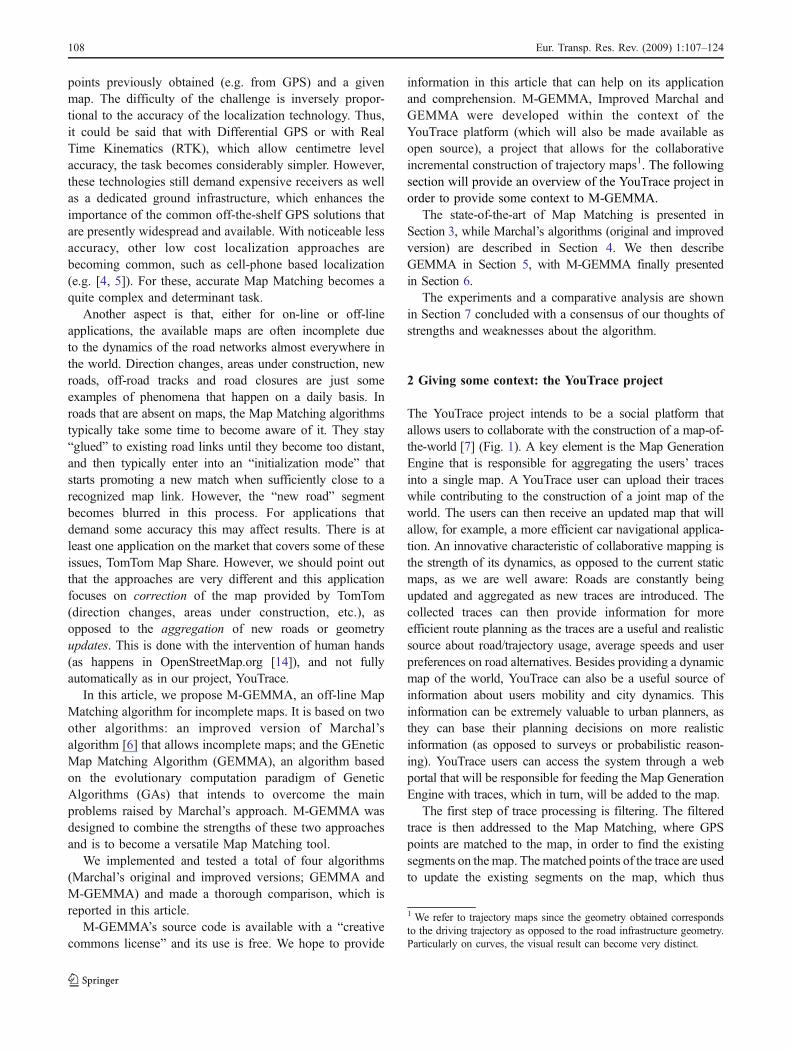
The YouTrace project intends to be a social platform thatallows users to collaborate with the construction of a map-of-the-world [7] (Fig. 1). A key element is the Map GenerationEngine that is responsible for aggregating the users’ tracesinto a single map. A YouTrace user can upload their traceswhile contributing to the construction of a joint map of theworld. The users can then receive an updated map that willallow, for example, a more efficient car navigational applica-tion. An innovative characteristic of collaborative mapping isthe strength of its dynamics, as opposed to the current staticmaps, as we are well aware: Roads are constantly beingupdated and aggregated as new traces are introduced. Thecollected traces can then provide information for moreefficient route planning as the traces are a useful and realisticsource about road/trajectory usage, average speeds and userpreferences on road alternatives. Besides providing a dynamicmap of the world, YouTrace can also be a useful source ofinformation about users mobility and city dynamics. Thisinformation can be extremely valuable to urban planners, asthey can base their planning decisions on more realisticinformation (as opposed to surveys or probabilistic reason-ing). YouTrace users can access the system through a webportal that will be responsible for feeding the Map GenerationEngine with traces, which in turn, will be added to the map.

The first step of trace processing is filtering. The filteredtrace is then addressed to the Map Matching, where GPSpoints are matched to the map, in order to find the existingsegments on the map. The matched points of the trace are usedto update the existing segments on the map, which thus

1 We refer to trajectory maps since the geometry obtained correspondsto the driving trajectory as opposed to the road infrastructure geometry.Particularly on curves, the visual result can become very distinct.

108 Eur. Transp. Res. Rev. (2009) 1:107–124

improves road precision. The non-matched points of the traceare aggregated on to the map, creating new roads (ortrajectories). Two databases are then generated from thisprocess; the map database and the statistics database. Thesedatabases serve to provide data for external services such asroute planning and traffic analysis. For more information onthe YouTrace project, please refer to [7]. As can beunderstood, the Map Matching is a key element forYouTrace, which is entirely responsible for finding the partsof the trace that already exist on the map. This allows for thedistinction between the parts that should be aggregated andthose that should be updated, therefore the quality of thefinal map is dependable of the quality of the match.

3 Current trends on map-matching

Map-Matching algorithms are used to fix location data intoa spatial road network. They are used in the most variedapplications. The most common are noticeably the GPS carnavigation devices, which are constantly indicating the roadsegment where the user is located based on informationretrieved from GPS satellites. The purpose of a Map-Matching algorithm can be divided in two parts. Firstly, thealgorithm determines which road segment, from a givennetwork, corresponds to each given position. Afterwards, itwill determine the exact location of the same position insidethe segment previously selected [8, 9].

There are algorithms designed specifically for givenapplications and others that are generic. In some situations,the path is known in advance so the set of roads to perform thematching is restricted. For instance, the match of bus locationdata can be improved by restricting the road network to theknown path taken [9]. Generic algorithms can also be one oftwo types: online or offline [8]. Real-time applications, suchas GPS navigation devices use online algorithms, meaningthat the matching is performed as the data is being receivedand thus it is based only on past matches. On the other hand,post-processing applications use offline algorithms. Onlinealgorithms are less effective. Offline algorithms can take theadvantage of not only matching each point according to pastdata but also based on the following of a “future” point,which helps the algorithm to select the correct road when nearto junctions. The literature review made by [8] states that themajority of the existent algorithms are for real-time applica-tions since the demand is higher than in post-processing ones.In fact, only one offline algorithm is presented [6]. Thesealgorithms use GPS coordinates as input source to performthe matching, but most consider using an integration of GPSdata with Dead-Reckoning (DR) in order to improve thematching accuracy [10]. DR systems use some sensors likeodometers and gyroscopes in order to calculate subsequentpositions in relation to the initial one. In these systems, the

probability of incorrectly estimated positions increases dras-tically as more readings are made since a new position iscalculated based on previous readings from inaccurate sensors[10]. In [8], the author classifies Map-Matching algorithmsinto four groups, depending on the techniques applied byeach to perform the match. They are: geometric, topological,probabilistic and other advanced algorithms.

3.1 Geometric algorithms

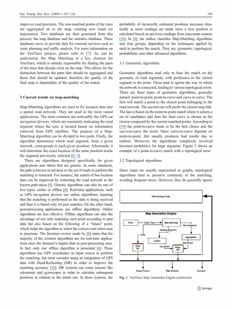
Geometric algorithms tend only to base the match on thegeometry of road segments, with preference to the closestsegment to the point. These tend to ignore the way in whichthe network is connected, leading to various topological errors.There are three types of geometric algorithms, generallynamed: point-to-point, point-to-curve and curve-to curve. Thefirst will match a point to the closest point belonging to theroad network. The second one will prefer the closest map link.The last is based on the point-to-point match where it selects aset of candidates and then the final curve is chosen as theclosest composed by the current matched points. According to[10] the point-to-curve tends to be the best choice and thecurve-to-curve the worst. Since curve-to-curve depends onpoint-to-point, this usually produces bad results due tooutliers. Moreover, the algorithmic complexity involvedbecomes prohibitive for large segments. Figure 2 shows anexample of a point-to-curve match with a topological error.

3.2 Topological algorithms

Since maps are usually represented as graphs, topologicalalgorithms tend to preserve continuity in the matching,avoiding frequent errors. However, they do generally ignore

Fig. 1 YouTrace Map Generation Engine architecture

Eur. Transp. Res. Rev. (2009) 1:107–124 109

additional readings from certain GPS readable data such asspeed or heading and might be sensitive to outliers as well.One example of a topological algorithm is the Marchal’salgorithm [6], which will be explained below in detail. Thesealgorithms can generally be divided into two stages. The firstis the initial matching process, where the algorithm willselect the most suitable link from the closest to the initialpoints. At the second stage, the algorithm will continuematching the points while keeping the network topology inconsideration. In [8], the author also adds that these kinds ofalgorithms have some problems at certain junctions wherethe direction of links is not similar. This can only be solvedvia a sub-routine that selects the appropriate subsequent roadsegment. Since this routine runs in a post-processing mode,these algorithms tend to be useless in real-time applications.

3.3 Probabilistic algorithms

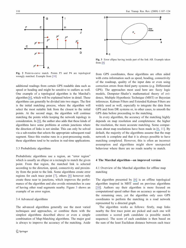
Probabilistic algorithms use a region, an “error region”which is usually an ellipse or a rectangle to match the givenpoint. From that region, the matched link is selectedaccording to the direction, speed, connectivity and proxim-ity from the point to the link. Some algorithms create errorregions for each trace point [7], others [8] however onlycreate these near to junctions, which improves the perfor-mance of the algorithm and also avoids mismatches in caseof having other road segments nearby. Figure 3 shows anexample of an error region.

3.4 Advanced algorithms

The advanced algorithms generally use the most variedtechniques and approaches, or combine them with thesimplest algorithms described above or even a simplecombination of Map-Matching algorithms. The major goalis always to improve the accuracy of the matching. Aside

from GPS coordinates, these algorithms are often aidedwith extra information such as speed, heading, connectivityof the roadmap, quality of the input data or even usingcorrection errors from third party systems (e.g. DifferentialGPS). The approaches most used here are: fuzzy logicmodels, Dempster–Shafer’s mathematical theory of evi-dence, Multiple Hypothesis Technique (MHT) or Bayesianinferences. Kalman Filters and Extended Kalman Filters arewidely used as well, especially to integrate the data fromGPS and from DR systems or, in other cases, to smooth theGPS data before proceeding to the matching.

In every algorithm, the accuracy of the matching highlydepends on map resolution and completeness: the higherthe resolution, the more accurate matching. Some compar-isons about map resolutions have been made in [6, 11]. Bydefault, the majority of the algorithms assume that the mapnetwork is complete and that it is always possible to havematching completed. However, this is often an incorrectassumption and algorithms might show unexpectedbehaviour where there are no roads nearby to match.

4 The Marchal algorithm—an improved version

4.1 Overview of the Marchal algorithm for offline mapmatching

The algorithm presented by [6] is an offline topologicalalgorithm inspired in MHT used on previous algorithms[10]. Authors say their algorithm is more focused oncomputational speed rather than on accuracy as opposed tothe remaining ones, yet the algorithm only uses GPScoordinates to perform the matching in a road networkrepresented by a directed graph.

The algorithm works as follows: firstly, map linksnearby the first trace point are picked and each one willconstitute a scored path candidate (a possible matchsequence). The score of each candidate is then based onthe sum of the least Euclidean distance between each trace

Fig. 2 Point-to-curve match. Points P3 and P4 are topologicalwrongly matched. Example from [10]

Fig. 3 Error ellipse having inside part of the link AB. Example takenfrom [8]

110 Eur. Transp. Res. Rev. (2009) 1:107–124

point and its matched link (also named as matchingdistance). Hence, best candidates have lowest scores.

After the initial matching process, for each point of thetrace, it is assumed that the current point matches the lastlink of each candidate. Then, an update of the score occursand the candidate is put into a new set. Afterwards, if thetrace has reached the end of the link, new path candidatesare created. To see if an intersection has been reached, acomparison is made between the travelled length throughthe trace points and the travelled length through the links ofthe path candidate. If the first length is longer than a givenpercentage of the second, it is assumed that the nextjunction has possibly been reached2. For this percentage,the authors fixed the value in 50%, which in their opiniontends to give fair results. New candidates are created, theyare similar to the current one and a link per new roadsegment starting on that junction will be added to each oneof the new candidates. Their score is updated and they areinserted into the new set. When no more candidates tomatch the current point are available, the algorithm willpick only the best N candidates of the new set, it passes tothe following trace point and does everything all overagain. The authors tested some values for N and, based onthese experiments, they say that with values above 30,improvements on matching accuracy are insignificant. Thebest candidate obtained gives the final match. Thisalgorithm has some additional mechanisms that permitsbreaking the match and restarting it from scratch when thedistance between two consecutive points or the differencebetween timestamps of two consecutive points is abovegiven thresholds. The authors use, as an example, 300 m forthe distance and 30 s for time difference.

4.2 Our implementation and modifications

The implementation of the algorithm has been modifiedfrom the original version due to several reasons. The firstand more obvious reason is that the addition of amechanism to detect whenever a new set of pointscorrespond to a non-existent road in the map. For thisreason, every matched distance (between GPS point andmatched map position) should fall below a given threshold(fixed at 20 m, after several experiments). This conditionmust be verified in the initial matching process and duringsubsequent matches, for the best candidate path. Thisconfirms that every set of unmatched points will be thenadded to the map as a new road. If the subsequent matchingis broken, then the best candidate (without considering the

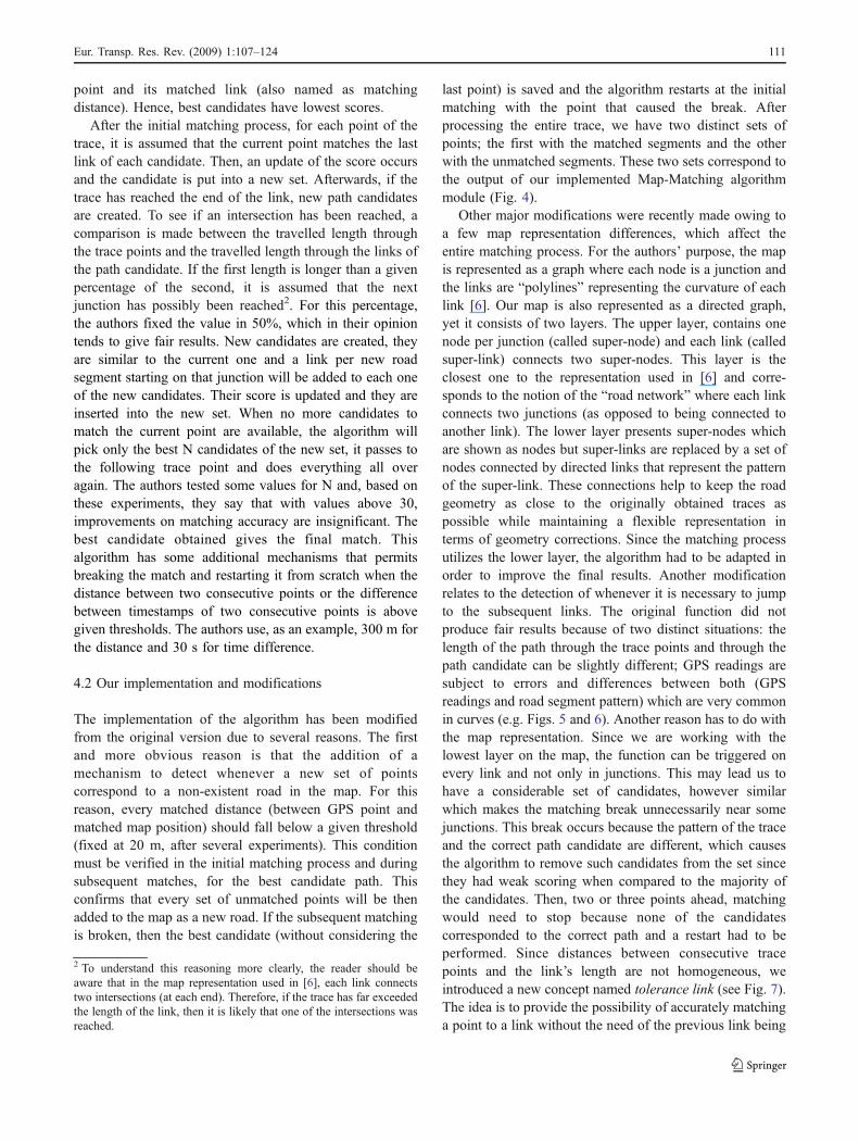
last point) is saved and the algorithm restarts at the initialmatching with the point that caused the break. Afterprocessing the entire trace, we have two distinct sets ofpoints; the first with the matched segments and the otherwith the unmatched segments. These two sets correspond tothe output of our implemented Map-Matching algorithmmodule (Fig. 4).

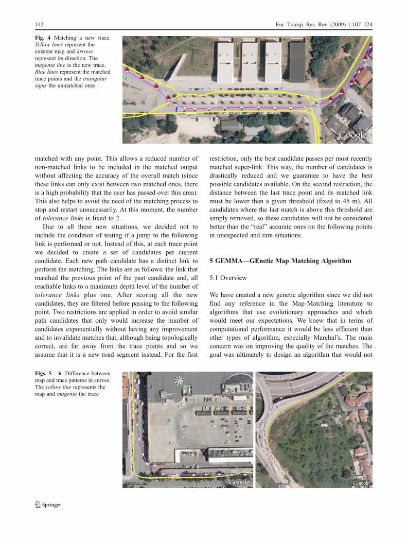
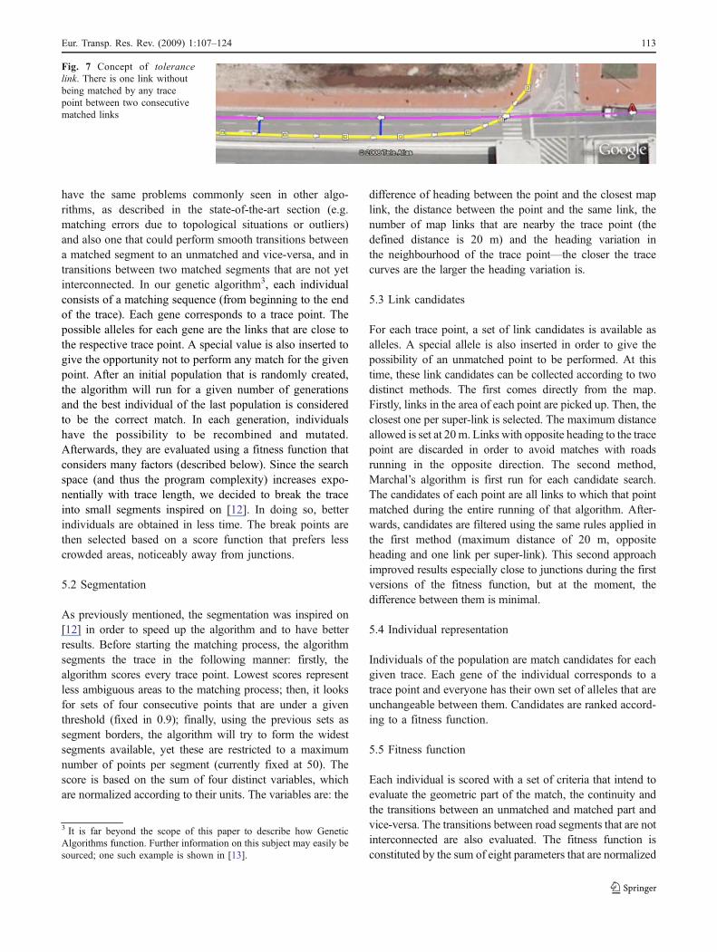
Other major modifications were recently made owing toa few map representation differences, which affect theentire matching process. For the authors’ purpose, the mapis represented as a graph where each node is a junction andthe links are “polylines” representing the curvature of eachlink [6]. Our map is also represented as a directed graph,yet it consists of two layers. The upper layer, contains onenode per junction (called super-node) and each link (calledsuper-link) connects two super-nodes. This layer is theclosest one to the representation used in [6] and corre-sponds to the notion of the “road network” where each linkconnects two junctions (as opposed to being connected toanother link). The lower layer presents super-nodes whichare shown as nodes but super-links are replaced by a set ofnodes connected by directed links that represent the patternof the super-link. These connections help to keep the roadgeometry as close to the originally obtained traces aspossible while maintaining a flexible representation interms of geometry corrections. Since the matching processutilizes the lower layer, the algorithm had to be adapted inorder to improve the final results. Another modificationrelates to the detection of whenever it is necessary to jumpto the subsequent links. The original function did notproduce fair results because of two distinct situations: thelength of the path through the trace points and through thepath candidate can be slightly different; GPS readings aresubject to errors and differences between both (GPSreadings and road segment pattern) which are very commonin curves (e.g. Figs. 5 and 6). Another reason has to do withthe map representation. Since we are working with thelowest layer on the map, the function can be triggered onevery link and not only in junctions. This may lead us tohave a considerable set of candidates, however similarwhich makes the matching break unnecessarily near somejunctions. This break occurs because the pattern of the traceand the correct path candidate are different, which causesthe algorithm to remove such candidates from the set sincethey had weak scoring when compared to the majority ofthe candidates. Then, two or three points ahead, matchingwould need to stop because none of the candidatescorresponded to the correct path and a restart had to beperformed. Since distances between consecutive tracepoints and the link’s length are not homogeneous, weintroduced a new concept named tolerance link (see Fig. 7).The idea is to provide the possibility of accurately matchinga point to a link without the need of the previous link being

2 To understand this reasoning more clearly, the reader should beaware that in the map representation used in [6], each link connectstwo intersections (at each end). Therefore, if the trace has far exceededthe length of the link, then it is likely that one of the intersections wasreached.

Eur. Transp. Res. Rev. (2009) 1:107–124 111

matched with any point. This allows a reduced number ofnon-matched links to be included in the matched outputwithout affecting the accuracy of the overall match (sincethese links can only exist between two matched ones, thereis a high probability that the user has passed over this area).This also helps to avoid the need of the matching process tostop and restart unnecessarily. At this moment, the numberof tolerance links is fixed to 2.

Due to all these new situations, we decided not toinclude the condition of testing if a jump to the followinglink is performed or not. Instead of this, at each trace pointwe decided to create a set of candidates per currentcandidate. Each new path candidate has a distinct link toperform the matching. The links are as follows: the link thatmatched the previous point of the past candidate and, allreachable links to a maximum depth level of the number oftolerance links plus one. After scoring all the newcandidates, they are filtered before passing to the followingpoint. Two restrictions are applied in order to avoid similarpath candidates that only would increase the number ofcandidates exponentially without having any improvementand to invalidate matches that, although being topologicallycorrect, are far away from the trace points and so weassume that it is a new road segment instead. For the first

restriction, only the best candidate passes per most recentlymatched super-link. This way, the number of candidates isdrastically reduced and we guarantee to have the bestpossible candidates available. On the second restriction, thedistance between the last trace point and its matched linkmust be lower than a given threshold (fixed to 45 m). Allcandidates where the last match is above this threshold aresimply removed, so these candidates will not be consideredbetter than the “real” accurate ones on the following pointsin unexpected and rare situations.

5 GEMMA—GEnetic Map Matching Algorithm

5.1 Overview

We have created a new genetic algorithm since we did notfind any reference in the Map-Matching literature toalgorithms that use evolutionary approaches and whichwould meet our expectations. We knew that in terms ofcomputational performance it would be less efficient thanother types of algorithm, especially Marchal’s. The mainconcern was on improving the quality of the matches. Thegoal was ultimately to design an algorithm that would not

Fig. 4 Matching a new trace.Yellow lines represent theexistent map and arrowsrepresent its direction. Themagenta line is the new trace.Blue lines represent the matchedtrace points and the triangularsigns the unmatched ones

Figs. 5 – 6 Difference betweenmap and trace patterns in curves.The yellow line represents themap and magenta the trace

112 Eur. Transp. Res. Rev. (2009) 1:107–124

have the same problems commonly seen in other algo-rithms, as described in the state-of-the-art section (e.g.matching errors due to topological situations or outliers)and also one that could perform smooth transitions betweena matched segment to an unmatched and vice-versa, and intransitions between two matched segments that are not yetinterconnected. In our genetic algorithm3, each individualconsists of a matching sequence (from beginning to the endof the trace). Each gene corresponds to a trace point. Thepossible alleles for each gene are the links that are close tothe respective trace point. A special value is also inserted togive the opportunity not to perform any match for the givenpoint. After an initial population that is randomly created,the algorithm will run for a given number of generationsand the best individual of the last population is consideredto be the correct match. In each generation, individualshave the possibility to be recombined and mutated.Afterwards, they are evaluated using a fitness function thatconsiders many factors (described below). Since the searchspace (and thus the program complexity) increases expo-nentially with trace length, we decided to break the traceinto small segments inspired on [12]. In doing so, betterindividuals are obtained in less time. The break points arethen selected based on a score function that prefers lesscrowded areas, noticeably away from junctions.

5.2 Segmentation

As previously mentioned, the segmentation was inspired on[12] in order to speed up the algorithm and to have betterresults. Before starting the matching process, the algorithmsegments the trace in the following manner: firstly, thealgorithm scores every trace point. Lowest scores representless ambiguous areas to the matching process; then, it looksfor sets of four consecutive points that are under a giventhreshold (fixed in 0.9); finally, using the previous sets assegment borders, the algorithm will try to form the widestsegments available, yet these are restricted to a maximumnumber of points per segment (currently fixed at 50). Thescore is based on the sum of four distinct variables, whichare normalized according to their units. The variables are: the

difference of heading between the point and the closest maplink, the distance between the point and the same link, thenumber of map links that are nearby the trace point (thedefined distance is 20 m) and the heading variation inthe neighbourhood of the trace point—the closer the tracecurves are the larger the heading variation is.

5.3 Link candidates

For each trace point, a set of link candidates is available asalleles. A special allele is also inserted in order to give thepossibility of an unmatched point to be performed. At thistime, these link candidates can be collected according to twodistinct methods. The first comes directly from the map.Firstly, links in the area of each point are picked up. Then, theclosest one per super-link is selected. The maximum distanceallowed is set at 20m. Links with opposite heading to the tracepoint are discarded in order to avoid matches with roadsrunning in the opposite direction. The second method,Marchal’s algorithm is first run for each candidate search.The candidates of each point are all links to which that pointmatched during the entire running of that algorithm. After-wards, candidates are filtered using the same rules applied inthe first method (maximum distance of 20 m, oppositeheading and one link per super-link). This second approachimproved results especially close to junctions during the firstversions of the fitness function, but at the moment, thedifference between them is minimal.

5.4 Individual representation

Individuals of the population are match candidates for eachgiven trace. Each gene of the individual corresponds to atrace point and everyone has their own set of alleles that areunchangeable between them. Candidates are ranked accord-ing to a fitness function.

5.5 Fitness function

Each individual is scored with a set of criteria that intend toevaluate the geometric part of the match, the continuity andthe transitions between an unmatched and matched part andvice-versa. The transitions between road segments that are notinterconnected are also evaluated. The fitness function isconstituted by the sum of eight parameters that are normalized

3 It is far beyond the scope of this paper to describe how GeneticAlgorithms function. Further information on this subject may easily besourced; one such example is shown in [13].

Fig. 7 Concept of tolerancelink. There is one link withoutbeing matched by any tracepoint between two consecutivematched links

Eur. Transp. Res. Rev. (2009) 1:107–124 113

according to their dimensions. Since this is a minimizationproblem, best individuals who have the lowest scores arealways greater or equal to zero. One of these parameters is theaverage distance between each trace point and its matchedlink. Unmatched points are also considered with a defaultvalue of 20 m. The maximum distance previously obtained isanother parameter, and the other is the maximum of theminimum distances of each matched segments. The lattertends to penalize matched zones where every matched point istoo distant from the road segment. A parameter is also used topenalize candidates that privilege non-matching rather thanmatching on acceptable conditions. This is measured with the

length of the trace that is unmatched. The concept of tolerancelink also exists here (see Fig. 7). In fact, it was created firstlyfor this algorithm and was later adapted to our Marchal’simplementation. Another parameter consists of the sum ofdistances between two links when it is not possible to reachthe second from the first one. The number of tolerance linksused in the genetic algorithm is currently 5, so if it is notpossible to go from one link to the other at a maximum deepof 6, the Euclidean distance between the end point of the firstlink and the start point of the second link is added to thespecific parameter. In order to keep matching continuity asmuch as possible, another parameter is used to store the sum

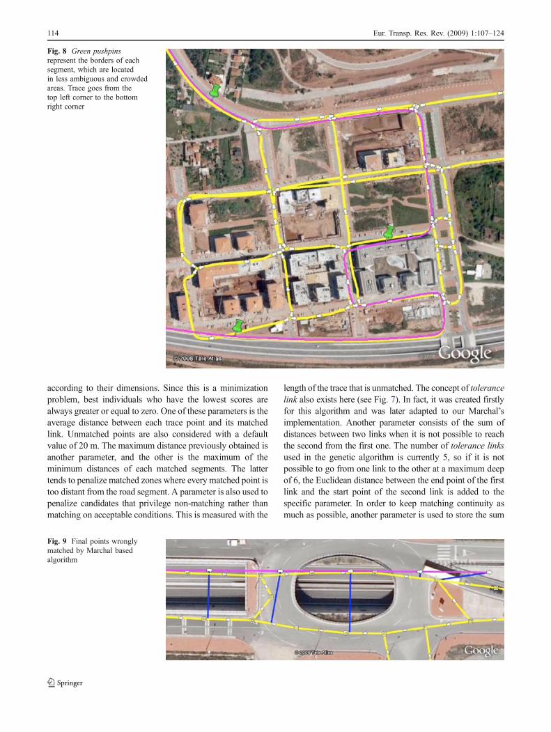
Fig. 9 Final points wronglymatched by Marchal basedalgorithm

Fig. 8 Green pushpinsrepresent the borders of eachsegment, which are locatedin less ambiguous and crowdedareas. Trace goes from thetop left corner to the bottomright corner

114 Eur. Transp. Res. Rev. (2009) 1:107–124

of the square of the matched lengths of each segment. Sincewe want to minimize the score, the inverse of the obtainedvalue is used. Finally, the last two parameters are used tosmooth the transitions between matched and unmatchedareas and vice-versa. One of these parameters stores theaverage distance between an unmatched trace point and thefollowing matched link or the distance between the lastmatched link and the following unmatched trace point. Theother one stores the maximum of these distances. Eachparameter is weighted, thus allowing for different orders ofimportance. For example, we prefer continuity to geometricproximity, so the three parameters that measure the un-

matched lengths, the distances between unreachable linksand the square of the continued matched lengths have thehighest weights (Fig. 8).

5.6 Running the algorithm

For each segment of the trace, the algorithm generates arandom population. Each gene has a roulette wheel withrespective alleles. Every allele has the same probability exceptfor the special one that represents an unmatched situation,which has a fixed probability of 15%. The population in eachgeneration has the opportunity to be recombined and mutated.

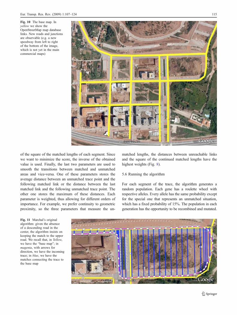
Fig. 10 The base map. Inyellow we show theOpenStreetMap map databaselinks. New roads and junctionsare observable (e.g. a newspeedway from left to rightof the bottom of the image,which is not yet in the maincommercial maps)

Fig. 11 Marchal’s originalalgorithm: given the absenceof a descending road in thecenter, the algorithm insists onkeeping the match to the upperroad. We recall that, in Yellow,we have the “base map”; inmagenta, with arrows fordirection, we have the incomingtrace; in blue, we have thematches connecting the trace tothe base map

Eur. Transp. Res. Rev. (2009) 1:107–124 115

Pairs of two individuals are then selected using the tournamentselection method and have a probability to be recombined,fixed at 75%. This recombination method uses one pointcrossover, with a randomly selected point. Afterwards, eachgene of the individual in the population has a slight probability

to be mutated (0.5%). The new link is picked up randomlyfrom the correspondent roulette wheel built at the beginning.From one generation to the next, we decided to include the bestprevious individuals without being recombined or mutated. 3%of the population passes directly, which corresponds to sixindividuals (since the population size is two hundred). One stopcondition only exists for the algorithm; it stops when the bestindividual has not being changed for the last given generations.Currently, this number of generations is three hundred.

5.7 Observations

The output of the algorithm is equal to the one presentedabove: a set with the matched paths and another one withthe unmatched trace points. These are built from the bestindividuals of each trace segment. As it is in its nature, thegenetic algorithm itself has been suffering some evolutionthrough time, especially in regard to the fitness function.Consequently all the thresholds discussed here weredefined based on observations in our set of traces, after arelatively large number of experiments (three months ofdaily tests, in which we refined both the algorithm and theparameters), meaning that new situations can always comeup and new improvements to the fitness function or somethresholds adjustments might be needed. The same happenswith the remaining parameters of the algorithm, includingcrossover and mutation rates, and size of population. Thevalues have not been as frequently changed as in the fitnessfunction, and it is less likely that they need new modi-fications. Adjustments were made after running severaltests showing that these could improve the quality of thematching process. We currently have a set of traces with atotal of 526,728 points that corresponds to an approximatelength of 11,486 km throughout Portugal (essentially thecentral area).

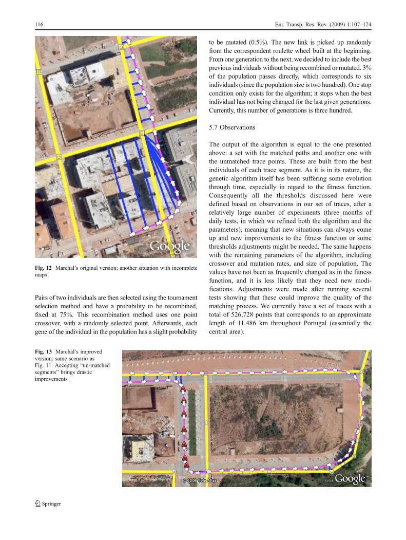
Fig. 12 Marchal’s original version: another situation with incompletemaps

Fig. 13 Marchal’s improvedversion: same scenario asFig. 11. Accepting “un-matchedsegments” brings drasticimprovements

116 Eur. Transp. Res. Rev. (2009) 1:107–124

6 M-GEMMA—joining the best from two worlds

As we could see in the last section, the strengths andweaknesses of both algorithms are complementary. For thisreason, we thought that an integration of both algorithmscould lead us to better results than to carry any of these outseparately. Since GEMMA is extremely time consuming, weneeded to restrict its usage to ambiguous areas whereMarchal’s has performed some difficulties. Firstly, we runMarchal’s algorithm in both directions (processing the traceforwards and then backwards). This gives us two possiblepath matches, which can be different or exactly the same,depending on trace and map complexity. If the results areexactly the same then there is no ambiguity in the match andthus, no need to run GEMMA. However, even when both runsgive the same output, the final points of the trace (or/and theinitial) can be wrongly matched as seen in Fig. 9, so GEMMAis run for the first and last few points (about 5) of the tracejust to confirm that the output given by Marchal’s is correct.

For areas where both Marchal’s forwards and backwardsruns produce different matches (and sets of candidate links),the whole set of candidate links for every participating pointare added to a list. After testing all points, segments arecreated based on consecutive points that are on the list. Foreach segment, two unambiguous trace points are added in theborders (to force the start and end of the segment to “fit” intothe remaining matches). This way, GEMMA can guaranteethe continuity of the match and avoid topological errors.Candidates running on GEMMA are thus taken from theoutput of both Marchal’s runs. Since continuity is guaranteedon GEMMA, the output for the ambiguous areas fitsautomatically in the remaining map. With this integration,some parameters on GEMMA had to be adapted, namely the

population size, the number of generations of the bestindividual that leads the algorithm to stop and some weightsin the fitness function. Since the new segments are commonlyvery small, the population size remained fixed to fiftyindividuals and the number of stabilized generations neces-sary for stopping is set at seventy-five. This helped thealgorithm find the best individual in the first few generations.Processing time became longer than simply runningMarchal’salone since we have to run Marchal’s twice per trace andGEMMA on some segments. Despite that, results show a gainin quality which justifies a loss of performance and as the mapbecomes more complete, fewer ambiguous segments appearto run on the genetic algorithm, thus further reducing the time.

7 Experiments and comparative analysis

Having implemented the four algorithms described, it isnecessary to find which one adapts better to the objectivesand performs better results. Each algorithm has benefits anddrawbacks, either related to computational speed or tomatching accuracy.

The base map to work with was extracted from Open-StreetMap.org [14]. This choice was due to several reasons: itis open source and freely available; it is partially complete; incovered areas, it is comparable to TeleAtlas or NavTeqcommercial solutions in terms of accuracy and completeness.For the sake of the experiments, we are confident that thischoice is as valid as any other map database available(commercial or not). At most, it could be said that Open-StreetMap is globally less complete and more imprecise thanthose other professional databases, which becomes more of achallenge for our purposes.

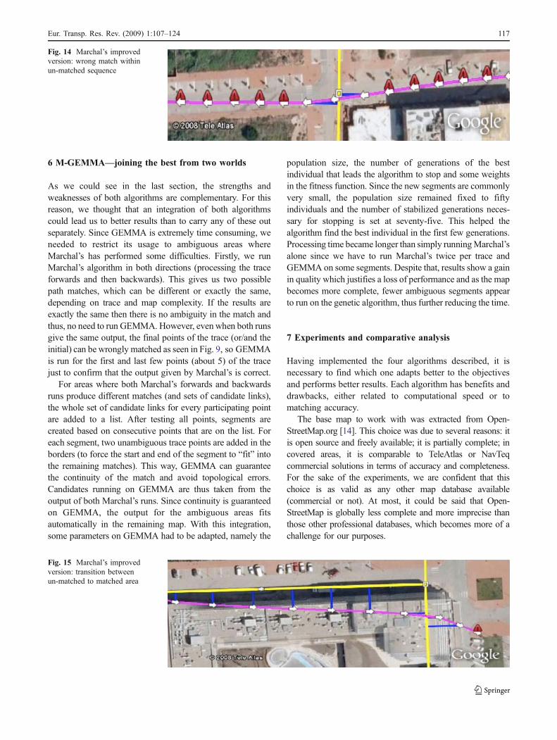
Fig. 15 Marchal’s improvedversion: transition betweenun-matched to matched area

Fig. 14 Marchal’s improvedversion: wrong match withinun-matched sequence

Eur. Transp. Res. Rev. (2009) 1:107–124 117

We made two main experiments, one in the large area ofCoimbra (Portugal) to assess general performance issues;the other in a smaller area, near to our department, whichcontains many junctions, buildings, areas under construc-tion and new roads (see Fig. 10). With the latter weintended to find accuracy issues.

For the first experiment, we initially built a base map withYouTrace with 225 km of traces in the area of Coimbra,originating 730 intersections and 15,901 links (1,264 super-links). We applied both algorithms to match 11 traces with atotal of 16 km. With an IntelCore™ 2 Duo processor runningat 2.2 GHzwith 2GB of RAM, ImprovedMarchal’s algorithmtook 0.171 s to determine the entire match. M-GEMMA took0.874 s to do the same task, of which 0.468 were necessary forthe GEMMA part to process 152 ambiguous points in a totalof 1.363 km. On average, M-GEMMA needed nearly fivetimes more processing effort thanMarchal’s approach in areaswith high density of intersections.

More experiments would be necessary (in other cities,rural areas, areas with plenty of multi-path effect, etc.) toachieve more conclusive results. However, these results arecoherent with the experience we had during the develop-ment of the algorithms and with other experiments. We are

also aware that a thorough algorithmic complexity analysisis needed in order to present a more explicit view of theefficiency involved. On a first analysis, Marchal’s algo-rithm time grows linearly with the size of the trace, with aquadratic component for local search of Euclidean distance.GEMMA behaves in an O(n * p * m * g), with n being thetrace size, p the population size, m the average number ofalleles and g the number of generations. M-GEMMAcorresponds to a combination of these two measures. This,however, is a naive analysis, since no attention is given toaspects such as distribution of segmentation, sensitive areasor other parameters on any of the algorithms.

Regarding the second experiment, we focused on asmaller area, extracting the exact base map from Open-StreetMap.org (the actual roads drawn, not the traces) as wecan see in Fig. 10. Within this scenario, we tested a set often small traces in order to raise and focus on the mainproblems found in each algorithm: Marchal “originalversion”; Marchal “improved version”; GEMMA; and M-GEMMA.

Although Marchal’s algorithm behaves reasonably wellwith traces with regular samples (in space and time) and with acomplete map, it becomes inaccurate when either of these

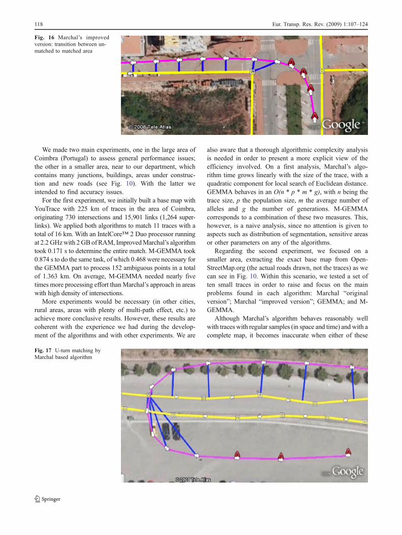
Fig. 17 U-turn matching byMarchal based algorithm

Fig. 16 Marchal’s improvedversion: transition between un-matched to matched area

118 Eur. Transp. Res. Rev. (2009) 1:107–124

premises fail (Figs. 11 and 12). Aiming to solve some ofthose weaknesses we added the improvements described inSection 4.2. As can be seen in Fig. 13 we did achieve somebetter results, particularly in unmatched areas. However, itstill had mistakes in transitions where the algorithm tends toinsist in making matches (where it is already in a “newroad”). See Figs. 14, 15 and 16.

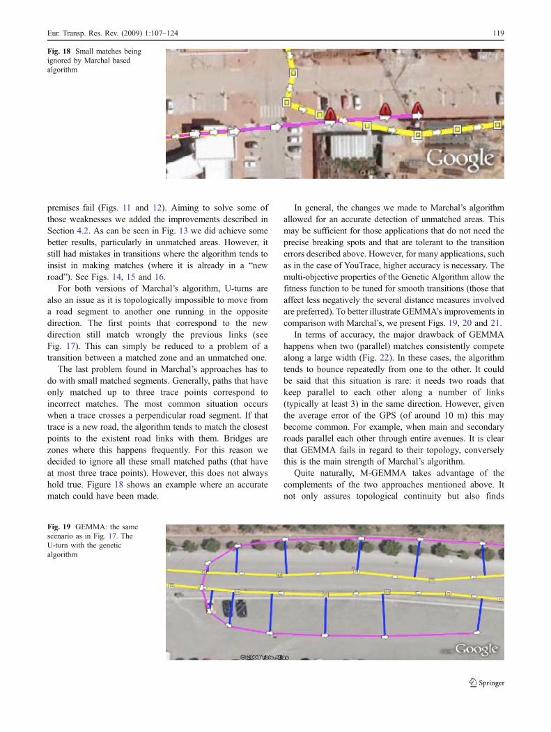
For both versions of Marchal’s algorithm, U-turns arealso an issue as it is topologically impossible to move froma road segment to another one running in the oppositedirection. The first points that correspond to the newdirection still match wrongly the previous links (seeFig. 17). This can simply be reduced to a problem of atransition between a matched zone and an unmatched one.

The last problem found in Marchal’s approaches has todo with small matched segments. Generally, paths that haveonly matched up to three trace points correspond toincorrect matches. The most common situation occurswhen a trace crosses a perpendicular road segment. If thattrace is a new road, the algorithm tends to match the closestpoints to the existent road links with them. Bridges arezones where this happens frequently. For this reason wedecided to ignore all these small matched paths (that haveat most three trace points). However, this does not alwayshold true. Figure 18 shows an example where an accuratematch could have been made.

In general, the changes we made to Marchal’s algorithmallowed for an accurate detection of unmatched areas. Thismay be sufficient for those applications that do not need theprecise breaking spots and that are tolerant to the transitionerrors described above. However, for many applications, suchas in the case of YouTrace, higher accuracy is necessary. Themulti-objective properties of the Genetic Algorithm allow thefitness function to be tuned for smooth transitions (those thataffect less negatively the several distance measures involvedare preferred). To better illustrate GEMMA’s improvements incomparison with Marchal’s, we present Figs. 19, 20 and 21.

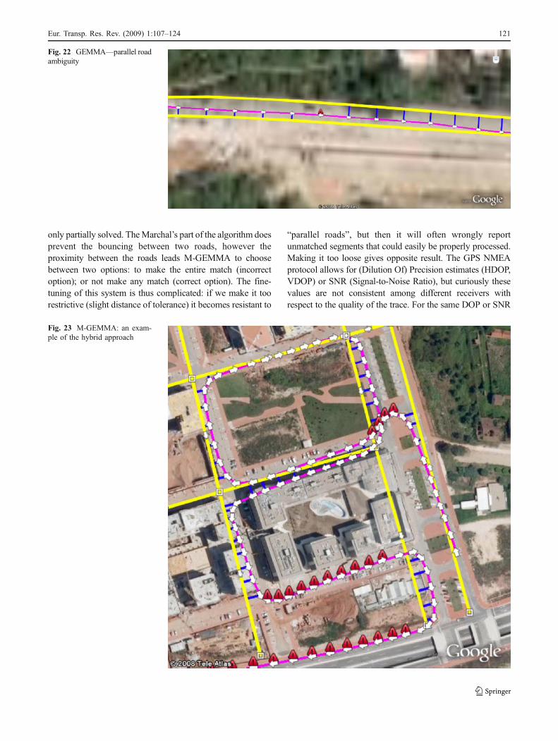
In terms of accuracy, the major drawback of GEMMAhappens when two (parallel) matches consistently competealong a large width (Fig. 22). In these cases, the algorithmtends to bounce repeatedly from one to the other. It couldbe said that this situation is rare: it needs two roads thatkeep parallel to each other along a number of links(typically at least 3) in the same direction. However, giventhe average error of the GPS (of around 10 m) this maybecome common. For example, when main and secondaryroads parallel each other through entire avenues. It is clearthat GEMMA fails in regard to their topology, converselythis is the main strength of Marchal’s algorithm.

Quite naturally, M-GEMMA takes advantage of thecomplements of the two approaches mentioned above. Itnot only assures topological continuity but also finds

Fig. 19 GEMMA: the samescenario as in Fig. 17. TheU-turn with the geneticalgorithm

Fig. 18 Small matches beingignored by Marchal basedalgorithm

Eur. Transp. Res. Rev. (2009) 1:107–124 119

smoother transitions between matched and unmatchedareas. Figure 23 shows an example of a trace that includesa variety of transitions, matched areas, unmatched areas andirregular sized samples. The journey starts on the right and

then goes around two blocks, finally moving out of the areathrough the speedway at the bottom.

In terms of map-matching accuracy, M-GEMMA still hasits limitations. For example, the problem of parallel roads is

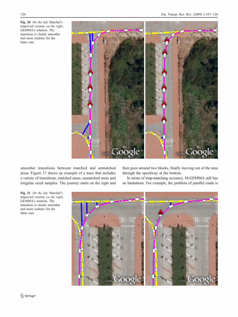
Fig. 21 On the left, Marchal’simproved version; on the right,GEMMA’s solution. Thetransition is clearly smootherand more realistic for thelatter case

Fig. 20 On the left, Marchal’simproved version; on the right,GEMMA’s solution. Thetransition is clearly smootherand more realistic for thelatter case

120 Eur. Transp. Res. Rev. (2009) 1:107–124

only partially solved. TheMarchal’s part of the algorithm doesprevent the bouncing between two roads, however theproximity between the roads leads M-GEMMA to choosebetween two options: to make the entire match (incorrectoption); or not make any match (correct option). The fine-tuning of this system is thus complicated: if we make it toorestrictive (slight distance of tolerance) it becomes resistant to

“parallel roads”, but then it will often wrongly reportunmatched segments that could easily be properly processed.Making it too loose gives opposite result. The GPS NMEAprotocol allows for (Dilution Of) Precision estimates (HDOP,VDOP) or SNR (Signal-to-Noise Ratio), but curiously thesevalues are not consistent among different receivers withrespect to the quality of the trace. For the same DOP or SNR

Fig. 23 M-GEMMA: an exam-ple of the hybrid approach

Fig. 22 GEMMA—parallel roadambiguity

Eur. Transp. Res. Rev. (2009) 1:107–124 121

values, we have observed very different qualities of tracesalong the 4 GPS receivers tested. For the case of YouTrace, werely on the statistics to distinguish between an error and aparallel road (with many traces, there should be two centre-lines gradually emerging out of the “statistical evidence”). Theproblem with parallel roads increases drastically whenspeaking of several road platforms on top of each other, asso happens at the entrance and exit of highways (although,normally, geometry helps distinguish this correct solutions).

Regarding time performance and complexity of thealgorithms, we knew from the beginning that, in terms ofspeed GEMMA would have a poor performance due to itsnature. Some modifications were made such as the creation ofthe upper layer of the map in order to speed up some searches

in the map, which benefitted Marshal’s algorithm as well.Despite these modifications and other minor ones, GEMMAalone remains slow. Moreover, with adding some moremodifications to the Marchal’s algorithm, this solution wasspeeded up. The difference of time when running bothalgorithms with the same set of data is noticeable.

8 Applying M-GEMMA to YouTrace

Regarding the inclusion of these algorithms in YouTrace,the large base map from above (225 km, 730 intersections)needed 186 s to be generated, while with Improved Marchal125 s were necessary. The results were different, however,

Fig. 25 Two generated crossings (zoom of Fig. 24)

Fig. 24 Map generated fromscratch out of 24 traces (2,926points)

122 Eur. Transp. Res. Rev. (2009) 1:107–124

Marchal’s algorithm failed in some areas. On a differenttest, with a set with 87,005 points which correspondedapproximately to 1,392 km of trace length, Marchal’salgorithm (either version) took 20 s in the matchingprocess, for GEMMA it took approximately one hour and79 s for M-GEMMA.

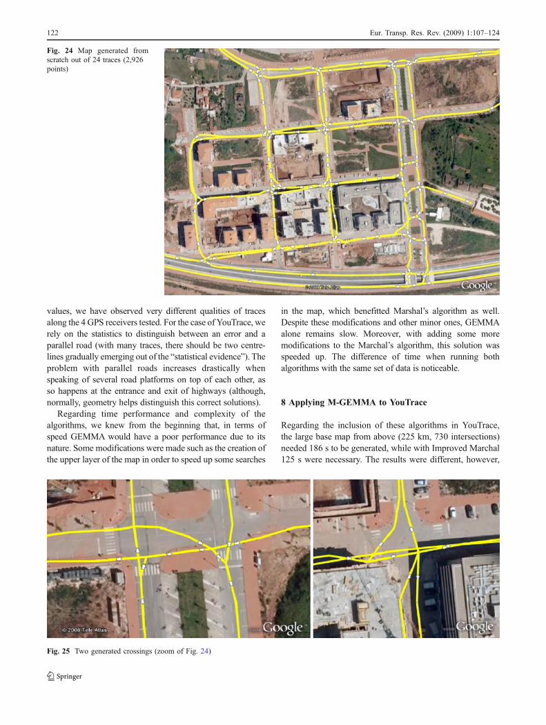
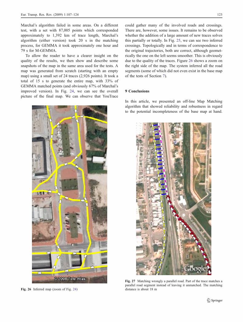
To allow the reader to have a clearer insight on thequality of the results, we then show and describe somesnapshots of the map in the same area used for the tests. Amap was generated from scratch (starting with an emptymap) using a small set of 24 traces (2,926 points). It took atotal of 15 s to generate the entire map, with 33% ofGEMMA matched points (and obviously 67% of Marchal’simproved version). In Fig. 24, we can see the overallpicture of the final map. We can observe that YouTrace

could gather many of the involved roads and crossings.There are, however, some issues. It remains to be observedwhether the addition of a large amount of new traces solvesthis partially or totally. In Fig. 25, we can see two inferredcrossings. Topologically and in terms of correspondence tothe original trajectories, both are correct, although geomet-rically the one on the left seems smoother. This is obviouslydue to the quality of the traces. Figure 26 shows a zoom onthe right side of the map. The system inferred all the roadsegments (some of which did not even exist in the base mapof the tests of Section 7).

9 Conclusions

In this article, we presented an off-line Map Matchingalgorithm that showed reliability and robustness in regardto the potential incompleteness of the base map at hand.

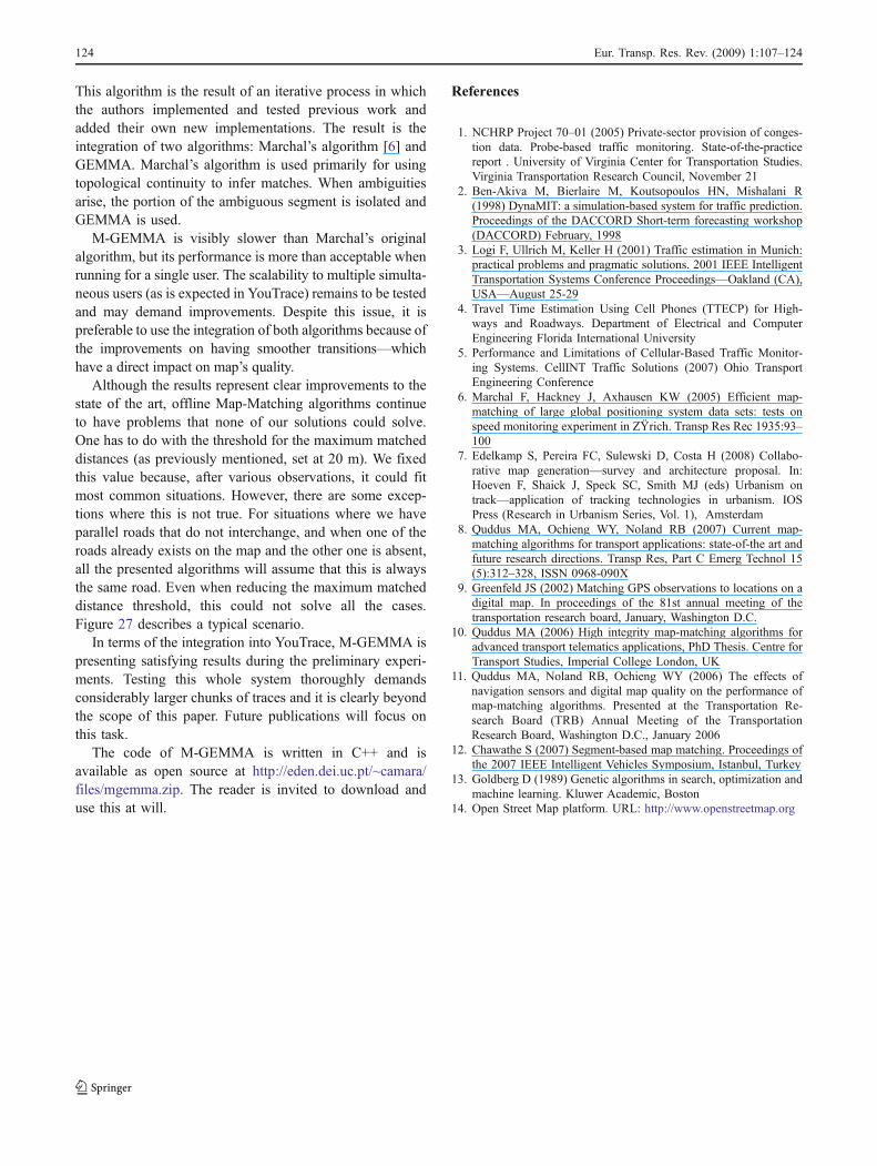
Fig. 27 Matching wrongly a parallel road. Part of the trace matches aparallel road segment instead of leaving it unmatched. The matchingdistance is about 18 mFig. 26 Inferred map (zoom of Fig. 24)

Eur. Transp. Res. Rev. (2009) 1:107–124 123

This algorithm is the result of an iterative process in whichthe authors implemented and tested previous work andadded their own new implementations. The result is theintegration of two algorithms: Marchal’s algorithm [6] andGEMMA. Marchal’s algorithm is used primarily for usingtopological continuity to infer matches. When ambiguitiesarise, the portion of the ambiguous segment is isolated andGEMMA is used.

M-GEMMA is visibly slower than Marchal’s originalalgorithm, but its performance is more than acceptable whenrunning for a single user. The scalability to multiple simulta-neous users (as is expected in YouTrace) remains to be testedand may demand improvements. Despite this issue, it ispreferable to use the integration of both algorithms because ofthe improvements on having smoother transitions—whichhave a direct impact on map’s quality.

Although the results represent clear improvements to thestate of the art, offline Map-Matching algorithms continueto have problems that none of our solutions could solve.One has to do with the threshold for the maximum matcheddistances (as previously mentioned, set at 20 m). We fixedthis value because, after various observations, it could fitmost common situations. However, there are some excep-tions where this is not true. For situations where we haveparallel roads that do not interchange, and when one of theroads already exists on the map and the other one is absent,all the presented algorithms will assume that this is alwaysthe same road. Even when reducing the maximum matcheddistance threshold, this could not solve all the cases.Figure 27 describes a typical scenario.

In terms of the integration into YouTrace, M-GEMMA ispresenting satisfying results during the preliminary experi-ments. Testing this whole system thoroughly demandsconsiderably larger chunks of traces and it is clearly beyondthe scope of this paper. Future publications will focus onthis task.

The code of M-GEMMA is written in C++ and isavailable as open source at http://eden.dei.uc.pt/~camara/files/mgemma.zip. The reader is invited to download anduse this at will.

References

1. NCHRP Project 70–01 (2005) Private-sector provision of conges-tion data. Probe-based traffic monitoring. State-of-the-practicereport . University of Virginia Center for Transportation Studies.Virginia Transportation Research Council, November 21

2. Ben-Akiva M, Bierlaire M, Koutsopoulos HN, Mishalani R(1998) DynaMIT: a simulation-based system for traffic prediction.Proceedings of the DACCORD Short-term forecasting workshop(DACCORD) February, 1998

3. Logi F, Ullrich M, Keller H (2001) Traffic estimation in Munich:practical problems and pragmatic solutions. 2001 IEEE IntelligentTransportation Systems Conference Proceedings—Oakland (CA),USA—August 25-29

4. Travel Time Estimation Using Cell Phones (TTECP) for High-ways and Roadways. Department of Electrical and ComputerEngineering Florida International University

5. Performance and Limitations of Cellular-Based Traffic Monitor-ing Systems. CellINT Traffic Solutions (2007) Ohio TransportEngineering Conference

6. Marchal F, Hackney J, Axhausen KW (2005) Efficient map-matching of large global positioning system data sets: tests onspeed monitoring experiment in ZŸrich. Transp Res Rec 1935:93–100

7. Edelkamp S, Pereira FC, Sulewski D, Costa H (2008) Collabo-rative map generation—survey and architecture proposal. In:Hoeven F, Shaick J, Speck SC, Smith MJ (eds) Urbanism ontrack—application of tracking technologies in urbanism. IOSPress (Research in Urbanism Series, Vol. 1), Amsterdam

8. Quddus MA, Ochieng WY, Noland RB (2007) Current map-matching algorithms for transport applications: state-of-the art andfuture research directions. Transp Res, Part C Emerg Technol 15(5):312–328, ISSN 0968-090X

9. Greenfeld JS (2002) Matching GPS observations to locations on adigital map. In proceedings of the 81st annual meeting of thetransportation research board, January, Washington D.C.

10. Quddus MA (2006) High integrity map-matching algorithms foradvanced transport telematics applications, PhD Thesis. Centre forTransport Studies, Imperial College London, UK

11. Quddus MA, Noland RB, Ochieng WY (2006) The effects ofnavigation sensors and digital map quality on the performance ofmap-matching algorithms. Presented at the Transportation Re-search Board (TRB) Annual Meeting of the TransportationResearch Board, Washington D.C., January 2006

12. Chawathe S (2007) Segment-based map matching. Proceedings ofthe 2007 IEEE Intelligent Vehicles Symposium, Istanbul, Turkey

13. Goldberg D (1989) Genetic algorithms in search, optimization andmachine learning. Kluwer Academic, Boston

14. Open Street Map platform. URL: http://www.openstreetmap.org

124 Eur. Transp. Res. Rev. (2009) 1:107–124