
Designing, Building, and Using Databases
409
UC BERKELEY EXTENSION Database/Application/Programming Courses Instructor: Michael Kremer, Ph.D. Course Title: Designing, Building, and Using Databases Course Subtitle: Beginning Microsoft Access Course Number: X405.4
-
Upload
khangminh22 -
Category
Documents
-
view
3 -
download
0
Transcript of Designing, Building, and Using Databases

UC BERKELEY EXTENSION
Database/Application/Programming Courses
Instructor: Michael Kremer, Ph.D.
Course Title: Designing, Building, and Using Databases
Course Subtitle: Beginning Microsoft Access
Course Number: X405.4


Designing, Building, and Using Databases
Instructor: Michael Kremer, Ph.D.
E-mail: [email protected]
Web Site: http://www.ucb-access.org
Copyright © 2016
All rights reserved. This publication, or any part thereof, may not be reproduced or transmitted in any form or by any means,
electronic or mechanical, including photocopying, recording, storing, or otherwise without expressed permission.
9th Edition
Icon Key User Name Password
Note Windows
Example Evaluation
Warning


TABLE OF CONTENT
CLASS 1: SECTION 1 ........................................................................................................................................................................... 1
1. INTRODUCTION TO RELATIONAL DATABASE SYSTEMS ..................................................................................................................................... 1
1.1 What is a Database? ................................................................................................................................................................... 1
1.2 Database Systems ....................................................................................................................................................................... 4
Flat File Systems ................................................................................................................................................................................................. 4
Hierarchical Database Systems .......................................................................................................................................................................... 4
Network Database Systems ............................................................................................................................................................................... 5
Relational Database Systems ............................................................................................................................................................................. 6
Object-Oriented Database Systems ................................................................................................................................................................... 7
1.3 Database Functions ..................................................................................................................................................................... 8
Online Transaction Processing (OLTP) Database ................................................................................................................................................ 8
Online Analytical Processing (OLAP) Database .................................................................................................................................................. 8
1.4 Database Architectures ............................................................................................................................................................... 9
One-Tier ............................................................................................................................................................................................................. 9
Two-Tier ........................................................................................................................................................................................................... 10
N-Tier ............................................................................................................................................................................................................... 10
1.5 Why use a relational database? ................................................................................................................................................ 12
Data Redundancy ............................................................................................................................................................................................. 12
Benefits of Relational Databases...................................................................................................................................................................... 14
2. DATA NORMALIZATION AND INTEGRITY RULES ............................................................................................................................................ 16
2.1 Data Collection .......................................................................................................................................................................... 16
2.2 Intuitive Database Design ......................................................................................................................................................... 17
2.3 The Relational Model ................................................................................................................................................................ 19
Column Characteristics .................................................................................................................................................................................... 20
Row Characteristics .......................................................................................................................................................................................... 20
2.4 Normalization Process ............................................................................................................................................................... 21
2.5 First Normal Form (1NF) ............................................................................................................................................................ 23
Atomic Value .................................................................................................................................................................................................... 23
Single Value ...................................................................................................................................................................................................... 24
2.6 Primary Key (Entity Integrity) .................................................................................................................................................... 26
2.7 Second Normal Form (2NF) ....................................................................................................................................................... 29
2.8 Third Normal Form (3NF) .......................................................................................................................................................... 32
2.9 Determining Relationships (Referential Integrity) ..................................................................................................................... 34
One-To-Many Relationship .............................................................................................................................................................................. 34
Many-To-Many Relationships .......................................................................................................................................................................... 37
One-To-One Relationships ............................................................................................................................................................................... 40

CLASS 1: SECTION 2 ......................................................................................................................................................................... 43
3. INTRODUCTION TO MICROSOFT ACCESS .................................................................................................................................................... 43
3.1 Microsoft Access Backstage View ............................................................................................................................................. 43
Backstage Tabs ................................................................................................................................................................................................. 45
3.2 Quick Access Toolbar & Office Fluent Ribbon ............................................................................................................................ 47
Quick Access Toolbar ....................................................................................................................................................................................... 47
The Office Fluent Ribbon .................................................................................................................................................................................. 48
3.3 Single vs. Multiple Document Interface ..................................................................................................................................... 50
3.4 Client vs. Web Database ............................................................................................................................................................ 52
3.5 Microsoft Access User Interface ................................................................................................................................................ 53
4. TABLE DESIGN ...................................................................................................................................................................................... 56
4.1 Creating a Table ........................................................................................................................................................................ 56
4.2 Data Types ................................................................................................................................................................................. 59
4.3 Field Properties .......................................................................................................................................................................... 62
4.4 Format Property ........................................................................................................................................................................ 68
Data Formats for ShortText and LongText Fields ............................................................................................................................................. 68
Format for Numbers and Currency Fields ........................................................................................................................................................ 71
Data Formats for Date/Time Fields .................................................................................................................................................................. 75
Data Formats for Yes/No Fields........................................................................................................................................................................ 76
4.5 Input Mask ................................................................................................................................................................................ 78
4.6 Validation Rule, Validation Text ................................................................................................................................................ 81
4.7 Lookup Wizard ........................................................................................................................................................................... 83
5. SETTING UP RELATIONSHIPS ................................................................................................................................................................... 85
5.1 Introduction to Relationships .................................................................................................................................................... 85
5.2 Setting a Primary Key ................................................................................................................................................................ 86
5.3 Creating Relationships in MS Access ......................................................................................................................................... 91
5.4 Referential Integrity .................................................................................................................................................................. 95
CLASS 2: SECTION 3 ....................................................................................................................................................................... 101
6. INTRODUCTION TO QUERIES .................................................................................................................................................................. 101
6.1 What is a Query? ..................................................................................................................................................................... 102
6.2 Types of Queries ...................................................................................................................................................................... 105
Select Query ................................................................................................................................................................................................... 106
Total Query .................................................................................................................................................................................................... 109
Action Queries................................................................................................................................................................................................ 109
Crosstab Queries ............................................................................................................................................................................................ 111
SQL Queries .................................................................................................................................................................................................... 111
6.3 Capabilities of Queries ............................................................................................................................................................. 112
7. SELECT QUERIES ................................................................................................................................................................................. 114
7.1 Create a SELECT Query ............................................................................................................................................................ 114

7.2 Working with Fields in Design Grid ......................................................................................................................................... 121
Selecting Fields in Design Grid Pane............................................................................................................................................................... 121
Managing Fields in Design Grid Pane ............................................................................................................................................................. 123
Field Names/Column Header in a Query ........................................................................................................................................................ 124
Sorting Data in a Query .................................................................................................................................................................................. 127
7.3 Simple Criteria Expression in Queries ...................................................................................................................................... 130
CLASS 2: SECTION 4 ....................................................................................................................................................................... 137
8. ADVANCED SELECT QUERIES ................................................................................................................................................................. 137
8.1 Wildcard Character Comparisons ............................................................................................................................................ 137
Simple Wildcard Characters ........................................................................................................................................................................... 137
Advanced Wildcard Characters ...................................................................................................................................................................... 141
8.2 Using Complex Criteria ............................................................................................................................................................ 144
Mathematical Operators ................................................................................................................................................................................ 145
Relational Operators ...................................................................................................................................................................................... 146
Logical Operators ........................................................................................................................................................................................... 147
String Operators ............................................................................................................................................................................................. 149
Miscellaneous Operators ............................................................................................................................................................................... 151
Complex Criteria............................................................................................................................................................................................. 152
8.3 Creating Calculated/Derived Fields ......................................................................................................................................... 158
8.4 Query Properties ...................................................................................................................................................................... 162
9. PARAMETER QUERIES .......................................................................................................................................................................... 166
9.1 Overview of Parameter Queries .............................................................................................................................................. 166
9.2 Simple Parameter Queries ....................................................................................................................................................... 168
9.3 Multiple Parameter Queries .................................................................................................................................................... 170
CLASS 3: SECTION 5 ....................................................................................................................................................................... 175
10. TOTAL QUERIES ................................................................................................................................................................................ 175
10.1 Overview of Total Queries ..................................................................................................................................................... 175
10.2 Creating a Total Query .......................................................................................................................................................... 177
10.3 Total Row Options ................................................................................................................................................................. 178
Group By Category ......................................................................................................................................................................................... 178
Expression Category ....................................................................................................................................................................................... 180
Filter Category ................................................................................................................................................................................................ 181
Aggregate Category ........................................................................................................................................................................................ 182
10.4 Performing Record Aggregation ............................................................................................................................................ 186
Aggregation on all Records ............................................................................................................................................................................ 186
Aggregation on Groups of Records ................................................................................................................................................................ 187
Aggregation on Multiple Tables ..................................................................................................................................................................... 187
Aggregation on Multiple Groups .................................................................................................................................................................... 189
10.5 Criteria in Total Queries......................................................................................................................................................... 190
Criteria for Group By Fields ............................................................................................................................................................................ 190

Criteria for Aggregate Fields .......................................................................................................................................................................... 191
Criteria for Non-Output Fields ....................................................................................................................................................................... 192
11. CROSSTAB QUERIES ........................................................................................................................................................................... 194
11.1 Overview of Crosstab Queries ............................................................................................................................................... 194
11.2 Criteria in Crosstab Queries ................................................................................................................................................... 200
11.3 Advanced Crosstab Queries ................................................................................................................................................... 202
Column Headings ........................................................................................................................................................................................... 202
Row/Column Totals ........................................................................................................................................................................................ 205
Parameters in Crosstab Queries ..................................................................................................................................................................... 207
CLASS 3: SECTION 6 ....................................................................................................................................................................... 209
12. FORMS IN MS ACCESS ....................................................................................................................................................................... 209
12.1 Form Basics ........................................................................................................................................................................... 209
Capabilities of Forms ...................................................................................................................................................................................... 211
12.2 Form Controls ........................................................................................................................................................................ 212
12.3 Form Types ............................................................................................................................................................................ 215
Columnar Form .............................................................................................................................................................................................. 215
Tabular Form .................................................................................................................................................................................................. 216
MS Access Form Options ................................................................................................................................................................................ 217
Tabular vs. Datasheet Form Type ................................................................................................................................................................... 219
Split Form ....................................................................................................................................................................................................... 220
12.4 Creating Basic Forms using Wizards ...................................................................................................................................... 222
Using the Form Wizard ................................................................................................................................................................................... 222
Saving/Undoing Data Changes ....................................................................................................................................................................... 225
Navigation Bar, Filtering Data ........................................................................................................................................................................ 227
Making Design Changes ................................................................................................................................................................................. 229
Using a Form .................................................................................................................................................................................................. 233
13. MAIN/SUB FORMS ........................................................................................................................................................................... 237
13.1 Main/Sub Form Basics ........................................................................................................................................................... 237
13.2 Creating a Main/Sub Form using Wizards ............................................................................................................................. 240
14. COMBO/LIST BOX CONTROLS .............................................................................................................................................................. 244
14.1 Introduction to Combo/List Box Controls .............................................................................................................................. 244
14.2 Navigational Combo/List Boxes............................................................................................................................................. 246
14.3 Lookup Combo/List Boxes...................................................................................................................................................... 250
CLASS 4: SECTION 7 ....................................................................................................................................................................... 259
15. INTRODUCTION TO REPORTS ............................................................................................................................................................... 259
15.1 Reports Basics ....................................................................................................................................................................... 259
What are Reports? ......................................................................................................................................................................................... 259
Why use Reports? .......................................................................................................................................................................................... 260
Grouping of Data ............................................................................................................................................................................................ 262
Report Sections .............................................................................................................................................................................................. 264

15.2 Types of Reports .................................................................................................................................................................... 266
Tabular Report ............................................................................................................................................................................................... 266
Columnar Report ............................................................................................................................................................................................ 269
Mailing Label Report ...................................................................................................................................................................................... 270
Chart Report ................................................................................................................................................................................................... 271
15.3 Designing Reports ................................................................................................................................................................. 272
16. CREATING REPORTS USING WIZARDS .................................................................................................................................................... 279
16.1 Defining the Report Layout ................................................................................................................................................... 279
16.2 Report Wizards ...................................................................................................................................................................... 282
16.3 Creating a Main/Sub Report .................................................................................................................................................. 297
16.4 Creating a Mailing Report ..................................................................................................................................................... 301
CLASS 4: SECTION 8 ....................................................................................................................................................................... 305
17. ADVANCED FORMS/REPORTS .............................................................................................................................................................. 305
17.1 Creating Form Applications ................................................................................................................................................... 305
17.2 Using Chart Controls.............................................................................................................................................................. 310
Overview of Chart Controls ............................................................................................................................................................................ 310
Creating a Simple Form with Chart ................................................................................................................................................................ 310
Modifying Charts ............................................................................................................................................................................................ 316
18. BUILDING NAVIGATION SYSTEMS ......................................................................................................................................................... 319
18.1 Introduction to Application Navigation ................................................................................................................................. 319
18.2 Building a Navigation Form (Single Screen) .......................................................................................................................... 321
18.3 Building a Custom Form Navigation (Multiple Screen) ......................................................................................................... 324
18.4 The Navigation Pane ............................................................................................................................................................. 325
Overview of Navigation Pane ......................................................................................................................................................................... 325
Setting Up Custom Groups ............................................................................................................................................................................. 330
18.5 Setting Application Options ................................................................................................................................................... 332
19. USER-DEFINED DATA FORMATS........................................................................................................................................................... 334
19.1 Advanced Formats for Short/Long Text Fields ....................................................................................................................... 334
19.2 Advanced Formats for Number Fields ................................................................................................................................... 337
19.3 Advanced Formats for Date/Time Fields ............................................................................................................................... 338
19.4 Advanced Input Masks .......................................................................................................................................................... 341
CLASS 5: SECTION 9 ....................................................................................................................................................................... 345
20. INTRODUCTION TO FUNCTIONS ............................................................................................................................................................ 345
20.1 What is a Function? ............................................................................................................................................................... 345
20.2 Types of Functions ................................................................................................................................................................. 347
21. MS ACCESS BUILT-IN FUNCTIONS ........................................................................................................................................................ 349
21.1 Conversion Functions ............................................................................................................................................................. 349
21.2 Date/Time Functions ............................................................................................................................................................. 355
21.3 Financial Functions ................................................................................................................................................................ 361

21.4 Mathematical Functions ........................................................................................................................................................ 363
21.5 Text/String Functions ............................................................................................................................................................ 364
21.6 Domain Functions .................................................................................................................................................................. 372
CLASS 5: SECTION 10 ..................................................................................................................................................................... 375
22. BUILDING A SIMPLE DATABASE APPLICATION ......................................................................................................................................... 375
22.1 Designing the Database ........................................................................................................................................................ 375
22.2 Building the Application ........................................................................................................................................................ 375
INDEX OF FIGURES ......................................................................................................................................................................... 377
INDEX OF TABLES........................................................................................................................................................................... 383
TABLE OF EXAMPLES ..................................................................................................................................................................... 385
INDEX ............................................................................................................................................................................................ 393

Designing, Building, and Using Databases Class 1: Section 1
1. Introduction to Relational Database Systems 1 1.1 What is a Database?
CLASS 1: SECTION 1
1. Introduction to Relational Database Systems
Today’s world relies on information more than ever. Database and other information systems are
fundamental in storing all this information. This chapter presents an overview of database
systems and the historical evolution of database technologies.
1.1 What is a Database?
The term database is used in many different contexts these days. Fundamentally, a database is
a collection of organized information to provide efficient retrieval. The collected information
could be in any number of formats (electronic, printed, graphic, audio, statistical, combinations).
There are physical (paper/print) and electronic databases.
Although most people think only of computerized databases, in fact we are surrounded by
databases of all types. A dictionary, for instance, is a common database that allows users to
determine a word's spelling and definition quickly and easily. Similarly, a card file containing
friends' names and addresses, a phone book, a collection of recipes, and TV Guide are all
common forms of databases. Computerized databases include customer relation management
systems (CRM), human resource systems, equipment inventories, and sales transactions.
In very simple terms, a database is a container storing data. To be more specific, the data
stored in a database is a collection of related data. A database is also known as an abstraction of
real-world, complex sets of data to make data more meaningful and useful to humans.
At the software level, a database is comprised of three main building blocks:
➢ The database server including operating system that stores the data on disks (multiple
disk arrays).
➢ The database engine is the underlying software component that a database management
system (DBMS) uses to create, read, update and delete (CRUD) data from a database.
➢ The database management system (DBMS) is the software that manages access to the
database engine.

Designing, Building, and Using Databases Class 1: Section 1
1. Introduction to Relational Database Systems 2 1.1 What is a Database?
A database’s primary purpose is to store and extract data. To be more specific, it has the
following four main purposes:
➢ To query data (optimize queries)
➢ To add data
➢ To maintain/update data
➢ To delete data
The database management system performs the following main tasks:
➢ Controlling data access
➢ Enforcing data integrity
➢ Managing concurrency control
➢ Recovering the database after failures and restoring it from backup files
➢ Maintaining database security
A database application obviously consists of a database (as discussed above), a graphical user
interface (GUI) to interact with the database, a reporting system, a navigation system including
dashboards, and a notification/messaging system. Note that not all components have to present
to form a database application, at a minimum the database and the user interface.
The database is also referred to as the back-end, whereas the user interface is called front-end.
Note: The front-end component is most likely offered by a different vendor than the
database software vendor. Most database vendors are not in the market of offering development
tools to build applications.

Designing, Building, and Using Databases Class 1: Section 1
1. Introduction to Relational Database Systems 3 1.1 What is a Database?
Forms
Database Engine GUI
Database Server
Reports
Database Management
System
Figure 1: Database Application System
Some common examples of complete database application systems include PeopleSoft HR,
Oracle Financials, Salesforce CRM, SAP Enterprise Resource Planning (ERP) systems, etc.

Designing, Building, and Using Databases Class 1: Section 1
1. Introduction to Relational Database Systems 4 1.2 Database Systems
1.2 Database Systems
Database systems can be classified in different ways. Let us first take a look at the historical
evolution of database systems.
Flat File Systems
In the early years of databases when data was simple, a flat file system (such as a spreadsheet)
is sufficient. Data is stored in one table. Examples include spreadsheet files, word processing
data files, and personal address books.
Figure 2: Flat File System
Hierarchical Database Systems
One of the most important applications for the earliest database management systems was
managing operations for the manufacturing industry, most notably the automobile sector.
Keeping track of all parts for a particular car model was an immense task and perfectly suited
for computer systems. A car had to be decomposed into hundreds of assemblies (body, engine),
sub-assemblies (valves, spark plugs, cylinders), and sub-sub assemblies (nuts, bolts, washers).
This particular problem has a natural hierarchical structure (inverted tree). To store this data,
the hierarchical data model was developed. A parent record (such as a car) can have many child
records, but one child can only be related to one parent. Furthermore, the child records contain
an implicit, physical pointer to the parent.

Designing, Building, and Using Databases Class 1: Section 1
1. Introduction to Relational Database Systems 5 1.2 Database Systems
Car
Body Engine Chassis
Cylinder Valves
Cyl. Cast Seals
Figure 3: Hierarchical Database System
The advantage of hierarchical databases is that they can be accessed and updated rapidly
because the tree-like structure and the relationships between records are defined in advance
through physical pointers from one data record to another. However, this feature is a two-edged
sword. The disadvantage of this type of database structure is that each child in the tree may
have only one parent, and relationships or linkages between children are not permitted, even if
they make sense from a logical standpoint. Hierarchical databases are so rigid in their design
that adding a new field or record requires that the entire database be redefined.
Network Database Systems
To overcome the limitation that one child can belong to only one parent, hierarchical databases
evolved to become network databases. These DBMSs allowed more complex data relationships
to be "hard wired" into the system. Instead of allowing only top-down parent-child relationships,
network DBMSs can support entire systems of pre-defined relationships, including lateral links.
Of course, the user still had to understand these hard-wired relationships in order to access
data.
For example, in the car decomposition example, a valve (child record belonging to the parent
engine) can now also be related to a supplier record, meaning a child record can be related to
two different parent records.

Designing, Building, and Using Databases Class 1: Section 1
1. Introduction to Relational Database Systems 6 1.2 Database Systems
Car
Body Engine
Cylinder Valves
Cyl. Cast Seals
Supplier
Figure 4: Network Database System
The Network Database system was far more flexible than hierarchical database systems,
however, they still relied on the same concept of storing physical pointers in the data records.
While this approach ensures superfast performance, it makes the Network Database system rigid
and predefined, any changes in the database structure required typically rebuilding the entire
database.
Querying both the hierarchical and network systems was very difficult and time consuming.
Programmers had to write programs for each query request, navigating the tree structure to find
the data.
Relational Database Systems
A break through mathematical model published in 1970 by Dr. E.F. Codd paved the way to a
new paradigm of representing data. The relational model eliminated the explicit parent/child
structures and instead represented all data in a database as simple row/column tables of data
values. An informal definition of a relational database is listed below:
A relational database is a database where all data visible to the user is organized strictly as
tables of data values, and where all database operations work on these tables.
This definition is intended specifically to rule out any user-invisible structures such as the
embedded pointers of a hierarchical or network database. A relational DBMS can represent
parent/child relationships, but they are visible only through the data values contained in the
database tables. This means that data is used to link data, all that data is available and visible to

Designing, Building, and Using Databases Class 1: Section 1
1. Introduction to Relational Database Systems 7 1.2 Database Systems
the user. Additionally, you can link the data in any way you want, there are no prescribed
relationships.
Object-Oriented Database Systems
The object-oriented model came into existence when we had to deal with more complex data,
such as images, drawings, and audio-video files. An object is a logical grouping of related data
and program logic representing a real world thing, such as a customer. Individual data items
such as CustomerID are called fields or variables and are stored within the object. A method is a
piece of application programming logic that operates on the data, such as checking a customer’s
credit limit. The most important concept in the object-oriented world is that fields or variables
can only be accessed through methods, they can never be manipulated directly. This concept is
called encapsulation.
CustomerIDCustomerNameStreetCityStateZipCode
Fields/Variables
Add Customer
Set Customer Inactive
Update Address
Print Mailing Label
Check Credit Limit
List Customers
Update Phone
Numbers
Methods
Figure 5: Object Structure (Fields and Methods)
Object-oriented concepts have found their way into almost every aspect of modern computer
systems. There are object-oriented databases (OODBMS) which fully implement the concepts of
objects into the database system as well as object-relational database that have adopted certain
aspects of the object concepts into their database systems (ORDBMS).

Designing, Building, and Using Databases Class 1: Section 1
1. Introduction to Relational Database Systems 8 1.3 Database Functions
1.3 Database Functions
Databases can be categorized by their main purpose, whether the database is used for many
data changes (including adding new data) or mainly for querying data to explore trends and
other valuable information of historical data.
Online Transaction Processing (OLTP) Database
Database in which frequent changes to data occur. Daily transactions are entered into the
system, and data is modified along the process, that is data is highly volatile. OLTP systems are
designed for high transaction throughput. Old data is archived, may or may not be accessible.
OLTP systems contain few indexes since updating data also involves updating the corresponding
indexes which in turn compromises performance.
Online Analytical Processing (OLAP) Database
Business decisions are made based on an organization’s complete data set without the need to
access the most current data. A data warehouse is a separate database holding mostly non-
volatile data (data which does not change anymore). Tools to analyze the data are included in a
data warehouse such as ad-hoc query tools. Two main tools evolved in the recent past, OLAP
and data mining. OLAP systems contain many indexes since indexes speed up searches. Many
indexes will not compromise performance here since no data updates are performed.

Designing, Building, and Using Databases Class 1: Section 1
1. Introduction to Relational Database Systems 9 1.4 Database Architectures
1.4 Database Architectures
The database architecture mostly affects system performance and scalability (=number of users)
by distributing the workload onto different servers and separating the application logic. The
application logic is comprised of three components:
➢ Presentation logic (Presenting and formatting data)
➢ Business logic (Business rules)
➢ Database logic (Storing data, ensuring data integrity)
There are one-tier, two-tier, and n-tier architectures.
One-Tier
A One-Tier architecture basically means that all three components of the application logic are
processed in the CPU of one computer. This is true for a typical desktop application, and
Microsoft Access falls into this category. Some desktop database systems can also be setup as
multi-user applications where the database back-end file is stored on a file server. This enables
multiple users to share the same data through a file-server. However, all application logic is
processed on the desktop computers of the users.
File ServerWork Station
Work Station
Work Station
Desktop database system
Multi-User Desktop database system
Figure 6: One-Tier Database System

Designing, Building, and Using Databases Class 1: Section 1
1. Introduction to Relational Database Systems 10 1.4 Database Architectures
Two-Tier
In a two-tier configuration, also called client-server, the database logic is processed in the CPU
on a server, whereas the presentation and business logic is processed in the client’s CPU.
Database ServerWork Station
Work Station
Web ServerWork Station
Work StationDatabase
Server
NetworkHttp
Thick Client(Local App)
Thin Client (Browser)
Figure 7: Two-Tier Database Systems
Note: There are two possible variations in a two-tier system. A so-called fat client processes
the presentation and business logic, whereas a thin client simply serves the presentation logic.
In this situation, the business logic is also processed on the database server.
N-Tier
Most n-tier database architectures exist in a three-tier configuration. In this architecture the
client/server model expands to include a middle tier (business tier), which is an application
server that houses the business logic. This middle tier relieves the client application(s) and
database server of some of their processing duties by translating client calls into database
queries and translating data from the database into client data in return. Consequently, the
client and server never talk directly to one-another.

Designing, Building, and Using Databases Class 1: Section 1
1. Introduction to Relational Database Systems 11 1.4 Database Architectures
Application ServerWork Station
Work StationDatabase
Server
Network
Web ServerWork Station
Work StationDatabase
Server
Http
Application Server
Figure 8: N-Tier Database Systems

Designing, Building, and Using Databases Class 1: Section 1
1. Introduction to Relational Database Systems 12 1.5 Why use a relational database?
1.5 Why use a relational database?
The main benefit of using a relational database is to avoid data duplication, or redundancy.
Simple databases start out with a single table, but over time the data structure becomes more
and more complex. Complex data was “forced” into the single table to maintain simplicity, at the
cost of data issues.
Take a look at the data entry form in Figure 9, a form to collect and maintain data about bank
customers and their accounts. This particular bank’s information system is stuck in the past, but
it works great to explain why using a relational database would be very beneficial.
Data Redundancy
This bank’s business is based on the past, where we were all happy having just one account.
Imagine when one customer all of sudden wanted to put some money away into a savings
account. The entire customer information had to be entered again along with the new account.
Figure 9: Data Entry Form for Some Bank
As you can imagine, this data redundancy leads to many problems down the road, not only the
additional data entry tasks to get this data into database. In general, one customer is one object
in the real world, and it should be stored only once in a database.

Designing, Building, and Using Databases Class 1: Section 1
1. Introduction to Relational Database Systems 13 1.5 Why use a relational database?
When you look at the data and how it is stored in the table, it is probably easier to recognize the
data redundancy as shown in Figure 10
Figure 10: Redundant Data
Redundant data can cause other data problems, the so-called data anomalies. This includes the
Insert, Update, and Delete anomaly.
Data Update Anomaly
Just imagine if the customer shown in Figure 10 is going to move. Also imagine that he is not
the only the customer the bank has. The customer calls the bank to report the new address, and
the bank service representative gladly takes the new information by pulling up the checking
account information in the system since every customer must have at least a checking account.
If the bank employee does not ask the customer whether s/he has any other accounts, then all
of a sudden one customer was morphed into two customers, having the same name but living at
two different addresses. To the bank, these are two customers.
To maintain duplicate data over time is difficult and time consuming, and it does not represent
the real world facts. Again, one physical customer should be stored in one place in the database.
As we will see later, we cannot entirely avoid data duplication, nor is it necessarily desired
(depending on circumstances). But if data must be duplicated, the database system should
provide a mechanism to verify and validate duplicate data so that they are entered correctly.
Data Insertion Anomaly
Today’s business environment is very competitive, and the bank is holding various promotional
events to attract new customers. Wouldn’t it be nice if we could enter prospective customers into
the system? Indeed, that would be very nice, yet the system allows only customers having an
account to be entered and saved.
Another scenario would be to add a new account type into the bank’s database system. Again,
we cannot enter just an account into the system without being associated with a customer.
This is what we call data insertion anomaly, a very typical constraint in non-relational systems.

Designing, Building, and Using Databases Class 1: Section 1
1. Introduction to Relational Database Systems 14 1.5 Why use a relational database?
Data Deletion Anomaly
The last situation deals with the sad fact that if a customer is taking their business elsewhere.
We need to close the account and actually remove the information from the transactional system
(the history information could be stored in the data warehouse). But removing the account
information also inadvertently removes the customer information with it. We would like to be
able to send promotional, incentive mailings to the customer to get him back to our bank. But in
this system, a customer without account information cannot exist.
Benefits of Relational Databases
The following lists the main benefits of relational databases
Efficient Data Entry
If there is one and only one customer, it takes little time to enter this customer, even though
that customer wants to open several bank accounts.
Minimal Data Maintenance
Maintaining existing data is also minimized due to the fact that there is only one place to update
a customer record.
Minimal Structural Maintenance
Relational database should be designed vertically rather that horizontally. That means data
should be added in form of adding records to an existing table rather than adding columns (or
fields) to an existing table (structural change).
Accurate Data Analysis
Because of “clean” data in a relational database due to the above mentioned items, analyzing
data becomes more accurate (for example counting existing customers).
Avoiding Data Anomalies
Using a well-designed relational database takes care of the data anomalies, that is, Insertion,
Update, and Delete Anomaly.
Designing, Building, and Using Databases Class 1: Section 1
1. Introduction to Relational Database Systems 15 1.5 Why use a relational database?
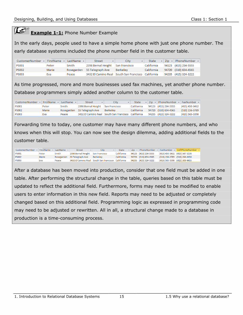
Example 1-1: Phone Number Example
In the early days, people used to have a simple home phone with just one phone number. The
early database systems included the phone number field in the customer table.
As time progressed, more and more businesses used fax machines, yet another phone number.
Database programmers simply added another column to the customer table.
Forwarding time to today, one customer may have many different phone numbers, and who
knows when this will stop. You can now see the design dilemma, adding additional fields to the
customer table.
After a database has been moved into production, consider that one field must be added in one
table. After performing the structural change in the table, queries based on this table must be
updated to reflect the additional field. Furthermore, forms may need to be modified to enable
users to enter information in this new field. Reports may need to be adjusted or completely
changed based on this additional field. Programming logic as expressed in programming code
may need to be adjusted or rewritten. All in all, a structural change made to a database in
production is a time-consuming process.

Designing, Building, and Using Databases Class 1: Section 1
2. Data Normalization and Integrity Rules 16 2.1 Data Collection
2. Data Normalization and Integrity Rules
Normalization is the process of efficiently organizing data in a database. There are two goals of
the normalization process: eliminating redundant data (for example, storing the same data in
more than one table) and ensuring data dependencies make sense (only storing related data in a
table). Both of these are worthy goals as they reduce the amount of space a database consumes
and ensure that data is logically stored. This will make the database more flexible by eliminating
redundancy and inconsistent dependency.
We will explore the data normalization process using an invoice example. If you design a new
database system or redesign an existing system you want to make sure to follow the same steps
as outlined in the next sub chapters.
2.1 Data Collection
The ideal approach to gathering information about data is to solicit input from all users,
administrators, and management staff of the database system, such as data entry personnel,
managers, clerical personnel, sales personnel, computer operators, database administrators, etc.
There are several methods to conduct an efficient data collection process: collecting data via
questionnaires, interviews, observations, and collection of input forms, output reports,
procedures, and if exist, functional and technical documentation of the current system.
Input is needed from the users by talking to users, collecting current data entry forms and data
output reports, observing the workflow within an organization or a department, attending
business meetings.
Input is also needed from the management of the organization to determine how much
resources are available, what are the short and long term needs, etc.
Last but not least input is needed from the technical side with respect to database software,
network architecture, security, etc.
Also make sure to ask the right questions, many times the members involved do not voluntarily
provide you with the information since they cannot anticipate what information you want. This
process requires specific skills, the so-called system and business analysis skills.

Designing, Building, and Using Databases Class 1: Section 1
2. Data Normalization and Integrity Rules 17 2.2 Intuitive Database Design
2.2 Intuitive Database Design
After the data is collected, it is also important to note that understanding the data is crucial in
achieving a well-designed database. Understanding the data means each of the following:
➢ Data source (where it comes from)
➢ When it can be deleted
➢ How it interacts with other data
➢ Its contribution to the generation of information (Data → Information)
➢ The processes and transactions in which it is utilized
Once all data has been collected and an understanding of the data is attained, the data needs to
be organized to form a preliminary design. The first step involved in this process is to identify
the main database tables. This step is also called intuitive database design method.
The database designer needs to scan through the data, reviewing each individual item and
create a subject class for that item. Basically, this step is like categorizing the data into groups
or subjects. These groups or subjects may eventually form a database table, also called an
“Entity Class”.
Each individual data item is placed into these entities, they may become the fields of the table,
or also called “Attributes”. The fields in a table should relate to the subject of the table.
For example, let us take a look at a simple invoice ( Figure 11 ). By inspecting the individual
data items on the invoice, the following main subjects can be derived:
➢ Customer (who orders products)
➢ Products/Services (ordered by the customer)
➢ Company (which sells the products)
That means, intuitively, there are three database tables for an invoice database system.

Designing, Building, and Using Databases Class 1: Section 1
2. Data Normalization and Integrity Rules 18 2.2 Intuitive Database Design
Figure 11: Sample Invoice
Note: Later we will see that there are more tables necessary due to data normalization.
The database design process transforms user-perceived objects (like an invoice) into conceptual
database objects (like Customer, Products, Company tables) and ultimately into physical
database objects (MS Access tables and indexes).
Note: The way in which users need to view data often differs substantially from how the data
are organized and stored in the database. A designer needs to view the data from the user’s
perspective as well as from the database’s physical representation.

Designing, Building, and Using Databases Class 1: Section 1
2. Data Normalization and Integrity Rules 19 2.3 The Relational Model
2.3 The Relational Model
The relational model is based on mathematical principles and they were first applied to data
modeling by Dr. E.F. Codd. His publication in 1970 was a milestone for relational database
design methods. The relational model defines the way data can be represented (data structure),
the way data can be protected (data integrity), and the operations that can be performed on
data (data manipulation).
Let us first define some common terms for relational database design. When you design
databases and establish a conceptual model (logical), you use specific terms for objects such as
tables, fields, etc. that are different from the names of the actual database objects (physical).
This is to ensure that a logical table may translate, for example, into two physical tables in the
database due to software, security, or performance constraints. Table 1 shows the common
names for objects in the logical and physical world.
Logical Term Physical Term
Relation Table
Unique Identifier Primary Key
Attribute Column/Field
Tuple Row
Table 1: Logical and Physical Database Terms
In mathematical set theory, a relation is defined as a table of columns (attributes) and rows
(tuples).The definition specifies what will be contained in each column of the table, but it does
not include data. When you include rows of data, you have an instance of a relation.
This definition looks like a flat file or a spreadsheet. However, because it has its underpinnings in
mathematical set theory, a relation has some very specific characteristics that distinguish it from
other rectangular ways of looking at data.

Designing, Building, and Using Databases Class 1: Section 1
2. Data Normalization and Integrity Rules 20 2.3 The Relational Model
Column Characteristics
A column in a relation has the following properties:
➢ A name that is unique within the table. Within one database (schema) two or more tables
may have the same column name, however, to refer to such columns you must use the
fully qualified syntax, such as table_name.column_name.
➢ The values in a column are drawn from one and only one domain. As a result, relations
are said to be column homogenous.
➢ Columns are subject to domain constraints. Besides the data type (such as integer or
Date/Time, for example), other domain rules may be created for particular columns.
Row Characteristics
A row in a relation has the following properties:
➢ Only one value at the intersection of a column and a row. A relation does not allow
multivalued attributes.
➢ There are no duplicate rows in a relation (Uniqueness).
➢ Rows in a relation are unordered. Depending on the DBMS product, rows may be sorted
when viewing table data, but this is an implementation of the specific database platform.
➢ A primary key is a column or combination of columns that uniquely identifies each row. As
long as you have unique primary keys, you will ensure that you have also unique rows.

Designing, Building, and Using Databases Class 1: Section 1
2. Data Normalization and Integrity Rules 21 2.4 Normalization Process
2.4 Normalization Process
After completing the intuitive database design, the next task is to place the data items into the
tables. Furthermore, a closer look at each individual data item is necessary to adhere to the
relational database rules.
FifthNormal
Form
Fourth Normal Form
Boyce-Codd Normal Form
Third Normal Form
Second Normal Form
First Normal Form
Figure 12: Normal Forms of a Relation
The theoretical rules that the design of a relation must meet are known as normal forms. Each
normal form represents an increasingly stringent set of rules. Theoretically, the higher the
normal form, the better the design of the relation. There are basically six nested, normal forms,
as shown in Figure 12. In most cases, if you place your relation in third normal form, then you
will have avoided most of the common problems in relational database design.
Applying the normal forms on a relation is called data normalization. The main goal of
Normalization is to organize data in a consistent manner. For the scope of this class, the first
three normalization rules are discussed here.

Designing, Building, and Using Databases Class 1: Section 1
2. Data Normalization and Integrity Rules 22 2.4 Normalization Process
Each of these normal forms represents a specific rule. When a normal form is applied to a table,
the table is said to be in that normal form. At the beginning of the process, the tables are in a
denormalized state.
Example 1-2: Applying the first normal form
A table in a denormalized state is examined and consequently altered to comply with the first
normal form. The table is now in its first normal form.
Note: In the real world, adhering to all relational database rules is simply impossible.
Whenever normalization rules are compromised, the table is said to be denormalized. It is
important to realize that knowingly breaking the rules is very common, as long you understand
why you are breaking the rules.
Example 1-3: Denormalize a Customer Table
Accessing the total order volume for a given customer is performed by scanning the orders
table, and summing up the total amount for each line item of all orders for that specific
customer. This can be a lengthy and time consuming process. Running a process (for example
overnight) and calculating the total order volume for each customer and storing it in the
customer table is an example of denormalizing the customer table.

Designing, Building, and Using Databases Class 1: Section 1
2. Data Normalization and Integrity Rules 23 2.5 First Normal Form (1NF)
2.5 First Normal Form (1NF)
Below is the original definition of the first normal form:
1NF: A relation is in first normal form if the domain of each attribute contains only atomic
values, and the value of each attribute contains only a single value from that domain.
As you can see, the first normal form is a two part rule. Let us first address the first part, the
atomic value.
Atomic Value
We need to first define what a domain is. A domain is the set of all possible values that an
attribute may validly contain. Domains are often confused with data type. A data type is a
physical concept, whereas a domain is a logical one. Furthermore, a domain is a subset of all
possible values that a specific data type allows. For example, if you define a column named age
as an Integer (all whole numbers, negative and positive ones) data type, the domain of values
for age is 0 through 120 (or whatever you deem possible for the maximum age of a person).
The concept of atomic value means that a value cannot be sub-divided any further. The rule is to
store data in its smallest logical part, that is breaking the data into small pieces so that each
piece still contains logical information. For example, the following Zip Code: 94122-1233 should
be divided into Zip = 94122 and Zip+4=1233. Breaking down the Zip field into five individual
numbers 9,4,1,2,2 would not make sense and each individual number is not a logical piece of
the entire Zip Code field.
Note: In the above example of Zip Code each individual number represents a zone. But the
individual numbers make only sense in the context of all numbers. For example, the zone 2 in
zip code 94122 is a zone in the San Francisco Bay Area, whereas zone 2 in zip code 10022 is a
zone in New York City.

Designing, Building, and Using Databases Class 1: Section 1
2. Data Normalization and Integrity Rules 24 2.5 First Normal Form (1NF)
Single Value
The single value issue addresses the second part of the first normal form. This is a bit more
complex, so take a look at a customer record in Figure 13.
Figure 13: Multiple Values
The field named CommNumbers could contain a telephone number, a fax number, a pager
number, etc. It would be very difficult to extract only phone numbers for all customers, to find
out which customer has a fax number, and so on.
Note: A simple way to identify possible, multiple occurrences of data in one field is to look at
the field name. If the field name is in plural form (like CommNumbers as above), it is likely that
multiple data is stored in that field.
One way of solving this problem is to create individual fields for each of the communication
numbers, such as Phone, Fax, Pager, etc. This is also called a horizontal design. This design
basically works as long as there are no new communication devices invented. Note that part of
the data (PH, FA, PA) became metadata, that is the field name.
Figure 14: Repeating Groups, Horizontal Design
What if a customer now has a cellular phone? Where is the cellular number going to be stored? A
new field has to be added to store the new number, but this design change propagates
throughout the entire database, meaning queries, forms, reports, and code must be modified to
accommodate the new field. This is a very cumbersome and tedious process (see Example 1-1).
Instead of having multiple instances of data in one field, we have now repeating groups of data
in separate fields. Data of the same kind, or better yet belonging to the same domain, should be
stored in one field. In this example we are storing a number (Phone, Fax, and Pager) in different
fields. This number is used to uniquely identify a target device (Phone, Fax, and Pager) with the
telecommunication network. For that reason, this number should be stored in one field.

Designing, Building, and Using Databases Class 1: Section 1
2. Data Normalization and Integrity Rules 25 2.5 First Normal Form (1NF)
Consequently, a better way is to design the table vertically (vertical design). For this example
that means to create two fields, one for the Phone Number and one for the Device Type. Now if
there is a customer with a new device and number, simply adding a new record vertically does
not cause any further changes in the database design. However, this process creates the
unwanted redundancy of customer information.
Figure 15: Repeating Groups, Vertical Design
Now we have repeating groups of data vertically, in this case the customer information, due to
multiple communication numbers for one customer. This creates redundancy on the customer
side, we are now back to our initial flat file or spreadsheet problem.
When you encounter repeating groups of data in one entity, move the repeating groups along
with the unique identifier into a new table. Figure 16 shows the new table design for multiple
communication devices belonging to one customer.
Customer Table
Communication Table
Figure 16: Remove Repeating Groups
The customer table is now in its first normal form, that is, it contains no repeating groups
horizontally or vertically nor does it contain multi-valued data.

Designing, Building, and Using Databases Class 1: Section 1
2. Data Normalization and Integrity Rules 26 2.6 Primary Key (Entity Integrity)
2.6 Primary Key (Entity Integrity)
Why do we need a primary key? You may be used to spreadsheets or small databases where you
can interact with the data through a graphical user interface, scroll to the row of data you are
interested in and perform some data changes. However, when dealing with large, enterprise
scale databases, you cannot scroll through millions of rows of data. You use a data retrieval and
update language called SQL (Structured Query Language) to make changes to the data in your
database. For this reason, you need to be able to identify a single row to update or even delete.
As far as a relational database is concerned, you only need three pieces of information to
retrieve any specific bit of data: the name of the table, the name of the column, and the primary
key of the row. In order to uniquely identify a record, either one field or a combination of fields
must be unique. This set of one or more fields is called primary key.
Note: It is important to understand that simply inspecting data in a table and determining a
primary key field(s) based on existing data does not always yield a correct primary key. Not only
existing data, but any possible occurrence of data at all times must be considered to ensure
uniqueness.
A primary key can be composed of a single field (simple key) or a combination of fields
(composite key) which uniquely identifies a record in a table. A primary key cannot contain a
null value.
Example 1-4: Primary Key
To uniquely identify citizens eligible to vote in an election, the combination of last name, street
address, and date of birth was chosen as primary key based on existing data. This primary key
probably is unique for most households, however, consider the possibility of twin siblings living
at their parent’s home. Since the date of birth is the same (unless born around midnight) as well
as last name and street address, the primary key candidate fails for this particular situation.

Designing, Building, and Using Databases Class 1: Section 1
2. Data Normalization and Integrity Rules 27 2.6 Primary Key (Entity Integrity)
As seen in the previous example, when the number of fields composing a primary key becomes
quite large, it may be better to create an additional field to store a random, unique value to
function as a primary key. MS Access uses the AutoNumber feature to perform that task. This is
a sequence generator, which automatically creates unique numbers for a given table. This key is
called a surrogate key.
Whether to use existing data or auto-generated sequence numbers to function as a primary key
is an important one during the database design process. When considering existing data fields as
a primary key candidate, apply the following rules:
➢ A primary key should be some value that is highly unlikely ever to be null(for composite
key, any field should never be null). Also understand that the data needs to be available
at the time the record is entered in the database, and not at a later time.
➢ A primary key should never change, ever.
➢ The primary key value should be of uniform length. For example, the social security
number is a nine-digit number for everybody, and not five-digits for some and seven-
digits for others.
Another requirement for the primary key is it must be irreducible or minimal. That is a
composite key must not contain any unnecessary fields.
Example 1-5: Minimal or Irreducible Primary Key
If the primary key in the customer table were comprised of Social Security Number (SSN) and
Customer Name, the combination would still be unique. However, the Customer Name field in
the primary key is unnecessary since the SSN field is already unique.
When choosing an auto-generated sequence number as a primary key, make sure that you still
identify the logical key, meaning the field or fields that would formed the primary key. The
logical key is still used for enforcing uniqueness of the data, because the AutoNumber does not
prevent you from entering the same customer twice (it generates automatically two different
numbers for the same customer).

Designing, Building, and Using Databases Class 1: Section 1
2. Data Normalization and Integrity Rules 28 2.6 Primary Key (Entity Integrity)
Another important concept in relational databases is the functional dependency. That is, a
specific value for one field determines the value or values for one or more other fields in the
same table. Most notably, this concept becomes clear in discussion with the primary key and its
uniqueness. For a specific value of the primary key, say X, the value of another field in the same
table is determined, say Y. X ->Y, which reads X functionally determines Y.
Social Security Number
Name
City
Address
Figure 17: Functional Dependencies
In the Figure 17, SSN (=X) functionally determines Name, City and Address (=Y).

Designing, Building, and Using Databases Class 1: Section 1
2. Data Normalization and Integrity Rules 29 2.7 Second Normal Form (2NF)
2.7 Second Normal Form (2NF)
Below is the original definition of the second normal form:
A relation is in 2NF if and only if it is in 1NF and no non prime attribute is dependent on any
proper subset of any candidate key of the table. A non prime attribute of a table is an attribute
that is not a part of any candidate key of the table.
The second normal form goes back to the issue that all fields in a table should relate to the
subject of the table. Here it is formulated in a stricter way. By selecting a primary key value in a
table and navigating to a specific record, all fields in that record must be fully dependent on that
primary key value.
Specifically, this rule only applies to tables having a composite primary key, meaning a primary
key comprised of more than one field. All non-primary key fields (non prime) must fully depend
on the entire primary key, and not on part of the primary key. To perform the full dependency
test, vary each field of the primary key and determine whether the non-key fields are
functionally dependent on this key field. Only if all non-key fields are functionally dependent on
all fields of the primary key, the table is said to be in second normal form.
Note: A table with a simple primary key (one field primary key) is automatically in second
normal form due to the primary key definition as discussed in the previous chapter. Consider a
field which does not depend on a simple primary key. That means for one specific value of the
primary key multiple different values for that field may exist. Consequently, there are multiple
records with the same primary key but different values for that field. This is a clear violation of
the primary key rules that it must be unique within one table.
Back to invoice example where we intuitively created three tables (customer, company,
products). The communication table was initially derived from the customer table to be
compliant with the first normal form. To test for second normal form, we have to first set the
primary key. This is a good example that choosing a primary key is also a business decision, as
it imposes constraints on the data.

Designing, Building, and Using Databases Class 1: Section 1
2. Data Normalization and Integrity Rules 30 2.7 Second Normal Form (2NF)
For example, if we select the CustomerNumber and the DeviceID as the primary key, what are
the consequences of this choice? Setting the primary key on CustomerNumber and DeviceID
allows for one device per customer only, such as one phone (land line), one fax, and one pager.
If this constraint is too restrictive, then you have to choose another primary key. Figure 18
shows this particular primary key.
Primary Key Fields Non-Primary Key Fields
Figure 18: Testing 2NF
Now we apply the second normal form and test the functional dependencies of the non-key fields
(here Number and Device) on the composite primary key (here CustomerNumber and
DeviceID):
Number field: Does the Number field functionally depend on the combination of
CustomerNumber and DeviceID? Yes, it does, because :
➢ For the same customer (same CustomerNumber) there are different number values for
different DeviceID values.
➢ For the same DeviceID there are different number values for different customers.
Using only the CustomerNumber does not functionally determine a specific Number, and using
the DeviceID does not functionally determine a specific Number value.
CustomerNumber
NumberDeviceID
Figure 19: Full-Functional Dependency
Device Field: Does the Device field functionally depend on the combination of CustomerNumber
and DeviceID? No, it does not, because:
➢ For the same customer (same CustomerNumber) ) there are different Device values for
different DeviceID values.
➢ For the same DeviceID there are not different Device values for different customers.

Designing, Building, and Using Databases Class 1: Section 1
2. Data Normalization and Integrity Rules 31 2.7 Second Normal Form (2NF)
Here we see that the Device field only depends on the DeviceID part of the primary key, but not
on the CustomerNumber. This partial dependency violates the second normal form.
CustomerNumber
DeviceDeviceID
Figure 20: Partial Dependency
Consequently, the Device field (including DeviceID) must be moved to a new table. The
communication table in second normal form is shown in Figure 21.
Figure 21: Second Normal Form

Designing, Building, and Using Databases Class 1: Section 1
2. Data Normalization and Integrity Rules 32 2.8 Third Normal Form (3NF)
2.8 Third Normal Form (3NF)
Below is the original definition of the third normal form:
A relation is in 3NF if and only if it is in second normal form(2NF) and every non-prime attribute
is non-transitively dependent (i.e. directly dependent) on the primary key.
This rule is a bit confusing, and it is expressed in a negative way. In other words, all non-key
fields must depend on the primary key only, meaning no other dependencies are allowed. This
normal form is about removing transitive dependencies, meaning dependencies among non-key
fields.
A memorable statement of Codd's definition of 3NF, paralleling the traditional pledge to give true
evidence in a court of law, was given by Bill Kent: "Every non-key attribute must provide a fact
about the key, the whole key, and nothing but the key." A common variation supplements this
definition with the oath: "so help me Codd".
Let us take a look at a common example. In Figure 22 the customer table is shown again with a
slight variation, we have included the state abbreviation in this table.
Figure 22: Customer Table in 2NF
Note: Storing derived or calculated data also violates 3NF as there is a dependency between
the source data and the derived/calculated data. For example, storing an order total would mean
every time there is a change affecting the price in one or more of the line items of an order, the
order total would change accordingly.

Designing, Building, and Using Databases Class 1: Section 1
2. Data Normalization and Integrity Rules 33 2.8 Third Normal Form (3NF)
By now you probably notice that there is a functional dependency between StateCode and State,
very much like in the example of the 2NF. The only difference is that this is a dependency
among non-key fields. This is violating the 3NF, and we need to move the State field along with
a copy of the StateCode field (to link it back to the customer table) into a new table as shown in
Figure 23.
Figure 23: Customer Table in 3NF

Designing, Building, and Using Databases Class 1: Section 1
2. Data Normalization and Integrity Rules 34 2.9 Determining Relationships (Referential Integrity)
2.9 Determining Relationships (Referential Integrity)
After normalizing the data and creating additional tables due to the normalization process, the
next step is to link the tables together. During this step, additional data problems may be
encountered which leads to the creation of additional tables.
First of all, it is important to understand that relational databases can only utilize the table
object to describe real-world business processes. We have seen in the previous chapter that one
function of a table is to categorize data based on subjects. This chapter now introduces another
function of a table, that is to implement relationships between tables. Furthermore, depending
on the kind of relationship, additional tables may need to be created. These tables are not
“subject” tables, they are relationship tables to model a specific relationship.
Tables engaged in a relationship are called participants of a relationship. Depending on the
number of participants, the so-called degree of a relationship, there are binary (two tables) and
ternary (three tables) relationships. Sometimes, another degree exists, the unary degree (one
table), that is a table is related to itself. The most common degree is the binary relationship.
Note: Relational databases are not named after the term relationships, but after the term
relation. A relation is the formal word for a table. It contains related data, data based on a
subject.
Relationships are also classified by how many records in one table are associated with how many
records in the other table of the relationship. For example, let us look at the customer –
communication relationship. One customer record may have zero, one, or many records in the
communication table. This property of a relationship is called cardinality, and there are three
main categories as listed below:
➢ One-To-Many
➢ One-To-One
➢ Many-To-Many
Following is a detailed explanation of these three relationships.
One-To-Many Relationship
The One-To-Many is the most common relationship. One record in table A can have zero, one or
more matching record in table B, but one record in table B has at most one matching record in
table A.

Designing, Building, and Using Databases Class 1: Section 1
2. Data Normalization and Integrity Rules 35 2.9 Determining Relationships (Referential Integrity)
The Cardinality is an important property of the relationship. In Figure 24, the one-to-many
relationship between the customer table and the communication table is shown. You also see the
minimum and maximum cardinalities. For example, one customer may have zero to many
communication numbers, whereas one communication number is related to at least and at most
one customer.
CommNumbers
CustomerNumber (FK,IE1)DeviceID
Number
Customer
CustomerNumber
FirstName LastName City StateCode
Minimum Cardinality
Maximum Cardinality
Figure 24: One-to-Many Relationship
Example 1-6: Optionality of a Relationship
Must a customer record in the customer table have a telephone number (or fax number or any
other communication number) or is it optional? This is an important fact about the database and
it needs to be clearly determined during the information gathering process.
The optionality is mostly found in the many side, but it can be also in the one side. For example,
customers are assigned customer service representatives (CSR).
Example 1-7: Optionality of a Relationship in the one side
One customer may have zero or one CSR, and one CSR is assigned to zero, one, or many
customers. When adding a new customer to the database, a CSR is not assigned right away to
that new customer, a CSR is assigned once an order is placed. This is part of the business rule
for that company. That means, the one side, the CSR table is optional for a customer (the many
side).

Designing, Building, and Using Databases Class 1: Section 1
2. Data Normalization and Integrity Rules 36 2.9 Determining Relationships (Referential Integrity)
To implement a relationship in the database, the primary key field of the one side is also placed
in the many side table. In the many side table, it is called the foreign key. The primary key and
foreign key are used to link matching records together.
MS Access allows for a different field names to link primary key and foreign key. For example, in
the customer table the primary key is named CustomerNumber, and in the communications
table the foreign key is named CustID. Still, both fields hold the same value, the
CustomerNumber of a customer.
During the normalization process of the order example, we identified the Customer table, the
CommNumbers table, the Device table, and the States table.
Device
DeviceID(PK)
Device
State
StateCode(PK)
State
Customer
CustomerNumber(PK)
FirstName LastName City StateCode (FK)
CommNumbers
CustomerNumber (FK)DeviceID (FK)
Number
Figure 25: ERD Diagram for Invoice Example
The relationships are as follows:
One Customer may have one or many communication numbers. One communication record
belongs to one and only one customer.
One customer lives in one and only one state, and one state belongs to zero, one, or many
customers.
One device belongs to zero, one or many communication numbers, and one communication
number belongs to one and only one device.
In order to determine a One-To-Many relationship correctly, one must asked the relationship
question in both ways (round trip) as shown above. This is very important in order to detect
possible other relationships, such as One-To-One or Many-To-Many relationships.

Designing, Building, and Using Databases Class 1: Section 1
2. Data Normalization and Integrity Rules 37 2.9 Determining Relationships (Referential Integrity)
Note: The CommNumber table is a special one in that the primary key consists of
CustomerNumber and DeviceID together, however, CustomerNumber as well as DeviceID serve
individually as foreign keys too.
Many-To-Many Relationships
A record in table A can have more than one matching record in table B, and a record in table B
can have more than one matching record in table A.
If such a relationship is encountered, the database design must be amended and additional
tables created.
In our invoice example we have already intuitively determined that there must be a product
entity. And these products must have been ordered, otherwise we would not have an invoice.
Hence we also have an Order entity, this is an entity based on an event rather than a tangible
object.
Order
OrderID CustomerNumber OrderDate ShipMethod
Product
ProductID ProductName Price
Figure 26: Order and Product Tables
We know that there must be relation between the Order table and the Product table. Let us
follow the procedures and ask the relationship questions:
One order contains one or many products (Order table). One product is contained on zero, one,
ore many orders (Product table).
Warning: As mentioned earlier it is absolutely important to establish a relationship from
both participants when determining relationships. That is one record in table Products can have
how many records in table Orders? If we had stopped the process here, it would have been a
one-to-many relationship. But when we ask the other around, that is one record in table Orders
can have how many records in table Products, we found out that this is a true many-to-many
relationship.

Designing, Building, and Using Databases Class 1: Section 1
2. Data Normalization and Integrity Rules 38 2.9 Determining Relationships (Referential Integrity)
This type of relationship cannot be modeled in a relational database using primary and foreign
keys. The following example will demonstrate that.
To link the tables, the primary key must be placed into the other table as a foreign key. Below
the ProductID (primary key of table Product) is placed into the table Order. Because one order
can contain many products, the order information is repeated over and over, that is redundancy.
Furthermore, OrderID cannot be the primary key anymore because it is not unique.
Figure 27: ProductID as Foreign Key in Order Table
Trying to place the OrderID (primary key of table Order) into the product table produces the
same result. Product records are repeated due to the fact that one product can be contained on
many orders, which in turn creates redundancy. Also, ProductID cannot be the primary key in
the table Product.
Figure 28: OrderID as Foreign Key in Table Product
By placing the primary key from one table into the other table as a foreign key, these tables
become denormalized. For example, in Figure 28 the ProductID and the OrderID together could
serve as a primary key. However, the second normal form is violated because Product Name and
Price are functionally dependent only on Product ID, and not on Order ID.
Obviously, the OrderID must be moved to a different table. To link the new table with the
Product table, the Product ID must be placed into the new table as a foreign key.
The new table only contains the ProductID and the Order ID. Together both fields serve as
primary key, individually they are foreign keys to their respective one-side table.

Designing, Building, and Using Databases Class 1: Section 1
2. Data Normalization and Integrity Rules 39 2.9 Determining Relationships (Referential Integrity)
This new table is called intersection or junction table. The general rule is that both primary keys
from the two participating tables are placed into the intersection table as foreign keys.
Basically, one Many-To-Many relationship is broken down into two One-To-Many relationships.
The new table can be named after both original tables (such as Order/Product) or, if applicable,
named after what it represents in the data model, such as Order Detail table.
Based on the previous example, the intersection table is shown below:
Figure 29: Intersection Table Order Details
Both primary keys serve individually as foreign keys in the junction table, but together they
serve as primary key. The combination of OrderID and ProductID is always unique, because on
one specific order the same product is not ordered twice and one specific product is not
contained more than once on an order. If the same customer decides to order the same product
again, even on the same day, a new OrderID is assigned.
Note: The intersection table does not represent a subject, such as Customer, Order, or
Product. It models a many-to-many relationship through the means of a table, the only object
relational databases have.

Designing, Building, and Using Databases Class 1: Section 1
2. Data Normalization and Integrity Rules 40 2.9 Determining Relationships (Referential Integrity)
One-To-One Relationships
One record in table A can have no more than one record in table B and one record in table B can
have no more than one in table A.
A One-To-One relationship is fairly unusual in a relational database, however, there are valid
reasons for it in specific cases.
When you encounter a One-To-One relationship, why not combine both tables into one table.
The problem of redundancy will not surface because of one-to-one. Verify that none of the
normalization rules are violated due to the combination of both tables.
Note: So far the normalization process created many new tables, which could lead to the
general impression the more tables the better. That is not true, you should try not to create too
many tables as it increases the complexity of a database system and therefore decreases the
performance.
Listed below are some common situations for a one-to-one relationship:
• Limitations due to the number of fields per table. For example, a table in MS Access can
have up to 255 fields. That seems sufficient for most cases, but for situations where more fields
are needed for one table, the table must be divided into two tables and linked through a one-to-
one relationship.
• One or more fields are not populated for most records in a table. For example, a student
table may contain mostly domestic students and some international students. For international
students, additional fields are needed such as Visa status, immigration entry data, etc. These
fields do not apply to US Citizens or residents, they would be all blank. Move fields attributable
to international students to a new table and link the student table and the new table with a one-
to-one relationship.
• Table Subclassing: For certain tables, groups of records have different properties and
therefore need different fields than other groups of records in the same table. For example,
consider a table named Automobiles. This table obviously stores information about cars.
Depending of the type of car, whether it is sedan, van, pickup truck, bus, etc. additional fields
are necessary for each type of car. These additional fields are different for each type of car. To
accommodate these additional fields, create new tables for each type of car, include car specific

Designing, Building, and Using Databases Class 1: Section 1
2. Data Normalization and Integrity Rules 41 2.9 Determining Relationships (Referential Integrity)
fields in these tables, then link all these sub tables to the main table car (also called supertype)
with a one-to-one relationship.
Example 1-8: Validity of a One-To-One relationship
Suppose a big company with 100,000 employees worldwide. The branch office in San Francisco
employs 100 employees (0.1% of all employees). The San Francisco office decided to host a
fundraising event in form of a Ping-Pong tournament. Employees of the branch office may
volunteer to play Ping-Pong for a good cause.
To better plan the event, the office needs to track some additional information of the volunteer
Ping-Pong players, such as their Ping-Pong level (Beginner, Intermediate, and Advanced).
To store this information, the original table of the company must be altered to accommodate
additional fields, something the DBA(database administrator) is very reluctant to do. Remember
what we said earlier in the chapter, any structural change in a database system requires you
validate the entire application to ensure that no existing features of the application are broken.
Now assume that only 10 employees feel confident enough to play Ping-Pong (0.01% of all
employees worldwide). The issue here is that for only ten records in a table of 100,000 records
additional information is needed to track, for all other employees these additional fields would be
blank. What a waste of storage capacity.
Main Employees Table(100,000 records, 200 fields)
Additional Ping-Pong
related information(10 records,
5 fields)

Designing, Building, and Using Databases Class 1: Section 1
2. Data Normalization and Integrity Rules 42 2.9 Determining Relationships (Referential Integrity)
Example 1-8 (continued): Validity of a One-To-One relationship
Therefore, it is much easier and more efficient to create an additional table, which holds 10
records and tracks the additional information for the Ping-Pong event. The employeeID is carried
over into this table to link the main employee table with the Ping-Pong table. The DBA is also
much happier because adding a new table to an existing system is less likely to break any of the
existing database application.
Main Employees Table(100,000 records, 200 fields)
Additional Ping-Pong related information(10 records, 5 fields)
1 1
Furthermore, once the event is over, the information is no longer needed. Again, it is much
simpler to drop an entire table with its data than to touch the original employees table.
Below is a summary of the database design process as discussed so far:
➢ The information collection process.
➢ The intuitive database design.
➢ First Normal Form (Elimination of Repeating Groups).
➢ Primary Keys (Entity Integrity)
➢ Second Normal Form (Elimination of Partial Dependencies).
➢ Third Normal Form (Elimination of Transitive Dependencies).
➢ Create relationships and thereby identify foreign keys (Referential Integrity).
➢ During this process, additional tables need to be created. This is the modeling step, after
that the physical implementation process follows where tables, primary keys, index, and
foreign keys are set up in the database.

Designing, Building, and Using Databases Class 1: Section 2
3. Introduction to Microsoft Access 43 3.1 Microsoft Access Backstage View
CLASS 1: SECTION 2
3. Introduction to Microsoft Access
Microsoft Access has been around since late 1992 as a pretty powerful desktop database system.
It is designed for beginners as well as for developers to build versatile, multi-user information
system applications.
The Microsoft Access version history is shown below:
1992 20171993 1994 1995 1996 1997 1998 1999 2000 2001 2002 2003 2004 2005 2006 2007 2008 2009 2010 2011 2012 2013 2014 2015 2016
Nov 92
1.0 (1.0)
May 1993
1.1(1.1)Apr 94
2.0 (2)
Aug 95
95 (7)
Jan 97
97 (8)
Jun 99
2000 (9)
May 01
2002 (10)
Nov 03
2003 (11)
Jan 07
2007 (12)
Jul 10
2010 (14) Jan 13
2013 (15)
Version 13 was skipped of fear of number 13.
Versions 3,4,5,and 6 were skipped due to synchronizing version numbers between Word and Office.
Oct 15
2016 (16)
Figure 30: Microsoft Access Version History
3.1 Microsoft Access Backstage View
Microsoft Access belongs to the MS Office family, therefore, the interface looks very familiar at
first. Because of its distinct features, however, there are some differences to point out. When
you start MS Access 2013, the introductory page is displayed as shown in Figure 31.
At this point, the user may start a new, blank database or open an existing database. In
addition, the user may choose to use the Access templates to create basic databases based on
common business models.
The start screen has become very busy in Access 2013. It is now called Backstage view, which I
think is similar to the Office button in version 2007 or to the old File menu in prior versions of
Access.

Designing, Building, and Using Databases Class 1: Section 2
3. Introduction to Microsoft Access 44 3.1 Microsoft Access Backstage View
Navigation Bar
Back Command
Backstage Tabs
Figure 31: Microsoft Access 2013 Start Screen
The navigation bar on the left side drives what you see in the rest of the screen. It contains the
Backstage tabs such as Info, New, Open, Save, Save As, etc.. The Back command allows you to
exit the Backstage view and return to the MS Access application.

Designing, Building, and Using Databases Class 1: Section 2
3. Introduction to Microsoft Access 45 3.1 Microsoft Access Backstage View
Backstage Tabs
The Backstage tabs in the navigation bar contain the following commands:
Info: This tab lists the database name and path and a few specific database operations, such as
database properties, compact & repair, and encrypting with password.
New: This is always the tab that is shown when you open Microsoft Access. In the center of this
tab you have multiple options to create a new database. You can create a new, blank database
(client) or a blank web database. Or you can choose from the recently used templates or browse
through all templates. Once you select an option, a pop up window is displayed to choose the
filename and location. Then you would click the big Create button at the bottom of the pop up
window.
Open: Open any existing database file on your computer or network.
Warning: Keep in mind that only one database can be opened at any given time, unlike in
other Office applications where one can open up to 9 documents.
Save: Save design changes for the database object that is open and has the focus in the
Navigation pane.
Save As: Save a copy of the current open object that has the focus or the object that has the
focus in the Navigation pane or save a copy of the current database. Note that if you click this
command, Access closes the database that is currently open so that it can create the copy. Also
you can save your database as a template, package and sign (advanced feature), or deploy your
web database onto SharePoint.
Print: There are three options, Quick Print, Print, and Print Preview. The Quick Print option
sends the currently selected object in the Navigation pane directly to the printer. Selecting Print
opens the print dialog box. Print Preview allows you view first what you are about to print.
Close: Close the currently open database and return to the MS Access application.
Account: This is new in Access 2013. Here you can sign into the online Office account to
manage documents online. It also contains the About command.
Options: Displays the Option dialog box as shown in Figure 32.

Designing, Building, and Using Databases Class 1: Section 2
3. Introduction to Microsoft Access 46 3.1 Microsoft Access Backstage View
Figure 32: Microsoft Access Options Dialog

Designing, Building, and Using Databases Class 1: Section 2
3. Introduction to Microsoft Access 47 3.2 Quick Access Toolbar & Office Fluent Ribbon
3.2 Quick Access Toolbar & Office Fluent Ribbon
The new menu interface called Ribbons was introduced with Office 2007. In Figure 33 you see
the Quick Access toolbar in the top right corner and the Access Ribbon.
Quick Access ToolbarCustomization
Options
Office Fluent Ribbon
Figure 33: Quick Access Toolbar & Ribbon
Quick Access Toolbar
The Quick Access toolbar contains by default three buttons, Save, Undo and Redo. You can
customize this toolbar by clicking on the down arrow on the right side and add any valid
command that is otherwise available through the Access interface. When you click on the drop-
down arrow, you will have immediate options that you can select. Furthermore, you can select
More Commands and the Quick Access Toolbar customization in the Access Options dialog box is
displayed as shown in Figure 34.

Designing, Building, and Using Databases Class 1: Section 2
3. Introduction to Microsoft Access 48 3.2 Quick Access Toolbar & Office Fluent Ribbon
Figure 34: Quick Access Toolbar Customization
The Office Fluent Ribbon
The Office Fluent Ribbon is a strip that contains all the functionality of the older menu bar
options and the various toolbars from older versions of Office before version 2007.
The ribbon is a context-rich environment displaying all the program functions and commands
with large icons for key functions and smaller icons for less-used functions. The ribbon contains
a host of various controls such as lists, command buttons, galleries and dialog box launchers.
The ribbon in MS Access consists of four main tabs – Home, Create, External Data, and Database
Tools – that group together common tasks and contain a major subset of the program functions
in Access.

Designing, Building, and Using Databases Class 1: Section 2
3. Introduction to Microsoft Access 49 3.2 Quick Access Toolbar & Office Fluent Ribbon
These main tabs are visible at all times when you are working in Access because they contain
the most common tools you need when working with any database object. Other tabs, called
contextual tabs, appear and disappear to the right of the Database Tools tab when you are
working with specific database objects and in various views.
Contextual Tab
Figure 35: Contextual Tab
Each tab on the ribbon has commands that are further organized into groups. The name of the
group is listed at the bottom, and each group has various commands logically grouped by
subject matter.

Designing, Building, and Using Databases Class 1: Section 2
3. Introduction to Microsoft Access 50 3.3 Single vs. Multiple Document Interface
3.3 Single vs. Multiple Document Interface
In versions of Access before version 2007, all objects opened in their own windows where you
could edit, view, or print them. This type of interface, multiple-document interface (MDI) for
short, was the cornerstone for working with objects in Access. In version 2007, a new interface
was introduced, the so-called single-document interface (SDI). In the SDI model, all objects
open in a series of tabs along the top of the object window to the right of Navigation pane. In
the older MDI model, switching between open objects usually meant constantly minimizing,
resizing, and maximizing the various objects in order to work with them, as shown in Figure 36.
Multiple Document Interface
Figure 36: Multiple Document Interface (MDI)
In the SDI mode, each open object appears on a tab to the right of the Navigation Pane as
shown in Figure 37.
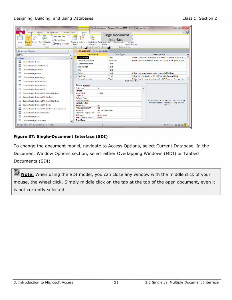
Designing, Building, and Using Databases Class 1: Section 2
3. Introduction to Microsoft Access 51 3.3 Single vs. Multiple Document Interface
Singe Document Interface
Figure 37: Single-Document Interface (SDI)
To change the document model, navigate to Access Options, select Current Database. In the
Document Window Options section, select either Overlapping Windows (MDI) or Tabbed
Documents (SDI).
Note: When using the SDI model, you can close any window with the middle click of your
mouse, the wheel click. Simply middle click on the tab at the top of the open document, even it
is not currently selected.

Designing, Building, and Using Databases Class 1: Section 2
3. Introduction to Microsoft Access 52 3.4 Client vs. Web Database
3.4 Client vs. Web Database
In Access 2010, a new type of database was born, the so-called Web Database. You might
remember that in the Start screen, under the New tab, you have the option of creating a blank
database (client database) or a web database. A web database can be published to a Windows
SharePoint © server using Access services and be accessed through a web browser. Microsoft
has tried over the years to make Access more web-accessible. In earlier versions of Access, for
example, the Data Access Pages (DAP) concept was such an attempt.
A web database contains web tables, which are different than “regular” or client tables. You do
not have all the rich features available as in client tables. For example, there is no Design View
for web tables, you have very limited features available to build a web table. Besides the special
object of a web table, a web database can contain other, “regular” client objects such as queries,
forms, reports, macros, and modules.
In this course, and in the other courses of the Access series, we will be focusing on and using
the client database concept. This will enable the student to learn more broadly about general
database and application development concepts.

Designing, Building, and Using Databases Class 1: Section 2
3. Introduction to Microsoft Access 53 3.5 Microsoft Access User Interface
3.5 Microsoft Access User Interface
Once a database is opened in Access, you have many user interfaces and process wizards that
guide your through the process of creating and maintaining Access objects, such as tables,
queries, forms, reports, macros and modules. Many of these interfaces will discussed throughout
these course when dealing with specific objects.
In Figure 38 the main Access Interface is shown with its individual sections.
Document Window
Ribbon
Navigation Pane
Backstage View
Status Bar
Quick Access Toolbar Help
Figure 38: Access Main User Interface
Besides the Quick Access toolbar and the Ribbon one of the other main tools to manage an
Access database is the Navigation Pane on the left of the application window. In older versions of

Designing, Building, and Using Databases Class 1: Section 2
3. Introduction to Microsoft Access 54 3.5 Microsoft Access User Interface
Access before 2007 this pane was embodied in the Main Database Window. This navigational tool
allows you to manage the main Access objects:
➢ Tables to store relational data
➢ Queries to select, analyze, and manipulate data
➢ Forms to implement sophisticated user interfaces to interact with the data
➢ Reports to output formatted data
➢ Macros & Modules to automate user interfaces and database processes
You can filter the navigation pane by one of these objects, or show related objects together in
groups. Furthermore, you can customize the navigation page in many different ways to display
the objects of interest. We will further explore the Navigation page at the end of this course.
Note: The objects in the navigation page appear like files, with a date created, date
modified, etc. However, all these objects are contained in one physical operating system file with
the extension accdb (or mdb), for or Access Database (Microsoft Database). The .mdb format is
the older format before Access version 2007.
The database that will be used in the course as well as the remaining courses in the Access
series uses a Pet Hospital database example named Mountain Animal Hospital. This databases
tracks customers, their pets, and the pet visits to the hospital due to illnesses and/or injuries.
You will become familiar with the data model fairly quickly in this course.

Designing, Building, and Using Databases Class 1: Section 2
3. Introduction to Microsoft Access 55 3.5 Microsoft Access User Interface
Example 2-1: Create new database
1. Open MS Access.
2. From the Backstage View page under
Available Templates, choose Blank
Desktop database.
3. A pop-up window is displayed as shown
on the right to create the file name and
select the folder. Click on the yellow folder button on the right side.
4. Navigate to C:\Temp\MS_Access.
5. Name the database PetHospital.accdb.
6. Click on OK.
7. Now finally click on Create button.
8. Close the default table1.
9. From Backstage View, navigate to Options
10. Select General in the left hand side, then under Creating Databases, set the default
folder to c:\Temp\MS_Access.
11. Now select Object Designers in the left hand side, then under Table Design View make
sure that there is no entry in
AutoIndex on Import/Create.
12. Click on OK to close the Options dialog box.

Designing, Building, and Using Databases Class 1: Section 2
4. Table Design 56 4.1 Creating a Table
4. Table Design
There are many different ways to create a table object in MS Access. For example, you could
create an entire database based on templates which would include table objects. You can also
use a new feature in Access 2010 called Application Parts, which are somewhat like database
templates, but are smaller in scope.
You can also create a table object by actually typing in data and Access builds the table
definition based on the kind of data that you enter. And another new feature in Access 2010,
called Data Type Parts, assists you with creating tables and fields.
Note: There is no more table wizard since Access version 2007.
There are actually even more ways to create a table, by using a Make-Table query or by
importing data from external sources, such as an Excel spreadsheet or an Oracle database.
These advance topics are covered in the next course.
In this course, we are going to create a table from scratch without any additional automatic or
pre-built features provided by MS Access. While this is probably the most difficult and
cumbersome way to create a table, it provides for the greatest learning benefit.
4.1 Creating a Table
To create a new table in MS Access, select the Create tab in the ribbon, then in the Tables
section, click on Table Design. By choosing Table Design from the Create tab, the user is
presented with the table design interface as shown in Figure 39. The upper pane is called Field
Entry area, the lower left part is called Field Properties area and in the lower right some basic
help information is displayed depending on your current selection in the table design window.
Field Entry area (consists of three columns):
➢ Field Name: Assign a field name, up to 64 characters long. Field names can contain blank
spaces, however, it is not recommended to do so (Required).
➢ Data Type: The type of data for the field, such as text, numbers, date/time, etc
(Required).
➢ Description: This is an optional entry for additional information about the field. It is a good
idea to document the database here at the table level (Optional).

Designing, Building, and Using Databases Class 1: Section 2
4. Table Design 57 4.1 Creating a Table
The Field Properties area:
Depending on the data type chosen for a specific field, additional properties can be set here,
such as field length, format, etc.
Basic Help Information area:
Whether you are in the Field Entry or Field Properties area, additional basic information is
displayed for the currently selected item.
Field Entry Area
Field Properties Area
Basic Help Information
Figure 39: Table Design Interface
Note: The optional description for each field is displayed in the Status bar of the application
window (up to a certain limit). Therefore, it is a good idea to provide some “mini help” for each
field such as possible formats or other rules about the data to be entered.
A table must have at least one field, without having a field, you cannot save a “blank” table.

Designing, Building, and Using Databases Class 1: Section 2
4. Table Design 58 4.1 Creating a Table
Example 2-2: Create new Table
1. Select the Create tab
in the ribbon.
2. Click on Table Design.
3. Enter the fields as shown
on the right.
4. Save the table by clicking
on the disk button in the
Quick Access toolbar.
5. Name the table
tbl_Customer.
6. Click on OK.
7. After clicking on OK you receive a
warning message as shown below.
8. This message is an alert that no fields
have been assigned as primary
key. Select No as we will create our own primary key.
9. The table tbl_Customer should now be displayed in the Navigation Pane.

Designing, Building, and Using Databases Class 1: Section 2
4. Table Design 59 4.2 Data Types
4.2 Data Types
Choosing the right data type for a field is a very important step and has implications on
database performance and functionality. A drop-down menu is provided in the table design
interface to select a data type. There are 12 different options to choose from, and they are
explained in detail below. Some of these options are actually not data types, but special features
to set up a data type.
Keep in mind that a database in general deals most of time with three main data types:
➢ Text (varchar, variable character data type)
➢ Number (various number sub types, such as Integers, fixed and floating point decimals)
➢ Date/Time
Table 2 shows the implementation of the main data types in MS Access.
Data type Usage Size
Short Text Alphanumeric characters. Use for text, or for
numbers that are not used in calculations (for
example, a product ID). A numeric value that is
stored as text can be sorted and filtered more
logically, but cannot be easily used in calculations.
Up to 255 characters.
Long Text Alphanumeric characters (longer than 255 characters
in length) or text that uses rich text formatting.
Notes, lengthy descriptions, and paragraphs that use
text formatting, such as bold or italics, are good
examples of where to use a Long Text field.
Up to 1 gigabyte of
characters, or 2 gigabytes
of storage (2 bytes per
character), of which you
can display 65,535
characters in a control. Number Numeric values (integers or fractional values). Use
for storing numbers that are used in calculations,
except for monetary values (use the Currency data
type for monetary values).
1, 2, 4, or 8 bytes, or 16
bytes when used for a
replication ID.
Date/Time Dates and times. Use for storing date/time values.
Note that each value stored includes both a date
component and a time component.
8 bytes.
Table 2: Base Data Types

Designing, Building, and Using Databases Class 1: Section 2
4. Table Design 60 4.2 Data Types
Most special data types are derived from these base data types. And there are a few other data
types for storing complex data, such as binary objects (audio, video, images, and documents).
Data type Usage Size
Currency Monetary values. Use for storing monetary
values (currency).
8 bytes.
AutoNumber A unique numeric value that Access
automatically inserts when a record is added.
Use for generating unique values that can be
used as a primary key. Note that values for
AutoNumber fields can be incremented
sequentially or by a specified value, or
assigned randomly.
4 bytes or 16 bytes when used
for replication ID.
Yes/No Boolean values (yes/no). You can use one of
three formats: Yes/No, True/False, or On/Off.
1 bit (8 bits = 1 byte).
OLE Object OLE objects or other binary data. Use for
storing OLE objects from other Microsoft
Windows programs.
Up to 1 gigabyte.
Attachment Pictures, Images, Binary files, Office files. This
is the preferred data type for storing digital
images and any type of binary file.
For compressed attachments, 2
gigabytes. For uncompressed
attachments, approximately
700kb, depending on the degree
to which the attachment can be
compressed.
Hyperlink Hyperlinks. Use for storing hyperlinks to
provide single-click access to Web pages
through a URL (Uniform Resource Locator) or
files through a name in UNC (universal naming
convention) format. You can also link to Access
objects stored in a database.
Up to 1 gigabyte of characters,
or 2 gigabytes of storage (2
bytes per character), of which
you can display 65,535
characters in a control.
Table 3: Derived & Special Data Types

Designing, Building, and Using Databases Class 1: Section 2
4. Table Design 61 4.2 Data Types
Table 3 lists the special data types in MS Access. Currency, AutoNumber, and the Yes/No data
type is based on the number base data type. The OLE Object and Attachment data type are used
for binary data. The hyperlink data type is based on the Long Text data type and is specifically
formatted to implement a file or URL link.
Table 4 shows the two feature based options in the data type column in table design.
Feature type Usage Size
Lookup Wizard Not actually a data type; instead, this starts
the Lookup Wizard. Use to start the Lookup
Wizard so that you can create a field that
uses a combo box to look up a value in
another table, query, or list of values.
Table or query based: The size of
the bound column. Value based:
The size of the Text field used to
store the value.
Calculated Allows creating an expression based on
data from one or more fields. You can
designate different result data types from
the expression.
Dependent on the data type of
the result data type property.
Text data type can have up to
243 characters, Long Text,
Number, Yes/No, and Date/Time
should match their respective
data types.
Table 4: Data Type Features

Designing, Building, and Using Databases Class 1: Section 2
4. Table Design 62 4.3 Field Properties
4.3 Field Properties
Each field has its own field properties displayed in the Field Properties area (the lower pane in
the table design interface). Field properties vary depending on the data type chosen for a
particular field. For example, a text data type has a field size property, whereas a Date/Time
field does not have a field size (the size is fixed and already determined by the kind of data). By
setting field properties one can further customize the behavior of a field such as specifying a
special format, a default value, and additional validation rules.
Table 5 shows the field properties of text, number, and date/time data types. We will discuss
most of them in this chapter, some of them are covered in more detail, such as Format.
Data Type
Field Property
Text Number Date/Time
Field Size Maximum number of
characters
Number type, such as
Integer, Single, etc.
N/A
Format Apply either predefined formats (depending on data type) or create
customized formatting expressions
Decimal Places N/A To set the maximum
number of decimal
places
N/A
Input Mask Very similar to Format, provides formatting and an input validation
mechanism.
Caption More descriptive field name that Access uses for column headings in
queries, or labels in forms and reports.
Default Value When adding a new record, prefills field with value specified.
Validation Rule Additional constraint for data domain, enforce specific rules
Validation Text Customer message displayed when violating specified validation rule.

Designing, Building, and Using Databases Class 1: Section 2
4. Table Design 63 4.3 Field Properties
Data Type
Field Property
Text Number Date/Time
Required No null value allowed if set to Yes.
Allow Zero Length No zero-length (“”) value allowed if set to Yes.
Indexed To create an index when set to yes to speed up joins and searches.
Unicode Compression Access stores characters using a double-byte (Unicode) character set to
support extended character sets in languages that require them. Access
stores compressible characters(character sets that require only 1 byte)
in 1 byte instead of 2 (if set to Yes).
IME Mode, IME
Sentence Mode
For computers with Asian version of Windows and appropriate Input
Method Editor (IME) installed, these properties control conversion of
characters in kanji, hiragana, katakana, and hangul character sets.
Smart Tags To register a specific smart tag indicating an action associated with the
field.
Text Align To align text. By default, text is left aligned, whereas number and dates
are right aligned.
Show Date Picker N/A N/A To display a calendar
control if set to yes.
Table 5: Properties of Text, Number, and Date/Times
The field size property for numbers is a very important one as it determines the specific number
type. When dealing with numbers, you have to understand the basic concepts of precision, scale
(accuracy), and significant digits.
The precision is the total number of digits of a number (excluding a possible decimal point). The
scale (accuracy) is the number of digits after the decimal point. The significant figures (also
known as significant digits, and often shortened to sig figs) of a number are those digits that
carry meaning contributing to its precision.

Designing, Building, and Using Databases Class 1: Section 2
4. Table Design 64 4.3 Field Properties
Note: Further explanation of significant digits:
Non-zero digits are always significant. Thus, 22 has two significant digits, and 22.3 has three
significant digits. With zeroes, the situation is more complicated:
a) Zeroes placed before other digits are not significant; 0.046 has two significant digits.
b) Zeroes placed between other digits are always significant; 4009 kg has four significant
digits.
c) Zeroes placed after other digits but behind a decimal point are significant; 7.90 has three
significant digits.
Zeroes at the end of a number are significant only if they are behind a decimal point as in (c).
Otherwise, it is impossible to tell if they are significant. For example, in the number 8200, it is
not clear if the zeroes are significant or not. The number of significant digits in 8200 is at least
two, but could be three or four. To avoid uncertainty, use scientific notation to place significant
zeroes behind a decimal point:
8.200 103 has four significant digits
8.20 103 has three significant digits
8.2 103 has two significant digits
There are basically three different number categories:
➢ Whole Numbers
➢ Floating-point decimals
➢ Fixed-point decimals
MS Access offers various number types in each of these categories with the difference being the
range of possible number values.
Table 6 lists the various number types available in MS Access.
Byte, Integer, and Long Integer number types are whole integers with the Long Integer being
the one covering the largest range.
The Single and Double number types are floating-point decimals.
The Decimal number type is a fixed-point decimal.

Designing, Building, and Using Databases Class 1: Section 2
4. Table Design 65 4.3 Field Properties
Number
Type
Number
Category
Range Notes Storage
Size
Byte Whole 0-255 None 1 byte
Integer Whole -32,768 to 32,767 None 2 bytes
Long Integer Whole -2,147,483,648 to
2,147,483,647
None 4 bytes
Single Floating Point -3.4 1038 to 3.4 1038 Up to 7 significant
digits
4 bytes
Double Floating Point -1.797 10308 to 1.797 10308 Up to 15 significant
digits
8 bytes
Decimal Fixed Point -7.9228 1028 to 7.9228 1028 Default Precision 18,
Default Scale 0
12 bytes
ReplicationID Whole N/A GUID 16 bytes
Table 6: MS Access Number Types
Besides the listed properties so far, there are a few more properties that deserve some
attention.
Note: Not all field properties will be discussed in this course, some will be covered in the
next course.
When the maximum number of significant digits is exceeded, arithmetic rounding takes place.
Example 2-3: Testing significant digits for data type Single
1. Open the table tbl_Customer in design view.
2. Change the data type of the OutstandingBalance field to Single.
3. Save the table and navigate to the View.
4. Enter the number 1.2345678 into the OutstandingBalance field,
then click into another field.
5. Notice how the last digit is rounded.

Designing, Building, and Using Databases Class 1: Section 2
4. Table Design 66 4.3 Field Properties
Table 7 displays additional field properties for various data types.
Data Type Property Description
Number, Decimal Precision The total number of digits.
Number, Decimal Scale The total number of digits to the right of the
decimal point.
AutoNumber New Values
(Increment,Random)
Whether to increment the value by for each new
row or to assign a random number.
Long Text Text Format (Plain
Text, Rich Text)
When set to Rich Text, text can be formatted as
rich text.
Long Text Append Only When set to Yes, data changes are appended and
the data is stamped with date and time.
Calculated Expression The expression to create the calculated field.
Calculated Result Type The data type that results from the expression
property.
Table 7: Additional Field Properties for Specific Data Types

Designing, Building, and Using Databases Class 1: Section 2
4. Table Design 67 4.3 Field Properties
All the above listed properties appear under the general tab in the field properties of the table
design view. Another tab called lookup displays some additional properties to be set for a field as
shown in Figure 40.
Figure 40: Lookup Properties
The lookup properties serve two purposes:
First of all, depending on the data type, a default control can be selected. A control is an
element on a form or report displaying data from database tables.
Secondly, a list of values for a field can be set. For example, for the state field a list may be
created to include the values for different states. That list may be stored in a separate table as
lookup table or as a list of values in the current table.
Note: When using the lookup wizard in the list of data types the display properties are set
through the wizard.

Designing, Building, and Using Databases Class 1: Section 2
4. Table Design 68 4.4 Format Property
4.4 Format Property
The format property is used for changing the way existing data is displayed without changing the
actual data entered into the database. For example, a user enters a state code in lowercase, but
the format is set to display all data in uppercase. The data in the database is still stored in
lowercase, however, when the data is viewed it is displayed in uppercase. Consider the format
property as a “make up” property, the appearance of the data is changed, but not the actual
value stored in the database.
Data Formats for ShortText and LongText Fields
A format for a specific field can be constructed by using place holder characters (@ and &).
Below is the definition for those two placeholder characters:
@ Significant text character: Displays the entered text character or a blank space if no text
character is available.
& Optional text character: Displays only entered text characters.
Example 2-4: Format for Phone Number
1. Open the table tbl_Customer in design view.
2. Select the PhoneNumber field, then enter the
following format property: (@@@) @@@-@@@@
3. Save the table and switch to Datasheet view.
4. Enter a phone number without an area code and any formatting symbols.
5. Tab out of the field and notice how the entered number is formatted.
6. Each @ placeholder character takes up a space if no data exists.
By default, Access fills text placeholder characters using characters from the underlying data
from right to left. In Example 2-4 the “strange” fill-order works very well for the phone number
field since phone numbers are more likely to be entered without an area code versus just
entering an area code without a phone number.
Note: If a text field contains more characters than the number of placeholder characters you
provide, Access first uses up the placeholder characters and then displays the remaining
characters as though you had specified the @ placeholder character in that position.

Designing, Building, and Using Databases Class 1: Section 2
4. Table Design 69 4.4 Format Property
Now let us take a look at an example using the & placeholder character.
Example 2-5: Format for Phone Number
1. Open the table tbl_Customer in design view.
2. Select the PhoneNumber field, then enter the
following format property: (&&&) @@@-@@@@
3. Save the table and switch to Datasheet view.
4. Enter a phone number without an area code and any formatting symbols.
5. Tab out of the field and notice how the entered number is formatted.
6. If no data exists the space is not preserved and the parentheses are collapsed.
Table 8 shows a complete list of all formatting characters for Short Text and Long Text fields.
Character Description
@ Significant text character: Displays the entered text character or a blank space if
no text character is available.
& Optional text character: Displays only entered text characters.
< Use to display all characters in lowercase. This character must appear at the
beginning of the format string and can be preceded only by the ! character.
> Use to display all characters in uppercase. This character must appear at the
beginning of the format string and can be preceded only by the ! character.
! Use at the very beginning of the format string to reverse the fill order of the
format. By default, fill order is from right to left, placing an exclamation mark in
the beginning fills the format from left to right.
Table 8: Formatting Placeholder Characters for Short and Long Text Fields

Designing, Building, and Using Databases Class 1: Section 2
4. Table Design 70 4.4 Format Property
Table 9 lists placeholder characters that can be used in the format string irrespective of the data
type of the field.
Character Description
\ Use to display the character immediately following as text.
- + $ () or
blank space
Use these characters where needed in the format string
“text” Use double quotation marks to embed any text or other characters than - + $ () or
a blank space.
* Use to designate the immediately following character as the fill character. Access
usually displays formatted text data left aligned and filled with blank spaces to the
right. You can embed the fill character anywhere in the format string.
[color] Use brackets to display the text in the color specified. Valid color names are Black,
Blue, Green, Cyan, Red, Magenta, Yellow and White.
Table 9: Common Formatting Placeholder Characters
Example 2-6: Format for State Field
1. Open the table tbl_Customer in design view.
2. Select the State field, then enter the
following format property: >@@
3. Save the table and switch to Datasheet view.
4. Enter a state, such as ca in lowercase.
5. Tab out of the field and notice how the text data is formatted into uppercase.
Note: The uppercase (>) or lowercase (<) symbols can only be used at the beginning of the
format property. If you enter these symbols anywhere in the format property and save it, MS
Access places them automatically at the beginning. That means you can only apply the case to
the entire text value in this field.

Designing, Building, and Using Databases Class 1: Section 2
4. Table Design 71 4.4 Format Property
Example 2-7: Format for ZipCode field
1. Open the table tbl_Customer in design view.
2. Select the ZipCode field, then enter the
following format property: !@@@@@-&&&&**
3. Save the table and switch to Datasheet view.
4. Enter a 5 digit zip code.
5. Tab out of the field and notice how the text data is formatted.
6. Now enter a zip +4 code.
7. Tab out the field and view the formatted data.
Note: The format property is in effect only when the field does not have the focus, that is
the user moved out of the field to another field. When the users navigates back to this field, the
format disappears and the data is displayed in the manner it was originally entered.
Format for Numbers and Currency Fields
There are seven predefined formats available in MS Access for number and currency fields. In
addition, customized formats can be created.
Note: There are no predefined formats for Short Text and Long Text fields. Predefined
formats exist only for number and date/time fields.
The placeholder character symbols are similar to the ones for Short and Long Text fields.
However, there are of course some symbols that relate only to number fields. Refer to Table 9
for the common placeholder symbols. Table 10 lists the number specific formatting symbols.

Designing, Building, and Using Databases Class 1: Section 2
4. Table Design 72 4.4 Format Property
Character Description
# Optional digit or space, plus and minus signs are allowed, and blanks are
converted to spaces.
0 Required digit, no plus or minus signs are allowed. Any digit not entered will be
converted to 0 (zero).
, (Comma) Thousands Separator. Use the Thousands Separator as defined in the
Regional and Language Settings of the Windows operating system.
. (Period) Decimal Separator. Use the Decimal Separator as defined in the Regional
and Language Settings of the Windows operating system.
% Percentage. The entered value is multiplied by 100 and a percent sign is
appended.
E- or e- Use to generate scientific (exponential) notation and to display a minus sign
preceding negative exponents. It must be used with other number formatting
symbols such as 0.00E-00.
E+ or e+ Use to generate scientific (exponential) notation and to display a plus sign
preceding positive exponents. It must be used with other number formatting
symbols such as 0.00E+00.
! Use to force left alignment. You cannot use any other number formatting symbol,
however, you can use text formatting symbols.
Table 10: Formatting Placeholder Characters for Number and Currency Fields

Designing, Building, and Using Databases Class 1: Section 2
4. Table Design 73 4.4 Format Property
The seven predefined formats are:
Predefined Format Number as entered Number as displayed Format
General 123456.789 123456.789 ######.###
Currency 123456.789 $123,456.79 $###,##0.00
Euro 123456.789 €123,456.79 €###,##0.00
Fixed 123456.789 123456.79 #.##
Standard 123456.789 123456.79 ###,###.##
Percent .123 12.3% ###.##%
Scientific 123456.789 1.23E+05 #.##E+00
Table 11: Predefined Formats for Number and Currency Fields
Field Property Decimal Places
In this context, let us address the field property Decimal Places. This property is only in effect if
a number format is specified. It also does not impact the predefined format General Number.
The Decimal Places property affects only the number of decimal places that display, not how
many decimal places are stored. To change the way a number is stored you must change the
Field Size property in table Design view.
You can use the Decimal Places property to display numbers differently from the Format
property setting or from the way they are stored. For example, the Currency setting of the
Format property displays only two decimal places ($5.35). To display Currency numbers with
four decimal places (for example, $5.3523), set the Decimal Places property to 4.

Designing, Building, and Using Databases Class 1: Section 2
4. Table Design 74 4.4 Format Property
Table 12 shows a more detailed description of the seven predefined formats.
Format Description
General Number Displays numbers as entered, with up to 11 significant digits. If the number
contains more than 11 significant digits, Access first rounds the displayed
number and then uses scientific notation for very large or small numbers
(more than 10 digits to the right or left of the decimal point).
Currency Displays numbers according to the Currency setting in the Regional and
Language Options in the Windows operating system. Negative numbers are
enclosed in parentheses.
Euro Same as the Currency predefined format except it uses the Euro currency
symbol (€).
Fixed Displays numbers without thousands separators and with two decimal places
if Decimal Places is set to Auto. The number displayed is rounded if the
underlying value contains more than two decimal places.
Standard Same as the Fixed predefined format except is displays thousands separators.
Percent Multiplies the value entered by 100, displays two decimal places, and adds a
trailing percent sign. The number displayed is rounded if the underlying value
contains more than two decimal places.
Scientific Displays number in scientific notation.
Table 12: Predefined Number Format Definitions
Example 2-8: Format for OutstandingBalance field
1. Open the table tbl_Customer in design view.
2. Select the OutstandingBalance field, then enter the
following format property: $#,##0.00
3. Save the table and switch to Datasheet view.
4. Enter various number values to test this format setting.

Designing, Building, and Using Databases Class 1: Section 2
4. Table Design 75 4.4 Format Property
Data Formats for Date/Time Fields
There are seven predefined formats for date/time fields. The General Date format is for date and
time data, then there are three date formats and three time formats.
Format Description Example
General
Date
Displays the date as numbers separated by the date separator
character. Displays the time as hours, minutes, and seconds
separated by the time separator character and followed by an
AM/PM indicator. If the value has no time component, Access
displays the date only. If the value has no date component,
Access displays the time only.
6/28/2012
08:19:23 PM
Long
Date
Displays the date according to the Long Date setting in the
Regional And Language Options section of the Control Panel.
Tuesday, June 28,
2012
Medium
Date
Displays the date as two-digit day, a hyphen, three-letter
abbreviation for the month, followed by another hyphen and
the two-digit year (Unless four-digit year formatting is turned
on).
28-Jun-12
Short
Date
Displays the date according to the Short Date setting in the
Regional And Language Options section of the Control Panel.
6/28/2012
Long
Time
Displays the time according to the Time setting in the Regional
And Language Options section of the Control Panel.
8:19:23 PM
Medium
Time
Displays the time as hours and minutes separated by the time
separator character and followed by an AM/PM indicator.
08:19 PM
Short
Time
Displays the time as hours and minutes separated by the time
separator character, using a 24-hour clock.
20:19
Table 13: Predefined Date/Time Format Definitions

Designing, Building, and Using Databases Class 1: Section 2
4. Table Design 76 4.4 Format Property
Note: To avoid confusion for dates in the twenty-first century, it is strongly recommended
you take advantage of the Use Four-Digit Year formatting options. Click the File tab on the
Backstage view, click Options, click the Client Settings category, and then set these options in
the General section.
Warning: MS Access automatically treats all entered two digit years before 30 as 2000-
2029. Other dates are treated as 1930 – 1999.
Example 2-9: Format for CustomerSince field
1. Open the table tbl_Customer in design view.
2. Select the CustomerSince field, then enter the
following format property: Medium Date
3. Save the table and switch to Datasheet view.
4. Enter today’s date to test this format setting.
Data Formats for Yes/No Fields
A Yes/No field is actually a field having a number data type. A value of 0 represents No or False,
any non-zero value represents Yes or True.
Note: When you enter a non-zero value into a Yes/No field, it is automatically converted
into -1.
Yes/No fields are displayed by default as checkbox in datasheet view. As a consequence, any
predefined or custom format is ignored. You can change this behavior by selecting the Lookup
tab next to the Field Properties and select Text Box as the display control as shown in Figure 41.
By changing the control to a text box you will be able to view the format specified for a Yes/No
field.

Designing, Building, and Using Databases Class 1: Section 2
4. Table Design 77 4.4 Format Property
Figure 41: Selecting Display Control
There are three predefined formats for Yes/No fields as shown in Table 14.
Format Description
Yes/No (Default) Displays 0 as No, and any non-zero value as Yes.
True/False Displays 0 as False, and any non-zero value as True.
On/Off Displays 0 as Off, and any non-zero value as On.
Table 14: Predefined Yes/No Formats Definitions
Example 2-10: Format for Active field
1. Open the table tbl_Customer in design view.
2. Select the Active field, then remove the format property.
3. Select the Lookup tab and select TextBox as the display control
4. Save the table and switch to Datasheet view.
5. Enter a non-zero value. Notice that once you tab over to another field, the value is
automatically changed to -1.
6. Back in design view, set the format to Yes/No.

Designing, Building, and Using Databases Class 1: Section 2
4. Table Design 78 4.5 Input Mask
4.5 Input Mask
The input mask property serves two purposes. First, it allows for more control at the data entry
level, and secondly it also formats existing data. It is important to note that the input mask is
more suited for fixed-width data since you create a mask on a character by character basis. You
can make certain input mask characters optional, so if there is a maximum length of the data
you could set up the input mask for variable length data.
The main difference to the format property is that the input mask affects how the data is stored
in the database. Remember, the format property simply changes the appearance of the data,
but does not affect the way the data is saved in the database.
In Figure 42 you see how the input mask is displayed for a phone number.
Figure 42: Input Mask for Phone Number
Warning: It is important to determine first whether you want to store the format characters
(parentheses, hyphens, blank spaces, etc.) along with the data in database or not. One
consideration is whether your database interacts with other systems through interfaces.
Switching the settings for this behavior will not update existing data, only newly added data will
get affected.
The underscore symbol serves as a placeholder, so the user can visualize how many characters
to enter. In addition, the parentheses and the hyphen are displayed.
Warning: When specifying an input mask for date/time field, the calendar control will be
automatically disabled even if the property Show Date Picker is turned “on” (For dates).
MS Access provides a wizard for setting up an input mask as shown in the next example.

Designing, Building, and Using Databases Class 1: Section 2
4. Table Design 79 4.5 Input Mask
Example 2-11: Create an Input Mask for Phone Number Field
1. Open the table tbl_Customer in design view.
2. Select the PhoneNumber field.
3. In the field properties tab,
click inside the Input Mask
property, then click on the
Build button to the right.
4. The first step of the Input Mask
Wizard is launched.
5. Select the Phone Number mask, then
click inside the Try It text box to
test it out.
6. Click on Next.
7. The second step of the wizard is
displayed.
8. In this step, you can tweak the Input
Mask behavior by changing the mask
characters.
9. A 0 (zero) means a require digit and a
9 stands for an optional digit.
10. Also you can change the placehoder
character. The default is the underscore
character.
11. Again, you can click in the Try It
textbox to verify the Input Mask.
12. Click on Next.

Designing, Building, and Using Databases Class 1: Section 2
4. Table Design 80 4.5 Input Mask
Example 2-11(continued): Create an Input Mask for Phone Number Field
13. The third step of the wizard
is displayed.
14. Here you two options, save the data
with the formatting symbols or just
save the data.
15. For the phone number example, the
data stored in the database would like
this:
(415) 333-1234 (with symbols)
4153331234 (without the symbols)
16. Select the second option (without
symbols)
17. Click on Next.
18. The last step of the wizard is
displayed.
19. This last step does not require any
action.
20. Simply click on Finish.
21. Save the table and enter a phone
number.
22. Note that the area code is optional.
The input mask may be edited by changing the syntax symbols. We will cover the input mask
symbols and their meaning towards the end of this course.
Not storing the literals is generally a good idea because it saves data storage. When data is
exported, then it may be a good idea to save the literals in the database so that they get
exported with the data together.

Designing, Building, and Using Databases Class 1: Section 2
4. Table Design 81 4.6 Validation Rule, Validation Text
4.6 Validation Rule, Validation Text
So far, some data validation has already occurred. For example, just choosing a data type is a
kind of data validation because it requires the user to enter a date compliant value in a
date/time field. The input mask is another kind of validation because it limits the data entered
into the database. The validation rule and text property allows for further, customized data
validation. And in case new data is entered and violates the validation rule, a message box
appears with a customized message informing the user about the problem or what kind of data
to enter.
User-defined data validation can be as simple as a range of values or it can be a complex
expression allowing only for specific data.
Note: MS Access allows validation rules for individual fields as well as for an entire record. In
this chapter only field validation rules are discussed. Record level validation rules are used to
validate data across multiple fields.
Use the And or Or operators to create more complex validation rules. Other relational operators
include the less than sign (<), the greater than sign (>), or the equal sign(=). We will cover how
to build complex expressions when we discuss queries.
Example 2-12: Create a Validation Rule for TypeOfCustomer Field
1. Open the table tbl_Customer in design view.
2. Select the TypeOfCustomer field.
3. The TypeOfCustomer field uses 1 for Individual Customer, 2 for Pet Store, and 3 for Zoo,
Museum, Aquarium.
4. In the field properties tab, select
the Validation Rule property.
5. Type the following rule and text:
6. Save the table.
7. Switch to Datasheet view and type a value of 4
in the TypeOfCustomer field. You should see the
following message box:
8. Also type a value of 1, 2 or 3 to ensure that it works
for those values.

Designing, Building, and Using Databases Class 1: Section 2
4. Table Design 82 4.6 Validation Rule, Validation Text
Note: The violation rule in Example 2-12 does not prevent a null value, that is, not enter
anything in this field. To force the user to enter a value in this field, add the following rule to the
existing rule: And is Not Null. Another option is to set the required property to yes to force the
user to enter a value in this field.
Example 2-13: Create a Validation Rule for CustomerSince Field
1. Open the table tbl_Customer in design view.
2. Select the CustomerSince field.
3. In the field properties tab, enter the
following validation rule and text:
4. Save the table and switch to Datasheet view.
5. Enter a date in the past, today’s date, and
a date in the future.
6. When violating this rule, you should see the
following message box:

Designing, Building, and Using Databases Class 1: Section 2
4. Table Design 83 4.7 Lookup Wizard
4.7 Lookup Wizard
The lookup wizard in the list of data types and the second tab in the field properties (Display
tab) are very closely related. These two features enable the user to set up a list of values for a
specific field and to specify which type of control is the default control when this field is used in
forms and reports.
The lookup features are available only for text, number, and yes/no fields. The lookup wizard
simplifies the task of setting the properties in the Display tab of the field properties.
There are two fundamentally different methods of looking up data:
➢ Static list of values stored in table object
➢ Dynamic list of values by looking up data in another table or query
To create a static list of values, you simply type a list values for a field, these values are stored
in the table object. These values are available on forms and reports. However, changes to the
list of values, that is adding, deleting, or modifying values requires the database developer to
make changes to the table object.
The second method is to retrieve data from a so-called lookup table. A list of values, for
examples state names, is stored in a table. By choosing the lookup wizard, these values can be
accessed for a field in another table. If changes to the list of values are necessary, the user can
access the lookup table, make the changes, and the updated list of values is immediately
available wherever it is referenced.
Warning: A Lookup field in a table displays the looked-up value. For instance, if a user
opens a table datasheet and sees a column of company names, what is in the table is, in fact, a
numeric CompanyID, and the table is linked with a select statement to the company table by
that ID.
Any query that uses that lookup field to sort by that company name will not work. Nor will a
query that uses a company name in that field as a criterion. If a user creates a combobox to
select the company using a value list, the data in the table can be over-written.

Designing, Building, and Using Databases Class 1: Section 2
4. Table Design 84 4.7 Lookup Wizard
Example 2-14: Create a Lookup for Status Field
1. Open the table tbl_Customer in design view.
2. Select the Status field.
3. In the data type column, select
Lookup Wizard…
4. In the first step, select the second
option: I will type in the values that
I want.
5. Click on Next.
6. The second step of the wizard
is displayed.
7. Leave 1 as for the number of columns.
8. Enter the values for col1
as shown on the left.
9. Click in between the column headings
of col1 and col2, hold the mouse button
and reduce the width of col1 to zero (so
that the column is hidden).
10. Click on Next.
11. The third step of the wizard
is displayed.
12. Here you can define the name for
the column (which is already done).
13. Check the option Limit To List.
14. Do not check the option
Allow Multiple Values.
15. Now just click on Finish.
16. Save the table and switch to
Datasheet view.
17. Click inside the Status column
and notice that a drop-down list
is available.

Designing, Building, and Using Databases Class 1: Section 2
5. Setting Up Relationships 85 5.1 Introduction to Relationships
5. Setting Up Relationships
Once you have two or more tables, you need to set up the relationships in order to link and use
them in a meaningful way.
5.1 Introduction to Relationships
Your database design should have already defined the relationships. Setting up a relationship
involves a couple of steps:
➢ Setting the Primary Key in the parent table.
➢ Adding the Foreign Key field in the child table (if not already done).
➢ Create the relationship between the parent and the child table.
➢ Setting additional relationship properties.
In order to link two tables together the fields’ data types and field size (for numbers) must be
the same. Also make sure that the field size for text fields is the same for both fields, although
MS Access does not enforce this rule.
Even more important, to make the link work correctly, the information in both the primary and
the foreign key field(s) must be the same. A database allows you to set up a relationship in
almost any way, as long as data type and field length are the same. A primary key and/or
foreign key are not required for a relationship.
Note: There is one exception to the same data type rule: For an AutoNumber primary key
field the corresponding foreign key data type must be Long Integer. Since the foreign key
represents the many side, that is multiple instances of the same value are possible, the
AutoNumber data type would not work as it generates unique numbers. The AutoNumber itself is
a Long Integer data type.

Designing, Building, and Using Databases Class 1: Section 2
5. Setting Up Relationships 86 5.2 Setting a Primary Key
5.2 Setting a Primary Key
Every table should have a primary key, one or more fields whose contents are unique to each
record. Establishing a primary key for a table (or formal entity) is called entity integrity. Having
a primary key enables the user to tell two records apart, even though almost all of the
information contained in both records is the same. For example, father and son living at the
same address having the same name (may have different suffixes, like jr. or sr.).
When a table is created and saved and no primary key specified, the following message box
appears:
Figure 43: Warning Message when no Primary Key is defined
The default button is yes, when clicked or pressed an additional field named ID is created with a
data type AutoNumber. Sometimes there is no primary key necessary, or temporarily the user
does not want a primary key (for example importing legacy data into Access), then simply click
No. The user/developer should always be aware of the primary key necessity, simply clicking yes
does not solve the primary key issue.
In most cases it is trivial to decide on a primary key, but sometimes some more thought is
required. One of the best examples is the customer table. If the Social Security Number is a
viable option, then the problem is solved because the SSN system is supposed to be set up as a
unique number system (at least we sure hope so).
But if for legal reasons collecting the SSN is not possible, what would be a good primary key for
customers (or for human beings)? Last name alone obviously does not work anymore, it is not
unique for a long time. Last and first name is probably better, but still it does not guarantee
uniqueness anymore. Adding more fields to compose a primary key is definitely necessary, such
as date of birth, zip code, street number, etc.

Designing, Building, and Using Databases Class 1: Section 2
5. Setting Up Relationships 87 5.2 Setting a Primary Key
Also keep in mind that one of the desired features of a primary key is a stable value. A primary
key involving the last name may not be as stable as it used to be, due to name changes
(marriage, divorce, or any other reason).
Adding more and more fields to achieve uniqueness has a limit in terms of database
performance and practicality (entering all the fields to search for a particular record). At some
point one may consider to use part of a field or fields and combine them together into a new
field to create a new primary key. For example, one could use the first four letters of the last
name, the middle initial (if any), the first say six letters of the first name, and a sequential
number to achieve uniqueness. This is a semi-intelligent key because in contains partial
information of the last and first name. Building this key can be set up programmatically so that
the user does not have to type it. Or one could set up a system using a random method of
combining information.
The last choice is to create an additional field using the data type AutoNumber. The AutoNumber
feature in MS Access is an integer generator which produces integer numbers increasing it by
one for each new record.
Note: When records are deleted, the AutoNumber value for that record will not be reused
again. Therefore, it is totally common that there are breaks in the sequence of an AutoNumber
field.
Note: The AutoNumber field is a system-generated field. Consequently, it cannot be edited
or deleted. Whenever a new record is added, MS Access automatically populates this field.

Designing, Building, and Using Databases Class 1: Section 2
5. Setting Up Relationships 88 5.2 Setting a Primary Key
To assign a primary key in MS Access, follow these steps:
1. In table design view, select the field by clicking in the corresponding row. For a composite
primary key, select multiple rows by moving the mouse to the row selector on the left, click and
hold the mouse button and drag over the fields. For non-adjacent fields click in the row selector
of one row, then hold the control key, and then click in the other row selectors.
Figure 44: Selecting Multiple Fields for Setting Primary Key
2. Either right-click (shortcut menu displayed below) and select Primary Key or click in the
toolbar on the button with the yellow key icon. The icon should appear in every row selector
which was selected for the primary key.
Figure 45: Setting Primary Key in Table Design
3. Click on the Save button in the Quick Access toolbar.

Designing, Building, and Using Databases Class 1: Section 2
5. Setting Up Relationships 89 5.2 Setting a Primary Key
Warning: At this point you might receive an error, most likely due to null values in your
primary key field(s). This is a catch 22 situation. To go to Datasheet view and enter a value, you
have to save the table, but you cannot because of the primary key violation. You have to undo
the primary key by clicking in one of fields of the primary key, then click on the button in the
ribbon. Then save and switch to Datasheet view and either delete the row or add non-null data.
Figure 46: Primary Key Icon in Row Selector
To modify the primary key (adding or deleting fields), click in the Ribbon on the button with a
lightning bolt icon (right to the property sheet button). An additional window appears displaying
primary keys and all other indexes (see Figure 47).
Selecting a row by clicking in the row indicator and hitting the [Del] key will delete the primary
key or part of the primary key. Adding additional fields simply click in the row below the last
field name and select an additional field from the drop-down list of available fields.
When saving the table design after designating the primary key you might receive two different
errors. The first error is due to a null value in one or more fields participating in the primary key.
The other common error message is due to duplicate data in the primary key (see Figure 48).

Designing, Building, and Using Databases Class 1: Section 2
5. Setting Up Relationships 90 5.2 Setting a Primary Key
Figure 47: Indexes Dialog Box
Figure 48: Error Messages arising from Primary Key Violation
Example 2-15: Creating a Primary Key on CustomerID Field
1. Open the table tbl_Customer in design view.
2. Select the CustomerID field.
3. Either right-click and select Primary key from the shortcut menu or click on the key button
in the Table Design tab of the ribbon.
4. Click on the Save button in the Quick Access toolbar.
5. Resolve any errors that you might get.

Designing, Building, and Using Databases Class 1: Section 2
5. Setting Up Relationships 91 5.3 Creating Relationships in MS Access
5.3 Creating Relationships in MS Access
Once all tables are created, the relationships can be set. First of all, all necessary primary keys
should be assigned. Furthermore, all foreign key fields must be added to the many-side tables.
MS Access has the Relationship Builder Tool, a graphical interface to create relationships. In the
tab Database Tools click on the Relationships button as shown in Figure 49.
Figure 49: Relationships Button in Database Tools Tab
Note: Creating a relationship is part of the table design process. A relationship is a
constraint added to a table, although MS Access uses a different interface to perform the
relationship creation. For that reason, it is important to close all tables when relationships are
established or modified.
If no previous relationships have been defined, the Show dialog box is displayed as shown in
Figure 50. In this dialog box you select tables to be added to this graphical interface.

Designing, Building, and Using Databases Class 1: Section 2
5. Setting Up Relationships 92 5.3 Creating Relationships in MS Access
Figure 50: Show Table Dialog Box
If relationships have been already defined, the Show Table dialog box is not automatically
displayed. You must click on the yellow plus sign button in the contextual tab of the relationship
builder tool (see Figure 51).
Figure 51: Show Table Button

Designing, Building, and Using Databases Class 1: Section 2
5. Setting Up Relationships 93 5.3 Creating Relationships in MS Access
Example 2-16: Creating a Child Table and Relationship
1. Click on the Create tab, then on Table Design.
2. Add the fields and field
sizes as shown on the
right.
3. Set PetID as the primary
key.
4. Click on the Save button in the Quick Access toolbar and save the table as tbl_Pets.
5. Close this table and any other table that is open.
6. Access the Relationship Builder tool and add table tbl_Customer and tbl_Pets to the
graphical interface.
7. You can move the tables around by
clicking on the title bar and holding
and dragging the mouse.
8. Click on CustomerID in either table,
hold the mouse button, and drag onto
CustomerID in the other table, then
release the mouse button.
9. The Edit Relationship dialog box is
displayed. Click on Create to create
the relationship.
10. The two tables are now linked
by line between the two fields
as shown to the right.
11. Close the relationship builder
tool. A dialog box is displayed
asking the user to save the
current layout.
12. Click on Yes.

Designing, Building, and Using Databases Class 1: Section 2
5. Setting Up Relationships 94 5.3 Creating Relationships in MS Access
Note: A selected table is indicated by any highlighted field of that table. When the [Del]
button is pressed, the entire table is deleted from the relationship window, not only the
highlighted field.
The tables in this view may be dragged to a different location by clicking in the table title bar.
When the user clicks on the title bar, the first field becomes active and is highlighted in orange.
When the relationship tool is closed and there are any pending layout changes, MS Access
displays a dialog box asking the user whether to save these changes. Changes made to
relationships are immediately saved and there exists no dialog box to save any pending
relationship changes.
To delete a relationship, select the line of the relationship in the relationship builder tool. If
correctly selected, the line is now in bold. At this point hit the delete key. A confirmation
message is displayed as shown in Figure 52.
Figure 52: Confirmation Dialog Box when Deleting Relationships

Designing, Building, and Using Databases Class 1: Section 2
5. Setting Up Relationships 95 5.4 Referential Integrity
5.4 Referential Integrity
The Edit Relationship dialog box shows a two column view. At the top, it indicates the table
name. Below the field name to be linked is displayed. The two columns represent the one-side
and the many-side (or one-side for a One-To-One relationship). The one-side is also referred to
as the Parent, whereas the many-side is referred to as the child.
Note that MS Access displays the relationship type at the bottom of the dialog box (One-To-
Many, etc.). How does MS Access know the type of relationship? It is based on the existence or
non-existence of the primary key in the parent table linked to a primary key or a non-primary
key field in the child table.
In Example 2-16, we have linked a primary key field to a non-primary key field. A primary key
field contains unique values by definition, and linking it to a non-primary key field means that
the child table may contain multiple instances.
Figure 53: One-To-Many Relationship Type
When a key field is linked to another key field, then the relationship is a One-To-One
relationship.

Designing, Building, and Using Databases Class 1: Section 2
5. Setting Up Relationships 96 5.4 Referential Integrity
Figure 54: One-To-One Relationship Type
If a non-primary key field of one table is dragged onto a non-primary key field of another table,
then the relationship type is Indeterminate.
Figure 55: Indeterminate Relationship Type
The Edit Relationship dialog box is a comparatively small dialog box, however, the selections
made at this step are of utmost importance for the database. Below the two-column view of
parent and child is a little checkbox named Referential Integrity. Checking this box turns the
Referential Integrity for this relationship on, deselecting this box turns it off. Below is a detailed
explanation of what is referential integrity.

Designing, Building, and Using Databases Class 1: Section 2
5. Setting Up Relationships 97 5.4 Referential Integrity
First of all, MS Access knows based on the primary key alone which table is the parent and which
is the child. Turning referential integrity on basically means that MS Access (or the database part
of MS Access) will check automatically the integrity of the link between these two tables every
time a record is added in either table, deleted, or modified. This process happens in the
background, however, any violation of the integrity will result in message boxes indicating the
kind of problem
Example 2-17: Explaining Referential Integrity
1. Let’s take a look at an example to explain referential integrity: Imagine you are in charge
of the loan department of a bank.
2. Now suppose that there is no business rule that says: Before deleting a customer record
verify that there are no outstanding loans for that customer.
Although we wish this rule would not exist, in the business world it does. At this point referential
integrity comes into play. Referential integrity validates the links between tables at all times,
and for example deleting a customer (parent record) where child records are present (loan
table) is one violation of referential integrity.
Referential integrity strictly operates on the basis of the table’s key fields, because the link
between two tables is set up based on primary and foreign key.
Every time a new record is added, whether it is parent or a child (primary key or foreign key),
every time an existing record is modified, or every time a record is deleted, referential integrity
verifies automatically whether these changes violate referential integrity or not.
Warning: There is one exception to the referential integrity rule. A child record can be
added having a foreign key value of null, meaning the field is left blank. This may or may not be
desired, depending on business rules. To tighten this loophole, make the foreign key a required
field in the child table. This way the user must enter a value in the foreign key field, and
furthermore a parent record must exist in order to enter a child record.

Designing, Building, and Using Databases Class 1: Section 2
5. Setting Up Relationships 98 5.4 Referential Integrity
Example 2-18: Setting Up Referential Integrity
1. Navigate to the Relationship Builder tool.
2. Select the relationship line between
tbl_Customer and tbl_Pets.
3. Right-click and select Edit
Relationships.
4. Now check the option:
Enforce Referential Integrity
5. Click on OK.
6. Notice the 1 and the infinity sign
next to the line.
The following are violations of referential integrity:
1. Changing a primary key when child records exist. This would break the link between the
parent and the child table.
2. Deleting a parent record when child records exist. This would leave a child record or
records without a parent record, called orphan records.
3. Adding child records (that is adding a new foreign key) without a parent record.
4. Changing the foreign key value. This would also break the link between the child table and
the parent table.
If the referential integrity checkbox is turned off, all the above violations would not be tracked
by the database and allowed for that particular relationship. There may be circumstances where
this behavior is desired based on business rules, however, in most cases referential integrity
should be turned on.

Designing, Building, and Using Databases Class 1: Section 2
5. Setting Up Relationships 99 5.4 Referential Integrity
The error message as shown in Figure 56 is displayed when you violate rules 1 and 2.
Figure 56: Error Message when Violating Referential Integrity (Parent Table)
The error message as shown in Figure 57 is displayed when you violate rules 3 and 4.
Figure 57: Error Message when Violating Referential Integrity (Child Table)
Once referential integrity is turned on, two more checkboxes below become active as shown in
Example 2-18 and in Figure 58.
Figure 58: Cascade Checkboxes in Edit Relationship Dialog Box

Designing, Building, and Using Databases Class 1: Section 2
5. Setting Up Relationships 100 5.4 Referential Integrity
Cascade Update Related Fields
This option allows MS Access to automatically update corresponding foreign key values when a
primary key is changed.
Warning: When a foreign key is changed, it will NOT automatically update the primary key.
You cannot change the foreign key to a non-existing primary key value.
When a primary key value is changed, the first process is to verify entity integrity, that is, if the
change of the primary key value results in a duplicate value in that table. If it results in a
duplicate, then it will be disallowed. After checking entity integrity, the primary key and the
foreign key values are changed automatically.
Warning: Turning the Cascade Update Related Fields option on result in an automatic action
with no warning or message box to cancel this operation.
Checking this checkbox will prevent the referential integrity violations 1.
Cascade Delete Related Records
This option allows MS Access to automatically delete child records when a parent record is
deleted. Therefore, no orphan records are created. When deleting a parent record having child
records, the following warning message is displayed:
Checking this checkbox will prevent the referential integrity violation 2.
After turning on both cascade checkboxes, the only “unhandled” violations are adding a child
record without having a parent record (3) or changing the foreign key value (4).

Designing, Building, and Using Databases Class 2: Section 3
6. Introduction to Queries 101 5.4 Referential Integrity
CLASS 2: SECTION 3
6. Introduction to Queries
Before we get started on querying the database, let us take a look at the class Entity
Relationship diagram. This is important to understand in order to design efficient queries.
tbl_Customer
PK CustomerID
TypeofCustomer CustomerName Street/Apt CityFK1 State ZipCode PhoneNumber FaxNumber CustomerSince Discount OutstandingBalance ResponsiblePaymentParty Relationship
tbl_Animals
PK Animals
tbl_Pets
PK PetID
FK2,I1 CustomerID PetNameFK1 TypeOfAnimal Breed DoB Gender Colors Neutered/Spayed Length Weight CurrentVaccinations Deceased Picture Comments
tbl_Employees
PK EmployeeID
LastName Initial FirstName Title EducDegree BirthDate HireDate Address City State PostalCode HomePhone Extension Photo Supervisor
tbl_Service
PK ServiceID
Treatment/Medication Price
tbl_States
PK StateCode
StateName TaxRate
tbl_VisitDetails
PK,FK1,I2 VisitNumberPK,FK2,I1 ServiceID
tbl_Visits
PK VisitNumber
FK1,I2 PetID VisitDate VisitType FollowUpType FollowUpDate TotalAmount PaymentType DatePaid AmountPaid Taxable TaxRate Invoiced DetailsFK2,I1 EmployeeID
Mountain Animal Hospital DatabaseERD Diagram
LookupMaster
Transaction
Transaction
Master
Master
Master
Lookup
Lookup = Table data nearly staticMaster = Table data somewhat static, somewhat volatileTransaction = Table data highly volatile
Legend:PK – Primary KeyFK – Foreign KeyU – Unique IndexI – Non-Unique Index
Figure 59: Mountain Animal Hospital ERD

Designing, Building, and Using Databases Class 2: Section 3
6. Introduction to Queries 102 6.1 What is a Query?
In the very first chapter, we discussed a database’s primary purpose, which is to store and
extract information. So far in this class, we have been concerned with getting the data into a
database by designing it according to the normalization rules and creating tables to store the
data.
The next endeavor entails extracting the data back out in a meaningful manner to the user.
Since we created many more tables than initially thought (due to normalization), we need to use
a tool to link the data back together in order for it to be useful to the users. That particular tool
is called a query. Using a query, you can display your data in any way you want, even
denormalized, since the result of a query is just stored temporarily in memory.
6.1 What is a Query?
The database design process and the normalization process break the vast pool of data into
small tables. Since the information is now scattered over many tables, the query tool functions
like temporary glue, to bring the data together on demand. By using the glue temporarily, the
data remains stored in the tables, and only when it is needed, it returns the data requested.
The query tool basically returns information based on a question. The user poses a question to
the database, and the query tool goes out, scans all necessary tables, fetches the data, and
returns a result set of back to the user.
The query tool in MS Access uses a specific data retrieval language called SQL (pronounced
Sequel). SQL stands for Structured Query Language and is a universal language used by all
relational database applications.
Note: Although most databases use the standardized SQL language as the data retrieval
language, each database vendor modifies SQL a bit to meet specific needs. Consequently, each
database platform comes with its own flavor of SQL. However, the core language is universal
and standardized.
As explained previously, the main purpose of a database is to store and extract data. Storing
data is performed through tables, and extracting the data is performed through queries.
The query tool not only assembles data and returns the data back to the user, queries can also
analyze data, such us counting or summarizing data. In addition, the query tool enables the user
to modify data, that is adding, deleting, and updating data.

Designing, Building, and Using Databases Class 2: Section 3
6. Introduction to Queries 103 6.1 What is a Query?
In a manual filing system, to retrieve information from 5 years ago, one has to go to the location
where the data is stored (such as an archive location), finds the corresponding file cabinet,
opens a drawer, and scanning through files manually until the desired data is found.
Furthermore, different kind of data may be stored in different locations. This process can be very
tedious and time consuming.
Figure 60: Manual Filing System
A computerized database system makes this process much more efficient. Scanning through
millions of records is an easy task for a database, and finding related data is found through the
concept of primary/foreign key.
This is the real power of a database, capable of examining the data in any way the user
requested.
Figure 61: Computerized Filing System

Designing, Building, and Using Databases Class 2: Section 3
6. Introduction to Queries 104 6.1 What is a Query?
The real power of queries is that the sets of data returned are not stored in the database, rather
the instructions on how to retrieve the data. That means queries are little programs stored in the
database using little storage capacity. Furthermore, every time a query is run, it returns a
subset of data of the current data in the database.
Queries make the data more “human”, the scattered data in the tables is a very abstract, though
efficient in concept. However, for the average user it is not useful anymore. Tools were
developed over time as a separate layer (over the database layer) to bridge the gap between
the abstract database and the human user.
One tool is a query, other tools are forms and reports, which are covered later in this course.
Forms and reports are also based on queries, again a testament of how import the query tool is.
Result Set returned to user
User requests data
Query Tool (SQL)
Figure 62: Basic Query Process
Note: Queries may return data in a denormalized view, for example a query may show the
customer table and the accounts table joined together. Consequently, one customer having
three accounts, the customer information is repeated is three times. The output of queries is not
stored in the database, the instructions to retrieve the data is stored only.

Designing, Building, and Using Databases Class 2: Section 3
6. Introduction to Queries 105 6.2 Types of Queries
6.2 Types of Queries
MS Access contains many different kinds of queries. All these queries are based on a common
language, called SQL, the Structured Query Language. The different kinds of queries are
categorized based on the effect on the data. For example, Select queries simply select data, that
is fields and rows.
The different types of queries are explained below:
➢ Select Query
➢ Total Query
➢ Action Query
➢ Crosstab
➢ SQL
Select Query: Selecting data, that is fields and rows, specifying sort order of records and field
order, filtering data.
Total Query: Analyzing data by groups of data. Available functions for analyzing data are sum,
minimum, maximum, average, count, standard deviation, and variance. Furthermore, two basic
select operations are available, select first and select last.
Action Query: Making bulk changes to data, that is update, append, or delete data. Another
kind of action query is the Make-Table query.
Crosstab Query: Presenting data in a pivot-table like format. A crosstab query is an extension
of the total query, where information can be presented in a two dimensional view.
SQL Query: Special types of queries which must be created by using SQL rather than using the
graphical query interface.
Note: All queries in MS Access are based on SQL. The last query in the above list is named
SQL query because the user must type SQL commands rather than using the graphical interface
to construct a query.

Designing, Building, and Using Databases Class 2: Section 3
6. Introduction to Queries 106 6.2 Types of Queries
Select Query
This is the most common type of query. The select query selects information from one or more
tables, that is, selecting fields and limiting the number of records by imposing criteria. The
information is returned in form of a datasheet, the so-called dynaset.
The user can view the data, analyze the data, and under certain circumstances make changes to
the data. In a select query, the user can also perform calculations and create additional fields
based on field values stored in the database (derived or calculated data).
Note: When the query is saved and closed, the dynaset is gone. However, the data displayed
in the dynaset is still stored in the underlying database tables.
A select query can also be used to sort records in a different way than in a table. Sorting can be
performed on one or more fields.
The data is returned in the form of a datasheet. It looks exactly like the datasheet view of a
table. However, the data in this view is not stored, it is dynamically created with the aid of the
query tool. It is called a dynaset. The dynaset is created every time the query is run; it
represents a real-time subset of the database data at the time the query was run.
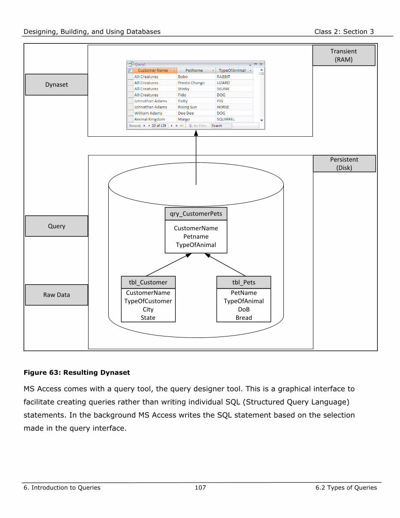
Designing, Building, and Using Databases Class 2: Section 3
6. Introduction to Queries 107 6.2 Types of Queries
tbl_Customer
CustomerNameTypeOfCustomer
CityState
tbl_Pets
PetNameTypeOfAnimal
DoBBread
qry_CustomerPets
CustomerNamePetname
TypeOfAnimal
Persistent(Disk)
Transient(RAM)
Dynaset
Raw Data
Query
Figure 63: Resulting Dynaset
MS Access comes with a query tool, the query designer tool. This is a graphical interface to
facilitate creating queries rather than writing individual SQL (Structured Query Language)
statements. In the background MS Access writes the SQL statement based on the selection
made in the query interface.

Designing, Building, and Using Databases Class 2: Section 3
6. Introduction to Queries 108 6.2 Types of Queries
Figure 64 shows an example of how a single table query looks. The customer table is shown in
the upper area, and the selected fields are selected in the lower area.
Figure 64: Single-Table Query in Query Designer Interface
Figure 65 displays a multi table query. The three tables, tbl_Customer, tbl_Pets, and tbl_Visits
are added to the upper area. The lower area shows the fields selected. Note that the
relationships are added automatically into the Query Designer interface, they are inherited from
the database.
Figure 65: Multi-Table Query in Query Designer Interface

Designing, Building, and Using Databases Class 2: Section 3
6. Introduction to Queries 109 6.2 Types of Queries
Total Query
A total query is a special version of a select query. In addition to selecting tables and fields, the
user can analyze the data by using the so-called aggregate functions, such as count or sum.
Data will be analyzed for the entire table or for groups of records within the table.
Figure 66: Total Query Example
A simple example is to count the customers within each state. Within the table customer the
records are grouped by the State field, then within each group the records are counted.
Action Queries
Besides selecting tables and fields and analyzing data, queries can accomplish more tasks. The
group of Action queries can actually make changes to the data, such as adding, deleting, or
modifying data as well as creating tables.
Action queries make changes in bulk, that is, for an entire group of records or for the entire
table. This makes it a very powerful tool to apply major changes to a database rather than
scanning one record at a time and apply the change. A simple example is to increase medication
prices by 10% in the table services.

Designing, Building, and Using Databases Class 2: Section 3
6. Introduction to Queries 110 6.2 Types of Queries
The different types of Action queries are:
Make-Table Query: A new table is created based on a query. Even a multi table query can be
saved as a new table. Basically, the resulting dynaset is saved as a new table, defying the
advantage of a query because the dynaset can always be generated at any time. However, there
may reasons for doing so, such as archiving data, exporting data, etc.
Update Query: Record changes can be performed with an Update query. Either one field or
multiple fields can be modified at once. In addition, either the field values of all records or a
subset of records can be updated based on a criterion.
Append Query: Records can be moved from one table into another by using an append query.
One example is archiving customer records from the main customer table to a archive customer
table based on a specific criteria or business rule (such as inactive customers for more than a
year).
Delete Query: All the records in one table can be deleted or a subset of records in a table
based on criteria. A delete query can be used in conjunction with an append query to move
records. An append query copies records from one table to another and then records in the
source table are deleted using a delete query.
Figure 67: Action Queries in MS Access

Designing, Building, and Using Databases Class 2: Section 3
6. Introduction to Queries 111 6.2 Types of Queries
Crosstab Queries
Simply put, a crosstab query is a spreadsheet like summary of data items specified by the row
and column header that is created from table data. It is an extension of a total query in that you
group by at least two fields and present the information in a matrix/table like format where the
column and row headers are generated dynamically.
Figure 68: Crosstab Query Example
Figure 68 shows an example of the count of pets by state and type of animal. You can see that
the state column header is currently comprised of three states, ID, OR, and WA. If a new
customer is added living in California, for example, then automatically when this query is
executed again, the column header of CA would be automatically added. Also if a new type of
animal would be added to the database, this value would be automatically displayed as a row
header in this query.
SQL Queries
The graphical interface to create queries in MS Access is very user-friendly and powerful.
Unfortunately, for complex and very specific queries this wonderful interface does not work
anymore. At that point the developer has to resort to writing plain SQL in order to construct the
query. Luckily, MS Access allows this backdoor by creating a so-called SQL statement.
Again, remember, all queries in MS Access are based on SQL, but the SQL Query name in Access
refers to the interface where you manually type SQL commands.

Designing, Building, and Using Databases Class 2: Section 3
6. Introduction to Queries 112 6.3 Capabilities of Queries
6.3 Capabilities of Queries
As mentioned earlier, queries are a very powerful tool to get information from the database in
almost any way. Following is a list of basic features of queries, and a short explanation.
Capability Description
Choose Tables Queries can retrieve information from multiple tables that are related to
each other. The resulting dynaset returns the information in form of a flat
file, the starting point for a relational database. If information is needed
from multiple tables, the tables must be connected through relationships. If
not, add additional tables to complete the relational path, even though no
fields are necessary from these tables.
Choose Fields Many database tables are quite complex, that is have a lot of fields. A query
can return a subset of fields, which facilitates viewing the information for
specific users since they only see pertinent information. There may be many
different queries for only one table, because different users need different
views of the data.
Choose Records By imposing criteria records are selected from a table. Again, this is very
important in today’s information society since not one single user needs to
view all records.
Sort Records A table is sorted by default by the primary key , however, users need to sort
data in many different ways. The query tool possesses sorting features
where records can be sorted on one or multiple fields.
Perform
Calculations
In addition to retrieving fields from the database tables, new fields can be
introduced at the query level. Remember, derived or calculated data should
not be stored in the database. However, many times users need to see one
kind of data in many different ways, such as a Customer Name.

Designing, Building, and Using Databases Class 2: Section 3
6. Introduction to Queries 113 6.3 Capabilities of Queries
Capability Description
Create Tables Using a Make-Table query additional tables can be created for archiving or
exporting data.
Create Forms or
Reports based
on a Query
Queries build the foundations for forms and reports. Especially for reports,
very complex queries are necessary to present data. For forms queries are
not as common because entering data through queries has its limitations.
Create a Query
based on Query
For complex queries, it is necessary to break the query down into separate
queries. Also for ad-hoc querying you may want to create a temporary
query based on a main query leaving the main query intact.
Create Graphs
based on a
Query
Very commonly, queries are used as a source for graphs, which are included
in forms and reports.
Make Changes
to Tables
Using select queries one can make changes to data in the underlying tables
(to a certain degree) or by using Action queries, bulk changes can be
performed.
Table 15: Capabilities of Queries

Designing, Building, and Using Databases Class 2: Section 3
7. Select Queries 114 7.1 Create a SELECT Query
7. Select Queries
We are finally ready to create our first SELECT query. Thanks to the wonderful, graphical
interface creating queries is pretty simple. You will learn how to use the graphical query
interface to create a query. This interface will be used for all the other queries except for the
special SQL queries.
7.1 Create a SELECT Query
To create a query in MS Access, follow these steps:
➢ Select the Create tab in the ribbon. Then click on Query Design in the Queries section.
➢ After choosing Query design view, the Show Table dialog box is displayed (the same as in
the Relationship Builder Tool). Select the tables necessary for the query and click on Add,
when done click on Close.
➢ Then add fields and create expressions, specify any criteria, and view the dynaset results.
➢ Save the query as a new query object, use the prefix qry and a meaningful name for the
query object.
Note: Using prefixes for all objects in MS Access proves to be a very efficient way of
database documentation. The main reason for prefixes is to differentiate between table and
query objects. Sometimes all tables and all queries are displayed in one view, and without
prefixes there is no way to differentiate between a table and a query.

Designing, Building, and Using Databases Class 2: Section 3
7. Select Queries 115 7.1 Create a SELECT Query
Warning: You cannot use the same name for a query as for a table. A query object is
basically not different from a table, at least when viewing the data. The data is comprised of
rows and columns.
There is also a query wizard allowing you to create a query using a step-by-step wizard.
Figure 69: New Query Wizard

Designing, Building, and Using Databases Class 2: Section 3
7. Select Queries 116 7.1 Create a SELECT Query
Example 3-1: Create a Simple SELECT Query
1. Navigate to the Create tab in the ribbon.
2. Click on Query Design.
3. The Show Table dialog box is displayed.
4. Select tbl_Customer and click
on Add (or double-click).
5. Click on Close
6. Select the field CustomerName
and drag into the field row below.
7. Repeat step 6 for fields State and City.
8. Save the query as qry_Example3_1.

Designing, Building, and Using Databases Class 2: Section 3
7. Select Queries 117 7.1 Create a SELECT Query
The query designer interface is divided into two areas, very similar to the table designer
interface. The upper area is called the Table/Query Entry area and the lower pane is the Design
Grid area, see Figure 70.
Table/Query Entry Area
Design Grid Area
Figure 70: Query Designer Interface
In the Table/Query Entry area all tables (and/or queries) involved in a query are displayed as
well as the relationships that are already saved in the database. In the Design Grid area fields
are selected, sorting is performed, and criteria are specified.
The two window panes can be resized by dragging the horizontal bar up or down. Place the
mouse pointer on the dividing bar between the upper and the lower area. The mouse pointer
shape changes to vertical double arrows pointing in opposite directions as shown in Figure 71.
Additionally, the tables in the upper pane can be resized vertically and horizontally so that more
fields can be displayed. Simply place the mouse pointer on the border of a table, hold the mouse
button and drag to resize the table. Tables may also be moved to a different location. As in the
relationship tool, click on the table title bar and drag the table to its new location.

Designing, Building, and Using Databases Class 2: Section 3
7. Select Queries 118 7.1 Create a SELECT Query
Figure 71: Resizing Upper and Lower Pane in Query Designer
The lower pane consists of a grid view with the following rows:
Field Row: To select fields (various methods).
Table Row: The table name which a selected field belongs to. This is especially important for
primary keys and foreign keys since these fields may have the same name, but they are stored
in different tables.
Sort Row: To sort records ascending, descending or not sorted.
Show: To show a field in the resulting dynaset.
Criteria: To specify one or more criteria for one field or multiple fields.
Or: To specify multiple criteria using a Boolean operator of or.
The design grid’s column represents the fields of the query in the datasheet view once the query
is run. The order of fields is from left to right. Each column contains information about a single
field from a table or query or represents a calculated or derived column defined in the query.
Each of the output fields has properties, very similar to fields in a table. To access these query
field properties, either right-click in the column and select properties from the shortcut-menu or

Designing, Building, and Using Databases Class 2: Section 3
7. Select Queries 119 7.1 Create a SELECT Query
click in the column and then click the Property Sheet button in the contextual tab Query Tools,
Design, in the ribbon as shown in Figure 72.
Property Sheet Button
Short-Cut Menu, Properties
Figure 72: Accessing Property Sheet

Designing, Building, and Using Databases Class 2: Section 3
7. Select Queries 120 7.1 Create a SELECT Query
The property sheet dialog box is shown in Figure 73. This property sheet shows some table field
properties which can be overridden at the query level for this particular query only. The field
property settings at the table level remain intact.
Note: There are also overall query properties, not only for each field. We will discuss this at
a later point in this course.
Figure 73: Field Property Sheet

Designing, Building, and Using Databases Class 2: Section 3
7. Select Queries 121 7.2 Working with Fields in Design Grid
7.2 Working with Fields in Design Grid
The Query Designer interface is a very powerful interface. At first glance it may not seem that
way, but once you start creating many queries, you will experience all features that make this
tool so user-friendly yet powerful.
Selecting Fields in Design Grid Pane
There are several methods to add fields from the Query/Table Entry pane to the Design Grid
pane. As we will see later, sometimes the same field must be added twice to the Design Grid
pane. Selecting fields in the tables is similar to selecting files in Windows Explorer. The use of
the [Shift] and the [Ctrl] keys is crucial for this operation.
The most commonly used method is selecting one field in a table, holding the mouse button, and
dragging the field into the Design Grid pane. We have used this method in Example 3-2. Using
this method the user has the most control over where to place to field.
While dragging the mouse into the Design Grid pane, the mouse pointer shape changes to a
Field Icon (rectangle) with a plus sign. When dragging a selecting field over the Table/Query
Entry pane, a circle with a backslash is displayed, indicating that you cannot drop a field here as
shown in Figure 74. This icon is commonly referred as No-Sign or Prohibition Sign.
No-Sign, Prohibition Sign
Field Icon with Plus Sign
Figure 74: Mouse Pointer Shapes when Dragging Field into Design Grid Pane

Designing, Building, and Using Databases Class 2: Section 3
7. Select Queries 122 7.2 Working with Fields in Design Grid
Other Field Selection methods:
➢ Double-clicking on a field will add this field automatically to the Design Grid pane into the
next available column.
➢ Selecting multiple adjacent fields: Click with the mouse on the first field, hold down the
[Shift] key and select the last field of the range. All fields in between the first and the last
field are selected indicated by the fields highlighted in orange. Then click in the orange
highlighted area and drag it into the design grid area. Release the mouse button in the
Design Grid area.
➢ Selecting multiple, non-adjacent fields: Select the first field, then hold down the [Ctrl],
then select the other fields. Then again, click in the highlighted area and drag it into the
design grid pane. Release the mouse button in the Design Grid area.
➢ Each table in the Table/Query Entry pane contains an asterisk at the very top. This is not
a field, but is part of a SQL command. The asterisk functions like a wildcard character,
double-clicking on it transfers all fields into the Design Grid area.
➢ The last method is clicking in the field row of the Design Grid area, a little drop-down
arrow appears to the right. Clicking on this arrow lists all available fields.

Designing, Building, and Using Databases Class 2: Section 3
7. Select Queries 123 7.2 Working with Fields in Design Grid
Figure 75: Selecting Fields in Design Grid Pane
Managing Fields in Design Grid Pane
To change the field order in the Design Grid pane, move the mouse to the top of the column
(small gray area above the field row) to be moved. The mouse pointer shape changes to a
vertical arrow, now click and hold the mouse button while you drag the mouse to the left or
right. A vertical bar moves with the mouse movement, position the bar to the new position and
the release the mouse button. The column will be moved to the new position.

Designing, Building, and Using Databases Class 2: Section 3
7. Select Queries 124 7.2 Working with Fields in Design Grid
Field Selection Arrow Field Selected
Figure 76: Selecting Fields in Design Grid Pane
To remove a field, simply select the column as described above and hit the [Del] button to
delete the column.
To insert a field, drag a field from the Table/Query Entry pane and place it in the Design Grid
pane at the desired location. Existing fields will be moved automatically to the right to
accommodate the new field.
To show a field in the datasheet view, select the checkbox in the Show row of the Design Grid
pane. This checkbox is turned on by default. We will learn later why sometimes this checkbox is
turned off.
Warning: When you turn off the Show checkbox and do not change the field properties,
sorting or criteria settings for this field, MS Access will automatically remove this field when you
save and close the query.
Field Names/Column Header in a Query
When you view a query in datasheet view, the column headers are normally the field names as
defined at the table level. Now we will look at the Caption property in table design and query
design and see how they work. In the next Example, we will first set the Caption property in
table design. Then we will override this property in query design.

Designing, Building, and Using Databases Class 2: Section 3
7. Select Queries 125 7.2 Working with Fields in Design Grid
Example 3-2: Caption Property in Table and Query Design
1. Navigate to the table tbl_Customer in design view.
2. Select the CustomerName field and then type Cust Name in the Caption property.
3. Save and close the table designer.
4. Now create a new query and save
it as qry_Example3_2.
5. Add CustomerName, City and
State as fields.
6. Click on the View button in the
ribbon to view the data in
datasheet view.
7. Notice that the column header now
shows Cust Name.
8. Navigate back to Design View.
9. Select the column CustomerName and display
the property sheet.
10. Type Customer Name into the Caption property.
11. Save the query and click on View button.
12. Notice now that the column heading reads
Customer Name.
13. Effectively, we can overwrite certain table
properties in a specific query.
When you export the resulting data from a query out of Access into some kind of other format,
for example into a text file, the Caption property does not get exported. The actual database
field names are used in this case.

Designing, Building, and Using Databases Class 2: Section 3
7. Select Queries 126 7.2 Working with Fields in Design Grid
This is an important point to recognize, because it shows the difference between the actual
database engine in and the application layer of MS Access. The application layer is mainly
comprised of forms and reports to build applications. However, there are other components,
such as table and query designer, macro designer, and some table and query properties.
For example, the format and input mask are properties that do not exist in the database. These
are properties of the application layer, because eventually they are used in forms and reports.
The caption property is another example of an application layer property. If you want to rename
a field in a query and use a customized field header (rather than the field name), you can use
another method called field alias. In the field row, before the field name, type a customized field
header followed by a colon. This will also change the column header in datasheet view. But it is
also the field name when the data is exported out of MS Access.
Example 3-3: Field Alias Method
1. Create a new query and save it as
qry_Example3_3.
2. Add CustomerName, City, State and
ZipCode as fields.
3. Click inside the field row for the field
CustomerName.
4. Type Cust: before the field name.
5. Click inside the field row for the field
ZipCode.
6. Type Postal Code: before field name.
7. Save the query and view the data in
datasheet view.
8. Notice that the column header for
CustomerName did not change
whereas for ZipCode it has changed to Postal Code.

Designing, Building, and Using Databases Class 2: Section 3
7. Select Queries 127 7.2 Working with Fields in Design Grid
Note: If the Caption property has been set for a field, it cannot be overridden by the field
alias method described above, meaning in datasheet view you still see the Caption property
setting. However, when exporting data out of MS Access, the field alias will be used in the
exported file and not the caption property.
Sorting Data in a Query
To sort on a specific field, click inside the sort row of that field. Three choices appear in a drop-
down list as shown in Figure 77: Ascending, Descending, and (not sorted).
Sort Options
Figure 77: Specifying Sort Order in Query Design
By default, a query is sorted by the primary key of the underlying table. To change the sort
order, select one or more fields to be sorted. Sort order will be processed from left to right, that
is the leftmost field to be sorted will be processed first for sorting, then the next field to the
right, and so on.
Warning: One of the rules of the relational model is that data stored in a relation is
unsorted. MS Access violates this rule as it shows table data and query data using that table
sorted by primary key. If no primary key is specified, then data is displayed in the order the data
was entered into a table.

Designing, Building, and Using Databases Class 2: Section 3
7. Select Queries 128 7.2 Working with Fields in Design Grid
Example 3-4: Specifying Sort Order in a Query
1. Create a new query and save it as
qry_Example3_4.
2. Add CustomerName, City, and State
as fields.
3. Select Ascending as sort order for
the state field.
4. Save the query and view the
datasheet output.
5. Notice how the data is now saved by
state in ascending order.
6. Navigate back to design view.
7. Now we want to sort by CustomerName
within the sort order of state.
8. Select Ascending as sort order
for the CustomerName field.
9. Save the query and view the datasheet output.
10. You notice that this is not the expected sort order. Now the data is sorted by
CustomerName only (it is also sorted by state, but is has no real effect since customer
names are unique).

Designing, Building, and Using Databases Class 2: Section 3
7. Select Queries 129 7.2 Working with Fields in Design Grid
Example 3-4 (continued): Specifying Sort Order in a Query
11. We know that sort order is processed from left to right.
12. Move the State field to the left of the
CustomerName field.
13. Save the query and view the datasheet output.
14. Now the sort order is correct, but we still want the
CustomerName field displayed first.
15. Navigate back to design view.
16. Move the State field back to the right. Set the
CustomerName field to not sorted.
17. Add the CustomerName field again to the query
design grid to the right of the State field.
18. Select Ascending as sort order and uncheck the
Show checkbox.
19. Save the query and view the datasheet output.
20. Now the data is displayed and sorted exactly as expected.
21. The output order is CustomerName, City, and State.
22. The sort order is State, CustomerName.
Note: Sometimes the output and the sort order of fields are different. In that case, a field
has to be added twice to the query design grid, one field for output order (Show checkbox
turned on) and the other field for sorting order (Show checkbox turned off).

Designing, Building, and Using Databases Class 2: Section 3
7. Select Queries 130 7.3 Simple Criteria Expression in Queries
7.3 Simple Criteria Expression in Queries
To vertically limit the number of records, specify one or more criteria in the criteria row of the
query design grid in the query interface. By imposing criteria, MS Access will scan the entire
table, but only retrieve records which meet the criteria condition.
For example, typical criteria expressions could be:
Pets Table: Show me all female pets only.
Pets Table: Retrieve a list of pets born before January 1990.
Customer and Pets Table: Show me all dogs from customers in California.
Example 3-5: Specifying a Criterion in a Query
1. Create a new query and save it as qry_Example3_5
2. Add CustomerName, City and State as fields
3. In the Criteria row for the State field, enter wa or WA.
4. Click outside the criteria row and notice the double quotation marks around WA.
5. Save the query and view the datasheet output.
6. Notice that you only see customer records residing in the state of Washington.

Designing, Building, and Using Databases Class 2: Section 3
7. Select Queries 131 7.3 Simple Criteria Expression in Queries
To enter a criterion for a text field, simply type a value in the criteria row for that field. MS
Access will automatically enclose the criterion string in quotation marks when the user leaves
the criteria row. The criterion reads that the field value must equal the criterion value. The equal
sign is the default relational operator; therefore it does not have to be typed in the criteria row.
Below are some examples of typical criteria expressions. As explained above, text criteria are
enclosed in quotation marks (“). Number fields are not enclosed in any delimeters. Date/time
criteria are enclosed in pound signs (#).
When you enter MS Access displays and retrieves records where
Borderville “Borderville” City field value equals Borderville
1 1 TypeOfCustomer field value equals 1
< 1/1/1998 < #1/1/1998# CustomerSince field value is less than 1/1/1998
Tall Pines “Tall Pines” City field value equals Tall Pines
Between 1/1/1995
AND 1/1/2000
Between #1/1/1995#
AND #1/1/2000#
CustomerSince field values are between 1/1/1995
and 1/1/2000, inclusive
Table 16: Sample Criterion Expressions
Note: In most situations, the special delimiters for text and date/time fields are
automatically added by MS Access when the user navigates out of the criterion cell. However,
there could be a situation where a text entry might be misunderstood by MS Access. For
example, typing the following in a criteria cell: This is a test. And navigating out of the criteria
cell will cause the following dialog box to be
displayed:
In this particular example the “is” word is
causing the problem as it is a reserved keyword
of SQL and therefore MS Access will interpret
it as a SQL command. Enclose the entire criterion in quotation marks to avoid this error.

Designing, Building, and Using Databases Class 2: Section 3
7. Select Queries 132 7.3 Simple Criteria Expression in Queries
Example 3-6: Criterion Example: Range of Records
1. Create a new query and save it as qry_Example3_6
2. Add tbl_Visits to the query.
3. Select VisitNumber, VisitDate, and VisitType as fields.
4. Type the following criterion for the VisitDate field: Between 1/1/2011 and 12/31/2011.
5. Save the query and view the datasheet
output.
Example 3-7: Criterion Example: OLE Objects
1. Create a new query and save it as qry_Example3_7
2. Add tbl_Employees to the query.
3. Select LastName, FirstName and Photo as fields.
4. Type the following criterion for the Photo field: Is Null.
5. Save the query and view the datasheet output.

Designing, Building, and Using Databases Class 2: Section 3
7. Select Queries 133 7.3 Simple Criteria Expression in Queries
Example 3-8: Criterion Example: Exclude Records
1. Create a new query and save it as qry_Example3_8
2. Add tbl_Customer to the query.
3. Select CustomerName, State and City as fields.
4. Type the following criterion for the
State field: <> OR
5. Save the query and view the datasheet output.
Example 3-9: Criterion Example: Less than criteria
1. Create a new query and save it as qry_Example3_9
2. Add tbl_Services to the query.
3. Select ServiceID, Medication/Treatment, and Price as fields.
4. Type the following criterion for the Price field: < 10.
5. Save the query and view the datasheet output.

Designing, Building, and Using Databases Class 2: Section 3
7. Select Queries 134 7.3 Simple Criteria Expression in Queries
To specify criteria for Yes/No field keep in mind that Yes/No fields can be formatting using a
multitude of values. Most commonly Yes or No is used, but the following values are also
acceptable. Therefore the criteria expressions may look like:
Yes values: True, On, Not No, <>No, <No, -1
No values: False, Off, Not Yes, <>Yes, >Yes, 0
A Yes/No field is stored as -1/0 in the database.
Example 3-10: Criterion Example: Yes/No Fields
1. Create a new query and save it as qry_Example3_10
2. Add tbl_Pets to the query.
3. Select PetName and Neutered/Spayed as fields.
4. Type the following criterion for the Neutered/Spayed field: - 1.
5. Save the query and view the datasheet output.
6. Switch back to design view and you may notice that the -1 was changed to True
automatically.
7. Try out the other criterion values for true such as Yes, <> No, and < No.

Designing, Building, and Using Databases Class 2: Section 3
7. Select Queries 135 7.3 Simple Criteria Expression in Queries
Example 3-11: Creating a Lookup Wizard relationship and querying it.
1. Navigate to the Relationship Builder tool and delete the relationship between
tbl_Customer.State and tbl_States.StateCode.
2. Open the table tbl_Customer in design view.
3. Select the Lookup Wizard for the State Field. Leave
the first option selected and click on Next.
4. Select tbl_States and click on Next.
5. Select the fields
StateCode and StateName.
6. Click through all the other steps without
making any changes.
7. Save the table and close it.
8. Create a new query and save it as qry_Example3_11.
9. Add tbl_Customer to the query.
10. Select CustomerName, City and State.
11. Click on Datasheet View to view the data. Notice that
the State field now contains the long state names
such as Washington, Idaho, and Oregon.

Designing, Building, and Using Databases Class 2: Section 3
7. Select Queries 136 7.3 Simple Criteria Expression in Queries
Example 3-11 (continued): Creating a Lookup Wizard relationship and querying it.
12. Navigate back to design view and enter
the following criterion in the State field.
13. Click on Datasheet View and view the resulting data.
14. You will notice that no data is returned, this is due
to the fact that the actual data contained in the State
field in tbl_Customer is hidden by the dynamic link
to tbl_States created by the Lookup Wizard.
15. You would need to enter “WA” as a criterion in order
to filter correctly for state Washington, yet you can
never see this value!
16. Undo the Lookup Wizard setup for the State field in
tbl_Customer.
17. Re-create the relationship using
the Relationship Builder tool.

Designing, Building, and Using Databases Class 2: Section 4
8. Advanced Select Queries 137 8.1 Wildcard Character Comparisons
CLASS 2: SECTION 4
8. Advanced Select Queries
We will now further explore the SELECT query. First we are going to discuss wildcard characters
in a criterion querying for patterns in data. Following we cover complex criteria using Boolean
operators, first against a single field, then across multiple fields. Then we move over to creating
calculated/derived expressions. The last chapter deals with the overall Query properties, such as
Unique Values and others.
8.1 Wildcard Character Comparisons
To search for patterns of characters use the wildcard character asterisk (*). This character
stands for zero, one, or many characters. Use the question mark (?) for a single character
expression, any character, but one and only one. Wildcard character comparisons are mostly
used in situations where the user does not know the exact value for a field value or wants to
include a range of records.
Simple Wildcard Characters
When using a wildcard character, the relational operator is “Like”. Because the field value need
not be equal the criterion, the equal sign does not apply. The value needs to be similar to the
criterion expression, therefore, the Like operator is required.
Note: In most cases, MS Access will automatically insert the Like operator when a wildcard
character is used.
In the following example, we want to retrieve all Medication/Treatment records starting with the
Letter B. The criteria expression is written as Like “B*” to match records where the
Treatment/Medication field starts with the letter B. There may be 0, one or many arbitrary
characters following the initial letter B.

Designing, Building, and Using Databases Class 2: Section 4
8. Advanced Select Queries 138 8.1 Wildcard Character Comparisons
Example 4-1: Show Treatment/Medication records starting with B
1. Create a new query and save it as qry_Example4_1.
2. Add the table tbl_Service.
3. Add the ServiceID, Treatment/Medication and the Price field.
4. In the criteria row for the Treatment/Medication field, type B* and tab over to another
criteria row.
5. You will notice that MS Access
automatically adds the Like operator
and the quotes.
6. Run the query by clicking on the
View button.
Below are some more examples demonstrating pattern matches using Wildcard characters. All
examples use the table tbl_Pets and the fields PetName and Colors. The colors field is actually a
violation of the normalization rules since we are storing multiple values in a field of one record.
Warning: Wildcard characters are to be used in criteria for ShortText or LongText fields
only. Using wildcards with number or date/time fields may lead to unexpected results.

Designing, Building, and Using Databases Class 2: Section 4
8. Advanced Select Queries 139 8.1 Wildcard Character Comparisons
Example 4-2: tbl_Pets, field value in colors starts with “Black” and ends in “White”.
1. Create a new query and save it as qry_Example4_2.
2. Add table tbl_Pets and the fields PetName and Colors.
3. Type the following criterion in the colors field: Like “Black*White”
Example 4-3: tbl_Pets, field value in colors contains “White”.
1. Create a new query and save it as qry_Example4_3.
2. Add table tbl_Pets and the fields PetName and Colors.
3. Type the following criterion in the colors field: Like “*White*”

Designing, Building, and Using Databases Class 2: Section 4
8. Advanced Select Queries 140 8.1 Wildcard Character Comparisons
Example 4-4: tbl_Pets, field value in colors starts with “White”.
1. Create a new query and save it as qry_Example4_4.
2. Add table tbl_Pets and the fields PetName and Colors.
3. Type the following criterion in the colors field: Like “White*”
Example 4-5: tbl_Pets, field value in PetName starts with “Mo”, ends in “se” and any,
but one character in between.
1. Create a new query and save it as qry_Example4_5.
2. Add table tbl_Pets and the fields PetName and Colors.
3. Type the following criterion in the PetName field: Like “Mo?se”

Designing, Building, and Using Databases Class 2: Section 4
8. Advanced Select Queries 141 8.1 Wildcard Character Comparisons
Advanced Wildcard Characters
Besides the * and the ? wildcard characters MS Access offers a few more. Below is a table listing
all wildcard characters available in MS Access.
Character Description
* Matches any number of characters. You can use the asterisk (*) anywhere in a
character string.
? Matches any single alphabetic character.
[ ] Matches any single character against a list of characters within the brackets.
! Matches any character not in the brackets.
- Matches any one of a range of characters within the brackets. You must specify
the range in ascending order (A to Z, not Z to A).
# Matches any single numeric character.
Table 17: Wildcard Characters
MS Access automatically adds the LIKE operator and quotation marks if you meet these
conditions:
➢ There are no spaces in your expression.
➢ You use only the wildcard character ?, *, #.
➢ You use brackets ([ ]) inside quotation marks.

Designing, Building, and Using Databases Class 2: Section 4
8. Advanced Select Queries 142 8.1 Wildcard Character Comparisons
Example 4-6: tbl_Customer, field value in CustomerName starts with A or D or G or T.
1. Create a new query and save it as qry_Example4_6.
2. Add table tbl_Customer and the fields
CustomerName, City and State.
3. Type the following criterion in the
CustomerName field: Like “[ADGT]*”
Example 4-7: tbl_Customer, field value in CustomerName does not start with A or D or
G or T.
1. Create a new query and save it as qry_Example4_7.
2. Add table tbl_Customer and the fields
CustomerName, City and State.
3. Type the following criterion in the
CustomerName field: Like “[!ADGT]*”

Designing, Building, and Using Databases Class 2: Section 4
8. Advanced Select Queries 143 8.1 Wildcard Character Comparisons
Example 4-8: tbl_Customer, field value in Street/Apt starts with numeric characters,
then a space followed by any character
1. Create a new query and save it as qry_Example4_8.
2. Add table tbl_Customer and the fields
CustomerName and Street/Apt.
3. Type the following criterion in the
Street/Apt field: Like “### *”

Designing, Building, and Using Databases Class 2: Section 4
8. Advanced Select Queries 144 8.2 Using Complex Criteria
8.2 Using Complex Criteria
A query commonly involves multiple tables to extract information from the database, though
queries containing only one table are not uncommon. Limiting the number of records is
particularly important in multiple-table queries, because a One-To-Many relationship increases
the number of datasheet records significantly. The more One-To-Many relationships are
involved, the more datasheet records are generated. To limit the output, complex criteria are
used to return only the data required by the user.
We have used so far criteria for a single field. Criteria for a single field consist of either one value
or multiple values connected by an Or operator. For example, to retrieve customers residing in
Idaho the user must type the criterion “ID” in the criteria row for the state field. To display
customers from Washington and Idaho, the criterion is “ID” Or “WA”.
Warning: It is common mistake to get OR and AND mixed up when composing compound
criteria against a single field. For example, show me all customers from Washington and Idaho.
Notice the word “and”. Yet when you write the criteria, you use the OR operator “WA” Or “ID”.
Using the AND operator would not retrieve any rows because in a single record the state field
cannot be WA and at the same time ID.
As mentioned earlier, using the Lookup wizard in table design except for storing static values is
in general not a good idea. If you use the lookup wizard to maintain a dynamic lookup
relationship or you allow the option of “Allow Multiple Values” (new since Access 2007), you will
have difficulties querying the data without knowing the details of that relationship.
For example, if you had set up a table names Status to store Active, Inactive, Pending using a
code column (A=Active, I=Inactive, P=Pending) and linked this table using the lookup wizard to
your table Customer, for example. What you would see in table Customer would be Active,
Inactive, or Pending. But what is actually stored in the table is A, I, or P. In order to filter Active
customer records only, you have to enter the criteria “A” rather than Active, although that is
what you see in the table. This is very confusing.
If you allow the new option of multiple values in one field, then if one value matches the criteria
condition, the record is retrieved.
When entering values into the criteria row without any additional operator, the field value of
each record is compared with the criterion using an equal (=) sign. There are many other
operators used in query expressions. We will discuss them in the following sections.

Designing, Building, and Using Databases Class 2: Section 4
8. Advanced Select Queries 145 8.2 Using Complex Criteria
Mathematical Operators
There are basically four main operators:
➢ (multiply)
➢ / (divide)
➢ + (add)
➢ (subtract)
The mathematical operators are used in calculated fields or complex criterion expressions. For
example, to calculate the total of an invoice of a specific visit, add all visit detail records (the
price field) to arrive at the total.
Example 4-9: qry_VisitsTable, field value in Visit_Date within last 90 days
1. Create a new query and save it as qry_Example4_9.
2. Add query qry_VisitsTable and the fields
VisitNumber, Visit_Date, and VisitType.
3. Type the following criterion in the
Visit_Date field:
Between Date() And Date() – 90
Note: This example requires the use of a query where the visit date is adjusted to the current
year in order to retrieve some result records. The number of output records depends exactly
when the query is executed.

Designing, Building, and Using Databases Class 2: Section 4
8. Advanced Select Queries 146 8.2 Using Complex Criteria
In the previous example, we have used the Date function, which will always return the current
date. This is a built-in function, and we will cover those at the end of this course. By default, you
can add to or subtract from a date a number, which is interpreted as the number of days.
Relational Operators
If a criterion is to be exactly equal to a field value, no relational operator needs to be specified in
the criteria row. However, any relational operator other than equal must be specified in the
criteria row before the condition.
A list of relational operators is shown below:
➢ = (equal)
➢ <> (not equal) (may also use Not = )
➢ > (greater than)
➢ >= (greater than or equal to)
➢ < (less than)
➢ <= (less than or equal to)
Relational operators are used to specify criteria for selecting ranges of records. Note that a
combination of these operators is allowed, such as >= (greater or equal than).
Warning: When using the greater (>) than and/or the less (<) than operator together with
an equal sign, make sure to place the equal sign after the less than or greater than operator.
Otherwise you will receive an error message.

Designing, Building, and Using Databases Class 2: Section 4
8. Advanced Select Queries 147 8.2 Using Complex Criteria
Example 4-10: Criterion Example: Less, Greater than criterion
1. Create a new query and save it as qry_Example4_10
2. Add tbl_Services to the query.
3. Select ServiceID, Medication/Treatment,
and Price as fields.
4. Type the following criterion in the
Price field: >= 10 And <= 20
The criterion in example 4-10 could have also been written using the Between And operator.
Logical Operators
Logical operators are used to specify multiple criteria in one field or multiple criteria across many
fields. Later we will see how the query design grid implements this concept.
When using criteria against a single field, you use the Or operator. An exception is a range
criterion where a field needs be greater than or equal to a value and less than or equal to a
value. When using criteria across multiple fields, you use the And and Or operators depending
on the business requirements.

Designing, Building, and Using Databases Class 2: Section 4
8. Advanced Select Queries 148 8.2 Using Complex Criteria
Example 4-11: tbl_Service, field value in Price within range of $50 to $200
1. Create a new query and save it as qry_Example4_11.
2. Add table tbl_Service and the
fields ServiceID,
Medication/Treatment, and Price.
3. Type the following criterion in the
Price field: >= 50 And <= 200.
4. Change the criterion by replacing the And operator with an Or operator: >=50 Or <=200
5. How many records are returned? All records since the Or operator requires now only one
of the criteria to be met.

Designing, Building, and Using Databases Class 2: Section 4
8. Advanced Select Queries 149 8.2 Using Complex Criteria
String Operators
The following list shows the most common string operators:
➢ Like (wildcard character comparisons)
➢ & (concatenation, Null insensitive)
➢ + (concatenation, Null sensitive)
The Like operator is used in wildcard character comparison expressions to find field values
similar to the criterion specified. The Ampersand (&) operator is used in derived fields in a query
or table (Calculated Field) to add string values together.
For example, to connect the City, State, and ZipCode fields together, use the following
expression: [City] & “, “ & [State] & “ “ & [ZipCode]. You can concatenate database fields and
static strings (like “, “) together.
The plus operator can also be used to add string values together. However, the difference
between the & and the + operator lies in dealing with Null values. When adding strings together
and one string contains a Null value, the & operator will replace the Null with a zero-length
string and display the whole string. Using the + operator in this situation will result in a total
Null value for the concatenated portion of the string.
The order of precedence of operators as shown in Table 18.
Category Operators
1. Mathematical 1. Exponentiation
2. Negation 3. Multiplication and/or Division (left to right)
4. Integer Division 5. Modulo 6. Addition and/or Subtraction (left to right)
7. String concatenation
2. Comparison,Relational 1. Equal
2. Not Equal 3. Less than
4. Greater than 5. Less than or equal to 6. Greater than or equal to
7. Like
3. Logical 1. Not 2. And 3. Or
Table 18: Order of Precedence of Operators

Designing, Building, and Using Databases Class 2: Section 4
8. Advanced Select Queries 150 8.2 Using Complex Criteria
Example 4-12: & and + concatenation operators
1. Create a new query and save it as qry_Example4_12.
2. Add table tbl_Employees and the
fields LastName, FirstName, and
Initial.
3. In the next empty column in the field
row type the following expression:
Name&: [LastName] & “, “ & [Initial]
4. Switch back to design view and modify the expression as shown below:
Name&: [LastName] & “, “ + [Initial]
5. Using the & operator a comma would be displayed even though no Initial existed. When
using the plus operator, due to the Null propagation, the comma is not displayed when
there is a Null Initial.

Designing, Building, and Using Databases Class 2: Section 4
8. Advanced Select Queries 151 8.2 Using Complex Criteria
Note: In the above example the order of precedence of operators is important. The
arithmetic plus (+) operation is performed before the string concatenation (&). Therefore, the
string containing the comma (“, “) is arithmetically added with a null initial, and this operation
results in a null. Then the LastName is concatenated with a null, which results simply in the
LastName.
Miscellaneous Operators
The following list shows some miscellaneous operators:
➢ Between…And
➢ Is Null, Is Not Null
➢ In( )
The Between…And operator is a powerful tool to select a range of records. One could also use
the greater or equal (>=) and less or equal (<=) operators to achieve the same result, however,
the Between…And operator is much more efficient. The In operator is a very good tool to find
records matching multiple criteria in one field.
The IN operator connects the different values listed in the parentheses using a logical OR
operator. There is no need to list the OR operator, it is implicitly built into the IN operator.
The Is Null operator is used to test for fields that contain Null values. You cannot simply type
Null in the criteria row (= Null), this always results in false.

Designing, Building, and Using Databases Class 2: Section 4
8. Advanced Select Queries 152 8.2 Using Complex Criteria
Example 4-13: In Operator
1. Create a new query and save it as qry_Example4_13.
2. Add table tbl_Pets and the
fields PetName, and TypeOfAnimal.
3. Type the following criterion for the TypeOfAnimal field:
In(”Horse”,“Squirrel”,”Lamb”)
Complex Criteria
Complex criteria consist of multiple criteria either within one field or across multiple fields. These
criteria must be connected either with the And or Or operator to tell the database exactly which
records to fetch.
Multiple criteria for one field:
State must be Idaho or Oregon: [State] = “OR” or “ID”
Multiple criteria for multiple fields:
City must be Borderville and State must be Oregon: [City] = “Borderville” And [State] = “OR”
State must be Idaho or Washington and city must be Borderville:
([State] =“ID” and [City] =“Borderville”) OR ([State] =“WA” and [City] = “Borderville”)

Designing, Building, and Using Databases Class 2: Section 4
8. Advanced Select Queries 153 8.2 Using Complex Criteria
As we have seen previously, specifying multiple criteria for one field is implemented using either
the Or/And operator or the In operator if many criteria values are used.
The other two examples now introduce the concept of applying multiple criteria across multiple
fields in a query. To connect multiple criteria across multiple fields, the MS Access Query
interface has been specifically designed to accommodate this concept. The query design grid
contains many rows, the first ones serving prescribed purposes such as field name, table name,
sort order, and show.
Figure 78: Criteria and Or Rows in Query Design Grid
The next row is labeled Criteria, that is the row the criteria have been entered so far. The
following row is named or, that is an additional criteria row for criteria connected with the
operator Or to the previous row. All following rows are criteria rows connected through the
operator Or
The basic concept is that criteria entered horizontally across fields are connected with the And
operator, and criteria entered in different rows vertically are connected with the Or operator.
Or
And
Figure 79: And and Or Operators in Query Design Grid

Designing, Building, and Using Databases Class 2: Section 4
8. Advanced Select Queries 154 8.2 Using Complex Criteria
Example 4-14: State must be Idaho or Washington and city must be Borderville
1. Create a new query and save it as qry_Example4_14.
2. Add table tbl_Customer and the
fields CustomerName, City and State.
3. Type the following criteria:
4. Reading the criteria expression can be a bit cumbersome, but it should be read line by line
from left to right. Each line should be enclosed in parentheses: (City equals Borderville
And State equals ID) OR (City equals Borderville And State equals WA).
5. The criteria expression can be simplified as shown below:

Designing, Building, and Using Databases Class 2: Section 4
8. Advanced Select Queries 155 8.2 Using Complex Criteria
Example 4-15: Complex Criteria
1. Create a new query and save it as qry_Example4_15.
2. Add table tbl_Customer and tbl_Pets and the
fields CustomerName, City, State, PetName and TypeOfAnimal.
3. Type the following criteria:

Designing, Building, and Using Databases Class 2: Section 4
8. Advanced Select Queries 156 8.2 Using Complex Criteria
To comprehend this complex criterion it is good practice to read this line by line from left to
right.
First line: (CustomerName starts with a C followed by any character AND
City is Borderville AND
TypeOfAnimal is Fish)
OR
Second Line: (State is Washington)
OR
Third Line: (TypeOfAnimal contains the letter S anywhere in the name)
The And/Or operators are the most common relational operators in complex criteria expression.
The operator connects two equations (on each side of the operator), each equation is evaluated
individually to determine whether it is True or False. Finally, both sides are compared for a
resultant True/False result.
Take a look at Figure 80. The criterion is comprised of City=Lakeville AND State = OR.
Figure 80: Criterion Example City=Lakeville and State = OR
For each record, first the left side is evaluated, and then the right side. In this case if only if both
sides are True the resultant answer is True. In the above example, the first record meets both
criteria, therefore the result is True and the record would be retrieved. The next two records
only meet one criteria, the other criteria is False, therefore the resultant answer is False.
Figure 81: Criterion Example City=Lakeville OR State=OR

Designing, Building, and Using Databases Class 2: Section 4
8. Advanced Select Queries 157 8.2 Using Complex Criteria
In Figure 81 we modified the criterion by replacing the And operator with an or. In the case of
an Or operator, only one condition has to be met for the resultant answer to be True. That
means, all three records would carry a True answer and therefore would be retrieved.
Another important consideration in regards to Boolean logic is the existence of null values. What
if one condition yields a null value (that is no city name is entered)?
In combination with the operator And, a null value and a True value yield a resultant answer of
False, because both sides of the equation must be True. A null value and a True value in
conjunction with the operator Or yield a resultant answer of True, because only one part must
be True.
Table 18 shows the possible combinations of True and False results using the And and the Or
operators.
AND Operator OR Operator
Left Side Operator Right Side Result Left Side Operator Right Side Result
True AND True True True OR True True
False AND True False False OR True True
True AND False False True OR False True
True AND Null False True OR Null True
Null And True False Null OR True True
Null And Null False Null OR Null False
False Or False False
Figure 82: Boolean Truth Tables
The resultant answer for the And operator is True only when both sides are True. For the Or
operator, only side must be True for the result to be True.
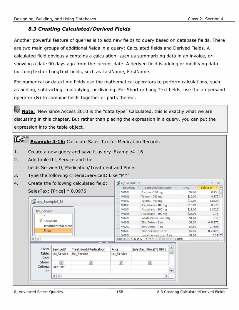
Designing, Building, and Using Databases Class 2: Section 4
8. Advanced Select Queries 158 8.3 Creating Calculated/Derived Fields
8.3 Creating Calculated/Derived Fields
Another powerful feature of queries is to add new fields to query based on database fields. There
are two main groups of additional fields in a query: Calculated fields and Derived Fields. A
calculated field obviously contains a calculation, such us summarizing data in an invoice, or
showing a date 90 days ago from the current date. A derived field is adding or modifying data
for LongText or LongText fields, such as LastName, FirstName.
For numerical or date/time fields use the mathematical operators to perform calculations, such
as adding, subtracting, multiplying, or dividing. For Short or Long Text fields, use the ampersand
operator (&) to combine fields together or parts thereof.
Note: New since Access 2010 is the “data type” Calculated, this is exactly what we are
discussing in this chapter. But rather than placing the expression in a query, you can put the
expression into the table object.
Example 4-16: Calculate Sales Tax for Medication Records
1. Create a new query and save it as qry_Example4_16.
2. Add table tbl_Service and the
fields ServiceID, Medication/Treatment and Price.
3. Type the following criteria:ServiceID Like “M*”
4. Create the following calculated field:
SalesTax: [Price] * 0.0975

Designing, Building, and Using Databases Class 2: Section 4
8. Advanced Select Queries 159 8.3 Creating Calculated/Derived Fields
In the previous example, only medication records were displayed due to the criteria Like “M*”.
What if we want to see all records but calculate the sales tax only for medication records. At this
point, an advanced tool comes into play, the use of built-in functions. Functions can be used in
queries to display or calculate data selectively based on conditions. One of the most important
functions is the immediate or inline If function, also named IIf:
The immediate if function processes an If..Else..End If programming construct in one line,
therefore it is called an immediate if function. Because a query is based on SQL, and SQL
statements are single-line statements, no multi-line programming is possible.
Programming Construct(3 lines) Immediate If Function (One line)
If [ServiceID] Like “M*” then
[Price] * 0.0975
End if
IIf([ServiceID] Like “M*”,[Price]*0.0975)
(Condition) (True part)
Example 4-17: Calculate Sales Tax for Medication Records using IIf Function
1. Create a new query and save it as qry_Example4_17.
2. Add table tbl_Service and the fields ServiceID, Medication/Treatment and Price.
3. Create the following calculated field: SalesTax: IIf([ServiceID] Like “M*”,[Price]*0.0975)
4. Select the SalesTax field, display the property sheet and set the Format to Currency.

Designing, Building, and Using Databases Class 2: Section 4
8. Advanced Select Queries 160 8.3 Creating Calculated/Derived Fields
Based on the previous example, add another calculated field to display the total, that is the price
and the sales tax, if applicable, otherwise just the price.
Example 4-18: Based on Example 4-17 add a Total Calculated Field
1. Save qry_Example4_17 as qry_Example4_18.
2. Create the following calculated field: Total: [Price] + [SalesTax]
The total field for treatment records does not show any value, not even the original price. This
effect is due to the propagation of Null in an expression. Null means currently unknown,
meaning there is something, but I cannot tell how much. When a known amount is added to
something unknown, the total is still unknown.

Designing, Building, and Using Databases Class 2: Section 4
8. Advanced Select Queries 161 8.3 Creating Calculated/Derived Fields
In order to avoid null propagation in arithmetic expressions, we have to modify the IIf statement
and add an Else branch to it. When a service record is not a mediation record, then set the value
to 0 (rather than null).
The IIf function has a third argument that can be used for an else part as shown below:
IIf(condition, true part, false part)
Example 4-19: Based on Example 4-18 modify IIf expression to avoid Null propagation
1. Save qry_Example4_18 as qry_Example4_19.
2. Modify the following calculated field:
SalesTax: IIf([ServiceID] Like "M*",[Price]*0.0975,0)

Designing, Building, and Using Databases Class 2: Section 4
8. Advanced Select Queries 162 8.4 Query Properties
8.4 Query Properties
Besides each field having properties the overall query also has a property sheet that exposes the
query properties. We will just discuss a few here in this chapter. The others are covered in the
following Access courses.
To display the property sheet for queries, you can either click in an empty field in query design
grid or click in a blank space in the Table/Query Entry pane. Then either right-click and select
Properties from the short-cut-menu or click on Property Sheet in the Show/Hide section of the
Query Design tab.
Figure 83: Query Property Sheet
Description: A place to document what the query does. This can be displayed in the navigation
pane when the view is set to details.
Output All Fields: If set to yes, the query will always include all fields regardless which fields you
have selected in the query designer.

Designing, Building, and Using Databases Class 2: Section 4
8. Advanced Select Queries 163 8.4 Query Properties
Top Values: This is a property that allows you to filter a certain number or percentage from the
top displayed records. As top indicates, a certain sort order needs to be defined in order to use
this property in a meaningful way.
Example 4-20: Top n Query
1. Create a new query and save it as qry_Example4_20.
2. Select table tbl_Visits and VisitNumber, VisitDate, VisitType and TotalAmount as fields.
3. Set a descending sort order on the TotalAmount field.
4. In the query property sheet, enter 10 in the Top Values property.
5. Note that the number of output records is 10.
6. Switch back to design view and enter 10% in the Top Values property.
7. Switch to Datasheet view and note that 9 rows are returned. There are a total of 81 rows,
10% rounded up results in 9 rows.
Note: You can also set the Top Values property in the Query Setup section in the Query
Design tab of the ribbon.

Designing, Building, and Using Databases Class 2: Section 4
8. Advanced Select Queries 164 8.4 Query Properties
Unique Values: To suppress duplicate values based on the fields selected for datasheet output.
Selecting unique values is a useful method to limit the number of output records. For example,
querying the pets table by type of animal displays all pet records showing the type of animal
field. What if I am only interested in pets without repeating types? If one pet is a cat, then I do
not want to see the type cat again.
Using unique values is commonly used to find out how many different lookup values have been
used in the child table. Again, using the Animal Type table as a lookup table (parent), which of
these values have actually been used in the Pets table (child)? We will explore this question in
the next example.
Example 4-21: Unique Values Property
1. Create a new query and save it as qry_Example4_21.
2. Select table tbl_Pets and TypeOfAnimal as field.
3. Set the sort order to Ascending on TypeOfAnimal field.
4. View the output in datasheet view. Note that there are
129 records.
5. Back in design view, set the Unique Values property to
Yes.
6. View the output datasheet and note that there are now only 30 records.

Designing, Building, and Using Databases Class 2: Section 4
8. Advanced Select Queries 165 8.4 Query Properties
Unique Records: You can use the UniqueRecords property when you want to omit data based on
entire duplicate records, not just duplicate fields. Microsoft Access considers a record to be
unique as long as the value in one field in the record differs from the value in the same field in
another record.
The UniqueRecords property has an effect only when you use more than one table in the query
and select fields from the tables used in the query. The UniqueRecords property is ignored if the
query includes only one table.
You use the UniqueRecords property when you have a one-to-many relationship where the many
side is just used to filter the data but not for displaying any data. The one-side will show
redundant data because of potentially having more than one child record. Setting the
UniqueRecords property to yes will suppress duplicate records of the one-side.
Example 4-22: Unique Records Property
1. Create a new query and save it as
qry_Example4_22.
2. Select table tbl_Customer and tbl_Pets and
CustomerName, City, State and TypeOfAnimal
as fields.
3. Type the following criterion in the
TypeOfAnimal field: dog
4. Uncheck the Show checkbox (so that
TypeOfAnimal is not displayed).
5. Switch to Datasheet view and note that the output includes some duplicate customers.
6. Switch back to design view and set the UniqueRecords property to yes.
7. Again switch to Datasheet view and verify that the duplicate records are now suppressed.

Designing, Building, and Using Databases Class 2: Section 4
9. Parameter Queries 166 9.1 Overview of Parameter Queries
9. Parameter Queries
Parameter queries are based on SELECT queries, the ones we have been using so far. The only
difference is that instead of hard-coded criterion values we add a dynamic parameter as a
criterion where the user at execution time can provide a value for filtering the resulting dynaset.
9.1 Overview of Parameter Queries
Parameter queries are basically Select queries. However, parameter queries take advantage of a
feature in MS Access, the Parameters prompt, to specify criteria at run time to be entered by the
user. This feature makes a select query more dynamic, in that, the users specify criteria and not
the designer/developer. Furthermore parameter queries reduce the number of queries necessary
because one query can be run using different criteria.
Parameter queries eliminate the need to go into the design view of a query and modify hard-
coded criteria every time a criterion needs to be changed. It allows for quick ad-hoc data
analysis, because if no parameter is entered, it will not apply a criterion.
Also, multiple parameters can be specified, either for multiple criteria in one field or for multiple
criteria across several different fields.
Parameter queries are very useful for forms and reports, because the user can specify the
records to be retrieved and the view only a portion of the data.
As mentioned earlier, a parameter query uses a feature built into MS Access, the Enter
Parameter Value dialog box. When MS Access runs a query and it cannot find a field specified in
the query (for example in an expression), it will display the Enter Parameter Value dialog box.
For the designer/developer this is an indication of an incorrect field reference, mostly due to
typos.
To take advantage of this feature and create a Parameter Query, a criteria prompt is used in the
criteria row and it is enclosed in square brackets. Items in square brackets indicate to MS Access
a field, and consequently when the query is run, MS Access cannot find this “imaginary” field. To
offer a solution to the user, it displays the prompt dialog box to enter a criterion at run-time.

Designing, Building, and Using Databases Class 2: Section 4
9. Parameter Queries 167 9.1 Overview of Parameter Queries
Example 4-23: Parameter Prompt/Value Dialog Box
1. Create a new query and save it as qry_Example4_23.
2. Select table tbl_Customer and CustomerName, City, and State as fields.
3. Switch to Datasheet view and you should see all the customer records.
4. Navigate back to design view and rename the CustomerName field to CustomerName1.
5. Let us assume that this is a typo. Save the query and run it again. You should now see a
Parameter Prompt dialog box as shown below:
6. Type Unknown and click on OK.
7. Note the word Unknown is now
substituted in the Datasheet view
for CustomerName1.
We are going to exploit this feature in queries as a means to enter criteria values at run time.
Warning: Whenever you see a parameter prompt and you did not intentionally set up a
parameter query a field or table name is mistyped. In this case the parameter prompt functions
as an error message and you should find the mistyped field or table reference and fix it.
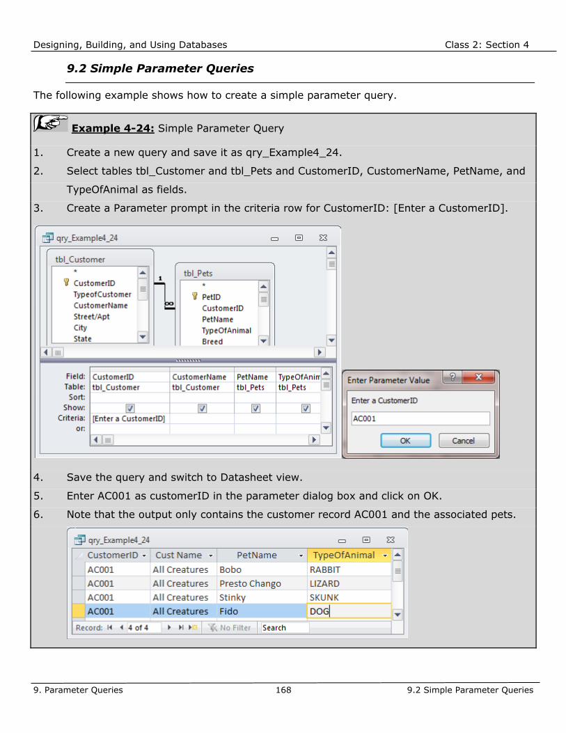
Designing, Building, and Using Databases Class 2: Section 4
9. Parameter Queries 168 9.2 Simple Parameter Queries
9.2 Simple Parameter Queries
The following example shows how to create a simple parameter query.
Example 4-24: Simple Parameter Query
1. Create a new query and save it as qry_Example4_24.
2. Select tables tbl_Customer and tbl_Pets and CustomerID, CustomerName, PetName, and
TypeOfAnimal as fields.
3. Create a Parameter prompt in the criteria row for CustomerID: [Enter a CustomerID].
4. Save the query and switch to Datasheet view.
5. Enter AC001 as customerID in the parameter dialog box and click on OK.
6. Note that the output only contains the customer record AC001 and the associated pets.

Designing, Building, and Using Databases Class 2: Section 4
9. Parameter Queries 169 9.2 Simple Parameter Queries
The square brackets are important for parameter to work properly. MS Access identifies names
enclosed in square brackets as database objects, such as fields, tables, indexes, etc. The field
name Enter a Customer ID cannot be found in the entire database, therefore MS Access displays
the parameter dialog box.
Note: It is important that the text entered in the square brackets does not resemble a field
name or any other object name, otherwise the parameter dialog box will not be displayed and
the results will not be correct.
The entry the users make in this box replaces the square bracket entry in the criteria cell in the
query. That means, the value the user enters in the Enter Parameter Value dialog box is the
criteria to be used for this particular run of the query. Another user may specify different
criteria, but the query is still the same.
Note: The text entered in the square brackets in the query appears in the Enter Parameter
Value dialog box. Use a meaningful description of what the user is to enter in this dialog box.
Warning: Only up to approximately 50 characters will fit as a prompt text in Parameter
dialog box.

Designing, Building, and Using Databases Class 2: Section 4
9. Parameter Queries 170 9.3 Multiple Parameter Queries
9.3 Multiple Parameter Queries
As mentioned earlier, one may enter as many parameters as necessary in a parameter query.
Multiple parameters may be used for one field, as shown in the next example.
The user may only enter one, and ignore the other parameter prompts by simply not entering
anything and clicking OK. This allows for great flexibility. Make sure to name the parameters
differently (for example by using first, second, third, etc), otherwise the same parameter will be
used in all three criteria rows.
Example 4-25: Multiple Parameter Query
1. Create a new query and save it as qry_Example4_25.
2. Select tables tbl_Customer and tbl_Pets and CustomerID, CustomerName, and PetName,
as fields.
3. Create a Parameter prompt in the criteria row for CustomerID: [Enter a CustomerID].
4. In the Criteria row below, create a second prompt: [Enter a second CustomerID]
5. And finally, add a third prompt:[Enter a third CustomerID].

Designing, Building, and Using Databases Class 2: Section 4
9. Parameter Queries 171 9.3 Multiple Parameter Queries
Example 4-26: Multiple Parameter Criteria across Multiple Fields.
1. Create a new query and save it as qry_Example4_26.
2. Select tables tbl_Customer, tbl_Pets, and tbl_Visits.
3. Select CustomerID, CustomerName, PetName, TypeOfAnimal, and VisitDate as fields.
4. Create a Parameter prompt in the criteria row for TypeOfAnimal: [Enter a Type of Animal].
5. Create a Parameter prompt in the criteria row for VisitDate:
Between [Enter Start Date] AND [Enter End Date]
6. Run the query and enter the following parameters:
Type of Animal = Dog
Start date = 1/1/2011
End date = 12/31/2011

Designing, Building, and Using Databases Class 2: Section 4
9. Parameter Queries 172 9.3 Multiple Parameter Queries
The order of multiple parameters is again determined from left to right. That means, the first
parameter from the left will be displayed first, then the next, and so on.
If a change in order is desired or necessary, use the Parameters dialog box to specify the order
of Parameter Prompts. To access the Parameter dialog box, navigate to the Design tab, then in
the Show/Hide group click on the Parameters button.
Figure 84: Parameters Button in Design Contextual Tab
The easiest way to enter the parameters is to select the parameter including the square brackets
and copy it into the clipboard (Ctrl + C). Then navigate to the Parameters dialog box and paste
the parameter into Parameter column of this dialog box. You must use the keystrokes [Ctrl] +
[V], because the Parameters dialog box is modal and does not allow any menu selections or any
other selection outside this dialog box.
Figure 85: Query Parameters Dialog Box

Designing, Building, and Using Databases Class 2: Section 4
9. Parameter Queries 173 9.3 Multiple Parameter Queries
In addition to specifying the parameter, choose the correct data type. This ensures additional
data validation, especially with date/time fields.
Example 4-27: Multiple Parameter Criteria across Multiple Fields.
1. Save qry_Example4_26 as qry_Example4_27.
2. Select the parameter [Enter Start Date] and select copy ([Ctrl] + C).
3. Display the Parameters dialog box and paste the parameter into it. Select the Date/Time
data type.
4. Repeat step 3 for the parameter [Enter End Date].
5. Now select the parameter [Enter Type of Animal]
and copy it into the Parameters dialog box.
Select text as a data type.
6. Save the query and execute it. Test the
date/time validation for the date prompts.
7. The validation message for an incorrect
date entered is shown below.
Wildcard characters may be used in conjunction with parameters, which improves the capability
of finding the desired records even more.
Concatenate the wildcard character with the parameter prompt by using the ampersand (&)
character.

Designing, Building, and Using Databases Class 2: Section 4
9. Parameter Queries 174 9.3 Multiple Parameter Queries
Example 4-28: Multiple Parameter Criteria across Multiple Fields.
1. Create a new query and save it as qry_Example4_28.
2. Select tables tbl_Customer, tbl_Pets, and tbl_Visits.
3. Select CustomerID, CustomerName, PetName, TypeOfAnimal, and VisitDate as fields.
4. Type in the criteria row for the CustomerName field the following expression:
Like [Enter partial of full customer name] & “*”.
5. Run the query and type A in the parameter prompt dialog box.

Designing, Building, and Using Databases Class 3: Section 5
10. Total Queries 175 10.1 Overview of Total Queries
CLASS 3: SECTION 5
10. Total Queries
This chapter deals with a special kind of Select query, the Total query. This query allows for
analysis of your data using the aggregation concept. Data is grouped by data in the tables and
then an aggregate operation on the records in those groups is applied.
10.1 Overview of Total Queries
Total queries are special select queries, in that tables and fields are selected, and data is not
modified. However, the data returned is analyzed and manipulated, but that view only exists in
this query.
Since total queries are select queries, the data in the underlying tables remain intact (no
changes made). As the name suggests, total queries summarize data. For example, the user
wants to know how many animals were treated or the total amount spent last year.
Total queries only work on a group of records and not on a single record. The total query process
is a two-step process. First, records are grouped together, either all records of a table, or groups
of records based on a field or even an expression in a table. Then, data in these groups is
aggregated, such as counting or summing up.
Some typical examples of summarizing data include:
➢ Counting students in each class
➢ Counting number of orders placed by each customer
➢ Calculating the average amount of orders by each customer
As you can see, Total queries allow you to answer some important questions about data stored
in tables.
Creating a total query is easy in MS Access, what is not so easy is to understand how do you
want to group, analyze, and filter the data.

Designing, Building, and Using Databases Class 3: Section 5
10. Total Queries 176 10.1 Overview of Total Queries
When building a total query, you first create a SELECT query. Then you might want to sort the
data, either ascending or descending, on those fields that you want to eventually group your
data by.
To transform a SELECT query into a TOTAL query, you click on the Total button in the contextual
tab Query Tools → Design. This button displays the Greek sigma, the sign for sum as shown in
Figure 86.
Figure 86: Total Button in Query Tools, Design
A new row is added to the Query Design Grid below the Table row, the Total row. This row is
now needed to identify certain functions for each field in the Total query. There is a drop-down
list with many different options as shown in Figure 87.
Figure 87: Total Row Options
We will discuss all these options in detail in the next chapters. The default option is the Group By
option, which indicates that the data will be grouped by the distinct values of this field.

Designing, Building, and Using Databases Class 3: Section 5
10. Total Queries 177 10.2 Creating a Total Query
10.2 Creating a Total Query
To set up a total query, first create a select query and add the tables and fields necessary. To
convert a select query to a total query, click the Total button in the contextual tab Design in the
Show/Hide group.
After clicking on this button, the Total row is added to the Query Design Grid with the Group By
option selected as a default.
Example 5-1: Total Query: Count customers by state.
1. Create a new query and save it as qry_Example5_1.
2. Select table tbl_Customer and State, CustomerID as fields.
3. Set the sort order on State in ascending order.
4. Switch to Datasheet view and look at the data. Imagine now that for records of state ID,
count the number of CustomerIDs, then do the same for
state OR, and finally for WA.
5. Navigate back to design view and click on the Total button
in the ribbon.
6. Leave the State field as a
Group By field, and set the
CustomerID field to Count.
7. Switch back to Datasheet view
and inspect the output.

Designing, Building, and Using Databases Class 3: Section 5
10. Total Queries 178 10.3 Total Row Options
10.3 Total Row Options
The total row contains 12 different options. These 12 options can be divided into four categories
as shown in Figure 88. The different categories have different effects on the query design and
are crucial for creating a total query.
Group By
Aggregate
Expression
Filter
Figure 88: Total Row Options Categories
Group By Category
There is only one option, the Group By option. By specifying this option for a field, it will be used
as a grouping field, that is records containing the same value in this field will be grouped
together. Note that you can also build your own expressions and then group your records based
on those expressions.
For example, I would like to count the number of individual customers (TypeOfCustomer=1) and
business customers (TypeOfCustomer=2 and 3). In perform such a count, I need to first create
an expression using the immediate IIf function and give this expression an appropriate column
name. Then I can assign the Group By option to this field and count the customer records.

Designing, Building, and Using Databases Class 3: Section 5
10. Total Queries 179 10.3 Total Row Options
Example 5-2: Total Query: Group by →Count pets by Animal Type.
1. Create a new query and save it as qry_Example5_2.
2. Select table tbl_Pets and TypeOfAnimal and PetID as fields.
3. Set TypeOfAnimal to Group By and PetID to Count.

Designing, Building, and Using Databases Class 3: Section 5
10. Total Queries 180 10.3 Total Row Options
Expression Category
If a complex expression consisting of multiple, different aggregate functions must be used, then
use the expression option in the total row. This is necessary if more than one aggregate function
is needed or if the result of one aggregate function needs to be manipulated further, for example
divided by 2. Using the drop-down list in the total row enables the user to select only one
aggregate function.
Example 5-3: Total Query: Using Expression Category → Weight MidRange.
1. Create a new query and save it as qry_Example5_3.
2. Select table tbl_Pets and TypeOfAnimal and Weight twice as fields.
3. Set TypeOfAnimal to Group By and one Weight to Min and the other Weight field to Max.
4. Create the following expression in the field row in the next, empty column:
MidRange: (Min([Weight]) + Max([Weight]) ) / 2
5. Set the Total Option to Expression.
6. Switch to Datasheet view to inspect
the resulting data.

Designing, Building, and Using Databases Class 3: Section 5
10. Total Queries 181 10.3 Total Row Options
Filter Category
There is only one option in this category, the Where option. This option is for specifying a
criterion for a field which not being displayed and used in the total query. When this option is
selected, the Show check box is automatically turned off. This field will not show in the resulting
datasheet view, in fact, when the user turns the Show check box on, an error message is
produced as shown in Figure 89.
Figure 89: Error Message for Where Option in Total Query
Note: We will discuss filtering in more detail in a Total Query as there are some special
rules.
Example 5-4: Total Query: Filter Category → Filter by Gender = f
1. Save qry_Example5_3 as qry_Example5_4.
2. Add the Gender field, set the Total row option to Where, and enter “f” in the criteria row.
3. Switch to Datasheet view and inspect the resulting data.

Designing, Building, and Using Databases Class 3: Section 5
10. Total Queries 182 10.3 Total Row Options
Aggregate Category
This category has nine options. There are seven mathematical functions and two select
functions.
Sum: Adds up all values in a group
Avg: Finds the average value in a group.
Min: Finds the minimum value in a group.
Max: Finds the maximum value in a group.
Count: Counts the number of records within a group.
StDev: Calculates the standard deviation within a group.
Var: Calculates the variance within a group.
First: Selects the first record within a group.
Last: Selects the last record within a group.
Here is another example where one field may be added more than once in order to perform
multiple aggregate operations.
Table 19 shows all aggregate options and their allowable data types. The user must be careful in
selecting the correct aggregate function, for example in order to use the sum function, the field
must be a number, currency, date/time, or AutoNumber field, in short it must be a number field.
If an aggregate function is selected incompatible with the data type, the following error message
appears:
Figure 90: Error Message Mismatch between Data Type and Aggregate Function

Designing, Building, and Using Databases Class 3: Section 5
10. Total Queries 183 10.3 Total Row Options
Example 5-5: Total Query: Aggregate Category → Sum CurrentVaccinations
1. Create a new query and save it as qry_Example5_5.
2. Select table tbl_Pets and TypeOfAnimal and CurrentVaccinations as fields.
3. Click on the Total button in the ribbon, set TypeOfAnimal to Group By and
CurrentVaccinations to Sum.
4. Switch to Datasheet view and inspect the resulting data.
5. For groups of TypeOfAnimal where the sum is 0 all animals are not current in their
vaccinations. Remember, No or False is stored as 0. The sum of many zeros results in
zero. Any group where the sum is unequal to zero, one or more animal is current in their
vaccinations.
All mathematical aggregate functions do not consider null values. The count function, for
example, does not count records if the specified field contains null values. The sum function will
not propagate null values if field specified contains null values.
The first and last functions should be only used if you create a query first where you specify a
sort order within the grouping. Then use this query as a base for a total query to retrieve the
first or last record for each group. Simply using a table as a base for a total query might return
unpredictable results since data in a table is not sorted in general.
Table 19 lists all aggregate functions in detail in MS Access.

Designing, Building, and Using Databases Class 3: Section 5
10. Total Queries 184 10.3 Total Row Options
Aggregate Function Usage Field Type Support
Count Returns the count of the rows in which
the specified field is not a Null value.
You can also use Count(*) in the field
row to count all rows in each group
regardless of null values.
Short/Long Text, Number
(incl. AutoNumber, Currency,
Yes/No),Date/Time, OLE
object
Sum Calculates the sum of all the non-null
values for the specified field in each
group.
Number(incl. AutoNumber,
Currency, Yes/No),Date/Time
Avg Calculates the arithmetic average value
in a field.
Number(incl. AutoNumber,
Currency, Yes/No),Date/Time
Max Returns the highest value in a field
within each group. For dates, the most
recent date is returned. For text, the
highest value in the collating sequence
(dictionary order) without regard to case
on a character by character basis.
Text ,Number (incl.
AutoNumber, Currency,
Yes/No),Date/Time, OLE
object
Min Returns the lowest value in a field within
each group. For dates, the oldest date is
returned. For text, the lowest value in
the collating sequence (dictionary order)
without regard to case on a character by
character basis.
Text,Number (incl.
AutoNumber, Currency,
Yes/No),Date/Time, OLE
object
StDev Calculates the statistical standard
deviation of all values in a field within
each group. A minimum of two rows is
required, otherwise it returns null.
Number(incl. AutoNumber,
Currency, Yes/No),Date/Time

Designing, Building, and Using Databases Class 3: Section 5
10. Total Queries 185 10.3 Total Row Options
Aggregate Function Usage Field Type Support
Var Calculates the statistical variance of all
values in a field within each group. A
minimum of two rows is required,
otherwise it returns null.
Number(incl. AutoNumber,
Currency, Yes/No),Date/Time
First Returns the value from the first record
in each group based on sort order. If the
query is based on a table, then first
might return unpredictable results. Use
a query with a specified sort order as a
base for a total query.
Short/Long Text, Number
(incl. AutoNumber, Currency,
Yes/No),Date/Time, OLE
object
Last Returns the value from the last record in
each group based on sort order. If the
query is based on a table, then first
might return unpredictable results. Use
a query with a specified sort order as a
base for a total query.
Short/Long Text, Number
(incl. AutoNumber, Currency,
Yes/No),Date/Time, OLE
object
Table 19: Aggregate Functions in MS Access

Designing, Building, and Using Databases Class 3: Section 5
10. Total Queries 186 10.4 Performing Record Aggregation
10.4 Performing Record Aggregation
Aggregation can take place on the entire table (not very common) or for each group as specified
in the total query. The count function is probably used the most on entire tables, this is to obtain
a count of records of tables in a database. But in most situations, you want to analyze data in
groups of data.
Aggregation on all Records
To use any of the aggregate functions, you do not have to specify a field to group by. If no
group by option is selected, then the entire table or query serves as a group and the aggregation
is performed on all records. That means the Group By option is not required for a Total query.
However, in most practical applications a Group By option is specified.
When performing aggregation on the entire table, the resulting dataset contains at most one
row. Once you specify a Group By field, then you will receive multiple output records depending
on the number of unique values of the specified field.
Example 5-6: Count the total number of pets and their minimum and maximum weight
1. Create a new query and save it as qry_Example5_6.
2. Select table tbl_Pets and PetID, Length and Weight as fields.
3. Click on the Total button in the ribbon, set PetID to Count, the Length and the Weight
fields to Avg.

Designing, Building, and Using Databases Class 3: Section 5
10. Total Queries 187 10.4 Performing Record Aggregation
Aggregation on Groups of Records
Once a group by option is specified, the total number of records of a table or query is subdivided
into groups. The number of resulting groups depends on how many distinct values in the field
exist on which the group by option is specified.
The Group By option divides a table into partitions. When you combine all partitions together
you arrive at the entire table.
Example 5-7: Count the total number of pets and their minimum and maximum weight
by type of animal
1. Save qry_Example5_6 as qry_Example5_7.
2. Add field TypeOfAnimal, move it to the very left, and set its Total option to Group By.
3. Switch to datasheet view and inspect the resulting dataset.
Aggregation on Multiple Tables
A total query can be constructed against multiple tables. It is just important to understand when
a one-to-many relationship is involved that the parent table is denormalized. That means, there
will be redundant data if a parent record is associated with more than one child record. If you
apply the count function against a field in the parent table, the redundant data is counted. No
error message is displayed. The next example will demonstrate that.

Designing, Building, and Using Databases Class 3: Section 5
10. Total Queries 188 10.4 Performing Record Aggregation
Example 5-8: Aggregation on Multiple Tables
1. Create a new query and save it as qry_Example5_8.
2. Add table tbl_Customer and fields State and CustomerID.
3. Group By State and Count by CustomerID.
4. Navigate back to design view, click on the Show Tables button, and add tbl_Pets.
5. You noticed that the count of customers is now off due to redundancy of customer records
simply by adding the child table tbl_Pets.

Designing, Building, and Using Databases Class 3: Section 5
10. Total Queries 189 10.4 Performing Record Aggregation
In the previous example, table tbl_Pets could have been used to filter some data, say count the
customers who own only dogs and cats. Therefore, when using multi-table Total queries, use the
higher-level parent(s) table to group and potentially filter, and use only fields of the lowest child
table to apply aggregate functions.
Aggregation on Multiple Groups
So far we have only used on Group By fields, but there is basically no limit. Grouping is
performed from left to right, very much in the same fashion as sorting. The more Group By fields
you include, the more you slice your data and therefore results in more output rows. For
example, if we count customers not only by state, but also by city within each state, you will
receive multiple counts of customers per state.
Example 5-9: Aggregation on Multiple Groups and Multiple Tables
1. Create a new query and save it as qry_Example5_9.
2. Add table tbl_Customer and tbl_Pets and fields CustomerID, CustomerName,
TypeOfAnimal and PetID.
3. Group By CustomerID, CustomerName, and TypeOfAnimal. Count by PetID
4. Note that we used the parent table only gouping, and the child table for grouping and
aggregation.

Designing, Building, and Using Databases Class 3: Section 5
10. Total Queries 190 10.5 Criteria in Total Queries
10.5 Criteria in Total Queries
After grouping records and applying aggregate functions, another important aspect is to limit the
number of records participating in a total query. Since a total query is structurally very different
compared to a regular SELECT query, imposing criteria on these fields have a different impact on
the outcome of the query.
We have to differentiate three different types of fields in a total query:
➢ Group By fields: These are fields or expressions used for grouping data.
➢ Aggregate fields: These are fields or expressions used for aggregation.
➢ Non-Output fields: These are fields that are not part of the query output and simply used
for filtering.
When applying criteria to a Total query, we have to keep in mind the kinds of field as listed
above.
Criteria for Group By Fields
If a criteria is applied against a group by field, MS Access retrieves only records matching the
criteria specified in the Group By field. That means, before the grouping takes place, the data is
filtered first. Then, the aggregate total is calculated on the retrieved groups of records.
Example 5-10: Criteria for Group By Fields
1. Create a new query and save it as qry_Example5_10.
2. Add table tbl_Pets and fields TypeOfAnimal and PetID.
3. Group By TypeOfAnimal and Count by PetID.
4. Add a criterion for the TypeOfAnimal field: In(“Bear”,”Cat”,”Wolf”)

Designing, Building, and Using Databases Class 3: Section 5
10. Total Queries 191 10.5 Criteria in Total Queries
Criteria for Aggregate Fields
If a criterion is specified for an aggregate total field, the following processing will take place:
1. MS Access will retrieve all records involved from the database regardless of the criteria.
2. MS Access will process the total operation, meaning calculating the aggregate totals based
on the functions selected.
3. MS Access will then apply the criteria on any aggregate field and limit the number of
records in the final datasheet.
MS Access first needs to process the total query operation before it can apply the criteria on any
aggregate total field. That means all records from the database must be retrieved and the
aggregate functions must be processed before any criteria are applied. These queries may take a
long time to process and are not very efficient, even though a criteria is used to limit the
number of records, all records must be first retrieved and processed.
Database
1. Retrieving 1,000 records over network
File Server (where database resides) 2.Processing Total Query
3. Applying Aggregate Criteria4. Displaying Filtered Output
Figure 91: Processing Architecture for Queries in MS Access (File-Server)

Designing, Building, and Using Databases Class 3: Section 5
10. Total Queries 192 10.5 Criteria in Total Queries
Example 5-11: Criteria for Aggregate Fields: Count Pets by TypeOfAnimal for average
length greater than 30
1. Create a new query and save it as qry_Example5_11.
2. Add table tbl_Pets and fields TypeOfAnimal, Length and PetID.
3. Group By TypeOfAnimal, set Length to Avg and count by PetID.
4. Switch to Datasheet view and inspect the resulting output.
Criteria for Non-Output Fields
A non-output Total field is a field which is not part of the total query at all. A non-output field is
a field in the query designer with the Show checkbox turned off. For a total query, sometimes
you need to apply a filter on a field that would not be part of the Total query otherwise.
A criterion for such a field would limit the number of records retrieved from the database before
performing the total operation (the same is true for criteria specified for group by fields).
Such fields are not participating the total query, however, they have to be added to the query in
order to specify a criterion. Therefore, choose the option Where, and in doing so, the Show
check box is automatically turned off. This field will not be displayed in the resulting datasheet
view.

Designing, Building, and Using Databases Class 3: Section 5
10. Total Queries 193 10.5 Criteria in Total Queries
Example 5-12: Criteria for Aggregate Fields: Count Pets by TypeOfAnimal for average
length greater than 30
1. Create a new query and save it as qry_Example5_12.
2. Add table tbl_Pets and fields TypeOfAnimal, PetID and DoB.
3. Group By TypeOfAnimal and count by PetID.
4. Set the DoB to Where and use the following criterion: > 1/1/1990
5. Switch to Datasheet view and compare the output to Example 5-2.

Designing, Building, and Using Databases Class 3: Section 5
11. Crosstab Queries 194 11.1 Overview of Crosstab Queries
11. Crosstab Queries
The Crosstab query is an extension of the total query. In addition to row headers (group by
fields) column headers can be created. This transforms a total query into a two-dimensional
datasheet, where row and column headers are dynamically created from database values.
11.1 Overview of Crosstab Queries
Crosstab queries enable the user to summarize information in a spreadsheet-like format. Besides
Group By fields as row headers (total query) a Crosstab query also utilizes Group By fields as
column headers (see Figure 92). It is an extension of the total query in that it adds an additional
level of flexibility.
Column Headings
Row Headings
Value Column
Figure 92: Overview of Crosstab Query
It is always a good idea to start out with a simple select query. Then, I recommend converting it
to a total query and view the dynaset and become familiar with the results. Fine tune the Total
query before upgrading to a Crosstab query.

Designing, Building, and Using Databases Class 3: Section 5
11. Crosstab Queries 195 11.1 Overview of Crosstab Queries
If a Total query is upgraded to Crosstab query, the Total row options remain since a Crosstab
query is an extension of a total query. If a basic Select query is upgraded to a Crosstab query,
then the Total row options must be specified.
To create a crosstab query, select the Crosstab query button in the contextual tab of the Query
Design ribbon in the query design interface (Figure 93). An additional row besides the Total row
is added to the Design Grid pane, the crosstab row. The Show checkbox row is removed from
the query designer. The crosstab row has three options as shown in Figure 93.
Figure 93: Crosstab Button and Crosstab Row

Designing, Building, and Using Databases Class 3: Section 5
11. Crosstab Queries 196 11.1 Overview of Crosstab Queries
Example 5-13: Total Query: Count Customers by State and City
1. Create a new query and save it as qry_Example5_13.
2. Add table tbl_Customer and fields State, City and CustomerID.
3. Group By State and City and count by CustomerID.
4. Switch to Datasheet view and inspect the resulting data.
Let us look at the differences between a total query and a crosstab query. In the previous
example, a total query was created using two columns as Group By fields.
Because there are two Group By fields, they both appear as row header to the left. For each
group city the state name is displayed too. Therefore, a state having customers residing in
different cities the state name is repeated for all cities. That sounds like redundancy, something
we have discussed at the very beginning of this Access series.

Designing, Building, and Using Databases Class 3: Section 5
11. Crosstab Queries 197 11.1 Overview of Crosstab Queries
Now the Crosstab query comes in by moving one row header from the total query to a column
header in the Crosstab query. This way the redundant state name is removed and it appears
only once as a column header. Especially for queries with two Group By fields the Crosstab query
is ideal.
Total Query Crosstab Query
Figure 94: Conversion Total --> Crosstab Query

Designing, Building, and Using Databases Class 3: Section 5
11. Crosstab Queries 198 11.1 Overview of Crosstab Queries
Example 5-14: Crosstab Query: Count Customers by State and City
1. Save qry_Example5_13 as qry_Example5_14,
2. Click on the Crosstab button.
3. Set the State field as Column Header in the crosstab row, the City field as Row Header,
and the CustomerID as Value.
4. Switch to Datasheet view and inspect the resulting data.
Choose a Group By field as column header with the fewest possible values, so that the
spreadsheet like view is not extended too far horizontally. Choose a Group By field as row
header with many possible values, in the example above the City field. Users are more adapt to
scrolling vertically. The intersection of row and column represents the value of the aggregate
function. If no value exists, a null value is assigned.
In order to avoid error messages when creating a Crosstab query, consider the following rules:
➢ A Crosstab query must at least have three fields, a row header, a column header, and a
value, otherwise an error message is displayed.
➢ The row and column header fields must be Group By fields.
➢ The value field must be an aggregate total field, such as Count or Sum.
➢ You can only have one value and one column heading field, but many row heading fields.

Designing, Building, and Using Databases Class 3: Section 5
11. Crosstab Queries 199 11.1 Overview of Crosstab Queries
The value field is displayed where the column and row header meet, the so-called intersecting
value. Because a Crosstab query arranges the information in a two-dimensional way, there are a
lot of null values displayed, that is a pair of row and column header does not yield a value.
Note: Using custom expression and built-in functions you could display 0 values when there
is a null value. Even more sophisticated, you could check whether a city exists in a certain state,
and only if it does display 0, otherwise leave it null because it really should be a n/a value.
Example 5-15: Crosstab Query: Count Customers by State, City, and TypeOfCustomer
1. Save qry_Example5_14 as qry_Example5_15.
2. Add the field TypeOfCustomer and move it into third position from the right.
3. Set the TypeOfCustomer field as Row Header in the crosstab row.
4. Switch to Datasheet view and inspect the resulting output.
The resulting snapshot now shows one column header (state), and two row headers (City and
TypeOfCustomer). Because of the additional row header, the view expanded vertically and city
values are redundant.
Warning: The same rule applies for Crosstab queries when multiple tables are involved. The
parent table may include group by fields, however, value fields should be selected only from the
child table. Otherwise, summarized data may not be correct.

Designing, Building, and Using Databases Class 3: Section 5
11. Crosstab Queries 200 11.2 Criteria in Crosstab Queries
11.2 Criteria in Crosstab Queries
Criteria in crosstab queries are a bit more complex than in Total queries. They can be specified
for three different types of Crosstab query fields: Row heading field, column heading field, and a
non-output field (field which is not part of the Crosstab query at all). However, no criteria can be
specified for the value field.
Row/Column Header Field:
Simply specify criteria in the criteria row of these fields. The query will limit the number of
records at the database level before computing the aggregate total.
Non-Output Field:
Simply add a new field to the Crosstab query and specify a criterion. Do not select any option in
the Crosstab row. Change the total row value to Where. Again, the number of records is filtered
before the aggregate total is calculated.
Value Field:
A criterion cannot be specified for a value field. The following error message is displayed if a
criterion is used for a value field:
Figure 95: Error Message for Criterion in Value Field
Because one value column in the query design interface becomes multiple columns in the
snapshot view, a criterion cannot be specified. One column value may meet the condition
whereas the other column value in the same row may not meet the criteria. If one column value
meets the condition, then the entire row is displayed but other column values do not meet the
conditions. Because of this inconsistency no criterion can be specified.

Designing, Building, and Using Databases Class 3: Section 5
11. Crosstab Queries 201 11.2 Criteria in Crosstab Queries
Figure 96: Criterion for Value Field
In Figure 96 a criterion for the count of CustomerID is specified (count > 5). Take a look at the
first row in the output, for ID the count 1 which does not meet the criterion, for OR the count is
9 which actually meets the criterion, and the last state column WA again does not meet the
criterion. This inconsistent situation is the reason why you cannot specify a criterion for the
value field.

Designing, Building, and Using Databases Class 3: Section 5
11. Crosstab Queries 202 11.3 Advanced Crosstab Queries
11.3 Advanced Crosstab Queries
Now that we have introduced the powerful crosstab query, we will discuss a few advanced topics
of crosstab queries.
Column Headings
MS Access allows the user to specify column headings in the query properties of a crosstab
query. This may have certain advantages. First of all, it improves performance. If the query
already knows what column headers to generate, there is no need to dynamically generate these
headers. For example, if the column headers are the twelve months of the year, that information
is known in advance and remains constant (unless someone is going to change the calendar).
The months can be hard-coded into the query through the query properties.
Another advantage is that one can filter columns without specifying criteria. If a column header
is not specified in the query properties, but a value does exist in the database, this column will
not be displayed in the resulting output.
Furthermore, it allows for specific sorting of column headers. This is especially important when
working with dates. For example, when grouping by the month formatted in the short format
(Jan, Feb, etc.) you want the months to be in chronological order and not in alphabetical order.
Warning: Misspelling a column header or accidentally excluding column headers will cause
the crosstab query to not display those columns. Use the column headings property when you
can anticipate column headers, such as months, for example.

Designing, Building, and Using Databases Class 3: Section 5
11. Crosstab Queries 203 11.3 Advanced Crosstab Queries
Example 5-16: Crosstab Query: Count Visits by Type of Animal and Month
1. Create a new query and save it as qry_Example5_16.
2. Add the tables tbl_Pets and tbl_Visits and fields TypeOfAnimal, VisitDate(twice) and
VisitNumber.
3. Create an expression for the VisitDate field to display the short month name:
Month: Format([VisitDate],”mmm”)
4. Create an expression for the second VisitDate field to display the year: Year:
Year([VisitDate]).
5. Change the query to a Total query, set the TypeofAnimal and the Month fields to Group
By, the VisitNumber to Count and the Year field to Where. Use the year 2012 as a
criterion.
6. Click on the Crosstab button,
set the TypeOfAnimal to
Row Heading, Month to
Column Heading, and the
VisitNumber to Value.
7. Switch to Datasheet view and look at the output. Note that the months are in alphabetical
order.

Designing, Building, and Using Databases Class 3: Section 5
11. Crosstab Queries 204 11.3 Advanced Crosstab Queries
Example 5-16(continued): Crosstab Query: Count Visits by Type of Animal and Month
8. Navigate back to Design View.
9. Display the Query Properties and enter the months in chronological order in the Column
Headings property.
10. Switch back to Datasheet view and note the order of the column header.
11. If you misspell the months or leave one or more months out, those months are not
displayed in the output.

Designing, Building, and Using Databases Class 3: Section 5
11. Crosstab Queries 205 11.3 Advanced Crosstab Queries
Row/Column Totals
Now that we have gone that far, we would like to also calculate row and column totals. In
general, this is possible in a crosstab query. However, in the end, you probably should use the
reporting tool in MS Access and generate a professional looking report where you can easily
include row and column totals.
To create row totals, you simply have to add the value column again into the query and set the
Crosstab row option to Row Heading. When you run the query, you can move the new totals
column to the right side and save the query. That way, the totals column will now always be
displayed at the right side.
To create column totals, first run the query (switch to Datasheet view) and then click on the
Totals button in the Home tab of the ribbon under the Record group (as shown in Figure 97).
When you click on the Totals button, a total row is inserted at the bottom of the crosstab query.
Clicking in each cell allows you to specify the total operation, such as sum or count.
Figure 97: Totals Button for Column Totals
Warning: Unfortunately, the column total row cannot be saved. Next time you run the
query, the column total row is not displayed. But once you click on the Totals button, the
previously selected aggregate function will be used.

Designing, Building, and Using Databases Class 3: Section 5
11. Crosstab Queries 206 11.3 Advanced Crosstab Queries
Example 5-17: Crosstab Query: Count Visits by Type of Animal and Month inlcuding
Row and Column Totals
1. Save qry_Example5_16 as qry_Example5_17.
2. Copy and paste the value column in query design. Set its Crosstab option to Row Heading.
3. Add a column header and name it Row Total:
4. Save the query and switch to Datasheet view. You can now move the Row Total column to
the right.
5. Click on the Totals button and set the column total to sum for each month and the Row
Total column.

Designing, Building, and Using Databases Class 3: Section 5
11. Crosstab Queries 207 11.3 Advanced Crosstab Queries
Parameters in Crosstab Queries
Using parameters in a crosstab query cause an error message as shown in Figure 98 unless you
perform one of the following steps:
➢ Declare the parameter using the Parameters dialog box.
➢ Specify column headings using Column Headings property.
Figure 98: Error Message when using Parameters in Crosstab Queries
To declare the parameter, click on the Parameters button in the Show/Hide group of the Design
tab and enter the parameter name and the data type.
The other option is to specify values in the Column Headings property, if this is possible in a
particular situation.
Example 5-18: Crosstab Query including a Parameter: Count Visits by Type of Animal
and Month
1. Save qry_Example5_16 as qry_Example5_18.
2. Replace the criterion 2012 with [Enter a Year] as a parameter.
3. Add the parameter in the Parameters dialog box.
4. Switch to Datasheet view, enter 2012 and inspect the resulting dataset.

Designing, Building, and Using Databases Class 3: Section 5
11. Crosstab Queries 208 11.3 Advanced Crosstab Queries
(This page is left intentionally blank)

Designing, Building, and Using Databases Class 3: Section 6
12. Forms in MS Access 209 12.1 Form Basics
CLASS 3: SECTION 6
12. Forms in MS Access
So far we have interacted with the data in the database directly through tables and/or queries.
This is probably sufficient for the technical developers, but not convenient and user-friendly for
the end-user of a database application. You want to build an interface that is located between
the end-user and the data in the database. The form object in MS Access is a tool that allows
you to build fairly sophisticated user interfaces.
12.1 Form Basics
The main purpose of a form is to enter data into the database. A form can be also used to view
data in various different ways, rather than print out information all the time. Lastly a form can
be also used to print out data, however, the MS Access report object is a much better choice for
doing that.
Forms are divided into three sections, form header, detail section, and form footer.
Header Section
Detail Section
Footer Section
Figure 99: Form Sections

Designing, Building, and Using Databases Class 3: Section 6
12. Forms in MS Access 210 12.1 Form Basics
The header and footer sections are used to place non-data elements, such as help instructions,
command buttons to perform specific tasks, title of the form, etc. The detail section is used to
display actual database data.
Note: Headers and footers can contain database data, however, they will only show data of
the first record.
Forms are comprised of controls, elements comparable to building blocks to design and create a
customized form. These controls can be data elements such as text boxes, list or combo boxes,
or non-data elements, such as labels, command buttons, lines and rectangles.
Forms may contain additional features to ensure data validation and integrity.
Example Data Integrity
For a certain group of users data should be read only, and for others data is updateable only,
and for another group of users data can be updated, deleted, and added. The data integrity is
maintained by allowing or disallowing user access and privileges to data. Another example of
data integrity is the combo box, the so-called drop-down list, a list of acceptable values for a
field. The user can only select a value from the list and not type or edit any values.
Furthermore, forms can be set up to simulate work flow processes, that is, data is processed at
different stages by different users.
Example Workflow Process
A group of users enter the basic data of a record into the database. Then, another group of user
verifies the entered data and adds additional data. Finally, a group of supervisors approve the
data records and release the data for further processing. This process can be supported by
creating one or more forms for each group of users to perform the specific tasks of each group.
A form may take up part of the screen or the entire screen. A form behaves very much like a
regular window, it contains the common controls like many other windows such as close, move,
minimize, maximize/restore.
The main title bar of a form is the bar at the top the form window. Clicking into the title bar and
dragging the mouse moves the window around. Double-clicking in the blue title bar
maximizes/restores the window.

Designing, Building, and Using Databases Class 3: Section 6
12. Forms in MS Access 211 12.1 Form Basics
A form may be based on a single table or a query. The query may contain only one table, or
could consist of many tables.
Capabilities of Forms
Capability Description
Present data in an
attractive format
Unlike datasheets, forms can present data in an attractive format
including special fonts and other graphical elements such as different
colors and shading.
Familiarity with
paper forms
Forms can be set up to resemble existing paper forms. For example, a
scanned existing paper form can be used as a background for a form,
where the data entry fields can be arranged at the same position as on
the paper form.
Calculate totals Forms can calculate totals without having to create special queries such
as a total query.
Contain a graph Forms can contain graphs to display data in a different format.
Display data from
more than one
table
A form can be based on a query which includes multiple tables or a
main/sub form can be used to represent data from multiple tables.
Automate common
tasks
A form can contain command buttons linked to macros or Visual Basic
code to perform repetitive tasks.
Simplify adding
new data
Designing special data entry forms that are very different from forms
used for data maintenance.
Display system or
error messages
Using special forms such as dialog forms.
Navigation forms Present users with special navigation forms to enable them to display
forms, run reports, or execute special processes.
Table 20: Capabilities of Forms

Designing, Building, and Using Databases Class 3: Section 6
12. Forms in MS Access 212 12.2 Form Controls
12.2 Form Controls
Controls are elements on a form that can either display database data, contain static
information, or are simply graphic elements such as lines and rectangles. Figure 100 shows a
typical form having all different kinds of controls.
Title Bar
Navigation Bar
Record Selector
Controls
Figure 100: Form Controls
The most common control is the text box control. This is the white rectangle box where you can
enter text, number, or date/time values. A text box control comes with a label control attached.
Label Text Box
Figure 101: Text Box Control with Associated Label

Designing, Building, and Using Databases Class 3: Section 6
12. Forms in MS Access 213 12.2 Form Controls
Table 21 shows all the form controls in MS Access capable of displaying database data.
Text Box
Check Box
Combo Box
Text Box with
Calendar
List Box
Toggle Button
Bound
Object
Control
Option Button
ActiveX
Control
Option Group
Table 21: Data-Bearing Form Controls
A form contains most likely text boxes, these are the white fields (by default) on a form. These
fields represent the database fields, and data can be modified by navigating to a text box field
and typing over the old data. Each text box has a label associated with it, which is either the
field name or the caption property set at the table level.

Designing, Building, and Using Databases Class 3: Section 6
12. Forms in MS Access 214 12.2 Form Controls
The database information is displayed in text boxes or other controls capable of representing
database fields. However, forms can contain also controls not related to any database
information. The most common example is a label. A label is static text on a form, it can be a
form header, or a field description for a text box.
There is one more type of control, the calculated or derived control. This control is not bound to
a database field, it is called unbound control. Any of the above listed controls can be an unbound
control. This type of control is displaying database information, however, this information is not
saved in the database. A calculated or derived control cannot be updated, even though the user
is able to navigate into such a control with the mouse.
A form may contain other controls unable to handle any database data as shown in Table 22.
Line Tab Control
Rectangle Image Control
Label
Unbound Object
Control
Table 22: Non-Data Bearing Form Controls
Note: Using programming code (VBA) a label may also display database data, however, its
inherent use is as a static text label. A tab control itself does not hold any data, however, data
controls may be placed onto a tab control.
Graphical elements such as line or rectangles are also controls not displaying any database
information. A company logo is another example of static information on a form.
The static information, such as labels or company logos are stored in the form design, whereas
the database information displayed in data controls is retrieved from the database every time
the form is opened.
Note: Another control, the sub form control, is a special control, linking a main form and a
sub form. The concept of main and sub form will be introduced later.

Designing, Building, and Using Databases Class 3: Section 6
12. Forms in MS Access 215 12.3 Form Types
12.3 Form Types
Microsoft Access contains quite a few different types of forms. The biggest driving factor is how
to display the records in a form, either one record or multiple records per form page. Another
consideration for building a form is whether you want to build a form to add new data or a form
to maintain existing data.
Columnar Form
When you create a form displaying one record at a time (or per form page), the fields are
arranged in a columnar format as shown in Figure 102.
Column 1 Column 2
Figure 102: Columnar Form
A columnar form contains fields arranged in a column format. The form may occupy more than
one screen page, meaning the user has to use the scrollbars to view all the information on a
form. This form is used to simulate the hard-copy entry of data. The fields may be arranged in
any order, most likely to resemble the same order on the hard-copy form. These forms are
simple and easy to understand, making the data entry process more effective.

Designing, Building, and Using Databases Class 3: Section 6
12. Forms in MS Access 216 12.3 Form Types
A columnar form can consist of more than one column, depending on the type of database fields.
For example, Long Text fields and OLE fields take up more space than regular database fields.
A columnar form shows one record at a time, also called a single form. This kind of form is most
commonly used in database application. A single form is also used for the main form in a
main/sub form configuration.
Tabular Form
When you create a form displaying multiple records at a time (per form page), then the fields
are arranged in a tabular or horizontal fashion as shown in Figure 103.
Fields on a tabular form are arranged horizontally to allow for more than one record on one
screen page. Tabular form resembles the datasheet view as seen in tables or queries, however,
the user has more control to customize the form and add special effects.
This form allows for horizontal and vertical scrolling, horizontal scrolling to view all fields of one
record, vertical scrolling to view all records.
Record 1
Record 2
Record 3
Figure 103: Tabular Form

Designing, Building, and Using Databases Class 3: Section 6
12. Forms in MS Access 217 12.3 Form Types
MS Access Form Options
In Figure 104 you see the different form types in the Create tab, Forms section of the Ribbon
Figure 104: Different Form Options in MS Access
First let us review all the different form options in the Forms section of the Create tab.
Out of all these form options, the most important one for this course is the Form wizard. This
wizard allows you to build any kind of form guided by a step-by-step process.
Most other form types are created automatically (meaning no other steps are involved) based on
the data source of the currently selected object in the Navigation Pane.
Note: If no object having a data source is currently selected in the Navigation Pane, then all
form tool buttons that use a data source are disabled. For example, if a Macro is selected, the
only form tools available are Form Design, Blank Form, Form Wizard, Navigation and Modal
Dialog.

Designing, Building, and Using Databases Class 3: Section 6
12. Forms in MS Access 218 12.3 Form Types
In Table 23 you see a detailed explanation of all different form options.
Form Option Description
Form Creates automatically a columnar form based on the data source of the
currently selected object in the Navigation Pane. If the data source is a parent
table and a relationship exists in the database, then the child data is also added
to the form in form of a datasheet type. The form is displayed in Layout View.
Form Design The interface to create forms from scratch without any wizard. Special tools are
used in design view to build forms, such as toolbox, field list, property sheets,
design grid and rulers.
Blank Form Creates a blank form in Layout view with no data source.
Form Wizard The main form wizard which includes all types of forms. This wizard should be
used if at the beginning the user did not decide on a specific form type yet.
Navigation This is actually an unbound form in design view containing the new navigational
control. There are 6 options to configure navigation controls on a form
(horizontal or vertical arrangement of navigation buttons).
Multiple Items Creates a tabular form based on the data source of the currently selected object
in the Navigation Pane. This type allows you to customize the form in great
detail.
Datasheet Structurally the same as Multiple Items, meaning it creates a tabular form.
However, the format of this form is Datasheet View, the same view we have
already experienced when viewing data in a table or query. This is a compact
form that allows for limited customization.
Split Form Creates a columnar (one record) and a tabular form (multiple records) in one
form. The tabular form is a Datasheet format that allows for navigation. The
selected record in the tabular form is displayed in the columnar form.
Modal Dialog Creates a form template to build modal dialog boxes.
Pivot Chart Creates a pivot chart in a form.
Pivot Table Create a pivot table in a form.
Table 23: Form Options in MS Access

Designing, Building, and Using Databases Class 3: Section 6
12. Forms in MS Access 219 12.3 Form Types
Tabular vs. Datasheet Form Type
Another form type is the datasheet form. This form looks like the datasheet view of a table or
query. However, because it is a form, it contains more features than the table or query
datasheet view. A datasheet form is a tabular form type, that means it displays multiple records
per form page.
The only situation where a datasheet form is useful is as a sub form in a main/sub form
configuration.
With a datasheet form, there is little control over the display of data. The user may change the
font type or size, rearrange fields, or hide columns. However, a datasheet form comes with the
built-in functionality of sorting and filtering columns.
Figure 105: Datasheet Built-In Functionality
Having a tabular form you do have more flexibility in changing the appearance of data. A variety
of controls is available to enhance a form. Furthermore, additional controls may be used to
improve data validation, such as option buttons and drop-down lists.
Note: OLE objects are only visible on a tabular/columnar form or report, but not on a
datasheet form.

Designing, Building, and Using Databases Class 3: Section 6
12. Forms in MS Access 220 12.3 Form Types
Tabular Form
Datasheet Form
Figure 106: Tabular vs. Datasheet Form
Split Form
Both Columnar Form (single-record) and Datasheet/Tabular (multiple-record) views have their
advantages. Having a single-record view allows you to focus and examine one record and do not
get distracted or overwhelmed by the condensed layout of multiple-record views. With multiple-
record view type forms, you have the advantage to compare records and examine other
information about a number of records.

Designing, Building, and Using Databases Class 3: Section 6
12. Forms in MS Access 221 12.3 Form Types
A new form type was developed in MS Access that solved this dilemma. The Split Form type
gives you the best of both worlds. It combines both form types in one form. The main idea is to
use the multiple-view form type to scroll and navigate through your records whereas the single
form type allows you to edit a single record.
You can arrange this form type in various different ways. Either place the multiple-record view at
the top and the single-record view at the bottom, or vice-versa. Or you can even split the form
vertically and arrange the form sections to the left or to the right. The splitter bar in the middle
can be moved using the mouse to divide the two sections based on the form layout.
There are additional properties that can be set in design view, for example, to make the
multiple-record form type read-only so that users can only edit records using the single-record
form type.
Splitter Bar
Tabular Form
Columnar Form
Figure 107: Split Form

Designing, Building, and Using Databases Class 3: Section 6
12. Forms in MS Access 222 12.4 Creating Basic Forms using Wizards
12.4 Creating Basic Forms using Wizards
We will now discuss and use the Form wizard to create a basic form. As mentioned earlier, the
form wizard is the most powerful form generation tool as it allows you to create any kind of form
type.
Using the Form Wizard
Example 6-1: Create a Customer Form using Form Wizard, Step 1
1. On the Create tab, in the forms section, click on the Form Wizard button.
2. The first step of the Form Wizard is displayed.
Select a field
Move selected field
Move all available fields
Remove all fields
Remove selected field
3. Select table tbl_Customer from the drop-down list.
4. A list of available fields is displayed below. The right arrow button allows you to select one
field at a time, whereas the double-right arrow button selects all fields. And you can
deselect fields by either clicking on the single left arrow or the double-left arrow button.
5. Select all fields by clicking on the double-arrow button.
6. Click on Next.

Designing, Building, and Using Databases Class 3: Section 6
12. Forms in MS Access 223 12.4 Creating Basic Forms using Wizards
Note: The drop-down list for Tables/Queries in the first step of the Form Wizard shows the
object type (Table or Query) first followed by a colon and then the table or query name. This
allows you to differentiate between these two object types. However, there are other interfaces
in MS Access where this convenient differentiation has not been added, so you see tables and
queries mixed together in one drop-down list. Here you see why it is important to use the
prefixes tbl for tables and qry for queries.
Example 6-1 (continued): Create a Customer Form using Form Wizard, Step 2
7. The second step of the Form Wizard is displayed.
8. In this step you simply choose a form type or layout.
9. As you can see, besides the familiar form types of Columnar, Tabular, and Datasheet a
new one is listed, the Justified. Justified is like a Columnar form, that means one record at
a time, but the fields are not in columns but justified.
10. Click on Next.
Note: The Justified form type is only available through the Form Wizard.

Designing, Building, and Using Databases Class 3: Section 6
12. Forms in MS Access 224 12.4 Creating Basic Forms using Wizards
Example 6-1 (continued): Create a Customer Form using Form Wizard, Step 3
11. The third step of the Form Wizard is displayed.
12. This is the last step where you specify the form’s title. Enter frm_Example6_1.
13. Furthermore, you can select whether you want to view the form and enter information or
to modify the form by switching to design view.
14. Click on finish.

Designing, Building, and Using Databases Class 3: Section 6
12. Forms in MS Access 225 12.4 Creating Basic Forms using Wizards
Warning: The form’s title in the last step of the form wizard becomes also the form’s object
name. It is highly recommended to choose a good object name here (using prefix frm) and then
later in form design to change the title. Renaming your form later can cause problem, especially
when building a main/sub form.
Note: One major drawback to the wizards in MS Access is that once they are finished with
the process (when the user clicks the finish button), the form cannot be modified using the
wizard again.
Saving/Undoing Data Changes
In database applications, in general, you have to distinguish between saving object design
changes and saving data. These are two completely different processes.
The record selector bar on the left side of the form indicates the form’s data status as shown in
Figure 108.
Record is saved
Record is edited(not saved yet)
Record is locked
Figure 108: Record Selector Bar Data Statuses
As you can see when a record is being edited, a little pencil is shown in the record selector bar.
When data is changed on a form, the data is said to be dirty. That is, the data on the form is
different than the data saved in the database. To save a record, you have multiple options:
➢ Closing the form (implicit save)
➢ Navigating to another record (implicit save)
➢ Clicking on the disk button (Ctrl+S) in the Quick Access Toolbar (explicit save)
➢ Clicking on the record save button in the Home tab, records group (explicit save)

Designing, Building, and Using Databases Class 3: Section 6
12. Forms in MS Access 226 12.4 Creating Basic Forms using Wizards
When you close a form with pending data changes, there is no prompt alerting the user whether
to save or not. The data will be always saved.
When you close a form with pending design changes, a prompt is displayed asking the user
whether to save the changes or not as shown in Figure 109.
Figure 109: Message Box Saving Design Changes
Warning: If fields which are required (set at the table level) are not included on a form, the
user will never be able to save a record because of the missing required field. The form will not
function properly and must be recreated.
To undo changes to your data, use the [Esc] key. When a specific field is edited, pressing the
[Esc] key once performs an undo, that is, the previously saved value will be restored. Pressing
[Esc] once more and the entire record will be restored to the last saved state. You can also use
the Undo button in the Quick Access toolbar.
Figure 110: Undo Button in Quick Access Toolbar
There is one more undo level: When a record has been changed, meaning multiple fields have
been edited, and the record was saved by the user. If the user did not initiate any other data
changes or did not close the form, then there is one more last straw to undo the record. Select
the Undo button again or use keystroke combination [Ctrl] + [Z]. This option is only available
under the above described circumstances.

Designing, Building, and Using Databases Class 3: Section 6
12. Forms in MS Access 227 12.4 Creating Basic Forms using Wizards
Navigation Bar, Filtering Data
The Navigation Bar at the bottom of the bar is another distinct feature of the form object.
Navigating to first record
Navigating to previous record
Navigating to next record
Navigating to last record
Adding new record
Navigating to specific record
Finding records meeting search criterion
Figure 111: Navigation Bar
Using the buttons on the Navigation Bar allows you to move through the records forward and
backward. And it also enables you to add a new record by using the button with the yellow star.
When this button is used, the form is displayed with no existing data, meaning all fields on the
form are blank.
To navigate to a specific record, you can also type a number into the text box that displays the
current record number and total number of records. Keep in mind that a record number does not
really bear any meaning, it is either based on the primary key order or another specific sort
order.
To find specific data, you have a multitude of options. First off, you can use the Search textbox
in the Navigation Bar. Type in any value or even partial value, and MS Access searches
immediately and navigates to the record with the first match. It searches through all fields of a
given record on the form, and searching is initiated on a character by character basis. That
means, after you type the first character, MS Access performs a search. When you type the next
character, then it performs the search on the two characters, and so on.
If after typing a character no more match is found, MS Access remains on the record where the
last match was found. To search for multiple matches of an entered value, simply hit the [Enter]

Designing, Building, and Using Databases Class 3: Section 6
12. Forms in MS Access 228 12.4 Creating Basic Forms using Wizards
key over and over again. Searching for data on a form does not filter the data, it simply
navigates to the records where a match occurs.
Filtering data is different than searching, when filtering data you will only see those records that
matches the filter criteria. To filter data displayed in a form, you have many options available:
➢ AutoFilter shortcut menu
➢ Sort/Filter group in Home tab of the ribbon:
o Filter by Selection
o Filter by Form
o Advanced Filter
The AutoFilter shortcut menu is data type dependent. Depending on the data type of the field in
which you initiated this menu by right-clicking your mouse, the options will be different as
shown in Figure 112.
Text Data Type
Number Data Type
Date/Time Data Type
Figure 112: AutoFilter Shortcut Menu
You probably recognize the terminology used in the various filter options such as less than or
Between…And, this is essentially performing a query using criteria.

Designing, Building, and Using Databases Class 3: Section 6
12. Forms in MS Access 229 12.4 Creating Basic Forms using Wizards
In the Sort/Filter group of the Home tab you have other options of filtering data on a form as
shown in Figure 113.
Figure 113: Filter Options in Sort/Filter Group
The Selection option enables the user to filter based on the currently active field of the form.
These options are also available in the AutoFilter shortcut menu. The Selection option again
depends on the data type of the current field, whether it is a text, a number, or a Date/Time
field.
Under the Advanced drop-down list you see a Filter By Form option that turns your form into a
query tool where you type in values in various fields using And and Or Boolean operators. The
Advanced Filter/Sort option is basically utilizing the query tool to set sophisticated criteria for the
current form. You can also load queries that have been already saved in your database and you
can save the current criteria settings as a query.
Making Design Changes
The form wizards are fantastic tools, however, they hardly accomplish exactly what the user
wants and/or needs. Therefore, some modifications are necessary. Navigating to the design view
of the form is easy, simply click the drop-down list on the very left side in the Home tab of the
ribbon and select Design View. The design view of the customer form is shown Figure 114.
Be careful when using the mouse in this view as one can easily move items inadvertently
around. Clicking on a text box control as shown in Figure 114 also selects the associated label.
By selecting controls they can be moved on the form by dragging the selected items.

Designing, Building, and Using Databases Class 3: Section 6
12. Forms in MS Access 230 12.4 Creating Basic Forms using Wizards
Figure 114: Design View of a Form Object
In form design view one could change the title of the form, resize fields, or rearrange fields.
Make sure to save after each successful design change, click on the disk button in the form
toolbar.
In the next Examples we will make some minor design changes. However, covering the entire
form design process would go beyond the scope of this course. This is covered in much detail in
the next course, the Intermediate Access course.
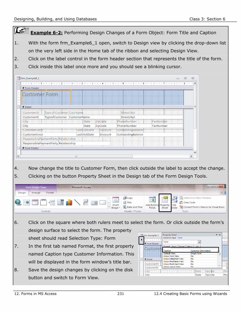
Designing, Building, and Using Databases Class 3: Section 6
12. Forms in MS Access 231 12.4 Creating Basic Forms using Wizards
Example 6-2: Performing Design Changes of a Form Object: Form Title and Caption
1. With the form frm_Example6_1 open, switch to Design view by clicking the drop-down list
on the very left side in the Home tab of the ribbon and selecting Design View.
2. Click on the label control in the form header section that represents the title of the form.
3. Click inside this label once more and you should see a blinking cursor.
4. Now change the title to Customer Form, then click outside the label to accept the change.
5. Clicking on the button Property Sheet in the Design tab of the Form Design Tools.
6. Click on the square where both rulers meet to select the form. Or click outside the form’s
design surface to select the form. The property
sheet should read Selection Type: Form
7. In the first tab named Format, the first property
named Caption type Customer Information. This
will be displayed in the form window’s title bar.
8. Save the design changes by clicking on the disk
button and switch to Form View.

Designing, Building, and Using Databases Class 3: Section 6
12. Forms in MS Access 232 12.4 Creating Basic Forms using Wizards
Example 6-3: Performing Design Changes of a Form Object: Sizing a Text Box control
1. Click inside the Street/Apt field of the first record. Now hit the down arrow key on your
keyboard. You noticed that there is a second line in this text box.
2. Now switch to design view.
3. Select all controls by using the rectangle or the ruler method below the Street/Apt textbox
control.
4. Using the Down Arrow key slowly move this group of controls downward.
5. Select the Street/Apt textbox control (white box) and click and hold on the bottom middle
square of the selection.
6. Drag this square down to increase the height of this text box.
7. If necessary, move the controls below this textbox up closer.
8. Save the design changes and switch to Form View. Verify that the textbox control now
displays the Street/Apt in its entirety.

Designing, Building, and Using Databases Class 3: Section 6
12. Forms in MS Access 233 12.4 Creating Basic Forms using Wizards
Using a Form
If the form contains more fields and other elements than can be accommodated in the form
window, or if the form window is resized to a smaller size, scroll bars will automatically appear if
the entire form as designed does not fit anymore in the form window as shown in Figure 115.
Figure 115: Horizontal and Vertical Form Scrollbars
Another distinct feature of the form window is that the descriptive information entered at the
table level for each field will be displayed in the status bar of the MS Access application window
once a user navigates to that field. That makes the optional description field even more
valuable. Important information about what kind of data to enter can be communicated to the
data entry user.
Note: The status bar is part of the Application window (the outer window) and not the form
window.

Designing, Building, and Using Databases Class 3: Section 6
12. Forms in MS Access 234 12.4 Creating Basic Forms using Wizards
Figure 116: Field Description in Status Bar
To navigate within the entire recordset, use the navigation buttons at the bottom. To navigate
within the fields of one record on a form, use the following methods:
Using a mouse: Simply click in a field or any other database control and update or enter values.
Using a keyboard: For most data entry users, using the keyboard and mouse is time consuming.
Most users would rather use only the keyboard.
To move from one field to another, simply use the [Enter] key or [Tab] key. If the field is a Long
Text field, using the [Enter] key simply breaks the line in the Long Text field, but does not move
to the next field. Therefore use the [Tab] key. If a form contains command buttons, navigating
to a command button can be done with the [Tab] key, however, pressing or pushing the button
must be done with the [Enter] key.

Designing, Building, and Using Databases Class 3: Section 6
12. Forms in MS Access 235 12.4 Creating Basic Forms using Wizards
Navigational Direction Keystrokes
Turn on Navigation Mode F2 (Entire field value is selected)
Next Field Tab, Enter, Right or Down Arrow key
Previous Field Shift+Tab, Left or Up Arrow key
First Field of current record Home, Ctrl+Home
Last Field of current record End, Ctrl+End
Next Record PgUp
Previous Record PgDn
Table 24: Keystroke Commands for Field Navigation
Note: The form must be in navigation mode for the keystroke commands to work properly.
Following are editing techniques using the keyboard: For example, for date/time fields to use the
current date, simply press the [Ctrl] + [;] keys, and the current date is inserted.
Note: An easier method to have the current date populated in a date/time field is to specify
a default value at the table design level of current date. The current date can be represented in
MS Access with the function Date().
Editing Technique Keystrokes
Move insertion point within field Left or right arrow key
Insert a value within a field Select the insertion point and type the new data
Select entire field F2 or double-click
Replace entire field value Select entire field and type the new data
Replace with value of preceding record Ctrl+’ (Apostrophe)
Insert the current Date Ctrl + ; (Semicolon)
Insert the current time Ctrl+Shift+: (Colon)
Insert the default value for a field Ctrl+Alt+Spacebar
Add a new record Ctrl+ +(Plus Sign)
Insert a new line Ctrl+Enter
Table 25: Keystroke Commands for Editing
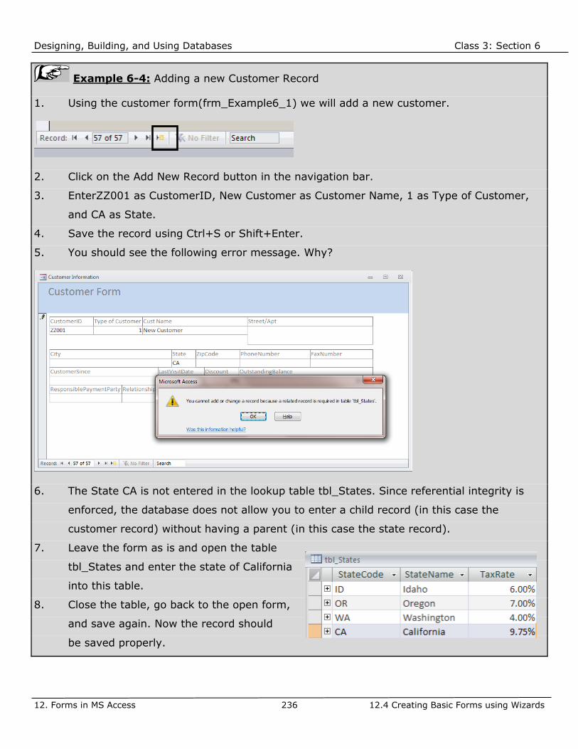
Designing, Building, and Using Databases Class 3: Section 6
12. Forms in MS Access 236 12.4 Creating Basic Forms using Wizards
Example 6-4: Adding a new Customer Record
1. Using the customer form(frm_Example6_1) we will add a new customer.
2. Click on the Add New Record button in the navigation bar.
3. EnterZZ001 as CustomerID, New Customer as Customer Name, 1 as Type of Customer,
and CA as State.
4. Save the record using Ctrl+S or Shift+Enter.
5. You should see the following error message. Why?
6. The State CA is not entered in the lookup table tbl_States. Since referential integrity is
enforced, the database does not allow you to enter a child record (in this case the
customer record) without having a parent (in this case the state record).
7. Leave the form as is and open the table
tbl_States and enter the state of California
into this table.
8. Close the table, go back to the open form,
and save again. Now the record should
be saved properly.

Designing, Building, and Using Databases Class 3: Section 6
13. Main/Sub Forms 237 13.1 Main/Sub Form Basics
13. Main/Sub Forms
One of the main features of relational databases is the one-to-many relationship to avoid
redundant data in spreadsheets or flat files. For this very reason, it is also important to
represent these relationships in form so that one can enter parent and child data using one
form.
13.1 Main/Sub Form Basics
The main/sub form is a configuration made up of at least two forms, the main form and the sub
form. This form type is used to display a One-To-Many relationship.
The main form is used to display information from the one side, one record per page, therefore
the main form is of type columnar (single).
The sub form is used to display the many side. Due to the fact that this form may need to
display many records in a confined space, the datasheet form type or the tabular form type is
most commonly used.
Figure 117 shows the all pets (many side) belonging to one customer (one –side). The main
form is based on a table or query using tbl_customer. The sub form shows information from the
pets table. Note the scrollbar at the right side of the sub form, this is an important tool to view
all many records in case the sub form height cannot accommodate all records.
Main Form
Sub Form
Figure 117: Main/Sub Form Configuration (Tabular Sub Form)

Designing, Building, and Using Databases Class 3: Section 6
13. Main/Sub Forms 238 13.1 Main/Sub Form Basics
Figure 118: Main/Sub Form Configuration (Datasheet Sub Form)
A main/sub form can be created with the form wizard, the same wizard we have used to create
forms based on single table.
The main difference lies in the first wizard step, where tables and fields are selected. At this
step, the user may select one table, select the desired fields for the form, and then select
another table, and select fields from that table to be displayed on a form.
MS Access detects among the fields selected for a form whether they come from one or more
tables. However, it is important that the user understands the data relationship of the database
and selects adjacent, related tables.
When more than one table is involved, the wizard will introduce additional steps for the user to
be completed in order to create a main/sub form.
Note: When the same field name is used in different tables (such as primary/foreign key),
the wizard differentiates the fields by prefixing them with the table name as shown in Figure
119.

Designing, Building, and Using Databases Class 3: Section 6
13. Main/Sub Forms 239 13.1 Main/Sub Form Basics
Figure 119: Form Wizard Step 1, Select Multiple Tables

Designing, Building, and Using Databases Class 3: Section 6
13. Main/Sub Forms 240 13.2 Creating a Main/Sub Form using Wizards
13.2 Creating a Main/Sub Form using Wizards
Creating a main/sub form is shown by using an example. A form is to be created showing for
each customer (parent record) all the pets belonging to that customer (child records). Creating a
main/sub form can only be performed with the Form wizard.
Example 6-5: Creating a Main/Sub Form using Form Wizard
1. Click on Form Wizard button in
the Forms group of the Home
tab.
2. Select tbl_Customer first and
move the following fields over
into the available fields
section:
CustomerName, Street/Apt,
City, State, ZipCode,
PhoneNumber.
3. Now do not click on Next,
select tbl_Pets from the
drop-down list.
4. Select the following fields:
PetID, PetName,
TypeOfAnimal,
DoB, Gender.
5. Click on Next.

Designing, Building, and Using Databases Class 3: Section 6
13. Main/Sub Forms 241 13.2 Creating a Main/Sub Form using Wizards
Example 6-5(continued): Creating a Main/Sub Form using Form Wizard
6. The next step is an important one as you choose exactly how to configure the Main/Sub
form.
7. On the left side you can choose the level of hierarchy, in this example by tbl_Customer
(Parent) or by tbl_Pets (child). If the child level is selected, your form will be a single form
displaying your data in a denormalized fashion (redundant parent records).
8. If you select a parent level, then you can choose from a form with a subform or a linked
form, which is a stand-alone, separate form window that filters its data based on the
current primary key of the parent form.
9. In the example, select tbl_Customer and Form with subform.
10. Click on Next.

Designing, Building, and Using Databases Class 3: Section 6
13. Main/Sub Forms 242 13.2 Creating a Main/Sub Form using Wizards
Example 6-5(continued): Creating a Main/Sub Form using Form Wizard
11. In this step, you have to decide whether your sub form should be a tabular or a datasheet
form type.
12. In this example, choose tabular. Click on Next.
13. This is the last step. Now there are entries for the title of the forms, again, we use the
object name here to name these forms correctly. Type frm_Example6_5 and
frm_Example6_5_sub.
14. Click on Finish.

Designing, Building, and Using Databases Class 3: Section 6
13. Main/Sub Forms 243 13.2 Creating a Main/Sub Form using Wizards
Example 6-5(continued): Creating a Main/Sub Form using Form Wizard
15. Your final form should like the one shown below:
16. We will make some minor design changes to fine-tune this form configuration.
17. Delete the label control for the sub form, move the State, ZipCode and PhoneNumber
fields to the right, and size the main and sub form so that no horizontal scroll bars are
displayed.

Designing, Building, and Using Databases Class 3: Section 6
14. Combo/List Box Controls 244 14.1 Introduction to Combo/List Box Controls
14. Combo/List Box Controls
Besides the textbox control the combo and listbox controls are probably the next important
ones. These controls are used for a variety of functions. MS Access provides some built-in
wizards to create and setup these controls.
14.1 Introduction to Combo/List Box Controls
The List and Combo box control are very special controls in that they can display data from other
tables or queries. These are the only two controls having a RowSource property similar to the
form’s RecordSource property. That means an underlying data source can be attached to these
controls besides the form’s underlying data source.
The data for a List or Combo Box control can be derived from a table or query, additionally the
data can be also stored in the control itself. This is advisable if there are only a few records and
fields.
Note: Storing static lookup data can be also achieved at the table level using Lookup Wizard
in the data type column.
A List or Combo box for a form can be already set up at the table level for a specific field. The
Lookup properties for a specific field allows the designer/developer to set up the data source,
and then specify the Display Control (List or Combo Box). Setting List or Combo boxes up at the
table level is in general not recommended as it will cause query problems, for example when
using criteria. You should use it only when you want to store static values as a lookup table.
The most important use of a List or Combo Box is to display lookup data from a lookup table,
and storing the primary key of the lookup table in the foreign key field of the child table the form
is based on.
The main differences between the List Box and the Combo Box controls are listed below:
1. A List Box control can display multiple rows and columns at all times, whereas a combo
box displays one row and one column at all times. Only when a combo box is activated by
clicking on the drop-down arrow, multiple rows and columns are displayed.
2. A List box control is limited to the values based on the underlying data source, whereas a
combo box is not (LimitToList property).

Designing, Building, and Using Databases Class 3: Section 6
14. Combo/List Box Controls 245 14.1 Introduction to Combo/List Box Controls
3. The List Box control allows for a multiple-selection feature (more than one row can be
selected), whereas the Combo box control only allows for one row to be selected. However, to
take advantage of this feature, the List box must be unbound and macros and/or VBA code must
utilized.
List Box Control Combo Box Control
Textbox Like Behavior
Listbox Like Behavior
Figure 120: ListBox and ComboBox Controls
When a combo box does not have the focus, it displays one value only (one row, one column).
The behavior is similar to a text box control. When a combo box is activated and the drop-down
arrow is clicked, the behavior is similar to a list box control.
Due to the design, the combo box takes up less space than the list box.
A combo or list box control can also be utilized as a navigational tool on a form. The combo or
list box contains the same underlying data as the form and when a record is selected, the form
navigates to that selected record.

Designing, Building, and Using Databases Class 3: Section 6
14. Combo/List Box Controls 246 14.2 Navigational Combo/List Boxes
14.2 Navigational Combo/List Boxes
In this chapter the navigational feature of a combo box or list box is covered in detail. Basically,
a combo or list box control may replace the navigation buttons at the bottom of the form. The
built-in wizards to create combo or list box controls are very helpful and powerful.
Rather than navigation by some kind of irrelevant number in the navigation bar you can use a
list box or combo box control to select a record by its data. This is much more meaningful and
useful.
Example 6-6: Creating a Navigation List/Combo box Control
1. Create a simple customer form by using the Form Wizard and selecting CustomerID
through PhoneNumber. Save the form as frm_Example6_6.
2. Navigate to Design View by clicking in the drop-down list on the left side in the Home tab.
3. In the Controls group of the Form Design contextual tab, select the combo box control
and drag a rectangle in the form’s header section as shown below.
4. After you release the mouse button, the first step of the list/combo box wizard is
launched.

Designing, Building, and Using Databases Class 3: Section 6
14. Combo/List Box Controls 247 14.2 Navigational Combo/List Boxes
Example 6-6 (continued): Creating a Navigation List/Combo box Control
5. Select the last option to utilize the navigational feature as shown below:
6. Click on Next.
7. Select CustomerID, CustomerName, and State as shown below:

Designing, Building, and Using Databases Class 3: Section 6
14. Combo/List Box Controls 248 14.2 Navigational Combo/List Boxes
Example 6-6 (continued): Creating a Navigation List/Combo box Control
8. These three fields will be used by the combobox. The CustomerID is the key field to
enable navigation to a specific record, and the CustomerName and State will be used as
display field. Click on Next.
9. Here you decide which fields to hide and which ones to show. The primary key field is by
default hidden (see checkbox).Size the CustomerName field to make it a bit wider and the
state field to make a bit narrower.
10. Click on Next.
11. In this last step, simply type in the label information as shown below:

Designing, Building, and Using Databases Class 3: Section 6
14. Combo/List Box Controls 249 14.2 Navigational Combo/List Boxes
Example 6-6 (continued): Creating a Navigation List/Combo box Control
12. Click on Finish. You may need to move the label control a bit to the left. The final form is
shown below.
13. Test the navigational feature of the combo box by selecting different values.
You see that the combo box control contains the same records as the form itself, except only a
few fields. A combo box control may display many fields, but when a value is selected and the
combo box list collapses, only one value is shown.

Designing, Building, and Using Databases Class 3: Section 6
14. Combo/List Box Controls 250 14.3 Lookup Combo/List Boxes
14.3 Lookup Combo/List Boxes
The most useful feature of the Combo/List box control is its ability to display data from a data
source other than the underlying data source on the form. Looking up data is the most common
use of Combo/List box controls. Particularly, the primary/foreign key concept plays an important
role in this discussion.
Consider the following example: On the form frm_Customer the state field is stored in the
customer table as a foreign key of the lookup table tbl_States. A combo box displaying the state
information is used to select the appropriate state, once a record is selected, the primary key
value is stored in the state field of the customer table (foreign key).
tbl_Customer
PK CustomerID
TypeofCustomer CustomerName Street/Apt CityFK1,I1 StateI3 ZipCodeI2 PhoneNumber FaxNumber CustomerSince LastVisitDate Discount OutstandingBalance ResponsiblePaymentParty Relationship
tbl_States
PK StateCode
StateName TaxRate
Row Source
Control Source
Figure 121: Combobox Lookup Relationship
This lookup setup can be established at the table level (not recommended) or at the form level.
At the table level, use the Lookup wizard “data type” to create the lookup, at the form level,
either use combo or list box wizard (available through the toolbox).

Designing, Building, and Using Databases Class 3: Section 6
14. Combo/List Box Controls 251 14.3 Lookup Combo/List Boxes
Example 6-7: Creating a Table Lookup Combo box Control
1. Use the simple customer form (frm_Example6_6) and switch to Design View.
2. Select the State textbox control and press the [Delete] key.
3. In the Controls group of the Design tab, click on the Combo box control and drag a
rectangle in the place where you deleted the State textbox control.
4. The first step of the wizard is displayed.
5. Select the first option, to lookup a table or query. Click on Next.
6. Select the table tbl_States. Click on Next.

Designing, Building, and Using Databases Class 3: Section 6
14. Combo/List Box Controls 252 14.3 Lookup Combo/List Boxes
Example 6-7(continued): Creating a Table Lookup Combo box Control
7. Select all fields. Click on Next.
8. Sort the data by StateName in ascending order. Click on Next.

Designing, Building, and Using Databases Class 3: Section 6
14. Combo/List Box Controls 253 14.3 Lookup Combo/List Boxes
Example 6-7(continued): Creating a Table Lookup Combo box Control
9. In this step you can configure which columns you want to show and size them accordingly
to the data they contain. The primary key column is hidden by default using the checkbox.
10. Make both columns a bit narrower and hide the primary key column. Click on Next.
11. In this step you link the selected value of the combo box to the column in the underlying
table. In this example you want the selected value (which is the statecode, first column)
to link to the State field in the customer table, which is the underlying table of the form.

Designing, Building, and Using Databases Class 3: Section 6
14. Combo/List Box Controls 254 14.3 Lookup Combo/List Boxes
Example 6-7(continued): Creating a Table Lookup Combo box Control
12. Click on Next.
13. In this last step, you simply create a label for the combo box. Type State:.
14. Click on Finish. Test the form by selecting a different state from the combo box. Note that
the pencil is displayed in the record selector bar because you changed the value of the
state in the first record of the customer table.

Designing, Building, and Using Databases Class 3: Section 6
14. Combo/List Box Controls 255 14.3 Lookup Combo/List Boxes
In the last example we create a list box lookup control. The only difference is that we are not
pulling data from a lookup table, we are typing the values (since there are so few) directly as a
static table into the control.
Example 6-8: Creating a Static Lookup List box Control
1. Use the simple customer form (frm_Example6_6) and switch to Design View.
2. Select the TypeOfCustomer textbox control and press the [Delete] key.
3. Select all controls below and move them downward so to create more space for the list
box control.
4. In the Controls group of the Design tab, click on the List box control and drag a rectangle
in the place where you deleted the TypeOfCustomer textbox control.
5. The first step of the wizard is displayed. Select the second option.
6. Click on Next.

Designing, Building, and Using Databases Class 3: Section 6
14. Combo/List Box Controls 256 14.3 Lookup Combo/List Boxes
Example 6-8(continued): Creating a Static Lookup List box Control
7. Type 2 for the number of columns at the top. Then type the values as shown below.
8. As you can see, this is a little lookup table, except it is not stored in the database but
directly at the control level. Click on Next.
9. In the next step you designate which of the two columns are to be stored in the control
and eventual into the field of the underlying table of the form. It is good practice to
always use the first column as the ID or key column. Click on Next.

Designing, Building, and Using Databases Class 3: Section 6
14. Combo/List Box Controls 257 14.3 Lookup Combo/List Boxes
Example 6-8(continued): Creating a Static Lookup List box Control
10. In this step, you link the value that is stored in the control to a field in the underlying
datasource of the form. Select the TypeOfCustomer field and click on Next.
11. In the last step you simply create the label control. Type Type of Customer:.
12. Click on Finish.
13. Save the form and then switch to datasheet view to test the listbox control.

Designing, Building, and Using Databases Class 3: Section 6
14. Combo/List Box Controls 258 14.3 Lookup Combo/List Boxes
(This page is left intentionally blank)

Designing, Building, and Using Databases Class 4: Section 7
15. Introduction to Reports 259 15.1 Reports Basics
CLASS 4: SECTION 7
15. Introduction to Reports
Reports are nothing but formatted output. However, the report writer tool that comes with MS
Access is very powerful and allows you to assemble and display your data in any way, even
more sophisticated than queries can do
15.1 Reports Basics
So far, the main focus has been on getting the data into a database and viewing data. Finally,
we are at a point where the formatted data output is discussed. Reports are very powerful in
that the information can be even more analyzed than with the query tool. The report tool is a
very effective way to present data in a printed document.
Reports have more features than forms or queries, especially in presenting summary
information. As we will see, creating reports is very similar to creating forms.
Since reports are used for formatted data output, there is no need to modify data through a
report. Consequently, unlike forms, reports are mostly based on queries, even on queries which
are not updateable.
What are Reports?
Reports organize and format information to fit user specifications. They retrieve data from the
database and through the use of queries present the information in a meaningful way.
Some examples of reports are shown below
➢ Mailing Labels
➢ Invoices
➢ Sales Summaries
➢ Telephone Lists
➢ Dashboards

Designing, Building, and Using Databases Class 4: Section 7
15. Introduction to Reports 260 15.1 Reports Basics
Note: Reports are very similar to forms, however, due to the fact that no data is entered
through a report, there are fewer types of controls on a report.
Reports have different design elements, such as static text, data, pictures, lines, boxes and
graphs.
Note: Since color printers are still quite expensive to maintain, and reports can be very
lengthy, almost no colors are used in reports. Black and white as well as gray shades are the
best format elements to emphasize data or groups of data.
Why use Reports?
Reports are an efficient way to print information that is used regularly. Report design is saved in
MS Access, but not the data. The most current data will be retrieved from the database every
time a report is run. If your reporting needs change, you can adjust the report design or create
a similar report based on the original report.
Capabilities of Reports:
➢ Organize and present data in groups.
➢ Calculate running totals, group totals, grand totals, and percentages of totals.
➢ Include sub reports.
➢ Include graphs.
➢ Present data in an attractive format.
In Figure 122 you see an example of a report with some of the sophisticated features, such as
sub reports, sub totals, and grouping.

Designing, Building, and Using Databases Class 4: Section 7
15. Introduction to Reports 261 15.1 Reports Basics
Sub Reports
Grouped By Customers
Graphs
Sub Totals
Figure 122: Report Example Showing Distinct Features
As with forms, reports are based on a table or query. Reports can be also based on a Parameter
Query. When the user executes the report, the parameter query is run first. The user then
enters run time parameters and views the resulting data in form of a report.

Designing, Building, and Using Databases Class 4: Section 7
15. Introduction to Reports 262 15.1 Reports Basics
Grouping of Data
One of the main features is that data can be grouped in almost any way. Grouping is a feature
forms do not have, and grouping is more powerful than the Group By option in a total query.
Example 7-1: Creating a Basic Report Using Grouping
1. In the Create tab, Reports group, click on the Report Wizard button.
2. Select table tbl_Customer, then TypeOfCustomer, CustomerName, City, and State.
3. Click on Next.
4. MS Access automatically groups the report data by state (because there are so few,
distinct values). Add TypeOfCustomer and City to the grouping by clicking on the right
arrow.
5. Click on Next.

Designing, Building, and Using Databases Class 4: Section 7
15. Introduction to Reports 263 15.1 Reports Basics
Example 7-1 (continued): Creating a Basic Report Using Grouping
6. In this step you set the sort order after the grouping, meaning in this example for the
customer name field. Select CustomerName and click on Next.
7. In this next step you can select certain styles and the page orientation. Leave everything
as is. Click on Next.
8. As with forms, use a meaningful object name for the title as this entry will be also used as
the object name. Type rpt_Example7_1 and click on Finish.

Designing, Building, and Using Databases Class 4: Section 7
15. Introduction to Reports 264 15.1 Reports Basics
Report Sections
Because of this rich grouping feature, the design view of a report may look quite complex. Each
group of data may have a header and a footer section.
Note: Forms can have only one header and one footer section whereas reports can have
many such sections, one set for each group by section.
The header is reserved for introducing the group and displaying the value by which its data is
grouped, and the footer may contain summary information of that group.
Each group header, group details (the data records), and the footer is represented by gray
horizontal bands in the report design view.
In between these bands, text boxes or labels are placed to show information. And additional
design elements may emphasize data in certain sections and under certain circumstances.
State Header
Type of Customer Header
City Header
Detail Section
Figure 123: Report Group Sections
After all the grouping is performed, there is only one detail section. This section is used for the
remainder of the data that is not grouped. In our example, we only included four fields, three of
which were used to group the data, therefore only one field, the CustomerName is left and

Designing, Building, and Using Databases Class 4: Section 7
15. Introduction to Reports 265 15.1 Reports Basics
displayed in the detail section. Any customer record that falls within this particular grouping is
displayed here.
Note: The detail section must be used to display multiple record data. The header and footer
sections are used to display distinct grouping values (header) or summarized data (footer).
Besides the group header and footer sections and the detail section there are other report
sections.
Page Header Page Header Page Header
Page Footer
Report Header
Report FooterGroup Header
Group Header
Group Header
Group Footer
Group Footer
Group Footer
Detail Section
Detail Section
Detail Section
Page Footer Page Footer
Figure 124: Other Report Sections
The report header is displayed once at the beginning of the report. Note that this section can
span multiple pages.
The report footer is displayed at the end of report, after where the last row is printed on the
report. Note that this can be anywhere on the page, it does not have to be at the bottom.
The page header is displayed at the top of each physical page. It can be turned off for the report
header page only, for the report header footer page, for both report header and footer, or for all
pages.
The page footer is printed at the bottom of each physical page. As with the page header, it can
be turned off in the same way as the page header.
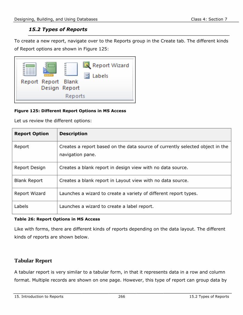
Designing, Building, and Using Databases Class 4: Section 7
15. Introduction to Reports 266 15.2 Types of Reports
15.2 Types of Reports
To create a new report, navigate over to the Reports group in the Create tab. The different kinds
of Report options are shown in Figure 125:
Figure 125: Different Report Options in MS Access
Let us review the different options:
Report Option Description
Report Creates a report based on the data source of currently selected object in the
navigation pane.
Report Design Creates a blank report in design view with no data source.
Blank Report Creates a blank report in Layout view with no data source.
Report Wizard Launches a wizard to create a variety of different report types.
Labels Launches a wizard to create a label report.
Table 26: Report Options in MS Access
Like with forms, there are different kinds of reports depending on the data layout. The different
kinds of reports are shown below.
Tabular Report
A tabular report is very similar to a tabular form, in that it represents data in a row and column
format. Multiple records are shown on one page. However, this type of report can group data by

Designing, Building, and Using Databases Class 4: Section 7
15. Introduction to Reports 267 15.2 Types of Reports
more than one field, and it can summarize and analyze data on a per group basis (using Report
Wizard).
A tabular report can also have snaked columns to create directories, such as a customer
directory. Snaked columns are columns where the data are sorted either first vertically, then
horizontally or first horizontally, and the vertically.
Figure 126: Tabular Report with Sub and Grand Totals

Designing, Building, and Using Databases Class 4: Section 7
15. Introduction to Reports 268 15.2 Types of Reports
Figure 127: Tabular Report without Totals

Designing, Building, and Using Databases Class 4: Section 7
15. Introduction to Reports 269 15.2 Types of Reports
Columnar Report
Columnar reports normally display one record per page, however, in case the underlying data
source contains only a few fields, more than one record may be displayed on one page.
The fields are always arranged in one column.
This type of report is also known as form report.
Figure 128: Columnar Report

Designing, Building, and Using Databases Class 4: Section 7
15. Introduction to Reports 270 15.2 Types of Reports
Mailing Label Report
The Mailing Label wizard arranges data to fit on specific mailing labels. The user may choose
from pre-defined label styles, and the wizard will place the data correctly on the label for print
out.
This type of report, however, can also be used to create other documents such as directories,
which are not intended to be printed on mailing labels.
Figure 129: Mailing Label Report

Designing, Building, and Using Databases Class 4: Section 7
15. Introduction to Reports 271 15.2 Types of Reports
Chart Report
Chart reports use an OLE object to create the chart control embedded in a report which is same
as in MS Excel.
To create a chart report, the user usually creates a query and includes only fields necessary for
the chart control.
Figure 130: Chart Report
To create a chart in a report or form, you need to use the Form or Report design selection and
then drag a chart control onto the form or report. A chart wizard does not exist anymore as in
previous version of MS Access.

Designing, Building, and Using Databases Class 4: Section 7
15. Introduction to Reports 272 15.3 Designing Reports
15.3 Designing Reports
Creating reports is different from creating forms in that more data are compiled on a report and
more consideration must be given to the layout and the design of the report before creating a
report.
One of the first steps is most likely to create a query and view the data. Then using this query or
queries the user may want to manipulate criteria or sorting order and inspect the resulting data
in order to get familiar with the data and to get ideas for the report layout.
A report can be unbound, that is, not displaying any database information. One reason for that is
a report could serve as an internal help file containing user instructions or other documentation
about the database. An unbound report could be also a static cover letter for other reports.
Furthermore, an unbound report could hold two unrelated sub reports.
For a bound report, the data source for a report is most likely a query. Create a query and
include all fields necessary, or select all fields in the query and then select the desired fields in
the report wizard. A parameter query can be used too for reports, making the report even more
dynamic in that the user selects criteria to filter the data for the report.
Example 7-2: Creating a Tabular Report based on tbl_Customer
1. Create a query based on tbl_Customer, select TypeOfCustomer, CustomerName, City and
State.
2. Save the query as qry_Example7_2.
3. Close the query but make sure that the query is still selected in Navigation Pane.
4. In the Create tab, Reports group, click on the Report button.
5. An automatic tabular report based on the currently selected object in the Navigation Pane
is created.
6. In the Design Tab of the Report Design Tools click on the drop-down list on the left side.

Designing, Building, and Using Databases Class 4: Section 7
15. Introduction to Reports 273 15.3 Designing Reports
Example 7-2 (continued): Creating a Tabular Report based on tbl_Customer
7. Select Print Preview to view the report.
8. Save the query as rpt_Example7_2.

Designing, Building, and Using Databases Class 4: Section 7
15. Introduction to Reports 274 15.3 Designing Reports
The navigation buttons at the bottom (only visible when in Print Preview) are designed to
navigate on per page basis, not by records. For large reports, you can type a page number into
the page text box and press the [Enter] key to navigate to that page.
Figure 131: Report Navigation Bar
In the Design Tab of the Report Design Tools contextual tab on the very left side you have the
same functionality as with forms, that is to switch between different views. Since there is one
more view for reports, we will cover all those views now. The drop-down arrow shows a list of
views as Figure 132.
Figure 132: Report View Options
Table 27 lists the different views and their particular meaning. The Report View and Print
Preview options only apply to reports. Forms have a Form View, which is exactly the same as
Report View for reports. And Design View also applies to both forms and reports and exhibits the
exact the same behavior.
Warning: If you do not see the layout view option in the drop-down list, then navigate to
options in Backstage view, under Current Database, verify that Enable Layout View is turned on.

Designing, Building, and Using Databases Class 4: Section 7
15. Introduction to Reports 275 15.3 Designing Reports
View Applies To Description
Forms The final view of a form, the form is presented in the form
window to the user. Using this view, the user can interact
with the data displayed on the form or perform other
actions, such as clicking a command button. No design
changes are allowed.
Reports The final view of a report, but without pagination. No
design changes are allowed.
Forms, Reports This view is part design view and part form/report view.
You see actual, live data, but you can also make still some
minor design changes. This is particular useful for sizing
controls to fit the data.
Reports The final view of a report with pagination. This is the exact
representation of the report when sent to a printer. This
view is important to verify page breaks, especially when
using grouping. The Navigation Bar is visible for this view
only.
Forms, Reports This view is used to use all design tools, but no actually
data is displayed. For example, you use this view to add a
control, but layout view to size the control according to
your data.
Table 27: Form/Report Views
When using Print Preview, you also have the option to zoom in and zoom out using the right side
of the application Status Bar. Additionally, you can also switch views using the buttons in the
Status Bar.
Note: You can also simply click inside the report when using Print Preview to perform a one-
step zoom in and out. You notice that the mouse pointer shape changes to a magnifying glass.

Designing, Building, and Using Databases Class 4: Section 7
15. Introduction to Reports 276 15.3 Designing Reports
View Buttons Zoom Control
Figure 133: Status Bar View Buttons and Zoom Control
Occasionally, a report can include unexpected blank pages. Typically, these occur when the
dimensions of the report exceed the paper size. The total width of the report plus the margins
should not exceed the paper size specified, see Figure 134.
Another issue related to blank pages is that a report may contain a lot of white, unprinted space.
This is due to one control using more space than other adjacent controls. View the report in
layout view and resize controls or move controls to reduce white space.
Note: Sometimes other control properties must be set in order to reduce white space. This is
discussed in the Intermediate Access course.

Designing, Building, and Using Databases Class 4: Section 7
15. Introduction to Reports 277 15.3 Designing Reports
Page 1
Page 2
Figure 134: Report Width + Margins Exceed Paper Size
To specify page setup option, use the Page Setup tab under Report Design Tools. To access all
options in one tabbed, dialog box, click on Page Setup button.

Designing, Building, and Using Databases Class 4: Section 7
15. Introduction to Reports 278 15.3 Designing Reports
The dialog box and its three different tabs are shown in Figure 135.
Figure 135: Page Setup Dialog Boxes
Margins can be set on the Print Options tab. The minimum margins depend on the printer
selected. The checkbox Print Data Only, if selected, omits labels for text boxes, and any other
graphic elements such as lines, pictures, etc.
The page tab contains the page orientation (Portrait or Landscape) and the paper size (Letter,
Legal, etc.). For printers with more than one tray, a specific tray can be selected. For example, a
report should be printed out on colored paper, which is stored in tray 2. Or it can be set to
Manual Feed, so that the user can feed a label sheet for a mailing label report. Select a specific
printer if different from the default printer set up in the windows environment.
The layout of a columnar report can be set in the columns tab. The number of columns, the size
and the spacing as well as the column layout can be specified in this tab.
Figure 136: Column Layout Options
The column layout can be set as first going horizontally across, then snake down to the next
row. The other option is to first go vertically down on column, and then snake across to the top
of the next column.

Designing, Building, and Using Databases Class 4: Section 7
16. Creating Reports using Wizards 279 16.1 Defining the Report Layout
16. Creating Reports using Wizards
The report wizard process is similar to the form wizard. However, there are some different steps
due to the different nature of reports in terms of data grouping.
16.1 Defining the Report Layout
Before using the report wizard, special consideration must be given to the report layout, such as
fields needed, layout of fields, and grouping of data. Then the data needs to be assembled
together using one or more queries. Then the report generation using a wizard can be started.
Figure 137: Report Layout Sketch
Figure 137 shows an example how a report should be sketched out by simply using paper and
pencil. It is especially important for the database developer/designer to ask appropriate
questions to those users asking for these reports, so that there is a common agreement from
the onset of the report generation. It is always more time consuming to make major changes to
database objects once they are in production.

Designing, Building, and Using Databases Class 4: Section 7
16. Creating Reports using Wizards 280 16.1 Defining the Report Layout
Daily Hospital Report - [VisitDate]
Customer Name Pet Name Type of Animal Total Amount
[---------------------]
[--------][--------][--------]
[--------][--------][--------]
[--------][--------][--------]
[---------------------]
[--------][--------][--------]
[--------][--------][--------]
[--------][--------][--------]
Customer Total [--------]
Grand Total [--------]
Figure 138: Report Sketch for Daily Hospital Report
The example in Figure 138 shows that the report is grouped by Customer Name, and then for
each customer listing the Pet Name, the Type of Animal, and the Total Amount for each pet. The
customer total is to be calculated at the end of each customer group.
At the end of the report, a grand total is to be calculated. The title of the report is Daily Hospital
Report, and showing the visit date.
Note that the Pet Name and the Type of Animal fields belong to the Pets table, and the Total
Amount field belongs to the Visit table. However, these three fields are grouped together,
something we need to recognize later in the wizard generation process.
Before even thinking about building the report it is import to create the appropriate data
source(s) for your report. Building the query, testing the query, and incorporating parameters
are the first steps.

Designing, Building, and Using Databases Class 4: Section 7
16. Creating Reports using Wizards 281 16.1 Defining the Report Layout
Example 7-3: Creating the Daily Hospital Report
1. Create a query based on tbl_Customer, tbl_Pets and tbl_Visits.
2. Select the following fields:
CustomerName, PetName, TypeOfAnimal, TotalAmount, VisitDate
3. Save the query as qry_Example7_3.
4. Switch to Datasheet view and take a look at the data.
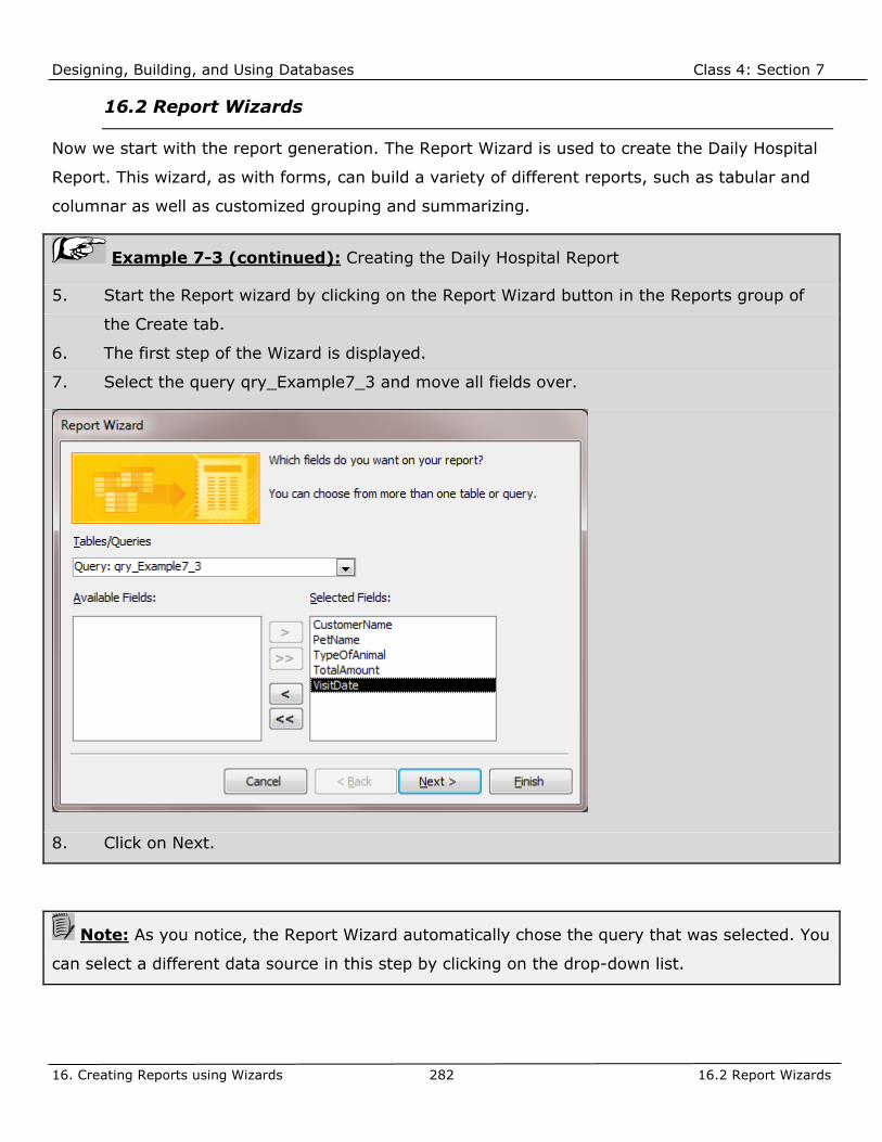
Designing, Building, and Using Databases Class 4: Section 7
16. Creating Reports using Wizards 282 16.2 Report Wizards
16.2 Report Wizards
Now we start with the report generation. The Report Wizard is used to create the Daily Hospital
Report. This wizard, as with forms, can build a variety of different reports, such as tabular and
columnar as well as customized grouping and summarizing.
Example 7-3 (continued): Creating the Daily Hospital Report
5. Start the Report wizard by clicking on the Report Wizard button in the Reports group of
the Create tab.
6. The first step of the Wizard is displayed.
7. Select the query qry_Example7_3 and move all fields over.
8. Click on Next.
Note: As you notice, the Report Wizard automatically chose the query that was selected. You
can select a different data source in this step by clicking on the drop-down list.

Designing, Building, and Using Databases Class 4: Section 7
16. Creating Reports using Wizards 283 16.2 Report Wizards
Example 7-3 (continued): Creating the Daily Hospital Report
9. This step is similar to the form wizard step, where you specify how to view the data from
a relational hierarchy perspective.
10. Since there are three tables involved, you can view the data in three different hierarchical
perspectives.

Designing, Building, and Using Databases Class 4: Section 7
16. Creating Reports using Wizards 284 16.2 Report Wizards
By table tbl_Customer
Table customer is at the top of the relationship
hierarchy. Therefore grouping is performed
along the relational path, first by table
customer (CustomerName), then by table Pets
(PetName, TypOfAnimal), and finally by table
visits(Total Amount, VisitDate).
By table tbl_Pets
Now the data from table pets and any other
table hierarchically above the table pets are
grouped together (CustomerName, PetName,
TypeOfAnimal), and then the last table
grouped beneath, the table visit
(TotalAmount, VisitDate).
By table tbl_Visits
Since table visits is hierarchically the lowest
table, all fields are grouped together at one
level.

Designing, Building, and Using Databases Class 4: Section 7
16. Creating Reports using Wizards 285 16.2 Report Wizards
Example 7-3 (continued): Creating the Daily Hospital Report
11. Since the desired grouping cannot be achieved in this step, select table visits so that all
fields are grouped together at one level. In the next step the user can add customized
grouping by any field. Click on Next.
12. Select CustomerName as a grouping field. Now this grouping reflects what the design
specification prescribes. Click on Next.
This step allows for additional grouping by fields. The previous, hierarchical grouping will be
retained, and additional grouping can be selected here.
Depending on which table was selected as a grouping option in the previous step, not all the
fields will be available.
For this example, since no grouping was selected in the previous step, select the customer name
field as an additional grouping field. Note that the customer name field is blue now and is moved
to a new group above the previous group.
Note that once a grouping has been selected, the Grouping Options button becomes available.

Designing, Building, and Using Databases Class 4: Section 7
16. Creating Reports using Wizards 286 16.2 Report Wizards
Note: The Grouping Options button is available only when additional grouping fields are
selected. Furthermore, grouping options vary by data type.
Click on the Grouping Options button in the lower left hand corner. The dialog box as shown in
Figure 139 is displayed.
Figure 139: Grouping Options Dialog Box
By default, all custom grouping fields are grouped normal, that means by their entire value.
However, the user can now specify even more detailed grouping levels within one field. This is
one of the powerful features of MS Access reports. The available grouping intervals depend on
the data type as shown in Table 28.
Data Type Grouping Options Description
Text 1st Letter, 2 Initial
Letters, etc.
Grouping is performed on the beginning part of the field,
such as first letter, the first two letters, etc.
Number 10s, 50s, 100s,
200s
Grouped in intervals of the specified interval. For example,
if 100s is selected, the values are grouped by 0-99.99..,
100-199.99…, 200-290.99.., etc.
Date/Time Year, Month, Day,
etc.
Grouped by the specified date part, such as month for
example.
Table 28: Grouping Options by Data Type

Designing, Building, and Using Databases Class 4: Section 7
16. Creating Reports using Wizards 287 16.2 Report Wizards
Text Number Date/Time
Figure 140: Grouping Options by Data Type Drop Down Menus
An example of a grouping by 1st letter is shown in Figure 141.
Figure 141: Text Field Grouping Report Example

Designing, Building, and Using Databases Class 4: Section 7
16. Creating Reports using Wizards 288 16.2 Report Wizards
An example of an interval grouping is shown in Figure 142.
Figure 142: Number Field Grouping Report Example
If you need other ranges or more initial letters, then you have to manually edit the report in
design view and make those changes. This is part of the next course, the Intermediate Access
course.

Designing, Building, and Using Databases Class 4: Section 7
16. Creating Reports using Wizards 289 16.2 Report Wizards
An example of a Date grouping is shown in Figure 143.
Figure 143: Date Field Grouping Report Example

Designing, Building, and Using Databases Class 4: Section 7
16. Creating Reports using Wizards 290 16.2 Report Wizards
Example 7-3 (continued): Creating the Daily Hospital Report
13. In this step you set the grouping of the detail section. Grouped fields are automatically
sorted in ascending order. Set the sort order to TypeOfAnimal, then PetName.
14. Note the Summary Options button at the bottom. This is yet another powerful feature of
the report wizard.
Warning: This button is only enabled if, at least one numeric or currency field is contained
in the data source and, if at least one grouping field has been set, either hierarchical or custom
grouping.
The summary feature allows you to aggregate the data in the report. The following aggregate
functions can be used to summarize data:
➢ Sum
➢ Avg
➢ Max
➢ Min

Designing, Building, and Using Databases Class 4: Section 7
16. Creating Reports using Wizards 291 16.2 Report Wizards
Furthermore, two choices are available how the summaries are displayed in the report.
Detail and Summary:
The report shows all detail records and aggregate function is calculated for the details records at
each group level as well as at the end of the report (grand total).
Figure 144: Detail & Summary Setting
Summary Only:
The report shows only the summary values for each group, but not the detail records.
Figure 145: Summary Only Setting

Designing, Building, and Using Databases Class 4: Section 7
16. Creating Reports using Wizards 292 16.2 Report Wizards
Calculate Percent of Totals for Sums:
If the checkbox “Calculate Percent of Total for Sums” is checked, then the report displays for
each total the percentage of that total to the grand total.
Figure 146: Calculate Percent of Totals
Example 7-3 (continued): Creating the Daily Hospital Report
15. Click on the Summary Options button and select the Sum checkbox. This will calculate the
sum of the Total Amount field for every customer record.
16. Click on Next.

Designing, Building, and Using Databases Class 4: Section 7
16. Creating Reports using Wizards 293 16.2 Report Wizards
Example 7-3 (continued): Creating the Daily Hospital Report
17. In this step you simply decide the main layout style and the page orientation. The
checkbox at the bottom is important as it includes all selected fields regardless of whether
they all fit on the page or not. If they do not fit, the size of the textbox controls is reduced
to make them fit. You can later in Design View fine tune the controls.
18. Click on Next.
19. The last step is assigning the report an object name which also becomes the title of the
report. We can change the title later in Report Design, again it is important here to choose
a meaningful object name. Type rpt_Example7_3 into the title textbox control.
20. Click on Finish.
As with all wizard processes, the final output is not perfect or even near perfect. Some or more
modifications have to be made. We will change the title, remove the summary for customer

Designing, Building, and Using Databases Class 4: Section 7
16. Creating Reports using Wizards 294 16.2 Report Wizards
control (too much clutter), adjust the VisitDate field (since it is showing pound (#) symbols and
move the label Sum and Grand Total labels more to the right.
Example 7-4: Performing Design Changes for Daily Hospital Report
1. Switch to Design View.
2. Click inside the title label control, and then click once more to see the insertion point. Now
type Daily Hospital Report. Then click outside the label control.
3. Select the label controls TypeOfAnimal, PetName, TotalAmount and VisitDate and the
corresponding label controls and move them to the left by using the left arrow key on
your keyboard.
4. Reduce the width of the PetName label and textbox control and increase the width of both
labels and textboxes of the TotalAmount and the VisitDate.
5. Delete the wide control which reads “Summary for ..”.
6. Move the Sum and the Grand Total labels to the right closer to the actual textbox that
displays the sum. Align the sum textboxes with the TotalAmount textbox.
7. Select the sum textbox control, display the property sheet, and set the format property to
Currency.
8. Save the report and view the report.

Designing, Building, and Using Databases Class 4: Section 7
16. Creating Reports using Wizards 295 16.2 Report Wizards
Example 7-4 (continued): Performing Design Changes for Daily Hospital Report
9. The print preview of the report is shown below.
10. The last big change will be to add a parameter for the VisitDate field in the query since we
want to run this report for specific days only. Hence the VisitDate field in the details
section will always carry the same value. Therefore we can move it into the header
section.
11. Open the query qry_Example7_3 in design view and add a parameter for the VisitDate
field in the criteria row reading [Enter a Visit Date]. Save and close the query.

Designing, Building, and Using Databases Class 4: Section 7
16. Creating Reports using Wizards 296 16.2 Report Wizards
Example 7-4 (continued): Performing Design Changes for Daily Hospital Report
12. Navigate to the report rpt_Example7_3 in design view.
13. Select the VisitDate textbox control, press Ctrl + X to cut and click inside the Header
section.
14. Press Ctrl + V to paste. The control is positioned at the upper, left hand corner. Move it to
the right of the title.
15. Repeat these steps for the label VisitDate and adjust the label and textbox controls in the
Header section. The design view of the header section is shown below:
16. Save the report and run the report. Use the following Visit Dates to test the report:
8/17/2011, 9/16/2012.

Designing, Building, and Using Databases Class 4: Section 7
16. Creating Reports using Wizards 297 16.3 Creating a Main/Sub Report
16.3 Creating a Main/Sub Report
This chapter explains the generation of a main/sub report. The process is very similar to forms
except for the report specific features pointed out earlier. You have two options here:
Create a query involving all necessary tables and fields and base the report on this query.
Use the report wizard and select all tables and fields necessary through the wizard.
The main difference between these two methods is that the first method creates a separate
query object to build the report. When exporting the report object into a different database
(from development into production, for example), you need to export the query as well. The
report wizard method stores the query definition inside the report, so there is no external query
object.
If the query is complex and involves lots of data, use an external query object because MS
Access will optimize this query when it is executed. For simple queries/reports you can use the
report wizard method, hence you do not generate too many query objects in your database.
Example 7-5: Creating a Main/Sub Report showing Customer and Pets
1. Launch the report wizard.
2. In the first step, select tbl_Customer first, then CustomerID, CustomerName, City, and
State.
3. Now select tbl_Pets and the fields PetName, TypeOfAnimal, DoB, and Gender.

Designing, Building, and Using Databases Class 4: Section 7
16. Creating Reports using Wizards 298 16.3 Creating a Main/Sub Report
Example 7-5 (continued): Creating a Main/Sub Report showing Customer and Pets
4. Click on Next.
5. This is the hierarchical view step, leave everything as is, meaning the parent information
(Customer) is grouped by to show for each customer their respective pets. Click on Next.
6. We want to group our customer records by state. Therefore, add the state field as an
additional custom group field.
7. Click on Next.

Designing, Building, and Using Databases Class 4: Section 7
16. Creating Reports using Wizards 299 16.3 Creating a Main/Sub Report
Example 7-5 (continued): Creating a Main/Sub Report showing Customer and Pets
8. This step involves sorting the data in the detail section. Select TypeOfCustomer, then
PetName. Click on Next.
9. The report layout option, the page orientation, and the checkbox to adjust the fields
should be all selected as is. Click on Next.

Designing, Building, and Using Databases Class 4: Section 7
16. Creating Reports using Wizards 300 16.3 Creating a Main/Sub Report
Example 7-5 (continued): Creating a Main/Sub Report showing Customer and Pets
10. Type rpt_Example7_5 as the object name/title in the last step. Click on Finish.
11. View the report and page through the report.
12. Change the report title to Customer and Pets, move the fields to the left so that the DoB
field can be widened to fit the data.

Designing, Building, and Using Databases Class 4: Section 7
16. Creating Reports using Wizards 301 16.4 Creating a Mailing Report
16.4 Creating a Mailing Report
Creating a mailing label report using the Label Report wizard is a streamlined process that you
do not want to perform manually. Setting up a mailing label manually is quite time consuming
and tedious considering the various margins and padding measurements, see Figure 147.
Figure 147: Custom Mailing Label Setup
To create a mailing label report, you need to have the data source selected before you run the
wizard. Either select a table or create a query first and then run the mailing label wizard. Keep in
mind that this kind of report is not necessarily always used just for mailing labels. You can print
information in a very compact format, such as a customer listing.
To launch the wizard, select a table or query, then in the Create tab click on Labels.
Figure 148: Label Report Wizard

Designing, Building, and Using Databases Class 4: Section 7
16. Creating Reports using Wizards 302 16.4 Creating a Mailing Report
Example 7-6: Creating Mailing Label Report
1. Select tbl_Customer in the Navigation Pane.
2. Launch the Mailing Label report wizard.
3. Select Avery 5160 as the mailing label format.
4. Click on Next.
5. Select semi-bold in the Font weight section.
6. Click on Next.

Designing, Building, and Using Databases Class 4: Section 7
16. Creating Reports using Wizards 303 16.4 Creating a Mailing Report
Example 7-6 (continued): Creating Mailing Label Report
7. Set up the label fields as shown below. Select the field, click the right arrow button. You
may use other literal characters such as blanks and commas.
8. Click on Next.
9. Specify the sort order by CustomerName.
10. Click on Next.

Designing, Building, and Using Databases Class 4: Section 7
16. Creating Reports using Wizards 304 16.4 Creating a Mailing Report
Example 7-6 (continued): Creating Mailing Label Report
11. In the last step simply provide the object name. There is no title for a mailing label reprt.
Type rpt_Example7_6.
12. Click on Finish.

Designing, Building, and Using Databases Class 4: Section 8
17. Advanced Forms/Reports 305 17.1 Creating Form Applications
CLASS 4: SECTION 8
17. Advanced Forms/Reports
Now we are at a point where we covered the main building blocks of a database application,
tables, queries, forms and reports. We will now take a look at integration those blocks into more
coherent application components.
17.1 Creating Form Applications
We have learned how to build a simple Master/Sub form configuration. In this chapter, we will
combine two Master/Sub form configurations together to create a form application.
We will take the Customer/Pets (frm_Example6_5) and the Visits/Visit Details
(frm_InClassPractice6_1) Master/Sub form configurations and combine them together through a
command button.
Now let us think what we are trying to do here. When we navigate to a specific customer record,
we can see all the pets that belong to that customer. Now we will create a button on the pets
form that will open up the Visits/Visit Details form for the selected pet only. Now we can scroll
through the visit records for that pet only and also see the visit details for each visit.
We have to open the pets sub form in design view and place a command button in the header
section of the form. Once a button is placed onto the form, a wizard is launched that will guide
us through the process of creating this particular feature.

Designing, Building, and Using Databases Class 4: Section 8
17. Advanced Forms/Reports 306 17.1 Creating Form Applications
Example 8-1: Combining two forms using a button control
1. Open subform frm_Example6_5_sub in design view.
2. In the Controls group of the Design tab, click on the command button control.
3. Move your mouse into the header section and drag a rectangle to place the button, then
release the mouse button. The first step of the command button wizard is launched.
4. Select Form Operations on the left side (Categories) and Open Form (Actions) on the right
side.
5. Click on Next.

Designing, Building, and Using Databases Class 4: Section 8
17. Advanced Forms/Reports 307 17.1 Creating Form Applications
Example 8-1 (continued): Combining two forms using a button control
6. In the second step, select the form to be opened, in this example frm_InClassPractice6_1.
7. Click on Next.
8. In the next step, you can choose between showing all records on the form or only filtered
records based on the currently selected record. We want the latter option, because for a
selected Pet we want to see the related Visit records.
9. Click on Next.

Designing, Building, and Using Databases Class 4: Section 8
17. Advanced Forms/Reports 308 17.1 Creating Form Applications
Example 8-1 (continued): Combining two forms using a button control
10. Now you have to define the linking fields for the record filtering. Select PetID on both
sides and then click the double-arrowed button in the middle. The linked information is
now displayed at the bottom.
11. Click on Next.
12. In this step you can choose to have an image displayed on your button or simply text.
Choose text and type Visit Information.
13. Click on Next.

Designing, Building, and Using Databases Class 4: Section 8
17. Advanced Forms/Reports 309 17.1 Creating Form Applications
Example 8-1 (continued): Combining two forms using a button control
14. In this last step, you simply assign a name to the button control. Use cmdVisits.
15. Click on Finish.
16. Close the form and open form frm_Example6_5. Click on Pet Fido, then click the button.
17. You should see 3 visit records for Fido.

Designing, Building, and Using Databases Class 4: Section 8
17. Advanced Forms/Reports 310 17.2 Using Chart Controls
17.2 Using Chart Controls
Overview of Chart Controls
Charts can be embedded in forms as well as in reports. It is a control which contains many
different types of charts. This control is very similar to the chart features in MS Excel.
To create a chart using the chart wizard, you need to either use an existing form or report and
navigate to form design. Then you create a chart control by selecting it from the Controls group
in the Design tab and placing it in your form or report. Then the wizard starts and guides you
through the process of building a chart. In order to build a form containing data and a chart, one
must do this manually.
Charts can be based on tables or queries. However, the chart wizard will create its own data
source for the chart control and convert the table or query into a total or crosstab SQL
statement.
When creating a query, make sure to include all fields to be used in the chart. Additionally, add
any required linking fields to the query. A linking field is necessary if you want to link the chart
to specific records, similar to a main/sub form configuration.
The chart control icon is shown below as it appears in the Controls group when in design mode
for a form or report.
Figure 149: Chart Control in Controls Group
Creating a Simple Form with Chart
We will create a pet form containing a chart in the next example. The basics steps are outlined
below:
1. First, a pet form must be created in columnar format.
2. Secondly, a chart must be generated using the visits table.
3. Third, the chart control linked to the pet information by virtue of the PetID field.

Designing, Building, and Using Databases Class 4: Section 8
17. Advanced Forms/Reports 311 17.2 Using Chart Controls
The first step is to create a pets form. We will create a simple form using the form wizard.
The next step involves creating a chart based on the visits table. This chart will show the total
amount spent over time (in months).
Finally, we will establish a link using PetID, this step is part of the wizard.
When the form is finished, the chart will display the total amount spent over time for the current
pet record in the pets form.
Example 8-2: Creating a form containing a chart
1. Launch the Form Wizard.
2. Select table tbl_Pets, then PetID,
PetName, TypeOfAnimal, DoB,
Gender.
3. Select Columnar Layout.
4. Save the form as
frm_Example8_2.
5. Switch to design view.
6. Widen the form window to the right and also increase the width of the form’s design area.
This is needed to make room for the chart control.
7. Click on the chart control in the Controls group of the design tab and draw a rectangle on
the right side of the form.
8. The first step of the chart wizard is launched.

Designing, Building, and Using Databases Class 4: Section 8
17. Advanced Forms/Reports 312 17.2 Using Chart Controls
Example 8-2 (continued): Creating a form containing a chart
9. Select tbl_Visits.
10. Click on Next.
11. Since we want to see how much money was spent on a selected pet over time, we select
VisitDate and TotalAmount.
12. Click on Next.

Designing, Building, and Using Databases Class 4: Section 8
17. Advanced Forms/Reports 313 17.2 Using Chart Controls
Example 8-2 (continued): Creating a form containing a chart
13. Select the type of chart. This can be changed later in design view as this is not always
obvious what the best type is until you view the chart. Select the 3-D Column Chart.
14. Click on Next.
15. This is probably the most important step. Here you place your data elements into the
appropriate places of your chart and decide on the aggregation of your data.

Designing, Building, and Using Databases Class 4: Section 8
17. Advanced Forms/Reports 314 17.2 Using Chart Controls
Example 8-2 (continued): Creating a form containing a chart
16. By default, MS Access calculates the sum of the TotalAmount field and places it on the y-
axis. It groups the VisitDate by month and places it on the x-axis. If you had a third data
element, you could place it on the z-axis.
17. Double-clicking on the gray data elements allows you to change the aggregation as shown
below:
18. You can preview the chart by clicking on the Preview button in the top left corner.
19. Click on Next.
20. In this step you set up the linking fields. By default MS Access links on fields having the
same name.

Designing, Building, and Using Databases Class 4: Section 8
17. Advanced Forms/Reports 315 17.2 Using Chart Controls
Example 8-2 (continued): Creating a form containing a chart
21. Click on Next.
22. In the last step you can type a title for the chart and specify whether you want a legend
or not. Type Visit Income History and do not display a legend.
23. Click on Finish.
24. Switch to Form View and scroll through the pet records.

Designing, Building, and Using Databases Class 4: Section 8
17. Advanced Forms/Reports 316 17.2 Using Chart Controls
Note: The title does not serve the additional purpose of a form or report object name as in
forms or reports. Since the chart is a separate control, after clicking on finish the form or report
can be saved separately using a different name.
When using charts to display data, data will be almost always grouped, unless you have only a
few data points. The grouping options of your data depends on the data type as shown in
Data Type Grouping Options
Text By distinct values only, no other grouping options available.
Number By distinct values only, no other grouping options available.
Date/Time By Year, Month, Day, etc.
Table 29: Grouping Options for Chart Controls
Warning: Since text and number fields are always grouped by their distinct values, double-
clicking on their items in the chart control causes the following message to display:
Modifying Charts
You can modify charts by navigating to design view of the form or report containing the chart
control. Then double-click on the chart control which will cause the Microsoft Graph application
to launch within the application window of MS Access as shown in Figure 150.
You notice that this application is still an old style application (no ribbon), you see the old
fashioned tool and menu bars. The menus apply only to the chart control.

Designing, Building, and Using Databases Class 4: Section 8
17. Advanced Forms/Reports 317 17.2 Using Chart Controls
Figure 150: Microsoft Graph Application within MS Access
Select the menu option Chart, the Chart Options. This is the central dialog box that allows you to
change the format of your existing chart. Another option under the chart menu is the chart type
allowing you to choose a different chart type.
Figure 151: Chart Options Dialog Box

Designing, Building, and Using Databases Class 4: Section 8
17. Advanced Forms/Reports 318 17.2 Using Chart Controls
There are many more options to modify an existing chart, covering them all here is beyond the
scope of this course.
Example 8-3: Modifying an existing chart
1. Open form frm_Example8_2 in design view. Double-click on the chart control.
2. Click inside the chart control again to actually select the chart itself. Size the chart by
making it taller and wider.
3. Select menu Chart, then Chart Options.
4. Type Months for x-axis title and Visit
Income for z-axis title. Right click on the
Visit Income label and choose Format
Axis Title. Now rotate the text 90
degrees.
5. Click outside the label control and now
save the form.
6. Switch to Form View.

Designing, Building, and Using Databases Class 4: Section 8
18. Building Navigation Systems 319 18.1 Introduction to Application Navigation
18. Building Navigation Systems
After covering some advanced form topics it is time to take a look at options and tools to
package the different objects, mainly forms and reports into an application. One of the main
challenges is the build a user-friendly navigation system.
18.1 Introduction to Application Navigation
Getting the navigation right is one of the most important aspects of design. Navigation is the
framework within which screens, interaction, and the visual appearance are designed. The most
basic axiom of usability is that one should make interaction with the software as easy as
possible, allowing users to focus on the tasks that brought them to the software in the first
place.
The term "navigation" conveys the idea of traveling from place to place. It suggests that there
are paths you follow to get from point to point and an underlying framework that directs (and
restricts) how you get there. Yet, although we talk freely about navigating through a software
product, we never actually go anywhere. We stay in one place while the image on the screen
changes in response to our interactions with it. So "navigation" is really a metaphor, a mental
game we play to get our minds around the design.
When most people think about navigation, they focus on menus as the way to move from screen
to screen. There are two main possible options of designing navigation:
➢ A menu system allowing the user to navigate to forms and reports (Multiple Screens).
➢ A single screen within which you present the different forms and reports (Single Screen).
There is a great deal of value in the simplicity of the single screen metaphor. But most programs
are built around the metaphor of multiple screens (or pages). Once you decide to design your
presentation layer around multiple pages, you can generate a lot of confusion.
When you think about it, it is not surprising that navigating from screen to screen is disorienting.
Disorientation means that the user has lost direction. Look at the two users in Figure 152. User
1 is working with a program designed around a single screen. User 2 is working with a program
designed around multiple screens.
When designing multiple screen navigation, pay a lot of attention to the navigational paths,
meaning the user knows at any point in time the position within this path and how to get back

Designing, Building, and Using Databases Class 4: Section 8
18. Building Navigation Systems 320 18.1 Introduction to Application Navigation
easily. Otherwise, you impose a steep learning curve through your application just for
navigation.
Single Screen Multiple Screen
Figure 152: Single vs. Multiple Screen Options
When designing a single Screen navigation, make sure that the page is not cluttered with too
much information which can distract and confuse the user.

Designing, Building, and Using Databases Class 4: Section 8
18. Building Navigation Systems 321 18.2 Building a Navigation Form (Single Screen)
18.2 Building a Navigation Form (Single Screen)
MS Access has introduced a new tool in version 2010, the so-called navigational control. Using
this control, you can build pretty sophisticated navigation forms. You basically host your forms
and reports in subform controls on one main form.
To create a navigation form, click on Forms group on the Navigation drop-down list as shown
Figure 153. There are basically horizontal and vertical oriented form navigations available having
one or two row(s) of tabs.
Figure 153: Navigation Form Options

Designing, Building, and Using Databases Class 4: Section 8
18. Building Navigation Systems 322 18.2 Building a Navigation Form (Single Screen)
Navigation Control Type Description
Horizontal Tabs Single row of navigation buttons horizontally across the top of the
form.
Vertical Tabs, Left Single column of navigation buttons down the left side of the form.
Vertical Tabs, Right Single column of navigation buttons down the right side of the
form.
Horizontal Tabs, 2 Levels Two rows of navigation buttons horizontally across the top of the
form. The second level of navigation buttons are controlled by the
top level.
Horizontal Tabs and
Vertical Tabs, Left
Single row of navigation buttons horizontally across the top and a
single column of navigation buttons down the left side. The vertical
buttons are controlled by the horizontal buttons.
Horizontal Tabs and
Vertical Tabs, Right
Single row of navigation buttons horizontally across the top and a
single column of navigation buttons down the right side. The
vertical buttons are controlled by the horizontal buttons.
Table 30: Navigation Form Options Explained

Designing, Building, and Using Databases Class 4: Section 8
18. Building Navigation Systems 323 18.2 Building a Navigation Form (Single Screen)
Example 8-4: Creating a Navigation Form
1. In the Forms group of the Create tab, click on Navigaton.
2. Select Horizontal Tabs, 2 Levels.
3. In the top row, type Customers inside the first tab and Pets inside the second tab.
4. Make sure to select the first tab again.
5. From the Navigation pane, drag frm_Example6_1 onto the first tab in the second row.
6. Type Customer in the first tab of the second row.
7. Drag form frm_Example6_5 onto the second tab.
8. Type Customer && (double ampersand) Pets in the second tab in the second row.
9. Now select the second, top tab named Pets.
10. Drag form frm_InClassPractice6_2 and type Pets inside the tab.
11. Drag form frm_Example6_5 into the second tab. Again type Customer && Pets.
12. Change the form’s title to Mountain Animal Hospital Database.
13. Save the form as frm_Example8_4.
14. Switch to Form View and test the Navigation form.
Warning: Form frm_InClassPractice6_2 is a split form, however, only the columnar part is
displayed as all forms in the navigation form are hosted in subform controls.

Designing, Building, and Using Databases Class 4: Section 8
18. Building Navigation Systems 324 18.3 Building a Custom Form Navigation (Multiple
Screen)
18.3 Building a Custom Form Navigation (Multiple Screen)
You can also build a custom-design navigation system by using an unbound form and command
buttons to open various forms and reports.
For complex system with many forms and reports, you could even combine the custom form
using command buttons and open individual navigation forms which would contain many forms
and reports.
Example 8-5: Creating a Custom Navigation Form
1. Click on Blank Form in the Forms group of the Create tab
2. Drag a Label control onto the form, and type inside Mountain Animal Hospital Database.
3. Set the label to bold and increase the font size and center it.
4. Drag a command button onto the form. Select Form Operations, Open Form.
5. Select frm_Example6_1, use as text Customer, and as a name cmdCustomer.
6. Drag another command button control onto the form to open up form frm_Example6_5.
7. Use Customer && Pets as text and cmdCustPets as name for the button.
8. Save the form as frm_Example8_5 and display it in Form View.
9. Test the form navigation.

Designing, Building, and Using Databases Class 4: Section 8
18. Building Navigation Systems 325 18.4 The Navigation Pane
18.4 The Navigation Pane
Another possible tool for navigation is the built-in navigation pane. There are many
customizations possible, therefore you could create a nice navigation system for your users
using the navigation pane. Furthermore, you can also customize the navigation pane for you as
a developer to organize your objects better.
Overview of Navigation Pane
Let us first explore the navigation pane in all of its details. The interface elements of the
navigation pane are shown in Figure 154.
Non-clickable Headers
Non-clickable Headers
Category Options
Group Options
Figure 154: Navigation Pane Main Interface
First and foremost, the menu actually contains two menus. These two menus are introduced by
the non-clickable headers as shown above. The top menu allows you to set how to categorize
the objects in the database (Category Menu). The bottom menu (Groups Menu) then shows the
different groups based on the selection in the top menu.

Designing, Building, and Using Databases Class 4: Section 8
18. Building Navigation Systems 326 18.4 The Navigation Pane
Table 31shows the different group options based on selected category options.
Category Type Group Menu
or
Table 31: Navigation Pane Category/Group Options

Designing, Building, and Using Databases Class 4: Section 8
18. Building Navigation Systems 327 18.4 The Navigation Pane
Note: The Group menu only shows groups for which objects exist. For example, in the Figure
154 only Tables, Queries, Forms, and Reports are shown in group options, but not Macros or
Modules since there are no such objects in this particular database.
To simulate the former main database window (previous versions of Access) where database
objects were categorized by object type, you would choose Object Type in the Category menu
(top menu). The Group menu (bottom menu) then displays menu options as shown above, such
as Tables, Queries, Forms, etc.
An additional group option of All Access objects is added that allows you see all objects (still
grouped by type) in the navigation pane.
We will discuss the Custom Category later in this chapter. By default you will see two groups,
Custom Group 1 and Unassigned Objects. The group Unassigned Objects contains initially all
database objects contained in your database. Once you assign them into custom groups, they
will disappear from the Unassigned group.
The object type group is probably the most common one and useful one. Maybe this is due to
the fact that this option resembles the old main database window the most. Once we are weaned
off, we may get used to other options.
The next option is Table and Related Views. This is an interesting one. It will group objects
based on the tables they use. That means all queries, forms, reports based on a specific table
are grouped together (including the table itself). When you select this option for the first time,
the following warning dialog box is displayed:
Figure 155: Tables and Related Views Warning Message
Depending on the size of the database this step may take some time.

Designing, Building, and Using Databases Class 4: Section 8
18. Building Navigation Systems 328 18.4 The Navigation Pane
Note: Any object that does not depend on a particular table is grouped into the Unassigned
Object group. Most notable Macros and Modules will be grouped here, but also unbound forms
and reports. Also objects that depend on more than one table will be shown in all table groups
they belong to.
The last two categories are similar, they group the object by either date created or date last
modified. Depending on the date range you will see groups such as Today, Last Week, Last
Month, Older Dates, and finally the option of All Dates.
To further sort within each group, right-click on the navigation menu top bar to change the sort
order, such as by Object, Name, Date Created, and Date Modified, see Figure 156.
Figure 156: Navigation Pane Settings Menu (right-click)
There are even more options to further customize the navigation bar and the menus. Right-click
on the navigation bar drop-down menu or in an empty section of the navigation bar and select
Navigation Options. The dialog box shown in Figure 157 is displayed.
This dialog box allows you to change the groups for the following Categories:
➢ Tables and Related Views
➢ Object Type
➢ Custom Groups

Designing, Building, and Using Databases Class 4: Section 8
18. Building Navigation Systems 329 18.4 The Navigation Pane
Figure 157: Navigation Pane Options
Grouping Options:
The Tables and Related Views and the Object Type category customization includes only
changing the order in which groups appear within the Navigation Bar. You cannot add, delete, or
rename a group. The buttons are disabled except for Custom Groups, which allows you to set up
your own groups.
Display Options:
In this section you can choose to display System or Hidden objects and whether to display the
Search Bar in the Navigation Bar.
Open Objects with
In this section you specify whether to open objects using a single or double-click.

Designing, Building, and Using Databases Class 4: Section 8
18. Building Navigation Systems 330 18.4 The Navigation Pane
Setting Up Custom Groups
You can customize the Navigation Bar so that is functions as a main navigation menu for your
database. This is another alternative to the navigation form. The Navigation Pane object allows
you to add up to 10 custom categories (main menu selections), within each of those you can
create custom groups (sub menu selections). Basically, you can create a two-level menu system.
To set up custom grouping, display the Navigation Options dialog box. One custom group
already exists, and by default it is named Custom Group. You can rename it or leave as is and
add new custom groups to your liking. We will explore creating custom groups using an
example.
Example 8-6: Building Navigation System using Navigation Pane
1. We will create one new Item named Mountain Animal Hospital. In this item, we will create
a Form and a Report group
2. Display the Navigation Option dialog box by right-clicking on the top bar in the navigation
pane.
3. Create a new category by clicking on Add Item and name it Mountain Animal Hospital.
4. By default, you will always have the Unassigned Objects as a group. Now create new
groups such as Forms and Reports

Designing, Building, and Using Databases Class 4: Section 8
18. Building Navigation Systems 331 18.4 The Navigation Pane
Example 8-6 (continued): Building Navigation System using Navigation Pane
5. Click on Add Group and name it Forms. Repeat this process and name the second group
reports.
6. The last step is now assigning objects into the individual categories. Close the Navigation
Options dialog box and click on the Navigation Menu. You should see now the Mountain
Animal as an additional Category.
7. Select the Mountain Animal Hospital category, you should see now all objects in the
current database under the Unassigned Object group.
8. Right-click on form frm_Example6_1, select Add to Group,
then select Forms.
9. Repeat this process for some forms and reports (assigning
to group Reports).
10. Right-click on Unassigned Objects and select Hide. Now you
should see only Forms and Reports.
11. You could now also rename the items in the Forms and
Reports groups as they are shortcuts pointing to the actual forms
or reports.

Designing, Building, and Using Databases Class 4: Section 8
18. Building Navigation Systems 332 18.5 Setting Application Options
18.5 Setting Application Options
To round up this chapter, we will briefly introduce some of the options that can be set in the
Options dialog box for the current database to customize startup behavior and to make the
application look more professionally.
Navigate to Backstage View by clicking on the File Tab. Select Options from the left Navigation
Bar. Set the following options:
Option Name Action
Application Title: Mountain Animal Hospital Database
Application Icon: Mountain.ico
Display Form: frm_Example8_3
Display Navigation Pane: uncheck
Allow Full Menus: uncheck
Allow Full Shortcut Menus: uncheck
Table 32: Option Settings for Application
After setting these options you have to close and open the database to have those options take
effect.
Notice the application title, the application icon, the navigation form displayed at startup, and
the reduced tabs in the ribbon.
Also error message dialog box will now carry the title of your application as shown in Figure 159
Figure 158: Title Bar in Error Message Dialog Box

Designing, Building, and Using Databases Class 4: Section 8
18. Building Navigation Systems 333 18.5 Setting Application Options
Icon and Application Title
File and Home Tab Only
Navigation Form Displayed upon Startup
Figure 159: Application Configuration using Options
To quickly display the navigation pane, hit the [F11] key. This can be turned off as well. And to
bypass all these options when opening the database, hold down the [Shift] key while you open
the database.

Designing, Building, and Using Databases Class 4: Section 8
19. User-Defined Data Formats 334 19.1 Advanced Formats for Short/Long Text Fields
19. User-Defined Data Formats
This chapter expands on the topic of data formats and input masks. In particular, it covers
advanced formats and input masks to further customize the appearance of data and data input
19.1 Advanced Formats for Short/Long Text Fields
There are no predefined formats for Short/Long Text fields. However, there are predefined
formats available through the Input Mask property, such as phone number or Social Security
Number. The input mask property is an excellent choice for fixed-width data. For variable length
data, it may not be the best choice.
If possible, choose the input mask over the format property as the dominant format tool. The
input mask offers the user additional data entry features, such as placeholder characters, as well
as a rich formatting syntax for existing data.
If the input mask property is specified for a field, then the format property does not have to be
set at all. The only situation where both input mask and format property should be used is when
different formats are required for inputting data and viewing existing data.
Warning: It is not advisable to specify both format and input mask as the different
formatting of both of these properties may conflict with each other. If you want to specify both
properties, test this setup thoroughly to ensure it works as expected.

Designing, Building, and Using Databases Class 4: Section 8
19. User-Defined Data Formats 335 19.1 Advanced Formats for Short/Long Text Fields
Example 8-7: Specifying Format and Input Mask together
1. Create the following format for the PhoneNumber field:
(&&&) @@@ - @@@@. Note the extra two blank spaces surrounding the hyphen.
2. Now create an input mask for the PhoneNumber field using the input wizard. Choose the
default setup, the input mask entry should look like as shown below: !\(999") "000\-
0000;;_
3. Save the table and switch to table view. Navigate to the bottom of the table to add a new
record, simply choose ZZ100 as a primary key and navigate to the phone number field.
4. Enter the following phone number without an area code: 1234567.
5. Notice when you leave the field, the format property takes over as shown below:
6. Notice when you enter the PhoneNumber field, the format part of the input mask takes
over as shown below:
7. When the PhoneNumber field does not have the focus, you see the additional blank spaces
around the hyphen separating the 3-digit and 4-digit number. Once you click inside the
PhoneNumber field, the input mask takes over with its format specification, meaning no
more additional blank spaces.
The format property for Short/Long Text fields is actually a three-part property. The individual
parts are separated by semicolons. The first part specifies the format for non-null or non-zero-
length values.

Designing, Building, and Using Databases Class 4: Section 8
19. User-Defined Data Formats 336 19.1 Advanced Formats for Short/Long Text Fields
The second part can be used to display a different format for zero-length values. A zero-length
value looks like an empty or null entry, but it is entered as two double quotes. Once the entry is
saved, the two double quotes disappear. A zero-length value for Short/Long Text fields means
that there is no value, it is comparable to a zero in a numeric context (meaning the glass is
empty, or the content is zero).
The third part of the format property is for null values. A Null value indicates a currently
unknown value, that means there might be a value later on.
Example 8-8: Three-part format property for Text fields
1. Access the table tbl_Customer in design view.
2. Navigate to the field FaxNumber.
3. Enter the following property settings for that field:
4. (@@@) @@@-@@@@;"No Fax";"Unknown Fax"
5. Save the table and view the data.
Warning: The three-part format property is undocumented at this time. Microsoft only lists
a two-part property in its help file. However, some earlier versions of MS Access contained the
three-part format property, then it disappeared, and now it is back. Just as a warning not to rely
too much on this useful feature since it might go away again.
For each part of the property setting you can also apply different colors. Use the following colors
in square brackets after each property setting:
black, blue, cyan, green, magenta, red, yellow, and white
We will do one example with the number format in the following chapter.

Designing, Building, and Using Databases Class 4: Section 8
19. User-Defined Data Formats 337 19.2 Advanced Formats for Number Fields
19.2 Advanced Formats for Number Fields
We have already discussed the predefined number formats such as General Number, Currency,
etc. Furthermore, we touched also on setting up custom number formats very similar to the
formatting in Excel©. In Table 10 the number format syntax symbols are listed that allows you
to build a custom number format.
Using these symbols you can define your own customer number. Furthermore, the format
property for numbers is a four-part property. Each individual part is separated by a semicolon.
The four parts are:
➢ First part: Format for positive numbers
➢ Second part: Format for negative numbers
➢ Third part: Format for zero values
➢ Fourth part: Format for null values
This is very similar to the multi-part format property for Short/Long text fields, with the
exception that we can distinguish here between negative and positive numbers in addition to
zero (or zero-length string in text context) and null values.
To top things off, we can also apply different colors to each individual part using a predefined
color value enclosed in square brackets following each part. The next example will demonstrate
this concept.
Example 8-9: Four-part format property for Number fields
1. Navigate to table tbl_Customer in design view
2. Select the Outstanding Balance field and click inside the Format
property.
3. Enter the following format property setting:
4. $#,##0.00[Green];($#,##0.00)[Red];”Zero”;”Null”
5. Save the table and view the data. Enter some negative values
and test the format property.
Note: If the multiple sections feature of the format property is used, formats for sections not
specified will either display nothing or default to the format of the first section.

Designing, Building, and Using Databases Class 4: Section 8
19. User-Defined Data Formats 338 19.3 Advanced Formats for Date/Time Fields
19.3 Advanced Formats for Date/Time Fields
There are seven pre-defined date/time formats for a Date/Time field in MS Access as discussed
in an earlier chapter. Date/Time fields are the most complex data elements in terms of
formatting. In fact, if we think relational, one of the first rules that say data in fields should be
scalar or atomic is violated here. The day, month, year, and the time are all stored in one field.
For that reason MS Access provides a large array of custom formats for date/time data.
Note: Custom formats are displayed according to the settings specified in the Regional
Settings Properties dialog box in Windows Control Panel. Custom formats inconsistent with the
settings specified in the Regional Settings Properties dialog box are ignored.
Table 33 shows date/time symbols that can be used to create a custom format for date/time
fields.

Designing, Building, and Using Databases Class 4: Section 8
19. User-Defined Data Formats 339 19.3 Advanced Formats for Date/Time Fields
Symbol Description
: (colon) Time separator. Separators are set in the Regional Settings Properties dialog box in
Windows Control Panel. / Date separator.
c Same as the General Date predefined format.
d Day of the month in one or two numeric digits, as needed (1 to 31).
dd Day of the month in two numeric digits (01 to 31).
ddd First three letters of the weekday (Sun to Sat).
dddd Full name of the weekday (Sunday to Saturday).
ddddd Same as the Short Date predefined format.
dddddd Same as the Long Date predefined format.
w Day of the week (1 to 7).
ww Week of the year (1 to 53).
m Month of the year in one or two numeric digits, as needed (1 to 12).
mm Month of the year in two numeric digits (01 to 12).
mmm First three letters of the month (Jan to Dec).
mmmm Full name of the month (January to December).
q Date displayed as the quarter of the year (1 to 4).
y Number of the day of the year (1 to 366).
yy Last two digits of the year (01 to 99).
yyyy Full year (0100 to 9999).
h Hour in one or two digits, as needed (0 to 23).
hh Hour in two digits (00 to 23).
n Minute in one or two digits, as needed (0 to 59).
nn Minute in two digits (00 to 59).
s Second in one or two digits, as needed (0 to 59).
ss Second in two digits (00 to 59).
ttttt Same as the Long Time predefined format.
AM/PM Twelve-hour clock with the uppercase letters "AM" or "PM", as appropriate.
am/pm Twelve-hour clock with the lowercase letters "am" or "pm", as appropriate.
A/P Twelve-hour clock with the uppercase letter "A" or "P", as appropriate.
a/p Twelve-hour clock with the lowercase letter "a" or "p", as appropriate.
AMPM Twelve-hour clock with the appropriate morning/afternoon designator as defined in the Regional Settings Properties dialog box in Windows Control Panel.
Table 33: Date/Time Formatting Symbols

Designing, Building, and Using Databases Class 4: Section 8
19. User-Defined Data Formats 340 19.3 Advanced Formats for Date/Time Fields
Example 8-10: Custom for Date/Time fields
1. For all the examples below, navigate to the design view of the customer table and set the
format property for the CustomerSince field.
2.
3.
4.
5.
6.
Note: To include additional separators or other characters besides the date/time syntax
symbols, use the backward slash for one character or quotation marks for multiple characters.
MS Access initially attempts to add quotation marks for any characters not recognized as
date/time format symbols. However, if any additional characters are part of the date/time
format syntax, MS Access will exclude them from the quotation marks. See the second example
on this page.

Designing, Building, and Using Databases Class 4: Section 8
19. User-Defined Data Formats 341 19.4 Advanced Input Masks
19.4 Advanced Input Masks
The input mask controls when data is entered as well formats existing data. More and richer
syntax is available to create customized input masks and data formats. The input mask creates
placeholder characters to assist the user in the data entry task. Since the input mask also serves
as a format, there is generally no need to specify an additional format property.
The input mask syntax symbols are shown Table 34.
Character Description
0 Digit (0-9), entry required, [+] and [-] signs not allowed
9 Digit or space (entry not required, [+] and [-] signs not allowed
# Digit or space (entry not required, blanks converted to spaces, [+] and [-] signs
allowed
L Letter (A-Z, entry required)
? Letter (A-Z, entry optional)
A Letter or digit (entry required)
a Letter or digit (entry optional)
& Any character or space (entry required)
C Any character or space (entry optional)
< Causes all characters that follow to be converted to lowercase
> Causes all characters that follow to be converted to uppercase
! Causes Input Mask to fill from right to left, rather than from left to right, when
characters on the left side of the input mask are optional. Include the exclamation
point anywhere in the input mask.
\ Causes the character that follows to be displayed as a literal.
. , : ; - / Decimal placeholder and thousand, date, and time separators. (The actual
character used depends on the settings in the Regional Settings Properties dialog
box in Windows Control Panel).
Table 34: Input Masks Character

Designing, Building, and Using Databases Class 4: Section 8
19. User-Defined Data Formats 342 19.4 Advanced Input Masks
Note: The input mask is most useful for fixed-length, fixed format data. For example, a
currency field should have a format only because it is variable length, whereas the Social
Security Number field is a fixed-length, fixed format field.
Note: The input mask fills from left to right, just the opposite behavior of the format
property. The exclamation mark causes the input mask to fill from right to left. However, the
formatting part of the input mask behaves the same way as the format property.
When using only the format property and editing a field, the format disappears. When using an
input mask, whether editing or viewing data, it always is displayed in a formatted way.
Edited Data
Non-Edited Data
Format Input Mask
Figure 160: Format/Input Mask Behavior When Editing Data
The input mask is comprised of three parts, separated by semicolons:
First part: Specifies the actual input mask.
Second part: Specifies whether to store the literals in the database.
0 all literal display characters are saved.
1 or blank only actual data is saved in the database.
Third part: Specifies the placeholder character. By default, MS Access uses the
underscore(_) as a placeholder.
Note: If only the first part is entered as an input mask property, MS Access assumes the
second part to be 0 and the third part to be the underscore character(_).

Designing, Building, and Using Databases Class 4: Section 8
19. User-Defined Data Formats 343 19.4 Advanced Input Masks
Note: Setting the input mask property to password creates a password-entry like behavior,
that is, the entry is hidden by displaying asterisks (*). However, the data entered is stored in
the same way in the database.
If any required values are not provided when data is entered, an error message box is displayed
to the user as shown in Figure 161.
Figure 161: Error Message When Violating Input Mask Rules
Note: Using copy and paste will include any literals for fields where an input mask is defined,
even for those input masks where literals are not stored in the database.
Input Mask Formatted Data
(000) 000-0000 (206) 555-0248
(999) 999-9999 (206) 555-0248, ( ) 555-0248
(000) AAA-AAAA (206) 555-TELE
#999 –20, 2000
>L????L?000L0 GREENGR339M3, MAY R 452B7
>L0L 0L0 T2F 8M4
00000-9999 98115-, 98115-3007
>L<?????????????? Maria, Brendan
SSN 000-00-0000 SSN 555-55-5555
>LL00000-0000 DB51392-0493
Table 35: Selected Input Maks Examples

Designing, Building, and Using Databases Class 4: Section 8
19. User-Defined Data Formats 344 19.4 Advanced Input Masks
(This page is left intentionally blank)

Designing, Building, and Using Databases Class 5: Section 9
20. Introduction to Functions 345 20.1 What is a Function?
CLASS 5: SECTION 9
20. Introduction to Functions
This chapter introduces functions, those built-in functions installed with MS Access. Some
selected functions out of each category will be introduced and explained in detail using
examples.
20.1 What is a Function?
A function is a small program, which performs some kind of evaluation or calculation or returns a
system value back to the calling instance. Sometimes values must be passed into a function to
perform a calculation; sometimes simply calling the function is sufficient to return a value.
MS Access contains many built-in functions to perform a variety of tasks, such as date
arithmetic, conversion between data types, calculating financial information, manipulating
strings, and also accessing data in other tables.
Furthermore, the user can create its own functions using VBA, that is Visual Basic for
Applications. This is an advanced topic and will be covered in the Advanced MS Access class.
Functions can be initiated or called from various different places in MS Access. In general,
wherever you can use expressions, you can call a function, see Table 36.
Object Function Usage
Table Default Value, Validation Rule
Query Field Row, Criteria Row
Forms Calculated Controls
Reports Calculated Controls
Table 36: Function Usage in MS Access

Designing, Building, and Using Databases Class 5: Section 9
20. Introduction to Functions 346 20.1 What is a Function?
Functions can be easily identified by the parentheses at the end of the function name. The
parentheses are to hold arguments or values to be passed into a function for evaluation or
calculation.
Example: IIf([ServiceID Like “M*”,[Price] * 0.0975)
If no arguments are necessary, the parentheses are still required, even though they do not
contain anything.
Example: Date()
Many functions need more than one argument. Multiple arguments in a function are separated
by commas. Furthermore, most function arguments are passed as string values. This can cause
difficulties if a parameter that is a variable holding a specific value must be enclosed in string
quotation marks. That is a string must be enclosed in a string. Different quotation marks must
be differentiated, such as using single and double quotation marks.
The situation of double quotation marks occurs in domain functions, which will be discussed
later.

Designing, Building, and Using Databases Class 5: Section 9
20. Introduction to Functions 347 20.2 Types of Functions
20.2 Types of Functions
MS Access has over 200 built-in functions, and the main categories are shown below:
➢ Conversion functions
➢ Date/Time functions
➢ Mathematical Functions
➢ Financial Functions
➢ Text/String Functions
➢ Domain functions
Note: There are other function categories, but the ones listed above are the most important
ones and relevant to this course. You will get exposed to more categories of functions and
specific functions in the following two Access courses.
All the functions are listed in the help file. To find help topics related to functions is not as easy
as it used to be. First of all, there are two main help files, the Access Help and the Developer
Reference. You can download the Access Developer Reference help file to find more information
about functions. Type “Access Developer Documentation” in a search engine and select the link
http://www.microsoft.com/en-us/download/details.aspx?id=40326 to download a chm help file
as shown in Figure 162.
Figure 162: Access Help File, Developer Reference
Once downloaded, you might need to unblock the file by right-clicking on the file, select
properties and click on unblock. Then simply double-click on the file to open it.

Designing, Building, and Using Databases Class 5: Section 9
20. Introduction to Functions 348 20.2 Types of Functions
To find a list of all functions in the help file, do the following:
➢ Click on the Search tab.
➢ Type functions and hit the [Enter] key.
➢ Double-click on Functions (Category List)
➢ Click on the Locate button in the top toolbar to show this topic in the Contents pane.
Figure 163: Functions Help Topics

Designing, Building, and Using Databases Class 5: Section 9
21. MS Access Built-In Functions 349 21.1 Conversion Functions
21. MS Access Built-In Functions
In this chapter we will cover the most important functions within each of the main categories
using examples.
21.1 Conversion Functions
Conversion functions change the data type from one to another. This is sometimes necessary,
for example: Number fields not to be used in calculations carry the text data type (SSN), when
sorting it is sorted according to ASCII character set, not numerically. Use the Val function to
convert the field temporarily for sorting purposes.
In Figure 164 you see a list of all conversion functions in MS Access based on the help file topic.
We will only discuss a few here, but it is important to remember that the concept for using all
these functions is the same.
Figure 164: List of Conversion Functions

Designing, Building, and Using Databases Class 5: Section 9
21. MS Access Built-In Functions 350 21.1 Conversion Functions
We will cover the following functions:
➢ Val Function
➢ Nz Function
➢ Format Functions
The Val function stops reading the string at the first character it cannot recognize as part of a
number. Symbols and characters that are often considered parts of numeric values, such as
dollar signs and commas, are not recognized. Blanks, tabs, and linefeed characters are stripped
from the argument.
Syntax: Val(string)
Example: Val(" 1615 198th Street N.E.") returns 1615198
The opposite conversion is performed by the String function, Str(). The string function converts
a number into a string value. When numbers are converted to strings, a leading space is always
reserved for the sign of number. If number is positive, the returned string contains a leading
space and the plus sign is implied.
Syntax: Str(number)
Example: Str(452) returns “ 452” (note the leading space)

Designing, Building, and Using Databases Class 5: Section 9
21. MS Access Built-In Functions 351 21.1 Conversion Functions
Example 9-1: Using the Val Function
1. Create a new query based on tbl_Number, include both fields.
2. Save the query as qry_Example9_1.
3. Sort on the Text field in ascending order.
4. Switch to Datasheet View.
5. As you notice, this is textual sort order and not numeric sort order.
6. Go back in design view.
7. Add the following expression in the third column: ValSort: Val([Text])
8. Remove the sort order from the field Text and add a sort order on the new field ValSort.
9. Turn off the Show checkbox.
10. Switch to Datasheet View.
11. Notice now that the data is sorted in numeric order.
Textual Sort Order Numerical Sort Order

Designing, Building, and Using Databases Class 5: Section 9
21. MS Access Built-In Functions 352 21.1 Conversion Functions
Example 9-2: Using the Nz Function
1. Create a new query based on tbl_Employees, include first_name, last_name, and Initial.
2. Save the query as qry_Example9_2.
3. Create the following expression in the third empty column:
Initial_Null: Nz([Initial],”No Initial”)
4. Switch to Datasheet View.
5. Notice that where the Initial field contains a null value, the Nz function converts it to the
string “No Initial”.

Designing, Building, and Using Databases Class 5: Section 9
21. MS Access Built-In Functions 353 21.1 Conversion Functions
Using the Format function, you can basically perform the same tasks as with the format property
in either table or query design. The only difference is that using the format function will cause
data to be formatted at the database level rather than at the application layer level in MS
Access. Why is that important? It becomes important when you want to export data from a
query out into another format, such as text or spreadsheet. The export process is performed at
the database level and therefore using the format function the formatted data is exported in that
format rather than just the raw data.
There are many specialized format functions, such as FormatCurrency, but the plain format
function covers the entire functionality of formatting. Listed below are the specialized format
functions:
➢ FormatCurrency
➢ FormatDateTime
➢ FormatNumber
➢ FormatPercent
Using the general format function you basically provide the field or expression that you want to
format and a format expression. The format expression is exactly what you would enter in the
format property in table or query design using the specific symbols that we have discussed in
Chapter 4.
Syntax: Format(field/expression, format string)
Example: Format(Date(),”yyyymmdd”) returns 20130508 (if today’s date were 5/8/2013)
Formatting of data is particular important when building expressions since there is no format
property for the expression at the table level. You could use the property sheet in query design
to assign a format setting to the expression or use the format function directly in the expression.

Designing, Building, and Using Databases Class 5: Section 9
21. MS Access Built-In Functions 354 21.1 Conversion Functions
Example 9-3: Using the Format Function
1. Create a new query based on tbl_Employees, include first_name, last_name, and
BirthDate.
2. Save the query as qry_Example9_3.
3. Switch to Datasheet View. Note the format of the BirthDate field is the medium format
defined at the table level.
4. Navigate back to Design View. Now
simply add 5 days to the Birthdate
fields. Use this expression:
BirthDay_Offset: [BirthDate] + 5
5. Note the format of the date! It is now
unformatted, displaying in the default
date format.
6. Add the format function and format
the expression to: “dd-mmm-yyyy”.
7. Save and Switch to Datasheet View.

Designing, Building, and Using Databases Class 5: Section 9
21. MS Access Built-In Functions 355 21.2 Date/Time Functions
21.2 Date/Time Functions
Date/Time functions are essential tools to perform arithmetic calculations containing date and/or
time values. For example, calculate the payment due date based on the invoice date. The
payment due date is 90 days from the invoice date, if it falls on a weekend day, forward to the
next weekday.
First of all, there are three system date/time functions:
Date() returns the system date only.
Time() returns the system time only
Now() returns the system date and time.
For date/time fields, often the Date() function is used as default value. When a new record is
added, date/time fields are automatically populated with the current date.
For reports, the Now() function is used in the page footer to indicate when the report was run
and printed out. This is important when two of the same printed out reports are compared.
Figure 165: Now Function in Report Footer

Designing, Building, and Using Databases Class 5: Section 9
21. MS Access Built-In Functions 356 21.2 Date/Time Functions
There are many Date/Time functions in MS Access. There are some “generic” ones that can
perform multiple operations by supplying specific arguments, those are the most versatile ones.
And as with the Format function, there are some specific functions that are tailored towards
performing one specific date/time operation. In Figure 166 you see a list of all Date/Time
functions in MS Access.
Figure 166: Date/Time Functions in MS Access
In this chapter we will discuss the following functions
➢ DateAdd
➢ DateDiff
➢ DatePart

Designing, Building, and Using Databases Class 5: Section 9
21. MS Access Built-In Functions 357 21.2 Date/Time Functions
Syntax: DateAdd(interval, number, date)
interval Unit of date/time to be added:
yyyy Year
q Quarter
m Month
d Day
Number number of intervals to be added, either positive or negative(add, subtract).
Date Date to which interval is added.
The DateAdd function will not return an invalid date. The following example adds one month to
January 31:
DateAdd(“m”, 1, “31-Jan-2005”)
In this case, DateAdd returns 28-Feb-2005, not 31-Feb-2005. If date is 31-Jan-2006, it returns
29-Feb-2006 because 2006 is a leap year. If simply 31 days are added to a date, 3-Mar-2005
(or 2-Mar-96 for the year 2006) is returned.
Example 9-4: Using the DateAdd Function
1. Create a query based on tbl_Pets (PetName) and tbl_Visits(VisitNumber, VisitDate).
2. Save the query as qry_Example9_4.
3. Create the following expression:
4. Visit90: DateAdd(“d”,90,[VisitDate])
5. Save and switch to Datasheet View.

Designing, Building, and Using Databases Class 5: Section 9
21. MS Access Built-In Functions 358 21.2 Date/Time Functions
The DateDiff function returns the difference between two dates in number of specified intervals.
Syntax: DateDiff(interval, date1, date2)
interval Unit of date/time for date/time difference:
yyyy Year
q Quarter
m Month
d Day
date1 Earlier date to calculate difference from.
date2 Later date to calculate difference to.
Notes:
To calculate the number of days between date1 and date2, you can use either Day of year ("y")
or Day ("d").
When interval is Weekday ("w"), DateDiff returns the number of weeks between the two dates.
If date1 falls on a Monday, for example, DateDiff counts the number of Mondays until date2. It
counts date2 when it falls on a Monday, but not date1.
If interval is Week ("ww"), however, the DateDiff function returns the number of calendar weeks
between the two dates. It counts the number of Sundays between date1 and date2. DateDiff
counts date2 if it falls on a Sunday; but it does not count date1, even if it does fall on a Sunday.
Note: If date1 refers to a later point in time than date2, the DateDiff function returns a
negative number.

Designing, Building, and Using Databases Class 5: Section 9
21. MS Access Built-In Functions 359 21.2 Date/Time Functions
Example 9-5: Using the DateDiff Function
1. Save qry_Example9_4 as qry_Example9_5.
2. Add the following expression: VisitDiffMonths: DateDiff(“m”,[VisitDate],[Visit90]).
3. Save and switch to Datasheet View.
4. Note that the difference is mostly 3 months, but sometimes only 2 months.
Warning: In the previous example we have referenced a calculated expression ([Visit90]) in
another calculated expression. This is possible in MS Access, but not in many other database
platforms.

Designing, Building, and Using Databases Class 5: Section 9
21. MS Access Built-In Functions 360 21.2 Date/Time Functions
The DatePart function returns a part of date, such as the month, the day, or the year, or even
another element, such as the quarter.
Syntax: DatePart(interval, date)
interval Unit of date/time for date/time difference:
yyyy Year
q Quarter
m Month
d Day
date Date to display the date part from.
Example 9-6: Using the DatePart Function
1. Save qry_Example9_5 as qry_Example9_6.
2. Add the following expression:Quarter: DatePart(“q”, [VisitDate]).
3. Save and switch to Datasheet View.

Designing, Building, and Using Databases Class 5: Section 9
21. MS Access Built-In Functions 361 21.3 Financial Functions
21.3 Financial Functions
MS Access contains a variety of financial functions. First of all, the aggregate functions of a total
query can be considered financial functions. These functions are part of SQL language used
across database platforms. Furthermore, as part of Visual Basic, there are a lot more financial
functions in MS Access.
The financial aggregate functions are: Sum, Avg, StDev, Var, Min, Max. Furthermore, as part of
Visual Basic, many more financial tools exist. A complete listing of all financial functions is shown
in Figure 167.
Figure 167: List of Financial Functions in MS Access
The Pmt function returns a number (double data type) specifying the payment for an annuity
based on periodic, fixed payments and a fixed interest rate.
Syntax: Pmt(rate, nper, pv[, fv[, type]])
rate Number (double) representing the interest rate per period.
nper Number (integer) specifying the number of payments.
pv Present value (double) of the loan or annuity.
Example: Pmt(0.01,60,10000) returns -365

Designing, Building, and Using Databases Class 5: Section 9
21. MS Access Built-In Functions 362 21.3 Financial Functions
Notes:
An annuity is a series of fixed cash payments made over a period of time. An annuity can be a
loan (such as a home mortgage) or an investment (such as a monthly savings plan).
The rate and nper arguments must be calculated using payment periods expressed in the same
units. For example, if rate is calculated using months, nper must also be calculated using
months.
Example 9-7: Using the Pmt Function
1. Create a new query based on table tbl_Number and save it as qry_Example9_7.
2. Select field Number and create the following two expressions:
MonthlyPayment: FormatCurrency(Pmt(0.01,[Number],10000))
InterestPaid: FormatCurrency(Abs([MonthlyPayment])*[Number]-10000)
3. Save and switch to Datasheet View.
Notes:
The Abs function is a mathematical
function to display the absolute value of a
number without the sign.
The FormatCurrency function displays
negative numbers in parentheses.

Designing, Building, and Using Databases Class 5: Section 9
21. MS Access Built-In Functions 363 21.4 Mathematical Functions
21.4 Mathematical Functions
MS Access contains many mathematical functions. In addition, there are many more derived
mathematical functions provided (Developer help file →derived math functions). A list of all core
mathematical functions is shown in Figure 168.
Figure 168: List of Mathematical Functions in MS Access
Example 9-8: Using the Round Function
1. Create a new query based on table
tbl_Number and save it as qry_Example9_8.
2. Select field Number and create
the following two expressions:
Divide: 1/[Number]
Rounded: Round([Divide],4)
3. Save the query and switch to
Datasheet View.

Designing, Building, and Using Databases Class 5: Section 9
21. MS Access Built-In Functions 364 21.5 Text/String Functions
21.5 Text/String Functions
String manipulation functions are an important tool in today’s databases, they count number of
characters of a string or sub string, find specific sub strings (such as blank) in a string, and they
trim strings from the left or right. Figure 169 shows all string functions in MS Access.
Figure 169: List of String Functions in MS Access
String functions are used to extract substrings out of a string, either from the left or from the
right, or even somewhere in the middle. A number of characters is provided to specify how many
characters to extract. Sometimes, you must search for a specific occurrence of a string within a
string to determine how many characters to extract or from which position to start extracting.

Designing, Building, and Using Databases Class 5: Section 9
21. MS Access Built-In Functions 365 21.5 Text/String Functions
Many times these extractions are necessary because the data was not stored in a normalized
state in the database. It is fairly easy to concatenate string together when they are stored in
separate fields, but if multiple values are stored in one field, it is much more difficult to extract
the individual values. An analogy is the situation when you mix water and sugar, which is easy,
it is far more difficult to separate sugar and water if they are mixed together (denormalized).
We will cover a few of the most important string functions in this chapter as listed in Table 37.
Function Description
Instr([start,]str_search, str_match) Returns the character position as a whole number of
the first occurrence of a string within another string.
LCase(string) Converts string to lowercase.
Left(string,no_char) Extracts a sub string from the left of a string.
Len(string) Returns the length as a whole number of characters in
a string.
Mid(string,start,no_char) Returns a sub string within a string.
Right(string,no_char) Extracts a sub string from the right of a string.
Space(no_char) Creates a blank space.
UCase(string) Converts a string to uppercase.
InstrRev(str_search, str_match[,start]) Same as Instr, except it searches from the end of the
string.
Table 37: List of String Functions

Designing, Building, and Using Databases Class 5: Section 9
21. MS Access Built-In Functions 366 21.5 Text/String Functions
Table 38 shows some sample expressions using string functions to gain a basic understanding of
these string functions.
Function Call Result Explanation
Len(“Mississippi”) 11 The string “Mississippi” is 11 characters long.
Left(“Mississippi”, 4) “Miss” From the left (beginning), extract 4 characters.
Right(“Mississippi”,2) “pi” From the right(end), extract 2 characters
Mid(“Mississippi”,4,3) ”sis” From character position 4, extract 3 characters.
InStr(“Mississippi”,”ss”) 3 Find the first occurrence of a double ss in string Mississippi.
InStr(5,“Mississippi”,”ss) 6 Find the first occurrence of a double ss in string Mississippi
starting at character position 5.
Table 38: Examples of String Functions
In the next example we are going to enhance the Customer Directory report that was created in
an In-Class practice.
The Customer Name column in tbl_Customer contains First and Last name for individuals
(TypeOfCustomer=1, separated by a space) and the business name for all types of customers,
such a pet stores. In order to sort correctly by last name for individuals and by the whole name
for all other customers we have to build a sophisticated expression.

Designing, Building, and Using Databases Class 5: Section 9
21. MS Access Built-In Functions 367 21.5 Text/String Functions
Example 9-9: Enhancing the Customer Directory Report
1. Create a new query based on tbl_Customer and save it as qry_Example9_9.
2. Add the following fields: CustomerName, Street/Apt, City, State, ZipCode, PhoneNumber
3. Create a new column and name it Last_Full_Name.
4. To separate First and Last name, we need to find the position of the blank space first
using the Instr function: Last_Full_Name: InStr([CustomerName]," ")
5. Save the query and switch to Datasheet View to verify the result.
6. Note that the number represents the character position at which it found the first blank
space.

Designing, Building, and Using Databases Class 5: Section 9
21. MS Access Built-In Functions 368 21.5 Text/String Functions
Example 9-9 (continued): Enhancing the Customer Directory Report
7. Building upon the expression, we need to now move one character position to the right
from the found blank space position. We can then extract the rest of the string using the
mid function, we can omit the third argument (which is optional), that way it extracts the
remainder of the string:
Last_Full_Name: Mid([CustomerName],InStr([CustomerName]," ")+1)
8. Save the query and switch to Datasheet View.
9. Note that you see the extracted name from the first blank space position.

Designing, Building, and Using Databases Class 5: Section 9
21. MS Access Built-In Functions 369 21.5 Text/String Functions
Example 9-9 (continued): Enhancing the Customer Directory Report
10. The last step is to apply this logic only for individual customers testing the
TypeOfCustomer field for a value of 1. We are going to use the IIf function here again and
use this expression when the TypeofCustomer = 1, otherwise just display the entire
customer name.:
Last_Full_Name: IIf([TypeOfCustomer]=1,
Mid([CustomerName],InStr([CustomerName]," ")+1),
[CustomerName])
11. Save and switch to Datasheet View. Verify the output to make sure that you see the last
name for individual customers only and the full name for all other customers.

Designing, Building, and Using Databases Class 5: Section 9
21. MS Access Built-In Functions 370 21.5 Text/String Functions
Example 9-9 (continued): Enhancing the Customer Directory Report
12. Now we need to run the report wizard again to build the Customer Directory report using
this query.
13. Start the report wizard, use query qry_Example9_9 and select all fields.
14. In the next step, remove the state grouping and add the Last_Full_Name field for
grouping. Click on the Grouping Options button and select by 1st letter.
15. In the next step, sort also by Last_Full_Name in the detail section.
16. In the next steps, leave everything as selected. In the last step, use rpt_Example9_9 as
the object name. Click on Finish.

Designing, Building, and Using Databases Class 5: Section 9
21. MS Access Built-In Functions 371 21.5 Text/String Functions
Example 9-9 (continued): Enhancing the Customer Directory Report
17. You can make a few design changes to fine-tune the report. Remove the labels and
textbox controls relating to Last_Full_Name. Adjust the textbox controls so that the data
is displayed completely.
18. You may notice at the top there is one record that is not in a group at all, John
Williamson. If you look closely, or if you open the customer table and navigate to that
record, you will notice that there are two blank spaces between the first name and the last
name.
19. Remove one of the blank spaces and run the report again. This record should be now
grouped correctly under the letter W.

Designing, Building, and Using Databases Class 5: Section 9
21. MS Access Built-In Functions 372 21.6 Domain Functions
21.6 Domain Functions
Domain functions are used to retrieve or calculate values in other tables or queries.
Syntax: DCount(field, table/query[, criterion])
Example: DCount(“[PetID]”,”[tbl_Pets]”) →Count of pets in table tbl_Pets
Using domain functions one can retrieve values from a specific table within a query without
adding that table to the query. This is useful, if only one or a few values are needed, rather than
adding the table to the query.
The Dlookup and DCount function are very common functions to look up or count values in a
different data source. For example, in a query based on a customer table, one could retrieve the
PetName of pets for a customer or count the numbers of pets for a customer.
Example 9-10: Using DLookUp Domain Function
1. Create a new query based on tbl_Customer
and add CustomerName and State.
2. Create the following derived column:
PetName: Dlookup(“[PetName]”,”tbl_Pets”)
3. Save the query as qry_Example_9-10.
4. Save and switch to Datasheet View.

Designing, Building, and Using Databases Class 5: Section 9
21. MS Access Built-In Functions 373 21.6 Domain Functions
You may notice that each customer record is associated with the same pet named Bobo. The
reason being is that the domain function looks up the first record in tbl_Pets based on primary
key order if no criterion is specified. To display the first pet of each customer, we have to link
the pets table to the customer table using CustomerID using the criteria argument.
The tricky part is now that CustomerID is a text data type and needs to be enclosed in quotes
(for SQL). But the entire criteria argument needs to be passed as string using quotes. And last
but not least, the field reference CustomerID needs to be outside a string context in order for
the actual value (AC001) to be used rather than the literal “CustomerID”.
Here is how the criteria expression must look:
“[CustomerID] = ΄” & [CustomerID] & “΄”
The single quotes in the above expression are the SQL quotes, one before the CustomerID value
and one after. For the first customer record, this expression will evaluate to:
“[CustomerID]=’AC001’”
Example 9-10 (continued): Using DLookup Domain Function
1. Modify the PetName expression to: PetName:
DLookup(“[PetName]”,”[tbl_Pets]”,”[CustomerID]= ΄” & [CustomerID] & “΄”
2. Save the query and switch to Datasheet View.

Designing, Building, and Using Databases Class 5: Section 9
21. MS Access Built-In Functions 374 21.6 Domain Functions
(This page is left intentionally blank)

Designing, Building, and Using Databases Class 5: Section 10
22. Building a Simple Database Application 375 22.1 Designing the Database
CLASS 5: SECTION 10
22. Building a Simple Database Application
The last section of this class is devoted to designing and creating an entire database system.
This exercise is to reinforce most of the material covered in the entire class and to increase
confidence in building databases using MS Access.
22.1 Designing the Database
In the first part of this exercise you will design a database based on information in various
formats, such as e-mails, reports, etc.
22.2 Building the Application
In the second part of this exercise you will be given a partial database based on the design of
the first part and as discussed in class. You will be asked to add a few tables, set up all
relationships, build some forms and reports, and finally a navigation system.

Designing, Building, and Using Databases Class 5: Section 10
22. Building a Simple Database Application 376 22.2 Building the Application

Designing, Building, and Using Databases Index of Figures
INDEX OF FIGURES
FIGURE 1: DATABASE APPLICATION SYSTEM ......................................................................................................................................................... 3
FIGURE 2: FLAT FILE SYSTEM ............................................................................................................................................................................. 4
FIGURE 3: HIERARCHICAL DATABASE SYSTEM ....................................................................................................................................................... 5
FIGURE 4: NETWORK DATABASE SYSTEM............................................................................................................................................................. 6
FIGURE 5: OBJECT STRUCTURE (FIELDS AND METHODS) ......................................................................................................................................... 7
FIGURE 6: ONE-TIER DATABASE SYSTEM ............................................................................................................................................................. 9
FIGURE 7: TWO-TIER DATABASE SYSTEMS ......................................................................................................................................................... 10
FIGURE 8: N-TIER DATABASE SYSTEMS ............................................................................................................................................................. 11
FIGURE 9: DATA ENTRY FORM FOR SOME BANK ................................................................................................................................................. 12
FIGURE 10: REDUNDANT DATA ....................................................................................................................................................................... 13
FIGURE 11: SAMPLE INVOICE .......................................................................................................................................................................... 18
FIGURE 12: NORMAL FORMS OF A RELATION ..................................................................................................................................................... 21
FIGURE 13: MULTIPLE VALUES ........................................................................................................................................................................ 24
FIGURE 14: REPEATING GROUPS, HORIZONTAL DESIGN ....................................................................................................................................... 24
FIGURE 15: REPEATING GROUPS, VERTICAL DESIGN ............................................................................................................................................ 25
FIGURE 16: REMOVE REPEATING GROUPS ......................................................................................................................................................... 25
FIGURE 17: FUNCTIONAL DEPENDENCIES .......................................................................................................................................................... 28
FIGURE 18: TESTING 2NF .............................................................................................................................................................................. 30
FIGURE 19: FULL-FUNCTIONAL DEPENDENCY ..................................................................................................................................................... 30
FIGURE 20: PARTIAL DEPENDENCY ................................................................................................................................................................... 31
FIGURE 21: SECOND NORMAL FORM................................................................................................................................................................ 31
FIGURE 22: CUSTOMER TABLE IN 2NF .............................................................................................................................................................. 32
FIGURE 23: CUSTOMER TABLE IN 3NF .............................................................................................................................................................. 33
FIGURE 24: ONE-TO-MANY RELATIONSHIP ........................................................................................................................................................ 35
FIGURE 25: ERD DIAGRAM FOR INVOICE EXAMPLE ............................................................................................................................................. 36
FIGURE 26: ORDER AND PRODUCT TABLES ........................................................................................................................................................ 37
FIGURE 27: PRODUCTID AS FOREIGN KEY IN ORDER TABLE ................................................................................................................................... 38
FIGURE 28: ORDERID AS FOREIGN KEY IN TABLE PRODUCT ................................................................................................................................... 38
FIGURE 29: INTERSECTION TABLE ORDER DETAILS ............................................................................................................................................... 39
FIGURE 30: MICROSOFT ACCESS VERSION HISTORY ............................................................................................................................................. 43
FIGURE 31: MICROSOFT ACCESS 2013 START SCREEN ......................................................................................................................................... 44
FIGURE 32: MICROSOFT ACCESS OPTIONS DIALOG ............................................................................................................................................. 46

Designing, Building, and Using Databases Index of Figures
FIGURE 33: QUICK ACCESS TOOLBAR & RIBBON ................................................................................................................................................. 47
FIGURE 34: QUICK ACCESS TOOLBAR CUSTOMIZATION ........................................................................................................................................ 48
FIGURE 35: CONTEXTUAL TAB ......................................................................................................................................................................... 49
FIGURE 36: MULTIPLE DOCUMENT INTERFACE (MDI) ......................................................................................................................................... 50
FIGURE 37: SINGLE-DOCUMENT INTERFACE (SDI) .............................................................................................................................................. 51
FIGURE 38: ACCESS MAIN USER INTERFACE ....................................................................................................................................................... 53
FIGURE 39: TABLE DESIGN INTERFACE .............................................................................................................................................................. 57
FIGURE 40: LOOKUP PROPERTIES ..................................................................................................................................................................... 67
FIGURE 41: SELECTING DISPLAY CONTROL ......................................................................................................................................................... 77
FIGURE 42: INPUT MASK FOR PHONE NUMBER .................................................................................................................................................. 78
FIGURE 43: WARNING MESSAGE WHEN NO PRIMARY KEY IS DEFINED ..................................................................................................................... 86
FIGURE 44: SELECTING MULTIPLE FIELDS FOR SETTING PRIMARY KEY ..................................................................................................................... 88
FIGURE 45: SETTING PRIMARY KEY IN TABLE DESIGN ........................................................................................................................................... 88
FIGURE 46: PRIMARY KEY ICON IN ROW SELECTOR .............................................................................................................................................. 89
FIGURE 47: INDEXES DIALOG BOX .................................................................................................................................................................... 90
FIGURE 48: ERROR MESSAGES ARISING FROM PRIMARY KEY VIOLATION.................................................................................................................. 90
FIGURE 49: RELATIONSHIPS BUTTON IN DATABASE TOOLS TAB.............................................................................................................................. 91
FIGURE 50: SHOW TABLE DIALOG BOX ............................................................................................................................................................. 92
FIGURE 51: SHOW TABLE BUTTON ................................................................................................................................................................... 92
FIGURE 52: CONFIRMATION DIALOG BOX WHEN DELETING RELATIONSHIPS ............................................................................................................. 94
FIGURE 53: ONE-TO-MANY RELATIONSHIP TYPE ................................................................................................................................................ 95
FIGURE 54: ONE-TO-ONE RELATIONSHIP TYPE .................................................................................................................................................. 96
FIGURE 55: INDETERMINATE RELATIONSHIP TYPE................................................................................................................................................ 96
FIGURE 56: ERROR MESSAGE WHEN VIOLATING REFERENTIAL INTEGRITY (PARENT TABLE) ......................................................................................... 99
FIGURE 57: ERROR MESSAGE WHEN VIOLATING REFERENTIAL INTEGRITY (CHILD TABLE) ............................................................................................ 99
FIGURE 58: CASCADE CHECKBOXES IN EDIT RELATIONSHIP DIALOG BOX .................................................................................................................. 99
FIGURE 59: MOUNTAIN ANIMAL HOSPITAL ERD .............................................................................................................................................. 101
FIGURE 60: MANUAL FILING SYSTEM ............................................................................................................................................................. 103
FIGURE 61: COMPUTERIZED FILING SYSTEM ..................................................................................................................................................... 103
FIGURE 62: BASIC QUERY PROCESS ................................................................................................................................................................ 104
FIGURE 63: RESULTING DYNASET ................................................................................................................................................................... 107
FIGURE 64: SINGLE-TABLE QUERY IN QUERY DESIGNER INTERFACE ...................................................................................................................... 108
FIGURE 65: MULTI-TABLE QUERY IN QUERY DESIGNER INTERFACE ....................................................................................................................... 108
FIGURE 66: TOTAL QUERY EXAMPLE .............................................................................................................................................................. 109
FIGURE 67: ACTION QUERIES IN MS ACCESS ................................................................................................................................................... 110
FIGURE 68: CROSSTAB QUERY EXAMPLE ......................................................................................................................................................... 111

Designing, Building, and Using Databases Index of Figures
FIGURE 69: NEW QUERY WIZARD .................................................................................................................................................................. 115
FIGURE 70: QUERY DESIGNER INTERFACE ........................................................................................................................................................ 117
FIGURE 71: RESIZING UPPER AND LOWER PANE IN QUERY DESIGNER ................................................................................................................... 118
FIGURE 72: ACCESSING PROPERTY SHEET ........................................................................................................................................................ 119
FIGURE 73: FIELD PROPERTY SHEET ................................................................................................................................................................ 120
FIGURE 74: MOUSE POINTER SHAPES WHEN DRAGGING FIELD INTO DESIGN GRID PANE .......................................................................................... 121
FIGURE 75: SELECTING FIELDS IN DESIGN GRID PANE ........................................................................................................................................ 123
FIGURE 76: SELECTING FIELDS IN DESIGN GRID PANE ........................................................................................................................................ 124
FIGURE 77: SPECIFYING SORT ORDER IN QUERY DESIGN .................................................................................................................................... 127
FIGURE 78: CRITERIA AND OR ROWS IN QUERY DESIGN GRID ............................................................................................................................. 153
FIGURE 79: AND AND OR OPERATORS IN QUERY DESIGN GRID ........................................................................................................................... 153
FIGURE 80: CRITERION EXAMPLE CITY=LAKEVILLE AND STATE = OR ..................................................................................................................... 156
FIGURE 81: CRITERION EXAMPLE CITY=LAKEVILLE OR STATE=OR ....................................................................................................................... 156
FIGURE 82: BOOLEAN TRUTH TABLES ............................................................................................................................................................. 157
FIGURE 83: QUERY PROPERTY SHEET.............................................................................................................................................................. 162
FIGURE 84: PARAMETERS BUTTON IN DESIGN CONTEXTUAL TAB ......................................................................................................................... 172
FIGURE 85: QUERY PARAMETERS DIALOG BOX ................................................................................................................................................. 172
FIGURE 86: TOTAL BUTTON IN QUERY TOOLS, DESIGN ...................................................................................................................................... 176
FIGURE 87: TOTAL ROW OPTIONS ................................................................................................................................................................. 176
FIGURE 88: TOTAL ROW OPTIONS CATEGORIES ................................................................................................................................................ 178
FIGURE 89: ERROR MESSAGE FOR WHERE OPTION IN TOTAL QUERY .................................................................................................................... 181
FIGURE 90: ERROR MESSAGE MISMATCH BETWEEN DATA TYPE AND AGGREGATE FUNCTION .................................................................................... 182
FIGURE 91: PROCESSING ARCHITECTURE FOR QUERIES IN MS ACCESS (FILE-SERVER) .............................................................................................. 191
FIGURE 92: OVERVIEW OF CROSSTAB QUERY ................................................................................................................................................... 194
FIGURE 93: CROSSTAB BUTTON AND CROSSTAB ROW ........................................................................................................................................ 195
FIGURE 94: CONVERSION TOTAL --> CROSSTAB QUERY...................................................................................................................................... 197
FIGURE 95: ERROR MESSAGE FOR CRITERION IN VALUE FIELD ............................................................................................................................. 200
FIGURE 96: CRITERION FOR VALUE FIELD ........................................................................................................................................................ 201
FIGURE 97: TOTALS BUTTON FOR COLUMN TOTALS .......................................................................................................................................... 205
FIGURE 98: ERROR MESSAGE WHEN USING PARAMETERS IN CROSSTAB QUERIES .................................................................................................... 207
FIGURE 99: FORM SECTIONS ......................................................................................................................................................................... 209
FIGURE 100: FORM CONTROLS ..................................................................................................................................................................... 212
FIGURE 101: TEXT BOX CONTROL WITH ASSOCIATED LABEL ................................................................................................................................ 212
FIGURE 102: COLUMNAR FORM .................................................................................................................................................................... 215
FIGURE 103: TABULAR FORM ....................................................................................................................................................................... 216
FIGURE 104: DIFFERENT FORM OPTIONS IN MS ACCESS .................................................................................................................................... 217

Designing, Building, and Using Databases Index of Figures
FIGURE 105: DATASHEET BUILT-IN FUNCTIONALITY .......................................................................................................................................... 219
FIGURE 106: TABULAR VS. DATASHEET FORM .................................................................................................................................................. 220
FIGURE 107: SPLIT FORM............................................................................................................................................................................. 221
FIGURE 108: RECORD SELECTOR BAR DATA STATUSES ....................................................................................................................................... 225
FIGURE 109: MESSAGE BOX SAVING DESIGN CHANGES ..................................................................................................................................... 226
FIGURE 110: UNDO BUTTON IN QUICK ACCESS TOOLBAR .................................................................................................................................. 226
FIGURE 111: NAVIGATION BAR ..................................................................................................................................................................... 227
FIGURE 112: AUTOFILTER SHORTCUT MENU ................................................................................................................................................... 228
FIGURE 113: FILTER OPTIONS IN SORT/FILTER GROUP ....................................................................................................................................... 229
FIGURE 114: DESIGN VIEW OF A FORM OBJECT................................................................................................................................................ 230
FIGURE 115: HORIZONTAL AND VERTICAL FORM SCROLLBARS ............................................................................................................................. 233
FIGURE 116: FIELD DESCRIPTION IN STATUS BAR .............................................................................................................................................. 234
FIGURE 117: MAIN/SUB FORM CONFIGURATION (TABULAR SUB FORM) .............................................................................................................. 237
FIGURE 118: MAIN/SUB FORM CONFIGURATION (DATASHEET SUB FORM) ........................................................................................................... 238
FIGURE 119: FORM WIZARD STEP 1, SELECT MULTIPLE TABLES .......................................................................................................................... 239
FIGURE 120: LISTBOX AND COMBOBOX CONTROLS .......................................................................................................................................... 245
FIGURE 121: COMBOBOX LOOKUP RELATIONSHIP ............................................................................................................................................. 250
FIGURE 122: REPORT EXAMPLE SHOWING DISTINCT FEATURES ........................................................................................................................... 261
FIGURE 123: REPORT GROUP SECTIONS .......................................................................................................................................................... 264
FIGURE 124: OTHER REPORT SECTIONS .......................................................................................................................................................... 265
FIGURE 125: DIFFERENT REPORT OPTIONS IN MS ACCESS ................................................................................................................................. 266
FIGURE 126: TABULAR REPORT WITH SUB AND GRAND TOTALS .......................................................................................................................... 267
FIGURE 127: TABULAR REPORT WITHOUT TOTALS ............................................................................................................................................ 268
FIGURE 128: COLUMNAR REPORT ................................................................................................................................................................. 269
FIGURE 129: MAILING LABEL REPORT ............................................................................................................................................................ 270
FIGURE 130: CHART REPORT ........................................................................................................................................................................ 271
FIGURE 131: REPORT NAVIGATION BAR .......................................................................................................................................................... 274
FIGURE 132: REPORT VIEW OPTIONS ............................................................................................................................................................. 274
FIGURE 133: STATUS BAR VIEW BUTTONS AND ZOOM CONTROL ......................................................................................................................... 276
FIGURE 134: REPORT WIDTH + MARGINS EXCEED PAPER SIZE ............................................................................................................................ 277
FIGURE 135: PAGE SETUP DIALOG BOXES ....................................................................................................................................................... 278
FIGURE 136: COLUMN LAYOUT OPTIONS ........................................................................................................................................................ 278
FIGURE 137: REPORT LAYOUT SKETCH ............................................................................................................................................................ 279
FIGURE 138: REPORT SKETCH FOR DAILY HOSPITAL REPORT ............................................................................................................................... 280
FIGURE 139: GROUPING OPTIONS DIALOG BOX ............................................................................................................................................... 286
FIGURE 140: GROUPING OPTIONS BY DATA TYPE DROP DOWN MENUS ............................................................................................................... 287

Designing, Building, and Using Databases Index of Figures
FIGURE 141: TEXT FIELD GROUPING REPORT EXAMPLE...................................................................................................................................... 287
FIGURE 142: NUMBER FIELD GROUPING REPORT EXAMPLE ................................................................................................................................ 288
FIGURE 143: DATE FIELD GROUPING REPORT EXAMPLE ..................................................................................................................................... 289
FIGURE 144: DETAIL & SUMMARY SETTING ..................................................................................................................................................... 291
FIGURE 145: SUMMARY ONLY SETTING .......................................................................................................................................................... 291
FIGURE 146: CALCULATE PERCENT OF TOTALS ................................................................................................................................................. 292
FIGURE 147: CUSTOM MAILING LABEL SETUP .................................................................................................................................................. 301
FIGURE 148: LABEL REPORT WIZARD ............................................................................................................................................................. 301
FIGURE 149: CHART CONTROL IN CONTROLS GROUP ........................................................................................................................................ 310
FIGURE 150: MICROSOFT GRAPH APPLICATION WITHIN MS ACCESS .................................................................................................................... 317
FIGURE 151: CHART OPTIONS DIALOG BOX ..................................................................................................................................................... 317
FIGURE 152: SINGLE VS. MULTIPLE SCREEN OPTIONS ........................................................................................................................................ 320
FIGURE 153: NAVIGATION FORM OPTIONS ..................................................................................................................................................... 321
FIGURE 154: NAVIGATION PANE MAIN INTERFACE ........................................................................................................................................... 325
FIGURE 155: TABLES AND RELATED VIEWS WARNING MESSAGE ......................................................................................................................... 327
FIGURE 156: NAVIGATION PANE SETTINGS MENU (RIGHT-CLICK) ........................................................................................................................ 328
FIGURE 157: NAVIGATION PANE OPTIONS ...................................................................................................................................................... 329
FIGURE 158: TITLE BAR IN ERROR MESSAGE DIALOG BOX .................................................................................................................................. 332
FIGURE 159: APPLICATION CONFIGURATION USING OPTIONS .............................................................................................................................. 333
FIGURE 160: FORMAT/INPUT MASK BEHAVIOR WHEN EDITING DATA ................................................................................................................. 342
FIGURE 161: ERROR MESSAGE WHEN VIOLATING INPUT MASK RULES ................................................................................................................. 343
FIGURE 162: ACCESS HELP FILE, DEVELOPER REFERENCE ................................................................................................................................... 347
FIGURE 163: FUNCTIONS HELP TOPICS ........................................................................................................................................................... 348
FIGURE 164: LIST OF CONVERSION FUNCTIONS ................................................................................................................................................ 349
FIGURE 165: NOW FUNCTION IN REPORT FOOTER ............................................................................................................................................ 355
FIGURE 166: DATE/TIME FUNCTIONS IN MS ACCESS ........................................................................................................................................ 356
FIGURE 167: LIST OF FINANCIAL FUNCTIONS IN MS ACCESS ............................................................................................................................... 361
FIGURE 168: LIST OF MATHEMATICAL FUNCTIONS IN MS ACCESS ........................................................................................................................ 363
FIGURE 169: LIST OF STRING FUNCTIONS IN MS ACCESS .................................................................................................................................... 364

Designing, Building, and Using Databases Index of Figures

Designing, Building, and Using Databases Index of Tables
INDEX OF TABLES
TABLE 1: LOGICAL AND PHYSICAL DATABASE TERMS ............................................................................................................................................ 19
TABLE 2: BASE DATA TYPES ............................................................................................................................................................................ 59
TABLE 3: DERIVED & SPECIAL DATA TYPES ........................................................................................................................................................ 60
TABLE 4: DATA TYPE FEATURES ....................................................................................................................................................................... 61
TABLE 5: PROPERTIES OF TEXT, NUMBER, AND DATE/TIMES ................................................................................................................................. 63
TABLE 6: MS ACCESS NUMBER TYPES .............................................................................................................................................................. 65
TABLE 7: ADDITIONAL FIELD PROPERTIES FOR SPECIFIC DATA TYPES ....................................................................................................................... 66
TABLE 8: FORMATTING PLACEHOLDER CHARACTERS FOR SHORT AND LONG TEXT FIELDS ............................................................................................ 69
TABLE 9: COMMON FORMATTING PLACEHOLDER CHARACTERS .............................................................................................................................. 70
TABLE 10: FORMATTING PLACEHOLDER CHARACTERS FOR NUMBER AND CURRENCY FIELDS ........................................................................................ 72
TABLE 11: PREDEFINED FORMATS FOR NUMBER AND CURRENCY FIELDS ................................................................................................................. 73
TABLE 12: PREDEFINED NUMBER FORMAT DEFINITIONS ...................................................................................................................................... 74
TABLE 13: PREDEFINED DATE/TIME FORMAT DEFINITIONS ................................................................................................................................... 75
TABLE 14: PREDEFINED YES/NO FORMATS DEFINITIONS ...................................................................................................................................... 77
TABLE 15: CAPABILITIES OF QUERIES .............................................................................................................................................................. 113
TABLE 16: SAMPLE CRITERION EXPRESSIONS .................................................................................................................................................... 131
TABLE 17: WILDCARD CHARACTERS ............................................................................................................................................................... 141
TABLE 18: ORDER OF PRECEDENCE OF OPERATORS ........................................................................................................................................... 149
TABLE 19: AGGREGATE FUNCTIONS IN MS ACCESS ........................................................................................................................................... 185
TABLE 20: CAPABILITIES OF FORMS ................................................................................................................................................................ 211
TABLE 21: DATA-BEARING FORM CONTROLS ................................................................................................................................................... 213
TABLE 22: NON-DATA BEARING FORM CONTROLS ............................................................................................................................................ 214
TABLE 23: FORM OPTIONS IN MS ACCESS ....................................................................................................................................................... 218
TABLE 24: KEYSTROKE COMMANDS FOR FIELD NAVIGATION ............................................................................................................................... 235
TABLE 25: KEYSTROKE COMMANDS FOR EDITING .............................................................................................................................................. 235
TABLE 26: REPORT OPTIONS IN MS ACCESS .................................................................................................................................................... 266
TABLE 27: FORM/REPORT VIEWS .................................................................................................................................................................. 275
TABLE 28: GROUPING OPTIONS BY DATA TYPE ................................................................................................................................................. 286
TABLE 29: GROUPING OPTIONS FOR CHART CONTROLS ..................................................................................................................................... 316
TABLE 30: NAVIGATION FORM OPTIONS EXPLAINED ......................................................................................................................................... 322
TABLE 31: NAVIGATION PANE CATEGORY/GROUP OPTIONS ............................................................................................................................... 326
TABLE 32: OPTION SETTINGS FOR APPLICATION ................................................................................................................................................ 332

Designing, Building, and Using Databases Index of Tables
TABLE 33: DATE/TIME FORMATTING SYMBOLS ................................................................................................................................................ 339
TABLE 34: INPUT MASKS CHARACTER ............................................................................................................................................................. 341
TABLE 35: SELECTED INPUT MAKS EXAMPLES .................................................................................................................................................. 343
TABLE 36: FUNCTION USAGE IN MS ACCESS .................................................................................................................................................... 345
TABLE 37: LIST OF STRING FUNCTIONS ............................................................................................................................................................ 365
TABLE 38: EXAMPLES OF STRING FUNCTIONS ................................................................................................................................................... 366

Designing, Building, and Using Databases Table of Examples
TABLE OF EXAMPLES
EXAMPLE 1-1: PHONE NUMBER EXAMPLE ........................................................................................................................ 15
EXAMPLE 1-2: APPLYING THE FIRST NORMAL FORM ........................................................................................................ 22
EXAMPLE 1-3: DENORMALIZE A CUSTOMER TABLE .......................................................................................................... 22
EXAMPLE 1-4: PRIMARY KEY ............................................................................................................................................ 26
EXAMPLE 1-5: MINIMAL OR IRREDUCIBLE PRIMARY KEY .................................................................................................. 27
EXAMPLE 1-6: OPTIONALITY OF A RELATIONSHIP ............................................................................................................. 35
EXAMPLE 1-7: OPTIONALITY OF A RELATIONSHIP IN THE ONE SIDE .................................................................................. 35
EXAMPLE 1-8: VALIDITY OF A ONE-TO-ONE RELATIONSHIP .............................................................................................. 41
EXAMPLE 2-1: CREATE NEW DATABASE ............................................................................................................................ 55
EXAMPLE 2-2: CREATE NEW TABLE ................................................................................................................................... 58
EXAMPLE 2-3: TESTING SIGNIFICANT DIGITS FOR DATA TYPE SINGLE ............................................................................... 65
EXAMPLE 2-4: FORMAT FOR PHONE NUMBER ................................................................................................................. 68
EXAMPLE 2-5: FORMAT FOR PHONE NUMBER ................................................................................................................. 69
EXAMPLE 2-6: FORMAT FOR STATE FIELD ......................................................................................................................... 70
EXAMPLE 2-7: FORMAT FOR ZIPCODE FIELD ..................................................................................................................... 71
EXAMPLE 2-8: FORMAT FOR OUTSTANDINGBALANCE FIELD ............................................................................................ 74
EXAMPLE 2-9: FORMAT FOR CUSTOMERSINCE FIELD ....................................................................................................... 76
EXAMPLE 2-10: FORMAT FOR ACTIVE FIELD ..................................................................................................................... 77

Designing, Building, and Using Databases Table of Examples
EXAMPLE 2-11: CREATE AN INPUT MASK FOR PHONE NUMBER FIELD ............................................................................. 79
EXAMPLE 2-12: CREATE A VALIDATION RULE FOR TYPEOFCUSTOMER FIELD .................................................................... 81
EXAMPLE 2-13: CREATE A VALIDATION RULE FOR CUSTOMERSINCE FIELD ....................................................................... 82
EXAMPLE 2-14: CREATE A LOOKUP FOR STATUS FIELD ..................................................................................................... 84
EXAMPLE 2-15: CREATING A PRIMARY KEY ON CUSTOMERID FIELD ................................................................................. 90
EXAMPLE 2-16: CREATING A CHILD TABLE AND RELATIONSHIP ........................................................................................ 93
EXAMPLE 2-17: EXPLAINING REFERENTIAL INTEGRITY ...................................................................................................... 97
EXAMPLE 2-18: SETTING UP REFERENTIAL INTEGRITY ...................................................................................................... 98
EXAMPLE 3-1: CREATE A SIMPLE SELECT QUERY ............................................................................................................. 116
EXAMPLE 3-2: CAPTION PROPERTY IN TABLE AND QUERY DESIGN ................................................................................. 125
EXAMPLE 3-3: FIELD ALIAS METHOD .............................................................................................................................. 126
EXAMPLE 3-4: SPECIFYING SORT ORDER IN A QUERY ..................................................................................................... 128
EXAMPLE 3-5: SPECIFYING A CRITERION IN A QUERY ..................................................................................................... 130
EXAMPLE 3-6: CRITERION EXAMPLE: RANGE OF RECORDS ............................................................................................. 132
EXAMPLE 3-7: CRITERION EXAMPLE: OLE OBJECTS ......................................................................................................... 132
EXAMPLE 3-8: CRITERION EXAMPLE: EXCLUDE RECORDS ............................................................................................... 133
EXAMPLE 3-9: CRITERION EXAMPLE: LESS THAN CRITERIA ............................................................................................. 133
EXAMPLE 3-10: CRITERION EXAMPLE: YES/NO FIELDS .................................................................................................... 134
EXAMPLE 3-11: CREATING A LOOKUP WIZARD RELATIONSHIP AND QUERYING IT. ........................................................ 135
EXAMPLE 3-11 (CONTINUED): CREATING A LOOKUP WIZARD RELATIONSHIP AND QUERYING IT. .................................. 136

Designing, Building, and Using Databases Table of Examples
EXAMPLE 4-1: SHOW TREATMENT/MEDICATION RECORDS STARTING WITH B .............................................................. 138
EXAMPLE 4-2: TBL_PETS, FIELD VALUE IN COLORS STARTS WITH “BLACK” AND ENDS IN “WHITE”. ................................ 139
EXAMPLE 4-3: TBL_PETS, FIELD VALUE IN COLORS CONTAINS “WHITE”. ........................................................................ 139
EXAMPLE 4-4: TBL_PETS, FIELD VALUE IN COLORS STARTS WITH “WHITE”. .................................................................... 140
EXAMPLE 4-5: TBL_PETS, FIELD VALUE IN PETNAME STARTS WITH “MO”, ENDS IN “SE” AND ANY, BUT ONE CHARACTER
IN BETWEEN. ................................................................................................................................................................................. 140
EXAMPLE 4-6: TBL_CUSTOMER, FIELD VALUE IN CUSTOMERNAME STARTS WITH A OR D OR G OR T. ........................... 142
EXAMPLE 4-7: TBL_CUSTOMER, FIELD VALUE IN CUSTOMERNAME DOES NOT START WITH A OR D OR G OR T. ............ 142
EXAMPLE 4-8: TBL_CUSTOMER, FIELD VALUE IN STREET/APT STARTS WITH NUMERIC CHARACTERS, THEN A SPACE
FOLLOWED BY ANY CHARACTER .................................................................................................................................................... 143
EXAMPLE 4-9: QRY_VISITSTABLE, FIELD VALUE IN VISIT_DATE WITHIN LAST 90 DAYS ................................................... 145
EXAMPLE 4-10: CRITERION EXAMPLE: LESS, GREATER THAN CRITERION ........................................................................ 147
EXAMPLE 4-11: TBL_SERVICE, FIELD VALUE IN PRICE WITHIN RANGE OF $50 TO $200 ................................................... 148
EXAMPLE 4-12: & AND + CONCATENATION OPERATORS ................................................................................................ 150
EXAMPLE 4-13: IN OPERATOR ........................................................................................................................................ 152
EXAMPLE 4-14: STATE MUST BE IDAHO OR WASHINGTON AND CITY MUST BE BORDERVILLE ....................................... 154
EXAMPLE 4-15: COMPLEX CRITERIA ................................................................................................................................ 155
EXAMPLE 4-16: CALCULATE SALES TAX FOR MEDICATION RECORDS .............................................................................. 158
EXAMPLE 4-17: CALCULATE SALES TAX FOR MEDICATION RECORDS USING IIF FUNCTION ............................................. 159
EXAMPLE 4-18: BASED ON EXAMPLE 4-17 ADD A TOTAL CALCULATED FIELD ................................................................. 160
EXAMPLE 4-19: BASED ON EXAMPLE 4-18 MODIFY IIF EXPRESSION TO AVOID NULL PROPAGATION ............................. 161

Designing, Building, and Using Databases Table of Examples
EXAMPLE 4-20: TOP N QUERY ........................................................................................................................................ 163
EXAMPLE 4-21: UNIQUE VALUES PROPERTY ................................................................................................................... 164
EXAMPLE 4-22: UNIQUE RECORDS PROPERTY ................................................................................................................ 165
EXAMPLE 4-23: PARAMETER PROMPT/VALUE DIALOG BOX ........................................................................................... 167
EXAMPLE 4-24: SIMPLE PARAMETER QUERY .................................................................................................................. 168
EXAMPLE 4-25: MULTIPLE PARAMETER QUERY .............................................................................................................. 170
EXAMPLE 4-26: MULTIPLE PARAMETER CRITERIA ACROSS MULTIPLE FIELDS. ................................................................ 171
EXAMPLE 4-27: MULTIPLE PARAMETER CRITERIA ACROSS MULTIPLE FIELDS. ................................................................ 173
EXAMPLE 4-28: MULTIPLE PARAMETER CRITERIA ACROSS MULTIPLE FIELDS. ................................................................ 174
EXAMPLE 5-1: TOTAL QUERY: COUNT CUSTOMERS BY STATE......................................................................................... 177
EXAMPLE 5-2: TOTAL QUERY: GROUP BY →COUNT PETS BY ANIMAL TYPE. ................................................................... 179
EXAMPLE 5-3: TOTAL QUERY: USING EXPRESSION CATEGORY → WEIGHT MIDRANGE. ................................................. 180
EXAMPLE 5-4: TOTAL QUERY: FILTER CATEGORY → FILTER BY GENDER = F .................................................................... 181
EXAMPLE 5-5: TOTAL QUERY: AGGREGATE CATEGORY → SUM CURRENTVACCINATIONS .............................................. 183
EXAMPLE 5-6: COUNT THE TOTAL NUMBER OF PETS AND THEIR MINIMUM AND MAXIMUM WEIGHT ......................... 186
EXAMPLE 5-7: COUNT THE TOTAL NUMBER OF PETS AND THEIR MINIMUM AND MAXIMUM WEIGHT BY TYPE OF
ANIMAL ......................................................................................................................................................................................... 187
EXAMPLE 5-8: AGGREGATION ON MULTIPLE TABLES ..................................................................................................... 188
EXAMPLE 5-9: AGGREGATION ON MULTIPLE GROUPS AND MULTIPLE TABLES ............................................................... 189
EXAMPLE 5-10: CRITERIA FOR GROUP BY FIELDS ............................................................................................................ 190

Designing, Building, and Using Databases Table of Examples
EXAMPLE 5-11: CRITERIA FOR AGGREGATE FIELDS: COUNT PETS BY TYPEOFANIMAL FOR AVERAGE LENGTH GREATER
THAN 30 ........................................................................................................................................................................................ 192
EXAMPLE 5-12: CRITERIA FOR AGGREGATE FIELDS: COUNT PETS BY TYPEOFANIMAL FOR AVERAGE LENGTH GREATER
THAN 30 ........................................................................................................................................................................................ 193
EXAMPLE 5-13: TOTAL QUERY: COUNT CUSTOMERS BY STATE AND CITY ....................................................................... 196
EXAMPLE 5-14: CROSSTAB QUERY: COUNT CUSTOMERS BY STATE AND CITY ................................................................ 198
EXAMPLE 5-15: CROSSTAB QUERY: COUNT CUSTOMERS BY STATE, CITY, AND TYPEOFCUSTOMER ................................ 199
EXAMPLE 5-16: CROSSTAB QUERY: COUNT VISITS BY TYPE OF ANIMAL AND MONTH .................................................... 203
EXAMPLE 5-17: CROSSTAB QUERY: COUNT VISITS BY TYPE OF ANIMAL AND MONTH INLCUDING ROW AND COLUMN
TOTALS .......................................................................................................................................................................................... 206
EXAMPLE 5-18: CROSSTAB QUERY INCLUDING A PARAMETER: COUNT VISITS BY TYPE OF ANIMAL AND MONTH ......... 207
EXAMPLE 6-1: CREATE A CUSTOMER FORM USING FORM WIZARD, STEP 1 .................................................................... 222
EXAMPLE 6-2: PERFORMING DESIGN CHANGES OF A FORM OBJECT: FORM TITLE AND CAPTION .................................. 231
EXAMPLE 6-3: PERFORMING DESIGN CHANGES OF A FORM OBJECT: SIZING A TEXT BOX CONTROL .............................. 232
EXAMPLE 6-4: ADDING A NEW CUSTOMER RECORD....................................................................................................... 236
EXAMPLE 6-5: CREATING A MAIN/SUB FORM USING FORM WIZARD ............................................................................. 240
EXAMPLE 6-6: CREATING A NAVIGATION LIST/COMBO BOX CONTROL .......................................................................... 246
EXAMPLE 6-7: CREATING A TABLE LOOKUP COMBO BOX CONTROL ............................................................................... 251
EXAMPLE 6-8: CREATING A STATIC LOOKUP LIST BOX CONTROL .................................................................................... 255
EXAMPLE 7-1: CREATING A BASIC REPORT USING GROUPING ........................................................................................ 262
EXAMPLE 7-2: CREATING A TABULAR REPORT BASED ON TBL_CUSTOMER .................................................................... 272

Designing, Building, and Using Databases Table of Examples
EXAMPLE 7-3: CREATING THE DAILY HOSPITAL REPORT ................................................................................................. 281
EXAMPLE 7-4: PERFORMING DESIGN CHANGES FOR DAILY HOSPITAL REPORT .............................................................. 294
EXAMPLE 7-5: CREATING A MAIN/SUB REPORT SHOWING CUSTOMER AND PETS ......................................................... 297
EXAMPLE 7-6: CREATING MAILING LABEL REPORT ......................................................................................................... 302
EXAMPLE 8-1: COMBINING TWO FORMS USING A BUTTON CONTROL ........................................................................... 306
EXAMPLE 8-2: CREATING A FORM CONTAINING A CHART .............................................................................................. 311
EXAMPLE 8-3: MODIFYING AN EXISTING CHART ............................................................................................................. 318
EXAMPLE 8-4: CREATING A NAVIGATION FORM ............................................................................................................. 323
EXAMPLE 8-5: CREATING A CUSTOM NAVIGATION FORM .............................................................................................. 324
EXAMPLE 8-6: BUILDING NAVIGATION SYSTEM USING NAVIGATION PANE ................................................................... 330
EXAMPLE 8-7: SPECIFYING FORMAT AND INPUT MASK TOGETHER ................................................................................ 335
EXAMPLE 8-8: THREE-PART FORMAT PROPERTY FOR TEXT FIELDS ................................................................................. 336
EXAMPLE 8-9: THREE-PART FORMAT PROPERTY FOR NUMBER FIELDS ........................................................................... 337
EXAMPLE 8-10: CUSTOM FOR DATE/TIME FIELDS ........................................................................................................... 340
EXAMPLE 9-1: USING THE VAL FUNCTION ...................................................................................................................... 351
EXAMPLE 9-2: USING THE NZ FUNCTION ........................................................................................................................ 352
EXAMPLE 9-3: USING THE FORMAT FUNCTION ............................................................................................................... 354
EXAMPLE 9-4: USING THE DATEADD FUNCTION ............................................................................................................. 357
EXAMPLE 9-5: USING THE DATEDIFF FUNCTION ............................................................................................................. 359
EXAMPLE 9-6: USING THE DATEPART FUNCTION ............................................................................................................ 360

Designing, Building, and Using Databases Table of Examples
EXAMPLE 9-7: USING THE PMT FUNCTION ..................................................................................................................... 362
EXAMPLE 9-8: USING THE ROUND FUNCTION................................................................................................................. 363
EXAMPLE 9-9: ENHANCING THE CUSTOMER DIRECTORY REPORT ................................................................................... 367
EXAMPLE 9-10: USING DLOOKUP DOMAIN FUNCTION ................................................................................................... 372

Designing, Building, and Using Databases Table of Examples

Designing, Building, and Using Databases Index
INDEX
A
accuracy ................................................................................. 63
aggregate function
avg ................................................................................... 184
count ............................................................................... 184
first .................................................................................. 185
last ................................................................................... 185
max .................................................................................. 184
min................................................................................... 184
stdev ................................................................................ 184
sum .................................................................................. 184
var .................................................................................... 185
append only ........................................................................... 66
application navigation .......................................................... 319
application options .............................................................. 332
application parts .................................................................... 56
atomic value ........................................................................... 23
autonumber ........................................................................... 27
AutoNumber .................... 60, 61, 66, 85, 86, 87, 182, 184, 185
B
back-end .............................................................................. 2, 9
backstage view
fast commands .................................................................. 44
backstage view ....................................................................... 43
navigation bar .................................................................... 44
backstage view ....................................................................... 55
backstage view ....................................................................... 55
backstage view ....................................................................... 76
backstage view
navigation bar .................................................................. 246
backstage view ..................................................................... 274
backstage view .................................................................... 332
base data types ...................................................................... 60
boolean logic ....................................................................... 157
boolean truth tables ............................................................ 157
business logic ........................................................................... 9
C
calculated fields ................................................................... 158
client database ...................................................................... 52
column characteristics ........................................................... 20
concurrency ............................................................................. 2
controls
activeX ............................................................................. 213
bound object ................................................................... 213
calendar ........................................................................... 213
chart control grouping options ....................................... 316
check box ......................................................................... 213
combo box ....................................................................... 213
differences list and combo box ....................................... 244
image ............................................................................... 214
label ................................................................................. 214
line ................................................................................... 214
list box ............................................................................. 213
list, combo box lookup feature ....................................... 250
list, combo box navigational feature ............................... 246
modify charts .................................................................. 316
option button .................................................................. 213
option group .................................................................... 213
rectangle ......................................................................... 214
tab control ....................................................................... 214
text box ........................................................................... 212
toggle button ................................................................... 213
unbound object ............................................................... 214

Designing, Building, and Using Databases Index
custom-design navigation .................................................... 324
D
dashboards............................................................................... 2
data anomalies
data deletion anomaly ....................................................... 14
data insertion anomaly ...................................................... 13
data update anomaly......................................................... 13
data collection ....................................................................... 16
data dependencies ................................................................. 16
data integrity.......................................................... 2, 9, 19, 210
data normalization ..................................................... 16, 18, 21
data redundancy .............................................................. 12, 13
data structure .................................................................. 12, 19
data type .. 20, 23, 57, 59, 60, 61, 62, 65, 66, 67, 70, 76, 81, 84,
85, 86, 87, 173, 182, 207, 228, 229, 244, 250, 286, 316,
361, 373
data type parts ....................................................................... 56
data types
calculated ............................................ 61, 66, 149, 158, 160
currency ............... 59, 60, 61, 72, 73, 74, 159, 184, 185, 337
lookup wizard ................................................ 61, 83, 84, 244
ole object ..................................................................... 60, 61
yes/no ...................................... 60, 61, 76, 77, 134, 184, 185
database logic .......................................................................... 9
database management .................................................... 1, 2, 4
database server .................................................................. 1, 10
denormalized ........................... 22, 38, 102, 104, 187, 241, 365
derived Fields ....................................................................... 158
E
entity integrity ......................................................... 26, 86, 100
Entity Integrity ....................................................................... 42
F
fast commands ....................................................................... 45
fat client ................................................................................. 10
field properties .............................................. 56, 57, 62, 66, 76
allow zero length ............................................................... 63
caption .............................................. 62, 124, 125, 127, 231
decimal places ....................................................... 62, 73, 74
default value.............................................................. 62, 345
field Size ...................................................................... 62, 73
format ... 62, 66, 68, 69, 70, 71, 73, 74, 75, 76, 77, 159, 203,
231, 318, 337, 350, 353
ime mode .......................................................................... 63
indexed .............................................................................. 63
input mask ............................... 62, 78, 79, 80, 334, 341, 343
required ................................................................. 56, 63, 72
show date picker ......................................................... 63, 78
smart tags .......................................................................... 63
text align ............................................................................ 63
unicode compression ........................................................ 63
validation rule ............................................... 62, 81, 82, 345
validation text ............................................................. 62, 81
first normal form ................................................. 22, 24, 25, 29
fixed-point decimals .............................................................. 64
flat file .................................................................. 4, 19, 25, 112
floating-point decimals .......................................................... 64
foreign key ..... 36, 37, 38, 39, 42, 85, 91, 97, 98, 100, 103, 118,
238, 244, 250
form options
blank form ....................................................................... 218
datasheet ........................................................................ 218
form ................................................................................. 218
form design ..................................................................... 218
form wizard ..................................................................... 218
modal dialog .................................................................... 218
multiple items ................................................................. 218
navigation ........................................................................ 218
pivot chart ....................................................................... 218
pivot table ....................................................................... 218
split form ......................................................................... 218

Designing, Building, and Using Databases Index
format property
colors ............................................................................... 336
date/time fields ......................................................... 75, 338
euro ............................................................................. 73, 74
fixed ....................................................................... 64, 73, 74
four-part property ........................................................... 337
general date ............................................................... 75, 339
general number ................................................... 73, 74, 337
long date .................................................................... 75, 339
long time .................................................................... 75, 339
medium date ............................................................... 75, 76
medium time ..................................................................... 75
numbers and currency fields ............................................. 71
on/off ........................................................................... 60, 77
percent ........................................................................ 73, 74
predefined formats ...................... 62, 71, 73, 74, 75, 77, 334
scientific ....................................................................... 73, 74
short date .................................................................. 75, 339
short time .......................................................................... 75
standard....................................................................... 73, 74
text and memo fields ................................................... 68, 69
three-part property ......................................................... 335
true/false ............................................................. 60, 77, 156
yes/no ................................................................................ 77
yes/no fields ...................................................................... 76
forms
columnar form ......................................................... 215, 237
controls ............................................................................ 210
datasheet form ................................................................ 237
design view .............................................................. 230, 275
detail ................................................................................ 210
editing techniques ........................................................... 235
explicit save ..................................................................... 225
footer ............................................................................... 210
form ................................................................................. 209
form option...................................................................... 218
form view ........................................................................ 275
form wizard ..................................................................... 222
header ............................................................................. 210
implicit save ..................................................................... 225
justified form ................................................................... 223
keyboard shortcuts ......................................................... 234
layoyut view .................................................................... 275
navigation bar ......................................................... 227, 234
scroll bars ........................................................................ 233
search textbox ................................................................. 227
sections ........................................................................... 209
split form ......................................................................... 220
status bar ......................................................................... 233
tabular form ............................................................ 216, 237
front-end ................................................................................. 2
functional dependency .................................................... 28, 33
functions
arguments ....................................................................... 346
dateadd ........................................................................... 357
datediff ............................................................................ 358
datepart ........................................................................... 360
dlookup ........................................................................... 372
format function ............................................................... 353
initiated ........................................................................... 345
nz Function ...................................................................... 352
pmt function .................................................................... 361
round Function ................................................................ 363
string function ................................................................. 350
string functions................................................................ 364
system date ..................................................................... 355
system date and time ...................................................... 355
system time ..................................................................... 355
val function ...................................................................... 350
G
graphical user interface ..................................................... 2, 26

Designing, Building, and Using Databases Index
H
hierarchical data model ........................................................... 4
hierarchical databases ............................................................. 5
historical evolution .............................................................. 1, 4
horizontal design.................................................................... 24
I
If function ............................................................................. 159
immediate if function .......................................................... 159
IN operator........................................................................... 151
input mask
placeholder ........................ 68, 69, 70, 71, 78, 334, 341, 342
input mask property
password ......................................................................... 343
three parts ....................................................................... 342
intuitive database design ........................................... 17, 21, 42
L
leap year .............................................................................. 357
logical operators .................................................................. 147
lookup properties .................................................................. 67
lookup wizard ............................................................... 144, 250
dynamic list of values ........................................................ 83
static list of values ............................................................. 83
M
main data types ..................................................................... 59
mathematical operators ...................................................... 145
miscellaneous operators ...................................................... 151
multiple screens ................................................................... 319
multiple-document interface ................................................. 50
N
navigation ... 2, 45, 54, 162, 211, 218, 236, 246, 248, 266, 319,
320, 321, 322, 323, 324, 327, 328
navigation control
types ................................................................................ 322
navigation pane . 50, 53, 58, 217, 218, 272, 302, 325, 326, 328,
330, 332
custom groups ................................................................. 330
display options ................................................................ 329
grouping options ............................................................. 329
navigation options ........................................................... 328
non-clickable headers ..................................................... 325
open objects with ............................................................ 329
navigational control ............................................................. 321
navigational paths ............................................................... 319
network database ................................................................ 5, 6
new values ............................................................................. 66
normal form
first .................................................................................... 23
second ....................................................... 29, 30, 31, 32, 38
third ............................................................................. 21, 32
normalization ................................................................... 16, 21
partial dependencies ......................................................... 42
transitive dependencies .................................................... 42
n-tier .................................................................................. 9, 10
N-Tier ..................................................................................... 11
null propagation .................................................................. 161
number types......................................................................... 64
byte ............................................................................. 64, 65
decimal .................................. 62, 64, 65, 66, 72, 73, 74, 341
double ................................................................. 64, 65, 314
integer ............................................... 23, 62, 64, 65, 85, 149
long integer ....................................................................... 65
replicationID ...................................................................... 65
single ............................24, 50, 51, 62, 64, 65, 320, 321, 322
O
object-oriented databases ....................................................... 7
office fluent ribbon .......................................................... 47, 48
contextual tabs .................................................................. 49
create ................................................................................ 48
database tools ................................................................... 48

Designing, Building, and Using Databases Index
external data ..................................................................... 48
home.................. 48, 205, 225, 228, 229, 231, 235, 240, 246
olap .......................................................................................... 8
OLAP ......................................................................................... 8
oltp ........................................................................................... 8
OLTP ......................................................................................... 8
one-tier .................................................................................... 9
online analytical processing ..................................................... 8
online transaction processing .................................................. 8
order of precedence ............................................................ 149
P
parameter prompt ............................................... 167, 173, 174
parameters dialog box ......................................................... 172
precision ..................................................................... 63, 65, 66
presentation logic .................................................................... 9
primary key .... 20, 26, 27, 28, 29, 30, 31, 32, 36, 37, 38, 39, 58,
60, 85, 86, 87, 88, 89, 95, 96, 97, 98, 100, 112, 127, 227,
241, 244, 248, 250, 253, 373
assign primary key ............................................................. 88
Irreducible ......................................................................... 27
properties
limit to list ........................................................................ 244
rowsource ........................................................................ 244
Q
query
action queries .................................................. 109, 110, 113
append query .................................................................. 110
crosstab query 105, 111, 194, 196, 198, 199, 200, 202, 205,
207
delete query .................................................................... 110
field alias .................................................................. 126, 127
make-table query ............................................................ 110
parameter queries ........................................................... 166
parameters dialog box ..................................................... 172
query tool ........................ 102, 104, 106, 107, 112, 229, 259
select query ..................................... 106, 109, 166, 177, 194
sql queries ....................................................................... 111
top n query ...................................................................... 163
total queries .................................................... 175, 189, 200
total query ....... 105, 109, 111, 177, 178, 181, 183, 185, 186,
187, 190, 191, 192, 194, 196, 211, 262, 361
types of queries ............................................................... 105
update query ................................................................... 110
query designer
criteria ............................................................................. 118
design grid area ............................................................... 117
expression option ............................................................ 180
field row .......................................................................... 118
field selection methods ................................................... 122
group by option ............................................................... 178
or 118
property sheet ................................................................. 120
show 63, 78, 91, 92, 114, 116, 118, 124, 129, 130, 165, 172,
177, 181, 188, 192, 195, 207, 351
sort row ........................................................................... 118
table row ......................................................................... 118
table/query entry area .................................................... 117
total option...................................................................... 182
total row .......................................................................... 178
where option ................................................................... 181
query properties
description ...................................................................... 162
output all fields ............................................................... 162
top values ........................................................................ 163
unique records ................................................................ 165
unique values .................................................................. 164
quick access toolbar ........................ 47, 53, 58, 88, 90, 93, 226
R
redundant data .............................................. 16, 165, 187, 237
referential integrity ................... 34, 42, 95, 96, 97, 98, 99, 236
cascade delete related records ....................................... 100

Designing, Building, and Using Databases Index
cascade update related fields .......................................... 100
referential integrity checkbox ........................................... 98
violations of referential integrity ............................... 98, 100
relational database .... 6, 7, 12, 19, 21, 22, 26, 38, 40, 102, 112
relational databases ............................................................... 14
benefits .............................................................................. 14
Relational Databases.............................................................. 14
relational operators ............................................................. 146
relationship .... 34, 35, 36, 37, 38, 39, 40, 41, 42, 85, 91, 92, 93,
94, 95, 96, 98, 117, 144, 165, 187, 218, 237, 238, 284
relationship builder tool ................................................ 91, 114
relationships
intersection .................................................................. 20, 39
junction .............................................................................. 39
many-to-many ................................................. 34, 36, 37, 39
one-to-many .................................... 34, 36, 39, 95, 144, 237
one-to-one ..................................... 34, 36, 40, 41, 42, 95, 96
optionality ......................................................................... 35
repeating groups ........................................................ 24, 25, 42
report options ...................................................................... 266
blank report ..................................................................... 266
labels................................................................................ 266
report ............................................................................... 266
report design ................................................................... 266
report wizard ................................................................... 266
reporting system ...................................................................... 2
reports
blank pages ...................................................................... 276
bound .............................................................................. 272
calculate percent of totals ............................................... 292
chart ................................................................................ 271
column layout .................................................................. 278
columnar .......................................................................... 269
daily hospital report ........................................................ 282
design view ...................................................................... 275
detail and summary ......................................................... 291
footer .............................................................................. 264
group details ................................................................... 264
group header ................................................................... 264
grouping feature ............................................................. 262
grouping intervals ........................................................... 286
grouping options button ................................................. 285
header ............................................................................. 264
hierarchical grouping ...................................................... 285
layout view ...................................................................... 275
mailing label .................................................................... 270
mailing label setup manual ............................................. 301
margins ............................................................................ 278
navigation buttons .......................................................... 274
page footer ...................................................................... 265
page header .................................................................... 265
page orientation .............................................................. 278
page setup ....................................................................... 277
print data only ................................................................. 278
print preview ................................................................... 275
report footer ................................................................... 265
report header .................................................................. 265
report view ...................................................................... 275
snaked columns ............................................................... 267
summary only .................................................................. 291
tabular ............................................................................. 266
unbound .......................................................................... 272
zoom control ................................................................... 275
result type .............................................................................. 66
row characteristics ................................................................ 20
S
saving data ........................................................................... 225
saving objects ...................................................................... 225
scale ..................................................................... 26, 63, 65, 66
security .................................................................. 2, 16, 19, 27
show table dialog box ............................................ 92, 114, 116
significant digits ................................................... 63, 64, 65, 74

Designing, Building, and Using Databases Index
single screen ........................................................................ 319
single-document interface ..................................................... 50
sql ........... 26, 102, 105, 107, 111, 114, 122, 131, 159, 361, 373
string operators ................................................................... 149
subclassing ............................................................................. 40
T
table design .............................................. 56, 57, 58, 88, 90, 93
field entry area .................................................................. 56
Field Properties area ............................................. 56, 57, 62
table design interface ................................................ 56, 59, 62
thin client ............................................................................... 10
two-tier .............................................................................. 9, 10
U
undoing data changes .......................................................... 226
V
vertical design ........................................................................ 25
W
web database ........................................................................ 52
whole numbers ...................................................................... 64
wildcard character
asterisk ............................................................................ 137
question mark ................................................................. 137
wildcard characters ......................................................... 141
wildcard charactrer
like operator .................................................................... 137