Foundations of Semantic Web Databases

Claudio Gutierreza, Carlos Hurtadob, Alberto O. Mendelzon1, Jorge Perezc

aComputer Science Department, Universidad de ChilebEngineering and Sciences Faculty, Universidad Adolfo Ibanez

cComputer Science Department, Pontificia Universidad Catolica de Chile

Abstract

The Semantic Web is based in the idea of a common and minimal language to enable large quantities ofexisting data to be analyzed and processed. This triggers the need to develop the database foundations ofthis basic language, which is the Resource Description Framework (RDF).

This paper addresses this challenge by: 1) developing an abstract model and query language suitable toformalize and prove properties about the RDF data and query language; 2) studying the RDF data model,minimal and maximal representations, as well as normal forms; 3) studying systematically the complexityof entailment in the model, and proving complexity bounds for the main problems; 4) studying the notionsof query answering and containment arising in the RDF data model; and 5) proving complexity bounds forquery answering and query containment.

1. Introduction

The Semantic Web is a proposal to build an infrastructure of machine-readable semantics for the dataon the Web. In 1999 the W3C issued a recommendation of a metadata model and language to serve asthe basis for such infrastructure, the Resource Description Framework (RDF) [45]. As time passed, RDFevolved and increasingly gained attraction from both researchers and practitioners as a data model apt torepresent the first layer of semantics on the Web [51].

RDF follows the W3C design principles of interoperability, extensibility, evolution and decentralization.Particularly, the RDF model was designed with the following goals: simple data model; formal semanticsand provable inference; extensible URI-based vocabulary; allowing anyone to make statements about anyresource. In the RDF model, the universe to be modeled is a set of resources, essentially anything that canhave a universal resource identifier, URI. The language to describe them is a set of properties, technicallybinary predicates. Descriptions are statements very much in the subject-predicate-object structure, wherepredicate and object are resources or strings. Both subject and object can be anonymous objects, known asblank nodes. In addition, the RDF specification includes a built-in vocabulary with a normative semantics(RDFS). This vocabulary deals with inheritance of classes and properties, as well as typing, among otherfeatures [47]. Good introductory references for the RDF model are [48] and [49]. Figure 1 shows a simpleexample of RDF data. Simultaneously to the release of data model, the natural problem of querying RDFwas raised. In fact, several languages for querying RDF were developed in parallel with RDF itself (seethe studies [13] and [12] for detailed comparisons of RDF query languages). In 2008 the RDF Data AccessWorking Group (part of the Semantic Web Activity) released the standard of a query language for RDF,called SPARQL [50] which address the basic needs of querying RDF, leaving several issues open for thefuture: inclusion of RDFS vocabulary, paths, nesting, premises, etc.

All these developments have triggered the need of a more systematic research on formal aspects of theRDF database model, that is, its data model and query language. Among the first formal studies of the

1Alberto O. Mendelzon passed away June 16, 2005.

Preprint submitted to Elsevier June 21, 2009

º¹ ¸·

³´ µ¶prop

º¹ ¸·

³´ µ¶Artistº¹ ¸·

³´ µ¶createsdomoo ran //

type

OO

º¹ ¸·

³´ µ¶Artifactº¹ ¸·

³´ µ¶exhibiteddomoo ran //

typemm

º¹ ¸·

³´ µ¶Museum

º¹ ¸·

³´ µ¶Sculptor

sc55

º¹ ¸·

³´ µ¶sculpts

sp

88rrrrrrrrrr

domffran //º¹ ¸·

³´ µ¶Sculpture

sc

88qqqqqqqqqqº¹ ¸·

³´ µ¶has-style

dom

``

ran //º¹ ¸·

³´ µ¶Style

º¹ ¸·

³´ µ¶Riveratype //º¹ ¸·

³´ µ¶Painter

sc

==

º¹ ¸·

³´ µ¶paints

sp

ee

domoo ran //º¹ ¸·

³´ µ¶Paint

sc

OO

º¹ ¸·

³´ µ¶Cubist

sc

@@

º¹ ¸·

³´ µ¶Picassotype

oo paints //º¹ ¸·

³´ µ¶Guernica

type

HH

º¹ ¸·

³´ µ¶Zapata

type

ffMMMMMMMMMM

Figure 1: An RDF graph specifying a schema to describe art resources. The relations subclass (sc), subproperty (sp), type,domain and range belong to the RDFS vocabulary. The triple (Picasso, paints, Guernica) shows that in RDF specifications,schemas and data can be described at the same level. Note that the set of arc labels and node labels may intersect, e.g. paintsis both a node label and an arc label. There are arcs not depicted to avoid crowding the figure. Example taken from [7].

characteristic of the RDF data model was the paper Foundations of Semantic Web Databases, presented atthe PODS conference in 2004 [23]. That paper presented an integrated analysis of fundamental databaseproblems in the realm of RDF, including normal forms and redundancy elimination, minimal representationfor data exchange, semantics of query languages, query containment and complexity of query processing

The RDF data model allows several representations for the same information, which raises the questionabout the existence of normal forms and testing of equivalence among them. On the same lines, query lan-guage features deserve a systematic and integrated study. Traditional database notions of query containmentdo not translate directly to the RDF setting. They need to be reformulated to take into account the factthat RDF queries process logical specifications rather than plain data. Additionally, if one adds premisesand constraints on queries, further complexity to the problem is added. Regarding query processing, thepresence of predefined semantics and blank nodes in RDF introduce new problems. These include testingentailment of databases and query conditions for keeping RDF databases and query outputs as concise aspossible.

The PODS 2004 paper introduced a simple and abstract version of RDF which captured the core aspectsof the language, as well as a query language in a streamlined form to have a basic core to focus on thecentral aspects of the aforementioned problems. The abstract model was not intended for practical use, butdesigned to be simple enough to make it easy to formalize and prove results about its properties. The querylanguage design addressed the basic features that arise in querying RDF graphs as opposed to standarddatabases: the presence of blank nodes, premises in queries, and the role played in this scenario by RDFSvocabulary with predefined semantics.

This paper is an extended, modified and updated version of [23]. Besides including the formal proofs thatfor space reasons were all absent in that conference version, in this paper we have extended several resultson minimal representations and query containment. In the meantime, since the publication of [23], severalresults presented in the paper has been developed and improved by the RDF community. Of particularinterest in this direction was the introduction of an abstract fragment to study RDF [32], which correctedthe fragment presented in [23]. Thus, this paper incorporates these new improvements when necessary toour discussion, and points to other relevant developments of the area. We expect this paper to serve as abasic, self-contained and updated reference regarding the formal study of the RDF model on the lines of[23].

Related Work. The RDF model was introduced in 1999 as a W3C recommendation [45]. In 2004 a standardsemantics for the data model [46] was issued by the W3C. The first formal analysis on RDF from a database

2

point of view was presented by Gutierrez el at. [23], where complexity bounds on entailment and computingcores were given. The RDF specification has been also object of several analysis in the W3C Committeesand in the academic world. The studies of Marin [30] and ter Horst [27] formalized the notation andcorrected minor problems. Horst [27] also proved completeness and complexity results for an extension tosome vocabulary of OWL. From a logical point of view, Yang and Kifer in [42], present an F-logic versionof RDF. They define two notions of entailment for RDF graphs and concentrate mainly in the semanticsof blank nodes and reification. De Bruijn et al. [9, 10] present a logical analysis of the theory of RDFin a classical first order logic setting. In other direction, Munoz et al. [32] study fragments of RDF andsystematize the core fragment which was introduced in [23]. Extensions of the model, adding expressivenessleading to the realm of descriptive logics, can be found in the Web Ontology Language, OWL [38]. This lineof development has rich developments which we will not survey here.

Languages for querying RDF have been developed in parallel with RDF itself. We can mention rdfDB [20],an influential simple graph-matching query language from which several other query languages evolved.Among them, SquishQL [31] is a graph-navigation query language that was designed to test some of thefunctionalities of an RDF query language. It adds constraints on the variables and returns a table as result.SquishQL has several implementations like RDQL and Inkling [31]. RQL [28] has a very different syntaxbased on OQL, but can perform similar sorts of queries. It is a typed language following a functional approachand supports generalized path expressions. Its new version is [7]. Other languages are Triple [40], a queryand transformation language, QEL [33], a query-exchange language designed to work across heterogeneousrepositories, and DQL [44], a language for querying DAML+OIL knowledge bases, that consider RDF dataas a knowledge base, applying reasoning techniques to RDF querying. Good surveys are [39, 29], and morerecent ones [13, 12]. Recent developments in RDF query languages include studies of the W3C standardSPARQL [50], its formal semantics and complexity [35] and expressive power [4], as well as extensions indifferent directions [3, 15, 36].

There are several ideas developed in the database community that are of interest to RDF. Ideas fromthe processing of semistructured data are of use in the RDF context, e.g. incomplete answers [14], andquery rewriting [34]. Despite the apparent similarities of the models, aspects like blank nodes, graph-like structure, and semantics, make the problems studied in this paper somehow orthogonal to problemsaddressed in previous research on semistructured data. The notion of core has appeared in various contexts,e.g. graphs [26], data exchange [16]. Queries with premises (see Section 4.2) have been studied in the logicprogramming community, e.g. [17]. Their complexity aspects from a database point of view are studied in [8].Premises also appear in the context of query languages for knowledge bases, e.g. DQL [44]. In SQL-likeRDF query languages, this feature appears as a specification of a schema to be used when processing thequery [7, 31].

The paper is organized as follows. Section 2 gives the abstract formalization of RDF, including thesemantics, a deductive system, and studies the complexity of entailment. Section 3 studies normal formsfor RDF data. This section studies maximal representations (notions of closure), minimal representations(including notions such as core), and normal forms for RDF data. Section 4 studies RDF query languages.First we study the notion of answer in this context and then study query with premises. Section 5 dealswith query containment. In this section we show that in the RDF context there are diverse notions ofcontainment. Then we present results about query containment for queries with and without premises.In Section 6 we study the complexity of query answering for the models presented. Finally we presentbrief conclusions. To easy cross-referencing to readers, we enumerated theorems, propositions, corollaries,definitions, notes, etc. with a unique sequential numbering.

2. Formalization of Abstract RDF

The RDF model is specified in a series of W3C documents [45, 46, 47, 49]. In this section we introducean abstract version of the RDF data model, which is both, a fragment following faithfully the originalspecification, and an abstract version more suitable to do formal analysis. What is left out are features ofRDF directed to the implementations, such as detailed typing issues, some distinguish vocabulary which hasno particular semantics, and all topics involved with the XML-based syntax and serialization. The original

3

formulation of this fragment was introduced in [23] and enriched and corrected in [32], and we present ithere to make this paper self-contained. The details can be found in [32].

The main objective of isolating and working over such a fragment is to have a simple and stable coreover which to discuss theoretical issues dealing with RDF from a database point of view.

2.1. RDF graphs

Assume there is an infinite set U (RDF URI references) and an infinite set B = Nj : j ∈ N (Blanknodes). A triple (s, p, o) ∈ (U ∪ B) × U × (U ∪ B) is called an RDF triple.2 In such a triple, s is called thesubject, p the predicate and o the object. We often denote by UB the union of the sets U and B.

Definition 1. An RDF graph (just graph from now on) is a set of RDF triples. A subgraph is a subset ofa graph. The universe of a graph G, universe(G), is the set of elements of UB that occur in the triples ofG. The vocabulary of G, voc(G), is the set universe(G)∩U . A graph is ground if it has no blank nodes. Ingeneral we will use uppercase letters N,X, Y, . . . to denote blank nodes, the initial lowercase letters a, b, c, . . .(and p) for URIs and final lowercase letters v, w, x, . . . (and s, o) to denote general elements in UB.

Graphically we represent RDF graphs as follows: each triple (s, p, o) is represented by sp

−→ o. Notethat the set of arc labels can have non-empty intersection with the set of node labels. Note that technicallyspeaking, and “RDF graph” is not a graph in classical graph theoretic terms. The problem is that the setof nodes and arcs are not empty. For a further discussion of this issue see [25].

We will need some technical definitions. A map is a function µ : UB → UB preserving URIs, i.e., µ(u) = ufor all u ∈ U . Given a graph G, we define µ(G) as the set of all (µ(s), µ(p), µ(o)) such that (s, p, o) ∈ G. Wesay that the graph µ(G) is an instance of the graph G. An instance of G is proper if µ(G) has fewer blanknodes than G. This means that either µ sends a blank node to a URI, or identifies two blank nodes of G.We will overload the meaning of map and speak of a map µ : G1 → G2 if there is a map µ such that µ(G1)is a subgraph of G2.

Two RDF graphs G1, G2 are isomorphic, denoted G1∼= G2, if there are maps µ1, µ2 such that µ1(G1) =

G2 and µ2(G2) = G1.We define two operations on graphs. The union of G1, G2, denoted G1 ∪G2, is the set theoretical union

of their sets of triples. The merge of G1, G2, denoted G1 + G2, is the union G1 ∪ G′2, where G′

2 is anisomorphic copy of G2 whose set of blank nodes is disjoint with that of G1. Note that G1 + G2 is unique upto isomorphism.

2.2. RDFS Vocabulary

The RDF specification includes a set of reserved words, the RDFS vocabulary (RDF Schema [47])designed to describe relationships between resources as well as to describe properties like attributes ofresources (traditional attribute-value pairs).

Roughly speaking, this vocabulary can be divided conceptually in the following groups:(a) A set of properties which are binary relations between subject resources and object resources:

rdfs:subPropertyOf [we will denote it by sp in this paper], rdfs:subClassOf [sc], rdfs:domain [dom], rdfs:range [range]

and rdf:type [type].(b) A set of classes, that denote set of resources. Elements of a class are known as instances of that class.

To state that a resource is an instance of a class, the property type may be used.(c) Other functionalities, like a system of classes and properties to describe lists, a systems for doing

reification.(d) Utility vocabulary used to document, comment, etc. The complete vocabulary can be consulted in

[47].

2Note that we are not considering literals as independent objects in this model. In [23] literals were considered, but theyplayed no role in the development at that abstraction level. Thus, to simplify the model we simply disregarded them here.

4

The groups in (b), (c) and (d) have a light semantics, essentially describing its internal function in theontological design of the system of classes of RDFS. Their semantics is defined by “axiomatic triples” [46]which are relationships among these reserved words. All axiomatic triples are “structural”, in the sensethat do not refer to external data but talk about themselves. Much of this semantics correspond to what instandard languages is captured via typing.

On the contrary, the group (a) is formed by predicates whose intended meaning is non-trivial and isdesigned to relate individual pieces of data external to the vocabulary of the language. Their semantics isdefined by rules which involve variables (to be instantiated by real data). For example, rdfs:subClassOf[sc]is a binary property reflexive and transitive; when combined with rdf:type[type] specify that the type of anindividual (a class) can be lifted to that of a superclass. This group (a) forms the core of the RDF language.From a theoretical point of view it has been shown to be a very stable core to work with. The detailedarguments supporting this choice are given in [32].

Thus, throughout the paper we will denote the rdfs-vocabulary by rdfsV ,

rdfsV = sp, sc, type, dom, range.

2.3. Semantics of RDF graphs

In this section we present the formalization of the semantics of RDF following [46, 32]. The normativesemantics for RDF graphs given in [46] follows standard classical treatment in logic with the notions ofmodel, interpretation, entailment, and so on. We follow here a simplification of the normative semanticsproposed in [32]. The two semantics were shown to be equivalent when focusing on the fragment of theRDFS vocabulary that we are considering.

2.3.1. RDF Model Theory

We first present the notion of intepretation for RDF graphs following [32]. An RDF interpretation isa tuple I = (Res, Prop, Class, PExt, CExt, Int) such that: (1) Res is a nonempty set of resources, calledthe domain or universe of I; (2) Prop is a set of property names (not necessarily disjoint from Res); (3)Class ⊆ Res is a distinguished subset of Res identifying if a resource denotes a class of resources; (4) PExt :Prop → 2Res×Res, a mapping that assigns an extension to each property name; (5) CExt : Class → 2Res amapping that assigns a set of resources to every resource denoting a class; (6) Int : U → Res ∪ Prop, theinterpretation mapping, a mapping that assigns a resource or a property name to each element of U .

Intuitively, a ground triple (s, p, o) in a graph G is true under the interpretation I, if p is interpreted asa property name, s and o are interpreted as resources, and the interpretation of the pair (s, o) belongs tothe extension of the property assigned to p. More formally, we say that I satisfies the ground triple (s, p, o)if Int(p) ∈ Prop and (Int(s), Int(o)) ∈ PExt(Int(p)). An interpretation must also satisfy additionalconditions induced by the usage of the rdfs-vocabulary. For example, an interpretation satisfying the triple(c1, sc, c2) must interpret c1 and c2 as classes of resources and must assign to c1 a subset of the set assigned toc2. More formally, we say that I satisfies (c1, sc, c2) if Int(c1), Int(c2) ∈ Class and CExt(c1) ⊆ CExt(c2).

Blank nodes work as existential variables. Intuitively the triple (X, p, o) would be true under I if thereexists a resource s such that (s, p, o) is true under I. When interpreting blank nodes an arbitrary element canbe chosen, taking into account that the same blank node must always be interpreted as the same element.

To formally deal with blank nodes, an extension of the interpretation mapping Int is used in the followingway. Let A : B → Res be a function between blank nodes and resources. Denote by IntA : UB → Res theextension of function Int defined by IntA(x) = A(x) for x ∈ B, and IntA(x) = Int(x) for x /∈ B.

We next formalize the notion of model for an RDF graph [46, 32]. We say that the RDF interpretationI = (Res, Prop, Class, PExt, CExt, Int) models (is an interpretation for, is a model for) an RDF graph G,denoted by I |= G, if every one of the following conditions hold:

Simple Interpretation:

• there exists a function A : B → Res such that for each (s, p, o) ∈ G,

Int(p) ∈ Prop and (IntA(s), IntA(o)) ∈ PExt(Int(p)).

5

Properties and Classes:

• Int(sp), Int(sc), Int(type), Int(dom), Int(range) ∈ Prop

• if (x, y) ∈ PExt(Int(dom)) ∪ PExt(Int(range)) then x ∈ Prop and y ∈ Class

Sub-property :

• PExt(Int(sp)) is transitive and reflexive over Prop

• if (x, y) ∈ PExt(Int(sp)) then x, y ∈ Prop and PExt(x) ⊆ PExt(y)

Sub-class:

• PExt(Int(sc)) is transitive and reflexive over Class

• if (x, y) ∈ PExt(Int(sc)) then x, y ∈ Class and CExt(x) ⊆ CExt(y)

Typing :

• (x, y) ∈ PExt(Int(type)) iff y ∈ Class and x ∈ CExt(y)

• if (x, y) ∈ PExt(Int(dom)) and (u, v) ∈ PExt(x) then u ∈ CExt(y)

• if (x, y) ∈ PExt(Int(range)) and (u, v) ∈ PExt(x) then v ∈ CExt(y)

Given G1 and G2 RDF graphs, we say that G1 entails G2, denoted by G1 |= G2, when for everyinterpretation I, if I |= G1 then I |= G2. We say that two RDF graphs are equivalent, denoted G1 ≡ G2, ifand only if G1 |= G2 and G2 |= G1. In [32], the authors showed that this entailment notion between RDFgraphs is equivalent to the W3C normative notion of entailment [46], when we focus on the fragment of theRDFS vocabulary that we consider in this paper.

The normative semantics of RDF graphs introduces a simplified notion of model to deal with graphsthat do not mention vocabulary with predefined semantics. An interpretation I is a simple model of a graphG, if I satisfies the Simple Interpretation condition for G. Note that the Simple Interpretation condition isthe only one in the formalization of models of RDF graphs that does not mention the rdfs-vocabulary. Thisdiscussion motivates the following definition.

Definition 2. A simple RDF graph is a graph that does not mention the rdfs-vocabulary, i.e. G is simpleiff rdfsV ∩ voc(G) = ∅.

Note 3 (RDF versus Standard First Order Semantics). Probably the reader is asking [her/him]selfwhy all these non-standard idiosyncracies are needed to define a model theory for RDF. The problem is givenby the double role of some elements both, as predicates and as objects. For example the triple (a, type, type)is a legal one in RDF. In a standard first order logic semantics it should be assigned a binary expressiontype(a, type), which does not typecheck.

2.3.2. Deductive System

In this section, we present a deductive system for the notion of entailment. This system follows the onepresented in [32], and is based on a set of rules for |= given in [46].

The system is arranged in five groups of rules. Group A describes the semantics of blank nodes, which isessentially the semantics of simple RDF graphs. Group B and Group C describe the semantics of sp and sc,respectively. Group D states the semantics of dom and range, the domain and range of a relation. Group Eand Group F force the reflexivity conditions over sp and sc, respectively. In every rule, capital letters arevariables representing elements in UB.

GROUP A (Existential) For a map µ : G′ → G:G

G′(1)

GROUP B (Subproperty)

6

(A, sp, B) (B, sp, C)

(A, sp, C)(2)

(A, sp, B) (X, A, Y )

(X, B, Y )(3)

GROUP C (Subclass)

(A, sc, B) (B, sc, C)

(A, sc, C)(4)

GROUP D (Typing)

(A, sc, B) (X, type, A)

(X, type, B)(5)

(A, dom, B) (C, sp, A) (X, C, Y )

(X, type, B)(6)

(A, range, B) (C, sp, A) (X, C, Y )

(Y, type, B)(7)

GROUP E (Subproperty reflexivity)

(X, A, Y )

(A, sp, A)(8)

(p, sp, p)for p ∈ sp, sc, dom, range, type (9)

(A, p, X)

(A, sp, A)for p ∈ dom, range (10)

(A, sp, B)

(A, sp, A) (B, sp, B)(11)

GROUP F (Subclass reflexivity)

(X, p, A)

(A, sc, A)for p ∈ dom, range, type (12)

(A, sc, B)

(A, sc, A) (B, sc, B)(13)

Note 4. As noted in [30, 27], the set of rules presented in [46] is not complete for |=. The problemis produced when a blank node X is implicitly used as standing for a property in triples like (a, sp,X),(X, dom, b), or (X, range, c). Here we solve the problem following the solution proposed by Marin [30] addingrules 6 and 7. These rules are not defined in [46].

An instantiation of a rule is a uniform replacement of the variables occurring in the triples of the rule byelements of UB, such that all the triples obtained after the replacement are well formed RDF triples, thatis, not assigning blank nodes to variables in predicate positions.

Definition 5 (Proof). Let G and H be RDF graphs. Define G ⊢ H iff there exists a sequence of graphsP1, P2, . . . , Pk, with P1 = G and Pk = H, and for each j (2 ≤ j ≤ k) one of the following cases hold:

• there exists a map µ : Pj → Pj−1 (rule (1)),

• there is an instantiation RR′

of one of the rules (2)–(13), such that R ⊆ Pj−1 and Pj = Pj−1 ∪ R′.

The sequence of rules used at each step (plus its instantiation or map), is called a proof of H from G.

The soundness and completeness of this deductive was shown in [32]:

Theorem 6 (Soundness and completeness [32]). Let G and H be RDF graphs, then G |= H iff G ⊢ H.

7

2.4. Characterizations and Complexity of Entailment

In this section we present some well-known results about the complexity of testing entailment betweenRDF graphs [23, 10, 27]. For the sake of completeness we present full proofs of some of these results.

We start by presenting a characterization of the semantic notions of entailment, via mappings betweengraphs. First we need to define the following notion of closure, similar versions of which has been consideredin [46, 30, 27] using different sets of deductive rules. In Section 3.1 we will discuss in depth the notion ofclosure.

Definition 7 (Closure RDFS-cl). The graph RDFS-cl(G), the closure of G, is defined as the set of triplest which can be deduced from G using rules (2)-(13).

Note that RDFS-cl(G) is an RDF graph over universe(G) plus the rdfs-vocabulary. Because it consistof adding triples by a fixed set of rules starting from G, it is not difficult to check that for a given G, theclosure RDFS-cl(G) is unique.

The following result appears in [46], in a slightly different formulation.

Theorem 8 ([46]). Let G1 and G2 be RDF graphs.

1. G1 |= G2 iff there is a map µ : G2 → RDFS-cl(G1).

2. If G1 and G2 are simple graphs then G1 |= G2 iff there is a map µ : G2 → G1.

Notice that, from the above theorem it follows directly that two simple RDF graphs G1 and G2 areequivalent if and only if there exist mappings µ1 : G1 → G2 and µ2 : G2 → G1.

To state the complexity results we use a simple encoding of a standard graph with an RDF graph. LetH = (V,E) be a standard graph, with V a nonempty set of nodes and E ⊆ V × V . Assume we have a setBV = Xv | v ∈ V ⊆ B in order to represent the nodes of H, and let e be a distinguished URI reference(e ∈ U). Then H is encoded by the RDF graph G = (Xu, e,Xv) | (u, v) ∈ E. We name G as enc(H).

With the above encoding, we obtain a straightforward connection between the classical notions of ho-momorphism and isomorphism of standard graphs, and the notions of mapping and isomorphism of RDFgraphs. A homomorphism from a (standard) graph H1 = (V1, E1) to a graph H2 = (V2, E2), is a functionh : V1 → V2 such that (h(u), h(v)) ∈ E2 whenever (u, v) ∈ E1. When there is a homomorphism from H1 toH2 we say that H1 is homomorphic to H2. An isomorphism between H1 = (V1, E1) and H2 = (V2, E2) is abijection f : V1 → V2 such that (f(u), f(v)) ∈ E2 if and only if (u, v) ∈ E1. If there is an isomorphism fromH1 to H2 we say that H1 and H2 are isomorphic. Given graphs H1 = (V1, E1) and H2 = (V2, E2) it is easyto prove that H1 is homomorphic to H2 if and only if there exists a map enc(H1) → enc(H2). Similarly, itholds that H1 and H2 are isomorphic if and only if enc(H1) ∼= enc(H2).

The following complexity results have appeared in several papers in different formulations [46, 23, 6, 27,10]. This results belong to the folklore of RDF.

Theorem 9 (Folklore I). Given G1 and G2 two simple RDF graphs,

1. Deciding if G1 |= G2 is NP-complete.

2. Deciding if G1 ≡ G2 is NP-complete.

Proof.

1. Membership in NP follows taking the map as the witness. NP-hardness follows from an encoding ofGraph Homomorphism problem, that asks given two graphs H and H ′ if there is a homomorphismfrom H to H ′. Several NP-complete problems are restrictions of Graph Homomorphism. For ex-ample the Clique problem is the restriction when H is a complete graph. For our purpose, take twostandard graph H = (V,E) and H ′ = (V ′, E′) and their encodings as simple RDF graphs G = enc(H)and G′ = enc(H ′). We know that H is homomorphic to H ′ if and only if there is a mapping G → G′,and then we obtain that H is homomorphic to H ′ if and only if G′ |= G.

8

2. Membership in NP follows taking the two maps as the witness. NP-hardness follows from an encodingof the problem of determining whether two graphs H and H ′ are homomorphically equivalent, i.e.,whether H is homomorphic to H ′ and H ′ is homomorphic to H. Several NP-complete problems arerestrictions of this problem. For example, if one restrict this problem to the case in which H is atriangle (K3) then H is homomorphically equivalent to H ′ if and only if H ′ contains a triangle and is3-colorable. For our purpose, take the standard graphs H and H ′ and their encodings as simple RDFgraphs G = enc(H) and G′ = enc(H ′). Now we know that G ≡ G′ if and only if there are mappingsG → G′ and G′ → G, and thus, G ≡ G′ if and only if H is homomorphic to H ′ and H ′ is homomorphicto H.

¤

There is also a straightforward connection between the problem of testing entailment of simple RDFgraphs, and the problem of evaluating Boolean conjunctive queries. Given an RDF graph G consider forevery p ∈ voc(G) such that (s, p, o) ∈ G, a relation name Rp. We associate to G a Boolean conjunctive queryQG obtained by taking the conjunction of all the predicates Rp(s, o) such that (s, p, o) ∈ G, and consideringthe blank nodes of G as existentially quantified variables in QG (the elements in voc(G) are considered asconstants in QG). Similarly, we can associate a relational database DG to every simple RDF graph G asfollows. For every p ∈ voc(G) such that (s, p, o) ∈ G there is a relation Rp in DG containing the set of tuples(s, o) | (s, p, o) ∈ G. Notice that the active domain of DG is the the set universe(G), thus blank nodes areallowed to appear in the tuples of the relations in DG. It is straightforward that, given G1 and G2 simpleRDF graphs, DG1

|= QG2in the database sense if and only if there is a map G2 → G1. Thus, DG1

|= QG2

if and only if G1 |= G2.The above connection can be used to obtain polynomial-time upper bounds for the problem of testing

entailment of simple RDF graphs, when one focuses on special classes of graphs. For instance, it is immediatethat given a fixed RDF graph G2, testing G1 |= G2 can be done in polynomial time. This is obtained asa direct consequence of the data-complexity version of the evaluation problem for conjunctive queries [43],that is, the complexity of the problem when the query is consider to be fixed and only the database is aninput parameter. Another case on which testing G1 |= G2 can be done in polynomial time, and generalizessome results that appear in the folklore of RDF [23, 27, 10], is the case when G2 has no cycles inducedby blank nodes. More formally, a cycle induced by blank nodes in a simple RDF graph G, is a sequence(x1, x2, . . . , xn) of elements in universe(G) where xn = x1 and for every i such that 1 ≤ i < n, thereexists p ∈ voc(G) with (xi, p, xi+1) ∈ G or (xi+1, p, xi) ∈ G, and xi, xi+1 ∈ B. If a simple RDF graph Ghas no cycles induced by blank nodes, then the associated conjunctive query QG is an acyclic conjunctivequery [41]. In [41] it was shown that evaluating an acyclic conjunctive query can be done in polynomialtime. Thus, it follows directly that if G2 has no cycles induced by blank nodes, then G1 |= G2 can be testedin polynomial time. Another notion that can be straightforwardly applied to obtain polynomial-time resultsfor the entailment problem, is the notion of tree-width of conjunctive queries (see [11, 19] for a definition oftree-width of conjunctive queries). It is well known that conjunctive queries of bounded tree-width can beevaluated in polynomial time [11, 19]. The notion of bounded tree-width has been recently applied in theRDF context [37].

We end this section by stating the complexity of testing entailment in the presence of rdfs-vocabulary.

Theorem 10 (Folklore II). Checking G1 |= G2 is NP-complete for general (not necessarily simple) RDFgraphs.

Proof. The hardness part of the proof follows from the fact that simple RDF graphs are special cases ofRDF graphs. For the problem of deciding G1 |= G2 the witness is a proof of G2 from G1. In particular,the witness is composed by the graph RDFS-cl(G1), a map µ : G2 → RDFS-cl(G1), a sequence of graphsG1

1, G21, . . . , G

k1 , and a sequence r1, r2, . . . , rk−1 of instantiations of rules (8)-(7), such that (1) G1

1 = G1,(2) Gk

1 = RDFS-cl(G1), and (3) for 1 ≤ i < k, Gi+11 is obtained from Gi

1 by applying rule ri. Notice thatevery Gi

1 is a graph over universe(G1) and then the size of Gi1 is at most cubic with respect to the size

of G1 (because |Gi1| ≤ |universe(G1)|

3 ≤ |G1|3). More over, the application of every rule adds at least

9

one triple, and then k ≤ |G1|3, implying that the witness is of polynomial size. The witness can be used

to check entailment in polynomial time, first checking that Gi+11 is obtained from Gi

1 for every i, checkingthat RDFS-cl(G1) is closed under application of rules r (8)-(7), and then using the mapping µ and thecharacterization of Theorem 8. ¤

3. Normal Forms

For each RDF graph there exist many different equivalent RDF graphs. For several purposes, it isconvenient to choose a distinguished representative of each such equivalence class, that is, a “normalized”version of an RDF graph.

In the normative document specifying the semantics of RDF [46] there are notions that point in thisdirection, although none completely satisfactory. Given an RDF graph, that document defines a notion ofminimal graph, a lean graph. We prove that for each RDF graph G, there is a unique lean graph equivalentto it (modulo isomorphism), and following well known notions in graph theory, called it the core of G. On theother hand, the document defines is a notion of maximal graph, that of closure (formalized in Definition 7)which we call RDFS closure in this paper.)

In this section we discuss pros and cons of these notions, and propose a notion of normal form for RDFgraphs. In Section 3.1, we study maximal representations, give a semantics definition of closure and showthat it is equivalent to the RDFS closure. In Section 3.2, we study minimal representations, in particularthe notion of core. Based on the notions of core and closure, we formalize the notion of normal form, showthat it improves the RDFS closure in different aspects, and study the complexity of computing it.

3.1. Maximal Representations

In this section we explore maximal representations of RDF graphs, where the standard mathematicalnotion is that of closure: a maximal (with respect to some metric) object of the same kind but equivalentto the original one. Thus a naive definition is the following:

Definition 11 (naive closure). A closure of a graph G is a maximal set of triples G′ over universe(G)plus the rdfs-vocabulary such that G′ contains G and is equivalent to it.

Example 12 shows that with this definition, there could be more than one closure for a graph.

Example 12. There could be more than one closure of a graph. For example the graph

cr

ººa

p66

p //

p((

X d

bq

GG

where p, q, r are different properties, has two different non-isomorphic closures, namely, either adding thetriple (X, r, d) or the triple (X, q, d) (but not both).

A relation between the notions of closure of Definitions 7 and 11 is presented in the following lemma.

Lemma 13. Let G′ be any closure of G as defined in Definition 11. Then RDFS-cl(G) ⊆ G′.

Proof. Let G′ be a closure of G, we will show that RDFS-cl(G)∩G′ = RDFS-cl(G). Let G⋆ = RDFS-cl(G)∩G′, and suppose that G⋆ 6= RDFS-cl(G). Then the set RDFS-cl(G)−G⋆ is not empty. By the constructionof RDFS-cl(G) and because G ⊆ G⋆ there exists t ∈ RDFS-cl(G) − G⋆ such that G⋆ ⊢r G⋆ ∪ t and then

10

because G⋆ ⊆ G′ we have that G′ ⊢r G′∪t, and then G′ ≡ G′∪t. Note that t /∈ G′ and then G′ ≡ G′∪tis a contradiction with the maximality of G′. Finally G⋆ = RDFS-cl(G) and then RDFS-cl(G) ⊆ G′. ¤

What make the difference between the semantic notion of closure of Definition 11 and RDFS-cl are thepresence and treatment of blank nodes. The following notion is motivated by this observation.

The notion of Herbrand Model of a structure, is, roughly speaking, a model in which each syntacticobject (ground term) is represented as itself. When constructing Herbrand Models for sets of existentialfirst order sentences, the idea of Skolemization comes into play. The Skolemization of an existential sentenceconsists simply in replacing every existentially quantified variable by a brand new constant. Following thisidea we can construct a ground graph associated to every RDF graph. Formally, given an RDF graph G,define G∗ as the RDF graph obtained by replacing each blank X in G by a fresh constant cX . Conversely,H∗ denotes the graph obtained from H after replacing each constant cX by the blank X and deleting tripleshaving blanks as predicates (which are not well defined triples in the RDF specification).

From the definition of RDFS-cl follows without difficulty the next lemma:

Lemma 14. Let G be an RDF graph, then RDFS-cl(G) = (RDFS-cl(G∗))∗.

We are ready to present a robust semantic notion of closure, not depending on the set of rules as RDFS-cl,and not having the problems of Definition 11:

Definition 15. A closure of a graph G, denoted cl(G), is a graph G′ that satisfies: if G is a ground graph,then G′ is a maximal ground graph equivalent to G, otherwise, G′ = H∗, where H is a closure of G∗.

Theorem 16 (cf. [32]). For each graph G:1. The closure cl(G) is unique.2. cl(G) coincides with the operational definition given in Hayes’ document, that is, cl(G) = RDFS-cl(G).3. cl(G) has size Θ(|G|2).4. Deciding if t ∈ cl(G) can be computed in time O(|G| log |G|).

Proof.1. Suppose that G′ and G′′ are closures of a ground graph G, that is, G′ and G′′ are two maximal

ground RDF graphs equivalent to G. Then, by Theorem 8, G′ ⊆ RDFS-cl(G) and G′′ ⊆ RDFS-cl(G). But,since RDFS-cl(G) ≡ G, and G′ and G′′ are maximal, it must be the case that G′ = RDFS-cl(G) = G′′. Fornon-ground graph uniqueness follows from the injective nature of the operators (·)∗ and (·)∗.

2. If G is a ground graph, the previous proof shows that cl(G) = RDFS-cl(G). Otherwise, wehave cl(G∗) = RDFS-cl(G∗), and hence (cl(G∗))∗ = (RDFS-cl(G∗))∗. Thus, it is enough to prove thatRDFS-cl(G) = (RDFS-cl(G∗))∗, which is Lemma 14.

The items 3 and 4 are Theorems 6 and 7 in [32], where the proofs can be found. ¤

3.2. Minimal Representations

We study in this section the notion of core for RDF graphs which is related to the notion of lean presentedin [46]. Similar notions have been investigated in other contexts [26, 24, 16]. For RDF graphs, this notionis closely bound to minimal representations.

Definition 17. A graph G is lean if there is no map µ such that µ(G) is a proper subgraph of G.

Example 18. Let p, q, r be different predicates and consider:

G1 ap //

p

²²

X

Y

G2 ap //

p

²²

X

q

²²Y r

// b

Then G1 is not lean, but G2 is lean because there is no proper map of G2 into itself.

11

Lemma 19. Let G1 and G2 be two lean RDF graphs. Then G1∼= G2 if and only if there are maps G1 → G2

and G2 → G1.

Proof. The “only if” part is trivial by the definition of ∼=. For the “if” part, suppose that there are twomappings µ1 : G1 → G2 and µ2 : G2 → G1. First, we know that µ1(G1) ⊆ G2 and µ2(G2) ⊆ G1 implyingthat (µ1µ2)(G2) ⊆ µ1(G1) ⊆ G2. We have that µ1µ2 is a mapping such that (µ1µ2)(G2) ⊆ G2 and then(µ1µ2)(G2) = G2 because G2 is lean. We have obtained that G2 = (µ1µ2)(G2) ⊆ µ1(G1) ⊆ G2, and thenµ1(G1) = G2. Similarly we obtain that µ2(G2) = G1 and then G1

∼= G2. ¤

The following theorem will be the basis of the applications of the notion of core in the context of RDFgraphs.

Theorem 20 (Core). Each RDF graph G contains a unique (up to isomorphism) lean subgraph which isan instance of G. We will denote this unique subgraph by core(G).

Proof. First we show by induction on the size of G that every G contains a lean subgraph which is aninstance of G. If G is lean there is nothing to prove. Assume that G is not lean, then by definition there is amap µ such that µ(G) ( G. By induction hypothesis the graph µ(G) contains a lean subgraph which is aninstance of µ(G), i.e. there is a map µ′ such that µ′(µ(G)) ⊆ µ(G) and µ′(µ(G)) is lean, then µ′(µ(G)) ⊆ Gand µ′(µ(G)) is a lean instance of G, completing this part of the proof.

Now we must show that the lean sub-instance is unique up to isomorphism. Consider G and two leansubgraphs G1 and G2 that are instances of G. Because G1 is an instance of G there is a map G → G1, andbecause G2 ⊆ G there is a map (the identity) G2 → G, and then there is a map G2 → G1. Similarly there isa map G1 → G2 and because G1 and G2 are lean graphs and applying Lemma 19 we obtain that G1

∼= G2.¤

Note that by definition of core we have G ⊢ core(G) and core(G) ⊢ G, and then every RDF graph isequivalent to its core, that is G ≡ core(G).

For simple graph cores behave well: the concept of lean graph corresponds exactly to minimal represen-tations, and allow to reduce logical equivalence to isomorphism of graphs, as the next theorem shows.

Theorem 21 (Cores for Simple RDF Graphs). Let G,G1, G2 be simple RDF graphs. Then:

1. core(G) is the unique (up to isomorphism) minimal (w.r.t. number of triples) graph equivalent to G.

2. G1 ≡ G2 if and only if core(G1) ∼= core(G2).

Proof.(1) Suppose that Gm is another minimal graph such that G ≡ Gm. First note that Gm must be a lean

graph, because, if it were not lean then core(Gm) ( Gm and core(Gm) ≡ Gm ≡ G and then Gm wouldnot be a minimal (w.r.t. number of triples) graph equivalent to G. Now Gm ≡ G ≡ core(G) and thenGm ≡ core(G), and because they are both lean simple graphs, and by Theorem 8 and Lemma 19, it holdsthat Gm

∼= core(G).(2) Let G1 and G2 be simple RDF graphs, then G1 ≡ G2 iff G1 → G2 and G2 → G1 iff core(G1) →

core(G2) and core(G2) → core(G1) iff core(G1) ∼= core(G2) by Lemma 19. ¤

The bad news is that computing cores is hard:

Theorem 22. Let G,G′ be RDF graphs.1. Deciding if G is lean is coNP-complete.2. Deciding if G′ ∼= core(G) is DP-complete.

Proof. Both proof are based on encodings of graph theoretic problems dealing with the well-known notionof core: The core of a graph H is the smallest subgraph of H that is also a homomorphic image of H.

12

1. The proof is an encoding of the problem Core:Instance: A graph HQuestion: Is there a homomorphism of H to a proper subgraph?This problem was shown to be NP-complete by Hell and Nesetril [26]. Encode the graph H = (V,E)as the RDF graph G = enc(H). Now H has a homomorphism to a proper subgraph iff the RDF graphG has an instance that is a proper subgraph, i.e. iff G is not lean. We have show that deciding if G isnot lean is NP-hard. Now for the membership in NP the certificate is the mapping µ such that µ(G)is a proper subset of G, µ(G) ( G can be checked in polynomial time.

2. The proof is an encoding of the problem Core Identification:Instance: Two graphs H and H ′.Question: Is H ′ the graph theoretic core of H.This problem was shown to be DP-complete in [16]. Encode the graphs H and H ′ as RDF graphsG = enc(H) and G′ = enc(H ′). H ′ is the graph theoretic core of H, iff H ′ is isomorphic to a subgraphof H that is an homomorphic image of H and has non homomorphism to a proper subgraph, iff G′ isisomorphic to a subgraph of G that is an instance of G and has no instance that is a proper subgraph,iff G′ is isomorphic to a lean subgraph of G that is an instance of G, iff G′ ∼= core(G) by uniquenessof the core. Now for the membership in DP, one can split the problem in two, first checking if G′ isisomorphic to a subgraph of G and an instance of G which both are NP (taking the maps as certificate),and then checking if G′ is lean that we know is coNP.

¤

For the case of RDF graphs with RDFS vocabulary, things become more complex. Let us introduce anotion of minimal representation.

Definition 23. A minimal representation of a graph G is a minimal (w.r.t. number of triples) graphequivalent to G and contained in G.

We have seen that in the case of simple graphs core(G) is the (unique up to isomorphism) minimalrepresentation of G. Unfortunately, for the case of general graphs we do not have such unique minimalrepresentations in the general case. The semantics of the vocabulary plays a crucial role.

Example 24. There could be more than one reduction of a given graph. This follows from the transitiveproperty of sc and sp and classical results on transitive reduction on graphs [1]. The standard example is:

G a

b

sp77

sp

** csp

jj

spgg

The graphs obtained by deleting either (b, sp, a) or (c, sp, a), are two non isomorphic reductions of G.

It is known that the transitive reduction of an acyclic graph is unique [1]. The class of graphs acyclicfor the properties of sp and sc form a big and important class. In fact, in modeling, this is considered goodpractice [18]. Hence this could be a promising class with minimal representation. Unfortunately, we still wehave problems. Consider the following graph:

Example 25. Consider the graph G = (a, sc, b), (type, dom, a), (x, type, a), (x, type, b)Even though it is acyclic w.r.t. subProperty and subClass, it has two non-isomorphic minimal represen-

tations:G1 = (a, sc, b), (type, dom, a), (x, type, a)G2 = (a, sc, b), (type, dom, a), (x, type, b)In G1 the missing triple can be obtained via rule (5), and in G2 via rule (6) (replacing A = type, C = A,

B = b and X = x).13

The problem occurs because of the presence of vocabulary with predefined semantics in the subject orobject positions in a triple. If we forbid these triples, we get an important subclass of RDF graphs withvocabulary for which there are minimal representations.

Theorem 26. Let G be an RDF graph with no reserved vocabulary in the subject nor in the object position,and acyclic w.r.t. subProperty and subClass. Then G has a unique minimal representation.

Proof. Consider the intersection of all minimal representations of G. We will prove that this graph isthe unique minimal representation of G. We will prove that if t is a triple of G, either it is in all minimalrepresentations, or it is in none of them (thus, by definition of minimal representation, it can be deduced inall of them).

Before we need some additional notions. Construct the graph Gsc build based on all triples (a, sc, b) ofG as follows: vertices, all subject and object elements of such triples; a directed edge (a, b) if and only if thetriple (a, sc, b) is in G. Similarly construct Gsp.

Next, if c is a vertex in Gsp, and if there is a triple (x, c, y) in G, mark in the graph Gsp the node c andall its descendants with the pair (x, y).

First, assume the graph G has no reflexive triples of the kind (a, sc, a) nor (a, sp, a). Assume G1 andG2 are minimal representations of G.

1. (a, sc, c). The only triples in all minimal representations are the ones in a transitive reduction of Gsc,which is unique for acyclic graphs.Note that because of our assumptions (no reserved vocabulary in subject nor object positions) the rule(3) will not deduce triples of the kind (a, sc, c). Thus the only way to deduce such triples is using thetransitivity rule (4).

2. (a, sp, c). Similar as before.3. All triples of the form (a, dom, c) and (a, range, c) are preserved in any minimal representation, because

there is no way of deducing them from other triples.4. If t = (a, b, c) with no vocabulary RDFS involved, then (a, c) is a label of node b in Gsp (which is the

same graph as (G1)sp and (G2)sp; In fact, one key point in the analysis is that these graphs do notchange because the are no triples with sc nor sp allowed in object or subject positions). The only wayto deduce (a, b, c) is the existence of node d in Gsp with label (a, c) which is an ancestor of b.Then if b = d the triple (a, b, c) should be in all minimal representations. If b 6= d, then (a, b, c) can besafely ignored in any minimal representation.

5. (a, type, c). This kind of triple deserves careful analysis. Assume there is a triple (a, type, b) which isin G1. With the restrictions imposed, note that a triple of the form (a, type, c) can be deduced onlyby rule (5) or rules ( 6) or (7). Hence a triple (a, type, c) is in a minimal representation if and only ifis deduced by these rules. By induction, we already now that the antecedents of these rules must bethe same in any minimal representation. Hence the result follows.

Now, if G has a reflexive triple of the kind (a, sc, a) or (a, sp, a), note that either, it can be eliminated inany minimal representation because can be obtained by one of the rules (8)-(13), or it cannot be obtainedby these rules, in which case is must be in any minimal representation. ¤

3.3. Normal Form

Although the notion of closure allows us to reduce RDF entailment to the existence of a mapping betweentwo RDF graphs (as Theorem 8 shows), it has some drawbacks, probably the most relevant is that it is syntaxdependent, that is, for graphs G,H it is not necessarily the case that cl(G) ∼= cl(H).

Example 27. Consider the following equivalent graphs G and H (where N is a blank node):

N

G : asc

// b sc//

sc

??ÄÄÄÄÄÄÄÄ

c

14

and

H : asc

//

sc

BBb sc// c

Then we have that even though G ≡ H, RDFS-cl(G) 6∼= RDFS-cl(H) and cl(G) 6∼= cl(H). Moreover, alsocore(G) 6∼= core(H).

In fact, one would like a data representation, usually called normal form, with the following properties:

1. (Uniqueness) The normal form of a graph G, nf(G), is unique (up to isomorphism).2. (Syntax-independence) For all graphs H,G, G ≡ H if and only if nf(G) ∼= nf(H).

The maximal and minimal representations we studied do not have these properties as example 27. Forsimple RDF graphs, the core is really a normal form. But in general, it does not work because it not unique.On the other hand, the closure is not syntax independent. Hence we will have to look for a compromise.The following definition introduces, a combination of the closure and the core, fulfill the desiderata.

Definition 28. For a graph G, define its normal form, denoted nf(G), as the core of the closure of G, thatis, nf(G) = core(cl(G)).

The next theorem shows that the notion of normal form meets our desiderata.

Theorem 29 (Normal forms for RDF graphs). Let G and H be RDF graphs. Then:

1. The normal form is unique.2. The normal form nf(G) is syntax independent, that is, G ≡ H if and only if nf(G) ∼= nf(H).

Proof.1. Direct consequence of Proposition 16 and the uniqueness (up to to isomorphism) of the core.2. Proposition 16 and Theorem 8 implies that G |= H if and only if H → cl(G) → core(cl(G)) = nf(G).

Hence, the statement follows using the fact that nf(G) and nf(H) are lean graphs applying Lemma 19. ¤

Note that the normal form for graphs G and H of Example 27 is H.Unfortunately, computing the normal form is hard:

Theorem 30. Let G,G′ be graphs. The problem of deciding if G′ is the normal form of G is DP-complete.

Proof. The hardness part follows from the fact that if G is a simple graph deciding if G′ is the normalform of G is equivalent to deciding if G′ is the core of G. By Theorem 22 we know that this last problem isDP-hard. For the membership in DP, the problem is equivalent to test whether G′ is the core of cl(G). Wecan split this problem in two, first checking if there is a map cl(G) → G′ which is NP, and then checking ifG′ is lean that we know is coNP. ¤

4. RDF Query Languages

Let V be a set of variables (disjoint from UB). Individual variables will be denoted ?X, ?Y, ?Person, etc.As query language, we will use the notion of tableau borrowed from the database literature (see for

example [2]) but slightly extended to allow also a set of tuples in the head. A tableau is a pair (H,B) whereH,B are RDF graphs with some elements of UBs replaced by variables in V , B has no blank nodes, and allvariables of H occur also in B. We often write a tableau in the form H ← B to indicate the similarity withlogic programming and Datalog.

For example, a tableau such as

(?A, creates, ?Y ) ← (?A, type, F lemish), (?A,paints, ?Y ), (?Y, exhibited,Uffizi)

where identifiers preceded by ? are variables, intuitively defines the artifacts created by Flemish artists beingexhibited at Uffizi Gallery.

15

Definition 31. A query is a tableau (H,B) plus a set of premises P and a set of constraints C, where P isa graph over UB (i.e. with no variables) and C is a subset of the variables occurring in H. In other words,a query is a tuple (H,B,P,C).

When P is omitted we assume the premise is empty, i.e. write (H,B,C) instead of (H,B, ∅, C). Similarlyfor the set of constraints C or both.

The set of constraints C gives the user the possibility to discriminate between blank and ground nodes inanswers and plays the same role as IS NOT NULL in SQL. For example, the tableau above is a query withno constraints. We can add to it the constraint ?A; intuitively, as we will formalize in the next subsection,this means that the ?A variable must be bound to a non-blank element in each answer to the query.

The premise P represents information the user supplies to the database to be queried in order to answerthe query. For example, the query:

(?X, relative, P eter) ← (?X, relative, P eter)with premise P = (son, sp, relative) ask for all relatives of Peter knowing that “son” is a subproperty of“relative”.

Note 32. The condition var(H) ⊆ var(B) avoids the presence of free variables in the head of the query.The presence of blank nodes in the body of the query is unnecessary, because –as we will see– a variable playsexactly the same role in this position. However, we do allow blank nodes in the head of the query to permitsome features which will clear in what follows.

4.1. Answers to a query

Let q = (H,B,P,C) be a query, D a database, and V a set of variables. This section defines the semanticsof the query q over the database D.

A valuation is a function v : V → UB. For a set C ⊆ V of variables, the valuation v satisfies theconstraint C (denoted v |= C) if for all x ∈ C, v(x) is not blank.3 We define v(B) as the graph obtainedafter replacing every occurrence of a variable x in B by v(x).

A matching of the graph B in database D is a valuation v such that v(B) ⊆ nf(D). The matchings thatinterest us are those that satisfy the constraints C.

The semantics includes, for each blank node N occurring in H, a Skolem function fN : (UB)k → C,where k is the number of distinct variables occurring in B and C a set of blank nodes disjoint with anyappearing in the query or the database. For each valuation v, v(H) is the graph obtained by replacing eachvariable ?X occurring in H by v(?X) and each blank node N occurring in H by fN (v(?X1), . . . , v(?Xk))where ?X1, . . . , ?Xk are the variables occurring in B.

Definition 33. Let q = (H,B,P,C) be a query and D a database. A pre-answer to q over D is the set

preans(q,D) = v(H) | v is a matching of B in D+P and v |= C, and v(H) is a well formed RDF graph.

A graph v(H) in preans(q,D) is called a single answer of the query q over D.

Note 34. Some clarifications about the notion of matching are in order. We would like to preserve thesemantics of answers under equivalence of datasets, that is if D ≡ D′, then the answer of q against Dshould be the same as the answers of q against D′.

For this, we need to query nf(D) instead of just D in order to deal with rdfs vocabulary because entailmentin this case is characterized in terms of nf (cf. Theorem 29). Recall that using simply a closure D′ of Dinstead of nf(D) would not give unique answers as shown by the RDF graphs in Example 27.

A more general definition of matching obtained by replacing “v(B) ⊆ nf(D)” by “D |= v(B)” does notwork properly because it could give infinite answers. For example, given D = (a, b, c) and the query definedas (?X, ?Y, ?Z) ← (?X, ?Y, ?Z), the answers would be D union all triples of the form (N, b,M) with N,Mblank nodes.

3This constraint is called a must-bind variable in DQL [44].

16

A desirable property a query language for RDF should have is compositionality, i.e., the property thatcomplex queries can be composed from simpler ones [7]. For this, we need to output results in the sameformat as input data. In our case, we can combine single answers in several different ways to obtain as finalanswer an RDF graph. We concentrate on two approaches to do this:

1. ans∪(q,D) is the union of all single answers. With this approach, queries properly capture the in-formation carried by blank nodes inside D (in particular when blank nodes play the role of bridgesbetween two single answers).

2. An alternative approach, ans+(q,D), is to merge all single answers, which means to rename blanknodes if necessary to avoid name clashes.

Note that if there are no blank nodes in D, both approaches are the same.The merge-semantics could be useful when querying several sources (e.g. several different files of metadata

corresponding to different web pages). In this case we do not want clashes of blank nodes of differentspecifications. One important drawback of the merge-semantics is that there could be no data-independentquery that retrieves the whole database. An approach similar to merge-semantics can be found in querylanguages for semistructured data [34].

The union-semantics is more intuitive. First, there exists an identity query (see Note 37 below). Asanother illustration, consider a database D which has a blank node N with several properties, i.e., thereexist in D several triples (N, p1, z1), (N, p2, z3), . . . . If we follow the merge-semantics, we cannot retrieve theproperties of N with a data independent query. On the other hand, if we follow the union-semantics, thequery (?X, feature, ?Y ) ← (?X, ?Y, ?Z) will do it.

Proposition 35. Let q = (H,B,C, P ) be a query. Assume that when querying any database, the sameSkolem function fN is used for every blank node N in H. Then:

1. For both semantics, if D′ |= D then ans(q,D′) |= ans(q,D).

2. For all D, ans∪(q,D) |= ans+(q,D).

Proof.1. Note that from D′ |= D follows that D′ + P |= D + P and then by Theorem 29 there is map µ with

µ(nf(D + P )) ⊆ nf(D′ + P ). In the proof we will use a map µ′ equal to µ in the blanks of D + P and theidentity outside. The restriction on µ′ to be the identity outside the blanks of D is to ensure that µ′ do notchange the value of any Skolem function used in the answer.

For merge semantics is enough to show that for every graph G ∈ preans(q,D), there is a graph G′

in preans(q,D′) such that G′ |= G. Let G ∈ preans(q,D), then G = v(H) for some valuation v thatsatisfies the conditions C and v(B) ⊆ nf(D + P ). Note that the function µ′v : V → UB is a valuation thatsatisfies the conditions C (because µ′ is the identity over U) and (µ′v)(B) ⊆ µ(nf(D + P )) ⊆ nf(D′ + P ),and then (µ′v)(H) ∈ preans(q,D′) because (µ′v)(N) = v(N) for any blank node N in H. Finally, letG′ = (µ′v)(H) = µ′(G), then G′ |= G and G′ ∈ preans(q,D′) completing this part of the proof.

For union semantics, let t ∈ µ′(ans∪(q,D)), then t ∈ µ′(v(H)) for a valuation v that satisfies C andsuch that v(B) ⊆ nf(D + P ). This last statement implies that (µ′v)(B) ⊆ nf(D′ + P ), and becauseµ′v : V → UB is a valuation that satisfies the conditions C and (µ′v)(N) = v(N) for any blank node N inH, we have that (µ′v)(H) ∈ preans(q,D′), and then (µ′v)(H) ⊆ ans∪(q,D′). Finally t ∈ ans∪(q,D′) andthen µ′(ans∪(q,D)) ⊆ ans∪(q,D′) which implies that ans∪(q,D′) |= ans∪(q,D).

2. It follows from the general fact G1 ∪ G2 |= G1 + G2. ¤

Theorem 36. Let q = (H,B,C, P ) be a query, if D ≡ D′ then ans(q,D) ∼= ans(q,D′).

Proof. From D′ ≡ D follows that D′ +P ≡ D +P and then by Theorem 29 there nf(D +P ) ∼= nf(D′ +P ).Consider an isomorphism µ : nf(D + P ) → nf(D′ + P ) such that µ is the identity outside the blanks ofD ∪ D′. Then µ witnesses the desired isomorphism. The restriction on µ to be the identity outside theblanks of D ∪D′ is to ensure that µ do not change the value of any Skolem function used in the answer. ¤

17

Note 37 (The identity query). The identity query is defined as (H,B) with H = B = (?X, ?Y, ?Z).Observe that this query works as identity modulo equivalence only with the union-semantics. Consider

the database D = (X, b, c), (X, b, d). Then ans∪(q,D) ≡ D, but ans+(q,D) = (X, b, c), (Y, b, d), whichis not equivalent to D because there is no map from D to ans+(q,D). This shows also that the converse ofProposition 35, item 2, does not hold.

In the sequel, unless stated otherwise, we will assume the union-semantics.

4.2. Premises

Having premises in queries extends classical querying in several aspects: The possibility of simulatingif-then queries while still remaining within the expressiveness of the language; hypothetical analysis ofinformation; and the ability to query incomplete information by supplying information not in the database.This is particularly relevant when querying sources which use external ontologies.

Our definition of premises differs from Bonner’s [8] in that we have one fixed premise for the whole query.We also allow blank nodes, but not variables, in the premise.

It is important to remark that premises cannot be simulated with Datalog programs. For exampleconsider the following query:

(?X, relative,Mary) ← (?X, relative,Mary)with premise P = (son, sp, descendant).

It is not possible to write a data-independent Datalog-like query equivalent to it. The reason is thatwe do not know in advance the existence, in a given database, of triples like (descendant, sp, relative) thatcould indirectly link “son” with “relative” via the transitive relation sp.

5. Query containment

In this section we explore different notions of query containment and their characterizations. In Section5.1, we introduce two different notions of query containment for RDF queries. In Section 5.2 we givecharacterizations for the two notions in terms of mappings between the queries involved, for the case ofqueries without premises. Finally, in sections 5.3 and 5.4, respectively, we study the containment problemunder premises and constraints.

5.1. Notions of Query Containment

Any reasonable notion of query containment q ⊑ q′ should embody the idea that ans(q′,D) comprisesall the information of ans(q,D). In relational databases, set-theoretical inclusion of tuples captures thisrequirement. When databases are viewed as knowledge bases having a notion of entailment (denoted inwhat follows by |=), the information comprised by a database is all that can be entailed from it. Hence theright notion of q ⊑ q′ is ans(q′,D) |= ans(q,D) for all D. In the relational case both notions coincide. Thisis not the case in our context. In what follows we will discuss these two versions of containment.

Given sets S, S′ of RDF graphs, we write that S ⊆iso S′ iff for each G ∈ S, there is G′ ∈ S′ with G′ ∼= G.

Definition 38 (containment). Let q, q′ be queries.1. (standard containment) q ⊑p q′ iff for all databases D, preans(q,D) ⊆iso preans(q′,D).2. (entailment-based containment) q ⊑m q′ iff for all databases D, ans(q′,D) |= ans(q,D).

Proposition 39. ⊑p implies ⊑m.

Proof. Let q = (H,B,P,C) and q′ = (H ′, B′, P ′, C ′) two queries. Suppose that q ⊑p q′, then given a simpleanswer v(H) ∈ preans(q,D), there must exist v′(H ′) ∈ preans(q,D) with v′(H ′) ∼= v(H) via a map µ thatpreserves blank nodes of D. Otherwise we replace blanks of D by fresh constants obtaining a contradiction.Now the union of such maps

⋃µ is a map from ans(q,D) to ans(q′,D). ¤

The converse of this proposition is not true as the following examples show.

18

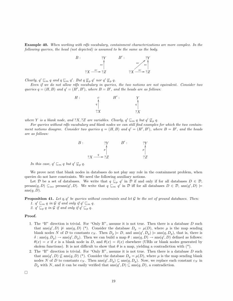
Example 40. When working with rdfs vocabulary, containment characterizations are more complex. In thefollowing queries, the head (not depicted) is assumed to be the same as the body.

B : ?Y

?Xsc // ?Z

sc

OO B′ : ?Y

?X

sc

==zzzzzzzz

sc // ?Z

sc

OO

Clearly, q′ ⊑m q and q ⊑m q′. But q 6⊑p q′ nor q′ 6⊑p q.Even if we do not allow rdfs vocabulary in queries, the two notions are not equivalent. Consider two

queries q = (H,B) and q′ = (H ′, B′), where B = B′, and the heads are as follows:

H : c

?X

q

OO H ′ : Y

?X

q

OO

where Y is a blank node, and ?X, ?Z are variables. Clearly, q′ ⊑m q but q′ 6⊑p q.For queries without rdfs vacabulary and blank nodes we can still find examples for which the two contain-

ment notions disagree. Consider two queries q = (H,B) and q′ = (H ′, B′), where B = B′, and the headsare as follows:

B : ?Y

?Xq // ?Z

p

OO B′ : ?Y

?Z

p

OO

In this case, q′ ⊑m q but q′ 6⊑p q.

We prove next that blank nodes in databases do not play any role in the containment problem, whenqueries do not have constraints. We need the following auxiliary notions.

Let D be a set of databases. We write that q ⊑p q′ in D if and only if for all databases D ∈ D,preans(q,D) ⊆iso preans(q′,D). We write that q ⊑m q′ in D iff for all databases D ∈ D, ans(q′,D) |=ans(q,D).

Proposition 41. Let q, q′ be queries without constraints and let G be the set of ground databases. Then:1. q′ ⊑m q in G if and only if q′ ⊑m q.2. q′ ⊑p q in G if and only if q′ ⊑p q.

Proof.

1. The “If” direction is trivial. For “Only If”, assume it is not true. Then there is a database D suchthat ans(q′,D) 6|= ans(q,D) (*). Consider the database Dg = µ(D), where µ is the map sendingblank nodes N of D to constants cN . Then Dg |= D, and ans(q′,Dg) |= ans(q,Dg), that is, there isδ : ans(q,Dg) → ans(q′,Dg). Then we can build a map θ : ans(q,D) → ans(q′,D) defined as follows:θ(x) = x if x is a blank node in D, and θ(x) = δ(x) elsewhere (URIs or blank nodes generated byskolem functions). It is not difficult to show that θ is a map, yielding a contradiction with (*).

2. The “If” direction is trivial. For “Only If”, assume it is not true. Then there is a database D suchthat ans(q′,D) 6⊆ ans(q,D) (*). Consider the database Dg = µ(D), where µ is the map sending blanknodes N of D to constants cN . Then ans(q′,Dg) ⊆ ans(q,Dg). Now, we replace each constant cN inDg with N , and it can be easily verified that ans(q′,D) ⊆ ans(q,D), a contradiction.

¤

19

5.2. Testing Containment

In this section we study the notions of containment for queries without premises and without constraints.Testing standard containment of queries without premises resembles containment of conjunctive rela-

tional queries. A characterization of entailment-based containment is more subtle. The next theorem givescharacterizations for both notions.

Define G1 |= G2 for graphs G1, G2 containing variables, as v(G1) |= v(G2), where v is a valuation sendingthe variables to fresh constants.

Theorem 42. Consider the queries q = (H,B) and q′ = (H ′, B′). Then:

1. q ⊑p q′ if and only if there is a sustitution of variables θ such that (a) θ(B′) ⊆ nf(B) and (b)θ(H ′) ∼= H.

2. q ⊑m q′ if and only if there are substitutions θ1, . . . , θn (of variables) such that (a) θj(B′) ⊆ nf(B)

and (b)⋃

j θj(H′) |= H.

Proof.

1. (If) Let D be a database, and v a substitution with v(H) ∈ preans(q,D), that is, v(B) ⊆ nf(D).Hence nf(v(B)) ⊆ nf(D). But it can be easily verified (by structural induction on derivation rules) thatv(nf(B)) ⊆ nf(v(B)). Therefore, we obtain v(nf(B)) ⊆ nf(D). Now, let µ = v(θ()), using Condition(a) of the theorem, we obtain v(θ(B′)) ⊆ nf(D), that is µ(H ′) ∈ preans(q′,D). But Condition (b) ofthe theorem states that θ(H ′) ∼= H. Then v(θ(H ′))) ∼= v(H), hence, µ(H ′) ∼= v(H). Therefore q ⊑p q′.(Only If) Assume q ⊑p q′. Consider the database D = µ(B), where µ(x) = x if x is a constant andµ(x) = cx if x is a variable. Clearly, µ(H) ∈ preans(q,D), then there is µ′(H ′) ∈ preans(q′,D) suchthat µ(H) ∼= µ′(H ′). Therefore, µ′(B′) ⊆ nf(D). Now, let θ = µ−1(µ′()). It can be easily verified thatθ satisfies conditions (a) and (b) of the theorem.

2. Because of Proposition 41, we need to show the statement for q ⊑m q′ in G, for G being the set ofground databases.(If) Let D be a ground database and ans(q,D) =

⋃vi(H) and ans(q′,D) =

⋃ui(H

′) (the vi(H)and ui(H) are preanswers), we will prove that there is a map ω : ans(q,D) → ans(q′,D). Since D isa ground database the preanswers do not share blank nodes and therefore it is enough to prove thatthere are maps ωi : vi(H) → ans(q′,D), for each vi(H) ∈ preans(q,D). Consider the maps θ1, . . . , θj .For each j, θj(B

′) ⊆ nf(B), hence vi(θj(B′)) ⊆ vi(nf(B)) ⊆ nf(D). Hence, vi(θj(H

′)) ∈ preans(q′,D).Therefore,

⋃j vi(θj(H

′)) ⊆ ans(q′,D). Let α be the map of Condition (b), that is α(H) ⊆⋃

j θj(H′).

Notice that α only replace blank nodes, but the variables are preserved. Now let define ωi as follows:ωi(x) = α(x) for each blank node x in v(H), and ωi(x) = x for each constant. From Condition (b), itfollows that ωi(vi(H)) ⊆

⋃j vi(θj(H

′)), and hence ωi : vi(H) → ans(q′,D).(Only If) Consider the database DB = v(B), where v is the 1-1 valuation assigning x to a freshconstant ax. By hypothesis, we have ans(q′,DB) |= v(H). So, there are maps v′

1, . . . , v′n : B′ →

nf(DB), such that⋃

j v′j(H

′) |= v(H). Now, applying v−1 to both sides of the expression, and using

that (a) v−1 is 1-1 and works only over ground elements, and (b) considering variables resulting from theapplication of v−1 as ground elements, we have that v−1(

⋃j v′

j(H′)) |= H. Then

⋃j v−1(v′

j(H′)) |=

H. Thus, let θj = v−1 v′j , and we have conditions (1) and (2) of the theorem.

¤

We end the section by giving complexity bounds for the containment problem (for queries withoutpremises).

Theorem 43. Consider the queries q = (H,B) and q′ = (H ′, B′). Then:

1. Testing whether q ⊑p q′ is NP-complete.

2. Testing whether q ⊑m q′ is NP-complete.

20

Proof.

1. NP-hardness: we can encode the problem of deciding G |= G′, where G,G′ are simple graphs. FromTherem 9 this problem is NP-complete. We just construct the queries q : (a, b, c) ← B and q′ :(a, b, c) ← B′, where a, b, c are constants, and B,B′ are obtained from G,G′, respectively, by replacingblanks with variables. From theorems 8 and 42 it can be easily verified that the two problems areequivalent, that is q ⊆p q′ (i.e., there is a substitution of variables θ such that θ(B′) ⊆ B) iff G |= G′

(i.e., there is a map from G′ to G). Membership in NP follows directly from Theorem 42: just use θas a certificate.

2. NP-hardness: notice that, for the queries q, q′ given in the item 1 of this proof, Theorem 42 (2)becomes: q ⊆m q′ iff there is a substitution θj such that θj(B

′) ⊆ nf(B) (because q, q′ have the samehead). Therefore, for q, q′ the two containment problems are equivalent, and we can use the encodingfrom the previous proof. For proving membership in NP just notice that, from the proof of Theorem42 (2), the number of maps θj is at most the number of triples of H. Then, the witness is the set θjand the map that witness the entailment of Condition (b) of Therem 42 (2).

¤

5.3. Containment of Queries with Constraints

The results of Section 5.2 can be easily generalized to handle constraints. Next, we extend Theorem 42to handle constraints.

Theorem 44. Consider the queries q = (H,B) and q′ = (H ′, B′). Then:

1. q ⊑p q′ if and only if there is a sustitution of variables θ such that (a) θ(B′) ⊆ nf(B) and (b)θ(H ′) ∼= H, and (c) θ(C ′) ⊆ C

2. q ⊑m q′ if and only if there are substitutions θ1, . . . , θn (of variables) such that (a) θj(B′) ⊆ nf(B)

and (b)⋃

j θj(H′) |= H, and (c) θj(C

′) ⊆ C.

Proof. Given a query q = (H,B,C), we define qc as the query (H,Bc, ∅), where Bc is obtained from B byadding a triple (?X, is, ground) (which we will refer to as a constraint triple) for each ?X ∈ C.

Now, for a database D, we define Dc as D union a set including a triple (c, is, ground) for each constantc that appears in D. We define Dc as the set containing Dc for all databases D.

Notice that for all queries q: ans(q,D) = ans(qc,Dc) and preans(q,D) = ans(qc,Dc). Therefore we havethat: q ⊑p q′ iff qc ⊑p q′c in Dc and q ⊑m q′ iff qc ⊑m q′c in Dc.

Now, Theorem 42 also applies for qc ⊑p q′c in Dc and qc ⊑m q′c in Dc. The new conditions (c) of bothparts of the theorem make explicit that the maps of Thereom 42 should include the new constraint triples.¤

5.4. Containment of Queries with Premises

In this section, we present a first study of containment for queries with premises. We tackle the contain-ment problem in the realm of RDF graphs over non-interpreted vocabulary, that is, rdfs graphs are treatedas simple graphs wherever they appear, that is in bodies, heads, and premises and databases. We refer tothis class of queries as simple queries.

We prove that simple queries with premises can be transformed into union of queries without premises,which yields a characterization and complexity bounds for testing entailment. This result does not hold ifthe semantics of rdfs vocabulary is considered, even if premises are simple RDF graphs. The results herecan also be extended to include constraints using the trick in the proof of Theorem 44, but for the sake ofsimplicity, we omit constraints in this section.

We start by proving that, when testing q ⊑p q′ or testing q ⊑m q′, a mild extension of Theorem 42 canhandle a premise in q′.

21

Theorem 45. Consider the simple queries q = (H,B, ∅) and q′ = (H ′, B′, P ′). Then:

1. q ⊑p q′ if and only if there is a sustitution (of variables and blank nodes) θ such that (a) θ(B′) ⊆ P ′+Band (b) θ(H ′) ∼= H.

2. q ⊑m q′ if and only if there are substitutions θ1, . . . , θn (of variables) such that (a) θj(B′) ⊆ P ′ + B

and (b)⋃

j θj(H′) |= H.

Proof. The proof mirrors closely that of Theorem 42 and we write it down for the sake of completeness.

1. (If) Let D be a database, and v a substitution with v(H) ∈ preans(q,D), that is, (a) v(B) ⊆ D. Letµ = v(θ()). From (a) and (1) we obtain v(θ1(B

′)) ⊆ P ′ + D, and hence µ(H ′) ∈ preans(q′,D). But(2) states that θ1(H

′) ∼= H. Then v(θ1(H′))) ∼= v(H), hence, µ(H ′) ∼= v(H). Therefore q ⊑p q′.

(Only If) Assume q ⊑p q′. Consider the database D = µ(B), where µ(x) = x if x is a constant andµ(x) = cx if x is a variable. Clearly, µ(H) ∈ preans(q,D), then there is µ′(H ′) ∈ preans(q′,D) suchthat µ(H) ∼= µ′(H ′). Therefore, µ′(B′) ⊆ P ′ + D. Now, let θ = µ−1(µ′()). It can be easily verifiedthat θ satisfies conditions (a) and (b) of the theorem.

2. Because of Proposition 41, we need to show the statement for q ⊑m q′ in G, for G being the set ofground databases.(If) Let D be a ground database and ans(q,D) =

⋃vi(H) and ans(q′,D) =

⋃ui(H

′) (the vi(H) andui(H) are preanswers), we will prove that there is a map ω : ans(q,D) → ans(q′,D). Since D is aground database the preanswers do not share blank nodes and therefore it is enough to prove that thereare maps ωi : vi(H) → ans(q′,D), for each vi(H) ∈ preans(q,D). Consider the maps θ1, . . . , θj . Foreach j, θj(B

′) ⊆ P ′ + B, hence vi(θj(B′)) ⊆ P ′ + vi(B) ⊆ P ′ + D. Hence, vi(θj(H

′)) ∈ preans(q′,D).Therefore,

⋃j vi(θj(H

′)) ⊆ ans(q′,D). Let α be the map of Condition (b), that is α(H) ⊆⋃

j θj(H′).

Notice that α only replace blank nodes, but the variables are preserved. Now let define ωi as follows:ωi(x) = α(x) for each blank node x in v(H), and ωi(x) = x for each constant. From Condition (b), itfollows that ωi(vi(H)) ⊆

⋃j vi(θj(H

′)), and hence ωi : vi(H) → ans(q′,D).(Only If) Consider the database DB = v(B), where v is the 1-1 valuation assigning to each variable

X a fresh constant aX . By hypothesis, we have ans(q′,DB) |= v(H). So, there are maps v′1, . . . , v

′n :

B′ → nf(DB), such that⋃

j v′j(H

′) |= v(H). Now, applying v−1 to both sides of the expression,

and using that (a) v−1 is 1-1 and works only over ground elements, and (b) considering variablesresulting from the application of v−1 as ground elements, we have that v−1(

⋃j v′

j(H′)) |= H. Then

⋃j v−1(v′

j(H′)) |= H . Thus, let θj = v−1 v′

j , and we have conditions (1) and (2) of the theorem.

¤

Next, we prove that, if the semantics rdfs vocabulary is not taken into account, a query with premisescan be transformed into a union of queries without premises.

Proposition 46. Let q = (H,B,P ) be a simple query. And let Ωq be the set of queries defined as:

Ωq = qµ = (µ(H), µ(B − R), ∅) | µ : R → P and R ⊆ B and µ(B − R) has no blanks.

Then, q =⋃

qµ∈Ωqqµ, that is, for all databases D, ans(q,D) =

⋃qµ∈Ωq

ans(qµ,D).

Proof.(⊆) Consider a database D, and v(H) ∈ preans(q,D). Then v(B) ⊆ D + P . Now, we can split B into

R and B − R, such that v(R) ⊆ P and v(B − R) ⊆ D. Now let µ be the map obtained by restrictingthe domain of v to the variables in R. And let w be the map obtained by restricting the domain of v tovariables in B − R. If µ(B − R) has a blank, then there is a variable x such that µ(x) is a blank in P andalso µ(x) is a blank in D, contradicting the restriction that blanks of premises are disjoint with blanks ofdatabases. Therefore qµ is a query in the set given in the theorem. In addition, it can be easily verified thatw(µ(B − R)) ∈ D and hence w(µ(H)) ∈ preans(qµ,D), and hence v(H) ∈ preans(qµ,D).

(⊇) Consider a query qu, a database D and a preanswer v(µ(H)) ∈ preans(qu,D). Then v(µ(B−R)) ∈ Dand also from the definition of qµ we have µ(R) ∈ P . Then, we have v(µ(R)) ∈ P (because v(µ(R)) = µ(R)).

22

Therefore, v(µ(B)) ⊆ P +D, hence v(µ(H)) ∈ preans(q,D). We can encode containment of classical tableauinto queries without premises. ¤

Example 47. As an example, the answer returned by the query q defined by:q : (?X, p, ?Y ) ← (?X, q, ?Y ), (?Y, t, s), with P = (a, t, s), (b, t, s)).

is the same as the union of the answers returned by the following queries:q1 : (?X, p, a) ← (?X, q, a), with P1 = ∅,q1 : (?X, p, b) ← (?X, q, b), with P2 = ∅,q3 : (?X, p, ?Y ) ← (?X, q, ?Y ), (?Y, t, s), with P3 = ∅.

Proposition 48. Let q1, q2 be queries without premises, and let q′ = (H ′, B′, P ′). Then:

1. (q1 ∪ q2) ⊑p q′ iff q1 ⊑p q′ and q2 ⊑p q′.

2. (q1 ∪ q2) ⊑m q′ iff q1 ⊑m q′ and q2 ⊑m q′.

Proof.

1. It follows directly from the definition of ⊑p.

2. (If) Then q1 ⊑m q′ in G and q2 ⊑m q′ in G, where G is the set of ground databases. Then for all constantdatabases D, we have maps: µ1 : ans(q1,D) → ans(q′,D) and µ2 : ans(q2,D) → ans(q′,D). But,because D is constant ans(q1,D) and ans(q2,D) do not share blanks, and hence µ1∪µ2 : (ans(q1,D)∪ans(2,D)) → ans(q′,D). Hence, (q1 ∪ q2) ⊑m q′ in G. The conclusion follows from Proposition 41.The “Only If” part is direct.

¤

Theorem 46 and propositions 46 and 48 yield the following algorithm for testing the containment q ⊑p q′

(respectively q ⊑m q′). First, we transform q into Ωq and then for each query qµ ∈ Ωq we use Theorem 45 totest if qµ ⊑p q′ (respectively qµ ⊑m q′). We end this section by given complexity bounds for the conteinmentproblems.

Theorem 49. Let q = (H,B,P ) and q′ = (H ′, B′, P ′) be simple queries.

1. Testing whether q ⊑p q′ is NP-hard and in Π2P .

2. Testing whether q ⊑m q′ is NP-hard and in Π2P .

3. If P = ∅ then both testing q ⊑p q′ and testing q ⊑m q′ are NP-complete.

Proof.

1. NP-hardness: follows from the same encoding as in the proof Theorem 43 (1). From Proposition 46and Theorem 42, this can be solved by a NP machine with an NP oracle. The certificate is a query qµ

in the set given by Proposition 46, we use the oracle to test whether qµ 6⊑p q′. Hence the complement

problem is in NPNP, and the problem is in coNPNP.

2. Similar to the previous proof.

3. Follows directly from Theorem 45: just use θ as a certificate to prove membership in NP. For NP-hardeness the encoding given in the proof of Theorem 43 (1) works here.

¤

23

6. Complexity of query answering

6.1. Computing matchings

In order to understand the complexity of computing the set of matchings for a query over a database,we consider the simpler problem of testing emptiness of the query answer set.

1. Query complexity version: For a fixed database D, given a query q, is q(D) non-empty?2. Data complexity version: For a fixed query q, given a database D, is q(D) non-empty?

Theorem 50. The evaluation problem is NP-complete for the query complexity version, and polynomial forthe data complexity version.

Proof. Reduction of 3SAT to the problem of evaluating a conjunctive query over a database. Membershipin NP follows immediately.

Data complexity version: This follows from the fact that the number of potential matchings of the bodyof q in nf(D) is bounded by the number of subgraphs of nf(D) of size q, and the fact that the size of nf(D)is polynomial in D. ¤

From the proof of Theorem 50 follows that the size of the set of answers of a query q issued against adatabase D is bounded by |D||q|, where |D| is the size of the normal form of the database (number of triples)and |q| is the number of symbols in the query.

6.2. Redundancy elimination

We give some observations on redundancies in queries, databases and set of answers.It is desirable and possible to have queries with lean heads. Otherwise, the answer generated will have

redundancies which could have been avoided.On the contrary, it is not always possible to have lean graphs in body of queries. For example,

consider the query q = (H,B, ∅), where H = (?Course, related, “DB”) and B = (?Dept, offers, “DB”),(?Dept, offers, ?Course). B is not lean and is equivalent to the lean graph B′ = (?Dept, offers, “DB”). Itturns out that there is no query equivalent to q with body B′ (using any notion of equivalence).

Even having lean databases and queries with lean heads and bodies does not avoid redundancies in theanswer set. Consider the lean graph G2 in Example 18, and the query (?Z, p, ?U) ← (?Z, p, ?U). The answerset is G1 which is not lean.

Answers to queries in RDF usually have redundancies. Ideally, the answer set ans(q,D) should reducethese redundancies to the minimum, i.e. to an equivalent lean graph. The naive approach to eliminateredundancy in answers is to compute: (1) ans(q,D), and (2) a lean equivalent to ans(q,D). The nexttheorem shows that in the worst case there is no better approach.

Theorem 51. Given a lean database D and a query q, to decide whether ans∪(q,D) is lean is coNP-complete(in the size of D).

The theorem follows from the fact that there is a query that computes the identity and from Theorem 22.For merge-semantics redundancy elimination can be done much more efficiently:

Theorem 52. Given a lean database D and a query q, deciding whether ans+(q,D) is lean can be done inpolynomial time in the size of D.

Proof. Let A = ans+(q,D) and let us refer to maps from single answers to A as single maps. The keyobservation is that, because single answers do not share variables in merge-semantics, maps µ : A → Aare exactly unions of single maps µj : Gj → A for each Gj single answer. (Note that in the case ofunion-semantics the union of the µj would not be a function.)

Thus an algorithm for finding a proper map µ : A → A only needs to compute single maps and checkwhether (1) at least a single map is proper, or (2) two of them share a blank node in their range. This canbe done in time polynomial on the set of single maps, whose size is polynomial in the size of D. Thus thecomplete test can be done in polytime. ¤

24

7. Conclusions and Future Work

The RDF data model poses new challenges to query languages. We have studied some fundamentalproblems introduced by this model. This formalization needs to be extended to richer properties andmechanisms of current working query languages for RDF, to establish a solid base to compare functionalities,features and limitations of RDF query languages. Features like connectedness, reachability, paths, recursion,extended constraints, aggregation and views must be developed.

Acknowledgments

The authors were supported by: Gutierrez - ...; Hurtado - ...; Perez - Conicyt Ph.D. Scholarship.

References

[1] A. V. Aho, M. R. Garey, J. D. Ullman, The transitive reduction of a directed graph, SIAM J. Comput. 1 (1972) 131–137.[2] S. Abiteboul, R. Hull, V. Vianu, Foundations of Databases, Addison-Wesley Publishing Co., 1995.[3] F. Alkhateeb, Querying RDF(S) with Regular Expressions, Ph.D. Thesis, Universite Joseph Fourier, Grenoble, France,

2008.[4] R. Angles, C. Gutierrez, The Expressive Power of SPARQL, ISWC 2008, LNCS 5318, pp. 114-129, 2008.[5] F. Baader, T. Nipkow, Term Rewriting and All That, Cambridge Univ. Press, 1998.[6] J. Baget RDF Entailment as Graph Homomorphism, In ISWC 2005, 82-96.[7] J. Broeskstra, A. Kampman, SeRQL: A Second Generation RDF Query Language, SWAD-Europe Workshop on Semantic

Web Storage and Retrieval, 13-14, 2003.[8] A. Bonner, Hypothetical Datalog: Complexity and Expressibility. In Proceedings the Second International Conference on

Database Theory, ICDT 1988, 144-160.[9] J. de Bruijn, S. Tessaris, E. Franconi, Logical reconstruction of RDF and ontology languages In Proc. PPSWR-05, pp.

65-71, 2005.[10] J. de Bruijn, E. Franconi, S. Tessaris. Logical Reconstruction of normative RDF, In Proceedings of the Workshop on OWL

Experiences and Directions, OWLED 2005.[11] Ch. Chekuri, A. Rajaraman, Conjunctive Query Containment Revisited, In ICDT 1997, 56-70.[12] T. Furche, B. Linse, F. Bry, D. Plexousakis, G. Gottlob, G., RDF querying: Language constructs and evaluation methods

compared. Reasoning Web. 1–52, 2006.[13] P. Haase, J. Broekstra, A. Eberhart, R. Volz, A comparison of RDF query languages. International Semantic Web

Conference 2004, 502–517.[14] Y. Kanza, W. Nutt, Y. Sagiv, Queries with incomplete answers over semistructured data, In PODS 1999, 227-236.[15] K. Kochut, M. Janik, SPARQLeR: Extended SPARQL for Semantic Association Discovery, ESWC 2007, LNCS 4519, pp.

145-159, 2007.[16] R. Fagin, Ph. G. Kolaitis, L. Popa, Data exchange: getting to the core. ACM Trans. Database Syst. 30(1): 174-210 (2005)[17] D. M. Gabbay, U. Reyle, N-Prolog: an Extension of Prolog with Hypothetical Implications. I, Journal of Logic Program-

ming (JLP), 1(4):319-355, 1984.[18] A. Gomez-Perez, M. C. Suarez-Figueroa, Results of Taxonomic Evaluation of RDF(S) and DAML+OIL Ontologies using

RDF(S) and DAML+OIL Validation Tools and Ontology Platforms Import Services, 2nd Workshop on Evaluation ofOntology-based Tools, EON2003.

[19] M. Grohe, T. Schwentick, L. Segoufin, When is the evaluation of conjunctive queries tractable?, In STOC 2001, 657-666.[20] R. V. Guha, rdfDB Query Language, in http://www.guha.com/rdfdb/query.html

[21] G. Gottlob, Computing Cores for Data Exchange: New Algorithms and Practical Solutions. In PODS 2005, 148–159.[22] G. Gottlob, A. Nash, Data Exchange: Computing Cores in Polynomial Time. In PODS 2006, 40–49.[23] C. Gutierrez, C. Hurtado and A. Mendelzon. Foundations of Semantic Web Databases. In PODS 2004, pages 95–106.[24] C. Gutierrez, Normal forms for connectedness in categories, Annals of Pure and Applied Logic 108 (2001) 237-247.[25] J. Hayes, C. Gutierrez, Bipartite Graphs as Intermediate Model for RDF, In ISWC 2004, 47-61-[26] P. Hell, J. Nesetril, The core of a graph, Discrete Math. 109 (1992), 117-126.[27] H. J. ter Horst, Completeness, decidability and complexity of entailment for RDF Schema and a semantic extension

involving the OWL vocabulary, J. Web Sem. 3(2-3): 79-115 (2005).[28] G. Karvounarakis, S. Alexaki, V. Christophides, D. Plexousakis, M. Scholl, RQL: A Declarative Query Language for RDF,

In WWW 2002, 592-603.[29] A. Magkanaraki et al. Ontology Storage and Querying, Technical Report No. 308, April 2002, Foundation for Research

and Technology Hellas, Institute of Computer Science, Information System Laboratory.[30] D. Marin. RDF Formalization, Santiago de Chile, 2004. Technical Report Universidad de Chile, TR/DCC-2006-8.

http://www.dcc.uchile.cl/~cgutierr/ftp/draltan.pdf

[31] L. Miller, A. Seaborne, A. Reggiori, Three Implementations of SquishQL, a Simple RDF Query Language, In ISWC 2002,399-403.

[32] S. Munoz, J. Perez, C. Gutierrez, Minimal deductive systems for RDF, In ESWC 2007, 53-67.

25

[33] RDF Query Exchange Language (QEL), Edit. M. Nilsson, W. Siberski,http://edutella.jxta.org/spec/qel.html

[34] Y. Papakonstantinou, V. Vassalos, Query Rewriting for Semistructured Data, In SIGMOD 1999, 455-466.[35] J. Perez, M. Arenas, C. Gutierrez, Semantics and Complexity of SPARQL, ISWC 2006, LNCS 4273, pp. 30-43, 2006.[36] J. Perez, M. Arenas, C. Gutierrez, nSPARQL: A Navigational Language for RDF, ISWC 2008, LNCS 5318, pp. 66-81,

2008.[37] R. Pichler, A. Polleres, F. Wei and S. Woltran, dRDF: Entailment for Domain-Restricted RDF, In ESWC 2008, 200-214.[38] OWL Web Ontology Language Reference, W3C Candidate Recommendation 18 August 2003, Editors: M. Dean, G.

Schreiber.[39] E. Prud’hommeaux, B. Grosof, RDF Query and Rules: A Framework and Survey,

http://www.w3.org/2001/11/13-RDF-Query-Rules/

[40] M. Sintek, S. Decker, TRIPLE—A Query, Inference, and Transformation Language for the Semantic Web, In ISWC2002, 364-378.

[41] M. Yannakakis, Algorithms for acyclic database schemes, In VLDB 1981, 82-94.[42] G. Yang, M. Kifer, On the Semantics of Anonymous Identity and Reification In ODBASE 2002, 1047-1066. Applications

of[43] M. Vardi. The Complexity of Relational Query Languages (Extended Abstract). In STOC 1982, 137–146.[44] DAML Query Language (DQL), April 2003, Abstract Specification. DAML Joint Committee, R. Fikes, P. Hayes, I.

Horrocks, Ed.[45] Resource description framework (RDF) model and syntax specification, Edit. O. Lassila, R. Swick, Working draft, W3C,

1998.[46] RDF Semantics, W3C Recommendation 10 February 2004 Edit. Patrick Hayes[47] RDF Vocabulary Description Language 1.0: RDF Schema, W3C Working Draft 23 January 2003, Edit. Dan Brickley,

R.V. Guha.[48] RDF Concepts and Abstract Syntax, W3C Recommendation 10 February 2004, Edit. G. Klyne, J. J. Carroll.[49] RDF Primer, W3C Recommendation 10 February 2004, Edit. F. Manola, E. Miller.[50] SPARQL Query Language for RDF. W3C Recommendation 15 January 2008. Edit. E. Prud’hommeaux, A. Seaborne.

http://www.w3.org/TR/rdf-sparql-query/

[51] W3C Semantic Web Activityhttp://www.w3.org/2001/sw/

26