INDUSTRIAL ENGINEERING

FOUNDATIONS

LICENSE, DISCLAIMER OF LIABILITY, AND LIMITED WARRANTY By purchasing or using this book (the “Work”), you agree that this licensegrants permission to use the contents contained herein, but does not giveyou the right of ownership to any of the textual content in the book orownership to any of the information or products contained in it. Thislicense does not permit uploading of the Work onto the Internet or on anetwork (of any kind) without the written consent of the Publisher.Duplication or dissemination of any text, code, simulations, images, etc.contained herein is limited to and subject to licensing terms for therespective products, and permission must be obtained from the Publisheror the owner of the content, etc., in order to reproduce or network anyportion of the textual material (in any media) that is contained in theWork. MERCURY LEARNING AND INFORMATION (“MLI” or “the Publisher”) andanyone involved in the creation and writing of the text and anyaccompanying Web site or software of the Work, cannot and do notwarrant the performance or results that might be obtained by using thecontents of the Work. The author, developers, and the Publisher have usedtheir best efforts to insure the accuracy and functionality of the textualmaterial and/or information contained in this package; we, however, makeno warranty of any kind, express or implied, regarding the performance ofthese contents. The Work is sold “as is” without warranty (except fordefective materials used in manufacturing the book or due to faultyworkmanship). The author, developers, and the publisher of any accompanying content,and anyone involved in the composition, production, and manufacturing ofthis Work will not be liable for damages of any kind arising out of the useof (or the inability to use) the textual material contained in this

publication. This includes, but is not limited to, loss of revenue or profit,or other incidental, physical, or consequential damages arising out of theuse of this Work. The sole remedy in the event of a claim of any kind is expressly limited toreplacement of the book, and only at the discretion of the Publisher. Theuse of “implied warranty” and certain “exclusions” vary from state tostate, and might not apply to the purchaser of this product.

INDUSTRIAL ENGINEERING

FOUNDATIONS

Bridging the Gap between Engineering andManagement

FARROKH SASSANI, Ph.D.The University of British Columbia

MERCURY LEARNING AND INFORMATIONDulles, Virginia

Boston, MassachusettsNew Delhi

Copyright ©2017 by MERCURY LEARNING AND INFORMATION LLC. All rightsreserved. This publication, portions of it, or any accompanying software may not bereproduced in any way, stored in a retrieval system of any type, ortransmitted by any means, media, electronic display or mechanical display,including, but not limited to, photocopy, recording, Internet postings, orscanning, without prior permission in writing from the publisher. Publisher: David PallaiMERCURY LEARNING AND INFORMATION

22841 Quicksilver DriveDulles, VA 20166info@merclearning.comwww.merclearning.com1-800-232-0223 F. Sassani. Industrial Engineering Foundations.ISBN: 978-1-942270-86-7 The publisher recognizes and respects all marks used by companies,manufacturers, and developers as a means to distinguish their products. Allbrand names and product names mentioned in this book are trademarks orservice marks of their respective companies. Any omission or misuse (of anykind) of service marks or trademarks, etc. is not an attempt to infringe on theproperty of others. Library of Congress Control Number: 2016953727

161718321 Printed in the USA on acid-free paper. Our titles are available for adoption, license, or bulk purchase by institutions,corporations, etc. For additional information, please contact the CustomerService Dept. at 800-232-0223(toll free). All of our titles are available in digital format at authorcloudware.com andother digital vendors. The sole obligation of MERCURY LEARNING AND

INFORMATION to the purchaser is to replace the book, based on defectivematerials or faulty workmanship, but not based on the operation or content ofthe product.

Tothe loving memory of my father,

the resilience of my mother,and

my family, from whom I borrowed the time.

CONTENTS

Preface

Chapter 1 Introduction1.1 Industrial Engineering1.2 Duties of an Industrial Engineer1.3 Subject Coverage1.4 Suggestions for Reading the Book1.5 How to Be a Manager

1.5.1 Guidelines to Follow1.5.2 Working with People1.5.3 Decision Making

Chapter 2 Organizational Structure2.1 Introduction2.2 Basic Principles of Organization2.3 Forms of Organizational Structure

2.3.1 Line Organization2.3.2 Line and Staff Organization

2.4 Organizational Design Strategies2.5 Major Forms of Departmentation

2.5.1 Functional Departmentation2.5.2 Product/Divisional Departmentation2.5.3 Geographic Departmentation2.5.4 Clientele Departmentation

2.5.5 Process Departmentation2.5.6 Time Departmentation2.5.7 Alphanumeric Departmentation2.5.8 Autonomy Departmentation

2.6 Management Functions2.6.1 Contemporary Operations Management2.6.2 Span of Control2.6.3 Complexities of Span of Control2.6.4 Informal Organization

2.7 Organizational Activities of a Production Control System2.8 Typical Production and Service SystemsExercises

Chapter 3 Manufacturing Systems3.1 Introduction3.2 Conventional Manufacturing Systems

3.2.1 Job Shop Production3.2.2 Batch Production3.2.3 Mass Production

3.3 Physical Arrangement of Manufacturing Equipment3.3.1 Fixed-Position Layout3.3.2 Functional Layout3.3.3 Group Technology Layout3.3.4 Line Layout and Group Technology Flow Line3.3.5 Comparison of Plant Layouts3.3.6 Hybrid and Nested Manufacturing Systems

3.4 Modern Manufacturing Systems3.5 Flexible Manufacturing Systems

3.5.1 Advantages of FMSs3.5.2 Disadvantages of FMSs

3.6 Physical Configuration of Flexible Manufacturing Systems3.6.1 Cell Layout3.6.2 Linear Layout3.6.3 Loop Layout3.6.4 Carousel System

3.6.5 Other Layouts and Systems3.7 General CommentsExercises

Chapter 4 Classification and Coding4.1 Introduction4.2 Group Technology

4.2.1 Part Families4.2.2 Part Classification and Coding

4.3 Classification and Coding Schemes4.3.1 Monocodes4.3.2 Polycodes4.3.3 Hybrids4.3.4 The Opitz Classification System4.3.5 Commercially Developed Systems4.3.6 Custom-Engineered Classification and Coding Systems

Exercises

Chapter 5 Sequencing and Scheduling of Operations5.1 Introduction5.2 Definition of Scheduling Terms5.3 Scheduling Algorithms

5.3.1 Objectives in Scheduling Problems5.3.2 Industrial Problems5.3.3 The Practice

5.4 n-Job 1-Machine Problem5.4.1 Classification of Scheduling Problems

5.5 Johnson’s Algorithm5.6 Johnson’s Extended Algorithm5.7 Jackson’s Algorithm5.8 Akers’ Algorithm5.9 The Branch and Bound Method

5.9.1 Lower Bounds for Completion Time5.9.2 Branch and Bound Algorithm

5.10 Mathematical Solutions

5.11 Closing RemarksExercises

Chapter 6 Forecasting6.1 Introduction

6.1.1 Pre-Forecasting Analysis6.1.2 Forecasting Horizon

6.2 Mathematical Forecasting Methods6.2.1 Linear Regression6.2.2 Simple Moving Average6.2.3 Weighted Moving Average6.2.4 Exponential Smoothing

6.3 Measure of Quality of Forecasts6.3.1 Coefficient of Correlation6.3.2 Analysis of Forecast Errors

6.4 Closing RemarksExercises

Chapter 7 Statistical Quality Control7.1 Introduction7.2 Determining Quality

7.2.1 Why is Quality Inconsistent?7.3 Economics of Quality7.4 The Role of Distributions

7.4.1 The Scatter of Data7.4.2 Normal Distribution

7.5 Distribution of Sample Averages7.6 Statistical Quality Control Methods

7.6.1 Quality Control for Variables: and R Charts7.6.2 The Aimed-at-Values Method7.6.3 The Estimated-Values Method7.6.4 Evaluation of the Level of Control7.6.5 Distinction between Defective and Reworkable Parts7.6.6 Interpretation of Sample Behavior7.6.7 Nature and Frequency of Sampling

7.6.8 Control Charts Limits7.6.9 Areas of Application

7.7 Quality Control for Attributes7.7.1 Quality Control for Defectives7.7.2 Number of Defectives in a Sample7.7.3 Mean and Dispersion7.7.4 Quality Control for Defectives: p-Chart and np-Chart7.7.5 Estimated-Values Method7.7.6 Interpretation of Sample Behavior7.7.7 Sample Size

7.8 Control Chart for Defects: c-Chart7.8.1 Counting Defects

7.9 Revising the Control LimitsExercises

Chapter 8 Facility Location8.1 Introduction8.2 Forms of Distance8.3 Objective Function Formulation8.4 Mini-Sum Problems

8.4.1 Squared Euclidean Distance8.4.2 Euclidean Distance8.4.3 Rectilinear Distance—Point Locations8.4.4 Rectilinear Distance—Area Locations

8.5 Mini-Max Location ProblemsExercises

Chapter 9 System Reliability9.1 Introduction9.2 Definition of Reliability9.3 Failure over the Operating Life9.4 The Reliability Function

9.4.1 Failure Rate9.5 Reliability of Multiunit Systems

9.5.1 Series Configuration

9.5.2 Parallel Configuration9.6 Combined Series-Parallel Configurations

9.6.1 System-Level Redundancy9.6.2 Component-Level Redundancy

9.7 More Complex Configurations9.8 The Method of Path Enumeration

9.8.1 Sensitivity AnalysisExercises

Chapter 10 Queueing Theory10.1 Introduction10.2 Elements of Queueing Systems

10.2.1 Arrival Pattern10.2.2 Queue Discipline10.2.3 Service Arrangement10.2.4 Service Duration10.2.5 Performance Metrics10.2.6 System Modification

10.3 Queueing Models10.3.1 Single-Channel Queues10.3.2 Multiple-Channel Queues

Exercises

Chapter 11 Application of Principles11.1 Introduction11.2 5S Concept

11.2.1 Detailed Explanation of 5S Action Items11.3 Supply-Chain Management

11.3.1 Principles of Supply-Chain Management11.4 Six-Sigma Techniques11.5 Lean ThinkingExercises

Appendices

A Effective MeetingsB Effective Presentations

Bibliography

Index

PREFACE

As an applied science, industrial engineering embraces concepts andtheories in such fields as mathematics, statistics, social sciences,psychology, economics, management and information technology. Itdevelops tools and techniques to design, plan, operate and control service,manufacturing, and a host of engineering and non-engineering systems.Industrial engineering is concerned with the integrated systems of people,materials, machinery, and logistics, and ensures that these systems operateoptimally and efficiently, saving time, energy, and capital. An industrialengineer, or an engineer equipped with the tools and techniques ofindustrial engineering is the professional who is responsible for all thesetasks.

This book aims to expose the reader at an introductory level to the basicconcepts of a range of topics in industrial engineering and to demonstratehow and why the application of such concepts are effective.

The target audience for this abridged volume encompasses all engineers.In other words, the book is written for motivated individuals from a broadrange of engineering disciplines who aim for personal and professionaldevelopment. They would benefit from having a foundational book on

important principles and tools of industrial engineering. They would beable to apply these principles not only to initiate improvements in theirplace of work but also to open up a career path to management andpositions with a higher level of responsibility and decision-making.

The level of coverage and the topics included in this book have beendistilled from over thirty years of teaching a technical elective course inindustrial engineering to non-industrial engineering students in their finalyear of studies. From direct and indirect feedback from the students on theusefulness of various industrial engineering methods in their work, thecourse content has evolved to what is now presented as a book.

In writing this book, I am most grateful to Dr. Mehrzad Tabatabian, fromthe British Columbia Institute of Technology, for his encouragement,sharing his book-writing experiences, and putting me in contact with awonderful publisher, Mr. David Pallai, who supported and providedguidance throughout the effort. I am also indebted to my colleagues in theMechanical Engineering Department at the University of BritishColumbia: Professor Peter Ostafichuk and Mr. Markus Fengler for givingme invaluable advice about writing a book, and I deeply acknowledge aspecial debt of gratitude to Professor Tatiana Teslenko for graciouslyediting and proofreading the manuscript.

This is an opportune time to thank Ms. Aleteia Greenwood, Head ofUBC Woodward Library and Hospital Branch Libraries, for her adviceand expert assistance in the literature search and library matters for manyyears. I also would like to extend my appreciation to my graduate studentsMorteza Taiebat, Abbas Hosseini, and Masoud Hejazi for their tolerance.Last, but not the least, I express my heartfelt gratitude to my family fortheir patience, encouragement, and support.

F. Sassani

November 2016

Chapter 1 INTRODUCTION

1.1 INDUSTRIAL ENGINEERING

A complete study of industrial engineering would typically require fouryears of university education. Industrial engineering sits at the intersectionof many disciplines, such as engineering science and technology, socialsciences, economics, mathematics, management, statistics, and physicalsciences. An industrial engineer is akin to a manager on the site ofoperations. Industrial engineering is an ideal bridge between all hard-coreengineering fields such as mechanical, chemical, electrical, andmanufacturing engineering, and the field of management. This book is anintroduction to the basic principles and techniques used by industrialengineers to control and operate production plants and service systems.The reader will become familiar with the most important industrialengineering concepts and will gain adequate knowledge of where and whatto look for if he or she needs to know more.

Some engineers, in their own words, are unenthusiastic and unexcitedabout their long-term careers in engineering because they envision nopossibility for enhancing their effectiveness or progress through the ranks.Many would like to be involved in management, process improvement,and decision making and in this way pave a path to production control,engineering and its management, and the operational aspects ofmanufacturing and the service industries in which they work. It is notalways practical to earn another relevant degree. Without knowledge andunderstanding of how an enterprise operates, and how to improve theefficiency of tasks and processes, it will be difficult to become involved,

or be called on to participate in the management of engineering operationsand decision making. We witness how various disciplines, such asmechanical engineering and electrical engineering, have joined forces totrain “Mechatronics Engineers” or biomedical science and engineeringhave pooled together their expertise to train “Biomedical Engineers.”Industrial engineering is a discipline that, when integrated with any otherengineering field, can educate competent engineers who not only designand develop equipment, processes, and systems but also know howefficiently utilize and manage them.

An industrial engineer attempts to make an organization more efficient,cost-effective, and lean, and he/she may deal with topics like“productivity” and “profitability.” For the sake of an example, let’s brieflydiscuss the two and see what we learn.

It is expected that a productive firm will also be a profitable one.However, because profits are strictly sales oriented, there must besufficient sales to be profitable. A manufacturing enterprise may be veryefficient in the use of its resources, but reviews for inferior quality, misseddelivery promises, and poor customer service, for example, may hindersales to secure a net profit. Therefore, firms have to not only deal withmany internal factors, but they also have to consider the externalinfluences ranging from raw material availability and cost of purchase toclientele opinion, union matters, and governmental regulations.

1.2 DUTIES OF AN INDUSTRIAL ENGINEER

Industrial engineers are hands-on managers who determine, eliminate,enhance, or implement, as appropriate, to deal with the following:

• Waste and deficiencies• Better means of control• Cost-effective analysis

• Improved technology• More efficient operations• Greater use of plant facilities• Safety and human aspects• Equipment layout• Delivery and quality issues• Personnel assignment• Other related functions and tasks depending on the case

There are many techniques and principles available to industrial engineersto effectively tackle and manage any of the above scenarios.

1.3 SUBJECT COVERAGE

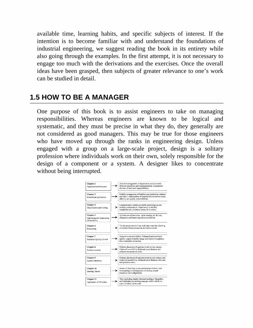
The topics covered in this book comprise some of the important conceptsand tools of industrial engineering and are certainly not exhaustive by anymeans. Some subjects are still of great importance in the field and inpractice, such as inventory control, but more and more inventory controlsare implemented through commercial software that is readily available andwidely used. For such reasons and the fact that this book is intended tocover the foundations of industrial engineering, essentially, fornonindustrial engineers, the subject coverage converged to what ispresented. Figure 1.1 shows the topics and what is expected to be achievedif they are applied to any enterprise of interest.

1.4 SUGGESTIONS FOR READING THE BOOK

The goal of this book is to provide an overview of some importantconcepts in industrial engineering. It is also intended to be light andportable and, thus, readily at hand for reading practically at any time.Every reader has his or her own style of reading that suits his or her

available time, learning habits, and specific subjects of interest. If theintention is to become familiar with and understand the foundations ofindustrial engineering, we suggest reading the book in its entirety whilealso going through the examples. In the first attempt, it is not necessary toengage too much with the derivations and the exercises. Once the overallideas have been grasped, then subjects of greater relevance to one’s workcan be studied in detail.

1.5 HOW TO BE A MANAGER

One purpose of this book is to assist engineers to take on managingresponsibilities. Whereas engineers are known to be logical andsystematic, and they must be precise in what they do, they generally arenot considered as good managers. This may be true for those engineerswho have moved up through the ranks in engineering design. Unlessengaged with a group on a large-scale project, design is a solitaryprofession where individuals work on their own, solely responsible for thedesign of a component or a system. A designer likes to concentratewithout being interrupted.

Figure 1.1. Chapter topics and the effects of their application to systems.

The majority prefer it this way, quietly accepting the challenges ofengineering design as individuals who have a high regard for their owndesign skills—more power to them, because the society and theengineering community need dedicated design engineers.

Most of these engineers choose the design of products in distinctpreference to the uncertainty of working with people. One reason might bethat their academic backgrounds generally did not include training indirecting and motivating other people; they concentrated on becomingtechnically competent. Thus, they usually find it difficult to make thetransition from dealing with the technical discipline to dealing withpeople. Industrial engineers, however, must work with many individuals,and, as mentioned earlier, they are managers of systems and people on thesite. They must arrange one-to-one and group meetings; seek input,feedback, and suggestions for improvement; and act on them by usingindustrial engineering methods and tools.

1.5.1 Guidelines to FollowThere are a number of guidelines to effective management that should befollowed when an engineer transfers from his or her independent designrole to the additional job of manager. These guidelines can help oneorganize and encourage employees to greater productivity.

The first guideline is to establish personal relationships. Suchrelationships should be comfortable and open. Engineers have justifiablepride in their professional skills and want to be treated by their managerswith respect and as equals. They also want to know what is going on andfeel they have the right to ask questions in order to get such information.

While managers clearly cannot be fully open to their employees onconfidential matters, they should make every effort to keep areas ofconfidentiality to a minimum. Those instances where they cannot be fullyopen to their employees should be the exceptions to their practice.

A manager should also be systematic and organized. Managers who areorganized will help their employees see their own tasks more clearly andthus be organized and systematic in their work. Much of this organization

is observed in the information a manager conveys to the employees abouttheir jobs and the way a manager uses his or her own time.

1.5.2 Working with PeopleEmployees need to know the relationship of the parts to the whole. Theymay have many questions about the roles of other people in theorganization, and how their jobs relate to others. They need to be clear onlines of authority and know the extent of their own authority. This subjectmatter is addressed in Section 2.2.

It is important to assess the work of employees with an emphasis onlearning. Managers should not comment only if something goes wrong.When this occurs, employees hear the comments as a criticism of thempersonally. If comments and observations are both positive and negative, itis much more likely that employees will interpret them as constructive andlearn from the process. For example, Chapters 5 and 7 cover topics thatrequire feedback and data from the personnel, as well as instructions to begiven to them. Their cooperation is certain when the changes do not implycriticism of their work.

Managers ought to be on the lookout and have an attitude of readiness tochange. As new ideas emerge and technology advances, earlier conceptsbecome obsolete. Therefore, it is important for managers to have an openmind and be willing to listen to employees’ ideas and suggestions. There isa good chance that these ideas will lead to a better way of doing things.

Employees can sense a manager’s willingness to listen to their ideas. Bycreating a receptive and dynamic climate, employees will be less hesitantto express their creative and innovative ideas to perform the tasks betterand to become more productive.

An effective manager will delegate as much as possible, but no more!There are two major reasons why managers do not delegate well. First,they are skilled in the technology or the tasks themselves and frequentlythink others cannot perform the work as well as they do. Second, they donot know how to teach others to be as good as they are. They oftenperform their work intuitively and are not able to explain how it is done.To be a good manager, one will need to overcome these two barriers to

delegation if productivity or quality of service is to improve.

1.5.3 Decision MakingA manager must also know how frequently to give individual employeesinformation on how they are doing. Some people need feedback morefrequently than others. When managers make a decision, it usually affectsall the personnel working for them. Thus, they will want to feel they had asay in the decisions that affected them.

Consultative decision making has three positive results. First, it teachesemployees an analytical approach to the process. Second, it helpsemployees feel more involved in the important issues affecting them.Third, it encourages employees to be committed to carrying out thedecisions reached. As a manager, in every chapter of this book, you willfind an opportunity to seek feedback. As an engineer, knowing the subjectmatters in this book, you will have the courage to share your ideas, expressyour opinion, and be in a position to participate in decision making andmanagement functions.

Chapter

2ORGANIZATIONALSTRUCTURE

2.1 INTRODUCTION

An organization is an association of individuals supported by resourcesand capital working collectively to achieve a set of goals and objectives.There are many factors in effectively managing an organization, and oneof the most essential is the organizational structure. Without a structurethat defines the flow of information and physical entities, control ofoperations, and the tasks and responsibilities, it is doubtful that anythingwill function efficiently and as desired. It is then clear that the goals of anynature will be difficult to achieve.* Considering a manufacturing companyas an example, Figure 2.1 shows the diversity of the functions and entitiesthat could be involved.

Referring to Figure 2.1, it is hard to imagine how an enterprise canoperate without thoughtfully bridging so many islands of activities andprescribing appropriate rules of conduct. Organizational structure andmanagement are so important that it is essential that when even twoindividuals cooperate in a work effort, the tasks are divided, but only oneof them directs the activities of the team. Otherwise, conflicting situationswill arise. Therefore, every enterprise must have a well-integratedorganizational structure for its personnel and departments, the form ofwhich depends on the goals of the enterprise. A consulting firm, a hospital,or a chemical plant, for example, all have different organizational needsand structures. In a manufacturing or production company, the termproduction implies transformational processes in which raw materials are

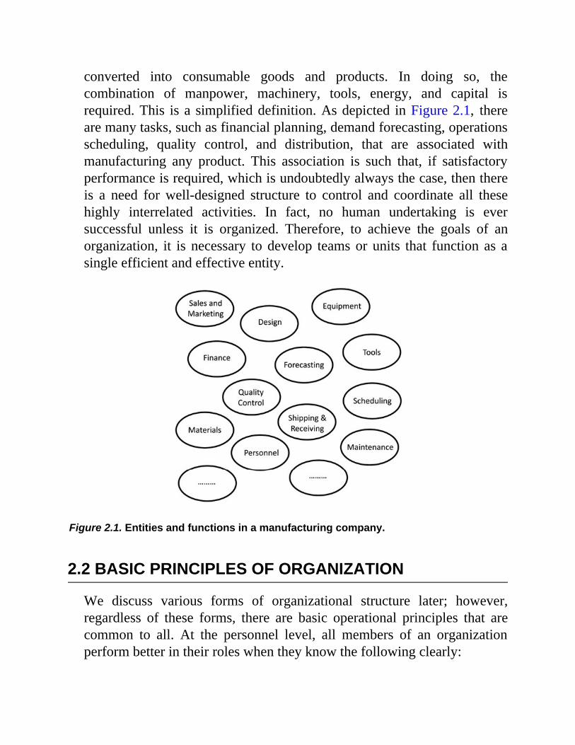
converted into consumable goods and products. In doing so, thecombination of manpower, machinery, tools, energy, and capital isrequired. This is a simplified definition. As depicted in Figure 2.1, thereare many tasks, such as financial planning, demand forecasting, operationsscheduling, quality control, and distribution, that are associated withmanufacturing any product. This association is such that, if satisfactoryperformance is required, which is undoubtedly always the case, then thereis a need for well-designed structure to control and coordinate all thesehighly interrelated activities. In fact, no human undertaking is eversuccessful unless it is organized. Therefore, to achieve the goals of anorganization, it is necessary to develop teams or units that function as asingle efficient and effective entity.

Figure 2.1. Entities and functions in a manufacturing company.

2.2 BASIC PRINCIPLES OF ORGANIZATION

We discuss various forms of organizational structure later; however,regardless of these forms, there are basic operational principles that arecommon to all. At the personnel level, all members of an organizationperform better in their roles when they know the following clearly:

- What their job is- Who their direct supervisor is- Where their position in the organizational structure is- What their authority is- To whom they must report relevant information

These factors are essential to a good organization and apply to everyone inthe organization. It is fundamental for every position that there is a clearjob description, and the members pay attention to and understand theirroles and responsibilities, both individually and collectively. A key rule isthat every member should report to only one supervisor. Knowing theirposition within the organizational structure enables the personnel to followthe proper channels of interaction, patterns of information and materialflow, and appropriate forms of communication. On occasion,unanticipated situations, such as an emergency, can arise that may requireimmediate action. Despite the fact that no rules can be set out ahead oftime for unforeseen events, some guidelines as to who among thepersonnel present must act, and on what degree of authority, will be usefulfor all staff.

At the organizational level, it is clear that no universal principles can bedeveloped because different organizations require different forms ofstructure. However, the following general guidelines apply in manyinstances:

- Clear Objectives: The appropriate form of an organizationdepends directly on what is to be achieved. Theorganization should have clearly stated objectives, andevery unit of the organization should understand and worktoward achieving its purpose.

- Logical Work Division: An organization must be dividedinto appropriate units where work of a similar nature isperformed.

- Unitary Command: Every organization should have onlyone person at the top who is responsible for its performance.

- Work Delegation: It is impractical for one person todirectly supervise and coordinate the work of too manysubordinates. Therefore, top persons must assign duties tocapable associates and subordinates within the frameworkof the organization.

- Well-Defined Responsibilities: Subordinates must be givena job description and some autonomy to freely perform theirjobs. All responsibilities assigned to all units and allmembers should be clear, specific, and understandable.

- Reciprocative Communications: Top persons should alsoseek feedback from subordinates in improving processesand participating in decision making.

Many organizations develop vision and mission statements to set out theirobjectives. A vision statement expresses an organization’s ultimate goaland the reason for its existence. A mission statement provides an overviewof how the organization plans to achieve its vision. Vision and missionstatements are well publicized as identifying symbols of the organization.

Without underestimating the importance and necessity of developing avision statement, a comparison of such statements reveals significantsimilarities. This is particularly noticeable in certain areas with closelyrelated goals. For example, how much can a vision statement of oneuniversity differ from another? Nevertheless, universities find a particularniche on which to build. Therefore, any organization must spend someeffort in developing a vision statement that succinctly reflects theirphilosophy for the products or services they offer. For the substantialdetail on its vision and mission statements, we consider the University ofBritish Columbia (UBC) as an illustrative organization. The following isthe vision statement of UBC.

Vision:

As one of the world’s leading universities, The University of BritishColumbia creates an exceptional learning environment that fosters globalcitizenship, advances a civil and sustainable society, and supportsoutstanding research to serve the people of British Columbia, Canada, andthe world.

Mission statements are sometimes expressed in several annotations. UBCstates these as values:

Values:

Academic FreedomThe University is independent and cherishes and defends free inquiry andscholarly responsibility.

Advancing and Sharing KnowledgeThe University supports scholarly pursuits that contribute to knowledgeand understanding within and across disciplines and seeks everyopportunity to share them broadly.

ExcellenceThe University, through its students, faculty, staff, and alumni, strives forexcellence and educates students to the highest standards.

IntegrityThe University acts with integrity, fulfilling promises and ensuring openand respectful relationships.

Mutual Respect and EquityThe University values and respects all members of its communities, each ofwhom individually and collaboratively makes a contribution to create,strengthen, and enrich our learning environment.

Public InterestThe University embodies the highest standards of service and stewardshipof resources and works within the wider community to enhance societalgood.

Within a large organization, often individual units have their own visionand mission statements, but under the umbrella of the organization’s corestatements. This is more so for the mission statement because its purposeis to elucidate the commitments and means of accomplishing the vision.Since different units in an organization have difference ways and tools, itis appropriate to have a suitably tailored mission statement.

The following are two examples of the mission statement from twodifferent units at UBC.

Mission:UBC Continuing Studies is an academic unit that inspires curiosity,develops ingenuity, stimulates dialogue and facilitates change amonglifelong learners locally and internationally. We anticipate and respond toemerging learner needs and broaden access to UBC by offering innovativeeducational programs that advance our students’ careers, enrich their livesand inform their role in a civil and sustainable society.

Mission:UBC Library advances research, learning and teaching excellence byconnecting communities, within and beyond the University, to the world’sknowledge.

2.3 FORMS OF ORGANIZATIONAL STRUCTURE

There are no rules or uniquely defined models for organizational structure.For a given company and known set of objectives, and depending on thephilosophy taken, the specific organizational structure will emerge. Thebasic structure of an industrial organization depends on the size of thecompany, the nature of business, and the complexity of its activities.However, there are some basic forms of structuring an organization. Themost common is the ‘‘line and staff’’ structure, but there are a number ofvariations of this basic form that will be reviewed in the followingsections. The layouts of these forms are referred to as the organization ororganizational chart.

2.3.1 Line OrganizationThe simplest form of organization is the straight line. The straight-lineconcept implies that the positions on the organizational chart follow avertical line, as shown in Figure 2.2.

Figure 2.2. Line Organizational Chart.

In such an organization, the chief or president handles all issues that arise,from production to sales, finance, or personnel, because the chief orpresident has no specialized staff to aid them. Small and start-upcompanies begin with the line type of organization. The principal owner isthe general manager or the president, and he or she will possibly have onlya few staff members working in the company. As the business grows, heor she will be overwhelmed with diverse tasks, and will need to expand theorganization by upgrading to a “line and staff” type of structure.

2.3.2 Line and Staff OrganizationThe line and staff organization in a simplified form is shown in Figure 2.3.

The main difference between this and the line type of organization is theaddition of some specialists who are appointed where the president needsthe most assistance. The chief engineer may be responsible for both designand manufacturing processes. The sales manager, in addition to sales, mayalso be responsible for marketing and public relations. Certainresponsibilities could be shared by two specialists, but they report to the

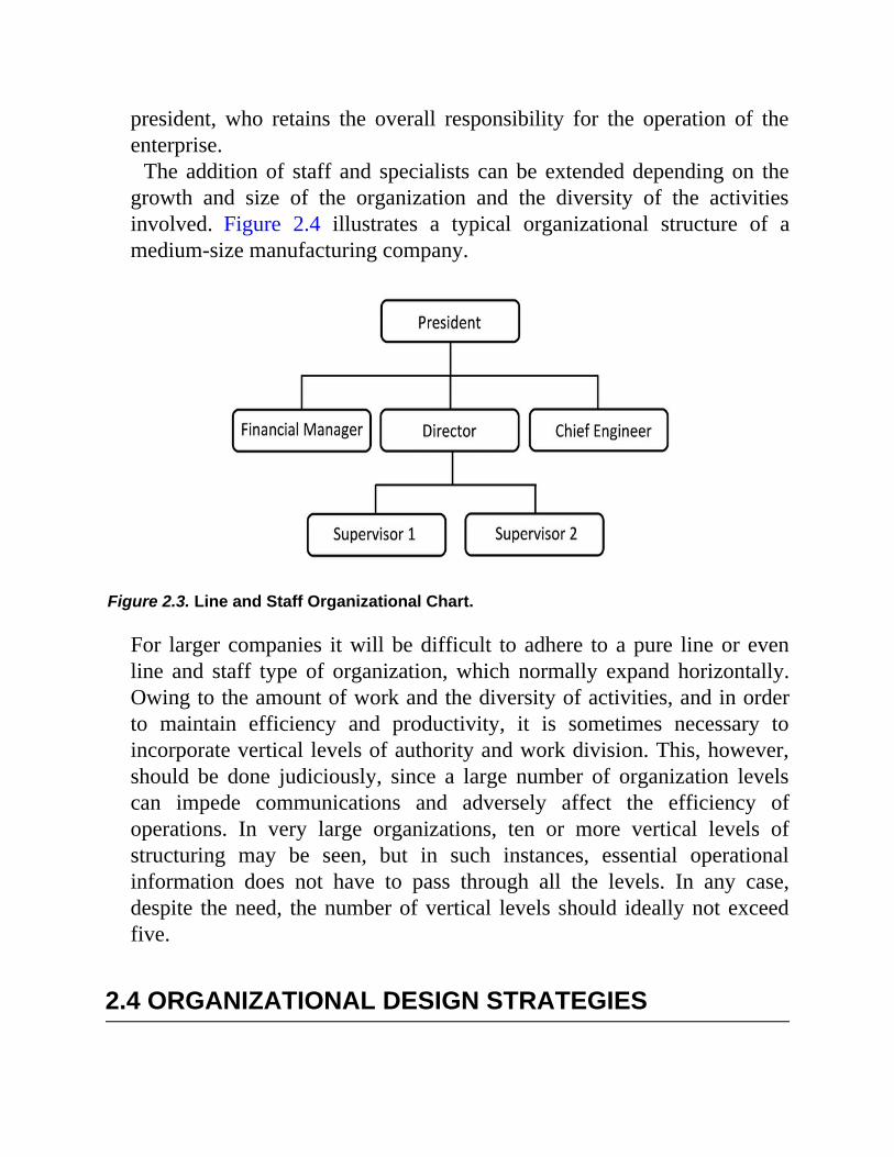
president, who retains the overall responsibility for the operation of theenterprise.

The addition of staff and specialists can be extended depending on thegrowth and size of the organization and the diversity of the activitiesinvolved. Figure 2.4 illustrates a typical organizational structure of amedium-size manufacturing company.

Figure 2.3. Line and Staff Organizational Chart.

For larger companies it will be difficult to adhere to a pure line or evenline and staff type of organization, which normally expand horizontally.Owing to the amount of work and the diversity of activities, and in orderto maintain efficiency and productivity, it is sometimes necessary toincorporate vertical levels of authority and work division. This, however,should be done judiciously, since a large number of organization levelscan impede communications and adversely affect the efficiency ofoperations. In very large organizations, ten or more vertical levels ofstructuring may be seen, but in such instances, essential operationalinformation does not have to pass through all the levels. In any case,despite the need, the number of vertical levels should ideally not exceedfive.

2.4 ORGANIZATIONAL DESIGN STRATEGIES

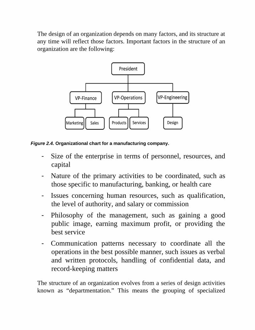
The design of an organization depends on many factors, and its structure atany time will reflect those factors. Important factors in the structure of anorganization are the following:

Figure 2.4. Organizational chart for a manufacturing company.

- Size of the enterprise in terms of personnel, resources, andcapital

- Nature of the primary activities to be coordinated, such asthose specific to manufacturing, banking, or health care

- Issues concerning human resources, such as qualification,the level of authority, and salary or commission

- Philosophy of the management, such as gaining a goodpublic image, earning maximum profit, or providing thebest service

- Communication patterns necessary to coordinate all theoperations in the best possible manner, such issues as verbaland written protocols, handling of confidential data, andrecord-keeping matters

The structure of an organization evolves from a series of design activitiesknown as “departmentation.” This means the grouping of specialized

activities and resources to accomplish a total task.

2.5 MAJOR FORMS OF DEPARTMENTATION

Theoretically, there are as many ways to departmentalize as there areorganizations. Even two organizations of similar products and goals candiffer in details as a result of many reasons, from geographical location tomanagement style. However, significant generic forms of departmentationare as follows:

- Functional- Product/divisional- Geographic- Clientele- Process- Time- Alphanumeric- Autonomy

A description of these concepts for departmentation and their importantmerits/demerits is presented next.

2.5.1 Functional DepartmentationThis most common type of departmentation is ideal for small-mediumcompanies, where the organization is divided into departments accordingto the tasks they must perform. There is typically only one of eachspecialized unit, such as finance, manufacturing, marketing, and so on, andnormally in one location, but not necessarily. This formation is especiallysuitable for single-product companies, such as steel foundries andaluminum plants.

Advantages

• Efficient operations result from specialization in eachdepartment.

• Focusing on specific related tasks provides an opportunityfor continuous improvement in personnel andorganizational performance.

• Effective long-range planning and major decision makingare more readily accomplished.

Disadvantages

• After an optimal size is reached, poor communication andcoordination often ensue.

• Lack of motivation and a feeling of being unimportant candevelop.

• Overlapping authorities and problems with decision makingcan appear.

2.5.2 Product/Divisional DepartmentationA second common form of departmentation is organized along the productlines. Most companies organized in this fashion were initially functionallyorganized. Expanding product diversity can overwhelm the organization inevery aspect of its operation and can cause inefficiencies. In productdepartmentation, different products or family of products are managedseparately. For example, there may be divisions for audiovisualequipment, appliances, and health-care products each having their ownfinance, production, marketing, and other relevant departments.

Advantages

• It efficiently integrates the main activities required to makea particular product.

• It works independently while relying on support from themother organization.

• It allows development of significant expertise as divisionscompete to supersede in performance.

Disadvantages

• It impedes the direct transfer of information and technicalknowledge between divisions.

• It necessitates duplication of some resources.• Recruiting and retaining capable managers requires effort

and can be costly.

2.5.3 Geographic DepartmentationThe purpose of this form of departmentation is to provide goods andservices in the geographical locations where they are required, such as postoffices, hospitals, and transit systems that serve communities at dispersedgeographical locations. Large corporations can have departments invarious cities or countries.

Advantages

• There is effective provision of goods and services closer tothe location of demand.

• It provides the opportunity to hire local personnel.

Disadvantages

• There can be duplication of resources.• The possibility exists for a lack of direct management and

support.

2.5.4 Clientele DepartmentationCustomer or clientele departmentation is used to provide specific goodsand services for specific classes of clients, such as children, youth, oradults.

Advantages

• Specialization and expertise in products and services arepossible.

• Better relationships with clients can be fostered.

Disadvantages

• There can be a duplication of resources.• There may be difficulty in maintaining uniform services.

2.5.5 Process DepartmentationThis form of departmentation is common in some manufacturing plants,where processes of similar nature are grouped together to enhanceresource availability and accumulate a greater level of expertise.

Advantages

• It improves coordination of similar processes.• It allows better decision making and implementation of

changes.• It reduces duplication of resources.

Disadvantages

• It lacks coordination with other processes.• It creates conflict in authority in large departments.

2.5.6 Time DepartmentationThis form of departmentation involves the breaking down of theorganization’s operations into time-dependent components. Often,resources must be reorganized and reassigned to accomplish the requiredtasks within the allotted time.

Advantage

• The organization can be flexible and dynamic in respondingand adapting to change.

Disadvantage

• There is difficulty in establishing permanent and consistentprocedures.

2.5.7 Alphanumeric DepartmentationAlphabetical and numerical departmentations are used to assign employeesto a team or department when the level of skills required is not significant,or there is evidence that skills needed are relatively homogeneous. It canalso be used to divide the work, such as postal code for distribution ofmail, or direct the clientele, such as service counters in a passport office.

Advantage

• There is great ease and speed of implementation.

Disadvantage

• If the assumption of homogeneous skills is unrealistic, itcan result in departments with imbalanced capabilities.

2.5.8 Autonomy Departmentation

If the activities of an organization are diverse, unrelated to one another,and do not require “direct” management, then this form of departmentationis the most appropriate.

For instance, major conglomerate corporations, whose main goal is toinvest in well-established companies regardless of the products or servicesoffered, fall in this category. They show little interest in directly managingthe acquired companies and allow autonomy in their operations.

Advantage

• There is freedom from direct involvement.

Disadvantage

• There can be a lack of knowledge about developingproblems.

2.6 MANAGEMENT FUNCTIONS

One of the many purposes of any organizational structure of an enterpriseis to enable and guide the management in its operations. These pertain tospecific functions of planning, organizing, directing, and controlling.

- Planning is the process of determining the future activitiesby developing goals and objectives, and establishingguidelines and timelines for achieving them.

- Organizing deals with providing and integrating therequired resources, such as personnel, equipment, materials,tools, and capital to perform the planned activities.

- Directing assigns specific tasks and responsibilities topersonnel, provides support, motivates, and coordinatespersonnel’s effort.

- Controlling, which is more associated with directing,evaluates performance, rectifies issues, and ascertains that

all activities are satisfactorily progressing toward the setgoals and objectives.

Figure 2.5 shows the process flow within these four functions.

Figure 2.5. Management functions.

The management functions are dynamic in the sense that they apply toongoing activities within, and they also respond to changes occurringoutside the organization, such as new technology, regulations, andeconomic conditions. For instance, if it becomes mandatory to implementcertain quality assurance plans to improve safety, the entire organizationwill be affected, and the functions of planning, organizing, directing, andcontrolling will be responsible for accomplishing the change.

2.6.1 Contemporary Operations ManagementThere are ever-increasing trends to provide high-quality goods andservices. Whereas traditional operations management functions ascertainthat ongoing activities are proceeding satisfactorily, contemporaryoperations management attempts to be more dynamic and improve thenature and effectiveness of the management functions. Activities of a

progressive forward-looking organization include the following:

• Gathering information on customer needs, gaging theirsatisfaction, and using these to improve the products andservices offered

• Exploiting new technology to improve quality, productivity,and efficiency

• Providing an opportunity for all members of theorganization for professional and skill development

• Genuinely linking with customers and community toimprove the well-being of society

2.6.2 Span of ControlSpan of control refers to the number of personnel who report to onesupervisor. It is one of the most widely known and used organizationalprinciples. The ideal span of control is between four and eight. In practice,however, there is a much greater span than this, perhaps twelve or more—but this is undesirable. Higher levels in organizations have a smaller spanof control. A typical company or university will have one president andpossibly five or so vice presidents for various functions, such as finance,public relations, research and development, and operations.

2.6.3 Complexities of Span of ControlWith the increase in the span of control, the different combinations of therelationship with subgroups increase exponentially. There aremathematical equations to determine the total number of suchrelationships, but it will be more tangible if we show this by means of anexample. Suppose there is one supervisor S, and there are fivesubordinates A, B, C, D, and E.

Excluding a large number of possible relationships among thesubordinates, the number of relationships between the supervisor and thesubordinates is still high, as shown in Table 2.1.

Clearly, this is an extreme representation, but it is easy to see how thecombinations can rise dramatically. With five subordinates, if we assumemany relationships unnecessary in practice, even a dozen differentrelationships are difficult to maintain. It is also very challenging to arrangea common time for meetings when every subordinate is available.

2.6.4 The Informal OrganizationThe discussion in the preceding sections concerned what might be termedthe formal organization. We showed precise relationships among thevarious positions in the enterprise in terms of a formal organizationalchart, and the need for such an organization is emphasized. We must alsoconsider the facts of life within an organization, however, and recognizethat these positions are held by people with social interests. As a result,some informal relationships will always exist. Superimposed on the formalorganizational chart in Figure 2.6 is an informal organization that mightexist. The informal organization is shown by the dashed lines.

Table 2.1 Relationships between one supervisor and five subordinates

Pattern of Relationships Involving Supervisor Number of RelationshipsWith listed individual when the other four are not present:S → A, B, C, D, E 5

With listed two individuals when the other three are not present:S → AB, AC, AD, AE, BC, BD, BE, CD, CE, DE 10

With listed three individuals when the other two are not present:S → ABC, ABD, ABE, ACD, ACE, ADE, BCD, BCE, BDE, CDE 10

With listed four, when the remaining individual is not present:S → ABCD, ABCE, ABDE, ACDE, BCDE 5

When all individuals are present:S → ABCDE 1

Total relationships 31

Executive 2b, for instance, has some relationship with employee h4, with

whom he or she has no formal organizational connection. Such informalrelationships exist for a variety of reasons. Some people are natural leadersand problem solvers wherever they are placed in an organization, and

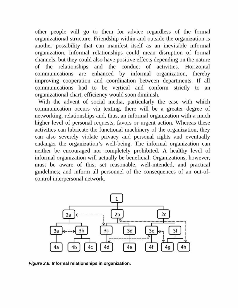
other people will go to them for advice regardless of the formalorganizational structure. Friendship within and outside the organization isanother possibility that can manifest itself as an inevitable informalorganization. Informal relationships could mean disruption of formalchannels, but they could also have positive effects depending on the natureof the relationships and the conduct of activities. Horizontalcommunications are enhanced by informal organization, therebyimproving cooperation and coordination between departments. If allcommunications had to be vertical and conform strictly to anorganizational chart, efficiency would soon diminish.

With the advent of social media, particularly the ease with whichcommunication occurs via texting, there will be a greater degree ofnetworking, relationships and, thus, an informal organization with a muchhigher level of personal requests, favors or urgent action. Whereas theseactivities can lubricate the functional machinery of the organization, theycan also severely violate privacy and personal rights and eventuallyendanger the organization’s well-being. The informal organization canneither be encouraged nor completely prohibited. A healthy level ofinformal organization will actually be beneficial. Organizations, however,must be aware of this; set reasonable, well-intended, and practicalguidelines; and inform all personnel of the consequences of an out-of-control interpersonal network.

Figure 2.6. Informal relationships in organization.

2.7 ORGANIZATIONAL ACTIVITIES OF A PRODUCTIONCONTROL SYSTEM

In the previous sections, the overall organizational structure for productionwas reviewed. At the operational and control level, a different form ofstructure showing the relationships between the various functionalelements can be constructed. Figure 2.7 illustrates the managementfunctions and decisions necessary to plan and control production andclassifies them by the length of the planning horizon needed to consideradequate factors that are relevant to the decision.

Long-range decisions involve the definition of priorities, product lines,the establishment of customer service policies, selection of distributionchannels, further investment, determination of warehouse capacity, andperhaps allocation of capacity to different product lines. The decisions aremade and reviewed quarterly or annually and require planning horizons ofone to five years. Market research, long-range forecasting, and resourceplanning are necessary activities.

Intermediate-range planning is done within the framework of policy andresource constraints resulting from the long-range planning process.Planning horizons of three months to a year are often sufficient. Necessarymanagement functions include forecasting, workforce planning, andproduction planning. Typically these activities are carried out on amonthly cycle, although it is not unusual to see a shorter review periodused.

Short-range activities involve scheduling and control of production.Decisions involve adjustment of production rates to adapt to forecasterrors, material shortages, machine breakdown, and other uncertainties;the assignment of workers to work activities; the determination ofpriorities and the sequence of operations; the assignment of work toworkstations; the use of overtime; and the adjustment of in-processinventory levels. Formally these activities may be carried out weekly ordaily, but they often are a continuous function of the production controldepartment and line supervision. Decisions can be made at any time. Theplanning horizon is short, usually one or two weeks, but could be longer ifthe manufacturing cycle time is long.

Figure 2.7. Planning horizons for production control.

2.8 TYPICAL PRODUCTION AND SERVICE SYSTEMS

Figures 2.8 and 2.9 represent arrangements for a production system and aservice system. Such arrangements as shown in Figures 2.8 and 2.9 arereferred to as the “manufacturing cycle,” or the “operational cycle,” sincethe information flow is more or less cyclic through the system. Thearrangements shown in these figures are not unique, and variations arepossible depending on the nature of the products or services, the size of theenterprise, specific objectives, and the management style. In both figures,the department designated as “finance” has been distinctly identified toshow that every aspect of the organization’s activities has financialimplications.

Despite different appearances of the structure of production and servicesystem as depicted in Figures 2.8 and 2.9, both share similar functional

activities, the pattern of information flow, and application of industrialengineering techniques. Basically, they bridge together many of theislands of activities shown in Figure 2.1.

Figure 2.8. A production planning and operation system.

Figure 2.9. A service planning and operation system.

EXERCISES

2-1 Referring to Figure 2.1:

a. Identify the functions and entities that are relevant toyour current place of occupation.

b. List functions and activities that your present workdeals with, but that do not appear in Figure 2.1.

c. Make a list of all the functions relevant to yourpresent work. Have items of the list in mind whilereading the book, and note where each topic may beapplicable.

2-2 Draw an organizational chart for an enterprise that you haveworked for and do the following:

a. Highlight your position on the chart.b. Examine the presence of what we called the

“informal organization” and superimpose it on thechart.

c. If you sensed that some sort of span of control was inplace, what were the typical numbers?

d. Can you say anything especially positive or negativeabout your organization’s structure?

2-3 Using the Internet, search and obtain an organizational chart for arange of companies, industries, or governmental agencies to seehow they organize themselves to offer better services and achievetheir objectives.

2-4 Think of an enterprise that may be best organized by geographicdepartmentation, draw a representative organizational chart, andwrite a vision statement for it.

2-5 Find a company that may be best organized by clienteledepartmentation, draw a representative organizational chart, andwrite a mission statement for it.

2-6 In your place of work, can you identify individuals, groups, ordepartments who deal with planning, organizing, directing, and/or

controlling?2-7 In your place of work, identify the activities that fit long-range,

intermediate-range, and short-range planning.

* We frequently refer to production and manufacturing environments to exemplify an organizationthat reflects the engineering scope of this book and to allow us to highlight the key concepts better.In general, these concepts can be equally applied to many organizations that have identifiableentities and functions, and provide products or services.

Chapter

3MANUFACTURINGSYSTEMS

3.1 INTRODUCTION

The operation and performance of a manufacturing system depend heavilyon its physical layout, and this physical layout varies significantly fromone firm to the next. The ability to recognize the dominant form of amanufacturing system of an enterprise and its layout is an important firststep for analyzing, assessing, and applying appropriate controls andimprovement plans.

The nature of a company’s manufacturing system depends on manyfactors. The size of the firm, the type of products, production volume, andthe diversity of the products influence the adoption of a particularorganization for its manufacturing resources.

Over the last several decades, owing to significant advances inautomation, robotics, sensing technology, and computer science,manufacturing systems have been revolutionized and fully automated,flexible, and many forms of computer-integrated manufacturing plantshave emerged. Nevertheless, a significant proportion of products is stillmanufactured in the conventional form, although more and more oldermachinery is being replaced with advanced precision equipment. Beingfamiliar with both traditional and modern manufacturing systems isessential for industrial engineers.

3.2 CONVENTIONAL MANUFACTURING SYSTEMS

In general, there are three types of conventional manufacturing systems:

1. Job shop production2. Batch production3. Mass production

Job shop–type environments will probably always exist in the classicalform, as will be discussed in Section 3.2.1. Batch manufacturing systemsencompass well over 50 percent of the world production of goods, and,along with mass production systems, they can be highly automated and“modern” in equipment. Next, we review these manufacturing systems.Modern concepts of manufacturing systems are discussed in Section 3.4.

3.2.1 Job Shop ProductionThis most general form of manufacturing, also called one-off, ischaracterized by production volumes of small quantity that are oftennonrepeating. Therefore, specialized and automated types of machineryand equipment are usually not required. Job shop production is used tohandle a large variation in the type of products and work that must beperformed. This is the reason that production equipment must be general-purpose to allow for the variety of work, but the skill level of thepersonnel must be relatively high so that they can perform a range ofnonroutine work. Successful operation in a job shop environment reliesheavily on the skills of its workforce and the flexibility in adapting to thechanging conditions. Products typically manufactured in a job shop areaircraft, space vehicles, prototypes of new products, and research andexperimental equipment.

Shipbuilding and fabrication of major outdoor structures are notnormally categorized as job shop production, although the quantitiesproduced are typical of a job shop environment.

Often with one-of-a-kind production and no previous experience theproduction rate of a job shop will be low compared with othermanufacturing systems. This does not necessarily mean that the job shopenvironment is inefficient or unproductive. In fact, many products that are

produced in higher quantities and rates in dedicated systems were initiallymanufactured in a job shop environment as prototypes. Production in a jobshop environment constantly enhances workforce skills such that workerscan fabricate complex, intricate, and unique prototypes and products usinggeneral-purpose equipment.

3.2.2 Batch ProductionBatch production is the most common form of manufacturing systems.This mode of production is characterized by the fact that medium-size lots,hence the term batch, of the same component or product may be producedonce, or they may be produced at some determined intervals. Themanufacturing equipment used in batch production is general-purpose butcapable of a higher rate of production. Since it is known ahead of timewhat products will be produced, the machine tools used in batchmanufacture are often supported by specially designed jigs and fixtures,special tooling, and a good degree of automation or programmability.They greatly facilitate work, and the production rates can be noticeablyhigh. A certain level of operator skill is also necessary because operatorsswitch from product to product and deal with a variety of materials,equipment, tools, and manufacturing requirements.

The production process in this type of systems can be defined as themanufacturing of batches of identical parts by passing them through aseries of operations such that, preferably, each operation is completed onan entire batch before it moves to its next operation. However, if deemedbeneficial and appropriate, provisions are made so that sub-batches ofparts can be transferred to their subsequent operation to improve the flowof work. Batch production is relevant because a large variety of parts andproducts will be needed in small quantities. The purpose of batchproduction is sometimes to satisfy the continuous or seasonally continuousdemand for a product. Such a plant, however, is often capable of aproduction rate that exceeds the demand rate. Therefore, the plant firstproduces sufficient inventory of an item to satisfy the continuous demand;then it switches over to other products. This cycle is repeated, based ondemand, the inventory levels desired, and the production rate. If thedemand is seasonal, the production is accordingly coordinated. Examples

of products made in a batch production environment include many typesof industrial supplies, products with a different size and model, andhousehold appliances, especially of seasonal type, such as heating units forwinter and cooling units for summer. Batch production plants includemachine shops, casting shops, plastic-molding factories producingcontainers for other industries, plants producing various colors of paint,and some chemical plants.

3.2.3 Mass ProductionIn mass production systems, manufacturing facilities are permanentlyallocated to produce a single part or product. Mass production is generallycharacterized by a large volume of output using specialized and oftenautomatic equipment and machinery. This allows a low level of operatorskill to be employed; the work involves very few tasks, often onlyloading/unloading of parts or supervising the operation of equipment.Commonly an entire plant is arranged with various production linesdedicated to producing different parts of one product to be assembled intoa complete product. The investment in highly automated machines,integrated part transfer, and specialized tooling is significant. Comparedwith any other form of manufacturing, the skill level of workers in a massproduction plant tends to be low. Because of specialized equipment andspecific tooling for a particular product, flexibility to change to a differentproduct, although possible, is low and could be costly.

Table 3.1 summarizes some of the important characteristics of job shop,batch, and mass production systems. The above description of these threetypes of production systems has been simplified. In practice, differentapproaches in the organization of production facilities must be used tomanufacture goods as they rarely fall into one single category; that is,elements of one system might be present in the other. The reason is that itis not always possible, and in fact not necessary to maintain only one typeof production system. For example, a dominantly batch manufacturingfacility may have a mass or continuous production line for items that areused in large quantities within the plants. Similarly, a manufacturingfacility may have two major sections, one section dedicated to the massproduction of various products, and the other a batch manufacturing

environment that can adapt to the demand variation to ensure that allproducts are available at all times.

Table 3.1. Characteristics of different production systems

Characteristic

Production SystemJob Shop Batch Mass

Production quantity Low High Higher

Production rate Low High Higher

Workforce skill Very high High Low

Equipment General-purpose General-purpose Special-purpose

Tooling General-purpose Special-purpose Special-purpose

Plant layout Functional (process)Functional or

group technologyLine (product)

Degree of automation Low High Higher

Figure 3.1 shows a typical range of application of machine tools andequipment within the conventional manufacturing systems in terms ofproduction volume.

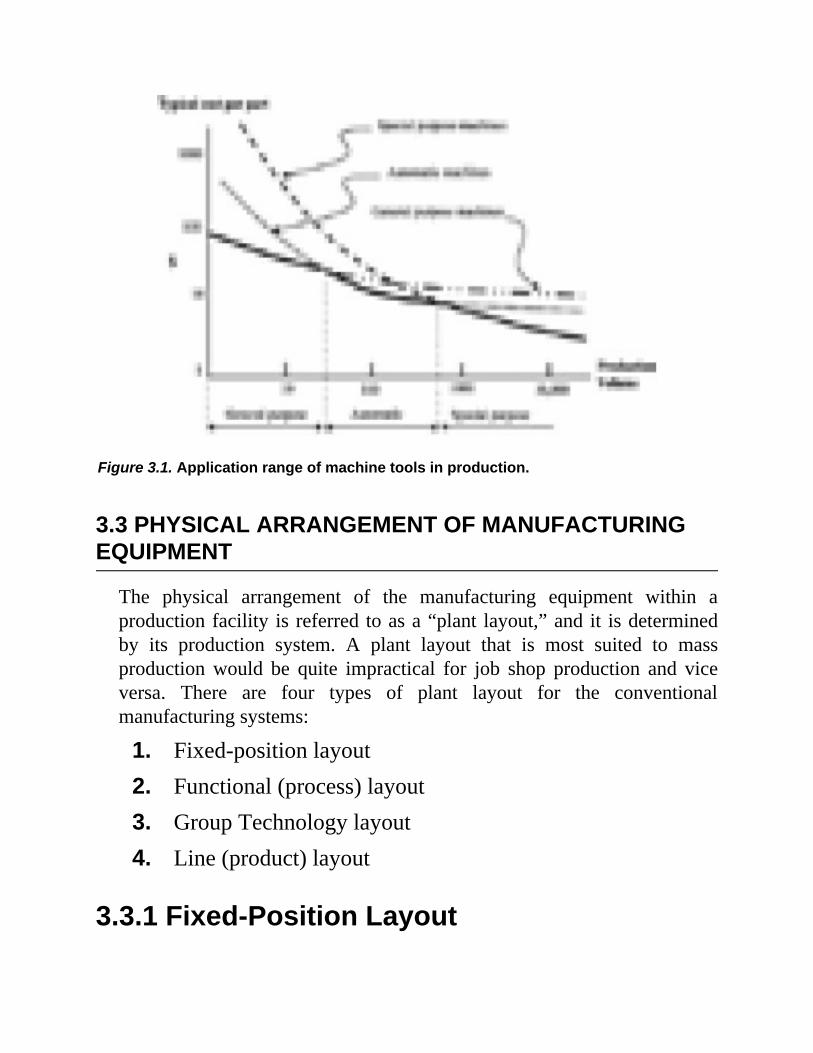
Figure 3.1. Application range of machine tools in production.

3.3 PHYSICAL ARRANGEMENT OF MANUFACTURINGEQUIPMENT

The physical arrangement of the manufacturing equipment within aproduction facility is referred to as a “plant layout,” and it is determinedby its production system. A plant layout that is most suited to massproduction would be quite impractical for job shop production and viceversa. There are four types of plant layout for the conventionalmanufacturing systems:

1. Fixed-position layout2. Functional (process) layout3. Group Technology layout4. Line (product) layout

3.3.1 Fixed-Position Layout

In this form of layout, the product remains in a “fixed position” because ofits large size and high weight. The equipment required for manufacturingand assembly is moved to and away from the product, as shown in Figure3.2. Typical industrial scenarios include shipbuilding and aircraftmanufacturing, which are characterized by a relatively low productionvolume and rate. In fixed-position layout, consumables such as nuts andbolts, tools, materials, prefabricated modules, and equipment must bearranged in a carefully organized fashion around the product whileensuring convenient access and open and safe pathways for unrestrictedmovement of materials, hardware, and personnel. As the production andassembly proceeds, congestion may ensue. Therefore, task planning andscheduling become increasingly critical.

Figure 3.2. Fixed-position layout.

3.3.2 Functional LayoutThe functional layout, which is primarily used for batch production, is theresult of grouping production equipment or plant according to its functionor type. Therefore, all milling machines, for example, would form onegroup, and all drilling machines would form another functional group, and

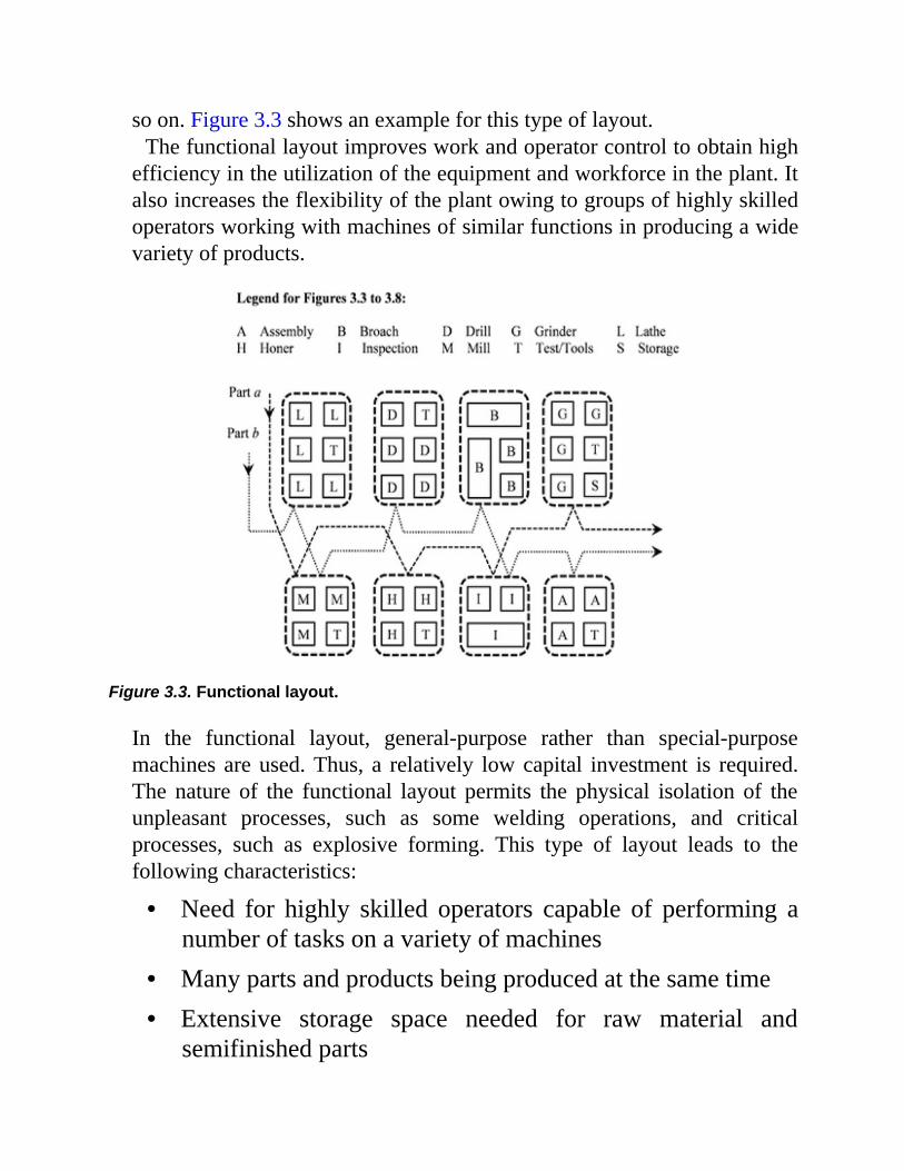
so on. Figure 3.3 shows an example for this type of layout.The functional layout improves work and operator control to obtain high

efficiency in the utilization of the equipment and workforce in the plant. Italso increases the flexibility of the plant owing to groups of highly skilledoperators working with machines of similar functions in producing a widevariety of products.

Figure 3.3. Functional layout.

In the functional layout, general-purpose rather than special-purposemachines are used. Thus, a relatively low capital investment is required.The nature of the functional layout permits the physical isolation of theunpleasant processes, such as some welding operations, and criticalprocesses, such as explosive forming. This type of layout leads to thefollowing characteristics:

• Need for highly skilled operators capable of performing anumber of tasks on a variety of machines

• Many parts and products being produced at the same time• Extensive storage space needed for raw material and

semifinished parts

• Considerable storage and work space around machines• High inventories of work-in-progress parts• Need for various part-handling implements and

transportation equipment• Complex scheduling of work and tracking of materials flow

through the plant• Great flexibility in terms of producing different parts• Frequent movement of materials between operations and

departments, with the possibility of damage to parts andmisplacement

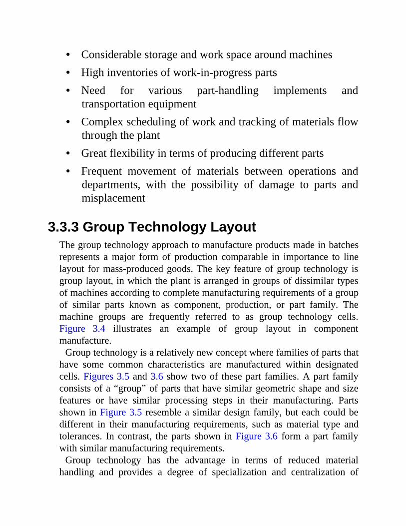
3.3.3 Group Technology LayoutThe group technology approach to manufacture products made in batchesrepresents a major form of production comparable in importance to linelayout for mass-produced goods. The key feature of group technology isgroup layout, in which the plant is arranged in groups of dissimilar typesof machines according to complete manufacturing requirements of a groupof similar parts known as component, production, or part family. Themachine groups are frequently referred to as group technology cells.Figure 3.4 illustrates an example of group layout in componentmanufacture.

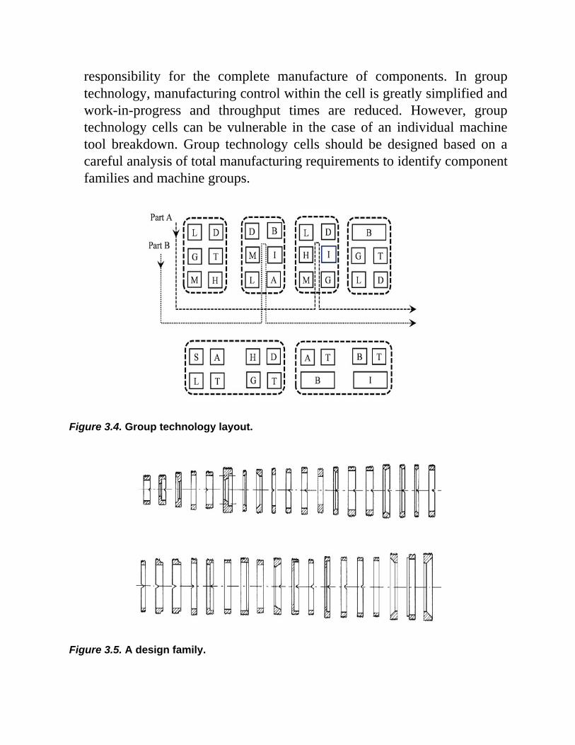
Group technology is a relatively new concept where families of parts thathave some common characteristics are manufactured within designatedcells. Figures 3.5 and 3.6 show two of these part families. A part familyconsists of a “group” of parts that have similar geometric shape and sizefeatures or have similar processing steps in their manufacturing. Partsshown in Figure 3.5 resemble a similar design family, but each could bedifferent in their manufacturing requirements, such as material type andtolerances. In contrast, the parts shown in Figure 3.6 form a part familywith similar manufacturing requirements.

Group technology has the advantage in terms of reduced materialhandling and provides a degree of specialization and centralization of

responsibility for the complete manufacture of components. In grouptechnology, manufacturing control within the cell is greatly simplified andwork-in-progress and throughput times are reduced. However, grouptechnology cells can be vulnerable in the case of an individual machinetool breakdown. Group technology cells should be designed based on acareful analysis of total manufacturing requirements to identify componentfamilies and machine groups.

Figure 3.4. Group technology layout.

Figure 3.5. A design family.

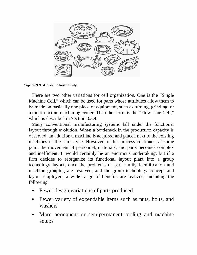
Figure 3.6. A production family.

There are two other variations for cell organization. One is the “SingleMachine Cell,” which can be used for parts whose attributes allow them tobe made on basically one piece of equipment, such as turning, grinding, ora multifunction machining center. The other form is the “Flow Line Cell,”which is described in Section 3.3.4.

Many conventional manufacturing systems fall under the functionallayout through evolution. When a bottleneck in the production capacity isobserved, an additional machine is acquired and placed next to the existingmachines of the same type. However, if this process continues, at somepoint the movement of personnel, materials, and parts becomes complexand inefficient. It would certainly be an enormous undertaking, but if afirm decides to reorganize its functional layout plant into a grouptechnology layout, once the problems of part family identification andmachine grouping are resolved, and the group technology concept andlayout employed, a wide range of benefits are realized, including thefollowing:

• Fewer design variations of parts produced• Fewer variety of expendable items such as nuts, bolts, and

washers• More permanent or semipermanent tooling and machine

setups

• Convenient and less congested material handling• Better production and inventory control• More efficient smaller process planning tasks• Employee skill enhancement and job satisfaction

3.3.4 Line Layout and Group Technology FlowLine

With a line layout, the plant is divided into groups on a component basissimilar to the case of the group layout. The order of processes to beperformed on the component or product is the determining factor in thephysical arrangement of manufacturing equipment. With conventionalmass production, these groups of machines are arranged in lines, eachpermanently set up to produce one component. The high efficiency ofmass production is generally the result of using a line layout whereconveyors or gravity shoots are used to move parts from one machine tothe next quickly. In a well-paced line, very high production rates areachieved, and the equipment and machines are rarely idle.

The line layout is also used for group technology families of similarcomponents in such a way that every part in the family must (ideally) usethe same machines in the same sequence. Certain steps can be omitted, butthe flow of work through the system must be in one direction. Thisparticular layout is frequently referred to as group technology flow line.Figure 3.7 shows an example of this type of layout.

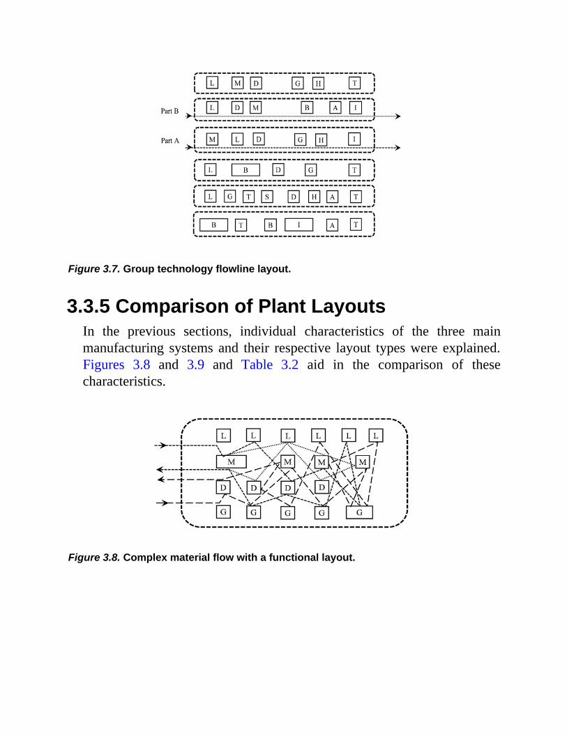
Figure 3.7. Group technology flowline layout.

3.3.5 Comparison of Plant LayoutsIn the previous sections, individual characteristics of the three mainmanufacturing systems and their respective layout types were explained.Figures 3.8 and 3.9 and Table 3.2 aid in the comparison of thesecharacteristics.

Figure 3.8. Complex material flow with a functional layout.

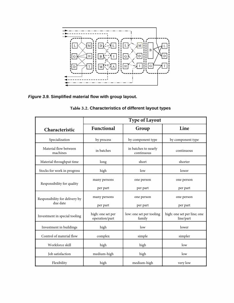
Figure 3.9. Simplified material flow with group layout.

Table 3.2. Characteristics of different layout types

Characteristic

Type of LayoutFunctional Group Line

Specialization by process by component type by component type

Material flow betweenmachines in batches in batches to nearly

continuous continuous

Material throughput time long short shorter

Stocks for work in progress high low lower

Responsibility for qualitymany persons

per part

one person

per part

one person

per part

Responsibility for delivery bydue date

many persons

per part

one person

per part

one person

per part

Investment in special tooling high: one set peroperation/part

low: one set per toolingfamily

high: one set per line; oneline/part

Investment in buildings high low lower

Control of material flow complex simple simpler

Workforce skill high high low

Job satisfaction medium-high high low

Flexibility high medium-high very low

3.3.6 Hybrid and Nested ManufacturingSystems

Purely functional or purely group technology layout may be rare inindustrial settings. Commonly a production system is composed ofelements of different manufacturing concepts and layout type, eachcomplementing the other in an attempt to balance the particular situation’sneed with an economic solution. An expensive and less frequently usedfacility might be shared between a number of independent cells, or withina functional group, there may be machines with different functions.Certain components might only be produced by a certain subgroup ofmachines. On the other hand, within a group technology cell, a number ofsimilar machines could be installed to balance the production capacity forparticular components. The key is to pay attention to the pros and cons ofany deviation from standard forms, and the ultimate goal should be toimprove functionality and efficiency.

3.4 MODERN MANUFACTURING SYSTEMS

With the advent of computers, development of a multitude of sensors, andpossibility of networking and real-time data transmission, manufacturingmethods and systems have been tremendously revolutionized over the lastfew decades. Such manufacturing systems are commonly referred to as theComputer Integrated Manufacturing (CIM). In CIM, many facets of amanufacturing concern, such as process planning, inventory control,machining codes, in-process quality control, and some assembly, areintegrated providing a high degree of efficiency, coordination, andproductivity. Within CIM there exists the fully automated category ofFlexible Manufacturing Systems (FMSs).

3.5 FLEXIBLE MANUFACTURING SYSTEMS

FMSs come in various designs, sizes, combinations of equipment, toolingprovisions, material storage and handling, and specific unique features.The key characteristics of FMSs are the following:

1. Group technology, where a subtle variety of parts can bemanufactured. This is because the system is primarily andoften permanently fitted with tools and auxiliary devicesthat handle a known range of weight, volume, and shape ofcomponents.

2. Computer-controlled material-handling equipment and/orrobots. These implements are generally immediatelyavailable to load, unload, or transfer parts throughout thesystem.

3. Computer-controlled workstation of various types. Thecycle time per part on the workstations must be highlysynchronized and coordinated so that they don’t stay idlefor too long or block each other as a result of havingaccumulated unfinished parts.

4. Loading and unloading stations. The stations that in somesystems are used as temporary buffers are integrated withthe material-handling system for a continuous, smoothoperation.

5. Coordinated operation. All the above elements must behighly synchronized, have compatible cycle times, wellintegrated, and have “look ahead” intelligence to preventblockage, and, if an unpredictable blockage occurs, havemeans of unblocking and resuming operation.

Despite the term flexible (and indeed these systems are highly flexible),their flexibility is within a narrow range of the parts that they can produce.With constant developments in technology, their flexibility has beenbroadened, and a greater variety of parts can be produced within thesesystems.

3.5.1 Advantages of FMSs

With known-in-advance parts to produce and highly coordinatedoperations, it is possible to gain major advantages using FMSs, such as thefollowing:

• Low manufacturing cost per part due to dedicated toolingand machinery

• High machine utilization due to synchronized cycle times• Improved and more consistent quality due to absence of

direct human involvement• Increased system reliability due to self-adaptation, quick

replanning and resumption of operation, and elimination ofhuman errors

• Reduced part inventories and work in progress due toautomated handling and synchronized operations

• Short work flow lead times due to elimination of idle timeand continuous activities in the system

• Significantly improved overall efficiency considering theabove factors

Figure 3.10 shows the percentage of time spent by a typical part inconventional manufacturing facilities from entry to exit. Effectively, it is30 percent of 5 percent, that is, 1.5 percent of net machining or processingtime, leading to significant costs and minimal returns. In well-synchronized flexible manufacturing, the net machining and processingtimes could be as high as 80 percent.

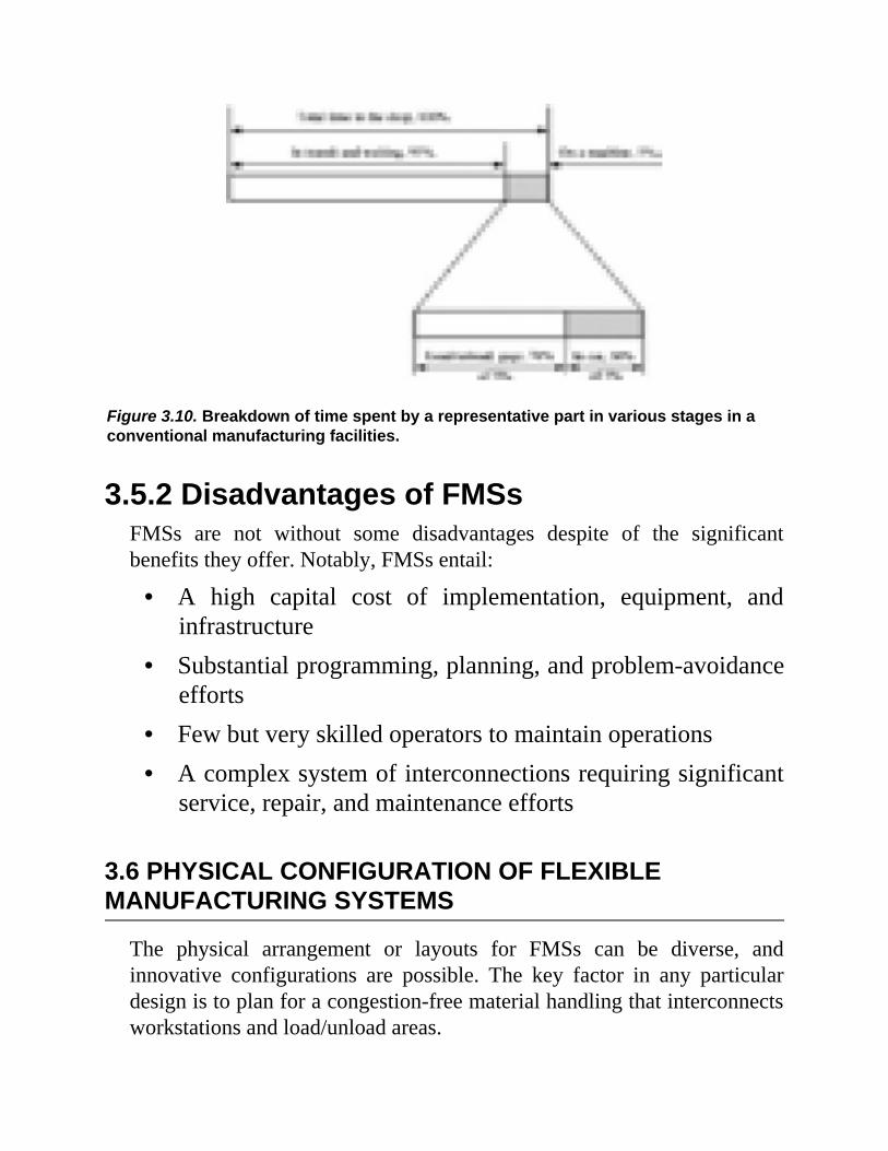
Figure 3.10. Breakdown of time spent by a representative part in various stages in aconventional manufacturing facilities.

3.5.2 Disadvantages of FMSsFMSs are not without some disadvantages despite of the significantbenefits they offer. Notably, FMSs entail:

• A high capital cost of implementation, equipment, andinfrastructure

• Substantial programming, planning, and problem-avoidanceefforts

• Few but very skilled operators to maintain operations• A complex system of interconnections requiring significant

service, repair, and maintenance efforts

3.6 PHYSICAL CONFIGURATION OF FLEXIBLEMANUFACTURING SYSTEMS

The physical arrangement or layouts for FMSs can be diverse, andinnovative configurations are possible. The key factor in any particulardesign is to plan for a congestion-free material handling that interconnectsworkstations and load/unload areas.

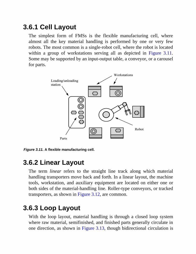
3.6.1 Cell LayoutThe simplest form of FMSs is the flexible manufacturing cell, wherealmost all the key material handling is performed by one or very fewrobots. The most common is a single-robot cell, where the robot is locatedwithin a group of workstations serving all as depicted in Figure 3.11.Some may be supported by an input-output table, a conveyor, or a carouselfor parts.

Figure 3.11. A flexible manufacturing cell.

3.6.2 Linear LayoutThe term linear refers to the straight line track along which materialhandling transporters move back and forth. In a linear layout, the machinetools, workstation, and auxiliary equipment are located on either one orboth sides of the material-handling line. Roller-type conveyors, or trackedtransporters, as shown in Figure 3.12, are common.

3.6.3 Loop LayoutWith the loop layout, material handling is through a closed loop systemwhere raw material, semifinished, and finished parts generally circulate inone direction, as shown in Figure 3.13, though bidirectional circulation is

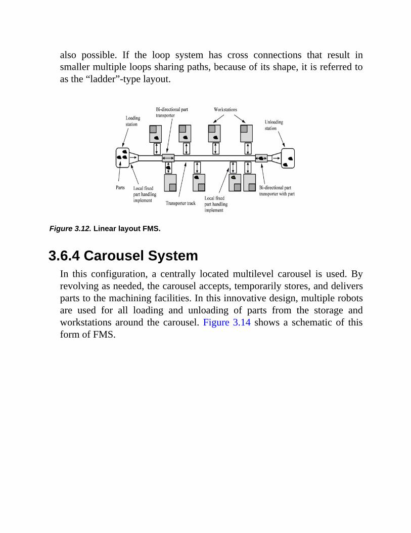
also possible. If the loop system has cross connections that result insmaller multiple loops sharing paths, because of its shape, it is referred toas the “ladder”-type layout.

Figure 3.12. Linear layout FMS.

3.6.4 Carousel SystemIn this configuration, a centrally located multilevel carousel is used. Byrevolving as needed, the carousel accepts, temporarily stores, and deliversparts to the machining facilities. In this innovative design, multiple robotsare used for all loading and unloading of parts from the storage andworkstations around the carousel. Figure 3.14 shows a schematic of thisform of FMS.

Figure 3.13. Loop layout FMS.

Figure 3.14. Carousel type FMS.

3.6.5 Other Layouts and SystemsThere is no limit to innovative designs for FMSs in capability and layouttype. In these systems, however, for continuous machining operations thechip removal from the cutting zone is perhaps one of the most challenging

tasks. With the use of chip-beaker tools and tool bits, this can be resolvedto some extent. Nevertheless, chips will still be produced at a high rate andoften accumulated on the machining table. Use of coolant fluid and blastof air can displace most of the chips. However, any chip-pieces remainingon the machining bed can cause improper placement of workpieces on themachine. One idea to reduce the possibility of this occurring is to useworkstations that are either installed entirely upside down or have acutting module that can be rotated 180 degrees so that all chips fall off intothe ground collection basins. Additionally, cutting coolant can assist theprocess further by washing away the chips produced.

This form of FMS requires specially built machinery and workstationsthat are expected to have significant cost implications.

3.7 General CommentsThe typical systems shown were simplified to demonstrate some of thegeneral configurations possible. In practice, many support and auxiliaryunits, not explicitly shown in the figures, are necessary to facilitate thefunctioning of an FMS. These include the following:

• A central computer that coordinates and controls the entireoperation

• Palletizing/de-palletizing of parts• A tool crib for workstations• Intermediate wash and degreasing stations• Means for effective problem-free chip removal in

machining operations

EXERCISES

3-1 In your place of study or work, a university machine shop, a smallor a large manufacturing plant, determine the form of themanufacturing system that is in place and whether its arrangementof equipment is closest to the line, functional, or group technology

layout.3-2 In a follow-up to Exercise 3-1, investigate whether another type of

layout would be a more suitable choice.3-3 In which type of manufacturing systems is scheduling of work

simpler?3-4 Comparing functional and group technology layouts, which one

offers better opportunity for control and responsibility over theparts or products?

3-5 If your place of work is a conventional manufacturingenvironment, and you were to propose a plan to convert it to anFMS, which layout form will you choose and why?

3-6 What does the statement “future products will be mass-producedin batches of one” mean?

3-7 Why does a typical part spend only 1.5 percent of its time in aconventional manufacturing system in the actual fabricationprocess?

Chapter

4CLASSIFICATION ANDCODING

4.1 INTRODUCTION

Classification and coding method, or, more specifically, part classificationand coding method, entails identifying the similarities among a largenumber of parts and manufactured pieces, and expressing these similaritiesthrough a structured coding system. In production plants, two types of partsimilarities are of interest: similarities that relate to the design features,such as geometric shape and size, and similarities that stem frommanufacturing attributes and relate to the type and sequence of productionprocesses required to fabricate the part. In addition to design andmanufacturing classification, which already include some materialproperties, dedicated classification and coding systems can be developedand utilized for solid materials, chemical compounds and liquids, and tomany other industrial materials and settings. For example, classification ofchemical compounds can help in proper storage assignment to reduce therisk of reaction or help extinguish fires with appropriate retardants.

In manufacturing, using a classification and coding system cansignificantly reduce the number of different parts and tools required,simplify storage and retrieval, standardize design, and facilitate productionand assembly. The extended benefits will be reviewed in detail later in thischapter.

One of the important applications of classification and coding is forgroup technology (see Chapter 3), where some classification effort isrequired to implement the group technology concept. We focus on part

classification and coding using group technology as a prime example, butthe concepts are general and can be used in a wide range of situations.With the use of common software such as Excel, a customizedclassification and coding system can be tailored for modest cases anddeveloped in-house.

4.2 GROUP TECHNOLOGY

We saw in Chapter 3 that group technology is a concept in which similarparts are grouped together to benefit from their similarities in design andmanufacturing. For instance, in a plant producing five thousand differentparts, it may be possible to group a vast majority of these parts into, say,fifty distinct part families. Some parts may not readily fit into a particularfamily, and the production personnel must carefully assess these forspecial accommodation. For the part families formed, the requiredproduction equipment is rearranged into groups known as cells. Each cellpossesses a variety of machines necessary to process one or severalfamilies of parts and functions fairly independently from the other cells.Normally, families of parts are released to the cell one family at a time andin predetermined batch sizes.

4.2.1 Part FamiliesWe defined a part family as a group of parts that are similar in geometricshape, form, and size, or because similar processing steps are required intheir manufacture. Most existing or traditional plants are laid out in thefunctional form. In order to implement the group technology concept, achangeover is necessary. The classification and coding method is the mostefficient way to accomplish this and generate appropriate design andproduction part families. The method involves classifying a population ofparts into families by examining the individual design and/ormanufacturing attributes, or CAD-CAM records of each part. Theclassification results in a series of digits or a code number that uniquelyidentifies the part’s attributes. A number of different classification andcoding schemes have been devised, and there are also several

commercially available systems. In the following sections, we review keypoints and benefits of implementing the concept of classification andcoding and outline its various coding structures.

4.2.2 Part Classification and CodingImplementing a classification and coding system requires effort andcommitment of time regardless of the method used. From the generalconcepts to specially developed software, none has become an industrystandard because the requirements of various companies differ in nature.However, application of any classification and coding system in grouptechnology provides a range of benefits, including the following:

1. It facilitates the generation of part families and machinegroups or cells.

2. It permits quick access and retrieval of CAD and CAMinformation.

3. It reduces design duplication and thus the variety of parts.4. It provides reliable workpiece statistics.5. It facilitates estimation of machine tool requirements and

efficient utilization of the machines.6. It permits streamlining of tooling, jigs, and fixtures, thus

reducing setup and production throughput times.7. It allows standardization and improvements in tool design.8. It aids production planning and scheduling procedures.9. It provides better machine tool utilization and better use of

tools, fixtures, and manpower.10. It facilitates part programming for numerically controlled

(NC) machining.

The design and manufacturing attributes that are generally used inclassification schemes for manufacturing are listed in Table 4.1. It is

important to pay attention to the overlap between the design andmanufacturing attributes. On one hand, it may not interfere with theclassification effort at hand, and even provide some flexibility in choosinga part family. On the other hand, it can lead to a wrong classificationdecision being made.

Table 4.1. Attributes of two forms of part families

Part Design Attributes Part Manufacturing Attributes

Basic external shape

Basic internal shape

Length/diameter ratio

Features for assembly

Features for functionality

Material type

Part function

Major dimensions

Minor dimensions

Tolerances

Surface finish

Major processes

Minor processes

Major dimension

Length/diameter ratio

Surface finish

Machine tools required

Operation sequence

Production time

Batch size

Production volume

Fixtures required

Cutting tools required

4.3 CLASSIFICATION AND CODING SCHEMES

A number of classification and coding schemes have been developed thatcan be categorized into the following forms:

• Monocodes• Polycodes• Hybrids

4.3.1 Monocodes

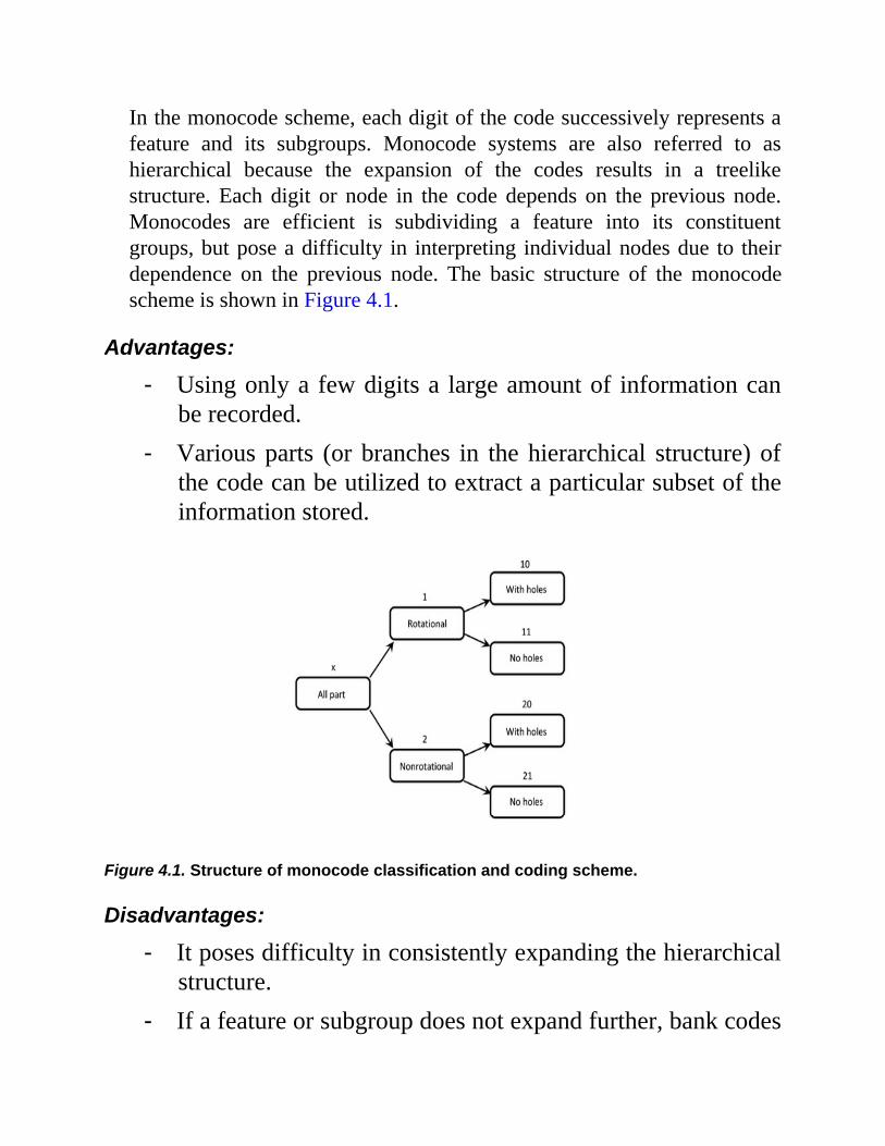
In the monocode scheme, each digit of the code successively represents afeature and its subgroups. Monocode systems are also referred to ashierarchical because the expansion of the codes results in a treelikestructure. Each digit or node in the code depends on the previous node.Monocodes are efficient is subdividing a feature into its constituentgroups, but pose a difficulty in interpreting individual nodes due to theirdependence on the previous node. The basic structure of the monocodescheme is shown in Figure 4.1.

Advantages:

- Using only a few digits a large amount of information canbe recorded.

- Various parts (or branches in the hierarchical structure) ofthe code can be utilized to extract a particular subset of theinformation stored.

Figure 4.1. Structure of monocode classification and coding scheme.

Disadvantages:

- It poses difficulty in consistently expanding the hierarchicalstructure.

- If a feature or subgroup does not expand further, bank codes

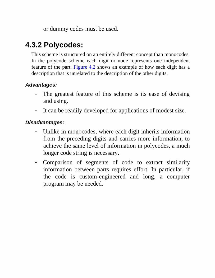
or dummy codes must be used.

4.3.2 Polycodes:This scheme is structured on an entirely different concept than monocodes.In the polycode scheme each digit or node represents one independentfeature of the part. Figure 4.2 shows an example of how each digit has adescription that is unrelated to the description of the other digits.

Advantages:

- The greatest feature of this scheme is its ease of devisingand using.

- It can be readily developed for applications of modest size.

Disadvantages:

- Unlike in monocodes, where each digit inherits informationfrom the preceding digits and carries more information, toachieve the same level of information in polycodes, a muchlonger code string is necessary.

- Comparison of segments of code to extract similarityinformation between parts requires effort. In particular, ifthe code is custom-engineered and long, a computerprogram may be needed.

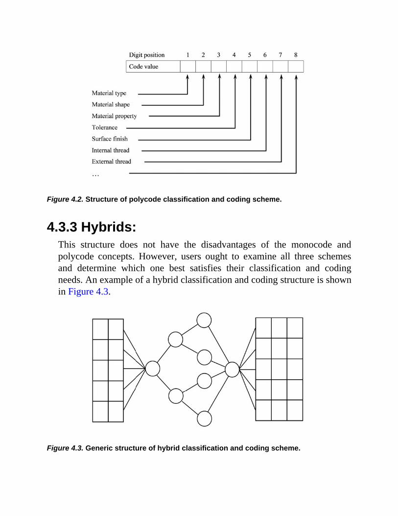
Figure 4.2. Structure of polycode classification and coding scheme.

4.3.3 Hybrids:This structure does not have the disadvantages of the monocode andpolycode concepts. However, users ought to examine all three schemesand determine which one best satisfies their classification and codingneeds. An example of a hybrid classification and coding structure is shownin Figure 4.3.

Figure 4.3. Generic structure of hybrid classification and coding scheme.

Advantages:

- Hybrid structures combine the benefits of monocode andpolycode systems, thereby providing flexibility to fit avariety of applications.

- Most commercial systems are of the hybrid type, henceproviding greater choice.

Disadvantage:

- There are no specific disadvantages.

4.3.4 The Opitz Classification SystemDeveloped by H. Opitz of the University of Aachen in Germany, andnamed after him, the Opitz classification and coding system is consideredone of the pioneering efforts in the field. It has become a popular platformand a generic model in introducing the fundamental concepts ofclassification and coding. The Opitz coding structure is of hybrid type andconsists of the following three-part digit sequence:

12345 6789 ABCD

The first group of five digits, 12345, is referred to as the “form code” anddescribes the geometry and design attributes of the part. The next group ofdigits, 6789, represents the “supplementary code,” which specifies some ofthe attributes that must be known to manufacture the part. The last groupof digits, ABCD, is designated as the “secondary code” and is used toindicate the production processes and their sequence. The secondary codecan be tailored to serve specific needs of a company. The interpretation ofthe first nine digits is given in Figure 4.4.

The code definition for the first five digits for the rotational part classes0, 1 and 2 (digit 1 in Figure 4.4) is given in Figure 4.5. The completecoding system covering all part classes and their code description isextensive.

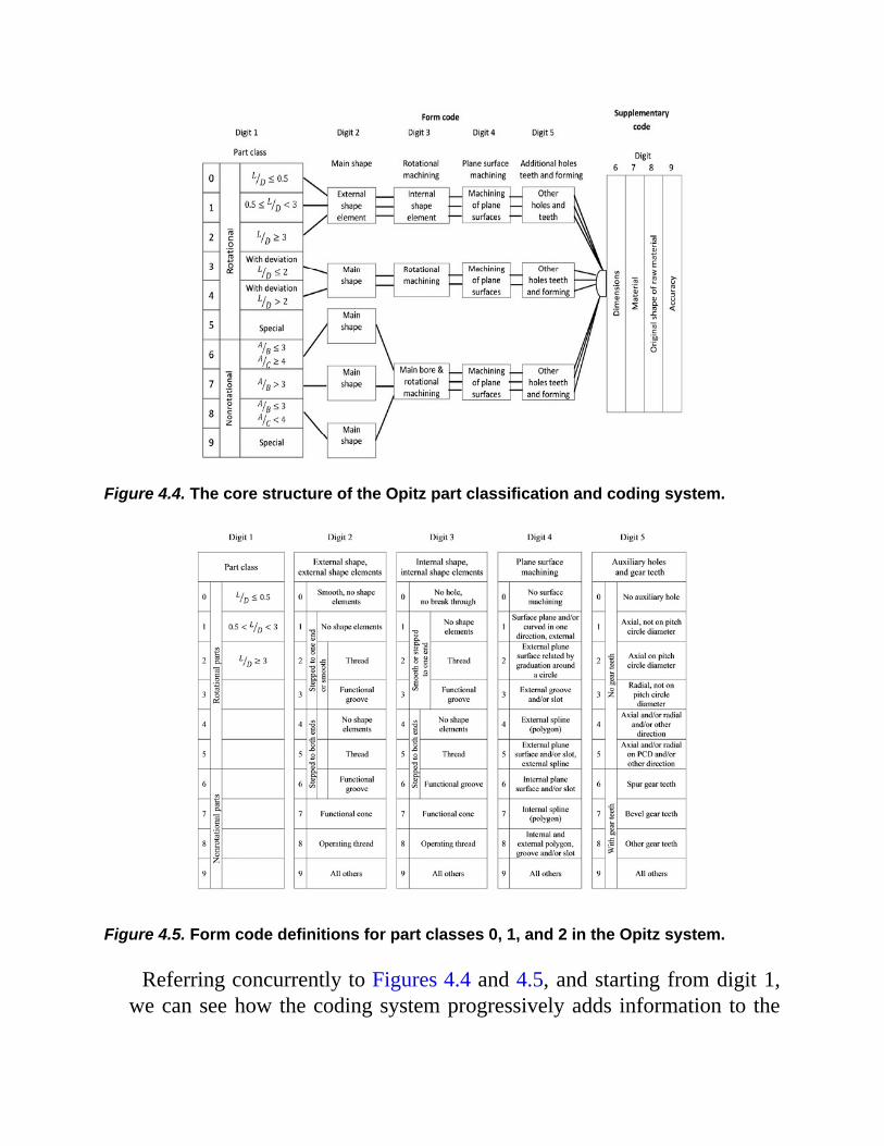
Figure 4.4. The core structure of the Opitz part classification and coding system.

Figure 4.5. Form code definitions for part classes 0, 1, and 2 in the Opitz system.

Referring concurrently to Figures 4.4 and 4.5, and starting from digit 1,we can see how the coding system progressively adds information to the

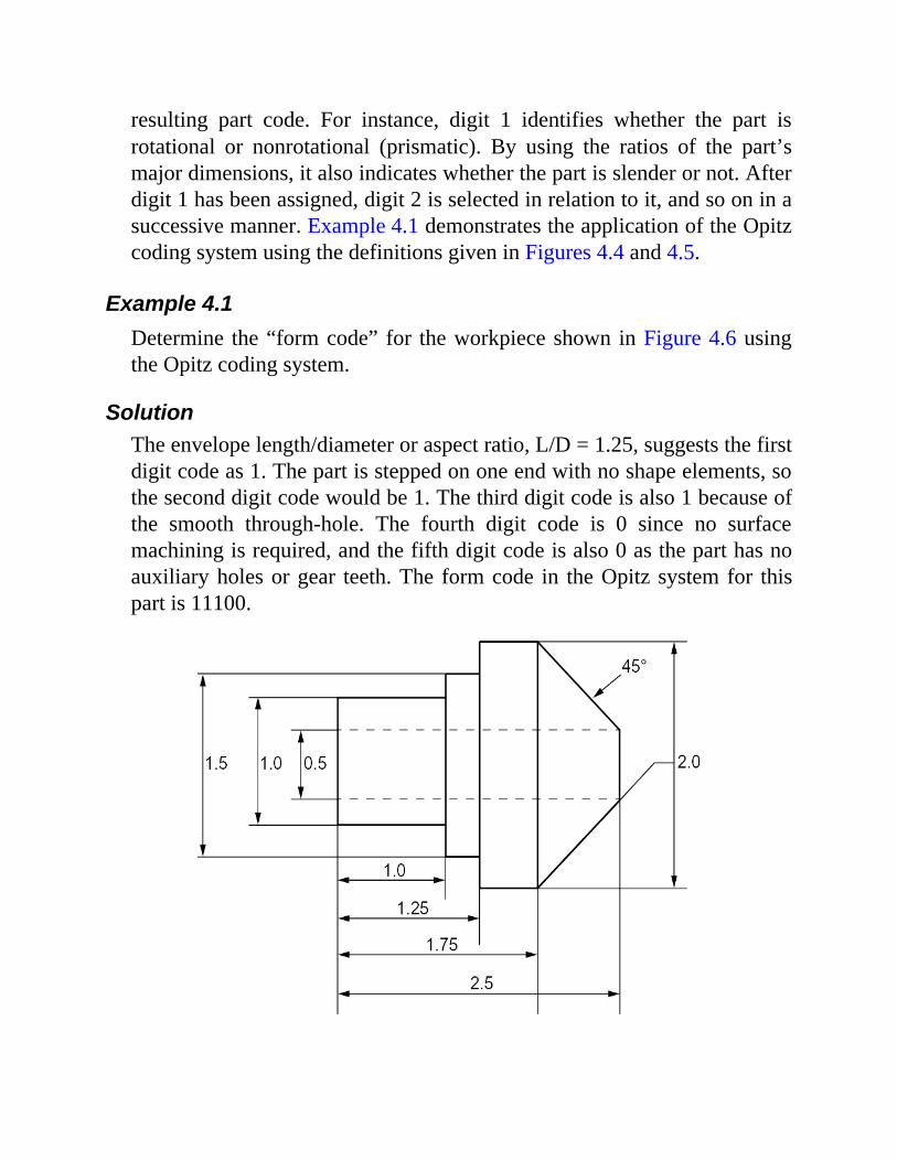
resulting part code. For instance, digit 1 identifies whether the part isrotational or nonrotational (prismatic). By using the ratios of the part’smajor dimensions, it also indicates whether the part is slender or not. Afterdigit 1 has been assigned, digit 2 is selected in relation to it, and so on in asuccessive manner. Example 4.1 demonstrates the application of the Opitzcoding system using the definitions given in Figures 4.4 and 4.5.

Example 4.1Determine the “form code” for the workpiece shown in Figure 4.6 usingthe Opitz coding system.

SolutionThe envelope length/diameter or aspect ratio, L/D = 1.25, suggests the firstdigit code as 1. The part is stepped on one end with no shape elements, sothe second digit code would be 1. The third digit code is also 1 because ofthe smooth through-hole. The fourth digit code is 0 since no surfacemachining is required, and the fifth digit code is also 0 as the part has noauxiliary holes or gear teeth. The form code in the Opitz system for thispart is 11100.

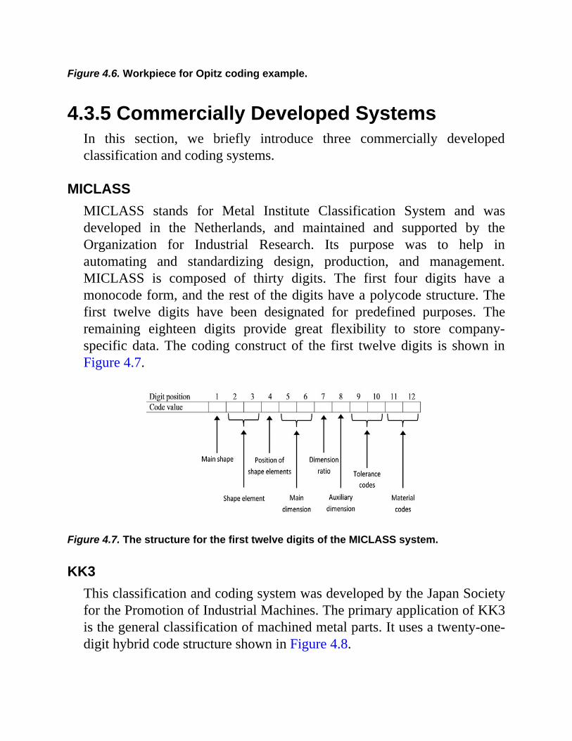
Figure 4.6. Workpiece for Opitz coding example.

4.3.5 Commercially Developed SystemsIn this section, we briefly introduce three commercially developedclassification and coding systems.

MICLASSMICLASS stands for Metal Institute Classification System and wasdeveloped in the Netherlands, and maintained and supported by theOrganization for Industrial Research. Its purpose was to help inautomating and standardizing design, production, and management.MICLASS is composed of thirty digits. The first four digits have amonocode form, and the rest of the digits have a polycode structure. Thefirst twelve digits have been designated for predefined purposes. Theremaining eighteen digits provide great flexibility to store company-specific data. The coding construct of the first twelve digits is shown inFigure 4.7.

Figure 4.7. The structure for the first twelve digits of the MICLASS system.

KK3This classification and coding system was developed by the Japan Societyfor the Promotion of Industrial Machines. The primary application of KK3is the general classification of machined metal parts. It uses a twenty-one-digit hybrid code structure shown in Figure 4.8.

Figure 4.8. The code structure of the KK3 system.

MultiClassMultiClass is a classification and coding system developed by theOrganization for Industrial Research. It is the newest and most flexible ofthe three systems and allows the users to customize the coding system tofit their requirements and applications. MultiClass can be used forapplications in manufacturing machined and sheet metal parts, tooling,electronics, and assemblies.

MultiClass uses a monocode or hierarchical coding structure and has amenu-driven software. The same as MICLASS, its structure consists of upto thirty digits. The first eighteen digits have a preassigned use (see Figure4.9), and the remaining twelve digits can be defined by the user to codeadditional information. A prefix (digit 0) precedes the thirty-digit string tocategorize parts into major classes.

Figure 4.9. The structure for the first eighteen digits of the MultiClass system.

4.3.6 Custom-Engineered Classification and

Coding SystemsFor a modest-size application, if a commercial system is not available ordeemed unsuitable, an enthusiastic and determined industrial engineer cancustom-design their own classification scheme. Using software such asExcel, a practical classification and coding system can be developed in-house. Since the monocode scheme stores more information and quicklycategorizes the part population into major classes than the polycodescheme, in custom-designing a classification and coding system it may beworthwhile to giving consideration, at least for the first few digits, to havea monocode structure.

EXERCISES

4-1 To assist in convenient and safe storage of an inventory of a largenumber of different chemicals, develop a five-digit Opitz-likecode with the following features:

i. Select five characteristics that you think are the mostimportant to consider. Say, for example,flammability, volatility, and reactivity.

ii. Assign each of these characteristics to one of thedigits of the code. For example, digit 2 (from left)could be flammability, volatility, and reactivity.

iii. For each digit, then assign at least three classes. Forinstance, for the flammability:0 = Nonflammable1 = Semiflammable (that is, flammable under

certain conditions, such as being exposed toopen flames for an extended period of time)

2 = Flammable4-2 For the machined part shown in Figure 4.10, define the five-digit

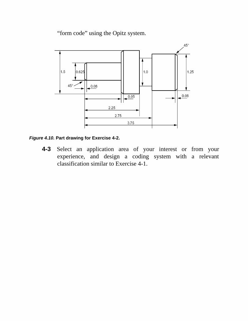
“form code” using the Opitz system.

Figure 4.10. Part drawing for Exercise 4-2.

4-3 Select an application area of your interest or from yourexperience, and design a coding system with a relevantclassification similar to Exercise 4-1.

Chapter

5SEQUENCING ANDSCHEDULING OFOPERATIONS

5.1 INTRODUCTION

The words sequencing and scheduling are often used interchangeably tothe point that sometimes they seem indistinguishable. But they are, in fact,two different concepts. Sequencing refers to the order determined to carryout a set of operations or tasks, whereas scheduling, relative to a referencetime, indicates the start, duration, and the end time for each task. We alsouse these terms having the same meaning in our explanations, but whendrawing a time chart, the difference will become apparent.

To appreciate the importance of scheduling, it is perhaps more effectiveto think of the consequences of the lack of it. For instance, in amanufacturing facility, the resources will be underutilized, deliverypromises will be missed, and client dissatisfaction will ensue.

Some concepts of sequencing and scheduling are straightforward andpractical, while others are complex, mathematically involved, and mostlyof academic nature.

Scheduling or sequencing is an important aspect of production controland providing services, in determining the order and the correct use offacilities within each instant of time. The primary goal is to make thegreatest use of the facilities available by maintaining a balanced andconcurrent level of activities in all machines, equipment, and departmentsso that expensive resources and skills are seldom idle. However, the

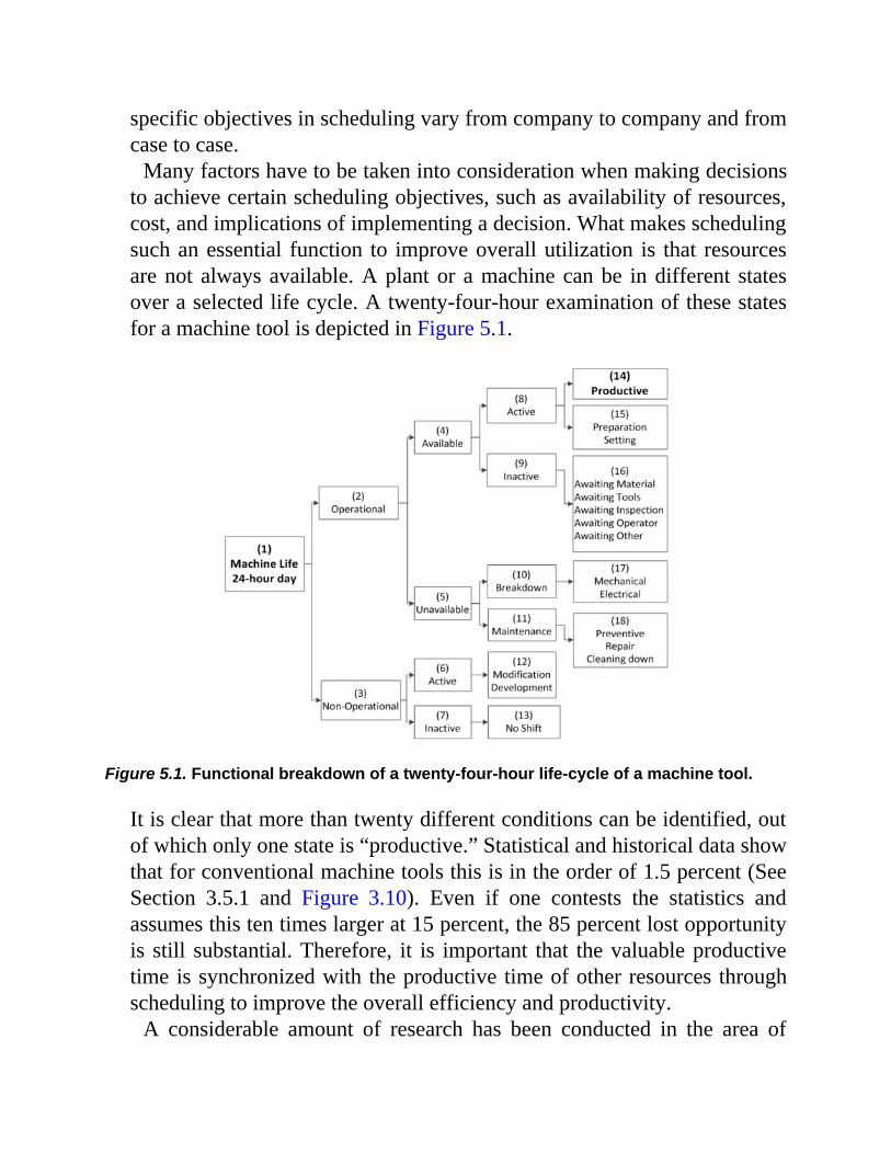
specific objectives in scheduling vary from company to company and fromcase to case.

Many factors have to be taken into consideration when making decisionsto achieve certain scheduling objectives, such as availability of resources,cost, and implications of implementing a decision. What makes schedulingsuch an essential function to improve overall utilization is that resourcesare not always available. A plant or a machine can be in different statesover a selected life cycle. A twenty-four-hour examination of these statesfor a machine tool is depicted in Figure 5.1.

Figure 5.1. Functional breakdown of a twenty-four-hour life-cycle of a machine tool.

It is clear that more than twenty different conditions can be identified, outof which only one state is “productive.” Statistical and historical data showthat for conventional machine tools this is in the order of 1.5 percent (SeeSection 3.5.1 and Figure 3.10). Even if one contests the statistics andassumes this ten times larger at 15 percent, the 85 percent lost opportunityis still substantial. Therefore, it is important that the valuable productivetime is synchronized with the productive time of other resources throughscheduling to improve the overall efficiency and productivity.

A considerable amount of research has been conducted in the area of

scheduling, or, as it is more often referred to, “job shop scheduling andsequencing of operations.” No single-most effective solution can bedeveloped because of the diversity of problems. The scale of the problemsrises further, and complexity is added when practical aspects of productionare also considered. To counter this to some extent and make thedevelopment of a schedule feasible, many simplifying assumptions areoften made. One must, however, pay attention to these simplificationsbecause too many assumptions can diminish the relevance and value of thedetermined schedule. Figure 5.2 shows a view of the scope of schedulingsolutions.

Figure 5.2. The extent of scheduling solutions.

Given the complexity of practical scheduling problems, the stochasticnature of nonproductive states shown in Figure 5.1 can lead to thedeterioration of an existing schedule. Typically, generating a new scheduleor modifying an existing one, among other things, can be an inconvenienttask in the least, and the constantly changing priorities and constraints ofthe scheduling problem make the prospect of a practical and an optimal

dynamically responsive schedule an elusive ideal.Despite these issues, working without a schedule that can shed light on

the state of affairs is a hazardous choice. It is interesting to note thatefficient and intelligent solutions for thousands of scenarios have beendeveloped. Some tend to be theoretical, but many have practicalapplications. In this chapter, we review several important categories ofscheduling and sequencing problems, their classification, and solutionalgorithms. Many algorithms exist for various situations, but they oftenhave a number of simplifying assumptions. Despite such limitations, theanalysis and application of such methods will help us understand, applysome of the ideas in practice, and, especially when some experience hasbeen gained, even develop solutions with intuition and without resorting toany mathematical calculation.

5.2 DEFINITION OF SCHEDULING TERMS

To be able to formulate, address, classify, and develop solutions forscheduling problems, it is necessary to define and understand somestandard terms and notations. The common terms and their definition areas follows.

• Processing time. The time required to complete a task on amachine or a process.

• Due date. The agreed delivery time or deadline for a taskbeyond which it would be considered late or tardy (see thedefinition below). Sometimes some form of penalty forbeing tardy may be applied.

• Lateness. The difference between a task’s completion timeand its due date will have a positive lateness if the task iscompleted after its due date and negative lateness ifcompleted before its due date.

• Tardiness. This is the measure of positive lateness. If a taskis early, it has negative lateness but zero tardiness. If a task

has positive lateness, it has equal positive tardiness.• Slack. A measure of the difference between the remaining

time to a task’s due date and its processing time.• Completion time. The span between the beginning of work

on the first job on the first machine, which is referred to as t= 0, and the time when the last task is finished on the lastmachine.

• Flow time. The time between the point at which a job isavailable for processing and the point at which it iscompleted. When all the jobs are available at time zero (alsoknown as the Ready Time r = 0), then flow time is equal tothe completion time.

In dealing with scheduling problems, we often work with these time-basedterms. Figure 5.3 schematically shows the relationship between some ofthese terms.

From Figure 5.3 many relations can be written and used depending onthe objectives of the problem at hand.

Figure 5.3. Time-based terms in scheduling problems.

When there is more than one job, these relations also stand in terms of

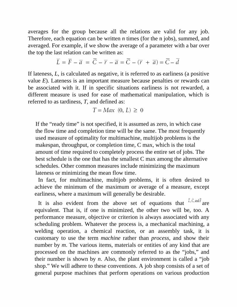
averages for the group because all the relations are valid for any job.Therefore, each equation can be written n times (for the n jobs), summed, andaveraged. For example, if we show the average of a parameter with a bar overthe top the last relation can be written as:

If lateness, L, is calculated as negative, it is referred to as earliness (a positivevalue E). Lateness is an important measure because penalties or rewards canbe associated with it. If in specific situations earliness is not rewarded, adifferent measure is used for ease of mathematical manipulation, which isreferred to as tardiness, T, and defined as:

If the “ready time” is not specified, it is assumed as zero, in which casethe flow time and completion time will be the same. The most frequentlyused measure of optimality for multimachine, multijob problems is themakespan, throughput, or completion time, C max, which is the totalamount of time required to completely process the entire set of jobs. Thebest schedule is the one that has the smallest C max among the alternativeschedules. Other common measures include minimizing the maximumlateness or minimizing the mean flow time.In fact, for multimachine, multijob problems, it is often desired to

achieve the minimum of the maximum or average of a measure, exceptearliness, where a maximum will generally be desirable.

It is also evident from the above set of equations that areequivalent. That is, if one is minimized, the other two will be, too. Aperformance measure, objective or criterion is always associated with anyscheduling problem. Whatever the process is, a mechanical machining, awelding operation, a chemical reaction, or an assembly task, it iscustomary to use the term machine rather than process, and show theirnumber by m. The various items, materials or entities of any kind that areprocessed on the machines are commonly referred to as the “jobs,” andtheir number is shown by n. Also, the plant environment is called a “jobshop.” We will adhere to these conventions. A job shop consists of a set ofgeneral purpose machines that perform operations on various production

orders or jobs. In this context we do not consider the operations sequencein a mass (continuous) production line, where an order for the machines isdetermined on a permanent basis, and job scheduling is immaterial as itwill not affect the long-term production rates. Many of the job shopproblems and the algorithms and solutions deal with a pool of n jobs,which are often all available at the same time, and a group of m machines.

5.3 SCHEDULING ALGORITHMS

Algorithms are a set of rational rules or iterative procedures applied to thedata available to solve the related problem in a finite number of steps.Different algorithms can be developed for a specific scheduling problemleading to the same optimal or near-optimal solutions. Before introducingsuch algorithms for scheduling, let us examine what the alternative mightbe. A common criterion for a job shop is to minimize the completion time.Suppose it is desired to process three jobs, a, b, and c, through twomachines, M1 and M2, in the shortest possible time with the restriction thatfor any job sequence the machine sequence will be fixed, that is, either M1

is always first or M2. The brute force approach is to generate all possiblecombinations. The combinations when one fixed sequence is used for bothmachines are shown in Figure 5.4. If the job sequence varies for thesecond machine, the total number of combinations will be seventy-two.

For each of the sequences a process time chart, commonly known as theGantt chart, can be drawn and the smallest completion time selected as theoptimal solution. This can also be done mathematically through acomputer program. A sample Gantt chart for Figure 5.4 is shown in Figure5.5.

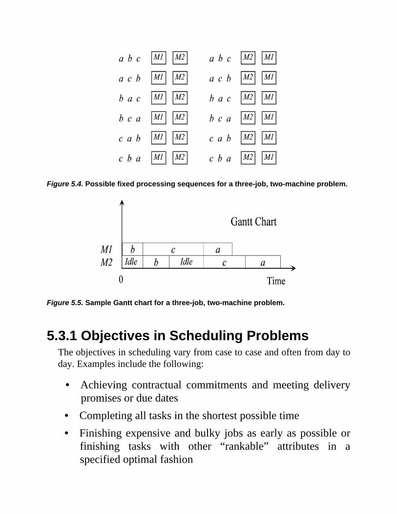
Figure 5.4. Possible fixed processing sequences for a three-job, two-machine problem.

Figure 5.5. Sample Gantt chart for a three-job, two-machine problem.

5.3.1 Objectives in Scheduling ProblemsThe objectives in scheduling vary from case to case and often from day today. Examples include the following:

• Achieving contractual commitments and meeting deliverypromises or due dates

• Completing all tasks in the shortest possible time• Finishing expensive and bulky jobs as early as possible or

finishing tasks with other “rankable” attributes in aspecified optimal fashion

• Maintaining a balanced level of activity in allmachines/departments, so that all resources are utilized tothe highest degree possible

5.3.2 Industrial ProblemsExamples of industrial problems include the following:

• Scheduling jobs through manufacturing processes in a plant• Executing different programs on a computer (time-sharing,

file transfer traffic)• Determining landing order of airplanes (based on fuel left,

size of the aircraft, next departure time, type of runwayavailable)

• Scheduling surgeries in operating rooms (shortest possibletime, giving priority to the most ill)

5.3.3 The PracticeIn design, analysis, and use of algorithms, simplifying assumptions areoften made. For example, processing times are taken to be sequenceindependent. In practice, however, machine setup times can changedepending on the sequence used. For instance, if jobs a, b, and c followone another, and they are all made of the same material, then the “machinecleaning time” may be eliminated in between their processing—meaningthat the actual processing time could be shorter than initially assumed. It isthe industrial engineer’s responsibility to note, discover, and use suchtime-saving factors involved in the real world.

5.4 n-JOB ONE-MACHINE PROBLEM

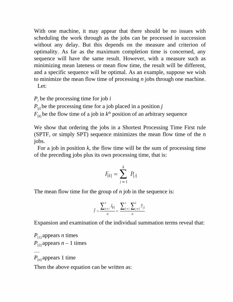
With one machine, it may appear that there should be no issues withscheduling the work through as the jobs can be processed in successionwithout any delay. But this depends on the measure and criterion ofoptimality. As far as the maximum completion time is concerned, anysequence will have the same result. However, with a measure such asminimizing mean lateness or mean flow time, the result will be different,and a specific sequence will be optimal. As an example, suppose we wishto minimize the mean flow time of processing n jobs through one machine.

Let:

Pi be the processing time for job iP[j] be the processing time for a job placed in a position jF[k] be the flow time of a job in kth position of an arbitrary sequence

We show that ordering the jobs in a Shortest Processing Time First rule(SPTF, or simply SPT) sequence minimizes the mean flow time of the njobs.

For a job in position k, the flow time will be the sum of processing timeof the preceding jobs plus its own processing time, that is:

The mean flow time for the group of n job in the sequence is:

Expansion and examination of the individual summation terms reveal that:

P[1] appears n timesP[2] appears n – 1 times…P[n] appears 1 time

Then the above equation can be written as:

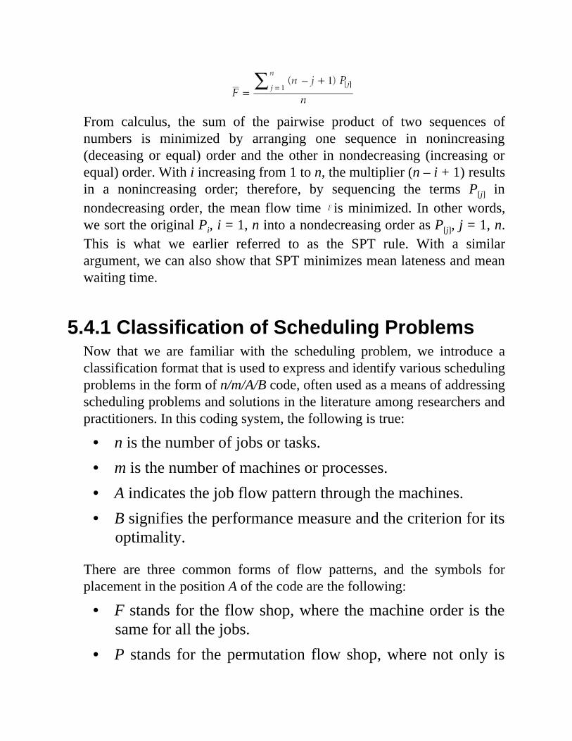
From calculus, the sum of the pairwise product of two sequences ofnumbers is minimized by arranging one sequence in nonincreasing(deceasing or equal) order and the other in nondecreasing (increasing orequal) order. With i increasing from 1 to n, the multiplier (n – i + 1) resultsin a nonincreasing order; therefore, by sequencing the terms P[j] innondecreasing order, the mean flow time is minimized. In other words,we sort the original Pi, i = 1, n into a nondecreasing order as P[j], j = 1, n.This is what we earlier referred to as the SPT rule. With a similarargument, we can also show that SPT minimizes mean lateness and meanwaiting time.

5.4.1 Classification of Scheduling ProblemsNow that we are familiar with the scheduling problem, we introduce aclassification format that is used to express and identify various schedulingproblems in the form of n/m/A/B code, often used as a means of addressingscheduling problems and solutions in the literature among researchers andpractitioners. In this coding system, the following is true:

• n is the number of jobs or tasks.• m is the number of machines or processes.• A indicates the job flow pattern through the machines.• B signifies the performance measure and the criterion for its

optimality.

There are three common forms of flow patterns, and the symbols forplacement in the position A of the code are the following:

• F stands for the flow shop, where the machine order is thesame for all the jobs.

• P stands for the permutation flow shop, where not only is

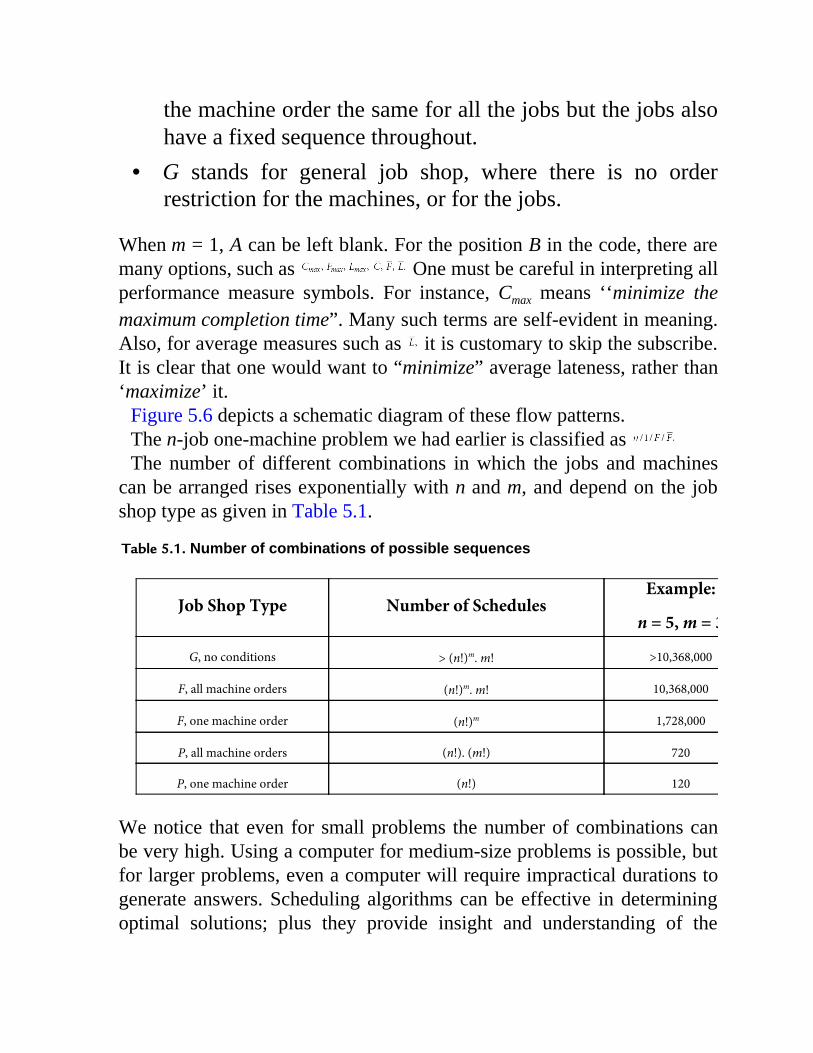
the machine order the same for all the jobs but the jobs alsohave a fixed sequence throughout.

• G stands for general job shop, where there is no orderrestriction for the machines, or for the jobs.

When m = 1, A can be left blank. For the position B in the code, there aremany options, such as One must be careful in interpreting allperformance measure symbols. For instance, Cmax means ‘‘minimize themaximum completion time”. Many such terms are self-evident in meaning.Also, for average measures such as it is customary to skip the subscribe.It is clear that one would want to “minimize” average lateness, rather than‘maximize’ it.

Figure 5.6 depicts a schematic diagram of these flow patterns.The n-job one-machine problem we had earlier is classified as The number of different combinations in which the jobs and machines

can be arranged rises exponentially with n and m, and depend on the jobshop type as given in Table 5.1.

Table 5.1. Number of combinations of possible sequences

Job Shop Type Number of SchedulesExample:

n = 5, m = 3

G, no conditions > (n!)m. m! >10,368,000

F, all machine orders (n!)m. m! 10,368,000

F, one machine order (n!)m 1,728,000

P, all machine orders (n!). (m!) 720

P, one machine order (n!) 120

We notice that even for small problems the number of combinations canbe very high. Using a computer for medium-size problems is possible, butfor larger problems, even a computer will require impractical durations togenerate answers. Scheduling algorithms can be effective in determiningoptimal solutions; plus they provide insight and understanding of the

solution method. This experience can be invaluable in analyzing andhandling day-to-day scheduling problems.

Figure 5.6. Classification of flow patterns in a job shop.

5.5 JOHNSON’S ALGORITHM

Johnson’s algorithm is used for the n-job two-machine scheduling problemand is sometimes referred to as n/2/F/Cmax classification, but its correctclassification is n/2/P/Cmax.

The letter P (permutation) in n/2/P/Cmax indicates that jobs go in onedirection from the first machine to the second, and the queue order(sequence) in front of both machines is the same. So one overall sequenceis determined and used throughout. The restriction that jobs go from onemachine to the next is often referred to as the “technological order”,meaning that the physical properties of the job are altered in the givenorder, which is typical of most industrial scenarios.

Application of Johnson’s algorithm is easy and straightforward, and anumerical example is the best way to demonstrate it.

Assume the information in Table 5.2 for a four-job problem. Thenumerical entries in the table indicate the processing times in the unitused.

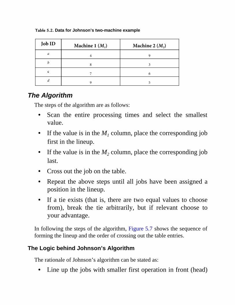
Table 5.2. Data for Johnson’s two-machine example

Job ID Machine 1 (M1) Machine 2 (M2)a 4 9

b 8 3

c 7 6

d 9 5

The AlgorithmThe steps of the algorithm are as follows:

• Scan the entire processing times and select the smallestvalue.

• If the value is in the M1 column, place the corresponding jobfirst in the lineup.

• If the value is in the M2 column, place the corresponding joblast.

• Cross out the job on the table.• Repeat the above steps until all jobs have been assigned a

position in the lineup.• If a tie exists (that is, there are two equal values to choose

from), break the tie arbitrarily, but if relevant choose toyour advantage.

In following the steps of the algorithm, Figure 5.7 shows the sequence offorming the lineup and the order of crossing out the table entries.

The Logic behind Johnson’s Algorithm

The rationale of Johnson’s algorithm can be stated as:

• Line up the jobs with smaller first operation in front (head)

of the queue so that the second machine is fed as soon aspossible.

• Line up the jobs with smaller second operation in back (tail)of the queue so that the second machine stays busy withlonger operations.

5.6 JOHNSON’S EXTENDED ALGORITHM

Johnson’s n-job two-machine method can be extended to the n-job three-machine, n/3/P/Cmax, problem under the following conditions:

Figure 5.7. Steps of Johnson’s algorithm for the example.

where ti, j stands for processing time of job i on machine j. In other words,Johnson’s method can be applied if the second machine is completelydominated by either of the first or third machines. In this algorithm thethree machines are converted into a two dummy or virtual machines andthen Johnson’s two-machine algorithm is applied.

Example 5.1

Data for processing of four jobs on three machines are given in Table 5.3.Using Johnson’s extended algorithm, determine the job processing orderfor minimum completion time.

Table 5.3. Data for Johnson’s three-machine example

Job ID M1 M2 M3

a 3 1 6

b 5 4 5

c 4 2 8

d 2 3 7

Solution

First, we examine to see whether any of the conditions is present:

Since the algorithm can be applied. We now generate the twodummy or virtual machines and the sum the processing times as follows inTable 5.4.

Table 5.4. Dummy machines for Johnson’s three-machine example

Job IDDummy Machine 1

M1 ⊕ M2

Dummy Machine 2

M2 ⊕ M3

a 3+1 = 4 1+6 = 7

b 5+4 = 9 4+5 = 9

c 4+2 = 6 2+8 = 10

d 2+ 3 = 5 3+7 = 10

The solution is usually shown as in Figure 5.8.

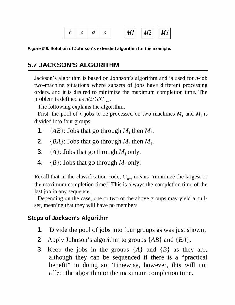
Figure 5.8. Solution of Johnson’s extended algorithm for the example.

5.7 JACKSON’S ALGORITHM

Jackson’s algorithm is based on Johnson’s algorithm and is used for n-jobtwo-machine situations where subsets of jobs have different processingorders, and it is desired to minimize the maximum completion time. Theproblem is defined as n/2/G/Cmax.

The following explains the algorithm.First, the pool of n jobs to be processed on two machines M1 and M2 is

divided into four groups:

1. {AB}: Jobs that go through M1 then M2.

2. {BA}: Jobs that go through M2 then M1.3. {A}: Jobs that go through M1 only.

4. {B}: Jobs that go through M2 only.

Recall that in the classification code, Cmax means “minimize the largest orthe maximum completion time.” This is always the completion time of thelast job in any sequence.

Depending on the case, one or two of the above groups may yield a null-set, meaning that they will have no members.

Steps of Jackson’s Algorithm

1. Divide the pool of jobs into four groups as was just shown.2 Apply Johnson’s algorithm to groups {AB} and {BA}.3 Keep the jobs in the groups {A} and {B} as they are,

although they can be sequenced if there is a “practicalbenefit” in doing so. Timewise, however, this will notaffect the algorithm or the maximum completion time.

4. Line up the four groups as shown in Figure 5.9.

The schematic diagrams of Figure 5.9 is interpreted as: once any of thesequenced groups {AB} and {BA} completes its first operation, itimmediately moves to its second operation.

Figure 5.9. Jackson’s algorithm.

The Rationale behind Jackson’s Algorithm

Let’s first recall the rationale supporting Johnson’s algorithm:

• Line up the jobs with smaller first operation in front of thequeue so that the second machine is fed as soon as possible.

• Line up the jobs with smaller second operation in back ofthe queue so that the second machine stays busy with longeroperations.

These ideas are used twice in the Jackson’s algorithm as follows:

• The sequenced group {AB} in front of M1 is meant to startfeeding M2 as quickly as possible.

• Similarly, the ordered group {BA} in front of M2 is meant to

start feeding M1 as quickly as possible.

• If the processing times of group {AB} are such that M1

completes it early, then there is group {A} to maintain themachine M1 busy until group {BA} arrives from M2.

• Likewise, if the processing times of group {BA} are suchthat M2 completes it early, then there is group {B} tomaintain the machine M2 busy until group {AB} arrivesfrom M1.

The overall Rationale is to achieve as many concurrent operations aspossible on the two machines. The concept is smart and plausible.

With the sequence and all the processing times known, one can eithermathematically, using a computer, or by drawing a Gantt chart determinethe “completion” time. That is, the completion time of the last job, which,depending on the processing times, can occur on either of the machines.

5.8 AKERS’ ALGORITHM

This is a practical scheduling method for two-job m-machine casesclassified as 2/m/z/Fmax. The letter z in the classification is explainedshortly. Akers’ method is essentially a graphical method using a two-axescoordinate system. Figure 5.10 represents a problem and its solution. Onejob is assigned to each axis. Both axes must be drawn to the same scale.The alphabetic letters along each axis indicate the machine name and thestated order of processing, and the marked divisions for each machinealong the axes are proportional to the processing times of the respectivejob.

A schedule is specified by moving (that is, graphically drawing segmentsof a straight line) in increasing time from zero through conflict-free areasor zones along both axes to a point akin to (x, y), where x is the totalprocessing time of Job1 on its respective axis, and y is the total processingtime of Job2 on its respective axis. Note that neither coordinate is the flowor completion time. A conflict area is where one machine is needed by

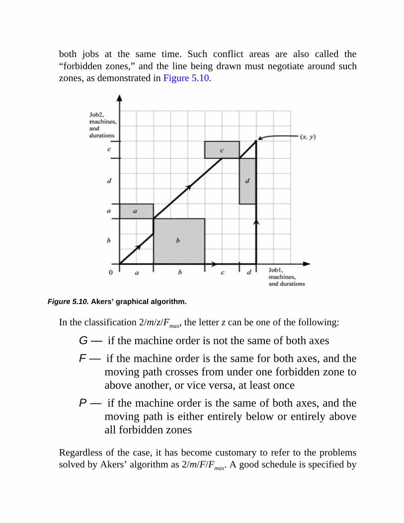
both jobs at the same time. Such conflict areas are also called the“forbidden zones,” and the line being drawn must negotiate around suchzones, as demonstrated in Figure 5.10.

Figure 5.10. Akers’ graphical algorithm.

In the classification 2/m/z/Fmax, the letter z can be one of the following:

G — if the machine order is not the same of both axesF — if the machine order is the same for both axes, and the

moving path crosses from under one forbidden zone toabove another, or vice versa, at least once

P — if the machine order is the same of both axes, and themoving path is either entirely below or entirely aboveall forbidden zones

Regardless of the case, it has become customary to refer to the problemssolved by Akers’ algorithm as 2/m/F/Fmax. A good schedule is specified by

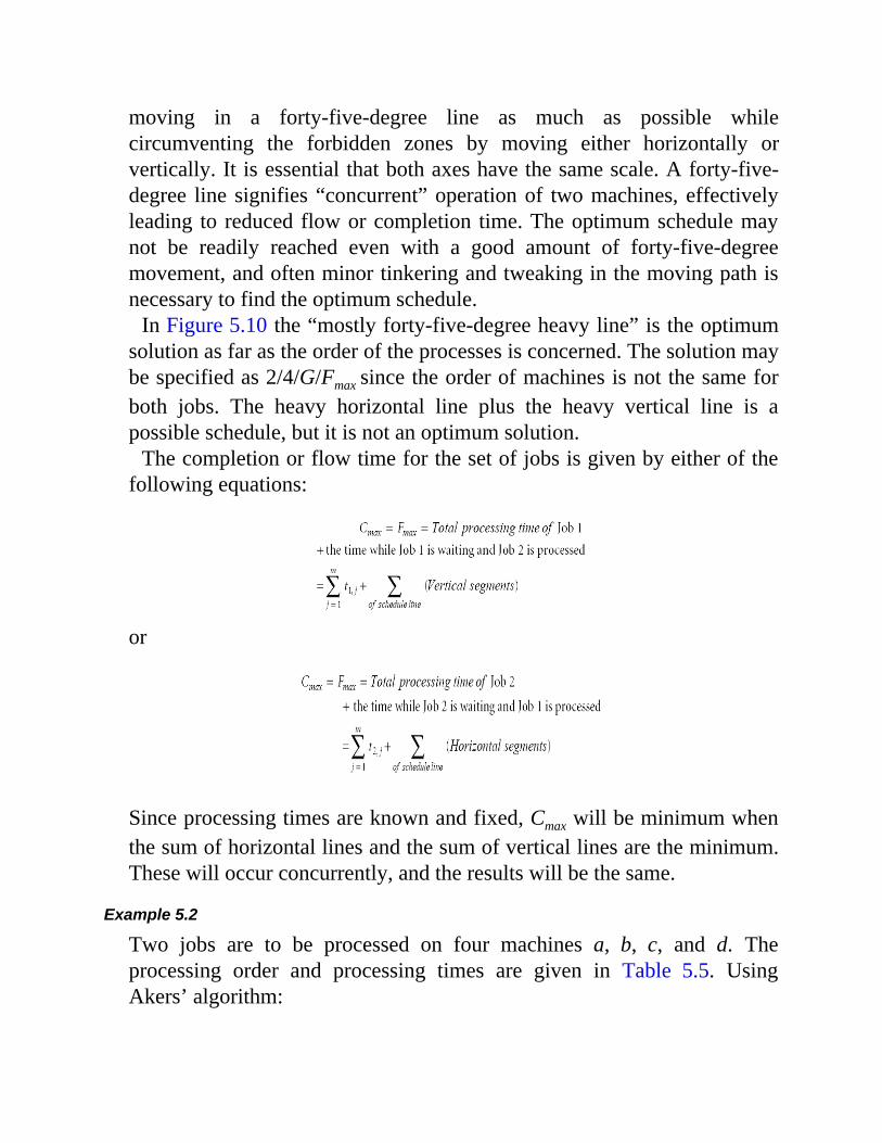
moving in a forty-five-degree line as much as possible whilecircumventing the forbidden zones by moving either horizontally orvertically. It is essential that both axes have the same scale. A forty-five-degree line signifies “concurrent” operation of two machines, effectivelyleading to reduced flow or completion time. The optimum schedule maynot be readily reached even with a good amount of forty-five-degreemovement, and often minor tinkering and tweaking in the moving path isnecessary to find the optimum schedule.

In Figure 5.10 the “mostly forty-five-degree heavy line” is the optimumsolution as far as the order of the processes is concerned. The solution maybe specified as 2/4/G/Fmax since the order of machines is not the same forboth jobs. The heavy horizontal line plus the heavy vertical line is apossible schedule, but it is not an optimum solution.

The completion or flow time for the set of jobs is given by either of thefollowing equations:

or

Since processing times are known and fixed, Cmax will be minimum whenthe sum of horizontal lines and the sum of vertical lines are the minimum.These will occur concurrently, and the results will be the same.

Example 5.2

Two jobs are to be processed on four machines a, b, c, and d. Theprocessing order and processing times are given in Table 5.5. UsingAkers’ algorithm:

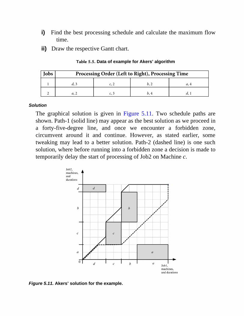
i) Find the best processing schedule and calculate the maximum flowtime.

ii) Draw the respective Gantt chart.

Table 5.5. Data of example for Akers’ algorithm

Jobs Processing Order (Left to Right), Processing Time

1 d, 3 c, 2 b, 2 a, 4

2 a, 2 c, 3 b, 4 d, 1

Solution

The graphical solution is given in Figure 5.11. Two schedule paths areshown. Path-1 (solid line) may appear as the best solution as we proceed ina forty-five-degree line, and once we encounter a forbidden zone,circumvent around it and continue. However, as stated earlier, sometweaking may lead to a better solution. Path-2 (dashed line) is one suchsolution, where before running into a forbidden zone a decision is made totemporarily delay the start of processing of Job2 on Machine c.

Figure 5.11. Akers’ solution for the example.

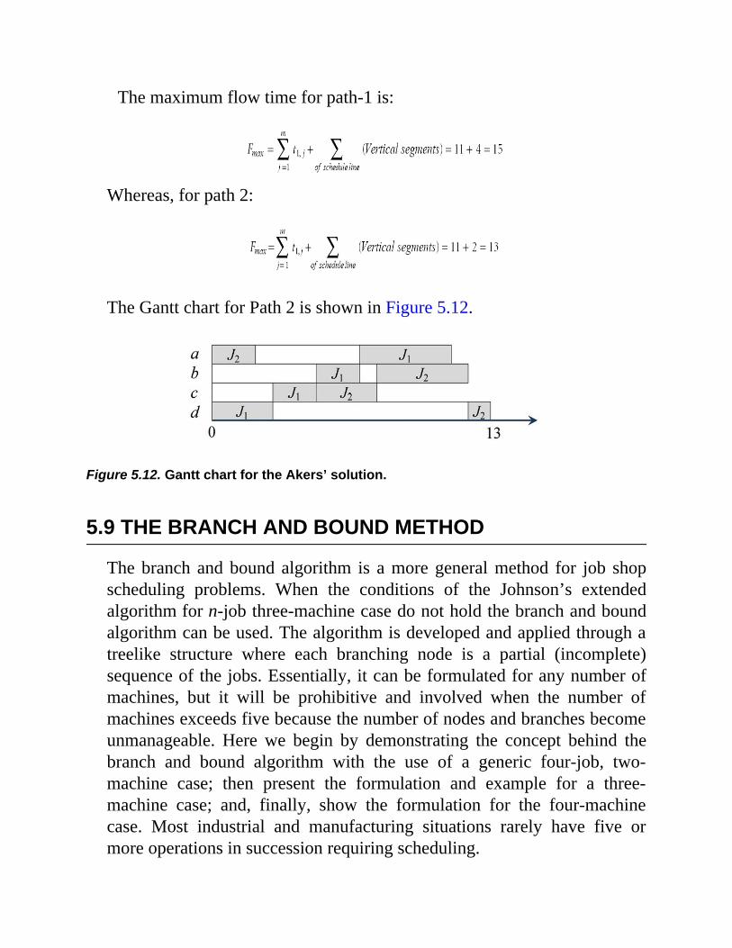
The maximum flow time for path-1 is:

Whereas, for path 2:

The Gantt chart for Path 2 is shown in Figure 5.12.

Figure 5.12. Gantt chart for the Akers’ solution.

5.9 THE BRANCH AND BOUND METHOD

The branch and bound algorithm is a more general method for job shopscheduling problems. When the conditions of the Johnson’s extendedalgorithm for n-job three-machine case do not hold the branch and boundalgorithm can be used. The algorithm is developed and applied through atreelike structure where each branching node is a partial (incomplete)sequence of the jobs. Essentially, it can be formulated for any number ofmachines, but it will be prohibitive and involved when the number ofmachines exceeds five because the number of nodes and branches becomeunmanageable. Here we begin by demonstrating the concept behind thebranch and bound algorithm with the use of a generic four-job, two-machine case; then present the formulation and example for a three-machine case; and, finally, show the formulation for the four-machinecase. Most industrial and manufacturing situations rarely have five ormore operations in succession requiring scheduling.

5.9.1 Lower Bounds for Completion TimeA lower bound means the lowest possible (not exact) completion time thatwe can determine from partially processed information. To illustrate this,let’s begin with a simple four-job, two-machine problem. The Gantt chartfor an arbitrarily chosen sequence will have two possible cases, and thesecases are shown in Figure 5.13.

Now we can write two lower bounds on the possible shortest time bywhich all four jobs can be completed:

The equation for B1 indicates the reality that the last job cannot start itsprocess on M2 until it is completed on M1.

Figure 5.13. Gantt chart cases for the branch and bound concept.

Likewise, equation B2 indicates the fact that none of the jobs can beprocessed on M2 until Job1 is completed on M1.

We can also look at the situation in a different way. Contrasting theabove two equations against Case 1 Gantt chart of Figure 5.13, we see thatB1 gives the correct completion time and covers the duration continuouslyfrom time zero to time Tc. Equation B2 misses the gaps (the idle times onM2) and consequently does not give a correct completion time. We notethat between the two equations, B1 has a larger value. If we now match theabove equations with Case 2 Gantt chart of Figure 5.13, we notice thatnow B2 gives the correct completion time, and B1 misses the waiting timeof Job4 between M1 and M2. In this case, B2 has a larger value.

No other Gantt chart case can be drawn. So, whatever the case, we cansay that the correct bound on the completion time is given by thefollowing equation:

This means that if we determine the lower LB for a particular instance, theactual completion time, Tc, will be greater or equal to LB.The lower bounds can be readily extended to a three-machine case, and theequations will be:

With similar reasoning as we had for two-machine problem, we can saythat the correct bound on the completion time for the three-machineproblem is given by the following equation:

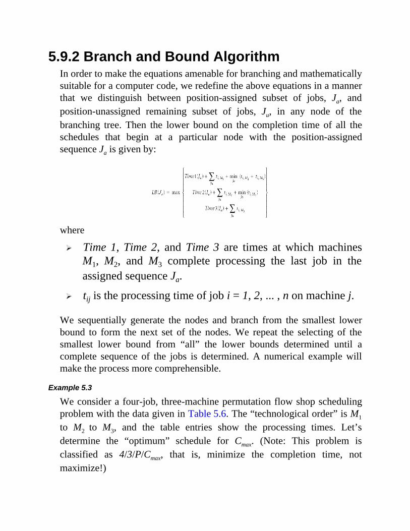
5.9.2 Branch and Bound AlgorithmIn order to make the equations amenable for branching and mathematicallysuitable for a computer code, we redefine the above equations in a mannerthat we distinguish between position-assigned subset of jobs, Ja, andposition-unassigned remaining subset of jobs, Ju, in any node of thebranching tree. Then the lower bound on the completion time of all theschedules that begin at a particular node with the position-assignedsequence Ja is given by:

where

Time 1, Time 2, and Time 3 are times at which machinesM1, M2, and M3 complete processing the last job in theassigned sequence Ja.

tij is the processing time of job i = 1, 2, ... , n on machine j.

We sequentially generate the nodes and branch from the smallest lowerbound to form the next set of the nodes. We repeat the selecting of thesmallest lower bound from “all” the lower bounds determined until acomplete sequence of the jobs is determined. A numerical example willmake the process more comprehensible.

Example 5.3

We consider a four-job, three-machine permutation flow shop schedulingproblem with the data given in Table 5.6. The “technological order” is M1

to M2 to M3, and the table entries show the processing times. Let’sdetermine the “optimum” schedule for Cmax. (Note: This problem isclassified as 4/3/P/Cmax, that is, minimize the completion time, notmaximize!)

Table 5.6. Data for branch and bound example

Job ID M1 M2 M3

1 32 30 10

2 20 26 34

3 16 22 8

4 28 12 30

Solution

First, we branch from node 0 (the initial set where all jobs are unassigned)and construct nodes 1, 2, 3, and 4 as shown in Figure 5.14. The branchesare generated progressively, although this figure depicts the entire assessednodes and branches. Individual digits inside the circles indicate the jobsthat have already been assigned a sequence. For example, “31” meansJob3 followed by Job1.

Using the equation in Section 5.9.2, we now commence on computingthe lower bounds that are shown in Figure 5.14.

To compute the lower bounds, we need the following terms: Time 1 (1) = 32, Time 2 (1) = 62, Time 3(1) = 72, Time 1 (2) = 20, Time 2(2) = 46Time 3 (2) = 80, Time 1 (3) = 16, Time 2 (3) = 38, Time 3 (3) = 46, Time 1(4) = 28Time 2 (4) = 40, Time 3 (4) = 70 The lower bounds are:

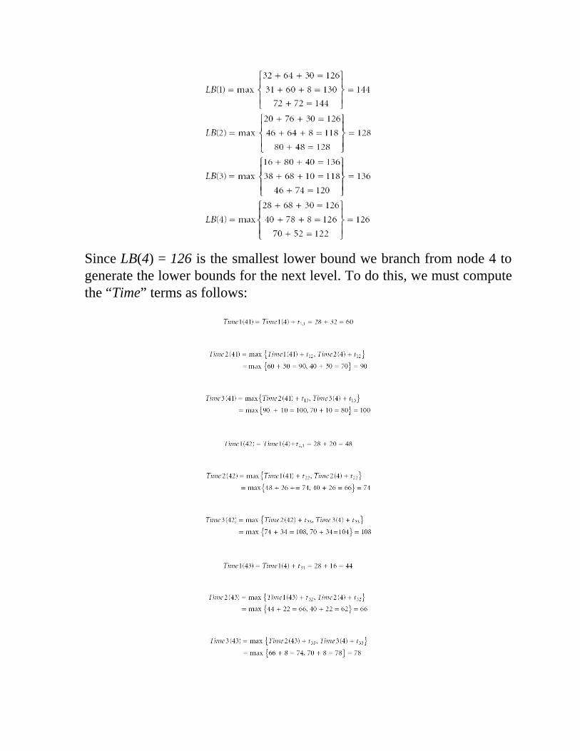
Since LB(4) = 126 is the smallest lower bound we branch from node 4 togenerate the lower bounds for the next level. To do this, we must computethe “Time” terms as follows:

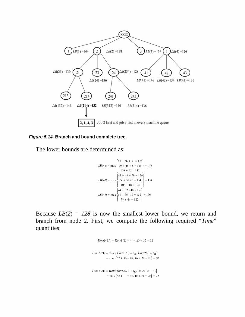
Figure 5.14. Branch and bound complete tree.

The lower bounds are determined as:

Because LB(2) = 128 is now the smallest lower bound, we return andbranch from node 2. First, we compute the following required “Time”quantities:

The lower bounds are determined as:

Since LB(24) = 128 is the smallest lower bound, we branch from node 24and compute the following terms:

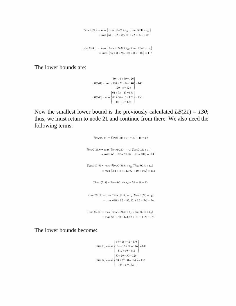
The lower bounds are:

Now the smallest lower bound is the previously calculated LB(21) = 130;thus, we must return to node 21 and continue from there. We also need thefollowing terms:

The lower bounds become:

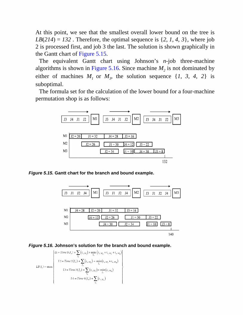
At this point, we see that the smallest overall lower bound on the tree isLB(214) = 132 . Therefore, the optimal sequence is {2, 1, 4, 3}, where job2 is processed first, and job 3 the last. The solution is shown graphically inthe Gantt chart of Figure 5.15.

The equivalent Gantt chart using Johnson’s n-job three-machinealgorithms is shown in Figure 5.16. Since machine M2 is not dominated byeither of machines M1 or M3, the solution sequence {1, 3, 4, 2} issuboptimal.

The formula set for the calculation of the lower bound for a four-machinepermutation shop is as follows:

Figure 5.15. Gantt chart for the branch and bound example.

Figure 5.16. Johnson’s solution for the branch and bound example.

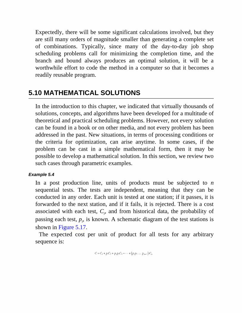
Expectedly, there will be some significant calculations involved, but theyare still many orders of magnitude smaller than generating a complete setof combinations. Typically, since many of the day-to-day job shopscheduling problems call for minimizing the completion time, and thebranch and bound always produces an optimal solution, it will be aworthwhile effort to code the method in a computer so that it becomes areadily reusable program.

5.10 MATHEMATICAL SOLUTIONS

In the introduction to this chapter, we indicated that virtually thousands ofsolutions, concepts, and algorithms have been developed for a multitude oftheoretical and practical scheduling problems. However, not every solutioncan be found in a book or on other media, and not every problem has beenaddressed in the past. New situations, in terms of processing conditions orthe criteria for optimization, can arise anytime. In some cases, if theproblem can be cast in a simple mathematical form, then it may bepossible to develop a mathematical solution. In this section, we review twosuch cases through parametric examples.

Example 5.4

In a post production line, units of products must be subjected to nsequential tests. The tests are independent, meaning that they can beconducted in any order. Each unit is tested at one station; if it passes, it isforwarded to the next station, and if it fails, it is rejected. There is a costassociated with each test, Ci, and from historical data, the probability ofpassing each test, pi, is known. A schematic diagram of the test stations isshown in Figure 5.17.

The expected cost per unit of product for all tests for any arbitrarysequence is:

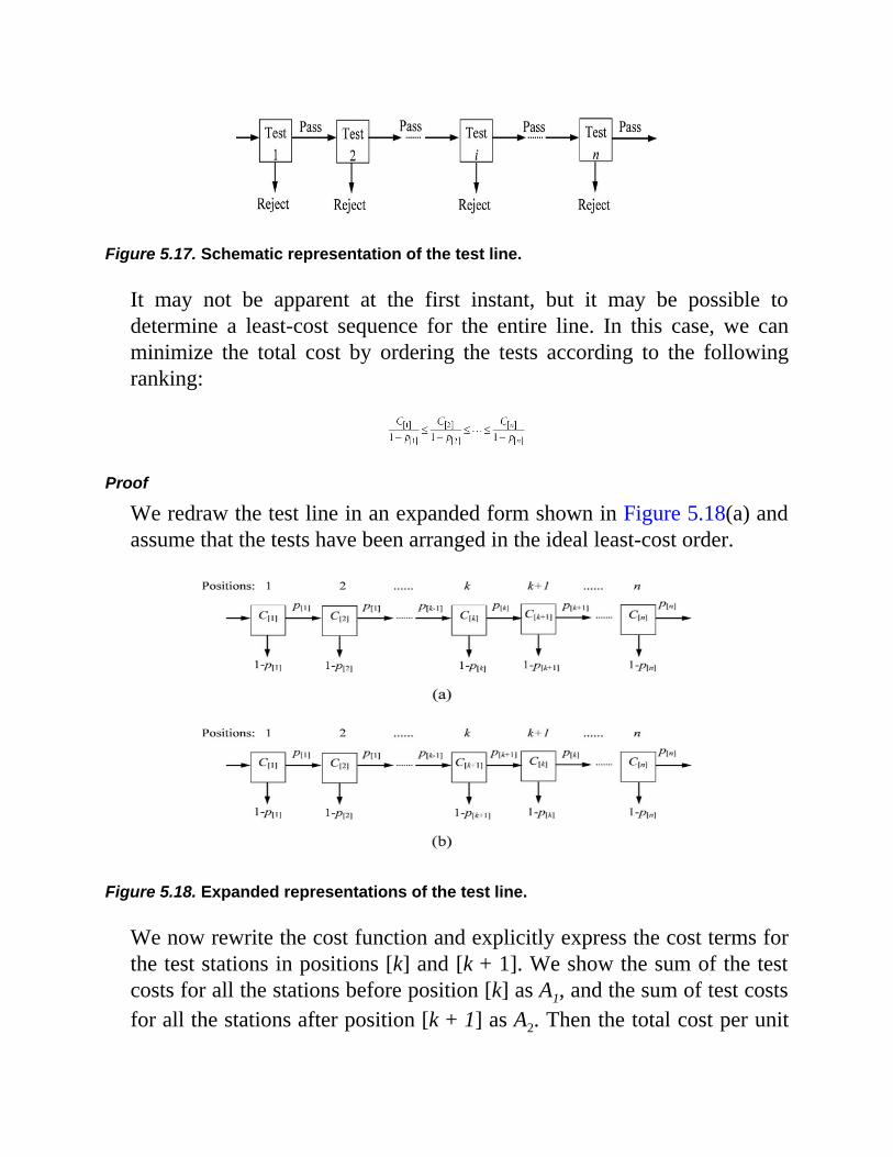
Figure 5.17. Schematic representation of the test line.

It may not be apparent at the first instant, but it may be possible todetermine a least-cost sequence for the entire line. In this case, we canminimize the total cost by ordering the tests according to the followingranking:

Proof

We redraw the test line in an expanded form shown in Figure 5.18(a) andassume that the tests have been arranged in the ideal least-cost order.

Figure 5.18. Expanded representations of the test line.

We now rewrite the cost function and explicitly express the cost terms forthe test stations in positions [k] and [k + 1]. We show the sum of the testcosts for all the stations before position [k] as A1, and the sum of test costsfor all the stations after position [k + 1] as A2. Then the total cost per unit

of product will be:

We now switch around the stations in the positions [k] and [k + 1] asshown in Figure 5.18(b). This will be a non ideal order, and the total costper unit of product will be:

Subtracting one equation from the other, the terms A1 and A2 areeliminated, and knowing that the cost for the nonideal case could begreater or at most the same, we obtain:

Crossing out the common terms (from p[1] to p [k – 1]) we have:

After factorizing, we obtain:

Transposing the terms we arrive at:

This relation implies that the least-cost testing sequence will be achieved if

the ranking term is calculated for all the tests, and the tests arecarried out in the increasing order of the value of the ranking term.

Example 5.5

We repeat Example 5.4 with an embellishment such that each unit is testedat one station and if it passes it is forwarded to the next station, but if itfails it is first repaired at a cost of Ri and then routed to the next teststation. As before, there is a cost associated with each test, denoted by Ci,and from historical data the probability of passing each test, pi, is known.

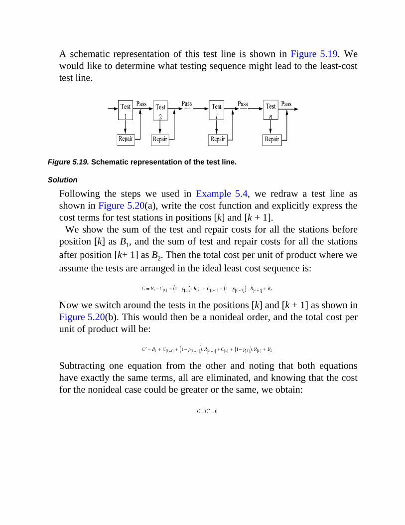
A schematic representation of this test line is shown in Figure 5.19. Wewould like to determine what testing sequence might lead to the least-costtest line.

Figure 5.19. Schematic representation of the test line.

Solution

Following the steps we used in Example 5.4, we redraw a test line asshown in Figure 5.20(a), write the cost function and explicitly express thecost terms for test stations in positions [k] and [k + 1].

We show the sum of the test and repair costs for all the stations beforeposition [k] as B1, and the sum of test and repair costs for all the stationsafter position [k+ 1] as B2. Then the total cost per unit of product where weassume the tests are arranged in the ideal least cost sequence is:

Now we switch around the tests in the positions [k] and [k + 1] as shown inFigure 5.20(b). This would then be a nonideal order, and the total cost perunit of product will be:

Subtracting one equation from the other and noting that both equationshave exactly the same terms, all are eliminated, and knowing that the costfor the nonideal case could be greater or the same, we obtain:

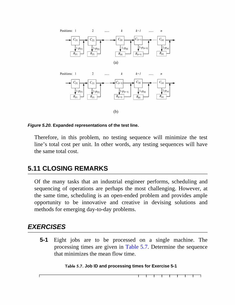
Figure 5.20. Expanded representations of the test line.

Therefore, in this problem, no testing sequence will minimize the testline’s total cost per unit. In other words, any testing sequences will havethe same total cost.

5.11 CLOSING REMARKS

Of the many tasks that an industrial engineer performs, scheduling andsequencing of operations are perhaps the most challenging. However, atthe same time, scheduling is an open-ended problem and provides ampleopportunity to be innovative and creative in devising solutions andmethods for emerging day-to-day problems.

EXERCISES

5-1 Eight jobs are to be processed on a single machine. Theprocessing times are given in Table 5.7. Determine the sequencethat minimizes the mean flow time.

Table 5.7. Job ID and processing times for Exercise 5-1

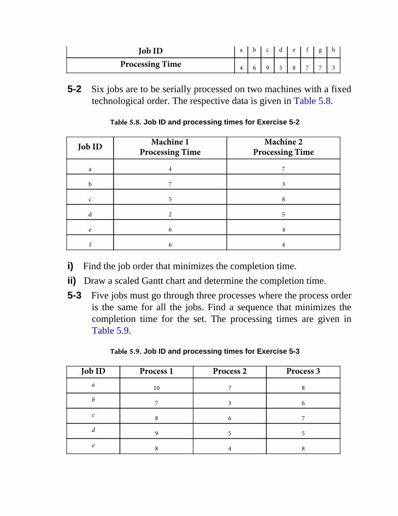
Job ID a b c d e f g h

Processing Time 4 6 9 5 8 7 7 3

5-2 Six jobs are to be serially processed on two machines with a fixedtechnological order. The respective data is given in Table 5.8.

Table 5.8. Job ID and processing times for Exercise 5-2

Job ID Machine 1Processing Time

Machine 2Processing Time

a 4 7

b 7 3

c 5 8

d 2 5

e 6 4

f 6 4

i) Find the job order that minimizes the completion time.ii) Draw a scaled Gantt chart and determine the completion time.5-3 Five jobs must go through three processes where the process order

is the same for all the jobs. Find a sequence that minimizes thecompletion time for the set. The processing times are given inTable 5.9.

Table 5.9. Job ID and processing times for Exercise 5-3

Job ID Process 1 Process 2 Process 3a 10 7 8

b 7 3 6

c 8 6 7

d 9 5 5

e 8 4 8

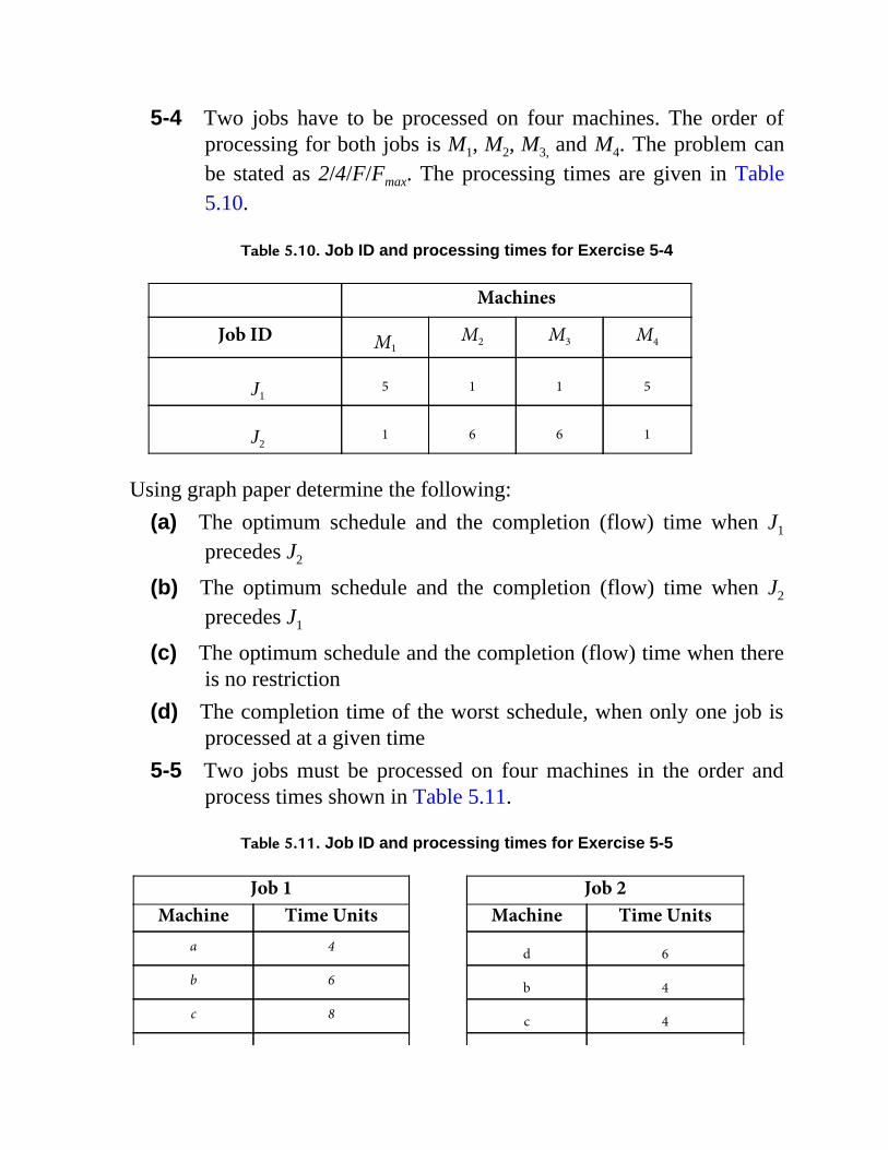
5-4 Two jobs have to be processed on four machines. The order ofprocessing for both jobs is M1, M2, M3, and M4. The problem canbe stated as 2/4/F/Fmax. The processing times are given in Table5.10.

Table 5.10. Job ID and processing times for Exercise 5-4

Machines

Job ID M1M2 M3 M4

J15 1 1 5

J21 6 6 1

Using graph paper determine the following:(a) The optimum schedule and the completion (flow) time when J1

precedes J2

(b) The optimum schedule and the completion (flow) time when J2

precedes J1

(c) The optimum schedule and the completion (flow) time when thereis no restriction

(d) The completion time of the worst schedule, when only one job isprocessed at a given time

5-5 Two jobs must be processed on four machines in the order andprocess times shown in Table 5.11.

Table 5.11. Job ID and processing times for Exercise 5-5

Job 1 Job 2Machine Time Units Machine Time Units

a 4 d 6

b 6 b 4

c 8 c 4

d 4 a 8

a) Graphically show the best sequence or strategy you might use.b) Calculate the completion time.c) What will be the n/m/A/B classification for the solution you have

provided?d) Draw a properly scaled Gantt chart showing the completion time.5-6 Table 5.12 shows the list of jobs that are all available and must be

processed on a single machine. It is known that the set of jobs (c,f, i, l) is for a customer, say, #1, and the set of jobs (a, b, d, h, j,) isfor another customer, say, #2. The jobs in each set must beprocessed back-to-back (that is, together as a group and deliveredto each customer). The problem can be stated as .Where is interpreted as “minimize the mean flow time for thetwo sets.” In other words, determine the order of processing thesets such that the mean flow time is minimum.

Table 5.12. Job ID and processing times for Exercise 5-6

Job ID a b c d e f g h i j k l

Processing Time 2 1 5 6 3 4 1 2 5 6 1 6

5-7 Applying Jackson’s algorithm, produce a sequence that wouldminimize the completion time for the processing of a batch offourteen jobs on two machines with the data given in Table 5.13.The table entries are processing times where a zero time impliesno operation. Draw two symbolic machines and show the joblineup in front of each machine indicating the beginning and endof the lineups.

Table 5.13. Job ID and processing times for Exercise 5-7

JobID

FirstOperation

on M1

SecondOperation on

M2

JobID

FirstOperation

on M2

SecondOperation on

M1

A 3 6 F 15 (0)

B 7 4 G 6 6

C 5 8 H 10 3

D 6 12 I 5 12

E 2 1 J 1 (0)

K 7 8

L 9 4

M 14 (0)

N 2 16

Chapter 6 FORECASTING

6.1 INTRODUCTION

Forecasting, as the name implies, is estimating a future value of a time-oriented variable. Depending on the case and intent, it can take eithermathematical predicting or nonmathematical surveying forms. Our focushere is on forecasting through mathematical techniques. These forms offorecasting essentially embrace various curve-fitting concepts, and the keyis on deciding which concept is the best for a given situation.

6.1.1 Pre-Forecasting AnalysisSince mathematical forecasting is based on some existing data, it could beuseful if the relevance of data is ascertained and visually examined. Oftenwe have tabular data in two or more columns. The first column is theindependent variable and is usually “time,” although it can be anyvariable, and the other column(s) will be the values of the parameter ofinterest observed or collected in different contexts or from differentsources. A forecast will only make sense when the pairs of data exhibitsome meaningful relationship. The best way to investigate this is to plotthe variable of interest against the independent variable. This will not onlyenable one to qualitatively observe the correlation between the data butalso could reveal what form of mathematical forecasting technique may beappropriate.

6.1.2 Forecasting Horizon

In Chapter 2 we discussed the topic of the planning horizon, and wedivided it into three long, medium, and short ranges. Forecasting is one ofthe key tasks in the management planning process. It is also divided intothree ranges.

Long-range or strategic forecasting involves major decisions that mustbe made on matters such as investment, expansion of business, and newproduct and services, or research and development. Sometimes thesedecisions are made based on governmental policies that are usually long-term, and corporations must forecast and determine how they might beaffected and adapt accordingly. Long-range forecasting for five years andbeyond must be looked into carefully, and some deep analysis andplanning may be required. Too many external influences make long-rangeforecasting an arduous task that often leads to an inaccurate outcome.

Medium-range or tactical forecasting is typically from six months to fiveyears. A frequent assessment of a medium range forecast can to someextent make up for the inaccuracies of long-range forecasting. Whatshould be considered in medium range planning depends on the nature ofthe organization. Hospitals and educational institutions, producers ofconsumer goods, and heavy-duty machinery manufacturers may findmedium-range forecasting most suitable for their planning purposes.

Short-range or operational forecasting horizon is from hours to one yearor so. There are, of course, no sharp boundaries between the threeforecasting horizons. A short-range forecasting horizon for an organizationmay be well over one year. Much of this depends highly on how often databecome available to run or update a forecast, and how fast the enterprisecan react to the results of a forecast. Typical examples of applicationsinclude production and personnel planning, inventory control, and spaceissues.

6.2 MATHEMATICAL FORECASTING METHODS

Forecasting can be done in a number of ways. In the absence of historicalor relevant data, it can be accomplished without mathematical meansthrough meetings, guessing, and seeking an expert opinion. In some cases,such as when launching a new product, past data will not be available, and,

if judged relevant, the historical data of similar products may be used. Forestablished enterprises, best forecasting can be done using their own data.There are many methods of mathematical forecasting available, and wereview some fundamental techniques.

6.2.1 Linear RegressionLinear regression is a line-fitting technique that is common in analyzingexperimental data to determine the relationship between two variables.Linear regression also has applications in the forecasting of a future valueof a variable of interest. If the underlying observed data tend to have alinear trend, increasing or decreasing, then the linear regression is a logicalchoice. In this method, a straight line that “best” fits the data ismathematically determined based on what is frequently referred to as the“least squares” method.

Given a set of n paired data (xi, yi), where normally xi is the independentvariable and yi is the corresponding observation, a line in the form of

is constructed, where is the linear estimation of the dependentvariable as a function of the independent variable. The numerical values ofthe slope, m, and the intercept, c, are determined from the data set usingthe least squares method as follows.

For a point i, the error between the actual observed value and theregressed value is:

Figure 6.1 shows the error for two sample points.

The sum of squared errors is:

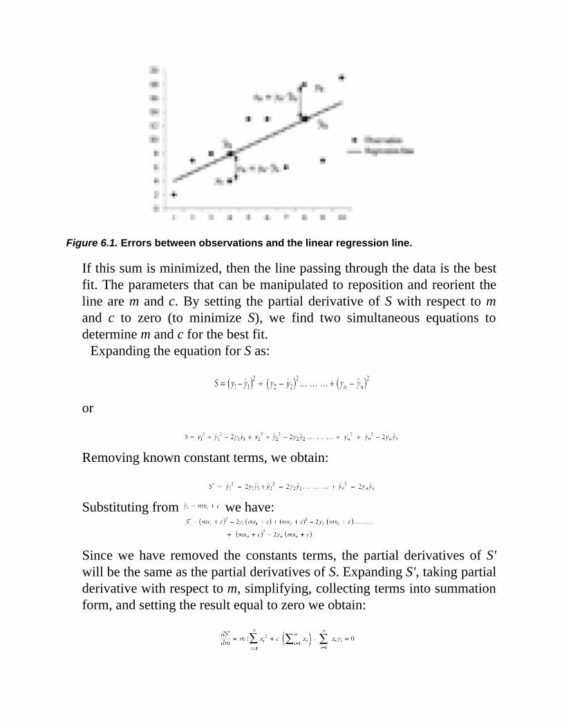
Figure 6.1. Errors between observations and the linear regression line.

If this sum is minimized, then the line passing through the data is the bestfit. The parameters that can be manipulated to reposition and reorient theline are m and c. By setting the partial derivative of S with respect to mand c to zero (to minimize S), we find two simultaneous equations todetermine m and c for the best fit.

Expanding the equation for S as:

or

Removing known constant terms, we obtain:

Substituting from we have:

Since we have removed the constants terms, the partial derivatives of S'will be the same as the partial derivatives of S. Expanding S', taking partialderivative with respect to m, simplifying, collecting terms into summationform, and setting the result equal to zero we obtain:

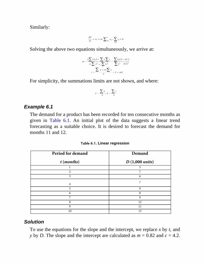
Similarly:

Solving the above two equations simultaneously, we arrive at:

For simplicity, the summations limits are not shown, and where:

Example 6.1The demand for a product has been recorded for ten consecutive months asgiven in Table 6.1. An initial plot of the data suggests a linear trendforecasting as a suitable choice. It is desired to forecast the demand formonths 11 and 12.

Table 6.1. Linear regression

Period for demand

t (months)

Demand

D (1,000 units)1 52 73 6

4 7

5 96 87 98 129 11

10 13

SolutionTo use the equations for the slope and the intercept, we replace x by t, andy by D. The slope and the intercept are calculated as m = 0.82 and c = 4.2.

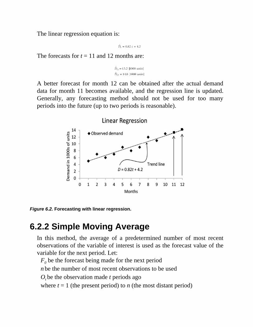
The linear regression equation is:

The forecasts for t = 11 and 12 months are:

A better forecast for month 12 can be obtained after the actual demanddata for month 11 becomes available, and the regression line is updated.Generally, any forecasting method should not be used for too manyperiods into the future (up to two periods is reasonable).

Figure 6.2. Forecasting with linear regression.

6.2.2 Simple Moving AverageIn this method, the average of a predetermined number of most recentobservations of the variable of interest is used as the forecast value of thevariable for the next period. Let:

F0 be the forecast being made for the next periodn be the number of most recent observations to be usedOt

be the observation made t periods agowhere t = 1 (the present period) to n (the most distant period)

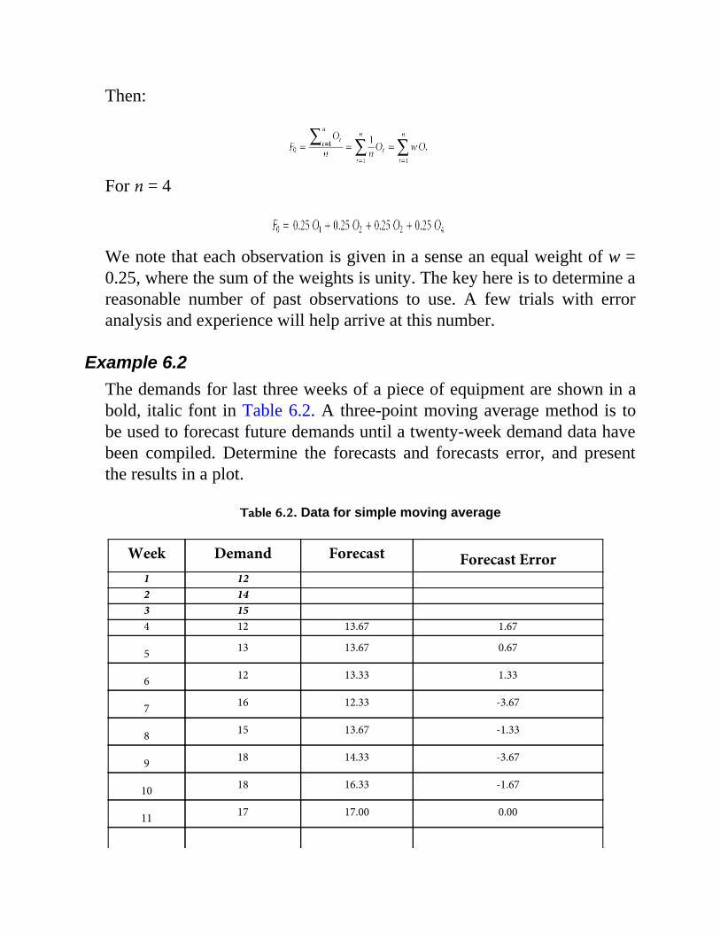
Then:

For n = 4

We note that each observation is given in a sense an equal weight of w =0.25, where the sum of the weights is unity. The key here is to determine areasonable number of past observations to use. A few trials with erroranalysis and experience will help arrive at this number.

Example 6.2The demands for last three weeks of a piece of equipment are shown in abold, italic font in Table 6.2. A three-point moving average method is tobe used to forecast future demands until a twenty-week demand data havebeen compiled. Determine the forecasts and forecasts error, and presentthe results in a plot.

Table 6.2. Data for simple moving average

Week Demand Forecast Forecast Error1 12 2 14 3 15 4 12 13.67 1.67

5 13 13.67 0.67

6 12 13.33 1.33

7 16 12.33 -3.67

8 15 13.67 -1.33

9 18 14.33 -3.67

10 18 16.33 -1.67

11 17 17.00 0.00

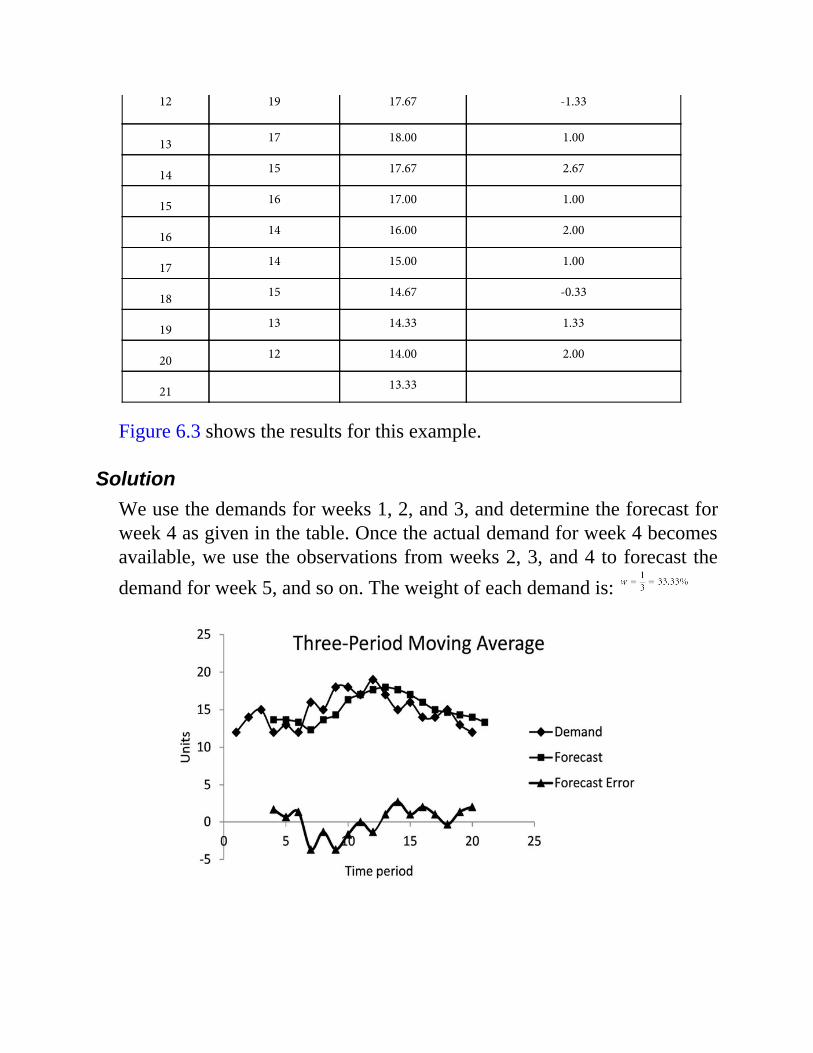
12 19 17.67 -1.33

13 17 18.00 1.00

14 15 17.67 2.67

15 16 17.00 1.00

16 14 16.00 2.00

17 14 15.00 1.00

18 15 14.67 -0.33

19 13 14.33 1.33

20 12 14.00 2.00

21 13.33

Figure 6.3 shows the results for this example.

SolutionWe use the demands for weeks 1, 2, and 3, and determine the forecast forweek 4 as given in the table. Once the actual demand for week 4 becomesavailable, we use the observations from weeks 2, 3, and 4 to forecast thedemand for week 5, and so on. The weight of each demand is:

Figure 6.3. Forecasting with the simple moving average.

6.2.3 Weighted Moving AverageThe concept of “weights” gives rise to the weighted moving averagemethod. Unlike the simple moving average method, where the observeddata points have equal weights, in this approach, a predetermined numberof most recent observations are each given a specific weight, wt, wherethey are unequal, but the weights must sum to unity. The period t isdefined as in Section 6.2.2, and the forecast is given by:

The number of observed points and the value of each weight can bedetermined from the consideration of the problem at hand, and the use oftrial and error analysis. Typically, the more recent the observation, thelarger the weight associated with it.

Example 6.3Suppose for data given in the previous example, Table 6.2, it is nowdesired to use the three-point (n = 3) weighted moving average method forthe forecasts. The weight for the successive demands are w1 = 70%, w2 =20%, and w3 = 10%, where the first is associated with the most recentdemand and the last with the most distant. The initial data is given in thefirst three rows of Table 6.3.

Table 6.3. Weighted moving average

Week Demand Forecast Forecast Error1 12 2 14 3 15 4 12 14.5 2.5

5 13 12.8 -0.2

6 12 13.0 1

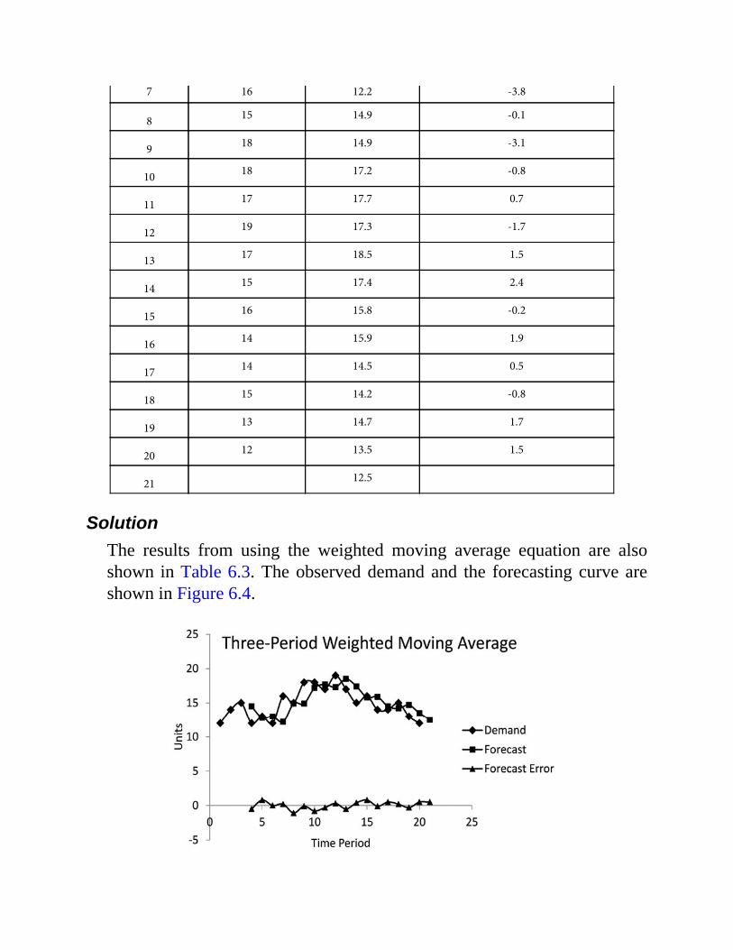
7 16 12.2 -3.8

8 15 14.9 -0.1

9 18 14.9 -3.1

10 18 17.2 -0.8

11 17 17.7 0.7

12 19 17.3 -1.7

13 17 18.5 1.5

14 15 17.4 2.4

15 16 15.8 -0.2

16 14 15.9 1.9

17 14 14.5 0.5

18 15 14.2 -0.8

19 13 14.7 1.7

20 12 13.5 1.5

21 12.5

SolutionThe results from using the weighted moving average equation are alsoshown in Table 6.3. The observed demand and the forecasting curve areshown in Figure 6.4.

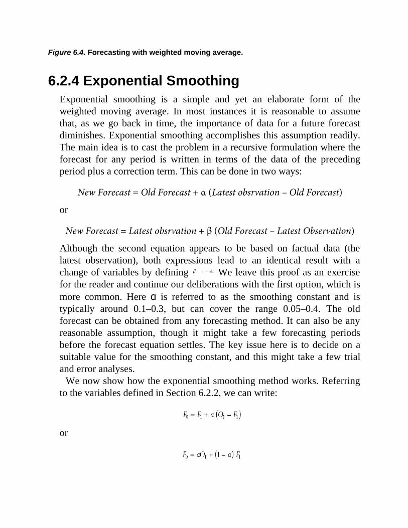
Figure 6.4. Forecasting with weighted moving average.

6.2.4 Exponential SmoothingExponential smoothing is a simple and yet an elaborate form of theweighted moving average. In most instances it is reasonable to assumethat, as we go back in time, the importance of data for a future forecastdiminishes. Exponential smoothing accomplishes this assumption readily.The main idea is to cast the problem in a recursive formulation where theforecast for any period is written in terms of the data of the precedingperiod plus a correction term. This can be done in two ways:

New Forecast = Old Forecast + α (Latest obsrvation – Old Forecast)

or

New Forecast = Latest obsrvation + β (Old Forecast – Latest Observation)

Although the second equation appears to be based on factual data (thelatest observation), both expressions lead to an identical result with achange of variables by defining We leave this proof as an exercisefor the reader and continue our deliberations with the first option, which ismore common. Here α is referred to as the smoothing constant and istypically around 0.1–0.3, but can cover the range 0.05–0.4. The oldforecast can be obtained from any forecasting method. It can also be anyreasonable assumption, though it might take a few forecasting periodsbefore the forecast equation settles. The key issue here is to decide on asuitable value for the smoothing constant, and this might take a few trialand error analyses.

We now show how the exponential smoothing method works. Referringto the variables defined in Section 6.2.2, we can write:

or

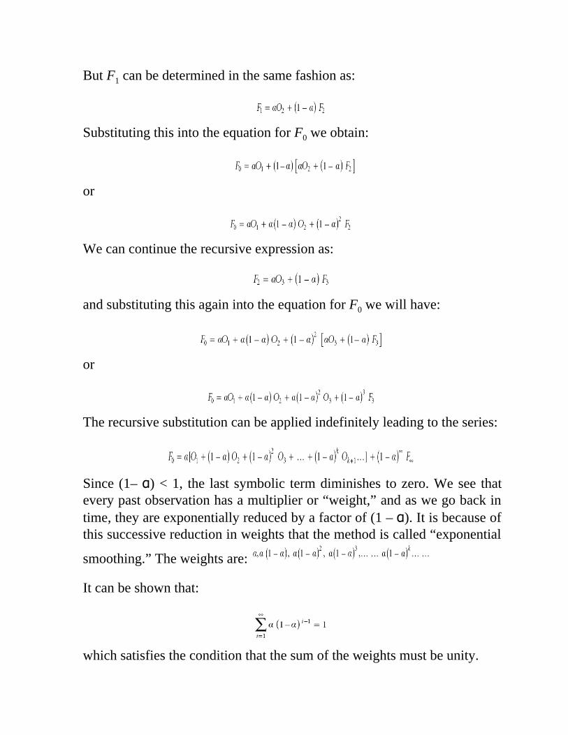
But F1 can be determined in the same fashion as:

Substituting this into the equation for F0 we obtain:

or

We can continue the recursive expression as:

and substituting this again into the equation for F0 we will have:

or

The recursive substitution can be applied indefinitely leading to the series:

Since (1– α) < 1, the last symbolic term diminishes to zero. We see thatevery past observation has a multiplier or “weight,” and as we go back intime, they are exponentially reduced by a factor of (1 – α). It is because ofthis successive reduction in weights that the method is called “exponential

smoothing.” The weights are:

It can be shown that:

which satisfies the condition that the sum of the weights must be unity.

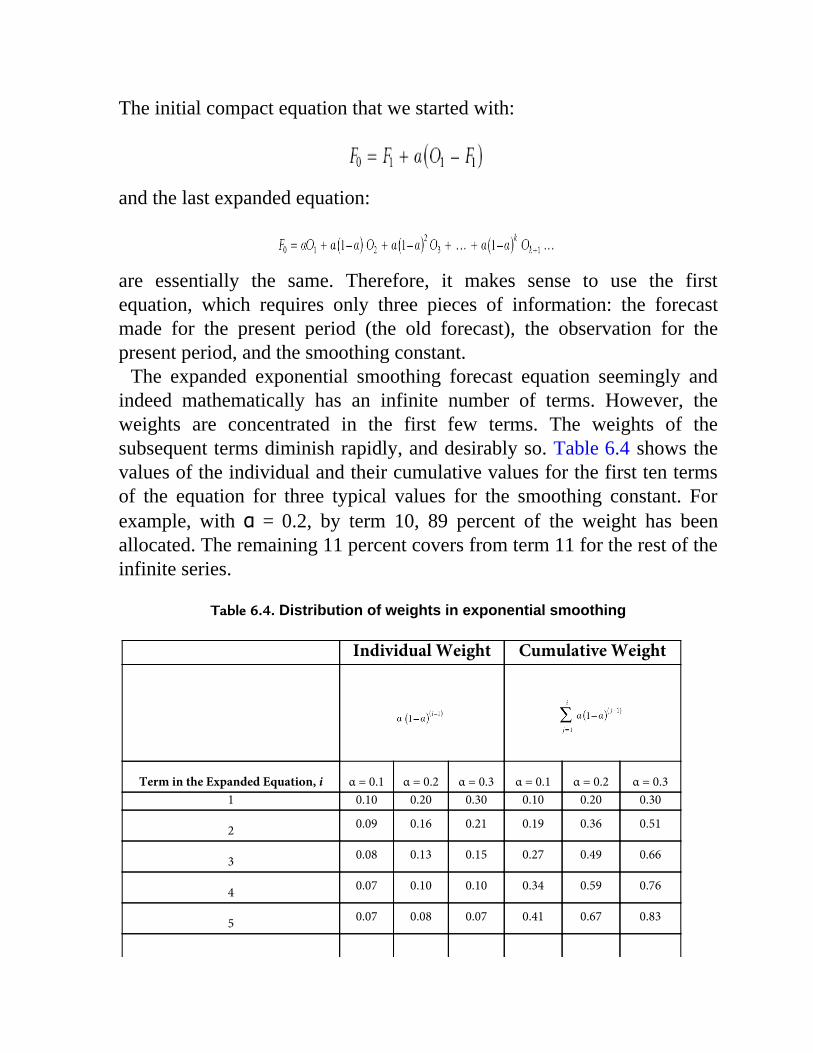
The initial compact equation that we started with:

and the last expanded equation:

are essentially the same. Therefore, it makes sense to use the firstequation, which requires only three pieces of information: the forecastmade for the present period (the old forecast), the observation for thepresent period, and the smoothing constant.

The expanded exponential smoothing forecast equation seemingly andindeed mathematically has an infinite number of terms. However, theweights are concentrated in the first few terms. The weights of thesubsequent terms diminish rapidly, and desirably so. Table 6.4 shows thevalues of the individual and their cumulative values for the first ten termsof the equation for three typical values for the smoothing constant. Forexample, with α = 0.2, by term 10, 89 percent of the weight has beenallocated. The remaining 11 percent covers from term 11 for the rest of theinfinite series.

Table 6.4. Distribution of weights in exponential smoothing

Individual Weight Cumulative Weight

Term in the Expanded Equation, i α = 0.1 α = 0.2 α = 0.3 α = 0.1 α = 0.2 α = 0.31 0.10 0.20 0.30 0.10 0.20 0.30

2 0.09 0.16 0.21 0.19 0.36 0.51

3 0.08 0.13 0.15 0.27 0.49 0.66

4 0.07 0.10 0.10 0.34 0.59 0.76

5 0.07 0.08 0.07 0.41 0.67 0.83

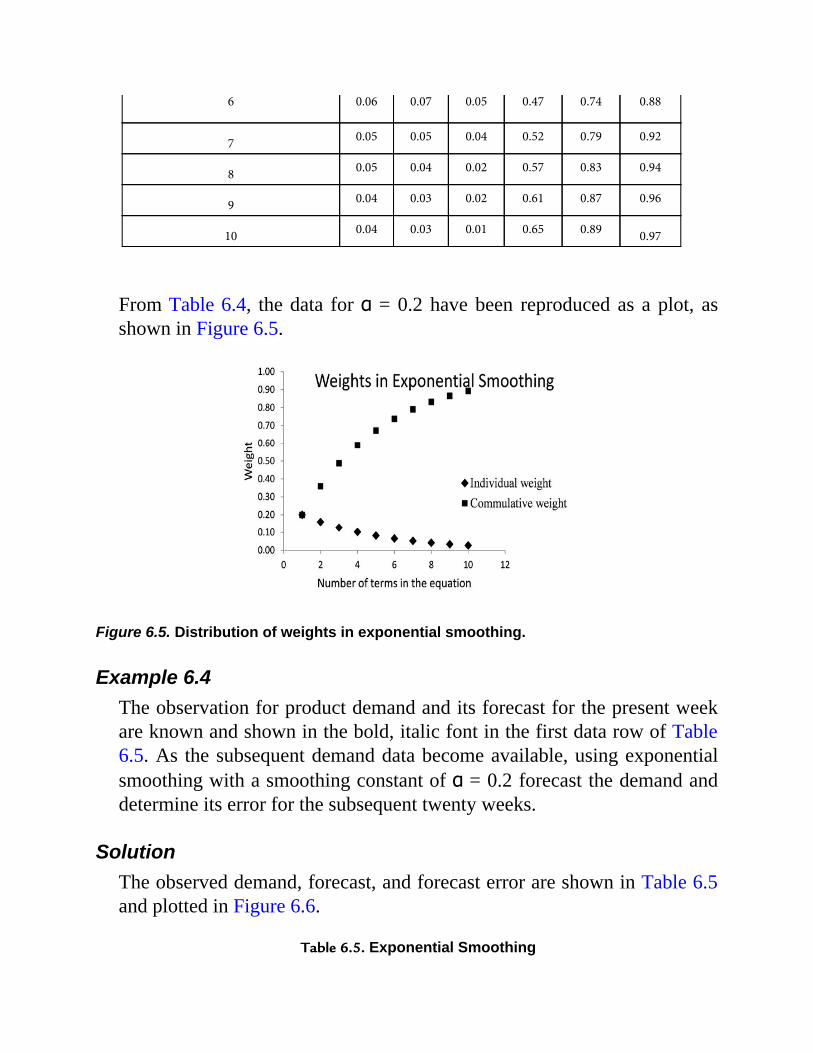
6 0.06 0.07 0.05 0.47 0.74 0.88

7 0.05 0.05 0.04 0.52 0.79 0.92

8 0.05 0.04 0.02 0.57 0.83 0.94

9 0.04 0.03 0.02 0.61 0.87 0.96

10 0.04 0.03 0.01 0.65 0.89 0.97

From Table 6.4, the data for α = 0.2 have been reproduced as a plot, asshown in Figure 6.5.

Figure 6.5. Distribution of weights in exponential smoothing.

Example 6.4The observation for product demand and its forecast for the present weekare known and shown in the bold, italic font in the first data row of Table6.5. As the subsequent demand data become available, using exponentialsmoothing with a smoothing constant of α = 0.2 forecast the demand anddetermine its error for the subsequent twenty weeks.

SolutionThe observed demand, forecast, and forecast error are shown in Table 6.5and plotted in Figure 6.6.

Table 6.5. Exponential Smoothing

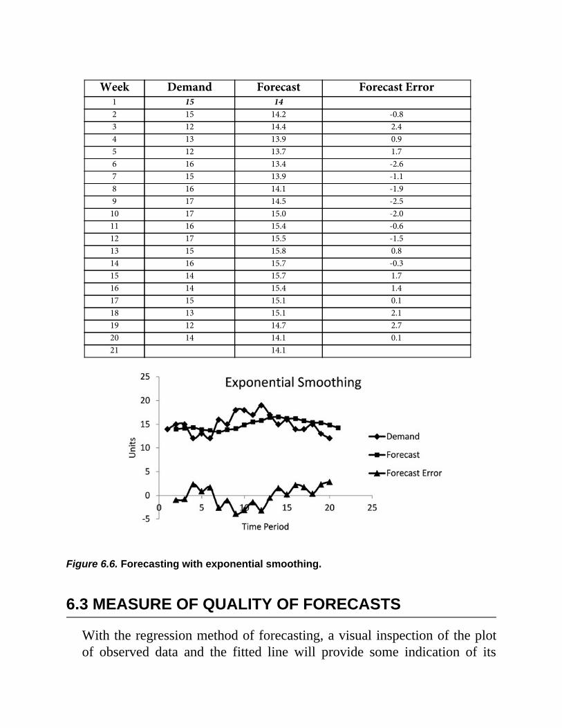
Week Demand Forecast Forecast Error1 15 14 2 15 14.2 -0.83 12 14.4 2.44 13 13.9 0.95 12 13.7 1.76 16 13.4 -2.67 15 13.9 -1.18 16 14.1 -1.99 17 14.5 -2.5

10 17 15.0 -2.011 16 15.4 -0.612 17 15.5 -1.513 15 15.8 0.814 16 15.7 -0.315 14 15.7 1.716 14 15.4 1.417 15 15.1 0.118 13 15.1 2.119 12 14.7 2.720 14 14.1 0.121 14.1

Figure 6.6. Forecasting with exponential smoothing.

6.3 MEASURE OF QUALITY OF FORECASTS

With the regression method of forecasting, a visual inspection of the plotof observed data and the fitted line will provide some indication of its

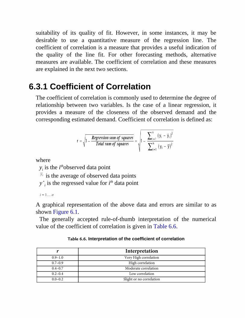
suitability of its quality of fit. However, in some instances, it may bedesirable to use a quantitative measure of the regression line. Thecoefficient of correlation is a measure that provides a useful indication ofthe quality of the line fit. For other forecasting methods, alternativemeasures are available. The coefficient of correlation and these measuresare explained in the next two sections.

6.3.1 Coefficient of CorrelationThe coefficient of correlation is commonly used to determine the degree ofrelationship between two variables. Is the case of a linear regression, itprovides a measure of the closeness of the observed demand and thecorresponding estimated demand. Coefficient of correlation is defined as:

where

yi is the ithobserved data point is the average of observed data points

yˆi is the regressed value for ith data point

A graphical representation of the above data and errors are similar to asshown Figure 6.1.

The generally accepted rule-of-thumb interpretation of the numericalvalue of the coefficient of correlation is given in Table 6.6.

Table 6.6. Interpretation of the coefficient of correlation

r Interpretation0.9–1.0 Very High correlation0.7–0.9 High correlation0.4–0.7 Moderate correlation0.2–0.4 Low correlation0.0–0.2 Slight or no correlation

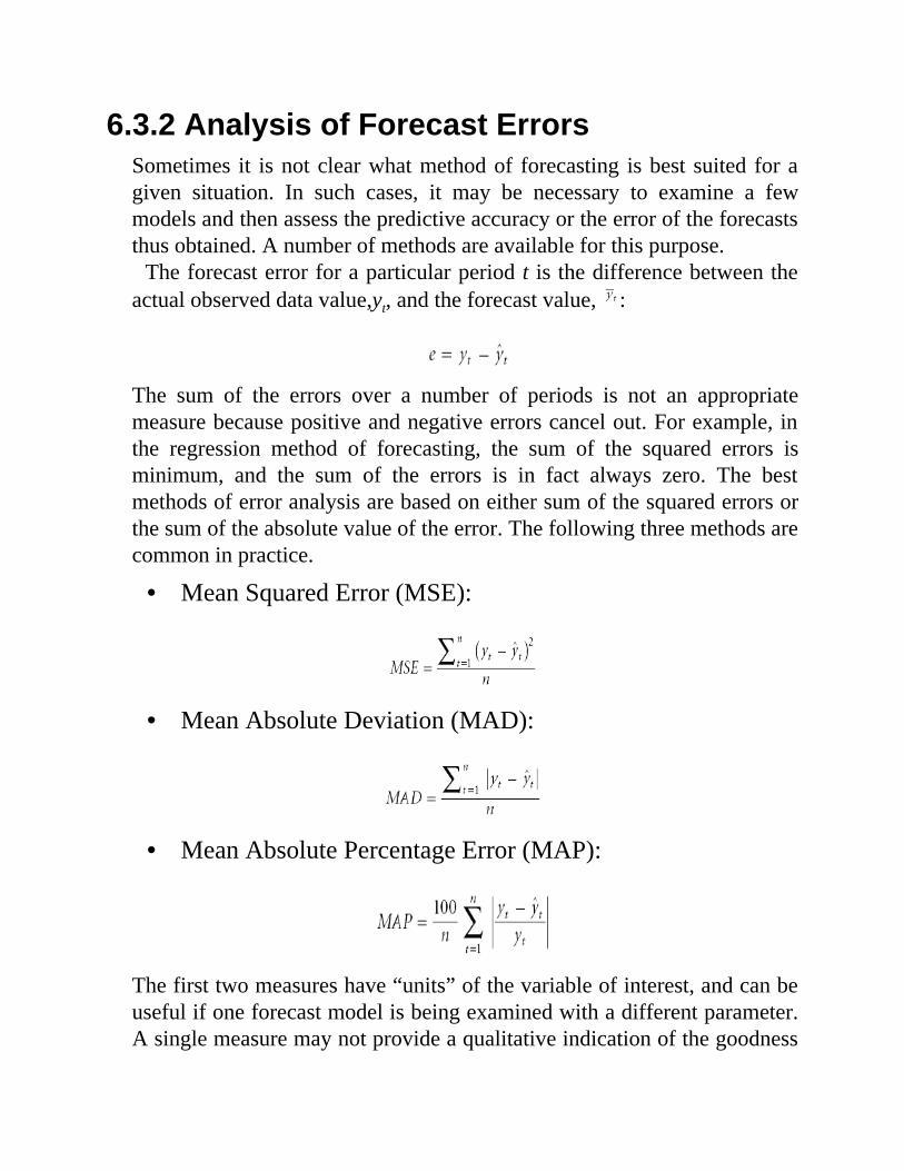
6.3.2 Analysis of Forecast ErrorsSometimes it is not clear what method of forecasting is best suited for agiven situation. In such cases, it may be necessary to examine a fewmodels and then assess the predictive accuracy or the error of the forecaststhus obtained. A number of methods are available for this purpose.

The forecast error for a particular period t is the difference between theactual observed data value,yt, and the forecast value, :

The sum of the errors over a number of periods is not an appropriatemeasure because positive and negative errors cancel out. For example, inthe regression method of forecasting, the sum of the squared errors isminimum, and the sum of the errors is in fact always zero. The bestmethods of error analysis are based on either sum of the squared errors orthe sum of the absolute value of the error. The following three methods arecommon in practice.

• Mean Squared Error (MSE):

• Mean Absolute Deviation (MAD):

• Mean Absolute Percentage Error (MAP):

The first two measures have “units” of the variable of interest, and can beuseful if one forecast model is being examined with a different parameter.A single measure may not provide a qualitative indication of the goodness

of the forecast. The third measure, MAP, is unit-less and provides apercentage error that is a more familiar and tangible measure.

6.4 CLOSING REMARKS

Forecasting is essentially a curve-fitting process. The key is to find theform and parameters of the best fitting curve, and then throughmathematical means assess the predictive accuracy of such a curve.

EXERCISES

6-1 If you are working in an organization where forecasting is afrequent activity, what is short-range forecasting is used for? Arerelevant observations properly recorded? Is error analysisperformed and appropriate actions are taken?

6-2 If the answer to Exercise 6-1 is negative, do you thinkimplementing a forecasting program will be beneficial? Are youin a position to suggest such and plan and take on the task?

6-3 In follow up to Exercise 6-2, if you are able to make a suggestion,what will be your preferred choice of the forecasting method?And why?

6-4 To make better use of time in faster achieving some results, whatdo you think of spending some efforts to implement twoforecasting methods concurrently and determine which oneperforms better based on error analyses?

6-5 Find the linear regression line for the data given in Table 6.7.

Table 6.7. Data for Exercise 6-5

x y1.6 2.62.0 2.92.4 2.02.7 3.13.5 3.43.8 4.1

5.0 4.55.4 5.5

Perform all three methods of forecast error analysis and comment onresults.

6-6 Apply exponential smoothing to the data shown in Table 6.8 witha smoothing constant of α = 0.2. Show the results in a table withcolumn headings Observation, Forecast, and Forecast Error.

Table 6.8. Data for Exercise 6-6

20 20 20 20 24 24 24 24 24 24

6-7 Similar to Exercise 6-6, apply exponential smoothing to the datagiven in Table 6.9 with a smoothing constant of α = 0.2. Show theresults in a table with column headings Observation, Forecast, andForecast Error.

Table 6.9. Data for Exercise 6-7

24 25 24 25 20 20 20 20 20 20

6-8 Carefully examine the numerical values of the errors in each of theExercises 6-6 and 6-7. What overall observation do you make?

Chapter

7STATISTICAL QUALITYCONTROL

7.1 INTRODUCTION

The importance of quality cannot be underestimated. The least impactresulting from a low-quality product is probably only economical, and thisby itself can severely impair the financial health of any enterprise. In theworst case, inferior quality can lead to irreversible consequences, such asloss of life—which can inflict severe financial damages and endanger theexistence of the enterprise. A credible enterprise must aim to producegoods and services of the right quantity and value, and also of the rightquality. It is important to know the difference between inspection andquality control. Inspection is used to verify the quality of what has alreadybeen produced, whereas quality control is a process that is used to foresee,direct, and control the quality of the products yet to be produced.

When an item or product fails to meet expectations or perform itsintended function, then it is associated with inferior or unacceptablequality. Technically, by “quality” we mean to what degree a measuredvalue of a feature deviates from its stated specifications. The smaller thedeviation, the better the quality.

To gauge quality, the general public and consumers rely on a company’sreputation for quality and reliability, and the brand name, as they lack anysystematic tools to measure quality.

The volume of the business, natural desire for profits, and sometimes theregulations in place justify, encourage and force organizations to resort tomore scientific and consistent methods of assessment to produce goods of

acceptable quality and constantly look for ways of improvement.Statistical quality control (SQC) is an approach that can cost-effectivelyhelp any organization to achieve these. We will show that it is notnecessary for SQC to screen each and every one of the product items orcomponents. Proven sampling techniques allow only a small part of theoutput to be examined, yet provide significant insight into the quality andquality trends of the entire production.**

It is not even necessary to maintain quality control efforts at all times andfor all products. With good measures and a proper combination of factorsof production, a process may in time indicate that active quality control isno longer needed. Nonetheless, maintaining some degree of inspection andcontrol provides assurance that the achieved quality levels do notdeteriorate.

We define factors of production as all elements that play a role inmanufacturing a product or when providing a service. In manufacturing,for example, these are primarily equipment, tools, materials, operatorskills, and instructions. Other factors may be such things as maintenanceand ambient temperature. If proper resources and factors of production arenot provided, the expectation for good quality will be unrealistic.

Ultimately, quality control efforts are inherently linked to much broaderaspects of any production system and running an enterprise. These includedesign, performance and market indicators, cost analysis and finance,management philosophy and safety.

7.2 DETERMINING QUALITY

For small and relatively inexpensive goods, such as consumables and food,for example, personal experience is the primary means of associating aquality rating. For major products and products of high value, customersand consumers actively search various media and seek advice from others.The third, and unfortunate, means of finding out about quality is when amanufacturer or supplier issues a recall of their product as a result ofdefects, deficiencies, and poor quality and performance. The following is alist of a few common recall scenarios:

• Automobiles, practically from all manufacturers

• A range of household items, such as strollers, toys, andelectronic devices

• Processed and packaged food

A simple search on the Internet with the keyword recall and any productor automobile brand name will invariably return a list of recalls. This isparticularly prevalent in the automobile industry, as every year themanufacturers implement new designs and functionality or introduce newmodels that accompany new issues in quality.

When the deficiencies are significant and affect a broader base ofconsumers, the companies involved issue public and mediaannouncements. Otherwise, many recalls are handled through the mail andgo unnoticed by the general public. A recall can tarnish the reputation anddamage the financial health of the manufacturer, and critical defects anddeficiencies can lead to catastrophic consequences.

7.2.1 Why Is Quality Inconsistent?When components or products are produced, a set of design,manufacturing, and performance specifications are necessary. It is almostimpossible to state and achieve the exact specifications of the product.Even if it were possible, the manufacturing and quality control costs wouldbe prohibitive. In fact, from the cost consideration point of view, it is noteven necessary to achieve exact specifications. For example, when a shaftis being machined to support a ball bearing, we commonly state thespecification as a desired target diameter plus/minus some acceptabletolerance. If a thousand such shafts are produced, they will hardly be thesame.

But this is fine because we want shafts to be practically usable andeconomically justifiable. Inconsistencies and deviations come fromnumerous sources. They are occasionally random in nature, and most oftenthe result of variations in the factors of production. Taking a machiningoperation, we can name the following as typical examples:

– Tool wear

– Slack in machine parts and joints– Error in proper setting of measures and adjustments– Variation in temperature– Inconsistency in material properties– Other reasons depending on the case

With automation, compensatory feedback, and improvements in themanufacturing precision of equipment and machine tools, such variationsand errors have been significantly reduced. However, with higherexpectations for quality, in the majority of common manufacturingprocesses, they will still be present.

7.3 ECONOMICS OF QUALITY

After safety has been sufficiently and legally addressed for a product orservice, it is the “economics” that truly controls the level of quality.Attempts are constantly made to reduce or eliminate the effects of externalfactors and improve quality. Clearly, refining and improving qualityexceedingly costs the manufacturer, but it also increases the value of theproduct. The difference between the product value and the cost of qualityis the gain due to quality control efforts. Figure 7.1 shows typical trendsfor the cost and value of a product as a function of quality refinement. Themaximum gain occurs at an optimum quality level. This is the lowest levelof quality that must be attained to sustain the market. Certainmanufacturers may operate above the optimum level of quality to gainreputation. This results in some brand names benefiting from a positivepublic opinion about their products. We should always have in mind thatcustomers and consumers seek an acceptable level of quality that satisfiestheir needs in terms of cost-effectiveness. They do not need excessivequality, at least in certain aspects of the product they buy, nor are theywilling to pay extra for it.

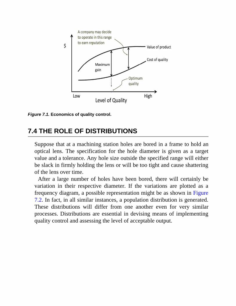
Figure 7.1. Economics of quality control.

7.4 THE ROLE OF DISTRIBUTIONS

Suppose that at a machining station holes are bored in a frame to hold anoptical lens. The specification for the hole diameter is given as a targetvalue and a tolerance. Any hole size outside the specified range will eitherbe slack in firmly holding the lens or will be too tight and cause shatteringof the lens over time.

After a large number of holes have been bored, there will certainly bevariation in their respective diameter. If the variations are plotted as afrequency diagram, a possible representation might be as shown in Figure7.2. In fact, in all similar instances, a population distribution is generated.These distributions will differ from one another even for very similarprocesses. Distributions are essential in devising means of implementingquality control and assessing the level of acceptable output.

Figure 7.2. Distribution of diameters.

7.4.1 The Scatter of DataDistributions have certain characteristic parameters, such as the well-known and well-used “arithmetic mean” and “standard deviation.” Thesemeasures allow us to employ useful features of the distribution.

Arithmetic MeanThe average, arithmetic mean, or simply the “mean” of a distribution isgiven as:

where Xi designates members of the population, and N is the size of thepopulation.

Measures of DispersionThe arithmetic mean alone does not provide a sufficient description of thedistribution. Two distributions can have the same mean but significantlydifferent populations. To better characterize a distribution, we needanother measure that explains the spread or dispersion of the data. For thisvariability, two measures are available: the range and the standarddeviation. The range is defined as:

where Xmax is the largest observation and Xmin is the smallest observationwithin the population. The standard deviation (STD) is defined as:

If all members of a population have the same value, then the range and thestandard deviation will be zero. As the scatter grows, both the range andstandard deviation increase. As opposed to the range, which is based ontwo members of the population, standard deviation accounts for everymember of the population. Therefore, the standard deviation is asignificantly better measure. We show later that for statistical qualitycontrol purposes, and the manner in which the procedures are applied,there is a relationship between R and σ, and since R is more convenient touse, and indeed sufficient, the use of R is common and dominant.

When we have a set of reasonably related data, which is from onegenerating source, we can express it as a credible distribution in amathematical form in terms of its statistical measures. One of the mostcommon, applicable, and useful distributions is the normal distribution. Infact, the distribution of a variable, such as the diameter of machined shafts,which is influenced by several external factors, will most likely be normal,though this is not a universal rule. A machined shaft is affected by factorssuch as the settings on the machine tool, operator skills, sharpness of thecutting tool, and the ambient temperature.

Normal distribution is easy to understand and use. It plays a central rolein statistical quality control.

7.4.2 Normal DistributionNormal distribution is a continuous distribution, and it is entirelydescribed in terms of its population average (arithmetic mean or simplymean) µ, and its standard deviation σ. The mathematical expression or so-called probability density function for normal distribution is:

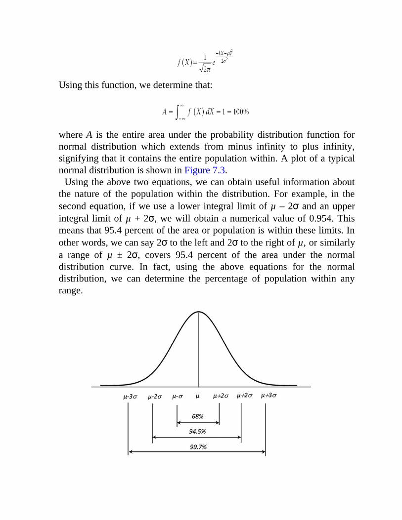
Using this function, we determine that:

where A is the entire area under the probability distribution function fornormal distribution which extends from minus infinity to plus infinity,signifying that it contains the entire population within. A plot of a typicalnormal distribution is shown in Figure 7.3.

Using the above two equations, we can obtain useful information aboutthe nature of the population within the distribution. For example, in thesecond equation, if we use a lower integral limit of µ – 2σ and an upperintegral limit of µ + 2σ, we will obtain a numerical value of 0.954. Thismeans that 95.4 percent of the area or population is within these limits. Inother words, we can say 2σ to the left and 2σ to the right of µ, or similarlya range of µ ± 2σ, covers 95.4 percent of the area under the normaldistribution curve. In fact, using the above equations for the normaldistribution, we can determine the percentage of population within anyrange.

Figure 7.3. The normal distribution.

Referring to our example of the bored holes, let us suppose that we havea normal distribution of the diameters with a mean of 1.502 inches and astandard deviation of 0.003 inches. Therefore, 95.4 percent of the itemswill have a diameter between 1.502 ± 2(0.003) or 1.496 and 1.508 inches.This means that if an item is randomly selected from the population, thereis 95.4 percent probability that the item diameter will be within thetolerance limits.

These calculations were carried out on the assumption that thedistribution of the items (hole diameters) is normal. We also noted thatnormal distribution is a continuous distribution and theoretically extendsfrom minus infinity to plus infinity. We might then question the validity ofits application for quality control purposes, arguing the following:

• Our population will not contain an infinite number of items.• The possible diameter values will in no way extend to

minus infinity or plus infinity, as they will have finitepositive values in the neighborhood of the statedspecification.

• The diameters are measured and expressed in thousandthsof an inch and therefore represent a population of discretevalues.

We do acknowledge these concerns, but justify our use of the normaldistribution on the following basis:

• The population of the items, in the long run, will besufficiently large.

• 99.997 percent of the population will be within the range of± 4σ. This means that essentially the highly skewed tails ofthe distribution contain a negligible population.

• With the major portion of the population within a finiterange, the density of measurements will be sufficiently high

to assume continuous values.• Even if the distribution is only close to normal, the induced

errors will be negligible.

Normal Distribution TableInstead of integrating to determine the portion of the population within aspecific range, standard tables, as the one shown in Table 7.1, have beenprepared that are very convenient to use.

Table 7.1. Areas under the normal distribution curve

Z 0.00 0.01 0.02 0.03 0.04 0.05 0.06 0.07 0.08 0.090.0 0.0000 0.0040 0.0080 0.0120 0.0160 0.0199 0.0239 0.0279 0.0319 0.0359

0.1 0.0398 0.0438 0.0478 0.0517 0.0557 0.0596 0.0636 0.0675 0.0714 0.0753

0.2 0.0793 0.0832 0.0871 0.0910 0.0948 0.0987 0.1026 0.1064 0.1103 0.1141

0.3 0.1179 0.1217 0.1255 0.1293 0.1331 0.1368 0.1406 0.1443 0.1480 0.1517

0.4 0.1554 0.1591 0.1628 0.1664 0.1700 0.1736 0.1772 0.1808 0.1844 0.1879

0.5 0.1915 0.1950 0.1985 0.2019 0.2054 0.2088 0.2123 0.2157 0.2190 0.2224

0.6 0.2257 0.2291 0.2324 0.2357 0.2389 0.2422 0.2454 0.2486 0.2517 0.2549

0.7 0.2580 0.2611 0.2642 0.2673 0.2704 0.2734 0.2764 0.2794 0.2823 0.2852

0.8 0.2881 0.2910 0.2939 0.2967 0.2995 0.3023 0.3051 0.3078 0.3106 0.3133

0.9 0.3159 0.3186 0.3212 0.3238 0.3264 0.3289 0.3315 0.3340 0.3365 0.3389

1.0 0.3413 0.3438 0.3461 0.3485 0.3508 0.3531 0.3554 0.3577 0.3599 0.3621

1.1 0.3643 0.3665 0.3686 0.3708 0.3729 0.3749 0.3770 0.3790 0.3810 0.3830

1.2 0.3849 0.3869 0.3888 0.3907 0.3925 0.3944 0.3962 0.3980 0.3997 0.4015

1.3 0.4032 0.4049 0.4066 0.4082 0.4099 0.4115 0.4131 0.4147 0.4162 0.4177

1.4 0.4192 0.4207 0.4222 0.4236 0.4251 0.4265 0.4279 0.4292 0.4306 0.4319

1.5 0.4332 0.4345 0.4357 0.4370 0.4382 0.4394 0.4406 0.4418 0.4429 0.4441

1.6 0.4452 0.4463 0.4474 0.4484 0.4495 0.4505 0.4515 0.4525 0.4535 0.4545

1.7 0.4554 0.4564 0.4573 0.4582 0.4591 0.4599 0.4608 0.4616 0.4625 0.4633

1.8 0.4641 0.4649 0.4656 0.4664 0.4671 0.4678 0.4686 0.4693 0.4699 0.4706

1.9 0.4713 0.4719 0.4726 0.4732 0.4738 0.4744 0.4750 0.4756 0.4761 0.4767

2.0 0.4772 0.4778 0.4783 0.4788 0.4793 0.4798 0.4803 0.4808 0.4812 0.4817

2.1 0.4821 0.4826 0.4830 0.4834 0.4838 0.4842 0.4846 0.4850 0.4854 0.4857

2.2 0.4861 0.4864 0.4868 0.4871 0.4875 0.4878 0.4881 0.4884 0.4887 0.4890

2.3 0.4893 0.4896 0.4898 0.4901 0.4904 0.4906 0.4909 0.4911 0.4913 0.4916

2.4 0.4918 0.4920 0.4922 0.4925 0.4927 0.4929 0.4931 0.4932 0.4934 0.4936

2.5 0.4938 0.4940 0.4941 0.4943 0.4945 0.4946 0.4948 0.4949 0.4951 0.4952

2.6 0.4953 0.4955 0.4956 0.4957 0.4959 0.4960 0.4961 0.4962 0.4963 0.4964

2.7 0.4965 0.4966 0.4967 0.4968 0.4969 0.4970 0.4971 0.4972 0.4973 0.4974

2.8 0.4974 0.4975 0.4976 0.4977 0.4977 0.4978 0.4979 0.4979 0.4980 0.4981

2.9 0.4981 0.4982 0.4982 0.4983 0.4984 0.4984 0.4985 0.4985 0.4986 0.4986

3.0 0.4987 0.4987 0.4987 0.4988 0.4988 0.4989 0.4989 0.4989 0.4990 0.4990

Using Table 7.1, Figure 7.4 shows which side of the distribution Z1 and Z2

(the standard deviation multipliers) are used. The entries in Table 7.1 arethe fraction (percentage) of the total area under the curve measured fromthe mean of the distribution as the reference point to Z1σ or Z2σ. We can,therefore, determine the percentage of population that falls between anytwo specified values using the table.

Referring to our numerical example, we may want to determine whatpercentage of items has a hole between the lower limit (LL) of 1.495inches and the upper limit (UL) of 1.510 inches.

In order to do so, we relate these limit values to the population mean(1.502) and the standard deviation (0.003).

We can write two equations:

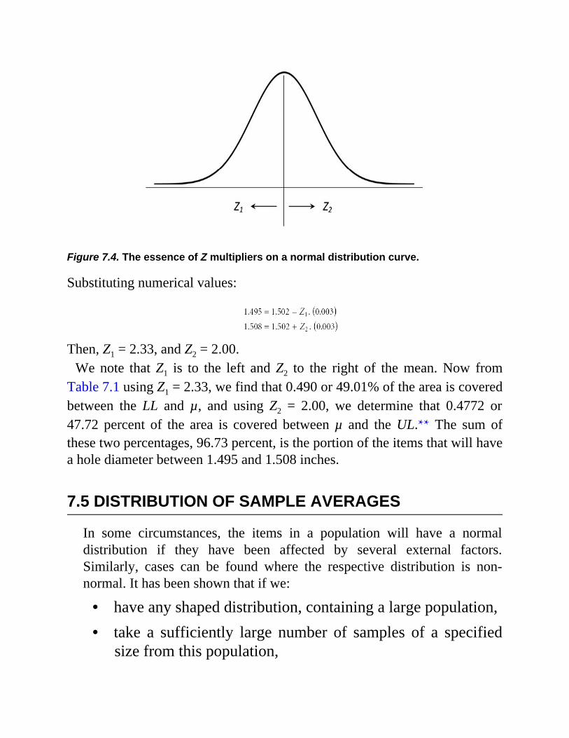
Figure 7.4. The essence of Z multipliers on a normal distribution curve.

Substituting numerical values:

Then, Z1 = 2.33, and Z2 = 2.00.

We note that Z1 is to the left and Z2 to the right of the mean. Now fromTable 7.1 using Z1 = 2.33, we find that 0.490 or 49.01% of the area is coveredbetween the LL and µ, and using Z2 = 2.00, we determine that 0.4772 or47.72 percent of the area is covered between µ and the UL.** The sum ofthese two percentages, 96.73 percent, is the portion of the items that will havea hole diameter between 1.495 and 1.508 inches.

7.5 DISTRIBUTION OF SAMPLE AVERAGES

In some circumstances, the items in a population will have a normaldistribution if they have been affected by several external factors.Similarly, cases can be found where the respective distribution is non-normal. It has been shown that if we:

• have any shaped distribution, containing a large population,• take a sufficiently large number of samples of a specified

size from this population,

• calculate the average of each sample,• plot the frequency of occurrence for the averages thus

obtained, the resulting distribution of the sample averagespractically will have a normal distribution.

This distribution has a mean and a standard deviation, as does any otherdistribution. The statistical properties of this distribution are related tothose of the main population when the number of samples takenapproaches infinity or, for practical purposes, is at least very large.

If we show:

• Sample size by n• Mean of the population by µ• Average of each sample by • Mean of the sample averages (grand average) by

• Standard deviation of the population by σ• Standard deviation of the sample means by

Then in the long run:

is more commonly referred to as the standard error of the sample

averages. and define the resulting normal distribution.The transformation of a population into a normal distribution by

sampling allows us to take advantage of the convenient and usefulproperties of the normal distribution.

7.6 STATISTICAL QUALITY CONTROL METHODS

There are various approaches and methods for different applications. Wefocus on the principal areas of application as depicted in Figure 7.5.

We now introduce these methods with respect to their areas ofapplication and implementation in practice.

Figure 7.5. Statistical quality control for variables and attributes.

7.6.1 Quality Control for Variables: X_ and RCharts

There are products where the feature of interest, for example, a length, canbe measured and expressed as a numerical value. In such cases the use ofthe method of “quality control for variables” is relevant. We argued thatwhen a product is produced in large quantities, the measurements of avariable of interest will not all be the same despite the fact that a specifictarget value is ideally desired. A plot of the frequency of observationsagainst the measurements will reveal the nature of the distribution of themeasurements.

The properties of the normal distribution have been found to have a highutility in SQC. However, any variable so controlled must then be normallydistributed. Fortunately, as outlined earlier, the “sampling” nature of SQCtransforms any distribution, normal or non-normal, to a normaldistribution of the sample averages allowing us to use the properties ofnormal distribution and its associated tables. Therefore, we will not be tooconcerned if the population being produced is not normal.

The quality of an item can be determined by measuring its desired

feature and comparing it with the specifications for this feature.Specifications are typically given as a desired target value, commonlyreferred to as the mean value, plus/minus a tolerance. This tolerance neednot be symmetric with respect to the mean value, though often it is. If themeasurement of a produced part falls within the specification limits, thepart is acceptable. Otherwise, it is considered as defective.

Assume that a manufacturer has received orders for a part whose criticalfeature is the depth of a drilled hole and the desired specification is given.

Accepting the orders is a sign that the firm believes it has the necessarycombination of factors of production to produce such parts. In otherwords, since it is a fact that there will be variability in the depth of theholes produced, the firm will attempt to generate a population with asatisfactory mean and standard deviation such that an acceptableproportion of parts will fall within the specification limits.

In order to control the quality of this variable of interest in terms ofsample averages, we need to set up a chart as shown in Figure 7.6.

Figure 7.6. Control chart template for sample averages.

We now discuss the values of CL, LCL, and UCL in the chart. Asoutlined in Section 7.5, when we sample a distribution, we obtain . Weset the centerline The values LCL and will UCL depend on howstringent the quality control must be. It has been experienced by industrialpractitioners that a three-sigma limit satisfies the majority of qualitycontrol needs and, it is very common in practice. Using this concept,Figure 7.6 is shown again as Figure 7.7 in applying the control chart.

This chart is posted adjacent to the manufacturing equipment, and asitems are produced, samples of a specified size are randomly taken from

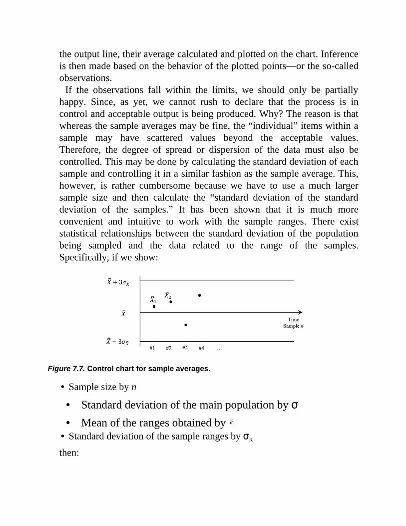
the output line, their average calculated and plotted on the chart. Inferenceis then made based on the behavior of the plotted points—or the so-calledobservations.

If the observations fall within the limits, we should only be partiallyhappy. Since, as yet, we cannot rush to declare that the process is incontrol and acceptable output is being produced. Why? The reason is thatwhereas the sample averages may be fine, the “individual” items within asample may have scattered values beyond the acceptable values.Therefore, the degree of spread or dispersion of the data must also becontrolled. This may be done by calculating the standard deviation of eachsample and controlling it in a similar fashion as the sample average. This,however, is rather cumbersome because we have to use a much largersample size and then calculate the “standard deviation of the standarddeviation of the samples.” It has been shown that it is much moreconvenient and intuitive to work with the sample ranges. There existstatistical relationships between the standard deviation of the populationbeing sampled and the data related to the range of the samples.Specifically, if we show:

Figure 7.7. Control chart for sample averages.

• Sample size by n

• Standard deviation of the main population by σ• Mean of the ranges obtained by

• Standard deviation of the sample ranges by σR

then:

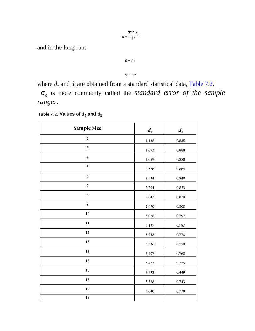
and in the long run:

where d2 and d3 are obtained from a standard statistical data, Table 7.2.σR is more commonly called the standard error of the sample

ranges.

Table 7.2. Values of d2 and d3

Sample Size d2 d3

2 1.128 0.835

3 1.693 0.888

4 2.059 0.880

5 2.326 0.864

6 2.534 0.848

7 2.704 0.833

8 2.847 0.820

9 2.970 0.808

10 3.078 0.797

11 3.137 0.787

12 3.258 0.778

13 3.336 0.770

14 3.407 0.762

15 3.472 0.755

16 3.532 0.449

17 3.588 0.743

18 3.640 0.73819

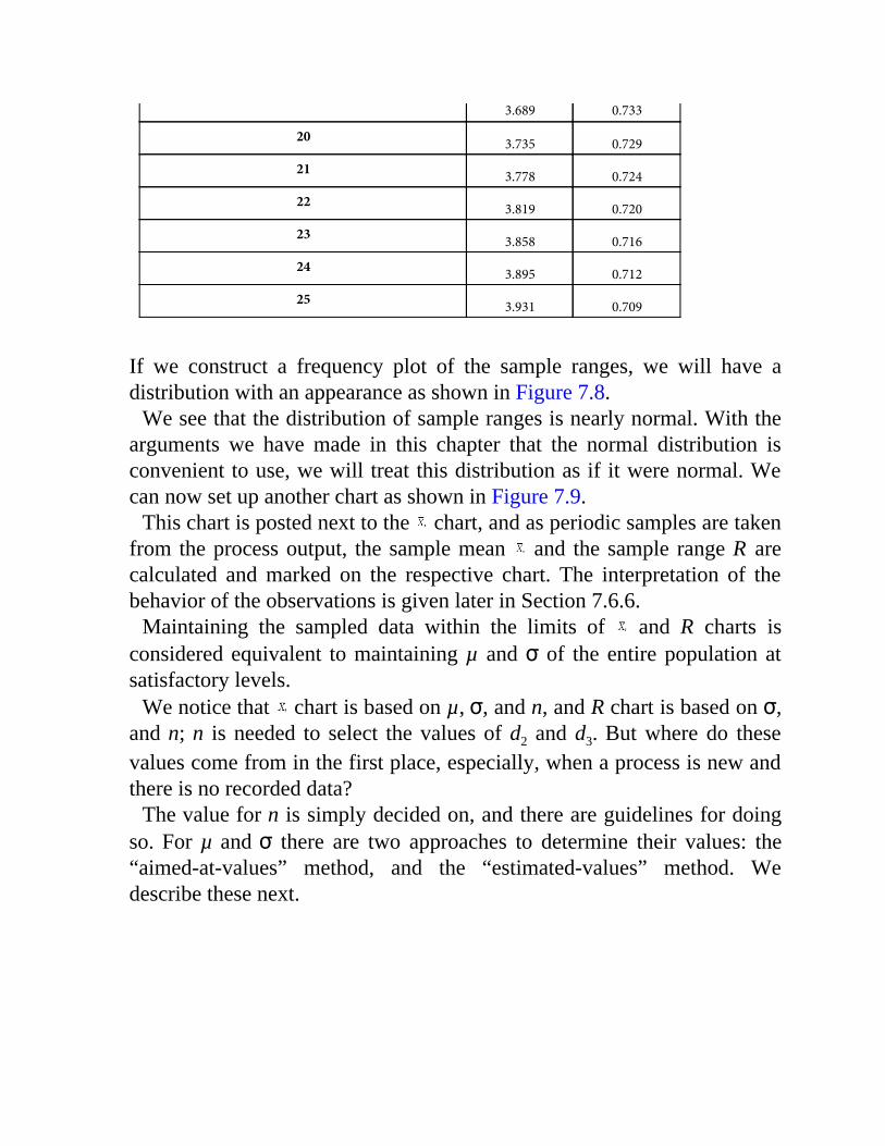
3.689 0.733

20 3.735 0.729

21 3.778 0.724

22 3.819 0.720

23 3.858 0.716

24 3.895 0.712

25 3.931 0.709

If we construct a frequency plot of the sample ranges, we will have adistribution with an appearance as shown in Figure 7.8.

We see that the distribution of sample ranges is nearly normal. With thearguments we have made in this chapter that the normal distribution isconvenient to use, we will treat this distribution as if it were normal. Wecan now set up another chart as shown in Figure 7.9.

This chart is posted next to the chart, and as periodic samples are takenfrom the process output, the sample mean and the sample range R arecalculated and marked on the respective chart. The interpretation of thebehavior of the observations is given later in Section 7.6.6.

Maintaining the sampled data within the limits of and R charts isconsidered equivalent to maintaining µ and σ of the entire population atsatisfactory levels.

We notice that chart is based on µ, σ, and n, and R chart is based on σ,and n; n is needed to select the values of d2 and d3. But where do thesevalues come from in the first place, especially, when a process is new andthere is no recorded data?

The value for n is simply decided on, and there are guidelines for doingso. For µ and σ there are two approaches to determine their values: the“aimed-at-values” method, and the “estimated-values” method. Wedescribe these next.

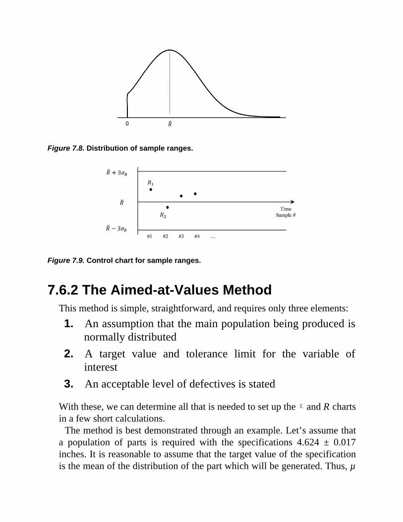
Figure 7.8. Distribution of sample ranges.

Figure 7.9. Control chart for sample ranges.

7.6.2 The Aimed-at-Values MethodThis method is simple, straightforward, and requires only three elements:1. An assumption that the main population being produced is

normally distributed2. A target value and tolerance limit for the variable of

interest3. An acceptable level of defectives is stated

With these, we can determine all that is needed to set up the and R chartsin a few short calculations.

The method is best demonstrated through an example. Let’s assume thata population of parts is required with the specifications 4.624 ± 0.017inches. It is reasonable to assume that the target value of the specificationis the mean of the distribution of the part which will be generated. Thus, µ

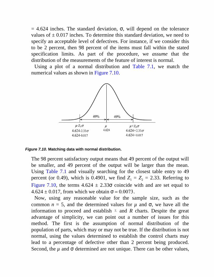
= 4.624 inches. The standard deviation, σ, will depend on the tolerancevalues of ± 0.017 inches. To determine this standard deviation, we need tospecify an acceptable level of defectives. For instance, if we consider thisto be 2 percent, then 98 percent of the items must fall within the statedspecification limits. As part of the procedure, we assume that thedistribution of the measurements of the feature of interest is normal.

Using a plot of a normal distribution and Table 7.1, we match thenumerical values as shown in Figure 7.10.

Figure 7.10. Matching data with normal distribution.

The 98 percent satisfactory output means that 49 percent of the output willbe smaller, and 49 percent of the output will be larger than the mean.Using Table 7.1 and visually searching for the closest table entry to 49percent (or 0.49), which is 0.4901, we find Z1 = Z2 = 2.33. Referring toFigure 7.10, the terms 4.624 ± 2.33σ coincide with and are set equal to4.624 ± 0.017, from which we obtain σ = 0.0073.

Now, using any reasonable value for the sample size, such as thecommon n = 5, and the determined values for µ and σ, we have all theinformation to proceed and establish and R charts. Despite the greatadvantage of simplicity, we can point out a number of issues for thismethod. The first is the assumption of normal distribution of thepopulation of parts, which may or may not be true. If the distribution is notnormal, using the values determined to establish the control charts maylead to a percentage of defective other than 2 percent being produced.Second, the µ and σ determined are not unique. There can be other values,

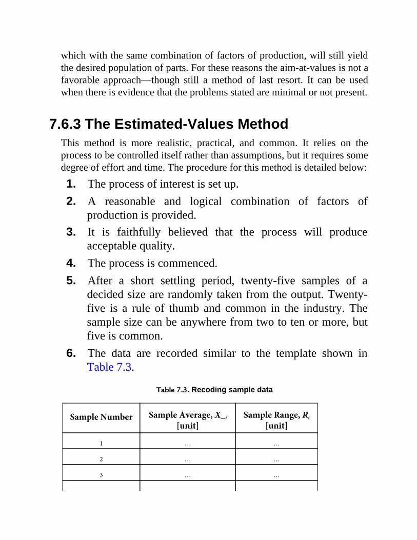
which with the same combination of factors of production, will still yieldthe desired population of parts. For these reasons the aim-at-values is not afavorable approach—though still a method of last resort. It can be usedwhen there is evidence that the problems stated are minimal or not present.

7.6.3 The Estimated-Values MethodThis method is more realistic, practical, and common. It relies on theprocess to be controlled itself rather than assumptions, but it requires somedegree of effort and time. The procedure for this method is detailed below:

1. The process of interest is set up.2. A reasonable and logical combination of factors of

production is provided.3. It is faithfully believed that the process will produce

acceptable quality.4. The process is commenced.5. After a short settling period, twenty-five samples of a

decided size are randomly taken from the output. Twenty-five is a rule of thumb and common in the industry. Thesample size can be anywhere from two to ten or more, butfive is common.

6. The data are recorded similar to the template shown inTable 7.3.

Table 7.3. Recoding sample data

Sample Number Sample Average, X_i

[unit]Sample Range, Ri

[unit]

1 … …

2 … …

3 … …

. . .

. . .

. . .

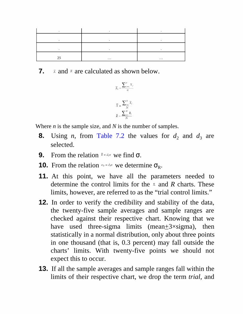
25 … …

7. and are calculated as shown below.

Where n is the sample size, and N is the number of samples.

8. Using n, from Table 7.2 the values for d2 and d3 areselected.

9. From the relation we find σ.10. From the relation we determine σR.

11. At this point, we have all the parameters needed todetermine the control limits for the and R charts. Theselimits, however, are referred to as the “trial control limits.”

12. In order to verify the credibility and stability of the data,the twenty-five sample averages and sample ranges arechecked against their respective chart. Knowing that wehave used three-sigma limits (mean+3×sigma), thenstatistically in a normal distribution, only about three pointsin one thousand (that is, 0.3 percent) may fall outside thecharts’ limits. With twenty-five points we should notexpect this to occur.

13. If all the sample averages and sample ranges fall within thelimits of their respective chart, we drop the term trial, and

call the control limits and the charts “final.” If any of thepoints fall outside the chart limits, we cross out thosepoints in the table of data, for instance, say, X3, and R6 andR7, return to Step 7, and repeat the calculations with theremaining twenty-four sample averages and twenty-threesample ranges. The removed data points are called theoutliers and are attributed to random variation, or to suchfactors as errors in measurement and insufficient operatorlearning period.

14. With the new values of and determined in Step 7, werepeat Steps 9 to 13 until either we finalize the charts andgo to Step 17, or too few sample data remain in Step 13 tomake sound estimates, and we go to Step 15. The reasonfor the continued iteration is that the revised limits becomenarrower and shifted, which may and often do result insome of the remaining data points to fall outside the newlimits.

15. If final charts cannot be established, we conclude that thefactors of production need to be examined, and after fixingthe suspected source(s) of the corrupt data, while havingStep 16 in mind, we repeat the entire procedure from Step1 and work with twenty-five fresh samples.

16. If multiple attempts to establish the and R charts prove tobe unsuccessful, we can say with good confidence thatthere are significant issues and the combination of thefactors of production is inadequate for the process at hand.For example, we may have tight tolerances, but lowprecision machines to achieve them. Therefore, it isnecessary to rectify the problem in a major way, such asacquiring more suitable equipment, lowering theexpectation by relaxing the tolerances, or considering

alternative designs and processes. This matter is dictated bythe specific circumstances present.

17. If the charts are successfully established, periodic samplesare taken, and and R values are calculated and marked onthe respective chart.

7.6.4 Evaluation of the Level of ControlAfter and R charts have been established using the estimated-valuesmethod, the subsequent application may prove that the process behavior isacceptable, and it is in control. Although such may be the case, however,we should determine an indication of whether the estimated values of µand σ will yield a satisfactory population of parts. At this point, the onlyoption is to assume that the respective population distribution is normal,and by using the upper and lower specification limits estimate thepercentages of acceptable and defective parts. We show this processgraphically with the aid of Figure 7.11.

Suppose that the specification for the part remains as 4.624+0.017 inchesas in our previous example, and by using the estimated-values method wehave determined that µ = 4.6156 inches, and σ = 0.0053 inches.Referring to Figure 7.11, we can write two equations:

At Lower Specification Limit (LSL): Target – Tol = μ – Z1σAt Upper Specification Limit (USL): Target + Tol = μ + Z2σ

Substituting numerical values:

Figure 7.11. Determining the level of control.

From which we obtain Z1 = 1.62, and from Table 7.1 we find that 0.5 –0.4463 = 5.37% of the parts will be undersize.

Similarly, we obtain Z2 = 4.79, and since it is a large value, practically 0percent of the parts will be oversize.

Therefore, with the assumption of normal distribution, 5.37 percent ofthe parts will be defective. Although this is an approximation, it cannot betoo significantly in error, and a decision must now be made whether this isan acceptable level of defectives. If this is not the case, then correctiveaction must be taken. In this example, an attempt to increase thepopulation mean toward the target specification will reduce the amount ofdefectives. This can be done by instructing the operator to make someadjustments when setting up the equipment used.

Example 7.1A quality control analyst has decided to establish and R Control charts ata machining center where a hole is drilled in a part. He instructed thatthirty samples of size 4 should be taken from the process output, thediameter of the hole of each part contained in each sample measured, andthe sample average and sample range calculated and recorded. Theoutcome is as shown in Table 7.4.

Table 7.4. Data for quality control example

SampleNumber

SampleAverage,

[in.]

SampleRange, Ri

[in.]

SampleNumber

SampleAverage,

[in.]

SampleRange, Ri

[in.]

1 1.0969 0.012 16 1.1008 0.012

2 1.1068 0.003 17 1.1034 0.003

3 1.1037 0.008 18 1.1040 0.005

4 1.1027 0.007 19 1.1080 0.008

5 1.0988 0.001 20 1.1061 0.002

6 1.1101 0.016 21 1.1050 0.011

7 1.0976 0.011 22 1.1068 0.009

8 1.0985 0.011 23 1.1074 0.013

9 1.0998 0.003 24 1.0984 0.032

10 1.1034 0.003 25 1.1030 0.006

11 1.0954 0.031 26 1.1040 0.007

12 1.1000 0.006 27 1.1001 0.005

13 1.1010 0.007 28 1.0960 0.007

14 1.0971 0.002 29 1.1052 0.012

15 1.0930 0.010 30 1.0999 0.003

a. Determine the values of the central line and thethree-sigma limits for the control charts.

b. The current specification for the hole is 1.100 ±0.008 inches. There is evidence that the individualmeasurements are normally distributed. Assumingthe process remain in control at the present level;determine the percentage defective output expectedfrom the process.

c. To improve the quality of the final product, the

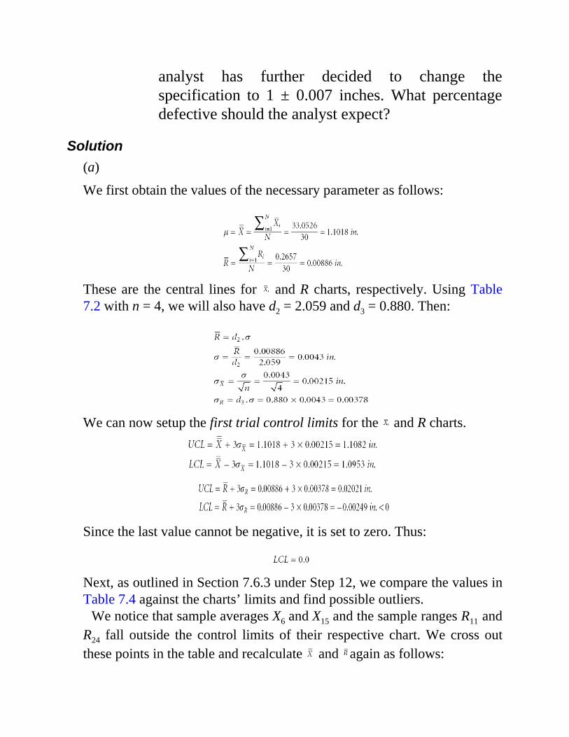
analyst has further decided to change thespecification to 1 ± 0.007 inches. What percentagedefective should the analyst expect?

Solution(a)

We first obtain the values of the necessary parameter as follows:

These are the central lines for and R charts, respectively. Using Table7.2 with n = 4, we will also have d2 = 2.059 and d3 = 0.880. Then:

We can now setup the first trial control limits for the and R charts.

Since the last value cannot be negative, it is set to zero. Thus:

Next, as outlined in Section 7.6.3 under Step 12, we compare the values inTable 7.4 against the charts’ limits and find possible outliers.

We notice that sample averages X6 and X15 and the sample ranges R11 andR24 fall outside the control limits of their respective chart. We cross outthese points in the table and recalculate and again as follows:

These are the new central lines for the and R charts. We can repeat the

previous calculations with these values. The parameters that remainunchanged are d2 = 2.059 and d3 = 2.880.

We now set up the second trial control limits for the and R charts:

Since the last value is negative, it is set to zero. Thus:

These are the new control limits for and R charts. Checking theremaining twenty-eight data points against these control chart limits, wesee that three new sample averages, X11, X19, and X28, fall outside thecontrol limits, but all the ranges are within their respective limits. We dohave the option of removing both and R values for the outlier samples;however, here we choose to remove only the data. Then the controllimits for the R chart are final. Similar to the procedure followed above,we cross out these points in the table of data, and proceed to determine yetanother set of new control limits for the chart. Since the R chart has beenfinalized, the only parameter that we must recalculate is the mean of thesample averages:

This new value for the mean of the sample average happens to be the sameas the previous value, and this is purely a coincidence. In this numericalexample, the removed points have simply canceled their effect on themean. Since no other parameters need to be calculated, we have the samemean for the averages, and with the outlier points having been removed,the previous limits determined in Trial 2 are retained and declared as final,and this precludes setting up the third trial control limits. Forcompleteness, however, we restate the final control limits.

Control limits for the chart:

Control limits for the R chart:

The charts will simply look as shown in Figure 7.12, which are postedadjacent to the process under study or made available electronically.

Solution(b)

For Part (a) of the problem, since sampling was used, the assumption ofnormality and working with the respective equations were justified. In Part(b), we would like to determine what percentage of the main population ofparts may be defective and outside the specification limits. For thispurpose, we need to make an assumption that the population is normallydistributed. This way we can certainly compute some numbers, but wemust exercise caution as the underlying population may or may not beactually normal.

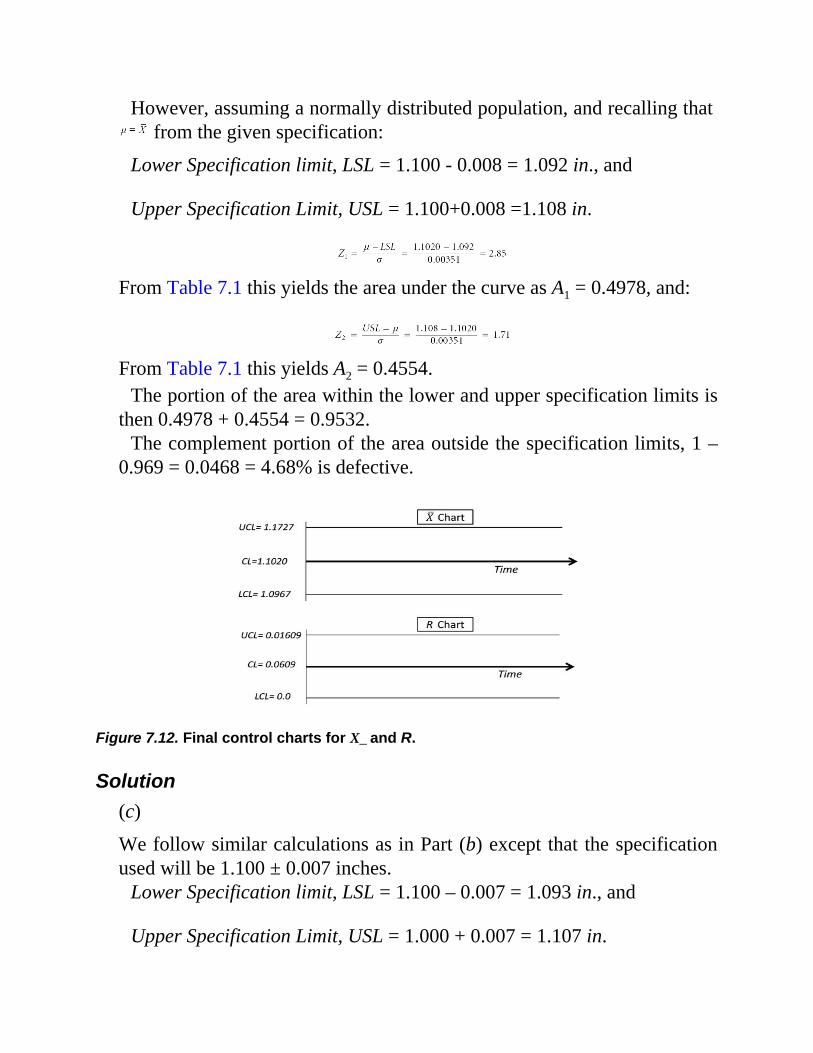
However, assuming a normally distributed population, and recalling that from the given specification:

Lower Specification limit, LSL = 1.100 - 0.008 = 1.092 in., and

Upper Specification Limit, USL = 1.100+0.008 =1.108 in.

From Table 7.1 this yields the area under the curve as A1 = 0.4978, and:

From Table 7.1 this yields A2 = 0.4554.

The portion of the area within the lower and upper specification limits isthen 0.4978 + 0.4554 = 0.9532.

The complement portion of the area outside the specification limits, 1 –0.969 = 0.0468 = 4.68% is defective.

Figure 7.12. Final control charts for X_ and R.

Solution(c)

We follow similar calculations as in Part (b) except that the specificationused will be 1.100 ± 0.007 inches.

Lower Specification limit, LSL = 1.100 – 0.007 = 1.093 in., and

Upper Specification Limit, USL = 1.000 + 0.007 = 1.107 in.

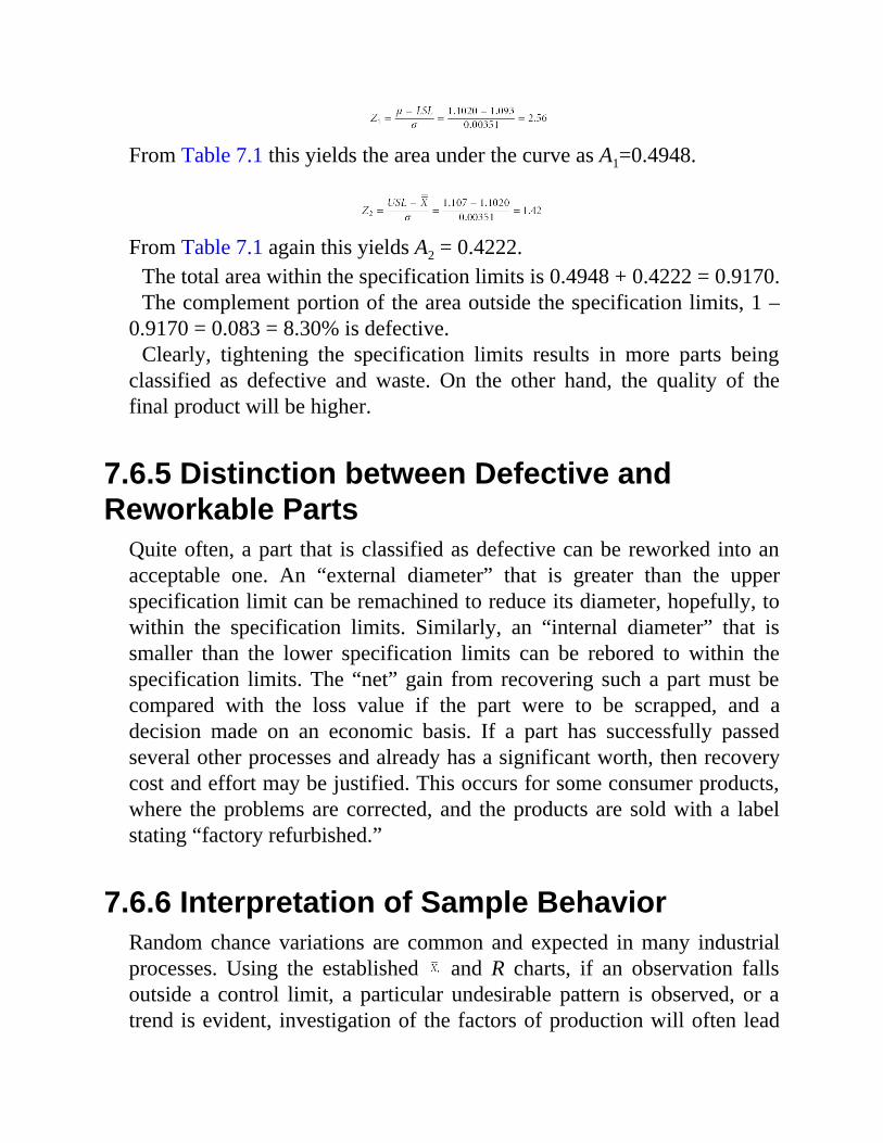
From Table 7.1 this yields the area under the curve as A1=0.4948.

From Table 7.1 again this yields A2 = 0.4222.

The total area within the specification limits is 0.4948 + 0.4222 = 0.9170.The complement portion of the area outside the specification limits, 1 –

0.9170 = 0.083 = 8.30% is defective.Clearly, tightening the specification limits results in more parts being

classified as defective and waste. On the other hand, the quality of thefinal product will be higher.

7.6.5 Distinction between Defective andReworkable Parts

Quite often, a part that is classified as defective can be reworked into anacceptable one. An “external diameter” that is greater than the upperspecification limit can be remachined to reduce its diameter, hopefully, towithin the specification limits. Similarly, an “internal diameter” that issmaller than the lower specification limits can be rebored to within thespecification limits. The “net” gain from recovering such a part must becompared with the loss value if the part were to be scrapped, and adecision made on an economic basis. If a part has successfully passedseveral other processes and already has a significant worth, then recoverycost and effort may be justified. This occurs for some consumer products,where the problems are corrected, and the products are sold with a labelstating “factory refurbished.”

7.6.6 Interpretation of Sample BehaviorRandom chance variations are common and expected in many industrialprocesses. Using the established and R charts, if an observation fallsoutside a control limit, a particular undesirable pattern is observed, or atrend is evident, investigation of the factors of production will often lead

to discovering the source of the problem. Such a source is commonlyreferred to as an assignable cause. One of the main purposes ofimplementing a quality control program for a process is to locate suchassignable causes and take appropriate steps to correct them. Learninglessons from industrial practice, below are some rules of thumb for theobservations that call for an investigation of the factors of productionwhile using the and R charts:

• Seven consecutive points fall on one side of the center line.• Ten out of eleven points fall on one side of the center line.• Twelve out of fourteen points fall on one side of the center

line.• Fourteen out of seventeen points fall on one side of the

center line.• Sixteen out of twenty points fall on one side of the center

line.

In day-to-day operations, we would ideally like the observations to follownatural and chance variations, and be fairly evenly spread about the centerline. Other observations that also call for an investigation include thefollowing:

• Seven consecutive points with upward or downward trend• Points consistently too close to the control limits• Points consistently too close to the centerline in chart• Points consistently too close to the lower control limit in R

chart• Points erratically moving from near one control limit to the

other

A trend in one direction indicates the likelihood of future observationsfalling outside the control limit being approached. In the case of chart,

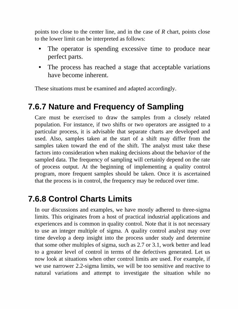
points too close to the center line, and in the case of R chart, points closeto the lower limit can be interpreted as follows:

• The operator is spending excessive time to produce nearperfect parts.

• The process has reached a stage that acceptable variationshave become inherent.

These situations must be examined and adapted accordingly.

7.6.7 Nature and Frequency of SamplingCare must be exercised to draw the samples from a closely relatedpopulation. For instance, if two shifts or two operators are assigned to aparticular process, it is advisable that separate charts are developed andused. Also, samples taken at the start of a shift may differ from thesamples taken toward the end of the shift. The analyst must take thesefactors into consideration when making decisions about the behavior of thesampled data. The frequency of sampling will certainly depend on the rateof process output. At the beginning of implementing a quality controlprogram, more frequent samples should be taken. Once it is ascertainedthat the process is in control, the frequency may be reduced over time.

7.6.8 Control Charts LimitsIn our discussions and examples, we have mostly adhered to three-sigmalimits. This originates from a host of practical industrial applications andexperiences and is common in quality control. Note that it is not necessaryto use an integer multiple of sigma. A quality control analyst may overtime develop a deep insight into the process under study and determinethat some other multiples of sigma, such as 2.7 or 3.1, work better and leadto a greater level of control in terms of the defectives generated. Let usnow look at situations when other control limits are used. For example, ifwe use narrower 2.2-sigma limits, we will be too sensitive and reactive tonatural variations and attempt to investigate the situation while no

problems actually exist. This condition is called Type I error. Or if we use,for instance, wider 3.4-sigma limits, we may be too slow in attending tothe evolving problems and miss the opportunity to rectify them. Thiscondition is referred to as Type II error. A compromise that suits manypractical situations is the common three-sigma limits. A quality controlanalyst, however, may decide to use what he or she argues to be morerelevant limits for his or her application. For instance, in the aircraftindustry, much narrower limits are used to maintain tight tolerances andprecision and to detect developing problems quickly. Because of stringentmanufacturing processes, the standard deviations are also generallysmaller, leading to narrower control limits.

7.6.9 Areas of ApplicationIn general, any process that generates a population with measurablefeatures can be subjected to quality control for variables. Quality controlefforts can cause a delay in operations and have cost implications.Therefore, only processes that are known or expected to produce asubstantial amount of defective parts that must either be scrapped orreworked should be considered for quality control. Over time, the qualitycontrol personnel may find that it is adequate to maintain only one of the and R charts, or abandon both charts altogether for a process when itremains steady and consistently produces satisfactory output. This occursparticularly with new processes that settle, and new operators who gainexperience and improve their skills over time.

Another important factor that must be taken into consideration is thetrade-off between the cost incurred by the quality control efforts and thecost of scraps. If the difference is insubstantial, it is advisable toimplement a quality control program, because, in the long run, it will mostlikely prove to be a more economical choice.

7.7 QUALITY CONTROL FOR ATTRIBUTES

In Section 7.6.1, we stated that the quality control for variables requiredthe quality of an individual item to be determined by first measuring the

magnitude of a particular feature and then comparing it with that of thestated specification. However, on many occasions, alternative approachesmust be used. In some situations, the inspection process does not yield aquantitative measure of the part, but rather it indicates whether the part isdefective or not. In such instances and R charts could not be used. Thequality control for attributes covers two distinct categories: quality controlfor defectives and quality control for defects. Respective methods aredescribed next.

7.7.1 Quality Control for DefectivesThere are many industrial situations where the inspection of the product orfeature of interest does not yield a quantitative value, such as inspectingthe quality of an electrical switch by subjecting it to an electrical test. Thetest will simply reveal whether the switch is faulty or not. Therefore, andR charts are inapplicable for quality control in this case. In suchcircumstances quality control for defectives must be used. Other situationsalso arise, for example, when a go-no-go gauge is used to determinewhether a particular dimension is within the stated specification. Again, and R charts cannot be used. Go-no-go gauges are mechanical orelectronic devices that are available for a variety of applications such asverifying inside diameters, outside diameters, lengths, and threads. A go-no-go gauge can quickly determine whether a part is within the desiredspecification. Figure 7.13 show a schematic of a mechanical go-no-gogauge for an outside diameter. A part is acceptable if it passes through the“go” gap, indicating that it is smaller than the upper specification limit,and does not pass through the “no-go” gap, indicating that it is larger thanthe lower specification limit. Otherwise, it will be classified as a defectiveor nonconforming part.

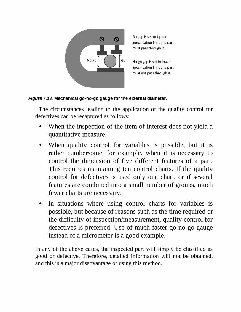
Figure 7.13. Mechanical go-no-go gauge for the external diameter.

The circumstances leading to the application of the quality control fordefectives can be recaptured as follows:

• When the inspection of the item of interest does not yield aquantitative measure.

• When quality control for variables is possible, but it israther cumbersome, for example, when it is necessary tocontrol the dimension of five different features of a part.This requires maintaining ten control charts. If the qualitycontrol for defectives is used only one chart, or if severalfeatures are combined into a small number of groups, muchfewer charts are necessary.

• In situations where using control charts for variables ispossible, but because of reasons such as the time required orthe difficulty of inspection/measurement, quality control fordefectives is preferred. Use of much faster go-no-go gaugeinstead of a micrometer is a good example.

In any of the above cases, the inspected part will simply be classified asgood or defective. Therefore, detailed information will not be obtained,and this is a major disadvantage of using this method.

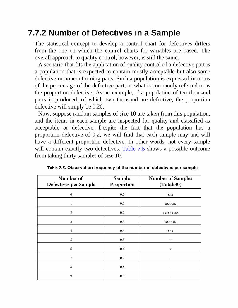
7.7.2 Number of Defectives in a SampleThe statistical concept to develop a control chart for defectives differsfrom the one on which the control charts for variables are based. Theoverall approach to quality control, however, is still the same.

A scenario that fits the application of quality control of a defective part isa population that is expected to contain mostly acceptable but also somedefective or nonconforming parts. Such a population is expressed in termsof the percentage of the defective part, or what is commonly referred to asthe proportion defective. As an example, if a population of ten thousandparts is produced, of which two thousand are defective, the proportiondefective will simply be 0.20.

Now, suppose random samples of size 10 are taken from this population,and the items in each sample are inspected for quality and classified asacceptable or defective. Despite the fact that the population has aproportion defective of 0.2, we will find that each sample may and willhave a different proportion defective. In other words, not every samplewill contain exactly two defectives. Table 7.5 shows a possible outcomefrom taking thirty samples of size 10.

Table 7.5. Observation frequency of the number of defectives per sample

Number of Defectives per Sample

Sample Proportion

Number of Samples(Total:30)

0 0.0 xxx

1 0.1 xxxxxx

2 0.2 xxxxxxxxx

3 0.3 xxxxxx

4 0.4 xxx

5 0.5 xx

6 0.6 x

7 0.7 -

8 0.8 -

9 0.9 -

10 1.0 -

We notice that each observation appears with different frequency. Themost likely number of defectives per sample is two, and the most likelysample proportion is 0.2. For a large number of samples, the plot of therelative frequency will be as shown in Figure 7.14. This frequency plot iscalled the “binomial distribution.”Identically, Figure 7.14 can also be expressed in terms of the sampleproportions as shown in Figure 7.15.

Figure 7.14. Binomial distribution of the number of defectives per sample.

Figure 7.15. Binomial distribution of the proportion defective per sample.

Binomial distribution has a mathematical expression from which theprobability of the occurrence of a particular range of values can be found.In statistical quality control and for the reasons that will be explained in

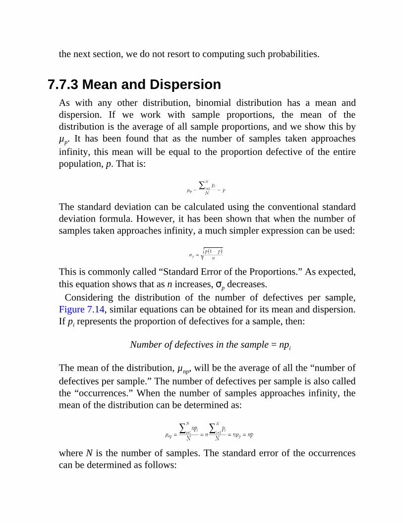
the next section, we do not resort to computing such probabilities.

7.7.3 Mean and DispersionAs with any other distribution, binomial distribution has a mean anddispersion. If we work with sample proportions, the mean of thedistribution is the average of all sample proportions, and we show this byµp. It has been found that as the number of samples taken approachesinfinity, this mean will be equal to the proportion defective of the entirepopulation, p. That is:

The standard deviation can be calculated using the conventional standarddeviation formula. However, it has been shown that when the number ofsamples taken approaches infinity, a much simpler expression can be used:

This is commonly called “Standard Error of the Proportions.” As expected,this equation shows that as n increases, σp decreases.

Considering the distribution of the number of defectives per sample,Figure 7.14, similar equations can be obtained for its mean and dispersion.If pi represents the proportion of defectives for a sample, then:

Number of defectives in the sample = npi

The mean of the distribution, µnp, will be the average of all the “number ofdefectives per sample.” The number of defectives per sample is also calledthe “occurrences.” When the number of samples approaches infinity, themean of the distribution can be determined as:

where N is the number of samples. The standard error of the occurrencescan be determined as follows:

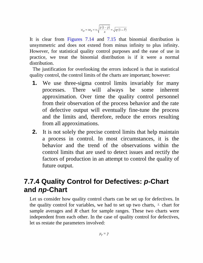
It is clear from Figures 7.14 and 7.15 that binomial distribution isunsymmetric and does not extend from minus infinity to plus infinity.However, for statistical quality control purposes and the ease of use inpractice, we treat the binomial distribution is if it were a normaldistribution.

The justification for overlooking the errors induced is that in statisticalquality control, the control limits of the charts are important; however:

1. We use three-sigma control limits invariably for manyprocesses. There will always be some inherentapproximation. Over time the quality control personnelfrom their observation of the process behavior and the rateof defective output will eventually fine-tune the processand the limits and, therefore, reduce the errors resultingfrom all approximations.

2. It is not solely the precise control limits that help maintaina process in control. In most circumstances, it is thebehavior and the trend of the observations within thecontrol limits that are used to detect issues and rectify thefactors of production in an attempt to control the quality offuture output.

7.7.4 Quality Control for Defectives: p-Chartand np-Chart

Let us consider how quality control charts can be set up for defectives. Inthe quality control for variables, we had to set up two charts, chart forsample averages and R chart for sample ranges. These two charts wereindependent from each other. In the case of quality control for defectives,let us restate the parameters involved:

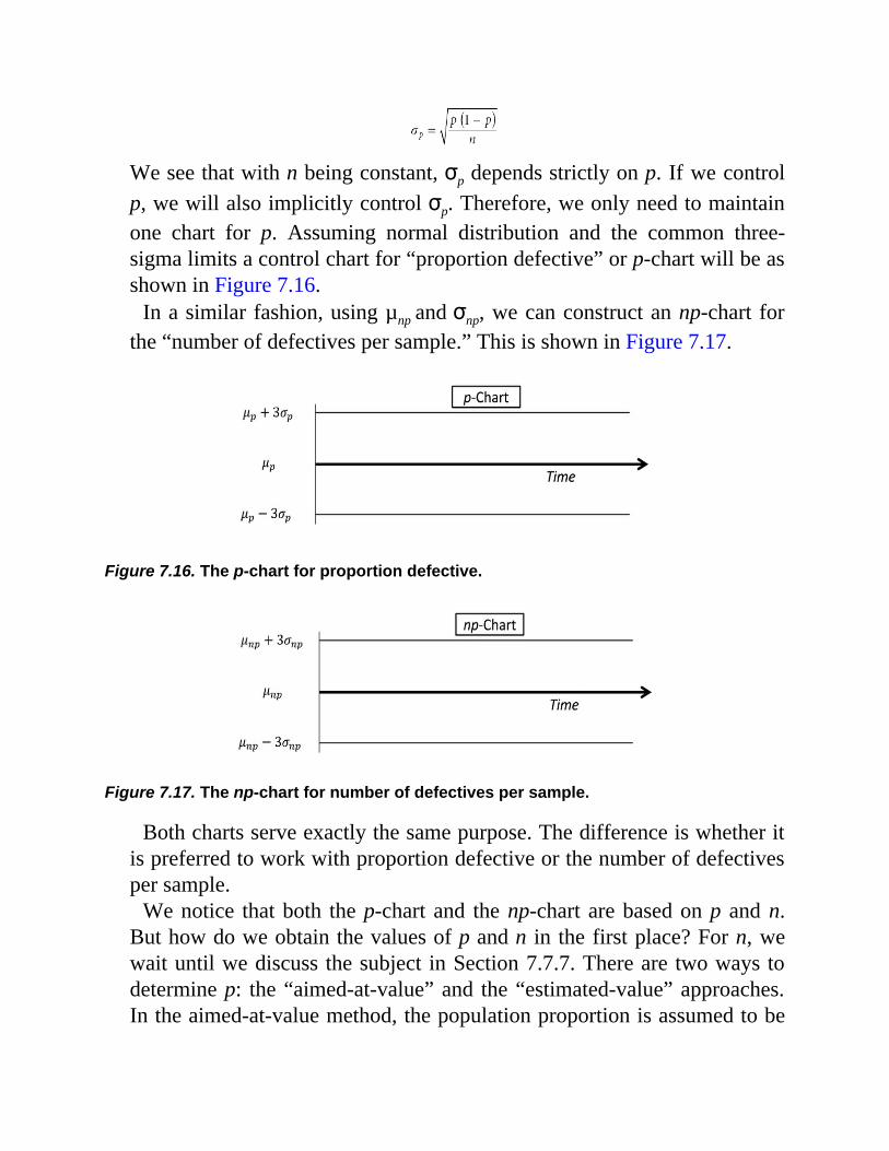
We see that with n being constant, σp depends strictly on p. If we controlp, we will also implicitly control σp. Therefore, we only need to maintainone chart for p. Assuming normal distribution and the common three-sigma limits a control chart for “proportion defective” or p-chart will be asshown in Figure 7.16.

In a similar fashion, using µnp and σnp, we can construct an np-chart forthe “number of defectives per sample.” This is shown in Figure 7.17.

Figure 7.16. The p-chart for proportion defective.

Figure 7.17. The np-chart for number of defectives per sample.

Both charts serve exactly the same purpose. The difference is whether itis preferred to work with proportion defective or the number of defectivesper sample.

We notice that both the p-chart and the np-chart are based on p and n.But how do we obtain the values of p and n in the first place? For n, wewait until we discuss the subject in Section 7.7.7. There are two ways todetermine p: the “aimed-at-value” and the “estimated-value” approaches.In the aimed-at-value method, the population proportion is assumed to be

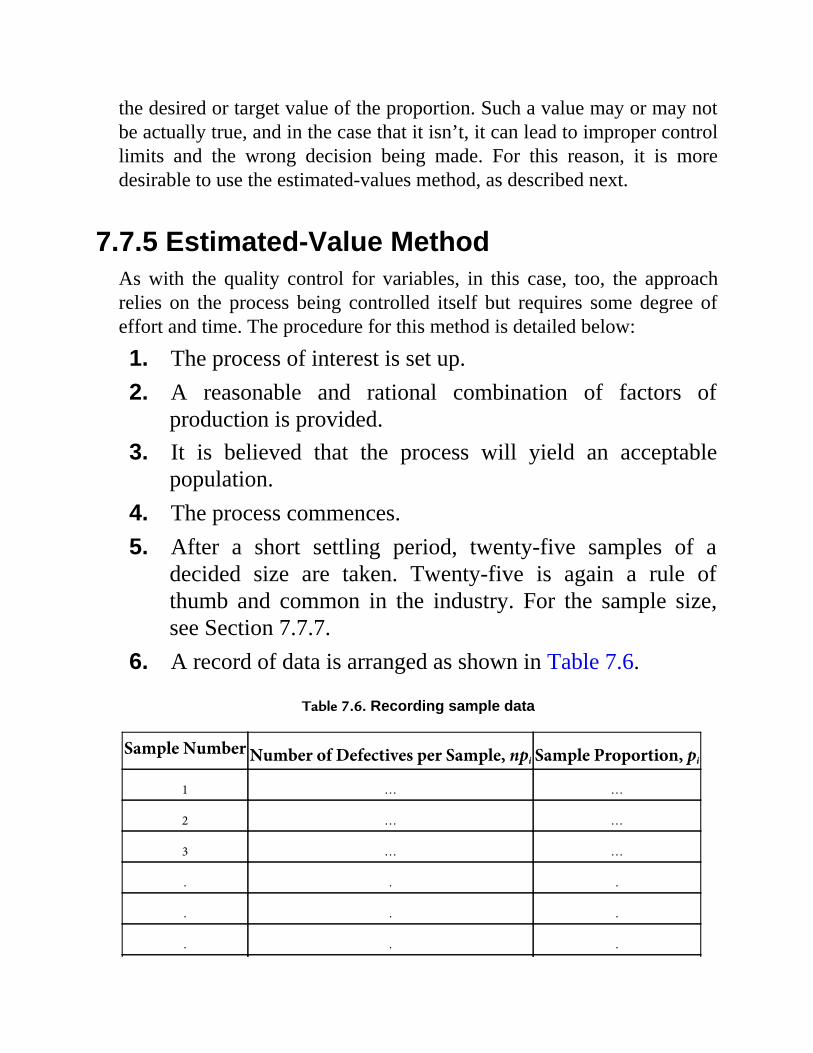
the desired or target value of the proportion. Such a value may or may notbe actually true, and in the case that it isn’t, it can lead to improper controllimits and the wrong decision being made. For this reason, it is moredesirable to use the estimated-values method, as described next.

7.7.5 Estimated-Value MethodAs with the quality control for variables, in this case, too, the approachrelies on the process being controlled itself but requires some degree ofeffort and time. The procedure for this method is detailed below:

1. The process of interest is set up.2. A reasonable and rational combination of factors of

production is provided.3. It is believed that the process will yield an acceptable

population.4. The process commences.5. After a short settling period, twenty-five samples of a

decided size are taken. Twenty-five is again a rule ofthumb and common in the industry. For the sample size,see Section 7.7.7.

6. A record of data is arranged as shown in Table 7.6.

Table 7.6. Recording sample data

Sample Number Number of Defectives per Sample, npi Sample Proportion, pi

1 … …

2 … …

3 … …

. . .

. . .

. . .

25 … …

7, µp, p and σp are calculated as shown below:

8. At this point, we have all that is needed to determine the

control limits for the p-chart. These limits, however, arereferred to as the trial control limits.

9. In order to verify the credibility and stability of the data,the twenty-five sample proportions are checked against thecontrol limits. Knowing that we have used three-sigmalimits, only about three points in one thousand (or 0.3percent) are expected to fall outside the control chart limits.

10. If all the points are within the control limits, we drop theterm trial, call the control limits and the chart “final,” andgo to Step 14. If any of the sample proportions fall outsidethe chart limits, we cross out those samples in the table ofdata, return to Step 7, and repeat the calculations with theremaining sample data.

11. With the new p (or identically µp) we repeat Steps 8 to 11until either we finalize the chart and go to Step 14, or toofew sample data points are left to make a sound estimate ofp.

12. If the final chart cannot be established, we conclude thatthe factors of production need to be reexamined, and afterfixing the suspected sources of the corrupt data, we taketwenty-five fresh samples and repeat the entire procedure.

13. If attempts to establish a p-chart prove unsuccessful, we

can say with confidence that the factors of production areunsuitable for achieving the expected output. At this point,a decision is made to rectify the problem, for instance, byacquiring suitable equipment, lowering the expectations, ormodifying the design. The exact nature of any remedy willdepend on the case at hand.

14. If the chart is successfully established, periodic samplesare taken and the proportion defectives are calculated andmarked on the chart.

Example 7.2A quality control engineer has taken twenty samples of size 200 from theoutput of an assembly line. The items in each sample have been inspected,and the number of defectives in each sample recorded. The results aregiven in Table 7.7.

Table 7.7. Data for quality control example

SampleNumber

Number of

Defectives, npi

SampleNumber

Number of

Defectives, npi

1 18 11 12

2 11 12 13

3 7 13 10

4 12 14 11

5 16 15 9

6 7 16 9

7 14 17 10

8 15 18 15

9 9 19 8

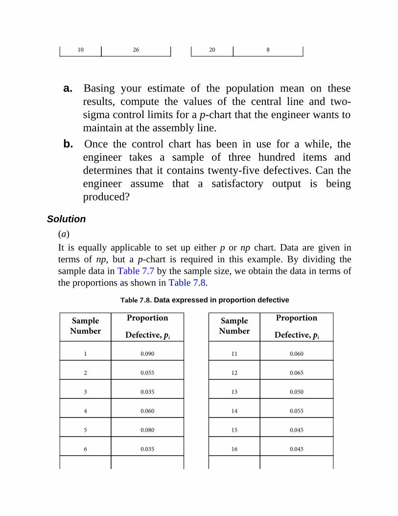
10 26 20 8

a. Basing your estimate of the population mean on theseresults, compute the values of the central line and two-sigma control limits for a p-chart that the engineer wants tomaintain at the assembly line.

b. Once the control chart has been in use for a while, theengineer takes a sample of three hundred items anddetermines that it contains twenty-five defectives. Can theengineer assume that a satisfactory output is beingproduced?

Solution(a)It is equally applicable to set up either p or np chart. Data are given interms of np, but a p-chart is required in this example. By dividing thesample data in Table 7.7 by the sample size, we obtain the data in terms ofthe proportions as shown in Table 7.8.

Table 7.8. Data expressed in proportion defective

SampleNumber

Proportion

Defective, pi

SampleNumber

Proportion

Defective, pi

1 0.090 11 0.060

2 0.055 12 0.065

3 0.035 13 0.050

4 0.060 14 0.055

5 0.080 15 0.045

6 0.035 16 0.045

7 0.070 17 0.050

8 0.075 18 0.075

9 0.045 19 0.040

10 0.130 20 0.040

We calculate the required measures as follows:

Next we determine the control limits.First trial limits:

Checking the data in Table 7.8 against these limits, we find that p10 = 0.13falls outside. We cross out this outlier and recompute the parameters:

Second trial limits:

We see that in this round p1 = 0.09 falls outside the limits. We cross outthis outlier and recompute the parameters for a third time:

Third trial limits:

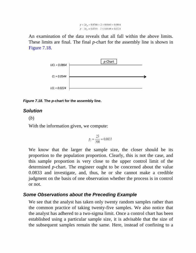
An examination of the data reveals that all fall within the above limits.These limits are final. The final p-chart for the assembly line is shown inFigure 7.18.

Figure 7.18. The p-chart for the assembly line.

Solution(b)

With the information given, we compute:

We know that the larger the sample size, the closer should be itsproportion to the population proportion. Clearly, this is not the case, andthis sample proportion is very close to the upper control limit of thedetermined p-chart. The engineer ought to be concerned about the value0.0833 and investigate, and, thus, he or she cannot make a crediblejudgment on the basis of one observation whether the process is in controlor not.

Some Observations about the Preceding ExampleWe see that the analyst has taken only twenty random samples rather thanthe common practice of taking twenty-five samples. We also notice thatthe analyst has adhered to a two-sigma limit. Once a control chart has beenestablished using a particular sample size, it is advisable that the size ofthe subsequent samples remain the same. Here, instead of confining to a

sample size of two hundred, the analyst has taken a sample of threehundred items. From these efforts, we can say that the analyst is perhapsexploring the options to arrive at some optimal quality control conditions.

7.7.6 Interpretation of Sample BehaviorThe same rules of thumb as outlined in Section 7.6.6 for and R charts arealso used for the p-chart.

7.7.7 Sample SizeThe larger the sample size, the more likely it is that the sample proportionwill approach the population proportion. Although this reduces the risk ofmaking a wrong decision, the cost of sampling will be higher. A commonrule of thumb is that both np and n(1 – p) are equal or greater than 5. Formost manufacturing processes and products, the proportion p is muchsmaller than its complement 1 – p. Therefore, np is the deciding factor.However, n and p are both generally unknown, unless reliable historicaldata exits for p. To circumvent this uncertainty, a simpler rule is that thesample should be greater than one hundred. Gaging the process at hand,the analyst can exercise some thoughtful judgment and decide on thesample size. Once p has been estimated through sampling and more datahave become available, the sample size can be better estimated and thecontrol limits revised.

7.8 CONTROL CHART FOR DEFECTS: C-CHART

If a product is such that it can contain an infinite number of defects, thenthe control chart for defects or c-chart is used. It may seem rather frightfulas to how an infinite number of defects in a sample is possible. This isonly a modeling analogy, and we can identify real cases where we can seethe relevance of this concept. Let us consider a sheet of glass. We can saythat the sheet of glass is a single unit, a sample of size 1. We can also treatit as a container or a sample of infinite size because we can subject it to acountless number of scratches or defects, and it can accommodate them. In

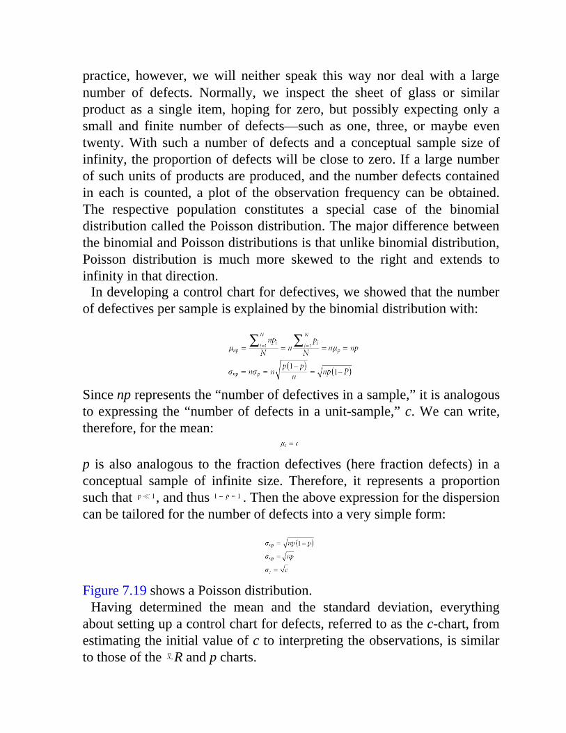
practice, however, we will neither speak this way nor deal with a largenumber of defects. Normally, we inspect the sheet of glass or similarproduct as a single item, hoping for zero, but possibly expecting only asmall and finite number of defects—such as one, three, or maybe eventwenty. With such a number of defects and a conceptual sample size ofinfinity, the proportion of defects will be close to zero. If a large numberof such units of products are produced, and the number defects containedin each is counted, a plot of the observation frequency can be obtained.The respective population constitutes a special case of the binomialdistribution called the Poisson distribution. The major difference betweenthe binomial and Poisson distributions is that unlike binomial distribution,Poisson distribution is much more skewed to the right and extends toinfinity in that direction.

In developing a control chart for defectives, we showed that the numberof defectives per sample is explained by the binomial distribution with:

Since np represents the “number of defectives in a sample,” it is analogousto expressing the “number of defects in a unit-sample,” c. We can write,therefore, for the mean:

p is also analogous to the fraction defectives (here fraction defects) in aconceptual sample of infinite size. Therefore, it represents a proportionsuch that , and thus . Then the above expression for the dispersioncan be tailored for the number of defects into a very simple form:

Figure 7.19 shows a Poisson distribution.

Having determined the mean and the standard deviation, everythingabout setting up a control chart for defects, referred to as the c-chart, fromestimating the initial value of c to interpreting the observations, is similarto those of the R and p charts.

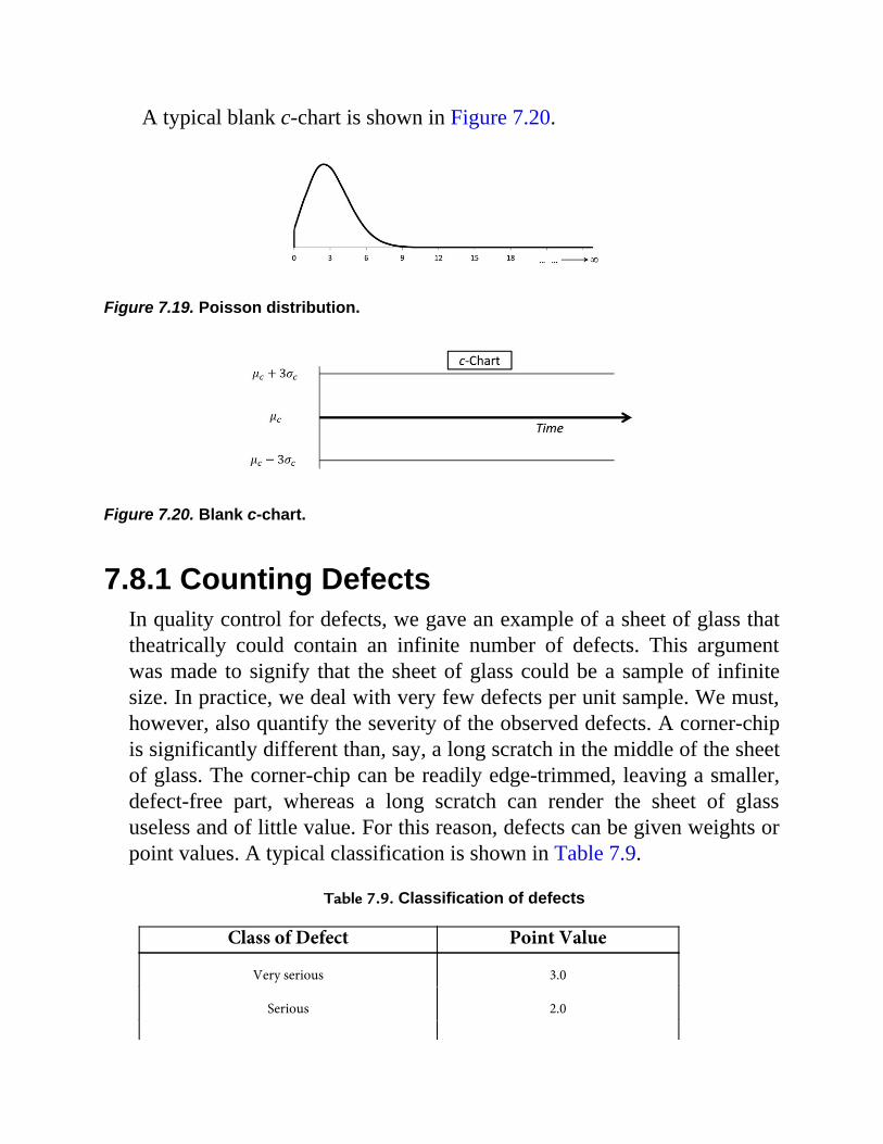
A typical blank c-chart is shown in Figure 7.20.

Figure 7.19. Poisson distribution.

Figure 7.20. Blank c-chart.

7.8.1 Counting DefectsIn quality control for defects, we gave an example of a sheet of glass thattheatrically could contain an infinite number of defects. This argumentwas made to signify that the sheet of glass could be a sample of infinitesize. In practice, we deal with very few defects per unit sample. We must,however, also quantify the severity of the observed defects. A corner-chipis significantly different than, say, a long scratch in the middle of the sheetof glass. The corner-chip can be readily edge-trimmed, leaving a smaller,defect-free part, whereas a long scratch can render the sheet of glassuseless and of little value. For this reason, defects can be given weights orpoint values. A typical classification is shown in Table 7.9.

Table 7.9. Classification of defects

Class of Defect Point Value

Very serious 3.0

Serious 2.0

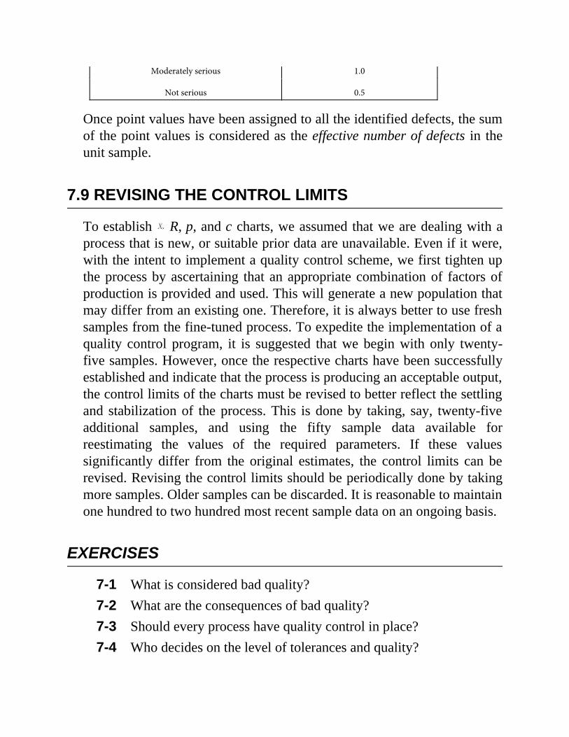
Moderately serious 1.0

Not serious 0.5

Once point values have been assigned to all the identified defects, the sumof the point values is considered as the effective number of defects in theunit sample.

7.9 REVISING THE CONTROL LIMITS

To establish R, p, and c charts, we assumed that we are dealing with aprocess that is new, or suitable prior data are unavailable. Even if it were,with the intent to implement a quality control scheme, we first tighten upthe process by ascertaining that an appropriate combination of factors ofproduction is provided and used. This will generate a new population thatmay differ from an existing one. Therefore, it is always better to use freshsamples from the fine-tuned process. To expedite the implementation of aquality control program, it is suggested that we begin with only twenty-five samples. However, once the respective charts have been successfullyestablished and indicate that the process is producing an acceptable output,the control limits of the charts must be revised to better reflect the settlingand stabilization of the process. This is done by taking, say, twenty-fiveadditional samples, and using the fifty sample data available forreestimating the values of the required parameters. If these valuessignificantly differ from the original estimates, the control limits can berevised. Revising the control limits should be periodically done by takingmore samples. Older samples can be discarded. It is reasonable to maintainone hundred to two hundred most recent sample data on an ongoing basis.

EXERCISES

7-1 What is considered bad quality?7-2 What are the consequences of bad quality?7-3 Should every process have quality control in place?7-4 Who decides on the level of tolerances and quality?

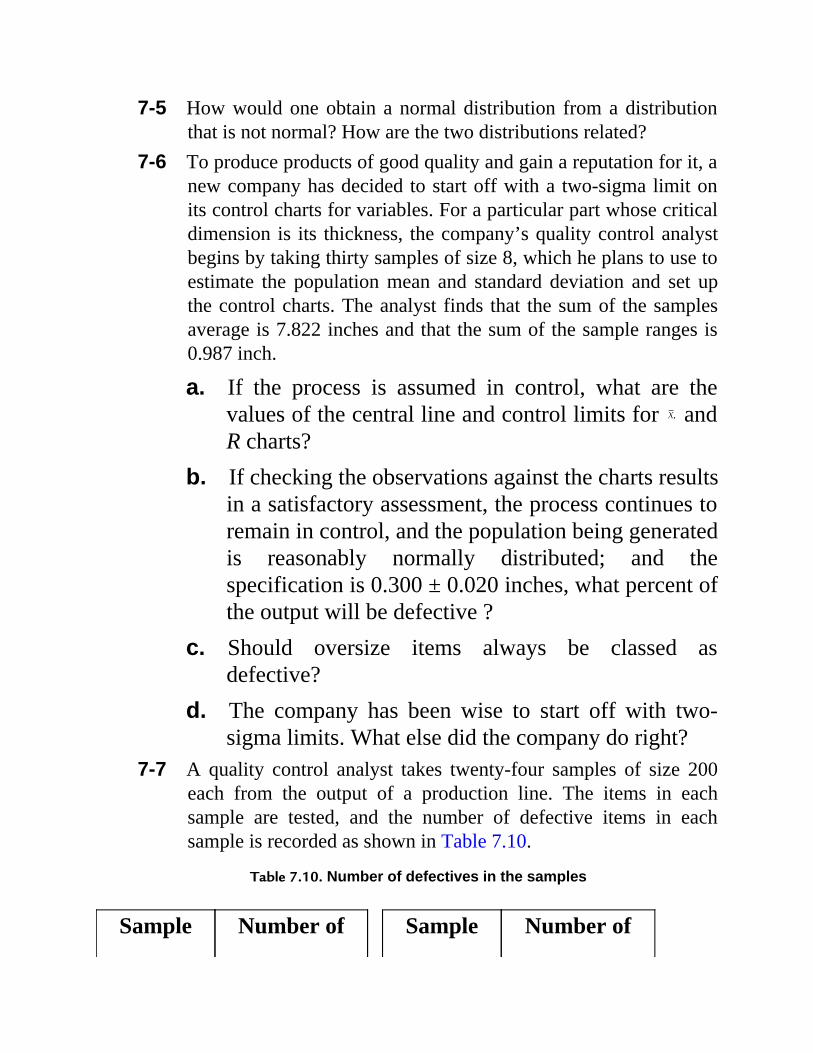
7-5 How would one obtain a normal distribution from a distributionthat is not normal? How are the two distributions related?

7-6 To produce products of good quality and gain a reputation for it, anew company has decided to start off with a two-sigma limit onits control charts for variables. For a particular part whose criticaldimension is its thickness, the company’s quality control analystbegins by taking thirty samples of size 8, which he plans to use toestimate the population mean and standard deviation and set upthe control charts. The analyst finds that the sum of the samplesaverage is 7.822 inches and that the sum of the sample ranges is0.987 inch.

a. If the process is assumed in control, what are thevalues of the central line and control limits for andR charts?

b. If checking the observations against the charts resultsin a satisfactory assessment, the process continues toremain in control, and the population being generatedis reasonably normally distributed; and thespecification is 0.300 ± 0.020 inches, what percent ofthe output will be defective ?

c. Should oversize items always be classed asdefective?

d. The company has been wise to start off with two-sigma limits. What else did the company do right?

7-7 A quality control analyst takes twenty-four samples of size 200each from the output of a production line. The items in eachsample are tested, and the number of defective items in eachsample is recorded as shown in Table 7.10.

Table 7.10. Number of defectives in the samples

Sample Number of Sample Number of

Number Defectives Number Defectives

1 8 13 122 13 14 143 14 15 124 10 16 105 27 17 96 17 18 97 11 19 108 8 20 169 17 21 710 12 22 2211 13 23 1812 15 24 8

Determine the values of the central line and two-sigma control limits for achart for fraction defective (p-chart) that the analyst must maintain at theproduction line.

7-8 A manufacturer of outdoor digital advertising display panels isplanning to implement a quality control scheme. The displays arefifty LEDs wide and two hundred LEDs long. It has beenobserved that some LEDs on the panels fail to function. Such anLED is considered a defect in the product. (Although it does notaffect your calculations, the company counts two adjacent flawsas three defects.) The average number of defects per unit of outputis estimated to be ten and is considered satisfactory. For qualitycontrol purposes, the quality control analyst treats the actualdistribution of defects per sample as if it were a Poissondistribution; 50 × 200 = 10,000 is large enough to assume asample of size infinity:

a. What should be the values for the central line andtwo-sigma control limits for a c-chart?

b. Is two-sigma control limits a reasonable choice forthe type of product? Explain your opinion.

** In this chapter we frequently use the terms items, components, products, enterprise, firm, andorganization in the context of manufacturing industries to give examples and show the implementationof the quality control concepts. This, however, does not preclude in any way the application of thetechniques developed to other settings such as the service industry, the health-care sector, educationalinstitutions, and governmental organizations.

** The corresponding table entry for a Z value is found as follows. For example, taking Z1 = 2.33, wesplit it into a sum of two parts as: 2.30+ 0.03. The first term is located in the first column of the table.The second term is identified as column heading 0.03. The intersection of the row emanating for thefirst term and the column emanating from the second term as the column heading will read the value0.4901. Knowing a value within the table, the corresponding Z value can be found by following the stepsin reverse. The reason for this particular construct is to avoid a long two-column table.

Chapter 8 FACILITY LOCATION

8.1 INTRODUCTION

The increase in demand for a product or service as well as upgrading,renovation, and expansion of business require procurement, installation, orconstruction of new equipment and facilities. Typically, the newequipment or facility will have significant interaction in terms of materialor vehicular movement with the existing facilities. Transportation costs areamong the largest components of expenditure in the operation of manyenterprises. Therefore, to minimize the costs, it is essential to determine anoptimal location for the new facility to be established. There are numerousexamples of where a new facility may be needed, such as the following:

- Warehouse to provide supplies for a number of outlets- Tool dispenser in a manufacturing plant- Library, fire station, or police station in a residential district- Suburban airport to provide services for remote

communities- Power-generating plant- Boiler in a processing plant

In addition to minimizing the direct transportation costs, there areinstances where some other measures of optimality could be of interest.The response of a fire truck to fire is not primarily driven by the cost, butrather the travel time or distance. Therefore, for such cases, the goal is to

minimize the maximum distance to travel. In this chapter, we review bothcost and distance minimization for location problems.

Location problems can also be categorized into two classes:

1. Single new facility2. Multiple new facility

We focus on the single-facility location problems.

8.2 FORMS OF DISTANCE

The common concept of distance is the straight line between two points.This is true as a strict geometric definition and can be used in manylocation problems, such as in an airport where aircraft take off and flymuch of the distance to their destination in a straight line. However, thereare other instances where different concepts of distance must be used. In afactory environment, the machinery and facilities are usually laid out insuch a way that movement or transportation is accomplished throughperpendicular aisles and passages. This form of movement and distance isreferred to as the rectilinear or rectangular.

In one class of problems, the cost is proportional to the square of the“straight-line” distance. In some rare problems, which are outside thescope of this book, the cost may be proportional to an unconventionaldefinition of distance, such as hyper-rectilinear. It is customary to use thepositive quadrant of a Cartesian coordinate system to express distancesand places for the facility location problems.

8.3 OBJECTIVE FUNCTION FORMULATION

First, we explain the formulation of the objective function for two classesof new facility location problems:

• Minimization of total cost—mini-sum problemsWe consider m existing point-location facilities identified as P1, P2, ... Pm,where a new facility is to be located at a point Q(x,y), given that

transportation costs are incurred and are proportional to an applicable formof distance between the new and the existing facility Pi.

If d(Q, Pi) represents the distance traveled per trip between the points Qand Pi; and if wi represents the product of cost per unit distance traveledand the number of trips per unit time between the new facility and theexisting facility i, then the total travel cost per unit time (typically a year)is given by:

The cost factors wi are referred to as the “weights.” The objective is todetermine the coordinates of the new facility, Q*, such that the total costper unit time is minimized. The typical units for the terms in the equationare as follows:

f(x, y) [dollar/unit time]wi [dollar/distance][trips/unit time]d(Q, Pi) [distance/trip]

• Minimization of maximum distance—mini-maxproblems

In this class of problems, no direct cost is involved, and the objectivefunction is stated as:

Notice that the formulation does not involve any form of weights.

8.4 MINI-SUM PROBLEMS

We consider three mini-sum new facility location problems where thetransportation and movement costs are proportional to the following:

• Squared Euclidean distance• Euclidean distance• Rectilinear distance

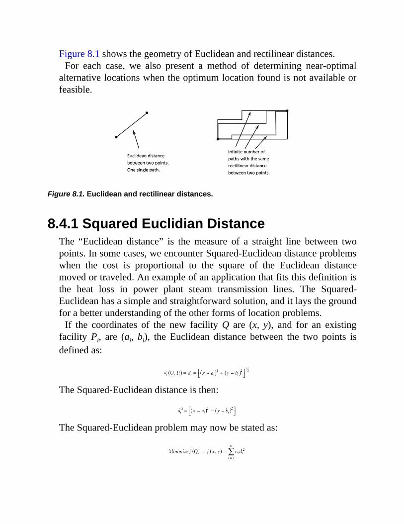
Figure 8.1 shows the geometry of Euclidean and rectilinear distances.For each case, we also present a method of determining near-optimal

alternative locations when the optimum location found is not available orfeasible.

Figure 8.1. Euclidean and rectilinear distances.

8.4.1 Squared Euclidian DistanceThe “Euclidean distance” is the measure of a straight line between twopoints. In some cases, we encounter Squared-Euclidean distance problemswhen the cost is proportional to the square of the Euclidean distancemoved or traveled. An example of an application that fits this definition isthe heat loss in power plant steam transmission lines. The Squared-Euclidean has a simple and straightforward solution, and it lays the groundfor a better understanding of the other forms of location problems.

If the coordinates of the new facility Q are (x, y), and for an existingfacility Pi, are (ai, bi), the Euclidean distance between the two points isdefined as:

The Squared-Euclidean distance is then:

The Squared-Euclidean problem may now be stated as:

or

The typical units for the terms used in the above equation are:

f(x,y) [dollar/unit time]wi[dollar/distance-square][trips/unit time]di(Q, Pi)[distance/trip]The approach to determining the coordinates of the new facility is to

compute the partial derivatives of the cost function with respect to x and y,set them to zero, and solve:

or

Leading to:

The point Q* = (x*, y*) is the optimum location that minimizes the totalcost of interaction per unit time used.

Owing to resemblance to the common weighted average calculations,such as the grade point average (GPA) in academic transcripts, theSquared-Euclidean solution is also referred to as the “centroid” or the“center of gravity” solution.

Iso-Cost Contour LinesThere is always the possibility that the optimum location determined is notreadily available because of inaccessibility and physical limitations, suchas a body of water or a highway. In such cases, it would be desirable andindeed helpful to construct constant- or iso-cost contour lines where amultitude of feasible alternative locations can be found. To demonstratethe concept of contour lines, we begin with two simple cases. When thereis only one existing facility, the optimum new facility location coincideswith it, and regardless of its weight, the iso-cost contour lines areconcentric circles centered on the optimum location, as shown in Figure8.2(a). If there are two existing facilities with equal weights, the optimumpoint is halfway between the two existing facilities and the iso-costcontour lines are also concentric circles, and centered on the optimumpoint, as shown in Figure 8.2(b).

Figure 8.2. Contour lines for simple Squared-Euclidean distance problems.

Interestingly, the iso-cost contour for any number of existing facilities,even with unequal weights, will still be concentric circles centered on theoptimum point. We derive this mathematically because it is useful whensearching for an alternative near-optimal new facility location.

For the optimum location obtained, the least cost is:

For any Cc > Cmin, where Cc is an acceptable cost, the set of all points thatsatisfy the equation:

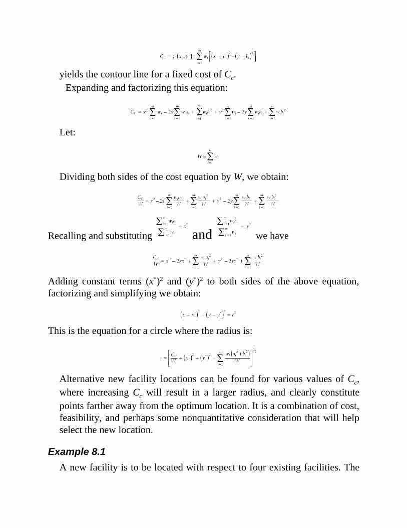
yields the contour line for a fixed cost of Cc.

Expanding and factorizing this equation:

Let:

Dividing both sides of the cost equation by W, we obtain:

Recalling and substituting and we have

Adding constant terms (x*)2 and (y*)2 to both sides of the above equation,factorizing and simplifying we obtain:

This is the equation for a circle where the radius is:

Alternative new facility locations can be found for various values of Cc,where increasing Cc will result in a larger radius, and clearly constitutepoints farther away from the optimum location. It is a combination of cost,feasibility, and perhaps some nonquantitative consideration that will helpselect the new location.

Example 8.1A new facility is to be located with respect to four existing facilities. The

interaction between the new facility and the existing facilities is such thatthe cost is proportional to the squared Euclidean distance. The existingfacilities are given as:

P1 = (20, 10), P2 = (8, 4), P3 = (12, 6), and P4 = (8, 24)

with the corresponding weights:

w1 = 8, w2 = 5, w3 = 6, and w4 = 1

Find a new facility location for which the total interaction cost at most is25 percent greater than the minimum total interaction cost.

SolutionFirst, we determine the coordinates of the optimum location:

Next we compute the minimum interaction cost:

The total cost being considered:

This is the cost if the new facility is located on the contour line. Within thecircle, the cost will be less and will depend on the location.

Using the contour line radius equation:

Therefore, any point within or on a circle of 3.4 radius (Figure 8.3) is alocation within the acceptable total cost.

Figure 8.3. Solution for Example 1.

ObservationWe notice that although cost is proportional to the square of the distancetraveled, but since the interaction weights of the points P1, P2, and P3 aresignificantly larger, the optimum new facility location is much closer tothese points than to point P4. With 25 percent greater interaction cost, asignificant area becomes available, within which the new facility can belocated. In fact, point P3, which is within the contour line circle as anexisting facility, if feasible, may be a convenient location for the newfacility. In which case, the total annual interaction will be:

This amount is about 17 percent more than the minimum cost.

8.4.2 Euclidean Distance

Following a similar formulation as with the Squared-Euclidean distanceproblems, the objective function for the Euclidean distance problem for asingle new facility location can be obtained.

We defined the Euclidean distance between a new facility location andan existing facility as:

The objective function then is:

or

For these forms of minimization problems the standard mathematicalmethod, as was shown in the previous section for the Squared-Euclideanproblem, is to obtain the partial derivatives of the cost function withrespect to the variables x and y, and on setting them equal to zero,determine the coordinates of the optimum new facility location. Thepartial derivatives are:

We notice that owing to the form of these equations, if the location of thenew facility coincides with the location of an existing facility, one of the

terms in each of the equations will become undefined as The onlycondition that allows continuing the procedure is that:

But this cannot be readily verified when the new location is unknown. Theway around this is to redefine the partial derivatives as proposed by Kuhn(1967).

If , it would be sufficient to solve the following set:

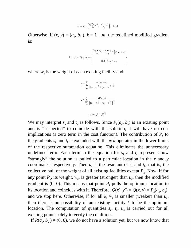
Otherwise, if (x, y) = (ak, bk ), k = 1 ...m, the redefined modified gradientis:

where wk is the weight of each existing facility and:

We may interpret sk and tk as follows. Since Pk(ak, bk) is an existing pointand is “suspected” to coincide with the solution, it will have no costimplications (a zero term in the cost function). The contribution of Pk tothe gradients sk and tk is excluded with the ≠ k operator in the lower limitsof the respective summation equation. This eliminates the unnecessaryundefined term. Each term in the equation for sk and tk represents how“strongly” the solution is pulled to a particular location in the x and ycoordinates, respectively. Then uk is the resultant of sk and tk, that is, thecollective pull of the weight of all existing facilities except Pk. Now, if forany point Pk, its weight, wk, is greater (stronger) than uk, then the modifiedgradient is (0, 0). This means that point Pk pulls the optimum location toits location and coincides with it. Therefore, Q(x*, y*) = Q(x, y) = Pk(ak, bk),and we stop here. Otherwise, if for all k, wk is smaller (weaker) than uk,then there is no possibility of an existing facility k to be the optimumlocation. The computation of quantities sk, tk, uk is carried out for allexisting points solely to verify the condition.

If R(ak, bk ) ≠ (0, 0), we do not have a solution yet, but we now know that

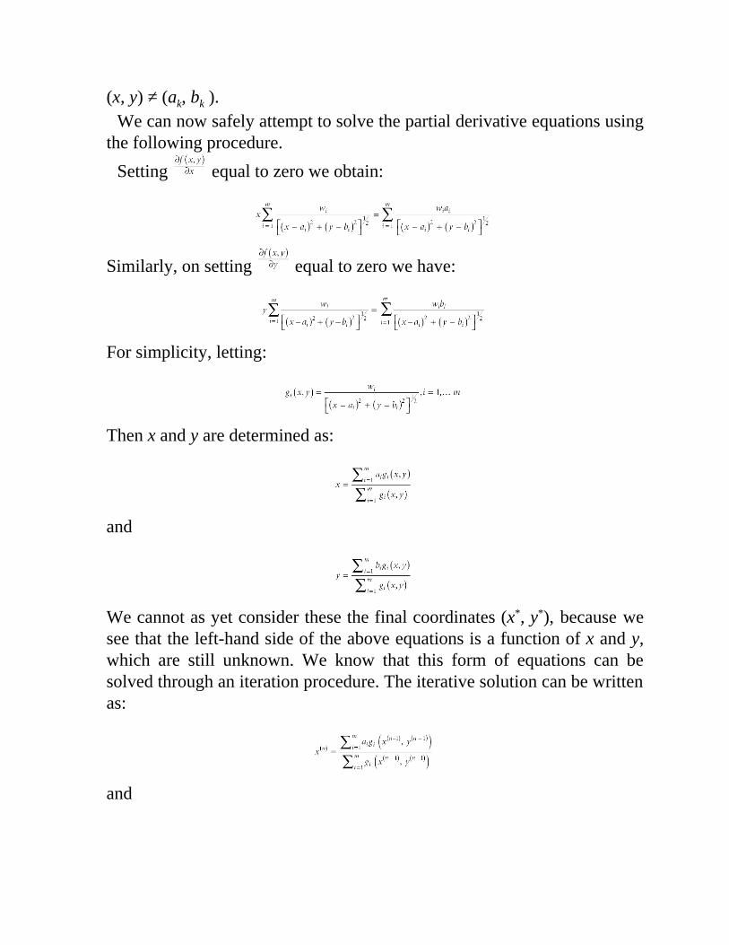
(x, y) ≠ (ak, bk ).We can now safely attempt to solve the partial derivative equations using

the following procedure.Setting equal to zero we obtain:

Similarly, on setting equal to zero we have:

For simplicity, letting:

Then x and y are determined as:

and

We cannot as yet consider these the final coordinates (x*, y*), because wesee that the left-hand side of the above equations is a function of x and y,which are still unknown. We know that this form of equations can besolved through an iteration procedure. The iterative solution can be writtenas:

and

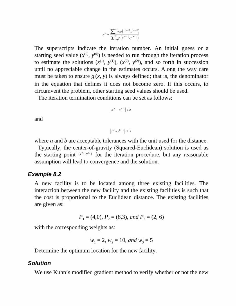
The superscripts indicate the iteration number. An initial guess or astarting seed value (x(0), y(0)) is needed to run through the iteration processto estimate the solutions (x(1), y(1)), (x(2), y(2)), and so forth in successionuntil no appreciable change in the estimates occurs. Along the way caremust be taken to ensure gi(x, y) is always defined; that is, the denominatorin the equation that defines it does not become zero. If this occurs, tocircumvent the problem, other starting seed values should be used.

The iteration termination conditions can be set as follows:

and

where a and b are acceptable tolerances with the unit used for the distance.

Typically, the center-of-gravity (Squared-Euclidean) solution is used asthe starting point for the iteration procedure, but any reasonableassumption will lead to convergence and the solution.

Example 8.2A new facility is to be located among three existing facilities. Theinteraction between the new facility and the existing facilities is such thatthe cost is proportional to the Euclidean distance. The existing facilitiesare given as:

P1 = (4,0), P2 = (8,3), and P3 = (2, 6)

with the corresponding weights as:

w1 = 2, w2 = 10, and w3 = 5

Determine the optimum location for the new facility.

SolutionWe use Kuhn’s modified gradient method to verify whether or not the new

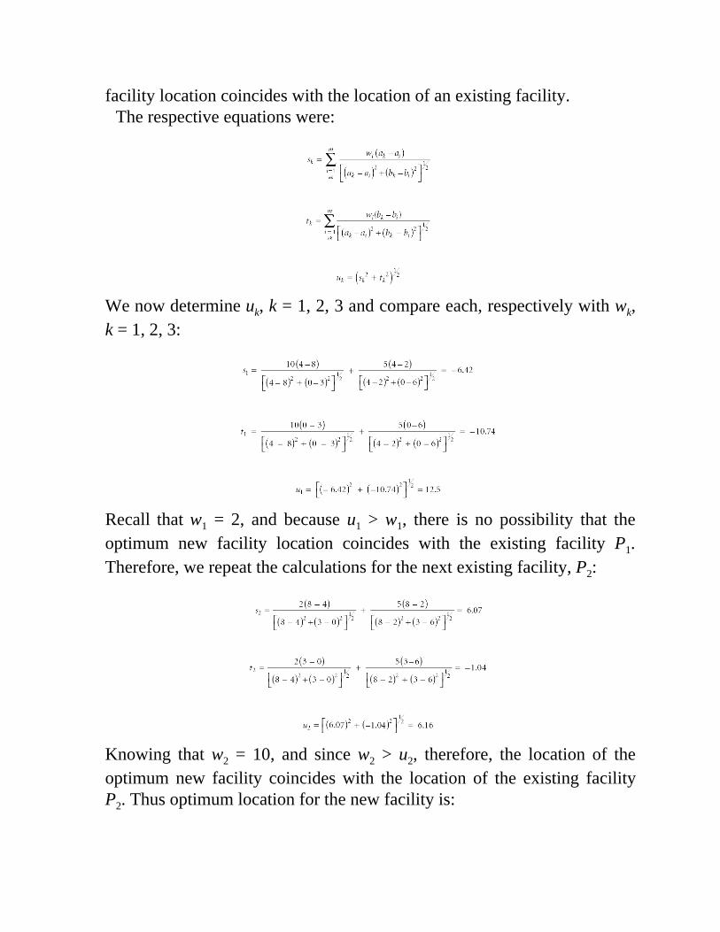
facility location coincides with the location of an existing facility.The respective equations were:

We now determine uk, k = 1, 2, 3 and compare each, respectively with wk,k = 1, 2, 3:

Recall that w1 = 2, and because u1 > w1, there is no possibility that theoptimum new facility location coincides with the existing facility P1.Therefore, we repeat the calculations for the next existing facility, P2:

Knowing that w2 = 10, and since w2 > u2, therefore, the location of theoptimum new facility coincides with the location of the existing facilityP2. Thus optimum location for the new facility is:

(x*, y* ) = (8, 3)Because the new facility location has been found and confirmed, there isno need to continue the procedure to calculate u3 for the third existingfacility, P3.

Graphical Solutions to Simple CasesFor a few simple Euclidean distance problems there exist geometric-graphical solutions that provide some intuitive understanding of theproblems. These simple cases and their solutions are shown in Figure 8.4.

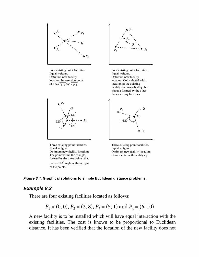
Figure 8.4. Graphical solutions to simple Euclidean distance problems.

Example 8.3There are four existing facilities located as follows:

P1 = (0, 0), P2 = (2, 8), P3 = (5, 1) and P4 = (6, 10)

A new facility is to be installed which will have equal interaction with theexisting facilities. The cost is known to be proportional to Euclideandistance. It has been verified that the location of the new facility does not

coincide with the location of any existing facility. Determine the locationof the new facility.

SolutionSince it is known that the location of the new facility does not coincidewith the location of an existing facility, we proceed to find the optimumlocation using the iteration method.

First, we determine the gravity (Squared-Euclidean) solution to use asthe starting point:

Using the equations:

and

the iterations result in the following numerical values.

Iteration #1 (x(1), y(1)) = (3.208, 4.851)Iteration #2 (x(2), y(2)) = (3.195, 4.933)Iteration #3 (x(3), y(3)) = (3.189, 5.000)……Iteration #12 (x(12), y(12)) = (3.170, 5.237)Iteration #13 (x(13), y(13)) = (3.170, 5.245)

If the accuracies and are acceptable, then theiteration can be terminated, and we take:

as the optimum location for the new facility. Otherwise, we continue theiteration until the desired accuracy is reached.

Iso-Cost Contour LinesUsing contour lines can provide many alternative near-optimal solutionswhen the optimum location is unavailable or inaccessible. We have theminimum cost due to the optimum location as:

For any Cc, where Cc > Cmin the equation:

yields the set of points (x, y), where the cost is fixed at Cc. However,except for a few simple cases, there is no straightforward procedure forconstructing the contour lines for Euclidean distance location problems.

For m = 1 and any weight, the optimum location for the new facilitycoincides with location of the existing facility. We place the coordinatesystem at this common point, that is, at:

Q* = P1 = (0, 0)

Then the cost equation becomes:

or

This is the definition of a circle, and the contour lines for various values ofCc are concentric circles around the optimum location, as shown in Figure8.5(a).

For another simple case when m = 2 and equal weights, the contour linesfor various values of Cc will be ellipses with focal points at the location ofthe two existing facilities a shown in Figure 8.5(b).

Figure 8.5. Contour lines for two simple Euclidean distance location problems.

To derive an easy-to-use mathematical relation for the contour lines, weplace the x-axis along the line connecting the two points, locate the y-axishalfway between these points, and reorient the new axes to the finalposition shown in Figure 8.5(b).

Without loss of generality, we denote the transformed coordinates of thetwo existing facilities as:

P1 = (a, 0) and P2 = (–a, 0)

We can rewrite the iso-cost equation in terms of these points:

The geometric relation (where is a constant) is the definition ofan ellipse.

For m ≥ 3 and any values of wi there is no regular-shaped or predictablepattern for the contour lines. However, for any Cc (Cc > Cmin) the contourlines can be numerically generated and plotted using most mathematicalsoftware, such as MATLAB®. The iso-cost contour lines will be irregular,smoothly varying, closed loop curves. A larger loop will signify a highervalue of Cc.

8.4.3 Rectilinear Distance—Point LocationsEarlier in this chapter, we briefly introduced the concept of rectilinear

distance. The rectilinear distance between two points Q(x, y) and Pi(ai, bi)is defined as:

If the interaction, transportation or movement between Pi, i = 1, ..., mexisting facilities and a new facility being considered occur through therectilinear distance, the objective function for the optimum location of thenew facility is:

or

Because the two terms in this equation are positive, each can be minimizedseparately. The mathematical features of each summation term, forexample, the first term, leads to a solution where the optimum x coordinateof the new facility:

i. Will be the same as the x coordinate of an existing facility.ii. This x coordinate will be such that less than one half of the

total weight will be to its left, and less than one half will beto its right. This can also be said in a different way, that thex coordinate is such that the difference between the partialtotal weight to the left of x and the partial total weight tothe right of x (as a positive quantity) is the smallestpossible.

This solution is also referred to as the “median condition.” The samesolution approach holds for the y coordinate of the optimum new facility.This method can be readily illustrated using a numerical example.

Example 8.4There are five existing service centers in a city, where a distribution

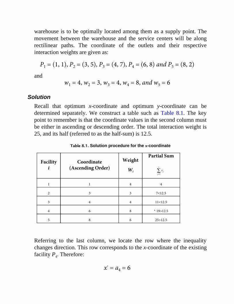
warehouse is to be optimally located among them as a supply point. Themovement between the warehouse and the service centers will be alongrectilinear paths. The coordinate of the outlets and their respectiveinteraction weights are given as:

P1 = (1, 1), P2 = (3, 5), P3 = (4, 7), P4 = (6, 8) and P5 = (8, 2)

andw1 = 4, w2 = 3, w3 = 4, w4 = 8, and w5 = 6

SolutionRecall that optimum x-coordinate and optimum y-coordinate can bedetermined separately. We construct a table such as Table 8.1. The keypoint to remember is that the coordinate values in the second column mustbe either in ascending or descending order. The total interaction weight is25, and its half (referred to as the half-sum) is 12.5.

Table 8.1. Solution procedure for the x-coordinate

Facilityi

Coordinate(Ascending Order)

Weight

Wi

Partial Sum

1 1 4 4

2 3 3 7<12.5

3 4 4 11<12.5

4 6 8 * 19>12.5

5 8 6 25>12.5

Referring to the last column, we locate the row where the inequalitychanges direction. This row corresponds to the x-coordinate of the existingfacility P4. Therefore:

x* = a4 = 6

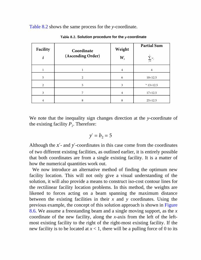
Table 8.2 shows the same process for the y-coordinate.

Table 8.2. Solution procedure for the y-coordinate

Facility

iCoordinate

(Ascending Order)Weight

Wi

Partial Sum

1 1 4 4

5 2 6 10<12.5

2 5 3 * 13>12.5

3 7 4 17>12.5

4 8 8 25>12.5

We note that the inequality sign changes direction at the y-coordinate ofthe existing facility P2. Therefore:

y* = b2 = 5

Although the x*- and y*-coordinates in this case come from the coordinatesof two different existing facilities, as outlined earlier, it is entirely possiblethat both coordinates are from a single existing facility. It is a matter ofhow the numerical quantities work out.

We now introduce an alternative method of finding the optimum newfacility location. This will not only give a visual understanding of thesolution, it will also provide a means to construct iso-cost contour lines forthe rectilinear facility location problems. In this method, the weights arelikened to forces acting on a beam spanning the maximum distancebetween the existing facilities in their x and y coordinates. Using theprevious example, the concept of this solution approach is shown in Figure8.6. We assume a freestanding beam and a single moving support, as the xcoordinate of the new facility, along the x-axis from the left of the left-most existing facility to the right of the right-most existing facility. If thenew facility is to be located at x < 1, there will be a pulling force of 0 to its

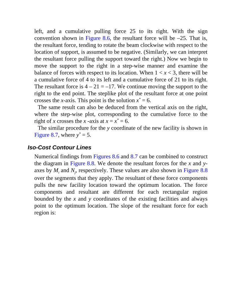
left, and a cumulative pulling force 25 to its right. With the signconvention shown in Figure 8.6, the resultant force will be –25. That is,the resultant force, tending to rotate the beam clockwise with respect to thelocation of support, is assumed to be negative. (Similarly, we can interpretthe resultant force pulling the support toward the right.) Now we begin tomove the support to the right in a step-wise manner and examine thebalance of forces with respect to its location. When 1 < x < 3, there will bea cumulative force of 4 to its left and a cumulative force of 21 to its right.The resultant force is 4 – 21 = –17. We continue moving the support to theright to the end point. The steplike plot of the resultant force at one pointcrosses the x-axis. This point is the solution x* = 6.

The same result can also be deduced from the vertical axis on the right,where the step-wise plot, corresponding to the cumulative force to theright of x crosses the x -axis at x = x* = 6.

The similar procedure for the y coordinate of the new facility is shown inFigure 8.7, where y* = 5.

Iso-Cost Contour LinesNumerical findings from Figures 8.6 and 8.7 can be combined to constructthe diagram in Figure 8.8. We denote the resultant forces for the x and y-axes by Mi and Nj, respectively. These values are also shown in Figure 8.8over the segments that they apply. The resultant of these force componentspulls the new facility location toward the optimum location. The forcecomponents and resultant are different for each rectangular regionbounded by the x and y coordinates of the existing facilities and alwayspoint to the optimum location. The slope of the resultant force for eachregion is:

Figure 8.6. Force analogy for x-axis.

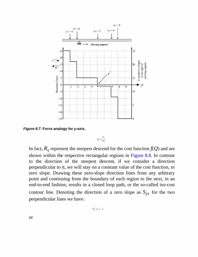
Figure 8.7. Force analogy for y-axis.

In fact, Rij represent the steepest descend for the cost function f(Q) and areshown within the respective rectangular regions in Figure 8.8. In contrastto the direction of the steepest descent, if we consider a directionperpendicular to it, we will stay on a constant value of the cost function, orzero slope. Drawing these zero-slope direction lines from any arbitrarypoint and continuing from the boundary of each region to the next, in anend-to-end fashion, results in a closed loop path, or the so-called iso-costcontour line. Denoting the direction of a zero slope as Sij, for the twoperpendicular lines we have:

or

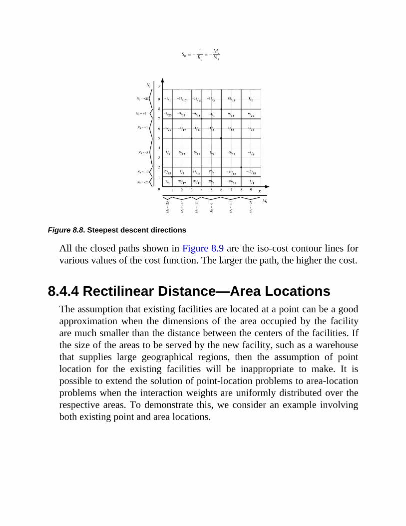
Figure 8.8. Steepest descent directions

All the closed paths shown in Figure 8.9 are the iso-cost contour lines forvarious values of the cost function. The larger the path, the higher the cost.

8.4.4 Rectilinear Distance—Area LocationsThe assumption that existing facilities are located at a point can be a goodapproximation when the dimensions of the area occupied by the facilityare much smaller than the distance between the centers of the facilities. Ifthe size of the areas to be served by the new facility, such as a warehousethat supplies large geographical regions, then the assumption of pointlocation for the existing facilities will be inappropriate to make. It ispossible to extend the solution of point-location problems to area-locationproblems when the interaction weights are uniformly distributed over therespective areas. To demonstrate this, we consider an example involvingboth existing point and area locations.

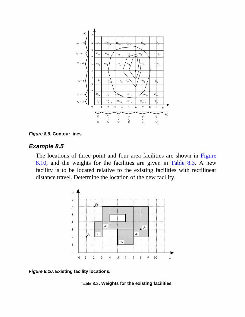
Figure 8.9. Contour lines

Example 8.5The locations of three point and four area facilities are shown in Figure8.10, and the weights for the facilities are given in Table 8.3. A newfacility is to be located relative to the existing facilities with rectilineardistance travel. Determine the location of the new facility.

Figure 8.10. Existing facility locations.

Table 8.3. Weights for the existing facilities

Point Weight Area Weight

1 3 1 4

2 4 2 5

3 1 3 4

4 4

SolutionArea weights are denoted by vj. Similar to the case of the point locationproblem, we begin by plotting the cumulative weight to the right of x forthe range 0 ≤ x ≤ 9, as shown in Figure 8.11. The plot of cumulativeweight to the right of x crosses the x-axis at x = x* = 4. Similarly, for the y-axis this occurs at y = y*= 3.3, as shown in Figure 8.12.

The numerical value of y* = 3.3 is determined from interpolation betweenend points of the line segment between y = 3 and y = 4. The key in plottingthe diagrams of Figures 8.11 and 8.12 is in considering uniformlydistributed weight over the respective areas. For instance, in Figure 8.12,traversing from y = 2 to y = 3, we cover the following distributed weights:

Figure 8.11. Weight distribution for x-axis.

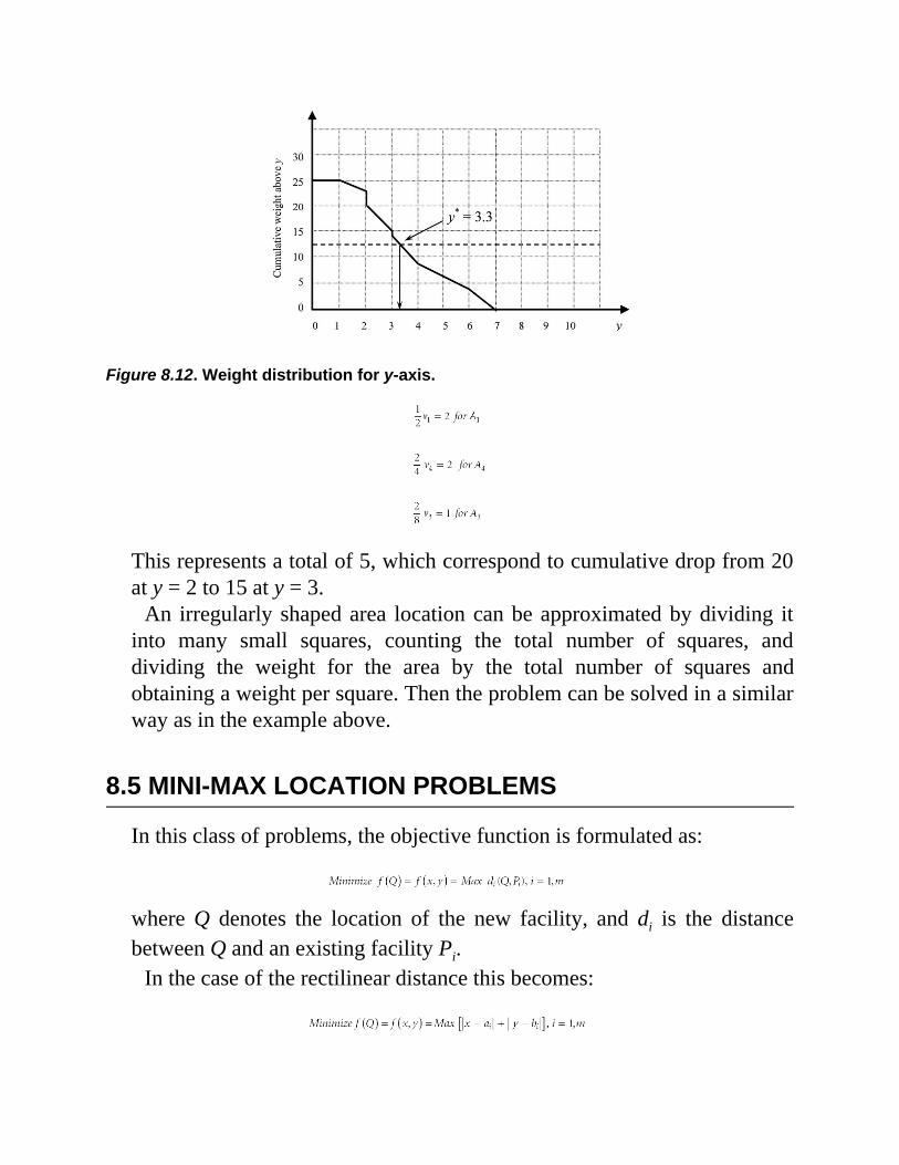
Figure 8.12. Weight distribution for y-axis.

This represents a total of 5, which correspond to cumulative drop from 20at y = 2 to 15 at y = 3.

An irregularly shaped area location can be approximated by dividing itinto many small squares, counting the total number of squares, anddividing the weight for the area by the total number of squares andobtaining a weight per square. Then the problem can be solved in a similarway as in the example above.

8.5 MINI-MAX LOCATION PROBLEMS

In this class of problems, the objective function is formulated as:

where Q denotes the location of the new facility, and di is the distancebetween Q and an existing facility Pi.

In the case of the rectilinear distance this becomes:

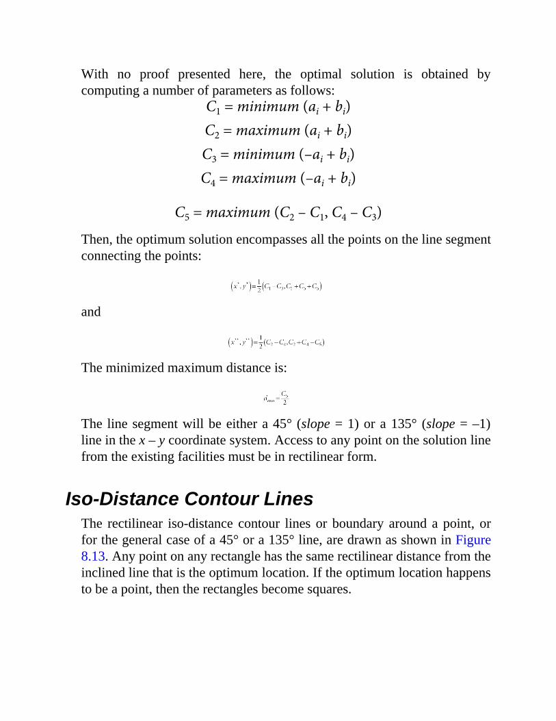
With no proof presented here, the optimal solution is obtained bycomputing a number of parameters as follows:

C1 = minimum (ai + bi)C2 = maximum (ai + bi)C3 = minimum (–ai + bi)C4 = maximum (–ai + bi)

C5 = maximum (C2 – C1, C4 – C3)

Then, the optimum solution encompasses all the points on the line segmentconnecting the points:

and

The minimized maximum distance is:

The line segment will be either a 45° (slope = 1) or a 135° (slope = –1)line in the x – y coordinate system. Access to any point on the solution linefrom the existing facilities must be in rectilinear form.

Iso-Distance Contour LinesThe rectilinear iso-distance contour lines or boundary around a point, orfor the general case of a 45° or a 135° line, are drawn as shown in Figure8.13. Any point on any rectangle has the same rectilinear distance from theinclined line that is the optimum location. If the optimum location happensto be a point, then the rectangles become squares.

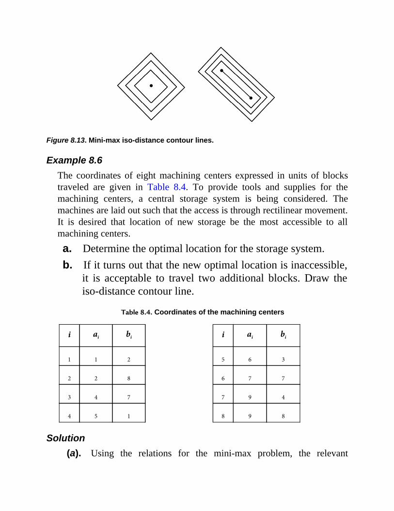
Figure 8.13. Mini-max iso-distance contour lines.

Example 8.6The coordinates of eight machining centers expressed in units of blockstraveled are given in Table 8.4. To provide tools and supplies for themachining centers, a central storage system is being considered. Themachines are laid out such that the access is through rectilinear movement.It is desired that location of new storage be the most accessible to allmachining centers.a. Determine the optimal location for the storage system.b. If it turns out that the new optimal location is inaccessible,

it is acceptable to travel two additional blocks. Draw theiso-distance contour line.

Table 8.4. Coordinates of the machining centers

i ai bi i ai bi

1 1 2 5 6 3

2 2 8 6 7 7

3 4 7 7 9 4

4 5 1 8 9 8

Solution(a). Using the relations for the mini-max problem, the relevant

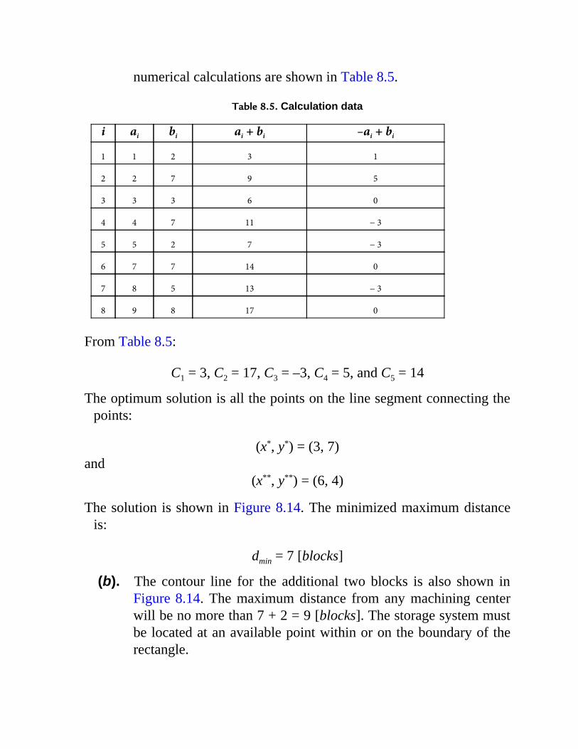
numerical calculations are shown in Table 8.5.

Table 8.5. Calculation data

i ai bi ai + bi –ai + bi

1 1 2 3 1

2 2 7 9 5

3 3 3 6 0

4 4 7 11 − 3

5 5 2 7 − 3

6 7 7 14 0

7 8 5 13 − 3

8 9 8 17 0

From Table 8.5:

C1 = 3, C2 = 17, C3 = –3, C4 = 5, and C5 = 14

The optimum solution is all the points on the line segment connecting thepoints:

(x*, y*) = (3, 7)and

(x**, y**) = (6, 4)

The solution is shown in Figure 8.14. The minimized maximum distanceis:

dmin = 7 [blocks]

(b). The contour line for the additional two blocks is also shown inFigure 8.14. The maximum distance from any machining centerwill be no more than 7 + 2 = 9 [blocks]. The storage system mustbe located at an available point within or on the boundary of therectangle.

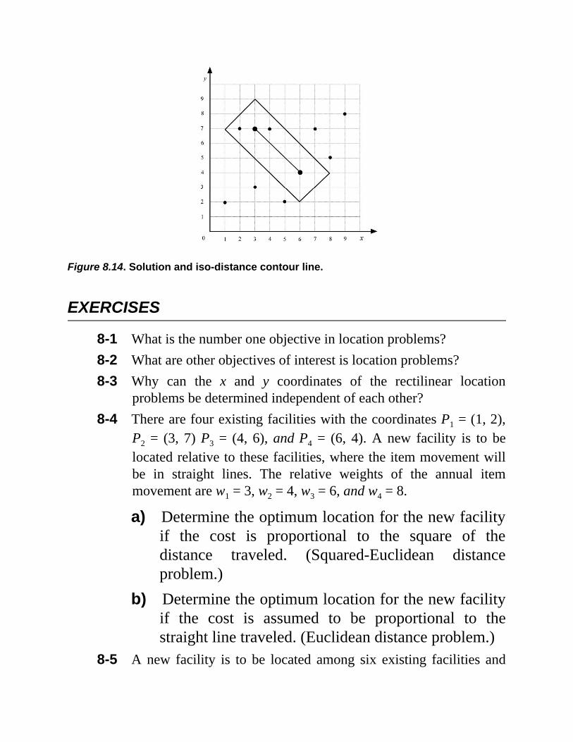
Figure 8.14. Solution and iso-distance contour line.

EXERCISES

8-1 What is the number one objective in location problems?8-2 What are other objectives of interest is location problems?8-3 Why can the x and y coordinates of the rectilinear location

problems be determined independent of each other?8-4 There are four existing facilities with the coordinates P1 = (1, 2),

P2 = (3, 7) P3 = (4, 6), and P4 = (6, 4). A new facility is to belocated relative to these facilities, where the item movement willbe in straight lines. The relative weights of the annual itemmovement are w1 = 3, w2 = 4, w3 = 6, and w4 = 8.

a) Determine the optimum location for the new facilityif the cost is proportional to the square of thedistance traveled. (Squared-Euclidean distanceproblem.)

b) Determine the optimum location for the new facilityif the cost is assumed to be proportional to thestraight line traveled. (Euclidean distance problem.)

8-5 A new facility is to be located among six existing facilities and

supply them with their raw material needs through rectilineardistance transportation. The relative locations of the existingfacilities are P1 = (0, 0), P2 = (2, 3), P3 = (2, 5), P4 = (3, 7), P5 =(5, 5) and P6 = (6, 4). The interaction weights between the newand each of the existing facilities are w1 = 3, w2 = 3, w3 = 5, w4 =4, w5 = 2, and w6 = 6.

a) Determine the location of the new facility thatminimizes the total weighted interaction effort.

b) If the new facility cannot be located closer than 2rectilinear distance to any existing facility, usingonly a geometric graph, make a prediction of theoptimum location. (This is only a guess, and theresult may not be accurate.)

c) In follow-up to (b), determine optimum location withthe aid of iso-cost contour lines. Compare the resultwith the prediction made in (b).

8-6 A new facility is to be located to serve four points and three arealocations. The existing facilities are shown in Figure 8.15, andtheir weights are given in Table 8.6. The weights are uniformlydistributed over the areas, and rectilinear distance is used.

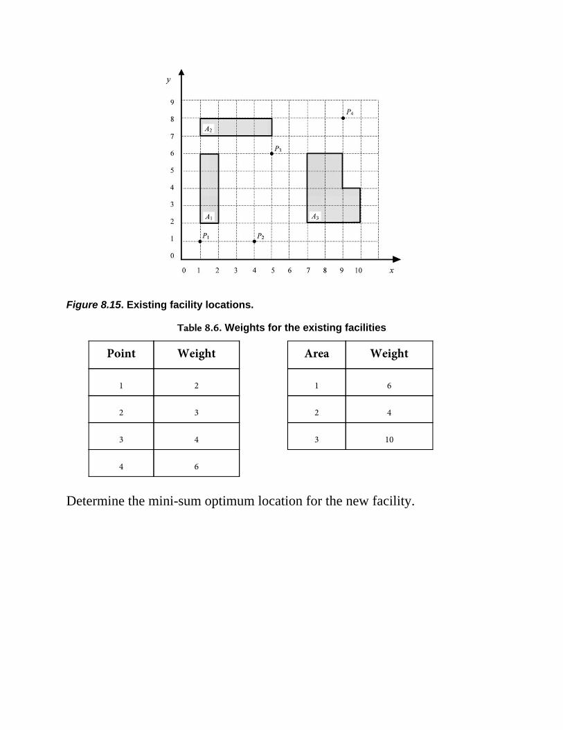
Figure 8.15. Existing facility locations.

Table 8.6. Weights for the existing facilities

Point Weight Area Weight

1 2 1 6

2 3 2 4

3 4 3 10

4 6

Determine the mini-sum optimum location for the new facility.

Chapter 9 SYSTEM RELIABILITY

9.1 INTRODUCTION

The general concept of reliability is extremely wide, and reliability is aconcern in almost every system that one can think of, from a simple deviceto most complex engineering systems. Reliability directly affects safetyand availability. Lack of safety and unavailability can lead to a host ofissues ranging from bodily harm to loss of productivity, or from frustrationto damage to reputation for quality.

How many times have you wanted to use something or have been usingsomething when a breakdown has dampened your spirit? Think aboutautomobile problems, computer malfunctions, and the like in everydaylife. Extend this to the operation of a transit system, hospital andemergency equipment, machinery, and the production facility, and theconsequences of unreliability can be costly. Unreliability is generallyassociated with and is the result of a failure of a component or a module inthe system. In theory, well-designed, well-engineered, thoroughly tested,and properly maintained equipment or systems should not fail inoperation. But experience has shown that no amount of care cancompletely eliminate the chances of such failures from occurring. We can,however, by controlling the environmental effects, through design, andproper instructions for use, significantly influence and improve thereliability of a system.

9.2 DEFINITION OF RELIABILITY

Reliability is the capability of a device or a system to perform its intendedfunction without breakdown.

We can formalize the reliability of equipment and systems based on thereliability of their individual modules and components and analyze them.The component level of the study of reliability is primarily the concern ofdesign engineers, such as improving the reliability or the probability of asuccessful operation of a device or a sensor. But the reliability of largersystems, as integrated units to perform as a whole, can be an issue forindustrial engineers. With this in mind, after reviewing the preliminaries ofrelevant functions and factors, we limit ourselves to reliability analysis ofsystems for which we know the probability of success for each of itsconstituent components. Such systems could include manufacturing lines,material handling and transportation systems, and, in fact, anyinterconnected system. For any meaningful analysis to be carried out, weneed to know at least three elements:

1. The reliability or probability of success of the operation ofthe individual components or modules. These primarilycome from recorded and historical data, experience,scientific or previous reliability analysis, claims bymanufacturers, and, if none of the preceding is available,from intuition and guess. With the latter two, anythingconcluded will be an approximation and must be treatedcautiously.

2. How the individual components and modules areinterconnected to process an input and direct it to theoutput. The function of the elements of the system and thenature of inputs and outputs can relate to entities such aselectricity, steam, parts in a manufacturing plant, people,equipment, or sensors in a control loop.

3. The methods and means of determining the reliability ofthe entire system, and how we can influence it. A majorpurpose of a reliability analysis often is to identify weak

links and modules in terms of their individual reliabilityand their role in the total reliability of the system.

9.3 FAILURE OVER THE OPERATING LIFE

The failure rate or, more precisely, the instantaneous failure rate of manycomponents and systems over their operating life can be divided into threephases or periods, as shown in Figure 9.1.

• Period A. This is called the early failure, run-in, burn-in ordebugging phase. As the time passes for a new system, thefailure rate decreases both naturally and as a result of fixesand fine-tunings performed.

• Period B. This constitutes the extended operating life, and itis appropriately called the “useful life.” In this phase thereare occasional failures and breakdowns that are mostlyrandom in nature—or by chance, although in somecircumstances a failure can be related to the construct of thesystem and how it is used. Based on economicconsiderations, the nature and function of the componentsof the system, the operating instruction for a system, or thephilosophy of an organization, the system may require someform of service and maintenance to be in place.

• Period C. This is the phase where increasingly frequentfailures affect the operation of the system. Known as agingand the wearing-out period, repeated failures of differentcomponents of the system hamper the successful operationof the system. Not only can operating a system in this rangebe dangerous; it can also be very costly to maintain. Relyingon an economic analysis, a major overhaul, and replacementof certain critical and aging components can move thesystem back into region B for a period of time.

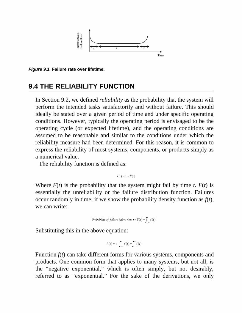
Figure 9.1. Failure rate over lifetime.

9.4 THE RELIABILITY FUNCTION

In Section 9.2, we defined reliability as the probability that the system willperform the intended tasks satisfactorily and without failure. This shouldideally be stated over a given period of time and under specific operatingconditions. However, typically the operating period is envisaged to be theoperating cycle (or expected lifetime), and the operating conditions areassumed to be reasonable and similar to the conditions under which thereliability measure had been determined. For this reason, it is common toexpress the reliability of most systems, components, or products simply asa numerical value.

The reliability function is defined as:

Where F(t) is the probability that the system might fail by time t. F(t) isessentially the unreliability or the failure distribution function. Failuresoccur randomly in time; if we show the probability density function as f(t),we can write:

Substituting this in the above equation:

Function f(t) can take different forms for various systems, components andproducts. One common form that applies to many systems, but not all, isthe “negative exponential,” which is often simply, but not desirably,referred to as “exponential.” For the sake of the derivations, we only

consider the exponential density function, which is defined as:

where λ is the failure rate, and t is the operating time of interest. Then:

The mean life is defined as:

For the exponential function, this is more appropriately referred to at theMean Time between Failures (MTBF).

To be able to determine the reliability (probability of success) over thetime period t, we need the failure rate λ.

9.4.1 Failure RateThe failure rate is the frequency with which a system or a component fails,and it is expressed as:

The failure rate may be expressed in any unit of time depending on thesystem, but failure per hour, although numerically may appear small, iscommon. The reason is that the MTBF, is then expressed in tangibleunits of “hour.” The failure rate can be obtained in a number of ways:from past data of similar components, recorded data, specific testsconducted on a set of components, or, as a last resort, from intuition andexperience—in which case rather than estimating the failure rate, it may bemore useful to directly express the reliability R.

We now review in detail an example of determining the failure rate.Suppose that a total of ten components were concurrently put to the testunder typical operating conditions. The failure data are given in the firstcolumn of Table 9.1. In this experiment after the failure of the fifthcomponent at 480 hours, the relevant computation is shown in the rest ofthe table.

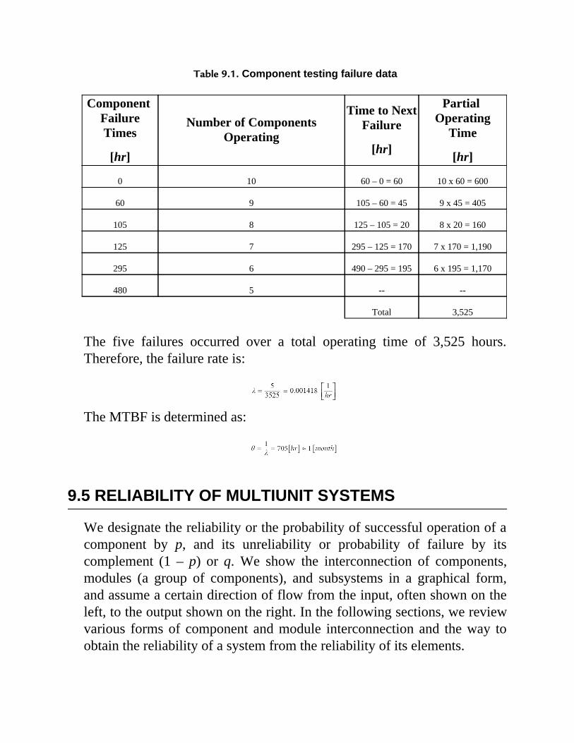
Table 9.1. Component testing failure data

Component FailureTimes

[hr]

Number of ComponentsOperating

Time to NextFailure

[hr]

Partial Operating

Time

[hr]

0 10 60 – 0 = 60 10 x 60 = 600

60 9 105 – 60 = 45 9 x 45 = 405

105 8 125 – 105 = 20 8 x 20 = 160

125 7 295 – 125 = 170 7 x 170 = 1,190

295 6 490 – 295 = 195 6 x 195 = 1,170

480 5 -- --

Total 3,525

The five failures occurred over a total operating time of 3,525 hours.Therefore, the failure rate is:

The MTBF is determined as:

9.5 RELIABILITY OF MULTIUNIT SYSTEMS

We designate the reliability or the probability of successful operation of acomponent by p, and its unreliability or probability of failure by itscomplement (1 – p) or q. We show the interconnection of components,modules (a group of components), and subsystems in a graphical form,and assume a certain direction of flow from the input, often shown on theleft, to the output shown on the right. In the following sections, we reviewvarious forms of component and module interconnection and the way toobtain the reliability of a system from the reliability of its elements.

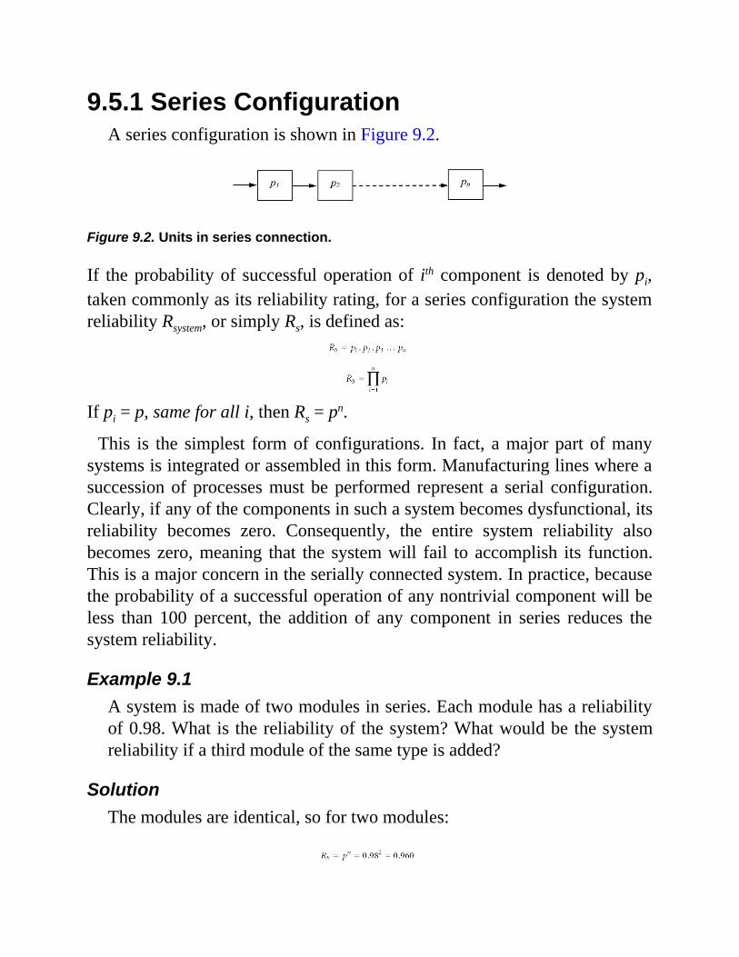
9.5.1 Series ConfigurationA series configuration is shown in Figure 9.2.

Figure 9.2. Units in series connection.

If the probability of successful operation of ith component is denoted by pi,taken commonly as its reliability rating, for a series configuration the systemreliability Rsystem, or simply Rs, is defined as:

If pi = p, same for all i, then Rs = pn.

This is the simplest form of configurations. In fact, a major part of manysystems is integrated or assembled in this form. Manufacturing lines where asuccession of processes must be performed represent a serial configuration.Clearly, if any of the components in such a system becomes dysfunctional, itsreliability becomes zero. Consequently, the entire system reliability alsobecomes zero, meaning that the system will fail to accomplish its function.This is a major concern in the serially connected system. In practice, becausethe probability of a successful operation of any nontrivial component will beless than 100 percent, the addition of any component in series reduces thesystem reliability.

Example 9.1A system is made of two modules in series. Each module has a reliabilityof 0.98. What is the reliability of the system? What would be the systemreliability if a third module of the same type is added?

SolutionThe modules are identical, so for two modules:

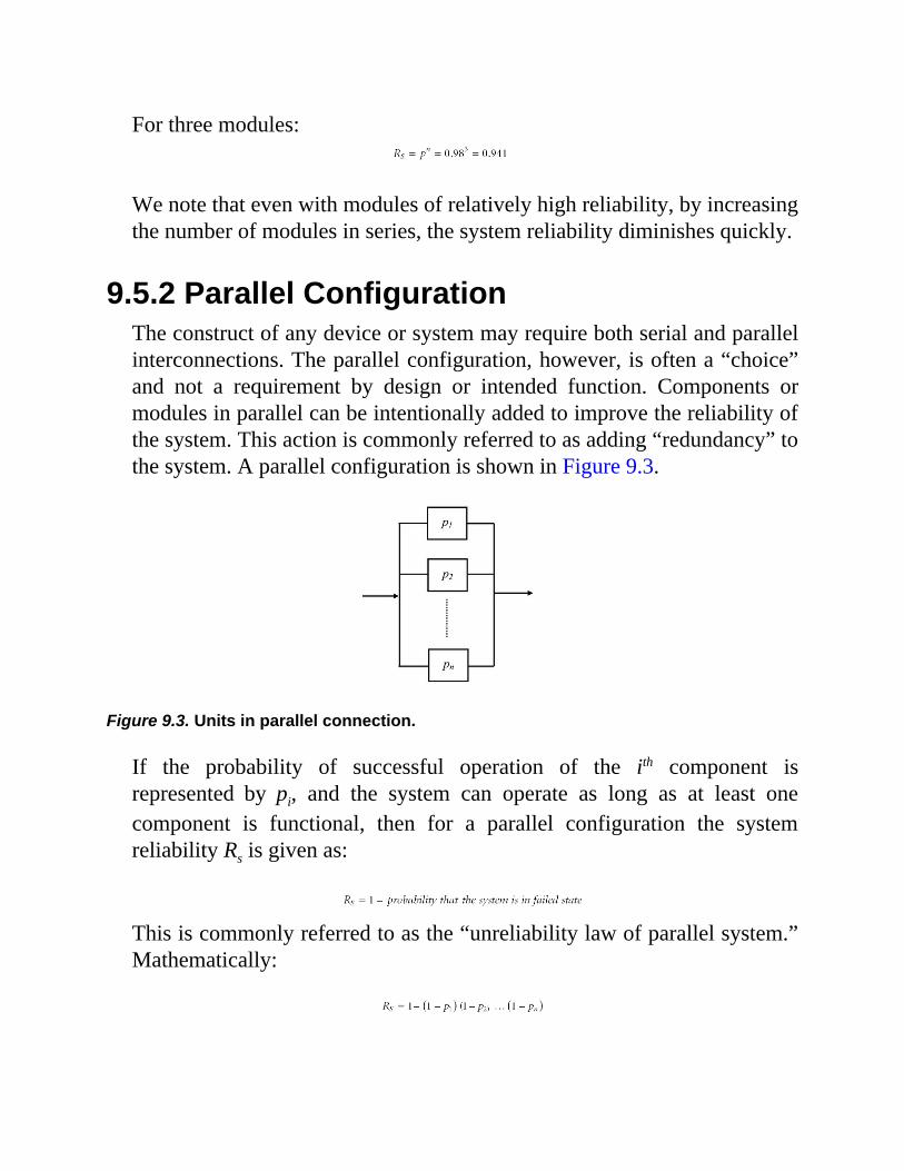
For three modules:

We note that even with modules of relatively high reliability, by increasingthe number of modules in series, the system reliability diminishes quickly.

9.5.2 Parallel ConfigurationThe construct of any device or system may require both serial and parallelinterconnections. The parallel configuration, however, is often a “choice”and not a requirement by design or intended function. Components ormodules in parallel can be intentionally added to improve the reliability ofthe system. This action is commonly referred to as adding “redundancy” tothe system. A parallel configuration is shown in Figure 9.3.

Figure 9.3. Units in parallel connection.

If the probability of successful operation of the ith component isrepresented by pi, and the system can operate as long as at least onecomponent is functional, then for a parallel configuration the systemreliability Rs is given as:

This is commonly referred to as the “unreliability law of parallel system.”Mathematically:

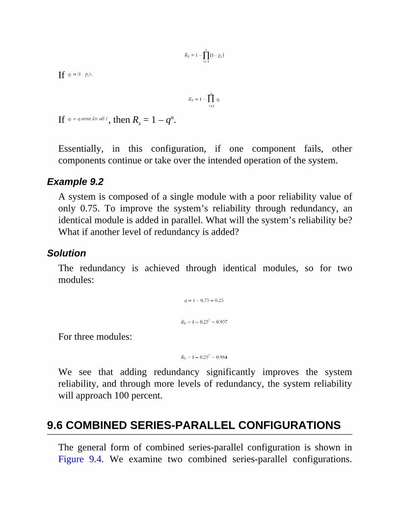
If

If , then Rs = 1 – qn. Essentially, in this configuration, if one component fails, othercomponents continue or take over the intended operation of the system.

Example 9.2A system is composed of a single module with a poor reliability value ofonly 0.75. To improve the system’s reliability through redundancy, anidentical module is added in parallel. What will the system’s reliability be?What if another level of redundancy is added?

SolutionThe redundancy is achieved through identical modules, so for twomodules:

For three modules:

We see that adding redundancy significantly improves the systemreliability, and through more levels of redundancy, the system reliabilitywill approach 100 percent.

9.6 COMBINED SERIES-PARALLEL CONFIGURATIONS

The general form of combined series-parallel configuration is shown inFigure 9.4. We examine two combined series-parallel configurations.

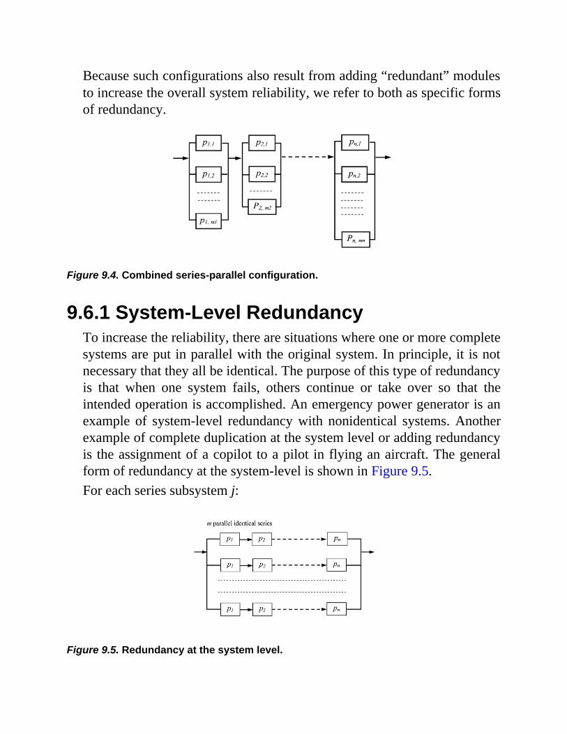
Because such configurations also result from adding “redundant” modulesto increase the overall system reliability, we refer to both as specific formsof redundancy.

Figure 9.4. Combined series-parallel configuration.

9.6.1 System-Level RedundancyTo increase the reliability, there are situations where one or more completesystems are put in parallel with the original system. In principle, it is notnecessary that they all be identical. The purpose of this type of redundancyis that when one system fails, others continue or take over so that theintended operation is accomplished. An emergency power generator is anexample of system-level redundancy with nonidentical systems. Anotherexample of complete duplication at the system level or adding redundancyis the assignment of a copilot to a pilot in flying an aircraft. The generalform of redundancy at the system-level is shown in Figure 9.5.For each series subsystem j:

Figure 9.5. Redundancy at the system level.

For m parallel subsystems:

or

9.6.2 Component-Level RedundancyAn alternative to system-level redundancy is to use the same number ofeach of the system’s components and rearrange them in parallel. Forexample, the system of Figure 9.5 can be redesigned as in Figure 9.6.

At each stage, for m parallel modules we have:

Figure 9.6. Redundancy at the component level.

For the n stages in series we obtain:

Example 9.3Several families of components, Fi, are to be produced on four types ofmachines, L, M, D, and G. Four machines of each type are available, andtwo systems of physical arrangements have been proposed as reviewed inChapter 3: functional layout, designated as System I, and group technologylayout, designated as System II, as shown in Figures 9.7 and 9.8.

In System I, although each component family may use any of themachines within each group, during the normal operation of the system ithas been found both practical and convenient for component family F1 touse machines L1, M1, D1, and G1 on a permanent basis. Similarly, in SystemII, component family F1 has been assigned to Group 1. During certainperiods of time the component family received a high demand and becauseof this, it is given top priority. Under such circumstances other machinesin the case of System I and other groups in the case of System II areimmediately made available to the component family F1 on an activeredundancy basis:

(a) Determine the reliability of each system as far as the production ofthe component family F1 is concerned using the followingreliability data:

Figure 9.7. System I.

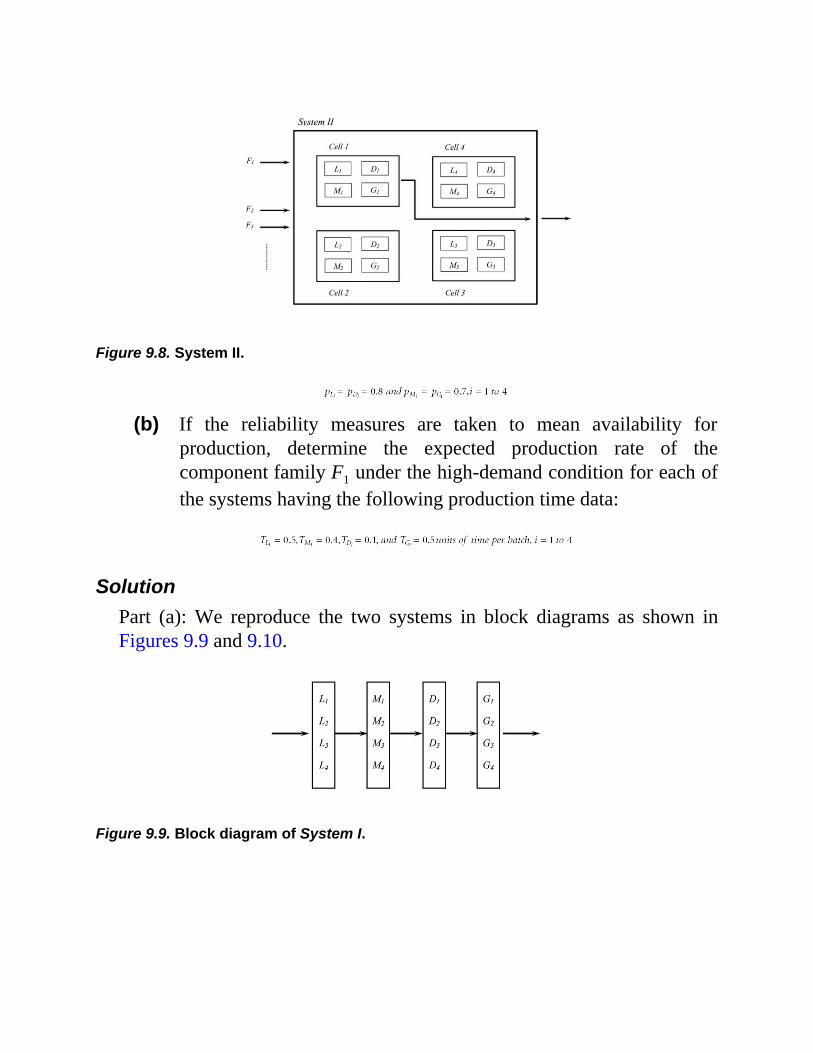
Figure 9.8. System II.

(b) If the reliability measures are taken to mean availability for

production, determine the expected production rate of thecomponent family F1 under the high-demand condition for each ofthe systems having the following production time data:

SolutionPart (a): We reproduce the two systems in block diagrams as shown inFigures 9.9 and 9.10.

Figure 9.9. Block diagram of System I.

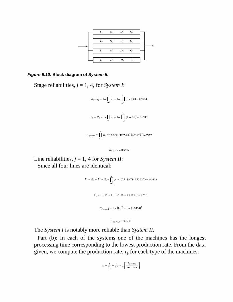
Figure 9.10. Block diagram of System II.

Stage reliabilities, j = 1, 4, for System I:

Line reliabilities, j = 1, 4 for System II:

Since all four lines are identical:

The System I is notably more reliable than System II.

Part (b): In each of the systems one of the machines has the longestprocessing time corresponding to the lowest production rate. From the datagiven, we compute the production rate, rk for each type of the machines:

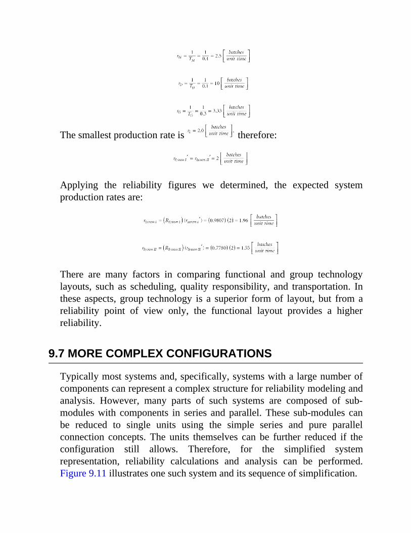
The smallest production rate is therefore:

Applying the reliability figures we determined, the expected systemproduction rates are:

There are many factors in comparing functional and group technologylayouts, such as scheduling, quality responsibility, and transportation. Inthese aspects, group technology is a superior form of layout, but from areliability point of view only, the functional layout provides a higherreliability.

9.7 MORE COMPLEX CONFIGURATIONS

Typically most systems and, specifically, systems with a large number ofcomponents can represent a complex structure for reliability modeling andanalysis. However, many parts of such systems are composed of sub-modules with components in series and parallel. These sub-modules canbe reduced to single units using the simple series and pure parallelconnection concepts. The units themselves can be further reduced if theconfiguration still allows. Therefore, for the simplified systemrepresentation, reliability calculations and analysis can be performed.Figure 9.11 illustrates one such system and its sequence of simplification.

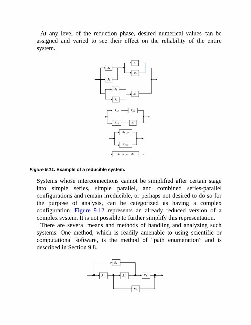
At any level of the reduction phase, desired numerical values can beassigned and varied to see their effect on the reliability of the entiresystem.

Figure 9.11. Example of a reducible system.

Systems whose interconnections cannot be simplified after certain stageinto simple series, simple parallel, and combined series-parallelconfigurations and remain irreducible, or perhaps not desired to do so forthe purpose of analysis, can be categorized as having a complexconfiguration. Figure 9.12 represents an already reduced version of acomplex system. It is not possible to further simplify this representation.

There are several means and methods of handling and analyzing suchsystems. One method, which is readily amenable to using scientific orcomputational software, is the method of “path enumeration” and isdescribed in Section 9.8.

Figure 9.12. Simplest form of a complex reliability diagram.

9.8 THE METHOD OF PATH ENUMERATION

A complex configuration may look like the one shown in Figure 9.13.Note that in this system, modules R4 and R5 can be simplified into one

unit. But, for the sake of illustration, assume that it is desired that wemaintain them as separate modules. For such a system, reliability isdefined as the successful functioning of all the modules in at least onepath. A path is a group of modules in series that form a connectionbetween input and output when traversed in a stated direction. We alsodefine the “minimal” path as a path that consists of a minimum number ofmodules. In other words, no module is traversed more than once in tracingthe path.

Figure 9.13. Reliability diagram of a complex system.

If Pi, i = 1, 2,.., M, are the minimal paths, then the reliability of thesystem Rs is expressed as:

Rs = Probability that at least one path is successful

or in mathematical terms:

where denotes the union operator.

Using the expansion rule for the probability of the union of M concurrentevents, we have:

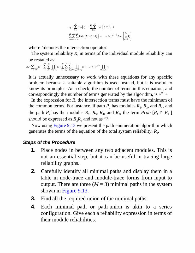
where denotes the intersection operator.The system reliability Rs in terms of the individual module reliability can

be restated as:

It is actually unnecessary to work with these equations for any specificproblem because a suitable algorithm is used instead, but it is useful toknow its principles. As a check, the number of terms in this equation, andcorrespondingly the number of terms generated by the algorithm, is

In the expression for R, the intersection terms must have the minimum ofthe common terms. For instance, if path P1 has modules R1, R3, and R4, andthe path P2 has the modules R2, R3, R4, and R5, the term Prob [P1 ∩ P2 ]should be expressed as R3R4 and not as

Now using Figure 9.13 we present the path enumeration algorithm whichgenerates the terms of the equation of the total system reliability, Rs.

Steps of the Procedure1. Place nodes in between any two adjacent modules. This is

not an essential step, but it can be useful in tracing largereliability graphs.

2. Carefully identify all minimal paths and display them in atable in node-trace and module-trace forms from input tooutput. There are three (M = 3) minimal paths in the systemshown in Figure 9.13.

3. Find all the required union of the minimal paths.4. Each minimal path or path-union is akin to a series

configuration. Give each a reliability expression in terms oftheir module reliabilities.

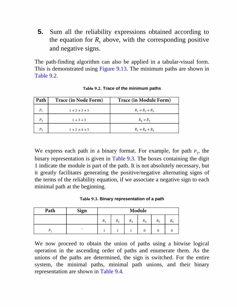
5. Sum all the reliability expressions obtained according tothe equation for Rs above, with the corresponding positiveand negative signs.

The path-finding algorithm can also be applied in a tabular-visual form.This is demonstrated using Figure 9.13. The minimum paths are shown inTable 9.2.

Table 9.2. Trace of the minimum paths

Path Trace (in Node Form) Trace (in Module Form)

P1 1 → 2 → 3 → 5 R1 → R2 → R3

P2 1 → 3 → 5 R6 → R3

P3 1 → 2 → 4 → 5 R1 → R4 → R4

We express each path in a binary format. For example, for path P1, thebinary representation is given in Table 9.3. The boxes containing the digit1 indicate the module is part of the path. It is not absolutely necessary, butit greatly facilitates generating the positive/negative alternating signs ofthe terms of the reliability equation, if we associate a negative sign to eachminimal path at the beginning.

Table 9.3. Binary representation of a path

Path Sign Module

R1 R2 R3 R4 R5 R6

P1- 1 1 1 0 0 0

We now proceed to obtain the union of paths using a bitwise logicaloperation in the ascending order of paths and enumerate them. As theunions of the paths are determined, the sign is switched. For the entiresystem, the minimal paths, minimal path unions, and their binaryrepresentation are shown in Table 9.4.

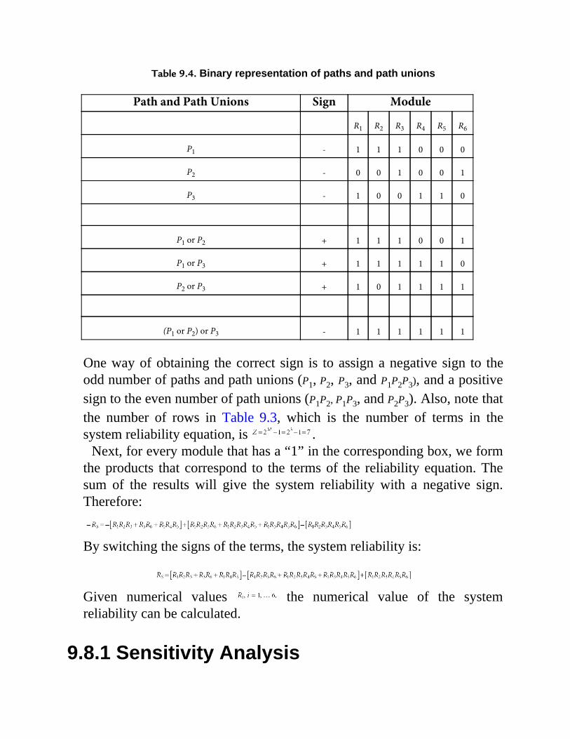
Table 9.4. Binary representation of paths and path unions

Path and Path Unions Sign Module

R1 R2 R3 R4 R5 R6

P1 - 1 1 1 0 0 0

P2 - 0 0 1 0 0 1

P3 - 1 0 0 1 1 0

P1 or P2 + 1 1 1 0 0 1

P1 or P3 + 1 1 1 1 1 0

P2 or P3 + 1 0 1 1 1 1

(P1 or P2) or P3 - 1 1 1 1 1 1

One way of obtaining the correct sign is to assign a negative sign to theodd number of paths and path unions (P1, P2, P3, and P1P2P3), and a positivesign to the even number of path unions (P1P2, P1P3, and P2P3). Also, note thatthe number of rows in Table 9.3, which is the number of terms in thesystem reliability equation, is .

Next, for every module that has a “1” in the corresponding box, we formthe products that correspond to the terms of the reliability equation. Thesum of the results will give the system reliability with a negative sign.Therefore:

By switching the signs of the terms, the system reliability is:

Given numerical values the numerical value of the systemreliability can be calculated.

9.8.1 Sensitivity Analysis

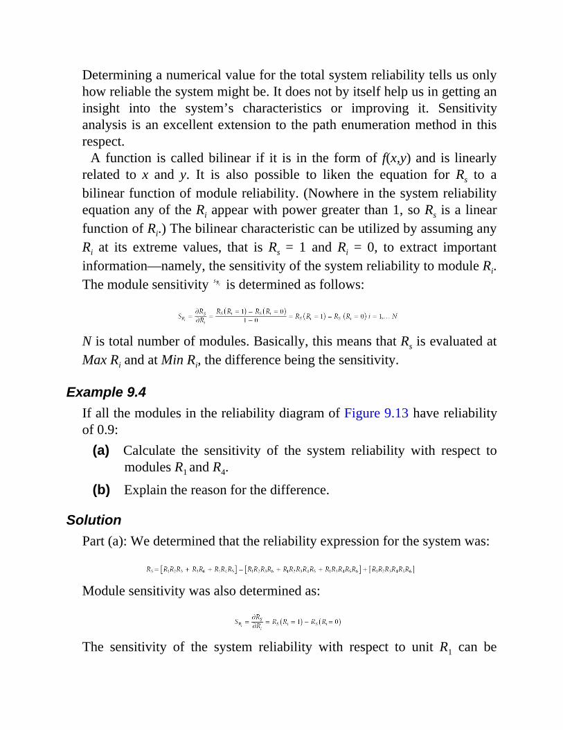
Determining a numerical value for the total system reliability tells us onlyhow reliable the system might be. It does not by itself help us in getting aninsight into the system’s characteristics or improving it. Sensitivityanalysis is an excellent extension to the path enumeration method in thisrespect.

A function is called bilinear if it is in the form of f(x,y) and is linearlyrelated to x and y. It is also possible to liken the equation for Rs to abilinear function of module reliability. (Nowhere in the system reliabilityequation any of the Ri appear with power greater than 1, so Rs is a linearfunction of Ri.) The bilinear characteristic can be utilized by assuming anyRi at its extreme values, that is Rs = 1 and Ri = 0, to extract importantinformation—namely, the sensitivity of the system reliability to module Ri.The module sensitivity is determined as follows:

N is total number of modules. Basically, this means that Rs is evaluated atMax Ri and at Min Ri, the difference being the sensitivity.

Example 9.4If all the modules in the reliability diagram of Figure 9.13 have reliabilityof 0.9:

(a) Calculate the sensitivity of the system reliability with respect tomodules R1 and R4.

(b) Explain the reason for the difference.

SolutionPart (a): We determined that the reliability expression for the system was:

Module sensitivity was also determined as:

The sensitivity of the system reliability with respect to unit R1 can be

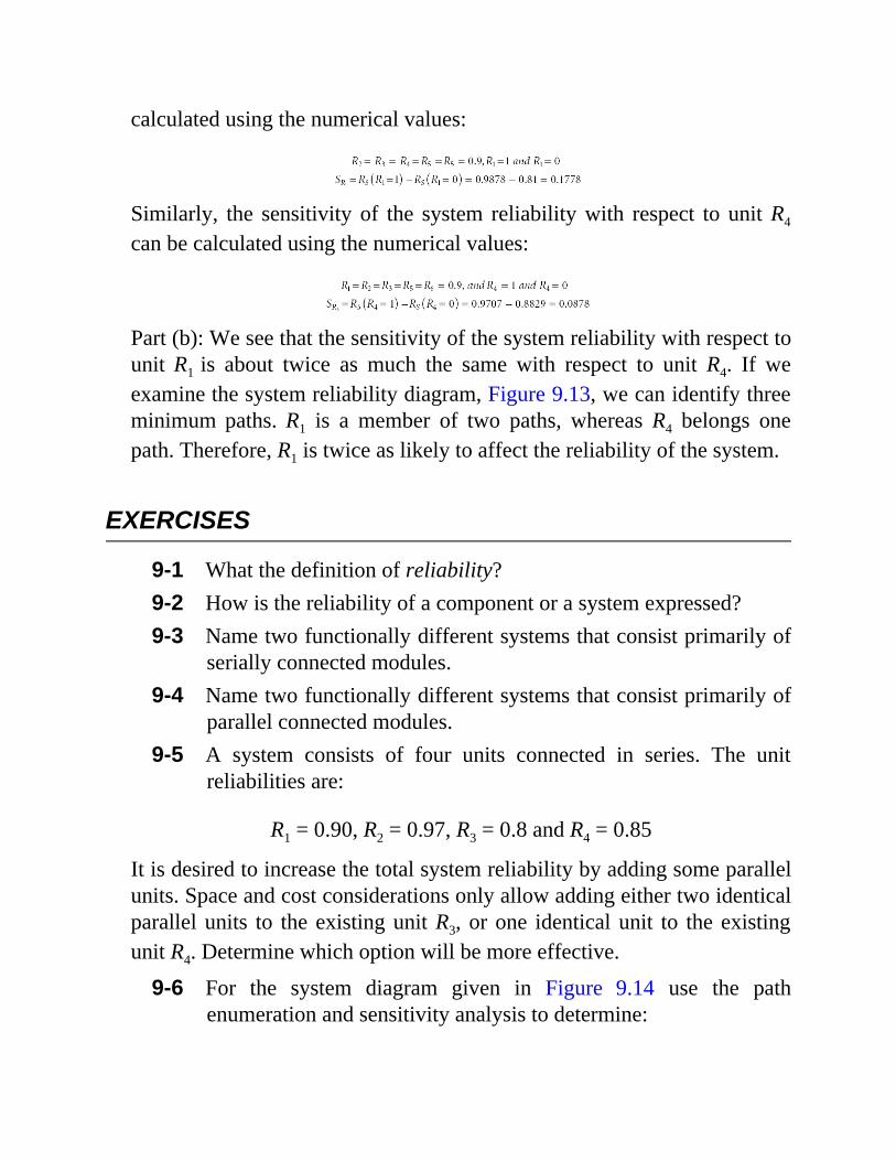
calculated using the numerical values:

Similarly, the sensitivity of the system reliability with respect to unit R4

can be calculated using the numerical values:

Part (b): We see that the sensitivity of the system reliability with respect tounit R1 is about twice as much the same with respect to unit R4. If weexamine the system reliability diagram, Figure 9.13, we can identify threeminimum paths. R1 is a member of two paths, whereas R4 belongs onepath. Therefore, R1 is twice as likely to affect the reliability of the system.

EXERCISES

9-1 What the definition of reliability?9-2 How is the reliability of a component or a system expressed?9-3 Name two functionally different systems that consist primarily of

serially connected modules.9-4 Name two functionally different systems that consist primarily of

parallel connected modules.9-5 A system consists of four units connected in series. The unit

reliabilities are:

R1 = 0.90, R2 = 0.97, R3 = 0.8 and R4 = 0.85

It is desired to increase the total system reliability by adding some parallelunits. Space and cost considerations only allow adding either two identicalparallel units to the existing unit R3, or one identical unit to the existingunit R4. Determine which option will be more effective.

9-6 For the system diagram given in Figure 9.14 use the pathenumeration and sensitivity analysis to determine:

a) The system reliabilityb) The sensitivity of the system reliability with respect

to R5 and R6

Figure 9.14.

Chapter 10 QUEUEING THEORY

10.1 INTRODUCTION

Many situations arise in manufacturing plants, industrial and governmentalorganizations, and other settings where queues form if the service requiredby a customer or entity is not immediately available. The instances of suchdemands are generally random in nature, and they are often caused by theengagement of the servers to attend to the existing customers in thesystem. Each demand normally requires a different duration of service.Therefore, the availability of service is also random and irregular innature. These variabilities can cause queues to build up frequently anddiminish over time.

The mathematical theory of queueing systems is rich, and its treatment israther complex. But many different concepts have been worked out to fit avariety of real scenarios, and the developed set of equations provideinsight and means to analyze and influence the behavior of the underlyingsystem. The primary factors in using the queueing theory and obtainingreliable results are to have appropriate data and determine which model isbest suited for the system being studied.

10.2 ELEMENTS OF QUEUEING SYSTEMS

Essentially, the queueing theory offers a modeling concept that ismathematical in nature and composed of a set of equations for specificproblems. For modeling and analysis of queueing systems, the followingkey information is required:

• Arrival pattern of jobs, customers, or any entity of interest• Queue discipline by which the entities join the system• Configuration of service facilities for the flow of entities• Service duration for each entity• Metrics of analysis• Options for system modification

In the following sections we describe these elements.

10.2.1 Arrival PatternFor most queueing problems the arrival of entities is an independentrandom event beyond the direct control of the system’s operator. If arrivaldata are available from past experience, or they have been recorded,appropriate probability distributions can be found to pseudo-generate thearrival times or the number of arrivals within a specific period of time forthe mathematical modeling.

10.2.2 Queue DisciplineWhen customers or entities arrive and service is not available, they line upin a queue. Some systems may have multiple queues of equal importance,and the arriving entity or customer can choose the queue; however, underidentical circumstances, it is highly likely that they join the shorter queue.The nature of the lineup is governed by certain rules known as “queuedisciplines”; the following are typical examples:

• First Come First Served (FCFS). With this discipline, thearriving entities join the end or tail of the existing queue.This is the most common discipline that is easy to apply andfollow in many practical situations. This rule is also called“First-In-First-Out.”

• Last Come First Served (LCFS). With this discipline

arriving entities go the beginning or head of the queue. Thisrule is less common, at least intentionally, but unavoidablefor some systems. It applies, for example, when entities arestored in a limited-access warehouse or stacked vertically,where the last entity must be removed (attended to) first toaccess the previous other entities. This discipline is alsocalled “Last-In-First-Out.”

• High-Value First (HVF). In order to implement thisdiscipline, a certain attribute of the arriving entities is usedto rank them for the lineup. For example, for relevantreasons, the weight or volume of an entity may be used toassign priorities. An example would be the loading of cargoships, where, for stability and efficient use of space, heavyor bulky items are often given high priority.

• Low-Value First (LVF). This is similar to the HVFdiscipline, only applied in reverse order. Similarly, a certainattribute of the arriving entities is used to prioritize them forservice. For example, entities requiring short service timemay be given high priority to reduce the queue length andhave a larger number of service tasks accomplished in ashorter period of time.

10.2.3 Service ArrangementThe service facility can have single or multiple channels (multipleservers). This is often a design or controllable feature of a queueingsystem. Because the arrival patterns cannot always be altered at will by theanalyst as a design factor, if long lineups and delays are observed,additional service channels can be added. A larger, more complexqueueing system may have multiple or parallel points of arrival, and havemany service channels in series. The modeling and analysis of suchsystems may pose a challenge for implementing the queueing concepts.

Such a system can be readily analyzed using Discrete Event Simulation.

10.2.4 Service DurationThe service times depend on the nature of the service required and thecapability of the service mechanism. The service times typically havemuch less variability than the arrival patterns or, more specifically, inter-arrival times. In some cases, the service time may even be constant.

Once the requirements of a queueing analysis have been determined, andinformation about the elements of the queueing system has been gathered,a model can be developed, and performance indicators, or metrics, can becomputed.

10.2.5 Performance MetricsThe typical measures or metrics are the average number of customers orentities in the queue, and the average time an entity spends in the queueover an extended period of operation. More metrics are listed in Section10.3.1, Table 10.1.

10.2.6 System ModificationThe ultimate goal of the queueing modeling and analysis is to determineproblem areas and investigate the feasibility and effects of variousmodifications. Three factors can be considered for change:

• Arrival pattern. This is often an independent variable for thesystem as a whole, but by adding new service channels inparallel, the arrival rate per channel will change. Anotherway of influencing an arrival pattern is to force someentities to “balk” (turn away) and not enter the system. Suchas imposing a weight restriction for trucks entering aloading/unloading bay.

• Service time. Changing the mechanism of the servicefacility, such as replacing older equipment with faster and

perhaps automated equipment, reduces the service time and,hence, the queue length.

• Service facility configuration. Depending on the problemsituation, and the consideration given to the availability ofspace and other limitations, the service facility can bereconfigured. For example, parallel entrance and servicechannels can be added, or a service point can be split intofaster serial processes.

In some cases, it is only required to change the numerical values of theparameters used, while in other situations where major changes are beingconsidered, the queueing model must be reconstructed.

10.3 QUEUEING MODELS

Many forms of queueing models with different arrival patterns, servicetimes, configuration, and operational conditions have been developed.Many real systems can be modeled using these standard forms. Morecomplex systems can also be modeled by judiciously combining thestandard models. Figure 10.1 shows several forms of queueing systems. Inthe following section, we review simple single-channel and multiple-channel models.

10.3.1 Single-Channel QueuesA number of assumptions that we explicitly did not mention earlier mustbe made in using the queueing theory. We consider a queueing systemwith the following characteristics:

- Infinite population of potential customers. This means thatthere will be no interruption in the probabilistic generationof the customers, such as interruption due to the night shift.

- FCFS queue discipline.

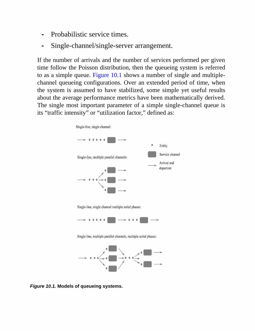
- Probabilistic service times.- Single-channel/single-server arrangement.

If the number of arrivals and the number of services performed per giventime follow the Poisson distribution, then the queueing system is referredto as a simple queue. Figure 10.1 shows a number of single and multiple-channel queueing configurations. Over an extended period of time, whenthe system is assumed to have stabilized, some simple yet useful resultsabout the average performance metrics have been mathematically derived.The single most important parameter of a simple single-channel queue isits “traffic intensity” or “utilization factor,” defined as:

Figure 10.1. Models of queueing systems.

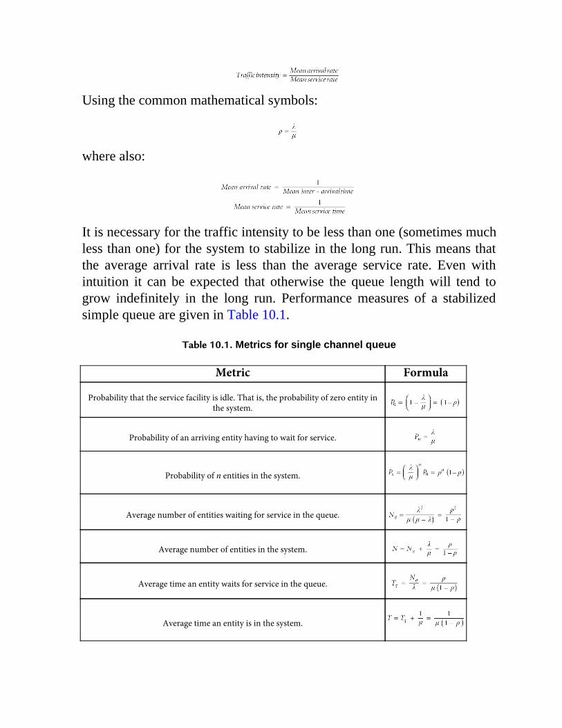
Using the common mathematical symbols:

where also:

It is necessary for the traffic intensity to be less than one (sometimes muchless than one) for the system to stabilize in the long run. This means thatthe average arrival rate is less than the average service rate. Even withintuition it can be expected that otherwise the queue length will tend togrow indefinitely in the long run. Performance measures of a stabilizedsimple queue are given in Table 10.1.

Table 10.1. Metrics for single channel queue

Metric Formula

Probability that the service facility is idle. That is, the probability of zero entity inthe system.

Probability of an arriving entity having to wait for service.

Probability of n entities in the system.

Average number of entities waiting for service in the queue.

Average number of entities in the system.

Average time an entity waits for service in the queue.

Average time an entity is in the system.

10.3.2 Multiple-Channel QueuesFor simple systems, this is a common model. If not explicitly specified,this model has one queue for a number of service channels that are inparallel. Performance measures of a stabilized simple single-line c parallelchannel system are given in Table 10.2. For a multiple-channel queue, forthe system to be stable in the long run, the traffic intensity must also beless than unity, that is:

Table 10.2. Metrics for multiple channel queue

Metric Formula

Probability that all c service channels are idle. That is, the probabilityof zero entity in the system.

Probability of an arriving entity having to wait for service.

Probability of n entities in the system.

Average number of entities waiting for service in the queue.

Average number of entities in the system.

Average time an entity waits for service in the queue.

Average time an entity is in the system.

Example 10.1

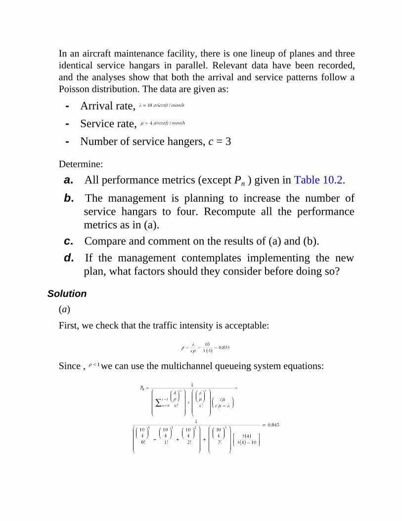
In an aircraft maintenance facility, there is one lineup of planes and threeidentical service hangars in parallel. Relevant data have been recorded,and the analyses show that both the arrival and service patterns follow aPoisson distribution. The data are given as:

- Arrival rate, - Service rate, - Number of service hangers, c = 3

Determine:

a. All performance metrics (except Pn ) given in Table 10.2.

b. The management is planning to increase the number ofservice hangars to four. Recompute all the performancemetrics as in (a).

c. Compare and comment on the results of (a) and (b).d. If the management contemplates implementing the new

plan, what factors should they consider before doing so?

Solution(a)

First, we check that the traffic intensity is acceptable:

Since , we can use the multichannel queueing system equations:

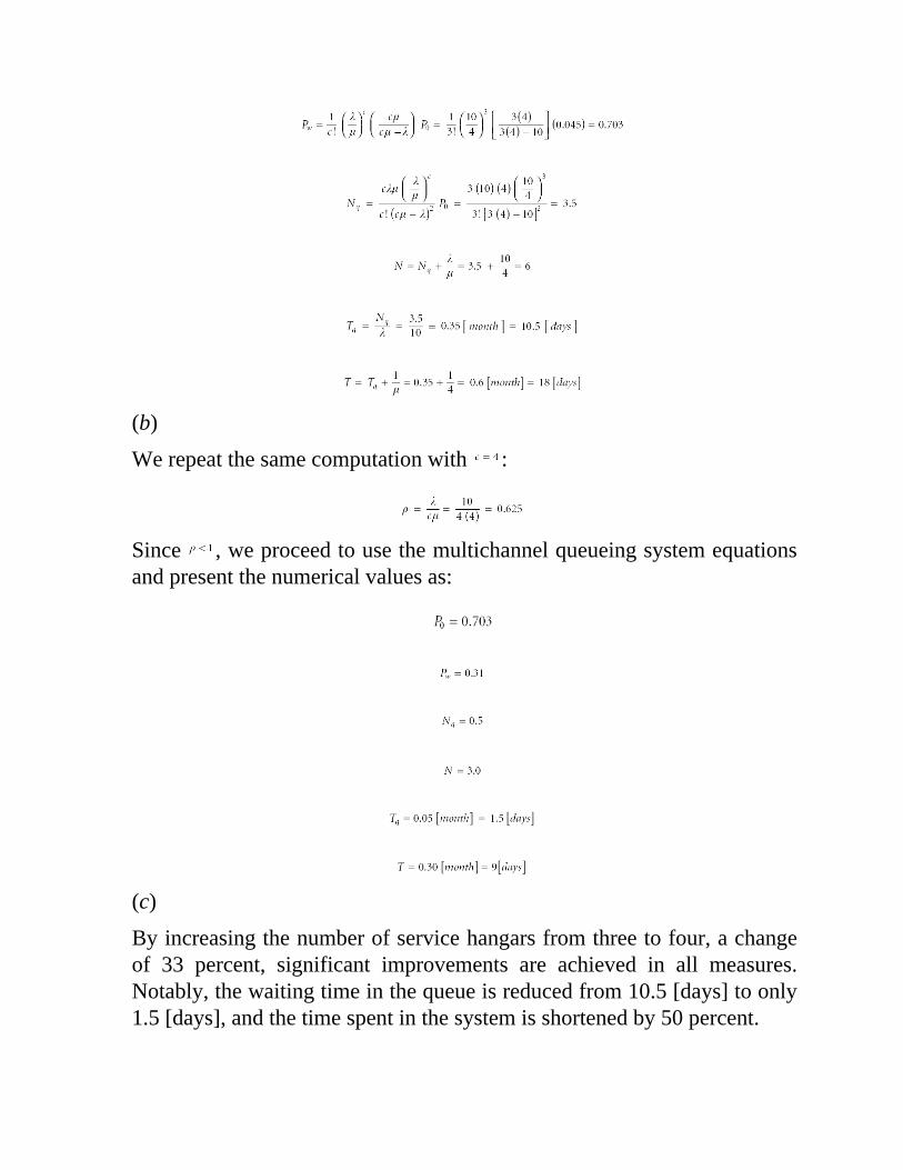
(b)

We repeat the same computation with :

Since , we proceed to use the multichannel queueing system equationsand present the numerical values as:

(c)

By increasing the number of service hangars from three to four, a changeof 33 percent, significant improvements are achieved in all measures.Notably, the waiting time in the queue is reduced from 10.5 [days] to only1.5 [days], and the time spent in the system is shortened by 50 percent.

(d)

The investment in an extra service hangar will certainly be substantial. Onthe other hand, time reduced in waiting can be used for flying. Themanagement must, on the basis of the number of aircraft serviced per year,and the time saved per aircraft, determine the potential annual incomefrom additional flying time, compare it with the cost investment capitalrequired, and make the appropriate decision.

EXERCISES

10-1 In using the queueing theory, why should the trafficintensity (utilization factor) be less than unity?

10-2 Assume a single-channel queueing system with arrivalrate λ and service rate µ. Then assume another queueingsystem with arrival rate of 2λ, service rate µ, and twochannels in parallel. Select and determine someperformance metrics and compare the two systems.Comment on your observations.

10-3 In a similar fashion to Exercise 10-2, using all the metricsin Table 10.1 compare two queueing systems: one witharrival and service rates of λ and µ, and the other witharrival and service rates of 2λ and 2µ.

10-4 Cargo ships arrive at a port according to a negativeexponential distribution of inter-arrival time, at a rate ofone every five hours. The time a ship spends at a dock forunloading and loading also has a negative exponentialdistribution, and its average is eighteen hours. The portoperates twenty-four hours a day, and there is a plan toincrease the number of docks to keep average waitingtime below nine hours. How many docks in total shouldthe port have to accomplish this?

Chapter

11APPLICATION OFPRINCIPLES

11.1 INTRODUCTION

In the previous chapters, we addressed some fundamental concepts and afair range of techniques that have proven useful in the field of industrialengineering.

The concepts covered in the previous chapters can be appliedindividually in many manufacturing and service industries. Every concepthas reducing cost and inefficiencies as its goal, and, consequently,ensuring a better return on investment of capital, time, or effort.

It makes sense, however, to be in a position to apply as many ideas aspossible from the preceding chapters, bearing in mind that no twoorganizations are exactly alike. They have different sizes, missions, stylesof management, and unique facilities and personnel; thus, any treatmentmust fit the goals of the organization. In this last chapter, we consider howwe can make collective use of these techniques to impact the entireorganization on a large scale.

The first step is to master the fundamentals of industrial engineering andgain experience in their application in various settings on modestproblems. The next step is the study of advanced and dedicated books onsubjects of interest and the handling of larger problem cases and projects.

In putting it all together, there are several industrial engineering,operations management, and controls techniques available. Thesetechniques work at the macro-level and encompass the organization in itsentirety. They aim to improve the quality of the products and services and

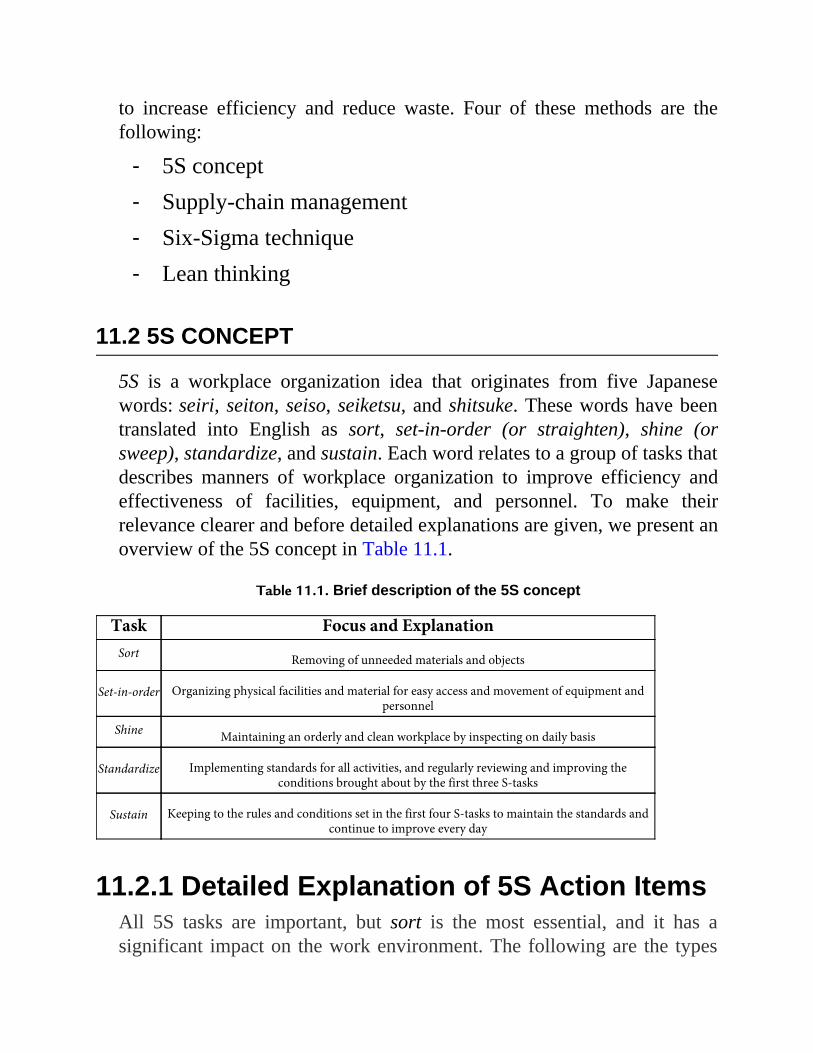
to increase efficiency and reduce waste. Four of these methods are thefollowing:

- 5S concept- Supply-chain management- Six-Sigma technique- Lean thinking

11.2 5S CONCEPT

5S is a workplace organization idea that originates from five Japanesewords: seiri, seiton, seiso, seiketsu, and shitsuke. These words have beentranslated into English as sort, set-in-order (or straighten), shine (orsweep), standardize, and sustain. Each word relates to a group of tasks thatdescribes manners of workplace organization to improve efficiency andeffectiveness of facilities, equipment, and personnel. To make theirrelevance clearer and before detailed explanations are given, we present anoverview of the 5S concept in Table 11.1.

Table 11.1. Brief description of the 5S concept

Task Focus and ExplanationSort Removing of unneeded materials and objects

Set-in-order Organizing physical facilities and material for easy access and movement of equipment andpersonnel

Shine Maintaining an orderly and clean workplace by inspecting on daily basis

Standardize Implementing standards for all activities, and regularly reviewing and improving theconditions brought about by the first three S-tasks

Sustain Keeping to the rules and conditions set in the first four S-tasks to maintain the standards andcontinue to improve every day

11.2.1 Detailed Explanation of 5S Action ItemsAll 5S tasks are important, but sort is the most essential, and it has asignificant impact on the work environment. The following are the types

of actions that must be undertaken in this step:

• Inspect the workplace and remove items that are notimmediately needed.

• Make work easier by eliminating obstacles.• Prevent hazards and accidents by removing unnecessary and

dangerous distractions.• Remove all waste material and scraps.• Improve and maintain the tidiness achieved.

In essence, sort provides a safe work environment and makes it easier tolocate the items that may be needed or be moved around the plant.

Set-in-order or straighten is a complement to sort. In fact, sort is moreabout clearing obstacles, and set-in-order is about organizing theremaining necessary materials and equipment. The following is a list oftypical action items:

• Arrange all necessary items so that they can be easilyaccessed when needed.

• Arrange work cells and workstation such that tooling andsupplies are in close proximity for easy access.

• Investigate design and tooling changes to improveefficiency.

• Establish a proper priority for accessing and borrowingtools. Often, First-Come-First-Served (FCFS) is a goodbasis, but it is not a universal rule.

• Make work flow smooth and easy.• Organize physical facilities for convenient and safe

movement of equipment, personnel, and material.• Improve and maintain the order accomplished.

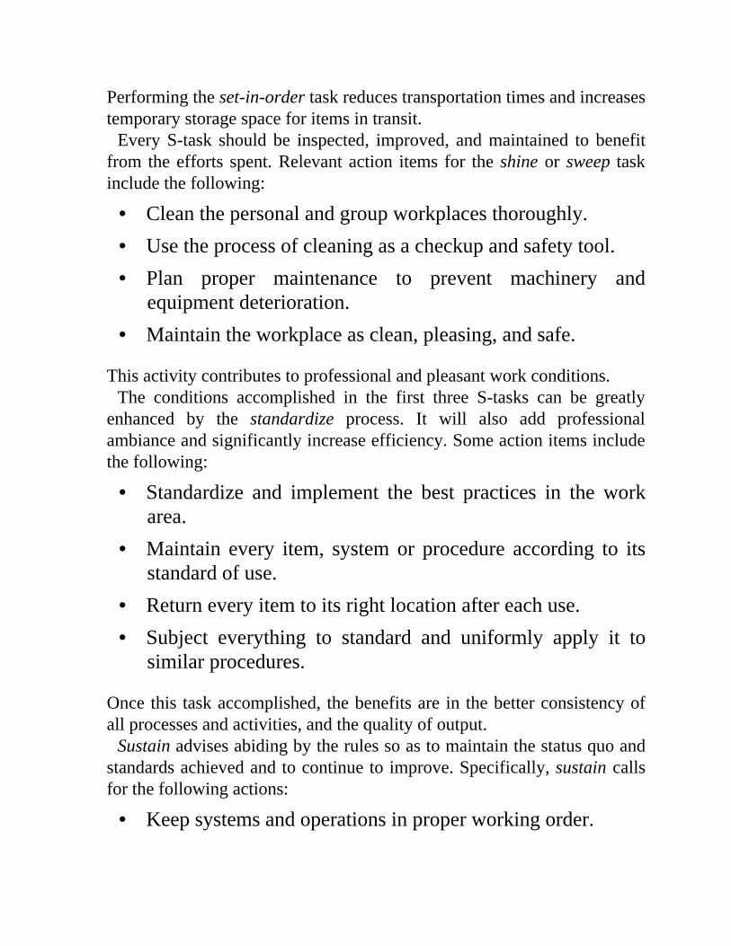
Performing the set-in-order task reduces transportation times and increasestemporary storage space for items in transit.

Every S-task should be inspected, improved, and maintained to benefitfrom the efforts spent. Relevant action items for the shine or sweep taskinclude the following:

• Clean the personal and group workplaces thoroughly.• Use the process of cleaning as a checkup and safety tool.• Plan proper maintenance to prevent machinery and

equipment deterioration.• Maintain the workplace as clean, pleasing, and safe.

This activity contributes to professional and pleasant work conditions.The conditions accomplished in the first three S-tasks can be greatly

enhanced by the standardize process. It will also add professionalambiance and significantly increase efficiency. Some action items includethe following:

• Standardize and implement the best practices in the workarea.

• Maintain every item, system or procedure according to itsstandard of use.

• Return every item to its right location after each use.• Subject everything to standard and uniformly apply it to

similar procedures.

Once this task accomplished, the benefits are in the better consistency ofall processes and activities, and the quality of output.

Sustain advises abiding by the rules so as to maintain the status quo andstandards achieved and to continue to improve. Specifically, sustain callsfor the following actions:

• Keep systems and operations in proper working order.

• Perform regular audits of systems and operations.• Use training and encourage discipline to sustain and

improve the achieved results.

This last step in the 5S concept prevents deterioration of the state of theimproved system.

Implementing the components of the 5S concept can be done by oneindividual depending on the size of the enterprise. However, it is alwaysdesirable that a small core team undertakes the entire implementationprocess, and along the way seeks input and further ideas from thepersonnel involved.

11.3 SUPPLY-CHAIN MANAGEMENT

Supply-chain management is the process of planning for a well-coordinated flow of goods, services, and information relating to six corecomponents of the supplier, manufacturer, distributor, logistics, retailer,and customer. Depending on the organization and the nature of itsactivities, the chain or, more generally, the link or network can berepresented in a variety of forms. Each component can also receivedifferent emphasis and importance for the same reasons. Figure 11.1shows a generic supply chain, and Figure 11.2 shows an example of acustomer-centered supply network. In fact, a supply chain can be thoughtof as a special case of a supply network; however, it has becomecustomary to refer to all forms of relationship and interaction between thefacilities and functions as a “supply chain.”

11.3.1 Principles of Supply-Chain ManagementSupply-chain management can be improved and coordinated in manyways. Its successful application in the manufacturing industry has led tothe development of seven effective principles. The essence of theseprinciples is given in definitions in the form of instructions.

Segment customers based on their needs. Not all customers are alike.

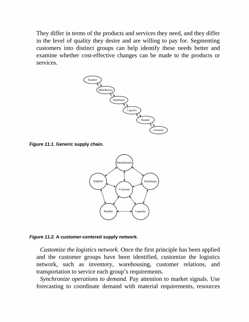
They differ in terms of the products and services they need, and they differin the level of quality they desire and are willing to pay for. Segmentingcustomers into distinct groups can help identify these needs better andexamine whether cost-effective changes can be made to the products orservices.

Figure 11.1. Generic supply chain.

Figure 11.2. A customer-centered supply network.

Customize the logistics network. Once the first principle has been appliedand the customer groups have been identified, customize the logisticsnetwork, such as inventory, warehousing, customer relations, andtransportation to service each group’s requirements.

Synchronize operations to demand. Pay attention to market signals. Useforecasting to coordinate demand with material requirements, resources

allocation, and scheduling of operations.Differentiate the product closer to the customer. This principle means

that one should keep the requirements, in terms of inventory, processes,and other necessary tasks, as common as possible, and only near the endand closer to the customer differentiate (categorize) the product andservices in the supply chain. This shortens the lead time and expedites thedelivery to customers.

Strategically manage the source of supply. Manage sources of suppliesstrategically to reduce the cost of acquiring materials and services. Thecheapest or closest sources of supply may not always be the best.Consistency and reliability in the sources of supply are essential to quality,on-time delivery, and customer satisfaction. In the long run, these translateto reduced costs of procurement.

Develop a supply-chain-wide technology strategy. Provide multiplelevels of decision making, giving a clear view of the flow of products,services, and information. The technology strategy should encompassinformation technology and other technologies to facilitate day-to-day andlong-term activities along the supply chain.

Use supply-chain-spanning performance measures. Develop through-the-chain end-to-end performance indicators to measure effectiveness andefficiency. Use the metrics to improve and control the processes.

11.4 SIX-SIGMA TECHNIQUES

Six-Sigma is a management philosophy composed of a set of techniquesfor process improvement. Essentially, Six-Sigma aims to improve thequality of the process output by identifying and eliminating the causes ofdefects, thereby minimizing the variability of the process. Six-Sigma isused in diverse manufacturing and service industries. It is based on qualitymanagement and statistical methods. Its implementation requires a team ofexperts in the field who work on a specifically defined project and followa defined set of steps to achieve the desired goal. Typical goals include,for example, reduced costs, reduced cycle time, or improved customersatisfaction—all through improving the quality characteristics of theprocess and its output.

A Six-Sigma process is designed such that 99.99966 percent of allobservations, occurrences, or “opportunities” should be defect-free, thecomplement of which will be 0.00034 percent or 3.4 defective occurrencesper million opportunities. Recalling the concept of three-sigma limits, usedin the discussion of the statistical quality control in Chapter 7, it is clearthat Six-Sigma calls for setting extremely rigorous performanceobjectives. This relates to collecting data, analyzing the results, anddeveloping and implementing a plan to reduce the defects in the processoutput.

Two methodologies have been defined for two areas of application, and,correspondingly, two acronyms have also been defined:

1. DMAIC (pronounced “duh-may-ick”) is used for projectsaimed at improving an existing process.

2. DMADV (pronounced “duh-mad-vee”) is used for projectsaimed at designing a new product or process.

DMAIC stands for the following five phases:

1. Define the system, the project goals, and the customerrequirements.

2. Measure the current key process, collect relevantperformance data, and calculate the process capability.

3. Analyze the data to investigate cause-and-effectrelationships. From the relationships, determine the rootcauses of the defect or the error.

4. Improve the process or fix the error based on the dataanalysis using techniques such as the design ofexperiments, simulation, brainstorming, and pilot runs.

5. Control the future process performance and ensure that anydeviations from the target are corrected in a timely fashion.Implement statistical process control and control charts,develop standards, and continuously monitor the process to

stay on course.

DMADV also has five phases and stands for the following:

1. Define design goals consistent with the customer needs andthe management strategy.

2. Measure and identify all characteristics that are critical toquality (CTQs), measure product and production processcapabilities, and assess risks.

3. Analyze products and processes, and make adjustments forimprovements.

4. Design an improved alternative, by assessing the enhancedprocess, and seeking feedback from test-based-customers.

5. Verify the design as final, implement the process, andcontinue monitoring the product and customer feedback.

According to the Motorola company, who initiated the Six-Sigmamethodology, the standard Six-Sigma processes are executed byprofessionals designated as Six-Sigma Green Belts or Six-Sigma BlackBelts, whose work is then overseen by Six-Sigma Master Black Belts toensure total compliance with the concepts.

It has been reported that by implementing Six-Sigma technique, up to 50percent process cost reduction, cycle-time improvement, and less waste ofmaterials can be achieved. Adopting and committing to Six-Sigma can becostly and may take several years before a company begins to realize thebenefits.

11.5 LEAN THINKING

The emphasis in Six-Sigma is on eliminating defects and reducingvariability in processes and their output. Lean thinking is a similarconcept, but it focuses on eliminating waste and coordinating activitiesfrom end to end. This will lead to optimality in all aspects of the operation

of an enterprise. It was primarily intended for the automotive industry as“lean manufacturing,” but the concept has been expanded in its scope ofapplication.

Lean ThinkingSome variants of lean thinking include the following:

- Lean manufacturing- Lean Sigma- Lean supply chain

In fact, lean thinking can be applied in any enterprise, when itsfundamental concepts have been understood. With reference to leanmanufacturing, the core concept of lean thinking is based on threeJapanese words.

In English muda means waste. As a process in the lean concept, it meansthe elimination of waste and loss. Excess inventory of parts with no added-value, unnecessarily occupied space, and avoidable costs are all primeexamples of resources wasted.

Seven key resources that can benefit from muda have been identified asthe following:

1. Transportation: moving products that are not required inthe processing

2. Inventory: raw materials, work-in-progress, and finishedproducts not being processed

3. Motion: unnecessary moving of equipment and walking ofpersonnel

4. Waiting: idle and waiting for the next processing step.5. Overproduction: producing excessive product inventory

ahead of demand6. Overprocessing: a consequence of improper design and

process planning

7. Defects: the effort needed to inspect for defect and applythe corrections

In English muri means overburden. As a lean concept activity, it meansbalancing the production activities and arriving at the most appropriateproduction pace.

In English mura means irregularity or variability. In lean terms, it meansthe elimination of unevenness by balancing machine capacity andautomating and task sharing by personnel.

Indeed, to fully benefit from the application of any of the 5S, supply-chain management, Six-Sigma, and lean thinking philosophies,management must be committed to providing facilities and a certain levelof freedom, capital, and personnel. And the personnel charged withimplementing the techniques must bear in mind the duties we outlined atthe beginning of the book in Section 1.2.

EXERCISES

11-1 Using the concept of 5S, prepare a list of action items inyour personal work environment.

11-2 As a follow-up to Exercise 11-1, develop a list of actionitems for your section in your work place.

11-3 Identify by name the six elements of the supply chain inyour place of work. Then, by properly connecting theelements, determine whether they form a straight supplychain or a supply network.

11-4 In extension to Exercise 11-3, investigate theapplicability of the seven principles of supply-chainmanagement.

11-5 With reference to Six-Sigma, explore the applicability ofDMAIC and DMADV in your workplace.

11-6 Reexamine Exercises 11-1 to 11-5 for a hypothetical orexisting company of your choice.

11-7 In any of the above exercises, do you notice any potentialgains? If so, make a list and provide a few action itemsfor each.

Appendix A EFFECTIVE MEETINGS*

Between 35 and 50 percent of any manager’s time is spent in meetings ofone kind or another; many managers would put it even higher than this.Yet the conduct and outcome of meetings are often criticized severely. It isnot uncommon to hear comments such as: “A committee is a body ofpeople who keep minutes and waste time”; and “A meeting is a process bywhich a body of people decide when to have the next meeting.” There issome truth in these comments and many valuable manpower hours can bewasted by ineffectual meetings, both formal and informal. Too often, thisis because the person officially in charge of the meeting is ill prepared,lacks the expertise to lead and control a group, or is unaware of thecommunication problems that may arise. It may also be because those whoattend the meeting have been briefed inadequately about the intendedcontent. In this case, they, too, will lack preparation or arrive with hiddenagendas—objectives of their own which have little to do with the originalaims of the meeting. These will often dominate the discussion. Thepurpose of the material presented here is to improve the effectiveness ofyour meetings; saving you time, effort, money, and a great deal offrustration.

WHAT IS A MEETING?

A meeting is an occasion when a group of people comes together to shareideas and experiences. Meetings widely differ in size, composition,

organization, and purpose, but they all have certain things in common.They should all do the following:

• Exist for a purpose.• Involve people communicating with one another.• Have someone in control.

It is fundamental to the success of any meeting that its purpose is clear andrelevant. Unless the meeting serves a useful purpose, it not only wastestime and effort but it can cause frustration, misunderstanding, andgenerally demotivate people. Meetings can become an end in themselves.This is particularly the case of regular meetings, which tend to take placebecause they always have. Regular meetings do have uses, but it isessential that there is some worthwhile business to discuss.

INFORMAL AND FORMAL MEETINGS

DifferencesInformal meetings do not have a constitution, a set procedure, or specificneeds for documentation; they are usually called and controlled by themost senior member present, in order to meet the requirements of routineplanning or problem solving. They can be advisory in nature—the seniormembers retain the right to make the final decision. The majority ofmeetings held at work are of this type. Yet far too little consideration isgiven to the methods by which they are conducted and to their results. Theperson controlling the meeting has to achieve two basic objectives: toaccomplish a task and to maintain the group as a team working towardthis. “Informal” does not mean “unstructured.”

Formal meetings always have a set constitution and procedure, as well asbasic terms of reference. These are defined by memoranda, articles ofassociation, acts of parliament, standing orders, or other forms of writtenconstitution, according to the type of institution, public body, ororganization in which they take place and the requirements of companylaw. Formal meetings have officers to conduct their business and record

their proceedings and are controlled by a chairperson or president, who iselected or appointed and has well-defined duties. Meetings can beexecutive in nature, and decisions are taken by voting. Writtendocumentation is an essential requirement. As the procedure is laid down,such meetings are perhaps a little easier to control but the main objectives,as for informal meetings, are just as relevant. Having contrasted the twotypes of meetings, it is worth seeing what they have in common.

SimilaritiesThe similarities between these two broad divisions lie in the generalobjectives and aims and in the problems of leadership and control, whichare common to both. Meetings serve a variety of purposes but basicallythey should be concerned with the following:

• Giving information or instruction• Gathering information or opinions• Persuading• Planning• Problem solving• Decision making• Initiating action

The way they are organized and the role of the leader of the meeting varyaccordingly.

Categories of Informal MeetingsInformal meetings is the broad term covering a number of categories andthese can be defined as follows:

• The briefing meeting. This is usually called by a manager inorder to give instruction to the work group, to train them innew tasks, or to plan work. It is a highly useful method ofcommunication, giving people an opportunity to interpret

policy, test opinion, and provide personal explanations. Itallows people to ask questions and clarify for themselveswhat is required. It may even result in new points andproblems being raised, which the manager may not haveconsidered, thus avoiding difficulties in advance.

• The progress meeting. This meeting reviews the progress ofwork, in discussing the problems that have arisen,measuring achievement, and planning further action. Theadvantages are similar to those of the briefing meeting. Inaddition, it allows problems to be detected and discussed atregular intervals so that they can be remedied quickly.

• The planning meeting. Similar to the previous two types,this meeting may initiate a project, plan its strategy, andallocate work to the appropriate people. Its main purpose isto achieve a rational approach to the task, in consultationwith all those who can offer expertise or who will take partin its completion, thus taking advantage of their advice andachieving their support.

• The problem-solving meeting. This is usually called to dealwith a particular emergency or solve an important problemthat has arisen. All those who can offer advice, evidence,help, or expertise should be consulted in order to getadequate information to reach a solution.

• The brainstorming meeting (also called a “buzz group”).Connected with the two preceding categories, this is aparticular approach that can be taken when planning (forexample, the marketing strategy of a new product) orproblem solving, when the causes of the problem may beparticularly diverse, complex, or impenetrable. It is the mostunstructured of the meetings, as anyone present has a right

to call out any ideas, which may give a “lead.” These areusually recorded on a flip chart or board. The elimination ofthe impossible or unlikely ideas is then followed up by anopen discussion of the others until a few possiblealternatives are chosen for further consideration anddevelopment.

Categories of Formal MeetingsThis category in industry and commerce covers such things as annualgeneral meetings and board meetings, which we will not discuss here.

THE RESPONSIBILITIES OF THE MEETING LEADER

The leader of any meeting has a variety of responsibilities, which includethe following:

• Defining the purpose of the meeting• Planning and preparation• Conducting the meeting efficiently• Controlling the discussion without doing all the talking• Dealing effectively with problem situations and individuals• Ensuring that the meeting keeps to the schedule• Making sure everyone participates in the meeting• Making sure the purpose of the meeting is achieved, and the

members know what is expected of them as a result• Liaising with the secretary, if there is one, to ensure that an

efficient recording mechanism exists when requiredIn many instances, the secretary of the committee or meeting will takeresponsibility for organizing the date, time, and place of the meeting. Thesecretary may also draw up and circulate the agenda and write and

distribute minutes. For maximum efficiency, there needs to be some levelof consultation between the meeting leader and secretary about the agendaand minutes.

PLANNING AND PREPARATION

A well-planned meeting has much greater chance of success than the onethat is called with five minutes’ notice and has not been well thought out.There are four areas where planning and thorough preparation can assistthe leader of the meeting:1. Defining the purpose of the meeting2. Planning the content of the meeting—the “agenda”3. Deciding who should attend and for how long4. Planning the domestic arrangement for the meeting

Defining the Purpose of the MeetingTwo questions need to be answered: What is the purpose of holding thismeeting? Is the purpose best achieved by holding a meeting?

Many meetings are ineffective because the purpose is not clear. Thisapplies especially to regular monthly meetings, for example. The mainpurpose of these sometimes seems to be the self-perpetuation of themonthly meetings.

It is, therefore, crucial that the person calling the meeting asks thequestion “what is the purpose” before doing anything else. It is sometimesa good idea to write the purpose down in one or two sentences so that it isclear and can be stated at the beginning of the meeting, if necessary. Oncethe purpose is defined, the second question should be asked. Sometimesthe assumption is automatically made that the meeting is necessary when,in fact, several telephone calls, messages or a memo would serve as well.If the leader cannot clearly state the purpose of the meeting being called, ameeting is usually not necessary at all.

Planning the Content of the Meeting—the “Agenda”

For any meeting to succeed, the participants need to have a good idea ofwhat is going to be discussed, and why they are there. The most effectiveway of ensuring this is to distribute an agenda detailing the topics to bediscussed, who is to be there, where the meeting is to be held, and, ifpossible, the approximate time the meeting will take. In the case of aregular meeting the participants, timing and venue will normally remainthe same and need not be highlighted each time. The agenda should fulfilltwo basic functions:

1. To inform the members of the topics to be dealt with, whythey are being discussed, and what contribution is required

2. To act as a structural basis for discussion

The agenda should be as detailed as necessary and not just a list ofheadings. Checklist 1 details the stages necessary in the preparation of anagenda. This may be done by the secretary, but it is essential that themeeting leader is aware of the function and purpose of the agenda at thisstage. The meeting leader also needs to plan a rough guide of how themeeting will be conducted. The actual skills of chairing will be importanthere and are detailed in a later section.

Planning the Arrangement for the MeetingThe leader is responsible for calling the meeting and deciding who is toattend, although, in some instances, the secretary will carry out this duty,together with booking the room and the time. Three points are worthmentioning here.

1 Recording the MeetingIn all cases, it is essential that someone be appointed to take notes orminutes. One of the main causes of unsuccessful meetings is the decisionof the meeting leader to take notes. Neither role can be carried outeffectively by the same person. Conflicts of interest may arise if the notetaker is also a participating member of the meeting. Ideally, someone whois fully competent with the subject matter but not directly involved is inthe best position to take notes. Where this is not possible, the note takingcould be organized on a rotational basis, among those attending.

2 The Meeting PlaceThe meeting place should be comfortable and convenient and as free fromnoise and interruptions, such as telephone calls and “through traffic” ofother people as possible.

3 Cooperating with the SecretaryThe meeting leader and the secretary (or note/minute taker) can benefitfrom having a short get-together before the meeting starts. The followingtopics can be discussed:

• Technical terminology: if the secretary is unfamiliar withany of the terminology used, the meeting leader can explainsome of the words and terms most likely to arise.

• Structure of the meeting: how the meeting will be chaired.• Type of the minute needed: they can decide on the type of

minutes needed, that is, action notes, verbatim record,threads of discussion and decisions, and so on.

• Summarizing: the secretary can encourage the use ofsummaries to make the note taking easier.

• Clarifying the decision: the secretary can establish theacceptability of interrupting the meeting for clarification ifthe secretary is unsure of what to note down for minutes.

Cooperation between both parties is essential to the success of meetingsand will prevent lengthy drafting and redrafting of minutes afterward.

THE SKILLS OF CHAIRING MEETINGS

The leader of a meeting should have a number of skills to help maintaincontrol of the discussion during meetings. The leader should not do all thetalking and should ensure that everyone participates and no particularmembers dominate.

Opening the Meeting

The leader should open the meeting in a friendly but businesslike manner.This will help create the right climate. The meeting should start with anintroductory statement summarizing what the meeting is for, what isknown, what is required, and how it is going to be tackled.

Conducting the MeetingIn terms of leadership and control, there are two sets of specific objectivesfor the leader. The first set relates to the achievement of the task itself; thesecond refers to the control of the group working on that task. In eachcase, there are various functions, which the leader should perform. Thesecan be listed as follows.

Task Functions

These keep the group working on the task or project and include thefollowing:

(a) Initiating—proposing tasks and goals, defining the groupproblem and suggesting procedures or ideas

(b) Information/opinion-seeking—requesting facts, seekingrelevant information and asking for suggestions or ideas

(c) Information/opinion-giving—stating a belief andproviding relevant information

(d) Summarizing—pulling together related ideas, restatingsuggestions after the group discussion, and offering adecision or conclusion for the group

(e) Clarifying—elaborating, interpreting, or reflecting ideas,restating suggestion, clearing up any confusion, indicatingalternatives and issues, and giving examples

(f) Consensus testing—checking to see how much agreementhas been reached

(g) Action planning—delegating the tasks, now agreed, tothose appropriate, and confirming them in writing

Human Relations or Group Maintenance Functions

These ensure that the group works as a team to achieve the objectives.They include the following:

(a) Encouragement—being friendly and responsive to thegroup, accepting contributions, and giving opportunitiesfor recognition

(b) Expressing group feelings—sensing feelings, moods, andrelationships within the group and sharing one’s feelingswith others

(c) Harmonizing—attempting to reconcile arguments and toreduce tensions, and getting people to explore theirdifferences (not always an easy task)

(d) Modifying—staying conflicts-free, by adjusting stand tobe able to admit error and maintain self-discipline forgroup cohesion (this function is particularly difficult forsome)

(e) Keeping the channels of communication open—ensuringparticipation by providing procedures for discussion

(f) Evaluating—expressing standards for the group toachieve, evaluating the achievement, and the degree ofcommitment to action

The leader should be aware of the needs of the group and should draw outsilent members and control the talkative. The leader should prevent privatediscussions in splinter groups. The leader’s participation will varyaccording to the type of meeting, but it should be remembered that themaximum involvement of the leader means minimum participation by themembers

Conducting the MeetingAchievement of the objective is the whole purpose of the meeting. The

leader needs to establish and emphasize this achievement and commendindividuals and group contributions. Even if the result has not beenentirely satisfactory, the leader should try to emphasize the positive aspect.The leader should make a final summary confirming the conclusions of themeeting and highlighting action and who is to take it.

SummariesThe use of interim and final summaries is one of the most powerful skillsavailable to the leader.

Interim summaries serve to accomplish the following:

• Indicate the progress or lack of it.• Refocus off-track discussions.• Tie up one point and move to the next issue.• Highlight important points.• Guide the minute taker.• Clarify misunderstandings.

The final summary establishes the group’s conclusions, points to action,and gives members a sense of what has been achieved. Both interim andfinal summaries should be presented to the members for their agreement.This practice will also help the minute taker and cut down on unnecessaryargument about the accuracy of the minutes.

PROBLEM SITUATIONS

The meeting leader may also have to deal with difficult situations inmeetings, not only because of the subject matter, but also the followingissues.

Unpopular DecisionsLeaders may find themselves under attack from individuals or the wholegroup. They must be prepared to present their case, acknowledging the

weaknesses, anticipating the opponent’s objections, and emphasizing thepositive aspects. If there are members of the group in support of the case,encourage them to express their views—they may carry more weight thanthose of the leader.

Bad NewsThe leader must try to find a positive side.

Lack of InterestThe leader must recognize that every item on the agenda cannot be ofequal interest to everyone. The likely causes of this are the following:

• The wrong items have been selected.• Too many items are being dealt with, so attention wanes.• The case is poorly presented so that relevance to members is

not clear.

Some remedies are the following:

• Direct questions to individuals, for example, “How does thisaffect you?”

• Drop the subject entirely and return to it later, dealing witha more interesting subject in the meantime.

Discussion Going off TrackThis may be indicative of a lack of interest. The group may start talkingabout other things or asking irrelevant questions. If there is genuineconcern over something else, which is worrying the group, it is best to dealwith it. Otherwise, frequent summarizing will help keep the discussion oncourse.

Status DifferencesIt is the leader’s responsibility to protect the weaker members of thegroup. If there are more junior members present, it is often a good idea toask for their thoughts first. They may be unwilling to express a view once

more senior members have made their position clear.

People ProblemsPerhaps the most difficult problem of leadership and control is one thatconcerns human relations—the individuals in the group have differentpersonalities and objectives, which conditions how they behave. Althoughit is out of the scope this book to discuss the psychology of individuals andgroup dynamics, it may be worth giving some general principles:

• Every group contains those who wish to talk and those who,for a variety of reasons, are silent. It is a mistake to supposethat the extrovert talkers have necessarily the greatestcontribution to make. Those who listen may have learnedmore and may have considerable expertise.

• In order to involve those who are silent, one or twostrategies can be used. A procedure should be developed bywhich each person is asked for a contribution in turn, or thespeaking time of those who normally have a great deal tosay should be limited by inviting someone else to comment.Those members who are shy (or withdrawn for some otherreason) should be asked questions about their particular areaof expertise. This combines the advantage of asking themsomething, which they find easy to answer, thus developingtheir self-confidence and giving them special recognition, towhich they are likely to respond.

• If a conflict develops between two members of a group, therest of the group should be asked to comment on the twosides. This avoids driving the conflict underground, where itis likely to smolder, leading to withdrawal and frustration.This is sometimes known as “the conference method.”

• If aggression is shown toward the leader, the leader mustparaphrase the aggressive statement in a milder form and

ask the group to comment. If it becomes evident that thereis truth in what is said, the leader must be prepared tomodify his or her position. This should not be considered“backing down” but as a step that allows progress toward anew position.

• If it becomes evident that some members of the group arerepeating themselves and holding on tenaciously to oneview only, the discussion should be stopped and thealternative views expressed should be summarized. Often itis helpful to do this in writing if a visual aid is available (aflip chart or board in the room is useful). This preventsthose members from retaining a mental image dominated bytheir view and can be used to move the discussion forward.

• When agreement seems to be present, a true consensus mustbe reached before defining what actions should be taken andallocating tasks. Otherwise people will depart from themeeting still in disagreement and proceed to sabotage therecommended action by expressing doubts to others—oftentheir own subordinates.

• The leader must ensure that everyone knows what action isexpected and that the meeting is not closed until this isdecided. Too many meetings appear ineffective to thosewho have attended them because they leave unsure of whathas been achieved and what results are expected. There ismore motivation and satisfaction if they are certain on thesefronts. A written reminder (action notes or minutes) mayhelp.

STATING A CASE AT A MEETING

The best preparation and planning can be lost if someone finds it difficult

to express their case coherently. Some people find it particularly difficultto put over their ideas to a group and will remain silent for fear of beingridiculed if they speak. Effective speakers know exactly what they want tosay, have something to say, and say it well. In contrast, ineffectivespeakers are never clear in their own minds as to what they intend to say.As they speak, they move about in verbal confusion, following no set planand developing no relevant argument.

Some of these problems can be overcome by following the guidelinesbelow:

• Be sure of the facts. Sum them up briefly, and define anyterms that need explaining. State the proposition.

• Face the facts. Weigh what is against you and anticipateobjections. This also acts as a check on the soundness ofyour reasoning.

• Prove your case by selecting and highlighting the bestreasons for the proposition. The strength of the argumentwill depend on the quality, not the quantity of your reasons.

• Show solid evidence. Have examples available to supportthe fact, but be careful not to slant the evidence to suit thecase.

• End by repeating the proposition.

By following these simple rules and by having thought out the argumentsbefore the meeting, persuading people to support your viewpoint will bemade simpler.

MINUTES AND FURTHER FOLLOW-UP ACTION

It is essential that minutes are produced, but they will vary depending onthe type of meeting. Formal committees sometimes require detailedminutes, whereas informal meetings may produce only an action list ofthings to be done as a result of the meeting. Whichever is the case, it is

important that minutes do the following:

• Are produced quickly• Are accurate• Are not a verbatim report• Show what action is required and by whom

Checklist 2 provides guidance on taking notes and writing up the minutes.The leader of a meeting should note the following points, which will helpthe minute taker to produce accurate and concise minutes:

• Summarize at the end of each point on the agenda. In mostinstances this is all that is required in the minutes, and asummary will help the minute taker, especially if thematerial is unfamiliar.

• Explain any unfamiliar terms or expressions, particularlytechnical jargon, which may be used during the meeting.

• Encourage the secretary to interrupt if a point has not beenfully understood.

Where follow-up action is required, it is important to monitor progress.Giving individuals deadlines for follow-up action is useful. “As soon aspossible” means something different to different people. If precise datesare given during the meeting and recorded in the minutes, monitoringprogress is a much more straightforward task.

CHECKLIST 1: THE AGENDA

Subject MatterDecide what topics need to be included on the agenda. It is alwaysworthwhile, especially in the case of regular meetings, to check with thoseattending to see if they have any items they wish to include.

Avoid Being Vague

Do not have a vague heading “matters arising from the minutes.” Ifmatters need to be discussed against, place them on the agenda as specificitems. The term any other business is often the cause of uncontrolled andtime-wasting discussion. If members are asked beforehand whether theyhave items for inclusion on the agenda, a formal “Any Other Business”can quite easily be left out. This does not prevent last-minute items frombeing discussed, but it will prevent long, rambling, and unstructureddiscussions from taking place.

Be LogicalPut the items in a logical sequence. This will be decided by the following:

• The urgency of the items• The length of the time each item will take

Try not to waste the first hour on trivialities and then run out of time forreally important issues.

TimingThere are four aspects to timing.

1 The Actual Time Available for the MeetingThis will be determined by the other activities in the working day as wellas the commitments of those participating in the meeting. A very lengthymeeting tends to be demotivating, especially if little progress is made.Short meetings encourage people to keep to the point. Frequent meetings(for example, weekly interdepartmental meetings) usually need less timethan the less frequent ones (for example, quarterly management reviews).

2 The Time of DayMost people will have attended the dreaded Friday afternoon meetingwhen others are concentrating on getting home for the weekend and not onthe meeting. The actual time of day needs to be thought out carefully so asto cause the least disruption to all concerned. If one wants a short meeting,start it just before lunch.

3 The Amount of Time to Spend on Each ItemThis will be determined to some extent by the amount of time available forthe whole meeting. Some items may have to be left off the agendaaltogether and discussed at a separate meeting. It is a good idea to workout a rough plan of how much time is available for each item individually.This may also be put on the agenda itself to act as guidance for eachmember. It is useful when asking for a contribution to the agenda to askhow much time will be needed for each item.

4 Start on Time and Finish on TimeStarting on time, even if a participant is late, shows that one meansbusiness, and it will encourage punctual attendance. Finishing on timeencourages brief, meaningful contributions and also lets participants get onwith their other tasks.

Give GuidanceMake sure each topic is described in enough detail so that members maycome fully prepared.

CirculateCirculate the agenda in a timely fashion before the meeting. Remember toattach any relevant reports or written briefs to the agenda and ensureparticipants receive them in advance.

CHECKLIST 2: THE MINUTES

There are two aspects to producing minutes: taking the notes and writingup the minutes/action notes

Taking Notes

i.

Listen carefully throughout the meeting, in particular, for theleader’s interim and final summaries for guidance. Ifnecessary, ask the leader for a summary during the meeting ifimplications of the discussion are not clear.

ii.

Take brief, relevant notes under each agenda item. Leave spacebetween items in case the discussion returns to an earlier point.This saves time on sorting out afterward which notes arerelevant to which points. Record the main points raised (by theimportance of contribution, not length) and record the action tobe taken by whom, and, if relevant, by when.

iii.Check that notes are satisfactory after the meeting. Ifinformation is missing or vague, check with the relevantmember.

Writing the Minutes/Action Notesi. Draft the minutes as soon as possible after the meeting.

ii. Keep all notes until the minutes have been approved (this isusually done at the next meeting).

iii.Be selective—be accurate, brief, and clear with the writing.

iv.Specify any action required in a separate column, indicatingthe name of the person concerned and, if appropriate, the targetdate.

v. Structure the minutes so they follow the structure of the agendaand avoid complicated numbering systems.

vi.Circulate the minutes as soon as possible after the meeting,having first checked them with the leader.

* “Effective Meetings” has been reproduced with the kind permissions of its author, Dr. Ghulam Shabir,managing director of DGS Pharma Consulting Ltd. and the Institute of Manufacturing, UK. Theoriginal manuscript appeared in volume 3, number 4 (2002) issue of the institute’s InternationalJournal of Manufacturing Management. The manuscript has been revised to fit the tone and languageof the book.

Appendix

BEFFECTIVEPRESENTATIONS

It is often necessary to make a presentation on a topic in a seminar-likeformat using software applications, such as PowerPoint. Specifically, inthe business, service, and industrial settings an oral presentation may berequired for many reasons including the following:

- Proposal for a new idea- Budget and financial report on expenditure and income- Progress report on a project

An engineer in the role of an industrial engineer/manager is likely to befrequently in a position that requires a presentation. An accurate and well-prepared presentation goes a long way in convincing the audience andgaining support for a new endeavor, for instance. As a complement toAppendix A, we highlight some key points for preparing an effectivepresentation.

PREPAREDNESS

1. Prepare the required material ahead of time.2. Check your draft carefully at least a couple of times.3. Check the conditions, availability and type of audiovisual

equipment and other materials ahead of time.4. Have a second copy of your presentation available, in a

medium suitable for the audiovisual equipment used, if theneed arises.

5. Rehearse your presentation to control timing. If possible,try to rehearse your speech out loud. This will give you abetter indication of the timing than whispering to self.

6. Arrive at the seminar location five minutes ahead ofschedule.

SPEAKING STYLE

1. Relax and be in control.2. Speak loudly and clearly; do not shout.3. Face the audience; look at everybody in the room and not a

particular section.

QUALITY OF THE PROJECTED TEXT

1. Use a proper font size.2. Use short/simple equations, and not too many.3. Use headings and subheadings.4. Use short sentencelike descriptions, and paraphrase them

in your speech.5. Use clear drawings and plots with legible captions.6. Use clear photographs. There is no need to include dark or

unclear images and then apologize for their inferior quality.The same applies to any audio-video clip.

QUALITY OF PRESENTATION CONTENT

1. Introduction: succinctly highlight what it is all about.2. Justify the relevance of the work.3. Be sure of the accuracy and reliability of the material.4. State the position of the material in the context of existing

knowledge, that is, references:(a) Do not forget them.(b) Do not just list them!(c) Briefly, discuss their relevance, shortcomings, and so

on.5. Clearly explain the theory/idea proposed.6. Give key information about the

approach/methods/equipment/experiments used.7. Explain the physics/mathematical treatment/assumptions

considered.8. Highlight the expected or achieved results and

contributions made.9. Discuss the results (if available). The discussion should not

be limited to a plain explanation of numbers and graphs. Adiscussion highlights the reasons for a particular resultobtained, or how it can be affected.

10. End with a solid conclusion. A conclusion is not asummary; it explains what is learned and what iscontributed.

OTHER QUALITIES

1. The content of the presentation must be suitable for theexperts as well as for the novice in the field. This is, ofcourse, a tough task to accomplish.

2. Respond to questions clearly, giving short, to-the-pointanswers so as to provide the opportunity for more people toask questions.

3. In your answers, treat the audience with respect!

BIBLIOGRAPHY

Aft, Lawrence S. Fundamentals of Industrial Quality Control, CRC Press, 1988.Allen, Theodore T. Introduction to Engineering Statistics and Six Sigma: Statistical Quality Control and

Design of Experiments and Systems, Springer, 2006.Ashore, S. Sequencing Theory, Springer-Verlag, 1972.Baker, Kenneth R. Elements of Sequencing and Scheduling, Kenneth R. Baker, 1993.Basu, Ron.Implementing Six Sigma and Lean—A Practical Guide to Tools and Techniques, Elsevier,

2009.Bedworth, David D., and Bailey, James E. Integrated Production Systems, Wiley, 1987.Blanchard, Benjamin S. Logistics Engineering and Management, Prentice-Hall, 1986.Bridges, William.The Character of Organization, Consulting Psychologists Press, 1992.Chandra, M. Jeya.Statistical Quality Control, CRC Press, 2001.Chase, Richard B., and Aquilano, Nicholas J. Production and Operations Management, Irwin, 1995.Conway, Richard W., Maxwell, William L., and Miller, Louis W.Theory of Scheduling, Addison-Wesley,

1976.Elbert, Mike.Lean Production for the Small Company, CRC Press, 2013.Elsayed, Elsayed A., and Boucher, Thomas O. Analysis and Control of Production Systems, Prentice-

Hall, 1985.Evans, James R. Applied Production and Operations Management, West Publishing, 1993.Evans, James R. Production/Operations Management—Quality, Performance, and Value, West

Publishing, 1993.Evans, James R., and Lindsay, William M. The Management and Control of Quality, West Publishing,

1993.Field, S. W., and Swift, K. G. Effecting a Quality Change, Arnold, 1996.Francis, R. L. Geometrical Solution Procedure for Rectilinear Distance, Minimax Location Problem, AIIE

Transactions, 1972.Francis, R. L., and White, John A. Facility Layout and Location—An Analytical Approach, Prentice-Hall,

1974.

French, S. Sequencing and Scheduling—An Introduction to the Mathematics of the Job-Shop, EllisHorwood, 1986.

George, Mike, Rowlands, Dave, and Kastle, Bill.What Is Lean Six Sigma, McGraw-Hill, 2004.Grant Eugene L. Statistical Quality Control, McGraw-Hill, 1996.Groover, Mikell P. Automation, Production Systems, and Computer-Aided Manufacturing, Prentice-

Hall, 1980.Groover, Mikell P. Automation, Production Systems, and Computer-Integrated Manufacturing, Prentice-

Hall, 1980.Handfield, Robert B. Introduction to Supply Chain Management, Prentice-Hall 1999.Hatch, Mary Jo, with Cunliffe, Ann, L. Organization Theory—Modern, Symbolic, and Postmodern

Perspectives, Oxford University Press, 2013.Henley, Ernest J., and Williams, R. A. Graph Theory in Modern Engineering, Academic Press, 1973.Herzog, Donald R. Industrial Engineering Methods and Controls, Reston Publishing, 1985.Hirano, Hiroyuki. JIT Factory Revolution—A Pictorial Guide to Factory Design of the Future,

Productivity Press, 1988.Jacobs, F. Robert, and Chase, Richard.Operations and Supply Chain Management—The Core, McGraw-

Hill Ryerson, 2010.Jardine, A. K. S. Maintenance, Replacement and Reliability, Pitman Publishing, 1973.Jardine, A. K. S., and Tsang, Albert H. C. Maintenance, Replacement and Reliability, CRC Press, 2006.Joglekar, Anand M. Statistical Methods for Six Sigma—In R&D and Manufacturing, Wiley, 2003.Johnson, Lynwood A., and Montgomery, Douglas C. Operations Research in Production Planning,

Scheduling, and Inventory Control, Wiley, 1974.Jozefowska, Joanna.Just-in-Time Scheduling—Models and Algorithms for Computer and Manufacturing

Systems, Springer, 2007.Jugulum, Rajesh, and Samuel, Philip.Design for Lean Six Sigma, Wiley, 2008.Kilduff, Martin, and Krackhardt, David.Interpersonal Networks in Organizations—Cognition,

Personality, Dynamics, and Culture, Cambridge University Press, 2008.Kline, Theresa J. B. Teams That Lead, Lawrence Erlbaum Associates, 2003.Kuhn, H. W. On the Pair of Dual Non-Linear Problems, Non-Linear Programming, Chapter 3, J. Abadie,

Ed., Wiley, 1967.Kusiak, Andrew, Editor.Flexible Manufacturing Systems: Methods and Studies, Elsevier Science

Publishers, 1986.Kutz, Myer.Environmentally Conscious Manufacturing, Wiley, 2007.Lee, Sang M., Moore, Laurence J., and Tayler Bernard W. Management Science, Wm. C. Brown

Company Publishers, 1981.Lenz, John E. Flexible Manufacturing—Benefits for Low-Inventory Factory, Marcel Dekker, 1989.Littlechils, S. C., Editor.Operational Research for Managers, Philip Allan Publishers, 1977.Luggen, William W. Flexible Manufacturing Cells and Systems, Prentice-Hall, 1991.Mackie, Dan.Engineering Management of Capital Projects—A Practical Guide, McGraw-Hill, 1984.Makower, M. S., and Williamson, E. Operational Research, Hodder and Stoughton, 1975.Mayer, Raymond R.Production and Operations Management, McGraw-Hill, 1982.Miller, David M., and Schmidt, J. W. Industrial Engineering and Operations Research, Wiley, 1984.Montgomery, Douglas C. Introduction to Statistical Quality Control, Wiley, 2013.Myerson, Paul A. Supply Chain Management Made Easy: Methods and Applications for Planning,

Operations, Integration, Control and Improvement, and Network Design, Pearson Education, 2015.Opitz, H. A Classification System to Describe Workpieces, Pergamon Press, 1970.Page, E. Queueing Theory in OR, Butterworths, 1972.Papadopoulos, H. T., Heavey, C., and Browne, J. Queueing Theory in Manufacturing Systems Analysis

and Design, Chapman & Hall, 1993.Pinedo, Michael.Scheduling—Theory, Algorithms, and Systems, Prentice-Hall, 1995.Puccio, Gerard J., Mance, Marie, and Murdock, Mary C. Creative Leadership—Skills That Drive Change,

Sage Publications, 2011.Pyzdek, Thomas.What Every Engineer Should Know about Quality Control, Marcel Dekker, 1989.Robson, George D. Continuous Process Improvement—Simplifying Work Flow Systems, Free Press, 1991.Ryan, Thomas P. Statistical Methods for Quality Improvement, Wiley, 2011.Santos, Javier, Wysk, Richard A., and Torres, Jose M. Improving Production with Lean Thinking, Wiley,

2006.Sarkis, Joseph.Green Supply Chain Management, ASME Press, 2014.Schroeder, Roger G. Operations Management, McGraw-Hill, 1985.Shooman, M. L. Probabilistic Reliability—An Engineering Approach, McGraw-Hill, 1968.Singh, Chanan, and Billinton, Roy.System Reliability Modelling and Evaluation, Hutchinson Publishers,

1977.Stapenhurst, Tim.Mastering Statistical Process Control—A Handbook for Performance Improvement

Using Cases, Elsevier, 2005.Stebbing, Lionel.Quality Assurance—The Route to Efficiency and Competitiveness, Elis Horwood, 1993.Sule, Dileep R. Production Planning and Industrial Scheduling, CRC Press, 2008.Taguchi, Genichi.Introduction to Quality Engineering—Designing Quality into Products and Processes,

Asian Productivity Organization, 1989.Taguchi, Genichi, Elsayed, A., and Hsiang, Thomas.Quality Engineering in Production Systems,

McGraw-Hill, 1989.T’kindt, Vincent, and Billaut, Jean-Charles.Multicriteria Scheduling—Theory, Models and Algorithms,

Springer, 2002.Tompkins, James A. Facilities Planning, Wiley, 1984.Tompkins, James A., White, John, A., Bozer, Yavuz A., and Tanchoco, J. M. A. Facilities Planning,

Wiley, 2003.Turner, Wayne C., Mize, Joe H., and Case, Kenneth E.Introduction to Industrial and Systems

Engineering, Prentice-Hall, 1987.Wood, Douglas C., Editor.Principles of Quality Costs—Financial Measures for Strategic Implementation

of Quality Management, ASQ Quality Press, 2013.Wu, B. Manufacturing Systems Design and Analysis, Chapman & Hall, 1992.

INDEX

AAcceptable total cost, 169 Aimed-at-values methods, 131–132Alphanumeric departmentation, 17–18Akers’ algorithm, 74–78

Gantt chart for, 78Analysis of forecast errors, 112–113Application of principles, 227Arithmetic mean, 119Arrival pattern, 218Assignable cause, 141Autonomy departmentation, 18

BBlank c-chart, 157Batch production, 29Binary representation of path, 213–214Binomial distribution, 146, 148, 156

of number of defectives per sample, 146of proportion defective per sample, 147

Biomedical engineers, 2Branch and bound method, 78–88Branch and bound algorithm, 80–88

complete tree, 83data, 81Gantt chart, 87

Johnson’s solution, 87lower bound for a four-machine permutation shop, 87lower bounds, 82–86scheduling problem and solutions, 81smallest lower bound, 85–86

CCarousel system, 43–44c-chart, 155–158Cell layout, FMS, 42“Center of gravity” solution, 165, 174Classification and coding system, 47

custom-engineered, 57hybrids, 52KK3, 56metal institute classification system (MICLASS), 55–56monocodes systems, 50–51MultiClass, 56–57Opitz classification system, 52–55polycodes, 51–52

Clientele departmentation, 16–17Coefficient of correlation, 111–112Combined series-parallel configurations, 203–210

component-level redundancy, 204–209system-level redundancy, 203–204

Complex configurations, 209–211Complex reliability diagram, 211Component-level redundancy, 204–209Computer-controlled material-handling equipment, 39Computer-controlled workstation, 40Computer Integrated Manufacturing (CIM), 39Conference method, 247Contemporary operations management, 19–20Continuous distribution, 122Contour line radius equation, 169Control chart for defects, c-chart, 155–158Control chart for sample ranges, 130Control chart template for sample averages, 127Control charts limits, 142–143Control limits for the R chart, 139Control limits, revising, 158Conventional manufacturing systems, 28–31Cost factors, 163Cost per unit of product in arbitrary sequence, 88–89Counting defects, 157–158

D

Departmentation, major forms, 14–18Design family, 35Discrete event simulation, 219Dispersion measures, 120Distributions, 118–125

of diameters, 119of sample averages, 125–126of sample ranges, 130

DMADV, 233–234DMAIC, 233

EEffective meetings, 237Effective presentations, 253

preparedness, 253–254quality of presentation content, 254–255quality of the projected text, 254speaking style, 254

Estimated-values method, 130, 132–134, 150–155Euclidean and rectilinear distances, 164Euclidean distance location problems, 170–180

contour lines, 179graphical solutions, 176iso-cost equation, 179

Expanded exponential smoothing forecast equation, 108Exponential density function, 198Exponential smoothing, 106–111

distribution of weights, 109

FFacility location, 161

forms of distance, 162mini-sum problems, 163–189new facility location problems, 162objective function formulation, 162–163

Failure over the operating, 196–197Failure rate, 198–199First come first served (FCFS), 218, 229First-in-first-out, 218First trial limits, 153Fixed-position layout, plant, 31–32Flexible manufacturing systems (FMS), 39–41

advantages of, 40–41disadvantages, 41physical configuration of, 41–45

Flow line cell, 36Forecast errors analysis, 112–113

mean absolute deviation (MAD), 113mean absolute percentage error (MAP), 113mean squared error (MSE), 112–113

Forecasting, 97exponential smoothing, 106–111horizon, 98linear regression, 99–102long-range or strategic, 98mathematical forecasting methods, 98–111measure of quality of forecasts, 111–113medium-range or tactical, 98pre-forecasting analysis, 97short-range or operational, 98simple moving average, 102–104weighted moving average, 104–106

Forecasts, measure of quality, 111–113analysis of forecast errors, 112–113coefficient of correlation, 111–112

Formal meetings, 238–240categories, 240

Functional departmentation, 15Functional layout, plant, 32–33

complex material flow, 37

GGantt chart, 64–65Generic supply chain, 231Geographic departmentation, 16Go-no-go gauge, 144

mechanical, 144–145Grade point average (GPA), 165Group technology, 48–49

classification and coding system in, 49Group technology flowline layout, 36–37Group technology layout, plant, 34–36

simplified material flow, 38Guidelines for effective management, 5

HHigh-value first (HVF), 218Hybrid and nested manufacturing systems, 39

IIndividual module reliability, 212Industrial engineer, 1

duties of, 2–3

Industrial engineering, 1–2Industrial problems, 66Inference, 127Informal and formal meetings, 238–240

categories of informal meetings, 239–240differences, 238–239similarities, 239

Informal organization, 20–22Intermediate-range planning, 22–23Iso-cost contour lines, 166, 178

force analogy for x-axis, 183force analogy for y-axis, 184steepest descent directions, 185

Iso-distance contour lines, 190–192mini-max, 190solution, 192

Iteration number, 173Iteration procedure, 173Iteration termination conditions, 173

JJackson’s algorithm, 72–74

practical benefit, 73rationale behind, 74steps of, 73

Job shop production, 28n-job one-machine problem, 66–69Johnson’s algorithm, 69–70

application, 69four-job problem, 69–70logic, 70two-machine example, 70

Johnson’s extended algorithm, 70–72branch and bound algorithm, 80–88for n-job three-machine case, 78Gantt chart cases, 79–80lower bounds for completion time, 79–80steps, 71

Johnson’s n-job three-machine algorithms, 87

KKK3, 56Kuhn’s modified gradient method, 174

LLadder-type layout, 43

Last come first served (LCFS), 218Last-in-first-out, 218Lean manufacturing, 234Lean thinking, 234–235Least-cost order, ideal, 89–91Least-cost test line, 89–91Least squares method, 99Level of control, evaluation of, 134–141Line and staff organizational chart, 13Line and staff type, organization type, 12–13Line layout and group technology flow line, 36–37Line organization, 12Line organizational chart, 12Linear layout, FMS, 42Linear regression

equation, 101line, 99

Linear regression technique, forecasting of a future value, 99Loading and unloading stations, 40Long-range decisions, 22Loop layout, FMS, 42–43Lower specification limit (LSL), 134, 139–140Low-value first (LVF), 219

MManagement functions, 18–22Manager, to be, 3–4

decision making, 6guidelines to follow, 5working with people, 5–6

Manufacturing companyentities, 8tasks, 8

Manufacturing equipment, physical arrangement, 31–39Manufacturing systems, 27

characteristics of different production systems, 30Mass production, 29–31Mathematical forecasting methods, 98–111

exponential smoothing, 106–111linear regression, 98–102simple moving average, 102–104weighted moving average, 104–106

Mathematical solutions, 88–92Mean absolute deviation (MAD), 113Mean absolute percentage error (MAP), 113Mean and dispersion, 147–148Mean squared error (MSE), 112–113

Mean time between failures (MTBF), 198Mechatronics engineers, 2Meeting

checklist 1, the agenda, 249checklist 2, the minutes, 250definition, 238minutes and further follow-up action, 248planning and preparation, 241–243problem situations, 245–247responsibilities, 240–241skills for chair, 243–245stating a case, 247–248

Metal Institute Classification System (MICLASS), 55–56structure for the first twelve digits of, 56

MICLASS, 55–56Mini-max location problems, 189–192

iso-distance contour lines, 190Minimization of maximum distance, 163Minimum interaction cost, 168Mini-sum new facility location problems, 163–189

Euclidean distance, 170–180rectilinear distance—area locations, 185–189rectilinear distance—point locations, 180–185squared Euclidian distance, 164–170

Modern manufacturing systems, 39Module sensitivity, 215Monocodes systems, 50–51

advantages, 50disadvantages, 51structure, 50

MultiClass, 56–57Multiple-channel queues, 222–226Multiple new facility, 162

NNested manufacturing systems, 39Normal distribution, 120–125, 131, 148

curve, 123–124matching data with, 131table, 122–125

OOne-off manufacturing, 28Operations management, contemporary, 19–20Opitz classification system, 52–55Opitz coding structure, 53

core structure, 53

secondary code, 53supplementary code, 53workpiece, 55

Organizational activities of production control system, 22–23Organizational design strategies, 13–14Organizational structure, 7

forms of, 11–13Organizational chart for manufacturing company, 14Organization, basic principles, 8–11

general guidelines, 9mission, 11values, 10vision, 10

PParallel configuration, 201–203Part classification and coding, 48–49Part families, 48Path enumeration method, 211–216

sensitivity analysis, 214–216Path-finding algorithm, 213P-chart for the assembly line, 154Performance metrics, 219Planning and preparation for meeting, 241–243

arrangement, 242content or agenda, 241cooperating with secretary, 242defining purpose, 241meeting place, 242recording, 242

Plant layout, 31–38characteristics, 38comparison of, 37

Poisson distribution, 156–157, 220Polycodes, 51–52

advantages, 51disadvantages, 51–52structure, 51

Position-assignedsequence, 81subset of jobs, 80

Position-unassigned remaining subset of jobs, 80–81Pre-forecasting analysis, 97Probability density function, 121, 198Probability distribution function, 121Problem situations in meeting, 245–247

bad news, 245

discussion going off track, 246lack of interest, 245people problems, 246status differences, 246unpopular decisions, 245

Process departmentation, 17Product/divisional departmentation, 15–16Production control, planning horizons, 23Production family, 35Production planning and operation system, 24Productivity, 2, 5Profitability, 2Proportion defective of population, 147

QQuality

determination, 116–117economics of, 118inconsistent, 117

Quality controlexample, data, 136for attributes, 143–155

Quality control for defectives, 144–145number of defectives in a sample, 145–147p-chart and np-chart, 148–150

Queue discipline, 218–219Queueing models, 220–226

multiple-channel queues, 222–226single-channel queues, 220–222

Queueing systemsarrival pattern, 218elements of, 217–220key information, 217–218mathematical theory, 217performance metrics, 219queue discipline, 218–219service arrangement, 219service duration, 219system modification, 219–220

Queueing theory, 217

RReady time, 63Recoding sample data, 132–133Rectilinear distance—area locations, 185–189

contour lines, 186existing facility locations, 187

weight distribution for x-axis, 188weight distribution for y-axis, 189

Rectilinear distance—point locations, 180–185Recursive expression, 107Recursive substitution, 108Reducible system, 210Redundancy

at component level, 205at system level, 203

Relationships, supervisor and subordinates, 21Reliability

definition, 196equation, 214of multi unit systems, 199–203

Reliability diagram of complex system, 211Reliability function, 197–199

failure rate, 198–199

S5S action items, detailed explanation, 228–2305S concept, 228–230

brief description of, 228Sample behavior, interpretation, 141–142Sampling, nature and frequency, 142Scatter of data, 119–120Scheduling

algorithms, 64–66solutions, 61terms, definition of, 62–64

Scheduling problemsclassification, 67–69objectives, 65time-based terms in, 63

Second trial control limits, 138Second trial limits, 153Segment customers, 230Sensitivity analysis, 214–216Sequencing and scheduling of operations, 59Series configuration, reliability, 200Service

arrangement, 219duration, 219facility configuration, 220planning and operation system, 24–25time, 220

Shortest processing time first rule (SPTF), 67Short-range activities, 23

2.2-sigma limits, 143Simple moving average, 102–104Single-channel queues, 220–222Single machine cell, 36Single new facility, 162Six-sigma techniques, 232–234Skills for chair a meeting, 243–245

conducting the meeting, 243human relations or group maintenance functions, 244opening the meeting, 243summaries, 245task functions, 243–244

Span of control, 20Squared Euclidian distance problems, 164–170Standard deviation (STD), 120, 125, 128, 147

conventional formula, 147Standard error

proportions, 148sample averages, 126sample ranges, 129

Statistical quality control (SQC), 115, 126–143for variables, X and R charts, 126–131for variables and attributes, 126

Supply-chain management, 230–232Supply-chain-spanning performance measures, 232Supply-chain-wide technology strategy, 232System modification, 219–220Supply network, customer-centered, 231System-level redundancy, 203–204System reliability, 195

equation, 214–215

TThird trial limits, 154Three-sigma control limits, 148, 233Time departmentation, 17Traffic intensity, 221Transportation costs, 161

total travel cost per unit time, 163Trial control limits, 133, 151Type I error, 143Type II error, 143

UUpper specification limit (USL), 134, 139–140Utilization factor, 221

WWeighted moving average, 104–106