TI 2001-034/1 Tinbergen Institute Discussion Paper

Complete and Incomplete Markets with Short-Sale Constraints

Eduardo L. Giménez

Tinbergen Institute The Tinbergen Institute is the institute for economic research of the Erasmus Universiteit Rotterdam, Universiteit van Amsterdam and Vrije Universiteit Amsterdam. Tinbergen Institute Amsterdam Keizersgracht 482 1017 EG Amsterdam The Netherlands Tel.: +31.(0)20.5513500 Fax: +31.(0)20.5513555 Tinbergen Institute Rotterdam Burg. Oudlaan 50 3062 PA Rotterdam The Netherlands Tel.: +31.(0)10.4088900 Fax: +31.(0)10.4089031 Most TI discussion papers can be downloaded at http://www.tinbergen.nl

Complete and Incomplete Markets with Short-SaleConstraints

Eduardo L. Gimenez ∗

Universidade de VigoE36200 Vigo (Galiza) Spain

e-mail: <egimenez@setei.uvigo.es>

March 14, 2001

Abstract

This paper argues that the introduction of a short-sale constraint in the Arrow-Radner framework invalidates standard definitions of complete and incomplete mar-kets. In this constrained set-up, two threshold values with familiar properties arise.The case of a zero short-sale bound set on some security fulfills the standard defi-nition of “incomplete” financial markets. Beyond a particular level of the short-salebound financial markets are “complete”, since the short-sale constraint is not active.For intermediate bounds the distinction between complete and incomplete financialmarkets is blurred. Although some technical definitions hold, agents can not fullytransfer wealth among states. These intermediate cases, called “technically incompletemarkets”, exhibit interesting welfare properties. For instance, the resulting equilib-rium allocations may not be Pareto dominated by those of the non-restricted completemarkets equilibrium.

Keywords: Complete Markets, Incomplete Markets, Technically Incomplete Mar-kets, Short-Sale Constraint.

JEL: D52, D61, G12

∗The discussions with Narayana Kocherlakota and Edward Green have inspired this work. I thank DavidCass for useful insights.

1

1.- Introduction

In the standard Arrow-Debreu framework there are several equivalent characterizations ofcomplete and incomplete financial markets. First, financial markets are complete wheneverthe matrix of dividends has full rank; else, markets are incomplete.1 Second, the standardeconomic intuition is that financial markets are complete if agents can transfer as muchwealth as desired among different states. In contrast, when financial markets are incompleteindividuals can only make wealth transfers over a certain subspace. Third, financial marketsare said to be complete if a unique state price process verifies the asset pricing equation.Fourth, financial markets are complete whenever any new security introduced into the econ-omy can be uniquely priced; else, for the latter two cases, financial markets are incomplete.

This paper illustrates that in the presence of a short-sale constraint on a security, thedistinction between complete and incomplete financial markets becomes blurred. In suchrestricted set-up financial markets lie at an intermediate case between complete and in-complete markets, referred to as “technically incomplete markets” by Santos and Woodford(1992, 1996). The present work clarifies previous arguments discussed by Santos and Wood-ford.

Regarding efficiency, it is known that incomplete markets generate allocations that arePareto dominated by those found in complete markets, because agents are unable to smooththeir consumption patterns.2 The reason for this inefficiency stems from the existing scarcityof securities. An example will be presented in which the existence of a short-sale constrainton an asset may have perverse welfare effects, although the number of non-redundant secu-rities is equal to the number of successor states.

The example consists of a stochastic two-period Arrow-Radner economy. There are twoagents with identical quasilinear preferences but heterogeneous in endowments. Two insideArrow securities are traded in the first period. Initially, an equilibrium allocation and cor-responding prices are found for the non-constrained case. The state price process is uniqueand thus any new security introduced into the economy is uniquely priced. Then a short-sale constraint on one security is introduced. Two threshold values with familiar propertiesarise. On the one hand, in the case of a zero-bound constraint, the standard definition of“incomplete markets” is satisfied. The restricted security is not traded because of the insidefeature of the assets. On the other hand, there exists a value of the short-sale bound forwhich the restriction is not binding for any agent. The level of this threshold value dependson the primitives of the economy, i.e., the discount factor, [[and]] the agent’s preferences andendowment distribution. Beyond this threshold value, the standard definition of “completemarkets” is verified in this setting, since the constraint is not active. In contrast, when theshort-sale bound lies between zero and this threshold, the short-sale constraint is bindingand financial markets fall into a category of markets called “technically incomplete markets”.

1To illustrate, consider an economy with 2 periods t = 0, 1. There is a single node at period t = 0 andthere are S = {s1, s2, ..., sS} states at period t = 1. It is said that financial markets are complete at periodt = 0 if the number of non-redundant securities (defined by (q,D), where q is a vector of security prices andD a matrix of dividends) traded at this period is equal to the number of immediate successor states; i.e.,rank (D) = S. If rank (D) < S, financial markets are incomplete.

2See Hart (1975), Wilson (1987) and LeRoy and Werner (2001, Chap.16).

1

A primary implication of this analysis is that when the space of available portfolios isrestricted, the technical definitions of complete and incomplete markets are no longer valid.In the presence of a financial constraint, the standard technical definitions of complete mar-kets and the underlying economic intuition fail. For example, an agent may not be able tosmooth consumption as desired even though the number of non-redundant securities is equalto the number of immediate successor states; i.e., when the matrix of dividends has fullrank. Further, several state-price processes verify the same asset pricing equation becausethe existence of a short-sale constraint introduces an additional shadow price in the assetpricing equation. And, any new security introduced into the economy may not be uniquelypriced.

In addition, exogenous changes in the borrowing restriction may lead to interesting wel-fare features. Equilibrium welfare properties will be analyzed for the intermediate regionthat ranges from “standard incomplete markets” to “standard complete markets”, in whichthe short-sale constraint is active. Under incomplete markets, both agents become worseoff. Relaxing the short-sale bound makes both agents better off. For any of these short-salebounds the unconstrained agent’s welfare is always below his welfare resulting from his non-restricted complete markets allocations. However, from a particular value of the short-salebound on, the restricted agent’s welfare is higher than the resulting welfare obtained whenthe short-sale constraint is not active. Thus, one can find a short-sale bound for whichthe restricted agent achieves maximum welfare. Beyond this point, her welfare decreases,although it remains above the level of the non-restricted complete markets. In summary,when financial markets are “technically incomplete”, i.e., when the restriction is binding,some equilibrium allocations may not be Pareto dominated by those of the non-restrictedcomplete markets equilibrium. The reason is that the existence of the restriction increasesthe equilibrium prices of the restricted security, even though the agents are price takers forany given short-sale bound. Hence, the restricted agent ought to borrow less wealth butmore cheaply.

Let us conclude with two further comments. First, in the example presented below agentscould manipulate prices. An agent could understand that she may improve her welfare if sherestrained herself from trading on some security held in short position, i.e., in negative hold-ings. Thus, the example shows that the equilibrium may be agent-manipulated by increasingthe equilibrium price of the self-restricted security. Second, this result may suggest that inthe real world some (restricted) financial markets are not open (or deregulated) because theymay be subject to lobbying pressures from the part of those agents who may lose welfare–or profits– with higher efficiency in the whole economy.

In the next section, the same example with and without short-sale constraint is pre-sented. Then, a detailed study on completeness and incompleteness of the financial marketsis conducted. Section 3 deals with a welfare analysis of equilibria under different short-salebounds. Section 4 concludes.

2

2.- “Complete Markets” and “Incomplete Markets” with a short-sale constraint

For a sequential competitive market economy it is said that financial markets are completeif the following equivalent criteria –technically and intuitively– are fulfilled: [1] The rankof the matrix of dividends, which coincides with the number of non-redundant securities, isequal to the number of successor states;3 [2] agents are unrestricted in their wealth transfersacross states;4 [3] a unique state price process verifies the asset pricing-equation;5 and [4]the introduction of any new security into the economy can be priced in a unique way.6

An example follows to illustrate that these criteria may not apply in the presence of aconstraint that precludes some kinds of security transactions.

Non-restricted example. Consider a two-period economy, with two states s and s atthe second period. The state at period t = 0 is denoted by s0. The economy is populated bytwo agents represented by h = P , R. Their endowments are ωh =

(

ωh0 , ω

h, ωh)

. Preferencesare defined by a quasilinear utility function U(ch

0 , ch, ch) = ch

0+βLnch+βLnch with β ∈ (0, 1).Suppose that there exist two Arrow securities: z defined by (q, (1, 0)), and z defined by(q, (0, 1)). Here financial markets are (obviously) complete at t = 0. Equilibrium allocationsfor any agent h, security prices, and state price process (a0, a, a), given the normalizationa0 = 1, are as follows

s0 s s . .

ch ωh0 + 2β

(

ωh

ω + ωh

ω − 1)

ω2

ω2 zh ω

2 − ωh ω2 − ωh

a 1 2βω

2βω q 2β

ω2βω

where ω and ω are the aggregate endowment in the state s and s, respectively. In this set-upagents can freely transfer wealth across states using the available financial structure. Theresultant utility level achieved by each agent is then

Uh = ωh0 + 2β

(

ωh

ω+

ωh

ω− 1

)

+ β(

Lnω2

+ Lnω2

)

.

3See Hakansson (1987). That is, rank (D) = N = S, where N is the number of non-redundant securitiesand S the number of successor states. Duffie (1996, p.8) offers an analogous definition: “With span(D) ≡{D′z : z ∈ RN} denoting the set of possible portfolio payoffs, markets are complete if span(D) = RS , andare otherwise incomplete.”

4Mas-Collel et al (1995) p.704. That is, agents can freely transfer wealth across states.5For example, see LeRoy and Werner (2001, Sec. 2.5 and Sec. 5.5) or Duffie (1996, ex.1.14).6See LeRoy and Werner (2001, Sec. 2.5 and Theorem 5.5.1). This criterium and the previous one are

equivalent, since both are a direct consequence of the uniqueness of the pay-off pricing functional in completemarkets.

3

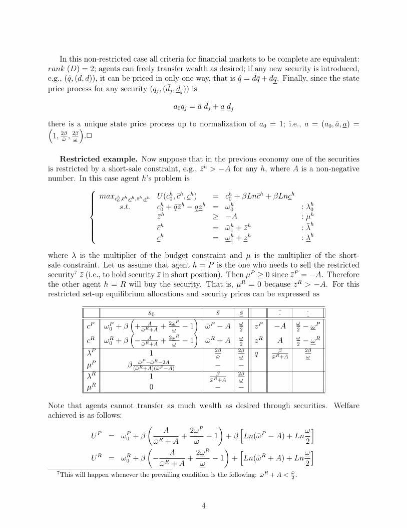
In this non-restricted case all criteria for financial markets to be complete are equivalent:rank (D) = 2; agents can freely transfer wealth as desired; if any new security is introduced,e.g., (q, (d, d)), it can be priced in only one way, that is q = dq + dq. Finally, since the stateprice process for any security (qj, (dj, dj)) is

a0qj = a dj + a dj

there is a unique state price process up to normalization of a0 = 1; i.e., a = (a0, a, a) =(

1, 2βω , 2β

ω

)

.2

Restricted example. Now suppose that in the previous economy one of the securitiesis restricted by a short-sale constraint, e.g., zh > −A for any h, where A is a non-negativenumber. In this case agent h’s problem is

maxch0 ,ch,ch,zh,zh U(ch

0 , ch, ch) = ch

0 + βLnch + βLnch

s.t. ch0 + qzh − qzh = ωh

0 : λh0

zh ≥ −A : µh

ch = ωh1 + zh : λh

ch = ωh1 + zh : λh

where λ is the multiplier of the budget constraint and µ is the multiplier of the short-sale constraint. Let us assume that agent h = P is the one who needs to sell the restrictedsecurity7 z (i.e., to hold security z in short position). Then µP ≥ 0 since zP = −A. Thereforethe other agent h = R will buy the security. That is, µR = 0 because zR > −A. For thisrestricted set-up equilibrium allocations and security prices can be expressed as

s0 s s . .

cP ωP0 + β

(

+ AωR+A + 2ωP

ω − 1)

ωP − A ω2 zP −A ω

2 − ωP

cR ωR0 + β

(

− AωR+A + 2ωR

ω − 1)

ωR + A ω2 zR A ω

2 − ωR

λP 1 2βω

2βω q β

ωR+A2βω

µP β ωP−ωR−2A(ωR+A)(ωP−A) − −

λR 1 βωR+A

2βω

µR 0 − −

Note that agents cannot transfer as much wealth as desired through securities. Welfareachieved is as follows:

UP = ωP0 + β

(

AωR + A

+2ωP

ω− 1

)

+ β[

Ln(ωP − A) + Lnω2

]

UR = ωR0 + β

(

− AωR + A

+2ωR

ω− 1

)

+[

Ln(ωR + A) + Lnω2

]

7This will happen whenever the prevailing condition is the following: ωR + A < ω2 .

4

The key question here is the following: are financial markets complete at t = 0? Inline with the previous criteria, the answer would be in the affirmative since rank (D) = 2,which equals the number of successor states.8 Hence, a unique state price process satisfingthe asset pricing equation a0qj = a dj + a dj should exist. This means that “only therich agent matters”, and only his first order conditions has to be taken into account. Thepoor agent experiences a short-sale restriction, so her first order conditions involve certainside-constraints.9 Thus, in equilibrium

q =λR

λR0

× 1 +λR

λR0

× 0 =λR

λR0

=∂UR

∂cR

∂UR

∂c0

=β

ωR + A

q =λR

λR0

× 0 +λR

λR0

× 1 =λR

λR0

=∂UR

∂cR

∂UR

∂c0

=2βω

Therefore, making a0 = 1, there is a unique state price process , i.e., a = (a0, a, a) =(

1, βωR+A , 2β

ω

)

. It then seems that financial markets are complete.On the other hand, can agents transfer all the wealth they desire between periods? No. In

such a case, it may be suggested that there exist incomplete financial markets (or perhaps, itwould be better to call them “technically incomplete” markets, as do Santos and Woodford,1992, 1996). In this scenario, several state-price processes verify the asset pricing equationshould exist. Which one is then the right asset pricing equation? Following of Svensson(1985), Santos and Woodford (1992, 1996), and Gimenez (1996, 1998) intangible returns hasto be taken into account when a financial restriction is introduced in the standard Arrow-Radner economy. Then, the asset pricing formula is,

a0qj = adj + adj + r0

where r0 is a shadow price which results from the existence of the short-sale restriction.Both agents’ first order conditions are taken into account, since there are several equilibriumstate-price processes.10 For the rich agent

q =λR

λR0

× 1 +λR

λR0

× 0 +µR

λR0

=λR

λR0

+µR

λR0

q =λR

λR0

× 0 +λR

λR0

× 1 =λR

λR0

8Observe, however, that in the presence of a constraint on security trading the definition of completemarkets in Duffie (1996) is not equivalent, since spanD ⊂ RS .

9Agent h’s first order conditions for securities are the following

λh0 q = λh + µh

λh0q = λh

µh[−A− zh] = 0

10Realize now that, in equilibrium, agents’ first order conditions could be reinterpreted as the asset pricingequations.

5

Therefore, after the normalization a0 = 1, one generalized state price process is (a, r) =(a0, a, a, r0) =

(

1, βωR+A , 2β

ω , 0)

.Regarding the poor agent

q =λP

λP0

× 1 +λP

λP0

× 0 +µP

λP0

=λP

λP0

+µP

λP0

q =λP

λP0

× 0 +λP

λP0

× 1 =λP

λP0

After the normalization a0 = 1, other generalized state price system is given by (a, r) =(a0, a, a, r0) =

(

1, 2βω , 2β

ω , β ωP−ωR−2A(ωR+A)(ωP−A)

)

. That is, there exist different multipliers for eachagent. These are “personalized multipliers”, which are not collinear. Consequently severalstate price processes are possible, which suggests that financial markets are incomplete.

In addition, if any new security is introduced, e.g., (q, (d, d)), it can not be priced in asingle way. It might be expected that q = dq + dq. However, if this security is introducedin the maximization problem, its equilibrium price would be q∗ = 2β dω+dω

ωω > q, indicatingagain that financial markets are incomplete.

Finally, in line with Santos and Woodford (1992), one can say that financial markets arecomplete in an Arrow-Radner economy with short-sale constrains if the matrix of dividendsof securities not restricted by the short-sale constraint is equal to the number of successorstates; else, financial markets are incomplete. Under this definition, in the above examplethere exist incomplete markets (or “technically incomplete markets”).2

3- Comparative statics on welfare

In this section a welfare analysis under different short-sale bounds is carried out. Twothreshold values with familiar properties arise when a short-sale constraint on one securityis introduced in the standard Arrow-Radner economy. On the one hand, for the zero-bound constraint, the standard definition of “incomplete markets” is satisfied. The restrictedsecurity is not traded because of the inside feature of the assets. On the other hand, thereexists a value of the short-sale bound beyond which the restriction is not binding for anyagent. The level of this threshold value depends on the primitives of the economy, i.e.,the discount factor, and the agent’s preferences and endowment distribution.11 Passing thisthreshold value, the standard definition of “complete markets” is verified in this setting, sincethe constraint is not active. In contrast, when the short-sale bound lies between zero andthis threshold, the short-sale constraint is binding and financial markets fall into a categoryof markets called “technically incomplete markets”.

11In the previous example this happens when A = 12 ω − ωR.

6

Thus, for changes in these short-sale bounds one can compute the gains and losses inagents’ welfare. In the case of incomplete markets, when the short-sale bound is zero,both agents are worse off than in complete markets. (See Figure 1 for a particular setof parameters.) It is well known that incomplete markets generate allocations that arePareto inferior to those of the equilibrium allocations in complete markets (see Hart, 1975).Relaxing the short-sale bound makes both agents better off. For any of these limits, theunconstrained agent’s welfare is always below his welfare resulting from his non-restrictedcomplete markets allocation. However, from a particular value of the short-sale bound on(see Figure 1), the restricted-agent’s welfare is higher than the resulting welfare obtainedwhen the financial constraint is not active. Thus, one can find a short-sale bound for whichthe restricted-agent achieves maximum welfare. Beyond this point, her welfare decreases,although it remains always above her non-restricted complete markets welfare. In summary,when financial markets are “technically incomplete” some equilibrium allocations may not bePareto dominated by those of the non-restricted complete markets equilibrium. The reasonis that the existence of the restriction increases the equilibrium prices of the restrictedsecurity, even though the agents are price takers for any given short-sale bound. Hence,the restricted-agent ought to borrow less wealth from some state, but more cheaply than inthe non-restricted case (i.e., the return for debts on restricted security R = 1

q decreases).Consequently, she can consume more at the restricted equilibrium price in period t = 0 andin state s at period t = 1.

As a final comment, this example presents an economy where agents can manipulateprices. An agent can improve her welfare if she restrained herself from trading the securityheld in short position, i.e., in negative holdings. This suggests that if some agent understandsthat she can manipulate equilibrium prices by restricting certain trades, the non-restrictedcomplete markets equilibrium could not be stable.

4.- Concluding Remarks

A simple example has revealed that the standard definitions of complete and incompletemarkets for an Arrow-Radner economy must be adapted if a financial restriction on securitytrading is active (e.g., a short-sale constraint). A detailed study of different equivalentcriteria or definitions of standard complete markets suggests that certain situations constitutean intermediate case between complete markets and incomplete markets, what Santos andWoodford (1996) call “technically incomplete markets”. A welfare analysis was also carriedout under different short-sale bounds ranging from standard complete markets to standardincomplete markets. The equilibrium allocations under the restricted set-up are not Paretodominated by the non-restricted equilibrium allocations. The restricted agent may achievehigher welfare than in the non-restricted complete markets set-up because the existence ofthe restriction increases the equilibrium price of the restricted security. Hence, this agentcan transfer less wealth, but in a cheaper way.

As an extension of this work, a case of interest within this set-up is presented in monetaryeconomies within an infinite horizon framework. Since agents cannot hold short positions on

7

a security called “money,” this asset is restricted by a short-sale constraint. Some authorshave argued that, whenever a type of friction (such as a short-sale constraint) is introduced,money represents a claim on an infinite stream of future services represented by its role inthe trading process. See Svensson (1985) and Santos and Woodford (1992, 1996) for thecash-in-advance case, Santos and Woodford (1992) for the case of a short-sale constraint,and Gimenez (1996, 1998) for the case of reserve requirements. In Gimenez (2000) the samemethodology of these authors (the work rests mainly on Santos and Woodford’s 1992 paper)is employed to criticize two examples given by Kocherlakota (1992, example 1) and by Santosand Woodford (1997, example 4.2), where money is presented as pure bubble pricing.

References

1. Duffie, D.: Dynamic Asset Pricing Theory. Princenton University Press. Princeton.1996.

2. Gimenez-Fernandez, E. L.: Valoracion de Activos en un Contexto de Restricciones deReserva. Ph.D.Thesis. Depart. de Economıa. Universidad Carlos III de Madrid, 1996.

3. Gimenez, E. L.: Rational Asset Pricing with Reserve Requirement Restrictions. Mimeo-graph, Universidade de Vigo, January 1998.

4. Gimenez, E. L.: On the Positive Fundamental Value of Money with Short-Sale Con-straints: A comment on two examples. Mimeograph, Universidade de Vigo, May 2000.

5. Hakansson, N. H.: Financial Markets. in John Eatwell, Murray Milgate and PeterNewman (eds.), The New Palgrave. A dictionary of economics. 351–354. MacMillanPress, London, 1987.

6. Hart, O.D.: On the Optimality of Equilibrium when the Market Structure is Incom-plete. J. of Econ. Theory 11, 418–443. 1975

7. Kocherlakota, N. R.: Bubbles and Constraints on Debt Accumulation. J. of Econ.Theory 57, 245–256. 1992

8. LeRoy, S. F., Werner J.: Principles of Financial Economics. Cambridge UniversityPress, Edimburg. 2001.

9. Mas-Collel, A.,Whinston, M. D., Green J. R. Microeconomic Theory. Oxford Univer-sity Press. New York. 1995.

10. Santos, M. S., Woodford, M.: A Value Theory of Money. Mimeograph. UniversidadCarlos III de Madrid, November 1992.

11. Santos, M. S., Woodford, M.: A Value Theory of Money. Mimeograph, ITAM, Mexico,D.F., May 1996.

8

12. Santos, M. S., Woodford, M.: Rational Speculative Bubbles. Econometrica, 65 n.1,19–57. 1997.

13. Svensson, L. O.: Money and Asset Prices in a Cash-in-Advance Economy. J. Polit.Econ., 93 n.5, 919–944. 1985.

14. Wilson, C.: Incomplete Markets, in John Eatwell, Murray Milgate and Peter Newman(eds.), The New Palgrave. A dictionary of economics. 759–760. MacMillan Press,London. 1987.

-1 ,2

-1

-0 ,8

-0 ,6

-0 ,4

-0 ,2

0

0 ,2

0-0

,1-0

,2-0

,3-0

,4-0

,5-0

,6-0

,7-0

,8-0

,9 -1-1

,1-1

,2-1

,3-1

,4-1

,5-1

,6-1

,7-1

,8-1

,9 -2-2

,1-2

,2-2

,3-2

,4-2

,5-2

,6-2

,7-2

,8-2

,9 -3-3

,1-3

,2-3

,3-3

,4-3

,5-3

,6-3

,7-3

,8-3

,9 -4

Re str icted a ge nt N on-Re str icted age nt

Figure 1. Gains and losses in welfare, under changes on the short-sale boundA, with respect to the non-restricted complete markets equilibrium. Case: ωP =(10, 10, 5) and ωR = (10, 2, 5), and β = 0, 9.Given the restriction zh ≥ −A: incomplete markets are obtained for A = 0; completemarkets are obtained for A = 4; the maximum gain of welfare for the restricted agent isobtained for A = 2.

9