arX

iv:0

807.

4587

v1 [

hep-

ph]

29

Jul 2

008

Signatures of Pseudoscalar Photon Mixing in CMB

Radiation

Nishant Agarwala, Pankaj Jainb, Douglas W. McKayc and John P. Ralstonc

aDepartment of Astronomy, Cornell University, Ithaca, NY - 14853, USAbPhysics Department, IIT, Kanpur - 208016, India

cDepartment of Physics & Astronomy, University of Kansas,

Lawrence, KS - 66045, USAnagarwal@astro.cornell.edu; pkjain@iitk.ac.in; dmckay@ku.edu; ralston@ku.edu

July 29, 2008

Abstract: We model the effect of photon and ultra-light pseudoscalar mixing on the propagationof electromagnetic radiation through the extragalactic medium. The medium is modelled as a largenumber of magnetic domains, uncorrelated with one another. We obtain an analytic expression forthe different Stokes parameters in the limit of small mixing angle. The different Stokes parametersare found to increase linearly with the number of domains. We also verify this result by directnumerical simulations. We use this formalism to estimate the effect of pseudoscalar-photon mix-ing on the Cosmic Microwave Background (CMB) polarization. We impose limits on the modelparameters by the CMB observations. We find that the currently allowed parameter range admitsa CMB circular polarization up to order 10−7.

1 Introduction

Pseudoscalars with very small mass and very weak coupling with visible matter arise in manyextensions of the standard model. The most well known example is the axion [1, 2, 3, 4, 5, 6, 7].The subject of pseudoscalar-photon mixing in background magnetic field has been studied by manyauthors [8, 9, 10, 11, 12, 13, 14]. The mixing changes the intensity as well as the state of polarizationof the photons. This phenomenon has also been used to search for very low mass pseudoscalarsby laboratory experiments as well as by astrophysical observations. This search has put stringentlimits on the mass and coupling parameters of such pseudoscalars [15, 16, 17, 18, 19, 20, 21, 22].The astrophysical and cosmological consequences have been studied extensively in the literature[22, 23, 24, 25, 26, 27, 28, 29, 30].

The polarization of electromagnetic waves can also change due to the presence of a backgroundpseudoscalar field. This phenomenon also has many astrophysical consequences [31, 32].

The propagation through intergalactic medium has been studied earlier by several authors[24, 26, 27, 28]. The medium is expected to be turbulent and it is reasonable to model it as alarge number of uncorrelated magnetic domains. The magnetic field in a particular domain is

1

assumed to be uniform but points in different, random, directions as we move from one domainto another. Earlier studies were primarily interested in the effect of mixing on the intensity ofthe wave. In the present paper we are interested in determining the effect on all of the Stokesparameters. This has a wide range of astrophysical and cosmological applications in radio [25, 33],CMB [22, 27, 34] and optical [25, 35, 36, 37]. Polarization is a particularly sensitive probe of thepseudoscalar-photon mixing [25, 38]. We assume that all the magnetic domains have equal lengthand the plasma density is assumed to be uniform throughout. A detailed analysis of the mixing,taking into account turbulent plasma density, is given in [13, 25].

We apply our results to determine the effect on cosmic microwave background radiation. Themixing affects the intensity of radiation as well as the linear and circular polarization. The mixingalso results in a distortion of the cosmic microwave background (CMB) spectrum. CMB observa-tions [39] can lead to stringent limits on the pseudoscalar-photon mixing, given current estimatesof the intra-galactic magnetic fields and plasma density.

We first set up the basic equations [38]. We consider electromagnetic waves propagating in abackground magnetic field. The action can be written as,

S =

∫

d4x[

− 1

4FµνF

µν +gφ

4φ ǫµναβF

µνF αβ

+jµAµ +

1

2∂µφ∂

µφ− V (φ)]

. (1)

Maxwell’s equations excluding the effects due to gravitation are given by:

∇ · ~E = gφ∇φ · ( ~B + ~B) + ρ; (2)

∇× ~E +∂ ~B

∂t= 0; (3)

∇× ~B − ∂ ~E

∂t= gφ

(

~E ×∇φ− ( ~B + ~B)∂φ

∂t

)

+~j; (4)

∇ · ~B = 0. (5)

Here Bi and Ei are the usual magnetic and electric fields and ~B is the background magnetic field.We assume that ~B is independent of space and time and hence set its derivatives to zero.

The pseudoscalar field’s equation of motion is

∂2φ

∂t2−∇2φ+m2

φφ = −gφ~E · ( ~B + ~B). (6)

We choose the coordinate system such that the z-axis points along the direction of propagationand the x-axis is parallel to the transverse component of the background magnetic field ~B. Asshown in Ref. [38], the longitudinal component of the background magnetic field plays a negligiblerole and can be ignored. We assume a quasi-monochromatic wave and hence the terms which arequadratic in the fluctuating fields give negligible contribution. We may write the field equationsas

(ω2 + ∂2z )

(

A‖(z)φ(z)

)

−M

(

A‖(z)φ(z)

)

= 0, (7)

2

where ~A = ~E/ω and A‖ refers to the component parallel to the transverse background magneticfield. The “mass matrix” or “mixing matrix” is

M =

(

ω2P −gφBTω

−gφBTω m2φ

)

, (8)

where ωP is the plasma frequency, mφ the pseudoscalar mass and BT is the magnitude of the

transverse component of ~B. The plasma frequency is given in terms of the electron density, ne, by

ω2P =

4παne

me. (9)

The component of ~A along the y-axis does not mix with the pseudoscalar field. The matrixM is diagonalized by an orthogonal transformation, OMOT = MD, where MD is diagonal. Weparameterize the orthogonal matrix,

O =

(

cos θ − sin θsin θ cos θ

)

.

The angle θ is given bytan 2θ = lgφBT , (10)

where the symbol l denotes the oscillation length,

l =2ω

ω2P −m2

φ

. (11)

We assume that the pseudoscalar mass is very small, mφ ≪ ωP . If the mass is much heavier thanthis, then their mixing with photons produces negligible effect for intergalactic propagation for therange of allowed parameters. The two eigenvalues of the matrix M , µ±, may be expressed as,

µ2± =

ω2P +m2

φ

2± 1

2

√

(ω2P −m2

φ)2 + (2gφBTω)2. (12)

2 Basic equations of polarization propagation

The basic field equations, given in the Introduction, are solved by the procedure described in Ref.[38]. Here we simply quote the final results for propagation of the correlation functions, which arethe density matrix elements of the polarization. The most general form of the different correlationfunctions after propagation through distance z, written out explicitly as coupled equations inAppendix A, can be summarized in matrix form as

ρ(z) = P (z)ρ(0)P (z)−1, (13)

where the matrix ρ(0) is defined by

ρ(0) =

< A||(0)A∗||(0) > < A||(0)A∗

⊥(0) > < A||(0)φ∗(0) >

< A⊥(0)A∗||(0) > < A⊥(0)A∗

⊥(0) > < A⊥(0)φ∗(0) >

< φ(0)A∗||(0) > < φ(0)A∗

⊥(0) > < φ(0)φ∗(0) >

, (14)

3

and the unitary matrix P (z), the solution to the field equations for a given mode ω, is given in thecase that the coordinates are chosen so that the “parallel” axis lies along the transverse componentof the external field, ~BT , by

P (z) = ei(ω+∆A)z

1 − γ sin2 θ 0 γ cos θ sin θ0 e−i(ω+∆A−(ω2−ω2

P )1/2)z 0γ cos θ sin θ 0 1 − γ cos2 θ

. (15)

In the above equations, ∆ = ∆φ − ∆A, while γ = (1 − ei∆z). ∆A and ∆φ are defined in terms ofthe frequency, ω, and the eigenvalues, µ2

±, as

∆A =√

ω2 − µ2+ − ω,

∆φ =√

ω2 − µ2− − ω . (16)

We may approximate ∆ as

∆ = ∆φ − ∆A ≈ 1

l

√

1 + tan2 2θ ≈ 1

l. (17)

The approximation, applicable to our work here, is that ω ≫ ωP , mφ and gφBT . We also find thatin our case tan 2θ ≪ 1, as we elaborate below. For later reference, we give the leading term in theexpansion of the phase in the 22 element of Eq. (15), which we will denote δz, in terms of sin θ, oforder 10−5 in our application:

iδz ≡ i(ω + ∆A − (ω2 − ω2P )1/2)z ≈ −iz

lsin2 θ, (18)

where ωP ≪ ω for ne ≈ 10−8 cm−3, as commonly estimated [24], and ω ∼ 50 GHz for the CMB.The consequent expansion of the 22 element of P (z) reads

e−iδz ≈ 1 + iz

lsin2 θ. (19)

In the model that we consider, the medium has a uniform value of ωP , namely uniform electrondensity, and the cluster diameters are all the same, with value z, over which the direction andstrength of the magnetic field is assumed to be uniform. Each cluster has a random orientationwith respect to some “external” coordinate system, where the propagation direction is z. Eq. (13)may be taken as the propagation from the initially prescribed polarization correlation matrix ρ(0)through a distance z, in a uniform field of strength BT that is oriented along the “parallel” axis.We take the magnetic field in the first cluster to be aligned at an angle β1 to the fixed externalcoordinate system. Therefore we rotate the initial state by an angle β1 with rotation matrix R(β1)to align the “parallel” axis along the magnetic field direction in the first cluster. After a distance z,a new zone (cluster) is entered, where the field has the same strength but a random orientation withrespect to the first. At this point, after the propagation through the first cluster, the polarizationstate has changed. The new state is still expressed in terms of the rotated coordinate system, ofcourse. So we rotate back by angle β1 to return to the frame of the external coordinate system.Now the state is rotated by an angle β2 with rotation matrix R(β2) to align the new “parallel”axis along the magnetic field direction in the second cluster. The propagation through distance

4

z in the second cluster results in a new polarization density matrix, expressed now in terms ofthe new rotated coordinates. Rotate back to the original coordinate system, then forward to thenew (third) cluster’s magnetic field direction. This process continues until the propagation wavereaches “Earth”, after, say, n clusters have been traversed. The propagation then amounts to thefollowing matrix product:

ρn(z) = R−1(βn)P (z)R(βn)R−1(βn−1)P (z)R(βn−1)R−1(βn−2)...R

−1(β1)P (z)R(β1)× ρ(0)R−1(β1)P

−1(z)R(β1)R−1(β2)P

−1(z)R(β2)...R−1(βn)P−1(z)R(βn), (20)

where the rotation matrix R(βm) acts only on the two dimensional space transverse to the propa-gation direction, and it reads

R(βm) =

cosβm sin βm 0− sin βm cosβm 0

0 0 1

. (21)

Further simplifications occur, because R(βm)R−1(βm−1) = R(βm − βm−1), since R−1(β)=R(−β).The reference axis for β is arbitrary, since only the relative angles between the field directionsin adjoining clusters are relevant. The difference between two random angles is obviously arandom angle, so the structure of Eq. (20) amounts to the unitary transformation ρn(z) =U(z, n)ρ(0)U−1(z, n), where U(z, n) is the product of random rotations of P (z). Next, since theparameter θ is very small (≈ 10−5 in our case), we develop Eq. (20) to the leading order in θ.

To expand the propagation matrix in powers of sin θ, write it as the sum of a (nearly) unitmatrix and a matrix proportional to sin θ:

P (z) ≡ I(z) + sin θ P(z, θ). (22)

Suppressing the irrelevant over all phase in Eq. (15), the matrices I(z) and P(z, θ) are given by

I(z) =

1 0 00 1 00 0 ei∆z

(23)

and

P(z, θ) =

−γ sin θ 0 γ cos θ0 iz

lsin θ 0

γ cos θ 0 γ sin θ

, (24)

and γ is defined as in Eq. (15). Using the fact that I(z) and R(β) commute and I(z)−1 andR(β)−1 = I(−z) and R(−β), respectively, one finds that to leading order in sin θ P(z, θ),

ρ[1]n (Z) = I(z)nρ(0)I(−z)n

+ sin θn

∑

j=1

[

I(z)n−jR(−βj)P(z, θ)R(βj)I(z)j−1ρ(0)I(−z)n + h.c.]

, (25)

where Z = nz is the total distance travelled. The form of ρn ≈ ρ[1]n , Eq. (25), a leading zeroth

order term and a sum of pairs of first order terms, each corresponding to non trivial propagation

5

in only one of the n cells, is what one expects to leading order. The above treatment of the modelis perfectly general.

We next assume that the electromagnetic wave is initially unpolarized. Furthermore we assumethat the initial correlators,

< φ(0)A∗||(0) > = < φ(0)A∗

⊥(0) > = < φ(0)φ∗(0) > = 0 . (26)

Hence the initial density matrix,ρ(0) = diag(1, 1, 0). (27)

In this case the order sin θ terms, as defined in Eqs. (22) and (24), are actually of order sin2 θ inthe terms ρ(z)11, ρ(z)12, ρ(z)21 and ρ(z)22 that affect the polarization parameters at first order in

sin θ P(z, θ). The jth term of the sum in the expression for ρ[1]n reads, for the special case where

ρ(0) = (1, 1, 0),

ρ[1]n (z)j =

−2 sin2 θ cos2 βj(1 − cos ∆z) − sin2 θ sin 2βj(1 − cos ∆z) γ∗e−i∆z(n−j) cosβj sin(2θ)/2− sin2 θ sin 2βj(1 − cos ∆z) −2 sin2 θ sin2 βj(1 − cos ∆z) γ∗e−i∆z(n−j) sin βj sin(2θ)/2γei∆z(n−j) cosβj sin(2θ)/2 γei∆z(n−j) sin βj sin(2θ)/2 0

,

(28)At second order in sin θ P(z, θ), the mixing between A|| and φ, and A⊥ and φ induces order sin2 θterms, so these must be included as well, and we deal with them next.

There are 2n(2n−1)/2 ways to choose two propagation factors P(z, θ) from the 2n positions inthe general expression Eq. (20). The general second order expression is an extension of the form

shown in Eq. (25). Denoting it ρ[2]n , we find

ρ[2]n (Z) = sin2 θ

{

n∑

k=2

k−1∑

j=1

[I(z)n−kR(−βk)P(z, θ)I(z)k−j−1R(βk − βj)P(z, θ)R(βj)I(z)j−1

× ρ(0)I(−z)n + h.c.]

+

n∑

k=1

n∑

j=1

[I(z)n−jR(−βj)P(z, θ)R(βj)I(z)j−1ρ(0)

× I(−z)k−1R(−βk)P(−z, θ)R(βk)I(−z)n−k]}

. (29)

Using Eq. (23), I(z)m is simply diag(1,1,ei∆mz), so R(β) and I(z) commute. Thus their ordersin Eqs. (25) and (29) are immaterial and can be chosen for convenience. Only the propagationmatrix P(z, θ) and, in principle, the initial conditions matrix, ρ(0), do not generally commute witheach other and with the R(β) and I(z) matrix. In general their positions in the matrix productare fixed, though for special cases such as ours, which has the unpolarized initial condition withzero value for the φ field initially, ρ(0) = diag(1,1,0), the matrices can be collapsed and simplifiedeven further, as illustrated in Eq. (28) and below in Eq. (30).

When ρ(0) = diag(1,1,0), the ρ(z) elements relevant to our study of spontaneous polarization atleading order are of the form γ2 sin2 θ × products of cosines and sines of rotation angles. Correctionsto the leading terms are themselves of order sin2 θ ≈ 10−10 for the parameters we choose for ourmodel. Assembling all of the contributions of terms of second order in sin θ P(z, θ), we find thatthe j-, k- th term of the sum in Eq. (29), yields the following elements of the 2 × 2 submatrix

6

relevant to polarization:

ρ[2]n (z, j, k)11 = −4 sin2 θ(1 − cos ∆z) cos[∆z(k − j)] cosβk cos βj

ρ[2]n (z, j, k)12 = −2 sin2 θ(1 − cos ∆z) cos[∆z(k − j)](sin(βk + βj) − i sin(βk − βj) tan[∆z(k − j)])

ρ[2]n (z, j, k)21 = −2 sin2 θ(1 − cos ∆z) cos[∆z(k − j)](sin(βk + βj) + i sin(βk − βj) tan[∆z(k − j)])

ρ[2]n (z, j, k)22 = −4 sin2 θ(1 − cos ∆z) cos[∆z(k − j)] sin βk sin βj . (30)

It turns out that all of these contributions come from the terms in the first double sum in Eq.(29), since the zero in the 33 entry of ρ(0) prevents the order one elements 13, 23, 31 and 32 in

ρ[1]n (z)j from communicating with those in ρ

[1]n (z)k to form order one elements in the 11, 22, 12 and

21 product in the second double sum term in Eq. (29).At this point, combining each term with its hermitian conjugate, we have displayed n(n −

1)/2 + n = n2/2 + n/2 terms at order sin2 θ. It is this second order term in sin θ P(z, θ) thatdominates the CMB photon’s random walk through the clusters. Inspection of Eq. (30) revealsthat the polarization parameters Q, U and V are, on average, all the same order of magnitude.Our analysis leads to the conclusion that the number of contributing “steps” in the random walkrepresented by the propagation process is proportional to n2, so the effective displacement willbe proportional to n, with the spontaneous polarization at a step being of order 10−10. Thedependence of the intensity on the number of domains has been discussed earlier [24, 26, 27, 28].However the linear dependence of polarization observables Q, U and V on n is a new result. For thetransport through a thousand cells, or clusters, we expect a typical net displacement (polarization)of order 10−7, given our parameter assumptions.

We can compute reduced Stokes parameters using the correlation functions of A||(z) and φ(z),

I = < A||(z)A∗||(z) > + < A⊥(z)A∗

⊥(z) >= ρ11 + ρ22, (31)

Q = < A||(z)A∗||(z) > − < A⊥(z)A∗

⊥(z) >= ρ11 − ρ22, (32)

U = < A⊥(z)A∗||(z) > + < A||(z)A

∗⊥(z) >= ρ12 + ρ21, (33)

V = i(− < A⊥(z)A∗||(z) > + < A||(z)A

∗⊥(z) >) = i(−ρ12 + ρ21). (34)

The linear polarization angle is given by,

tan 2ψ =U

Q, (35)

and the degree of polarization is given by,

p =

√

Q2 + U2 + V 2

I. (36)

With this background analysis of the model, we turn to applications to CMB temperature andpolarization.

3 CMB Temperature and Polarization

In this section we consider the effect of pseudoscalar mixing on the propagation of CMB photons.The mixing affects both the CMB temperature and polarization. We can impose a limit on the

7

pseudoscalar-photon coupling by requiring that the CMB is distorted to less than one part in 105,which is the amplitude of CMB temperature fluctuations. Furthermore we also demand that themixing does not generate a CMB polarization larger than 10−6. Finally since the WMAP has notobserved B modes at the level of 10−6, we require that these are at least an order of magnitudesmaller. The limit can be imposed only if we assume a value for the background magnetic fieldand plasma density. The magnetic field, in particular, is very poorly known. Furthermore theresults can change significantly if the magnetic field and plasma density changes along the pathas well as if there is a background flux of pseudoscalars. We set the incident pseudoscalar flux tozero. Furthermore we assume a uniform background field and plasma density within a particulardomain. The result is also found to depend significantly on the domain size that we assume andhence on the details of how we model in the intergalactic medium. Due to the uncertainty in themagnitude of the magnetic field it is best to impose a limit on the product gφBT . This is possiblesince the magnetic field always occurs in the form of this product. The model dependence impliesthat the limit also depends on some parameters of the model, such as the domain size and/or thetotal number of domains. We shall address this issue later in this section.

The most stringent limits on the coupling gφ are obtained from astrophysics [15]. The currentastrophysical limit is gφ < 6 × 10−11 GeV−1. The typical upper limit value of the intergalacticmagnetic field is about 10−9 G [40] and the electron number density ne ≈ 10−8 cm−3 [24]. Wepoint out that the supercluster magnetic field may be significantly larger, of order 10−7 G [41]. Inbroad outline, we model the intergalactic medium with several magnetic domains, each of size zof order a few Mpc. The total propagation distance is of the order of a few Gpc. We shall assumethat the magnetic field in different domains is uncorrelated.

Choosing specific values, we calculate the effect on CMB temperature and polarization observ-ables as CMB radiation propagates through n = 1000 magnetic domains, each of size z = 1 Mpc.The relevant physical quantities are:

1. Magnetic field, BT = 10−9 G,

2. Electron number density, ne = 10−8 cm−3,

3. Frequency of radiation (CMB), ν = 50 GHz, hence the oscillation length parameter, l = 200pc.

We set the coupling gφ = 6 × 10−11 GeV−1. We numerically compute the Stokes parameters afterpropagating through n clusters by using the equations given in Appendix A. After propagatingthrough each cluster we rotate the electromagnetic wave vector in order to account for the changein the direction of the transverse magnetic field from one cluster to the next. For this purpose weneed to transform the correlators in a fixed reference frame, at the begining of each cluster, to thereference frame with x-axis parallel to the transverse magnetic field in the cluster. The relevantformulas for the transformation of the correlators are given explicitly in Appendix B. We pointout that the initial density matrix is given by Eq. (27).

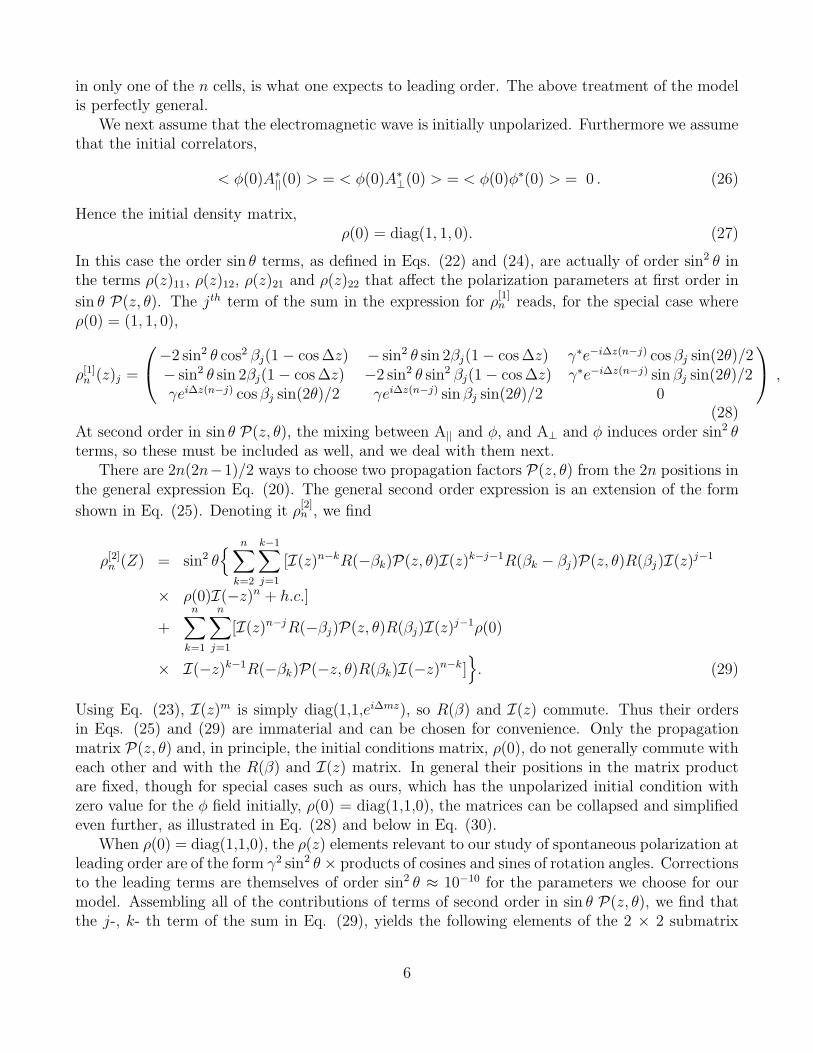
In Fig. 1 we show histograms of 1000 simulations of I0 − I, Q, U and V Stokes parametersafter propagating over 1000 clusters. All the parameters are normalized by the initial intensity I0.Here we have assumed that initially the wave is unpolarized. If initially the wave has a non-zerovalue of the Stokes Q parameter, our results remain essentially unchanged with the mean value ofthe Q parameter shifted by its initial value. The effect on the U and V polarization is negligible.

8

In CMB studies one deals with the coordinate independent E and B modes. In the presentcase we work directly with the coordinate dependent Q and U Stokes parameters. This is fine aslong as we are working in a particular direction in the sky. We align the coordinate system suchthat in the absence of pseudoscalar-photon mixing, only the Q polarization is non-zero. Then theU polarization generated by the mixing in the chosen frame provides an estimate of the B modes.Hence the polarization generated by the pseudoscalar-photon mixing must be less than the currentlimit on the B modes.

In Fig. 1 the intensity is found to deviate from its inital values by less than 1 part in 106

due to mixing for the chosen parameters. Hence the effect of mixing on temperature anisotropyis negligible. Also the Stokes parameter Q remains very close to its initial value of zero. We seethat the predictions are not in conflict with the current observations. We predict relatively largefluctuations in the U parameter and the circular polarization V . The sample mean values of U andV are found to be approximately zero, typically of the order of 10−9. The corresponding standarddeviations are found to be 2.0× 10−7 for both of the parameters. Hence we find that the choice ofparameters already predict the fluctuations in the U polarization close to its limiting value. We,therefore, impose a limit on the product gφBT < 0.2 Mpc−1 due to CMB polarization.

In Fig. 2 we show the fluctuations in Q, U and V as a function of distance for a particularrealization of the model. The plot for this individual case shows similar magnitudes induced forall the three Stokes parameters. This is true for the entire distribution of realizations as well, asshown in Fig. 1.

With results of the full simulation in hand, we can check how the results depend on the numberof clusters. In Fig. 3 we plot the dependence of mean (absolute value) and standard deviation ofU on the number of clusters. The cluster size is kept fixed in this calculation. As we anticipatefrom our discussion in Sec. 2, we find that both the mean and standard deviation increase linearlywith the number of clusters. The standard deviation shows very little digression from the linearplot, whereas the mean shows relatively large fluctuations. We point out that this linear behavioris expected as long as the Stokes parameters are much smaller compared to unity. If the numberof clusters or the magnetic field in each cluster becomes too large then the linear dependence willbreak down.

We next determine how our predictions depend on the assumed model of intergalactic space. InFig. 4 we show how the mean and standard deviation of the U parameter change as we reduce thesize of each cluster and proportionately increase the total number of clusters such that the totaldistance of propagation remains unchanged. We find that the U Stokes parameter increases as thecluster size is reduced. This is easily understood. The oscillation length l is much smaller than thesize of each cluster. Hence, statistically, the contribution per cluster remains almost unchangedas we decrease the size z of the cluster as long as z ≫ l. This is clear from the analytical result,Eq. (30), obtained in Sec. 2. The result depends on z only through the functions such as cos ∆z,tan[∆z(k − j)]. Since the arguments of the trigonometric functions are much larger than unity,adding a large number of such terms yields a negligible or fluctuating dependence on z. Howeverthe total number of clusters, n, keeps increasing, leading to a linear increase with n in the totalcontribution, as explained in Sec. 2. Due to this model dependence we may express the limit morereliably as

gφBT <

√

1000

n× 0.2 Mpc−1. (37)

We expect this to be valid as long as the cluster size, z, is much larger than 1/∆. Although we

9

1060 0(I −I)/I

0

1

2

3

4

0 0.4 0.6 0.8 10.2

106 Q/I 0

0

0.5

1

1.5

2

2.5

3

3.5

4

−0.8 −0.6 −0.4 −0.2 0 0.2 0.4 0.6 0.8 1−1

U/I 0106

0

0.5

1

1.5

2

2.5

3

3.5

4

−1 −0.8 −0.6 −0.4 −0.2 0 0.2 0.4 0.6 0.8 1

0V/I610

0

0.5

1

1.5

2

2.5

3

3.5

4

−1 −0.8 −0.6 −0.4 −0.2 0 0.2 0.4 0.6 0.8 1

Figure 1: The distribution, f(x) (×10−6), of the normalized Stokes I, Q, U and V parameters forthe CMB. For I we only show the difference I0 − I, where I0 is the initial intensity. All of theparameters have been normalized by dividing by I0. Each histogram contains the results of 1000simulations.

10

V

Q

U

Distance (Mpc)

−3E−7

−2E−7

−1E−7

0

1E−7

2E−7

3E−7

4E−7

0 100 200 300 400 500 600 700 800 900 1000

Figure 2: The distance dependence of the normalizedQ, U and V Stokes parameters for a particularrandom realization.

standard deviation

abs(mean)

Number of clusters (n)

E−10

E−9

E−8

E−7

E−6

E−5

100 1000 10000 100000

Figure 3: The mean and standard deviation of U/I0 as a function of the number of magneticclusters n. For each n we use a total of 1000 simulations. Both the mean (lower curve) andstandard deviation (upper curve) show linear dependence on n.

11

abs(mean)

standard deviation

Number of clusters (n)

E−10

E−9

E−8

E−7

E−6

E−5

E−4

100 1000 10000 100000

Figure 4: The mean and standard deviation of U/I0 as a function of the number of magneticclusters n. Here the total distance of propagation is kept fixed. For each n we use a total of 1000simulations. Both the mean (lower curve) and standard deviation (upper curve) show roughlylinear dependence on n.

have obtained this assuming uniform cluster size, and magnetic field strength equal in all clusters,the result is approximately valid even if the magnetic field and cluster size fluctuates from clusterto cluster. In this case we interpret the magnetic field strength in Eq. (37) as the mean magneticfield over all the clusters. We have explicitly verified this numerically by allowing fluctuationsin the magnetic field and cluster size with standard deviation of the order of these parameters.However the result may deviate significantly if these parameters show much larger fluctuations.

What part of the density matrix is driving the linear growth with the number of clusters n?From our discussion in Sec. 2, we see that the linear growth comes from the second order termswhich involve the correlators of φ with A|| and A⊥. We can verify this numerically by setting allsuch correlators to zero at each step. In Fig. 5 we show the result of this numerical experiment.The consequence is a growth in the Stokes parameter U proportional to

√n. This confirms our

expectation in Sec. 2 that the linear growth is driven by the correlators < φ(z)A∗||(z) > and

< φ(z)A∗⊥(z) >.

The values of the U and V Stokes parameters are found to be relatively large. Such large valuesof the U and V parameters are somewhat surprising and it is useful to get an independent estimateto verify the numerical results. For the parameters chosen the mixing angle |θ| ≈ gφBT l/2 ≈ 10−5.Furthermore the oscillation length l ≈ 10−4 Mpc ≪ z. Hence we expect that in one domain the Upolarization would be of order θ2 ≈ 10−10. As we have seen above the effect is linearly proportionalto the number of clusters. Hence for 1000 clusters we multiply this number by 1000 to get 10−7,in agreement with the value found by direct numerical computation.

12

abs(mean)

standard deviation

Number of clusters (n)

E−12

E−11

E−10

E−9

E−8

E−7

100 1000 10000

Figure 5: The mean and standard deviation of U/I0 as a function of the number of magneticclusters n. Here all the correlations of φ with fields other than φ have been artificially set to zeroat the beginning of each cluster. For each n we use a total of 1000 simulations. Both the mean(lower curve) and standard deviation (upper curve) show linear dependence on

√n.

4 Summary and discussion

Proposed as an extension to the standard model in order to solve the strong-CP problem inquantum chromodynamics (QCD), axions today still remain undetected. Direct and indirect (suchas ours) methods of detection are being used to search for axion-like particles. Future missionssuch as Planck will improve the sensitivity to the polarization of the CMB, which is a crucial nextstep in pinning down the origin of anisotropies in the CMB. A detection of circular polarizationwould certainly strengthen the case for existence of ultra-light pseudoscalars (such as axions).

In this paper we have analyzed the mixing of pseudoscalars and photons in order to explainthe polarization of the cosmic microwave background radiation. We have treated the intergalacticregion as a collection of magnetic domains (each of size 1 Mpc), and have shown, both theoreticallyand numerically, that the polarization of radiation increases linearly with the number of clusters(domains). Within the experimentally allowed range of gφBT values, our model predicts a B modepolarization and circular polarization up to order 10−7.

The model that we have used assumes that magnetic fields in adjoining clusters are completelyuncorrelated. Although this is the most reasonable assumption, it would be interesting to see howthings change if the fields are instead correlated. We might, for example, be able to explain thereported observation of large scale alignment of the optical polarization of quasars [35]. We intendto address this issue in a future publication.

13

Appendix A

Spelled out in components, the propagation equation of the density matrix ρ(z) amounts to sixindependent equations:

< A||(z)A∗||(z) > =

1

2< A||(0)A∗

||(0) >[

1 + cos2 2θ + sin2 2θ cos[z(∆φ − ∆A)]]

+1

2< φ(0)φ∗(0) >

[

sin2 2θ − sin2 2θ cos[z(∆φ − ∆A)]]

+

{

1

2< φ(0)A∗

||(0) >[

sin 2θ cos 2θ − sin 2θ cos 2θ cos[z(∆φ − ∆A)]

− i sin 2θ sin[z(∆φ − ∆A)]]

+ c.c.

}

(38)

< A⊥(z)A∗⊥(z) > = < A⊥(0)A∗

⊥(0) > (39)

< A⊥(z)A∗||(z) > = < A⊥(0)A∗

||(0) >[

cos2 θ ei Fz + sin2 θ ei Gz]

+ < A⊥(0)φ∗(0) >[

sin θ cos θ(

ei Fz − ei Gz)

]

(40)

< φ(z)φ∗(z) > =1

2< A||(0)A∗

||(0) >[

sin2 2θ − sin2 2θ cos[z(∆φ − ∆A)]]

+1

2< φ(0)φ∗(0) >

[

1 + cos2 2θ + sin2 2θ cos[z(∆φ − ∆A)]]

+

{

1

2< φ(0)A∗

||(0) >[

−sin 2θ cos 2θ + sin 2θ cos 2θ cos[z(∆φ − ∆A)]

+ i sin 2θ sin[z(∆φ − ∆A)]]

+ c.c.

}

(41)

< φ(z)A∗||(z) > =

1

2< A||(0)A∗

||(0) >[

sin 2θ cos 2θ − sin 2θ cos 2θ cos[z(∆φ − ∆A)]

− i sin 2θ sin[z(∆φ − ∆A)]]

+1

2< φ(0)φ∗(0) >

[

−sin 2θ cos 2θ + sin 2θ cos 2θ cos[z(∆φ − ∆A)]

+ i sin 2θ sin[z(∆φ − ∆A)]]

+1

2< φ(0)A∗

||(0) >[

sin2 2θ +(

1 + cos2 2θ)

cos[z(∆φ − ∆A)]

+ 2i cos 2θ sin[z(∆φ − ∆A)]]

+1

2< A||(0)φ∗(0) >

[

sin2 2θ − sin2 2θ cos[z(∆φ − ∆A)]]

(42)

< φ(z)A∗⊥(z) > = < A||(0)A∗

⊥(0) >[

sin θ cos θ(

e− i Fz − e− i Gz)

]

+ < φ(0)A∗⊥(0) >

[

sin2 θ e− i Fz + cos2 θ e− i Gz]

, (43)

14

where

F ≈ 1

2ω(µ2

+ − ω2P ) (44)

G ≈ 1

2ω(µ2

− − ω2P ) (45)

and the remaining symbols are defined in Sec. 1 and 2 in the text.

Appendix B

Let A1(n, 0) and A2(n, 0) be the two components of the electromagnetic field in a fixed referenceframe at the begining of the nth cluster. For each cluster we define a local reference frame withx-axis aligned parallel to the transverse component of the background magnetic field. In thelocal frame corresponding to the nth cluster we denote the two electromagnetic field componentsas A||(n, 0) and A⊥(n, 0). We assume that initially, i.e. at n = 0, z = 0, only the correlators< A1(0, 0)A∗

1(0, 0) > and < A2(0, 0)A∗2(0, 0) > are nonzero. After propagation through the first

cluster all the six correlation functions are likely to be non-zero. After transforming into the localframe, the initial correlators for the nth cluster are,

< A||(n, 0)A∗||(n, 0) > = cos2 α < A1(n, 0)A∗

1(n, 0) > + sin2 α < A2(n, 0)A∗2(n, 0) >

+ sin α cos α (< A2(n, 0)A∗1(0) > + < A1(n, 0)A∗

2(0) >), (46)

< A⊥(n, 0)A∗⊥(n, 0) > = sin2 α < A1(n, 0)A∗

1(n, 0) > + cos2 α < A2(n, 0)A∗2(n, 0) >

− sin α cos α (< A2(n, 0)A∗1(n, 0) > + < A1(n, 0)A∗

2(n, 0) >), (47)

< A⊥(n, 0)A∗||(n, 0) > = cos2 α < A2(n, 0)A∗

1(n, 0) > − sin2 α < A1(n, 0)A∗2(n, 0) >

+ sin α cos α (< A2(n, 0)A∗2(n, 0) > − < A1(n, 0)A∗

1(n, 0) >), (48)

< φ(n, 0)A∗||(n, 0) > = cos α < φ(n, 0)A∗

1(n, 0) > + sin α < φ(n, 0)A∗2(n, 0) >, (49)

< φ(n, 0)A∗⊥(n, 0) > = − sin α < φ(n, 0)A∗

1(n, 0) > + cos α < φ(n, 0)A∗2(n, 0) >, (50)

and < φ(n, 0)φ∗(n, 0) >.

References

[1] R. D. Peccei and H. Quinn, Phys. Rev. Lett. 38, 1440 (1977); Phys. Rev. D16, 1791 (1977).

[2] S. Weinberg, Phys. Rev. Lett. 40, 223 (1978); F. Wilczek, Phys. Rev. Lett., 40, 279 (1978).

[3] D. McKay, Phys. Rev. D 16, 2861 (1977).

[4] J. E. Kim, Phys. Rev. Lett. 43, 103 (1979).

[5] M. Dine, W. Fischler and M. Srednicki, Phys. Lett., B 104, 199 (1981).

[6] D. McKay and H. Munczek, Phys. Rev. D 19, 985 (1979).

[7] J. E. Kim, Phys. Rept. 150, 1 (1987).

15

[8] J. N. Clarke, G. Karl and P.J.S. Watson, Can. J. Phys. 60, 1561 (1982).

[9] P. Sikivie, Phys. Rev. Lett. 51, 1415 (1983); Phys. Rev. D 32, 2988 (1985); P. Sikivie, Phys.

Rev. Lett. 61, 783 (1988).

[10] L. Maiani, R. Petronzio and E. Zavattini, Phys. Lett. B175, 359 (1986).

[11] G. G. Raffelt and L. Stodolsky, Phys. Rev. D 37, 1237 (1988).

[12] R. Bradley et al, Rev. Mod. Phys. 75, 777 (2003).

[13] E. D. Carlson and W. D. Garretson, Phys. Lett. B 336, 431 (1994).

[14] A. K. Ganguly, Annals of Physics, 321, 1457 (2006).

[15] W.-M. Yao et al., Journal of Physics, G 33, 1 (2006).

[16] L. J. Rosenberg and K. A. van Bibber, Phys. Rep. 325, 1 (2000).

[17] J. W. Brockway, E. D. Carlson and G.G. Raffelt, Phys. Lett. B383, 439 (1996); J. A. Grifols,E. Masso and R. Toldra, Phys. Rev. Lett. 77, 2372 (1996).

[18] D. Dicus, E. Kolb, V. Teplitz and R. Wagoner, Phys. Rev. D 18, 1829 (1978) and Phys.Rev. D 22, 839 (1980); G. G. Raffelt and D. Dearborn, Phys. Rev. D 36, 2211 (1987); D.Dearborn, D. Schramm and G. Steigman, Phys. Rev. Lett. 56, 26 (1986); G. G. Raffelt andD. Seckel, Phys. Rev. Lett. 60, 1793 (1988); M. Turner, Phys. Rev. Lett. 60, 1797 (1988);H.-T. Janka et al., Phys. Rev. Lett. 76, 2621 (1996); W. Keil et al.. Phys. Rev. D 56, 2419(1997); M. I. Vysotsky, Ya. B. Zeldovich, M. Yu. Khlopov and V. M. Chechetkin, JETP Lett.(1978) 27, 502 (1978).

[19] K. Zioutas et al., Phys. Rev. Lett. 94, 121301 (2006); S. Andriamonje et al., JCAP 0704, 010(2007).

[20] J. Jaeckel, E. Masso, J. Redondo, A. Ringwald and F. Takshashi, Phys. Rev. D 75, 013004(2007).

[21] E. Zavattini et al. Phys. Rev. D 77, 032006 (2008).

[22] G. G. Raffelt, Ann. Rev. Nucl. Part. Sci. 49, 163, (1999); hep-ph/9903472; Lect. Notes. Phys.741, 51 (2008).

[23] S. Mohanty and S. N. Nayak, Phys. Rev. Lett. 70, 4038, (1993).

[24] C. Csaki, N. Kaloper, J. Terning, Phys. Rev. Lett. 88, 161302, (2002); Phys. Lett. B 535,33, (2002).

[25] P. Jain, S. Panda and S. Sarala, Phys. Rev. D 66, 085007 (2002).

[26] Y. Grossman, S. Roy and J. Zupan, Phys. Lett. B 543, 23 (2002).

[27] A. Mirizzi, G. G. Raffelt and P. D. Serpico, Phys. Rev. D72, 023501 (2005).

16

[28] A. Mirizzi, G. G. Raffelt and P. D. Serpico, Phys. Rev. D76, 023001 (2007). Phys. Lett. B

543, 23 (2002).

[29] Y.-S. Song and W. Hu, Phys. Rev. D 73, 023003 (2006).

[30] Y. N. Gnedin, M. Yu. Piotrovich and T.M. Natsvlishvili, MNRAS, 374, 276 (2007).

[31] D. Harari and P. Sikivie, Phys. Lett. B 289, 67 (1992).

[32] P. Das, P. Jain and S. Mukherjee, Int. Jour. of Mod. Phys. A 16, 4011 (2001); S. Kar, P.Majumdar, S. Sengupta and A. Sinha, Eur. Phys. J. C23, 357 (2002); S. Kar, P. Majumdar,S. Sengupta and S. Sur, Class. Quant. Grav. 19, 677 (2002). and T. M. Natsvlishvili, MNRAS,374, 276 (2007).

[33] P. Jain and J. P. Ralston, Mod. Phys. Lett. A14, 417 (1999); B. Nodland and J. P. Ralston,Phys. Rev. Lett. 78, 3043 (1997).

[34] S. Lee, G. C. Liu and K. W. Ng, Phys. Rev. D73, 083516 (2006).

[35] D. Hutsemekers and H. Lamy, Astronomy and Astrophysics, 367, 381 (2001); D. Hutsemekers,Astronomy and Astrophysics, 332, 410 (1998); P. Jain, G. Narain and S. Sarala, MNRAS,347, 394 (2004).

[36] A. Payez, J.R. Cudell and D. Hutsemekers, arXiv:0805.3946.

[37] M. Yu. Piotrovich, Yu. N. Gnedin, T. M. Natsvlishvili, arXiv:0805.3649.

[38] S. Das, P. Jain, J. P. Ralston and R. Saha, JCAP 0506, 002 (2005); Pramana 70, 439 (2008).

[39] Boomerang Collaboration (A. Netterfield et al.), Astrophys. J. 571, 604 (2002); BoomerangCollaboration (P. De Bernardis et al.), Astrophys. J. 564, 559 (2002); Acbar Collaboration(J. Goldstein et al.), Astrophys. J. 599, 773 (2003); WMAP Collaboration (D. Spergel et al.),Astrophys. J. Suppl. 148, 175 (2003); WMAP Collaboration (G. Hinshaw et al.), Astrophys.J. Suppl. 148, 135 (2003); Boomerang Collaboration (C. MacTavish et al.), Astrophys. J.647, 813 (2006); Boomerang Collaboration (F. Montroy et al.), Astrophys. J. 647, 813 (2006);WMAP Collaboration ( E. Komatsu et al.), arXiv:0803.0547 [astro-ph]; WMAP Collaboration(M. Nolta et al.), arXiv: 0803.0593 [astro-ph].

[40] P. Kronberg, Rep. Prog. Phys. 57, 325 (1994).

[41] J. P. Vallee, The Astronomical Journal 99, 459 (1990); The Astronomical Journal 124, 1322(2002).

17