Prepared for submission to JCAP

The large scale polarization explorer(LSPE) for CMB measurements:performance forecast

The LSPE collaborationG. Addamo,a P. A. R. Ade,b C. Baccigalupi,c A. M. Baldini,dP. M. Battaglia,e E. S. Battistelli, f ,g A. Baù,h P. de Bernardis, f ,g

M. Bersanelli,i, j M. Biasotti,k,l A. Boscaleri,m B. Caccianiga, j

S. Caprioli,i, j F. Cavaliere,i, j F. Cei, f ,n K. A. Cleary,o F. Columbro, f ,g

G. Coppi,p A. Coppolecchia, f ,g F. Cuttaia,q G. D’Alessandro, f ,g

G. De Gasperis,r,s M. De Petris, f ,g V. Fafone,r,s F. Farsian,cL. Ferrari Barusso,k,l F. Fontanelli,k,l C. Franceschet,i, j T.C. Gaier,uL. Galli,d F. Gatti,k,l R. Genova-Santos,t,v M. Gerbino,D,CM. Gervasi,h,w T. Ghigna,x,I D. Grosso,k,l A. Gruppuso,q,HR. Gualtieri,G F. Incardona,i, j M. E. Jones,x P. Kangaslahti,oN. Krachmalnicoff,c L. Lamagna, f ,g M. Lattanzi,D,CC. H. López-Caraballo, j,t,v M. Lumia,a R. Mainini,h D. Maino,i, jS. Mandelli,i, j M. Maris,y S. Masi, f ,g S. Matarrese,z A. May,AL. Mele, f ,g P. Mena,B A. Mennella,i, j R. Molina,B D. Molinari,q,E,C,DG. Morgante,q U. Natale,C,D F. Nati,h P. Natoli,C,D L. Pagano,C,DA. Paiella, f ,g F. Panico, f F. Paonessa,a S. Paradiso,i, j A. Passerini,hM. Perez-de-Taoro,t O. A. Peverini,a F. Pezzotta,i, j F. Piacentini, f ,g,1

L. Piccirillo,A G. Pisano,b G. Polenta,F D. Poletti,c G. Presta, f ,g

S. Realini,i, j N. Reyes,B A. Rocchi,r,s J. A. Rubino-Martin,t,vM. Sandri,q S. Sartor,y A. Schillaci,o G. Signorelli,d B. Siri,k,lM. Soria,o F. Spinella,d V. Tapia,B A. Tartari,d A. C. Taylor,x

L. Terenzi,q M. Tomasi,i, j E. Tommasi,F C. Tucker,b D. Vaccaro,dD. M. Vigano,i, j F. Villa,q G. Virone,a N. Vittorio,r,s A. Volpe,FR. E. J. Watkins,x A. Zacchei,y M. Zannonih,w

aCNR–IEIIT, Corso Duca degli Abruzzi, 24, 10129 Torino TO, ItalybSchool of Physics and Astronomy, Cardiff University, Queens Buildings, The Parade, Cardiff, CF243AA, U.K.

1Corresponding author

arX

iv:2

008.

1104

9v3

[as

tro-

ph.I

M]

9 A

ug 2

021

cSISSA, Astrophysics Sector, via Bonomea 265, 34136, Trieste, ItalydINFN–Sezione di Pisa, Largo B. Pontecorvo 3, 56127 Pisa (Italy)eINAF/IASF Milano, Via E. Bassini 15, Milano, Italyf Dipartimento di Fisica, Sapienza Università di Roma, P.le A. Moro 5, 00185, Roma, ItalygINFN–Sezione di Roma1, P.le A. Moro 5, 00185, Roma, ItalyhUniversità degli studi di Milano-Bicocca, Dipartimento di Fisica, Piazza delle Scienze 3, 20126Milano, Italy

iDipartimento di Fisica, Università degli Studi di Milano, Via Celoria, 16, Milano, ItalyjINFN–Sezione di Milano, Via Celoria 16, Milano, ItalykDipartimento di Fisica - Università di Genova, Via Dodecaneso, 33, 16146 Genova GE, ItalylINFN–Sezione di Genova, Via Dodecaneso, 33, 16146 Genova GE, Italy

mIFAC–CNR, Via Madonna del Piano, 10, 50019 Sesto Fiorentino, FI, ItalynPhysics Department Pisa University, Largo B. Pontecorvo 3, 56127 Pisa (Italy)oDepartment of Physics, California Institute of Technology, Pasadena, California 91125, U.S.A.pDepartment of Physics and Astronomy, University of Pennsylvania, 209 south 33rd street, 19103,Philadelphia, Pennsylvania, U.S.A.

qINAF–OAS Bologna, Istituto Nazionale di Astrofisica - Osservatorio di Astrofisica e Scienza delloSpazio di Bologna, Via P. Gobetti 101, 40129, Bologna, Italy

rDipartimento di Fisica, Università di Roma Tor Vergata, Via della Ricerca Scientifica, 1, 00133Roma, Italy

sINFN–Sezione di Roma2, Via della Ricerca Scientifica, 1, 00133 Roma, ItalytInstituto de Astrofísica de Canarias, C/Vía Láctea s/n, La Laguna, Tenerife, SpainuJet Propulsion Laboratory, California Institute of Technology, 4800 Oak Grove Drive, Pasadena,California, U.S.A.vDepartamento de Astrofísica, Universidad de La Laguna (ULL), E-38206 La Laguna, Tenerife,Spain

wINFN–Sezione di Milano Bicocca, Piazza delle Scienze 3, 20126 Milano, ItalyxSub-department of Astrophysics, University of Oxford, Denys Wilkinson Building, Keble Road,Oxford OX1 3RH, UKyINAF–Osservatorio Astronomico di Trieste, Via G.B. Tiepolo 11, Trieste, ItalyzDipartimento di Fisica e Astronomia G. Galilei, Università degli Studi di Padova, via Marzolo 8,35131 Padova, Italy

AJodrell Bank Centre for Astrophysics, School of Physics and Astronomy, University of Manchester,Manchester, UK

BUniversidad de Chile (UdC), Santiago, ChileCDipartimento di Fisica e Scienze della Terra, Università di Ferrara, Via Saragat 1, 44122 Ferrara,

ItalyDINFN–Sezione di Ferrara, Via Saragat 1, 44122 Ferrara, ItalyECineca, Via Magnanelli, 6/3, 40033 Casalecchio di Reno BO, ItalyFAgenzia Spaziale Italiana, Via del Politecnico snc, 00133, Roma, ItalyGArgonne National Labs, 9700 S. Cass Ave, Lemont, IL 60439, USAHINFN, Sezione di Bologna, Viale Berti Pichat 6/2, 40127 Bologna, ItalyIKavli Institute for the Physics and Mathematics of the Universe (Kavli IPMU, WPI), UTIAS, TheUniversity of Tokyo, Kashiwa, Chiba 277-8583, Japan

E-mail: francesco.piacentini@roma1.infn.it

Abstract. The measurement of the polarization of the Cosmic Microwave Background (CMB)radiation is one of the current frontiers in cosmology. In particular, the detection of the primordialdivergence-free component of the polarization field, the B-mode, could reveal the presence of grav-itational waves in the early Universe. The detection of such a component is at the moment the mostpromising technique to probe the inflationary theory describing the very early evolution of the Uni-verse. We present the updated performance forecast of the Large Scale Polarization Explorer (LSPE),a program dedicated to the measurement of the CMB polarization. LSPE is composed of two instru-ments: LSPE-Strip, a radiometer-based telescope on the ground in Tenerife-Teide observatory, andLSPE-SWIPE (Short-Wavelength Instrument for the Polarization Explorer) a bolometer-based instru-ment designed to fly on a winter arctic stratospheric long-duration balloon. The program is amongthe few dedicated to observation of the Northern Hemisphere, while most of the international effortis focused into ground-based observation in the Southern Hemisphere. Measurements are currentlyscheduled in Winter 2022/23 for LSPE-SWIPE, with a flight duration up to 15 days, and in Summer2022 with two years observations for LSPE-Strip. We describe the main features of the two instru-ments, identifying the most critical aspects of the design, in terms of impact on the performanceforecast. We estimate the expected sensitivity of each instrument and propagate their combined ob-serving power to the sensitivity to cosmological parameters, including the effect of scanning strategy,component separation, residual foregrounds and partial sky coverage. We also set requirements onthe control of the most critical systematic effects and describe techniques to mitigate their impact.LSPE will reach a sensitivity in tensor-to-scalar ratio of σr < 0.01, set an upper limit r < 0.015 at95% confidence level, and improve constraints on other cosmological parameters.

Keywords: CMBR experiments; CMBR polarization; cosmological parameters from CMBR.

ArXiv ePrint: 2008.11049

Contents

1 Introduction 1

2 The instruments 22.1 Observation strategy and sky coverage 32.2 LSPE-Strip 5

2.2.1 Observation site 62.2.2 Telescope and mount structure 62.2.3 Instrument and cryogenics 8

2.3 LSPE-SWIPE 122.3.1 Winter polar balloon flight 142.3.2 Power supply 142.3.3 Gondola and pointing system 162.3.4 Cryostat 162.3.5 Optical system 172.3.6 Polarization modulator 202.3.7 Detectors 212.3.8 Readout 22

3 Sensitivity of instruments 243.1 LSPE-Strip noise estimation 253.2 LSPE-SWIPE noise estimation 25

3.2.1 Cosmic rays rate 29

4 Systematic effects and calibration 304.1 LSPE-Strip systematic effects 304.2 LSPE-Strip calibration 334.3 LSPE-SWIPE systematic effects and calibration 34

4.3.1 LSPE-SWIPE optical parameters requirements 354.3.2 Polarization angle and detector time response requirements 364.3.3 HWP synchronous systematic effects: mitigation and requirements 374.3.4 LSPE-SWIPE calibration 41

5 Results 425.1 Component separation 435.2 Likelihood 445.3 Reionization optical depth constraints 465.4 Tensor-to-scalar ratio constraints 475.5 Constraints on cosmic birefringence 47

6 Conclusion 48

A LSPE-SWIPE scanning and modulation parameters 50

B Instrument simulators 51

– i –

C Atmospheric fluctuations estimation for Strip 52

D LSPE-SWIPE time response knowledge requirements 53

E LSPE-SWIPE iterative map-making 54

1 Introduction

The Large Scale Polarization Explorer (LSPE) is designed to measure the polarization of the CosmicMicrowave Background (CMB) at large angular scales, and in particular to constrain the curl com-ponent of CMB polarization (B-mode). This is produced by tensor perturbations generated duringcosmic inflation in the very early Universe [1, 2]. The level of this signal is unknown: current infla-tion models are unable to provide a firm reference value. However, the detection of this signal wouldbe of utmost importance, providing a way to measure the energy-scale of inflation and a window onthe physics at extremely high energies. While the level of CMB temperature anisotropy is of the orderof 100 µK r.m.s. and the level of the gradient component of CMB polarization (E-mode generated byscalar - density perturbations) is of the order of 3 µK, the current upper limits for the level of B-modepolarization are a fraction of µK, corresponding to a ratio between the amplitude of tensor perturba-tions and the amplitude of scalar perturbations (tensor-to-scalar ratio) r < 0.044 at 95% confidencelevel, combining data from the Planck satellite and the BICEP/Keck ground telescopes [3–5]. TheB-mode of inflationary origin is observable at large angular scales, greater than 1.5.

The main scientific target of LSPE is to improve this limit. This and the additional scientifictargets of the mission are reported in the following list:

• a detection of B-mode of CMB polarization at a level corresponding to a tensor-to-scalar ratior = 0.03 with 99.7% confidence level (CL); or an upper limit to tensor-to-scalar ratio r = 0.015at 95% CL;

• an improved measurement of the optical depth to the cosmic microwave background τ, mea-sured from the large scale E-mode CMB polarization; a measurement of τ is also critical toconstraints on the sum of neutrino masses, from large-scale-structure probes [6, 7];

• investigation of the so called low-` anomalies, a series of anomalies observed in the largeangular scales of the CMB polarization, including lack of power on the largest angular scales,asymmetries and alignment of multipole moments;

• wide maps of foreground polarization produced in our galaxy by synchrotron emission andinterstellar dust emission, which will be important to mapping the magnetic field in our Galaxyand to studying the properties of the ionized gas and of the diffuse interstellar dust in the MilkyWay;

• improved limits or detection of cosmic birefringence;

• an improved measurement of the quality of the atmosphere at Teide Observatory (Tenerife) forCMB polarization measurements.

The observational cosmology community is carrying on a global effort to improve the measure-ment of the CMB polarization, aiming at a detection, or an improved upper limit, on the tensor-to-scalar ratio r. A list of the main experiments observing CMB polarization at large scales includes1:

1For a complete list and data, see https://lambda.gsfc.nasa.gov/product/expt/.

– 1 –

the BICEP/Keck array program [8, 9] deployed at South Pole, aiming at improving the current upperlimit (multipole range 21 < ` < 335); CLASS [10], in operation in the Atacama, aiming at detect-ing r = 0.01 (2 < ` < 200); Polarbear-2/Simons Array [11], beginning operations in the Atacama,aiming at σ(r) = 0.006 if r = 0.1 (30 < ` < 3000); SPT-Pol [12], operated at the South Pole, mea-sured r < 0.44 at 95% c.l. (52 < ` < 2301) and the third SPT generation SPT-3G [13], aiming atσ(r) = 0.01 (50 < ` < 11000); ACT [14, 15], operated in the Atacama, providing relevant constraintsat smaller angular scales (225 < ` < 8725); Simons Observatory [16], in preparation in the Atacamafor early 2020s, aiming at σ(r) = 0.003 (30 < ` < 8000); GroundBIRD [17], in preparation in theTenerife-Teide observatory, aiming at σ(r) ' 0.01 (6 < ` < 300); QUBIC [18], in preparation for in-stallation in Alto Chorrillos (Argentina, altitude 4869 m a.s.l), aiming atσ(r) = 0.021 (30 < ` < 200);CMB-S4 [19], in preparation for ground-based observations in 2027, aiming at detecting r > 0.003at greater than 5σ, or r < 0.001 at 95% c.l.; SPIDER [20], balloon-based, waiting for the secondflight, aiming at detecting r > 0.03 at 99.7% c.l. (2 < ` < 200); PIPER [21], balloon-based, aiming atconstraining r < 0.007 after 8 flights; PICO [22], a satellite-based instrument currently in study phaseaiming at detection of r = 5 × 10−4 at 5σ c.l. (full sky); and LiteBIRD [23, 24], which is currentlythe only approved satellite-based mission, planned for a launch in early 2028, aiming at δr < 0.001,where δr is the total error on r, including statistical, systematic error, and margin (2 < ` < 200).

The overall design of the LSPE program has largely evolved since its first proposal [25–28],and this paper presents its final design and expected performance. Section 2 describes the two in-struments in detail; section 3 reports the expected instrumental sensitivities; section 4 describes themajor systematic effects, mitigation techniques and calibration; section 5 presents the methods usedin the foreground cleaning and likelihood evaluation and reports the expected performances on cos-mological parameters. Finally, section 6 draws conclusions.

2 The instruments

Since the expected B-mode signal is smaller than the polarized foreground from our Galaxy, a widefrequency coverage is needed to monitor precisely the foregrounds at frequencies where they aremost important, and to subtract them, in order to estimate the cosmological part of the detected B-mode signal. For the synchrotron foreground, prominent at frequencies below ∼100 GHz, whereatmospheric transmission and noise are favorable, a ground based instrument is the most effectivestrategy, while for the CMB and the interstellar dust foreground, prominent at higher frequencies,a stratospheric balloon mission is preferred. For this reason, the LSPE program is based on thecombination of two independent instruments: the Strip ground-based telescope, observing at 44 GHz,plus a 95 GHz channel for atmospheric measurements, to be implemented at the Teide Observatory(Tenerife); and the SWIPE balloon-borne mission, observing at 145, 210 and 240 GHz in a winterarctic stratospheric flight.

Table 1 reports basic parameters for the two instruments, in the baseline configuration. Map sen-sitivity is an approximated value, computed as the square root of σ2

Q,U = p NET2 4π fsky/(TobsNdet),where p = 1 for Strip and p = 2 for SWIPE, to take into account that each SWIPE detector is in-stantaneously sensitive to one polarization only, Tobs is the effective integration time, NET is thenoise equivalent temperature of each detector, fsky is the observed sky fraction, and Ndet is thenumber of detectors. The power spectrum of the noise in polarization can be approximated byN

E,B`

= σ2Q,U/ fsky,cmb, where fsky,cmb is the sky fraction used for CMB analysis, after masking the

Galactic plane. More accurate performance is estimated using the instrument simulators, componentseparation, and cosmological parameters extraction algorithms, as described in sections 3 and 5.

– 2 –

Instrument Strip SWIPESite . . . . . . . . . . . . . . . . . . . . . . . . . . . . . . . . . . . . . . . . . . . Tenerife balloonFreq (GHz) . . . . . . . . . . . . . . . . . . . . . . . . . . . . . . . . . . . . 43 95 145 210 240Bandwidth . . . . . . . . . . . . . . . . . . . . . . . . . . . . . . . . . . . . . 17% 8% 30% 20% 10%Angular resolution FWHM . . . . . . . . . . . . . . . . . . . . . . 20′ 10′ 85′

Field of view . . . . . . . . . . . . . . . . . . . . . . . . . . . . . . . . . . . ±5 ±11

Detector technology . . . . . . . . . . . . . . . . . . . . . . . . . . . . . HEMT Multi-moded TESNumber of polarimeters (Strip) / detectors (SWIPE) 49 6 162 82 82NET (µKCMB s1/2) . . . . . . . . . . . . . . . . . . . . . . . . . . . . . . 515 1139 12.6 15.6 31.4Observation time . . . . . . . . . . . . . . . . . . . . . . . . . . . . . . . 2 years 8 – 15 daysObserving efficiency . . . . . . . . . . . . . . . . . . . . . . . . . . . . 50%1 90%Sky coverage2 (nominal) fsky,0 . . . . . . . . . . . . . . . . . . . 28% 38%Sky coverage2 (this paper) fsky . . . . . . . . . . . . . . . . . . . 50% 38%Masked sky coverage for CMB analysis fsky,cmb . . . 25% 25%Map sensitivity (nominal) σQ,U,0 (µKCMB arcmin) . 102 777 10 17 34Map sensitivity (this paper) σQ,U (µKCMB arcmin) . 130 990 10 17 34Noise power spectrum (NE,B

`)1/2 (µKCMB arcmin) . . 260 1980 20 34 68

1We estimate as 50% the time dedicated to sky observations, including calibration sources. We split the remain-ing 50% as follows: (i) 15% of lost time due to bad weather, (ii) 15% of unusable data when the Sun will havean angular distance from the nearest feed less than 10 [29], 20% of time dedicated to relative calibration (seesection 4.2).2 We consider two cases for Strip coverage, the nominal case with zenith angle βnominal = 20, and the casespecific to this paper with zenith angle β = 35, which maximises the overlap as discussed in section 2.1 andillustrated in figure 2.

Table 1. LSPE baseline instrumental parameters. Details are reported in tables 2 and 4.

2.1 Observation strategy and sky coverage

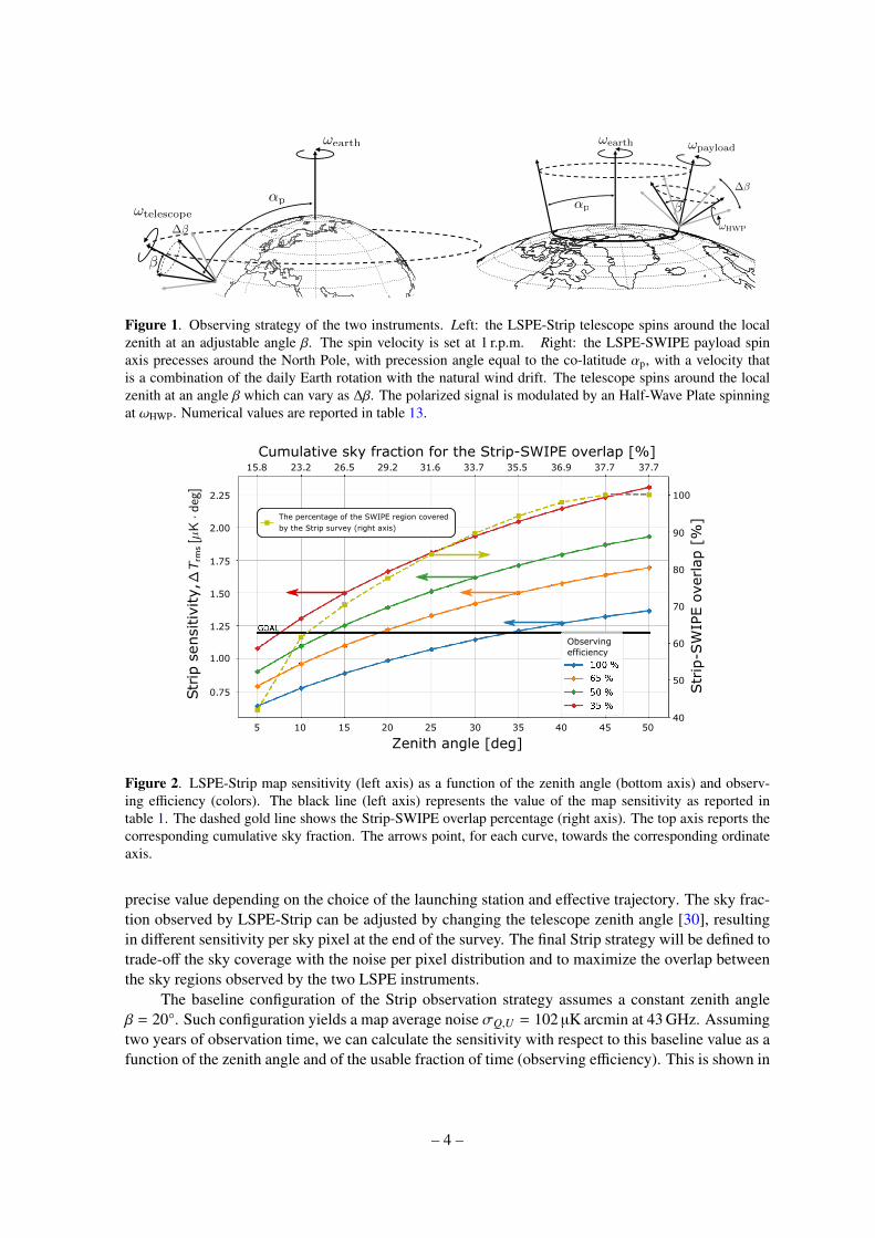
Figure 1 illustrates the observation strategies for the two instruments. The Strip telescope will scan thesky at a constant zenith angle β with ωtelescope = 1 r p m spin rate. With this strategy, the observationscover a strip in equatorial declination δ ranging lattelescope − β < δ < lattelescope + β, where lattelescope =

28°18′0′′N. This strategy minimizes atmospheric effects and, in combination with Earth rotation, tocover a large sky fraction.

The SWIPE observation strategy consists in continuous spinning of the payload, around the lo-cal zenith axis (spin axis), at fixed angular velocity ωpayload. This is combined with steps in telescopezenith angle β (a few steps per day), to cover an altitude range from 35to 55. The Earth rotation,combined with the drift of the payload around the Arctic, ensures a slow precession of the vertical spinaxis around the Equatorial North Pole (precession axis). Precession angle αp (co-latitude) and preces-sion angular velocity ωEarth are not exactly defined, due the partially random motion of the balloon,drifted by stratospheric winds. This strategy is combined with a Half-Wave Plate (HWP) based po-larization modulator continuously spinning at rate fHWP. The optimal payload spinning velocity andHWP rate are derived in Appendix A from detectors time constant and telescope angular response,and are found to be ωpayload ' 0.7 ° s−1 and fHWP = 0.5 Hz. If the latitude remains constant, the ob-servation covers a strip in equatorial declination δ in the range 90°−(αp+βmax) < δ < 90°−(βmin−αp)(see figure 1). The values of βmin and βmax also take into account the wide field of view ±10.

SWIPE is expected to have a fixed sky coverage of about 38% of the Northern Sky, with the

– 3 –

!earth<latexit sha1_base64="oGC2a+aA7/mJMqom0F9GyZJ7nfM=">AAAB/HicbVDLSsNAFJ34rPUV7VKEYBFclaQudFlw02UF+4AmlMn0ph06eTBzI8ZQf8WNC0Xc+gF+gjtX/orTx0JbD1w4nHPvzL3HTwRXaNtfxsrq2vrGZmGruL2zu7dvHhy2VJxKBk0Wi1h2fKpA8AiayFFAJ5FAQ19A2x9dTfz2LUjF4+gGswS8kA4iHnBGUUs9s+TGIQxoz0W4wxyoxOG4Z5btij2FtUycOSnXjj/umRLfjZ756fZjloYQIRNUqa5jJ+jl+jHOBIyLbqogoWxEB9DVNKIhKC+fLj+2TrXSt4JY6orQmqq/J3IaKpWFvu4MKQ7VojcR//O6KQaXXs6jJEWI2OyjIBUWxtYkCavPJTAUmSaUSa53tdiQSspQ51XUITiLJy+TVrXinFeq1065ViczFMgROSFnxCEXpEbqpEGahJGMPJJn8mI8GE/Gq/E2a10x5jMl8gfG+w+VTJkb</latexit>

<latexit sha1_base64="YE5AkvvNq7/51aSqGlMejrE080k=">AAAB83icbVDJSgNBEO2JW4xb1KMijUHwFGbiQY9BPXhMwCyQGUJPp5I06VnorhHCkKO/4MWDIl695zu8+Q3+hJ3loIkPCh7vVVFVz4+l0GjbX1ZmZXVtfSO7mdva3tndy+8f1HWUKA41HslINX2mQYoQaihQQjNWwAJfQsMf3Ez8xgMoLaLwHocxeAHrhaIrOEMjue4tSGTU9QFZO1+wi/YUdJk4c1IoH4+r348n40o7/+l2Ip4EECKXTOuWY8fopUyh4BJGOTfREDM+YD1oGRqyALSXTm8e0TOjdGg3UqZCpFP190TKAq2HgW86A4Z9vehNxP+8VoLdKy8VYZwghHy2qJtIihGdBEA7QgFHOTSEcSXMrZT3mWIcTUw5E4Kz+PIyqZeKzkWxVHUK5WsyQ5YckVNyThxyScrkjlRIjXASkyfyQl6txHq23qz3WWvGms8ckj+wPn4Aa4+U/A==</latexit>

<latexit sha1_base64="hVmNR27mGnQDWlkKaYqELLNe52w=">AAAB7HicbZC7SwNBEMbn4ivGV9TS5vAIWIW7WGgZsEkZwTwgOcLeZi9Zsrd37M4J4QiCrYWNhSIWafyD7Pxv3DwKTfxg4cf3zbAzEySCa3Tdbyu3sbm1vZPfLeztHxweFY9PmjpOFWUNGotYtQOimeCSNZCjYO1EMRIFgrWC0c0sb90zpXks73CcMD8iA8lDTgkaq9ENGJJe0XHL7lz2OnhLcKpO6enxYTqt94pf3X5M04hJpIJo3fHcBP2MKORUsEmhm2qWEDoiA9YxKEnEtJ/Nh53YJeP07TBW5km05+7vjoxEWo+jwFRGBId6NZuZ/2WdFMNrP+MySZFJuvgoTIWNsT3b3O5zxSiKsQFCFTez2nRIFKFo7lMwR/BWV16HZqXsXZYrt55TrcFCeTiDc7gAD66gCjWoQwMocHiGV3izpPVivVsfi9Kctew5hT+yPn8AQHeSAQ==</latexit>

↵p<latexit sha1_base64="qGHhaAYbX+m83xbKz3ucjcTZ5W0=">AAACAHicbVDLSgNBEJz1GeMr6sGDl8UgCELYFYI5BkTMMYJ5QDaE2UlvMmR2Z5npFcOSi7/ixYMiXv0Mb36F4Bc4eRw0saChqOqmu8uPBdfoOJ/W0vLK6tp6ZiO7ubW9s5vb269rmSgGNSaFVE2fahA8ghpyFNCMFdDQF9DwB5djv3EHSnMZ3eIwhnZIexEPOKNopE7u0JMh9GjHQ7jHFEGAZjKGUSeXdwrOBPYicWckXz77vr4qfRWrndyH15UsCSFCJqjWLdeJsZ1ShZwJGGW9RENM2YD2oGVoREPQ7XTywMg+MUrXDqQyFaE9UX9PpDTUehj6pjOk2Nfz3lj8z2slGJTaKY/iBCFi00VBImyU9jgNu8sVMBRDQyhT3Nxqsz5VlKHJLGtCcOdfXiT184JbLDg3br5cIVNkyBE5JqfEJRekTCqkSmqEkRF5JM/kxXqwnqxX623aumTNZg7IH1jvPz9/mn4=</latexit>!telescope

!earth<latexit sha1_base64="oGC2a+aA7/mJMqom0F9GyZJ7nfM=">AAAB/HicbVDLSsNAFJ34rPUV7VKEYBFclaQudFlw02UF+4AmlMn0ph06eTBzI8ZQf8WNC0Xc+gF+gjtX/orTx0JbD1w4nHPvzL3HTwRXaNtfxsrq2vrGZmGruL2zu7dvHhy2VJxKBk0Wi1h2fKpA8AiayFFAJ5FAQ19A2x9dTfz2LUjF4+gGswS8kA4iHnBGUUs9s+TGIQxoz0W4wxyoxOG4Z5btij2FtUycOSnXjj/umRLfjZ756fZjloYQIRNUqa5jJ+jl+jHOBIyLbqogoWxEB9DVNKIhKC+fLj+2TrXSt4JY6orQmqq/J3IaKpWFvu4MKQ7VojcR//O6KQaXXs6jJEWI2OyjIBUWxtYkCavPJTAUmSaUSa53tdiQSspQ51XUITiLJy+TVrXinFeq1065ViczFMgROSFnxCEXpEbqpEGahJGMPJJn8mI8GE/Gq/E2a10x5jMl8gfG+w+VTJkb</latexit> !payload

<latexit sha1_base64="dz8ikgEqmdNbdp4dCdRSbsLE2Vk=">AAAB/nicbVDLSgNBEJz1bXytiicvi0EQhLAbEXMMiOhRwZhAEkLvpBMHZ3eWmV4xLAF/xYsHRbz6Hd78CsEvcPI4qLGgoajqprsrTKQw5PsfztT0zOzc/MJibml5ZXXNXd+4MirVHCtcSaVrIRiUIsYKCZJYSzRCFEqshjfHA796i9oIFV9SL8FmBN1YdAQHslLL3WqoCLvQahDeUZZATypo91tu3i/4Q3iTJBiTfHn/6/Sk9Hl43nLfG23F0whj4hKMqQd+Qs0MNAkusZ9rpAYT4DfQxbqlMURomtnw/L63a5W211HaVkzeUP05kUFkTC8KbWcEdG3+egPxP6+eUqfUzEScpIQxHy3qpNIj5Q2y8NpCIyfZswS4FvZWj1+DBk42sZwNIfj78iS5KhaCg0LxIsiXz9gIC2yb7bA9FrAjVmZn7JxVGGcZe2BP7Nm5dx6dF+d11DrljGc22S84b9+YyJmQ</latexit>

<latexit sha1_base64="YE5AkvvNq7/51aSqGlMejrE080k=">AAAB83icbVDJSgNBEO2JW4xb1KMijUHwFGbiQY9BPXhMwCyQGUJPp5I06VnorhHCkKO/4MWDIl695zu8+Q3+hJ3loIkPCh7vVVFVz4+l0GjbX1ZmZXVtfSO7mdva3tndy+8f1HWUKA41HslINX2mQYoQaihQQjNWwAJfQsMf3Ez8xgMoLaLwHocxeAHrhaIrOEMjue4tSGTU9QFZO1+wi/YUdJk4c1IoH4+r348n40o7/+l2Ip4EECKXTOuWY8fopUyh4BJGOTfREDM+YD1oGRqyALSXTm8e0TOjdGg3UqZCpFP190TKAq2HgW86A4Z9vehNxP+8VoLdKy8VYZwghHy2qJtIihGdBEA7QgFHOTSEcSXMrZT3mWIcTUw5E4Kz+PIyqZeKzkWxVHUK5WsyQ5YckVNyThxyScrkjlRIjXASkyfyQl6txHq23qz3WWvGms8ckj+wPn4Aa4+U/A==</latexit>

<latexit sha1_base64="hVmNR27mGnQDWlkKaYqELLNe52w=">AAAB7HicbZC7SwNBEMbn4ivGV9TS5vAIWIW7WGgZsEkZwTwgOcLeZi9Zsrd37M4J4QiCrYWNhSIWafyD7Pxv3DwKTfxg4cf3zbAzEySCa3Tdbyu3sbm1vZPfLeztHxweFY9PmjpOFWUNGotYtQOimeCSNZCjYO1EMRIFgrWC0c0sb90zpXks73CcMD8iA8lDTgkaq9ENGJJe0XHL7lz2OnhLcKpO6enxYTqt94pf3X5M04hJpIJo3fHcBP2MKORUsEmhm2qWEDoiA9YxKEnEtJ/Nh53YJeP07TBW5km05+7vjoxEWo+jwFRGBId6NZuZ/2WdFMNrP+MySZFJuvgoTIWNsT3b3O5zxSiKsQFCFTez2nRIFKFo7lMwR/BWV16HZqXsXZYrt55TrcFCeTiDc7gAD66gCjWoQwMocHiGV3izpPVivVsfi9Kctew5hT+yPn8AQHeSAQ==</latexit>

↵p

!HWP

Figure 1. Observing strategy of the two instruments. Left: the LSPE-Strip telescope spins around the localzenith at an adjustable angle β. The spin velocity is set at 1 r.p.m. Right: the LSPE-SWIPE payload spinaxis precesses around the North Pole, with precession angle equal to the co-latitude αp, with a velocity thatis a combination of the daily Earth rotation with the natural wind drift. The telescope spins around the localzenith at an angle β which can vary as ∆β. The polarized signal is modulated by an Half-Wave Plate spinningat ωHWP. Numerical values are reported in table 13.

5 10 15 20 25 3530 40 45 5040

50

60

70

80

90

100

0.75

1.00

1.25

1.50

1.75

2.00

2.25

15.8 23.2 26.5 29.2 31.6 33.7 35.5 36.9 37.7 37.7

Strip

sens

itiv

ity,

Str

ip-S

WIP

E ov

erla

p [%

]The percentage of the SWIPE region covered by the Strip survey (right axis)

Cumulative sky fraction for the Strip-SWIPE overlap [%]

Zenith angle [deg]

Observingefficiency

Figure 2. LSPE-Strip map sensitivity (left axis) as a function of the zenith angle (bottom axis) and observ-ing efficiency (colors). The black line (left axis) represents the value of the map sensitivity as reported intable 1. The dashed gold line shows the Strip-SWIPE overlap percentage (right axis). The top axis reports thecorresponding cumulative sky fraction. The arrows point, for each curve, towards the corresponding ordinateaxis.

precise value depending on the choice of the launching station and effective trajectory. The sky frac-tion observed by LSPE-Strip can be adjusted by changing the telescope zenith angle [30], resultingin different sensitivity per sky pixel at the end of the survey. The final Strip strategy will be defined totrade-off the sky coverage with the noise per pixel distribution and to maximize the overlap betweenthe sky regions observed by the two LSPE instruments.

The baseline configuration of the Strip observation strategy assumes a constant zenith angleβ = 20°. Such configuration yields a map average noise σQ,U = 102 µK arcmin at 43 GHz. Assumingtwo years of observation time, we can calculate the sensitivity with respect to this baseline value as afunction of the zenith angle and of the usable fraction of time (observing efficiency). This is shown in

– 4 –

Figure 3. Map in Equatorial coordinates of the Strip-SWIPE coverage. The yellow area represents the SWIPEsky coverage; the blue area represents the Strip sky coverage, in the case of 35zenith angle; the green areashows the overlap and the grey area represent a Galactic mask that covers 30% of the whole sky. The Strip-coverage ranges from -7 to 63in latitude, and the SWIPE coverage from 13 to 77. The map also shows theposition of the Crab and Orion nebula, of the Perseus molecular cloud and the trajectories of Jupiter (orange),Saturn (dark red) and the Moon (white) from April 2021 to April 2023.

figure 2, together with the percentage of overlap, and the total sky fraction as a function of the zenithangle.

In the analysis reported in this paper, we assume a standard coverage for SWIPE, with a launchfrom Longyearbyen. In this case, the optimal overlap is obtained with a Strip zenith angle of β = 35°,resulting in a full-frequency coverage over 37% of the sky, as shown in figure 3. The map noise isin this case σQ,U = 130 µK arcmin at 43 GHz, with a wider coverage, providing the best trade-off forfinal results reported in sections 5. The two cases for Strip zenith angle β = 20 and β = 35 arelisted in table1 as nominal and this-paper, respectively.

2.2 LSPE-Strip

LSPE-Strip is a coherent polarimeter array that will observe the microwave sky from the Teide Ob-servatory in Tenerife in two frequency bands centred at 43 GHz (Q-band, 49 receivers) and 95 GHz(W-band, 6 receivers) through a dual-reflector crossed-Dragone telescope of ∼ 1.5 m projected aper-ture.

The Strip array uses coherent technology exploiting low noise high electron mobility transis-tor (HEMT) amplifiers, together with high-performance wave-guide components. The instrument iscooled to 20 K by a two-stage Gifford-McMahon (GM) cooling system and integrated at the focalplane of the telescope that is able to rotate continuously in azimuth. The polarimeter’s design allowsStrip to directly measure the Stokes Q and U parameters through a double-demodulation scheme thatis explained in section 2.2.3. This design ensures excellent rejection of 1/ f noise from amplifier gainfluctuations as well as of temperature-to-polarization leakage, without the need to introduce extraoptical elements to modulate the polarized signal.

The main objective of Strip is to accurately measure Galactic synchrotron emission in the LSPEsky region in Q-band. Recent studies [31] show that the polarized synchrotron emission is signifi-cantly structured and characterized by non-trivial variations in its spectral index. Deep measurementsat 43 GHz, complemented by lower frequency data, are crucial to constrain synchrotron contamina-tion in the foreground minimum accounting for spectral index variations. Furthermore, achieving

– 5 –

a resolution of ∼ 20 arcmin will provide key information on the spatial properties of synchrotronforeground.

The W-band array, composed of 6 modules, will complement the Q-band data in monitoringthe atmospheric load and fluctuations (mostly due to water vapor) during the Strip observations.Atmospheric effects in Q-band can be effectively monitored by measurements in W-band, wherethe water vapor component is significantly higher. Note anyway that at the Teide Observatory theatmospheric contamination of Q-band data is clearly dominated by O2, which is stable spatially andwith time. Yet the W-band channels will help to mitigate Q-band atmospheric fluctuations, expectedto be of the order of ∼ 2 K.

2.2.1 Observation site

Strip will be deployed at the Teide Observatory in Tenerife, at an altitude of 2400 m above sea level,coordinates: 28°18′0′′N, 16°30′35′′W. The site provides excellent observing conditions and hasbeen well-tested for astronomical observations for more than 30 years. The median precipitablewater vapour is 3.5 mm, reaching values below 2 mm during 30% of the time [32]. The inversionlayer lies below the observatory for approximately 80% of the time.

The observatory has a long tradition in CMB research, including past experiments like theTenerife radiometers [33], the IAC-Bartol [34], the JBO-IAC two-element interferometer [35], theCOSMOSOMAS experiment [36] and the Very Small Array interferometer (VSA [37]). The Striptelescope will be installed inside an aluminium ground screen to limit interference and ground-spill.The telescope will be protected by a sliding roof that will cover the whole enclosure.

In addition to serving as low frequency monitor for LSPE, Strip also will complement two ex-isting CMB experiments in Tenerife, QUIJOTE [38] and GroundBIRD [39], by observing in differentfrequency bands: 10–40 GHz for QUIJOTE, 40–95 GHz for Strip, and 145–225 GHz for Ground-BIRD. All three Tenerife projects (QUIJOTE, LSPE-Strip and GroundBIRD) aim at measuring ap-proximately the same area in the Northern sky and at degree scales, opening the possibility of futurecombined analyses, including useful redundancy for cross-checks of systematic effects. Strip mea-surements are currently scheduled to start during Summer 2022 and last two years.

The Strip telescope will scan the sky at a constant zenith angle, nominally 20, with 1 r.p.m.azimuthal spin rate. This strategy will allow us to minimize atmospheric effects and to cover about38% of the Northern sky, thus ensuring a large overlap with the SWIPE observations. After two yearsof operations with 50% observing efficiency we will reach a sensitivity of ∼102 µKCMB arcmin at43 GHz and ∼777 µKCMB arcmin at 95 GHz (see section 2.1, table 1 and figure 2 for more details).The observing efficiency does not account for down time due to the Moon, glitches, Radio-FrequencyInterference (RFI), or other unpredictable instrument-specific anomalies, thus moving our estimatesomewhat on the optimistic side. A breakdown of our estimated data loss is given in the footnote oftable 1.

2.2.2 Telescope and mount structure

The Strip telescope consists of two reflectors, a parabolic primary mirror and hyperbolic secondarymirror, arranged in a Dragonian cross-fed design, originally developed for the CLOVER experiment[40]. This configuration preserves polarization purity on the optical axis and gives low aberrationsacross a wide, flat focal plane. The projected diameter of the main reflector is 1.5 m and the entiresystem has an equivalent focal length of 2700 mm, resulting in ∼ f/1.8.

The telescope is surrounded by a co-moving baffle made of aluminum plates coated by amillimetre-wave absorber, which reduces the contamination due to stray light. The optical assem-bly is installed on top of an alt-azimuth mount, which allows the rotation of the telescope around two

– 6 –

Optical Enclosure

Chiller

Instrument ElectronicsCabinet

Motor ElectronicsCabinet

Compressor

Elevation

Azimuth Fork

Rotary Joint

Baseplate

PrimaryMirror

SecondaryMirror

Azimuth GearboxAssembly

Elevation GearboxAssembly

Star Tracker

Cryostat

Cold head

External shields

Cold head

Yoke

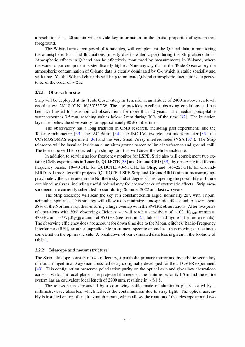
Figure 4. LSPE-Strip optical system overview. The mirrors are held inside a co-moving optical enclosure.

perpendicular axes to change the azimuth and elevation angle. An integrated rotary joint will transmitpower and data to the telescope and the instrument, and will allow a continuous spin as required bythe scanning strategy. A general view of the Strip system is shown in figure 4.

The telescope provides an angular resolution of ∼20′ in the Q-band and ∼10′ in the W-band.The feedhorn array is placed in the focal region, ensuring no obstruction of the field of view. All themodules are optimally oriented according to the shape of the focal surface, with illumination centredon the primary mirror. The two mirrors determine the main beam shapes of the Strip detectors, whilethe shielding structures affect the near and far sidelobes [41].

Optical performance. We have modeled the optical assembly with the GRASP2 software and themodel includes the nominal reflectors, the focal plane unit, the IR filters, and the shielding structures.The model is also able to reproduce the dual circular polarization antenna-feed system [42].

We have simulated the main beam radiation patterns using the Physical Optics (PO) method,which is needed to correctly model the detector patterns in the far field. Given the off-axis config-uration, the main beams are characterized by several parameters, such as the angular resolution, theellipticity, the main beam directivity, and the cross-polar discrimination factor (XPD).

Sidelobes have been computed using the Multi-Reflector Geometrical Theory of Diffraction(MrGTD). While less accurate than PO, this ray-tracing technique is much more efficient and it isable to predict the full-sky radiation pattern of complex optical systems. The 4π radiation patternsshow unevenly distributed features that are due to multiple reflections inside the shielding structure

2https://www.ticra.com/software/grasp/

– 7 –

‒0.10 ‒0.05 0.00 0.05 0.10

u

‒0.10

‒0.05

0.00

0.05

0.10v

‒10

‒8

‒6

‒4

‒2

0

Rela

tive p

ow

er

[dB

]

120

100

80

60

40

20

0

0.1 1 10 100

Angle from the beam axis [deg]

Figure 5. Left: footprint of the LSPE-Strip main beams in the (u, v) plane (large beams, 43 GHz, small beams,95 GHz). Right: beam cut for φ = 0 of the central horn. We have flipped the beam section for θ < 0 onthe positive axis to better highlight the asymmetries. The (u, v) variables are defined as u = sin(θ) cos(φ),v = sin(θ) sin(φ), where (θ, φ) are standard spherical coordinates, with the center of the telescope pointingtowards θ = 0. The inset table reports the averaged main optical parameters.

and rays entering the feedhorns without any interaction with the reflectors. Each contribution hasbeen analyzed separately and then combined in an integrated model beam. We find that the level ofsidelobes at angles larger than 1° is less than −55 dB at 43 GHz and less than −65 dB at 95 GHz.

In the top-left panel of figure 5 we show the footprint of the Strip main beams in the (u, v) plane.We can see the 49 Q-band beams grouped in seven hexagonal structures of seven beams each and thesix outer W-band beams. In the top-right panel of the same figure we show a cut corresponding toφ = 0 of the central beam. We have flipped the beam section for θ < 0 on the positive axis to betterhighlight the asymmetries. The bottom inset table displays the average main optical parameters.

2.2.3 Instrument and cryogenics

The Strip focal plane array of corrugated feedhorns is placed inside the dewar surrounded by a radia-tive shield cooled to 80 K by the cooler first stage (see the left panel of figure 6).

Copper thermal straps connect the focal plane and the cooler cold head allowing the polarimeterchain to be cooled down to 20 K. The cryostat window is an ultra-high molecular weight polyethylene(UHMWPE) window with a diameter of 586 mm and a thickness of 56.34 mm. We stop the IR radi-ation from the 300 K environment with 13 polytetrafluoroethylene (PTFE) filters with anti-reflectioncoating at 150 K. We have one filter for each horn at 95 GHz (diameter 52 mm and thickness 23 mm)

– 8 –

Window

Back-end electronics

Vacuum port Vacuum Gauge

Harness

18K StageCryo

Harness

Harness

feed-thru

Thermal

strapsCryo

Harness

IR filters

100 K shield

Optical Axis

Gravity direction

80 K stage

GFRP struts

MLI

MLI

Front-

en

d

ele

ctro

nic

s

Cryo

cooler

880 mm

GFRP struts Q-band 7-feedhorn module

W-band feedhorn

Figure 6. Left: schematic drawing of the Strip instrument. The focal plane array is inside the cryostat sur-rounded by the 80 K shield and thermally connected to the cooler cold head. Note that this drawing does notinclude the W-band horns that are visible in the real picture on the right. Right: the complete Strip focal planearray with 49 feedhorns in Q band and 6 feedhorns in W band. We also show a cutaway of one Q-band module(top) and the detailed view of one of the six W-band feedhorns (bottom).

and one filter for each 7-horns module at 43 GHz (diameter 170 mm and thickness 23 mm). The filtersare attached to the 100 K thermal shield in front of the 20 K feedhorn array.

The detector assembly is based on coherent polarimeters connected to an optical chain consti-tuted of corrugated feedhorns, each coupled to a polarizer-orthomode transducer (OMT) system at43 GHz and to a septum polarizer at 95 GHz [43].

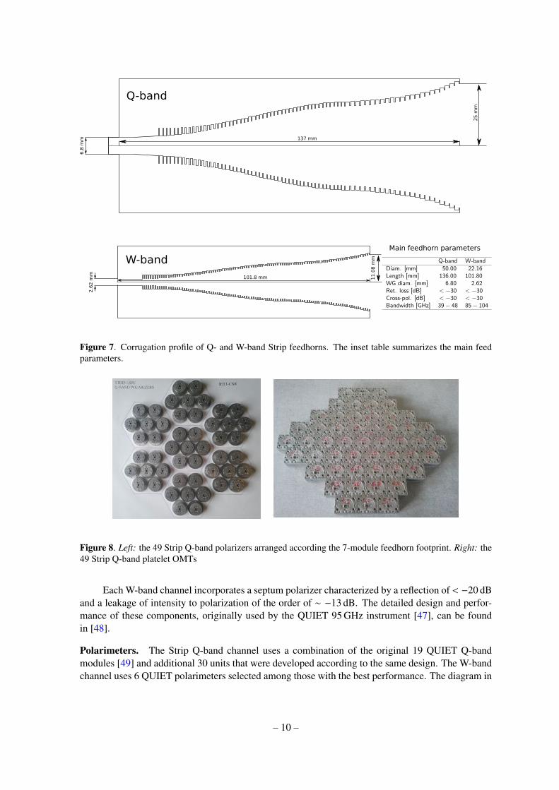
Feedhorns. The feedhorns are designed implementing a dual profile to obtain an optimal illumina-tion of the secondary with a limited feed size, and are manufactured in aluminum using the platelettechnique [44]. The right panel of figure 6 shows a picture of the entire Strip focal plane, with the 49Q-band feedhorns arranged in 7-unit modules surrounded by the six W-band feedhorns. A cutaway ofone of the Q-band modules and a detailed view of one of the W-band feedhorns are also presented. Inthe cutaway it is possible to appreciate the platelet structure of the module and the tightening screwsthat allowed to assemble the horns without the need of bonding material or thermal brazing. In fig-ure 7 we show the corrugation profile of the Strip feedhorns in both frequency bands and a summarytable of the main parameters.

Polarizers and OMTs. Each feedhorn is connected to a polarizer system that converts the twoorthogonal components of the electric field, (Ex, Ey) into right- and left-circular polarization com-ponents,

[(Ex + i Ey)/

√2, (Ex − i Ey)/

√2], which propagate through the polarimeter module. This

conversion is obtained differently in Q- and W-band.In Q-band we convert linear to circular polarization using a groove polarizer [45] connected to a

platelet OMT [46]. In figure 8 we show the complete set of Q-band polarizers (left panel) and OMTs(right panel) implemented in the Strip focal plane. This solution allowed us to obtain a very goodmeasured performance in terms of transmission (& −0.5 dB), reflection (< −25 dB) and cross-talk(∼ −40 dB).

– 9 –

25

mm

6.8

mm 137 mm

11

.08

mm

101.8 mm

2.6

2 m

m

Main feedhorn parameters

Q-band

W-band

Figure 7. Corrugation profile of Q- and W-band Strip feedhorns. The inset table summarizes the main feedparameters.

Figure 8. Left: the 49 Strip Q-band polarizers arranged according the 7-module feedhorn footprint. Right: the49 Strip Q-band platelet OMTs

Each W-band channel incorporates a septum polarizer characterized by a reflection of < −20 dBand a leakage of intensity to polarization of the order of ∼ −13 dB. The detailed design and perfor-mance of these components, originally used by the QUIET 95 GHz instrument [47], can be foundin [48].

Polarimeters. The Strip Q-band channel uses a combination of the original 19 QUIET Q-bandmodules [49] and additional 30 units that were developed according to the same design. The W-bandchannel uses 6 QUIET polarimeters selected among those with the best performance. The diagram in

– 10 –

HE

MT

am

plif

iers

Ph

ase

switc

hes

Po

wer

div

ider

s

Po

lariz

er

OM

T

Fee

dho

rn

180° hybrid 90° hybrid

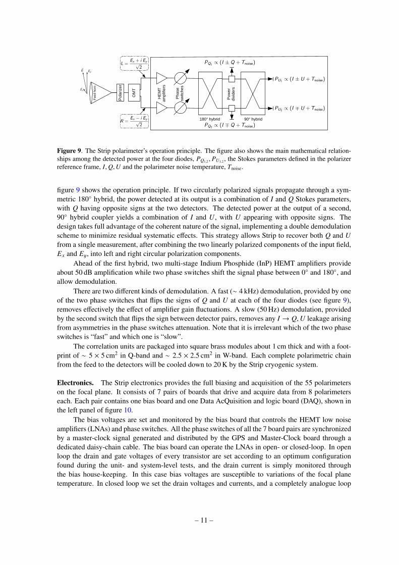
Figure 9. The Strip polarimeter’s operation principle. The figure also shows the main mathematical relation-ships among the detected power at the four diodes, PQ1,2 , PU1,2 , the Stokes parameters defined in the polarizerreference frame, I,Q,U and the polarimeter noise temperature, Tnoise.

figure 9 shows the operation principle. If two circularly polarized signals propagate through a sym-metric 180 hybrid, the power detected at its output is a combination of I and Q Stokes parameters,with Q having opposite signs at the two detectors. The detected power at the output of a second,90 hybrid coupler yields a combination of I and U, with U appearing with opposite signs. Thedesign takes full advantage of the coherent nature of the signal, implementing a double demodulationscheme to minimize residual systematic effects. This strategy allows Strip to recover both Q and Ufrom a single measurement, after combining the two linearly polarized components of the input field,Ex and Ey, into left and right circular polarization components.

Ahead of the first hybrid, two multi-stage Indium Phosphide (InP) HEMT amplifiers provideabout 50 dB amplification while two phase switches shift the signal phase between 0 and 180, andallow demodulation.

There are two different kinds of demodulation. A fast (∼ 4 kHz) demodulation, provided by oneof the two phase switches that flips the signs of Q and U at each of the four diodes (see figure 9),removes effectively the effect of amplifier gain fluctuations. A slow (50 Hz) demodulation, providedby the second switch that flips the sign between detector pairs, removes any I → Q,U leakage arisingfrom asymmetries in the phase switches attenuation. Note that it is irrelevant which of the two phaseswitches is “fast” and which one is “slow”.

The correlation units are packaged into square brass modules about 1 cm thick and with a foot-print of ∼ 5 × 5 cm2 in Q-band and ∼ 2.5 × 2.5 cm2 in W-band. Each complete polarimetric chainfrom the feed to the detectors will be cooled down to 20 K by the Strip cryogenic system.

Electronics. The Strip electronics provides the full biasing and acquisition of the 55 polarimeterson the focal plane. It consists of 7 pairs of boards that drive and acquire data from 8 polarimeterseach. Each pair contains one bias board and one Data AcQuisition and logic board (DAQ), shown inthe left panel of figure 10.

The bias voltages are set and monitored by the bias board that controls the HEMT low noiseamplifiers (LNAs) and phase switches. All the phase switches of all the 7 board pairs are synchronizedby a master-clock signal generated and distributed by the GPS and Master-Clock board through adedicated daisy-chain cable. The bias board can operate the LNAs in open- or closed-loop. In openloop the drain and gate voltages of every transistor are set according to an optimum configurationfound during the unit- and system-level tests, and the drain current is simply monitored throughthe bias house-keeping. In this case bias voltages are susceptible to variations of the focal planetemperature. In closed loop we set the drain voltages and currents, and a completely analogue loop

– 11 –

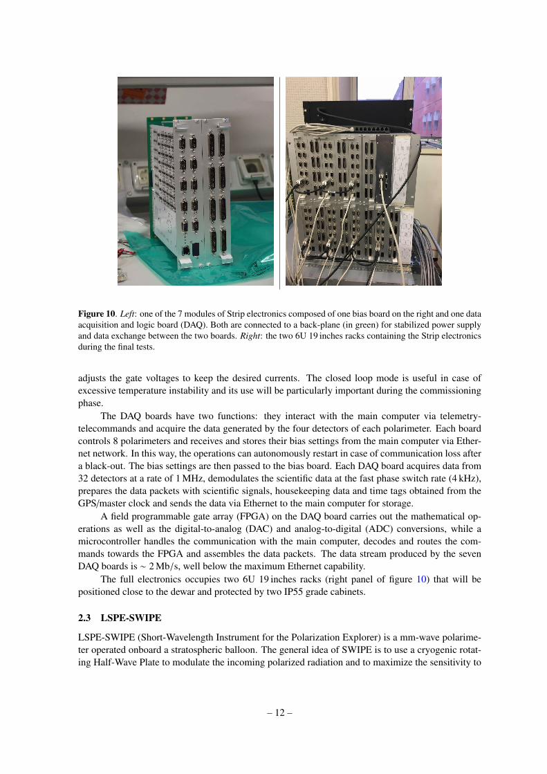
Figure 10. Left: one of the 7 modules of Strip electronics composed of one bias board on the right and one dataacquisition and logic board (DAQ). Both are connected to a back-plane (in green) for stabilized power supplyand data exchange between the two boards. Right: the two 6U 19 inches racks containing the Strip electronicsduring the final tests.

adjusts the gate voltages to keep the desired currents. The closed loop mode is useful in case ofexcessive temperature instability and its use will be particularly important during the commissioningphase.

The DAQ boards have two functions: they interact with the main computer via telemetry-telecommands and acquire the data generated by the four detectors of each polarimeter. Each boardcontrols 8 polarimeters and receives and stores their bias settings from the main computer via Ether-net network. In this way, the operations can autonomously restart in case of communication loss aftera black-out. The bias settings are then passed to the bias board. Each DAQ board acquires data from32 detectors at a rate of 1 MHz, demodulates the scientific data at the fast phase switch rate (4 kHz),prepares the data packets with scientific signals, housekeeping data and time tags obtained from theGPS/master clock and sends the data via Ethernet to the main computer for storage.

A field programmable gate array (FPGA) on the DAQ board carries out the mathematical op-erations as well as the digital-to-analog (DAC) and analog-to-digital (ADC) conversions, while amicrocontroller handles the communication with the main computer, decodes and routes the com-mands towards the FPGA and assembles the data packets. The data stream produced by the sevenDAQ boards is ∼ 2 Mb/s, well below the maximum Ethernet capability.

The full electronics occupies two 6U 19 inches racks (right panel of figure 10) that will bepositioned close to the dewar and protected by two IP55 grade cabinets.

2.3 LSPE-SWIPE

LSPE-SWIPE (Short-Wavelength Instrument for the Polarization Explorer) is a mm-wave polarime-ter operated onboard a stratospheric balloon. The general idea of SWIPE is to use a cryogenic rotat-ing Half-Wave Plate to modulate the incoming polarized radiation and to maximize the sensitivity to

– 12 –

gondola

cryostat andreceiver

insulated battery and electronics box

blackened optical baffling

azimuth pivot / thrust bearing

elevation bearing

Figure 11. LSPE-SWIPE overview. The instrument is contained in a large liquid Helium cryostat, which alsocontains the optical elements, including the HWP based Stokes polarimeter. The on-board electronics and theLithium batteries based power system are contained in an Aerogel insulated box, to optimize thermal balance.

CMB polarization at large scales using a very wide focal plane populated with multi-moded bolome-ters.

The spectral coverage of SWIPE has been optimized to be very sensitive to CMB polarizationwith one broad-band channel matching the peak of CMB brightness (145 GHz, 30% bandwidth), andto be able to monitor and separate the signals from interstellar dust (the main polarized foregroundat this frequency) by means of two ancillary, narrower channels at 210 and 240 GHz. These arededicated to measuring the slope of the specific brightness of interstellar dust.

The focal planes of SWIPE are large enough that a total of 8800 modes of the incoming radiationare collected by the multi-moded 326 detectors, thus boosting the sensitivity of the polarimeter tounprecedented levels for such a comparatively low number of detectors. The detectors arrays arecooled to 0.3 K by a large wet cryostat, which also cools the polarization modulator and the entiretelescope.

The cryostat is mounted in a frame, the gondola, providing accommodation for an attitudecontrol system, the power system and electronics. The gondola interfaces to the flight train of thestratospheric balloon through an azimuth pivot allowing for azimuth spin and/or scan. A generalview of the SWIPE instrument is shown in figure 11. LSPE-SWIPE measurements are currentlyscheduled for Winter 2022/23.

– 13 –

2.3.1 Winter polar balloon flight

LSPE-SWIPE is designed to fly on a stratospheric long-duration balloon in the arctic winter. Strato-spheric balloon altitudes (about 35 km above sea level) are needed to avoid most of the atmosphericemission, which is relevant at 145 GHz and very important at higher frequencies. A winter launchguarantees the possibility to exploit the absence of the Sun and cover a large fraction of the sky byspinning the full payload, allowing efficient exploration of the CMB polarization anisotropy at largeangular scales. It also ensures higher stability of the observing conditions, due both to the thermalstability of the instrument and to the lowest residual turbulence in the atmosphere.

The instrument is designed for a 15-day long flight. This long duration is needed to reach thesensitivity that matches the scientific goal of the LSPE experiment. Options for launching in thepolar night are at the moment only possible from the Northern Hemisphere, due to the logistics dif-ficulties related to the access to Antarctic regions during austral winter. In particular, two possiblelaunching stations are Longyearbyen, in the Svalbard islands (Norway), with a latitude above 78.2N,and Kiruna (Sweden) at a latitude of 67.8N. Several launches have been performed from Longyear-byen, with different balloon and payload sizes, both in Summer and in Winter over the last few years.Kiruna offers an established alternative, although at lower latitudes. Stratospheric balloon flights areorganized by the Swedish Space Corporation in the Esrange Space Center.

In order to assess the feasibility of winter polar northern hemisphere flights, we have developeda trajectory simulator, based on the publicly available data from The Research Data Archive (RDA)3,managed by the Data Support Section (DSS) of the Computational and Information Systems Lab-oratory (CISL) at National Center for Atmospheric Research (NCAR). With these data is possible:(1) to simulate balloon trajectories in the past years, for a statistical analysis of flight opportunities;(2) to predict trajectory in the near future, based on a stratospheric wind model, with a predictionof 225 hours in the future; and (3) to compare historical predictions and historical data, to assessprediction reliability. Figure 12 illustrates a snapshot of trajectories’ statistical analysis, that will beincluded in a separate paper. The simulation tool has also been validated by comparison of predic-tions with real trajectories, for Summer and Winter flights. The payload recovery is essential in thecase of LSPE-SWIPE, due to the detectors’ data-rate higher than the possible telemetry rate. Fromthe top panels of figure 12 it is clear that the typical winter trajectory is followed with a much higherspeed with respect to summer trajectories. For this reason, the probability to have the payload stalledover the ocean is low, increasing the recovery chances, with unpredictable difference between the twoconsidered launch sites.

Such a long duration flight in the winter, while being appealing from the scientific point ofview, is very demanding in terms of power system and thermal balance. A series of technologicaltest flights has been carried out over the years, as reported in [50? –54]. All the LSPE-SWIPE partsare designed to cope with temperatures as low as −90 °C, except the battery pack and part of theelectronics, which are contained in a thermally insulated box.

2.3.2 Power supply

For a long-duration night-time flight, a relatively cheap, consolidated, high energy-density power-supply solution is based on lithium batteries. The total power budget of the SWIPE instrument is∼ 370 W, and the energy necessary for the entire mission is ∼ 0.48 GJ. This is stored in a stackof ∼ 3500 cells (each 14 Ah @ 3.3 V). Due to the low internal resistance of these cells, and thefact that their capacity decreases at low temperatures, it is necessary to keep the cells warm (at atemperature > 0 °C) during the flight. This is obtained by hosting the batteries in the same box

3https://rda.ucar.edu/

– 14 –

Figure 12. Winter polar northern hemisphere trajectories and statistical analysis. Left column plots arefor a launch from Kiruna and right plots from Longyearbyen. Top: in red a simulated trajectory based onhistorical forecast, for 9 days after a launch on December 28, 2017; in blue the simulated trajectory based onhistorical data, for the same launch day. Dots represent 24 hours steps. The green dot indicates hours with solarillumination on the payload (Sun higher than −4 above the horizon). The trajectory based on wind predictionis very well reproduced by the trajectory based on real wind data. Center: the panels show an analysis of fullwinter 2017/18. The abscissa axes indicate the launch date. The ordinate axes indicate the days of flight. Forevery hour of flight, a blue dot represents an hour in the dark, while a white dot represents an hour with solarillumination. A fully blue vertical area indicates a launch day with full flight in the dark. Bottom: the plotsreport the fraction of time with solar illumination given a launch day.

– 15 –

hosting the electronics of the experiment, and in good thermal contact. The box is insulated from thecold external environment by a blanket made of three layers of metal reflective foil separated by twothick (∼ 2.5 cm) layers of aerogel. According to the thermal model, with 200 W of power dissipatedin the electronics inside the box, and an external temperature of 200 K, the internal temperature ismaintained at 280 K. A prototype of this power and thermal insulation system was flown in a winterarctic balloon in December 2017 [54], and further tests are planned for the future.

2.3.3 Gondola and pointing system

The gondola is a simple riveted frame of aluminum beams, hosting all the components of the pay-load and of the flight system, and structurally optimized to withstand an acceleration of 10 g (g =

gravitational acceleration) at the opening of the parachute after the flight termination. The telescopeattitude is controlled by the attitude control system (ACS). Its main purpose is to spin in azimuth theentire gondola. The azimuth pivot separates the payload from the flight chain, and is based on thrustbearings and a torque motor. The motor torques directly against the flight chain, to obtain an azimuthspin rate up to 10 /s, much faster than the nominal rate of 0.7 /s .

Mechanically and electrically, the system is very similar to the ones used in ARGO [55],BOOMERanG [56, 57], Archeops [58], OLIMPO [59–61], and described in detail in [62–64]. Giventhe measured friction of the thrust ball bearing, we expect to use up to ∼ 70 W to rotate the ∼ 2000 kgpayload at the 10 /s scan speed. The azimuth speed is sensed by a laser-gyroscope, the signal ofwhich is compared to the desired spin rate, in a feedback loop controlling the current in the torquemotor. The elevation of the boresight can be changed by tilting the entire cryostat, using a geared DCmotor driving a linear actuator with linear recirculating ball bearing. The pointing reconstruction isbased on a high altitude GPS receiver to obtain geographical coordinates and on two orthogonal faststar sensors [65], the same successfully used for the Archeops flight [66], for the celestial coordinatesof the boresight. The system allows for pointing reconstruction with ∼ arcmin accuracy.

2.3.4 Cryostat

SWIPE makes use of a custom-designed main cryostat with a bath of 250 liters of superfluid helium,connected to the external low-pressure environment to operate at 1.6 K. The cryostat shell, the internalshields and the LHe tank are all made of aluminum alloys, to reduce their mass, as developed for thecryostats used in the ARGO [67], BOOMERanG [68], PILOT [69] and OLIMPO [70] balloon-borneinstruments. Two vapor-cooled intermediate shields, separated by super-insulation blankets, are usedto minimize the radiative heat load on the LHe bath. The main cryostat provides the base temperatureto cool down the polarization modulator and the optical system, and to operate a 3He evaporator[71]. The latter cools down to 0.3 K the two focal plane arrays, as required to operate the SWIPEbolometric detectors. The hold time forecast for the LHe in the main cryostat is ∼ 20 days, whilethe 3He refrigerator has a hold time of ∼ 7 days, and can be recycled in flight. In order to minimizethe radiative load on the detectors, the 600 mm diameter window has been designed in a similarway as the one used by the EBEX group [72], and, less recently, in [73] and in [74]. In practice, athick UHMWPE [75] window used for laboratory tests is removed at float, leaving only a very thin( λ) Mylar window to withstand the small pressure difference between the cryostat vacuum andthe stratospheric pressure. The thick window also implements a highly reflective filter to operate thereceiver on the ground under radiative loadings representative of the stratospheric environment. Justbefore the termination of the flight, the motor unit is remotely operated again to put the thick windowback in place for a relatively safe receiver landing.

– 16 –

2.3.5 Optical system

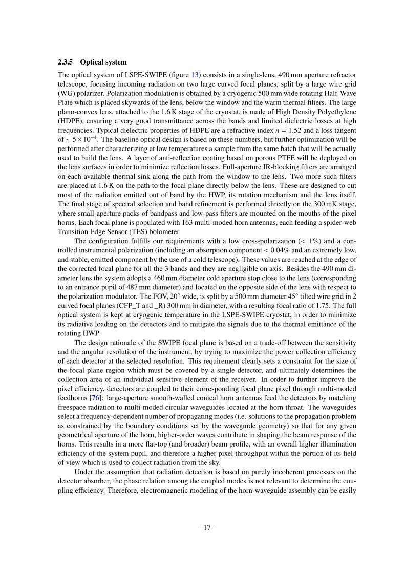
The optical system of LSPE-SWIPE (figure 13) consists in a single-lens, 490 mm aperture refractortelescope, focusing incoming radiation on two large curved focal planes, split by a large wire grid(WG) polarizer. Polarization modulation is obtained by a cryogenic 500 mm wide rotating Half-WavePlate which is placed skywards of the lens, below the window and the warm thermal filters. The largeplano-convex lens, attached to the 1.6 K stage of the cryostat, is made of High Density Polyethylene(HDPE), ensuring a very good transmittance across the bands and limited dielectric losses at highfrequencies. Typical dielectric properties of HDPE are a refractive index n = 1.52 and a loss tangentof ∼ 5×10−4. The baseline optical design is based on these numbers, but further optimization will beperformed after characterizing at low temperatures a sample from the same batch that will be actuallyused to build the lens. A layer of anti-reflection coating based on porous PTFE will be deployed onthe lens surfaces in order to minimize reflection losses. Full-aperture IR-blocking filters are arrangedon each available thermal sink along the path from the window to the lens. Two more such filtersare placed at 1.6 K on the path to the focal plane directly below the lens. These are designed to cutmost of the radiation emitted out of band by the HWP, its rotation mechanism and the lens itself.The final stage of spectral selection and band refinement is performed directly on the 300 mK stage,where small-aperture packs of bandpass and low-pass filters are mounted on the mouths of the pixelhorns. Each focal plane is populated with 163 multi-moded horn antennas, each feeding a spider-webTransition Edge Sensor (TES) bolometer.

The configuration fulfills our requirements with a low cross-polarization (< 1%) and a con-trolled instrumental polarization (including an absorption component < 0.04% and an extremely low,and stable, emitted component by the use of a cold telescope). These values are reached at the edge ofthe corrected focal plane for all the 3 bands and they are negligible on axis. Besides the 490 mm di-ameter lens the system adopts a 460 mm diameter cold aperture stop close to the lens (correspondingto an entrance pupil of 487 mm diameter) and located on the opposite side of the lens with respect tothe polarization modulator. The FOV, 20 wide, is split by a 500 mm diameter 45 tilted wire grid in 2curved focal planes (CFP_T and _R) 300 mm in diameter, with a resulting focal ratio of 1.75. The fulloptical system is kept at cryogenic temperature in the LSPE-SWIPE cryostat, in order to minimizeits radiative loading on the detectors and to mitigate the signals due to the thermal emittance of therotating HWP.

The design rationale of the SWIPE focal plane is based on a trade-off between the sensitivityand the angular resolution of the instrument, by trying to maximize the power collection efficiencyof each detector at the selected resolution. This requirement clearly sets a constraint for the size ofthe focal plane region which must be covered by a single detector, and ultimately determines thecollection area of an individual sensitive element of the receiver. In order to further improve thepixel efficiency, detectors are coupled to their corresponding focal plane pixel through multi-modedfeedhorns [76]: large-aperture smooth-walled conical horn antennas feed the detectors by matchingfreespace radiation to multi-moded circular waveguides located at the horn throat. The waveguidesselect a frequency-dependent number of propagating modes (i.e. solutions to the propagation problemas constrained by the boundary conditions set by the waveguide geometry) so that for any givengeometrical aperture of the horn, higher-order waves contribute in shaping the beam response of thehorns. This results in a more flat-top (and broader) beam profile, with an overall higher illuminationefficiency of the system pupil, and therefore a higher pixel throughput within the portion of its fieldof view which is used to collect radiation from the sky.

Under the assumption that radiation detection is based on purely incoherent processes on thedetector absorber, the phase relation among the coupled modes is not relevant to determine the cou-pling efficiency. Therefore, electromagnetic modeling of the horn-waveguide assembly can be easily

– 17 –

LHe LHe

detectors

detectors

filters

lens

window

cold-stop

filters

1430mm

feedhorns

feedhorns

HWP

fridge

Figure 13. LSPE-SWIPE cryostat and optical system. Radiation enters from the top window, passes acrossfilters, HWP, lens, cold-stop, and other filters. It then is split by the large wire grid and collected in the twocurved focal planes.

performed by solving one reverse-propagation problem per each of the coupled modes selected by thewaveguide. A far-field calculation of the field solution at the horn aperture then yields the individualcontribution of each mode to the horn response, and the full multi-moded response is then computedas a power summation over the coupled modes. This operation has been performed through the AnsysHFSS4 software, and the calculated beam profile for the SWIPE horns is shown in figure 14. Herethe contributions from the individual modes have been evenly weighted, as expected under energyequipartition conditions, and confirmed by numerical simulation of the absorber/cavity sub-system(see section 2.3.7). A measurement of the feed angular response is reported in [77].

Integration of the numerically evaluated profile times the horn effective area yields a value veryclose to AeffΩtot = Nmodes(rwg, ν)λ2, where Nmodes(rwg, ν) is the number of propagating wave solutions(i.e. modes with imaginary wavenumber) in a cylindrical waveguide of radius rwg at frequency ν, andλ is the free-space wavelength of monochromatic radiation. This result is expected in the few-modesregime and under equipartition conditions, where each coupled mode provides the same fraction ofthe total working throughput. In addition, since we use a full-field polarizer to split polarization in twoindependent focal planes, the polarization properties of the individual pixel assembly are irrelevantfor the end-to-end performance evaluation. Therefore, no concern arises due to the co-polar and

4https://www.ansys.com

– 18 –

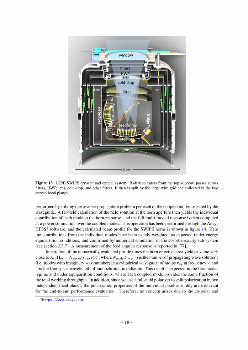
Figure 14. Top panels: simulated beam response of the SWIPE multi-moded horns. Radiation is propagatedinto the far field with linear polarization parallel to the v axis in the plane of the horn aperture, correspondingto the φ = 90° axis in the far field. Bottom panels: simple physical optics simulation of the SWIPE telescopemain beam, for a pixel at the center of the focal plane. The simulation includes the feed pattern shown above,the aperture stop and the HDPE lens. A perfectly absorbing tube and no further obstructions apart from thecold aperture stop have been assumed. Co-polar and cross-polar patterns have been calculated according toLudwig’s third definition in [78] and are mapped as a function of u = sin(θ) cos(φ) and v = sin(θ) sin(φ), where(θ, φ) are the standard spherical coordinates, and the telescope bore-sight is pointing at θ = 0. Contours areshown every 3 dB for the co-polar patterns and every 6 dB for the cross-polar patterns.

cross-polar response behavior of the horns.In order to simplify the design and production cycle of the horns, no additional optimization

is performed at the pixel level. Instead, further suppression of power at large angles from the skyis obtained by heavily over-illuminating the cold aperture stop (with an edge taper of −10 dB at145 GHz). The multi-moded beam of each horn thus ensures a very uniform illumination pattern ofthe telescope lens, maximizing the aperture efficiency of the telescope, while unwanted power pickupin the horn sidelobes is mitigated through implementation of cold, stable, highly absorptive surfacesinside the telescope tube. Additional large-angle pickup due to strong beam truncation at the aperturewill be mitigated through an absorptive external baffle.

This multi-moded approach ensures an optimal trade-off between the need for a conspicousnumber of independent focal plane elements and the net sensitivity of the individual pixels. This

– 19 –

scanning direction

Local sky meridian

telescopevertical

axis

HWP

angle

WG angle

<latexit sha1_base64="27v8V45P4COIH1Crw7mfqyk7KqM=">AAAB63icbZC7SgNBFIbPeo3xkqiFhc1gEKzCbiy0EAnYWEYwF0iWMDuZTYbMzC4zs0JY8go2ForY+gS+iZ0PYJtncDZJoYk/DHz8/znMOSeIOdPGdb+cldW19Y3N3FZ+e2d3r1DcP2joKFGE1knEI9UKsKacSVo3zHDaihXFIuC0GQxvsrz5QJVmkbw3o5j6AvclCxnBJrM6sWbdYsktu1OhZfDmUKoeTSaFq4/vWrf42elFJBFUGsKx1m3PjY2fYmUY4XSc7ySaxpgMcZ+2LUosqPbT6axjdGqdHgojZZ80aOr+7kix0HokAlspsBnoxSwz/8vaiQkv/ZTJODFUktlHYcKRiVC2OOoxRYnhIwuYKGZnRWSAFSbGnidvj+AtrrwMjUrZOy9X7rxS9RpmysExnMAZeHABVbiFGtSBwAAe4RleHOE8Oa/O26x0xZn3HMIfOe8/oQKSXQ==</latexit>

HWP<latexit sha1_base64="s2PT+adj4DT4uveeeU7KbyyxdIY=">AAAB+nicbVDJTgJBEO3BDcFlwKOXiWjCiczgQU+GxAtHTGRJgJCepgY69CzprlHJiF/gD3jw4kFjvPol3vwbm+Wg4EsqeXmvKlX13Ehwhbb9baTW1jc2t9LbmezO7t6+mcs3VBhLBnUWilC2XKpA8ADqyFFAK5JAfVdA0x1dTv3mDUjFw+AaxxF0fToIuMcZRS31zFwHh4C010G4w6TarE16ZsEu2TNYq8RZkEIl//T4UDzO1nrmV6cfstiHAJmgSrUdO8JuQiVyJmCS6cQKIspGdABtTQPqg+oms9Mn1olW+pYXSl0BWjP190RCfaXGvqs7fYpDtexNxf+8dozeeTfhQRQjBGy+yIuFhaE1zcHqcwkMxVgTyiTXt1psSCVlqNPK6BCc5ZdXSaNcck5L5SunULkgc6TJITkiReKQM1IhVVIjdcLILXkmr+TNuDdejHfjY96aMhYzB+QPjM8fqCCWdw==</latexit>

WG<latexit sha1_base64="ElY2Mn5+MyfCYBV/Vy2Dr7eR6Qo=">AAAB9XicbVC7SgNBFJ31GeMjUQsLm8EgWIXdWGghErDQMoJ5QHYNs5PZZMjs7DJzVw1L/sPGQhFbC//Ezg+wzTc4eRSaeODC4Zx7ufcePxZcg21/WQuLS8srq5m17PrG5lYuv71T01GiKKvSSESq4RPNBJesChwEa8SKkdAXrO73LkZ+/Y4pzSN5A/2YeSHpSB5wSsBIt27c5S0X2AOk9ctBK1+wi/YYeJ44U1Io7w2HubOP70or/+m2I5qETAIVROumY8fgpUQBp4INsm6iWUxoj3RY01BJQqa9dHz1AB8apY2DSJmSgMfq74mUhFr3Q990hgS6etYbif95zQSCUy/lMk6ASTpZFCQCQ4RHEeA2V4yC6BtCqOLmVky7RBEKJqisCcGZfXme1EpF57hYunYK5XM0QQbtowN0hBx0gsroClVQFVGk0CN6Ri/WvfVkvVpvk9YFazqzi/7Aev8BVgqWzA==</latexit>

!HWP<latexit sha1_base64="KD0IyPT9/JSIT+oQg8onIuwqaWU=">AAAB+3icbVC7TsNAEDyHV0h4mFDSWASkVJEdCqhQJJqUQSIPKbai82WTnHI+W3drlMgKX8AP0NBQgBAtP0LH3+A8CkgYaaXRzK52d/xIcI22/W1kNja3tneyu7n83v7BoXlUaOowVgwaLBShavtUg+ASGshRQDtSQANfQMsf3cz81j0ozUN5h5MIvIAOJO9zRjGVumbBDQMY0K6LMMak1qpPc12zaJftOax14ixJsVp4enwoneXrXfPL7YUsDkAiE1TrjmNH6CVUIWcCpjk31hBRNqID6KRU0gC0l8xvn1rnqdKz+qFKS6I1V39PJDTQehL4aWdAcahXvZn4n9eJsX/lJVxGMYJki0X9WFgYWrMgrB5XwFBMUkKZ4umtFhtSRRmmcc1CcFZfXifNStm5KFdunWL1miyQJSfklJSIQy5JldRInTQII2PyTF7JmzE1Xox342PRmjGWM8fkD4zPH87iln4=</latexit>

Figure 15. LSPE-SWIPE Stokes polarimeter angles as seen from the boresight. The dashed line is theinstantaneous local sky meridian; the telescope vertical axis is tilted by an angle ψ with respect to the skymeridian, and is orthogonal to the scanning direction. The wire grid inside the cryostat is oriented at an angleφWG orthogonal to the vertical axis; the HWP is spinning with angular velocity ωHWP, and forms an angleθHWP = ωHWPt with the telescope vertical axis.

comes at the price of a lower angular resolution of the receiver, which is acceptable since the mainobservational target of SWIPE is polarization detection at large scales, from ∼ 2° to one third of thefull sky.

2.3.6 Polarization modulator

In order to modulate the polarized component of the signal, LSPE-SWIPE adopts a Stokes polarime-ter based on a Half-Wave Plate built of metal mesh metamaterials. This technology has been devel-oped by the Astronomy Instrumentation Group at the Department of Physics and Astronomy of theCardiff University [79]. The mesh HWP consists of anisotropic metal grids, stacked together andembedded into polypropylene, which mimic the behaviour of a birefringent plate [80, 81]. The ge-ometry and the spacing of the grids are chosen in such a way to provide high in-band transmission(above 95%) and high polarization modulation efficiency (at 98% level) across all the bands.

Due to the requirements of cryogenic temperature and continuous rotation of the HWP, we se-lected a superconducting magnetic bearing (SMB) [82–84] as the technology to spin the HWP andto modulate the polarized signal at a sufficiently high rate (the nominal values for SWIPE are 0.5 Hzfor HWP spin rate and 2 Hz modulation rate, as derived in appendix A ). An innovative frictionlessclamp/release device [85], based on electromagnetic actuators, keeps the rotor in position at roomtemperature, and releases it below the superconductive transition temperature, when magnetic levita-tion works properly. A simple method to measure the temperature and levitation height of the HWProtating at cryogenic temperatures was developed specifically for LSPE-SWIPE [86].

In an ideal Stokes polarimeter, the power hitting the detector can be computed as the first el-ement of the Stokes vector obtained from the combination of Mueller matrices, taking into accountboth the rotating HWP and the WG polarizer:

S out = M−1rot (φWG)MWGMrot(φWG)M−1

rot (θHWP)MHWPMrot(θHWP)Mrot(ψ)S sky

where S sky is the Stokes vector (I,Q,U,V) of the observed direction in the sky; Mrot is the rotationMueller matrix; MHWP is the HWP Mueller matrix; MWG is the wire grid Mueller matrix; ψ is theangle between the local meridian and the telescope vertical axis; θHWP = ωHWPt is the rotation angle,

– 20 –

40 60 80 100Freq (GHz)

10 20

10 19

10 18

10 17

10 16

10 15

Brig

htne

ss (W

m2 s

r1 H

z1 )

Atmosphere (Teide)WindowCMB43 GHz95 GHz

100 125 150 175 200 225 250 275 300Freq (GHz)

0

20

40

num

ber o

f mod

es

145 GHz210 GHz240 GHz

100 125 150 175 200 225 250 275 300Freq (GHz)

10 20

10 19

10 18

10 17

10 16

10 15

Brig

htne

ss (W

m2 s

r1 H

z1 )

AtmosphereWindowCMB

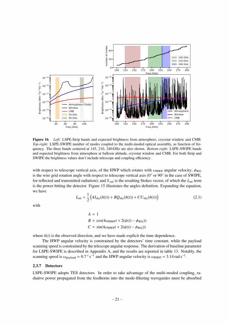
Figure 16. Left: LSPE-Strip bands and expected brightness from atmosphere, cryostat window and CMB.Top-right: LSPE-SWIPE number of modes coupled to the multi-moded optical assembly, as function of fre-quency. The three bands centered at 145, 210, 240 GHz are also shown. Bottom-right: LSPE-SWIPE bandsand expected brightness from atmosphere at balloon altitude, cryostat window and CMB. For both Strip andSWIPE the brightness values don’t include telescope and coupling efficiency.

with respect to telescope vertical axis, of the HWP which rotates with ωHWP angular velocity; φWGis the wire grid rotation angle with respect to telescope vertical axis (0° or 90° in the case of SWIPE,for reflected and transmitted radiation); and S out is the resulting Stokes vector, of which the Iout termis the power hitting the detector. Figure 15 illustrates the angles definition. Expanding the equation,we have

Iout =12

(AIsky(n(t)) + BQsky(n(t)) + CUsky(n(t))

)(2.1)

with

A = 1

B = cos(4ωHWPt + 2(ψ(t) − φWG))

C = sin(4ωHWPt + 2(ψ(t) − φWG))

where n(t) is the observed direction, and we have made explicit the time dependence.The HWP angular velocity is constrained by the detectors’ time constant, while the payload

scanning speed is constrained by the telescope angular response. The derivation of baseline parameterfor LSPE-SWIPE is described in Appendix A, and the results are reported in table 13. Notably, thescanning speed is ωpayload ' 0.7 ° s−1 and the HWP angular velocity is ωHWP = 3.14 rad s−1.

2.3.7 Detectors

LSPE-SWIPE adopts TES detectors. In order to take advantage of the multi-moded coupling, ra-diative power propagated from the feedhorns into the mode-filtering waveguides must be absorbed

– 21 –

by the detector with as low an impedance mismatch as possible for all the propagated modes. Oneway to fulfill this requirement is to compress the effective wavelengths of the coupled modes intoa narrower bandwidth by progressively re-enlarging the waveguide cross-section into a larger ter-minated cavity (flared waveguide), where a 15 mm large spider-web absorber collects the power fordetection by the TES. This solution has been validated through HFSS, providing a mode-dependent,frequency-dependent S 11 scattering parameter5 evaluation of the pixel assembly along the path fromthe waveguide to the absorber. The relative S 11-parameter dispersion for the 150 GHz band is about2% over the coupled modes and frequencies, with an average return loss of −22.6 dB when the cavitytermination is set to a quarter of the average free-space wavelength of the band collected by the de-tector, and the absorber impedance is ∼ 300 Ω. This result, to be validated also through experimentalverification of the pixel performance, is used here to support the hypothesis that the main impact ofthe broadband performance evaluation for SWIPE is the variable number of modes Nmodes(rwg, ν) cou-pled by the waveguide when fed with broadband radiation. Figure 16 illustrates the coupled modes asa function of frequency, and the selected bands; in the bottom-right panel, it shows the power enteringthe system, with contribution from the CMB, the atmosphere and the cryostat window (for Strip inthe bottom-left panel). These are the input to the noise calculation analysis reported in section 3.2and in table 4.

The TES bolometer is a single Si chip 15 × 15 mm2 with Au absorber deposited on a centralfree-standing Si3N4 membrane, 1 µm thick and 10 mm diameter. After the TES and Au absorber filmhave been grown, the membrane is first etched in the shape of a 8 mm diameter circular spider-websupported by 32 narrow legs and then suspended by means of Deep Reactive Ion Etching of the sil-icon beneath. The TES is located aside the circular spider-web and is in strong electronic contactwith the external perimeter of the gold absorber. The TES consists of 120 nm of a Au-Ti bilayer,which is manufactured taking care to maintain a process temperature profile below 100 °C, to ensurea superconducting to normal transition at Tc = 500 − 550 mK. In fact, it has been observed that highprocess temperatures reduce Tc towards its bulk value of 350 − 400 mK, as demonstrated in [87].These operating temperatures represent an optimal compromise between the SWIPE’s bath temper-ature of 300 mK and the detector saturation limits due to the high optical power (order of 10 pW) ofthe multi-mode configuration. The thermal conductance G, in the range of 65 − 100 pW K−1, wasmeasured in the first prototypes that have been operated at a base temperatures of about 350 mK. Theeffective time constants in the Electro-Thermal Feedback (ETF) regime were evaluated from the fre-quency response to a sinusoidal sweep excitation to be 20−33 ms, about a factor 2−3 larger than theones expected by the model. In these working points the thermal fluctuation noise equivalent power,NEP, is about 3 × 10−17 W Hz−1/2 (see section 3.2 for details).

The left panel of figure 17 shows the distribution of detectors in one of the two equivalent focalplanes. The payload rotates so that the scanning direction is along the x axis in the figure. Theright panel of figure 17 shows the LSPE-SWIPE large spider-web TES bolometer integrated in thebackshort of the microwave cavity.

2.3.8 Readout

The 326 TES bolometers are read-out by Superconducting Quantum Interference Devices (SQUIDs)using a Frequency-Domain Multiplexing scheme (FDM), with each DC-SQUID sensing 16 TES [88].In the FDM scheme a group of detectors is readout with a single SQUID by connecting in parallelseveral RLC chains in which R is given by the TES variable resistance, and the LC filters define

5Input port reflection coefficient.

– 22 –

Figure 17. Left: distribution of detectors in one of the two equivalent focal planes. The payload rotates so thatthe scanning direction is along the x-axis. Right: a LSPE-SWIPE large spider-web TES bolometer integratedin the backshort of the microwave cavity.

different frequencies. A single signal containing all the different frequencies is therefore needed tobias all TESs simultaneously. The detectors modulate the signal which is in turn sent to the SQUIDinput, amplified and demodulated by digital electronics. The multiplexing tones are in the range from100 kHz to 2 MHz, to be faster than the bolometers’ response but below the cut-off frequency of thereadout, the latter determined mainly by the length of the cables inside the cryostat. In this range wecan safely accommodate 16 tones that readout TESs coupled to detectors at all the three bands. Somechannels are coupled to blind detectors and/or calibration resistor to monitor gain fluctuations of thereadout chain.

The readout electronic chain is composed of a cold section inside the cryostat, at the sametemperature of the detectors, and a warm section, outside the cryostat. The entire chain is composed,going from the lowest to the highest temperature, of the LC filters and the bias resistors board, theSQUIDs boxes, the SQUID control unit and the warm electronics (see figure 18).

LC filters. The LC filters necessary to the frequency domain multiplexing are assembled ondedicated boards placed at 300 mK in close proximity to the TESs. The filters are composed of aniobium inductor fabricated by optical lithography coupled to a commercial Surface Mount Device(SMD) capacitor [89]. Given the inductance L ≈ 15 µH, the capacitors are chosen in order to giveresonance frequencies in the 200 kHz to 2 MHz range. Bolometers are connected to the LC boardwith shielded twisted pair wires. Furthermore the TES bias resistor is also placed on the board tominimize Johnson noise. Each board hosts three LC chains to read a quarter of focal plane. Foursuch boards are used for each focal plane for a total of eight boards.

SQUID boxes. Each LC board is connected with a custom low-inductance flat cable to a SQUIDbox placed at 1.6 K. Each box is used to thermalize and shield three SQUIDs, for a total of 24 SQUIDsfor the two focal planes. SQUIDs convert the modulated current signal into a modulated and amplifiedvoltage signal which in turn is sent to a further amplification stage outside the cryostat. The SQUIDsthat are baselined for LSPE/SWIPE are 6-stage SQUID arrays from VTT (model K3B) with criticalcurrent Ic ≈ 65 µA, input inductance 2 nH and a transimpedance of 30 to 50 V A−1 typically. Theflux coupling and noise are 36 µA Φ−1

0 and . 0.1 µΦ0 Hz−1/2 respectively (Φ0 being the magnetic flux

– 23 –

Figure 18. Schematic of the LSPE-SWIPE readout with the indication of the temperatures of the differentstages.

quantum). Two different coupling strengths can be selected for the feedback coil: M−1f ' 40 µA Φ−1

0and M−1

f ' 90 µA Φ−10 .

SQUID Control Units. The SQUID control units (SCUs) are placed outside the cryostat andperform the main following tasks: (i) they provide the SQUID bias signal (which will be set at theSQUID operating temperature and will be tuned in flight); (ii) they linearize SQUID response bymeans of a flux-locked loop (FLL hereafter); and (iii) they host the amplification stage needed to am-plify the SQUID output voltage before the digitizing stage. The desired amplification is achieved intwo stages, in order to obtain the desired bandwidth and to minimize the noise referred to the ampli-fier’s input. The SQUID output is first amplified by a very low noise preamplifier based on a discreteJFET (IF3602) input differential cascode architecture, followed by a low noise CMOS operationalamplifier (OPA301). The equivalent input noise density is 0.6 nV Hz−1/2 and the bandwidth extendsup to at least 2 MHz [90].

Warm readout. The warm readout boards contain the ADCs (LTM9001IV) and the DACs(LTC1668IG) that are used to generate the sum of sinusoids to bias the TES detectors and to digitizethe modulated output. They in turn perform the digital demodulation and the data compression.They perform these operations by means of a system-on-module board hosting a FPGA and an ARMmicroprocessor (MitySOM 5CSX System-On-Module6). Each board, with a single SOC, runs tworeadout chains, therefore the complete readout system is composed of a total of 12 boards in a 6Ustandard, placed in a custom aluminum crate that provides the mechanical support and dissipates thegenerated heat. Each warm readout board builds the packets that are sent to the on-board computerto be assembled in one single event.

3 Sensitivity of instruments

Realistic simulations of the observations are obtained for LSPE by means of noise estimation for6https://www.criticallink.com/product/mitysom-5csx/

– 24 –

Strip and SWIPE, and propagated from time-ordered data to maps using the instrument simulatorsdescribed in detail in Appendix B.

3.1 LSPE-Strip noise estimation

We model the noise of the Strip polarimeters as the sum of a white noise plus a 1/ f α component, sothat the post-detection power spectrum can be written as:

P( f ) = σ2[1 +

(fknee

f

)α], (3.1)

where the knee frequency, fknee, is the frequency where the white noise and the 1/ f α componentscontribute equally (P( fknee) = 2σ2). Previous experience (QUIET, WMAP, Planck-LFI) shows thatthis simple model provides a very good first-order description of the noise properties of HEMT-based coherent devices. The standard deviation of the white noise component of the Q and U Stokesparameters measured by each Strip polarimeter in antenna temperature is given by:

∆Tr.m.s. =1√

2

Tsys√

∆ν τ, (3.2)

where Tsys is the total intensity detected by the polarimeters (sky signals, emissions from the opticalcomponents and receiver noise temperature), ∆ν is the receiver bandwidth and τ is the integrationtime. The factor 1/

√2 in equation 3.2 results from the polarimeter correlation architecture and it is

explained in [91] and section 4 of [92]. In table 2 we detail the budget leading to the current estimateof the average receiver white noise performance.

We now discuss briefly the low-frequency properties of the noise spectrum and show how theexpected impact from 1/ f α noise components is small. In our measurements we expect two mainsources of noise fluctuations on long time scales: (i) fluctuations in the receiver gain and (ii) variationsin the atmospheric load. Both contribute to the 1/ f α shape of the noise spectrum at low frequencies.Strip polarimeters have a very low susceptibility to gain fluctuations and 1/ f α noise contributes inpolarization only at frequencies less than few tens of mHz.

This stability is the result of the differential nature of the receiver that allows one to recoverthe Q and U Stokes parameters by differentiating signals having essentially the same intensity, thuseffectively canceling out common modes. The penalty is that these detectors are practically blindto the CMB total intensity, as these measurements retain all the common-mode fluctuations and arecharacterized by knee frequencies of the order of several Hz.

If we assume zero or negligible polarization in the atmospheric signal, then we can neglect,to first order, also the effect of 1/ f α fluctuations in the atmospheric load. These will contaminatepolarization measurements only through any leakage from total intensity to polarization that couldbe present in our receivers and that will be caused mainly by asymmetries in the polarizer-OMTsystem. Considering that our current estimates from OMT laboratory measurements [46] indicatea leakage of the order of ∼ 0.01% this effect is likely to be negligible. We are currently workingon a simulation framework that will model the expected fluctuations in the atmosphere brightnesstemperature and their effect of the sky polarization measurement and will allow us to quantify theimpact of this systematic effect.

3.2 LSPE-SWIPE noise estimation

The LSPE-SWIPE detector’s noise is given by the combination of photon noise, detector thermalnoise, readout electronics noise, and the effect of cosmic rays.

– 25 –

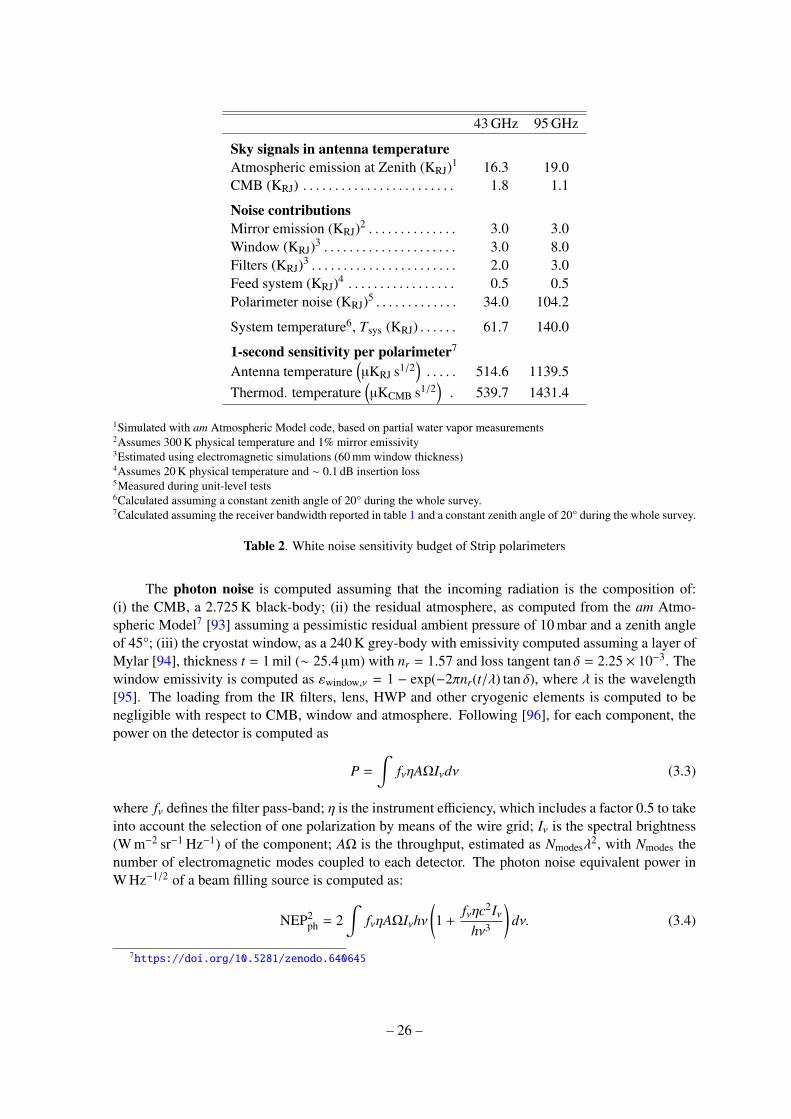
43 GHz 95 GHz

Sky signals in antenna temperatureAtmospheric emission at Zenith (KRJ)1 16.3 19.0CMB (KRJ) . . . . . . . . . . . . . . . . . . . . . . . . 1.8 1.1

Noise contributionsMirror emission (KRJ)2 . . . . . . . . . . . . . . 3.0 3.0Window (KRJ)3 . . . . . . . . . . . . . . . . . . . . . 3.0 8.0Filters (KRJ)3 . . . . . . . . . . . . . . . . . . . . . . . 2.0 3.0Feed system (KRJ)4 . . . . . . . . . . . . . . . . . 0.5 0.5Polarimeter noise (KRJ)5 . . . . . . . . . . . . . 34.0 104.2

System temperature6, Tsys (KRJ) . . . . . . 61.7 140.0

1-second sensitivity per polarimeter7

Antenna temperature(µKRJ s1/2

). . . . . 514.6 1139.5

Thermod. temperature(µKCMB s1/2

). 539.7 1431.4

1Simulated with am Atmospheric Model code, based on partial water vapor measurements2Assumes 300 K physical temperature and 1% mirror emissivity3Estimated using electromagnetic simulations (60 mm window thickness)4Assumes 20 K physical temperature and ∼ 0.1 dB insertion loss5Measured during unit-level tests6Calculated assuming a constant zenith angle of 20° during the whole survey.7Calculated assuming the receiver bandwidth reported in table 1 and a constant zenith angle of 20° during the whole survey.

Table 2. White noise sensitivity budget of Strip polarimeters

The photon noise is computed assuming that the incoming radiation is the composition of:(i) the CMB, a 2.725 K black-body; (ii) the residual atmosphere, as computed from the am Atmo-spheric Model7 [93] assuming a pessimistic residual ambient pressure of 10 mbar and a zenith angleof 45°; (iii) the cryostat window, as a 240 K grey-body with emissivity computed assuming a layer ofMylar [94], thickness t = 1 mil (∼ 25.4 µm) with nr = 1.57 and loss tangent tan δ = 2.25 × 10−3. Thewindow emissivity is computed as εwindow,ν = 1 − exp(−2πnr(t/λ) tan δ), where λ is the wavelength[95]. The loading from the IR filters, lens, HWP and other cryogenic elements is computed to benegligible with respect to CMB, window and atmosphere. Following [96], for each component, thepower on the detector is computed as

P =

∫fνηAΩIνdν (3.3)

where fν defines the filter pass-band; η is the instrument efficiency, which includes a factor 0.5 to takeinto account the selection of one polarization by means of the wire grid; Iν is the spectral brightness(W m−2 sr−1 Hz−1) of the component; AΩ is the throughput, estimated as Nmodesλ

2, with Nmodes thenumber of electromagnetic modes coupled to each detector. The photon noise equivalent power inW Hz−1/2 of a beam filling source is computed as:

NEP2ph = 2

∫fνηAΩIνhν

(1 +

fνηc2Iνhν3

)dν. (3.4)

7https://doi.org/10.5281/zenodo.640645

– 26 –

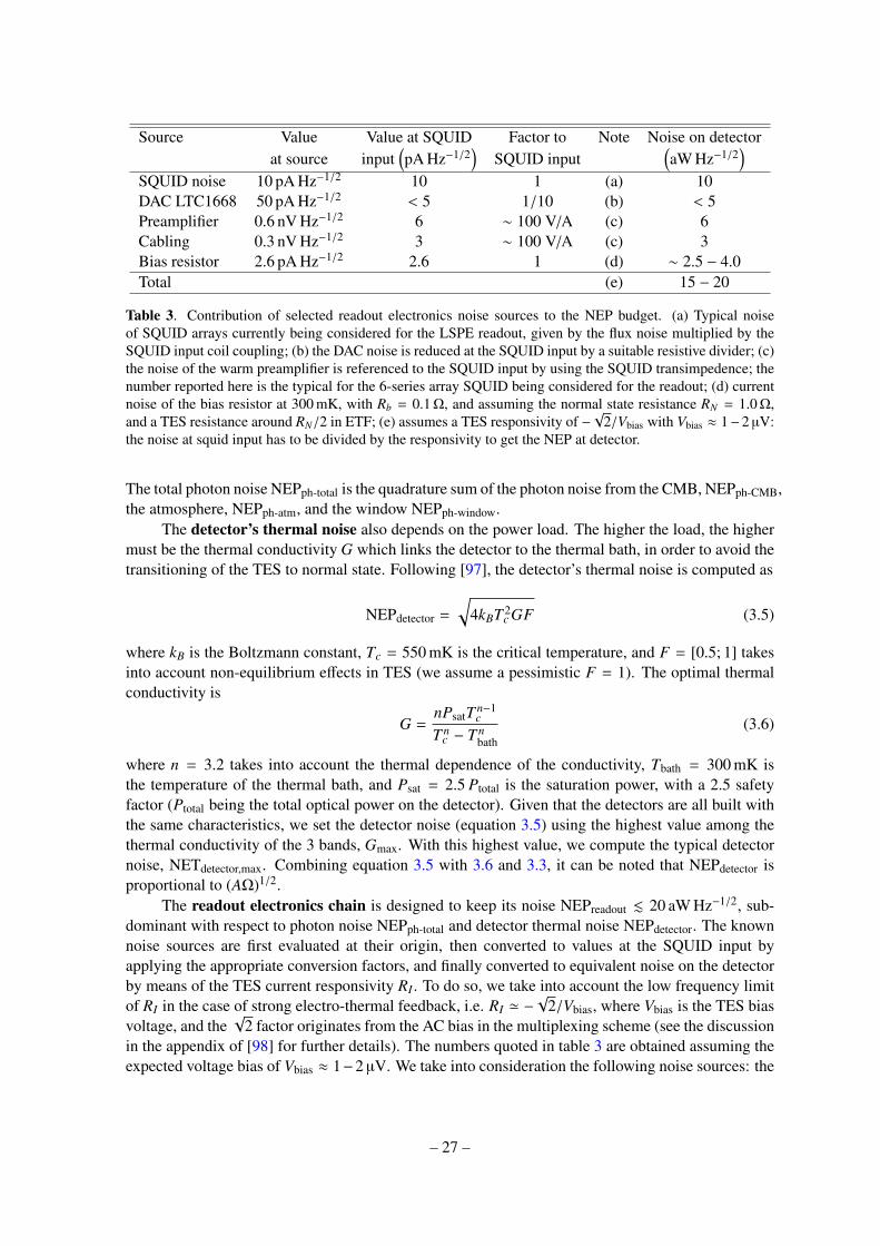
Source Value Value at SQUID Factor to Note Noise on detectorat source input

(pA Hz−1/2

)SQUID input

(aW Hz−1/2

)SQUID noise 10 pA Hz−1/2 10 1 (a) 10DAC LTC1668 50 pA Hz−1/2 < 5 1/10 (b) < 5Preamplifier 0.6 nV Hz−1/2 6 ∼ 100 V/A (c) 6Cabling 0.3 nV Hz−1/2 3 ∼ 100 V/A (c) 3Bias resistor 2.6 pA Hz−1/2 2.6 1 (d) ∼ 2.5 − 4.0Total (e) 15 − 20

Table 3. Contribution of selected readout electronics noise sources to the NEP budget. (a) Typical noiseof SQUID arrays currently being considered for the LSPE readout, given by the flux noise multiplied by theSQUID input coil coupling; (b) the DAC noise is reduced at the SQUID input by a suitable resistive divider; (c)the noise of the warm preamplifier is referenced to the SQUID input by using the SQUID transimpedence; thenumber reported here is the typical for the 6-series array SQUID being considered for the readout; (d) currentnoise of the bias resistor at 300 mK, with Rb = 0.1 Ω, and assuming the normal state resistance RN = 1.0 Ω,and a TES resistance around RN/2 in ETF; (e) assumes a TES responsivity of −

√2/Vbias with Vbias ≈ 1−2 µV:

the noise at squid input has to be divided by the responsivity to get the NEP at detector.

The total photon noise NEPph-total is the quadrature sum of the photon noise from the CMB, NEPph-CMB,the atmosphere, NEPph-atm, and the window NEPph-window.

The detector’s thermal noise also depends on the power load. The higher the load, the highermust be the thermal conductivity G which links the detector to the thermal bath, in order to avoid thetransitioning of the TES to normal state. Following [97], the detector’s thermal noise is computed as

NEPdetector =

√4kBT 2

c GF (3.5)

where kB is the Boltzmann constant, Tc = 550 mK is the critical temperature, and F = [0.5; 1] takesinto account non-equilibrium effects in TES (we assume a pessimistic F = 1). The optimal thermalconductivity is

G =nPsatT n−1

c

T nc − T n

bath(3.6)

where n = 3.2 takes into account the thermal dependence of the conductivity, Tbath = 300 mK isthe temperature of the thermal bath, and Psat = 2.5 Ptotal is the saturation power, with a 2.5 safetyfactor (Ptotal being the total optical power on the detector). Given that the detectors are all built withthe same characteristics, we set the detector noise (equation 3.5) using the highest value among thethermal conductivity of the 3 bands, Gmax. With this highest value, we compute the typical detectornoise, NETdetector,max. Combining equation 3.5 with 3.6 and 3.3, it can be noted that NEPdetector isproportional to (AΩ)1/2.

The readout electronics chain is designed to keep its noise NEPreadout . 20 aW Hz−1/2, sub-dominant with respect to photon noise NEPph-total and detector thermal noise NEPdetector. The knownnoise sources are first evaluated at their origin, then converted to values at the SQUID input byapplying the appropriate conversion factors, and finally converted to equivalent noise on the detectorby means of the TES current responsivity RI . To do so, we take into account the low frequency limitof RI in the case of strong electro-thermal feedback, i.e. RI ' −

√2/Vbias, where Vbias is the TES bias

voltage, and the√

2 factor originates from the AC bias in the multiplexing scheme (see the discussionin the appendix of [98] for further details). The numbers quoted in table 3 are obtained assuming theexpected voltage bias of Vbias ≈ 1−2 µV. We take into consideration the following noise sources: the

– 27 –

Band (GHz) . . . . . . . . . . . . . . 145 210 240bandwidth . . . . . . . . . . . . . . . . 30% 20% 10%Nmodes

1 . . . . . . . . . . . . . . . . . . . [10;13.1;17] [23;27.0;32] [32;34.5;39]AΩ

(m2 sr

). . . . . . . . . . . . . . . . Nmodesλ

2

efficiency η . . . . . . . . . . . . . . . 0.3 0.25 0.25

Power on cryostat entrancePCMB

(pW

). . . . . . . . . . . . . . . 9.1 7.7 3.9

Patm(pW

). . . . . . . . . . . . . . . . 0.9 1.9 9.8

Pwindow(pW

). . . . . . . . . . . . . . 1.0 2.8 2.4

Ptotal(pW

). . . . . . . . . . . . . . . . 11.0 12.4 16.1

Power on detectorPtotal-detector

(pW

). . . . . . . . . . 3.3 3.1 4.0

Noise on detectorNEPph-CMB

(aW Hz−1/2

). . . . 23.5 23.3 17.6

NEPph-atm(aW Hz−1/2

). . . . . 8.4 12.3 34.1

NEPph-window(aW Hz−1/2

). . 7.8 14.2 13.9

NEPph-total(aW Hz−1/2

). . . . 26.1 29.9 40.8

G(pW K−1

). . . . . . . . . . . . . . 56.1 52.7 68.4

Gmax(pW K−1

). . . . . . . . . . . 68.4

NEPdetector(aW Hz−1/2

). . . . 30.6 29.7 33.8

NEPdetector,max(aW Hz−1/2

). 33.8

NEPreadout(aW Hz−1/2

). . . . . 20

NEPtotal(aW Hz−1/2

). . . . . . . 47.2 49.4 56.6

Optical noiseNEPoptical-total

(aW Hz−1/2

). . 157 197 226

NET(µKCMB s1/2

). . . . . . . . 11.4 12.3 26.2

margin m (%) . . . . . . . . . . . . . 5 20 20NETeff

(µKCMB s1/2

). . . . . . . 12.6 15.6 31.4

1The number of modes varies across the band (see figure 16), with less modes in the lowerside of the band, and more modes in the higher side. The three values in the square bracketsindicate the number of modes at the minimum frequency of each band, the average acrossthe band, and number at the maximum frequency of each band.

Table 4. LSPE-SWIPE detectors radiative power and noise estimation. See text for details.

– 28 –

SQUID current noise, the DAC current noise, the SQUID preamplifier noise and the Johnson noise ofbias resistor and cabling between the cold (inside the cryostat) and the warm (outside) section of theelectronics. In table 3 we quote their typical values together with the factor needed for comparison atthe SQUID input. See [99] for further details on the assumed noise model. The total readout currentnoise NEPreadout is computed as the quadrature sum of these contributions.

The total noise equivalent power, NEPtotal, is computed by quadrature sum of the photon noisefrom different sources, the detector thermal noise and the readout noise. The optical noise, whichconverts the noise on the detector to noise at the instrument aperture, taking efficiency into account,is computed as

NEPoptical-total = NEPtotal/η

Results of this calculation are converted to µKCMB s1/2 as:

NET =TCMB∫

fνAΩB(TCMB) xex

ex−1 dx

NEPoptical-total√

2(3.7)

where B(TCMB) is the CMB black-body brightness, x = hν/(kBTCMB) is the reduced frequency, andthe factor 1/

√2 takes into account the conversion from µKCMB Hz−1/2 to µKCMB s1/2. Notably, the

photon noise NEP (as the thermal noise) is proportional to (AΩ)1/2, while the NET is inverse propor-tional to (AΩ)1/2 and thus to N1/2

modes. This is the advantage of multi-moded detectors: higher photonnoise, which relaxes the detector noise requirement, and lower NET. Background and noise calcula-tion results are reported in table 4. In order to take into account possible effects such as contaminationby cosmic rays (see next section), atmospheric background variation, detectors yield, detector excessnoise, and other unexpected effects, we also report the margin m value and the effective noise,

NETeff = NET(1 + m),

which we use as input in the instrument simulator, for the results reported in section 5. The marginm is not the same for all channels, due to the largest uncertainty in the atmospheric modeling inthe highest frequencies. In SWIPE, the 1/ f noise term has negligible impact, due to the polarizationmodulation by means of the HWP. Measurements of the detector noise power spectra show the typicalbehaviour of 1/ f evident at low frequency, on top of a flat spectrum, with an high frequency roll-off

due to the detectors’ time constants cut-off.

3.2.1 Cosmic rays rate

TES detectors are sensitive to any form of energy deposited on the absorber, including the effectof cosmic rays. The flux of primary cosmic rays in the upper atmosphere is fairly well known,as well as its dependence on the latitude and on the solar cycles. We evaluated the expected rateof interactions by cosmic rays in the upper atmosphere (altitude 40 km) along the orbit of SWIPEby using the measured fluxes and simulating the interactions of primary protons and alphas on theSWIPE cryostat, instrument and focal plane. An energy-integrated flux of 1.5 particles cm−2 s−1 isobtained at the minimum of the solar activity cycle, decreasing by a factor ≈ 2.5 at the solar activitymaximum.

We assume that cosmic rays release a signal in the bolometers whenever they interact withthe gold-plated spider-web structure. By using the geometrical characteristics of our spider-webbolometers (diameter 8 mm, fill factor 8%) we estimate an interaction rate of 60 mHz per bolometer,giving roughly a 1 Hz rate of interaction per readout chain, given that the bolometers are multiplexedin groups of 16. The 60 mHz rate is reasonable once compared with the (inverse of the) bolometertime constant, nevertheless suitable algorithms for cosmic ray hit identification and removal must be

– 29 –

Strip systematic effect Goal Requirement(µK) (µK)

I → Q/U leakage . . . . . . . . . . 0.030 0.050Q→ U and U → Q leakage . 0.020 0.030Polarization angle uncertainty 0.010 0.0301/ f noise . . . . . . . . . . . . . . . . . . 0.015 0.050Far sidelobes . . . . . . . . . . . . . . . 0.030 0.060Pointing . . . . . . . . . . . . . . . . . . . 0.010 0.030Scan synchronous signals . . . 0.010 0.030Other periodic signals . . . . . . . 0.001 0.003Calibration-dependent effects 0.010 0.030

Total (quadrature sum1) . . . . . 0.053 0.1141The quadrature sum results from the assumption that the various effects

are uncorrelated. This assumption will be tested by detailed end-to-end

simulations that are currently ongoing and that will be reported in a

dedicated paper.

Table 5. Strip systematic effects budget. The numbers indicate the maximum systematic uncertainty on a pixelsize equal to the angular resolution.

implemented. These algorithms also subtract the long tail after the glitch in the data. In a typicalcase, after a glitch, it is impossible to recover the first part of the tail, equal to [5; 10] τLP. With a rateof one event every 16.7 s and a time constant τLP = 30 ms, this correspond to removing between 1and 2% of the data, well within our margins.

4 Systematic effects and calibration

In this section we present the most relevant systematic effects for the two instruments, with partic-ular focus on the systematic effects critical for the measurement of the CMB polarization. We alsoset requirements on the knowledge of the most important instrumental parameters, and discuss thecalibration plans.

4.1 LSPE-Strip systematic effects

Here we provide a brief summary of the Strip susceptibility to systematic effects, deferring to forth-coming papers a more detailed treatment.

Systematic effects budget. We start by setting a top-level requirement on the maximum uncertaintyfrom systematic effects on a single sky pixel having the size of the Q-band optical angular resolution.In general we want this uncertainty to be much less than that imposed by the white noise. Followingthe approach already adopted for Planck-LFI [100, 101] we set this limit to 5% of the white noiselevel as a goal and 10% of the white noise level as a requirement. In table 5 we provide a list ofsystematic effects that could affect Strip polarimetric measurements and goal/requirement values forthe upper limit in the systematic uncertainty. The detailed breakdown has been defined according toour best current knowledge of the instrumental properties.

– 30 –

Polarimetric effects. Strip polarimeters are based on the QUIET design, which provides significantadvantage: (i) the Q and U Stokes parameters are measured directly for each horn in the focal plane,instead of being recovered through the inversion of a condition matrix, (ii) the system is unaffectedby gain and bandpass mismatches between the two acquisition lines of the same polarimeter, as wellby as unbalances in phase switch states, and (iii) 1/ f noise and other common-mode effects areefficiently removed from Q/U timelines thanks to double demodulation.

The most important polarization effect in the polarimetric chain is the leakage from total in-tensity to polarization that is caused by non ideal performance of the polarizer-OMT assembly. Inparticular the transmission imbalance, δLpol, of the two electrical ports of the polarizer cause a leak-age LI→Q = δLpol, while the OMT cross-polarization, XOMT, causes a leakage LI→Q = 2

√XOMT.

Considering the combined effect of δLpol and XOMT we obtain LI→Q = δLpol. + 2Lpol√

XOMT, whereLpol is the polarizer average transmission.

If we consider the averaged measured OMT and polarizer cross-polarization and amplitudeimbalance, XOMT ∼ −55 dB and δLpol ∼ 0.01 dB, we obtain a leakage term LI→Q ∼ 0.5%. Noticethat we have negligible leakage from I to U, as also reported in [49]. The reader will find furtherdetails about the polarimeter mathematical model and polarizer-OMT measurements is a series oftechnical papers about Strip that is currently in preparation for submission to JINST.

Another possible source of systematic effects is the difference in the bandpass among the variouspolarimeters. In fact, the polarimeters average the incoming signal over the bandpass, so that ifthe bandpasses are different and the source is not a black-body (as it contains, for example, theGalactic synchrotron emission) we have a residual systematic effect in the final, averaged map. Wehave performed simulations using bandpasses measured in the laboratory, a synthetic sky with CMB,Galactic synchrotron and dust emissions, and Monte Carlo realizations of the instrumental noise.Our results show that the angular power spectrum of the residual effect in polarization is about threeorders of magnitude below the noise level, so that we can neglect it.

Other imperfections are either compensated for by design (e.g. gain unbalance), or generate aleakage between U and Q that we estimate to be . 1% on the basis of the measured and simulatedparameters of the various components in the polarimetric chain.

Thermal/electrical fluctuations. Variations in temperature and bias voltages will generate common-mode fluctuations in the total intensity signal that will be canceled by the double demodulation. Onlytemperature variations in the feedhorn-OMT system can, in principle, leave a small residual in theQ and U parameters because of the leakage from intensity to polarization caused by the front-endcross-polarization. This residual effect is expected to be negligible and we will control its impactduring data analysis by exploiting the instrument temperature housekeeping data.

Fluctuations in the atmosphere. The atmosphere impacts CMB polarization measurements fromthe ground in two ways: (i) its average brightness temperature increases the white noise level of themeasurements and (ii) it is a source of low-frequency noise due to the correlation structures in thewater vapor bubbles [102].

Regarding the atmospheric load, we have estimated an average brightness temperature of 16.3 Kat 43 GHz and 19.0 K at 95 GHz (see table 2). This estimate is based on simulations carried out withthe am Atmospheric Model code using precipitable water vapor (PWV) measurements collected in2018.

Brightness temperature fluctuations in the atmosphere are caused by PWV variations that followthe typical sub-tropical seasonal modulation. The effect of these fluctuations are canceled to firstorder in the polarization data by the pseudo correlation architecture of the Strip polarimeters. Asmall fraction of these intensity fluctuations, however, leaks into Q and U because of the non-zero

– 31 –

cross polarization of the polarizer-OMT assembly. Although this fraction is small (∼ 0.5%) we aredeveloping a Monte Carlo simulations to estimate their impact on polarization measurements (seeappendix C).

Stray-light. We define stray-light as the overall signal detected by the instrument from directionsoutside the main beam. The origin of these signals, detected by the optics sidelobes, can be astrophys-ical (e.g. the Galaxy), terrestrial (the emissions from the ground) and instrumental (e.g. the emissionsfrom the telescope enclosure shields). The sidelobes can contribute to a spurious polarization in twoways: (i) by detecting directly a polarized signal far from the main beam (from the sky, from theEarth and from the Sun) and (ii) by converting a total intensity emission to polarization due to thecross-polar response of the telescope-feed system.

Regarding the first point, our preliminary estimates based on the simulated beam far sidelobesshow that spurious polarization detected directly from the sky is less than ∼ 3 nK and, therefore,negligible. The assessment of the polarized input from the Earth is more difficult, because of thelack of data on the polarization properties of the microwave Earth emissions. Using Earth brightnesstemperature data measured at 37 GHz by the Special Sensor Microwave/Imager instrument on boardthe Defense Meteorological Satellite Program8 we estimated an upper limit of 0.1 K of polarizedemission from the Earth potentially entering the telescope far sidelobes. We also estimated that withthe current shielding this contribution should be maintained below ∼ 0.05 µK in the scientific data.

To avoid Sun contamination during daytime we will discard data where the Sun is at an angulardistance less than 10° from the telescope line-of-sight. Our simulations show that this fraction cor-responds to about 15% of the data and is included in our duty cycle computation. When the Sun isfarther than 10° its emission will be detected by the beam far sidelobes that are at the level of about−100 dB, enough to dilute this signal to negligible levels.

Regarding the intensity-to-polarization leakage caused by the Strip optics we have consideredthe input from the sky and from temperature variations in the optical enclosure. Considering the44 GHz Planck sky maps combined with the −40 dB upper limit of the cross-polar beam (see insettable of figure 5) we find that the sky contributes with a spurious polarization of ∼ 0.01 µK. Thepolarization systematic effect induced by optical enclosure temperature fluctuations is not a concern,provided that we will be able to measure and decorrelate these fluctuations from the data.

Main beam asymmetry. Asymmetry in the main beams is a source of leakage from intensity topolarization that can be corrected in the power spectra, provided that one knows the main beams withpercent precision down to about −25 dB. In Strip we further control this effect “in hardware”, thanksto the very symmetric optical response of the telescope crossed-Dragonian design that guaranteesan average beam ellipticity less than 1% with a corresponding cross-polar discrimination better than−40 dB (see, again, the inset table of figure 5).

Pointing effects. Strip will implement a night optical star tracker that will allow us to reconstructthe pointing with a precision of 15 ′′ or better, resulting in negligible pointing systematic effects. Asa reference, the precision reached by Planck for the 44 GHz LFI channel was 27 ′′ for the pointingreconstructed from the nominal Jupiter scans and 19 ′′ for the pointing reconstructed from the deepJupiter scans [101, section 5.3]. This precision was enough to guarantee the scientific performanceand the impact of errors in the pointing reconstruction could be considered negligible [103, figure 8].

Calibration effects. An important source of systematic effects is the uncertainty in the instrumentcalibration parameters: (i) the photometric calibration (also named “responsivity”) that converts the

8http://www.remss.com/missions/ssmi

– 32 –

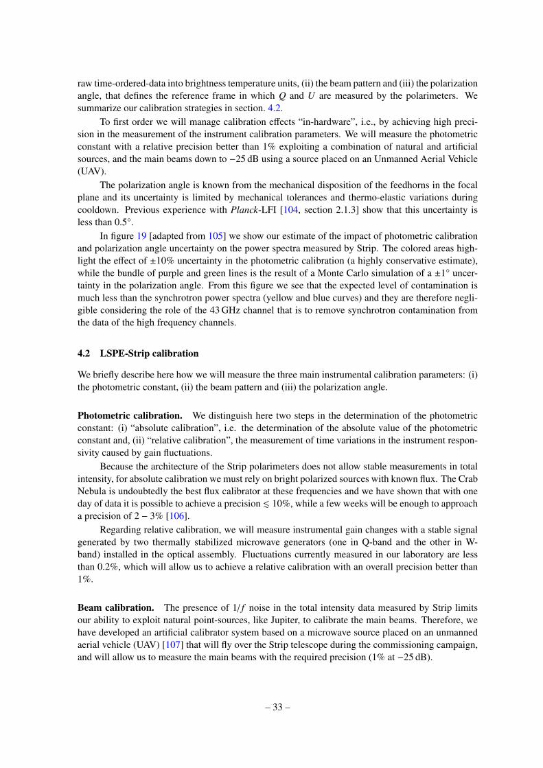
raw time-ordered-data into brightness temperature units, (ii) the beam pattern and (iii) the polarizationangle, that defines the reference frame in which Q and U are measured by the polarimeters. Wesummarize our calibration strategies in section. 4.2.

To first order we will manage calibration effects “in-hardware”, i.e., by achieving high preci-sion in the measurement of the instrument calibration parameters. We will measure the photometricconstant with a relative precision better than 1% exploiting a combination of natural and artificialsources, and the main beams down to −25 dB using a source placed on an Unmanned Aerial Vehicle(UAV).

The polarization angle is known from the mechanical disposition of the feedhorns in the focalplane and its uncertainty is limited by mechanical tolerances and thermo-elastic variations duringcooldown. Previous experience with Planck-LFI [104, section 2.1.3] show that this uncertainty isless than 0.5°.

In figure 19 [adapted from 105] we show our estimate of the impact of photometric calibrationand polarization angle uncertainty on the power spectra measured by Strip. The colored areas high-light the effect of ±10% uncertainty in the photometric calibration (a highly conservative estimate),while the bundle of purple and green lines is the result of a Monte Carlo simulation of a ±1° uncer-tainty in the polarization angle. From this figure we see that the expected level of contamination ismuch less than the synchrotron power spectra (yellow and blue curves) and they are therefore negli-gible considering the role of the 43 GHz channel that is to remove synchrotron contamination fromthe data of the high frequency channels.

4.2 LSPE-Strip calibration

We briefly describe here how we will measure the three main instrumental calibration parameters: (i)the photometric constant, (ii) the beam pattern and (iii) the polarization angle.

Photometric calibration. We distinguish here two steps in the determination of the photometricconstant: (i) “absolute calibration”, i.e. the determination of the absolute value of the photometricconstant and, (ii) “relative calibration”, the measurement of time variations in the instrument respon-sivity caused by gain fluctuations.

Because the architecture of the Strip polarimeters does not allow stable measurements in totalintensity, for absolute calibration we must rely on bright polarized sources with known flux. The CrabNebula is undoubtedly the best flux calibrator at these frequencies and we have shown that with oneday of data it is possible to achieve a precision . 10%, while a few weeks will be enough to approacha precision of 2 − 3% [106].

Regarding relative calibration, we will measure instrumental gain changes with a stable signalgenerated by two thermally stabilized microwave generators (one in Q-band and the other in W-band) installed in the optical assembly. Fluctuations currently measured in our laboratory are lessthan 0.2%, which will allow us to achieve a relative calibration with an overall precision better than1%.

Beam calibration. The presence of 1/ f noise in the total intensity data measured by Strip limitsour ability to exploit natural point-sources, like Jupiter, to calibrate the main beams. Therefore, wehave developed an artificial calibrator system based on a microwave source placed on an unmannedaerial vehicle (UAV) [107] that will fly over the Strip telescope during the commissioning campaign,and will allow us to measure the main beams with the required precision (1% at −25 dB).

– 33 –

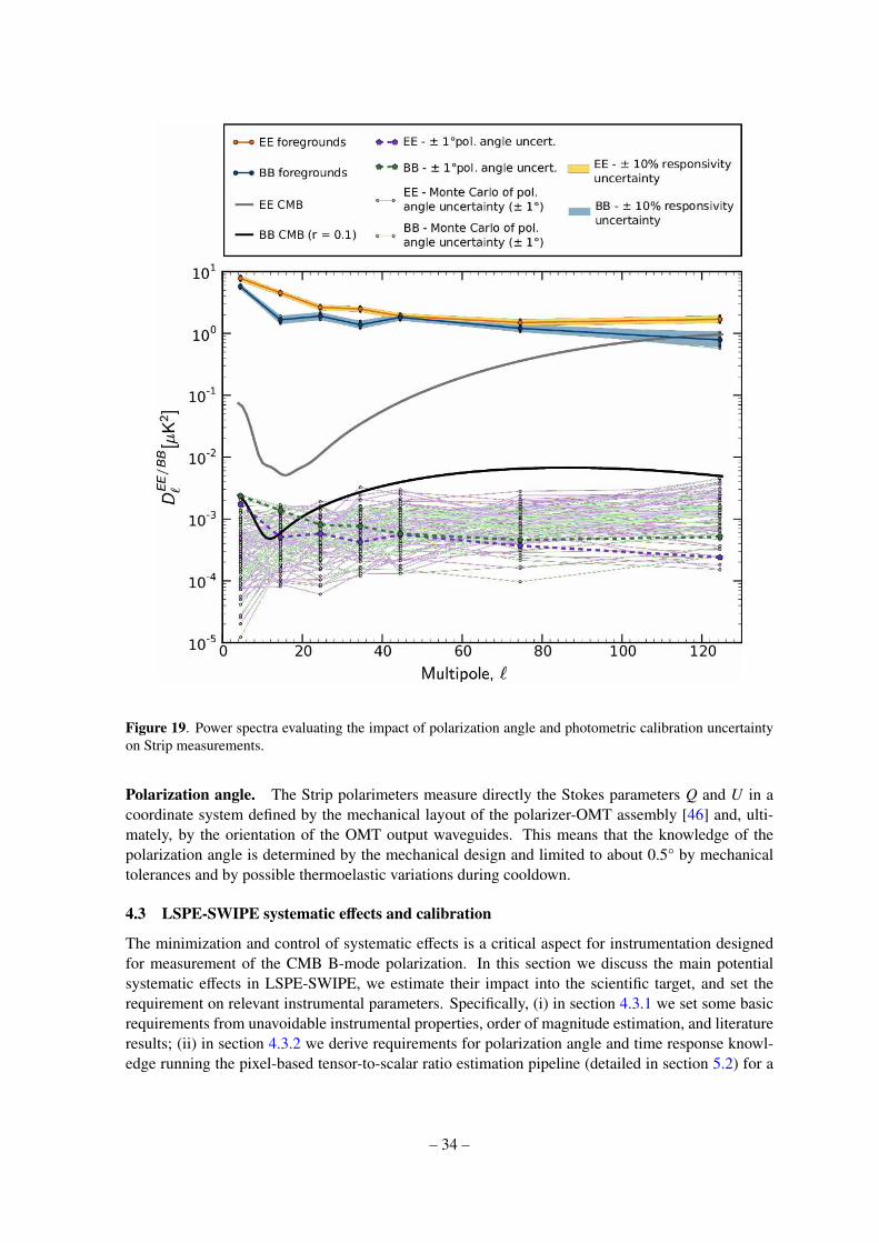
Figure 19. Power spectra evaluating the impact of polarization angle and photometric calibration uncertaintyon Strip measurements.

Polarization angle. The Strip polarimeters measure directly the Stokes parameters Q and U in acoordinate system defined by the mechanical layout of the polarizer-OMT assembly [46] and, ulti-mately, by the orientation of the OMT output waveguides. This means that the knowledge of thepolarization angle is determined by the mechanical design and limited to about 0.5° by mechanicaltolerances and by possible thermoelastic variations during cooldown.

4.3 LSPE-SWIPE systematic effects and calibration

The minimization and control of systematic effects is a critical aspect for instrumentation designedfor measurement of the CMB B-mode polarization. In this section we discuss the main potentialsystematic effects in LSPE-SWIPE, we estimate their impact into the scientific target, and set therequirement on relevant instrumental parameters. Specifically, (i) in section 4.3.1 we set some basicrequirements from unavoidable instrumental properties, order of magnitude estimation, and literatureresults; (ii) in section 4.3.2 we derive requirements for polarization angle and time response knowl-edge running the pixel-based tensor-to-scalar ratio estimation pipeline (detailed in section 5.2) for a

– 34 –

coherent rotation of the polarization in the sky; (iii) in section 4.3.3 we derive requirements on thesystematic effects produced by the HWP at the frequency of the plate rotation, and its harmonics,including a requirement on the knowledge of the HWP angular velocity and of the HWP angle, interms of random error and systematic offset; this is obtained by a full end-to-end simulation of theLSPE-SWIPE observation, using the instrument simulator, prior of running the tensor-to-scalar ratioestimation pipeline; (iv) finally in section 4.3.4 we summarize the requirements and briefly describethe calibration philosophy.

4.3.1 LSPE-SWIPE optical parameters requirements

LSPE-SWIPE is designed to minimize instrumental polarization. This is the spurious signal resultingfrom the measurement of unpolarized radiation. In the case of CMB, the amount of unpolarizedradiation coming from the sky is overwhelming with respect to the polarized signal, minimizinginstrumental polarization is the most important driver of instrument design. In the case of SWIPE,some level of instrumental polarization is inevitably generated by the cryostat window, in case ofincident radiation not orthogonal to the window surface itself. This is due to multiple reflections inan isotropic dielectric slab [108]. For the off-axis detectors, considering the physical properties of thethin window reported in section 3.2, this instrumental polarization will be up to 0.04%. Despite beinga small value, it will produce a constant polarized signal at the level of 1 mK from the unpolarizedCMB monopole, up to 2 µK spurious polarization from CMB dipole, and less than 25 nK from CMBanisotropy. The high constant signal is treated as an offset, removed in the data analysis. Its stabilitydepends on the stability of the gain of the electronics and of the responsivity of the detectors and theeffect of the instability is not synchronous with the observed sky. The detailed removal techniqueis described in section 4.3.3. Beyond this inevitable term, instrumental polarization is reduced bysystem design, with an optical system close to on-axis, avoiding mirrors in favor of lenses, andusing the polarization modulator as the first optical element (except window and thermal filters), thusrelaxing significantly the requirements on the following optical components.

The second parameter to be considered is cross-polarization, defined as the response of a po-larimeter to an input signal polarized in direction orthogonal to the nominal polarimeter direction.Cross-polarization results in leakage of E-mode into B-mode. Our requirement is that the maximumacceptable level of cross-polarization is below 2%. This is achieved again by means of an accurateoptical design, as described in section 2.3.5.

The third parameter to be considered is the ellipticity of the main beam (detector angular re-sponse in the sky). Spinning of the Half-Wave Plate allows the system to observe the same sky regionwith the same beam orientation, and different polarimeter orientation. This strongly mitigates theellipticity requirement, which was tested with simulations up to 25% without a relevant impact, anddifferential ellipticity among different detectors.

Correct measurement of the angles of the polarimeters is crucial to avoid leakage from E-modeinto B-mode, and to avoid contamination in the measurement of fundamental physics effects such ascosmic birefringence. In this context, our system is characterized by the presence of a single, largewire grid polarizer, defining the reference system for polarization measurements. With this designthe system is similar to an ideal polarimeter, and the angle of the single large wire grid polarimetercan be accurately measured. The requirement on the polarimeter angle measurement is set in the nextsection.

Spectral matching among detectors has been historically a problem for instruments without apolarization modulator, just comparing two independent measurements of the orthogonal polarizationcomponents. In LSPE-SWIPE we use a Stokes polarimeter, where the same detector measures bothpolarizations, alternated by means of the rotating HWP. In this configuration the most important

– 35 –

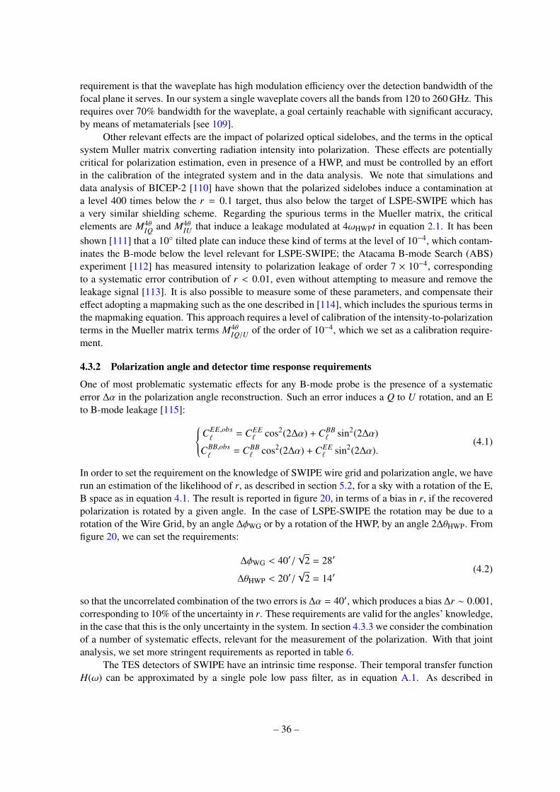
requirement is that the waveplate has high modulation efficiency over the detection bandwidth of thefocal plane it serves. In our system a single waveplate covers all the bands from 120 to 260 GHz. Thisrequires over 70% bandwidth for the waveplate, a goal certainly reachable with significant accuracy,by means of metamaterials [see 109].

Other relevant effects are the impact of polarized optical sidelobes, and the terms in the opticalsystem Muller matrix converting radiation intensity into polarization. These effects are potentiallycritical for polarization estimation, even in presence of a HWP, and must be controlled by an effortin the calibration of the integrated system and in the data analysis. We note that simulations anddata analysis of BICEP-2 [110] have shown that the polarized sidelobes induce a contamination ata level 400 times below the r = 0.1 target, thus also below the target of LSPE-SWIPE which hasa very similar shielding scheme. Regarding the spurious terms in the Mueller matrix, the criticalelements are M4θ

IQ and M4θIU that induce a leakage modulated at 4ωHWPt in equation 2.1. It has been

shown [111] that a 10 tilted plate can induce these kind of terms at the level of 10−4, which contam-inates the B-mode below the level relevant for LSPE-SWIPE; the Atacama B-mode Search (ABS)experiment [112] has measured intensity to polarization leakage of order 7 × 10−4, correspondingto a systematic error contribution of r < 0.01, even without attempting to measure and remove theleakage signal [113]. It is also possible to measure some of these parameters, and compensate theireffect adopting a mapmaking such as the one described in [114], which includes the spurious terms inthe mapmaking equation. This approach requires a level of calibration of the intensity-to-polarizationterms in the Mueller matrix terms M4θ

IQ/U of the order of 10−4, which we set as a calibration require-ment.

4.3.2 Polarization angle and detector time response requirements

One of most problematic systematic effects for any B-mode probe is the presence of a systematicerror ∆α in the polarization angle reconstruction. Such an error induces a Q to U rotation, and an Eto B-mode leakage [115]: CEE,obs

`= CEE

` cos2(2∆α) + CBB` sin2(2∆α)

CBB,obs`

= CBB` cos2(2∆α) + CEE

` sin2(2∆α).(4.1)

In order to set the requirement on the knowledge of SWIPE wire grid and polarization angle, we haverun an estimation of the likelihood of r, as described in section 5.2, for a sky with a rotation of the E,B space as in equation 4.1. The result is reported in figure 20, in terms of a bias in r, if the recoveredpolarization is rotated by a given angle. In the case of LSPE-SWIPE the rotation may be due to arotation of the Wire Grid, by an angle ∆φWG or by a rotation of the HWP, by an angle 2∆θHWP. Fromfigure 20, we can set the requirements:

∆φWG < 40′/√

2 = 28′

∆θHWP < 20′/√

2 = 14′(4.2)

so that the uncorrelated combination of the two errors is ∆α = 40′, which produces a bias ∆r ∼ 0.001,corresponding to 10% of the uncertainty in r. These requirements are valid for the angles’ knowledge,in the case that this is the only uncertainty in the system. In section 4.3.3 we consider the combinationof a number of systematic effects, relevant for the measurement of the polarization. With that jointanalysis, we set more stringent requirements as reported in table 6.

The TES detectors of SWIPE have an intrinsic time response. Their temporal transfer functionH(ω) can be approximated by a single pole low pass filter, as in equation A.1. As described in

– 36 –

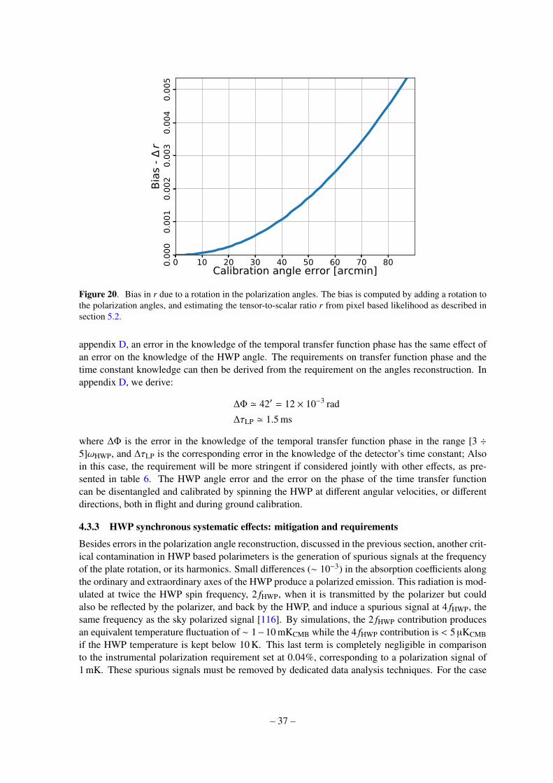
0 10 20 30 40 50 60 70 80Calibration angle error [arcmin]0.

000

0.00

10.

002

0.00

30.

004

0.00

5Bi

as -

r

Figure 20. Bias in r due to a rotation in the polarization angles. The bias is computed by adding a rotation tothe polarization angles, and estimating the tensor-to-scalar ratio r from pixel based likelihood as described insection 5.2.

appendix D, an error in the knowledge of the temporal transfer function phase has the same effect ofan error on the knowledge of the HWP angle. The requirements on transfer function phase and thetime constant knowledge can then be derived from the requirement on the angles reconstruction. Inappendix D, we derive:

∆Φ ' 42′ = 12 × 10−3 rad

∆τLP ' 1.5 ms

where ∆Φ is the error in the knowledge of the temporal transfer function phase in the range [3 ÷5]ωHWP, and ∆τLP is the corresponding error in the knowledge of the detector’s time constant; Alsoin this case, the requirement will be more stringent if considered jointly with other effects, as pre-sented in table 6. The HWP angle error and the error on the phase of the time transfer functioncan be disentangled and calibrated by spinning the HWP at different angular velocities, or differentdirections, both in flight and during ground calibration.

4.3.3 HWP synchronous systematic effects: mitigation and requirements

Besides errors in the polarization angle reconstruction, discussed in the previous section, another crit-ical contamination in HWP based polarimeters is the generation of spurious signals at the frequencyof the plate rotation, or its harmonics. Small differences (∼ 10−3) in the absorption coefficients alongthe ordinary and extraordinary axes of the HWP produce a polarized emission. This radiation is mod-ulated at twice the HWP spin frequency, 2 fHWP, when it is transmitted by the polarizer but couldalso be reflected by the polarizer, and back by the HWP, and induce a spurious signal at 4 fHWP, thesame frequency as the sky polarized signal [116]. By simulations, the 2 fHWP contribution producesan equivalent temperature fluctuation of ∼ 1−10 mKCMB while the 4 fHWP contribution is < 5 µKCMBif the HWP temperature is kept below 10 K. This last term is completely negligible in comparisonto the instrumental polarization requirement set at 0.04%, corresponding to a polarization signal of1 mK. These spurious signals must be removed by dedicated data analysis techniques. For the case

– 37 –

of SWIPE, we developed a specific pipeline to deal with any spurious term synchronous with theHWP spin frequency and harmonics. This is based on application of notch filters, centered at thecontaminated frequencies, and an iterative map-making to recover the removed signal, as describedin Appendix E. In order to assess the efficacy of this technique, we performed a set of simulations,using a multi-notch filter, i.e. a chain of notch filters, each with different central frequency. Thepayload rotation period is set to 8.6 min in accordance with equation A.2 and the notch filters widthis set to ∆ f = 1 mHz. HWP synchronous systematic effects are introduced at 1 fHWP, 2 fHWP,3 fHWP,4 fHWP and 5 fHWP with amplitude 10 mK, 10 mK, 1 mK, 1 mK and 1 mK respectively. The same fre-quencies are used as centers of a stack of 5 notch filters. Notably, the application of these 5 notchfilters and the iterative map-making impact the polarization map with a r.m.s of the residual map oforder 5 × 10−12 KCMB, showing that the procedure has unitary transfer function at all angular scales.In order to have a more realistic simulation, this contamination has been combined with:

• an error in the measurement of the HWP angle. This is defined by the uncertainty withwhich we can readout the HWP angle. This is described by the parameter σθHWP . We haveexplored σθHWP = [0, 3, 10] ′. Our measurement precision, with Kalman filter approach 9, is oforder σθHWP ≤ 0.1′;

• an offset in the knowledge of the HWP angle. This is described by the parameter ∆θHWP. Weexplored the values ∆θHWP = [0, 3, 10] ′;

• an instability in the HWP rotation rate, modeled as a noise in the angular velocity of theHWP. This is described in terms of relative error by the parameter σωHWP/ωHWP. The angularvelocity samples are simulated as

ωi = ωHWP

1 +σωHWP

ωHWPni

√fsampling

fHWP/dpr

(4.3)

where ni is a sample of a normal distributed random number, fsampling is the simulation samplingrate (100 Hz in our case), fHWP is the HWP rotation frequency, and dpr = 64 is the number ofangle measurements of the HWP in a revolution. The ratio fsampling/( fHWP/dpr) correspondsto the number of simulated samples between two subsequent HWP measured positions (dataper revolution). The simulation with equation 4.3 results in the same angular drift between twoHWP angle measurements, independently of the sampling rate of the simulation. We exploredthe values σωHWP/ωHWP = [0, 0.6× 10−8, 0.6× 10−7, 0.6× 10−6, 0.6× 10−5]. Using the Kalmanfilter approach, we have measured a precision in the determination of the HWP angular velocityof order σωHWP/ωHWP = 2 × 10−6.

The major contribution from HWP spin rate instability is due to the fact that the various HWP syn-chronous effects are not at a single frequency anymore, but are spread in frequency due to the insta-bility, thus reducing the efficacy of the notch filter; this is partially compensated by measuring thisinstability, and filtering in the angle domain instead of the time domain, but with some limitationcoming from the uncertainty in the angular velocity measure, σωHWP/ωHWP.

9The Kalman filter combines the dynamic model of the polarization modulation mechanism, the physical propertiesof the system, and multiple sequential measurements to make an estimate of the varying quantities that is better than theestimate obtained by using only measurements. The filter works on discrete sampling, and combines a dynamical predictionof the next position with its noisy measurement. The combination is done using proper weights, that take optimally intoaccount the noise level and the quality of the dynamical prediction.

– 38 –

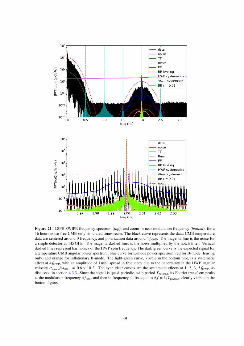
Figure 21. LSPE-SWIPE frequency spectrum (top), and zoom-in near modulation frequency (bottom), for a16 hours noise-free CMB-only simulated timestream. The black curve represents the data; CMB temperaturedata are centered around 0 frequency, and polarization data around 4 fHWP. The magenta line is the noise fora single detector at 145 GHz. The magenta dashed line, is the noise multiplied by the notch filter. Verticaldashed lines represent harmonics of the HWP spin frequency. The dark green curve is the expected signal fora temperature CMB angular power spectrum, blue curve for E-mode power spectrum, red for B-mode (lensingonly) and orange for inflationary B-mode. The light-green curve, visible in the bottom plot, is a systematiceffect at 4 fHWP, with an amplitude of 1 mK, spread in frequency due to the uncertainty in the HWP angularvelocity σωHWP/ωHWP = 0.6 × 10−6. The cyan clear curves are the systematic effects at 1, 2, 3, 5 fHWP, asdiscussed in section 4.3.3. Since the signal is quasi-periodic, with period Tpayload, its Fourier transform peaksat the modulation frequency 4 fHWP and then in frequency shifts equal to ∆ f = 1/Tpayload, clearly visible in thebottom figure.

– 39 –

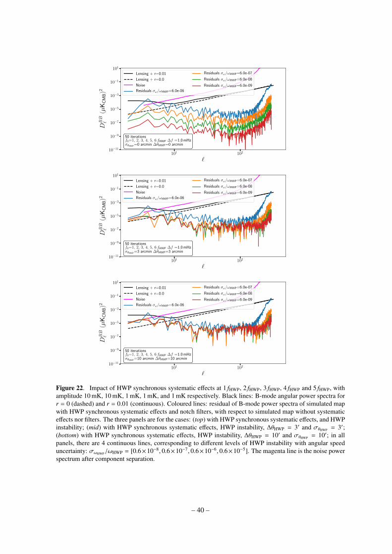
101 102

`

10−11

10−9

10−7

10−5

10−3

10−1

101

DBB

`(µ

KC

MB)2

50 iterationsf0=1, 2, 3, 4, 5, 6 fHWP ∆f =1.0 mHzσθHWP

=0 arcmin ∆θHWP=0 arcmin

Lensing + r=0.01

Lensing + r=0.0

Noise

Residuals σω/ωHWP=6.0e-06

Residuals σω/ωHWP=6.0e-07

Residuals σω/ωHWP=6.0e-08

Residuals σω/ωHWP=6.0e-09

101 102

`

10−11

10−9

10−7

10−5

10−3

10−1

101

DBB

`(µ

KC

MB)2

50 iterationsf0=1, 2, 3, 4, 5, 6 fHWP ∆f =1.0 mHzσθHWP

=3 arcmin ∆θHWP=3 arcmin

Lensing + r=0.01

Lensing + r=0.0

Noise

Residuals σω/ωHWP=6.0e-06

Residuals σω/ωHWP=6.0e-07

Residuals σω/ωHWP=6.0e-08

Residuals σω/ωHWP=6.0e-09

101 102

`

10−11

10−9

10−7

10−5

10−3

10−1

101

DBB

`(µ

KC

MB)2

50 iterationsf0=1, 2, 3, 4, 5, 6 fHWP ∆f =1.0 mHzσθHWP

=10 arcmin ∆θHWP=10 arcmin

Lensing + r=0.01

Lensing + r=0.0

Noise

Residuals σω/ωHWP=6.0e-06

Residuals σω/ωHWP=6.0e-07

Residuals σω/ωHWP=6.0e-08

Residuals σω/ωHWP=6.0e-09

Figure 22. Impact of HWP synchronous systematic effects at 1 fHWP, 2 fHWP, 3 fHWP, 4 fHWP and 5 fHWP, withamplitude 10 mK, 10 mK, 1 mK, 1 mK, and 1 mK respectively. Black lines: B-mode angular power spectra forr = 0 (dashed) and r = 0.01 (continuous). Coloured lines: residual of B-mode power spectra of simulated mapwith HWP synchronous systematic effects and notch filters, with respect to simulated map without systematiceffects nor filters. The three panels are for the cases: (top) with HWP synchronous systematic effects, and HWPinstability; (mid) with HWP synchronous systematic effects, HWP instability, ∆θHWP = 3′ and σθHWP = 3′;(bottom) with HWP synchronous systematic effects, HWP instability, ∆θHWP = 10′ and σθHWP = 10′; in allpanels, there are 4 continuous lines, corresponding to different levels of HWP instability with angular speeduncertainty: σωHWP/ωHWP = [0.6×10−8, 0.6×10−7, 0.6×10−6, 0.6×10−5]. The magenta line is the noise powerspectrum after component separation.

– 40 –

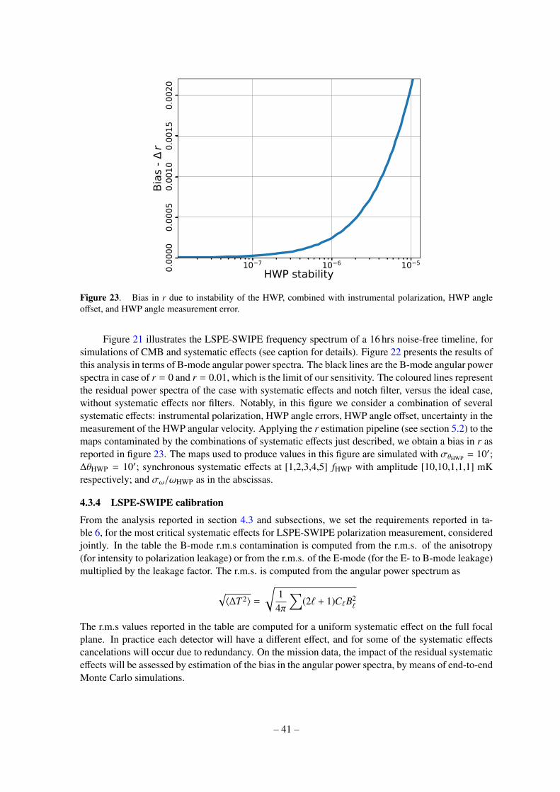
10 7 10 6 10 5

HWP stability0.00

000.

0005

0.00

100.

0015

0.00

20Bi

as -

r

Figure 23. Bias in r due to instability of the HWP, combined with instrumental polarization, HWP angleoffset, and HWP angle measurement error.

Figure 21 illustrates the LSPE-SWIPE frequency spectrum of a 16 hrs noise-free timeline, forsimulations of CMB and systematic effects (see caption for details). Figure 22 presents the results ofthis analysis in terms of B-mode angular power spectra. The black lines are the B-mode angular powerspectra in case of r = 0 and r = 0.01, which is the limit of our sensitivity. The coloured lines representthe residual power spectra of the case with systematic effects and notch filter, versus the ideal case,without systematic effects nor filters. Notably, in this figure we consider a combination of severalsystematic effects: instrumental polarization, HWP angle errors, HWP angle offset, uncertainty in themeasurement of the HWP angular velocity. Applying the r estimation pipeline (see section 5.2) to themaps contaminated by the combinations of systematic effects just described, we obtain a bias in r asreported in figure 23. The maps used to produce values in this figure are simulated with σθHWP = 10′;∆θHWP = 10′; synchronous systematic effects at [1,2,3,4,5] fHWP with amplitude [10,10,1,1,1] mKrespectively; and σω/ωHWP as in the abscissas.

4.3.4 LSPE-SWIPE calibration

From the analysis reported in section 4.3 and subsections, we set the requirements reported in ta-ble 6, for the most critical systematic effects for LSPE-SWIPE polarization measurement, consideredjointly. In the table the B-mode r.m.s contamination is computed from the r.m.s. of the anisotropy(for intensity to polarization leakage) or from the r.m.s. of the E-mode (for the E- to B-mode leakage)multiplied by the leakage factor. The r.m.s. is computed from the angular power spectrum as

√〈∆T 2〉 =

√1

4π

∑(2` + 1)C`B2

`

The r.m.s values reported in the table are computed for a uniform systematic effect on the full focalplane. In practice each detector will have a different effect, and for some of the systematic effectscancelations will occur due to redundancy. On the mission data, the impact of the residual systematiceffects will be assessed by estimation of the bias in the angular power spectra, by means of end-to-endMonte Carlo simulations.

– 41 –

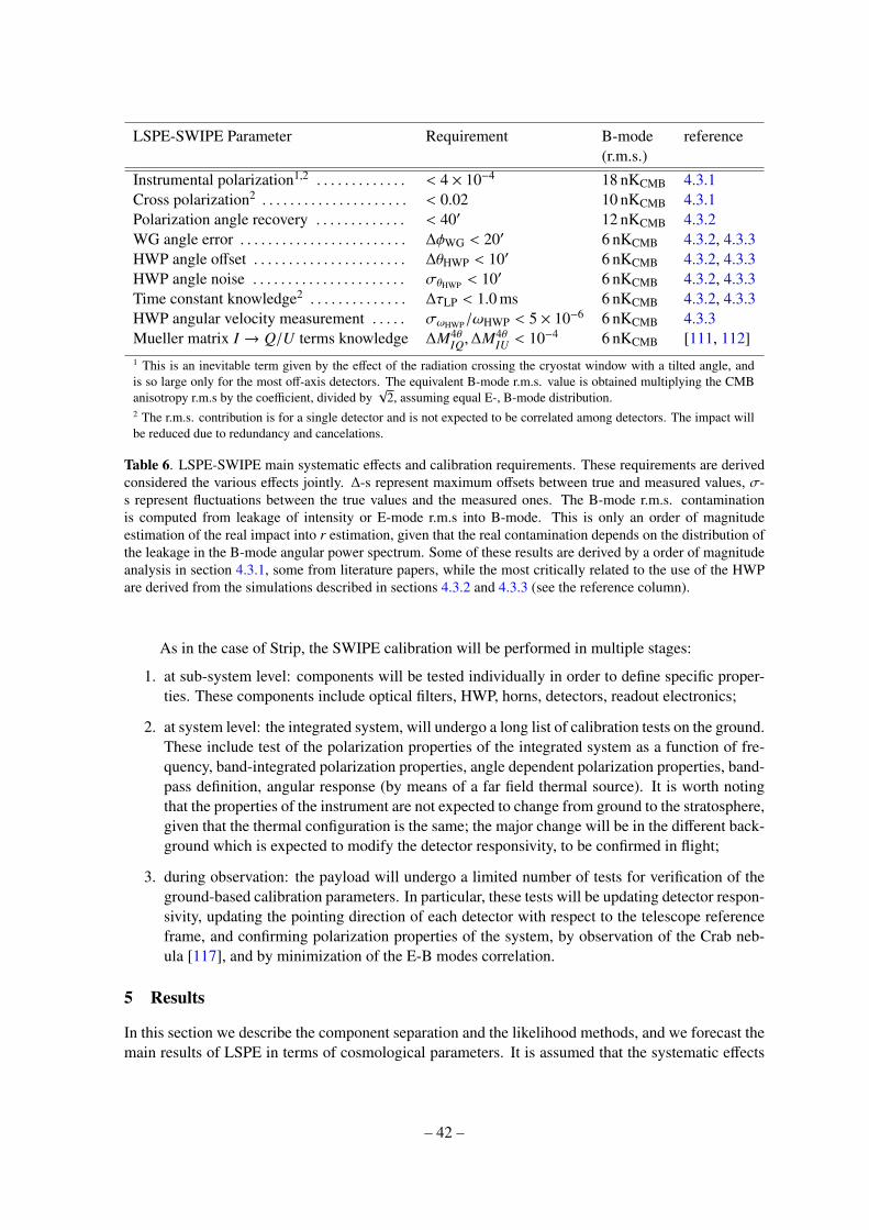
LSPE-SWIPE Parameter Requirement B-mode reference(r.m.s.)

Instrumental polarization1,2 . . . . . . . . . . . . . < 4 × 10−4 18 nKCMB 4.3.1Cross polarization2 . . . . . . . . . . . . . . . . . . . . . < 0.02 10 nKCMB 4.3.1Polarization angle recovery . . . . . . . . . . . . . < 40′ 12 nKCMB 4.3.2WG angle error . . . . . . . . . . . . . . . . . . . . . . . . ∆φWG < 20′ 6 nKCMB 4.3.2, 4.3.3HWP angle offset . . . . . . . . . . . . . . . . . . . . . . ∆θHWP < 10′ 6 nKCMB 4.3.2, 4.3.3HWP angle noise . . . . . . . . . . . . . . . . . . . . . . σθHWP < 10′ 6 nKCMB 4.3.2, 4.3.3Time constant knowledge2 . . . . . . . . . . . . . . ∆τLP < 1.0 ms 6 nKCMB 4.3.2, 4.3.3HWP angular velocity measurement . . . . . σωHWP/ωHWP < 5 × 10−6 6 nKCMB 4.3.3Mueller matrix I → Q/U terms knowledge ∆M4θ

IQ,∆M4θIU < 10−4 6 nKCMB [111, 112]

1 This is an inevitable term given by the effect of the radiation crossing the cryostat window with a tilted angle, andis so large only for the most off-axis detectors. The equivalent B-mode r.m.s. value is obtained multiplying the CMBanisotropy r.m.s by the coefficient, divided by

√2, assuming equal E-, B-mode distribution.

2 The r.m.s. contribution is for a single detector and is not expected to be correlated among detectors. The impact willbe reduced due to redundancy and cancelations.

Table 6. LSPE-SWIPE main systematic effects and calibration requirements. These requirements are derivedconsidered the various effects jointly. ∆-s represent maximum offsets between true and measured values, σ-s represent fluctuations between the true values and the measured ones. The B-mode r.m.s. contaminationis computed from leakage of intensity or E-mode r.m.s into B-mode. This is only an order of magnitudeestimation of the real impact into r estimation, given that the real contamination depends on the distribution ofthe leakage in the B-mode angular power spectrum. Some of these results are derived by a order of magnitudeanalysis in section 4.3.1, some from literature papers, while the most critically related to the use of the HWPare derived from the simulations described in sections 4.3.2 and 4.3.3 (see the reference column).

As in the case of Strip, the SWIPE calibration will be performed in multiple stages:

1. at sub-system level: components will be tested individually in order to define specific proper-ties. These components include optical filters, HWP, horns, detectors, readout electronics;

2. at system level: the integrated system, will undergo a long list of calibration tests on the ground.These include test of the polarization properties of the integrated system as a function of fre-quency, band-integrated polarization properties, angle dependent polarization properties, band-pass definition, angular response (by means of a far field thermal source). It is worth notingthat the properties of the instrument are not expected to change from ground to the stratosphere,given that the thermal configuration is the same; the major change will be in the different back-ground which is expected to modify the detector responsivity, to be confirmed in flight;

3. during observation: the payload will undergo a limited number of tests for verification of theground-based calibration parameters. In particular, these tests will be updating detector respon-sivity, updating the pointing direction of each detector with respect to the telescope referenceframe, and confirming polarization properties of the system, by observation of the Crab neb-ula [117], and by minimization of the E-B modes correlation.

5 Results

In this section we describe the component separation and the likelihood methods, and we forecast themain results of LSPE in terms of cosmological parameters. It is assumed that the systematic effects

– 42 –

are within the requirements defined in section 4. In each of the maps the noise is estimated using theNETs from tables 2 and 4, projected into maps by means of the instrument simulators described inappendix B.

5.1 Component separation

Component separation is a key element in CMB data analysis, and it turns out to be particularlychallenging for the extraction of CMB polarization (see e.g. [118–120]). In particular, diffuse Galac-tic dust and synchrotron emissions are the most relevant foregrounds in polarization. For the anal-ysis presented in this paper, we consider the component separation apparatus represented by theForeGroundBuster10, which is currently used to assess the foreground cleaning capabilities of anumber of CMB B-mode probes [121, 122]. The method fits, in each pixel observed by both Stripand SWIPE, for CMB signal, amplitude and spectral index of synchrotron, temperature, amplitudeand spectral index of dust. In our analysis, we include thermal dust and synchrotron as polarized fore-grounds. We exploit the publicly available package Python Sky Model (PySM)11 which generatesfull sky simulated foregrounds in intensity and polarization, and consider the d0s0 configuration out-lined below [123]. The synchrotron spectral brightness is modeled as a power law in frequency witha constant spectral index βs = −3: Is(ν, n) = As(n)(ν/ν0)βs , where As(n) is the synchrotron amplitude.The dust component is modeled as a grey body, i.e. an almost thermal component at a temperature ofTd = 20 K, heated back by starlight which is represented as an emissivity factor scaling as a powerlaw in frequency, with spectral index βd = 1.54: Id(ν, n) = τ0(n)(ν/ν0)βd B(ν,Td). The componentseparation procedure is performed only in polarization and recovers the value of the spectral indicesβs, βd which are not varying in the sky, as well as the amplitude of the synchrotron signal As(n) anddust optical depth τ0(n), which vary with the sky direction. The assumption of uniform spectral in-dices could lead to biases on the estimation of the tensor-to-scalar ratio. This is true, in particular, forexperiments targeting r ' 10−3, for which the estimation of the foreground parameters must be donein the various regions of the sky independently. For experiments targeting higher values of r, suchas LSPE, the impact of this spatial variation is expected to be less dramatic, leading to a bias lowerthan or comparable to the statistical uncertainties. This result is confirmed by the SO paper [16],section 3.4.2, in particular in Table 4, where the first row of the table reports the case of fitting a skymodel built with varying spectral indices, assuming uniform spectral indices in the reconstruction.This results in a bias in r of order ∆r ' 2 × 10−3.

In addition to the LSPE bands, we also consider the observations of the Planck satellite between30 and 353 GHz [3], and the ones of QUIJOTE at 11 GHz [38, 124]. At each of the frequenciescorresponding to these probes, and separately for the Q and U Stokes parameters, we generate andadd foregrounds and CMB using the PySM, and also add noise realizations according to the SWIPE,Strip, Planck and QUIJOTE sensitivities. We convolve all maps with a Gaussian beam in order toreach a common 85 arcmin FWHM, which corresponds to the largest beam associated to the LSPEchannels. All maps are generated using HEALPix12 at Nside = 128. We did not consider any pixel-pixel correlation property of the noise. The data model which is implemented in ForeGroundBusterand used in this paper is d(ν) ≡ As+n, where d(ν) contains measured signal at each frequency ν, s arethe maps of the different components, A is the mixing matrix which contains the parametric modelto fit, and n represents the noise in the maps. The parametric component separation process consistsin obtaining an estimate s = Wd of the components, by means of a kernel operator W. Therefore,the key element of component separation is the W matrix, which is the linear operator that mixes the

10https://github.com/fgbuster/fgbuster11https://github.com/bthorne93/PySM_public12Hierarchical Equal Latitude Pixelization

– 43 –

101 102

Multipole -

105

104

103

102

101

100

[K

2 ]

EETensor BB r=0.03Total BB

Figure 24. CMB E-mode (blue) and B-mode (orange) power spectra averaged over 1000 simulations afterComponent separation in the baseline case of table 7.

frequency maps in the component maps, taking into account the sensitivity and the contribution ofeach frequency to each astrophysical component. The elements Wi, j of the W matrix (often referredas weights) admit negative values for frequencies that must be subtracted in order to solve for theastrophysical component. Frequency bands and weights for each component are shown in table 7.From this table it is clear that the 145 GHz channel is the most important one for reconstructingthe CMB, clearly adding sensitivity to the currently available datasets. The table also quantitativelyshows relevance of higher and lower frequency bands for fitting and subtracting foregrounds. Asan illustration, figure 24 shows the polarization CMB power spectra [125] obtained averaging 1000simulations after component separation.

In table 8, we show a minimal case, where we have used just the 30 GHz channel of Planck andLSPE frequencies. Moreover, table 9 shows the accuracy of the component separation in terms ofdust and synchrotron spectral indices.

5.2 Likelihood

The likelihood used in the parameter estimation is based on maps of Stokes parameters T,Q,U inHEALPix format. For the temperature map we assume perfect component separation outside a Galac-tic masks with 2 µK per pixel of white noise13. The polarization maps after the component separationprocedure, described in the previous section, are modeled as a sum of CMB signal, instrumental Gaus-sian noise and foreground Gaussian residuals. This modeling is consistent with analyses performedon current data at large angular scales [126] and with forecasts performed on other forthcoming

13In temperature we assume signal dominated observations. The white noise added is only necessary for regularizingthe inversion of the temperature block of the TQU covariance matrix, see e.g. [126]

– 44 –

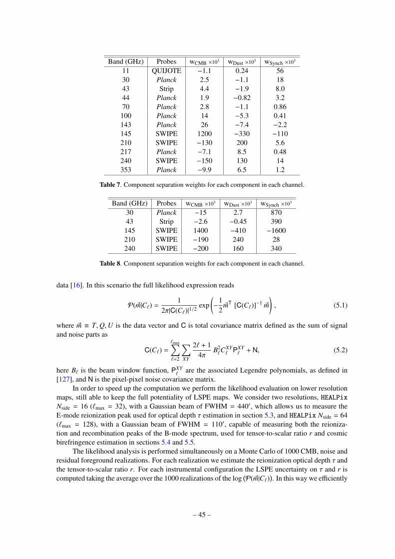
Band (GHz) Probes wCMB ×103 wDust ×103 wSynch ×103

11 QUIJOTE −1.1 0.24 5630 Planck 2.5 −1.1 1843 Strip 4.4 −1.9 8.044 Planck 1.9 −0.82 3.270 Planck 2.8 −1.1 0.86100 Planck 14 −5.3 0.41143 Planck 26 −7.4 −2.2145 SWIPE 1200 −330 −110210 SWIPE −130 200 5.6217 Planck −7.1 8.5 0.48240 SWIPE −150 130 14353 Planck −9.9 6.5 1.2

Table 7. Component separation weights for each component in each channel.

Band (GHz) Probes wCMB ×103 wDust ×103 wSynch ×103

30 Planck −15 2.7 87043 Strip −2.6 −0.45 390145 SWIPE 1400 −410 −1600210 SWIPE −190 240 28240 SWIPE −200 160 340

Table 8. Component separation weights for each component in each channel.

data [16]. In this scenario the full likelihood expression reads

P(~m|C`) =1

2π|C(C`)|1/2exp

(−

12~mT [C(C`)]−1 ~m

), (5.1)

where ~m ≡ T,Q,U is the data vector and C is total covariance matrix defined as the sum of signaland noise parts as

C(C`) =

`max∑`=2

∑XY

2` + 14π

B2`C

XY` PXY

` + N, (5.2)

here B` is the beam window function, PXY` are the associated Legendre polynomials, as defined in

[127], and N is the pixel-pixel noise covariance matrix.In order to speed up the computation we perform the likelihood evaluation on lower resolution

maps, still able to keep the full potentiality of LSPE maps. We consider two resolutions, HEALPixNside = 16 (`max = 32), with a Gaussian beam of FWHM = 440′, which allows us to measure theE-mode reionization peak used for optical depth τ estimation in section 5.3, and HEALPix Nside = 64(`max = 128), with a Gaussian beam of FWHM = 110′, capable of measuring both the reioniza-tion and recombination peaks of the B-mode spectrum, used for tensor-to-scalar ratio r and cosmicbirefringence estimation in sections 5.4 and 5.5.

The likelihood analysis is performed simultaneously on a Monte Carlo of 1000 CMB, noise andresidual foreground realizations. For each realization we estimate the reionization optical depth τ andthe tensor-to-scalar ratio r. For each instrumental configuration the LSPE uncertainty on τ and r iscomputed taking the average over the 1000 realizations of the log

(P(~m|C`)

). In this way we efficiently

– 45 –

Parameter Mean σ

βd 1.539 0.001βs −2.999 0.002

Table 9. Dust and synchrotron spectral indices obtained by parametric component separation. The componentseparation algorithm fits for a single value in each map. The uncertainties are derived from the standarddeviation of 1000 realizations of the noise in the maps.

0.05 0.06 0.07 0.08Optical depth

0.2

0.4

0.6

0.8

1.0

Rela

tive

Prob

abilit

y

LSPE (15 days) + Planck + QUIJOTELSPE (8 days) + Planck + QUIJOTELSPE (15 days) + QUIJOTELSPE (15 days) + Planck 30GHzPlanck 2018 + SRoll2

0.0 0.1 0.2 0.3 0.4 0.5103 ×

0.02

0.04

0.06

0.08

0.10

PlanckPlanck + LSPE

Figure 25. Left: posterior probability for optical depth τ. The colored lines show different component sep-aration configurations, see text for details. The black line shows the current best estimate on τ. Right: Jointposterior probability for scale parameter ∆ in (Mpc−1) and optical depth τ. Blue and cyan are 68% and 95%CL for Planck; red and orange for Planck and LSPE.

take care of the scatter due to cosmic variance and instrumental noise. The other ΛCDM parametersare not sampled in this analysis, nonetheless we verified that opening the parameter exploration to fullΛCDM, and including a high-` likelihood with noise performance compatible with Planck, providesequivalent results.

5.3 Reionization optical depth constraints

Measuring the polarization at very large scales, in particular the so-called reionization bump, allowsconstraining the Thompson scattering optical depth τ. LSPE provides a cosmic variance limitedmeasure of the polarization signal at very large scales (` <

∼ 20) on ∼ 35% of the sky. For theanalysis presented here we conservatively consider a smaller portion, fsky,cmb ' 25%, removingregions close to the Galactic plane potentially contaminated by residual foregrounds. The LSPEsensitivity over such a sky fraction overcomes the current best estimates provided by Planck HFI, i.e.τ = 0.059 ± 0.006 [128], reaching 1 − σ error on τ of ∼ 0.004.

The constraints on the reionization optical depth τ are reported in table 10 and figure 25 fordifferent data combinations. For Strip we consider 2 years of observations, for SWIPE we exploretwo possibilities, 15 days (SWIPE 15) or 8 days of observation (SWIPE 8). Planck and QUIJOTEare assumed with their nominal observational strategies and only considered in the portion of sky incommon with LSPE. The τ constraints are rather stable showing that even after 8 days of SWIPEobservations we reach the mission goal. Furthermore, even in a minimal configuration which consid-ers only LSPE plus Planck 30 GHz as additional synchrotron tracer, the τ measure does not changesubstantially, showing that we are not heavily dependent on the usage of external datasets.

– 46 –

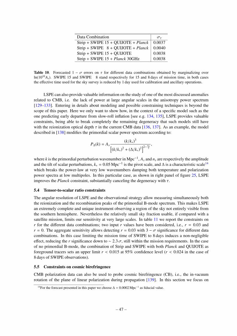
Data Combination στStrip + SWIPE 15 + QUIJOTE + Planck 0.0037Strip + SWIPE 8 + QUIJOTE + Planck 0.0040Strip + SWIPE 15 + QUIJOTE 0.0038Strip + SWIPE 15 + Planck 30GHz 0.0038

Table 10. Forecasted 1 − σ errors on τ for different data combinations obtained by marginalizing overln(1010As). SWIPE 15 and SWIPE 8 stand respectively for 15 and 8 days of mission time, in both casesthe effective time used for the sky survey is reduced by 1 day used for calibration and ancillary operations.

LSPE can also provide valuable information on the study of one of the most discussed anomaliesrelated to CMB, i.e. the lack of power at large angular scales in the anisotropy power spectrum[129–133]. Entering in details about modeling and possible constraining techniques is beyond thescope of this paper. Here we only want to show how, in the context of a specific model such as theone predicting early departure from slow-roll inflation [see e.g. 134, 135], LSPE provides valuableconstraints, being able to break completely the remaining degeneracy that such models still havewith the reionization optical depth τ in the current CMB data [136, 137]. As an example, the modeldescribed in [138] modifies the primordial scalar power spectrum according to:

P∆(k) = As(k/k∗)3[

(k/k∗)2 + (∆/k∗)2]2− ns

2,

where k is the primordial perturbation wavenumber in Mpc−1, As and ns are respectively the amplitudeand the tilt of scalar perturbations, k∗ = 0.05 Mpc−1 is the pivot scale, and ∆ is a characteristic scale14

which breaks the power-law at very low wavenumbers damping both temperature and polarizationpower spectra at low multipoles. In this particular case, as shown in right panel of figure 25, LSPEimproves the Planck constraint, substantially canceling the degeneracy with τ.

5.4 Tensor-to-scalar ratio constraints

The angular resolution of LSPE and the observational strategy allow measuring simultaneously boththe reionization and the recombination peaks of the primordial B-mode spectrum. This makes LSPEan extremely complete and unique instrument observing a region of the sky not entirely visible fromthe southern hemisphere. Nevertheless the relatively small sky fraction usable, if compared with asatellite mission, limits our sensitivity at very large scales. In table 11 we report the constraints onr for the different data combinations; two input r values have been considered, i.e., r = 0.03 andr = 0. The aggregate sensitivity allows detecting r = 0.03 with 3 − σ significance for different datacombinations. In this case limiting the mission time of SWIPE to 8 days induces a non-negligibleeffect, reducing the r significance down to ∼ 2.3σ, still within the mission requirements. In the caseof no primordial B-mode, the combination of Strip and SWIPE with both Planck and QUIJOTE asforeground tracers sets an upper limit r < 0.015 at 95% confidence level (r < 0.024 in the case of8 days of SWIPE observations).

5.5 Constraints on cosmic birefringence

CMB polarization data can also be used to probe cosmic birefringence (CB), i.e., the in-vacuumrotation of the plane of linear polarization during propagation [139]. In this section we focus on

14For the forecast presented in this paper we choose ∆ = 0.0002 Mpc−1 as fiducial value.

– 47 –

Data Combination σr 95%clStrip + SWIPE 15 + QUIJOTE + Planck 0.0093 0.015Strip + SWIPE 8 + QUIJOTE + Planck 0.013 0.024Strip + SWIPE 15 + QUIJOTE 0.0098 0.016Strip + SWIPE 15 + Planck 30GHz 0.010 0.018

Table 11. Expected sensitivity on the tensor-to-scalar ratio r. The second column shows 1−σ errors assumingan input r = 0.03. The third column shows 95% c.l. upper limits assuming no tensor B-modes (i.e. r = 0).

0.000 0.005 0.010 0.015 0.020 0.025 0.030 0.035Tensor-to-scalar ratio

0.2

0.4

0.6

0.8

1.0

Rela

tive

Prob

abilit

y

LSPE (15 days) + Planck + QUIJOTELSPE (8 days) + Planck + QUIJOTELSPE (15 days) + QUIJOTELSPE (15 days) + Planck 30GHz

0.00 0.01 0.02 0.03 0.04 0.05 0.06 0.07Tensor-to-scalar ratio

0.2

0.4

0.6

0.8

1.0

Rela

tive

Prob

abilit

y

LSPE (15 days) + Planck + QUIJOTELSPE (8 days) + Planck + QUIJOTELSPE (15 days) + QUIJOTELSPE (15 days) + Planck 30GHz

Figure 26. Posterior probability for tensor-to-scalar ratio r in case of r = 0 (left) and r = 0.03 (right). Thecolored lines show different component separation configurations, see text for details.

isotropic birefringence rotation, see e.g., [140–145]. For those measurements the calibration of thepolarization angle of polarimeters is a key aspect, since miscalibration of such angle is completelydegenerate with the rotation induced by CB, see section 4.3.2 and references therein15. Assumingnegligible calibration error on the polarization angle, we can constrain CB angle, αCB, with the sametechnique used to constrain τ and r, i.e. a pixel-based approach for the likelihood estimation. Anotherpossible approach is to use the so called D-Estimators, as defined in e.g. [144], which employ TB andEB power spectra. In table 12 we report constraints of αCB for different data combinations for boththe approaches mentioned above, in figure 27 we show the posteriors obtained with the pixel-basedmethod. LSPE data will constrain uniform birefringence angle down to 0.2°, improving by a factor 3the current best estimate [145].

6 Conclusion

The Large Scale Polarization Explorer is a program dedicated to the measurement of the CMB po-larization and its B-mode component in particular. We have presented the instruments’ design and adetailed forecast of its performance. LSPE can put an upper limit to the tensor-to-scalar ratio at thelevel of r < 0.015 at 95% confidence level, and can detect a signal corresponding to r = 0.03 with99.7% confidence. Moreover, LSPE can improve constraints on other parameters, like the opticaldepth of the Universe to the CMB, τ, and the rotation angle originated by a cosmic birefringence.

15A new method has been proposed recently which aims at breaking the degeneracy between birefringence angle andinstrumental polarization angle [146, 147].

– 48 –

Data Combination σPBαCB

σDEαCB

Strip + SWIPE 15 + QUIJOTE + Planck 0.22 0.19Strip + SWIPE 8 + QUIJOTE + Planck 0.30 0.29Strip + SWIPE 15 + QUIJOTE 0.23 0.21Strip + SWIPE 15 + Planck 30 GHz 0.24 0.22

Table 12. Forecasted sensitivity on the cosmic birefringence angle αCB in degrees. The second and thirdcolumns show 1 − σ errors obtained with the pixel-based approach and D-Estimators approach, respectively.

1.0 0.5 0.0 0.5 1.0 1.5Birefringence angle [degree]

0.2

0.4

0.6

0.8

1.0

Rela

tive

Prob

abilit

yLSPE (15 days) + Planck + QUIJOTELSPE (8 days) + Planck + QUIJOTELSPE (15 days) + QUIJOTELSPE (15 days) + Planck 30GHz

Figure 27. Posterior probability for cosmic birefringence angle obtained with the pixel-based likelihood.

This analysis is obtained by a full set of end-to-end simulations, including detailed noise estima-tion, instrument observations (for each detector), contamination by foregrounds, map-making, com-ponent separation with realistic foreground residuals, and cosmological parameter extraction withpixel-based likelihood. The assumption about systematic effects is that their contribution can be re-duced to below the noise level by means of stringent requirements at design level and by system levelcalibration. We also present techniques for the control and removal of HWP synchronous systematiceffects, including the case of HWP rotational instability.

With its rotating HWP, LSPE-SWIPE represents an important pathfinder of the forthcomingLiteBIRD mission from the point of view of the instrument requirements, instrument design, calibra-tion, control of systematic effects, and data analysis.

– 49 –

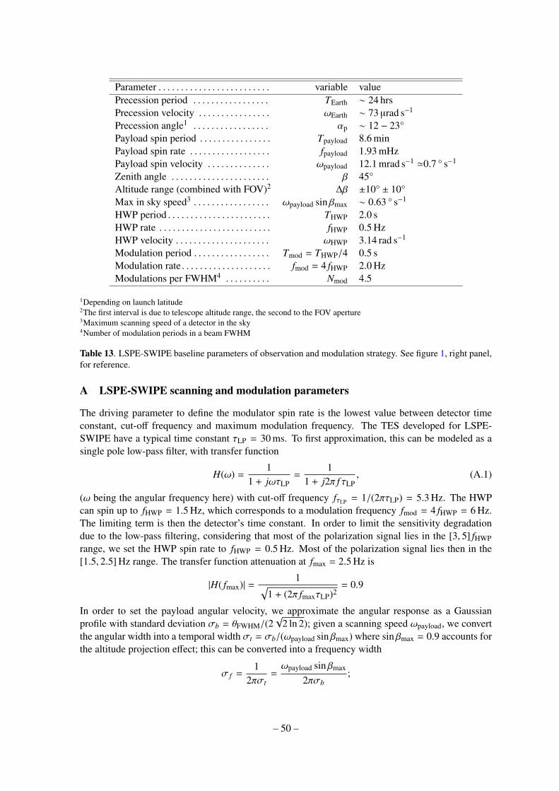
Parameter . . . . . . . . . . . . . . . . . . . . . . . . . variable valuePrecession period . . . . . . . . . . . . . . . . . TEarth ∼ 24 hrsPrecession velocity . . . . . . . . . . . . . . . . ωEarth ∼ 73 µrad s−1

Precession angle1 . . . . . . . . . . . . . . . . . αp ∼ 12 − 23°Payload spin period . . . . . . . . . . . . . . . . Tpayload 8.6 minPayload spin rate . . . . . . . . . . . . . . . . . . fpayload 1.93 mHzPayload spin velocity . . . . . . . . . . . . . . ωpayload 12.1 mrad s−1 '0.7 ° s−1

Zenith angle . . . . . . . . . . . . . . . . . . . . . . β 45°Altitude range (combined with FOV)2 ∆β ±10° ± 10°Max in sky speed3 . . . . . . . . . . . . . . . . . ωpayload sin βmax ∼ 0.63 ° s−1

HWP period . . . . . . . . . . . . . . . . . . . . . . . THWP 2.0 sHWP rate . . . . . . . . . . . . . . . . . . . . . . . . . fHWP 0.5 HzHWP velocity . . . . . . . . . . . . . . . . . . . . . ωHWP 3.14 rad s−1

Modulation period . . . . . . . . . . . . . . . . . Tmod = THWP/4 0.5 sModulation rate . . . . . . . . . . . . . . . . . . . . fmod = 4 fHWP 2.0 HzModulations per FWHM4 . . . . . . . . . . Nmod 4.5

1Depending on launch latitude2The first interval is due to telescope altitude range, the second to the FOV aperture3Maximum scanning speed of a detector in the sky4Number of modulation periods in a beam FWHM

Table 13. LSPE-SWIPE baseline parameters of observation and modulation strategy. See figure 1, right panel,for reference.

A LSPE-SWIPE scanning and modulation parameters

The driving parameter to define the modulator spin rate is the lowest value between detector timeconstant, cut-off frequency and maximum modulation frequency. The TES developed for LSPE-SWIPE have a typical time constant τLP = 30 ms. To first approximation, this can be modeled as asingle pole low-pass filter, with transfer function

H(ω) =1

1 + jωτLP=

11 + j2π f τLP

, (A.1)

(ω being the angular frequency here) with cut-off frequency fτLP = 1/(2πτLP) = 5.3 Hz. The HWPcan spin up to fHWP = 1.5 Hz, which corresponds to a modulation frequency fmod = 4 fHWP = 6 Hz.The limiting term is then the detector’s time constant. In order to limit the sensitivity degradationdue to the low-pass filtering, considering that most of the polarization signal lies in the [3, 5] fHWPrange, we set the HWP spin rate to fHWP = 0.5 Hz. Most of the polarization signal lies then in the[1.5, 2.5] Hz range. The transfer function attenuation at fmax = 2.5 Hz is

|H( fmax)| =1√

1 + (2π fmaxτLP)2= 0.9

In order to set the payload angular velocity, we approximate the angular response as a Gaussianprofile with standard deviation σb = θFWHM/(2

√2 ln 2); given a scanning speed ωpayload, we convert

the angular width into a temporal width σt = σb/(ωpayload sin βmax) where sin βmax = 0.9 accounts forthe altitude projection effect; this can be converted into a frequency width

σ f =1

2πσt=ωpayload sin βmax

2πσb;

– 50 –

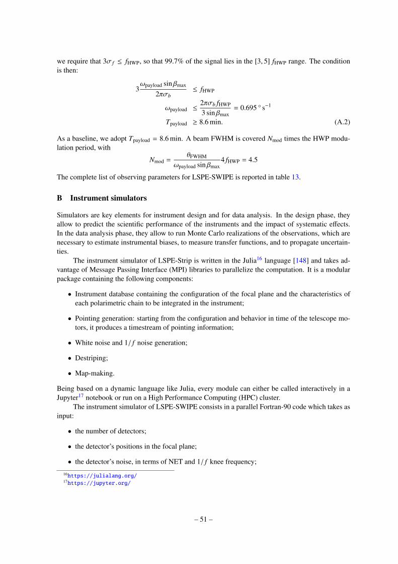
we require that 3σ f ≤ fHWP, so that 99.7% of the signal lies in the [3, 5] fHWP range. The conditionis then:

3ωpayload sin βmax

2πσb≤ fHWP

ωpayload ≤2πσb fHWP

3 sin βmax= 0.695 ° s−1

Tpayload ≥ 8.6 min. (A.2)

As a baseline, we adopt Tpayload = 8.6 min. A beam FWHM is covered Nmod times the HWP modu-lation period, with

Nmod =θFWHM

ωpayload sin βmax4 fHWP = 4.5

The complete list of observing parameters for LSPE-SWIPE is reported in table 13.

B Instrument simulators

Simulators are key elements for instrument design and for data analysis. In the design phase, theyallow to predict the scientific performance of the instruments and the impact of systematic effects.In the data analysis phase, they allow to run Monte Carlo realizations of the observations, which arenecessary to estimate instrumental biases, to measure transfer functions, and to propagate uncertain-ties.

The instrument simulator of LSPE-Strip is written in the Julia16 language [148] and takes ad-vantage of Message Passing Interface (MPI) libraries to parallelize the computation. It is a modularpackage containing the following components:

• Instrument database containing the configuration of the focal plane and the characteristics ofeach polarimetric chain to be integrated in the instrument;

• Pointing generation: starting from the configuration and behavior in time of the telescope mo-tors, it produces a timestream of pointing information;

• White noise and 1/ f noise generation;

• Destriping;

• Map-making.

Being based on a dynamic language like Julia, every module can either be called interactively in aJupyter17 notebook or run on a High Performance Computing (HPC) cluster.

The instrument simulator of LSPE-SWIPE consists in a parallel Fortran-90 code which takes asinput:

• the number of detectors;

• the detector’s positions in the focal plane;

• the detector’s noise, in terms of NET and 1/ f knee frequency;

16https://julialang.org/17https://jupyter.org/

– 51 –

• the mission starting date and duration;

• the angular response in the sky of each detector, as a 2d matrix; this is convolved in pixel space,in a radius specified also as input parameter;

• the HWP operation strategy (stepping, spinning, spinning rate, stepping period);

• the level of HWP synchronous systematic effects, as a signal in µKCMB at the HWP spinningfrequency and its harmonics;

• HWP angle offset, angular velocity instability, and error in angle measurement;

• timeline filter (high-pass, low-pass, band-pass, notch-filter);

• map-making algorithm details, as simple re-binning, or iterative destriping.

It generates in output:

• timeline of each detector;

• maps of each detector;

• map of combined detectors;

• coverage map;

• noise covariance 3 × 3 matrix for each observed pixel.

Both simulators can take as input sky maps of any kind. In the analysis presented in this paper,the sky maps have been generated with HEALPix code, for CMB maps, and PySM for foregroundsmaps, as detailed in section 5.1. The atmospheric noise is not included in the simulations, but only theatmospheric background power and the corresponding white noise. Noise correlation among differentdetectors can be included in the SWIPE simulator, but are not included in this analysis. Similarly,realistic beams (angular response) of the telescope can be used, including sidelobes, but only sym-metrical main-beams have been considered in this work. In particular for SWIPE, the presence ofthe HWP strongly attenuates the impact of beam asymmetries. On the other side, beam sidelobes arepotentially strong sources of contamination if not properly measured or modeled, and removed fromtimelines and maps.

C Atmospheric fluctuations estimation for Strip

The atmospheric fluctuations are very difficult to model and forecast. For this reason, a statisticalapproach is mandatory. Since we are interested in assessing the atmospheric transparency and itsmedium-time fluctuations (seasonal and day/night cycles), the atmospheric model has to rely on thestatistical fluctuations of the PWV, TS (Surface Temperature), and P0 (Surface Pressure). For eachhour of each month, we have created the cumulative distribution functions (CDFs18) of weather pa-rameters used by the am software to evaluate the atmospheric brightness temperature. To build theCDFs we have used the ERA-5 reanalysis dataset19, which estimates the atmosphere’s history using anumerical model to assimilate historical measurements. We then use the simulation-framework Cmb

18The CDF is the integral of the probability density function, PDF. We used the CDF instead of the PDF derived fromthe data because is smoother and is not biased by the binning.

19https://www.ecmwf.int

– 52 –

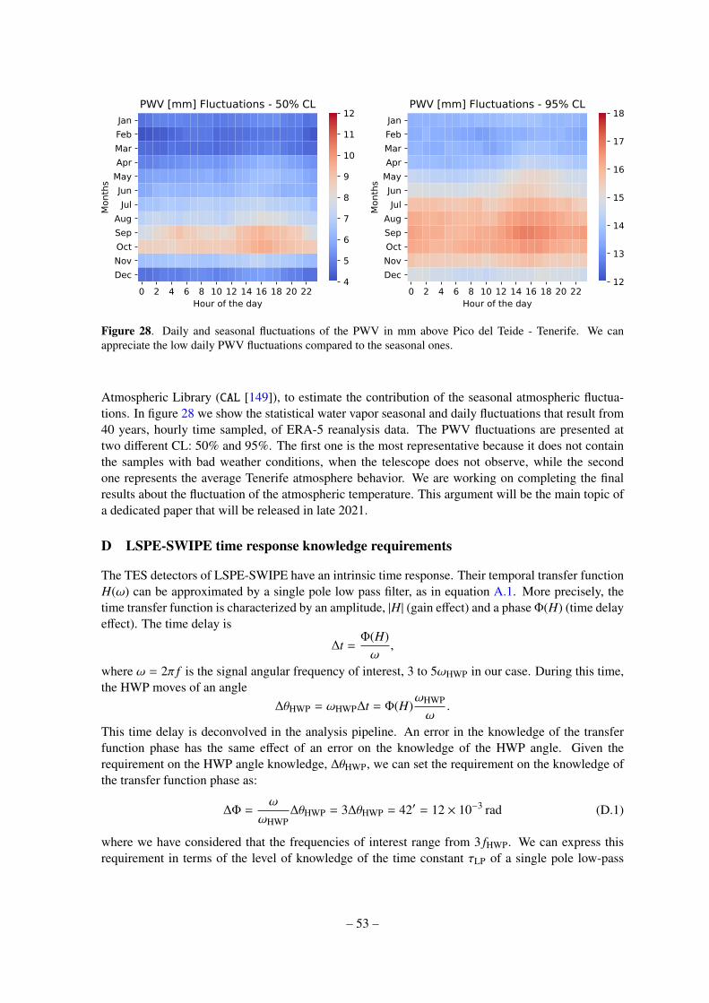
Figure 28. Daily and seasonal fluctuations of the PWV in mm above Pico del Teide - Tenerife. We canappreciate the low daily PWV fluctuations compared to the seasonal ones.

Atmospheric Library (CAL [149]), to estimate the contribution of the seasonal atmospheric fluctua-tions. In figure 28 we show the statistical water vapor seasonal and daily fluctuations that result from40 years, hourly time sampled, of ERA-5 reanalysis data. The PWV fluctuations are presented attwo different CL: 50% and 95%. The first one is the most representative because it does not containthe samples with bad weather conditions, when the telescope does not observe, while the secondone represents the average Tenerife atmosphere behavior. We are working on completing the finalresults about the fluctuation of the atmospheric temperature. This argument will be the main topic ofa dedicated paper that will be released in late 2021.

D LSPE-SWIPE time response knowledge requirements

The TES detectors of LSPE-SWIPE have an intrinsic time response. Their temporal transfer functionH(ω) can be approximated by a single pole low pass filter, as in equation A.1. More precisely, thetime transfer function is characterized by an amplitude, |H| (gain effect) and a phase Φ(H) (time delayeffect). The time delay is

∆t =Φ(H)ω

,

where ω = 2π f is the signal angular frequency of interest, 3 to 5ωHWP in our case. During this time,the HWP moves of an angle

∆θHWP = ωHWP∆t = Φ(H)ωHWP

ω.

This time delay is deconvolved in the analysis pipeline. An error in the knowledge of the transferfunction phase has the same effect of an error on the knowledge of the HWP angle. Given therequirement on the HWP angle knowledge, ∆θHWP, we can set the requirement on the knowledge ofthe transfer function phase as:

∆Φ =ω

ωHWP∆θHWP = 3∆θHWP = 42′ = 12 × 10−3 rad (D.1)

where we have considered that the frequencies of interest range from 3 fHWP. We can express thisrequirement in terms of the level of knowledge of the time constant τLP of a single pole low-pass

– 53 –

filter, considering that tan Φ = −ωτLP. An error on the time constant ∆τLP generates an error on thephase

∆Φ =ω

(ωτLP)2 + 1∆τLP.

Inverting

∆τLP =(ωτLP)2 + 1

ω∆Φ =

(ωτLP)2 + 1ωHWP

∆θHWP,

where we have used equation D.1. With a time constant τLP = 30 ms and a frequency in the 1.5 to2.5 Hz range, this means a requirement:

∆τLP ' 1.5 ms (D.2)

(relative error ∆τLP/τLP = 5%). Also in this case, the requirement will be more stringent if consideredjointly with other effects.

E LSPE-SWIPE iterative map-making

We briefly describe the notch filters and iterative map-making used by the SWIPE instrument sim-ulator pipeline to remove systematic effects appearing at the HWP spin frequency and harmonicsm,and recover the filtered signal.

The notch filters are defined as

F( f ) =

1 if f ≤ f10.5

(1 + cos

(π

f− f1f2− f1

))if f1 < f ≤ f2

0 if f2 < f ≤ f30.5

(1 − cos

(π

f− f3f4− f3

))if f3 < f ≤ f4

1 if f > f4

(E.1)

where f1 = f0 − 2∆ f , f2 = f0 − ∆ f , f3 = f0 + ∆ f , and f4 = f0 + 2∆ f are the frequencies where thefilter starts to drop, reaches 0, starts to rise, reaches 1 respectively; f0 is the notch filter frequency,and ∆ f is the notch filter width. In simulations, we set f0 to the HWP spin frequency and harmonics,and ∆ f = 1 mHz, lower than the payload default spin rate, set at 1.93 mHz (table 13). The notch filterapplied at 4 times the HWP spin rate, 4 fHWP, can remove part of the signal at the largest scales in thesky. This happens despite the fact that the payload spin rate is above the notch filter width. In fact,the sky signal is not exactly periodic, and part of it is spread in the interval [4 fHWP ± fpayload] , i.e.within the spin rate frequency from modulation frequency. This signal is recovered by an iterativemapmaking process.

In the following, P is the pointing matrix, MP is the rebinning matrix; ⊗ means a filtering. Theiterative procedure is applied to the timeline d j of the j-th detector:

• each timeline is notch-filtered to remove the contamination d j = F ⊗ d j;

• all filtered timelines are combined in a first map, by simple rebin m0 =∑

j MPd j;

• here starts the iteration, from i = 0;

• a synthetic timeline is produced for each detector: h j = Pmi;

• the synthetic timeline is filtered by 1 − F, to recover the missing signal: h j,i = (1 − F) ⊗ h j,i;

– 54 –

• the filtered synthetic timeline is added to the filtered original timeline: d j,i = d j + h j,i;

• a new map is produced: mi+1 =∑

j MPd j,i, and the procedure is iterated.

Testing different numbers of iterations, we have found that 50 iterations represents a good trade-off

between computational time and residual signal in the map with filtered timelines.

Acknowledgments

The development of LSPE is supported by ASI (grant LSPE I/022/11/0) and INFN. We acknowledgethe usage of the HEALPix[150] and am software packages, computational resources from NERSC,Cineca and CNAF. We acknowledge support from the COSMOS network (www.cosmosnet.it) throughthe ASI (Italian Space Agency) Grants 2016-24-H.0 and 2016-24-H.1-2018, and Sapienza Univer-sity. JARM, RGS and MPdT acknowledge financial support from the Spanish Ministry of Scienceand Innovation (MICINN) under the project AYA2017-84185-P, and the European Union’s Horizon2020 research and innovation programme under grant agreement number 687312 (RADIOFORE-GROUNDS). The authors gratefully acknowledge the time and expertise devoted to reviewing themanuscript by the referees.

References

[1] U. Seljak and M. Zaldarriaga, Signature of gravity waves in the polarization of the microwavebackground, Phys. Rev. Lett. 78 (1997) 2054.

[2] M. Kamionkowski and E.D. Kovetz, The Quest for B Modes from Inflationary Gravitational Waves,Annu. Rev. Astron. Astr. 54 (2016) 227.

[3] Planck Collaboration, N. Aghanim, Y. Akrami, F. Arroja, M. Ashdown, J. Aumont et al., Planck 2018results. I. Overview and the cosmological legacy of Planck, A&A 641 (2020) A1 [1807.06205].

[4] M. Tristram, A.J. Banday, K.M. Górski, R. Keskitalo, C.R. Lawrence, K.J. Andersen et al., Planckconstraints on the tensor-to-scalar ratio, A&A 647 (2021) A128 [2010.01139].

[5] P.A.R. Ade, Z. Ahmed, R.W. Aikin, K.D. Alexander, D. Barkats, S.J. Benton et al., Constraints onPrimordial Gravitational Waves Using Planck, WMAP, and New BICEP2/Keck Observations throughthe 2015 Season, Phys. Rev. Lett. 121 (2018) 221301 [1810.05216].

[6] M. Archidiacono, A. Cooray, A. Melchiorri and S. Pandolfi, Cmb neutrino mass bounds andreionization, Phys. Rev. D 82 (2010) 087302.

[7] R. Allison, P. Caucal, E. Calabrese, J. Dunkley and T. Louis, Towards a cosmological neutrino massdetection, Phys. Rev. D 92 (2015) 123535.

[8] J.A. Grayson, P.A.R. Ade, Z. Ahmed, K.D. Alexander, M. Amiri, D. Barkats et al., BICEP3performance overview and planned Keck Array upgrade, in Millimeter, Submillimeter, andFar-Infrared Detectors and Instrumentation for Astronomy VIII, W.S. Holland and J. Zmuidzinas, eds.,vol. 9914 of Society of Photo-Optical Instrumentation Engineers (SPIE) Conference Series,p. 99140S, July, 2016, DOI [1607.04668].

[9] L. Moncelsi, P.A.R. Ade, A. Z, M. Amiri, D. Barkats, R.B. Thakur et al., Receiver development forBICEP Array, a next-generation CMB polarimeter at the South Pole, in Millimeter, Submillimeter, andFar-Infrared Detectors and Instrumentation for Astronomy X, J. Zmuidzinas and J.-R. Gao, eds.,vol. 11453, pp. 189 – 206, International Society for Optics and Photonics, SPIE, 2020, DOI.

[10] K. Harrington, T. Marriage, A. Ali, J.W. Appel, C.L. Bennett, F. Boone et al., The Cosmology LargeAngular Scale Surveyor, in Millimeter, Submillimeter, and Far-Infrared Detectors and Instrumentation

– 55 –

for Astronomy VIII, W.S. Holland and J. Zmuidzinas, eds., vol. 9914 of Society of Photo-OpticalInstrumentation Engineers (SPIE) Conference Series, p. 99141K, July, 2016, DOI [1608.08234].

[11] A. Suzuki, P. Ade, Y. Akiba, C. Aleman, K. Arnold, C. Baccigalupi et al., The Polarbear-2 and theSimons Array Experiments, J. Low Temp. Phys. 184 (2016) 805 [1512.07299].

[12] J.T. Sayre, C.L. Reichardt, J.W. Henning, P.A.R. Ade, A.J. Anderson, J.E. Austermann et al.,Measurements of B -mode polarization of the cosmic microwave background from 500 square degreesof SPTpol data, Phys. Rev. D 101 (2020) 122003 [1910.05748].

[13] B.A. Benson, P.A.R. Ade, Z. Ahmed, S.W. Allen, K. Arnold, J.E. Austermann et al., SPT-3G: anext-generation cosmic microwave background polarization experiment on the South Pole telescope, inMillimeter, Submillimeter, and Far-Infrared Detectors and Instrumentation for Astronomy VII,W.S. Holland and J. Zmuidzinas, eds., vol. 9153, pp. 552 – 572, International Society for Optics andPhotonics, SPIE, 2014, DOI.

[14] S. Aiola, E. Calabrese, L. Maurin, S. Naess, B.L. Schmitt, M.H. Abitbol et al., The AtacamaCosmology Telescope: DR4 maps and cosmological parameters, J. Cosmol. Astropart. P. 2020 (2020)047 [2007.07288].

[15] S.K. Choi, M. Hasselfield, S.-P.P. Ho, B. Koopman, M. Lungu, M.H. Abitbol et al., The AtacamaCosmology Telescope: a measurement of the Cosmic Microwave Background power spectra at 98 and150 GHz, J. Cosmol. Astropart. P. 2020 (2020) 045 [2007.07289].

[16] P. Ade, J. Aguirre, Z. Ahmed, S. Aiola, A. Ali, D. Alonso et al., The Simons Observatory: sciencegoals and forecasts, J. Cosmol. Astropart. P. 2019 (2019) 056 [1808.07445].

[17] S. Oguri, J. Choi, T. Damayanthi, M. Hattori, M. Hazumi, H. Ishitsuka et al., GroundBIRD: ObservingCosmic Microwave Polarization at Large Angular Scale with Kinetic Inductance Detectors andHigh-Speed Rotating Telescope, J. Low Temp. Phys. 184 (2016) 786.

[18] J.C. Hamilton, L. Mousset, E.S. Battistelli, M.A. Bigot-Sazy, P. Chanial, R. Charlassier et al., QUBICI: Overview and ScienceProgram, arXiv e-prints (2020) arXiv:2011.02213 [2011.02213].

[19] The CMB-S4 Collaboration, :, K. Abazajian, G.E. Addison, P. Adshead, Z. Ahmed et al., CMB-S4:Forecasting Constraints on Primordial Gravitational Waves, arXiv e-prints (2020) arXiv:2008.12619[2008.12619].

[20] R. Gualtieri, J.P. Filippini, P.A.R. Ade, M. Amiri, S.J. Benton, A.S. Bergman et al., SPIDER: CMBPolarimetry from the Edge of Space, J. Low Temp. Phys. 193 (2018) 1112 [1711.10596].

[21] N.N. Gandilo, P.A.R. Ade, D. Benford, C.L. Bennett, D.T. Chuss, J.L. Dotson et al., The PrimordialInflation Polarization Explorer (PIPER), in Millimeter, Submillimeter, and Far-Infrared Detectors andInstrumentation for Astronomy VIII, W.S. Holland and J. Zmuidzinas, eds., vol. 9914 of Society ofPhoto-Optical Instrumentation Engineers (SPIE) Conference Series, p. 99141J, July, 2016, DOI[1607.06172].

[22] S. Hanany, M. Alvarez, E. Artis, P. Ashton, J. Aumont, R. Aurlien et al., PICO: Probe of Inflation andCosmic Origins, in Bulletin of the American Astronomical Society, vol. 51, p. 194, Sept., 2019[1908.07495].

[23] M. Hazumi, P.A.R. Ade, Y. Akiba, D. Alonso, K. Arnold, J. Aumont et al., LiteBIRD: A Satellite forthe Studies of B-Mode Polarization and Inflation from Cosmic Background Radiation Detection, J.Low Temp. Phys. 194 (2019) 443.

[24] H. Sugai, P.A.R. Ade, Y. Akiba, D. Alonso, K. Arnold, J. Aumont et al., Updated Design of the CMBPolarization Experiment Satellite LiteBIRD, J. Low Temp. Phys. (2020) [2001.01724].

[25] P. de Bernardis, S. Aiola, G. Amico, E. Battistelli, A. Coppolecchia, A. Cruciani et al., SWIPE: abolometric polarimeter for the Large-Scale Polarization Explorer, in Millimeter, Submillimeter, andFar-Infrared Detectors and Instrumentation for Astronomy VI, vol. 8452 of Proc. SPIE, p. 84523F,Sept., 2012, DOI [1208.0282].

– 56 –

[26] S. Aiola, G. Amico, P. Battaglia, E. Battistelli, A. Baó, P. de Bernardis et al., The Large-ScalePolarization Explorer (LSPE), in Ground-based and Airborne Instrumentation for Astronomy IV,vol. 8446 of Proc. SPIE, p. 84467A, Sept., 2012, DOI.

[27] M. Bersanelli, A. Mennella, G. Morgante, M. Zannoni, G. Addamo, A. Baschirotto et al., A coherentpolarimeter array for the Large Scale Polarization Explorer (LSPE) balloon experiment, inGround-based and Airborne Instrumentation for Astronomy IV, vol. 8446 of Proc. SPIE, p. 84467C,Sept., 2012, DOI [1208.0164].

[28] L. Lamagna, G. Addamo, P.A.R. Ade, C. Baccigalupi, A.M. Baldini, P.M. Battaglia et al., Progressreport on the Large Scale Polarization Explorer, J. Low Temp. Phys. (2020) arXiv:2005.01187[2005.01187].

[29] F. Incardona, Observing the polarized Cosmic Microwave Background from the Earth : scanningstrategy and polarimeters test for the LSPE / STRIP instrument, Ph.D. thesis, University of Milan,2020.

[30] F. Incardona, M. Benetti, M. Bersanelli, C. Franceschet, D. Maino, A. Mennella et al., Preliminaryscanning strategy analysis for the LSPE-STRIP instrument, in Society of Photo-OpticalInstrumentation Engineers (SPIE) Conference Series, vol. 10708, p. 107082F, Jul, 2018, DOI.

[31] N. Krachmalnicoff, E. Carretti, C. Baccigalupi, G. Bernardi, S. Brown, B.M. Gaensler et al., S-PASSview of polarized Galactic synchrotron at 2.3 GHz as a contaminant to CMB observations, Astron.Astrophys. 618 (2018) A166 [1802.01145].

[32] J.A. Castro-Almazán, C. Muñoz-Tuñón, B. García-Lorenzo, G. Pérez-Jordán, A.M. Varela andI. Romero, Precipitable Water Vapour at the Canarian Observatories (Teide and Roque de losMuchachos) from routine GPS, in Observatory Operations: Strategies, Processes, and Systems VI,vol. 9910 of Society of Photo-Optical Instrumentation Engineers (SPIE) Conference Series, p. 99100P,Jul, 2016, DOI.

[33] C.M. Gutiérrez, R. Rebolo, R.A. Watson, R.D. Davies, A.W. Jones and A.N. Lasenby, The TenerifeCosmic Microwave Background Maps: Observations and First Analysis, Astrophys. J. 529 (2000) 47[astro-ph/9903196].

[34] B. Femenía, R. Rebolo, C.M. Gutiérrez, M. Limon and L. Piccirillo, The Instituto de Astrofísica deCanarias-Bartol Cosmic Microwave Background Anisotropy Experiment: Results of the 1994Campaign, Astrophys. J. 498 (1998) 117 [astro-ph/9711225].

[35] D.L. Harrison, J.A. Rubiño-Martin, S.J. Melhuish, R.A. Watson, R.D. Davies, R. Rebolo et al., Ameasurement at the first acoustic peak of the cosmic microwave background with the 33-GHzinterferometer, Mon. Not. Roy. Astron. Soc. 316 (2000) L24 [astro-ph/0004357].

[36] S. Fernández-Cerezo, C.M. Gutiérrez, R. Rebolo, R.A. Watson, R.J. Hoyland, S.R. Hildebrandt et al.,Observations of the cosmic microwave background and galactic foregrounds at 12-17GHz with theCOSMOSOMAS experiment, Mon. Not. Roy. Astron. Soc. 370 (2006) 15 [astro-ph/0601203].

[37] R.A. Watson, P. Carreira, K. Cleary, R.D. Davies, R.J. Davis, C. Dickinson et al., First results from theVery Small Array - I. Observational methods, Mon. Not. Roy. Astron. Soc. 341 (2003) 1057[astro-ph/0205378].

[38] J.A. Rubiño-Martín, R. Rebolo, M. Aguiar, R. Génova-Santos, F. Gómez-Reñasco, J.M. Herreroset al., The QUIJOTE-CMB experiment: studying the polarisation of the galactic and cosmologicalmicrowave emissions, in Ground-based and Airborne Telescopes IV, vol. 8444 of Society ofPhoto-Optical Instrumentation Engineers (SPIE) Conference Series, p. 84442Y, Sep, 2012, DOI.

[39] K. Lee, J. Choi, R.T. Génova-Santos, M. Hattori, M. Hazumi, S. Honda et al., GroundBIRD: A CMBPolarization Experiment with MKID Arrays, Journal of Low Temperature Physics 200 (2020) 384[2011.07705].

[40] A.C. Taylor, Clover - A B-mode polarization experiment, New Astron. Rev. 50 (2006) 993 .

– 57 –

[41] C. Franceschet, S. Realini, A. Mennella, G. Addamo, A. Baú, P.M. Battaglia et al., The STRIPinstrument of the Large Scale Polarization Explorer: microwave eyes to map the Galactic polarizedforegrounds, in Millimeter, Submillimeter, and Far-Infrared Detectors and Instrumentation forAstronomy IX, vol. 10708 of Society of Photo-Optical Instrumentation Engineers (SPIE) ConferenceSeries, p. 107081G, Jul, 2018, DOI.

[42] S. Realini, C. Franceschet and A. Mennella, Modelling the radiation pattern of a dual circularpolarization system, J. Instrum. 14 (2019) P03005.

[43] O.A. Peverini, G. Virone, F. Del Torto, C. Franceschet, F. Villa, M. Lumia et al., Q-band antenna-feedsystem for the Large Scale Polarization Explorer balloon experiment, in 2015 InternationalConference on Electromagnetics in Advanced Applications (ICEAA), pp. 883–886, IEEE, sep, 2015,DOI.

[44] F. Del Torto, M. Bersanelli, F. Cavaliere, A. De Rosa, O. D’Arcangelo, C. Franceschet et al., W-bandprototype of platelet feed-horn array for CMB polarisation measurements, J. Instrum. 6 (2011) 6009[1107.1157].

[45] S.Y. Eom and Y.B. Korchemkin, A New Comb Circular Polarizer Suitable for Millimeter-BandApplication, ETRI Journal 28 (2006) 656.

[46] G. Virone, O.A. Peverini, M. Lumia, G. Addamo and R. Tascone, Platelet Orthomode Transducer forQ-Band Correlation Polarimeter Clusters, IEEE T. Microw. Theory 62 (2014) 1487.

[47] QUIET Collaboration, D. Araujo, C. Bischoff, A. Brizius, I. Buder, Y. Chinone et al., Second seasonQUIET observations: Measurements of the cosmic microwave background polarization powerspectrum at 95 GHz, Astrophys. J. 760 (2012) [1207.5034].

[48] Y.-L. Chen, T. Chiueh and H.-F. Teng, A 77-118 GHz RESONANCE-FREE SEPTUM POLARIZER,Astrophys. J., Suppl. Ser. 211 (2014) 11.

[49] QUIET Collaboration, C. Bischoff, A. Brizius, I. Buder, Y. Chinone, K. Cleary et al., First SeasonQUIET Observations: Measurements of Cosmic Microwave Background Polarization Power Spectraat 43 GHz in the Multipole Range 25 ≤ ` ≤ 475, Astrophys. J. 741 (2011) 111 [1012.3191].

[50] A. Iarocci, P. Benedetti, F. Caprara, A. Cardillo, F. di Felice, G. di Stefano et al., PEGASO: An ultralight long duration stratospheric payload for polar regions flights, Adv. Space Res. 42 (2008) 1633.

[51] S. Peterzen, S. Masi, P. Dragoy, R. Ibba and D. Spoto, Long Duration Balloon flights development.(Italian Space Agency), Mem. Soc. Astron. Italiana 79 (2008) 792.

[52] Masi, Silvia, Coppolecchia, A., Battistelli, E., de Bernardis, P., Columbro, F., D´Alessandro, G. et al.,Balloon-borne cosmic microwave background experiments, EPJ Web Conf. 209 (2019) 01046.

[53] P. de Bernardis, S. Masi and OLIMPO and LSPE Teams, Precision CMB measurements withlong-duration stratospheric balloons: activities in the Arctic, in Astrophysics from Antarctica,M.G. Burton, X. Cui and N.F.H. Tothill, eds., vol. 288 of IAU Symposium, pp. 208–213, Jan., 2013,DOI.

[54] F. Piacentini, A. Coppolecchia, P. de Bernardis, G. Di Stefano, A. Iarocci, L. Lamagna et al., Winterlong duration stratospheric balloons from Polar regions, arXiv e-prints (2018) arXiv:1810.05565[1810.05565].

[55] P. de Bernardis, E. Aquilini, A. Boscaleri, M. de Petris, M. Gervasi, L. Martinis et al., ARGO: aballoon-borne telescope for measurements of the millimeter diffuse sky emission, Astron. Astrophys.271 (1993) 683.

[56] B.P. Crill, P.A.R. Ade, D.R. Artusa, R.S. Bhatia, J.J. Bock, A. Boscaleri et al., BOOMERANG: ABalloon-borne Millimeter-Wave Telescope and Total Power Receiver for Mapping Anisotropy in theCosmic Microwave Background, Astrophys. J., Suppl. Ser. 148 (2003) 527 [astro-ph/0206254].

– 58 –

[57] S. Masi, P.A.R. Ade, J.J. Bock, J.R. Bond, J. Borrill, A. Boscaleri et al., Instrument, method,brightness, and polarization maps from the 2003 flight of BOOMERanG, Astron. Astrophys. 458(2006) 687 [astro-ph/0507509].

[58] A. Benoît, P. Ade, A. Amblard, R. Ansari, E. Aubourg, J. Bartlett et al., Archeops: a high resolution,large sky coverage balloon experiment for mapping cosmic microwave background anisotropies,Astropart. Phys. 17 (2002) 101 [astro-ph/0106152].

[59] S. Masi, M. Calvo, L. Conversi, P. de Bernardis, M. de Petris, G. de Troia et al., A balloon-bornesurvey of the mm/sub-mm sky: OLIMPO, in 17th ESA Symposium on European Rocket and BalloonProgrammes and Related Research, B. Warmbein, ed., vol. 590 of ESA Special Publication,pp. 581–586, Aug., 2005.

[60] A. Paiella, A. Coppolecchia, L. Lamagna, P. Ade, E. Battistelli, M.G. Castellano et al., Kineticinductance detectors for the OLIMPO experiment: design and pre-flight characterization, J. Cosmol.Astropart. P. 2019 (2019) 039.

[61] S. Masi, P. de Bernardis, A. Paiella, F. Piacentini, L. Lamagna, A. Coppolecchia et al., KineticInductance Detectors for the OLIMPO experiment: in-flight operation and performance, J. Cosmol.Astropart. P. 2019 (2019) 003 [1902.08993].

[62] A. Boscaleri, V. Venturi and R. Colzi, Time-domain computer simulation program as first step of a fulldigital high-precision pointing system for platform in balloon-borne remote sensing, in InfraredTechnology XVI, I.J. Spiro, ed., vol. 1341, pp. 58 – 65, International Society for Optics and Photonics,SPIE, 1990, DOI.

[63] A. Boscaleri, A time domain design technique for high precision full digital pointing system inballoon-borne remote infrared sensing, in Acquisition, Tracking, and Pointing IV, S. Gowrinathan, ed.,vol. 1304, International Society for Optics and Photonics, SPIE, 1990, DOI.

[64] A. Boscaleri, V. Venturi and D. Tirelli, The ARGO experiment pointing system as an example for othersingle-axis platform pointing systems, Meas. Sci. Technol. 5 (1994) 190.

[65] F. Nati, P. de Bernardis, A. Iacoangeli, S. Masi, A. Benoit and D. Yvon, A fast star sensor for balloonpayloads, Rev. Sci. Instrum. 74 (2003) 4169.

[66] J.F. Macías-Pérez, G. Lagache, B. Maffei, K. Ganga, A. Bourrachot, P. Ade et al., Archeops in-flightperformance, data processing, and map making, Astron. Astrophys. 467 (2007) 1313[astro-ph/0603665].

[67] P. Palumbo, E. Aquilini, P. Cardoni, P. de Bernardis, A. De Ninno, L. Martinis et al., Balloon-borne3He cryostat for millimetre bolometric photometry, Cryogenics 34 (1994) 1001.

[68] S. Masi, P. Cardoni, P. de Bernardis, F. Piacentini, A. Raccanelli and F. Scaramuzzi, A long durationcryostat suitable for balloon borne photometry, Cryogenics 39 (1999) 217.

[69] J.P. Bernard, P. Ade, Y. André, J. Aumont, L. Bautista, N. Bray et al., PILOT: a balloon-borneexperiment to measure the polarized FIR emission of dust grains in the interstellar medium, Exp.Astron. 42 (2016) 199.

[70] A. Coppolecchia, L. Lamagna, S. Masi, P. Ade, G. Amico, E. Battistelli et al., The long durationcryogenic system of the olimpo balloon-borne experiment: design and in-flight performance,Cryogenics (2020) 103129.

[71] G. Coppi, P. de Bernardis, A.J. May, S. Masi, M. McCulloch, S.J. Melhuish et al., Developing a longduration 3He fridge for the LSPE-SWIPE instrument, in Proc. SPIE, vol. 9912 of Society ofPhoto-Optical Instrumentation Engineers (SPIE) Conference Series, p. 991265, SPIE (2016), DOI.

[72] K. Zilic, A. Aboobaker, F. Aubin, C. Geach, S. Hanany, N. Jarosik et al., A double vacuum windowmechanism for space-borne applications, Rev. Sci. Instrum. 88 (2017) .

– 59 –

[73] G. dall’Oglio, P. de Bernardis, S. Masi and F. Melchiorri, Measurement of the 3K Cosmic BackgroundNoise in the Far Infrared, in Early Evolution of the Universe and its Present Structure, G.O. Abell andG. Chincarini, eds., vol. 104 of IAU Symposium, p. 135, Jan., 1983.

[74] J.F. Macías-Pérez, G. Lagache, B. Maffei, K. Ganga, A. Bourrachot, P. Ade et al., Archeops in-flightperformance, data processing, and map making, Astron. Astrophys. 467 (2007) 1313[astro-ph/0603665].

[75] G. D’Alessandro, A. Paiella, A. Coppolecchia, M.G. Castellano, I. Colantoni, P. de Bernardis et al.,Ultra high molecular weight polyethylene: Optical features at millimeter wavelengths, Infrared Phys.Technol. 90 (2018) 59 [1803.05228].

[76] S. Legg, L. Lamagna, G. Coppi, P. de Bernardis, G. Giuliani, R. Gualtieri et al., Development of themulti-mode horn-lens configuration for the LSPE-SWIPE B-mode experiment, in Millimeter,Submillimeter, and Far-Infrared Detectors and Instrumentation for Astronomy VIII, vol. 9914 ofProceeding SPIE, p. 991414, July, 2016, DOI.

[77] F. Columbro, P.G. Madonia, L. Lamagna, E.S. Battistelli, A. Coppolecchia, P. de Bernardis et al.,Swipe multi-mode pixel assembly design and beam pattern measurements at cryogenic temperature, J.Low Temp. Phys. 199 (2020) 312.

[78] A.C. Ludwig, The definition of cross polarization., IEEE T. Antenn. Propag. 21 (1973) 116.

[79] G. Pisano, C. Tucker, P.A.R. Ade, P. Moseley and M.W. Ng, Metal mesh based metamaterials formillimetre wave and thz astronomy applications, in 2015 8th UK, Europe, China Millimeter Waves andTHz Technology Workshop (UCMMT), pp. 1–4, 2015, DOI.

[80] G. Pisano, M. Ng, V. Haynes and B. Maffei, A broadband metal-mesh half-wave plate for millimetrewave linear polarisation rotation, in Progress In Electromagnetics Research M, vol. 25, pp. 101–114,2012, DOI.

[81] G. Pisano, P. Ade, C. Tucker and M.W. Ng, Large bandwidth mesh half-wave plates for millimetre andthz wave astronomy, in 2015 40th International Conference on Infrared, Millimeter, and Terahertzwaves (IRMMW-THz), pp. 1–1, 2015.

[82] T. Matsumura, H. Kataza, S. Utsunomiya, R. Yamamoto, M. Hazumi and N. Katayama, Design andperformance of a prototype polarization modulator rotational system for use in space using asuperconducting magnetic bearing, IEEE Trans. Appl. Supercond. 26 (2016) 1.

[83] B. Johnson, F. Columbro, D. Araujo, M. Limon, B. Smiley, G. Jones et al., A large-diameterhollow-shaft cryogenic motor based on a superconducting magnetic bearing for millimeter-wavepolarimetry, Rev. Sci. Instrum. 88 (2017) .

[84] F. Columbro, P. de Bernardis, L. Lamagna, S. Masi, A. Paiella, F. Piacentini et al., A polarizationmodulator unit for the mid- and high-frequency telescopes of the LiteBIRD mission, vol. 11443 ofSociety of Photo-Optical Instrumentation Engineers (SPIE) Conference Series, p. 114436Z, Dec.,2020, DOI.

[85] F. Columbro, P. de Bernardis and S. Masi, A clamp and release system for superconductive magneticbearings, Rev. Sci. Instrum. 89 (2018) .

[86] P. de Bernardis, F. Columbro, S. Masi, A. Paiella and G. Romeo, A simple method to measure thetemperature and levitation height of devices rotating at cryogenic temperatures, Rev. Sci. Instrum. 91(2020) 045118 [https://doi.org/10.1063/5.0005498].

[87] D. Vaccaro, B. Siri, A.M. Baldini, M. Biasotti, F. Cei, V. Ceriale et al., Tuning the TC of Titanium ThinFilms for Transition-Edge Sensors by Annealing in Argon, J. Low Temp. Phys. 193 (2018) 1122.

[88] D. Vaccaro, A.M. Baldini, F. Cei, L. Galli, M. Grassi, D. Nicolò et al., "The FDM readout for theLSPE/SWIPE TES bolometers", in Millimeter, Submillimeter, and Far-Infrared Detectors andInstrumentation for Astronomy IX, J. Zmuidzinas and J.-R. Gao, eds., vol. 10708, pp. 732 – 742,International Society for Optics and Photonics, Proc. SPIE, 2018, DOI.

– 60 –

[89] D. Vaccaro, A. Baldini, F. Cei, L. Galli, M. Grassi, D. Nicolò et al., A frequency domain multiplexingsystem to readout the TES bolometers on the LSPE/SWIPE experiment, Nucl. Instrum. Meth. A 936(2019) 169.

[90] F. Fontanelli, M. Biasotti, A. Bevilacqua and F. Siccardi, The front-end electronics of the LSPE-SWIPEexperiment, in Space Telescopes and Instrumentation 2016: Optical, Infrared, and Millimeter Wave,H.A. MacEwen, G.G. Fazio, M. Lystrup, N. Batalha, N. Siegler and E.C. Tong, eds., vol. 9904,pp. 1633 – 1638, International Society for Optics and Photonics, Proc. SPIE, 2016, DOI.

[91] C. Bischoff, A. Brizius, I. Buder, Y. Chinone, K. Cleary, R.N. Dumoulin et al., THE Q/U IMAGINGEXPERIMENT INSTRUMENT, Astrophys. J. 768 (2013) 9.

[92] K. Cleary, Coherent polarimeter modules for the QUIET experiment, in Society of Photo-OpticalInstrumentation Engineers (SPIE) Conference Series, vol. 7741 of Society of Photo-OpticalInstrumentation Engineers (SPIE) Conference Series, jul, 2010, DOI.

[93] S. Paine, The am atmospheric model, Sept., 2019. 10.5281/zenodo.3406496.

[94] M.N. Afsar, K.A. Korolev, L. Subramanian and I.I. Tkachov, Complex Dielectric Measurements ofMaterials at Q- Band, V- Band and W- Band Frequencies with High Power Sources, in 2005 IEEEInstrumentationand Measurement Technology Conference Proceedings, vol. 1, pp. 82–87, 2005.

[95] J.W. Lamb, Miscellaneous data on materials for millimetre and submillimetre optics, J. Infrared.Millim. W. 17 (1996) 1997.

[96] J.M. Lamarre, Photon noise in photometric instruments at far-infrared and submillimeter wavelengths,Appl. Opt. 25 (1986) 870.

[97] R. Gualtieri, E.S. Battistelli, A. Cruciani, P. de Bernardis, M. Biasotti, D. Corsini et al., Multi-modeTES Bolometer Optimization for the LSPE-SWIPE Instrument, J. Low Temp. Phys. 184 (2016) 527[1602.07744].

[98] M. Dobbs et al., Frequency Multiplexed SQUID Readout of Large Bolometer Arrays for CosmicMicrowave Background Measurements, Rev. Sci. Instrum. 83 (2012) 073113 [1112.4215].

[99] A. Tartari, A.M. Baldini, F. Cei, L. Galli, M. Grassi, D. Nicolò et al., Development and testing of thefdm read-out of the tes arrays aboard the lspe/swipe balloon-borne experiment, J. Low Temp. Phys.199 (2020) 212.

[100] Planck Collaboration III, Planck 2013 results. III. LFI systematic uncertainties, Astron. Astrophys. 571(2014) A3 [1303.5064].

[101] Planck Collaboration, P.A.R. Ade, J. Aumont, C. Baccigalupi, A.J. Banday, R.B. Barreiro et al.,Planck 2015 results. III. LFI systematic uncertainties, Astron. Astrophys. 594 (2016) A3.

[102] S. Church, Predicting residual levels of atmospheric sky noise in ground-based observations of thecosmic background radiation, Mon. Not. Roy. Astron. Soc. 272 (1995) 551.

[103] Planck Collaboration, P.A.R. Ade, N. Aghanim, M. Ashdown, J. Aumont, C. Baccigalupi et al., Planck2015 results. IV. Low Frequency Instrument beams and window functions, Astron. Astrophys. 594(2016) A4.

[104] Planck Collaboration III, Planck 2015 results. III. LFI systematic uncertainties, Astron. Astrophys. 594(2016) A3 [1507.08853].

[105] N. Krachmalnicoff, Challenges for Present and Future Cosmic Microwave Background Observations:Systematic Effects and Foreground Emission in Polarization, Ph.D. thesis, University of Milan, 2015.

[106] G. Montresor, A responsivity calibration strategy for the LSPE-STRIP balloon experiment, Master’sthesis, University of Milan, 2012.

[107] F. Paonessa, G. Virone, L. Ciorba, G. Addamo, M. Lumia, G. Dassano et al., Design and verificationof a Q-Band test source for UAV-based radiation pattern measurements, IEEE Trans. Instrum. Meas.69 (2020) 9366.

– 61 –

[108] M. Salatino, P. de Bernardis and S. Masi, Modeling transmission and reflection mueller matrices ofdielectric half-wave plates, Journal of Infrared, Millimeter, and Terahertz Waves 38 (2017) 215.

[109] G. Pisano, G. Savini, P.A.R. Ade, V. Haynes and W.K. Gear, Achromatic half-wave plate forsubmillimeter instruments in cosmic microwave background astronomy: experimentalcharacterization, Appl. Opt. 45 (2006) 6982.

[110] Y.D. Takahashi, P.A.R. Ade, D. Barkats, J.O. Battle, E.M. Bierman, J.J. Bock et al., Characterizationof the BICEP Telescope for High-precision Cosmic Microwave Background Polarimetry, Astrophys. J711 (2010) 1141 [0906.4069].

[111] H. Imada, T. Matsumura, R. Takaku, G. Patanchon, H. Ishino, Y. Sakurai et al., Instrumentally inducedspurious polarization of a multi-layer half wave plate for a cmb polarization observation, pp. 61–67,Jan., 2018.

[112] A. Kusaka, J. Appel, T. Essinger-Hileman, J.A. Beall, L.E. Campusano, H.-M. Cho et al., Results fromthe Atacama B-mode Search (ABS) experiment, J. Cosmol. Astropart. P. 2018 (2018) 005[1801.01218].

[113] T. Essinger-Hileman, A. Kusaka, J.W. Appel, S.K. Choi, K. Crowley, S.P. Ho et al., Systematic effectsfrom an ambient-temperature, continuously rotating half-wave plate, Rev. Sci. Instrum. 87 (2016)094503 [1601.05901].

[114] S.A. Bryan, T.E. Montroy and J.E. Ruhl, Modeling dielectric half-wave plates for cosmic microwavebackground polarimetry using a Mueller matrix formalism, Appl. Opt. 49 (2010) 6313 [1006.3359].

[115] L. Pagano, P. de Bernardis, G. de Troia, G. Gubitosi, S. Masi, A. Melchiorri et al., CMB polarizationsystematics, cosmological birefringence, and the gravitational waves background, Phys. Rev. D 80(2009) 043522 [0905.1651].

[116] F. Columbro, E.S. Battistelli, A. Coppolecchia, G. D’Alessandro, P. de Bernardis, L. Lamagna et al.,The short wavelength instrument for the polarization explorer balloon-borne experiment: Polarizationmodulation issues, Astron. Nachr. 340 (2019) 83 [1904.01891].

[117] J. Aumont, J.F. Macías-Pérez, A. Ritacco, N. Ponthieu and A. Mangilli, Absolute calibration of thepolarisation angle for future CMB B-mode experiments from current and future measurements of theCrab nebula, Astron. Astrophys. 634 (2020) A100 [1911.03164].

[118] M. Tucci, E. Martínez-González, P. Vielva and J. Delabrouille, Limits on the detectability of the CMBB-mode polarization imposed by foregrounds, Mon. Not. Roy. Astron. Soc. 360 (2005) 935[https://academic.oup.com/mnras/article-pdf/360/3/935/3206389/360-3-935.pdf].

[119] A. Buzzelli, M. Migliaccio, G. de Gasperis, P. de Bernardis, S. Masi and N. Vittorio, Impact ofpolarized foregrounds on LSPE-SWIPE observations, in J. Phys. Conf. Ser., vol. 956, p. 012002, Jan.,2018, DOI.

[120] Planck Collaboration, Y. Akrami, M. Ashdown, J. Aumont, C. Baccigalupi, M. Ballardini et al., Planck2018 results. IV. Diffuse component separation, Astron. Astrophys. 641 (2020) A4 [1807.06208].

[121] P. Campeti, D. Poletti and C. Baccigalupi, Principal component analysis of the primordial tensorpower spectrum, J. Cosmol. Astropart. P. 1909 (2019) 055 [1905.08200].

[122] R. Stompor, J. Errard and D. Poletti, Forecasting performance of CMB experiments in the presence ofcomplex foreground contaminations, Phys. Rev. D94 (2016) 083526 [1609.03807].

[123] B. Thorne, J. Dunkley, D. Alonso and S. Naess, The Python Sky Model: software for simulating theGalactic microwave sky, Mon. Not. Roy. Astron. Soc. 469 (2017) 2821 [1608.02841].

[124] J.A. Rubiño-Martín, Planck Collaboration and QUIJOTE Collaboration, Cosmology with the CosmicMicrowave Background: Latest Results from the PLANCK satellite and the QUIJOTE experiment, inHighlights on Spanish Astrophysics X, B. Montesinos, A. Asensio Ramos, F. Buitrago, R. Schödel,E. Villaver, S. Pérez-Hoyos et al., eds., pp. 32–43, Mar., 2019.

– 62 –

[125] LSST Dark Energy Science collaboration, A unified pseudo-C` framework, Mon. Not. Roy. Astron.Soc. 484 (2019) 4127 [1809.09603].

[126] Planck Collaboration V, Planck 2018 results. V. Power spectra and likelihoods, Astron. Astrophys.,submitted (2019) [1907.12875].

[127] M. Tegmark and A. de Oliveira-Costa, How to measure CMB polarization power spectra withoutlosing information, Phys. Rev. D64 (2001) 063001 [astro-ph/0012120].

[128] L. Pagano, J.-M. Delouis, S. Mottet, J.-L. Puget and L. Vibert, Reionization optical depthdetermination from Planck HFI data with ten percent accuracy, Astron. Astrophys. 635 (2020) A99[1908.09856].

[129] C. Monteserin, R.B.B. Barreiro, P. Vielva, E. Martinez-Gonzalez, M.P. Hobson and A.N. Lasenby, Alow CMB variance in the WMAP data, Mon. Not. Roy. Astron. Soc. 387 (2008) 209 [0706.4289].

[130] M. Cruz, P. Vielva, E. Martinez-Gonzalez and R.B. Barreiro, Anomalous variance in the WMAP dataand Galactic Foreground residuals, Mon. Not. Roy. Astron. Soc. 412 (2011) 2383 [1005.1264].

[131] A. Gruppuso, P. Natoli, F. Paci, F. Finelli, D. Molinari, A. De Rosa et al., Low Variance at large scalesof WMAP 9 year data, J. Cosmol. Astropart. P. 1307 (2013) 047 [1304.5493].

[132] D.J. Schwarz, C.J. Copi, D. Huterer and G.D. Starkman, CMB Anomalies after Planck, Class. Quant.Grav. 33 (2016) 184001 [1510.07929].

[133] U. Natale, A. Gruppuso, D. Molinari and P. Natoli, Is the lack of power anomaly in the CMB correlatedwith the orientation of the Galactic plane?, J. Cosmol. Astropart. P. 1912 (2019) 052 [1908.10637].

[134] E. Dudas, N. Kitazawa, S.P. Patil and A. Sagnotti, CMB Imprints of a Pre-Inflationary ClimbingPhase, J. Cosmol. Astropart. P. 1205 (2012) 012 [1202.6630].

[135] N. Kitazawa and A. Sagnotti, Pre-inflationary clues from String Theory?, J. Cosmol. Astropart. P.1404 (2014) 017 [1402.1418].

[136] A. Gruppuso, N. Kitazawa, N. Mandolesi, P. Natoli and A. Sagnotti, Pre-Inflationary Relics in theCMB?, Phys. Dark Univ. 11 (2016) 68 [1508.00411].

[137] A. Gruppuso, N. Kitazawa, M. Lattanzi, N. Mandolesi, P. Natoli and A. Sagnotti, The Evens and Oddsof CMB Anomalies, Phys. Dark Univ. 20 (2018) 49 [1712.03288].

[138] A. Gruppuso and A. Sagnotti, Observational Hints of a Pre–Inflationary Scale?, Int. J. Mod. Phys.D24 (2015) 1544008 [1506.08093].

[139] S.M. Carroll, G.B. Field and R. Jackiw, Limits on a Lorentz and Parity Violating Modification ofElectrodynamics, Phys. Rev. D 41 (1990) 1231.

[140] G.-C. Liu, S. Lee and K.-W. Ng, Effect on cosmic microwave background polarization of coupling ofquintessence to pseudoscalar formed from the electromagnetic field and its dual, Phys. Rev. Lett. 97(2006) 161303 [astro-ph/0606248].

[141] B. Feng, M. Li, J.-Q. Xia, X. Chen and X. Zhang, Searching for CPT Violation with CosmicMicrowave Background Data from WMAP and BOOMERANG, Phys. Rev. Lett. 96 (2006) 221302[astro-ph/0601095].

[142] G. Gubitosi, L. Pagano, G. Amelino-Camelia, A. Melchiorri and A. Cooray, A Constraint onPlanck-scale Modifications to Electrodynamics with CMB polarization data, J. Cosmol. Astropart. P.0908 (2009) 021 [0904.3201].

[143] A. Gruppuso, M. Gerbino, P. Natoli, L. Pagano, N. Mandolesi, A. Melchiorri et al., Constraints oncosmological birefringence from Planck and Bicep2/Keck data, J. Cosmol. Astropart. P. 1606 (2016)001 [1509.04157].

[144] A. Gruppuso, G. Maggio, D. Molinari and P. Natoli, A note on the birefringence angle estimation inCMB data analysis, J. Cosmol. Astropart. P. 1605 (2016) 020 [1604.05202].

– 63 –

[145] Planck Collaboration Int. XLIX, Planck intermediate results. XLIX. Parity-violation constraints frompolarization data, Astron. Astrophys. 596 (2016) A110 [1605.08633].

[146] Y. Minami, H. Ochi, K. Ichiki, N. Katayama, E. Komatsu and T. Matsumura, Simultaneousdetermination of the cosmic birefringence and miscalibrated polarization angles from CMBexperiments, Prog. Theor. Exp. Phys. 2019 (2019) 083E02 [1904.12440].

[147] Y. Minami, Determination of miscalibrated polarization angles from observed CMB and foregroundEB power spectra: Application to partial-sky observation, Prog. Theor. Exp. Phys. 2020 (2020)063E01 [2002.03572].

[148] J. Bezanson, A. Edelman, S. Karpinski and V.B. Shah, Julia: A fresh approach to numericalcomputing, SIAM review 59 (2017) 65.

[149] S. Mandelli, T. Kisner, R. Keskitalo, A. Zonca and G. Puglisi, cmbgroundbased/cal: First officialrelease - v1.0, Jan., 2021. 10.5281/zenodo.4439199.

[150] K.M. Górski, E. Hivon, A.J. Banday, B.D. Wandelt, F.K. Hansen, M. Reinecke et al., HEALPix: AFramework for High-Resolution Discretization and Fast Analysis of Data Distributed on the Sphere,Astrophys. J. 622 (2005) 759 [astro-ph/0409513].

– 64 –