arX

iv:0

912.

2993

v5 [

hep-

th]

19

Aug

201

0 Generation of circular polarization of the CMB

E. Bavarsad, M. Haghighat, R. Mohammadi, I. Motie, Z. Rezaei

and M. Zarei

Department of Physics, Isfahan University of Technology, Isfahan 84156-83111, Iran

Abstract

According to the standard cosmology, near the last scattering surface, the

photons scattered via Compton scattering are just linearly polarized and then

the primordial circular polarization of the CMB photons is zero. In this work

we show that CMB polarization acquires a small degree of circular polarization

when a background magnetic field is considered or the quantum electrodynamic

sector of standard model is extended by Lorentz-noninvariant operators as well as

noncommutativity. The existence of circular polarization for the CMB radiation

may be verified during future observation programs and it represents a possible

new channel for investigating new physics effects.

1 Introduction

The observation of polarization in the cosmic microwave background (CMB) and its

correlation to the temperature anisotropies is a very promising tool to test the physics

of early universe. The CMB radiation is expected to be linearly polarized of the order

of 10 %. This Linearity is a result of the anisotropic Compton scattering around the

epoch of recombination which has been widely discussed in the literature [1, 2, 3]. A

1

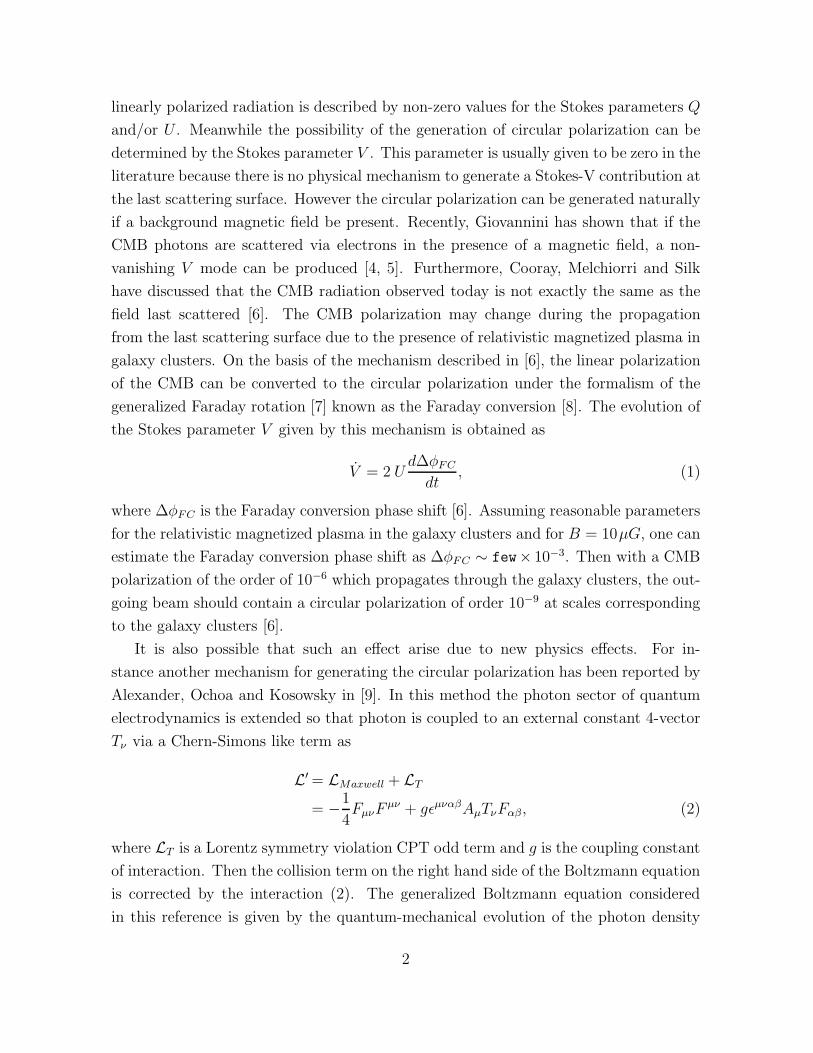
linearly polarized radiation is described by non-zero values for the Stokes parameters Q

and/or U . Meanwhile the possibility of the generation of circular polarization can be

determined by the Stokes parameter V . This parameter is usually given to be zero in the

literature because there is no physical mechanism to generate a Stokes-V contribution at

the last scattering surface. However the circular polarization can be generated naturally

if a background magnetic field be present. Recently, Giovannini has shown that if the

CMB photons are scattered via electrons in the presence of a magnetic field, a non-

vanishing V mode can be produced [4, 5]. Furthermore, Cooray, Melchiorri and Silk

have discussed that the CMB radiation observed today is not exactly the same as the

field last scattered [6]. The CMB polarization may change during the propagation

from the last scattering surface due to the presence of relativistic magnetized plasma in

galaxy clusters. On the basis of the mechanism described in [6], the linear polarization

of the CMB can be converted to the circular polarization under the formalism of the

generalized Faraday rotation [7] known as the Faraday conversion [8]. The evolution of

the Stokes parameter V given by this mechanism is obtained as

V = 2 Ud∆φFC

dt, (1)

where ∆φFC is the Faraday conversion phase shift [6]. Assuming reasonable parameters

for the relativistic magnetized plasma in the galaxy clusters and for B = 10µG, one can

estimate the Faraday conversion phase shift as ∆φFC ∼ few× 10−3. Then with a CMB

polarization of the order of 10−6 which propagates through the galaxy clusters, the out-

going beam should contain a circular polarization of order 10−9 at scales corresponding

to the galaxy clusters [6].

It is also possible that such an effect arise due to new physics effects. For in-

stance another mechanism for generating the circular polarization has been reported by

Alexander, Ochoa and Kosowsky in [9]. In this method the photon sector of quantum

electrodynamics is extended so that photon is coupled to an external constant 4-vector

Tν via a Chern-Simons like term as

L′ = LMaxwell + LT

= −1

4FµνF

µν + gǫµναβAµTνFαβ, (2)

where LT is a Lorentz symmetry violation CPT odd term and g is the coupling constant

of interaction. Then the collision term on the right hand side of the Boltzmann equation

is corrected by the interaction (2). The generalized Boltzmann equation considered

in this reference is given by the quantum-mechanical evolution of the photon density

2

matrix. In fact it is shown that the time derivative of the polarization brightness

associated with the Stokes parameter V receives a source term such that the V mode

becomes nonzero.

Also in reference [10], Finellia and Galavernid have considered an axion-like cosmo-

logical pseudoscalar field acting as dark matter coupled to the photons as

L = −gφ4φFµνF

µν , (3)

where gφ is the coupling constant between axion field φ and the electromagnetic

field strength Fµν and F ρσ = ǫµνρσFρσ. Then it has been shown that such an interaction

between the pseudoscalar field and photons rotates the plane of linear polarization and

generates the circular polarization for the cosmic microwave background. A similar

approach with the pseudoscalar photon mixing shows a CMB circular polarization up

to the order of 10−7 [11].

In this work we address new possibilities and propose new channels to produce the

circular polarization for the CMB in three different contexts. First we consider the QED

part of an effective field theory for Lorentz violation (LV) symmetry [12, 13, 14, 15, 16,

17, 18] that is called the Standard-Model Extension (SME) [13]. In this case we only

investigate that Lorentz violation terms of SME that have not been considered in [9].

Then we examine the noncommutative QED (NCQED) with Seiberg-Witten expansion

of fields [19] as well as the presence of the primordial magnetic field background in

the last scattering surface [20]. For this purpose we use the generalized Boltzmann

equation formulated in [9], to study the evolution of Stokes parameter V under the

influence of these new phenomena. This equation shows that a non-zero background

field can generate the circular polarization through either the interaction of photon with

the background itself or the corrections on the Compton scattering of photon on the

electron in the presence of the background field. One should note that the quantum

corrections on the scattering cross section, for the low energy particles, are usually

negligible. Nevertheless, the circular polarization of CMB itself as a small quantity can

be produced potentially via accumulation of these small effects.

On the dimensional ground one can expect ∆φFC at the lowest order depends on the

appropriate combination of the parameters of the model which is dimensionless. There-

fore, for the magnetic field ∆φFC should be proportional to eB/m2 that is about 10−19

for the micro gauss magnetic field. Meanwhile in the NC space it should be depended

on αm2θ which is of the order 10−17 for 1/√θ about 10 TeV. For the Lorentz violation

case the Faraday conversion phase should be linearly proportional to the dimensionless

LV-parameters which are less than the present existing bound about 10−15. Therefore

3

at first sight it seems that the effect of the magnetic field is at least two order of magni-

tudes less than the other new interactions. But as we will show soon this is not the case

and due to the wavelength dependence of the solutions the background magnetic field

has main contribution on the polarization of the CMB. However, it should be also noted

that the resulting circular polarization modes are certainly small due to the smallness

of quantum effects. Meanwhile the probe of circular polarization of the CMB radiation

through the future subtle experiments, certainly give more information about the new

physics or the primordial magnetic fields in the early universe. The main condition

which is assumed everywhere during the paper is a cold plasma at the last scattering

surface at a red shift of about 1100 or an age of about 180, 000 (Ω0h2)−1/2 yrs and a

temperature of the order of O(eV). The low temperature is always applicable for the

calculation of the Compton scattering amplitude.

The paper is organized as follows: In section 2 we review the Stokes parameters

formalism and the generalized Boltzmann equation. In section 3 the generation of

circular polarization due to the Lorentz violation is discussed. In section 4 the same

calculation is done for the noncommutativity. In section 5 we examine the generation

of circular polarization in the presence of a background magnetic field. Finally in the

last section we discuss about the result.

2 Stokes parameters and Boltzmann equation

The polarization of CMB is usually characterized by means of the Stokes parameters

of radiation: I, Q, U and V [3]. For a quasi-monochromatic wave propagating in the z-

direction, in which the electric and magnetic fields vibrate on the x-y plane, the electric

field E in a given point can be written as

Ex = ax(t) cos(ω0t− δx), Ey = ay(t) cos(ω0t− δy), (4)

where the wave is nearly monochromatic with frequency ω0. Then the Stokes parameters

are defined by time averaging of the parameters of electric fields (4) as follows

I ≡⟨

a2x⟩

+⟨

a2y⟩

, (5)

Q ≡⟨

a2x⟩

−⟨

a2y⟩

, (6)

U ≡ 〈axay cos(δx − δy)〉 , (7)

V ≡ 〈axay sin(δx − δy)〉 . (8)

These parameters are physically interpreted as follows: I is the total intensity of wave, Q

measures the difference between x and y polarization, the parameter U gives the phase

4

information for the two linear polarization and V determines the difference between pos-

itive and negative circular polarization. The time evolution of these Stokes parameters

is given through Boltzmann equation. We now turn to the Boltzmann equation which

is vital in our study. The CMB radiation is generally described by the phase space

distribution function f for each polarization state. Boltzmann equation is a systematic

mechanism in order to describe the evolution of the distribution function under gravity

and collisions. The classical Boltzmann equation generally is written as [21]

df

dt= C[f ], (9)

where the left hand side is known as the Liouville term deals with the effects of grav-

itational perturbations about the homogeneous cosmology. An important point that

must be mentioned here is that we have disregarded the scalar fluctuation of metric on

the left hand side of the Boltzmann equation. The right hand side of the Boltzmann

equation contains all possible collision terms. For photons, the Compton scattering with

free electrons, γ(p) + e(q) ↔ γ(p′) + e(q′), is more important and must be included on

the right hand side. To compute the evolution of polarization we follow the approach

of references [3, 9]. At first, the distribution function f is generalized to the density

matrix ρij

ρ =1

2

(

I +Q U − iV

U + iV I −Q

)

=1

2(I1l +Qσ3 + Uσ1 + V σ2), (10)

where 1l is the identity matrix and σi are the Pauli spin matrices. The density matrix

ρij is related to the number operator Dij(k) = a†i(k)aj(k) as

〈Dij(k)〉 = (2π)32k0δ(3)(0)ρij(k). (11)

and the time evolution of the number operator is given by

⟨

d

dtDij

⟩

(t) ≃ i〈[Hint(t), Dij ]〉 −∫ t

0

dt′〈[Hint(t− t′), [Hint(t′), Dij]]〉. (12)

Hence in terms of ρ, the evolution equation leads to

(2π)3δ3(0)2k0d

dtρij(0,k) = i〈[Hint(0), Dij(k)]〉 −

1

2

∫ ∞

−∞

dt′ 〈[Hint(t′), [Hint(0), Dij(k)]]〉,

(13)

where the first term on the right hand side is referred as the refractive term and the

second one as the damping term. Note that in (13), all factors of δ3(0) will be canceled

5

from the final expressions. Equation (13) can be viewed as a quantum mechanical

Boltzmann equation for the phase space function ρ. In the case where the interaction

term is the convenient QED interaction, the time evolution of the Stokes parameter V

is always equal to zero which leads to the absence of circular degrees of freedom for the

CMB photons. In this paper during the next sections, we will show that if one consider

beyond standard model interaction terms, the time evolution of the V receives a source

term which is interpreted as a non-zero circular polarization. If the Stokes parameter

V be non-zero, then it contributes on the new angular power spectrum elements such

as CV Tl , CV E

l and CV Vl where may be detectable in future CMB experiments.

3 Generation of circular polarization in the pres-

ence of Lorentz violation terms

In the present section we consider a new class of Lorentz invariance violation (LIV)

terms as a generic class of interaction between photons and an external field and ex-

plore whether they can produce circular polarization for the CMB photons or not.

Although the source of these asymmetry terms is unknown, physicists usually suppose

that they come from presumably short-distance physics which manifest themselves in

the interactions of standard model (SM) fields [12, 13, 14, 15, 16, 17, 18]. The renor-

malizable sector of the general QED extension for a single Dirac field ψ of mass m and

a photon also has been studied by some authors for which the Lagrangian L is written

as

L = LQED + LelectronLIV + Lphoton

LIV , (14)

where

LQED = i ψγµDµψ −mψψ − 1

4FµνF

µν , (15)

LelectronLIV =

i

2cµνψγ

µDνψ +i

2dµνψγ5γ

µDνψ, (16)

LphotonLIV = −1

4(kF )µναβF

αβF µν +1

2(kAF )

αǫαβµνAβF µν , (17)

where the Dµ is the covariant derivative. In the electron sector, cµν and dµν are the di-

mensionless Hermitian coefficients with symmetric and antisymmetric space-time com-

ponents. For the photon sector, it will be useful to decompose the coefficient kF into

a tensor with 10 independent components analogous to the Weyl tensor in general rel-

ativity and one with 9 components analogous to the trace-free Ricci tensor with the

6

following symmetries of the Riemann tensor

(kF )µναβ = − (kF )νµαβ = − (kF )µνβα = (kF )νµβα = (kF )αβµν . (18)

So it contains 19 independent real components. Various experiments have bounded

these coefficients both in fermion and photon sectors. For instance, the only rotation-

invariant component of (kF )µνβα is constrained to ≤ 10−23 [12] and all other components

of (kF )µνβα which are associated with violations of rotation invariance can be bounded

of about ≤ 10−27 [13]. The high-quality spectropolarimetery of distant galaxies at

infrared, optical, and ultraviolet frequencies, also constrains the coefficients kF to less

than 3× 10−32 [15]. In references [16, 17], another bound has been estimated. For the

couplings cµν and dµν in the electron sector, one can find a variety of bounds such as

cµν ≤ 10−15 and dµν ≤ 10−14 in [18] and references there in.

The 12(kAF )

αǫαβµνAβF µν term in the photon sector, has been studied in [9] and it

was shown that the CMB photons acquire small degree of circular polarization. In this

section we consider the three remaining terms in the LIV Lagrangian. We study the

contributions of each terms in the Boltzmann equation and calculate the evolution of

the Stokes parameters. Firstly, the photon sector term with kF coupling and then the

electron sector with cµν and dµν couplings are investigated.

3.1 The pure photon sector

In this part the Lorentz violation terms (17) are investigated. These terms do not

modify the Compton scattering but the dynamics of the CMB photons can be influ-

enced. Here we consider Hint = −14(kF )µναβF

αβF µν on the right hand side of the

generalized Boltzmann equation (13). Using the canonical commutation relations of

the creation and annihilation operators and their expectation values given in [3], the

equations (4.11a)-(4.11e), one can calculate the refractive term as

⟨[

Hint(t), Dij(k)]⟩

= −1

2(kF )

µναβ(2π)3δ(3)(0)(kαkµǫ∗s′βǫsν) [δsiρs′j(k)− δjs′ρis(k)] ,(19)

where ǫsµ(k) are the photon polarization 4-vectors with s = 1, 2. Now using the sym-

metry properties of kµναβF summarized in Eq. (18), one can write ρij as

d

dtρij(k) = − 4

k0(kF )

µναβ(kαkµǫs′βǫ∗sν) [δs′iρsj(k)− δjs′ρis(k)] . (20)

The photon density matrix can be expanded about a uniform unpolarized distribution

ρ(0) as follows

ρij = ρ(0)ij + ρ

(1)ij , (21)

7

where ρ(0)11 = ρ

(0)22 and ρ

(0)12 = ρ

(0)21 = 0. Therefore the components of the time derivative

of the density matrix are given by

ρ(1)11 (k) = − 4

k0(kF )

µναβkαkµ[ǫ1βǫ∗2νρ

(1)21 − ǫ2βǫ

∗1νρ

(1)12 ], (22)

ρ(1)22 (k) = − 4

k0(kF )

µναβkαkµ[ǫ2βǫ∗1νρ

(1)12 − ǫ1βǫ

∗2νρ

(1)21 ], (23)

ρ(1)12 (k) = − 4

k0(kF )

µναβkαkµ[ǫ1βǫ∗1νρ

(1)12 + ǫ1βǫ

∗2νρ

(1)22 − ǫ1βǫ

∗2νρ

(1)11 − ǫ2βǫ

∗2νρ

(1)12 ], (24)

ρ(1)21 (k) = − 4

k0(kF )

µναβkαkµ[ǫ2βǫ∗1νρ

(1)11 + ǫ2βǫ

∗2νρ

(1)21 − ǫ1βǫ

∗1νρ

(1)21 − ǫ2βǫ

∗1νρ

(1)22 ]. (25)

Note that the polarization vectors ǫsµ(q) are real. Hence the evaluation of the Stokes

parameters are given as

I(1) = 0, (26)

Q(1) = −16

k0(kF )

µναβkαkµ(ǫ1βǫ∗2ν − ǫ2βǫ

∗1ν) V

(1), (27)

U (1) = − 4

k0(kF )

µναβkαkµ(ǫ2βǫ∗1ν − ǫ1βǫ

∗2ν)Q

(1), (28)

V (1) = − 4

k0(kF )

µναβkαkµ

(ǫ1βǫ∗1ν − ǫ2βǫ

∗2ν) U

(1) − (ǫ1βǫ∗2ν + ǫ2βǫ

∗1ν)Q

(1)

. (29)

Therefore in the first order of Lorentz violation parameter kF , V is nonzero. This

shows that although the usual Compton scattering of CMB photons can’t generate

circular polarization, the interaction of photon with a nontrivial LIV background clearly

produces a nonzero circular polarization. To have an estimate of the Faraday phase

conversion we rewrite (29) as follows

V (1) = −4k0 (kF )µναβ

LUαµβν U

(1) − LQαµβν Q

(1)

, (30)

where LUαµβν = kα

k0kµk0(ǫ1βǫ

∗1ν − ǫ2βǫ

∗2ν) and a corresponding relation for LQ

αµβν . Now for

λ0 = 1cm, z=1000 and for 1 kpc one has

∆φFC ∼ 4× 1020kF , (31)

or to have a phase of order one we should have kF ∼ 10−20.

8

3.2 The electron sector

3.2.1 cµν term

We now turn to the LIV terms in the electron sector (16). Calculating the refractive

term on the right hand side of the generalized Boltzmann equation (13), leads to V = 0

for interaction (16). Therefore, We move on to the damping term. This term gives

corrections to the Compton scattering of the CMB photons and electrons. These cor-

rections modify the right hand side of the equation (13) and then may influence the

evolution of the Stokes parameter V . In this part we investigate whether these correc-

tions lead to a circular polarization mode or not. Firstly, the gauge field Aµ is expanded

in terms of annihilation and creation operators a and a† and the fermion fields ψ and

ψ are expended in terms of b and b†. Then the interaction Hamiltonian can be written

in the momentum space as

Hint(t) =

∫

dq dq′ dp dp′ (2π)3δ(3)(q′ + p′ − q− p) exp(it(q′0 + p′0 − qo − p0))

× b†r′(q′)a†s′(p

′)(M1 +M2)as(p)br(q), (32)

where q and q′ are the momenta of electrons and p and p′ are the momenta of photons.

Also we have used the following shorthand notations

dq =d3q

(2π)3m

q0, dp =

d3p

(2π)32p0. (33)

The M1 and M2 are the amplitude for the Compton scattering process up to the first

order of LIV parameters cµν and dµν . Consequently, the commutator in the damping

term, finds the following form

[

Hint(t), Dij(k)]

=

∫

dq dq′ dp dp′ (2π)3δ(3)(q′ + p′ − q− p)(M1 +M2)

×[b†r′(q′)br(q)a

†s′(p

′)as(p)2p0(2π)3δisδ

3(p− k)

−b†r′(q′)br(q)a†s′(p

′)as(p)2p′0(2π)3δjs′δ

3(p′ − k)]. (34)

In appendix A we detail the calculation of (34) and it’s expectation value. Quoting

the results of Appendix A, and expanding the density matrix as ρij = ρ(0)ij + ρ

(1)ij , the

evolution of Stokes parameters is derived as

I(1) = 0, (35)

9

Q(1) =e2

2mk0

∫

dq ne(q)[ 2cµν

q.kq.kǫ1µǫ2ν − kνq.ǫ

2ǫ1µ − q.kǫ1νǫ2µ + kνq.ǫ

1ǫ2µ

+ qν(q.ǫ1ǫ2µ + q.ǫ2ǫ1µ)+

4cµν

(q.k)2(qνqµ + kνkµ)(q.ǫ

1q.ǫ2)]

V (1), (36)

U (1) =e2

2k0m

∫

dqne(q)[2cµν

q.kq.k(ǫ1µǫ1ν − ǫ2µǫ

2ν)− kνq.ǫ

1ǫ1µ + kνq.ǫ2ǫ2µ

+2qν(q.ǫ1ǫ1µ − q.ǫ2ǫ2µ)+

2cµν

(q.k)2(qνqµ + kνkµ)(q.ǫ

1q.ǫ1 − q.ǫ2q.ǫ2)]

V (1), (37)

and

V (1) =ie2

2k0m

∫

dqne(q)(2cµν

q.k(q.k(ǫ1µǫ2ν + ǫ2µǫ

1ν)− kνq.ǫ

2ǫ1µ + kνq.ǫ1ǫ2µ

+qν(q.ǫ1ǫ2µ + q.ǫ2ǫ1µ)+

cµν

(q.k)2(qνqµ + kνkµ)(q.ǫ

1q.ǫ2))

(−Q(1))

+(cµν

q.kq.k(ǫ1µǫ1ν − ǫ2µǫ

2ν)− kνq.ǫ

1ǫ1µ + kνq.ǫ2ǫ2µ

+qν(q.ǫ1ǫ1µ − q.ǫ2ǫ2µ) −

2cµν

(q.k)2(qνqµ + kνkµ)(q.ǫ

1q.ǫ1 − q.ǫ2q.ǫ2))

U (1)

.(38)

An exact solution for the evolution of the Stokes parameters involving the coupled

evolution equation for all of the species can only be accomplished through numerical

integration. The time derivative of the Stokes parameter V has a source term which

indicates the appearance of circular polarization for the CMB photons if they scatter

from electrons through Compton process with an extra Lorentz violation cµν term. Here

again to have an estimate of the value of circular polarization we can find the order

of magnitude of the Faraday phase conversion. For this purpose we consider only the

largest term and confine ourselves to q0 ≃ m≫ |q|, |k|. Therefore one has

V (1) =ie2m

2k30nec

µνvµvν−v.ǫ1v.ǫ2Q(1) + 2(v.ǫ2v.ǫ2 − v.ǫ1v.ǫ1)U (1), (39)

where∫

d3q

(2π)3ne(q) = ne ;

∫

d3q

(2π)3qine(q) = mvine, (40)

and v = (1,v). Thus for λ0 = 1cm, z=1000 and for length scale about 1 kpc and

number density of electrons about 0.1 per cm3 one has

∆φFC ∼ 1× 1020|cµν |, (41)

10

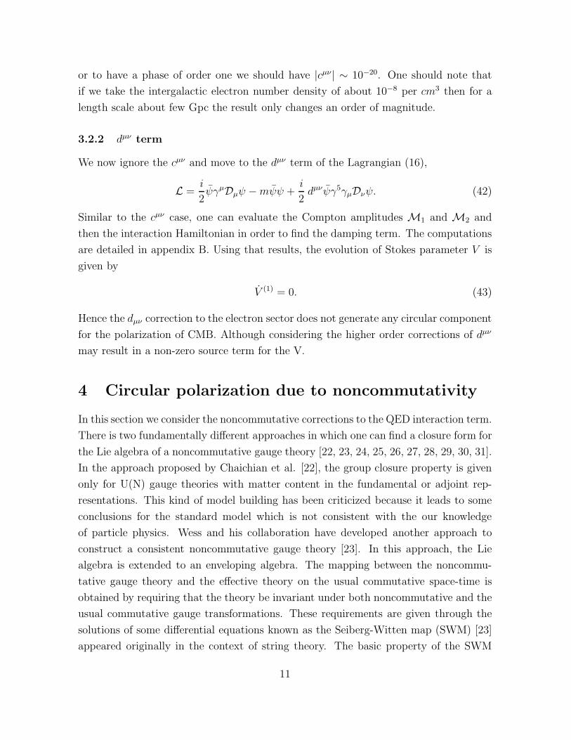
or to have a phase of order one we should have |cµν | ∼ 10−20. One should note that

if we take the intergalactic electron number density of about 10−8 per cm3 then for a

length scale about few Gpc the result only changes an order of magnitude.

3.2.2 dµν term

We now ignore the cµν and move to the dµν term of the Lagrangian (16),

L =i

2ψγµDµψ −mψψ +

i

2dµνψγ5γµDνψ. (42)

Similar to the cµν case, one can evaluate the Compton amplitudes M1 and M2 and

then the interaction Hamiltonian in order to find the damping term. The computations

are detailed in appendix B. Using that results, the evolution of Stokes parameter V is

given by

V (1) = 0. (43)

Hence the dµν correction to the electron sector does not generate any circular component

for the polarization of CMB. Although considering the higher order corrections of dµν

may result in a non-zero source term for the V.

4 Circular polarization due to noncommutativity

In this section we consider the noncommutative corrections to the QED interaction term.

There is two fundamentally different approaches in which one can find a closure form for

the Lie algebra of a noncommutative gauge theory [22, 23, 24, 25, 26, 27, 28, 29, 30, 31].

In the approach proposed by Chaichian et al. [22], the group closure property is given

only for U(N) gauge theories with matter content in the fundamental or adjoint rep-

resentations. This kind of model building has been criticized because it leads to some

conclusions for the standard model which is not consistent with the our knowledge

of particle physics. Wess and his collaboration have developed another approach to

construct a consistent noncommutative gauge theory [23]. In this approach, the Lie

algebra is extended to an enveloping algebra. The mapping between the noncommu-

tative gauge theory and the effective theory on the usual commutative space-time is

obtained by requiring that the theory be invariant under both noncommutative and the

usual commutative gauge transformations. These requirements are given through the

solutions of some differential equations known as the Seiberg-Witten map (SWM) [23]

appeared originally in the context of string theory. The basic property of the SWM

11

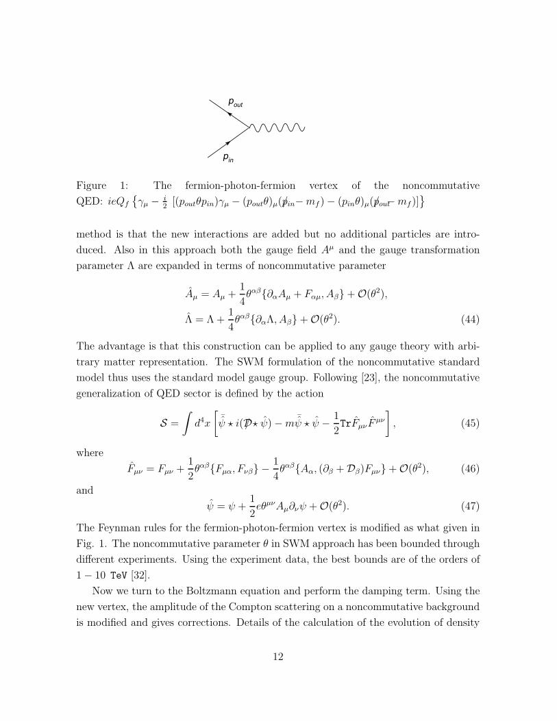
Figure 1: The fermion-photon-fermion vertex of the noncommutative

QED: ieQf

γµ − i2[(poutθpin)γµ − (poutθ)µ(pin/ −mf )− (pinθ)µ(pout/ −mf )]

method is that the new interactions are added but no additional particles are intro-

duced. Also in this approach both the gauge field Aµ and the gauge transformation

parameter Λ are expanded in terms of noncommutative parameter

Aµ = Aµ +1

4θαβ∂αAµ + Fαµ, Aβ+O(θ2),

Λ = Λ +1

4θαβ∂αΛ, Aβ+O(θ2). (44)

The advantage is that this construction can be applied to any gauge theory with arbi-

trary matter representation. The SWM formulation of the noncommutative standard

model thus uses the standard model gauge group. Following [23], the noncommutative

generalization of QED sector is defined by the action

S =

∫

d4x

[

¯ψ ⋆ i(D/ ⋆ ψ)−m

¯ψ ⋆ ψ − 1

2TrFµνF

µν

]

, (45)

where

Fµν = Fµν +1

2θαβFµα, Fνβ −

1

4θαβAα, (∂β +Dβ)Fµν+O(θ2), (46)

and

ψ = ψ +1

2eθµνAµ∂νψ +O(θ2). (47)

The Feynman rules for the fermion-photon-fermion vertex is modified as what given in

Fig. 1. The noncommutative parameter θ in SWM approach has been bounded through

different experiments. Using the experiment data, the best bounds are of the orders of

1− 10 TeV [32].

Now we turn to the Boltzmann equation and perform the damping term. Using the

new vertex, the amplitude of the Compton scattering on a noncommutative background

is modified and gives corrections. Details of the calculation of the evolution of density

12

matrix elements are presented in Appendix C. Quoting the results (94-95) and similar

to the previous section, the evolution of the Stokes parameter V is given as

V (1) = i(ρ12 − ρ21)

=ie2

2k0m

∫

dq ne(q)(

2(qθǫ1q · ǫ1 + qθǫ2q · ǫ2)(ρ12 − ρ21)− 2(qθǫ2q · ǫ1 + qθǫ1q · ǫ2)ρ11

+2(qθǫ2q · ǫ1 + qθǫ1q · ǫ2)ρ22)

, (48)

where it can be more simplified as follows

V (1) =ie2

k0m

∫

dq ne(q)(qθǫ2q · ǫ1 + qθǫ1q · ǫ2)Q(1). (49)

Hence similar to the Lorentz symmetry violating interaction terms discussed in the

previous section, the noncommutative quantum electrodynamics based on the SWM,

also can generate the circular polarization for the CMB radiation in the first order of

noncommutative parameter θ. Now (49) can be cast into

V (1) =ie2nem

Λ2NCk0

(v.θ.ǫ2v · ǫ1 + v.θ.ǫ1v · ǫ2)Q(1), (50)

where ΛNC is the value of the non-commutativity parameter and θ is unit vector that

shows the non-commutativity direction and is a constant. Therefore the Faraday phase

conversion for ΛNC ∼ 1 − 10 TeV will be around 10−7 − 10−9 radians for λ0 = 1cm,

z=1000 and for length scale about 1 kpc.

5 Circular polarization and magnetic field

When photons impinge electrons in the presence of a magnetic field, the circular po-

larization is generated naturally which leads to a non vanishing Stokes parameter V

whose magnitude depends upon the intensity of the radiation field [4, 5]. For instance,

If the magnetic field is considered of the order of B ∼ nG, the angular power spectra

for small values of l are derived as O(10−7)(µK)2 and O(10−15)(µK)2 for the V T and

V V components respectively [4, 5]. In these references, the electron-photon scattering is

computed by classical considerations. Here we want to investigate a similar phenomenon

by considering the Compton scattering of electrons and photons. A physical situation is

considered when prior to recombination a cold plasma of electrons is supplemented by a

weak magnetic field whose typical inhomogeneity scale is at least comparable to Hubble

radius H−1 at the corresponding epoch. In the epoch of recombination, magnetic field

13

is estimated to be about 10−3µG to 10−1µG [33]. This value of magnetic field is very

weak compared to the critical value Bc = m2e/e = 4.414× 1013G. For this reason during

our strategy, the effect of magnetic field on the electron wave functions is ignored and

only the electron propagators are corrected. The propagator of a Dirac particle in an

external constant electromagnetic field background is well known from Schwinger work

[34]

S(x, y) = Φ(x, y)

∫

d4p

(2π)4e−ip.(x−y)S(p), (51)

where the phase factor Φ(x, y) is defined by

Φ(x, y) = exp

(

−ie2xαBαβy

β

)

, (52)

in which Bα = −12Bαβx

β and Bαβ represents the strength background magnetic field

tensor. The other part of Schwinger propagator, S(p), can be expanded up to the linear

background field as

S(p) = S0(p) + SB(p) +O(B2), (53)

for which S0 is the usual electron propagator and SB is the linear modified part of the

Schwinger propagator given by [35]

SB(p) = −1

2eBαβ

γα(p/−m)γβ

(p2 −m2)2. (54)

Therefore invoking the above considerations, the Compton scattering matrix element

in the presence of background magnetic field is given by

M = M1 +M2, (55)

where

M1 = ur′(q′)

∫

d4xd4x′eix′.q′(−ieǫ/s′(p′)eix

′.p′)S(x′, x)(

−ieǫ/s(p)e−ix.p)

e−ix.qur(q), (56)

and

M2 = ur′(q′)

∫

d4xd4x′eix′.q′(

−ieǫ/s(p)e−ix′.p)

S(x′, x)(

−ieǫ/s′(p′)eix.p′

)

e−ix.qur(q),

(57)

where ur(q) and ur′(q′) respectively are the wave functions for the incoming electron

with spin index r and outgoing electron with spin index r′. Also ǫµs (p) and ǫµs′(p′)

are polarization vectors for incoming and outgoing photon chosen to be real and with

indexes s, s′ = 1, 2 labeling the physical transverse polarizations of photon. Using the

14

linear expanded Schwinger propagator (53) and by expanding the Φ(x, y) factor up to

order B, for the amplitude (56) one can write

M1= ur′(q′)

∫

d4xd4x′d4k

(2π)4eix

′.(q′+p′−k)e−ix.(q+p−k) (−ieǫ/s′(p′))

×(

S0(k) + SB(k)−ie

2x′αBαβx

βS0(k)

)

(−ieǫ/s(p))ur(q). (58)

Integrating over the first two terms of (58) gives

(2π)4δ4(q′+p′− q−p)ur′(q′) (−ieǫ/s′(p′)) (S0(q + p) + SB(q + p)) (−ieǫ/s(p)) ur(q). (59)

The remaining ie2x′αBαβx

βS0(k) term explicitly violates the four momentum conser-

vation. One can assume that during the interaction time a small momentum δqµ is

transferred from background into the internal electron of the associated Feynman di-

agram so that the momentum conservation will be preserved and takes the following

form

q′µ + p′µ = qµ + pµ + δqµ. (60)

Substituting the condition (60) into the last term of (58) and expand the exponential

factor yieldsie

2Bαβ

∫

d4xd4x′ei(x′−x).(q+p−k)x′αxβ(1 + ix′.δq). (61)

In the above expression, the term that is independent of δq is vanished because of anti-

symmetric properties of Bαβ with respect to α and β while the term that is dependent

on δq remains. From classical electrodynamics we know that the four-momentum of

electron that propagates between two space-time points, changes similar to the Lorentz

force ∆pµ = −eBµν∆xν . Then the magnitude of δqµ can be approximated to be of the

order of external background field δq ∼ eB. Therefore this term becomes of the order

of O(B2) and hence can be ignored in the scattering amplitude M1. With a similar

procedure, the amplitude M2 is given by

M2 = (2π)4δ4(q′+p′−q−p)ur′(q′) (−ieǫ/s(p)) (S0(q − p′) + SB(q − p′)) (−ieǫ/s′(p′))ur(q).(62)

The B-independent terms of M1 and M2 give the usual Compton scattering. The

correction up to the linear background field is represented as MB and is written as

MB = M1B +M2B

= (2π)4δ4(q′ + p′ − q − p)u(q′)[

(−ieǫ/s′(p′))SB(q + p) (−ieǫ/s(p))

+ (−ieǫ/s(p))SB(q − p′) (−ieǫ/s′(p′))]

ur(q). (63)

15

Using these amplitudes, the damping term on the right hand side of the Boltzmann

equation can be computed. Computing the damping term is detailed in appendix D.

By using these results the density matrix element and then the evolution of the Stokes

parameter V up to order of e4 is derived as

V (1)= i(ρ12 − ρ21)

=πe4

4m2k

∫

dqdpδ(k − p)

(

1

q.k− 1

q.p

)(

1

(q.k)2− 1

(q.p)2

)

(q.ǫ1(k)q.ǫ2(k)− q.ǫ2(k)q.ǫ1(k))

×ne(q)[

((q.ǫ1(p))2 + (q.ǫ2(p))

2)(I(1)(k)− I(1)(p))− (q.ǫ1(p)q.ǫ1(p)− q.ǫ2(p)q.ǫ2(p))Q(1)(p)

− 2q.ǫ1(p)q.ǫ2(p)U(1)(p)

]

+O(k, p), (64)

where qµ = −eBµνqν . Hence similar to the LIV interaction terms and the noncom-

mutativity, corrections due to the external magnetic field can generate the circular

polarization for the CMB radiation as well. But in contrast, it is not needed a prior

linear polarization to have a nonzero Stokes-V parameter that is in agreement with

references [4, 5]. But it should be noted that in [4, 5] the scattering matrix is classi-

cally obtained in the electron-ion magnetized plasma, while in our model the Compton

scattering is calculated by considering the correction on the electron propagator in an

external magnetic field. Here one can easily see that the circular polarization is linearly

proportional to the background magnetic field. Meanwhile if we integrate (64) over the

momentum p and use the approximation q0 ≃ m ≫ |q|, |k| then one can see that the

correction will be proportional to λ3 as follows

V (1) =e4mλ3

8π

∫

dΩ

4πne(v.(k− p))2(

eB

m2)F (v, p, ǫ1, ǫ2, I, U,Q,

Bµν

B), (65)

where F can be easily define by comparing (64) and (65). Here again one can estimate

the Faraday phase conversion for z = 1000 as

∆φFC ∼ 1 rad (B

10µG) (

λ01cm

) (ne

0.1cm3) (

L

1kpc). (66)

6 Discussion and Conclusion

In this work we have considered the evolution of the Stokes parameters in the context of a

general extension of quantum electrodynamics allowing for Lorentz violation (LVQED),

NCQED and in the presence of the background magnetic field. In fact all nonzero

backgrounds can potentially produce the circular polarization for the CMB radiation.

In the LVQED we have explored three cases, one case in the photon sector and two cases

16

in the electron sector. In the former one the induced circular polarization is provided

through the interaction of photon with the background Lorentz violation field, Eq.(30),

while in the latter cases the corrections on the Compton scattering in the LVQED

cause the polarization, see Eqs.(39) and (43). It is shown that the Stokes parameter

V in both sectors are linearly proportional to the dimensionless Lorentz parameters kF

and c that is in contrast with the result of [9] where the second term of Lagrangian

(17) is considered as the interaction term and it is found that V depends quadratically

on the kAF that is too small with respect to our result. We have also estimated the

Faraday phase conversion in the LV case to give an upper bound on the dimensionless

Lorentz parameters c and kF about 10−20 that is comparable to the current bounds on

these parameters. In the NCQED we have found the nonzero parameter V through a

correction on the Compton scattering in the NC space that is linearly proportional with

the parameter of non commutativity as given in (50). Our estimation on the Faraday

phase conversion is about 10−7 − 10−9 radians for ΛNC ∼ 1− 10TeV that is too small

to be detectable. Finally we have examined the Stokes parameter V for the background

magnetic field. In this case the refractive term is zero but the damping term has a

nonzero V parameter that depends linearly on the magnetic field, see Eq.(65). This

result can be compared with the result of [6] in which the circular polarization of CMB

due to the Faraday conversion depends quadratically on the background magnetic field.

Furthermore, in contrast with [6], all the other Stokes parameters (I, Q and U) have some

contributions on the generation of the Stokes-V parameter in the background magnetic

field. In fact it is not necessary a prior linear polarization to have a nonzero Stokes-V

parameter that is in agreement with references [4, 5]. By comparing our results together

we see a λ3-dependence for the magnetic field and LV on one hand and λ-dependence

for non-commutativity on the other hand which leads to different spectrum for different

wavelengths. Because the required sensitivity level to detect circular polarization of

CMB is beyond the current instrumental techniques, the experimental bound on the

V modes is rare. The bound reported in [36], constrains it as V ≤ 1 µK. However,

the post-Planck CMB polarization experiments are already under study [37]. Then it

is time to address the question whether CMB is circularly polarized or not and what

physical information can be extracted from its measurement. Also it seems that if a

new experimental device can be built with sufficient polarimetric sensitivity beyond

the µK range and with good control of systematic errors, the resulting observations

may have the potential to realize the physics at energy scales far beyond the reach of

the largest feasible particle accelerators and provide a window to new physics at these

energy scales. Therefore we encourage experimenters to make experiments in order to

17

measure the circular polarization of cosmic microwave radiation.

A The calculation of density matrix elements with

cµν coefficients

In this appendix at first the scattering amplitudes M1 andM2 are calculated as follows.

For the Lagrangian (16) with cµν term, the equation of motion for the electron ψ is found

as

(i6∂ −m+ i cνµγν∂µ)ψ = 0. (67)

for which the modified Dirac equation is written as

(6q −m+ cνµγνqµ) us(q) = 0, (68)

in which ψ = us(q) exp(−iq.x). In the Weyl chiral representation for the Dirac matrices,

after some straightforward calculations, one finds the following solution for the Dirac

equation (68)

us(q) =

( √q.σ + cνµqµσν ζs√q.σ + cνµqµσν ζs

)

, (69)

where σ = (1, ~σ) and σ = (1,−~σ). The electron propagator can be also calculated

straightforwardly with a correction in the denominator as

S(p) =i

q/−m + cνµqµγν. (70)

Since |cνµ| ≪ 1, the propagator can be expanded up to the linear order of cνµ as

S(q) = S0(q) + S0(q)(icνµqµγν)S0(q) + · · ·

=i

q/−m+

i

q/−m(icνµqµγν)

i

q/−m+ · · ·, (71)

where S0(q) is the usual electron propagator. The us(q) solutions can be also expanded

in terms of cνµ,

us(q) = u0(q) + u(q) + · · ·, (72)

where u0(q) ≡ us0(q) is the free electron solution for the usual Dirac equation in the

absence of cνµ term and u(q) ≡ us(q) is the correction of the cνµ order. The dots show

the higher order corrections. Consequently, the Compton scattering amplitude M is

18

modified with corrections given by

M = M1 +M2

= u(q′)(−ie) (γµ + cνµγν) ǫ∗s′

µ (p′)S(q + p)(−ie) (γρ + cνργν) ǫsρ(p)u(q)

+ u(q′)(−ie) (γρ + cνργν) ǫsρ(p)S(q − p′)(−ie) (γµ + cνµγν) ǫ

∗s′

µ (p′)u(q), (73)

where ǫ(p) and ǫ′(p′) are transverse polarization vectors for the external real photons.

The scattering amplitudes up to the order of cνµ are simplified as follows

M1 ≡ −e2u0(q′)γµǫ∗s′

µ (p′)S0(q + p)cνργνǫsρ + γµǫ∗s

′

µ (p′)S0(q + p)(

icνβqβγν)

×S0(q + p)γρǫsρ(p)c

νµγνǫ∗s′

µ (p′)S0(q + p)γρǫsρ(p)u0(q)−e2u(q′)γµǫ∗µ(p

′)S0(q + p)γρǫsρu(q), (74)

and

M2 ≡ −e2u0(q′)γρǫsρ(p)S0(q − p′)cνµγνǫ∗s′

µ (p′)γρǫsρ(p′)S0(q − p′)

(

icνβqβγν)

×S0(q − p′)γµǫ∗s

′

µ (p′) + cρνγνǫsρ(p)S0(q − p′)γµǫ∗s

′

µ (p′)u0(q)−e2u(q′)γρǫsρ(p)S0(q − p′)γµǫ∗s

′

µ u(q). (75)

Substituting these amplitudes in the Eq. (34) and using the expectation values computed

in [3] and using the photon polarization vector properties ǫi(k) · k = 0 and ǫi · ǫj = δij ,

it follows that

⟨[

Hint(t), Dij(k)]⟩

= e2(2π)3δ3(0)

∫

dqne(q) [δsiρs′j(k)− δs′jρsi(k)]

×(

(1

2k.q)cρνǫsρ(k)(q.kǫs

′

ν (k)− q.ǫ∗s′

kν) + cνµǫ∗s′

µ (k)(q.kǫsν(k)− q.ǫskν) +

cνβqβ(q.ǫsǫ∗s

′

ν + q.ǫ∗s′

ǫsν)+2cνβ

(q.k)2(qβqν + kβkν)(q.ǫ

sq.ǫ∗s′

))

, (76)

where the quantity ne(q) is the number density of electrons of momentum q per unit

volume. It is now straightforward to calculate the time derivative of the density matrix

which result in

ρ11(k) =e2

2mk0

∫

dq ne(q)[ cµν

q.k[(q.kǫ1µǫ2ν − kνq.ǫ

2ǫ1µ) + (q.kǫ1νǫ2µ − kνq.ǫ

1ǫ2µ)

+qν(q.ǫ1ǫ2µ + q.ǫ2ǫ1µ)ρ21 − (q.kǫ2µǫ1ν − kνq.ǫ

1ǫ2µ) + (q.kǫ1µǫ2ν − kνq.ǫ

2ǫ1µ)

+qν(q.ǫ2ǫ1µ + q.ǫ1ǫ2µ)ρ12] +

2cµν

(q.k)2[(qµqν + kµkν)q.ǫ

1q.ǫ2(ρ21 − ρ12)]]

, (77)

19

ρ22(k) =e2

2mk0

∫

dqne(q)[ cµν

q.k[(q.kǫ2µǫ1ν − kνq.ǫ

1ǫ2µ) + (q.kǫ2νǫ1µ − kνq.ǫ

2ǫ1µ)

+qν(q.ǫ2ǫ1µ + q.ǫ1ǫ2µ)ρ12 − (q.kǫ1µǫ2ν − kνq.ǫ

2ǫ1µ)

+(q.kǫ2µǫ1ν − kνq.ǫ

1ǫ2µ) + qν(q.ǫ1ǫ2µ + q.ǫ2ǫ1µ)ρ21]

+2cµν

(q.k)2(qµqν + kµkν)q.ǫ

1q.ǫ2(ρ12 − ρ21)]

, (78)

ρ12(k) =e2

2mk0

∫

dqne

[

(q)cµν

q.k[(q.kǫ1µǫ2ν − kνq.ǫ

2ǫ1µ) + (q.kǫ1νǫ2µ − kνq.ǫ

1ǫ2µ)

+qν(q.ǫ1ǫ2µ + q.ǫ2ǫ1µ)(ρ22 − ρ11) + q.k(ǫ1µǫ1ν − ǫ2µǫ

2ν)− kνq.ǫ

1ǫ1µ + kνq.ǫ2ǫ2µ

−ǫ2µǫ2ν)− (kνq.ǫ1ǫ1µ − kνq.ǫ

2ǫ2µ) + 2qν(q.ǫ1ǫ1µ − q.ǫ2ǫ2µ)ρ12]

+2cµν

(q.k)2(qµqν + kµkν)[q.ǫ

1q.ǫ2(ρ22 − ρ11) + ((q.ǫ1)2 − (q.ǫ2)2)ρ12]]

, (79)

and

ρ21(k) =e2

2mk0

∫

dqne

[

(q)cµν

q.k[(q.kǫ2µǫ1ν − kνq.ǫ

1ǫ2µ)

+(q.kǫ2νǫ1µ − kνq.ǫ

2ǫ1µ) + qµ(q.ǫ2ǫ1ν + q.ǫ1ǫ2ν)(ρ11 − ρ22)

+2q.k(ǫ2ρǫ2ν − ǫ1µǫ1ν)− 2(kνq.ǫ

2ǫ2µ − kνq.ǫ1ǫ1µ) + 2qν(q.ǫ

2ǫ2µ − q.ǫ1ǫ1µ)ρ21]

+2cµν

(q.k)2(qµqν + kµkν)[q.ǫ

1q.ǫ2(ρ11 − ρ22) + ((q.ǫ2)2 − (q.ǫ2)2)ρ21]]

. (80)

B The calculation of density matrix elements with

dµν coefficients

In this appendix we compute the density matrix elements with interaction given by

(42). The equation of motion for the Lagrangian (42) is calculated as

us(q) =

(

√

q.σ + (dνµqµσν) ζs√

q.σ − (dνµqµσν) ζs

)

, (81)

and the propagator changes as

S(q) =i

p/−m + dνµpµγ5γν. (82)

20

similar to the cµν case, one can write the following expansion for the propagator up to

the order O(dµν)

S(q) = S0(q) + S0(p)(idνµqµγ

5γν)S0(q)

≡ i

q/−m+

i

q/−m(idνµqµγ

5γν)i

q/−m. (83)

Then the Compton scattering matrix elements M1 andM2 in this theory are calculated

as

M= M1 +M2

= u(q′)(−ie)(

γµ + dνµγ5γν)

ǫ∗s′

µ (k′)S(q + p)(−ie)(

γρ + dνργ5γν)

ǫsρ(p)u(q)

+ u(q′)(−ie)(

γρ + dνργ5γν)

ǫsρ(k)S(q − p′)(−ie)(

γµ + dνµγ5γν)

ǫ∗s′

µ (pk′)u(q),(84)

where

M1≡ (−e2)u0(q′)γµǫ∗s′

µ (p′)S0(q + p)(

dνργ5γν)

ǫsρ

+γµǫ∗s′

µ (k′)S0(q + p)(

idνβqβγ5γν)

S0(q + p)γρǫsρ(p)

+dνµγ5γνǫ∗s′

µ (p′)S0(q + p)γρǫsρ(p)u0(q)−e2u(q′)γµǫ∗µ(p′)S0(q + p)γρǫsρu(q), (85)

and

M2 ≡ (−e2)u0(q′)γρǫsρ(p)S0(q − p′)(

dνµγ5γν)

ǫ∗s′

µ (p′) +

γρǫsρ(p′)S0(q − p′)

(

idνβqβγ5γν)

S0(q − p′)γµǫ∗s′

µ (p′) +

dνργ5γνǫsρ(p)S0(q − p′)γµǫ∗s

′

µ (p′)u0(q) +(−e2)u(q′)γρǫsρ(p)S0(q − p′)γµǫ∗s

′

µ u(q). (86)

Substituting these amplitudes in the Eq. (34), and using the expectation values calcu-

lated in [3], leads to

⟨[

Hint(t), Dij(k)]⟩

=e2

2m(2π)3δ3(0)

∫

dqne(q) [δisρs′j(k)− δjs′ρis(k)]

dνµ

(k.q)2(ǫ∗s

′

β ǫsσ − ǫ∗s′

σ ǫsβ)[(−2qαkρ(qµqν + kµkν)− 2qαqρ(qµkν + kµqν))

ǫαβρσ + (k2qαkµ − 2m2qµkα + 2(q.k)qαqµ)ǫαβ

νρ] +

2dνµ

q.kǫν

αβρ

[ǫ∗s′

µ qα(qβǫsρ − qρǫ

sβ)− ǫsµqα(qβǫ

∗s′

ρ − qρǫ∗s′

β )]− 4idνµ

q.kǫαβρνqµqβǫ

∗s′

α ǫsρ

, (87)

21

where ǫαβσρ is the Levi-Civita symbol appeared through tracing process when γ5 is

present. Similar to the cµν case, the time evolution of the ρ12 and ρ21 are obtained as

ρ12(k) =e2

2mk0

∫

dqne(q)

ρ12

[4idνµ

q.kǫαβρνqµqβ(ǫ

1αǫ

1ρ − ǫ2αǫ

2ρ)] + (ρ22 − ρ11)

[dνµ

(q.k)2(ǫ2βǫ

1σ − ǫ2σǫ

1β)[(−2qαkρ(qµqν + kµkν)− 2qαqρ(qµkν + kµqν))ǫ

αβρσ

+(k2qαkµ − 2m2qµkα + 2(q.k)qαqµ)ǫαβ

νρ] +

2dνµ

q.kǫαβρν

[qαqρ(ǫ2µǫ

1β − ǫ1µǫ

2β) + qαqβ(ǫ

1µǫ

2ρ − ǫ2µǫ

1ρ) + 2iqµqβǫ

2αǫ

1ρ]]

, (88)

and

ρ21(k) =e2

2mk0

∫

dqne(q)q0

− ρ21

[4idνµ

q.kǫαβρνqµqβ(ǫ

1αǫ

1ρ − ǫ2αǫ

2ρ)] + (ρ11 − ρ22)

[dνµ

(q.k)2(ǫ1βǫ

2σ − ǫ1σǫ

2β)[(−2qαkρ(qµqν + kµkν)− 2qαqρ(qµkν + kµqν))ǫ

αβρσ

+(k2qαkµ − 2m2qµkα + 2(q.k)qαqµ)ǫαβ

νρ] +

2dνµ

q.kǫαβρν

[qαqρ(ǫ1µǫ

2β − ǫ2µǫ

1β) + qαqβ(ǫ

2µǫ

1ρ − ǫ1µǫ

2ρ) + 2iqµqβǫ

1αǫ

2ρ]]

. (89)

C The calculation of density matrix elements for

noncommutative theory

The density matrix elements for the noncommutative theory are calculated in this ap-

pendix. In the Boltzmann equation (13), the commutator [Hint(0),D0ij] has the form

[Hint(0),Dij(k)] =

∫

dqdq′dpdp′(2π)3δ3(q′ + p′ − q− p)(Mθ1 +Mθ

2 +Mθ3 +Mθ

4)

×[b†r′(q′)br(q1)a

†s′(p

′)aj(k)2p′0(2π)3δisδ

3(p− k)

−b†r′(q′)br(q)a†i (k)as(p)2p

′0(2π)3δjs′δ3(p′ − k)], (90)

where Mθi are the noncommutative parameter dependent parts of the amplitudes of the

diagrams shown in Fig. 2. In this figure the box shows vertex in the noncommutative

22

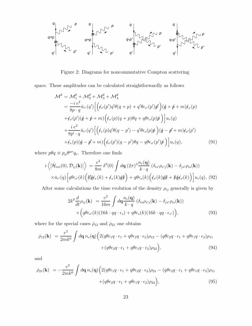
Figure 2: Diagrams for noncommutative Compton scattering

space. These amplitudes can be calculated straightforwardly as follows

Mθ = Mθ1 +Mθ

2 +Mθ3 +Mθ

4

=−i e28p · q ur′(q

′)[(

ǫs′/ (p′)q′θ(q + p) + q′θǫs′(p′)p′/)

(q/+ p/+m)ǫs/ (p)

+ǫs′/ (p′)(q/+ p/+m)(

ǫs/ (p)(q + p)θq + qθǫs(p)p/)]

ur(q)

+i e2

8p′ · q ur′(q′)[(

ǫs/ (p)q′θ(q − p′)− q′θǫs(p)p/)

(q/− p′/+m)ǫs′/ (p′)

+ǫs/ (p)(q/− p′/+m)(

ǫs′/ (p′)(q − p′)θq − qθǫs′(p′)p/)]

ur(q), (91)

where pθq ≡ pµθµνqν . Therefore one finds

i⟨

[Hint(0),Dij(k)]⟩

=e2

8mδ3(0)

∫

dq (2π)3ne(q)

k · q (δis′ρs′j(k)− δjs′ρis(k))

×ur′(q)[

qθǫs′(k)(

k′/q/ǫs/ (k) + ǫs/ (k)q/k/)

+ qθǫs(k)(

ǫs′/ (k)q/k/+ k/q/ǫs′/ (k))]

ur(q), (92)

After some calculations the time evolution of the density ρij generally is given by

2k0d

dtρij(k) =

e2

16m

∫

dqne(q)

k · q (δisρs′j(k)− δjs′ρis(k))

×(

qθǫs′(k)(16k · qq · ǫs) + qθǫs(k)(16k · qq · ǫs′))

, (93)

where for the special cases ρ12 and ρ21 one obtains

ρ12(k) =e2

2mk0

∫

dq ne(q)(

2(qθǫ1q · ǫ1 + qθǫ2q · ǫ2)ρ12 − (qθǫ2q · ǫ1 + qθǫ1q · ǫ2)ρ11

+(qθǫ2q · ǫ1 + qθǫ1q · ǫ2)ρ22)

, (94)

and

ρ21(k) = − e2

2mk0

∫

dq ne(q)(

2(qθǫ1q · ǫ1 + qθǫ2q · ǫ2)ρ21 − (qθǫ2q · ǫ1 + qθǫ1q · ǫ2)ρ11

+(qθǫ2q · ǫ1 + qθǫ1q · ǫ2)ρ22)

, (95)

23

D The calculation of density matrix elements for

magnetic field background

In this appendix we calculate the density matrix elements in the presence of a back-

ground magnetic field. Vanishing of the refractive term on the right hand side of (13)

forces us to go to the next order and calculate the damping term of the Boltzmann

equation (13). As it has been clarified in [3], using the expectation values of creation

and annihilation operators calculated in this reference, the damping term can be written

in terms of amplitudes in the following form

1

2

∫ ∞

−∞

dt′〈[Hint(t′), [Hint(0),Dij(k)]]〉

=1

4(2π)3δ3(0)

∫

dqdpdq′M(q′r′, ps′1, qr, ks1)M(qr, ks′2, q′r′, ps2)

×(2π)4δ4(q′ + p− q − k)[ne(q)δs2s′1(δis1ρs′2j(k) + δjs′2ρis1(k))

−2ne(q′)δis1δjs′2ρs′1s2(p)]. (96)

Up to the linear order of Bαβ , the evaluating of the product of matrix elements yields

M(q′r′, ps′1, qr, ks1)×M(qr, ks′2, q′r′, ps2) |B-term

= − e4

4m2

(

tr(q′/+m)[ǫ/s′1(p)S0(q + k)ǫ/s1(k) + ǫ/s1(k)S0(q − p)ǫ/s′

1(p)](q/+m)

×[ǫ/s′2(k)SB(q

′ + p)ǫ/s2(p) + ǫ/s2(p)SB(q′ − k)ǫ/s′

2(k)]+ tr(q′/ +m)

×[ǫ/s′1(p)SB(q + k)ǫ/s1(k) + ǫ/s1(k)SB(q − p)ǫ/s′

1(p)](q/+m)[ǫ/s′

2(k)S0(q

′ + p)ǫ/s2(p)

+ ǫ/s2(p)S0(q′ − k)ǫ/s′

2(k)]

)

, (97)

where the B-term shows the terms that are linear in terms of the background magnetic

field. For relevant cosmological situations one can consider the cold plasma of electrons

and photons that their kinetic energies are small compared to the electron mass i.e.

p, k and q ≪ m. As mentioned in [3], if the electron and photon temperatures are

comparable which means p, k ≪ q, then various functions in (96) can be expanded in

terms of p/q and q/m. Hence by computing the traces in (97), for the leading order,

24

the matrix element is simplified as

M(q′r′, ps′1, qr, ks1)×M(qr, ks′2, q′r′, ps2) |B-term

=ie4

2m2

(

1

q.k− 1

q.p

)(

1

(q.k)2− 1

(q.p)2

)

×[

q.ǫs2(p)q.ǫs1(k)q.ǫs′1(p)q.ǫs′2(k)− q.ǫs′2(k)q.ǫs2(p)q.ǫs1(k)q.ǫs′1(p)

+q.ǫs1(k)q.ǫs′1(p)q.ǫs2(p)q.ǫs′2(k)− q.ǫs′1(p)q.ǫs1(k)q.ǫs2(p)q.ǫs′2(k)

+O(k, p)]

, (98)

where qµ = −eBµνqν . Now by substituting (98) in (96) and integrating over the q′,

gives functions such as ne(q+ (k− p)) and δ(k − p+E(q)−E(q+ k− p)) where can

be expanded as follows

ne(q + (k− p)) ∼ ne(q)

[

1− (k− p).(q−mv)

mTe− (k− p)2

2mTe+ · · ·

]

, (99)

and

δ(k − p + E(q)−E(q + k− p)) ∼ δ(k − p) +(k− p).q

m

∂δ(k − p)

∂p+ · · · . (100)

Inserting the above equations into the (96) leads to the density matrix ρ12 and ρ21.

References

[1] M. Zaldarriaga and U. Seljak, “An All-Sky Analysis of Polarization in the Mi-

crowave Background,” Phys. Rev. D 55, 1830 (1997) [astro-ph/9609170].

[2] W. Hu and M. J. White, “A CMB Polarization Primer,” New Astron. 2, 323 (1997)

[arXiv:astro-ph/9706147].

[3] A. Kosowsky, “Cosmic microwave background polarization,” Annals Phys. 246, 49

(1996) [arXiv:astro-ph/9501045].

[4] M. Giovannini, “Circular dichroism, magnetic knots and the spectropolarimetry of

the Cosmic Microwave Background,” 0909.4699 [astro-ph.CO].

[5] M. Giovannini, “The V-mode polarization of the Cosmic Microwave Background,”

0909.3629 [astro-ph.CO].

[6] A. Cooray, A. Melchiorri and J. Silk, “Is the Cosmic Microwave Background Cir-

cularly Polarized?,” Phys. Lett. B 554, 1 (2003) [arXiv:astro-ph/0205214].

25

[7] A. G. Pacholczyk, Mon. Not. R. Astron. Soc. 163, 29 (1973); M. Kennett and D.

Melrose, Publ. Astron. Soc. Aust. 15, 211 (1998).

[8] T. W. Jones and S. L. O?Dell, Astrophys. J. 214, 522 (1977); M. Ruszkowski and

M. C. Begelman, [astro-ph/0112090 (2001)].

[9] S. Alexander, J. Ochoa and A. Kosowsky, “Generation of Circular Polarization of

the Cosmic Microwave Background,” arXiv:0810.2355 [astro-ph].

[10] F. Finelli and M. Galaverni, “Rotation of Linear Polarization Plane and Circular

Polarization from Cosmological Pseudo-Scalar Fields,” arXiv:0802.4210 [astro-ph].

[11] N. Agarwal, P. Jain, D. W. McKay and J. P. Ralston, “Signatures of Pseu-

doscalar Photon Mixing in CMB Radiation,” Phys. Rev. D 78, 085028 (2008)

[arXiv:0807.4587 [hep-ph]].

[12] S. Coleman and S. Glashow, Phys. Rev. D 59 (1999) 116008.

[13] D. Colladay and V. A. Kostelecky, “Lorentz-violating extension of the standard

model,” Phys. Rev. D 58, 116002 (1998) [arXiv:hep-ph/9809521].

[14] R. Jackiw and V. A. Kostelecky, “Radiatively induced Lorentz and CPT violation

in electrodynamics,” Phys. Rev. Lett. 82, 3572 (1999) [arXiv:hep-ph/9901358].

[15] V. A. Kostelecky and M. Mewes, “Cosmological constraints on Lorentz violation

in electrodynamics,” Phys. Rev. Lett. 87, 251304 (2001) [arXiv:hep-ph/0111026].

[16] V. A. Kostelecky and M. Mewes, “Signals for Lorentz violation in electrodynamics,”

Phys. Rev. D 66, 056005 (2002) [arXiv:hep-ph/0205211].

[17] V. A. Kostelecky and M. Mewes, “Lorentz-violating electrodynamics and the

cosmic microwave background,” Phys. Rev. Lett. 99, 011601 (2007) [astro-

ph/0702379].

[18] V. A. Kostelecky and N. Russell, “Data Tables for Lorentz and CPT Violation,”

arXiv:0801.0287 [hep-ph].

[19] F. A. Schaposnik, “Three lectures on noncommutative field theories,” arXiv:hep-

th/0408132; R. J. Szabo, “Quantum Gravity, Field Theory and Signatures of Non-

commutative Spacetime,” arXiv:0906.2913 [hep-th].

26

[20] M. Giovannini, “Primordial magnetic fields,” [arXiv:hep-ph/0208152]; M. Giovan-

nini and K. E. Kunze, “Faraday rotation, stochastic magnetic fields and CMB

maps” Phys. Rev. D 78, 023010 (2008) arXiv:0804.3380 [astro-ph]; M. Giovannini

and K. E. Kunze, “Birefringence, CMB polarization and magnetized B-mode,”

Phys. Rev. D 79, 087301 (2009) arXiv:0812.2804 [astro-ph]; M. Giovannini, “Pa-

rameter dependence of magnetized CMB observables,” Phys. Rev. D 79, 103007

(2009) arXiv:0903.5164 [astro-ph.CO]; A. Mack, T. Kahniashvili and A. Kosowsky,

“Vector and Tensor Microwave Background Signatures of a Primordial Stochastic

Magnetic Field,” Phys. Rev. D 65, 123004 (2002) [arXiv:astro-ph/0105504].

[21] S. Dodelson, Modern Cosmology, Academic Press, Amsterdam, 2003.

[22] M. Chaichian, P. Presnajder, M. M. Sheikh-Jabbari and A. Tureanu, Noncommu-

tative Standard Model: Model Building, Eur. Phys. J. C 29, 413 (2003) [arXiv:hep-

th/0107055].

[23] X. Calmet, B. Jurco, P. Schupp, J. Wess and M. Wohlgenannt, The standard

model on non-commutative space-time, Eur. Phys. J. C 23, 363 (2002) [arXiv:hep-

ph/0111115].

[24] B. Melic, K. Passek-Kumericki, J. Trampetic, P. Schupp and M. Wohlgenannt,

“The standard model on non-commutative space-time: Electroweak currents and

Higgs sector,” Eur. Phys. J. C 42, 483 (2005) [arXiv:hep-ph/0502249].

[25] B. Melic, K. Passek-Kumericki, J. Trampetic, P. Schupp and M. Wohlgenannt,

“The standard model on non-commutative space-time: Electroweak currents and

iggs sector,” Eur. Phys. J. C 42, 483 (2005) [arXiv:hep-ph/0502249].

[26] X. Calmet, B. Jurco, P. Schupp, J. Wess and M. Wohlgenannt, “The standard

model on non-commutative space-time,” Eur. Phys. J. C 23, 363 (2002) [arXiv:hep-

ph/0111115].

[27] P. Aschieri, B. Jurco, P. Schupp and J. Wess, “Non-commutative GUTs, standard

model and C, P, T,” Nucl. Phys. B 651, 45 (2003) [arXiv:hep-th/0205214].

[28] J. Madore, S. Schraml, P. Schupp and J. Wess, Gauge theory on noncommutative

spaces, Eur. Phys. J. C 16, 161 (2000) [arXiv:hep-th/0001203].

[29] B. Jurco, S. Schraml, P. Schupp and J. Wess, Enveloping algebra valued gauge

transformations for non-Abelian gauge groups on non-commutative spaces, Eur.

Phys. J. C 17, 521 (2000) [arXiv:hep-th/0006246].

27

[30] B. Jurco, L. Moller, S. Schraml, P. Schupp and J. Wess, Construction of non-

Abelian gauge theories on noncommutative spaces, Eur. Phys. J. C 21, 383 (2001)

[arXiv:hep-th/0104153].

[31] B. Melic, K. Passek-Kumericki, J. Trampetic, P. Schupp and M. Wohlgenannt, The

standard model on non-commutative space-time: Electroweak currents and Higgs

sector, Eur. Phys. J. C 42, 483 (2005) [arXiv:hep-ph/0502249].

[32] M. Haghighat, “Bounds on the Parameter of Noncommutativity from Super-

nova SN1987A,” Phys. Rev. D 79, 025011 (2009) arXiv:0901.1069 [hep-ph]. ;

M. Haghighat, M. M. Ettefaghi and M. Zeinali, “Photon neutrino scattering in non-

commutative space,” Phys. Rev. D 73, 013007 (2006) [hep-ph/0511042]; M. M. Et-

tefaghi and M. Haghighat, “Massive Neutrino in Non-commutative Space-time,”

Phys. Rev. D 77, 056009 (2008) 0712.4034 [hep-ph].

[33] A. Kosowsky, A. Loeb, “Faraday rotation of microwave background polarization by

a primordial magnetic field,”Astrophys.J.469 (1996) 1, [arXiv:astro-ph/9601055];

J. A. Adams, U. H. Danielsson, D. Grasso and H. Rubinstein, “Distortion of the

acoustic peaks in the CMBR due to a primordial magnetic field,” Phys. Lett. B

388, 253 (1996) [arXiv:astro-ph/9607043].

[34] J. S. Schwinger, Phys. Rev. 82, 664 (1951).

[35] J. F. Nieves and P. B. Pal, “Perturbative vs Schwinger-propagator method for the

calculation of amplitudes in a magnetic field,” Phys. Rev. D 73, 105003 (2006)

[arXiv:hep-ph/0603024].

[36] R. B. Partridge, Jean Nowakowski H. M. Martin “Linear polarized fluctuations in

the cosmic microwave background” Nature 331, 146 (1988).

[37] D. Baumann et al. [CMBPol Study Team Collaboration], “CMBPol Mission Con-

cept Study: Probing Inflation with CMB Polarization”, AIP Conf. Proc. 1141, 10

(2009) 0811.3919 [astro-ph].

28