arX

iv:0

708.

3786

v3 [

astr

o-ph

] 4

Oct

200

7

C

Temperature and polarization CMB maps from primordial non-Gaussianities of the

local type

Michele Liguori1, Amit Yadav2, Frode K. Hansen3, Eiichiro Komatsu4, Sabino Matarrese5, Benjamin Wandelt21Department of Applied Mathematics and Theoretical Physics,

Centre for Mathematical Sciences, University of Cambridge,

Wilberfoce Road, Cambridge, CB3 0WA, United Kingdom2Department of Astronomy, University of Illinois at Urbana-Champaign, 1002 W. Green Street, Urbana, IL 61801

3Institute of Theoretical Astrophysics, University of Oslo, P.O. Box 1029 Blindern, 0315 Oslo, Norway4Department of Astronomy, University of Texas at Austin, 2511 Speedway, RLM 15.30 6, TX 78712 and

5Dipartimento di Fisica “G. Galilei”, Universita di Padova and INFN,

Sezione di Padova, via Marzolo 8, I-35131, Padova, Italy

(Dated: January 15, 2014)

The forthcoming Planck experiment will provide high sensitivity polarization measurements thatwill allow us to further tighten the fNL bounds from the temperature data. Monte Carlo simulationsof non-Gaussian CMB maps have been used as a fundamental tool to characterize non-Gaussiansignatures in the data, as they allow us to calibrate any statistical estimators and understand theeffect of systematics, foregrounds and other contaminants. We describe an algorithm to generatehigh-angular resolution simulations of non-Gaussian CMB maps in temperature and polarization.We consider non-Gaussianities of the local type, for which the level of non-Gaussianity is definedby the dimensionless parameter, fNL. We then apply the temperature and polarization fast cubicstatistics recently developed by Yadav et al. to a set of non-Gaussian temperature and polarizationsimulations. We compare our results to theoretical expectations based on a Fisher matrix analysis,test the unbiasedness of the estimator, and study the dependence of the error bars on fNL. All ourresults are in very good agreement with theoretical predictions, thus confirming the reliability ofboth the simulation algorithm and the fast cubic temperature and polarization estimator.

I. INTRODUCTION

Small, but non-vanishing non-Gaussianity of primordial cosmological perturbations is a general prediction of in-flation. The amplitude of the expected non-Gaussian signal is model-dependent and can vary by many orders ofmagnitude from one inflationary scenario to another. For example, the non-Gaussian signatures produced by single-field slow-roll inflation models are tiny and far below the present and forthcoming experimental sensitivity [1, 2]. Onthe other hand many other scenarios predict a level of non-Gaussianity that is within reach of present and forthcomingexperiments like WMAP and Planck (see e.g. [3, 4, 5, 6, 7, 8, 9, 10]). For this reason an experimental detection ofnon-Gaussianity would rule out the simplest scenarios of slow-roll inflation. More in general, experimental bounds onprimordial non-Gaussianity allow us to significantly constrain different scenarios for the generation of perturbationsin the context of primordial inflation.

Primordial non-Gaussianity from inflation can be described in terms of the 3-point correlation function of thecurvature perturbations, Φ(k), in Fourier space:

〈Φ(k1)Φ(k2)Φ(k3)〉 = (2π)3δ(3)(k1 + k2 + k3)F (k1, k2, k3) . (1)

Note that Φ is the curvature perturbation during the matter era, and temperature anisotropy in the Sachs-Wolfelimit is given by ∆T/T = −Φ/3. Depending on the shape of the function F (k1, k2, k3), we can divide non-Gaussianityfrom inflation into two different classes: local non-Gaussianity, where F is large for squeezed configurations (i.e.configurations in which k1 << k2, k3), and non-local non-Gaussianity of the equilateral type, where the largestcontributions come from modes with k1 ∼ k2 ∼ k3. The former kind of non-Gaussianity can be produced in modelswhere primordial perturbations are not generated by inflaton itself but by a second light scalar field (like e.g. inthe curvaton model). The latter comes from single field models with a non-minimal Lagrangian containing higherderivative operators. In this paper we will focus on non-Gaussianity of the local type, where the primordial curvatureperturbation Φ can be described in terms of the following real space parameterization:

Φ(x) = ΦL(x) + fNL

(

Φ2L(x) − 〈Φ2

L(x)〉)

. (2)

2

In the last formula fNL is a parameter that defines the amplitude of the primordial non-Gaussian signal. Ourprevious statement about the detectability of non-Gaussian signatures from inflation can be precisely quantified interms of this parameter. In standard scenarios of single-field slow roll inflation fNL is generally predicted to be verysmall and undetectable (∼ 10−2 at the end of inflation, ∼ 1 when second order perturbation theory after inflation istaken into account) whereas other scenarios, like the curvaton or variable decay width models, can naturally give riseto relatively large values of fNL (fNL ∼ 10). This justifies the claim that an experimental detection of fNL would ruleout the simplest single-field inflationary paradigm and allow us to put significant constraints on the other inflationaryscenarios.

The best way to put experimental bounds on fNL is to look for non-Gaussianities in CMB anisotropies (but ithas been recently pointed out that future deep galaxy-surveys and 21 cm background measurements could providepromising results [11, 12, 13]). The most stringent constraints on fNL so far come from measurements of the CMBangular bispectrum on the WMAP temperature data −36 < fNL < 100 (95% c.l.) [14, 15, 16]. This constraintcorresponds to a 1 − σ error of ∆fNL = 34. A Fisher matrix analysis by the authors of [17] showed that WMAPwill in principle be able to reach ∆fNL = 20, while the forthcoming Planck satellite can achieve ∆fNL = 5. Thismeans that Planck will be sensitive to the level of non-Gaussianity predicted by a vast range of different inflationarymodels. We can improve this constraint further by including the polarization data. For WMAP all the non-Gaussianinformation is basically contained in the temperature data, due to large errors in polarization measurements. Planck,on the other hand, will characterize polarization fluctuations with high accuracy. This will allow us to exploit theadditional information contained in polarization data and to gain a further factor of order 2 in ∆fNL, thus yielding∆fNL ≃ 3 [18]. A crucial step in order to exploit all the information contained in the future Planck dataset is then toextend the tools previously developed for temperature non-Gaussianity in order to include polarization. This programhas been recently started by the authors of [19], where the fast cubic statistic used to analyze WMAP temperaturedata [20, 21] was taken as a starting point to build an optimal cubic estimator that is sensitive to a combination oftemperature and polarization primordial fluctuations. In this paper we will extend the non-Gaussian analysis toolkitin order to include the second fundamental element: Monte Carlo simulations of primordial non-Gaussian polarizedCMB maps.

In section II we will summarize the original algorithm and describe its extension to polarization. We will thenapply the fast cubic statistic of [19] to a set of polarized non-Gaussian maps. In this paper we will manly focus ourattention on map generation, so the purpose for applying the estimator is mainly to check the reliability of the finalmaps. This will be done by comparing the final outputs to theoretical predictions in ideal conditions. However in aforthcoming publication we will describe how we actually used the maps in order to test, calibrate and optimize theestimator.

II. GENERATION OF POLARIZED NON-GAUSSIAN CMB MAPS

Realistic simulations of non-Gaussian CMB maps are indispensable tools for measurements of non-Gaussian signalsin the data, as they allow us to test and calibrate estimators and also to include and study all the spurious non-Gaussian signals introduced by contaminants like foregrounds, secondary anisotropies, instrumental noise and soon.

The first simulations of temperature maps with primordial non-Gaussianity from fNL were carried out by Komatsuet al., and used extensively to study Gaussianity of the WMAP data [14] as well as non-trivial topology of the universe[22]. Then, Liguori et al.[23] have succeeded in increasing the computational speed, reducing the memory requirementand, most importantly, improving accuracy of the simulated temperature maps. We take this new algorithm developedin [23] as a starting point.

Our starting point is the relation between the primordial curvature perturbation Φ and the CMB multipoles aXℓm

via radiation transfer functions ∆Xℓ .

aXℓm =

∫

d3k

(2π)3Φ(k)Yℓm(k)∆X

ℓ (k) , (3)

where X refers to either the temperature component T or the polarization component E.The kind of non-Gaussianity we are considering has a very simple form in real space, where it is local and the

non-Gaussian part of the curvature perturbation is simply the square of the Gaussian part (see formula 2). For thisreason it is convenient to work in real space and define the real space transfer functions ∆ℓ(r) as:

∆Xℓ (r) ≡

2

π

∫

dkk2jℓ(kr)∆Xℓ (k) , (4)

3

FIG. 1: CMB angular power spectra extracted from 10 simulations (triangles) are compared to the theoretical ones computedwith CMBfast for the same model (solid black lines) . The cosmological parameters are Ωb = 0.042, Ωcdm = 0.239, ΩL = 0.719,h = 0.73 n = 1, and τ = 0.09 (same for all the following figures, unless otherwise stated).

where jℓ(kr) is the spherical Bessel function of order ℓ. It can be shown that ∆ℓ(r) links the primordial curvatureperturbation Φ(r) in real space to the aX

ℓm through the following relation [14, 23]

aXℓm =

∫

drr2∆Xℓ (r)Φℓm(r) . (5)

In this last formula we have introduced the quantities Φℓm(r), which represent the spherical harmonic expansionmultipoles of the curvature perturbation Φ(r, r) on a shell of given radius r. In formulae:

Φℓm(r) =

∫

dΩrYℓm(r)Φ(r, r) . (6)

We define the radius r as r = c(τ0 − τ), where c is the speed of light and τ0 − τ is the lookback conformal time.The radius r varies from the origin r = 0 to the present time cosmic horizon r = cτ0. The radii in which Φℓm(r) mustbe generated depend on the features of the real space transfer function ∆X

ℓ (r) in equation (5). We will come back tothis shortly.

4

l = 20

l = 200

l = 500

l = 1000

l = 20

l = 200

l = 500

l = 1000

FIG. 2: Temperature (bottom panel) and polarization (upper panel) transfer functions at high ℓ at last scattering.

Let us assume for the moment that we have been able to numerically generate the Gaussian part of the curvatureperturbation multipoles ΦL

ℓm(r) for the chosen set of radii. Starting from here we can now generate the non-Gaussianpart ΦNL

ℓm (r) in the following way. First of all we harmonic transform ΦLℓm(r) to get the gaussian part of the curvature

perturbation in real space:

ΦL(r, r) =∑

ℓ

∑

m

ΦLℓm(r)Yℓm(r) . (7)

Then we square ΦL(r, r) to get the non Gaussian part of the curvature perturbation on each sampled spherical shell:ΦNL(r, r) ≡ Φ2

L(r, r) − 〈Φ2L(r, r)〉. We then calculate the multipoles of this non-Gaussian part through a backward

harmonic transform:

ΦNLℓm(r) ≡

∫

dΩrΦNL(r, r)Yℓm(r) . (8)

Having computed ΦLℓm(r) and ΦNL

ℓm (r) we can finally obtain the Gaussian and non-Gaussian part of the CMB

multipoles, aX,Lℓm and aX,NL

ℓm respectively, by applying formula (5):

aX,Lℓm =

∫

drr2∆Xℓ (r)ΦL

ℓm(r) (9)

aX,NLℓm =

∫

drr2∆Xℓ (r)ΦNL

ℓm(r) . (10)

5

l = 2 l = 5 l = 10

l = 2

l = 5

l = 10

FIG. 3: Temperature (bottom panel) and polarization (upper panel) transfer functions at low ℓ (reionization and late ISWcontributions are visible). The oscillations visible in the plots are little numerical artifacts which have negligible impact onthe final results. We have explicitly checked this by increasing the resolution in the k and r-grid by factors of 2 and 4 withoutnoticing any improvement in the accuracy of the final Cℓ, that can be already reconstructed well using the sampling chosen inthe paper (see fig. 1)

A CMB map for a chosen value of fNL can then be obtained simply by summing aX,Lℓm + fNLaX,NL

ℓm . This means

that with a single generation of aXℓm and aX,NL

ℓm it is possible to generate maps for any value of fNL.We are still left with one problem unsolved i.e. how do we generate the Gaussian curvature perturbation multipoles

ΦLℓm(r) ? This issue is complicated by the fact that curvature perturbation multipoles are correlated in real space.

The obvious solution would be to generate curvature perturbations in Fourier space, Φ(k), Fourier transform backto real space to obtain Φ(x), change the coordinates from Cartesian to polar to obtain Φ(r, n), and finally harmonictransform to obtain Φℓm(r). This is the original approach taken by [14], which is computationally quite expensive.Also, the coordinate transformation from Cartesian to polar limits accuracy of the maps, especially at high multipoles.

A novel approach developed in [23] solves this issue by generating Φℓm(r) directly, without ever worrying about thecoordinate transformation. It has been shown in [23] that the Φℓm(k) and Φℓm(r) are related by a spherical Besseltransform:

Φℓm(r) =(−i)ℓ

2π

∫

dkk2jℓ(kr)Φℓm(k) . (11)

The problem with this expression is that the Bessel functions oscillate very rapidly. This implies that, for each(ℓ, r), the integral above must be sampled in many different k in order to attain sufficient accuracy, thus making thecomputational cost of such an algorithm prohibitive. A much more convenient solution was found in [23]; the idea isto start with a set of Gaussian independent “white noise” coefficients nℓm(r) characterized by the following correlationfunction:

6

l = 20

l = 200

l = 500

l = 1000

FIG. 4: Temperature transfer functions at high ℓ and r corresponding to the epoch of reionization. Polarization transferfunctions at large ℓ are zero in this range.

⟨

nℓ1m1(r1)n

∗

ℓ2m2(r2)

⟩

=δD(r1 − r2)

r2δℓ2ℓ1

δm2

m1; (12)

it can be now shown that Gaussian curvature perturbation multipoles ΦLℓm(r) with the right correlation properties

can be obtained through a convolution of the nℓm coefficients with suitable “filters” Wℓ:

ΦLℓm(r) =

∫

dr1 r21 nℓm(r1)Wℓ(r, r1) , (13)

where the functions Wℓ are defined as

Wℓ(r, r1) =2

π

∫

dk k2√

PΦ(k) jℓ(kr)jℓ(kr1) , (14)

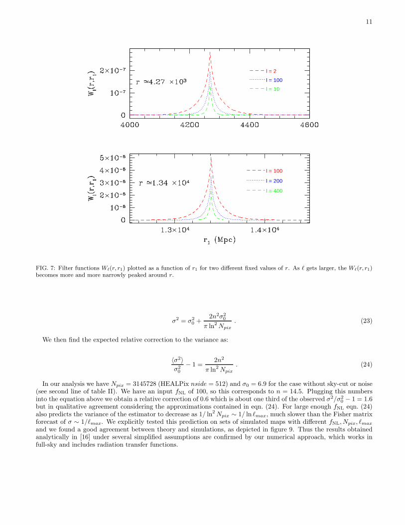
and PΦ(k) is the power spectrum of the primordial curvature perturbation ΦL(k). As depicted in Fig. 6, 7 thefilter functions Wℓ are smooth. Moreover, as also suggested by the Limber approximation applied to equation (14),Wℓ(r, r1) is narrowly peaked around r when l & 10. This allows to sample the integral (13) in much less points thanit would be required for the Bessel transform (11), thus making the problem computationally feasible. Obviously theproblem of sampling a highly oscillatory integrand has not disappeared completely, but it has been reduced to thegeneration of Wℓ(r, r1). A trick here is that the filters Wℓ(r, r1) can be pre-computed and stored once and for all for agiven cosmological model and their calculation does not enter in the actual Monte Carlo simulation algorithm. Thesame argument applies to the radiation transfer functions ∆ℓ(r) defined in (4).

7

Region Bounds ∆r N. of shells

Recombination 12632 Mpc < r < 13682 Mpc 3.5 Mpc 300

Reionization 1 10007 Mpc < r < 12632 Mpc 105Mpc 25

Reionization 2 9377 Mpc < r < 10007 Mpc 35Mpc 18

Low redshifts 0 Mpc < r < 9377 Mpc 105Mpc 89

TABLE I: Sampling of the r-coordinate in different regions of the simulation box. Different intervals must be sampled withdifferent resolutions, according to the radiative transfer physics described in section II A.

Non-Gaussian temperature maps produced with the algorithms described in this section had been already describedin [23]. Adding polarization to those maps is conceptually straightforward: all one needs to do is to replace X = Twith X = E in the previous expressions. This amounts to generating the primordial curvature perturbation in exactlythe same way for temperature and polarization maps and finally to use polarization transfer functions in place oftemperature transfer functions in the line of sight integral (5) in order to get aE

ℓm. Despite its conceptual immedi-ateness, including polarization in the maps is not technically straightforward. The reason is that CMB polarizationis produced by different physical mechanisms with respect to those producing CMB temperature anisotropies. Thepolarization transfer functions ∆E

ℓ (r) present then several differences with respect to ∆Tℓ (r) and must be sampled in a

different way, thus changing sampling regions and discretization of the r-coordinate which appears in Φℓm(r), ∆ℓ(r),Wℓ(r, r1). These technical details will be illustrated in the following two sections.

A. Real space transfer functions

The cosmological model we chose to generate our non-Gaussian maps is characterized by the following parameters:Ωcdm = 0.239, Ωb = 0.042, ΩΛ = 0.719, τ = 0.09, h = 0.73. We considered both a scale invariant primordialspectral index n = 1 and n = 0.95, the latest one being the WMAP 3-years best-fit value [15]. Starting fromthese parameters we generate and extract the Fourier space radiation transfer functions ∆X

ℓ (k) from a Boltzmannintegrator, like for example CMBfast, and then make the integral (4) to get ∆X

ℓ (r). The behavior of ∆Xℓ (r) reflects the

underlying temperature and polarization CMB physics. In Fig. 2, we plot the real space temperature and polarizationtransfer functions for several different values of ℓ > 20. For the model under examination the conformal time at lastscattering, defined as the peak of the visibility function, is τ∗ ≃ 277 Mpc (c = 1) while the present cosmic horizon isτ0 ≃ 13682 Mpc. We thus expect most of the signal to be generated at r∗ ≡ τ0 − τ∗ ≃ 13400 Mpc, consistently withwhat shown in the figure. Despite being smaller, contributions at lower redshifts cannot be neglected. We know thatboth reionization and the late integrated Sachs Wolfe effect produce significant contributions, especially at low ℓ’s.The reionization signal is particularly important for polarization, as it produces the observed bump at low ℓ’s in thepolarization spectrum. This is reflected in the behavior of the temperature and polarization transfer functions at lowℓ in the post-recombination region, accordingly to what depicted in Fig. 4 and Fig. 3. According to the radiativetransfer physics contained in ∆ℓ(r), the last scattering surface must be sampled using a large number of points inorder to accurately reproduce the acoustic oscillations in the CMB spectrum, while in the low redshift region a goodaccuracy can be reached with a coarser sampling. More details about the sampled regions and intervals are in tableI; the idea was to refine the r-grid until a good accuracy in the final Cℓ from the simulated map was reached (see Fig.1). However further sampling optimization in order to improve the speed of the algorithm is probably possible; analgorithm aimed at this kind of optimization is described in [24] in the context of bispectrum estimation.

B. Filter functions

After generating the real radiation transfer functions and fixing the radial coordinate grid, the Wℓ(r, r1) functionsdefined in (14) must be generated for each value of ℓ, r. Due to the highly oscillatory nature of the Bessel functionsappearing in the definition of Wℓ(r, r1), a large number of points is required when sampling the integrand. Thismakes the numerical computation of Wℓ(r, r1) quite slow. However, as we were already stressing above, this is nota problem as the Wℓ(r, r1) functions are pre-computed and stored before the actual Monte Carlo map generation.When computing Wℓ it is useful to make the simple substitution t = kr in the integrand of (14). This substitutionyields:

8

Wℓ(r, r1) = 2πr−n−2

2 Iℓ

(r1

r

)

, (15)

where we have defined:

Iℓ(x) ≡

∫

dttn

2 jl(t)jl(tx) . (16)

From the last formulae we see that Wℓ(r, r1) actually depends only on the ratio r1/r and not on r1 and r separately.This allows to reduce the dimensionality of the problem and thus to speed up the calculations.

In figures 6 and 7 we plot some Wℓ functions for different values of ℓ, r, r1. As expected, Wℓ(r, r1) approximatesa Dirac delta function centered on r with increasing accuracy for larger and larger ℓ. So for l & 10 the coordinater1 needs to be sampled in a narrow region centered around r. On the other hand, for low values of ℓ, Wℓ(r, r1) isnon-negligible over a broad r1 range. Thus a coarser r1 sampling over a larger r1 interval is required in this case. Tocheck the accuracy of the numerical computation of Wℓ(r, r1) it is useful to compute the angular power spectrum ofΦL

ℓm(r) on a given spherical shell. Starting from formula (13), and using the correlation properties of the coefficientsnℓm(r1) described by eqn. (12) one gets:

⟨

ΦLℓ1m1

(x)ΦL∗

ℓ2m2(y)

⟩

=2

πδℓ1ℓ2δm1m2

∫

dr1dr2r21r

22

[

〈nℓ1m1(r1)n

∗

ℓ2m2(r2)〉 ×

×Wℓ1(x, r1)Wℓ2(y, r2)]

=2

π

∫

dr1dr2r21r

22

δ(D)(r1 − r2)

r21

Wℓ1(x, r1)Wℓ2 (y, r2)

=2

πδℓ1ℓ2δm1m2

∫

dr1r21Wℓ1(x, r1)Wℓ2(y, r2) , (17)

which immediately yields:

〈|ΦLℓm(r)|2〉 =

2

π

∫

dr1r21W

2ℓ (r, r1) . (18)

Alternatively it is possible to use the following formula for the Φℓm correlation function [23]:

⟨

ΦLℓ1m1

(x)ΦL∗

ℓ2m2(y)

⟩

=2

πδℓ2ℓ1

δm2

m1

∫

dkk2PΦ(k)jℓ1(kx)jℓ2 (ky) , (19)

to find:

〈|ΦLℓm(r)|2〉 =

2

π

∫

dkk2P (k)j2ℓ (kr) . (20)

For a primordial curvature perturbation power spectrum described by a power law expression, P (k) = Akn−4, andusing a well-known formula for the Sachs-Wolfe effect, one finally gets:

〈|ΦLℓm(r)|2〉 =

2n−3Ar1−n

π

Γ(

ℓ + n2 − 1

2

)

Γ (3 − n)

Γ(

ℓ + 52 − n

2

)

Γ2(

2 − n2

) . (21)

For a scale invariant primordial power spectrum one obtains, as expected, |〈|ΦLℓm(r)|2〉| ∝ 1/l(l + 1). As we were

anticipating above, one can use formulae (18) and (21) to test the Φℓm(r) power spectrum on different shells and thenormalization of Wℓ(r, r1). Results from our simulations are shown in picture 5.

9

Noise Sky-cut 〈fNL〉 σmaps σfisher

No No 102.5 11.1 6.9

Homogeneous No 104.5 15.8 11

Homogeneous fsky = 80 105.2 25.7 12.2

TABLE II: Results obtained from the application of the fast temperature + polarization cubic statistics of [19] to a set of 300non-Gaussian maps with an input fNL of 100. First column describes the noise properties of the map, second column is theadopted sky-cut, third column is the average fNL measured by the estimators, fourth column is the measured fNL standarddeviation, fifth column is the expected standard deviation from a Fisher matrix analysis (i.e. neglecting corrections from thenon-Gaussian part of the multipoles).

FIG. 5: Angular power spectrum of the Gaussian curvature perturbation multipoles ΦLℓm(r) obtained by averaging over all the

spherical shells of a given simulation. In this example we consider a spectral index n = 0.95 and divide |ΦLℓm(r)| by

√r(1−n)

in order to make the normalization of the spectrum independent of the shell radius before averaging. We compare the resultsextracted from our simulations (red triangles) to the expected shell power spectrum obtained from formula (21), (blue line)

III. FAST CUBIC STATISTICS AND NON-GAUSSIAN MAPS

In order to test our algorithm we applied the temperature + polarization fast-cubic statistics described in [19]to a set of 300 non-Gaussian simulations obtained from the cosmological parameters Ωb = 0.042, Ωcdm = 0.239,ΩL = 0.719, h = 0.73 n = 1, τ = 0.09. In figure 8 we show a temperature and a polarization intensity map extractedfrom this set.

When skycut is included a non-trivial correlation between large and small ℓ is introduced. This correlation in turnproduces a leakage of power from high to low multipoles which tends to bias the estimator. This effect has beenaccurately studied in [19], where it has also been shown that removing the lowest multipoles from the analysis allows

10

l = 2

l = 5

l = 10

l = 2

l = 5

l = 10

FIG. 6: Filter functions Wℓ(r, r1) plotted as a function of r1 for two different fixed values of r. Here we consider low l-valuesl ≤ 10, for which the Wℓ(r, r1) are different from zero and must therefore be sampled in a large r1 region. At high ℓ thesefunctions become more and more peaked around r, as shown in Fig. 7.

to circumvent this problem without a significant loss of signal. For this reason the first 30 multipoles were not used inour analysis when a skycut was considered. The exact ℓmin was determined by preliminary applying the estimator toa set of Gaussian simulation and estimating its variance as a function of ℓmin. We considered different sky cut levelsand accounted for the presence of homogeneous noise. Our results are summarized in table II .

Our computation provides evidence for the unbiasedness of the estimator but shows at the same time a discrepancybetween the calculated error bars and Fisher matrix based expectations (note that these expectations are obtainedat zeroth order in fNL, thus neglecting fNL-dependent terms in the three point function). These discrepancies arefNL dependent: for small undetectable fNL we find a good agreement between Fisher matrix estimates and ourresults whereas increasing values of fNL produce larger and larger differences. This effect had been predicted andexplained by the authors of [16]. It arises from fNL dependent correction terms in the variance of the estimator.These terms become important when fNL is detected at several sigma. The comparison of our results with those in[16] is necessarily approximate because the latter were obtained in the flat-sky approximation and ignoring radiationtransfer functions. However we can still cross-check for a qualitative agreement between the two results. Using theabove approximations, the fNL-dependent formula describing the estimator variance is:

σ2 = 〈σ2〉fNL=0

(

1 +8f2

NLANpix

π lnNpix

)

, (22)

where 〈σ2〉fNL=0 is the estimator variance in the Gaussian case (i.e. the variance estimated from the Fisher matrix),A is the amplitude of primordial perturbations and Npix is the number of pixels in the map. To simplify the notationwe define σ2

0 ≡ 〈σ2〉fNL=0. Following [16] we consider an fNL detection at nσ0. From the formula above:

11

l = 100

l = 200

l = 400

l = 2

l = 100

l = 10

FIG. 7: Filter functions Wℓ(r, r1) plotted as a function of r1 for two different fixed values of r. As ℓ gets larger, the Wℓ(r, r1)becomes more and more narrowly peaked around r.

σ2 = σ20 +

2n2σ20

π ln2 Npix

. (23)

We then find the expected relative correction to the variance as:

〈σ2〉

σ20

− 1 =2n2

π ln2 Npix

. (24)

In our analysis we have Npix = 3145728 (HEALPix nside = 512) and σ0 = 6.9 for the case without sky-cut or noise(see second line of table II). We have an input fNL of 100, so this corresponds to n = 14.5. Plugging this numbersinto the equation above we obtain a relative correction of 0.6 which is about one third of the observed σ2/σ2

0 − 1 = 1.6but in qualitative agreement considering the approximations contained in eqn. (24). For large enough fNL eqn. (24)also predicts the variance of the estimator to decrease as 1/ ln2 Npix ∼ 1/ ln ℓmax, much slower than the Fisher matrixforecast of σ ∼ 1/ℓmax. We explicitly tested this prediction on sets of simulated maps with different fNL, Npix, ℓmax

and we found a good agreement between theory and simulations, as depicted in figure 9. Thus the results obtainedanalytically in [16] under several simplified assumptions are confirmed by our numerical approach, which works infull-sky and includes radiation transfer functions.

12

FIG. 8: Left column: temperature and polarization intensity Gaussian CMB simulations obtained from our algorithm. Po-larization intensity is defined as I ≡

p

Q2 + U2 where Q and U are the Stokes parameters. Right column: temperature andpolarization non-Gaussian maps with the same Gaussian seed as in the left column and fNL = 3000. The reason for the choiceof such a large fNL is that we wanted to make non-Gaussian effects visible by eye in the figures. The cosmological modeladopted for this plots is characterized by: Ωb = 0.042, Ωcdm = 0.239, ΩL = 0.719, h = 0.73, n = 1, τ = 0.09. Temperatures arein mK.

IV. COMPUTATIONAL REQUIREMENTS AND POSSIBLE APPLICATIONS

Our algorithm takes about 3 hours on a normal PC to generate a map with ℓmax = 500, Npix ≃ 106, correspondingto an analysis at WMAP angular resolution. The most time consuming part is the computation of the harmonictransforms required to generate ΦNL

ℓm from ΦLℓm. As we generate the primordial curvature perturbation in about 400

spherical shells we need to make 400 calls to the HEALpix synfast and anafast subroutines respectively. Thus we canroughly quantify the CPU time for a non-Gaussian simulation at a given resolution as the time required to produce 800Gaussian maps at the same resolution. It is thus clear that the generation of maps at the resolution achieved by Planck

constitutes a very intensive computational task and requires a parallelization of the algorithm. Only the temperatureversion of the code has been parallelized so far, enabling us to generate a map at ℓmax = 3000, nside = 2048 inabout 2 hours on 60 processors. A set of 300 temperature maps with this angular resolution has been generatedand tested. Extending the parallel code in order to include polarization should be straightforward, because all thesampling-related problems have been already solved for the serial version of the algorithm presented in this paper andincluding polarization transfer functions is trivial. The total CPU time to generate a map is going to be unchangedwith respect to the temperature-only version, because the primordial curvature perturbation generation scheme isidentical and the total number of shells is basically the same. We would like to note here that a different algorithmhas been proposed for the generation of non-Gaussian maps in [24]. This algorithm can generate maps with a giventwo and three point function but does not reproduce the higher order correlation functions predicted by the model.By making this approximation, the authors of [24] are able to dramatically speed up the computation (∼ 3 minutesfor a map at ℓmax = 1000 on a single processor). In the limit of weak non-Gaussianity citenote1 neglecting higherorder correlation functions should be a good approximation. In particular it has been explicitly shown in [16] that no

13

FIG. 9: Error bars estimated from different sets of simulations including various ℓlmax and input fNL. The error bars arecompared to the corresponding Fisher matrix forecast. As explained in the text, an fNL-dependent correction to the estimatorvariance make the error bars to scale as 1/ ln ℓmax instead of 1/ℓmax when fNL is large enough to produce a several sigmadetection at a given angular resolution.

additional information on fNL can be added by applying estimators based on higher order correlators. This conclusionis strictly related to the presence of fNL-dependent correction terms in the variance of the local bispectrum. Notehowever that these terms have originally been studied in flat-sky approximation and neglecting transfer functions. Asan application of our algorithm, in the previous section of this paper we have explicitly cross-checked the results of[16] using our simulations which are full-sky and account for radiative transfer [31]

We would also like to stress that being able to correctly reproduce higher order correlation functions in the sim-ulations was fundamental in order to make this test. The reason is that what we are studying here is actually anfNL-dependent correction to the 6-point function (bispectrum variance) coming from a product of the 2-point functionwith the 4-point function (see again [16] for further details).

Another obvious application for these simulated maps is given by the possibility to use them in order to test andcalibrate not only the bispectrum but any kind of estimator (like e.g. Minkowski functionals, wavelets and so on). Inparticular the analytical formulae of the Minkowski functionals recently derived by [25] may be compared with oursimulations of the temperature maps. Our preliminary investigation shows a very good agreement, which gives usfurther confidence in the accuracy of the simulated temperature maps. Despite the optimality of the bispectrum justdiscussed above, using different estimators is still important, especially in view of a possible fNL detection by Planck.Alternative estimators should in fact be used in this case in order to cross-validate such detection.

Furthermore, it is interesting to notice that the algorithm we are describing is not only able to generate non-GaussianCMB maps, but it also produces maps of the primordial curvature perturbation Φ(r, r), sampled in the relevant radiifor the generation of the final CMB signal. This allows us to apply and test tomographic reconstruction techniquesof the curvature perturbation like those proposed in [26]. This will be the object of a forthcoming publication [27].Finally we would like to observe that the same elegant r-sampling optimization technique introduced in [24] canbe implemented in our case in order to drastically reduce the number of radii in which the primordial curvatureperturbation must be evaluated. Following the results of [24], a good accuracy in the final maps should be obtainedusing only 20 spherical shells in our code after this optimization. As we are now using 400 shells, we estimate a speedimprovement of a factor ∼ 20. In this way the parallel version of the algorithm should allow the generation of a mapat full Planck resolution in ∼ 10 minutes against the present 2 hours. For this reason CPU time does not seem to bea problem and tests of non-Gaussianity at Planck angular resolution using our algorithm are perfectly feasible.

14

V. CONCLUSIONS

In this paper the algorithm for the generation of non-Gaussian primordial CMB maps originally introduced in [23]has been generalized by including a polarization component in the simulations. Using this generalized algorithm wehave produced a set of 300 temperature and polarization maps at WMAP angular resolution. We have then analyzedthese simulations using the fast cubic temperature + polarization statistics recently introduced by the authors of [19].We have verified that we can extract the correct input fNL from the maps, thus checking at the same time both theunbiasedness of the estimator and the reliability of the simulations. We also studied the estimator variance on differentsets of maps including various angular resolutions and input fNL. We found that an fNL-dependent correction to theestimator variance induces a discrepancy between the error bars extracted from the simulations and the Fisher matrixestimate of the same error bars at fNL = 0. We therefore confirmed previous findings by the authors [16]. At thesame time, differently from previous approaches, our numerical Monte Carlo analysis allowed us to work in full skyand account for radiation transfer functions. We finally discussed future applications of our simulations, which willinclude a detailed analysis of non-Gaussian temperature and polarization simulations at Planck angular resolution.

Acknowledgments

We acknowledge the use of the HEALpix software [28, 29] (see http://healpix.jpl.nasa.gov/ for further informationon HEALpix). We acknowledge partial financial support from from the ASI contract Planck LFI Activity of PhaseE2. We would like to thank Paolo Cabella for stimulating discussions and contributions in an early phase of thisproject. We would also like to thank Paolo Creminelli for useful discussions. ML is supported by PPARC.

[1] V. Acquaviva, N. Bartolo, S. Matarrese and A. Riotto, Nucl. Phys. B 667 (2003) 119, [arXiv:astro-ph/0209156][2] J. Maldacena, JHEP 0305 (2003) 013, [arXiv:astro-ph/0210603][3] D.H. Lyth, C. Ungarelli, D. Wands, Phys.Rev. D67 (2003) 023503, [arXiv:astro-ph/0208055][4] N. Bartolo, S. Matarrese, A. Riotto, JHEP 0404 (2004) 006, [arXiv:astro-ph/0308088][5] N. Bartolo, E. Komatsu, S. Matarrese, A. Riotto, Phys.Rept. 402 (2004) 103-266, [arXiv:astro-ph/0406398][6] N. Arkani-Hamed, P. Creminelli, S. Mukohyama, M. Zaldarriaga, JCAP 0404 (2004) 001, [arXiv:hep-ph/0312100][7] M. Alishahiha, E. Silverstein, D. Tong Phys.Rev. D70 (2004) 123505, [arXiv:hep-th/0404084][8] X. Chen, Phys.Rev. D72 (2005) 123518, [arXiv:astro-ph/0507053][9] G.I. Rigopoulos, E.P.S. Shellard, B.J.W. van Tent, [arXiv:astro-ph/0511041]

[10] L.E. Allen, S. Gupta, D. Wands, JCAP 0601 (2006) 006, [arXiv:astro-ph/0509719][11] E. Sefusatti and E. Komatsu, [arXiv:0705.0343][12] A. Pillepich, C. Porciani, S. Matarrese, Astrophys.J. 662, 1 (2007) 1-14, [arXiv:astro-ph/0611126][13] A. Cooray, Phys.Rev.Lett. 97 (2006) 261301, [arXiv:astro-ph/0610257][14] E. Komatsu, et al., Astrophys.J.Suppl. 143 (2003) 119[15] D.N. Spergel, et al., Astrophys.J.Suppl. 170 (2007) 377[16] P. Creminelli, L. Senatore, M. Zaldarriaga, JCAP 0703 (2007) 005, [arXiv:astro-ph/0606001][17] E. Komatsu and D. Spergel, Phys.Rev. D63 (2001) 063002, [arXiv:astro-ph/0005036][18] D. Babich, M. Zaldarriaga, Phys.Rev. D70 (2004) 083005, [arXiv:astro-ph/0408455][19] A. P. S. Yadav, E. Komatsu, B. D. Wandelt, arXiv:astro-ph/0701921[20] E. Komatsu, B. Wandelt, D. Spergel, Astrophys.J. 634 (2005) 14-19, [arXiv:astro-ph/0305189][21] P. Creminelli, A. Nicolis, L. Senatore, M. Tegmark, M. Zaldarriaga, JCAP 0605 (2006) 004[22] N.J. Cornish, D.N. Spergel, G.D. Starkman, E. Komatsu, Phys.Rev.Lett. 92 (2004) 201302[23] M. Liguori, S. Matarrese, L. Moscardini, Astrophys.J. 597 (2003) 57-65, [arXiv:astro-ph/0306248][24] K. M. Smith, M. Zaldarriaga, [arXiv:astro-ph/0612571][25] C. Hikage, E. Komatsu, T. Matsubara, Astrophys. J., 653 (2006) 11[26] A. P. S. Yadav, B. D. Wandelt, Phys.Rev. D71 (2005) 123004, [arXiv:astro-ph/0505386][27] A. P. S. Yadav et al., in preparation[28] K.M. Gorski, et al., Astrophys.J. 622 (2005) 759-771, [arXiv:astro-ph/0409513 ][29] K.M. Gorski, et al., [arXiv:astro-ph/9905275][30] This limit is verified in our case as non-Gaussianity from inflation is small.[31] As a subject of future work, all these checks will be repeated by taking into account possible contaminant effects, like e.g.

foreground residuals, second order anisotropies, systematics, map-making effects and so on, in order to study their impacton the estimator.