Alignments in quasar polarizations:pseudoscalar-photon mixing in the presence of correlated magnetic fields

Nishant Agarwal1, Archana Kamal2, and Pankaj Jain3

1Department of Astronomy, Cornell University, Ithaca, New York - 14853, USA2Department of Physics, Yale University, New Haven, Connecticut - 06520, USA3Department of Physics, Indian Institute of Technology, Kanpur - 208016, India

We investigate the effects of pseudoscalar-photon mixing on electromagnetic radiation in the pres-ence of correlated extragalactic magnetic fields. We model the Universe as a collection of magneticdomains and study the propagation of radiation through them. This leads to correlations betweenStokes parameters over large scales and consistently explains the observed large-scale alignment ofquasar polarizations at different redshifts within the framework of the big bang model.

I. INTRODUCTION

Light pseudoscalar particles, such as the axion, arise naturally as pseudo-Goldstone bosons in spontaneously brokenglobal symmetries [1–9]. An axion has an effective coupling to two photons, therefore in an external magnetic field itcan oscillate into a photon and vice versa [10–21]. This mixing between axions and photons can lead to observablechanges in the intensity and polarization of photons, having interesting astrophysical and cosmological implications[22–37]. Since the mixing depends on the frequency of radiation, it also affects the electromagnetic spectrum [38–42]. Various experimental searches of pseudoscalar particles have led to significant limits on their masses and on thecoupling parameters of the models [24, 34, 43–61].

In the current paper we study pseudoscalar-photon mixing in the presence of correlated background magnetic fieldsin order to understand the results reported by Hutsemekers et al. [62–64] pertaining to the coherent alignment ofquasar polarizations over Gpc scales. It has been shown earlier that propagation of radiation through the extragalacticmedium, in the presence of a background magnetic field, can affect all Stokes parameters due to pseudoscalar-photonmixing. These changes have been investigated for radio [31, 65, 66], optical [31, 62–64, 67–69], and cosmic microwavebackground (CMB) [33, 34, 53, 70, 71] photons. We explicitly show that in our model it is possible to obtain nonzerocorrelations between the optical polarization of quasars separated by large distances in the sky. These nonzerocorrelations lead to an effect similar to the observed large-scale alignment of the polarizations.

We consider the extragalactic medium to be a large collection of magnetic domains, the background magnetic fieldin each domain being constant. This model was recently used in [71] where the extragalactic medium was consideredas a large collection of uncorrelated magnetic domains in order to study the effects of pseudoscalar-photon mixing onCMB polarization. We extend the model of [71] to include correlations between magnetic fields in different domains,as motivated in [72–74], and study the propagation of optical radiation from quasars through these domains.

The paper is organized as follows. In Sec. II we outline the main concepts and equations of pseudoscalar-photonmixing and describe the domain propagation model. In Sec. III we obtain magnetic field correlations between differentdomains. In Sec. IV we bring together results derived in the previous two sections and study alignments among theangles of polarization using a full numerical propagation model. We conclude with a brief discussion of our results andoffer perspectives in Sec. V. We also discuss an approximate analytical treatment to explain correlations in quasarpolarizations in the Appendix.

II. PSEUDOSCALAR-PHOTON MIXING

In this section, we consider the coupling of a light pseudoscalar to an electromagnetic field and discuss the prop-agation of electromagnetic waves in the presence of a background magnetic field. We first present a short review ofthe field of pseudoscalar-photon mixing in II A and subsequently describe our model of propagation in II B.

A. Basic concepts and equations

The interaction Lagrangian for the coupling of pseudoscalars with an electromagnetic field can be written as,

Lint =gφ4φFµν F̃

µν , (1)

arX

iv:0

911.

0429

v3 [

hep-

ph]

15

Mar

201

1

2

where gφ is the pseudoscalar-photon coupling constant, φ the pseudoscalar field, Fµν the electromagnetic field tensor,

and F̃µν = 12εµνρσF

ρσ its dual. A single pseudoscalar is therefore effectively coupled to two photons. As shown in[18, 19], the longitudinal component of the background magnetic field plays a negligible role in pseudoscalar-photonmixing. Since only photons polarized parallel to the transverse component of the background magnetic field (BT )decay, this effect can lead to a change in polarization of the electromagnetic wave. Alternately, photons can mix withoff-shell axions or axions may decay into photons, in either case leading to a change in polarization. Pseudoscalars canthus mix with photons from distant galaxies or the background CMB radiation, and lead to a rotation of polarization.

In order to describe the propagation of electromagnetic waves, we choose a coordinate system such that the z axislies along the direction of propagation, and the x axis is parallel to the transverse component of the backgroundmagnetic field BT . We define the gauge invariant quantity A = E/ω (E being the usual electric field and ω thefrequency of radiation) and resolve it in components parallel (A‖) and perpendicular (A⊥) to the direction of BT .This enables us to write the field equations solely in terms of A‖ and φ, since A⊥ does not mix with the field φ,

(ω2 + ∂2z )

(A‖(z)φ(z)

)−M

(A‖(z)φ(z)

)= 0. (2)

The “mass matrix” or “mixing matrix”, M , is given by,

M =

(ω2P −gφBTω

−gφBTω m2φ

), (3)

where ωP is the plasma frequency, mφ the pseudoscalar mass, and BT = |BT |.The solution of the field equations follows from diagonalizing the above matrix equation using the mixing angle θ

defined by,

tan 2θ = lgφBT , (4)

where l denotes the oscillation length,

l =2ω

ω2P −m2

φ

. (5)

In this paper we will be working in the limit of very small pseudoscalar mass, mφ � ωP , since for masses much heavierthan this, the mixing with photons produces a negligible effect for intergalactic propagation, for the range of allowedparameters.

B. Equations of polarization propagation

Polarization of radiation can be quantified in terms of Stokes parameters, which can be written as linear combi-nations of correlations between different components of the field A. A convenient way to formulate the correlationfunctions between initial components of A and φ is to arrange them as elements of a physical density matrix ρ(0),given by,

ρ(0) =

〈A||(0)A∗||(0)〉 〈A||(0)A∗⊥(0)〉 〈A||(0)φ∗(0)〉〈A⊥(0)A∗||(0)〉 〈A⊥(0)A∗⊥(0)〉 〈A⊥(0)φ∗(0)〉〈φ(0)A∗||(0)〉 〈φ(0)A∗⊥(0)〉 〈φ(0)φ∗(0)〉

. (6)

The correlation functions propagated through a distance z can then be expressed as,

ρ(z) = P (z)ρ(0)P (z)−1, (7)

where the unitary matrix P (z) describes the solution to the field equations, for a given mode ω [18, 71]. In ourcoordinate system, P (z) is given by,

P (z) = ei(ω+∆A)z

1− γ sin2 θ 0 γ cos θ sin θ

0 e−i[ω+∆A−(ω2−ω2P )1/2]z 0

γ cos θ sin θ 0 1− γ cos2 θ

, (8)

3

where γ = (1− ei∆z), ∆ = ∆φ −∆A, and ∆A, ∆φ are defined in terms of the frequency, ω, and the eigenvalues, µ2±,

of the matrix M ,

∆A =√ω2 − µ2

+ − ω, (9)

∆φ =√ω2 − µ2

− − ω. (10)

For typical values of the electron density (ne ≈ 10−8 cm−3), and for optical radiation of quasars, with frequencyν ≈ 106 GHz (which corresponds to l ≈ 4 Mpc, here ν = ω/2π), we have ω � ωP , mφ, and gφBT . Also, for typicalvalues of the coupling, gφ = 6× 10−11 GeV−1, and magnetic field, BT = 1 nG, we can approximate ∆ as,

∆ = ∆φ −∆A ≈1

l

√1 + tan2 2θ =

1

lsec 2θ. (11)

We now study the propagation of electromagnetic radiation through the intergalactic medium in the presence ofpseudoscalar-photon mixing. Similar studies have been carried out earlier by several authors, e.g. [28–30, 33, 36, 71].It is reasonable to model the medium as a large number of magnetic domains, with a uniform direction and strengthof magnetic field in each domain. Additionally, the medium is assumed to have a uniform value of ωP . In the ensuinganalysis we will use this model to explain correlations in the optical polarization of quasars as reported by Hutsemekerset al. [62–64]. A crucial component of our analysis will be the inclusion of correlations between magnetic fields insuccessive domains which has hitherto not been considered in any such study to the best of our knowledge. Detailsof these correlations will be presented in the next section.

The transverse magnetic field BT in the ith domain is taken to be oriented at an angle βi with respect to the xaxis (the “parallel axis”) of the external coordinate system. Starting with the density matrix ρ(0) = diag(1, 0, 0),corresponding to an initially unpolarized electromagnetic wave, the density matrix is propagated through each domainusing (7). After propagation through each domain, the electromagnetic wave vector is rotated back in order to accountfor the change in direction of the transverse magnetic field from one domain to another. The propagation through ndomains of size z each (the nth one being closest to the Earth) gives us an expression for ρn(Z = nz) [71],

ρn(Z = nz) = R−1(βn)P (z)R(βn)R−1(βn−1)P (z)R(βn−1)R−1(βn−2) ... R−1(β1)P (z)R(β1)× ρ(0)R−1(β1)P−1(z)R(β1)R−1(β2)P−1(z)R(β2) ... R−1(βn)P−1(z)R(βn), (12)

where R(βm) is the rotation matrix that acts only on the two-dimensional space transverse to the propagationdirection; i.e., it represents a rotation by the angle βm about the z axis. Explicit expressions for the propagation aregiven in the appendixes of [71].

We also give here expressions for the reduced Stokes parameters in terms of different components of the densitymatrix, for use later in the paper,

I(z) = ρ11(z) + ρ22(z) = 〈A||(z)A∗||(z)〉+ 〈A⊥(z)A∗⊥(z)〉, (13a)

Q(z) = ρ11(z)− ρ22(z) = 〈A||(z)A∗||(z)〉 − 〈A⊥(z)A∗⊥(z)〉, (13b)

U(z) = ρ12(z) + ρ21(z) = 〈A||(z)A∗⊥(z)〉+ 〈A⊥(z)A∗||(z)〉, (13c)

V (z) = i(ρ12(z)− ρ21(z)) = i(〈A||(z)A∗⊥(z)〉 − 〈A⊥(z)A∗||(z)〉). (13d)

Also, the linear polarization angle ψ and the degree of polarization p are given in terms of Stokes parameters by,

tan 2ψ = U/Q, (14)

p =√Q2 + U2 + V 2/I. (15)

III. MAGNETIC FIELD CORRELATIONS

We now calculate the correlations between components of the magnetic field in different domains. The analysisderives from the magnetic field spectrum M(k) discussed in [72–74], which can be defined using magnetic correlationsof the form,

〈bi(k)b∗j (q)〉 = δk,qPij(k)M(k)

= δk,qσ2ij(k), (16)

4

where σ2ij(k) = Pij(k)M(k) and k = |k|. Here b(k) is the Fourier transform of the present day magnetic field B(r)

and Pij(k) =(δij − kikj

k2

)is the projection operator included to be consistent with a divergenceless magnetic field.

Although this distribution was originally proposed for primordial magnetic fields, it is justified to use it here since ongalactic and larger scales the magnetic field simply redshifts away, as discussed in [73–76]. The magnetic field in realspace is defined as,

Bj(r) =1

V

∑bj(k)eik.r, (17)

where V is the volume in real space. In accordance with [72], we consider a power-law dependence for M(k),

M(k) = AknB ; nB > −3, (18)

where nB is the power spectral index, and use a sharp k-space filter (window function) of the form,

W (θ) =

{1 θ < 10 θ > 1

. (19)

Using the above relations and taking the continuum limit by replacing∑

k by V(2π)3

∫d3k, we find that the spatial

correlation between magnetic field components at two different points in space separated by a distance r′ is given by,

〈Bi(r + r′)Bj(r)〉 =1

V

∫d3k

(2π)3eik.r

′σ2ij(k)W 2(krG), (20)

where rG is the “galactic” scale, taken to be 1 Mpc here. The constant A in (18) is evaluated by assuming a smoothvariation of the field B(r) over the scale kG = r−1

G = 1 Mpc−1. Further, we consider a completely isotropic distributionof magnetic fields for simplicity, for which Pij(k) = (2/3)δij . In view of the above assumptions, the spatial correlationcalculated over a sphere of radius rG = 1 Mpc gives the constant A as,

A = V π2B20

(3 + nB)

k3+nB

G

, (21)

where B0 is the fiducial constant magnetic field whose value is assumed to be 1 nG [74, 77]. It may be appropriateto impose a large distance cutoff, rmax, on the correlation for distances comparable to the size of the system (theUniverse). In such a case the lower limit of the integral in (20) will be kmin = r−1

max; here we assume that this cutoffis small enough and can be approximated as zero.

We now use (20) to obtain the correlations between magnetic field values in different domains. Consider the mth andnth domains along a given line of sight, separated by the distance rmn. The transverse magnetic fields (of strength BT )in these domains are aligned at angles βm and βn with respect to the fixed external coordinate system, respectively.Hence the correlation between their components in the fixed coordinate system can be computed as,

B2T 〈cosβm cosβn〉 =

∫ kG

0

dk

k∆2b(k)

(sin krmnkrmn

), (22)

using Pij(k) = δij (since for transverse magnetic fields ki = kj = 0). Here ∆2b(k) = 1

Vk3

2π2M(k) =B2

0

2 (3 +

nB)(kkG

)3+nB

is the power per logarithmic interval in k-space residing in the magnetic field. Therefore,

B2T 〈cosβm cosβn〉 =

1

2B2

0

(rGrmn

)3+nB[

(3 + nB)

∫ rmn/rG

0

x1+nB sinx dx

], (23)

where the term in square brackets is of order unity. For example, for nB = −2.37, which was reported as the best fitvalue in the statistical and numerical analysis of the matter and CMB power spectrum in [77], an explicit numericalevaluation yields a value for this term between 0.96 and 1.33 for rmn/rG = 1 and large rmn/rG, respectively. Further,for nB → −3.0 this term rapidly approaches unity.

For the completely isotropic case considered in this analysis we have Pij(k) ∝ δij , leading to a cancellation of anycross correlations between transverse components of the magnetic field, i.e., 〈cosβm sinβn〉 = 0. Also, the invariance of

5

correlations under rotation of the external coordinate system immediately implies an equality between 〈cosβm cosβn〉and 〈sinβm sinβn〉. The final set of correlations can therefore be summarized as:

〈cosβm cosβn〉 =1

2

B20

B2T

(rGrmn

)3+nB

, (24a)

〈cosβm sinβn〉 = 0, (24b)

〈sinβm sinβn〉 =1

2

B20

B2T

(rGrmn

)3+nB

. (24c)

IV. CORRELATIONS IN THE OPTICAL POLARIZATION OF QUASARS

In this section we use the domain propagation model described in Sec. II, with magnetic fields correlated accordingto the correlation functions discussed in Sec. III, to understand the large-scale alignment of quasar polarizationsobserved by Hutsemekers et al. [62–64]. We perform a detailed numerical analysis of the correlations by directintegration of the propagation equations, using a magnetic field distribution that follows from our discussion in theprevious section. We also refer interested readers to the Appendix, where we have included an analytical approach toestimate such correlations in quasar polarizations in the regime z/l� 1 and θ � 1.

We first extract a one-dimensional (1D) magnetic field distribution along a given line of sight from (20), by inte-grating over the transverse components of k. This gives

〈Bi(z + z′)Bj(z)〉 =1

V

∫ kG

0

dkz2π

eikzz′σ2ij(kz), (25)

where σ2ij(kz) = δijM̂(kz). The 1D magnetic field spectrum M̂(kz) is now given by,

M̂(kz) =A

3π

(k2+nB

G − k2+nBz

2 + nB

). (26)

A distribution function compatible with the above correlations can be written as,

f(bi(kz), bj(kz)) = Ni(kz)Nj(kz) exp

[−

(b2i (kz) + b2j (kz)

2M̂(kz)

)], (27)

where Ni(kz), Nj(kz) are the normalizations. This represents an uncorrelated Gaussian distribution for two compo-nents of the magnetic field in Fourier space, corresponding to the wave vector kz.

Using the above distribution, we generate the transverse Fourier components bx(kz) and by(kz) of the magneticfield for the discretized wave vector kz. This can be done for each domain in Fourier space independently as thedistribution is uncorrelated for different kz. The magnetic field components Bx(z) and By(z) in real space can thenbe obtained by implementing the inverse Fourier transform in (17). The transverse component of the magnetic field is

characterized by the magnitude BT =√B2x(z) +B2

y(z) and the angle β = tan−1(By(z)/Bx(z)) that it makes with the

x axis of the external coordinate system. We repeat this exercise for every domain to obtain the complete magneticfield landscape along a given line of sight.

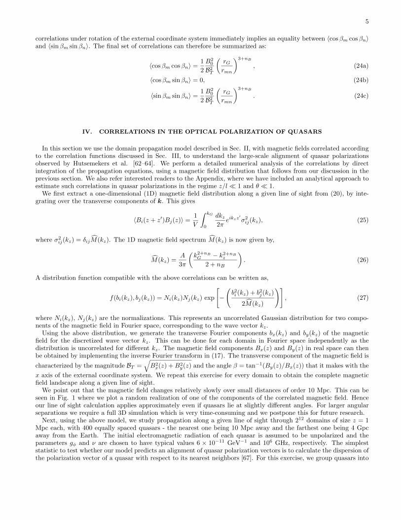
We point out that the magnetic field changes relatively slowly over small distances of order 10 Mpc. This can beseen in Fig. 1 where we plot a random realization of one of the components of the correlated magnetic field. Henceour line of sight calculation applies approximately even if quasars lie at slightly different angles. For larger angularseparations we require a full 3D simulation which is very time-consuming and we postpone this for future research.

Next, using the above model, we study propagation along a given line of sight through 212 domains of size z = 1Mpc each, with 400 equally spaced quasars - the nearest one being 10 Mpc away and the farthest one being 4 Gpcaway from the Earth. The initial electromagnetic radiation of each quasar is assumed to be unpolarized and theparameters gφ and ν are chosen to have typical values 6 × 10−11 GeV−1 and 106 GHz, respectively. The simpleststatistic to test whether our model predicts an alignment of quasar polarization vectors is to calculate the dispersion ofthe polarization vector of a quasar with respect to its nearest neighbors [67]. For this exercise, we group quasars into

6

Mag

net

ic f

ield

(nG

)

Distance (Mpc)

-2

-1.5

-1

-0.5

0

0.5

1

1.5

2

2.5

3

0 20 40 60 80 100

FIG. 1: A random realization of one of the components of the correlated magnetic field as a function of distance.

ns sets of nv quasars each, and calculate the mean value of the vector [cos(2ψi), sin(2ψi)], ψi being the polarizationangle [calculated using (14)], for each set. A measure of the dispersion dk of vectors in each set is given by,

dk =1

nv

nv∑i=1

cos[2(ψi − ψk)], (28)

where ψk is the mean polarization angle in the kth set. The statistic defined as,

SPD =1

ns

ns∑k=1

dk, (29)

gives us a measure of the dispersion in the data. A large value of SPD indicates a strong alignment between polarizationvectors.

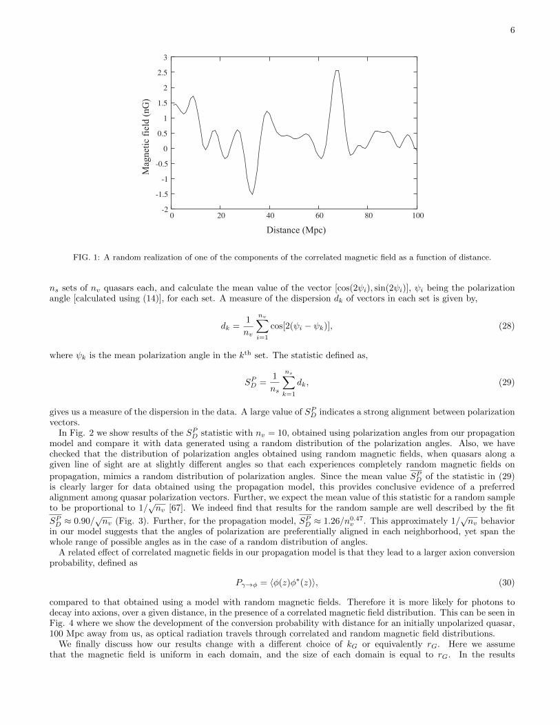
In Fig. 2 we show results of the SPD statistic with nv = 10, obtained using polarization angles from our propagationmodel and compare it with data generated using a random distribution of the polarization angles. Also, we havechecked that the distribution of polarization angles obtained using random magnetic fields, when quasars along agiven line of sight are at slightly different angles so that each experiences completely random magnetic fields on

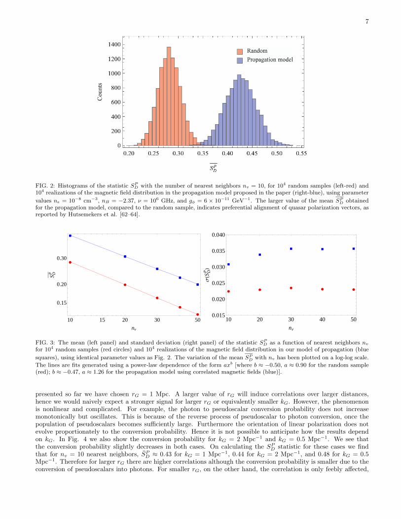
propagation, mimics a random distribution of polarization angles. Since the mean value SPD of the statistic in (29)is clearly larger for data obtained using the propagation model, this provides conclusive evidence of a preferredalignment among quasar polarization vectors. Further, we expect the mean value of this statistic for a random sampleto be proportional to 1/

√nv [67]. We indeed find that results for the random sample are well described by the fit

SPD ≈ 0.90/√nv (Fig. 3). Further, for the propagation model, SPD ≈ 1.26/n0.47

v . This approximately 1/√nv behavior

in our model suggests that the angles of polarization are preferentially aligned in each neighborhood, yet span thewhole range of possible angles as in the case of a random distribution of angles.

A related effect of correlated magnetic fields in our propagation model is that they lead to a larger axion conversionprobability, defined as

Pγ→φ = 〈φ(z)φ∗(z)〉, (30)

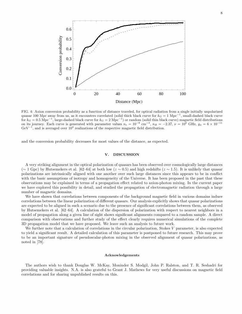
compared to that obtained using a model with random magnetic fields. Therefore it is more likely for photons todecay into axions, over a given distance, in the presence of a correlated magnetic field distribution. This can be seen inFig. 4 where we show the development of the conversion probability with distance for an initially unpolarized quasar,100 Mpc away from us, as optical radiation travels through correlated and random magnetic field distributions.

We finally discuss how our results change with a different choice of kG or equivalently rG. Here we assumethat the magnetic field is uniform in each domain, and the size of each domain is equal to rG. In the results

7

FIG. 2: Histograms of the statistic SPD with the number of nearest neighbors nv = 10, for 104 random samples (left-red) and104 realizations of the magnetic field distribution in the propagation model proposed in the paper (right-blue), using parameter

values ne = 10−8 cm−3, nB = −2.37, ν = 106 GHz, and gφ = 6 × 10−11 GeV−1. The larger value of the mean SPD obtainedfor the propagation model, compared to the random sample, indicates preferential alignment of quasar polarization vectors, asreported by Hutsemekers et al. [62–64].

æ

æ

æ

æ

æ

à

à

à

à

à

æ

æ

æ

æ

æ

à

à

à

à

à

10 5020 3015

0.20

0.30

0.15

nv

S DP

ææ

ææ æ

à

à

à à à

10 20 30 40 500.015

0.020

0.025

0.030

0.035

0.040

nv

ΣHS

DPL

FIG. 3: The mean (left panel) and standard deviation (right panel) of the statistic SPD as a function of nearest neighbors nvfor 104 random samples (red circles) and 104 realizations of the magnetic field distribution in our model of propagation (blue

squares), using identical parameter values as Fig. 2. The variation of the mean SPD with nv has been plotted on a log-log scale.

The lines are fits generated using a power-law dependence of the form axb [where b ≈ −0.50, a ≈ 0.90 for the random sample(red); b ≈ −0.47, a ≈ 1.26 for the propagation model using correlated magnetic fields (blue)].

presented so far we have chosen rG = 1 Mpc. A larger value of rG will induce correlations over larger distances,hence we would naively expect a stronger signal for larger rG or equivalently smaller kG. However, the phenomenonis nonlinear and complicated. For example, the photon to pseudoscalar conversion probability does not increasemonotonically but oscillates. This is because of the reverse process of pseudoscalar to photon conversion, once thepopulation of pseudoscalars becomes sufficiently large. Furthermore the orientation of linear polarization does notevolve proportionately to the conversion probability. Hence it is not possible to anticipate how the results dependon kG. In Fig. 4 we also show the conversion probability for kG = 2 Mpc−1 and kG = 0.5 Mpc−1. We see thatthe conversion probability slightly decreases in both cases. On calculating the SPD statistic for these cases we findthat for nv = 10 nearest neighbors, S̄PD ≈ 0.43 for kG = 1 Mpc−1, 0.44 for kG = 2 Mpc−1, and 0.48 for kG = 0.5Mpc−1. Therefore for larger rG there are higher correlations although the conversion probability is smaller due to theconversion of pseudoscalars into photons. For smaller rG, on the other hand, the correlation is only feebly affected,

8

0 20 40 60 80 1000.0

0.1

0.2

0.3

0.4

0.5

0.6

Distance HMpcL

Con

vers

ion

prob

abili

ty

FIG. 4: Axion conversion probability as a function of distance traveled, for optical radiation from a single initially unpolarizedquasar 100 Mpc away from us, as it encounters correlated (solid thick black curve for kG = 1 Mpc−1, small-dashed black curvefor kG = 0.5 Mpc−1, large-dashed black curve for kG = 2 Mpc−1) or random (solid thin black curve) magnetic field distributionson its journey. Each curve is generated with parameter values ne = 10−8 cm−3, nB = −2.37, ν = 106 GHz, gφ = 6 × 10−11

GeV−1, and is averaged over 104 realizations of the respective magnetic field distribution.

and the conversion probability decreases for most values of the distance, as expected.

V. DISCUSSION

A very striking alignment in the optical polarization of quasars has been observed over cosmologically large distances(∼ 1 Gpc) by Hutsemekers et al. [62–64] at both low (z ∼ 0.5) and high redshifts (z ∼ 1.5). It is unlikely that quasarpolarizations are intrinsically aligned with one another over such large distances since this appears to be in conflictwith the basic assumptions of isotropy and homogeneity of the Universe. It has been proposed in the past that theseobservations may be explained in terms of a propagation effect related to axion-photon mixing. In the current paperwe have explored this possibility in detail, and studied the propagation of electromagnetic radiation through a largenumber of magnetic domains.

We have shown that correlations between components of the background magnetic field in various domains inducecorrelations between the linear polarization of different quasars. Our analysis explicitly shows that quasar polarizationsare expected to be aligned in such a scenario due to the presence of significant correlations between them, as observedby Hutsemekers et al. [62–64]. A calculation of the dispersion of polarization with respect to nearest neighbors in amodel of propagation along a given line of sight shows significant alignments compared to a random sample. A directcomparison with observations and further study of the effect clearly requires numerical simulations of the complete3D propagation model that we have proposed. We leave such an analysis to future work.

We further note that a calculation of correlations in the circular polarization, Stokes V parameter, is also expectedto yield a significant result. A detailed calculation of this parameter is postponed to future research. This may proveto be an important signature of pseudoscalar-photon mixing in the observed alignment of quasar polarizations, asnoted in [78].

Acknowledgements

The authors wish to thank Douglas W. McKay, Moninder S. Modgil, John P. Ralston, and T. R. Seshadri forproviding valuable insights. N.A. is also grateful to Grant J. Mathews for very useful discussions on magnetic fieldcorrelations and for sharing unpublished results on this.

9

Appendix: Analytical treatment of the correlations

In this appendix we discuss an analytical approach to estimate the correlations in quasar polarizations for smalldomain size (z/l � 1) and small mixing angle (θ � 1). In this limit, we expand the 22 element of (8) to leadingorder,

e−i[ω+∆A−(ω2−ω2P )1/2]z ≈ 1− i z

2l(1− sec 2θ), (A1)

where we have omitted the overall phase factor. We can further write the propagation matrix as the sum of a quasiunitmatrix and a matrix proportional to sin θ,

P (z) = I(z) + sin θ P(z, θ). (A2)

Suppressing the irrelevant overall phase in (8), the matrices I(z) and P(z, θ) are given by,

I(z) = diag(1, 1, ei∆z), (A3)

and,

P(z, θ) =

−γ sin θ 0 γ cos θ0 i zl sin θ sec 2θ 0

γ cos θ 0 γ sin θ

. (A4)

We can now express ρn(Z = nz) as a power series in sin θ. For an initially unpolarized electromagnetic wavecorresponding to a density matrix ρ(0) = diag(1, 1, 0), the calculation outlined above gives the following leading orderterms in different powers of sin θ P(z, θ),

ρ[0]n (Z) = ρ(0), (A5)

ρ[1]n (Z) =

n∑j=1

ρ[1]n (Z, j), (A6)

ρ[2]n (Z) =

n∑k=2

k−1∑j=1

ρ[2]n (Z, j, k), (A7)

where,

ρ[1]n (Z, j) =

−2 sin2 θ cos2 βj(1− cos ∆z) − sin2 θ sin 2βj(1− cos ∆z) γ∗e−i∆z(n−j) cosβj sin(2θ)/2− sin2 θ sin 2βj(1− cos ∆z) −2 sin2 θ sin2 βj(1− cos ∆z) γ∗e−i∆z(n−j) sinβj sin(2θ)/2γei∆z(n−j) cosβj sin(2θ)/2 γei∆z(n−j) sinβj sin(2θ)/2 0

, (A8)

and,

ρ[2]n,11(Z, j, k) = −4 sin2 θ cos2 θ(1− cos ∆z) cos[∆z(k − j)] cosβk cosβj , (A9a)

ρ[2]n,12(Z, j, k) = −2 sin2 θ cos2 θ(1− cos ∆z) cos[∆z(k − j)]

(sin(βk + βj)− i sin(βk − βj) tan[∆z(k − j)]

), (A9b)

ρ[2]n,21(Z, j, k) = −2 sin2 θ cos2 θ(1− cos ∆z) cos[∆z(k − j)]

(sin(βk + βj) + i sin(βk − βj) tan[∆z(k − j)]

), (A9c)

ρ[2]n,22(Z, j, k) = −4 sin2 θ cos2 θ(1− cos ∆z) cos[∆z(k − j)] sinβk sinβj . (A9d)

Here we only report elements of the 2 × 2 submatrix relevant to polarization for ρ[2]n (Z, j, k). Further, we ignore

higher-order terms in writing (A9). This approximation is valid as long as sin2 θ and (z/l) sin2 θ are much smallerthan unity.

For two quasars (along a given line of sight) at distances Z1 = nz and Z2 = mz, where n and m are the number ofdomains of size z that lie between us and the two quasars, we wish to estimate the correlation 〈U(Z1 = nz)U(Z2 =mz)〉. Using (13) we find that,

〈U(Z1)U(Z2)〉 = 〈ρn,12(Z1)ρm,12(Z2)〉+ 〈ρn,12(Z1)ρm,21(Z2)〉+ 〈ρn,21(Z1)ρm,12(Z2)〉+ 〈ρn,21(Z1)ρm,21(Z2)〉. (A10)

10

On removing the constant zeroth order part of the propagated density matrix we can write,

ρn(Z) ≈ ρ[1]n (Z) + ρ[2]

n (Z). (A11)

Using (A8) and (A9) in this expression to calculate (A10), we end up with four-point correlation functions in the sinesand cosines of rotation angles. We assume that the magnetic field fluctuations at any point are Gaussian, so that wecan express these four-point correlations in terms of two-point correlations using the following decomposition,

〈S(r1)S(r2)S(r3)S(r4)〉 = 〈S(r1)S(r2)〉〈S(r3)S(r4)〉+ 〈S(r1)S(r3)〉〈S(r2)S(r4)〉+ 〈S(r1)S(r4)〉〈S(r2)S(r3)〉,(A12)

where S(r) is some function (such as a Gaussian) that falls off sufficiently fast with r. Now we can further use (24),and write the correlation in (A10) as,

〈U(Z1)U(Z2)〉 = 4

(B0

BT

)4

sin4 θ(1− cos ∆z)2 ×

[n∑i=1

m∑p=1

(rGrip

)2(3+nB)

+ 2 cos2 θ

n∑i=1

m∑q=2

q−1∑p=1

(r2G

rqirip

)3+nB

cos[∆z(q − p)] +

m∑p=1

n∑j=2

j−1∑i=1

(r2G

rjprpi

)3+nB

cos[∆z(j − i)]

+ cos4 θ

n∑j=2

j−1∑i=1

m∑q=2

q−1∑p=1

{(r2G

rqjrpi

)3+nB

+

(r2G

rqirpj

)3+nB}(

cos[∆z(j + q − i− p)] + cos[∆z(j − q − i+ p)])].

(A13)

The above equation suggests that the linear polarization of quasars at different redshifts along a given line of sightis correlated, as observed by Hutsemekers et al. [62–64]. Here in using the correlations (24) we have set the term insquare brackets in (23) to unity. Further we choose a constant value of 1 nG for BT . These approximations affect theanalytical result to within a factor of order unity.

The analytical calculation presented here makes several approximations and hence only provides a rough estimate ofthe correlations. Nonetheless, it is very important since it establishes the presence of correlations among polarizationsof electromagnetic radiation from quasars separated by large distances. These correlations arise due to the presenceof correlations in the intergalactic magnetic field. The analytical result also provides useful insight into how thecorrelations among polarizations depend on the intergalactic magnetic field. In order to study correlations beyond theregime of validity of the analytical method discussed here, a complete numerical treatment of propagation, as donein Sec. IV of this paper, is necessary.

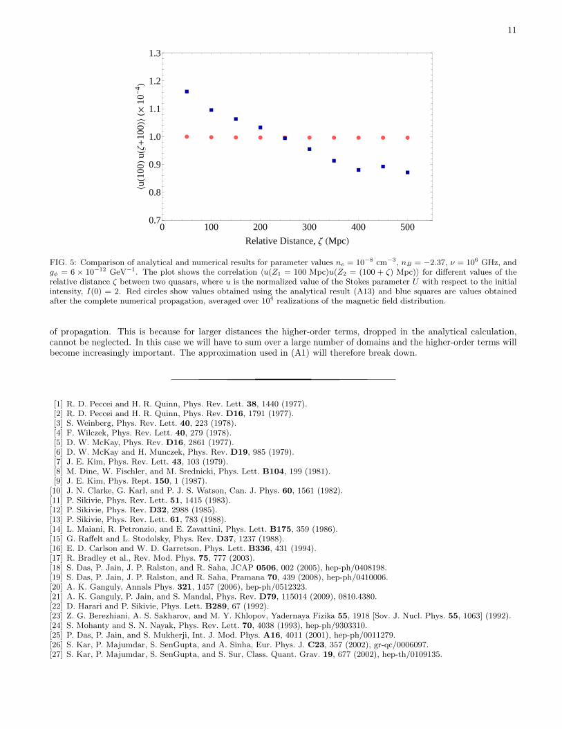
It is also interesting to use the numerical propagation model in the regime where the analytical calculation holds,and compare the result with that obtained using (A13). For this, we study propagation along a given line of sightthrough a total of 210 domains of size z = 1 Mpc each, with 100 equally spaced quasars - the nearest one being10 Mpc away and the farthest one being 1 Gpc away from the Earth. The initial electromagnetic radiation of eachquasar is assumed to be unpolarized. We choose the following parameter values: electron density ne = 10−8 cm−3,spectral index nB = −2.37, frequency of radiation ν = 106 GHz, coupling gφ = 6 × 10−12 GeV−1, and B0 = 1 nG.This choice of parameters ensures that z/l < 1 and θ � 1. Further, in the analytical result we set BT = 1 nG andcalculate rip as rip = z|i − p|, while rii = rG. In the numerical propagation, the value of BT and the angle β ineach domain are obtained from the magnetic field distribution discussed in Sec. IV. For the purpose of comparisonwith the analytical result, however, we set the magnitude of the magnetic field at every point to be equal to 1 nG inthe numerical calculation as well. Direct calculation shows that allowing the magnitude to vary makes a significantdifference in the final answer. Hence it does not provide a fair comparison with the analytical result where we havefixed the magnitude of the field in order to make the calculation tractable. Fig. 5 shows a plot of analytical andnumerical values of the correlation between the Stokes U parameters of two quasars separated by a relative distanceζ.

We find that the analytical and numerical results agree to within about 20%. The discrepancy between the tworesults may be attributed to several other approximations made in the analytical treatment, where (i) we have setthe term in square brackets in (23) to unity and (ii) we have ignored higher-order corrections. As a rough estimate,including the term in square brackets in (23) increases the analytical values of correlations by 60%−70%. In addition,we also observe that the numerical propagation model has a small dependence on the “system size” (i.e., the totalnumber of domains chosen), unlike the analytical result in (A13). This can be ascribed to dependence on the numberof domains, of the discrete values of the wave vector kz used in the inverse Fourier transform. As the magnetic fieldvalues depend on kz, this introduces a small system size dependence in the results. Hence we should expect the tworesults to agree only within a factor of about 2. We also point out that we expect best agreement for small distances

11

æ æ æ æ æ æ æ æ æ æ

à

à

à

à

à

à

à

àà

à

0 100 200 300 400 5000.7

0.8

0.9

1.0

1.1

1.2

1.3

Relative Distance, Ζ HMpcL

XuH10

0LuHΖ

+10

0L\H´

10-

4 L

FIG. 5: Comparison of analytical and numerical results for parameter values ne = 10−8 cm−3, nB = −2.37, ν = 106 GHz, andgφ = 6 × 10−12 GeV−1. The plot shows the correlation 〈u(Z1 = 100 Mpc)u(Z2 = (100 + ζ) Mpc)〉 for different values of therelative distance ζ between two quasars, where u is the normalized value of the Stokes parameter U with respect to the initialintensity, I(0) = 2. Red circles show values obtained using the analytical result (A13) and blue squares are values obtainedafter the complete numerical propagation, averaged over 104 realizations of the magnetic field distribution.

of propagation. This is because for larger distances the higher-order terms, dropped in the analytical calculation,cannot be neglected. In this case we will have to sum over a large number of domains and the higher-order terms willbecome increasingly important. The approximation used in (A1) will therefore break down.

[1] R. D. Peccei and H. R. Quinn, Phys. Rev. Lett. 38, 1440 (1977).[2] R. D. Peccei and H. R. Quinn, Phys. Rev. D16, 1791 (1977).[3] S. Weinberg, Phys. Rev. Lett. 40, 223 (1978).[4] F. Wilczek, Phys. Rev. Lett. 40, 279 (1978).[5] D. W. McKay, Phys. Rev. D16, 2861 (1977).[6] D. W. McKay and H. Munczek, Phys. Rev. D19, 985 (1979).[7] J. E. Kim, Phys. Rev. Lett. 43, 103 (1979).[8] M. Dine, W. Fischler, and M. Srednicki, Phys. Lett. B104, 199 (1981).[9] J. E. Kim, Phys. Rept. 150, 1 (1987).

[10] J. N. Clarke, G. Karl, and P. J. S. Watson, Can. J. Phys. 60, 1561 (1982).[11] P. Sikivie, Phys. Rev. Lett. 51, 1415 (1983).[12] P. Sikivie, Phys. Rev. D32, 2988 (1985).[13] P. Sikivie, Phys. Rev. Lett. 61, 783 (1988).[14] L. Maiani, R. Petronzio, and E. Zavattini, Phys. Lett. B175, 359 (1986).[15] G. Raffelt and L. Stodolsky, Phys. Rev. D37, 1237 (1988).[16] E. D. Carlson and W. D. Garretson, Phys. Lett. B336, 431 (1994).[17] R. Bradley et al., Rev. Mod. Phys. 75, 777 (2003).[18] S. Das, P. Jain, J. P. Ralston, and R. Saha, JCAP 0506, 002 (2005), hep-ph/0408198.[19] S. Das, P. Jain, J. P. Ralston, and R. Saha, Pramana 70, 439 (2008), hep-ph/0410006.[20] A. K. Ganguly, Annals Phys. 321, 1457 (2006), hep-ph/0512323.[21] A. K. Ganguly, P. Jain, and S. Mandal, Phys. Rev. D79, 115014 (2009), 0810.4380.[22] D. Harari and P. Sikivie, Phys. Lett. B289, 67 (1992).[23] Z. G. Berezhiani, A. S. Sakharov, and M. Y. Khlopov, Yadernaya Fizika 55, 1918 [Sov. J. Nucl. Phys. 55, 1063] (1992).[24] S. Mohanty and S. N. Nayak, Phys. Rev. Lett. 70, 4038 (1993), hep-ph/9303310.[25] P. Das, P. Jain, and S. Mukherji, Int. J. Mod. Phys. A16, 4011 (2001), hep-ph/0011279.[26] S. Kar, P. Majumdar, S. SenGupta, and A. Sinha, Eur. Phys. J. C23, 357 (2002), gr-qc/0006097.[27] S. Kar, P. Majumdar, S. SenGupta, and S. Sur, Class. Quant. Grav. 19, 677 (2002), hep-th/0109135.

12

[28] C. Csaki, N. Kaloper, and J. Terning, Phys. Lett. B535, 33 (2002), hep-ph/0112212.[29] C. Csaki, N. Kaloper, and J. Terning, Phys. Rev. Lett. 88, 161302 (2002), hep-ph/0111311.[30] Y. Grossman, S. Roy, and J. Zupan, Phys. Lett. B543, 23 (2002), hep-ph/0204216.[31] P. Jain, S. Panda, and S. Sarala, Phys. Rev. D66, 085007 (2002), hep-ph/0206046.[32] Y.-S. Song and W. Hu, Phys. Rev. D73, 023003 (2006), astro-ph/0508002.[33] A. Mirizzi, G. G. Raffelt, and P. D. Serpico, Phys. Rev. D72, 023501 (2005), astro-ph/0506078.[34] G. G. Raffelt, Lect. Notes Phys. 741, 51 (2008), hep-ph/0611350.[35] Y. N. Gnedin, M. Y. Piotrovich, and T. M. Natsvlishvili, Mon. Not. Roy. Astron. Soc. 374, 276 (2007), astro-ph/0607294.[36] A. Mirizzi, G. G. Raffelt, and P. D. Serpico, Phys. Rev. D76, 023001 (2007), 0704.3044.[37] F. Finelli and M. Galaverni, Phys. Rev. D79, 063002 (2009), 0802.4210.[38] L. Ostman and E. Mortsell, JCAP 0502, 005 (2005), astro-ph/0410501.[39] D. Lai and J. Heyl, Phys. Rev. D74, 123003 (2006), astro-ph/0609775.[40] D. Hooper and P. D. Serpico, Phys. Rev. Lett. 99, 231102 (2007), 0706.3203.[41] K. A. Hochmuth and G. Sigl, Phys. Rev. D76, 123011 (2007), 0708.1144.[42] D. Chelouche, R. Rabadan, S. Pavlov, and F. Castejon, Astrophys. J. Suppl. 180, 1 (2009), 0806.0411.[43] D. A. Dicus, E. W. Kolb, V. L. Teplitz, and R. V. Wagoner, Phys. Rev. D18, 1829 (1978).[44] M. I. Vysotsskii, Y. B. Zel’Dovich, M. Y. Khlopov, and V. M. Chechetkin, Pis’ma ZhETF 27, 533 [JETP Lett. 27, 502]

(1978).[45] D. S. P. Dearborn, D. N. Schramm, and G. Steigman, Phys. Rev. Lett. 56, 26 (1986).[46] G. G. Raffelt and D. S. P. Dearborn, Phys. Rev. D36, 2211 (1987).[47] G. Raffelt and D. Seckel, Phys. Rev. Lett. 60, 1793 (1988).[48] M. S. Turner, Phys. Rev. Lett. 60, 1797 (1988).[49] H.-T. Janka, W. Keil, G. Raffelt, and D. Seckel, Phys. Rev. Lett. 76, 2621 (1996), astro-ph/9507023.[50] W. Keil et al., Phys. Rev. D56, 2419 (1997), astro-ph/9612222.[51] J. W. Brockway, E. D. Carlson, and G. G. Raffelt, Phys. Lett. B383, 439 (1996), astro-ph/9605197.[52] J. A. Grifols, E. Masso, and R. Toldra, Phys. Rev. Lett. 77, 2372 (1996), astro-ph/9606028.[53] G. G. Raffelt, Ann. Rev. Nucl. Part. Sci. 49, 163 (1999), hep-ph/9903472.[54] L. J. Rosenberg and K. A. van Bibber, Phys. Rept. 325, 1 (2000).[55] K. Zioutas et al. (CAST), Phys. Rev. Lett. 94, 121301 (2005), hep-ex/0411033.[56] W. M. Yao et al. (Particle Data Group), J. Phys. G33, 1 (2006).[57] J. Jaeckel, E. Masso, J. Redondo, A. Ringwald, and F. Takahashi, Phys. Rev. D75, 013004 (2007), hep-ph/0610203.[58] S. Andriamonje et al. (CAST), JCAP 0704, 010 (2007), hep-ex/0702006.[59] C. Robilliard et al., Phys. Rev. Lett. 99, 190403 (2007), 0707.1296.[60] E. Zavattini et al. (PVLAS), Phys. Rev. D77, 032006 (2008), 0706.3419.[61] A. Rubbia and A. S. Sakharov, Astropart. Phys. 29, 20 (2008), 0708.2646.[62] D. Hutsemekers, Astron. Astrophys. 332, 410 (1998).[63] D. Hutsemekers and H. Lamy, Astron. Astrophys. 367, 381 (2001), astro-ph/0012182.[64] D. Hutsemekers, R. Cabanac, H. Lamy, and D. Sluse, Astron. Astrophys. 441, 915 (2005), astro-ph/0507274.[65] P. Jain and J. P. Ralston, Mod. Phys. Lett. A14, 417 (1999), astro-ph/9803164.[66] J. P. Ralston and P. Jain, Int. J. Mod. Phys. D13, 1857 (2004), astro-ph/0311430.[67] P. Jain, G. Narain, and S. Sarala, Mon. Not. Roy. Astron. Soc. 347, 394 (2004), astro-ph/0301530.[68] A. Payez, J. R. Cudell, and D. Hutsemekers, AIP Conf. Proc. 1038, 211 (2008), 0805.3946.[69] M. Y. Piotrovich, Y. N. Gnedin, and T. M. Natsvlishvili (2008), 0805.3649.[70] S. Lee, G.-C. Liu, and K.-W. Ng, Phys. Rev. D73, 083516 (2006), astro-ph/0601333.[71] N. Agarwal, P. Jain, D. W. McKay, and J. P. Ralston, Phys. Rev. D78, 085028 (2008), 0807.4587.[72] K. Subramanian, T. R. Seshadri, and J. D. Barrow, Mon. Not. Roy. Astron. Soc. 344, L31 (2003), astro-ph/0303014.[73] T. R. Seshadri and K. Subramanian, Phys. Rev. D72, 023004 (2005), astro-ph/0504007.[74] T. R. Seshadri and K. Subramanian, Phys. Rev. Lett. 103, 081303 (2009), 0902.4066.[75] K. Jedamzik, V. Katalinic, and A. V. Olinto, Phys. Rev. D57, 3264 (1998), astro-ph/9606080.[76] K. Subramanian and J. D. Barrow, Phys. Rev. D58, 083502 (1998), astro-ph/9712083.[77] D. G. Yamazaki, K. Ichiki, T. Kajino, and G. J. Mathews, Phys. Rev. D81, 023008 (2010), 1001.2012.[78] D. Hutsemekers et al. (2008), 0809.3088.