arX

iv:0

808.

0507

v1 [

astr

o-ph

] 4

Aug

200

8

The Mass of the Black Hole in the Quasar PG2130+099

C. J. Grier1, B. M. Peterson1,2, M. C. Bentz3, K. D. Denney1, J. D. Eastman1,

M. Dietrich1, R. W. Pogge1,2, J. L. Prieto1, D. L. DePoy1,2, R. J. Assef1, D. W. Atlee1,

J. Bird1, M. E. Eyler4, M. S. Peeples1, R. Siverd1, L. C. Watson1, J. C. Yee1

ABSTRACT

We present the results of a recent reverberation-mapping campaign under-

taken to improve measurements of the radius of the broad line region and the

central black hole mass of the quasar PG 2130+099. Cross correlation of the

5100 A continuum and Hβ emission-line light curves yields a time lag of 22.9+4.4−4.3

days, corresponding to a central black hole mass MBH = (3.8 ± 1.5)×107M⊙.

This value supports the notion that previous measurements yielded an incor-

rect lag. We re-analyzed previous datasets to investigate the possible sources

of the discrepancy and conclude that previous measurement errors were appar-

ently caused by a combination of undersampling of the light curves and long-term

secular changes in the Hβ emission-line equivalent width. With our new measure-

ments, PG 2130+099 is no longer an outlier in either the RBLR–L or the MBH–σ∗

relationships.

Subject headings: galaxies: active — galaxies: nuclei — galaxies: Seyfert —

quasars: emission lines

1. INTRODUCTION

Reverberation mapping uses observations of continuum and emission-line variability to

probe the structure of the broad line region (BLR) in active galactic nuclei (Blandford &

McKee 1982; Peterson 1993). It has been extensively used to estimate the physical size of

1Department of Astronomy, The Ohio State University, 140 W 18th Ave, Columbus, OH 43210

2Center for Cosmology & AstroParticle Physics, The Ohio State University, 191 West Woodruff Ave,

Columbus, OH 4321

3Department of Physics and Astronomy, University of California at Irvine, 4129 Frederick Reines Hall,

Irvine, CA 92697

4Department of Physics, U.S. Naval Academy, 572C Holloway Road, Annapolis, MD 21401

– 2 –

the BLR and the mass of central black holes in active galactic nuclei (AGN). The observed

continuum variability precedes the observed emission-line variability by a time related to

the light travel time across the BLR; by obtaining an estimate of the time delay, or “lag” τ ,

between the change in continuum flux and the change in emission-line flux, one can estimate

the size of the BLR. While this is an extremely effective method, high-quality datasets

are difficult to obtain, as they require well-spaced observations over long timescales. To

date, over three dozen AGN have estimated black hole masses obtained using reverberation

methods.

In addition to being important physical parameters, the BLR radius and central black

hole mass (MBH) measurements are crucial in calibrating relationships between different

properties of AGN. A useful relationship that has emerged is the correlation between the

radius of the BLR (RBLR) and the optical luminosity of the AGN (e.g. Kaspi et al. 2000,

2005; Bentz et al. 2006). Another key relationship is that between MBH and bulge stellar

velocity dispersion (σ∗) which is seen in both quiescent (Ferrarese & Merritt 2000; Gebhardt

et al. 2000a; Tremaine et al. 2002) and active galaxies (Gebhardt et al. 2000b; Ferraresse et

al. 2001; Nelson et al. 2004; Onken et al. 2004; Dasyra et al. 2007). These two relationships

are critical because they allow us to estimate the masses of black holes in AGN from a

single spectrum (see McGill et al. 2008 for a recent summary) — we estimate RBLR from

the AGN luminosity, the velocity dispersion of the BLR is determined by the emission-line

width, and the quiescient MBH–σ∗ relationship provides the calibration of the reverberation-

based mass scale. Obtaining high-quality single-epoch spectra is much less observationally

demanding than obtaining high-quality reverberation measurements; once relations such

as these are properly calibrated, we can measure MBH in many more objects than would

otherwise be possible. An extensive set of objects with reliable black hole masses allows

us to explore the connection between black holes and AGN evolution over cosmologically

interesting timescales.

PG 2130+099 has been a source of curiosity because it is an outlier in both the MBH–

σ∗ and RBLR–L relations. Previous measurements obtained by Kaspi et al. (2000) and

reanalyzed by Peterson et al. (2004) found Hβ lags of about 180 days. These measurements

yield a black hole mass MBH upwards of 108 M⊙. At luminosity λLλ(5100 A)=(2.24 ±0.27)×1044 erg s−1, this places PG 2130+099 well above the RBLR–L relationship (Bentz et al.

2006). Dasyra et al. (2007) also note that PG 2130+099 falls above the MBH–σ∗ relationship.

Together these suggest that this discrepancy could be caused by measurement errors in the

BLR radius. Our suspicions are also fueled by two other factors. First, the optical spectrum

of PG 2130+099 is similar to that of narrow-line Seyfert 1 (NLS1) galaxies, which are widely

supposed to be AGN with high accretion rates relative to the Eddington rate (see Komossa

2008 for a recent review). However, the accretion rate derived from this mass and luminosity

– 3 –

(under common assumptions for all reverberation-mapped AGN as described by Collin et

al. 2006) is quite low compared to NLS1s, again suggesting that MBH and therefore τ are

overestimated. Second, as we discuss further below, a lag of approximately half a year on an

equatorial source means that fine-scale structure in the two light curves will not match up

in detail, and cross-correlation becomes very sensitive to long-term secular variations that

may or may not be an actual reverberation signal.

For these reasons, we decided to undertake a new reverberation campaign to remeasure

the Hβ lag for PG 2130+099. In this paper, we present a new lag determination from this

campaign. We also present a re-analysis of the earlier dataset that suggests that the true lag

is consistent with our new lag value and investigate possible sources of error in the previous

analysis.

2. OBSERVATIONS AND DATA ANALYSIS

2.1. Observations

The data were obtained as a part of queue-scheduled program during the SDSS-II Super-

nova Survey follow-up campaign (Frieman et al. 2008). We obtained spectra of PG 2130+099

with the Boller and Chivens CCD Spectrograph on the MDM 2.4m telescope for 21 different

nights from 2007 September through 2007 December. We used a 150 grooves/mm grating

which yields a dispersion of 3.29 A pixel−1 and covers the spectral range 4000–7500 A. The

slit width was set to 3′′.0 projected on the sky and the spectral resolution was 15.2 A. We

used an extraction aperture that corresponds to 3′′.0 × 7′′.0.

2.2. Light Curves

The reduced spectra were flux-calibrated using the flux of the [O iii]λ5007 emission

line in a reference spectrum created using a selection of 9 nights with the best observing

conditions. Using a χ2 goodness-of-fit estimator method (van Groningen & Wanders 1992),

each individual spectrum was scaled to the reference spectrum. For three epochs, no reason-

able fit could be obtained, hence we scaled these spectra by hand to match the [O iii]λ5007

flux of the reference spectrum, which was 1.36×10−13 erg s−1 cm−2 in the observed frame

(z = 0.06298). We then removed the narrow-line components of the Hβ and [O iii]λλ 4959,

5007 lines using relative line strengths given by Peterson et al. (2004). Figure 1 shows the

mean and rms spectra of PG 2130+099, created from the entire set of 21 flux-calibrated

observations.

– 4 –

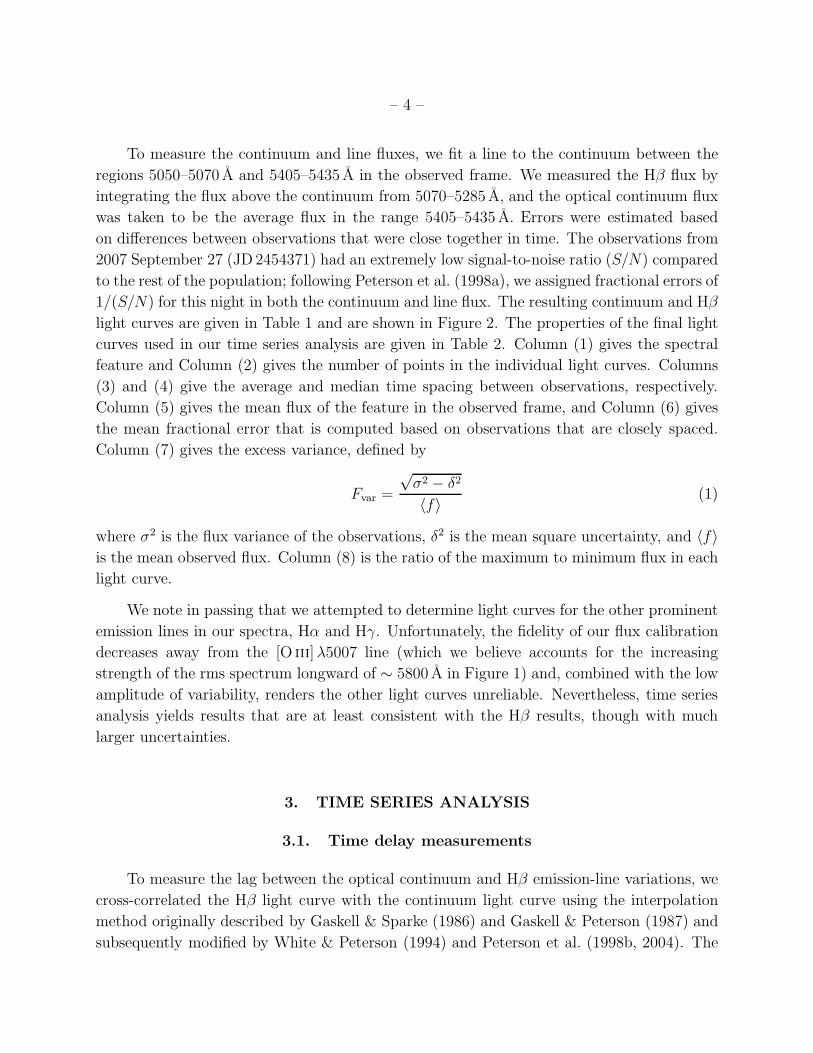
To measure the continuum and line fluxes, we fit a line to the continuum between the

regions 5050–5070 A and 5405–5435 A in the observed frame. We measured the Hβ flux by

integrating the flux above the continuum from 5070–5285 A, and the optical continuum flux

was taken to be the average flux in the range 5405–5435 A. Errors were estimated based

on differences between observations that were close together in time. The observations from

2007 September 27 (JD 2454371) had an extremely low signal-to-noise ratio (S/N) compared

to the rest of the population; following Peterson et al. (1998a), we assigned fractional errors of

1/(S/N) for this night in both the continuum and line flux. The resulting continuum and Hβ

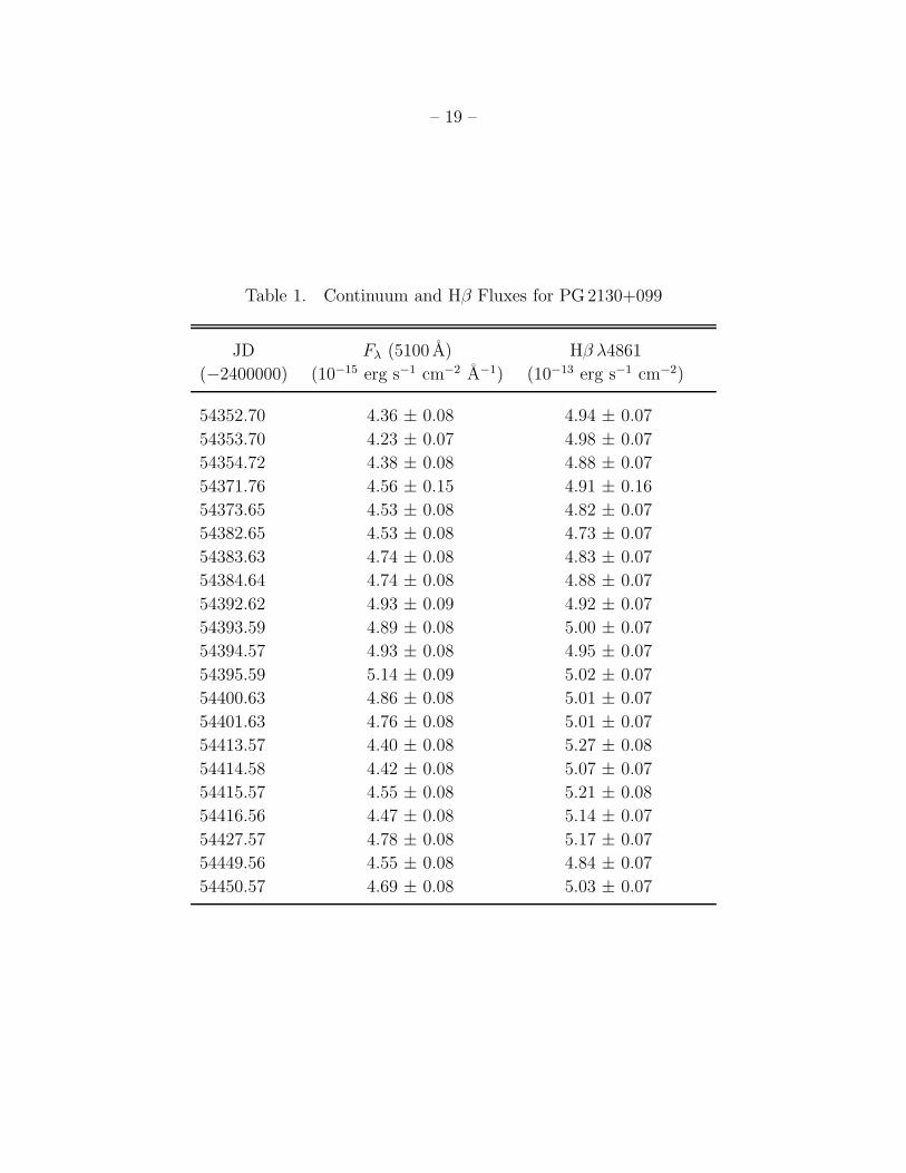
light curves are given in Table 1 and are shown in Figure 2. The properties of the final light

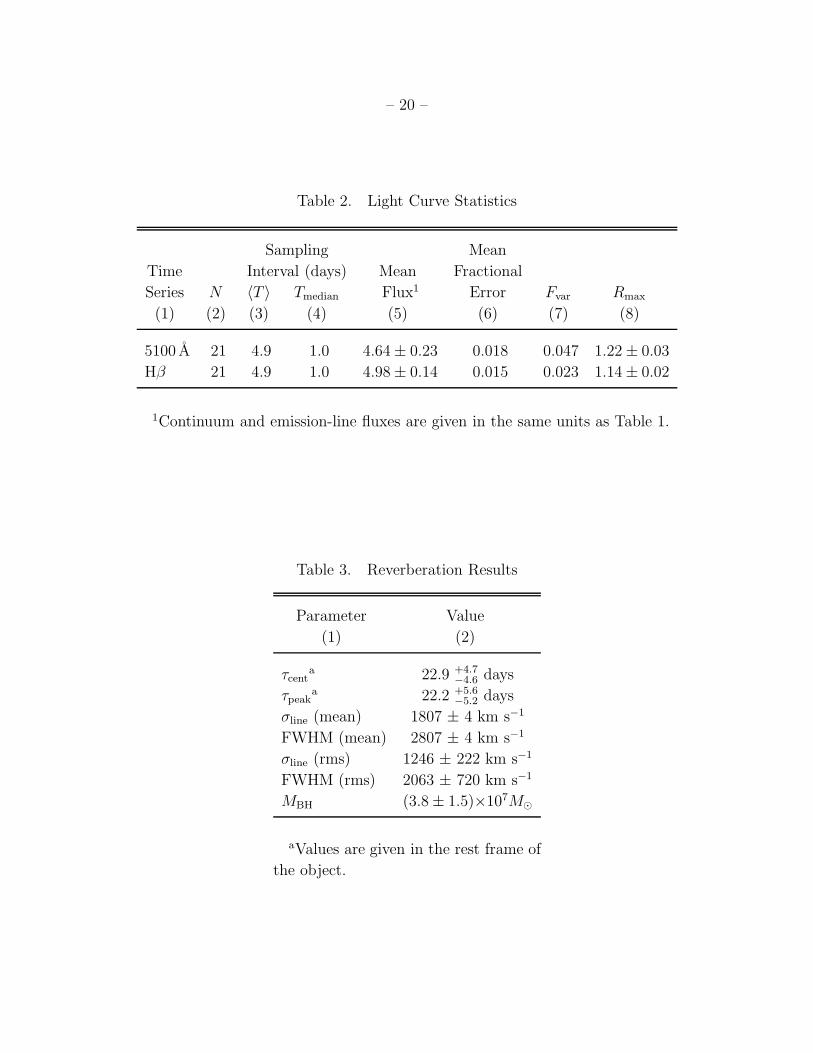
curves used in our time series analysis are given in Table 2. Column (1) gives the spectral

feature and Column (2) gives the number of points in the individual light curves. Columns

(3) and (4) give the average and median time spacing between observations, respectively.

Column (5) gives the mean flux of the feature in the observed frame, and Column (6) gives

the mean fractional error that is computed based on observations that are closely spaced.

Column (7) gives the excess variance, defined by

Fvar =

√σ2 − δ2

〈f〉 (1)

where σ2 is the flux variance of the observations, δ2 is the mean square uncertainty, and 〈f〉is the mean observed flux. Column (8) is the ratio of the maximum to minimum flux in each

light curve.

We note in passing that we attempted to determine light curves for the other prominent

emission lines in our spectra, Hα and Hγ. Unfortunately, the fidelity of our flux calibration

decreases away from the [O iii]λ5007 line (which we believe accounts for the increasing

strength of the rms spectrum longward of ∼ 5800 A in Figure 1) and, combined with the low

amplitude of variability, renders the other light curves unreliable. Nevertheless, time series

analysis yields results that are at least consistent with the Hβ results, though with much

larger uncertainties.

3. TIME SERIES ANALYSIS

3.1. Time delay measurements

To measure the lag between the optical continuum and Hβ emission-line variations, we

cross-correlated the Hβ light curve with the continuum light curve using the interpolation

method originally described by Gaskell & Sparke (1986) and Gaskell & Peterson (1987) and

subsequently modified by White & Peterson (1994) and Peterson et al. (1998b, 2004). The

– 5 –

method works as follows: because the data are not evenly spaced in time, we interpolate

between points to obtain an evenly-sampled light curve. The linear correlation coefficient

r is then calculated using pairs of points, one from each light curve, separated by a given

time lag. When r is calculated for a range of time lag values, the cross correlation function

(CCF) is obtained, which consists of the value of r for each time lag value. We interpolated

between the points on a 0.5 day timescale to obtain the CCF for our dataset, which is shown

in Figure 3.

To determine the most probable delay and its uncertainty, we employed the flux random-

ization/random subset sampling Monte Carlo method described by Peterson et al. (1998b).

The “random subset sampling” method takes a light curve of N points and samples it N

times without regard to whether or not any given point has been selected already. The flux

uncertainty of a data point selected n times is correspondingly reduced by a factor n−1/2

(Welsh 1999; Peterson et al. 2004). The flux value of each point is then altered by a random

Gaussian deviate based on the uncertainty assigned to the point; this is known as “flux

randomization”. A CCF was calculated for each altered light curve using interpolation as

before. Using 2000 iterations of this process, we obtain a distribution of τpeak, measured

from the CCF of each Monte Carlo realization and defined by the location of the peak value

of r. We also calculate and obtain a distribution of the lag values τcent that represents the

centroid of each CCF using the points surrounding the peak, based on all lag values with

r ≥ 0.8rmax. We then adopt the mean values of both the centroid and peak 〈τcent〉 and

〈τpeak〉 for our analysis. We estimate the uncertainties in τcent and τpeak such that 15.87% of

the realizations fall below the mean minus the lower error and 15.87% of the realizations fall

above the mean plus the upper error. Our final lag values and errors are τcent = 22.9+4.4−4.3 days

and τpeak = 22.2+5.6−5.2 days in the rest frame of PG 2130+099. It is important to note that the

CCF is heavily dependent on the timespan of the light curve relative to the actual delay, and

if the data timespan is short with respect to the lag, the CCF will be biased towards short

lag measurements (Welsh 1999). We note that because our data span just over three months,

our CCF is not capable of producing a lag measurement as large as previous measurements

and is subject to this bias. However, if the actual lag is shorter as the evidence presented in

this work suggests, our data span a sufficiently long period to identify the true delay.

As a check on our time series analysis, we also employed an alternative method known as

the z-transformed discrete correlation function (ZDCF), as described by Alexander (1997).

This method is a modification of the discrete correlation function (DCF) described by Edel-

son & Krolik (1988). The DCF is obtained by correlating data points from the continuum

with points from the Hβ light curve by binning the data in time rather than interpolating

between points. The ZDCF similarly uses bins rather than interpolation, but bins the data

by equal population rather than by equal spacing in time and applies Fisher’s z-transform

– 6 –

to the cross correlation coefficients. Discrete correlation functions have the advantage that

they only use real data points, and are therefore less likely to find spurious correlations in

data where there are large time gaps. However, datasets with few points tend to yield lag

values with large uncertainties; hence this method is primarily useful as a check on the in-

terpolation method when the data are undersampled. Figure 3 shows the computed ZDCF

for our PG 2130+099 dataset. It should be noted that the z-transform requires a minimum

of 11 points per bin to be statistically significant (Alexander 1997); because our light curves

contained only 21 points, we were unable to obtain a well-sampled ZDCF with a minimum of

11 points per bin. We used a minimum of 8 points per bin and do not obtain an independent

lag measurement, but the ZDCF is very consistent with our calculated CCF, indicating that

the interpolation results are credible.

3.2. Line width measurement and mass calculations

We use the second moment of the line profile, σline (Fromerth & Melia 2000; Peterson

et al. 2004) to characterize the width of the Hβ line. To determine the best value of σline

and its uncertainties, we use Monte Carlo simulations similar to those used in determining

the time lag (see Peterson et al. 2004). We measure the line widths from both the mean

and rms spectra created in the simulations from N randomly chosen spectra and correct

them for the spectrograph resolution. We obtain a distribution of each line width from

multiple realizations, from which we take the mean value for our measure of σline or FWHM

and the standard deviation as the measurement uncertainty. The measured line widths and

uncertainties are given in Table 3.

Assuming that the motion of the Hβ-emitting gas is dominated by gravity, the relation

between MBH, line width, and time delay is

MBH =fcτ∆V 2

G, (2)

where τ is the emission-line time delay, ∆V is the emission-line width, and f is a dimension-

less factor that is characterized by the geometry and kinematics of the BLR. Onken et al.

(2004) calculated an average value of 〈f〉 by assuming that AGN follow the same MBH–σ∗

relationship as quiescent galaxies. By normalizing the reverberation black hole masses to the

relation for quiescent galaxies, they obtain 〈f〉 = 5.5 when the line width is characterized by

the line dispersion σline of the rms spectrum.1 Using our values of τcent and σline, we compute

1Differences between the use of σline and the FWHM in calculating MBH are discussed by Collin et al.

(2006).

– 7 –

MBH = (3.8 ± 1.5)×107M⊙.

We also compute the average 5100 A luminosity of our sample to see where our new

RBLR value places PG 2130+099 on the RBLR–L relationship. Following Bentz et al. (2006),

we correct our luminosity for host-galaxy contamination. Assuming H0 = 70 km s−1 Mpc−1,

Ωm = 0.30 and ΩΛ = 0.70, we calculate log λLλ(5100 A)= 44.40±0.02 for our recent mea-

surements of PG 2130+099. The relevant measurements and computed quantities are given

in Table 4.

4. DISCUSSION

Analysis of previous datasets of PG 2130+099 yields lags greater than 150 days and MBH

values above 108 M⊙, in both cases approximately an order of magnitude larger than our new

value. To investigate the source of these discrepancies, we closely scrutinized the previous

dataset, which consists of data obtained at Steward Observatory and Wise Observatory

(Kaspi et al. 2000). The 5100 A continuum and emission-line light curves, along with their

respective CCF and ZDCFs, are shown in Figure 4. We first ran the full light curve through

the time series analysis as described in section 2.3 to confirm the previous results, and

successfully reproduced a lag measurement of ∼ 168 days, in agreement with Kaspi et al.

(2000) and Peterson et al. (2004). However, visual inspection of the light curves suggests

that these values were in error; we were able to identify several features that are present in

the continuum, Hβ and Hα light curves that are quite visibly lagging on timescales shorter

than 50 days, as we show below.

It is clear that the Kaspi et al. results are dominated by the data spanning the years

1993-1995, as this period contains the most significant variability as well as time sampling

that is sufficient to resolve features in the light curves. We show the light curves for all

spectral features measured by Kaspi et al. during this time period in Figure 5. Over this

period, we can match behavior in the continuum with the behavior of the emission lines,

most noticeably in the data from 1995. The most prominent features in the light curves are

the maximum in the continuum at the end of the 1994 series and the maxima in the lines

at the beginning of the 1995 series, which, based on the continuum variations, one would

expect to be lower relative to the fluxes in 1994. However, inspection of the relative flux

levels of the lines and continuum in the 1994 and 1995 data reveals that the equivalent width

of the emission lines changes during this timespan, which results in a rise in emission-line

flux apparently unrelated to reverberation. The maximum in the continuum and those in

the emission lines do not correspond to the same features— the maxima in the emission line

light curves in 1995 correspond to the similar feature in the continuum at the beginning of

– 8 –

1995. Because there are no observations during the six months or so between these features,

the CCF and ZDCF lock onto the two unrelated maxima that are separated by 196 days

and yield lags of ∼200 days over this three-year span. The emission lines likely continued to

increase in flux during the time period for which there were no observations.

Inspection of the light curve segments in Figure 5 reveals similar structures in each

of them within a given year. To quantify the time delays between the continuum and

lines on short timescales, we cross-correlated each individual year, this time using only flux

randomization in the Monte Carlo realizations, as there were too few points in each year to

use random subset sampling, so the uncertainties are underestimated. The resulting lags are

given in Table 5. Again we must consider that the CCF cannot produce a lag that is greater

than the duration of observations, so the individual CCFs for these three years are limited to

short delays. However, the presence of the 1995 feature in both the continuum and emission-

line light curves is unmistakable and it is extremely unlikely that it lags by a value exceeding

the sensitivity limit of the CCF. From this we surmise that the discrepancies in measured

lag values are mostly a result of large time gaps in the data and/or underestimation of the

error bars in the Kaspi et al. data.

Welsh (1999), and even earlier, Perez, Robinson, & de la Fuente (1992), pointed out

that emission-line lags can be severely underestimated with light curves that are too short in

duration, particularly if the BLR is extended: certainly our 98-day campaign is insensitive

to lags as long as ∼ 180 days. Is it possible that the original lag determination of Kaspi

et al. (2000) and Peterson et al. (2004) is correct (or more nearly so) and we have been

fooled by reliance on light curves that are too short? We think not, based on (1) the

reasonable match between details in the continuum and emission-line light curves for four

different observing seasons (1993, 1994, 1995, and 2007), (2) the improved agreement with the

RBLR-L relationship with the smaller lag (demonstrated in Figure 6), and (3) the improved

agreement with the MBH-σ∗ relationship with the smaller lag (Figure 7). It is also worth

pointing out the difficulty of accurately measuring a ∼ 180 day lag, particularly in the case

of equatorial sources which have a relatively short observing season. The short observing

season, typically 6-7 months, means that there are very few emission-line observations that

can be matched directly with continuum points: the observed emission-line fluxes represent

a response to continuum variations that occurred when the AGN was too close to the Sun

to observe.

Welsh (1999) has also pointed out the value in “detrending” the light curves— removing

long-term trends by fitting the light curves with a low-order function can reduce the bias

toward underestimating lags. In this particular case, we find that detrending has almost

no effect: in particular, the highest points in the continuum (in late 1994) and the highest

– 9 –

points in the line (early in the 1995 observing season) remain so after detrending, and both

the interpolation CCF and ZDCF weight these points heavily. It is also interesting to note

that the peak in the ZDCF agrees with the peak of the interpolation CCF (Figure 4), which

demonstrates that the ∼ 180 day lag is not simply ascribable to interpolation across the gap

between the 1994 and 1995 observing seasons.

The data from our 2007 campaign are not ideal: the amplitude of variability was low,

the time sampling was adequate, but only barely, and the duration of the campaign was

short enough that we lack sensitivity to lags of ∼ 50 days or longer. But the preponderance

of evidence at this point argues that our smaller lag measurement is more likely to be correct

than the previous determination. Certainly better-sampled light curves of longer duration

would yield a more definitive result.

5. SUMMARY

From a new reverberation campaign, we obtain a measurement of the time lag of the Hβ

line in PG 2130+099 of τcent= 22.9+4.4−4.3 days and calculate a central black hole mass MBH =

(3.8 ± 1.5)×107M⊙. Previous measurements of τcent overestimated the size of the BLR and

therefore the mass of the black hole, most likely due to the undersampling in the light curves.

A re-analysis of the previous data, using both visual and algorithmic methods, suggests that

the true BLR size and MBH are consistent with our new values. The recent reverberation

measurements for PG 2130+099 presented in this study remove the discrepancies previously

found for this object based on the MBH–σ∗ and RBLR–L relationships.

We are grateful for support of this program by the National Science Foundation through

grant AST-0604066 to The Ohio State University. We would also like to thank H. Netzer,

S. Kaspi, and referee C. M. Gaskell for their helpful suggestions.

REFERENCES

Alexander, T. 1997, in Astronomical Time Series, ed. D. Maoz, A. Sternberg, & E.M. Lei-

bowitz (Dordrecht: Kluwer), 163

Bentz, M.C., Peterson, B.M., Pogge, R.W., Vestergaard, M., & Onken, C.A. 2006, ApJ, 644,

133

– 10 –

Bentz, M.C., Peterson, B.M., Netzer, H., Pogge, R.W., & Vestergaard, M. 2008, ApJ, sub-

mitted

Blandford, R.D., & McKee, C.F. 1982, ApJ, 255, 419

Collin, S., Kawaguchi, T., Peterson, B.M., & Vestergaard, M. 2006, A&A, 456, 75

Dasyra, K.M., Tacconi, L.J., Davies, R.I., Genzel, R., Lutz, D., Peterson, B.M., Veilleux, S.,

Baker, A.J., Schweitzer, M., & Sturm, E. 2007, ApJ, 657, 102

Edelson, R.A., & Krolik, J.H. 1988, ApJ, 333, 646

Ferrarese, L., & Merritt, D.M. 2000, ApJ, 539, L9

Ferrarese, L., Pogge, R.W., Peterson, B.M., Merritt, D., Wandel, A., & Joseph, C.L. 2001,

ApJ, 555, L79

Frieman, J. A., et al. 2008, AJ, 135, 338

Fromerth, M.J., & Melia, F. 2000, ApJ, 533, 172

Gaskell, C.M., & Peterson, B.M. 1987, ApJS, 65, 1

Gaskell, C.M., & Sparke, L.S. 1986, ApJ, 305, 175

Gebhardt, K., et al. 2000a, ApJ, 539, L13

Gebhardt, K., et al. 2000b, ApJ, 543, L5

Kaspi, S., Maoz, D., Netzer, H., Peterson, B.M., Vestergaard, M., & Jannuzi, B.T. 2005,

ApJ, 629, 61

Kaspi, S., Smith, P.S., Netzer, H., Maoz, D., Jannuzi, B.T., & Giveon, U. 2000, ApJ, 533,

631

Komossa, S. 2008, in The Nuclear Region, Host Galaxy, and Environment of Active Galaxies,

ed. E. Benıtez, I. Cruz-Gonzalez, and Y. Krongold, Revista Mexicana de Astronomia

y Astrofısica (Serie de Conferencias), Vol. 32, pp. 86-92

McGill, K.L., Woo, J.-H., Treu, T., Malkan, M.A. 2008, ApJ, 673, 703

Nelson, C.H., Green, R.F., Bower, G., Gebhardt, K., & Weistrop, D. 2004, ApJ, 615, 652

Onken, C.A., Ferrarese, L., Merritt, D., Peterson, B.M., Pogge, R.W., Vestergaard, M., &

Wandel, A. 2004, ApJ, 615, 645

– 11 –

Peterson, B.M. 1993, PASP, 105, 247

Peterson, B.M., Wanders, I., Bertram, R., Hunley, J.F., Pogge, R.W., & Wagner, M. 1998a,

ApJ, 501, 82

Peterson, B.M., Wanders, I., Horne, K., Collier, S., Alexander, T., & Kaspi, S. 1998b, PASP,

110, 660

Peterson, B.M., et al. 2004, ApJ, 613, 682

Tremaine, S., et al. 2002, ApJ, 574, 740

van Groningen, E., & Wanders, I. 1992, PASP, 104, 700

Watson, L.C. et al. 2008, ApJL, 682, 21

Welsh, W.F. 1999, PASP, 111, 1347

This preprint was prepared with the AAS LATEX macros v5.2.

– 12 –

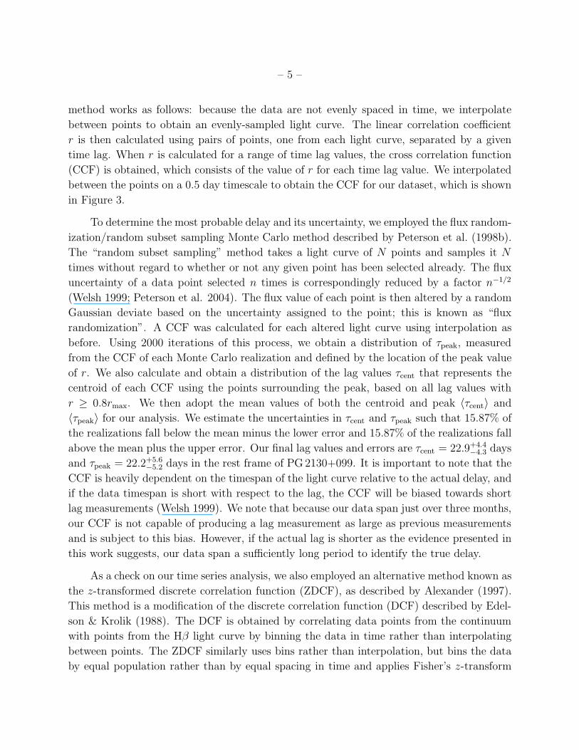
Fig. 1.— The flux-calibrated mean and rms spectra of PG 2130+099 in the observed frame

(z = 0.06298). The flux density is in units of 10−15 erg s−1 cm−2 A−1.

– 13 –

4.2

4.4

4.6

4.8

5

5.2

54360 54380 54400 54420 544404.6

4.8

5

5.2

Fig. 2.— Continuum (upper panel) and Hβ (lower panel) light curves that were used in

the time series analysis. Continuum flux densities are in units of 10−15 erg s−1 cm−2 A−1.

Emission-line flux densities are in units of 10−13 erg s−1 cm−2. All fluxes are in the observed

frame.

– 14 –

Fig. 3.— The CCF (solid line) and ZDCF (filled circles) from the time series analysis of our

recent observations of PG 2130+099.

– 15 –

Fig. 4.— The left column shows the light curves of PG 2130+099 from Kaspi et al. (2000).

The 5100 A continuum light curve is shown in the top left panel and the Hα, Hβ, and Hγ light

curves are displayed below. The right column shows the CCF and corresponding ZDCF for

each spectral feature, with the top right panel showing the auto-correlation function (ACF)

of the continuum. The continuum flux density is given in units of 10−15 erg s−1 cm−2 A−1

and the Hβ flux density is in units of 10−13 erg s−1 cm−2.

– 16 –

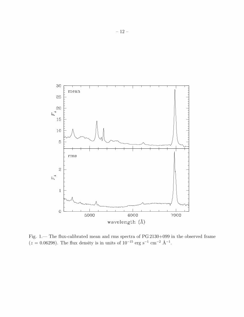
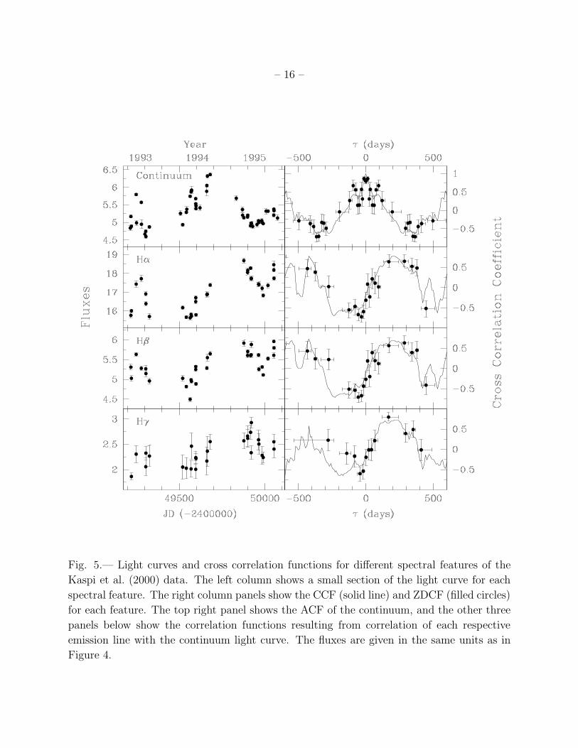
Fig. 5.— Light curves and cross correlation functions for different spectral features of the

Kaspi et al. (2000) data. The left column shows a small section of the light curve for each

spectral feature. The right column panels show the CCF (solid line) and ZDCF (filled circles)

for each feature. The top right panel shows the ACF of the continuum, and the other three

panels below show the correlation functions resulting from correlation of each respective

emission line with the continuum light curve. The fluxes are given in the same units as in

Figure 4.

– 17 –

Fig. 6.— The position of PG 2130+099 on the most recent RBLR–L relationship from

Bentz et al. (2008), denoted by the solid line. The starred circle represents the position

of PG 2130+099 with a lag of 158.1 days, as given by Peterson et al. (2004). The filled

square represents the measurement of 22.9 days from our recent dataset. The open squares

represent other objects from Bentz et al.

– 18 –

Fig. 7.— The position of PG 2130+099 on the MBH–σ∗ relationship (from Tremaine et al.

2002), denoted by the solid line. The open squares show data points based on Onken et

al. (2004) and Nelson et al. (2004) and the open circle is PG 1426+015 from Watson et al.

(2008). The starred circle and filled square represent the position of PG 2130+099 using the

same data sets as in Figure 6.

– 19 –

Table 1. Continuum and Hβ Fluxes for PG 2130+099

JD Fλ (5100 A) Hβ λ4861

(−2400000) (10−15 erg s−1 cm−2 A−1) (10−13 erg s−1 cm−2)

54352.70 4.36 ± 0.08 4.94 ± 0.07

54353.70 4.23 ± 0.07 4.98 ± 0.07

54354.72 4.38 ± 0.08 4.88 ± 0.07

54371.76 4.56 ± 0.15 4.91 ± 0.16

54373.65 4.53 ± 0.08 4.82 ± 0.07

54382.65 4.53 ± 0.08 4.73 ± 0.07

54383.63 4.74 ± 0.08 4.83 ± 0.07

54384.64 4.74 ± 0.08 4.88 ± 0.07

54392.62 4.93 ± 0.09 4.92 ± 0.07

54393.59 4.89 ± 0.08 5.00 ± 0.07

54394.57 4.93 ± 0.08 4.95 ± 0.07

54395.59 5.14 ± 0.09 5.02 ± 0.07

54400.63 4.86 ± 0.08 5.01 ± 0.07

54401.63 4.76 ± 0.08 5.01 ± 0.07

54413.57 4.40 ± 0.08 5.27 ± 0.08

54414.58 4.42 ± 0.08 5.07 ± 0.07

54415.57 4.55 ± 0.08 5.21 ± 0.08

54416.56 4.47 ± 0.08 5.14 ± 0.07

54427.57 4.78 ± 0.08 5.17 ± 0.07

54449.56 4.55 ± 0.08 4.84 ± 0.07

54450.57 4.69 ± 0.08 5.03 ± 0.07

– 20 –

Table 2. Light Curve Statistics

Sampling Mean

Time Interval (days) Mean Fractional

Series N 〈T 〉 Tmedian Flux1 Error Fvar Rmax

(1) (2) (3) (4) (5) (6) (7) (8)

5100 A 21 4.9 1.0 4.64 ± 0.23 0.018 0.047 1.22 ± 0.03

Hβ 21 4.9 1.0 4.98 ± 0.14 0.015 0.023 1.14 ± 0.02

1Continuum and emission-line fluxes are given in the same units as Table 1.

Table 3. Reverberation Results

Parameter Value

(1) (2)

τcenta 22.9 +4.7

−4.6 days

τpeaka 22.2 +5.6

−5.2 days

σline (mean) 1807 ± 4 km s−1

FWHM (mean) 2807 ± 4 km s−1

σline (rms) 1246 ± 222 km s−1

FWHM (rms) 2063 ± 720 km s−1

MBH (3.8 ± 1.5)×107M⊙

aValues are given in the rest frame of

the object.

– 21 –

Table 4. Host Galaxy Flux Removal Parameters

Parameter Value

(1) (2)

Position angle of slit 0.0

Aperture size 3′′.0 × 7′′.0

Fgalaxy (5100 A)a (0.405±0.037) ×10−15 erg s−1 cm−2 A−1

log λLλ(5100 A)b (44.40±0.02)

aGalaxy flux is in the observed frame, from Bentz et al. (2008).

b5100 A rest-frame luminosity in erg s−1, with host galaxy sub-

tracted and corrected for extinction, following Bentz et al. (2006;

2008).

Table 5. Reverberation Results From Kaspi et al. Dataset

Data Spectral τcent τpeak

Subset Feature (days) (days)

Entire Data Set Hα 215.2 +32.1−27.8 217.4 +20.0

−20.0

Entire Data Set Hβ 168.2 +36.7−21.4 177.4 +60.0

−100.0

Entire Data Set Hγ 197.6 +37.9−28.5 208.3 +40.0

−80.0

1993-1995 Hα 199.1 +4.8−0.7 203.0 +10.0

−10.0

1993-1995 Hβ 203.5 +5.2−17.4 202.9 +0.0

−10.0

1993-1995 Hγ 195.6 +35.1−27.6 219.5 +21.0

−93.0

1993 Hα 15.6 +0.6−1.4 19.1 +0.0

−3.0

1993 Hβ 12.2 +1.5−2.5 13.1 +3.0

−2.0

1994 Hα 15.2 +0.9−1.6 16.0 +0.0

−0.0

1994 Hβ 13.7 +1.8−0.8 16.0 +0.0

−1.0

1994 Hγ 10.0 +5.3−3.4 12.0 +51.0

−9.0

1995 Hα 36.6 +4.7−3.3 44.0 +0.0

−10.0

1995 Hβ 46.5 +4.0−2.9 44.0 +8.0

−0.0

1995 Hγ 67.4 +7.7−8.5 67.0 +7.7

−8.5

All in-text references underlined in blue are linked to publications on ResearchGate, letting you access and read them immediately.