Woods Hole Oceanographic Institution \ ft* - DTIC

$: Woods Hole Oceanographic Institution \ ft* - DTIC$
WHOI-2001-02

Woods Hole Oceanographic Institution Woods Hole, MA 02543

oC^lS, \

1930

Turbulence in the Shallow Nearshore Environment

during SANDYDUCK '97 f s*» TS»!*;*^."; -«äfSSf *T%¥ *'*! "^ ? ys*"«.^:"»,;'*?:-*^-*?.- *^ :":*"'*"!-:»1^ iV***^''-? H7! (*??/# ;*c w; ?•:"•••>•,:(£.<:;-< v.,-^ if«..

i' 'ÄEH \ ft*

mm

by

J.J. Fredericks, John H. Trowbridge and George Voulgaris

February 2001

Technical Report

Funding was provided by the National Science Foundation under Grant No. OCE-9810609, the Mellon Foundation and Rinehart Coastal Research Center.

Approved for public release; distribution unlimited.

WHOI-2001-02

Turbulence in the Shallow Nearshore Environment

during Sandy Duck '97

by

JJ. Fredericks John H. Trowbridge

George Voulgaris

February 2001

Technical Report

Funding was provided by the National Science Foundation under Grant No. OCE-9810609, the Mellon Foundation and Rinehart Coastal Research Center.

Reproduction in whole or in part is permitted for any purpose of the United States Government. This report should be cited as Woods Hole Oceanog. Inst. Tech. Rept.,

WHOI-2001-02.


Approved for Distribution:

Timothy K. Stanton, Chair

Department of Applied Ocean Physics and Engineering

20010323 089

TABLE OF CONTENTS

LIST OF FIGURES « LIST OF TABLES »

I. INTRODUCTION 1 II. INSTRUMENTATION 3 III. DEPLOYMENT , 7 IV. DATA PROCESSING 9 V. DATA SUMMARffiS 11 VI. DATA ANALYSES 33 VII. FILE DESCRIPTIONS 39 VIII. ACKNOWLEDGMENTS 43 IX. REFERENCES 45

LIST OF FIGURES

Figure 1. Experiment site iv Figure 2. Collaborative experiments (site map) 2 Figure 3. Picture of instrumentation 3 Figure 4. Illustration of instrumentation with orientation 5 Figure 5. Bathymetric surveys during deployment 6 Figure 6. Pictures showing scouring and fouling 8

TIME SERIES FOR FIRST SIX DAYS Figure 7. Stickplot of horizontal velocity 12 Figure 8. Onshore velocity 13 Figure 9. Alongshore velocity 14 Figure 10. Vertical velocity 15 Figure 11. Water depth, significant wave height and water temperature 16 Figure 12. Bottom orbital velocity 17 Figure 13. Angle of incidence of waves 18 Figure 14. Dissipation 19 Figure 15. Stress 20 Figure 16. Mean signal strength 21 Figure 17. Standard deviation of signal strength 22 Figure 18. Wind speed and air temperature 23 Figure 19. Wind stress and heat flux 24

TIME SERIES from 8/25/97 -10/23/97 Figure 20. Horizontal and vertical velocity (m/s) 25 Figure 21. Water depth, significant wave height and water temperature 26 Figure 22. Bottom orbital velocity, angle of incidence of waves and wave frequency .... 27 Figure 23. Dissipation 28 Figure 24. Stress 29 Figure 25. Mean and standard deviation of signal strength 30 Figure 26. Wind speed and air temperature 31 Figure 27. Wind stress and heat flux 32

Figure 28. Comparisons of Urms and Hs from pressure and velocity data 33 Figure 29. Comparison of depth from pressure and tide data 34 Figure 30. Comparison of variance of depth from pressure and tide data 35 Figure 31. Comparison of wind velocity and stress from sonic

and K-Gill Vane anemometers 36 Figure 32. Comparison of wind velocity and stress compared to

Large & Pond estimates of stress 37

XX

LIST OF TABLES

Table 1. Height and model numbers of ADVs 4 Table 2. Binary format of field probe loggers 39 Table 3. Binary format of ocean probe logger 40

in

20' 75^

Figure 1. The deployment site was at the Field Research Facility (FRF) at Duck, NC.

IV

I. INTRODUCTION

An array of five acoustic Doppier velocimeters (ADV), which produce high quality measurements of the three-dimensional velocity vector in a sample volume with a scale of one centimeter, was deployed from late August through late November of 1997 at a water depth of approximately 4.5 m off Duck, North Carolina (Figure 1). The sensors were deployed near the sea floor but above the centimeters-thick wave boundary layer, and the sampling scheme was designed to resolve turbulence statistics averaged over tens of minutes, much longer than typical wave periods but shorter than time scales associated with variability of energetic wind-driven and wave-driven alongshore flows.

A part of the SANDYDUCK 97 field program, the experiment addresses turbulence in the shallow nearshore environment, where water depths are on the order of meters, energetic currents are forced by both winds and breaking waves, and the motion of water and sand is of primary scien- tific interest and practical concern. Existing models and measurements indicate that turbulence is particularly important in this environment: the effect of bottom drag, which plays a dominant role in controlling the magnitude of wind-driven and wave-driven flows, is believed to be trans- mitted through the water column by turbulent Reynolds stresses; near-bottom turbulent stresses are believed to control the entrainment of sediment from the sea floor; and turbulence in the water column is believed to maintain sediment in suspension against the action of gravity. In spite of its importance, turbulence in the nearshore environment has rarely been measured. Direct measurements of turbulent Reynolds shear stress, in particular, have never been obtained in this environment, because of fundamental problems produced by surface waves.

The objectives of the analysis are (1) to obtain direct estimates of turbulent Reynolds shear stress, by using a novel method involving the difference between velocity measurements obtained by pairs of spatially separated sensors; (2) to obtain indirect inertial-range estimates of the dissipation rate for turbulent kinetic energy; (3) to test, in collaboration with other SANDY- DUCK principal investigators, a wave-averaged alongshore momentum equation in which wind stress and cross-shore gradient of wave-induced radiation stress balance bottom stress; and (4) to test a simplified turbulence energy balance in which shear production balances dissipation.

Other notable components of the SANDYDUCK 97 field program, for the present purposes, were an array of pressure and velocity sensors, deployed by Steve Elgar (WHOI), Britt Rauben- heimer (WHOI), Tom Herbers (Naval Postgraduate School), Bob Guza (Scripps Institution of Oceanography) and Bill O'Reilly (University of California at Berkeley); an Acoustic Doppler Current Profiler, recording flow profiles in the mid and upper portions of the water column, deployed by Peter Howd (University of South Florida) and Kent Hathaway (FRF); and a set of wind sensors maintained by Chuck Long (FRF) and Jim Edson (WHOI) on a mast at the end of the FRF pier (Figure 2). The bottom-mounted ADV frame was deployed between the two furthest-seaward lines of Elgar, Herbers, Guza and O'Reilly, so that an estimate of the cross- shore gradient of wave-induced radiation stress can be obtained along these two lines. The me- teorological instrumentation deployed by Long and Edson provided direct covariance estimates of wind stress, approximately 20 m above the water surface, throughout the measurement period. A NOAA tide gauge, deployed near the site, provided height of the water column above the frame.

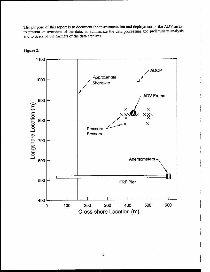
The purpose of this report is to document the instrumentation and deployment of the ADV array, to present an overview of the data, to summarize the data processing and preliminary analysis and to describe the formats of the data archives.

Figure 2.

1100

1000

900 -

c o

"ro 800 o o

2 o sz CO O) c o

700

600

500

400

ADCP Approximate Shoreline

D'

ADV Frame

x 0% X

xxxO< xxx

Pressure Sensors

x x

x x

Anemometers

1

FRF Pier

1 I

100 200 300 400 500

Cross-shore Location (m) 600

II. INSTRUMENTATION

A low-profile frame was designed and built to provide a platform on which to mount five SonTek1 acoustic Doppler velocity (ADV) meters. The instrument array (Figure 3) included three of the 10 MHz field version of SonTek's acoustic Doppler velocimeter (ADVF) and two of the more rugged 5 MHz ocean version (ADVO). The relative positions of the two sensors within each sensor pair were suitable for providing estimates of Reynolds stress by means of the dif- ferencing technique (Trowbridge, 1998) and the sensing volumes were at different heights, so that the measurements can provide estimates of the vertical gradient of Reynolds-averaged horizontal velocity. The offshore ADVF (Figure 4) was likely too far from the other ADVFs to provide reliable stress estimates, and it was included primarily to provide information about vertical structure. Measurements from either the pair of ADVOs or the farthest-onshore pair of ADVFs are sufficient to achieve the objectives described in the previous section.

Figure 3.

1SonTek®, Incorporated, San Diego, CA 92121

The upward-looking ocean probes were simultaneously sampled at 140 msec intervals and logged on a TattleTale2 6-1M for approximately 26 minutes at the beginning of each hour. The side-looking field probes, ADVF_a, ADVF_b and ADVF_c were logged by three separate TattleTale 6F loggers. The sampling was synchronized by using a master logger (ADVF_a), which sent a sync pulse to slave #1 (ADVF_b) and slave #2 (ADVF_c) to initiate simultaneous sampling and logging. The field probes sampled at 25Hz for 9.6 minutes at the beginning of each hour. The ADVs were placed along one side of the frame, which was designed to face the prevailing along-shore current at the experiment site. The battery and logger pressure cases were placed behind ADVF_c, where the sensing volume was above any flow obstruction. The heights of each sensing volume from a nominal bottom are given in the table below.

Sensor ID

ADVFb

ADVF_a

ADVO_B

ADVO A

ADVFc

Serial Number

SN/1160

SN/1152

SN/5026

SN/0005

SN/1154

Height of Sensing Volume (m)

0.36

0.46

0.76

0.86

0.98

ADVO_A was equipped with a strain-gauge pressure sensor, compass, tilt meter and a temperature sensor, which were housed in the probe casing. The probes were coated with two to three coats of antifouling paint, except the transducer faces, which were coated with only one coat.

A static salinity and temperature were defined to provide identical calibration of sound speed (1529.7 m/s) across the sensors. Each of the sensors was set up as follows:

Outformat: Temp: TempMode: VelocityRange: SampleRate: SampleMode: CoordiateSystem:

BINARY 20.31 Sal: 29.71 USER ADVF (250cm/s) ADVO (200 cm/s) ADVF (25 Hz) ADVO (N/A) ADVF (SYNC, master SAMPLE, slaves) ADVO (SAMPLE) XYZ

2Onset Computer Corporation, Pocasset, MA 02559-3450

Figure 4. Instrumentation and orientation

«s^m^^^mmm^eji^^s^mi«^»»».

$ Geographic Coordinates Shoreline Coordinates

<§> SAMPLING VOLUUS

ADF_b ADF_a

<8>

4^J1 0.5 m

ADO_B

N<

>UJO_,4

<8>—

I / \ O.S

n

ADF_c

t m

9 HfömQ

<^ZZ SHOREWARD

Figure 5. Bathymetry from FRF surveys with the location of the ADV array (X)

FRF Survey 8/28/97 FRF Survey 9/16/97

200 300 400 Cross-shore (m)

FRF Survey 10/23/97

500 200 300 400 Cross-shore (m)

500

1100 Points sJwwiitg density of contours

1100 I lie 6 4 Tfct->,-*<# A . »V..r,».-.«.«.>>->l*M<

1000

E, mm, a wn-mer^.^ M*^««'«« % « ff tt #fl »■*■»■■'

900 b sz T 800 -—•——-y

OJ c o < 700 «Hi » ff * n ■««•>■> » «■ ■* v * * m W*M'-*P*L *• •

B00 . - ■•-

200 300 400 Cross-shore (m)

EDO 200 300 400 500 Cross-shore (m)

-2 -■

.1^ 'S > LU _6

-8

•r ■ i' i i

VSW : ; 8/28

^fti_ : 9/16

I 1 — - I I 1

TNV : 10/23

i^^^ : : : :

I I I i i i i

100 200 300 400 500 600 700 800 900 1000 Cross-shore (m|

III. DEPLOYMENT

The frame was deployed on 8/25/97 off the coast at the Field Research Facility (FRF) of the U.S. Army Engineer Waterways Experiment Station (WES), Coastal Engineering Research Center (CERC), using the Coastal Research Amphibious Buggy (cover figure). It was positioned in 4.5 meters at 426.07 meters offshore and 830.38 meters along-shore. (See Figure 2). The position was noted by divers and is relative to the center of the securing post which was nearest ADVF_b. Three separate surveys were conducted by the FRF during the deployment of the ADV array, providing the bathymetry near the deployment site, as seen in Figure 5. Five posts were hydrau- lically driven approximately 15 feet into the sandy bottom to secure the frame, both above and below each foot. This provided a stationary height, but, as noted by divers, the bottom beneath the frame scoured as much as 30 cm (Figure 6a). The orientation of the frame was observed to be such that the instrumented edge of the tripod was 80° from Magnetic North. The magnetic deviation at the site is approximately 10° from True North, which confirmed that the edge was shore normal, as planned. Upon recovery of the instrument (11/21/97), it was found that the base of each sensor, the channel and the pressure casings were encrusted with deposits from the sand builder worm, sabellaria vulgaris (personal communication, A. Frese and V. Starczak ,WHOI). (See Figure 6b). These deposits may have caused significant flow disturbance in the latter part of the experiment.

The head of ADVO_A developed a small leak, which eventually caused intermittent failure of the velocity sensor after 8/31 04:00 EST, and ultimate failure of the velocity sensor by 10/29 16:00. The compass, tilt and velocity boards were affected, but the pressure appeared to be pro- tected and continued to function for the duration. ADVF_b was bumped on 8/31 04:00 which caused contamination of the vertical axes with flow from the x direction and on 9/4 04:00 path 2 dropped out (correlation coefficient went from about 96% to 41%). Upon recovery, the angle of tilt seemed to be on the order of 20° about the x axis with the shoreward side of the head coming up out of the x-y plane. ADVF_a was completely mangled upon recovery, but it appeared to work well through 9/3 19:00 EST. The field probe loggers failed after 10/10/97.

Since 1978, the National Oceanic and Atmospheric Administration (NOAA)/National Ocean Service (NOS) has operated a primary tide station (No.865-1370) at the seaward end of the FRF pier, tide gauge #11. A NOS acoustic tide gauge (Next Generation Water Level Measurement System, NGWLMS) is used to collect water level data every 6 minutes throughout the month. Data are referenced from meters to NGVD.

Two anemometers were mounted on a mast at the end of the pier. Jim Edson (WHOI) deployed a 3-axis Solent ultrasonic anemometer model 1012R2A1 at 21.7 meters above NGVD, providing wind speed, air temperature, tilt, covariance of horizontal wind and temperature with vertical wind velocity. The data were observed at 20.833Hz for twenty minutes continuously. A K-Gill Impellor vane anemometer (Model 35301)2 was deployed at 24.6 m above NGVD by Chuck Long (FRF), sampling at 4 Hz for approximately 51 minutes for each burst.

-■-Solent mfgrd by Gill Instruments Limited, Lymington, Hampshire (England) 2K-Gill mfgrd by R.M.Young Co., Traverse City, MI

Figure 6a. Scouring below the sensor was evident in photo taken 9/4/97, courtesy Steve Elgar.

Figure 6b. Fouling of frame was evident upon recovery on 11/21/97.

IV. DATA PROCESSING

The data were unpacked and each burst was stored in a Matlab®1 file, using the month, day, hour and minute (EDT) in the filename. The format for each of these files is described in Section VII. The data were then converted to real world coordinates (Figure 4), where v is along-shore southward flow (m/s), u is cross-shore (shore-ward) flow (m/s) and w is vertical flow (upward) (m/s).

For probes ADVF_a, ADVF_b and ADVOJB, data were flagged bad when the correlation coefficient was less than 70 and were replaced with NaNs. Probe c had signal amplitudes significantly lower than the other field probes, which resulted in lower correlation coefficients. Beam 3 of field probe c often had correlation coefficients below the 70% threshold. For ADVF_c, the correlation coefficients were not used to clean up the burst data, but they were used in determing the burst averaged statistics.

Velocity data for all probes were wild point edited by replacing all points greater than four standard deviations away from the mean of each burst with NaNs.

For ADVO_B, about 91% of the bursts lost no more than 5% of the data in using these techniques. Most were flagged bad due to the correlation coefficient test and these were primarily between year day 277 and 287, when the signal strength was low.

The correlation coefficient and signal strength did not provide a reliable means to determine valid data for the faulty probe ADVO_A, so a technique was developed which compared 100 point (14 second) blocks of ADVO_A with simultaneously sampled ADVO_B, accepting the block when there were more than 10 valid (non-zero) samples in the block and the two velocities were highly correlated, with the squared correlation coefficient, R2, greater than 0.9 and 0.8, for horizontal and vertical velocities, respectively. Otherwise, the block was replaced with NaNs. The data were truncated to 11000 points per burst, being an even interval of 100 blocks, using N = 37:11037 and 38:11038 for ADVO_A and ADVO_B, respectively, to provide the best cross-correlation between the probes.

The orientation of ADVF_c was resolved by determining the principal axes of the burst averaged velocities during the first six days. The transformation matrix is presented below and was applied to each burst as follows:

[vuw]= (C'x[zyx]y

c = -0.5176 -0.8513 -0.0857

-0.8437 0.4912 0.2167

0.1423 -0.1845 0.9725

J-The MathWorks, Inc., Natick, MA 01760

Two sets of burst statistics were created. A set of 132 hours of data between 8/25/97 10:00 and 8/30/97 21:10 EST, representing the mean of the first 9.6 minutes of data at the top of each hour. Times when the mean correlation coefficient of probe ADVF_c, path 3, was less than 70 were masked with NaNs. The second set of data includes 25.7 minute burst statistics from the ocean probes for 2083 hours. Sta- tistics using data from ADVO_A contains NaNs when the instrument was not functioning during more than 90% of the burst.

The standard deviation of the velocity and signal strength was computed from detrended data.

The mean half-hourly estimates of cross-shore and along-shore bottom stress were computed using a dif- ferencing technique (Trowbridge, 1998). Field probes were paired (ADVF_a with ADVF_b) and ocean probes were paired (ADVO_A with ADVO_B). Outliers in du, dv and dw (points more than 4 standard deviations away from the mean) were excluded from the estimates of <u'w'> and <v'w'>.

As documented in Section VI, our pressure sensor did not provide reliable estimates of depth. There- fore, depth was derived by adding the tide data from NOS tide gauge #11 to the NGDV elevation of the ADV frame (determined by the location and the FRF surveys). The variance from pressure was not affected and is used as described below. Pressure counts were converted to meters using Sontek supplied calibration coefficients: meters = dbars = 0.000287*counts-1.13.

Dissipation was derived from spectra computed using 14 second blocks with a Hanning window and no overlap. Integration was performed between 1 and 2 Hz, in an attempt to stay within a region of fre- quencies above the wave peak and below the noise floor. Spectra were corrected for advection of surface waves (Lumley and Terray, 1983; Trowbridge and Elgar, submitted).

The bottom orbital velocity, U^, was computed as the square root of the sum of the variance of the horizontal velocity between 0.05 and 0.5 Hz. Significant wave heights, Hs, were estimated by convert- ing the pressure spectra to surface wave variances, Sim, using linear wave theory, and integrating in the wave peak (0.05 - 0.21 Hz). Significant wave heights were also calculated from horizontal velocity variance, using linear wave theory, and are compared with the estimates derived from the pressure data in Section VI. For these parameters, spectra were computed using 1028 point (144 second) blocks with a Hanning window and no overlap. The mean frequency in the wave band was computed as a weighted mean:

f 0.5Hz (Suu+Sw) »f «df

p J 0.05Hz V '_

^bar ~ r0.5Hz /•u.jnz

(Suu+Sw) • df J 0.05Hz V /

The sonic anemometer data were converted to the along-shore, oceanographic coordinate system (Fig- ure 4.). The twenty minute burst statistics were computed without detrending or windowing. Variance greater than 0.6 m2/s2 was replaced by NaN. The time (year day) was converted to EST, with 0.5 desig- nating noon on 1/1/1997 and linearly interpolated to correspond with the 9.6 and 25.7 minute burst data for each set. Density (p) was computed using air temperature (T), p = 101300/287/(T+273.16) and heat

flux was derived as 1004*p*<wT'>.

10

V. DATA SUMMARIES

Figures 7-19 present data from all five ADVs along with wind statistics from the sonic anemometer, for the first five and a half days, when all the sensors were functioning well. Figures 20 - 27 present data, as it was available, through the first 60 days. The data were truncated for the report, since there were no turbulence statistics available after ADVO_A failed.

The significant wave heights presented are those computed from the pressure spectra and the bottom orbital velocity are those computed from horizontal velocities. For the long time series, the bottom orbital velocities presented are those from the horizontal velocities of ADVO_B.

11

Figure 7. Unfiltered flow (up is along-shore, southward & right is onshore)

— 0.05 m/s

1

M :.0 mab

0.9 mab

V .w

\

^

8 mab

5sb^>

ÖLLs

s\\V lUk

MiJ

•^ .\\\\]

^••\y/

^'^"iy

,fxW,\Li

.5 mab

it4ii»ii.i.>4LkiiJkx

\MlllllNIK 0:4 mab

!i\L.

\\/M\w

'~-^l \s\\v

\ ,\\\ yi\ I j «H A\ i //A A ?\ ^

i\v A\\V\\

\v

l\

MmM\

V ,,\im K

,,A^v\\iI

,v,rtA ^v

M

236 237 238 239 240 241 242 Year day 1997

12

Figure 8. Onshore velocity

0.05

0

-0.05

: 1 j

0.9 mab 1 M^ vvK H />

■ 1 1

V I

0.05

0

-0.05

236 237 238 239 Year day 1997

240 241

: : :

0.5 n lab A r- v /J ■<\ A .—

f i^W 4 /^

' ■ ■

242

13

Figure 9. Alongshore velocity

-0.1

0.3

0.2 H

0.1

0

-0.1

0.3

0.2-

0.1 -

-0.1

0.3

0.2

0.1

0

-0.1

0.3

0.2 h

0.1

0

1 1 !

0.9rhab \

i • ' I ' -J •

■■

.... i i

0.8 rhab

■ • • i '

.... -

0.5 rhab y^ ̂ M • ■

1 '

-0.1

... r

0.4 rhab

• ■ ■ ' ■ •

236 237 238 239 Year day 1997

240 241 242

14

0.05

0.025

0

-0.025 h

Figure 10. Upward velocity :

1.0 mab

^V^

■ ■

0.025

0

-0.025

-0.05

; j ! ; j ;

0.4 mab

"IN^AÄ : A^^ . v i^^y ;

• I i i

236 237 238 239 Year day 1997

240 241 242

15

Figure 11a. Water Depth from FRF tide gauge 11

242

Figure 11b. Significant wave height from pressure

242

Figure 11c. Water temperature at ADVO_A

239 Year day 1997

242

16

Figure 12. Bottom orbital velocity

236 237 238 239 Year day 1997

240 241 242

17

Figure 13. Angle of incidence of waves (+90 represents waves from south)

0

25

20

15

10

236 237

- i : : ! I

^ -

0.4 mab

■ ■ ■ I I

238 239 Year day 1997

240 241 242

Figure 14a. 0.25

Dissipation estimates from vertical flow of ocean probes

236 237 238 239 240 241 242

Figure 14b. Dissipation estimates from vertical flow from field probes

236 237 238 239 Year day 1997

240 241 242

19

Figure 15. Estimates of stress from sensor pairs (Pa)

field probes ocean probes

0.15-

IE 0.1

0.05-

236 237 238 239 240 242

0.15

ß 0.05

-0.05 236 237 238 239 240 241 242

0.05

.a-0.05

-0.1 -

-0.15 236 237 238 239 240

Year day 1997 241 242

20

Figure 16a. Mean signal stength of each 5 MHz ocean probe

242

Figure 16b. Mean signal stength of each 10 MHz field probe

236 237 238 239 Year day 1997

240 241 242

21

Figure 17a. Mean standard deviation in signal stength of each 5 MHz ocean probe

236 237 238 239 240 241 242

Figure 17b. Mean standard deviation in signal stength of each 10 MHz field probe

236 237 238 239 Year day 1997

240 241 242

22

Figure 18. Wind speed (up is southward / right is onshore) from sonic anemometer

242

242

28

27.5

_ 27 O 5? 26.5

Q. 26 £ r 25.5 "<

25

24.5

24 236 237 238 239

Year day 1997 240 241 242

23

-0.08 236

Figure 19. Wind stress (up is southward / right is onshore) from sonic anemometer -l : 1 : T

237 238 239 240 241 242

-0.08 236 237 238 239 240 241 242

x LL

"S CD X

20

15-

10-

5-

-5

-10 236 237 238 239

Year day 1997 240 241 242

24

■ !C ! ■__ —»- ■

CD

(M

CO

CM

O

CM

00 CM

co CM

oo CM

CO

CM

in CM

CM

CM

N§ CO 5* CD CO CM "O

1_

CQ 00 CD co >- CM

o CD CM

Lf) CM

lO CM

CM

CO

CM

CM

CM

CM

CO CM

CO CM

~c5

O C\J

~o

"O

■sl-

"o

oo ~c5

in "o

co

o -co o5

o (S/LU) A

v- o t— CM CO ■* CD ■* CM o o

1 O

1 o

1 o

1 o CD

o Ö

O

CD

CM O

(s/w) n

CD CO

■*CM O CD

I

-CM >, S5 «

■* CO -CM T>

_ <0

o5

co

o5

in

o5

CM

o5

_cn o5

-CD o5

-co o5

-cö co

co -CJ

co

m -CM

co

(S/w) M

25

LO LO lO LÖ -^

(m) indea

CO

o

"o

"o

CO

"o

CO

o -co

-C\i

-CVJ O)

-C\J CD

CO

en

in

a5

<M

o5

-CJ3 CD

-co o5

-CO en

-co oo

oo -CM oo

in -OJ oo

I (sjejeui) H (0 ß9Q) ejn;BJedaiei

i 26 i

!

1

%

4 *

4

>

*

CO

C\J

o C\J

1^- oo CM

CO CM

00 C\J

CO

CM

If)

CM

CM

CM

CO CO CM

CD CO CM

N. O) OS

>s CO

■D

CO CD CD CD >- CM

(2s/zui) n (seajßap) SSABM JO e|ßuy

•«fr CO CM T-

ö d ö d (ZH) >|Bed 9ABM

o CD CM

1^. LD CM

in CM

oo CM

IT)

CM

CM

CM

CD CO CM

CD CO

OCM

CO CM

~o

o CM

O

~o

"o

00 ~c3

JO

CO

"o

o -co o5

-CM

-CM

CO

-CM

CO

oo

o5

ID

o5

CM

o5

o5

-CD o5

-CO

o5

oo

oo -CM

oo

in -CM

00

i \ 27

c o '■*—'

CO Q.

'co to

CO

£ to LU

CO CM a>

CO +_

coT

_L

CO +_

CO"

E ■i'

0- o

CO.

E o -i

CO CO CM m CM O

o CO CM m CM O

Is- O T— m CM o

Is- 00 _^^, CM

T— ■* ^_ m ~"^- CM o

,_ CO CO CM "CD

00 LO

CM "Ö

LO CO Is- <M "CD

CM o Is- -co CM en

CD r-- CO Is- -CM CM 05

O) en

CO >. ■*

CO CO - -CM CM •a

CO

en

CO CD T—

CO CM

>- " -CM en

O CO CO —^~ CM 05

Is- LO in —T~~

CM c55

■* CM LO —r— CM en

LO -CJ5 CM en

CO -CO CM en

LO -CO CM en

CM ,_ ■* -co CM CO

en co CO -CM CM co

CO CO

LO LCM 00 CO -* CM

(VOAQV) 3 o oo CO rf CM

(a_OAav) 3 00 ^MM "^ ^ /Mim \

( s LU04) 3

OCM 00

28

1 1 1 1

~: ~^_

^^g"

~i

j CO CD .a o Q. c CO CD Ü O

T3 CD Ü

CD

CD 3=

-A

J

—

-a E

*♦—

CO 0)

-^=-

E to CD

CO CO CD

: 4 •• • 5-

tt) *

CM <U

1 1 i i 1 *

<

I

>

■

^

CD

CM

CO

CM

o CM

00 CM

oo <M

00 CM

00

CM

in CM

CM

CM

as

>> CO

T3

CO CO CD co >- CM

T- 00 co CM o o o o

(Bd) \\

in d

<BdA (Bd)

in ö 4

o CD CM

m CM

in CM

-\ in CM

CO •- ■*

CM

m CM

CM

CM

0) CO CM

CO CO CM

CO CM

"o O CM

O

00

in "o

co "o

o -co

5>

-CM

o5

-CM

o

-CM

oo

3> in

o5

CM

o5

_cn o5

-CD o5

-CO

o5

1—

-CO 00

00 -CM

oo

in -CM

00

29

in o in o in o in o m o O) CT> oo 03 r-- i*- CD to in m C\J

(gp) aßejeABjsjnq

o co co rr c\j

(gp) uo!;BjA8p pjepuejs isjnq

00 CO ~o

o

~o

r*-

~o

"o

00

in "o

CO

o -co o5

-OJ OS

O)

-C\J O)

oo

o5

m

o>

CM

o5

o5

-CD o5

-00 o5

-cö oo

oo -CM 00

in -CJ co

30

I

CO CD C\l <n CM o

o CO CM rr> CM O

o <n —"*-^. CM o

K en CM o

^ T_ en —■-»».

CM o

,_ 00 oo CM

~c3

on in

CM "Ö

ID CO

CM ~c5

CM o r^- -co CM o>

<J) i^ co h» -CM CM CD

05 o

CO >- ■* CO CC - -CM CM T3

CO

O)

C) CD T— co >- ~ -CM CM O)

o CO CO —T~* CM o5

r>- in m —f—

CM CD

rf CM LO —r- CM OJ

in -O) CM O)

oo -CD

CM CT>

-CO CM CT>

CM ,_ •* -C) CM CO

CD co CO -CM CM oo

CO in CO LCM

in o m o in o mcM I T- 1-

I I (s/w) A (s/w) n

in o T

incvjin T- co

o CO

in CM

O CM

OCM 00

(0 ßsp) doiei Jiv

I I 31

CD co

ocvi in

i

CO CM o

o

"o

"o

oo _c5

in "o

co "o

o -co 05

-JM

-CM as

oo

55

m

o5

CM

o5

-52

-co o5

_co o5

-co oo

co -CM

oo

in -CM

co

(Bd) * (S_uu/V\) xnid }B9H

32

VI. DATA ANALYSES

Comparison of wave characteristics from ocean probes and pressure sensor

Figure 28a shows that the significant wave heights computed from velocity and pressure are highly correlated. Figure 28b documents the strong correlation in the wave peak between the two ocean probes. The data are only compared for the first 5.5 days when both probes were fully functional and the full wave peak could be resolved.

Figure 28a. 8/25/97 - 10/23/97 Figure 28b. 8/25/97-8/31/97

2.5

00 i

O £l < E o

2

.5

0.5

r I—— . n

Jp 1

■*

Jr • R2 = 1.00;

m = 0.94 ± 0:00

b = 0.03 ± 0.00

0.5 1 1.5 2 H from pressure (m)

2.5

2.5

CD I

O Q 1.5 < E 2 1

0.5

0

: : '

R2 = 1.00;

m = 1

b = 0.

.03 ± 0:01

01 ±0.01

0 0.5 1 1.5 2 2.5 H fromADVO A (m) s — \ i

33

in LO

m in rr m

(LU) ejnssajd LUOJJ u.;dea in"

in m ■<- m ■^ co

(LU) L L eßneß apji WOJJ indea

34

Comparison of pressure from ADVO_A with the FRF tide gauge No. 11

Tide gauge data from NOS Tide gauge 11, averaged to represent the first half-hour of each hour, are compared here with pressure data from the strain gauge sensor mounted in the end cap of ADVO_A. Figure 29 documents the offset presumably from the temperature sensitivity of the strain gauge sensor. Figure 30 compares the tidal fluctuations and indicates that the temperature sensitivity of the strain-gauge pressure sensor only affects an offset, not a change in gain. Low- pass filtering was applied using pl64t.m (Rosenfield, 1983) to derive the tidally averaged depth, so it could be removed.

Figure 30. Tidal variance in depth from FRF gauge vs. ADVOA pressure sensor

0.8

0.6

0.4

-O-0.2 D. CD

CD Q.

I

£-0.2 -

a. ■D -0.4

-0.6 -

-0.8

-1

1 ,..,, I

R2 = O.99 ;

1 ]--■ '

.•. }/

m = 1.04 ±0.01 •V

b = 0.00 ± 0.00 jBr

■

• tJpF ;

IF*"• ■ ■ ■

9

»

~ jfir'**

«

/ i i i i i '

-1 -0.8 -0.6 -0.4 -0.2 0 0.2 0.4 0.6 0.8 1 depthtg11-pl64t(depthtg)(m)

35

Figure 31.

Cross-shore wind speed (m/s)

0.6

0.4

0.2 c o « 0 LU

-0.2

-0.4

Long

Cross-shore wind stress (Pa)

c

• V/

.

• +tr ft***

» : R2 = 0.68

. *ro-. 1.1.1.±0.06..

b = 0.00 ± 0.01

Along-shore wind speed (m/s)

Long

Along-shore wind stress (Pa) U.b

0.4

0.2

d /... ..

c o

■D U 111

-0.2

. jt fr •

>*"• R2 = Q.85

-0.4 b = -

1.35 +

-0.01 ±

0.04 ..

0.01

-0.4 -0.2 0 0.2 0.4 T,

Long

-0.4 -0.2 0 0.2 0.4 T,

Long

36

Comparison of wind data from FRF K-vane anemometer with Edson sonic anemometer

The data from the sonic anemometer are compared here with the data from the vane anemometer. Much of the scatter in the comparisons of the turbulence statistics can be attributed to different processing techniques. The vane data were processed by detrending the data, using smaller win- dows (512 second) and cleaning up times when there was slow wind speed or the wind, at any time, passed through the 5-degree 'dead zone'. As seen in Figure 32, both sensors observe en- hanced turbulence when any component of the wind blows off-shore.

Figure 32. Comparison of observed stress with estimated stress (Large & Pond, 1981)

Cross-shore wind stress (Pa) Along-shore wind stress (Pa) 0.6

0.4

0.2 CD

§ 0

-0.2

-0.4

a

• * • •• fy*

■ m't^r

»

: / y : R2 = Q.68 . . m~1.76.+:0.10..

/ ' b =-0.04 ±0.01

0.6

0.4

0.2 c o -o U LU

-0.2

-0.4

-0.4 -0.2 0 0.2 0.4 TL&P(Long)

Cross-shore wind stress (Pa)

c

• */

/jf ^^

. . *m.=

R2 = 0.50 2.04±.Q.17..

-0.04 ±0.01 t

b = -

0.6

0.4

0.2

§ 0

-0.2

-0.4

b

!'... !£/

'sJf

...

/,-•). : R2 = 0.77

. . ras 1.2.1.±0.05..

b = -0.01 ±0.01

0.6

0.4

0.2

0

-0.2

-0.4

-0.4 -0.2 0 0.2 0.4 TL&P(Long)

Along-shore wind stress (Pa)

d :$ :& &*?}

«.

A|7&*

■■■■/*§■ :R2 = O

. . ra-.1.56.±

b = -0.01 ±

.75 0.07..

0.01

-0.4 -0.2 x,

0 0.2 0.4 LSP(Edson)

-0.4 -0.2 0 0.2 0.4 \&P(Edson)

37

VII. FILE DESCRIPTIONS

ADV FIELD PROBE

Binary data files

All three loggers placed a time stamp at the beginning of each burst. Each file block is 529288 bytes long and contains two bursts. Each burst contains data which were logged continously for 9.6 minutes at 25 Hz and formatted as described below.

ADV field probe format Each block began with a date stamp (EDT): MMDDHHMNSE (month,day,hour,minute,second)

and was followed by two sets of about 14400 records as follows:

Variable # variables bytes/variable bytes units

Keyword(8112) Sample Id Velocity Signal Strength Correlation Coefficient Checksum

1 1 3 3 3 1

2 2 2 1 1 2

2 2 6 3 3 2

1 - number of samples in burst (0.1 mm/sec)

(counts, where 0.43 dB/count) (0 to 100, where > 70 is considered ok)

sum of bytes plus base (0xa596)

Total bytes/record: 18

The data were unpacked, and truncated to the first 14400 samples, using binadvfps.m and docleans.m, where s is the sensor id (a, b or c).

Processed burst data files

Field probe data were stored on one CD for 8/25 11:00 - 9/4 23:00 (EDT). Each sensor's data was stored in its respective file which was named sMODAHRx.mat, where s is a, b or c for ADVF_a, _b & _c, respectively, and x is either V for velocity data, A for signal strength or C for correlation coefficients. These files include the following data:

vs, us, ws - along-shore, cross-shore and vertical velocity (m/s), where s is the sensor. Data includes NaNs.

samp - signal strength (dB) of sensor s (a, b or c) sec - correlation coefficient for each of the sensors (s) (%)

39

ADV OCEAN PROBE

Raw data files

The ocean probes were logged simultaneously. Each 140 milliseconds, a burst was recorded from each sensor, beginning on the hour and recording for 25.6 minutes. Two bursts were recorded per file block (1015808 bytes).

ADV ocean probes format Each block began with a date stamp (EDT): MMDDHHMNSE (month,day,hour,minute,second)

and was followed by 11038 records as follows:

Variable # variables bytes/variable bytes Probe units

Keyword(871c) Sample Id Velocity Signal Strength Correlation Coefficient heading pitch roll temperature pressure Checksum Keyword(8112) Sample Id Velocity Signal Strength Correlation Coefficient Checksum

1 1 3 3 3

3 3 3 1

2 2 2 1 1 2 2 2 2 2 2 2 2 2 1 1 2

2 2 6 3 3 2 2 2 2 2 2 2 2 6 3 3 2

A A A A A A A A A A A B B B B B B



(0.1 degrees) (0.1 degrees) (0.1 degrees)

(0.01 degrees C) (counts)





Total bytes/record: 46

Processed burst data files

These unpacked raw files were cleaned up (docleanA.m & docleanB.m) and shifted so that Ocean Probe A & Ocean Probe B are in phase. (See Section III.) The cleaned up data files con- tain vP, uP, and wP, where P is either A or B in files named sdP_MMDDHHV.mat, and the correlation coefficient and signal strength (in integer dB) were stored in sdP_MMDDHHC or sdP_MMDDHHA.mat, respectively. The data for Ocean Probe A should be dealt with in blocks of 100, since the processing was completed on those blocks. (See dissipation.m.) The pressure (m) and temperature (degrees C) are stored in sdP_MMDDHHPT.mat. Time (month, day and hour) for these files are taken from the filename (EDT) and the minute can be reconstructed by adding (37*0.14:0.14:11000)760/24 to the day of year.

40

BURST AVERAGED PROCESSED DATA

By computing the burst averages of each parameter, hourly estimates centered at 12.8 minutes after the top of the hour are stored in sandyduckL.mat. Time (tdoy) is year day, with 0.5 representing noon on January 1, 1997 (EST). windL.mat contains the sonic anemometer hourly averaged wind statistics for the long record.

sandyduckS.mat contains the first six days only, containing the field probe data and the burst averaged data from the ocean probes, during the times corresponding to when the field probes were sampling. Time (tdoy) is year day (EST), with 0.5 representing noon on January 1, 1997. windS.mat contains the wind statistics from the sonic anemometer, interpolated to correspond to the burst averaged time of the field probes.

I

I 41

42

VIII. ACKNOWLEDGMENTS

We thank the following WHOI personnel: Sandy Williams, for his experienced guidance and assistance in the development of the data loggers; Don Peters and Glenn McDonald for the development and supervision of the building of the instrument frame; and, Cully Sullivan and Chris Lumping for the technical drawings.

We gratefully acknowledge the excellent support provided by the staff at U.S. Army Corps of Engineers, Coastal Engineering Research Center, Field Research Facility. Also, we thank Steve Elgar and Britt Raubenheimer and their group for their invaluable assistance in the deployment of the frame and subsequent surveillance dives on the frame. We also credit the NOAA, NOS, for the use of the tide gauge data, and Chuck Long (FRF) for providing us the use of the wind data from the K-Gill Impellor Vane at the end of the pier.

We thank Bill Shaw and the divers of Max Marine, Kill Devil Hills, NC, 27948, for their assistance in the recovery of the instruments.

This project was funded by grants from the Mellon Foundation, Rinehart Coastal Research Cen- ter (WHOI), and the National Science Foundation (Grant number OCE-9810609).

43

44

IX. REFERENCES

Lumley, J. L. and E. A. Terray, 1983. Kinematics of turbulence convected by a random wave field. J. Phys. Oceanogr. 13, 2000-2007.

Rosenfield, L. K. (Ed.), "CODE 1: Moored Array and Large-Scale Data Report", Woods Hole Tech. Rep. WHOI 83-23, 185 pp, Woods Hole Oceanogr. Inst., Woods Hole,Mass., 1983.

Shaw, William J., A.J.Williams 3rd, and J.H.Trowbridge, "Measurement of Turbulent Sound Speed Fluctuations with an Acoustic Travel-Time Meter", Proceedings OCEANS'96 MTS/IEEE, pp. 105-110.

Shaw, William J., A.J.Williams, and J.H.Trowbridge, "Measurement of Near-bottom Turbluent Fluxes in the Presence of Energetic Wave Motions". J. Atm. and Ocean. Tech., submitted.

Shaw, William J. and J.H.Trowbridge, "The Budgets of Turbulent Kinetic Energy and Scalar Variance in the Continental Shelf Bottom Boundary Layer", Journal of Geophysical Research, submitted.

Trowbridge, John H. "On a Technique for Measurement of Turbulent Shear Stress in the Pres- ence of Surface Waves", J. Atm. and Ocean. Tech., 15:290-298, 1998.

Trowbridge, J. H. and Elgar, S., "Turbulence Measurements in the Surfzone", J. Phys. Ocean- ogr., submitted.

Voulgaris, George, J.H.Trowbridge, W.J.Shaw & A.J.Williams, "High Resolution Measure- ments of Turbulent Fluxes and Dissipation Rates in the Benthic Boundary Layer", Coastal Dy- namics'97, ASCE: 177-186.

45

DOCUMENT LIBRARY Distribution List for Technical Report Exchange -July 1998

University of California, San Diego SIO Library 0175C 9500 Gilman Drive Lajolla, CA 92093-0175

Hancock Library of Biology & Oceanography Alan Hancock Laboratory University of Southern California University Park Los Angeles, CA 90089-0371

Gifts & Exchanges Library Bedford Institute of Oceanography P.O. Box 1006 Dartmouth, NS, B2Y 4A2, CANADA

NOAA/EDIS Miami Library Center 4301 Rickenbacker Causeway Miami, FL 33149

Research Library U.S. Army Corps of Engineers Waterways Experiment Station 3909 Halls Ferry Road Vicksburg, MS 39180-6199

Marine Resources Information Center Building E38-320 MIT Cambridge, MA 02139

Library Lamont-Doherty Geological Observatory Columbia University Palisades, NY 10964

Library Serials Department Oregon State University Corvallis, OR 97331

Pell Marine Science Library University of Rhode Island Narragansett Bay Campus Narragansett, RI 02882

Working Collection Texas A&M University Dept. of Oceanography College Station, TX 77843

Fisheries-Oceanography Library 151 Oceanography Teaching Bldg. University of Washington Seattle, WA 98195

Library R.S.M.A.S. University of Miami 4600 Rickenbacker Causeway Miami, FL 33149

Maury Oceanographic Library Naval Oceanographic Office Building 1003 South 1002 Balch Blvd. Stennis Space Center, MS, 39522-5001

Library Institute of Ocean Sciences P.O. Box 6000 Sidney, B.C. V8L 4B2 CANADA

National Oceanographic Library Southampton Oceanography Centre European Way Southampton SO 14 3ZH UK

The Librarian CSIRO Marine Laboratories G.P.O. Box 1538 Hobart, Tasmania AUSTRALIA 7001

Library Proudman Oceanographic Laboratory Bidston Observatory Birkenhead Merseyside L43 7 RA UNITED KINGDOM

IFREMER Centre de Brest Service Documentation - Publications BP 70 29280 PLOUZANE FRANCE

50272-101

REPORT DOCUMENTATION PAGE

1. REPORT NO. WHOI-2001-02

3. Recipient's Accession No.

4. Title and Subtitle Turbulence in the Shallow Nearshore Environment during SANDYDUCK '97

5. Report Date February 2001

7. Author(s) jj. Fredericks, John H. Trowbridge, George Voulgaris 8. Performing Organization Rept. No.

WHOI-2001-02

9. Performing Organization Name and Address

Woods Hole Oceanographic Institution Woods Hole, Massachusetts 02543

10. Project/Task/Work Unit No.

11. Contract(C) or Grant(G) No.

(C) OCE-9810609

(G)

12. Sponsoring Organization Name and Address

National Science Foundation Mellon Foundation Rinehart Coastal Research Center

13. Type of Report & Period Covered

Technical Report

14.

15. Supplementary Notes

This report should be cited as: Woods Hole Oceanog. Inst. Tech. Rept., WHOI-2001-02.

16. Abstract (Limit: 200 words)

An array of five acoustic Doppier velocimeters (ADV), which produce high quality measurements of the - three-dimensional velocity vector in a sample volume with a scale of one centimeter, was deployed from

late August through late November of 1997, at a water depth of approximately 4.5 m off Duck, North Carolina. The sensors were deployed near the sea floor but above the centimeters-thick wave boundary layer, and the sampling scheme was designed to resolve turbulence statistics averaged over tens of minutes, much longer than typical wave periods but shorter than time scales associated with variability of energetic wind-driven and wave-driven along shore flows. The purpose of this report is to document the instrumentation and deployment of the ADV array, to present an overview of the data, to describe the data processing and preliminary analysis, and to document the formats of the data archives.

a. Descriptors 17. Document Analysis turbulence nearshore SANDYDUCK

b. Identifiers/Open-Ended Terms

c. COSATI Field/Group

18. Availability Statement


19. Security Class (This Report)

UNCLASSIFIED 20. Security Class (This Page)

21. No. of Pages

54 22. Price

(SeeANSI-Z39.18) See Instructions on Reverse OPTIONAL FORM 272 (4-77) (Formerly NTIS-35) Department of Commerce

Woods Hole Oceanographic Institution \ ft* - DTIC

Documents

Transcript of Woods Hole Oceanographic Institution \ ft* - DTIC