arX

iv:a

stro

-ph/

0512

476v

1 1

9 D

ec 2

005

AJ, accepted for publication 15 Dec 2005

A Synoptic, Multiwavelength Analysis of a Large Quasar Sample

A.W. Rengstorf1, R.J. Brunner, and B.C. Wilhite

Department of Astronomy, University of Illinois, Urbana, IL 61801

and

National Center for Supercomputing Applications, Champaign, IL 61820

ABSTRACT

We present variability and multi-wavelength photometric information for the

933 known quasars in the QUEST Variability Survey. These quasars are grouped

into variable and non-variable populations based on measured variability confi-

dence levels. In a time-limited synoptic survey, we detect an anti-correlation be-

tween redshift and the likelihood of variability. Our comparison of variability like-

lihood to radio, IR, and X-ray data is consistent with earlier quasar studies. Us-

ing already-known quasars as a template, we introduce a light curve morphology

algorithm that provides an efficient method for discriminating variable quasars

from periodic variable objects in the absence of spectroscopic information. The

establishment of statistically robust trends and efficient, non-spectroscopic selec-

tion algorithms will aid in quasar identification and categorization in upcoming

massive synoptic surveys. Finally, we report on three interesting variable quasars,

including variability confirmation of the BL Lac candidate PKS 1222+037.

Subject headings: galaxies: active – methods: data analysis – quasars:general –

quasars:individual (PKS 1222+037) – surveys

1. Introduction

A considerable amount of analysis has been carried out on various aspects of quasar

variability (see Helfand et al. 2001, for a review of past surveys). For example, Cristiani et

1current address: Department of Chemistry & Physics, Purdue University Calumet, Hammond, IN 46383;

adamwr@calumet.purdue.edu

– 2 –

al. (1996) merged variability results from quasars in three separate photographic plate fields:

SA 57 (Trevese et al. 1994), SA 94 (Cristiani et al. 1996), and the South Galactic Pole (Hook

et al. 1994) to study ensemble and individual quasar variability for several hundred quasars.

Recent work (Vanden Berk et al. 2004; de Vries et al. 2005) has utilized the large number of

quasars discovered by the Sloan Digital Sky Survey (SDSS) to make statements on quasar

variability on an ensemble basis for ∼104 quasars with two or three data points per quasar

light curve. In summary, most previous variability studies focus either on a large number

of epochs for a relatively small sample of quasars, or a small number of epochs for a large

sample of quasars.

In this paper, we take a somewhat different approach. The QUEST Variability Survey

(QVS: Rengstorf et al. 2004b, hereafter, R04b) contains light curves in up to four bandpasses

for nearly 200,000 objects. The QVS contains 69 scans of a thin strip of high Galactic latitude

equatorial sky (−1.2 ≤ δ ≤ 0.2; 10h ≤ α ≤ 15h30m) collected between 1999 February and

2001 April. Four broadband filters (camera filter order: RBRV ) were used throughout

the variability scans. Typical seeing at the site was about 2.′′8 and a limiting magnitude of

r = 19.06 was reached. The filter set and observing cadence were chosen to optimize between

multiple variability-driven projects, including a SNe 1a search and a recently published RR

Lyrae catalog (Vivas et al. 2004). The synoptic study of ∼105 light curves with several

observations per lunation for several lunations per year for several years will serve as a

testbed for algorithms and selection techniques for upcoming massive synoptic surveys (e.g.,

LSST, JDEM, Pan-STARRS). We see a need to develop robust techniques that bridge the

gap between working with well-sampled individual quasars (e.g., 3C 273) and working with

105 − 106 objects.

We combine the synoptic data from the QVS with published spectroscopic quasar cat-

alogs to study the variability of confirmed quasars. We use the Global Confidence Level

(GCL) parameter (see R04b for complete details) to construct populations of variable and

non-variable quasars. This technique identifies variable objects based on the statistical like-

lihood that the object is reliably varying above the photometric noise of the entire ensemble.

An object’s GCL value is the weighted average of confidence levels for every bandpass in

which we have data for that object. In using the likelihood of variability rather than the

amplitude of variability to identify variable objects, we account for increased photometric

noise near the magnitude limit of the QVS. Using a critical GCL value for the determination

of variability allows easy fine-tuning for completeness and efficiency based on the particular

needs of the study.

Extending our analysis to other wavelengths, we match the QVS synoptic data of the

known quasars to several large-area, non-optical catalogs. First, we identify differences

– 3 –

in global variability statistics based on quasar rest-frame time baseline and known quasar

detection/non-detection in non-optical (Radio, IR, and X-ray) catalogs. Second, we look at

the redshift and multi-wavelength luminosities of variable and non-variable populations of

quasars.

Finally, we develop a light curve morphology test that cleanly delineates highly variable

objects into periodic and aperiodic sources. We apply this novel technique to the data from

the QVS, using spectroscopically confirmed variable objects from the SDSS Third Public

Data Release (DR3; Abazajian et al. 2005) as our training sample. Such a morphology

test can improve quasar-star separation among variable objects, aiding, for example, in

identifying false positives in serendipitous quasar lens searches (see, e.g., Pindor 2005).

Throughout this paper, we assume the standard WMAP cosmology (Spergel et al. 2003),

Ω = 1, ΩΛ = 0.73, and Ho = 71 km s−1 Mpc−1.

2. Known Quasars

Between the SDSS DR3, the 2dF Quasar Redshift Survey (2QZ; Croom et al. 2004)

and the Veron-Cetty & Veron catalog (VC03; Veron-Cetty & Veron 2003), we have matched

nearly 1, 000 known quasars to our light curve catalog: 751 quasars from the SDSS DR3, 614

from the 2QZ, and 130 from the VC03 catalog. Considering the overlap among these three

catalogs, we have light curves for 933 unique, previously identified quasars. With nearly

1,000 quasars and roughly 25 data points per R-band light curve, our total data set (number

of objects × number of light curve points) is of the same order of magnitude as studies

carried out on SDSS quasars: ∼25, 000 data points in this work compared to ∼50, 000 data

points used by Vanden Berk et al. (2004) and ∼ 115, 000 data points used by de Vries et

al. (2005, Table 1). With somewhat fewer quasars but a larger number of light curve data

points, we are investigating a different realm of phase space than earlier work. We see this

as a vital step between earlier work, which often relied on highly sampled light curves for a

small number of quasars (e.g., 3C273) and the upcoming spate of large, all-sky surveys which

will have of order several observations per lunation for of order several years for 105 − 106

quasars. The existing methods of light curve analyses, developed during the era of single-

or few-quasar observations need to be updated to function robustly and automatically on

future large data sets.

– 4 –

2.1. Matching to Known Quasar Catalogs

The QVS contains 198,213 objects matched with SDSS DR3 photometry, 751 of which

have been spectroscopically confirmed by SDSS as quasars. We follow the SDSS convention2

of considering only objects with a redshift confidence greater than 0.35 and which have

been identified as quasars or high-redshift quasars (zConf > 0.35 && (specClass = 3 ||

specClass = 4)). As with our previous astrometric matching (R04b), objects within 2.′′0

were accepted as valid matches; the average astrometric offset for the matched quasars is

0.′′43 ± 0.′′15.

Matching the entire QVS catalog to the SDSS DR3 shows that our catalog is 90%

complete to an SDSS r magnitude of 19.06. 726 of the known quasars have r < 19.06.

The normalized redshift distribution of these 726 quasars is given in Figure 1 by the solid-

line histogram. Figure 1 also shows the normalized redshift distribution for 17,806 SDSS

DR3 confirmed quasars brighter than r = 19.06 (dashed line). Note the relative paucity of

low-redshift, matched quasars compared to the full SDSS sample. As previously discussed

(R04b), the QUEST quasar selection techniques reject objects which are not point sources.

Quasars which may have had resolved host galaxies in the QUEST scans are not expected

to be present in our data.

There are 614 high confidence quasars listed in the 2QZ catalog that were successfully

matched to the QVS. Only objects with the highest 2QZ quality rating (1,1) were considered

for this study. Again, only objects with an astrometric match better than 2.′′0 were accepted

as valid matches. The average astrometric offset for the matched 2QZ quasars is 0.′′52±0.′′22.

We matched 130 quasars in the VC03 catalog, 117 of which are also seen in either the

SDSS DR3 or 2QZ catalog. As with both the DR3 and 2QZ catalogs, only objects matched

to better than 2.′′0 were considered. The average astrometric offset for the matched VC03

quasars is 0.′′95 ± 0.′′49. The increase in the VC03 mean astrometric offset and error over

both the SDSS and 2QZ matching can be explained by the heterogeneous nature of the

VC03 catalog. The VC03 quasars were assembled from a multitude of independent surveys,

each with their own systematic and astrometric errors and biases, which result in a noticeably

larger discrepancy in object astrometry compared to the more recent, homogeneous SDSS

and 2dF surveys.

2as mentioned in the redshift status caveat on the SDSS spectral data products webpage:

http://www.sdss.org/dr3/products/spectra/.

– 5 –

2.2. Cross-matching to Other Catalogs

The entire QVS was also matched to several publicly available, multi-wavelength sur-

veys: the ROSAT All-Sky Survey catalog (RASS; Voges et al. 1999, 2000), the VLA FIRST

Survey catalog (White, Becker, Helfand, & Gregg 1997), the 2 Micron All Sky Survey All

Sky Data Release Point Source Catalog3 (2MASS PSC), and an SDSS type II quasar catalog

(Zakamska et al. 2004). Unless specifically noted otherwise, a 2.′′0 astrometric tolerance was

used during the catalog matching.

A total of 118 objects were matched with the VLA FIRST Survey catalog with an

average astrometric offset of 0.′′70 ± 0.′′43. Of these matches, 80 are among the 933 known

quasars. A total of 148,204 objects were matched to 2MASS, with an average astrometric

offset of 0.′′54 ± 0.′′30. Out of the 933 known quasars, 205 have 2MASS detections.

With the relatively large positional uncertainty in the RASS, it is often the case that

more than one object in an optical survey lies within the error radius of an RASS object. We

modified our cross-identification procedures to account for the RASS positional uncertainty

of each object. Unique matches were found within search radii of 1, 2, and 3 times an object’s

RASS positional uncertainty. There were 22 uniquely matched quasars within the 1σ search

radius. A total of 38 known quasars have a unique RASS match within 3 times the RASS

positional uncertainty. The mean positional error for these 38 matches is 14.′′7 ± 7.′′8 with a

median value of 11.′′2. All 38 matches were better than 33.′′8. Given the sky density of the

933 matched quasars (6.94 objects per sq. deg.) and given the RASS positional uncertainty

(mean positional uncertainty = 18.′′9), there is only a 0.0006 probability of one of the 933

known quasars falling within the mean RASS uncertainty radius by chance.

2.3. The Data

Variability, multi-wavelength luminosity data, and cross-matched identifiers for all 933

quasars are given in Table 1. The entire table is available in the electronic version of the

Astronomical Journal. A subset is presented here for guidance regarding its form and con-

tent. Data presented consists of the QUEST identifier (column 1), calculated GCL and

Qi values (columns 2,3), published redshifts (column 4), calculated 2500 A, 2 keV , and 2

3This publication makes use of data products from the Two Micron All Sky Survey, which is a joint project

of the University of Massachusetts and the Infrared Processing and Analysis Center/California Institute

of Technology, funded by the National Aeronautics and Space Administration and the National Science

Foundation.

– 6 –

µm luminosity densities (columns 5-7), FIRST integrated flux densities (column 8), and

the cross-identifications (column 9). If a quasar was seen in more than one catalog, cross-

identification is given from SDSS DR3, 2QZ, or VC03 in that order of preference. Redshift

values are also taken in that order. GCL is described in the following section; Qi is explained

in §5; the non-optical luminosity and flux densities are discussed in §4. The QUEST identifier

can be used to obtain full light-curve information for every object in the QVS (R04b).

3. Variability Properties of Known Quasars

Variability is characterized herein by the Global Confidence Level (GCL), a weighted

average of the variability confidence level in each of the 4 QUEST filters through which the

object was detected.

GCL =

∑4i=1(No/Nt)iCLi∑4

i=1(No/Nt)i

, (1)

where i is the index over the four different filters, Nt is the total number of valid scans in

the ensemble for a given filter, No is the number of times the object actually appears in the

ensemble for a given filter, and CLi is the variability confidence level for a given filter. The

individual CL values are calculated using the χ2 probability function according to Press,

Teukolsky, Vetterling, & Flannery (1992),

CL P (ν/2, χ2/2) [Γ(ν/2)]−1

∫ χ2/2

0

e−tt(ν/2)−1dt, (2)

where P is the incomplete gamma function, Γ is the gamma function, ν = N − 1 is the

number of degrees of freedom, where N is the number of appearances of a given object

in the ensemble and χ2 is the chi-square value for the object. GCL is a measure of our

confidence in the existence of variability, not the magnitude of variability. It measures only

whether a quasar is varying at a significant level above photometric noise, not how much

above the noise it is varying nor whether the quasar exhibits a bursting behavior or a smooth,

monotonic change. In this work, we adopt the GCL parameter to define variable and non-

variable quasar populations. A complete discussion of the GCL parameter and the variability

selection criteria for the QVS is given in R04b.

For comparison with other quasar variability studies, a reduced, first-order structure

function is calculated for the entire population of 933 quasars. Following di Clemente et al.

(1996), we define the structure function as

– 7 –

S1(∆τ) =

√

π

2〈|∆m(∆τ)|〉2 − 〈σ2

n〉, (3)

where |∆m(∆τ)| = |mi(t) − mj(t + ∆τ)|, σ2n = σ2

mi+ σ2

mj, and mi(t) and mj(t + ∆τ) are

any two data points in the quasars’ light curve separated by a time ∆τ in the quasar’s rest

frame. The individual error for each light curve point, σm, is the quadrature sum of the

instrumental magnitude error and the error associated with determining the transparency

of an individual exposure in the QVS (R04b, §5.3). The factor of π2

assumes the noise

and photometric variability in the sample both have a Gaussian distribution. The values of

∆m and σ2n are binned by rest-frame time lag (∆τ), in bins 100d in width. The brackets

indicate that those values are are averaged over each bin. The structure function for the full

sample is shown in Figure 2 (black squares). The error bars are obtained through standard

error propagation of eq. (3). The uncertainties in the quantities < ∆m > and < σ2n > are

simply the statistical error in the mean for the values in that bin. We note that these

errors are calculated with no attempt to account for covariance between points, though an

individual quasar may contribute 50—100 values of ∆m and σ2n to any given bin. A full

treatment of the covariant errors is beyond the scope of this paper. We simply present these

structure functions, their errors, and the resultant fits to the data, for surface comparisons

with previous work.

Figure 2 also shows the best linear (black dashed line) and power law (black solid line)

fits to S1. Following the idealized model for the structure function described by Hughes et

al. (1992), the shortest time frame bin is consistent with the fluctuation noise floor of the

structure function and therefore not used in the fitting process. The longest time frame bin

contains time lags which approach the length of the entire QVS survey. Poor sampling at

the time-limit of the survey can cause the structure function to turn over, as seen in Figure

2, or otherwise act erratically (Hughes et al. 1992). This data point as well was not used in

the fitting process. The intermediate, well-sampled region of the structure function shows

growth with increasing time lag. The power law fit was done via least-squares fitting in

log-log space using bins with time lags greater than 50 and less than 600 days. Both the

linear and power law fit yield acceptable results. The somewhat better linear fit yields a

slope of 2.1± 0.3× 10−4 mag/day with a reduced Chi-squared value of 1.46. The power law

fit yields a power-law index of α = 0.47 ± 0.07 with a reduced Chi-squared value of 1.37.

Assuming a functional form (t/to)α for the power-law fit gives a characteristic time scale,

to, = 1.9 × 104 days.

Figure 3 shows the cumulative percentage of the 933 quasars that have a GCL above a

certain value, GCLo, shown by the bold solid curve. Roughly 26% (243) of the known quasars

were seen as variable in the QUEST variability scans with GCLo = 99. Almost 39% (361)

– 8 –

are variable with GCL ≥ 93. After an initial rise due to strongly variable quasars, decreasing

GCLo only gradually increases the percentage of known quasars reliably considered to vary.

The break in the distribution at GCLo = 93, shown by the solid vertical line, suggests an

empirical criterion for considering a QVS object as significantly variable. However, Figure

3 is somewhat misleading as it fails to take into account the relativistic time dilation. To

correct for this, it is necessary to shift to the quasars’ rest frames and to study the variability

completeness as a function of redshift.

3.1. Variability Detection as Function of Redshift

The nominal time baseline between first and last observations for the QVS is 26 months.

Data were taken between February 1999 and April 2001; however, considering the patchy

RA coverage over the course of the scans, any given light curve may have a time baseline

noticeably shorter than the full 26 months. The left-hand panel in Figure 4 shows a histogram

of the observer-frame time baselines for the 933 known quasars. The right-hand panel of

Figure 4 shows a histogram of the rest-frame time baselines, deredshifted using published

redshifts. The mean quasar rest-frame time baseline for the 933 known quasars is 335± 124

days. While deredshifting works to reduce the amount of time which we are investigating, it

also results in better light curve coverage as a function of time in the quasars’ rest frames.

Figure 3 also shows the cumulative distributions for quasars in various rest-frame time

bins. With the range of rest-frame time baselines shown in Figure 4, there is not an exact

correspondence between time frame and redshift bins. Figure 5 shows the redshift distribu-

tions for each of the time bins in Figure 3. With the exception of the longest time baseline

bin, all histograms have a low redshift tail, corresponding to the few short observer-frame

time baselines shown in the left-hand plot of Figure 4.

As expected, there is a strong correlation between rest-frame time baseline and vari-

ability detection (Cristiani, Vio, & Andreani 1990; Trevese et al. 1994; Cristiani et al. 1996;

Cristiani, Trentini, La Franca, & Andreani 1997; Kawaguchi & Mineshige 1999). Over 60%

of the quasars in the longest time baseline bin have GCL > 93, compared to roughly 10% of

quasars in the shortest time baseline bin. When considering the stochastic nature of quasars’

light curves, there is no a priori reason for a preferred time scale for their variability. How-

ever, given the typical photometric errors in the QVS, we do see a minimum time scale for

detecting variability in a significant fraction of quasars. The curves in Figure 3 show that

many quasars are not picked as variable with GCL ≥ 93 until after approximately one year

in the quasar rest frame. When considering quasars that were sampled for at least 15 months

in their rest frame, we expect with high confidence that the majority will vary above the

– 9 –

photometric noise.

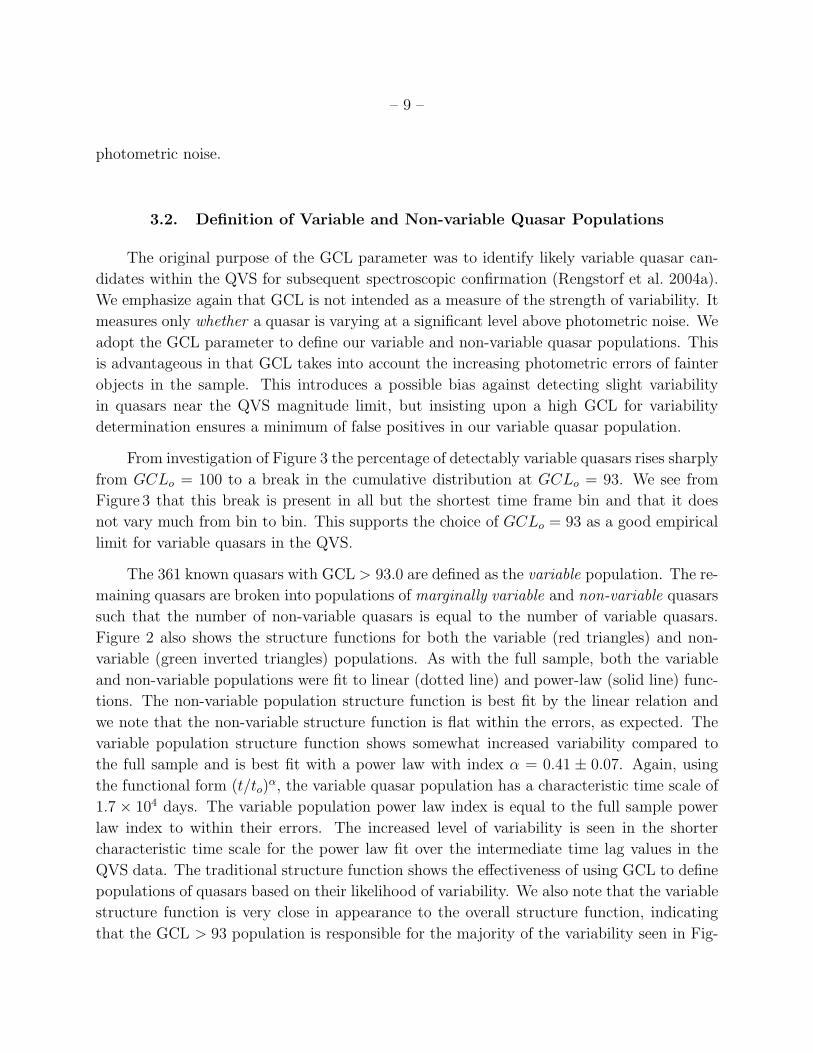
3.2. Definition of Variable and Non-variable Quasar Populations

The original purpose of the GCL parameter was to identify likely variable quasar can-

didates within the QVS for subsequent spectroscopic confirmation (Rengstorf et al. 2004a).

We emphasize again that GCL is not intended as a measure of the strength of variability. It

measures only whether a quasar is varying at a significant level above photometric noise. We

adopt the GCL parameter to define our variable and non-variable quasar populations. This

is advantageous in that GCL takes into account the increasing photometric errors of fainter

objects in the sample. This introduces a possible bias against detecting slight variability

in quasars near the QVS magnitude limit, but insisting upon a high GCL for variability

determination ensures a minimum of false positives in our variable quasar population.

From investigation of Figure 3 the percentage of detectably variable quasars rises sharply

from GCLo = 100 to a break in the cumulative distribution at GCLo = 93. We see from

Figure 3 that this break is present in all but the shortest time frame bin and that it does

not vary much from bin to bin. This supports the choice of GCLo = 93 as a good empirical

limit for variable quasars in the QVS.

The 361 known quasars with GCL > 93.0 are defined as the variable population. The re-

maining quasars are broken into populations of marginally variable and non-variable quasars

such that the number of non-variable quasars is equal to the number of variable quasars.

Figure 2 also shows the structure functions for both the variable (red triangles) and non-

variable (green inverted triangles) populations. As with the full sample, both the variable

and non-variable populations were fit to linear (dotted line) and power-law (solid line) func-

tions. The non-variable population structure function is best fit by the linear relation and

we note that the non-variable structure function is flat within the errors, as expected. The

variable population structure function shows somewhat increased variability compared to

the full sample and is best fit with a power law with index α = 0.41 ± 0.07. Again, using

the functional form (t/to)α, the variable quasar population has a characteristic time scale of

1.7 × 104 days. The variable population power law index is equal to the full sample power

law index to within their errors. The increased level of variability is seen in the shorter

characteristic time scale for the power law fit over the intermediate time lag values in the

QVS data. The traditional structure function shows the effectiveness of using GCL to define

populations of quasars based on their likelihood of variability. We also note that the variable

structure function is very close in appearance to the overall structure function, indicating

that the GCL > 93 population is responsible for the majority of the variability seen in Fig-

– 10 –

ure 3. In the rest of our analysis, we only utilize the variable (GCL > 93) and non-variable

(GCL ≤ 66.5) populations of known quasars.

4. Properties of the Variable and Non-variable Quasar Populations

4.1. Redshift

As mentioned above and as illustrated in Table 2, those quasars with lower redshift

(i.e., longer rest-frame time baseline) are more likely to appear as variable in the QVS. This

is entirely expected, given a survey with a fixed time frame (R04b). The entire quasar

population has a mean redshift of 1.32 ± 0.69 with a median value of 1.27. The variable

quasar population has a mean value of 1.12 ± 0.63 with median of 1.04. The non-variable

population has a mean value of 1.51 ± 0.70 with a median of 1.47.

Previous studies have shown quasar variability to increase with time lag for at least

several years. (see, e.g., Cristiani et al. 1996, §4). Our survey, with its fixed observer-frame

time baseline of 26 months, shows an increased likelihood of variability with longer time lags

(i.e., the smaller redshifts). Previous studies have also shown that less luminous quasars

show more variability than more luminous quasars (e.g., Vanden Berk et al. 2004). Since

nearby quasars tend to be less luminous than more distant quasar in a flux-limited survey,

this tendency also agrees with our observation that nearby quasars are more likely to be

variable. The inverse trend we see between redshift and likelihood of variability is likely

entirely due to the time lag and luminosity effects.

Given our current time baselines, however, we do not see the previously published trend

of increasing variability with redshift, whether due to the more variable, higher frequency

photons redshifting into longer wavelength bandpasses (e.g., Helfand et al. 2001, and refer-

ences therein) or to actual evolutionary effects (e.g., Hook et al. 1994; Cristiani et al. 1996;

Vanden Berk et al. 2004).

4.2. 2500 A Luminosity

To characterize any differences in UV/optical luminosity between our variable and non-

variable populations, we calculated a 2500 A flux density for the 933 quasars. 2500 A was

chosen because it is a fairly clean region for typical quasar spectra (Vanden Berk et al.

2001). Flux densities were calculated by convolving a redshifted composite quasar spectrum

(Vanden Berk et al. 2001) with the SDSS filter response curves, using effective wavelengths

– 11 –

from York et al. (2000), and SDSS DR3 PSF magnitudes, corrected for Galactic extinction

and shifted to the AB magnitude system4.

The luminosity values (in units of erg s−1 Hz−1) reported in Table 2 include the median

and quartile values for the entire quasar sample, for the variable population, and for the

non-variable population. These data show that the median luminosity of our non-variable

population is more than double that of our variable population, with overlapping 1st-to-3rd

quartile ranges. Non-variable quasars have a median value of 1.63 × 1031 while variable

quasars have a median of 8.11× 1030. A Kolmogorov-Smirnov (KS) test shows that the two

samples are rejected as coming from the same parent distribution to a level of significance

of 0.001. We interpret this result as a confirmation that the difference between the median

luminosity densities is statistically significant. This shows that selecting quasars based on

likelihood of variability returns results consistent with trends seen in quasars ranked by

amplitude of variability.

4.3. 2µm Luminosity

The upper-left panel in Figure 6 shows the variability likelihood of the known quasars,

split into 2MASS detections (N = 205) and non-detections (N = 728). Quasars which were

detected by 2MASS have a 63% higher chance of being seen as photometrically variable

in the QVS as those not detected by 2MASS (54.5% versus 33.4% with GCL > 93). For

reference, the upper-right panel in Figure 6 shows the cumulative distribution for all 933

quasars, repeated from Figure 3.

As with the 2500 A luminosity density, we calculated the luminosity density at 2µm for

every 2MASS match to our data. We used an optical-infrared composite quasar spectrum

from the SDSS quasars in the SWIRE ELAIS N1 field (Hatziminaoglou et al. 2005) and the

J-, H-, and KS-band total response curves (Cutri et al. 2001). Table 2 reports the median,

1st quartile, and 3rd quartile 2µm luminosity density values for the full population of 205

2MASS-detected quasars, for the variable sample, and for the non-variable sample. As with

the 2500 A result, the median luminosity is noticeably larger for the non-variable population

than that for the variable population (9.51×1031 versus 1.43×1031), again with overlapping

1st-to-3rd quartile ranges. The 2µm variable and non-variable samples’ luminosity densities

were also subjected to a KS test, showing that the differences between the variable and non-

variable populations were significant to 99.9%. As with 2500 A, the 2µm luminosity density

4SDSS magnitudes are very close to the AB system, but the u and z filters have a small zero point offset.

See http://www.sdss.org/dr3/algorithms/fluxcal.html for a complete description.

– 12 –

is smaller for optically variable quasars compared to the non-variable quasars. Again, in our

likelihood-selected sample of variable quasars, we see results consistent with the trend that

more luminous quasars, even in the near-IR, are less optically variable.

4.4. 2 keV Luminosity

The lower-right panel in Figure 6 shows the cumulative percentage of known quasars

with GCL > GCLo, split into RASS detections and non-detections. As was the case with the

2MASS detections, there is a marked difference between the two X-ray populations. Quasars

which were detected by the RASS are much more likely to appear photometrically variable.

This supports the suggestion that combining optical variability and X-ray flux measurements

is an efficient quasar selection technique (e.g., Sarajedini, Gilliland, & Kasm 2003; Brandt

2004).

A hard X-ray (0.5 − 2.0keV ) flux is calculated from the published RASS counts per

second using the PIMMS v3.5 software application (Mukai 1993) with Γ = 2.0, α = −1,

and the weighted average neutral hydrogen column density calculated from HEASARC’s nH

application using the Dickey & Lockman (1990) HI map. From the hard X-ray flux, the rest-

frame 2 keV flux density is determined, which was used to determine the 2 keV luminosity

density. Of the 38 RASS detections, 28 are in the variable population and only 3 are in

the non-variable population. Table 2 reports the median, 1st quartile, and 3rd quartile

luminosity densities. Again, the non-variable population has a higher median luminosity

than the variable population (3.92×1026 versus 1.69×1026). This result provides a tentative

suggestion for the existence of an anti-correlation between X-ray luminosity and optical

variability; but with only three non-variable X-ray detected quasars, additional observations

are required for a more definitive statement.

4.5. Radio Properties

The lower-left panel in Figure 6 shows the cumulative percentage of quasars with GCL

> GCLo, split into FIRST detections (N = 80) and non-detections (N = 853). The samples

exhibit roughly the same cumulative GCL distribution, both tracing the overall distribution

shown in the upper-right panel of Figure 6. This finding is consistent with the comparison

between FIRST detections and non-detections in the SDSS by Vanden Berk et al. (2004).

To quantify any difference in radio flux between the variable and non-variable popu-

lations, we looked at the radio-detected quasars within each group. An equal number (N

– 13 –

= 32) were variable as were non-variable. Table 2 reports the FIRST flux density median,

1st quartile, and 3rd quartile values. Unlike the IR and X-ray detections, the radio loud

quasars show a correlation between integrated FIRST flux density and optical variability.

The non-variable population has a median integrated radio flux of 3.96 mJy, while the vari-

able population has a median of 9.64 mJy. A KS test shows that the radio flux values for the

variable and non-variable populations are reliably rejected as coming from the same parent

distribution. This is in agreement with earlier works that report radio-loud quasars are more

variable (e.g., Vanden Berk et al. 2004; Helfand et al. 2001).

5. Light Curve Morphology

Using a light curve morphology test, our variable population may be separated into

populations which are likely to be quasars (and other aperiodic variables) and those likely

to be periodic variables. The light curves from different filters for each object are analyzed

individually. The results are then averaged together, similar to the method used for calculat-

ing the GCL from the individual CLs for a given object, as detailed in R04b. The light curve

morphology test is predicated on the theory that a variable quasar will tend to vary little on

the time scale of an individual QUEST observing season (six to eight weeks), but may vary

significantly between observing seasons. The opposite will tend to be true for shorter-term

periodic variable stars, which will tend to exhibit a higher level of variability during a single

observing season, with the annual average magnitude remaining fairly constant from one

year to the next. This is effectively a null detection test, similar to proper motion cuts to

detect quasars. By rejecting variable objects which are detectably periodic, we still keep

in consideration aperiodic variable objects, which will include those stellar variables which

do not show periodic behavior, those whose periodicity was missed due to insufficient time

sampling, and those which have periods longer than those sampled in the QVS.

A light curve morphology parameter, denoted by qi, is calculated. qi is the ratio of

two indices, both of which exploit the qualitative difference between periodic and aperiodic

variables: a variance index, Vi, and a magnitude difference index, ∆mi. Vi is the average

of the ratio of the global variance to the single observing season variance, weighted by the

percentage of total data points in a given observing season.

Vi =

∑

i Ni(σ/σi)2

∑

i Ni

, (4)

where Ni is the number of light curve points within a given observing season, σ is the

standard deviation of the light curve points over the entire light curve σi is the standard

– 14 –

deviation of light curve points within a given observing season, and the index i runs over the

three individual observing seasons. Short-term periodic variables will see larger variations

within an observing season, so σi and σ will be comparable, leading to smaller values for Vi.

Visual inspection of the representative light curves in Figure 7 shows that an aperiodic light

curve will tend to have a larger Vi than a periodic variable.

∆mi compares the global standard deviation to the largest difference in mean magnitude

between any two observing seasons.

∆mi =σ

∆<m>max

, (5)

where σ is again the global standard deviation and ∆ < m >max is the largest difference

between single-observing-season average magnitudes. Another visual inspection of Figure 7

shows that an aperiodic light curve will tend to have a smaller ∆mi than a periodic variable.

The qi value is formulated by dividing eq. (4) by eq. (5), giving aperiodic light curves

larger values and periodic light curves smaller values:

qi =Vi

∆mi

. (6)

The qi values from each of the broadband filters are then averaged together for a global

index, denoted by Qi. As with the GCL calculation, the Qi is weighted by the fraction of

valid scans in which the object was detected.

Qi =

∑

(No/Nt)qi∑

(No/Nt), (7)

where the summation runs over the four different filters, Nt is the total number of possible

scans in the ensemble for a given filter, No is the number of times the object actually appears

in the ensemble for a given filter, and qi is the value for that filter, as calculated in eq. (6).

As an initial test of the efficacy of our light curve morphology classifier, we calculated

Qi for every variable source, which is defined here to be any object in the QVS which has a

GCL > 93 and a corresponding SDSS spectral identification. There are 299 variable SDSS

quasars (specClass = 3 || specClass = 4)and 92 variable SDSS stars (specClass = 1)

included in this test. Fig. 8 shows a histogram of the 391 SDSS DR3 spectral objects. Only 6

out of the 92 variable stars (6.5%) have Qi > 2.0. Likewise, only 7 of the 299 variable quasars

(2.3%) have Qi < 2.0. The low-Qi variable quasars presumably fall below the cutoff due

to insufficient sampling of their light curves. Of the 6 high-Qi variable stars, one (QUEST

J121727.5-014036.5) is a previously unstudied variable star (SDSS J121727.4-014036.9) and

– 15 –

requires additional observation, one (QUEST J143500.2-004605.8) is the SU Uma-type dwarf

nova OU Vir (Downes et al. 2001) caught in outburst during the 2000 observing season, and

4 were RR Lyrae stars, cataloged during the QUEST RR Lyrae Survey (Vivas et al. 2004).

The RR Lyrae stars in question happened to be sampled during the 1999 observing season

such that their full intra-epoch range in magnitude was not observed, causing the objects to

appear to vary in mean magnitude between the 1999 and subsequent observing seasons. In

short, these 6 variable stars fell above the cutoff due to either insufficient sampling of their

light curves, or due to their periodicity occurring over timescales longer than the QVS.

Considering only the SDSS DR3 spectra, a cut at Qi = 2 is 97.7% complete and 98.0%

efficient at separating variable objects into groups of periodic (i.e., stars) and aperiodic (i.e.,

quasars) variables. If we expect that ∼ 10% of all variable stars fall above the Qi = 2

cutoff, the efficiency will diminish as the number count of stars increases with respect to

the number of quasars, dropping to ∼ 50% efficiency when the stellar population is ∼ 10

times larger than the quasar population. It should be stressed that this is a secondary cut,

meant to increase the efficiency of the primary variability cut, as detailed in R04b. We show

that it can increase the efficiency of the quasar candidate list without greatly reducing the

completeness.

Of the 198,213 objects in the QVS, 1,610 have GCL > 93. Among those objects, 624

have Qi > 2.0. Of these 624 candidates, 351 are among the 933 known quasars. This

indicates that the combination of GCL and Qi returns a list of quasar candidates that is

at least 56.3% efficient. A minimum efficiency is reported because it is not known a priori

whether there are unconfirmed quasars among the remaining 273 objects. Recall there is a

total of 361 previously known quasars with GCL > 93. This corresponds to a completeness

of 97.2% among the known variable quasars. In considering the entire population of known

quasars, using GCL and Qi cuts returns 351 out of 933 quasars, or a 37.6% complete sample,

with the 26-month time baseline. The completeness of the quasar candidate list, as calculated

from the previously known quasars, decreased from 38.7% using only the GCL cut to 37.6%

using GCL plus Qi. However, the efficiency increases from at least 22.4%, considering only

the GCL of only the known quasars, to at least 56.3% considering GCL plus Qi. Table 3

summarizes the GCL and Qi cuts and reports their effectiveness at recovering known quasars

and their minimum efficiency with respect to the known quasars.

6. Discussion

Our current data set is trained upon known quasars which were predominantly found via

traditional color-selection methods. We are therefore limited by both our variability selection

– 16 –

biases (e.g., relatively fewer low-z quasars due to a point source requirement) and the color-

selection techniques. Nevertheless, our sample of 933 confirmed quasars allows us to make

substantive statements regarding the contrasting behavior of our variable and non-variable

populations. Given the time-limited nature of the QVS, we see that 36% of quasars reliably

show optical variability with GCLo = 93 after ∼26 observer-frame months. Correcting

these data to the quasars’ rest frames, we see that a majority of quasars reliably exhibit

variability in our data after ∼15 months. We do not, however, suggest this as evidence of

any quasi-periodicity or of a preferred time scale. We also see that loosening our variability

criteria does little to increase the variable quasar population. There is a definite break in

the cumulative distribution of variable quasars at GCL= 93. This break is seen at roughly

the same GCL value in all time lag bins of reasonable length and was used to define our

variable quasar population. The first-order structure functions (Figure 2) of the variable and

non-variable quasar populations show GCL to be an effective method for separating quasars

for further study.

In a time-limited survey, the longest rest-frame time lags correspond to the most nearby

objects, resulting in our observed anti-correlation between redshift and variability. We note

that this as an inherent bias and do not make any substantive claims as to the supposedly

evolutionary correlation between redshift and variability seen by others. Our smaller number

of quasars do not allow the fine binning in redshift-magnitude-time lag space as used by

Vanden Berk et al. (2004) to decouple these competing effects.

With a range of over 4 orders of magnitude, the distribution of 2500 A luminosity den-

sity for the entire quasar sample, as well as for the variable and non-variable sub-samples,

deviates significantly from Gaussian, complicating their statistical analyses. Nevertheless,

the luminosity density median values of the variable and non-variable quasars are consis-

tent with the anti-correlation between variability and luminosity seen in earlier work; this

result is supported by the KS test run between the two samples. The fact that optical/UV

variability-luminosity anti-correlation is mirrored in both the IR and X-ray regimes supports

the standard unification model.

We suggest this similar behavior arises from the fact that the IR and X-ray emission

are at least partially coupled to the UV/optical accretion disk emission, as described by the

generally accepted model for active galactic nuclei (see, e.g., Antonucci 1993). IR radiation

presumably originates in the outer, cooler portions of the accretion disk and in the torus from

re-processed disk emission. X-ray emisson is due to UV photons from the inner accretion disk

being up-scattered by relativistic electrons in the corona. Any correlations between intrinsic

variations and luminosity originating in the inner accretion disk would be expected to also

be seen in both the IR and X-ray regimes. A larger sample of X-ray detections and a robust

– 17 –

strength of variability parameter, capable of reliably characterizing an individual quasars’

photometric activity, are required to further investigate this multi-wavelength trend.

The radio data, however, show a qualitatively different behavior: a positive correlation

between optical variability and radio flux. Blazars tend to be primarily both radio-loud and

highly variable (see, e.g., Antonucci 1993; Ulrich et al. 1997, and references therein). Within

the standard unification model, blazars and other core-dominant radio sources are seen when

our line of sight aligns with relativistic jets perpendicular to the accretion disk. The physics

and continuum emission mechanisms for radio-loud AGN originate with the relativistic jets

(Ulrich et al. 1997, and references therein) and are fundamentally different from the behavior

seen in other quasars. Our radio-loud quasars are not all necessarily blazars; but we suspect

that there are enough blazars in our sample to give rise to the observed correlation between

radio flux and optical variability.

As more quasars are observed for longer periods of time, the quantity and quality

of these types of analyses will continue to increase. With robust light curves for larger

numbers of quasars, we are able to explore the unification model in novel ways and can also

take advantage of the unique aspects of accretion disk physics to refine variability selection

techniques for quasars and other active galactic nuclei. For example, by looking at how a

quasar has varied, rather than merely by how much it varies, we see new ways to discriminate

quasars from other variable point sources. The Qi cut is very efficient at finding aperiodically

variable objects (i.e., quasars) amongst periodic variables. This is an appealing avenue of

study. As quasar detection efficiency increases, the amount of time required for spectroscopic

follow-up decreases. We can also answer remaining questions about the unification model

by finding and analyzing the variability properties of a larger sample of Type II quasars. If

the inclination angle of a host galaxy or our line of sight through an obscuring torus does

indeed affect the level of observed variability in a large quasar population, this would help

fill in some of the remaining gaps in unification schemes.

6.1. Interesting Objects

There was one match between the QVS and the Type II quasars reported by (Zakamska

et al. 2004): QUEST J133633.7-003936.0 was matched to an SDSS DR1 Type II quasar

(SDSS J133633.65-003936.4). QUEST J133633.7-003936.0 is a faint (SDSS r = 19.2), non-

variable (GCL = 17.85) nearby (z = 0.416) object. This quasar was observed over all three

epochs of the QVS and has a rest-frame time baseline of 545 days. Its long rest-frame

time baseline puts it among the quasars most likely to be seen as variable in the QVS (the

upper-most curve in Figure. 3). However with its low GCL, this quasar is less likely to be

– 18 –

variable than 98% of the quasars in the longest time baseline bin. This quasar has somewhat

red colors (u − g = 0.92; g − r = 1.36; r − i = 0.41; i − z = 0.21) and is missed both by

standard photometric selection techniques (see, e.g., Richards et al. 2002, Fig. 7) and by

our variability technique. If the optical depth of the obscuring material is greatest towards

the nuclear region of the AGN, then the region responsible for the origin of the quasar’s

variability would be preferentially obscured, damping the photometric variability. We would

therefore expect that Type II quasars are less likely to be detected as being variable than

Type I quasars. However, a sample size greater than one Type II quasar is needed to make

a substantive claim to this effect.

Two quasars were seen as high variability outliers in the structure function analy-

sis: QUEST J121835.0-011954.2 and QUEST J120010.9-020451.6. The quasar QUEST

J121835.0-011954.2 was matched to an SDSS point source (SDSS J121834.93-011954.3), ear-

lier identified as PKS 1216-010. It is a moderately bright (SDSS r = 17.6), variable (GCL =

100; Qi = 6.40), nearby (z = 0.415) object. This quasar was observed over all three epochs

of QVS and shows both considerable intra- and inter-epoch variability. This quasar was part

of an optical polarization study by Sluse et al. (2005) and was mentioned as a candidate for

optical variability due to its variable polarization level between March and May 2002. The

QVS light curve certainly bears out this prediction, and we note that the QUEST data actu-

ally precedes the polarization observations by a small margin. The upper panels in Figure 9

show an R-band instrumental-magnitude light curve for this quasar. The strong variability

on both long and short time scales suggest that this object was correctly identified as a BL

Lac object.

QUEST J120010.9-020451.6 is another moderately bright (SDSS r = 17.4), highly vari-

able (GCL = 100; Qi = 57.05), nearby (z = 0.09) quasar, also identified by the SDSS (SDSS

J120010.93-020451.8). This object was seen as a point source in the QUEST scans, but was

resolved and targeted as a galaxy by the SDSS photometry. Following SDSS spectroscopy,

it was classified as a quasar. It shows a steady increase in brightness over the three QVS

epochs, but little variability in any single epoch. The quasar brightened by over one a magni-

tude in both R and V filters in the QVS data. The lower panels in Figure 9 show an R-band

instrumental-magnitude light curve for this quasar. The lack of short time scale variability

compared to the inter-epoch variability suggests this is a typical Type I quasar.

7. Conclusions

We have used a unique, synoptic dataset, federated with large-scale optical and non-

optical public survey data, to explore quasar variability in a realm of phase space not previ-

– 19 –

ously examined. We have larger numbers of light curve points than recent work using SDSS

data and we are spanning more area than earlier pointed observations. Using data from

the QVS and known quasars from the SDSS, 2QZ, and VC03 catalogs, we have assembled

933 quasar light curves in multiple bandpasses. Using the GCL parameter from R04b, we

defined populations of variable and non-variable quasars. Converting the light curves to the

quasars’ rest frames, we find a bias towards nearby objects being more likely to vary in a

time-limited synoptic survey, likely due to luminosity and time lag effects. This trend will

need to be accounted for in the upcoming synoptic surveys.

The anti-correlation between variability and redshift is evidence that we are sampling

time lags in which quasar variability is still rapidly increasing with time lag. Previous work

using ensemble structure function analysis has shown that quasar variability is expected to

increase with time lag over at least several years (e.g., Hook et al. 1994; Cristiani, Trentini,

La Franca, & Andreani 1997; Vanden Berk et al. 2004; de Vries et al. 2005). Recent work

has indicated a positive correlation between redshift and variability, decoupled from the

correlation between variability and photon wavelength (Vanden Berk et al. 2004). We did

not see the redshift-variability correlation in our data, which is not surprising given our

sampled time baselines and the reported weakness of the redshift-variabilty correlation.

A near-UV (2500 A) luminosity density was calculated for every known quasar. The

median luminosity densities for the variable and non-variable quasar populations showed an

anti-correlation with likelihood of variability, consistent with earlier work (e.g., Hook et al.

1994; Trevese et al. 1994; Cristiani et al. 1996; Vanden Berk et al. 2004; de Vries et al. 2005).

The known quasars were also matched to the FIRST, 2MASS, and ROSAT surveys. Cor-

relations between 2MASS and ROSAT detection and optical variability were found. Those

quasars which were detected in either the IR or the X-ray were significantly more likely to

be seen as variable than those quasars not detected. In each of the non-optical surveys, the

detected sub-sample was then divided into variable and non-variable populations. Both the

IR- and X-ray-detected populations showed that the variable population had a lower median

luminosity than the non-variable population.

Unlike the IR and X-ray surveys, the FIRST survey showed no difference in detection

between the variable and non-variable populations. The median integrated radio flux density,

however, was larger for the variable population than the non-variable population, also in

contrast with the other non-optical surveys. Vanden Berk et al. (2004) reported the same

behavior and suggest blazars as a possible explanation.

A simple light curve morphology analysis shows that the unique, aperiodic time signa-

ture inherent to quasars can be utilized to further refine variability selection techniques. The

Qi parameter efficiently separates variable point source objects in our data into groups of

– 20 –

periodic (i.e., stellar) and aperiodic (i.e., quasars etc.) objects. While somewhat fine-tuned

to the particulars of the QVS, this is an appealing test, as it is easy to implement, takes

advantage of the light curve details, and is fairly robust to unevenly sampled data. These

techniques used on the QVS are a useful testbed for techniques to identify and characterize

quasars using synoptic photometric data without the need for follow-up spectroscopy.

The authors would like to acknowledge support from NASA through grants NAG5-

12578 and NAG5-12580 as well as support through the NSF PACI Project. AWR thanks

A.D. Myers and B.F. Lundgren for insightful discussions which improved the overall quality

of this paper.

The authors made extensive use of the storage and computing facilities at that National

Center for Supercomputing Applications and would like to thank the technical staff for their

assistance in enabling this work to proceed.

The QUEST data used in this paper is based on observations obtained at the Llano del

Hato National Astronomical Observatory, operated by CIDA for the Ministerio de Ciencia

y Tecnologia of Venezuela.

Funding for the creation and distribution of the SDSS Archive has been provided by

the Alfred P. Sloan Foundation, the Participating Institutions, the National Aeronautics

and Space Administration, the National Science Foundation, the U.S. Department of En-

ergy, the Japanese Monbukagakusho, and the Max Planck Society. The SDSS Web site is

http://www.sdss.org/.

The SDSS is managed by the Astrophysical Research Consortium (ARC) for the Par-

ticipating Institutions. The Participating Institutions are The University of Chicago, Fermi-

lab, the Institute for Advanced Study, the Japan Participation Group, The Johns Hopkins

University, the Korean Scientist Group, Los Alamos National Laboratory, the Max-Planck-

Institute for Astronomy (MPIA), the Max-Planck-Institute for Astrophysics (MPA), New

Mexico State University, University of Pittsburgh, University of Portsmouth, Princeton Uni-

versity, the United States Naval Observatory, and the University of Washington.

REFERENCES

Abazajian, K., et al. 2005, AJ, 129, 1755

Antonucci, R. 1993, ARA&A, 31, 473

Aretxaga, I., Cid Fernandes, R., & Terlevich, R. J. 1997, MNRAS, 286, 271

– 21 –

Brandt, W. N. 2004, To appear in the conference proceedings of “Wide Field Imaging from

Space” published in New Astronomy Reviews (astro-ph/0407490)

Cristiani, S., Vio, R., & Andreani, P. 1990, AJ, 100, 56

Cristiani, S., Trentini, S., La Franca, F., Aretxaga, I., Andreani, P., Vio, R., & Gemmo, A.

1996, A&A, 306, 395

Cristiani, S., Trentini, S., La Franca, F., & Andreani, P. 1997, A&A, 321, 123

Croom, S. M., Smith, R. J., Boyle, B. J., Shanks, T., Miller, L., Outram, P. J., & Loaring,

N. S. 2004, MNRAS, 349, 1397

Cutri, R. M., et al. 2001, “Explanatory Supplement to the

2MASS Second Incremental Data Release” (Pasadena:IPAC),

http://www.ipac.caltech.edu/2mass/releases/second/doc/explsup.html

de Vries, W. H., Becker, R. H., White, R. L., & Loomis, C. 2005, AJ, 129, 615

di Clemente, A., Giallongo, E., Natali, G., Trevese, D., & Vagnetti, F. 1996, ApJ, 463, 466

Dickey, J. M. & Lockman, F. J. 1990, ARA&A, 28, 215

Downes, R. A., Webbink, R. F., Shara, M. M., Ritter, H., Kolb, U., & Duerbeck, H. W.

2001, PASP, 113, 764

Hatziminaoglou, E., et al. 2005, AJ, 129, 1198

Hawkins, M. R. S. 2002, MNRAS, 329, 76

Helfand, D. J., Stone, R. P. S., Willman, B., White, R. L., Becker, R. H., Price, T., Gregg,

M. D., & McMahon, R. G. 2001, AJ, 121, 1872

Hook, I. M., McMahon, R. G., Boyle, B. J., & Irwin, M. J. 1994, MNRAS, 268, 305

Hughes, P. A., Aller, H. D., & Aller, M. F. 1992, ApJ, 396, 469

Joint IRAS Science Working Group 1988, IRAS Point Source Catalog (1988), 0

Kawaguchi, T., Mineshige, S., Umemura, M., & Turner, E. L. 1998, ApJ, 504, 671

Kawaguchi, T. & Mineshige, S. 1999, IAU Symp. 194: Activity in Galaxies and Related

Phenomena, 194, 356

Lupton, R. H., Gunn, J. E., & Szalay, A. S. 1999, AJ, 118, 1406

– 22 –

Mukai, K. 1993, Legacy, vol. 3, p.21-31, 3, 21

Pindor, B. 2005, ApJ, 626, 649

Press, W. H., Teukolsky, S. A., Vetterling, W. T., & Flannery, B. P. 1992, Numerical Recipes

in FORTRAN, 2nd ed., Cambridge: University Press

Rengstorf, A. W., et al. 2004a, ApJ, 606, 741

——–. 2004b, ApJ, 617, 184 (R04b)

Richards, G. T., et al. 2002, AJ, 123, 2945

Richards, G. T., et al. 2004, ApJS, 155, 257

Sarajedini, V. L., Gilliland, R. L., & Kasm, C. 2003, ApJ, 599, 173

Sluse, D., Hutsemekers, D., Lamy, H., Cabanac, R., & Quintana, H. 2005, A&A, 433, 757

Spergel, D. N., et al. 2003, ApJS, 148, 175

Trevese, D., Kron, R. G., Majewski, S. R., Bershady, M. A., & Koo, D. C. 1994, ApJ, 433,

494

Ulrich, M., Maraschi, L., & Urry, C. M. 1997, ARA&A, 35, 445

Urry, C. M. & Treister, E. 2004, Growing Black Holes, Proc. Garching Conference, June 2004,

ed. A. Merloni, A. Nayakshin, R. Sunyaev (Springer-Verlag), (astro-ph/0409603)

Vanden Berk, D. E., et al. 2001, AJ, 122, 549

Vanden Berk, D. E., et al. 2004, AJ, 601, 692

Veron-Cetty, M.-P. & Veron, P. 2003, A&A, 412, 399

Vignali, C., Brandt, W. N., & Schneider, D. P. 2003, AJ, 125, 433

Vivas, A. K., et al. 2004, AJ, 127, 1158

Voges, W., et al. 1999, VizieR Online Data Catalog, 9010, 0

Voges, W., et al. 2000, VizieR Online Data Catalog, 9029, 0

White, R. L., Becker, R. H., Helfand, D. J., & Gregg, M. D. 1997, VizieR Online Data

Catalog, 8048, 0

– 23 –

York, D. G., et al. 2000, AJ, 120, 1579

Zakamska, N. L., Strauss, M. A., Heckman, T. M., Ivezic, Z., & Krolik, J. H. 2004, AJ, 128,

1002

This preprint was prepared with the AAS LATEX macros v5.2.

– 24 –

Fig. 1.— The solid line shows the normalized redshift distribution of known quasars with

r < 19.06 matched to the QVS. For comparison, the dashed line shows the normalized

redshift distribution of 17,806 spectrally confirmed, r < 19.06 SDSS quasars.

– 25 –

Fig. 2.— First-order structure function, S1, for known quasars in the QVS. Individual points

are plotted at the average time lag value within each bin. Black squares show S1 for all 933

quasars. Red triangles show S1 for the variable (GCL > 93) population and inverted green

triangles show S1 for the non-variable (GCL ≤ 66.5) population. Solid curves are the best

power-law fit and dotted lines are the best linear fit to the data. For clarity, bin centers

are shifted slightly to the right for the variable population and slightly to the left for the

non-variable population.

– 26 –

Fig. 3.— Cumulative percentage of 933 known quasars which have a GCL value greater than

a critical GCL value, GCLo. Solid bold curve shows distribution for all 933 quasars. The

dotted line shows distribution for 124 quasars with a rest frame baseline less than 211d. The

short-dashed line shows that for 396 quasars with rest frame baselines between 211d and

335d. The long-dashed line shows that for 261 quasars with rest frame baselines between

335d and 459d. The dot-dashed line shows that for 152 quasars with rest frame baselines

greater than 459d. The solid vertical line at GCLo = 93 indicates the empirical cutoff for

variability consideration.

– 27 –

Fig. 4.— Left-hand plot shows histogram of time baselines for single-bandpass light curves

of 933 known quasars in the observer’s rest frame. Right-hand plot shows the histogram of

the same data set, corrected to the quasars’ rest frames.

– 28 –

Fig. 5.— Redshift distributions for each of the timeframe bins shown in Figure 3. Each

panel contains the redshift distribution of the full population of 933 quasars shown by the

dotted-line histogram.

– 29 –

Fig. 6.— The upper-left plot shows cumulative percentage of quasars which have GCL value

greater than a critical value, GCLo, split into groups of 2MASS detections (solid line) and

non-detections (dotted line). The lower-left plot shows the same for FIRST detections (solid

line) and non-detections (dotted line) and the lower-right for unique ROSAT detections (solid

line) and non-detections (dotted line). For reference, the upper-right plot shows that for the

entire population of 933 quasars.

– 30 –

Fig. 7.— Top panel shows an R-band light curve for a typical periodic variable star (GSC

05000-00417). Bottom panel shows an R-band light curve for a typical variable quasar (SDSS

J152809.55-000044.8).

– 31 –

Fig. 8.— Histogram showing the Qi distributions for variable (GCL > 93), spectrally con-

firmed objects from the SDSS DR3; 99 spectrally verified stars (dashed line) and 299 spec-

trally verified quasars (solid line).

– 32 –

Fig. 9.— QVS light curves for two highly variable, previously identified quasars: PKS 1216-

010, suggested to be variable due to earlier polarimetry study and shown to vary by nearly

2 mag in the QVS and SDSS J120010.93-020451.8, which shows ∼ 1 mag of variation in the

QVS.

– 33 –

Table 1. Known Quasars in the QVS

Identifier GCL Qi Redshifta lg(L2500A

)b lg(L2keV ) lg(L2µm) FIRST Fint Cross-identification

(QUEST J...) (mJy)

100110.5-004049.0 75.42 0.82 0.13 28.52 · · · · · · · · · SDSSJ100110.52-004049.2

100113.6-001234.2 77.95 1.26 2.46 31.72 · · · · · · · · · SDSSJ100113.63-001234.5

100143.3-003610.2 58.22 2.34 1.48 31.12 · · · · · · · · · SDSSJ100143.28-003610.5

100145.1-011220.6 66.71 2.20 0.46 29.72 · · · · · · · · · 2QZJ100145.0-011221

100215.9-001055.7 71.77 2.00 0.35 29.55 · · · · · · · · · SDSSJ100215.83-001056.1

100250.0-002453.1 59.40 1.47 0.80 31.08 · · · 31.60 · · · SDSSJ100249.94-002453.5

100253.2-001726.6 11.32 0.15 0.74 30.36 · · · · · · · · · 2QZJ100253.2-001728

100255.1-002449.4 100.00 4.16 0.12 28.85 25.93 29.55 · · · SDSSJ100255.11-002449.8

100350.2-005658.2 74.92 2.92 0.79 30.44 · · · · · · · · · 2QZJ100350.1-005658

100356.2-005940.6 44.70 1.05 2.11 31.84 · · · · · · · · · SDSSJ100356.15-005940.5

aReported redshift values are from source indicated by Cross-identification.

bAll luminosity densities are in units of erg s−1 Hz−1.

Note. — Table 1 is presented in its entirety in the electronic edition of the Astronomical Journal. A portion is shown here for guidance

regarding its form and content.

– 34 –

Table 2. Multiwavelength Luminosities for Quasar Subsets

Sample N 1st Quartile median 3rd Quartile

L2500A

(1031 erg s−1 Hz−1)

Full Sample var 361 0.214 0.811 2.31

Full Sample all 933 0.363 1.19 3.26

Full Sample non 361 0.637 1.63 3.84

FIRST Fint (mJy)

FIRST var 32 3.54 9.64 42.7

FIRST all 80 2.38 6.05 30.9

FIRST non 32 1.77 3.96 27.7

L2µm(1031 erg s−1 Hz−1)

2MASS var 111 0.351 1.43 6.93

2MASS all 205 0.488 2.83 21.3

2MASS non 39 1.37 9.51 26.6

L2keV (1026 erg s−1 Hz−1)

ROSAT var 28 0.416 1.69 7.41

ROSAT all 38 0.540 1.98 9.38

ROSAT non 3 (1.13)a 3.92 (12.9)a

aROSAT non-variable population contains 3 quasars. Parenthet-

ical first and third quartile amounts reflect entire range of flux

values.

– 35 –

Table 3. Quasar Variability Statistics

Sample (N) GCL > 93 Qi > 2 Both

Only Only Tests

QVS (198,213) 1,610 4,130 624

Known Quasars (933) 361 604 351

Recovery of Known Quasars 38.7% 64.7% 37.6%

Efficiency ≥ 22.4% ≥ 14.6% ≥ 56.3%