arX

iv:0

807.

0230

v4 [

astr

o-ph

] 2

2 Ju

l 200

8

PHYSICAL CONDITIONS IN QUASAR OUTFLOWS:

VLT OBSERVATIONS OF QSO 2359–12411

Kirk T. Korista

Department of Physics, Western Michigan University

Kalamazoo, MI 49008-5252

kirk.korista@wmich.edu

Manuel A. Bautista and Nahum Arav2

Department of Physics, Virginia Polytechnic and State University, Blacksburg, VA 24061

Maxwell Moe

Department of Astronomy, University of Colorado, Boulder, CO

Elisa Costantini

SRON National Institute for Space Research

Sorbonnelaan 2, 3584 CA Utrecht, The Netherlands

Chris Benn

Isaac Newton Group, Observatorio del Rogue de los Muchachos, Spain

ABSTRACT

We analyze the physical conditions of the outflow seen in QSO 2359–1241

(NVSS J235953–124148), based on high resolution spectroscopic VLT observa-

tions. This object was previously studied using Keck/HIRES data. The main

improvement over the HIRES results is our ability to accurately determine the

number density of the outflow. For the major absorption component, level pop-

ulation from five different Fe II excited level yields nH = 104.4 cm−3 with less

than 20% scatter. We find that the Fe II absorption arises from a region with

1Based on observations made with ESO Telescopes at the Paranal Observatories under programme ID

078.B-0433(A)

2previously at Department of Astronomy, University of Colorado, Boulder, CO

– 2 –

roughly constant conditions and temperature greater than 9000 K, before the ion-

ization front where temperature and electron density drop. Further, we model

the observed spectra and investigate the effects of varying gas metalicities and

the spectral energy distribution of the incident ionizing radiation field. The accu-

rately measured column densities allow us to determine the ionization parameter

(log UH ≈ −2.4) and total column density of the outflow (log NH(cm−2) ≈ 20.6).

Combined with the number density finding, these are stepping stones towards

determining the mass flux and kinetic luminosity of the outflow, and therefore

its importance to AGN feedback processes.

Subject headings: quasars: absorption lines—quasars: individual (QSO 2359–

1241)

1. INTRODUCTION

In recent years, the potential impact of quasar outflows on their environment has be-

come widely recognized (e.g., Silk & Rees 1998, King 2003, Cattaneo et al. 2005, Hop-

kins et al. 2006). Outflows are detected as absorption troughs in quasar spectra that

are blueshifted with respect to the systemic redshift of their emission line counterparts.

The absorption troughs are mainly associated with UV resonance lines of various ionic

species (e.g., Mg II λλ2796.35,2803.53, Al III λλ1854.72,1862.79, C IV λλ1548.20,1550.77,

Si IV λλ1393.75,1402.77, N V λλ1238.82,1242.80).

Some quasar outflows show absorption troughs from excited and metastable states.

The ratio of the population level between the excited or metastable states and the ground

state is sensitive to the number density and temperature of the plasma (Wampler, Chugai

& Petitjean 1995; de Kool et al. 2001). Therefore, accurate measurements of the column

densities associated with both excited or metastable states and the ground state of a given

ion can yield the gas number density of the outflow. In addition, these measurements and

similar ones of troughs from other ions and elements allow us to determine the ionization

equilibrium and total column density in the outflow (Arav et al. 2001; Arav et al. 2007).

Accurate column densities for the outflow’s troughs are difficult to determine since the

outflow does not cover the emission source homogeneously (Barlow 1997; Telfer et al. 1998;

Arav 1997; Arav et al. 2003). Over the past several years, we have developed techniques for

extracting reliable column densities for such situations (Arav et al. 1999a; Arav et al. 1999b;

de Kool et al. 2001, 2002a,b; Arav et al. 2002; Scott et al. (2004) Gabel et al. (2005); Arav

et al. 2005). These efforts culminated with the analysis of spectroscopic VLT observations of

– 3 –

the outflow seen in QSO 2359–1241 (Arav et al. 2008; hereafter Paper I). These data contain

absorption troughs from five resonance Fe II lines, as well as those from several other metal

species and metastable excited state He I, with a resolution of ∼7 km s−1 and signal-to-noise

ratio per resolution element of order 100.

QSO 2359–1241 (NVSS J235953–124148; E = 15.8) is an intrinsically reddened (AV ≈

0.5), luminous (MB = −28.7), radio-moderate, optically polarized (∼ 5%), low-ionization

broad absorption line quasar, at relatively low redshift z ≈ 0.868. See Brotherton et al.

(2001) for further details. Brotherton et al. (2005) describes its X-ray spectrum. An initial

investigation of the physical properties of the outflow in this object using HST FOC and

especially Keck HIRES spectra is described in Arav et al. (2001).

The VLT spectral data set of QSO 2359–1241 is described in detail in Paper I. Its un-

precedented high-quality allowed us to test a variety of absorber distribution models needed

to derive reliable ionic column densities of the outflow (see Paper I). In the present paper

we report these column densities and use them to determine the physical conditions within

the main component of the outflow (e, see Paper I): the ionization equilibrium, total column

density and number density of the absorbing material. To do so we use the photoionization

code Cloudy (Ferland et al. 1998) as well as a separate Fe II ion model (Bautista & Pradhan

1998).

The plan of the paper is as follows: In Section 2 we describe the column density mea-

surements. In Section 3 we determine the physical conditions in the main component of the

outflow. Finally, in Section 4 we summarize and discuss our results and provide a simple

estimate of the outflow’s distance from the central continuum source.

– 4 –

Table 1. Absorption lines identified in the VLT spectrum of QSO 2359–1241

λ log(gf)a Ion Elow(cm−1) glow Eup(cm−1) gup

2764.62 -1.95 He I* 159856 3 196027 9

2829.92 -1.74 He I* 159856 3 195193 9

2945.98 -1.58 He I* 159856 3 193801 9

3188.69 -1.16 He I* 159856 3 191217 9

3889.80 -0.72 He I* 159856 3 185565 9

2852.97 0.270 Mg I 0 1 35051 3

2796.36 0.100 Mg II 0 2 35761 4

2803.54 -0.210 Mg II 0 2 35669 2

1854.72 0.060 Al III 0 2 53917 4

1862.79 -0.240 Al III 0 2 53683 2

1808.01 -2.100 Si II 0 2 55309 4

1816.93 -1.840 Si IIm* 287 4 55325 6

3934.83 0.134 Ca II 0 2 25414 4

3969.65 -0.166 Ca II 0 2 25192 2

2576.87 0.433 Mn II 0 7 38807 9

2594.49 0.270 Mn II 0 7 38543 7

2606.46 0.140 Mn II 0 7 38366 5

2344.2139 0.057 Fe II 0 10 42658 8

2374.4612 -0.504 Fe II 0 10 42115 10

2382.7652 0.505 Fe II 0 10 41968 12

2586.6500 -0.161 Fe II 0 10 38660 8

2600.1729 0.378 Fe II 0 10 38459 10

2333.5156 -0.206 Fe II* 385 8 43239 6

2365.5518 -0.402 Fe II* 385 8 42658 8

2389.3582 -0.180 Fe II* 385 8 42237 8

2396.3559 0.362 Fe II* 385 8 42115 10

2599.1465 -0.063 Fe II* 385 8 38859 6

2612.6542 0.004 Fe II* 385 8 38660 8

2626.4511 -0.452 Fe II* 385 8 38459 10

2328.1112 -0.684 Fe II* 668 6 43621 4

2349.0223 -0.269 Fe II* 668 6 43239 6

2381.4887 -0.693 Fe II* 668 6 42658 8

2399.9728 -0.148 Fe II* 668 6 42335 6

2405.6186 0.152 Fe II* 668 6 42237 8

2607.8664 -0.150 Fe II* 668 6 39013 4

2618.3991 -0.519 Fe II* 668 6 38859 6

– 5 –

Table 1—Continued

λ log(gf)a Ion Elow(cm−1) glow Eup(cm−1) gup

2632.1081 -0.287 Fe II* 668 6 38660 8

2338.7248 -0.445 Fe II* 863 4 43621 4

2359.8278 -0.566 Fe II* 863 4 43239 6

2405.1638 -0.983 Fe II* 863 4 42440 2

2407.3942 -0.228 Fe II* 863 4 42401 4

2411.2433 -0.076 Fe II* 863 4 42335 6

2614.6051 -0.365 Fe II* 863 4 39109 2

2631.8321 -0.281 Fe II* 863 4 38859 6

2345.0011 -0.514 Fe II* 977 2 43621 4

2411.8023 -0.377 Fe II* 977 2 42440 2

2414.0450 -0.455 Fe II* 977 2 42401 4

2622.4518 -0.951 Fe II* 977 2 39109 2

2629.0777 -0.461 Fe II* 977 2 39013 4

2332.00 -0.720 Fe II* 1873 10 44754 8

2348.81 -0.470 Fe II* 1873 10 44447 8

2360.70 -0.700 Fe II* 1873 10 44233 10

2563.30 -0.050 Fe II* 7955 8 46967 6

2715.22 -0.440 Fe II* 7955 8 44785 6

2740.36 0.240 Fe II* 7955 8 44447 8

2756.56 0.380 Fe II* 7955 8 44233 10

2166.19 0.230 Ni II* 8394 10 54557 10

2217.14 0.480 Ni II* 8394 10 53496 12

2223.61 -0.140 Ni II* 8394 10 53365 10

2316.72 0.268 Ni II* 8394 10 51558 8

agf -values were taken from Kurucz (1995) for all but the Fe II lines with

wavelengths given more than two decimal figures. gf -values for these come

from Morton (2003).

– 6 –

2. THE MEASURED COLUMN DENSITIES

In Paper I, we presented 6.3 hours of VLT/UVES high-resolution (R ≈ 40, 000) spectro-

scopic observations of QSO 2359–1241 and identified all the absorption features associated

with the outflow emanating from this object. The unprecedented high signal-to-noise data

from five unblended troughs of Fe II resonance lines yielded tight constraints on outflow

trough formation models.

As expected we found that the apparent optical depth model (τap ≡ − ln(I), where I

is the residual intensity in the trough) gives a very poor fit to the data and greatly under-

estimates the ionic column density measurements. We found that a power-law distribution

model for absorption material in front of the emission source gives a better fit to the Fe II

data than does the standard partial covering factor model (see Sections 1, 3, 4, and Fig. 4

of Paper I). The power-law distribution model is one in which the outflow fully covers the

source, but does so inhomogeneously. This has the characteristic of allowing for non-black

saturation of absorption troughs at a large source distance (∼ 1 kpc; see de Kool et al.

2002c and Arav et al. 2005 for more detailed investigations of inhomogeneous source cov-

erage). Physically, this requires the outflow to contain many “cloudlets” with dimensions

smaller than the physical span of the source. The inhomogeneous nature of the absorption

also allows the possibility of structure at the bottoms of otherwise “saturated” absorption

troughs. Important for the physical conditions analysis of the present paper was the finding

that the partial coverage and inhomogeneous absorption models yield similar column den-

sity estimates (see Fig. 6 of Paper I). This gives us greater confidence in the derived column

density values, as they are somewhat model-independent (the reasons both methods yield

similar estimates are described in Paper I).

Finally, in Paper I we concluded that the power-law distribution model is more physically

plausible than the partial covering model for outflow such as this one. We thus used the

power-law model as presented there to extract the column densities of all ions and ionic

energy levels present in the data. For consistency we used the power-law exponent as a

function of velocity of the E = 0 Fe II lines for all other Fe II energy level and for troughs

from all other ions. This assumption should be robust for the Fe II troughs, but perhaps less

so for the troughs of other ions. We direct the reader to Paper I for details concerning this

column density extraction model. In Table 1 we provide the identifications for all transitions

observed in outflow troughs. In Table 2 we provide the measured column densities of all

species identified for the strongest absorption component, e (see Paper I), many of which

will be used to constrain the photoionization models, as we discuss in the next section.

– 7 –

Table 2. Measured and model predicted column densities for the major outflow trough in

QSO 2359–1412.

Species E(cm−1) log10 N (cm−2)

Observed Modela

H I 18.59

He I* 14.14±0.03 14.11

He I Total 17.14

He II Total 19.46

Fe II 0 13.86±0.02 13.84

Fe II 385 13.51±0.04 13.48

Fe II 668 13.26±0.03 13.28

Fe II 863 13.06±0.03 13.08

Fe II 977 12.85±0.03 12.79

Fe II 1873 13.89±0.05b 13.83

Fe II 7955 12.70±0.04 12.67

Fe II Total 14.41

Mg I Total 11.92±0.03 13.01

Mg II Total >13.81 15.22

Si II 287 14.9±0.1 15.19

Si II Total 14.9±0.1 15.38

Al III Total >13.9 14.35

Ca II Total 12.52±0.03 12.90

Mn II Total 12.71±0.03 12.26

Ni II 0 13.50c

Ni II 8394 12.79±0.04 12.98c

Ni II Total 13.70

aPredicted column densities are from an

optimal photoionization model with: MF87

SED, solar abundances, constant gas density

log nH(cm−3) = 4.4, log NH(cm−2) = 20.556,

log UH = −2.418.

bTrough partially contaminated with those of

other Fe II transitions.

cCalculated from the Ni II model of Bautista

(2004) assuming pure collisional excitation.

– 8 –

3. PHOTOIONIZATION MODELS

3.1. General Methodology

The observed spectrum of QSO 2359–1241 is rich in absorption lines from singly ionized

species, such as Mg II, Si II and Ca II, and notably from iron-peak species. We determine

the physical conditions within the main absorbing component centered on –1376 km s−1

(component e; see Paper I) and integrated over the range in radial velocity from –1320

km s−1 to –1453 km s−1. Our analysis of the spectrum is mostly based on the column

density in the metastable 2 3S excited state of He I (hereafter, He I∗) and the column

densities of Fe II. For Fe II we have the level-specific column densities for the ground level

(a 6D9/2) as well as for the excited levels a 6D7/2 at 385 cm−1, a 6D5/2 at 668 cm−1, a 6D3/2

at 863 cm−1, and a 6D1/2 at 977 cm−1 within the ground term, and the a 4D7/2 level at 7955

cm−1 within the second excited term. The total column density in Fe II is estimated by

scaling from the sum of the above levels (see below). These column densities as measured

from our VLT spectra are presented in the upper half of Table 2. Together they constrain the

physical conditions of the outflow near its hydrogen ionization front (where the bulk of He I∗

and Fe II form), as well as its total column density, as we show below. Moreover, modeling

the ionization structure of these two species combined is secure because the photoionization

and recombination cross sections for hydrogen and helium are well known and the ionization

fraction of Fe II near the ionization front of the cloud closely tracks that of H+ due to charge

exchange reactions. Table 2 also lists the measured column densities of several other ions

identified in the spectra.

The diagnostic power of the combined He I∗ and Fe II lines results from their different

responses to temperature and density. The He I∗ column density depends on the population

of the 2 3S level of He I, which is populated by recombination from He II and varies with

temperature, in the sense that the lower the temperature the higher the recombination rate.

An additional mechanism to populate the 2 3S occurs through thermalization by electronic

collisions with the very long-lived 2 1S level. The main de-population mechanisms of the 2 3S

level are magnetic dipole radiative decay to the ground level and electron impact excitation

to the neighboring 2 1S (the dominant channel) and 2 3P levels. For T < 15, 000 K collisional

ionization can be neglected as a depopulation mechanism of this level (see Clegg 1987). The

net result is that the population of the 2 3S level becomes nearly independent of density for

electron densities substantially above the critical density ≈ 3− 4× 103 cm−3 (Osterbrock &

Ferland 2006; see also Arav et al. 2001). The column density in He I∗ is then set by that in

He II, which in turn is set by the ionization parameter for a fixed spectral energy distribution

of the incident continuum.

– 9 –

The Fe II lines in our spectrum arise from the ground and first excited multiplets

of the ion. The populations of these levels are dominated by electron impact excitation,

thus the populations depend approximately linearly on electron density for densities up to

∼ 105 cm−3. The populations, particularly that of the a 4D7/2 at 7955 cm−1 level, also

increase monotonically with temperature under collisional excitation conditions.

For the present work we use the photoionization modeling code Cloudy (v06.02; Ferland

et al. 1998) to compute spectral models of the outflowing absorbing gas in QSO 2359–1241.

This version of cloudy includes the 371-level Fe+ model atom of Verner et al. (1999),

as well as the detailed model He I atom of Porter et al. (2005). The default version of

the model He I atom (nLS-resolved up through principle quantum number n=6, plus 20

additional LS-collapsed levels lying above) was determined to be sufficient for our purposes.

We assume constant total hydrogen density “clouds” of solar abundances (in particular

log (He/H) = −1.0 and log (Fe/H) = −4.5498 by number; (Holweger 2001), and adopted the

Mathews & Ferland (1987) quasar spectral energy distribution (hereafter, the MF87 SED)

as the incident continuum spectrum. The solar abundances are from Allende Prieto et al.

(2002, 2001) for C and O, Holweger (2001) for N, Ne, Mg, Si, and Fe, and Ander & Grevesse

(1989) for the rest.)

3.2. Some General Physical Considerations

Before we proceed to determine the physical conditions within the outflow of QSO 2359–

1241, let us first examine the formation of Fe II and He I∗ within a photoionized cloud.

Figure 1a shows the ionic fractions of Fe II and of helium in the He I* state within a

representative photoionized gas cloud. Note that we plot the He I* fraction relative to

that of the total iron abundance so that the comparison of the curves for He I(2 3S) and

Fe II is then independent of the iron abundance. The conditions of this model cloud are:

hydrogen number density, nH = 104.4 cm−3, ionization parameter, given by log UH = −2.418,

solar abundances, and the MF87 SED. The particular choice of nH and UH will become

apparent below. Here, the ionization parameter UH ≡ ΦH/cnH , where ΦH (cm−2 s−1) is the

hydrogen ionizing photon flux and nH (cm−3) is the total hydrogen number density. The

cloud is bounded by a total hydrogen column density log NH(cm−2) = 21. Note that the

column densities of Fe II and He I∗ vary rapidly approaching the hydrogen ionization front

(at log NH(cm−2) ≈ 20.6 in this model). In particular, the Fe II/Fe ratio rises ∼ 4 orders

of magnitude to values approaching unity within He II zone (as indicated by the bump in

He I(2 3S)), with most of this change occurring just inside the hydrogen ionization front. For

the cloud shown, 90% of the Fe II column density forms within 20% of the cloud volume lying

– 10 –

to the left of the vertical dashed line. By comparison the He I∗ column density increases by

just 25% over the same volume of the cloud. Since nearly all of the observable Fe II forms

right along the hydrogen ionization front, the model results will depend only weakly on the

iron abundance.

– 11 –

19.5 20 20.5 213

3.5

4

4.5

-4

-3

-2

-1

0

Fig. 1.— Physical structure of a photoionized cloud vs. total hydrogen column density.

The parameters of the model are given in the text. The upper panel shows the fraction of

neutral helium in the 2 3S level and the ionic fractions of H I, Fe II. The He I* fraction

has been normalized to the total iron abundance. The lower panel depicts the behavior of

the electron density and electron temperature. The vertical dashed line indicates the total

hydrogen column density of the model to match the observed column densities of Fe II and

He I* in QSO 2359–1241. See text for details.

– 12 –

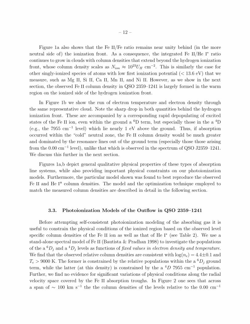
Figure 1a also shows that the Fe II/Fe ratio remains near unity behind (in the more

neutral side of) the ionization front. As a consequence, the integrated Fe II/He I∗ ratio

continues to grow in clouds with column densities that extend beyond the hydrogen ionization

front, whose column density scales as Nion ≈ 1023UH cm−2. This is similarly the case for

other singly-ionized species of atoms with low first ionization potential (< 13.6 eV) that we

measure, such as Mg II, Si II, Ca II, Mn II, and Ni II. However, as we show in the next

section, the observed Fe II column density in QSO 2359–1241 is largely formed in the warm

region on the ionized side of the hydrogen ionization front.

In Figure 1b we show the run of electron temperature and electron density through

the same representative cloud. Note the sharp drop in both quantities behind the hydrogen

ionization front. These are accompanied by a corresponding rapid depopulating of excited

states of the Fe II ion, even within the ground a 6D term, but especially those in the a 4D

(e.g., the 7955 cm−1 level) which lie nearly 1 eV above the ground. Thus, if absorption

occurred within the “cold” neutral zone, the Fe II column density would be much greater

and dominated by the resonance lines out of the ground term (especially those those arising

from the 0.00 cm−1 level), unlike that which is observed in the spectrum of QSO J2359–1241.

We discuss this further in the next section.

Figures 1a,b depict general qualitative physical properties of these types of absorption

line systems, while also providing important physical constraints on our photoionization

models. Furthermore, the particular model shown was found to best reproduce the observed

Fe II and He I* column densities. The model and the optimization technique employed to

match the measured column densities are described in detail in the following section.

3.3. Photoionization Models of the Outflow in QSO 2359–1241

Before attempting self-consistent photoionization modeling of the absorbing gas it is

useful to constrain the physical conditions of the ionized region based on the observed level

specific column densities of the Fe II ion as well as that of He I∗ (see Table 2). We use a

stand-alone spectral model of Fe II (Bautista & Pradhan 1998) to investigate the populations

of the a 6Dj and a 4Dj levels as functions of fixed values in electron density and temperature.

We find that the observed relative column densities are consistent with log(ne) = 4.4±0.1 and

Te > 9000 K. The former is constrained by the relative populations within the a 6Dj ground

term, while the latter (at this density) is constrained by the a 4D 7955 cm−1 population.

Further, we find no evidence for significant variations of physical conditions along the radial

velocity space covered by the Fe II absorption troughs. In Figure 2 one sees that across

a span of ∼ 100 km s−1 the the column densities of the levels relative to the 0.00 cm−1

– 13 –

ground level are constant within the error bars, as also demonstrated by linear fits to all

three curves. This implies that ne is similarly constant across this outflow component. As

seen in Figure 1 the photoionization model solution is reached (vertical dashed line) before

the values of ne and Te begin plummeting due to the H I ionization front. If the absorption

had taken place deeper within or behind the ionization front, we should have then seen a

rapid decline of the N(Fe II*)/N(Fe II) at either high or low velocity, assuming the velocity of

the flow changes monotonically with radius (see the discussion regarding the physical nature

of the outflow in Section 4 of Paper I). This is because the relative level populations within

a 6Dj term are roughly linearly dependent on ne for ne well below the critical densities of

the excited levels, and that of the 7955 cm−1 level also depends on Te (primarily via the

Boltzmann factor) in our temperature range. Both effects work in the same direction: the

lowering of ne and Te, which occurs deep within and beyond the hydrogen ionization front

(see Figure 1), results in significantly reduced populations of the excited levels, as mentioned

in Section 3.1. For example, in the range of electron density log(ne) = 3.4 − 4.4 the excited

state level populations within the a 6Dj term fall by about a factor of 5, while that of the

7955 cm−1 level falls by a decade due to electron density alone and a factor of ∼2 as the

temperature falls from 11,500 K to half that.

¿From these preliminary investigations we conclude that the observed Fe II troughs form

mostly within a narrow region of the outflow near the hydrogen ionization front for which the

electron density and temperature do not vary significantly, and that a hydrogen ionization

front does not fully form within the flow (see Figure 1). This then constrains the cloud

column density to be log NH < 20.6 + log(UH/10−2.4)). This is in contrast to the findings

of de Kool et al. (2001; 2002a,b) in their analysis of intrinsic Fe II troughs in other quasars.

This is an important conclusion, since the rapidly plunging values of electron density and

temperature behind the hydrogen ionization front would make for more difficult modeling.

– 14 –

Fig. 2.— Ratios of observed column densities of excited Fe II levels to the ground level vs.

velocity shift along the trough.

– 15 –

We also use the analytic formula of Clegg (1987; see also Equation 3 of Arav et al. 2001)

to estimate a ratio n(23S)/n(He+) ≈ 5× 10−6 for the above electron density and a tempera-

ture of 104 K. Further, if we assume a solar (He/H) abundance and that (He+/He) ∼ 0.8 for

the ionized portion of the cloud (as is typical for standard AGN SEDs), we estimate a total

hydrogen column density of NH ∼ 2.5 × 106N(23S) ∼ 1020.5 cm−2, given our measurement

of N(23S) quoted in Table 2. The substantial improvement in quality of the spectral data of

QSO 2359–1241 (see also Paper I) over that presented in Arav et al. (2001) has thus already

yielded much stronger constraints in the physical conditions within the outflow. We next

proceed with the more detailed modeling.

In building a fully self-consistent photoionization model of the outflow of QSO 2359–

1241 based on the intrinsic absorption lines, we adopt a two-step iterative photoionization

modeling procedure. Using the default parameter optimization scheme built into Cloudy,

the ionization parameter UH and total hydrogen column density NH are optimized to simul-

taneously match the total column density in Fe II and the column density in the excited

state He I∗.

In the first pass we adopt a hydrogen number density, nH , equal to the electron density

derived from the Fe II level specific column densities (104.4 cm−3), and the total Fe II column

density is estimated from the sum of the level specific column densities determined from the

observations and the results of our stand-alone Fe II model atom for the above density and

a temperature of 10,000 K. The Cloudy optimizer minimizes χ2 between the computed and

measured target column densities (with assumed equal weighting) for various values of UH

and NH . To speed up computations and since we are not concerned with the detailed Fe II

level populations during this step, the default 16-level model atom of Fe+ within Cloudy is

utilized during the optimization. This subset of the full 371-level model atom includes all

levels up through a 4P near 13,500 cm−1, i.e., the four lowest terms of the ion. For a model

of this size only electron impact excitation followed by radiative decay through forbidden

transitions is considered in the excitation. However, as verified later, radiative processes

contribute little to the excitation of the Fe II levels observed.

Once a solution is found, we update the value of the total Fe II column density (this

converges to be 1.80 times the sum over the six most reliably determined level-specific column

densities), and then fine-tune the value of nH by computing a grid in total hydrogen number

density, spanning a decade to either side of the starting density in 0.05 dex steps, for fixed

values in UH and NH as determined during the previous optimization step. To provide

sufficient accuracy in the predictions of the level populations under study, the Cloudy models

computed in the gas density grid use a 99-level model atom of Fe+ (a subset of the full

371-level model atom), which includes all levels up through 50,212.8 cm−1. This model

– 16 –

atom accounts for the dominant channels for photoexcitation by continuum radiation and

other processes. Turning on the full 371-level model atom, that accounts for H I Lyman α

fluorescence and other processes, has virtually no impact on the level populations relevant

to our study. By comparing the predicted Fe II column densities for all levels observed with

the measured values in Table 2, we are able to choose the most appropriate value in total

hydrogen gas number density nH . This procedure converges rapidly to a final solution. The

final fit parameters are log nH = 4.4 and log UH = −2.418, which were used for the modeled

cloud shown in Figure 1, and log NH = 20.556, which is indicated by the vertical dashed

line in that figure. As a further point of interest, this model’s electron density-weighted

temperature in the Fe+ zone is 11, 500 K.

– 17 –

3 3.5 4 4.5 5 5.5 6 6.5 7

log nH

(cm-3

)

0

0.1

0.2

0.3

0.4

0.5

0.6

0.7

0.8

level

popula

tion r

ati

o r

ela

tive t

o 0

.00 c

m-1 384.79 cm

-1

667.68 cm-1

862.61 cm-1

977.05 cm-1

7955.32 cm-1

observed ratios

Fig. 3.— Calculated level populations of excited levels of Fe II relative to the ground level vs.

hydrogen number density in the photoionization model. The points indicate the observed

column densities of each level relative to the ground level. See text for details. All five

independent measurements are consistent with log nH = 4.4 with less than 20% dispersion.

– 18 –

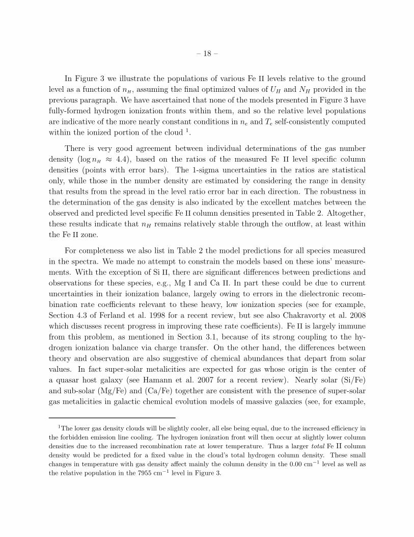
In Figure 3 we illustrate the populations of various Fe II levels relative to the ground

level as a function of nH , assuming the final optimized values of UH and NH provided in the

previous paragraph. We have ascertained that none of the models presented in Figure 3 have

fully-formed hydrogen ionization fronts within them, and so the relative level populations

are indicative of the more nearly constant conditions in ne and Te self-consistently computed

within the ionized portion of the cloud 1.

There is very good agreement between individual determinations of the gas number

density (log nH ≈ 4.4), based on the ratios of the measured Fe II level specific column

densities (points with error bars). The 1-sigma uncertainties in the ratios are statistical

only, while those in the number density are estimated by considering the range in density

that results from the spread in the level ratio error bar in each direction. The robustness in

the determination of the gas density is also indicated by the excellent matches between the

observed and predicted level specific Fe II column densities presented in Table 2. Altogether,

these results indicate that nH remains relatively stable through the outflow, at least within

the Fe II zone.

For completeness we also list in Table 2 the model predictions for all species measured

in the spectra. We made no attempt to constrain the models based on these ions’ measure-

ments. With the exception of Si II, there are significant differences between predictions and

observations for these species, e.g., Mg I and Ca II. In part these could be due to current

uncertainties in their ionization balance, largely owing to errors in the dielectronic recom-

bination rate coefficients relevant to these heavy, low ionization species (see for example,

Section 4.3 of Ferland et al. 1998 for a recent review, but see also Chakravorty et al. 2008

which discusses recent progress in improving these rate coefficients). Fe II is largely immune

from this problem, as mentioned in Section 3.1, because of its strong coupling to the hy-

drogen ionization balance via charge transfer. On the other hand, the differences between

theory and observation are also suggestive of chemical abundances that depart from solar

values. In fact super-solar metalicities are expected for gas whose origin is the center of

a quasar host galaxy (see Hamann et al. 2007 for a recent review). Nearly solar (Si/Fe)

and sub-solar (Mg/Fe) and (Ca/Fe) together are consistent with the presence of super-solar

gas metalicities in galactic chemical evolution models of massive galaxies (see, for example,

1The lower gas density clouds will be slightly cooler, all else being equal, due to the increased efficiency in

the forbidden emission line cooling. The hydrogen ionization front will then occur at slightly lower column

densities due to the increased recombination rate at lower temperature. Thus a larger total Fe II column

density would be predicted for a fixed value in the cloud’s total hydrogen column density. These small

changes in temperature with gas density affect mainly the column density in the 0.00 cm−1 level as well as

the relative population in the 7955 cm−1 level in Figure 3.

– 19 –

Ballero et al. 2008), although these are not likely to explain the full discrepancies. Unfor-

tunately, too few observational constraints as well as uncertainties in the atomic data for

these third and, especially, fourth row elements (Ca, Mn) do not allow us to draw definitive

conclusions at the present time.

3.4. Additional considerations: alternative metalicities and SEDs

We have found a good model for the outflow in QSO 2359–1241 by self-consistent opti-

mization of the total hydrogen gas density, ionization parameter and total hydrogen column

density. In particular, for reasons already provided we believe our derived value in the hy-

drogen gas number density is robust. However, the model contains two basic assumptions

concerning the gas elemental abundances (solar) and the adopted SED (MF87), neither of

which are well-constrained by the observations. Each of these assumptions independently

can have important effects on the physical conditions and so on some of the inferred physical

parameters such as ionization parameter and total hydrogen column density, but in at least

some cases can cancel each other under the constraints of our observations.

The assumed metalicity of the cloud affects the thermal structure of the cloud, because

metals as a whole provide radiative cooling to the plasma. Thus, for a fixed SED, super-

solar metalicity clouds are cooler than our optimized model, and sub-solar metalicity clouds

would be warmer. Thus, increasing the gas metalicity (along with Fe/H) also decreases the

column density of the ionized zone, all else being equal, as the lower electron temperatures

result in more rapid recombination rates and as the heavy elements become increasingly

important opacity sources. However, we find that models with metalicities exceeding 2–3×

solar, for a fixed MF87 SED, are too cool (T falls below 9000 K) to reproduce the observed

column density ratio between the 7955 cm−1 and the ground 0.00 cm−1 levels. For larger gas

metalicities, the incident SED must be correspondingly harder than the MF87 SED to push

back up the electron temperature within the ionized zone. The observations of excited Fe II

offer good constraints on the minimum temperature near the ionization front (T > 9000 K),

but provide no upper limit to the temperature below 20,000 K.

The shape of the ionizing SED also affects the temperature structure of the cloud,

as well as the sharpness of onset of the ionization front. The distribution of hydrogen

and helium ionizing photons determines the temperature of the plasma at the illuminated

face, and then the distribution of the EUV and X-ray photons determines how sharply

temperature and ionization drop at the ionization front and beyond. A hard SED, i.e., with

a large fraction of photons in the EUV and X-rays, leads to an extended ionization front,

while a soft SED, with relatively more photons concentrated near 1 Rydberg, results in

– 20 –

sharper declines in temperature, ionization, and electron density. We find that gas of solar

abundances illuminated by an SED with a logarithmic X-ray to UV flux ratio αox < −1.7

has electron temperatures that are too low near the hydrogen ionization front to explain the

observed Fe II column densities. Based on the high optical-UV luminosity of QSO 2359–1241

(Brotherton et al. 2001) and the empirical relation between αox and Luv in quasars (e.g.,

see Strateva et al. 2005), an αox ≈ −1.6 ± 0.2 might be expected. What little we do know

about the X-rays in QSO 2359–1241 comes from Chandra observations of modest quality

(16 photons detected) that find αox ≈ −1.4 ± 0.1 (Brotherton et al. 2005 and Brotherton

2008, private communication; estimated error bar is statistical only), consistent with the

above empirical relation and more importantly is the same value as that in our assumed

SED (MF87). We refer the reader to Arav et al. (2001) and to Brotherton et al. (2001) for

information pertaining to this object’s rest frame opt-UV spectrum.

In conclusion, the few observational constraints available do support an incident contin-

uum SED whose average ionizing photon energy is similar to the MF87 spectrum, although

there remains the possibility (we consider unlikely) that it is substantially harder. Further-

more, the gas metalicity is unlikely to be severely sub-solar. Therefore, the total column

density of the absorbing gas as derived in the previous section seems secure to within a factor

of 2–3.

4. Discussion and Conclusions

First, we compare the results of this investigation to the analysis of the Keck/HIRES

observations of QSO 2359–1214 by Arav et al. (2001; hereafter HIRES paper). Using the

same MF87 SED, the HIRES analysis found log NH = 20.2 and log UH = −2.7, compared

to log NH = 20.6 and log UH = −2.4 for the VLT analysis. These factors of ∼ 2 differences

are mainly attributed to using apparent optical depth methods to extract the Fe II and

He I* column densities. As pointed out in the HIRES paper, the data was not of high

enough signal-to-noise ratio to permit more sophisticated analyses. Even so, the HIRES

paper already showed that the outflow is not shielded by a hydrogen ionization front, a

result confirmed by the VLT analysis.

The important leap in diagnostic power for the VLT data came from the ability to

accurately measure the population levels of the excited Fe II levels, allowing us to pin point

the number density of the outflow to log(ne) = 104.4 cm−3 to better than 20% accuracy.

This is both qualitatively and quantitatively a great improvement over the lower limit of

log(ne) = 105 cm−3 available from the HIRES data. This result is not accidental. The main

reason we invested 6.5 hours of VLT observation on this outflow was precisely to yield a data

– 21 –

set from which an accurate ne could be extracted. This determination of ne will allow us to

determine the distance of the outflow from the central source and thus measure its mass flux

and kinetic luminosity. This demonstrates the importance of taking high quality spectra of

such outflows.

Other important results arising from the measured populations of the Fe II levels are

the determination of a lower limit to the temperature of the Fe II region and the realization

that the absorption spectrum forms before the hydrogen ionization front, beyond which the

temperature and ionization drop sharply. The temperature determination was crucial in

constraining a whole family of SEDs and gas metalicities that would yield very different

temperatures in the Fe II region, and consequently allowing for a more secure determination

of the total gas column density and ionization parameter. That the Fe II absorption occurs

in a region of nearly constant conditions before the hydrogen ionization front is a key to

being able to model the absorption spectrum.

Photoionization modeling allowed us to reproduce quite well the observed Fe II and

He I* column densities in the main, e, component of the quasar outflow absorption spectrum.

Reiterating, we found log NH ≈ 20.6 and log UH ≈ −2.4. The dominant error bars to these

values come from the uncertainties in the assumed SED and gas metalicities and come to

∼ 0.3 dex.

Given the above gas density, ionization parameter, an estimate to an unobscured incident

bolometric luminosity of ∼ 4.7× 1047 ergs s−1 based on the intrinsic reddening correction in

Brotherton et al. (2001, 2005), and a standard cosmology (Ho = 70 km s−1 Mpc−1, ΩΛ = 0.70,

Ωm = 0.30), we estimate a distance of component e of the outflow from the central continuum

source of ∼ 3 kpc. In a future paper we will similarly determine the physical conditions in

the weaker, lower velocity outflow components a–d, as well as the distances and estimates

of the kinetic luminosities for all components in the outflow, important to AGN feedback

scenarios of galaxy evolution.

We acknowledge support from NSF grant number AST 0507772 and from NASA LTSA

grant NAG5-12867. We also would like to thank the anonymous referee for his or her helpful

comments and suggestions.

– 22 –

REFERENCES

Allende Prieto, C., Lambert, D.L., & Asplund, M. 2001, ApJ, 556, L63

Allende Prieto, C., Lambert, D.L., & Asplund, M. 2002, ApJ, 573, L137

Anders, E., & Grevesse, N. 1989, Geochim. Cosmochim. Acta, 53, 210

Arav, N.; Barlow, T.A.; Laor, A.; Blandford, R.D. 1997, MNRAS 288, 1015

Arav, N., Becker, R.H., Laurent-Muehleisen, S.A., Gregg, M.D., White, R.L.; Brotherton,

M.S.; de Kool, M. 1999a, ApJ 524, 566

Arav, N., Brotherton, M.S., Becker, R.H., Gregg, M.D., White, R.L., Price, T., Hack, W.

2001a, ApJ 546, 140

Arav, N., Gabel, J.R., Korista, K.T., Kaastra, J.S., Kriss, G.A., et al. 2007, ApJ 658, 829

Arav, N., Kaastra, J., Kriss, G.A., Korista, K.T., Gabel, J., Proga, D. 2005, ApJ 620, 665

Arav, N., Kaastra, J.; Steenbrugge, K., Brinkman, B., Edelson, R., Korista, K.T., de Kool,

M. 2003, ApJ 560, 174

Arav, N.; Korista, K.T.; de Kool, M.; Junkkarinen, V.T.; Begelman, M.C. 1999b, ApJ 516,

27

Arav, N.; Korista, K.T.; de Kool, M. 2002, ApJ 566, 699

Arav, N., Moe, M., Costantini, E., Korista, K.T., Benn, C., Ellison, S. 2008, ApJ (in press)

Ballero, S.K., Matteucci, F., Ciotti, L., Calura, F., & Padovani, P. 2008, A&A, 478, 335

Barlow, T.A., Hamann, F., & Sargent, W.L.W. 1997, in ASP Conf. Ser. 128, Mass Ejection

from AGN, ed. R. Weymann, I. Shlosman, & N. Arav (San Francisco: ASP), 13

Bautista, M.A. 2004, A&A 420, 763

Bautista, M.A. & Pradhan, A.K. 1998, ApJ 492, 650

Blandford, R, D., Begelman, M. C. 2004, MNRAS 349, 68

Brotherton, M.S., Arav, N., Becker, R.H., Tran, H.D., Gregg, M.D., White, R.L., Laurent-

Muehleisen, S.A. & Hack, W. 2001, ApJ, 546, 134

Brotherton, M.S., Laurent-Muehleisen, S.A., Becker, R.H., Gregg, M.D., Telis, G., White,

R.L., & Shang, Z. 2005, AJ, 130, 2006

– 23 –

Cattaneo et al. 2005 MNRAS, 364, 407

Chakravorty, S., Kembhavi, A.K., Elvis, M., Ferland, G., & Badnell, N.R. 2008,

MNRAS, 384, L24

Clegg, R.E.S. 1987, MNRAS, 229, 31

de Kool, M., Arav, N., Becker, R.H., Gregg, M.D., White, R.L., Laurent-Muehleisen, S.A.,

Price, T., & Korista, K.T. 2001, ApJ, 548, 609

de Kool, M., Becker, R.H., Gregg, M.D., White, R.L., & Arav, N. 2002a, ApJ, 567, 58

de Kool, M., Becker, R.H., Arav, N., Gregg, M.D., & White, R.L. 2002b, ApJ, 570, 514

de Kool, M., Korista, K.T., & Arav, N. 2002c, ApJ, 580, 54

Ferland, G.J., Korista, K.T., Verner, D.A., Ferguson, J.W., Kingdon, J.B., Verner, E.M.

1998, PASP 110, 761

Haiman et al. 2006, ApJ, 650, 7

Hamann, F., Warner, C., Dietrich, M., & Ferland, G. 2007, ASP Conference Series, volume

373, 653 (astro-ph/0701503)

Holweger, H. 2001, Joint SOHO/ACE workshop Solar and Galactic Composition. Ed. by

Robert, F. Wimmer-Schweingruber. Publisher: American Institute of Physics Con-

ference proceedings vol. 598 location: Bern, Switzerland, March 6 - 9, 2001, p.23

Hopkins, P.F., Hernquist, L., Cox, T.J., Di Matteo, T., Robertson, B., & Springel, V. 2006,

ApJS 163, 1

King, A., 2003, ApJ 596, L27

Kurucz, K.T. & Bell, B., Atomic Line Data, Kurucz CD-ROM No. 23. Cambridge, Mass.:

Smithsonian Astrophysical Observatory, 1995

Mathews, W.G., & Ferland, G.J. 1987, ApJ, 323, 456

Menci, N., et al., 2006, ApJ, 647, 753

Morton, D.C. 2003, ApJS 149, 205

Scannapieco, E., Oh, S.P. 2004, ApJ 608, 62

Silk, J., Rees, M.J. 1998, A&A 331, L1S

– 24 –

Springel, V., et al. 2005, MNRAS, 361, 776

Osterbrock, D.E. & Ferland, G.J. 2006, Astrophysics of Gaseous Nebulae and Active Galactic

Nuclei, 2nd. Ed. University Science Books, 2006

Strateva, I. V., Brandt, W.N., Schneider, D.P., Vanden Berk, D.G., & Vignali, C. 2005, AJ,

130, 387

Porter, R.L.; Bauman, R.P.; Ferland, G.J.; MacAdam, K.B. 2005, ApJ, 622, 73

Telfer, R.C., Kriss, G.A., Zheng, W., Davidsen, A.F., Green, R.F. 1998, ApJ 509, 132

Vernaleo, J. C., & Reynolds, C. S., 2006, ApJ, 645, 83

Verner, E.M., Verner, D.A., Korista, K.T., Ferguson, J.W., Hamann, F., Ferland, G.J. 1999,

ApJS 120, 101

Wampler, E. J., Chugai, N. N., & Petitjean, P. 1995, ApJ, 443, 586

This preprint was prepared with the AAS LATEX macros v5.2.