Prepared for submission to JCAP

Quasar-Lyman α ForestCross-Correlation from BOSS DR11 :Baryon Acoustic Oscillations

Andreu Font-Ribera,a,b David Kirkby,c Nicolas Busca,d JordiMiralda-Escude,e,f Nicholas P. Ross,b,g Anze Slosar,h EricAubourg,d Stephen Bailey,b Vaishali Bhardwaj,i,b Julian Bautista,d

Florian Beutler,b Dmitry Bizyaev,i Michael Blomqvist,c HowardBrewington,j Jon Brinkmann,j Joel R. Brownstein,k Bill Carithers,b

Kyle S. Dawson,k Timothee Delubac,l Garrett Ebelke,j Daniel J.Eisensteinm Jian Ge,n Karen Kinemuchi,i Khee-Gan Lee,o ViktorMalanushenko,j Elena Malanushenko,j Moses Marchante,i DanielMargala,c Demitri Muna,p Adam D. Myers,q PasquierNoterdaeme,r Daniel Oravetz,i Nathalie Palanque-Delabrouille,l

Isabelle Paris,s Patrick Petitjean,r Matthew M. Pieri,t GrazianoRossi,l Donald P. Schneider,u,v Audrey Simmons,i Matteo Viel,w,x

Christophe Yeche,l Donald G. Yorky

aInstitute of Theoretical Physics, University of Zurich, Winterthurerstrasse 190, 8057 Zurich,SwitzerlandbLawrence Berkeley National Laboratory, 1 Cyclotron Road, Berkeley, CA, USAcDepartment of Physics and Astronomy, University of California, Irvine, CA 92697, USAdAPC, Universite Paris Diderot-Paris 7, CNRS/IN2P3, CEA, Observatoire de Paris, 10, rueA. Domon & L. Duquet, Paris, FranceeInstitut de Ciencies del Cosmos (IEEC/UB), Martı i Franques 1, 08028 Barcelona, Catalo-niaf Institucio Catalana de Recerca i Estudis Avancats, Passeig Llus Companys 23, 08010Barcelona, CataloniagDepartment of Physics, Drexel University, 3141 Chestnut Street, Philadelphia, PA 19104,USAhBrookhaven National Laboratory, Blgd 510, Upton NY 11375, USAiDepartment of Astronomy, University of Washington, Box 351580, Seattle, WA 98195, USAjApache Point Observatory and New Mexico State University, P.O. Box 59, Sunspot, NM,88349-0059, USA

arX

iv:1

311.

1767

v1 [

astr

o-ph

.CO

] 7

Nov

201

3

kDepartment of Physics and Astronomy, University of Utah, 115 S 1400 E, Salt Lake City,UT 84112, USAlCEA, Centre de Saclay, IRFU, 91191 Gif-sur-Yvette, FrancemHarvard-Smithsonian Center for Astrophysics, 60 Garden Street, Cambridge, MA 02138,

USAnAstronomy Department, University of Florida, 211 Bryant Space Science Center, Gainesville,FL 32611-2055, USAoMax-Planck-Institut fur Astronomie, Konigstuhl 17, D-69117 Heidelberg, GermanypDepartment of Astronomy, Ohio State University, Columbus, OH, 43210, USAqDepartment of Physics and Astronomy 3905, University of Wyoming, 1000 East University,Laramie, WY 82071, USArInstitut d’Astrophysique de Paris, CNRS-UPMC, UMR7095, 98bis bd Arago, 75014 Paris,FrancesDepartamento de Astronomıa, Universidad de Chile, Casilla 36-D, Santiago, ChiletInstitute of Cosmology and Gravitation, Dennis Sciama Building, University of Portsmouth,Portsmouth, PO1 3FX, UKuDepartment of Astronomy and Astrophysics, The Pennsylvania State University, UniversityPark, PA 16802vInstitute for Gravitation and the Cosmos, The Pennsylvania State University, UniversityPark, PA 16802

wINAF, Osservatorio Astronomico di Trieste, Via G. B. Tiepolo 11, 34131 Trieste, ItalyxINFN/National Institute for Nuclear Physics, Via Valerio 2, I-34127 Trieste, ItalyyDeptartment of Astronomy and Astrophysics and The Fermi Institute, The University ofChicago, 5640 South Ellis Avenue, Chicago, IL 60615, USA

E-mail: font@physik.uzh.ch

Abstract. We measure the large-scale cross-correlation of quasars with the Lyα forest ab-sorption, using over 164,000 quasars from Data Release 11 of the SDSS-III Baryon OscillationSpectroscopic Survey. We extend the previous study of roughly 60,000 quasars from DataRelease 9 to larger separations, allowing a measurement of the Baryonic Acoustic Oscillation(BAO) scale along the line of sight c/(H(z = 2.36) rs) = 9.0±0.3 and across the line of sightDA(z = 2.36) / rs = 10.8± 0.4, consistent with CMB and other BAO data. Using the bestfit value of the sound horizon from Planck data (rs = 147.49 Mpc), we can translate theseresults to a measurement of the Hubble parameter of H(z = 2.36) = 226±8 km s−1 and of theangular diameter distance of DA(z = 2.36) = 1590±60 Mpc. The measured cross-correlationfunction and an update of the code to fit the BAO scale (baofit) are made publicly available.

Keywords: large-scale structure: redshift surveys — large-scale structure: Lyman alphaforest — cosmology: dark energy

– 1 –

Contents

1 Introduction 1

2 Data Sample 2

2.1 Quasar sample 2

2.2 Lyα sample 3

2.3 Independent sub-samples 3

3 Cross-correlation 4

3.1 Continuum fitting 4

3.2 From flux to δF 5

3.3 Estimator and covariance matrix 5

3.4 Measured cross-correlation 6

4 Fitting the BAO Scale 7

4.1 BAO model 8

4.1.1 Theoretical model for the cross-correlation 8

4.1.2 Quasar redshift errors 9

4.1.3 Broadband distortion 9

4.2 BAO fits 9

4.3 Systematic tests 11

4.4 Test of the covariance matrix 11

4.5 Alternative uncertainty estimates of the BAO scales 12

4.6 Visualizing the BAO Peak 13

5 Discussion & Conclusions 14

5.1 Lyα auto-correlation vs. quasar-Lyα cross-correlation 16

A Public Access to Data and Code 20

B Fisher Matrix Forecasts 20

B.1 Auto-correlation 20

– i –

B.2 Cross-correlation 21

B.3 Forecast for a BOSS-like survey 22

1 Introduction

Fifteen years ago, two independent studies of the luminosity distance of type Ia supernovae([1],[2]) showed that the Universe was undergoing an accelerated expansion. In order toexplain such an unintuitive result, different authors have suggested the need for a cosmologicalconstant in Einstein’s equations of general relativity, more profound modifications of thegravitational theory, or the presence of a new energy component usually referred to as darkenergy.

Following this discovery, different cosmological probes have provided a wealth of newdata, allowing us to constrain the cosmological parameters of the model at a few-percentlevel. The simplest possible solution, a flat universe with a cosmological constant, is ableto explain all current data [3], and ongoing and future cosmological surveys will continue toreduce the errorbars of these measurements and place even more stringent constraints on themodels.

There are different observational probes that can measure the history of the acceleratedexpansion (see [4] for a review). One is the measurement of the Baryon Acoustic Oscillation(BAO) scale on the clustering of any tracer of the density field, which can be used as a cosmicruler to study the geometry of the Universe [5]. This technique has gained considerableattention during the last decade, and the list of BAO measurements is rapidly increasing.

In theory, any tracer of the large-scale matter distribution can be used to measure BAO.Even though the first measurements came from the clustering of low redshift galaxies (SloanDigital Sky Survey [6] at 0.2 < z < 0.4, Two-degree-Field Galaxy Redshift Survey [7] at0.1 < z < 0.2), and the tightest constraints are obtained from intermediate redshift galaxysurveys (WiggleZ Dark Enery Survey [8] at 0.4 < z < 0.8, Baryon Oscillation SpectroscopicSurvey [9] at 0.4 < z < 0.7), there are also a variety of undergoing or planned surveysthat aim to measure BAO at higher redshift from the clustering of x-ray sources (eROSITA[10]), 21cm emission (Canadian Hydrogen Intensity Mapping Experiment 1, Baryon AcousticOscillation Broadband and Broad-beam Array [11]), Lyα emitting galaxies (Hobby-EberlyTelescope Dark Energy Experiment [12], Dark Energy Spectroscopic Instrument [13]) andquasars (Extended Baryon Oscillation Spectroscopic Survey [14]).

The spatial distribution of neutral hydrogen, as traced by the Lyman-α forest (Lyαforest) can also be used to measure BAO. The first measurement of the three-dimensionallarge-scale structure of Lyα absorption was presented in [15], using over 14,000 spectra fromthe first year of BOSS. This study was extended using approximately 50,000 quasar spectrafrom the ninth data release of SDSS (DR9, [16]), and the first detections of the BAO atz = 2.4 were presented in [17], [18] and [19].

Using the same set of spectra, [20] presented an analysis of the large scale cross-correlation of quasars and the Lyα absorption. In this analysis the cross-correlation was

1http://chime.phas.ubc.ca/

– 1 –

clearly detected up to separations of r ∼ 70h−1 Mpc, and was accurately described by a lin-ear bias and redshift-space distortion theory for comoving separations r > 15h−1 Mpc. Theirmeasurement of the quasar bias of bq = 3.64± 0.14 was fully consistent with measurementsof the quasar auto-correlation function at the same redshift, e.g., [21].

In this paper, we use over 164,000 quasars from the eleventh data release of SDSS(DR11, which will be publicly released at the end of 2014 together with DR12) to extendthe measurement of the cross-correlation to larger separations, and we present an accuratedetermination of the BAO scale in cross-correlation at high-redshift (z ∼ 2.4).

Throughout, we use the fiducial cosmology (Ωm = 0.27, ωb = 0.0227, h = 0.7, σ8 = 0.8,ns = 0.97) that was used in the previous Lyα BAO measurements ([17], [18], [19]). Weuse the publicly available code CAMB [22] to compute the comoving distance to the soundhorizon at the redshift at which baryon-drag optical depth equals unity, zdrag = 1059.97, andobtain a value of rs = 149.72 Mpc. Some previous BAO studies have used the equations from[23] to compute the value of rs, resulting in a few percent difference with respect to the valuecomputed with CAMB, as discussed in [3].

We start by introducing our data sample in section 2. In section 3 we present ourmeasurement of the quasar-Lyα cross-correlation and summarize our analysis method. Insection 4 we describe our fits of the BAO scale, present our main results, and test possiblesystematic effects. In section 5 we compare our results with previous BAO measurements atsimilar redshifts.

2 Data Sample

In this section we describe the data set used in this study, and present a series of referencesfor further details.

The eleventh Data Release (DR11) of the SDSS-III Collaboration ( [24], [25], [26], [27],[28], [29] ) contains all spectra obtained during the first four years of the Baryon OscillationSpectroscopic Survey (BOSS, [30]), including spectra of 238,978 visually confirmed quasars.The quasar target selection used in BOSS is summarized in [31], and combines differenttargeting methods described in [32], [33], and [34].

In this study we measure the cross-correlation of two tracers of the underlying densityfield: the number density of quasars and the Lyα absorption along a set of lines of sight. Wewill use the term “quasar sample” to refer to the quasars used as tracers of the density field,and the term “Lyα sample” to refer to those quasar lines of sight where the Lyα absorptionis measured.

2.1 Quasar sample

We use a preliminary version of the DR11Q quasar catalog, an updated version of the DR9Qcatalog presented in [35]. This catalog contains a total of 238,978 visually confirmed quasars,distributed in an area of 8976 square degrees in two disconnected parts of the sky: the SouthGalactic Cap (SGC) and the North Galactic Cap (NGC). To avoid repeated observations ofthe same object, we only use quasars in the catalog that have the SPECPRIMARY flag [30].

– 2 –

The performance of the BOSS spectrograph rapidly deteriorates at wavelengths bluerthan λ ∼ 3650 A, corresponding to a Lyα absorption of z = 2; this wavelength sets the lowerlimit in the redshift range used in this study. Since the number of identified quasars dropsrapidly at high redshift, we restrict our quasar sample to those with redshifts in the range2.0 ≤ zq ≤ 3.5. This redshift constraint reduces the number of quasars used as tracers of thedensity field to 164,017. In this paper we use the Z VI redshift estimate from [35].

2.2 Lyα sample

Not all spectra from the quasar sample are included in our Lyα sample. We first drop thespectra from quasars with a redshift lower than zq = 2.15, since only a small part of theirLyα forest can be observed with the BOSS spectrograph. This choice reduces the number ofspectra to 153,496.

During the visual inspection, Broad Absorption Line quasars (BAL) are identified [35].We discard any spectra from BAL quasars, reducing the number of spectra to 136,431. Wefinally exclude spectra with less than 150 pixels covering the Lyα forest, further reducingthe number of spectra used in the Lyα sample to 130,825. We use the same definitionof the Lyα forest as in [36], which contains all pixels in the rest-frame wavelength range1040 A ≤ λrest ≤ 1200 A.

In the left panel of figure 1 we show the redshift distribution of objects in the quasarsample (red in the NGC, blue in the SGC) and the distribution of these quasars that havespectra included in the Lyα sample (green in the NGC, purple in the SGC).

We use an updated (DR11) version of the Damped Lyman α system (DLA) cataloguefrom [37], based on DLA profile recognition as described in [38], to mask the central part ofDLA in the spectra (up to a transmitted flux fraction of F < 0.8), and correct the rest ofthe spectra using the inferred Voigt profile.

We correct the noise estimate from the pipeline using the method described in [17].Following the same reference, we rebin our spectra by averaging the flux over three adjacentpipeline pixels. These new pixels have a width of 210 km s−1, ∼ 2 h−1 Mpc at the redshiftof interest, much smaller than the minimum separation in which we are interested (r >40h−1 Mpc), and smaller than the width of the BAO peak (∆r ∼ 25h−1 Mpc). We will usethe term “pixel” to refer to these rebinned pixels.

2.3 Independent sub-samples

In section 3 we explain the method to estimate the covariance matrix of our measurement.To reduce the required computing time, the survey is split into 66 sub-samples with a similarnumber of quasars and combine the measurement of each sub-sample assuming that they areindependent. The right panel of figure 1 shows the different sub-samples, 51 of them in thenorth galactic cap (NGC) and 15 in the south (SGC).

These sub-samples are also used in section 4 to compute bootstrap errors on the bestfit parameters. Since we are interested in scales smaller than 150h−1 Mpc and the typicalarea of these sub-samples is roughly (800h−1 Mpc)2 (140 deg2 at z = 2.4), the assumptionthat the sub-samples are independent is justified.

– 3 –

Figure 1: Left panel: Redshift distribution of the 164,017 quasars used as density tracers(red in NGC, blue in SGC), and of the 130,825 quasars with Lyα spectra (green in NGC,purple in SGC). Right panel: DR11 footprint in J2000 equatorial coordinates with the 66sub-samples indicated in different colors.

3 Cross-correlation

In this section we briefly describe the method used to measure the cross-correlation and itscovariance matrix, referring the reader to previous publications for a detailed explanation([39], [20]), and present the measured cross-correlation.

3.1 Continuum fitting

The first step necessary to estimate the Lya transmitted flux fraction F (λ) = e−τ(λ) from aset of pixels with flux f(λ) is estimating the quasar continuum, Cq(λ),

F (λ) =f(λ)

Cq(λ). (3.1)

Among various approaches for the determination of the continuum available in theliterature, we use Method 2 in [17], which is also being used for the analysis of the BAOLya autocorrelation for DR11 [36]. This method assumes that all quasars have the samecontinuum C(λrest), except for a linear multiplicative function that varies for each quasar:

Cq(λ) = (aq + bqλ)C(λrest) , (3.2)

where aq and bq are fitted to match an assumed probability distribution function (PDF), asexplained in [17].

The construction of the continuum is a critical step for those Lyα studies focused onthe line of sight power spectrum or in the flux PDF, where errors in the continuum fittingcan systematically bias the results. In three dimensional clustering measurements of Lyαabsorption, one would expect that the continuum fitting errors in different lines of sight areuncorrelated, getting rid of any potential bias in the measurement. However, as noted by [15],if the continuum of each quasar is rescaled in order to match an external mean transmission

– 4 –

or flux PDF, the errors in the continuum fitting will be correlated with large scale densityfluctuations. We discuss this issue further in section 3.4.

In section 4 (table 1) we present an alternative analysis using a different method to fitthe continua, based on the Principal Component Analysis (PCA) presented in [40], and showthat the measurement of the BAO scale is in very good agreement with our fiducial analysis.

3.2 From flux to δF

Using the continua described above, we now measure the mean transmitted flux fractionF (z), also known as the “mean transmission”. The redshift of absorption z is related to theobserved wavelength λ by the Lyα transition line λα = 1216 A = λ/(1 + z) . We measurethe mean transmission as a function of redshift, in Nz = 300 bins between 1.9 ≤ z ≤ 3.4,

F (z) =

⟨f(λ)

Cq(λ)

⟩, (3.3)

where the average is computed over all pixels in each redshift bin. The Lyα absorptionfluctuation is then defined as

δF =f

CqF− 1 . (3.4)

As noted in [17], there are sharp features in the measurement of the mean transmissiondue to imperfections in the calibration vector of the BOSS data reduction pipeline. We donot expect this error to bias our results on the quasar-Lyα cross-correlation because it shouldbe corrected when the quasar spectra are divided by the measured mean transmission, andany residual errors are not expected to correlate with the quasar detection efficiency thatvaries across the BOSS survey area.

3.3 Estimator and covariance matrix

We estimate the cross-correlation ξA between quasars and Lyα absorption, in a bin rA,employing the same method that was used in previous analyses of cross-correlations in BOSS([39], [20]):

ξA =

∑i∈Awi δFi∑i∈Awi

, (3.5)

where the sum is over all pixels i that are at a separation ri in bin A from a quasar, and wherethe weights wi are computed independently at each pixel from the pipeline noise varianceand assuming a model for the intrinsic Lyα absorption variance (equation 3.10 in [39]).

We use 16 bins of constant width 10h−1 Mpc in transverse separation r⊥, up to amaximum separation of r⊥ < 160h−1 Mpc. Since r‖ can be positive (pixel behind the quasar)or negative (pixel in front of the quasar) we use 32 bins in r‖ with the limits −160h−1 Mpc <r‖ < 160h−1 Mpc. We use a single bin in redshift, ranging from 2.0 < z < 3.4. Other BAO

studies that measure the correlation in multipoles, or grids defined in the (r =√r2‖ + r2

⊥,

µ = r‖/r) plane, use narrower bins in order to better resolve the BAO peak. Coarser bins canbe used in studies where the correlation is measured in the (r‖,r⊥) plane, since each point

– 5 –

corresponds to a different value of r. For instance, we cover 48 different values of r in therange 90h−1 Mpc < r < 120h−1 Mpc.

We compute the covariance matrix using the same method as ([39], [20]), which assumesGaussian errors and ignores the contribution from cosmic variance. As shown in appendixB, simple Fisher forecasts predict that cosmic variance should indeed have only a smallcontribution given the large volume of the survey and its sparse sampling. In this study,we further simplify the calculation by ignoring the correlation among Lyα pixels in differentlines of sight.

The cross-correlations and their covariance matrices are obtained in each of the 66sub-samples shown in figure 1, ξα and Cα, and are combined using:

C−1 =∑α

C−1α , ξ = C

∑α

C−1α ξα . (3.6)

When measuring the correlation in one of the sub-samples we only use Lyα pixels fromspectra in that given part of the sky. However, we cross-correlate the absorption in thesepixels not only with quasars from the sub-sample, but also with quasars in the neighboringsub-samples. We are therefore not losing any interesting quasar-pixel pairs, at the expenseof adding a small correlation between the different measurements.

3.4 Measured cross-correlation

The quasar-Lyα cross-correlation that is obtained with the method just described is plottedin the left panel of figure 2. The model that we use to fit its functional form has twocomponents: first, the theoretical cross-correlation function in the absence of systematics,and second, a broadband function that models systematic distortions that are introducedinto the measurement. This will be described in detail in section 4, but it is useful to discussnow the general reason to fit a model with these two terms.

The middle panel in figure 2 shows the cosmological component of the best fit model, andthe right panel is the broadband distortion part. The fit to the observed cross-correlationis the sum of the functions in the middle and right panels. The shape of the broadbanddistortion and its asymetric nature can be explained by our method to determine the quasarcontinuum, which involves fitting a multiplicative function aq + bqλ to each spectrum tomatch an assumed PDF of the transmission F . This effectively removes large-scale powerin the observed Lyα forest: roughly speaking, the mean value and the gradient of the large-scale density fluctuations over the line of sight of each Lyα spectrum are removed by thecontinuum fitting operation.

The distortion effect that this introduces on three-dimensional correlation measurementswas first discussed in the context of the Lyα auto-correlation in Appendix A of [15]. Thecorresponding distortion on the cross-correlation was considered in [39], where it was modeledand computed in terms of the quasar redshift distribution and the interval of the observedLyα forest spectra. This expected distortion, plotted in figure 17 of [39], is a strong functionof r⊥ and a weaker function of r‖, and is asymetric under a sign change of r‖ because theaverage quasar redshift is higher than the average Lyα pixel redshift.

– 6 –

Figure 2: Left panel: Observed quasar-Lyα cross-correlation, r2ξ(r‖, r⊥), as a function ofline of sight (r‖) and transverse (r⊥) separations. Mid panel: Cosmological contribution tothe best fit model (see next section). Right panel: contribution of the broadband distortionto the best fit model. The fit to the observed cross-correlation is the sum of the middle andright panels. As discussed in the text, the asymetric nature of the broadband distortion canbe explained by the continuum fitting method.

An analytical prescription to correct for this distortion in the fitted theoretical modelwas presented in [39], valid for the simpler continuum fitting method that was used there.This was crucial for that work and in [20], where the goal was to accurately measure the fullshape of the cross-correlation to obtain the bias and redshift distortion parameters.

In this paper, our goal is to measure the position of the BAO peak without any depen-dence on possible systematics in our modeling of the broadband shape of the cross-correlation.We therefore decide not to apply any correction to the theoretical model. Instead, a broad-band term is added to the cross-correlation with enough free parameters to absorb a genericsmooth distortion, as explained in section 4. This approach, also used in the recent BAOmeasurements from the Lyα auto-correlation ([17], [18], [19]), relies on the narrowness ofthe BAO peak, which decouples its position from the broadband shape. Unfortunately, thisdegrades our ability to measure the bias and redshift distortion parameters because they areaffected by the broadband model.

4 Fitting the BAO Scale

In this section we describe the method used to measure the scale of the Baryon AcousticOscillations (BAO) from the measured cross-correlations, and present our main results. Weconclude with a detailed analysis of possible sources of systematic errors.

– 7 –

4.1 BAO model

We adapted the publicly available fitting code baofit [19] to work with cross-correlations.The code can be downloaded from the URL in footnote 2, together with the measured cross-correlation and its covariance matrix, as described in appendix A.

A detailed description of the fitting code can be found in [19]; here we only summarizethe main points and highlight the differences between fitting the Lyα auto-correlation andthe quasar-Lyα cross-correlation.

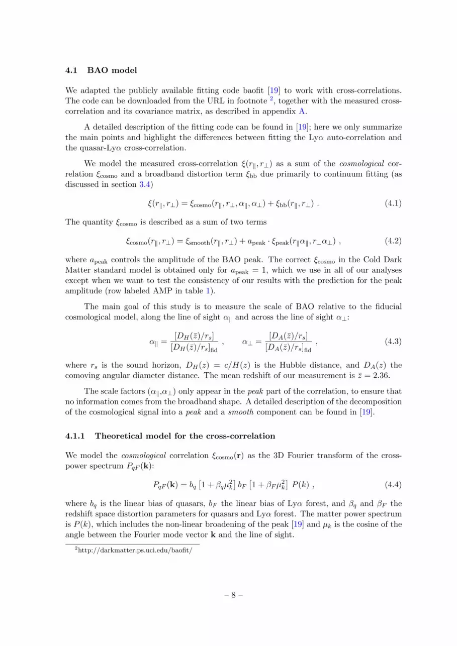
We model the measured cross-correlation ξ(r‖, r⊥) as a sum of the cosmological cor-relation ξcosmo and a broadband distortion term ξbb due primarily to continuum fitting (asdiscussed in section 3.4)

ξ(r‖, r⊥) = ξcosmo(r‖, r⊥, α‖, α⊥) + ξbb(r‖, r⊥) . (4.1)

The quantity ξcosmo is described as a sum of two terms

ξcosmo(r‖, r⊥) = ξsmooth(r‖, r⊥) + apeak · ξpeak(r‖α‖, r⊥α⊥) , (4.2)

where apeak controls the amplitude of the BAO peak. The correct ξcosmo in the Cold DarkMatter standard model is obtained only for apeak = 1, which we use in all of our analysesexcept when we want to test the consistency of our results with the prediction for the peakamplitude (row labeled AMP in table 1).

The main goal of this study is to measure the scale of BAO relative to the fiducialcosmological model, along the line of sight α‖ and across the line of sight α⊥:

α‖ =[DH(z)/rs]

[DH(z)/rs]fid

, α⊥ =[DA(z)/rs]

[DA(z)/rs]fid

, (4.3)

where rs is the sound horizon, DH(z) = c/H(z) is the Hubble distance, and DA(z) thecomoving angular diameter distance. The mean redshift of our measurement is z = 2.36.

The scale factors (α‖,α⊥) only appear in the peak part of the correlation, to ensure thatno information comes from the broadband shape. A detailed description of the decompositionof the cosmological signal into a peak and a smooth component can be found in [19].

4.1.1 Theoretical model for the cross-correlation

We model the cosmological correlation ξcosmo(r) as the 3D Fourier transform of the cross-power spectrum PqF (k):

PqF (k) = bq[1 + βqµ

2k

]bF[1 + βFµ

2k

]P (k) , (4.4)

where bq is the linear bias of quasars, bF the linear bias of Lyα forest, and βq and βF theredshift space distortion parameters for quasars and Lyα forest. The matter power spectrumis P (k), which includes the non-linear broadening of the peak [19] and µk is the cosine of theangle between the Fourier mode vector k and the line of sight.

2http://darkmatter.ps.uci.edu/baofit/

– 8 –

Following [20] we leave two of the four bias parameters free (bq and βF ) and derive theother two from them, using the well-constrained combination bF (1 + βF ) = −0.336 ± 0.03[15] and the Kaiser relation bqβq = f(Ωm) [41], where f(Ωm) is the logarithmic growthrate of structure. Note that the same relation does not apply to the Lyα forest (e.g., [15]).These values of the bias parameters are defined at z = 2.25, and we translate them to ourmean redshift z = 2.36 assuming that only bF evolves with redshift, following (bF (z)g(z))2 ∝(1 + z)3.8, where g(z) is the linear growth factor (as discussed in [15]).

4.1.2 Quasar redshift errors

Determining precise quasar redshifts is a difficult task. As noted in [20], quasar redshift errorshave two main effects on the cross-correlation: a) the r.m.s. in the quasar redshift estimates(σz ∼ 500 km s−1) smooths the cross-correlation along the line of sight (with an equivalenteffect on the quasar auto-correlation, [21]); b) a systematic offset in the BOSS redshiftestimates shifts the cross-correlation along the line of sight by a non-negligible amount ∆z ∼−180 km s−1 (see [20]).

Since we restrict our analysis to large separations (r > 40h−1 Mpc), we do not expectquasar redshift errors to have a significant impact on our fits. We leave ∆z as a free parameterin all our fits, presenting our results after marginalizing over it. We do not include an explicitσz parameter since it would be highly degenerate with the non-linear broadening model.

4.1.3 Broadband distortion

All BAO analyses to date have used a broadband model that parameterizes each multipoleas a function of r, or a parameterization as a function of (r,µ) as in [18]. However, theshape of the distortion discussed in section 3.4 that is introduced into the cross-correlationby the continuum fitting operation is better separated in terms of the (r‖, r⊥) coordinates,as inferred from the analysis that was presented in [39] (see their figure 17). We thereforeuse the following broadband model:

ξbb(r‖, r⊥) =

imax∑i=imin

jmax∑j=jmin

bij ri‖ r

j⊥ , (4.5)

where the sums are understood to be over consecutive integers, and they go from imin = 0to imax = 2, and from jmin = −3 to jmax = 1 in our fiducial analysis. The dependence of ourresults on the broadband model is discussed in section 4.3.

4.2 BAO fits

Our fiducial BAO fit is performed over the separation range 40h−1 Mpc < r < 180h−1 Mpcusing a broadband model with (imin = 0, imax = 2, jmin = −3, jmax = 1). The total numberof bins included is 440, and the number of free parameters is 20: α‖, α⊥, βF , bq, ∆z and the15 parameters bij in our broadband distortion model. In table 1 we present the best fit valuesfor our fiducial analysis, and for a series of illustrative alternative analyses: an isotropic BAOanalysis (ISO) imposing α ≡ α‖ = α⊥; a no-wiggles fit (NW) with apeak = 0; a fit allowing

– 9 –

βF bq apeak α α‖ α⊥ χ2 (d.o.f)FID 1.09± 0.29 3.02± 0.22 - - 1.042± 0.034 0.930± 0.036 426.4 (420)ISO 1.09± 0.30 3.00± 0.22 - 0.988± 0.022 - - 429.5 (421)NW 1.13± 0.34 2.71± 0.21 - - - - 448.5 (422)

AMP 1.14± 0.32 3.02± 0.22 1.15± 0.24 - 1.041± 0.033 0.933± 0.035 426.0 (419)PCA 1.54± 0.42 3.14± 0.22 - - 1.052± 0.035 0.922± 0.044 474.7 (420)

Table 1: Best fit parameters for different analyses : fiducial BAO fit (FID), istropic BAOfit (ISO), non-BAO fit (NW), fit with free amplitude (AMP) and using a continuum fittingmethod based on a Principal Component Analysis (PCA, [40]).

0.7 0.8 0.9 1.0 1.1 1.20.8

0.9

1.0

1.1

1.2

1.3

HDArsLHDArsLfid

HrsH

L fidH

rsH

L

10

20

30

40

-6-4-20246

Figure 3: ∆χ2 as a function of α‖,α⊥ (defined in equation 4.3) in our fiducial analysis,after marginalizing over the remaining 18 parameters. The solid contours correspond to∆χ2 = 2.27, 5.99 and 11.62, equivalent to Gaussian probabilities of 68%, 95% and 99.7%.The fiducial model is consistent at the ∼ 1.5σ level.

the amplitude of the peak apeak to vary (AMP); and a fit using a different method to fit thecontinua based on a Principal Component Analysis (PCA, [40]).

The BAO peak position is significantly measured to an accuracy better than ∼ 4% bothalong and across the line of sight directions. The measured amplitude of the BAO peak isconsistent with the expected in our fiducial model.

In figure 3 we present the main result of this paper: the value of ∆χ2 as a function of(α‖,α⊥) for our fiducial BAO analysis, fully marginalized over the other 18 free parameters.The solid contours correspond to ∆χ2 = 2.27, 5.99 and 11.62, equivalent to likelihood con-tours of 68%, 95% and 99.7% for a Gaussian likelihood. The fiducial model is consistent atthe ∼ 1.5σ level.

We can translate our measurement of (α‖,α⊥) to a measurement of the Hubble pa-rameter and the angular diameter distance at our mean redshift z = 2.36, up to a factor

– 10 –

rs:c/(H(z = 2.36) rs) = 9.0± 0.3 , DA(z = 2.36) / rs = 10.8± 0.4 . (4.6)

Using the best fit value of the sound horizon from the Planck collaboration (rs =147.49 Mpc) [3] 3, we can present the results as:

H(z = 2.36) = 226± 8 km s−1 DA(z = 2.36) = 1590± 60 Mpc . (4.7)

4.3 Systematic tests

Table 2 presents the dependence of our results on the broadband model for our fiducial anal-ysis. We find that the BAO results deviate by much less than the 1σ error under variations ofthe broadband model, as long as sufficient broadband flexibility is allowed to obtain a goodfit.

βF bq α‖ α⊥ χ2 (d.o.f)

FID 1.09± 0.29 3.02± 0.22 1.042± 0.034 0.930± 0.036 426.4 (420)

NO BB 2.85± 0.62 2.75± 0.16 1.049± 0.039 0.902± 0.048 482.9 (435)BB1 0.87± 0.21 3.13± 0.21 1.044± 0.034 0.928± 0.036 430.8 (423)BB2 1.04± 0.21 3.11± 0.21 1.043± 0.034 0.929± 0.036 424.6 (423)BB3 1.03± 0.24 3.12± 0.22 1.042± 0.034 0.931± 0.037 422.1 (419)RMU 41.4± 190 5.53± 1.3 1.054± 0.030 0.913± 0.045 441.5 (426)

Table 2: Best fit parameters for the fiducial analysis and for different broadband models:FID (ri‖r

j⊥, with i = 0, 1, 2 and j = −3,−2,−1, 0, 1), NO BB (no broadband), BB1 (ri‖r

j⊥,

with i = 0, 1, 2, 3, and j = −2,−1, 0), BB2 (ri‖rj⊥, with i = 0, 1, 2, 3, and j = −1, 0, 1),

BB3 (ri‖rj⊥, with i = 0, 1, 2, 3, and j = −1, 0, 1, 2) and RMU (riµj , with i = −2,−1, 0, and

j = 0, 2, 4).

Table 3 presents the dependence on the separation range over which the cross-correlationis fitted, when the maximum separation is modified from the fiducial value of 180h−1 Mpcto 170h−1 Mpc (RMAX 170) or to 190h−1 Mpc (RMAX 190), and the minimum separationfrom 40h−1 Mpc to 30h−1 Mpc (RMIN 30) or to 50h−1 Mpc (RMIN 50). The last three rowsshow the results of restricting the range of the angle cosine µ = r‖/r to ‖µ‖ < 0.8 (MU 08),‖µ‖ < 0.9 (MU 09), or ‖µ‖ < 0.95 (MU 095). The results in this table show that the BAOmeasurement in general has little dependence on the fitting range. The broadband distortionis most important for separations near the line of sight (i.e., ‖µ‖ near one), but the removalof this most contaminated part does not significantly alter the BAO peak position that isobtained, except in the MU 095 case where the position that is obtained shifts to a valuecloser to the expected one in our fiducial model by nearly 1σ.

4.4 Test of the covariance matrix

In table 1 we can see that the χ2 value in our fiducial fit is good, in the sense that it iscompatible with being drawned from a χ2 distribution with mean equal to the degrees offreedom in the problem, i.e., the number of bins used in the fit (440) minus the number offree parameters (20).

3Table 2, column with 68% limits for Planck+WP.

– 11 –

βF bq α‖ α⊥ χ2 (d.o.f)

FID 1.09± 0.29 3.02± 0.22 1.042± 0.034 0.930± 0.036 426.4 (420)

RMAX 170 1.07± 0.28 3.07± 0.22 1.046± 0.034 0.926± 0.036 397.4 (394)RMAX 190 1.05± 0.27 3.04± 0.22 1.042± 0.034 0.929± 0.036 438.3 (436)RMIN 30 1.03± 0.21 2.85± 0.14 1.043± 0.035 0.930± 0.038 443.5 (430)RMIN 50 1.65± 0.71 3.01± 0.34 1.044± 0.034 0.923± 0.038 407 (406)

MU 08 2.26± 2.0 2.61± 0.38 1.025± 0.088 0.937± 0.055 257.1 (244)MU 09 1.39± 0.89 2.73± 0.41 1.023± 0.054 0.938± 0.041 306.7 (302)MU 095 0.88± 0.32 3.13± 0.27 1.009± 0.041 0.949± 0.037 353.6 (344)

Table 3: Best fit parameters for the fiducial analysis (FID), and different fitting ranges (inh−1 Mpc). The last rows show the results when using only bins that are far from the line ofsight, with |µ| < 0.8 (MU 08), |µ| < 0.9 (MU 09) and |µ| < 0.95 (MU 095).

-4 -2 0 2 40

10

20

30

40

50

60

Covariance Mode Residual

Num

ber

of

Modes

Χ2dof =

426.4H440-20L

prob= 40.4%

Figure 4: Histogram of χ2 values for the different eigenmodes of the covariance matrix,compared to a zero-mean Gaussian with variance (440 − 20)/440, where 440 is the numberof bins in the fit, and 20 is the number of free parameters. The agreement between thedistributions supports the validity of our covariance matrix.

In order to test our estimate of the covariance matrix, we examine the distributionof χ2 for its different eigenmodes. The results of this test are compared to a zero-meanGaussian with variance (440 − 20)/440 in figure 4. The agreement supports the validity ofour covariance matrix.

4.5 Alternative uncertainty estimates of the BAO scales

The error on the fitted parameters reported so far have been computed from the secondderivatives of the log-likelihood function at its maximum, assuming this likelihood functionto be Gaussian at 1σ. The BAO scale uncertainties in the fiducial analysis obtained in thisway are 0.034 for α‖ and 0.036 for α⊥. An alternative error estimate can be computedfrom the full likelihood surface in figure 3, without assuming a Gaussian likelihood. Theuncertainties obtained in the fiducial analysis are then 0.032 for α‖ and 0.036 for α⊥, in goodagreement with the previous ones.

Both these estimates rely on the accuracy of the covariance matrix that we have com-

– 12 –

puted as described in section 3. We test this by computing an alternative bootstrap errorthat does not rely on our covariance matrix. We generate 1,000 bootstrap realizations of thesurvey [42], combining the measurements from the 66 different sub-samples. The fitting anal-ysis is done for each realization, and the uncertainties are computed from their distributionof best fit values. The resulting uncertainties on the BAO scales are 0.031 on α‖ and 0.036on α⊥, in excellent agreement with the previous estimates.

4.6 Visualizing the BAO Peak

Even though we do not use multipoles anywhere in our analysis, we present here a fit ofthe multipoles from the measured cross-correlation in order to better see the BAO peak inthe data. We start by constructing a multipole expansion of our measured cross-correlation,ξ(r‖, r⊥), using a linear least-squares fit to:

ξ(r, µ) =∑l

Ll(µ)ξl(r) , (4.8)

where r =√r2‖ + r2

⊥ and µ = r‖/r, Ll(x) is the Legendre polynomial of order l and ξl(r) are

the multipoles we wish to measure.

In figure 2 we show the measured cross-correlation, as a function of line of sight (r‖)and transverse (r⊥) separation, together with our best fit model. From the right panel of thefigure, one can see that the best fit model of the broadband distortion is asymmetric withrespect to r‖ = 0. Therefore we expect a net non-zero contribution from odd multipoles. Forthe purpose of visualization, however, we only fit the monopole (l = 0) and the quadrupole(l = 2), since these two multipoles contain most of the cosmological infomation. We use36 equidistant interpolation points separated by 4h−1 Mpc and ranging from 40h−1 Mpc to180h−1 Mpc.

Our estimates of the multipoles at different separations are highly correlated. In orderto improve the visualization of the BAO peak, we apply a correction to the multipoles basedon the analysis presented in [19]. We start by examining the eigenmodes of the covariancematrix and identify a particular mode being essentially a DC offset of the monopole, andtherefore responsible for much of the correlations between separations. We then project outthe mode from the data and its covariance matrix, and refit for the distortion while keepingall other parameters fixed from the baseline best fit.

Figure 5 shows the resulting monopole and quadrupole of the quasar-Lyα cross-correlation,expressed as the transverse correlation, ξ(r, µ = 0) = ξ0(r) − ξ2(r)/2 (left panel), and theparallel correlation ξ(r, µ = 1) = ξ0(r) + ξ2(r). We superimpose a fit with all parametersfixed from the 2D BAO fit except for the distortion. The solid black curve shows the bestfit, the red dashed curve is the BAO-only part (with parameters fixed from the 2D fit), andthe green dotted curve shows the distortion, which is parabolic after r2 weighting. Since theLyα fluctuation is defined in equation 3.4 as a transmission fluctuation, positive values of δFreflect negative density fluctuations, implying a negative value for the bias factor bF . Thisexplains why the BAO feature in the quasar-Lyα cross-correlation appears as a dip insteadof a peak, as seen in figure 5.

The orange curve in figure 5 shows the predicted cross-correlation for our fiducial cos-mological model with α‖ = α⊥ = 1, and an amplitude determined by a quasar bias factor

– 13 –

40 60 80 100 120 140 160

-5

0

5

Comoving Separation r HMpchL

Tra

nsv

erse

Corr

elat

ion

r2

ΞHr,

Μ=

0L

40 60 80 100 120 140 160

0

5

10

15

Comoving Separation r HMpchL

Par

alle

lC

orr

elat

ion

r2

ΞHr,

Μ=

1L

Figure 5: Transverse (left) and parallel (right) correlations, defined as ξ(r, µ = 0) = ξ0(r)−ξ2(r)/2 and ξ(r, µ = 1) = ξ0(r) + ξ2(r), after projecting out the mode responsible for mostof the correlation between separations. The best fit theory is shown in a solid black curve,its BAO-only part in a red dashed curve and the distortion in a dotted green curve. Theorange dot-dashed curve shows the cosmological signal for our fiducial cosmology (α = 1),using a quasar bias of bq = 3.64 and a Lyα redshift-space distortion parameter βF = 1.1,as measured in [20]. All datapoints and lines are weighted by r2 and are plotted after theprojection (see text for details).

bq = 3.64 and a Lyα redshift distortion parameter βF = 1.1, as measured in [20]. The factthat this model is consistent with the best fit that is obtained here to the DR11 data provesthat our result is consistent with that obtained in [20] using the DR9 data, and that thedifferent values that are obtained in our fit for bq and βF are caused by our addition of anarbitrary broadband function, with parameters that are degenerate with bq and βF . Theamplitude of the BAO dip, as visualized in figure 5, is consistent with our expectation. Thisis seen also in the model AMP in table 1, where the parameter apeak has a best fit valuethat is consistent with unity. A model with a suppressed BAO peak (model NW in table 1)has a χ2 that is worse than our fiducial model by 20, although we warn that this is not tobe directly interpreted as a statistical significance of a BAO detection because our likelihoodfunction is not necessarily Gaussian. In any case, our interest here lies in the statisticalconstraint obtained on the BAO scale, rather than the significance of the BAO detection inthe quasar-Lyα cross-correlation only.

5 Discussion & Conclusions

We have presented a measurement of the quasar - Lyα cross-correlation using approximately164,000 quasars from the eleventh Data Release (DR11) of SDSS. We are able to measurethe BAO scale along and across the line of sight (α‖, α⊥) with an uncertainty of 3.4% and

– 14 –

3.6% respectively. The measurement is in agreement with our fiducial cosmology well withinthe 95% confidence level.

We have checked the robustness of our measurement under changes of broadband mod-els, separation range used, and different error estimates. As discussed in section 3.4, we arenot particularly careful in our treatment of the non-BAO part of the cross-correlation. How-ever, the best fit values for the bias parameters of both quasars and Lyα forest are roughlyconsistent with previous analyses, with rather large uncertainties since we only use largeseparations to measure the BAO scale.

In table 4 we compare the results with other BAO measurements at the same redshiftfrom the Lyα auto-correlation measured with DR9 ([17], [18]). We also present our resultswhen using only data from DR10. Assuming that the uncertainties in these BAO measure-ments scale with the inverse of the square root of the survey area, we can extrapolate themfrom DR9 to DR11, using

√ADR11/ADR9 = 1.60. We show these extrapolations in the last

two rows of table 4.

Analysis Probe Data Release α α‖ α⊥Busca 2013 Auto DR9 1.01± 0.03 - -Slosar 2013 Auto DR9 0.98± 0.020 0.99± 0.035 0.98± 0.070This work Cross DR10 1.00± 0.027 1.06± 0.038 0.91± 0.041This work Cross DR11 0.99± 0.022 1.04± 0.034 0.93± 0.036

Busca 2013 Auto to DR11 ±0.019 - -Slosar 2013 Auto to DR11 ±0.013 ±0.022 ±0.046

Table 4: Comparison of different BAO analysis at z ∼ 2.4 from BOSS, from the auto-correlation in DR9 (Busca 2013 [17], Slosar 2013 [18]), and from this work. We show ourresults when using only DR10 data and when including DR11 data. In the last two rows weextrapolate the uncertainties of previous work to DR11, assuming that these scale with theinverse of the square root of the survey area.

The errors on the BAO scale (α‖,α⊥) from our DR10 analysis are considerably smallerthan those reported in [43]. An extensive comparison of the two analyses within the BOSSLyα working group concluded that the discrepancy can be explained by the differences inthe analysis. While [43] uses only the monopole and the quadrupole to fit the BAO scale, inthis analysis we use the full 2D contours of the cross-correlation function.

In the absence of any broadband distortion of ξ(r‖, r⊥) (or with a distortion that is a-priori known), we find that essentially all of the BAO signal is contained within the monopoleξ0(r) and quadrupole ξ2(r). However, when broadband distortion is present, as in our anal-ysis, it contributes significantly to multipoles other than the monopole and quadrupole, andleads to correlated uncertainties between distortion and BAO parameters and correspondingparameter degeneracies. As a result, we find that the unknown broadband distortion pa-rameters can be determined more precisely with a fit to the full ξ(r‖, r⊥) (or, equivalently,a larger set of multipoles) instead of a fit to only the monopole and quadrupole. Similarly,we find that a fit to ξ(r‖, r⊥) yields a more precise determination of the BAO parametersby helping to break the degeneracy between distortion and BAO parameters. The actualimprovement we find is a factor of 1.2 in α‖ and a factor of 1.3 in α⊥. [36] found that asimilar improvement is also seen when measuring BAO from the Lyα auto-correlation func-

– 15 –

tion, although a detailed study on mock data sets revealed a large scatter in the gain fromrealization to realization.

5.1 Lyα auto-correlation vs. quasar-Lyα cross-correlation

In appendix B we present a Fisher matrix projection comparing the relative strength ofmeasuring BAO with the Lyα auto-correlation and with the quasar-Lyα cross-correlation.In a BOSS-like survey, both probes should measure the transverse BAO scale with similaruncertainties, while the Lyα auto-correlation should be able to measure the line of sight scale∼ 40% better than the cross-correlation with quasars.

The measurement of BAO from the Lyα auto-correlation in DR9 was presented in [17]and [18]. Most of the difference between the uncertainties in these results can be explainedby the looser data cuts used in [18], that included lines with DLAs and that defined theirLyα forest with a wider wavelength range. In this analysis we used data cuts similar to thosein [18], and therefore we compare here our uncertainties with those from [18] extrapolatedto DR11 (see table 4).

Our measurement of α‖ is ∼ 55% worse than the results from the Lyα auto-correlationof [18] extrapolated to DR11, in good agreement with the prediction of ∼ 40% computedin the appendix. The Fisher forecast formalism predicted similar uncertainties in α⊥, andwe find that our measurement is ∼ 20% better than the extrapolated results from the auto-correlation.

In the same appendix we also show that on the scales of interest for BAO measurements(k > 0.05hMpc−1) cosmic variance is not the dominant contribution to our error budget.Assuming that the shot noise in the quasar density field is uncorrelated with the small scalefluctuations in the Lyα absorption and with the instrumental noise, we can then combineboth BAO measurements as if they were independent.

In figure 6 we compare the contours on (α‖,α⊥) from the Lyα auto-correlation func-tion from DR9 ([18] in blue, generated from the files in http://darkmatter.ps.uci.edu/

baofit/), and compare it to our measurement from the cross-correlation function from DR11(red) and the sum of their χ2 surfaces (in black), assuming they are independent. We com-pare these constraints with the 68% and 95% confidence limits obtained from the Planckresults [3] in an open ΛCDM cosmology, shown in green. 4 Note that by allowing for spacecurvature, the Planck constraints on the distance and expansion rate at our mean redshiftz = 2.36 are much less restrictive compared to a flat model.

We have shown that adding the cross-correlation of Lyα and quasars to the auto-correlation of Lyα can certainly improve the constraints on BAO scales at high redshfit.A detailed analysis of the cosmological implications of the measurements of the Lyα auto-correlation and the quasar-Lyα cross-correlation will be presented in a future publication,which will include the DR11 results from the Lyα auto-correlation, together with a morecomplete examination of potential correlations between the two measurements.

4We use the Planck + ACT/SPT + WP public chains available under the namebase omegak planck lowl lowLike highL.

– 16 –

Figure 6: Contours of ∆χ2 = 2.27 and 5.99, corresponding to Gaussian confidence levelsof 68% and 95%, from the Lyα auto-correlation analysis from DR9 ([18], in blue), fromthe cross-correlation from DR11 (this work, in red) and from the joint analysis (in black).The green contours show the 68% and 95% contours for the regions of this parameter spaceallowed by the Planck results [3] in an open ΛCDM cosmology.

Acknowledgments

We would like to thank Ross O’Connell for detailed comparisons with his analysis, and JamesRich and Shirley Ho for very useful comments.

This research used resources of the National Energy Research Scientific ComputingCenter (NERSC), which is supported by the Office of Science of the U.S. Department ofEnergy under Contract No. DE-AC02-05CH11231. DK would like to thank CEA Saclay fortheir hospitality and productive environment during his sabbatical. JM is supported in partby Spanish grant AYA 2009-09745.

Funding for SDSS-III has been provided by the Alfred P. Sloan Foundation, the Partic-ipating Institutions, the National Science Foundation, and the U.S. Department of EnergyOffice of Science. The SDSS-III web site is http://www.sdss3.org/.

SDSS-III is managed by the Astrophysical Research Consortium for the ParticipatingInstitutions of the SDSS-III Collaboration including the University of Arizona, the BrazilianParticipation Group, Brookhaven National Laboratory, University of Cambridge, CarnegieMellon University, University of Florida, the French Participation Group, the German Par-ticipation Group, Harvard University, the Instituto de Astrofisica de Canarias, the MichiganState/Notre Dame/JINA Participation Group, Johns Hopkins University, Lawrence Berke-ley National Laboratory, Max Planck Institute for Astrophysics, Max Planck Institute forExtraterrestrial Physics, New Mexico State University, New York University, Ohio State Uni-versity, Pennsylvania State University, University of Portsmouth, Princeton University, the

– 17 –

Spanish Participation Group, University of Tokyo, University of Utah, Vanderbilt University,University of Virginia, University of Washington, and Yale University.

References

[1] A. G. Riess, A. V. Filippenko, P. Challis, A. Clocchiatti, A. Diercks, P. M. Garnavich, R. L.Gilliland, C. J. Hogan, S. Jha, R. P. Kirshner, et al., AJ 116, 1009 (Sep. 1998),arXiv:astro-ph/9805201.

[2] S. Perlmutter, G. Aldering, G. Goldhaber, R. A. Knop, P. Nugent, P. G. Castro, S. Deustua,S. Fabbro, A. Goobar, D. E. Groom, et al., Astrophys. J. 517, 565 (Jun. 1999),arXiv:astro-ph/9812133.

[3] Planck Collaboration, P. A. R. Ade, N. Aghanim, C. Armitage-Caplan, M. Arnaud,M. Ashdown, F. Atrio-Barandela, J. Aumont, C. Baccigalupi, A. J. Banday, et al., ArXive-prints (Mar. 2013), 1303.5076.

[4] D. H. Weinberg, M. J. Mortonson, D. J. Eisenstein, C. Hirata, A. G. Riess, and E. Rozo, ArXive-prints (Jan. 2012), 1201.2434.

[5] H.-J. Seo and D. J. Eisenstein, Astrophys. J. 598, 720 (Dec. 2003).

[6] D. J. Eisenstein, I. Zehavi, D. W. Hogg, R. Scoccimarro, M. R. Blanton, R. C. Nichol,R. Scranton, H.-J. Seo, M. Tegmark, Z. Zheng, et al., Astrophys. J. 633, 560 (Nov. 2005).

[7] S. Cole, W. J. Percival, J. A. Peacock, P. Norberg, C. M. Baugh, C. S. Frenk, I. Baldry,J. Bland-Hawthorn, T. Bridges, R. Cannon, et al., Mon. Not. Roy. Astron. Soc. 362, 505(Sep. 2005), arXiv:astro-ph/0501174.

[8] C. Blake, E. A. Kazin, F. Beutler, T. M. Davis, D. Parkinson, S. Brough, M. Colless,C. Contreras, W. Couch, S. Croom, et al., Mon. Not. Roy. Astron. Soc. 418, 1707 (Dec.2011), 1108.2635.

[9] L. Anderson, E. Aubourg, S. Bailey, D. Bizyaev, M. Blanton, A. S. Bolton, J. Brinkmann,J. R. Brownstein, A. Burden, A. J. Cuesta, et al., Mon. Not. Roy. Astron. Soc. 427, 3435(Dec. 2012), 1203.6594.

[10] A. Merloni, P. Predehl, W. Becker, H. Bohringer, T. Boller, H. Brunner, M. Brusa, K. Dennerl,M. Freyberg, P. Friedrich, et al., ArXiv e-prints (Sep. 2012), 1209.3114.

[11] J. C. Pober, A. R. Parsons, D. R. DeBoer, P. McDonald, M. McQuinn, J. E. Aguirre, Z. Ali,R. F. Bradley, T.-C. Chang, and M. F. Morales, AJ 145, 65, 65 (Mar. 2013), 1210.2413.

[12] G. J. Hill, K. Gebhardt, E. Komatsu, N. Drory, P. J. MacQueen, J. Adams, G. A. Blanc,R. Koehler, M. Rafal, M. M. Roth, et al., in T. Kodama, T. Yamada, and K. Aoki, eds.,Astronomical Society of the Pacific Conference Series (Oct. 2008), vol. 399 of AstronomicalSociety of the Pacific Conference Series, pp. 115–+.

[13] D. J. Schlegel, C. Bebek, H. Heetderks, S. Ho, M. Lampton, M. Levi, N. Mostek,N. Padmanabhan, S. Perlmutter, N. Roe, et al., ArXiv e-prints (Apr. 2009), 0904.0468.

[14] G. Zhao and collaborators, The Extended BOSS Survey (eBOSS), in preparation (2013).

[15] A. Slosar, A. Font-Ribera, M. M. Pieri, J. Rich, J.-M. Le Goff, E. Aubourg, J. Brinkmann,N. Busca, B. Carithers, R. Charlassier, et al., JCAP 9, 1 (Sep. 2011), 1104.5244.

[16] C. P. Ahn, R. Alexandroff, C. Allende Prieto, S. F. Anderson, T. Anderton, B. H. Andrews,E. Aubourg, S. Bailey, E. Balbinot, R. Barnes, et al., Astrophys. J. Sup. 203, 21, 21 (Dec.2012), 1207.7137.

[17] N. G. Busca, T. Delubac, J. Rich, S. Bailey, A. Font-Ribera, D. Kirkby, J.-M. Le Goff, M. M.Pieri, A. Slosar, E. Aubourg, et al., A&A 552, A96, A96 (Apr. 2013), 1211.2616.

– 18 –

[18] A. Slosar, V. Irsic, D. Kirkby, S. Bailey, N. G. Busca, T. Delubac, J. Rich, E. Aubourg, J. E.Bautista, V. Bhardwaj, et al., JCAP 4, 26, 026 (Apr. 2013), 1301.3459.

[19] D. Kirkby, D. Margala, A. Slosar, S. Bailey, N. G. Busca, T. Delubac, J. Rich, J. E. Bautista,M. Blomqvist, J. R. Brownstein, et al., JCAP 3, 24, 024 (Mar. 2013), 1301.3456.

[20] A. Font-Ribera, E. Arnau, J. Miralda-Escude, E. Rollinde, J. Brinkmann, J. R. Brownstein,K.-G. Lee, A. D. Myers, N. Palanque-Delabrouille, I. Paris, et al., JCAP 5, 18, 018 (May2013), 1303.1937.

[21] M. White, A. D. Myers, N. P. Ross, D. J. Schlegel, J. F. Hennawi, Y. Shen, I. McGreer, M. A.Strauss, A. S. Bolton, J. Bovy, et al., Mon. Not. Roy. Astron. Soc. 424, 933 (Aug. 2012),1203.5306.

[22] A. Lewis, A. Challinor, and A. Lasenby, Astrophys. J. 538, 473 (Aug. 2000).

[23] D. J. Eisenstein and W. Hu, Astrophys. J. 496, 605 (Mar. 1998), arXiv:astro-ph/9709112.

[24] D. J. Eisenstein, D. H. Weinberg, E. Agol, H. Aihara, C. Allende Prieto, S. F. Anderson, J. A.Arns, E. Aubourg, S. Bailey, E. Balbinot, et al., AJ 142, 72 (Sep. 2011), 1101.1529.

[25] A. S. Bolton, D. J. Schlegel, E. Aubourg, S. Bailey, V. Bhardwaj, J. R. Brownstein, S. Burles,Y.-M. Chen, K. Dawson, D. J. Eisenstein, et al., AJ 144, 144, 144 (Nov. 2012), 1207.7326.

[26] J. E. Gunn, M. Carr, C. Rockosi, M. Sekiguchi, K. Berry, B. Elms, E. de Haas, Z. Ivezic,G. Knapp, R. Lupton, et al., AJ 116, 3040 (Dec. 1998).

[27] J. E. Gunn, W. A. Siegmund, E. J. Mannery, R. E. Owen, C. L. Hull, R. F. Leger, L. N.Carey, G. R. Knapp, D. G. York, W. N. Boroski, et al., AJ 131, 2332 (Apr. 2006),arXiv:astro-ph/0602326.

[28] S. A. Smee, J. E. Gunn, A. Uomoto, N. Roe, D. Schlegel, C. M. Rockosi, M. A. Carr, F. Leger,K. S. Dawson, M. D. Olmstead, et al., AJ 146, 32, 32 (Aug. 2013), 1208.2233.

[29] D. G. York, J. Adelman, J. E. Anderson, S. F. Anderson, J. Annis, N. A. Bahcall, J. A.Bakken, R. Barkhouser, S. Bastian, E. Berman, et al., AJ 120, 1579 (Sep. 2000).

[30] K. S. Dawson, D. J. Schlegel, C. P. Ahn, S. F. Anderson, E. Aubourg, S. Bailey, R. H.Barkhouser, J. E. Bautista, A. Beifiori, A. A. Berlind, et al., AJ 145, 10, 10 (Jan. 2013),1208.0022.

[31] N. P. Ross, A. D. Myers, E. S. Sheldon, C. Yeche, M. A. Strauss, J. Bovy, J. A. Kirkpatrick,G. T. Richards, E. Aubourg, M. R. Blanton, et al., Astrophys. J. Sup. 199, 3, 3 (Mar. 2012),1105.0606.

[32] C. Yeche, P. Petitjean, J. Rich, E. Aubourg, N. Busca, J.-C. Hamilton, J.-M. Le Goff, I. Paris,S. Peirani, C. Pichon, et al., A&A 523, A14, A14 (Nov. 2010).

[33] J. A. Kirkpatrick, D. J. Schlegel, N. P. Ross, A. D. Myers, J. F. Hennawi, E. S. Sheldon, D. P.Schneider, and B. A. Weaver, Astrophys. J. 743, 125, 125 (Dec. 2011), 1104.4995.

[34] J. Bovy, J. F. Hennawi, D. W. Hogg, A. D. Myers, J. A. Kirkpatrick, D. J. Schlegel, N. P.Ross, E. S. Sheldon, I. D. McGreer, D. P. Schneider, et al., Astrophys. J. 729, 141, 141 (Mar.2011), 1011.6392.

[35] I. Paris, P. Petitjean, E. Aubourg, S. Bailey, N. P. Ross, A. D. Myers, M. A. Strauss, S. F.Anderson, E. Arnau, J. Bautista, et al., A&A 548, A66, A66 (Dec. 2012), 1210.5166.

[36] T. Delubac and collaborators, Lyman alpha BAO constraints from SDSS DR11, in preparation(2013).

[37] P. Noterdaeme, P. Petitjean, W. C. Carithers, I. Paris, A. Font-Ribera, S. Bailey, E. Aubourg,D. Bizyaev, G. Ebelke, H. Finley, et al., A&A 547, L1, L1 (Nov. 2012), 1210.1213.

[38] P. Noterdaeme, P. Petitjean, C. Ledoux, and R. Srianand, A&A 505, 1087 (Oct. 2009),

– 19 –

0908.1574.

[39] A. Font-Ribera, J. Miralda-Escude, E. Arnau, B. Carithers, K.-G. Lee, P. Noterdaeme, I. Paris,P. Petitjean, J. Rich, E. Rollinde, et al., JCAP 11, 59, 059 (Nov. 2012), 1209.4596.

[40] K.-G. Lee, N. Suzuki, and D. N. Spergel, AJ 143, 51, 51 (Feb. 2012).

[41] N. Kaiser, Mon. Not. Roy. Astron. Soc. 227, 1 (Jul. 1987).

[42] B. Efron and G. Gong, American Statistician 37, 36 (1983).

[43] R. O’Connell and collaborators, BAO in QSO-LyaF Cross-correlation, in preparation (2013).

[44] F. James and M. Roos, Computer Physics Communications 10, 343 (Dec. 1975).

[45] P. McDonald and D. J. Eisenstein, Phys. Rev. D 76(6), 063009 (Sep. 2007),arXiv:astro-ph/0607122.

[46] M. McQuinn and M. White, Mon. Not. Roy. Astron. Soc. 415, 2257 (Aug. 2011), 1102.1752.

[47] P. McDonald, U. Seljak, S. Burles, D. J. Schlegel, D. H. Weinberg, R. Cen, D. Shih, J. Schaye,D. P. Schneider, N. A. Bahcall, et al., Astrophys. J. Sup. 163, 80 (Mar. 2006),arXiv:astro-ph/0405013.

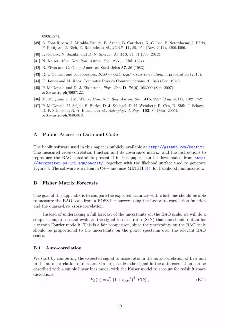
A Public Access to Data and Code

The baofit software used in this paper is publicly available at http://github.com/baofit/.The measured cross-correlation function and its covariance matrix, and the instructions toreproduce the BAO constraints presented in this paper, can be downloaded from http:

//darkmatter.ps.uci.edu/baofit/, together with the likehood surface used to generateFigure 3. The software is written in C++ and uses MINUIT [44] for likelihood minimization.

B Fisher Matrix Forecasts

The goal of this appendix is to compare the expected accuracy with which one should be ableto measure the BAO scale from a BOSS-like survey using the Lyα auto-correlation functionand the quasar-Lyα cross-correlation.

Instead of undertaking a full forecast of the uncertainty on the BAO scale, we will do asimpler comparison and evaluate the signal to noise ratio (S/N) that one should obtain fora certain Fourier mode k. This is a fair comparison, since the uncertainty on the BAO scaleshould be proportional to the uncertainty on the power spectrum over the relevant BAOscales.

B.1 Auto-correlation

We start by computing the expected signal to noise ratio in the auto-correlation of Lyα andin the auto-correlation of quasars. On large scales, the signal in the auto-correlation can bedescribed with a simple linear bias model with the Kaiser model to account for redshift spacedistortions:

PA(k) = b2A(1 + βAµ

2)2

P (k) , (B.1)

– 20 –

where bA and βA are the linear bias parameter of the tracer A and its redshift space distortionparameter, P (k) is the matter power spectrum, and µ is the cosine of the angle between theFourier mode k and the line of sight.

The accuracy with which one can measure the quasar power spectrum PA(k) in a givenbin centered at (k,µ) can be quantified by the signal to noise ratio (S/N),(

S

N

)2

A

= NkP 2A(k)

var[PA(k)], (B.2)

where Nk is the number of modes in the bin. Since we only care about relative performancein this appendix, we will drop any Nk and will plot signal to noise ratio per mode.

For a sample of point-like sources (for instance quasars), the variance of its measuredpower spectrum can be approximated by

var [PA(k)] = 2(PA(k) + n−1

A

)2, (B.3)

with nA the number density of systems.

Since the Lyα forest is not a discrete point sampling of the underlying matter densityfield, but rather a non-linear transformation of a continuous sampling along discrete linesof sight, we need to use a slightly different approach. [45] computed the expected S/N inthe measurement of PFF (k) in a spectroscopic survey, and highlighted the importance of the“ aliasing term ” due to the sparse sampling of the universe. Here we use the formalismfrom [46] that combines both the noise term and the aliasing term defining a noise-weighteddensity of lines of sight per unit area neff ,

var[PFF (k)] = 2(PFF (k) + P 1D(kµ) n−1

eff

)2, (B.4)

where P 1D(kµ) is the one-dimensional flux power spectrum.

B.2 Cross-correlation

The cross correlation between the Lyα absorption and the quasar density field can be definedas

〈δF (k) δq(k′)〉 = (2π)3δD(k + k′) PqF (k) . (B.5)

Again, in the linear regime we can relate the cross-correlation power spectrum with the linearpower spectrum P (k) using the linear bias parameters defined above,

PqF (k) = bq(1 + βqµ

2)bF(1 + βFµ

2)P (k) . (B.6)

[46] showed that the variance in the measurement of the cross-correlation can be approxi-mated by

var (PqF (k)) = PqF (k)2 +(Pqq(k) + n−1

q

) (PFF (k) + P 1D(kµ) n−1

eff

). (B.7)

In this approximation, the expected S/N in a bin of (k,µk) can be approximated by(S

N

)2

Fg

= Nk

P 2qF (k)

PqF (k)2 +(Pqq(k) + n−1

q

) (PFF (k) + P 1D(kµ) n−1

eff

) . (B.8)

– 21 –

B.3 Forecast for a BOSS-like survey

Here we quantify the previous results for the case of a spectroscopic survey with propertiessimilar to the BOSS survey. The BOSS survey has an area of A = 104 deg2, and if we restrictthe analysis to the redshift range 2 < z < 3, the total volume of the survey is roughlyV = 40(h−1 Gpc)3. The quasar density in the BOSS survey is roughly nq = 160000/V ∼4 × 10−6(h−1 Mpc)−3, and we assume a quasar bias of bq = 3.6 ([20],[21]). The effectivedensity of lines of sight for BOSS is estimated in [46] to be neff ≈ 10−3(h−1 Mpc)−2, andwe assume the values for the Lyα biases of bF = −0.15 and βF = 1.2, both compatible withthe 1D measurement of [47] and the 3D clustering from [15]. We compute the power spectraat our fiducial redshfit of zc = 2.36.

1

10

100

1000

0.01 0.1

P(k

)

k (h/Mpc)

LyaF auto-correlation

1000

10000

100000

1e+06

0.01 0.1

P(k

)

k (h/Mpc)

Quasar auto-correlation

10

100

1000

10000

100000

0.01 0.1

P(k

)

k (h/Mpc)

Quasar-LyaF cross-correlation

1e-05

0.0001

0.001

0.01

0.1

1

0.01 0.1

(S/N

)2 p

er

mode

k (h/Mpc)

Comparison

Figure 7: Study of the signal to noise ratio in different analyses: auto-correlation of Lyα(top left), auto-correlation of quasars (top right) and their cross-correlation (bottom left).The red solid lines show the signal, the green dashed lines the “shot noise” level and thedotted blue lines their sum, for different values of µ (increasing from lower to upper lines).The bottom-right panel shows the expected (S/N)2 per mode for the Lyα auto-correlation(dashed green), quasar auto-correlation (solid red) and cross-correlation (dotted blue).

In figure 7 we compare the signal and the different noise contributions for the differentanalyses: Lyα auto-correlation (top left), quasar auto-correlation (top right) and quasar-Lyα cross-correlation (bottom left). In the bottom-right panel we compare the expected

– 22 –

signal to noise ratio (squared) per mode for the three different analyses, and for differentvalues of µk. We can see that the S/N of the quasar-Lyα cross-correlation is much higherthan the quasar auto-correlation, and that for transverse modes (lower lines) is as high asthe Lyα auto-correlation. It is also clear from the figure that on scales relevant for BAO(k > 0.05hMpc−1), we are in the noise-dominated regime, and therefore cosmic variance isat best a secondary contribution to the the error budget.

– 23 –