arX

iv:1

007.

0989

v1 [

astr

o-ph

.HE

] 6

Jul 2

010

Astronomy & Astrophysicsmanuscript no. 0605 c© ESO 2010July 8, 2010

A possible jet precession in the periodic quasar B0605 −085N.A. Kudryavtseva1,2,3,⋆, S. Britzen1, A. Witzel1, E. Ros4,1, M. Karouzos1,⋆, M. F. Aller5, H. D. Aller5, H. Terasranta6,

A. Eckart7,1, and J.A. Zensus1,7

1 Max-Planck-Institut fur Radioastronomie, Auf dem Hugel69, D-53121 Bonn, Germany2 Physics Department, University College Cork, Cork, Ireland3 Astronomical Institute of St. Petersburg State University, Universitetskiy Prospekt 28, Petrodvorets, 198504, St. Petersburg, Russia4 Departament d’Astronomia i Astrofısica, Universitat de Valencia, E-46100 Burjassot, Valencia, Spain5 Astronomy Department, University of Michigan, Ann Arbor, MI 48109, USA6 Metsahovi Radio Observatory, TKK, Helsinki University ofTechnology, Metsahovintie 114, FI-02540 Kylmala, Finland7 I. Physikalisches Institut, Universitat zu Koln, Zulpicher Str. 77, D-50937 Koln, Germany

ABSTRACT

Context. The quasar B0605−085 (OH 010) shows a hint for probable periodical variability in the radio total flux-density light curves.Aims. We study the possible periodicity of B0605−085 in the total flux-density, spectra and opacity changes inorder to compare itwith jet kinematics on parsec scales.Methods. We have analyzed archival total flux-density variability atten frequencies (408 MHz, 4.8 GHz, 6.7 GHz, 8 GHz, 10.7 GHz,14.5 GHz, 22 GHz, 37 GHz, 90 GHz, and 230 GHz) together with thearchival high-resolution very long baseline interferometry data at15 GHz from the MOJAVE monitoring campaign. Using the Fourier transform and discrete autocorrelation methods we have searchedfor periods in the total flux-density light curves. In addition, spectral evolution and changes of the opacity have been analyzed.Results. We found a period in multi-frequency total flux-density light curves of 7.9 ± 0.5 yrs. Moreover, a quasi-stationary jetcomponentC1 follows a prominent helical path on a similar time scale of 8years. We have also found that the average instantaneousspeeds of the jet components show a clear helical pattern along the jet with a characteristic scale of 3 mas. Taking into accountaverage speeds of jet components, this scale corresponds toa time scale of about 7.7 years. Jet precession can explain the helicalpath of the quasi-stationary jet componentC1 and the periodical modulation of the total flux-density light curves. We have fitted aprecession model to the trajectory of the jet componentC1, with a viewing angleφ0 = 2.6 ± 2.2, aperture angle of the precessionconeΩ = 23.9 ± 1.9 and fixed precession period (in the observers frame)P = 7.9 yrs.

Key words. Galaxies:active - Galaxies:jets - Radio continuum:galaxies - quasars:general - quasars:individual:B0605−085

1. Introduction

The radio source B0605−085 (OH 010) is a very bright atcentimeter and millimeter wavelengths quasar with a redshiftof 0.872 (Stickel et al. 1993). B0605−085 was studied in X-ray and optical wavelengths withCHANDRA and HST tele-scopes by Sambruna et al. (2004) and is one of a few quasarswhich jets have been detected in the X-rays. Very Long-BaselineInterferometry (VLBI) observations revealed a complex struc-ture of the radio jet of the quasar, with multiple bends andcurves at scales from parsecs to kiloparsecs. High-resolutionspace VLBI observations show that the inner jet extends in thesouth-east direction and at∼0.2 mas it turns to the north-east(Scott et al. 2004). When observed at centimeter wavelengths theouter part of the jet continues to extend south-east with multipleturns and at kilo-parsec scales it goes eastwards with a south-eastbend at∼3 arcseconds (Cooper et al. 2007). The kinematics ofB0605−085 jet was studied by Kellermann et al. (2004) at 2 cmas part of the MOJAVE 2-cm survey. Based on three epochs ofobservations (1996, 1999 and 2001), two jet components werefound at 1.6 and 3.8 mas distance from the radio core with mod-erate apparent speeds of 0.10±0.21c and 0.18±0.02c, respec-tively. The kinematics of B0605−085 and its components accel-

Send offprint requests to: N.A. Kudryavtseva, nkudryav@mpifr-bonn.mpg.de⋆ Member of the International Max Planck Research School (IMPRS)

for Astronomy and Astrophysics

erations were also studied by Lister et al. (2009) and Homan etal. (2009) as part of the sample of 135 radio-loud active galac-tic nuclei. However, only average acceleration of jet componentshave been discussed in these papers.

The total flux-density radio light curves of B0605−085 fromUniversity of Michigan Radio Astronomical Observatory (e.g.,Aller et al. 1999) show hints of periodic variability. Several out-bursts appeared in the source at regular intervals. Periodic vari-ability of active galactic nuclei is a fascinating topic which isnot well understood at the moment. Only a few active galax-ies show evidence for possible periodicity in radio light curves(e.g., Raiteri et al. 2001, Aller et al. 2003, Kelly et al. 2003,Ciaramella et al. 2004, Villata et al. 2004, Kadler et al. 2006,Kudryavtseva & Pyatunina 2006, Qian et al. 2007, Villata et al.2009). Various mechanisms might cause periodic appearanceofoutbursts in radio wavelength, such as helical movement of jetcomponents (e.g., Camenzind & Krockenberger 1992, Villata& Raiteri 1999, Ostorero et al. 2004), shock waves propaga-tion (e.g., Gomez et al. 1997), accretion disc instabilities (e.g.,Honma et al. 1991, Lobanov & Roland 2005), jet precession(e.g., Stirling et al. 2003, Bach et al. 2006, Britzen et al. 2010),or they even might be indirectly caused by a secondary blackhole rotating around the primary super-massive black hole in thecenter (e.g., Lehto & Valtonen 1996, Rieger & Mannheim 2000).However, investigation of repeating processes in active galaxiesis extremely complicated due to various factors. The first com-plicity is that a light curve is usually a mixture of flares which

2 N.A. Kudryavtseva et al.: A possible jet precession in the periodic quasar B0605−085

are most likely not caused solely by one effect. Outbursts mightbe caused by multiple shock waves propagation, changes of theviewing angle or other conditions in the jet, such as magneticfield or electron density. Looking for periodicity is also com-plicated with possible quasi-periodic nature of variability (e.g.,OJ 287, Kidger 2000 and references therein) and long-term na-ture of periods, when the observed timescales are of the order oftens of years and really long observations are necessary in orderto detect such timescales. In this paper we aim to study the prob-able periodic nature of the radio total flux-density variability ofthe quasar B0605−085 and to check what might be a possiblereason for it, investigating the movement of the jet componentswith high-resolution VLBI observations together with an analy-sis of spectral indexes and opacity of B0605−085.

The structure of this paper is organized as follows: in Sect.2we describe the total flux-density variability of B0605−085 andfocus on periodicity analysis, spectral changes and frequency-dependent time lags of the flares. In Sect. 3 parsec-scale jetkine-matics of B0605−085 is presented. In Sect. 4 we apply a pre-cession model to the trajectory of B0605−085 jet component.In Sect. 5 we discuss and present the main conclusions and inSect. 6 we list main results of the paper.

2. Total flux-density light curves

2.1. Observations

For investigating the long-term radio variability of B0605−085we use University of Michigan Radio Astronomical Observatory(UMRAO) monitoring data at 4.8 GHz, 8 GHz and 14.5 GHz(Aller et al. 1999) complemented with the archival data from408 MHz to 230 GHz. Table 1 lists observed frequency, timespan of observations, and references. All references in thetablerefer to the published earlier data. We analyze total flux-densityvariability of the quasar at ten frequencies obtained at Universityof Michigan Radio Astronomical Observatory, Metsahovi RadioAstronomical Observatory, Haystack observatory, Bolognain-terferometer, Algonquin Radio Observatory, and SEST tele-scope. The UMRAO data at 4.8 GHz, 8 GHz and 14.5 GHz sinceMarch 2001 are unpublished, whereas data from all other tele-scopes are archival and have been published earlier.

The historical light curve is shown in Fig. 1 and spans almost40 years of observations. The longest light curve at an individ-ual frequency covers more than 30 years at 8 GHz (see Table 1).The individual light curves at 4.8, 8, 14.5, 22, and 37 GHz areshown in Fig. 2. The total-flux density variability of B0605−085shows hints for a periodical pattern. Four maxima have appearedat epochs around 1972.5, 1981.5, 1988.3, and 1995.8 with al-most similar time separation. The last three peaks have similarbrightness at centimeter wavelengths, whereas the first oneisaround 1 Jy brighter. The data at 22 GHz and 37 GHz are lessfrequent and cover shorter time ranges of observations, butit isstill possible to see that the last peak in 1995-1996 is of similarshape and reaches the maximum at the same time as at lowerfrequencies.

The flares at 14.5 GHz show sub-structure with the dip inthe middle of a flare of about 0.5 Jy, which is∼30% of flareamplitude, suggesting more complex structure of the outburst orpossible double-structure of the flares. Figure 3 shows a close-upview of the complex sub-structure of flares at 14.5 GHz. In orderto check whether the flares might show the double-peak struc-ture we have fitted the sub-structure of outbursts at 14.5 GHzwith the Gaussian functions (dotted lines in Fig. 3). The sumofthe Gaussian functions (solid line) follows the light curvefairly

well and the possible double peaks have similar separation,theyhave time difference of 2.11 years between 1986.43 and 1988.54sub-flares and 1.92 years between the 1994.45 and 1996.37 sub-flares.

We searched also for archival data at optical wavelengths.However, due to close proximity of a very bright foreground starof 9th magnitude, the optical observations of this quasar are dif-ficult and there are not enough data for reconstruction of opticallight curves.

2.2. Periodicity analysis

In order to check for possible periodical behavior of flares inthe B0605−085 total flux-density radio light curves we have ap-plied the Discrete Auto-Correlation Function (DACF) method(Edelson & Krolik 1988, Hufnagel & Bregman 1992) and thedate-compensated discrete Fourier transform method (Ferraz-Mello 1981). The discrete auto-correlation function method per-mits to study the level of auto-correlation in unevenly sam-pled data sets avoiding interpolation or addition of artificialdata points. The values are combined in pairs (ai, b j), for each0 ≤ i, j ≤ N, where N is the number of data points. First, theunbinned discrete correlation function is calculated for each pair

UDCFi j =(ai − a)(b j − b)√

σ2aσ

2b

, (1)

wherea, b are the mean values of the data series, andσa, σbare the corresponding standard deviations. The discrete correla-tion function values (DCF) for each time range∆ti j = t j − ti arecalculated as an average of all UDCF values, which time inter-val fall into the rangeτ − ∆τ/2 ≤ ∆ti j ≤ τ + ∆τ/2, whereτ isthe center of the bin. The higher is the value of∆τ the betteris the accuracy and the worse is time resolution of the correla-tion curve. In case of the auto-correlation function, the signal iscross-correlated with itself anda = b, a = b, andσa = σb. Theerror of the DACF is calculated as a standard deviation of theDCF value from the group of unbinned UDCF values

σ(τ) =1

M − 1

(∑

[UDCFi j − DCF(τ)]2)1/2. (2)

The DACF method yields different numbers of UDCF per bin,which can affect the final correlation curve. In order to check theresults of the DACF we also applied the Fisher z-transformedDACF method, which allows to create data bins with equal num-ber of pairs (Alexander 1997).

The Date-Compensated Discrete Fourier Transform(DCDFT) method was created in order to avoid the problemof finiteness of the Fourier transform and allows us to estimatetimescales of variability in unevenly sampled data with betterprecision. The method is based on power spectrum estimationfitting sinusoids with various trial frequencies to the dataset. Incase of a periodic process formed by several waves, the DCDFTmethod permits to filter the time series with an already knownfrequency and find additional harmonics.

We searched for periods in the light curves at 4.8 GHz,8 GHz, and 14.5 GHz, which span more than 30 years. Wehave removed a trend before applying a periodicity analysis. Thetrend was estimated by fitting a linear regression function intothe light curve. The auto-correlation method reveals periods of7.7±0.2 yr at 14.5 GHz, 7.2±0.1 yr at 8 GHz, and 8.0±0.2yr at4.8 GHz with high correlation coefficients of 0.84, 0.77, and 0.83respectively. We have estimated the periods by fitting a Gaussian

N.A. Kudryavtseva et al.: A possible jet precession in the periodic quasar B0605−085 3

Table 1.List of radio total flux-density observations used in the paper

ν Time Range Telescope Reference408 MHz 1975–1990 Bologna Bondi et al. 1996a4.8 GHz 1982–2006 Michigan Aller et al. 1999, Aller et al. 20036.7 GHz 1967–1971 Algonquin Medd et al. 19728 GHz 1970–2006 Haystack, Michigan Dent & Kapitzky 1976, Aller et al. 1999, Aller et al. 200310.7 GHz 1967–1971 Algonquin Medd et al. 1972, Andrew et al. 197814.5 GHz 1970–2006 Haystack, Michigan Dent & Kapitzky 1974,Aller et al. 1999, Aller et al. 200322 GHz 1989–2001 Metsahovi Terasranta et al. 199837 GHz 1989–2001 Metsahovi Terasranta et al. 199890 GHz 1986–1994 SEST Steppe et al. 1988, Steppe et al. 1992,

Tornikoski et al. 1996, Reuter et al. 1997230 GHz 1987–1993 SEST Steppe et al. 1988, Tornikoski et al. 1996

Fig. 1.Historical total flux-density light curves of B0605−085 at ten frequencies from 408 MHz to 230 GHz (see text and Table 1).

function into the DACF peak. The error bars are calculated asthe error bars from the fit. The Fisher z-transformed method forcalculating DACF provides the same results. An example of cal-culated discrete auto-correlation function at 14.5 GHz is shownin Fig. 4 (Left). The plot shows a smooth correlation curve witha large amplitude of about 0.8, which is an evidence for a strongperiod. The date-compensated Fourier transform method alsoshows presence of a strong periodicity of about 8 years. Thismethod indicates a period of 8.4 years with an amplitude of0.6 Jy at 14.5 GHz, 7.9 years with amplitude of 0.6 Jy at 8 GHz,and 8.5 years with amplitude of 0.3 Jy at 4.8 GHz. In Fig. 4(Right) we plot a periodogram calculated for the 8 GHz data.The dashed line marks a 5 % probability to get a periodogramvalue by chance. The peak corresponding to the detected periodis clearly distinguishable from the noise level and has a high am-plitude of about 0.6 Jy. The periodogram peak reaches 166.01atthe frequency 0.1268 yr−1, which corresponds to the period of7.88 years. The probability to get such peak by chance is lessthan 10−16. The estimated periods are much longer at 4.8 GHzand 14.5 GHz than at 8 GHz, which might be due to differentlength of observations at different frequencies. The light curves

at 4.8 GHz and 14.5 GHz span about 23 years (if we do not takeinto account a few data points in 1970 at 14.5 GHz), whereasthe light curve at 8 GHz lasts for 35 years, includes 4 periodsand therefore provides more reliable estimate of the period. Theperiodicity analysis might show longer periods at 4.8 GHz and14.5 GHz with the lack of the first peaks in the light curves.Comparison of the obtained sinusoidal signal, where the wave-length and phase are equal to the measured period, with the ob-served light curves is shown in Figs. 5 (14.5 GHz and 8 GHz)and 6 (4.8 GHz). It is clearly seen from the plots, that these si-nusoids follow fairly well the observed flux-density variabilityfor all four flares. The main difference is the absence of the lastpeak in 2003–2006 (expected maximum in 2005.9 at 4.8 GHz,2002.9 at 8 GHz, and 2004.1 at 14.5 GHz), which is predictedby the periodicity analysis, but is not observed. Both methodsgive similar results and one can calculate an average periodof7.9±0.5 years for all three frequencies and for the two methods.

The four main peaks in the total flux-density light curve in-dicate a periodical behavior of about 8 years. If the period pre-serves over time, we would expect a powerful outburst in∼ 2004.

4 N.A. Kudryavtseva et al.: A possible jet precession in the periodic quasar B0605−085

Fig. 4. Left: Discrete auto-correlation function for 14.5 GHz measurements;Right: Results of the date-compensated discrete Fouriertransform of the 8 GHz flux-density data. The dashed line marks a 5 % probability to get a peak by chance.

Fig. 5. Total flux-density light curves of B0605−085 at 14.5 GHz and 8 GHz. The red line shows sinusoids derivedfrom thedate-compensated Fourier transform method with periods of8.4 and 7.9 years respectively.

However, after year 2000, the flux-density of B0605−085 stayedat the same flux level of about 1.7 Jy at all five frequencies.

2.3. Frequency-dependent time delays

In case of variability caused solely by jet precession we canexpect that the flares will appear simultaneously at all frequen-cies. In order to check whether the peaks at different frequenciesreach a maximum at the same time, we calculated frequency-dependent time delays. The Gaussian functions were fitted tothe light curves at 4.8 GHz, 8 GHz, 14.5 GHz, 22 GHz, 37 GHz,and 90 GHz as was described in Pyatunina et al. (2006, 2007).The frequency-dependent time delays were estimated as the timedifference between the Gaussian peaks at different frequencies.Due to insufficient data, it was possible to calculate frequency-dependent time delays only for the outbursts happened in 1988and 1995-1996. However, from Fig. 1 it is seen that the 1973flare appeared almost simultaneously at 8 GHz and 14.5 GHz.We were not able to get reliable fits for the frequencies 22 GHzand 37 GHz due to sparse observations.

The parameters of the Gaussians, fitted to the light curves,are shown in Table 2, where frequency, amplitude of a flare,time of the maximum, width of a flareΘ, and time delay arelisted. We calculated frequency-dependent time delays with re-spect to the position of the peak at the highest frequency (22GHzfor the 1995-1996 flare and at 90 GHz for the 1988 flare). Itis clearly seen that theC outburst in 1988 appeared almost si-multaneously at all four frequencies with the negligible differ-ence in time between individual frequencies of about 0.08±0.05years. The 1995-1996 flareD shows similar properties, the lightcurves at all frequencies have reached the maxima almost si-multaneously in about 1995.9, except for 4.8 GHz, which has adelay of 0.43±0.07 years. On the other hand, the data at 4.8 GHzare poorly sampled during the flare rise, which could shift theGaussian peak. We have also calculated frequency-dependenttime lags using the cross-correlation function. Table 3 shows de-lays between various frequencies forC andD flares. The delaysfor the C flare are zero within the error bars. TheD flare hasshown the large time delay of 0.69±0.05 years between 4.8 GHzand 22.0 GHz, whereas the lags at all other frequencies are much

N.A. Kudryavtseva et al.: A possible jet precession in the periodic quasar B0605−085 5

shorter, from 0.08± 0.02 to 0.19± 0.03 years. These values areconsistent with the lags obtained from the Gaussian fitting,es-pecially that we obtained the larger time delay at 4.8 GHz andlower lags at other frequencies. The 1982 flare is poorly sam-pled, but it is seen from the plot in Fig. 1 that it appeared almostsimultaneously at 8 GHz and at low frequency 408 MHz. The1973 flare was observed only at 8 GHz and 14.5 GHz. There isnot enough data for this flare to fit Gaussian functions, but itisseen from Fig. 1 that rising of the flare appear simultaneously attwo frequencies. Therefore, we can conclude from the Gaussianfitting and from the visual analysis of the flares, that the 1973,1988, and 1995-1996 outbursts appeared almost simultaneouslyat different frequencies.

The bright outbursts appearing simultaneously at all frequen-cies can be an evidence for a periodic total flux-density vari-ability caused by the jet precession. We would expect that ifthe total flux-density variability is solely due to changes in theDoppler factor, then the peaks of flares should appear at the sametime at various frequencies, since the flux-densityS j is chang-ing like S j = S ′jδ(φ, γ)

p+α, whereα is the spectral index (Lind& Blandford 1985).

Table 2.B0605−085: Parameters of outbursts

Freq. Amplitude Tmax Θ Time delay[GHz] [Jy] [yr] [yr] [yr]

C flare4.8 1.36± 0.01 1988.22± 0.02 5.61± 0.02 −0.02± 0.068.0 1.66± 0.01 1988.29± 0.01 3.94± 0.01 0.06± 0.0514.5 1.93± 0.01 1988.30± 0.01 3.32± 0.02 0.08± 0.0590.0 2.21± 0.25 1988.22± 0.04 1.71± 0.05 0.00± 0.04D flare4.8 1.30± 0.01 1996.24± 0.02 4.51± 0.02 0.43± 0.078.0 1.71± 0.02 1995.84± 0.01 3.33± 0.02 0.03± 0.0714.5 1.67± 0.01 1995.91± 0.01 3.16± 0.01 0.09± 0.0722.0 1.56± 0.04 1995.81± 0.05 2.71± 0.05 0.00± 0.05

Table 3. B0605−085: Time delays estimated with the cross-correlation method

Freq. 1 Freq.2 Time delay[GHz] [GHz] [yr]

C flare4.8 90.0 0.12± 0.198.0 90.0 0.34± 0.0814.5 90.0 0.16± 0.2490.0 90.0 0.00D flare4.8 22.0 0.69± 0.058.0 22.0 0.19± 0.0314.5 22.0 0.08± 0.0222.0 22.0 0.00

2.4. Spectral evolution

In order to check whether all outbursts in the total flux-densitylight curves have similar spectral properties, we constructedthe quasi-simultaneous spectra for all available frequencies. Wehave selected and plotted spectra for various states of variabilityof B0605−085, such as minimum, rising, maximum and falling

states. Figure 7 shows the spectral evolution observed for the1988 (Left) and 1995-1996 (Right) bright outbursts. The 1988flare starts from a steep spectrum in 1983 and 1984, that thenchanges its turnover frequency in 1986. During the maximumof the 1988 flare, the spectrum becomes flat and then steepensagain during the minimum state after the flare. The 1995-1996flare shows similar spectral evolution, with a steep spectrum atthe beginning and at the end of the flare and a flat spectral shapeduring the maximum (Fig. 7).

The light curve of B0605−085 consists of four periodicalflares in 1973, 1981, 1988, and 1995-1996. The last two flareshave similar spectral evolution and similar brightness. The ob-servations during the 1973 flare are much sparser, but historicalradio light curve shows that the fluxes at 8 GHz and 14.5 GHzare similar, which indicates a flat spectrum. However, it is worthto notice that the second 1981 flare shows a completely differentspectral behavior. One can see from the historical light curve (seeFig. 1) that the spectrum of this flare is steep, since the bright-ness at 408 MHz significantly exceeds the brightness at centime-ter wavelengths. Therefore, we can conclude that although theperiodical flares look almost similar in brightness, they revealdifferent spectral properties.

3. Kinematics of B0605 −085

3.1. Observations

For an investigation of B0605−085 jet kinemat-ics we analyze 9 epochs of VLBA observations at15 GHz from the MOJAVE & 2cm survey programmes(http://www.physics.purdue.edu/astro/MOJAVE/). The obser-vations were performed between 1995.6 and 2005.7. The datawere fringe-fitted and calibrated before by the MOJAVE collab-oration (Lister & Homan 2005, Kellermann et al. 2004). Listeret al. (2009) and Homan et al. (2009) discussed jet componentsmovement and acceleration in this source in a framework ofstatistical studies of the sample of 135 active galaxies. Inthispaper we aim to study motion of B0605−085 jet components inmore detail, avoiding pre-established initial models during themodel-fitting process.

We performed map cleaning and model fitting of circu-lar Gaussian components using theDifmap package (Shepherd1997). We used uniform weighting scheme for map cleaning.Circular components were chosen in order to avoid extremelyelongated components and to ease comparison of features andtheir identification. In order to find the optimum set of com-ponents and parameters, we fit every data set starting from apoint-like model, adding a Gaussian component after each run ofmodel fitting. The position errors of core separation and positionangle were estimated as∆r = (dσrms

√

1+ S peak/σrms)/2S peakand∆θ = arctan(∆r/r), whereσrms is the residual noise of themap after the subtraction of the model,d is the full width at halfmaximum (FWHM) of the component andS peak is the peak fluxdensity (Fomalont 1999). However, this formula tends to under-estimate the error if the peak flux density is very high or thewidth of a component is small. Therefore, uncertainties have alsobeen estimated by comparison of different model fits (±1 com-ponent) obtained for the same set of data. This permits to checkfor possible parameter variations of individual jet componentsduring model-fitting. The final position error was calculated as amaximum value of error bars obtained by two methods.

The final hybrid maps with fitted Gaussian components areshown in Fig. 8. We list all parameters of jet components, such

6 N.A. Kudryavtseva et al.: A possible jet precession in the periodic quasar B0605−085

Fig. 7. Spectral evolution of B0605−085 during the 1988 flare (Left) and 1995-1996 (Right). It is clearly seen how spectral shapechanges from steep at the beginning and at the end of the flaresto flat during the maxima.

as the core separation, the position angle, the flux-density, thesize, and identification for all epochs in Table 5.

3.2. The component identification

The component identification was performed in such way thatthe core separation, the position angle and the flux of jet featureschange smoothly between adjacent epochs. In order to obtainthebest identification, the jet components were labelled in differentways and the identification which gave the smoothest changesin all parameters of jet features, such as mean flux and position,was chosen as final. The core separations and the flux densitiesof each individual jet component are shown in Fig. 9, left andright correspondingly. Individual jet features are markedby var-ious colors. Jet featureC1 appears quasi-stationary at an averagecore separation of 3.7 mas with a flux density of about 0.1 Jy atall epochs. It is marked with a dotted line on the plot. This quasi-stationary feature is well-detected in the first four epochs, but af-ter 2002 it is blended with the outwards moving jet componentd2, which was ejected in∼ 1998. This feature may be explainedwith a co-existence of a stationary component and jet featuresmoving outwards. Four outwards moving jet components (da,d0, d1, d2, andd3) were ejected during the time of the observa-tions, whereas the componentsd6 andd7 are located at a rangeof core separations between 6 and 8 mas, showing slow outwardmovement and have probably been ejected earlier. The jet com-ponents which were ejected at the time of observations are ata level of 0.3 – 0.4 Jy after ejection and then their flux-densityfades down to 0.1 Jy level or less.

3.3. Component ejections

We found seven jet components moving outwards with apparentspeeds from 0.12 to 0.66 mas/yr, which correspond to speeds of5.6 c – 31c (see Table 4). Thed3 component has been ejected in1996.9 during the 1995-1996 outburst, after the flare has reachedits peak. All other components ejected afterd3 feature, liked1,d0, andda show decreasing speeds for almost each successivecomponent. The jet componentd3 has a speed of 0.66± 0.01mas/yr, the next featured2 has speed of 0.57 ± 0.01 mas/yr,d1 has 0.44± 0.01 mas/yr, d0 has 0.46± 0.02 mas/yr, and thelast componentda has 0.12± 0.03 mas/yr. A few faint Gaussian

components could not be identified between different epochs(marked by black dots in Fig. 9). These components reveal flux-densities on the order of 0.05 Jy, and can either be blobs whichwere ejected before 1995 and can not be traced because of lackof data, or can be possibly trailing components (e.g., Agudoetal. 2001, Kadler et al. 2008).

The Doppler factor of a jet depends on the Lorentz factorγ,the angle between the jet flow direction and the line of sightφ,and the speed of a jet component in the source frameβ:

δ =1

γ(1− β cosφ). (3)

Using velocity of the jet component with the highest speed onecan calculate the maximal viewing angle

sinφmax = 2βapp/(1+ β2app) (4)

and a lower limit for the Lorentz factor

γmin =

√

1+ β2app, (5)

assuming that the highest apparent speed detected defines thelowest possible Lorentz factor of the jet (e.g., Pearson & Zensus1986). The fastest jet component of B0605−085 isd3, which hasa speed of 31c. The corresponding Lorentz factor isγmin = 31and the upper limit for the viewing angle isφmax = 3.7, whichgives us an estimation for the Doppler factorδmin = 12.4. Forsmaller viewing angles (φ → 0) the Doppler factors approach avalue of 62, which yields a range of the Doppler factorsδ = 12.4to 62 at viewing angles between 3.7 and 0.

The instantaneous speeds of the jet components have beencalculated as the core separation difference between two subse-quent positions of a jet component divided by the time elapsedbetween these two observations. The jet componentsd1, d3, andC1 show significant changes of instantaneous speeds which in-dicates that they experience acceleration and deceleration alongthe jet (see Fig. 10 for the jet componentd1). Figure 11 showsthe averaged instantaneous speeds of all jet components in the1-mas core separation bins. We have calculated instantaneousspeeds between each data point for each jet component and thenhave averaged all the instantaneous speeds for data points lo-cated within a certain bin of core separation. The average instan-taneous speeds of all jet components accelerate at about 0.1mas,

N.A. Kudryavtseva et al.: A possible jet precession in the periodic quasar B0605−085 7

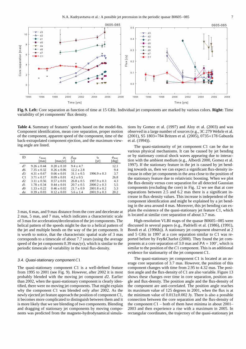
Fig. 9. Left: Core separation as function of time at 15 GHz. Individual jetcomponents are marked by various colors.Right: Timevariability of jet components’ flux density.

Table 4. Summary of features’ speeds based on the model-fits.Component identification, mean core separation, proper motionof the component, apparent speed of the component, time of theback-extrapolated component ejection, and the maximum view-ing angle are listed.

ID rmean µr βapp t0 φmax[mas] [mas/yr] [c] [yr] [deg]

d7 9.26± 0.44 0.20± 0.10 9.4± 4.7 12.1d6 7.35± 0.32 0.26± 0.06 12.2± 2.8 9.4d3 4.31± 0.67 0.66± 0.01 31.1± 0.5 1996.9± 0.3 3.7C1 3.71± 0.17 0.09± 0.01 4.2± 0.5 26.8d2 3.11± 0.56 0.57± 0.01 26.8± 0.5 1997.9± 0.3 4.3d1 1.78± 0.34 0.44± 0.01 20.7± 0.5 2000.2± 0.3 5.5d0 1.33± 0.22 0.46± 0.02 21.7± 0.9 2001.8± 0.2 5.3da 0.39± 0.03 0.12± 0.03 5.6± 1.4 2001.9± 0.3 20.2

3 mas, 6 mas, and 9 mas distance from the core and decelerate at2 mas, 5 mas, and 7 mas, which indicates a characteristic scaleof 3 mas for acceleration/deceleration of the jet components. Thehelical pattern of the speeds might be due to a helical pattern ofthe jet and multiple bends on the way of the jet components. Itis worth to notice, that the characteristic spatial scale of3 mascorresponds to a timescale of about 7.7 years (using the averagespeed of the jet components 0.39 mas/yr), which is similar to theperiodic timescale of variability in the total flux-density.

3.4. Quasi-stationary component C1

The quasi-stationary componentC1 is a well-defined featurefrom 1995 to 2001 (see Fig. 9). However, after 2002 it is mostprobably blended with the moving jet componentd2. Earlierthan 2002, when the quasi-stationary component is clearly iden-tified, there were no moving jet components. That might explainwhy the componentC1 was blended only after 2002. As thenewly ejected jet feature approach the position of componentC1,it becomes more complicated to distinguish between them anditis more likely that we see blending of two components. Blendingand dragging of stationary jet components by moving compo-nents was predicted from the magneto-hydrodynamical simula-

tions by Gomez et al. (1997) and Aloy et al. (2003) and wasobserved in a large number of sources (e.g., 3C 279 Wehrle et al.(2001), S5 1803+784 Britzen et al. (2005), 0735+178 Gabuzdaet al. (1994)).

The quasi-stationarity of jet componentC1 can be due tovarious physical mechanisms. It can be caused by jet bendingor by stationary conical shock waves appearing due to interac-tion with the ambient medium (e.g., Alberdi 2000, Gomez et al.1997). If the stationary feature in the jet is caused by jet bend-ing towards us, then we can expect a significant flux-density in-crease in other jet components in the area close to the position ofthe stationary feature due to relativistic boosting. When we plotthe flux-density versus core separation for all detected Gaussiancomponents (excluding the core) in Fig. 12 we see that at coreseparations between 2.5 and 6.2 mas there is a significant in-crease in flux-density values. This increase is independentof thecomponent identification and might be explained by a jet bend-ing in the area around 4 mas. Moreover, this jet bending can ex-plain the existence of the quasi-stationary jet featureC1, whichis located at similar core separation of about 3.7 mas.

High-resolution VLBI maps of the quasar B0605−085 werediscussed in several papers (e.g., Padrielli et al. (1986),(1991),Bondi et al. (1996b)). A stationary jet component observed at 2and 5 GHz in 1997 at a core separation similar toC1 was re-ported before by Fey&Charlot (2000). They found the jet com-ponents at a core separation of 3.0 mas andPA = 100, which issimilar to the position of theC1 component. This is an additionalevidence for stationarity of the jet componentC1.

The quasi-stationary jet componentC1 is located at an av-erage core separation of 3.7 mas. However, the position of thiscomponent changes with time from 2.95 to 4.32 mas. The posi-tion angle and the flux-density ofC1 are also variable. Figure 13shows these changes over time in core separation, position an-gle and flux-density. The position angle and the flux-densityofthe component are anti-correlated. The position angle reachesits maximum value of 125 degrees in 2001, when the flux is atthe minimum value of 0.013±0.002 Jy. There is also a possibleconnection between the core separation and the flux-densityofthe componentC1 – both of them have minima in about 2001–2003 and then experience a rise with a maximum in 2005. Inrectangular coordinates, the trajectory of the quasi-stationary jet

8 N.A. Kudryavtseva et al.: A possible jet precession in the periodic quasar B0605−085

componentC1 follows a clear helical path. Figure 14 shows atrajectory ofC1 in the plane of the sky. It is clearly seen fromthe plot that the quasi-stationary component follows a spiral tra-jectory. Moreover, the characteristic time scale of a helixturn isabout 8 years. This time scale is very close to the value of theperiod of the total flux-density variability discussed earlier. Thismight be evidence for a possible connection between the heli-cal movement ofC1 and the total flux-density periodicity. Thejet might precess and therefore due to variability of the Dopplerboosting we will see periodic flares in the light curves as well aschanges of position of a bend in the jet.

3.5. Comparison of trajectories

We plot the position angles of all featuresda–d7, including thequasi-stationary component C1 versus the core separation inFig. 15. The trajectories of the componentsd1, d2, d6, d7, andC1 follow significantly curved trajectories, whereas the trajec-tories of the componentsd0 andd3 follow a linear path. Thiscan be an evidence for a possible co-existence of two types ofjet component trajectories, similar to the source 3C 345 (Klareet al. 2005). The spread of position angles of all componentsischanging along the jet. In the inner part, within the first 1 mas,the position angles are in the range of 123–150 degrees, in themiddle part of the jet between 1 – 5 mas, the position anglesrange from 110 to 125, whereas in the outer part from 5 masto 10 mas, from 95 to 115.

4. Precession model

The probable periodical variability of the radio total flux-densities of B0605−085 and the helical motion of the quasi-stationary jet componentC1 can be explained by jet precession.We used a precession model, described in Abraham & Carrara(1998) and Caproni & Abraham (2004) for fitting the helical pathof the jet componentC1. In this model, the rectangular coordi-nates of a precession cone in the source frame are changing withtime t′ due to precession:

X(t′) = [cosΩ sinφ0 + sinΩ cosφ0 sinωt′] cosη0 −

sinΩ cosωt′ sinη0, (6)

Y(t′) = [cosΩ sinφ0 + sinΩ cosφ0 sinωt′] sinη0 +

sinΩ cosωt′ cosη0, (7)

whereΩ is the semi-aperture angle of the precession cone,φ0is the angle between the precession cone axis and the line ofsight and it is actually the average viewing angle of the source,andη0 is the projected angle of the cone axis onto the plane ofthe sky (see Fig. 16). The angular velocity of the precessionisω = 1/P, whereP is the period. We take aP value of 7.9-year(timescale found in the total flux-density radio light curves andin the helical movement ofC1). The time in the source frame(t′) and the frame of the observer (t) are related by the Dopplerfactorδ as

∆t′ =δ(φ, γ)1+ z

∆t. (8)

However, the only time-dependent term in the equations (6)and (7) isωt, which does not depend on this time corrections

sinceω ∼ 1/t. Therefore, we can fit the trajectory in the rectan-gular coordinateX(t) of the quasi-stationary jet componentC1,using the formula 6. We assume that the motion ofC1 reflectsthe movement of the jet. The non-linear least squares methodwas used for the precession model fitting. The angular velocityof the precessionω and the redshift of the sourcez are knownand we fix them during the fit, whereas the aperture angle of theprecessing coneΩ, φ0, andη0 are used as free parameters. Theresults of the fit are shown in Fig. 17 (Left) and the parameters ofthe precession model for the parsec jet of B0605−085 are listedin Table 6. The precession model fits well the trajectory of thequasi-stationary jet componentC1. The same parameters wereused to describe the motion ofC1 in declination. The model forthe declination is shown in Fig. 17 (Right).

We found another set of parametersΩ = 92.2, φ0 = 69.8,η0 = 12.9 as one of the possible solutions. However, the view-ing angle is very large. Using the equation

βapp =β sinφ

1− β cosφ, (9)

and taking average value of apparent speedsβapp,aver = 16.5c,we can calculate the speed in the source frameβ = 2.49c, whichis higher then the speed of light. Precession cone aperture angleΩ = 92.2 is also unlikely. Therefore, this set of parameters isnot plausible. The solution in Table 6 is the only physicallyfea-sible, since all the parameter space was covered during the fittingprocedure.

Table 6.Precession model parameters (see Sect. 4).

Parameter Description Value

P Precession period, fixed 7.9 yrΩ Aperture angle, variable 23.9 ± 1.9

φ0 Viewing angle, variable 2.6 ± 2.2

η0 Projection angle, variable 33.6 ± 6.5

5. Discussion

Assuming that the helical motion of the quasi-stationary jet com-ponentC1 is caused solely by jet precession (with a period of 8years), we were able to determine the geometrical parametersof the jet precession, such as the aperture angle of a preces-sion cone, the viewing angle, and the projection angle. The fittedviewing angleφ0 = 2.6 ± 2.2 agrees well with the upper limitfor the viewing angle deduced from the apparent speeds of thejet componentsφmax = 3.7. It is also similar to the viewing an-gleφvar = 5 derived from the radio total flux-density variabilityby Hovatta et al. (2008). The jet precession will also cause theperiodical variability of the radio total flux-density light curveswith the same period of 8 years, due to periodical changes of theDoppler factor. The flux densityS j is changing with the Dopplerfactor due to the jet precessionS j = S ′jδ(φ, γ)

p+α, whereα isthe spectral index (Lind & Blandford 1985). From this equationwe can expect that the flares due to the jet precession will ap-pear simultaneously at different frequencies, which is actuallyobserved for the major outbursts in 1973, 1988, and 1995-1996.Therefore, the jet precession is probably responsible for the to-tal flux-density variability, periodicity in the outbursts, and thehelical motion of the quasi-stationary jet componentC1.

N.A. Kudryavtseva et al.: A possible jet precession in the periodic quasar B0605−085 9

Fig. 13.Time evolution of core separation (Left), position angle (Middle) and flux-density (Right) of the quasi-stationary componentC1.

Fig. 14.Trajectory of the quasi-stationary componentC1 in rectangular coordinates in three-dimensional space with the third axisshowing the time (Left) and in two dimensions (Right). The trajectory of the component seems to follow a helical path.

Some questions remain unclear. It is still not known why thefour major outbursts in the total flux-density light curve whichrepeat periodically with an 8-year period have different spectralproperties. Longer monitoring of this quasar at several frequen-cies is necessary in order to understand spectral properties of theflares.

The precession of B0605−085 jet can be caused by sev-eral physical mechanisms. Jet instabilities, a secondary blackholes rotating around the primary black hole, and accretiondiscinstabilities might be responsible for the observed changes ofjet direction (e.g., Camenzind & Krockenberger 1992, Hardee& Norman 1988, Lobanov & Roland 2005). At the moment itis impossible to claim exactly which mechanism can producethe observed jet precession. It is worth to notice, however,thatthe possible double-peak structure of the flares at 14.5 GHz inB0605−085 is similar to the double-peak flares of OJ 287 ob-served in optical light curves which were explained by the or-biting secondary black hole. At the moment we can not saywhether there is a secondary black hole in the center of a hostinggalaxy in B0605−085 and further observations and theoreticalmodelling are needed.

The next total flux-density flare of the source might appearin 2012 if the 8-year period will preserve over time. The 8-year

period in the flux-density variability has predicted the next pow-erful outburst to appear in∼ 2004. However, the flare was ofa very low flux level which might be due to long-term trendin flux-density variability. Recent observations of B0605−085have shown a rise in fluxes which might suggest a probable peakclose to 2012 taking into account the duration of the outburstsin this source. This will mean that the 8-year period interfereswith long-term changes of the flux-densities. Further radiototalflux-density and VLBI observations are needed in order to checkthis prediction.

6. Summary

Our analysis of the jet kinematics in B0605−085 shows:

– We find strong evidence for a period of the order of 8 years(7.9± 0.5 years when averaged over frequencies) in the totalflux-density light curves at 4.8 GHz, 8 GHz and 14.5 GHz,which was observed for four cycles.

– The measurement of frequency-dependent time delays forthe brightest outbursts in 1988, and 1995-1996 and the visualanalysis for the 1973 flare shows that these flares appearedalmost simultaneously at all frequencies.

10 N.A. Kudryavtseva et al.: A possible jet precession in theperiodic quasar B0605−085

Fig. 17.Sky trajectory of the quasi-stationary componentC1 in right ascension (Left) and declination (Right). The solid line showsthe fit of the precession model. The precession model fits wellthe trajectory of a quasi-stationary jet componentC1

– The spectral analysis of the flares shows that the main flaresin 1973, 1988, 1995-1996 have a flat spectrum, whereas theflare in 1981 has a steep spectrum, what suggests that thefour cycles of the 8-year period have different spectral prop-erties.

– The average instantaneous speeds of the jet components re-veal a helical pattern along the jet axis with a characteris-tic scale of 3 mas. This scale corresponds to a time scale ofabout 7.7 years, which is similar to the periodicity timescalefound in the total flux-densities.

– The quasi-stationary jet componentC1 follows a helical pathwith a period of 8 years. This time scale coincides with theperiod found in the total flux-density light curves.

– We found evidence that the jet components of B0605−085follow two different types of trajectories. Some componentsmove along the straight lines, whereas other components fol-low significantly curved paths.

– The fit of the precession model to the trajectory of the quasi-stationary jet componentC1 has shown that it can be ex-plained by changes of the jet direction with a precessionperiod of P = 8 yrs (in the observers frame), aperture an-gle of the precession coneΩ = 23.9 ± 1.9, viewing angleφ0 = 2.6 ± 2.2, and projection angleη0 = 33.6 ± 6.5.

Acknowledgements. This research has made use of data from the MOJAVEdatabase that is maintained by the MOJAVE team (Lister et al., 2009, AJ, 137,3718). N. A. Kudryavtseva and M. Karouzos were supported forthis researchthrough a stipend from the International Max Planck Research School (IMPRS)for Astronomy and Astrophysics. We would like to thank Christian Fromm forfruitful discussions and help with the picture. This research has made use of datafrom the University of Michigan Radio Astronomy Observatory which is sup-ported by the National Science Foundation and by funds from the Universityof Michigan. The Alonquin Radio Observatory is operated by the NationalResearch Council of Canada as a national radio astronomy facility. The oper-ation of the Haystack Observatory is supported by the grant from the NationalScience Foundation. The National Radio Astronomy Observatory is a facilityof the National Science Foundation operated under cooperative agreement byAssociated Universities, Inc. This publication has emanated from research con-ducted with the financial support of Science Foundation Ireland. This researchhas made use of the SIMBAD database, operated at CDS, Strasbourg, France.We thank the anonymous referee for a careful reading of the manuscript anduseful comments and suggestions that have improved this paper.

References

Abraham, Z., & Carrara, E.A. 1998, ApJ, 496, 172

Agudo, I., Gomez, J.-L., Martı, J.-M., et al. 2001, ApJ, 549, 183,astro-ph/0101188

Alexander, T. 1997, in Astronomical Time Series, ed. D. Maoz, A. Sternberg, &E.M. Leibowitz (Dordrecht:Kluwer) 163

Alberdi, A., Gomez, J. L., Marcaide, J. M., Marscher, A. P.,Perez-Torres, M. A.2000, A&A, 361, 529

Aller, H. D., Aller, M. F., Latimer, G. E., Hodge, P. E. 1985, ApJS, 59, 513Aller, M. F., Aller, H. D., Hughes, P. A., & Latimer, G. E. 1999, ApJ, 512, 601,

astro-ph/9810485Aller, M. F., Aller, H. D., & Hughes, P. A. 2003, ApJ, 586, 33, astro-ph/0211265Aloy, M.A., Martı, J.-M., Gomez, J.-L., et al. 2003, ApJ, 585, 109,

astro-ph/0302123Andrew, B. H., MacLeod, J. M., Harvey, G. A., Medd, W. J. 1978,AJ, 83, 863Bach, U., Villata, M., Raiteri, C. M., et al. 2006, A&A, 456, 105,

astro-ph/0606050Bondi, M., Padrielli, L., Fanti, R., et al. 1996a, A&AS, 120,89Bondi, M., Padrielli, L., Fanti, R., et al. 1996b, A&A, 308, 415Britzen, S., Witzel, A., Krichbaum, T. P., et al. 2005, MNRAS, 362, 966Britzen, S., Kudryavtseva, N. A., Witzel, A., et al. 2010, A&A, 511, 57,

arXiv:1001.1973Camenzind, M. & Krockenberger, M. 1992, A&A, 255, 59Caproni, A., & Abraham, Z. 2004, MNRAS, 349, 1218, astro-ph/0312407Ciaramella, A., Bongardo, C., Aller, H.D., et al. 2004, A&A,419, 485,

astro-ph/0401501Cooper, N. J., Lister, M. L., & Kochanczyk, M. D. 2007, ApJS, 171, 376,

astro-ph/0701072Dent, W. A., Kapitzky, J. E., & Kojoian, G. 1974, AJ, 79, 1232Dent, W. A., & Kapitzky, J. E. 1976, AJ, 81, 1053Edelson, R. A., & Krolik, J. H. 1988, ApJ, 333, 646Ferraz-Mello, S. 1981, AJ, 86, 619Fey, A. L., & Charlot, P. 2000, ApJS, 128, 17Fomalont, E. B. 1999, in Synthesis Imaging in Radio Astronomy II, ed. G. B.

Taylor, C. L. Carilli, & R. A. Perley, ASP Conf. Ser., 180, (San Francisco:ASP), 301

Gabuzda, D. C., Wardle, J. F. C., Roberts, D. H., Aller, M. F.,Aller, H. D. 1994,ApJ, 435, 128

Gomez, J. L., Martı, J. M. A., Marscher, A. P., Ibanez, J.M. A., Alberdi, A. 1997,ApJ, 482, 33

Hardee, P. E. & Norman, M. L. 1988, ApJ, 334, 70Homan, D. C., Kadler, M., Kellermann, K. I., et al. 2009, ApJ,706, 1253,

arXiv:0909.5102Honma, F., Kato, S., & Matsumoto, R. 1991, PASJ, 43, 147Hovatta, T., Valtaoja, E., Tornikoski, M., Lahteenmaki,A. 2009, A&A, 494, 527,

arXiv:0811.4278Hufnagel, B. R. & Bregman, J. N. 1992, ApJ, 386, 473Kadler, M., Hughes, P. A., Ros, E., Aller, M. F., Aller, H. D. 2006, A&A, 456, 1,

astro-ph/0605587Kadler, M., Ros, E., Perucho, M., et al. 2008, ApJ, 680, 867, arXiv:0801.0617Kellermann, K.I., Lister, M.L., Homan, D.C., et al. 2004, ApJ, 609, 539,

astro-ph/0403320Kelly, B. C., Hughes, P. A., Aller, H. D., Aller, M. F. 2003, ApJ, 591, 695,

astro-ph/0301002

N.A. Kudryavtseva et al.: A possible jet precession in the periodic quasar B0605−085 11

Kidger, M. R. 2000, AJ, 119, 2053Klare, J., Zensus, J. A., Lobanov, A. P., et al. 2005, in Future Directions in High

Resolution Astronomy: The 10th Anniversary of the VLBA, ed.J. Romney,& M. Reid., ASP Conf. Ser. 340, 40

Kudryavtseva, N. A. & Pyatunina, T. B. 2006, ARep, 50, 1, astro-ph/0511707Lehto, H. J., & Valtonen, Mauri J. 1996, ApJ, 460, 207Lind, K. R., & Blandford, R. D. 1985, ApJ, 295, 358Lister, M. L., & Homan, D. C. 2005, AJ, 130, 1389, astro-ph/0503152Lister, M. L., Cohen, M. H., Homan, D. C., et al. 2009, AJ, 138,1874,

arXiv:0909.5100Lobanov, A. P. & Roland, J. 2005, A&A, 431, 831, astro-ph/0411417Medd, W. J., Andrew, B. H., Harvey, G. A., Locke, J. L. 1972, MmRAS, 77, 109Ostorero, L., Villata, M., & Raiteri, C. M. 2004, A&A, 419, 913,

astro-ph/0402551Padrielli, L., Romney, J. D., Bartel, N., et al. 1986, A&A, 165, 53Padrielli, L., Eastman, W., Gregorini, L., Mantovani, F., Spangler, S. 1991 A&A,

249, 351Pearson, T.J. & Zensus, J.A. in Superluminal Radio Sources (eds Pearson, T.J.

& Zensus, J.A.), 1-11 (Cambridge Univ. Press, 1987).Pyatunina, T.B., Kudryavtseva, N.A., Gabuzda, D.C., et al.2006, MNRAS, 373,

1470, astro-ph/0609494Pyatunina, T.B., Kudryavtseva, N.A., Gabuzda, D.C., et al.2007, MNRAS, 381,

797Qian, Shan-Jie; Kudryavtseva, N. A.; Britzen, S. et al. 2007, ChJAA, 7, 364,

arXiv:0710.1876Raiteri, C. M., Villata, M., Aller, H. D. et. al. 2001, A&A, 377, 396,

astro-ph/0108165Reuter, H.-P., Kramer, C., Sievers, A., et al. 1997, A&AS, 122, 271Rieger, F. M., & Mannheim, K. 2000, A&A, 359, 948, astro-ph/0005478Sambruna, R. M., Gambill, J. K., Maraschi, L., et al. 2004, ApJ, 608, 698,

astro-ph/0401475Scott, W. K., Fomalont, E. B., Horiuchi, S., et al. 2004, ApJS, 155, 33,

astro-ph/0407041Shepherd, M.C., 1997, in Astronomical Data Analysis Software and Systems VI,

ed. G. Hunt & H. E. Payne, ASP Conf. Ser. 125, 77Steppe, H., Salter, C. J., Chini, R., et al. 1988, A&AS, 75, 317Steppe, H., Liechti, S., Mauersberger, R., et al. 1992, A&AS, 96, 441Stickel, M., Kuhr, H., & Fried, J.W. 1993, A&AS, 97, 483Stirling, A. M., Cawthorne, T. V., Stevens, J. A. et al. 2003,MNRAS, 341, 405Terasranta, H., Tornikoski, M., Mujunen, A., et al. 1998, A&AS, 132, 305Tornikoski, M., Valtaoja, E., Terasranta, H., et al. 1996,A&AS, 116, 157Valtaoja, E., Terasranta, H., Tornikoski, M., et al. 2000,ApJ, 531, 744Villata, M., & Raiteri, C. M. 1999, A&A, 347, 30Villata, M., Raiteri, C. M., Aller, H. D., et al. 2004, A&A, 424, 497Villata, M., Raiteri, C. M., Larionov, V. M., et al. 2009, A&A, 501, 455,

arXiv:0905.1616Wehrle, A. E., Piner, B. G., Unwin, S. C., et al. 2001, ApJS, 133, 297,

astro-ph/0008458

Fig. 2. Total radio flux-density light curves of B0605−085 atfive frequencies. The solid lines mark positions of the brightestflares.

12 N.A. Kudryavtseva et al.: A possible jet precession in theperiodic quasar B0605−085

Fig. 3. Complex sub-structure of flares at 14.5 GHz. The dottedlines show the Gaussian functions fitted to the sub-structure offlares. The solid line is the sum of fitted Gaussian functions.

Fig. 6. Total flux density light curve of B0605−085 at 4.8 GHz.The red line shows a sinusoid with a period of 8.5 years, derivedfrom the date-compensated Fourier transform method

Fig. 8. Contour images of B0605−085 and overlapped on themcircular Gaussian components to model the observed visibilities(see Table 5). The distance between images on the plot is pro-portional to time passed.

N.A. Kudryavtseva et al.: A possible jet precession in the periodic quasar B0605−085 13

Fig. 10. Instantaneous speeds of the jet componentd1, whichexperiences significant acceleration when moving along thejet.

Fig. 11. Instantaneous speeds of all jet components ofB0605−085 averaged in 1 mas core separation bins. We inter-pret that the jet is helical with a characteristic scale of 3 mas.

Fig. 12. Flux-density of all Gaussian components found in thejet of B0605−085 at 15 GHz. The core was excluded from theplot for smaller range of flux densities. It is clearly seen that allcomponents become significantly brighter when they are at therange of the core separations from 2.5 to 6.2 mas, which can beexplained by the jet bending.

Fig. 15. Position angle changes of the jet componentsda–d7,including the quasi-stationary componentC1 at 15 GHz.

14 N.A. Kudryavtseva et al.: A possible jet precession in theperiodic quasar B0605−085

Fig. 16.Jet precession geometry. The line of sight is parallel tothe z-axis.

N.A. Kudryavtseva et al.: A possible jet precession in the periodic quasar B0605−085 15

Table 5.Model-fit results for B0605−085 at 15 GHz. We list the epoch of observation, the jet component identification, the flux-density, the radial distance ofthecomponent center from the center of the map, the position angle of the center of the component, the FWHM major axis of the circular component, and the positionangle of the major axis of the component.

Epoch Id. S r θ Ma.A.[yr] [Jy] [mas] [deg] [mas]

1995.57 D 2.533±0.382 0.0±0.04 0.0 0.320.045±0.015 1.35±0.06 103.59±4.51 0.81

C1 0.084±0.014 3.20±0.02 108.79±0.41 0.331996.82 D 2.001±0.319 0.0±0.16 0.0 0.55

0.045±0.022 1.70±0.07 110.22±2.05 0.200.045±0.007 2.82±0.04 125.70±0.90 0.30

C1 0.067±0.011 3.19±0.05 107.67±0.97 0.531998.83 D 0.770±0.107 0.0±0.03 0.0 0.10

d2 0.281±0.035 0.50±0.01 123.65±1.92 0.43d3 0.248±0.047 1.38±0.05 127.61±0.86 0.51C1 0.099±0.014 3.80±0.04 108.49±0.86 0.76d6 0.022±0.009 6.43±0.37 112.29±3.20 2.59d7 0.008±0.001 8.38±0.43 98.75±3.01 0.84

0.011±0.002 9.95±0.98 108.37±5.50 1.662001.20 D 0.978±0.144 0.0±0.02 0.0 0.11

d1 0.384±0.008 0.43±0.01 126.68±1.09 0.39d2 0.073±0.028 1.69±0.07 130.95±1.01 0.97d3 0.058±0.044 2.32±0.08 117.61±1.18 1.08C1 0.013±0.002 3.61±0.17 126.00±2.70 0.61

0.109±0.013 4.22±0.05 112.50±0.76 1.34d6 0.011±0.002 6.71±0.27 117.50±2.30 0.87d7 0.013±0.002 8.83±0.29 104.45±1.90 1.21

2003.09 D 1.145±0.167 0.0±0.02 0.0 0.22d0 0.048±0.007 0.60±0.02 151.77±1.70 0.21d1 0.150±0.042 1.24±0.10 129.60±1.99 1.01d2+C1 0.039±0.007 2.95±0.08 123.91±1.40 0.77d3 0.051±0.044 4.25±0.08 110.50±2.68 2.14

2004.44 D 0.843±0.119 0.0±0.07 0.0 0.08da 0.376±0.067 0.30±0.03 133.42±3.42 0.15d0 0.141±0.022 1.31±0.06 133.02±2.01 1.17d1 0.031±0.003 1.79±0.02 110.46±0.63 0.10d2+C1 0.096±0.014 3.72±0.12 118.60±1.11 1.98d3 0.058±0.002 5.41±0.09 113.42±0.73 1.18d6 0.009±0.001 7.85±0.18 118.32±1.30 0.56d7 0.019±0.010 9.42±0.39 108.10±6.79 3.76

2005.17 D 0.835±0.119 0.0±0.06 0.0 0.05da 0.323±0.106 0.40±0.06 133.26±5.41 0.08d0 0.061±0.009 1.20±0.17 134.21±2.60 0.74d1 0.081±0.011 2.10±0.07 121.01±1.27 1.01d2+C1 0.100±0.016 4.28±0.06 121.57±0.87 1.50d3 0.033±0.005 5.75±0.08 114.90±0.80 0.75

0.007±0.002 6.18±0.09 106.30±0.90 0.13d6 0.027±0.006 7.73±0.33 103.00±2.50 2.94

0.005±0.001 11.73±0.34 103.70±1.70 0.480.007±0.001 13.26±0.31 101.00±1.40 0.490.012±0.002 19.83±1.24 111.90±3.60 3.99

2005.56 D 0.907±0.132 0.0±0.03 0.0 0.09da 0.358±0.058 0.44±0.02 135.27±1.18 0.16d0 0.084±0.017 1.77±0.05 126.35±1.53 1.13d1 0.019±0.006 2.54±0.08 116.81±1.83 0.42d2+C1 0.103±0.021 4.32±0.15 121.36±1.88 1.38d3 0.058±0.007 5.75±0.13 112.87±0.77 1.17d6 0.009±0.001 8.04±0.55 104.90±4.00 1.68d7 0.004±0.001 10.41±1.19 95.45±6.50 1.46

0.008±0.001 11.12±0.43 110.02±2.20 1.050.003±0.001 21.24±3.66 113.30±9.80 3.38

2005.71 D 0.822±0.123 0.0±0.04 0.0 0.13da 0.288±0.044 0.44±0.02 132.92±1.41 0.22d0 0.086±0.011 1.77±0.04 127.87±1.42 1.01d1 0.026±0.004 2.61±0.05 118.97±1.20 0.43d2+C1 0.053±0.008 4.28±0.06 124.57±1.18 1.08d3 0.108±0.016 5.31±0.09 114.02±0.98 2.10