Delineation of hydrochemical facies distribution in a regional groundwater system by means of fuzzy...

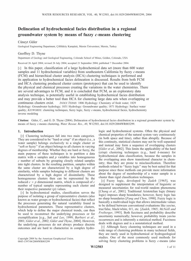
Delineation of hydrochemical facies distribution in a regional

groundwater system by means of fuzzy c-means clustering

Cuneyt Guler

Geological Engineering Department, Ciftlikkoy Kampusu, Mersin Universitesi, Mersin, Turkey

Geoffrey D. Thyne

Department of Geology and Geological Engineering, Colorado School of Mines, Golden, Colorado, USA

Received 26 April 2004; revised 26 July 2004; accepted 21 September 2004; published 7 December 2004.

[1] In this paper, classification of a large hydrochemical data set (more than 600 watersamples and 11 hydrochemical variables) from southeastern California by fuzzy c-means(FCM) and hierarchical cluster analysis (HCA) clustering techniques is performed andits application to hydrochemical facies delineation is discussed. Results from both FCMand HCA clustering produced cluster centers (prototypes) that can be used to identifythe physical and chemical processes creating the variations in the water chemistries. Thereare several advantages to FCM, and it is concluded that FCM, as an exploratory dataanalysis technique, is potentially useful in establishing hydrochemical facies distributionand may provide a better tool than HCA for clustering large data sets when overlapping orcontinuous clusters exist. INDEX TERMS: 1806 Hydrology: Chemistry of fresh water; 1829

Hydrology: Groundwater hydrology; 1831 Hydrology: Groundwater quality; 1871 Hydrology: Surface water

quality; KEYWORDS: clustering techniques, fuzzy logic, fuzzy c-means, hydrochemical facies, hydrochemistry

inverse modeling

Citation: Guler, C., and G. D. Thyne (2004), Delineation of hydrochemical facies distribution in a regional groundwater system by

means of fuzzy c-means clustering, Water Resour. Res., 40, W12503, doi:10.1029/2004WR003299.

1. Introduction

[2] Clustering techniques fall into two main categories.They are considered to be ‘‘hard or crisp’’ if an object (i.e., awater sample) belongs exclusively to a single cluster or‘‘soft or fuzzy’’ if an object belongs to all clusters in varyingdegrees of membership. Whether they are hard or fuzzy, themain purpose of these techniques is to partition a datamatrix with n samples and p variables into homogeneousc number of subsets by grouping closely related samplesinto tight clusters. In the resulting partition, samples withinthe same cluster are characterized by a high degree ofsimilarity, while samples belonging to different clusters arecharacterized by a high degree of dissimilarity. Thesehomogeneous clusters then can be represented by thereduced c � p dimensional matrix, which is composed of cnumber of typical samples representing each cluster andtheir respective parameter (p) values.[3] In hydrochemical studies, classification serves the

purpose of isolating a group of representative clusters (alsoknown as water groups or hydrochemical facies) that reflectthe processes generating the natural variability found inhydrochemical parameters. These representative clusters,which help to define the major chemical trends, can thenbe used to reconstruct the underlying processes or forexemplification [e.g., Suk and Lee, 1999; Barbieri et al.,2001; Guler et al., 2002; Guler and Thyne, 2004]. However,the underlying processes do not always produce discreteoutcomes and are hard to characterize in complex hydro-

logic and hydrochemical systems. Often the physical andchemical properties of the natural system vary continuously(in both space and time), rather than abruptly. Because ofthis continuity, statistical clusters may not be well separatedand instead may form a sequence of overlapping clusters[Guler et al., 2002]. This limits the applicability of the hard(crisp) clustering techniques (e.g., hard k-means) forhydrochemical data classification, because the samples inthe overlapping area show transitional character in chem-istry; thus they are prone to misclassification. Thereforemethods related to ‘‘fuzzy logic’’ may be best suited for thatpurpose since these methods can provide more informationabout the degree of membership of a water sample in acluster than rigid classification techniques.[4] Fuzzy logic, developed by Zadeh [1965], was

designed to supplement the interpretation of linguistic ormeasured uncertainties for real-world random phenomena[Chang et al., 2001]. Traditional Aristotelian logic (binarylogic) imposes sharp boundaries; however, fuzzy logic hasno sharp boundaries [Fang and Chen, 1990]. Fuzzy logic isbasically a multivalued logic that allows intermediate valuesto be defined between conventional evaluations like yes/no,true/false, black/white, 0/1, etc. [Zadeh, 1965; McNeill andFreiberger, 1993]. Both fuzziness and probability describeuncertainty numerically; however, probability treats yes/nooccurrences and is inherently a statistical method. Fuzzinessdeals with degrees and is a nonstatistical method.[5] Although fuzzy clustering techniques are used in a

wide range of clustering problems in many technical fields,they are rarely used in hydrochemical or hydrogeologicalstudies. One of the most commonly used methods forsolving fuzzy clustering problems is fuzzy c-means (also

Copyright 2004 by the American Geophysical Union.0043-1397/04/2004WR003299

W12503

WATER RESOURCES RESEARCH, VOL. 40, W12503, doi:10.1029/2004WR003299, 2004

1 of 11

known as fuzzy k-means) [Bezdek, 1981]. The fuzzyc-means (FCM) algorithm has been successfully appliedin various disciplines such as biology [Zhang et al., 1995],chemistry [Sun and Danzer, 1996; Linusson et al., 1998],climate [McBratney and Moore, 1985], food processing [Huet al., 1998], geology [Burrough et al., 2000; Rantitsch,2000], hydrochemistry [Barbieri et al., 2001; Guler et al.,2002], image analysis [Bezdek et al., 1993; Ahmed et al.,2002], and soil science [McBratney and deGruijter, 1992;Odeh et al., 1992]. FCM has been modified and generalizedin several ways in order to detect different cluster shapesand reduce the execution time of the algorithm for real-timeclassification purposes (i.e., image classification or gradingfish products). As a result of this, numerous variations of theFCM algorithm are available in the recent literature such asconditional fuzzy c-means (CFCM) [Pedrycz, 1996], fuzzysymbolic c-means (FSCM) [El-Sonbaty and Ismail, 1998],fuzzy c-medians (FCMED) [Kersten, 1999], hierarchicalunsupervised fuzzy clustering (HUFC) [Geva, 1999],fuzzy k-means with extragrades (FKME) [Minasny andMcBratney, 2002], fuzzy J-means (FJM) [Belacel et al.,2002], alternative fuzzy c-means (AFCM) [Wu and Yang,2002], bias-corrected fuzzy c-means (BCFCM) [Ahmed etal., 2002], and adaptive rough fuzzy leader clustering(ARFLC) [Asharaf and Murty, 2003]. All these fuzzyclustering algorithms rely on elements of Zadeh’s [1965]fuzzy set theory and many of them are based on the FCMalgorithm, originally proposed by Dunn [1974] andextended by Bezdek [1981].[6] In this study, the FCM clustering technique was

applied to a large hydrochemical data set from the IndianWells–Owens Valley area of southeastern California todelineate clusters of water samples with similar character-istics (hydrochemical facies) and to identify representativehydrochemical parameter values for each cluster. Then, thereduced data matrix (c � p matrix) was used to formulate(inverse) models to explain the hydrochemical variabilityobserved in the water samples.

2. Study Area

[7] The study area is located in southeastern Californiaand covers approximately 30,000 km2 stretching fromOwens Valley (OV) in the north to Indian Wells Valley(IWV) in the south (Figure 1). Both OV and IWV arebordered on the west by the Sierra Nevada with peaksrising from 1830 to 4400 m and on the east by severalranges with elevations ranging from 1500 to 2750 m.Topography of the valley floors is relatively flat and slopesto the south with elevations decreasing from 1100 m in theOV to nearly 663 m in the vicinity of IWV [Guler, 2002]. Ina classic basin and range groundwater system [Maxey,1968], water flows from high-elevation recharge areas in themountains to topographically lower discharge areas in thevalleys. Central portions of the valleys are generallyoccupied by playas, known in different localities as ‘‘saltlakes,’’ ‘‘soda lakes,’’ ‘‘alkali marshes,’’ ‘‘dry lakes’’ or‘‘borax lakes’’ where the groundwater discharges byevapotranspiration. The most important and probably wellknown of these playas are Owens Lake, China Lake, andSearles Lake, which are located in Owens Valley, IndianWells Valley, and Searles Valley, respectively (Figure 1).Because of the modern arid climate, surface water is scarce

in the area and mostly occurs in manmade reservoirs (e.g.,Haiwee Reservoir and Lake Isabella). The lithology of thearea consists of a wide variety of rocks and unconsolidateddeposits, which can be divided into five hydrogeologic unitsincluding igneous and metamorphic rocks, volcanic rocks,carbonate rocks, basin-fill deposits, and playa deposits.Detailed descriptions of these units and hydrogeology of thearea are given by Guler [2002] and Guler and Thyne[2004].

3. Methodology

[8] The basic methodology is to begin with statisticalclustering of the hydrochemical data followed by examiningthe spatial distribution of the clusters for spatial coherenceand coincidence with major hydrologic and geologicalfeatures. This process tests the choice of clustering methodsand can be iterated to refine the statistical clusters so theyare as geologically meaningful as possible. Then, the hydro-chemical validity of the clusters is tested with inversegeochemical modeling, which uses mass balances to deter-mine if the changes between the chemical compositions ofthe clusters can be explained as a result of water-rockinteractions with the local mineralogy.

3.1. Database and Data Treatment

[9] Throughout the last 80 years, extensive hydrochemicaldata has been collected in the Indian Wells–Owens Valleyarea. The database used in this study is a subset of these data.Database construction procedures are discussed in detail byGuler [2002] and Guler et al. [2002], where the sources ofthe data are also presented. The entire database consists ofchemical analyses of 152 spring, 153 surface, and 1063 well(groundwater) samples, including temporal series (samplescollected over a period of time at the same location). Of the39 hydrochemical variables (consisting of major ions, minorions, trace elements, and isotope data) in the compileddatabase, the variables specific conductance (SC), pH, Ca,Mg, Na, K, Cl, SO4, HCO3, SiO2, and F occur most oftenand were utilized in the FCM classification. These variableswere also considered as being of primary significance interms of delineating hydrochemical facies distribution. Theremaining 28 variables are not used because they contain ahigh percentage (60–100%) of censored values (i.e.,concentration values are reported as less than). In the caseof multiple samples from the same location, the more recentand/or the more complete sample data were included in theFCM analysis. Analysis of temporal series, as well asstatistical analysis of the entire database, suggested thatrelatively little change occurred in the water quality ofsamples with time [Guler, 2002; Guler et al., 2002]. Thisindicates that spatial variability is the most important sourceof variation in the data, rather than the temporal factor.Therefore removal of duplicate (in some cases multiple)water samples from the same location is warranted. Thisreduced the total number of samples from 1368 to 691.[10] Charge balance errors (CBE) are less than or equal to

±10% for the database, which is acceptable for the purposeof this study. Descriptive statistics of the data set have alsoshown that the values of variables varied by several ordersof magnitude in the data set [Guler et al., 2002]. In the FCMclustering, the results are strongly influenced by thosevariables with large variances, and therefore, a log-

2 of 11

W12503 GULER AND THYNE: DELINEATION OF HYDROCHEMICAL FACIES W12503

transformed (base 10) and standardized data matrix wasused as input data for the FCM clustering. Standardizationscales the data to a range of approximately �3 to +3standard deviations (s), centered about a mean (m) of zero,giving each variable equal weight in the analyses. Thestandardization procedure also eliminates the problem ofcomparison of variables measured in different units (e.g.,specific conductance (mS cm–1) and calcium (mg L–1)).

3.2. The Fuzzy c-Means Algorithm

[11] The following notation will be used throughout thispaper. FCM clustering algorithm [Bezdek, 1981] is amultivariate data analysis technique and partitions a dataset, X = {x1,. . ., xn} � <<<p (p-dimensional Euclideanspace), into c 2 {2,. . ., n � 1} overlapping or fuzzyclusters, which are identified by their cluster centers (orprototypes), vi (i = 1,. . ., c). The partitioning of data into

fuzzy clusters is achieved by minimizing the objectivefunction:

JFCM M ;Cð Þ ¼Xci¼1

Xnk¼1

umik k xk � vi k2 ð1Þ

using an iterative procedure. In equation (1), M is themembership matrix, C is the cluster centers matrix, c is thenumber of clusters (classes or groups), n is the number ofdata points, and uik is the degree of membership of sample kin cluster i. If the Euclidean distance (straight line distancebetween two points in p-dimensional space defined by pvariables) between datum xk and cluster center vi is high,JFCM is minimized. If the distance is small, the membershipvalue approaches unity [Hoppner, 2002]. The parameterm 2 (1, 1) is a weighting exponent (also known as

Figure 1. Location and important physiographic features of the Indian Wells–Owens Valley area,southeastern California.

W12503 GULER AND THYNE: DELINEATION OF HYDROCHEMICAL FACIES

3 of 11

W12503

fuzzification parameter) that controls the degree of thefuzziness of the resulting classification, which is the degreeof overlap between clusters. With the minimum meaningfulvalue of m = 1, the solution is a hard partition; that is, theresult obtained is hard (or crisp). As m approaches infinity(1) the solution approaches its highest degree of fuzziness[Bezdek, 1981]. The choice of m = 2 is widely accepted as agood choice of fuzzification parameter [Hathaway andBezdek, 2001]. The matrix M is constrained to containelements in the range [0,1] such that

Xci¼1

uik ¼ 1; 1 � k � n ð2Þ

The second constraint on M matrix is that the coefficientsfor each cluster center must sum to less than the number ofelements or

Xnk¼1

uik < n; 1 � i � c ð3Þ

The objective function, JFCM, is minimized by a two-stepiteration. First, the C matrix is initialized with randomvalues, and then the M matrix is estimated from the data set,X, m > 1, and C where

uik ¼Xcj¼1

k xk � vi k = k xk � vj k� �2�

m�1

!�1

ð4Þ

Then, the cluster centers (prototypes) are computed usingthe formula

vi ¼Xnk¼1

umik� �

Xk

!, Xnk¼1

umik� � !

; 1 � i � c ð5Þ

[12] In FCM results, samples may not be a 100% memberof a cluster or group; instead, the membership of samples isgraded (partitioned) between groups. For example, a watersample may be mostly a member of a certain group, but itmay be also a partial member of other groups. The assign-ment certainty of a sample to a specific cluster is describedby its membership value (u) ranging between 0 and 1. Thegreater the certainty of a sample belonging to a cluster, thecloser is its membership degree to 1. The membershipvalues of each sample sum to 1. A more detailed discussionof FCM and examples is given by Bezdek [1981] andBezdek et al. [1984, 1999]. The FCM algorithm forpartitioning the water samples into representative clustersor hydrochemical facies can be summarized in the followingsteps:[13] 1. Choose a value for the fuzzification parameter, m,

with m > 1.[14] 2. Choose a value for the stopping criterion, e (e.g.,

e = 0.0001 gives reasonable convergence).[15] 3. Choose a distance measure in the variable-space

(e.g., Euclidean distance).[16] 4. Choose the number of classes or groups, c, with

c 2 {2,. . ., n � 1}.[17] 5. Initialize M = M(0), e.g., with random member-

ships or with memberships from a hard k-means partition.

[18] 6. At iteration it = 1, 2, 3, recalculate C = C(it) usingequation (5) and M(it�1).[19] 7. Recalculate M = M(it) using equation (4) and C(it).[20] 8. Compare M(it) to M(it�1) in a convenient matrix

norm. If k M(it) � M(it�1)k < e, then stop; otherwise returnto step 6.

3.3. Cluster Validity Problem

[21] The fuzzy c-means algorithm partitions a data setinto a predefined c number of clusters, whether or not thedata set actually contains c clusters. For that reason, there isa need to establish a criterion for determination of theoptimal number of clusters (also known as natural clusters)in the data, the so-called cluster validity problem [Geva,1999; Setnes, 2000]. This problem is not unique to fuzzyclustering techniques but is shared by all the clusteringmethods. Cluster validity is a difficult problem that iscrucial for the practical application of fuzzy clusteringtechniques [Bezdek, 1975]. The criteria used for discrimi-nating between various cluster results are known as validityor performance measures [Hammah and Curran, 1999].While some researchers have avoided the problem alto-gether by choosing the number of clusters intuitively orusing their experience and familiarity with a particular dataset [e.g., McBratney and deGruijter, 1992], others haveused results from a hard clustering technique (e.g.,hierarchical cluster analysis) to choose the optimal numberof clusters [e.g., Guler et al., 2002]. Obviously, employingsuch techniques to choose optimal number of clusters couldbias the fuzzy clustering results.[22] Several formal functions have been proposed for

cluster validation that assess the goodness of a givenpartition considering criteria like the compactness of theclusters and the distance between the clusters [Gunderson,1978; Trauwert et al., 1991; Bezdek and Pal, 1998; Kothariand Pitts, 1999]. Among these, the most frequently usedones are partition coefficient [Bezdek, 1974], partitionentropy [Bezdek, 1975], proportion exponent [Windham,1981], Fukuyama and Sugeno index [Fukuyama andSugeno, 1989], compactness separability [Xie and Beni,1991], compose within and between scattering (CWB)[Ramze et al., 1998], fuzziness performance index (FPI),and normalized classification entropy (NCE) [Roubens,1982]. A drawback of these methods is the need forrepetitive clustering of the data using different number ofclusters to reach an optimal solution [Setnes, 2000].[23] In this study, the optimal number of clusters was

chosen by using the validation functions introduced byRoubens [1982]. FPI estimates the degree of fuzzinessgenerated by a specified number of classes and given as

FPI ¼ 1� cF � 1

c� 1; where F ¼ 1

n

Xci¼1

Xnk¼1

uikð Þ2 ð6Þ

NCE estimates the degree of disorganization created by aspecified number of classes and given as

NCE ¼ H

log c; where H ¼ 1

n

Xci¼1

Xnk¼1

uik � log uikð Þ ð7Þ

The optimum number of classes is established on the basisof minimizing these two measures. A detailed explanation

4 of 11


and examples of these methods is given by McBratney andMoore [1985] and Odeh et al. [1992]. In this study, theoptimal number of clusters determined by these twomeasures is compared to the results from a previous study[Guler and Thyne, 2004], which employed hierarchicalcluster analysis (HCA) to cluster a data set (with 579 watersamples and 11 variables) from the same area. In this study,a larger data set (691 samples with the same 11 variables)was used for fuzzy classification purposes. Therefore FCMclassification results from the present study are expected toproduce improved resolution compared to the previousstatistical clustering analysis.

4. Results

4.1. Fuzzy Classification of Water Samples IntoHydrochemical Facies

[24] Fuzzy classification of a large hydrochemical dataset (from the Indian Wells–Owens Valley area, southeasternCalifornia) into distinct hydrochemical groups was per-formed using the program FuzME (version 3) [Minasnyand McBratney, 2002]. In this method of clustering, notonly the number of clusters (c) is preselected but also thechoice of distance measure, stopping criterion (e), andfuzzification parameter (m) value need to be defined at thestart of the analysis. For our study, Euclidean distance waschosen as the distance measure, which gives an equalweight to all variables since they are standardized prior toanalysis. A value of 1 � 10–3 was used for the stoppingcriterion (e). The FCM clustering algorithm stops as soon asthe absolute value of differences of all pairs of elements in asuccessive pair of M matrices differs by less than 1 � 10–3.However, there still remains the problem of selecting theoptimal number of groups and fuzzification parameter valuefor a meaningful analysis result. For that reason, repetitiveclustering of the data set with varying number of clustersand fuzzification parameter values was required. Thelimitation of this approach is the high computational effortand time required. For this study, the lognormalized andstandardized data set is partitioned by means of FCMclustering into a range of c (between 3 and 10) and using aseries of m values (i.e., 1.10, 1.15,. . ., 3.00) at an incrementof 0.05. Using this procedure, a total of 312 runs were madeand the data set was clustered using different combinationsof c and m values.[25] For the selection of the optimal number of groups in

the data set, previously mentioned cluster validation func-tions (FPI and NCE) have been used. FuzME program alsocalculates the FPI and NCE values for each run and prints aseparate summary file for the analysis. Figure 2 shows theplot of FPI and NCE values versus the number of groups forselected m values. A total of 39 plots resulted from the 312FCM clustering runs, and only nine of them are given inFigure 2 for visualization purposes. Most of the plotsshowed similar patterns, and they are used in the selectionof the optimal number of groups and fuzzificationparameter. As we can see in Figure 2, in all plots bothFPI and NCE are minimal at either c = 5 or c = 4. Thismeans that the optimal number of c in the data set is either 5or 4. Number of classes was chosen to be 5, because it hasresulted in a hydrogeologically meaningful hydrochemicalfacies distribution (see below for further discussion).Choosing five groups also enables comparison of the results

with the previously defined hydrochemical facies distribu-tion using hierarchical cluster analysis (HCA) [Guler andThyne, 2004]. From the trial runs it appeared that m = 1.3resulted in membership values that were neither too fuzzynor too hard for spatial mapping purposes, so this value waschosen. FPI values in Figure 2 also show that resultsbecome extremely fuzzy when m approaches to 1.7 (FPI = 1is fuzzy and FPI = 0 nonfuzzy; in this study FPI = 0.25 wasobtained for c = 5 and m = 1.3).[26] The FCM analysis reduced the original 691 � 11

(row � column) data matrix to a 691 � 5 matrix ofmemberships M (Table 1) and to a 5 � 11 matrix of clustercenters (cluster prototypes) C (Table 2). Table 1 shows aportion of the membership matrix for the first 20 samples(the complete table is too large to present). The matrix ofclusters centers in Table 2 shows the representative param-eter values (for 11 physicochemical parameters) of the fivecluster centers (or five water groups: groups 1, 2, 3, 4, and 5)derived by FCM objective function. These values revealsome trends between the clusters. TDS (sum of anions andcations) seems to be a major distinguishing factor withaverage concentrations increasing following the order:group-1 (�77 mg L�1), group-2 (�318 mg L�1), group-3(�882 mg L�1), group-4 (�8584 mg L�1), and group-5(�17,716 mg L�1).

4.2. Spatial Distribution of the Hydrochemical Facies

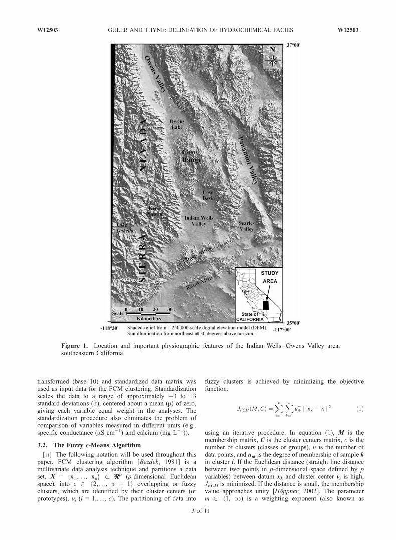
[27] The FCM clustering algorithm is an effective methodfor exploring the structure of complex data sets wheregrouping of overlapping and vague elements is necessary.However, the numerical results from the FCM have littlemeaning unless the underlying physical or chemical pro-cesses can be related to naturally occurring processes andthe spatial distribution of the clusters defined by FCM ismeaningful. For that reason the membership values (u) forwater samples in each water group were treated as aregionalized variable and separately interpolated on aregular grid by using the point kriging estimation methodto define the hydrochemical facies distribution in the studyarea. Kriged cluster membership values for each watergroup are displayed as color-coded cluster value contours(see Figure 3a). To achieve a better cluster separation, onlymembership values above 0.5 were plotted on the map. Inother words, u = 0.5 can be considered as a thresholdmembership value above which a given water sample isconsidered as belonging to the cluster.

4.3. Comparison of FCM With HCA

[28] Figures 3a and 3b show the results of the twoclustering techniques on map view. In Figure 3b the HCA(hard) clusters overlain on the shaded-relief map (digitalelevation model; DEM) for the study area. However, InFigure 3a the results of the FCM analysis are not overlainon the DEM to better highlight the differences. As we cansee in Figure 3a, spatial overlay of the membership valuesfor each cluster shows distinctive spatial patterns. The fivegroups are separated geographically, as well as physio-graphically with good correspondence between spatial loca-tions and the FCM clusters. The samples that belong to thesame group are located in close proximity to one another,suggesting the same processes and/or flow paths for thosegroups of samples. Both techniques (FCM and HCA)provide rapid and efficient methodology to cluster large


5 of 11

W12503

amounts of data. Both can utilize chemical and physicalmeasurements, although FCM can accommodate qualitativedata in addition to the quantitative data used in this study.Both techniques produced five clusters, with most samplesbelonging to the same group regardless of method. Theexceptions are the samples from Panamint Valley that wereclustered into group-5 by the HCA analysis, but group-4 bythe FCM technique and samples from southern OwensValley where the classification was reversed (group-4 byHCA, but group-5 by FCM). The chemical significance ofthe clusters is discussed in detail below, but both techniquesproduce clusters that are geochemically valid as descriptionsof the expected water-rock interactions along the regionalflow paths [Guler, 2002]. In addition, the HCA techniquerequires the user to select the number of groups, while theFCM method employs an objective method to choose thenumber of groups. In addition to using an objectivemethodology to choose the number of clusters, FCM alsoproduces clusters with gradational membership (soft parti-tion) allowing plotting of this property as gray scales orcolor shades. The FCM technique also produces areas withno color (Figure 3a) that indicate transitional areas where

membership is divided between more than two clusters(each having membership values below the 50% threshold(u < 0.5) and therefore they do not belong to any of thegroups).[29] There is a difference based on contouring technique

in that kriging extrapolates cluster membership values (u)from the FCM analysis over the entire study area even toportions without any data (Figure 3a), while the handcontours simply outline samples with the same clustervalues that were determined by HCA (Figure 3b). There arealso occasional artifacts generated such as the group-1triangular contours in the northwestern corner (Figure 3a).Nevertheless, the patterns are very similar including manyof the smaller-scale details. The FCM clusters also show thedegree of membership by shading and the transitional zones(white color), which is additional information not availablefrom HCA.[30] In order for the statistical clusters to be useful, they

should create a representation of the hydrochemical systemthat is robust and can be tested by additional means such asspatial coherence within the statistical groups, spatial cor-respondence between the groups, and hydrologic controls

Figure 2. Plots of fuzziness performance index (FPI) and normalized classification entropy (NCE)values against the number of classes for the Indian Wells–Owens Valley data set for fuzzificationparameter (m) values varying between 1.1 and 3.0. Minima of the FPI and NCE curves indicate theoptimal number clusters existing in the data set.

6 of 11


such as topography and hydrochemical evolution that canbe supported by inverse geochemical modeling [Thyne etal., 2004].[31] The FCM clusters display spatial distributions that

are closely related to physiography. Group-1 samples are alllocated in the recharge areas of the high Sierra Nevada andplot above the 2000-m contour line. Group-2 samples aremostly located below the 2000-m contour line in the SierraNevada and other mountain ranges. These areas provide themajority of recharge to the basin-fill aquifers in the area.Group-3 samples are usually located on the basin floors, andare spatially between group-2 and group-4 samples. Group-

4 samples are found in or very near the discharge areas(playas). Group-5 waters have the highest TDS concentra-tions and coincide with the playa or adjacent discharge areas(Figure 3a) and are characterized by lower Ca and Mgconcentrations than group-4 waters (Table 2). The highdegree of spatial and statistical coherence suggests thatthe changes between the hydrochemical facies define thenormal hydrochemical evolution of water in the region.[32] The TDS content of the waters is expected to

increase as the water moves down the flow path andwater-rock interaction takes place. In fact, the data showas the water moves eastward from the Sierran rechargeareas to the discharge areas near and around the playas(Figure 3a), evolving from very dilute water (TDS =�78 mg L�1) to dilute water (TDS = �319 mg L�1) tobrackish water (TDS = �883 mg L�1) to more salinewater (TDS = �8584 mg L�1), and finally to brine(TDS = �17,716 mg L�1, with TDS locally as high as342,186 mg L�1). Thus the water groups, as determinedby the FCM, appear to define hydrologic features such asdischarge zones and the hydrochemical evolution betweenrecharge zones and discharge zones.

4.4. Inverse Geochemical Modeling

[33] The validity of the statistical clusters, as representa-tions of the hydrochemical evolution of groundwater, can befurther evaluated with inverse geochemical models. Inversemodeling uses the mass balance approach to calculate allstoichiometric reactions that can produce the observedchemical changes between end-member waters [Plummerand Back, 1980]. A set of reactions needs to be definedbefore the inverse geochemical model can calculate thestoichiometric coefficients required to produce the observedset of compositions. This mass balance technique has beenused to quantify reactions controlling water chemistry alongflow paths and quantify mixing of end-member componentsin a flow system. For instance, Garrels and MacKenzie

Table 1. First 20 Rows of the FCM Membership Matrix (M)

SampleNumber Classa

Membership Value (u)

1 2 3 4 5

SP1 3 0.0005 0.0459 (0.8921) 0.0597 0.0018SP10 2 0.0082 (0.8281) 0.1608 0.0024 0.0005SP100 5 0.0033 0.0241 0.0337 0.0532 (0.8858)SP101B 3 0.0008 0.1670 (0.8261) 0.0053 0.0009SP102F 2 0.0015 (0.9479) 0.0502 0.0003 0.0001SP103 3 0.0003 0.2035 (0.7796) 0.0073 0.0092SP104 2 0.1295 (0.8022) 0.0653 0.0021 0.0009SP105 1 (0.9989) 0.0009 0.0002 0.0000 0.0000SP106 5 0.0001 0.0039 0.0049 0.0016 (0.9896)SP107 4 0.0059 0.0885 0.2871 (0.5199) 0.0987SP108 2 0.0030 (0.8825) 0.1126 0.0016 0.0004SP109 2 0.0004 (0.5845) 0.4131 0.0016 0.0004SP11 3 0.0022 0.1459 (0.8134) 0.0373 0.0013SP110 2 0.0021 (0.6936) 0.2991 0.0040 0.0012SP111 2 0.0023 (0.9046) 0.0919 0.0008 0.0005SP112 4 0.0002 0.0022 0.0130 (0.9726) 0.0120SP113B 4 0.0001 0.0101 0.2354 (0.7063) 0.0481SP114 3 0.0042 0.1599 (0.7989) 0.0340 0.0029SP115 3 0.0004 0.1144 (0.8737) 0.0085 0.0031SP116 2 0.3113 (0.6705) 0.0173 0.0005 0.0004

aClass memberships on the basis of which rows were selected are inparentheses.

Table 2. Main Features of the Cluster Centers (Representative Clusters) for Five Classes (Groups) Derived by FCM Objective Function

and Mean Water Chemistry of Five Principal Water Groups Determined From Hierarchical Cluster Analysis (HCA)a

Parameters Nb S. Cond. pH Ca Mg Na K Cl SO4 HCO3 SiO2 F

FCM Means Calculated Using Samples With u 0.50Group-1 88 101 7.4 9 1.2 11 1.0 2.0 3.8 56 22 0.3Group-2 236 515 8.0 33 7.7 66 3.6 44 40 184 32 0.9Group-3 213 1,372 7.8 81 29.4 185 11 192 184 326 36 1.1Group-4 94 10,591 7.5 185 125.5 2,817 65 4,153 883 585 61 3.2Group-5 60 17,529 9.0 8 7.3 7,112 185 7262 1447 3296 36 11.2

FCM Means Calculated Using Samples With u 0.75Group-1 81 90 7.3 9 1.2 8 1.0 1.5 2.9 52 22 0.3Group-2 171 477 8.0 33 6.5 59 3.0 40 39 171 31 0.8Group-3 145 1,222 7.8 79 30.9 152 10 138 186 322 35 1.0Group-4 70 11,529 7.5 214 146.8 3153 68 4,696 1,109 484 61 1.6Group-5 47 21,359 8.9 6 4.5 8,854 232 9,100 1,782 3,965 35 13.6

HCA Means Calculated Using All SamplesGroup-1 81 72 7.3 7 0.9 7 0.9 1.3 1.6 45 22 0.3Group-2 229 542 8.0 37 8.5 67 3.6 41 51 195 33 0.9Group-3 168 1,665 7.9 77 33.7 236 13 199 192 442 43 1.4Group-4 80 7,495 7.9 143 79.9 1,574 52 1,900 892 660 41 2.2Group-5 20 78,863 8.9 106 110.3 35,501 714 42,844 5,635 9,418 34 28.4

aFCM objective function means were calculated using samples having membership values 0.50 and 0.75. Group-1 and group-2 means were used ininverse geochemical calculations.

bNumber of samples within respective FCM classes or principal HCA groups. Specific conductance (mS cm�1), pH (standard units), mean concentrations(mg L�1).


7 of 11

W12503

[1967] modeled Sierran spring water evolution for a smallincrease (80 ppm) in total dissolved solids (TDS) success-fully. Inverse modeling is more difficult in systems thathave similar amounts of several ions with multiple possiblesources or large TDS changes typical in arid westernwatersheds [Thomas et al., 1989].[34] Three cases were evaluated, which include (1) the

means of the HCA groups; (2) FCM cluster means wheremembership in the cluster was limited to samples with u =0.50 or greater; and (3) FCM cluster means wheremembership in the cluster was limited to samples with u =0.75 or greater membership values. Table 2 shows themeans for the three cases. These mean values are used forinputs, together with the appropriate mineralogy [Guler,

2002], for the inverse geochemical models. All three casesproduced viable inverse modeling solutions. Table 3 showsthe results for the first two steps in the hydrochemicalevolution, those of precipitation to group-1 samples andgroup-1 to -2 samples. While there are small differences, thebasic reaction derived from inverse modeling for all threecases is the same:

Model 1

precipitation þ CO2 gasþ plagioclaseþ biotiteþ K-feldspar

þ haliteþ gypsum ¼ group-1 water þ amorphous silica

þ kaoliniteþ calcite

Figure 3. (a) Spatial distribution of the five hydrochemical facies determined by FCM objectivefunction. Cluster memberships (u) for each facies range between 0.5 and 1 and separately interpolated ona regular grid by using point kriging algorithm. Each hydrochemical facies overlain on a single map andcolor-coded for better visualization purposes. Darker colors indicate strong membership to a particularfacies, whereas lighter colors indicate a weak membership. (b) Spatial distribution of the statisticallydefined (by HCA) five principal water groups in the study area (modified from Guler and Thyne [2004]).In the HCA hard clustering method, samples are classified either as a group member or not (e.g., 1 or 0).Therefore, in the HCA method, samples close to group boundaries are more prone to misclassificationthan soft clustering methods such as FCM. See color version of this figure at back of this issue.

8 of 11


Model 2

group-1 water þ CO2 gasþ plagioclaseþ biotiteþ K-feldspar

þ forsteriteþ haliteþ gypsum ¼ group-2 water

þ amorphous silicaþ kaoliniteþ calcite

[35] This compares well with other models for the region[Feth et al., 1964; Garrels and Mackenzie, 1967; Thomas etal., 1989] and indicates that all three approaches can defineviable hydrochemical evolution models for the region. TheFCM analysis also provides a more robust classificationmethodology. Water samples that are close to the center of aHCA cluster (samples having FCM membership valuesclose to 1) are strong representatives of the cluster and areusually correctly classified by HCA. However, samples thatare close to the boundaries of clusters (samples having FCMmembership values close to 0.50 or lower) are weakerrepresentatives and are prone to misclassification. However,even though FCM produces much better mapping informa-tion (gray or color scale) and is more robust than the HCA,it cannot entirely eliminate the problem of samplemisclassification. The samples most prone to misclassifica-tion are those in white colored areas in Figure 3a.

5. Discussion

[36] The changes in water chemistry in the study area arecomplex with a transitional character. The statistical asso-ciations present the information in a compact format as thefirst step to determine if samples can be grouped intodistinct populations (hydrochemical facies) and help definea preliminary hydrochemical evolution for the study area.The associations (clusters) can be tested for spatial coher-ence, geological relevance, and hydrochemical validity toestablish cause-and-effect relationships. In this case, thehydrochemical facies showed strong spatial coherence andcorrelated well with the major hydrologic features, anunlikely result if the statistical associations did not reflectunderlying physical and chemical processes.[37] The mean values of the clusters also served as input

to inverse geochemical models to further verify that thestatistical clusters were significant in the hydrochemical

context. The use of mean values from clusters for inversemodel inputs enhances the power of the approach, whichworks best in simple systems with a few dominant water-rock reactions. Cluster analysis creates statistical groupsfrom multiple parameters, reducing the variability, whichcan be viewed as information noise, while still extractingthe essential aspects of each group. This input is particularlyuseful in handling large data sets and defining the importantcomponents of hydrochemical evolution.[38] The fuzzy clusters are fundamentally similar to the

HCA clusters but offer the additional advantages of a moreobjective criteria for choosing the number of clusters andgradation of cluster (degree of membership) that are impos-sible with hard partitioning. This information can be pre-sented as contours using a variety of standard techniquessuch as kriging. The ability to set the threshold for mem-bership can also allow multiple realizations that can beevaluated for the best match to criteria such as physiograph-ic and hydrologic features, internal spatial coherence, andhydrochemical validity.

6. Summary and Concluding Remarks

[39] In this study, the FCM clustering technique was usedto create a spatially and geochemically coherent classifica-tion of water chemistry data from a regional groundwatersystem. Using the FCM technique, five hydrochemicalfacies were delineated and cluster centers representing eachhydrochemical facies were determined. Plotting the krigedcluster membership value contours on a map demonstratedthe existence of five spatially continuous, well-definedclusters of water samples. Mean values of each variablefrom the hydrochemical facies were used for further eval-uation of the system with inverse geochemical models thatdescribe the major processes creating variability betweensamples. Hydrochemical facies defined by FCM can be alsoused to study the groundwater flow systems and as a tool toverify aquifer connectivity in the same fashion as hydro-chemical facies defined by nonfuzzy methods.[40] Our results show that a fuzzy classification gives

improved spatial definition and less error sensitive clustersthan a classical hard classification. Water samples close toclass boundaries are especially prone to misclassification

Table 3. Summary of Mass Transfer for Selected Inverse Geochemical Models Using Three Different Group Means Calculated Using

FCM (for u 0.50 and 0.75) and HCAa

Phases

FCM (u 0.50) FCM (u 0.75) HCA

Precipitationto Group-1

Group-1to Group-2


Group-1to Group-2


Group-1to Group-2

Amorphous silica �4.99E-04b �3.08E-03 �3.44E-04 �2.74E-03 �2.49E-04 �3.54E-03Biotite 1.36E-05 . . . 1.36E-05 . . . 1.15E-05 6.81E-05Calcite �5.03E-05 �7.16E-04 . . . �6.14E-04 . . . �8.74E-04CO2(g) 8.20E-04 3.13E-03 7.12E-04 2.77E-03 5.68E-04 3.68E-03Forsterite . . . 1.34E-04 . . . 1.08E-04 . . . 5.11E-05K-feldspar . . . 6.65E-05 . . . 5.12E-05 3.75E-06 . . .Plagioclase 6.71E-04 2.40E-03 5.43E-04 2.17E-03 4.63E-04 2.85E-03Kaolinite �4.69E-04 �1.69E-03 �3.81E-04 �1.52E-03 �3.27E-04 �2.00E-03Gypsum 2.91E-05 3.79E-04 1.97E-05 3.73E-04 3.86E-06 5.15E-04Halite 4.03E-05 1.18E-03 2.91E-05 1.09E-03 2.44E-05 1.13E-03

aModel-1, precipitation to group-1 waters; model-2, group-1 to group-2 waters. Phases and thermodynamic data are from PHREEQC and accompanyingdatabases [Parkhurst and Appelo, 1999]. Values in moles per kilogram H2O (positive values indicate dissolution and negative values indicate precipitation).Ellipsis dots indicate phase not used in model.

bRead as �4.99 � 104.


9 of 11

W12503

when using conventional hard clustering methods such asHCA. In contrast, fuzzy clustering allows each sample tobelong to several clusters minimizing misclassification. Themembership values (u) of the clusters, which are a statisticalcomposite of all the clustered parameters, can be displayedas contour maps. These contour maps can be overlain withother graphical information such as topography, lithology,etc., to produce enhanced visualization and analysis.[41] Our approach used the Euclidean distance and a

fuzziness coefficient (m) of 1.3 for optimal clustering. Thefive groups produced by the FCM analysis were hydro-chemically meaningful. The results suggest that fuzzyclassification may better reflect the continuous nature ofthe processes underlying the generation of water chemistryvariability in the study area. Furthermore, fuzzy clusteringmethods can handle large data matrices (typical of regional-scale studies) [Hoppner, 2002; Kolen and Hutcheson, 2002]and provide a rapid, systematic, and objective means forreducing large amounts of hydrochemical data into moreuseful information. We conclude that the robust classifica-tion scheme for partitioning water chemistry samples intohomogeneous groups produced by FCM can be animportant tool for the successful characterization ofregional-scale hydrogeologic systems.

[42] Acknowledgment. The authors thank the Ministry of NationalEducation of Turkey for the senior author’s financial support.

ReferencesAhmed, M. N., S. M. Yamany, N. Mohamed, A. A. Farag, and T. Moriarty(2002), A modified fuzzy c-means algorithm for bias field estimation andsegmentation of MRI data, IEEE Trans. Med. Imaging, 21, 193–199.

Asharaf, S., and M. N. Murty (2003), An adaptive rough fuzzy single passalgorithm for clustering large data sets, Pattern Recognit., 36, 3015–3018.

Barbieri, P., G. Adami, A. Favretto, A. Lutman, W. Avoscan, andE. Reisenhofer (2001), Robust cluster analysis for detecting physico-chemical typologies of freshwater from wells of the plain of Friuli (north-eastern Italy), Anal. Chim. Acta, 440, 161–170.

Belacel, N., P. Hansen, and N. Mladenovic (2002), Fuzzy J-means: A newheuristic for fuzzy clustering, Pattern Recognit., 35, 2193–2200.

Bezdek, J. C. (1974), Cluster validity with fuzzy sets, J. Cybern., 3, 58–73.Bezdek, J. C. (1975), Mathematical models for systematics and taxonomy,in Proceedings of the Eighth International Conference on NumericalTaxonomy, edited by G. Estabrook, pp. 143–166, W. H. Freeman,New York.

Bezdek, J. C. (1981), Pattern Recognition With Fuzzy Objective FunctionAlgorithms, Plenum, New York.

Bezdek, J. C., and N. R. Pal (1998), Some new indexes of cluster validity,IEEE Trans. Syst. Man Cybern., 28, 301–315.

Bezdek, J. C., R. Ehrlich, and W. Full (1984), FCM: The fuzzy c-meansclustering algorithm, Comput. Geosci., 10, 191–203.

Bezdek, J. C., L. O. Hall, and L. P. Clarke (1993), Review of MR imagesegmentation techniques using pattern recognition, Med. Phys., 20,1033–1048.

Bezdek, J. C., J. M. Keller, R. Krishnapuram, and N. R. Pal (1999), FuzzyModels and Algorithms for Pattern Recognition and Image Processing,Kluwer Acad., Norwell, Mass.

Burrough, P. A., P. F. M. van Gaans, and R. A. McMillan (2000), High-resolution landform classification using fuzzy k-means, Fuzzy Sets Syst.,113, 37–52.

Chang, N.-B., H. W. Chen, and S. K. Ning (2001), Identification of riverwater quality using the fuzzy synthetic evaluation approach, J. Environ.Manage., 63, 293–305.

Dunn, J. C. (1974), A fuzzy relative ISODATA process and its use indetecting compact well-separated clusters, J. Cybern., 3, 32–57.

El-Sonbaty, Y., and M. A. Ismail (1998), Fuzzy clustering for symbolicdata, IEEE Trans. Fuzzy Syst., 6, 195–204.

Fang, J. H., and H. C. Chen (1990), Uncertainties are better handled byfuzzy arithmetic, AAPG Bull., 74, 1228–1233.

Feth, J. H., C. E. Roberson, and W. L. Polzer (1964), Sources of mineralconstituents in water from granitic rocks, Sierra Nevada, California andNevada, U.S. Geol. Surv. Water Supply Pap., 1535-I.

Fukuyama, Y., and M. Sugeno (1989), A new method of choosing thenumber of clusters for the fuzzy c-means method, in Proceedings ofthe Fifth Fuzzy Systems Symposium, pp. 247–250, Japan.

Garrels, R. M., and F. T. MacKenzie (1967), Origin of the chemical com-positions of some springs and lakes, in Equilibrium Concepts in NaturalWaters, pp. 222–242, Am. Cancer Soc., Washington, D. C.

Geva, A. B. (1999), Hierarchical unsupervised fuzzy clustering, IEEETrans. Fuzzy Syst., 7, 723–733.

Gunderson, R. (1978), Application of fuzzy ISODATA algorithms to star-tracker pointing systems, paper presented at the 7th Triannual WorldIFAC Congress, Helsinki, Finland.

Guler, C. (2002), Hydrogeochemical evaluation of the groundwater re-sources of Indian Wells –Owens Valley area, southeastern California,Ph.D. dissertation, 262 pp., Colo. School of Mines, Golden, Colo.

Guler, C., and G. D. Thyne (2004), Hydrologic and geologic factors con-trolling surface and groundwater chemistry in Indian Wells–Owens Val-ley area, southeastern California, USA, J. Hydrol., 285, 177–198.

Guler, C., G. Thyne, J. E. McCray, and A. K. Turner (2002), Evaluation ofgraphical and multivariate statistical methods for classification of waterchemistry data, Hydrogeol. J., 10, 455–474.

Hammah, R. E., and J. H. Curran (1999), On distance measures for thefuzzy k-means algorithm for joint data, Rock Mech. Rock Eng., 32, 1–27.

Hathaway, R. J., and J. C. Bezdek (2001), Fuzzy c-means clustering ofincomplete data, IEEE Trans. Syst. Man Cybern. B, 31, 735–744.

Hoppner, F. (2002), Speeding up fuzzy c-means: Using a hierarchical dataorganization to control the precision of membership calculation, FuzzySets Syst., 128, 365–378.

Hu, B.-G., R. G. Gosine, L. X. Cao, and C. W. de Silva (1998), Applicationof a fuzzy classification technique in computer grading of fish products,IEEE Trans. Fuzzy Syst., 6, 144–152.

Kersten, P. R. (1999), Fuzzy order statistics and their application to fuzzyclustering, IEEE Trans. Fuzzy Syst., 7, 708–712.

Kolen, J. F., and T. Hutcheson (2002), Reducing the time complexity of thefuzzy c-means algorithm, IEEE Trans. Fuzzy Syst., 10, 263–267.

Kothari, R., and D. Pitts (1999), On finding the number of classes, PatternRecognit. Lett., 20, 405–416.

Linusson, A., S. Wold, and B. Norden (1998), Fuzzy clustering of 627alcohols, guided by a strategy for cluster analysis of chemical com-pounds for combinatorial chemistry, Chemom. Intell. Lab. Syst., 44,213–227.

Maxey, G. B. (1968), Hydrogeology of desert basins, Ground Water, 6,10–22.

McBratney, A. B., and J. J. deGruijter (1992), A continuum approach to soilclassification by modified fuzzy k-means with extragrades, J. Soil Sci.,43, 159–175.

McBratney, A. B., and A. W. Moore (1985), Application of fuzzy sets toclimatic classification, Agric. For. Meteorol., 35, 165–185.

McNeill, D., and P. Freiberger (1993), Fuzzy Logic: The RevolutionaryComputer Technology That Is Changing Our World, Simon and Schuster,New York.

Minasny, B., and A. B. McBratney (2002), FuzME version 3, Aust. Cent.for Precis. Agric., Univ. of Sydney, Sydney, N. S. W., Australia. (Avail-able at http://www.usyd.edu.au/su/agric/acpa.)

Odeh, I. O. A., A. B. McBratney, and D. J. Chittleborough (1992), Soilpattern recognition with fuzzy c-means: Application to classification andsoil-landform interrelationship, Soil Sci. Soc. Am. J., 56, 505–516.

Parkhurst, D. L., and C. A. J. Appelo (1999), User’s guide to PHREEQC(Version 2): A computer program for speciation, batch-reaction, one-dimensional transport, and inverse geochemical calculations, U.S. Geol.Surv. Water Resour. Invest. Rep., 99-4259.

Pedrycz, W. (1996), Conditional fuzzy c-means, Pattern Recognit. Lett., 17,625–631.

Plummer, L. N., and W. W. Back (1980), The mass balance approach:Application to interpreting the chemical evolution of hydrological sys-tems, Am. J. Sci., 280, 130–142.

Ramze, M., R. B. P. F. Lelieveldt, and J. H. C. Reiber (1998), A new clustervalidity index for fuzzy c mean, Pattern Recognit. Lett., 19, 237–246.

Rantitsch, G. (2000), Application of fuzzy clusters to quantify lithologicalbackground concentrations in stream-sediment geochemistry, J. Geo-chem. Explor., 71, 73–82.

Roubens, M. (1982), Fuzzy clustering algorithms and their cluster validity,Eur. J. Oper. Res., 10, 294–301.

Setnes, M. (2000), Supervised fuzzy clustering for rule extraction, IEEETrans. Fuzzy Syst., 8, 416–424.

10 of 11


Suk, H., and K.-K. Lee (1999), Characterization of a ground water hydro-chemical system through multivariate analysis: Clustering into groundwater zones, Ground Water, 37, 358–366.

Sun, L.-X., and K. Danzer (1996), Fuzzy cluster analysis by simulatedannealing, J. Chemom., 10, 325–342.

Thomas, J. M., A. H. Welch, and A. M. Preissler (1989), Geochemicalevolution of ground water in Smith Creek Valley: A hydrologicallyclosed basin in central Nevada, U.S.A., Appl. Geochem., 4, 493–510.

Thyne, G. D., C. Guler, and E. Poeter (2004), Sequential analysis of hydro-chemical data for watershed characterization, Ground Water, 42, 711–723.

Trauwert, E., L. Kaufman, and P. Rousseeuw (1991), Fuzzy clusteringalgorithms based on the maximum likelihood principle, Fuzzy Sets Syst.,42, 213–227.

Windham, M. P. (1981), Cluster validity for fuzzy clustering algorithms,Fuzzy Sets Syst., 5, 177–185.

Wu, K.-L., and M.-S. Yang (2002), Alternative c-means clusteringalgorithms, Pattern Recognit., 35, 2267–2278.

Xie, L. X., and G. Beni (1991), A validity measure for fuzzy clustering,IEEE Trans. Pattern. Anal. Machine Intell., 13, 841–847.

Zadeh, L. A. (1965), Fuzzy sets, Inf. Control, 8, 338–353.Zhang, C.-T., K.-C. Chou, and G. M. Maggiora (1995), Predicting proteinstructural classes from amino acid composition: Application of fuzzyclustering, Protein Eng., 8, 425–435.

��C. Guler, Geological Engineering Department, Ciftlikkoy Kampusu,

Mersin Universitesi, Mersin 33342, Turkey. ([email protected])G. D. Thyne, Department of Geology and Geological Engineering,

Colorado School of Mines, 1500 Illinois Street, Golden, CO 80401, USA.


11 of 11

W12503

Figure 3. (a) Spatial distribution of the five hydrochemical facies determined by FCM objectivefunction. Cluster memberships (u) for each facies range between 0.5 and 1 and separately interpolated ona regular grid by using point kriging algorithm. Each hydrochemical facies overlain on a single map andcolor-coded for better visualization purposes. Darker colors indicate strong membership to a particularfacies, whereas lighter colors indicate a weak membership. (b) Spatial distribution of the statisticallydefined (by HCA) five principal water groups in the study area (modified from Guler and Thyne [2004]).In the HCA hard clustering method, samples are classified either as a group member or not (e.g., 1 or 0).Therefore, in the HCA method, samples close to group boundaries are more prone to misclassificationthen soft clustering methods such as FCM.


8 of 11

Delineation of hydrochemical facies distribution in a regional groundwater system by means of fuzzy...

Documents

Transcript of Delineation of hydrochemical facies distribution in a regional groundwater system by means of fuzzy...