Delineation of Flood-Prone Areas Using Remote Sensing Techniques
15
Water Resources Management (2005) 19: 333–347 DOI: 10.1007/s11269-005-3281-5 C Springer 2005 Delineation of Flood-Prone Areas Using Remote Sensing Techniques SANJAY K. JAIN ∗ , R. D. SINGH, M. K. JAIN and A. K. LOHANI Remote Sensing Application Division, National Institute of Hydrology, Bhawan-Roorkee, Jalvigyan 247 667, India ( ∗ author for correspondence, e-mail: [email protected]) (Received: 15 April 2004; in final form: 7 September 2004) Abstract. Flood problems resulting due to heavy rainfall and drainage congestion are being regularly experienced in plain areas of Bihar, India. Due to this problem, power plant located in Koa catchment, Kahalgaon, Bihar, is faces huge loss at the time of flood. In this paper, the flood-affected areas in Koa catchment have been mapped using remote sensing satellite data (IRS LISS III, 1999 and Landsat TM, 1995). A range of image processing techniques has been used, including simple density slicing, Tasseled Cap Transformation and water-specific index. The results obtained using different approaches have been analysed. Result indicates that a Normalized Difference Water Index (NDWI) based approach produced best results. Key words: catchment, flood, rainfall, remote sensing, water 1. Introduction Floods are the major disaster affecting many countries in the world year after year. It is an inevitable natural phenomenon occurring from time to time in all rivers and natural drainage systems that not only damages the lives, natural resources and environment, but also causes the loss of economy and health. In India also, floods are most frequent mainly in the eastern part (Orissa, Bengal, Andhra Pradesh, Bihar). The annual precipitation in India, including snowfall is estimated at 4000 billion m 3 (BCM). Out of this, the seasonal rainfall in monsoon is of the order of 3000 BCM. The rainfall in India shows great temporal and spatial variations, unequal seasonal distribution and geographical distribution and frequent departures from the normal (Mohapatra and Singh, 2003). Accurate information on the extent of water bodies is important for flood predic- tion, monitoring, and relief (Smith, 1997; Baumann, 1999). Often, this information is difficult to produce using traditional survey techniques because water bodies can be fast moving as in floods, tides, and storm surges or may be inaccessible. The synoptic, repetitive nature of satellite remotely sensed data have allowed monitor- ing of water bodies over large regions of land. In the optical range (visible-infrared) water has a distinctively low spectral response. In many studies, Landsat data (TM
Transcript of Delineation of Flood-Prone Areas Using Remote Sensing Techniques
Water Resources Management (2005) 19: 333–347DOI: 10.1007/s11269-005-3281-5 C© Springer 2005
Delineation of Flood-Prone Areas Using RemoteSensing Techniques
SANJAY K. JAIN∗, R. D. SINGH, M. K. JAIN and A. K. LOHANIRemote Sensing Application Division, National Institute of Hydrology, Bhawan-Roorkee,Jalvigyan 247 667, India(∗author for correspondence, e-mail: [email protected])
(Received: 15 April 2004; in final form: 7 September 2004)
Abstract. Flood problems resulting due to heavy rainfall and drainage congestion are being regularlyexperienced in plain areas of Bihar, India. Due to this problem, power plant located in Koa catchment,Kahalgaon, Bihar, is faces huge loss at the time of flood. In this paper, the flood-affected areasin Koa catchment have been mapped using remote sensing satellite data (IRS LISS III, 1999 andLandsat TM, 1995). A range of image processing techniques has been used, including simple densityslicing, Tasseled Cap Transformation and water-specific index. The results obtained using differentapproaches have been analysed. Result indicates that a Normalized Difference Water Index (NDWI)based approach produced best results.
Key words: catchment, flood, rainfall, remote sensing, water
1. Introduction
Floods are the major disaster affecting many countries in the world year after year.It is an inevitable natural phenomenon occurring from time to time in all riversand natural drainage systems that not only damages the lives, natural resources andenvironment, but also causes the loss of economy and health. In India also, floods aremost frequent mainly in the eastern part (Orissa, Bengal, Andhra Pradesh, Bihar).The annual precipitation in India, including snowfall is estimated at 4000 billionm3 (BCM). Out of this, the seasonal rainfall in monsoon is of the order of 3000BCM. The rainfall in India shows great temporal and spatial variations, unequalseasonal distribution and geographical distribution and frequent departures fromthe normal (Mohapatra and Singh, 2003).
Accurate information on the extent of water bodies is important for flood predic-tion, monitoring, and relief (Smith, 1997; Baumann, 1999). Often, this informationis difficult to produce using traditional survey techniques because water bodies canbe fast moving as in floods, tides, and storm surges or may be inaccessible. Thesynoptic, repetitive nature of satellite remotely sensed data have allowed monitor-ing of water bodies over large regions of land. In the optical range (visible-infrared)water has a distinctively low spectral response. In many studies, Landsat data (TM

334 S. K. JAIN ET AL.
and MSS), IRS or SPOT have been used to determine the extent of water bodiesusing simple classification procedures, usually with an infrared band. These stud-ies have relied on the water bodies having a unique spectral response in this rangeof electromagnetic radiation when compared to the surrounding landscape (Wang,2002; Frazier and Page, 2000). Many studies using density slicing of Landsat MSSband 7 (Bennett, 1987), TM bands 4 and 7 (Wang, 2002; Frazier and Page, 2000)have been reported in literature. Manavalan et al. (1993) used Landsat TM band 4to map the extent of the Bhadra reservoir, India. Overton, 1997 used density slicingof Landsat TM band 5 and a high flood spatial mask to map water bodies on theMurray river between Blanchetown and Wentworth, South Australia. Shaikh et al.(1997) used band 4 of Landsat TM to map flood extent of the Mississippi riverbut experienced problems separating water from certain urban features without theinclusion of an additional band.
The river Ganges as it flows down in the flatter plain of Bihar and further toBengal, its flood plain extended much beyond the defined riverbanks. In both banksof the Ganges exists such land zones, which behaves not only as flood plain butalso as detention basin for up-land flows. Kahalgaon Super Thermal Power Project(KhSTPP) of NTPC is located near Kahalgaon town, District Bhagalpur of BiharState, India. The plant area and its adjoining areas were subjected to severe floodin August 1993, September 1995 and September 1999. The flood was brought byKoa river coupled with back water effect due to high flood level of Ganges riverand inundated a vast areas upstream and adjoining the power station (situated inKoa river basin) and also affected the drainage inside the plant area. The lowerpart of Koa basin out falling to Ganges where the Kahalgaon Power plant andother structures are situated is also in flood plain area. Topographically, the plantis situated at the mouth of a catchment (Koa nala) near the confluence of Ganga.Insufficient natural drainage aggravates the flood situation in the catchment of KoaNala. In this paper, IRS-1C LISS III and Landsat TM data for mapping of floodedareas have been used. A digital elevation model (DEM) has also been used.
2. The Study Area and Data Used
The river Koa emerges from the hills at an elevation of about 400 m. The riverin general has very narrow width and traverses about 48 km and then joins riverGanga. The general slope of the river is very mild except in some upper reachesof the catchment. The catchment area of Koa river up to Eastern Railway Bridgeis 677.0 km2 and up to Marry Go Round (MGR), 584 km2. The catchment isbounded between latitude 25◦00′00′′N to 25◦15′10′′N and Longitude 87◦13′51′′Eto 87◦38′28′′E. The catchment area has a shape of key, i.e. wide in the beginning andnarrow at the mouth. The annual normal rainfall is about 122 cm. On an average, itrains for about 50–60 days in a year. Most of the rain occurs (about 75–80%) duringthe monsoon season (June–September). The Public Works Department road bridgeis the most downstream bridge in Kao river and is just upstream of confluence of

DELINEATION OF FLOOD PRONE AREAS 335
Koa with Ganges river. The deck level is of the order of elevation about 34.5 m.The eastern railway bridge is approximately 100.0 upstream of the Public WorksDepartment road bridge and the clear water way is 100 m. The elevation of railwaytrack is about 35.50 (NHPC, 1995).
The satellite data used were as follows:
Satellite/sensor Path/row Date of pass
Landsat TM 139–43 27 May 1995
18 October 1995
IRS-1C LISS III 106–54 March 1999
December 1999
Topographical maps at a scale of 1:50,000 have been used. The area is coveredin topographical maps Nos. 72 O/4, 7, 8 and 12.
3. Methodology
3.1. PREPARATION OF DATABASE
In the present study for preparation of drainage map, contour map, etc., Surveyof India toposheets has been used. The Koa catchment is covered in two topo-graphical maps at a scale of 1:50,000. The drainage and contour maps of the Koacatchment were digitized directly from topographical maps. The drainage map ofthe Koa catchment along with MGR and the plant is shown in Figure 1. The data
Figure 1. The study showing MGR and road.

336 S. K. JAIN ET AL.
in raster format were converted to vector form using the raster to vector software,R2V. This software R2V for Windows is a powerful raster to vector conversionsoftware developed by Able Software Corp. (http://www.ablesoftware.com/r2v).R2V combines the power of intelligent automatic vectorizing technology with aneasy-to-use, menu-driven, graphical user interface in the Microsoft Windows en-vironment. The software converts scanned maps or images to vector formats formapping, geographic information systems (GIS), CAD, and scientific computingapplications. The data in vector format are required for providing elevation valuesto the contours as depicted in the topographical maps. For generation of the contourmap, each contour line is selected one by one and the elevation value is assigned.
For area estimation and creation of DEM, etc., the GIS software Integrated Landand Water Information System (ILWIS) was used. ILWIS is a GIS that integrates im-age processing capabilities, tabular databases and conventional GIS characteristics.This software is developed at International Institute for Geo-Information Scienceand Earth Observation (ITC) (www.itc.nl). The drainage network and catchmentboundary created in ILWIS was transferred to ERDAS 8.6 for further image pro-cessing. The satellite data of the years 1995 and 1999 received in digital formatfrom the National Remote Sensing Agency (NRSA), Hyderabad, India, was loadedin ERDAS.
3.2. PROCESSING OF SATELLITE DATA
To study the extent of flood inundation, the analysis of Landsat TM scenes andIRS-1C LISS III digital data have been performed. For flood mapping, two sets ofthe remotely sensed data are required; one set consisting of data acquired during theoccurrence of the flood. In reality, data availability may cause some compromise,because it is difficult to obtain cloud free data during floods. Therefore, in thisstudy, efforts were made to take satellite data just before and after the flood event.Selection of the dates of the satellite scenes is made based on observed floodevents.
Satellite data as mentioned earlier were geocoded with topographical maps usingground control points. The Polyconic projection system is used for geocoding thedigital data. The geocoded scenes are masked by boundaries for Koa catchment dig-itized from topographical maps and imported in ERDAS IMAGINE. Some clearlyidentifiable features like crossing of rivers, canals, sharp turns in the rivers, roads,bridges, etc., were located on both map and image and were selected as controlpoints. About 10 such points were selected for geo-referencing in all the cases.Now looking at the statistics, some points that generated big errors were deletedand replaced by other points so as to obtain the better geo-referencing. After com-pleting this process, the image was displayed over the map and the superimpositionwas compared. The geo-referencing was found to be quite good. Then the catch-ment area was masked. The False Colour Composite (FCC) of Landsat TM for twoseasons, i.e. May and October 1995 are shown in Figures 2 and 3.

DELINEATION OF FLOOD PRONE AREAS 337
Figure 2. False Colour Composite (FCC) of Landsat TM for May 1995.
Figure 3. False Colour Composite (FCC) of Landsat TM for May 1995.

338 S. K. JAIN ET AL.
3.3. IDENTIFICATION OF WATER AREAS
Though spectral signatures of water are quite distinct from other land use likevegetation, built-up area and soil surface, yet identification of water pixels at thewater/soil interface is very difficult and depends on the interpretative ability ofthe analyst. Deep water bodies have quite distinct and clear representation in theimagery. However, very shallow water/turbid water can be mistaken for soil whilesaturated soil can be mistaken for water pixels. Secondly, it is also possible that apixel, only at the soil/water interface, may represent mixed conditions (some partas water and other part as soil). Just by looking at the tone and colour of a pixel it isdifficult to tell the difference between suspended sediment and shallow water. Afterall, it is basically the same material with the same reflection properties. Therefore,very shallow water will have the same colour and brightness as very turbid (highconcentration of suspended sediment) water.
There are many possible methods for identifying water versus non-water areasusing satellite data. Initially, supervised and unsupervised classification approacheswere applied, but they did not produce very good results when compared with orig-inal satellite data. Therefore, the density-slicing approach using different band havebeen attempted. Then two approaches, one based on the Tasseled Cap Transforma-tion (wetness) and the other based on water index approaches were applied. Theresults of the all the methods have been analysed and compared. These methodsare discussed in the following sections.
3.4. DENSITY SLICING OF SINGLE BAND
In many studies, Landsat data (TM and MSS), IRS or SPOT have been used todetermine the extent of water bodies using density-slicing approach, usually withan infrared band. These studies have relied on the water bodies having a uniquespectral response in this range of electromagnetic radiation when compared to thesurrounding landscape. Baumann (1999) carried out a study using all the bandsof Landsat TM. He concluded that band 4 (NIR) represented the best spectralband that identifies the flood-inundated area well. Wang et al. (2002) carried outa study for identifying the water-affected area and he observed that bands 4 and 7(2.08–2.35 µm) are well suited for the purpose. In this study, initially, six bands ofLandsat TM (except thermal band) and three bands of IRS LISS III (except MIRband) have been analysed. In Figure 4, six Landsat TM individual band histogramsfor the October 1995 scene are presented. It is seen that in bands 1–3, there isconsiderable spectral overlap between the digital values found on the water bodiesand those in the surrounding urban/vegetation areas. The infrared band gives a muchbetter representation in the water-related features than the visible bands did. Eachof the visible bands displays a uni-model histogram with no indication of a separategroup of data for water pixel. The infrared bands show a bi-model histogram. Thedensity slicing ranges for infrared band starts at near zero, meaning that water pixelsare the darkest in the image. In this study, the analysis of bands 4 and 7 of TM data

DELINEATION OF FLOOD PRONE AREAS 339
Figure 4. Individual Landsat TM band histograms October 1995.
and band 3 of LISS III have been made. It was found that the results obtainedusing band 7 are not representing water-related features very well when comparedwith raw data; therefore, only band 4 has been taken. Initially, near infrared band(band 4 in TM data and band 3 in IRS LISS III) has been taken for mapping offlood. As the reflectance of water in near infrared (NIR) band is minimum, the area

340 S. K. JAIN ET AL.
of low reflectance has been taken using this approach. Once the representation ofthe reflectance values for water and non-water features was clear, a cut-off value ofdigital numbers could be determined to separate the two categories. For the OctoberTM image the cut-off value was 53, means if the digital number was less than 53,that pixel was assigned as water category. For the May image of TM data, the cut-offvalue was 60, i.e. if digital number was less than 60, that pixel was classified aswater, otherwise as non-water. In case of IRS LISS III data, the cut-off values forDecember 1999 scene was 54 and for March 1999 scene it was 71. NIR band isable to identify most of the major water features, but there is still some mixing withthe hill shadows, vegetation area, and therefore another method based on TasseledCap Transformation (wetness) has been applied.
3.5. TASSELED CAP TRANSFORMATION
There are numerous methods available for enhancing spectral information content ofsatellite data. The Tasseled Cap Transformation compressed the total informationinto three bands: greenness, brightness and wetness. Besides expressing a largeamount of image variability within three bands, tasseled cap bands could be directlyrelated to physical scene characteristics. A Tasseled Cap Transformation to datafrom the Landsat TM has been given (Crist and Cicone, 1984). The coefficients forwetness functions are:
1 2 3 4 5 6 7
0.1509 0.1793 0.3299 0.3406 0.306 −0.7112 −0.4572
One of the main reasons for supporting the use of the Tasseled Cap Transfor-mation method against, for example, the principal component technique is that thecoefficients of the transformation are defined a priori. This method was applied onthe Landsat TM data only. The coefficients for IRS LISS III data were not avail-able. The earlier wetness function was applied and threshold values of this index−52.0 to −34.0 for October and −35.0 to 19.0 for May have been chosen for waterfeatures. This method was good for identification of water-related features whencompared with original satellite data. But it could not eliminate the shadow effectscaused mainly due to forest, etc. To overcome the problem of shadows, a band ratiotechnique has been applied.
3.6. NDWI APPROACH
There are numerous vegetation indices developed to estimate vegetation cover withthe remotely sensed imagery. A vegetation index is a number that is generated bysome combination of remote sensing bands. The most common spectral index usedto evaluate vegetation cover is the Normalized Difference Vegetation Index (NDVI).McFeeters (1996) developed an index similar to the NDVI, which is called theNormalized Difference Water Index (NDWI). Any sensor having a green band and a
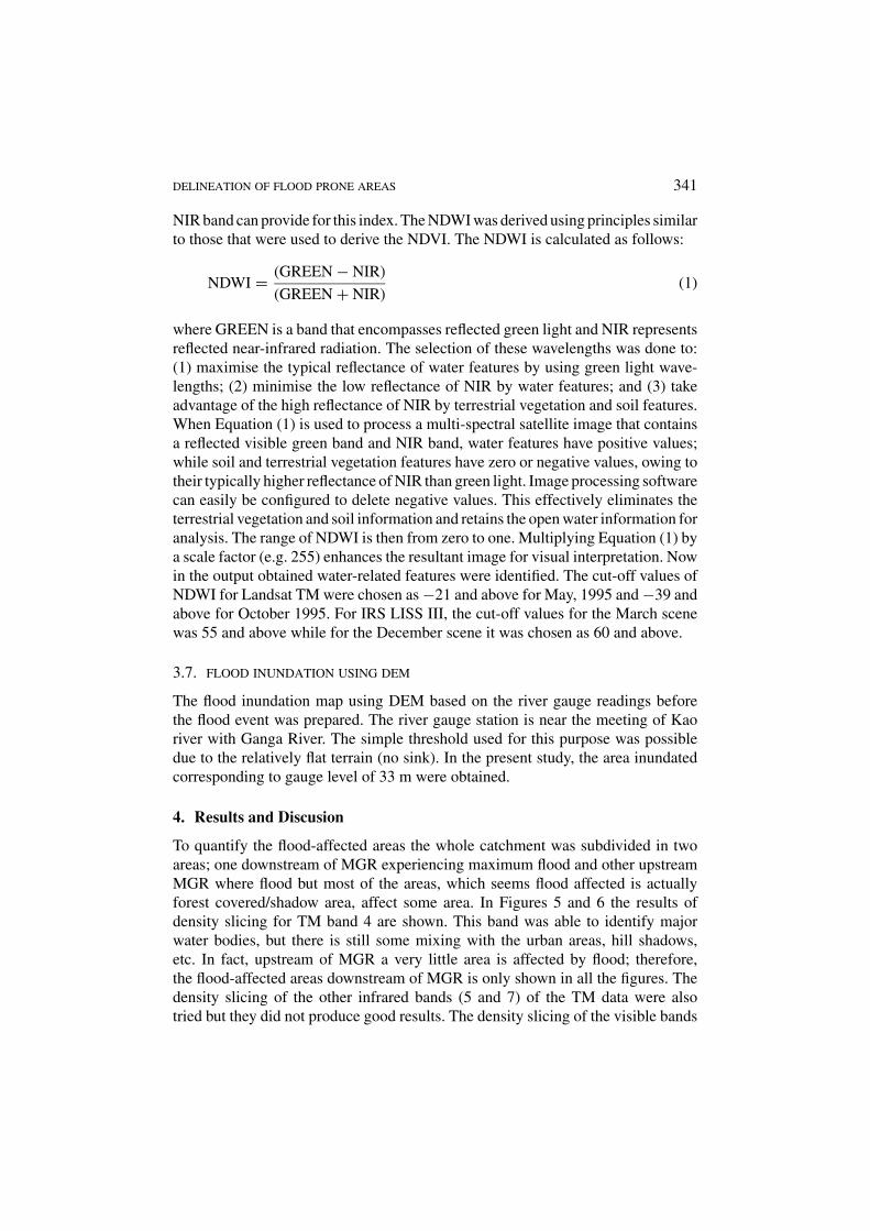
DELINEATION OF FLOOD PRONE AREAS 341
NIR band can provide for this index. The NDWI was derived using principles similarto those that were used to derive the NDVI. The NDWI is calculated as follows:
NDWI = (GREEN − NIR)
(GREEN + NIR)(1)
where GREEN is a band that encompasses reflected green light and NIR representsreflected near-infrared radiation. The selection of these wavelengths was done to:(1) maximise the typical reflectance of water features by using green light wave-lengths; (2) minimise the low reflectance of NIR by water features; and (3) takeadvantage of the high reflectance of NIR by terrestrial vegetation and soil features.When Equation (1) is used to process a multi-spectral satellite image that containsa reflected visible green band and NIR band, water features have positive values;while soil and terrestrial vegetation features have zero or negative values, owing totheir typically higher reflectance of NIR than green light. Image processing softwarecan easily be configured to delete negative values. This effectively eliminates theterrestrial vegetation and soil information and retains the open water information foranalysis. The range of NDWI is then from zero to one. Multiplying Equation (1) bya scale factor (e.g. 255) enhances the resultant image for visual interpretation. Nowin the output obtained water-related features were identified. The cut-off values ofNDWI for Landsat TM were chosen as −21 and above for May, 1995 and −39 andabove for October 1995. For IRS LISS III, the cut-off values for the March scenewas 55 and above while for the December scene it was chosen as 60 and above.
3.7. FLOOD INUNDATION USING DEM
The flood inundation map using DEM based on the river gauge readings beforethe flood event was prepared. The river gauge station is near the meeting of Kaoriver with Ganga River. The simple threshold used for this purpose was possibledue to the relatively flat terrain (no sink). In the present study, the area inundatedcorresponding to gauge level of 33 m were obtained.
4. Results and Discusion
To quantify the flood-affected areas the whole catchment was subdivided in twoareas; one downstream of MGR experiencing maximum flood and other upstreamMGR where flood but most of the areas, which seems flood affected is actuallyforest covered/shadow area, affect some area. In Figures 5 and 6 the results ofdensity slicing for TM band 4 are shown. This band was able to identify majorwater bodies, but there is still some mixing with the urban areas, hill shadows,etc. In fact, upstream of MGR a very little area is affected by flood; therefore,the flood-affected areas downstream of MGR is only shown in all the figures. Thedensity slicing of the other infrared bands (5 and 7) of the TM data were alsotried but they did not produce good results. The density slicing of the visible bands

342 S. K. JAIN ET AL.
Figure 5. Flood-affected area using density-slicing approach, May 1995.
Figure 6. Flood-affected area using density-slicing approach, October 1995.

DELINEATION OF FLOOD PRONE AREAS 343
substantially overestimate the area of water on the image, the explanation was givenearlier. The combination of mixed pixels and high turbidity limits the use of a singleNIR band to classify water bodies. The second approach applied was based on theTasseled Cap Transformation. In this method, the wetness index based on certaincoefficient has been computed. Using this approach also, mixing of land use andoverestimation of water area has been observed. It was observed that this method isgood during post-monsoon season (after floods) when enough water is available butit is not effective during pre-monsoon season. Also this method could not eliminateshadow areas. The flood-inundated areas for May 1995 scene is shown in Figure 7and for October 1995 shown in Figure 8.
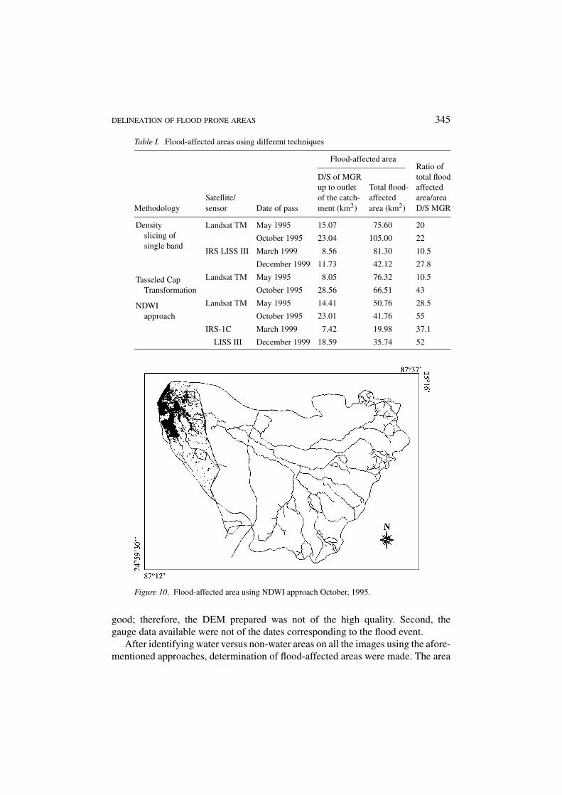
In the NDWI approach, the results was better and the mixing of pixels have beeneliminated up to certain extent. Using this approach also, flood-affected areas couldnot be delineated clearly because this area is not like water body. In case of IRSLISSIII data, the water and sediment-laden water both are represented by positivevalues of NDWI. While in case of TM data, the values of NDWI are positive forclear water but the values for sediment-laden water is negative also. For TM data,the flood-affected areas are shown in Figures 9 and 10 for May 1995 and October1995, respectively.
Even applying different approaches of image processing, scattered water fea-tures were observed. In case of river gauge/DEM method area submerged with watercan be obtained clearly, but there are other limitations of the method. First, the con-tour interval available for the study area was at a interval of 20 m which is not quite
Figure 7. Flood-affected area using Tasseled Cap Transformation May, 1995.

344 S. K. JAIN ET AL.
Figure 8. Flood-affected area using Tasseled Cap Transformation October, 1995.
Figure 9. Flood-affected area using NDWI approach May, 1995.
DELINEATION OF FLOOD PRONE AREAS 345
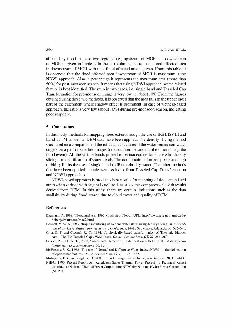
Table I. Flood-affected areas using different techniques
Flood-affected areaRatio of
D/S of MGR total floodup to outlet Total flood- affected
Satellite/ of the catch- affected area/areaMethodology sensor Date of pass ment (km2) area (km2) D/S MGR
Densityslicing ofsingle band
Landsat TM May 1995 15.07 75.60 20
October 1995 23.04 105.00 22
IRS LISS III March 1999 8.56 81.30 10.5
December 1999 11.73 42.12 27.8
Landsat TM May 1995 8.05 76.32 10.5Tasseled CapTransformation October 1995 28.56 66.51 43
Landsat TM May 1995 14.41 50.76 28.5NDWIapproach October 1995 23.01 41.76 55
IRS-1C March 1999 7.42 19.98 37.1
LISS III December 1999 18.59 35.74 52
Figure 10. Flood-affected area using NDWI approach October, 1995.
good; therefore, the DEM prepared was not of the high quality. Second, thegauge data available were not of the dates corresponding to the flood event.
After identifying water versus non-water areas on all the images using the afore-mentioned approaches, determination of flood-affected areas were made. The area
346 S. K. JAIN ET AL.
affected by flood in these two regions, i.e., upstream of MGR and downstreamof MGR is given in Table I. In the last column, the ratio of flood-affected areain downstream of MGR with total flood-affected area is given. From this table, itis observed that the flood-affected area downstream of MGR is maximum usingNDWI approach. Also in percentage it represents the maximum area (more than50%) for post-monsoon season. It means that using NDWI approach, water-relatedfeature is best identified. The ratio in two cases, i.e. single band and Tasseled CapTransformation for pre-monsoon image is very low i.e. about 10%. From the figuresobtained using these two methods, it is observed that the area falls in the upper mostpart of the catchment where shadow effect is prominent. In case of wetness-basedapproach, the ratio is very low (about 10%) during pre-monsoon season, indicatingpoor response.
5. Conclusions
In this study, methods for mapping flood extent through the use of IRS LISS III andLandsat TM as well as DEM data have been applied. The density-slicing methodwas based on a comparison of the reflectance features of the water versus non-watertargets on a pair of satellite images (one acquired before and the other during theflood event). All the visible bands proved to be inadequate for successful densityslicing for identification of water pixels. The combination of mixed pixels and highturbidity limits the use of single band (NIR) to classify water. The other methodsthat have been applied include wetness index from Tasseled Cap Transformationand NDWI approaches.
NDWI-based approach is produces best results for mapping of flood-inundatedareas when verified with original satellite data. Also, this compares well with resultsderived from DEM. In this study, there are certain limitations such as the dataavailability during flood season due to cloud cover and quality of DEM.
References
Baumann, P., 1999, ‘Flood analysis: 1993 Mississippi Flood’, URL: http://www.research.umbc.edu/∼tbenjal/baumann/mod2.html.
Bennett, M. W. A., 1987, ‘Rapid monitoring of wetland water status using density slicing’, in Proceed-ings of the 4th Australian Remote Sensing Conference, 14–18 September, Adelaide, pp. 682–691.
Crist, E. P. and Ciconel, R. C., 1984, ‘A physically based transformation of Thematic Mapperdata—The TM Tasseled Cap’, IEEE Trans. Geosci. Remote Sens. GE-22, 256–263.
Frazier, P. and Page, K., 2000, ‘Water body detection and delineation with Landsat TM data’, Pho-togrametric Eng. Remote Sens. 66, 12.
McFeeters, S. K., 1996, ‘The use of Normalised Difference Water Index (NDWI) in the delineationof open water features’, Int. J. Remote Sens. 17(7), 1425–1432.
Mohapatra, P. K. and Singh, R. D., 2003, ‘Flood management in India’, Nat. Hazards 28, 131–143.NHPC, 1995, Project Report on “Kahalgaon Super Thermal Power Project”, a Technical Report
submitted to National Thermal Power Corporation (NTPC) by Naitonal Hydro Power Corporation(NHPC).

DELINEATION OF FLOOD PRONE AREAS 347
Kundu, B. S. and Mohi Kumar, K. E., 1995, ‘Mapping and management of flood affected areas throughremote sensing. A case study of Sirsa district, Harayana’, J. Indian Soc. Remote Sens. 23(3).
Smith, L. C., 1997. ‘Satellite remote sensing of river inundation area, stage, and discharge: A review’,Hydrol. Process. 11, 1427–1439.
Wang, Y., Colby, J. D. and Mulcahy, K. A., 2002, ‘An efficient method for mapping flood extent in acoastal flood plain using Landsat TM and DEM data’, Int. J. Remote Sens. 23(18), 3681–3696.