Improving ECG Beats Delineation With an Evolutionary Optimization Process

Improving ECG beats delineation with an evolutionary

optimization process.

Jerome Dumont, Alfredo Hernandez, Guy Carrault

To cite this version:

Jerome Dumont, Alfredo Hernandez, Guy Carrault. Improving ECG beats delineation with anevolutionary optimization process.. IEEE Transactions on Biomedical Engineering, Institute ofElectrical and Electronics Engineers, 2010, 57 (3), pp.607-15. <10.1109/TBME.2008.2002157>.<inserm-00361377>

HAL Id: inserm-00361377

http://www.hal.inserm.fr/inserm-00361377

Submitted on 26 May 2009

HAL is a multi-disciplinary open accessarchive for the deposit and dissemination of sci-entific research documents, whether they are pub-lished or not. The documents may come fromteaching and research institutions in France orabroad, or from public or private research centers.

L’archive ouverte pluridisciplinaire HAL, estdestinee au depot et a la diffusion de documentsscientifiques de niveau recherche, publies ou non,emanant des etablissements d’enseignement et derecherche francais ou etrangers, des laboratoirespublics ou prives.

https://hal.archives-ouvertes.fr

http://www.hal.inserm.fr/inserm-00361377

IEEE TRANSACTIONS ON BIOMEDICAL ENGINEERING, VOL. XX, NO. Y, MONTH 2008 1

Improving ECG Beats Delineation with an

Evolutionary Optimization ProcessJ. Dumont, A.I. Hernandez, G. Carrault

INSERM, U642, Rennes, F-35000, France;

Universite de Rennes 1, LTSI, Rennes, F-35000, France;

LTSI, Campus de Beaulieu, Universite de Rennes 1,

263 Avenue du General Leclerc - CS 74205 - 35042 Rennes Cedex, France

Abstract—As in other complex signal processing tasks, ECGbeat delineation algorithms are usually constituted of a set ofprocessing modules, each one characterized by a certain numberof parameters (filter cutoff frequencies, threshold levels, timewindows...). It is well recognized that the adjustment of theseparameters is a complex task that is traditionally performed em-pirically and manually, based on the experience of the designer. Inthis work, we propose a new automated and quantitative methodto optimize the parameters of such complex signal processingalgorithms. To solve this multiobjective optimization problem,an evolutionary algorithm (EA) is proposed. This method forparameter optimization is applied to a Wavelet-Transform-basedECG delineator that has previously shown to present interestingperformances. An evaluation of the final delineator, using the op-timal parameters, has been performed on the QT database fromPhysionet and results are compared with previous algorithmsreported in the literature. The optimized parameters providea more accurate delineation, with a global improvement, overall the criteria evaluated, and over the best results find in theliterature, measured of 7.7%, which is a proof of the interest ofthe approach.

Index Terms—Electrocardiography, Wavelet transforms, Opti-mization methods, Genetic algorithms

I. INTRODUCTION

ECG wave delineators supply fundamental features, like

peak amplitudes (peaks of P, T or R waves) and wave intervals

(PR, QT...) for each detected beat. These features can be

used to formulate hypotheses on the underlying physiological

phenomena or as a previous step in automatic ECG analysis

systems. Performing an accurate segmentation is not an easy

task and results obtained with current algorithms are not

always satisfactory. A recurrent problem encountered in these

algorithms is the adjustment of the numerous parameters. For

example, several Wavelet-Transform (WT) based algorithms

have already been proposed in the literature to perform a

segmentation of ECG beats [1], [2], [3], [4], [5]. They have

demonstrated good performances compared to other methods

such as low pass differentiators [6], mathematical models [7],

adaptive filtering [8] or dynamic time warping [9] and thus

have been retained for our purpose. Although this method is

globally appropriate to this segmentation task, it presents some

limitations: firstly, it requires the definition of a great number

This work has been partly supported by the ECOS-NORD cooperationprogram, action number V03S03.

of parameters (thresholds, time windows...), secondly, there is

no obvious way to tune all these parameters in a joint manner,

mostly because the detection is performed in the time-scale

domain and a priori physiological information, like potential

wave position, is harder to use. In previous approaches, all

these parameters are usually defined empirically and manually

and, considering the complexity of the problem (great number

of beat morphologies, no universal definition of the boundary

positions...), it is clear that the delineation can be improved if

the parameters are optimized by a rigorous process.

To achieve this goal, in the present work, an optimization

methodology based on evolutionary algorithms has been de-

signed to tune the parameters of an ECG WT-based delineator.

However, this methodology is generic and it could be easily

transposed to any kind of delineators, detectors or classifiers

that are characterized by many parameters.

The remainder of this paper is organized as follows. Section

II gives an overview of the methodology, presenting the delin-

eation process (subsection II-A) and the optimization process

(subsection II-B). Section III presents the results in two parts:

firstly, in subsection III-A, the learning stage is described

and the parameters obtained are commented. Secondly, in

subsection III-B, the delineator has been evaluated on an

annotated database and with the optimal parameters. The

performances are compared to those published in the literature.

II. PROPOSED METHODOLOGY

The objective here is to adjust the parameters of an ECG

delineator in order to get similar results between the automatic

detector and manual annotations, stored by cardiologists in

biosignal databases, and supposed here as the reference. The

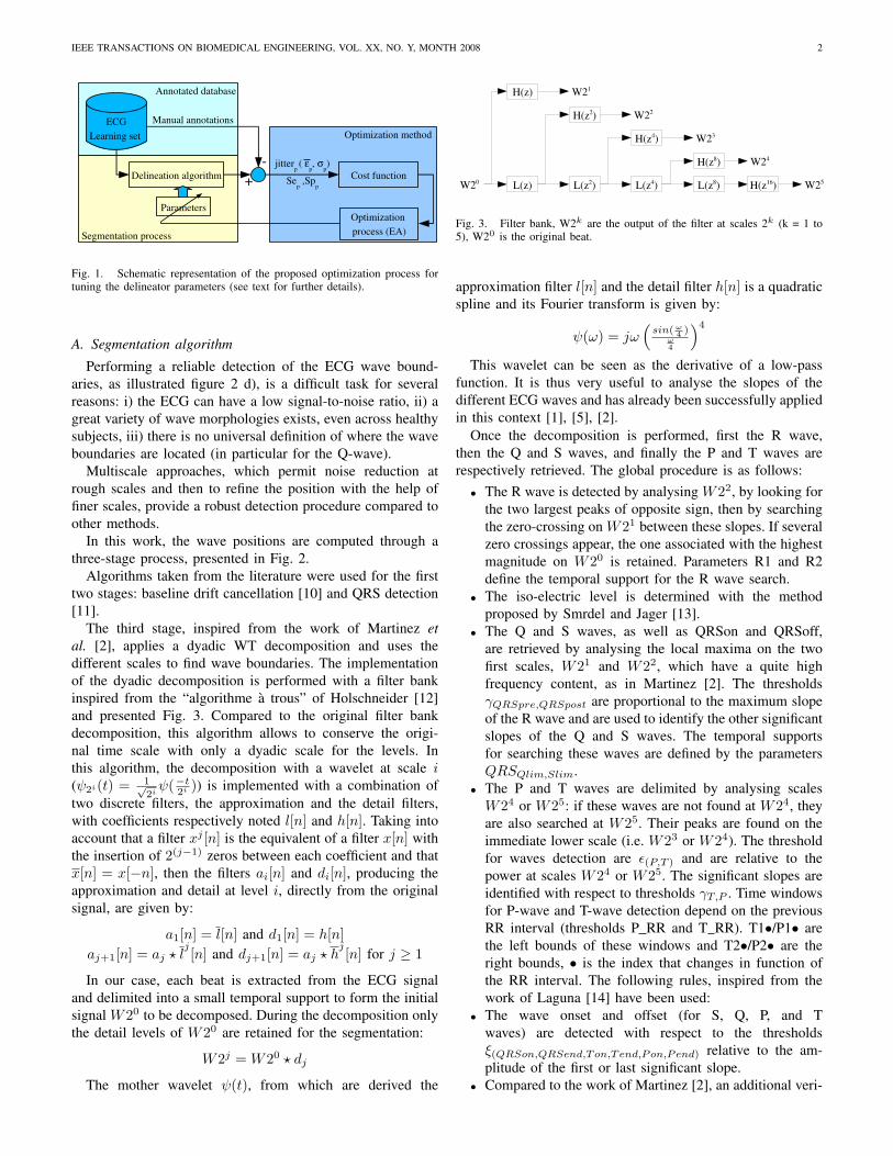
whole procedure is depicted in Fig. 1. It involves three

important components: i) the annotated database, ii) the seg-

mentation algorithm and its parameters iii) the optimization

method, which includes a procedure to adjust the parameters

of the delineator and the definition of a cost function, to be

minimized. As already mentioned, the proposed methodology

is generic and can be used for other complex signal-processing

algorithms. However, in this paper, we will present a particular

application to WT-based ECG delineators. The two following

subsections detail, firstly, the delineator algorithm and sec-

ondly, the cost function and the optimization method.


ECG

Learning set

Delineation algorithm

Optimization

process (EA)

-

+

Manual annotations

jitterp ( ε

p, σ

p)

Sep ,Sp

p

Parameters

Cost function

Annotated database

Segmentation process

Optimization method

Fig. 1. Schematic representation of the proposed optimization process fortuning the delineator parameters (see text for further details).

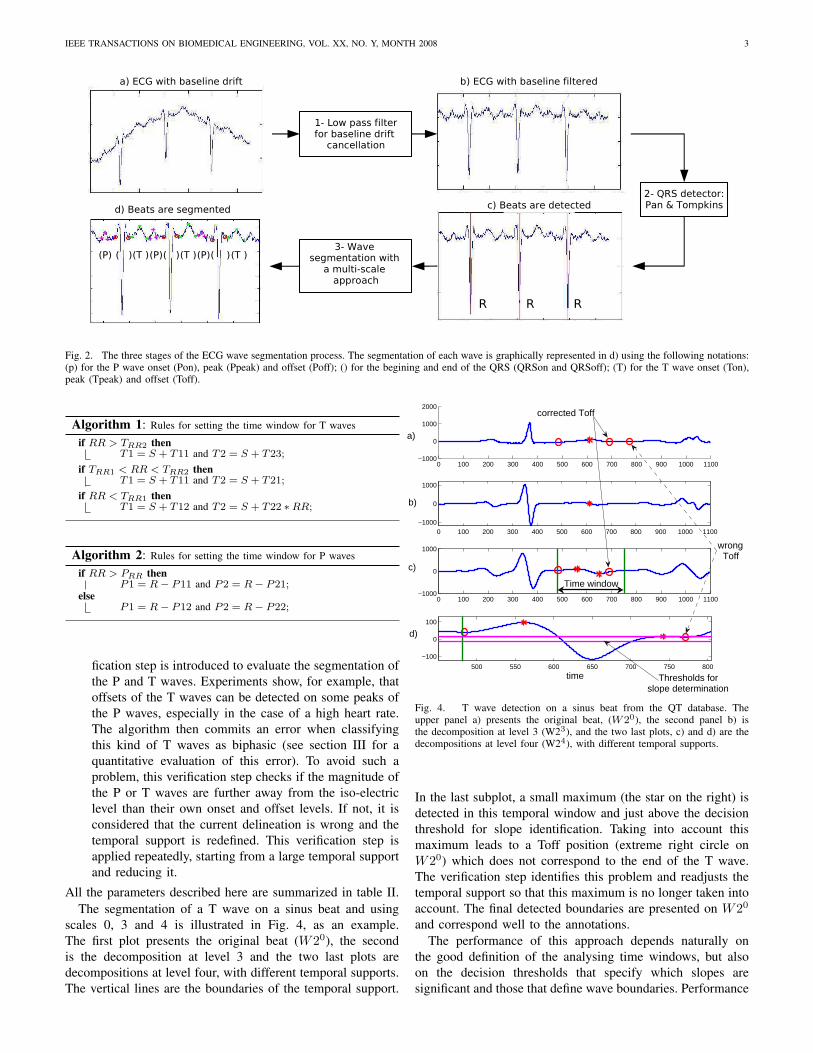
A. Segmentation algorithm

Performing a reliable detection of the ECG wave bound-

aries, as illustrated figure 2 d), is a difficult task for several

reasons: i) the ECG can have a low signal-to-noise ratio, ii) a

great variety of wave morphologies exists, even across healthy

subjects, iii) there is no universal definition of where the wave

boundaries are located (in particular for the Q-wave).

Multiscale approaches, which permit noise reduction at

rough scales and then to refine the position with the help of

finer scales, provide a robust detection procedure compared to

other methods.

In this work, the wave positions are computed through a

three-stage process, presented in Fig. 2.

Algorithms taken from the literature were used for the first

two stages: baseline drift cancellation [10] and QRS detection

[11].

The third stage, inspired from the work of Martinez et

al. [2], applies a dyadic WT decomposition and uses the

different scales to find wave boundaries. The implementation

of the dyadic decomposition is performed with a filter bank

inspired from the “algorithme a trous” of Holschneider [12]

and presented Fig. 3. Compared to the original filter bank

decomposition, this algorithm allows to conserve the origi-

nal time scale with only a dyadic scale for the levels. In

this algorithm, the decomposition with a wavelet at scale i

(ψ2i(t) = 1√2i

ψ(−t2i )) is implemented with a combination of

two discrete filters, the approximation and the detail filters,

with coefficients respectively noted l[n] and h[n]. Taking into

account that a filter xj [n] is the equivalent of a filter x[n] with

the insertion of 2(j−1) zeros between each coefficient and that

x[n] = x[−n], then the filters ai[n] and di[n], producing the

approximation and detail at level i, directly from the original

signal, are given by:

a1[n] = l[n] and d1[n] = h[n]

aj+1[n] = aj ⋆ lj[n] and dj+1[n] = aj ⋆ h

j[n] for j ≥ 1

In our case, each beat is extracted from the ECG signal

and delimited into a small temporal support to form the initial

signal W20 to be decomposed. During the decomposition only

the detail levels of W20 are retained for the segmentation:

W2j = W20 ⋆ dj

The mother wavelet ψ(t), from which are derived the

L(z)

H(z)

L(z2) L(z4)

H(z2)

H(z4)

H(z8)

W23

L(z8) H(z16)

W22

W21

W24

W20 W25

Fig. 3. Filter bank, W2k are the output of the filter at scales 2k (k = 1 to5), W20 is the original beat.

approximation filter l[n] and the detail filter h[n] is a quadratic

spline and its Fourier transform is given by:

ψ(ω) = jω(

sin( ω4)

ω4

)4

This wavelet can be seen as the derivative of a low-pass

function. It is thus very useful to analyse the slopes of the

different ECG waves and has already been successfully applied

in this context [1], [5], [2].

Once the decomposition is performed, first the R wave,

then the Q and S waves, and finally the P and T waves are

respectively retrieved. The global procedure is as follows:

• The R wave is detected by analysing W22, by looking for

the two largest peaks of opposite sign, then by searching

the zero-crossing on W21 between these slopes. If several

zero crossings appear, the one associated with the highest

magnitude on W20 is retained. Parameters R1 and R2

define the temporal support for the R wave search.

• The iso-electric level is determined with the method

proposed by Smrdel and Jager [13].

• The Q and S waves, as well as QRSon and QRSoff,

are retrieved by analysing the local maxima on the two

first scales, W21 and W22, which have a quite high

frequency content, as in Martinez [2]. The thresholds

γQRSpre,QRSpost are proportional to the maximum slope

of the R wave and are used to identify the other significant

slopes of the Q and S waves. The temporal supports

for searching these waves are defined by the parameters

QRSQlim,Slim.

• The P and T waves are delimited by analysing scales

W24 or W25: if these waves are not found at W24, they

are also searched at W25. Their peaks are found on the

immediate lower scale (i.e. W23 or W24). The threshold

for waves detection are ε(P,T ) and are relative to the

power at scales W24 or W25. The significant slopes are

identified with respect to thresholds γT,P . Time windows

for P-wave and T-wave detection depend on the previous

RR interval (thresholds P RR and T RR). T1•/P1• are

the left bounds of these windows and T2•/P2• are the

right bounds, • is the index that changes in function of

the RR interval. The following rules, inspired from the

work of Laguna [14] have been used:

• The wave onset and offset (for S, Q, P, and T

waves) are detected with respect to the thresholds

ξ(QRSon,QRSend,Ton,Tend,Pon,Pend) relative to the am-

plitude of the first or last significant slope.

• Compared to the work of Martinez [2], an additional veri-


��

��

��

��

�� !�"��#��

� � �

$ %$ %$ % $��% $��% $��%$"�% $"�% $"�%

�%�&'(�� %�&'(��

�%�)�� %�)��

Fig. 2. The three stages of the ECG wave segmentation process. The segmentation of each wave is graphically represented in d) using the following notations:(p) for the P wave onset (Pon), peak (Ppeak) and offset (Poff); () for the begining and end of the QRS (QRSon and QRSoff); (T) for the T wave onset (Ton),peak (Tpeak) and offset (Toff).

Algorithm 1: Rules for setting the time window for T waves

if RR > TRR2 thenT1 = S + T11 and T2 = S + T23;

if TRR1 < RR < TRR2 thenT1 = S + T11 and T2 = S + T21;

if RR < TRR1 thenT1 = S + T12 and T2 = S + T22 ∗ RR;

Algorithm 2: Rules for setting the time window for P waves

if RR > PRR thenP1 = R − P11 and P2 = R − P21;

elseP1 = R − P12 and P2 = R − P22;

fication step is introduced to evaluate the segmentation of

the P and T waves. Experiments show, for example, that

offsets of the T waves can be detected on some peaks of

the P waves, especially in the case of a high heart rate.

The algorithm then commits an error when classifying

this kind of T waves as biphasic (see section III for a

quantitative evaluation of this error). To avoid such a

problem, this verification step checks if the magnitude of

the P or T waves are further away from the iso-electric

level than their own onset and offset levels. If not, it is

considered that the current delineation is wrong and the

temporal support is redefined. This verification step is

applied repeatedly, starting from a large temporal support

and reducing it.

All the parameters described here are summarized in table II.

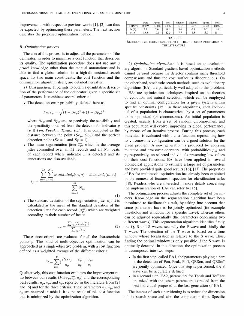
The segmentation of a T wave on a sinus beat and using

scales 0, 3 and 4 is illustrated in Fig. 4, as an example.

The first plot presents the original beat (W20), the second

is the decomposition at level 3 and the two last plots are

decompositions at level four, with different temporal supports.

The vertical lines are the boundaries of the temporal support.

0 100 200 300 400 500 600 700 800 900 1000 1100−1000

0

1000

2000

500 550 600 650 700 750 800

−100

0

100

time

0 100 200 300 400 500 600 700 800 900 1000 1100−1000

0

1000

0 100 200 300 400 500 600 700 800 900 1000 1100−1000

0

1000

d)

Time window

Thresholds forslope determination

wrongToff

corrected Toff

c)

b)

a)

Fig. 4. T wave detection on a sinus beat from the QT database. Theupper panel a) presents the original beat, (W20), the second panel b) isthe decomposition at level 3 (W23), and the two last plots, c) and d) are thedecompositions at level four (W24), with different temporal supports.

In the last subplot, a small maximum (the star on the right) is

detected in this temporal window and just above the decision

threshold for slope identification. Taking into account this

maximum leads to a Toff position (extreme right circle on

W20) which does not correspond to the end of the T wave.

The verification step identifies this problem and readjusts the

temporal support so that this maximum is no longer taken into

account. The final detected boundaries are presented on W20

and correspond well to the annotations.

The performance of this approach depends naturally on

the good definition of the analysing time windows, but also

on the decision thresholds that specify which slopes are

significant and those that define wave boundaries. Performance


improvements with respect to previous works [1], [2], can thus

be expected, by optimizing these parameters. The next section

describes the proposed optimization method.

B. Optimization process

The aim of this process is to adjust all the parameters of the

delineator, in order to minimize a cost function that describes

its quality. The optimization procedure does not use any a

priori knowledge other than the manual annotations and is

able to find a global solution in a high-dimensional search

space. Its two main constituents, the cost function and the

optimization algorithm itself, are detailed hereafter:

1) Cost function: It permits to obtain a quantitative descrip-

tion of the performance of the delineator, given a specific set

of parameters. It combines several criteria:

• The detection error probability, defined here as:

Perrp =√

(1 − Sep)2 + (1 − Spp)2

where Sep and Spp are, respectively, the sensibility and

the specificity obtained from the detector for indicator p

(p ∈ Pon, Ppeak,... Tpeak, Toff ). It is computed as the

distance between the point (Sep, Spp) and the perfect

detection point (Se = 1 and Sp = 1).

• The mean segmentation jitter εp, which is the average

jitter committed over all M records and all Nm beats

of each record where indicator p is detected and its

annotations are also available:

εp =

M∑

m=1

Nm∑

n=1

annotatedp(m,n) − detectedp(m,n)

M∑

m=1

Nm

(1)

• The standard deviation of the segmentation jitter σp. It is

calculated as the mean of the standard deviation of the

detection jitter for each record (σmp ) which are weighted

according to their number of beats:

σp =

∑

m(Nmσmp )

∑

m Nm

(2)

These three criteria are evaluated for all the characteristic

points p. This kind of multi-objective optimization can be

approached as a single-objective problem, with a cost function

defined as a weighted average of the different criteria:

O =

P∑

p=1

(Perrp

ap

+εp

bp

+σp

cp

)

Qualitatively, this cost function evaluates the improvement ra-

tio between our results (Perrp, εp, σp) and the corresponding

best results, ap, bp, and cp, reported in the literature from [2]

and [6] and for the three criteria. These parameters ap, bp, and

cp are resumed in table I. It is the result of this cost function

that is minimized by the optimization algorithm.

Pon Ppeak Poff QRSon QRSoff Tpeak Toff

a (Perr) 0.089 0.089 0.089 0.07 0.07 0.022 0.022

b (ε) 2.7 3.6 0.1 3.6 0.8 0.2 1.6

c (σ) 13.3 10.6 12.3 7.7 8.3 13.9 18.1

TABLE IREFERENCE CRITERIA ISSUED FROM THE BEST RESULTS PUBLISHED IN

THE LITERATURE.

2) Optimization algorithm: It is based on an evolution-

ary algorithm. Standard gradient-based optimization methods

cannot be used because the detector contains many threshold

comparisons and thus the cost surface is discontinuous. On

the other hand, stochastic search methods, such as evolutionary

algorithms (EA), are particularly well adapted to this problem.

EAs are optimization techniques, inspired on the theories

of evolution and natural selection, which can be employed

to find an optimal configuration for a given system within

specific constraints [15]. In these algorithms, each individ-

ual of a population is characterized by a set of parameters

to be optimized (or chromosome). An initial population is

created, usually from a set of random chromosomes, and

this population will evolve, improving its global performance,

by means of an iterative process. During this process, each

individual is evaluated with a cost function, representing how

its chromosome configuration can be a good solution for the

given problem. A new generation is produced by applying

mutation and crossover operators, with probabilities pm and

pc respectively, on selected individuals presenting low values

on their cost functions. EA have been applied in several

biomedical applications to estimate a large set of parameters

and have provided quite good results [16], [17]. The properties

of EA for multimodal optimization has already been exploited

in the context of features inspection for classification tasks

[18]. Readers who are interested in more details concerning

the implementation of EAs can refer to [15].

The optimization process adjusts the complete set of param-

eters. Knowledge on the segmentation algorithm have been

introduced to facilitate this task, by taking into account that

some parameters have to be jointly optimized (for example

thresholds and windows for a specific wave), whereas others

can be adjusted sequentially (the parameters concerning two

different waves). This segmentation algorithm identifies firstly

the Q, R and S waves, secondly the P wave and thirdly the

T wave. The detection of the T wave is based on a time

window whose localisation is relative to the S wave. Thus,

finding the optimal window is only possible if the S wave is

optimally detected. In this direction, the optimization process

is decomposed into two steps:

• In the first step, called EA1, the parameters playing a part

in the detection of Pon, Peak, Poff, QRSon, and QRSoff

are jointly optimized. Once this step is performed, the S

wave can be accurately defined.

• In a second step, EA2, parameters for Tpeak and Toff are

optimized with the others parameters extracted from the

best individual proposed at the last generation of EA1.

The interest of such a partitioning is to reduce the dimension

of the search space and also the computation time. Specific


details on the configuration of these two EA-based process

are the following:

• individual coding : individuals are coded with real-

valued chromosomes. Values for each parameter were

bounded to a meaningful interval: time windows are

defined from possible extreme positions and durations

of each wave whereas boundaries of other thresholds

are determined by largely increasing (upper bounds) and

decreasing (lower bounds) parameters from [2]. These

intervals are employed by the EA during the construction

of the initial population.

• selection method and genetic operators: the ranking

selection method was used in this work. Standard ge-

netic operators for real-valued chromosomes were used:

arithmetic and heuristic crossover, uniform mutation [15].

For these two steps, the population is trained over 80 gen-

erations and with 60 individuals. The probability of crossover,

pc, is set to 0.7 [19]. In order to obtain more reliable and

stable solutions, the probability of mutation, pm, has been

adapted through the evolutionary process, starting at a high

value during the first generations, to ensure a wider individual

distribution over the search space and decreasing until the

end, to facilitate the convergence to a reliable minimum. The

solution of Back [20] has been retained according to the

satisfying results which have been reported in the literature:

pm = (2 +(Np−2)

Maxgen−1 ∗ gen)−1

where Np is the number of parameters, Maxgen is the

maximum number of generations, gen is the number of the

current generation.

III. RESULTS

Results are presented in two parts. Firstly, an analysis of

the parameters obtained after the learning phase is performed.

Secondly, the delineation performance, obtained with the op-

timal parameters, are presented and compared to other results

from the literature. The database used for this application is

the QTDB from physionet [21]. The QTDB provides a wide

variety of pathologies in a total of 105 records, with two

channels sampled at 250Hz. Compared to other databases, it

contains also a large number of annotated beats per record: 30

beats instead of 1 in the CSE database. The annotations are

also very complete with all the positions of the onset, peak

and offset points of the P, QRS and T waves. For all these

reasons, this database has been used to train and to validate

our delineator algorithm.

A. Learning stage and optimal parameters

Previous works on wavelet-based ECG segmentation rely

on a manual definition of the set of parameters of the signal

processing chain. In Martinez [2], a specific database is used to

set the parameters but these last ones are empirically defined,

as in the work of Li [1]. Considering the problems due to

the number of morphologies, the number of parameters, and

the competitive objectives, it is difficult to obtain reliable

results from such an approach. Using the previously described

EA1 EA2

P11 278±31 γQRSpre 0.09±0.03 εT 0.24±0.06

P12 240±17 γQRSpost 0.11±0.03 γT 0.28±0.07

P21 88±14 ξQRSonpos 0.07±0.04 ξT on 0.17±0.09

P22 99±27 ξQRSonneg 0.07±0.04 ξT end 0.36±0.07

R1 118±34 ξQRSendpos 0.21±0.12 T11 111±24

R2 111±37 ξQRSendneg 0.23±0.11 T21 441±75

PRR 664±182 QRSQlim 88±22 T12 90±16

εP 0.12±0.05 QRSSlim 154±32 T22 0.6±0.08

γP 0.4±0.09 T23 581±94

ξP on 0.41±0.08 TRR1 705±155

ξP end 0.76±0.05 TRR2 1231±70

TABLE IIPARAMETERS USED BY THE DELINEATOR (SUBSECTION II-A) WITH THEIR

OPTIMAL VALUES, REPRESENTED AS MEAN ± STANDARD DEVIATION,OBTAINED FROM THE OPTIMIZATION PROCESS.

optimization process on a manually annotated database, like

the QTDB, can solve this problem.

To compare our results with those obtained with other

methods [2], [21], it is required to perform a test on all the

beats of the database. Since the training stage is also performed

on the same database, a training set L and test T set have to be

defined. To achieve this, all the records are firstly divided into

three equivalent parts, called subrecords. Two thirds of all sub-

records are randomly chosen from all subrecords and affected

to a training set. The remaining subrecords are allocated to the

test set. 13 couples of training/test sets are generated with this

method in order to perform a cross-validation analysis of the

performances of the delineator and to evaluate the sensitivity

of the optimal parameters obtained to a particular instance of L

and T . L{1-13} and T{1-13} are respectively the training and

test sets whereas OPL{1−13} are the optimized parameters.

An overview of all the parameters, optimized with the EA

process carried out on the different learning sets, is presented

in table II, with their means and standard deviations for the

13 different training sets.

The values of some of these optimal parameters present low

variations, like the temporal windows for the P, Q, S and T

waves or the thresholds that define the onset or offset of P and

T waves, indicating the high sensitivity of the segmentation

algorithm to these parameters. In the other hand, the temporal

windows used to search the R wave or the thresholds that

define the QRSonset and offset show a wider dispersion across

the different learning sets. These results were expected and

show the reduced sensitivity of the QRS segmentation step

to these parameters. Indeed, the R wave presents commonly

a high signal-to-noise ratio and is always very close to the

fiducial point, the slopes of the QRS onset and offset are

also more enhanced than the slopes of the P and T waves,

so a wide range of parameters give approximately the same

results. When only one set of parameters is required for future

segmentations, the mean value of the parameters obtained

over the different training sets, which can be expected to

give the minimum of the cost function, found on the QTDB,

is conserved. It is important to underline that the proposed

approach is not only particularly useful for the tuning of

these parameters, but also to analyse the sensitivity of each

parameter with respect to the final detection results.

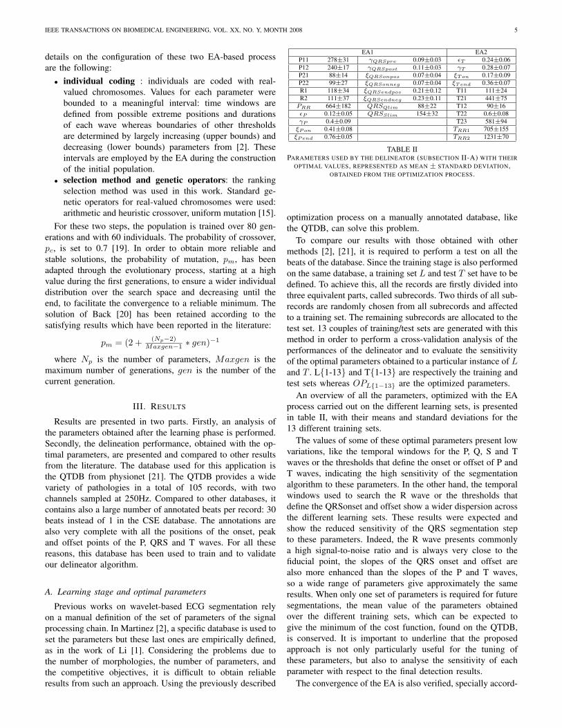
The convergence of the EA is also verified, specially accord-


500 1000 1500 2000 2500 3000 3500 4000

5

6

7

8

9

10

11

12

Number of evaluations

Low

est c

ost

Ni = 20Ni = 40Ni = 60Ni = 80Ni = 100

(1) Ni = 20

(2) Ni = 40

Fig. 5. Evolution of the lowest cost according to the cost function numberof evaluation, for several convergence tests and with different values of Ni.

ing to the population size. This parameter is crucial to ensure

as far as possible to find the global minima of the cost function.

In this perspective, a test with multiple realisations have been

carried out to study the convergence of EA1 (the parameter

space of EA2 is smaller than the parameters space of EA1 so

it can be naturally supposed that EA2 will correctly converge

for the same condition as EA1) for different numbers Ni of

individuals (Ni = {20, 40, 60, 80, 100}). For each of these

numbers, the optimisation is run 6 times. Figure 5 a) presents

the evolution of the cost function of the best individuals over

the number of evaluation and for several tests. It can be

observed that there is a global convergence around a cost

of 5, whatever the number of individuals in the population.

However looking more deeply on the tests performed with Ni

= 20, it is clear that the convergence is achieved only with the

occurrence of a few good mutations or crossovers: the curves

are not as smooth as with more individuals and the lowest

score is sometimes decreasing abruptly (curve noted (1)) or

remains at a high value. This effect is less visible with more

individuals (Ni = 40 to 100). It can be observed that with Ni =

20 or Ni = 40, the minimum of the cost function is not always

reached (for example, the case noted (2) figure 5). From this

experiment, Ni = 60 represents a good compromise between

the number of evaluation of the cost function and the minimum

of this cost.

B. Delineation results

Jane [22] has proposed a general framework to analyse the

results of delineator algorithms evaluated on a given database,

such as the QTDB. Our results are issued from the same

framework and compared to those achieved by [2] and [21]

(a low-pass-differentiator-based algorithm). Mean errors and

standard deviations are weighted by the number of beats

per record, and averaged over all the records of the test set

(equations 1 and 2). As we disposed of two channels and

cardiologists used a combination of both to detect only one

position, we chose, for each point, the channel with the lowest

error. The detection error probabilities (Perrp) are derived

from the sensitivity and specificity, computed as in [2]. All

these criteria are evaluated for all indicators. Fig. 6 shows the

distributions of our results over the different test sets. The

cross (+) and the stars (*) are respectively the results from [2]

and [21], as presented in these references.

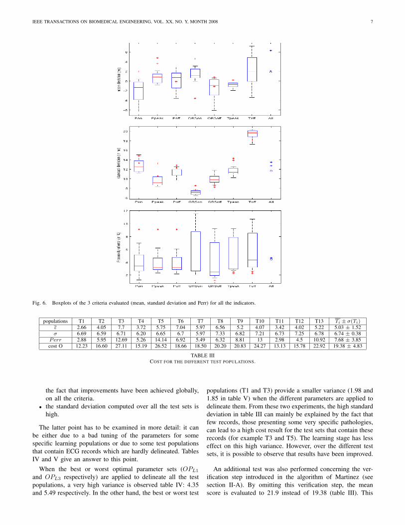
A few comments can be made for each criterion:

• For the mean deviation, the median of the results are

closer to 0 than the two other methods for the points

Pon, Ppeak and QRSon. It is also better than [2] for Poff

and better than [21] for QRSoff, Tpeak and Toff.

• For the standard deviation, the median is lower for Pon,

Peak, Poff, QRSon and Tpeak, higher than [2] for Toff

and higher than both [2] and [21] for QRSoff.

• The detection error probability is lower for the P wave

but not for the T wave.

The behaviour of the detection error probability is more

difficult to analyse than the other criteria because all the beats

automatically segmented have not been manually annotated,

leading to a biased measure of the specificity. To check that

the obtained detection error probability is well optimized,

an additional test has been performed: Receiver Operating

Characteristic (ROC) curves for P and T wave detection are

plotted for a test set and it is checked if the points that

minimize the error probability on the ROC curves, are close

to the points obtained by the optimization process, on the

corresponding training set (the points given by the optimized

parameters εP or εT ).

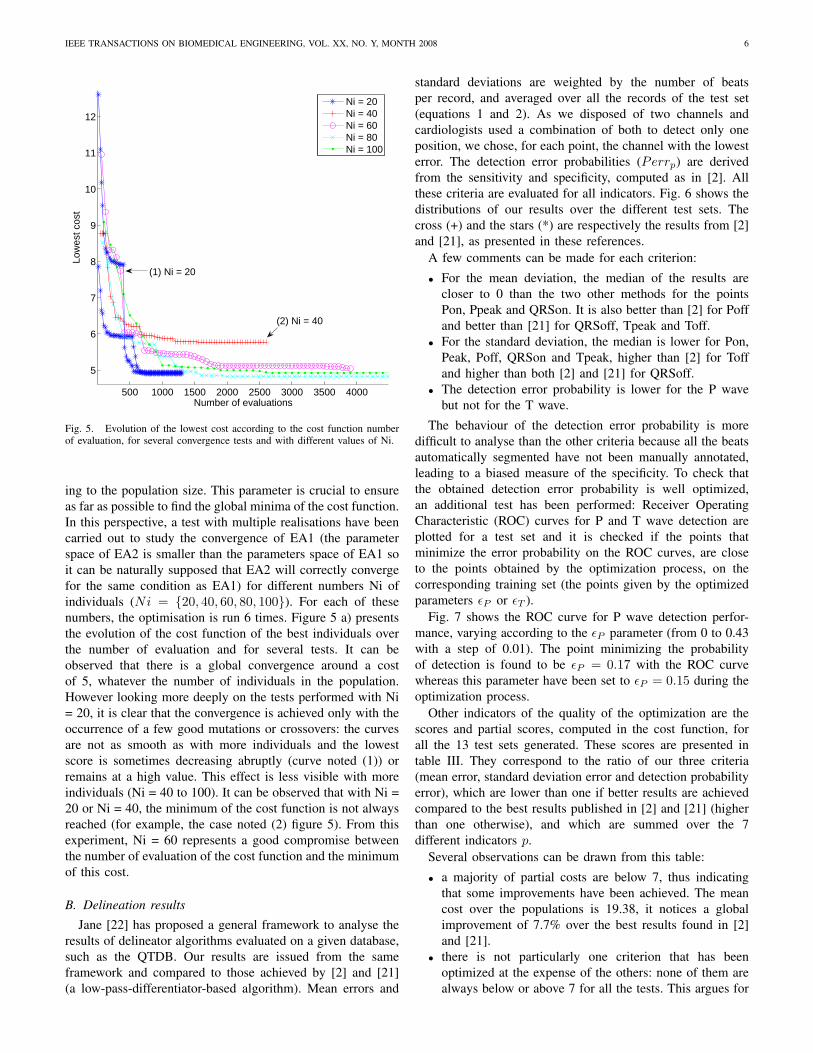
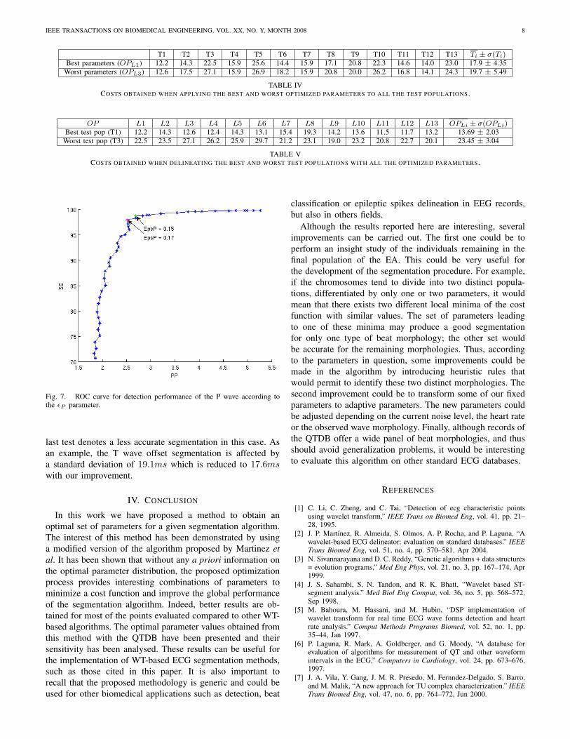
Fig. 7 shows the ROC curve for P wave detection perfor-

mance, varying according to the εP parameter (from 0 to 0.43

with a step of 0.01). The point minimizing the probability

of detection is found to be εP = 0.17 with the ROC curve

whereas this parameter have been set to εP = 0.15 during the

optimization process.

Other indicators of the quality of the optimization are the

scores and partial scores, computed in the cost function, for

all the 13 test sets generated. These scores are presented in

table III. They correspond to the ratio of our three criteria

(mean error, standard deviation error and detection probability

error), which are lower than one if better results are achieved

compared to the best results published in [2] and [21] (higher

than one otherwise), and which are summed over the 7

different indicators p.

Several observations can be drawn from this table:

• a majority of partial costs are below 7, thus indicating

that some improvements have been achieved. The mean

cost over the populations is 19.38, it notices a global

improvement of 7.7% over the best results found in [2]

and [21].

• there is not particularly one criterion that has been

optimized at the expense of the others: none of them are

always below or above 7 for all the tests. This argues for


Fig. 6. Boxplots of the 3 criteria evaluated (mean, standard deviation and Perr) for all the indicators.

populations T1 T2 T3 T4 T5 T6 T7 T8 T9 T10 T11 T12 T13 Ti ± σ(Ti)ε 2.66 4.05 7.7 3.72 5.75 7.04 5.97 6.56 5.2 4.07 3.42 4.02 5.22 5.03 ± 1.52

σ 6.69 6.59 6.71 6.20 6.65 6.7 5.97 7.33 6.82 7.21 6.73 7.25 6.78 6.74 ± 0.38

Perr 2.88 5.95 12.69 5.26 14.14 6.92 5.49 6.32 8.81 13 2.98 4.5 10.92 7.68 ± 3.85

cost O 12.23 16.60 27.11 15.19 26.52 18.66 18.50 20.20 20.83 24.27 13.13 15.78 22.92 19.38 ± 4.83

TABLE IIICOST FOR THE DIFFERENT TEST POPULATIONS.

the fact that improvements have been achieved globally,

on all the criteria.

• the standard deviation computed over all the test sets is

high.

The latter point has to be examined in more detail: it can

be either due to a bad tuning of the parameters for some

specific learning populations or due to some test populations

that contain ECG records which are hardly delineated. Tables

IV and V give an answer to this point.

When the best or worst optimal parameter sets (OPL1

and OPL3 respectively) are applied to delineate all the test

populations, a very high variance is observed table IV: 4.35

and 5.49 respectively. In the other hand, the best or worst test

populations (T1 and T3) provide a smaller variance (1.98 and

1.85 in table V) when the different parameters are applied to

delineate them. From these two experiments, the high standard

deviation in table III can mainly be explained by the fact that

few records, those presenting some very specific pathologies,

can lead to a high cost result for the test sets that contain these

records (for example T3 and T5). The learning stage has less

effect on this high variance. However, over the different test

sets, it is possible to observe that results have been improved.

An additional test was also performed concerning the ver-

ification step introduced in the algorithm of Martinez (see

section II-A). By omitting this verification step, the mean

score is evaluated to 21.9 instead of 19.38 (table III). This


T1 T2 T3 T4 T5 T6 T7 T8 T9 T10 T11 T12 T13 Ti ± σ(Ti)Best parameters (OPL1) 12.2 14.3 22.5 15.9 25.6 14.4 15.9 17.1 20.8 22.3 14.6 14.0 23.0 17.9 ± 4.35

Worst parameters (OPL3) 12.6 17.5 27.1 15.9 26.9 18.2 15.9 20.8 20.0 26.2 16.8 14.1 24.3 19.7 ± 5.49

TABLE IVCOSTS OBTAINED WHEN APPLYING THE BEST AND WORST OPTIMIZED PARAMETERS TO ALL THE TEST POPULATIONS .

OP L1 L2 L3 L4 L5 L6 L7 L8 L9 L10 L11 L12 L13 OPLi ± σ(OPLi)Best test pop (T1) 12.2 14.3 12.6 12.4 14.3 13.1 15.4 19.3 14.2 13.6 11.5 11.7 13.2 13.69 ± 2.03

Worst test pop (T3) 22.5 23.5 27.1 26.2 25.9 29.7 21.2 23.1 19.0 23.2 20.8 22.7 20.1 23.45 ± 3.04

TABLE VCOSTS OBTAINED WHEN DELINEATING THE BEST AND WORST TEST POPULATIONS WITH ALL THE OPTIMIZED PARAMETERS .

Fig. 7. ROC curve for detection performance of the P wave according tothe εP parameter.

last test denotes a less accurate segmentation in this case. As

an example, the T wave offset segmentation is affected by

a standard deviation of 19.1ms which is reduced to 17.6ms

with our improvement.

IV. CONCLUSION

In this work we have proposed a method to obtain an

optimal set of parameters for a given segmentation algorithm.

The interest of this method has been demonstrated by using

a modified version of the algorithm proposed by Martinez et

al. It has been shown that without any a priori information on

the optimal parameter distribution, the proposed optimization

process provides interesting combinations of parameters to

minimize a cost function and improve the global performance

of the segmentation algorithm. Indeed, better results are ob-

tained for most of the points evaluated compared to other WT-

based algorithms. The optimal parameter values obtained from

this method with the QTDB have been presented and their

sensitivity has been analysed. These results can be useful for

the implementation of WT-based ECG segmentation methods,

such as those cited in this paper. It is also important to

recall that the proposed methodology is generic and could be

used for other biomedical applications such as detection, beat

classification or epileptic spikes delineation in EEG records,

but also in others fields.

Although the results reported here are interesting, several

improvements can be carried out. The first one could be to

perform an insight study of the individuals remaining in the

final population of the EA. This could be very useful for

the development of the segmentation procedure. For example,

if the chromosomes tend to divide into two distinct popula-

tions, differentiated by only one or two parameters, it would

mean that there exists two different local minima of the cost

function with similar values. The set of parameters leading

to one of these minima may produce a good segmentation

for only one type of beat morphology; the other set would

be accurate for the remaining morphologies. Thus, according

to the parameters in question, some improvements could be

made in the algorithm by introducing heuristic rules that

would permit to identify these two distinct morphologies. The

second improvement could be to transform some of our fixed

parameters to adaptive parameters. The new parameters could

be adjusted depending on the current noise level, the heart rate

or the observed wave morphology. Finally, although records of

the QTDB offer a wide panel of beat morphologies, and thus

should avoid generalization problems, it would be interesting

to evaluate this algorithm on other standard ECG databases.

REFERENCES

[1] C. Li, C. Zheng, and C. Tai, “Detection of ecg characteristic pointsusing wavelet transform,” IEEE Trans on Biomed Eng, vol. 41, pp. 21–28, 1995.

[2] J. P. Martınez, R. Almeida, S. Olmos, A. P. Rocha, and P. Laguna, “Awavelet-based ECG delineator: evaluation on standard databases.” IEEE

Trans Biomed Eng, vol. 51, no. 4, pp. 570–581, Apr 2004.

[3] N. Sivannarayana and D. C. Reddy, “Genetic algorithms + data structures= evolution programs,” Med Eng Phys, vol. 21, no. 3, pp. 167–174, Apr1999.

[4] J. S. Sahambi, S. N. Tandon, and R. K. Bhatt, “Wavelet based ST-segment analysis.” Med Biol Eng Comput, vol. 36, no. 5, pp. 568–572,Sep 1998.

[5] M. Bahoura, M. Hassani, and M. Hubin, “DSP implementation ofwavelet transform for real time ECG wave forms detection and heartrate analysis.” Comput Methods Programs Biomed, vol. 52, no. 1, pp.35–44, Jan 1997.

[6] P. Laguna, R. Mark, A. Goldberger, and G. Moody, “A database forevaluation of algorithms for measurement of QT and other waveformintervals in the ECG,” Computers in Cardiology, vol. 24, pp. 673–676,1997.

[7] J. A. Vila, Y. Gang, J. M. R. Presedo, M. Fernndez-Delgado, S. Barro,and M. Malik, “A new approach for TU complex characterization.” IEEE

Trans Biomed Eng, vol. 47, no. 6, pp. 764–772, Jun 2000.


[8] E. Soria-Olivas, M. Martınez-Sober, J. Calpe-Maravilla, J. F. Guerrero-Martınez, J. Chorro-Gasco, and J. Espı-Lopez, “Application of adaptivesignal processing for determining the limits of P and T waves in anECG.” IEEE Trans Biomed Eng, vol. 45, no. 8, pp. 1077–1080, Aug1998.

[9] H. Vullings, M. Verhaegen, and H. Verbruggen, “Automated ecg seg-mentation with dynamic time warping,” Proc. 20th Ann. Int. Conf. IEEE

Engineering in Medecine and Biology Soc. Hong Kong, pp. 163–166,1998.

[10] V. Shusterman, S. I. Shah, A. Beigel, and K. P. Anderson, “Enhancingthe precision of ECG baseline correction: selective filtering and removalof residual error.” Comput Biomed Res, vol. 33, no. 2, pp. 144–160, Apr2000.

[11] J. Pan and W. J. Tompkins, “A real-time QRS detection algorithm.”IEEE Trans Biomed Eng, vol. 32, no. 3, pp. 230–236, Mar 1985.

[12] M. Holschneider, R. Kronland-Martinet, M. Morlet, andP. Tchamitchian, “A real-time algorithm for signal analysiswiththe help of the wavelet transform,” in Wavelets, Time-Frequency

Methods and Phase Space, Springer-Verlag, Ed., Berlin, 1989, pp.289–297.

[13] A. Smrdel and F. Jager, “Automated detection of transient ST-segmentepisodes in 24h electrocardiograms,” Med Biol Eng Comput, vol. 42,no. 3, pp. 303–311, May 2004.

[14] P. Laguna, N. V. Thakor, P. Caminal, R. Jane, H. Yoon, A. Bayes deLuna, A. V. Marti, and J. Guindo, “New algorithm for qt interval analysisin 24-hour holter ecg: performance and applications,” in Medical and

Biological Engineering and Computing, S. B. . Heidelberg, Ed., vol. 28,no. 1, January 1990, pp. 67–73.

[15] Z. Michalewicz, Genetic Algorithms + Data Structures = Evolution

Programs. Springer, Berlin and Heidelberg, 3rd edition, 1996.[16] A. I. Hernandez, G. Carrault, F. Mora, and A. Bardou, “Model-based

interpretation of cardiac beats by evolutionary algorithms: signal andmodel interaction.” Artif Intell Med, vol. 26, no. 3, pp. 211–235, Nov2002.

[17] R. E. West, E. D. Schutter, and G. Wilcox, “”using evolutionary algo-rithms to search for control parameters in a nonlinear partial differentialequation”,” University of Minnesota Supercomputer Institute Research,Report UMSI 97/61, Tech. Rep., April 1998.

[18] F. de Toro, E.Ros, S.Mota, and J.Ortega, “Evolutionary algorithms formultiobjective and multimodal optimisation of diagnostic schemes,”IEEE Transactions on Biomedical Engineering, vol. 53, no. 2, pp. 178–189, 2006.

[19] V. Khare1, X. Yao1, and K. Deb, “Performance scaling of multi-objective evolutionary algorithms,” in Lecture Notes in Computer Sci-

ence, Evolutionary Multi-Criterion Optimization: Second International

Conference. Springer Berlin / Heidelberg, February 2004, p. 72.[20] T. Back and M. Schutz, “Intelligent mutation rate control in canonical

genetic algorithms,” Proc of the International Sympoisum on Method-

ologies for Intelligent Systems, pp. 158–167, 1996.[21] P. Laguna, R. Jane, and P. Caminal, “Automatic detection of wave

boundaries in multilead ECG signals: validation with the CSE database.”Comput Biomed Res, vol. 27, no. 1, pp. 45–60, Feb 1994.

[22] R. Jane, A. Blasi, J. Garcia, and P. Laguna, “Evaluation of an automaticdetector of waveforms limits in holter ECG with the QT database,”Computers in Cardiology, vol. 29, pp. 295–298, 1997.

Jerome Dumont Jerome Dumont received the Mas-ter of Engineering degree in electronic and electricalengineering from the University of Strathclyde, in2004, in Glasgow. He is working since 2004 as aPhD student in the Signal and Image ProcessingLaboratory (LTSI) of the University of Rennes 1. Hisresearch interests are in biomedicad digital signalprocessing and spatio-temporal data mining.

Alfredo I. Hernandez Alfredo I. Hernandez re-ceived the M.S. degree in electronic engineering(biomedical option) from the Simon Bolıvar Uni-versity in 1996 in Caracas, Venezuela and his Ph.D.degree in signal processing and telecommunicationsin 2000 from the University of Rennes 1, France. Heis working since 2001 as a full-time researcher atthe French National Institute of Health and MedicalResearch (INSERM) with the Signal and ImageProcessing Laboratory (LTSI) of the University ofRennes 1. His research interests are in biomedical

digital signal processing and model-based biosignal interpretation.

Guy Carrault Guy Carrault received his PhD in1987 in Signal processing and telecommunicationsfrom the Universit de Rennes 1. He is workingin the Signal and Image Processing laboratory ofUniversit de Rennes 1 since 1984. He is currentlyprofessor at the Institut Universitaire de Technologiede Rennes. His research interests include detectionand analysis of electrophysical signals by means ofnonstationnary and statistical processing methods, aswell as intelligent instrumentation design.

Improving ECG Beats Delineation With an Evolutionary Optimization Process

Documents

Transcript of Improving ECG Beats Delineation With an Evolutionary Optimization Process