lable at ScienceDirect

European Journal of Mechanics A/Solids 30 (2011) 95e104

Contents lists avai

European Journal of Mechanics A/Solids

journal homepage: www.elsevier .com/locate/ejmsol

3D frictional contact of anisotropic solids using BEM

L. Rodríguez-Tembleque*, F.C. Buroni, R. Abascal, A. SáezEscuela Técnica Superior de Ingenieros, Universidad de Sevilla, Camino de los Descubrimientos s/n, E-41092 Sevilla, Spain

a r t i c l e i n f o

Article history:Received 27 May 2010Accepted 29 September 2010Available online 8 October 2010

Keywords:Contact mechanicsAnisotropyIndentationBoundary element method

* Corresponding author.E-mail addresses: luisroteso@us.es (L. Rodríguez

(F.C. Buroni), abascal@us.es (R. Abascal), andres@us

0997-7538/$ e see front matter � 2010 Elsevier Masdoi:10.1016/j.euromechsol.2010.09.008

a b s t r a c t

A numerical method to study three-dimensional (3D) contact problems in solids with anisotropic elasticbehavior is developed in this work. This formulation is based on the Boundary Element Method (BEM)for computing the elastic influence coefficients and on projection functions over the augmentedLagrangian for contact restrictions fulfillment. The constitutive equations of the potential contact zoneare Signorini’s contact conditions and Coulomb’s law of friction. The formulation uses a recently intro-duced explicit approach for fundamental solutions evaluation, which are valid for general anisotropicbehavior meanwhile mathematical degeneracies are allowed. The accuracy and robustness of theproposed method is illustrated by solving some examples previously presented in the literature. Thisapproach is further applied to study the influence of solids anisotropy on the contact problem.

� 2010 Elsevier Masson SAS. All rights reserved.

1. Introduction

The growing use of anisotropic materials in composites, thinfilms, coatings, micro- and nano-electronic devices, smart struc-tures, single-crystal turbine blades among others, has focussed theresearchers attention on elastically anisotropic problems duringthe last decades. Several issues in these materials are originated bythe mechanical interaction such as contact indentation of hardceramics or fretting damage mechanisms.

The anisotropic elastic contact has been initially treated byWillis (1966), who provided an analytical treatment for contact oftwo non-conforming bodies, and later by Turner (1980), whoconsidered the special case of transversely anisotropic solids incontact such that their axes of symmetry are both parallel to thecommon normal at the point of contact. Willis’ analysis wasparticularized to a transversely isotropic medium by Gladwell(1980) on his book. More recently the works of Vlassak and Nix(1993, 1994), Vlassak et al. (2003), Hwu and Fan (1998),Swadener and Pharr (2001), Batra and Jaing (2008) should bementioned. However due to mathematical complexity, analyticalsolutions incorporate several restrictive assumptions (rigid mediaindenters, half-space domains, .).

Due to the large development which currently takes place in thearea of ceramics and crystal materials technological applications, itis necessary to have robust, flexible and accurate numerical

-Tembleque), fburoni@us.es.es (A. Sáez).

son SAS. All rights reserved.

methods for modeling the mechanical interaction of these systems,being able to consider 3D real geometries, friction and differentmaterials interaction, to compensate the analytical solution limi-tations. Furthermore helping to better understand the behavior incontact mechanics associated to anisotropic solids.

In the numerical area, the Finite Element Method (FEM) iscommonly used to solve contact problems between anisotropicsolids. Some works can be found in the literature. Alart and Lebon(1998) and Peillex et al. (2008) use the FEM to model the frictionalcontact problem of composite materials, considering a homogeni-zation of the frictional contact law between solids. Also we can findthe application works of Lovell (1998) and Arakere et al. (2006). Asit can be seen in these works, it is necessary for a very fine mesh toapproximate the contact problem between the anisotropic solids.The Boundary Element Method (BEM) has been a well recognized,very accurate and efficient numerical tool for the stress analysis oflinear elastic problems (Aliabadi, 2002; Brebbia and Dominguez,1992). In particular, boundary elements have been shown to bevery suitable to study contact problems as Abascal and Rodríguez-Tembleque (2007); González et al. (2008); Rodríguez-Temblequeand Abascal (2010a,b); Rodríguez-Tembleque et al. (2010) present.The real help of BEM for linear elastic contact problems betweenanisotropic solids is the good approximation for contact tractionsthat BEM presents, allowing to use fewer elements than FEM.

To the best of the authors’ knowledge, BEM has never been usedfor modeling 3D contact problem in anisotropic materials. Based onan explicit boundary element scheme presented by Buroni et al.(in press), the aim of this work is to provide a BEM formulation,and to demonstrate its feasibility to simulate 3D frictional contactproblems between anisotropic solids. The contact methodology

L. Rodríguez-Tembleque et al. / European Journal of Mechanics A/Solids 30 (2011) 95e10496

suggested in this work is based on an augmented Lagrangianformulation precursor works of Alart and Cournier (1991),Klarbring (1992, 1993), Laursen (2002) and Wriggers (2002). Theboundary elements technique computes the elastic influencecoefficients, and the projection functions acting over theaugmented Lagrangian guarantee the contact restrictions fulfill-ment. The proposed formulation is applied to solve some exampleswhere frictional contact between similar and dissimilar materials isconsidered.

2. Contact kinematic equations

Consider the contact of two linear anisotropic elastic bodies Ua,a ¼ 1, 2 with boundary vUa defined in a Cartesian coordinatesystem {xi} (i ¼ 1e3) in R3. The general anisotropic behavior ischaracterized by a fourth-rank elasticity tensor with componentsCijkma , verifying the symmetry relations Cijkma ¼ Cjikm

a , Cijkma ¼ Cijmka and

Cijkma ¼ Ckmij

a . In order to know the relative position between bothbodies at all times s, a gap variable is defined for the pair Ih {P1, P2}of points (Pa ˛ vUa, a ¼ 1, 2), as

g ¼ BT�x2 � x1

�(1)

where xa is the position of Pa at every instant, defined as:xa ¼ Xa þ uo

a þ ua (Xa: global position; uoa: rigid body global

displacement; ua: elastic displacement expressed in the globalsystem). Matrix B ¼ ½~t1j~t2jn�, is a base change matrix expressingthe pair I gap in relation to the local orthonormal base f~t1;~t2;ngassociated with every I pair. The unitary vector n is normal to thecontact surfaces with the same direction as the normal to vU1 andexpressed in the global system. Vectors f~t1;~t2g are the tangentialunitarian vectors (see Fig. 1).

The Expression (1) can be written as: g ¼ BT(X2 � X1) þBT(uo

2 � uo1) þ BT(u2 � u1), being BT(X2 � X1) the geometric gap

between two solids in the reference configuration (gg), andBT(uo

2 � uo1) the gap originated due to the rigid body movements (go).

Therefore, the gap of the I pair remains as follows:

g ¼ ggo þ BT�u2 � u1

�(2)

where ggo ¼ gg þ go. In this work, the reference configuration foreach solid (Xa) that will be considered is the initial configuration(before applying load). Consequently, gg may also be termed initialgeometric gap. In the expression (2) two components can be

Fig. 1. Contact pair I of points Pa ˛ Ua (a ¼ 1, 2).

identified: the normal gap, gn ¼ ggo,n þ un2 � un

1, and the tangentialgap or slip, gt ¼ ggo,t þ ut

2 � ut1, being un

a and uta the normal and

tangential components of the displacements.

3. Contact restrictions

To sum up, for a quasi-static analysis, the unilateral contactcondition and the law of friction defined for any pair I h {P1,P2} ˛ vUc (vUc: Contact Zone) of points in contact can be compiled asfollows, according to their contact status:

Contact� Stick :Contact� Slip :No Contact :

8>><>>:tn � 0; gn ¼ 0; _gt ¼ 0

tn � 0; gn ¼ 0kttk ¼ mjtnj; _gt$tt ¼ ��� _gt�� kttk

tn ¼ 0; gn > 0; tt ¼ 0

(3)

In the expression above, gn is the pair I normal gap, and tn is thenormal contact traction defined as: tn ¼ Bn

Tt1 ¼ � BnTt2, where ta is

the traction of point Pa ˛ Gca expressed in the global system of

reference, and Bn ¼ [n] is the third column in the change of basematrix: B[ ½Bt jBn� ¼ ½~t1j~t2jn�. The normal tractions acting uponthe pair I points are of the same value and opposite signs, inaccordance with Newton’s third law. The tangential tractions aredefined as tt ¼ Bt

Tt1 ¼ � BtTt2 and satisfy the Coulomb’s friction law,

where m is the coefficient of friction. _gt is the tangential slip timerate. A simple finite difference is introduced as in Strömberg (1997),so _gt can be expressed at time sk as: _gtxDgt=Ds, whereDgt ¼ gt(sk) � gt(sk � 1) and Ds ¼ sk � sk � 1. The anisotropy of thesolids implies the anisotropy of the friction, but friction is alsoconditioned by the surface properties and treatment of the solids.The use of Coulomb’s law in this work is a simple approximationthat we consider because we are interested in the influence ofsolids anisotropy on contact problems, and this is a partial workwhere friction law is not our main objective. So it is assumed thatsurfaces have equal friction coefficient in all directions.

The constraints of the combined normal-tangential contactproblem can be formulated as: t � PCf

ðt*Þ ¼ 0. The contact oper-ator PCf

is defined as PCfðt*Þ ¼ fPCrðt*t Þ; PR� ðt*nÞg, being

PR� and PCr the normal and tangential projection function,respectively, both defined in Appendix B. On PCr, the region Cr

radius is r ¼ jmPR�ðt*nÞj. The augmented Lagrangian of the contacttractions are: (t*)T ¼ [(tt*)Ttn*], being t*t ¼ tt � r _gt and tn* ¼ tn þ rgn,where r is a dimensional positive penalization parameter ðr˛RþÞ.The equation, t � PCf

ðt*Þ ¼ 0, compiles the law of unilateralcontact and the law of friction, taking the following valuesdepending on the contact status of the I pair of points:

� (tn*)I > 0 (No-Contact): (t)I ¼ 0� (tn*)I � 0 (Contact):

e k(tt*)Ik < jmPR((tn*)I)j (Stick): f _gtgn

gI¼ 0

e k(tt*)Ik � jmPR((tn*)I)j (Slip): f tt þ mt*nu*t

gngI¼ 0

being ut* ¼ tt*/ktt*k.

4. Anisotropic boundary element equations

4.1. Explicit boundary integral equations

The BEM formulation for an elastic continuum Uwith boundaryvU is well known and can be found in many classical texts such asBrebbia and Dominguez (1992); Aliabadi (2002). For a boundarypoint (P ˛ vU), the Somigliana identity can be written as:

L. Rodríguez-Tembleque et al. / European Journal of Mechanics A/Solids 30 (2011) 95e104 97

~CuðPÞ þ CPV

8><>:ZvU

T*udS

9>=>; ¼ZU

U*bdUþZvU

U*tdS (4)

where u, t and b are, respectively, the displacements, the boundarytractions and the body forces of U. U* ¼ {Uij

*(P, Q)} is the funda-mental solution tensor for displacement (free-space Green’s func-tions), and T* ¼ {Tij*(P, Q)} stands for tractions fundamental solutionat point Q in the ith direction due to a unit load applied at point P inthe jth direction. The matrix ~C is equal to 1/2I for a smoothboundary vU, and CPV{!$dS} denotes the Cauchy Principal Value ofthe integral !$dS.

The Green’s function for anisotropic media can be expressed asa singular term by a modulation function H as

U*�rbe� ¼ 1

4prH�be� (5)

where r ¼ kx(Q) � x(P)k and be ¼ ðxðQÞ � xðPÞÞ=r, being k$k theEuclidic norm. HðbeÞ is one of the three Barnett-Lothe tensors whichis symmetric and positive-definite. The tensor HðbeÞ can be evalu-ated as (Ting and Lee, 1997)

H�be� ¼ 1

p

ZþN

�N

GL1ðpÞdp (6)

with G(p) ¼ Q þ (R þ RT)p þ Tp2, expressed in terms of theparameter p, and

Qjk ¼ Cijklbnibnl Rjk ¼ Cijklbni bml Tjk ¼ Cijkl bmi bml (7)

where bni and bmi are the components of any two mutuallyorthogonal unit vectors such that fbn;cm; beg is a right-handed triad.Repeated indexes imply sum.

The components of the traction fundamental solution followeasily from the derivative of the Green’s function as

T*ik ¼ CijlmhjvU*

lkvxm

(8)

where hj are the components of the external unit normal vector tothe boundary vU at point Q. The derivative of the Green’s functionmay be expressed in a similar way to equation (5), as a singularterm by a modulation function which only depends on be as

vU*�rbe�

vxq¼ 1

4pr2v~U

*�be�

vxq(9)

where, according to Lee’s (2003) approach , the components of themodulation function are given by

v~U*

ij

�be�vxl

¼ �belHij þCpqrsp

�Mlqiprjbes þMsliprjbeq� (10)

The Msliprj are integrals (10) that have the following represen-tation in terms of the parameter p (Lee, 2003):

Mijklmn

�be� ¼ 1

jTj2ZþN

�N

FijklmnðpÞðp� p1Þ2ðp� p2Þ2ðp� p3Þ2

dp (11)

where T has been previously defined in (7), pa are the Stroh’seigenvalues and correspond to the three complex roots of the sixth-order polynomial equation jG(p)j ¼ 0 with positive imaginary part(Ting, 1996). In equation (11),

FijklmnðpÞ :¼DijðpÞbGklðpÞbGmnðpÞ

ðp� p1Þ2ðp� p2Þ2ðp� p3Þ2dp (12)

has been introduced together with the definition of Dij :¼bnibnj þ ðbni bmj þ bmibnjÞpþ bmi bmjp2, being bGjk the adjoint of Gjk,defined as Gpj

bGjk ¼ jGðpÞjdpk; where dpk is the Kronecker delta.In order to provide an explicit boundary element formulation,

the Cauchy’s residue theory for multiple poles is applied to evaluatethe integrals in (6) and (11), so no integration is performed (Buroniet al., in press). Explicit formulae are summarized in Appendix Ataking into account possible repeated Stroh’s eigenvalues.

The integral equation (4) can be written as follows:

~CuðPÞ þXNe

e¼1

CPV

8><>:ZvU

e

T*udS

9>=>; ¼XNe

e¼1

8><>:ZvU

e

U*tdS

9>=>; (13)

in case of absence of body loads (b ¼ 0), where the boundary vUis divided into Ne elements, vUe ˛ vU, so: vU ¼ WNe

e¼1 vUe

and XNee¼1 vU

e ¼ B.The fields u and t are approximated over each element vUe using

shape functions, as a function of the nodal values (de and pe):uxbu ¼ Nde and; txbt ¼ Npe, being N the shape functionsapproximation matrix.

After the discretization, the equation (13) can be written as

~Ciui þXNj¼1

~Hei d

e ¼XNj¼1

~Gei p

e (14)

being: ~Hei ¼ CPVf R

vUeT*NdG

�; ~G

ei ¼ R

vUeU*NdG, the integrals over

the element e when the collocation point is the node i. Finally, thecontribution for all i nodes can be written together in matrix formto give the global system of equations,

~Hd ¼ ~Gp (15)

where d and p are the displacements and tractions nodal vectors,respectively. Matrices ~G and ~H are constructed collecting the termsof matrices ~H

ei and ~G

ei .

4.2. Contact discrete variables

To consider the contact between two solids, the contact trac-tions (tc), the gap (g), the tangential slip velocity ð _gtÞ, and the solidsdisplacements (ua, a ¼ 1, 2), are discretized over the contactinterface (vUc). To that end, vUc is divided into Ne

f elementalsurfaces ðvUe

cÞ, thus: vUc ¼ WNfe

e¼1 vUec ;W

Nfe

e¼1 vUec ¼ B. These

elements ðvUecÞ constitute a contact frame.

The contact tractions are discretized over the contact frameas:tcxbtc ¼ PNf

i¼1 dPili where dP is the Dirac’s delta on each contactframe node i, and li is the Lagrange multiplier on the node(i ¼ 1.Nf). The gap (g) is approximated in the sameway:gxbg ¼ PNf

i¼1 dPiki, where ki is the nodal value. The tangentialslip velocity is approximated as: _gxDcgt=Ds.

The discrete expression of equation (2) can be written as:

k ¼ Lgkgo þ�L2

�Tx2 �

�L1

�Tx1 (16)

being k the contact pairs gap vector and kgo the initial geometricalgap and rigid body movement vector. The matrices La (a¼ 1, 2) and

Lg are defined as: La ¼ PNai¼1

PNf

j¼1ði;jÞbIðLai ÞTBjL

fj ; Lg ¼ PNf

i¼1PNf

j¼1ði;jÞbIðLfi ÞTBjL

fj ;, where La

i andLfi are Boolean assembling

operators: dai ¼ La

i xa and li ¼ L

fiL. Matrix operator La

i allows

Fig. 2. (a) Schematic cylinder against flat specimen. (b) Boundary elements mesh details.

L. Rodríguez-Tembleque et al. / European Journal of Mechanics A/Solids 30 (2011) 95e10498

to extract the contact node i displacement (dia), from vector xa, and

Lfi extracts from the multipliers vector (L), the variable associated

with node i (li). Vector xa is organized as (xa)T ¼ [(xpa)T(dca)T] (xpa:

external unknowns; dca: contact displacement unknowns), so

matrix La has the following structure: ðLaÞT ¼ ½0ð~LaÞT �. The matrixLg is equal to the identity matrix: Lg ¼ I.

4.3. BEMeBEM contact discrete equations

Equation (15) can be written for contact problems as:Axxþ Appc ¼ f, being (x)T ¼ [(xq)T (dd)T] the nodal unknowns vectorthat collects the external unknowns (xq), and the contact nodaldisplacements (dc). pc is the nodal contact tractions. Ap is con-structed with the columns of ~G belonging to the contact nodalunknowns, and Ax ¼ [Ax$Ad] with the columns matrices ~H and ~G,

a

Fig. 3. (a) BEM contact pressure distribution on the contact zone. (b) Comparison of the BEsolution.

corresponding to the exterior unknowns (Ax), and the contact nodaldisplacements (Ad).

The BEMeBEM non-linear contact equations set is expressedaccording with (Rodríguez-Tembleque and Abascal, 2010a,b) as:Q(z) ¼ A(z) � f ¼ 0, where z ¼ {d1, d2, L, k} and

AðzÞ ¼

266664A1x 0 A1

p~L1

0

0 A2x �A2

p~L2

0�L1

�T ��L2

�T0 Cg

0 0 Pl Pg

3777758>><>>:x1

x2

L

k

9>>=>>;; f ¼

8>><>>:f 1

f 2

Lgkgo0

9>>=>>;(17)

The first two rows in the expression above represent the equilib-rium of each solid Ua (a ¼ 1, 2). The third row is the contact kine-matics equations and the last row express the nodal contactrestrictions. Vector L represents the nodal contact tractions, so

b

M computed contact pressure distribution on plane x2 ¼ 0 with Hwu and Fan (1998)

Fig. 4. Similar materials (orthotropiceorthotropic) and dissimilar materials (isotropiceorthotropic) contact.

L. Rodríguez-Tembleque et al. / European Journal of Mechanics A/Solids 30 (2011) 95e104 99

that: p1c ¼ ~L

1Landp2

c ¼�~L2L. Matrices Pl and Pg are the non-

linear terms obtained by assembling the matrices (Pl)I and (Pg)I,

associated to the I pair of nodes in contact: Pl ¼PNf

j¼1P

j¼1

ði;jÞ^IðLfi ÞT ðPlÞILf

j and Pg ¼PNf

i¼1PNf

j¼1ði;jÞ^IðLfi ÞT ðPgÞILf

j . The

values of the matrices depends on the I pair contact state:

� No-Contact: (Ln* )I ‡ 0

ðPlÞI ¼241 0 00 1 00 0 1

35I

�Pg

�I ¼

240 0 00 0 00 0 0

35I

(18)

� Contact-Adhesion: (Ln*)I < 0 and k(Lt

*)Ik < mj(Ln*)Ij

ðP Þ ¼240 0 00 0 0

35 �Pg

� ¼24 rt 0 00 rt 0

35 (19)

l I0 0 0 I

I0 0 �rn I

� Contact-Slip: (Ln*)I < 0 and k(Lt

*)Ik � mj(Ln*)Ij

ðP Þ ¼241 0 mu*

t1*

35 �P

� ¼240 0 00 0 0

35 (20)

Fig. 5. Relative Young’s modulus E12/E11 influence on P.

l I 0 0 mut20 0 0 I

g I0 0 �rn I

being (ut)I ¼ (Lt*)I/k(Lt

*)Ik, and (Ln*)I and (Lt

*)I the normal andtangential augmented variables components associated to thecontact pair I: (Ln

*)I ¼ (Ln)I D rn(kn)I and (Lt*)I ¼ (Lt)I � rt(kt)I.

5. Solution procedure

To solve the system Q(z) ¼ 0, the Generalized Newton Methodwith Line Search (GNMLS) has been used. The GNMLS is an effectiveextension of the Newton’s method for B-differentiable functionsproposed by Pang (1990) in a general context and particularized byAlart (1997) and Christensen et al. (1998) for the contact case. This

method is based on the computation of the non-linear directionalderivative of the objective function. However, it is well known thatin contact problems this non-linear directional derivative rarelyneeds to be computed and can be substituted by a linearizedversion without affecting the algorithm convergence.

Defining b ˛ (0, 1), s ˛ (0, 1/2), and 3 > 0, but small, the appli-cation of the GNMLS algorithm to solve the non-linear equations,can be summarized in the following steps:

(1) Start iteration, loop n.(2) Solve for Dz(n), the system vQ(z(n);Dz(n)) ¼ � Q(z(n)).(3) Obtain first integer m ¼ 1, 2, . that fulfills the following

decreasing error condition: JðzðnÞ þ aðnÞDzðnÞÞ � ð1� 2saðnÞÞJðzðnÞÞ, with JðzÞ ¼ 1

2kQðzÞk2, and a ¼ bm.

L. Rodríguez-Tembleque et al. / European Journal of Mechanics A/Solids 30 (2011) 95e104100

(4) Actualize solution: z(nþ1) ¼ z(n) þ aDz(n).(5) If Finish J(z(n þ 1)) � 3 solution is z(nþ1), else compute new

iteration (n ) n þ 1).

The algorithm uses a loop n for the Newton subiteration toobtain the solution z. On each one of this subiterations a linearsystem has to be solved to compute Dz(n). Using the scheme ofresolution and the projection function presented in Rodríguez-Tembleque and Abascal (2010b), the linear system presents anunknowns number reduction, thanks to the contact variablesquasi-complementarity obtained with the contact projectionoperator.

6. Application examples

To validate the formulation presented in this work, we solvesome examples. The results are compared with previous works

a

c

Fig. 6. Contact tractions ln and lx1 for simila

presented in the literature. This formulation allows to considerfriction, and similar and dissimilar contact problems. Therefore,some studies about friction, material orientation influence andmaterial dissimilarities are presented as well.

6.1. Anisotropic indentation by an elastic parabolic punch

We solved an indentation of an orthotropic domain by a smoothrigid paraboloid indenter, as it is presented in Fig. 2(a). The solidsdimensions are: L1 ¼ 1 � 103 mm, L2 ¼ 0.2 � 103 mm,L3¼ 0.4�103mm, and R¼ 0.5�103mm, as it is considered in Batraand Jaing (2008). The potential contact zone is a rectangular area of200 120 mm. Each domain is discretized by 1252 linear quadrilat-eral boundary elements, using 20 � 14 elements on the potentialcontact zone, as Fig. 2(b) shows.

On x2 ¼ 0 plane, the results can be compared with the analyticalsolution proposed by Hwu and Fan (1998), where plane-strain

d

b

r case (aec), and dissimilar case (bed).

L. Rodríguez-Tembleque et al. / European Journal of Mechanics A/Solids 30 (2011) 95e104 101

deformation is considered. First of all, the punch U2 is assumedto be rigid, so only the solid U1 elastic constants need to beconsidered. The elasticity tensor Cijkl components can be written,for plane-strain deformation in the x1-x3-plane, as

C1111¼ð1�v23v32ÞE1=D C3333¼ð1�v12v21ÞE3=DC1133¼ðv31�v21v32ÞE1=D¼ðv13�v12v23ÞE3=D C1313¼G31

D¼1�v12v21�v23v32�v31v13�2v21v32v13

(21)

where Ei is the Young’s modulus along the xi-direction, G31 is theshear modulus in the x3-x1-plane, and

vij ¼ �normal strain in the xj � directionnormal strain in the xi � direction

(22)

for uniaxial stress applied along the xi-direction. In this example,the same material properties as Batra and Jaing (2008) areconsidered: E1 ¼ 25 � 103 MPa, E2 ¼ E3 ¼ 1 � 103 MPa,G23 ¼ 0.2 � 103 MPa, G12 ¼ G31 ¼ 0.5 � 103 MPa andn12 ¼ n23 ¼ n13 ¼ 0.25.

According to Hwu and Fan (1998), the frictionless contactpressure distribution can be expressed as

tnðxÞ ¼ p0

ffiffiffiffiffiffiffiffiffiffiffiffiffiffiffiffiffiffiffiffiffiffiffiffiffi1� �

x1=a�2q; jx1j < a (23)

being

p0 ¼ a=ðARÞ A ¼ 1=a3k3E3

a3 ¼ ð1� v23v32Þ�1=2 k3 ¼�E3=G13 þ 2f1

ffiffiffiffiffiffiffiffiffiffiffiffiffiE3=E1

p ��1=2

f1 ¼ ffiffiffiffiffiffiffiffiffiffiffiffiffiffiffiffiffiffiffiffiffiffiffiffiffiffiffiffiffiffiffiffiffiffiffiffiffiffiffiffiffiffiffiffiffiffiffiffiffiffiffið1� v12v21Þð1� v32v23Þp � ffiffiffiffiffiffiffiffiffiffiffiffiffiffiffiffiffiffiffiffiffiffiffiffiffiffiffiffiffiffiffiffiffiffiffiffiffiffiffiffiffiffiffiffiffiffiffiffiffiffiffiffiffiffiffiffiffiffiðv31 � v21v32Þðv13 � v23v12Þ

p(24)

Fig. 3(a) shows the frictionless boundary elements normal contactpressure distribution on the potential contact zone, caused bya normal indentation (P ¼ popa/2, Q ¼ 0) which causes a contactsemi-width a ¼ 50 mm. Fig. 3(b) compares the BEM contact pres-sure at x2 ¼ 0 plane with (23,24), presenting an excellentagreement.

The BEM formulation allows us to consider U2 as non rigidmaterial. On Fig. 4, the orthotropiceorthotropic and isotropiceorthotropic materials contact problem solutions are presented fora fixed contact semi-width a. The orthotropic material propertieswhere defined previously, and the isotropic material propertiesare: E ¼ 103 MPa and n ¼ 0.25.

The solutions are satisfactorily compared with the analyticaldistributions, which consider in (24) A¼ A1 þ A2, due to the contactsurfaces are coincident with the symmetry planes of both materials(Swadener and Pharr, 2001). The expression of Aa (a ¼ 1, 2) for anorthotropic material (Aortho) was presented on (24). For an isotropicmaterial (Aisot) can be found in Hills et al. (1993).

In orthotropiceorthotropic materials case, we can study theinfluence of the relative Young’s modulus E1

2/E11 influence on thenormal load value (P), considering the same contact semi-width. InFig. 5, it can be observed that the load increases a 4% untila constant value.

Fig. 7. Relative Young’s modulus E12/E11 influence on P and Q.

6.2. Tangential load

Next, two tangential load (Q s 0) examples are considered. Forthe first case, we consider a similar frictional contact problembetween two orthotropic domains. The solid material is the same asin the previous example. In the second case, a dissimilar contactproblem is solved, modifying only the Young’s modulus:E12 ¼ 50 � 103 MPa. In both cases the coefficient of friction is m ¼ 0.1and go;x1 ¼ 0:15 mm.

Fig. 6 shows the contact traction components ln and lx1 forsimilar and dissimilar contact. There is no difference on normaltraction distributions, as we can see in Fig. 6(aeb), but thetangential traction distribution is completely different. Fig. 6(c)presents a symmetric tangential contact traction distribution, witha central stick region. Fig. 6(d) shows a nonsymmetric distributionas a consequence of the relative tangential slip. Themain part of thestick zone is situated on the x1 < 0 region. The tangential solutionsfulfill the maximum energy dissipation principle presented in (3).

A relative Young’s modulus E12/E11 influence study on the normaland tangential loads (P and Q), for a given values of go;x1 and go;x3 , isconsidered. We can see how the relations P� go;x3 and Q � go;x1 areaffected by the relative Young’s modulus E1

2/E11. Fig. 7 presentsa normal load increasing until a constant value (close to 4%), what isthe expected behavior. The tangential load presents a significantreduction, though despite the constant friction coefficient value.

6.3. Anisotropic half-space indentation by a rigid sphere

The indentation on a half-space with cubic elastic symmetry bya rigid sphere is considered. The punch radii is R ¼ 10 mm, and thedimensions are: Lo ¼ 0.1 � 103 mm and L1 ¼ L2 1 � 103 mm (seeFig. 8(a)). A rigid body displacement go;x3 ¼ 7� 10�4 mm isapplied, and m¼ 0. The domain is discretized by linear quadrilateralboundary elements, using 20 � 20 elements on the potentialcontact zone, as Fig. 8(b) shows.

In order to study the anisotropy influence, a material with cubicelastic symmetry is considered. The three independent elasticconstants for this group of materials can be normalized as twoparameters according with Swadener and Pharr (2001): Poisson’sratio n ¼ C1122/(C1111 þ C1122), and the anisotropy factor F ¼ 2C1212/(C1111 � C1122). Note that F ¼ 1 corresponds to an isotropic behaviorsatisfying C1212 ¼ (C1111 � C1122)/2. Then different values of F and n

are considered for indentation on a surface whose normal lies inthe plane that contains the x3-axis and to form a 45� angle with thex1-x3-plane. Thus, for each material the normal to the indentationsurface varies from f1=

ffiffiffi2

p; 1=

ffiffiffi2

p; 0g ([110] in usual crystallog-

raphy notation) to {0, 0, 1} ([001]) including f1=ffiffiffi3

p; 1=

ffiffiffi3

p; 1=

ffiffiffi3

pg

([111]), covering 90�.

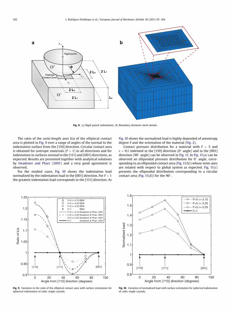
Fig. 8. (a) Rigid punch indentation. (b) Boundary elements mesh details.

L. Rodríguez-Tembleque et al. / European Journal of Mechanics A/Solids 30 (2011) 95e104102

The ratio of the semi-length axes b/a of the elliptical contactarea is plotted in Fig. 9 over a range of angles of the normal to theindentation surface from the [110] direction. Circular contact areais obtained for isotropic materials (F ¼ 1) in all directions and forindentation in surfaces normal to the [111] and [001] directions, asexpected. Results are presented together with analytical solutionsby Swadener and Pharr (2001) and a very good agreement isobserved.

For the studied cases, Fig. 10 shows the indentation loadnormalized by the indentation load in the [001] direction. For F > 1the greatest indentation load corresponds to the [111] direction. As

Fig. 9. Variation in the ratio of the elliptical contact axes with surface orientation forspherical indentation of cubic single-crystals.

Fig. 10 shows the normalized load is highly depended of anisotropydegree F and the orientation of the material (Fig. 2).

Contact pressure distribution for a material with F ¼ 5 andn ¼ 0.1 indented in the [110] direction (0� angle) and in the [001]direction (90� angle) can be observed in Fig. 11. In Fig. 11(a) can beobserved an ellipsoidal pressure distribution for 0� angle, corre-sponding to an ellipsoidal contact area (Fig. 11(b)) whose semi-axesare rotated with respect to global system as expected. Fig. 11(c)presents the ellipsoidal distribution corresponding to a circularcontact area (Fig. 11(d)) for the 90�.

Fig. 10. Variation of normalized load with surface orientation for spherical indentationof cubic single-crystals.

a b

c d

Fig. 11. Contact pressure distribution (case: F ¼ 5, n ¼ 0.1) for 0� (aeb), and 90� (ced).

L. Rodríguez-Tembleque et al. / European Journal of Mechanics A/Solids 30 (2011) 95e104 103

7. Summary and conclusions

An explicit boundary element formulation for 3D contactproblems between elastically anisotropic solids has been pre-sented in this work. Its robustness and accuracy has beendemonstrated with several examples comparing with analyticalsolution presented in the literature. The procedure allows toconsider a general anisotropic material behavior which could beany mathematical degeneracy in a Stroh formalism context,being the isotropy a special case. Furthermore, this formulationconsiders 3D real geometries, frictional contact, and similar anddissimilar materials contact problems. Therefore, some studiesconsidering friction, material orientation influence and materialdissimilarities are presented. On the first example, we could seehow, on frictionless and frictional contact problems, the discrep-ancies on solids transverse indentation direction Young moduleaffects the normal and tangential contact compliance. Same effectcould be appreciated on the second example, considering thedegree of anisotropy and material orientation. Also significantchanges on the contact pressures distributions are revealed due tothe material anisotropy.

So, as the numerical examples show, this formulation enables tostudy the materials mechanical interaction properties, finding thebest material orientation preferent for contact or tangential load

behavior, with potential application in analysis of damage mecha-nisms such as fretting.

Acknowledgments

This work was co-funded by the DGICYT of Ministerio de Cienciay Tecnología, Spain, research projects DPI2006-04598 and DPI2007-66792-C02-02, and by the Consejería de Innovación Ciencia yEmpresa de la Junta de Andalucía, Spain, research projects P06-TEP-02355 and P08-TEP-03804.

Appendix A. Explicit expressions of Mijklmn and Hjk

Considering possible mathematical degenerate cases, explicitexpressions to evaluate the components of Barnett-Lothe tensor Hjk

and the components of Mijklmn are presented in this appendix. Fordetails on the derivation and implementation see the work ofBuroni et al. (in press).

A.1. Mathematical non-degenerate case (p1 s p2 s p3)

Hjk

�be� ¼ 1jT j

X3a¼1

bGjkðpaÞba

Q3x ¼ 1

�pa � px

��pa � px

� (25)

xsa

L. Rodríguez-Tembleque et al. / European Journal of Mechanics A/Solids 30 (2011) 95e104104

Mijklmn

�be� ¼ 2pi

jTj2X3a¼1

AðpaÞnF0ijklmnðpaÞ � 2FijklmnðpaÞBðpaÞ

o(26)

where AðpaÞ :¼ 1=½ðpa � paþ1Þ2ðpa � paþ2Þ2� and BðpaÞ :¼ 1=½pa�paþ1� þ 1=½pa � paþ2�, being p4 ¼ p1, p5 ¼ p2 and the imaginarynumber i ¼

ffiffiffiffiffiffiffi�1

p. F0

ijklmnðpÞ denotes the first-order derivative ofthe function Fijklmn(p) with respect to the argument p.

A.2. Mathematical degenerate case (p1 ¼ p2 ¼ p0 s p3)

Hjk

�be� ¼ 1jT j

24 2i2

bG0jkðp0Þ

�4b0ðp0 � p3Þðp0 � p3Þ

� bGjkðp0Þ

1p0 � p3

þ 1p0 � p3

þ 1ib0

��

þbGjkðp3Þ

b3ðp3 � p0Þ2�p3 � p0

�235 (27)

Mijklmn

�be� ¼ 2pi

jT j2

"F000ijklmnðp0Þ

6ðp0 � p3Þ2� F00

ijklmnðp0Þðp0 � p3Þ3

þ 3F0ijklmnðp0Þ

ðp0 � p3Þ4

�4Fijklmnðp0Þðp0 � p3Þ5

þAðp3ÞnF0ijklmnðp3Þ

�2Fijklmnðp3ÞBðp3Þo#

(28)

where the primes are used to denote the derivatives of the func-tions with respect to the argument p.

A.3. Mathematical degenerate case (p1 ¼ p2 ¼ p3 ¼ p0)

� � 3bGjkðp0Þ � b0

3ibG0

jkðp0Þ þ b0bG00jkðp0Þ

�

Hjk be ¼

4jTjb50(29)

Mijklmn

�be� ¼ pi2

d55Fijklmðp0Þ (30)

60jTj dp

Appendix B. Contact projection functions

The normal contact operator or normal projection function:PR�ð$Þ : R/R�;

PR� ðxÞ ¼ minðx;0Þ (31)

projects the variable x in R�, the admissible region of the contactnormal tractions.

The tangential contact operator, or tangential projection function,PCpð$Þ : R/R�,

PCrðxÞ ¼

x ifkxk < rret ifkxk � r ðet ¼ x=kxkÞ (32)

ensures that the value of the variable x˛R2 remains within theCoulomb disk, Cr, of radium r ¼ jmtnj.

References

Abascal, R., Rodríguez-Tembleque, L., 2007. Steady-state 3D rolling-contact usingboundary elements. Commun. Numer. Meth. Eng. 33, 905e920.

Alart, P., Cournier, A., 1991. A mixed formulation for frictional contact problemsprone to Newton like solution methods. Comput. Methods Appl. Mech. Eng. 92,353e375.

Alart, P., Lebon, F., 1998. Numerical study of a stratified composite couplinghomogenization and frictional contact. Math. Comput. Model. 28, 273e286.

Alart, P., 1997. Méthode de newton généralisée en mécanique du contact. J. Math.Pure Appl. 76, 83e108.

Aliabadi, M.H., 2002. The Boundary Element Method. In: Applications in Solids andStructures, vol. 2. John Wiley & Sons.

Arakere, N.K., Kundsen, E., Swanson, G.R., Duke, G., Ham-Battista, G., 2006.Subsurface stress fields in face-centered-cubic single-crystal anisotropiccontact. J. Eng. Gas Turbines Power 128, 879e888.

Batra, R.C., Jaing, W., 2008. Analytical solution of the contact problem of a rigidindenter and an anisotropic linear elastic layer. Int. J. Solids Struct. 45,5814e5830.

Brebbia, C.A., Dominguez, J., 1992. Boundary Elements: An Introductory Course,second ed. Computatinal Mechanics Publications, John Wiley & Sons.

Buroni, F.C., Ortiz, J.E., Sáez, A. Multiple pole residue approach for 3D BEM analysisof mathematical degenerate and non-degenerate materials. Int. J. Numer, Meth.Eng. in press.

Christensen, P.W., Klarbring, A., Pang, J.S., Strömberg, N., 1998. Formulation andcomparison of algorithms for frictional contact problems. Int. J. Numer. Meth.Eng. 42, 145e173.

Gladwell, G.M.L., 1980. Contact Problem in the Classical Theory of Elasticity. Sijthoffand Noordhoff, Alphen aan den Rijn, The Netherlands.

González, J.A., Park, K.C., Felippa, C.A., Abascal, R., 2008. A Formulation based onlocalized Lagrange multipliers for BEM-FEM coupling in contact problems.Comput. Methods Appl. Mech. Eng. 197, 623e640.

Hills, D.A., Nowell, D., Sackfield, A., 1993. Mechanics of Elastic Contact. Butterworth-Heinemann, Oxford, UK.

Hwu, C., Fan, C.W., 1998. Sliding punches with or without friction along the surfaceof an anisotropic elastic half-plane. Q.J. Mech. Appl. Math. 51, 159e177.

Klarbring, A., 1992. Mathematical Programming and augmented lagrangianmethods for frictional contact problems. In: Curnier, A. (Ed.), ProceedingsContact Mechanics International Symposium. Presses Polytechniques et Uni-versitaires Romandes, Lausanne, pp. 409e422.

Klarbring, A., 1993. Mathematical programimg in contact problems. In:Aliabadi, M.H., Brebbia, C.A. (Eds.), Computational Methods in ContactMechanics. Computational Mechanics Publications.

Laursen, T.A., 2002. Computational Contact and Impact Mechanics. Springer,England.

Lee, V.G., 2003. Explicit expressions of derivatives of elastic Greens functions forgeneral anisotropic materials. Mech. Res. Comm. 30, 241e249.

Lovell, M., 1998. Analysis of contact between transversely isotropic coated surfaces:development of stress and displacement relationships using FEM. Wear 194,60e70.

Pang, J.S., 1990. Newton’s method for B-differentiable equations. Math. Oper. Res. 15(2), 311e341.

Peillex, G., Baillet, L., Berthier, Y., 2008. Homogenization in non-linear dynamics dueto frictional contact. Int. J. Solids Struct. 45, 2451e2469.

Rodríguez-Tembleque, L., Abascal, R., 2010a. A 3D FEM-BEM rolling contactformulation for unstructured meshes. Int. J. Solids Struct. 47, 330e353.

Rodríguez-Tembleque, L., Abascal, R., 2010b. A FEM-BEM fast methodology for 3Dfrictional contact problems. Comput. Struct. 88, 924e937.

Rodríguez-Tembleque, L., Abascal, R., Aliabadi, M.H., 2010. A boundary elementformulation for wear modeling on 3D contact and rolling-contact problems. Int.J. Solids Struct. 47, 2600e2612.

Strömberg, N., 1997. An augmented Lagrangian method for fretting problems. Eur. J.Mech. A Solid. 16 (4), 573e593.

Swadener, J.G., Pharr, G.M., 2001. Indentation of elastically anisotropic half-spacesby cones and parabolae of revolution. Philos. Mag. A. 81, 447e466.

Ting, T.C.T., Lee, V.G., 1997. The three-dimensional elastostatic Green’s function forgeneral anisotropic linear elastic solids. Q.J. Mech. Appl. Math. 50, 407e426.

Ting, T.C.T., 1996. Anisotropic Elasticity. Oxford University Press, Oxford.Turner, J.R., 1980. Contact on a transversely isotropic half-space, or between two

transversely isotropic bodies. Int. J. Solids Struct. 16, 409e419.Vlassak, J.J., Nix, W.D., 1993. Indentation modulus of elastically anisotropic half

spaces. Philos. Mag. A. 67, 1045e1056.Vlassak, J.J., Nix, W.D., 1994. Measuring the elastic properties of anisotropic mate-

rials by means of indentation experiments. J. Mech. Phys. Solids. 42, 1223e1245.Vlassak, J.J., Ciavarella, M., Barber, J.R., Wang, X., 2003. The indentation modulus of

elastically anisotropic materials for indenters of arbitrary shape. J. Mech. Phys.Solids. 51, 1701e1721.

Willis, J.R., 1966. Hertzian contact of anisotropic bodies. J. Mech. Phys. Solids. 14,163e176.

Wriggers, P., 2002. Computational Contact Mechanics (West Sussex, England).