Leverage and Covariance Matrix Estimation in Finite-Sample IV Regressions
Upload
khangminh22Category
view
2download
0
Error Analysis and Estimation
for the Finite Volume Method
with Applications to
Fluid Flows
Hrvoje Jasak
Thesis submitted for the
Degree of Doctor of Philosophy of the University of London
and
Diploma of Imperial College
Department of Mechanical Engineering
Imperial College
of Science, Technology and Medicine
June 1996


3
Abstract
The accuracy of numerical simulation algorithms is one of main concerns in modern
Computational Fluid Dynamics. Development of new and more accurate mathe-
matical models requires an insight into the problem of numerical errors.
In order to construct an estimate of the solution error in Finite Volume cal-
culations, it is first necessary to examine its sources. Discretisation errors can be
divided into two groups: errors caused by the discretisation of the solution domain
and equation discretisation errors. The first group includes insufficient mesh reso-
lution, mesh skewness and non-orthogonality. In the case of the second order Finite
Volume method, equation discretisation errors are represented through numerical
diffusion. Numerical diffusion coefficients from the discretisation of the convection
term and the temporal derivative are derived. In an attempt to reduce numeri-
cal diffusion from the convection term, a new stabilised and bounded second-order
differencing scheme is proposed.
Three new methods of error estimation are presented. The Direct Taylor Series
Error estimate is based on the Taylor series truncation error analysis. It is set up to
enable single-mesh single-run error estimation. The Moment Error estimate derives
the solution error from the cell imbalance in higher moments of the solution. A
suitable normalisation is used to estimate the error magnitude. The Residual Error
estimate is based on the local inconsistency between face interpolation and volume
integration. Extensions of the method to transient flows and the Local Residual
Problem error estimate are also given.
Finally, an automatic error-controlled adaptive mesh refinement algorithm is set
up in order to automatically produce a solution of pre-determined accuracy. It uses
mesh refinement and unrefinement to control the local error magnitude. The method
is tested on several characteristic flow situations, ranging from incompressible to
supersonic flows, for both steady-state and transient problems.

Dedicated to Henry Weller
Imperial College, September 1998 - June 1996

7
Acknowledgements
I would like to express my sincere gratitude to my supervisors, Prof A.D. Gosman
and Dr R.I. Issa for their continuous interest, support and guidance during this
study.
I am also indebted to my friends and colleagues in the Prof Gosman's CFD
group, particularly to Henry Weller and other people involved in the development
of the FOAM C++ numerical simulation code.
The text of this Thesis has benefited from numerous valuable comments from
Prof I. Demirdzié and C. Kralj.
Finally, I would like to thank Mrs N. Scott-Knight for the arrangement of many
administrative matters.
The financial support provided by the Computational Dynamics Ltd. is grate-
fully acknowledged.

Contents
1 Introduction 41
1.1 Background ................................41
1.2 Previous and Related Studies ......................44
1.2.1 Convection Discretisation ....................44
1.2.2 Error Estimation .........................49
1.2.3 Adaptive Refinement .......................54
1.3 Present Contributions ..........................58
1.4 Thesis Outline ...............................61
2 Governing Equations 63
2.1 Governing Equations of Continuum Mechanics .............63
2.2 Constitutive Relations for Newtonian Fluids ..............65
2.3 Turbulence Modelling ...........................67
3 Finite Volume Discretisation 73
3.1 Introduction ................................73
3.2 Discretisation of the Solution Domain ..................75
3.3 Discretisation of the Transport Equation ................77
3.3.1 Discretisation of Spatial Terms .................78
3.3.1.1 Convection Term ....................80
3.3.1.2 Convection Differencing Scheme ............81
3.3.1.3 Diffusion Term .....................83
3.3.1.4 Source Terms ......................86
10
Contents
3 3.2 Temporal Discretisation .....................87
3.3.3 Implementation of Boundary Conditions ............92
3.3.3.1 Numerical Boundary Conditions ...........93
3.3.3.2 Physical Boundary Conditions .............95
3.4 A New Convection Differencing Scheme .................97
3.4.1 Accuracy and Boundedness ...................97
3.4.1.1 TVD Differencing Schemes ..............97
3.4.1.2 Convection Boundedness Criterion and the NVD Di-
agram..........................100
3.4.1.3 Convergence Problems of Flux-Limited Schemes . . . 103
3.4.2 Modification of the NVD Criterion for Unstructured Meshes . 104
3.4.3 Gamma Differencing Sheme ...................107
3.4.3.1 Accuracy and Convergence of the Gamma Differenc-
ingScheme .......................110
3.5 Solution Techniques for Systems of Linear Algebraic Equations . . 111
3.6 Numerical Errors in the Discretisation Procedure ...........115
3.6.1 Numerical Diffusion from Convection Differencing Schemes . . 116
3.6.2 Numerical Diffusion from Temporal Discretisation .......118
3.6.3 Mesh-Induced Errors .......................122
3.7 Numerical Examples ...........................125
3.7.1 Numerical Diffusion from Convection Discretisation ......125
3.7.2 Comparison of the Gamma Differencing Scheme with Other
High-Resolution Schemes .....................129
3.7.2.1 Step-profile .......................130
3.7.2.2 szn2-pro file ....................... 130
3.7.2.3 Semi-ellipse .......................133
3 7 3 Numerical Dffusion from Temporal Discre isation .......133
3.7.3 1 1-D Tests ........................135
3 7.3.2 2-D Transport of a "Bubble" .............137
3 7 4 Compars n of Non Orth gonality Treatments .......138
Contents
11
3.8 Discretisation Procedure for the Navier-Stokes System ........143
3.8.1 Derivation of the Pressure Equation ...............145
3.8.2 Pressure-Velocity Coupling ....................146
3.8.2.1 The PISO Algorithm for Transient Flows .......147
3.8.2.2 The SIMPLE Algorithm ................148
3.8.3 Solution Procedure for the Navier-Stokes System .......150
3.9 Closure ...................................151
4 Error Estimation 153
4.1 Introduction ................................153
4.1.1 Error Estimators and Error Indicators .............155
4.2 Requirements on an Error Estimate ...................157
4.3 Methods Based on Taylor Series Expansion ...............159
4.3.1 Richardson Extrapolation ....................161
4 3 2 Direct Taylor Series Error Estimate .............164
4.3.3 Measuring Numerical Diffusion .................167
4.4 Moment Error Estimate .........................168
4.4.1 Normalisation of the Moment Error Estimate .........170
4.4.2 Consistency of the Moment Error Estimate ...........171
4.5 Residual Error Estimate .........................173
4.5.1 Normalisation of the Residual Error Estimate .........179
4.6 Local Problem Error Estimate ......................181
4.6.1 Elliptic Model Problem ......................182
4.6.1.1 Balancing Problem in Finite Volume Method . . . . 185
4.6.2 Generalisation to the Convection-Diffusion Problem ......187
4.6.3 Generalisation to the Navier-Stokes Problem ..........190
4.6.3.1 Error Norm for the Navier-Stokes System ......191
4.6.3.2 Formulation of the Local Problem ...........192
4.6.4 Solution of the Local Problem ..................193
4.6.4.1 Solution of the Indeterminate Local Problem . . . . 194

12
Contents
4.6.4.2 Solution of the Determinate Local Problem .....195
4.6.5 Application of the Local Problem Error Estimate .......196
4.7 Error Estimation for Transient Calculations ..............197
4.7.1 Residual in Transient Calculations ...............198
4.7.2 Spatial and Temporal Error Contributions ...........199
4.7.3 Evolution Equation for the Error ................201
4.8 Numerical Examples ...........................202
4.8.1 Line Source in Cross-Flow ....................202
4.8.1.1 Mesh Aligned with the Flow ..............203
4.8.1.2 Non-Orthogonal Non-Aligned Mesh ..........208
4.8.2 Line Jet ..............................213
4.8.3 Transient One-Dimensional Convective Transpo't .......218
4.8.4 Local Problem Error Estimation .................221
4.9 Closure ...................................225
5 Adaptive Local Mesh Refinement and Unrefinement 227
5.1 Introduction ................................227
5.2 Selecting Regions of Refinement and Unrefinement ...........230
5.3 Mesh Refinement and Unrefinement ...................234
5.4 Mapping of Solution Between Meshes ..................237
5.5 Numerical Example ............................238
5.6 Closure ...................................258
6 Case Studies 261
6.1 Introduction ................................261
6.2 Inviscid Supersonic Flow Over a Forward-Facing Step .........263
6.3 Laminar and Turbulent Flow Over a 2-D Hill .............280
6 3.1 Laminar Flow ...........................281
6.3.2 Turbulent Flo'c...........................297
6.4 Turbulent Flow over a 3-D Swept Backward-Facing Step .......329
6.5 Vortex Shedding Behind a Cylinder ..................355

Contents 13
6 .6 Closure ...................................365
7 Summary and Conclusions 369
7.1 Discretisation ...............................370
7.2 Error Estimation .............................371
7.3 Adaptive Mesh Refinement ........................373
7.4 Performance of the Error-Controlled Adaptive Refinement Algorithm 374
7.5 Future Work ................................376
A Comparison of the Euler Implicit Discretisation and Backward Dif-
ferencing in Time 379

14Contents
List of Figures
3.1 Control volume 75
3.2 Face interpolation.............................81
3.3 Vectors d and S on a non-orthogonal mesh...............83
3.4 Non-orthogonality treatment in the "minimum correction" approach 84
3.5 Non-orthogonality treatment in the "orthogonal correction" app"oach 85
3.6 Non-orthogonality treatment in the "over-relaxed" approach.....85
3.7 Control volume with a boundary face..................93
3.8 Variation of around the face f..................... 99
3.9 Sweby's diagram..............................99
3.10 Convection Boundedness Criterion in the Normalised Variable Dia-
gram....................................102
3.11 Common differencing schemes in the NVD diagram..........102
3.12 Modified definition of the boundedness criterion for unstructured
meshes...................................105
3.13 Shape of the profile for 0 < q <urn................... 108
3.14 Gamma differencing scheme in the NVD diagram............110
3.15 Skewness error on the face........................124
3.16 Step-profile test setup...........................126
3.17 Convection of a step-profile, 9 = 00, UD.................127
3.18 Convection of a step-profile, 9 = 30°, UD................127
3.19 Convection of a step-profile, 0 = 300, CD................127
3.20 Convection of a step-profile, 9 = 30°, UD, CD and Gamma differ-
encingschemes...............................128
16
List of Figures
3.21 Convection of a step-profile, 9 - 45°, UD, CD and Gamma differ-
encingschemes...............................128
3.22 Convection of a step-profile, 9 300, CD, SFCD and Gamma differ-
encingschemes...............................131
3.23 Convection of a step-profile, 9 = 30°, van Leer, SUPERBEE and
Gamma differencing schemes.......................131
3.24 Convection of a step-profile, 9 = 30°, SOUCUP, SMART and Gamma
differencingschemes............................131
3.25 Convection of a sin2-profile, 9 = 30°, CD, SFCD and Gamma differ-
encingschemes...............................132
3.26 Convection of a szn 2-profile, 9 = 30°, van Leer, SUPERBEE and
Gamma differencing schemes.......................132
3.27 Convection of a szn 2-profile, 0 = 30°, SOUCUP, SMART and Gamma
differencingschemes............................132
3.28 Convection of a semi-ellipse, 0 = 30°, CD, SFCD and Gamma dif-
ferencingschemes.............................134
3.29 Convection of a semi-ellipse, 9 = 30°, van Leer, SUPERBEE and
Gamma differencing schemes.......................134
3.30 Convection of a semi-ellipse, 9 - 30 , SOIJCIJP, SMART and Gamma
differencingschemes............................134
3.31 Transport of a step-profile after 300 time-steps, four methods of tem-
poraldiscretisation............................136
3.32 Transport of a half-sin 2 profile after 300 time-steps, four methods of
temporaldiscretisation..........................136
3.33 Setup for the transport of the bubble..................137
3.34 Initial shape of the bubble.....................139
3.35 Transport of the bubble after 800 time-steps, Euler Implicit .....139
3.36 Transport of the bubble after 800 time-steps, Explicit discretisati n 139
3 37 Transport of the bubble after 800 time-steps, Crank-Nicholson. . . . 139
3.38 N n-orth gonal test with uniform grid angle..............140
List of Figures 17
3.39 Convergence history, c = 100
141
3.40 Convergence history, a = 30°
141
3.41 Convergence history, a, = 400
141
3.42 Convergence history, a, = 450
142
3.43 Convergence history, a = 650
142
4.1 Hexahadral control volume aligned with the coordinate system. . . . 163
4.2 Inconsistency between face interpolation and the integration over the
cell.....................................174
4.3 Scaling properties of the residual error estimate.............179
4.4 Estimating the convection and diffusion transport...........180
4.5 Line source in cross-flow: mesh aligned with the flow..........203
4.6 Aligned mesh: exact solution.......................204
4.7 Aligned mesh: Exact error magnitude..................204
4.8 Aligned mesh: Direct Taylor Series Error estimate...........204
4.9 Aligned mesh: Moment Error estimate.................205
4.10 Aligned mesh: Residual Error estimate.................205
4.11 Aligned mesh: scaling of the mean error.................207
4.12 Aligned mesh: scaling of the maximum error..............207
4.13 Line source in cross-flow: non-orthogonal non-aligned mesh......208
4.14 Non-aligned mesh: exact solution....................209
4.15 Non-aligned mesh: Exact error magnitude................209
4.16 Non-aligned mesh: Direct Taylor Series Error estimate.........209
4.17 Non-aligned mesh: Moment Error estimate...............210
4.18 Non-aligned mesh: Residual Error estimate...............210
4.19 Non-aligned mesh: scaling of the mean error..............211
4.20 Non-aligned mesh: scaling of the maximum error............211
4.21 Non-aligned mesh: scaling of the mean error with UD.........21
4.22 Non-aligned mesh: scaling of the maximum error with UD.......212
4.23 Line jet: test setup............................214
18
List of Figures
4.24 Line jet: exact solution 215
4.25 Line jet: exact error magnitude.....................215
4.26 Line jet: Direct Taylor Series Error estimate..............215
4.27 Line jet: Moment Error estimate.....................216
4.28 Line jet: Residual Error estimate.....................216
4.29 Line jet: scaling of the mean error....................217
4.30 Line jet: scaling of the maximum error.................217
4.31 1-D convective transport: exact and analytical solution after 350
time-steps.................................218
4.32 1-D convective transport: change in the solution during a single
time-step..................................219
4.33 1-D convective transport: estimated and exact single time-step error 219
4.34 1-D convective transport: estimated and exact error after 350 time-
steps....................................220
4.35 Elliptic test case: Exact solution.....................221
4.36 Elliptic test case: Estimated error norm distribution..........221
4.37 Line source in cross fio, aligned mesh: estimated error norm.....223
4.38 Line jet: estimated error norm......................224
5.1 Directionality of mesh refinement....................233
5.2 Refining a hexahedral cell.........................235
5.3 "1-irregular" mesh.............................236
5.4 Initial mesh................................240
5.5 First level of adaptive refinement.....................240
5.6 Second level of adaptive refinement...................240
5 7 Third level of adaptive refinement....................240
5.8 Fourth level of adaptive refinement.................241
5.9 Fifth level of adaptive refinement....................241
5.10 Sixth level of adaptive refinement....................241
5 11 Tenth level of adaptive refinement ..................241
List of Figures 19
5.12 Initial distribution of the exact error...................242
5.13 Exact error distribution after two levels of adaptive refinement . . . 243
5.14 Exact error distribution after four levels of adaptive refinement . . . 243
5.15 Exact error distribution after six levels of adaptive refinement.....243
5.16 Uniform and adaptive refinement: scaling of the mean error......244
5.17 Uniform and adaptive refinement: scaling of the maximum error. . . 244
5.18 Uniform and adaptive refinement: scaling of the volume-weighted
meanerror.................................245
5.19 Optimality index for uniform and adaptive refinement.........246
5.20 Refinement/unrefinement: solution at x = 0.2 m on the initial mesh 248
5.21 Refinement unrefinement: solution at x = 0.2 m after the first level
ofrefinement................................248
5.22 Refinement/unrefinement: solution at x = 0.2 m after the second
levelof refinement.............................249
5.23 Refinement/unrefinement: solution at x = 3 m after the second level
ofrefinement................................249
5.24 Refinement/unrefinement: solution at x = 0.2 m after the tenth level
ofrefinement................................250
5.25 Refinement/unrefinement: solution at x = 3 m after the tenth level
ofrefinement................................250
5.26 Adaptive refinement: scaling of the mean error for different error
estimatesand the exact error.......................252
5.27 Adaptive refinement: scaling of the maximum error for different error
estimates and the exact error.......................252
5.28 Initial mesh for refinement unrefinement................254
5.29 Second level of refinement unrefinement.................254
5.30 Second level of refinement-only......................254
5.31 Refinement/unrefinement: scaling of the mean error..........255
5.32 Refinement/unrefinement: scaling of the maximum error........255

20
List of Figures
5.33 Optimality index for uniform refinement, adaptive refinement-only
and adaptive refinement/unrefinement..................256
5.34 Refinement unrefinement: scaling of the mean error for different er-
rorestimates................................257
5.35 Refinement unrefinement: scaling of the maximum error for different
errorestimates...............................257
6.1 Supersonic flow over a forward-facing step: Mach number distribu-
tion, uniform mesh, 840 CV.......................264
6.2 Supersonic flow over a forward-facing step: Mach number distribu-
tion, uniform mesh, 5250 CV.......................264
6.3 Supersonic flow over a forward-facing step: Mach number distribu-
tion, uniform mesh, 53000 CV......................264
6.4 Supersonic flow over a forward-facing step: error indicator T, uni-
formmesh. 840 CV............................266
6.5 Supersonic flow' over a forward-facing step: error indicator T, uni-
formmesh, 5250 CV............................266
6.6 Supersonic flow over a forward-facing step: error indicator T, uni-
formmesh, 53000 CV...........................266
6.7 Supersonic flow over a forward-facing step: Direct Taylor Series Error
estimate for the momentum, uniform mesh, 5250 CV..........267
6.8 Supersonic flow over a forward-facing step: Moment Error estimate
for the momentum, uniform mesh, 5250 CV...............267
6.9 Supersonic flow over a forward-facing step: Residual Error estimate
for the momentum, uniform mesh, 5250 CV...............267
6.10 S personic flow over a forward-facing step coarse mesh, 840 CV. . . 268
6.11 Supersonic flow over a forward-facing step: intermediate mesh, 5250 CV.268
6 12 Supersonic flow over a forward-facing step: first level of adaptive
refinement starting from the mesh in Fig 6 10 ............269

List of Figures 21
6.13 Supersonic flow over a forward-facing step: second level of adaptive
refinement starting from the mesh in Fig. 6.10.............269
6.14 Supersonic flow over a forward-facing step: third level of adaptive
refinement starting from the mesh in Fig. 6.10.............269
6.15 Detail of the adaptively refined mesh..................270
6.16 Supersonic flow over a forward-facing step: Mach number distribu-
tion on the adaptively refined mesh after three levels of refinement. . 271
6.17 Supersonic flow over a forward-facing step: Mach number distribu-
tion on the adaptively refined mesh after five levels of refinement. . . 271
6.18 Supersonic flow over a forward-facing step: third level of adaptive
refinement starting from the mesh in Fig. 6.11.............272
6.19 Supersonic flow over a forward-facing step: first level of adaptive
refinement/unrefinement starting from the mesh in Fig. 6.11.....273
6.20 Supersonic flow over a forward-facing step: second level of adaptive
refinement/unrefinement starting from the mesh in Fig. 6.11.....273
6.21 Supersonic flow over a forward-facing step: third level of adaptive
refinement/unrefinement starting from the mesh in Fig. 6.11.....273
6.22 Supersonic flow over a forward-facing step: Mach number distribu-
tionfor the mesh in Fig. 6.18.......................274
6.23 Supersonic flow over a forward-facing step: Mach number distribu-
tionfor the mesh in Fig. 6.21.......................274
6.24 Supersonic flow over a forward-facing step: scaling of the mean error
foruniform refinement..........................277
6.25 Supersonic flow over a forward-facing step: scaling of the maximum
error for uniform refinement.......................277
6.26 Supersonic flow over a forward-facing step: scaling of the mean error
foradaptive refinement..........................278
6.27 Supersonic flow over a forward-facing step: scaling of the maximum
error for adaptive refinement.......................278
22
List of Figures
6.28 Supersonic flow over a forward-facing step: scaling of the mean error
forrefinement unrefinement.......................279
6.29 Supersonic flow over a forward-facing step: scaling of the maximum
error for refinement/unrefinement....................279
6.30 Two-dimensional hill test case......................280
6.31 Two-dimensional hill: uniform mesh with 2044 CV...........281
6.32 Laminar flow over a 2-D hill: velocity field...............282
6.33 Laminar flow over a 2-D hill: pressure field...............282
6.34 Laminar flow over a 2-D hill: vector velocity error, uniform mesh,
2044 CV.................................283
6.35 Laminar flow over a 2-D hill: velocity error magnitude, uniform
mesh, 2044 CV...............................283
6.36 Laminar flow over a 2-D hill: velocity error magnitude, uniform
mesh, 8584 CV...............................284
6.37 Laminar flow over a 2-D hill: Direct Taylor Series Error estimate for
the velocity, uniform mesh, 2044 CV...................285
6.38 Laminar flow over a 2-D hill: Moment Error estimate for the velocity,
uniformmesh, 2044 CV..........................285
6.39 Laminar flow over a 2-D hill: Residual Error estimate for the velocity,
uniformmesh, 2044 CV..........................285
6.40 Laminar flow over a 2-D hill: scaling of the mean error for uniform
refinement.................................286
6.41 Laminar flow over a 2-D hill: scaling of the maximum error for uni-
formrefinement..............................286
6.42 Laminar flow over a 2-D hill. estimated error norm, uniform mesh,
2044 CV................................287
6.43 Laminar flow over a 2-D hi1l scaling of the relative error in dissipa-
tionfor uniform refinement........................288
6.44 Laminar flow over a 2-D hill. mesh after the first level of refinement 289
645 Laminar flow over a 2-D hill: mesh after the second level of refinement.289
List of Figures 23
6.46 Laminar flow over a 2-D hill: mesh after the third level of refinement. 289
6.47 Laminar flow over a 2-D hill: first level of refinement/unrefinement. . 290
6.48 Laminar flow over a 2-D hill: second level of reflnement/unrefinement.290
6.49 Laminar flow over a 2-D hill: Residual Error estimate after the first
levelof refinement.............................292
6.50 Laminar flow over a 2-D hill: Residual Error estimate after the sec-
ondlevel of refinement..........................292
6.51 Laminar flow over a 2-D hill: Residual Error estimate after the third
levelof refinement.............................292
6.52 Laminar flow over a 2-D hill: Residual Error estimate on the uniform
mesh, 8584 CV-s..............................293
6.53 Laminar flow over a 2-D hill: Residual Error estimate after the first
level of refinement/unrefinement from the fine mesh..........293
6.54 Laminar flow over a 2-D hill: Residual Error estimate after the sec-
ond level of refinement/unrefinement from the fine mesh........293
6.55 Laminar flow over a 2-D hill: second level of refinement-only from
thefine mesh................................294
6.56 Laminar flow over a 2-D hill: Residual Error estimate after the sec-
ond level of refinement/unrefinement..................294
6.57 Laminar flow over a 2-D hill: scaling of the maximum Moment Error
for different types of refinement....................295
6.58 Laminar flow over a 2-D hill: scaling of the maximum Residual Error
for different types of refinement.....................295
6.59 Turbulent flow over a 2-D hill: velocity field, uniform mesh, 2044 CV. 299
6.60 Turbulent flow over a 2-D hill: turbulent kinetic energy field, uniform
mesh, 2044 CV...............................299
6.61 Turbulent flow over a 2-D hill: dissipation of turbulent kinetic energy,
uniformmesh, 2044 CV..........................299
6.62 Turbulent flow over a 2-D hill: Direct Taylor Series Error estimate
for velocity, uniform mesh, 2044 CV...................300

24
List of Figures
6.63 Turbulent flow over a 2-D hill: Moment Error estimate for velocity,
uniformmesh, 2044 CV..........................300
6.64 Turbulent flow over a 2-D hill: Residual Error estimate for velocity,
uniformmesh, 2044 CV..........................300
6.65 Turbulent flow over a 2-D hill: Direct Taylor Series Error estimate
for k, uniform mesh, 2044 CV......................301
6.66 Turbulent flow over a 2-D hill: Moment Error estimate for k, uniform
mesh, 2044 CV...............................301
6.67 Turbulent flow over a 2-D hill: Residual Error estimate for k, uniform
mesh, 2044 CV...............................301
6.68 Turbulent flow over a 2-D hill: Direct Taylor Series Error estimate
forc, uniform mesh, 2044 CV.......................302
6.69 flow over a 2-D hill: Moment Error estimate for €, uniform mesh,
2044 CV..................................302
6.70 Turbulent flow over a 2-D hill: Residual Error estimate for f, uniform
mesh. 2044 CV...............................302
6.71 Turbulent flow over a 2-D hill: estimated error norm for velocity,
uniformmesh, 2044 CV..........................305
6.72 Turbulent flow over a 2-D hill: estimated error norm for k, uniform
mesh, 2044 CV...............................305
6.73 Turbulent flow over a 2-D hill: estimated error norm for c, uniform
mesh, 2044 CV...............................305
6.74 Turbulent flow over a 2-D hill: scaling of the mean velocity error for
uniformrefinement............................306
6.75 Turbulent flow over a 2-D hill: scaling of the maximum velocity error
foruniform refinement..........................306
6.76 Turbulent flow over a 2-D hill. scaling of the mean error in k for
uniformrefinement............................307
6 77 Turbulent flow over a 2-D hill: scaling of the maximum error in k
forunif rm refinement .........................307
List of Figures 25
6.78 Turbulent flow over a 2-D hill: scaling of the mean error in € for
uniformrefinement............................308
6.79 Turbulent flow over a 2-D hill: scaling of the maximum error in e for
uniformrefinement............................308
6.80 Turbulent flow over a 2-D hill: mesh after the first level of refinement.311
6.81 Turbulent flow over a 2-D hill: mesh after the second level of refinement.311
6 82 Turbulent flow over a 2-D hill: mesh after the third level of refinement.311
6.83 Turbulent flow over a 2-D hill: Moment Error estimate for velocity
after the first level of adaptive refinement................312
6.84 Turbulent flow over a 2-D hill: Moment Error estimate for velocity
after the second level of adaptive refinement..............312
6.85 Turbulent flow over a 2-D hill: Momeat Error for velocity estimate
after the third level of adaptive refinement...............312
6.86 Turbulent flow over a 2-D hill: Residual Error estimate after the first
level of adaptive refinement........................313
6.87 Turbulent flow over a 2-D hill: Residual Error estimate after the
second level of adaptive refinement....................313
6.88 Turbulent flow over a 2-D hill: Residual Error estimate after the
third level of adaptive refinement....................313
6.89 Turbulent flow over a 2-D hill: second level of refinement-only from
thefine mesh................................314
6.90 Turbulent flow over a 2-D hill: second level of refinement/unrefinement
fromthe fine mesh.............................314
6.91 Turbulent flow over a 2-D hill: Moment Error estimate for velocity
after two levels of refinement/unrefinement...............316
6.92 Turbulent flow over a 2-D hill: Residual Error estimate for k after
two levels of refinement/unrefinement..................316
6.93 Turbulent flow over a 2-D hill: scaling of the maximum Moment
Error for velocity for different types of refinement...........318
26
List of Figures
6.94 Turbulent flow over a 2-D hill: scaling of the maximum Moment
Error for velocity without the near-wall cells for different types of
refinement.................................318
6.95 Turbulent flow over a 2-D hill: scaling of the maximum Moment
Error for k for different types of refinement...............319
6.96 Turbulent flow over a 2-D hill: scaling of the maximum Residual
Error for k for different types of refinement...............319
6.97 Turbulent flow over a 2-D hill: velocity distribution at x = 0 for
uniformmeshes..............................320
6.98 Turbulent flow over a 2-D hill: velocity distribution at x = 0, first
levelof refinement.............................320
6.99 Turbulent flow over a 2-D hill: velocity distribution at x = 0, second
levelof refinement.............................320
6.100 Turbulent flow over a 2-D hill: velocity distribution at x = 134 for
uniformmeshes..............................321
6.101 Turbulent flow over a 2-D hill: velocity distribution at x = 134, first
levelof refinement.............................321
6.102 Turbulent flow over a 2-D hill: velocity distribution at x 134,
secondlevel of refinement.........................321
6.103 Turbulent flow over a 2-D hill: distribution of k at x 0 for uniform
meshes...................................322
6.104 Turbulent flow over a 2-D hill: distribution of k at x = 0, first level
ofrefinement................................322
6.105 Turbulent flow over a 2-D hill: distribution of k at x = 0, second
levelof refinement.............................322
6.106 Turbulent flow over a 2-D hilF distribution of k at x = 134 for
uniformmeshes..............................323
6.107 Turbulent flow over a 2-D hill S distribution of k at x = 134 first
levelof refinement.............................323

List of Figures 27
6.108 Turbulent flow over a 2-D hill: distribution of k at x = 134, second
levelof refinement.............................323
6.109 Turbulent flow over a 2-D hill: uniform mesh for the low-Re calculation.325
6.110 Turbulent flow over a 2-D hill: velocity field for the low-Re turbu-
lencemodel................................325
6.111 Turbulent flow over a 2-D hill: maximum error reduction for velocity
with adaptive refinement and the low-Re turbulence model......326
6.112 Turbulent flow over a 2-D hill: maximum error reduction for k with
adaptive refinement and the low-Re turbulence model.........328
6.113 Turbulent flow over a 2-D hill: maximum error reduction for E with
adaptive refinement and the low-Re turbulence model.........328
6.114 3-D swept backward facing step: test setup..............329
6.115 3-D swept backward-facing step: coarse uniform mesh, 16625 CV. . . 331
6.116 3-D swept backward-facing step: stream ribbons close to the inlet. . 333
6.117 3-D swept backward-facing step: stream ribbon in the vortex.....333
6.118 3-D swept backward-facing step: velocity field cut, y/H = 0.125. . . 334
6.119 3-D swept backward-facing step: velocity field cut, y/H = 0.5.....334
6.120 3-D swept backward-facing step: velocity field cut, y/H = 1.125. . . 335
6.121 3-D swept backward-facing step: surface pressure............335
6.122 3-D swept backward-facing step: near-surface k distribution......336
6.123 3-D swept backward-facing step: k iso-surface..............336
6.124 3-D swept backward-facing step: Moment Error estimate for velocity. 338
6.125 3-D swept backward-facing step: Residual Error estimate for velocity. 338
6.126 3-D swept backward-facing step: Moment Error estimate for k. . . . 339
6.127 3-D swept backward-facing step: Residual Error estimate for k. . . . 339
6.128 3-D swept backward-facing step: Moment Error estimate for . . . . 340
6.129 3-D swept backward-facing step: Residual Error estimate for . . . . 340
6.130 3-D swept backward-facing step: coarse uniform mesh at the corner
ofthe triangular part...........................343
28
List of Figures
6.131 3-D swept backward-facing step: mesh detail after the first level of
refinement.................................343
6.132 3-D swept backward-facing step: mesh detail after the second level
ofrefinement................................344
6.133 3-D swept backward-facing step: mesh detail after the third level of
refinement.................................344
6.134 3-D swept backward-facing step: iso-surface of the Moment Error
estimate for velocity on the initial mesh.................346
6.135 3-D swept backward-facing step: iso-surface of the Moment Error
estimate for velocity after the first level of refinement.........346
6.136 3-D swept backward-facing step: iso-surface of the Moment Error
estimate for velocity after the second level of refinement........347
6.137 3-D swept backward-facing step: iso-surface of the Moment Error
estimate for velocity after the third level of refinement.........347
6.138 3-D swept backward-facing step: iso-surface of the Residual Error
estimate for k on the initial mesh....................348
6.139 3-D swept backward-facing step: iso-surface of the Residual Error
estimate for k after the first level of refinement.............348
6.140 3-D swept backward-facing step: iso-surface of the Residual Error
estimate for k after the second level of refinement...........349
6.141 3-D swept backward-facing step: iso-surface of the Residual Error
estimate for k after the third level of refinement............349
6.142 3-D swept backward-facing step: scaling of the maximum velocity
error for adaptive refinement.......................350
6.143 3-D swept backward-facing step: scaling of the mean velocity error
foradaptive refinement..........................350
6.144 3-D swept backward-facing step: scaling of the maximum velocity
error for uniform and adaptive refinement................351
6 145 3-D swept backward-facing step S scaling of the maximum k error for
unif rm and adaptive refinement.....................352
List of Figures 29
6.146 3-D swept backward-facing step: scaling of the maximum k error for
adaptiverefinement............................352
6.147 3-D swept backward-facing step: scaling of the maximum error for
adaptiverefinement............................353
6.148 Vortex shedding behind a cylinder: test setup..............355
6.149 Vortex shedding: uniform mesh.....................355
6.150 Vortex shedding: velocity field......................356
6.151 Vortex shedding: pressure field......................356
6.152 Vortex shedding: enstrophy distribution.................356
6.153 Vortex shedding: pressure trace for different methods of temporal
discretisation................................357
6.154 Vortex shedding: full Residual Error for El on Co = 0.4........358
6.155 Vortex shedding: spatial Residual Error for El on Co 0.4......358
6.156 Vortex shedding: temporal Residual Error for El on Co = 0.4.....360
6.157 Vortex shedding: temporal Residual Error for BD on Co = 0.4. . . 360
6.158 Vortex shedding: temporal Residual Error for CN on Co = 2.....360
6.159 Vortex shedding: full Residual Error for El on Co = 2.........361
6.160 Vortex shedding: temporal Residual Error for El on Co = 2.....361
6.161 Vortex shedding: pressure trace for the Euler Implicit discretisation
ontwo Courant numbers.........................362
6.162 Vortex shedding: adaptively refined mesh changing in time......363
6.163 Vortex shedding: mesh refinement based on the error in the complete
sheddingcycle...............................363
6.164 Vortex shedding: spatial Residual Error after the first level of refine-
ment....................................364
6.165 Vortex shedding: spatial Residual Error after the second level of
refinement.................................364
6.166 Vortex shedding: temporal Residual Error after the second level of
refinement.................................364
30 List of Figures
List of Tables
4.1 Determinate local problem: accuracy of the approximate solution. . . 222
4.2 Indeterminate local problem: accuracy of the approximate solution. . 223
4.3 Line source in cross flow, aligned mesh: global error norm and effec-
tivityindex.................................224
4.4 Line jet: global error norm and effectivity index............224
6.1 Supersonic flow over a forward-facing step: number of cells for adam
tive and uniform refinement starting from the coarse mesh......275
6.2 Supersonic flow over a forward-facing step: number of cells for refinement-
only and refinement/unrefinement starting from the intermediate mesh 275
6.3 The profile of the hill...........................280
6.4 3-D swept backward-facing step: iso-surface level for the Moment
and Residual Error estimates.......................337
6.5 3-D swept backward-facing step: number of cells for adaptive and
uniform refinement starting from the coarse mesh...........345
6.6 3-D swept backward-facing step: number of cells for refinement-only
and refinement/unrefinement starting from the fine mesh.......354
32 List of Tables
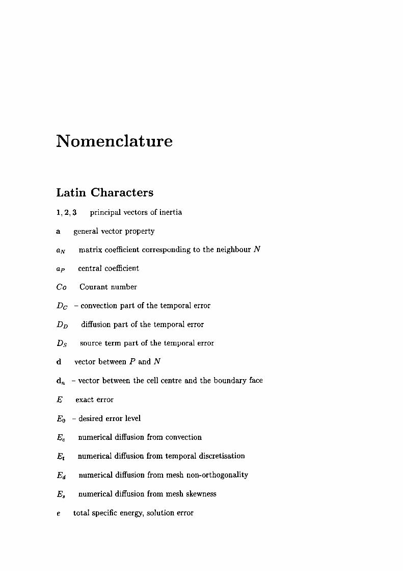
Nomenclature
Latin Characters1, 2, 3 principal vectors of inertia
a general vector property
aN matrix coefficient corresponding to the neighbour N
ap central coefficient
Co Courant number
Dc - convection part of the temporal error
DD diffusion part of the temporal error
D source term part of the temporal error
d vector between P and N
d - vector between the cell centre and the boundary face
E exact error
E0 - desired error level
E numerical diffusion from convection
E numerical diffusion from temporal discretisation
Ed numerical diffusion from mesh non-orthogonality
E5 numerical diffusion from mesh skewness
e total specific energy, solution error

34 List of Tables
em Moment Error estimate
er Residual Error estimate
et Taylor Series Error estimate
enum numerical diffusion error
eM kinetic energy
F mass flux through the face
F 0 convection transport coefficient
Fd diffusion transport coefficient
Fnorm normalisation factor for the residual
f face. point in the centre of the ft ce
f + downstream face
f upstream face
f2 point of interpolation on the face
f interpolation factor
g body force
gb boundary condition on the fixed gradient boundary
H transport part
h mesh size
I unit tensor
i,j unit vectors
k non-orthogonal part of the face area vect r
k turbulent kinetic energy
1 desired I cal mesh size
M second geometric moment tensor
m ske'v ness c rrection vector

List of Tables 35
ma second moment of a
m second moment of
A number of identically performed experiments
N point in the centre of the neighbouring control volume
P pressure, point in the centre of the control volume
p position difference vector
p kinematic pressure, order of accuracy
Q volume energy source
Q surface source
Q v volume source
q heat flux
R right-hand size of the algebraic equation
r smoothness monitor for TVD differencing schemes
Re Reynolds number
resm moment imbalance
rest transient residual
resL spatial residual
resp cell residual
resT temporal residual
S outward-pointing face area vector
Sjface area vector
source term
5e error source term
Sp linear part of the source term
Su constant part of the source term
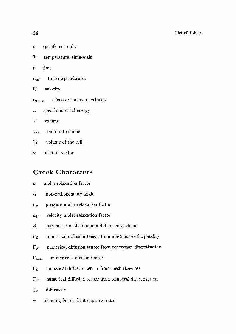
36
List of Tables
s specific entrophy
T temperature, time-scale
t time
tref time-step indicator
U velocity
Utrans effective transport velocity
u specific internal energy
I - volume
M material volume
1 volume of the cell
x position vector
Greek Charactersunder-relaxation factor
0 non-orthogonality angle
ci', pressure under-relaxation factor
< velocity under-relaxation factor
parameter of the Gamma differencing scheme
1'D numerical diffusion tensor from mesh non-orthogonality
FN numerical diffusion tensor from convection discretisation
Fnum numerical diffusion tensor
F numerical diffusi n ten r from mesh skewness
ITTnumerical diffusi n tensor from temporal discretisation
IT 0diffusivitv
'y blending fa tor, heat capa ity ratio
List of Tables
37
z orthogonal part of the face area vector
dissipation rate of turbulent kinetic energy
- effectivity index
0 mesh-to-flow angle
A heat conductivity
Arej refinement criterion
Aunrej unrefinement criterion
u dynamic viscosity
- kinematic viscosity
Vj kinematic eddy viscosity
directionality parameter
p density
a stress tensor
r error directionality
x general tensorial property
W TVD limiter
cI exact solution
0 general scalar property
SuperscriptsqT transpose
mean
q' fluctuation around the mean value
qfl new time-level
q° old time-level
38
List of Tables
q°° "second old" time-level
q unit vector
normalised
Subscriptsq1 value on the face
q value on the boundary face
AbbreviationsBD Blended Differencing
Bi-CG Bi-Conjugate Gradient
BSUD Bounded Streamwise Upwind Differencing
CAD Computer-Aided Design
CAE Computer-Aided Engineering
CAM Computer-Aided Manufacturing
CBC Convection Boundedness Criterion
CD Central Differencing
CFD Computational Fluid Dynamics
CG Conjugate Gradient
CV Control Volume
DNS Direct Numerical Simulation
EOC Experimental Order of Convergence
FCT Flux-Corrected Transport
FV Finite Volume
FVM Finite Volume Method
ICCG Incomplete Cholesky Conjugate Gradient
LDA Laser-Doppler Anemometry
LES Large-Eddy Simulation
LOADS Locally Analytical Differencing Scheme
40
List of Tables
LUD Linear Upwind Differencing
NDR Numerical Diffusion Ratio
NVA Normalised Variable Approach
NVD Normalised Variable Diagram
NURBS Non-Uniform Rational b-Spline
PISO Pressure-Implicit with Splitting of Operators
QUICK - Quadratic Upstream Interpolation for Convective Kinematics
RNG Renormalisation Group
SFCD Self-Filtered Central Differencing
SHARP Simple High-Accuracy Resolution Program
SIMPLE - Semi-Implicit Method for Pressure-Linked Equations
SMART Sharp and Monotonic Algorithm for Realistic Transport
SOT] CUP Second-Order Upwind-Central Differencing-First- Order-Upwind
T\T - Total Variation
TVD Total Variation Diminishing
UD Upwind Differencing
UMIST Upstream Monotonic Interpolation for Scalar Transport

Chapter 1
Introduction
1.1 Background
Numerical tools for structural analysis have been widely accepted in the modern en-
gineering community. The concept of Computer-Aided Design (CAD), Computer-
Aided Manufacturing (CAM) and more generally, Computer-Aided Engineering
(CAE) provides the possibility of optimising the design of the final product in many
different ways. Quick and accurate structural analysis is an important part of the
development process and numerical structures analysis packages are integrated into
most modern CAD systems.
The performance of many products, ranging from kitchen appliances to nuclear
submarines, depends not only on their structural properties, but also on the char-
acteristics of heat transfer, fluid flow and even fluid-solid interaction which play an
important role in their functionality. In order to improve their design, it is necessary
to extend the optimisation by including the fluid flow phenomena into the numeri-
cal simulation. The progress in this area has been much slower the flow problems
generally require a solution of the systems of coupled non-linear partial differential
equations, which are more difficult to solve.
Computational Fluid Dynamics (CFD) provides the methods for numerical sim-
ulation of fluid flows. In spite of the fact that CFD analysis is regularly done in some
areas of engineering, it is still not a widely accepted design tool. The complexity of
42
Introduction
flow regimes in, for example, internal combustion engines, is such that an accurate
and predictive simulation becomes very expensive in terms of time and computer
resources. In order to simulate the features of the flow well, complicated models and
accurate solutions are needed.
The accuracy of numerical solutions represents an interesting field. A numerical
solution is obtained following a set of rules that provide a discrete description of the
governing equations and the solution domain. Its accuracy is determined from the
correspondence between the exact solution and its numerical approximation. The
judgement on the solution accuracy should therefore be done by comparing it with
the exact solution, which is usually unavailable. Error estimation is therefore an
important integral part of numerical solution procedures.
Numerical solutions of fluid flow and heat transfer problems generally include
three groups of errors (Lilek and Perié [88]):
• Modelling errors are defined as the difference between the actual flow and
the exact solution of the mathematical model, describing the behaviour of the
system in terms of coupled partial differential equations. In the case of laminar
flows, modelling errors may be considered negligible for practical purposes -
the Navier-Stokes equations represent a sufficiently accurate model of the flow.
In the case of turbulent, two-phase or reacting flows, the additional models do
not always describe the underlying physical processes accurately. In order to
produce a "manageable" mathematical model certain simplifications are intro-
duced in its construction, potentially causing high modelling errors. A better
mathematical model requires a better understanding of the underlying phys-
ical processes, implies larger systems of equations and an increase in overall
computational effort
• The second group of errors originates from the method used to solve the math-
ematical model. Considering the complexity of the problem and non-linearity
of the equations, it is unreasonable to expect analytical solutions for all but
simplest fi w situations. We are forced to resort to an approximate numerical
1.1 Background
43
solution method. Discretisation errors describe the difference between the
exact solution of the system of algebraic equations obtained by discretising the
governing equations on a given grid and the (usually unknown) exact solution
of the mathematical model. Discretisation errors depend on the accuracy of
the equation discretisation method, as well as the discretisation of the solution
domain.
• The system of algebraic equations obtained from the discretisation is solved
using an iterative solver. The difference between the approximate solution of
the system obtained from the iterative solver and the exact solution of the
system is described by the iteration convergence errors. They can be
reduced to an arbitrary level, specified by the solver tolerance.
Most mathematical models require some kind of empirical input to calibrate the
model constants. For this calibration, it is necessary to ensure that the discretisation
and iteration convergence errors are sufficiently small. As the mathematical models
become more and more accurate, the issue of discretisation accuracy becomes more
important.
Having in mind the properties of the discretisation, it is possible to state several
a-prwn facts about the error. Numerical discretisation of a particular problem con-
sists of two steps: discretisation of the solution domain and equation discretisation.
In the first step, the solution domain is decomposed into discrete space and time
intervals. In equation discretisation a variation of the variable over each region is
prescribed, usually in a polynomial form. As the number of discrete regions increases
to infinity, the approximate solution tends to the exact solution of the mathemati-
cal model. Alternatively, an increase in the order of interpolation leads to the same
result. It is therefore possible to establish two ways of improving the accuracy of a
numerical solution: increasing the number of computational points and increasing
the order of interpolation.
The desired solution accuracy can be specified before the actual analysis it
depends on the objective of the analysis and the accuracy of the mathematical

44 Introduction
models used. If the solution is not accurate enough, the discretisation practice can
be changed. Error estimation, on the other hand, requires a numerical solution
in order to estimate the error. An adaptive procedure, producing the numerical
solution of pre-determined accuracy will therefore consist of several numerical solu-
tions, followed by error estimation and a suitable modification of the discretisation
practice.
In this study, the Finite Volume method of discretisation has been coupled with
an error-driven adaptive mesh refinement procedure in order to automatically pro-
duce numerical solutions of pre-determined accuracy. The procedure consists of a
Finite Volume-type discretisation, followed by an a-posteriori error estimation tool
and adaptive local mesh refinement algorithm. These parts interact automatically,
without an y user intervention. The adaptive procedure creates the solution that
satisfies the accuracy criterion.
In the next Section an overview of the subject is presented, covering the relevant
studies concerning the accuracy of Finite Volume discretisation. a-posteriorz error
estimation and adaptive refinement.
1.2 Previous and Related Studies
1.2.1 Convection Discretisation
The majority of fluid flows encountered in nature and industry are characterised by
high Reynolds numbers, implying the dominance of convective effects (Hirsch [65]).
While the fundamentals of the Finite V lume discretisation are well understood
(Patankar [105], Hirsch [65] , discretisation of the convection term has been a subject
of c ntinual intense debate.
In the framework of the second- rder accurate Finite Volume Method FVM)
a consistent discretisation scheme for the convection term would be second-order
ac urate Central Differencing CD However, the combination of the expUcit time-
in egration, standard in the early development of numerical meth ds, and Cen-

1.2 Previous arid Related Studies 45
tral Differencing creates an unconditionally unstable discretisation practice (Hirsch
[65] . In order to achieve stability, first-order accurate differencing schemes have
been introduced (Courant, Isaacson and Rees [33], Lax [78], Gentry et al. [50]).
The unsatisfactory behaviour of first-order schemes has led Lax and Wendroff [79]
to search for the second-order accurate discretisation. In the Lax-Wendroff family
of schemes, stability is obtained by combining the spatial and temporal discretisa-
tion, leading to a variety of two-step (MacCormack [90], Lerat and Peyret [85]) and
implicit schemes (MacCormack [91], Lerat [84]). In the case of steady-state calcu-
lations, the combined spatial and temporal discretisation introduces an unrealistic
dependence of the solution on the time-step used to create it. In order to overcome
this anomaly, a family of second-order schemes with independent time integration
has been developed in the work of Beam and Warming [13, 14] and Jameson et al.
[68]. Although this approach removes the dependence of spatial accuracy on the
size of the time-step, the differencing schemes of the Beam and Warming family
cause non-physical oscillations in the solution, severely reducing its quality. As a
consequence, the numerical procedure can produce values of the dependent variable
that are outside of its physically meaningful bounds. If one considers the transport
of scalar properties common in fluid flow problems, such as phase fraction, turbulent
kinetic energy, progress variable etc., the importance of boundedness becomes clear.
For example, a negative value of turbulent kinetic energy in calculations involving
k - turbulence models results in negative viscosity, with disastrous effects on the
solution algorithm. It is therefore essential to obtain bounded numerical solutions
when solving transport equations for bounded properties.
The Beam and Warming family of schemes attempts to solve the boundedness
problem by introducing a fourth-order artificial dissipation term (Hirsch [65]), but
boundedness still cannot be guaranteed. Artificial diffusion terms, on the other
hand, reduce the accuracy of the scheme, particularly in the regions of high gradients.
The task of creating a good differencing scheme boils down to a balance between
boundedness and accuracy.
An alternative view on the issues of accuracy and boundedness can be based on
46 Introduction
the sufficient boundedness criterion for the system of algebraic equations. The only
convection differencing scheme that guarantees boundedness is Upwind Differencing
(UD), as all the coefficients in the system of algebraic equations will be positive
even in the absence of physical diffusion (Patankar [105]). This is effectively done
by introducing an excessive amount of numerical diffusion, which changes the na-
ture of the problem from convection-dominated to convection-diffusion balanced. It
was noted by several researchers (Boris and Book [20], Raithby [112, 114], Leonard
[81]) that in cases of high streamline-to-grid skewness, this degradation of accuracy
becomes unacceptable. Although, in principle, mesh refinement solves the prob-
lem, the necessary number of cells is totally impractical for engineering problems
(Leonard [81]).
Several possible solutions to these problems have been proposed, falling into one
of the following categories:
• Locally analytical schemes (LOADS by Raithby [148], Power-Law scheme by
Patankar [105]) use the exact or approximate one-dimensional solution for
the convection-diffusion equation in order to determine the face value of the
dependent variable. Although bounded and somewhat less diffusive than UD,
their accuracy in 2-D and 3-D is still inadequate.
• Upwind-biased differencing schemes, including first-order Upstream-weighted
differencing by Raithby and Torrance [114], Linear Upwinding by Warming
and Beam [146] and Leonard's QUICK differencing scheme [81]. The idea
behind the upwind-biased schemes is to preserve the boundedness of UD by
biasing the interpolation depending on the direction of the flux. The amount
of numerical diffusion is somewhat smaller than for UD, but boundedness is
not preserved.
• Skew-Upwind Differencing schemes Raithby [112, 113] owe their derivation
to the fact that UD does not smear the solution in the case of mesh-to-flow
alignment It is therefore logical to create an upwind scheme that follows the
directi n of the flow, rather than the mesh. The resulting differencing scheme
1.2 Previous and Related Studies
47
behaves better than UD, but with better resolution also introduces unbound-
edness. Bounding of such schemes considerably reduces their accuracy, as in
the case of Bounded Streamwise Upwinding (BSUD) of Gosman and Lai [55]
and Sharif and Busnaina [122].
• Switching schemes. In his Hybrid Differencing scheme, Spalding [126], recog-
nises that the sufficient boundedness criterion holds even for Central Differ-
encing if the cell Peclet number is smaller than two. Under such conditions,
Hybrid Differencing prescribes the use of CD, while UD is used for higher
Pe-numbers in order to guarantee boundedness. However, in typical flow situ-
ations, the Pe-number is considerably higher than two and the scheme reduces
to UD in the bulk of the domain.
• Blended Differencing, introduced by Perié [109]. Recognising the sufficient
boundedness criterion as too strict for practical use, Perié proposes a "blend-
ing" approach, using a certain amount of upwinding combined with a higher-
order scheme (CD or LUD) until boundedness is achieved. Although this
approach potentially improves the accuracy, it is not known in advance how
much blending should be used. In spite of the fact that the amount of blend-
ing needed to preserve boundedness varies from face to face, Perié proposes a
constant blending factor for the whole mesh.
The quest for bounded and accurate differencing schemes continues with the
concept of flux-limiting. Boris and Book [20] introduce a flux-limiter in their Flux
Corrected Transport (FCT) differencing scheme, generalised for multi-dimensional
problems by Zalesak [152]. The idea has been extensively used by van Leer in a series
of papers working "Towards the ultimate conservative differencing scheme" [138,
139, 140, 141, 142]. These methods are sometimes classified as "shock-capturing
schemes", eventually resulting in the class of Total Variation Diminishing (TVD)
differencing schemes. TVD schemes have been developed by Harten [58, 59], Roe
[118], Chakravarthy and Osher [27] and others. A general procedure for constructing
a TVD differencing scheme has been described by Osher and Chakravarthy [103].
48 Introduction
Sweby [129] introduces a graphical interpretation of limiters (Sweby's diagram) and
examines the accuracy of the method.
TVD methodology has been originally derived from the entrophy condition for
supersonic fio'v s and subsequently extended to general scalar transport. The effec-
tive "blending factor" between the higher-order unbounded and first-order bounded
differencing scheme depends on the local shape of the solution, thus introducing a
non-linear dependence of the solution on itself. The convergence of this non-linear
coupling to a unique solution can be strictly proven only for the explicit discretisa-
tion in one spatial dimension1.
One of the main conclusions of the TVD analysis is that a differencing scheme has
to be non-linear in order to be bounded and more than first-order accurate. TVD can
be classified as a switching-blending methodology in which the liscretisation practice
depends on the local shape of the solution. If offers reasonably good accuracy
and at the same time guarantees boundedness. It has been noted (Hirsch [65],
Leonard [83]) that limiters giving good step-resolution, such as Roe's SUPERBEE
[118] tend to distort smooth profiles. On the other hand, limiters such as MINMOD
(Chakravarthy and Osher [27]), although being suitable for smooth profiles are still
too diffusive.
In order to develop a differencing scheme that is able to give good resolution
of sharp profiles and at the same time follow smooth profiles well, the Normalised
Variable Approach N\ TA) has been introduced by Leonard [82]. The TVD criterion
has been rejected as too diffusive. The new condition requires local boundedness
on a cell-by-cell basis. A series of differencing schemes based on the Normalised
Variable Diagram NVD has been presented in recent years. The most popular are
SHARP by Leonard, [82], SMART by Gaskell and Lau [49], UMIST by Lien and
Leschziner [87] and Zhu's HLPA {153]. Leonard [83] introduces a general bounding
method based on the NVD diagram. Unlike the TVD criteri n, NVA d es not offer
any guarantee as regards the convergence of the differencing scheme, even on simple
'The proof hinges n the fact that all expli it duff r n ing s h m s of the La.x-W ndr if and
Beam-\Varming type reduce to UD f r Co—i F r details see eg Wrs h [65

1.2 Previous and Related Studies 49
one-dimensional situations.
NVD differencing schemes produce remarkably good results for both stepwise
profiles and smooth variations of the dependent variable. The amount of numerical
diffusion is reduced to a minimum. However, as a result of the locally changing
discretisation practice problems with convergence sometimes occur. A modified
implementation proposed by Zhu [154] improves convergence, but boundedness can
be guaranteed only for the converged solution.
Apart from the issues of accuracy and boundedness, which are essential for ac-
curate calculations, modern differencing schemes are also required to be convergent
and computationally inexpensive. The issue of computational cost includes both
the additional face-by-face operations required to determine the weighting factors
in TVD and NVD schemes and the additional effort required to obtain solutions for
steady-state problems. With the developmenc of NVD, the accuracy and bound-
edness of differencing schemes has been improved at the expense of convergence.
For this reason, in author's opinion, the issue of convection discretisation is still not
fully resolved.
1.2.2 Error Estimation
The use of error estimates as control parameters in numerical procedures is an old
subject in numerical analysis. Automatic step-control and higher order predictor-
corrector schemes in the numerical solution of ordinary differential equations have
been standard tools for several decades.
The idea of using a-posteriori error estimates on the solutions of partial differ-
ential equations is more recent. In the Finite Element community the idea has been
popularised by Babuska, Rheinboldt and their colleagues [8, 9, 10], Bank and Weiser
[12], Oden et al. [99] and others. These efforts have been mainly directed at elliptic
boundary value problems.
There is a wide range of popular error estimation procedures for Finite Element
calculations. Oden et al. [98] present five groups of error estimators. These include
Element- and Subdomain-Residual methods, Duality methods, Interpolation and

50 Introduction
Post-processing methods. Element Residual methods use the residual in a numerical
solution to estimate the local error. The residual is a function measuring how much
the approximate solution fails to satisfy the governing differential equations and
boundary conditions for the particular finite element. Duality methods, valid for
self-adjoint elliptic problems, use the duality theory of convex optimisation to derive
the upper and lower bounds of the error. Subdomain-Residual methods are based on
the solution of the local error problem over a patch of finite elements. Interpolation
methods use the interpolation theory of finite elements to produce a crude estimate
of the leading term of the truncation error. Post-processing methods are based on
the fact that the solution (which is expected to be smooth) can be improved by
some smoothing algorithm. The estimate of the error is obtained by comparing
the post-processed version of the solution with the one obtained from the actual
calculation.
All these methods are strongly mathematically based and their properties have
been examined for a wide range of shape functions. They have been used not only for
symmetric boundary value problems but have also been extended to unisymmetric
and convection-diffusion problems.
The Local Residual Problem Error estimate is the most recent error estimation
method in the Finite Element method. It produces impressive results, consistently
giving highly accurate estimates for a large variety of problems. It has been devel-
oped mainly by Ainsworth and Oden [2, 3, 4] and Ainsworth [1], but also includes
the previous work by Bank and Weiser [11, 12] and Kelly [71]. The method has been
extended to the Navier-Stokes problem in the work of Oden [101, 102]. It is based
on the element residual method with elements of the duality theory. It is possible
to show that this error estimate gives a strict upper bound on the solution error in
the energy norm. It requires the s lution of a local error problem over each finite
element and an error flux equilibration procedure. Err r flux equilibrati n has been
discussed in length by Kelly 71] and Ainsworth and Oden [3]. Kelly sh ws that
non-equilibrated fluxes result in gross over-estimation of the solution error. The
analysis of the flux equilibration problem has been given by Ainsw rth and Oden

1 2 Previous and Related Studies 51
[4]. Recent work of Oden et al. [102] presents an adaptive refinement technique
based on this error estimate applied to incompressible Navier-Stokes equations.
Error estimation for the Finite Volume Method has been originally examined in
conjunction with turbulence modelling (McGuirk et al. [93]). The main objective
was to estimate the accuracy of the solution in absolute terms. In order to remove
unphysical oscillations in the solution, the convection term of the Navier-Stokes
equation has been discretised using Upwind Differencing. This introduces excessive
amounts of numerical diffusion which interferes with the turbulent diffusion intro-
duced by the turbulence model. Validation of turbulence models becomes a compli-
cated task it is not easy to determine how much of the additional diffusion comes
from the model and how much should be attributed to inaccurate discretisation.
McGuirk and Rodi [92] and McGuirk et al. [93] describe a technique fo measuring
the numerical diffusion of Upwind Differencing. The numerical diffusion term is then
compared with other terms in the transport equation. The accuracy of the solution
depends on the ratio of the numerical diffusion term and the largest physical term in
the equation, called the Numerical Diffusion Ratio (NDR). It has been shown that
some of the computational grids used for model evaluation were too coarse to be used
to study the performance of turbulence models and that grid-independence studies
were misleading. In a later work by Tattersall and McGuirk [130], the numerical dif-
fusion estimate has been coupled with an adaptive node-movement technique. The
method has been used to calculate separated flows around airfoils. It is interesting
to note that the first mesh adaptation in the presented test case actually increased
the solution error due to the loss of orthogonality and mesh-to-flow alignment.
Richardson extrapolation is by far the most popular error estimation method
in Finite Volume calculations. It has been extensively used on a variety of situa-
tions, ranging from supersonic flows (Berger and Oliger [17], Berger and Collela [16],
Berger and Jameson [19] to incompressible problems (Thompson and Ferziger [134],
Muzaferija [97]). In order to estimate the error, Richardson extrapolation uses two
solutions of the same problem on two different grids. The method naturally cou-
ples with the use of multigrid acceleration techniques, where two solutions on grids
52 Introduction
with different cell sizes are already available. Richardson extrapolation is the only
method that can treat non-linearities of the problem, as it compares the solutions
of the complete coupled systems (Muzaferija [97]). Provided that the meshes are
fine enough, the accuracy of the error estimate is acceptable.
For industrial CFD problems, it is not always feasible to produce two solutions.
In some cases, it might be necessary to use hundreds of thousands of cells just to
represent the geometrical features of the computational domain, as in the case of
internal combustion engine cooling systems, steam turbine stators etc.. Single-mesh
single-run error estimates are therefore required.
Haworth et al. [61], Kern [72] and Muzaferija [97] present a new approach to the
problem of error estimation. With the development of NVD differencing schemes,
convection discretisation is becoming more and more accurate. The amount of
numerical diffusion introduced in order to preserve the boundedness of the solution
has been considerably decreased. As a consequence, errors from other sources, such
as insufficient mesh resolution and mesh quality have become more important. In
such cases, an error estimate based only on numerical diffusion cannot produce
an accurate overall picture of the solution quality. It has become necessary to
estimate the error in the case of full second-order accurate discretisation without
any numerical diffusion at all. If the numerical diffusion error is still of interest, the
error estimates can subsequently be modified to capture these effects as well.
Haworth et al. [61] propose the use of the cell to cell imbalances in angular
momentum and kinetic energy to measure of the local solution error. The method
has been tested on a transient flow problem in an axisymmetric internal combus-
tion engine. Unfortunately, the complexity of the selected test case does not allow
comparison of the error estimate with the "exact" error. Also, the method is not
capable of estimating the absolute error levels. An extension of the same approach
to higher moments of the variable has also been suggested but the results of this
extension have not been reported to date.
Muzaferija [97] proposes a method of error estimation based on the higher deriva-
tives of the S lution. This method uses higher-order face interp lation to obtain
1.2 Previous and Related Studies 53
better estimates of the face values for the flow variables. The imbalance resulting
from higher-order interpolation corresponds to the truncation error source of Phillips
[110] and is consequently used to estimate the error for each cell. In order to deter-
mine the absolute error level, a suitable normalisation practice has been suggested.
A second error estimator suggested in this work solves the transport equation for
the solution error, with the aforementioned cell imbalance as the source term. The
estimated error is compared with the "exact" error, obtained using a numerical so-
lution on a very fine mesh. The method is slightly less accurate than Richardson
extrapolation, but it provides a single-mesh measure of the error even in the absence
of numerical diffusion and a means of estimating its magnitude.
The work of Kern [72] is mainly concerned with the formulation of an error
estimator for transient Euler and Navier-Stokes equations. The analysis is performed
for scalar hyperbolic equations in one and two spatial dimensions. In order to follow
the development of the numerical error in time, an error evolution equation has been
derived. Control volumes for the error evolution equation are staggered in space
and time relative to the basic mesh. In order to stabilise the solution procedure for
hyperbolic equations, a certain amount of numerical diffusion has been introduced
either by the Godunov (upwind) differencing scheme, or through flux limiting. In a
similar way to Muzaferija [97], more accurate face values for the flow variables are
obtained using Central Differencing and used as the source in the error evolution
equation. The method therefore measures the difference in the solution between
the effective discretisation and the second-order accurate approximation, which is,
in effect, numerical diffusion. The evolution equation for the error is extended to
two-dimensional problems with constant and variable coefficients, as well as systems
of differential equations. For equations with a diffusion term, the error source term
is modified to include higher-order derivatives, taking into account the error in the
diffusion term. Error estimation results are presented in terms of the Experimental
Order of Convergence (EOC), representing the rate of reduction of the error with
the number of cells. The accuracy of the method has not been tested against the
analytical solution.

54
Introduction
In comparison with the abundance of well-tested and reliable error estimators in
the Finite Element field, Finite Volume error estimation is still in its early stages
of development. The only well-examined and widely used method is Richardson
extrapolation, which in turn requires two solutions of the same problem on two
different meshes. A wide scope of ideas from the Finite Element field can, however,
be modified for the use in the Finite Volume method, as will be demonstrated later
in this Thesis.
1.2.3 Adaptive Refinement
In order to improve the accuracy of subsequent solutions, the distribution of the
error can be used to introduce an appropriate change in the discretisation practice
in the region of high error. In other parts of the domain, where the local error is
considered to be sufficiently small, such change may not be necessary. The local
changes in discretisation are commonly known as "mesh refinement".
Mesh refinement strategies are usually divided into three groups, depending on
the type of the change introduced in the discretisation.
• In h-refinement additional computational points are inserted locally in re-
gions of high numerical error without disturbing the rest of the mesh. It is
also possible to remove points from regions in which the error is low through
an "unrefinement" procedure. Thus, the total number of points generally
changes during the refinement/unrefinement process. The method is particu-
larly suitable for problems with discontinuous solutions, requiring high local
refinement. Examples of h-refinement can be found in the works of Coelho
et at. [31], Vilsmeier and Hãnel [145], Muzaferija [97] and others.
• r-reflnemerit keeps the number of computational points constant throughout
the calculation, but redistributes them depending on the distribution of the
soluti n error. The structure of the mesh is preserved, which makes the method
particularly interesting f r single r multi-block structured meshes The main
dra'back of this approach is that it is not knosn in advan e whether the
1.2 Previous and Related Studies
55
desired level of accuracy is obtainable with the available number of points.
In cases where high local refinement is needed, r-refinement may cause high
mesh distortion and severely degrade the mesh quality in regions where the
resolution is not needed (Hawken et al. [60]). Point relocation algorithms
are based on weighting functions derived from the error estimate. In order
to perform the adaptation, the mesh is described as an elastic mass-spring
system with weighting functions as the load. The distribution of points in the
refined mesh corresponds to the locations of points under the load (see eg.
Ramakrishnan [115]). Particular care has to be taken in order to prevent the
mesh from overlapping. Examples of r-refinement can be found in Tattersall
and McGuirk [130], Ramakrishnan [115], Dwyer [41] and Dandekar et al. [35].
• The third method of refinement is called p-refinement. It is particularly
suitable for Finite Element calculations. This refinement procedure involves
the use of higher-order shape functions in regions of high numerical error. As
the higher-order finite element uses more computational nodes embedded in
the original mesh, changes in the mesh structure and connectivity result. In
order to close the system, additional coupling equations are required, com-
plicating the form of the resulting system of algebraic equations and usually
requiring much more computational effort for the solution (Rachowicz et al.
[111] . The method is suitable for the problems with smoothly changing solu-
tions. In the vicinity of steep gradients, the higher-order shape functions are
prone to spurious oscillations even more than their lower-order ounterparts.
While p-refinement seems to be practical for Finite Element calculations, it
has been rarely used outside of the Finite Element community. Calculations
with p-refinement have been presented by eg. Zienkiewicz [156], Oden et al.
[100] and others.
Reviews of adaptive techniques can be found in eg. Anderson [6], Thompson
[133] and Hawken et al. [60].
In the framework of h-refinement for the Finite Volume method, several different

56 Introduction
ways of point addition have been suggested, with different implications with respect
to the solution accuracy and complexity of the flow solver. Early developments of
adaptive grid techniques based on error estimation in the Finite Difference and Fi-
nite Volume methods were associated with the multigrid approach. The effort was
directed towards the solution of the Euler and Navier-Stokes equations. Brandt [22]
describes a coupled multigrid-local refinement method in which patches of refine-
ment cover the regions where high resolution is needed. The method is referred to
as the "segmental approach". It has been further modified by Caruso [24, 25]. This
type of method is used for transonic and supersonic flows with discontinuities. It
uses a sequence of overlapping grids of increased fineness, thus a1lo' ing multiple
levels of refinement. Each of the overlapping "patches" is an orthogonal structured
grid which can be rotated relative to the basic grid. An optimisation procedure
is used in order to determine the optimum number, size, relative distribution and
orientation of the refinement "patches". In the flow solver, each "patch" is treated
independentl y, with the information transfer between the different parts of the mesh
performed through the "patch" boundary conditions. The algorithm is computa-
tionally efficient since it deals with a series of uniform orthogonal structured grids,
but the critical point is the transfer of information between the overlapping grids
through boundary conditions. This is done explicitly, resulting in weaker coupling
and slower convergence. Resolution problems have been reported at places where
flow features intersect with "patch" boundaries (Berger [16, 17, 18]).
Segmental refinement procedure has been further modified by Berger and Oliger
[17] and Berger and Collela [16], with an error estimation procedure based on
Richardson extrapolation. The problem is solved on two grids with different cell
sizes and with different time-step sizes for each patch. The difference in the solution
is used to estimate the I ading term of the truncation error Since the meshes are
structured, unif rm and orth gonal, no additi nal St rag is required The coarser
mesh is obtained by using every other point of the fine mesh. Cells in which the
error is larger than some pre-determined value are then marked for refinement. A
clustering algorithm developed by Berger [15 is used to optimise the construc ion
1 2 Previous and Related Studies 57
of patches, their position and mesh size. It uses concepts from pattern recognition
and artificial intelligence theory. The simple optimisation algorithm is described
in [17]. One of the attractive features of this approach is that it can be used for
moving shocks in transient calculations although such a calculation has never been
reported.
Thompson and Ferziger [134] presented an adaptive multigrid algorithm for
steady-state Navier-Stokes equations coupled with the multigrid approach. The
error estimation procedure is again based on Richardson extrapolation. Reductions
of the CPU time and computer memory of 20 % and 40 % respectively, compared to
the "pure" multigrid method have been reported. The adaptive refinement proce-
dure is based on the work of Caruso [24, 25]. As a consequence of the interpolation
procedure needed to determine boundary conditions on the refinement "patches",
the method is does not guarantee local mass conservation until a converged solution
is reached. A modified interpolation practice has been proposed but the problem
has never been appropriately solved.
All these methods use structured orthogonal grids and are usually coupled with
multigrid acceleration. The grids are superimposed on the basic grid and the calcu-
lation is coupled through the explicit update of "patch" boundary conditions.
Simpson [124] and Chen et al. [28] suggests the refinement procedure in which
the refinement patches are embedded into the original mesh, thus removing the
interpolation problem. The resulting mesh is then treated in a multi-block manner.
Although this approach presents a considerable improvement in comparison with the
earlier work, it is not appropriate for the situations with a large number of embedded
refinement levels, as the number of blocks becomes so large that it significantly
impairs the performance of the code (Chen et al. [28]).
A number of mesh refinement algorithms based on tetrahedral grids for Euler cal-
culations have been proposed recently (eg. Vidwans and Kallinderis [70, 144], Sonar
et al. [125]). Tetrahedral meshes offer geometrical flexibility, allow simple and high!1
localised refinement and can be created by automatic mesh generation procedures.
Although this approach produces very good results in inviscid calculations, the ex-

58 Introduction
tension of the method to viscous flows has been somewhat less successful. Vilsmeier
and Hänel [145] have developed an adaptive Finite Volume algorithm on tetrahedral
meshes for Euler and Navier-Stokes equations using h-refinement on a cell-by-cell
basis. The emphasis has been placed on the improvement of mesh quality through
successive refinement and anisotropic stretching. Virtual stretching of triangular
elements has been introduced to provide the capability of mesh alignment. It is
performed in the vicinity of walls and in regions of high shear, with the stretching
direction determined from the gradients of the flow variables. Unfortunately, this
results in high distortion of the mesh, decreasing the accuracy of the method.
Muzaferija [97] and Coelho et al. [31] present a method that combines the quality
of hexahedral meshes with the capability of mesh refinement. Regions of local
refinement are embedded into the original grid. The interaction between the coarse
and fine mesh regions is done implicitly, using "split hexahedral" cells. A split
hexahedron is a cell type, hexahedral in topology, which can have more than six
faces. This approach guarantees local and global conservation after every iteration,
but requires an appropriate addressing structure of the mesh.
All efforts reviewed above provide encouraging evidence of the usefulness of the
adaptive refinement techniques, particularly for the flows with discontinuities. In
general. adaptive refinement is at its best when the regions of high error cover
oni) a small portion of the computational domain. The performance of adaptive
algorithms for incompressible flows has been examined almost exclusively for laminar
flow regimes. In spite of the encouraging results, extensions to turbulent flows (eg.
Chen et al. [28]) reported to date are very rare.
1.3 Present Contributions
This studs makes the following specific contribution to the field of Computati nal
Fluid Dynamics:
. A Finite Volume discretisation technique applicable to arbitrarily unstru -
tured meshes in three spatial dimensions is presented The governing equations
1.3 Present Contributions
59
are solved in real space, using a fixed Cartesian coordinate system, for both
steady-state and transient problems. The discretisation practice is second-
order accurate in space and time, making it suitable for second-order contin-
uum mechanics problems. The computational mesh consists of non-uniform
polyhedral control volumes, with a variable number of neighbours. This sim-
plifies the problems of mesh generation for complex geometries, as well as
adaptive mesh refinement. In order to preserve high efficiency of the method
on vector and parallel computer architectures, a "face-addressing" implemen-
tation is used.
• In order to establish the sources of the discretisation error, a detailed analy-
sis of the present discretisation technique is performed. Numerical diffusion
terms resulting from the convection differencing scheme, discretisation of the
transient term and mesh-induced errors are derived.
• In an attempt to increase the accuracy of the method, a new second-order
bounded differencing scheme is proposed. The Gamma differencing scheme is
formulated as a bounded version of Central Differencing, following the Nor-
malised Variable Approach (Leonard [82]). The efficiency of the algorithm
on non-orthogonal meshes is improved through the choice of decomposition of
the face area vector into the orthogonal and non-orthogonal part, based on
the stability of the resulting non-orthogonal treatment.
• The issue of a-posteriori error estimation is analysed in general terms. The
requirements on an error estimate are outlined, as well as three approaches to
error estimation. Following each of these approaches, three new error estimates
are proposed:
- The Direct Taylor Series Error estimate is based on the Taylor series
truncation error analysis. Unlike the widely accepted Richardson extrap-
olation, this new error estimate can be used on a single-mesh solution.
In spite of its asymptotic exactness, the accuracy of this error estimate

60
Introduction
is not considered satisfactory.
- The Moment Error estimate derives the solution error from the imbal-
ance in higher moments of the variable. In order to provide the error
magnitude, the imbalance is normalised in an appropriate way.
- The Residual Error estimate measures the error from the inconsistency
between the prescribed variation of the function over the control volume
and the face interpolation practice, enabling the estimation of the error
in the convection-diffusion part of the discretisation. A normalisation
procedure is used to estimate the influence of the residual on the local
solution accuracy.
The Residual error estimate is also extended to include the influence of the
temporal error. The presented approach allows a separate evaluation of the
spatial and temporal error, which can be used to select the optimal time-step
size for a given spatial mesh.
• Ainsworth and Oden [1, 2, 3, 4] show a possible use of the residual in order to
derive the strict upper bound on the error in the energy norm. Their approach
is extended to the Finite Volume discretisation, with an appropriate error flux
balancing procedure.
The accuracy of the proposed error estimates is tested on several problems
with analytical solutions.
• A mesh adaptation technique is presented. Having in mind the quality of
the available automatic mesh generators, the adaptive local mesh refinement
algorithm has been preferred over adaptive mesh generation. The present
technique enables both insertion and removal of the computational points,
depend ng on the level of the local error.
• Finally, an automatic error-controlled adaptive local refinement unrefinement
alg rithm is assembled and successfully aplhed to several steady-state and
transient laminar and turbulent fi vs
1.4 Thesis Outline 61
1.4 Thesis Outline
In Chapter 2, the governing equations of continuum mechanics are summarised,
together with the constitutive relations for Newtonian fluids. A short overview of
turbulence modelling techniques is also presented.
Chapter 3 presents a second-order accurate Finite Volume method on arbitrarily
unstructured meshes. The setup of the computational mesh and the addressing
structure are described. Discretisation of a general scalar transport equation is
examined term by term. The Gamma differencing scheme is derived and tested or'
several simple situations. The numerical diffusion tensors for the discretisation errors
are derived and their influence on the solution is illustrated on simple problems.
The performance of the proposed non-orthogonality treatments is also presented.
Finally, the segregated approach for the coupled systems of differential equations
used in this study is described and a solution methodology for steady-state and
transient turbulent flow calculations is summarised.
The issue of a-posteriori error estimation is addressed in Chapter 4. Several
new methods of error estimation for both steady-state and transient problems are
proposed. A Taylor series truncation error analysis is performed and its result is
compared with Richardson extrapolation. An alternative form of Taylor series error
estimation is proposed. The Moment Error estimate is derived from the transport
equation for the second moment of the solution. Inconsistency between face inter-
polation and volume integration is used to define the residual as the measure of the
local solution error, resulting in the Residual Error estimate. The concept is modi-
fied in order to include the temporal derivative, thus extending its applicability to
transient calculations. The proposed formulation of the residual is used to extend
the Local Problem Error estimate to Finite Volume discretisation. The performance
of error estimates is examined on simple cases with analytical solutions.
Chapter 5 outlines algorithms for error-driven adaptive mesh generation and
local mesh refinement. Their interaction with the estimated error distribution is
examined. The selected algorithm, based on cell-by-cell embedded refinement and
62
Introduction
unrefinement and "1-irregular" meshes is described. Comparison of uniform and
adaptive refinement is performed on a simple test case.
In Chapter 6, the proposed solution procedure is applied on four test cases. Su-
personic inviscid flow over a forward-facing step is used to test the performance of
adaptive refinement/unrefinement in conjunction with an error indicator. The accu-
racy of error estimation is examined on steady-state two-dimensional flow over a hill,
in both laminar and turbulent flow regimes. The interaction of the wall-functions
and low-Re turbulence models with error estimation and mesh refinement is also ex-
amined. A three-dimensional turbulent flow over a swept backward-facing step has
been selected to examine the overall performance of the error-controlled adaptive
refinement approach in a 3-D situation. Finally, laminar vortex shedding behind a
cylinder illustrates the capabilities of the algorithm for transient flow calculations.
Chapter 7 summarises the Thesis and offers some conclusions and suggestions
for future research.

Chapter 2
Governing Equations
2.1 Governing Equations of Continuum
Mechanics
The numerical procedure presented in this study deals with the problems of con-
tinuum mechanics. Characteristic length- and time-scales for such problems are
considerably larger than the scales of the discrete structure of the matter. It is
therefore possible to describe any macroscopic physical property of the matter as a
continuous function in macroscopic coordinates (time, space).
We shall start by introducing the concept of the material derivative, describing
the rate of change of the intensive physical property in time
pq(x,t)dV - pq5dV+ dS.(pq5U), (2.1)dt VMt LMt 8VMt
where U is the velocity vector and dS is the outward pointing unit normal on i9VM(t).
The rate of change of in VM is equal to its volume and surface sources:
-- f pq5dV + dS.(pq5U) = J Qv(cb) dV + dS.Qs(q5),ôt VMt OVMt VMt 8VMt
(2.2)
or, in the differential form:
Qv 5)+V.Qs ). (2.3)
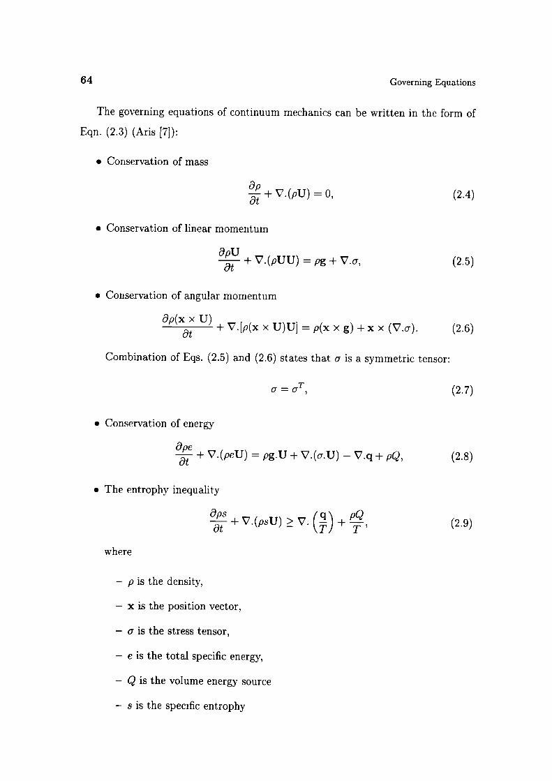
64
Governing Equations
The governing equations of continuum mechanics can be written in the form of
Eqn. (2.3) (Aris [7]):
. Conservation of mass
+ V.(pU) = 0, (2.4)
• Conservation of linear momentum
DpU + V.(pUU) = pg + V.cr, (2.5)
• Conservation of angular momentum
8p(x x U) + V.[p(x x U)U] = p(x x g) + x x (V.a). (2.6)
Combination of Eqs. (2.5) and (2.6) states that a is a symmetric tensor:
a = aT
(2.7)
• Conservation of energy
+ V.(peU) = pg.0 + V.(a.U) - V.q + pQ, (2.8)
• The entrophy inequality
fq\ pQ+ V.(psU) ^ V. +
-_,
(2.9)at
where
- p is the density,
- x is the position vector,
- a is the stress tensor,
- e is the total specific energy,
- Q is the volume energy source
- s is the specific entrophy
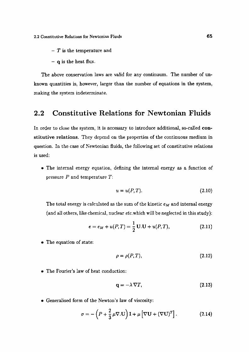
2.2 Constitutive Relations for Newtonian Fluids 65
- T is the temperature and
- q is the heat flux.
The above conservation laws are valid for any continuum. The number of un-
known quantities is, however, larger than the number of equations in the system,
making the system indeterminate.
2.2 Constitutive Relations for Newtonian Fluids
In order to close the system, it is necessary to introduce additional, so-called con-
stitutive relations. They depend on the properties of the continuous medium in
question. In the case of Newtonian fluids, the following set of constitutive relations
is used:
The internal energy equation, defining the internal energy as a function of
pressure P and temperature T:
u = u(P,T). (2.10)
The total energy is calculated as the sum of the kinetic eM and internal energy
(and all others, like chemical, nuclear etc.which will be neglected in this study):
e = eM + u(P,T) = U.0 +u(P,T), (2.11)
The equation of state:
p=p(P,T), (2.12)
. The Fourier's law of heat conduction:
q=—XVT, (2.13)
. Generalised form of the Newton's law of viscosity:
a = - ( + iiv.u) i + [vu + (vu)T] . (2.14)
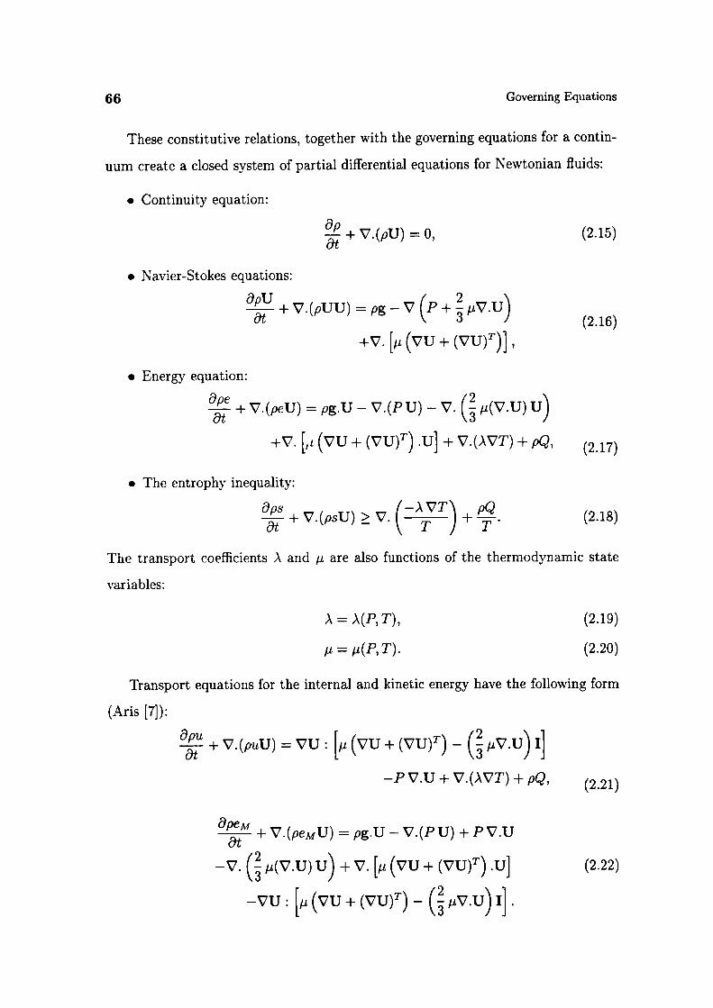
66
Governing Equations
These constitutive relations, together with the governing equations for a contin-
uum create a closed system of partial differential equations for Newtonian fluids:
Continuity equation:
+ V.(pU) = 0, (2.15)
• Navier-Stokes equations:
aU+ V.(pUU) = pg - v ( + pv.u)
(2.16)
+v. [ (vu + (vu)T)],
• Energy equation:
+ V.(peu) = pg.0 - V.(Pu) - v. ( ,(v.u) u)
+v. {, (vu + (VU) T) .u] + v.(AVT) + pQ, (2.17)
• The entrophy inequality:
Ops f—AVT\ pQ--- + V.(psU) ^ V.
T ) +(2.18)
The transport coefficients A and ,i are also functions of the thermodynamic state
variables:
A=
(2.19)
= p(P,T). (2.20)
Transport equations for the internal and kinetic energy have the following form
(Aris [7]):
+ v.(puu) = vu: [ (vu + (vu)T) - ( zv.u) i]
—Pv.0 + v.(AvT) + (2.21)
+ v . (peMu) = pg.0 - V.(Pu) + Pv.0
—v. ( (v.u) u) + v. [ (vu + (vu)T) .u] (2.22)
—vu: (vu + (vu)T) - ( iv.u) i].

2.3 Turbulence Modelling
67
For incompressible isothermal fluids (p = const., ). = oo), the system can be
further simplified:
VU = 0, (2.23)
+V.(UU)=g—Vp+V.(uVU), (2.24)
where ii is the kinematic viscosity and p kinematic pressure. All other equations in
the system are decoupled.
Most dependent variables require a gradient-diffusion term of the following form
(Patankar [105]):
—V.(FV). (2.25)
This term will therefore be included into the transport equation for a general ten-
sorial property x:
+ V.(pU) - V.(prV) = S(x), (2.26)
where S(x) contains all terms that cannot be fitted on the left-hand side.
2.3 Turbulence Modelling
Most fluid flows occurring in nature are turbulent. Turbulence can be described as
a state of continuous instability in the flow, where it is still possible to separate the
fluctuations from the mean flow properties. It is characterised by irregularity in the
flow, increased diffusivity and energy dissipation (Tennekes and Lumley [132]). Tur-
bulent flows are always three-dimensional and time dependent, even if the boundary
conditions of the flow do not change in time. The range of scales in such flows is very
large, from the smallest turbulent eddies characterised by Kolmogorov microscales,
to the flow features comparable with the size of the geometry. A comprehensive
review of simulation techniques for turbulent flows can be found in Ferziger [47]. A
brief overview of the modelling techniques will be given here.
There are several possible approaches to the simulation of turbulent flows. The
first, Direct Numerical Simulation (DNS) (Eswaran and Pope [44, 45], Rogallo and
68 Governing Equations
Mom [119], Rogers and Mom [120]) numerically integrates the governing equations
over the whole range of turbulent scales. The requirements on mesh resolution
and time-step size put very high demands on the computer resources, rendering it
unsuitable for engineering applications.
The second approach is generally known as Large Eddy Simulation (LES). In
order to separate different length scales in a turbulent flow field, a spatial filter is
applied. Large scale structures that can be resolved by the numerical method on
a given mesh are called the super-grid scales. The influence of all other (sub-grid)
scales to the super-grid behaviour is modelled. The rationale behind this princi-
ple lies in the fact that the small scales of turbulence are more homogeneous and
isotropic and therefore easier to model. As the mesh gets finer, the number of scales
that require modelling becomes smaller, thus approaching the Direct Numerical
Simulation. Examples of this approach can be found in Deardorif [38], Givi [53] and
Mom and Kim [95].
An alternative approach to the simulation of turbulent flows is statistical. Sep-
arating the local value of the variable into the mean and the fluctuation around the
mean, it is possible to derive the equations for the mean properties themselves. The
selection of averaging methods depends on the characteristics of turbulent flow, and
according to Hinze [64], the following three averaging method can be distinguished:
1. Time averaging in a fixed point of spaee, for stationary turbulence,
2. Space averaging for a fixed moment in time in the case of homogeneous tur-
bulence,
3. Ensemble averaging for a series of identical experiments. This is the most
general form of averaging.
Ml these methods can appear in two versions, unweighted (Reynolds and weighted
eg densi y-weighted Favre averaging, [46]). The Reynolds averaging technique
perates as follows:
x,t —(x,t +11(x,t , (2.27)
2.3 Turbulence Modelling 69
where '(x, t) denotes the fluctuation about the mean value, defined as:
1w(x, t) = lim -- q 2 (x, t), (2.28)
N—+oo Jv-1
and A1 is the number of identically performed experiments.
Applying the above averaging procedure to the incompressible Navier-Stokes
equations, the following form of the averaged equations can be obtained:
v.U=o, (2.29)
+ V.(tYU) = g - v + V. (vVU) + U' U'. (2.30)
In the case of compressible flows, Favre averaging is usually applied (see eg. Favre
[46], Cebeci and Smith [26]).
The term UTU7 is called the Reynolds stress tensor. In order to close the system,
further modelling is necessary.
The task of Reynolds averaged turbulence modelling is to express the Reynolds
stress tensor in terms of the known quantities. There are two widely accepted
approaches. The first approach formulates and solves the transport equation for the
Reynolds stress tensor (and higher moments, depending on the order of the closure).
It is, however, still necessary to model some of the terms, since the number of
unknowns increases faster than the number of equations. Examples of this treatment
can be found in Rotta [121], Launder et al. [75] and Hanjalié and Rodi [56]. The
second, and more popular approach prescribes a relationship between the Reynolds
stress and mean velocity gradient. Although models prescribing non-linear relations
have been proposed recently (Speziale [127] and Shih et al. [123]), the most popular
approach is to use the Boussinesq approximation (Boussinesq [21]), which prescribes
a linear relation of the form:
u'u' = (vu + (VU)T) + k I, (2.31)
where
k=U'.U'. (2.32)
70
Governing Equations
The kinematic eddy viscosity t can be evaluated in many different ways, rang-
ing from algebraic relations and local equilibrium assumptions to the solution of
transport equations. The most popular approach is to express zi as a function of
the turbulent kinetic energy k and its dissipation rate i, leading to a "two-equation"
turbulence model:
lit = k2
(2.33)
e = U'U' : VU', (2.34)
so named because k and e are obtained by the solution of their respective transport
equations. The first model of this kind has been proposed by Harlow and Nakayama
[57]. Derivation of the transport equations for k and c can be found in eg. Launder
and Spalding [77].
In fact, a wide variety of k - e models exists, the most noteworthy being the
standard k - c model by Launder and Spalding [77] and the RNG k - e variant by
Yakhot and Orszag [150, 151].
The physics of turbulence in the vicinity of impermeable no-slip walls is consid-
erably different from the other parts of the flow. It is therefore necessary to use
appropriate turbulence models in the near-wall region. For the most general and
detailed treatment, low-Re versions should be used (see eg. Lam and Bremhorst [74],
Launder and Sharma [76] etc.). However, in order to resolve the near-wall details
well, the computational mesh needs to be very fine in this region.
It is possible to compensate for the existence of the wall without resolving the
near-wall region, albeit at the expense of considerable approximation and, as will
be shown later, also with adverse effects on numerical resolution). Wall-functions
Launder and Spalding [77] represent a simpEfied model of turbulence, which mim-
ics the near-wall behaviour of the velocity, k and e. It assumes that the flow near
the solid wall behaves like a fully developed turbulent boundary layer. In numerical
simulations, this mod 1 is used to bridge the regions of high gradients near the wall
and couples with the high-Re k - c model in the rest of the domain. For the details
2.3 Turbulence Modelling
71
of its derivation and implementation, the reader is referred to Launder and Spalding
[77] and Gosman and Ideriah [54].

72 Governing Equations
Chapter 3
Finite Volume Discretisation
3.1 Introduction
The purpose of any discretisation practice is to transform one or more partial differ-
ential equations into a corresponding system of algebraic equations. The solution of
this system produces a set of values which correspond to the solution of the original
equations at some pre-determined locations in space and time, provided certain con-
ditions, to be defined later, are satisfied. The discretisation process can be divided
into two steps. the discretisation of the solution domain and equation discretisation
(Hirsch [65], Muzaferija [97]).
The discretisation of the solution domain produces a numerical description of
the computational domain, including the positions of points in which the solution is
sought and the description of the boundary. The space is divided into a finite number
of discrete regions, called control volumes or cells. For transient simulations, the
time interval is also split into a finite number of time-steps. Equation discretisation
gives an appropriate transformation of terms of governing equations into algebraic
expressions.
This Chapter presents the Finite Volume method (FVM) of discretisation, with
the following properties:
. The method is based on discretising the integral form of governing equations
74
Finite Volume Discretisation
over each control volume. The basic quantities, such as mass and momentum,
will therefore be conserved at the discrete level.
• Equations are solved in a fixed Cartesian coordinate system on the mesh that
does not change in time. The method is applicable to both steady-state and
transient calculations.
• The control volumes can be of a general polyhedral shape, with a variable
number of neighbours, thus creating an arbitrarily unstructured mesh. All
dependent variables share the same control volumes, which is usually called
the colocated or non-staggered variable arrangement (Rhie and Chow [117],
Perié [109]).
• Systems of partial differential equations are treated in the segregated way
(Patankar and Spalding [107], van Doormaal and Raithby [137]), meaning
that they are solved one at a time, with the inter-equation coupling treated
in the explicit manner. Non-linear differential equations are linearised before
the discretisation and the non-linear terms are lagged.
The details of the discretisation practice and implementation of boundary con-
ditions will be described in the remainder of this Chapter. In Section 3.2 the mesh
arrangement is described. Section 3.3 presents a discretisation procedure for a scalar
transport equation. The discretisation of the convection, diffusion and source terms
is presented in Section 3.3.1. Several possibilities for the discretisation of the tem-
poral derivative are given in Section 3.3.2. The implementation of the boundary
conditions is discussed in Section 3.3.3. A new second order accurate and bounded
convection differencing scheme is proposed in Section 3.4. Some details of the so-
lution procedure, including the treatment of mesE non-orth Ohãlitdeferred cor-
rection and the under-relaxation are given in Section 3.5. Section 3.6 discusses the
errors introduced during the discretisation process. Numerical examples, illustrat-
ing the behaviour of the discretised terms and numerical errors, are presented in
Section 3.7.
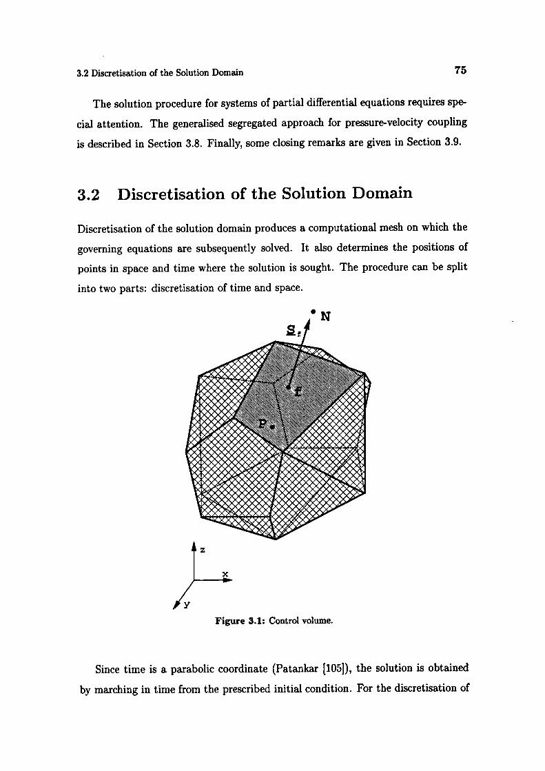
3.2 Discretisation of the Solution Domain 75
The solution procedure for systems of partial differential equations requires spe-
cial attention. The generalised segregated approach for pressure-velocity coupling
is described in Section 3.8. Finally, some closing remarks are given in Section 3.9.
3.2 Discretisation of the Solution Domain
Discretisation of the solution domain produces a computational mesh on which the
governing equations are subsequently solved. It also determines the positions of
points in space and time where the solution is sought. The procedure can be split
into two parts: discretisation of time and space.
Figure 3.1: Control volume.
Since time is a parabolic coordinate (Patankar [105]), the solution is obtained
by marching in time from the prescribed initial condition. For the discretisation of
76 Finite Volume Dis retisation
time, it is therefore sufficient to prescribe the size of the time-step that will be used
during the calculation.
The discretisation of space for the Finite Volume method used in this study
requires a subdivision of the domain into control volumes (CV). Control volumes do
not overlap and completely fill the computational domain. In the present study all
variables share the same CV-s.
A typical control volume is shown in Fig. 3.1. The computational point P is
located at the centroid of the control volumes, such that:
Jx—xp)dV==O. (3.1)
'P
The control volume is bounded by a set of fiat faces and each face is shared with
only one neighbouring CV. The topology of the control volume is not important -
it is a general polyhedron.
The cell faces in the mesh can be divided into two groups internal faces (between
two control volumes) and boundary faces, which coincide with the boundaries of the
domain. The face area vector S j is constructed for each face in such a way that it
points outwards from the cell with the lower label, is normal to the face and has the
magnitude equal to the area of the face. The cell with the lower label is called the
"owner" of the face its label is stored in the "owner" array. The label of the other
cell "neighbour" is stored in the "neighbour" array. Boundary face area vectors
point outwards from the computational domain boundary faces are "owned" by
the adjacent cells. For the shaded face in Fig. 3.1, the owner and neighbour cell
centres are marked with P and N, as the face area vector S 1 points outwards from
the P control volume. For simplicity, all faces of the control volume will be marked
with f, which also represents the point in the middle of the face (see Fig. 3.1
The capability of the discretisation practice to deal with arbitrary control vol-
umes gives considerable freed m in mesh generation. It is particularly useful in
meshing c mplex geometrical configurations in three spatial dimensions. Arbitrar-
dv unstructured m sh s als mt r ct well with the concept of local grid refinement,
where the computational points are added in the parts of the domain where high
3.3 Discretisation of the fransport Equation 77
resolution is necessary, without disturbing the rest of the mesh.
3.3 Discretisation of the Transport Equation
The standard form of the transport equation for a scalar property 0 is:
+ V.(pUO) - V.(pFV) = s(0). (3.2)at -
convection term diffusion term source termtemporal denvative
This is a second-order equation, as the diffusion term includes the second derivative
of in space. For good accuracy, it is necessary for the order of the discretisation to
be equal to or higher than the order of the equation that is being discretised. The
discretisation practice adopted in this study is second-order accurate in space and
time and will be presented in the rest of this Chapter. The individual terms of the
transport equation will be treated separately.
In certain parts of the discretisation it is necessary to relax the accuracy re-
quirement, either to accommodate for the irregularities in the mesh structure or to
preserve the boundedness of the solution'. Any deviation from the prescribed order
of accuracy creates a discretisation error, which is of the order of other terms in the
original equation and dissappers only in the limit of excessively fine mesh. Particu-
lar attention will therefore be paid to the sources of discretisation error representing
such behaviour.
The accuracy of the discretisation method depends on the assumed variation of
the function 0 = x, t in space and time around the point P. In order to obtain a
second-order accurate method, this variation must be linear in both space and time,
i.e. it is assumed that:
0(x) = çbp + (x - xp).(VqS p, (3.3)
( alt0(t + z.t) = 0 + t - , (3.4)
'These issues will be addressed in length in Sections 3.3.1 and 3.6.
78
Finite Volume Discretisation
where
qp = q(xp), (3.5
= (3.6)
Let us consider the Taylor series expansion in space of a function around the
point x:
x) = Øp + (x - xp).(V p + - Xp 2: (VV)p
+ - xp) 3 :: (VVVq)p
1+ . . . + -,(x - xp) :(Vç5)p +... (3.7)
The expression (x - xp)" in Eqn. (3.7) and consequent equations in this study
represents the nth tensorial product of the vector (x - Xp) with itself, producing an
nth rank tensor. The operator ::: " is the inner product of two nth rank tensors,
creating a scalar.
Comparison between the assumed variation, Eqn. (3.3), and the Taylor series
expansion, Eqn. (3.7), shows that the first term of the truncation error scales with
(x - Xp) 2 , which is for a 1-D situation equal to the square of the size of the control
volume. The assumed spatial variation is therefore second-order accurate in space.
An equivalent analysis shows that the truncation error in Eqn. (3.4) scales with t2,
resulting in the second-order temporal accuracy.
The Finite Volume method requires that Eqn. (3.2) is satisfied over the control
volume Vp around the point P in the integral form:
+ a j pdV + f V.(pU) dV - [ V.(pFV) dv] dt
3tt+i
=j (J S dv) dt. (3.8VP
The discretisation of Eqn. (3.8 will now be examined term by term.
3.3.1 Discretisation of Spatial Terms
Let us first examine the discretisation of spatial terms. The generalised form of
Gauss' theorem il1 be used throughout the discretisation procedure, involving the e
3.3 Discretisation of the '&ansport Equation 79
identities:
= ydS.a, (39)
(3.10)
]dSa (3.11)
where 9V is the closed surface bounding the volume V and dS represents an in-
finitesimal surface element with associated outward pointing normal on V.
A series of volume and surface integrals needs to be evaluated. Taking into
account the prescribed variation of over the control volume P, Eqn. (3.3), it
follows:
ç5(x) dV =
[cAp + (x - xp).(V)p] dV
=" fVp {Jx_xPdvJ.vcA)P
= qpVp, (3.12)
where Vp is the volume of the cell. The second integral in Eqn. (3.12) is equal to
zero because the point P is the centroid of the control volume.
Let us now consider the terms under the divergence operator. Having in mind
that the CV is bounded by a series of flat faces, Eqn. (3.9) can be transformed into
a sum of integrals over all faces:
JV.adV=(
Vp OVp
=(jds.a). (3.13)
The assumption of linear variation of cA leads to the following expression for the
face integral in Eqn. (3.13):
J ds.a= (fiis) .a1 + {jds(x_xf)] : (Va)1
= S.af . (3.14)
Combining Eqs. (3.12), (3.13) and (3.14), a second-order accurate discretised form

80
Finite Volume Discretisation
of the Gauss' theorem is obtained:
(V.a) Vp = S.a. (3.15)I
Here, the subscript f implies the value of the variable (in this case, a) in the middle
of the face and S is the outward-pointing face area vector. In the current mesh
structure, the face area vector S 1 point outwards from P only if f is "owned' by
P. For the "neighbouring" faces S points inwards, which needs to be taken into
account in the sum in Eqn. (3.15). The sum over the faces is therefore split into
sums over "owned" and "neighbouring" faces:
S.a = - (3.16)f Owner neighbour
This is true for every summation over the faces. In the rst of the text, this split is
automatically assumed.
3.3.1.1 Convection Term
The discretisation of the convection term is obtained using Eqn. (3.15):
fV.(pU)dV=S.(pUq)1lP I
= S.(pU) qjI
=F75f , 3.17)I
where F in Eqn. (3.17) represents the mass flux through the face:
F = S.(pU) 1 . (3.18)
The calculation of these face fluxes will later be discussed separately in Section 3.8.
For now it can be assumed that the flux is calculated from the interpolated values
of p and U.
Eqs. 3 17 and (3 18) also require the face value of the variable q calculated from
the values in the cell centres, s hich is obtained using the convection differencing
scheme.
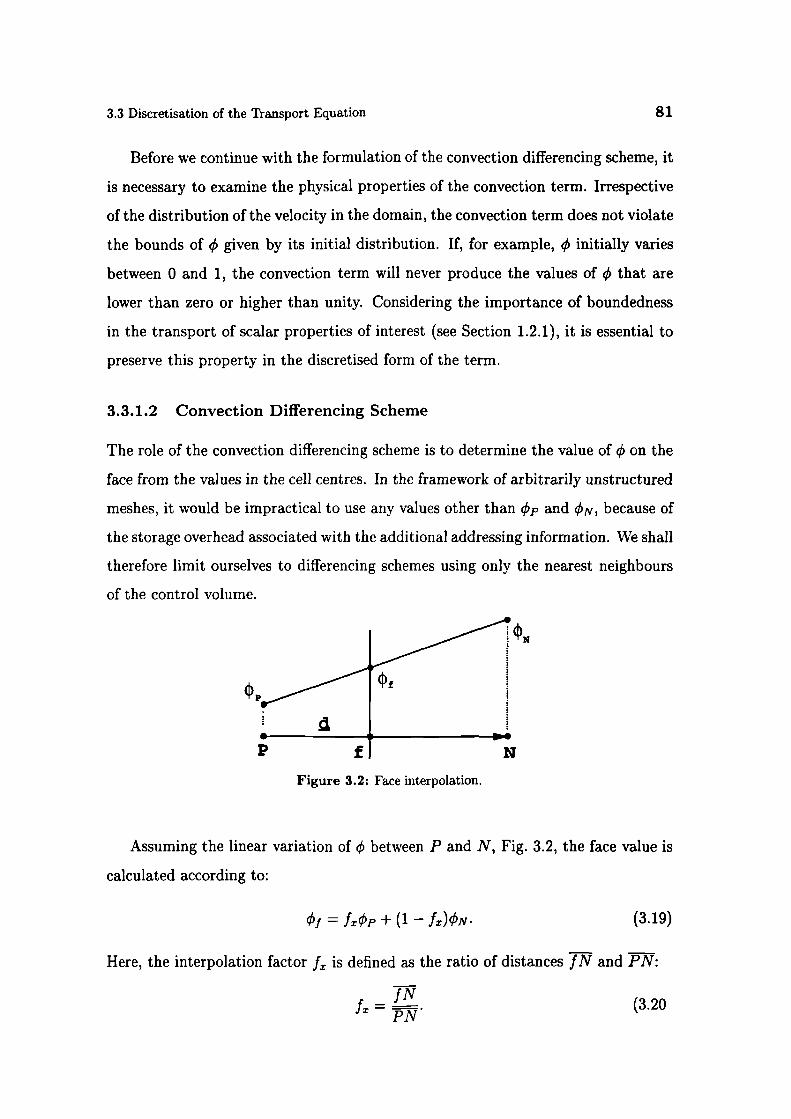
I
3.3 Discretisation of the Transport Equation
81
Before we continue with the formulation of the convection differencing scheme, it
is necessary to examine the physical properties of the convection term. Irrespective
of the distribution of the velocity in the domain, the convection term does not violate
the bounds of g5 given by its initial distribution. If, for example, 4' initially varies
between 0 and 1, the convection term will never produce the values of 4' that are
lower than zero or higher than unity. Considering the importance of boundedness
in the transport of scalar properties of interest (see Section 1.2.1), it is essential to
preserve this property in the discretised form of the term.
3.3.1.2 Convection Differencing Scheme
The role of the convection differencing scheme is to determine the value of 4' on the
face from the values in the cell centres. In the framework of arbitrarily unstructured
meshes, it would be impractical to use any values other than çbp and 4'N, because of
the storage overhead associated with the additional addressing information. We shall
therefore limit ourselves to differencing schemes using only the nearest neighbours
of the control volume.
Figure 3.2: Face interpolation.
Assuming the linear variation of 4' between P and N, Fig. 3.2, the face value is
calculated according to:
= fc/,j, + (1 - f)cbN . (3.19)
Here, the interpolation factor f is defined as the ratio of distances JN and PN:
f = (3.20
82
Finite Volume Discretisation
The differencing scheme using Eqn. (3.19 to determine the face value of çb is
called Central Differencing (CD). Although this has been the subject of some
debate, Ferziger and Perié [48] show that it is second order accurate even on non-
uniform meshes. This is consistent with the overall accurac y of the method. It
has been noted, however that CD causes unphysical oscillations in the solution for
convection-dominated problems (Patankar, [105], Hirsch [65]), thus violating the
boundedness of the solution.
An alternative discretisation scheme that guarantees boundedness is Upwind
Differencing (UD). The face value of is determined according to the direction of
the flow:
- Icbi=cbp for F ^ 0.(3.2])
for F < 0.
Boundedness of the solution is guaranteed through the sufficient boundedness crite-
rion for systems of algebraic equations (see eg. Patankar, [105]). As it will be shown
later (Section 3.6), boundedness of UD is effectively insured at the expense of the
accuracy, by implicitly introducing the numerical diffusion term This term violates
the order of accuracy of the discretisation and can severely distort the solution.
Blended Differencing (BD) (Perié [109]) represents an attempt to preserve
both boundedness and accuracy of the solution. It is a linear combination of UD,
Eqn. (3.21) and CD, Eqn. (3.19
qf=(1—_y qf)uD+ycbf)cD, (3.22)
or
ç51=[(i—y max(sgnF),0 +7f]p
-i- [(1 -y) mzm(sgn(F), 0) + 'y ( l f)]N (3.23
The blending factor y, 0 1, determines how much numerical diffusion will be
introduced Peric [109] proposes a constant y for all faces of the mesh For 0
the scheme reduces to liD.
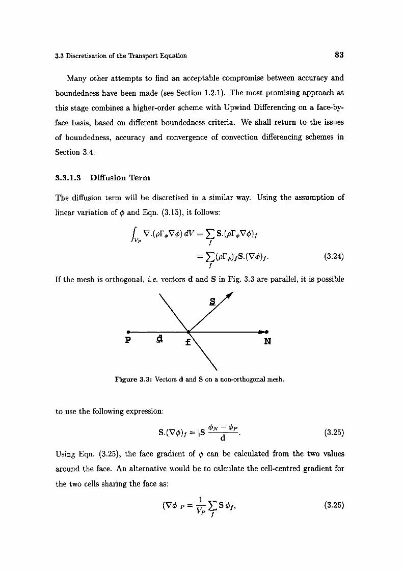
I
3.3 Discretisation of the Transport Equation
83
Many other attempts to find an acceptable compromise between accuracy and
boundedness have been made (see Section 1.2.1). The most promising approach at
this stage combines a higher-order scheme with Upwind Differencing on a face-by-
face basis, based on different boundedness criteria. We shall return to the issues
of boundedness, accuracy and convergence of convection differencing schemes in
Section 3.4.
3.3.1.3 Diffusion Term
The diffusion term will be discretised in a similar way. Using the assumption of
linear variation of and Eqn. (3.15), it follows:
fV.(pI'Vq5) dV = S.(pT,V)1
Vp
/
= >(pI')fS.(V')f. (3.24)I
If the mesh is orthogonal, i.e. vectors d and S in Fig. 3.3 are parallel, it is possible
Figure 3.3: Vectors d and S on a non-orthogonal mesh.
to use the following expression:
S.(Vq) 1IS". (3.25)
Using Eqn. (3.25), the face gradient of can be calculated from the two values
around the face. An alternative would be to calculate the cell-centred gradient for
the two cells sharing the face as:
(Vp-ESj, (3.26)
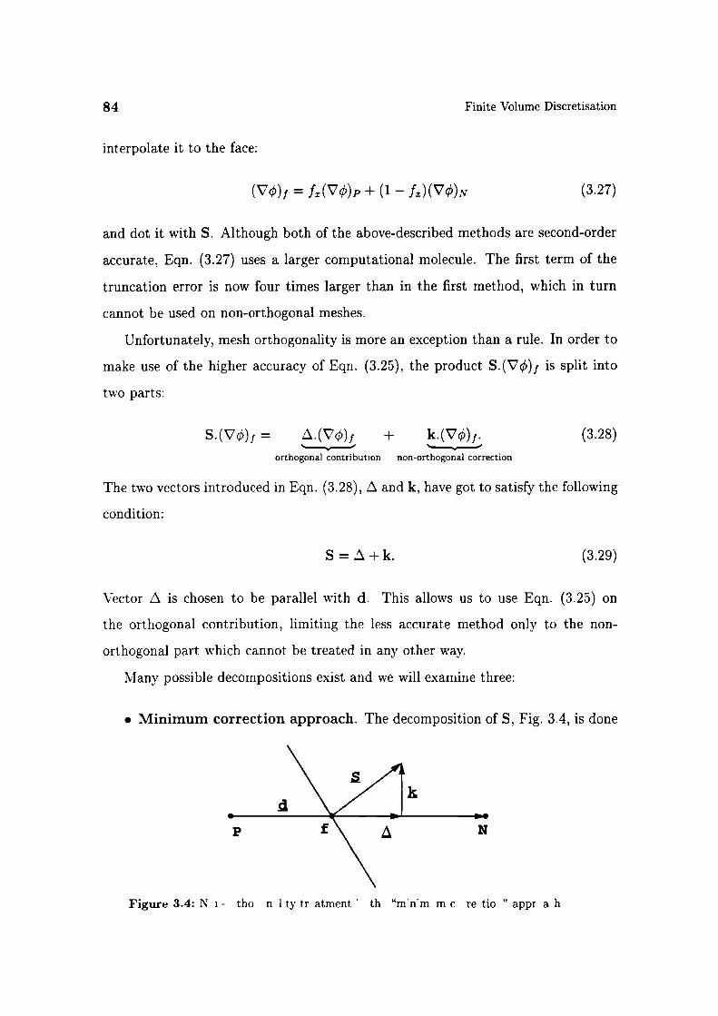
84 Finite Volume Discretisation
interpolate it to the face:
(V) = f(V)p + (1 - fS )(Vq5) N (3.27)
and dot it with S. Although both of the above-described methods are second-order
accurate, Eqn. (3.27) uses a larger computational molecule. The first term of the
truncation error is now four times larger than in the first method, which in turn
cannot be used on non-orthogonal meshes.
Unfortunately, mesh orthogonality is more an exception than a rule. In order to
make use of the higher accuracy of Eqn. (3.25), the product S.(Vq5) 1 is split into
two parts:
S.(V)j = .(V)f + k.(V)1. (3.28)
orthogonal contribution non-orthogonal correction
The two vectors introduced in Eqn. (3.28), z and k, have got to satisfy the following
condition:
S =+k. (3.29)
Vector L is chosen to be parallel with d. This allows us to use Eqn. (3.25) on
the orthogonal contribution, limiting the less accurate method only to the non-
orthogonal part which cannot be treated in any other way.
Many possible decompositions exist and we will examine three:
. Minimum correction approach. The decomposition of S, Fig. 3.4, is done
Figure 3.4: N i - tho n 1 ty tr atmenL th "mnm m c re tio " appr a h
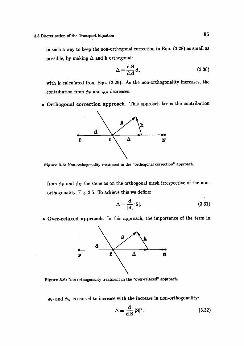
3.3 Discretisation of the Transport Equation 85
in such a way to keep the non-orthogonal correction in Eqn. (3.28) as small as
possible, by making z and k orthogonal:
(3.30)
with k calculated from Eqn. (3.29). As the non-orthogonality increases, the
contribution from çbp and bN decreases.
Orthogonal correction approach. This approach keeps the contribution
Figure 3.5: Non-orthogonality treatment in the "orthogonal correction" approach.
from qSp and q5 the same as on the orthogonal mesh irrespective of the non-
orthogonality, Fig. 3.5. To achieve this we define:
= jS. (3.31)
. Over-relaxed approach. In this approach, the importance of the term in
Figure 3.6: Non-orthogonality treatment in the "over-relaxed" approach.
bp and cbN is caused to increase with the increase in non-orthogonality:
= ist. (3.32)

86
Finite V lume Discretisation
The decomposition of the face area vector is shown in Fig. 3.6.
The diffusion term, Eqn. (3.24), in its differential form exhibits the bounded be-
haviour. Its discretised form will preserve this property only on orthogonal meshes.
The non-orthogonal correction potentially creates unboundedness, particularly if
mesh non-orthogonality is high. If the preservation of boundedness is more impor-
tant than accuracy, the non-orthogonal correction has got to be limited or completely
discarded, thus violating the order of accuracy of the discretisation. This will be
further discussed in Section 3.6.
All of the approaches described above are valid Eqn. (3.29) is satisfied for all
of them. The difference occurs in their accuracy and stability on non-orthogonal
meshes and will be addressed later, namely in Sections 3.6 and 3.7.4.
The final form of the discretised diffusion term is the same for all three ap-
proaches. The orthogonal part of Eqn. (3.28) is discretised in the following way:
since d and are parallel, it follows that:
=cP (3.33)
and Eqn. (3.28) can be written as:
S.(V) 1 =d
+ k.(V) 1 . (3.34)
The face interpolate of V is calculated using Eqn. (3.27).
3.3.1.4 Source Terms
All terms of the original equation that cannot be written as convection, diffusion or
temporal terms are treated as sources. The source term, S(), can be a general
function of . When deciding on the form of the discretisation for the source, its
interaction with other terms in the equation and its influence on boundedness and
accuracy should be examined. Some general comments on the treatment of source
terms are given in Patankar [105]. A simple procedure will be explained here.
Before the actual discretisation, the source term needs to be linearised:
S q5 =Su+Spq, 3.35
3.3 Discretisation of the Transport Equation
87
where Su and Sp can also depend on qS. Following Eqn. (3.12), the volume integral
is calculated as:
fVp S0(q5)dV SuVp+ SpVpq5p. (3.36)
The importance of the linearisation becomes clear in implicit calculations. It is
advisable to treat the source term as "implicitly" as possible. This will be further
explained in Section 3.5.
3.3.2 Temporal Discretisation
In the previous Section, the discretisation of spatial terms has been presented. This
can be split into two parts the transformation of surface and volume integrals into
discrete sums and expressions that give the face values of the variable as a function
of cell values. Let us again consider the integral form of the transport equation,
Eqn. (3.8):
t+t I 3
{pçdV + J V.(pU) dV - I V.(prV) dv] dt
Vp JVpt+t
=j (J Sø(cb)dV) dt.Vp
Using Eqs. (3.17), (3.34) and (3.36), and assuming that the control volumes do not
change in time, Eqn. (3.8) can be written as:
+Vp + Fq j - (PfØ)fS.(V)f] dt
(3.37)
=1t+t
(SuVp+SpVpq5p) dt.
The above expression is usually called the "semi-discretised" form of the transport
equation (Hirsch [65]).
Having in mind the prescribed variation of the function in time, Eqn. (3.4), the
temporal integrals and the time derivative can be calculated directly as:
I p'—p°pq5,(3.38
t+tI' t) dt = (q ° + q ) t, (3.39)
Jt
g fl = + Lt,
(3.40)
88
Finite Volume Discretisation
where
Assuming that the density and diffusivity do not change in time, Eqs. (3.37),
(3.38) and 3.39) give:
Vp + Fçb') - pF,)1S.(V
+ Fq - >(pI') jS (V
—SuIp+SpV+SpVpq°p. (3.41)
This firm of temporal discretisation is called the Crank-Nicholson method. It is
second-order accurate in time. It requires the face values of and V5 as well as
the cell values for both old and new time-level. The face values are calculated from
the cell values on each side of the face, using the appropriate differencing scheme
for the convection term, and Eqn. (3.34) for diffusion. The evaluation of the non-
orthogonal correction term will be discussed later (see Section 3.5). Our task is to
determine the new value of qp. Since q and (V) 1 also depend on values of in
the surrounding cells, Eqn. (3.41) produces an algebraic equation:
apqp + aNq5 = R. (3.42)
For every control volume, one equation of this form is assembled. The value of
depends on the values in the neighbouring cells, thus creating a system of algebraic
equations:
[A] [] = [R], (3.43)
where [A] is a sparse matrix, with coefficients ap on the diag nal and aN off the
diagonal, [] is the vector of t1-s for all control volumes and [R] is the source term
v ct r The sparseness pattern of the matrix depends on the order in which the
control volumes are labelled, with every off-diagonal coefficient above and below the
3.3 Discretisation of the 1ansport Equation 89
diagonal corresponding to one of the faces in the mesh. In the rest of this study,
Eqn. (3.43) will be represented by the typical equation for the control volume,
Eqn. (3.42).
When this system is solved, it gives a new set of q values - the solution for the
new time-step. As will be shown later, the coefficient ap in Eqn. (3.42) includes
the contribution from all terms corresponding to g5' - the temporal derivative,
convection and diffusion terms as well as the linear part of the source term. The
coefficients aN include the corresponding terms for each of the neighbouring points.
The summation is done over all CV-s that share a face with the current control
volume. The source term includes all terms that can be evaluated without knowing
the new 's, namely, the constant part of the source term, and the parts of the
temporal derivative, convection and diffusion terms corresponding to the old time-
level.
The Crank-Nicholson method of temporal discretisation is unconditionally stable
(Hirsch [65]), but does not guarantee boundedness of the solution. Examples of
unrealistic solutions given by the Crank-Nicholson scheme can be found in Patankar
and Baliga [106]. As in the case of the convection term, boundedness can be obtained
if the equation is discretised to first order temporal accuracy.
it has been customary to neglect the variation of the face values of q5 and Vq5 in
time (Patankar [105]). This leads to several methods of temporal discretisation. The
new form of the discretised transport equation combines the old and new time-level
convection, diffusion and source terms, leaving the temporal derivative unchanged:
pPq—pPc5, Vp + Fq j -I
= SuVp + SpVpqp. (3.44)
The resulting equation is only first-order accurate in time and a choice has to be
made about the way the face values of and Vq5 are evaluated.
in explicit discretisation, the face values of 4 and Vq' are determined from
90
Finite Volume Discretisation
the old time-field:
cj = fxcb°p + (1 - (3.45
S.(V) 1 = + k.(V. (3.46
The linear part of the source term is also evaluated using the old-time value.
Eqn. (3.44) can be written in the form:
= +
> Fq j - (pFØ)fS.(V) f + SuVp + SpVpq°ppPvP f I (3.47)
The consequence of this choice is that all terms on the r.h.s. of Eqn. (3.47) depend
only on the old-time field. The new value of qp can be calculated directly it is
no longer necessary to solve the system of linear equations. The drawback of this
method is the Courant number limit (Courant et al. [32]). The Courant number is
defined as:
Co- U1. d
(3.48)
If the Courant number is larger than unity, the explicit system becomes unstable.
This is a severe limitation, especially if we are trying to solve a steady-state problem.
The Euler Implicit method expresses the face-values in terms of the new
time-level cell values2:
(3.49)
S.(V)f = + k.(V. (3.50)
This is still only first order accurate but, unlike the explicit method, it creates an
system of equations like Eqn. (3.42). The coupling in the system is much stronger
than in the explicit approach and the system is stable even if the Courant number
limit is violated (Hirsch [65]). Unlike the explicit method, this form of temporal
dis retisation guarantees boundedness
2 The evalua ion of the n n-orthogonal correction will be discussed later in Se tion 3 5

3.3 Discretisation of the Transport Equation
91
Backward Differencing in time is a temporal scheme which is second-order
accurate in time and still neglects the temporal variation of the face values. In order
to achieve this, each individual term of Eqn. (3.8) needs to be discretised to second
order accuracy.
The discretised form of the temporal derivative in Eqn. (3.44) can be obtained
in the following way: consider the Taylor series expansion of q in time around
(t) = q50 = q51' - + _t2 + O(Z^t3 ). (3.51)2 9t2
The temporal derivative can therefore be expressed as:
çb" — qb° ia2s
-+ + O(zt2 ). (3.52)
In spite of the prescribed linear variation of q in time, Eqn. (3.38) approximates
the temporal derivative only to first order accuracy, since the first term of the
truncation error in Eqn. (3.52) scales with t. However, if the temporal derivative
is discretised up to second order, the whole discretisation of the transport equation
will be second-order accurate even if the temporal variation of cb and (V) 1 is
neglected.
In order to achieve this, the Backward Differencing in time uses three time levels.
The additional Taylor series expansion for the "second old" time level is:
- t) = = - 2Lt + 2zt2 + O(zt3 ). (3.53)
It is now possible to eliminate the term in the truncation error which scales with t.
Combining Eqs. (3.51) and (3.53) the second-order approximation of the temporal
derivative is:
-- 1i-2°+fr°
-. (3.54)
Again, the boundedness of the solution cannot be guaranteed. Comparison between
the Backward Differencing and the Crank-Nicholson method will be made in Sec-
tion 3.6. The final form of the discretised equation with Backward Differencing in

92
Finite Volume Discretisation
time is:
-2° +Vp + F - (pFS.(V /
Lt I
= SuVp + SpVpq5p. (3.55)
This produces a system of algebraic equations that must be solved for ç5.
Steady-state problems are quite common in fluid flows. Their characteristic is
that the solution is not a function of time, i.e. the transport equation reduces to:
V.(pUq) - V. (pF0V) = Su + Sp . ( 3.56)
If we are solving a single equation of this type, the solution can be obtained in a
single step. This is generally not the case: fluid flow problems require a solution of
non-linear systems of coupled equations. If the non-lineazity of the system is lagged,
which is the case in the segregated approach used in this study, it is still necessary
to solve the system in an iterative manner. In order to speed up the convergence,
an implicit formulation is preferred. The convergence of the iterative procedure can
be improved through under-relaxation, which will be described in Section 3.5.
3.3.3 Implementation of Boundary Conditions
Let us now consider the implementation of boundary conditions. The computa-
tional mesh includes a series of faces which coincide with the boundaries of the
physical domain under consideration. The conditions there are prescribed through
the boundary conditions.
In order to simplify the discussion, the boundary conditions are divided into
numerical and physical boundary conditions.
There are two basic types of numerical boundary conditions. Dirichiet (or fixed
value boundary condtion prescribes the value of the variable on the boundary.
Von Neumann boundary condition, on the other hand, prescribes the gradient of
the variable normal t the b undary. These two types of boundary conditions can
be built into the system of algebraic equations, Eqn. (3.42), before the solution.
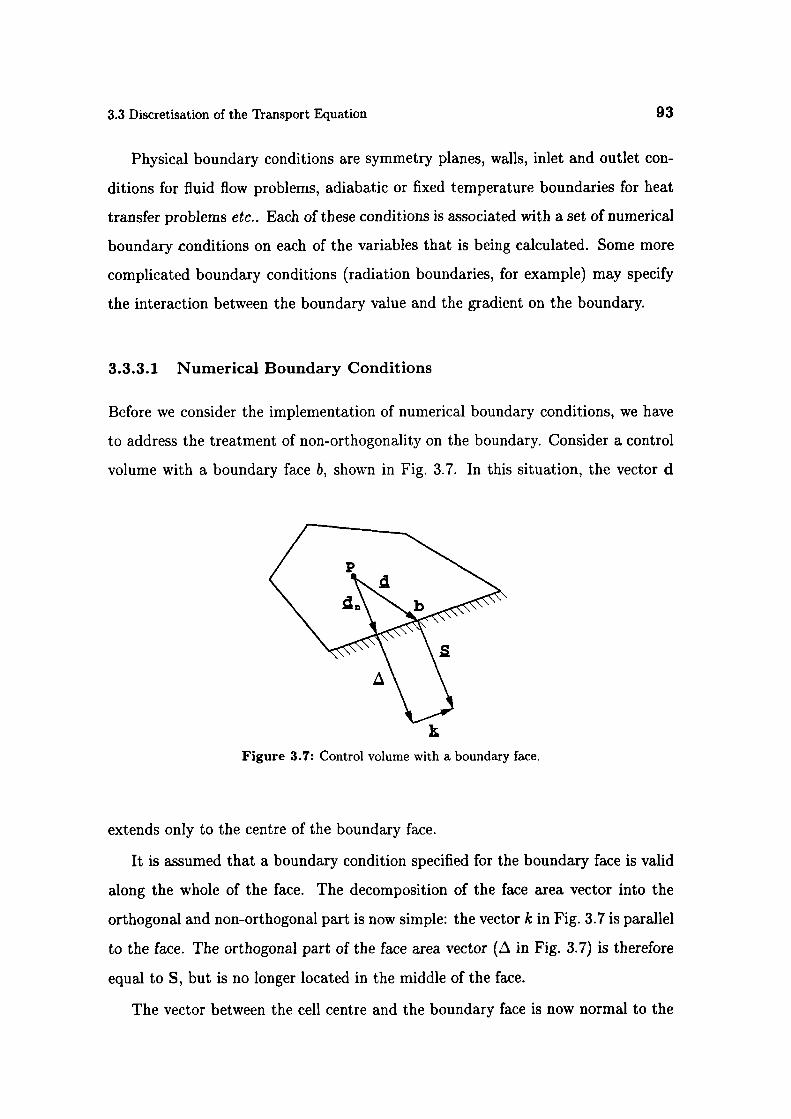
3.3 Discretisation of the Transport Equation
93
Physical boundary conditions are symmetry planes, walls, inlet and outlet con-
ditions for fluid flow problems, adiabatic or fixed temperature boundaries for heat
transfer problems etc.. Each of these conditions is associated with a set of numerical
boundary conditions on each of the variables that is being calculated. Some more
complicated boundary conditions (radiation boundaries, for example) may specify
the interaction between the boundary value and the gradient on the boundary.
3.3.3.1 Numerical Boundary Conditions
Before we consider the implementation of numerical boundary conditions, we have
to address the treatment of non-orthogonality on the boundary. Consider a control
volume with a boundary face b, shown in Fig. 3.7. In this situation, the vector d
k
Figure 3.7: Control volume with a boundary face.
extends only to the centre of the boundary face.
It is assumed that a boundary condition specified for the boundary face is valid
along the whole of the face. The decomposition of the face area vector into the
orthogonal and non-orthogonal part is now simple: the vector k in Fig. is parallel
to the face. The orthogonal part of the face area vector (. in Fig. 3.7) is therefore
equal to S, but is no longer located in the middle of the face.
The vector between the cell centre and the boundary face is now normal to the
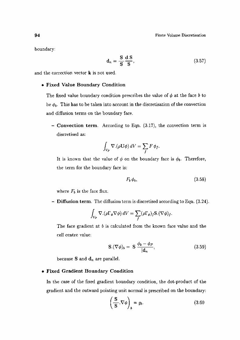
94
Finite Volume Discretisation
boundary:
d= S d.S
(3.57)
and the correction vector k is not used.
. Fixed Value Boundary Condition
The fixed value boundary condition prescribes the value of q at the face b to
be cSb. This has to be taken into account in the discretisation of the convection
and diffusion terms on the boundary face.
- Convection term. According to Eqn. (3.17), the convection term is
discretised as:
fV.(pU)dV =Vp j.
It is known that the value of on the boundary face is Therefore,
the term for the boundary face is:
Fbb, (3.58)
where Fb is the face flux.
- Diffusion term. The diffusion term is discretised according to Eqn. (3.24).
fV.(pF,V) dV =
Vp
The face gradient at b is calculated from the known face value and the
cell centre value:
S (V-- (3.59)-d
because S and d are parallel.
. Fixed Gradient Boundary Condition
In the case of the fixed gradient boundary condition, the dot-product of the
gradient and the outward pointing unit normal is prescribed on the boundary:
(_.vc) = g,. (3.60

3.3 Discretisation of the Transport Equation 95
- Convection term. The face value of is calculated from the value in
the cell centre and the prescribed gradient:
= Q5P + d,,.(Vq5),
= çbp + d 9b (3.61)
- Diffusion term. The dot product between the face area vector and
(VØ) b is known to be
S g (3.62)
and the resulting term is:
(Pi')b S 9b (3.63)
As the vector d does not point to the middle of the boundary face, the face
integrals in the fixed gradient boundary condition are calculated only to first
order accuracy. This can be rectified by including the boundary face correction
based on the vector k (Fig. 3.7) and the component of the gradient parallel to
the face in the first cell next to the boundary. However, Section 3.6 will show
that the error of the same type is neglected for the internal faces of the mesh
and this correction is omitted for the sake of consistency.
3.3.3.2 Physical Boundary Conditions
Let us now consider some physical boundary conditions for fluid flow calculations.
For simplicity, we shall start with the incompressible flow.
. Inlet boundary. The velocity field at the inlet is prescribed and, for consis-
tency, the boundary condition on pressure is zero gradient (Hirsch [65]).
. Outlet boundary. The outlet boundary condition should be specified in such
a way that the overall mass balance for the computational domain is satisfied.
This can be done in two ways:
96
Finite Volume Discretisation
- The velocity distribution for the boundary is projected from the inside
of the domain (first row of cells next to the boundary). These velocities
are scaled to satisfy overall continuity. This approach, however, leads to
instability if inflow through a boundary specified as outlet occurs. The
boundary condition on pressure is again zero gradient.
- The other approach does not require the velocity distribution across the
outlet the pressure distribution is specified instead. The fixed value
boundary condition is used for the pressure, with the zero gradient bound-
ary condition on velocity. Overall mass conservation is guaranteed by the
pressure equation (see Section 3.8).
• Symmetry plane boundary. The symmetry plane boundary condition im-
plies that the component of the gradient normal to the boundary should be
fixed to zero. The components parallel to it are projected to the boundary
face from the inside of the domain.
• Impermeable no-slip walls. The velocity of the fluid on the wall is equal to
that of the wall itself, so the fixed value boundary conditions prevail. As the
flux through the solid wall is known to be zero, the pressure gradient condition
is zero gradient.
Compressible flows at low Mach numbers are subject to the same approach as
above. The situation is somewhat more complex in case of transonic and supersonic
flows the number of boundary conditions fixed at the inlet and outlet depends on
the number of characteristics pointing into the domain. For these cases the reader
is referred to Hirsch [65] or Uslu [135].
For turbulent flows, the inlet and outlet boundary conditions on turbulence
variables (k and €, for example are typically assigned to fixed values and zero
gradients, respectively The boundary conditions for the turbulence properties on
the wall depend on the form of the selected turbulence model and the near-wall
treatment.
3 4 A New Convection Differencing Scheme 97
3.4 A New Convection Differencing Scheme
In this Section, a new convection differencing scheme will be proposed. It is based
on the Normalised Variable Approach (NVA) of Leonard [82] and Gaskell and Lau
[49]. It guarantees boundedness of the solution by introducing a small amount
of numerical diffusion in regions where it is needed. The scheme is formulated
as a stabilised version of Central Differencing (CD) in order to preserve overall
second-order accuracy. The necessary modification of the Convection Boundedness
Criterion of Gaskell and Lau [49] for non-uniform unstructured meshes is also given.
The description of the new differencing scheme will start with an analysis of
the issues of accuracy and boundedness, and introduction of the concepts of Total
Variation Diminishing (TVD) and the Normalised Variable Approach (NVA).
3.4.1 Accuracy and Boundedness
As has been mentioned before, none of the basic convection differencing schemes
produces a numerical solution which is bounded and accurate at the same time.
This problem has been tackled in several different ways, including the introduc-
tion of "streamwise-upwind schemes" (eg. Raithby [112, 113]), higher-order upwind
schemes (eg. QUICK by Leonard [81]) and flux-limited schemes (eg. FCT by Boris
and Book [20]). Flux limiting is a procedure that creates a differencing scheme which
is higher than first-order accurate, but without the spurious oscillations associated
with the classical second-order schemes. This has proven to be the most promising
approach. Harten [58] introduces the notion of Total Variation Diminishing (TVD)
to characterise oscillation-free flux-limited schemes.
3.4.1.1 TVD Differencing Schemes
The derivation of the TVD criterion starts with the derivation of semi-discrete
schemes for the unsteady convection problems by Usher, named the "E-schemes".
He shows that these schemes are at most first-order accurate but converge to the
98
Finite Volume Discretisation
correct physical solution which satisfies the entrophy condition3.
It is well known (eg. Sweby [129], Harten [58]) that a crucial estimate involved
in convergence proofs of differencing schemes is a bound on the variation of the
solution. The Total Variation TV(q5 1 ) [129] of the solution is defined by:
TV(cb") = - , (3.64)I
where P and N are the points around the face f . The Total Variation Diminishing
schemes satisfy the following condition (Sweby [129]) for every time-step:
TV(,b') <TV(ri) (3.65)
Sweby also shows that the schemes satisfying the above condition are also "E-
schemes", thus producing the solution that obeys the entrophy condition.
The above condition is now applied to the higher-order flux-limited schemes
in the way suggested by Sweby [129]: a selected higher-order differencing scheme is
written as a sum of the first-order bounded differencing scheme (UD) and a "limited"
higher order correction:
= (c)uD + '4'[( q ) Ho - (c)uD], (3.66)
where ()Ho represents the face value of for the selected higher-order scheme and
'I' is the flux limiter. Following van Leer [139] and Chakravarthy and Osher [27],
Sweby [129] assumes that the limiter is a function of consecutive gradients of ,
Fig 3.8, as measured by:
r = cbc -— cbc
Thus:
(3.67)
(3.68)
The points U, C and D are selected according to the direction of the flow on the
face f.
The weak solutions of this equation are non-unique (Sweby [129] and so an extra constraint
is needed to select the unique physical soluti n

3.4 A New Convection Differencing Scheme 99
flow dir.ction I / D
U C If D
Figure 3.8: Variation of 4 around the face f.
Sweby [129] shows that the following constraint on the limiter guarantees that
the scheme satisfies the TVD condition:
o ^ (W(rr')
2. (3.69)
The points that satisfy the TVD condition can be presented as the shaded region
in Sweby's diagram, Fig. 3.9, showing 'I' as a function of r. The hatched region in
Fig. 3.9 is known as the second-order region of the TVD diagram (Sweby [129]).
Figure 3.9: Sweby's diagram.
The TVD boundedness criterion as derived by Sweby [129] includes the depen-
dence of the limited scheme on the Courant number. The TVD condition given

100 Finite Volume Discretisation
by Eqn. (3 69), applies to explicit second-order differencing schemes on a five-point
computational molecule in one-dimensional problems. All second-order schemes
are considered to be a linear combination of explicit versions of Linear Upwinding
Warming and Beam [146]) and Central Differencing (Lax-Wendroff [79]), where
the face value of q5 depends on the Courant number in order to guarantee stability.
As the Courant number increases, the differencing scheme becomes more and more
diffusive and in the limit of Co = 1, both schemes reduce to Upwind Differencing.
This type of behaviour is essential to prove the convergence of TVD differencing
schemes.
The dependence of the convection differencing scheme on the Courant number
cannot be accepted it would imply that a steady-state solution for a convection-
dominated problem depends on the time-step used to reach the steady state.
In spite of its deficiencies, the TVD approach has been widely accepted. It
has, however, been noted (Leonard [83]) that TVD schemes are either too diffusive,
introducing too much numerical diffusion (for example MINMOD by Zhu and Rodi
[155] , or too compressive, distorting the smoothly changing solutions through the
introduction of "down-winding", where the influence of D to is larger than that
of c (SUPERBEE by Roe [118]
A less restrictive and more general approach to boundedness can be found in the
Normalised Variable Approach (NVA), described below.
3.4.1.2 Convection Boundedness Criterion and the NVD Diagram
The Normalised Variable Approach and Convection Boundedness Criterion have
been introduced by Leonard [82] and Gaskell and Lau [49]. Unlike the TVD ap-
proach, it does not guarantee convergence of the proposed differencing scheme, but
tackles the problem of boundedness in a more general way
Consider the variation of a convected scalar around the face f in a one
dimensional case, Fig 3.8. The normalised variable is defined as [82]
- 370
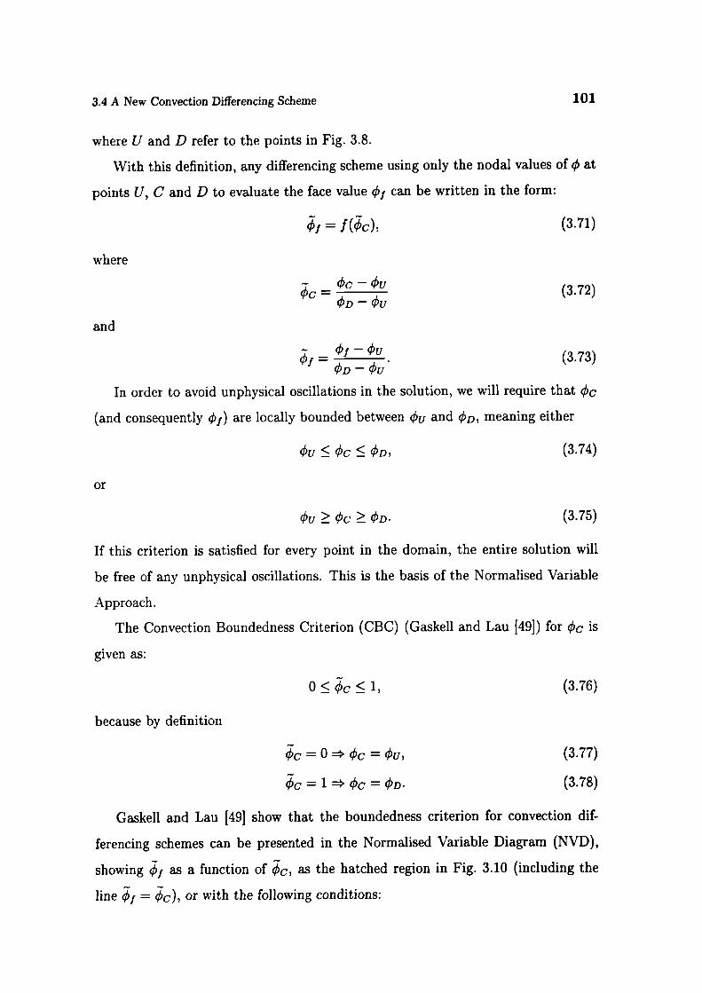
3.4 A New Convection Differencing Scheme
101
where U and D refer to the points in Fig. 3.8.
With this definition, any differencing scheme using only the nodal values of at
points U, C and D to evaluate the face value q can be written in the form:
(3.71)j=f(cbc),
where
c1c—cbucbc=
- cbu
and
(3.72)
(3.73)
In order to avoid unphysical oscillations in the solution, we will require that qS.
(and consequently are locally bounded between qu and Q5D, meaning either
U ^ C ^ QD, (3.74)
or
øu ^ c ^
(3.75)
If this criterion is satisfied for every point in the domain, the entire solution will
be free of any unphysical oscillations. This is the basis of the Normalised Variable
Approach.
The Convection Boundedness Criterion (CBC) (Gaskell and Lau [49]) for Q5c is
given as:
0 ^ c ^ 1, (3.76)
because by definition
= 0 cbc = cbu, (3.77)
= 1 c5c =
(3.78)
Gaskell and Lau [49] show that the boundedness criterion for convection dif-
ferencing schemes can be presented in the Normalised Variable Diagram (NVD),
showing j as a function of cbc, as the hatched region in Fig. 3.10 (including the
line I = or with the following conditions:
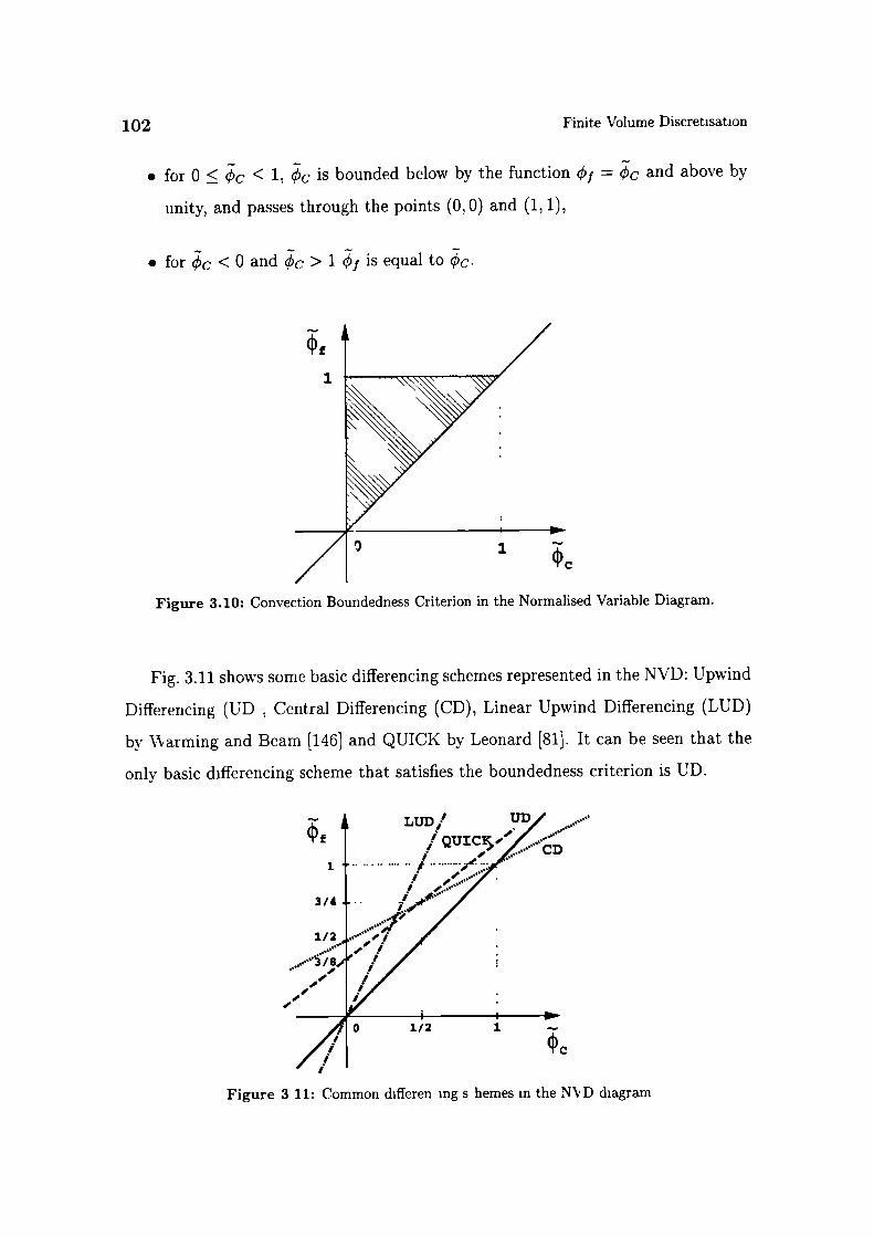
102
Finite Volume Discretisation
. for 0 ^ cc < 1, q5c is bounded below by the function çb1 = c'c and above by
unity, and passes through the points (0,0) and (1, 1),
. for c <0 and qc> 1 q is equal to qc.
Figure 3.10: Convection Boundedness Criterion in the Normalised Variable Diagram.
Fig. 3.11 shows some basic differencing schemes represented in the NVD: Upwind
Differencing (UD , Central Differencing (CD), Linear Upwind Differencing (LUD)
by Varming and Beam [146] and QUICK by Leonard [81]. It can be seen that the
only basic differencing scheme that satisfies the boundedness criterion is UD.
Figure 3 11: Common differen ing s hemes in the N\' D diagram
3.4 A New Convection Differencing Scheme
103
It should be noted that the NVD makes no reference to the Courant number,
thus resolving the problem of dependence of the steady-state solution on the time-
step. In a later paper, Leonard [83] includes the "transient interpolation modelling"
of the face value of q5 depending on the time-step, again restricting all differencing
schemes to UD for Co 1.
NVD diagrams for a number of TVD and NVD schemes as well as the relationship
between NVD and Sweby's diagram can be found in Leonard [83].
3.4.1.3 Convergence Problems of Flax-Limited Schemes
According to both TVD and NVA, any differencing scheme that is more than first-
order accurate must be non-linear in order to guarantee boundedness. Non-linearity
of the differencing scheme is introduced through the dependence of the flux limiter
on the solution itself (see Eqs. (3.68) and (3.71)).
This additional non-linearity does not cause the divergent behaviour, as the orig-
inal higher-order scheme satisfies the stability condition. It has, however, been noted
that the NVD schemes under some conditions do not produce a unique solution for
a steady-state problem, as the change in the discretisation practice changes the solu-
tion between the time-steps and vice versa. For the TVD schemes, the convergence
of the non-linear system to a unique solution can be proven only for explicit calcula-
tions, introducing the dependence of the limiter on the Courant number. In the case
of implicit calculations in two or three dimensions, or for Co > 1, the convergence
properties of TVD schemes cannot be proven. The NVD criterion, on the other
hand, does not guarantee that the differencing scheme will be convergent under any
conditions. Experience with some NVD difl'erencing schemes (Zhu [154]) shows that
special modifications in the implementation of the differencing scheme are needed
in order to improve convergence.
The creation of a differencing scheme in either the TVD or NVA framework can
be divided into three steps:
. A basic differencing scheme needs to be selected. This scheme can be un-
bounded, but should be accurate and stable. This basic differencing scheme

104 Finite Volume Discretisaton
will be used unaltered in those regions where it produces a bounded solution.
The regions of the domain in which problems with boundedness occur need
to be detected in some way. For this purpose the TVD schemes use the
"smoothness monitor" r, Eqn. (3.67), whereas the NVD schemes introduce
the concept of the "normalised variable" , Eqn. (3.70).
• Finally, a change in the discretisation in regions of unboundedness needs to be
introduced. This change is partially dictated by the TVD or NVD criterion
itself, Figs. 3.9 and 3.10.
The Convection Boundedness Criterion represents the most general approach to
the issue of local boundedness of the solution. It has therefore been selected as the
boundedness indicator for the new bounded differencir g scheme. According to its
original formulators, the Normalised Variable Approach is not readily extendible to
arbitrarily unstructured meshes, but in the present work we show that this is not
the case. The next Section introduces the necessary changes in the calculation of
the Normalised Variable to achieve this.
The choice of the basic differencing scheme comes from the desired order of ac-
curac of the Finite Volume method presented in this study. In order to achieve the
second order behaviour, consistent with the rest of the discretisation practice, CD
has been selected. It uses a compact computational molecule, which is advantageous
for unstructured meshes.
The bounding process for the new differencing scheme is based on the NVD
diagram. Once the basic framework has been established, the issue of accuracy vs.
c nvergence will be addressed.
3.4.2 Modification of the NVD Criterion for Unstructured
Meshes
Th CBC us s the value of the dependent variable q in the U far up md node
in order to determine c. This is n t practical f r arbitrarily unstructured meshes

D
3 4 A New Convection Differencing Scheme
105
because the far upwind cell label is not known, or that point does not even exist.
The definition of the normalised variable, Eqn. (3.70), is originally given for a
uniform mesh. This implies that a differencing scheme based on Eqn. (3.71) will
be sensitive to sudden changes in the mesh spacing. A generalisation of the NVD
criterion to non-uniform meshes has been given by Darwish [37]. However, this
generalisation is complex and introduces additional computational cost.
In this Section, a modification of the Normalised Variable in terms of gradients of
the dependent variable will be presented. It enables the use of the NVA on arbitrarily
unstructured and non-uniform meshes without an increase in the computational cost.
The information available for each cell face includes the gradients of the depen-
dent variable over both cells sharing the face and the gradient across the face itself.
Using the fact that the computational point is located in the middle of the control
volume, definition of q5c can be changed as follows.
If the value of qc is bounded by çu and D, Fig. 3.12, it is also bounded by the
interpolated face values and . The advantage of this formulation is that the
calculation of the gradient of q across the cell on the basis of the interpolated face
values is valid both on uniform and non-uniform meshes. The new definition of cbc
Figure 3.12: Modified definition of the boundedness criterion for unstructured meshes.
is therefore:
- cbc -= 1 -
-(3.79)0c
01-01
106 Finite Volume Discretisati n
In the case of a uniform mesh, Eqn. (3.72) and Eqn. (3.79) are equivalent.
The next step is to reformulate Eqn. (3.79) in terms of gradients across the face
and the "upwind" cell C. Using the interpolation factor Eqn. (3.20), and vector
d, Fig. 3.6, the difference - q5c can be written as:
J.+ ,( _tLI- PC - JxPD - PC
- cbc=f (XD-XC)
XD - XC
f1 (V)f.(xD - XC), (3.80)
since
DC = (Vi) 1 .d. (3.81)XD - XC
Here, d is the unit vector parallel with CD:
a=. (3.82)
The transformation of - can be done in the following way:
____ ++ x1—x1)Xj - Xf
= (Vq5 C.d(4 - Xj ). (3.83)
Using Eqs 3 20 , (3.80) and (3.83 , the transformation of Eqn. (3.79) is simple:
.+ .- 1 _____
(PC - 1- + -Pf - Wf
= 1 - f(V) f .a XD - XC) (3 84(Vq)C.X7-xj)
Since the computational point C is located in the middle of the cell, the following
geometrical relation can be used:
- X1 - - XC = 2f (3 85
X D XC XD-XC
giving the final form of cc•
(V .ã 1 - (V 1.d(3 86'p_C 1
2Vc.d 2(Vq5Cd
3 4 A New Convection Differencing Scheme 107
There is no reference to the "far upstream" node U, or even to the previous upstream
face. The product (V4 1 .d is calculated directly from the values of the variable on
each side of the face:
(V)1.d = - q5c. (3.87)
Implementation of the NVD criterion on any mesh is now simple. The informa-
tion about the topological structure of the mesh is irrelevant. Even the existence of
the opposite face f is not required it is only necessary to have the point C in the
middle of the control volume.
3.4.3 Gamma Differencing Scheme
The following Section gives the description of the Gamma differencing scheme.
CD is used in the bulk of the domain. For the values of 4'c <0 and q5c> 1 the
boundedness criterion prescribes the use of UD in order to guarantee boundedness.
Therefore, some sort of "switching" between the schemes is needed. This causes the
most serious problems with the family of NVD differencing schemes there is no
guarantee that a steady-state solution will be obtained because of the perturbations
introduced by "switching". In order to overcome this difficulty, the majority of
existing NVD schemes use some form of linear upwinding in the range of values
0 < < (3m, where (3m is a constant of the differencing scheme, usually around
1/6 (Gaskell and Lau [49fl. The meaning of (3m will become clear from the further
discussion, Section 3.4.3.1. Numerical experiments show that LUD is not really
appropriate for this purpose, because it causes both distortion and the shift of the
profile in comparison with the exact solution.
Values of Øc close to 0 (q5c> 0) represent the profile of the dependent variable
similar to the one shown in Fig. 3.13.
If the line passing through ctu, bc and cbD is regarded as the exact form of the
bounded local profile, it can be seen that the exact face value çbj is bounded by the
values obtained from UD and CD. It follows that some kind of blending between
the two can be used to obtain a good estimate of the face value.

108
Finite Volume Discretisation
Figure 3.13: Shape of the profile for 0 < c <13m.
In order to establish a smooth transition, the blending between UD and CD
should be used smoothly over the interval 0 < c < /3m and the blending factor -y
should be determined on the basis of c such that:
• cbc = 0 = -y = 0 Upwind Differencing),
= =' -y = 1 (Central Differencing
This practice simultaneously satisfies two important requirements:
• The face value in situations of rapidly-changing derivative of the dependent
variable is el1 estimated and a smooth change in gradients is secured. This
has proven to be much better than forms of the Linear upwinding usually used
in this situati n Gaskell and Lau [49], Darwish [36]
• The transition between UD and CD is smooth. This reduces the amount
of switching in the differencing scheme and improves convergence. In other
NVD schemes there is a p mt where a small change in the value of qfc causes
3 4 A New Convection Differencing Scheme 109
an abrupt change in the discretisation practice, causing the deterioration in
convergence. With the Gamma differencing scheme, this is not the case.
The blending factor y has been selected to vary linearly between q5c = 0 and
= 13m
(3.88)
The proposed form of the Gamma differencing scheme thus includes the follow-
ing.
. For all the faces of the mesh, check the direction of the flux and calculate:
- cbc—cbucc=
-
—1— (V5)1.d- 2(Vq5)c.d
from the previous available solution or the initial guess.
. Based on calculate çb1 as:
- 4'c^Oorc5c^luseUD:
= cbc = c5 = cbc, (3.89)
- 13m^q5c<1useClTh
çbf = + C, (3.90)
or, in terms of un-normalised variables:
q5i = fc5c + (1 - f) q D, (3.91)
- U <fim blending is used:
=+ (i + ---)
(3.92)
or, in terms of un-riormalised variables:
(i - (1 - fr)) øc +
- fx)D. (3.93)
The blending factor is calculated from the local value of q and the pre-
specified constant of the scheme, /3m.

110
Finite Volume Discretisation
The NVD diagram for this differencing scheme is shown in Fig. 3.14.
Figure 3.14: Gamma differencing scheme in the NVD diagram.
The Gamma differencing scheme uses a compact computational molecule, in-
cluding one computational point on either side of each face. The calculation of cc
has been modified in such a way that it does not require the far upwind node ad-
dressing. The differencing scheme can therefore be easily implemented on arbitrarily
unstructured meshes. The scheme is upwind-biased not through an increase in the
computational molecule, but in the way the blending factor is calculated it can
therefore be seen as a stabilised version of Central differencing.
3.4.3.1 Accuracy and Convergence of the Gamma Differencing Scheme
The role of the /3m coefficient can be seen in Fig. 3.14 - the larger the value of urn,
the more blending will be introduced. At the same time, the transition between UD
and CD will be smoother For good resolution, the value of should ideally be
kept as low as p ssible.
An upper limit on comes from the accuracy requirement. For - , the
ariati n f q5 is linear between U and D and CD reproduces the exact value of
çb 1 . /3m should therefore always be less than . Higher values of urn result in more

(3.94)
3.5 Solution Techniques for Systems of Linear Algebraic Equations 111
numerical diffusion. For good resolution of sharp profiles, /3m should ideally be
kept to about 0.1. Lower values do not improve the accuracy, but introduce the
"switching" instability. The useful range of urn is therefore:
The other factor influencing the choice of 13m is the convergence for steady-state
calculations. The problem of convergence with the Gamma differencing scheme is
less serious than with other schemes of the switching type because of the smooth
transition between UD and CD. A universal remedy for convergence problems is to
increase the value of I-3m (but not over
It should also be mentioned that the face value of qS in the Gamma differencing
scheme does not in any way depend on the Courant number. Steady-state solutions
will therefore be independent of the size of the time-step used to reach it.
3.5 Solution Techniques for Systems of Linear
Algebraic Equations
Let us again consider the system of algebraic equations created by the discretisation,
Eqn. (3.42):
apq +aNq' = R.N
This system can be solved in several different ways. Existing solution algorithms
fall into two main categories: direct and iterative methods. Direct methods give
the solution of the system of algebraic equations in a finite number of arithmetic op-
erations. Iterative methods start with an initial guess and then continue to improve
the current approximation of the solution until some "solution tolerance" is met.
While direct methods are appropriate for small systems, the number of operations
necessary to reach the solution raises with the number of equations squared, making
them prohibitively expensive for large systems Muzaferija [97]). Iterative methods
are more economical, but they usually pose some requirements on the matrix.
112
Finite Volume Discretisation
The matrix resulting from Eqn. (3.42) is sparse most of the matrix coefficients
are equal to zero. If it were possible to choose a solver which preserves the sparsity
pattern of the matrix, the computer memory requirements would be significantly de-
creased. Unlike direct solvers, some iterative methods preserve the sparseness of the
original matrix. These properties make the use of iterative solvers very attractive.
Iterative solvers require diagonal dominance in order to guarantee convergence.
A matrix is said to be diagonally equal if the magnitude of the diagonal (central)
coefficient is equal to the sum of magnitudes of off-diagonal coefficients. The addi-
tional condition for diagonal dominance is that ap > aN I for at least one row
of the matrix.
In order to improve the solver convergence, it is desirable to increase the diagonal
dom nance of the system. Discretisation of the linear part of the source term,
Eqn. (3.36), is closely related to this issue. If Sp < 0, its contribution increases
diagonal dominance and Sp is included into the diagonal. In the case of Sp > 0,
diagonal dominance would be decreased. It is more effective to include this term
into the source and update it when the new solution is available. This measure is,
however, not sufficient to guarantee the diagonal dominance of the matrix.
The analysis of the structure of the matrix brings us back to the issue of bound-
edness. The sufficient boundedness criterion for systems of algebraic equations men-
tioned in Section 3.3.1 states that the boundedness of the solution will be preserved
for diagonally equal systems of equations with positive coefficients. This allows us
to examine the discretised form of all the terms in the transport equation from the
point of view of boundedness and diagonal dominance and identify the troublesome
parts of discretisation.
The convection term creates a diagonally equal matrix only for Upwind Dif-
ferencing. Any other differencing scheme will create negative coefficients, violate
the diagonal equality and potentially create unbounded solution. in the case of
Central Diferencing on a uniform mesh, the problem is further complicated by the
fa t that the central coefficient is equal to zero. In order to improve the quality
of the matrix for high r-order differencing schemes, Khosla and Rubin [73] propose

3.5 Solution Techniques for Systems of Linear Algebraic Equations 113
a deferred correction implementation for the convection term. Here, any dif-
ferencing scheme is treated as an upgrade of UD. The part of the convection term
corresponding to UD is treated implicitly (i.e. built into the matrix) and the other
part is added into the source term. This, however, does not affect the boundedness
in spite of the fact that the matrix is now diagonally equal, as the "troublesome"
part of the discretisation still exists in the source term.
The diffusion term creates a diagonally equal matrix only if the mesh is orthog-
onal. On non-orthogonal meshes, the second term in Eqn. (3.34) introduces the
"second neighbours" of the control volume into the computational molecule with
negative coefficients, thus violating diagonal equality. As a consequence of mesh
non-orthogonality, the boundedness of the solution cannot be guaranteed. The in-
crease in the computational molecule would result in a higher number of non-zero
matrix coefficients, implying a considerable increase in the computational effort re-
quired to solve the system. On the other hand, the non-orthogonal correction is
usually small compared to the implicit part of the diffusion term. It is therefore
reasonable to treat it through the source term. In this study, the diffusion term
will therefore be split into the implicit orthogonal contribution, which includes only
the first neighbours of the cell and creates a diagonally equal matrix and the non-
orthogonal correction, which will be added to the source. If it is important to resolve
the non-orthogonal parts of the diffusion operators (like in the case of the pressure
equation, see Section 3.8), non-orthogonal correctors are included. The system of
algebraic equations, Eqn. (3.42), will be solved several times. Each new solution will
be used to update the non-orthogonal correction terms, until the desired tolerance
is met. It should again be noted that this practice only improves the quality of
the matrix but does not guarantee boundedness. If boundedness is essential, the
non-orthogonal contribution should be discarded, thus creating a discretisation error
described in Section 3.6.
At this point, the difference between the non-orthogonality treatments proposed
in Section 3.3.1.3 becomes apparent. The decomposition of the face area vector into
the orthogonal and non-orthogonal part determines the split between the implicit
114
Finite Volume Discretisati n
and explicit part of the term, with the consequences on the accuracy and convergence
of non-orthogonal correctors. The comparison of different treatments is based on
several criteria:
• On which angle of non-orthogonality is it necessary to introduce non-orthogonal
correctors how good an approximation of the converged solution can be ob-
tained after only one solution of the system?
. How many non-orthogonal correctors are needed to meet a certain tolerance?
. How does the number of solver iterations change with the number of correc-
tors?
If the non-orthogonal correction needs to be discarded for the sake of bound-
edness, which approach causes the smallest discretisation error?
The discretisation error for the diffusion term will be derived in Section 3.6.
Numerical results for the convergence of three non-orthogonality treatments will be
given in Section 3.7.
The discretisation of the temporal derivative creates only the diagonal coefficient
and a source term contribution, thus increasing the diagonal dominance. Unfortu-
nately, the sufficient boundedness criterion cannot be used to establish the bound -
edness of the discretisation, as it does not take into account the influence of the
source term.
The above discussion concentrates on the analysis of the discretisation on a term-
by-term basis. In reality, all of the above coefficients contribute to the matrix, thus
influencing the properties of the system. It has been shown that the only terms that
actually enhance the diag nal dominance are the linear part of the source and the
temp ral derivative
In steady-state calculations, the beneficial influence of the temporal d rivative on
the diagonal dominance does not exist. In order to enable the use iterative s ivers,
the diagonal d minance needs to be enhanced in some other wa, namely through

3.6 Numerical Errors in the Discretisation Procedure 115
under-relaxation. Consider the original system of equations, Eqn. (3.42):
apq5' + aNcbN = Rp.N
Diagonal dominance is created through an artificial term added to both left and
right-hand side of Eqn. (3.42):
1—aapq5 + aLF, + ajqçb = R + apçb,, (3.95)
N a
or
1—a+ = R
+ a apq5°ç. (3.96)
Here, here represents the value of q! ' from the previous iteration and a is the
under-relaxation factor (0 < a ^ 1). Additional terms cancel out when steady-state
is reached ( =
In this study, the iterative solution procedure used to solve the system of a!-
gebraic equations is the Conjugate Gradient (CG) method, originally proposed by
Hestens and Steifel [63]. It guarantees that the exact solution will be obtained in the
number of iterations smaller or equal to the number of equations in the system. The
convergence rate of the solver depends on the dispersion of the eigenvalues of the
matrix [A] in Eqn. (3.43) and and can be improved through pre-conditioning. For
symmetric matrices, the Incomplete Cholesky preconditioned Conjugate Gradient
(ICCG) solver will be used. The method is described in detail by Jacobs, [67]. The
adopted solver for asymmetric matrices is the Bi-CGSTAB by van der Vorst [136].
3.6 Numerical Errors in the Discretisation
Procedure
This Section gives an overview of numerical errors introduced through the discreti-
sation procedure. Errors come from two sources. The first group of errors is a con-
sequence of discretisation practices that are lower than second-order accurate. This
includes the discretisation of temporal terms and convection differencing schemes,

116 Finte V lume Discretisation
where it was necessary to lower the order of discretisation in order to preserve the
boundedness of the solution. The second group of errors is caused by the discreti-
sation of the solution domain. They are a direct consequence of mesh quality. This
group of errors includes insufficient mesh resolution, skewness and non-orthogonality
errors.
The Finite Volume method described above is characterised as second-order ac-
curate and therefore also creates higher-order errors. Since the method has been
developed for second-order continuum mechanics problems, the higher-order errors
will be neglected4.
3.6.1 Numerical Diffusion from Convection Differencing
Schemes
The second-order numerical error in the Finite Volume method can be described nu-
merical diffusion. It is a consequence of the discretisation practice which is not fully
second-order accurate, selected to preserve the boundedness of the solution. The
change in accuracy of the convection discretisation can be examined by comparing
the selected differencing scheme, with the second-order (unbounded) Central Dif-
ferencing (CD). Bounded differencing schemes produce a numerical diffusion-type
term of the form:
V. (F . (3.97)
where FN is the numerical diffusion tensor.
Every bounded differencing schemes of the TVD and NVD family can be written
as a sum of Central Differencing and the numerical diffusion term of the above form,
possibly with some higher-order terms in the case when the original (unbounded)
differencing scheme is more than second-order accurate. Here, we shall present
a method for the evaluation of the numerical diffusion for Blended Differencing,
Eqn. 3 23 , and examine the properties of the numerical diffusion term
4 An extension of the FVM to four h-order a curacy can be found in Lilek and Peri [88]. An
illustrati n of the behavi ur of higher-order err rs has been presented by Leonard [83].

3.6 Numerical Errors in the Discretisation Procedure
117
Consider the face value of obtained by CD, Eqn. (3.19) and BD, Eqn. (3.23):
(c51)cD =fçbp + (1 - f)cbN,
(c5f)BD =[(1 - ' rny) inax(sgn(F), 0) + 'yf}
+ [(1 - 'y) min(sgn(F), 0) + y(l - fX)]qN.
The difference in the face value is:
Scb1 — ( cbl)cr, - (qf)BD
=[(1 - 'y) f - (1 - y) max(sgri(F), 0)]q5p
+ [(1—y) (1 -fr) —(1 —y)min(sgn(F),0)Jc N . (3.98)
To clarify the meaning of this expression, let us assume that F > 0:
8çbf=[(1—'y)fS—(1-7)p+(1-7)(1—f)q5N
=(1--y)(1—f)(qN—cp). (3.99)
For the whole convection term, the difference can be written as:
E = = S.(pU) j [(1 - 'y)(l - fX)(cbN - qJP)]f
= S.[(1 - 'y)(l - f)(pU)fd.(V)f]I
= S.{{(1 - 'y)( l -I
= S.(I'.Vq), (3.100)I
where 1'N is a tensorial numerical viscosity:
'TN = (1 - 'y)(l - f)(pU) 1d. (3.101)
More generally, the numerical diffusion tensor can be written as:
['N = (1 - ) pU) 1d[(1 - f) max(sgn(F), 0) + f mirt(sgn(F), 0)].
(3.102)
Eqs. (3.100 and (3.102) give us an insight into the properties of numerical dif-
fusion. Firstly, it can be seen that the term is indeed diffusion-like, depending on
118 Finite Volume Discretisation
gradients of . For a uniform distribution of , this term vanishes. Other important
facts are that the term scales linearly with the mesh-spacing (i.e. with d ), that it
is large in the cases of large convection velocity and that it disappears when (U)1.S
goes to zero (this is usually called "mesh-to-flow alignment"). For Central Differ-
encing (y = 1), FN also goes to zero. The numerical diffusion tensor for Upwind
Differencing on a uniform mesh (f = ) can be simplified to:
FN = (pU) 1 d. (3.103)
Numerical diffusion for the Gamma differencing scheme (Section 3.4) can also be
calculated from Eqn. (3.102). The blending factor is calculated from the face value
of cc as:
,y=0
for cc < 0 and cc ^ 1,
-Y=
for 0 <ciC < /m, (3.104)
,y=1
for 13m ^ c < 1.
The error coming from numerical diffusion has been well-known. Many attempts
to reduce its influence on the solution have been made, mainly by reducing the
effective blending factor. The effects of numerical diffusion on the accuracy of the
solution will be illustrated in Section 3.7.
3.6.2 Numerical Diffusion from Temporal Discretisation
A detailed analysis of the temporal discretisation shows that it can also produce
a numerical diffusion error. This is important for transient calculations - the de-
velopment of the solution in time can be severely smeared The Crank-Nicholson
me hod, Eqn 3.41 , gives a fully second-order accurate discretisation in time. In
order to derive the numerical diffusion term for any other temporal discretisation
sch me. we need only to c mpare it with the Crank Nicholson method. Let us first
consider the Euler Implicit temporal discretisation.

3.6 Numerical Errors in the Discretisation Procedure 119
The comparison between the Crank-Nicholson discretisation, Eqn. (3.41):
ppcb - ppq5, VP + Fcb -
+ Fçb -
SuVp + SpVpØ + SpVpçb
and the Euler Implicit method, Eqn. (3.50):
ppçb - ppçb1 Vp + Fq5 - (pfS.(V4)j
I
= SuVp + SpVpç,
gives the difference of
E = - F - i: F]
+ [(PF J S.(VØ)) -
— (SpVqY - SpVpç5).
Using Eqn. (3.4):
qfl = ç0+
(3.105)
and
(Vq = (Vq5)° +
t, (3.106)
Eqn. (3.105) can be written as:
E=_>F()
+
Lt I- --SpVp (3.107)
E can be decomposed into three parts:
120
Finite Volume Discretisation
• Convection error:
(
5q5 \Dc=—)F -a-)1'
(3.108)
• Diffusion error:
= _-(pF)fS.ô v:)f , (3.109)/
. Source term error:
( OD5 = —SpVp
-).(3.110)
In order to perform the analysis of E, it is necessary to express the temporal
derivative of q as a combination of spatial terms. The original transport equation
will be used in this form:
= S) - V.(pU) + V.(pFV). (3.111)
The convection term can be split into two parts:
V.(pU) = pU.V + V.(pU). (3.112)
In order to simplify the derivation, it is assumed that p = const. It follows:
a S5)____ - U.Vq - q5V.0 + V.(TVp). (3.113)
at
Using Eqn. (3.113 , the convection error, Eqn. (3.108), splits into four terms:
= —EF [sø()]
(3.114)
= F [U.V] 1 , (3.115
D F[V.U]1, 3.116)
D 4 = F[V. r0v ]. 3.117)
D1 cannot be further analysed, as it d pends on the distribution of the source.
It ill be shown that D2 has an important effect it can be transformed intc

3 6 Numerical Errors in the Discretisation Procedure 121
a numerical diffusion-type term. Dc3 scales with the divergence of velocity. In
standard situations V.0 is considered to be small and this term is neglected. D4
includes higher derivatives of and is therefore neglected.
Let us now come back to Dc2, Eqn. (3.115). Following a procedure similar to
the one in Section 3.6.1, this term can be written as:
Dc2 = i S. [(pUU) .Vq5] 1 . (3.118)
A closer look into Eqn. (3.118), reveals that this term has the form V.(FT.V4)
where FT is a form of tensorial diffusion. This (numerical) diffusion has a maximum
if vectors 5, U and Vq are parallel:
rtDc2 = S. {---PIU 2(V)] . (3.119)
I
This would correspond to a one-dimensional transport of a wa"e. The maximum
equivalent numerical diffusion is therefore:
2(FT)max=TPU . (3.120)
Eqn. (3.120) can be written in terms of the Courant number, Eqn. (3.48):
(FT)mur = Cop U d. (3.121)
Comparison of Eqs. (3.121) and (3.103) shows that for Co = 1 the numerical diffu-
sion from the temporal discretisation is the same as numerical diffusion from UD.
This effect is far from negligible. For good temporal accuracy, a higher-order tem-
poral scheme is as important as a higher order convection differencing scheme.
Following the equivalent path for the diffusion error DD, Eqn. (3.109), it can be
shown that it produces terms that either cannot be analysed or depend on higher
gradients of q. For the similar reason, the source error Ds cannot be analysed either.
An equivalent analysis for the explicit temporal discretisation produces a
similar result. The main error term comes from the convection part of the decompo-
sition. It can be written as the diffusion term equivalent to Eqn. (3.119), but with
numerical diffusion of the opposite sign:
(FT)rnax = - Cop U d. (3.122)
122
Finite Volume Discretisation
Eqs. (3.102) and (3.122) can also be used to confirm some well-known stability
analysis results. It is, for example, well known that explicit Central Differencing is
an unconditionally unstable combination of spatial and temporal discretisation for
transport equations without a diffusion term. According to Eqn. (3.103), CD does
not introduce any numerical diffusion in the system. The numerical diffusion from
the Explicit discretisation in time is negative, producing negative effective diffusion.
Any system with negative diffusion is unstable. In the case of explicit Upwind
Differencing, the effective diffusion in the system is positive if the numerical diffusion
from UD is larger than the negative diffusion from the temporal discretisation. This
is the case if Co < 1, which agrees with the classical stability result (see eg. Hirsch
[65]). For Go> 1, the effective diffusion becomes negative and the system becomes
unstable.
Backward Differencing in time is a second-order accurate scheme. It can
be shown that the additional part of the temporal derivative actually cancels out
the numerical diffusion term resulting from D (see Appendix A). The leading
term of the truncation error is, however, four times larger than for the Crank-
Nicholson method. The major deficiency of the scheme comes from its extrapolative
behaviour in time, which causes unboundedness. An example of its behaviour, given
in Section 3.7 shows that a combination of a bounded convection differencing scheme
and the Crank-Nicholson temporal discretisation creates a bounded solution, which
is not the case if the Backward differencing in time is used.
3.6.3 Mesh-Induced Errors
Let us start the overvi w of mesh-induced errors with the insufficient mesh reso-
lution. If the solution changes rapidly in some regions of the domain and the local
number of computational points is not sufficient to describe that change, the shape
of the solution will effectively be lost. Even if the exact solution is available in a
certain number of points, the picture of the overall solution depends on the distribu-
tion and the number of those points. In Finite Volume calculations, the accuracy of
interactions described by the differential equation depends on the mesh resolution.

3.6 Numerical Errors in the Discretisation Procedure 123
It is therefore important that the selected computational points can provide a good
picture of the solution.
For the second-order spatial discretisation, the mesh resolution error is a con-
sequence of the assumed linear variation of the solution over the control volume.
Although it does not change the nature of the differential equation that is being
solved, insufficient mesh resolution may produce a completely incorrect picture of
the solution.
The influence of mesh non-orthogonality on boundedness has been described in
Section 3.5. The advantage of orthogonal meshes in the discretisation of the diffusion
term comes from the fact that only the first neighbours of the cell are included into
the computational molecule. The non-orthogonal term, irrespective of its implicit
or explicit treatment, also uses the second neighbours of the cell, thus increasing the
size of the computational molecule. Although both methods of discretisation are
second order accurate, the increase in the computational module implies a larger
leading term in the Taylor series expansion and higher errors.
Non-ortliogonality error, which violates the order of discretisation comes
into effect only if it is necessary to guarantee the boundedness of the solution. In
this case, the non-orthogonal component in Eqn. (3.34) is discarded, thus creating
a discretisation practice that obeys the sufficient boundedness criterion. For the
complete diffusion term, the non-orthogonality error has the following form:
Ed = S. [(pU)1k.(V)1]I
= V.(I'DV), (3.123)
where
= (pU) jk. (3.124)
The magnitude of 1'D depends both on the non-orthogonality angle of the mesh and
the selected non-orthogonality approach (see Section 3.3.1.3). For the same angle
of non-orthogonality, Ed will be smallest for the minimum correction approach, as
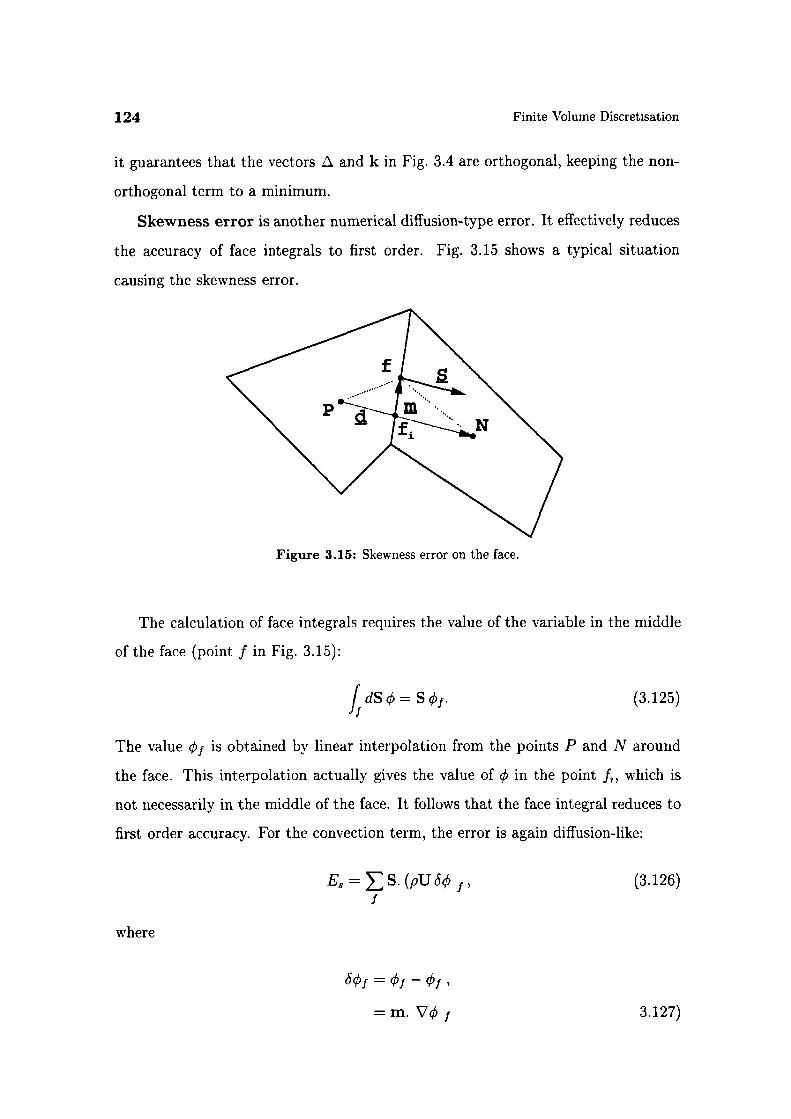
124 Finite Volume Discretisation
it guarantees that the vectors z and k in Fig. 3.4 are orthogonal, keeping the non-
orthogonal term to a minimum.
Skewness error is another numerical diffusion-type error. It effectively reduces
the accuracy of face integrals to first order. Fig. 3.15 shows a typical situation
causing the skewness error.
Figure 3.15: Skewness error on the face.
The calculation of face integrals requires the value of the variable in the middle
of the face (point f in Fig. 3.15):
fdScb=St51 . (3.125)
The value qj is obtained by linear interpolation from the points P and N around
the face. This interpolation actually gives the value of in the point f,, which is
not necessarily in the middle of the face. It follows that the face integral reduces to
first order accuracy. For the convection term, the error is again diffusion-like:
E=S.(pUöq 1 , (3.126)I
where
öq5j = - çb1,
= m. Vq5 3.127)

3.7 Numerical Examples 125
and
m = x1 - x12 . (3.128)
E3 can be transformed into:
E3 = S. [(pU)jm.(V)1]/
= V.(fsV), (3.129)
where
= (pU) 1rm. (3.130)
When examining the importance of Eqn. (3.129) one should keep in mind that S
and m are orthogonal to each other, Fig. 3.15. On meshes of reasonable quality Im!
is smaller than d. The influence of Eqn. (3.129) is expected to be smaller than the
numerical diffusion from the convection differencing scheme. On highly distorted
meshes the influence of this term can be significant.
As in the case of mesh non-orthogonality, the error in Eqn. (3.129) can be re-
moved using the face interpolate of Vq5. This, however, increases the size of the
computational molecule and potentially causes unboundedness.
3.7 Numerical Examples
In this Section, numerical data for some of the discretisation errors will be pre-
sented. We shall start with the properties of basic convection differencing schemes.
A comparison of the Gamma differencing scheme with other high-resolution differ-
encing schemes will be given in Section 3.7.2. The behaviour of different temporal
discretisation schemes is presented in Section 3.7.3. Finally, in Section 3.7.4, three
non-orthogonality treatments (see Section 3.3.1.3) are tested.
3.7.1 Numerical Diffusion from Convection Discretisation
In order to present the behaviour of UD, CD and Gamma differencing scheme, the
following test case has been selected. Consider a steady-state convection of a scalar
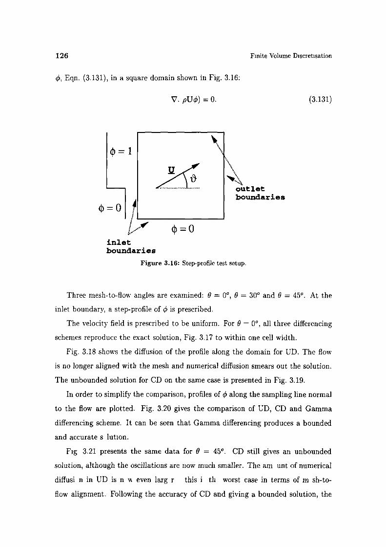
126
Finite Volume Discretisation
, Eqn. (3.131), in a square domain shown in Fig. 3.16:
V. pU5) =0. (3.131)
outletboundaries
inletboundaries
Figure 3.16: Step-profile test setup.
Three mesh-to-flow angles are examined: 9 = 0°, 9 = 300 and 0 = 450 At the
inlet boundary, a step-profile of is prescribed.
The velocity field is prescribed to be uniform. For 9 - 0 0 , all three differencing
schemes reproduce the exact solution, Fig. 3.17 to within one cell width.
Fig. 3.18 shows the diffusion of the profile along the domain for UD. The flow
is no longer aligned with the mesh and numerical diffusion smears out the solution.
The unbounded solution for CD on the same case is presented in Fig. 3.19.
In order to simplify the comparison, profiles of ç5 along the sampling line normal
to the flow are plotted. Fig. 3.20 gives the comparison of UD, CD and Gamma
differencing scheme. It can be seen that Gamma differencing produces a bounded
and accurate s lution.
Fig 3.21 presents the same data for 0 = 450 CD still gives an unbounded
solution, although the oscillations are now much smaller. The am unt of numerical
diffusi n in UD is n v even larg r this i th worst case in terms of m sb-to-
flow alignment. Following the accuracy of CD and giving a bounded solution, the
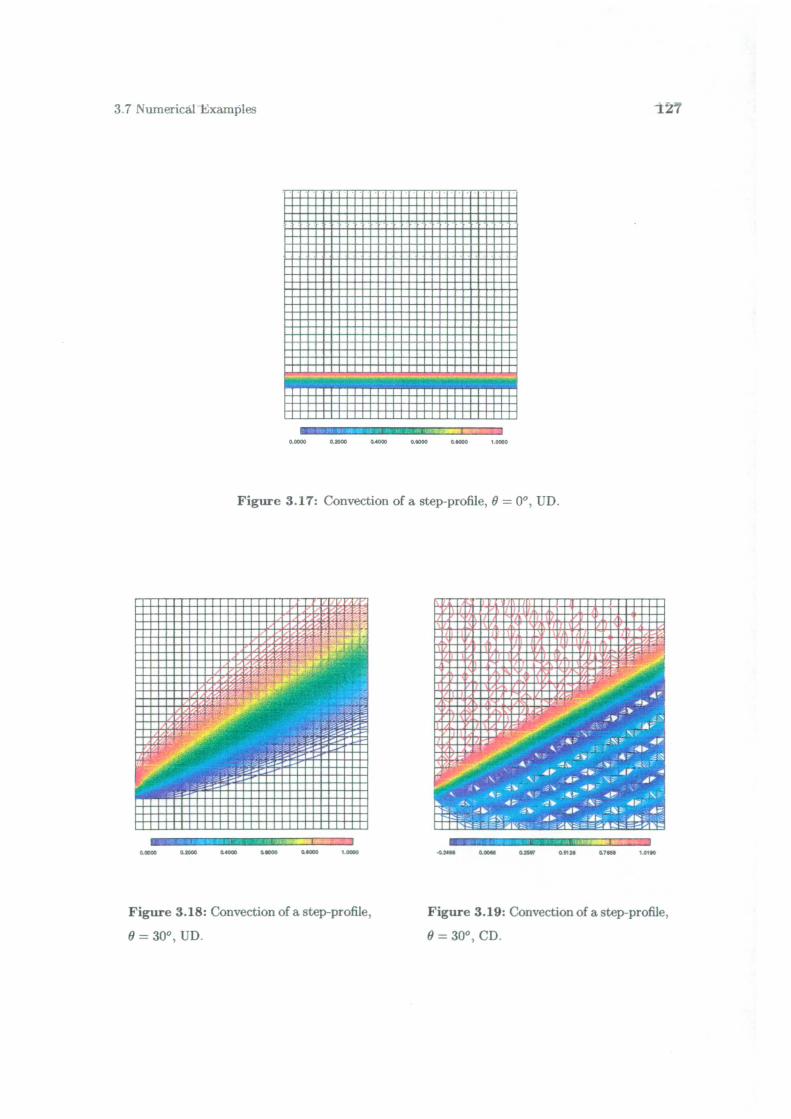
00000 00000 00000 0000 0000 1.0000--
.00100 00001 0000 00100 01050 1.0100
i73.7 Numerical Examples
00000 00000 04000 000 01000 0X0
Figure 3.17: Convection of a step-profile, 0 = 0°, UD.
Figure 3.18: Convection of a step-profile, Figure 3.19: Convection of a step-profile,
0 = 3O, UD. 0 = 30°, CD.
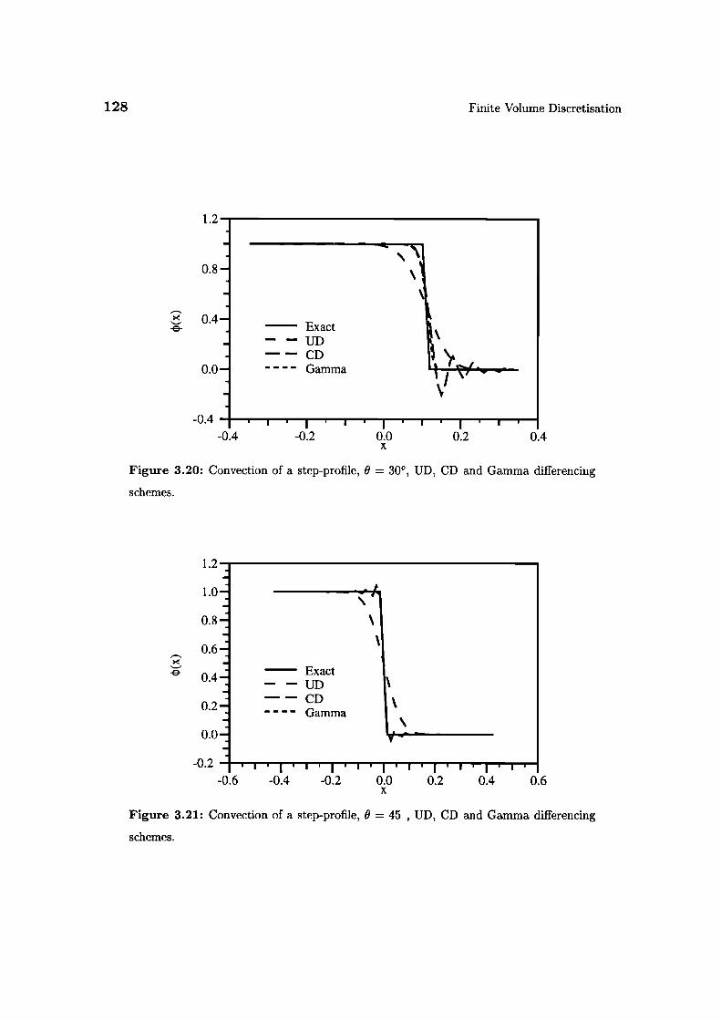
1.2
0.8
0.4
0.0
1.2
1.0
0.8
0.6
-e- 0.4
0.2
0.0
-0.2
Exact—-UD--CD— — — — Gamma
128
Finite Volume Discretisation
.4' II
Exact— UD '--CD— — — — Gamma
-0.4sJ.r 'J.iJ i.J.4.
x
Figure 3.20: Convection of a step-profile, 9 = 30 0 , UD, CD and Gamma differencing
schemes.
-0.6 -0.4 -0.2 0.0 0.2 0.4 0.6x
Figure 3.21: Convection of a step-profile, 0 = 45 , UD, CD and Gamma differencing
schemes.
3.7 Numerical Examples 129
Gamma differencing scheme reproduces the exact profile.
3.7.2 Comparison of the Gamma Differencing Scheme with
Other High-Resolution Schemes
Let us now present a comparison of the Gamma differencing scheme with a group of
other high-resolution schemes. The test setup is similar to Fig. 3.16, with different
profiles of at the inlet boundary. The mesh to-flow angle is fixed to 300. Following
Leonard [83], three boundary profiles of b are selected:
Step-profile:
. sin2-profile:
. Semi-ellipse:
10 for0<x<1- 6'
(1 fork^x^1,
(x)={3
[37r(x—)] forx<2,I
0 elsewhere,
(3.132)
(3.133)
[(1)2 for x <
(3.134)
0
elsewhere.
The comparison of the profiles is given along the line in the centre of the domain,
normal to the flow. The differencing schemes included in this comparison are:
. Gamma differencing scheme, Section 3.4,
. Self-filtered Central Differencing (SFCD) [128],
. van Leer TVD scheme [139],
. SUPERBEE TVD differencing scheme by Roe [118],
. SOUCUP NVD differencing scheme by Zhu and Rodi [155],
. SMART NVD scheme by Gaskell and Lau [49].

130
Finite Volume Discretisation
3.7.2.1 Step-profile
The results for the first test case are shown in Figs. 3.22, 3.23 and 3.24. Several
interesting features can be recognised. The step-resolution for Gamma is far su-
perior to the older version of stabilised Central Differencing (SFCD). The Gamma
differencing scheme gives the resolution of CD over the step and completely removes
unphysical oscillations.
SUPERBEE, Fig. 3.23, actually gives better step-resolution than Gamma. This
is the most compressive TVD differencing scheme. While SUPERBEE is very good
for sharp profiles, distortions of smooth solutions are too large to be accepted
(Leonard [83]).
SOUCUP, Fig. 3.24, is more diffusive than Gamma. The other NVD scheme,
SMART. gives a solution very close to the one obtained from the Gamma differenc-
ing scheme. One should have in mind that SMART is actually a stabilised version of
QUICK by Leonard, [81]. QUICK uses a computational molecule which is twice the
size of the one used by CD and Gamma. Apart from that, SMART is usually imple-
mented in a deferred correction mode, causing distortions in the temporal behaviour.
The Gamma differencing scheme, with its compact computational molecule, does
not require such treatment.
3.7.2.2 szn2-profile
The results for the convection of a sin2 profile are shown in Figs. 3.25, 3.26 and 3.27.
This test case has been selected to present the behaviour of the differencing schemes
on smoothly changing profiles. Another interesting feature of this test is a one-
point peak in the exact solution, Fig. 3.25. It is known that TVD schemes reduce to
first-order accuracy in the vicinity of extrema. This phenomenon is usually called
"clipping'. The amount of "clipping" giv s us a direct mdi ati n of the quality f
the differencing scheme.
SFCD, Fig. 3.25, shows a considerable amount of "clipping". The maximum of
the profile for the Gamma differencing scheme is about 0 85 considerably less than
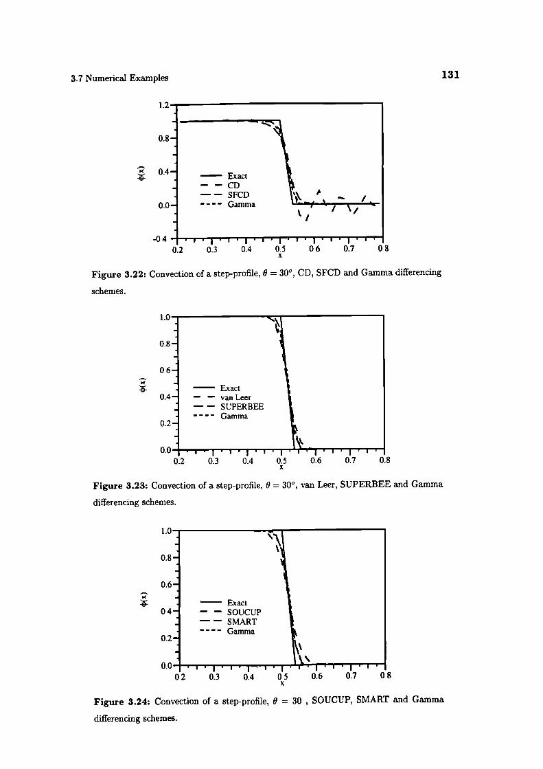
1.0
0.8
06
0.4
0.2
3.7 Numerical Examples 131
1.2
0.8
0.4 —'____.1 Exact
SFCDCD
0.0 Gamma - - \/ 'I
0.2 0.3 0.4 0.5 0 6 0.7 0 8x
Figure 3.22: Convection of a step-profile, 0 = 300 , CD, SFCD and Gamma differencing
schemes.
0.0 1 .1. 1 .1. 1 .1. 1 . . I .- 1.1.1.1.10.2 0.3 0.4 0.5 0.6 0.7 0.8
x
Figure 3.23: Convection of a step-profile, 9 = 300 , van Leer, SUPERBEE and Gamma
differencing schemes.
1.0
0.8
0.6
04
0.2
0.0 1 . i.i.i.i.i.i.•i-.1.I.i''.I02 0.3 0.4 05 0.6 0.7 08
x
Figure 3.24: Convection of a step-profile, 9 = 30 , SOUCUP, SMART and Gamma
differencing schemes.
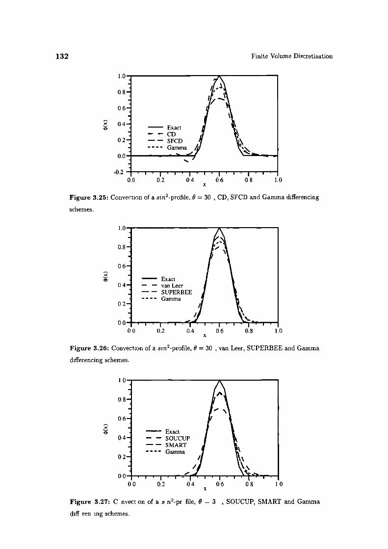
I.
0
0
0
0
0.
132
Finite Volume Discretisation
0.0 0.2 04 06 08 1.0x
Figure 3.25: Convection of a sin2 -profile. 9 = 30 , CD, SFCD and Gamma differencing
schemes.
1.0
0.8
06
04
02
00I.i.i.,.j. ji.i.ir.I00 0.2 0.4 06 0.8 1.0
x
Figure 3.26: Convection of a szn 2-profile, 9 = 30 , van Leer, SUPERBEE and Gamma
differencing schemes.
10
08
06x
04
02
•i.'T'rI00 0.2 04 06 08 10
x
Figure 3.27: C nvect on of a s n2-pr file, 8 - 3 , SOUCUP, SMART and Gamma
duff ren ing schemes.
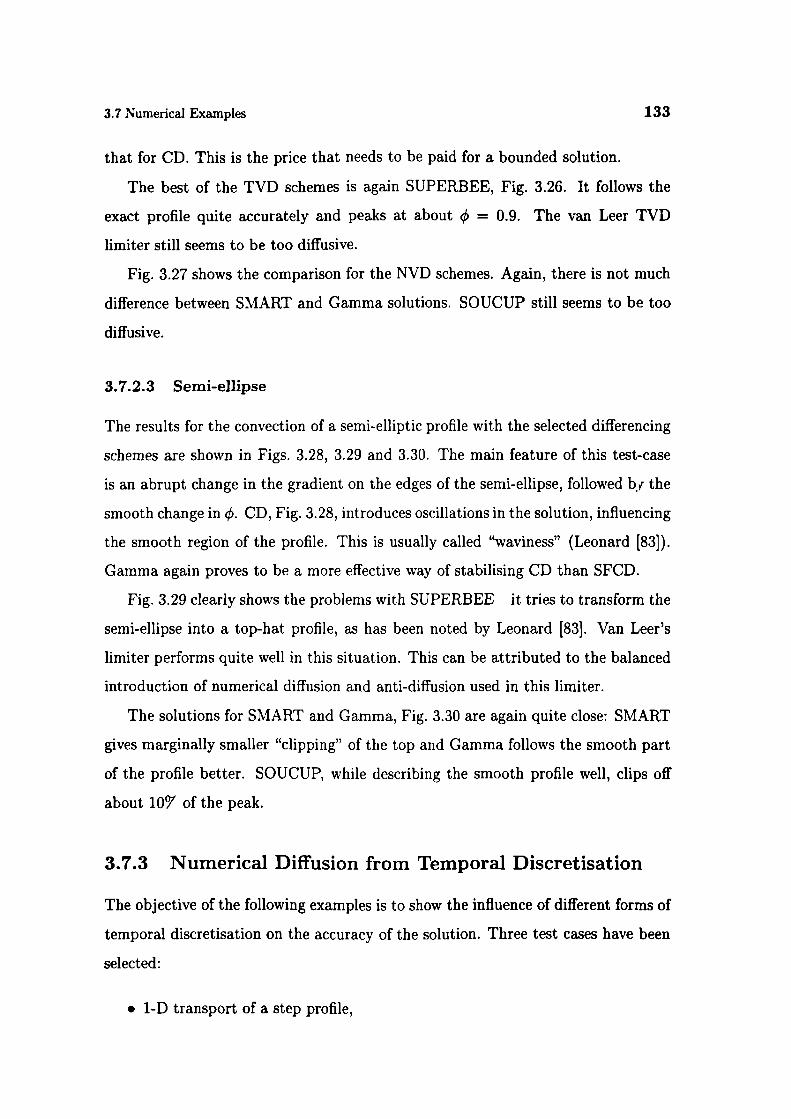
3.7 Numerical Examples 133
that for CD. This is the price that needs to be paid for a bounded solution.
The best of the TVD schemes is again SUPERBEE, Fig. 3.26. It follows the
exact profile quite accurately and peaks at about = 0.9. The van Leer TVD
limiter still seems to be too diffusive.
Fig. 3.27 shows the comparison for the NVD schemes. Again, there is not much
difference between SMART and Gamma solutions. SOUCUP still seems to be too
diffusive.
3.7.2.3 Semi-ellipse
The results for the convection of a semi-elliptic profile with the selected differencing
schemes are shown in Figs. 3.28, 3.29 and 3.30. The main feature of this test-case
is an abrupt change in the gradient on the edges of the semi-ellipse, followed by the
smooth change in q. CD, Fig. 3.28, introduces oscillations in the solution, influencing
the smooth region of the profile. This is usually called "waviness" (Leonard [83]).
Gamma again proves to be a more effective way of stabilising CD than SFCD.
Fig. 3.29 clearly shows the problems with SUPERBEE it tries to transform the
semi-ellipse into a top-hat profile, as has been noted by Leonard [83]. Van Leer's
limiter performs quite well in this situation. This can be attributed to the balanced
introduction of numerical diffusion and anti-diffusion used in this limiter.
The solutions for SMART and Gamma, Fig. 3.30 are again quite close: SMART
gives marginally smaller "clipping" of the top and Gamma follows the smooth part
of the profile better. SOUCUP, while describing the smooth profile well, clips off
about 1091 of the peak.
3.7.3 Numerical Diffusion from Temporal Discretisation
The objective of the following examples is to show the influence of different forms of
temporal discretisation on the accuracy of the solution. Three test cases have been
selected:
. 1-D transport of a step profile,
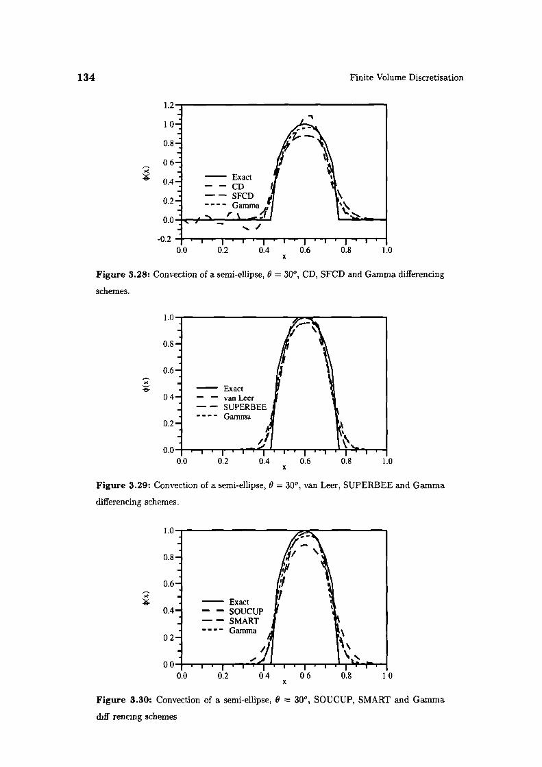
1.1
10
0.8
06
0.4
0.2
0.0
-0.2
134
Finite Volume Discretisation
0.0 0.2 0.4 0.6 0.8 1.0x
Figure 3.28: Convection of a semi-ellipse, 9 = 30°, CD, SFCD and Gamma differencing
schemes.
1.0
0.8
0.6
.904
0.2
I IU.'.,
. • I III'I'I I0.0 0.2 0.4 0.6 0.8 1.0
x
Figure 3.29: Convection of a semi-ellipse, 9 = 30°, van Leer, SUPERBEE and Gamma
differencing schemes.
1.0
0.8
0.6
-80.4
02
00 1 . •. i r11.• • • 1 r I
0.0 0.2 04 06 0.8 10x
Figure 3.30: Convection of a semi-ellipse, 9 30°, SOUCUP, SMART and Gamma
duff rencing schemes
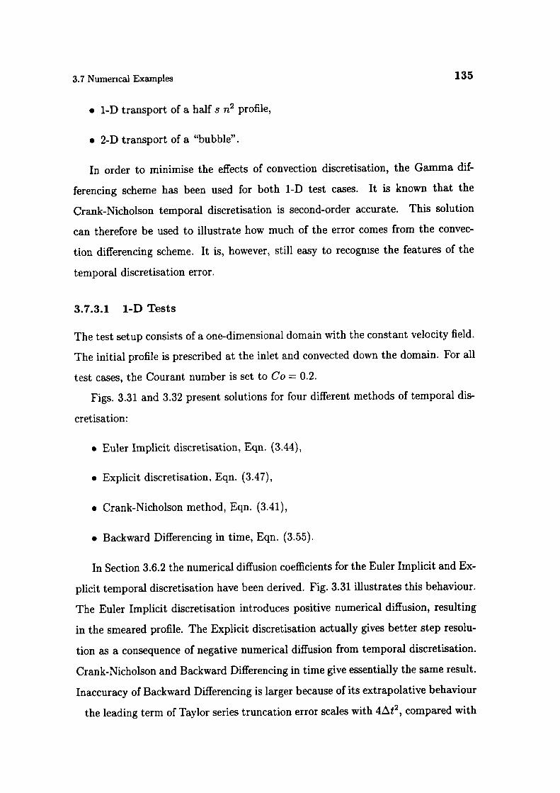
3.7 Numerical Examples 135
. 1-D transport of a half s n2 profile,
. 2-D transport of a "bubble".
In order to minimise the effects of convection discretisation, the Gamma dif-
ferencing scheme has been used for both 1-D test cases. It is known that the
Crank-Nicholson temporal discretisation is second-order accurate. This solution
can therefore be used to illustrate how much of the error comes from the convec-
tion differencing scheme. It is, however, still easy to recognise the features of the
temporal discretisation error.
3.7.3.1 1-D Tests
The test setup consists of a one-dimensional domain with the constant velocity field.
The initial profile is prescribed at the inlet and convected down the domain. For all
test cases, the Courant number is set to Co = 0.2.
Figs. 3.31 and 3.32 present solutions for four different methods of temporal dis-
cretisat ion:
. Euler Implicit discretisation, Eqn. (3.44),
• Explicit discretisation, Eqn. (3.47),
• Crank-Nicholson method, Eqn. (3.41),
• Backward Differencing in time, Eqn. (3.55).
In Section 3.6.2 the numerical diffusion coefficients for the Euler Implicit and Ex-
plicit temporal discretisation have been derived. Fig. 3.31 illustrates this behaviour.
The Euler Implicit discretisation introduces positive numerical diffusion, resulting
in the smeared profile. The Explicit discretisation actually gives better step resolu-
tion as a consequence of negative numerical diffusion from temporal discretisation.
Crank-Nicholson and Backward Differencing in time give essentially the same result.
Inaccuracy of Backward Differencing is larger because of its extrapolative behaviour
the leading term of Taylor series truncation error scales with 4t 2 , compared with
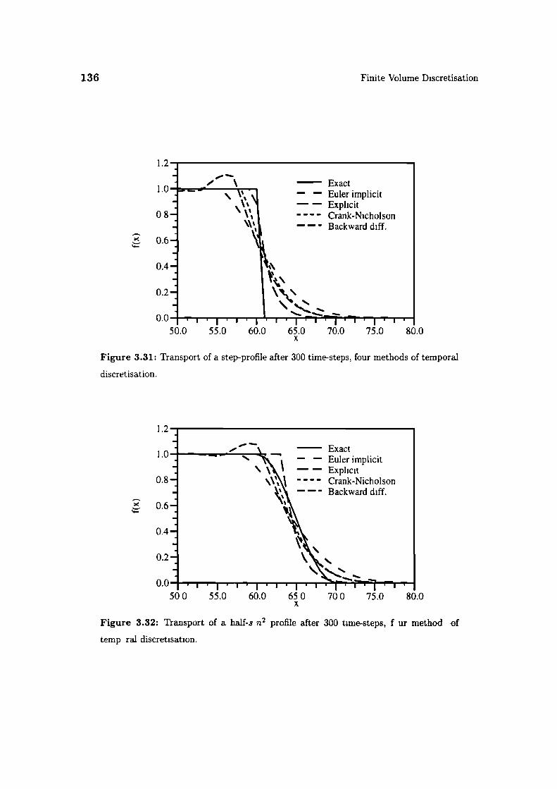
136
Finite Volume Discretisation
1.2
1.0
08
0.6
0.4
0.2
O.OI.i.iii'.,jrTr?r1r-i.i.I50.0 55.0 60.0 65.0 70.0 75.0 80.0
x
Figure 3.31: Transport of a step-profile after 300 time-steps, four methods of temporal
discretisation.
1.2
1.0
0.8
' 06C-
0.4
0.2
0.0 1 . i.i.i.i.i.i.
50 0 55.0 60.0 65 0 700 75.0 80.0x
Figure 3.32: Transport of a half-s n2 profile after 300 time-steps, f ur method of
temp ral discretisation.
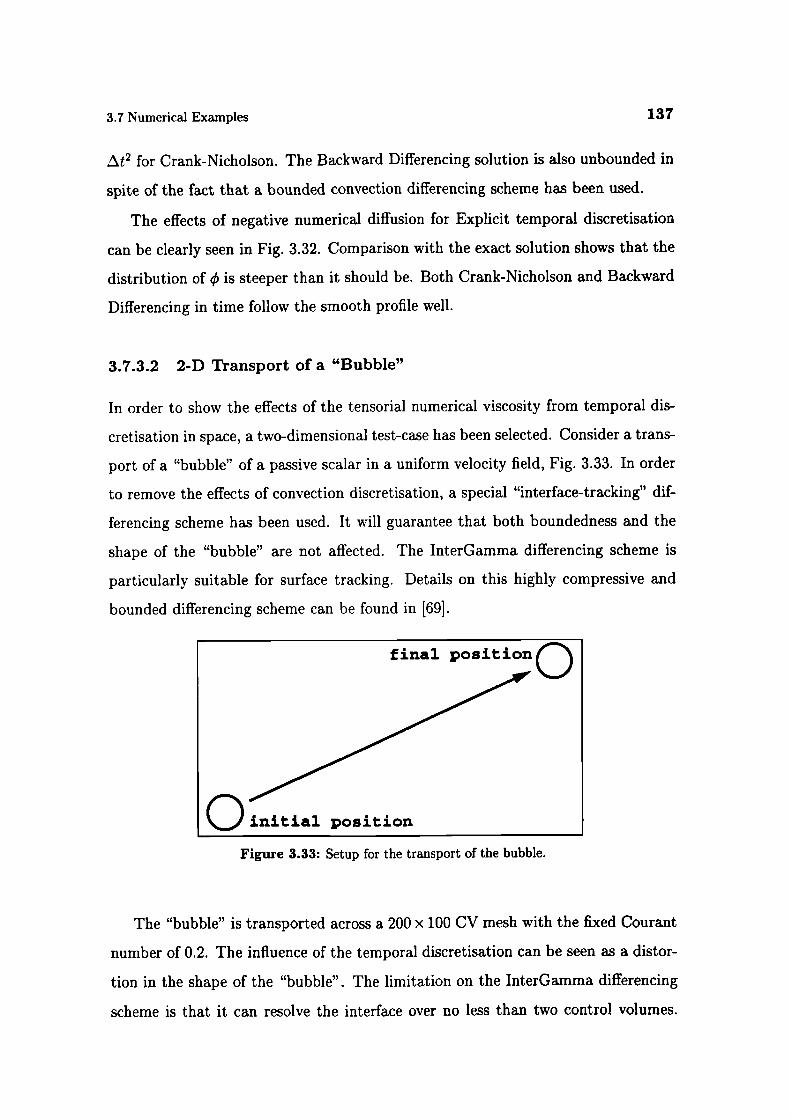
final ositionQ
initial position
3.7 Numerical Examples 137
t2 for Crank-Nicholson. The Backward Differencing solution is also unbounded in
spite of the fact that a bounded convection differencing scheme has been used.
The effects of negative numerical diffusion for Explicit temporal discretisation
can be clearly seen in Fig. 3.32. Comparison with the exact solution shows that the
distribution of is steeper than it should be. Both Crank-Nicholson and Backward
Differencing in time follow the smooth profile well.
3.7.3.2 2-D Transport of a "Bubble"
In order to show the effects of the tensorial numerical viscosity from temporal dis-
cretisation in space, a two-dimensional test-case has been selected. Consider a trans-
port of a "bubble" of a passive scalar in a uniform velocity field, Fig. 3.33. In order
to remove the effects of convection discretisation, a special "interface-tracking" dif-
ferencing scheme has been used. It will guarantee that both boundedness and the
shape of the "bubble" are not affected. The InterGamma differencing scheme is
particularly suitable for surface tracking. Details on this highly compressive and
bounded differencing scheme can be found in [69].
Figure 3.33: Setup for the transport of the bubble.
The "bubble" is transported across a 200 x 100 CV mesh with the fixed Courant
number of 0.2. The influence of the temporal discretisation can be seen as a distor-
tion in the shape of the "bubble". The limitation on the InterGamma differencing
scheme is that it can resolve the interface over no less than two control volumes.

138 Finite Volume Discretisation
This has been taken into account in the initial setup by smearing the interface over
two cells.
Fig. 3.34 gives the initial shape of the bubble. If we recall Eqn. (3.118 , it can be
seen that the numerical diffusion for the Euler Implicit discretisation is large where
U.V is large. Fig. 3.35 illustrates the behaviour of this error term. The bubble
is smeared in the direction of the velocity. In the direction normal to the flow the
"bubble" is squeezed because of the conservative form of discretised equation.
The opposite effect for the Explicit discretisation, Fig. 3.36, is the result of
negative numerical diffusion. The Crank-Nicholson method, Fig. 3.37 shows no
distortion of the shape.
3.7.4 Comparison of Non-Orthogonality Treatments
Finally, a comparison of the three procedures for handling non-orthogonality in the
solution algorithm will be given. If we limit ourselves to simple situations with
analytical solutions, it is very difficult to present their performance in terms of
accuracy and boundedness. It is, however, relatively easy to examine the first three
criteria laid down in Section 3.5. The test case used for this purpose is a Laplace
equation:
V.Vç =0, (3.135)
with fixed value boundary conditions on a mesh with uniform non-orthogonality
shown in Fig. 3.38.
The equation is solved on 5 meshes with different non-orthogonality angles, rang-
ing from a = 100 up to c = 65°.
For each of the non-orthogonality treatments, the convergence history through a
series of correctors for a selected computational point is plotted against the number
of non-orthogonal correctors.
For the mesh angle of c - 10 0 , there is no significant difference in convergence.
The overshoot in the first corrector is smallest for the over-relaxed approach.
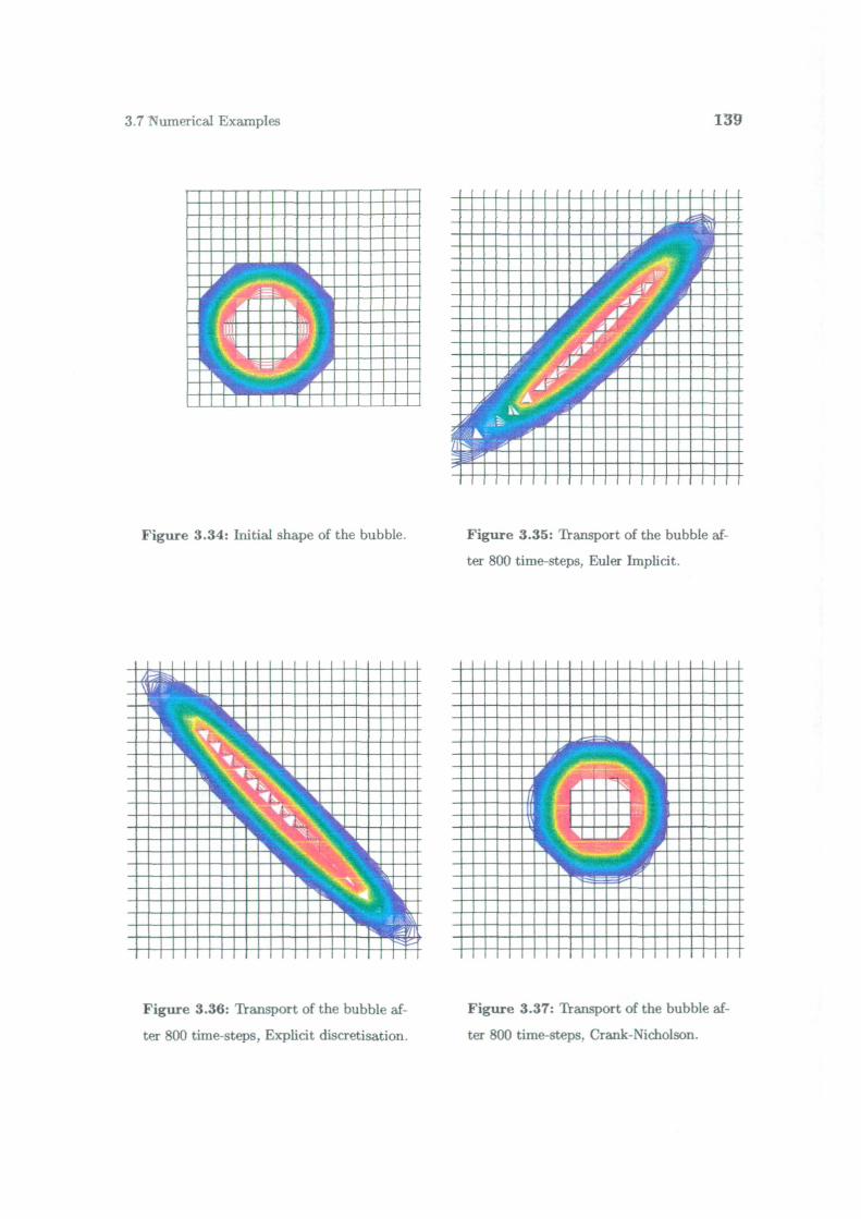
3.7 1umerical Examples 139
Figure 3.34: Initial shape of the bubble. Figure 3.35: Transport of the bubble af-
ter 800 time-steps, Euler Implicit.
Figure 3.36: Transport of the bubble af- Figure 3.37: Transport of the bubble af-
ter 800 time-steps, Explicit discretisation. ter 800 time-steps, Crank-Nicholson.
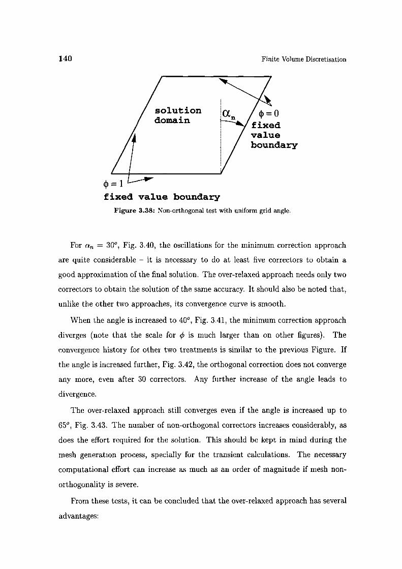
140
Finite Volume Discretisation
solutiondomain
fixedvalueboundary
fixed value boundary
Figure 3.38: Non-orthogonal test with uniform grid angle.
For , = 300, Fig. 3.40, the oscillations for the minimum correction approach
are quite considerable - it is necessary to do at least five correctors to obtain a
good approximation of the final solution. The over-relaxed approach needs only two
correctors to obtain the solution of the same accuracy. It should also be noted that,
unlike the other two approaches, its convergence curve is smooth.
When the angle is increased to 40°, Fig. 3.41, the minimum correction approach
diverges (note that the scale for q is much larger than on other figures). The
convergence history for other two treatments is similar to the previous Figure. If
the angle is increased further, Fig. 3.42, the orthogonal correction does not converge
any more, even after 30 correctors. Any further increase of the angle leads to
divergence.
The over-relaxed approach still converges even if the angle is increased up to
65°, Fig. 3.43. The number of non-orthogonal correctors increases considerably, as
does the effort required for the solution. This should be kept in mind during the
mesh generation process, specially for the transient calculations. The necessary
computational effort can increase as much as an order of magnitude if mesh non-
orthogonality is severe.
From these tests, it can be concluded that the over-relaxed approach has several
advantages:
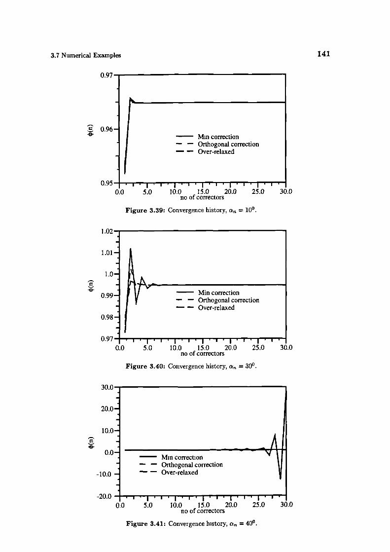
3.7 Numerical Examples 141
0.97-r
0.96Mm correction
- - Orthogonal correction- - Over-relaxed
I ii0.0 5.0 10.0 15.0 20.0 25.0
30.0
no of correctors
Figure 3.39: Convergence history, = 100.
1.02
1.01
1.0
0.99
0.98
0.970.0
30.0
20.0
10.0
0.0
-10.0
Mm correction- - Orthogonal correction
- Over-relaxed
Mm correction- Orthogonal correction
- - Over-relaxed
5.0 10.0 15.0 20.0 25.0no of correctors
Figure 3.40: Convergence history, = 30°.
30.0
-20.0 I0.0 5.0 10.0 15.0 20.0 25.0 30.0
no of correctors
Figure 3.41: Convergence history, = 40°.
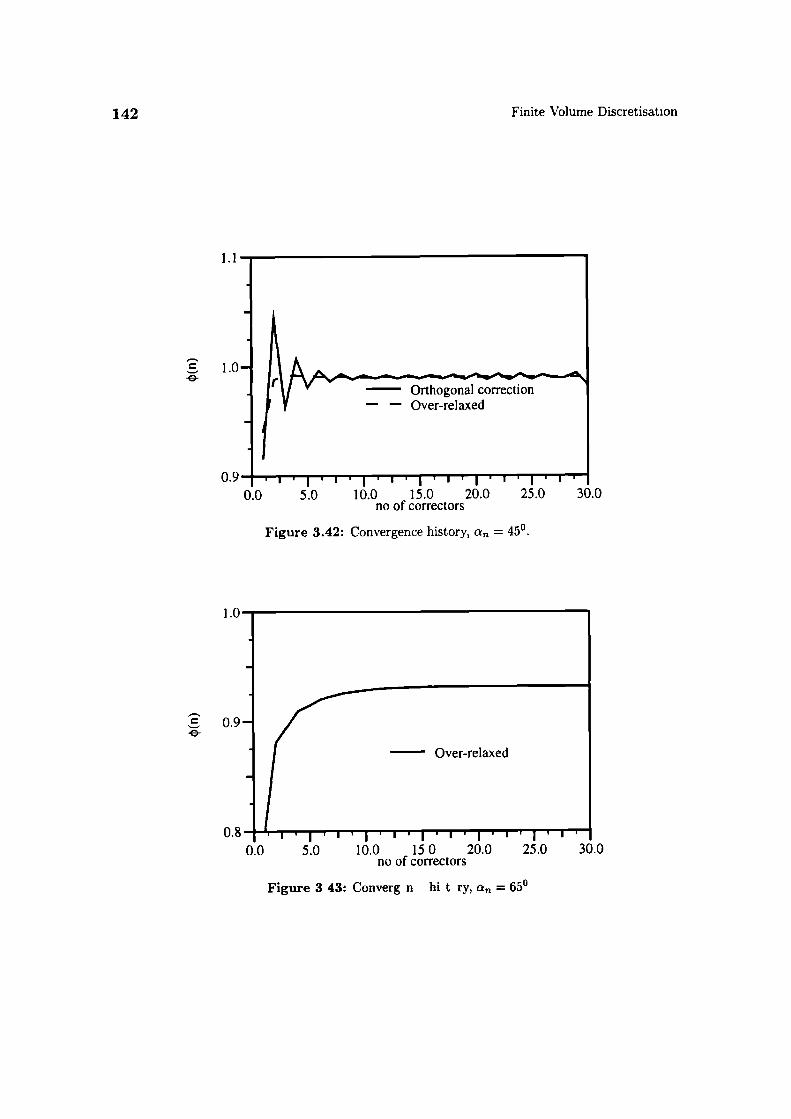
1.1
' 1.0
0.9
142
Finite Volume Discretisation
0.0 5.0 10.0 15.0 20.0 25.0 30.0no of correctors
Figure 3.42: Convergence history, = 450,
1.0
' 0.9
0.80.0 5.0 10.0 15 0 20.0 25.0 30.0
no of correctors
Figure 3 43: Converg n hi t z'y, = 65°
3.8 Discretisation Procedure for the Navier-Stokes System
143
• The solution after the first non-orthogonal corrector is closer to the converged
solution that in other non-orthogonality treatments. The angle of mesh non-
orthogonality that requires non-orthogonal correctors is therefore larger than
in other approaches.
. The convergence of non-orthogonal correctors is monotonic rather than oscil-
latory, resulting in the higher stability of the solution procedure.
. The over-relaxed approach reaches a converged solution even on meshes dis-
torted so severely that other non-orthogonality treatments diverge.
• It has been noted that the number of ICCG solver sweeps needed to solve a
non-orthogonal corrector decreases through the corrector series, which is not
the case for other non-orthogonality treatments. The overall computational
cost for the over-relaxed approach will therefore be smaller even in the case of
the same number of correctors.
These properties of the over-relaxed non-orthogonality treatment make it very
attractive, specially for transient calculations and it will be used in the rest of this
study.
3.8 Discretisation Procedure for the
Navier-Stokes System
In this Section, a discretisation procedure for the Navier-Stokes equations will be
presented. We shall start with the incompressible form of the system, Eqs. (2.23)
and (2.24):
v.U=o,
+ V.(UU) - V.(vVU) = —Vp.
Two issues require special attention: non-linearity of the momentum equation
and the pressure-velocity coupling.
144
Finite Volume Discretisation
The non-linear term in Eqn. (2.24) is V.(UU), i.e. velocity is "being transported
by itself". The discretised form of this expression would be quadratic in velocity and
the resulting system of algebraic equations would therefore be non-linear. There are
two possible solutions for this problem either use a solver for non-linear systems,
or linearise the convection term. Section 3.3.1 describes the discretisation of this
term:
V.(UU) =f
=
/
= apUp + aNUN,
N
where F, ap and aN are a function of U. rFhe important issue is that the fluxes F
should satisfy the continuity equation, Eqn. (2.23). Eqs. (2.23) and (2.24) should
therefore be solved together, resulting in an even larger (non-linear) system. Having
in mind the complexity of non-linear equation solvers and the computational effort
required, linearisation of the term is preferred. Linearisation of the convection term
implies that an existing velocity (flux) field that satisfies Eqn. (2.23) will be used to
calculate ap and aN.
The linearisation does not have any effect in steady-state calculations. When the
steady-state is reached, the fact that a part of the non-linear term has been lagged is
not significant. In transient flows two different approaches can be adopted: either to
iterate over non-linear terms or to neglect the lagged non-linearity effects. Iteration
can significantly increase the computational cost, but only if the time-step is large.
The advantage is that the non-linear system is fully resolved for every time-step,
whose size limitation comes only from the temporal accuracy requirements. If it is
necessary to resolve the temporal behaviour well, a small time-step is needed. On
the other hand, if the time-step is small, the change between consecutive solutions
will also be small and it is therefore possible to lag the non-linearity without any
significant effect.
In this study, the PISO procedure proposed by Issa [66] is used for pressure-
3 8 Discretisation Procedure for the Navier-Stokes System 145
velocity coupling in transient calculations. For steady-state calculations, a SIMPLE
pressure-velocity coupling procedure by Patankar [105] is used.
In Section 3.8.1 the problem of pressure-velocity coupling is presented. The
pressure equation is derived for the incompressible Navier-Stokes system. Gener-
alisation to compressible and transonic flows can be found in eg. Demirdzié et al.
[39]. Section 3.8.2 describes the pressure-velocity coupling algorithms. Finally, in
Section 3.8.3, a solution procedure for incompressible Navier-Stokes equations with
a turbulence model is presented.
3.8.1 Derivation of the Pressure Equation
In order to derive the pressure equation, a semi-discretised form of the momentum
equation will be used:
apUp = H(U) - Vp. (3.136)
In the spirit of the Rhie and Chow procedure [117], the pressure gradient term
is not discretised at this stage. Eqn. (3.136) is obtained from the integral form of
the momentum equation, using the discretisation procedure described previously.
It has been consequently divided through by the volume in order to enable face
interpolation of the coefficients.
The H U) term consists of two parts: the "transport part", including the matrix
coefficients for all neighbours multiplied by corresponding velocities and the "source
part" including the source part of the transient term and all other source terms
apart from the pressure gradient (in our case, there are no additional source terms):
HU)=—aNUN +. (3.137)
The discretised form of the continuity equation (Eqn. (2.23)) is:
V.0 = S.U1 =0. (3.138)/
Eqn. (3.136) is used to express U:
HU) 1Up = _____ - —Vp (3.139)
ap ap

(3.142)
(3.143)
146
Finite Volume Discretisation
Velocities on the cell face are expressed as the face interpolate of Eqn. (3.139
U1 (HU)- ap )
—)(V)i.
This will be used later to calculate the face fluxes.
(3.140
When Eqn. (3.140 is substituted into Eqn. (3.138), the following form of the
pressure equation is obtained:
v. = v. (H(UY\
ap I ap)
S. (H(U))
/ ap(3.141)
The Laplacian on the l.h.s. of Eqn. (3.141) is discretised in the standard way (see
Section 3.3.1.3).
The final form of the discretised incompressible Navier-Stokes sytem is:
apUp = H U) - PfI
s. 1(i (VP)f](H(U))
f [\ap)r ap
The face flux F is calculated using Eqn. (3.140):
F = S U1 - S. 1(H(U)ap )
- (I) (VP)f]ap j
3.144
When Eqn. (3.141) is satisfied, the face fluxes are guaranteed to be conservative.
3.8.2 Pressure-Velocity Coupling
Consider the discretised form of the Navier-Stokes system, Eqs. 3.142) and (3.143).
The form of the equations shows linear dependence of velocity on pressure and
vice-versa. This inter-equation coupling requires a special tr atment.
Simultaneous algorithms (eg. Caretto et al. [23], Vanka [143] operate by
solving the complete system of equations simultaneously over the whole domain.
Such a procedure might be considered when the number f c mputati nal p ints
is small and the number of simultaneous equations is not too large. The resulting
3.8 Discretisation Procedure for the Navier-Stokes System
147
matrix includes the inter-equation coupling and is several times larger than the
number of computational points. The cost of a simultaneous solution is great, both
in the number of operations and memory requirements.
In the segregated approach (eg. Patankar [105], Issa [66]) the equations are
solved in sequence. A special treatment is required in order to establish the necessary
inter-equation coupling. PISO [66], SIMPLE [105] and their derivatives are the most
popular methods of dealing with inter-equation coupling in the pressure-velocity
system.
3.8.2.1 The PISO Algorithm for Transient Flows
This pressure-velocity treatment for transient flow calculations has been originally
proposed by Issa [66]. Let us again consider the discretised Navier-Stokes syst m for
incompressible flow, Eqs. (3.142) and (3.143). The PISO algorithm can be described
as follows:
• The momentum equation is solved first. The exact pressure gradient source
term is not known at this stage the pressure field from the previous time-step
is used instead. This stage is called the momentum predictor. The solution
of the momentum equation, Eqn. (3.142), gives an approximation of the new
velocity field.
• Using the predicted velocities, the H U) operator can be assembled and the
pressure equation can be formulated. The solution of the pressure equation
gives the first estimate of the new pressure field. This step is called the pres-
sure solution.
• Eqn. (3.144) gives a set of conservative fluxes consistent with the new pressure
field. The velocity field should also be corrected as a consequence of the new
pressure distribution. Velocity correction is done in an explicit manner, using
Eqn. (3.139). This is the explicit velocity correction stage.
A closer look to Eqn. (3.139) reveals that the velocity correction actually consists
of two parts a correction due to the change in the pressure gradient (Vp term)
148 Finite Volume Discretisation
and the transported influence of corrections of neighbouring velocities term).
The fact that the velocity correction is explicit means that the latter part is neglected
- it is effectively assumed that the whole velocity error comes from the error in the
pressure term. This, of course, is not true. It is therefore necessary to correct the
H U) term, formulate the new pressure equation and repeat the procedure. In
other words, the PISO loop consists of an implicit momentum predictor followed by
a series of pressure solutions and explicit velocity corrections. The ioop is repeated
until a pre-determined tolerance is reached.
Another issue is the dependence of H(U) coefficients on the flux field. After each
pressure solution, a new set of conservative fluxes is available. It would be therefore
possible to recalculate the coefficients in H(U). This, however, is not done: it is
assumed that the non-linear coupling is less important than the pressure-velocity
coupling, consistent with the linearisation of the momentum equation. The coeffi-
cients in H(U) are therefore kept constant through the whole correction sequence
and will be changed only in the next momentum predictor.
3.8.2.2 The SIMPLE Algorithm
If a steady-state problem is being solved iteratively, it is not necessary to fully resolve
the linear pressure-velocity coupling, as the changes between consecutive solutions
are no longer small. Non-linearity of the system becomes more important, since the
effective time-step is much larger.
The SIMPLE algorithm by Patankar [1051 is formulated to take advantage of
these facts:
• An approximation of the velocity field is obtained by solving the momen-
tum equation. The pressure gradient term is calculated using the pressure
distribution from the previous iteration or an initial guess. The equation
is under-relaxed in an implicit manner (see Eqn. (3.96 ), 'with the velocity
under-relaxation factor c.
• The pressure equation is formulated and solved in order to obtain the new
3.8 Discretisation Procedure for the Navier-Stokes System
149
pressure distribution.
• A new set of conservative fluxes is calculated using Eqn. (3.144). As it has
been noticed before, the new pressure field includes both the pressure error and
convection-diffusion error. In order to obtain a better approximation of the
"correct" pressure field, it would be necessary to solve the pressure equation
again. On the other hand, the non - linear effects are more important than
in the case of transient calculations. It is enough to obtain an approximation
of the pressure field and recalculate the H(U) coefficients with the new set
of conservative fluxes. The pressure solution is therefore under-relaxed in
order to take into account the velocity part of the error:
pfleW = pold + ap(p' - pold) (3.145)
where
- pnew is the approximation of the pressure field that will be used in the
next momentum predictor,
- pold is the pressure field used in the momentum predictor,
- p1' is the solution of the pressure equation,
- cxp is the pressure under-relaxation factor, (0 < a ^ 1).
If the velocities are needed before the next momentum solution, the explicit
velocity correction, Eqn. (3.139), is performed.
Perié, [109] gives an analysis of the under-relaxation procedure based on the
expected behaviour of the second corrector in the PISO sequence. The recommended
values of under-relaxation factors are (Perié, [109]):
• cz,, = 0.2 for the pressure and
• au = 0.8 for momentum.

150
Finite Volume Discretisation
3.8.3 Solution Procedure for the Navier-Stokes System
It is now possible to describe the solution sequence for the Navier-Stokes system
with additional coupled transport equations (eg. a turbulence model, combustion
equations, energy equation or some other equations that influence the system).
In transient calculations, all inter-equation couplings apart from the pressure-
velocity system are lagged. If it is necessary to ensure a closer coupling between
some of the equations (eg. energy and pressure in combustion), they are included
in the PISO loop. A transient solution procedure for incompressible turbulent
flows can be summarised as follows:
1. Set up the initial conditions for all field values.
2. Start the calculation of the new time-step values.
3. Assemble and solve the momentum predictor equation with the available face
fluxes.
4. Go through the PISO loop until the tolerance for pressure-velocity system is
reached. At this stage, pressure and velocity fields for the current time-step
are obtained, as well as the new set of conservative fluxes.
5. Using the conservative fluxes, solve all other equations in the system. If the
flow is turbulent. calculate the effective viscosity from the turbulence variables.
6. If the final time is not reached, return to step 2.
The solution procedure for steady-state incompressible turbulent flow is
similar:
1. Set all field values to some initial guess.
2 Assemble and solve the under-relaxed momentum predictor equation
3. Solve the pressure equation and calculate the conservative fluxes. Update
the pressure field with an appropriate under-relaxation. Perform the explicit
velocity correction using Eqn. (3.139

3.9 Closure
151
4. Solve the other equations in the system using the available fluxes, pressure
and velocity fields. In order to improve convergence, under-relax the other
equations in an implicit manner, as shown in Eqn. (3.96).
5. Check the convergence criterion for all equations. If the system is not con-
verged, start a new iteration on step 2.
3.9 Closure
A Finite Volume discretisation technique for arbitrarily unstructured meshes has
been described. It allows the use of the control volumes of arbitrary topology,
simplifying the problem of mesh generation for complex geometries. In order to
preserve the efficiency of the algorithm, a "face addressing" approach by Weller
[1471 has been adopted.
The discretisation of the temporal and spatial terms based on the face addressing
procedure has been described in Section 3.3. The proposed discretisation treatment
is second-order accurate in space and time. Several methods of temporal discreti-
sations have also been examined. Implementation of boundary conditions has been
briefly discussed. A new non-orthogonality treatment has been proposed and tested
on a series of meshes with increasing non-orthogonality angles. The results show
that the over-relaxed approach has distinct advantages over the other two approaches
in terms of stability, although it causes the largest discretisation error if the non-
orthogonal correction is discarded. It provides better convergence behaviour and at
the same time allows higher angles of non-orthogonality.
In order to improve the discretisation of the convection term, the Gamma dif-
ferencing scheme has been proposed in Section 3.4. It is based on the Normalised
Variable Approach, first suggested by Leonard [82]. It guarantees bounded solutions
and preserves the second-order accuracy of the method. The Gamma differencing
scheme uses a compact computational molecule (including only first neighbours of
the control volume), making it specially useful on arbitrarily unstructured meshes.
A necessary modification in the formulation of the Normalised Variable is also pre-
152
Finite Volume Discretisation
sented.
Particular attention has been paid to the order of accuracy of the method and the
sources of the discretisation error. The main sources of the error are the convection
differencing scheme, discretisation of the transient terms and the mesh quality. The
effective numerical diffusion has been derived for each of those terms. Numerical
examples, showing the influence of different forms of numerical diffusion to the
solution, have been presented in Section 3.7.
Finally, in Section 3.8, a discretisation procedure for coupled systems of equations
has been presented. The adopted treatment of the pressure-velocity system is based
on the PISO algorithm for transient calculations and the SIMPLE approach for
steady-state flows. A sequence of operations for both steady-state and transient
calculations has been summarised.

Chapter 4
Error Estimation
4.1 Introduction
Chapter 3 describes the Finite Volume discretisation. The discretisation procedure
allows us to obtain a discrete approximation of governing equations for a particular
problem. When the resulting system of algebraic equations is solved, it produces an
approximate solution at a set of points in the computational domain. The quality
of the numerical solution depends on the distribution of the points as well as the
applied discretisation practice.
The presented method of discretisation is second-order accurate in space and
time, i.e. it is assumed that the variation of the function over each control volume is
linear. This is the major source of numerical errors. If a better solution is needed,
control volumes should be subdivided in such a way that the assumption about the
linear variation becomes acceptable.
Another source of numerical errors is the discretisation practice. For good accu-
racy, it is necessary for the order of discretisation to be equal to or higher than the
order of the partial differential equation that is being discretised. If that is not the
case, discretisation errors effectively introduce a term which is of the order of other
terms in the equation, resulting in high numerical errors unless the mesh is made
excessively fine.
The error in the numerical solution is defined as the difference between the exact
154 Error Estimation
solution of the governing equation c1 x, t), and the solution of the discrete system
E=—g. (4.1)
The purpose of error estimation is to detect inaccuracies in the numerical so-
lution, including both the errors coming from inappropriate discretisation of the
solution domain and discretisation errors. Adaptive refinement process consists of
a series of numerical solutions and error estimations, followed by appropriate im-
provements in the discretisation. The objective of the procedure is to automatically
produce a numerical solution of the prescribed accuracy.
The role of the error estimate is to provide an answer to the following questions:
\Vhat is the magnitude of the solution error?
. If the error is larger than some pre-determined level, what is the most effective
way of reducing it?
The answer to the first question controls the adaptive refinement process. If
the current solution satisfies the error level criterion, further refinement is no longer
necessary. If this is not the case, the error distribution can be used to introduce some
changes in the numerical procedure eg. better distribution of computational points
or higher order of discretisation, in order to improve the accuracy of consequent
solutions.
The only data available to the analyst containing the information about the error
is the numerical solution itself. This leads us to the concept of a—posteriori error
estimation. As the name suggests, an estimate of the solution error is obtained
after the numerical solution. An a-posteriorz error estimate is constructed having in
mind the the known characteristics of the discretisation practice and the equation
that is being solved.

4.1 Introduction 155
4.1.1 Error Estimators and Error Indicators
Early efforts in the field of error detection have been directed towards problems with
discontinuous solutions, like multiple shock structures in supersonic flows (see Berger
and Oliger [17], Berger and Collela [16], Löhner [89], Ramakrishnan et al. [116] etc.).
The solution has some distinct features - shocks, contact discontinuities, shock-to-
shock interaction points etc. that need to be resolved accurately. It is known in
advance that those features can be recognised by large gradients in flow variables.
Adaptive refinement is therefore directed towards the regions in which gradients are
high. In the exact solution, discontinuities are infinitely thin - mesh refinement is
therefore stopped when the thickness of discontinuities in the numerical solution is
considered to be small enilgh, or when the maximum number of computational
points is reached.
Combinations of gradients of flow variables used to control the adaptive refine-
ment procedure are called error indicators. An error indicator highlights the
regions of the domain where a better resolution is needed. In general, it does not
provide information about the absolute error level. Error indicators are cheap to
compute and for simple situations give reliable information about the solution.
Adaptive refinement for problems with smooth solutions cannot be controlled
by an error indicator. Flow features that need refinement cannot be identified in
advance and adaptive refinement should be stopped when some pre-determined accu-
racy is reached. An error estimate is therefore expected to give more information
about the accuracy than the error indicator. It should estimate the absolute error
level as well as the distribution of the error throughout the domain. Interaction
between error estimation and local mesh refinement should also be kept in mind.
If the refinement algorithm allows localised refinement with rapid changes in mesh
size, it is necessary to obtain accurate information about the error. Patch-based
refinement methods are not so sensitive to the accuracy of the error estimate.
The Effectivity index ( measures the quality of an error estimate. It is defined
156
Error Estimation
as the ratio of magnitudes of the estimated error e and the exact error E:
(4.2)
Good error estimates have effectivity indices close to unity.
In this Chapter several methods of error estimation are proposed. Section 4.2
outlines the requirements on an error estimate. In order to simplify matters, we shall
first examine the problem of error estimation in steady-state calculations, where the
whole error comes from the discretisation of spatial terms. Three approaches to
a-posteriori error estimation of the spatial error are examined.
The first group of methods derive the error from the known order of accuracy and
the local variation of the solution. They are based on the Taylor series truncation
error analysis, discussed in Section 4.3. Two different ways of estimating the first
term of the truncation error are presented: Richardson extrapolation, Section 4.3.1
and the Direct Taylor Series Error estimate. Section 4.3.2.
Section 4.4 describes a new approach to the problem of error estimation the
Moment Error estimate. It is derived from the analysis of the original equation in
the differential form. The imbalance in the transport equation for a higher moment
of the variable is used to estimate the error. Instead of measuring the numerical
error directly, it derives its value from the effects of the discretisation inaccuracy on
the balance in the discretised moment equation.
An alternative approach to error estimation is presented in Section 4.5. The
Residual Error estimate follows similar work in Finite Element error estimation.
Residual is a function that measures how well the original equations are satisfied
over each control volume. It is assembled on a cell-by-cell basis. A transport-based
normalisation of cell residuals is used to estimate the absolute error level.
Section 4.6 gives an extension of the Residual Error estimate. It is possible to
derive a strict upper bound on the solution error expressed through an appropriate
error norm. Unlike the other error estimation methods described in this Chapter,
it does not measure the error directl y. The Local Problem Error estimate is based
on the similar work of Bank and Weiser [12], Kelly [71], Oden et al. [98], Ainsworth

4.2 Requirements on an Error Estimate 157
and Oden [1, 2, 3, 4] and others in the Finite Element community. The approach by
Ainsworth and Oden [4] has been chosen as the most general and directly extendible
to the Finite Volume method. The basic error estimate has been developed for linear
elliptic problems and consequently extended to unisymmetric [2] and non-linear
(specifically incompressible Navier-Stokes equations) [101] problems. The error is
presented in the form of an error norm. One of the requirements for the successful
use of this error estimate is an accurate error flux balancing procedure. This has
been widely discussed in the Finite Element literature (see Kelly [71], Ainsworth
and Oden [3] or Ainsworth [4]). The conservation properties of the Finite Volume
solution removes the need for a special error flux balancing algorithm, as will be
shown in Section 4.6.1.1. A simplified solution procedure for the local error problem
is given in Section 4.6.4.
Error estimation for transient calculations is discussed in Section 4.7. The tran-
sient error estimate is derived as an extension of the Residual method, taking into
account the effects of the temporal discretisation on the accuracy of the solution. It
is possible to split the total error into the spatial and temporal contributions. The
requirement of equivalent temporal and spatial accuracy can be used to determine
the optimal time-step size for a given computational mesh.
The examples presented in Section 4.8 illustrate the performance of error esti-
mates in simple situations. Comparison of the estimated and real error is given
for test cases with analytical solutions. Finally, some closing remarks are given in
Section 4.9.
4.2 Requirements on an Error Estimate
Let us now outline a set of properties a good error estimate should have.
The purpose of error estimation is to give an insight into the accuracy of the
solution. It is desirable to present the error information in terms of the absolute
error value. The error estimate is easier to understand if its dimensions are the
same as those of the solution variable. This approach is not generally accepted
158 Error Estimation
because of its impracticality for singular problems. A typical example can be found
in linear elasticity (see Zienkiewicz [156]). Under a point load, the local displacement
(and hence the error) is locally equal to infinity. The net effect of this error on the
rest of the domain is usually negligible (Zienkiewicz [156]). The solution error for
such situations can, however, be presented as an error norm. Singular problems are
riot common in fluid flows and such treatment is not necessary.
The error estimate will be used to control an adaptive refinement procedure. It
should therefore provide reliable information about the distribution of the
error through the computational domain. Even if the error level is not estimated ac-
curately, a correct error distribution guarantees that refinement regions are properly
selected.
Accurate error distribution is critical in calculations with highly localised refine-
ment, where the successive levels of refinement are embedded into each other. First
levels of refinement should be located accurately in order to reduce unnecessary
overheads. Error estimation should therefore work well on coarse meshes.
The error estimate will regularly be calculated on adaptively refined meshes,
consisting of control volumes of different sizes. It is even possible to use different
orders of discretisation in different parts of the mesh. If an accurate estimate of the
error is to be obtained for such a mesh, the error estimate should scale correctly
with the order of discretisation and mesh size.
For transient calculations with tracking of flow features, error estimation will
have to be done very often. The mesh is refined every few time-steps, depending on
the level of the error. In order to keep the computational cost at a reasonable level,
both error estimation and mesh refinement need to be computationally efficient. The
error estimate should therefore be easy to compute. An efficient error estimate is
based on the local solution and mesh information and can be caIcuated on
a cell-by-cell basis. If error estimation requires a solution of a system of algebraic
equations over all control volumes, it is considered to be too expensive.
Error estimation method should have a strong methematical basis. It should
be applicable to all degenerate forms of the transport equation (elliptic problems,
4.3 Methods Based on Taylor Series Expansion 159
convection or source-dominated problems). It is also desirable that the error esti-
mate gives the exact value of the error if the order of solution is one order higher
than the order of discretisation.
The transient error estimate is expected to work well even if the change of the
solution in time is very slow, or the solution tends to a steady-state solution. It
would therefore be advisable to construct it as an extension of a steady-state error
estimator.
As the number of computational points goes to infinity, the error estimate should
tend to the exact error faster than the solution tends to the exact solution. The
error estimate with this property is said to be asymptotically exact. It is expected
that the error estimate will detect both the errors resulting from insufficient mesh
resolution and the discretisation errors. The error estimate should also be rliable
in the vicinity of points of singularity.
Finally, the error estimate should modestly over-estimate the actual error.
Considering the complexity of error estimation, one cannot expect extremely accu-
rate results. If it is known that the error can be estimated only up to a certain
accuracy, over-estimation is preferred. Once the desired accuracy of the solution is
achieved according to the error estimate, the actual error will be even smaller.
Some of the aforementioned requirements on the error estimate are quite hard to
fulfill, others are even contradictory. It would be difficult to create an error estimate
which is both very accurate and easy to compute. Accuracy of the estimate on coarse
meshes presents a particular problem. The error estimation methods presented in
this Chapter should be seen as a compromise between the suggested requirements.
4.3 Methods Based on Taylor Series Expansion
The first group of error estimation methods is based on the analysis of the numerical
solution in terms of the Taylor series expansion. Every smooth function can be
written as an expansion in its derivatives around a given point in space. This
expansion is potentially infinite, depending on the number of non-zero derivatives

160
Error Estimation
at the selected point.
The discretisation process can be considered as a truncation of the infinite series.
The truncated form of the expansion at the computational point is used to describe
the variation of the solution over the control volume surrounding it. The complete
solution is created as a union of these locally defined "shape functions".
A pth order accurate discretisation method describes the local variation of
with the first p terms of the Taylor series:
1(x) = qp +(x —xp).(Vq)p + + (
1)(X - Xp) 1 (VV..V)p.
p- i p-i(4.3)
The discretisation error can also be expressed as an (infinite) series in higher
derivatives of :
(VV (4.4)np n n
The estimate of the error in the computational point is based on the average
error in the control volume, consistent with the discretisation practice:
et () = -- j 1 -(x - xp):: (VV..V )] dVlp Vp
L- n
<4- f (ix - x) "(VV V )) dV. (4.5)IJJfl p) Vp fl'
fl Ti
Let us now consider the form of Eqn. (4.5). It is assumed that the magnitude of
the leading term in Eqn. (4.5) gives a good estimate of the whole truncation error.
If the exact solution 1(x) is smooth and the control volume is small, contributions
from higher terms of the expansion in Eqn. (4.5) will indeed decrease rapidly with
increasing n. This is strictly true only if the mesh resolution is adequate.
The Taylor series error estimate uses only the first term of the expansion in
Eqn. 4 5) to estimate the error:
et ) _fI_x_xp"(VVVdVp p1 1 [ x—xpdV1 ::: (VV..V5p . 4.6)7i LJ
p p
as:
11
VP
12V
4 3 Methods Based on Taylor Series Expansion
161
If the mesh is too coarse, the contribution of higher-order terms can be signifi-
cant, particularly if higher derivatives are large. It can therefore be expected that
Eqn. (4.6) under-estimates the actual error.
In the case of second order accurate (Finite Volume) discretisation, the prescribed
spatial variation of over the control volume is linear, Eqn. (3.3):
q(x) = çbp + (x - xp).(Vq)p
The leading term of the truncation error is:
e(x) = (x - xp)2: (VVq5)p. (4.7)
Following Eqn. (4.6), the Taylor series error estimate in the point P is calculated
[f (x - xp)2 dv] : (VV5)p
Vp
M: (VVq5)p
(4.8)
M in Eqn. (4.8) is the second geometric moment of the control volume:
M = f(x_ xp)2dV. (4.9)
The local error can be estimated in two ways, resulting in two methods of error
estimation. The first, Richardson extrapolation, uses numerical solutions from two
meshes with different spacing. The second method estimates the numerical error
from a single solution. An error estimate based on the latter idea is presented in
Section 4.3.2 below.
4.3.1 Richardson Extrapolation
Richardson extrapolation is the most popular form of error estimation based on the
Taylor series truncation error analysis. It has been used for a large variety of flow
problems, ranging from incompressible Navier-Stokes equations (see eg. Thompson
and Ferziger [134], Muzaferija [97], Chen et al. [28]) to inviscid supersonic flows (see

162
Error Estimation
eg. Berger and Oliger [17], Berger and Collela [16]). Since the method requires solu-
tions of the same problem on two meshes, it has been regularly used in conjunction
with multigrid acceleration techniques.
The basic idea of Richardson extrapolation is to obtain an approximation of the
leading term in the truncation error from suitably weighted solutions on two meshes
with different cell size (Muzaferija [97], Caruso [25]).
The spatial variation of the exact solution on two meshes with spacing h 1 and
h2 can be symbolically written as (Muzaferija [97]):
(x) = (x, h 1 ) + hçC(x) + O(x, h?), (4.10)
1(x) = q(x, h2 ) + hC(x) + O(x, h), (4.11)
where
(x, h) is the approximate solution on the mesh with spacing h,
• hC(x) is the leading term of the truncation error,
• h = h(x) is the local mesh size calculated as the ratio of cell volume and
surface area:
VP
>f S(4.12)
• p is the order of accuracy of the discretisation method,
• O(x, h) is the rest of the truncation error.
From Eqs. (4.10) and (4.11), C(x) can be approximated as:
q5(x, h2 ) - q5(x, h1)Cx= (4.13)
hç—h
The estimate of C x , Eqn. (4.13 , can be used to improve the fine mesh solution
x, h2 ). The improved (qth order accurate) solution is:
iap 1"h 2 __________x,0 - x,h21 -
x,h1 '!1P (4.14h2 )h2'
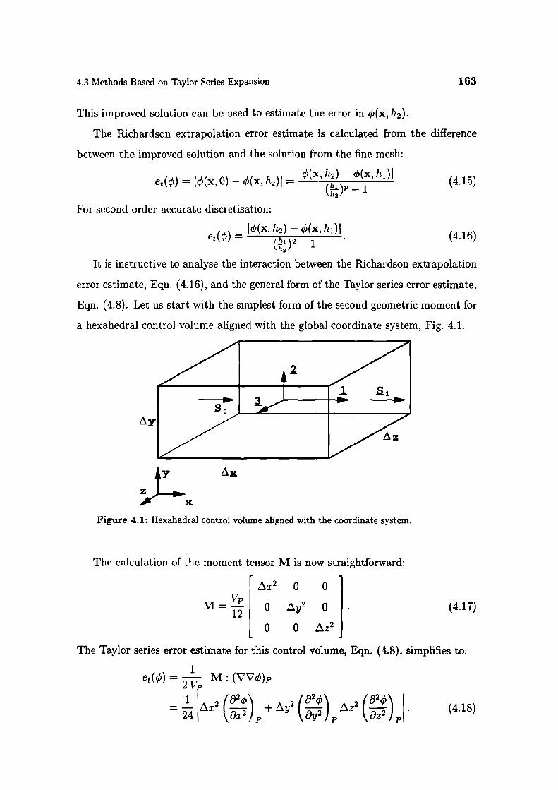
(4.17)
4.3 Methods Based on Taylor Series Expansion 163
This improved solution can be used to estimate the error in (x, h2).
The Richardson extrapolation error estimate is calculated from the difference
between the improved solution and the solution from the fine mesh:
= (x, h2) - q5(x, h1)Iet (q) = q5(x, 0) - qS(x, h2)I () - 1
For second-order accurate discretisation:
(4.15)
ej() = I5(x, h— (x, hi)
(4.16)
It is instructive to analyse the interaction between the Richardson extrapolation
error estimate, Eqn. (4.16), and the general form of the Taylor series error estimate,
Eqn. (4.8). Let us start with the simplest form of the second geometric moment for
a hexahedral control volume aligned with the global coordinate system, Fig. 4.1.
LX
Figure 4.1: Hexahadral control volume aligned with the coordinate system.
The calculation of the moment tensor M is now straightforward:
zx2
M=K 012
0
o o
Ly2 0
o Lz2
The Taylor series error estimate for this control volume, Eqn. (4.8), simplifies to:
et (q5) = -- M: (VVq5)pVP
2= zx2 ()+y2 (4.18)
164 Error Estimation
It is also known that (VV) should be independent of the mesh, as two numer-
ical solutions correspond to the same physical problem. The double-dot product
M : (VV4) p in Eqn. (4.18) is expected to scale quadratically with h. This is
independent of the orientation of the control volume in relation to the global co-
ordinate system. Richardson extrapolation, Eqn. (4.16), uses this property to esti-
mate the error. According to Eqn. (4.18), Richardson extrapolation assumes that
the magnitude of each term in M individually scales with h2 . This is valid only for
geometrically similar control volumes. If the control volumes of two meshes are not
similar in shape, Richardson extrapolation looses accuracy.
The Richardson extrapolation error estimate requires two solutions on meshes
with different spacing: (x, h 1 ) and (x, h2 ). In industrial applications this is not
always feasible the mesh necessary to appropriately describe the geometry and
boundary conditions can be of the order of several hundred thousands cells. Cal-
culation on a finer mesh could easily exceed the available computational resources.
The adaptive refinement algorithm proposed in this study does not include multi-
grid acceleration and two solutions are not readily available. As a consequence, the
Richardson extrapolation error estimate is considered to be expensive.
It is well known that Richardson extrapolation under-estimates the solution er-
ror. It is particularly inaccurate on coarse meshes. If a good error estimate is to
be obtained, both meshes need to be fine enough to approximate the solution well.
Once the solution is smooth in relation to mesh size on both meshes, the higher-
order truncation error terms vanish quickly and the accuracy of the error estimate
improves rapidly with mesh refinement.
4.3.2 Direct Taylor Series Error Estimate
It is possible to obtain the Taylor series error estimate from a single-mesh result.
This is a novel appr ach to Taylor series error estimation. The terms from Eqn. 4.8)
s ill be approximated from the available solution and mesh geometry. The error es-
timate obtained in such a way is called the Direct Taylor Series Error estimate.
The task of creating a single-mesh Taylor series error estimate can be di ided into
4.3 Methods Based on Taylor Series Expansion 165
two parts: estimating the second gradient of in P and evaluating the geometric
moment tensor M for the control volume, both appearing in Eqn. (4.18).
The (VVq5)p tensor is calculated from the available solution using Gauss' theo-
rem twice: Eqn. (3.10) is used to calculate (Vg)p, which is then used in Eqn. (3.11)
to obtain the second gradient. It should be noted however that the double Gauss'
theorem actually provides an average value of the second gradient over the con-
trol volume and the set of its neighbours, whereas Eqn. (4.8) requires the value in
the centroid the the control volume. The estimate will therefore be good only if
the numerical solution approximates the exact solution well and the mesh is fine
enough.
Calculation of M for control volumes in an arbitrarily unstructured mesh is
s]ightly more complex. The approach adopted here follows the work of Heif and
Küster [62j. Using Gauss' theorem, it is possible to reduce the volume integral
in Eqn. (4.9) to a set of geometric moment integrals over the faces and finally to
integrals over face edges. In order to simplify the derivation, the terms of M will be
assembled in a local coordinate system, with the origin in the centre of the control
volume. Eqn. (4.9) can be modified as follows:
M=J (x) 2 dV=f (xx)dVVp Vp
= J,V.[x(xx)]dV
=
= j(dS.x) (xx). (4.19)
The surface integrals in Eqn. (4.19) can be further simplified. It is known that
all faces are fiat. For every point on the face, the dot-product dS.x reduces to a
constant. It follows that:
(xx) = .xj j(xx) dA. (4.20)
Combining Eqs. (4.19 and (4.20), the volume integral is reduced to a sum of
surface integrals over fiat faces. Point x 1 has been selected as a sample point - any

166 Error Estimation
other point from the face plane will give the same product. Once the face integrals
are calculated for all faces of the mesh, they are added to control volumes on both
sides of the face with opposite signs.
Repeating the procedure once again, calculation of second geometric moments
for the face can be reduced to a sum of integrals over the face edges, which are easily
calculated.
This method is directly applicable on general polyhedral control volumes. In
spite of its recursive nature, it still seems computationally expensive. Calculation of
the error requires the evaluation of two second rank tensors (or a second rank and
a third rank tensor for vector properties), which is considered expensive.
Having in mind the limited accuracy of (VVq5)p, it would be wise to produce a
simple estimate o M. knowing that this simplification does not significantly degrade
the overall accuracy of the method. An appropriate transformation of the coordinate
system can reduce the second geometric moment tensor to diagonal terms only. Ori-
entation of the coordinate system then coincides with the principal geometric axes
of inertia for the control volume. If the product M : (VV)p were calculated in
that coordinate system, it would reduce to only three terms, similar to Eqn. (4.18).
Vectors 1, 2 and 3 in Fig. 4.1 represent the principal vectors of inertia for the
control volume. For a hexahedral cell of arbitrary orientation, they can be approxi-
mated from the face area vectors of the opposite face pairs. Thus, for example, 1 is
approximated with (Fig. 4.1):
(So S 1 '\ Vp
s0+s1
and the error estimate, Eqn. (4.8), simplifies to:
(4.21)
et(
M: (VVç)p
24V 1 1. VVç5 p) + 2. 2.(VV5)p + 3. 3.(VVq5 p
4 22
The off-diagonal terms in M which w uld arise for warp d c ntrol v lumes are
neglected. Eqn. (4.22) is still considered to be a reasonable estimate of the full

4 3 Methods Based on Taylor Series Expansion 167
tensorial product, since the aspect ratio of the cell is taken into account. This prin-
ciple can be extended to general polyhedral shapes by introducing an "orientation
vector", defined as the ratio of cell volume and the average cell surface in the given
direction.
The evaluation of the M: (VV)p term in the error estimate can be simplified
even further. If it is assumed that the control volume is not distorted in any way, the
product scales with the square of the characteristic linear size of the control volume,
Eqn. (4.12) and the magnitude of (VV')p. The error can therefore be estimated
as:
1et(q)=.V_
1')A IT'f VP
IM: (VVq)p(
h2 I(VV)p. (4.23)
Simplification in Eqn. (4.23) further reduces the accuracy of the estimate. This
is, however, a popular practice in the Finite Element community (Oden et al. [98]),
particularly for elliptic problems.
Having in mind the situations of mesh alignment to flow gradients and high cell
aspect ratios, Eqn. (4.22) has been selected in the present work as a good balance
of accuracy and computational cost.
4.3.3 Measuring Numerical Diffusion
The current formulation of the Direct Taylor Series Error estimate measures the
numerical diffusion only indirectly. Richardson extrapolation takes numerical dif-
fusion effects only partially, through the solutions on meshes with different mesh
spacing. An overview of numerical diffusion terms has been given in Section 3.6.
Their common property is that the magnitude of the numerical diffusion coefficient
scales with the mesh size. Numerical diffusion is therefore smaller on a finer mesh,
which is visible in the error estimate.
The Direct Taylor Series Error estimate cannot measure numerical diffusion er-
rors at all. If it is necessary to include it into the error estimation procedure, the
following procedure can be used:

168
Error Estimation
Using the expressions for numerical diffusion from different sources, the nu-
merical diffusion tensor is assembled for each face.
. The term V.(Fnum .V) is then evaluated for every control volume. The influ-
ence of this term on the total error is obtained through normalisation, (see Sec-
tion 4.4.1), using the characteristic time-scale T (defined later in Eqn. (4.33 ):
V.(Fnum.Vq5) dV T=
(4.24)VP
• is added to the truncation error estimate, Eqn. (4.8).
Gradients of are estimated from the current solution. Numerical diffusion
smears out local gradients as a consequence, enum will be under-estimated even if
the total numerical diffusion tensor is calculated exactly. In the uncommon case of
negative numerical diffusion coefficients (explicit temporal discretisation, compres-
sive differencing schemes), the opposite effect is expected.
4.4 Moment Error Estimate
The second approach to the problem of error estimation is based on the analysis of
the differential equation that is being solved. An estimate of the error is derived
from the properties of the exact solution.
Let us consider a steady-state scalar transport equation in the standard form,
Eqn. (3.56):
V.(pU) - V.(pFVç5) = Sn).
Finite Volume discretisation produces a solution that satisfies this equation over
each control volume in the integral form.
If Eqn. (3 56) were satisfied for each point in the computational domain (in the
differential form , its solution would also satisfy all higher moment equations. At
this stage, we shall limit ourselves to the second moment of q5:
1- 2
(4.25)
4.4 Moment Error Estimate
169
The transport equation for m can be derived from Eqs. (3.56) and (4.25) in the
following form:
V.(pUm) - V.(prVm) = S0(q) - p['(Vq5.V). (4.26)
The numerical solution of Eqn. (3.56) is, however, of limited accuracy. There is
no guarantee that Eqn. (4.26) will be satisfied for every control volume. This will
be the case only if the numerical solution of Eqn. (3.56) corresponds to the exact
solution on all cell centres and all faces of the mesh.
The imbalance in Eqn. (4.26) depends on the local difference between the ap-
proximate and exact solution - it can therefore be used to estimate the numerical
error.
Following Eqn. (4.26), the local imbalance is equal to:
resm(m4,) = j [V.(pUm) - V.(pI'Vm) - S) + pF(V.V)] dV.
(4.27)
The cell centre values of m 41, are calculated from the known values of çf' using
Eqn. (4.25). Following the discretisation practice presented in Chapter 3, convec-
tion, diffusion and source terms are assembled from the cell values of m. In the
calculation of face values from the convection term, Central Differencing is used.
Some attention should be given to the boundary condition treatment. On fixed
value boundary faces, the value of is prescribed. This value can be used to calcu-
late the corresponding face value of m. On fixed gradient boundaries, a different
approach is needed. The value of on the boundary face is calculated from the
value in the adjacent cell, consistent with the prescribed boundary condition. The
value of m0 on the boundary face is then calculated from , using Eqn. (4.25).
The same principle can be extended to a general steady-state vector (tensor)
transport equation. Let us consider a steady-state transport equation for a general
vector property a:
V.(pUa - V.(pI"aVa) = Su + Spa. (4.28)
1ma = a.a, (4.29)
170 Error Estimation
The steady state form of the transport equation for the second moment of a:
has the following formS
V.(pUma) - V. pFaVma) = Su.a+ 2Spma - pF(Va: Va).
(4.30)
The imbalance in ma is assembled similar to Eqn. (4.27):
resm(ma) = f [V.(pUma) - V.(pFa Vma) - Su.a(4.31)
—2 Spma + pF0 (Va: Va)] dv.
Unlike the Taylor series error estimation methods, the Moment Error estimate
produces a scalar error for both scalar and vector properties. Iii the case of a
vector transport equation, the resulting error estimate corresponds to the error in
the magnitude of a. The same is valid for tensor transport equations.
The Moment Error estimate measures the error through its influence on the
solution. The proposed approach can be extended to higher moments of q. In
the case of fourth order discretisation of Eqn. (3.56), the second moment transport
equation will be satisfied automatically. Effects of the numerical error can still be
detected as the imbalance in transport equations for higher moments of q.
The next step in the construction of the Moment Error estimate is to provide a
way of estimating the magnitude of the error from the imbalance.
4.4.1 Normalisation of the Moment Error Estimate
Dimensions of resm (m) from Eqn. (4.27) are []2[L]3/[T], i.e. it does not correspond
to the absolute error in q. In order to obtain the error magnitude, a suitable
n rmahsation practice is required.
Eqn. 4 27 shows that resm m) represents the volume integrated error in the
transport of m, The purpose of normalisation is to establish the influence of the
imbalance to the local value of . Normalisation of resm (m) will be based on
4 4 Moment Error Estimate 171
the local transport conditions for çb. The effective transport consists of two parts:
convective velocity and the effective diffusive transport. It is estimated as:
Utrans = IU + . (4.32)
The local characteristic length-scale h represents the mesh spacing. It is calculated
as the ratio of cell volume and surface area, Eqn. (4.12). It should be noted that
this length-scale does not have any physical meaning it merely represents the local
mesh size.
The characteristic time-scale T required for normalisation of resm(mc,,) is calcu-
lated from the characteristic transport velocity and the local cell size:
T= h h2
(4.33)Utrans lu h+I'q
Combination of Eqs. (4.33) and (4.27) enables us to estimate the solution error.
The error estimate constructed this way has the dimensions of , giving an insight
into the magnitude of the local error. The final form of the Moment Error estimate
for a steady-state transport equation is:
em(q5) - 2'/
resm(m) T(4.34)
- VP
4.4.2 Consistency of the Moment Error Estimate
As noted earlier, the task of error estimation is to pinpoint the regions of the com-
putational domain in which the difference between the numerical and real solution
is large. A good error estimator should also pinpoint regions in which the solution
is approximated well. If the polynomial order of local variation of the solution is
lower than or equal to the order of discretisation, the error estimate should return
zero.
Let us assume that the variation of over a certain region is linear. If the terms
of Eqn. (3.56) are discretised to second order, the resulting q5 field is exact. The
error estimate, Eqn. (4.34), should return zero. According to Eqn. (4.25), the local
variation of will be quadratic. If the terms of Eqn. (4.27) are also discretised to
172 Error Estimation
second order accuracy, resulting resm(m) will be non-zero simply because of the
discretisation error in Eqn. (4.27) we are trying to describe a quadratic variation
with a linear function. It follows that, for consistency with Eqn. (3.56), evaluation
of the terms in Eqn. (4.27) should be fourth-order accurate.
The error in the evaluation of volume integrals scales with the h4 . It can therefore
be expected that the Moment Error estimate tends to the exact error faster than
with h2 , producing exact asymptotic behaviour on very fine meshes. If the mesh
is too coarse, the scaling of the error estimate may be incorrect, depending on the
ratio of fourth-order terms and the actual solution error.
In practice, the problem is not so serious. It rarely happens that the order
of discretisation is high enough to follow the variation of the solution over the
control volume exactly. If this is the case, the fourth-order terms of Eqn. (4.27)
can be approximated accurately and added to the error estimate. Considering the
computational overhead from the evaluation of control volume moment tensors and
the limited gain in accuracy, the terms of Eqn. (4.27) will be discretised to second-
order.
The influence of fourth-order terms can be partially taken into account in the
normalisation of the imbalance in m. An improved estimate of the error can be
obtained if the local transport in Eqn. (4.32) is over-estimated, thus compensating
for the over-estimation of the imbalance. This has been done by including the whole
cell surface area into the convective transport estimate in Eqn. (4.32).
The proposed form of the Moment Error estimate measures the numerical dif-
fusion through its influence on the solution. Coming back to the derivation of the
transport equation for m, Eqn. (4.26 , it can be seen that every term in this equa-
tion has its equivalent in Eqn. (3.56). This is the reason why the exact solution
of Eqn. (3.56) also satisfies Eqn. (4.26 . The numerical errors introduced in the
discretisation change the structure of Eqn. (3.56) on the level of the discretisation
error, by introducing a numerical diffusion term. Numerical diffusion acts as an ad-
ditional term in the original transport equation which does n t have its equivalent
in the transport equation for the moment and therefore causes an imbalance in the
4.5 Residual Error Estimate 173
volume integral for m0.
The Moment Error estimate is cheap to compute. Its behaviour on coarse meshes
should be significantly better than any of the Taylor series error estimates. The
influence of discretisation error is measured without the need for explicit evaluation
of numerical diffusion terms. The main disadvantage of the method is its relative
inaccuracy on very fine meshes.
4.5 Residual Error Estimate
The idea for the Residual Error estimate comes from similar work in Finite Element
error estimation. In order to introduce the concept of residual, it is first necessary
to analyse the properties of a Finite Volume solution. An appropriate normalisation
ofthe residual is then used to estimate the magnitude of the error.
In the Finite Element method, equations are solved using the Galerkin principle
(Zienkiewicz [156]) minimisation of the weighted residual over the computational
domain. The governing equations are therefore not necessarily satisfied over each
finite element'. Once the solution is calculated, the residual distribution is available.
The residual is a function that measures how well the local solution satisfies the
original governing equations. It is therefore natural to associate the level of residual
with the local solution error.
The Finite Volume discretisation is derived from the integral form of the govern-
ing equation over the control volume. The numerical solution consists of cell centre
and cell face values that satisfy the original equation over each cell. Cell face values
are determined using an interpolation practice consistent with discretisation. The
idea of the residual as a measure of accuracy is therefore not immediately obvious.
In order to introduce the residual, the basis of the Finite Volume method will be
examined. For that purpose, let us assume that a numerical solution of a differential
equation on a given grid with a pth order accurate Finite Volume discretisation is
'More precisely, they are satisfied only if the the shape function can exactly follow the variation
of the solution over the finite element

174
Error Estimation
available: pth order accuracy implies that the function used to evaluate the sur-
face and volume integrals consists of the first p terms of Taylor series expansion,
Eqn. (4.3 , and that pth order accurate face interpolation is used. The variation of
the numerical solution over the control volume is therefore described by Eqn. (4.3).
Let us also assume that the exact solution of the problem is available.
If the exact solution varies over the control volume faster than the pth order, the
governing equation cannot be satisfied. In this situation, a control volume imbalance
should exist. This is in contradiction with the basic principle of Finite Volume
discretisation. In order to simplify further discussion, we shall limit ourselves to
second-order accurate Finite Volume method.
The inter-point coupling in the system of algebraic equations obtained by the
Finite Volume discretisation comes from the face interpolation. The cell value of ç
depends on the values in neighbouring cells through the calculation of face values and
face gradients of 5. Inconsistency between volume integration and face interpolation
can be explained on a simple 1-D situation, Fig. 4.2.
PA
NFigure 4.2: Inconsistency between face interp lation and the integration over the cell.
For ' olume integrals, a second-order accurate discretisation assumes linear van-
ati n f over the c ntrol volume P, Eqn. 3.3 (continuous line in Fig 4.2
x) = qp + x - xp).Vp.
4.5 Residual Error Estimate 175
Here, (V)p is calculated using discretised Gauss' theorem, Eqn. (3.26):
(V)p -- >S,.VP'
On the other hand, the face value of is obtained by linear interpolation between
the points P and N. The interpolated face values together with the cell-centred
volume integrals satisfy the integral form of the governing equation.
Let us consider an arbitrary point A inside the control volume P. The value of
in this point can be calculated in two ways:
Following the assumed distribution of q over the control volume (continuous
line in Fig. 4.2), q5(A) is:
q5(A) = çbp + (XA - xp).Vq5p, (4.35)
since A is inside the control volume P.
. On the other hand, the face value jr for the face between P and N is obtained
by interpolation. The same approach can be used for the point A which is
also between P and N (dashed line in Fig. 4.2):
çb(A) = Ia qp + ( 1 - fa) N, (4.36)
where
ANfa 7 (4.37)
Values of (A) obtained from Eqs. (4.35) and (4.36) are identical only in the case
of linear variation of the exact solution over the control volume and its neighbours,
in which case the numerical error is equal to zero. If this is not the case, for every
point inside the control volume two equally valid values of can be given.
On the face f, situation is even more complicated: q j obtained by interpolation,
Eqn. (3.19):
= fçbp+ (1— f)cbN,

176
Error Estimation
satisfies the governing equation in the integral form. For the point just left of the
face (in the P control volume), the value of 4) is:
4)! = q5p + (x1 - xp ) .V 4)p (4.38)
and for the point just right of f, it is:
= 4)N + (xf XN).V4)N. (4.39)
Let us now consider the construction of the cell residual. According to the
definition used in finite elements, residual is a consequence of insufficient order of
accuracy of the prescribed variation of 4) over the control volume. It has been shown
that the face values satisfying the governing equation are not consistent with the
variation of 4) used for volume integrals. A consistent face value of 4) for the P control
volume should be calculated using Eqn. (4.38). If this value is different from the
interpolated 4), the integral form of the governing equation for P is not satisfied any
more. The imbalance obtained this way is equivalent to the finite element definition
of the residual.
Information about the error can be obtained in two ways:
• Since every face is shared by two control volumes, three different face values
can be determined, Eqs. (3.19), (4.38) and (4.39). In case of the exact solution,
all three values will be identical. If a face jump exists, it can be used to measure
the error.
. The face values are calculated consistent with the prescribed variation of 4)
over the control volume. A residual is assembled for each control volume and
normalised in an appropriate way.
Although the first approach produces the estimate of the error on the face with
same dimensi ns as 4), it d es not take into account the convection-diffusion balance
of the equation, as the face jump in (V4) / should also be taken into account.
The second appr ach pr duces a cell bas d residual, taking into account the
convection-diffusion balance and the influence of mesh quality. A normalisation
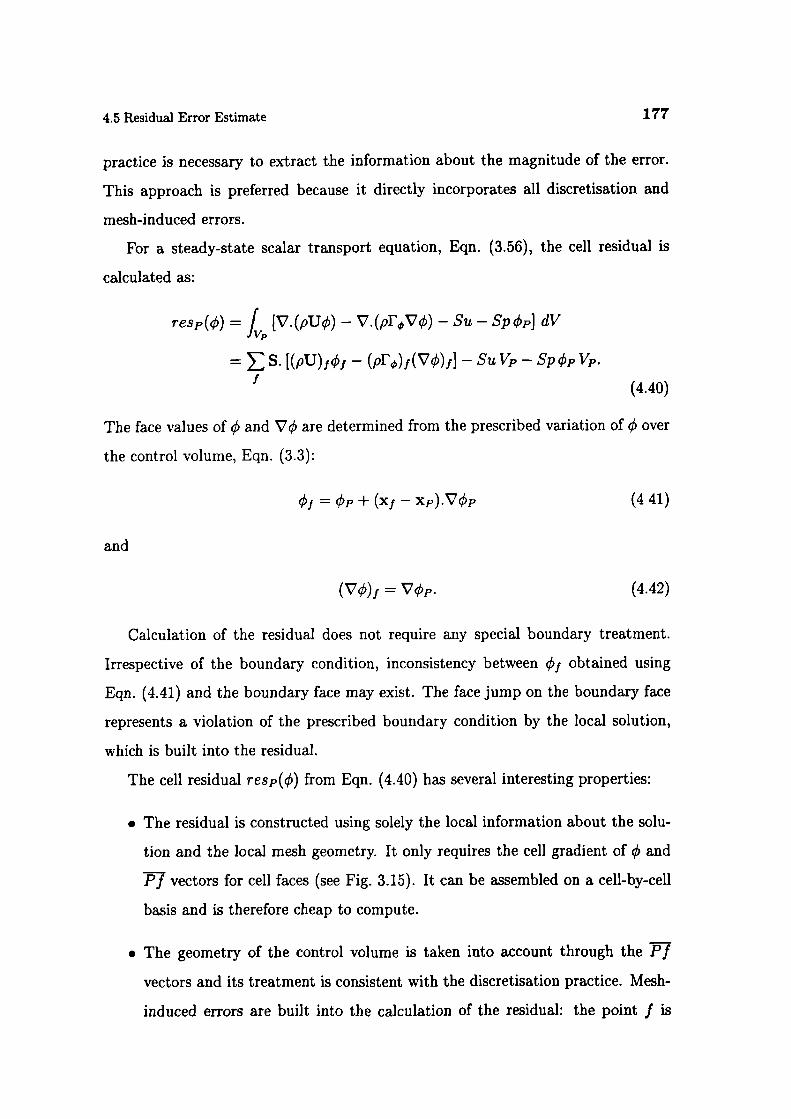
4.5 Residual Error Estimate
177
practice is necessary to extract the information about the magnitude of the error.
This approach is preferred because it directly incorporates all discretisation and
mesh-induced errors.
For a steady-state scalar transport equation, Eqn. (3.56), the cell residual is
calculated as:
resp(q5) = JVp [V.(pU4') - V.(prVc1) - Su - Spqp] dV
S.[(pU) 1 q5j - (pF4,) 1 (Vq5) j] - SuVp - SpçbpVp./
(4.40)
The face values of and Vç are determined from the prescribed variation of over
the control volume, Eqn. (3.3):
= çbp + (x1 - xp).Vq5p (4 41)
and
(V)1 = Vq5p. (4.42)
Calculation of the residual does not require any special boundary treatment.
Irrespective of the boundary condition, inconsistency between çbj obtained using
Eqn. (4.41) and the boundary face may exist. The face jump on the boundary face
represents a violation of the prescribed boundary condition by the local solution,
which is built into the residual.
The cell residual resp(q5) from Eqn. (4.40) has several interesting properties:
• The residual is constructed using solely the local information about the solu-
tion and the local mesh geometry. It only requires the cell gradient of 0 and
P7 vectors for cell faces (see Fig. 3.15). It can be assembled on a cell-by-cell
basis and is therefore cheap to compute.
• The geometry of the control volume is taken into account through the j
vectors and its treatment is consistent with the discretisation practice. Mesh-
induced errors are built into the calculation of the residual: the point f is

178 Error Estimation
located in the middle of the face (Fig. 3.15), accounting for the skewness
error, and (Vq) 1 does not include any non-orthogonal correction (the second
term in Eqn. (3.34)) from the larger computational molecule2.
. Numerical diffusion can also be detected by the residual. It has been shown
that the face interpolation used in the convection term is inconsistent with
the prescribed variation of over the cell irrespective of the choice of the
differencing scheme. On the other hand, a comparison of Upwind and Cen-
tral Differencing shows that UD produces a larger difference between q5j from
Eqs. (4.38) and (3.19) than CD, resulting in a larger residual.
. Residual Error estimation is directly extendible to Finite Volume discretisation
of any ord r of accuracy. The only change in the calculation of the residual
will be in tne assumed variation of over the control volume.
• According to the form of the residual, the accuracy of the error estimate should
not significantly change with mesh size it should work well both on fine and
coarse meshes.
• The correct scaling and as mptotic behaviour of the Residual Error estimate
can be explained on a one-dimensional situation, using Fig. 4.3, as explained
below.
For every control volume, two face values and a cell centre value are available.
Finite Volume discretisation guarantees that this combination of face and cell
centre values satisfies the governing equation in its integral form. It is therefore
possible to approximate the variation of the exact solution over the cell by
a parabola passing through the three available points. The error estimate
is assembled using the prescribed linear) variation of over the cell. The
difference between the two is represented by the shaded region in Fig. 4.3.
According to Fig 4.3, the distribution of the error over the control volume
is quadratic. This implies that the err r tends to the exact error with the
2 For the details f the mesh-induced errors the reader is referred to Se tion 3.6.3.

4.5 Residual Error Estimate 179
Figure 4.3: Scaling properties of the residual error estimate.
fourth power of m sh size, resulting in the asymptotically exact behaviour
of the estimate. ExLension of this analysis to multi-dimensional situations is
straightforward.
The above properties make the Residual Error estimate an attractive error esti-
mation tool. It is, however, still necessary to extract the information about absolute
error level from the residual.
4.5.1 Normalisation of the Residual Error Estimate
Evidently, resp(q5) has the dimensions of [q][L]3/[T]. As in the case of the Moment
Error estimate, an appropriate normalisation practice is needed to extract the error
magnitude. The form of the residual, Eqn. (4.40), shows that the terms contributing
to the error are the ones requiring the face values of and Vq5, namely the convection
and diffusion terms. The normalisation of resp(çb) will therefore be based on the
characteristic convection and diffusion transport for the control volume. In order
to maximise the accuracy of the method, geometric information will be used on a
face-by-face basis.
Consider a two-dimensional flow situation for the control volume around a point
P, Fig. 4.4. Estimation of the total diffusion transport flux is simple: for each of the

180
Error Estimation
F= 0
F<O F>O
F>0 N
Figure 4.4: Estimating the convection and diffusion transport.
neighbours, a face diffusion coefficient is known (same as in the discretised form of
the transport equation). d is used as the characteristic length and the area active
in the transport. is equal to S . A volume-weighted face sum of estimated diffusion
transport fluxes gives the approximation 3f the total diffusion transport coefficient:
Fd,ff = :: [s (pF) f 1
d ](4.43)
The convection transport term requires more attention. Let us assume a locally
uniform velocity field which is divergence-free. In that case, only half of the cell
surface is active in the transport of interest, which reduces the influence of the
residual to the local error. The convection transport coefficient can therefore be
estimated as the volume weighted flux going in (or out) of the control volume:
= . max(F, 0). (4.44)1P
If the velocity field is not divergence-free, discretisation of the convection term splits
into two parts, with the term containing V.(pU) being added to Sp. This will be
taken into account in the normalisation, by adding this part of Sp to the normali-
sation factor.
Let us finally consider the influence of source term errors. No discretisation error
is associated with the constant source term component - Su is considered to be
exact The error contfbution from the linear part of the s urce, Sp q5p, scales with
the erro in qlp and the sho1e of Sp should therefore be included into normalisation.
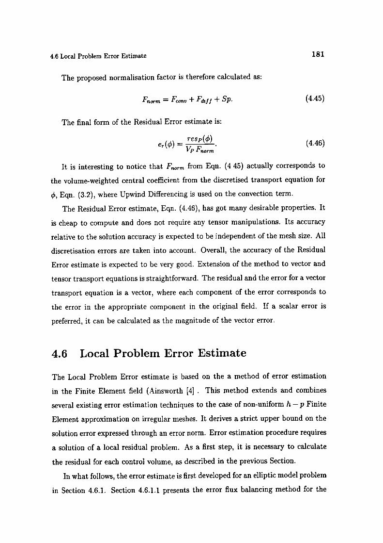
4.6 Local Problem Error Estimate 181
The proposed normalisation factor is therefore calculated as:
Fno,.m = + Fd,f / + Sp. (4.45)
The final form of the Residual Error estimate is:
e(çb) - resp(çb)(4.46)
- VpFnor
It is interesting to notice that Fno,.m from Eqn. (4 45) actually corresponds to
the volume-weighted central coefficient from the discretised transport equation for
, Eqn. (3.2), where Upwind Differencing is used on the convection term.
The Residual Error estimate, Eqn. (4.46), has got many desirable properties. It
is cheap to compute and does not require any tensor manipulations. Its accuracy
relative to the solution accuracy is expected to be independent of the mesh size. All
discretisation errors are taken into account. Overall, the accuracy of the Residual
Error estimate is expected to be very good. Extension of the method to vector and
tensor transport equations is straightforward. The residual and the error for a vector
transport equation is a vector, where each component of the error corresponds to
the error in the appropriate component in the original field. If a scalar error is
preferred, it can be calculated as the magnitude of the vector error.
4.6 Local Problem Error Estimate
The Local Problem Error estimate is based on the a method of error estimation
in the Finite Element field (Ainsworth [4] . This method extends and combines
several existing error estimation techniques to the case of non-uniform h - p Finite
Element approximation on irregular meshes. It derives a strict upper bound on the
solution error expressed through an error norm. Error estimation procedure requires
a solution of a local residual problem. As a first step, it is necessary to calculate
the residual for each control volume, as described in the previous Section.
In what follows, the error estimate is first developed for an elliptic model problem
in Section 4.6.1. Section 4.6.1.1 presents the error flux balancing method for the
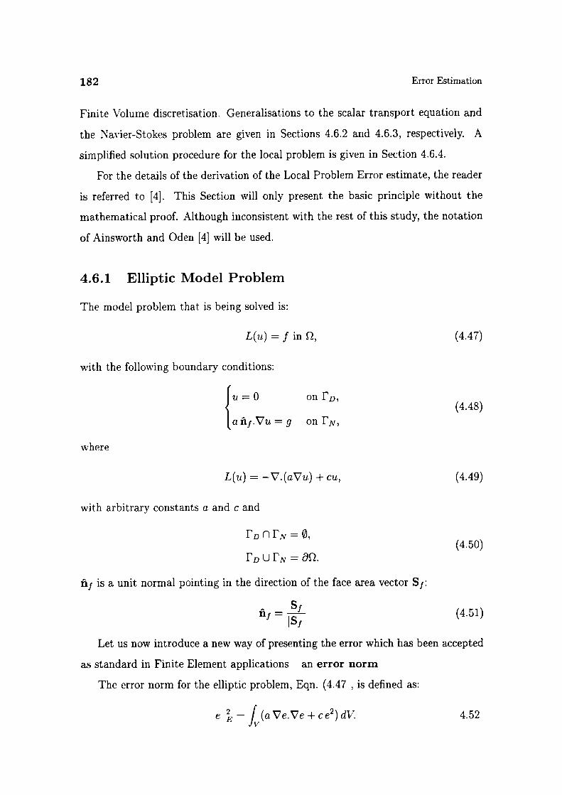
JJ
= 0
l añf .Vu = 9
rD,
on FN,
(4.48)
182 Error Estimation
Finite Volume discretisation. Generalisations to the scalar transport equation and
the Navier-Stokes problem are given in Sections 4.6.2 and 4.6.3, respectively. A
simplified solution procedure for the local problem is given in Section 4.6.4.
For the details of the derivation of the Local Problem Error estimate, the reader
is referred to [4]. This Section will only present the basic principle without the
mathematical proof. Although inconsistent with the rest of this study, the notation
of Ainsworth and Oden [4] will be used.
4.6.1 Elliptic Model Problem
The model problem that is being solved is:
L(u) = f in c, (4.47)
with the following boundary conditions:
where
L(u) = —V.(aVu) + Cu,
with arbitrary constants a and C and
F D FN = 0,
FDUFN =8g.
nj is a unit normal pointing in the direction of the face area vector S1:
(4.49)
(4.50)
= (4.51)
Let us now introduce a new way of presenting the error which has been accepted
as standard in Finite Element applications an error norm
The error norm for the elliptic problem, Eqn. (4.47 , is defined as:
e - J(a Ve.Ve + ce2 ) dV 4.52
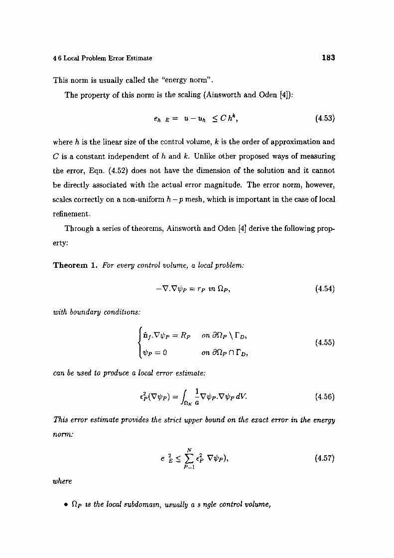
4 6 Local Problem Error Estimate
183
This norm is usually called the "energy norm".
The property of this norm is the scaling (Ainsworth and Oden [4]):
eh E U—Uh Ch1c , (4.53)
where h is the linear size of the control volume, k is the order of approximation and
C is a constant independent of h and k. Unlike other proposed ways of measuring
the error, Eqn. (4.52) does not have the dimension of the solution and it cannot
be directly associated with the actual error magnitude. The error norm, however,
scales correctly on a non-uniform h - p mesh, which is important in the case of local
refinement.
Through a series of theorems, Ainsworth and Oden [4] derive the following prop-
erty:
Theorem 1. For every control volume, a local problem:
= rp n (4.54)
with boundary conditions:
flj .Vbp R on(4.55)
OflaclPnrD,
can be used to produce a local error estimate:
= f(4.56)
a
This error estimate provides the strict upper bound on the exact error in the energy
norm:
N
e 4 V'p), (4.57)p_i
where
zs the local subdomain, usually a s ngle control volume,
{ R - g - anf.V.7uhRp
- —apañf.Vuh
(4.60)ac n F,
onöp
184
Error Estimation
• rp is the solution res dual over 2p, defined as:
rp = f - L u), (4.58)
. Rp is the residual error flux,
. N is the number of subdomazns (control volumes).
Proof. See Ainsworth and Oden [4]. D
The solution residual rp is equivalent to the residual defined in the previous
Section:
frp(u) dl' = —resp(u). (4.59)
As can be seen from the form of Eqn. (4.54), local problems are coupled through
the boundary conditions, specifically through the residual error flux Rp. The calcu-
lation of the residual error fluxes for the Finite Element method has been discussed
in detail in a number of papers [1, 4]. R on the cell faces is dependent on the face
jumps in the solution.
Following [4]. Rp is defined as:
The term añf .Vuh is defined on each internal face of the mesh as the local
jump in the gradient:
aii1 .Vu,j = [añf .(Vuh ) f] - [añf.(Vuh IJN' (4.61)
where P and N are the control volumes sharing the face and ñ1 . Similarly, the face
jump in the solution is defined as
IuI=[uh)fJp—[uhf]N. (4.62
Here, [ uh f}p and V h are the alues of Uh and VUh on th fa e f con ist nt
'vith the prescribed variation of Uh in the cell P.

4.6 Local Problem Error Estimate 185
We can also define an arbitrary linear interpolate of (uh)f and (ñf.Vuh)f:
(añf.Vuh) Q = apañf.[(Vuh)f]p + (1— ap) añf .[(Vuh ) f] N (4.63)
(U) = ap [(uh ) flp + (1 - ap) [(uh)f IN .( 4.64)
Nothing needs to be said about cxp in Eqs. (4.63) and (4.64) apart from that it
is the same as in Eqn. (4.60).
The necessary condition for the solution of the local problem is that the error
fluxes are balanced:
f rpdV+J RdA=0. (4.65)fZp Ocip
The problem of determining ap in such a way that Eqn. (4.65) is satisfied has
been discussed at length in the Finite Element community (see eg. Ainsworth and
Oden [3]). The performance of the Local Problem Error estimate is critically de-
pendent on this condition. If the error fluxes are not balanced, accuracy of the error
estimate is degraded to such an extent that the error bound of Eqn. (4.57) becomes
meaningless (see Ainsworth and Oden [4]).
In order to adopt the Local Problem Error estimate for the Finite Volume
method, it is necessary to provide a procedure for calculation of balanced resid-
ual error fluxes.
4.6.1.1 Balancing Problem in Finite Volume Method
The objective of the balancing procedure is to determine the boundary conditions
for local error problems, Eqn. (4.54), in such a way that the balance condition,
Eqn. (4.65) is satisfied for every control volume. It will be shown that this objective
can be reached without the actual calculation of ap coefficients as a consequence of
the conservative nature of the Finite Volume solution.
Error flux balancing will initially be done for the elliptic problem, Eqn. (4.47),
and is subsequently generalised to the convection-diffusion and Navier-Stokes prob-
lems. In order to simplify the expressions, the subscript h will be dropped. Face
values of u and Vu are assumed when they are needed, (i.e. on all mesh faces).

186
Error Estimation
Separating the boundary conditions, the volume residual Tp can be rewritten as:
J rp dV = f (f - C Up) dV + dS.a VUp. (4.66)
lip OI1PFD
a b
Following Eqn. (4.60), the integral of the face jump can be split into two parts:
Rp dA (g - ñ1 .a Vup) dA + —4a ñf.Vuhl dA.ôllp OIl flFN OIl' FN
(4.67)
The term (b) from Eqn. (4.66) can also be split into two, depending on the type
of the prescribed boundary condition:
dS.a Vup dS.a Vup + dS.a Vup.c9llp FD 9flpflFN t9flp rN FD
(4.68)
The residual balance condition, Eqn. (4.65), will now be assembled part by part,
using Eqs. (4.66), (4.67) and (4.68). To clarify further developments, it should be
said that Rp is not defined on I'D, as this is not necessary (see boundary conditions
for the local problem, Eqn. (4.55)).
Combining Eqn. (4.67) (c) and Eqn. (4.68) (e) yields:
(g - ñj .aVup) dA + dS.aVup = gdA.OflpflFN OlipflI'N
(4.69)
Combining Eqn. (4.67) (d) and Eqn. (4.68) (f) yields:
—c4añf.Vuh]ldA + dS.aVupJ8^lp FM JOlip FN 1'D
rN [ñ1 .a Vu - a ñ j.aVUp - ñf.aVuN } dA
FD (4.70
=
[(1 - ap) a flf .VUP + ap a ñf.VUN] dA
_f arlf.Vu dA.o^i N
vhere see Eqn. (4 63
(a flf.VU = (1 - ap a ñj V/Up + cxp a ñf.VUN. (471)
4.6 Local Problem Error Estimate
187
Assembling the balance, Eqn. (4.65), from Eqs. (4.66), (4.69) and (4.70), it
follows:
J(f - CUP) dV + gdA + (afij.Vu) 1—a) dA = 0.
cip aczpnrN Joc rN rD(4.72)
The result can be interpreted as follows: the interpolation method for the face
fluxes (a ñf.Vu) (1 _ should be selected in such a way that, together with the volume
integral, it satisfies the original problem, Eqn. (4 47), in the integral form over each
control volume.
Eqn. (4.72) provides a basis for the calculation of balanced fluxes. In the first
stage, the calculation of Rp can be modified. On internal faces of the mesh, Rp is:
- Ianf.VuhI = —ap(añ1 .Vup - añf.VUN)
= (1— cxp) añj .Vup + apañf.VuN - añ1.Vup
= (añf .Vu)( i _a) - añ1.Vup. (4.73)
On boundary faces, Eqn. (4.60) can be used directly.
The remaining problem is how to determine the interpolate (a fif.Vu)(1_). For-
tunately, the Finite Volume discretisation readily provides these fluxes. As a conse-
quence of the conservative form of the discretisation practice, the face fluxes calcu-
lated consistently with the discretisation automatically satisfy Eqn. (4.72).
For the model problem, the interpolated face gradient is
UN - Up(añ1 .Vu) = a
d(4.74)
In the case of non-orthogonal meshes, an explicit correction compatible with
the non-orthogonality treatment should be added. The balance condition given in
Eqn. (4.72) is satisfied to the solver tolerance. The calculation of R is straightfor-
ward, using Eqn. (4.73
4.6.2 Generalisation to the Convection-Diffusion Problem
The extension of the Local Problem Error estimate requires the analysis of the
convection term. Its contribution to the residual has been presented in Section 4.5.
188
Error Estimation
The face contribution for the balanced error fluxes uses the interpolated value of
to the face. For completeness, the expressions for the residual and R are given.
A steady-state convection-diffusion problem is specified as follows:
Find = x) such that
V. pUck) - V.(pFV) = Su + Spç in Q, (4.75)
with boundary conditions:
JD(X) on(4.76)
añ1 .Vç = g(x) on FN,
where
r'D 0,
I'DUITN
The volume integral of the residual for the control volume is
J rpdV = J [Su + Spq5 - V.(pUq5) +V.(pFV)] dV
= Su %'p + Sp qp Vp - S. pU)Øj) (pF 1,) j (V)1},f
(4.77)
consistent with Eqn. 4.40).
In order to satisfy the balance condition, Eqn. (4.65), residual error fluxes are
calculated as:
. On internal faces:
Rp = cxp - op[prq ñ1.V]
= F1 (— ( qS ) + q5j) - (- prfl1 .V + prnf.vf),
(4.78
. On fixed gradient boundary faces FN):
R = Qp F1 - cxpJpI'0 flf.V
= F1 - + q j ) - (—g + pF, ñj .V 1 , (4.79
4 6 Local Problem Error Estimate
189
• On fixed value boundary faces, the calculation of Rp splits into two parts:
- For the convection part, the face jump exists:
(Rp) opF1qJ
= Ff(— ()(i_a) + Q5f), (4.80)
- For the diffusion part, FD is treated as a fixed value boundary from the
elliptic problem. Since the exact boundary gradient is not known, the
local problem has to be solved with the fixed value boundary condition.
This somewhat complicates matters, as the residual also contains the face
jump from the convection term, Eqn. (4.80). An appropriate modification
can be easily introduced. Before the solution of the local problem, the
part of the residual from the convection term on the fixed value boundary
will be removed. Now the boundary can be treated in the same way as
for the elliptic problem, Section 4.6.1.
In Eqs. (4.78), (4.79) and (4.80) F1 is the face flux in respect to the direction of
the face area vector (see Chapter 3):
Ff = S1.(pU)j,
where S1 is the face area vector. (ç5) 1a) is calculated consistently with the convec-
tion differencing scheme used in discretisation.
The error norm for the convection-diffusion problem has the following form:
eJ=q5—q h = fv (pf Ve.Ve +Sp e2 ) dV (4.81)
The local problem is:
—V.Vbp = Vp in I p , (4.82)
with boundary conditions:
ñj.Vi,bp = Rp on ôZp \ rD,(4.83)
ñ1.Vp = (Rp)c, ?,bp = 0 on 512p fl 1'D
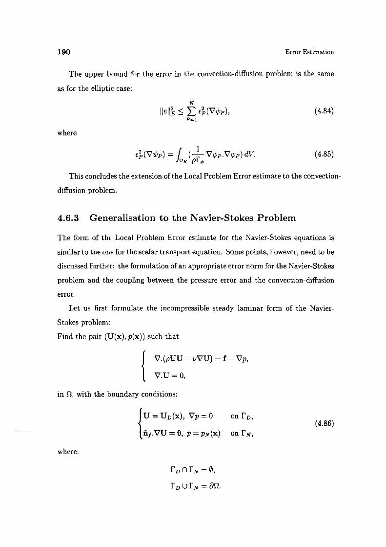
JU=UD (x) Vp=0
Ini .vu=o, p=pN(x
(4.86)on I'D,
190
Error Estimation
The upper bound for the error in the convection-diffusion problem is the same
as for the elliptic case:
N
II e II ^P= 1
where
r 1€,(VbP)
= LKPr
(4.84)
(4.85)
This concludes the extension of the Local Problem Error estimate to the convection-
diffusion problem.
4.6.3 Generalisation to the Navier-Stokes Problem
The form of th Local Problem Error estimate for the Navier-Stokes equations is
similar to the one for the scalar transport equation. Some points, however, need to be
discussed further: the formulation of an appropriate error norm for the Navier-Stokes
problem and the coupling between the pressure error and the convection-diffusion
error.
Let us first formulate the incompressible steady laminar form of the Navier-
Stokes problem:
Find the pair (U(x),p(x)) such that
V.(pUU - uVU) = f - Vp,
v.U=o,
in , with the boundary conditions:
where:
"D flFN =
I'D UFN =

(4.88)
(4.89)
(4.90)
(4.91)
(4.92)
4 6 Local Problem Error Estimate 191
4.6.3.1 Error Norm for the Navier-Stokes System
In order to simplify the discussion, from here on all the variables will be considered
to be dimensionless, with the characteristic scales equal to unity (following Girault
and Raviart [52]). The uniqueness of the solution of the Navier-Stokes problem has
been discussed by Oden et al. [101], Girault and Raviart [52] and Temam [131]. If
the uniqueness condition is satisfied, the following property of the numerical solution
can be proven (see Oden et al. [101], or Girault and Raviart [52]):
Theorem 2. Suppose that the conditions for the uniqueness of the solution for the
Navier-Stokes problem hold (see [101, 52]). Let (U,p) be the solution of Eqn. (4.86).
Then, for ii sufficiently large, there exists a mesh spacing h 0 such that for all h
the discretised form of Eqn. (4.86) has a unique solution (Uh,ph) and
lim(IU - Uh l + M - philo) = 0. (4.87)h-O
If, in addition, the solution (U, p) of Eqn. (4.86) is in the space of accessible func-
tions of the order k+1, where k is the order of accuracy of the discretisation method,
then a constant C> 0 exists, independent of k, such that
IU—Uh k+lp—ph Mo ^Chk.
Proof. See [52].
The norms in Theorem 2 are defined as:
v=fv(Vv : Vv)dV,
Iq =fq2jT/
Oden, [101], defines the error in the solution of Eqn. (4.86) as:
e = U - Uh,
E=p—ph
and introduces a new "star" norm (e, E) . It is consequently proven (Oden, [101])
that the new norm is equivalent to the norm for Navier-Stokes problem:
(e, E) * = U - Uh 1 + p - Ph o (4.93)
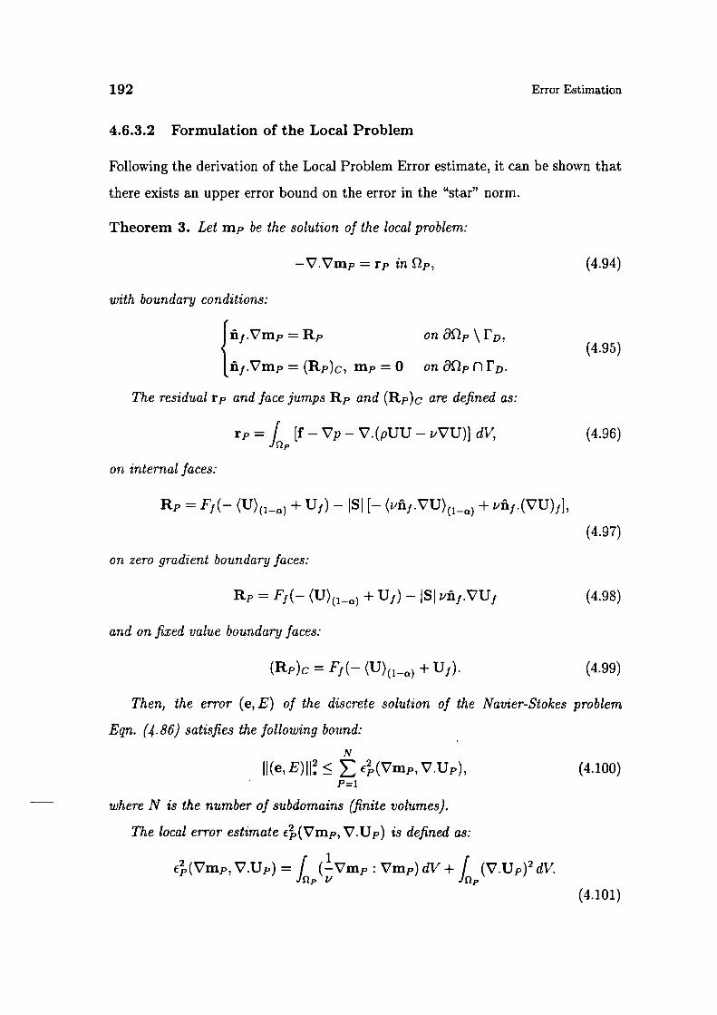
192
Error Estimation
4.6.3.2 Formulation of the Local Problem
Following the derivation of the Local Problem Error estimate, it can be shown that
there exists an upper error bound on the error in the "star" norm.
Theorem 3. Let mp be the solution of the local problem:
—V.Vmp = rp in Ip, (4.94)
with boundary conditions:
ñ1 .Vmp R on f9Ilp \ 1'D,(4.95)
ñj .Vmp = (Rp)c, mp 0 on Mp fl rD.
The residual rp and face jumps R and (Rp)c are defined as:
rp = f [f - Vp - V.(pUU - vVU)1 dv, (4.96)
on internal faces:
R = F1 (— (U) (l _a) + Uf ) - S [- (vñf.VU)(1_) + vn1.(VU)1],
(4.97)
on zero gradient boundary faces:
R Ff (— (U) (l _ ) + U1) - SI vñ1 .VU1 (4.98)
and on fixed value boundary faces:
(Rp) = F1 (— (U)( l a) + U1 ). (4.99)
Then, the error (e, E) of the discrete solution of the Navier-Stokes problem
Eqn. (4.86) satisfies the following bound:
II(e , E)II < e,(Vmp,V.Up), (4.100)
where N is the number of subdomains (finite votumes).
The local error estimate f,(Vmp, V.U) is defined as:
€,(Vmp, V.Up) = f (Vmp : Vmp) dV + J (V.Up) 2 dV.
(4.101)

4.6 Local Problem Error Estimate 193
Proof. See [101]. 0
The only difference between the convection-diffusion and the Navier-Stokes prob-
lem is the treatment of the additional source term: the pressure gradient. In the
convection-diffusion problem, constant source terms are considered to be exact,
whereas here the pressure gradient term carries a certain numerical error associ-
ated with the divergence of velocity.
4.6.4 Solution of the Local Problem
The results on the upper bound for the error, Eqs. (4.57), (4.84) and (4.100), assume
that the local problem is solved exactly over each subdomain. This is, however,
potentially expensive and for purposes of error estimation not really necessary. In
this Section, a simple method for the approximate solution of the local problem is
proposed in the framework of second-order accurate Finite Volume discretisation.
Numerical experiments show that this method is appropriate for error estimation.
Let us first take another look at the definition of the local problem for the elliptic
equation:
—V.Vp = Tp in Ilp, (4.102)
with boundary conditions:
ñj.Vçbp = R ôQ \ rD,(4.103)
OflocPnrD.
The boundary conditions show a certain peculiarity:
. If the control volume has a face on the fixed value boundary i'D, the problem
is well-posed.
. If, on the other hand, there are no fixed value boundary faces on the control
volume, the problem is indeterminate up to a constant.

194
Error Estimation
The actual error estimate does not require 'p, but only the volume integral of
its gradient. It can therefore be obtained without knowing the actual level of p.
The solution procedure for the local problem is set up in such a way that the level
of L'p is calculated only when the problem is well-posed.
Let us first discuss the situation when the cell does not have any fixed value
boundary faces.
4.6.4.1 Solution of the Indeterminate Local Problem
The local error estimate Cp is calculated as:
c(V) = /a
It will be assumed that VL' changes linearly through the cell the cell will not
be further subdivided. It is therefore oniy necessary to determine the value of Vp
in the cell centre. This will be done by formally solving the local residual problem
on a mesh consisting of a single cell.
The gradient of in the cell centre is calculated using the discretised version of
the Gauss' theorem:
= S (4.104)I
and
= p + (xf - xp).VL'p. (4.105)
It is further assumed that VL'p and V'151 are identical. ,j is then equal to:
= + (x1 - xp).V 1 . (4.106
Using Eqs. (4.104 and 4 106 , it f llows:
Vb= ---S[(x1—xp .VbjJ, (4.107VP1
where the p part disappears.
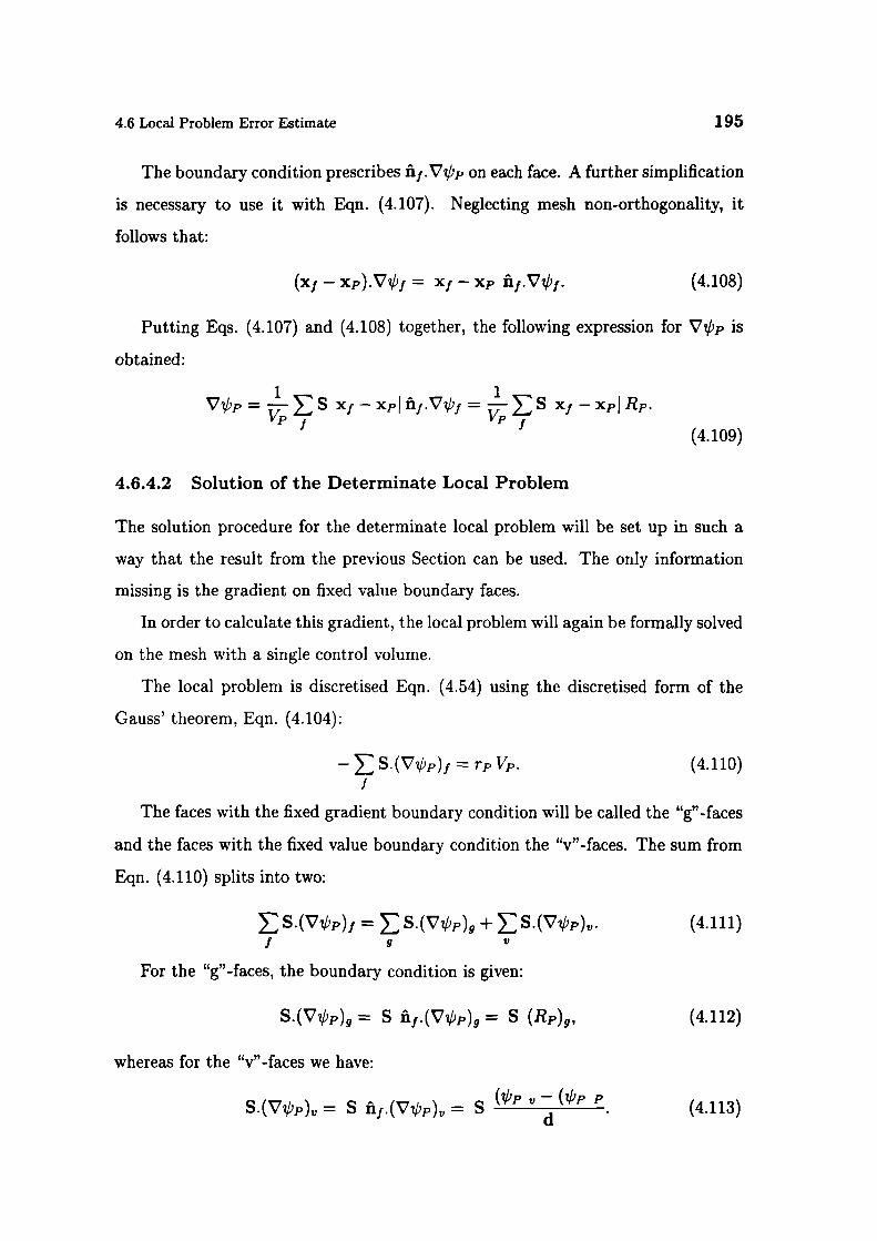
4.6 Local Problem Error Estimate
195
The boundary condition prescribes ñ1 .Vp on each face. A further simplification
is necessary to use it with Eqn. (4.107). Neglecting mesh non-orthogonality, it
follows that:
(xj - xp).Vb1 x1 - xp âj .Vbj . (4.108)
Putting Eqs. (4.107) and (4.108) together, the following expression for is
obtained:
Vp=-S x1 —xpJñj .Vi 1 =--S xj—xpJRp.P1 P1
(4.109)
4.6.4.2 Solution of the Determinate Local Problem
The solution procedure for the determinate local problem will be set up in such a
way that the result from the previous Section can be used. The only information
missing is the gradient on fixed value boundary faces.
In order to calculate this gradient, the local problem will again be formally solved
on the mesh with a single control volume.
The local problem is discretised Eqn. (4.54) using the discretised form of the
Gauss' theorem, Eqn. (4.104):
—S.(Vi') 1 = rpVp. (4.110)/
The faces with the fixed gradient boundary condition will be called the "g"-faces
and the faces with the fixed value boundary condition the "v"-faces. The sum from
Eqn. (4.110) splits into two:
S.(V&p) = S.(Vbp)9 + S.(V'bp)v/ 9
For the "g"-faces, the boundary condition is given:
S.(V) 9 S n1.(V) 9 = S (Rp)9,
whereas for the "v"-faces we have:
S.(Vp) = S ñ1.(Vp)v = S (bp - (bp pd
(4.111)
(4.112)
(4.113)

196
Error Estimation
Here, (p)p is the solution of the local problem in the cell centre. (1)p)v is equal
to zero, following the boundary condition on the local problem, Eqn. (4.55).
(4'p ) p is therefore:
frpdV+9 S (Rp)g(L')
S --(4.114)
and the face gradients for the "v"-faces are
—(,bp)p(4.115)
Id
All face gradients are now known and Eqn. (4.109) can again be used.
This concludes the solution procedure for the local problem in the elliptic case.
Generalisation to other types of the local problems is straightforward.
4.6.5 Application of the Local Problem Error Estimate
The Local Problem Error estimate does not describe the magnitude of the solution
error directly. It is therefore necessary to establish what kind of information about
the error can be recovered from this error norm.
The optimal mesh, irrespective of its size, is the one in which the error is uni-
formly distributed through the whole domain. The actual level of the error depends
on the problem that is being solved and the number of control volumes. It follows
that in an optimal mesh the error gradients are equal to zero. The error norm from
Eqn. (4.52 is based on the magnitude of the error gradient and therefore provides
information about the mesh quality.
The upper bound on the error norm, Eqn. (4.57), describes the relation between
the solution error and the solution of the local problem. In most cases, error flux
boundary conditions cause the indeterminacy of the local problem up to a con-
stant (see Section 4 6 4 This indeterminacy implies that no information about the
magnitude of the error can be recovered from the Local Problem Error estimate.
The energy (dissipation norm for the incompressible Navier-Stokes equations
can, however, be compared with the total dissipation in the system. Oden [102] de-
scribes an error-controlled adaptive refinement procedure based on the Local Prob-
4.7 Error Estimation for Transient Calculations
197
lem Error estimate. The accuracy of the solution is considered satisfactory when
the error is reduced to 3 - 5% of the total dissipation.
4.7 Error Estimation for Transient Calculations
Error estimation in transient calculations can be seen as an extension of steady-state
error estimation Apart from the error coming from spatial resolution, additional
temporal effects need to be taken into account.
In transient problems, three separate accuracy questions can be posed:
. In the first instance, it is necessary to measure the error introduced by each
tu n e_step of the transient calculation. Both the spatial and temporal error
should be taken into account.
. The second question is concerned with the accuracy of the solution after a
certain number of time-steps. To answer this question, it is necessary to follow
the evolution of the error in time.
• Finally, in transient cases with adaptive refinement and tracking of flow fea-
tures, results of error estimation are used to change the mesh and the time-step
size. It is therefore necessary to estimate the spatial and temporal errors sep-
arately. Decision on mesh refinement will be based on the spatial error only.
The ratio of spatial and temporal error can also be used for automatic time-
step control - the requirement for the equivalent temporal and spatial accuracy
enables us to estimate the optimal time-step size.
We shall start the analysis of the transient error with the formulation of the tern-
poral residual. Section 4.7.2 presents a procedure for separate estimation of spatial
and temporal errors. Finally, Section 4.7.3 gives an insight into the transportive
properties of the error.
198
Error Estimation
4.7.1 Residual in Transient Calculations
Let us consider the integral form of the transport equation for , Eqn. (3.8):
t+it I 3f {- f
pq dV + f V.(pUq5) dV - I V. pF0Vç) dv] dtVp JVp
t^g
= j (f S(q5) dv) dt.Vp
It has been shown that the assumption of linear variation in space and time leads
to the Crank-Nicholson form of discretisation, Eqn. (3.41):
pp - 'Vp + F) -
+ Fq - (pF, fS.(V
= Si1 + SpVpq + SpVp°p.
Section 4.5 gives the residual error analysis for a steady-state situation. The
convection-diffusion residual for a steady-state problem was assembled from the
prescribed linear) variation of in space. This spatial residual has the following
form Eqn. (4.40)
resp(q) = f [V.(pUq5) - V.(pFV) - Su - Spçp] dV
= S. [(pU)jj - (pF) 1 (V) 1] - Su Vp - Sp çbp V./
Eqn. (4.40 estimates the error in transport terms of Eqn. (3.41). The complete
residual can therefore be assembled by including the transient term:
= 'VP+resP )+resp(),resp
(4.116)
where resp ") and resp ) are calculated using Eqn. 4.40).
Eqn. 4.116 takes into account all deviations of second-order accuracy, thus
measuring all discretisati n errors. In order to obtain the error magnitude, the
normalisation described in Section 4.5.1 is used.

4.7 Error Estimation for Transient Calculations
199
4.7.2 Spatial and Temporal Error Contributions
The previous Section describes the formulation of the residual for transient calcu-
lations, including both the spatial and temporal error terms. It would be useful to
know how much of the total error is caused by spatial and how much by temporal
discretisation.
In transient tracking calculations, changes in the computational mesh follow
certain features that require high spatial resolution (moving shocks, pressure waves,
flame fronts etc.). The tracking effect is created by a region of fine mesh that travels
through the domain with the feature of interest. Since the speed and the direction of
its propagation are not known in advance, the adaptive algorithm relies on the error
estimate to add and remove computational points. The tracking problem can be
described as an adaptive calculatiDn with simultaneous refinement and unrefinement.
For such calculations, it is advisable to neglect the temporal part of the error, as
it obscures the spatial error sources of interest. From the refinement point of view,
the transient term is therefore considered to be exact. The spatial error alone gives
more accurate information about the location of the tracked flow feature.
For first-order temporal schemes (Euler Implicit and Explicit discretisation), the
spatial error residual is equal to:
E!,EX - PP -resL () Vp+resp(qY'). (4.117)
- At
Similarly, for Backward Differencing in time:
Ioores(q5) =
2 çb - 2° +VP + resp(). (4.118)
At
For Crank-Nicholson discretisation, the spatial error estimate is the same as for
the first-order temporal schemes, as the rate of change of the spatial error in time is
neglected. For other methods of temporal discretisation, the temporal error consists
of two parts: the temporal error of the Crank-Nicholson method and the additional
temporal numerical diffusion error (see Section 3.6.2). The error estimate can be
derived from the difference between Eqs. (4.116) and (4.117) or Eqs. (4.116) and
(4.118), respectively.

200
Error Estimation
For the first-order temporal schemes, the temporal component of the residual is
equal to:
El,EX El EXresT 0) = resF(c5) - resL (q)
= - resp(çb) + resp(çb°). (4.119)
An insight into Eqn. (4.119) can be given if it is assumed that spatial discreti-
sation produces no error. In that case resf'(cb) = 0, and from Eqn. (4.117) it
follows:
resp() --
VP. (4.120)-
Using Eqn. (4.120) for çb' and q° in Eqn. (4.119), it follows:
EI.EX 1 /9pQp - ppq5 - .: PP°p -resT =
2"P
I00- 1pp-2ppcb+ppp Vp.
(4.121)-
which approximates the second derivative in time. This is consistent with the leading
term of the truncation error for the first-order temporal schemes. The transient error
estimate therefore correctly estimates the temporal error in the case of the first-order
accurate temporal discretisation.
The separation of the residual into the spatial and temporal contribution enables
us to look into the issue of optimal time-step size. Equivalent temporal and spatial
accuracy implies that the peak error magnitudes from temporal and spatial discreti-
sation are the same. The influence of the spatial and temporal error is measured by
the time-step indicator
max resT )tref =
(4.122)max( resp q )
For tref > , temporal error dominates It is more efficient to reduce the time-
step than to refine the mesh; for tref < , the situation is opposite The time-step
indicator should, however, be used only as a global indicator of the relative quality
of temporal and spatia discretisation, as it will typically change in time.
4.7 Error Estimation for Transient Calculations 201
4.7.3 Evolution Equation for the Error
Let us consider a scalar transport equation in the standard form, Eqn. (3.2)
+ V.(pU) - V.(prV) =
In transient calculation, a residual is created for every time-step as a conse-
quence of the discretisation error. The error is built into the solution and follows
its development. The accuracy of the solution after several time-steps will therefore
depend not only on the current discretisation error, but on the errors in all previous
time-steps the error in transient calculations has potentially cumulative effects.
In order to estimate the total solution error, it is necessary to follow its devel-
opment from the initial condition. It is assumed that the initial condition is exact,
i.e. that no error has beed introduced by its discrete reprvsentation.
The local error source is expressed as the cell residual. It includes both the
effects of temporal and spatial discretisation.
Since the error is transported with the solution, both and the error are subject
to the same transport process. It is therefore possible to write the transport
equation for the error in the following form:
+ V.(pUe) - V.(prVe) = Se .( 4.123)
Boundary conditions for Eqn. (4.123) are easily derived. On fixed value bound-
aries for , no numerical error is introduced e is therefore fixed to zero. On all
other types of boundary conditions, e mimics the behaviour of qS. The local error
source, Se shows the influence of discretisation to local accuracy. It would be natural
to estimate S as the volume-weighted cell residual:
Se = resF(cb)
(4.124)
The solution of Eqn. (4.123) should in theory produce the "exact" distribution
of the numerical error through the domain. If the equation were solved exactly
with exact error sources, it would be possible to re-create the exact solution by
adding this error to the numerical solution. This is, however, not reasonable the
202 Error Estimation
numerical solution of Eqn. (4.123 is subject to the same discretisation problems
as the original transport equation Additional uncertainty comes from the estimate
of the error source 8e• An example one-dimensional convection study will be given
in Section 4.8. Attempts to solve the equivalent of Eqn. (4.123) for steady-state
problems have produced disappointing results. In the author's opinion, this is a
consequence of the local equilibrium of the error source and transport, which changes
the nature of the transported error.
4.8 Numerical Examples
In order to examine the accuracy of error estimation methods presented in this
Chapter, several numerical examples will be considered. The selected t'st cases
have analytical solutions, which allows comparison between the exact and edtimated
errors. Although the presented cases do not represent "real" flow situations, they
share some properties with them and pros ide an useful insight into the accuracy
and scaling properties of error estimates.
4.8.1 Line Source in Cross-Flow
The first test case is a convection-diffusion problem for a scalar variable eg. temper-
ature or concentration. It consists of a fixed strength line source of a passive scalar
in a fixed uniform velocity field. In order to avoid the singularity at the line source,
it is located outside the computational domain. The analytical solution for this test
case can be found in Hinze [641:
S' fUix2+y2\)'Y —____Ko(
2F)e (4125
2irF
Here
. x and y are the spatial co rdinates. The of gin of the coordinate system is
located at the source, with the x coordinate pointing in the direction of the
velocity vect r,
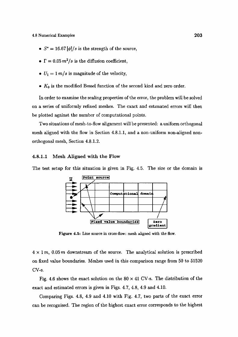
4.8 Numerical Examples 203
. S = 16.67 [J/s is the strength of the source,
. r = 0.05 m2/s is the diffusion coefficient,
. U1 = 1 rn/s is magnitude of the velocity,
. K1 is the modified Bessel function of the second kind and zero order.
In order to examine the scaling properties of the error, the problem will be solved
on a series of uniformly refined meshes. The exact and estimated errors will then
be plotted against the number of computational points.
Two situations of mesh-to-flow alignment will be presented: a uniform orthogonal
mesh aligned with the flow in Section 4.8.1.1, and a non-uniform non-aligned non-
orthogonal mesh, Section 4.8.1.2.
4.8.1.1 Mesh Aligned with the Flow
The test setup for this situation is given in Fig. 4.5. The size or the domain is
Fixed value boundariesl Zerogradient
Figure 4.5: Line source in cross-flow: mesh aligned with the flow.
4 x 1 m, 0.05 m downstream of the source. The analytical solution is prescribed
on fixed value boundaries. Meshes used in this comparison range from 50 to 51520
CV-s.
Fig. 4.6 shows the exact solution on the 80 x 41 CV-s. The distribution of the
exact and estimated errors is given in Figs. 4.7, 4.8, 4.9 and 4.10.
Comparing Figs. 4.8, 4.9 and 4.10 with Fig. 4.7, two parts of the exact error
can be recognised. The region of the highest exact error corresponds to the highest
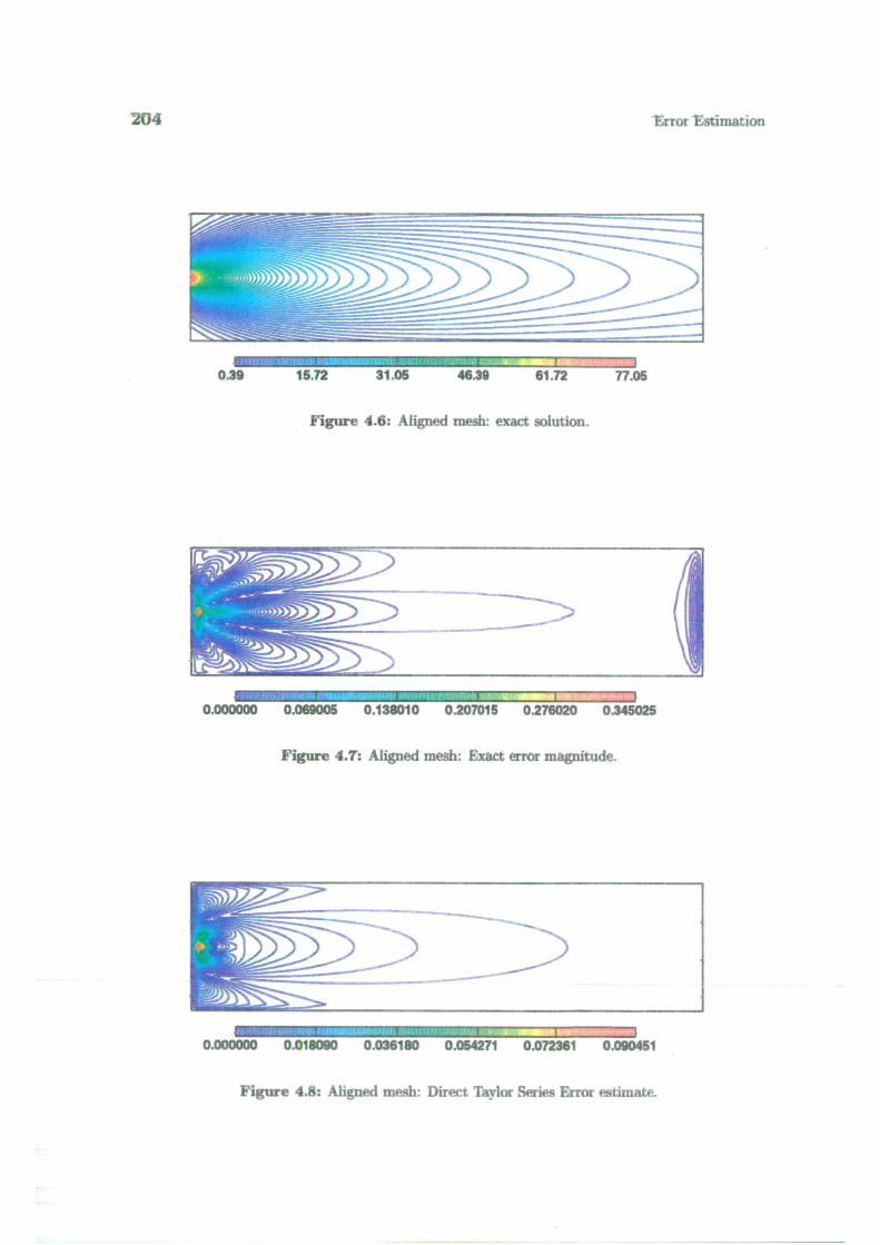
704
Error Estimation
0.39 15.72 31.05 46.39 61.72 77.05
Figure 4.6: Aligned mesh: exact solution.
0.000000 0.069005 0.138010 0.207015 0276020 0.345025
Figure 4.7: Aligned mesh: Exact error magnitude.
I I
0.000000 0.018090 0.036180 0.054271 0.072361 0.090451
Figure 4.8: Aligned mesh: Direct Taylor Series Error estimate.
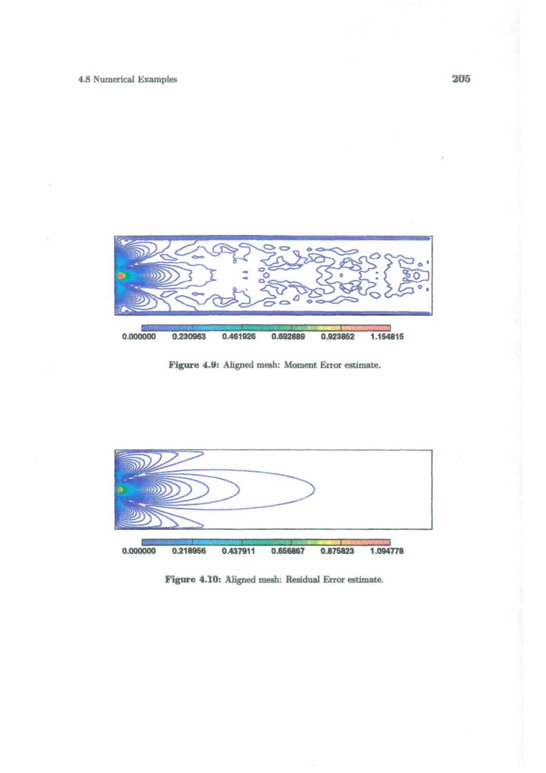
4.8 Numerical Examples
205
oci__
:1 jc (1%
0.000000 0.230963 0.461926 0.692889 0.923852 1.154815
Figure 4.0: Aligned mesh: Moment Error estimate.
• I
0.000000 0.218956 0.437911 0.656867 0.875823 1.094778
Figure 4.10: Aligned mesh: Residual Error estimate.

206 Error Estimation
local discretisation error. This error source has been accurately detected by all
error estimates. The secondary effect of this high error can be seen just downstream
from the error source. Here, the exact error is still large, but the estimates do not
pick up its source. The error is transported from the region with high discretisation
error and will disappear when the source is removed. The secondary error cannot be
detected by the error estimate because it does not result from the local discretisation
error. As the mechanism of error transport is not fully understood, we shall assume
that the error source only creates a local error. The results in the present study
show that this simplification does not degrade the accuracy of error estimation and
that it is particularly useful from the point of view of local mesh refinement, where
the detection of error sources is more important than the actual magnitude.
Let us now consider the scaling properties of the error and error estimates.
Figs. 4.11 and 4.12 show the reduction of the mean and maximum error with the
number of control volumes. It is expected that the error will reduce with the square
of the mesh size, following the second order accuracy of the method.
In two spatial dimensions, the number of computational points quadruples if the
mesh spacing is halfed in each direction. The slope of the curve in Fig. 4.11 should
therefore be —1. Slight variations of the slope and the rapid drop in the maximum
error on coarse meshes are attributed to the discretisation of the exact boundary
condition.
The advantage of the Moment and Residual Error estimates over the Direct
Taylor Series Error estimate can be clearly seen, both in the mean and maximum
error The Moment and Residual estimates give almost identical results on coarse
meshes. As the solution gets more accurate, the Moment Error estimate looses
accuracy the magnitude of the neglected fourth-order terms becomes similar to
the magnitude of the solution error. The Residual Error estimate consistently gives
good results.
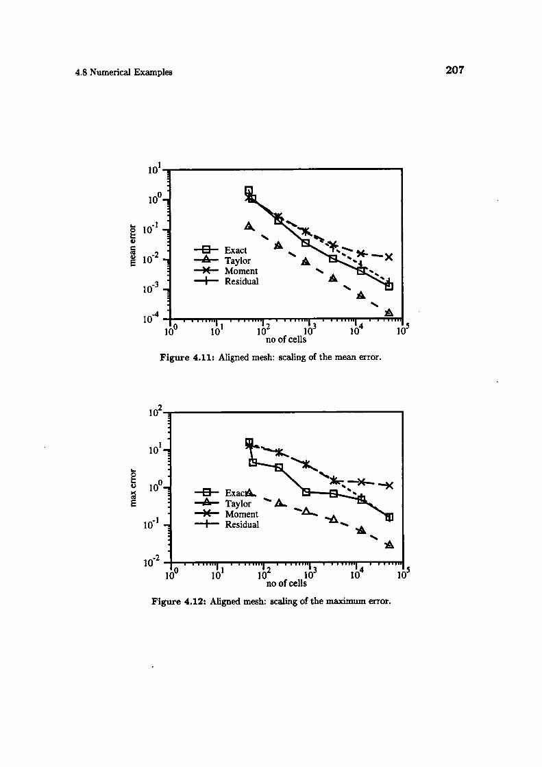
2074.8 Numerical Examples
10i_
100_
-110 -
0 Exacio 2 - .A Taylor
)( MomentI Residual
l0 - A
100 .i ......no of cells
Figure 4.11: Aligned mesh: scaling of the mean error.
1
101
00
10
E
10_i
p—K
)C Moment—A-- Taylor
I Residual
i _2
0 2 I •
10 10 10 10 10 10no of cells
Figure 4.12: Aligned mesh: scaling of the maximum error.
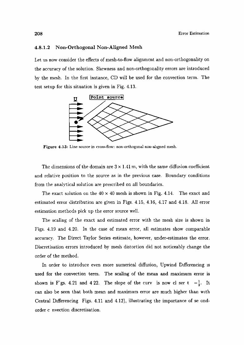
.
208
Error Estimation
4.8.1.2 Non-Orthogonal Non-Aligned Mesh
Let us now consider the effects of mesh-to-flow alignment and non-orthogonality on
the accuracy of the solution. Skewness and non-orthogonality errors are introduced
by the mesh. In the first instance, CD will be used for the convection term. The
test setup for this situation is given in Fig. 4.13.
U
I Point sourcel
Figure 4.13: Line source in cross-flow: non-orthogonal non-aligned mesh.
The dimensions of the domain are 3 x 1.41 m, with the same diffusion coefficient
and relative position to the source as in the previous case. Boundary conditions
from the analytical solution are prescribed on all boundaries.
The exact solution on the 40 x 40 mesh is shown in Fig. 4.14. The exact and
estimated error distribution are given in Figs. 4.15, 4.16, 4.17 and 4.18. All error
estimation methods pick up the error source well.
The scaling of the exact and estimated error with the mesh size is shown in
Figs. 4.19 and 4.20. In the case of mean error, all estimates show comparable
accuracy. The Direct Taylor Series estimate, however, under-estimates the error.
Discretisation errors introduced by mesh distortion did not noticeably change the
order of the method.
In order to introduce even more numerical diffusion, Upwind Differencing is
used for the convection term. The scaling of the mean and maximum error is
shown is F O gs. 4.21 and 4 22. The slope of the curv is now ci ser t -. It
can also be seen that both mean and maximum error are much higher than with
Central Differencing Figs. 4.11 and 4.12), illustrating the importance of se ond-
order c nvection discretisation.
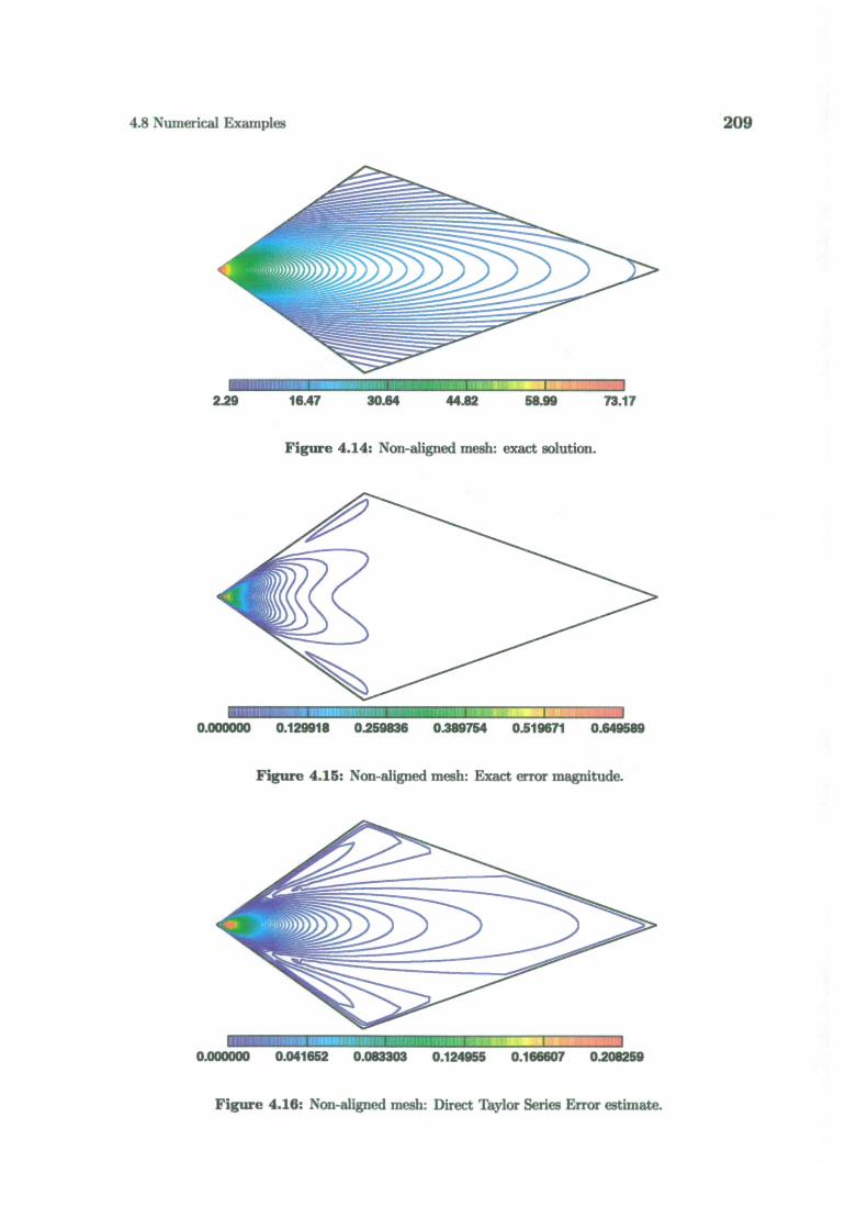
2094.8 Numerical Examples
2.29 16.47 30.64 44.82 58.99 73.17
Figure 4.14: Non-aligned mesh: exact solution.
0.000000 0.129918 0.259836 0.389754 0.519671 0.649589
Figure 4.15: Non-aligned mesh: Exact error magnitude.
0.000000 0.041652 0.083303 0.124855 0.166607 0.208259
Figure 4.16: Non-aligned mesh: Direct Taylor Series Error estimate.
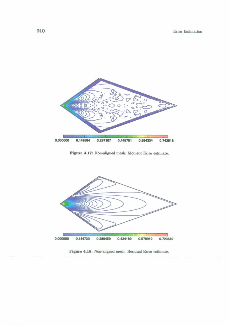
210
Error Estimation
-u- I - :1
0.000000 0.148584 0.297167 0.445751 0.594334 0.742918
Figure 4.17: Non-aligned mesh: Moment Error estimate.
0.000000 0.144730 0289459 0.434189 0.578919 0.723649
Figure 4.18: Non-aligned mesh: Residual Error estimate.
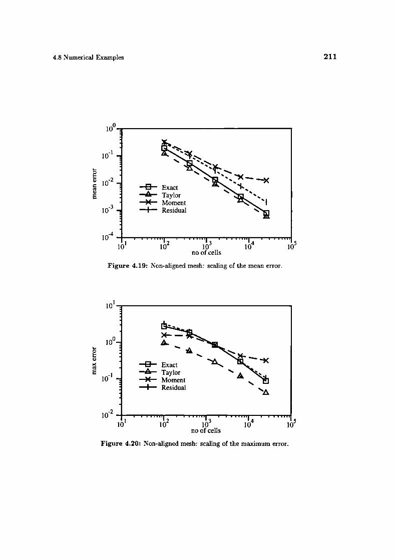
100
10_i
I-0
-2
1 Ø3
0 ExactA Taylor)( MomentI Residual
4.8 Numerical Examples
211
n II,.,,,.
10 -10 l0 10
I 0no of cells
Figure 4.19: Non-aligned mesh: scaling of the mean error.
l0
10:
)( MomentA Taylor A 'p Exact%,
I Residual
'1 '2 '3 '4 '510 10 10 10 10
no of cells
Figure 4.20: Non-aligned mesh: scaling of the maximum error.
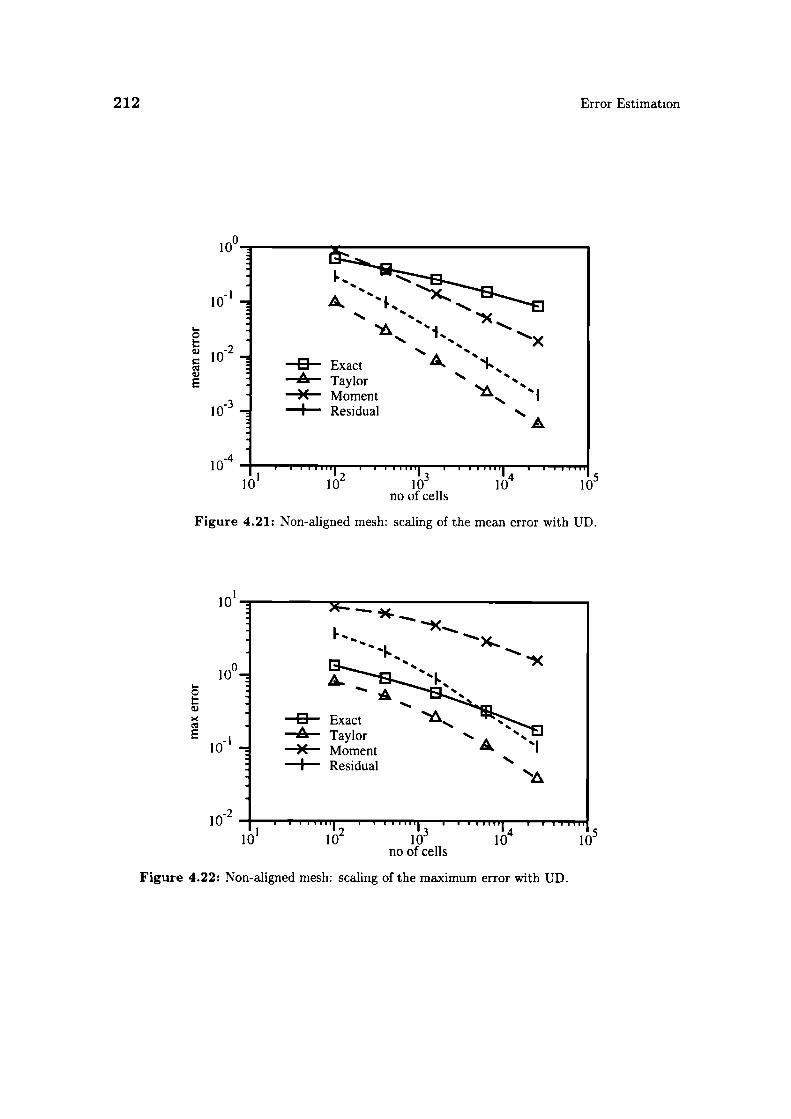
10
212
Error Estimation
10
10_I
5-0-2
E
%&
D Exact •& 1%___ •4.
A. Taylor)( Moment
I ResidualA
'1 '2 '3 '4 '510 10 10 10 10no of cells
Figure 4.21: Non-aligned mesh: scaling of the mean error with UD.
- 4
0 ExacA TaylorX Moment S...
I Residual
•1 II10 10 l0 l0
1 0
no of cells
Figure 4.22: Non-aligned mesh: scaling of the maximum error with UD.

(4.129)
(4.130)
4.8 Numerical Examples
213
Error estimates, however, do not follow the scaling behaviour of the error. Nu-
merical diffusion smears the gradients, producing a picture of a smoothly varying
field, which complicates the estimation of the error. The quality of the solution is
so bad that accurate error estimation is not possible. It should be noted that only
the Moment Error estimate shows slower error reduction with refinement. This is,
however, a very severe test for error estimates, with a combination of poor mesh
quality, high discretisation errors and steep gradients in the solution.
4.8.2 Line Jet
In order to test the behaviour of error estimates on a fluid flow situation, a line jet
test case will be considered. The test setup consists of an infinitely fast jet from
an infinitely thin line orifice entering a large domain. The amount of momentum
introduced by the jet is finite and equal to M. The analytical solution for this
problem can be found in Panton [104]. For the coordinate system located at the
mouth of the orifice with i pointing in the direction of the jet, the exact velocity
vector in the point (x, y) is:
U = ui + vj, (4.126)
where
AU = X 3 sech2
),(4.127)
v = A x tan/i2 (i ) + y sec/i2 (x4 ),(4.128)
A=(z,M3),
B— (48v2\
M)
and M3 = U h is the momentum carried by the jet.
In order to avoid the problems with accuracy of the discretised form of the exact
boundary condition, the computational domain will be located downstream from
the jet. The mesh is aligned with the main direction of the flow, Fig. 4.23. The
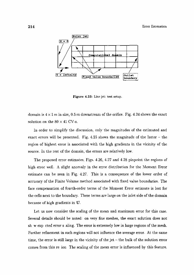
Point jeti
It; -
lu infiniyj lOutlet IFixed value boundariesi tbouny
214
Error Estimation
Figure 4.23: Line jet: test setup.
domain is 4 x 1 m in size, 0.5 m downstream of the orifice. Fig. 4.24 shows the exact
solution on the 80 x 41 CV-s.
In order to simplify the discussion, only the magnitudes of the estimated and
exact errors will be presented. Fig. 4.25 shows the magnitude of the latter - the
region of highest error is associated with the high gradients in the vicinity of the
source. In the rest of the domain, the errors are relatively low.
The proposed error estimates, Figs. 4.26, 4.27 and 4.28 pinpoint the regions of
high error well. A slight anomaly in the error distribution for the Moment Error
estimate can be seen in Fig. 4.27. This is a consequence of the lower order of
accuracy of the Finite Volume method associated with fixed value boundaries. The
face compensation of fourth-order terms of the Moment Error estimate is lost for
the cells next to the boundary. These terms are large on the inlet side of the domain
because of high gradients in U.
Let us now consider the scaling of the mean and maximum error for this case.
Several details should be noted: on very fine meshes, the exact solution does not
sh w exp cted error s aling. The error is extremely low in large regions of the mesh.
Further refinement in such regions will not influence the average error. At the same
time, the error is still large in the vicinity of the jet - the bulk of the solution error
comes from this re ion The scaling of the mean error is influenced by this feature.
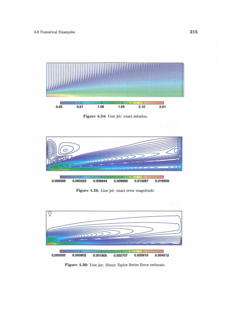
4.8 Numerical Examples
215
0.05 0.57 1.08 1.59 2.10 2.61
Figure 4.24: Line jet: exact solution.
0.000000 0.003322 0.006644 0.009966 0.01 3287 0.016609
Figure 4.25: Line jet: exact error magnitude.
0.000000 0.000902 0.001805 0.002707 0.003610 0.004512
Figure 4.26: Line jet: Direct Taylor Series Error estimate.
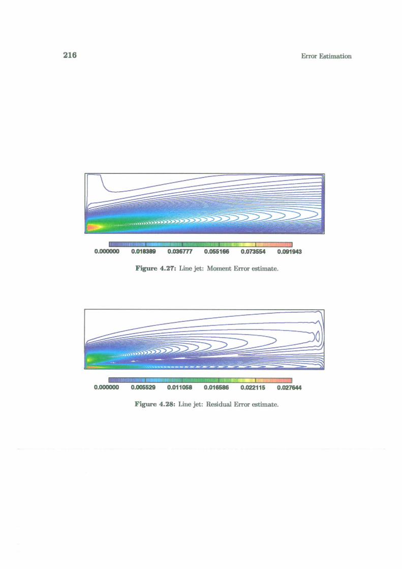
216
Error Estimation
0.000000 0.018389 0.036777 0.055166 0.073554 0.091943
Figure 4.27: Line jet: Moment Error estimate.
-- f I -.
0.000000 0.005529 0.011058 0.016586 0.022115 0.027644
Figure 4.28: Line jet: Residual Error estimate.
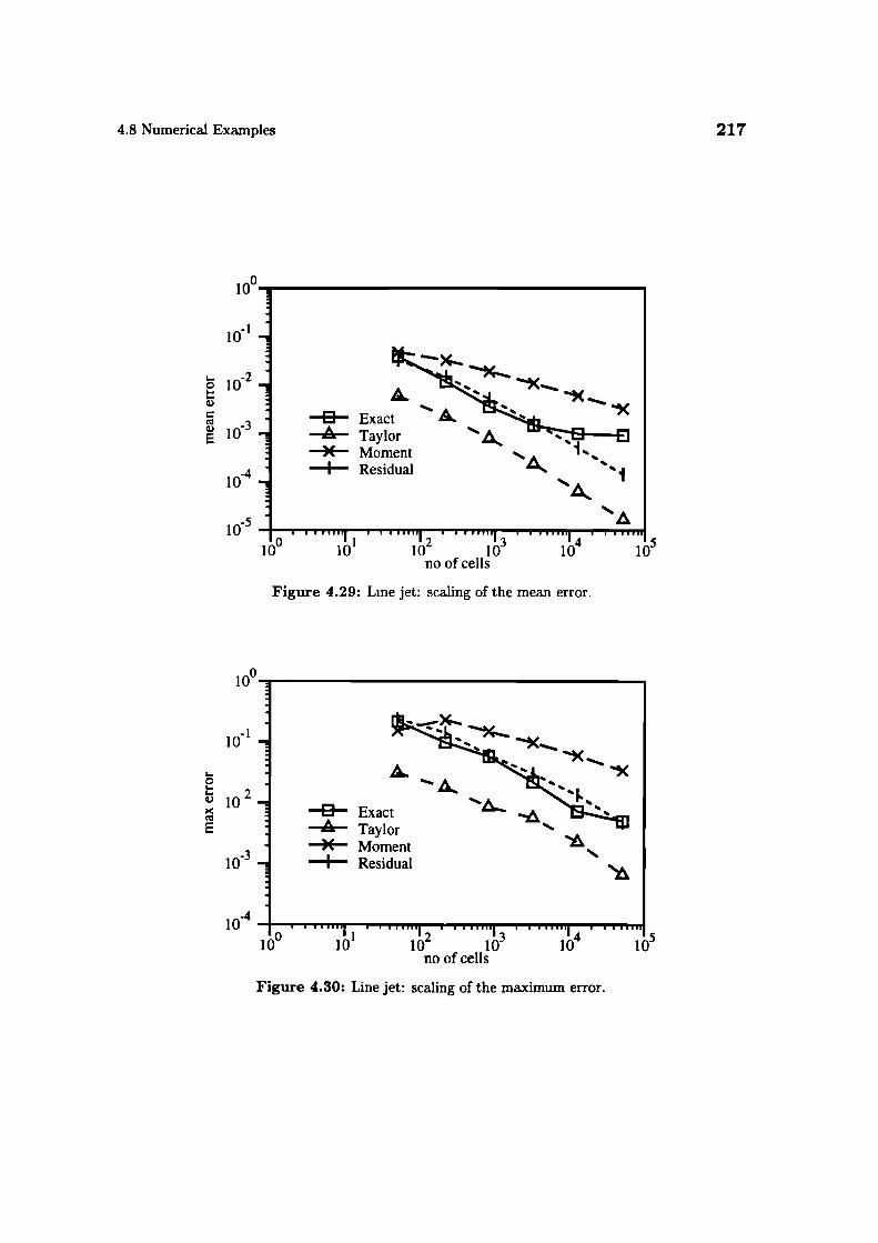
4.8 Numerical Examples
217
10
10_I
i- -2
20
1
p Exac'A Taylor
4%4
X Moment 1.I Residual
11111 1 1 rIuuuuPul,, uuuuul.uI,.IA
10' 10 10 10' 10-V
Ino of cells
Figure 4.29: Line jet: scaling of the mean error.
1 00 -
10_ I -
I-02
10 -
10 -
-
P ExactA Taylor)( MomentI Residual
I I .11.IA
10" 10' 1Q I0 10
1no of cells
Figure 4.30: Line jet: scaling of the maximum error.
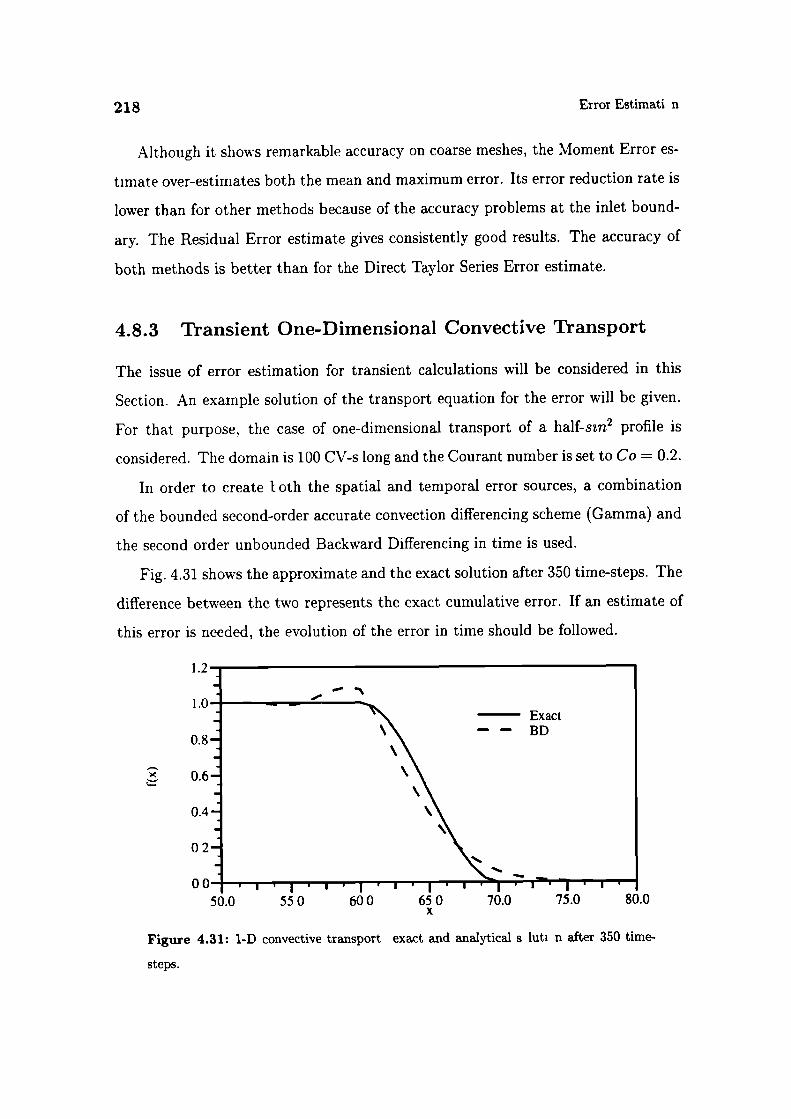
55 0 600 65 0 70.0 75.0 80.0x
1.2
1.0
0.8
0.6
0.4
02
0050.0
218
Error Estimati n
Although it shows remarkable accuracy on coarse meshes, the Moment Error es-
timate over-estimates both the mean and maximum error. Its error reduction rate is
lower than for other methods because of the accuracy problems at the inlet bound-
ary. The Residual Error estimate gives consistently good results. The accuracy of
both methods is better than for the Direct Taylor Series Error estimate.
4.8.3 Transient One-Dimensional Convective Transport
The issue of error estimation for transient calculations will be considered in this
Section. An example solution of the transport equation for the error will be given.
For that purpose, the case of one-dimensional transport of a half-sin 2 profile is
considered. The domain is 100 CV-s long and the Courant number is set to Co = 0.2.
In order to create I oth the spatial and temporal error sources, a combination
of the bounded second-order accurate convection differencing scheme (Gamma) and
the second order unbounded Backward Differencing in time is used.
Fig. 4.31 shows the approximate and the exact solution after 350 time-steps. The
difference between the two represents the exact cumulative error. If an estimate of
this error is needed, the evolution of the error in time should be followed.
Figure 4.31: 1-D convective transport exact and analytical s lut n after 350 time-
steps.
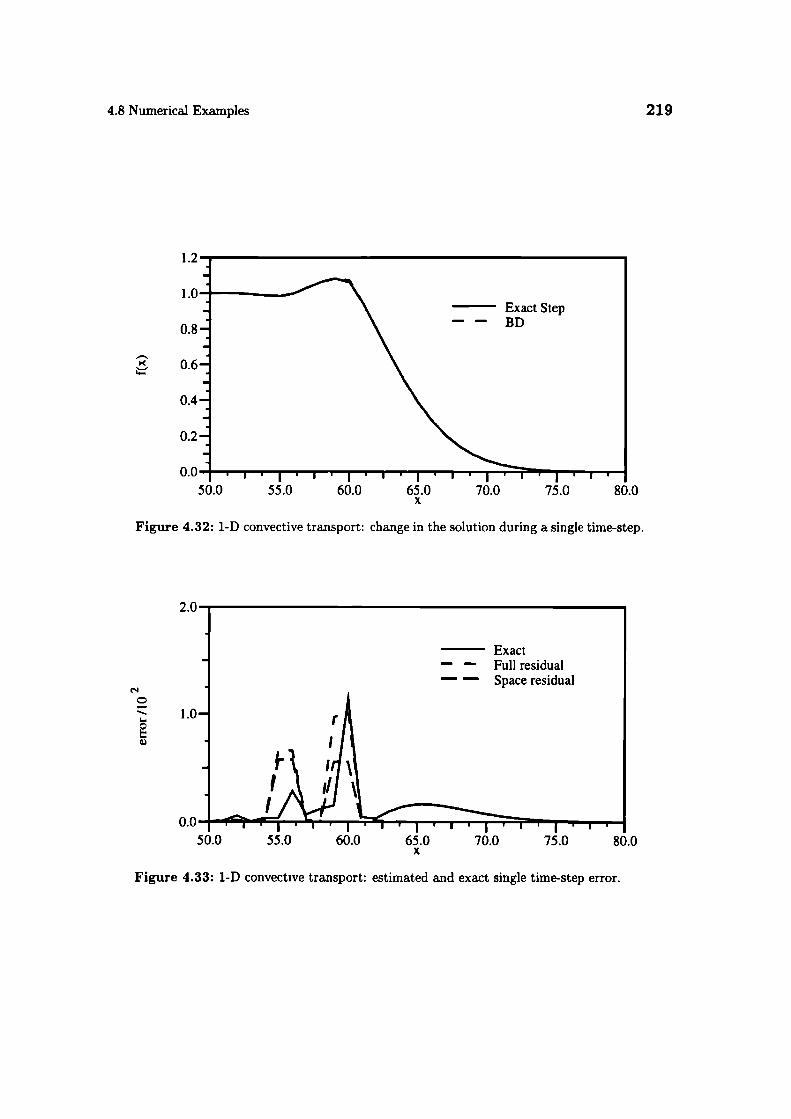
C1.0
4.8 Numerical Examples
219
1.2
1.0
0.8
E 0.6
0.4
0.2
0.0. 1 • i50.0 55.0 60.0 65.0 70.0 75.0 80.0
x
Figure 4.32: 1-D convective transport: change in the solution during a single time-step.
2.0
Exact- - Full residual- - Space residual
o.o I -1 'r---r i ••i_i...r::l
• I • • I•I50.0 55.0 60.0 65.0 70.0 75.0 80.0
x
Figure 4.33: 1-D convective transport: estimated and exact single time-step error.

0.2
0.1
I-.I-
0.0
-0.1
Exact- - Estimated, CN- - Estimated, BD
220 Error Estimation
Let us first examine the accuracy of the error estimate for a single time-step.
Comparing the shape of the solution in two consecutive steps (349th and 350th),
Fig. 4.32, it is possible to determine the error introduced during this step.
Fig. 4.33 presents the exact time-step error and the full Residual Error estimate.
The spatial error is included in the same gr ph for comparison. The full Residual
Error estimate approximates the exact error well. It can also be seen that the spatial
and temporal error are balanced in the region of highest error. The time-step size
is therefore appropriate for the given spatial resolution.
Using the full time-step residual as the error source, it is possible to follow
the evolution of the error in time from the onset of the calculation. The exact
error after 350 time-steps is calculated as the difference between the two curves in
Fig. 4.31. It is essential to solve the transport equation for the error as accurately as
possible in the first instance, Gamma differencing in space and Crank-Nicholson
in time are used. In Fig. 4.34, the estimated and exact errors are shown. The
50.0 55.0 60.0 65.0 70.0 75.0 80.0x
Figure 4.34: 1-D convective transport: estimated and exact error after 350 time-steps.
accuracy of this estimate is poor, as a consequence of the combined inaccuracies
in the estimation of the error source terms and the actual discretisation error in
the transport equation for the error. In order to determine the dependence of this
inaccuracy on the discretisation of the error transport equation, another solution
with Backward Differencing in time is given.
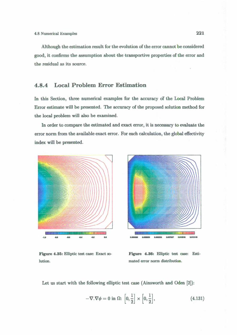
.11 _ .
. I
ts i.s ,.as .a.iw kINIs uuI
4.8 NumericaL ExamLes 221
Although the estimation result for the evolution of the error cannot be considered
good, it confirms the assumption about the t-ransportive properties of the error and
the residual as its source.
4.8.4 Local Problem Error Estimation
In this Section, three numerical examples for the accuracy of the Local Problem
Error estimate will be presented. The accuracy of the proposed solution method for
the local problem will also be examined.
In order to compare the estimated and exact error, it is necessary to evaluate the
error norm from the available exact error. For each calculation, the global effectivity
index will be presented.
Figure 4.35: Elliptic test case: Exact so- Figure 4.36: Elliptic test case: Esti-
lution. mated error norm distribution.
Let us start with the following elliptic test case (Ainsworth and Oden [21):
= 0 in fl: [o, ] x [o, ],
(4.131)

222
Error Estimation
with boundary conditions:
O, y- (e2
i) szn(2iry),(4.132)
q(x,O) 0.
The exact solution of the problem is:
(x,y) - e 1 v"1+21r2 - e xv'ik2 sin(27ry)
(4.133)
The exact solution on a 10 x 10 mesh and the estimated error norm are shown
in Figs. 4.35 and 4.36, respectively.
Exact and estimated global error norms are used to calculate the global effectivity
index:
e3 0.052461605 = 1.021.
Ie Iexact 0.0513568(4.134)
Let us now consider the accuracy of the solution procedure for the local problem.
For that purpose, two control volumes will be selected one for the determinate
form of the local problem (i.e. with a face on the fixed value boundary) and one for
the indeterminate form. The boundary conditions are calculated from the balanced
error fluxes, as explained in Section 4.6. The local problem is than solved on a series
of meshes and the solution is compared with the result of the simplified calculation.
The results are given in Tables 4.1 and 4.2, respectively. Having in mind a very high
Mesh size Local error norm, 10 6
5 x 5 1.73813
10 x 10 1.74598
20 x 20 1.74822
100 x 100 1.74896
Approximate solution 2.12916
Table 4.1: Determin te local problem: accuracy of the approximate soluti n.
cost associated with a more accurate (numerical) s lution procedure for the local
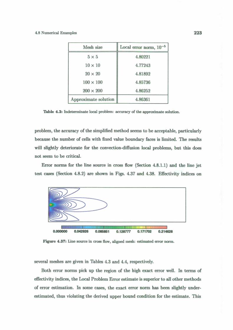
4.8 Numerical Examples
223
Mesh size Local error norm, i0
5 x 5 4.80221
10 x 10 4.77243
20 x 20 4.81892
100 x 100 4.85736
200 x 200 4.86252
Approximate solution 4.86361
Table 4.2: Indeterminate local problem: accuracy of the approximate solution.
problem, the accuracy of the simplified method seems to be acceptable, particularly
because the number of cells with fixed value boundary faces is limited. The results
will slightly deteriorate for the convection-diffusion local problems, but this does
not seem to be critical.
Error norms for the line source in cross flow (Section 4.8.1.1) and the line jet
test cases (Section 4.8.2) are shown in Figs. 4.37 and 4.38. Effectivity indices on
0.000000 0.042926 0.085851 0.128777 0.171702 0214628
Figure 4.37': Line source in cross flow, aligned mesh: estimated error norm.
several meshes are given in Tables 4.3 and 4.4, respectively.
Both error norms pick up the region of the high exact error well. In terms of
effectivity indices, the Local Problem Error estimate is superior to all other methods
of error estimation. In some cases, the exact error norm has been slightly under-
estimated, thus violating the derived upper bound condition for the estimate. This
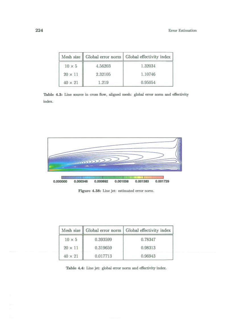
224
Error Estimation
Mesh size Global error norm J_Global effectivity index
10 x 5 4.56203 1.32034
20 x 11 2.32105 1.10746
40 x 21 1.219 0.95054
Table 4.3: Line source in cross flow, aligned mesh: global error norm and effectivity
index.
0.000000 0.000346 0.000692 0.001038 0.001383 0.001729
Figure 4.38: Line jet: estimated error norm.
Mesh size Global error norm Global effectivity indej
10 x 5 0.393599 0.78347
20 x 11 0.319659 0.98313
40 x 21 0.017713 0.96943
Table 4.4: Line jet: global error norm and effectivity index.
4.9 Closure
225
is attributed to the inaccuracies in the approximate solution of the local problem.
4.9 Closure
This Chapter presented an overview of error estimation methods for the Finite
Volume discretisation. Three new error estimates have been proposed. The Direct
Taylor Series Error estimate is based on the analysis of the Taylor series truncation
error. It is set up in such a way to enable single-mesh single-run error estimation. Its
accuracy is comparable with Richardson extrapolation. The Moment Error estimate
uses the imbalance in higher moments of the variable to provide an estimate of the
absolute error level. The Residual Error estimate measures the error using the cell
residual, caused by the inconsistency between the calculation of cell integrals and
face interpolation. Appropriate normalisation procedures are used to estimate the
error magnitude.
The definition of the residual for Finite Volume discretisation enables us to
generalise some results from the Finite Element field. The Local Problem Error
estimate has been extended to the Finite Volume method, together with the nec-
essary error flux balancing procedure, described in Section 4.6.1.1. This method
provides a highly accurate upper bound on the solution error in the energy norm.
The Local Problem Error estimate, originally derived for elliptic equations has been
subsequently extended to the convection-diffusion and Navier-Stokes problem.
An extension of the Residual Error estimate to transient calculations has been
presented in Section 4.7. It is possible to separately estimate the parts of the error
coming from spatial and temporal discretisation, as well as the total discretisation
error per time-step. Issues of solution accuracy after a given number of time steps
and the potential accumulation of the error have also been addressed. Finally, in
Section 4.8, numerical examples illustrating the accuracy of proposed error estimates
are given.
226 Error Estimation
Chapter 5
Adaptive Local Mesh Refinement
and Unrefinement
5.1 Introduction
Chapter 4 presented the tools that enable us to estimate the error in the numerical
solution. This information can now be used to change the distribution of computa-
tional points in order to improve the accuracy of subsequent solutions.
The mesh adaptation decreases the mesh-induced discretisation errors by im-
proving the distribution of computational points. An automatic error-based
adaptive mesh generation algorithm tries to create a computational mesh in
which the numerical error is uniformly distributed through the domain and corre-
sponds to the desired solution accuracy. This strategy produces a solution of desired
accuracy with the minimum number of computational points. It consists of several
steps:
1. The geometry of the domain and the boundary conditions are provided as
a set of surface descriptions and the appropriate specification of boundary
conditions along these surfaces. The required level of accuracy is defined as
the acceptable level of mean and maximum numerical error.
2. An initial computational mesh is created. The quality of this mesh is not

228
Adaptive Local Mesh Refinement and Unrefinement
critical. It should, however, be fine enough to provide a good basis for a-
posteriori error estimation. A poor initial mesh will increase the number of
mesh adaptation cycles.
3. The discretised set of governing equations is solved on the available mesh.
4. Using the tools described in Chapter 4, the numerical errors are estimated
from the information about the mesh and the available solution.
5. If the desired level of accuracy is reached, the mesh adaptation procedure is
stopped.
6. It is now possible to study the interaction between the numerical error and the
distribution of computational points. If necessary, additional computational
points can be introduced into the mesh in order to reduce the numerical error
to the desired level. As proposed by Zienkiewicz [156], the known order of
accuracy of the method can be used to estimate the desired local mesh size.
The new mesh is expected to have uniform error distribution.
7. A new computational mesh is created according to the criteria defined in the
step 6 and the original boundary description. In order to increase the efficiency
of the method, the existing numerical solution is mapped onto the new mesh
and used as an initial guess.
Steps 3 to 7 are repeated until the desired level of accuracy is reached or available
computer resources are exhausted.
The proposed adaptive mesh generation procedure tends towards the optimal
distribution of computational points the requirement for uniform distribution of
the error is built into step 6. The most difficult part of the procedure is the automatic
creation of the new mesh from the known boundary description and desired mesh
size distribution. Although this seems to be a reasonable request, presently available
automatic mesh generators are not able to produce meshes of reasonable quality.
An alternative approach to the subject of mesh adaptation comes from the re
quirement to make the pr cedure automatic. It is restricted by the issue of mesh
5.1 Introduction 229
generation: instead of creating a completely new mesh, the existing mesh will be
modified. Although this approach does not in general produce optimal meshes, it
attempts to maximise the increase of numerical accuracy per computational cost be-
tween two mesh changes. The mesh changes are done locally, in order to preserve the
"good" parts of the original mesh. If it can be assumed that the original mesh gives
a good representation of the geometry of the domain and boundary conditions, the
boundary description is not needed. This leads us towards an adaptive local mesh
refinement and unrefinement procedure, consisting of the following steps:
1. An initial computational mesh is created. It is expected that this mesh is fine
enough to describe the geometry and boundary conditions well1.
2. The discretised set of equations is solved on the available mesh.
3. The numerical error is estimated. If the desired level of accuracy is reached,
the calculation is stopped.
4. The estimated errors are used in order to decide what changes should be made
in the mesh in order to remove the regions of high error. At the same time, it is
possible that in some regions of the mesh, errors are much lower than average.
A required change of the mesh therefore consists of two parts: regions of the
mesh that need more computational points and regions in which the number
of computational points is too large according to the ratio of the local and
average error.
5. The mesh is then modified according to the requirements from the step 4.
Some additional changes in the mesh may be introduced in order to preserve
'In engineering calculations, this is rarely the case, as the boundary description consists of a set
of flat faces. It is therefore necessary to update the position of the points added on the boundary
in order to preserve the smooth description of the surface at the discrete level. This, on the other
hand, implies the availability of an alternative surface description, either in the analytical form,
or as a set on non-uniform rational b-splines NUR.BS , which brings us back to the interaction of
the mesh refinement algorithm and the CAD package. This is not the subject of the present study
and is therefore avoided.
230 Adaptive Local Mesh Refinement and Unrefinement
the mesh quality.
6. The existing numerical solution is mapped on the modified mesh and used as
an initial guess.
Steps 2 to 6 are repeated until the desired level of accuracy is reached.
In order to complete the adaptive local mesh refinement and unrefinement pro-
cedure, three questions need to be answered:
• How to select the regions of the mesh for refinement and unrefinement if the
error distribution is known?
. How to introduce the required change in the mesh and what additional changes
are needed in order to preserve the mesh quality?
• How to map the numerical solution from one mesh to the other with minimum
degradation of the solution accuracy?
The first question is answered in Section 5.2 refinement and unrefinement cri-
teria are based on the analysis of the estimated error field. An answer to the second
question is proposed in Section 5.3. The mesh changes are based on an embedded
cell-by-cell refinement and unrefinement procedure for "1-irregular" meshes. Some
details of the solution transfer between the meshes are given in Section 5.4. In order
to provide an insight into the relative merit of the proposed refinement technique in
comparison with uniform refinement, the error reduction on a simple test case is pre-
sented in Section 5.5. Finally, the adaptive local mesh refinement and unrefinement
algorithm is summarised in Section 5.6, together with some closing remarks.
5.2 Selecting Regions of Refinement and
Unrefinement
The procedure of selecting the regions of the mesh for refinement and unrefinement
is influenced by two issues: the mesh adaptation procedure that will be used and

5.2 Selecting Regions of Refinement and Unrefinement 231
the accuracy of the error estimate. The required information can also be two-fold.
Adaptive mesh generation algorithms need a distribution of the desired mesh size
through the domain, whereas local mesh refinement requires the lists of cells labelled
for refinement and unrefinement. Although these lists are related to the desired
mesh size distribution, it is easier to adopt a selection procedure rather than try to
transform one into the other.
Let us first show how to select the desired mesh size distribution. For each cell
of the computational mesh, the error magnitude and the mesh size h are known. It
is also known that the discretisation method is second-order accurate, i.e. that the
error scales with the square of the mesh size. If the desired error level is E0 , the
desired local mesh size l is calculated from the following scaling relations for the
error:
eI Ah2, (5.1)
E0 '- A1, (5.2)
where A is the unknown scaling factor. It follows that:
10 =
(5.3)
The quantity l is calculated for each computational point. The field of 1 can
subsequently be smoothed out in order to preserve reasonable mesh grading.
The local mesh refinement procedure can in theory use the same result. The local
value of l is compared with the existing mesh spacing in order to decide whether the
cell needs to be refined or unrefined. Unfortunately, this is not the best approach
in some cells, the desired mesh size can be considerably smaller than their current
size. If the mesh quality is to be preserved, grading between the fine and coarse
regions needs to be smooth.
As an alternative approach, the error in a cell can be compared with the average
error in the domain. Refinement and unrefinement criteria are then:
. If the error is larger than Arej , the cell is marked for refinement.
. If the error is smaller than )%unref , the cell is marked for unrefinement.
232 Adaptive Local Mesh Refinement and Unrefinement
Parameters Arej and Aunreí are the "safety" coefficients controlling the refinement
procedure, with the following properties:
Arej > 1, (5.4)
)tunref < 1
(5.5)
Although this system produces the refinement information efficiently, it is by no
means as accurate as the first approach. For example, in early stages of refinement
starting from a coarse mesh, the error level may be high everywhere and most of the
cells need to be refined. If, on the other hand, the solution is known to have some
localised features (shocks, propagating discontinuities etc.), a high level of localised
refinement is needed. Only a very small number of cells needs to be changed.
Parameters )'ref and )tunref effectively control the shape of the final mesh. Higher
'ref and lower )'unref result in a larger number embedded levels of refinement. Ide-
ally, )'ref and )'unref should be based on the statistics of the error distribution,
average error level and the required accuracy. Unfortunately, no simple relation be-
tween these parameters can be found. The recommended values of refinement and
unrefinement control parameters based on the experience in this study are:
)'ref = 1.5, (5.6)
)'unref - 0.5. (5.7)
Lists of cells for refinement and unrefinement do not contain all the information
needed to construct a good locally refined mesh. It is still desirable to create a
mesh with a smooth transition between the coarse and fine regions. The grading
information is not included smoothness of the mesh needs to be guaranteed in
some other way. One of the possibilities is to create a set of rules describing the
interaction between the coarse and fine regions. Cells for refinement (unrefinement)
are marked and the refinement information is propaga ed through the mesh. A more
detailed discussion of this issue will be given in Secti n 5.3. Another possibility
is to group the cells that require refinement into blocks and than add a "safety
margin" around each block (Brandt [22], Caruso [24, 25]). This moves the coarse-
fin mesh interface away fr m the region of high err r. Saf ty regions should in
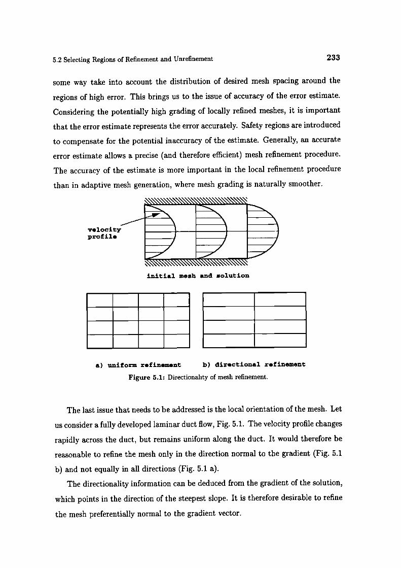
velocityprof ii.
5.2 Selecting Regions of Refinement and Unrefinement 233
some way take into account the distribution of desired mesh spacing around the
regions of high error. This brings us to the issue of accuracy of the error estimate.
Considering the potentially high grading of locally refined meshes, it is important
that the error estimate represents the error accurately. Safety regions are introduced
to compensate for the potential inaccuracy of the estimate. Generally, an accurate
error estimate allows a precise (and therefore efficient) mesh refinement procedure.
The accuracy of the estimate is more important in the local refinement procedure
than in adaptive mesh generation, where mesh grading is naturally smoother.
initial mesh and solution
a) uniform refinement b) directional refinement
Figure 5.1: Directionality of mesh refinement.
The last issue that needs to be addressed is the local orientation of the mesh. Let
us consider a fully developed laminar duct flow, Fig. 5.1. The velocity profile changes
rapidly across the duct, but remains uniform along the duct. It would therefore be
reasonable to refine the mesh only in the direction normal to the gradient (Fig. 5.1
b) and not equally in all directions (Fig. 5.1 a).
The directionality information can be deduced from the gradient of the solution,
which points in the direction of the steepest slope. It is therefore desirable to refine
the mesh preferentially normal to the gradient vector.

234
Adaptive Local Mesh Refinement and Unrefinement
If the computational procedure includes the solution of more than one equation,
cells for refinement are combined into a single list. It may happen that a single
cell is marked for refinement by more than one error field. In that case, the desired
refinement direction needs to take into account the gradients of all fields requiring
refinement of that particular cell.
The implementation of refinement directionality is easier in the context of local
mesh refinement than in adaptive mesh generation and will be further discussed in
the next Section.
5.3 Mesh Refinement and Unrefinement
Mesh refinement and unrefinement changes the topology of the mesh in order to
include the regions of iefinement and unrefinement. The available information in-
cludes:
Current computational mesh,
. List of cells that need to be refined with the desired direction of refinement,
. List of cells for unrefinement.
Let us first establish a refinement procedure for a single cell. A decision on the
type of the cell split needs to be made. In order to preserve the quality of the mesh,
the available cell types are limited to hexahedra and degenerate hexahedra.
Consider a hexahedral cell and a refinement direction R, Fig. 5.2. The shape
of the cell is described by three vectors: 1, 2 and 3. They carry the information
about the directional stretching of the control volume. These vectors have an average
direction of the two face area vectors for the pair of opposite faces of the hexahedron
and the magnitude corresponding to the ratio of the volume and the average cross-
section area.
For example, vector 1 is calculated as:
S 1 \ Vp_(:
+-_) +s 5.8)
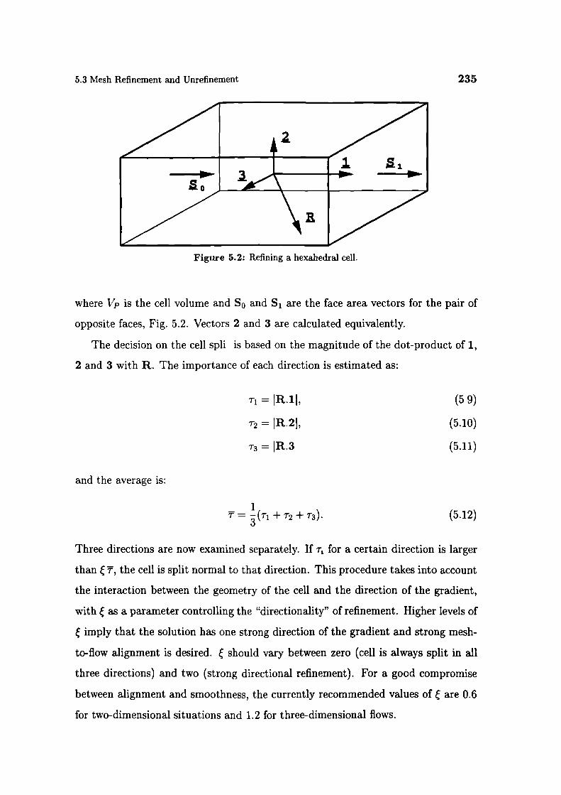
5.3 Mesh Refinement and Unrefinement
235
Figure 5.2: Refining a hexahedral cell.
where Vp is the cell volume and S0 and S 1 are the face area vectors for the pair of
opposite faces, Fig. 5.2. Vectors 2 and 3 are calculated equivalently.
The decision on the cell spli is based on the magnitude of the dot-product of 1,
2 and 3 with R. The importance of each direction is estimated as:
Ti = lR.1L
(59)
T2 = IR.21, (5.10)
T3 = IR.3
(5.11)
and the average is:
= (Ti+T2+T3). (5.12)
Three directions are now examined separately. If T, for a certain direction is larger
than T, the cell is split normal to that direction. This procedure takes into account
the interaction between the geometry of the cell and the direction of the gradient,
with as a parameter controlling the "directionality" of refinement. Higher levels of
imply that the solution has one strong direction of the gradient and strong mesh-
to-flow alignment is desired. should vary between zero (cell is always split in all
three directions) and two (strong directional refinement). For a good compromise
between alignment and smoothness, the currently recommended values of are 0.6
for two-dimensional situations and 1.2 for three-dimensional flows.
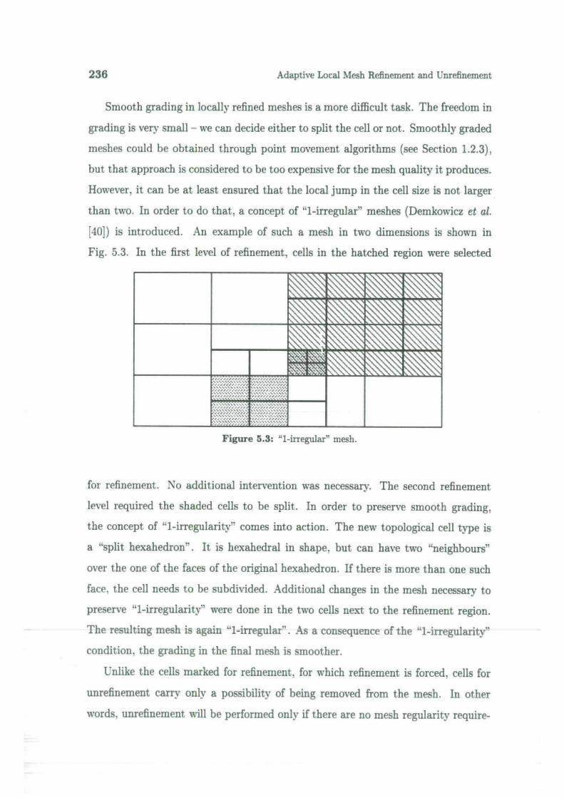
236
Adaptive Local Mesh Refinement and Unrefinement
Smooth grading in locally refined meshes is a more difficult task. The freedom in
grading is very small - we can decide either to split the cell or not. Smoothly graded
meshes could be obtained through point movement algorithms (see Section 1.2.3),
but that approach is considered to be too expensive for the mesh quality it produces.
However, it can be at least ensured that the local jump in the cell size is not larger
than two. In order to do that, a concept of "1-irregular" meshes (Demkowicz et al.
[40]) is introduced. An example of such a mesh in two dimensions is shown in
Fig. 5.3. In the first level of refinement, cells in the hatched region were selected
Figure 5.3: '1-irregu1ar' mesh.
for refinement. No additional intervention was necessary. The second refinement
level required the shaded cells to be split. In order to preserve smooth grading,
the concept of "1-irregularity" comes into action. The new topological cell type is
a "split hexahedron". It is hexahedral in shape, but can have two "neighbours"
over the one of the faces of the original hexahedron. If there is more than one such
face, the cell needs to be subdivided. Additional changes in the mesh necessary to
preserve "1-irregularity" were done in the two cells next to the refinement region.
The resulting mesh is again "1-irregular". As a consequence of the "1-irregularity"
condition, the grading in the final mesh is smoother.
Unlike the cells marked for refinement, for which refinement is forced, cells for
unrefinement carry only a possibility of being removed from the mesh. In other
words. unrefinement will be performed only if there are no mesh regularity require-
5.4 Mapping of Solution Between Meshes 237
ments to prevent it. A standard approach to mesh unrefinement enables the removal
of only those cells that have been added during the refinement procedure. This au-
tomatically implies that the mesh refinement starts from a very coarse mesh and
that the final mesh can only be locally as fine or finer than the original mesh. Cells
added into the mesh are stored into a "tree" data structure and can be removed on
request. An advantage of this strategy is that the original mesh can be recovered
after refinement and unrefinement.
In some situations, the refinement-only approach is not appropriate. The initial
mesh can be too coarse to produce a reasonable error estimate. A more general
procedure, including an arbitrary initial mesh with the possibility of both refinement
and unrefinement has been adopted in this study.
The unrefinement procedure is based on a "cell-pair" "oncept: the list of cells for
unrefinement is scanned in order to create "cell pairs" according to certain criteria.
The cell pair can be subsequently merged into a single cell if there are no regularity
limitations. It is no longer necessary to store the "history" of the mesh refinement,
as any cell is capable of unrefinement. One of the drawbacks of this approach
is that the recovery of the initial mesh after refinement and unrefinement is not
guaranteed. This is, however, desirable only in transient shock-tracking calculations.
If mesh recovery is essential, the refinement history can be built into the original
procedure.
5.4 Mapping of Solution Between Meshes
In order to speed up the solution of the problem on a refined mesh, a good initial
guess is needed. An approximate solution of the same problem on a different mesh
is already available, since the problem has been solved before the mesh is refined.
The mapping of the solution between two meshes is a straightforward task. The
assumed variation of the function over each control volume is linear. All fields
defined on cell centres can be mapped using the following procedure:
1. For each point P in the refined mesh, find the closest point T in the original
238
Adaptive Local Mesh Refinement and Unrefinement
mesh.
2. Calculate the position difference:
p - Xp - XT,
3. Calculate qp as
qp = T+P.(V)T.
(5.13)
(5.14)
The face flux transfer requires more care. The fluxes are defined on cell faces and
satisfy the continuity constraint. If the flux transfer is not accurate, continuity will
be violated, possibly causing unboundedness in the first solution of the new mesh
and other undesirable effects.
Since not all of the faces have their equivalents in the original mesi, a more
general (and more accurate) procedure is needed. For that purpose, we need to
come back to the calculation of fluxes (see Section 3.8). Fluxes are calculated using
Eqn. (3.144):
F=S. (H(U)\ ap
f1\ 1- (;) (V)i]
after the solution of the pressure equation, Eqn. (3.141):
v. (iVp) = >s. (H(U))
Eqn. (3.141) guarantees that the fluxes satisfy continuity. Instead of transferring
the fluxes directly, parts of the pressure equation will be interpolated to the new
mesh. The required fields are ap and H(U) both defined at cell centres and easy
to transfer. The pressure equation is then assembled and solved on the new mesh
before the calculation is resumed. This procedure can be performed between the
meshes bearing no similarity and will always produce conservative fluxes.
5.5 Numerical Example
The influence of the mesh changes introduced by the adaptive procedure to the
accuracy of consequent solutions is two-foldS
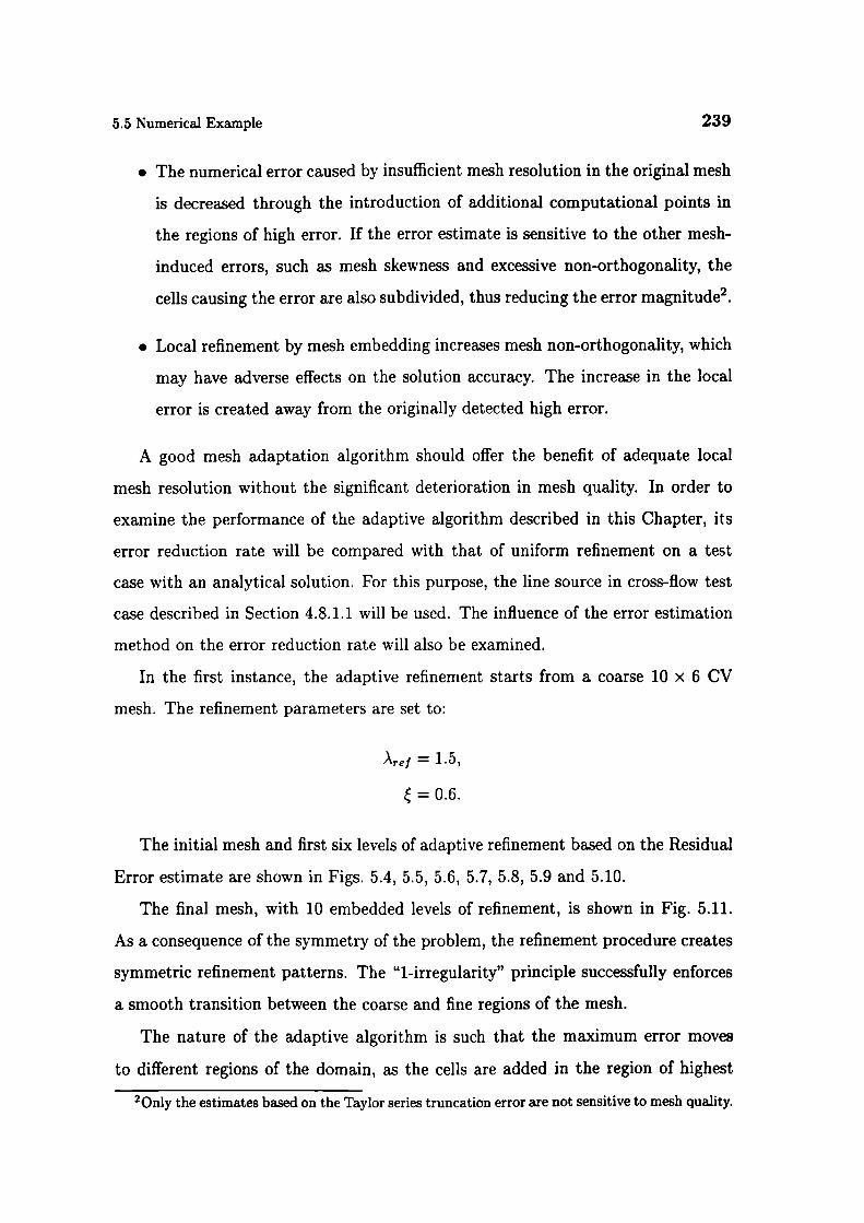
5.5 Numerical Example
239
• The numerical error caused by insufficient mesh resolution in the original mesh
is decreased through the introduction of additional computational points in
the regions of high error. If the error estimate is sensitive to the other mesh-
induced errors, such as mesh skewness and excessive non-orthogonality, the
cells causing the error are also subdivided, thus reducing the error magnitude2.
• Local refinement by mesh embedding increases mesh non-orthogonality, which
may have adverse effects on the solution accuracy. The increase in the local
error is created away from the originally detected high error.
A good mesh adaptation algorithm should offer the benefit of adequate local
mesh resolution without the significant deterioration in mesh quality. In order to
examine the performance of the adaptive algorithm described in this Chapter, its
error reduction rate will be compared with that of uniform refinement on a test
case with an analytical solution. For this purpose, the line source in cross-flow test
case described in Section 4.8.1.1 will be used. The influence of the error estimation
method on the error reduction rate will also be examined.
In the first instance, the adaptive refinement starts from a coarse 10 x 6 CV
mesh. The refinement parameters are set to:
Are1 = 1.5,
= 0.6.
The initial mesh and first six levels of adaptive refinement based on the Residual
Error estimate are shown in Figs. 5.4, 5.5, 5.6, 5.7, 5.8, 5.9 and 5.10.
The final mesh, with 10 embedded levels of refinement, is shown in Fig. 5.11.
As a consequence of the symmetry of the problem, the refinement procedure creates
symmetric refinement patterns. The "1-irregularity" principle successfully enforces
a smooth transition between the coarse and fine regions of the mesh.
The nature of the adaptive algorithm is such that the maximum error moves
to different regions of the domain, as the cells are added in the region of highest
2 Only the estimates based on the Taylor series truncation error are not sensitive to mesh quality.
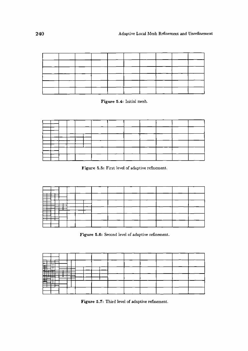
240
Adaptive Local Mesh Refinement and Unrefinement
Figure 5.4: Initial mesh.
Figure 5.5: First level of adaptive refinement.
Figure 5.6: Second level of adaptive refinement.
F:FH 1___ _ ____
Figure 5.7: Third level of adaptive refinement.
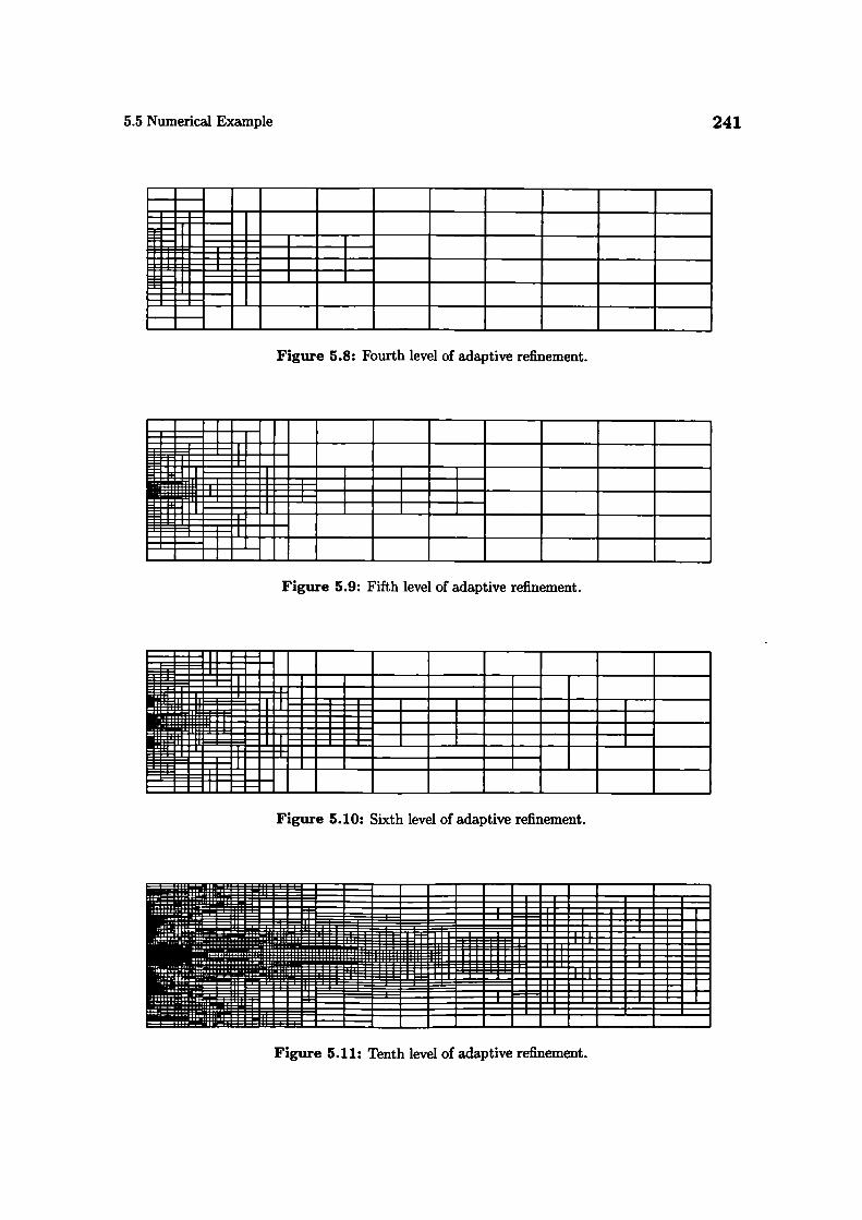
5.5 Numerical Example
241
Figure 5.8: Fourth level of adaptive refinement.
Figure 5.9: Fifth level of adaptive refinement.
Figure 5.10: Sixth level of adaptive refinement.
Figure 5.11: Tenth level of adaptive refinement.
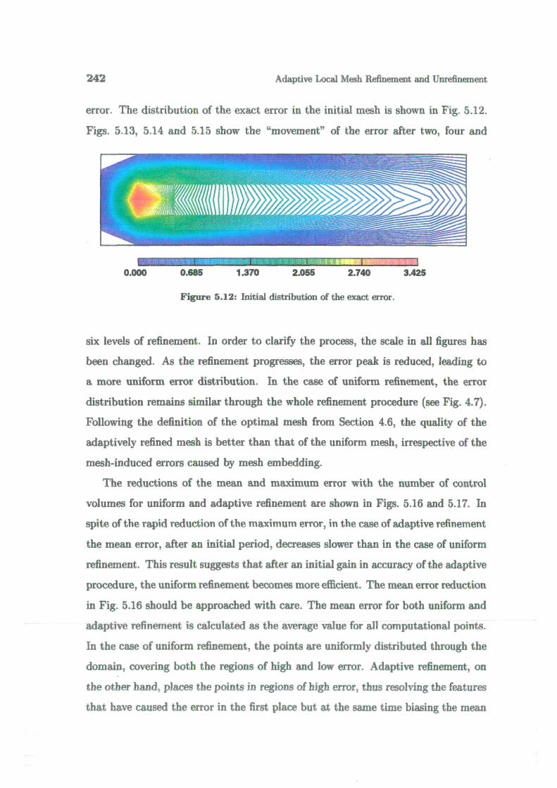
242 Adaptive Local Mesh Refinement and Unreflnement
error. The distribution of the exact error in the initial mesh is shown in Fig. 5.12.
Figs. 5.13, 5.14 and 5.15 show the "movement" of the error after two, four and
I I
0.000 0.685 1.370 2.055 2.740 3.425
Figure 5.12: Initial distribution of the exact error.
six levels of refinement. In order to clarify the process, the scale in all figures has
been changed. As the refinement progresses, the error peak is reduced, leading to
a more uniform error distribution. In the case of uniform refinement, the error
distribution remains similar through the whole refinement procedure (see Fig. 4.7).
Following the definition of the optimal mesh from Section 4.6, the quality of the
adaptively refined mesh is better than that of the uniform mesh, irrespective of the
mesh-induced errors caused by mesh embedding.
The reductions of the mean and maximum error with the number of control
volumes for uniform and adaptive refinement are shown in Figs. 5.16 and 5.17. In
spite of the rapid reduction of the maximum error, in the case of adaptive refinement
the mean error, after an initial period, decreases slower than in the case of uniform
refinement. This result suggests that after an initial gain in accuracy of the adaptive
procedure, the uniform refinement becomes more efficient. The mean error reduction
in Fig. 5.16 should be approached with care. The mean error for both uniform and
adaptive refinement is calculated as the average value for all computational points.
In the case of uniform refinement, the points are uniformly distributed through the
domain, covering both the regions of high and low error. Adaptive refinement, on
the other hand, places the points in regions of high error, thus resolving the features
that have caused the error in the first place but at the same time biasing the mean
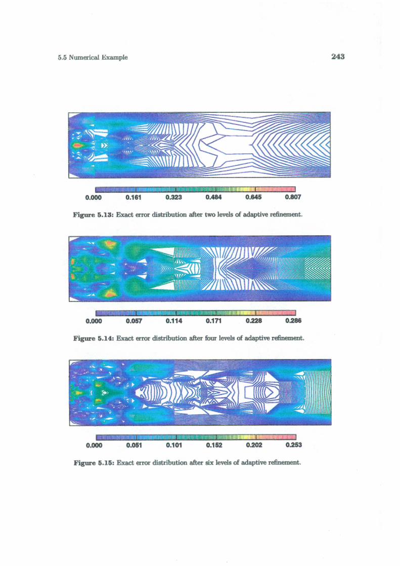
5.5 Numerical Example 243
0.000 0.161 0.323 0.484 0.645 0.807
Figure 5.13: Exact error distribution after two levels of adaptive refinement.
_biH . I
0.000 0.057 0.114 0.171 0.228 0.286
Figure 5.14: Exact error distribution after four levels of adaptive refinement.
I--
0.000 0.051 0.101 0.152 0.202 0.253
Figure 5.15: Exact error distribution after six levels of adaptive refinement.
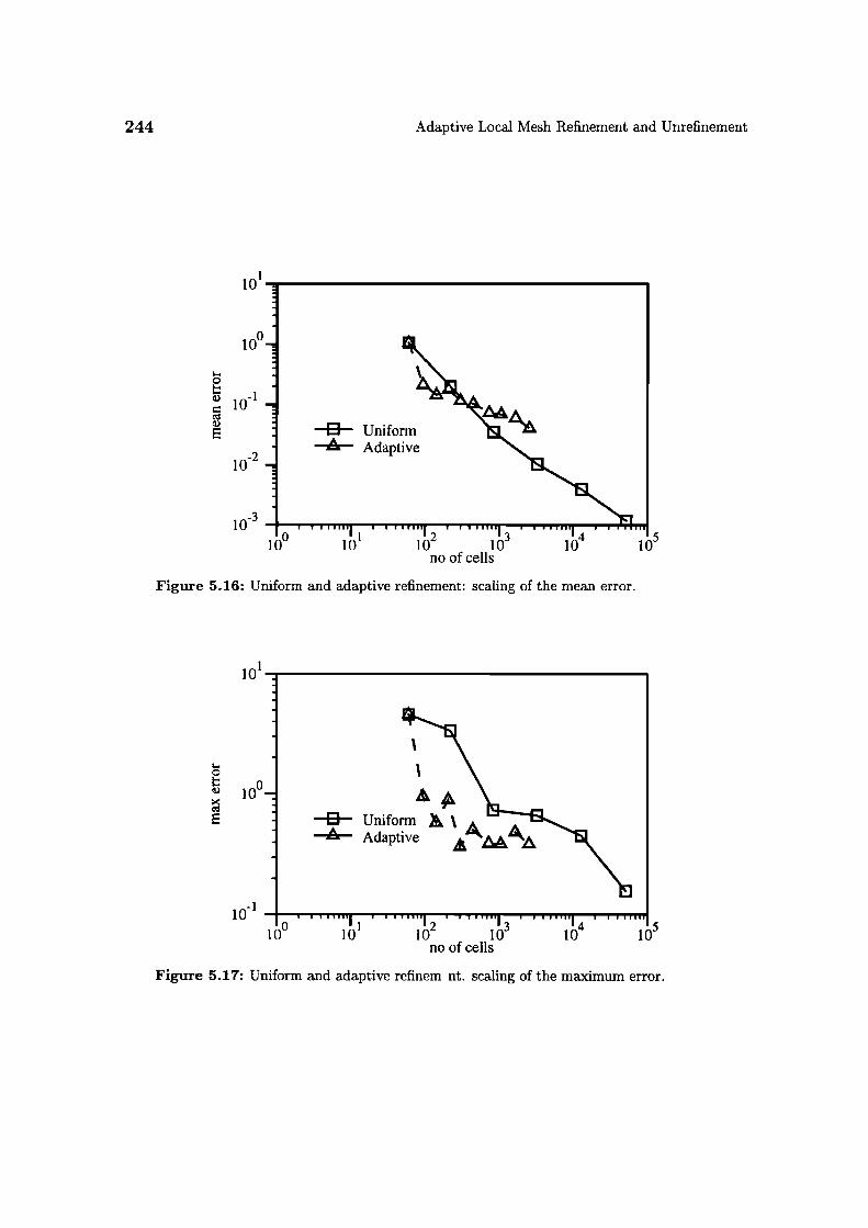
244
Adaptive Local Mesh Refinement and Unrefinement
101
100
C
10_i
1
10
0 Uniformá. Adaptive
I•••Ifl Iluuhlull, ........In
10" 10' 10- 10" 10'
Ino of cells
Figure 5.16: Uniform and adaptive refinement: scaling of the mean error.
101
C0
10
0 Uniformá. Adaptive
10_I '0 '1 '2 '3 '4 '510 10 10 10 10 10no of cells
Figure 5.17 Uniform and adaptive refinem nt. scaling of the maximum error.

5.5 Numerical Example 245
by higher sampling in those regions. This effect can be partially removed if a cell-
volume-weighted average error is used as shown in Fig. 5.18, but the sampling bias
still exists. Having in mind that the sampling problem cannot be resolved in an
101
10°
U
U -1E 10U
ID Uniform
--- Adaptive
-310 U ••, I IIIII I •u1111•1
'.' I I' IA
10"
10'
10 10 10
1no of cells
Figure 5.18: Uniform and adaptive refinement: scaling of the volume-weighted mean
error.
appropriate way, the unweighted mean error will be used in the rest of this study.
The sampling effect should be kept in mind when comparing the reduction of the
mean error for uniform and adaptive refinement.
The maximum error, Fig. 5.17, does not suffer from the sampling problem. Its
reduction in adaptive refinement is clearly much faster than in the case of uniform
refinement, indicating an improvement in the overall accuracy for the same number
of cells. The reduction of the maximum error still does not give the full picture of
the solution quality. Adaptively refined meshes resolve the regions of high gradients
considerably better than uniform meshes with the same number of cells, thus giving
a better picture of the real solution.
In order to provide a more objective comparison of the uniform and adaptive
refinement, we shall return to the concept of optimal meshes. According to the
definition from Section 4.6, an optimal mesh implies a uniform distribution of the
discretisation error. It is therefore possible to measure the mesh "optimality" as the
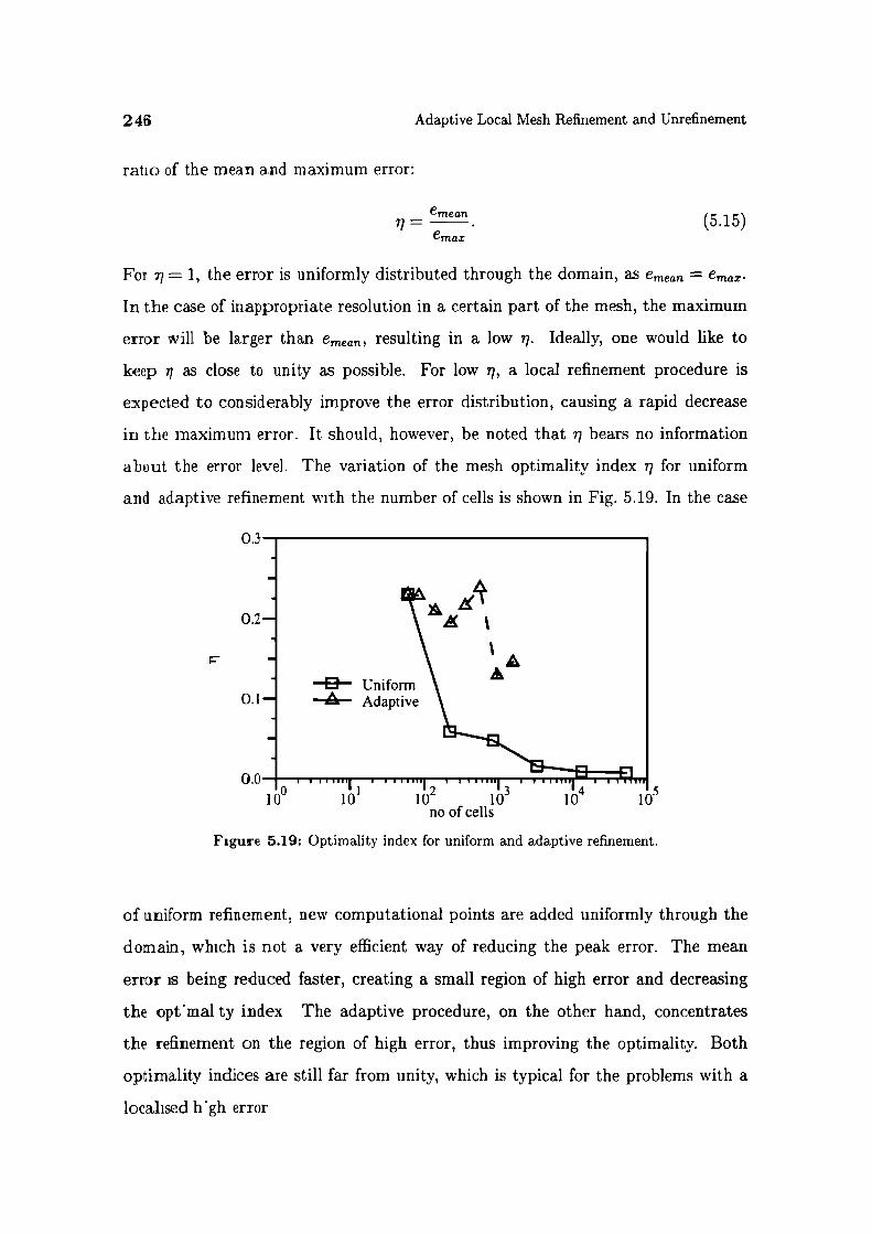
246
Adaptive Local Mesh Refinement and Unreflnement
ratio of the mean and maximum error:
emean(5.15)
Foir = 1, the error is uniformly distributed through the domain, as emean = emas.
In the case of inappropriate resolution in a certain part of the mesh, the maximum
error will be larger than emean, resulting in a low i. Ideally, one would like to
keep r as close to unity as possible. For low i, a local refinement procedure is
expected to considerably improve the error distribution, causing a rapid decrease
in the maximum error. It should, however, be noted that i bears no information
about the error level. The variation of the mesh optimality index i for uniform
and adaptive refinement with the number of cells is shown in Fig. 5.19. In the case
o.
0.2
0.1
0.0100
p Un'foAdaptive
A
'1 '2 '3 '4 '510 10 10 10 10
no of cells
Figure 5.19: Optimality index for uniform and adaptive refinement.
of uniform refinement, new computational points are added uniformly through the
domain, which is not a very efficient way of reducing the peak error. The mean
error is being reduced faster, creating a small region of high error and decreasing
the optmal ty index The adaptive procedure, on the other hand, concentrates
the refinement on the region of high error, thus improving the optimality. Both
optimality indices are still far from unity, which is typical for the problems with a
localised hgh error
5.5 Numerical Example
247
The "optimality" measure, Eqn. (5.15) should not be confused with the mesh
quality. The quality of the mesh is judged by the level of mesh-induced errors
caused by the cell distortion, non-orthogonality and mesh skewness. Although the
two issues are clearly connected, the difference can be drawn in the following way:
mesh quality is a property of the mesh, specifying the amount of mesh-induced
errors expected from a certain mesh. Mesh optimality, on the other hand, depends
on the interaction between the mesh and the particular problem that is being solved.
From the optimality point of view, the main cause of low i is inappropriate mesh
spacing in relation to the solution gradients, rather than the mesh-induced errors.
In order to present a more realistic picture of the influence of mesh changes
to the accuracy, the graphs showing the cell centre values in comparison with the
exact solution will be given. For this purpose, a cut through the domain, 0.2 m
downstream from the inlet boundary and normal to the flow is made. Figs. 5.20,
5.21 and 5.22 show the exact and numerical solution on the initial mesh and after
the first two levels of refinement (the meshes in question can be seen in Figs. 5.4, 5.5
and 5.6). The principle of adaptivity and the improvement in accuracy can now
be clearly seen: the computational points are added only when they are needed.
The solution after only two levels of adaptivity (Fig. 5.22) is accurate enough for all
practical purposes. Further downstream, the smoothly-changing solution does not
require the same number of computational points for the same level of accuracy. This
is demonstrated in Fig. 5.23, showing the cut through the domain 3 m downstream
from the inlet. The adaptively refined mesh resolves the profile with only 6 points,
but this is completely appropriate in comparison with the exact solution. The same
trend can be seen after ten levels of refinement, Figs. 5.24 and 5.25. The number of
computational points is large where the solution varies rapidly and depends on the
local curvature. Further downstream, the same level of accuracy can be obtained
with a much smaller number of cells.
As described in Section 5.2, the selection of cells for refinement is based on the
estimate of the local error. It could therefore be expected that the error reduction
rate depends not only on the applied refinement technique, but also on the accuracy
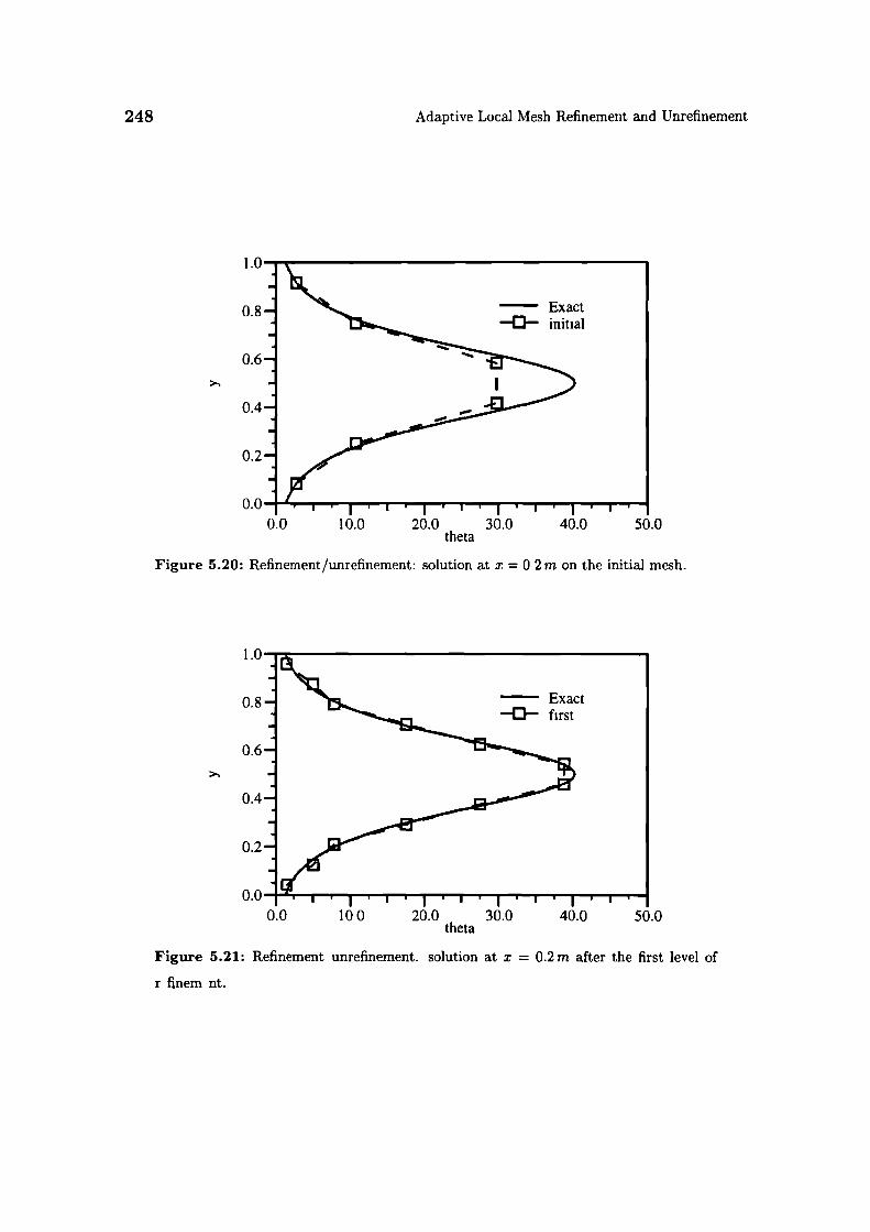
100 20.0 30.0 40.0 50.0theta
1.0
0.8
0.6
0.4
0.2
0.00.0
248
Adaptive Local Mesh Refinement and Unrefinement
1.0
0.8
0.6
0.4
0.2
0.0 '. I0.0 10.0 20.0 30.0 40.0 50.0
theta
Figure 5.20: Refinement/unrefinement: solution at x = 0 2m on the initial mesh.
Figure 5.21: Refinement unrefinement. solution at x 0.2m after the first level of
r fi.nem nt.

0
0
0
0
0
5 5 Numerical Example 249
0.0 10.0 20.0 30.0 40.0 50.0theta
Figure 5.22: Refinement/unrefinement: solution at x = 0.2 m after the second level of
refinement.
0.0 10.0 20.0 30.0 40.0 50.0theta
Figure 5.23: Refinement/unrefinement: solution at x = 3m after the second level of
refinement.

>..
250
Adaptive Local Mesh Refinement and Unrefinement
0.0 10.0 20.0 30.0 40.0 50.0theta
Figure 5.24: Refinement unrefinement: solution at x = 0.2 in after the tenth level of
refinement.
1.0
0.8
06
0.4
0.2
0.0 I0.0 100 20.0 30.0 40.0 50.0
theta
Figure 5.25: Refinement unrefinem nt solution at x = 3m after the tenth level of
refinement

5.5 Numerical Example
251
of the error estimate. In order to examine the importance of this interaction, the
adaptive procedure has been repeated, basing the choice of refinement regions on
the exact error and each of the error estimates described in Chapter 4. Scaling of
the mean and maximum of the exact error with the number of computational points
for different error estimates is shown in Figs. 5.26 and 5.27. Several interesting
conclusions can be drawn:
. The scatter of the points in Fig. 5.26 is relatively small, indicating similar
performance of all error estimates.
• The adaptive refinement technique moves the error from one region of the do-
main to the other, sometimes creating meshes with high mesh-induced errors.
This can be seen in the behaviour of the maximum error, Fig. 5.27. As the
error estimates are typically sensitive to the mesh quality, the mesh-induced
errors are removed in consequent mesh refinements.
• The adaptive procedure based on the exact error exhibits the slowest reduc-
tion of both mean and maximum error. Although this behaviour is by no
means obvious, its cause can be explained from the nature of the exact error.
Section 4.8 distinguishes two parts of the exact error: the locally induced error
and the transported error. An adaptive procedure based on the exact error
cannot distinguish between the two and, as a consequence, adds unnecessary
resolution in the regions where only the transported error exists. Error esti-
mates proposed in the present study neglect the mechanism of error transport
from the region of high error sources to the rest of the domain, resulting in a
more economical error removal.
• In the final stages of refinement, the maximum error reaches a plateau (see
Fig. 5.27) and the amount of refinement needed to further improve the accu-
racy becomes very large. At this stage, embedded refinement is spread through
the whole of the domain, creating strongly linked refinement patterns. The
"1-irregularity" condition introduces numerable changes in the mesh for ev-
ery prescribed cell split. The mesh quality (in terms of average skewness and

I-0b 0
100 ExactA TaylorX Moment
I ResidualI
252
Adaptive Local Mesh Refinement and Unrefinement
101
100_I...0
V0 Exact
V TaylorE 10' - )( Moment
I Residual
l 0 2 - IuuuIuV 13100 10 10 10 1O4
no of ce1s
Figure 5.26: Adaptive refinement: scaling of the mean error for different error estimates
arid the exact error.
1 0 1 I
10_i 10 l0
11111 11111!
no of cells
Figure 5.27: Adaptive refinement: scaling of the maximum error for different error
estimates and the exact err r

5.5 Numerical Example
253
non-orthogonality) is severely reduced. The bulk of the error should now be
attributed to the mesh quality rather than insufficient resolution in the regions
of high gradients. Since the objective of adaptivity is to produce accurate so-
lutions with only a slight increase in computational cost, further refinement
is not considered to be efficient. If the solution accuracy is still not appropri-
ate, the adaptive procedure should be repeated from a finer initial mesh. As
a guideline, in this particular case the plateau was reached when the initial
maximum error was reduced by a factor of 20. This is a property of the par-
ticular mesh adaptation algorithm rather than the adaptive approach itself.
If it were possible to create an adaptive procedure that does not impair the
mesh quality, this behaviour could be avoided altogether.
The second approach to the adaptive calculations starts from a relatively fine
initial mesh and use both refinement and unrefinement to improve the mesh qua!-
ity. In order to examine the performance of the unrefinement procedure, both
refinement-only and refinement/unrefinement calculations will be performed. The
initial mesh consists of 80 x 40 CV (Fig. 5.28), which is considered to be too fine
in the smooth parts of the solution and too coarse close to the singularity. The
refinement/unrefinement parameters are set to:
) ref = 1.5,
'unref = 0.5,
= 0.6.
Unlike refinement, the unrefinement algorithm adopted in this study does not
preserve the symmetry of the mesh for symmetric problems. The symmetry would
require some kind of global optimisation: the unrefinement procedure would have to
recognise the plane of symmetry not imposed from the outside. The adopted algo-
rithm selects the "cell pairs" on a cell-by-cell basis, with the final result depending,
among other things, on the order of cells in the cell list.
Although aesthetically pleasing, the symmetry is not essential for the accuracy
-
of the solution. If the mesh quality is deteriorated as a result of a "non-optimal"
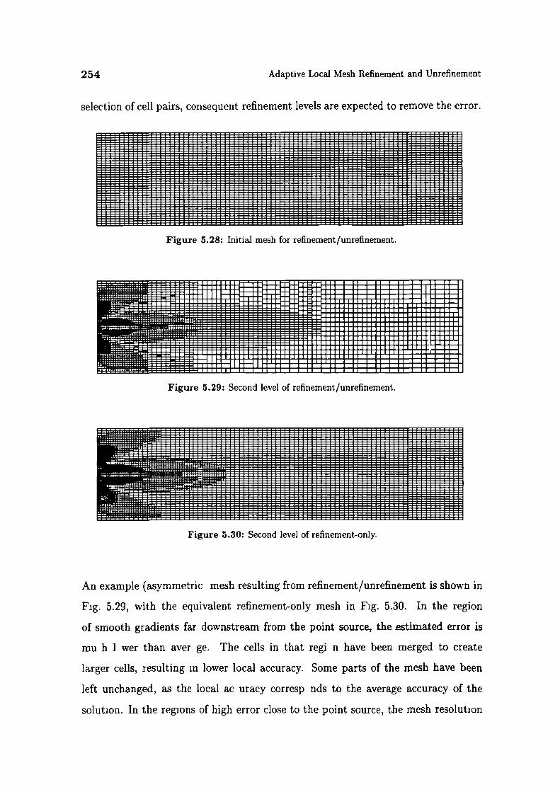
Figure 5.29: Second level of refinement/unrefinement.
Figure 5.30: Second level of refinement-only.
254
Adaptive Local Mesh Refinement and Unrefinement
selection of cell pairs, consequent refinement levels are expected to remove the error.
Figure 5.28: Initial mesh for refinement/unrefinement.
An example (asymmetric mesh resulting from refinement/unrefinement is shown in
Fig. 5.29, with the equivalent refinement-only mesh in Fig. 5.30. In the region
of smooth gradients far downstream from the point source, the estimated error is
mu h 1 wer than aver ge. The cells in that regi n have been merged to create
larger cells, resulting in lower local accuracy. Some parts of the mesh have been
left unchanged, as the local ac uracy corresp nds to the average accuracy of the
solution. In the regions of high error close to the point source, the mesh resolution

1
0 Uniform.. Refine/unrefineX Refine only
I.-0
0) 10
E
i
5.5 Numerical Example
255
has been improved.
100.
10_i
E l020 Uniform'k.. Refine/unrefine)( Refine only
10 iO 10" l0no of cells
Figure 5.31: Refinement/unrefInement: scaling of the mean error.
100
10 l0 10" IO5no of cells
Figure 5.32: Refinement/unrefinement: scaling of the maximum error.
A comparison of the mean and maximum error scaling for adaptive refinement
based on the Residual Error estimate is shown in Figs. 5.31 and 5.32. The sampling
problem can now be seen even more clearly. The scaling of the mean error suggests
that uniform refinement reduces the error more efficiently than both refinement-
only and refinement unrefinement. The reduction of the maximum error, Fig. 5.32

0 UniformA Refme/unrefineX Refine only
Irr,Iu. uuuu,u;,
1 0
10- 10' 10-Vno of cells
0.5
0.4
0.3
0.2
0.1
0.0100
I
AlII
II
II
I
256 Adaptive Local Mesh Refinement and Unrefinement
is again faster for the adaptive procedure than in the case of uniform refinement.
The plateau in the maximum error is reached when the initial peak error is reduced
by a factor of 10. It should, however, be noted that the error level on the initial
mesh is of the order of 1 %, which is lower than the typical accuracy needed for
engineering purposes.
A closer look into Figs. 5.31 and 5.32 reveals the correspondence between the
refinement only and refinement/unrefinement calculations. The peak error is in both
cases located in the refined region and its level is approximately the same. The unre-
finement procedure merges the cells in the region of low local error, thus moving both
graphs towards lower numbers of computational points. Refinement/unrefinement
therefore reaches the maximum error plateau with the smaller number of cells than
refinement-only. In terms of the mean error, the difference between the two adaptive
procedures is marginal.
Figure 5.33: Optimality index for uniform refinement, adaptive refinement-only and
adaptive refinement unr finement.
The variation of for refinement-only and refinement/unrefinement is shown in
Fig. 5.33. Both adapti e procedures increase the optimality index very rapidly. The
initial increase is Ia ger for refinement unrefinement, as the removal of unnecessary
c ils influences the mean error. It should also be noted that i for the final adaptively
refined mesh is much higher than for any uniform mesh in spite of the additional

0 ExactA TaylorX MomentI Residual
10_I
io2
5.5 Numerical Example
257
100
I1 2 I 14 IIII 15
10 10 10 10no of cells
Figure 5.34: Refinement/unrefinement: scaling of the mean error for different error
estimates.
l0-
10-I
10 - 0 Exact
A TaylorE)C MomentI Residual
i_2 -
10 ill' l0 10'no of cells
Figure 5.35: Refinement/unrefinement: scaling of the maximum error for different error
estimates.
258
Adaptive Local Mesh Refinement and Unrefinement
resolution added in the region of high error.
Let us finally examine the influence of error estimation on the error reduction rate
in the case of refinement/unrefinement. For that purpose, the adaptive calculation
has been repeated with the use of the proposed error estimates and the exact error.
The scaling of the mean and maximum error with the number of cells, for different
methods of estimation are shown in Figs. 5.34 and 5.35. The error reduction follows
a similar path for all error estimates, with the one based on the exact error again
showing the slowest drop. It can be therefore concluded that all error estimates
accurately highlight the error sources and the differences in the estimated error
distribution do not have a major influence on the adaptive process.
5.6 Closure
This Chapter presented some details of the adaptive local mesh refinement and un-
refinement procedure used in this study. The mesh adaptation algorithm is based
on the results of the error estimation procedure described in Chapter 4. Firstly,
the algorithms for an error-driven adaptive mesh generation and mesh refinement
procedure have been given. They consist of several parts: the analysis of the error
distribution, selection of regions for refinement and unrefinement, changing the ac-
tual computational mesh, and finally, mapping the solution from one mesh to the
other.
In order to overcome the problems connected with the issue of automatic mesh
generation, the selected procedure aims to change the existing computational mesh
in an optimal way. Smooth mesh grading is preserved through the concept of "1-
irregularity" of the mesh.
The mesh refinement procedure is controlled by three parameters: krej and
ef, controlling the grading between the coarse and fine regions of the mesh, and
determining the desired level of mesh alignment.
When the new mesh is created, an interpolate of the solution from the previous
mesh is used as an initial guess C nsistent with the discretisation practice, it is
5.6 Closure 259
assumed that the variation of the function over the control volume is linear. Some
attention needs to be given to the issue of the transfer of fluxes between two meshes.
A procedure that produces a set of conservative fluxes irrespective of the topological
interaction between the meshes has been described in Section 5.4. This completes
the adaptive local mesh refinement and unrefinement algorithm. An example of its
performance on a test case with an analytical solution has been given in Section 5.5.

260 Adaptive Local Mesh Refinement and Unrefinement
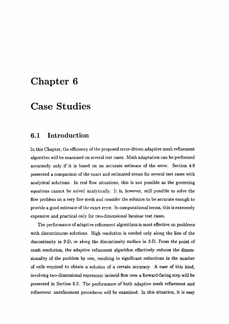
Chapter 6
Case Studies
6.1 Introduction
In this Chapter, the efficiency of the proposed error-driven adaptive mesh refinement
algorithm will be examined on several test cases. Mesh adaptation can be performed
accurately only if it is based on an accurate estimate of the error. Section 4.8
presented a comparison of the exact and estimated errors for several test cases with
analytical solutions. In real flow situations, this is not possible as the governing
equations cannot be solved analytically. It is, however, still possible to solve the
flow problem on a very fine mesh and consider the solution to be accurate enough to
provide a good estimate of the exact error. In computational terms, this is extremely
expensive and practical only for two-dimensional laminar test cases.
The performance of adaptive refinement algorithms is most effective on problems
with discontinuous solutions. High resolution is needed only along the line of the
discontinuity in 2-D, or along the discontinuity surface in 3-D. From the point of
mesh resolution, the adaptive refinement algorithm effectively reduces the dimen-
sionality of the problem by one, resulting in significant reductions in the number
of cells required to obtain a solution of a certain accuracy. A case of this kind,
involving two-dimensional supersonic inviscid flow over a forward-facing step will be
presented in Section 6.2. The performance of both adaptive mesh refinement and
refinement unrefinement procedures will be examined. In this situation, it is easy
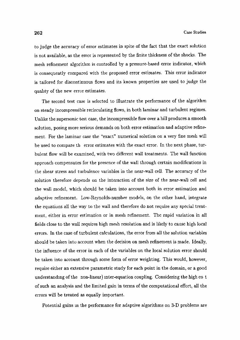
262 Case Studies
to judge the accuracy of error estimates in spite of the fact that the exact solution
is not available, as the error is represented by the finite thickness of the shocks. The
mesh refinement algorithm is controlled by a pressure-based error indicator, which
is consequently compared with the proposed error estimates. This error indicator
is tailored for discontinuous flows and its known properties are used to judge the
quality of the new error estimates.
The second test case is selected to illustrate the performance of the algorithm
on steady incompressible recirculating flows, in both laminar and turbulent regimes.
Unlike the supersonic test case, the incompressible flow over a hill produces a smooth
solution, posing more serious demands on both error estimation and adaptive refine-
ment. For the laminar case the "exact" numerical solution on a very fine mesh will
be used to compare th error estimates with the exact error. In the next phase, tur-
bulent flow will be examined, with two different wall treatments. The wall function
approach compensates for the presence of the wall through certain modifications in
the shear stress and turbulence variables in the near-wall cell. The accuracy of the
solution therefore depends on the interaction of the size of the near-wall cell and
the wall model, which should be taken into account both in error estimation and
adaptive refinement. Low-Reynolds-number models, on the other hand, integrate
the equations all the way to the wall and therefore do not require any special treat-
ment, either in error estimation or in mesh refinement. The rapid variation in all
fields close to the wall requires high mesh resolution and is likely to cause high local
errors. In the case of turbulent calculations, the error from all the solution variables
should be taken into account when the decision on mesh refinement is made. Ideally,
the influence of the error in each of the variables on the local solution error should
be taken into account through some form of error weighting. This would, however,
require either an extensive parametric study for each point in the domain, or a good
understanding of the non-linear) inter-equation coupling. Considering the high co t
of such an analysis and the limited gain in terms of the computational effort, all the
errors will be treated as equally important.
Potential gains in the performance for adaptive algorithms on 3-D problems are
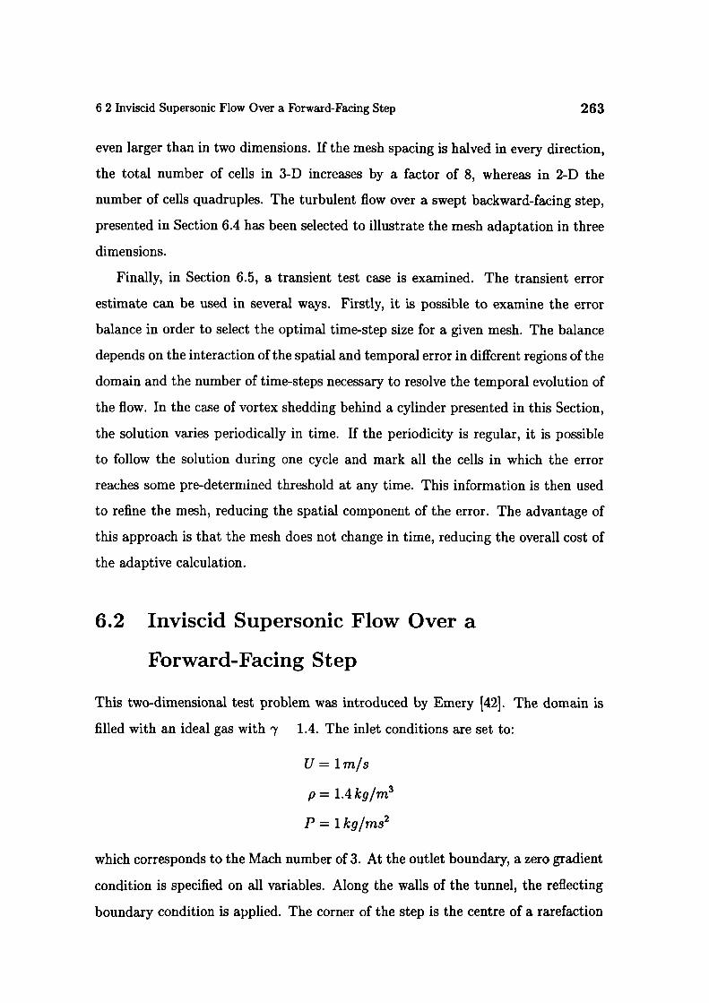
6 2 Inviscid Supersonic Flow Over a Forward-Facing Step 263
even larger than in two dimensions. If the mesh spacing is halved in every direction,
the total number of cells in 3-D increases by a factor of 8, whereas in 2-D the
number of cells quadruples. The turbulent flow over a swept backward-facing step,
presented in Section 6.4 has been selected to illustrate the mesh adaptation in three
dimensions.
Finally, in Section 6.5, a transient test case is examined. The transient error
estimate can be used in several ways. Firstly, it is possible to examine the error
balance in order to select the optimal time-step size for a given mesh. The balance
depends on the interaction of the spatial and temporal error in different regions of the
domain and the number of time-steps necessary to resolve the temporal evolution of
the flow. In the case of vortex shedding behind a cylinder presented in this Section,
the solution varies periodically in time. If the periodicity is regular, it is possible
to follow the solution during one cycle and mark all the cells in which the error
reaches some pre-determined threshold at any time. This information is then used
to refine the mesh, reducing the spatial component of the error. The advantage of
this approach is that the mesh does not change in time, reducing the overall cost of
the adaptive calculation.
6.2 Inviscid Supersonic Flow Over a
Forward-Facing Step
This two-dimensional test problem was introduced by Emery [42]. The domain is
filled with an ideal gas with y 1.4. The inlet conditions are set to:
U= lm/s
p= 1.4kg/rn3
P= 1kg/ms2
which corresponds to the Mach number of 3. At the outlet boundary, a zero gradient
condition is specified on all variables. Along the walls of the tunnel, the reflecting
boundary condition is applied. The corner of the step is the centre of a rarefaction
0.0 0.5 1.0 1.5 2.b 2.k
0.0 0.5 1.0 1.5 L) r 3.0
264
Case Studies
/
1'I
0.0 0.5 1.0 1.5 2.0 2.I'b
Figure 6.1: Supersonic flow over a forward-facing step: Mach number distribution,
uniform mesh, 840 CV.
Figure 6.2: Supersonic flow over a forward-facing step: Mach number distribution,
uniform mesh, 5250 CV.
Figure 6.3: Supersonic flow over a forward-facing step: Mach number distribution,
uniform mesh, 53000 CV.

6.2 Inviscid Supersonic Flow Over a Forward-Facing Step 265
fan and hence a singular point of the flow. This singularity has not been treated in
any special way and the local error causes a boundary layer of about one cell thick-
ness just above the step (Woodward and Colella [149]). A pressure-based supersonic
flow solver is used. In order to avoid spurious oscillations in velocity and pressure,
the Gamma differencing scheme is used on all equations.
In the first instance, the problem is solved on three uniform meshes, with 840,
5250 and 53000 CV-s, giving the Mach number distribution presented in Figs. 6.1,
6.2 and 6.3, respectively. An interesting feature is the over-expansion region at the
corner, followed by a weak shock originating just downstream of the edge. The
nature of the over-expansion and its interaction with the corner singularity has
been briefly discussed by Woodward and Colella [149]'. From the point of view of
adaptive refinement, the presence of both weak and strong shocks complicates the
situation considerably, particularly because the weak shock is not picked up in the
coarse mesh (see Fig. 6.1).
In the first instance, the following pressure based error indicator will be used:
T Vph2
The local cell size h is calculated from Eqn. (4.12). This error indicator measures
the pressure jump over a cell, giving a good indication of the shock resolution in
comparison with other flow features. This error indicator will be consequently used
to judge the performance of the error estimators described in Chapter 4.
Figs. 6.4, 6.5 and 6.6 show the distribution of T on three uniform meshes, cor-
responding to the Mach number distribution from Figs. 6.1, 6.2 and 6.3. The error
indicator correctly highlights the main shock structure on all meshes. The weak
shock originating from the corner is recognised only on the finest mesh.
The error indicator can now be compared with the estimated error distribution.
Figs. 6.7, 6.8 and 6.9 show the estimated errors on the intermediate mesh (5250
CV-s) using the Direct Taylor Series, Moment and Residual Error estimates for
the momentum equation. Unlike the error indicator, all three error estimates
'Similar effects occur in wind tunnel experiments of this type [149].
(6.1)

0.000 0.003 0.005 0.009 0.01 0.&15 0.d'18
0.000 0.003 0.006 0.000 0.012 0.01i18
0.000 0.003 0.006 0.009 0.01 0.05 ITIB
266
Case Studies
Figure 6.4: Supersonic flow over a forward-facing step: error indicator T, uniform mesh,
840 CV.
Figure 6.5: Supersonic flow over a forward-facing step: error indicator T, uniform mesh,
5250 CV.
Figure 6.6: Supersonic flow over a forward-facing step: error indicator T, uniform mesh,
53000 CV.

0.000 0.005 0.010 0.015 D. 0.05 0
0.000 0.125 0.250 0.375 0.500 0.6 'To
0.000 0.417 0.833 1.250 1.1 2.083 2.600
6.2 Inviscid Supersonic Flow Over a Forward-Fcing Step 4151
Figure 6.7: Supersonic flow over a forward-facing step: Direct Taylor Series Error
estimate for the momentum, uniform mesh, 5250 CV.
Figure 6.8: Supersonic flow over a forward-facing step: Moment Error estimate for the
momentum, uniform mesh, 5250 CV.
Figure 6.9: Supersonic flow over a forward-facing step: Residual Error estimate for the
momentum, uniform mcsh, 5250 CV.
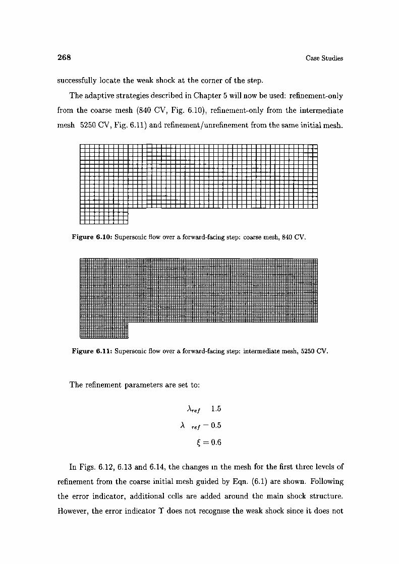
268
Case Studies
successfully locate the weak shock at the corner of the step.
The adaptive strategies described in Chapter 5 will now be used: refinement-only
from the coarse mesh (840 CV, Fig. 6.10), refinement-only from the intermediate
mesh 5250 CV, Fig. 6.11) and refinement/unrefinement from the same initial mesh.
Figure 6.10: Supersonic flow over a forward-facing step: coarse mesh, 840 CV.
Figure 6.11: Supersonic flow over a forward-facing step: intermediate mesh, 5250 CV.
The refinement parameters are set to:
Are1 1.5
A re0.5
= 0.6
In Figs. 6.12, 6.13 and 6.14, the changes in the mesh for the first three levels of
refinement from the coarse initial mesh guided by Eqn. (6.1) are shown. Following
the error indicator, additional cells are added around the main shock structure.
However, the error indicator T does not recognise the weak shock since it does not
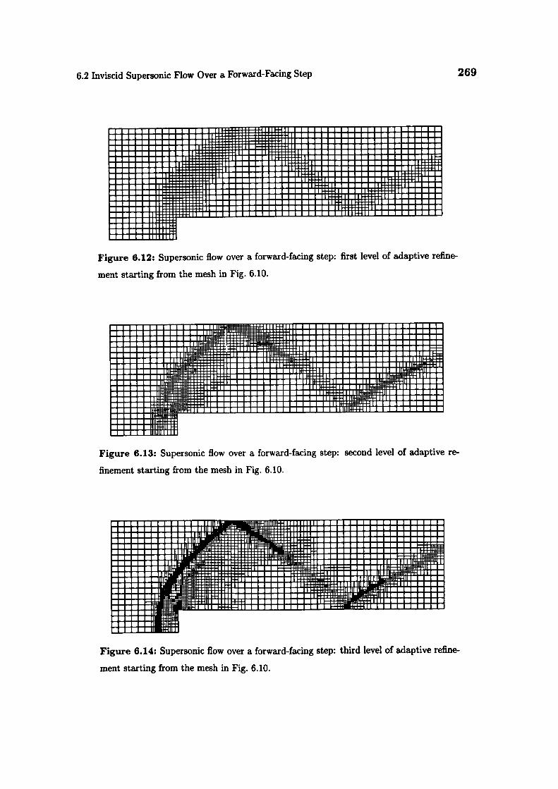
6.2 Inviscid Supersonic Flow Over a Forward-Facing Step 269
Figure 6.12: Supersonic flow over a forward-facing step: first level of adaptive refine-
ment starting from the mesh in Fig. 6.10.
Figure 6.13: Supersonic flow over a forward-facing step: second level of adaptive re-
finement starting from the mesh in Fig. 6.10.
-
Figure 6.14: Supersonic flow over a forward-facing step: third level of adaptive refine- -
ment starting from the mesh in Fig. 6.10.

270 Case Studies
exist in the coarse mesh solution (Fig. 6.1) and as a consequence, no new cells are
added in the region around it.
A detail of the refined mesh, showing the "1-irregularity" principle in action is
shown on Fig. 6.15. The grading between the coarse and fine parts of the mesh is
Figure 6.15: Detail of the adaptively refined mesh.
relatively smooth, preserving the quality of the refined mesh around the shock. If
the "1-irregularity" were not obeyed, rapid grading would cause high mesh-induced
errors, degrading the quality of the numerical solution.
The Mach number distribution after three levels of refinement is shown in Fig. 6.16
and the final solution, after five refinement levels in Fig. 6.17. The shock resolution
on the adaptively refined mesh with 15220 CV-s, (Fig. 6.17) is clearly superior to the
solution on a uniform mesh with 53000 CV-s (Fig. 6.3), demonstrating the potential
of the adaptive algorithm. The quality of the solution, however, cannot be judged
only by the resolution of strong shocks. The fine uniform mesh resolves the weak
shock originating from the corner of the step reasonably well. Although the adap-
tive solution picks up the same feature, its resolution is not comparable with the
resolution of the main shock structure. After three levels of refinement, Fig. 6.16,
the weak shock is not picked up at all. This is clearly an undesirable side-effect of
adaptive refinement. The key to the problem lies in the solution used to start the

0.0 0.5 1.0 1.5 2.0 2. To
6.2 Inviscid Supersonic Flow Over a Forward-Fcing Step 271
adaptive procedure. On the coarse mesh, the weak shock in question is not picked
up at all (see Fig. 6.1). The improvement of its resolution is possible only when the
mesh refinement progresses far enough the detect the shock in the first place.
Figure 6.18: Supersonic flow over a forward-facing step: Mach number distribution on
the adaptively refined mesh after three levels of refinement.
:'
0.0 0.5 1.0 1.5 2.0 2. "
Figure 6.17: Supersonic flow over a forward-facing step: Mach number distribution on
the adaptively refined mesh after five levels of refinement.
The preferred approach to the adaptive calculations would be to start from a
mesh that is capable of picking up all the features of the flow, leading us to the second
adaptive refinement strategy. The adaptive procedure starts from the intermediate
mesh (5250 CV-s, Fig. 6.11) and in the first instance performs refinement only. The
final mesh, after three levels of adaptive refinement, is shown in Fig. 6.18. This
mesh is considerably too fine in the region close to the inlet boundary. In this part
of the domain all the fields are constant, but the refinement-only procedure has no
meaus of removing the unnecessary computational points. The resolution of the
weak shock is now adequate, as it was possible to recognise It In the early stages of
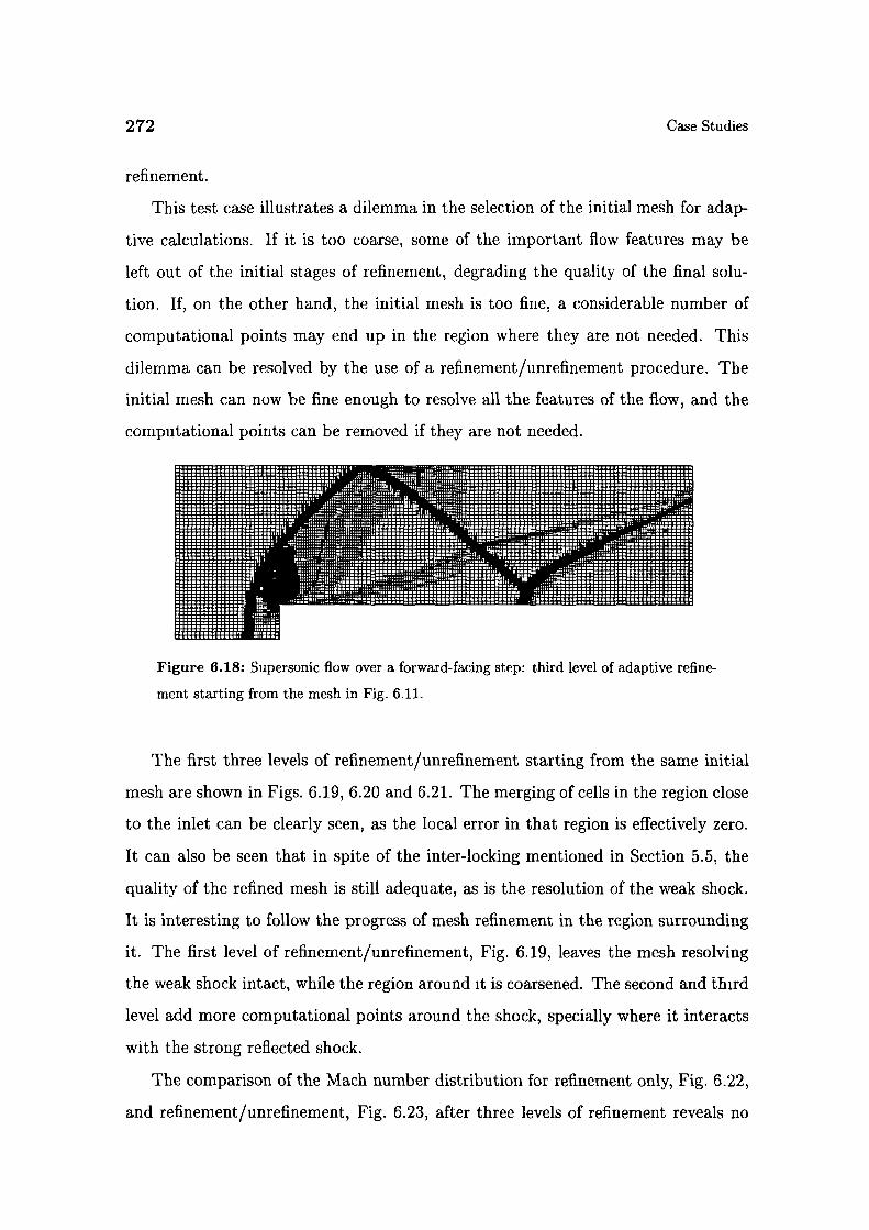
272
Case Studies
refinement.
This test case illustrates a dilemma in the selection of the initial mesh for adap-
tive calculations. If it is too coarse, some of the important flow features may be
left out of the initial stages of refinement, degrading the quality of the final solu-
tion. If, on the other hand, the initial mesh is too fine, a considerable number of
computational points may end up in the region where they are not needed. This
dilemma can be resolved by the use of a refinement/unrefinement procedure. The
initial mesh can now be fine enough to resolve all the features of the flow, and the
computational points can be removed if they are not needed.
Figure 6.18: Supersonic flow over a forward-facing step: third level of adaptive refine-
ment starting from the mesh in Fig. 6.11.
The first three levels of refinement/unrefinement starting from the same initial
mesh are shown in Figs. 6.19, 6.20 and 6.21. The merging of cells in the region close
to the inlet can be clearly seen, as the local error in that region is effectively zero.
It can also be seen that in spite of the inter-locking mentioned in Section 5.5, the
quality of the refined mesh is still adequate, as is the resolution of the weak shock.
It is interesting to follow the progress of mesh refinement in the region surrounding
it. The first level of refinement/unrefinement, Fig. 6.19, leaves the mesh resolving
the weak shock intact, while the region around it is coarsened. The second and third
level add more computational points around the shock, specially where it interacts
with the strong reflected shock.
The comparison of the Mach number distribution for refinement only, Fig. 6.22,
and refinement/unrefinement, Fig. 6.23, after three levels of refinement reveals no

6.2 Inviscid Supersonic Flow Over a Forward-Facing Step 273
Figure 6.19: Supersonic flow over a forward-facing step: first level of adaptive refine-
ment/unrefinement starting from the mesh in Fig. 6.11.
Figure 6.20: Supersonic flow over a forward-facing step: second level of adaptive re-
finement/unrefinement starting from the mesh in Fig. 6.11.
Figure 6.21: Supersonic flow over a forward-facing step: third level of adaptive refine-
ment/unrefinement starting from the mesh in Fig. 6.11.

2'T4
Case Studies
considerable differences.
k
0.0 0.5 1.0 1.5 2.0 2.Tb
Figure 6.22: Supersonic flow over a forward-facing step: Mach number distribution for
the mcsh in Fig. 6.18.
0.0 0.5 1.0 1.5 20 2. To
Figure 6.23: Supersonic flow over a forward-facing step: Mach number distribution for
the mesh in Fig. 6.21.
The objective of the adaptive procedure is to produce the accurate solution with
the minimum number of computational points. The performance of the algorithm
can therefore be measured in terms of the number of cells used vs. the number of
cells in the uniform mesh giving the equivalent resolution. Table 6.1 shows the in-
crease in the number of cells in four levels of adaptive refinement starting from the
coarse initial mesh and the number of cells for the uniform mesh with equivalent
resolution. The percentage ratio in the second column of Table 6.1 gives the number
of computational points in the adaptively refined mesh as a fraction of the number
of cells in the uniform mesh. This can be used to estimate the reduction in the corn-
putational effort needed to obtain a solution of a certain accuracy between adaptive
and uniform mesh refinement. The resolution of the initial mesh is inadequate in
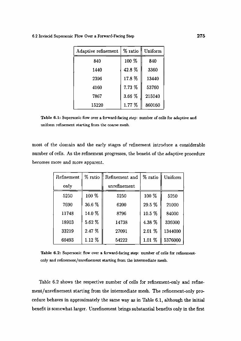
6.2 Inviscid Supersonic Flow Over a Forward-Facing Step
275
Adaptive refinement % ratio Uniform]
840 100 % 840
1440 42.8 % 3360
2396 17.8 % 13440
4160 7.73 % 53760
7867 3.66 % 215040
15220 1.77 % 860160
Table 6.1: Supersonic flow over a forward-facing step: number of cells for adaptive and
uniform refinement starting from the coarse mesh.
most of the domain and the early stages of refinement introduce a considerable
number of cells. As the refinement progresses, the benefit of the adaptive procedure
becomes more and more apparent.
Refinement % ratio Refinement and % ratio Uniform
only unrefinement
5250 100 % 5250 100 % 5250
7690 36.6 % 6200 29.5 % 21000
11748 14.0 % 8796 10.5 % 84000
18903 5.62 % 14738 4.38 % 336000
33219 2.47 % 27091 2.01 % 1344000
60493 1.12 % 54222 1.01 % 5376000
Table 6.2: Supersonic flow over a forward-facing step: number of cells for refinement-
only and refinement/unrefinement starting from the intermediate mesh.
Table 6.2 shows the respective number of cells for refinement-only and refine-
ment/unrefinement starting from the intermediate mesh. The refinement-only pro-
cedure behaves in approximately the same way as in Table 6.1, although the initial
benefit is somewhat larger. Unrefinement brings substantial benefits only in the first

276 Case Studies
three steps. As the refinement progresses, the difference between the two meshes
decreases, as more of the cells are placed where they are actually needed. The ben-
efit from unrefinement is also potentially larger if the starting mesh is finer. This
will generally be the case: when the shape of the solution is not known in advance,
the analyst will tend to create a mesh which is fine everywhere, knowing that the
adaptive procedure is capable of removing the excess cells where they are not needed.
Attention will now be turned to error estimation for supersonic flows. From
the numerical accuracy point of view, supersonic flows are singular and the shock
resolution is inadequate irrespective of the cell size. On uniform meshes the maxi-
mum error, Fig. 6.25, is therefore independent of mesh refinement. The mean error,
Fig. 6.24, decreases as the mesh gets finer, partly because of the better resolution
of the smooth profiles and partly because the number of cells away frori the shock
increases relative to the total number of cells.
The error scaling in the case of adaptive refinement starting from the coarse
mesh and refinement/unrefinement are shown in Figs. 6.26 and 6.27 and Figs. 6.28
and 6.29, respectively. The increase in the maximum error for the Direct Taylor
Series Error estimate corresponds to the improvement of the shock resolution. The
net effect of the sampling change in this case is that the mean error remains uniform
as the refinement progresses for both refinement-only and refinement/unrefinement.
In spite of the fact that the residual is well-defined, the Local Problem Error
estimate cannot be used on inviscid problems. Eqn. (4.101) shows that in the case
of v = 0, the local error estimate goes to infinity, rendering the upper bound on the
error meaningless.
In the case of supersonic flows, the comparison of the error estimate and the
exact error is not relevant - the physical thickness of the shock is infinitely small,
c mpared with the finite thickness in the numerical solution. The role of error
estimation is to control the adaptive procedure. Numerical experiments show that
any of the proposed error estimates can be used in place of the error indicator T,
producing equivalent refinement patterns.
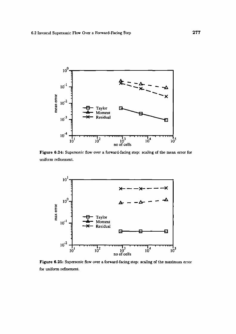
z.z-4Ap.-10_i
I-C
I'.,
E
I
0 Taylor•á. MomentX Residual
6.2 Inviscid Supersonic Flow Over a Forward-Facing Step 277
100
-410 I 13 14 5
10 10 10 10 10no of cells
Figure 8.24: Supersonic flow over a forward-facing step: scaling of the mean error for
uniform refinement.
101
- —&- - -
0 TaylorA Moment)( Residual
0— 0 0
io12 13 .14 ....... . 15
10 10 10 10 10no of cells
Figure 6.25: Supersonic flow over a forward-facing step: scaling of the maximum error
for uniform refinement.
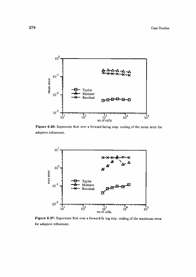
' ::0 Taylor
MomentX Residual
278
Case Studies
100
- -
I1 13.14 III..... 1510 10 10 10 10
no of cells
Figure 6.26: Supersonic flow over a forward-facing step: scaling of the mean error for
adaptive refinement.
101
A
0 TaylorA Moment)( Residual
1 _2 1...i2I
III IuuI
no of cells
Figure 6.27: Supersonic flow over a forward-fa ing step: scaling of the maximum error
for adaptive refinement.
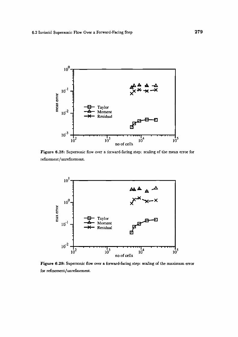
6.2 Inviscid Supersonic Flow Over a Forward-Facing Step
279
xx36 )( —x
0 Taylor-k- Moment
X Residual
1OL 10 IO JO5no of cells
Figure 6.28: Supersonic flow over a forward-facing step: scaling of the mean error for
refinement/unrefinement.
l0o_ -
::
l0 -
101
ul•1 1I1no of cells
Figure 6.29: Supersonic flow over a forward-facing step: scaling of the maximum error
for refinement/unrefinement.
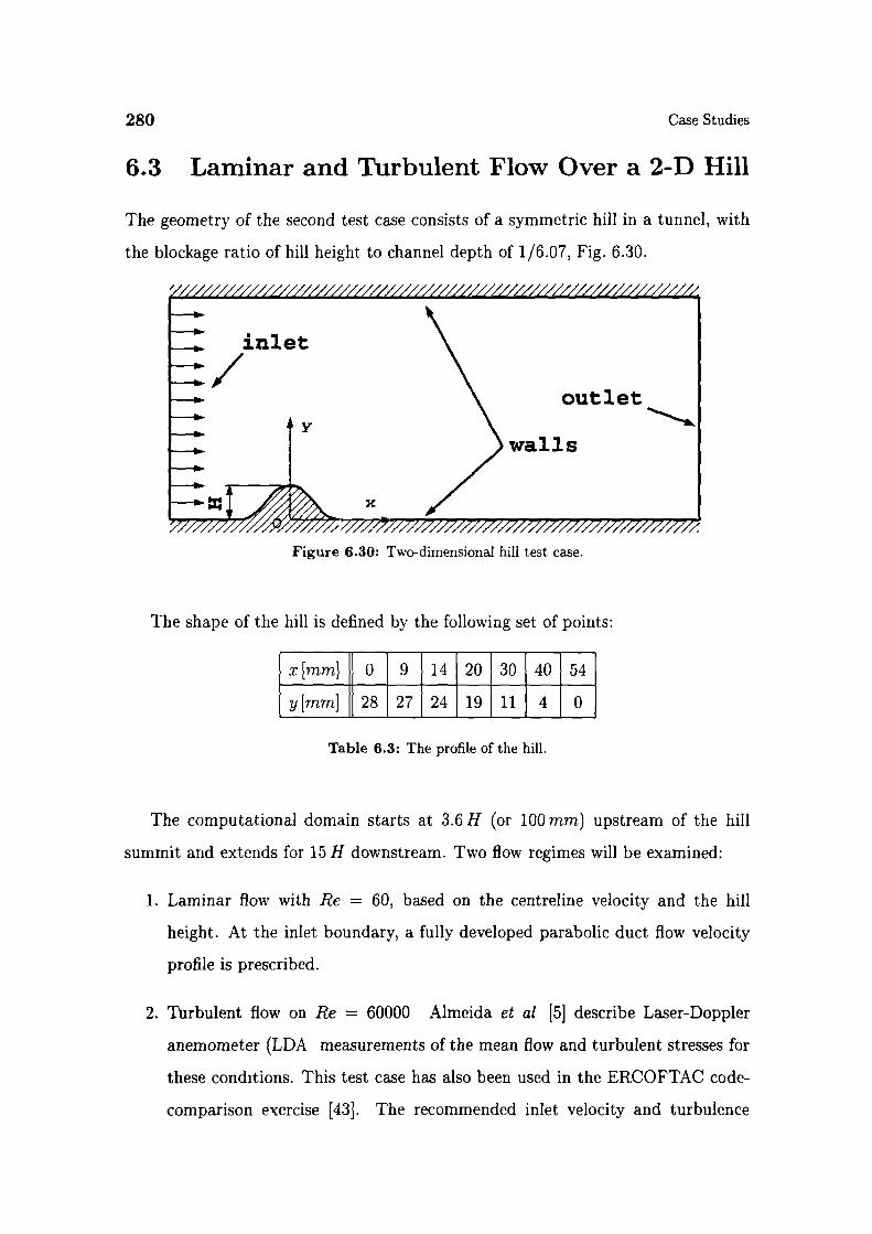
280
Case Studies
6.3 Laminar and Turbulent Flow Over a 2-D Hill
The geometry of the second test case consists of a symmetric hill in a tunnel, with
the blockage ratio of hill height to channel depth of 1/6.07, Fig. 6.30.
inlet/ outlet
Y \
walls
Figure 6.30: Two-dimensional hill test case.
The shape of the hill is defined by the following set of points:
x[mm] 0 9 14 20 30 40 1 1[jmm] 28 27 24 19 11 4 0
Table 6.3: The profile of the hill.
The computational domain starts at 3.6 H (or 100 mm) upstream of the hill
summit and extends for 15 H downstream. Two flow regimes will be examined:
1. Laminar flow with Re = 60, based on the centreline velocity and the hill
height. At the inlet boundary, a fully developed parabolic duct flow velocity
profile is prescribed.
2. Turbulent flow on Re 60000 Almeida et al [5] describe Laser-Doppler
anemometer (LDA measurements of the mean flow and turbulent stresses for
these conditions. This test case has also been used in the ERCOFTAC code-
comparison exercise [43]. The recommended inlet velocity and turbulence
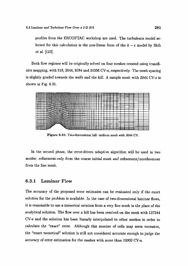
6.3 Laminar and Turbulent Flow Over a 2-D Hill
281
profiles from the ERCOFTAC workshop are used. The turbulence model se-
lected for this calculation is the non-linear form of the k - € model by Shih
et al. [123].
Both flow regimes will be originally solved on four meshes created using transfi-
nite mapping, with 518, 2044, 8584 and 34336 CV-s, respectively. The mesh spacing
is slightly graded towards the walls and the hill. A sample mesh with 2044 CV-s is
shown in Fig. 6.31.
Figure 6.31: Two-dimensional hifi: uniform mesh with 2044 CV.
In the second phase, the error-driven adaptive algorithm will be used in two
modes: refinement-only from the coarse initial mesh and refinement/unrefinement
from the fine mesh.
6.3.1 Laminar Flow
The accuracy of the proposed error estimates can be evaluated only if the exact
solution for the problem is available. In the case of two-dimensional laminar flows,
it is reasonable to use a numerical solution from a very fine mesh in the place of the
analytical solution. The flow over a hill has been resolved on the mesh with 137344
CV-s and the solution has been linearly interpolated to other meshes in order to
calculate the "exact" error. Although this number of cells may seem excessive,
the "exact numerical" solution is still not considered accurate enough to judge the
accuracy of error estimation for the meshes with more than 10000 CV-s.
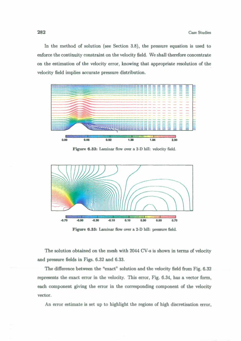
282
Case Studies
In the method of solution (see Section 3.8), the pressure equation is used to
enforce the continuity constraint on the velocity field. We shall therefore concentrate
on the estimation of the velocity error, knowing that appropriate resolution of the
velocity field implies accurate pressure distribution.
= = = = = = = = =
i___------------ - - -
------------
I '1IlIIPIU
0.00 0.46 0.52 1.39 114 2.30
Figure 6.32: Laminar flow over a 2-D hill: velocity field.
.0.70 .0.50 .0.30 .0.10 0.10 0.30 0.50 0.70
Figure 6.33: Laminar flow over a 2-D hill: pressure field.
The solution obtained on the mesh with 2044 CV-s is shown in terms of velocity
and pressure fields in Figs. 6.32 and 6.33.
The difference between the "exact" solution and the velocity field from Fig. 6.32
represents the exact error in the velocity. This error, Fig. 6.34, has a vector form,
each component giving the error in the corresponding component of the velocity
vector.
An error estimate is set up to highlight the regions of high discretisation error,
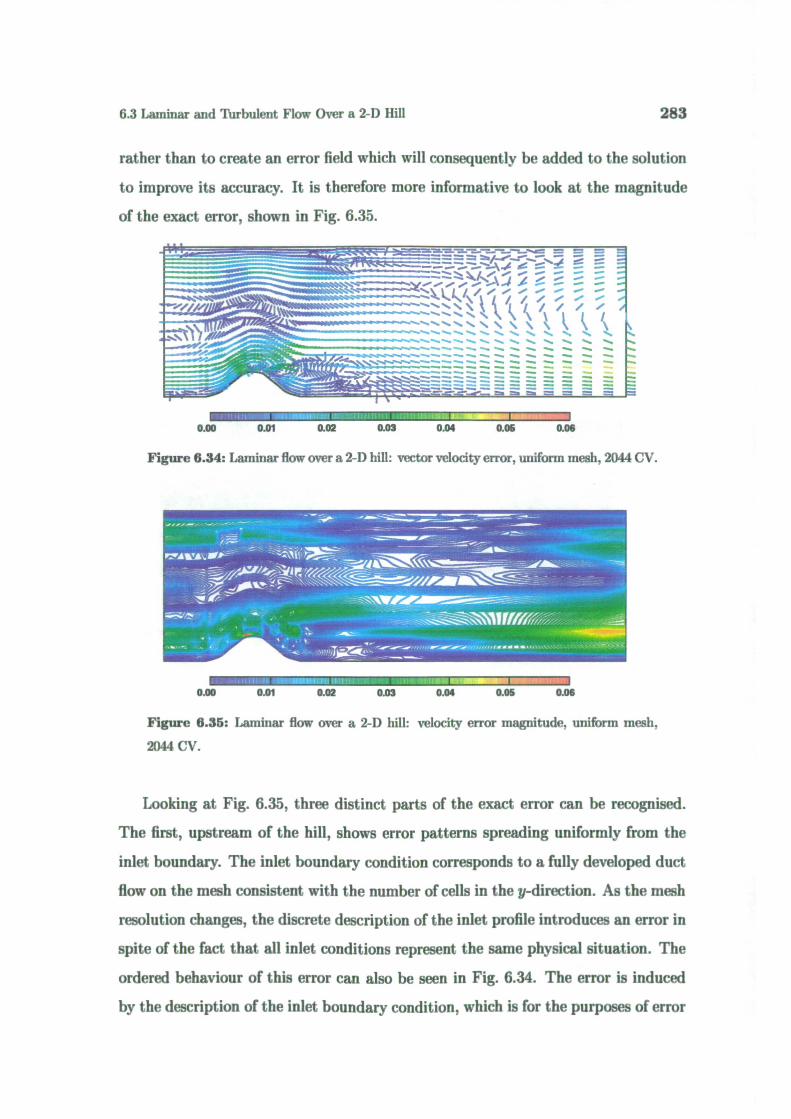
6.3 Laminar and Turbulent Flow Over a 2-D Hill
283
rather than to create an error field which will consequently be added to the solution
to improve its accuracy. It is therefore more informative to look at the magnitude
of the exact error, shown in Fig. 6.35.
JS%I- — — —% I / / # - - — -. —s\% I / / -. — -
'.' S .t I / / / / /S%%\ \ ' I I I'.iS%\ \ ' \ '
-.--,-..- •.- .-. . S...- -S S. - -S .. — — •..- — — — __ -S - S. -S S. •S.- - — - - - — -S — - .
0.00 0.01 0.02 0.03 0.04 0.05 0.06
Figure 6.34: Laminar flow over a 2-D hill: vector velocity error, uniform mesh, 2044 CV.
0.00 0.01 0.02 0.03 0.04 0.05 0.06
Figure 6.35: Laminar flow over a 2-D hill: velocity error magnitude, uniform mesh,
2044 CV.
Looking at Fig. 6.35, three distinct parts of the exact error can be recognised.
The first, upstream of the hill, shows error patterns spreading uniformly from the
inlet boundary. The inlet boundary condition corresponds to a fully developed duct
flow on the mesh consistent with the number of cells in the y-direction. As the mesh
resolution changes, the discrete description of the inlet profile introduces an error in
spite of the fact that all inlet conditions represent the same physical situation. The
ordered behaviour of this error can also be seen in Fig. 6.34. The error is induced
by the description of the inlet boundary condition, which is for the purposes of error

284 Case Studies
analysis considered to be exact. As a consequence, this error cannot be picked up
by an error estimate.
The second region of high error envelops the hill, including the area just above
the summit. The error in this region is mainly caused by insufficient mesh reso-
lution close to the summit, with the rest of the error being convected downstream
from the peak. The third interesting region lies further downstream, close to the
outlet boundary. It is assumed that the error here originates from the accumulated
upstream inaccuracies. It is rapidly removed with refinement and disappears on the
next finer mesh (see Fig. 6.36).
I.0.00 0.01 0.02 0.03 0.04 0.05
Figure 6.36: Laminar flow over a 2-D hill: velocity error magnitude, uniform mesh,
8584 CV.
The estimated error distributions using the Direct Taylor Series, Moment and
Residual Error estimates for the mesh with 2044 CV-s are shown in Figs. 6.37, 6.38
and 6.39. In order to highlight the error distribution rather than its magnitude, the
colour-scale in Figs. 6.37, 6.38 and 6.39 has been adjusted.
All three error estimates highlight the front of the hill as the region of high error
sources, corresponding to the maximum error in Fig. 6.35. The mesh-induced errors
are high at the connection of the orthogonal mesh in front and behind the hill with
the region of non-orthogonality above the hill and are visible in all error estimates.
Upstream of the hill, the estimated error is low and depends mainly on the mesh
spacing. The recirculation zone behind the hill also induces some error, caused by
the high velocity gradients between the recirculation bubble and the rest of the flow.

6.3 Laminar and Thrbulent Flow Over a 2-D Hill
285
0.000 0.002 0.004 0.006 0.00$ 0.010 0.012 0.014
Figure 6.37': Laminar flow over a 2-D hill: Direct Taylor Series Error estimate for the
velocity, uniform mesh, 2044 CV.
!' I
0.00 0.02 0.04 0.06 0.06 0.10 0.12 0.14
Figure 6.38: Laminar flow over a 2-D hill: Moment Error estimate for the velocity,
uniform mesh, 2044 CV.
.1 I IIuIl0.00 0.01 0.02 0.03 0.04 0.06 0.06 0.07 0.0$
Figure 6.39: Laminar flow over a 2-D hill: Residual Error estimate for the velocity,
uniform mesh, 2044 CV.

286
Case Studies
100
10_I
-210
'1) -
1 Ø5
1.0 Exact.á. Taylor)( Moment A
Residual ,
:10' 10 10' 10" 10' 10"
no of cells
Figure 6.40: Laminar flow over a 2-D hill: scaling of the mean error for uniform refine-
ment.
100
10_i
0-2
10 ____
E
I
'1 '2 '3 '4 '5 '610 10 10 10 10 10
no of cells
Figure 6.41: Laminar flow over a 2-D hill: scaling of the maximum error for uniform
refinement.
&SS.
0 Exact1
A Taylor .5.
)( Moment 4% 1
I Residual45
A
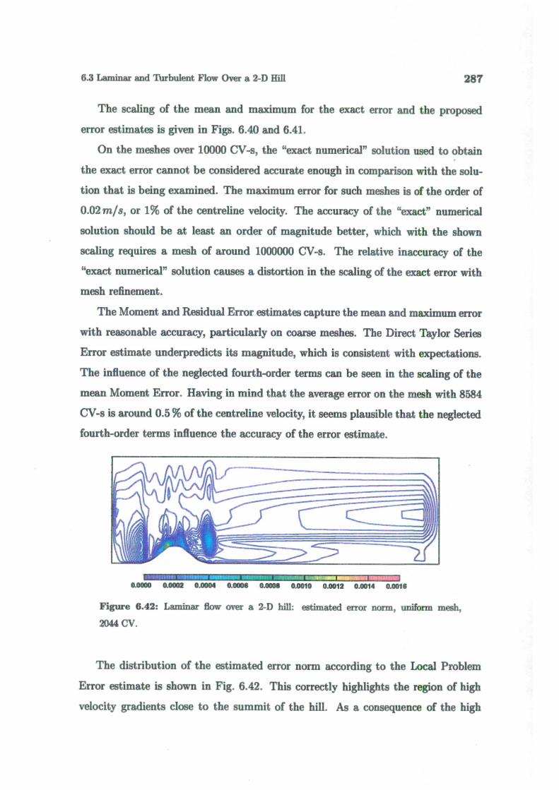
6.3 Laminar and Thrbulent Flow Over a 2-D Hill
287
The scaling of the mean and maximum for the exact error and the proposed
error estimates is given in Figs. 6.40 and 6.41.
On the meshes over 10000 CV-s, the "exact numerical" solution used to obtain
the exact error cannot be considered accurate enough in comparison with the solu-
tion that is being examined. The maximum error for such meshes is of the order of
0.02 m/s, or 1% of the centreline velocity. The accuracy of the "exact" numerical
solution should be at least an order of magnitude better, which with the shown
scaling requires a mesh of around 1000000 CV-s. The relative inaccuracy of the
"exact numerical" solution causes a distortion in the scaling of the exact error with
mesh refinement.
The Moment and Residual Error estimates capture the mean and maximum error
with reasonable accuracy, particularly on coarse meshes. The Direct Taylor Series
Error estimate underpredicts its magnitude, which is consistent with expectations.
The influence of the neglected fourth-order terms can be seen in the scaling of the
mean Moment Error. Having in mind that the average error on the mesh with 8584
CV-s is around 0.5 % of the centreline velocity, it seems plausible that the neglected
fourth-order terms influence the accuracy of the error estimate.
I I
0.0000 0.0002 0.0004 0.0006 0.0006 0.0010 0.0012 0.0014 0.0016
Figure 6.42: Laminar flow over a 2-D hill: estimated error norm, uniform mesh,
2044 CV.
The distribution of the estimated error norm according to the Local Problem
Error estimate is shown in Fig. 6.42. This correctly highlights the region of high
velocity gradients close to the summit of the hill. As a consequence of the high

288 Case Studies
local residual, this error norm also pinpoints the mesh-induced errors behind the
hill. Following Oden et al. [101, 102], the error norm from the Local Problem Error
estimate can be used in an alternative way. The formulation of the error norm
corresponds to the magnitude of the error in the quantity that is being minimised
by the numerical solution procedure. In the case of the laminar flow, this is the
total dissipation in the system, defined as:
tot =fdV=fv[VU+(VU) T] :VUdV (6.2)
The accuracy of the solution can therefore be measured in terms of the ratio of
(e, E) and 1tot, Fig. 6.43, corresponding to the relative error in the dissipation.
As a guideline, the "exact" error in 1tt can be calculated using the dissipation from
the "exact numerical" solution. The Local Problem Error estimate guarantees that
0.4
0.3
0
0.2
0.1
0.010
I
I
0 Exact•ô. IIe,EII * tot
11111111, I I !IIIIIIflIIIIIIIIIA
1
10' 10 10'no of cells
i
Figure 6.43: Laminar flow over a 2-D hill: s aling of the relative error in dissipation
for uniform refinement.
(e, E) provides the upper bound on the dissipation error, which is not the case
for the final point in Fig 6.43. This can be attributed partly to the inaccuracy of
the "exact" numerical solution and partly to the quality of the solution procedure
for the local error problems.
In the second phase, two refinement strat gies will be used. refinement-only from
the initial mesh with 2044 CV-s, Fig. 6.31 and refinement unrefinement from the
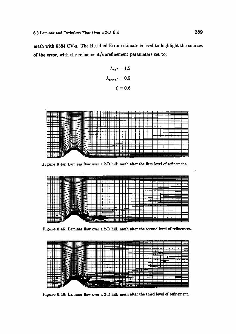
6.3 Laminar and Thrbulent Flow Over a 2-D Hill
289
mesh with 8584 CV-s. The Residual Error estimate is used to highlight the sources
of the error, with the refinement/unrefinement parameters set to:
)tref = 1.5
)'unref = 0.5
= 0.6
Figure 6.44: Laminar flow over a 2-D hill: mesh after the first level of refinement.
Figure 6.45: Laminar flow over a 2-D hill: mesh after the second level of refinement.
Figure 6.46: Laminar flow over a 2-D hill: mesh after the third level of refinement.
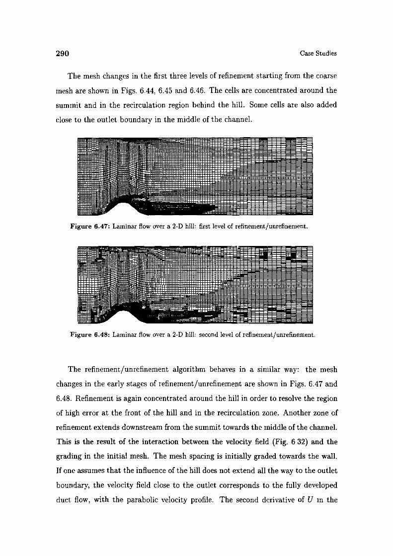
290
Case Studies
The mesh changes in the first three levels of refinement starting from the coarse
mesh are shown in Figs. 6.44, 6.45 and 6.46. The cells are concentrated around the
summit and in the recirculation region behind the hill. Some cells are also added
close to the outlet boundary in the middle of the channel.
Figure 6.47: Laminar flow over a 2-D hill: first level of refinement/unrefinement.
Figure 6.48: Laminar flow over a 2-D hill: second level of refinement/unrefinement.
The refinement/unrefinement algorithm behaves in a similar way: the mesh
changes in the early stages of refinement/unrefinement are shown in Figs. 6.47 and
6.48. Refinement is again concentrated around the hill in order to resolve the region
of high error at the front of the hill and in the recirculation zone. Another zone of
refinement extends downstream from the summit towards the middle of the channel.
This is the result of the interaction between the velocity field (Fig. 6 32) and the
grading in the initial mesh. The mesh spacing is initially graded towards the wall.
If one assumes that the influence of the hill does not extend all the way to the outlet
boundary, the velocity field close to the outlet corresponds to the fully developed
duct flow, with the parabolic velocity profile. The second derivative of U in the
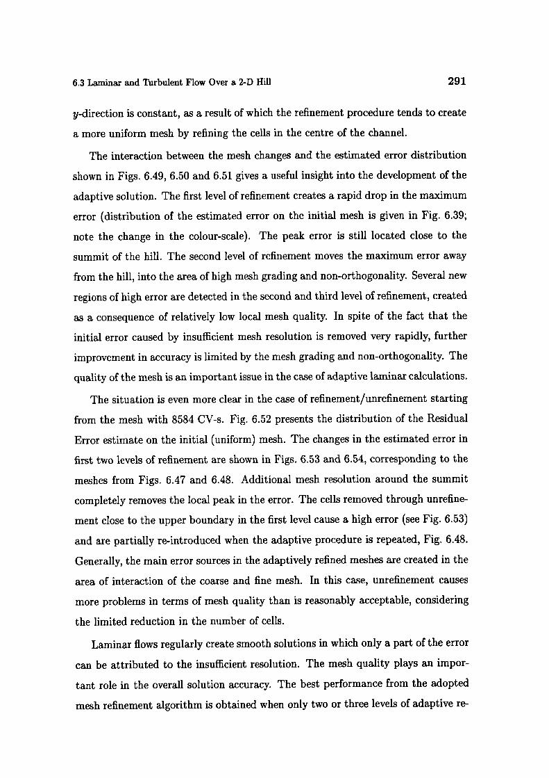
6.3 Laminar and Turbulent Flow Over a 2-D Hill 291
y-direction is constant, as a result of which the refinement procedure tends to create
a more uniform mesh by refining the cells in the centre of the channel.
The interaction between the mesh changes and the estimated error distribution
shown in Figs. 6.49, 6.50 and 6.51 gives a useful insight into the development of the
adaptive solution. The first level of refinement creates a rapid drop in the maximum
error (distribution of the estimated error on the initial mesh is given in Fig. 6.39;
note the change in the colour-scale). The peak error is still located close to the
summit of the hill. The second level of refinement moves the maximum error away
from the hill, into the area of high mesh grading and non-orthogonality. Several new
regions of high error are detected in the second and third level of refinement, created
as a consequence of relatively low local mesh quality. In spite of the fact that the
initial error caused by insufficient mesh resolution is removed very rapidly, further
improvement in accuracy is limited by the mesh grading and non-orthogonality. The
quality of the mesh is an important issue in the case of adaptive laminar calculations.
The situation is even more clear in the case of refinement/unrefinement starting
from the mesh with 8584 CV-s. Fig. 6.52 presents the distribution of the Residual
Error estimate on the initial (uniform) mesh. The changes in the estimated error in
first two levels of refinement are shown in Figs. 6.53 and 6.54, corresponding to the
meshes from Figs. 6.47 and 6.48. Additional mesh resolution around the summit
completely removes the local peak in the error. The cells removed through unrefine-
ment close to the upper boundary in the first level cause a high error (see Fig. 6.53)
and are partially re-introduced when the adaptive procedure is repeated, Fig. 6.48.
Generally, the main error sources in the adaptively refined meshes are created in the
area of interaction of the coarse and fine mesh. In this case, unrefinement causes
more problems in terms of mesh quality than is reasonably acceptable, considering
the limited reduction in the number of cells.
Laminar flows regularly create smooth solutions in which only a part of the error
can be attributed to the insufficient resolution. The mesh quality plays an impor-
tant role in the overall solution accuracy. The best performance from the adopted
mesh refinement algorithm is obtained when only two or three levels of adaptive re-
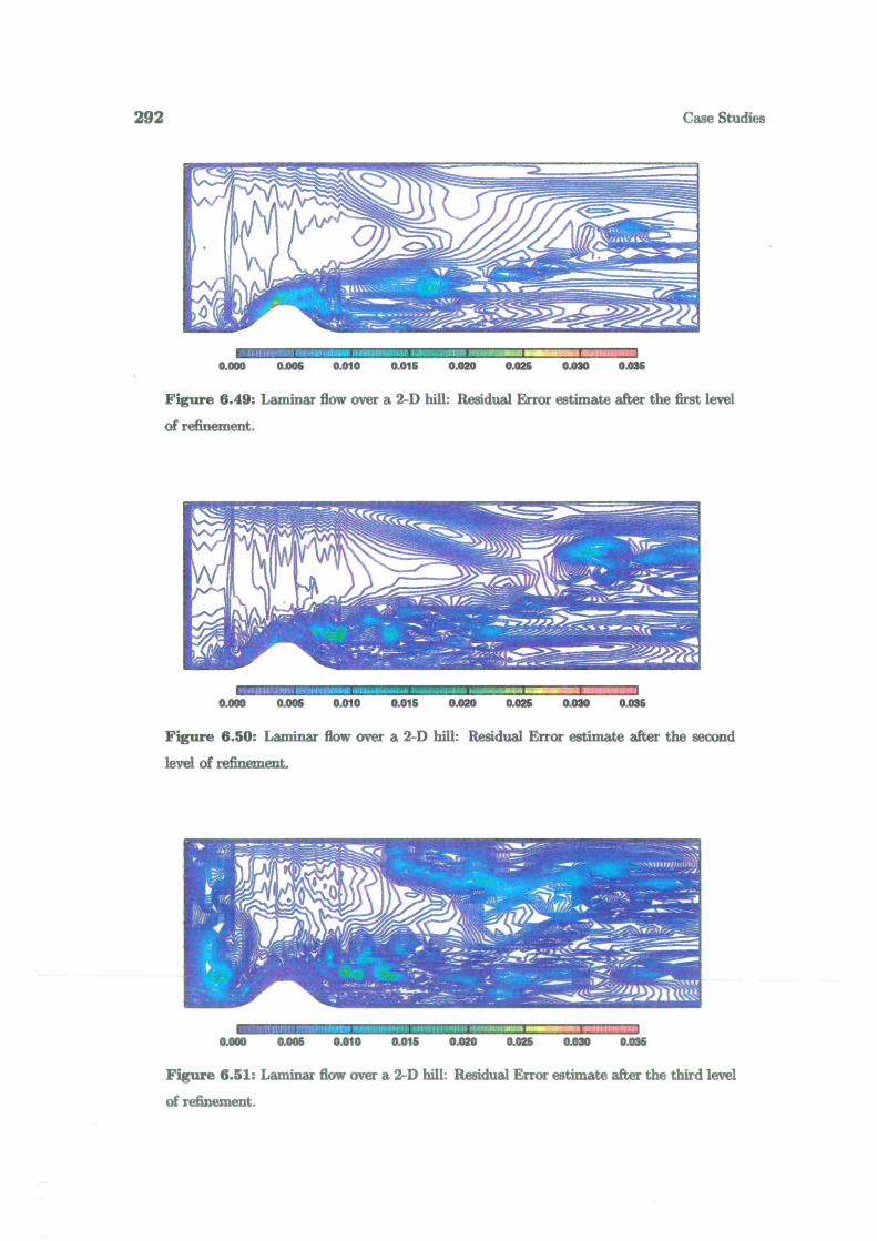
292
Case Studies
0.000 0.005 0.010 0.015 0.020 0.025 0.030 0.035
Figure 6.49: Laminar flow over a 2-D hill: Residual Error estimate after the first level
of refinement.
0.000 0.005 0.010 0.016 0.020 0.025 0.030 0.035
Figure 6.50: Laminar flow over a 2-D hill: Residual Error estimate after the second
level of refinement.
0.000 0.006 0.010 0.015 0.020 0.025 0.030 0.036
Figure 6.51: Laminar flow over a 2-D bill: Residual Error estimate after the third level
of refinement.
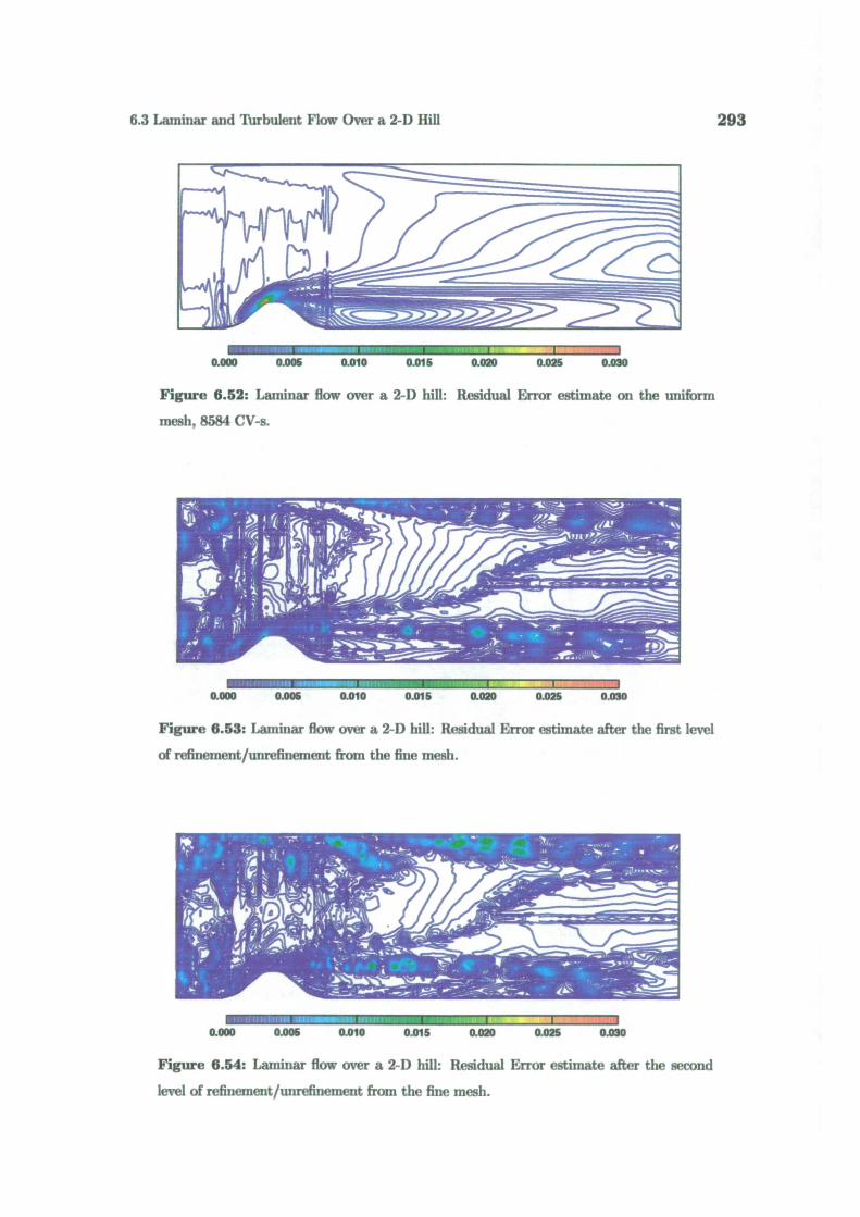
6.3 Laminar and Turbulent Flow Over a 2-D Hill
293
0.000 0.006 0.010 0.015 0.020 0.025 0.030
Figure 6.52: Laminar flow over a 2-D hill: Residual Error estimate on the uniform
mesh, 8584 CV-s.
0.000 0.005 0.010 0.015 0.020 0.025 0.030
Figure 6.53: Laminar flow over a 2-D hill: Residual Error estimate after the first level
of refinement/unrefinement from the fine mesh.
0.000 0.005 0.010 0.015 0.020 0.025 0.030
Figure 6.54: Laminar flow over a 2-D hill: Residual Error estimate after the second
level of refinement/unrefinement from the fine mesh.

294
Case Studies
finement are used. The unrefinement procedure introduces mesh distorsions of such
significance that its use cannot be justified in this case. In order to demonstrate this
fact, a refinement-only calculation starting from the mesh with 8584 CV-s has been
performed. The mesh after two levels of refinement is shown in Fig. 6.55, with the
Figure 6.55: Laini:iar flow iv&r a 2-I) hill: su4flId kvi1 of rehiieintiit-oiily froiii the fiiw
mesh.
u- I
0.000 0.005 0.010 0.015 0.020 0.025 0.080
Figure 6.56: Laminar flow over a 2-D hill: Residual Error estimate after the second
level of refinement/unrefinement.
corresponding Residual Error distribution in Fig. 6.56. The corresponding results
for refinement/unrefinement are given in Figs. 6.48 and 6.54. Refinement-only does
not degrade the quality of the mesh close to the top wall and the estimated error
levels are considerably lower than in the case of refinement/unrefinement.
Finally, the estimated error levels in the adaptively refined meshes will be exam-
med. Unfortunately, the "exact numerical" solution cannot be used to measure the
accuracy of the error estimates. Mesh adaptivity creates refinement patches that

iC
6.3 Laminar and Turbulent Flow Over a 2-D Hill
295
100
I-0-1
10
0 Uniform.á. Refine,coarse)( Refine,fineI Refinelunrefine
10 l0•' 10no of cells
Figure 6.57: Laminar flow over a 2-D hill: scaling of the maximum Moment Error for
different types of refinement.
100
0 Uniformir Refine,coarse)( Refine,fine
I-
I Refine/unrefine0
10
E
10•' 10" 10"no of cells
Figure 6.58: Laminar flow over a 2-D hill: scaling of the maximum Residual Error for
different types of refinement.

296 Case Studes
very quickly become as fine or finer than the mesh used for the "exact numerical"
solution, rendering it unusable for our purposes. It is therefore more interesting to
examine the performance of different adaptive procedures in terms of the reduction
of the estimated error.
Figs. 6.57 and 6.58 show the change in the error with the number of cells on
adaptively refined meshes. The adaptive procedure reduces the error faster than
uniform refinement according to both the Moment and Residual Error estimates,
although the gain seems to be much smaller than in the supersonic test case from
Section 6.2. Between the two estimates, the drop is faster for the Residual Error,
as it is used to mark the cells for refinement.
The refinement-only procedure starting from the coarse initial mesh consistently
performs better than uniform refinement in spite of the reduced mesh quality. If we
limit the refinement to only three levels, all refinement strategies perform reasonably
well.
The error reduction shown in Fig. 6.58 does not considerably change if the Direct
Ta\lor Series or Moment Error estimates are used to mark the cells for refinement.
The largest change in the performance can be made by changing the refinement
parameters 7'ref, Aunrei and ), as they influence the quality of the refined mesh.
Generally, lower creates smoother grading and improves the mesh quality by pre-
serving the original aspect ratio of the cell. At the same time, it also increases the
number of cells in the mesh through the "1-irregularity" principle, thus increasing
the cost of the compu ation. When specifying the refinement and unrefinement
thresholds, one should have in mind the desired accuracy relative to the accuracy
of the initial solution, as well as the importance of the mesh quality. It has been
shown that the cells initially removed through unrefinement were re-introduced in
the next level of refluement. This is t pical for a large number of refinement lev-
els on smoothly changing solutions and should be avoided, as it causes a potential
reduction of the mesh qu lity.
The performance of the adaptive pr cedure in laminar flows is critically depen-
dent on the quality of the refined mesh. An adaptive mesh generation able to create
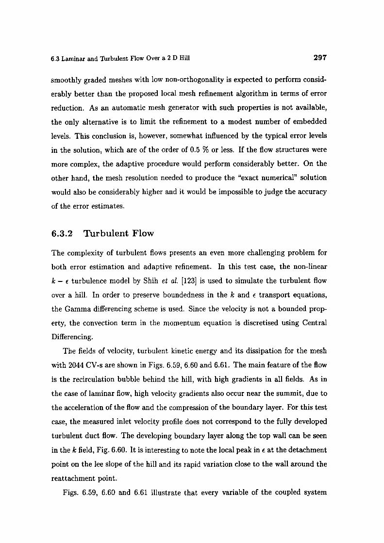
6.3 Laminar and Turbulent Flow Over a 2 D Hill 297
smoothly graded meshes with low non-orthogonality is expected to perform consid-
erably better than the proposed local mesh refinement algorithm in terms of error
reduction. As an automatic mesh generator with such properties is not available,
the only alternative is to limit the refinement to a modest number of embedded
levels. This conclusion is, however, somewhat influenced by the typical error levels
in the solution, which are of the order of 0.5 % or less. If the flow structures were
more complex, the adaptive procedure would perform considerably better. On the
other hand, the mesh resolution needed to produce the "exact numerical" solution
would also be considerably higher and it would be impossible to judge the accuracy
of the error estimates.
6.3.2 Turbulent Flow
The complexity of turbulent flows presents an even more challenging problem for
both error estimation and adaptive refinement. In this test case, the non-linear
k - € turbulence model by Shih et al. [123] is used to simulate the turbulent flow
over a hill. In order to preserve boundedness in the k and € transport equations,
the Gamma differencing scheme is used. Since the velocity is not a bounded prop-
erty, the convection term in the momentum equation is discretised using Central
Differencing.
The fields of velocity, turbulent kinetic energy and its dissipation for the mesh
with 2044 CV-s are shown in Figs. 6.59, 6.60 and 6.61. The main feature of the flow
is the recirculation bubble behind the hill, with high gradients in all fields. As in
the case of laminar flow, high velocity gradients also occur near the summit, due to
the acceleration of the flow and the compression of the boundary layer. For this test
case, the measured inlet velocity profile does not correspond to the fully developed
turbulent duct flow. The developing boundary layer along the top wall can be seen
in the k field, Fig. 6.60. It is interesting to note the local peak in € at the detachment
point on the lee slope of the hill and its rapid variation close to the wall around the
reattachment point.
Figs. 6.59, 6.60 and 6.61 illustrate that every variable of the coupled system
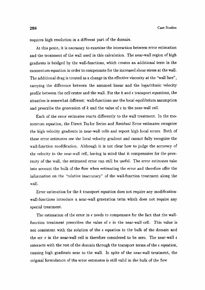
298
Case Studies
requires high resolution in a different part of the domain.
At this point, it is necessary to examine the interaction between error estimation
and the treatment of the wall used in this calculation. The near-wall region of high
gradients is bridged by the wall-functions, which creates an additional term in the
momentum equation in order to compensate for the increased shear stress at the wall.
The additional drag is treated as a change in the effective viscosity at the "wall face",
carrying the difference between the assumed linear and the logarithmic velocity
profile between the cell centre and the wall. For the k and € transport equations, the
situation is somewhat different: wall-functions use the local equilibrium assumption
and prescribe the generation of k and the value of € in the near-wall cell.
Each of the error estimates reacts differently to the wall treatment. In the mo-
mentum equation, the Direct Ta1or Series and Residual Error estimates recognise
the high velocity gradients in near-wall cells and report high local errors. Both of
these error estimates use the local velocity gradient and cannot fully recognise the
wall-function modification. Although it is not clear how to judge the accuracy of
the velocity in the near-wall cell, having in mind that it compensates for the prox-
imity of the wall, the estimated error can still be useful. The error estimates take
into account the bulk of the flow when estimating the error and therefore offer the
information on the "relative inaccuracy" of the wall-function treatment along the
wall.
Error estimation for the k transport equation does not require any modification:
wall-functions introduce a near-wall generation term which does not require any
special treatment.
The estimation of the error in f needs to compensate for the fact that the wall-
function treatment prescribes the value of € in the near-wall cell. This value is
not consistent with the solution of the € equation in the bulk of the domain and
the err r in the near-wall cell is therefore considered to be zero. The near-wall €
interacts with the rest of the domain through the transport terms of the € equation,
causing high gradients near to the wall. In spite of the near-wall treatment, the
original formulation of the error estimates is still valid in the bulk of the flow
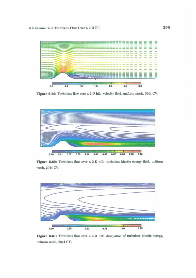
6.3 Laminar and Turbulent Flow Over a 2-D lull
299
-----. = = =__
-...
..................--.-. ......_------ ........
. .....
I..0.0 0.5 1.0 1.5 2.0 2.5 3.0
Figure 6.59: Turbulent flow over a 2-D hill: velocity field, uniform mesh, 2044 CV.
.1•- I I I I
0.00 0.01 0.02 0.03 0.04 0.05 0.06 0.07 0.06 0.06 0.10
Figure 6.60: Turbulent flow over a 2-D hill: turbulent kinetic energy field, uniform
mesh, 2044 CV.
I '?0.00 0.25 0.50 0.75 1.00 1.25
Figure 6.61: Turbulent flow over a 2-D hill: dissipation of turbulent kinetic energy,
uniform mesh, 2044 CV.

300
Case Studies
J
-irI I I Uo. 0.01 0.09 0.03 0.04 0.05 0.05 0.07 0.08 0.09 0.10
Figure 6.62: Thrbulent flow over a 2-D hill: Direct Taylor Series Error estimate for
velocity, uniform mesh, 2044 CV.
- -- I I0.00 0.05 0.10 0.15 0.20 0.25 0.30 0.35
Figure 6.63: Thrbulent flow over a 2-D hill: Moment Error estimate for velocity, uniform
mesh, 2044 CV.
0.00 0.05 0.10 0.15 0.20 0.25
Figure 6.64: Thrbulent flow over a 2-D hill: Residual Error estimate for velocity, uniform
mesh. 2044 CV.

6.3 Laminar and Turbulent Flow Over a 2-D Hill
301
o. 0.0002 0.0004 0.0000 0.0008 0.0010
Figure 6.65: Turbulent flow over a 2-D hill: Direct Taylor Series Error estimate for k,
uniform mesh, 2044 CV.
'- I I I
0.000 0.003 0.006 0.006 0.012 0.015 0.018
Figure 6.66: Turbulent flow over a 2-D hill: Moment Error estimate for k, uniform
mesh, 2044 CV.
-- - I I
0.000 0.001 0.002 0.003 0.004 0.006 0.001 0.007
Figure 6.67: Turbulent flow over a 2-D hill: Residual Error estimate for k, uniform
mesh, 2044 CV.

302
Case Studies
I I 'I
0.000 0.002 0.004 0.004 0.000 0.010 0.012 0.014
Figure 8.68: TUrbulent flow over a 2-D hill: Direct Taylor Series Error estimate for e,
uniform mesh, 2044 CV.
I ••0.0 0.1 0.2 0.3 0.4 0.5 0.6
Figure 6.69: flow over a 2-D hill: Moment Error estimate for €, uniform mesh, 2044 CV.
_.t1 Fri 1
0.00 0.01 0.02 0.03 0.04 0.05 0.06 0.07 0.06 0.09
Figure 6.70: TUrbulent flow over a 2-D hill: Residual Error estimate for €, uniform
mesh, 2044 CV.

6.3 Laminar and Turbulent Flow Over a 2-D Hill
303
It is possible to establish the level of the modelling error for the wall-functions,
based on the value of y. In spite of the fact that wall-functions are in principle
able to cover the whole range of y+, from the laminar sublayer to the log-law layer,
it is well-known that they produce the best results for 50 <y <100. The estimate
of the near-wall accuracy and consequently the refinement criterion can therefore be
based on y condition.
Figs. 6.62, 6.63 and 6.64 present the distribution of the Direct Taylor Series,
Moment and Residual Error estimates for the velocity field. The error estimates
highlight several regions of high error: the windward slope of the hill, the point of
flow detachment on the lee slope and the recirculation bubble. The Direct Taylor
Series Error estimate does not pick up the high error around detachment. Here, the
complex flow field creates a rapid variation in both the magnitude and the direction
of the velocity. The actual velocity magnitude is relatively small and the mesh is
too coarse to detect the local peak in the second gradient of the velocity used to
estimate the error. As the mesh becomes finer, the second gradient calculated on the
discrete mesh becomes closer to its exact value, resulting in a more accurate error
estimation. This is visible in the scaling of the maximum error with the number of
cells for uniform refinement, which will be shown later. On the windward slope, the
compression of the boundary layer increases the second velocity gradient, resulting
in the high local error. Here, the flow is aligned with the mesh and does not change
direction, making it easier to resolve the second velocity gradient. The Moment and
Residual Error estimate recognise both the compression of the boundary layer and
the detachment point as the regions of the high error.
The variation in the accuracy of the solution near the wall can be seen in
Fig. 6.64. The error in the near-wall cell downstream from the hill shows the de-
pendence on the velocity magnitude. If the local velocity is low (just behind the
hill or at the reattachment point), the error is smaller. The Moment Error estimate
Fig. 6.63, on the other hand, recognises the modified viscosity on the wall face, thus
giving a different picture of the relative importance of the near-wall error to the rest
of the domain.
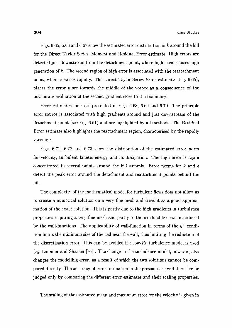
304
Case Studies
Figs. 6.65, 6.66 and 6.67 show the estimated error distribution in k around the hill
for the Direct Taylor Series, Moment and Residual Error estimate. High errors are
detected just downstream from the detachment point, where high shear causes high
generation of k. The second region of high error is associated with the reattachment
point, where varies rapidly. The Direct Taylor Series Error estimate Fig. 6.65),
places the error more towards the middle of the vortex as a consequence of the
inaccurate evaluation of the second gradient close to the boundary.
Error estimates for E are presented in Figs. 6.68, 6.69 and 6.70. The principle
error source is associated with high gradients around and just downstream of the
detachment point (see Fig. 6.61) and are highlighted by all methods. The Residual
Error estimate also highlights the reattachment region, characterised by the rapidly
varying E.
Figs. 6.71, 6.72 and 6.73 show the distribution of the estimated error norm
for velocity, turbulent kinetic energy and its dissipation. The high error is again
concentrated in several points around the hill summit. Error norms for k and €
detect the peak error around the detachment and reattachment points behind the
hill.
The complexity of the mathematical model for turbulent flows does not allow us
to create a numerical solution on a very fine mesh and treat it as a good approxi-
mation of the exact solution. This is partly due to the high gradients in turbulence
properties requiring a very fine mesh and partly to the irreducible error introduced
by the wall-functions. The applicability of wall-function in terms of the y condi-
tion limits the minimum size of the cell near the wall, thus limiting the reduction of
the discretisation error. This can be avoided if a low-Re turbulence model is used
(eg. Launder and Sharma [76] . The change in the turbulence model, however, also
changes the modelling error, as a result of which the two solutions cannot be com-
pared directly. The ac uracy of error estimation in the present case will theref re be
judged only by comparing the different error estimates and their scaling properties.
The scaling of the estimated mean and maximum error for the velocity is given in
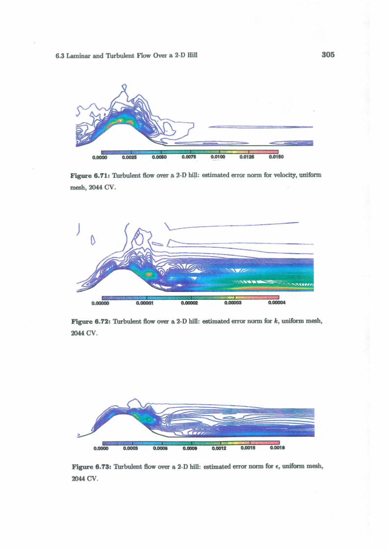
6.3 Laminar and Turbulent Flow Over a 2-D Hill
305
I I
0.0000 0.0025 0.0060 0.0075 0.0100 0.0125 0.0150
Figure 6.71: Turbulent flow over a 2-D hili: estimated error norm for velocity, uniform
mesh, 2044 CV.
) _
0.00001 0.00002 0.00003 0.00004
Figure 6.72: Turbulent flow over a 2-D hill: estimated error norm for k, uniform mesh,
2044 CV.
I I I
0.0000 0.0003 0.0005 0.0006 0.0012 0.0015 0.0018
Figure 6.73: Turbulent flow over a 2-D hill: estimated error norm for , uniform mesh,
2044 CV.
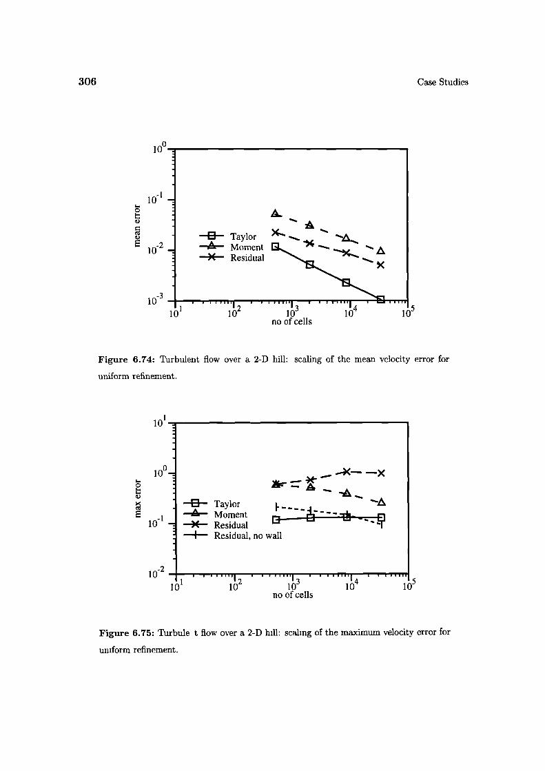
100
'
306
Case Studies
0 TaylorA Moment)C Residual .- .
A
I IA10 10 10' 10' l0
no of cells
Figure 6.74: Turbulent flow over a 2-D hill: scaling of the mean velocity error for
uniform refinement.
101
D
Taylor__
x-
AMoment ___________________)( Residual - - - th- -
I Residual, no wall
:
102 4.10
1 2 13 14 510 10 10 10
no of cells
Figure 6.75: Turbule t flow over a 2-D hill: scaling of the maximum velocity error for
uniform refinement.
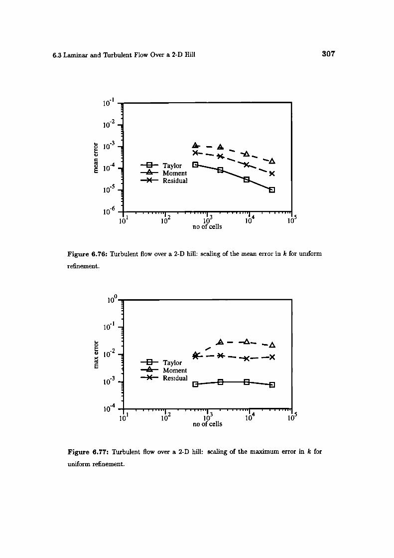
6.3 Laminar and Turbulent Flow Over a 2-D Hill
307
10_I
1
1
i101
4--.-$'z ---0 Taylor
AA Moment x)'( Residual
12 13 14 510 10 10 10
no of cells
Figure 6.76: Turbulent flow over a 2-D hill: scaling of the mean error in k for uniform
refinement.
100
10'
5-C
-210
E
1 Ø3
10
A— —A —A
— 9c.. —(— -x0 Taylor
—k-- MomentX Residual
'2 13 14 510 10 10 10
no of cells
Figure 6.77: Turbulent flow over a 2-D hill: scaling of the maximum error in k for
uniform refinement.
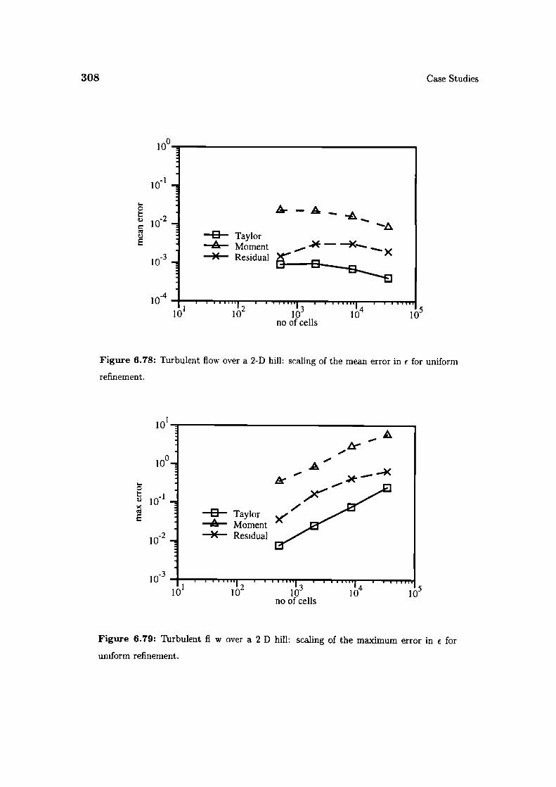
308
Case Studies
100
l0
I-0
0.)
0.)
I
0 Taylor•á. Moment ..)E - —X-._._X Residual
-I-;10
12 13 1410 10 10 10
no of cells
Figure 6.78: Turbulent flow over a 2-D hill: scaling of the mean error in e for uniform
refinement.
101
100
I-.C
10
E
1 02
10
A
0 Taylor•ó. MomentX Residual
i6 1J5no of cells
Figure 6.79: Turbulent fi w over a 2 D hill: scaling of the maximum error in c for
uniform refinement.
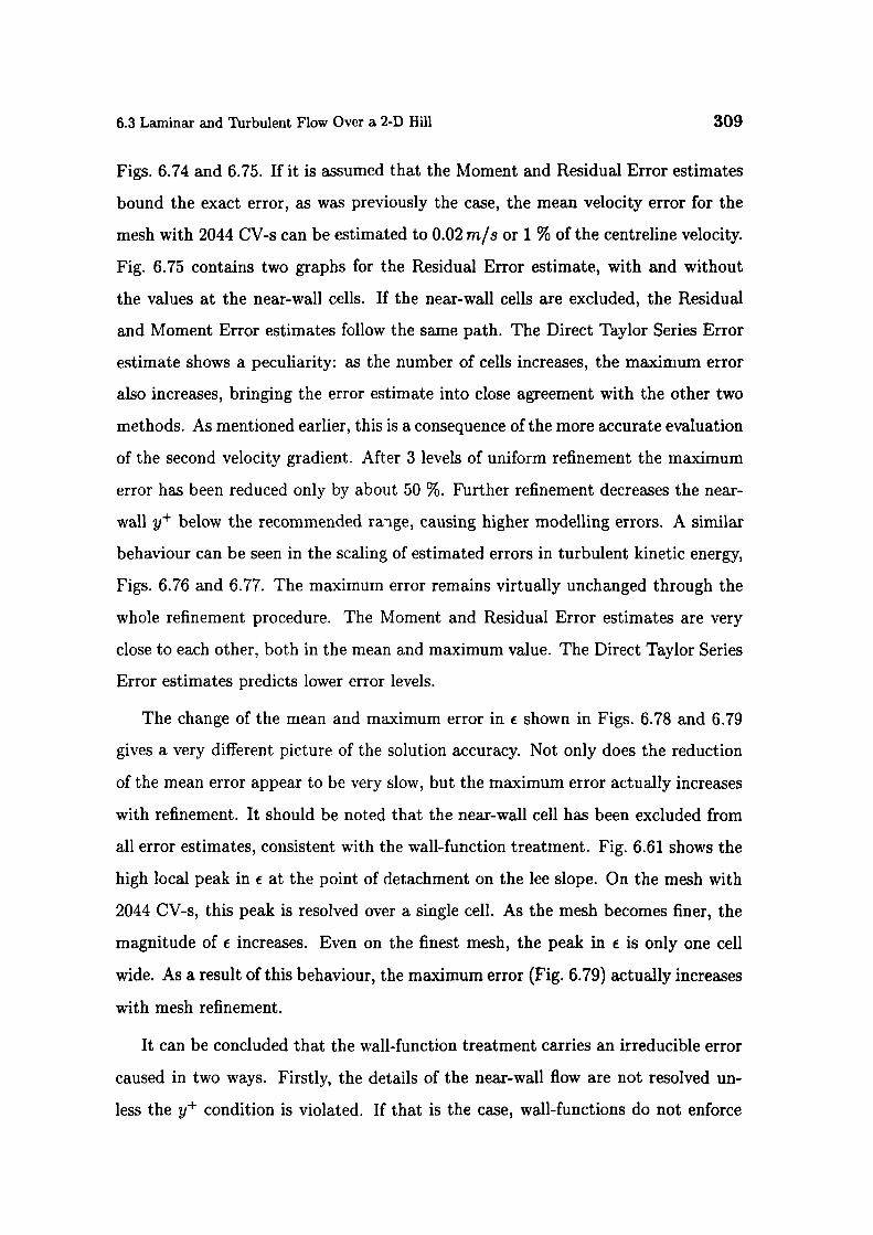
6.3 Laminar and Turbulent Flow Over a 2-D Hill 309
Figs. 6.74 and 6.75. If it is assumed that the Moment and Residual Error estimates
bound the exact error, as was previously the case, the mean velocity error for the
mesh with 2044 CV-s can be estimated to 0.02 rn/s or 1 % of the centreline velocity.
Fig. 6.75 contains two graphs for the Residual Error estimate, with and without
the values at the near-wall cells. If the near-wall cells are excluded, the Residual
and Moment Error estimates follow the same path. The Direct Taylor Series Error
estimate shows a peculiarity: as the number of cells increases, the maximum error
also increases, bringing the error estimate into close agreement with the other two
methods. As mentioned earlier, this is a consequence of the more accurate evaluation
of the second velocity gradient. After 3 levels of uniform refinement the maximum
error has been reduced only by about 50 %. Further refinement decreases the near-
wall y+ below the recommended ra-ige, causing higher modelling errors. A similar
behaviour can be seen in the scaling of estimated errors in turbulent kinetic energy,
Figs. 6.76 and 6.77. The maximum error remains virtually unchanged through the
whole refinement procedure. The Moment and Residual Error estimates are very
close to each other, both in the mean and maximum value. The Direct Taylor Series
Error estimates predicts lower error levels.
The change of the mean and maximum error in € shown in Figs. 6.78 and 6.79
gives a very different picture of the solution accuracy. Not only does the reduction
of the mean error appear to be very slow, but the maximum error actually increases
with refinement. It should be noted that the near-wall cell has been excluded from
all error estimates, consistent with the wall-function treatment. Fig. 6.61 shows the
high local peak in € at the point of detachment on the lee slope. On the mesh with
2044 CV-s, this peak is resolved over a single cell. As the mesh becomes finer, the
magnitude of increases. Even on the finest mesh, the peak in is only one cell
wide. As a result of this behaviour, the maximum error (Fig. 6.79) actually increases
with mesh refinement.
It can be concluded that the wall-function treatment carries an irreducible error
caused in two ways. Firstly, the details of the near-wall flow are not resolved un-
less the y+ condition is violated. If that is the case, wall-functions do not enforce

310 Case Studies
the logarithmic near-wall velocity profile and high-Re turbulence models produce
incorrect behaviour of the turbulence properties in the low-Re region near the wall,
resulting in high modelling errors (see eg. Pate! et al. [108]). If, on the other hand,
the y condition is obeyed, it limits the cell size near the wall, thus fixing the level
of the discretisation error.
In the adaptive calculations, the combination of the Moment Error estimate for
the velocity and the Residual Error estimate for k has been used. The y+ values
in near-wall cells are not allowed to drop below 50, by explicitly excluding the
cells from refinement parallel with the wall. It is, however, still allowed to split
the near-wall cells in a way that does not violate the y+ condition. The laminar
adaptive calculation implies that the major factor influencing the mesh quality is
the unrefinement procedure. Having in mind that the typical error distribution in
turbulent calculations contains high local error peaks, the refinement/unrefinement
parameters for this calculations have been set to:
)'ref = 1.8
) unref = 0.2
= 0.6
The first set of results is obtained by refining the initial uniform mesh with
2044 CV-s. The mesh changes in the first three levels of refinement are shown in
Figs. 6.80, 6.81 and 6 82. The changes in the Moment Error estimate for velocity
through the levels of refinement can be followed in Figs. 6.83, 6.84 and 6.85, with the
estimated error in k in Figs. 6.86, 6.87 and 6.88. The error reduction shows a very
different behaviour than in the case of laminar flow. The first level of refinement
reduces the error magnitude, but the maximum error remains at the same place,
just downstream from the summit. In the second level of refinement, the error peak
is m ved to the near-wall cell, with only a slight change in its magnitude. This cell
is consequently blocked from further refinement on the basis of the y+ condition.
Further adaptive mesh changes are unable to cause any change in the maximum
error.
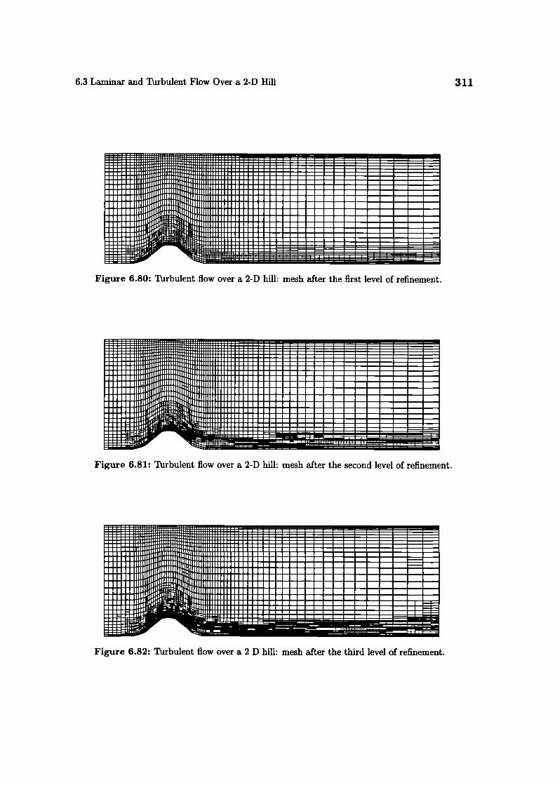
6.3 Laminar and Turbulent Flow Over a 2-D Hill
311
Figure 6.80: Turbulent flow over a 2-D hill: mesh after the first level of refinement.
Figure 6.81: Turbulent flow over a 2-D hill: mesh after the second level of refinement.
Figure 6.82: Turbulent flow over a 2 D hill: mesh after the third level of refinement.

-I
312
Case Studies
---- -
F
0.00 0.05 0.10 015 020. 0.35 030 0.35
Figure 6.83: Turbulent flow over a 2-D hill: Moment Error estimate for velocity after
the first level of adaptive refinement.
\._J ,-,s.z_ --/- \ /• ___-_._,
__________ .1 I I
0.00 0.06 0.10 0.15 0.20 0.25 0.30 0.35
Figure 6.84: Turbulent flow over a 2-D bill: Moment Error estimate for velocity after
the second level of adaptive refinement.
:Iu
0.00 0.06 0.10 0.15 0.20 0.25 0.30 0.35
Figure 6.85: Turbulent flow over a 2-D hill: Moment Error for velocity estimate after
the third level of adaptive refinement.
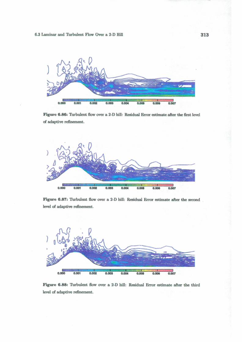
6.3 Laminar and Thrbulent Flow Over a 2-D Hill
313
_....., I -. 4lnI
0.000 0.001 0.000 0.003 0.004 0.005 0.001 0.007
Figure 6.86: Thrbulent flow over a 2-D hill: Residual Error estimate after the first level
of adaptive refinement.
0.000 0.001 0.000 0.003 0.003 0.005 0.003 0.007
Figure 6.87: Thrbulent flow over a 2-D hill: Residual Error estimate after the second
level of adaptive refinement.
)
I.- I T11
0.000 0.001 0.000 0.003 0.004 0.005 0.001 0.007
Figure 6.88: Turbulent flow over a 2-D hill: Residual Error estimate after the third
level of adaptive refinement.
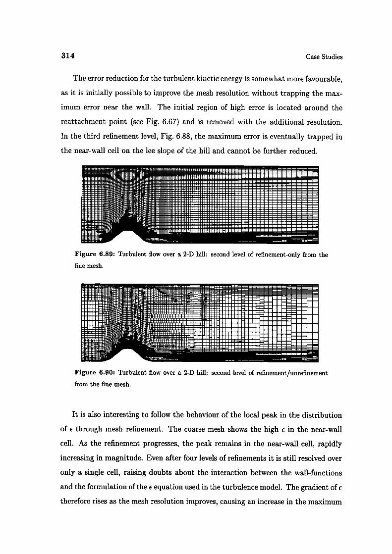
314
Case Studies
The error reduction for the turbulent kinetic energy is somewhat more favourable,
as it is initially possible to improve the mesh resolution without trapping the max-
imum error near the wall. The initial region of high error is located around the
reattachment point (see Fig. 6.67) and is removed with the additional resolution.
In the third refinement level, Fig. 6.88, the maximum error is eventually trapped in
the near-wall cell on the lee slope of the hill and cannot be further reduced.
Figure 6.89: Turbulent flow over a 2-D hill: second level of refinement-only from the
fine mesh.
Figure 6.90: Turbulent flow over a 2-D hill: second level of refinement/unrefinemerit
from the fine mesh.
It is also interesting to follow the behaviour of the local peak in the distribution
of € through mesh refinement. The coarse mesh shows the high f in the near-wall
cell. As the refinement progresses, the peak remains in the near-wall cell, rapidly
increasing in magnitude. Even after four levels of refinements it is still resolved over
only a single cell, raising doubts about the interaction between the wall-functions
and the formulation of the f equation used in the turbulence model. The gradient of e
therefore rises as the mesh resolution improves, causing an increase in the maximum
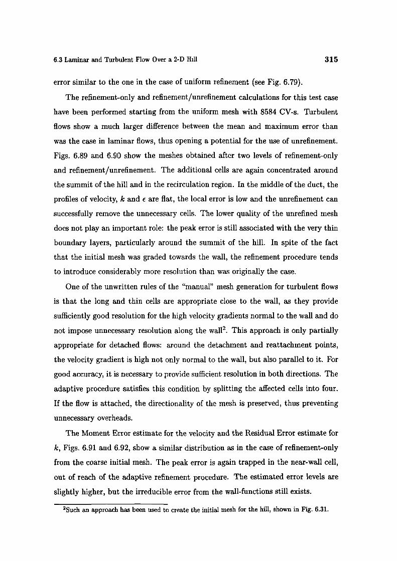
6.3 Laminar and Turbulent Flow Over a 2-D Hill
315
error similar to the one in the case of uniform refinement (see Fig. 6.79).
The refinement-only and refinement/unrefinement calculations for this test case
have been performed starting from the uniform mesh with 8584 CV-s. Turbulent
flows show a much larger difference between the mean and maximum error than
was the case in laminar flows, thus opening a potential for the use of unrefinement.
Figs. 6.89 and 6.90 show the meshes obtained after two levels of refinement-only
and refinement/unrefinement. The additional cells are again concentrated around
the summit of the hill and in the recirculation region. In the middle of the duct, the
profiles of velocity, k and e are flat, the local error is low and the unrefinement can
successfully remove the unnecessary cells. The lower quality of the unrefined mesh
does not play an important role: the peak error is still associated with the very thin
boundary layers, particularly around the summit of the hill. In spite of the fact
that the initial mesh was graded towards the wall, the refinement procedure tends
to introduce considerably more resolution than was originally the case.
One of the unwritten rules of the "manual" mesh generation for turbulent flows
is that the long and thin cells are appropriate close to the wall, as they provide
sufficiently good resolution for the high velocity gradients normal to the wall and do
not impose unnecessary resolution along the wall2 . This approach is only partially
appropriate for detached flows: around the detachment and reattachment points,
the velocity gradient is high not only normal to the wall, but also parallel to it. For
good accuracy, it is necessary to provide sufficient resolution in both directions. The
adaptive procedure satisfies this condition by splitting the affected cells into four.
If the flow is attached, the directionality of the mesh is preserved, thus preventing
unnecessary overheads.
The Moment Error estimate for the velocity and the Residual Error estimate for
k, Figs. 6.91 and 6.92, show a similar distribution as in the case of refinement-only
from the coarse initial mesh. The peak error is again trapped in the near-wall cell,
out of reach of the adaptive refinement procedure. The estimated error levels are
slightly higher, but the irreducible error from the wall-functions still exists.
2Such an approach has been used to create the initial mesh for the hill, shown in Fig. 6.31.
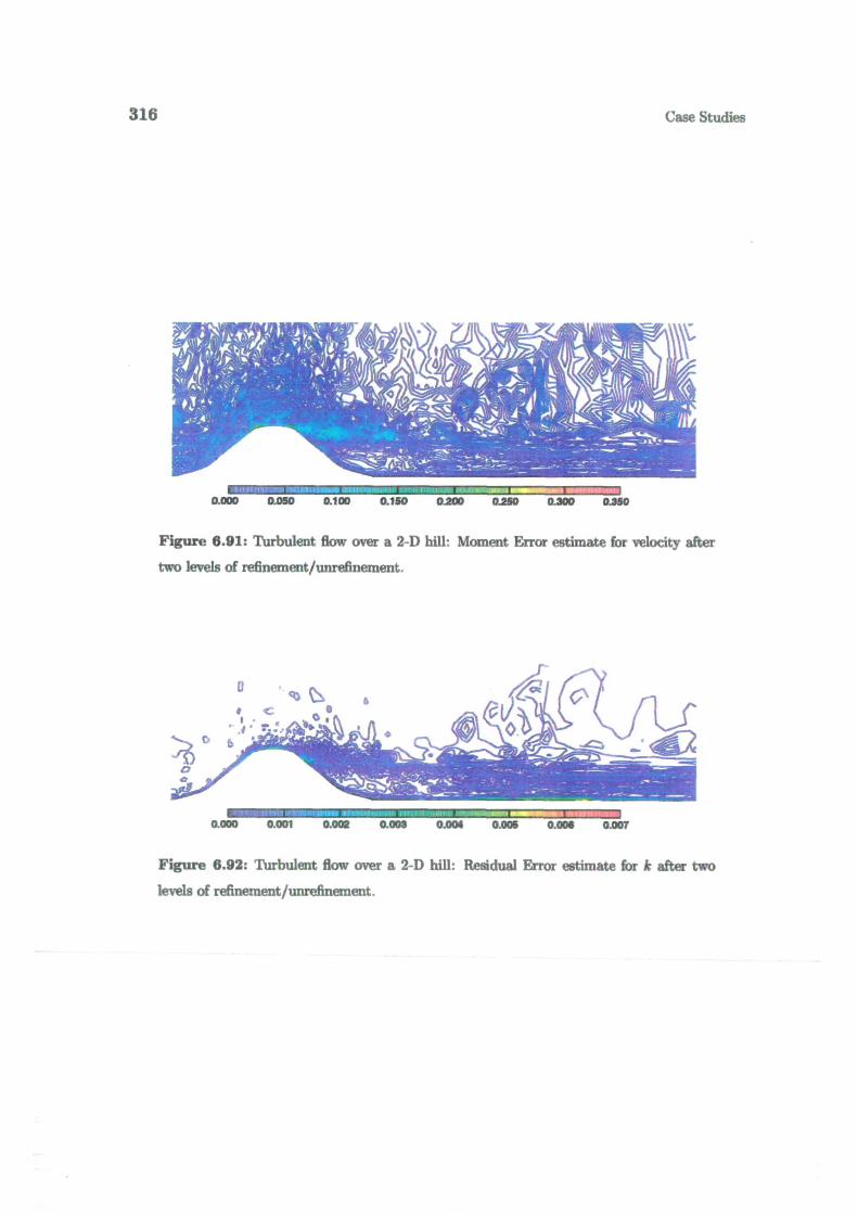
316
Case Studies
I I
0.000 0.050 0.100 0.150 0.200 0.250 0.300 0.350
Figure 6.91: Turbulent flow over a 2-D hill: Moment Error estimate for velocity after
two levels of refinement/unrefinement.
I
0.000 0.001 0.005 0.003 0.003 0.001 0.006 0.007
Figure 6.92: Turbulent flow over a 2-D hill: Residual Error estimate for k after two
levels of refinement/unrefinement.
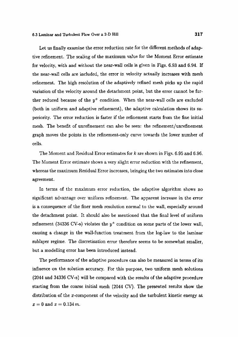
6.3 Laminar and Thrbulent Flow Over a 2-D Hill
317
Let us finally examine the error reduction rate for the different methods of adap-
tive refinement. The scaling of the maximum value for the Moment Error estimate
for velocity, with and without the near-wall cells is given in Figs. 6.93 and 6.94. If
the near-wall cells are included, the error in velocity actually increases with mesh
refinement. The high resolution of the adaptively refined mesh picks up the rapid
variation of the velocity around the detachment point, but the error cannot be fur-
ther reduced because of the y+ condition. When the near-wall cells are excluded
(both in uniform and adaptive refinement), the adaptive calculation shows its su-
periority. The error reduction is faster if the refinement starts from the fine initial
mesh. The benefit of unrefinement can also be seen: the refinement/unrefinement
graph moves the points in the refinement-only curve towards the lower number of
cells.
The Moment and Residual Error estimates for k are shown in Figs. 6.95 and 6.96.
The Moment Error estimate shows a very slight error reduction with the refinement,
whereas the maximum Residual Error increases, bringing the two estimates into close
agreement.
In terms of the maximum error reduction, the adaptive algorithm shows no
significant advantage over uniform refinement. The apparent increase in the error
is a consequence of the finer mesh resolution normal to the wall, especially around
the detachment point. It should also be mentioned that the final level of uniform
refinement (34336 CV-s) violates the y condition on some parts of the lower wall,
causing a change in the wall-function treatment from the log-law to the laminar
sublayer regime. The discretisation error therefore seems to be somewhat smaller,
but a modelling error has been introduced instead.
The performance of the adaptive procedure can also be measured in terms of its
influence on the solution accuracy. For this purpose, two uniform mesh solutions
(2044 and 34336 CV-s) will be compared with the results of the adaptive procedure
starting from the coarse initial mesh (2044 CV). The presented results show the
distribution of the x-component of the velocity and the turbulent kinetic energy at
x = 0 and x = 0.134m.
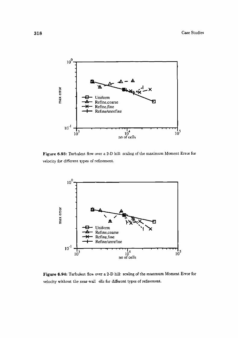
318
Case Studies
100
C
U UniformA
.LL Refine,co)( Refine,fineI Refine/unrefine
10_I1 4 14 •...'. 15
10 10 10no of cells
Figure 6.93: Thrbulent flow over a 2-D hill: scaling of the maximum Moment Error for
velocity for different types of refinement.
100
I..
C
0 Uniform.. Refine,coarseX Refine,fineI Refine/unrefine
1 0 1 - 14 U
10 l0no of cells
Figure 6.94: Turbulent flow over a 2-D hill: scaling of the maximum Moment Error for
velocity without the near-wall ells for different types of refinement.

i o2
100
::
1
I
0 UniformA Refine,coarse)( Refine,fine
I Refine/unrefine
A
Ino of cells
I
6.3 Laminar and Turbulent Flow Over a 2 D Hill
319
100
I-0-1
10
D Uniform-'k' Refine,coarseX Refine,fine
I Refine/unrefine
no of cells
Figure 6.95: Turbulent flow over a 2-D hill: scaling of the maximum Moment Error for
k for different types of refinement.
Figure 6.96: Turbulent flow over a 2-D hill: scaling of the maximum Residual Error for
k for different types of refinement.

--- I
01
320
Case Studies
0.2
> 0.1
00
U
Figure 6.97: Thrbulent flow over a 2-D hill: velocity distribution at x = 0 for uniform
meshes.
0
0
012 16 20 2.4 28 32
U
Figure 6.98: Ttirbulent flow over a 2-D hill: velocity distribution at x = 0, first level of
refinement.
0.2
00 I1.2 16 20 24 28 32
U
Figure 6.99: Turbulent fi w over a 2 D hil1 ye ocity distribution at x - 0, sec nd level
f refinem nt.

6.3 Laminar and Turbulent Flow Over a 2 D Hill
321
0.2
0.1
2044CV- - 34336 CV
1.4
-0.0
-0.5 0.0 0.5 1.0 1.5 2.0 2.5U
Figure 6.100: Turbulent flow over a 2-D hill: velocity distribution at x = 134 for
uniform meshes.
0.2
>' 0.1
34336 CV-0- first
0.0 1.-I-0.5 0.0 0.5 1.0 1.5 2.0 2.5
U
Figure 6.101: Turbulent flow over a 2-D hill: velocity distribution at x = 134, first level
of refinement.
C
0.1
34336 CV-0- second
0.01.1.1
-0.5 00 0.5 1 0 1.5 2.0 2 5U
Figure 6.102: Turbulent flow over a 2-D hill: velocity distribution at x = 134, second
level of refinement.

322
Case Studies
02
0.1
- 2044CV- - 34336CV
0.0 1 . ,.i.i.i.i.i.i. I0.0 2.0 4 (12 6.0 8.0
k/lo
Figure 6.103: Turbulent flow over a 2-D hill: distribution of k at z = 0 for uniform
meshes.
02
34336 CV
01 —0-- first
00 I0.0 2.0 6.0 80
k/l0
Figure 6.104: Turbulent flow over a 2-D hill: distribution of k at x = 0, first level of
refinement.
0.2
34336 CV
>' 01 —0-- second
00 1 . i.i.i.i.i.i.u._l00 20 402 60 80
k 10
Figure 6.105: Turbulent flow over a 2-D hill S distribution of k at x = 0, se ond level of
refinemen

6.3 Laminar and Turbulent Flow Over a 2-D Hill
323
0.2
2044 CV0.1 - - 34336 CV
0.0 1 . i.i'i.i. Tj r•T1 • . 10.0 0.02 0.04 0.06 0.08 0.1 0.12
k
Figure 6.106: Turbulent flow over a 2-D hill: distribution of k at x = 134 for uniform
meshes.
02
D
34336 CV)' 0.1 -0- first
-B- - - -0.0
r-i -1q-. -f-'
0.0 0.02 0.04 0.06 0.08 0.1 0.12k
Figure 6.107: Turbulent flow over a 2-D hill: distribution of k at x = 134, first level of
refinement.
0.2
34336 CV0.1 -0-- second
0.0 I • ' 81 • i-Jr 'r' . '1' ' T'Th • .
0.0 0.02 0.04 006 0.08 0.1 0.12k
Figure 6.108: Turbulent flow over a 2-D hill: distribution of k at x = 134, second level
of refinement.
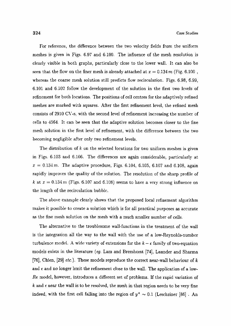
324
Case Studies
For reference, the difference between the two velocity fields from the uniform
meshes is given in Figs. 6.97 and 6.100. The influence of the mesh resolution is
clearly visible in both graphs, particularly close to the lower wall. It can also be
seen that the flow on the finer mesh is already attached at x = 0.134 m (Fig. 6.100
whereas the coarse mesh solution still predicts flow recirculation. Figs. 6.98, 6.99,
6.101 and 6.102 follow the development of the solution in the first two levels of
refinement for both locations. The positions of cell centres for the adaptively refined
meshes are marked with squares. After the first refinement level, the refined mesh
consists of 2910 CV-s, with the second level of refinement increasing the number of
cells to 4564. It can be seen that the adaptive solution becomes closer to the fine
mesh solution in the first level of refinement, with the difference between the two
becoming negligible after only two refinement levels.
The distribution of k on the selected locations for two uniform meshes is given
in Figs. 6.103 and 6.106. The differences are again considerable, particularly at
x = 0.134m. The adaptive procedure, Figs. 6.104, 6.105, 6.107 and 6.108, again
rapidly improves the quality of the solution. The resolution of the sharp profile of
k at x = 0.134 rn (Figs. 6.107 and 6.108) seems to have a very strong influence on
the length of the recirculation bubble.
The above example clearly shows that the proposed local refinement algorithm
makes it possible to create a solution which is for all practical purposes as accurate
as the fine mesh solution on the mesh with a much smaller number of cells.
The alternative to the troublesome wall-functions in the treatment of the wall
is the integration all the way to the wall with the use of a low-Reynolds-number
turbulence model. A wide variety of extensions for the k - e family of two-equation
models exists in the literature (eg. Lam and Bremhorst [74], Launder and Sharma
[76], Chien, [29] etc.). These models reproduce the correct near-wall behaviour of k
and e and no longer limit the refinement close to the wall. The application of a low-
Re model, however, introduces a different set of problems. If the rapid variation of
k and e near the wall is to be resolved, the mesh in that region needs to be very fine
indeed, with the first cell falling into the region of y '- 0.1 (Leschziner [86] . An
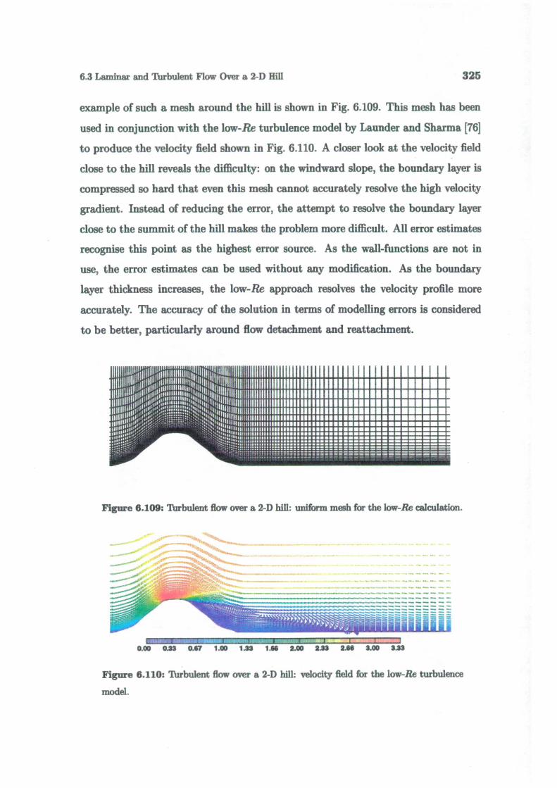
6.3 Laminar and Thrbulent Flow Over a 2-D Hill
325
example of such a mesh around the hill is shown in Fig. 6.109. This mesh has been
used in conjunction with the low-Re turbulence model by Launder and Sharma [76]
to produce the velocity field shown in Fig. 6.110. A closer look at the velocity field
close to the hill reveals the difficulty: on the windward slope, the boundary layer is
compressed so hard that even this mesh cannot accurately resolve the high velocity
gradient. Instead of reducing the error, the attempt to resolve the boundary layer
close to the summit of the hill makes the problem more difficult. All error estimates
recognise this point as the highest error source. As the wall-functions are not in
use, the error estimates can be used without any modification. As the boundary
layer thickness increases, the low-Re approach resolves the velocity profile more
accurately. The accuracy of the solution in terms of modelling errors is considered
to be better, particularly around flow detachment and reattachment.
Figure 6.109: Thrbulent flow over a 2-D hill: uniform mesh for the low-Re calculation.
IiaI -.3 I I I0.00 0.33 0.17 1.00 1.33 1.16 2.00 2.33 2.66 3.00 3.33
Figure 6.110: Thrbulent flow over a 2-D hill: velocity field for the low-Re turbulence
model.

p
o
1
ii::
10_i1
TaylorMomentResidual
10'no of cells
326
Case Studies
If it were possible to decrease the high error peak close to the summit of the
hill, the cost associated with the use of the low-Re model could be considered ac-
ceptable. For this purpose, the refinement-only procedure starting from the mesh
shown in Fig. 6.109 is used. The initial mesh consists of 13320 CV-s with strong
grading towards the wall. The y value in the near-wall cell is of the order of 0.1.
The method of error estimation and the refinement parameters are kept the same as
in previous calculations. After three levels of refinement, the mesh consists of 38076
CV-s. According to the error estimates, even this mesh is too coarse to resolve the
compressed boundary layer at the windward side of the hill. Figs. 6.111, 6.112 and
6.113 show the change in the estimated maximum error with refinement. The be-
Figure 6.111: Turbulent flow over a 2 D hill: maximum error reduction for velocity
with adaptive refinement and the low-Re turbulence model.
haviour of the estimates is slightly different than before. For the maximum velocity
error, the Moment and Direct Taylor Series Error estimates agree closely and show
that the error levels off after two refinement levels. The mesh is now fine enough to
start resolving the strongly compressed boundary layer close to the summit of the
hill. The Residual Error estimate still shows an increase in the error, but comes to
a closer agreement with other two error estimates. Only the final level of refinement
actually decreases the error. This is, however associated with a large increase in the

6.3 Laminar and Turbulent Flow Over a 2 D Hill 327
number of cells. The majority of cells added in the adaptive procedure are placed in
the near-wall region. The "1-irregularity" condition imposed to preserve the mesh
quality pushes the number of cells in the final refinement level up to 165470, consid-
erably increasing the cost of the calculation. The result is still impressive: all error
estimates on all fields report a drop in the maximum error.
The changes of the maximum error in k and are somewhat more favourable.
After an initial jump in the first level of refinement, the error consistently decreases.
The decrease is not uniform, as the position of the error peak changes as the reso-
lution around its previous position becomes better.
This test case allows us to draw several conclusions about the compatibility
between local mesh refinement and turbulent flow calculations. The performance of
the adaptive algorithm in terms of error reduction is worse than in the case of laminar
flows, primarily as a result of the more complicated mathematical model. The major
source of difficulties is near the wall, where all fields vary very rapidly. If this region
is effectively "bridged" by the wall-functions, the limits on their applicability in
terms of modelling errors introduce a limitation on the minimum cell size. When
the adaptive procedure moves the maximum error into the near-wall cell, it cannot
be reduced any further. Mesh adaptivity, however, does improve the accuracy away
from the wall and offers better resolution normal to the wall, which is of particular
importance around the detachment and reattachment point.
An alternative wall treatment in turbulent calculations is the use of a low-Re
turbulence model with integration all the way down to the wall. This approach
requires much higher near-wall resolution, with the first cell falling well into the
laminar sublayer. A low-Re model does not limit the adaptive procedure in any way,
thus allowing a considerable improvement in accuracy. It should, however, be kept
in mind that the rapid near-wall variation requires a very fine mesh and even with
an adaptive procedure the necessary number of cells will be much higher than for
the wall-function treatment. The peak error still remains near the wall. A potential
for better near-wall accuracy can be possibly found in alternative formulations of
the two-equation turbulence models, with the turbulence variables that vary linearly

328
100
10
Case Studies
0 TaylorA Moment)( Residual
)(
no of cells
Figure 6.112: Turbulent flow over a 2-D hill: maximum error reduction for k with
adaptive refinement and the low-Re turbulence model.
02
10
0 Taylor
4. A Moment, )( Residual
A
1o110
I 0no of cells
Figure 6.113: Tur ulent flow over a 2-D hill: maximum error reducti n for e wi h
adaptive refinement and the loss-Re turbulence model.
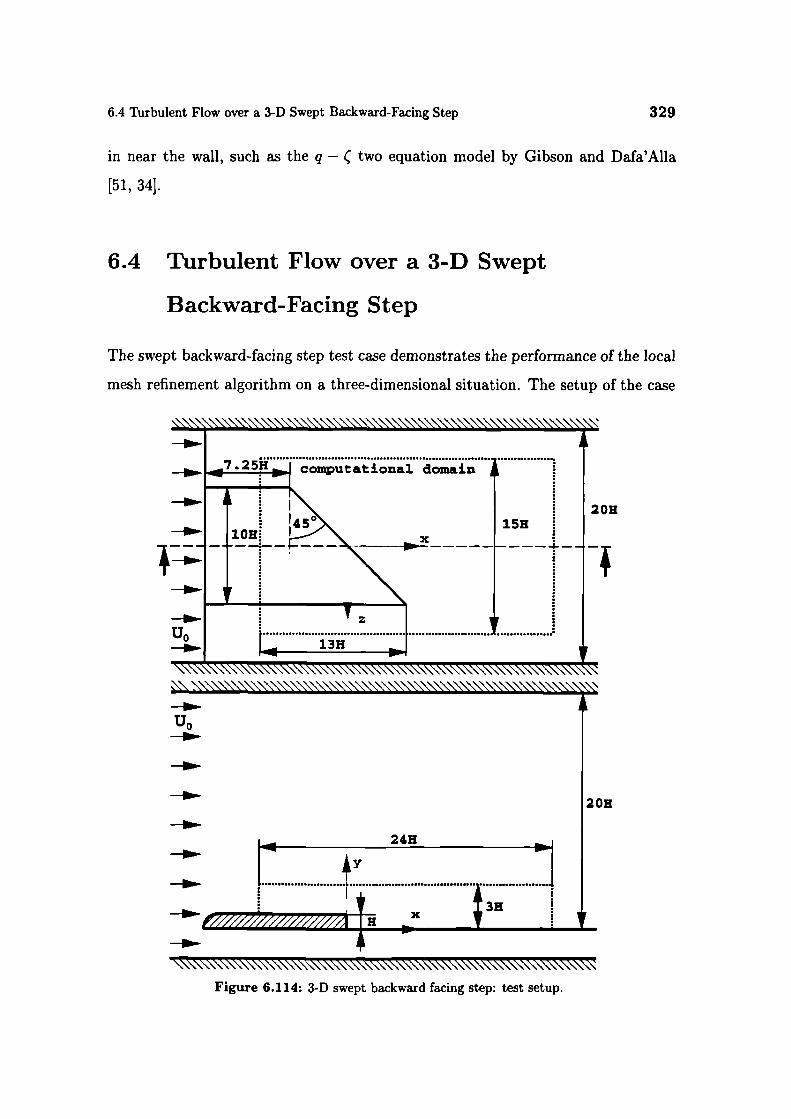
6.4 Turbulent Flow over a 3-D Swept Backward-Facing Step 329
in near the wall, such as the q - (two equation model by Gibson and Dafa'Alla
[51, 34].
6.4 Turbulent Flow over a 3-D Swept
Backward-Facing Step
The swept backward-facing step test case demonstrates the performance of the local
mesh refinement algorithm on a three-dimensional situation. The setup of the case
7.25B,,J computational dcnain
-
I45.•—ø' 1OH
4i:H
I 120H
I'5" I2! b1Lt4
U0 •13H
\\\\\\\\\\\\\\\\\\\\\\\\\\\\\\\\\\\\\\\\\\\\\\\\\\\\\\\\\\\'\Figure 6.114: 3-D swept backward facing step: test setup.

330 Case Studies
consists of an obstacle with a blunt leading edge and a triangular back mounted on
a plate inside the channel, Fig. 6.114.
The height of the step is H = 0.04 m. The flow in this geometry has been
experimentally investigated by LeHuuNho and Béguier [80], using visualisation and
Laser-Doppler Anemometry (LDA) in a water channel at Re = 3000 and a rotating
hot-wire probe in the wind-tunnel at Re = 60000. At high Reynolds number, a
vortex is formed behind the upstream corner of the step from the rolling of separating
shear layers (Moinat and Lesieur [96]). The vortex follows the step and is eventually
straightened by the side stream at the other side of the step.
Calculations for the same geometry on Re = 60000 have been done by Moinat
and Lesieur [96] using Large Eddy Simulation (LES) with the Structure function
sub-grid scale turbulence model (Métais and Lesieur [94]) and the standard k -
model with wall-functions.
In order to provide a reasonable mesh resolution around the vortex, the corn-
putational domain covers only a small region around and behind the step, marked
in Fig. 6.114. The inlet boundary is positioned downstream of the leading edge,
thus avoiding the modelling problems related to the laminar separation and tran-
sition to turbulence. Unfortunately, no experimental data is available upstream of
the triangular part of the obstacle. Following Moinat and Lesieur [96J, the velocity
distribution at the inlet is prescribed as a 1/7 power-law profile with a boundary
layer thickness of 8 = 0.3 H in the x-direction. The other two velocity components
are set to zero. On the top surface and the sides of the computational domain, a
symmetry plane boundary condition is specified. The free-stream velocity is set to
22.5 m s, corresponding to the measured wind-tunnel conditions.
The turbulence model selected for this calculation is again the non-linear version
of the k f model by Shih 1123] with wall-functions. The turbulent kinetic energy
and its dissipation at the ml t are prescribed to be in equilibrium with the velocity
field.
The flow field is particularl y complex around the corner of the triangular part,
where the '. rtex is created Previous calculations suggest that the mesh required to
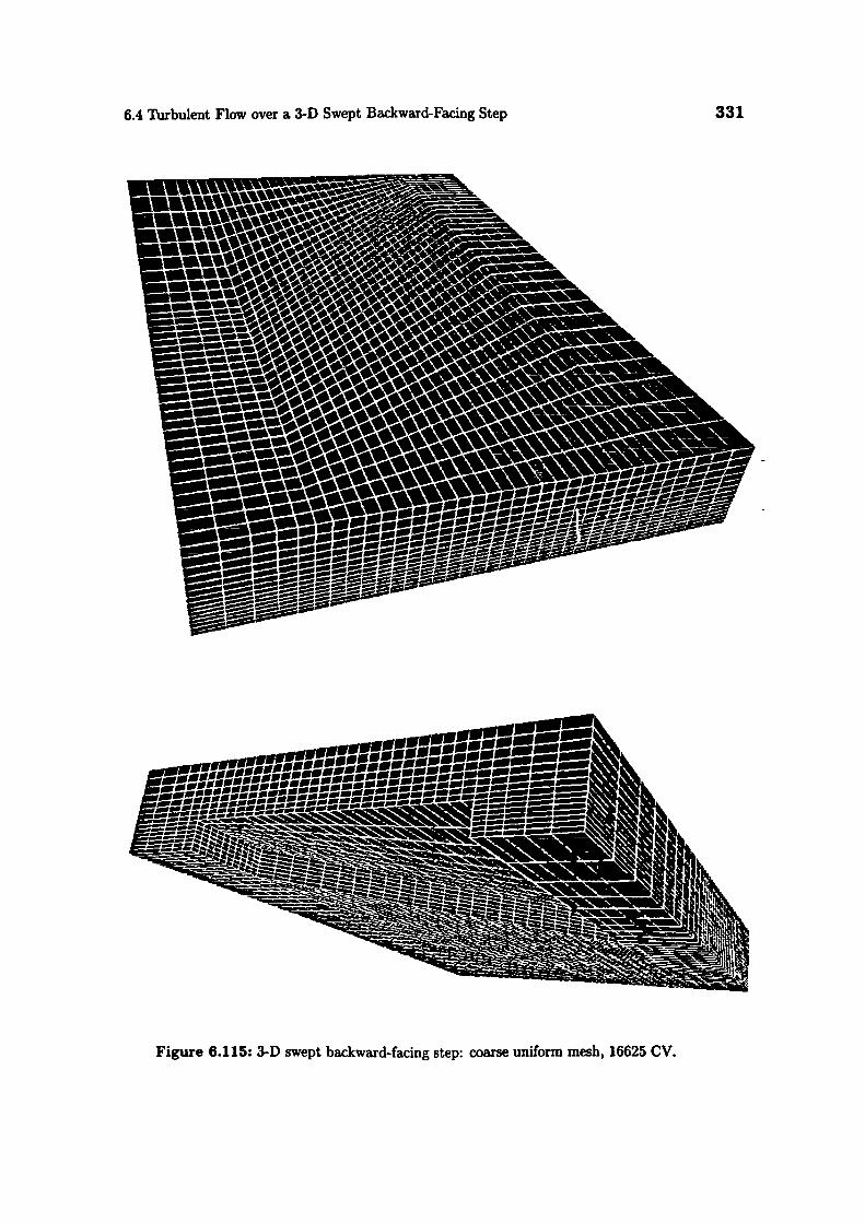
6.4 Turbulent Flow ovet a 3-D Swept Backward-Facing Step 331
Figure 6.115: 3-D swept backward-facing step: coarse uniform mesh, 16625 CV.
332 Case Studies
properly resolve such a situation would contain around 1 million cells, which exceeds
the computer resources available for this study. In an industrial environment it
is also often necessary to resolve the flows which are even more complicated on
relatively coarse meshes. This test case can provide an example of the benefits that
can be obtained from an adaptive algorithm in such a situation.
The uniform mesh calculations are made on two meshes, with 16625 and 133000
CV-s. The mesh, shown in Fig. 6.115, is slightly graded towards the step and the
solid walls.
The stream ribbons in Figs. 6.116 and 6.117 are used to visualise the main
features of the flow. In Fig. 6.116 the ribbons are released just above the obstacle
and are trapped by the vortex. Their colour represents the local velocity magnitude
and their width changes with the magnitude of the v )rticity. A single ribbon shown
in Fig. 6.117 is released next to the corner of the triangular part and follows the
vortex from its creation. The vortex can also be seen in the velocity distribution in
the x - z plane on three levels, Figs. 6.118, 6.119 and 6.120. The under-resolved
region at the corner of the triangular part in Fig. 6.118 gives an indication of a
rapidly changing three-dimensional flow structure over the height of the step. The
same conclusion can be reached from the rapid variation of the surface pressure at
the same point, shown in Fig. 6.121.
The internal structure of the vortex can be easily seen in the near-surface distri-
bution and the iso-surface of turbulent kinetic energy, Figs. 6.122 and 6.123.
Overall, the gradients in the solution are high for all fields close to the step, with
the solution becoming smoother further downstream. It can therefore be expected
that the principal error sources will be found along the edge of the step, particularly
at the corner of the triangular part.
In the previous test cases error estimation results obtained from the Moment
and Residual Error estimates sh wed g od agreement, with the Direct Taylor Series
estimate consistently underpredicting the error levels. The exact solution for this
test case is again not available and the quality of the estimated error distribution
will be judged by comparing the to estimation methods.

6.4 Thrbulent Flow over a 3-D Swept Backward-Facing Step 333
Figure 6.116: 3-D swept backward-facing step: stream ribbons close to the inlet.
Figure 6.117: 3-D swept backward-facing step: stream ribbon in the vortex.

334
Case Studies
Figure 6.118: 3-D swept backward-facing step: velocity field cut, y/H = 0.125.
Figure 6.119: 3-D swept backward-facing step: velocity field cut, y/H = 0.5.
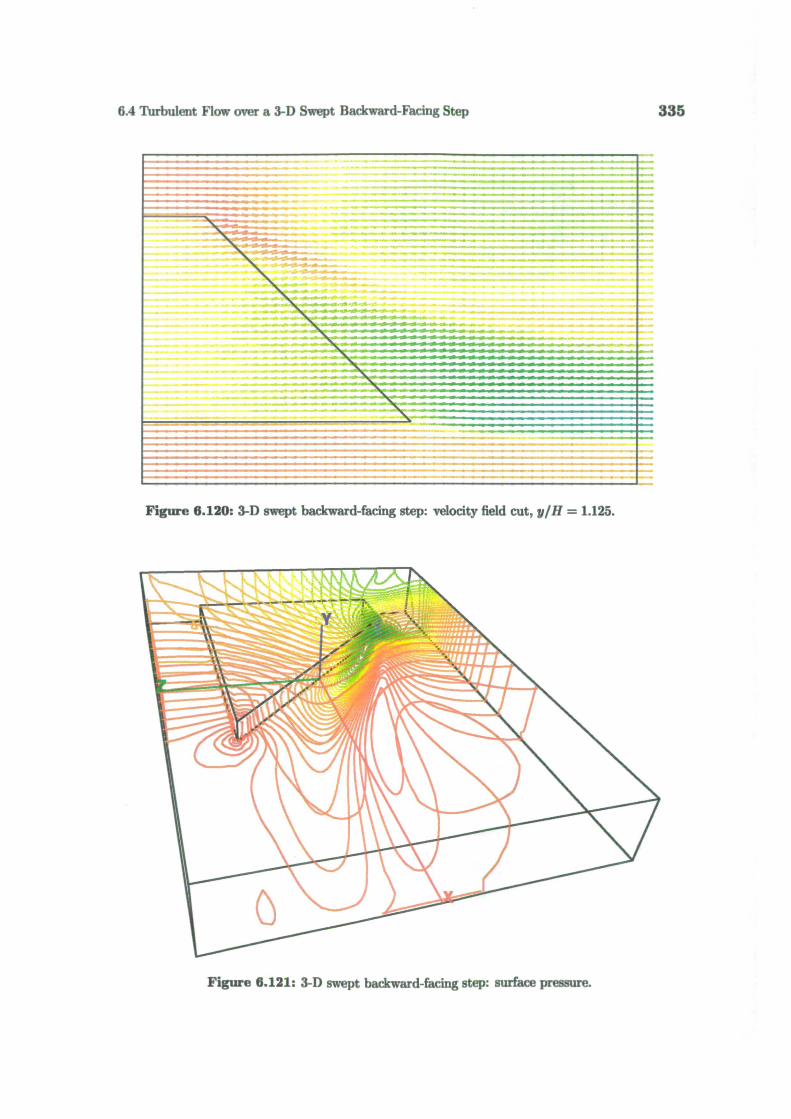
6.4 Turbulent Flow over a 3-D Swept Backward-Facing Step 335
- I
x s-.-----a- is ,.... -
I' - .. - .....- ------ -.-.-
- ----
Figure 6.120: 3-D swept backward-facing step: velocity field cut, y/H = 1.125.
Figure 6.121: 3-D swept backward-facing step: surface pressure.
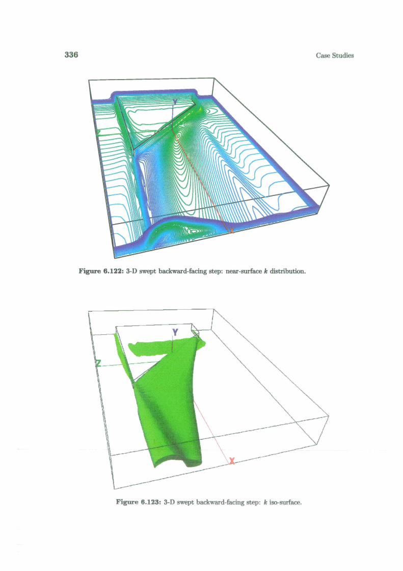
336
Case Studies
Figure 6.122: 3-D swept backward-facing step: near-surface k distribution.
Figure 6.12$: 3-D swept backward-facing step: k iso-surface.
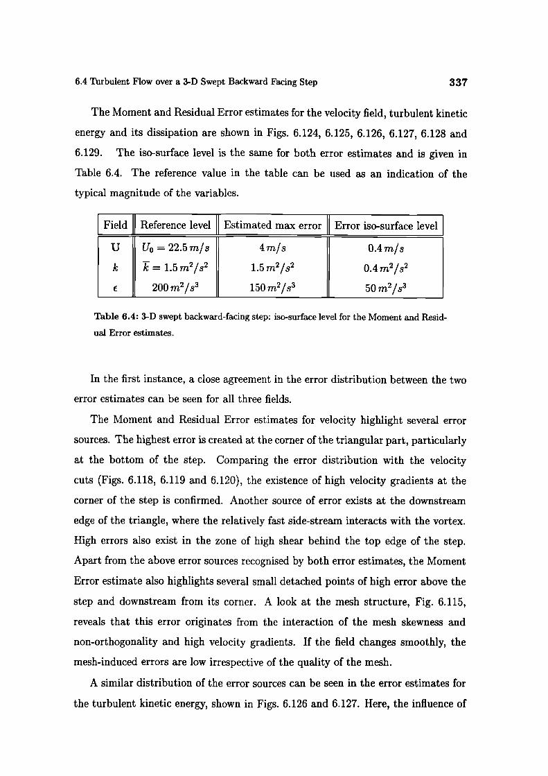
6.4 Turbulent Flow over a 3-D Swept Backward Facing Step 337
The Moment and Residual Error estimates for the velocity field, turbulent kinetic
energy and its dissipation are shown in Figs. 6.124, 6.125, 6.126, 6.127, 6.128 and
6.129. The iso-surface level is the same for both error estimates and is given in
Table 6.4. The reference value in the table can be used as an indication of the
typical magnitude of the variables.
Field Reference level Estimated max error Error iso-surface level
U U0 = 22.5 rn/s 4rn/s 0.4 in/s
k = 1.5 m2/s2 1.5 m2/s2 0.4 m2/s2
200 m2/s3 150 m2/s3 50m2/s3
Table 6.4: 3-D swept backward-facing step: iso-surface level for the Moment and Resid-
ual Error estimates.
In the first instance, a close agreement in the error distribution between the two
error estimates can be seen for all three fields.
The Moment and Residual Error estimates for velocity highlight several error
sources. The highest error is created at the corner of the triangular part, particularly
at the bottom of the step. Comparing the error distribution with the velocity
cuts (Figs. 6.118, 6.119 and 6.120), the existence of high velocity gradients at the
corner of the step is confirmed. Another source of error exists at the downstream
edge of the triangle, where the relatively fast side-stream interacts with the vortex.
High errors also exist in the zone of high shear behind the top edge of the step.
Apart from the above error sources recognised by both error estimates, the Moment
Error estimate also highlights several small detached points of high error above the
step and downstream from its corner. A look at the mesh structure, Fig. 6.115,
reveals that this error originates from the interaction of the mesh skewness and
non-orthogonality and high velocity gradients. If the field changes smoothly, the
mesh-induced errors are low irrespective of the quality of the mesh.
A similar distribution of the error sources can be seen in the error estimates for
the turbulent kinetic energy, shown in Figs. 6.126 and 6.127. Here, the influence of

338
Case Studies
Figure 6.124: 3-D swept backward-facing step: Moment Error estimate for ve1ocit
Figure 6.125: 3-D swept backward-facing step: RsiduaI Error estimate for velocity.
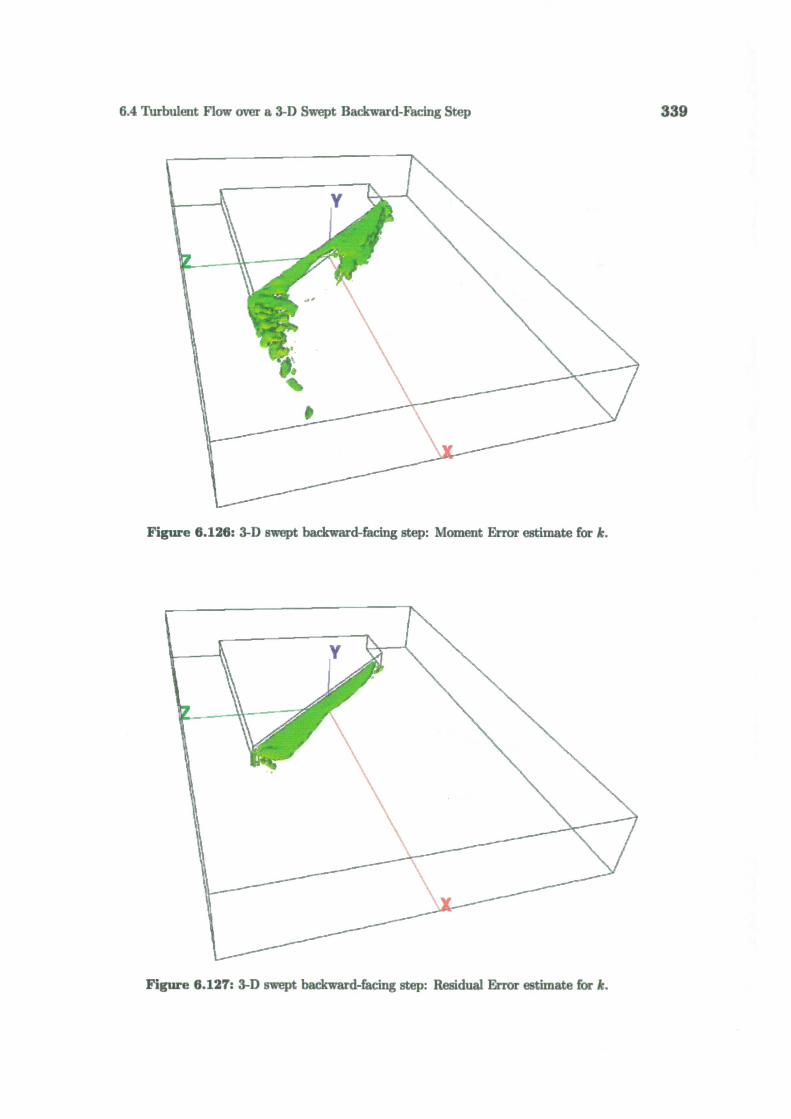
6.4 Turbulent Flow over a 3-D Swept Backward-Facing Step 339
Figure 6.126: 3-1) swept backward-facing step: Moment Error estimate for k.
Figure 6.127: 3-D swept backward-facing step: Residual Error estimate for k.
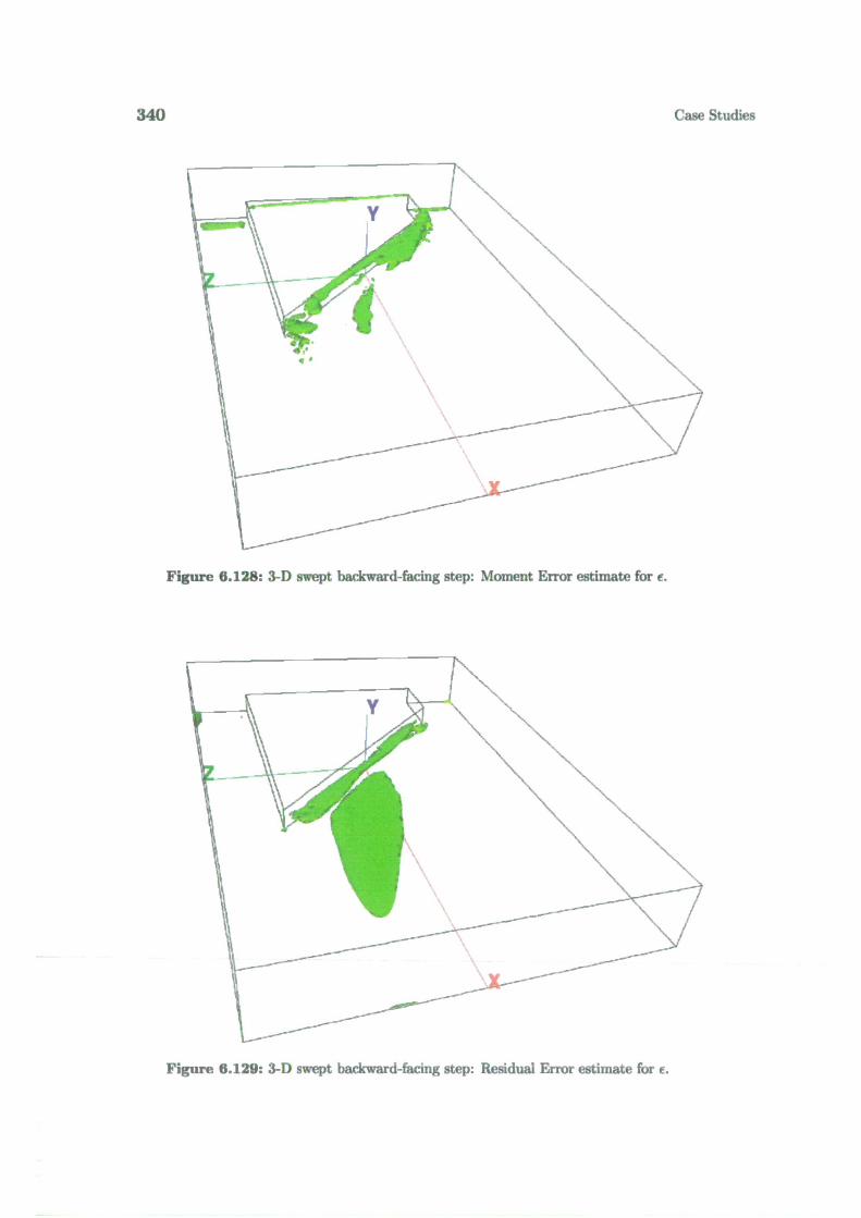
340
Case Studies
Figure 6.128: 3-D swept backward-facing step: Moment Error estimate for €.
Figure 6.129: 3-D swept backward-facing step: Residual Error estimate for €.
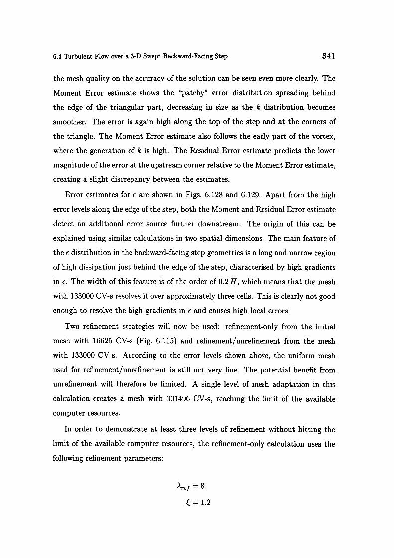
6.4 Turbulent Flow over a 3-D Swept Backward-Facing Step 341
the mesh quality on the accuracy of the solution can be seen even more clearly. The
Moment Error estimate shows the "patchy" error distribution spreading behind
the edge of the triangular part, decreasing in size as the k distribution becomes
smoother. The error is again high along the top of the step and at the corners of
the triangle. The Moment Error estimate also follows the early part of the vortex,
where the generation of k is high. The Residual Error estimate predicts the lower
magnitude of the error at the upstream corner relative to the Moment Error estimate,
creating a slight discrepancy between the estimates.
Error estimates for e are shown in Figs. 6.128 and 6.129. Apart from the high
error levels along the edge of the step, both the Moment and Residual Error estimate
detect an additional error source further downstream. The origin of this can be
explained using similar calculations in two spatial dimensions. The main feature of
the e distribution in the backward-facing step geometries is a long and narrow region
of high dissipation just behind the edge of the step, characterised by high gradients
in €. The width of this feature is of the order of 0.2 H, which means that the mesh
with 133000 CV-s resolves it over approximately three cells. This is clearly not good
enough to resolve the high gradients in € and causes high local errors.
Two refinement strategies will now be used: refinement-only from the initial
mesh with 16625 CV-s (Fig. 6.115) and refinement/unrefinement from the mesh
with 133000 CV-s. According to the error levels shown above, the uniform mesh
used for refinement/unrefinement is still not very fine. The potential benefit from
unrefinement will therefore be limited. A single level of mesh adaptation in this
calculation creates a mesh with 301496 CV-s, reaching the limit of the available
computer resources.
In order to demonstrate at least three levels of refinement without hitting the
limit of the available computer resources, the refinement-only calculation uses the
following refinement parameters:
ref = 8
= 1.2
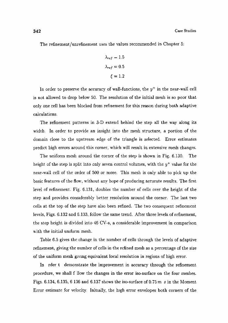
342
Case Studies
The refinement/unrefinement uses the values recommended in Chapter 5:
'ref - 1.5
Aref = 0.5
= 1.2
In order to preserve the accuracy of wall-functions, the y+ in the near-wall cell
is not allowed to drop below 50. The resolution of the initial mesh is so poor that
only one cell has been blocked from refinement for this reason during both adaptive
calculations.
The refinement patterns in 3-D extend behind the step all the way along its
width. In order to provide an insight into the mesh structure, a portion of the
domain close to the upstream edge of the triangle is selected. Error estimates
predict high errors around this corner, which will result in extensive mesh changes.
The uniform mesh around the corner of the step is shown in Fig. 6.130. The
height of the step is split into only seven control volumes, with the y value for the
near-wall cell of the order of 500 or more. This mesh is only able to pick up the
basic features of the flow, without any hope of producing accurate results. The first
level of refinement. Fig. 6.131, doubles the number of cells over the height of the
step and provides considerably better resolution around the corner. The last two
cells at the top of the step have also been refined. The two consequent refinement
levels, Figs. 6.132 and 6.133, follow the same trend. After three levels of refinement,
the step height is divided into 46 CV-s, a considerable improvement in comparison
with the initial uniform mesh.
Table 6.5 gives the change in the number of cells through the levels of adaptive
refinement, giving the number of cells in the refined mesh as a percentage of the size
of the uniform mesh giving equivalent local resolution in regions of high error.
In rder t demonstrate the improvement in accuracy through the refinement
procedure, we shall f how the changes in the error iso-surface on the four meshes.
Figs. 6.134, 6.135, 6 136 and 6.137 shows the iso-surface of 0.75 m s in the Moment
Error estimate for velocity. Initially, the high error envelopes both corners of the
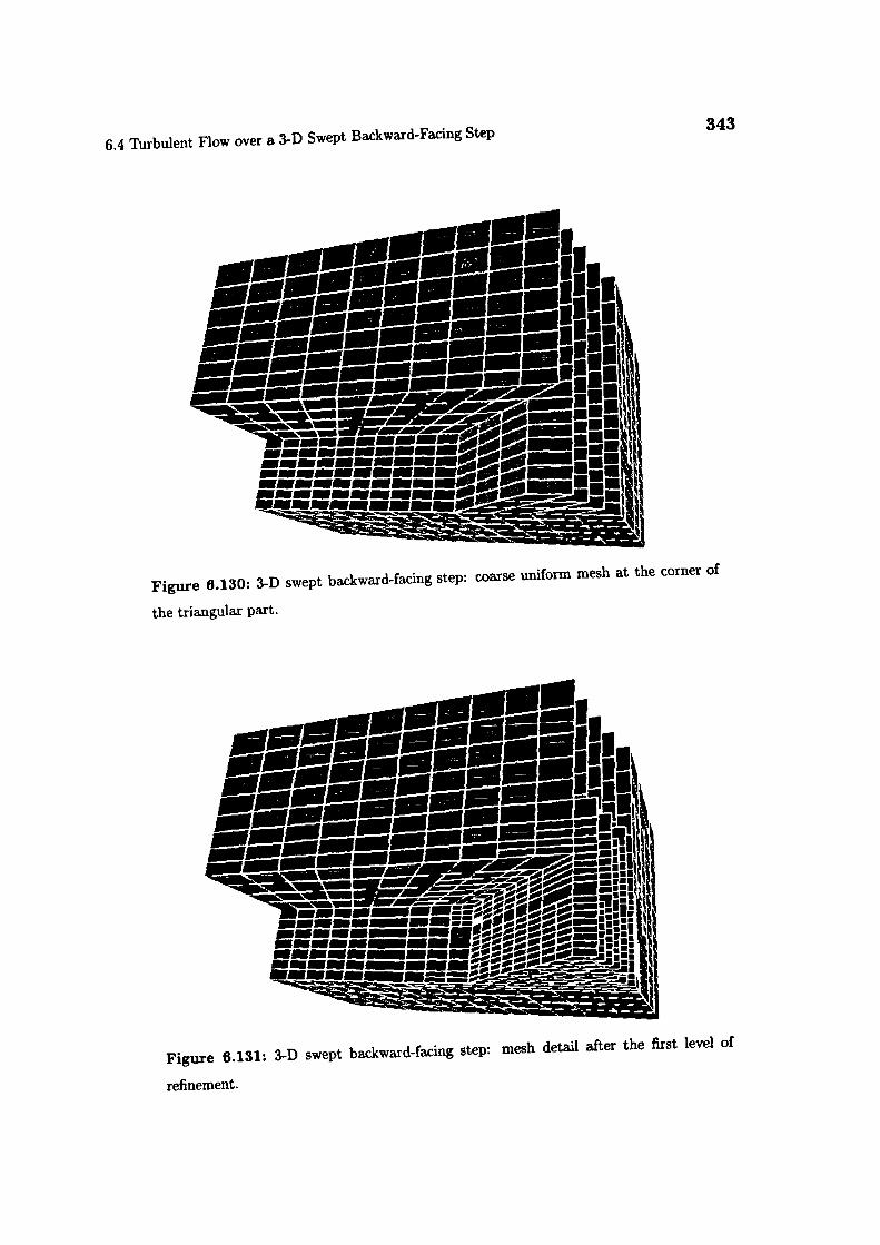
3436.4 Turbulent Flow over a 3-D Swept Backward-Facing Step
Figure 6.130: 3-D swept backward-facing step: coarse uniform mesh at the corner of
the triangular part.
Figure 6.131: 3-D swept backward-facing step: mesh detail after the first level of
refinement.

344
Case Studies
Figure 6.132: 3-D swept backward-facing step: mesh detail after the second level of
refinement.
Figure 6.133: 3-D swept backward-facing step: mesh detail after the third level of
refinement.

6.4 Turbulent Flow over a 3-D Swept Backward-Facing Step 345
Adaptive refinement % ratio Unifor
16625 100 % 16625
27563 20.7 % 133000
64003 6.01 % 1064000
202957 2.38 % 8512000
Table 6.5: 3-D swept backward-facing step: number of cells for adaptive and uniform
refinement starting from the coarse mesh.
triangle, also showing several points of high mesh-induced errors behind the step.
As the refinement progresses, the region of high error becomes smaller and closer to
the solid walls. The mesh-induced error is moved to the point where the refined part
interacts with the coarse mesh away from the step. In the final mesh, the Moment
Error estimate is high just at the tip of the triangle and close to the wall at the
upstream edge.
The changes in the Residual Error estimate for k are shown in Figs. 6.138, 6.139,
6.140 and 6.141, with the iso-surface of 0.35 m2/s. The error is initially high inside
the vortex, downstream from the step. As the refinement progresses, the error peak
moves closer to the wall and the top edge.
In terms of the maximum error reduction, neither uniform nor adaptive refine-
ment show the expected scaling. The change in the maximum error in velocity
for the adaptive calculation is shown in Fig. 6.142. All error estimates predict an
increase in its magnitude as the mesh becomes finer. The increase is highest in
the Direct Taylor Series Error estimate: as the mesh refinement picks up the new
features of the solution the second velocity gradient increases, pushing the error
estimate higher. The maximum error for the Residual Error estimate is given both
with and without the near-wall errors. The near-wall error is higher than for the
Moment Error estimate, as was the case for the turbulent flow over a hill. When the
near-wall cells are removed from the comparison, the Moment and Residual Error
estimates show a reasonable agreement. It is interesting to notice that in spite of

346
Case Studies
Figure 6.134: 3-D swept backward-facing step: iso-surface of the Moment Error esti-
mate for velocity on the initial mesh.
Figure 6.135: 3-D swept backward-facing step: iso-surface of the Moment Error esti-
mate for velocity after the first level of refinement.

6.4 Turbulent Flow over a 3-D Swept Backward-Facing Step 347
Figure 6.136: 3-D swept backward-facing step: iso-surface of the Moment Error esti-
mate for velocity after the second level of refinement.
Figure 6.137: 3-D swept backward-facing step: iso-surface of the Moment Error esti-
mate for velocity after the third level of refinement.

348
Case Studies
Figure 6.138: 3-D swept backward-facing step: iso-surface of the Residual Error esti-
mate for k on the initial mesh.
Figure 6.139: 3-D swept backward-facing step: iso-surface of the Residual Error esti-
mate fbr k after the first level of refinement.
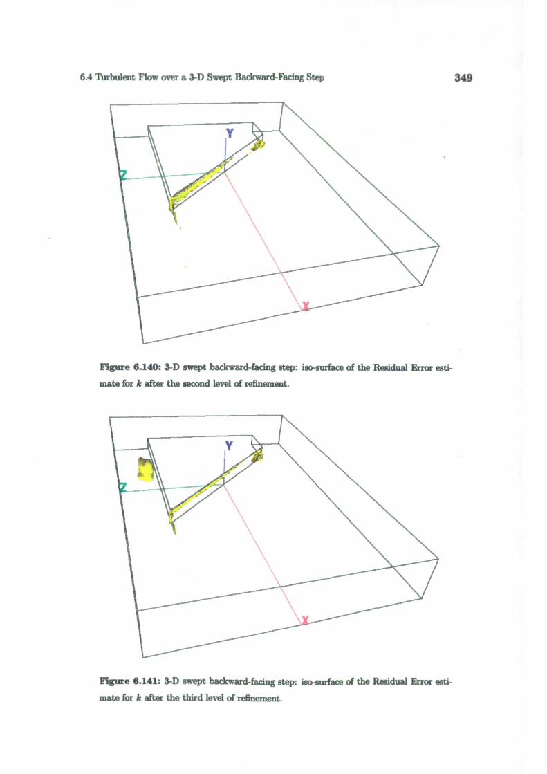
6.4 Turbulent Flow over a 3-D Swept Backward-Facing Step 349
Figure 6.140: 3-D swept backward-facing step: iso-surface of the Residual Error esti-
mMe for Ic after the second level of refinement.
Figure 6.14 1: 3-D swept backward-facing step: iso-surface of the Residual Error esti-
mate for Ic after the third level of refinement.
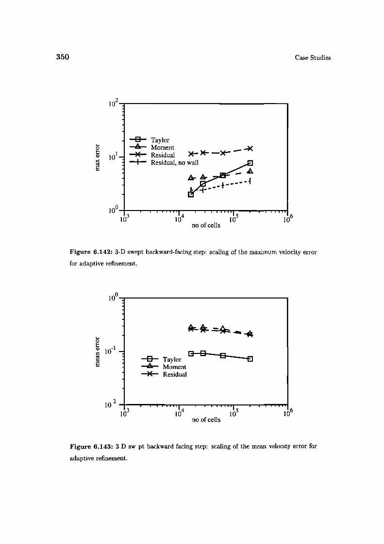
10610°—h
10 l0_ 10-ino of cells
100
0
0) -1
'1)E
10 2
I 0
0 Taylor—k-- Moment
X Residual
10_' 10'no of cells
i
350
Case Studies
i
I-C
10
E
0 Taylor.á. MomentX Residual ) *.
-x
I Residual, no wall
Figure 6.142: 3-D swept backward-facing step: scaling of the maximum velocity error
for adaptive refinement.
Figure 6.143: 3 D sw pt backward facing step: scaling of the mean velocity error for
adaptive refinement.
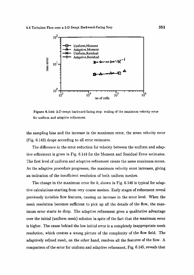
6.4 Turbulent Flow over a 3-D Swept Backward-Facing Step 351
i o2
I-010
10
0 Uniform,Momentr Adaptive,Moment
)( Uniform,ResidualI Adaptive,Residual
*-4 - -
-A ----'
10 l0 l0
1no of cells
Figure 6.144: 3-D swept backward-facing step: scaling of the maximum velocity error
for uniform and adaptive refinement.
the sampling bias and the increase in the maximum error, the mean velocity error
(Fig. 6.143) drops according to all error estimates.
The difference in the error reduction for velocity between the uniform and adap-
tive refinement is given in Fig. 6.144 for the Moment and Residual Error estimates.
The first level of uniform and adaptive refinement create the same maximum errors.
As the adaptive procedure progresses, the maximum velocity error increases, giving
an indication of the insufficient resolution of both uniform meshes.
The change in the maximum error for k, shown in Fig. 6.146 is typical for adap-
tive calculations starting from very coarse meshes. Early stages of refinement reveal
previously invisible flow features, causing an increase in the error level. When the
mesh resolution becomes sufficient to pick up all the details of the flow, the max-
imum error starts to drop. The adaptive refinement gives a qualitative advantage
over the initial (uniform mesh) solution in spite of the fact that the maximum error
is higher. The cause behind the low initial error is a completely inappropriate mesh
resolution, which creates a wrong picture of the complexity of the flow field. The
adaptively refined mesh, on the other hand, resolves all the features of the flow. A
comparison of the error for uniform and adaptive refinement, Fig. 6.145, reveals that
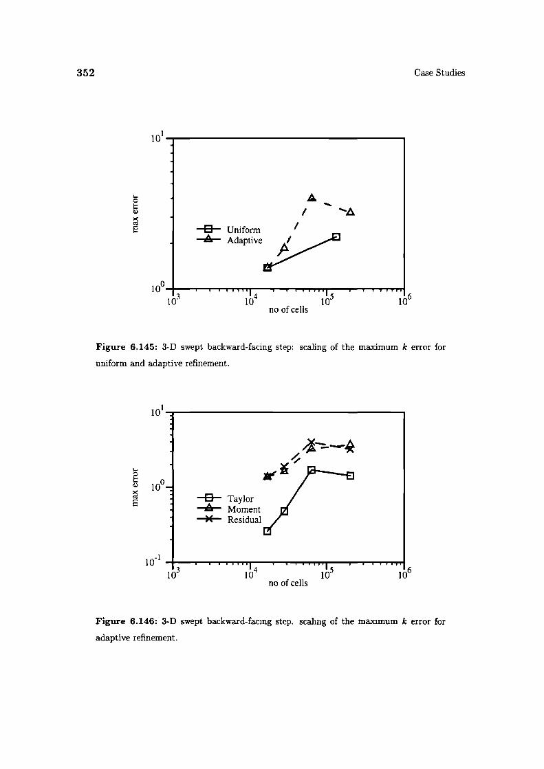
0 Taylor•á. Moment)C Residual
101
C
10
E
10_I1 0 l0 10
no of cells
352
Case Studies
101
I- A
/0 Uniform
. Adaptive
10°_f.10
10 l0
1no of cells
Figure 6.145: 3-D swept backward-facing step: scaling of the maximum k error for
uniform and adaptive refinement.
Figure 6.146: 3-D swept backward-facing step. scaling of the maximum k error for
adaptive refinement.
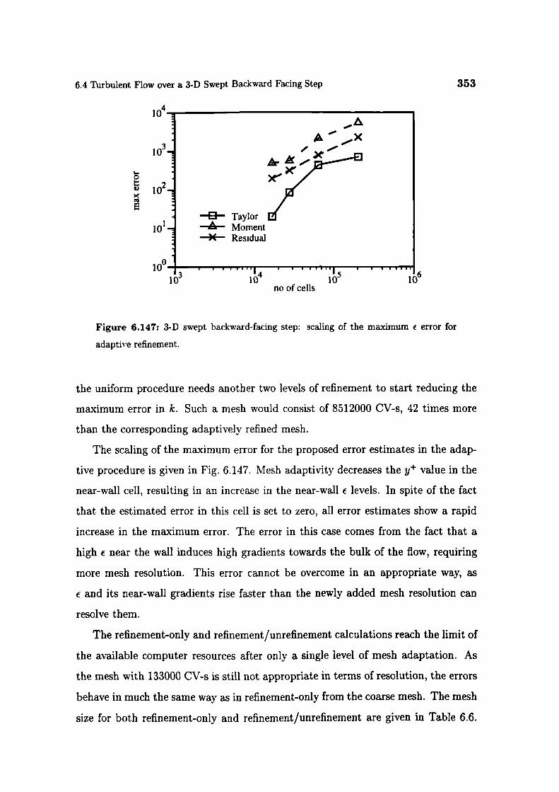
/ —Ak
0 Taylor-•- Moment
X Residual
l0_ 10'no of cells
1
I 0
I-.02
10
E
101
10I
6.4 Turbulent Flow over a 3-D Swept Backward Facing Step
353
Figure 6.147: 3-D swept backward-facing step: scaling of the maximum € error for
adaptive refinement.
the uniform procedure needs another two levels of refinement to start reducing the
maximum error in k. Such a mesh would consist of 8512000 CV-s, 42 times more
than the corresponding adaptively refined mesh.
The scaling of the maximum error for the proposed error estimates in the adap-
tive procedure is given in Fig. 6.147. Mesh adaptivity decreases the y value in the
near-wall cell, resulting in an increase in the near-wall e levels. In spite of the fact
that the estimated error in this cell is set to zero, all error estimates show a rapid
increase in the maximum error. The error in this case comes from the fact that a
high f near the wall induces high gradients towards the bulk of the flow, requiring
more mesh resolution. This error cannot be overcome in an appropriate way, as
i and its near-wall gradients rise faster than the newly added mesh resolution can
resolve them.
The refinement-only and refinement/unrefinement calculations reach the limit of
the available computer resources after only a single level of mesh adaptation. As
the mesh with 133000 CV-s is still not appropriate in terms of resolution, the errors
behave in much the same way as in refinement-only from the coarse mesh. The mesh
size for both refinement-only and refinement/unrefinement are given in Table 6.6.

354
Case Studies
Refinement 91 ratio Refinement and % ratio Uniform
only unrefinement
133000 100 % 133000 100 % 133000
323958 30.4 % 301496 28.3 % 1064000
Table 6.6: 3-D swept backward-facing step: number of cells for refinement-only and
refinement/unrefinement starting from the fine mesh.
The benefit from unrefinement in this case is quite limited, because of the low initial
resolution and only a single refinement level.
In summary, this test case shows much the same behaviour as the other turbulent
tet case presented in this Chapter. The error reduction is slow for both uniform and
aaaptive mesh refinement, with most of the problems caused by the treatment of the
wall. The mesh size necessary to appropriately resolve three-dimensional flows is
much larger than in 2-D. It can therefore be expected that in industrial applications
the user needs to rely on comparatively coarse meshes. In such situations, the
benefit of an adaptive procedure should be described more in terms of appropriate
resolution of the details of the solution than in the reduction of the error.
Considering the size of three-dimensional problems, the issue of efficiency of the
adaptive algorithm on vector and parallel computer architectures becomes impor-
tant. The error estimation methods presented in this study operate on a cell-by-cell
basis and therefore vectorise and parallelise naturally. The mesh refinement proce-
dure needs to be split into two parts. The first, selection of the type of the cell split
does not vectorise (it is based on non-vectorisable topological analysis), but can be
parallelised with the use of inter-processor face communication. The second part
includ s the actual creation of the new mesh and can again be paralleli ed with a
certain amount of eff rt. It ivcould, however, be very difficult to automatically keep
the load balance within reasonable limits. The refinement in this study has there-
fore been performed in a single-processor mode, followed by the mesh decomposition
which produces perfect load balancing irrespective of the mesh structure.
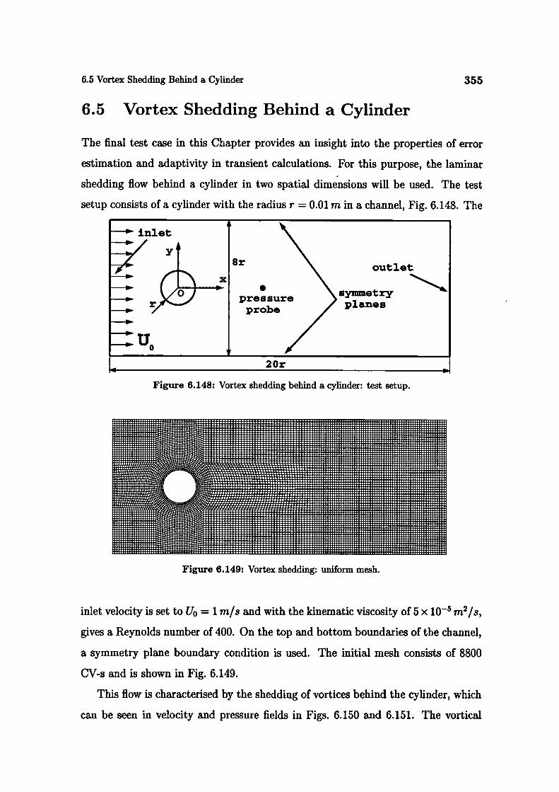
inlet
U0
6.5 Vortex Shedding Behind a Cylinder 355
6.5 Vortex Shedding Behind a Cylinder
The final test case in this Chapter provides an insight into the properties of error
estimation and adaptivity in transient calculations. For this purpose, the laminar
shedding flow behind a cylinder in two spatial dimensions will be used. The test
setup consists of a cylinder with the radius r = 0.01 m in a channel, Fig. 6.148. The
8r out let
Probe>
pressureplanes
20r
Figure 6.148: Vortex shedding behind a cylinder: test setup.
Figure 6.149: Vortex shedding: uniform mesh.
inlet velocity is set to U0 = 1 rn/s and with the kinematic viscosity of 5 x i0 m2/s,
gives a Reynolds number of 400. On the top and bottom boundaries of the channel,
a symmetry plane boundary condition is used. The initial mesh consists of 8800
CV-s and is shown in Fig. 6.149.
This flow is characterised by the shedding of vortices behind the cylinder, which
can be seen in velocity and pressure fields in Figs. 6.150 and 6.151. The vortical
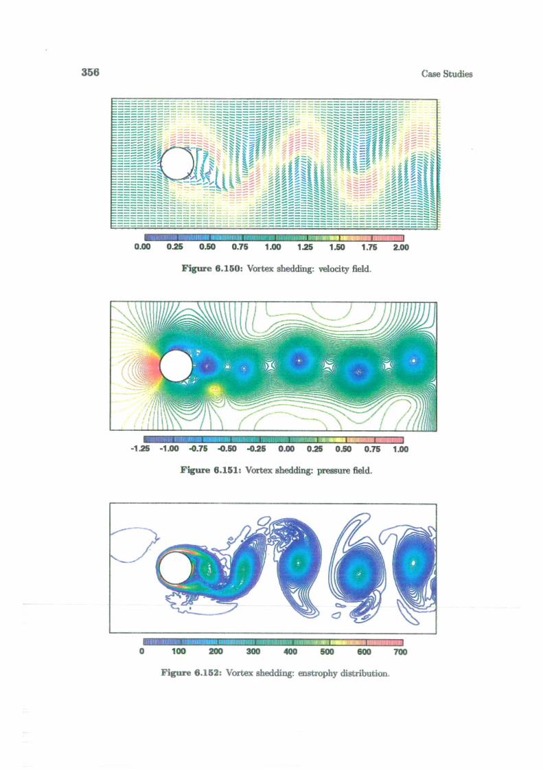
----%.,
7
358
Case Studies
--_...E
--.-- I
0.00 0.25 0.50 0.75 1.00 1.25 1.50 1.75 2.00
Figure 6.150: Vortex shedding: velocity field.
p.-1.25 -1.00 .0.75 -0.50 -025 0.00 0.25 0.50 0.75 1.00
Figure 6.151: Vortex shedding: pressure field.
I•
0 100 200 300 400 500 600 700
Figure 6.152: Vortex shedding: enstrophy distribution.

6.5 Vortex Shedding Behind a Cylinder 357
motion is also visible in the distribution of the enstrophy (magnitude of the curl of
the velocity), shown in Fig. 6.152.
In the first instance, the flow will be resolved on the same mesh with three tern-
poral discretisation schemes, namely the first-order Euler Implicit (El) discretisation
and two second-order schemes: Backward Differencing in time (BD) and the Crank-
Nicholson (CN) method. The temporal changes will be followed in the variation
of the pressure in the point 0.05 in downstream from the origin (see Fig. 6.148).
Initially, the time-step is set to 2 x 10 s, giving a maximum Courant number of
0.4. The pressure traces for the three methods of temporal discretisation are given
in Fig. 6.153. The results for the two second-order accurate temporal discretisation
0.0
-0.2
-0.4
-0.6 El—BD
-0.8 --CN
-1.02.0 2.1 2.2
t
Figure 6.153: Vortex shedding: pressure trace for different methods of temporal dis-
cretisation.
methods are very close to each other, with the Euler Implicit discretisation showing
small discrepancies in both the pressure amplitudes and the length of the period.
The accumulation of the temporal error can be seen even on this slowly evolving
flow3.
The Residual Error estimate for transient flows described in Section 4.7 will now
be used. The distribution of the full Residual Error estimate for this case is shown
31n this test case, a single pressure cycle is resolved over 200 time-steps.
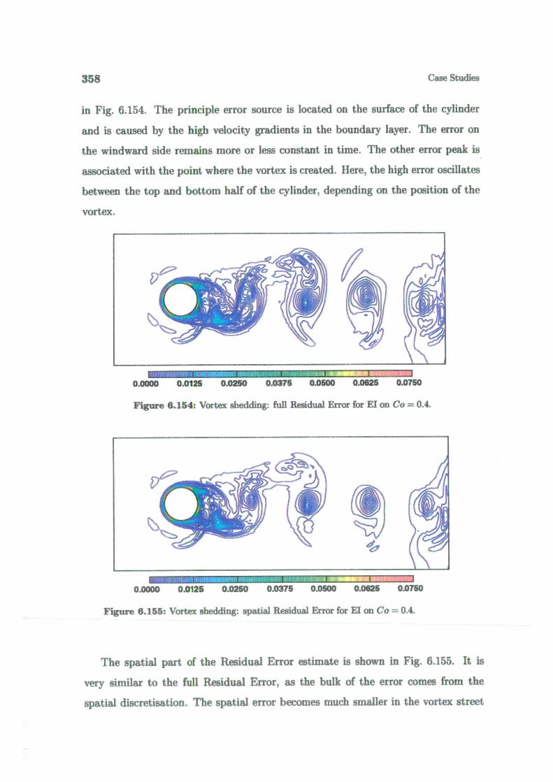
Ip
V
358
Case Studies
in Fig. 6.154. The principle error source is located on the surface of the cylinder
and is caused by the high velocity gradients in the boundary layer. The error on
the windward side remains more or less constant in time. The other error peak is
associated with the point where the vortex is created. Here, the high error oscillates
between the top and bottom half of the cylinder, depending on the position of the
vortex.
I I
0.0000 0.0125 0.0250 0.0375 0.0500 0.0625 0.0750
Figure 6.154: Vortex shedding: full Residual Error for El on Co = 0.4.
__.•zj. I
0.0000 0.01 25 0.0250 0.0375 0.0500 0.0625 0.0750
Figure 6.155: Vortex shedding: spatial Residual Error for El on Co = 0.4.
The spatial part of the Residual Error estimate is shown in Fig. 6.155. It is
very similar to the full Residual Error, as the bulk of the error comes from the
spatial discretisation. The spatial error becomes much smaller in the vortex street
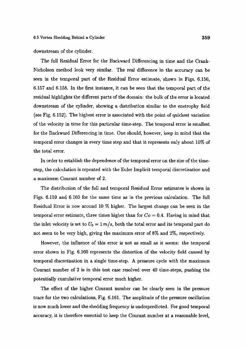
6.5 Vortex Shedding Behind a Cylinder
359
downstream of the cylinder.
The full Residual Error for the Backward Differencing in time and the Crank-
Nicholson method look very similar. The real difference in the accuracy can be
seen in the temporal part of the Residual Error estimate, shown in Figs. 6.156,
6.157 and 6.158. In the first instance, it can be seen that the temporal part of the
residual highlights the different parts of the domain: the bulk of the error is located
downstream of the cylinder, showing a distribution similar to the enstrophy field
(see Fig. 6.152). The highest error is associated with the point of quickest variation
of the velocity in time for this particular time-step. The temporal error is smallest
for the Backward Differencing in time. One should, however, keep in mind that the
temporal error changes in every time step and that it represents only about 10% of
the total error.
In order to establish the dependence of the temporal error on the size of the time-
step, the calculation is repeated with the Euler Implicit temporal discretisation and
a maximum Courant number of 2.
The distribution of the full and temporal Residual Error estimates is shown in
Figs. 6.159 and 6.160 for the same time as in the previous calculation. The full
Residual Error is now around 10 % higher. The largest change can be seen in the
temporal error estimate, three times higher than for Co = 0.4. Having in mind that
the inlet velocity is set to Uo = 1 m/s, both the total error and its temporal part do
not seem to be very high, giving the maximum error of 8% and 2%, respectively.
However, the influence of this error is not as small as it seems: the temporal
error shown in Fig. 6.160 represents the distortion of the velocity field caused by
temporal discretisation in a single time-step. A pressure cycle with the maximum
Courant number of 2 is in this test case resolved over 40 time-steps, pushing the
potentially cumulative temporal error much higher.
The effect of the higher Courant number can be clearly seen in the pressure
trace for the two calculations, Fig. 6.161. The amplitude of the pressure oscillation
is now much lower and the shedding frequency is underpredicted. For good temporal
accuracy, it is therefore essential to keep the Courant number at a reasonable level,
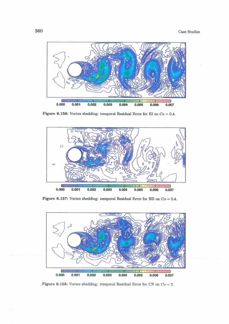
360
Case Studies
-r I I 1
0.000 0.001 0.002 0.003 0.004 0.005 0.006 0.007
Figure 6.156: Vortex shedding: temporal Residual Error for El on Co 0.4.
.rn I I P1
0.000 0.001 0.002 0.003 0.004 0.005 0.006 0.007
Figure 6.1ST: Vortex shedding: temporal Residual Error for BD on Co = 0.4.
: ii in IrJliThJn.0
0.000 0.001 0.002 0.003 0.004 0.005 0.006 0.007
Figure 6.158: Vortex shedding: temporal Residual Error for CN on Co =2.

6.5 Vortex Shedding Behind a Cylinder
I I I
0.00 0.01 0.02 0.03 0.04 0.05 0.06 0.07 0.08
Figure 6.159: Vortex shedding: full Residual Error for El on Co =2.
I ••1U
0.000 0.004 0.008 0.012 0.016 0.020
Figure 6.160: Vortex shedding: temporal Residual Error for El on Co =2.
361
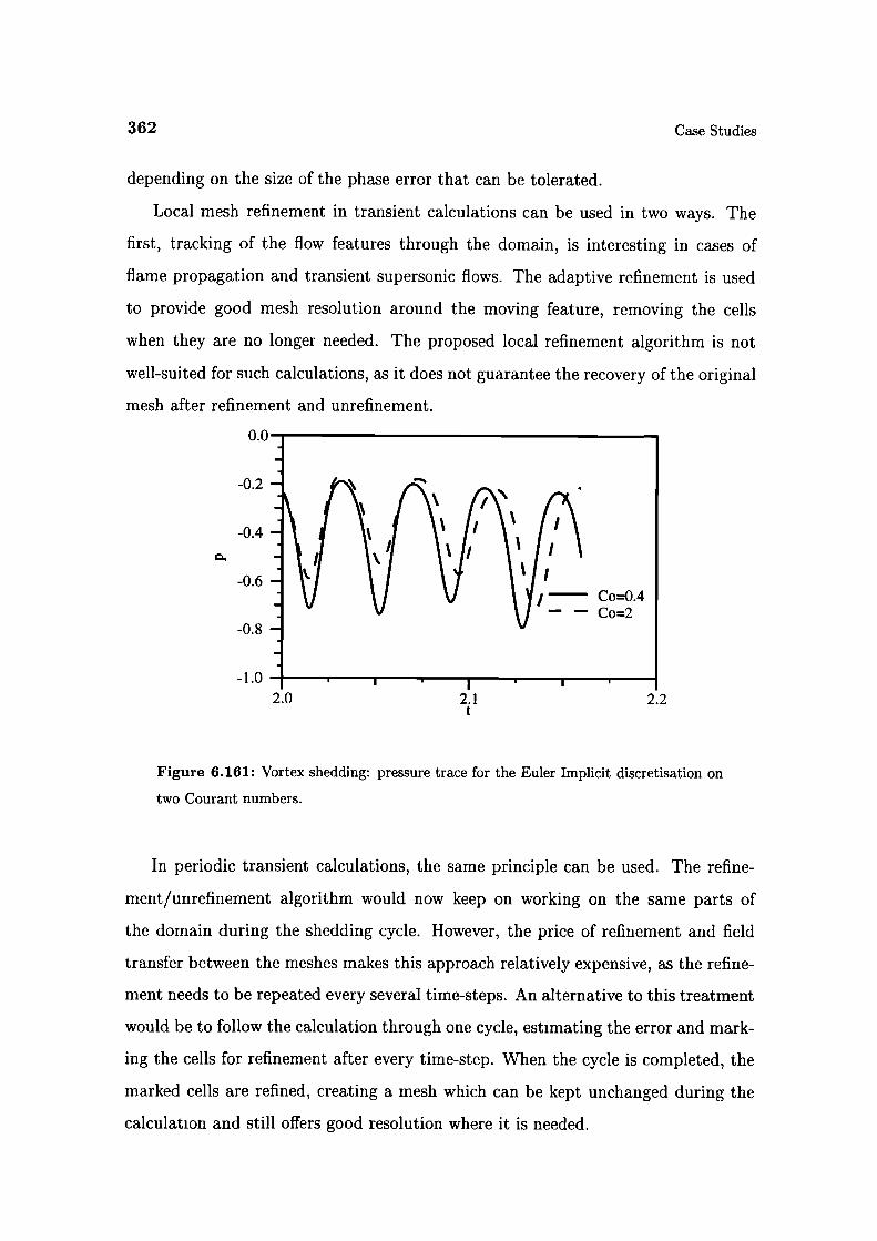
362
Case Studies
depending on the size of the phase error that can be tolerated.
Local mesh refinement in transient calculations can be used in two ways. The
first, tracking of the flow features through the domain, is interesting in cases of
flame propagation and transient supersonic flows. The adaptive refinement is used
to provide good mesh resolution around the moving feature, removing the cells
when they are no longer needed. The proposed local refinement algorithm is not
well-suited for such calculations, as it does not guarantee the recovery of the original
mesh after refinement and unrefinement.
0.0
-0.2
-0.4
-0.6
-0.8
-1.02.0 2.1 2.2
Figure 6.161: Vortex shedding: pressure trace for the Euler Implicit discretisation on
two Courant numbers.
In periodic transient calculations, the same principle can be used. The refine-
ment/unrefinement algorithm would now keep on working on the same parts of
the domain during the shedding cycle. However, the price of refinement and field
transfer between the meshes makes this approach relatively expensive, as the refine-
ment needs to be repeated every several time-steps. An alternative to this treatment
would be to follow the calculation through one cycle, estimating the error and mark-
ing the cells for refinement after every time-step. When the cycle is completed, the
marked cells are refined, creating a mesh which can be kept unchanged during the
calculation and still offers good resolution where it is needed.
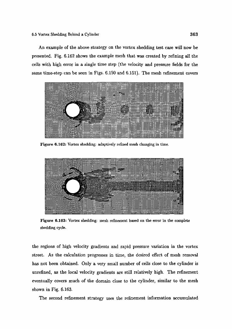
6.5 Vortex Shedding Behind a Cylinder 363
An example of the above strategy on the vortex shedding test case will now be
presented. Fig. 6.162 shows the example mesh that was created by refining all the
cells with high error in a single time step (the velocity and pressure fields for the
same time-step can be seen in Figs. 6.150 and 6.151). The mesh refinement covers
Figure 6.162: Vortex shedding: adaptively refined mesh changing in time.
Figure 6.163: Vortex shedding: mesh refinement based on the error in the complete
shedding cycle.
the regions of high velocity gradients and rapid pressure variation in the vortex
street. As the calculation progresses in time, the desired effect of mesh removal
has not been obtained. Only a very small number of cells close to the cylinder is
unrefined, as the local velocity gradients are still relatively high. The refinement
eventually covers much of the domain close to the cylinder, similar to the mesh
shown in Fig. 6.163.
The second refinement strategy uses the refinement information accumulated
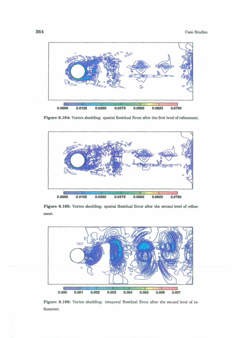
364
Case Studies
-..-- if i- I I I
0.0000 0.0125 0.0250 0.0375 0.0500 0.0625 0.0750
Figure 6.164: Vortex shedding: spatial Residual Error after the first level of refinement.
S
I -w: I i
0.0000 0.0125 0.0250 0.0375 0.0500 0.0625 0.0750
Figure 6.165: Vortex shedding: spatial Residual Error after the second level of refine-
ment.
F .ut-11
0.000 0.001 0.002 0.003 0.004 0.005 0.006 0.007
Figure 6.166: Vortex shedding: temporal Residual Error after the second level of re- -
finement.

6.6 Closure 365
during the complete shedding cycle. It produces the refined mesh shown in Fig. 6.163.
Refinement covers the surface of the cylinder, extends downstream over the part of
the domain where the vortices are created and follows them to the outlet. It also
covers a considerable part of the outlet boundary. Here, the high error is caused by
the interaction of the boundary condition and the velocity field. The zero gradient
condition used on this boundary is not appropriate when a vortex exits the domain.
This causes a distortion of the velocity field and high local errors.
The influence of local mesh refinement on the accuracy of the solution can be
seen in the distribution of the spatial part of the Residual Error estimate after one
and two refinement levels, shown in Figs. 6.164 and 6.165. The size of the time-step
is kept the same as on the initial mesh, increasing the maximum Courant number to
1.6 after two refinement levels. Th error peaks close to the wall are now removed.
The distribution of the temporal error is also different: the maximum error has
moved outside of the refined region (see Fig. 6.163). The overall solution accuracy
is now better, as a consequence of the better resolution in the area where the vortices
are created.
6.6 Closure
This Chapter presented five example applications of the error estimates and adaptive
mesh refinement. The variety of the presented flow regimes allows us to draw several
conclusions on the overall performance of the proposed error-controlled local mesh
refinement algorithm.
In supersonic flows, the solution in large parts of the domain varies very smoothly,
with the narrow regions of high gradients. In such situations, the local mesh refine-
ment algorithm is at its best. The bulk of the error is caused by inappropriate
mesh resolution around the shocks and contact discontinuities. The task of error
estimation is comparatively easy an error indicator is completely appropriate for
this purpose. From the point of view of adaptivity, the refinement/unrefinement
procedure behaves better than refinement-only. The capability of cell removal a!-

366 Case Studies
lows the adaptive calculation to be started from a comparatively fine mesh, which is
able to pick up all the details of the flow. Mesh unrefinement consequently removes
the cells where they are not needed.
Laminar calculations present a large contrast to the supersonic flows. The flow
field here is very smooth, thus presenting a greater challenge for both error estima-
tion and adaptive refinement. It is now possible to create a fine-mesh solution and
use it to examine the accuracy of the error estimates. The Moment and Residual
Error estimates bound the exact error, while the Direct Taylor Series Error estimate
underpredicting its value. The performance of the adaptive refinement technique is
limited by the quality of the mesh created by cell addition. In laminar calculations,
only a part of the solution error is caused by insufficient mesh resolution, which is
the type of the error removd by mesh refinement. As the number of cells increases,
the importance of mesh quality becomes larger. The proposed refinement procedure
does not produce the meshes of appropriate quality, which slows down the error
reduction rate.
The two-dimensional turbulent test case reveals a variety of problems related
to turbulent flows. The reduction error of the maximum error with the increase
in the mesh size is very slow, primarily as a consequence of the complexity of the
mathematical model. The main source of the problem is the near-wall region, for
both wall-function treatment and the integration to the wall with the low-Re models.
The use of wall-functions is connected with a limitation on the size of the near-wall
cell. When the error is trapped near the wall, it cannot be further decreased. This is
true for both uniform and adaptive mesh refinement, finally resulting in the inability
to create mesh-independent solutions. The low-Re near-wall treatment does not pose
such limitations, allowing the use of mesh adaptivity to its full extent. In this case,
however the details of the flow near the wall need to be fully resolved, considerably
in reasing the overall c mputational cost.
The refinement criterion in turbulent calculations cannot be based on the error
estimate for only one of the fields. Typically, each of the variables vary rapidly in
different parts of the domain, which needs to be taken into account when the cells

6.6 Closure 367
for refinement are selected.
In spite of the low error reduction rate, the adaptive algorithm in turbulent
calculations still offers the benefits in terms of accuracy, primarily by providing
good mesh resolution at a relatively low cost.
A three-dimensional flow over the swept backward-facing step illustrates the
behaviour of the adaptive algorithms in 3-D. The number of cells needed to resolve
a flow of such complexity is very high. In the situations of highly complex flow
fields and limited computer resources, the error-controlled local mesh refinement
algorithm is a very useful tool, enabling a solution of reasonable accuracy to be
obtained on a relatively small number of cells.
The final test case illustrates the application of the error estimate on a transient
flow problem. The vortex shedding behind the cylinder gives us an opportunity
to examine the relative influence of the spatial and temporal error on the overall
solution accuracy. The transient formulation of the Residual Error estimate reveals
that the temporal component of the error for a single time-step is considerably
smaller than its spatial counterpart. The potentially cumulative effect of this error
is still important, as it influences the shedding frequency. The overall accuracy of
the transient flow simulation depends on both the spatial and temporal component
of the error. Their balance should be estimated having in mind the number of time-
steps that are needed to resolve the evolution of the flow in time. The local mesh
refinement algorithm in this case can be used to eliminate the spatial component
of the error. In order to reduce the cost of the adaptive calculation, this has been
done by marking the cells for refinement through the whole shedding cycle and then
using the accumulated information to refine the mesh.
This completes the assessment of the error estimation and local mesh refinement
algorithms presented in this Thesis. In the next Chapter, the main findings of the
Thesis are summarised and some recommendations are given for future research.

368 Case Studies

Chapter 7
Summary and Conclusions
The main concern of this study is the accuracy of numerical simulations of fluid
flows with the Finite Volume method of discretisation. Several important areas
of interest have arisen. Primarily, it is necessary to understand the assumptions
introduced during the discretisation process and their implications on the quality
of the solution. When these implications are recognised, it is easier to use the
discretisation method in a such a way to produce accurate results with a minimum
expense in terms of time and computer resources.
The desired numerical accuracy depends on the objective of the analysis and the
quality of the applied mathematical models. The error caused by the discretisation
should be considerably smaller than the expected modelling error. If the results of
the simulations are to be used with confidence, it is necessary to provide an estimate
of the discretisation error in absolute terms.
It is often known in advance what level of discretisation error can be accepted.
An automatic procedure which creates a numerical solution of pre-determined ac-
curacy would therefore be a useful extension of the error estimation tools. This
can be achieved through an error-controlled adaptive mesh refinement procedure, in
which the the mesh is dynamically changed depending on the estimated error levels.
Three primary areas of research can therefore be distinguished: discretisation, error
estimation and adaptive mesh refinement.

370
Summary and Conclusions
7.1 Discretisation
The Finite Volume method is a well-established numerical procedure, particularly
suitable for fluid flow simulations because of its conservative properties. The dis-
cretisation method described in this study splits the computational domain into
polyhedral control volumes with a variable number of faces. The governing equa-
tions of continuum mechanics are consequently discretised in the integral form over
each control volume. The discretisation is performed in real space, using a fixed
Cartesian coordinate system on meshes that do not change in time. The discretisa-
tion uses a colocated variable arrangement, with all fields sharing the same control
volumes.
This study presents a formal analysis of the accuracy of the Finite Volume
method in the second-order framework. Certain modifications introduced during
the discretisation result in discretisation errors, influencing the order of accuracy of
the method. The error terms are divided into numerical diffusion and the mesh-
induced errors. The numerical diffusion tensors resulting from the convection term
and temporal derivative are derived and their characteristics are illustrated on simple
situations. The influence of mesh skewness and non-orthogonality on the accuracy
is also examined.
Having recognised the convection discretisation as the largest source of numerical
diffusion, Section 3.4 describes a new bounded and second-order accurate differenc-
ing scheme suitable for arbitrarily unstructured meshes. The Gamma differencing
scheme described in this Section is a bounded version of Central Differencing. It
belongs to the family of the Normalised Variable differencing schemes, first proposed
by Leonard [82] and Gaskell and Lau [49]. A modification in the formulation of the
Normalised Variable needed to u e the boundedness criterion on non-uniform arbi-
trarily unstructured meshes has also been presented. It is now possible to calculate
the value of the Normalised variable on a face-by-face basis, independent of the
mesh spacing and without the explicit reference to the far upwind node. The result-
ing differencing scheme uses blending and switching between Upwind and Central
7.2 Error Estimation 371
Differencing, with a very low level of numerical diffusion. The Gamma differencing
scheme, however, shares to some extent the convergence problems encountered in
most schemes of the NVD family.
The Finite Volume discretisation described above has been applied to fluid flow
problems. The solution algorithm for the Navier-Stokes system in the segregated
framework with and without the turbulence model is summarised. The pressure-
velocity coupling is treated by the SIMPLE algorithm (Patankar[105]) for steady-
state calculations. For transient problems, the PISO algorithm by Issa [66] has been
used.
7.2 Error Estimation
The problem of a-posteriori error estimation for steady-state calculations has been
approached in three different ways, resulting is three new error estimates presented
in Chapter 4.
The Direct Taylor Series Error estimate originates from the Taylor series trun-
cation error analysis. The discretisation error is calculated from the leading term
of the truncation error, similar to the widely accepted Richardson extrapolation
approach. However, unlike Richardson extrapolation, the Direct Taylor Series Er-
ror estimate calculates the error from a single numerical solution, using the Gauss'
theorem twice to obtain the necessary second gradient tensor.
The differential equation that is being solved can be used to derive the transport
equations for higher moments of the variable. If the original transport equation were
solved exactly, all higher moment equations would also be satisfied. The numerical
solution is, however, of limited accuracy and this is not the case. The Moment Error
estimate uses the imbalance in the higher moment transport equations in order to
estimate the discretisation error. The imbalance is calculated on a cell-by-cell basis
and normalised to provide a measure of the absolute error level.
The derivation of the Residual Error estimate comes from the analysis of the
basic assumptions in the Finite Volume discretisation. In order to calculate the
372 Summary and Conclusions
surface and volume integrals in the integral form of the governing equation, it is
necessary to prescribe the variation of the solution over the control volume. At the
same tin-ie, ut is also necessary to determine the face value of the dependent variable
from the distribution around the face. In the framework of the second-order accurate
Finite Volume niethod both of these functions are linear, but they offer two different
values of the variable for any point inside the control volume. The inconsistency
between the tvo values is used to assemble the cell residual. This is a function
whici nieasures how well the solution satisfies the original equation over the control
olume and is therefore naturally associated with the discretisation error. A suitable
normal sa ion practice is again used to estimate the error magnitude, thus creating
the Residual En or estimate.
A comparison of different methods of temporal discretisation allows extension
of the formulation of the residual and consequently the Residual Error estimate to
transeirit alculations. It is also possible to separate the parts of the total error
caused by the temporal and spatial discretisation, which in turn can be used to
adjust the size of t ie time-step to provide equivalent spatial and temporal accuracy.
The formulatioi of the residual proposed above allows the strict upper bound on
the ei ror in the enei gy norm to be obtained in the manner suggested by Ainsworth
and Oden in [1, 2, 3, 4] for the Finite Element method. The Local Problem Error
e timate is modified in a way appropriate for the Finite Volume discretisation and
accornpan ed with the necessary error flux balancing procedure. In order to calcu-
late the global error norm, an elliptic local error problem needs to be solved over
every control volume. A simplified solution procedure for the local problem is also
suggested.
The proprised error estimates are tested on several test cases with analytical
solutions The Ivioment and Residual Error estimate consistently show good per-
forrnance with the Direct Taylor Series estimate underpredicting the err r levels as
expected.

7.3 Adaptive Mesh Refinement 373
7.3 Adaptive Mesh Refinement
The distribution of the estimated error is used to improve the quality of consequent
solutions by modifying the computational mesh. This is done through an automatic
local mesh refinement algorithm described in Chapter 5. The local refinement pro-.
cedure used in this study consists of two parts: embedded cell-based h-refinement
and a new unrefinement method based on cell pairs.
The refinement algorithm allows us to add more computational points in the
parts of the domain where more resolution is needed. The algorithm marks the
cells in the original mesh based on the pre-defined error threshold and propagates
the refinement patterns through the mesh in order to enforce "1-irregularity". This
condition preserves the quality of the refined mesh by enforcing a smooth transition
between the coarse and fine regions. The direction of the cell split is determined
from the gradient of the solution, thus allowing the refinement procedure to create
refinement patterns aligned with the flow. The new cells are embedded into the
original mesh and are treated fully implicitly. This treatment allows a creation of
an adaptive solution procedure without violating the conservative properties of the
discretisation. The cell-based refinement is capable of creating rapid mesh grading
with a large number of embedded levels of refinement.
The primary requirement on the unrefinement algorithm was to allow the removal
of not only the cells added during refinement, but also of the cells from the initial
mesh. An unrefinement procedure satisfying this requirement is original to this work.
It merges the cell marked for unrefinement with one of its neighbours (also marked
for unrefinement) to create a larger cell. Smooth mesh grading is again enforced
through "1-irregularity". This method of unrefinement is cheaper and faster than
the traditional approach, which stores the history of refinement into a "tree" data-
structure and is capable of removing only the cells added in previous refinement
levels. The main drawback of the unrefinement algorithm in its current form is
the interlocking of unrefinement patterns, which prevents further unrefinement and
increases mesh non-orthogonality. It is also difficult to ensure that the original mesh

374
Summary and Conclusions
will be recovered when the cells added by refinement need to be removed.
The performance of the adaptive algorithm is examined on a two-dimensional
case with an analytical solution, in conjunction with the exact error and the error
estimates described above.
7.4 Performance of the Error-Controlled
Adaptive Refinement Algorithm
The Finite Volume discretisation, error estimation and local mesh refinement are
the components of an error-controlled adaptive refinement algorithm, capable of
automatically producing a solution of some pre-determined accuracy. Before such a
tool can be used for engineering purposes, it is necessary to examine the limits of its
applicability and its performance on the variety of flow problems. For this purpose,
five test cases have been examined, covering laminar and turbulent, incompressible
and supersonic flows in two and three spatial dimensions. The conclusions drawn
from these test cases can be summarised as follows:
• The adaptive refinement algorithm is at its best when the error caused by
insufficient mesh resolution covers only a small portion of the computational
domain. In this case, local refinement efficiently removes the error by aug-
menting mesh resolution in the affected areas. The error estimation in such
cases is also relatively simple, as it is only necessary to highlight the points of
high error. A typical example of such a situation is the supersonic flow with
strong shocks.
• Laminar flows present the exact opposite of the situation described above. The
error in the smoothly changing solution is caused not only by the insufficient
mesh resolution, but al o by the quality of the mesh. The error estimation now
performs very well, with the M ment and Residual Error estimates bounding
the exact error. Local mesh refinement, however, does not offer great gains
because of the deteriorating mesh quality. If the refinement is limited to a

7.4 Performance of the Error Controlled Adaptive Refinement Algorithm 375
modest number of levels, the gains from the improved mesh resolution are still
greater than the drawbacks of lower mesh quality.
• Turbulent flows present a considerable challenge for the local refinement algo-
rithm. It has been noted that the drop in the maximum error is much slower
than expected, both for uniform and adaptive refinement. The main source of
difficulty is the near-wall region. If this region is bridged by the wall-functions,
the size of the near-wall cell is limited, thus preventing further refinement near
the wall. If a low-Re turbulence model is used instead, a very large number of
cells is needed to resolve the rapid variation of the solution near the wall. It is
no longer possible to use the error estimate on only one of the fields to judge
the accuracy of the solution and decide on mesh refinement. This needs to be
taken into account in adaptive calculations by consulting the error estimate
for more than one variable. In spite of the slow error reduction, local mesh re-
finement still offers some benefits, mainly through good mesh resolution in the
regions of high gradients and efficient use of the available computer resources.
• In transient calculations, the overall accuracy of the solution depends on both
the spatial and temporal components of the error. The transient formulation
of the Residual Error estimate allows discrimination between the two. Al-
though the proposed local mesh refinement algorithm is not well suited for
the transient calculations with the tracking of flow features, it can still be
successfully used on periodic flow problems.
The present study contributes to the field of Computational Fluid Dynamics in
three ways. In the area of Finite Volume discretisation, the Gamma differencing
scheme offers a capability of improved accuracy, by creating bounded solutions with
a minimum amount of numerical diffusion. The proposed error estimates present a
reliable tool for predicting the levels of discretisation errors in a wide variety of flow
regimes. Finally, the properties of the local mesh refinement algorithm are examined
on a variety of flow problems and some conclusions on its performance are given.

376
Summary and Conclusions
7.5 Future Work
The results of this study can be improved in several ways, mainly in the areas of
discretisation accuracy and local mesh refinement. The following recommendations
for future work are proposed.
The critical part of the Finite Volume method from the point of view of solu-
tion accuracy is the discretisation of the convection term. An accurate convection
differencing scheme needs to preserve the boundedness of the solution and at the
same time introduce as little numerical diffusion as possible. At this stage, there
is no obvious alternative to the non-linear switching/blending schemes of the TVD
and NVD family. Scope for improvement within the existing framework still exists,
particularly from the point of view of the convergence of the scheme in steady-state
calculations.
Several researchers (eg. Choi et at. [301) have recently noted that the performance
of the TVD and NVD schemes deteriorates on highly non-orthogonal meshes. The
discretised form of the convection term does not immediately reveal the cause of this
behaviour. Numerical experiments, however, suggest that mesh non-orthogonality
needs to be taken into account in some way. In spite of the fact that high mesh
non-orthogonality is regularly present in industrial calculations, no attempts in this
direction have been reported to date.
The field of error estimation in the Finite Volume method is still in its early stages
of development. In general, room for improvement of the accuracy of error estimates
always exists. The primary objective in the near future will be extensive validation
of the proposed error estimates on a much larger number of test cases, having in
mind the potential of their further improvement. The main uncertainty at this stage
lies in the normalisation of cell imbalances. A more appropriate formulation can be
obtained only when the error estimates have been applied on a variety test cases,
well beyond the scope of this Thesis.
In the author's opinion, the most imp rtant issue in adaptive mesh refinement is
the development of an automatic mesh generation tool capable of producing high-

7.5 Future Work 377
quality meshes. In recent years, several commercial automatic mesh generators have
emerged, but none of them is yet capable of providing the mesh quality needed for
accurate CFD calculations. Some of the characteristics of a good mesh generator
would be the following:
• The mesh generator should automatically create a computational mesh with
a given number of cells in an arbitrarily complex three-dimensional domain
described by a CAD package.
• The mesh should consist of mainly hexahedral control volumes with low level
of distortion and non-orthogonality, particularly in the near-wall region. The
mesh generator needs to be able to create smooth grading towards some pre-
defined points, with the capa'ility of mesh alignment with a prescribed direc-
tion.
• It should be possible to automatically re-create the mesh in order to modify
the cell size in different parts of the domain, based on the information obtained
from an error estimate. At the same time, the mesh generator should interact
with the CAD model, such that the details of boundary description are not
lost in the refinement process.
Once such a tool is available, it will replace the proposed local mesh refinement
algorithm. In the meantime, the existing algorithm can be improved in several
ways, mainly in its unrefinement part. Firstly, it is necessary to develop a strategy
which will prevent the inter-locking of the cells. Although the problem looks simple,
it requires some sort of global optimisation or pattern recognition logic.
If the refinement/unrefinement procedure is to be used in transient tracking cal-
culations, a further modification is needed. The proposed method of point addition
and removal does not guarantee that the original mesh will be retrieved after multi-
ple levels of refinement and unrefinement. This needs to be enforced by storing the
cell pairs which should be preferentially merged when the cells are due for unrefine-
ment. With such a modification, the current form of the unrefinement algorithm

378
Summary and Conclusions
would be capable of recovering the original mesh and would avoid the inter-locking
problem.
Finally, the overall error-controlled local refinement procedure should be sub-
jected to further testing in order to establish the influence of the different refinement
parameters on the quality of results, particularly in turbulent flow regimes.
Appendix A
Comparison of the Euler Implicit
Discretisation and Backward
Differencing in Time
In this Appendix it will be shown that the difference between the Backward Dii-
ferencing in time and the Euler Implicit temporal discretisation (see Section 3.3.2)
cancels the D and DD terms in the temporal error, Eqs. (3.108) and (3.109). For
details of the derivation of the numerical diffusion term for the Euler Implicit tem-
poral discretisation, the reader is referred to Section 3.6.
The Euler Implicit temporal discretisation gives the following discretised form
of the temporal derivative, Eqn. (3.38):
- -
ot_ zt
The Backward Differencing in time, on the other hand, uses Eqn. (3.54):
- —2°+fr°Lt
When the difference between the two terms is integrated over the control volume and
the time-step, using the assumption of linear variation of in space, the following
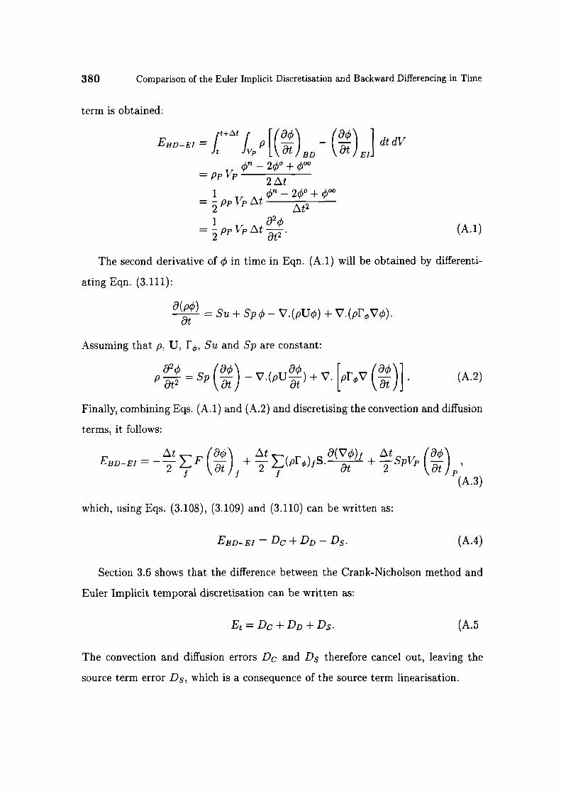
380 Comparison of the Euler Implicit Discretisation and Backward Differencing in Time
term is obtained:
t+t Ifa\ fa\ 1
EBD_EI - f I p I(I - \at) Eli
dt dV
i JVp L IBDqfl - 2° + q00
2zt
- __________--
- ppVpt 8
-- . (A.1)
The second derivative of qf in time in Eqn. (A.1) will be obtained by differenti-
ating Eqn. (3.111):
= Su + Sp - V.(pUq5) + V.(pFVq5).
Assuming that p, U, J', Su and Sp are constant:
(c9ç5\p = Sp - V.(pU) + V. [PFV ()].
(A.2)
Finally, combining Eqs. (A.1) and (A.2) and discretising the convection and diffusion
terms, it follows:
/EBD_E1 = - > F+ _ i (pF)fS.0 +
___ -(A.3)
which, using Eqs. (3.108), (3.109) and (3.110) can be written as:
EBD_EI - D + DD - D5 . (A.4)
Section 3.6 shows that the difference between the Crank-Nicholson method and
Euler Implicit temporal discretisation can be written as:
E = D + DD + D5 . (A.5
The convection and diffusion errors D and D therefore cancel out, leaving the
source term error D, which is a consequence of the source term linearisation.
Bibliography
[1] Ainsworth, M.: "A-posteriori error estimators for second-order elliptic sys-
tems: Part 1. Theoretical foundations and a-posteriori error analysis", Corn-
puters Math. Applic., 25(2):101-113, 1993.
[2] Ainsworth, M. and Oden, J. T.: "A procedure for a-posteriori error estimation
for h - p Finite Element methods", Comp. Meth. Appi. Mech. Engineering,
101:73 96, 1992.
[3] Ainsworth, M. and Oden, J. T.: "A-posteriori error estimators for second-
order elliptic systems: Part 2. An optimal order process for calculating self-
equilibrating fluxes", Computers Math. Applic., 26(9):75-87, 1993.
[4] Ainsworth, M. and Oden, J.T.: "A unified approach to a-posteriori error
estimation using Element Residual methods", Numerische Mat hematik, 65:23
50, 1993.
[5] Almeida, G.P., Durao, D.F.G., and Heitor, M.V.: "Wake flows behind two-
dimensional model hills", Experimental Thermal and Fluid Science, 7:87 101,
1993.
[6] Anderson, D.A.: "Adaptive grid methods for partial differential equations",
In Ghia, K.N. and Ghia, U., editors, Advances in grid generation. ASME, New
York, 1983.
[7] Aris, R.: Vectors, tensors and the basic equations of fluid mechanics: Dover
Publications, 1989.

382
Bibliography
[8] Babuka, I. and Rheinboldt, W.C.: "A-posteriori error estimates for the Finite
Element method", mt. J. Comp. Meth. Engineering, 12:1597 1615, 1978.
[9] Babuka, I. and Rheinboldt, W.C.: "Error estimates for adaptive Finite Ele-
ment calculations", SIAM J. Nurner. Analysis, 15(4):736 753, 1978.
[10] Babuka, I. and Rheinboldt, W.C.: "Reliable error estimation and mesh adap-
tation for the Finite Element method", In J.T., Oden, editor, Computational
Methods in Nonlinear Mechanics, pages 67-108. North Holland, New York,
1980.
[11] Bank, R.E.: "A-posteriori error estimates. Adaptive local mesh refinement
and multigrid iteration", In Lecture notes in mathematics, multigrid methods
II, pages 7 22. Springer Verlag, 1986.
[12] Bank, R.E. and Weiser, A.: "Some a-posteriori error estimators for elliptic
partial differential equations", Math. Comput., 44:283 301, 1985.
[13] Beam, R.M. and Warming, R.F.: "An implicit Finite-Difference algorithm for
hyperbolic system in conservation law form", J. Comp. Physics, 22:87 109,
1976.
[14] Beam, R.M. and Warming, R.F.: "An implicit factored scheme for the corn-
pressible Navier-Stokes equations", AIAA Journal, 16:393 402, 1978.
[15] Berge, M.J.: Adaptive mesh refinement for hyperbolic partial differential equa-
tions, PhD thesis, Department of Computer Science, Stanford University,
1982.
[16] Berger M J and Collela, P.: "Local adaptive mesh refinement for shock
hydrodynamics", J. Comp. Physics, 82:64 84, 1989.
[17] Berger, M. J. and Oliger, J.: "Adaptive mesh refinement for hyperbolic partial
differential equations", J. Comp. Physics, 53484 512, 1984.
Bibliography 383
[181 Berger, M.J.: "On conservation at grid interfaces", SIAM .1. Numer. Analysis,
24(5):967 984, 1987.
[19] Berger, M.J. and Jameson, A: "An adaptive multigrid method for the Euler
equations", Lecture Notes in Physics, 218:92 97, 1985.
[20] Boris, J.P. and Book, D.L.: "Flux-corrected transport. I. SHASTA, a fluid
transport algorithm that works", J. Comp. Physics, 11:38 69, 1973.
[21] Boussinesq, J.: "Théorie de l'écoulement tourbillant", Mem. par. div. Say.,
Paris, 23, 1877.
[22] Brandt, A.: "Multi-level adaptive solutions to boundary-value problems",
Math. Comp., 31:333, 1977.
[23] Caretto, L., Curr, R.M., and Spalding, D.B.: "Two numerical methods for
three-dimensional boundary layers", Comp. Methods Appi. Mech. Eng., 1:39,
1972.
[24] Caruso, S.: Adaptive grid techniques for fluid flow problems, PhD thesis,
Thermosciences Division, Department of Mechanical Engineering, Stanford
University, 1985.
[25] Caruso, S., Ferziger, J.H., and Oliger, J.: "Adaptive grid techniques for elliptic
flow problems", Technical Report TF-23, Thermosc. Div. Stanford University,
1985.
[26] Cebeci, T. and Smith, A.M.O.: Analysis of turbulent boundary layers: Aca-
demic Press, 1974.
[27] Chakravarthy, S.R. and Osher, S.: "High resolution application of the OSHER
upwind scheme for the Euler equation": AIAA Paper 83-1943, 1983.
[28] Chen, W.L., Lien, F.S., and Leschziner, M.Z.: "A local grid refinement scheme
within a multiblock structured-grid strategy for general flows", In 6th Int.
Symp. on CFD, Lake Tahoe, USA, September 1995.
384
Bibliography
[29] Chien, K.Y.: 'Predictions of chennel and boundary-layer flows with a low-
Reynolds-number turbulence model", AIAA Journal, 20:33 38, 1982.
[30] Choi, S.K., Nam, H.Y., and Cho, M.: "A comparison of higher-order bounded
convection schemes", Cornp. Meth. Appi. Mech. Engineering, 121:281 301,
1995.
[31] Coelho, P., Pereira, J.C.F., and Carvalho, M.G.: "Calculation of laminar
recirculating flows using a local non-staggered grid refinement system", mt.
J. Num. Meth. Fluids, 12(6):535 557, 1991.
[32] Courant, R., Friedrichs, K.O., and Lewy, H.: "Uber die partiellen differenzgle-
ichungen der matematishen Physik", Matematishe Annalen, 100:32 74, 1928.
[33] Courant, R., Isaacson, E., and Rees, M.: "On the solution of non-linear hy-
perbolic differential equation by finite differences", Comm. Pure Appi. Math.,
5:243, 1952.
[34] Dafa'Alla, A.D., Juntasaro, E., and Gibson, M.M.: "Calculation of oscillat-
ing boundary layers with the q - ( turbulence model", In 3rd International
Symposium on Engineering Turbulence Modelling and Measurements, Crete,
Greece, 1996.
[35] Dandekar, H.W., Hiavacek, V., and J., Degreve.: "An explicit 3D Finite-
Volume method for simulation of reactive flows using a hybrid moving
adaptive grid", Numerical Heat Transfer, part B, 24(1):1 29, 1993.
[36] Darwish, M.S.: 'A new high-resolution scheme based on the normalized van-
able formulation", Numerical Heat Transfer, part B 24353 371 1993.
[37] Darwish, M.S. and Moukalled, F.: "Normalized variable and space formulation
methodology for high-resolution schemes", Numerical Heat Transfer part B
26 1 • 79 96, 1994.
Bibliography 385
[38] Deardorff, J.W.: "A numerical study of three-dimensional turbulent channel
flow at large Reynolds numbers", J. Fluid Mechanics, 41(2):453 480, 1970.
[39] Demirdié, I., Perié, M., and Lilek, : "A colocated finite volume method
for predicting flows at all speeds", mt. J. Num. Meth. Fluids, 16:1029-1050,
1993.
[40] Demkowicz, L., Oden, J.T., Rachowicz, W., and Hardy, 0.: "Toward a univer-
sal h-p adaptive Finite Element strategy: Part 1: Constrained approximation
and data structure", Comp. Meth. Appi. Mech. Engineering, 77:79-112, 1989.
[41] Dwyer, H.A.: "Grid adaptation for problems in fluid dynamics", AIAA Jour-
nal, 22(12):1705-1712, December 1984.
[42] Emery, A.F.: "An evaluation of several differencing methods for inviscid fluid
flow problems", J. Comp. Physics, 2:306-331, 1968.
[43] "ERCOFTAC Workshop on Data Bases and testing of calculation Methods
for Turbulent Flows": 4th ERCOFTAC/IAHR Workshop of Refined Flow
Modelling, Karlsruhe, Germany, April 1995.
[44] Eswaran, V. and Pope, S.B.: "Direct numerical simulations of the turbulent
mixing of a passive scalar", Physics of Fluids, 31(3):506 520, 1988.
[45] Eswaran, V. and Pope, S.B.: "An examination of forcing in direct numerical
simulations of turbulence", Computers and Fluids, 16(3):257 278, 1988.
[46] Favre, A.: "Equations des gaz turbulents compressibles", J. de Mécanique,
4:361, 1965.
[47] Ferziger, J.H.: "Simulation of incompressible turbulent flows", J. Comp.
Physics, 69:1 48, 1987.
[48] Ferziger, J.H. and Perié, M.: Computational methods for fluid dynamics:
Springer Verlag, Berlin-New York, 1995.
386
Bibliography
[49] Gaskell, P.H. and Lau, A.K.C.: "Curvature-compensated convective trans-
port: SMART, a new boundedness-preserving transport algorithm", mt. J.
Num. Meth. Fluids, 8:617 641, 1988.
[50] Gentry, R.A., Martin, R.E., and B.J., Daly: "An Eulerian differencing method
for unsteady compressible flow problems", J. Comp. Physics, 1:87, 1966.
[51] Gibson, M.M. and Dafa'Alla, A.D.: "Two-equation model for turbulent wall
flow", AIAA Journal, 33(8):1514 1518, 1995.
[52] Girault, V. and Raviart, P.-A.: Finite Element methods for Navier-
Stokes equations, volume 5 of Springer series in computational mathematics:
Springer-Verlag, 1986.
[53] Givi, P.: "Model-free simulations of turbulent reactive flows", Prog. Energy
Combust. Sci., 15:1 107, 1989.
[54] Gosman. A.D. and Ideriah, H.J.K.: "TEACH-2e: A general computer pro-
gram for two-dimensional turbulent recirculating flows", Technical report, Flu-
ids Section, Department of Mechanical Engineering, Imperial College, London,
1983.
[55] Gosman. A.D. and Lai, K.Y.: "Finite Difference and other approximations
for the transport and Navier-Stokes equations", In Proc JAHR Symposium on
Refined Modelling of Fluid Flows, 1982.
[56] Hanjali, K. and Launder, B.E.: "A Reynolds stress model of turbulence and
its application to thin shear layer flows", J. Fluid Mechan cs, 52:609, 1972.
57 Harlow, F H and Nakayama, P.: 'Transport of turbulence energy decay rate',
Technical Report Report LA 3854, Los Alamos National Laboratory, 1968
[58] Harten, A.: "High resolution schemes for hyperbolic conservation laws", J.
Cornp. Phys Cs, 49.357 393, 1983.
Bibliography 387
[59] Harten, A.: "On a class of high resolution total variation stable Finite Differ-
ence schemes", SIAM J. Numer. Analysis, 31:1 23, 1984.
[60] Hawken, D.F., Gottlieb, J.J., and Hansen, J.S.: "Review of some adaptive
node-movement techniques in Finite-Element and Finite-Difference solutions
of partial differential equation", J. Comp. Physics, 95:254 302, 1991.
[61] Haworth, D C., El Tahry, S.H., and Huebler, M.S.: "A global approach to
error estimation and physical diagnostics in multidimensional fluid dynamics",
Int. J. Numer. Meth. Fluids, 17(1):75 97, 1993.
[62] Helf, C. and Küster, U.: "A Finite Volume method with arbitrary polygonal
conro1 volumes and high order reconstruction for the Euler equations", In
Wagner, S., Hirschel, E.H., Périaux, J., and Piva, R., editors, Computational
Fluid Dynamics, pages 234 238. J. Wiley and Sons, September 1994.
[63] Hestens, M.R. and Steifel, E.L.: "Method of conjugate gradients for solving
linear systems", Journal of Research, 29:409 436, 1952.
[64] Hinze, J.O.: Turbulence: McGraw-Hill, 1975.
[65] Hirsch, C.: Numerical computation of internal and external flows: John
Willey & Sons, 1991.
[66] Issa, R.I.: "Solution of the implicitly discretized fluid flow equations by
operator-splitting", J. Comp. Physics, 62:40 65, 1986.
[67] Jacobs, D.A.H.: "Preconditioned Conjugate Gradient methods for solving
systems of algebraic equations": Central Electricity Research Laboratories,
1980.
[68] Jameson, A., Schmidt, W., and Turkel, E.: "Numerical simulation of the
Euler equations by Finite Volume methods using Runge-Kutta time stepping
schemes": AIAA Paper 81-1259, 1981.
388
Bibliography
[69] Jasak, H. and Weller, H.G.:
"Interface-tracking capabilities of the In-
terGamma differencing scheme", Internal Report, CFD research group, Tm-
penal College, London, February 1995.
[70] Kallinderis, Y. and Vidwans, A.: "Generic parallel adaptive-grid Navier-
Stokes algorithm", AIAA Journal, 32 1):54 61, 1994.
[71] Kelly, D.W.: "The self-equilibration of residuals and complementary a pos-
tenon error estimates in the Finite Element method", mt. J. Num. Meth.
Engineering, 20:1491 1506, 1984.
[72] Kern, T.: Fehierkontrole für hyperbolisehe Dzfferentialgleichungen und
Navier-Stokes Gleichungen, PhD thesis, Mathematischen Fakultät der Albert-
Ludwigs- Universität Freiburg i.Br., 1993.
[73] Khosla, P.K. and Rubin, S.G.: "A diagonally dominant second-order accurate
implicit scheme", Computers and Fluids, 2:207 209, 1974.
[74] Lam, C.K.G. and Bremhorst, K.A.: "Modified form of the k - c model for
predicting wall turbulence", J. Fluids Engineering, 103:456 460, 1981.
[75] Launder, B.E., Reece, G.J., and Rodi, W.: "Progress in the development of a
Reynolds-stress turbulence closure", J. Fluid Mechanics, 68(3):537 566, 1975.
[76] Launder, B.E. and Sharma, B.I.: "Application of the energy-dissipation model
of turbulence to the calculation of a flow near a spinning disk", Letters in Heat
and Mass Transfer, 1:131 138, 1974.
[77] Launder, B.E. and Spalding, D.B.: "The numerical computation of turbulent
flows", Cornp. Meth. Appi. Mech. Engineering, 3:269 289, 1974.
[78] Lax, P.D.: "Weak solutions of non-linear hyperbolic equations and their nu-
merical computation", Comm. Pure Appi. Math, 7:159 193, 1954
[79 Lax, P.D. and endroff, B.: "S ystems of conservation laws" Comm Pu e
Appi. Math., 13:217 237, 1960.

Bibliography 389
[80] LeHuuNho, E. and Béguier, C.: "Experimental study of the flow over a swept
backward-facing step", to be submitted to the AIAA Journal.
[81] Leonard, B.P.: "A stable and accurate convective modelling procedure based
on quadratic upstream interpolation", Cornp. Meth. Appi. Mech. Engineering,
19:59-98, 1979.
[821 Leonard, B.P.: "Simple high-accuracy resolution program for convective mod-
eling of discontinuities", mt. J. Num. Meth. Fluids, 8:1291 1318, 1988.
[83] Leonard, B.P.: "The ULTIMATE conservative difference scheme applied to
unsteady one-dimensional advection", Comp. Meth. Appl. Mech. Engineering,
88:17-74, 1991.
[84] Lerat, A.: "Implicit methods of second order accuracy for Euler equation&',
AIAA Journal, 23:33 40, 1983.
[85] Lerat, A. and Peyret, R.: "Non-centered schemes and shock propagation
problems", Computers and Fluids, 2:35 52, 1974.
[86] Leschziner, M.Z.: Private communication, 1995.
[87] Lien, F.S. and Leschziner, M.A.: "Upstream monotonic interpolation for
scalar transport with application to complex turbulent flows", mt. J. Num.
Meth. Fluids, 19:527 548, 1994.
[881 Lilek, . and Perié, M.: "A fourth-order Finite Volume method with colocated
variable arrangement", Computers and Fluids, 24(3):239-252, 1995.
[89] Löhner, R.: "An adaptive Finite Element scheme for transient problems in
CFD", Comp. Meth. Appi. Mech. Engineering, 61:323 338, 1987.
[90] MacCormack, R.W.: "The effect of viscosity in hypervelocity impact crater-
ing": AIAA Paper 69-354, 1969.
[91] MacCormack, R.W.: "A numerical method for solving the equations of corn-
pressible viscous flow": AIAA Paper 81-0110, 1981.
390
Bibliography
[92] McGuirk, J.J. and Rodi, W.: "A depth-averaged mathematical model for
the near field of side discharges into open channel flow", J. Fluid Mechanics,
86:761, 1978.
[93] McGuirk, J.J., Taylor, A.M.P.K., and Whitelaw, J.H.: "The assessment of
numerical diffusion in the upwind-difference calculations of turbulent recircu-
lating flows", In Bradbury, L.J.S., Durst, F., Launder, B.E., Schmidt, F.W.,
and Whitelaw, J.H., editors, Selected papers from the Third International Sym-
posium on Turbulens Shear Flows, volume 3 of Turbulent Shear Flows, pages
206 224, The University of California, Davis, September 9-11 1981.
[94] Métais, 0. and Lesieur, M.: "Spectral large-eddy simulation of isotropic and
stably stratified turbulence", J. Fluid Mech., 239:157 194, 1992.
[95] Mom, P. and Kim, J.: "Numerical investigation of turbulent channel flow",
J. Fluid Mechanics, 118:341 377, 1982.
[96] Moinat, P. and Lesieur, M.: "Large-eddy simulations of turbulent flows over a
swept backward-facing step", Technical report, Laboratoire des Ecoulements
Géophysiques et Industriels - Institut de Méchanique de Grenoble, 1995.
[97] Muzaferija, S.: Adaptive Finite Volume method for flow prediction using Un-
structured meshes and multigrid approach, PhD thesis, Imperial College, Uni-
versity of London, 1994.
[98] Oden, J.T., Demkowicz, L., Rachowicz, W., and Westermann, T.A.: "Toward
a universal h - p adaptive Finite Element strategy: Part 2: A posteriori error
estimation", Comp Meth. Appi. Mech. Engneerzng, 77:113 180, 1989.
[99] Oden, J.T., Demk wi z, L., Str ubolis, T., and Deloo, P.: "Adaptive meth-
ods for problems in solid and fluid mechanics", In Babuka, I., Zienkiewicz,
0.C., de Gago, S.R., and de Oliveira, A., editors, Adaptive Methods and Error
Refinement in Finite Element Calculations. John Willey & Sons 1986.
Bibliography 391
[100] Oden, J.T., Stroubolis, T., and Devloo, P.: "Adaptive Finite Element
methods for the analysis of inviscid compressible flow: Part 1: Fast re-
finement/unrefinement and moving mesh methods for unstructured meshes",
Comp. Meth. Appi. Mech. Engineering, 59:327 362, 1986.
[1011 Oden, J.T., Wu, W., and Ainsworth, M.: "An a-posteriori error estimate for
Finite Element approximations of the Navier-Stokes equations", Comp. Meth.
Appi. Mech. Engineering, 111:185 202, 1994.
[102] Oden, J.T., Wu, W., and Legat, V.: "An h - p adaptive strategy for Finite
Element approximations of the Navier-Stokes equations", mt. J. Num. Meth.
Fluids, 20:831-851, 1995.
[103] Osher, S. and Chakravarthy, S.R.: "High resolution sthemes and the entropy
condition", SIAM J. Numer. Analysis, 21(5):955 984, 1984.
[104] Panton, R.L.: Incompressible flow: John Wiley and Sons, 1984.
[105] Patankar, S.V.: Numerical heat transfer and fluid flow: Hemisphere Publish-
ing Corporation, 1981.
[106] Patankar, S.V. and Baliga, B.R.: "A new Finite-Difference scheme for
parabolic differential equations", Numerical Heat Transfer, 1:27, 1978.
[107] Patankar, S.V. and Spalding, D.B.: "A calculation procedure for heat, mass
and momentum transfer in three-dimensional parabolic flows", mt. J. Heat
Mass Transfer, 15:1787, 1972.
[108] Patel, V.C., Rodi, W., and Scheurer, G.: "Turbulence models for near-wall
and low Reynolds number flows: a review", AIAA Journal, 23:1308 1319,
1985.
[109] Perié, M.: A Finite Volume method for the prediction of three-dimensional
fluid flow in complex ducts, PhD thesis, Imperial College, University of Lon-
don, 1985.
392
Bibliography
[110] Phillips, R.E: A multilevel rnultigrid method for recirculating flows, PhD the-
sis, Pennsylvania State University, 1984.
[111] Rachowicz, W., Oden, J.T., and Demkowicz, L.: "Toward a universal h - p
adaptive Finite Element strategy: Part 3: Design of h - p meshes", Comp.
Meth. Appi. Mech. Engineering, 77:181 212, 1989.
[112] Raithby, G.D.: "A critical evaluation of upstream differencing applied to
problems involving fluid flow", Comp. Meth. Appi. Mech. Engineering, 9:75
103, 1976.
[113] Raithby, G.D.: "Skew-upstream differencing schemes for problems involving
fluid flow", Comp. Meth. Appi. Mech. Enginfering, 9:153 164, 1976.
[114] Raithby, G.D. and Torrance, K.E.: "Upstream-weighted schemes and their
application to elliptic problems involving fluid flow", Computers and Fluids,
2:191 206, 1.974.
[115] Ramakrishnan, R.: "Structured and unstructured grid adaptation schemes
for numerical modelling of field problems", Appi. Numer. Mathematics, 14(1-
3):285 310, 1994.
[116] Ramakrishnan, R., Bey, K.S., and Thornton, E.A.: "Adaptive quadrilateral
and triangular Finite Element scheme for compressible flows", AIAA Journal,
28 1):51 59, January 1990.
[117] Rhie, C.M. and Chow, W.L.: "A numerical study of the turbulent flow past an
isolated airfoil with trailing edge separation": AIAA-82-0998, AIAA/ASME
3rd Joint Thermophysics, Fluids, Plasma and Heat Transfer Conference, St.
Louis, Missouri, 1982.
[118] Roe, P L "Large scale computati ns in fluid mechanics, Part 2", In Lectu es
in Applied Mathemat cs, volume 22, pages 163 193. Springer Verlag, 1985.

Bibliography 393
[119] Rogallo, R.S. and Mom, P.: "Numerical simulation of turbulent flows", Annual
Review of Fluid Mechanics, 16:99 137, 1984.
[120] Rogers, M.M. and Mom, P.: "The structure of the vorticity field in homoge-
neous turbulent flows", J. Fluid Mechanics, 176:33 66, March 1987,.
[121] Rotta, J.C.: "Statistiche Theorie nichthomogener Turbulenz", Z. Phys.,
129:547, 1951.
[122] Sharif, M.A.R. and Busnaina, A.A.: "Evaluation and comparison of bound-
ing techniques for convection-diffusion problems", J. Fluids Engineering-
Transactions of the ASME, 115(1):33-40, 1993.
[123] Shih, T.H., Liou, W.W, Shabir, A., Yang, Z., and Zhu, J.: "A new k -
eddy viscosity model for high Reynolds number turbulent flows": NASA TM
106721, 1994.
[124] Simpson, R.B.: "Automatic local refinement for irregular rectangular meshes",
Technical report, Department of Computer Science, University of Waterloo,
1978.
[125] Sonar, T., Hannemann, V., and Hempel, D.: "Dynamic adaptivity and resid-
ual control in unsteady compressible flow computation", Mathematical and
Computer Modelling, 20(10-11):201 213, 1994.
[126] Spalding, D.B.: "A novel Finite-Difference formulation for differential ex-
pression involving both first and second derivatives", mt. J. Comp. Meth.
Engineering, 4:551, 1972.
[127] Speziale, C.G.: "On non-linear k - 1 and k - models of turbulence", J. Fluid
Mechanics, 178:459-475, 1987.
[128] "STAR-CD Version 2.1 - Manuals": Computational Dynamics Limited, 1991.
[129] Sweby, P.K.: "High resolution schemes using flux limiters for hyperbolic con-
servation laws", SIAM J. Numer. Analysis, 21:995 1011, 1984.

394
Bibliography
[130] Tattersall, P. and McGuirk, J.J.: "Evaluation of numerical diffusion effects in
viscous flow calculations", Computers and Fluids, 23(1):177 209, 1994.
[1311 Temam, R.: Navier-Stokes equations: Theory and numerical analysis: North-
Holland, Amsterdam, 2nd edition, 1985.
[132] Tennekes, H. and J.L., Lumley: A first course in turbulence: The MIT Press,
1972.
[133] Thompson, J.F.: "A survey of dynamically-adaptive grids in the numerical
solution of partial differential equations", Appi. Numer. Mathematics, 1(1):3
27, 1985.
[134] Thompson. M.C. and Ferziger, J.H.: "An adaptive multigrid technique for the
incompressible Navier-Stokes equations", J. Comp. Physics, 82:94 121, 1989.
[135] Uslu, S.: Numerical prediction of transonic flow in turbine blade passages,
PhD thesis, Imperial College, University of London, 1994.
[136] Van Der Vorst, H.A.: "Bi-CGSTAB: A fast and smoothly converging variant
of Bi-CG for the solution of nonsymmetric linear systems", SIAM J. Scientific
Computing, 13(2 :631-644, 1992.
[137] Van Doormaal, J.P. and Raithby, G.D.: "An evaluation of the segregated
approach for predicting incompressible fluid flows", In National Heat Transfer
Conference, Denver, Colorado, August 4-7 1985.
[138] Van Leer, B.: "Towards the ultimate conservative differencing scheme", In
Cabannes, H. and Temem, R., editors, Proceedings of the Third International
Conference on Numerical Methods in Fluid Mechanics, volume 1, pages 163
168. Springer, 1973.
[139] Van Leer, B.: "Towards the ultimate conservative differencing scheme. II
Monotonicity and conservation combined in a second-order scheme", J Comp.
Physics, 14:361 370, 1974.
Bibliography 395
[140] Van Leer, B.: "Towards the ultimate conservative differencing scheme. III.
Upstream-centered finite-difference schemes for ideal compressible flow", J.
Comp. Physics, 23:263 275, 1977.
[141] Van Leer, B.: "Towards the ultimate conservative differencing scheme. IV. A
new approach to numerical convection", J. Comp. Physics, 23:276 299, 1977.
[142] Van Leer, B.: "Towards the ultimate conservative differencing scheme V: A
second-order sequel to Godunov's method", J. Comp. Physics, 23:101-136,
1977.
[143] Vanka, S.P.: "Block-implicit multigrid solution of Navier-Stokes equations in
primitive variables", J. Comp. Physics, 65:138-158, 1986.
[144] Vidwans, A. and Kallinderis, Y.: "A 3-D Finite-Volume scheme for the Euler
equations on adaptive tetrahedral grids", J. Camp. Physics, 113(2):249-267,
1994.
[145] Vilsmeier, R. and Hand, D.: "Adaptive methods on unstructured grids for
Euler and Navier-Stokes equations", Computers and Fluids, 22(4-5):485 499,
1993.
[146] Warming, R.F. and Beam, R.M.: "Upwind second order difference schemes
and applications in aerodynamic flows", AIAA Journal, 14:1241-1249, 1976.
[147] Weller, H.G.: Private communication, 1993.
[148] Wong, H.H. and Raithby, G.D.: "Improved Finite-Difference methods based
on a critical evaluation of the approximating errors", Numerical Heat Transfer,
2:131, 1979.
[149] Woodward, P. and Colella, P.: "The numerical simulation of two-dimensional
fluid flow with strong shocks", J. Comp. Physics, 54:115 173, 1984.
[150] Yakhot, V. and Orszag: "Renormalisation group analysis of turbulence. I.
Basic theory", SIAM J. Scientific Computing, 1:3 51, 1986.

396
Bibliography
[151] Yakhot, V., Orszag, S.A., Thangam, S., Gatski, T.B., and Speziale, C.G.:
"Development of turbulence models for shear flows by a double expansion
technique", Phys cs of Fluids, 4(7):1510 1520, July 1992.
[152] Zalesak, S.T.: "Fully multidimensional flux-corrected transport algorithms
for fluids", J. Comp. Physics, 31:335 362, 1979.
[153] Zhu, J.: "A low-diffusive and oscillation-free scheme", Communications in
Applied Numerical Methods, 7:225 232, 1991.
[154] Zhu, J.: "On the higher-order bounded discretisation schemes for Finite Vol-
ume computations of incompressible flows", Comp. Methods Appi. Mech. En-
gineering. 98:345 360, 1992.
[155] Zhu, J. and Rodi, W.: "A low dispersion and bounded convection scheme",
Cornp. Methods Appi. Mech. Eng., 92:87 96, 1991.
[156] Zienkiewicz, 0. C. and Taylor, R. L.: The Finite Element method, vol 1:
Basic formulation and linear problems: McGraw-Hill, 4th edition, 1989.
Copyright © 2022 FDOKUMEN