LLevera

i

Institute

age an

in Fini

Andre

for Emp

Univ

Work

IS

Worki

d Cov

ite‐Sam

eas Steinh

De

pirical Res

versity of

king Pape

SSN 1424‐

ing Paper

arianc

mple I

hauer and

ecember

search in

f Zurich

er Series

‐0459

r No. 521

ce Mat

V Reg

d Tobias W

2010

Economi

rix Est

gressio

Wuergler

ics

timatio

ons

r

on

Leverage and Covariance Matrix Estimation

in Finite-Sample IV Regressions

Andreas Steinhauer, University of Zurich∗ Tobias Wuergler, University of Zurich†‡

December 15, 2010

Abstract

This paper develops basic algebraic concepts for instrumental variables (IV) regressions

which are used to derive the leverage and influence of observations on the 2SLS estimate

and compute alternative heteroskedasticity-consistent (HC1, HC2 and HC3) estimators

for the 2SLS covariance matrix in a finite-sample context. Monte Carlo simulations and

applications to growth regressions are used to evaluate the performance of these estimators.

The results support the use of HC3 instead of White’s robust standard errors in small and

unbalanced data sets. The leverage and influence of observations can be examined with

the various measures derived in the paper.

JEL Classification: C12, C26

Keywords: Two stage least squares, leverage, influence, heteroskedasticity-consistent

covariance matrix estimation

∗University of Zurich, Institute for Empirical Research in Economics, Muehlebachstrasse 86, CH-8008 Zurich,

e-mail: steinhauer@iew.uzh.ch†University of Zurich, Institute for Empirical Research in Economics, Muehlebachstrasse 86, CH-8008 Zurich,

e-mail: wuergler@iew.uzh.ch‡We thank Michael Wolf for extensive comments, Joshua Angrist, A. Colin Cameron, Andreas Kuhn, Rafael

Lalive, Jorn-Steffen Pischke, Kevin Staub, Steven Stern and Jean-Philippe Wuellrich as well as seminar partic-

ipants in Lausanne and Zurich for valuable input.

1

1 Introduction

The implication of heteroskedasticity for inference based on OLS in the linear regression model

has been extensively studied. If the form of heteroskedasticity is known, generalized least

squares techniques can be performed, restoring the desirable finite-sample properties of the

classical model. In practice the exact form is rarely known and the famous robust estimator

presented by White (1980) is widely used to generate consistent estimates of the covariance

matrix (see also Eicker, 1963). However, the sample size is required to be sufficiently large

for this estimator to make valid inference. In a finite-sample context using Monte Carlo

experiments, MacKinnon andWhite (1985) demonstrated the limits of the robust estimator and

studied several alternative heteroskedasticity-consistent estimators with improved properties

(known as HC1, HC2 and HC3 standard errors as opposed to ”HC0” standard errors due to

White and Eicker). While HC1 incorporates a simple degrees of freedom correction, HC2 (due

to Horn, Horn and Duncan, 1975, and Hinkley, 1977) and HC3 (the jackknife estimator, see

Efron, 1982) aim to control explicitly for the influence of high leverage observations.

In the instrumental variables (IV) and generalized method of moments (GMM) literature

heteroskedasticity has been addressed (e.g. White, 1982, Hansen, 1982). It is common practice

to use White’s robust (HC0) standard errors which are consistent and valid in large samples.

However, while biasedness of IV estimators in finite samples has received wide attention (e.g.

Nelson and Startz, 1990a,b, Buse, 1992, Bekker, 1994, Bound, Jaeger, and Baker, 1995), the

small-sample properties of heteroskedasticity-consistent covariance estimators in IV regressions

have not been studied explicitly so far to the best of our knowledge. As it is possible to extend

the alternative forms of heteroskedasticity-consistent covariance matrix estimators from an

OLS to an IV environment, the present paper develops such estimators and evaluates them

with Monte Carlo experiments and an application to growth regressions.

We base our main results on the two-stage least squares (2SLS) approach to IV/GMM

estimation of single equation linear models. 2SLS is equivalent to other IV/GMM methods

2

in the exactly identified case, and serves as a natural benchmark in the overidentified case

as it is the efficient GMM estimator under conditional homoskedasticity (analogously to HC1

and HC2 standard errors for OLS being based on properties derived under homoskedasticity).

Moreover, it has been shown that the efficient GMM coefficient estimator has poor small-

sample properties as it requires the estimation of fourth moments, and that approaches like

2SLS or using the identity matrix as weighting matrix are superior in smaller samples (see July

1996 issue of the Journal of Business and Economic Statistics). Finally and most importantly,

the 2SLS approach is widely used in empirical research.

In the first part of the paper, the robust covariance matrix estimators are derived. We ana-

lyze the hat and residual maker matrix in 2SLS regressions and extend the Frisch-Waugh-Lovell

theorem for OLS (Frisch and Waugh, 1933, Lovell, 1963) to 2SLS. We then use these algebraic

properties to derive explicit expressions for the leverage and influence of single observations

on the 2SLS estimate. These measures are valuable tools on their own as they can be used

to perform influential diagnostics in IV regressions. Finally and most importantly, we demon-

strate that, analogous to the case of OLS, the leverage of single observations is intrinsically

linked to the problem of heteroskedasticity-consistent covariance estimation in finite-sample

IV regressions, and compute the alternative forms of robust estimators for 2SLS.

In the second part, the performance of the various covariance matrix estimators is evaluated

in Monte Carlo simulations as well as in growth regressions involving instrumental variables.

We begin with the simplest case of one (endogenous) regressor and one instrument, paramet-

rically generating data, simulating and computing the conventional non-robust as well as the

robust HC0-3 standard errors. We compare size distortions and other measures in various

parameterizations of the model with different degrees of conditional heteroskedasticity across

different sample sizes. We then analyze further specifications, changing the number of instru-

ments as well as the data generating process. Finally, we re-examine two well-known growth

regression studies of Persson and Tabellini (1994) and Acemoglu, Johnson and Robinson (2001)

which use countries as units of observations, so they are naturally subject to smaller sample

3

issues and consequently well suited to illustrate the derived concepts.

The Monte Carlo simulations show that similar to OLS the size distortions in tests based

on White’s robust (HC0) standard errors may be substantial. Empirical rejection rates may

exceed nominal rates by a great margin depending on the design. HC1-3 estimators mitigate

the problem with HC3 performing the best, bringing down the distortion substantially. HC3

standard errors have the further advantage of working relatively well both in a homoskedas-

tic and in a heteroskedastic environment as opposed to conventional non-robust and White’s

robust (HC0) standard errors. These results highlight the importance of computing and an-

alyzing leverage measures as well as alternative covariance matrix estimators especially when

performing IV regressions with smaller and less balanced data sets.

The application of the HC1-3 covariance matrix estimators to the two growth regression

studies mentioned above demonstrates that results without adjustments to robust standard

errors may indicate too high a precision of the estimation if the sample size is small and the

design unbalanced. In the presence of influential observations as in one specification of the

study of Persson and Tabellini (1994), the p-value may be substantially higher if the HC3

standard error estimator is used. On the other hand, in a relatively balanced design as the

one of Acemoglu, Johnson and Robinson (2001) where no single observation is of particular

influence, the use of HC3 does barely affect inference.

The paper is organized as follows: Section 2 provides an overview of the issue of covariance

matrix estimation in the presence of heteroskedasticity in 2SLS regressions. Section 3 derives

the basic algebraic concepts for 2SLS regressions which are used to compute the leverage and

influence of observations on the 2SLS estimate. Building on these concepts, Section 4 computes

the various forms of heteroskedasticity-consistent covariance matrix estimators. In Section 5,

we describe and present the results of Monte Carlo experiments to examine and compare the

performance of the alternative estimators. Section 6 applies the developed diagnostics and

standard error estimators to two growth regression studies. Section 7 concludes.

4

2 The Model and Covariance Matrix Estimation

Consider estimation of the model

y = Xβ + ε,

where y is a (n× 1) vector of observations of the dependent variable, X is a (n× L) matrix of

observations of regressors, and ε is a (n× 1) vector of the unobservable error terms. Suppose

that some of the regressors are endogenous, but there is a (n×K) matrix of instruments Z

(including exogenous regressors) which are predetermined in the sense of E(Z ′ε) = 0, and the

K × L matrix E(Z ′X) is of full column rank. Furthermore, suppose that yi, xi, zi is jointly

ergodic and stationary, zi · εi is a martingale difference sequence, and E[(zikxil)

2]exists and

is finite.

Under these assumptions the efficient GMM estimator

βGMM =(X ′Z(Z ′ΩZ)−1Z ′X

)−1X ′Z(Z ′ΩZ)−1Z ′y

is consistent, asymptotically normal and efficient among linear GMM estimators, where Ω ≡

diag(ε21, ε

22, ..., ε

2n

)is an estimate of the covariance matrix of the error terms Ω (see for example

Hayashi, 2000). As mentioned in the Introduction, however, it has been shown that GMM

estimators which do not require the estimation of fourth moments (Z ′ΩZ) tend to be superior

in terms of bias and variance in smaller samples. One such estimator which is widely used in

applied research is the 2SLS estimator,

β ≡ β2SLS = (X ′PX)−1X ′Py,

where P = Z(Z ′Z)−1Z ′ is the projection matrix associated with the instruments Z. The 2SLS

estimator is the efficient GMM estimator under conditional homoskedasticity (E(ε2i | zi

)= σ2).

Even if the assumption of conditional homoskedasticity cannot be made, 2SLS still is consistent

although not necessarily efficient since it is a GMM estimator with (Z ′Z)−1 as weighting matrix.

If one cannot assume conditional homoskedastictiy, the asymptotic estimator of the covariance

matrix is given by

V arHC0(β) = (X ′PX)−1X ′P ΩPX(X ′PX)−1,

5

which is White’s robust estimator also known as HC0 (heteroskedasticity-consistent). Unlike

the 2SLS coefficient estimator, the corresponding HC0 covariance matrix estimator requires

fourth moment estimation which lies at the heart of the issues studied here. Although being

valid in large samples, the HC0 estimator does not account for the fact that residuals tend to

be too small (in absolute value) and distorted in finite samples.

Robust estimators such as HC0 require the estimation of each diagonal element ωi =

V ar(εi). HC0 plugs in the squared residuals from the 2SLS regression, ωi = ε2i with εi ≡

yi − x′iβ. It is well known from OLS that these estimates tend to underestimate the true

variance of εi in finite samples since least square procedures choose the residuals such that the

sum of squared residuals is minimized. It is most apparent for influential observations which

”pull” the regression line toward itself and thereby make their residuals ”too small”. Since

the influence of any single observation vanishes (under the assumptions stated above), HC0

is asymptotically valid. But in small samples, using the simple HC0 estimator tends to lead

to (additional) bias in covariance matrix estimation. For OLS regressions, a set of alternative

covariance estimators with improved finite sample properties is available (MacKinnon and

White, 1985) with HC1 using a simple degrees of freedom correction and HC2 as well as HC3

aiming to control explicitly for the influence of observations.

In the case of 2SLS regressions, the issue is similar but involves two stages. An observation

affects the regression line in the first stage and in the reduced form. The effect on the residual

of the observation is ambiguous. In contrast to OLS, an observation might not pull the 2SLS

regression line toward itself but push it away through the combined effect of the two stages.

The next section derives and studies leverage and influence of observations before moving to

the computation and interpretation of the various HC covariance matrix estimators in 2SLS

regressions.

6

3 2SLS Leverage and Influence

We first compute the 2SLS hat and residual maker matrix whose diagonal elements play a

central role for the leverage of an observation. Then, the Frisch-Waugh-Lovell theorem is

extended to 2SLS regressions and used to derive the leverage and influence of observations.

3.1 2SLS Hat and Residual Maker Matrix

The fitted values of a 2SLS regression are given by

y = Xβ = X(X ′PX)−1X ′Py ≡ Qy,

where Q is defined as the 2SLS hat matrix. The 2SLS hat matrix involves both the regressorsX

and the conventional projection (hat) matrix P = Z(Z ′Z)−1Z ′ associated with the instruments

Z. The residuals are given by

ε = y −Xβ = (I −Q) y ≡ Ny,

= NXβ +Nε = Nε,

where N is defined as the 2SLS residual maker matrix.

It is easy to verify that the 2SLS hat and residual maker matrix are idempotent but not

symmetric like their OLS counterparts:

Q = X(X ′PX)−1X ′P, N = I −Q,

Q′ = PX(X ′PX)−1X ′, N ′ = I −Q′,

QQ′ = X(X ′PX)−1X ′, NN ′ = I − PX(X ′PX)−1X ′P = I − Q,

where we have defined Q ≡ PX(X ′PX)−1X ′P . While the 2SLS hat matrix self-projects and

the residual maker matrix annihilates X, the transposed 2SLS hat matrix self-projects and

the transposed residual maker matrix annihilates PX. The products of the matrices in the

last line are used to compute covariance matrices (for fixed regressors and instruments) of the

7

fitted values and residuals under conditional homoskedasticity:

V ar (y) = V ar(Qy) = QV ar(y)Q′ = σ2 ·QQ′,

V ar (ε) = V ar(Nε) = NV ar(ε)N ′ = σ2 ·NN ′ = σ2 · (I − Q). (1)

Note that these matrices simplify in the exactly identified case of K = L since Z ′X is a

square matrix, Q = X(Z ′X)−1Z ′ and Q = P , where P is the conventional projection matrix

of the instruments.

3.2 A Frisch-Waugh-Lovell Theorem for 2SLS

Split the instruments into two groups, Z = (Z1...Z2), where Z2 are predetermined regressors,

and rewrite the regression equation as

y = X1β1 + Z2β2 + ε. (2)

The normal equations are split accordingly,

Z ′1X1β1 + Z ′

1Z2β2 = Z ′1y, and Z ′

2X1β1 + Z ′2Z2β2 = Z ′

2y.

Premultiply the first group of equations by Z1(Z′1Z1)

−1,

P1X1β1 + P1Z2β2 = P1y,

where P1 = Z1(Z′1Z1)

−1Z ′1 is the conventional (OLS) projection matrix associated with the

first group of instruments Z1. Next, use the 2SLS hat matrix associated with X1 and Z1,

Q1 = X1(X′1P1X1)

−1X ′1P1, and premultiply again,

X1β1 +Q1Z2β2 = Q1y,

since P1 is idempotent, and plug X1β1 into the second group of normal equations,

Z ′2

(−Q1Z2β2 +Q1y

)+ Z ′

2Z2β2 = Z ′2y,

which yields

β2 =(Z ′2N1Z2

)−1Z ′2N1y,

where N1 is the 2SLS residual maker matrix associated with X1 and Z1. As a result, we have

8

Theorem 1 The 2SLS estimate of β2 from regression (2) with Z as instruments is numerically

identical to the 2SLS estimate of β2 from regression

N1y = N1Z2β2 + errors

with Z2 as instruments.

Proof. Since the normal equation

Z ′2N1Z2β2 = Z ′

2N1y

is exactly identified and Z ′2N1Z2 is a square matrix, respectively, we can solve for β2 by pre-

multiplying with the inverse, proofing that the two estimates for β2 are indeed numerically

identical.

With this Frisch-Waugh-Lovell (FWL) theorem for 2SLS at hand, we are now set to com-

pute the influence of single observations.

3.3 2SLS Leverage and Influential Analysis

The influence of an observation i on the 2SLS estimate β can be measured as the difference of

the estimate omitting the i-th observation β(i)

and the original estimate. Instead of running a

separate 2SLS regression on a sample with the observation dropped, one can derive a closed-

form expression for the difference by including a dummy variable for the i-th observation di

and applying the FWL theorem,1

y = Xβ + αdi + ε

with instruments (Z...di), and E[(Z

...di)′ε] = 0.2 Use the 2SLS hat and residual maker matrix

associated with (X...di) and (Z

...di), QD and ND, to express the regression as

y = QDy +NDy = Xβ(i)

+ αdi +NDy.

1See Davidson and MacKinnon (2004) for the case of OLS.2E [d′iε] = 0 since any element of the vector ε has zero expectation.

9

Premultiply with the regular 2SLS hat matrix Q,

Qy = Xβ(i)

+Qαdi,

as the transposed 2SLS residual maker annihilates PX, N ′DQ

′ = 0L, cancelling out the residual.

Since Qy = Xβ, we can rewrite the equation as

X(β(i)

− β) = −Qαdi.

Applying the FWL theorem for 2SLS, the estimate of α from the full 2SLS regression is

numerically equivalent to running the 2SLS regression

Ny = Ndiα+ errors

with di as instrument, which yields

α =d′iNy

d′iNdi=

εi1− qi

,

where qi is defined as the ith diagonal element of the original 2SLS hat matrix Q. Plug this

expression into the equation,

X(β(i)

− β) = −Qεi

1− qidi,

and premultiply with (X ′PX)−1X ′P to obtain the change of the coefficient due to observation

i,

β(i)

− β = −εi

1− qi

(X ′PX

)−1X ′Pdi = −

εi1− qi

(X ′PX

)−1X ′Z(Z ′Z)−1zi. (3)

This measure looks similar to the one of OLS,3 but the leverage of observation i,

qi = x′i(X′PX)−1X ′Z(Z ′Z)−1zi,

is the diagonal element of the 2SLS hat matrix Q. The influence of an observation depends

on both the residual εi and the leverage qi of the observation. The higher they are, the more

likely an observation is influential. Note that since Q is idempotent, its trace is equal to the

rank (L ≤ K) which implies∑

i qi = L.4

3For OLS the measure is δ(i)

OLS − δOLS = − [εi/ (1− pi)] (X′X)

−1xi with pi = x′

i (X′X)

−1xi.

4Trace(Z(Z′PZ)−1Z′P ) = Trace((Z′PZ)−1Z′PZ) = Trace(IL) = L

10

Consider the leverage in the most simple case of a constant and one nonconstant regressor

and instrument,

qi = x′i(Z′X)−1zi =

1

n+

(xi − x) (zi − z)∑j (xj − x) (zj − z)

.

In contrast to the OLS leverage, qi is not necessarily larger than n−1,5 as the individual leverage

depends on the sign of Cov (xi, zi) and the sign and magnitude of (xi − x) (zi − z) (which might

be of opposite sign). Hence, qi can potentially be smaller than n−1 (and even negative) for

some observations, pushing away the regression line as in the example above.

Leverage and influence are useful tools to investigate the impact of single observations in

2SLS regressions (cf. Hoaglin and Welsch, 1978, and others for OLS). The derived expressions

can be used to compute further diagnostic measures such as the studentized residual ti ≡

εi/√

s2 (1− qi) (where s2 =(ε′ε

)/ (n− L) and (1− qi) is the i-th diagonal element of the

matrix NN ′ = I − Q) as well as Cook’s distance (Cook, 1977) based on the F -test,

Di ≡

(β − β

(i))′

X ′PX(β − β

(i))

Ls2=

ε2i

(1− qi)2

qiLs2

.

This measure tells us that the removal of data point i moves the 2SLS estimate to the edge

of the z%-confidence region for β based on β where z is implicitly given by Di = F (L, n −

L, z). Leverage and influence play a crucial role in the computation and interpretation of the

alternative covariance matrix estimators which we now turn to.

4 Some Heteroskedasticity-Consistent Covariance Matrix Es-

timators for IV Regressions

The asymptotic covariance matrix of 2SLS is given by

V ar(β)= (X ′PX)−1X ′PΩPX(X ′PX)−1,

5For OLS the expression is pi = x′i(X

′X)−1xi = 1/n + (xi − x)2/∑

j(xj − x)2.

11

where Ω is a diagonal matrix with diagonal elements ωi = V ar(εi). In the case of conditional

homoskedasticity Ω = σ2 · I, the covariance matrix can be consistently estimated by

V arC(β) = σ2 ·(X ′PX

)−1,

which only requires a consistent estimate of the variance of the error term, σ2. In the case

of heteroskedasticity, the analyst faces the task of estimating every single diagonal element

ωi = V ar(ε2i ) of Ω.

If conditional homoskedasticity cannot be assumed, the standard approach to estimate the

covariance matrix consistently is to plug the individual squared residuals of the 2SLS regression

into the diagonal elements, ωi = ε2i ,

V arHC0(β) = (X ′PX)−1X ′P ΩPX(X ′PX)−1,

with Ω ≡ diag(ε21, ε

22, ..., ε

2n

), which produces the robust standard errors due to White (1980)

and Eicker (1963) also called HC0.

As already mentioned above, this estimator does not account for the fact that residuals

tend to be too small in finite samples. In order to see this for 2SLS, consider again the case

of conditional homoskedasticity where the variance of the residuals (for fixed regressors and

instruments; see equation 1) is

V ar (ε) = σ2 ·NN ′ = σ2 ·(I − PX(X ′PX)−1X ′P

)= σ2 ·

(I − Q

),

Recall that the 2SLS residual maker is not symmetric idempotent, NN ′ = (I − Q) 6= N , and

we have defined Q ≡ PX(X ′PX)−1X ′P . The diagonal elements qi of the matrix Q sum to

L given that Q is idempotent and of rank L. We can compute the expectation of the average

squared residuals,

E(σ2

)=

1

n

∑n

i=1E(ε2i)=

1

n

∑n

i=1σ2 (1− qi) =

n− L

nσ2,

which shows that the average tends to underestimate the true variance of the error term.

Analogously to OLS, an improved estimator for the standard error in finite samples is s2 ≡

12

ε′ε/ (n− L) in the case of conditional homoskedasticity. In the case of heteroskedasticity, using

the same degree of freedom correction to the single diagonal elements, ε2i (n/ (n− L)), yields

an improved robust estimator for the covariance matrix,

V arHC1(β) =n

n− L(X ′PX)−1X ′P ΩPX(X ′PX)−1,

which is referred to as HC1.

Not all residuals are necessarily biased equally. A residual of an observation with a high

leverage is biased downward more given its influence on the regression line. Hence, one should

inflate the residuals of high leverage observations more than of low leverage observations. In

the case of conditional homoskedasticity, we have seen that the expected squared residuals can

be expressed as

E(ε2i ) = σ2 · (1− qi),

with the diagonal elements of Q,

qi = z′i(Z′Z)−1Z ′X(X ′PX)−1X ′Z(Z ′Z)−1zi.

Hence, one could inflate the ε2i with (1 − qi)−1, which is referred to as an ”almost unbiased”

estimator by Horn, Horn and Duncan (1975) who suggested this adjustment for OLS. Using

these adjustments generates the HC2 estimator,

V arHC2(β) = (X ′PX)−1X ′P ΩPX(X ′PX)−1,

where

Ω ≡ diag (ω1, ω2, ..., ωn) with ωi ≡ ε2i (1− qi)−1,

which consistently estimates the covariance matrix (as the leverage of a single observation

vanishes asymptotically, qi → 0 as n → ∞, under the assumptions stated at the beginning),

yet adjusts residuals of high leverage observations in finite samples.

In the presence of heteroskedasticity, observations with a large error variance tend to influ-

ence the estimation ”very much”, which suggests using an even stronger adjustment for high

13

leverage observations. Such an estimator can be obtained by applying a jackknife method.

The jackknife estimator (Efron, 1982) of the covariance matrix of β is

V arJK(β) = ((n − 1)/n)∑n

i=1

[β(i)

− (1/n)∑n

j=1β(j)

] [β(i)

− (1/n)∑n

j=1β(j)

]′.

Plugging the expression for the influence from above (equation 3) into the covariance matrix

estimator, after some considerable manipulations (analogous to MacKinnon and White, 1985)6

one obtains

V arJK(β) = ((n− 1)/n)(X ′PX

)−1 [X ′PΩ∗PX − (1/n)X ′Pω∗ω∗′PX

] (X ′PX

)−1

where

Ω∗ ≡ diag(ω∗21 , ω∗2

2 , ..., ω∗2n

)with ω∗

i ≡ εi/ (1− qi) ,

and ω∗ ≡ (ω∗1, ω

∗2, ..., ω

∗n)

′. This expression usually is simplified by dropping the (n − 1)/n-

and the 1/n-terms which vanish asymptotically and whose omission is conservative since the

covariance matrix becomes larger in a matrix sense, yielding the HC3 estimator

V arHC3(β) = (X ′PX)−1X ′PΩ∗PX(X ′PX)−1,

which again is consistent, yet tends to adjust residuals of high leverage observations more than

HC2.

Another related issue in covariance matrix estimation is the bias of White’s robust (HC0)

standard errors if there is no or only little heteroskedasticity. Chesher and Jewitt (1987) showed

that HC0 standard errors in OLS are biased downward if heteroskedasticity is only moderate.

Consider an adaption of a simple OLS example by Angrist and Pischke (2009) to the IV

context. Take our simplest IV regression but without a constant (L = 1). Let s2z =∑n

i=1 z2i /n

and sxz =∑n

i=1 xizi/n, and note that Q = P = z′(zz′)−1z′ since the equation is exactly

identified. The expectation of the conventional non-robust covariance matrix estimator (for

6Given that for OLS β(i)

= β − [εi/ (1− pi)] (X′X)

−1xi, replace β with δ, [εi/ (1− qi)] with [εi/ (1− pi)],

(X ′X)−1

with (Z′PZ)−1

and xi with (Pz′i)′.

14

fixed regressors and instruments) in the case of conditional homoskedasticity is

E[V arC(β)

]= E

[σ2 · (xz′(zz′)−1zx′)−1

]=

σ2s2zsxzsxz

[1

n

∑n

i=1(1− qi)

]=

σ2s2znsxzsxz

[1−

1

n

],

as the 2SLS hat matrix Q = P has trace 1. The bias due to the missing correction of degrees

of freedom is small. The expectation of the robust White covariance estimator (HC0) in the

case of conditional homoskedasticity is

E[V arHC0

(β)]

= E[(zx′)−1zΩz′(xz′)−1

]=

σ2

sxzsxz

[1

n

∑n

i=1z2i (1− qi)

]

=σ2

nsxzsxz

[1

n

∑n

i=1s2z qi (1− qi)

]=

σ2s2znsxzsxz

[1−

∑n

i=1q2i

],

where the downward bias is larger if∑n

i=1 q2i > n−1 which is the case if ∃i such that qi > n−1

since qi = pi ≥ n−1 ∀i, that is if there is some variation in z. Hence, the downward bias from

using traditional HC0 may be worse than from using the conventional non-robust covariance

estimator in 2SLS regressions if there is conditional homoskedasticity, in line with the results

for OLS. Using HC1-3 mitigates the problem. However, one should optimally compute and

compare conventional non-robust as well as HC0-3 standard errors and investigate the role

of influential observations using the 2SLS regression diagnostics derived in the last section.

If there are influential observations and substantial differences between the various covariance

estimates, one should err on the side of caution by using the most conservative estimate. In the

next section we will compare the finite sample performance of the various covariance matrix

estimators.

5 Monte Carlo Simulations

For OLS regressions, MacKinnon and White (1985) examined the performance of HC0-3 es-

timators and found that HC3 performs better than HC1-2 which in turn outperform the tra-

ditional White’s robust (HC0) estimator in all of their Monte Carlo experiments. Later OLS

simulations by Long and Ervin (2000) confirmed these results. Angrist and Pischke (2009,

Chapter 8) provided further support with a very simple and illustrative example of an OLS

15

regression with one binary regressor. We first perform simulations for a simple IV regression

model with one as well more than one continuous instruments, and then redo the simulations

with binary instruments.

5.1 Continuous Instruments

Consider the simplest case of a linear model with one endogenous regressor and one instrument,

yi = β0 + β1xi + εi,

completing the system of equations with the first stage

xi = π0 + π1zi + vi,

where zi ∈ R is a continuous instrument and vi the error term of the first stage. The model is

parameterized such that β0 = 0, β1 = 0, π0 = 1, and π1 = 5. While the instrument is valid,7

the true effect of the regressor on the dependent variable is zero. The data generating process

is such that in each iteration observations are drawn from a standard normal distribution,

zi ∼ N (0, 1). The error terms are then drawn from a joint normal distribution with the

structural disturbance ε potentially being conditionally heteroskedastic,

εi

vi

∣∣∣∣∣∣∣∣zi ∼ N

0

0

,

α(zi)2 ρα(zi)η

ρα(zi)η η2

, with α(zi) =

√α2 + (1− α2) z2i .

While we set η = 1 and ρ = 0.8, we run simulations with substantial, moderate and no

conditional heteroskedasticity, α ∈ 0.5, 0.85, 1, respectively. The true standard deviation of

the error is α at zi = 0, 1 at zi = −1, 1, and increases in |zi|. We vary the sample size, analyzing

a very small sample of n = 30, a moderate sample of n = 100, and larger samples of n = 200

and n = 500 observations, using 25,000 replications for each sample size and heteroskedasticity

regime.

7The slope coefficient is chosen to be sufficiently high, π1 = 5, such that in small samples the probability of

drawing a sample generating an estimate close to zero which leads to exploding estimates in the second stage is

avoided.

16

The results of the simulations are presented in Table 1. The second column reports mean

and standard deviation of β1 and the fourth and fifth columns mean and standard deviation of

the standard error estimates, respectively. The last two columns show the empirical rejection

rates for a nominal 5% and 1% two-sided t-test for the (true) hypothesis, β1 = 0. As expected,

tests based on the conventional non-robust standard error estimator lead to massive size distor-

tions in heteroskedastic environments. In the case of substantial conditional heteroskedasticity

for the sample size of n = 30, the true null is rejected in ∼20% of the iterations instead of

5% (and ∼9% instead of 1%). Although White’s robust (HC0) estimator mitigates the prob-

lem, the size distortion still is substantial with an empirical rejection rate of ∼11% (∼4%).

The degree of freedom correction of HC1 and leverage adjustments of HC2 and HC3 succes-

sively lower the distortion. Tests based on HC3 standard errors come closest to the nominal

rate by a clear margin compared to the other estimators, especially HC0, yet inference is still

somewhat too liberal in this highly heteroskedastic environment. While the average standard

errors produced by more robust estimators are higher, the variability increases as well. Using a

guideline of taking the more conservative of the conventional and HC3 standard error reduces

the distortion only slightly compared to taking HC3 alone.

TABLE 1

For a moderate level of conditional heteroskedasticity (α = 0.85), conventional standard

errors perform similarly to White’s robust (HC0) standard errors, both leading to inference

substantially too liberal. HC3 standard errors, on the other hand, lead to much smaller size dis-

tortions. Taking the higher of the conventional and HC3 standard error removes the distortion

almost completely in this case. Finally, the case of no conditional heteroskedasticity (α = 1)

confirms that using HC0 standard errors in smaller samples may lead to large size distortions

in contrast to conventional non-robust standard errors if one has conditional homoskedastic-

ity. HC3 removes the distortion by adjusting for the impact of high leverage observations on

standard error estimation.

17

For n = 100, the distortions of tests based on HC0 standard errors are lower but still

nonneglible, while using HC3 leads to very small distortions. Table 2 reports the same results

for larger sample sizes. In the case of n = 200, size distortions become small with the difference

between HC0 and HC3 being less than 1%. With the larger sample size of n = 500 the leverage

of single observations is washed out such that HC0-3 perform similarly well.

TABLE 2

Figure 1 illustrates the size distortions for the smallest sample size of n = 30, plotting the

empirical size against various nominal size levels (1,2,...,20%). The absolute size distortions

increase with the nominal size for all estimators except HC3 where the distortions are small

and relatively constant across nominal levels (as for conventional standard errors in the case of

homoskedasticity). The graphs demonstrate that HC3 may perform well both in heteroskedas-

tic and homoskedastic environments as opposed to HC0 in smaller samples and non-robust

estimates in heteroskedastic environments.

FIGURE 1

Next, consider an extension of the basic model with three instruments,

xi = π0 + π1zi,1 + π2zi,2 + π3zi,3 + vi,

drawn from independent standard normal distributions, and all being excluded from the regres-

sion. The true standard deviation of the structural disturbance may depend on the instruments,

α(‖zi‖) =

√α2 + (1− α2) ‖zi‖

2.

where ‖zi‖ =√

z2i,1 + z2i,2 + z2i,3 is the Euclidian norm of the instruments. All other parameters

are the same as for the base case studied above. The results are reported in Table 3 and are

similar to the ones with one continuous, normally distributed instrument. Some observations

of the instruments tend to be far away of the center in an Euclidian sense, potentially leading

18

to liberal HC0 estimates. We also computed the efficient GMM estimates (given overidentifi-

cation). The size distortions are even larger than for tests in 2SLS regressions based on HC0

standard errors. As efficient GMM requires estimation of fourth moments to compute coef-

ficient estimates, influential observations interfere both with coefficient vector and covariance

matrix estimation in smaller samples, worsening size distortions.

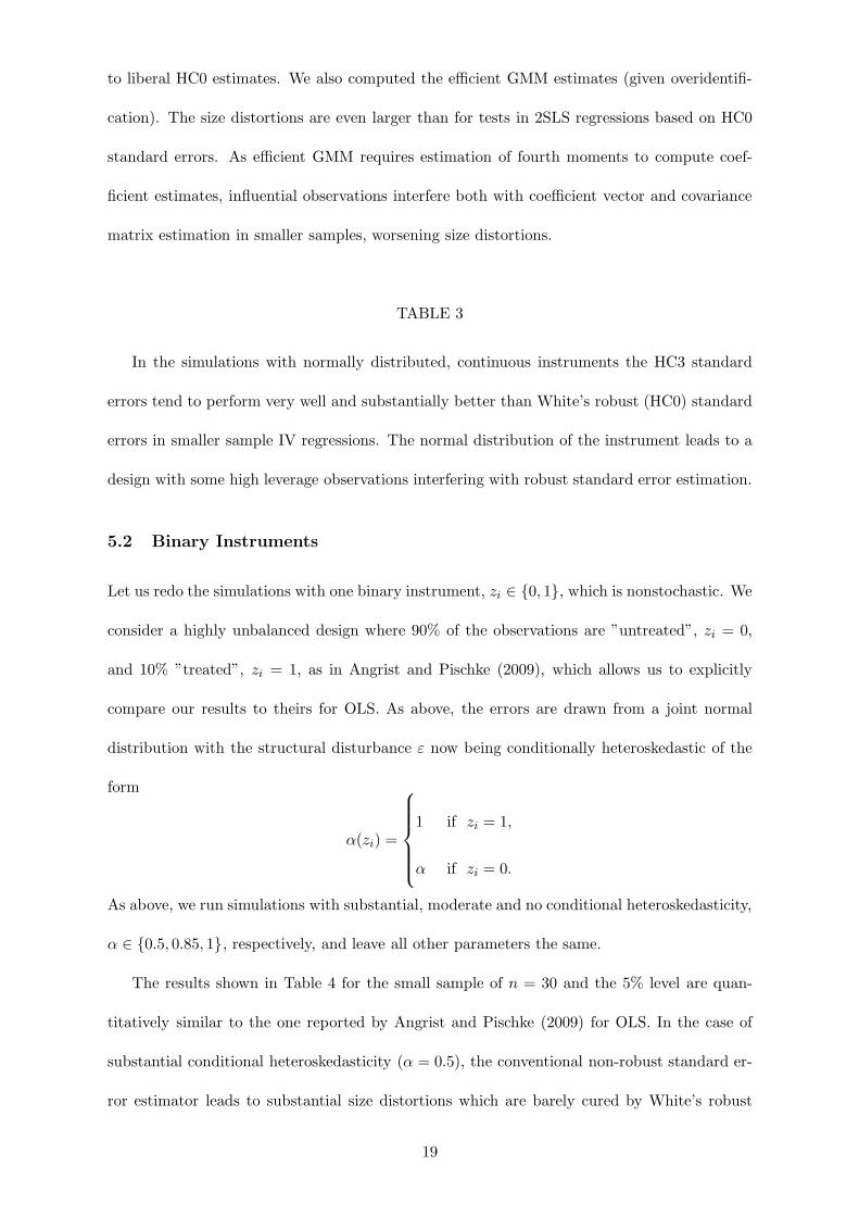
TABLE 3

In the simulations with normally distributed, continuous instruments the HC3 standard

errors tend to perform very well and substantially better than White’s robust (HC0) standard

errors in smaller sample IV regressions. The normal distribution of the instrument leads to a

design with some high leverage observations interfering with robust standard error estimation.

5.2 Binary Instruments

Let us redo the simulations with one binary instrument, zi ∈ 0, 1, which is nonstochastic. We

consider a highly unbalanced design where 90% of the observations are ”untreated”, zi = 0,

and 10% ”treated”, zi = 1, as in Angrist and Pischke (2009), which allows us to explicitly

compare our results to theirs for OLS. As above, the errors are drawn from a joint normal

distribution with the structural disturbance ε now being conditionally heteroskedastic of the

form

α(zi) =

1 if zi = 1,

α if zi = 0.

As above, we run simulations with substantial, moderate and no conditional heteroskedasticity,

α ∈ 0.5, 0.85, 1, respectively, and leave all other parameters the same.

The results shown in Table 4 for the small sample of n = 30 and the 5% level are quan-

titatively similar to the one reported by Angrist and Pischke (2009) for OLS. In the case of

substantial conditional heteroskedasticity (α = 0.5), the conventional non-robust standard er-

ror estimator leads to substantial size distortions which are barely cured by White’s robust

19

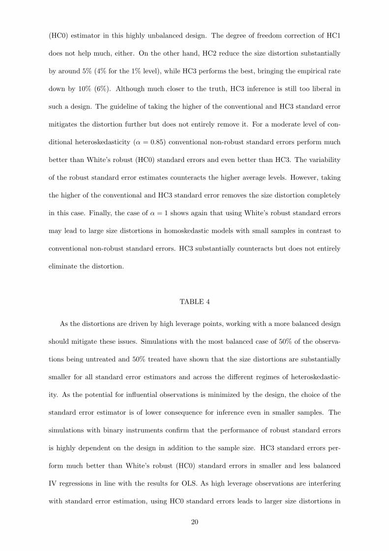
(HC0) estimator in this highly unbalanced design. The degree of freedom correction of HC1

does not help much, either. On the other hand, HC2 reduce the size distortion substantially

by around 5% (4% for the 1% level), while HC3 performs the best, bringing the empirical rate

down by 10% (6%). Although much closer to the truth, HC3 inference is still too liberal in

such a design. The guideline of taking the higher of the conventional and HC3 standard error

mitigates the distortion further but does not entirely remove it. For a moderate level of con-

ditional heteroskedasticity (α = 0.85) conventional non-robust standard errors perform much

better than White’s robust (HC0) standard errors and even better than HC3. The variability

of the robust standard error estimates counteracts the higher average levels. However, taking

the higher of the conventional and HC3 standard error removes the size distortion completely

in this case. Finally, the case of α = 1 shows again that using White’s robust standard errors

may lead to large size distortions in homoskedastic models with small samples in contrast to

conventional non-robust standard errors. HC3 substantially counteracts but does not entirely

eliminate the distortion.

TABLE 4

As the distortions are driven by high leverage points, working with a more balanced design

should mitigate these issues. Simulations with the most balanced case of 50% of the observa-

tions being untreated and 50% treated have shown that the size distortions are substantially

smaller for all standard error estimators and across the different regimes of heteroskedastic-

ity. As the potential for influential observations is minimized by the design, the choice of the

standard error estimator is of lower consequence for inference even in smaller samples. The

simulations with binary instruments confirm that the performance of robust standard errors

is highly dependent on the design in addition to the sample size. HC3 standard errors per-

form much better than White’s robust (HC0) standard errors in smaller and less balanced

IV regressions in line with the results for OLS. As high leverage observations are interfering

with standard error estimation, using HC0 standard errors leads to larger size distortions in

20

heteroskedastic as well as homoskedastic environments. When working with such designs, one

should be very cautious, compute conventional as well as HC1-3 standard error estimates, use

the most conservative estimate and complement inference with influential analysis and other

diagnostics.

6 Application to Growth Regressions

In this section, we apply the alternative covariance matrix estimators to growth regressions

with instruments using the data of Persson and Tabellini (1994) and Acemoglu, Johnson and

Robinson (2001). As growth regressions use countries as units of observations, they are nat-

urally subject to smaller sample issues and thus well suited to test the implications of the

alternative standard errors and diagnostics.

Persson and Tabellini (1994) estimated the effect of inequality on growth. According to

their theoretical framework, there should be a negative relationship between inequality and

growth in democracies. In one of their settings, they worked with a cross section of n = 46

countries, splitting the sample into democracies (29 observations) and nondemocracies (17),

and used three instruments for inequality: percentage of labor force participation in the agri-

cultural sector, male life expectancy, and secondary-school enrollments. Table 5 reports the

coefficient of MIDDLE (a measure of equality), the original non-robust as well as our com-

putations of the HC0-3 standard error estimates, and corresponding t- and p-values. While

the original estimates for the whole sample differ slightly from ours (potentially due to data

or computational issues), the ones for democracies match. Using conventional (non-robust)

standard errors, one finds a positive coefficient for democracies as predicted by Persson and

Tabellini’s theory with a p-value of 2%. When we use HC3 standard errors instead, signif-

icance is substantially reduced as the p-value increases to 8%. The shift in significance due

to using HC3 standard errors hints at the presence of influential observations. Panel a) of

Figure 2 plots the leverages (qi’s) against the squared residuals. Observations like Colombia

(COL), Venezuela (VEN) and India (IND) combine a relatively high leverage with a large

21

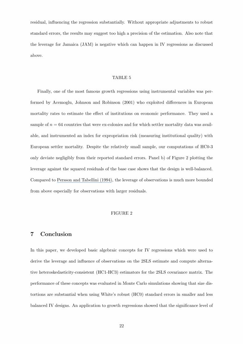
residual, influencing the regression substantially. Without appropriate adjustments to robust

standard errors, the results may suggest too high a precision of the estimation. Also note that

the leverage for Jamaica (JAM) is negative which can happen in IV regressions as discussed

above.

TABLE 5

Finally, one of the most famous growth regressions using instrumental variables was per-

formed by Acemoglu, Johnson and Robinson (2001) who exploited differences in European

mortality rates to estimate the effect of institutions on economic performance. They used a

sample of n = 64 countries that were ex-colonies and for which settler mortality data was avail-

able, and instrumented an index for expropriation risk (measuring institutional quality) with

European settler mortality. Despite the relatively small sample, our computations of HC0-3

only deviate negligibly from their reported standard errors. Panel b) of Figure 2 plotting the

leverage against the squared residuals of the base case shows that the design is well-balanced.

Compared to Persson and Tabellini (1994), the leverage of observations is much more bounded

from above especially for observations with larger residuals.

FIGURE 2

7 Conclusion

In this paper, we developed basic algebraic concepts for IV regressions which were used to

derive the leverage and influence of observations on the 2SLS estimate and compute alterna-

tive heteroskedasticity-consistent (HC1-HC3) estimators for the 2SLS covariance matrix. The

performance of these concepts was evaluated in Monte Carlo simulations showing that size dis-

tortions are substantial when using White’s robust (HC0) standard errors in smaller and less

balanced IV designs. An application to growth regressions showed that the significance level of

22

an estimator can be decisively reduced by using HC3 in the presence of influential observations.

The results suggest guidelines for applied IV projects, supporting the use of HC3 instead of con-

ventional White’s robust (HC0) standard errors especially in smaller, unbalanced data sets with

influential observations, in line with earlier results on alternative heteroskedasticity-consistent

estimators for OLS. The results also demonstrate the importance of analyzing leverage and

influence of observations in smaller samples which can be done conveniently with the measures

derived in the paper.

23

References

[1] Acemoglu, D., S. Johnson and J. A. Robinson, 2001, The Colonial Origins of Comparative

Development: An Empirical Investigation. American Economic Review 91, 1369-1401.

[2] Angrist, D. A. and J.-S. Pischke, 2009, Mostly Harmless Econometrics. Princeton Univer-

sity Press, Princeton and Oxford.

[3] Bekker, P. A., 1994, Alternative Approximations to the Distributions of Instrumental

Variable Estimators. Econometrica 62, 657-681.

[4] Bound, J., D. A. Jaeger, and R. M. Baker, 1995, Problems with Instrumental Variables

Estimation. Journal of the American Statistical Association 90, 443-450.

[5] Buse, A., 1992, The Bias of Instrumental Variable Estimators. Econometrica 60, 173-180.

[6] Chesher A. and I. Jewitt, 1987, The Bias of the Heteroskedasticity Consistent Covariance

Estimator, Econometrica 55, 1217-1222.

[7] Cook, R. D., 1977, Detection of Influential Observations in Linear Regressions. Techno-

metrics 19, 15-18.

[8] Davidson, R. and J. MacKinnon, 2004, Econometric Theory and Methods. Oxford Uni-

versity Press, New York and Oxford.

[9] Efron, B., 1982, The Jackknife, the Bootstrap and other Resampling Plans. SIAM,

Philadelphia.

[10] Eicker, F., 1963, Asymptotic Normality and Consistency of the Least Squares Estimators

for Families of Linear Regressions. Annals of Mathematical Statistics 34, 447-456.

[11] Frisch, R. and F. V. Waugh, 1933, Partial Time Regressions as Compared with Individual

Trends. Econometrica 1, 387–401.

[12] Hansen, L. P., 1982, Large Sample Properties of Generalized Method of Moments Esti-

mators. Econometrica 50, 1029-1054.

24

[13] Hayashi, F., 2000, Econometrics. Princeton University Press, Princeton and Oxford.

[14] Hinkley, D. V., 1977, Jackknifing in Unbalanced Situations. Technometrics 19, 285-292.

[15] Hoaglin, D. C. and R. E. Welsch, 1978, The Hat Matrix in Regression and ANOVA. The

American Statistician 32, 17-22.

[16] Horn, S. D., R. A. Horn and D. B. Duncan, 1975, Estimating heteroskedastic variances in

linear models. Journal of the American Statistical Association 70, 380-385.

[17] Long, J. S. and Laurie H. Ervin, 2000, Using Heteroskedasticity Consistent Standard

Errors in the Linear Regression Model. The American Statistician 54, 217-224.

[18] Lovell, M., 1963, Seasonal adjustment of economic time series. Journal of the American

Statistical Association 58, 993–1010.

[19] MacKinnon, J. and H. White, 1985, Some Heteroskedasticity-Consistent Covariance Ma-

trix Estimators with Improved Finite Sample Properties. Journal of Econometrics 29,

305-325.

[20] Nelson, C. R. and R. Startz, 1990a, The Distribution of the Instrumental Variables Es-

timator and Its t-Ratio When the Instrument is a Poor One. Journal of Business 63,

125-140.

[21] Nelson, C. R. and R. Startz, 1990b, Some Further Results on the Exact Small Sample

Properties of the Instrumental Variable Estimator. Econometrica 58, 967-976.

[22] Persson T. and G. Tabellini, 1994, Is Inequality Harmful for Growth. American Economic

Review 84, 600-621.

[23] White, H., 1980, A Heteroskedasticity-Consistent Covariance Matrix Estimator. Econo-

metrica 48, 817-838.

[24] White, H., 1982, Instrumental Variables Regression with Independent Observations.

Econometrica 50, 483-499.

25

26

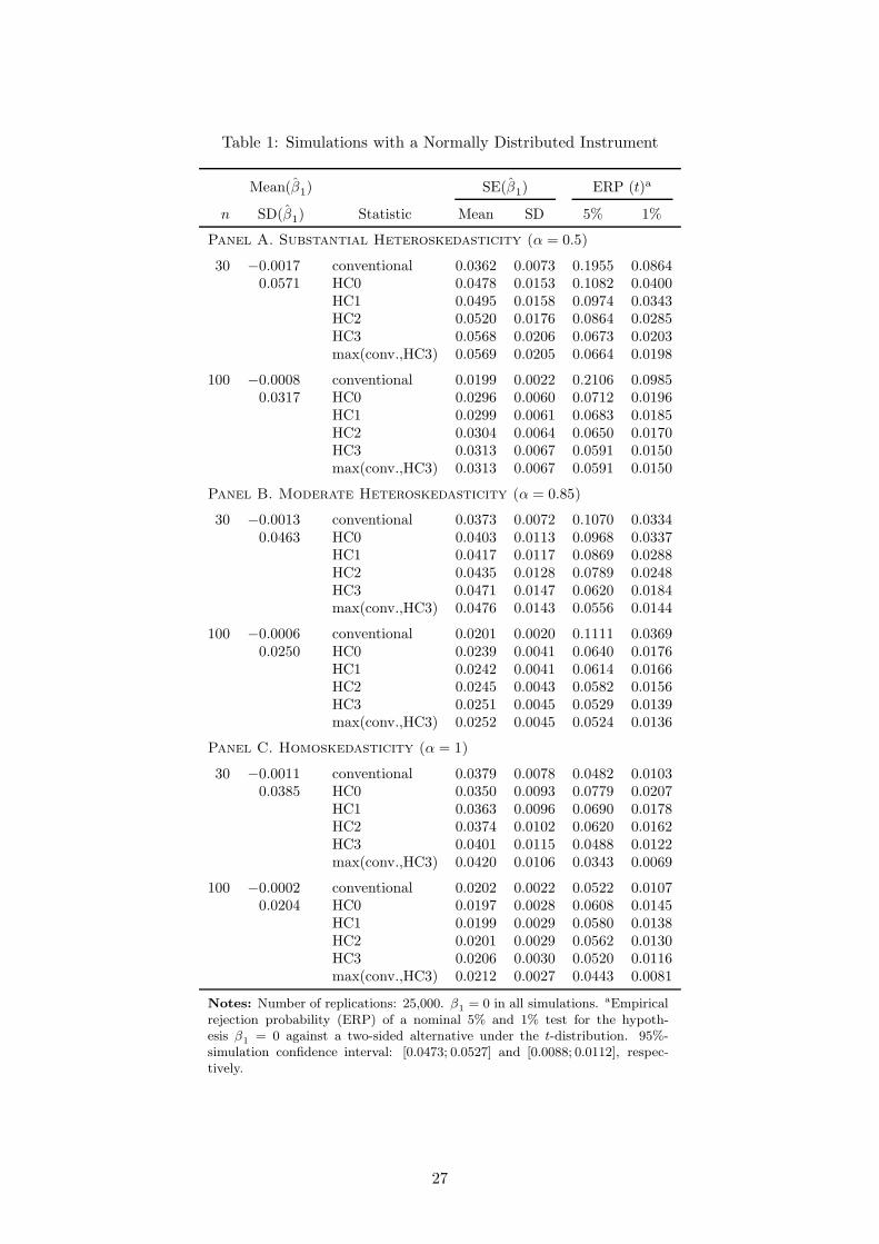
Table 1: Simulations with a Normally Distributed Instrument

Mean(β1) SE(β1) ERP (t)a

n SD(β1) Statistic Mean SD 5% 1%

Panel A. Substantial Heteroskedasticity (α = 0.5)

30 −0.0017 conventional 0.0362 0.0073 0.1955 0.08640.0571 HC0 0.0478 0.0153 0.1082 0.0400

HC1 0.0495 0.0158 0.0974 0.0343HC2 0.0520 0.0176 0.0864 0.0285HC3 0.0568 0.0206 0.0673 0.0203max(conv.,HC3) 0.0569 0.0205 0.0664 0.0198

100 −0.0008 conventional 0.0199 0.0022 0.2106 0.09850.0317 HC0 0.0296 0.0060 0.0712 0.0196

HC1 0.0299 0.0061 0.0683 0.0185HC2 0.0304 0.0064 0.0650 0.0170HC3 0.0313 0.0067 0.0591 0.0150max(conv.,HC3) 0.0313 0.0067 0.0591 0.0150

Panel B. Moderate Heteroskedasticity (α = 0.85)

30 −0.0013 conventional 0.0373 0.0072 0.1070 0.03340.0463 HC0 0.0403 0.0113 0.0968 0.0337

HC1 0.0417 0.0117 0.0869 0.0288HC2 0.0435 0.0128 0.0789 0.0248HC3 0.0471 0.0147 0.0620 0.0184max(conv.,HC3) 0.0476 0.0143 0.0556 0.0144

100 −0.0006 conventional 0.0201 0.0020 0.1111 0.03690.0250 HC0 0.0239 0.0041 0.0640 0.0176

HC1 0.0242 0.0041 0.0614 0.0166HC2 0.0245 0.0043 0.0582 0.0156HC3 0.0251 0.0045 0.0529 0.0139max(conv.,HC3) 0.0252 0.0045 0.0524 0.0136

Panel C. Homoskedasticity (α = 1)

30 −0.0011 conventional 0.0379 0.0078 0.0482 0.01030.0385 HC0 0.0350 0.0093 0.0779 0.0207

HC1 0.0363 0.0096 0.0690 0.0178HC2 0.0374 0.0102 0.0620 0.0162HC3 0.0401 0.0115 0.0488 0.0122max(conv.,HC3) 0.0420 0.0106 0.0343 0.0069

100 −0.0002 conventional 0.0202 0.0022 0.0522 0.01070.0204 HC0 0.0197 0.0028 0.0608 0.0145

HC1 0.0199 0.0029 0.0580 0.0138HC2 0.0201 0.0029 0.0562 0.0130HC3 0.0206 0.0030 0.0520 0.0116max(conv.,HC3) 0.0212 0.0027 0.0443 0.0081

Notes: Number of replications: 25,000. β1 = 0 in all simulations. aEmpiricalrejection probability (ERP) of a nominal 5% and 1% test for the hypoth-esis β1 = 0 against a two-sided alternative under the t-distribution. 95%-simulation confidence interval: [0.0473; 0.0527] and [0.0088; 0.0112], respec-tively.

27

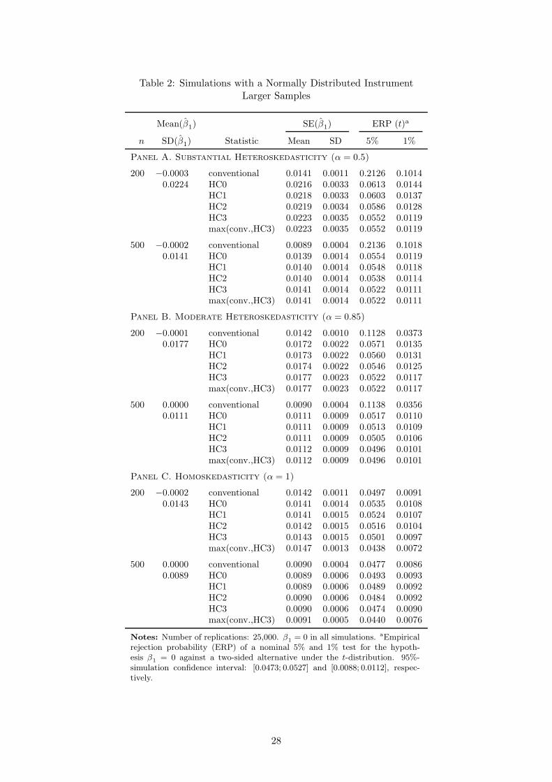
Table 2: Simulations with a Normally Distributed InstrumentLarger Samples

Mean(β1) SE(β1) ERP (t)a

n SD(β1) Statistic Mean SD 5% 1%

Panel A. Substantial Heteroskedasticity (α = 0.5)

200 −0.0003 conventional 0.0141 0.0011 0.2126 0.10140.0224 HC0 0.0216 0.0033 0.0613 0.0144

HC1 0.0218 0.0033 0.0603 0.0137HC2 0.0219 0.0034 0.0586 0.0128HC3 0.0223 0.0035 0.0552 0.0119max(conv.,HC3) 0.0223 0.0035 0.0552 0.0119

500 −0.0002 conventional 0.0089 0.0004 0.2136 0.10180.0141 HC0 0.0139 0.0014 0.0554 0.0119

HC1 0.0140 0.0014 0.0548 0.0118HC2 0.0140 0.0014 0.0538 0.0114HC3 0.0141 0.0014 0.0522 0.0111max(conv.,HC3) 0.0141 0.0014 0.0522 0.0111

Panel B. Moderate Heteroskedasticity (α = 0.85)

200 −0.0001 conventional 0.0142 0.0010 0.1128 0.03730.0177 HC0 0.0172 0.0022 0.0571 0.0135

HC1 0.0173 0.0022 0.0560 0.0131HC2 0.0174 0.0022 0.0546 0.0125HC3 0.0177 0.0023 0.0522 0.0117max(conv.,HC3) 0.0177 0.0023 0.0522 0.0117

500 0.0000 conventional 0.0090 0.0004 0.1138 0.03560.0111 HC0 0.0111 0.0009 0.0517 0.0110

HC1 0.0111 0.0009 0.0513 0.0109HC2 0.0111 0.0009 0.0505 0.0106HC3 0.0112 0.0009 0.0496 0.0101max(conv.,HC3) 0.0112 0.0009 0.0496 0.0101

Panel C. Homoskedasticity (α = 1)

200 −0.0002 conventional 0.0142 0.0011 0.0497 0.00910.0143 HC0 0.0141 0.0014 0.0535 0.0108

HC1 0.0141 0.0015 0.0524 0.0107HC2 0.0142 0.0015 0.0516 0.0104HC3 0.0143 0.0015 0.0501 0.0097max(conv.,HC3) 0.0147 0.0013 0.0438 0.0072

500 0.0000 conventional 0.0090 0.0004 0.0477 0.00860.0089 HC0 0.0089 0.0006 0.0493 0.0093

HC1 0.0089 0.0006 0.0489 0.0092HC2 0.0090 0.0006 0.0484 0.0092HC3 0.0090 0.0006 0.0474 0.0090max(conv.,HC3) 0.0091 0.0005 0.0440 0.0076

Notes: Number of replications: 25,000. β1 = 0 in all simulations. aEmpiricalrejection probability (ERP) of a nominal 5% and 1% test for the hypoth-esis β1 = 0 against a two-sided alternative under the t-distribution. 95%-simulation confidence interval: [0.0473; 0.0527] and [0.0088; 0.0112], respec-tively.

28

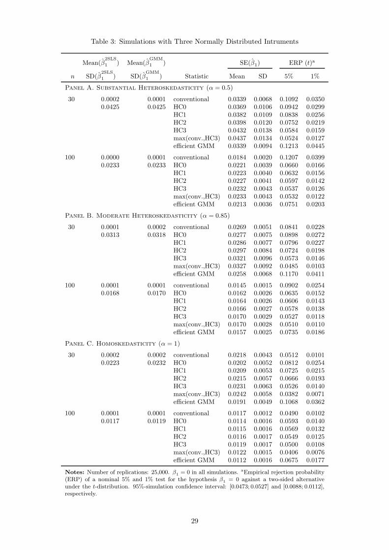
Table 3: Simulations with Three Normally Distributed Intruments

Mean(β2SLS

1 ) Mean(βGMM

1 ) SE(β1) ERP (t)a

n SD(β2SLS

1 ) SD(βGMM

1 ) Statistic Mean SD 5% 1%

Panel A. Substantial Heteroskedasticity (α = 0.5)

30 0.0002 0.0001 conventional 0.0339 0.0068 0.1092 0.03500.0425 0.0425 HC0 0.0369 0.0106 0.0942 0.0299

HC1 0.0382 0.0109 0.0838 0.0256HC2 0.0398 0.0120 0.0752 0.0219HC3 0.0432 0.0138 0.0584 0.0159max(conv.,HC3) 0.0437 0.0134 0.0524 0.0127efficient GMM 0.0339 0.0094 0.1213 0.0445

100 0.0000 0.0001 conventional 0.0184 0.0020 0.1207 0.03990.0233 0.0233 HC0 0.0221 0.0039 0.0660 0.0166

HC1 0.0223 0.0040 0.0632 0.0156HC2 0.0227 0.0041 0.0597 0.0142HC3 0.0232 0.0043 0.0537 0.0126max(conv.,HC3) 0.0233 0.0043 0.0532 0.0122efficient GMM 0.0213 0.0036 0.0751 0.0203

Panel B. Moderate Heteroskedasticity (α = 0.85)

30 0.0001 0.0002 conventional 0.0269 0.0051 0.0841 0.02280.0313 0.0318 HC0 0.0277 0.0075 0.0898 0.0272

HC1 0.0286 0.0077 0.0796 0.0227HC2 0.0297 0.0084 0.0724 0.0198HC3 0.0321 0.0096 0.0573 0.0146max(conv.,HC3) 0.0327 0.0092 0.0485 0.0103efficient GMM 0.0258 0.0068 0.1170 0.0411

100 0.0001 0.0001 conventional 0.0145 0.0015 0.0902 0.02540.0168 0.0170 HC0 0.0162 0.0026 0.0635 0.0152

HC1 0.0164 0.0026 0.0606 0.0143HC2 0.0166 0.0027 0.0578 0.0138HC3 0.0170 0.0029 0.0527 0.0118max(conv.,HC3) 0.0170 0.0028 0.0510 0.0110efficient GMM 0.0157 0.0025 0.0735 0.0186

Panel C. Homoskedasticity (α = 1)

30 0.0002 0.0002 conventional 0.0218 0.0043 0.0512 0.01010.0223 0.0232 HC0 0.0202 0.0052 0.0812 0.0254

HC1 0.0209 0.0053 0.0725 0.0215HC2 0.0215 0.0057 0.0666 0.0193HC3 0.0231 0.0063 0.0526 0.0140max(conv.,HC3) 0.0242 0.0058 0.0382 0.0071efficient GMM 0.0191 0.0049 0.1068 0.0362

100 0.0001 0.0001 conventional 0.0117 0.0012 0.0490 0.01020.0117 0.0119 HC0 0.0114 0.0016 0.0593 0.0140

HC1 0.0115 0.0016 0.0569 0.0132HC2 0.0116 0.0017 0.0549 0.0125HC3 0.0119 0.0017 0.0500 0.0108max(conv.,HC3) 0.0122 0.0015 0.0406 0.0076efficient GMM 0.0112 0.0016 0.0675 0.0177

Notes: Number of replications: 25,000. β1 = 0 in all simulations. aEmpirical rejection probability(ERP) of a nominal 5% and 1% test for the hypothesis β1 = 0 against a two-sided alternativeunder the t-distribution. 95%-simulation confidence interval: [0.0473; 0.0527] and [0.0088; 0.0112],respectively.

29

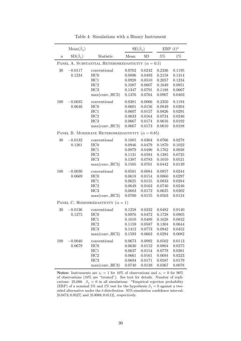
Table 4: Simulations with a Binary Instrument

Mean(β1) SE(β1) ERP (t)a

n SD(β1) Statistic Mean SD 5% 1%

Panel A. Substantial Heteroskedasticity (α = 0.5)

30 −0.0117 conventional 0.0702 0.0242 0.2336 0.11950.1234 HC0 0.0896 0.0493 0.2158 0.1314

HC1 0.0928 0.0510 0.2057 0.1234HC2 0.1087 0.0607 0.1649 0.0951HC3 0.1347 0.0791 0.1188 0.0667max(conv.,HC3) 0.1376 0.0764 0.0907 0.0403

100 −0.0035 conventional 0.0381 0.0066 0.2350 0.11940.0646 HC0 0.0601 0.0156 0.0849 0.0304

HC1 0.0607 0.0157 0.0826 0.0291HC2 0.0633 0.0164 0.0724 0.0246HC3 0.0667 0.0174 0.0616 0.0192max(conv.,HC3) 0.0667 0.0173 0.0610 0.0188

Panel B. Moderate Heteroskedasticity (α = 0.85)

30 −0.0132 conventional 0.1085 0.0304 0.0766 0.02780.1261 HC0 0.0946 0.0479 0.1870 0.1022

HC1 0.0979 0.0496 0.1762 0.0938HC2 0.1131 0.0594 0.1385 0.0735HC3 0.1387 0.0783 0.1010 0.0521max(conv.,HC3) 0.1505 0.0701 0.0442 0.0139

100 −0.0030 conventional 0.0581 0.0084 0.0857 0.02440.0669 HC0 0.0618 0.0154 0.0860 0.0297

HC1 0.0625 0.0155 0.0833 0.0284HC2 0.0649 0.0163 0.0740 0.0246HC3 0.0683 0.0172 0.0625 0.0202max(conv.,HC3) 0.0700 0.0155 0.0503 0.0124

Panel C. Homoskedasticity (α = 1)

30 −0.0136 conventional 0.1258 0.0332 0.0482 0.01400.1275 HC0 0.0976 0.0472 0.1728 0.0905

HC1 0.1010 0.0489 0.1628 0.0832HC2 0.1159 0.0587 0.1304 0.0644HC3 0.1412 0.0773 0.0942 0.0452max(conv.,HC3) 0.1593 0.0663 0.0294 0.0082

100 −0.0040 conventional 0.0673 0.0092 0.0502 0.01130.0679 HC0 0.0630 0.0152 0.0804 0.0275

HC1 0.0637 0.0154 0.0778 0.0261HC2 0.0661 0.0161 0.0694 0.0223HC3 0.0694 0.0171 0.0587 0.0179max(conv.,HC3) 0.0740 0.0139 0.0367 0.0078

Notes: Instruments are zi = 1 for 10% of observations and zi = 0 for 90%of observations (10% are “treated”). See text for details. Number of repli-cations: 25,000. β1 = 0 in all simulations. aEmpirical rejection probability(ERP) of a nominal 5% and 1% test for the hypothesis β1 = 0 against a two-sided alternative under the t-distribution. 95%-simulation confidence interval:[0.0473; 0.0527] and [0.0088; 0.0112], respectively.

30

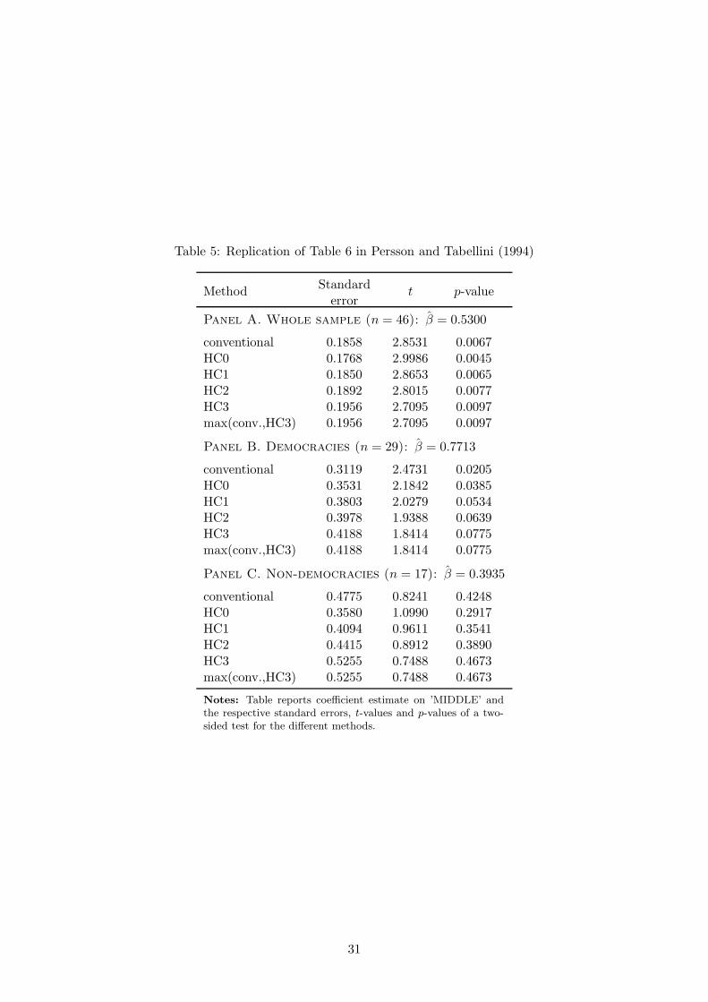
Table 5: Replication of Table 6 in Persson and Tabellini (1994)

MethodStandarderror

t p-value

Panel A. Whole sample (n = 46): β = 0.5300

conventional 0.1858 2.8531 0.0067HC0 0.1768 2.9986 0.0045HC1 0.1850 2.8653 0.0065HC2 0.1892 2.8015 0.0077HC3 0.1956 2.7095 0.0097max(conv.,HC3) 0.1956 2.7095 0.0097

Panel B. Democracies (n = 29): β = 0.7713

conventional 0.3119 2.4731 0.0205HC0 0.3531 2.1842 0.0385HC1 0.3803 2.0279 0.0534HC2 0.3978 1.9388 0.0639HC3 0.4188 1.8414 0.0775max(conv.,HC3) 0.4188 1.8414 0.0775

Panel C. Non-democracies (n = 17): β = 0.3935

conventional 0.4775 0.8241 0.4248HC0 0.3580 1.0990 0.2917HC1 0.4094 0.9611 0.3541HC2 0.4415 0.8912 0.3890HC3 0.5255 0.7488 0.4673max(conv.,HC3) 0.5255 0.7488 0.4673

Notes: Table reports coefficient estimate on ’MIDDLE’ andthe respective standard errors, t-values and p-values of a two-sided test for the different methods.

31

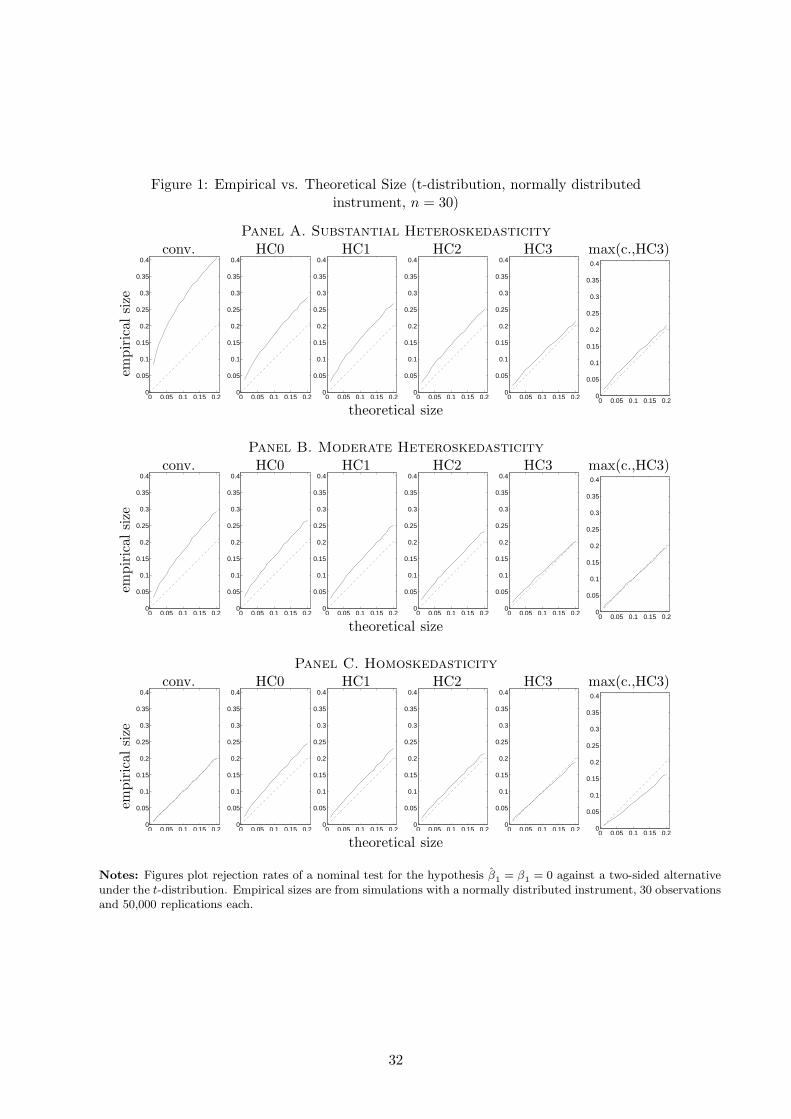
Figure 1: Empirical vs. Theoretical Size (t-distribution, normally distributedinstrument, n = 30)

Panel A. Substantial Heteroskedasticity

empirical

size

conv.

0 0.05 0.1 0.15 0.20

0.05

0.1

0.15

0.2

0.25

0.3

0.35

0.4HC0

0 0.05 0.1 0.15 0.20

0.05

0.1

0.15

0.2

0.25

0.3

0.35

0.4HC1

0 0.05 0.1 0.15 0.20

0.05

0.1

0.15

0.2

0.25

0.3

0.35

0.4HC2

0 0.05 0.1 0.15 0.20

0.05

0.1

0.15

0.2

0.25

0.3

0.35

0.4HC3

0 0.05 0.1 0.15 0.20

0.05

0.1

0.15

0.2

0.25

0.3

0.35

0.4max(c.,HC3)

0 0.05 0.1 0.15 0.20

0.05

0.1

0.15

0.2

0.25

0.3

0.35

0.4

theoretical size

Panel B. Moderate Heteroskedasticity

empirical

size

conv.

0 0.05 0.1 0.15 0.20

0.05

0.1

0.15

0.2

0.25

0.3

0.35

0.4HC0

0 0.05 0.1 0.15 0.20

0.05

0.1

0.15

0.2

0.25

0.3

0.35

0.4HC1

0 0.05 0.1 0.15 0.20

0.05

0.1

0.15

0.2

0.25

0.3

0.35

0.4HC2

0 0.05 0.1 0.15 0.20

0.05

0.1

0.15

0.2

0.25

0.3

0.35

0.4HC3

0 0.05 0.1 0.15 0.20

0.05

0.1

0.15

0.2

0.25

0.3

0.35

0.4max(c.,HC3)

0 0.05 0.1 0.15 0.20

0.05

0.1

0.15

0.2

0.25

0.3

0.35

0.4

theoretical size

Panel C. Homoskedasticity

empirical

size

conv.

0 0.05 0.1 0.15 0.20

0.05

0.1

0.15

0.2

0.25

0.3

0.35

0.4HC0

0 0.05 0.1 0.15 0.20

0.05

0.1

0.15

0.2

0.25

0.3

0.35

0.4HC1

0 0.05 0.1 0.15 0.20

0.05

0.1

0.15

0.2

0.25

0.3

0.35

0.4HC2

0 0.05 0.1 0.15 0.20

0.05

0.1

0.15

0.2

0.25

0.3

0.35

0.4HC3

0 0.05 0.1 0.15 0.20

0.05

0.1

0.15

0.2

0.25

0.3

0.35

0.4max(c.,HC3)

0 0.05 0.1 0.15 0.20

0.05

0.1

0.15

0.2

0.25

0.3

0.35

0.4

theoretical size

Notes: Figures plot rejection rates of a nominal test for the hypothesis β1 = β1 = 0 against a two-sided alternativeunder the t-distribution. Empirical sizes are from simulations with a normally distributed instrument, 30 observationsand 50,000 replications each.

32

Figure 2: Leverages vs. Standardized Residuals in Selected IV Studies

Panel A. Persson and Tabellini (1994)

SLV

COL

SEN

JAM

MEX

CRI

MDG

PHL

GRC

DEU

LKAPAN

FRA

ITA

TTO

FIN

MYS

JPN

IND

NLD

VENGBRSWE

USA

AUSKOR

NOR

ISR

DNK

−.1

0.1

.2.3

.4le

vera

ge (

q)

0 1 2 3 4 5 6 7 8standardized residual squared

Panel B. Acemoglu et. al. (2001)

AGOARG

AUS

BFA

BGDBHS BOL

BRA

CAN

CHLCIV

CMRCOG

COLCRIDOMDZAECUEGYETHGAB

GHAGIN

GMB

GTMGUY

HKG

HNDHTI

IDN

INDJAMKENLKAMAR

MDG

MEX

MLI

MLTMYSNER

NGA

NIC

NZL

PAKPANPERPRY SDN

SEN

SGP

SLESLVTGO

TTOTUN TZA

UGA

URY

USA

VENVNMZAF

ZAR

−.1

0.1

.2.3

.4le

vera

ge (

q)

0 1 2 3 4 5 6 7 8standardized residual squared

Notes: Figures plot leverages (q) against standardized residuals squared ((ǫ/σ)2), where σ denotes the standard

error of the regression. Panel A corresponds to column 2 (democracies sample) of Table 6 in Persson and Tabellini

(1994). Panel B corresponds to column 1 (base sample) of Table 4 in Acemoglu, Johnson and Robinson (2001).

33