DOCUMENT RESUME

ED 222 555 TM 820 709

AUTHOR Folsom, Ralph E.; Williams, Rick L.TITLE Design Effects and the Analysis of Survey Data.INSTITUTION Education Commission of the States, Denver, Colo.

National Assessment of Educational Progress.;Research Triangle Inst., Research Triangle Park,N.C.

SPONS AGENCY National Inst. of Education (ED), Washington, DC.REPORT NO RTI/2137-01-01FPUB DATE Apr 82GRANT NIE-G-80-0003NOTE '153p.; Appendix B is marginally legible due to small

print; For related documents, see TM 820 707-712 andTM 820 716.

14,EDRS PRICE MF01/PC07 Plus Postage.DESCRIPTORS Cluster Analyss; Educational Assessment; *Hypothesis

Testing; *Mathematics Achievement; National Surveys;Probability; *Research Design; *5amp14.ng; SecondaryEducation; *Statistical Analysis

IDENTIFIERS Chi Square; National Assessment of EducationalProgress; *NIE ECS NAEP Item Development Project;Second Mathematics Assessment (1978)

ABSTRACTThe National Assessment of Educational Progress

(NAEP), like most large national surveys, employs a complexstratified multistage unequal probability sample. The design providesa rigorous justification for extending survey results to the entireU.S. target population. Developments in the analysii of data fromcomplex surveys which provide a straightforward method for takingaccount of the sample design through proper'estimation ofsubpopulatiOn estimates and their covariance matrix are'reviewed.Relationships among.subpopulations are then evaluated via largesample Walddstatistics assumed to be asymptotically distributed ascentral chi-squared random variables. While these methods provide amechanism for analyzing NAEP data, the computer software required toproperly estimate sanple deiign-based covariance matrices is notgenerally available to NAEP data users. Design effect methods foradjusting test statistics obtained from standard statistical methodswhich implicitly assume simple random sampling from an infinitepopulation are presented with several new decompositions obtainedwhich display the effects of multistage clustering, stratification,and unequal weighting on Ole covariance matrix. A comparison of .

Psymptotically valid sample design-based chi-squared tests versusanalogous simple random sampling tests and design effect adjustedtests, is given. Design effect adjustments on NAEP mathematics dataare shown. Primary type of information provided by the report:Procedures (Sampling); Results (Secon(Thry Analysis). (Author/CM)

***********************************************************************Reproductions supplied by EDRS are the best that can be made

. from the original document.***********************************************************************

RTI/2137/01-01F

DESIGN EFFECTS AND THE'ANALYSISOF SURVEY DATA

by

Ralph E. Folsomand

Rick L. Williams

Prepared for

Education Commission of the StatesDenver, Colorado

U.S. DEPARTMENT OF EDUCATION 6

NATIONAL INSTITUTE OF EDUCATION

EDUCATIONAL RESOURCES INFORMATION

CENTER IERICI

y This document ,hos been reproduced as

ret erved hom the 1,015011 or ordanuatron

originating it

Melo' thews have been ore a improve

rt:oroduction quahty

Points nt view o, opinions stated in this docu-

ment do hm it ssanly represent Oficial NIE

Posaloowno.y

"The work upon which this publication is based is performedpursuant to Grant'NIE-G-80-0003 of the National Institute ofEducation% It does not, however, necessarily reflect theview of that agency."

April 1982

RESEARCH TR InArIGLE PARK, NORTH CAROLINA 27709

Abstract

Design Effects and the Analysis of Survey Data

by

Ralph E. Folsomand

Rick L. Williams

The National Assessment of Educational Progress (NAEP), like most

large national surveys, employs a complex stratified multistage unequal

probability sample. When properly accounted for in the analysis, the NAEPsample design provides a rigorous justification for extending survey

results to the entire U.S. student target population. This'paper reviews

recent developments in the analysis of data from complex surveys whiChprovide a straightforward method for taking account of the sample designthrough proper estimation of subpopulation estimates and their covariancematrix. Relationships among subpopulatiuns can then be evaluated via large.sample Wald statistics assumed to be asymptotically distributed as centralchi-squared random variables.

While these methods provide a mechanism for analyzing NAEP data, thecomputer software required to properly estimate sample design-based CQ-variahce matrices is not generally available to NAEP data users. Recent

literature has suggested methods for adjusting test statistics obtainedfrom standard statistical methods which implicitly'assume simple randomsampling from an infinite 'population. These so called design effect

adjustments are reviewed and several new decompositions obtained which

display the effects.. of multistage clustering, stratification and unequalweighting on the covariance matrix.

Finally, an empirical comparison is presented of asymptotically validsample design-based chi-squared tests versus analogous simple random samp-ling tests and design effect adjusted tests. These comparisons are madefor linear contrasts of domain means and proportions as sell as for linearmodels fitted to the domain estimates via weighted least squares. The data

were taken from the NAEP 1977-78 Mathematics assessment for 9-, 13- and

17-year-olds. For these data, the analyses indicate that the design effecttype adjustments of standard test statistics are not stable and are gener-ally too conservatiiie to be of practical value.

3

1.

TABLE OF CONTENTS

Page

INTRODUCTION 1

32. THEORETICAL RESULTS

2.1 The Wald Statistic/Weighted Least-Square Theory 3

2.2 Generalized Design Effect Methods 7

2,3 Design Effect Models for P-Value CovarianceMatrices 13

2.3..1 'Single Stage Covariance Matrix Models 16

2.3.2 Three-Stage Covariance Matrix Modelsfor Estimated Totals 19

2.3.3 Design Effect Model for the NAEP P-Value

Covariance Matrix 28

2.3.4 Estimates for Composite Covariance Matrix'

Components 35

2.3.5 Asymptotic Distribution of SRS based NAEP

Wald Statistics 42

2.4 Testing Balanced Fits Via Dummy Variable Regression . 48

2.5 Inference for NAEP Package Means 54 j

3. EMPIRICAL INVESTIGATION 60

3.1 Analysis Items and Subgroups 60

3.2 Analyses 60

3.3 Results 65

3.3.1 Wald Statistic/Weight Least Squares 65

3.3.2 Balanced Effects 84

4. COMMENTS ON NAEP DATA AND DOCUMENTATION

REFERENCESAppendix A:Appendix*B:Appendix C:Appendix D:

Appendix E:

86

87

NAEP Exercises A-1

Wald Statistic Chi. Squareds B-1

Balanced Effect F-Tests C-1

Contingency Tables of Wald Statistic Sample DesignBased Tests Verses Alternative Tests Accepted andRejected at the 5% Significance LevelContingency Tables of Balanced Effects SampleDesign Based Tests Versus Alternative TestsAccepted and Rejected at the 5% Significance

Level

D-1

E-1

LIST OF TABLES

Table

371 Hypothesis Tests for the Race*Sex*PARED Cross.Classification 63

3-2 Hypothesis Tests for the Sex*TOC*PARED Cross-Cldssification 64 ,

3-3 NAEP Item Design Effects for the Race*Sex*PAREDCross-Classification 67

3-4 NAEP Item Design Effects'for the Sex*TOC*PAREDCross-Classification 68

3-5 Mean SCores Design Effects 69

3-6 Hypothesis Test Design Effects by NAEP Item forthe Race*Sex*PARED Cross-Classifitation . . . - 71

3-7 Hypothesis Test Design Effects by NAEP Item forthe Sex*TOC*PARED Cross-Classification

3-8 Hypothesis Test Design Effects for Mean Scores

3-9 Hypothesis Test Design Effects for NAEP Items byTest Number for the Race*Sex*PARED Cross-Classification

72

73

75

3-10 , Hypothesis Test Design Effects for NAEP Items by TestNumber for the Sex*TOC*PARED'Cross-Classification . . 76

3-11 Hypothesis Test Design Effects for Mean Scores byTest Number for the RacerSex*PARED Cross-Classification

3-12 Hypothesis Test Design Effects for Mean Scores by'Test Number for the Sex*TOC*PARED Cross--Classification

3-13 Conditional Percent of Contrast Design Based (DB)Tests Versus Alternative Tests (AT) Reaching anOpposite Conclusion for NAEP Items

77

78

80

3-14 Conditional Percent of Contrast Design Based (DB)'Test Versus Alternative Tests (AT) Reaching'anOpposite Conclusion for Mean Scores 81

3715 donditional Percent of Linear Model Design Based (DB)Tests Versus Alternative Tests (AT) Reaching anOpposite Conclusion for.NAEP Items 82

LIST OP TABLES (continued)

Table

3-16 Conditional Percent of Linear Model Design Based (DB)

Tests Versus Alternative Tests (AT) Reaching an

Opposite Conclusion for Mean Scores

3-17 Conditional Percent of Balanced Effects Design Based

(DB) Test Versus Alternative Tests (AT) Reaching an

Opposite Conclusion

Page

83

85

1. INTRODUCTION

The,National Assessment data base provides a wealth of information on

the way student ability to correctlx answer NAEP test items relates to

student background and school.environment variables. When properly taken

account of in the analysis, the coinplex probability sample design used to

0

collect NAEP data provides a rigorous justification for extending survey

results to the entire U.S.,student population. Recent developments in the

analysis of categorical data from complex surveys provide a straight for-

ward methodology for taking account of sample design through the proper

estimation of subpopulation proportions (domain P-values) and their covari-

ance matrices [Koch, Freeman; and Freeman (1975)]. These vectors of sub-

population,P-values are then fit to linear models in the domain defining

variOles using the sample. design based covariance matrix to calculateIJ

weighted least squares fits. Wald statistics that take the form of

2

Hotelling's multivariate T statistic are then used to test for the good-

ness of fit of the model and to subsequently, test for the significance of

model effects. The following chapter surveying theoretical results begins

with a section on the-Wald statistic/weighted least squares theory for

testing hypotheses about NAEP domain p-values.

While the weighted least squares methodology provides a straight

forward solution to the NAEP p-value analysis problem, the computer soft-

ware required to properly estimate sample design based covariance matrices

is not generally available to. NAEP data users. Section 2.2 summarizes

me.thods explored by Fellegi (1980) and Rao and cott (1981) for adjusting

test statistics derived from standard statistical snftware packages. The

standard statistical software paCkages employ either implicitly or expli-

citly covariance matrix calculations appropriate for simple random samples.

The adjustments proposed-by Fellegi, Rao and Scott involve dividing the

standard chi-squared statistic by 'a generalized design effect CDeff) summa-1.

rizing the ratio of sample design based P-value variances and

divided by their respective simple random sampling variances

. ances. To display the sample design effects of multi-gtage

covariances

and covari-

clustering,

stratification, and unequal weighting on the generalized Deff, a design

effect model identity is developed in Section 2.3 for the P-value co-

,

variance matrix and for linear contrasts among sample P-values. The proper

sample -design based inference for NAEP balanced fits obtained as dummy

variable regression coefficients is presented in Section 2.4 along with the

analogous generalized Deff adjustment. Since much of the ,descriptive

analysis of NAEP data utilizes subpopulation averages across several indi-

vidual item P-values, the prOper covariance matrix estimation and gene-

ralized Deff adjustment methods for such statistics are explored in Sec-

tion 2.5.

-2-

0

2. THEORETICAL RESULTS

2.1 The Wald Statistic/Weighted Least-Square Theory

To illustrate the weighted least-squares approach to the analysis of

NAEP domain P-values, &insider asingle questionnaire dtem wita response

categories labelled r = 1,2,...,R. 'Suppose further that there are D sub-

population domains of-interest labelled d = 1,2,...,D. These domains can

be viewed as student subpopulations formed by a cross-classification of

background variables including Race, Sex,'Region, Type pf.Community, and

Parents Education. Let Xd(0 depict a subpopulation indicator variable

taking the Value 1 when student t belongs to domain d and zero otherwise.

Similarly, let Y(t) denote 'a response indicator variable taking the value

1 when student t gives response r to the specified item and zero otherwise.

With the U.S. student population size for a particular age class denoted by

M, the population count,of domain d members giving response r is

Y(dr) = 1 Xd(t) Yr(t) .

t=1

The U.S. stalent population size for subpopualtion dis specified as ,

X(d) = 2 Xd(t) .

t=1

The proportion of domain d members giving response r is then defined as the

ratio

P(dr). = Y(dr)/X(d) .

The NAEP sample estimates for these student subpopulation response propor-

tionS (domain P-values) have the form

73-

P(dr) = [ I W(k) Xd(k) Yr(k)] [ I W(k) Xd(k)]

k=1 k=1

where m denotes the number of sample students and W(k) is a sample.weighe

incorporating the reciprocal of the sample student k inclusion probability

n(k) and various adjustments for sample school and student nonresponse.

To simplify the notation, consider the column vector P(d) of (R-1)

subpopulation d response proportions conslsting of the first (R-1) esti-

mates defined above. Stacking these domaia specific vectors on top of one

another, a single column vector P with D(R-1) elements is produced. Let

11V (DES) denote the D(R-1) by D(R-1) estimated covariance matrix derived for

P according to one of the three asympotically equivalent methods of vari-, .

ance estimation fot nonlinear statistics from complex probability samples,

namely the Taylor Series linearization (MI.) method, balanced repeated

replication (BRR), and jackknife replication (JKR). Krewski'and Rao (1978)

have established limiting conditions for the asymptotic equivalence of

11these covariance mattix estimation methods. Aocentral limit theore673 m esta-

blishing conditions for the asymptotic normality of studentized P-values

1/2t(dr) = [P(dr) - P(dr)] / [VDEs(dr)]

is also presented by Krewski and Rao when any of the three linearization

methods is used to approximate the sample design based variance VDES

(dr)

for the ratio statistic P(dr). Such a central limit theorem provides the

theoretical ustification for assuming that the vector P of estimated

domain P-values will be distributed approximately as a D(R-1)- variate

normal vector with mean P and covariance matrix V (DES).~13

Assuming that the conditions for asymptotic normality apply, weighted

least, squares methods folloWing Grizzle, Starmer, and Koch (1969) can be

-4- 10

;

used to fit linear model\to functions of the estimated Aomain P-values.

Let G(P) denote a. vector o A continuous, linearly independent functions

with partial derivatives through second order. Define the A by D(R-1)

matrix of partial derivatives with row a denoted by

H (P) = 3Ga/aP = (aGa/aPl,a aGa /aPD(R-1)).

The matrix of these partial derivatives is evaluated at the estimated P

values to define

Consider, for example, the logit function where

G(P) = loge 4Pa/(1-Pa)

with a = 1,2,...D indexing the D domain P-values associated with the typical

R=2 (correct-incorrect) item response breakdown. For this logistic function

^

Ha = (0,0,...,1/Pa(1-Pa), . . . 0) .

Now, with G = G(P) denoting the sample estimate for the vector of A func-

tions, one notes that G is asymptotically A-variate normal with mean vector

G = G(P) and asymptotic covariance matrix

VG(DES) = [II V (DES) H

TI.P

where HT

denOtes the transpose of H. A consistent estimate for V.(DES) isG

GV (DES) = '111 V (DES) H

T].P

One can now proceed to fit a general linear model of the form

where Lhe columns of X specify selected main effect and interaction con-

trasts in terms of the domain defining Race, Sex, Type of Community and

F>

-5- 11_

a

--Parents Education variables. The' asymptotically. efficient BAN (Best

,

Asymptotially Normal) estimator for the coefficient vector A is then

A= [XT

VG(DES) X] X V (DES) G

--

with asymptotic covariance matrix

V,(DES) = [XT

VG(DES) x] .

P --

To:test the fit of the model, that a Ho: G(P) = X A, (the residual quadra-ticform

2 TT (Fit) = (G - X A) VG(DES) (G X A)

is a Wald (1943) statistic which has the form of Hotelling's multivariate.

2 2 .2T statistic. Asymptotically. T (Fit) is distributed as Chi-Square (x. )

with degrees of freedom df = rank of X under the null hypothesis. For

subasymptotic situations where the number'of replicates used. to form the

covariance matrix estimator does not substantially exceed the rank of X, a

2transformation of T to Snedecor's F may be appropriate. This leads to

F(df, L - df + 1) = - df + 1) T (Fit)/df(L)

where L is the 'dumber of degrees of freedom suggested by the.quadratic form

used to estimate V (DES) and df iS the rank of X. This transformed WaldPStatistic is compared against critical Nalues of Snedecor's F with di

numerator and L - di + 1 denominator degrees of freedom.

Failing to reject Ho: ,G(P) = X A, one can entertain linear hypothesesa

of the form Ho:, C A = 4), with (1) denoting a null vector. The associated .

Wald,Scatistic is

2 -1T (c) = (C A)

T[C V (DES) C

T] (C A)~ ~

which. is asymptotically x2 (rank of C).under the uull hypothesis. The F

transformed alternative

2F(c, L - c + 1) = (L c + 1) T (C)/cL

-6r12

is compared with critical values bf Senedecortg F with c = rank of C numera-

tor degrees of freedom and (L - c + 1) denominator degrees of freedom. In

the next section the approximate methods of Rao and Scott (1979) based on

simple random sampling covariance matrices Vp(SRS) and generalized design

effeCt (deff) adjustments are explored.

2.2 Generalized Design Effect Methods

Rao and Scott (1981) considered the asymptotic distribution df Wald

Statistics based on SRS covariance matrices for testing general hypotheses_

of the form

Ho: Ga(P) = 0, a =

where P can be viewed as the national response distribdtion for a specified

NAEP exercise'. This vector of universe level proportions corresp:Aits to

the P(d) domain specific item responSe-proportions introduced earlier with

P(dr) denoting the domain or subpopulation proportion selecting the coded

response option r = 1,2,.,.,(R-1). Since 'the P(dr) sum to one over all R

mutually exclusive response levels, only.(R-1) of the parameters is required

to fully characterize the response distribution. .While Rao and Scott's

results focus on the single population problem, they can be extended simply

to the Multiple subpopulation or domain problem by allowing P to represent-

the extended vector

Letting

PT = < PT (1), . .

Ha(P) = aGa(P)/aP

pT(D)

= [aGa(P)/aP(11), aGa(P)/aP(D,R-1)]

denote the vector of partial derivatives of Ga(P) with respect to the

D(R-1) elements of P, the population of-response Proportions, then

3-7r

X2 (G) = G [H V (SRS) H ]SRS

is the SRS based Wald statistic for testing the hypothesisthat the vector

of A functions GT

= [G1(P),,

. GA(p)] are simultaneously zero with H

denoting the matrix of all partial derivatives H(P) evaluated at

Interest in the SRS based X2 statistic stems from the simple computational

form for V (SRS). The simple random sampling covariance matrix for P is

approximated as a block diagonal matrix with (R-1) by (R-1) blocks of the

form

Vd(SRS) = [diag [P(d)] - P(d) P (d)l/m(d)

where m(d) is the doMain d sample size and diag [P(d)] is the (R-1) by

(R-1) diagonal matrix with diagonal elements P(dr). This SRS based covari-11/

ance matrix is formed simply from the weighted domain P-values and the

observed 'domain sample sizes. For the typical NAEP analysis of correct

responses 'with R = 2, ,

^ I/. Vd(SRS) = P(d) [1-P(d)]/m(d)

^ ^1/and V (SRS) is a D by D diagonal matrix with the V

d(SRS) quantities on the

P

diagonal. Under the null hypothesis Ho: G(P) = (0,

A

x2(G) 2 6oa a

,SRS a=1

where the'S's are the eigenvalues ofa

> .

[H V (SRS) HT] [H V (DES) HT]P'

. > 6. > 0, the X2a's are independent xf (single degree of freedom

A

chi-squared) random variables and 6oa

is the value ofjc5 under Ho.a -

Rao and Scott point out that the &a's can be interpreted as design

effects of linear combinations La

of the components of H P. Letting Aa"

1 4-8-

a

denote the a-th eigenvalue of_1

V (SRS) V (DES)P , p

then the 6 eigenvalues can be bounded by the X eigenvalues as follows:

Xa 6a XD(R-1)

for a = 1, ..., A, since the La

are particular linear combinations of the

P(drYs. Using a result in Anderson and Das Gupta (1963), Rao and Scott

establish pore precise bounds for the 6ain terms of the-X

a; namely,

Xa ->- 6a 1D(R-1)-A+a

This inequality is useful for specifying an alternative to the following.A2

test statistic- proposedby-kaoandScut-t---(R&S) ,

)(Ls (G) 4RS (2) / 6.

A

~ [6 /6. ] x2a=1

oa o a

where 6 denotes an estiMate of the mean eigenvalue 6 with the 6adepict-

ing eigenvalues of

[1 V (SRS)'HT] [H V (DES) HT

] .

,Since the estimation of the 6a

and associated 6. require knowledge of the

full design based covariance matrix, there is no real utility in using this

approximation when one could ju as well-use the appropriate design based

,Wald statistic. Using the sharp bounds fora

one notes that 6 Iies

between the average of the A largest Xa's and the mean of the A smallest

This implies that 6. should get close to X. as the number of Ga.

functions (A) approaches D(R-1). With A = D(R-1) independent Gafunctions

such that H is nonsingular it is clear that 6 = X. If the,Xa's show

little variation, .so that the mean of the A'largest and A smallest X's are

similar, then one can'also expect that 6. = X. The advantage of using X.

-9- 15

instead of 6 to adjust Chi-Square X2SRS

(G) is the ease of estimating,X..

We note that

V (SRS) = BLK-DIAG Hdieg [P(d)) - P(d) P(d)")/m(d)I

is block diagonal with blocks comprised of the domain specific multinomial

covariance matrices VP(d)

(SRS). Therefore, extending-results of Rao and

Seott one obtains

X = trace [V (SRS) V (DES)) / D(11-1.).

D , _12 trace V

P(d)(SRS) V

P(4)(DES) / D(R-1)

-d=1

where

D R-12 2' V(drIDES) m(d) / P(dr) D(R-1)

d=1 r=1

D R-1'2 2 [1-P(dr)] DEFF (dr) / D(R-1)d=1 r=1

DEFF(dr) = 'V (drIDES) / [P(dr) [1-P(dr)] / m(d))

is the design effect for the cell proportion P(dr).

Returning to the NAEP correct-incoirect response pattern (R=2), X.

simplifies to

D.

X. = 2 DEFF (dr) / D,d=1

the mean of the domain specific design effects. This result follows from'

the diagonal, form for

_1V (SRS) = diag [m(d)/[P(d) [1-P(d)])) .

In either case, the generalized design effect X. is a simple function of

a

domain P-value design effects. When the design effects for subpopulation

P-values, POO, are published then X. can be formed without knowledge of

16-10-

I.

the design based covariances between response porportions P(dr) and P(d'r")

1

from different subpopulations (Od ). In the following chapter, numerical

compaLsons of the adjusted SRS based X2 statistics

X2 (G) = X2S

(G) / XADJ SR

and the associated design based 4Es(G) Wald statistics 'are explored.

To model the effects of sample design features like stratification

clustering and unequal weighting on the 4M(G) statistic, one can develop

a model for the generalized design effect matrix

V (SRS) V (DES)P

Consider, for example, a two-stage design with S primary frame units (PFU's),

say schools, with M(s) secondary units (students) in the s-th PFU such

that I M(s) = M. A with ieplacement selection of n primary sampling units

s=1

(PSU's) is first made with single draw prob4bilities 0(s) = [M(s)/M].

A subsequent with replacement simple random sample of m second Stage units

is then drawn from each sample PSU. For a single universal domain, Rao and

Scott display the following partitioning for

V (DES) = V (SRS) + ( -1) I 0(s) (P - P)(P - P)T/nm

s=1

= V (SRS) [I + (m-1)R]

where 0(s) = M(s)/M is the fraction of all students who attend school s;

P = [P (1), . .

-s s

is the vector of (R-1) response option proportions for students in school s,

and

R = fdiag (P) - PPT -1

j 0(s)(P -s ss=1

9. is the matrix analogue of the intra-cluster correlation coefficient with P

denoting the universe level vector of (R-1) response option proportions.

With this partitioning one can show that the eigenvalues of

V (SRS) 1V (DES) = [I + (m-1)11]

have the form.

X = [1 + (m-1) pai

where pa is the a-th largest eigenvalue of the intracluster correlation

matrix R. Rao and Scott call these pa quantities generalized measures of

homogeneity, analogous to the intracluster correlation p. For the simple

goodness-of-fit hypothesis Ho: P = Po

, the simple random sample (SRS) X2

tan be written as

(R-1)

X2RS (I)0) = I [1+(m-l)p I X2S oa a

a=1

where the X 2 are singie degree of freedom central Chi-square variables.a

For a portable value of 13. useful for modeling X. = [1+(m-1)15.] in compar-

able samples with differing cluster sizes m, one could use

ut.71)/(m-1)

R-L= [[ I [1-P(r)]DEFF(r)/(R-1)1-1]/(m-1).

r=1

An extension of this self-weighting, two stage, with replacement model for

Xa

to a NAEls type design with effects for unequal weighting, stratifica-

tion, and clustering is presented in the following section. These results

are used to display the effect of sample design features on SRS based Wald

Statistics for testing the fit of linear models

H : G(P) = xp.

-12-18

and linear hypotheses regarding'the model 'paraMeters P; that is,

Ho

: cp =

2.3 Design Effect Models for P-Value Covariance Matrices

To develop a design effect model for the covariance matrix of a vector

P of D National Assessment domain P-values, we consider a three stage

design with n county sized primary sampling units selected from a universe

of N such, Units wtiere the random frequency of selection for primary frame

unit PFU(2) is n(2). These n(2) are akin to the X(2) random selection

indicato.rs for without replacement samples where X(2) is when PFU(k)

belongs to the sample and zero otherwise. The n(2) are allowed to assume

values greater than 1 so as to accomodate so-called self-representing !)r

certainty units. Following Chromy (1979), one can use th'ese random selec-

tion frequencies to characterize a class of probability proportional to

size (PPS) selection schemes including PPS with replaceMent, PPS without

replacement, and PPS minimum replacement (PMR). The PPS nature of these

selection schemes implies that

E{n(2)} = En(2) = ns(2)/s(+)'

= n0(2)

where s(2) is a size measure known fox e4.ch primary frame unit PFU(2) and

s(+) = I s(2)

2=1

?is the univerge level aggregate size measure. For the NAEP design, the -

size measure s(2) is typically the estimated PFU enrollment for the 13year-

old target, qopulation. For with replacement selections, the n(2) are

multinomial frequencies with

-13-

19

E[n(2)n(2')) = n(n-1)0(2)0(2')

when .02'. 'For without replacement PPS designs n(2) = X(.2), the zero-one

selection indicator, and

E[n(2)n(2')] = n(2.2').

with n(29') denoting the joint inclusion probability.for the frame units0

PFU(2) and PFU(2'). For Chromy's probability,minimum replacement (PMR)

design

In(2)-11(2)1=In(2)-110(2)1 < 1.

Specifically, for PMR designs

andPr[n(2) ='Int[n0(2)]+1) = Frac in0(2)]

Pr[n(2) = Int[0(2)]) = 1-Frac [n0(2)]

where Int(x) denotes the integer part of x and Frac(x) depicts the frac-

tional part of x. The PMR feature allows multiple selection from certainty

units with n0(2)>1 such that the number of hits n(2) is derived by randomly

rounding. the En(2) = n0(2) proportional to size allocations up or down.

The sampling variance function for this class of selection schemes has been

parameterized in terms of variance zad covariance components by Folsom

(1980) utilizing double draw probabilities

E[n(2)[ (2)-1])/n(n-1) if 2=2

=

'

E[n(2)n(2'))/n(n-1) if 22' .

These double draw probabilities 0(22') arid the associated single draw

probabilities 0(2) were dervied by Folsom as the expectations of single

draw sampling unit indicators X2(0 that take the value 1 when n(2)>0 and

-14-

,2o

t1.

selected primary frame unit PFU(2) is randomly assigned primary sampling

unit (PSU) label i with i ranging from 1 to n; otherwise A2(i) = 0. With

the labels assigned as a random permutation of the digits 1, . , n, one

can show that

and

EN(i)1 = 0(2) for all i

E[X2('..)X , ('')1 = 0(22') for all iti' ,

,where expectation is taken over repeated samples and repeated random PSU

label assignments. The single drawlindicators have,the additional proper7.

ties

for all i, and

2 A(i) = 12=1

2 X2(i) = n(2),

2=1

These results lead to the following 0(2) and 0(22') summation identities:

and

N= 1

2=1

I 0(22') = E[X2,(i) I X(i)12=1 . 2=1

=

In the following subsection, the single diaw indicators are used to define

unbiased single draw variates in terms of the following single PFU ratio

type estimators

where

y(2) = s(+) Y(i)/s(2)

=

Y(2)T'= EY11 CO, Ydr (2),

denotes a row vector of D(R-1) PFU totals and.the superscript T denotes

Matrix transposition. .In the illustration above, Ydr

(2) will denote the

(dr)-th element of the vector Y(2) specifying the number of age eligible

domain d students attending school in PFU(2). 'who would give response option

r to a particular NAEP item.

2.3.1 Single Stage Covariance Matrix Models-

To develop a design effect representatioddior the covariance matrix of I/

a three-stage design statistic we begin by developing single stage results.

Extending Folsom's (1980) single stage results to vector valued statistics, 1/

we considet the corresponding vector valued single draw variate-

X2 (i) Y(2),-2=1

with y(2) denoting the Single PFU ratio type eitimator Y(2)/(1)(2) defined

previously.,

Now, one can show that each single draw sample variate y(i) is an1/

unbiased estimator of the universe total.Y(+); that is,

E[y(i)1 = 2 E[X2(i)1 y(2)

= Y(2)2=1

= Y(+) for all i.

-16- 22

Sip:darly, the covariance matrix for each y(i) is

since

= E{ Z xsi(i)[y(2)Y(4-)]l { Z Alf(illy,(2')-I(4-)1T)

= E[ Z2=1

A.2(i) when 2 = 2'

A.2(i)

2'(i) =

0 when 2 2'.

Taking the expectation over repeated samples and PSU label assignments (E)

inside the summation onE obtains'

/ (PSU) =2=1

The cross-covariance matrix between y(i) and y(i') is derived similarly as

N Na (PSU) = Z

2=1 2'=1

N N

=2=1 2'=1

for all iti'. The fact that the single drawn sample variates have common

covariance and cross-covariance matrices, provides a simple classical

'derivation of the variance fOr the mean of the single draw variate vectors

= x(i)/ni=1

14.

n

= I [ 2 X2(i)]Y(2)/n0(2)2=1 i=1

= 2 n,(2)Y(2)/En(2).

2=1

-Notice that in the recast version y becomes the standard Hansen-Hurwitz

(1943) estimator for a PPS with replacement selection. For a without

replacement PPS sample with En(2)=n(2), is the Horvitz-Thompson (1952)

-estimator. For the. intermediate PMR designs, x is Chromy's (1979) esti-

mator. In terms of the common covariance and cross-covariance matrices

2y(PSU) and IR (PSU), the covariance matrix for is

V (PSU) = 2 (PSU)/n (n-1)2R (PSU)/n

:=2(PSU)[I-4-(n.:1)R.(PSU)Pn

with

R (PSU).= 2 (PSU)-1

IR (PSU)

defining the cross-correlation matrix and I denoting the D(R21) by D(R-1)

identity matrix.

The following alternative expressions for 2 (PSU) and 2R (PSU) make

it easy to see that the form for V_(PSU) developed above is equivalent to

the Yates-Grundy.(1953) type variance expression presented in Chromy for

this general class of designs:

N N

2 (HU) =2=1 2'2

andN N

2R (HU) =Y 2=1 2'2

-18- 24

T/2 .

Weighting these component matrices together as indicated in V_(PSU) leads to ,

N NV (PSU) = [0(2)0(2')-(n-1)0(22')/ray(2)-y(21)iiX(2)-X(21)1T/2

2=1 2,'02

N NV (PSU)

2=1-2'02

Y(2) Y(2') Y(2) Y(2') T

En(2) En(2') 1 En(2) En(2')

When the PSU selection scheme gives all pairs of primary frame units 2 and

2' a chance of being represented in the sample so that En(2)n(2') > 0 for

all 2 0 2', the alternative component matrix expressions suggest unbiased

estimators

N,

(PSU) = [n(2)n(2')/En(2)n(2')]0(2)0(2')6(22')6(22')T/2

2=1 2'02

and

IR (PSU) = [n(2)m(2')/En(2)n(2')][0(2)0(2')-0(22')]6(22')6(22')T/2

2=1 2'02

with.

6(22') = [y(2)-y(2')].

For a multi-stage sample such as the NAEP design, the PFU vector totals

y(2) imbeded in the,definition of our 6(22') quantities must be estimated

based on second and subsequent stages of sampling. The unbiased estimation

of stagespecific component matrices is complicated by this process. The

following section develops the three stage covariance matrix model far the

vector valued total estimator Y(+).

2.3.2 Three-Stage 6wariance Matrix Models for Estimated Totals

For a three-stage NAEP type design where c schools are selected for a

given package in each sample PSU and m'students are selected for, package

-19- 25

assignment in each sample school random selection frequencies t(2s) and

m(2st) characterize the number.,of selections of school s in PFU(2) and the

number of selections of:student t in school (is). For NAEP sample designs,

the school and student level selections are without replacemc.it. The

school selections are,made with probability proportional *.o estimated age

class enrollment, say A(2s)';.that is

EW2s)In(2)=1) =

= c 0(s12).

When multiple hits are allowed on the primary frame units, n(2) > 1 inde-

pendeht-repricated -S-aMpleS of c schooTSare' drawn from PFU(2).

The second stage conditional double draw probabilities are defined as

where

E{Als(iDx2s,(W)1A2(i)=1) =

x2s(ij)

E{t(2s)[t(2s)-11)/c(c-1) if s=s'

E{t(2s)t(2s'))/c(c-1) if ss'

= 0 (ss'12)

is 1 if t(2s)>0 and school s in PFU(2) is randomly assigned

sample school label (ij) given yi)=1. The third.stage sample is a'simple

random selection without,replacement so that

E{m(2st)It(2s) > 0) = m/M(2 )

= m0(t12s)

with equal single draw probabilities 0(t12s) = M(2s)-1 where 1(2s) denotes

the number of age eligible students in school list anit SCH(2s). The

conditional double draw probabilities at the third stage are

=EfX2st(ij k)A2st,(ijk'AX2(i)X2s(ij)

1) = 1/M(2s)[M(2s)-1) if tft.'

= 0(tt'125)

-20-

o

and otherwise 0(ttl2s) = 0 since for without replacement selections

A25t(ij1) 2st(ijk) = 0; _that is, the student list unit t can nnt be

labeled both sample student k and k' since student list unit t can be

selected only once. With these definitions, a three stage single draw

variate is defined as

N S(2) N(s)x(ijk) = I I a2st(ijk) Y(2st)/0(2st)

2=1 s=1 t=1

with the three stage single draw i_ficlicator a2st(ijk) defined as the prodUct"

Of.the stagewise indicators

a25t(ijk)''= A2(i) A2s(i4) Aist(ijk)

The corresponding three stage single draw probahility is defined analogous7

ly; that is,

Eta (ijk)1 = 0(2st) = 0(2) 0(s12) 0(t12s).2st

With these definitAns, it is not difficult to see that

N S(2) M(2s)

E Wijk)) =1 I I Y (2st)

2=1 s=1 t=1

= Y(+++)

for all sample students STU(ijk) where Y(+++) is the universe total of the

response 'vector Y(.est) with D(R-1) elements of the form

Ydr(2st) = Xd(2st) Yr(2st)

where Xd(est) takes the value one when student list unit SLU(2st) belongs

to subpopulation domain d and zero otherwise. The covariance matrices'for

these three stage single draw variables can be derived simply using condi-.

tional expectations. For example, con'Sider,t

where

EUx(ijk) - Y(+++)] [x(ijk) - Y(+++)]T) = I (PSU) + I .(SCH) + I (STU)Y Y'

= Cov [x(ijk)] ,

N S(2) M(2s)I (STU) = I I 0(2s) I 0(02s) [y(2st) y(2s.)] [y(2st) - y(2s.)]

T

Y 2=1 s=1 t=1

with the school list unit mean y(2s.) defined as

M(s)x(2s =- I 0(02s) x(2st)

t=1

= Y (2s+) / 0(2) 0(s12)

= Y (2s+) / 0(2s) .-

For NAEP type designs with simple random selections at the third,stage one

,obtains the simplified form

2 N S(2)02 (20

I (STU) = M(++) I I [ ] I (2s)0(2s)

2=1 s=1

where El(2s) = M(2s)/M(++) denotes the school list unit (2s) fraction of the

tbtal student population count M(++). The covariance matrix for school,

list unit (2s) is

with

n(ks)

I (2s) = [diag [n(2s)1 - n(2s) nas)T]

M(2s)I- Y(2st)

T/M(2s)

t=1

ndr 2s)' ';'' 7tD(R-1)(25)]

denoting'the.vector of'D(R-1) .cell;ptoportions.. for schooVjist Unit (25).'

The'dr-th cell in Our example denotes membership in domain d and item

response group

-22-

28

with

a

The school stage covariance matrix component has the form-

S(g)

(SCH) = OM Zg=1 s=1

= fY(2s+)/0(2) (s(2)

6(gs) 6(g)= M(1-0 [[T--5.1 n(2s) [---T] n(2)1

gs

y(2..)IT

where 6(g) = M(g+)/M(++) denotes the fraction of student age eliglbles in

PFU(g). If the relative size measure

(2s) = [S(g)/S(+)] [A(2s)/A(2-01

then the sampleois self-weighting since

(2st) = (gs)/M(gs)

and the total inclusion probability for student list unit SLU (gst)

n(2st) = ncm (gst) = ncm/W++),

a constant for all nsm sample.students. In 'thiS simplified case

and

2 N M(gs)I (STU) = M(++) I O(s) [diag [n(gs)] - n(s) n(gs)

T

g=1 s=1

. 2 N S(g)

I (SCH) = M(++) I I. O(s) [n(gs) - n(g)] [n(gs) - n(2)]T

g=1 s=1

The general form of the PSU level covariance component matrix is'

2 (PSU) = 2 0(2) [Y(*) y(..)] f y(2. ) y(...)]2=1

With. 4

= mt-vt) f.,,fiTIT I n(2). '

-23- 29

For a self-weighting sample

2 N

I (PSU) = 4-) I 0(2) [n(2)-111 [11(2) 'T

M(4-

2=1

In general, one notes that

Cov[x(ijk)] = 2y (PSU) + 2y (SCH) + 2y (STU)

N S(2) M(2s)= 2' 2 2 0(2st) [x(2st) - x(...)] [x(2st)

2=1 s=1 t=1x(...)1T

N S(2) M(2s)Y(2st) Y(2st)T/0(2st) - Y(+++) Y(+++)T

2=1 s=1 t=1

N S(2) M(2 )2 2=M(++) [2 2 Y(2st) Y(2st) /M(++) 0(2st) -nnT

)

2=1 s=1 t=1

=2(TOT).

When the- sample is self-weighting with

. ..0(2st) = 1/11(++),

tfie common covariance matrix for ,each x(ijk) is

2

2 (TOT) = M(++) {diag [n] - nTIT}

Notice that in the self-weighiing case, 2 (TOT)/M(++)2

is the SRS with

replacement multinomial covariahce component matrix.

Various cross-covariance components can be define for the three-stage

single draw VariableS. .These cross-covariance components are derived as

follows:

Cov [i(ijk); x(ijk')] = Cov [y(i..)] + E Cov [x(ij.)].PSU PSU SCH

+ E: Et Coy, . [x(ijk);'x(ijkL).j

PSU SCH STU.. .

= 2' (PSU) + (SCH) + 2R (STU)

3o

where

TU{Y(ij

k)IPSU, SCH}

S

denotes the conditional expectation of,y(ijk) over repeated student selec-

tions and label assignments given the PSU and school selections and label

assignments. The conditional expectation over-school and student selection

and label assignment of x(ijk) given the PSU selection and labelling is

similarly denoted by

= E E [y(ijkIPSUI.,SCH STU

The matrices 2 (PSU) and 2 (SCH) were defined previously, and

N S(2) M(2s) M(2.$)

2R (STU) = 2 4(s) 2 2 (5(2st)(5(2st)T/M(2s)M2s)-11

2=1 s=1 t=1 t'=1

with

(5(2st) = [x(2st)

= M(s) [Y(2st) -41(2s).];(0(2s).

.With further manipulation the following form for the between student within

school tross-covariance matrix is obtained

2 N S(2)02(2s) ] (2s)/IM(2s)-112R f(STU) = -M(++) 1. L 4,(2s) y

2=1 s=1

recalling that

2 (2s) = [diag [71(2s)] - n(s)Y

Turning,to the between school within PSU cross-covaLriance matrix ope obtains.

.Cov = C6v +

q3SU ,PSU SCH

with

= (PSU') + 211, .('SCH)Y

S(2) S(2)

211 (SCH) = WO / 4o(ss'12) (5(20

2=1 s=1 s'=1

-25-31

1,

where

§,(2s) = M(44) [teGes° n(2s) - (2)}

Finally, the between PSU cross-covariance matrix is _defined as follows

NCosi [x(ijk); z(i'j'k')] = 0(22')' 8(2)

T

2=1

= IR (PSU)

where

(5(2) = LX(2..)

0(2)= f [0(2)1 Ty2) !S).

Arthed with the covariance and cross-Covariance component definitions

specified above, one can derive the covariance matrix for

n c m

=II:x(ijk)/ncm,i=1 j=1 k=1

the three-stage analogue of the general class of with replacement and PMR

I/single stage estimators. The covariance matrix for i is

Cov [i] = I (PSU) [I + (n-1) RY(PSU)P

Yn + I-(SCH) [I + (c-1) R

Y(SCH)]./nc

Y

+ IY

(STU) [I + (m-1) RY

(STU)Pncm.

A design effect version of this model can be formed as follows:

where

Cov[i] = {ly,(SRS)/ncm} IT/ (ncm-1) Ay(PSU) Ry(PSU)

+ (cM-1) [A (PSU) {l - R (PSU)} + A (SCH) RY(SCH)]

Y Y

+.(m-i) [A (sp) [1 - RY(SCH)) + A (ST1P. R

Y(STV)]'1

.Y

IT/ = I (SRS)-1 X (TOT)

E The uncval weighting effect;

-26-

and

-1A.

(

PSU) = I (TOT) I (PSU)Y

E The within PSU clustering effect;

R (PSU) = I (PSU)-1 IR (PSU)Y

E The PSU stratification and PMR selection effect;

A (SCH) = 1 (TOT)71 (SCH5'Y

E The within school clustering effect;

R (SCH) = 2 (8CH)-212 (SCH)

E The school stratification and PMR selection effect;

A (STU) = I (TOT)-1 I (STU)Y . Y Y

= [I - A (PSU) - A (SCH)]

a Betw2en student within school fraction of total variation;

R (STU) =.I (STU)-1 IR (STU)

a The effect of without replacement student selection.

As suggested above, the cross-covariance matrices account for both the

effects ,of minimwt replaqement (PMR) or without replacement selections and

stratification. The effect of explicit and implicit stratification is

expressed through the samilling expectation of selection frequency products,

E n(2) n(2!), and associated double draw probabilities, 0(22'). Recalling

the Yates-Grundy form of the PSU level variance function

V (PSU) = 1 1 [En(2)En(2') - En(2)n(2')] d(22') d(22')T/2

2=1 2Wr1/4

wlth

41(22')., = [Y(2)/En(2) Y(2')/En(2!)1 ,

is 'clear that explicit itratification,would imply the '.odependence,of

.,selettiod frequencies n(2) and n(2') for,PFU's in different stra.ta. Thii

independence would cause the betWeen PSU contrasts. d(22') in v-(psp) toY

drop out since En(2)n(2') = En(2) En(2'). Therefore, while the Vi-r(PSU)

variance expression and the variance-covariance component analogue are not

written in the familiar stratified form, they reduce to such a form when

the [En(2) En(2') En(2)n(2')] coefficients are set,to zero for the be-

tween stratum terms. With Chromy's sequential PMR zone selection scheme,

implicit stratification effects are achieved by purposively ordering the

frame listing so that proximate units are expected to be more alike than

distant units in terms of the survey,putcome measures. The reduction in

sampling variance associated with the effect of implicit stratification is

reflected in the Yates-Grundy variance form by a tendency-for the coeffi-

cients

rEn(2) En(2') - En(2)n(2')]

toapproach zero as,the distance between frame units 2 and 2' increases.

The variance-covariance component representation for V-(PSU) displays the

combined effect of minimum replacement selection and implicit stratifica-

tion in the form [1 + (n-1) R (PSU)]. For a scalar statis'tic this express-

ion reduces to [1 + ( -1)p (PSU)] where p (PSU), the common correlation

among the n single draw variates y(i), is expected to be increasingly

negativeeas the efficacy of the impliOt stratification improves.

2.3.3 Design Effect Model for the NAEP P-Value Covariance Matrix

The design effect model developed for the linear statistic i, the

vector, of estimated do ain by item response category totals -i(dr), can be

extended to the vector P of D(R-1) response category proportions considered

preViously by applying the Taylor Series linearization technique implicit,

in the section.2:2 treatment nf,generalized.design.oeifect MethodS. Begin

by letting,.

0

-28-

1

G r[Y(+++)] = Y(dr)/ I Y(dr) = P(dr)r=1

and let Hdr

denote the 1 x D(R-1) vector with elements

hdr

(uv) = 3P(dr)/3Y(uv) .

The elements of Hdr

have the following form

where

[1 - P(dr)]/X(d) if u = d and v = r

Hdr

= - P(dr)/X(d) if u = d and v r

0 otherwise

X(d) = Y(dr) .

r=1

Letting H = (HII, .

uT uT' =.1dr'

defining the matrix of

partial derivatives of P with respect to the elements of v+++) where the T

superscript denotes matrix transposition, then

-,V

P(DES) = H Cov[x] H

T.

The expression for the design based covariance matrix of P stated above can

-

now bp used alon& with the three-stage component representation for Cov [x]

to produce an analogous component representation for Vp(DES). This is

accomplished by defining analogous covariance and cross-variance matrices

for each stage as. followS':

and

.1p(STAGE)' = H I;(STAGE) HT

ER (STAGE) = H ER (STAGE) HT.

P

with STAGE assuming the PSU, SCH, and STU levels for the NAEP design.

An alternative form of the Taylor series linearization that provides

explicit definitions for the component matrices is to define linearized

variates,

35-29-

I

z(ijk) = H x(ijk)

N S(2) M(2s)=

st .

II I u(ijk) z(2st)2

2=1 s=1 t=1

where -

z(2st) = H x(2st)

= H Y(2st)/0(2st)

= M(2s) Z(2s0/0(2)0(s12) .

The Z(2st) = HY(2st) vectors.defined above have elements

,Zdr(25t) = Xd(259 [Yr(2st) - P(dr)]/X(d)

of the form

recalling that Xd(2st) is the one-zero indicator for domain d membership

and Yr(2st) is the one-zero indicator for response category r. Using the

linearized three-stage single draw variates z(2st) in place of the x('.est)

vectors in the I ( ) and, ( ) definitions yields Iz( ) and )

matrices $uch,that

and

Ip(STAGE) = Iz(STAGE) = H 2,(STAGE) HT

ap(STAGE) = az(STAGE) H I (STAGE) HT

.

Y

In terms of these quantities, the school level population mean vectors

have elements

M(2s)z(2s.) = I z(2st)/M(2s)

t=1

zdr

-(2 ) = Xd(25+)(1)

dr(2s) - P(dr)]/X(d) 0(2s)

= 6 (2s) (Fdr(2s) - P(dr)]/6(2s)

where Pdr

(2s) is the proportion of domain d members of school list unit

I .

(2s).tha.t would giye item response option.r and Pd(2s iS the frac.tion of

all domain 'cf,members Atxen'Cling S'chool in schnol list unit (.4) : the PSU

level mean vector

-30-

S(2)

2..) = 4(s110z(2s.)s=1

has elements

zdr(1-.) Xd(11++).[ dr(2)P(dr)]/X(d)0(2)

ed(2) [Pdr(2)P(dr)]/0(2) .

If one lets D(s) denote a D(R-1) by D(R-1) diagonal matrix with the

(dr)-th elethent Cdr

(2s) =d

then the school level mean vector

of linearized variates is

z(s) = D(s) [P(s) - .

tefining bc(2) with (dr)-th element Cdr(2) = Ad(2)/0(2), a similar form for

the PSU level mean vector is obtained, namely

z(2..) = pc(2)(1)(2)-P]'

When no members of domain d attend school list unit SCH(2s), then Ad(2s) = 0

and Pdr

(2s) = 0. Similarly, if no members of domain d attend school in

primaky frame unit,PFU(2), then 0d(2) = 0 and Pdr(2) = 0.

In terms of these linearized variate vectors, the stage specific

covariance matrices have the form

N S(2) M(s)[z(2st)-z(2s )i [z(2st)-z(is.)jT/M(2s)

2=1 s=1 t=1

N S(2) M(s)T

-= 0(2s) 1- z(st)z(2 t) /M(2s)2=1 s=1 t=1

N S(2)

- 0(2s)z(2s.)z(2s.)T

.

2=1 s=1

'Letting D0(2st) de'nott a..b(R-1) bY*D(R-q)diagonal mat:rix. 'with elements,'

s/

Er( Xd2st)=-(2it)/X(d), the between student coVariance matrix becomes

37-31-,

N S(2) 11(2s) /3

2 (STU) =2 2 .2 D (2s0[Y(st)-P]2=1 s=1 t=1

[Y(2st)-PjTDe(est) M(2s)/0(2s)

N S(2)

2 0(2s)Dc(2s)[Eas)-El[p(2s)-E]T

- Dt(2s)2=1 s=1

where the (dr)-th element of Y(2st) is Yr(2st), the one-zero indicator for

item response category r. The between school within PSU covariance matrix

is

tiZi

Therefore

N S(2)(SCH) = 2

T

2=1 s=1

N S(2)

= 2 4(s)z(s)z(s)2=1 s=1

- Z 0(2)z(2...)z(2..)T

.

2=1

N S(2)Ip(SCH) = Z. Z 0(2s)Dt(2s)[P(2s)-P] [P(25)-P]T D (2s)

2=1 s=1

- Z

2.=1t t

The between PSU covariance matrix is

since

(PSU) = Z 0(2) [z(2..)-z(...)] [z(2..)-z(...)]T

2.= 1

= z 0(2) z(2..)z(2..)T2=1

,N

z(...) = I' .2=1

-32-

2' Od(2) [P(2) - Pj = 0 .

2=1

Therefore, with the 0 weighted mean of the linearized vectors z equivalent

_

to the null vector, the betWeen PSU covariance matrix cah-beWfitten as

2 (PSU) = 2 0(2)Dc(2) 1P(2)-11 [P(2)-1]Tpc(2)

2=1

,Combining these results, olie obtains the following expression for the total

covariance matrix

Cov [z(ijk)] = 2p(TOT)

= 5(PSU) + 2p(SCH) + 2p(STU)

N S(2) M(2s)= 2 2 2 D

0(2st)[Y(2st)7P] [Y(2st)-P]

TD0(2st)M(2s)/0(2s) .

2=1 s=1 t=1

Letting W(2st) = M(2s)/[ncm0(2s)1 denote the sample weight or inverse

selection probability for student (2st), one can recast 2p(TOT) as a block

diagonal matrix With blocks of the formz

N S(2) M(2s)2 (TOT) = ncm [ 2 2 2 W(2SOX

d(2stHY(2st)-P(d)] [Y(2st )-P(d)]

T/X(d)21

2=1 s=1 t=1

where

= ncm kd)i(d)(diag [PW(d)]-PW(d)P(d)TTP(d)PW(d)T+P.(d)P(i)Tj/Em(d)

N 'S(i) Mas5ci(dY 72,2 ,IW(2st)X (2st)/X(d)-

2=1 s=1 t=1--

is'the-average weight for all domain d members in'the universe.and

i(d) = Em(d)/X(d)

39-33-

is the expected sampling fraction for domain d with

N S(2) M(s)Em(d) = .2 2 2 Incm 0(2s)/M(2s)]Xd(2st)

2=1 s=1 t=1

N S(2) M(2s)= 2 2 W(2st)

-12 t)

2=1 s=1 t=1

denoting the expected domain d sample size over repeated.samples. The

PW(d) vectors represent the weighted universe level response option distri-

bution for domain d members; that is

N S(2) M(s)PW(d) =22 2W(2st)X(2st)Y(2st)/Wd(+++)

2=1 s=1 t=1

with Wd(+++) denoting the universe level weight sum for domain d members.

01

For a self-weighting sample with common weight

one observes that

and

W(2st) = M('2s)/ncm 4(2s)

= M(++)4ncm

Q(d) = M(++)/ncm

i(d) = ncm/M(++)

PW(d) P(d) .

For a self-weighting design one notes therefore that 2 (TOT)/nsm defined on-P

'Rage 34 assumes the with replacement simple random i.samplini. multihoMial.=a

,form; that is,

d(TOTY/ncm = {diag [i(d)] - P(d)P(d)

T]/Em(d)

P,

with the expecteddomain sample $ize specified as

Im(d) = ncm X(d)/W++)

= ncm n(d) .

-34-

4o

For the typical multi-stage, PPS sample design utilizing approximate size

measures, the unequal weighting-effect is defined as

tap = Vp(SRS)-1Ip(TOT)/ncM .

The matrix'1:11, is iUock diagonal,with. blocks

(d) = ci(d) !(d)laiag [P(d)]-P(d)P(d)T1-1 f diag [PW(d)]-PW(d)P(d)

P(d)-PW(d)T P(d)P(d)T

When a correct-incorrect dichotomous response distribiltion is considered,

the domain d effect of unequal weighting w(d) can be recast in the follow-

ing Torm

tup(d) = W(d)f(d) [PW(d)-2PW(d)P(d)+P(d)2]/P(d)[1-P(d)]

= W(d)f(d) UPW(d)/P(d)] + [1-PW(d)]/[1-0(d)] - 1) .

-Recalling that f(d) is the sUbpopulation d mean of the inclusion probabili-

,-1ties n(2st) = W(2st) , the product of the average weight iW(d) and the

expected domain d sampling fraction i(d) can be written as

where

ci(d) i(d) = ci(d) yd)

II= 1/1(d)

N S(2) M(C's)-1 -1

=[ 2 2 2 W(2st) Xd(2st)/X(d)]

2=1 s=1 t=1

is the universe level, harmonic mean of the W(2st) weights for domain d

members. Noting that the Wf2st) weights are nonnegative quantities, it is

clear that ci(d)1(d) 1 since the harmonic mean W(d) is less than the

arithmetic Mean Ci(d) for nonnegative variables.

2.3.4 Estimates for Composite Covariance.Matrix Components

To produce estimates for the three-stage covariance matrix components

defined.in the previous sectidn, one can begin by building a consistent

41

estimator for Ip(TOT). Note that

, I I Xd(ijk) W(ijk)/n(ijk) Ici(d) i=1 j=1 k=1

n c m[ 'I E. Xd(ijk) Wijk)i=1 j=1 k=1

is a consisteht ratio estimator for W(d) and that

n c mf(d) = m(d) + [ I I E. X

d((jk) W(ijk)*

i=1 j=1 k=1

is similarly a consistent estimator for i(d). Therefore

.ncm[ I I X

d(ijk) Wijk)2 1

= m(d) 1i=1 j=1 k=1kd)1(d)

Wijk) 12i=1 j=1 k=1

is a consistent estimator for the associated unequal weighting faCtor. The

consistent sample estimator W(d)1(d) is equivalent to the.unequal weighting0

-design effect proposed by Kish (1965) and others. The derivation presented

here shows that there is an additional term in the unequal weighting effect

that,contrasts the universe level weighted mean of the correct response

indicator, PW(d), with the 'subpopulation proportion correct P(d). This

dditional unequal weighting factor

Q(d) =. UPW(d)/P(d)1 + [1-PW(d)1/[1-P(d)] 11

is less than one.when P(d) 0.5 and PW(d) > P(d). When PW(d)-> P(d), this

,implies that cil(d).> ki(d) where'l(d) denotes the universe level mean of

the weights for domain d members who respond correctly and 1;10(d) is the

corresponding mean for domain d members who respond incorrectly. Therefore

.Q(d),< 1 when the harmonic mean of the inclusion probabilities for domain,d

members who respond incorrectly is'greater than the harmonic mean inclusion

-367

I.

probability for those domain d members who would respond correctly; that is

for P(d) 0.5, Q(d) < 1 when the sample design overrepresents domain d

members who "would respond incorrectly to the item. For items with

P(d) < 0.5, .Q(d) is less ihan one when PW(d) < P(d) which implies over,

representation of domain d members who would respond correctly. For the.

NAEP design Where schools in low income inner city areas are- over-,

represented, there will be a t:endency for overrepresentation of persons who

would respond incorrectly. The effect of this overrepresentation on the

Q(d) quantities should not be expected to counterbalance the rather substan-

.

tial unequal weighting design effects. The total population value of Wf is-

around 1.35 for a single NAEP package sample. Consider for example an item

with P = 0.55 and .PW = 0.95, then Q = 0.838 and t-up ,= 1.13. Consistent

sample estimates of the PW(d) can be formed using ,the squared weights

Wijk)2 to compute the weighted proportion giving response option r as

PW(dr) = [

n c mI I W(ijk)2 Xd(ijk) Yr(ijk)i=1 j=1 k=1

e"

n c mI I I Wijk)2 Xd(ijk)i=1 j=1 k=1 .

Utilizing these consistent estimators for kd), i(d), and PW(dr), a con-

sistent estimator for the domain d block of (TOT)/ncm is

where

-dW (TOT)/ncm = ci(d)i(d) SW (d)/m(d)

SW (d) = [ diag [PW(d)] - PW(d)P(d)T

P(d)PW(d)T

+ P(d)P(d)T

1 .

These considerations lead to the consistent estimator for I (TOT)P

I (TOT) = ncm BLK-DIAG [ci(d)i(d)SW (d)/m(d)1 .

While one can produce Taylor-Series approximations for the separate

stagewise covariahce and cross-covariance matrices Ir(STAGE) and IR (STAGE),

-

where.STAGE represents a generic design stage assuming the.levels PSU, SCH

(school), and STU (student) for the NAEP design, such approximations re-

quire the calculation of the PSU and school level double draw probabilities

0(2.V) and 0(ss'12). On the other hand,.simple analysis of variance type

estimators exist for the following composite component matrices

Sp(STU) Zp(STU) - iRp(STU)

S (SCH) E I (SCH) - ER (SCH) 4 ER (STU)P P P P

S (PSU) E I (PSU) - ER (SCH) + ER (STU).P P P P

These composite component Matricei are relatively easy to estimate and

provide the necessary ingredients for parameterizing the following design

effect version of the P-value covariance matrix model:

-V (DES) = V (SRS) wp [1 + (ncm-1)R (0) + (cm-1)R (PSU) +

where

-1)R (SCH)]

-Wp E Vp(SRS)

1Ip(TOT)/nsm

R(0) = Ip(TOT)-1 ap(PSU)

Rp(PSU) E Ip(TOT)-1 Sp(PSU)

-1R (SCH) a (TOT) S (SCH)

The composite component definitions above also lead to the following useful

identity

I (TOT) = 1 (PSU) + I (SCH) + I -(STU)P P P P

= ER (PSU) + S (PSU) + S (SCH) + S (STU) .

This identitY combined with the consistent estimator fol. I (TOT) and theP

Taylor Series ANOVA estimators for S (PSU), S (SCH), and S (STU) provide aP P P.

-38- 4 4

consistent estimate for the component ap(PSU) due to primary stratifi-

cation and without repracement (or PMR) selection; that is,

IR (PSU) = [2 (TOT) - S (PSU) - S (SCH1 - S (STU)] .

P P P

The S ( ) matrices are estimated using the Taylor-Series linearized single

draw variate vectors

N S(2) M(2s)2(ijk) = I I I a (ijk) 2(2st)

2st2=1 s=1 t=1

where the (dr)-th element of 2(2st) has the,form

2dr

(e_5t)-= M(2s) Xd(2st) [Y_(25t)-P(dr)]/X(d) 0(2s)

.

= ncm W(2st) Xd(25t) [Yr(2st)-P(dr)]/X(d)

with P(dr) and X(d).denoting saMPle estimates for the corresponding popula-

tion parameters. Recall that W(2st) = 1(2s)/ncm 0(2s) is the sample weight

for student listing unit SLU(est). Tn terms of the i'(ijk) lideariZed

single draw variate vectors, one computes the following ANOVA type matrix

of mean squares and cross-products:

n c m

MS (STU) = I I I [z(ijk),z(ij.)] (z(ijk)-z(ij.)1T/nc(m-1)i=1 j=1 k=1..

with 2(ij.) denoting the school level sample mean vector

2(ij.) = I 2(ijk)/m .

k=1

-

The corresponding between school within PSU mean square matrix is

mS (ScH) = I I Wij.) - 2(i..)][2(ij.) z(i..)]T

/ c-1)

i=1 j=1

I -39-4 5

with,

i(i. ) = 1 (ij )/c .

j=1

- The between PSU mean square matrix is

'MSp(PSU) =. 1.T/(n-1)

i=1

noting that the overall mean of the i(ijk) vectors is the null vector.f-

In terms of the Single draw variaie vector covariance and cross co-

variance matrices defined previously, it is not difficult to show that

E MSp(STU)} = Sp(STU) E [Ip(STU)-ap(STU)]

E {MSp(SCH)-MSp(STI)/M) = Sp(SCH) E [ySCH)-ap(SCH)+ap(STU)]

and

E (MSp(PSU)-MSp(SCH)/c) = Sp(PSU) E [1p(PSU)-ap(PSU)+ZRp(SCH)] .

The composite component model and associated component estimators for

theT-value covariance matrix V (DES) have obvious extensions to the trans-

formed P-value case. With H denoting the matrix of partial derivatives of

G(P) with respect to the elements of P evaluated at P = P, then

and

1G(TOT) = H 1p(TOT)HT

SG(STU) = H Sp(STU) H

SG(SCH) = H Sp(SCH) HT

SG(PSU) = H Sp(SCH) HT

G(PSU) = 1

G(TOT)-S

G(PSU)-S

G(SCH)-S

G(STU) .

With the simple random s,ampling covariance matrix estimator for O(P)

depitted byVG(SRS) = H V (SRS) H ,

-40-

the corresponding uneq4al weighting matrix wG and the compnsite correlation

matrix analogues RG(0), RG(PSU), and RG(SCH) havethe same form as the

original P-valUe component matrix estimators with G replacing P-in the

defining equations.

A straight forward extension of the Taylor Series linearization argu-

ment applied to,,G(P) provides an analogous model for the design based

covariance matrix of

A = ExT;G(sRs) v (sRs)-1

= M(SRS) G ,

the SRS based weighted least squares estimate for the G(P) = XA linear

Model coefficients. While one might initially question the use ofthe SRS

based covariance matrix in the definition of A above, recall that use of

VG(DES) implies full knowledge of the design based P-value covariance

matrix VG(DES) which in turn provides for calculation of design based Wald

statistics; that is to say, if one use VG(DES) in the definition of p then

.4Pno extension of Rgo and Scott's approximate methods are required. Returning

to our SRS base P, one can further consider a matrix of estimated contrasts

C. ks far as the first order Taylor Series linearization is concerned CA

is equivalent to a linear transformation of the originil vector P of domain

P-values; that is

CA = [CM(SRS) H] P .

The.corresponding Taylor Series component estimators haVe the form

= (CMH) 2 "(TOT) (CMH)T

2CP

4 7-41-

(S = (CMH)Sp(STU) (CM171 )T

and

s (sun (mos (scH) (cm)cp- p

^^T

s (psu) (cmos (psu) (cmcp p

where M is shorthand notation, for M(SRS). For a NAEP style three-stage

design, the generalized design effect-matrix for cp is therefore of the

form

DEFF(CP) = [C[X VG(SRS)-1

X]-1

C.]-11(CMH)V (DES)(CMH)T1

-= w [I+(ncm-1) R (0)+(cm-1) R (PSU)+(m-1) R

cp(SCH)].

cp cp cp

2.3.5 Asymptotic Distribution of SRS based NAEP Wald Statistics

The partitioning of the generalized design effect matrix for CP devel-rO

oped in the previous section leads to the following representation for the

asymptotic distribution of the SRS based Wald statistic

A-

XSRS2 (CP) = I wa[1+(ncm-l)pa(0)+(cm-1 pa(PSU)+(m-1 pa(SC1))X2

aa=1

where the x are independent single degree of freedom chi-square random

variables with coefficients defined in terms of the left and right hand

eigen vectors of DEFF(CP), say L and R, and the component matrices w ,

cp

Rcp(o), R63(PSU), and R (SCH). Specifically, if k is the a-th row of Lcp a

and r4

is the a-th column of R, then the generalized effects of unequal

weighting, stratification, PMR selection, and clustering are defined as

I{la -ICR La

}

7- w.

-w =a

[ la [kTRCP(0)Ia a

IIpa(PSU) = [ la IwCPRCP.( PSU)) La) wa

and

#-

Pa(ScH).= f R (Cp cp

SH)) ra 1 + Wa

For unstratified PPS with replacement selections at each stage of saMpling,

I/ the.

a ( ) cross-variance compOnent matrices are null so, that the com-P

posite components Sp( ) Bqual the corresponding.covariance components

In this case simple single'degree of freedom contrasts CP and more'

1/

complex single degree of freedom contrasts ct will have positive design

effects of the form'

DEFF(CP) = Wcp [1+(cm-l)pcp(PSU)+(m-l)pcp(SCH)]

since the cluster correlations

p (STAGE) = f(CMH) I (TOT)(CMH)T) f(CMH), I (STAGE)(CMH)T

1-1

cp P PInaNSO e.A., N.,

must be nonnegative. This follows from the fact that the I (TOT) andP

III (STAGE) matrices are all positive definite andP .

II (TOT) = I (PSU) + 1 (SCH) + I (STU)..P

-

P P,

P

As indiCated earlier, the wp matrix for the R = 2 correct-incorrect response

Ipattern case is aDxDdiagonal matrix with elements Wcp taking the form

D

1/ d=1 .

I q(21fP(d)fl-P(d))/m(d)] w(d)

Wcp

=D

I/d=1I q2P(0[1-P(d)]/m(d)

d

Iwhere q

ddenote's the d-th element of CMH. Notice that W is a weighted

cp

average of the w(d) quantities with the weights q.IP(d)f1-P(d))/m(d) all

11

-43- 4 9

positive and the 1;1,(d) all ,expected to exceed 1. Therefore, one should

_expect wcrto_exceed 1.

While one should therefore expect.deSign effects for single degree of

freedom P-value contrasts to exceed 1 for unstratified with replacement

cluster samples, the tendency for the PSU and SCH (school) stage" specific

covariance matrices I ( ) to have positive covariance terms for domains d

and d' that are- typically represented in the same schools and PSUs will6 0

cause contrasts among,such domain P-values to have smaller cluster correla-

tions than observed for the separate domain P-values. Lepkowski and Landis

(1980) examining data from the Health Examination Survey (HES) and a 1974

University of Michigan Survey Research Center Omnibus (OMNI) Survey, ob-

served this tendency for the DEFF of P-value contrasts to be substantially

smaller than the DEFF of individual P-values. The size of the proportional

reduction in an average contrast DEFF relative to the average P-vAlue DEFF

was 60 percent for the HES and 9 percent for the OMNI survey. .The size of

the propotional reduction factors observed by Lepkowski and Landis

depended oii the magnitude of the average P-value DEFF. For HES where the ,

P-value DEFF's averaged 3.91, an overall 60 percent reduction wai observed.

For the OMNI survey where the P-value DEFF's averaged 1,10, the overall

proportional reduction for contrast DEFF's was only 9 percent. A similar

tendency for the proportional reduction to vary with the mean P-value DEFF

was observed across dependent variates within the two surveys.

For designs with stratification and,without-replacement or PMR selec-

tions at the various stages, the general expressions for the composite

components contain cross-covariance matrices IR (PSU) and IR (SCH) that are

expected to be negative definite. In this general case, the PSU and SCH

cor'relation coefficients

-44-.

and

pco(pSU) = [qTE,(PSWEI-Rp(PSU)lq + qTERm:(SCH)q] + {cirl,(TOT)q}r r r

= Oco(Psu) - tco(scHA

-(SCH) = [qT1,(SCH)[i-Rti(SCH)1q + qTap(STU)ql + lciTZp(TOT)cilr

=160(SCH) - to(STU)]

may be negative if the combined stratification and without replacement or

PMR selection effects tco from the subsequent stage swamp the clustering

effects ow The general case also has the primary stage stratification

and without replacement or PMR selection effect

p (0) =T IR (PSU) 0/{q

T(TOT)q}

CO

= -tco(PSU)

which is expected to be negative and which has a large coefficient (nsm-1)

in the design effect expression.

The empirical results in chapter 3 of this report show that for simple

constrasts among NAEP P-values and for weighted-least squares coefficients,

a substantial fraction of the design effects are less than 1. Lepkowski

and Landis alSo observed numerous contrast DEFFs less than 1. In fact, the

OMNI data had mean contrast DEFFs for the ten dependent variables they

explored ranging from 0.75 to 1 19 with an average of 0.99. In such

instances, the SRS based chi-squared statistics are smaller and less sig-

nificant than-the design based chi-square. While one might attribute some

of these DEFF values less than 1 to negative bias in the design based

Taylor Series variance approximation, we feel that the incidence of such

cases is too great to be totally explained in this fashion. Furthermore,

-45- 5 -4

the variance formula used with the Taylor Series linearization to produce

-the estimates of V (DES) used in this report would overestimate the vari-P

ane of a linear statistic since it assumes that primary units were selec-

ted two or three per stratum with, replacement, when in fact they were

selected without replaceMent. Specifically, the linearized single draw

variates are formed separately by primary stratum h such that

dr(hij= M(hij) Xd(hij) [Yr:(hij) - P(d )]/X(d) Chin^z'k)

where Chij) = Chi) 0(j1hi) denotes the nonresponse adjusted single draw

probability for sample 4chool j of sample PSU(i) based on n(h) = 2 or 3 PSU

selections from primary stratum h and c(hi) school selections from sample

PSU(hi). The PSU level averages

c(hi) m(hij)2(hi..) = 2 z(hijk)/c(hi) m(hij)

j=1 k=1

are then formed with m(hij) denoting the number of package respondents from

:sample school (hij). The P-Value covariance matrix is then estimated by

the between PSU within stratum mean square

where

H n(h)(DES) = 2 [z(hi.Vp

h=1 i=1

2 MS (PSUlh)/n(h)h=1

n(h)z(h...) = z(hi..)/n(h)

i=1

h...)] [z(hi..)-z(h...)]T/n(h)[n(h)-11 .

is the primary stratum-h mean of the linearized single draw variate vector.

If the within stratum h primary selections had been with replacement, then

-46- 5°4

the,variance estimator above would be unbia'sed for a linear statistit like

the_vector of dnmain hy response o tion_Iotals Y (+). Since the NAEP pri-

maries were selected without replacement, the stratum h effect of without

replacement selection, namely 2R (PSUlh), is not accounted for. This

matrix is expected to be negative definite so that its excluSion fromthe,

variance function will enlarge the variance of any contrast.

In the Year 13 NAEP primary sample where sequential PMR selections

were made from a judicously ordered primary frame, the pseudo-strata formed

by pairing neighboring selections down the ordered listing should also lead

to some positive bias in the variance approximation due to ignoring the

deeper implicit Stratification. 3o explore this issue further one could-

contrast Wald statistics based on the Taylor Series covariance matrix

estimdLor with Wald statistics derived from Balanced Repeated Replication

(BRR) covariance matrix estimators. Krewski and Rao's (1979) small snple

comparisons of TSL and BRR variances.for combined ratio estimators suggests,

that TSL generally has a negative bias while UR has a positive bias under

the model

with

and

= a(h) + 8(h)X(hi) + e(hi)

E. [e(hi)1X(hi)] = 0

E [e2(hi)1X(hi)1 = X(hi)t

.

Rao and Krewski show that the absolute bias comparison favor& TLS when

t 1. When t = 2, the BRR variance estimators have smaller absolute bias.

In terms of mean-squared error, the results of Krewski and Rao (1979) and

Frankel (1971), suggest that the TSL variances are generally more accurate0

estimators. On the other hand, Frankel (1971) and'Campbell and Meyer

(1978) show that in reasonably small samples BRR may produte more robust

-47-53

,

inferences in terms of achieving the desired significance level. Direct

TSL and BRR comparisons would shed some light on the TSL ne ative bias

potential. Unfortunately such comparisons were beyond the scope of the

current project.

.4 Tet'trngifi1ancedFItiVi-i7Dummy Variable Regression

An alternative mode of analysis for exploring the effect of domain

classifiers on the Yr(ist) zero-one, correct response indicators has been

referred to as"Balanced Fitting" by NAEP analysts. This approach utiliZes

dummy variable regression models of-the form ,

Yr(ist) = X(ist) B ,

where the row vector X of independent variables includes a leading 1 for

-

the intercept parameter and zero-one indicator Variables for parameters

associated with the levels 'of student's race, sex, parent's education, and

type of community.where. the school is locat:ed. The proper sample design

based analysis for testing the significance of such regression coefficients

has been specified by Folsom (1974). The universe level least-squares

solution for the veceor of regression coefficients B is specified in terms

of the universe lever left '. and right hand sides of the so-called normal

equations; namely

and

N S(i) M(s)(XTX) = 1 X(ist)

TX(ist)

/=1 s=1 t=1

N S() M(s)(XTY) = X(2st) Y(ist) .

i=1 s=1 t=1

With the regression model parameterized such that (XTX) is nonsingular, the

B vectOr is defined as04.0

-1(XTY)

-48-54

with ( )-1

denoting matrix inversion.

In terms' of the balanced three stage analogue of the NAEP design

.explored in the previous sections, the unbiased sample estimators for the

left and right hand sides are formed from.the following single draw vari-

ates

and

N S(2) M(2s)(x

Tx)

ijk= I I

2st(ijk)M(2s)X(2st)

TX(2st)/0(2s)

2=1 s=1 t=1

N S(2) M(2s)

(x Y) = (ijk)M(2s)X(2st)TY(2st)/0(2s)

ijk xst2=1 s=1 t=1

The corresponding unbiased'estimators are formed as the sample means

and

(xTx)..

n c m= (x x)ijk n

i=1 j=1 k=1

n c mT

= (x y)ijk/ncm .

1=1 j=1 k=1

The associated sample estimator for the vector of regression coefficients is

T -1 TB = (x x)...(x y)... .

To'approximate the sampling variance of B, the folloWing Tayloryseries

linearized variate was derived independently by Folsom (1974) and Fuller-

(1974):

7 2(2st) = (XTX)-1 X(2st)T e(2st)

where

e(2st) = [Y(2st) - X(2st)B]

denotes the prediction error or deviation from regression for student list

unit (2st). The corresponding list unit single draw variate vector.is

q(2 = Mk2s)g(2st)/0(2s) .

Substituting these linearized single draw variate vectors for the z(2st)

vectors used previously to define the fp(STAGE) covariance and IRp(STAGE)

cross-covariance component matrices for the vector P of estimated domain

P-values, one obtains an analogous set of IB(STAGE) covaridnce and IRB(STAGE)

crnss-variance componentp,. Recalling the general form. for the total .co-

variance matrixB(TOT), one can,show that

N S(2) M(s)IB(TOT) = M(++)(X

TX)1 [ Z C(s) Z X(2st)

TX(2st)e(2st) ) (X

Tx)-1-

2=1 s=1, t=1

where

C(2s). = [1(2s)/M(++)] ±

This result derives from the fact that

(2.) M(s)= Z I 0(2s) f q(2st)/M(2s) = M

2=1 s=1 t=1

with M denotiqg the null vector. For a self-weighting sample with C(2s) = 1-

for all (2s), the total coyariance component matrix ZB(TOT) is equivalent

to the simple random sampling covariance matrix

N S(2) M(2s)

B(SRS) = M(++)(X

TX)

-1[ Z Z X(2st)

TX(2st)e(2st)21 (X

TX)

-1.

2=1 s=1 t=1

' The estimated linearized variate for B is defined as follows-44

with

4(st) = m(s) x(st)Truswo(s)

r(2st) = [Y(2st) - X(2st) B]

denoting the observed sample residuals. Composite component matrices

SB(PSU)

9S (SCH), and S

B(STU) are estimated from the analogous ANOVA typep

56-50-

matrix _mean squares MSB(PSU), MSB(SCH), and MSB(STU). These B mean-square

matrices are defined by analogy with the corresponding MSp matrices using

N S(2) M(2s)

= 2 2 2 a.et.

(ijk)4(2st)

2=1 s=1 t=1

in place of the i(ijk) linearized single draw vaiiate vectors.

A consistent estimator for 2B(TOT) is obtained by recasting 2B(TOT) in

a form involving the sample weights W(2st) = M(2s)/ncm (1)(2s); that is,

where

. N S(2) M(2s)

2B(TOT) = ncm [ 2 2 2 W(2st)q(2st)q(2st)

T]

2=1 s=1 t=1 ...., ~

N S(2) M(s)= fiu M2(++) [ 2 2 2 W(2st)2(2st)2(2st)

T/W(4-4-4"))

2=1 s=1 t=1

N S(2) M(2s)W(+++) = 2 2 2 W(2st)

2=1 s=1 t=1

is the universe weight sum;

=

is the universe level average weight, and

f,= ncm/M(++)

is the overall sampling fraction. As before, the unequal weighting design

effect is estimated by

n c m n c m-fw = ncm 2 2 2 Wijk)2/[ 2 2 2 Wijk)]2 .

i=1 j=1 k=1 i=1 j=1 k=1

Th matrix inside of curley brackets, say SWB(TOT) is estimated consistentlyby

SWB(TOT) = 2 2 2 W(ijk)22(ijk)2(ijk)

T/ 2 2 2 Wijk)2

\ i=1 j=1 k=1 i=1 j=1 k=1

where

Q(ijk) = (xTx):!. X.(ijk)r(ijk)

P

is the estimated Taylor Series linearized variate without the division by

our single draw probability 0(2.st) = 0(2.$)/M(Sts).

-

The simple random sampling covariance matrix IB(SRS)/M(++)2 is simi-

larly approximated by

c mSB(SRS) =ZZIW(ijk)Q(ijk)Q(ijk)T/ZZIW(ijk)

i=1 j=1 k=1 i=1 j=1 k=1

Notice that SWB(TOT) is the weighted sample mean of the (ijk)q(ijk)

T

matrices using squared weights W(ijk)2 while SB(SRS) is the comparable

weighted average based on the original sample weights. For the statistic

B, the effect of unequal weighting

-1wB = ZB (SRS) I

B(TOT)

is estimated by

-wB

= fw5B (5RS)-1

SW (TOT) .

The generalized design effect matrix for B has another component that

arises from the typical model based least-squares analysis. Assuming that

[W(ijk)]1/2Y(ijk) = [W(ijk)]11 X(ijk)B + e(ijk)

with errors having zero expectation and common variance a: conditional on

the given set of X(ijk) and Wijk) variables, ordinary least-squares theory

produces .our weighted B coefficients, and the model based covariance matrix

VB(MOD) =

e&2

where

n c m152 . 2 2 2 W(ijk)r(ijk)/(ncm - p)e

i=1 j=1 k=1

is the residual mean square of the W1/2 transformed variables. Recognizing

that

-nsm V (SRS) = M(++) (x

Tx).- ..[ 2;W(ijk)X

T(ijk)X(ijk)r(ijk)

2(x

Tx)

1

Bijk

with the total student-population size M(++) estimated by

M(++) = 2 Wijk),ijk

one can write.the estimated model effect as

-1^MB= V

B(MOD) V

B,(SRS)

= [(ncm-p)/ncm][ 2 Wijk)XT(ijk)X(ijk)r(ijk)2/aw:1(xTx):1..'ijk

where

aw2 = 2 Wijk)r(ijk)2/ 2 W(ijk)

ijk ijk

is the weighted residual mean square. -Under the model where E[r(ijk)21 = a:

for large samples, the model expectation of MB given the sample will be

appoximately 1.

For a set of linear contrasts among the B coefficients, say CB, one

can define corresponding component matrices

SCB

(STAGE) = C SB(STAGE)C

T

2CB

(TOT) = CB(TOT)C

T

2CB

(SRS) = C 2 B( SRS)CT

and

VCB

(MOD) = C VB(MOD)C

T.

These components lead to an estimated generalized design effect Matrix of

the forml

-53-

5 9

where

and

.1 A

DEFF(CB) = MCBwCB

[I+(ncm-1)RCB

(0)+(cm-1)RCB

(PSU)+(m-1)RCB

(SCH)]

^

RCB

(0) =I-RCB(PSU)

-Ra(SCH) -Ra(STU)]

RCB

(STAGE) = 1CB

(TOT)- SSB

(STAGE) .

With these results, one can again write the asymptotic distribution of the

ordinary least squares model based test statistic as

A -

XMOD2 (CB) / MCB

(a)wCB

(a)[1+(ncm-l)pCBa (0)+(cm-l)pCBa (PSD)+(m-1)PCBa (B0)1X2a

a=1

where the )( are 4ndependent single degree of freedom central chi-square

variables and the coefficient components are of the form

Ha(a) qamcgal

IIICB(a) ilaHCBLaCBLal ÷ HCB(a)

qB(STAGE) = f2 (STAGE)ral II'~aMCBIIICBRCB --7 MCB(a)wCB(a)

where 2 is the a-th row of the left hand eigenvectors of DEFF(CB) and r

is the a-th column of the corresponding right-hand eigenvectors. 11

0 ~a - --a

-

1

The empirical results presented in chapter 3 for NAEP balanced fit

parameters suggests that the design effects for these statistics are gen-

erally greater than one. We suspect that the extra model effect components

MCB

(a) contribute substantially to this result.

2.5 Inference for NAEP Package Means

In order to increase the precision of subgroup comparisons, NAEP

analysts have turned to averages of single exerciseT-values. Averaging

across exercises (e) within packages (indexed by u) shbuld reduce the

Go-54-

I.

variance inflating effect of stochastic response errors. Averaging exer-

cises across packages has the potential to substantially reduce sampling

errors, since each distinct package contributes a nonoverlapping sample of

approximately 2,600 students. Recalling the definition of an estimated

NAEP P-value presented in section 2.1, a within package average across

exercises labeled = 1, 2, . . . E(u) can be written in terms of the

weighted mean of a.student level proportion correct variable. With Yue(hijk)

denoting the torrect incorrect response indicatoy for exercise e of package

u from sample school j of PSU(i) as administered to sample student (hijk)

in primary stratum (h), the weighted package u mean for domain d is-

E(u),Pu.

(d) = Pue

(d)/E(u)e=1'

H n(h) cu uz(hi) m (hij) E(u)=f222 Wu(hijk)Xdu Y

(hijk)[ (hijk)/E(U)])/Xu(d)ue

h=1 1=1 j=1 k=1 e=1

where mu(hij) denotes the number of package u respondents from the j-th

cooperating package u school from PSU(hi) with j ranging over cu(hi) suCh

schools. The denominator of P(d) is the package u weight sum for domain d

members.

^, TTo estimate the design based covariance matrix for the vector P ku) =

Pu.(d), Pu.(D)] of package u means, the student

[Pu-(1)'.

' '

level P-values

oE(u)

Yu.

(hijk) = 2 Yue

(hijk)/E(u)

e=1

are used to form linearized variates

6 1

pdu hijk) Mu(hij)Xdu(hijk)N.(hijk)-Pu.(d)1/Xu(d)(11u(hij)

= n(h)cu(hi)mu(hij)Wu(hij)Xdu(hijk)[Yu.(hijk)-Pu'.(d)]/Xu(d)

These linearized variates lead to the following Taylor Series covariance

matrix estimator based on the paired tith replacement PSU selection model

where

VI-1(DES) = I MS1-1 (h)/n(h)

h=1

n(h)MS1.1(h) = I fp

u (hi..)-pu u (hi..)-pu(h...)]

T/[n(h)-1],

. - - . - -1=1

is the primary stratum h contribution to the covariance matrix. To produce

the PSU(hi) level mean vectors ku(hi..), t.he student level vectors of D

linearized variates

gu(hijk)T = [11111(hijk), Ildu(hijk)' Ppu(hijk)]

are first averaged over the mu(hij) students responding to package u in

cooperating school (hij) and then these ,school level mean vectors are

averaged over the cu(hi) cooperating schools from PSU(hi) t.hat are assigned

package u.

To allow, for the consideration of item P-value averages extending

across packages; say

U.P(d) = P .(d)/U ,

u=1 usto-

the full covariance matrix for the extended vector

P(u) .P = [P(1)T T

, , P(U))

of package level domain means is required. This extended covariance matrix

can'be produced simply by extending the PSU level linearized vector means

-56-

62

to include subvectors for each package u involved in the average;, that is,

one defines

U(hi )T

= [1 p (hi..

)T

, . . . ,

T(hi ), . Pu'thi..)T]

- -u

and forms Vp(DES)by substituting U(hi..) and U(h) for the associated

u1:),,tkagespecificvectorsinthedefinitionof Vp -(DES). Note that the

vector of D cross-package means is a simple linear transformation of the P

vector of the form

P = CP

with the d-th row of C having the form

C(d) = [(21(d), . . , Su(d), . . . , Au(d)]/U

where (5 (d) is a (1 x D) row vector with a 1 in position d and zeros else-

where. The estimated design based covariance matrix for P is therefore

Vp-(DES) = CV (DES)CT

.

ThesimplerandomsamplingcovariancematrixV-(SRS) for P is2

diagonal with d-th diagonal element

0

.whe're

^dVp -(SRS) = 2 S121(d)/mu(d)1/U2

u=1

H n(ii) c (hi) mu(hij)S 11121(d) = 2 2. 2 Wu(hijk)Xdu(hijk)[Yu.(hijk)-P (d)]2/Xu(d)

h=1 i=1 j=1 .k=1

is the estimated subpopulation d variance of the Yu.(hijk) student:, level

proportions correct. Recall that Xu(d) is the package u estimate of the

uniVerse count of students in subpopulation d.

The chi-square adjuStment factors proposed by Rao and Scott based on

the average eigenvalue of the generalized design effect matrix

have the form-

DEFF[P) = V-(SRS) V-P (DES)P

AVED[P] = 2 DEFF[P(d)]/Dd=1

were DEFF[P(d)) is ,the design effect for the d-th element of P.

In addition to the weighted least squares/Wald statistic type analysis

directed at the P., .vector, balanced fit type analyses directed at cross--

exercis.e and cross-package means have been pursued. For these analyses,

the student level P-values Yu-

(hijk) for all the U package samples involved

in the cross-package average were used as the dependent variables in a pair

of main effect regression models. For a fully interactive regression model

including for example race, sex, and patents education, the model based

predicted values for each race by sex by parents education cell (c) would

have the form of a weighted combined ratio mean

Y(c) =

2 2 Wu(hijk)X (hijk)Yu (hijk)uc

u=1 hijk

2 2 W (hijk)X (hijk)

u=1 hijk uuc,

= [ 2 Xu(c)Pu

(c)/ 2 Xu(c) )

u=1 . u=1

where Xu(c) is the package u sample estimate of the universe level student

count for subpopulation c. The main effect balanced fit models yield

reduced model approximations of the combined ratio means Y(c). The (DES)

-58- 6,/

1

1

1

1

1

covariance matrix for the main effect parameters fA to these student level

P-val es were obtained using the design based regression procedures des-

cribed in section 2.4. The corresponding covariance matrix applicable for

a standard model based regression analysis were obtained by running the

transformed variables Wu(hijk)11Y (hijk) and Wu(hijk)12Xu(hijk) through an

u.

ordinary least squares package yielding

-1 ^2A77(MOD) = (x

Tx) a

e

where a2 is the residual mean square among the transformed Y variates and

(xTx) denotes the inverse of the weighted sums of squares and cross

products matrix forming the left-hand sides of the normal equations.

65-59-

3. EMPIRICAL INVESTIGATION

3.1 Analysis Items and Subgroups

Intially, five NAEP exercises per age class were- selected for analysis

from the Year 09 Mathematics Assessment. One item was selected from each

ofthe following five content objectives:

A.

B.

C.

D.

E.

numbers and numeration,variables and relationships,size, shape, and position,measurement, andother topics.

Copies of the selected exercises are included in Appendix A. Each item was

recoded one for correct and'zero for incorrect. An additional score was

defined for each student as the proportion of the items analyzed on a

package that the- student ,answered correctly. This score was analyzed

within each age class to form three mean scores for analysis.

Four domain or subgroup defining variables were also selected. These

were, with their corresponding levels:.

SexMaleFemale

Type of Community'(TOC)Extreme RuralMetroOther

RaceWhiteOther

Parental Education (PARED)Not High School GraduateHigh School GraduatePost High School

3.2 Analyses

The ultimate goal of this study was to compare sample design based

analyses of NAEP data with those assuming a simple random sample. This was

done separately for two analytic methods. The first analytic method that

will be discussed is the Wald statistic/weighted least squares approach.

This will be followed by a discussion of the work done for the balanced

fits analyses.

60 66

The Wald statistic/weighted least (squares approach, described earlier

in section 2.1, proceeds by first estimating a vector of domain statistics

and its corresponding covariance matrix. Various hypotheses concerning

this vector can then be evaluated. Two vectors of domain means were formed

for each of the 15 item scores and the three mean scores. The first vector

contained 12 elements corresponding to the complete cross-classification of

Race, Sex and Parents Education (PARED). The second vector was derived

from the cross-classification of Sex, Type of Community (TOC) and PARED and

was of length 18. For the 15 item scores, these vectors consisted of

simple proportion correct p-values. Two covariance matrices were then

estimated for each vector. One based upon the actual sample design and the

other assuming a simple random sample of students. The details of the

estimation process were provided in Chapter 2.

At this point several exercises were excluded from the study because

their estimated covariance matrices were singular". For the Race*Sex*PARED

cross-classification only item N0317A was excluded. However, for the

Sex*TOC*PARED Cross-classification it was necessary to exclude items

N0227A, N0317A, N0323A, T0224A, and 50121A.

A linear model was then fitted, via weighted least squares, to each of

the remaining domain mean vectors. For. the Race*Sex*PARED domain cross-

classification vectors the model contained the main effects of Race ancf

Sex, a linear effect of PARED -and the four possible two- and three-way

interactions among these three effects. The Sex*TOC*PARED domain classifi-

cation model had the same form except that TOC was substituted for Race.

These models were fitted two ways -- one weighted with the design based

covariance matrix and the other weighted with the simple random sampling

covariance matrix. The lack of fit of each model and the significance of

d

each effect in the model was then assessed. These tests are labelled one

throughteight in Tables 371 and 3-2.

inladdition, nine other hypotheses were considered and are labeled

nine through 17. in Tables 3-1 and 3-2. These hypotheses were tested via

direct contrasts of the domain means. The tests labeled ,"average" (numbers

10, 11, \12 and 13) average the effect over the combined levels of the other

two variables. On.the othei hand, the "nested" tests (numbers 14, 15, 16

and 17) test for all the indicated simple effects being simultaneously null

over the combin4levels of the other two variables.

Thre&test statistics were entertained for each hypothesis. The first

test was a\ Wald statistic chi-squared based upon the actual NAEP sample

design. A Second Wald statistic chi-squared was 'also calculated assuming a

simple randOm sample of students. Finally, the simple random sampling

chi-squared sas adjusted as shown in section 2.2 by diyiding by the average

design effe4 to obtain the third test statistics. TheSe three test

statistics were calculated for each hypothesis for 14 NAEP items and three

mean scores for the Race*Sex*PARED cross-classification, as well, as for 10

NAEP iteMs pllus three mean scores for the Sex*TOCPARED cross7classification.

:t

All of these test statistics are shown in Appendix B along with their

-..

associated significance levels assuming that each has a chi-squared distri-e

bution. Thel test numbers in Appendix B correspond to those in Tables 3-1'

and 3-2.

Turning now to the balanced effects5analyses, the 15 NAEP items plus

. ,

three age ielated mean scores discussed earlier were studied. As noted in., 0

Chapter 2, ithe balanced effects methodology is used in.a -regression setting-

to assess ithe significance of a particular effect after, adjusting for the

other factors in the model. For this portion of the study', each of the

i

NAEP item' scores and three mean scores were,regressed on two models. One

f

1-62-

/

:

Table 371. Hypothesis Tests for the Race*SeX*PARED Cross-Classification

Test Number d.f. Description

Linear Model Tests

1 4 Lack of fit"2 1 Race3 1 Sex4 1 linear5 1 ,

,PARED

Race*Sex.6 1 Race*PARED linear7 -1' Sex*PARED linear8 1 , Race*Sex*PARED linear

Contrast Tests9 11

i

All cells equal10 1 Average Race.effect11 1 , ',Average Sex effect12

,'2 Average PARED effect

13 1 Average PARED linear'effect14 6 Nested Race effect15 6 Nested Sex effect16 8 Nested PARED effeét17 4 Nested PARED linear effect

/

Table 3-2. Hypothesis Tests for the Sex*TOC*PARED Cross-Classification

Test Number d.f.

Linear Model Tests

6

1

2

1

2

1

2

2

1

2

3

4

5

6 °

7

8

Contrast Tests9 17

10 1

11 2

.12 2

13 1

14 9

15 12

16 12

17 6

Description

Lack of fitRaceTOCPARED linearSex*TOCSex*PARED linearTOC*PARED linearSex*TOC*PARED linear

,

All cells equalAverage Sex effectAverage TOC effectAverage PARED effectAverage PARED linear effectNested Sex effectNested TOC effectNested PARED effectNested PARED linear effect

model contained the main effect of Sex, Race and PARED, while the other

contained the main.effect of Sex, TOC and PARED.. The three partial F-tests

for each effect in the model controlling for the Other two effects were

then considered for each model and 'mean or item score.

Each model, and hence each F-test, was fitted in three different ways

for comparison. One'approach employed the sampling weights and the Taylor

series variance estimation technique discussed in section 2.4. This yielded

strict design based significance tests. Test statistics were also obtained

using a standard regression package (the GLM procedure of SAS) ignoring

both the sample design ,and the sampling wei-ghts. This approach produces

biased estimates of the regression coefficient, as well as producing infer-

ential statistics under inappropriate standard regression assumptions.

Finally, a weighted version of the SAS GLM procedure was used. This process

properly incorporates the sampling weights to produce the correct statisti-

cally consistent estimates of the regression coefficients while still

appealling to inappropriate standard regression assumptions for inference.

Since the statistical package used for this last portion of the balanced

effects analysis uses unweighted sample counts to calculate its degrees of

freedom, the analyses so obtained are equivalent to those that would have

resulted from first scaling, the sampling weights so that they summed to the

unweighted sample size and then using a statistical package that used the

sum of the weights as its total degrees of freedom. The balanced effect

F-tests along with their significance or probability levels are presented

in Appendix C.

3.3 Results

3.3.1 Wald Statistic/Weight Least Squares

The design effects (DEFFs) fon each domain p-value and mean score used

in the Wald statistics/weighted and least squares analyses are summarized

-65- 71

in Tables 3-3, 3-4, an& 3-5. Each table presents the minimum, median,

maximum and mean DEFFs for a particular NAEP item or mean score across the

levels of the indicated_ domain defining cross-classification (i.e.,

Race*Sex*PARED or Sex*TOC*PARED). The design effects reported in these

three tables are consistent with previous NAEP, experience and tend to

average around 1.4. Also, as discussed in section 2.2, the mean DEFF's

given in the last column of each table are the exact quantities proposed by

Rao and Scott (1981) and Fellegi (1980) for adjusting simple random sampling

(SRS) based Wald Statistics chi-squareds to reflect the effects of the

sample design. These

discussion.

are the adjustment factors used in the subsequent

As was noted in section 3.2, two different methods of analyses or

hypothesis testing often used by researchers was considered within the Wald

statistic/weight least squares context. The first fitted a linear model to

the estimated domain statistics. Relevant hypotheses were then tested via

contrasts of the estimated linear model parameters. The parameters were

estimated weighting inversely proportional to the SRS covariance matrix of

the domain statistics to obtain the SRS test statistics. ,Another set of

parameter estimates was obtained by weighting by the inverse of the design

based covariance matrix and the asymptotically correct test statistics were

calculated. The second method of analysis evaluated hypotheses via direct

contrasts of the domain statistics. Again this was first accomplished

using the SRS covariance matrix to obtain the SRS test statistics, and was

then repeated using the design based covariance matrix to obtain the

asympotically correct tests. Results in the rest of this seqtion will be

presented sepatitely for these two modes of analysis (i.e., contrasts of

linear model coefficient and contrasts of cell means).

-66-

Table 3-3. NAEP Item Design Effects for the Race * Sex * PAREDCross-Massification

NAEPItem

MinimumDEFF

MedianDEFF

MaximumDEFF

MeanDEFF

NO222A .79 1.23 3.08 1.48

NO227A .80 1.36 1.94 1.40

NO305C .62 1.39 1.93 1.35

NO323A .59 1.27 1.67 1.14

TO105A .91 1.50 2.84 1.63

TO110A .56 1.26 2.38 1.43

TO203A .99 1.72 2.29 1.66

TO223A .69 1.13 2,32 1.28

T0224A 1.00 1.31 2.82 1.47

S0108A .63 .94 1.99 1.11

S0117A .61 1.17 2.44 1.23

S0121A .39 1.09 3.71 1.37

S0206A .72 1.25 3.44 1.40

S0225A .59 . 84 1.83 .99

Average .71 1.25 2.48 1.35

r,

Table 3-4. NAEP Item Design Effects for the Sex * TOC * PARED

Cross-Classification

NAEPItem

MinimumDEFF

MedianDEFF

Maximum.DEFF

MeanDEFF

N0222A .21 1.17 2.49 1.25

N0305C .37 1.53 2.21 1.35

T0105A .49 1.40 4.32 1.61

TO110A .64 1,28 3.02 1.31

T0203A .27 1.36 4.46 1.62

T0223A .68 1.14 2.10 1.25

S0108A .44 1.03 2.01 1.14

S0117A .35 1.11 2.14 1.14

S0206A .48 1.53 4.17 1.66

S0225A .47 .93 2.37 1.04

Average .44 1.25 2:93 1.34

Table 3-5. Mean Scores Design Effects

Model/Age

L

MinimumDEFF

MedianDEFF

MaximumDEFF

-MeanDEFF

RACE*SEX*PARED

9-year-olds .57 1.45 3.32 , 1.5013-year-olds .78 1.31 2.33 1.4617:year-olds .49 1.09 2,57 1.16

Average .61 1.28 2.74 1.37

SEX*TOC*PARED

.80 1.52 3.47 1.669-year-olds13-year-olds .59 1.50 3.57 1.6617-year-olds .75 1.30 2.61 1.45

Average .71 1.44 3.32 1.59

-69-0

For each hypothesis test entertained in this 'portion of the investiga-

tion, the ratio of the SRS based Wald statistic to the asymptotically

correct sample design based Wald statistic chi-squared was calculated.

These ratios are another measure"of the effect of the sample design and are

referred to in the remaining tables as hypothesis test design effects. Two

issues will be addressed by way of these test DEFFs. First, an indication

of the ordinal relationship between the two test statistics will be sought.

That is, does the SRS statistic tend to be generally smaller or lafger than

the design based chi-squared? Second, are the test DEFFs fairly.constant,

at least within an item or mean score? This second point is important if a

simple multiplicative adjustment to the SRS test statistics is to be

successful. Tables 3-6, 3-7, 3-8, present a summary of the test DEFFs for

each mean or item score for the indicated cross-classification. The

minimam, median, maximum and mean test design effects are shown separately

for linear model coefficient contrasts (test numbers 1 through 8.in Tables

3-1 and 3-2) and cell mean contrasts (test numbers 9 through 17 in Tables

3-1 and 3-2).

The most striking feature of these three tables is the extreme

instability of the test DEFFs for linear model coefficients. In virtually

every case the mean is far greater than the median, indicating a skewed

distribution with a long right,hand tail. It appears that adjusting the

SRS test statistic for the linear model coefficient contrasts will not

prove fruitful because "of the extreme range they cover. This may result

from using the SRS covariance matrix to estimate.,the linear model parameters

for the SRS test statistic. This process does not properly account for the

correlated nature of the domain statistics and leads to less precise

estimates of the model coefficients. Conversely, Table§ 3-6, 3-7, and 3-8

-770- 76

Table 3-6. Hypothesis Test Design Effects bY NAEP Item forthecRace * Sex * PARED Cross-Classification

NAEPItem

Contrast of LinearModel Coefficients Contrast of Cell Means

Minimum Median Maximum Mean Minimum Median Maximum Mean

N0222A .04 .82 5.42 1.41 .19 .74 1.81 .88

N0227A .00 .57 900.26 112.96 .23 1.02 1.60 .88

N0305C .09 .57 18.69 3.88 .62 1.33 2.40 1.38

NO323A .00 .48 1.08 .57 .51 1.08 2.01 1112

TO105A .32 .99 15.73 4.02 .44 1.16 1.98 1.27

TO110A .16 .63 1.72 .81 .56 1.18 2.18 1.19

T0203A .10 .86 2.29 1.03 .53 1.51 2.21 1.50

T0223A .49 5.10 284.87 45.21 .72 1.11 1.63 1.10

T0224A .80 1.68 34.09 9.05 .65 1.10 2.41 1.27

S0108A .03 .71 47.13 6.47 .55 .84 1.50 .93

50117A .19 .59 3.62 .97 .53 .75 1.75 1.00

50121A .00 .47 26.19 3.91 .60 .95 2.23 1.19

50206A .59 1.51 2.67 1.58 .59 q.10 2.09 1.12_

50225A .34 .65 2.33 .87 .43 .92 1.09 .84

Average 1 .23 1.12 96.15 13.77 .51 1.06 1.92 1.12

1

Table 3-7. Hypothesis Test Design Effects by NAEP Item forthe Sex * TOC * PARED Cross-Classification

NAEPItem

Contrast of Linear-Model Coefficients Contrast.of Cell Means

Minimum Median Maximum Mean Minimum Median Maximum Mean

N0222A .48 4.28 55.14 11.51 .11 .48 ' 2.82 .75

N0305C .10 1.08 190.09 29.98 .19 .97 1.81 .89

TO105A .04 .60 6.97 1.70 .13 .39 3.23 .98

TO110A .37 .76 1.57 .80 .19 .55 3.41 .84

T0203A .14 .44 3.93 .91 .27 1.08 1.84 .93

T0223A .22 1.23 10.30 2.40 .45 .86 1.13 .77

50108A .02 .14 .64 .22 .10 .36 2.62 .73

50117A .46 .97 2.80 1.22 .03 .36 2.46 .70

S0206A .11 .47 1.27 .54 .10 .64 1.27 .59

S0225A .05 75 2.98 .98 .23 .45 1.43 .60

Average .20 1.07 27.57 5.03. .18 .61 2.20 .78

-7-2-

78

Table 3-8. Hypc.besis Test Design Effects for Mean Scores

Model/AgeContrast of Linear Model Coefficients Contrast of Cell MeansMinimum Median MaximuM Mean Minimum Median Maximum .Mean

Race*Sex*PARED

9-year-olds .11 .22 -3.74 .85 .29 .91 1.67 1.00

13-year-olds .09 1.86 7064.23 885.11 .59 '. 1.19 2.23 1.26

17-:year-ol:ds .00 :43 1.16 .56 .40 1.08 1.32 .89

Average .07 :84 2356.38 295.51 .43 1.06 1.74 1.05

Sex*TOC*PABED

.23 .39 1.39 .55 .19 .62 2.53 .919-year-olds

13-year-olds .05 .50 1.96 .74 .17 .72 2.87 1.09

17-year-olds .02 -.65 223.55 28.54 .03 .50 1.27 .53,

Average .10 .51 75.63 9.94 .13 .61 2,22 .84

-73-

indicate that the cell mean contrast hypothesis test design effects tend to

be more symetrically distributed over a narrower range than their linear

model counterparts. However, they still exhibit enough variation on both

sides of unity to make a simple multipicative adjustment questionable.

As indicated earlier, theoretical considerations suggest that the mean

design effects presented in Tables 3-3, 3-4 and 3-5 may provide serviceable

adjustments to the SRS test statistics. Tilts conclusion is drawn into

questkon by comparing the standard mean DEFFs in these three tables with

the average test DEFFs for cell mean contrasts in Tables 3-6, 3-7, and 3-8.

Almost without exception the mean test DEFFs are .less than their correspond-

ing p-value DEFF average. In addition,the mean hypothesis test DEFFs are

generally near unity or less while the standard mean DEFFs are generally

much greater than unity. This implies that dividing the SRS test statistic

by the mean design effect will produce a test that is generally much too-

conservative. In fact, the adjnstment suggested by Rao and Scott (1981) or

Fellegi (1980) is in the wrong direction for the examples presented here.

The hypothesis test design effects are further summarizea in Table 3-9

through.3-12. These four tables display the distribution of the test DEFFs

over NAEP Items or mean score for each of the hypothesis tests shown in

Tables 3-1 and 3-2. As was noted before, the linear model tests are very

unstable. An interesting observation for the cell mean contrast test DEFFs

is the distinct relationship between the number of degrees of freedom

(d.f.) for the test and mean test DEFF. The larger d.f. tests have the

smaller mean test DEFFs. The relationship is almost deterministic. The

minimum, median and maximum test DEFFs also follow"this distinct relation-

ship. This observation is surprising in light cif the eigenvalue inequality

presented in section 2.2. This inequality indicates that as the number of

-74-

3

Table 3-9. Hypothesis Test Design Effects for NAEP Items by Test Numberfor the Race * Sex * -PARED CrOgs-Classification

TestNumbers d.f. Minimum Median Maximum Mean

Linear Model Tests

1 4 .72 .95 2.23 1.092 1 .31 .97 26.19 2.883 1 .14 .59 900.26 86.144 1 .66 1.17 18.69 2.415 1 .01 .58 17.38 2.596 1 .00 .64 12.10 2.207 1 .00 .44 55.51 10.168 1 .04 .56 15.73 2.67

Average .24 .74 131.01 13.77

Contrast Tests

9 11 .19 .64 1.18 .7210 1 1.07 1.62 2.41 1.7111 1 ..82 1.25 2.06 1.3812 2 .74 1.15 2.40 1.3413 1 .51 1.10 2.09 1.2214 6 .44 1.10 1.94 1.0715 6 .43 .70 P1.12 .7416 8 .37 .72 1.64 .8017 4 .72 .95 2.23 1.09

Average .59 1.03 1.90 1.12

-75-

I/

11

11

I

1/

II

I

Table 3-10. Hypothesis Test De7Agn Effects for NAEP Items by Test Numberfor the Sex * TOC* PARED Cross-Classification

TestNumbers d.f. Minimum

0

Median Maximum Mean

Linear Model Tests,

-1 6 .17 .52 1,53 .78

2 1 .09 .97 190.09 20.03

3 2 .11 .66 55.14 6.30-

4 1 .42 .77 3.85 1.11

5 2 . .02 .58 12.47 2.65

6 1 .04 .80 45.56 6.48

,7 2 .05 .69 4.42 1.00

8 2 .03 .62, 11.62 1.87

Average .12 .70 40.59 5.-03

Contrast Tests

9 17 .03 .16 .S0 .19

10 1 .35 .77 2.82 .98

11 2 .32 1.31 3.23- 1.53

12 2 .57 .85 1.38 .92

13 1 .41 1.05 3.41 1.34

14 9 .13 .36 1.08 .45

15 12 .11. .24 .45 .27

16 12 .14 .54 1.13 .55

17 6 .17 .52 1.53 .78

Average .., .25 .64 1.73 .78

Table 3-11. Hypothesis lest Design Effects for Mean Scores by Test Numberfor the Race * Sex * PARED Cross-Classification

TestNumbers d.f. Minimum

.

Median* *

Maximum" Mean

Lihear Model Tests

1 4 .29 1.15 1.83 1.09

2 1 .41 .44 3.74 1.53

3 1 .09 .15 .1.16 .47

4 1 1.01 1.06 1.90 1.32

5 1 .00 .21 3.46 1.226 1 .22 .42 7064.23 2354.967 1 .01 .11 7.91 2.688 1 .20 .28 1.88 .79

Average .28 .48 885.76 295.51

Contrast Tests

9 11 .42 .76 .81 .66

10 1, 1.23 1.67 2.23 1.71

11 1 .79 1.19 1.36, 1.11

12 2 1.08 1.49 1.71 1.43

13 1 .91 1.08 1.37 1.12

14 6 ,. .97 1.13 1.32 1.14

15 6 .49' .59 .76 .61

16 8 .40 .67 .76 , .61

17 4 .29 1.15 1.83f Loa

Average .73 1.08 1.35 -1.05

Only thtee. observations.

Table 3-12,7 Hypothesis Test Design Effects for Mean Scores by Test Numberfor the Sex * TOC * PARED Cross-Classification

TestNumbers d..f. Minimum Median Maximum

*Mean

Linear Model Tests

1 6 .5,4 .64 .69 .62

2 1 .02 .05 .26 .11

3 2 .31 .61 .82 .58

4 1 .19 .47 1.39 .68

5 2 .23 .58 1.96 .92

6 1 .26 1.32 223.55 75.04

7 2 .16 .53 1.24 .64

8 2 .26 1.11 1.44 .94

Average .25 .66 30.17 9.94

;

Contrast Tests

9 17 .03 .17 .43 .21

10 1 .50 .72 1.17 .80

11 2, 1.27 2.53 2.74 2.18

12 2 .66 .85 1.35 .95

13 1 .62 .86 2.87 1.45

14 9 .34 .61 .89 .61

15 12 .19 .21 .51 .30

16 12 .22 .48 .60 .43

17 6 .54 .64 .69 .62

Average .49 .79 1.25 .84

Oaly three observations.

-78-

8,1

contrasts simultaneously tested (i.e., degrees of freedom) increase the

mean test DEFF should approach the mean design effect if the adjustment to

the SRS test is effective: However, the exact opposite relationship is

observed. As the d.f. increase the mean test DEFF tends to depart further

from the thean DEFF. This casts further doubt on the appropriateness of the

mean DEFF adjustment.

The Wald statistic/weighted least squares data was also analyzed by

considering the tables in Appendix D. This appendix presents contingency

tables of the number of tests which were either accepted or rejected at the

five percent significance level by the sample design based test versus

either the SRS test or the adjusted SRS test. Recall that the adjusted

test was obtained by dividing the SRS test statistic by the appropriate

mean design effect given in Tables 3-3, 3-4 or 3-5. All three test

statistics were compared against the chi-squared distribution with the

appropriate degrees of freedom. Appendix D was further summarized by

calculating ,the four iditional percents of reaching an opposite ..:onclu-

sion for each contingency table which are reported in Tables 3-13 through

3-16. The'last column of the table for cell mean contrasts of NAEP items

(Table 3-13) indicates that the SRS tests are actually too conservative.

This seems to be especially apparent for the Sex*TOC*PARED cross-classifica-

tion. Approximately 15 percent of the Race*Sex*PARED and 32 percent of the

Sex*TOC*PARED hypotheses accepted by the SRS test should have been rejected.

Conversely, approximately ten percent of the hypotheses accepted :,by the

asymptotically correct sample design based test were rejected by the SRS

test. This implies that while the SRS test tends to be overly conservative,

it does not follow that any hypothesis rejected by the SRS test would be

rejeCted by- the sample design based test. In addition, note that the

-79- 85°

lel 10 Oa NISI 111111 lib MD OM 11111, NI MO al lilt AO Olt SW MS

Table 3-13. Conditional Percent of Contrast Design Based (DB) Tests Versus AlternativeTests (AT) Reaching an Opposite Conclusion for NAEP Items

Cross-Classification

AlternateTest

Rejected by ATgiven accepted

by DB

Accepted by DBgiven rejected

by AT

Accepted by ATgiven rejected

by DB

Rejected byDB given

accepted by AT

Race*Sex*PAREDSRS9-year-olds 10.0 13.3 18.8 14.3

13-year-olds 7.1 3.4 9.7 18.8

17-year-olds 6.3 3.6 6.9 11.8

co

All ages

Adjusted.

8.0 5.6 10.5 14.8

op9-year-olds 5.0 7.1 18.8 13.6

13-year-olds 7.1 3.6 12.9 23;5

17-year-olds 0.0 0.0 10.3 15.8

All ages. 4.0 2.9 13.2 17.2

Sex*TOC*PAREDSRS9-year-olds 0.0 0.0 38.5 50.013-year-olds 18.2 8.0 8.0 18.2

17-year-olds 10.0 4.3 15.4 30.8

All ages 11.5 5.4 17.2 32.4

Adjusted9-year-olds 0.0 0.0 61.5 61.5

13-year-olds 0.0 0.0 28.0 38.9

17-year-olds 10.0 4.8 23.1 40.0

All ages. 3.8 2.3 32.8 45:7

S687

Table 3-14. Conditional Percent of Contrast Design Based (DB) Test VersusAlternative Tests (AT) Reaching an Opposite Conclusion for Mean Scores

Cross-Ctassification

AlternateTest

Rejected by ATgiven accepted

by DB

Accepted by DBgiven rejected

by AT

Accepted by ATgiven rejected

by DB

Rejected byDB given

accepted by AT

Race*Sex*PAREDSRS9-year-olds 0.0, 0.0 0.0 0.0

13-year-olds 0.0 0.0 0.0 0.0

17-year-olds 0.0. 0.0 0.0 0.0

Allages 0.0 0.0 0.0

4 Adjusted9-year-olds 0.0 0.0 14.3 33.3

13-year-olds 0.0 0.0 0.0 0.0

17-year,-olds 0.0 0.0 0.0 0.0

All ages 0.0 0.0 5.0 12.5

Sex*TOC*PAREDSRS

9-year-olds 0.0 0.0 14.3 33.3

13-ye'ar-olds 33.3 14.3 0.0 0.0

17-yearao1ds 0.0 0.0 0.0 0.0

All ages 12.5 5.3 5.3 12.5

Adjusted9-year-olds 0.0 0.0 42.9 60.0

13-year-olds 33.3 , 25.0 50.0 60.0

17-year-olds 0.0 0.0 33.3 40.0

All ages 12.5 8.3 42.1 53.3

81i--- 8 9

11111 OD, ea I. _mi. ,111* lot INN III ell IMO 1119 me as

MI MI WO 111110 1110 .11111i Oa Olt NB MO 40 OW AM SO IMO 11111 1111111

Table 3-15. Conditional Percent of Linear Model Design Based (DB) Tests Versus Alternative Tests (AT)Reaching an Opposite Conclusion for NAEP Items

Cross-Classification

AlternateTest

Rejected by ATgiven accepted

by DB

Accepted by DBgiven rejected

by AT

-Accepted by ATgiven rejected

by DB

Rejected byDB given

accepted by AT

Race*Sex*PAREDSRS9-year-olds 3.8 16.7 16.7 3.8

13-year-olds 16.7 23.5 18.8' 13.0

17-year-olds 3.4 10.0 18.2 6.7

All ages 7.6 18.2 18.2 7.6

COtJ Adjusted

,9-year-olds 0.0 0.0 16.7 3.7

12.5 21.4 31.3 19.2_13-year-ofds-17-year-olds 3.4 10.0 18.2 6.7

All ages 5.1 13.8 24.2 9.6

Sex*TOC*PAREDSRS9-year-olds 8.3 33.3 50.0 15.4

13-year-olds 11.1 22.2 50.0 30:4

17-year-olds. 16.7 14.3 40.0 44.4

All ages 11.9 19.2 44.7 31.5a

Adjusted9-year-olds 0.0 0.0 75.0 20.0

13-year-olds 0.0 0.0 57.1 30.8

17-year-olds 16.7 15.4 45.0 47.4

All ages 4.8 10.0 52.6 33.3

9 c

Table 3-16. Conditional Percent of Linear Model Design Based (DB) Tests Versus Alternative Tests (AT)Reaching an Opposite Conclusion for Mean Scoxes

Cross-Classification

Race*Sex*PARED

Sex*TOC*PARED

(49

AlternateTest

Rejected by ATgiven accepted

by DB

Accepted by DBgiven rejected

by AT

Accepted by ATgiven rejected

by DB

Rejected byDB given

accepted by AT

SRS9-year-olds 0.0 0.0 60.0 50-013-year-oils 0.0 0.0 0.0 0.0

17-year-olds 0.0 0.0 33.3 16.7

All ages 0.0 0.0 46.0 22.2

Adjusted0.0 0.0 60.0 50.09-year-olds

13-yeay-olds 0.0 0.0 0.0 0.0

17-year-olds 0.0 0.0 33.3 16.7

All ages 0.0 0.0 40.0 22.2

SRS0.0 50.0 100.09-year-Olds

13-year-olds 0.0 0.0 20.0 25.0

17-year-olds 20.0 33.3 33.3 20.0

All ages 12.5 9.1 37.5 46.2

AdjUsted_9-year-o1ds 0.0 87:5 100.0

13-year-olds 0.0 0.0 60.0 50.0

17-year-olds, 0.0 0.0 --33.3 16.7

All ages 0.0 0.0 68.8 , 57.9.93

on we ea sib se sul Nis alt, as se t am an ale is

conservatism 'observed for the SRS test is exaggerated fqr the adjusted

test. This is a further reflection of the previous observation that the

mea design effect is too large of an adjustment to divide the SRS test

statistic by. The same observations can be made for the contrasts of NAEP

mean scores (Table j-14) However, the results are less dramatic. In

addition Tables 3-15 and 3-16 present the results for the,linear model

based tests. Because of the deficiencies preented previously for this

mode oi analysis, these two tables are 'presented for completeness only.

3.3.2 Balanced Effects

As noted in section 3.1, the balanced effects analysis proceeded by

fitting two different Linear models to the data and then assessing the'

significance of each term the model'after accounting from the remaining

terms. These tests-are preseated in Appendix C. ,As was done for the Wald ,

statistic/weighted least square data, continsency tables were formed of the

number of tests which were either accepted or rejected at the five percent -

significance level by the sample design based test versus either the sampl-

ing weighted standard regression test or the unweighted standard regression

test. Again, the contingency tables were further summarized to yield Table

3-17. This table presents the four conditional percents of reaching an

opposite.conclusion for each contingency table. The first column of this

table indicates that both of the non-sample design based testing procedures

are far too liberal. These two procedures tend to reject about 20 percent

too often.

Table 3-17. Conditional Percent of Balanced Effects Design Based (DB) TestVersus Alternative Tests (AT) Reaching an Opposite Conclusion

AlternateTest

Rejected by ATgiven accepted

by DB

Accepted by DBgiven rejected

by AT

Accepted by ATgiven rejected

by DB

Rejected by ,

DB givenaccepted by AT

Unweighted9-year-olds 17.6 21,4 15.4 12.5'

13-year-olds 22.2 ,08.7 00.0 00.017-year-olds 08.3 05.3 00.0 00.0All ages 15.8 10.7 03.8 05.9

Weighted,23.5 25.0 07.7 07.19-year-olds

13-year-olds 22.2 08.7 00.0 00.0

17-year-olds 25.0 15.0 05.6 10.0

All.ages. 23.7 15.3 03.8 06.5

-85-

4. COMMENTS ON NAEP DATA AND DOCUMENTATION

Two main problems were observed with the data or documentation. First

of all, the. documentation- contains an extensive description of the NAEP

sample design and indicates that this design should be considered when

:analyzing the data. Unfortunately, the docuMentation does not :.ndic.ate how

this design is reflected in the data. The variable ISVARES is listed as

the variance estimation code, but no indication is given as how to- interpret>2

this variable. Since this work was done at RTI, we were able to determine

how this variable 'relates to the sample desigw, e.g. strata .and primary

sampling units. The second item that we would have found useful was a

machine readable key for scoring the exercises.

REFERENCES

Anderson, T. W., and Das.Gupta, S. (1963), "Some Inequalities on Characteristic

Roots of Matrices," Biometrika, Volume.50.

Campbell, Caihy and Meyer, Michael (1978) "Some Properties of T ConfidenceIntervals for Survey Data." Proceedings nf the Section on SurveyResearch Methods, Annual Meeting of the American Statistical Association.

Chromy, James R. (1979) "Sequential Sample Selection Methods", Proceedings

of the Section on Survey Research Methods, Annual Meeting of the

American Statistical Association.

Felligi, I. P..(1980), "Approximate Tests of Independence and Goodness ofFit Based on Stratified Multistage Samples," Journal of the AmericanStatistical Association, Volume 75, Number 370.

Folsom, R. E. (1974), National Assessment Approach to Sampling ErrorEstimation, Draft prepared for National Assessment of EdutationalProgress, Project 25U7796, Research Triangle Institute.

Folsom, R. E. (1980), "U-Statistics Estimation of Variance Components for

Unequal Probability Samples' with Nonadditive Interviewer and Respondent

Errors," Proceedings of the Section. on Survey Research Methods,Annual, Meeting of the American Statistical Association.

Frankel, M. R. (1971). Inference from Survey Samples. Institute fo,r

Social Research, The University.of Michigan, Ann Arbor, Mi.

Fuller, Wayne A. (1975) "Regression Analysis for Sample Suivey". The

Indian Journal of Statistics. Volume 37: Series C.

Grizzle, J. E., Starmer, C. F., Koch, G. G. (1969), "Analyis of Categorical

Data by Linear Models," Biometrics, Volume 25.

Hansen, M. H., and Hurwitz, W. N. (1943). "On the Theory of Sampling from

Finite Populations" Ann. Math Stat., Volume 14.

Horvitz, D. G. and Thompson, D. J. (1952). "A Generalization of Sampling

Without Replacement'from a Finite Universe." Journal American

Statistical Association; Volume 47.

Kish, L. (1965). Survey Sampling. John Wiley & Sons, New York.

Koch, G. G., Freeman, D. H., Freeman, J. L: (1975), "Strategies in theMultivariate Analysis of Data from Complex Surveys," International

Statistical Review, Volume 43, 'Iumber 1.

Kre4ski, D., Rao, J. N. K. (1978), "Large Sample Properties of the Lineariza-tion, Jackknife and Balanced Repeated Replication Methods," Proceedings

of the Section on Survey Research Methods, Annual Meeting of theAmericajn Statistical Association.

-87-

97

Krewski, D., Rao, J. N. K. (1979); "Small Sample Properties of the. Linearization, Jackknife and Balanced Half-Sample Methods forRatio Estimation in Stratified Samples," Proceedings of theSection on Survey Researdi Methods, Annual Meeting of the Americi;hStatistical Association.

Lepkowski, James M. and Landis, J. Ricchard (1980) "Design Effects forLinear Contrasts of Proportions and Logits". Proqeedings of theSection on Survey Research Methods, Annual Meeting of the AmericanStatistical Association.

Rao, J. N. K., Scott, A. J. (1979), Chi-Squared Tests for Analyiis ofCategorical Data from Complex Surveys," Proceedings of the Sectionon Survey Research Methode, Annual Meeting of the American StatisticaiAssociatinn.

Rao, J. N. K., Scott, A. J. (1981)"The.Analysis of Categorical Datafrom Complex Sample Surveys: Chi-Squared Tests for Goodness ofFit and IndeOendence in Two-Way Tables," Journal of the AmericanStatistical Association, Volunie 76, Number 374.

Wald, A. (1943) "Tests of Statistical Hypotheses Cohcerning SeverslParameters When theyumber of Observations is Large," Trans. Amer.Math. 8o0., Vol. 54:

Yates, F., and Grundy, P. M. (1953) "Selection Without Replacement froMwithin Strata with Probability Proportional to Size." Jour. Roy.

Stat. Soc., Volume B15.

Appendix A

NAEP Exercises

A-1

9 9

22.

100=2:

80

ow.as/

onl

=1

O

60 -=

SIM.11

20 -EMal

gml

H 0

- 90

,.

70

30

10

-10

What temperature is shown on this therm'orneter?

-40°

5 0

O 5°

o 10°

(_._) I-don't know.

5-1)21322-919-1 2.3

Age Class 1Package 2Variable Name: N0222ANAEP No.: 5-D.1322Content Area: MeasurementUnweighted Percent Correct: 79.09

1A-2

DO NOT CONTINUEUNTIL TOLD TO DO SO.

L_J

1=1...1111=11

AMIN=

111-

a

-27.

( 3 )

)

3900+ = 6000

Which one of the following is CLOSEST to the number that goes in the box? .

CD J000

CD 2000

CD 3000

cL-) 5000

o I don't know.rs

Age Class 1Package 2Variable Name N0227ANAEP No. : 5-1.B22745

Content Area: Variables and relationships

Unweighted Percent Correct: 23.14

7,1422715 919,1.1: 3 A-3

0

0

DO NOT CONTINUFUNTIL TOLD .10 DO .S0

5. A. Which is longer?

o 2 feet Age Class 1Package 3o 1 yard Variable Name: N0305C

-I/NAEP No.: 5-E10003Content Area: Other Topics

I don't know.Unweighted PercentCorrect: 79.98 11/.

B. Which is heavier?

c=p 1-7 ounces

o 1 pound

c=1 I-don't know.

C. Which holds more water?

1o 3 pintso 2 quarts

I/CD I don't know.

DO NOT CONTINUE IIIjIJYI UNTIL TOLD TO 1)0 S

I 0 °CID

5-010811.429.1.2.3 A-4Fi;F:

I =

L.

cr.

Sarah paid $1.20 for 6 bottles of cola including the bottle deposit. If the

deposit on each bottle is 5 cents what is the cost of each bottle of cola?

Age'Class 1.Package 3Variable Name N0317ANAEP No. : 5-A60942Content Area: Numbers and Numeration.Unweighted Percent Correct: 1.80

ANSWER

rn

5-A0942.919.1,2,3

C_L.)

C=DCIDCID

A-5

103 DO NOT CONTINUEUNTIL Top TO DO SO.

aNNIM

MEM.

.11M7

=MD

41=16

fliMM

MIMS

=111111

..0.111

AMMO

AMIN

am=

aMIN

%MEM

.1=01

1110110

AMEN

diMINS

=111111

4111

MIN110

JIM/

/ONO

WEIN

5.C12411-919-1

23. A. Which figure is OPEN?

Air

c= I don't know.

B. Which: figure is CLOSED? ,

3

CID

I.don't know.

Age Class 1Package 3Variable Name:,N0323ANAEPNo. : 5-C12411Content Area: Shape, Size and.

PositionUnweighted PercentCorrect:. 95.37

DO NOT CONTINUEUNTIL TOLD TO DO SO.

5. :,9(),)+0.-: 6000

Which one of the following is CLOSEST to the number that goes in the box?

L7D 1000

L7D 2000

c= 3000

CD 5000

I don't know.

Age Class 2Package 1Variable Name: TO105ANAEP 'No.: 5-B22745Content Area: Variables and RelationshipsUnweighted Percent Correct : 64.53

A-7

105

C.,

STAi, po NOT CONTINUEN./ r UNTIL TOLD TO DO SO.

MOINIMINft

lb

0 .

crS

( )

)

0209:22.919 I

What is the weight of this bag of candy?

cz) 225 g

cz) more than 225 g

cz) less than 225 g

c= I don't know.

,Age Class 2Package 1Variable Name: TO110ANAEP No.:. 5-D20922Content Area: MeasurementUnweighted Percent Correct: 72.54

DO NOT CONTINUEUNTIL TOLD TO DO SO.

MEN..

et,

111

gio

!MIR

3. \A/hat does3

of 9 equal'?

' , ',;, ;

Age Class 2Package 2Variable Name: T0203ANAPE No.: 5-C20006Content Area: Shape, Size and PositionUnweighted Percent Correct: 47.72

107

1-9

DO NOT CONTINUE:L.NTIL TOLD TO 1)0 So.

aMIMIN4

11./11

MASIe1.1

23. Kate averages 10 miles per hour on her bike. At this rite how far Will she

travel in 5 hours?

= 2 miles= 5 miles= 15 miles

= 50 mites

= More information is needed to solve this problem.

= I don't know.

Age Class 2Package 2Variable Name: T0223ANAEP No.: 5-E20941Content Area: Other TopicsUnweighted Perce,-.t Correct: 86.27

DO NOT CONTINUE'UNTIL TOLD 10 DO SO.

24.

410

Ea

Ii

.......111

Ammo

11111

1

Sarah paid $1.20 for 6 bottles of cola including the bottle deposit. If the

deposit on each bottle is 5 cents what is the cost of each bottle of cola?

ANSWER

Age Class~2.package 2Variable Name: T0224ANAEP No.: 5-A60942Content Area: Numbers and NumerationUnweighted Percent Correct: .22.24

( z )

C )

( ) )

.5-A609,12 9191 2.,3 9

DO NOT CONTINUEUNTIn'TOLD TO DO SO.

',MED

7211M1

7IMI

WWI

NM.

1111

MOM

OMNI

SEIM

NOM

MMI

7IMI

7IMI

7IMI

MEM

7IMI

IMit

6. A car traveled eight kilometers in five minutes. At this speed, how many

KILOMETERS could it travel in one hour?

ANSWER

Age Class 3Package 2Variable Name: S0206ANAPE No: 5-050014Content Area: Shape, Size and PositionUnweighted Percent COrrect: 54.40

c,'7

( 3 )

C3:D

c.1_)

5-n92642-129-2.354'500 14-2,:i..4

Li 0

A-12

DO NOT CONTINUEUNTIL TOLD TO DO SO./

44,

25.

c

Sarah paid $1.20 for 6 bottles of cola including the bottle deposit. If the

depostt on each bOttle is 5c-e-n-t-s-what-is-the-cost-of-each-bottle-of-Gola?

Age Class 3Package 2Variable Name: ,S0225ANAEP No.: 5-A60942'

,Content Area: Numbers and NumerationUnweighted Percent Correct: 44.06

ANSWER

CD CD CZ)C)

CD 0 CID0 0CD COCED CD

0CDCO

5-A60942.919.1.2,3A-13

1)0 NOT CONTINUEUNTIL TOLD TO DO SO..

8.

Betty set the timer to run for 40 minutes. It had ruri for 15 minutes when she

CMD

C:=

C=.11

1,9.101:1.91 9-3

discovered it should have been set to run for 50 minutes. Where shduld she

reset-the timer now to correct the mistake?

ANSWER

Age Class 3Package 1Variable Name:, S0108ANAEP No: 5-D94043Content Area: MeasurementUnweighted Percent Crect: 61.29

1 1-a. 4,o

A-14

DO NOT CONTINUEUNTIL TOLD TO DO SO. eir

17. 3900 + = 6000

VVhich one of the following is CLOSEST to the number:that goes in the box?

c= 1000

2000

c= 3000

c= 5000

cz) I don't know.

Age Class 3Package 1Variable Name: S0117ANAEP No.: 5-822745Content Area: Variables and RelationshipsUnweighted Percent Correct: 85.66

CIDCIDCIDCIDCIDCIDCIDCIDCID

113,CID A-15

6,B22745.919,14,3

DO NOT CONTINUEUNTIL TOLD TO DO SO.

21. The lost dog is small and black.

A. Ii I see a small brown dog, then

it might be the lost dog.

it must be the lost dog.

it could not be the lost dog.

I don't know.

.1111111=

r=111

aw1

( 4 )

B. If I see a small, black.dog, then

it might be the lost dog.

it must be the lost dog.

it could not be the lost dog.

I don't know.

Age Class 3Package 1Variable Name: S0121A

.NAEP No.: 5-E50248.Content Area: Other TopicsUnweighted Percent Correct: 95.82

E:50248.9 I 9-1,2,3A-16

p

DO NOT CONTINUEUNTIL TOLD TO DO SO.

Wald Statistic Chi Squareds

Table NAEP Item Wald Statistic Chi Squareds for the RAce*Sex*PARED

Cross-Classification

NAurTrm

NUMFERTEST

NUMBER D.F.DESIGNBASED

CHI SOUAREDS

SRS .ADJUSTED

SIGNIFICANCE

DESIGNBASED SRS

LEVELS

ADJUSTED

N'222A 1 -4 S.49 6.76 4.55 0752 .1491 .3363

N:222A 2 1 0.12 0.10 0.^7 7298 .7512 .7947

N'222A 3 1 . 1.04 0.21. 0.14 .3C85 .6477 .7077

N'222A 4 1 2.20 1.8.9 1.28 .1377 .1607 .2587N ,222A 5 1 4.45 1.32 1.89. 5427 2503 .3454

N'222A 6 1 2.06 0.09 0.06 .1514 .7653 .8065

N-222A 7 1 4.72 0.82 0.55 .1)299 .3650 .4573N 2221% 8 1 U.32 1.76 1.18 .5691 .1849 .2767

.N:222A 9 11 94.83 17;58 11.84 .0400 .0919 .3760

W.222A 14 1 0.57 0.99 0.67 .4494 .3201 .4145

N.222A 11 1 n.19 0.16 0.11 .7632 .6849 .7391TT 222A 12 2 7.12 5.28 3.55 U285 .0714 .1691

N'222A 13 1 1.64 1.43 0.94 .2006 .2373 .3322

N-222A 14 6 9.31 6.92 4.66 .1570 .3202 .5800

Fr222A 15 6 7.36 4.16 2.82 .2885 .6549 .8333

N'222A 16 8 21.77 11.41 7.68 .0054 .1797 .4651

N'222A 17 4 8.49 6.76 4.55 .3752 .1491 .3363

N-227A 1 4 4.05 ,3.02 2.16 .3987 .5539 .7059

N'227A 2 1 3.68 3.93 2..81 .a55() .3474 .0936

N227A 3 1 0.'...0 0.73 C.52 .9773 .3933 .47G4

N'-227A 4 1 68.34 50.77 36.32 .0304 .S000 .0001N.227A 5 1 1.24 0.51 0.36 .2663 .4808 .5511

N'227A 6 1 0.21 0.03 6.00 .6439 .9944 .9953

N,227A 7 1 0\.35 0.15 0.04 .5535 .8158 .0438

N,"'227A 11.80 0.54 0.39 .1799 .4618 .5337

N.'227A

.8

9.1

11 598.22 138.12 98.79 .1060 .0000 .00G0

N'227A 10 1, 15.29 24.44 17.48 .0001, .1000 .0000

N'227A 11 1\ 2.11 2.45 1.75 1466 .1178 .1859

Nr227A 12 2 45.56 46.38 33.17 .0000 .0000 .0004

N7,227A 13 1 G.60 0.64 0.46 .4390 .4232 .4982N .2274 14 6 22.70 28.13 24.12 '.0309 .U001 .0026

N 227A 15 :-."6 10.15 5.05 3.61 .11415 .5379 .7294

N',227A 16 8 148.85 54.76 39.16 .0003 .000U .0000Nr227A 17 4 4.U5 3.32 2.16 .3987 .5539 .7059Nr315C 1 4 13.81 16.47 12.21 .0479 .0024 .0158

N:'30.5C 2 1 2.13 0.66 0.49 .1445 .4149 .4026

N1305C 3 1 1.33 0.23 0.17 .2480 .6307 .6789

Nr3G5C 4 1 0.C6 1.20 0.89 7996 2724 .3446

N'305C 5 1 4.48 3.30 0.22 .4870. .5857 .6388

6 1 n.31 2.91 2.16 .5791 .0881 .1419.

N:345C 7 1 1.11 0.10 0.07 .2914 .7549 .7881

N)345C a ; 0.73. 0.37 0.28 .3935 .5408 .5984

N'3C,5C 9 11 144-.11 106.54 79.01 .0000 .0000 .0000'

N:345C 10 1 --13.49 26.62 19.74 .0002 .0000 .0000

1C345C 11 1 0.44 0.50 0.43 :5088 .4457 .5113

Nr305C 12 2 2.99 7.18 5.33 .2237 .0276 .0698N7305C 13 1 1.80 3.05 2.26 .1794 .0806 .1325

Nr305C 14 6 87.93 70.44 52.24 03000 0000 .0000

Nr3r5C 15 6 3.97 2.44 1.8). .6812 .8749 .9362

N;365C 16 8 17.00 .27.92 2-0.71 .0301 .0005 .0080

N:305C 1.7 4 13.81 16.47 1221 0079. .0024 .0158

1111 OM Ole 1111. 1111111 SID IND MI MI

o as us as on ei we ow as on asTable B-1. (continued)

NAEPITEM

NUMPERTEST

NUMBER DFDESIGNCASED

CHI SOUAREDS

SRS ADJUSTED

SIGNIFICANCE

DESIGNBASED SRS

LEVELS

ADJUSTED

W.323.4 1 4 1.76 1.90 1.66 .7805 .7549 .*. 7983

N.3234 2, 1 10.67 11.24 9.85 .(011 .0008 .0017N .3234 3 1 0.79 0.12 0.18 .3751 .7294 7462N 3234 4 1 6.14 6.17 5.40 .0132 .013') .0201N-3234 5 1 0.29 8.08 0.07 .5919 .7824 .796147,3234 6 1 10.11 6.80 5.95 .0015 .0691 .0147N 3234 7 1 0.22 0.00 0.00 :6364 .9891 .9897N'3234 a 1 0.27 0.08 0.07 .6032 .7775' .7914

8.3234 9 11 22.46 26.48 23.19 ..0211 .0055 .0165Nn3234 In 1 ,"6.51 13.10 11.47 .0107 .0003 .0007N 323A 11 1 n.47 0.49 0.43 .4925 .4649 .5134N'3234 12 2 6.27 7.03 6.16 .0436 .0298 .0461N3234 13 1 C.t0 0.00 0.00 9639 .9743 .9759N'3234 14 6 11.64 16.64 14.57 .0704 .0107 .0239N 3234 15 6 5.52 '5.37 4.70 .4789 .4977 .5830N'3234 16 8 11.97 9.31 8.15 .1527 3166 .4186N3234 17 4 ,1.76 .1.90 1.66 .7805 .7549 798jTC1054 I' 4 5.80 6.73 4.14 .2143 '.1509 .3879

T'F'54 2 1 18.40 8.51 .5.23 .0013 .0035 .02221.1,54 3 1 0.15 0.06 6.03 .7009 8139 .8535T 1C5A 4 1 48.51 56.09 34.48 .006,0 .0001 .0000'

T:54 5 1 0.03 0.01 0.01 .8639 9224 .9391Tr1654 6 1 0.01 C.11 .0.07 .9254 .7448 .7985T 1L54 7 1 8.23 0.12 0.38 .6286 .7253 .7829T:1054 a 1 8.01 0.11 0.07 .9319 .7347 .7935T01054 9 11 314.21 179.88 110.57 .0000 .0000 .0000T11054 10 1 24.47 45.21 27.79 .0303 .3000 .0000T..1i,54 11 1 1.24 2.44 1.50 2663 .1179 2262

12 2 39.22 58.07 35.70 .0000 .3000 0063054 13 1 1.05 2.04 .1.25 .3059 .1535 .2631

T)1654 1 4 6 114.55 49.98 30.72 .0000 .0000 .0000P-1054 15 6 6.83 7.41 4.56 .3373 .2844 .6018T17,54 16 8 91.33 82.79 50.89 .0000 .0000 .0000T01',!54 17 4 5.80 6.73 4.14 0 .2143 .1509 .38731L1104 1 4 4.52 6.83 4.79 .3404 .1451 .3097Tr7.1104 2

)1 15.42 26.54 18.60 .0301 .0000 .0000

T''.1114 3 1 20.95 3.32 2.33 .0030 .0682 .1269TII.CJA 4 29.37 25.14 17-.62 .0000 .0000 .0000T.,1104 5 1 14.10 4.20 2.95 0002 .0404 .0861T01104 6 1 8.67 10.69 7.49 .0632 .0011 .0062T:1104 7 1 30.87 8.86 5.65 .0000 .0045 .0175111104 8 1 14.07 5.64 3.95 .1302 .0176 .0469Tr11DA 9 11 97.28 96.54 67.68 .0000 .0000 .0000Tr1114 10 1 2(1.57 44.85 31.44 .0000 .0000 .0000T%11)4 11 1 2.77 2.64 1.85 .0959 .1042 .1737T'1114 12 2 14.21 21.31 14.94 .0008 .0300 .3006T(1104 13 . 1 0.21 0.25.. ,0.17 .6466 .. .6179 .6762T%ICA 14 6 45.16 54.61. 38.28 .0000 ..0000 .0000T:11104 15 6 44.39 24.78 17.37 .0000 .0034 .0080Tr,1104 16 a 70.17 43.90 30.77 .0000 .0000 .30021-,1104 17 4 4.52 6.83 4.79 .3404 1451 .3097

117

NAEPITEM

NUMBER

T'233A7.2,03AT(2,3A.10

Tr233A7203AT 2:3A7%2334T'203AI:203ATt203ATf20347.2rJ3A7.2.13A12,03A7:203ATC233AT 20347223AT'7223A

P T'223ATk223AT'223AT'7223A'223,ATr223A7.223A

07..2234. T'223A

T 223AT'223A7.223A702234T;2234l223AT'224A1224AI '224A72244T'2244

D

70224Ar224A1.224A

0 7:1224A70224ATC224A70224A70224A71224A

11

TG224A7C224A73224A

11110 111

'Table B-1. (continued)

CHI SQUAREDS SIGNIFICANCE LEVELS

l'ES7

NUMBEW D FDESIGNBASED SRS ADJUSTED

DESIGNBASED SRS ADJUSTED

1 4 0.97 1.46 0.88 9149 .8332 .9272

2 1 1.54 1.36 0.82 .2150 .2432 ..3645

3 1 5.72 4.80 2.90 0168 .0285 .08830 . 1 u 13.32 30.49 18.40 .G003 .0000 .0000

5 1 3.6,7 2.68 1.62 .0554 .1015 20336 . 1 2.42 12.6U 1.57 .1199 .1069 211,47 1 2.23 1.80 1.09 .1351 .1799 .2975

8 1 n.46 0.05 0.03 .4962 .8261 .8645

9 11 394.74 209.24 126.27 .0003 .0000 .000D

11 1 30.87 49.39 29.81 .0000 .0030 .c0on

11 1 3.59 7.40 4.47 .0582 .0065 .0346

12 2 13.99 30.86 18.62 .0009 .0000 0,001

13 1 G.24 0.36 0.21 .6222 .5519 .6431

14 6 43.51 84.27 .50.85 .0000 .0000 .0000

15 6 43.42 48.40 29.21 .0000 .0033 .0001

16 fi 50.02 54.57 32.93 .0000 .0300 .0001

17 4 0.97 1.46 0.88 .9149 .833e .92704 11.92 8.63 6.72 .0180 ..0711 .1513.1

2 I 2.13 1.05 0.82 .1440 0054 .36553 1 0.02 4.89 3.81 .8958 .0271 .05104 1 4.03 5.46 4.26 .0446 .0194 .03915 1 0.59 5.20 4.05 .4435 .0226 .04416 1 1.49 0.91 0.71 .2226 .3399 .39957 1 C.10 5.60 4.36 .7507 .0179 .0367

8 1 P.57 5.32 4.14 .4495'4p .0211 .04189 11 61.54 69.13 53.86 .0j0J .0000 .0000

10 1 '14.63 23.85 18.58 .0001 .0000 .000C11 1 0.28 0.27 0.21 .5967 .6007 .6441

12 2 8.18 12.11 9.43 .0167 .0023 .0089

13 1 3.98 3.61 2.81 .0461 .0574 .0935

,14 6 37.66 41.91 32.65 .0000 .0000 .000G

15 6 9.17 6.77 5.27 .1643 .3429 .5093

16 E 24.34 29.27 22.80 .0020 .0003 .003617 4 11.92 8.63 6.72 .3180 .0711 .1513

1 4 10.67 8.51 5.77 .0306 .-.0746 .2167

2 ,1 0.09 ''' 0.19 0.13 .7648 .6616 .7184

3 1 0.03 ,, C.40 0.27 .8694 .5272 .60244 1 18.84 22.91 15.55 .G000 .GOU0 .00015 1 C..10 1.65 , 1.12 .7576 .1983 .2893

6 1 9.85 6.24 .0017 ,0024 .01257 1

.9.230.05 1.70 1.15 8234 .1926 .2831

8 1 1.93 2.04 1.38 .1648 1532 .23959 11 245.65 201.04 136.43 .0000 .0000 .0000

10 1 29.35 70.86 48.09 .0000 .0000 .000011 1 0.13 0.27 0.18 .7142 .6050 .6701

12 2 21.37 23.54 15.97 .0000 .0000 .000313 1 0.60. 0.68 0.46 .4395 .4104- .4977

14 6 75.95 115.41 78.32 .0000 .0000 .0000

1516

6

8

15.22 15.44 10.4876.96 50.40 34.20

-.0186 .0171.0000 .0000-

.1058

.0006

17 4 10.67 8.51 5.77 0.0306 .0746 .2167

aill ell IN SO alli lie MI WS AIN an

le ma No as on as an - as am on ils----

NAEPITEM

NUMNERTESTNUriBER

Table B-1. (continued)

,D.F..DESIGNBASED

CHI SQUAREOS SIGNIFICANCE LEVELS

DESIGNSRS ADJUSTED BASED SRS ADJUSTED

t 3

S'108A 1 4 7.65 5.67 5.12 .1051 .2255 2753SO1C8A 2 1 30.47 14.63 13.21 .0000 .0001 0003,6408A 3 1 1.14 0.16 0.15 .2852 6884 7031S 08A 4 1 27.46 20.53 18.54 .1100.1 0000S'1C.AA 5 '1 O.C3 0.05 0.05 .8688 .8227 8314S'108A 6 1 2.25 0.46 0.06 .1337 .7991 .8089

S'168A 7 1 6.00 0.19 0.17 .9494 ".6630 6767O. 1 D.45 ' 0.30 0.27 .5036 .5829 .6017

S7.1:.)8A 9 11 - - 154.91 18C.71 163.23 .C6C0 .0000 6006S0168A 10 1 51.82 77.47 69.98 .0000 .0000. 0300s,1raA 11 1 5.15 4.23 3.82 .0213 .0397 0506S1184 I 2 2 - 27.38 23.28 21.03 .r000 .0000 1060S.',1184 13 0.22 6.12 0.11 .6363 .7255 .738601r46A 14 6 73.31 '87.82 79.32 .3600 .0000 .0004

S'18A 15 6 9.33 7.87 7.11 .1557 .2480 3111s:IraA 16 8 46.09. 34.49 301.15 .6100 .0000 .0001

S'1'.1BA 17 4 7.65 5.67 5.12 .1651 .2255 Z753S01174 1 4 9.55 7.08 5.76 .0486 .1315 2180S"117A 2 1 5.03 5.97 4.85 .0249 .C146 40277

S'417A- 3 1 2.74 1.41 1.14 ,6977 .2353 2847S'117A 4 1 9.13 6.05 4.92 .0025 .0119 .0266

SA17A 5 .1 .3.34 0.64 0.52 .0676 .4234 :4705

S:1174 6 1 0.01 0.05 0.04 .9083 .6264 .8433

S'117A 7 1 2.56 1.34 .1396 2471 .2968

S7117A a 1 2.81 0.85 0.69 .0935. .3577 .4071

.S '117A 9 11 136.21 91.62 74.45 .0006 .000U 0000S117A 10 1 26.75 42.60 34.62 .6000 .0003 0001S117A 11 1 603 0.04 0.03 .8709 .8402 .8558

SW7A 12 2 1C42 9.32 7.57 .0055 .0095 0227S!117A 13 1 0.01 0.02 0.02 .9134 .8856 8968S''117A 14 6 65.G7 48.65 39.53 .U000 .0(01 .0000

S(117A 15 6 7.174 3.73 1.03 .3169 .7136 .8352

S-117A 16 A 44.33 23.55 19.13 .ocito .6027 .0142

S:117A 17 4 9.55 7.08 5.76 .40486 .1315 .2180

S/121A 1 4 101 2.25 1.65 .9681 .6895 8002S'.1121A 2 1 0.33 0.24 .9103 .5643 46219'

S1121A 3 1 1.21 6.80 0.59 .2722 .3700 4432SC121A 4 1 147 2.50 1.83 .2247 .1136 .1753

S.:1214 5 1 0.84 0.00 0.00 .3598 .9485 9560S"121A 6 1 0.16 0.02 0.02 .68,67 .8838 9005S'421ASr121A

7

fi

1

1

0.083.74

6.020.15

0.020.1;

.7837

.0530.8840.6979

.9007

.7399

S'121A 9 11 21.48 12.98 ,9.50 .0287 .2945 5766Sg'1214 1 0 . 1 1.92 2.28 1.67 .1655 .1310 1965S1/14 . 11 1 2.72 4.54 3.32 .0994 .0330 0682SC1214 12 2 170 3.05 2.23 4275 2176 ..3276

S:11214 13 1 0.59 0.51 0.38 .4406 .4736 5399Sn121A 14 6 6.45 3.88 2.84 .3749 .6934 8292SC121A 15 6 9.45 7.44 5.44 .1496 .2821 .4884

S,4214 16 8 6.59 6.24 4.56 .5818 .6205 .803G

.S/124A 17 4 1.61 2.25 4.65 .9081 .6895 8002

,

NAEFITEM

NUMBERTEST

NUMBER

Table B-l.

D.F.

(continned)

CHI SGUAREDS

DESIGNBASED SRS ADJUSTED

tIGNIFICANCE

DESIGNBASED, SRS

LEVELS

ADJUSTED

S'206A 1 4 0.89 1.07 0.77 .9257 .8987 .94315-.22.6A 2 , 1 14.43 11..52 3.22 .0001 .0007 .0041S7226A 3 1 5.66 11.61 8.28 .0173 00'07 .0041S'2,-,64 4 I 40.44 48.10 34.33 .000,1 .0001 .0001S:26A 5 1 v, C.25 01.45 0.32 623 5031 .571,6

S'266A 6 1 1.65 0.98 0.7? .1992 .3234 .40415'.206A 7 1 1.67 3.82 ,2.73 .1964 .0505 .0985S206A 8 1 0.12 0.33 0.23 .7269 .5681 .6297S-;266A 9 11 683.82 4?6.62 290421 .0J00 .0000 .1101S;266A Is I 73.61 116.97 83.48 .n00 .0000 .0000S"206A 11 I 13.64 15.02 10.72 .0002 .0001 .0311S'2L6A 12 2 f.32 47.25 33.72 0000 .000J .nuonS:2,:6A 13 1 C.'.18 0.16 0.11 .7825 6901 .136251206A 14 6 131.62 127.38 90.91 .1000 ,00005,206A 15 6 36.50 23.76 16.96 000 .0006 .0094Sr206A 16 a 122.41 84.94 60..62 .000: .3100 .000US"206A 17 4 v C.89 1.07 0.77 .9257 .8987 .94315-225A 1 4 12.29 10.56 10.16 .0153 .0395 .0378Sf,225A ? 1 1.70 3.96 4..01 .1919 .0465 .0454

0.53Spt225A 3 1 0.75 0.52 .3859 4698 .4675S;225A 4 1 22.49 26.47 26.74 .0000 .0000 .0000Sr225A 5 1 3.80 2.05 2.07 .C513 .1522 .15C1S0225A 6 1 .8.33 2.80 2.83 .0039 .094) .0925S:.225A 7 1 1.73 r.62 0.63 .1883 .4300 .4277Si225A a 1 1.21 1.73 0.74 .2714 .3921 .38955'225A 9 11 516.97 311.19 314.43 .0000 .G000 .0000S1225A ID 1 85.29 91.22 92.17 .0000 0000 .0000S.7.225A 11 1 1.13 16.67 16.84 .0000 .0000 .0100SC225A 1 2 2 25.68 26.72 27.00 .0100 .0001 .0000S7225A 13 1 6.t5 7.C8 7.15 .00,99 .0078 .00755C225A 14 6 104.31 113.36 114.55 .100,0 .0000 .0000S2225A 15 E 62.55 26.63 26.91 .0000 .000a .0002S2,225A 16 8 111.85 57.14 57.73 .0000 .0000 .0000Sf225A 17 4 12.29 10.06 10.16 .0153' .0395 .0378

120

so GM OM OM r r

al GO SIN In OM 61111 le. all SIM OM i INS In'Table B-2. NAEP 'Item. Wald Stat'istic Chi Squareds for the Sex*TOC*PARED

NAEPITEM

NAJMHER

Crdss-Classification

TESTNUMBER DF

DESIGNBASED

CHI SOUAREDS

SRS ADJUSTED

SIGNIFY0ANCE

DESIGNBASED SIRS

LEVELS

ADJUSTED

1'222A I 6 .15.78 7.50 5.98 .0150 .2769 .4256

N'222A 2 1 0.27 0.81 0.65 6322 °474 .4216

N'222A 3 2 6.03 1.46 1.16 .9869 .4826 .5595

N 1222A 4 I 4.76 4.13 3.29 0291 .0422 .0697

N'222A 5 2 0.33 4.14 3.30 .8471 1263 .1922

N 222A 6 I C.51 2.13 1.69 .4732 .1448 .1931

N'222A 7 2 C.18 0.80 0.64 .9134 .6700 .7268

N'222A _8 2 1.34 3.99 3.18 .8421 1358 .2537

N-2224 9 17 272.17 30.69 24.46 .0u10 .0218 .1075

N,222A 16 I 1.01 C.02 0.01 .9398 .8991 9099N 222A 11 2 2.93 2.76 2.20 .2310 .2513 .3325

N-222A 12 2 15.62 1C.29 8.20 .0004 0658 0165N2224 13 1 1.92 5.25 4.18 .7010 C220 0409N222A 14 9 37.64 13.70 IC.92 .0000 .1.334 .2814

N 222A 15 12 87.61 17.06 13.6D .0330 .1472 .3271

N,222A 16 12 24.40 17.69 14.09 ' .0180 .1255 .2947

N0222A 17 6 15.78 7.50 5.98 .0150 .2769 .4256

N0305C 1 6 14.50 22.05 16.28 .0245 0012 .0123

N30.5C 2 1 1.16 00.85 .9378 .2820 .3553

N:3C5C 3 2 5.29 0.55 0.41 0713 .7579 .8149

N 3'5C 4 1 3.39 5.06 3.73 .0656 .0245 .0533N'3C 5 2 15.28 1.73 1.27 .0005 .4218 .5288

N'305C 6 I 1.03 1.18 0.87 .8722' .2775 .3508N'3C5C 7 2 3.69 1.32 0.76 .1581 .5995 .6854

N. 3C5C 8 2 2.01 1.35 1.00 .3663 .5°089 .6073

N 3i.15C 9 17 248.C8 47.01 34.70 .0604 0301 G068N 37.,5(-,, 10 I C.49 0.59 0.44 .4847 .4422 .5091

N.35C 11 2 r.44 0.81 0.590

8110 .6686 .7429

N'305C 12 2 7.42 7.19 5.31 C245 .U275 37C4N'395C 13 I C.I1 0.13 0.11 .7366 .7167 .7553

N0305C : 14 9 20.74 6.70 4.95 .0139 .6681 .8389N,3,05C 15 12 100.11 23008 17.04 .0000 .0270 .1481

N'315C IL 12 (i 66..27 38.15 28.16 040 0001 0052N305C 17 6 14.50 22.05 16.28 .0245 .0012 .0123

70105A 1 6 190.59 33.11 20.56 .0000 .0000 .0022

7:15A 2 1 15.54 1.44 0.89 .0301 2301 .3444

T°1C5A . 3 2 5.83 5.92 3.68 .0543 .0517 159570105A 4 I 14.51 55.83 34.66 .0001 .0000 00C3TI1C5A 5 2 0.85 5.91 3.67 6546 0521 .1597

7175A 6 1 14.27 0.52- 0.32 .0302 .4712 .5703

T:.1'%5A 7 2 10.69 1.48 0.92 .0148 .4779 .6324

1C5A 8 2 5.62 6.63 4.11 .ne12 .0363 .1278

J01054 9 17 1103.92 156.36 97.06 .0000 .0000 .0000

T016540 10 I 2.93 4.24 2.63 .0867 .0394 .1047

TI1C5A 11 2 2.84 9.19 5.70 .2413 .:101 .0578

Ti1054 12 2 49.74 67.02 41.60 .0000 .cooa .0000

70105A 13 I 0.06 0.10 o.n6 .8056 7547 .8056

7135A 14 9 234.58 30.39 18.87 ..0040 0004 .0264

701L5A 15 12 117.33 45.94 28.52 .0000 0000711054 16 12 354.06 124.54' 77.30 .0000 .0000 0060TCIC5A 17 6 190.59 33.11 20.55 .0000 0000 0022

121

c.)

Table B-2. (continued)

CHI SQUAREDS SIGNIFICANCE CtVELS,NAEPSTEM

NUMBERIEST

NUMBER DFDESIGNBASED %RS ADJUSTEE0

,DESIGNBASED

T:111A 1 6 4.19 2.09 .1.60 .6514A I.110A 2 1 U.13 C.21 0.16 .7135

3 2 16.68 16.14 12.32 .0002T%11:A' 4 1 25.66 17.50 13.36 .0000T .11CA- 5 , 2 7.36 2.73 2.09 .0252T -110A 6 1 2.47 9.58 1.97 .1464T 11A 7\ 2 5.57 4.68 3.57 .0617T-110A 8

,2 7.57. 3.35 2.56 .0227

.Tr115A 9 17 445.48 82.67 63.11 .0000T'111A 10 1 14.21 5.14 3.93 .0302 ,

11 2 31.12 31.90 24.35 .9003 c

7..115A 1 2 2 27.58 18.15 13.85 .0000T0117)4 1 3 1 0.03 8.11 0.08 .8595T'110A 14 9 35.32 19.42 14.82 .00017 11":A 15 12 183.60 41.33 31.55 .0000T 111A 16 12 4(4-.20 26.90 20.54 .0G01T'1.1CA 17 6 4.19 ' 2.09 1.60 .6514T '263A 1 6 11.78 5.73 3.53 .0671T 203A 2 1 2.69 1.03 0.64 .1012.T 2C3A 3 2 12.96 5.19 .CD15'T'2.03A 4 1 56.15 51.33 31.62 0000T'.203A 5 2 C.35 .10.37 0.85 .8397T)203A 6 1 0.43 0.06 0.04 .51437'203A 7 2 7:28 5.69 3.50 .0262T.:203A 8 2 r..55 0.12 C.07 .7603'fl20:34 9 17 525.61 142.34 87.70 .0000T'203A 10 1 5.44 6.00 3.70 .0197T',2C3A 11 2 0.39 0.73 0.45 .8210T6203A 12 2 39.69 50.15 30.90 .0000T'203A 13 1 G.23 G.31 0.19 .6339T1263A 14 9 38.83 41.92 25.83 .0000T:203A 15 12 i. 55.45 18.35 11.3D .0000T'2G3A 16 12 , 147.27 91.34 56.28 .0000T12113A 17 6 11.78 5.73 3.53 .0671T 22?A 1 ...t00. 6 24.96 13.69 10.92 ".3303T'223A 2 1 1.86 2.50 2.00 .1724'fl223A 3 2 V.96 361 2.88 .6179T'223A 4 1 5.48 6.52 5.20 ,..91'92

T0223A 5 2 2.05 V.46 0.36 ;3597T:223A 6 1 C.41 4.27 3.41 .s.tbaT0223A 7 2 2.67 3.37 2.69 .2634T223A H 2 3.59 2.04 1.63 .1661P.221A 9 17 106.90 53.68 42.82 .0000T. 2.23A 10

..01C.05 0.54 0.03 .8244

T0223A 11 2 153 1.19 1.11 .46524 T 1223A 1 2 2 12.40 1-0.71 8.54 .0320

T0223A 13 1 0.83 1.77 0.62 .3611TI223A - 14 9 22.55 16.21 12.93 0073T)223A 15 12 47.94 21.63 17.25 .0000T'223A 16 12 37.83 42.60 33.98 .0002T0223A 17 6 24.96 13.69 10.92 .0003

MI WI all MI

.

0

SRS ADJUSTED

.9112 .9529

.6457 .6879

.0633 .102

.0030 )003

.254'8 ...1521

'.1081 .1604.0962 .1674'>1868 .2779.intia .ton.433 '.0475.0000 .0000,.0001 .OGIC.7439 .7753.U219 .0959Iova .00160080 .0576.3112 .9529.4537 .7396.3092 .4248.0746 .2021.0001.5033 -.6551.8088 .8493.05.82 .1735.9417 .9637.acco upoo.G143 .0545.6957 .7997.0030 .1000.5754 0 6602.0000 .0022.1055 .5030000G .1000.4537 .7396.0333 .0908.1136 .1576.1641 .2365.U107 .0225.7961 .8337.0388 .0650.1856 .2609.3601 .4428.3100 .0005.8344 .8519.4990 .5744.0047 .0140.3788 .4318.0626 .1657.3419 .1403.0000 .0007.0333 .0.9G8

11111111 IMP

47

122

Ills Imp alm alb 41111 ome Immi am as am imii

NAEPITEM

NUMBER`TE" ST

NUMBER

Table B-2. (continued)

CHI SOUAREDS

DESIGND.F. BASED SRS ADJUSTED

SIGNIFICANCE

DESIGNBASED SRS

LEVELS

ADJUSTED

SA1..08A 1 6 41.38 13.94 12.27 .0000 .0303 0562S'148A 2

o 4.97 6.51 0.45 . .0258 14762 5031S'168A 3 a 2 54.99 9.75 8.58 .0000 .0076 .0137S"1(TA 4 1 121.52 77.37 68.09 .560G .5000 oaco5.1C8A 5 2 T.41 0.17 0.15 0149 .9194 9287S 1:TA 6 1 2.32 1.19 0.17 1274 .6601 6799S'18A 7 2 30.22 0 11.94 10.51 ..0600 .0026 0352S'148A 8 2 4.91 0.16 0.14 .0859. 9226 .9315

- 9 17 1985.28 112.83 99.39 .3aco .000D ..0000

S 1C8A 15 1 3.64 1.48 0.95 .6832 .2993 .3302,S0168A I 1 2 2.69 7.04 6.20 .2609 .0296 .0452S'IaA 12 2 56.34 a77.56 68.26 .-0005 .0000 .0001S 13 1 2.24 1.43 1.26 .1344 .2317 .2619

14 . 9 ,23.19 8.14 .0058 .5204 .6243!:-108A 15 12 111.57 33.51

.7.1629.49 .0000 .0008 .3033

S158A. 16 12 193.65 98.54 86.73 .0300 .0000 .00TOS 1:8A 17 A 41.38 13.94. 12.27

t:.0000 .1303 .0562

57117A 1 6 18.47 28.19 24.72 .0052 .0001 .0004S'117A 2 1 14.77 6.31 5.53 .0410 .0125 .31875.117A 2 8.25 3.83 3.36 .0161 :1470 .1862S 174 4 1 39.17 22.74 19.94 .0060 .3010 .000150117A 5 2 c16.51 11.44 10.03 .0063 .0033 .0066S'117A 6 1 2.02 5.66 4.96 .1551 .'0174 .9260S,.11/A 7 2 2.63 2.52 2.21 .3619 .2838 .3315S'117A 8 2 5.42 1D.19 8.92 .0665 .U462 .1115S'117A 9 17 2562.63 72.84 63.87 .0000 .n000 .oucoS1174 1J 1 7.21 4.41 3.86 .0373 .J358 .5453S 117A 2 9.95 3.17 2.78 .0669 .2o51 - .2493S"117'A 12 2 48.63 27.68 24.27 .D060 .0000 ,-.T003

S1174 13 1 1.02 3.05 0..05 .8842 .8194 .8337S.1174 :4 9 48.46 12.29 10.78 .0000 .1974 .2914S-117A ,1 5 12 261.02 35.78 31.37 .0160 .0004 .0917S1174 16 12 179.17 64.90 56.90 .6060 .0000 .0000S.117A 17 6 :, 18.47 28.19 24.72 .0052 .6001 .0004

:'S"246A 1 6 7.72 9.81 5.89 .2593 .1330 .4356S:'206A 2 1 27.44 3.71 2.23 .0000 .3542 .1357

2064 3 2 2.29 1.94 1.16 .3184 .3797 .5590S'206A 4 1 214.11 88..87 53.38 .0010 .0000 .00635266A 5 2 32.41 15.24 9.15 .3doo .0005 .0103S'2:TA 6 1 :36.90 1.85 1.11 .3000 .1733 .2913S".256A 7 2 4.55 2.45 1.47 .1320 .2831 .478551206A 8 2 27.79 13.26 7.96 .0000 .0613 .0187S:2!'6A 9 17 2696.93 293.69 176.40 *.0000 .0000 .0060S'2L6A, 16 1 S.36 5.38 3.23 .0038 .0203 ,.0721,S2u6A 11 2 t.30 0.35 0.21 .8612 .8385 .8916'..,

5206A 12 2 127.86 83.99 50.45 .0000 .0000 .000uS2664 13 1 0.38 0.34 0.20- .5384 .5592 .6549S62564 14 9 178.38 51.24 30.78 .0400 .0000 .0003,-

55256A 15 12 361.28 37.89 22.76 .000D .0002 .0298SC2!"6A 16 12. 1763.83 240.56 144,49 ,.0000 .0000 .0000511266A 17 6 7.72 9.81 5.89 2590 .1330, .4356

Table,B,2. (continued)

NAEP.ITCMNUMBER

TESTNUMBER D.F.

DESIGNBASED

CHI SQUAREDS ,

SRS ADJUSTED

SIGNIFICANCE

DESIGNBASED SRS

LEVELS-

%

ADJUSTED

S'225A 1 6 7.71 7.20 6.90 .2611 .3331 .3305S'225A 2 1 r..20 0.60 0.57 .6544 .4397 .4493S 225A 3 2 A6.19 1.84 1.77 .0003 .3.979 .4134S225A 4 1 95.10 48.18 46.18 .0000 .00'00 .0000S'225A 5 2 1.22 1.52 1.46 .5435 .4672 .4825

225A 6 1.6.75 3.78 3.62 .0094 .0518 .0570

S.225.A 1 2 2G.62 1.66 1.02 .63OU .5883 .6014S1225A 8 2 1.09 1.55 1.49 .5790 .4606 .4757S'225A 9 17 592.72 133.88 128.31 .6000 .0000 .0000S 2254 1P 1 19.46 6.86 6.57 ,.. .0000 .0088 .11104

S225A 11 2 1.78 2.55 26.45 .4398 .2789 .2941S'225A 12 2 57.13 47.96 45.97 .0000 .0000 .0000S,225A. 13 1 1.61 0.66 0.6-3 .2049 .4161 .4260S '225A 14 9 59.5 27.55 26.41 .0000 .0011 .00185-225A 15 12 24.94 6.26 6.03 .C151 .9022 .91665-225A 16 12 233.74 105.97 131.56 .0000 .6000 .0000S'225A 17 6 7.73 7.20 6.90 .2611 .3031 .3305

124

am se sill am . *ow as so am-

111111 111.11111. 111110 1110.11.

Table B-3. Mean Score Wald Statistic Chi Squareds fof the Race*Sex* PARED

Cross-Classification

NAEPITEM

NUMBERTEST

NUMBER D.F.DESIGNBASED

CHI SQUAREDS

SRS ADJUSTED

SIGNIFI:ANCE

DESIGNBASED SRS

LEVELS

ADJUSTED

AGC9 1 4 54.14 15.88 10.59 .000C 1032 0315

AGEA 2 1 D.93 3.47 2.31 .3353 0626 .1282

AGE.9 1.09_ 0.72 .0674 .2976 .3949

AGE,9 4 1 18.63 35.41 2.3.62 .0000 .op-ao 4881;1)-

AGE:9 5 1 2.59 0.55 0.36 .1173 .4597 .5459

AGE9 6 1 4.59 1.03 0.69 .0321 3162 .4072

AGE:"? 7 1 . 5.88 0.63 0.42 .0153 .4275 .5169

AGE7,9 8 1 2.79 0.57 0.38 0946 .4-498 4..5371

AG.E:9 . 9 11 204.52 165.65 110.52 .0000 .0006 .0003

AGE 79 1 0 1 28.64 47.86 31.93 .0000 .1000 .6900

AGE79 11 1 1*10 1.51 1.00 .2938 .2209 .3174

12 2 32.26 48.17 32.14 .0000 .0000 .1060

AGE.,9 13 ' 1 5.22 4.74 3.16 0223 .0295 .0755

AGE 9 14 6 76.10 74.36 49.61 ..0100 .0600 .0106

AGto9 15 6 5....9 3.86 .2.57 .5324 .6962 .8603

AGE9 16 8 83.20 63.11 42.10 .0000 .0000 .0000

AGE.9 17 4 54.14 15.88 10.59 .3000 .0032 .0315

AGE13 4 1.74 3.19 2.18 .7827 .5273 .7021

AGEI3 2 1 59.33 24.52 16.81 .00G0 .0000 ._ .0110

AGE13, 3 1 0.16 0.02 0.01 6899 9023 .9191

.AGE13al

1 97.02 103.15 70.70 .0360 .0000 .0000

AGEII 5 1 0.17 0.58 0.40 .6810 .4447 .5269

AGE13 6 1 C.01 0.01 0.01 *9990 .9184 .9324

AGEI3 7 I 6.03 0.21 0.15 .8694 .6437 .7018

AGE13 8 1 3.02 0.03 0.02 .8945 .5556 .8803

AGE13 9 11 619.23 462.33 316.88 .0000 .0000 .6000

AGEI3 11 1 75:43 168.38 115.41 .1100 .3000 .3101

AGE13 11 1 1.24 1.48 1.01 .2651 2239 .3141

AGE13 12 2 61.34 104.64 71.72 .0000 .0000 .0000

fiGE,I3 23 2 V.20 0.28 0.19 6539 .5992 .6635

AGE13 14 6 159.30 180.27 123.56 .0000 .0001 .6003

AGEI3 15 6 31.93 18.71 12.82 .000.6 .0047 .0459

AGE13 16 8 226.51 151.74 104.00 .0300 .0000 .0000

£6E13 17 4 1.74 3.19 2.18 .7827 .5273 .7021

AGEI7 1 4 2.80 3.22 2.77 .5924 .5215 .5973

AGE17 2 1 57.01 24.96 21.45 .6000 .0000 .0000

AGEI7 3 1 2.44 2.83 2.44 .1181 .0923 .1186

AGEI7 4 1 81.54 82.43 70.84 .0000 .0010 W0000

AGE17 5 1 1.39 r.3o 3.10 .7661 .9841 .9852

AGE17 6 1 4.68 1.96 1.69 .0306 .1610 .1938

AGE17 7 1 0.06 0.00 0.0U .8144 .9829 .9841

AGE17 8 1 0.49 3.14 0.12 .4840 .7096 .7299

AGEI7 9 11 1735.18 732.85 629.82 .0000 .0000 .0000

AGEI7 lo 1 211.20 261.44 224.68 .0101 .0803 .8006

AGE17 11 1 24.29 19.16 ''. 16.47 .0006 .G000 .0000

AGE17 I 2 2 74.93 80.89 69.52 .0100 .0000 .0000

A,GE17 13 1 2.27 2.44 '2.10 .1319 ..1180 .1473

ABEI7 14 6 223.27 294.93 253.47 .0(100 .0000 .0000

AGE17 15 6 55.23 26.99 .Gi100 .0001.- .0007

AGE17 16 8 356.80 142.30.23.201.22.30 .0G00 .0000 .0000

AGE17 17 4 2.8o 3.22 2.77 .5924 5215 .5973-

125

_Table B-4. Mean Score Tlald Statistic-Chi-Ssfuareds for the Sex*TOC*PARFD

NAEPITEM

NUMBER

-Cross-Classification

TESTNUMBER D.F.

DESIGNBASED

CHI SQUAREDS

SRS ADJUSTED,

SIGNIFI:ANCE

DESIGNBASED SR.S.

LEVELS

ADJUSTED

AGE19 1 6 22.53 14.36 8.67 .0010 0259 19302 1 7.75 2.04 1.23 .0054 .1531 .2670

3 2 9.16 7.55 4.56 0102 .0230 1024A0E.09_ 4 37.40 52.09 31.45 .0000 .0000 .0000

AGEi9 5 2 11.46 2.65 1.6D .0032 2658 .4493

AGE09 6 1 13.51 3.49 2.11 .0002 -.0619 .1468

AGE:19 7 2 12.04 6.33 3.82 0024 4422 1480AGE'9 8 2 22.48 5.93 3.58 .0000 .0515 .1668

AGE,19 9 17 274.45 118.98 71.84 .0000 .0000 .0000

AGE)9 10 1 0.01 0.01 0.01 .9308 .9252 9418AGE09 1-1 2 1.57 3.96 2.39 .4569 .1379 3023AGE9 12 2 42.96 57.90, 34.96 .0000 .0000 .00DU

AGE'9 13 1 10.60 6.57 3.96 .0011 .0104 .0465

AGC9 14 9 22.44 13.76 8.31 .0376 .1310 5932AGE:9 15 12 128.46 24.93 15.05 .0000 0152 2385AGE7,9 16 12 173.84 104.41 63.04 .0000 .0000 .0003

AGE.)9 17 6 22.53 14.36 8.67 .0010 .0259 1933AGE13 1 6 25.92 13.91 8.38 .0302 .0306 2116AGE13 2 1 3.87 0.19 0.12 .0491 .6609 .7335

AGE13 3 2 39.25 .12.29 7.40 .0000 0021 .0247.

AGE13 4 1 299.09 139.61 84.09 .0000 .0000. .0000

AGE13 5 2 1.54 3.01 1.81 .4633 .2219 .4038

AGE13 6 1 1.21 1.59 0.96 .2720 5.2067 , 3271AGEI3 7 2 39.49 6.28 3.78 .0000 .0433 .1510

AGE13 8 2 3.12 3.46 2.08 .2104 .1774 .3528

AGE13 9 17 1586.04 274.84 165.55 .p0oa .0000 .0000

AGE13 10 1 2.39 1.72 1.03 1222 :1903 .3094

AGE13 11 2 5.88 16.12 9.71 .0528 .noo3 .0078

AGE13 12 2 159.26 135.15 81.41 .0000 .0000 ..0300

AGE13 13 1 .0.01 0.03 0.02 .9135 .8540 .8864

AGE 13 14 9 29.59 26.23 15.80 .0005 .0519 0712AGE 13 15 12 66.24 34.03 20.50 .0000 .0007 .0583

AGEI3 16 12 451.30 215.98 130.10 .0000 .0000 .0000

AGE13 17 6 25.92 13.91 8.38 .0032 .0306 .2115

AGE17 1 6 9.01 6.23 4.29 .1732 .3977 .6373

AGE17 1 1.84 0.03 0.02 .1753 .8645 .8874

AGE17 3 2 7.30 4.44' 3.05 .U2.60 .1089 .2172

AGEI7 4 1 947.62 182.14 125.43'. .00e0 .0000 .0000

AGEI7 5 2 17.95 10.35 7.13 .0001 .0056 .0283

AGE17 6 1 0.01 1.22 0.84 .9414 .2696' .3596

AGE17 7 2 3.13 3.87 2.66 .2088 .1445 .2639

AGE17 2 5.15 7.40 5.C9 .0763 .0248 .0783

AGEI7 9 . 17 11708.6 350.66 241.49 .0000 .0000 .0000

AGE17 10 1 10.61 5.34 3.68 .0011 .0209 .0552

AGE17 11 2 2.17 2.75 1.89 .3379 .2534 .3885

AGE17 12 2 276.0W 181.79 125.19 .0000 .0000 .0000

AGEI7 13 1 C.05 DeU4 0.03 .8314 .8437 .8700

AGE17 14 9 129.18 43.21 29.76 .0000 .0000 .0005

AGE17 15 12 112.17 23.05 15.87 .0000 .0273 .1971

AGE17 16 12 1389.07 305.93 210.68 .0000 .0000 :0000

AGE17 17 6 9.01 6.23 4.29 .1732 .3977 .6373

ow es No en am MB

126

1Appendix C

_

Balanced Effect F-Tests

C-1

12 '?

Table C-1. Balanced Effect F-Tests for 9-Year-Olds

NO222A

Design Basedd.f. F Prob

UnweightedF Prob

denominator

WeightedF Prob

(30 denominator d.f.) (2457 d.f.)

Sex 1 0.77 .39 0.98 .32 ) . 0.82 .37Race 1 ,7.76 _.01 12.66 .00 5.33 .02PARED 3 4.84 .01 1.64 .18 . 2.76 .04

NO227ASex 1 2.21 .15 1.05 .31 1.85 .17Race 1 15.19 .00 22.27 .00 14.64 .00PARED -- 3-- 39.76 .00 15.75 .00 17.94 .00

NO222A'Sex 1 0.89 .35 1.10 .29 0.95 .33TOC 2 0.66 -52. 0.30 .74 0.54 .58PARED 3 6.27 .00 2.64 .05 3.62 .01

NO227ASex 1 1.95 .17 0.98 .32 1.64 .20TOC 2 2.76 .08 2.89 .06 3.23 ,04PARED 3 56.72 .00 19.25 .00 20.81 .00

NO305CSex 1 1.79 .19 0.85 .36 1.99 .16Race 1 77.32 '.00 126.34 .00 126.25 .00PARED 3 10.60 .00 10.69 .00 14.83 .00

NO317ASex 1 0.01 .91 0.06 .81 .04 .85Race 1 4:88 .03 2.90 .09 2.18 .14PARED 3 2.09 .12 4.00 .01 3.93 .01

NO323ASex 1 1.47 .23 0.06 .81 1.62 .20

... Race 1 16.41 .00 80.81 .00 61.15 .. .00PARED 3.49 .03 3,93 .01. 2.94 .03

N0305C,, .

SexTOC..PARED'

2 '.

3

2.1.1.14,

12.20

.15,

.3,3

.00

1.22

, 6.9714 09

.27

:00

.00,

2.67 ,

.,3.45

16.87

.10

.03

,00

'N0317ASex 1 0.02 .89 0.05 .82 .05 .82TOC 2 0.19 .82 1:55 .21 .83 .44PARED 3 2.03 .13 4.27 .01 3.99 .01

-128C-2

(continued)

Table C-1. (continued)

NO323A

d.f.

(30

Design BasedF Prob

denominator d.f.)

Sex 1 ,1.80 .19

TOC 2 0.07 .93

PARED 3 3.95 .02

Mean (30 denomindtor d.f.)Sex 1 ',' 2.91 .,10

Race 1 -80.95 .00

PARED 3 26.08 .00

Sex 1 2.81 .10

TOC 2 1.66 .21

PARED 3 27.98 .00

C-3

Unweighted Weighted

F Prob F Prob

(2457 denominator d.f.)

0%15 .70 2.04 .15

2.21 .11 0.31 .73

6.15 .00 3.g1 .01

(4895 denominator d.f.)0.26 .61 209 '.15

133.84 .00 103.89 .00

23.75 .00 27.93 .00

0.28 .59 2.02 .15

4.25 .01 3.30 .04

32.23 .00 34.12 , .000

129

Table C-2. Balanced Effect F-TeS.ts for 13-Year-Olds

d.f.

TO105A (30

, Sex 1

Race 1

PARED ,.3

TO110ASex 1

Race 1

PARED 3

TO105A.Sex 1

TOC 2

PARED 3

,TO110ASex 1

TOC 2

PARED 3

TO263ASex 1

Race 1

pARED 3

TO223ASex 1

Race 1

PARED 3

T0224ASex 1

Race 1

PARED 3

TO203ASex 1

TOC 2

PARED 3

TO223ASex 1

TOC 2

PARED 3

,

denominator

Design BasedF Prob

Unweighted.F Prob

d.f.) . (2416

1.85 .18 2.91 .09

24.27 .00 65.93 .00

54.98 .00 29.21 .00

13.89 .00 11.95 .00

14.49 .00 60.12 .00

7.10' .00 9.86 .00,

1.68 .21 2.13 _142.87 .07 0.98 .37

56.33 .00 42.81 .00

19.01 .00 12.23 ..00

17.79 .00 ' 14.46 .00

11.74 .00 16.29 .00

18.72 .00 26.60 .00.

27.94 .00 76.78 .00

19.81 .00 25.10 .00

,

0.01 .92 0.82 .37

22.27 .00 79.67 .00

7.95 , .po 6.9Q .00

4.93 .63 7.77 .01

81.61 .00 87.00 .00

24.04 .00 12.42, .00

17.37- .00 22.75 .00

0.05 .95 1.50 .22

38.50 .00 41.09 .00

0.01 .93 0.43 .51

0.16 .85 2.89 :06

16.66 .00 15.58 .00

4

WeightedF Prob

denominator d.f.)2.65 .10

44.76 .00

35.58 .00

12.66 .00'

52.20 .00

9.30 .00

2.12 .15

8.23 .00

43.05 .00

13.63 .00

29.00 .00

14.09 .00

46.80 .00

62.74 .00

27.72 .00

0.01 .92

46.15 .00

9.28 -00

9.12 .00

70.14 :00

14.Q2 .00

42.33 .00

0.3,3, . .72.

44.29' ',..0.0.

.. 0.01 .94

0.33 .72

17.32 .00

(continued)

Table C-2. (continued)

TO224A

d.f.

Design BasedF Prob

UnweightedF Prob

WeightedProb

Sex 1 4.04 .05 6.45 .01 8.02 .00

TOC 2 1.02 -37 5.92 .00 2.10 .12

PARED 3 35.04 .00 25.80 .00 . 27.30 .00

Mean (30 denominator d.f.) (4849 denominator d.f.)Sex 1 13.87 .00 16.94 .00 22.17 .00

Race 1 59.41 .90 294.95 .00 224.55 .00

PARED 3 57,.31 .00 60.97 .00 68.98 .00

Sex 1 14.70 .00 15.45 .00 21.41 .00

TOC 2 10.47 .00 11.80 .00 20.44 .00

PARED 3, 81.71 .00 106.12 .00 108.98 .00

Table C-3. Balanced Effect F-Tests for 17-Year-Olds

d.f.

Design BasedF Prob

UnweightedF Prob

WeightedF Prob

S0108A (30 denominator d.f.) (2288 denominator d.f.)Sex 1 5.46 .03 6.07 .01 4.63 .03Race 1 57.77 .00 111.52 .00 89.05 .00PARED 3 12.11 .00 9.93 .00 16.66 .00

S0117ASex 1 0.28 .60 0.10 .75 0.35 .56Race 1 28.03 .00 86.78 .00 75.18 .00

PARED 3 12.30 .00 9.24 .00 8.30 .00

S0121ASex 1 3.47 .07 2.39 .12 5.66 .02

Race 1 1.11 .30 0.95 .33 1.65 .20

PARED 3 1.24 .31 1.87 .13 1.55 .20

S0108ASex 1 4.99 .03 5.25 .02 3.56 .06TOC 2 1.12 .34. 5.14 .01 3.09 .05

PARED 3 34.05 .00 27,61 .00 25.79 .00

S0117ASex 1 0.38 .54 0.15 .70 0.40 .53TOC 2 1.89 .17 1.84 .16 1.69 .19PARED 3 17.01 .00, 23.20 .00 18.86 .00

S0121ASex ,1 3.40 .08 2.25 .13 5.40 .02TOC , 2 2.09 .14 1.06 .35 1.60 .20PARED 3 1.12 .36- 1.89 .13 2.00 .11

S0206ASex 1 17.93 .o6 20.70 .00 19.28 .00

Race 1 76.02 .00 111.94 .00 120.39 .00

PAREb 3 34.91 .00 25.50 .00 27.88 .60,

.

S0225ASex 1 30.22 .00 18.22 .00 I 23.10 .00Race 121,03- .00 77:23 .00 86.55 .00PARED 3 27.81 .00 17.50 .00 22.25 .06

.

80206A .

.Sex: 1 22..23 .00 27.48 :.00 23.39 .00TOC 2 0.22 .81 0.57. .57 0.43 .65

PARED 3 32.75 .00 51.61 .00 55.71 .00

132C-6

(continued)

Table C-3. continued)

S0225A

Design.)3asedProb

UnweightedF Prob

Weighted ,F Prob

Sex 1 32.82 .00 23.59 .00 27.07 .00

TOC 2 0.23 .79 1.39 .25 0.45 .64

PARED 3 37.05 .00 34.75 .00 41.03 .00

Mean (30 denominator d.f.) (4562 denominator d.f,.)

Sex 1 23.40 .00 18.80 t .00 ; 19.91 .00

Race 1 76.56 .00 270.28 .00 297.57 .00

PARED 3 28.58 .00 31.23 .00 37.90 .00

Sex 1 26.86 .0Q 23.43 .00 20.41 .00

TOC 2 5,34 .01 Q.71 -49 6.25 .00

PARED 32.90 .00 76.10 .00 84.79 .00

133

I.

Appendix D

Contingency Tables of Wald Statistic Sample Design Based Test&VerSus Alternative Tests Accepted and Rejected at the 57.'

Significance Level

aP,

134

D-1

4

.0

Table D-1 Design Based Versus SRS Linear Model Tests of NAEP Itemsfor the Race *'Sex * PARED Cross-Classification

9-year-oldsDesign Bag'ed

SRSAcceptRejectTotal

Accept25

1

26

Reject1

5

6

Total26

6

32

137year-oldsDesign Based

SRSAcceptRejectTotal

Accept20

4

24

Reject3

13

16

Total23

17

40

17-year-olds

All Ages

Design Based

SRSAcceptRejectTotal

Accept28

1

29

Reject2

9

11

Total30

10

40

Design Based

sizs AcceptRejectTotal

Accept73

6

79

Reject6

27

33

Total79

33

112

D-2

1

-0, Table Design Based Versus Adjusted Linear Model Tests of NAEP Items

for the Race * Sex * PARED Cross-Classification

9-year-oldsDesign Based

AdjustedAcceptRejectTotal

Accept260

26

Reject1

5

6

Total275

32

13-year-oldsDesign Based

AdjustedAcceptRejectTotal

Accept21

3

24

Reject5

11

16

Total26

14

40

17-year-olds

All Ages

Design Based

AdjustedAcceptRejectTotal

Accept28

1

29

Reject2

9

11

Total3010

40

Design Based

AdjustedAcceptRejectTotal

Accept75

4

79

Reject8

25

33

Total8329-

112

D-3_t 6

Table D-3. Design Based Versus SRS Contrast Tests'of NAEP Iteths forthe Race * Sex * PARED Cross-ClasSification

,

)

97year-oldS

Design Based

SRSAcceptRejectTotal

Accept18

2020

Reject.

-3''

'13

16

Total21

15

36-

13-year-olds

Design Based

SRSAcceptRejectTotal

Accept13

1,

14

Reject Total3 16

28 29

31 45

17-year-olds

- All Ages

SRSAcceptRejectTotar

Design BasedTotal

17

2845

Accept151

10

Reject2

27

29

SRS

Design BasedAccept Reject Total

Accept '46 8 54Reject A 68 72Total 50 76 126

0

1

II.

II

D-4

137

Table D-4. Design Based Versus Adjusted Contrast Tests of NAEP Itsems

for. the Race * Sex * PARED Cross-Classification.

9-year-oldsIllesign.Dased

AdjustedAcceptRejectTotal

Accept19

1

20

Reject3

13

16

Total22

14

36

13-year-oldsDesign Based

AdjustedAcceptRejectTotal

ACcept13

1

14

Reject4

27

31

Total17

28

45

17-year-olds

All Ages.

Design Based

AdjustedAcceptRejectTotal

Accept16

0

16

Reject3

26

29

Total19

26

45

Design Based

AdjustedAcceptRejectTotal

Accept482

50

Reject10

66

76

Total58

68

126

Table D-5. Design Based Versus SRS Linear Model Tests of NAEP Items for theSex * TOC * PARED Cross-Classification

11

9-year-oldsDesign Based

SRS-AcceptRejectTotal

Accept11

1

12

Reject2

2

4

Total13

3

16

13-year-olds 11Design Based

SRSAcceptRejectTotal

Accept16

2

18

Reject'7

7

14

Total239

32

17-year-oldsDesign Based

All Ages

SRSAcceptReject.Total

Accept10

2

12

Reject8

12

20

Total18

14

32

Design Based

SRSAcceptRejectTotal

Accept37

5

42

Reject17

21

38

Total5426

80,

1139- ,

II', .

D-6

Table D-6. Design Based Versus Adjusted Linear MOdel Tests of NAEPItems for the SEX * TOC * PARED Cross,Classification

9-year-OldsDesign Based.

AdjustedAcceptRejectTotal

Accept'

12

0

12

Reject3

. 1

4

Total15

1

16

13-year-oldsDesign Based

AdjustedAcceptRejectTotal

Accept18

0

18

Reject8

6

14

Total266

32

17-year-olds

All Ages

1

Design Based

AdjustedAcceptRejectTotal

Accept10

2

12

'

Reject9

11

20

.Total19

13

32

Design BasedAccept Reject Total

Accept 40 ,', 20 60

Adjusted Reject 2 18 20

Total 42 38 80VP

D-7140

Table D-7. Design Based Versus SRS Contrasi Tests of NAEP Items for theSex * TOC * PARED Cross-Classification

9-year-olds

Design Based

SRSAcceptRejectTotal

Accept5

0

5

Reject5.

8

13

Total10

8

18

13-year-olds

Design Based

SRSAccept.RejectTotal

Accept9

2

11

Reject,2

23

25

Total11

25

36

17-year-olds

All Ages

Design Based

SRSAcceptRejectTotal'

Accept9

1

10

Reject4

2226

Total13

23

36

Design Based

SRSAcceptReject,Total

Accept'23.3

26

Reject11

5364

,Total345690

D-8

Table D-8. Design Based Versus Adjusted Contrast Tests of NAEP Itemsfor the Sex * TOC * PARED Cross-Classification

9-year-oldsDesign Based

Accept Reject Total

Accept 5 8 13Adjusted

Reject 0 5 5,

Total 5 13 18

13-year-oldsDesign Based

AdjustedAcceptRejectlotal

Accept11

0

11

Reject7

18

25

Total18

18

36

17-year-olds

All Ages

Design Based

Adjusted'AcceptRejectTotal

Accept9

1

10

Reject6

20

26

Total15

21

36

Design Based

AdjustedAcceptRejectTotal

Accept25

1

26

Reject21

43 .

64

Total46

4490

D-9 1 42

Table D-9. Design Based Versus Adjusted Linear Model Tests for Mean Scoresfor the Race * Sex * PARED Cross-Classification 1

9-year-oldsDesign Based

Ad'ustedAcceptRejectTotal

°Accept3

0

3

Reject3

2

5

Total6

2

8-

,13-year-oldsDesign Based

AdjustedAcceptRejectTotal

Accept6

0

6

Reject0

2

2

Total6

2

8

17-year-olds

All Ages

Design Based

AdjustedAccept.

RejectTotal

Accept5

0

5

Reject1

2

3

Total6

2

8

Design Based

AdjustedAcceptRejectTotal

Accept14

0

14

Reject4

6

10

Total18

6

24

1

1

I.

4 3

Table D-10.' :Design Based Versus SRS Linear Model Tests of Mean Scores

for the Race * Sex * PARED Cross-Classification

9-year-oldsDesign Based

SRS

.

,

AcceptRejectTotal

Accept3

0

S

Reject3.

2 ,.

5

Total6

2

13-year-olds.Design Based

SRSAcceptRejectTotal

Accept6

0

6

Reject0

2

2

Total6

2

8

17-year-olds

All Ages

Design Based

SRSAtceptRejectTotal

Accept5

0

5

Reject1

2

3

Total6

2

8

Design Based

SRSAcceptRejettTotal

Accept14

0

14

Reject4

6

10

Total18

6

24

D -II 144 ,

Table D-11. Design Based Versus SRS Contrast Test's of Mean. Scores-for the Race * Sex * PARED Cross-Classification-

9-year-oldsDesign Based

SRSAccept',RejectTotal

Accept2

0

2

Reject0

7

7

Total2

7

9

13-:year-oldsDesign Based

SRSAcceptRejectTotal

Accept3

-0

3

Reject0-

6

6

Total,36

9

17-year-olds

All Ages

Design Based

SRSAcceptRejectTotal

Accept2

0

2

Reject0

7

7

Total. 2

7

9

SRSAcceptRejectTotal

Design BasedTotal

7

20,

27

Accept7

0

7

Reject0

20

20

1

Table D-12. 'Design Based Versus Adjusted Contrast 'Tests of Mean Scores

for the Race * Sex *TARED Cross-ClasSification

0

9-year-oldsDesign Based

..- Accept Reject Total

Accept 2 1 3Adjusted

Reject 0 6 6

Total 2 7 9

13-year-aidsDesign Based

AdjustedAcceptReject'Total

Accept3

0

3

Reject0

6

6

Total3

6

9

17-year-olds

All .Ages

Adjusted

Adjusted

-Design Based'Accept Reject Total

Accept 2 0 2

Reject 0 7 7

Total 2 7 9

nesign BasedAccept Reject Total

Accept 7 1 8

Reject 0 19 19

Total 7 20 ' - 27

-4- 146

D-13

Table D-13. Design Based Versus SRS'Linear Model Tests of'Mean Scoresfor the Sex * TOC * PARED Cross-Classification

9-Year-oldsDesign Based

SRSAccept'RejectTotal

Accept0

0

0

Reject4

4

8

Total4

4

8

13-year-olds

SRS

17-year-olds

All Ages

SRS

SRS

Design BasedAccept Reject Total

Accept 3 I 4

Reject 0 4 4

Total 3 5 8

Design BasedAccept Rejett- Total

Accept 4 1 5

Reject 1 2. 3

Total 5 3 8

Design BasedAccept Reject Total

Accept 7 6 13

Reject 1 10 11

Total 8 16 24

D-14

147

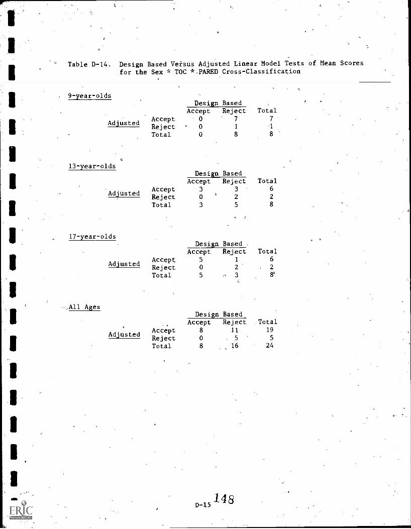
Table D-14. Design Based Versus Adjusted Linear Model Tests of Mean Scoresfor the Sex * TOC *-PARED Cross-Classification

9-year-olds

Adjusted

13-year-olds

Adjusted

17-year-olds

--All Ages

Adjusted

Adjusted

Design BasedAccept Reject Total

Accept 0 7 7

Reject 0 1 1

Total 0 8 8

Design BasedAccept Reject Total

Accept 3 3 6

Reject 0 G 2 2

Total 3 5 8

Design BasedAccept Reject Total

Accept 5 1 6

Reject 0 2 2

Total 5 3 e

Design BasedAccept Reject Total

Accept 8 11 19

Reject 0 5 5

Total 8 16 24

D-15148

e.

Table D-15. Design Based Versus SRS Contrast Tests Of Mean Scores for theSex * TOC * PARED Cross-Classification

9-year-olds.Design Based

SRSAcceptRejectTotal

Accept2

0

2

Reject1

.6

7

Total3

6

9

13-year-oldsDesign Based

SRSA'Ccept

RejectTotal

Accept2

1

3

Reject0

6

6

Total2

7

, 9

17-year-olds

All Ages

Design Based

SRSAcceptRejectTotal

Accept3

0

3

Reject0

6

6

Total3

6

9

Design BasedII

SRSAcceptRejectTotal

Accept7

1

8

Reject1

18

19

Total8-

19

27

D-16

49

Table D-16. Design Based Versus Adjusted Contrast Tests of Mean Scoresfor the Sex * TOC * PARED Cross-Classification

9-year-oldsDesign Based

AdjustedAcceptRejectTotal

Accept2

0

2 .

Reject3

4

7 .

Total5

4

9

13-year-olds

Adjusted

17-year-olds

All Ages

Adjusted

Design BasedAccept 'ReIct TOtal

Accept 2 5

Reject 1 , 3 4

Total 3 6 9

Design BasedAccept Reject Total

Accept 2 5

Reject '0 '4 4

3 6 9

Design Based

AdjustedAcceptRejectTotal

k

Accept7 :

1

8

Reject8

11

19

' Total

15

12

,27

D=17

150

'7

1

I.

I.

I.

Appendix E

Contingency Tables of Balanced Effects Sample DesignBased Tests Versus Alternative Tests Accepted andRejected at the 5% Significance Level

1 51

.E-1

Table E-1. Design Based Versus Alternative Tests forBalance Effects

9-year-olds

Design BasedTotalAccept .Beject

Accept 14 2 16Unweighted Reject 3 11 14

Total 17 13 30

Design BasedAccept Reject Total

Accept 13 1 14Weighted Reject 4 12 16

Total 17 13 30

13-year-olds

Design BasedTotalACcept Reject

Accept 7 ,0 7

Unweighted Reject 2 21 23Total 9 21 30

Design BasedEl

TotalAccept RejectAccept 7 0 7

Weighted Reject 2 21 23Total 9 21 30

17-year-olds

Design BasedAccept Reject total

. Accept 11 0 11\ ..

Unweighted Reject 1 , 18 19

Totai 12 18 30

Weighted

Design BasedAccept Reject Total,

Accept 9 1 10

Reject 3. 17 20Total 12 18 30

All Ages

Table E-1. (continued)

Design BasedTotalAccept Reject

Accept 32 2 34

Unweighted Reject 6 50 56

Total 38 52 90

Design BasedAccept Reject Total

0 Accept 29 2 31

Weighted Reject 9 50 59

Total 38 52 90

E-31