Sensation weighting in duration discrimination - BORIS

Sensation weighting in duration discrimination: A univariate,multivariate, and varied-design study of presentation-order effects

Åke Hellström1& Geoffrey R. Patching2

& Thomas H. Rammsayer3

# The Author(s) 2020, corrected publication 2020

AbstractStimulus discriminability is often assessed by comparisons of two successive stimuli: a fixed standard (St) and a varied com-parison stimulus (Co). Hellström’s sensation weighting (SW) model describes the subjective difference between St and Co as adifference between two weighted compounds, each comprising a stimulus and its internal reference level (ReL). The presentationorder of St and Co has two important effects: Relative overestimation of one stimulus is caused by perceptual time-order errors(TOEs), as well as by judgment biases. Also, sensitivity to changes in Co tends to differ between orders StCo and CoSt: the TypeB effect. In three duration discrimination experiments, difference limens (DLs) were estimated by an adaptive staircase method.The SW model was adapted for modeling of DLs generated with this method. In Experiments 1 and 2, St durations were 100,215, 464, and 1,000 ms in separate blocks. TOEs and Type B effects were assessed with univariate and multivariate analyses, andwere well accounted for by the SWmodel, suggesting that the two effects are closely related, as this model predicts. With short Stdurations, lower DLs were found with the order CoSt than with StCo, challenging alternative models. In Experiment 3, Stdurations of 100 and 215 ms, or 464 and 1,000 ms, were intermixed within a block. From the SW model this was predicted toshift the ReL for the first-presented interval, thereby also shifting the TOE. This prediction was confirmed, strengthening the SWmodel’s account of the comparison of stimulus magnitudes.

Keywords Duration discrimination . Presentation-order effect . Time-order error . Type B effect . Sensationweighting

Participants inmany psychological experiments have to comparethemagnitudes of two stimuli. The outcome of such comparisonsis not always as “common sense”would expect, which is still notfully explained. This is the point of departure of this study.

It is often assumed that comparative judgment is determinedonly by the difference between the stimuli’s magnitudes, as

experienced one by one. According to this simple differencemodel of comparison (Thurstone, 1927a, 1927b), no systematicunderestimation or overestimation of one stimulus relative tothe other should occur, regardless of the order in which they arepresented. Nevertheless, such effects do occur: Often, when twophysically equal stimuli are compared, one of them tends to bejudged as being greater (e.g., heavier or of longer duration) thanthe other. This kind of effect was first noted by the founder ofpsychophysics, Gustav Fechner (1860), who named it the time-order error (TOE). When the first stimulus is overestimatedrelative to the second stimulus, the TOE is positive, and in theopposite case, negative.

The Fechnerian TOEs have been the subject of much re-search throughout the years (see Hellström, 1985, for areview), and several explanations have been given. Most ofthese have assumed that the TOE is a perceptual/cognitivephenomenon. Yet, during the era of S. S. Stevens’s “new psy-chophysics,” it became an established “truth” that the TOEwas due to a methodological flaw (Stevens, 1957) or to someform of judgment bias (Allan, 1977; Allan & Kristofferson,1974; Engen, 1971; Luce & Galanter, 1963; Restle, 1961).However, Jamieson and Petrusic (1975) and Hellström(1977) varied the response format in TOE experiments and

The original version of this article was revised: Due to a printing error, thefactor “2” was missing in the last line of Equation 9. It has now beenreinstated.

Table 11 in the Appendix lists abbreviations and mathematical symbolsused in the article. Partial results from Experiments 1 and 2 werepresented as a poster at Fechner Day 2018, 34th Annual Meeting ofThe International Society for Psychophysics, Lüneburg, Germany,August 20–24, 2018.

* Åke Hellströ[email protected]

1 Department of Psychology, Stockholm University, SE-10691 Stockholm, Sweden

2 Lund University, Lund, Sweden3 University of Bern, Bern, Switzerland

https://doi.org/10.3758/s13414-020-01999-z

Published online: 27 April 2020

Attention, Perception, & Psychophysics (2020) 82:3196–3220

http://crossmark.crossref.org/dialog/?doi=10.3758/s13414-020-01999-z&domain=pdf

mailto:[email protected]

concluded from their results that a bias-based explanationcould not hold: The TOE proved virtually insensitive to theresponse format—for instance, judging the second stimulus asless or greater than the first, or the first as less or greater thanthe second. Whereas Ulrich and Vorberg (2009) as well asAlcalá-Quintana and García-Pérez (2011) and García-Pérezand Alcalá-Quintana (2017, 2019) have maintained that judg-ment bias is the major determining factor of the TOE, mostcontemporary researchers emphasize perceptual-cognitivemechanisms (e.g., Bausenhart, Dyjas, & Ulrich, 2015;Hellström & Rammsayer, 2015; Patching, Englund, &Hellström, 2012; Preuschhof, Schubert, Villringer, &Heekeren, 2010; Raviv, Ahissar, & Loewenstein, 2012; vanden Berg, Lindskog, Poom, & Winman, 2017). Nonetheless,stimulus comparison, like human judgment in general, cannotbe expected to be free from bias, and this fact has to be takeninto account. The most likely kind of bias in stimulus compar-ison seems to be “indecision bias” (García-Pérez & Alcalá-Quintana, 2017, 2019): When the participant compares twostimuli and must select one as being the greater, they have toguess when uncertain.

Measurement of difference limens

Studies of the comparison of stimuli are often performed inorder to measure discriminability, which is usually conceivedin terms of a difference limen (DL; also, just noticeabledifference). In typical experimental designs, based on the con-stant method (Guilford, 1954), a standard stimulus (St) and acomparison stimulus (Co) are presented in succession, St be-ing held at a constant magnitude, and Co varying from trial totrial. Two so-called limens (thresholds) can then be deter-mined: the upper limen (the value of Co that evokes 75%judgments of Co > St) and the lower one (the value of Co thatevokes 75% judgments of Co < St). Both of the limens areaffected when there is a TOE, so the DL is usually taken ashalf the difference between the upper and the lower limen(e.g., Luce & Galanter, 1963).

One problem with the DL is that its size has been found todepend on the presentation order of St and Co—that is, onwhether the changes to be detected are in the first stimulus orthe second one. Holding the first stimulus constant and varyingthe second one (order StCo) has an impact on the proportion ofjudgments of “second greater” that is often found to differ fromwhat is obtained in the reverse procedure (order CoSt). Thereby,the two DLs will differ. This is called the Type B effect(Bausenhart et al., 2015; Ulrich & Vorberg, 2009), or standardposition effect (SPE; Hellström & Rammsayer, 2015;Rammsayer & Wittkowski, 1990). In terms of DLs, the TypeB effect can be defined as the difference DLStCo − DLCoSt. Mostoften, the DL has been found to be smaller with the presentation

order StCo than with CoSt, so that there is a negative Type Beffect (Ellinghaus, Ulrich, & Bausenhart, 2018).

The TOE (also called the Type A effect) and the Type Beffect make accurate determination of stimulus discriminabil-ity a methodological challenge that has been largelyneglected, but it is a challenge that needs to be addressed.For instance, adequate assessment of duration discriminationis important in research on the neuropsychological basis oftime perception (Rammsayer, 2008). To take account of thepresentation-order effects, the simple difference model has tobe replaced by a better one. This is also required for a deeperunderstanding of what goes on in our minds when we carryout the experimental—and also everyday—task of comparingtwo successive stimulus magnitudes.

Modeling successive stimulus comparison

Michels–Helson (MH) model

Michels and Helson (1954; also in Helson, 1964, Ch. 4) stud-ied comparison of the magnitudes of two successive stimulion a difference rating scale. They found, besides the TOE, thatthe scaled difference between the two stimuli was determinedto a greater extent by the second-presented stimulus than bythe first-presented one. The MH model states that the second-presented stimulus in the pair is not compared directly to thefirst-presented one, but to a weighted compound of the first-presented stimulus and the series adaptation level (AL). Thelatter is, in turn, a weighted geometric mean of previouslyexperienced stimuli with weights according to their degreeof recency—termed by Helson (1964) as series, background,and residual stimuli. Hence, d12

* = u {[s · ψ1 + (1 − s) ψa] –ψ2}, where d12

* is the scaled stimulus difference, u is a scalefactor, ψ1 and ψ2 are the subjective stimulus magnitudes, ψa

is the subjective magnitude corresponding to the series AL,and s is the stimulus weight.

Internal reference (IR) model

This model (Dyjas, Bausenhart, & Ulrich, 2012) bears similarityto the MHmodel. The second stimulus in a pair is not comparedwith the first stimulus, but to an IR. This IR is updated in adynamic process, where the IR in the current trial is a weightedmean of the magnitudes of the first stimulus in the current pair(weight g; 0 < g < 1) and the IR in the previous trial (weight 1 −g): d12 = IR - ψ2 = [g · ψ1 + (1 − g) IRp] − ψ2, where ψ1 is themagnitude of the first stimulus of the current pair and IRp is theprevious IR. So, g thereby also becomes the impact weight of thefirst stimulus in its comparison with the second stimulus, whichgoes straight inwithWeight 1. Therefore, in the constantmethod,the DL is predicted to be smaller when the second stimulus isvaried (presentation order StCo) than with the order CoSt. This

3197Atten Percept Psychophys (2020) 82:3196–3220

is, by definition, a negative Type B effect. The IRmodel predictsno TOE, which is because (unlike in the MH model) stimulioutside the series have no influence on the internal reference.As is noted by Dyjas and Ulrich (2014), “the [IR model] implic-itly assumes that the Type B effect and the [TOE] are indepen-dent and that these effects reflect different underlying mecha-nisms” (p. 1139).

Sensation-weighting (SW) model

For clarity, it is pertinent to revisit the origins of the SWmodel. Hellström (1979) carried out a loudness comparisonexperiment with 16 stimulus magnitude combinations in eachof 16 combinations of stimulus duration and interstimulusinterval. To describe the total set of data, a preliminary linearmodel was adopted which, in terms of subjective magnitudes,was d12

* = B1k· ψ1 – B2k· ψ2 + Ck, where d12* is the scaled

subjective difference (calculated, for each stimulus combina-tion [k], on group data for 12 participants, different for eachcondition), ψ1 and ψ2 are the magnitudes of the first and thesecond stimulus, B1k and B2k their regression coefficients, andCk the intercept. This model was fitted to d12

* and to thephysical stimulus magnitudes via a power function with afitted exponent. Across conditions, Ck proved highly linearlydependent on B1k and B2k. Using the best-fitting account ofthis dependence, Ck = a2 B2k – a1 B1k + c, the total number offitted parameters in the model was reduced from 49 to 36,while preserving an excellent fit to the data (error variance3.50% in the raw model and 4.94% in the accepted model).By analogy with the MHmodel, a1 and a2 were interpreted asreference levels (ReLs), ψr1 and ψr2, associated with the firstand the second stimulus, respectively. c was interpreted as u(ψr1 - ψr2), where u is a scale factor. This resulted in the SWmodel, which can be written (Hellström, 1979; cf. Hellström,1985, 2000, 2003; Hellström & Rammsayer, 2004, 2015):

d12* ¼ u s1 � ψ1 þ 1−s1ð Þ ψr1½ �– s2 �ψ2 þ 1−s2ð Þ ψr2½ �f gþ b;

ð1Þ

where s1 and s2 are the weighting coefficients of the stim-uli, and ψr1 and ψr2 are their current ReLs. Judgment bias isrepresented by b (which was not included in the original ver-sion of the SW model).

The SW model is a natural generalization of the MH mod-el, assuming that an adaptation-weighting mechanismoperates on each of the compared stimuli, not only on the firstone, so that the real comparison is not between the stimuli assuch, but between two weighted compounds. Each of thesecompounds combines the subjective magnitudes of a stimulusand of its reference level (ReL). A ReL is conceptually similarto Helson’s (1964) adaptation level in being a product of the

pooling of stimulus information from various sources.However, in the SW model the ReLs are not tied toHelson’s specifications of adaptation levels as weighted geo-metric means. The ReLs should usually be located near thecenter of the stimulus range, but have often been found to beslightly lower. ψr2 may differ from ψr1: Hellström (1979)found sound pressure levels of 67.38 dB and 68.20 dB corre-sponding toψr1 andψr2. Both of these are in the middle rangeof the stimulus magnitudes, but clearly below their mean dBvalue, 69.75 (the series AL value predicted by Helson’s theo-ry). The difference between the two ReLs is likely to be due tothe updating of ψr2 with fresh magnitude information on thecurrent ψ1.

Importantly, the formulation of the SW model in Equation1 allows estimation of the scale factor u, and thereby of the“absolute” values of s1 and s2. These values, or their relation,are not subject to any formal restrictions. Although s valuesmay usually be expected to stay between 0 and 1, indicatingcompromise or assimilation, Hellström (1979) obtained svalues >1 in many stimulus conditions, implying negativeweights for ψr1 or ψr2 − a contrast effect (Hellström, 1985).

The three models discussed are all built on the common,empirically well-grounded notion of stimulus comparison, asdescribed by a linear model with different weights for the twostimuli. The SW model emerged as an extension of the MHmodel, generalized by assuming a weighting process for bothof the stimuli, not just the first one. Like theMHmodel, the IRmodel corresponds to the SW model with s2 = 1 (cf.Bausenhart et al., 2015; Dyjas et al., 2012). However, unlikethe MHmodel, the IR model recognizes no influence by stim-uli external to the current experimental series (but seeBausenhart, Bratzke, & Ulrich, 2016). It may be noted thatthis limitation may be more realistic for studies where thestandard stimulus is fixed within a block, as in the studies justcited, than for experiments where stimulus magnitudes showgreater variation between trials (e.g., Hellström, 1979, 2003;Michels & Helson, 1954).

Unlike the other models discussed, the SW model placesno restrictions on the values of s1 and s2. Thereby, it canaccount for such stimulus-condition dependent patterns ofnegative and positive TOEs and Type B effects as were foundby Hellström (1979, 2003). The SW model has proved ex-tremely useful for analysis and interpretation of the data in anumber of later studies (e.g., Hellström & Cederström, 2014;Hellström & Rammsayer, 2015). In the present study, the SWmodel correctly predicts an experimental outcome.

Explaining the TOE

In a common special case, ψr1 can be assumed equal to ψr2,and thereby both can be denoted byψr. In this case, lettingψ1

= ψ2 = ψ, Equation 1 becomes

3198 Atten Percept Psychophys (2020) 82:3196–3220

d12¼u s2−s1ð Þ ψr−ψð Þ þ b ð2Þ

When two stimuli of equal magnitude are compared, avalue of d12 ≠ 0 implies, by definition, a TOE. So, the SWmodel basically accounts for the TOE as being caused by thedifference between stimulus weights, multiplied by the sub-jective difference between the ReL and the stimulus level,and, additionally, a judgment bias. With s1 < s2 and ψr belowthe mean level of ψ, this results in the common finding of agenerally negative TOE. Also, in experiments with varyingstimulus magnitude level, the TOE becomes negatively relat-ed to the current level, a relation that reverses in the rarer caseof s1 > s2 (Hellström, 1979, 2003).

Type B effect in the SW model

The SW model accounts for the Type B effect as being, likethe TOE, a consequence of the differential weighting: Thestimulus that is changed has an impact on the discriminativeresponse in proportion to its weight (in presentation orderStCo, s2, and in order CoSt, s1) and the DL is therefore in-versely proportional to this weight.

Recently, Ellinghaus et al. (2018) surveyed the Type Beffect across several stimulus continua, and maintained thatwhen it is found, it is consistently negative, as predicted by theIR model. In contrast, results of Hellström and Rammsayer(2015) suggest that also positive Type B effects occur.Furthermore, results by Hellström (2003) and, in particular,Hellström (1979), obtained with methods that did not directlyassess the DL, show equivalents (in terms of the SWmodel, s1> s2) of large positive Type B effects for tonal loudness withbrief stimuli and short interstimulus intervals. Verifying theresults of Hellström and Rammsayer (2015) would thereforebe of theoretical importance, as this would refute the MH andIR models, but would be consistent with the SW model. Suchverification was attempted in the present study, for the case ofduration discrimination, which is no exceptional case withregard to the phenomena just discussed (Eisler, Eisler, &Hellström, 2008; Ellinghaus et al., 2018).

The present study

Hellström and Rammsayer (2004, 2015) used an adaptivestaircase method to measure the DL for interval duration, withseparate blocks for different stimulus presentation conditions.Experiment 2 in Hellström and Rammsayer (2015) employedfilled auditory intervals, with St durations of 100, 215, 464,and 1,000 ms. In the present Experiment 1 we replicated thisexperiment with an improved procedure (see the Appendix).We also conducted two experiments with empty visual inter-vals (bounded by brief flashes): Experiment 2 (analogous to

Experiment 1) and Experiment 3. In the two first experiments,we addressed perceptual-cognitive processes in duration dis-crimination, their expression as the TOE and the Type B ef-fect, and their separation from judgment bias. In Experiment3, we investigated whether, as is predicted by the SW model,the TOE can be shifted by manipulation of the ReLs. Thisattempted manipulation was done by using two St durations,instead of one as in Experiment 2, in each separate block oftrials. The prediction was tested by comparing the results ofExperiments 2 and 3.

Experiments 1 and 2

In Experiments 1 and 2, duration discrimination was assessedwith different presentation orders of standard (St) and com-parison (Co) stimuli, and different St durations. DLs weremeasured using an adaptive two-alternative, forced-choicestaircase method. Four interval durations were used in sepa-rate blocks. In Experiment 1, the intervals were filled auditory,and in Experiment 2, empty visual. These stimulus types wereselected from those (also empty auditory and filled visual)used in Experiment 1 of Hellström and Rammsayer (2015)in order to confirm and further investigate the effect of stim-ulus duration on the size and direction of the Type B effect,which was found by Hellström and Rammsayer (Experiments1 and 2) for these particular stimulus types.

Method

Participants

Undergraduate psychology students at the University of Berntook part in the experiments. In Experiment 1, there were 57females and eight males ranging in age from 19 to 48 years (M± SD = 22.4 ± 4.3 years), and in Experiment 2, 44 females and11 males, 19 through 29 years of age (21.3 ± 2.0 years). Theparticipants received course credit. All of them were naïveabout the purpose of the study and reported normal hearingand normal or corrected-to-normal vision. Because of the clearaudibility or visibility of the stimuli, and the task being tocompare the duration of the stimuli, not their magnitude, nofurther screening of hearing or vision was deemed necessary.All participants gave their written, informed consent.1

Apparatus and stimuli

Presentation of stimuli and recording of the participants’ re-sponses were controlled by a computer program written in

1 The study was approved by the ethics committee of the Faculty of HumanSciences of the University of Bern, Bern, Switzerland (date of approval:September 27, 2016; project identification code: 2016-9-00005).


Turbo Pascal and an assembler-based timing routine. Timingaccuracy of stimulus presentation was better than ±1 ms.Filled auditory stimuli (Experiment 1) were white-noise burstspresented binaurally through headphones (Sony CD 450) at anintensity of 66 dBA. Empty visual intervals (Experiment 2)were bounded by 3-ms flashes of a red light-emitting diode(LED; diameter 0.38°, viewing distance 60 cm, luminance 68cd/m2) positioned at the eye level of the participant. The in-tensity of the LED was clearly above threshold, but notdazzling.

Procedure

The procedure was identical in Experiments 1 and 2. Theparticipant was seated at a table with a keyboard and a com-puter monitor in a sound-attenuated and dimly lit room. Toinitiate the first trial, the participant pressed the space bar; thefirst stimulus interval was then presented after 900 ms, andthen, after the 900-ms interstimulus interval, the second stim-ulus interval. Thereafter, the response was given by pressingone of two designated keys on the keyboard, labeled “firstinterval longer” and “second interval longer,” respectively. 2

Accuracy, not speed, was emphasized in the instructions. Thenext trial started 900 ms after the participant’s response. Nocorrectness feedback was given.

Adaptive staircase method A more detailed description of thepsychophysical procedure is given in Rammsayer (2012).Participants compared the durations of two successive inter-vals, standard (St) and comparison (Co), using a two-alternative forced-choice response: “first interval longer” or“second interval longer.” On each trial of a series, the Cowas increased or decreased in duration after having beenjudged as shorter or longer, respectively, than the St. A stepthat increased the absolute difference between Co and St wasthree times longer than a step that decreased this difference,which made performance settle at 75% responses of “firstlonger” or “second longer” (see Hellström & Rammsayer,2015, for an explanation). Each participant took part in onlyone experiment, which was run in one experimental sessionconsisting of eight blocks, with a 1-min break following eachblock. After six practice trials, the experimental session com-prised four pairs of 64-trial blocks, each block pair using oneSt duration, with the order of the four St durations (100; 215;464; and 1,000 ms) balanced across participants. Each blockpair comprised one Hi-Co block, where Co was initially lon-ger than St, and one Lo-Co block, where Co was initiallyshorter than St. For half of the participants, each block pair

started with a Hi-Co block, and for the other half, with a Lo-Co block. Each block comprised two randomly interleaved32-trial series, one series of pairs with an Up (U) profile,where the second interval was initially longer than the first,and one with a Down (D) profile, where the second intervalwas initially shorter than the first. So, with StCo and CoStindicating the presentation order, the four series types wereStCoU, StCoD, CoStU, and CoStD. Trials in a Hi-Co blockwere, equally often and in random order, from the StCoU andthe CoStD series, and in a Lo-Co block, from the StCoD andthe CoStU series.

When the St was 100 (215; 464; 1,000) ms, the initialduration of the Co in a series was 35 (70, 100, 500) ms belowthe St duration (in Lo-Co blocks) or above it (in Hi-Coblocks). The Co duration was then changed, using the weight-ed up–down method as described above, to estimate the upperor the lower DL (i.e., the duration difference for which 75%judgments of “first interval longer” or “second interval lon-ger,” as pertinent, were obtained). In a Lo-Co (Hi-Co) block,the Co was increased (decreased) by 5 (9, 15, 100) ms afterhaving been judged as shorter (longer) than the St, and de-creased (increased) by 15 (27, 45, 300) ms after having beenjudged as longer (shorter) than the St. These steps were usedfor Trials 1–6; in Trials 7–32, the corresponding steps were 3(6, 10, 25) and 9 (18, 30, 75) ms. See Table 6 in the Appendixfor a summary of the procedure.

Measurement and modeling

Raw DLs. In experiments where d12 is measured on each ex-perimental trial (e.g., Hellström, 1979, 2003), fitting the SWmodel (Equation 1) to the data is quite straightforward. Incontrast, what is measured in each condition of the presentexperiments is the value of Co that evokes 75% or 25% judg-ments of “first interval longer.” For each participant and eachof the four conditions per St duration, the mean, across the last20 trials, of the duration difference between the first and sec-ond presented stimulus (i.e., Co − St in CoSt series and St −Co in StCo series) was computed. From this we obtained theraw DL − rDLD in D series and rDLU in U series. At the rDLDthe d12 value corresponds to the 75th percentile, and at therDLU to the 25th percentile, in this participant’s distributionof d12 across trials. We denote these d12 values by d12x and−d12x, respectively. The measured rDL values are, as is de-tailed in the text, subject to condition-specific effects, and theyshould not be taken as indices of discriminability.

Modeling approach To model the participant’s comparisonbehavior, the SW model (Equation 1) was adapted to the par-ticular type of experimental data obtained. Similar modelingwas used in Hellström and Rammsayer (2004, 2015). Thepsychophysical function was assumed to be the identity func-tion,ψ =ϕ, over the range of Co intervals for each St duration

2 These keys were “+” and “Enter,” respectively, which were located on theextreme right-hand side of the keyboard, with the “+” key located above the“Enter” key. Earlier pilot studies showed no evidence for any effect of re-sponse key designation on response times.


(no assumption was made concerning its shape across St du-rations). Also, d12 is specified in ϕ units, so that the scalefactor u can be dropped. From Equation 1 we obtain

d12 ¼ s1ϕ1 þ 1−s1ð Þ ϕr1½ �− s2ϕ2 þ 1−s2ð Þ ϕr2½ � þ b ð3Þ

For Experiments 1 and 2, the blocked design, with only oneSt duration per block, makes it reasonable to assume that thetwo ReLs are equal, ϕr1 = ϕr2 = ϕr (cf. Hellström, 2000),which yields the simpler expression

d12 ¼ s1ϕ1−s2ϕ2 þ s2−s1ð Þ ϕr þ b ð4Þ

The “noise” dispersion of d12 across trials, σd12, maybe termed the comparatal dispersion (Gulliksen, 1958),and we assume it to be proportional to the mean subjec-tive stimulus magnitude (as per Ekman’s law; see Eisleret al., 2008). For simplicity, in the equations the physicalmagnitudes of the St and the Co, ϕSt and ϕCo, are ab-breviated S and C. Our assumption ψ = ϕ then yieldsd12x = wi · S (as per Weber’s law in its simple form),where wi is the participant-specific value of σd12 / S,multiplied by 0.6745 (i.e., the standard normal deviatecorresponding to the 75th percentile). We term w theWeber constant; w is not the same thing as a measuredWeber fraction, but is assumed to underlie it. Judgmentbias is likewise modeled as a participant-specific propor-tion of the St duration, bi · S.

Weight ratio and Type B effect As appropriate for each of thefour series types (StCoU, StCoD, CoStU, CoStD), S and C, orC and S, were substituted in Equation 4 forϕ1 andϕ2, and thevalue of d12 was specified as either d12x (in D series) or -d12x(in U series). This resulted in Equations 14–17 (see theAppendix). From these equations we obtain, in terms ofWeber fractions (WFs), where WF = DL/S and the WF foran individual series type is called a raw WF (rWF),

WFStCo ¼ rWFStCoU þ rWFStCoDð Þ=2 ¼ w=s2 ð5ÞWFCoSt ¼ rWFCoStU þ rWFCoStDð Þ=2 ¼ w=s1 ð6Þ

Hence,

WFStCo=WFCoSt ¼ s1=s2 ð7Þ

Estimation of model parameters fromWeber fractions For themean WF across presentation orders, WFM, we have,

WFM ¼ 1= 2 WFStCo þWFCoStð Þ ¼ 1= 2 w s1 þ s2ð Þ= s1s2ð Þ ð8Þ

For s1 = s2 = s, WFM =w/s. From the data given in Table 7,in the Appendix, we obtained, with WFs estimated (by inter-polation) at s1/s2 ≈ 1, rough estimates of w/s: 11.7% forExperiment 1 and 23.3% for Experiment 2.

The Type B effect is here defined as the Type B effectquotient (QTBE), the difference between the WFs in presen-tation orders StCo and CoSt as a fraction of WFM,

QTBE ¼ WFStCo−WFCoStð Þ=WFM

¼ w s1−s2ð Þ= s1s2ð Þ½ �= 1= 2 w s1 þ s2ð Þ= s1s2ð Þ� �

¼ 2 s1−s2ð Þ= s1 þ s2ð Þ; ð9Þ

so that s1/s2 < 1 implies a negative, and s1/s2 > 1 a positiveType B effect.

Time-order errors (TOEs) A positive (negative) TOE meansthat the first stimulus is overestimated (underestimated) rela-tive to the second one. Thus, with a positive TOE, rDLU (in Useries) becomes larger than the corresponding rDLD (in Dseries). One might attempt to estimate the TOE, for each pre-sentation order (StCo or CoSt), as (rDLU − rDLD)/2.However, it may theoretically be expected that the psychomet-ric function, while symmetric on a logarithmic scale, is some-what asymmetric on the linear duration scale, its slope beingsteeper at low than at high stimulus magnitudes (Eisler et al.,2008). Such an asymmetry would increase the DL in blocks ofStCoU and CoStD (Hi-Co blocks; see the Appendix) as com-pared with blocks of StCoD and CoStU (Lo-Co blocks), andso bias the QTOE estimates (positively with the StCo orderand negatively with the CoSt order). Such an effect is bal-anced out by defining the QTOE as its mean across presenta-tion orders StCo and CoSt. Therefore, only this measure willbe discussed in the following.

Adapting the SW model, as described in the Appendix, tofit the S and rDL values in each of the four series types yieldsEquations 17–20 (in the Appendix), which in turn yieldEquations 18–21 that predict the rWFs from the SW modelparameters. From these equations, the TOE quotient (QTOE),TOE/S, can be predicted as follows:

QTOE ¼ 1= 2 rWFStCoU−rWFStCoDð Þ=2þ rWFCoStU−rWFCoStDð Þ=2½ �¼ 1= 2 bþ s2−s1ð Þ Q½ �=s2 þ bþ s2−s1ð Þ Q½ �=s1f g¼ 1= 2 b s1 þ s2ð Þ þ Q s22−s12

� �� =s1s2;

ð10Þ

where Q is the ReL distance quotient—that is, the relativedistance of the ReL from the St: Q = (ϕr − S) / S.

Origin of QTOE Equation 10 implies that QTOE depends onthe weight difference as well as on the judgment bias, b. Whenthe ReL is at a distance from the St, a QTOE arises frommultiplication of Q by (s2

2 − s12). With Q < 0, QTOE will

be negatively related to (s22 − s1

2), and thereby positivelyrelated to s1/s2.

Furthermore, it follows from the SW model that QTOEis closely related to QTBE. From Equations 9 and 10 weget


QTOE ¼ 1= 2 b s1 þ s2ð Þ þ Q s22−s12� ��

=s1s2

¼ 1= 2 b s1 þ s2ð Þ=s1s2− 1= 2 Q s1−s2ð Þ s1 þ s2ð Þ=s1s2¼ 1= 2 b s1 þ s2ð Þ=s1s2−Q

� QTBE 1= 4 s1 þ s2ð Þ2=s1s2h i

ð11Þ

For s1= s2 = s, QTBE = 0, and QTOE = b / s. For a widerange of s1/s2 ratios, the factor 1/4 (s1+ s2)

2 / s1s2 is close to 1,so that for moderate b values the slope of QTOE versus QTBEis predicted to be close to −Q (with QTOE andQ expressed inpercentages).

Results

All statistical analyses were conducted using IBM SPSSStatistics, Versions 25 and 26 for MacOS X.

Outlier exclusion

An initial screening for multivariate outliers (i.e., unusually de-viating data patterns) was conducted, using the procedure de-scribed in Tabachnick and Fidell (2007, p. 74). Each participant’ssquaredMahalanobis distance (based on the 16 rDLs) was testedagainst the χ2 distribution with df = 16 (matching the number ofvariables). Because of the limited number of participants in eachexperiment, failing to exclude a multivariate outlier might incurmisleading results. Therefore, a criterion of p < .025 was used,instead of p < .001 as recommended by Tabachnick and Fidell.The test resulted in exclusion of the data from four participants inExperiment 1 and five participants in Experiment 2. Their exclu-sion was further justified by their squaredMahalanobis distancesdeviating clearly from the straight line in “Q–Q” plots of theirquantiles against those of the χ2(16) distribution (cf. Garrett,1989). Consequently, the analyses were based on n = 61 inExperiment 1, and n = 50 in Experiment 2.

Weber fractions For each experiment, descriptive statistics ofrWF are given in Table 7, in the Appendix, for each of the fourseries types, as well as mean WFs for each St duration andacross St durations. Nonpositive rWF values were observed in7.1% and 4.6% of the cases in Experiments 1 and 2, respec-tively. For each experiment and St duration, the mean (M) andstandard error of the mean (SEM) of the WF for each presen-tation order are shown in Fig. 1, as well as the estimate ofWFStCo/WFCoSt (indicating s1/s2).

For each experiment, the values of WFStCo and WFCoSt foreach of the four St durations were submitted to a repeated-measures ANOVA, with St duration (100; 215; 464; 1,000ms) and presentation order (StCo, CoSt) as within-

participant factors. Here, as in all our ANOVAs, multivariate(Pillai) tests were used. The results are given in Table 1.

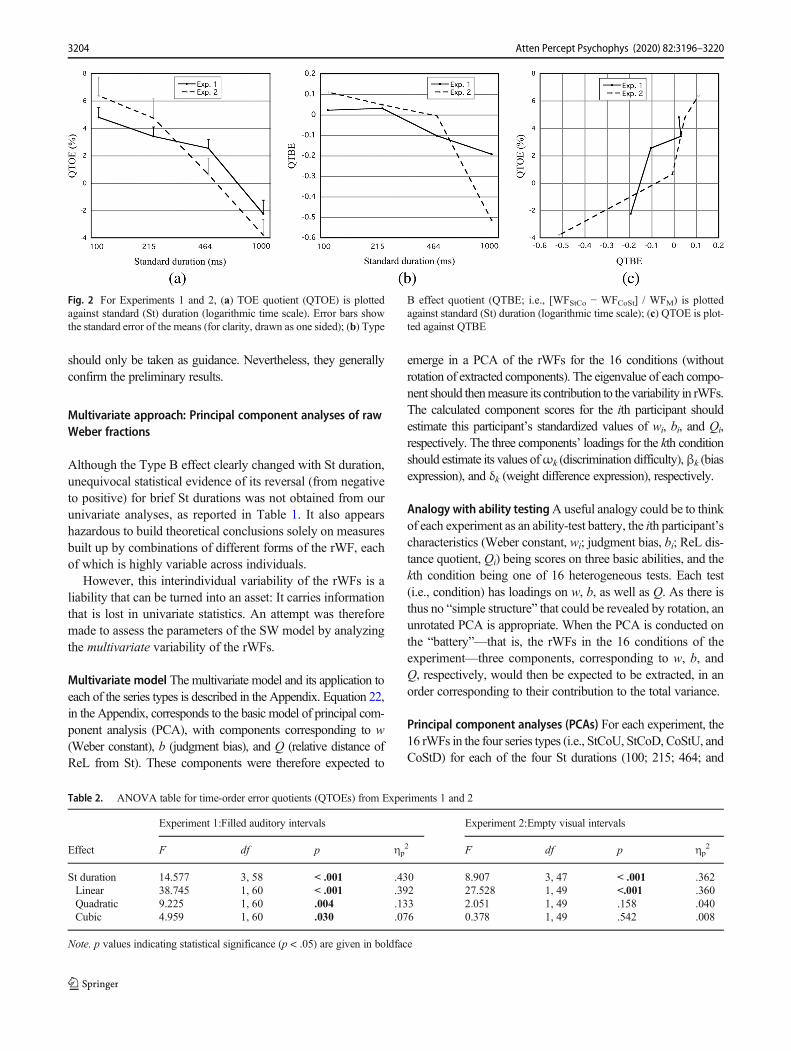
TOE Quotient (QTOE) Descriptive statistics of QTOE for eachSt duration are given in Table 7, in the Appendix. The meansand their standard errors are shown in Fig. 2. For St durationsthat yielded values of s1/s2 near 1 (i.e., 215 and 464 ms) QTOEwas positive, indicating b > 0—that is, a judgment bias in thedirection of “first interval longer.” Using Equation 11, b/s waspreliminarily and roughly estimated as the mean QTOE valuefor these durations, about +3.5% for both experiments.

For each experiment, the eight QTOE values were submit-ted to a repeated-measures ANOVA with St duration (100;215; 464; 1,000 ms) and presentation order (StCo, CoSt) aswithin-participant factors. The results are given in Table 2.

Interpretation of univariate results

The SW model (Equation 1) describes the perceptual stimulus-comparisonmechanism as being based on a comparison betweentwo weighted compounds, each comprising a stimulus magni-tude and a ReL. Accordingly, the model predicts that theweighting is reflected in Weber fractions as well as in TOEs.

Weber fractions Equation 9 predicts that QTBE changes withthe weighting balance (specifically, [s1 – s2] / [s1 + s2]) acrossSt durations. In accordance with this, the ANOVA ofWFs forExperiment 2 showed a significant St Duration × Order inter-action, p = .003, to which the linear effect of St duration madethe greatest contribution. Thus, the Type B effect—the effectof presentation order on the WF—was not constant, butchanged with the St duration. However, in post hoc t teststhe only clearly significant evidence for a nonzero Type Beffect occurred for the 1,000-ms St duration, where the effectwas negative (implying s1/s2 < 1).

For Experiment 1, the St Duration × Order interactionfailed to reach statistical significance, p = .076. Still, onemay note that the linear contribution of St duration to thisinteraction was significant, p = .008.

TOE quotients Equation 10 implies that QTOE should be di-rectly related to Q (s2

2 − s12) / (s1s2). Figure 2 gives some

support to this, as it shows QTOE to be generally positivelyrelated to QTBE, and thereby to s1 − s2. This suggests that ineach block Q < 0 (i.e., the ReL falls below the St). From theslopes of the linear regressions (QTOE vs. QTBE, group data)depicted in Fig. 2c, Q was estimated as −26.0% forExperiment 1 (r = .91) and −14.6% for Experiment 2 (r =.92). The b values were estimated as equal to the regressionintercepts, +3.7% (Experiment 1) and +3.3% (Experiment 2).

The negative Q values are as could be expected from theresults of Hellström and Rammsayer (2015). They are also inharmony with results for weight comparison with a single


standard (Hellström, 2000). A parallel is the finding in tem-poral bisection experiments, where participants classify inter-vals as long or short, that the bisection (neutral) point is locat-ed below the arithmetic mean of the interval durations(Brown, McCormack, Smith, & Stewart, 2005; Wiener,Thompson, & Coslett, 2014). Similar findings were addressedby Helson (e.g., 1964) by specifying the adaptation level as aweighted geometric mean of the stimulus magnitudes.

Model fitting by NLR For additional guidance regarding modelparameters, Equations 18–21, in the Appendix, were used to fitthe SW model, using the SPSS routine nonlinear regression

(NLR). For each experiment, all the individual rWF estimateswere entered together. Q, w, and b were assumed to be constantacross conditions, and s1 and s2 to be condition specific. Only thevalue of Q could be uniquely estimated; s1, s2, b, and w wereestimated relative to each other. Using the formula WFM = w/swith the above WFM estimates of 11.7% (Experiment 1) and23.5% (Experiment 2), the values of w were fixed at 5.85% forExperiment 1 and at 11.75% for Experiment 2 to yield plausibleaverage values for s1 and s2 of about 0.5 (cf. Hellström, 2003).The NLR results are given in Table 3. The model used in thisanalysis is obviously simplified, and R2 (corrected) is modest:.133 (Experiment 1) and .152 (Experiment 2), so the results

Table 1. ANOVA table for Weber fractions (WFs) from Experiments 1 and 2

Experiment 1:Filled auditory intervals Experiment 2:Empty visual intervals

Effect F df p ηp2 F df p ηp

2

St duration 4.848 3, 58 .004 .200 17.415 3, 47 < .001 .526

Linear 2.271 1, 60 .137 .036 46.269 1, 49 < .001 .486

Quadratic 9.082 1, 60 .004 .131 14.626 1, 49 < .001 .230

Cubic 0.120 1, 60 .730 .002 3.423 1, 49 .070 .065

Order 3.278 1, 60 .075 .052 2.396 1, 49 .128 .047

Dur. × Order 2.414 3, 58 .076 .111 11.490 3, 47 < .001 .423

Linear 7.445 1, 60 .008 .110 29.752 1, 49 < .001 .378

Quadratic 0.666 1, 60 .418 .011 9.275 1, 49 .004 .159

Cubic 0.197 1, 60 .659 .003 2.631 1, 49 .111 .051

Type B effectSt = 100 msSt = 215 msSt = 464 msSt = 1,000 ms

t0.3790.407−1.501−2.770

df60606060

p−−.554.030

t2.0890.724−0.093−5.536

df49494949

p.168−−< .001

Note.Bonferroni-corrected t-test results for Weber fraction difference between presentation orders StCo and CoSt (i.e., Type B effect), are also given foreach standard duration; p values indicating statistical significance (p < .05) are given in boldface

WF ratio 1.03 1.02 0.90 0.82 1.12 1.05 0.99 0.59

Fig. 1 For Experiments 1 and 2, mean Weber fractions for presentationorders StCo and CoSt are plotted against standard (St) duration (logarith-mic time scale). Error bars show the standard error of the mean (for

clarity, drawn as one sided). Below the graph, the WF ratio WFStCo/WFCoSt (which estimates s1/s2) is given for each St duration


should only be taken as guidance. Nevertheless, they generallyconfirm the preliminary results.

Multivariate approach: Principal component analyses of rawWeber fractions

Although the Type B effect clearly changed with St duration,unequivocal statistical evidence of its reversal (from negativeto positive) for brief St durations was not obtained from ourunivariate analyses, as reported in Table 1. It also appearshazardous to build theoretical conclusions solely on measuresbuilt up by combinations of different forms of the rWF, eachof which is highly variable across individuals.

However, this interindividual variability of the rWFs is aliability that can be turned into an asset: It carries informationthat is lost in univariate statistics. An attempt was thereforemade to assess the parameters of the SW model by analyzingthe multivariate variability of the rWFs.

Multivariate model The multivariate model and its application toeach of the series types is described in the Appendix. Equation 22,in the Appendix, corresponds to the basic model of principal com-ponent analysis (PCA), with components corresponding to w(Weber constant), b (judgment bias), and Q (relative distance ofReL from St). These components were therefore expected to

emerge in a PCA of the rWFs for the 16 conditions (withoutrotation of extracted components). The eigenvalue of each compo-nent should thenmeasure its contribution to the variability in rWFs.The calculated component scores for the ith participant shouldestimate this participant’s standardized values of wi, bi, and Qi,respectively. The three components’ loadings for the kth conditionshould estimate its values ofωk (discrimination difficulty),βk (biasexpression), and δk (weight difference expression), respectively.

Analogy with ability testingA useful analogy could be to thinkof each experiment as an ability-test battery, the ith participant’scharacteristics (Weber constant, wi; judgment bias, bi; ReL dis-tance quotient, Qi) being scores on three basic abilities, and thekth condition being one of 16 heterogeneous tests. Each test(i.e., condition) has loadings on w, b, as well as Q. As there isthus no “simple structure” that could be revealed by rotation, anunrotated PCA is appropriate. When the PCA is conducted onthe “battery”—that is, the rWFs in the 16 conditions of theexperiment—three components, corresponding to w, b, andQ, respectively, would then be expected to be extracted, in anorder corresponding to their contribution to the total variance.

Principal component analyses (PCAs) For each experiment, the16 rWFs in the four series types (i.e., StCoU, StCoD, CoStU, andCoStD) for each of the four St durations (100; 215; 464; and

Fig. 2 For Experiments 1 and 2, (a) TOE quotient (QTOE) is plottedagainst standard (St) duration (logarithmic time scale). Error bars showthe standard error of the means (for clarity, drawn as one sided); (b) Type

B effect quotient (QTBE; i.e., [WFStCo − WFCoSt] / WFM) is plottedagainst standard (St) duration (logarithmic time scale); (c) QTOE is plot-ted against QTBE

Table 2. ANOVA table for time-order error quotients (QTOEs) from Experiments 1 and 2

Experiment 1:Filled auditory intervals Experiment 2:Empty visual intervals

Effect F df p ηp2 F df p ηp

2

St durationLinearQuadraticCubic

14.57738.7459.2254.959

3, 581, 601, 601, 60

< .001< .001.004.030

.430

.392

.133

.076

8.90727.5282.0510.378

3, 471, 491, 491, 49

< .001<.001.158.542

.362

.360

.040

.008

Note. p values indicating statistical significance (p < .05) are given in boldface


1,000ms), were submitted to a PCA, using the FACTOR routinein SPSS. TheKaiser–Meyer–Olkin (KMO)measure of samplingadequacy3 (Kaiser, 1974)was .657 for Experiment 1 and .635 forExperiment 2. For each experiment, three components were ex-tracted, with eigenvalues of 3.9 (explaining 24.4% of the vari-ance), 3.1 (19.2%), and 1.6 (9.9%) for Experiment 1, and 4.4(27.2%), 2.8 (17.7%) and 1.7 (10.4%) for Experiment 2.

Results of the PCAs The unrotated component loadings aregiven in Table 8 in the Appendix. Scores of the three extractedcomponents (wi, bi, Qi) were also computed for each partici-pant. For an interpretation of the loadings, note that inEquations 18–21, in the Appendix, w always occurs as a pos-itively signed term, whereas the b term is positively signed forUp (U) series, and negatively signed for Down (D) series.

For Experiment 1, the first component had (after reversal ofloading signs) positive loadings for U series and negative load-ings for D series, and individual component scores correlatedhighly with QTOE (see Fig. 5). It could thereby be identified asb, the loading for condition k indicating this condition’s biasexpression, βk. The second component, whose scores correlat-ed highly with WFM and whose loadings (except one) werepositive, could be identified as w, the loading for condition kindicating this condition’s discrimination difficulty, ωk.

For Experiment 2, the first component was identified as w(all loadings positive, highly correlated with WFM) and thesecond (after reversal of signs) as b (scores highly correlatedwith QTOE, loadings generally positive for U series and neg-ative for D series). For each experiment, the third componentwas identified as Q (ReL distance quotient), its loading forcondition k reflecting the weight difference, δk, in this condi-tion, that is, the multiplier ofQi in determining the QTOE. Theresults are consistent with weight ratios s1/s2 > 1 for St dura-tions of 100 and 215 ms, and s1/s2 < 1 for 464 and 1,000 ms(as was found from the analysis of WFStCo/WFCoSt ratios) incombination withQ < 0 (i.e., the ReL being situated below theSt) for each St duration.

In Table 8, in the Appendix, mean values ofω,β, and δ foreach St duration are given, as estimated from the mean com-ponent loadings using Equation 22, in the Appendix. ForExperiment 1, β (bias expression) was positive for each Stduration, which indicates, in accordance with the estimatedpositive b value for s1/s2 = 1, a judgment bias that favorsjudgments of “first interval longer” for all St durations. ForExperiment 2, such a bias was obtained for all St durationsexcept 1,000 ms, where the bias was close to zero.

Variance components in the comparison processAs predict-ed by Equations 18–21, in the Appendix, the measured rWF isaffected by the SW mechanism as well as by two participant-specific factors—namely,Weber constant (w) and judgment bias(b). The present experimental designmade it possible to estimate,using PCA, the contributions of each of these factors to the totalvariance of the rWFs. As assessed by eigenvalues from PCAs ofthe rWFs, w and b dominated in this respect, leaving about 10%for the ReL distance quotient Q, the latter factor generating sys-tematic TOEs by multiplication with the weight difference (s2 −s1). This effect was limited by the blocked design, with the Stduration fixed within each block, which minimized the possibleasymmetry of Q as well as its interindividual variation. As isdemonstrated in the next section, the role of Q in modulatingthe shift of QTOE with the St duration was still considerable,as was predicted from the SW model.

Relating PCA-estimated model parameters to univariateresults: Comparison of univariate results from participantswith low, medium, and high PCA component scores

For each of the three extracted components, the scores werepartitioned at their low, medium, and high tertiles. Each ofFigs. 3, 4, and 5 shows mean WF or QTOE for each partitionof a component score, and is supplemented with ANOVAresults.

Weber fractions (WFs) Figure 3 shows, plotted against the Stduration, the mean WF for participants with lowest, medium,and highest third levels of the w (Weber constant) component

3 According to Kaiser (1974) KMOvalues of >.5 are acceptable, and values of.6–.7 are “mediocre.”

Table 3. Results from model fitting by SPSS NLR

St (ms) Experiment 1:Filled auditory intervals Experiment 2:Empty visual intervals

s1 s2 s1/s2 s1 s2 s1/s2

100 0.425 (0.022) 0.418 (0.022) 1.017 0.391 (0.020) 0.339 (0.015) 1.153

215 0.495 (0.029) 0.499 (0.027) 0.992 0.526 (0.034) 0.455 (0.025) 1.156

464 0.512 (0.031) 0.532 (0.030) 0.962 0.485 (0.030) 0.536 (0.033) 0.905

1,000 0.417 (0.025) 0.525 (0.039) 0.794 0.434 (0.026) 0.729 (0.070) 0.595

Note. Estimates (SEs in parentheses) of weights (s1 and s2), judgment bias (b, in %), and ReL distance quotient (Q). Except forQ, estimates are relative tofixed value of Weber constant (w, in %). Experiment 1: wfixed = 5.85%; b = 1.83% (0.70); Q = −27.04% (13.32). Experiment 2: wfixed = 11.75%; b =1.47% (0.39); Q = −13.58% (3.51)


score. As expected, mean WFs increased with increasing wscores.

TOE quotients (QTOEs) Figure 4 shows, in the same man-ner, the mean QTOE for participants with lowest, me-dium, and highest third levels of the b (judgment bias)

component score. Mean QTOEs were directly relatedto b scores, except for Experiment 2 with S = 1,000ms.

Finally, Fig. 5 shows the mean QTOE for participantswith lowest, medium, and highest third levels of the Q(ReL distance quotient) component score. Correlations

w level p < .001, 2p = .652 < .001, 2

p = .646

St duration p = .005, 2p p

p

p < .001, 2

p = .528

w lev. X St dur. p = .593, 2p = .026

= .070

= .622, 2p = .046

Fig. 3 For Experiments 1 and 2, mean Weber fraction is plotted against standard (St) duration (logarithmic time scale) at low, medium, and high thirdscore levels of w component. Included are ANOVA results for Weber fractions

b level p < .001, 2p = .796 < .001, 2

p = .626

St duration p < .001, 2p = .464 p

p

p < .001, 2

p = .460

b lev. X St dur. p = .199, 2p = .071 < .001, 2

p = .249

Fig. 4 For Experiments 1 and 2, mean TOE quotient (QTOE) is plotted against standard (St) duration (logarithmic time scale) at low, medium, and highthird score levels of b component. Included are ANOVA results for QTOEs


of the Q score with QTOE are also given for each Stduration. According to the SW model, QTOE is propor-tional to the squared-weight difference (s2

2 − s12), multi-

plied by Q. As is shown in Fig. 5, and verified by theANOVA results, scores of the Q component indeed mod-ulated the slope of QTOE against St duration, and therebyagainst weight difference. This slope did not become pos-itive even with the highest Q scores.

This suggests that most individual Q values stayed onthe negative side. In the univariate analyses we found ev-idence (clearly significant only for Experiment 2) that thedifference s2 − s1 was positive for S = 1,000 ms. This isconfirmed by the significantly positive correlations be-tween QTOE and Q component score for this St duration.Conversely, the significantly negative correlations for, inparticular, St = 100 ms in both experiments indicate nega-tive values of (s2 − s1). So, the univariate indications wereconfirmed: The weighting balance did reverse into s1/s2 > 1(equivalent to a positive Type B effect) for brief St dura-tions; significantly so for St = 100 ms (Experiments 1 and2) and for St = 215 ms (Experiment 1).

Response times

Response times in Experiments 1 and 2 are reported anddiscussed in the Appendix.

Discussion of Experiments 1 and 2

Weighting change and its interpretation

The present results are generally consistent with those ofHellström and Rammsayer (2015). In particular, in both stud-ies, the ratio s1/s2 tended to decrease with increasing stimulusduration. This parallels the decrease of s1/s2 with increasing

rQ,QTOE -.536*** -.521*** .218ns .396** -.455*** -.150ns .581*** .748***

Q level p = .678, 2p = .013 p = .862, 2

p = .006

St duration p < .001, 2p = .580 p < .001, 2

p = .586

Q level X St dur. p < .001, 2p = .306 p < .001, 2

p = .344

Fig. 5 For Experiments 1 and 2, mean TOE quotient (QTOE) is plottedagainst standard (St) duration (logarithmic time scale) at low, medium,and high third score levels of Q component. Correlation between Q

component and QTOE is given for each St duration (Bonferronicorrected: ***p < .001, **p < .01, ns = not significant). Included areANOVA results for QTOEs

WF ratio 1.51 0.82 0.90 0.66

Fig. 6 For Experiment 3 (empty visual intervals) mean Weber fraction,for presentation orders StCo and CoSt, is plotted against standard (St)duration (logarithmic time scale). Error bars show the standard error ofthe mean. Below the graph, the ratio WFStCo/WFCoSt (which estimates s1/s2) is given for each St duration.


interstimulus interval that generally occurs in TOE experi-ments (e.g., Hellström, 1979, 2003). The interval betweenthe onsets of the first and the second stimulus increases withthe interstimulus interval as well as with stimulus duration, soit seems likely that both of these temporal factors contribute tothe change of the weighting balance.

This change, to the disadvantage of the first stimulus,has been proposed to reflect the tuning of a mechanismthat increases discrimination sensitivity by optimalweighting-in of ReL magnitude information (Hellström,1989; Patching et al., 2012; cf. Preuschhof et al., 2010).In particular, the weighting change is thought to reflecta transition, with longer interstimulus intervals and/orstimulus durations, from stimulus interference to memo-ry loss.

Taking advantage of the interindividual variability provid-ed the extra statistical power needed to confirm the reversal ofthe weighting pattern (i.e., yielding s1 > s2) with brief St du-rations. Similarly, in Hellström and Rammsayer (2004), forduration comparison of filled auditory intervals across inter-stimulus intervals of 100–2,700 ms, s1/s2 > 1 was generallyfound for St durations of 50 ms, and s1/s2 < 1 for 1,000 ms.

Time order errors (TOEs)

Figures 3, 4 and 5 suggest that our univariate and multivariateanalyses of the rWFs captured the essential factors in thebuild-up of the TOEs: sensation weighting and judgment bias.Importantly, positive as well as negative TOEs were shown to

Fig. 7 For Experiments 2 and 3 (empty visual intervals), mean Weber fraction across stimulus orders (left) and TOE quotient (QTOE; right) is plottedagainst standard (St) duration (logarithmic time scale). Error bars indicate the standard error

Table 4. ANOVA table for analysis of Weber fractions and QTOEs from Experiment 3 (empty visual intervals)

Weber fractions QTOEs

Effect F df p η2p F df p η2pSt durationLinearQuadraticCubic

32.27782.78013.6350.031

3, 621, 641, 641, 64

< .001< .001< .001.862

.610

.564

.176

.000

99.715199.4129.56978.963

3, 621, 641, 641, 64

< .001< .001.003< .001

.828

.757

.130

.552

Order 0.975 1, 64 .327 .015 11.201 1, 64 .001 .149

Dur. x OrderLinearQuadraticCubic

26.35967.13911.79321.531

3, 621, 641, 641, 64

< .001<.001.001< .001

.561

.512

.156

.252

6.2854.26012.0086.271

3, 621, 641, 641, 64

< .001.043< .001.015

.233

.062

.158

.089

Type B effectSt = 100 msSt = 215 msSt = 464 msSt = 1000 ms

t6.586-2.796-2.091-5.737

df64646464

p< .001.027.162< .001

Note. Bonferroni-corrected t-test results for Weber fraction difference between presentation orders StCo and CoSt (i.e., Type B effect), are also given foreach standard duration; p values indicating statistical significance (p < .05) are given in boldface


occur even with a blocked design, that is, in the absence oftrial-to-trial variation of the St duration.

Judgment bias (b) contributes considerably to the interin-dividual variation of the TOE, but only moderately to its meanvalue across individuals. The bias and its interindividual var-iation are most easily understood as being due to individualguessing habits in cases of uncertainty (García-Pérez &Alcalá-Quintana, 2017). In Experiment 2, the impact of judg-ment bias vanished for the St duration of 1,000 ms. This maybe due to participants using different guessing strategies foruncertain cases with the longest St duration than with shorterdurations.

According to the present results, judgment bias does notaccount for the existence of the TOE or its variation across Stdurations and presentation orders. Instead, sensationweighting appears to be a major factor behind the TOE. InExperiment 3, this interpretation was put to a direct test.

Experiment 3

Background

In Experiments 1 and 2, one single St duration was used ineach experimental block. This resulted, according to our find-ings, in values of Q (ReL distance quotient; i.e., relative dis-location of ϕr from the St duration) that were consistentlynegative.

Manipulating the TOE

So far, only indirect evidence was obtained for the corollary ofthe SWmodel thatQ, multiplied by the weight difference (s2 −s1), affects the subjective stimulus difference, and thereby de-termines the QTOE. So, in Experiment 3, using empty visualintervals like in Experiment 2, an attempt was made to manip-ulate Q, and thereby the QTOE.

Double-standard design

A variation of the blocked experimental design, intermixingtwo St durations in the same block, offers an opportunity foran experimental test of this prediction. Thus, the procedurewas modified so that in each block two St durations, short(100 and 215 ms) or long (464 and 1,000 ms), alternatedrandomly.

Modeling for the double-standard design For this type ofdesign, it cannot be assumed that the two ReLs are equal(i.e., that ϕr1 = ϕr2). We therefore return to the basic versionof the SW model, in the form of Equation 3. This results inequations for the rWF in the four series types. These equations(24–27) are given in the Appendix. From those equations weobtain

QTOE ¼ rWFStCoU−rWFStCoDð Þ þ rWFCoStU−rWFCoStDð Þ½ �=4¼ 1−s1ð Þ Q1− 1−s2ð Þ Q2 þ b½ � 1=s1 þ 1=s2ð Þ=2

ð12Þ

It follows that if, under otherwise unchanged conditions,Q1 or Q2 is manipulated, this will shift QTOE, in a mannerdetermined by the values of (1 − s1) or (1 − s2), respectively. InExperiment 3, such manipulation was attempted by includingpairs with two different St durations in random order (100 and215 ms, or 464 and 1,000 ms) in the same experimental block.

In the double-standard design, when awaiting the first in-terval in the pair, participants cannot prepare for a particularapproximate interval duration, and adjust ϕr1 accordingly.Instead, they are expected to use a default value of ϕr1.Having perceived the first-presented interval, the participantwill then adjust ϕr2 in the direction of this interval. It is hereassumed that ϕr1 will be close to the geometric mean of thetwo St durations in the block (cf. Helson, 1964), and that, inlogarithmic measure, ϕr2 will be adjusted from this in thedirection of the first stimulus in the current pair by 20% of

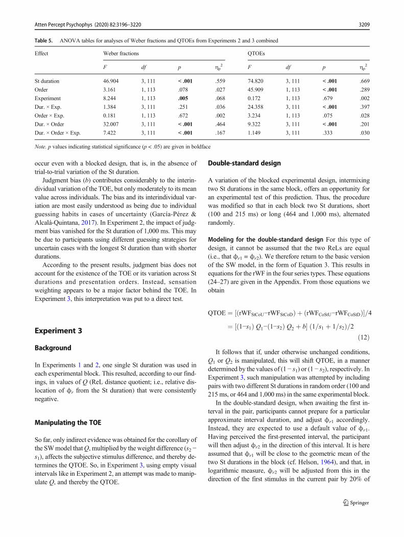
Table 5. ANOVA tables for analyses of Weber fractions and QTOEs from Experiments 2 and 3 combined

Effect Weber fractions QTOEs

F df p ηp2 F df p ηp

2

St duration 46.904 3, 111 < .001 .559 74.820 3, 111 < .001 .669

Order 3.161 1, 113 .078 .027 45.909 1, 113 < .001 .289

Experiment 8.244 1, 113 .005 .068 0.172 1, 113 .679 .002

Dur. × Exp. 1.384 3, 111 .251 .036 24.358 3, 111 < .001 .397

Order × Exp. 0.181 1, 113 .672 .002 3.234 1, 113 .075 .028

Dur. × Order 32.007 3, 111 < .001 .464 9.322 3, 111 < .001 .201

Dur. × Order × Exp. 7.422 3, 111 < .001 .167 1.149 3, 111 .333 .030

Note. p values indicating statistical significance (p < .05) are given in boldface


the distance (by analogy with results in Hellström, 1979,2003). Expressed in terms of weighted geometric means, wehave, on average, ϕr1 = StLower

0.5 . StHigher0.5, ϕr2Lower =

ϕr10.8 . StLower

0.2, and ϕr2Higher = ϕr10.8 . StHigher

0.2.Equation 12 predicts that in comparison with results from

Experiment 2, QTOE will shift by the amount

ΔQTOE ¼ 1−s1ð Þ ΔQ1− 1−s2ð Þ ΔQ2½ � 1=s1 þ 1=s2ð Þ=2;ð13Þ

whereΔQ1 = (Q1,Exp. 3 − Q1,Exp. 2), andΔQ2 = (Q2,Exp. 3 −

Q2,Exp. 2). From the above, it is predicted that |ΔQ2| < |ΔQ1|.This is because ϕr2, but not ϕr1, is partially adjusted in thedirection of the current St duration.

Predicting shifts in QTOE To get an idea of the likely shifts inQTOE between Experiments 2 and 3, rough estimates of Q1

and Q2 can be made from the above assumptions, using theNLR results (see Table 3). For Experiment 2, Q1 and Q2 areboth estimated as −13.6% throughout. For Experiment 3, es-timates of Q1 are +46.7% for St = 100 ms (blocked with 215ms) and St = 464 ms (blocked with 1,000 ms), and −31.8% forSt = 215 ms (blocked with 100 ms) and St = 1,000 ms(blocked with 464 ms); estimates of Q2 are +35.8% for St =100 ms and St = 464 ms, and −26.4% for St = 215 ms and St =1,000 ms. From this we get, for St = 100 ms and 464 ms,ΔQ1

= +60.3% and ΔQ2 = +49.4%; and for St = 215 ms and St =1,000 ms,ΔQ1 = −18.2% andΔQ2 = −12.8%. Also, using theNLR results (see Table 3), s1 is estimated (for Experiment 2 aswell as Experiment 3) as 0.391, 0.526, 0.485, and 0.434 for St= 100; 215; 464; and 1,000 ms, respectively, and s2 as 0.339,0.455, 0.536, and 0.729 for the same durations. UsingEquation 14, we then roughly predict QTOE shifts of+11.0% (100 ms), −3.4% (215 ms), +15.9 (464 ms), and−12.6% (1,000 ms). Most importantly, these shifts in QTOEare predicted to form a zig-zag pattern when plotted against Stduration. This is because as long as s1 < 1, s2 < 1, and |ΔQ2| <|ΔQ1|, the shift in QTOE will generally be positive in serieswith St intervals of 100 ms and 464 ms, which are blockedwith longer St intervals (215 ms and 1,000 ms, respectively),and negative for series with St intervals of 215 ms and 1,000ms, which are blocked with shorter St intervals (100 ms and464 ms, respectively). (A possible exception could occur for[1 − s1] / [1 − s2] << 1, for instance, with s1 close to 1.)

With the standard deviations (SDs) of QTOE forExperiment 2 given in Table 7 in the Appendix, the predictedshifts with the four standard durations represent Cohen’s dvalues of 1.15, 0.35, 1.91, and 1.57, respectively. The predict-ed zig-zag effect (calculated as the mean, 10.75%, of the un-signed shift percentages) represents (as compared with the SD,5.80, of the grand mean QTOE in Experiment 2) a Cohen’s dof 1.85, and with the current sample sizes even an effect half

as large should be detected with a probability > 0.99 at α =0.05.

Predictions of increased Weber fractions It was further pre-dicted that, due to the intermixing of St durations in a block,Q1 and Q2 would be less stable across trials in Experiment 3than in Experiment 2, where the standard was fixed withineach block. This would make perception of the duration dif-ference (d12) in the pair more variable from trial to trial. As aresult, WFs would be larger for corresponding conditions inExperiment 3 than in Experiment 2 (cf. Hellström, 2000). Theextent of this effect is hard to predict, but a moderate shift,with Cohen’s d = 0.5, of the meanWF (across St durations andpresentation orders) would be detectable (at α = 0.05) with apower of 0.76.

Method

Participants

Participants were undergraduate psychology students at theUniversity of Bern, 67 females and six males, ranging in agefrom 18 to 32 years (21.7 ± 2.6 years). The participants re-ceived course credit. All of themwere naïve about the purposeof the study and reported normal hearing and normal orcorrected-to-normal vision. None of them had participated inExperiment 1 or Experiment 2. All participants gave theirwritten informed consent (see Footnote 1).

Procedure

Apparatus and stimuli were the same as in Experiment 2. Theexperimental session comprised a total of eight blocks, with a1-min break between blocks. In four of the blocks, Co wasinitially longer than St (Hi-Co blocks) while in the other fourblocks Co was initially shorter than St (Lo-Co blocks).Furthermore, the St durations in four of the blocks were short(100 and 215 ms) and in the other four blocks, they were long(464 and 1,000 ms). Each block consisted of two randomlyinterleaved series of 32 trials each. In one of these series, thestimuli were always presented in the order StCo, and in theother series, in the order CoSt. As in Experiments 1 and 2,series types were StCoU, StCoD, CoStU, and CoStD. If the Stduration in the StCo series of a block was 100 (464) ms, the Stduration in the CoSt series of the same block was 215 (1,000)ms, and vice versa. Block order was balanced acrossparticipants.

Results

Following Experiments 1 and 2, a Mahalanobis distance cri-terion of p = .025 was applied for outlier detection, which


resulted in the exclusion of eight participants, so that analysesare based on n = 65.

Descriptives

In Table 9, in the Appendix, descriptive statistics forrWFStCoU, rWFStCoD, rWFCoStU, rWFCoStD, WFM, andQTOE are given for each St duration in Experiment 3, as wellas for mean WFM across St durations. Figure 6 shows themean (M) and standard error of the mean (SEM) of the WFfor each presentation order, as well as the ratio of the estimatesof WFStCo and WFCoSt (indicating s1/s2).

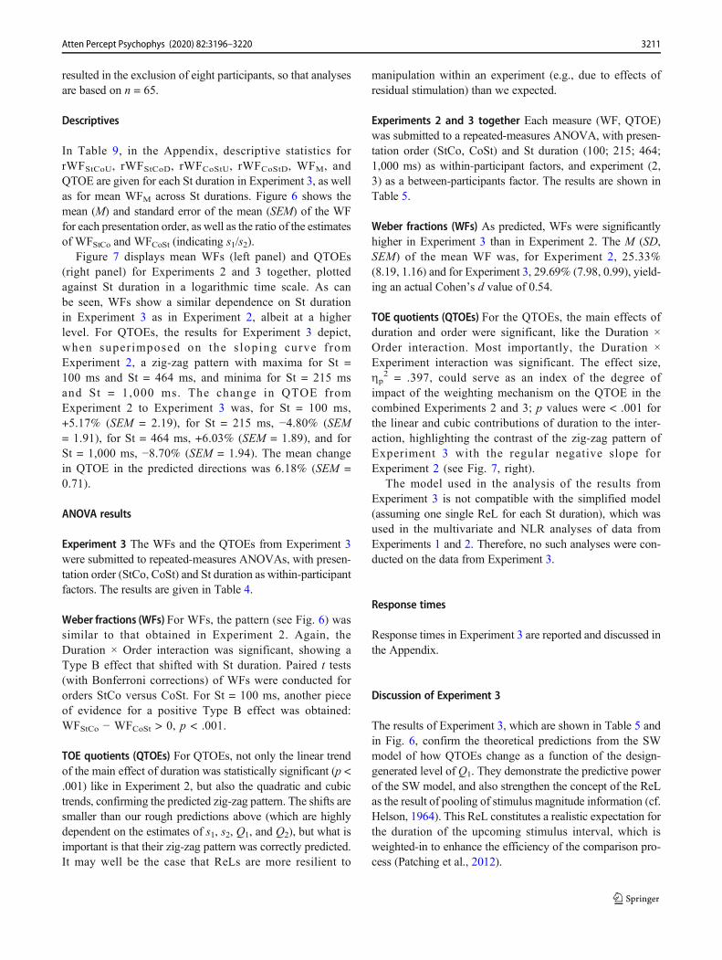
Figure 7 displays mean WFs (left panel) and QTOEs(right panel) for Experiments 2 and 3 together, plottedagainst St duration in a logarithmic time scale. As canbe seen, WFs show a similar dependence on St durationin Experiment 3 as in Experiment 2, albeit at a higherlevel. For QTOEs, the results for Experiment 3 depict,when super imposed on the s loping curve fromExperiment 2, a zig-zag pattern with maxima for St =100 ms and St = 464 ms, and minima for St = 215 msand St = 1,000 ms. The change in QTOE fromExperiment 2 to Experiment 3 was, for St = 100 ms,+5.17% (SEM = 2.19), for St = 215 ms, −4.80% (SEM= 1.91), for St = 464 ms, +6.03% (SEM = 1.89), and forSt = 1,000 ms, −8.70% (SEM = 1.94). The mean changein QTOE in the predicted directions was 6.18% (SEM =0.71).

ANOVA results

Experiment 3 The WFs and the QTOEs from Experiment 3were submitted to repeated-measures ANOVAs, with presen-tation order (StCo, CoSt) and St duration as within-participantfactors. The results are given in Table 4.

Weber fractions (WFs) For WFs, the pattern (see Fig. 6) wassimilar to that obtained in Experiment 2. Again, theDuration × Order interaction was significant, showing aType B effect that shifted with St duration. Paired t tests(with Bonferroni corrections) of WFs were conducted fororders StCo versus CoSt. For St = 100 ms, another pieceof evidence for a positive Type B effect was obtained:WFStCo − WFCoSt > 0, p < .001.

TOE quotients (QTOEs) For QTOEs, not only the linear trendof the main effect of duration was statistically significant (p <.001) like in Experiment 2, but also the quadratic and cubictrends, confirming the predicted zig-zag pattern. The shifts aresmaller than our rough predictions above (which are highlydependent on the estimates of s1, s2, Q1, and Q2), but what isimportant is that their zig-zag pattern was correctly predicted.It may well be the case that ReLs are more resilient to

manipulation within an experiment (e.g., due to effects ofresidual stimulation) than we expected.

Experiments 2 and 3 together Each measure (WF, QTOE)was submitted to a repeated-measures ANOVA, with presen-tation order (StCo, CoSt) and St duration (100; 215; 464;1,000 ms) as within-participant factors, and experiment (2,3) as a between-participants factor. The results are shown inTable 5.

Weber fractions (WFs) As predicted, WFs were significantlyhigher in Experiment 3 than in Experiment 2. The M (SD,SEM) of the mean WF was, for Experiment 2, 25.33%(8.19, 1.16) and for Experiment 3, 29.69% (7.98, 0.99), yield-ing an actual Cohen’s d value of 0.54.

TOE quotients (QTOEs) For the QTOEs, the main effects ofduration and order were significant, like the Duration ×Order interaction. Most importantly, the Duration ×Experiment interaction was significant. The effect size,ηp

2 = .397, could serve as an index of the degree ofimpact of the weighting mechanism on the QTOE in thecombined Experiments 2 and 3; p values were < .001 forthe linear and cubic contributions of duration to the inter-action, highlighting the contrast of the zig-zag pattern ofExperiment 3 with the regular negative slope forExperiment 2 (see Fig. 7, right).

The model used in the analysis of the results fromExperiment 3 is not compatible with the simplified model(assuming one single ReL for each St duration), which wasused in the multivariate and NLR analyses of data fromExperiments 1 and 2. Therefore, no such analyses were con-ducted on the data from Experiment 3.

Response times

Response times in Experiment 3 are reported and discussed inthe Appendix.

Discussion of Experiment 3

The results of Experiment 3, which are shown in Table 5 andin Fig. 6, confirm the theoretical predictions from the SWmodel of how QTOEs change as a function of the design-generated level of Q1. They demonstrate the predictive powerof the SW model, and also strengthen the concept of the ReLas the result of pooling of stimulus magnitude information (cf.Helson, 1964). This ReL constitutes a realistic expectation forthe duration of the upcoming stimulus interval, which isweighted-in to enhance the efficiency of the comparison pro-cess (Patching et al., 2012).


General discussion

Type B effects: Not always negative

Ellinghaus et al. (2018) state that “Type B effects reported inthe literature . . . are almost exclusively negative . . . . PositiveType B effects have rarely been reported in the case of veryshort-duration stimuli, especially when presented with veryshort interstimulus intervals” (p. 8). This may be true for thestimulus conditions usually employed, but this fact seems tobe due to researchers’ strange reluctance to use interstimulusintervals other than about 1,000 ms, or stimuli briefer than 500ms. With shorter interstimulus intervals and/or briefer stimuli,cases of (in terms of the SWmodel) s1/s2 > 1, with large TOEsand positive Type B effects or equivalent results, have beenfound (Hellström, 1979, 2003; Hellström & Rammsayer,2004). In our view, to fully explore the effects of stimuluspresentation conditions, psychophysical research should notavoid brief stimuli or fast stimulus presentation.

The results of Ellinghaus et al. (2018), whichwere obtainedby using only an interstimulus interval of 1,000 ms and an Stduration of 500 ms, across 10 different stimulus types,highlight the similarity between the comparison of durationsand of other stimuli. Bausenhart et al. (2015) used auditorydurations, with St durations of 100 ms and 1,000 ms, andfound consistently negative Type B effects when the inter-stimulus interval was 1,000 ms. In contrast, when it was 300ms, there was an interaction of presentation order (StCo,CoSt) and St duration, the Type B effect being negative forSt = 1,000 ms, but slightly and nonsignificantly positive for St= 100 ms. Bausenhart et al. (2015) acknowledge that “wecannot refute the findings of a positive Type B effect underspecific conditions. . . . A more general framework [than theIR model], such as Sensation Weighting . . . would be neededto account for any reversal of the Type B effect” (p. 1038).

The Type B effect can be seen primarily as an indicator ofthe sensation-weighting balance, but a rather insensitive one,as it is based on the comparison of measures of discrimination,such as DLs. In Experiments 1 and 2, this balance, as evi-denced also by the QTOE, was once more found to be heavilydependent on the stimulus conditions. The present results af-firm once more (cf. Hellström, 1979, 1985, 2003; Patchinget al., 2012) that it is unwarranted to conclude that s1/s2 < 1is a general rule in the comparison of successive stimuli.

Conclusion

Our results demonstrate the necessity of considering, whenassessing stimulus discrimination, methodological factors suchas the presentation order of St and Co, which are not recognizedby the time-honored simple difference model. Even in a designwith a single standard duration per stimulus block, TOEs depend

systematically on stimulus conditions (here, St duration) in com-bination with participant-specific factors such as judgment biasand ReL location. This means that a model for comparison ofinterval durations, and of stimulus magnitudes in general, mustbe able to account for both the Type B effect and the TOE, aswell as for each of these going in either direction. Because it hasthese capabilities, the SW model has proved useful in previousstudies using various study designs and stimulus modalities (e.g.,Englund&Hellström, 2012, 2013; Hellström, 1979, 1985, 2000,2003; Hellström, Aaltonen, Raimo, &Vilkman, 1994; Hellström& Cederström, 2014; Patching et al., 2012). The SWmodel alsopredicts the close relation between the TOE and the Type Beffect. Although, by necessity, it gives a simplified account ofwhat actually happened in the present experiments, the SWmod-el has once more helped to understand the contributions and theinterplay of the perceptual-cognitive factors behind the discrim-ination and comparison of stimulus magnitudes.

Our multivariate results from Experiments 1 and 2, as well asthe univariate results of Experiment 3, provide clear evidence fora reversal of theweighting balance, yielding s1/s2 > 1 and therebypositive Type B effects, for brief St durations (cf. Hellström,1979, 2003; Hellström & Rammsayer, 2004, 2015). This castsdoubt on theoretical models, like the MH and IR models, that donot allow for such cases. It is also a serious challenge for suchmodels (e.g., Preuschhof et al., 2010; Raviv et al., 2012) that reston the notion of Bayesian inference of the true magnitude of thefirst stimulus from its internal representation, which inevitablyyields s1/s2 < 1. The limitation of these models seems to be theirdisregard of the possibility that, for optimality in the comparisonof the two stimuli, also the true magnitude of the second one hasto be inferred. Like the MH and IR models, they consider therepresentation only of the first stimulus as being subject to mod-ification or supplementation, while the second stimulus enters thecomparison in a direct way. Instead, as pointed out by Hellström(1979), both of the stimuli should be seen as being in memory atthe time of comparison; an analogy with perceptual aftereffects,affecting the perception of the second out of two successivestimuli, may also be made (cf. Hellström, 1985). In summary,we argue that a more flexible model of stimulus comparison hasto be adopted, which allows stimulus weighting to be optimizedfor this task (Hellström, 1989; Patching et al., 2012). The SWmodel allows for such weighting, and also suggests an underly-ing mechanism: the weighting-in of supplementary magnitudeinformation by way of reference levels.

Acknowledgement We thank Miguel A. García-Pérez for helpful com-ments on an earlier draft of this manuscript.

Open practices statement The data for all experiments are availablefrom the first author by request. None of the experiments werepreregistered.

Funding information Open access funding provided by StockholmUniversity.


Appendix

Procedure modificationIn our earlier studies (Hellström & Rammsayer, 2004,

2015), the smallest difference in duration between the Coand the St was 1 ms in the direction of its initial value—thatis, the Co was not permitted to traverse the duration level ofthe St and cross over to the opposite side. However, as wasfound in detailed analyses of the results from Hellström andRammsayer (2015), this no-crossover rule tends to yield amisrepresentation of results in the presence of a large TOEor bias. For instance, with a large positive TOE in the condi-tion CoStD, Co may have to descend below St in order toreach the upper limen. In the present study the no-crossoverrule was therefore removed, so that measured DLs were free toattain nonpositive values.

Here we compare the results of Experiment 1 with those ofthe analogous Experiment 2 of Hellström and Rammsayer(2015), where the no-crossover rule was in force. Tworepeated-measures ANOVAs were conducted, with experi-ment (Hellström & Rammsayer 2015, present) as a between-participants factor, St duration (100; 215; 464; 1,000 ms) andstimulus presentation order (StCo, CoSt) as within-participantfactors, and QTOE and WF, respectively, as the dependentvariable. For QTOE, only the effect of St duration reachedsignificance, F(3, 113) = 25.170, p < .001, ηp

2 = .401, butnone of the effects involving experiment. For WF, the onlysignificant effects were those of St duration, F(3, 113) =5.856, p < .001, ηp

2 = .135, and experiment, F(1, 115) =17.414, p < .001, ηp

2 = .132. WFs tended to be lower in thepresent Experiment 1 than in Hellström and Rammsayer’s(2015) Experiment 2. The likely reason is that with the no-crossover rule used in the 2015 study, but not in the presentone, the individual rDLs could not reach nonpositive values,which might otherwise occur because of strong positive or

negative TOEs. For instance, in the present Experiment 1,with the St duration of 100 ms, QTOE was strongly positive(see Fig. 2), and accordingly, in series type CoStD, 18.0% ofthe rDLs were negative, but only 1.6% in series type CoStU.

Univariate and multivariate models, as appliedto the four series types in Experiments 1 and 2

Univariate model

Raw DLs The physical duration of the St is denoted by S. Foreach of the four series types, the left member of each ofEquations 14–17 (where i [participant] subscripts are omit-ted)—that is, w S or −w · S, represents the subjective stimulusdifference, d12X or −d12X, which corresponds to a raw DL(rDLD or rDLU, respectively). The right member of each equa-tion describes how w · S or −w · S is built up in the particularseries type:

StCoU : −w � S ¼ s1 � S−s2 S þ rDLStCoUð Þþ s2−s1ð Þ ϕr

þ b � S; ð14ÞStCoD : w � S ¼ s1 � S−s2 S−rDLStCoDð Þ þ s2−s1ð Þ ϕr

þ b � S; ð15ÞCoStU : −w � S ¼ s1 S−rDLCoStUð Þ−s2 � S þ s2−s1ð Þ ϕr

þ b � S; ð16ÞCoStD : w � S ¼ s1 S þ rDLCoStDð Þ−s2 � S þ s2−s1ð Þ ϕr

þ b � S: ð17Þ

Raw Weber fractions For comparability of effects between thefour St durations, each rDL was transformed into a rawWeberfraction (rWF): rWF = rDL/S. Expressions are obtained fromEquations 14–17 that describe how the rWF is built up, ac-cording to the SW model, in each series type:

StCoU : rWFStCoU ¼ 1=s2ð Þ wþ bþ s2−s1ð Þ Q½ �; ð18ÞStCoD : rWFStCoD ¼ 1=s2ð Þ w−b− s2−s1ð Þ Q½ �; ð19ÞCoStU : rWFCoStU ¼ 1=s1ð Þ wþ bþ s2−s1ð Þ Q½ �; ð20ÞCoStD : rWFCoStD ¼ 1=s1ð Þ w−b− s2−s1ð Þ Q½ �; ð21Þ

where Q is the ReL distance quotient, that is, the relativedistance of the ReL from the St: Q = (ϕr − S)/S. (Unlike inHellström and Rammsayer, 2015, a logarithmic transforma-tion of the rWFs could not be used, as individual rWF valueswere free to be nonpositive, as explained above. Also, thepresent approach differs from that used in the 2015 article inthat the possible difference in ϕr between Hi-Co and Lo-Coblocks is ignored.)

Table 6 Summary of the design of Experiments 1 and 2

4 Hi-Co blocks64 trials per block

4 Lo-Co blocks64 trials per block

St duration100 (215; 464; 1,000) ms

St duration100 (215; 464; 1,000) ms

Initial Co duration135 (285; 564; 1,500) ms

Initial Co duration65 (145, 364, 500) ms

Presentation order andseries type (Up [U]; Down [D])

StCoU (32 trials)CoStD (32 trials)

Presentation order andseries type (Up [U]; Down [D])

StCoD (32 trials)CoStU (32 trials)

Note. The four St durations (100; 215; 464; and 1,000 ms) in each blockpair were counterbalanced over participants. In each block, each presen-tation order, StCo and CoSt, was used on 32 randomly interleaved trials(see text for details)


Multivariate model

In the multivariate analysis, we attempt to describe each mea-sured rWF as a sum of products of participant-specific andcondition-specific factors. In our multivariate model, then,

the ith participant is characterized by this participant’s (1)Weber constant, wi; (2) judgment bias, bi, and (3) ReL dis-tance quotient, Qi. The kth stimulus condition (defined by Stduration and series type—StCoU, StCoD, CoStU, or CoStD)is characterized by this condition’s (1) discrimination difficul-ty, ωk, (2) sensitivity to bias, βk or −βk, and (3) weight dif-ference, δk (i.e., [s2k − s1k] or −[s2k − s1k])—that is, the

Table 7 Experiments 1 and 2: Descriptive statistics of raw Weber fraction (rWF, in %), Weber fraction (WF, in %), and TOE quotient (QTOE, in %)for each experiment

Experiment 1: Filled auditory intervals (N = 61) Experiment 2: Empty visual intervals (N = 50)

M SEM SD M SEM SD

St = 100 ms

rWFStCoU 18.77 1.39 10.89 41.79 2.32 16.43

rWFStCoD 9.31 0.85 6.65 26.48 2.13 15.06

rWFCoStU 18.61 1.19 9.28 35.64 2.32 16.40

rWFCoStD 8.86 1.38 10.77 25.50 2.95 20.89

WFStCo 14.04 0.88 6.85 34.14 1.81 12.77

WFCoSt 13.73 0.93 7.25 30.57 1.89 13.38

WFM 13.89 0.81 6.32 32.35 1.64 11.61

QTOE +4.80 0.70 5.49 +6.36 1.36 9.59

St = 215 ms

rWFStCoU 15.47 1.25 9.74 34.86 2.72 19.20

rWFStCoD 8.49 0.93 7.28 14.66 1.85 13.09

rWFCoStU 14.94 1.17 9.17 22.98 1.75 12.36

rWFCoStD 8.28 1.03 8.05 24.19 2.59 18.32

WFStCo 11.98 0.81 6.29 24.76 1.72 12.13

WFCoSt 11.61 0.67 5.24 23.59 1.54 10.90

WFM 11.79 0.59 4.59 24.17 1.42 10.01

QTOE +3.41 0.68 5.34 +4.75 1.39 9.86

St = 464 ms

rWFStCoU 13.24 0.96 7.46 26.16 2.58 18.22

rWFStCoD 7.95 0.94 7.36 20.19 1.48 10.46

rWFCoStU 14.19 0.95 7.41 21.59 1.88 13.32

rWFCoStD 9.31 1.02 7.95 25.05 2.00 14.11

WFStCo 10.60 0.64 5.01 23.18 1.62 11.46

WFCoSt 11.75 0.65 5.11 23.32 1.36 9.59

WFM 11.17 0.52 4.07 23.25 1.27 8.99

QTOE +2.54 0.66 5.16 +0.63 1.18 8.36

St = 1,000 ms

rWFStCoU 10.41 1.27 9.92 15.45 2.63 18.62

rWFStCoD 12.40 1.20 9.37 16.55 2.36 16.66

rWFCoStU 10.35 1.41 10.99 20.02 1.81 12.82

rWFCoStD 17.35 1.78 13.87 34.16 2.28 16.11

WFStCo 11.41 0.77 6.03 16.00 1.93 13.65

WFCoSt 13.85 1.01 7.89 27.09 1.45 10.26

WFM 12.63 0.78 6.12 21.545 1.38 9.78

QTOE -2.25 1.00 7.80 -3.81 1.14 8.06

Mean WFM 12.37 0.49 3.83 25.33 1.16 8.19


multiplier of Qi in determining the TOE. (As the analysis wasbased on correlations, not on covariances, all variables areconsidered standardized, and the factors 1/s1 and 1/s2, whichcan be expected to vary across St durations, are left outside theanalysis.) Thus, the predicted rWF for the ith participant in thekth condition is:

rWFik ¼ ωk wi þ βk bi þ δk Qi: ð22Þ

The last term is built on the assumption that the ReL dis-tance quotient (Q) is participant specific and (comparatively)invariant across stimulus conditions, while weighting (i.e., s2− s1) is condition specific and (comparatively) invariant acrossparticipants. This assumption we consider sufficiently justi-fied by the univariate results, which indicate that s2 − s1changes with the standard duration, whereas Q stays negativeacross conditions.

Experiment 3: Manipulation of ReLs

With the two ReLs potentially different, we may rewriteEquation 3 as

d12 ¼ ϕ1−ϕ2 þ 1−s1ð Þ ϕr1−ϕ1ð Þ− 1−s2ð Þ ϕr2−ϕ2ð Þþ b; ð23Þ

from which, setting d12 = d12X = w · S, we obtain the fol-lowing equations for rWF in the four series types (presentationorders StCo and CoSt; Up [U] and Down [D]):

Table 8 Experiments 1 and 2: Unrotated component loadings from principal component analyses of correlations between rawWeber fractions (rWFs).Estimated mean values of model parameters ω, β, and δ (Equation 22) for each St duration

Experiment 1: Filled auditory intervals Experiment 2: Empty visual intervals

Component No.InterpretationEigenvalue

2w3.1

1revb3.9

3Q1.6

1w4.4

2revb2.8

3Q1.7

St = 100 ms

rWFStCoU .656 .260 −.261 .623 .271 .269

rWFStCoD .534 −.388 .293 .504 −.439 .049

rWFCoStU .512 .269 −.446 .616 .251 −.422rWFCoStD .425 −.446 .262 .436 −.549 .258

Mean ω, β, δ .532 .340 −.315 .545 .378 −.249St = 215 ms

rWFStCoU .415 .518 −.180 .673 .334 −.209rWFStCoD .558 −.220 .309 .327 −.520 −.043rWFCoStU .430 .348 −.507 .633 .433 −.165rWFCoStD −.019 −.552 .307 .290 −.778 .023

Mean ω, β, δ .346 .410 −.326 .481 .516 −.089St = 464 ms

rWFStCoU .506 .424 .217 .641 .339 .403

rWFStCoD .302 −.719 −.113 .364 −.468 −.004rWFCoStU .447 .653 .083 .628 .274 .393

rWFCoStD .432 −.602 −.179 .380 −.537 −.484Mean ω, β, δ .422 .599 .148 .503 .404 .321

St = 1,000 ms

rWFStCoU .153 .609 .464 .547 .154 .380

rWFStCoD .396 −.544 .129 .517 .387 −.169rWFCoStU .352 .483 .553 .450 −.228 .637

rWFCoStD .454 −.531 −.208 .490 −.333 −.375Mean ω, β, δ .339 .542 .234 .501 −.032 .390

Note. rev loading signs are reversed


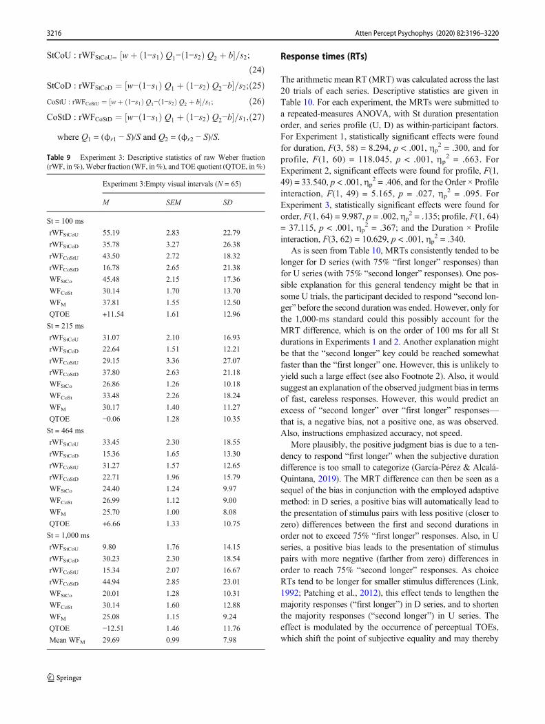
StCoU : rWFStCoU¼ wþ 1−s1ð Þ Q1− 1−s2ð Þ Q2 þ b½ �=s2;ð24Þ

StCoD : rWFStCoD ¼ w− 1−s1ð Þ Q1 þ 1−s2ð Þ Q2−b½ �=s2;ð25ÞCoStU : rWFCoStU ¼ wþ 1−s1ð Þ Q1− 1−s2ð Þ Q2 þ b½ �=s1; ð26ÞCoStD : rWFCoStD ¼ w− 1−s1ð Þ Q1 þ 1−s2ð Þ Q2−b½ �=s1;ð27Þ

where Q1 = (ϕr1 − S)/S and Q2 = (ϕr2 − S)/S.

Response times (RTs)

The arithmetic mean RT (MRT) was calculated across the last20 trials of each series. Descriptive statistics are given inTable 10. For each experiment, the MRTs were submitted toa repeated-measures ANOVA, with St duration presentationorder, and series profile (U, D) as within-participant factors.For Experiment 1, statistically significant effects were foundfor duration, F(3, 58) = 8.294, p < .001, ηp

2 = .300, and forprofile, F(1, 60) = 118.045, p < .001, ηp

2 = .663. ForExperiment 2, significant effects were found for profile, F(1,49) = 33.540, p < .001, ηp

2 = .406, and for the Order × Profileinteraction, F(1, 49) = 5.165, p = .027, ηp

2 = .095. ForExperiment 3, statistically significant effects were found fororder, F(1, 64) = 9.987, p = .002, ηp

2 = .135; profile, F(1, 64)= 37.115, p < .001, ηp

2 = .367; and the Duration × Profileinteraction, F(3, 62) = 10.629, p < .001, ηp

2 = .340.As is seen from Table 10, MRTs consistently tended to be

longer for D series (with 75% “first longer” responses) thanfor U series (with 75% “second longer” responses). One pos-sible explanation for this general tendency might be that insome U trials, the participant decided to respond “second lon-ger” before the second duration was ended. However, only forthe 1,000-ms standard could this possibly account for theMRT difference, which is on the order of 100 ms for all Stdurations in Experiments 1 and 2. Another explanation mightbe that the “second longer” key could be reached somewhatfaster than the “first longer” one. However, this is unlikely toyield such a large effect (see also Footnote 2). Also, it wouldsuggest an explanation of the observed judgment bias in termsof fast, careless responses. However, this would predict anexcess of “second longer” over “first longer” responses—that is, a negative bias, not a positive one, as was observed.Also, instructions emphasized accuracy, not speed.

More plausibly, the positive judgment bias is due to a ten-dency to respond “first longer” when the subjective durationdifference is too small to categorize (García-Pérez & Alcalá-Quintana, 2019). The MRT difference can then be seen as asequel of the bias in conjunction with the employed adaptivemethod: in D series, a positive bias will automatically lead tothe presentation of stimulus pairs with less positive (closer tozero) differences between the first and second durations inorder not to exceed 75% “first longer” responses. Also, in Useries, a positive bias leads to the presentation of stimuluspairs with more negative (farther from zero) differences inorder to reach 75% “second longer” responses. As choiceRTs tend to be longer for smaller stimulus differences (Link,1992; Patching et al., 2012), this effect tends to lengthen themajority responses (“first longer”) in D series, and to shortenthe majority responses (“second longer”) in U series. Theeffect is modulated by the occurrence of perceptual TOEs,which shift the point of subjective equality and may thereby

Table 9 Experiment 3: Descriptive statistics of raw Weber fraction(rWF, in%),Weber fraction (WF, in%), and TOE quotient (QTOE, in%)

Experiment 3:Empty visual intervals (N = 65)

M SEM SD

St = 100 ms

rWFStCoU 55.19 2.83 22.79

rWFStCoD 35.78 3.27 26.38

rWFCoStU 43.50 2.72 18.32

rWFCoStD 16.78 2.65 21.38

WFStCo 45.48 2.15 17.36

WFCoSt 30.14 1.70 13.70

WFM 37.81 1.55 12.50

QTOE +11.54 1.61 12.96

St = 215 ms

rWFStCoU 31.07 2.10 16.93

rWFStCoD 22.64 1.51 12.21

rWFCoStU 29.15 3.36 27.07

rWFCoStD 37.80 2.63 21.18

WFStCo 26.86 1.26 10.18

WFCoSt 33.48 2.26 18.24

WFM 30.17 1.40 11.27

QTOE −0.06 1.28 10.35

St = 464 ms

rWFStCoU 33.45 2.30 18.55

rWFStCoD 15.36 1.65 13.30

rWFCoStU 31.27 1.57 12.65

rWFCoStD 22.71 1.96 15.79

WFStCo 24.40 1.24 9.97

WFCoSt 26.99 1.12 9.00

WFM 25.70 1.00 8.08

QTOE +6.66 1.33 10.75

St = 1,000 ms

rWFStCoU 9.80 1.76 14.15

rWFStCoD 30.23 2.30 18.54

rWFCoStU 15.34 2.07 16.67

rWFCoStD 44.94 2.85 23.01

WFStCo 20.01 1.28 10.31

WFCoSt 30.14 1.60 12.88

WFM 25.08 1.15 9.24

QTOE −12.51 1.46 11.76

Mean WFM 29.69 0.99 7.98


lead to interactions of, for instance, Profile × Order, as wasfound in Experiment 2.

The mean MRT difference between U and D series wascomputed for each participant, and its correlations with thecomponent scores from the two PCAs were analyzed. Theonly correlations of the U–D MRT difference that reached orapproached significance were those with the component iden-tified with the bias term b. For Experiment 1, these correla-tions were −.286, p = .025, with (the reversed) Component 1;for Experiment 2, they were −.343, p = .015, with (the re-versed) Component 2. These correlations confirm that a morepositive b value (i.e., a greater tendency to judge “first lon-ger”) is associated with a shorter MRT for U series than for Dseries, and thereby strengthen the above account of the U–Ddifference in MRT as a consequence of how the positive judg-ment bias dictates the allocation of presented stimuli in theemployed adaptive staircase method.

Table 10. Experiments 1 and 2: Descriptive statistics (mean, standarderror of mean) for mean response time (MRT) in milliseconds (ms) ineach condition of each experiment

Experiment1:Filled auditoryintervals (N = 61)

Experiment2:Empty visualintervals (N = 50)


M SEM M SEM M SEM

St =100 ms

StCoU 1,039 50 1,071 50 1,143 55

StCoD 1,168 56 1,249 68 1,216 67

CoStU 1,057 46 1,138 56 1,233 56

CoStD 1,207 58 1,162 52 1,225 57

StCo 1,104 50 1,160 53 1,180 52

CoSt 1,132 50 1,150 51 1,229 51

U 1,048 45 1,105 49 1,188 50

D 1,187.5 55 1,205 56 1,220 55

Mean 1,118 49 1,155 51 1,204 50

St =215 ms

StCoU 1,015 56 1,043 51 1,145 55

StCoD 1,202 61 1,136 59 1,163 49

CoStU 1,029 56 1,087 61 1,253 71

CoStD 1,140 62 1,149 62 1,205 66

StCo 1,109 55 1,090 52 1,154 52

CoSt 1,085 56 1,118 58 1,229 60

U 1,022 52 1,065 54 1,199 60

D 1,171 58 1,142 57 1,184 54

Mean 1,097 54 1,104 54 1,191 54

St =464 ms

StCoU 939 43 1,084 64 1,098 45

StCoD 1,066 44 1,231 69 1,267 58

CoStU 986 48 1,059 50 1,149 51

CoStD 1,021 39 1,149 49 1,265 58

StCo 1,002 38 1,158 62 1,182 47

Table 10. (continued)

Experiment1:Filled auditoryintervals (N = 61)



M SEM M SEM M SEM

CoSt 1,003 41 1,104 46 1,207 48

U 963 42 1,072 51 1,123 42

D 1,043 37 1,190 55 1,266 53

Mean 1,003 38 1,131 52 1,195 45

St =1,000 ms

StCoU 932 55 1,106 59 1,093 56

StCoD 1,011 53 1,273 68 1,251 56

CoStU 898 42 1,129 52 1,081 58

CoStD 981 47 1,246 56 1,254 51

StCo 972 49 1,190 57 1,172 51

CoSt 940 43 1,188 50 1,168 51

U 915 46 1,118 49 1,087 52

D 996 47 1,260 58 1,252 50

Mean 956 45 1189 52 1,170 49

All St durations

StCo 1,047 41 1149 46 1,172 47

CoSt 1,040 41 1140 44 1,208 48

U 987 40 1090 42 1,149 46

D 1,100 43 1199 48 1,231 50

Grand mean 1,043 41 1145 44 1,190 47


Table 11 Abbreviations used in the present article

Abbreviation Meaning

b Judgment bias

C Physical magnitude of comparison stimulus (Co)

Co Comparison stimulus varied in physical magnitude (i.e., duration) from trial to trial

CoSt Stimulus presentation order comparison (Co) followed by standard (St)

D Series type Down: Second stimulus interval initially shorter than the first

d12 Subjective difference between the first and the second stimulus

d12X Subjective difference between the first and the second stimulus at the measured limen in Down (D)-series

−d12X Subjective difference between the first and the second stimulus at the measured limen in Up (U)-series

DL Difference limen: half the difference between the upper limen (value of Co that evokes 75% judgments of Co > St) and the lower limen(value of Co that evokes 75% judgments of Co < St)

IR model Internal reference model

MH model Michels–Helson model

ϕ Phi: physical stimulus magnitude; used to represent subjective stimulus and ReL magnitude, assuming the psychophysical function to bethe identity function

ψ1, ψ2 Subjective magnitude of the first stimulus and second stimulus, respectively

ψ Psi: Subjective magnitude of the stimuli when ψ1 = ψ2

ψr1, ψr2 Magnitude of reference levels (ReL1, ReL2) for ψ1 and ψ2 respectively

ψr Magnitude of reference level (ReL) when ψr1 = ψr2

Q Relative distance of ReL from the St: Q = (ϕr − S)/S

Q1 Relative distance of first stimulus’ ReL from the St: Q = (ϕr1 − S)/S

Q2 Relative distance of second stimulus’ ReL from the St: Q = (ϕr2 − S)/S

QTBE Type B effect quotient: Type B effect as a fraction of WFMQTOE TOE quotient: Time order error (TOE) as a fraction of S

rDL Raw difference limen: Difference limen estimated on the basis of the average physical duration of the Co over the last 20 trials of thestaircase procedure for each experimental condition

ReL Reference level

rWF RawWeber fraction: Estimated by dividing the raw difference limen (rDL) by the physical duration of the standard (St) stimulus, rDL / St

S Physical magnitude (i.e., duration) of St

s1, s2 Weighting coefficients of ψ1 and ψ2, respectively

St Standard stimulus held at constant physical magnitude (i.e., duration) in each experimental condition

StCo Stimulus presentation order standard (St) followed by comparison (Co)

SW model Sensation weighting model

TBE Type B effect: Difference between Weber fractions (in %) for presentation orders StCo and CoSt: TBE = WFStCo − WFCoSt. Also calledstandard position effect.

TOE Time order error (Fechner, 1860): systematic underestimation or overestimation of one stimulus relative to the other (also called Type Aeffect).

U Series type Up: Second stimulus interval initially longer than the first

wi Participant-specific value of theWeber constant, that is, the comparatal dispersion,σd12 (after Gulliksen, 1958), multiplied by 0.6745 (i.e.,the standard normal deviate corresponding to the 75th percentile) and divided by standard duration S. The subscript i is dropped insubsequent renditions.

WF Weber fraction: Traditionally defined asΔI / I, whereΔI is the difference threshold and I the standard stimulus intensity. Here, estimatedby dividing the measured difference limen by the physical duration of the standard, DL / S, and expressed in percentage.

WFM Mean WF across stimulus presentation orders (StCo, CoSt).


Open Access This article is licensed under a Creative CommonsAttribution 4.0 International License, which permits use, sharing,adaptation, distribution and reproduction in any medium or format, aslong as you give appropriate credit to the original author(s) and thesource, provide a link to the Creative Commons licence, and indicate ifchanges weremade. The images or other third party material in this articleare included in the article's Creative Commons licence, unless indicatedotherwise in a credit line to the material. If material is not included in thearticle's Creative Commons licence and your intended use is notpermitted by statutory regulation or exceeds the permitted use, you willneed to obtain permission directly from the copyright holder. To view acopy of this licence, visit http://creativecommons.org/licenses/by/4.0/.

References

Alcalá-Quintana, R., & García-Pérez, M. A. (2011). A model for thetime-order error in contrast discrimination. Quarterly Journal ofExperimental Psychology, 64, 1221–1248. https://doi.org/10.1080/17470218.2010.540018

Allan, L. G. (1977). The time-order error in judgments of duration.Canadian Journal of Psychology, 31, 24–31. https://doi.org/10.1037/h0081647

Allan, L. G., & Kristofferson, A. B. (1974). Psychophysical theories ofduration discrimination. Perception & Psychophysics, 16, 26–34.https://doi.org/10.3758/BF03203244

Bausenhart, K. M., Bratzke, D., & Ulrich, R. (2016). Formation andrepresentation of temporal reference information. Current Opinionin Behavioral Sciences, 8, 46–52. https://doi.org/10.1016/j.cobeha.2016.01.007

Bausenhart, K. M., Dyjas, O., & Ulrich, R. (2015). Effects of stimulusorder on discrimination sensitivity for short and long durations.Attention, Perception, & Psychophysics, 77, 1033–1043. https://doi.org/10.3758/s13414-015-0875-8

Brown, G. D., McCormack, T., Smith, M., & Stewart, N. (2005).Identification and bisection of temporal durations and tone frequen-cies: Common models for temporal and nontemporal stimuli.Journal of Experimental Psychology: Human Perception andPerformance, 31, 919–938. https://doi.org/10.1037/0096-1523.31.5.919

Dyjas, O., Bausenhart, K.M., & Ulrich, R. (2012). Trial-by-trial updatingof an internal reference in discrimination tasks: Evidence from ef-fects of stimulus order and trial sequence. Attention, Perception, &Psychophysics, 74, 1819–1841. https://doi.org/10.3758/s13414-012-0362-4

Dyjas, O., & Ulrich, R. (2014). Effects of stimulus order on discrimina-tion processes in comparative and equality judgements: Data andmodels. The Quarterly Journal of Experimental Psychology, 67,1121–1150. https://doi.org/10.1080/17470218.2013.847968

Eisler, H., Eisler, A. D., & Hellström, Å. (2008). Psychophysical issues inthe study of time perception. In S. Grondin (Ed.), Psychology of time(pp. 75–109). Bingley, England: Emerald.

Ellinghaus, R., Ulrich, R., & Bausenhart, K. M. (2018). Effects of stim-ulus order on comparative judgments across stimulus attributes andsensory modalities. Journal of Experimental Psychology: HumanPerception and Performance, 44(1), 7–12. https://doi.org/10.1037/xhp0000495

Engen, T. (1971). Psychophysics: 1. Discrimination and detection. In L.A. Kling & J. W. Riggs (Eds.), Woodworth & Schlosberg’s exper-imental psychology (3rd ed., pp. 11–46). New York, NY: Holt,Rinehart & Winston.

Englund, M. P., & Hellström, Å. (2012). Presentation-order effects foraesthetic stimulus preference. Attention, Perception, &

Psychophysics, 74(7), 1499–1511. https://doi.org/10.3758/s13414-012-0333-9

Englund, M. P., & Hellström, Å (2013). Beware how you compare:comparison direction dictates stimulus-valence-modulatedpresentation-order effects in preference judgment. Attention,Perception, & Psychophysics, 75(5), 1001–1011. https://doi.org/10.3758/s13414-013-0453-x.

Fechner, G. T. (1860). Elemente der Psychophysik [Elements ofpsychophysics]. Leipzig, Germany: Breitkopf & Härtel.

García-Pérez, M. A., & Alcalá-Quintana, R. (2017). The indecision mod-el of psychophysical performance in dual-presentation tasks:Parameter estimation and comparative analysis of response formats.Frontiers in Psychology, 8. https://doi.org/10.3389/fpsyg.2017.01142

García-Pérez, M. A., & Alcalá-Quintana, R. (2019). The do’s and don’tsof psychophysical methods for interpretability of psychometricfunctions and their descriptors. The Spanish Journal ofPsychology, 22, 1–30. https://doi.org/10.1017/sjp.2019.49

Garrett, R. G. (1989). The chi-square plot: A tool for multivariate outlierrecognition. Journal of Geochemical Exploration, 32, 319–341.https://doi.org/10.1016/0375-6742(89)90071-X

Guilford, J. P. (1954). Psychometric methods (2nd edn). New York, NY:McGraw-Hill.

Gulliksen, H. (1958). Comparatal dispersion, a measure of accuracy ofjudgment. Psychometrika, 23(2), 137–150. https://doi.org/10.1007/BF02289010

Hellström, Å. (1977). Time-errors are perceptual: An experimental inves-tigation of duration and a quantitative successive-comparison mod-el. Psychological Research, 39, 345–388. https://doi.org/10.1007/BF00308933

Hellström, Å. (1979). Time errors and differential sensation weighting.Journal of Experimental Psychology: Human Perception andPerformance, 5, 460–477. https://doi.org/10.1037/0096-1523.5.3.460

Hellström, Å. (1985). The time-order error and its relatives: Mirrors ofcognitive processes in comparing. Psychological Bulletin, 97, 35–61. https://doi.org/10.1037/0033-2909.97.1.35

Hellström, Å. (1989).What happens when we compare two stimuli? In G.Ljunggren & S. Dornic (Eds.), Psychophysics in action (pp. 25–39).Berlin, Germany: Springer. https://doi.org/10.1007/978-3-642-74382-5

Hellström, Å. (2000). Sensation weighting in comparison and discrimi-nation of heaviness. Journal of Experimental Psychology: HumanPerception and Performance, 26, 6–17. https://doi.org/10.1037/0096-1523.26.1.6

Hellström, Å. (2003). Comparison is not just subtraction: Effects of time-and space-order on subjective stimulus difference. Perception &Psychophysics, 65, 1161–1177. https://doi.org/10.3758/BF03194842

Hellström, Å., Aaltonen, O., Raimo, I., & Vilkman, E. (1994). The role ofvowel quality in pitch comparison. Journal of the Acoustical Societyof America, 96, 2133–2139. https://doi.org/10.1121/1.413117

Hellström, Å., & Cederström, C. (2014). Intramodal and cross-modalpairing and anchoring in comparisons of successive stimuli.Attention, Perception, & Psychophysics, 76, 1197–1211. https://doi.org/10.3758/s13414-014-0635-1

Hellström, Å., & Rammsayer, T. H. (2004). Effects of time-order, inter-stimulus interval, and feedback in duration discrimination of noisebursts in the 50- and 1000-ms ranges. Acta Psychologica, 116, 1–20.https://doi.org/10.1016/j.actpsy.2003.11.003

Hellström, Å., & Rammsayer, T. H. (2015). Time-order errors andstandard-position effects in duration discrimination: An experimen-tal study and an analysis by the sensation-weighting model.Attention, Perception, & Psychophysics, 77, 2409–2423. https://doi.org/10.3758/s13414-015-0946-x


http://creativecommons.org/licenses/by/4.0/

https://doi.org/10.1080/17470218.2010.540018

https://doi.org/10.1080/17470218.2010.540018

https://doi.org/10.1037/h0081647

https://doi.org/10.1037/h0081647

https://doi.org/10.3758/BF03203244

https://doi.org/10.1016/j.cobeha.2016.01.007

https://doi.org/10.1016/j.cobeha.2016.01.007

https://doi.org/10.3758/s13414-015-0875-8

https://doi.org/10.3758/s13414-015-0875-8

https://doi.org/10.1037/0096-1523.31.5.919

https://doi.org/10.1037/0096-1523.31.5.919

https://doi.org/10.3758/s13414-012-0362-4

https://doi.org/10.3758/s13414-012-0362-4

https://doi.org/10.1080/17470218.2013.847968





https://doi.org/10.3758/s13414-013-0453-x

https://doi.org/10.3758/s13414-013-0453-x

https://doi.org/10.3389/fpsyg.2017.01142

https://doi.org/10.3389/fpsyg.2017.01142

https://doi.org/10.1017/sjp.2019.49

https://doi.org/10.1016/0375-6742(89)90071-X

https://doi.org/10.1007/BF02289010

https://doi.org/10.1007/BF02289010

https://doi.org/10.1007/BF00308933

https://doi.org/10.1007/BF00308933

https://doi.org/10.1037/0096-1523.5.3.460

https://doi.org/10.1037/0096-1523.5.3.460

https://doi.org/10.1037/0033-2909.97.1.35

https://doi.org/10.1007/978-3-642-74382-5

https://doi.org/10.1007/978-3-642-74382-5

https://doi.org/10.1037/0096-1523.26.1.6

https://doi.org/10.1037/0096-1523.26.1.6

https://doi.org/10.3758/BF03194842

https://doi.org/10.3758/BF03194842

https://doi.org/10.1121/1.413117

https://doi.org/10.3758/s13414-014-0635-1

https://doi.org/10.3758/s13414-014-0635-1

https://doi.org/10.1016/j.actpsy.2003.11.003

https://doi.org/10.3758/s13414-015-0946-x

https://doi.org/10.3758/s13414-015-0946-x

Helson, H. (1964). Adaptation-level theory. New York, NY: Harper &Row.

Jamieson, D. G., & Petrusic, W. M. (1975). Presentation order effects induration discrimination. Perception & Psychophysics,17, 197–202.https://doi.org/10.3758/BF03203886

Kaiser, H. F. (1974). An index of factorial simplicity. Psychometrika, 39,31–36. https://doi.org/10.1007/BF02291575

Link, S. W. (1992). The wave theory of difference and similarity.Hillsdale, NJ: Erlbaum.

Luce, R. D., & Galanter, E. (1963). Discrimination. In R. D. Luce, R. R.Bush, & E. Galanter (Eds.), Handbook of mathematical psychology(Vol. 1, pp. 191–243). New York, NY: Wiley.

Michels, W. C., & Helson, H. (1954). A quantitative theory of time-ordererrors. American Journal of Psychology, 67, 327–334. https://doi.org/10.2307/1418635

Patching, G. R., Englund, M. P., & Hellström, Å. (2012). Time- andspace-order effects in timed discrimination of brightness and sizeof paired visual stimuli. Journal of Experimental Psychology:Human Perception and Performance, 38, 915–940. https://doi.org/10.1037/a0027593

Preuschhof, C., Schubert, T., Villringer, A., & Heekeren, H. R. (2010).Prior information biases stimulus representations during vibrotactiledecision making. Journal of Cognitive Neuroscience, 22, 875–887.https://doi.org/10.1162/jocn.2009.21260

Rammsayer, T. H. (2008). Neuropharmacological approaches to humantiming. In S. Grondin (Ed.), Psychology of time (pp. 295–320).Bingley, England: Emerald.

Rammsayer, T. H. (2012). Developing a psychophysical measure to as-sess duration discrimination in the range of milliseconds:Methodological and psychometric issues. European Journal ofPsychological Assessment, 28, 172–180. https://doi.org/10.1027/1015-5759/a000124

Rammsayer, T. H., & Wittkowski, K. M. (1990). Zeitfehler undPositionseffekt des Standardreizes bei der Diskrimination kurzer

Zeitdauern [Time-order error and position effect of the standardstimulus in the discrimination of short durations]. Archiv fürPsychologie, 142, 81–89.

Raviv, O., Ahissar, M., & Loewenstein, Y. (2012). How recent historyaffects perception: The normative approach and its heuristic approx-imation. PLOS Computational Biology, 8(e1002731), 1–10. https://doi.org/10.1371/journal.pcbi.1002731

Restle, F. (1961). Psychology of judgment and choice: A theoreticalessay. New York, NY: Wiley.

Stevens, S. S. (1957). On the psychophysical law. Psychological Review,64, 153–181. https://doi.org/10.1037/h0046162

Tabachnick, B. G., & Fidell, L. S. (2007). Using multivariate statistics(5th). Boston, MA: Pearson International Edition.

Thurstone, L. L. (1927a). A law of comparative judgment. PsychologicalReview, 34, 273–286. https://doi.org/10.1037/h0070288

Thurstone, L. L. (1927b). Psychophysical analysis. American Journal ofPsychology, 38, 368–389. https://doi.org/10.2307/1415006

Ulrich, R., & Vorberg, D. (2009). Estimating the difference limen in2AFC tasks: Pitfalls and improved estimators. Attention,Perception, & Psychophysics, 71, 1219–1227. https://doi.org/10.3758/APP.71.6.1219

van den Berg, R., Lindskog, M., Poom, L., &Winman, A. (2017). Recentis more: A negative time-order effect in nonsymbolic numericaljudgment. Journal of Experimental Psychology: HumanPerception and Performance, 43, 1084–1097. https://doi.org/10.1037/xhp0000387

Wiener, M., Thompson, J. C., & Coslett, H. B. (2014). Continuous car-ryover of temporal context dissociates response bias from perceptualinfluence for duration. PLOS ONE, 9(6): e100803. https://doi.org/10.1371/journal.pone.0100803

Publisher’s note Springer Nature remains neutral with regard to jurisdic-tional claims in published maps and institutional affiliations.


https://doi.org/10.3758/BF03203886

https://doi.org/10.1007/BF02291575

https://doi.org/10.2307/1418635

https://doi.org/10.2307/1418635

https://doi.org/10.1037/a0027593

https://doi.org/10.1037/a0027593

https://doi.org/10.1162/jocn.2009.21260

https://doi.org/10.1027/1015-5759/a000124

https://doi.org/10.1027/1015-5759/a000124

https://doi.org/10.1371/journal.pcbi.1002731

https://doi.org/10.1371/journal.pcbi.1002731

https://doi.org/10.1037/h0046162

https://doi.org/10.1037/h0070288

https://doi.org/10.2307/1415006

https://doi.org/10.3758/APP.71.6.1219

https://doi.org/10.3758/APP.71.6.1219

https://doi.org/10.1037/xhp0000387

https://doi.org/10.1037/xhp0000387

https://doi.org/10.1371/journal.pone.0100803

https://doi.org/10.1371/journal.pone.0100803

Sensation weighting in duration discrimination - BORIS

Documents

Transcript of Sensation weighting in duration discrimination - BORIS