Ole Gunnar Austvik Economics of Natural Gas Transportation ...

Ole Gunnar Austvik

Economics of Natural Gas Transportation

Research report no 53, 2000

Summary This report demonstrates that the existence of significant economies of scale and scope in the European gas industry make many transmission and local distribution companies natural monopolies in the markets in which they operate. Often, this gives them a strong market power and little competitive pressure. Substantial parts of the rent in the gas chain are accrued in the transportation segment rather than in production and/or to the benefit of consumers. This gives reason for public interventions into the functioning of the market, as seen under the initiatives taken by the European Commission, such as the “Gas Directive”. The report discusses gas transport regulations; arrangements that goes beyond the present EU initiatives. No schedule seems to secure any first-best outcome. However, different types of multipart tariffs and price discrimination under Ramsey principles may bring about social acceptable second-best results. The complexity of regulations and the huge interests at stake make it doubtful that such regulations are attainable throughout Europe in the coming decade. The report discusses a game between a public authority and the transporters where various level of conflict and cooperation will influence how far regulations will go and how they will be designed. Changing property rights (nationalization) and the use of market forces is discussed as alternatives to regulation. Key words: European gas, natural monopolies, regulation, transmission.

About the author: Ole Gunnar Austvik is trained as an economist (Cand. oecon 1980) and is Master in Public Administration from John F. Kennedy School of Govenrment, Harvard University (MC-MPA 1989). He worked with Statistics Norway 1981-85 and at the Norwegian Institute of International Affairs (NUPI) 1985-91. Since 1991 he has worked as an associate professor at Lillehammer College. His research concentrates on petroleum economics and politics and international trade. Tel: 612 88246 Fax: 612 88170 Mob: 90677251. E-mail: [email protected] www.kaldor.no/energy

Published by the library, HiL, 2001-08-14.

Introduction To understand the behavior of natural gas markets, one has to understand the economics

of gas transportation. Gas production look a lot like oil production, and gas competes with oil

Ole Gunnar Austvik: Economics of Natural Gas Transportation. Lillehammer college: Research report no 53, 2000.

mailto:[email protected]

and other fuels in end-user markets. Transportation costs for gas, however, is much higher than

for oil. When investments in transmission, distribution and storage facilities are made, most costs

of transportation are fixed. Variable costs for operation and maintenance, are usually relatively

low compared to capital costs. Thus, the use of the pipeline, or the load factor1, does not

influence total cost of transportation much.2 When capital (investment) is fixed, and, within

certain limits, even operational costs remains unchanged when volume transported changes, a

higher or lower load factor change per unit transportation cost, but not total cost.

Often, the benefits of large-scale operations and vertical integration in gas transportation

effectively make barrier to entry for newcomers prohibitive. This contributes in making markets

for natural gas transportation highly concentrated with few actors involved.3 Often, operations in

the industry are either taken hand of by firms owned by, or they are private firms facing strong

regulations from, governments.

The argument behind various forms for public intervention in the operation of natural

monopoly transport utilities is that if they are allowed to behave as profit maximizers, without

constraints, consumers and overall economic efficiency will suffer. By intervening into the

functioning of the market, governments wish to repair for market failures created by dominating

private enterprises. Inefficient operation and possible opportunistic behavior among monopolistic

firms, together with externalities in the use of gas as an important source of energy, the

environment, concerns over economic activity, rent distribution, reduced dependency on Middle

East oil and lack of information throughout the gas chain, have justified government

intervention.

This report discusses why public intervention into the behavior of natural gas

transportation may be needed also in Europe and analyses techniques for how it could be done.

Chapter 1 recalls some basic characteristics of competitive and monopoly markets. Then, it

defines a natural monopoly as a firm that inhibits significant economies of scale and/or scope in

1 The percentage use of capacity, relative to maximum, or peak, capacity.

2 The IEA (1994), page 49, argues that "operation and maintenance cost of pipelines, excluding compressors are fixed costs; estimates for them as an annual proportion of construction costs are in the region of 2 % onshore and 1 % offshore". They estimate maintenance costs for compressor stations to "run about 3-6 % of investment cost per year of operation at a relatively high load factor".

3 Among additional factors determining the routing, choice of dimension, installment of compressor stations of pipelines and building of storage facilities, are distance between producing and consuming areas, seasonal and daily variations in demand, Europe's physical and political geography, and various commercial and political actors' strategies.


relation to market size. The chapter also discusses where natural monopolies typically are found

in the European gas market, as well as limits to natural monopoly gas firms' overall market

power. Chapter 2 discusses reasons for public intervention into these types of imperfect markets,

what criteria should be used in order to maximize social welfare and the instruments at hand for

policy-makers.

Chapter 3 discusses some of the most commonly used techniques for regulating the

behavior of natural monopolies, such as rate-of-return regulation, price discrimination, the use of

subsides and the multipart tariffs. How optimal capacity and prices in a transmission system

should be determined when demand varies is discussed, as well. Chapter 4 presents a game

between the regulator and a transporter under the threat of being regulated. The question is

whether and/or when the (potentially) regulated firm benefit from an interplay with the regulator

and when it benefits from just opposing any intervention from public authorities. Finally, in

chapter 5, changing property rights (nationalization) and the use of market forces is discussed as

alternatives to regulation.

1. Natural Monopoly

Competitive and Monopoly Equilibrium’s As demonstrated in any microeconomic textbook, for competition to work, many profits

maximizing companies must offer a good or service on the supply side. No firm should hold a

dominant market position, everyone should be free to establish or close down a business and no

externalities should be present. Correspondingly, on the demand side, there must be many

consumers, each maximizing utility. Producers' and consumers' goals are attained if the good or

service is priced at the point where the marginal willingness to pay (WTP) equals marginal cost

of production. This also gives the largest social surplus.

Under perfect competition, equilibrium is determined by the intersection of market

demand and supply curves. At demand D0 and supply S0, this intersection determines market

price po and output qo, as shown in graph A in figure 1. Each seller is assumed to have marginal

cost (MC) and average cost (AC) curves defined for all possible outputs. Prices must be equal to

or above average total cost (ATC) (the sum of average variable cost, AVC, and average fixed

cost, AFC), to make the firm stay in business (normal profit is included in cost curves as an


opportunity cost).4 In graph B in figure 1, a single firm produces output q0* at market prices p0 at

minimum ATC (assuming identical cost curves for all firms). This is the long run equilibrium

under perfect competition where each firm is earning normal profit, but no economic profit. If

AVC < p < ATC firms will stay in business but only in the short run. In the long run, prices

must cover fixed costs, as well.

p

p0

q0

S0

D0qmarket

(A) marketp

p0

q0* qfirm

(B) firm

MC

ATC

AVC

Figure 1: Short and long run equilibrium under perfect competition

If market demand increases, price increases, as well, and each firm will earn an economic

profit. This economic profit will attract more firms into the business, which over time will push

market supply curve to the right and prices back down to p0. Without any change in cost curves,

each firm will remain at producing output q0* in the long run, but the number of firms has

increased as the size of the market has grown. Similarly, a negative shift in demand will decrease

market prices and force those firms not able to cut costs out of business. In perfectly competitive

markets, no firm will earn economic profit in the long run, only normal profit. Supply and

demand conditions will dynamically change output, prices and the number of firms in a way,

which is optimal also for society.

The other extreme market situation is monopoly, with only one active seller. There may

be 'inactive' sellers willing to enter the market, for example before a monopoly are constructed as

4 Normal profit is the opportunity cost of being in business, or what you could have earned in your next best alternative activity. This is the minimum return to the owners of the capital employed, for them not to close down the business and move to another activity or simply putting the money into the bank. It is a cost, just as wages, rent et.c., because it has to be covered if the firm shall continue producing. Therefore, normal profit is usually included in the cost curves. Economic profit, or rent, is, on the other hand, the excess of profit over normal profit. It is known under several alternative names: supernormal profit, pure profit, abnormal profit, positive profit, producer's surplus and sometimes simply profit. The reasons for earning economic profit can be many, and have led to more names to be employed for the same: 'Quasi rent' may be earned when supply is rather inelastic so that firms being in business earn a rent over some time until other firms manage to enter the market. This is the normal situation in most markets; 'Monopoly rent' may be earned if there is a strong consentration of market power on the supply side; 'Resource rent' may be earned if the product is an exhaustible resource such as oil and gas et.c.


a cartel. If a firm has a higher ATC than the cartel members at the possible level of output, this

firm is not producing at competitive prices. But as soon as the cartel is established and prices are

raised, possibly to a level above this firm's ATC, it can enter the business as a 'free rider'. In this

case, the cartel must take such companies' behavior into account, just as sellers in an oligopoly

market must consider the behavior of other active and inactive sellers in their strategy. Without

inactive sellers in the market, the monopolist is free to determine price and output in a way that

profits is maximized. This happens when marginal costs equal marginal revenue (MR) as shown

in figure 2.

MC

ATC

D (average revenue)qq0

MR

qmon

F

D

BA

C

E

pmon

p0

AC

p

Figure 2: Profit maximization under monopoly

For a price taking firm marginal revenue equals price determined in the market (MR=p0).

Profit is maximized where the firm's marginal cost equals marginal revenue (MC=MR=p0). For

a monopolistic "price making" firm, marginal revenue declines with output. The monopolist is

only constrained by the demand curve, as a higher price lower quantity demanded. For this firm,

profit is also maximized when the firm's marginal revenue equals marginal cost, which now

happens at a lower volume (MC=MR<p0), at point F in figure 2. Profit is maximized at output

qmon and prices set to pmon. The area ABDC represents the economic profit gained by the

monopoly. As consumers' marginal willingness to pay is higher than producers' marginal cost of

production at q0 < q < qmon, there is a welfare loss represented by the area BEF.


In addition to the efficiency loss due to monopolistic pricing, monopolies may also incur

X- inefficiency or allocative inefficiency: When there is no competitive pressure on profit

margins, cost control may become lax. The result may be overstaffing and spending on prestige

buildings and equipment, as well as less effort to introduce new technology, scrap old plants,

develop new products and markets. The more comfortable the situation, the less may be the

effort expended to improve it. The effect is that cost-curves are pushed higher and low quality

products are provided at increasingly higher prices. Because of the excessive pricing practice and

inferior efficiency, governments generally prohibit cartels, stimulate competition and intervene

into the behavior of monopolies in order to repair for the welfare losses.

Natural Monopoly

A natural monopoly is a type of monopoly that exists when it is less costly to satisfy demand with only one company operating in the market than for two or more firms. The monopoly is in this sense 'natural'. However, it is not necessarily optimal if the firm abuses it's monopolistic market power and/or allocate inefficiency. Without public intervention, such firms may behave as monopolists without much fear of competitors entering the market, rise prices excessively and serve increasingly more inferior products with inefficient use of resources. Natural monopolies can arise when there are economies of scale and/or scope in the production of goods or services. Economies of scale exist when it is less costly for one firm to produce a single commodity than it is for two or more firms. Economies of scope exist when one firm can produce two goods or services at a lower total cost than if independent firms produced each of them.

Economies of Scale In the very long run, all costs can be considered variable and fixed costs are zero. In most

cases, however, depending on what is considered to be short and long run, some costs are fixed,

and total costs of production consist of fixed plus variable costs. Whenever there are fixed costs,

average cost must be falling for output levels close to zero and rising with larger quantities of

output. Large fixed costs are the most prevalent source of economies of scale. The fixed costs

must be incurred no matter how many units of output are produced. In figure 3, average costs are

falling up to output q0 and rising thereafter. This plant has economies of scale at q < q0 and

diseconomies of scale at q > q0.


q0q

economies of scale diseconomies of scale

p

Average cost

Figure 3: Average costs and economies of scale

This is the general form of an ATC curve. The difference between a plant usually said to

be having economies of scale and a competitive firm is that q0, or cost minimum, occurs at high

output levels compared to market demand. When there are economies of scale for a sufficient

part of the production compared to demand the firm becomes a natural monopoly in producing

this product. Thus, for two transmissions companies having identical cost functions, one of them

can operate as a natural monopoly, while the other may face some degree of competition. The

difference is that demand in the second market is larger than in the first, and large enough so that

the economies of scale are exhausted. Figure 4 illustrates this in more detail.


Figure 4: Relation of average cost to demand

Price

c(q)Da

qq

(A) strong natural monopoly

Price

Dbq

(B) weak natural monopoly

c(q)q

0,5q1q0 q1

c(0,5q1 )

c(q1 )

Pricec(q)

Dc

q

q

(C) natural duopoly

c(2q0 )

2(cq0 )

q0 2q0

Price

Ddq

(D) competitive market

c(q)q

c(q0)q0

Nq0q0

Graph A shows a situation where average cost decreases over the entire scale of

operation to the left of the demand curve, Da. Let the average cost of producing output q be

expressed by the function c(q). Decreasing average costs can be expressed as:

(i) c(qi)/qi > c(qj)/qj (where qj > qi)

This is the most usual expression for economies of scale and secures that one firm can

produce the good at the lowest cost. However, this is not a necessary condition for economies of

scale to exist.

In graph B, the demand curve Db intersects the average cost curve within the area of

diseconomies of scale at q=q1>q0. Average cost are falling at outputs q<q0, but are increasing

for q>q0. Let average cost of producing q1 be c(q1). If two firms share the market equal, so that

each produces 0.5q1, average cost for each will be c(0.5q1) > c(q1) (assuming identical cost

functions for both firms). An uneven division of the market would give different average costs,

but the sum of costs would still be larger than c(q1) and the firm would operate as a natural

monopoly due to economies of scale.


The fact that the firm is a natural monopoly also for outputs q0<q<q1 is explained by the

term subadditivity. A cost function is subadditive at q if and only if:

m m m

(ii) c(Σ qi ) ≤ Σ c(qi) for all quantities of q1, q2, ...,qm where Σ qi = q. i=1 i=1 i=1

This condition is necessary and sufficient for costs to be lowest when one firm operate

the market. In a more compact form, the condition for subadditivity for output q1 can be written

as:

(iii) c(q1) < c(q) + c(q1 - q) for 0 < q < q1

If q1 is the largest possible demand in the industry (where demand curve intersect the

ATC curve) and inequality (ii) or (iii) holds, then c(q1) is strictly subadditive and the industry is a

natural monopoly. Thus, a cost function can be subadditive even if there are substantial

diseconomies of scale at the actual level of output. A firm that has decreasing average costs

across the scale is called a strong natural monopoly and satisfies function (i). If it only satisfies

function (ii) or (iii), it is called a weak natural monopoly (Berg & Tschirhart, 1988: 24).

If demand compared to cost should be as high as Dc in figure C, two companies can

produce 2q0 at a lower cost than one firm. If one firm should produce all output, it would to so at

a higher average cost, as c(2q0) > 2*c(q0). The market turns into a natural duopoly (or perhaps

oligopoly, if demand is even larger). If demand is really large as compared to the efficient scale

of operation, as illustrated by Dd in figure 4 graph D, firms are facing a competitive market.

Then, we are back to the situation with a number of firms (N) all producing q0, as illustrated in

figure 1.

Sunk cost is closely related to fixed cost. Sunk cost can be defined as the difference

between the ex ante opportunity cost and the value that could be recovered ex post after a

commitment to a given project has been made. Thus, the larger part of a project's fixed costs

that are sunk cost the stronger the natural monopoly.


Economies of Scope Costs can also be saved when one firm is producing more than one service. Even though

each segment of an industry produces a unique type of output, companies may "bundle" services

in order to save cost. When efficient bundling of services takes place, within each segment and

across the gas chain, it is due to economies of scope. For example, a producer can search for gas,

drill and run a gas field. The transmission company can, next to transporting the gas, also

function as a broker and wholesaler and offer storage for its customers. Production and

transmission may more efficiently be organized when planned together than independently.

Local distribution companies can, besides distributing gas to households and businesses, offer

storage, equipment for end-users and advice.

The existence of scope economies indicates that gas companies’ bundling services may

have competitive advantages over companies operating unbundled. Teece (1990) argues that

benefits from joint operation of successive operations may occur if there are:

• Informational efficiencies, where one firm may better know the bottle-necks in

transportation, producers' opportunities and limitations, customers demand situation etc. than

if operations are split to more firms.

• Operating efficiencies including pressure controls, rerouting of gas during maintenance work

etc. Since gas leaves and enters many stages on the way from producer to end-user, (many

of) these operations may better be dealt with under one management rather than many.

• Aggregation economies that is achieved if one supplier, better than two, can match demand

from different customers. The economic and political costs of failing to supply or purchase

are great.

By bringing the decision processes under the management of a single firm or under

coordination between firms, greater security and stability of supplies to the market can be

provided, when short-term supply disruptions are costly and rapid access to alternative

supplies is inhibited or impossible. With one management, or explicit coordination between

two or more managements, gas firms such as a transmission company may become more

credible if they have aggregated customers and suppliers to match changes. By integrating

vertically a firm may also avoid opportunistic behavior from parties earlier or later in the gas

chain. Centralized managements may handle vertically linked processes more easily than

through market transactions. Signing contracts may be time-consuming and costly and

hamper a firm's ability to produce efficiently. If overall profit is the goal, rather than


maximum profit in each segment, one firm may easier give an efficient solution than two may

or more firms may.

Ole Gunnar Austvik: Economics of Natural Gas Transportation.2000.

c(x.y)

c(x1,0)+c(0,y1)

c(x1,y1)

c(x1,0)c(0,y1)

0 y

x

x1 1

y1

Figure 6: Diseconomies of scope

When economies of scope

exist, the factors of production will be

used in a way that two or more

services can be produced at lower costs

than when produced separately. Let’s

assume that the average unit cost of

producing two goods or services, x and

y, can be expressed by the function

c(x,y). In figure 5, c(x,y) is drawn by

the U-shaped area showing the cost of

production at every combination of x

and y. At point 1, quantities x1 and y1,

are produced at total cost of c(x1,y1). If

one company produces only x and

none of good y, the costs for this single

product would be c(x1,0). Similarly, if

a company where to produce only y and none of x, it's cost function would be c(0,y1). The total

cost of producing x and y separately would be c(x1,0) + c(0,y1) > c(x1,y1). Thus, it costs less if

one company instead of dividing the

production between two or more

produces x1 and y1. Economies of

scope exist if c(x,y) < c(x,0) + c(0,y)

and minimum costs for combinations

of x and y are incurred along the u-

shaped curve.

c(x.y)

c(x1,0)+c(0,y1)

c(x1,y1)

c(x1,0)

c(0,y1)

0 y

x

x1 1

y1

Figure 5: Economies of scope

Figure 6 illustrates, on the

other hand, a situation with

diseconomies of scope. In this

situation, any co-production of x and

Lillehammer college: Research report no 53,

y will lead to higher costs than if production were separated and executed by independent

companies; c(x,y) > c(x,0) + c(0,y).

If a natural monopoly bundles services due to scope economics, many combinations of x

and y can make it earn an economic profit. A gas producer may i.e. run a normal profit, or even a

loss, on a petro-chemical plant, but obtain economic profit in the transmission system they

operate. Then, prices are cross-subsidizing each other. Equivalently, a transmission company

could run a broker- and wholesaler function with normal profits, while the transportation

function is run with an economic profit, and vice versa.

Economies or diseconomies of scope may occur with or without economies of scale. Cost

may be saved for one firm by producing both services at small volumes, but not at large volumes

even if the economies of scale are present all the time and vice versa. For the company, the

optimal mix of production will also be determined by how economies and diseconomies of scale

and scope are distributed compared to demand. This will also determine whether a single plant

and/or a firm producing more than one output is a natural monopoly or not.

Natural Monopolies in the European Gas Market The existence of economies of scale is a pressure to create firms that are relatively large

compared to the markets in which they operate. Smaller firms may integrate horizontally and

merge together into larger and more efficient firms. The situation for the European gas market is

illustrated in figure 7.

The four main supplying countries (Norway, Russia, Algeria and the Netherlands)

compete in selling gas. Often, producers have advantage of large-scale operations. However,

even if each gas field may produce most cheaply with one plant, and some of them are very

large, there are many independent fields both on- and offshore supplying the European market.

Generally, in today’s market, gas is sold from producers to the purchasing transmission

companies at the border in point A, and resold from them after transmission to the local buyers in

point B. In each of the exporting countries, gas sales are done by one body or are orchestrated

together (see discussion in Marbro & Wybrew Bond, 1999). This concentrated sales organization

does not represent a by-nature wellhead monopoly across fields due to economies of scale.

Producers supplying the European gas market have a greater potential for operating under some


degree of competition than the transportation segment does. Different fields of production could

from a large-scale-benefit point-of-view, compete with each other within and across countries.

On the other hand, there may be scope benefits between production, storage and transmission

within the exporting countries that gives argument in favor of coordination. The question is

whether the scope benefits are so large that bundling services gives the lowest overall costs in

providing the services.

Figur 7: Competition and monopolies in the European Gas market

EXPORTERS

Producing countries transmission systems

End-users

Large industrial users

Power Plants

ConsumersIMPORTERS

Norway

Russia

Algerie

Nether-land

Others

Distributor

Distributor

A B

CompetitionNatural monopolies

Natural monopolies

Storage Storage Storage

Consuming countries transmission systems

Competition

The transmission systems, in producing as well as in the consuming countries, inhibit on

the other hand, strong elements of natural monopoly. The purchasing monopsony that

transmission networks in consuming countries to a large extent have obtained in Europe is

created on the basis of by-nature natural monopolies. The position is reinforced in gas negations

with producers through collaboration between the transmission networks. This by-nature strong

position and cartelization towards the producers is reflected in the fact that the purchasing

transmission companies generally have attained a monopolistic position towards their customers

at the city-gate and towards power plants and large industrial users.

Each of the buyers of gas at the end of a transmission line is so small and geographically

spread that they usually are unable to construct alternative routes for supply. Power plants and

large industrial users are gas consumers themselves. The LDCs are, on the other hand, often

monopolists in serving local consumers in households and businesses at its exit due to scale

economies. In addition, they may have scope benefits in providing equipment for gas use etc.

reinforcing their strong position in these end-user markets. On the other hand, integration


between LDCs and pipelines seem to happen to a lesser extent. Probably, this is due to greater

dissimilarities between the transmission and retailing business, than between production and

transmission. Perhaps, integration between these is restrained by diseconomies of scope,

reinforcing the more competitive structure across customers.

Thus, a public authority that wants to liberalize the market at all levels of the gas chain

must, generally, seek to

• establish competition between exporters,

• regulate terms for access to producing and consuming countries transmission networks and

storage,

• enhance competition between the buyers (LDCs, power plants and the industry), and

• regulate the behavior of the LDCs.

This should all be done without destroying the benefits of bundling of services where scope

economies exist.

Obviously, the “Gas directive” (EU, 1998) is not introducing a fully liberalized market

per se (Austvik, 2000). Even though the directive addresses the transportation issue through

the suggested Third Part Access (TPA) obligations, it does not address the entire gas chain

from the gas field to the burner-tip, nor does it require specific terms for how transmission

should operate. However, this report will not discuss this directive explicitly. Rather, our

discussion will concentrate on how the transportation segment should be dealt with in a

completely liberalized market for gas in Europe, beyond the present directive.

Limits to Market Power With significant economies of scale (and scope), transmission companies tend to become

powerful towards producers as monopsonists, and towards customers as monopolists. As profit

maximizers they have the potential of negotiating low prices to the producers/exporters and

charge high prices and exploit any possible inelasticity of demand from their customers. An

invoice from the transmission company to shippers (being producers or customers) can incur the

cost of transportation, as common carriers, or implicitly as the difference between sales price to

customers and the purchase price from producers, as private carriers.


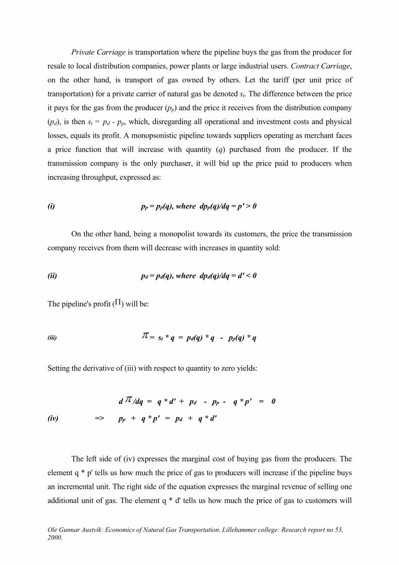
Private Carriage is transportation where the pipeline buys the gas from the producer for

resale to local distribution companies, power plants or large industrial users. Contract Carriage,

on the other hand, is transport of gas owned by others. Let the tariff (per unit price of

transportation) for a private carrier of natural gas be denoted st. The difference between the price

it pays for the gas from the producer (pp) and the price it receives from the distribution company

(pd), is then st = pd - pp, which, disregarding all operational and investment costs and physical

losses, equals its profit. A monopsonistic pipeline towards suppliers operating as merchant faces

a price function that will increase with quantity (q) purchased from the producer. If the

transmission company is the only purchaser, it will bid up the price paid to producers when

increasing throughput, expressed as:

(i) pp = pp(q), where dpp(q)/dq = p' > 0

On the other hand, being a monopolist towards its customers, the price the transmission

company receives from them will decrease with increases in quantity sold:

(ii) pd = pd(q), where dpd(q)/dq = d' < 0

The pipeline's profit (Π) will be:

(iii) π = st * q = pd(q) * q - pp(q) * q

Setting the derivative of (iii) with respect to quantity to zero yields:

d π /dq = q * d' + pd - pp - q * p' = 0

(iv) => pp + q * p' = pd + q * d'

The left side of (iv) expresses the marginal cost of buying gas from the producers. The

element q * p' tells us how much the price of gas to producers will increase if the pipeline buys

an incremental unit. The right side of the equation expresses the marginal revenue of selling one

additional unit of gas. The element q * d' tells us how much the price of gas to customers will


decrease if it sells one more unit of gas. Not surprisingly, the equation shows that at maximum

profit, marginal revenue from selling an additional unit of gas shall equal its marginal cost. The

special in this case is that the transmission company, by restricting quantity traded towards

producers and distributors, power plants and large industrial users in this optimal manner, can

simultaneously exploit inelasticities of demand and supply in order to maximize its own

advantage. It is possible, but not likely, that such a situation, that in a stylistic way describes how

the present European gas market is working, is socially efficient or maximizing public welfare.

However, several factors determine the transmission companies’ market power in

addition to scale and scope economies. One such factor is the power of producers and customers,

respectively, that the transporter meets at it end. By concentrating sellers and buyers power, a

counterforce to mitigate pipelines' market power is created. In the European gas market, this is,

to some extent, done at the supply side, which today better can be characterized as oligopolistic

than competitive. There are only a few exporting nations, and within each of these nations gas

sales are orchestrated through one body. At the customer’s side, however, it is more difficult to

concentrate purchasing power. Customers are placed in several consuming countries and there

are many LDCs, power plants and industrial users within each of them. Thus, on the customers’

side, the European and U.S. gas market is, from an economic point of view, more similar than on

the supply side, where in the U.S. there are thousands of producers.

In order to exploit economies of scope, producers have good reasons to integrate wholly

or partially with transmission activities. In the Norwegian North Sea, producing firms’ in most

cases has property rights in offshore pipelines. In Russia and Algeria, it is (so far) done by

centralized firm(s) in Moscow and Alger, planning production and transmission to the respective

countries' borders. In the Netherlands, Gasunie buys all gas, transports it to the border and sells

it. This product extension contributes in realizing the oligopolistic market structure on the supply

side. In the market, the long-term contracts between producers and consuming countries’

transmission companies may also be considered as an approach to optimizing the advantages of

joint management of transmission and production.

The market power of the transmission companies is also limited if there is an alternative

route or method of transportation. Often, the building of another pipeline may incur too high

costs to represent any credible threat to the existing one. LNG as an alternative to pipeline

transportation, may, in some cases, put a limit on how high pipeline fees can be (intermodal


competition). Investment costs for LNG transportation are largely connected with liquefaction of

gas (in producing countries) and regasification and storage (in consuming countries). Shipping

costs between producing and consuming nations are some 50 % higher than for oil, but represent

a much lower share of overall costs in bringing gas from producer to consumers than do gas

pipelines. The distance of transportation plays a much smaller role in LNG transportation and

there is no technical fixed relationship between producer and customers. "As a result, pipeline

transportation costs for onshore distances over 4000 km and offshore distances over 2000 km

generally exceed those of LNG where an offshore route of similar length is available" (IEA,

1994: 55). Within the European continent, often pipelines provide the only feasible link to

customers. However, gas from he Middle East, Nigeria and the Barents Sea, may prove to be

more cost effectively transported to the European market as LNG than through pipelines.

Transporting gas on lorries and trains, are not economically feasible with today's technology.

In end-user markets, competition from other fuels, in particular oil products, but also coal

and nuclear electricity, provide a price cap on gas. To the degree that customers can switch

quickly and cheaply between fuels when gas prices changes, LDCs monopoly power towards

end-users are restricted by this interfuel competition. The prices of alternative energies represent

the limit on total market turnover, and on how much rent the various segments of the gas chain

can "fight over". Competition from substitute products (in the case of gas: electricity, coal and

oil), makes demand more sensitive to price changes and, thus, restrict the degree of market

power by sellers, but it usually does not eliminate it.

Taken together, with some modifications, the barriers to entry is significant in pipeline

transportation and transmission companies have great potential of exercising market power both

towards producers and towards customers. The potential for and benefits of market power, may

lead to "over-bundling" of services and over-investment in capacity in order to deter

newcomers.5 Even if it is not cost-saving advantages in bundling all kind of services, firms may

nevertheless profit by doing so due to the benefits of increased market power. For a transmitter,

for example, there may be economies of scale in transportation of gas but not necessarily

economies of scope in the role as a wholesaler. The broker role may in some cases inhibit

elements of economies of scope with the transmission service and in other situations independent

firms could do it more efficiently. By having the exclusive rights (natural monopoly) in the

5 See Broadman (1986) for a discussion of market power in the U.S. natural gas pipeline industry.


transmission function, the pipeline company has the power to prohibit other companies wanting

to act as brokers, take over their potential profit and obtain a monopoly in providing merchant

services, as well. This will contain the contact between producers and end-users and decrease

market efficiency. While the pipeline gains, there may be a net loss for society.

2. Public Interests The problem for policy makers wanting to liberalize the market is that it’s concentrated

structure may also be the socially most efficient one, in spite of its inferiority. Because of scale

economies, more firms operating in the market may incur higher transportation costs unless the

market grows sufficiently in each geographic segment. This argument goes for product extension

through vertical (or horizontal) integration and the exploitation of economies of scope, as well.

Thus, the challenge for governments is to intervene in a way that preserve a market structure that

have the potential to minimize cost, and at the same time change its behavior in order to avoid

possible lax cost control and exploitation of market power.

One important question is how large the benefits of vertical integration and coordination

is. The existence of scope advantages indicates that liberalization of the market should open for

the possibility to bundle services in competition with provision of unbundled services. The

smaller the market and fewer the number of players, the less cost arguments seem to be in favor

of unbundling operations. If operations are unbundled and there exist economies of scope, the

gain from increased competition should be weighed against the losses of less efficient operations

of each firm. Thus, with the growth in the European market, gradually more arguments support

the idea of unbundling.

Maximizing Social Welfare The significant scale economy in trunk pipelines, sunk investments and capital

immobility, possible economies of scope in vertical integration and companies' bundling of

services influences vertical and horizontal ownership relations and contractual terms in the

European gas market. In specific segments of the markets, these relationships may promote

efficient investments and pricing without public interference, but the strong concentration of

market power indicates that this is rather the exception than the rule. Possibly high and rigid

prices paid for transportation may lead to under-investment in production, as an overly large part

of the market price ultimately paid for natural gas is accrued in the transportation sector rather


than by producers. Similarly, high or rigid prices to distribution companies may lead them to

exploit their strong position towards consumers (over time restrained by the price of the

alternatives to gas), making consumption of natural gas sub-optimal. Gas is fairly non-polluting

and, thus, inhibits a positive externality for the environment relative to the use of other fossil

fuels. The view from the EU (EU, 1988) is that a too rigid market structure may be harmful for

the economies involved, both from an environmental, efficiency and security-of-supply point of

view.

The transmission systems are integrated parts of the gas market that should balance in competing demand for transportation services, optimal resource management and risk evaluations. From a social point of view, it is important that the economies of scale and scope is exploited, but at the same time that market inequities caused by extensive pipeline concentration and excessive bundling by transmission companies are neutralized. An optimal gas grid should enhance security of supply for consumers as well as security of demand for producers. The system should secure flexibility both in a static and dynamic sense. Statically by creating a variety of arrangements suiting each actor. Dynamically, by permitting arrange-ments to evolve gradually based upon market trends rather than through radical change every few years. These goals are sometimes complementary and sometimes conflicting. Ideally, the grid should barely figure into the producers' production decisions and the consumers' choice of energies. A regulatory regime that aims at optimizing the transporters’ behavior should look for arrangements that do not primarily place this judgement upon public policy makers. If one could find self-regulative arrangements, the chances that the system contains the necessary dynamics when market conditions alter are better. This is also important in order to impose minimal administrative costs. Even if a possible regulation may yield a socially efficient outcome, the costs of the enforcement process need to be subtracted from the benefits achieved by regulation, and compared to the costs of operating the existing system, in order to appraise the net social benefits. In the U.S., conditions under which gas could be produced and transported have repeatedly led to undesired results. After some time, some of the regulations was removed and new regulations introduced, but only after having incurred considerable judicial and regulatory costs, loss of efficiency and social welfare (Austvik, 2000: chapter 6).

An additional argument in favor of self-regulative arrangements is that the regulator over

time need not necessarily seek to maximize social wealth only. A regulatory agency may begin

its existence with public interest in mind, but end up as an agency to protect producers and/or

pipeline companies. The persons employed in the regulatory agency may be influenced by his or

hers career opportunities, political motives, self-assertion, power, etc. The regulated companies

can gain control over the regulator and trap or capture the regulator to act in their interest and

influence the goals that the regulator sets and the way he/she seeks to attain them. Such


"capturing" can be encouraged by the movement of personnel between regulatory agencies and

the firms, which may increase the desire for cooperation and making close ties between them.

Regulatory policy that involves transfer of huge sums from a large group to a small group

is often lobbied for more easily by members of the small group. The small group has a lot at

stake per capita, and easier to organize than a large group. Therefore, small groups are usually

more successful in satisfying their demands towards public policy makers than large and often

more diffuse groups. With huge interests at stake, producers, consumers, pipelines and

distribution networks have good reasons to vociferously pursue their interests. Some countries

and companies may be better off by exploiting a possible monopoly power in the market, even if

it is not a zero-sum game in total. Usually consumers are associated with large groups and

companies with small groups. Stiegler (1971) argues that public regulation therefore often leads

to producer-protectionist results. Each party may also be too small to influence the situation and

therefore does not consider the optimal situation even if they would be better off if it prevailed,

and may stick to an existing sub-optimal situation.

Maximizing social welfare may, therefore, be an intriguing challenge. How to avoid

inefficient bundling in the natural gas industry and keep, or even create, efficient bundling and

exploitation of economies of scale and scope? How to prevent firms from taking unacceptable

advantage of a possible strong positions in segments of the market? The correct answers to these

questions will easily be viewed differently by competing parties, and these groups may pressure

regulators. In order to design an efficient and welfare-maximizing way of regulating the market

one needs a closer identification of the actual goal of the regulation.

Microeconomic theory is often used for this purpose, i.e. that the ideal situation exists in

the market when price equals marginal cost (corrected for externalities). In perfectly competitive

markets, there should be no need for public intervention (the first best solution). If one market

failure arises, such as the existence of a cartel or of pollution, marginal social cost no longer

equal marginal social benefit. In order to correct for this market failure, government should

intervene to restore the first-best situation, where social benefits equal social costs. A first-best

economy operates under conditions of social efficiency (Pareto optimality) and the policies

introduced correct the market distortions that occur.


However, in the real world, this is rarely possible. In a second-best economy,

compromises between theoretical first-best solutions and the real market are adopted. The

application of a second-best policy means to minimize the distortionary effects of the market.

Policy measures, other than nationalization, generally aims at second-best solutions. In fact, one

could argue that nationalization also is a second-best solution (at best), as it over time often does

not satisfy social efficiency goals even if it's intended to do so.

Of course, effective public intervention needs to consider political, psychological, cultural, practical and other issues, in addition to the knowledge of economics. Seeking to practice a pure economic model within the real world, i.e. in constructing tariffs for gas transportation, may lead to other results than what should be expected. Economics may first of all give insight into the processes around and the purpose of regulation, describing important forces operating towards optimality. By understanding these forces, the regulator can use this insight together with other aspects to be taken into consideration, to improve welfare and market efficiency and move towards optimality, although not necessarily reaching it.

Laissez-faire, Nationalization or Regulation? To illustrate the situation we will start with a strong simplification of the position of a

transmission company. Figure 8 considers a strong natural monopoly, due to economies of scale,

with low (and constant) marginal costs compared to fixed costs. The position and shape of the

demand curve (assumed linear and falling) determines which output-price combinations that are

possible in this market. We will discuss three possible outcomes. In point A, the firm acts as a

monopolist choosing a high price/low output combination. In point B, the firm acts as a 'cost-

plus' company where price is set equal to average cost. In point C, the firm produces an output so

large that price must equal marginal cost in order to make consumers absorb the entire output.


p

q

AC

MC

D

L C

B

demand curve/average revenue (AR)

G A

F E

JH

I

K

X

pmon

pac

pmc

qmon qac qcomp

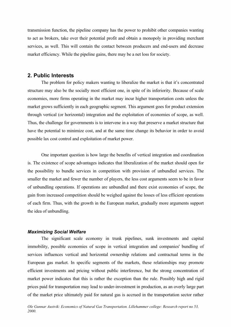
Figure 8: Decreasing average cost in a pipeline; Monopoly vs. competition

Point A: A monopolist would choose to produce where marginal revenue equals marginal

cost, which happens at point X. The production (or the amount of transported gas) will be qmon.

For this quantity, consumers are willing to pay the price, or tariff, denoted earlier as the share to

transmission company, pmon. The company's economic profit will be GAEF, which results from

the difference between market price and average costs at output qmon. If the company increased

production beyond this point, marginal cost would be higher than marginal revenue and it would

loose money on the margin.

Point C: If output increases beyond qmon, this would be more optimal from a social point

of view. The willingness to pay is larger than the marginal cost all the way up to point C. Thus,

point C is considered to be the socially most efficient way of production. The problem is that the

price for transmission at point C, pmc is below average cost and the company looses money

unless someone is willing to pay the deficit. The loss is represented by area HDCI, which is the

difference between the market price and average costs times output qmc. The net advantage for

society in moving production and prices from point A to point C is represented by area ACX.

Point B: If the company should break even, price must equal average cost. At point B an

output of qac is produced at price pac, and the company earns normal profit but no economic

profit. This point is also more optimal for society than the monopoly solution in point A. The


gain for consumers (GABJ) is obviously larger than the loss for the producers (GAEF). Society's

net gain equals area ABLX, while the deadweight loss is BCL compared to the first-best solution

in C. Point B is a second-best-solution from a social point of view compared to point C.

Historically, nationalization (point C) has been widely applied in Europe after Word War

II. Under nationalization, the government replaces the market by providing the service or good

itself. When nationalized, the governmental owned company, usually, sets price equal to

marginal cost. As long as average costs often exceed marginal cost for natural monopolies,

public budgets must transfer funds to the firm to cover the deficit (HDCI). However, marginal

cost pricing is a necessary, but not sufficient, criterion for maximizing social welfare, as it

ignores the question of the 'best' or 'fairest' distribution of income. It may be possible to reach a

higher level of welfare with an 'inefficient' way of production than with an efficient one. This

could happen if the income distribution is 'sufficiently wrong' or if it is difficult to reach the most

efficient way of producing. Then, it could be better to look for second-best solutions for how the

goods or service should be provided.

Regulation (point B) is such a second-best solution and has been the American way of

intervening into such markets. Public regulation may be made through force, or by incentives,

inducing the firm to act in its self-interest, which at the same time is compatible with social

goals. Under regulation, the goal is to make the firm decrease price/tariff, increase output and to

produce this output efficiently at minimum cost. The firm must earn normal profits on its

investments in order to remain in business, but no economic profit. However, this simple goal is

not that simple to reach.

Often laws about market structure and firms behavior are parts of a liberalization of a market. Laws may prohibit or regulate the behavior of firms that are imposing external costs. For example, a firm can be banned or restricted to perform polluting activities. In the case of monopolies and oligopolies, laws can be used to change the structure of the industry or the behavior of the firms within it. When affecting market structure, laws can make mergers (horizontal integration) illegal. Even though there may be a large number of firms in the market, one or a few may control the major part of it and, thus, behave as monopolist/oligopolists. Thus, market concentration can be measured in terms of how many firms control a certain market share. The government could make a merger illegal if the degree of concentration rises above a certain amount. If firms already control more than this percentage, they could be split into smaller firms. Whether this is efficient or not, depend on cost structure of the activity compared to size of market and the behavior of the firm. Competition laws in the EU, therefore, studies the actual performance of the firms rather than


market share to assess whether or not, for example, a merger should be considered illegal or not. Taxes and subsidies are often favored by economists to repair for market failures. These

are used both to improve social efficiency and to redistribute income. To improve efficiency,

taxes can be used to reduce the social costs of (negative) externalities, monopoly power,

imperfect knowledge and irrational behavior. In some simplistic cases, taxes can be used to

achieve first-best solutions. However, because it usually is infeasible to use different tax and

subsidy rates towards different firms, and because the government lack detailed knowledge about

markets, taxes and subsidies seldom achieves more than second-best solutions.

Under regulation, a "visible hand" is introduced in the absence of the market's

"invisible hand". By regulating the framework and conditions for how the firm may operate,

public authorities seek to achieve what is considered optimal for the society. The incentives

and disincentives given for pricing and production should create mechanisms leading to an

efficient allocation of resources and "acceptable" distribution of income. As part of

intervening into firms' behavior, regulation may be introduced to direct the firm to behave in

certain ways. The framework and regulatory mechanisms for the market must then be

constructed in a way that companies voluntarily produce an amount at a price that gives

maximal profits and simultaneously satisfies social goals. The regulations should lead to

consistency between the company's desire to maximize profits and the society's desire for

maximizing welfare, as in a perfectly competitive market. This is the core of regulatory

economics.

2. Schedules for Regulatory Regimes

Rate-of-Return (ROR) Regulation - the "A-J-Effect Averch-Johnson (1962) is considered one of the most influential investigations into

regulations' effects on firm’s behavior. They showed that a regulation of return on capital not

necessarily mitigate the aspects of monopoly control that the regulation addresses. They even

concluded that such regulation could make the situation worse.

Consider a monopolist producing a single output q and using two factors of production,

labor (L) and capital (K). The (market) price of capital and labor is denoted r and w, respectively.


Let q = q(L,K) denote the (neo-classical) production function, and the price of q as the inverse

demand function p = p(q). The firm's (economic) profit (π) will be:

(i) π= p(q) * q(L,K) - w*L - r*K

Unregulated, the firm will chose its capital-labor ratio in a way that costs be minimized.

This happens when the marginal rate of substitution between the two inputs q'K/q'L, are equal to

the ratio of input prices, r/w. When regulated, assume that the regulator allows a rate of return

on capital equal to m. Return on capital is defined as net revenues, which is gross revenues (p*q)

minus costs of labor (w*L) and other possible non-capital input factors (here: zero) divided on

amount of capital invested (K). The firm is otherwise unconstrained and can choose its

price/tariff, level of output and input as long as profit does not exceed this "fair" rate. The rate of

return constraint can be expressed as:

p(q) * q(L,K) - w*L(ii) m ≥ --------------------------

K

The behavior of the firm will vary a lot with which level of m is chosen. If the regulator

sets m < r, the firm will make more profit by closing down the business and selling it's capital

than continuing it's service (assuming no sunk cost and that it legally can do so).

If m = r, the firm makes zero economic profit which yields an indeterminate situation.

The firm would earn the same profit per unit whether it increases or decreases output, whether it

uses resources efficiently or inefficiently, or whether the input mix is optimal or not. The firm

would, in fact, make the same money if it closed down and sold off it's capital (assuming no sunk

cost). Thus, as the firm can chose many different outcomes, a ROR regulation that set r = m

cannot be relied upon as a device to make it act in any particular way.

If the regulator set m ≥ rmon, where rmon is the return of an unregulated firm, the constraint

is higher than what it possibly could make in the market. This will not change its behavior. In

such a case there is essentially no regulation.


If the regulator set rmon > m > r, the rate of return is higher than the cost of capital but

less than it would earn as unregulated monopolist, the firm will still earn an economic profit on

it's investment. If we subtract the (market) price of capital from both sides of inequality (ii) and

rearrange:

m - r ≥ (p*q - w*L) / K - r

m - r ≥ (p*q - w*L - r*K) / K

m - r ≥ π / K

(iii) π ≤ (m - r) / K

The maximum economic profit the firm can earn on it's investment is (m - r) / K.6 The

problem with this approach is that if the firm is allowed to increase it's (economic) profit by

increasing it's amount of capital. The rate of return (with an economic profit up to (m-r)) will

remain the same, but in absolute terms profit becomes higher.

The discussion above showed that the only way the regulator can set the return constraint

is by letting rmon > m > r. Whether it is feasible or not for the firm to earn an economic profit on

its investment under the constraint of an allowed profit ceiling depends on its technology and

demand for service. Some combinations of K and L could exactly yield a rate of return r = m. If

the firm can manage to find this set of K and L combinations, it chooses the one among them that

uses the greatest amount of capital. This gives the highest absolute profit. If the capital stock is

not increased, feasible profit will be lower (π< (m-r)K), and thus, inferior to the cost minimizing

point with the maximum use of capital. Other cost minimizing combinations of K and L, yields

the same economic profit but on a smaller amount of capital, and thus, less total profit.

In essence, the A-J analysis shows that the firm adopts an inefficient production plan, as

it's marginal rate of transformation between capital and labor exceeds it's cost-minimizing level

when the regulator set m > r:

q'K/q'L < r/w 6 If m = 0.12 (12 per cent), and r = 0.09 (9 per cent), the company's economic profit should not exceed 3 per cent.


This implies that it over-invests and accumulates capital in order to relax the rate of return

constraint. This is called the A-J effect. The regulated uses more capital than the unregulated;

(K/L)reg > (K/L)mon, which will be an inefficient way of production. Thus, the output produced by

the regulated firm can efficiently be produced with less capital and more labor at a lower cost.

Some modifications have been proposed to this type of regulation (Train, 1991: 20-67,

94-113 and Berg & Tschirhart, 1989: 324-333). Rather than constraining the rate-of-return on

capital, a constraint can be put on the return on output, revenue or cost. These modifications may

induce the firm to behave more optimal than when return on capital is regulated.

Regulating return on output: In this case, the firm is allowed to make a profit on each unit

of output. Now, the firm will expand output as long as consumers' willingness to pay is above

total production cost (including allowed profit). If allowed return on output is set sufficiently

low, the firm may end up close to where price equals average cost, or the second best solution in

figure 8 (point B).

Regulating return on revenue: If the firm is allowed to make a certain profit on each unit

of revenue, the firm will expand output in the same way as under a return-on-output regulation as

long as marginal revenue is positive. When marginal revenue becomes negative, expanded

output decreases revenue. Thus, the firm will produce at the point where total revenue is greatest,

or when MR=0. Therefore, a return-on-revenue regulation will only approach the second-best-

solution if MR≥0 to this point. In figure 8 the volume produced will be quite far from the

volumes representing point B.

Regulating return on cost: If the firm is allowed to make a certain profit on each unit of

cost, it increases its allowed profit by increasing its cost. Maximum cost is accrued when output

is maximized. However, increasing output, decreases revenues when MR < 0. Therefore, when

MR < 0 the firm wishes to increase cost rather than output. The firms start to waste at outputs at

this point. In the same way as under return-on-revenue regulation, although of a different reason,

a return-on-cost regulation will only approach the second-best-solution if MR≥ 0.

Thus, regulating either the return on capital, revenue or cost yields inefficiencies by the

firms’ behavior. Regulation of return on each output that is produced is the one form of


regulation that has the greatest chance of achieving a solution that in some sense may optimize

social welfare, disregarding the problem of actually setting this rate with weak insight in firms

cost curves.

Price Discrimination – "Ramsey Pricing" Under the regulations discussed above, we assumed that the firm charges the same price

to all its customers. Price discrimination is, on the other hand, a situation where the firm charges

prices for each unit of output equivalently to consumers' willingness to pay. Such price

discrimination can be performed towards different type of customers, at different levels of

output, seasons etc.

A firm that can charge prices equal to each consumer’s WTP performs a perfect price

discrimination. By doing so, the firm receives an extra profit that is represented by the entire area

under the demand curve and above the price equal to consumer's surplus. Referring to figure 8, a

firm can expand output beyond qac under price discrimination, as long as p≥MC, because it's

fixed costs are covered by already charging higher prices to customers with a high WTP (to the

left of point B). Under price discrimination, as the firm increases output it has to decrease price

all the way on the margin, but it does not have to lower the price taken from customers that are

willing to pay a higher price. The firm wishes to sell more units as long as the price it receives

from selling extra units exceeds the extra costs incurred by producing this unit (the marginal

cost) without reducing the price for volumes already sold.


p

q

B

ED

F

A

C

G

q1 q2

p1

p2

Figure 9: Effects of quantity changes on price and revenue

In figure 9, let's first assume that all customers buying the volume q1 are charged the

same price p1. If output is expanded from q1 to q2, without price discrimination, price must be

reduced for all customers from p1 to p2. Gain in total revenue due to higher volumes is

represented by the area DEFG and the loss in revenue due to lower prices is represented by the

area ABCD. If DEFG > ABCD, there is a net gain and MR>0. Otherwise there will be a loss of

revenue due to increased production. Let's then assume that increasing output from q1 to q2 do

not lower prices customers are willing to pay for q1 only. In this case, when the firms take one

price p1 for volumes q1, and another price p2 for volume q2-q1, the loss in revenues ABCD equals

zero. Net gain will now be DEFG.

Either selling for the same price or under price discrimination, the firm sells an extra unit

of output as long as its marginal revenue is above its marginal cost. When the firm must charge

the same price to all customers, this happens where MR=MC (< AR as in point X in figure 8).

Under perfect price discrimination, the firm chooses optimal output where p = MC = MR = AR,

as in point C in figure 8. Thus, under perfect price discrimination, the demand curve becomes the

marginal revenue curve. Under perfect price discrimination, the firm extracts all surpluses and

none is left to consumers.

Price discrimination could bring the firm to the first best solution rather than to the

second best solution and allows the firm to produce more output than under a regulatory


mechanism that requires the same price for all outputs. The social success of such discrimination

depend, inter alia, whether customers with a low WTP are able to resell their volumes to

customers with a higher WTP. Normally, the pipeline itself can prevent this when unregulated.

When regulated, the regulator must establish and enforce rules against such resale.

If prices on average shall equal average cost (firm breaks even) and prices are set

differently to customers, the firm must deviate from marginal cost pricing (at least) for parts of

it's sale. This should be done in a way that harms overall welfare as little as possible. At Ramsey

pricing7, prices are raised more in markets with less elastic demand than in market were demand

is more elastic, in inverse proportion to the values of each market's demand elasticity ("inverse

elasticity rule"). This way of discriminating minimizes the welfare losses when prices are

increased beyond marginal cost.

Under Ramsey pricing, output should be reduced from the point where p=MC by the

same proportion in each market. The higher prices obtained by these even output reductions and

uneven price reactions, reduces the firm's loss compared to a situation where prices are increased

similar in all markets until the (common) price equal marginal cost. Output should continuously

be reduced proportionately until the firm eventually breaks even. More revenue can be obtained

with less reduction of output (and less disruption in consumption patterns) if prices are raised

more in markets with inelastic demand. In this way, total surplus is reduced as little as possible,

and the firm can break-even without being subsidized by the government.

In figure 10, the product is sold in two markets, market 1 and market 2. At p=MC, each

market wants to consume equal amounts, q*, of the product (marginal cost is assumed constant).

The only difference between the markets is that demand in market 1 is more inelastic than

demand in market 2. If output is reduced by the same amount in each market, down to q**, price

in market 1 increases to p1 while price in market 2 increases to p2, where p1 > p2.

7 After Ramsey (1927). Ramsey showed how governments could set tax rates for various goods and at the same time disturb consumers' surplus as little as possible. Baumol and Bradford (1970) uses this principle for setting second-best pricing for multiproduct natural monopolies.


E

B

C

A

D

p1

FHG

p2

D1

p p

q q

MC

q** q*

∆q

Market 1: Inelastic demand Market 2: Elastic demand

MC

q** q*

Figure 10: Price changes depend on price elasticities; Ramsey pricing

∆q

By doing this, market 1 contributes with a profit to the firm represented by area ABCD

and market 2 to a profit represented by area EFGH. Total profit contribution from the two

markets would be ABCD + EFGH = (p1-MC) + (p2-MC) * q**. Output should be reduced in this

way until total profit contribution from the two markets makes the firm brakes even.

In a more general form, denoting the sale of q in the two markets as q1 and q2, the

Ramsey rule tells that the relative quantity change shall be the same in each market in order to

make consumers behave very much as they would have without the price increase:

(i) ∆q1/q1 = ∆q2/q2.

(i) is the “inverse elasticity rule” in volume terms. Expressed in price terms, prices should

be raised inversely related to elasticity of demand in each market:

(ii) (p1-MC)/p1) * ε1 = ((p2-MC)/p2) * ε2

where εi is the price elasticity of demand in market i (i=1,2): εi = dqi/dpi * pi/qi.

Ramsey pricing is already applied in the European gas market, for example when peak-

load pricing formulas are used. Under this system, the price that consumers pay varies, in order

for the firm to cover average costs, including normal profit. This principle would set prices


higher when demand in general is more inelastic (especially in winter months). Under this type

of price setting, parts of consumers’ surplus are transferred to transmission companies when

demand is inelastic and from transmission companies when demand is more elastic. Such pricing

satisfy efficiency considerations quite well, as they distort consumption patterns as little as

possible, and much less than if the same price were charges in both periods (for example in

winter and summer).

Subsidizing to Marginal Cost Pricing If a regulator possesses all information on cost and demand curves, he could simply

require prices to be set at marginal cost and give the firm a subsidy, equal to area HDCI in figure

8, in order to let it make a normal profit. Together with nationalization, this has been an

important principle for how natural monopolies have been dealt with in many European

countries after WW2. However, the regulator rarely has all this information. The company has

also incentives to misreport costs in order to increase profits. If reported correctly, incurred cost

may not be minimum cost of production, for example due to inefficiencies or sub-optimal

capacity choice. Thus, making the firm produce in the firs-best-option is not an easy challenge.

Our question here is whether it possible to design some subsidizing mechanisms that induces the

firm to produce at marginal cost without a public ownership and regulator’s knowledge of the

position and shape of cost curves?

Let's assume that the regulator knows that the firm will not charge prices higher than pa

in figure 11. This price could for example be the monopolistic price of an unregulated natural

monopoly. The regulator subsidizes the firm for the portion of consumer surplus between pa and

the price the firm actually charges. Thus, the lower price the firm charges, the higher the subsidy.

If the firm sets prices equal to pb = MC, the firm maximizes the transfer of subsidy and at the

same time behaves in an optimal manner.


pa

p

q

Figure 11: Subsidizing firm to marginal cost pricing

Demand curve

pb

subsidy

Loeb and Magat (1979) showed that, in general, if the regulator subsidizes the firm by the

entire consumer surplus (CS) generated at the price existing in the market, the firm would choose

to produce at p=MC. In order to do this, the regulator must have information on the demand

curve and the firm's price, and no information on cost is needed. Firm's profit would equal total

social surplus, or the sum of producers’ (PS) and consumers' surplus. Because this surplus is the

greatest when p=MC, the firm maximizes profit (the sum of PS and the subsidy = CS) at this

point.

This will be true even if many products exist. By setting all prices equal to marginal cost,

profit is maximized in all markets and market segments when receiving such a subsidy. Any

decrease in cost results in an increase in profits and firms have an incentive to produce

efficiently. As the government pays the subsidy, consumers' surplus is also maximized by this

rule, if we disregard that the funding for the subsidy must be collected from many (but not

necessarily all) of these consumers.

Such a transfer from the public to the firm may be considered inequitable. One way of

reducing it, but maintaining the main principle, is to subsidize only a portion of CS. As the firm

could never charge prices higher than pa in figure 11, it could not receive the CS accrued above

pa. By subsidizing only the portion accrued below pa, the same result is obtained as if transfers

should equal the entire area under the demand curve. This type of transfer should cost less for the


public, and thus, be of a less intolerable size from equity considerations. If we refer these results

to figure 8, unsubsidized profit for pmon(=pa in figure 11) is represented by area GAEF. Subsidy

when pmc (=pb in figure 11) is represented by the area GACI > GAEF.

By moving p (=pa in figure 11) down from pmon along the demand curve, the firm's

economic profit will decrease as will total subsidy. The difficulty is to set p sufficiently high, but

not higher than what is necessary, in order to make the firm brake even. But the inequality GACI

> GAEF holds all the way until the firm earns only normal profit. At this point, the subsidy will

equal the firm’s loss when producing at prices equal to marginal cost. Train (1991: 182-190)

discusses some regulatory mechanisms that have been proposed in order to find these optimal

prices. He suggests a multiperiod marginal cost approaches, where prices, revenues and

expenditures in one period determine the subsidy of the firm in the next period with or without

full information about the position and shape of the demand curve.8 Another alternative is to use

multipart tariffs.

Multipart Tariffs A multipart tariff consists of several billing components. There are two main types of

multipart tariffs: access/usage tariffs and block rates.

Access/usage tariffs consist of an access charge, which is a fixed fee for having the right

to use a system, and a usage charge, which is a per-unit tariff for actually using it. For example,

telephone companies often use access/usage tariffs, billing one fee for access to the network, and

one (per unit) fee for each call made. This system makes consumers’ marginal cost for each call

constant, but their average cost (the average price for consumption of telephone use over a

period) declines with the number of calls.

Block rate tariffs changes when total level of consumption reaches certain thresholds. For

example, electricity companies often charges one price for consumption of a certain number of

kilowatt-hours and another charge (higher or lower) for additional kilowatt-hours. This system

makes consumers' marginal cost of using electricity change with the level of consumption, while

8 See also Sappington and Sibley (1988) and Vogelsang and Finsinger (1979).


the average cost (the average price for using one kilowatt hour) is the weighed average of the

price of all units consumed and may increase or decrease depending on the tariff structure.

Access / Usage Tariffs – “the Coase Argument" Coase (1946) argued that the first-best solution for a natural monopoly (price equal

marginal cost) could be reached if demand for usage is fixed and an access/usage pricing system

is used. The access fee should be set to cover the natural monopoly's fixed costs and the usage

fee to cover marginal cost of usage. In this situation, the aggregated access fees are considered a

transfer of funds from consumers to producers as if the firm received a subsidy from

government. The access fee will not affect consumption of service as long as the access fee

covers fixed costs. The firm will benefit by supplying more output as long as price is equal to or

higher than marginal cost. When demand for access is fixed and the fixed cost are covered by the

"subsidy", the firm will gain by reducing usage fees down to marginal cost of production. Up to

this point consumer's willingness to pay is greater than firms marginal cost of providing the

service. Any other price or if the firm starts to waste, will incur a loss and, accordingly, the firm

will serve in an efficient manner.

However, demand for access is not always fixed, but may vary with the access charge.

When demand for access is price-sensitive, any rise in the access fee will, to some extent, lower

demand for access. Low access charges may, for example, increase the number of households

installing pipes and equipment for use of gas. In a situation with price-sensitive access demand,

the access fee influences demand for access and indirectly the demand for usage. The access fee

can no longer be considered only to be a transfer from customers to the firm.

Consider the access and the usage of the firm's services as two different goods with

separate but interrelated demand, each with a separate marginal cost. For example, there is one

demand for installing a new pipe and equipment into a house and another for the actual use of

gas when equipment is already installed. With price-sensitive demand for access, optimality can

be reached if access fees are set equal to marginal cost of access and usage fees equal to marginal

cost of usage. The problem is that with access fees set at marginal cost of access a loss is often

incurred to the firm, as average cost of access if often higher than it's marginal cost.


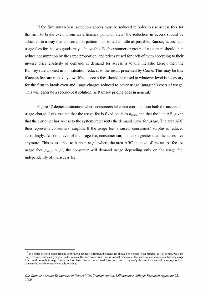
If the firm runs a loss, somehow access must be reduced in order to rise access fees for

the firm to brake even. From an efficiency point of view, the reduction in access should be

allocated in a way that consumption pattern is distorted as little as possible. Ramsey access and

usage fees for the two goods may achieve this. Each customer or group of customers should then

reduce consumption by the same proportion, and prices raised for each of them according to their

inverse price elasticity of demand. If demand for access is totally inelastic (zero), then the

Ramsey rule applied in this situation reduces to the result presented by Coase. This may be true

if access fees are relatively low. If not, access fees should be raised to whatever level is necessary

for the firm to break even and usage charges reduced to cover usage (marginal) costs of usage.

This will generate a second-best solution, as Ramsey pricing does in general.9

Figure 12 depicts a situation where consumers take into consideration both the access and

usage charge. Let's assume that the usage fee is fixed equal to pusage and that the line AE, given

that the customer has access to the system, represents the demand curve for usage. The area ADF

then represents consumers’ surplus. If the usage fee is raised, consumers’ surplus is reduced

accordingly. At some level of the usage fee, consumer surplus is not greater than the access fee

anymore. This is assumed to happen at p*, where the area ABC the size of the access fee. At

usage fees pusage < p*, the consumer will demand usage depending only on the usage fee,

independently of the access fee.

9 In a situation when usage demand is fixed, but not access demand, the access fee should be set equal to the marginal cost of access, while the usage fee is set sufficiently high in order to make the firm break even. That is, natural monopolies that does not use access fees, but only usage fees, can do so only if usage demand is less elastic than access demand. However, this is very rarely the case for a natural monopoly as fixed compared to variable costs are usually very high.


B C

A

D

P*

p

q

Figure 12: Ex ante and ex post demand curves

Size ofaccess fee

pusage

Consumers´net surplus

E

F

Obviously, ex ante, the size of the access fee must be taken into consumer’s

consideration as well. Consumers know that the surplus they get will be the consumers surplus

generated at the usage fee charged minus the access fee (ADF-ABC). Therefore, at pusage > p*,

the consumer will choose not to acquire access. In this case the benefit of usage will be less than

the cost of getting access. If pusage<p*, consumers get a net surplus equal to area BCDF. The

lower the usage fees the greater the surplus. This means that the consumer will have no demand

for service at usage fees above p*. Therefore, ex ante, the kinked line ABCE represents demand

for service. Ex post, when the customer has paid the access fee, the line AE will be the demand

curve. If consumers net surplus is sufficiently large, which happens when (relative) changes in

access and usage fees within 'reason' does not induce consumers to forego service, access

demand can be considered fixed. Then access fees can be raised to the point where fixed costs

are covered (the Coase result). However, demand for access is fixed only if the surplus from

usage is so much greater than the access fee, that “relevant” changes in access and usage fees

does not imply that consumers forego service.

Block Rates The term 'block' rates have arisen from the particular form of its graphical presentation,

as the pricing algorithm looks like series of blocks. Consumption of service under each of the


prices is called a 'block'. In a declining block rate tariff, as shown in figure 13, price (p) for each

unit consumed declines with the level of consumption (q). In the figure the following rates exist:

p1 for 0 < q < q1

p2 for q1 ≤ q < q2

p3 for q2 ≤ q

In this case, there exists three blocks: 0 < q < q1, q1 ≤ q < q2 and q2 ≤ q. The price the

consumer pays for an additional unit of consumption is called the marginal price and the prices

that applies for lower levels of consumption the inframarginal price. In figure 13, a customer

that consumes q1<q<q2 faces a marginal price of p=p2 and an inframarginal price of p=p1>p2. At

consumption q>q2, the marginal price would have been p=p3<p2 and two inframarginal prices

would exist, p1 and p2.

p2

p

q

Figure 13: Declining block rate tariff

p3

p1

q2q1

Block rates can, of course, also be 'inverted', as opposed to declining. Inverted block rates

consist of blocks with higher, instead of declining, prices with higher level of consumption.

Beyond the first block marginal price is below average price under declining block rates and

above average price under inverted block rates. Usage charges under a system with access/usage

tariffs can, of course, also consist of block rates, making a combination of the two pricing

systems possible.


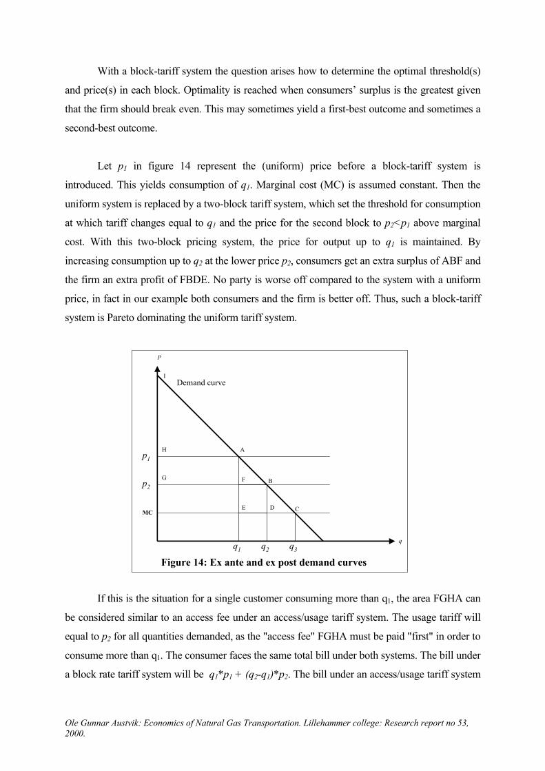
With a block-tariff system the question arises how to determine the optimal threshold(s)

and price(s) in each block. Optimality is reached when consumers’ surplus is the greatest given

that the firm should break even. This may sometimes yield a first-best outcome and sometimes a

second-best outcome.

Let p1 in figure 14 represent the (uniform) price before a block-tariff system is

introduced. This yields consumption of q1. Marginal cost (MC) is assumed constant. Then the

uniform system is replaced by a two-block tariff system, which set the threshold for consumption

at which tariff changes equal to q1 and the price for the second block to p2<p1 above marginal

cost. With this two-block pricing system, the price for output up to q1 is maintained. By

increasing consumption up to q2 at the lower price p2, consumers get an extra surplus of ABF and

the firm an extra profit of FBDE. No party is worse off compared to the system with a uniform

price, in fact in our example both consumers and the firm is better off. Thus, such a block-tariff

system is Pareto dominating the uniform tariff system.

B

C

I

D

p

q

Figure 14: Ex ante and ex post demand curves

Demand curve

E

p2

p1

q2q1 q3

H

F

A

G

MC

If this is the situation for a single customer consuming more than q1, the area FGHA can

be considered similar to an access fee under an access/usage tariff system. The usage tariff will

equal to p2 for all quantities demanded, as the "access fee" FGHA must be paid "first" in order to

consume more than q1. The consumer faces the same total bill under both systems. The bill under

a block rate tariff system will be q1*p1 + (q2-q1)*p2. The bill under an access/usage tariff system


will be q1*(p1-p2) + q2 * p2. Producers face the same marginal price (p2) under both systems and

receive the same total revenue as consumers pay the same total amount.10

By replacing a "one-block" tariff (or a uniform price) by a two-block tariff, the

deadweight loss is reduced to from ACE to DCB. It is easy to see from the figure that

introducing a third block at outputs with a threshold q2<q<q3 at any price MC<p<p2, reduces the

deadweight loss further to the benefit of consumers’ surplus and firm’s profit. Thus, surplus is

improved by increasing the number of blocks, and, in principle, until the first-best outcome is

reached (p=MC for the last unit). If number of blocks are N, an optimal N+1 tariff provides

greater surplus than the optimal N block tariff as long as the tariff of block number N is greater

than marginal cost of service.

At a given q=q1, the optimal prices for each block, p1 and p2, should be set in a way that

it distort consumption as little as possible (given that the firm shall break even). One good is

consider the output within one block. By using the inverse elasticity rule of Ramsey pricing, the

price is raised more for the good with the lower elasticity. For consumers in the second block, the

inframarginal price in block one does not affect their consumption. At increasingly higher

quantities of output, however, in particular in the second block, demand becomes more price

sensitive. Thus, prices in the first block should be higher than in the second if consumer surplus

should be distorted as little as possible. This is the reason why the optimal block-rate tariff

usually consists of declining blocks, rather than inverted block-rates with prices rising at each

successive threshold.11

In the example above, the threshold was set in a way that consumers demand exactly q1

at price p1. Under a uniform price system this will be the customer’s demand. The introduction of

a declining block rate tariff will be to the benefit for each consumer, as it makes it possible to

consume more. The two-block system will increase consumption to q2, and surplus is increased

by the area AFB in figure 14. Now, assume that the threshold for block 1 is set higher than q1

(q1<q=q*<q2), as shown in figure 15. Because the first block is larger than consumer’s

10 This is true if there is no (positive or negative) externalities or transactions costs and the consumer knows its demand. However, if these assumptions does not hold there is a difference between them as consumers could in certain situation desire access without having any charged usage.

11 However, from an equity consideration, inverted block rates may be preferable. Inverted block rates are lower for smaller quantities of output. Consumers face the lowest rates at low levels of consumption. This benefit low-income consumers, while declining rates benefit larger and high-income consumers.


willingness to pay, there is a loss of consuming more than q1 as illustrated by the area AJK. The

gain by increasing consumption to q2 is reduced from AFB to KLB. If KBL>AJK it is a net gain

of continue consuming q2 at the new threshold q=q*. However, the closer q* approaches q2, the

smaller the gain and eventually it becomes a net loss.

BL

K

p

q

Figure 15: Loss and gains by determining the block threshold

Demand curve

J

p2

p1

q*q1 q2

F

A

MC

loss

gain

As long as consumers continue to consume in the second block, their elasticity of

demand is zero in the first block. The inverse elasticity rule suggests that the price in the second

block should be set equal to firm's marginal cost and the price in the first block sufficiently high

for revenues to cover total cost. By using Ramsey pricing to determine p2 and p1, where p2=MC

and (p1-MC)*q1 equal the revenues needed for the firm to brake even (mainly fixed costs), first

best optimality can be achieved.

Thus, the optimal threshold in a two-block tariff system depends on which price-output

combination make the firm breaks even. A reduction in the threshold gives more consumption in

the second block, which benefits consumers, but simultaneously less revenue to the firm

(assuming p1 constant). Usually a reduction in the threshold will also increase the number of

customers. At the optimal threshold, the gains and losses for consumers and firms are equal

when the threshold is changed in either direction. Even if this is rather unprecise from a practical

perspective, it may nevertheless give some assistance in determining the threshold.


Determining Optimal Capacity In the long run, all costs for the firm can be considered variable. However, in periods

from when an investment decision is made until a pipeline actually operates, capacity must be

considered fixed. Ex post, capacity is determined by the investment done in a pipeline. Ex ante,

capacity can be adjusted. The question is how to determine the size of capacity.

Corrected for uncertainty, a new pipeline project should give a positive net present value

of the investment at an appropriate discount rate. One way of considering this investment is in

terms of flow of expenditures, rather than as a one-time payment. This flow of expenditures may

include mortgage payments on the loans taken to finance the project and varies in particular with

the repayment period and the interest rate.12

The annual flow of expenditures per unit of capacity (a) represents the cost of increasing

capacity from K to K+1, at all capacity uses at a given capacity. The short run marginal cost

(SRMC) for output q≤K is denoted b. Both a and b are assumed constant of reasons of

simplicity. Then, long run marginal cost (LRMC) of producing one output is the sum of the costs

of expanding capacity by one unit and the cost of producing it at this capacity; LRMC=a+b as

shown in figure 16.

At output q1, consumers are willing to pay the price p1. Their WTP exceed both variable

and average fixed costs. The difference between price p1 and SRMC is p1-b and represent the

amount consumers are willing to pay more than variable cost for capacity to be expanded in

order to get one additional unit of output.

12 With societies' lower discount rates compared to the private ones, caused by a usually longer time perspective and an overall view on the gas business and the economy, a project may be right to realize for the society but not for the private company. On the other hand, governments are normally risk averse, i.e. the numerical cost of the possibility of losing one dollar is often viewed as larger than the benefit of gaining one. Private businesses may be more risk neutral (the numerical cost of the possibility of losing one dollar equals the benefit of one). Some may even be risk lovers (the numerical cost of losing one dollar is smaller than the benefit of gaining one). If private industries are less risk averse than govern-ments, they may tend to invest sooner than governments. The assessment of the uncertainty, at a given discount rate, will depend on factors as the resources at hand, market possibilities, the presence of alternative energies, time horizon etc. The advantages of the government's longer and more general view, may be of particular importance for huge and strategically important pipelines due to reasons of security of supply, overall economic considerations et.c.


p

q

Kp1

q1 q0

LRMC

Capacity demand curve

Output demand curve

qlrmc

a+b

b

a

Figure 16: Optimal capacity determined at prices equal to long run marginal costs

At all levels of output q<q0 (where q0 is the amount demanded at p=b), consumers are

willing to pay for additional capacity. Thus, the demand curve for capacity is the bolded line in

figure 16 with a kink at q=q0. Demand for extra capacity at q≥q0 equals zero. However at

qlrmc<q<q0 prices does not cover more than a part of a pipelines' fixed cost. Only if consumers'

WTP for extra capacity exceed the cost of building extra capacity, it contributes with a net

surplus. The optimal level of capacity and capital investment is where the demand curve

intersects the LRMC-curve at K=qlrmc (where qlrmc is the amount demanded at p=a+b).

Social optimum is achieved if prices are set equal to marginal cost of production (at given

production capacity). In figure 16, short run marginal cost is constant equal to b for outputs q≤K.

If demand exceed K at p=b, no more output can be provided (in the short run), and marginal cost

increases infinitely. Thus, the (short run) marginal cost curve for providing q is horizontal for

0<q≤K and kinked at q=qlrmc to a vertical position for q>K at a given capacity (se figure 19).

Using a marginal cost pricing principle in this situation yield prices at or above b depending on

where the demand curve intersect the (short run) marginal cost curve (b).

A problem in determining demand is that it varies over the year. Figure 17 shows atypical pattern over seasons for the consumption of natural gas in Europe. Consumption in summer months is only one-third of winter peak consumption.


Figure 17. Seasonal consumption of natural gas in OECD-Europe.Source: (IEA (1994), page 35

45

40

35

30

25

20

15

10Jan Feb Mar Apr May Jun Jul Aug Sep Oct Nov Dec

Monthly Consumption (bcm)

Let’s denote the cost of adding capacity a in each period (summer and winter).

Customers in high and low demand periods are considered of equal importance. Thus, total cost

over both periods is 2a. If consumers’ WTP for capacity on average over high and low demand

periods exceed the cost per period, or a, capacity should be added. That is WTPsummer + WTPwinter

≥ 2a.

Combinations of high and low demand situations (peak and off-peak periods) with

consumers’ average WTP greater than the cost of adding capacity can exist if one or both of

them are willing to pay more than the cost of increasing capacity. In figure 18 we have drawn

one off-peak demand curve (Doff) and one peak demand curve (Dpeak) as one possible

combination of the two. qoff is the amount off-peak consumers are demanding and qpeak is the

amount peak consumers are willing to consume at price p=b (SRMC). We assume that the two

"groups" of customers consume only in their respective periods and each of them are willing to

pay for additional capacity as long as q<qoff for off-peak consumers and q<qpeak for peak

consumers.

As the two groups of consumers are weighed equal, the average willingness to pay can be

determined in the middle between peak and off-peak demand curves. For example at output q1,

off-peak consumers are willing to pay CE and peak consumers AE for additional outputs, where

AE>CE. The average willingness to pay will be in the middle between CE and AE, which is BE


(where AB=BC). Thus, B is one point on a new curve showing average demand over the two

periods.

p

q

L LRMC

Dpeak

qpeak

a+b

b

a

Figure 18: Optimal capacity with two period demand

Daverage

qoffq1

E

A

B

K

Doff

H

G

C

F I

Up to qoff, off-peak consumers are willing to pay for extra capacity while peak consumers

are willing to pay for additional capacity up to qpeak. At output levels qoff<q<qpeak, off-peak

consumers are not willing to pay for adding new capacity to the system. Thus, demand for new

off-peak capacity is zero a q>qoff and off-peak consumers' demand curve will be a curve kinked

at F, running through the points CFI. Capacity demand for peak consumers (AG) will be zero at

q>qpeak and will be kinked at G, running through point AGI. The average demand curve can be

drawn in the middle between these two kinked curves, shown as Daverage running through points

BHGI. The distance between this new curve and b, expresses consumers' average WTP for extra

capacity. Optimal capacity is determined where average willingness to pay in the two periods

equal long run marginal cost, equivalent to the one-period example above. This happens at point

L, with capacity K at LRMC prices a+b. At point L, average willingness to pay for extra

capacity equals the cost of adding it.

Pricing in Peak and Off-Peak Periods – "Riordan Regulation"

A situation of high and low demand (peak and off-peak demand) compared to capacity is shown in figure 19. Marginal cost curves at fixed capacity (K) is shown as kinked bolded


lines. Graph A shows a situation with low demand (≤K) and graph B a situation with high demand (>K), both at prices equal to short run marginal cost (b).

p

q

excesscapacity

b

q* K

Dlow

Figure 19: Optimal marginal cost pricing at high and low demand

(A) p=MC and q≤Kp

q

b

K=

Dhigh

(B) p=MC and q>K

p*

excessdemand

q*

In graph A, quantity q*<K is demanded at p=b. There is no way capacity K-q* can be

used as long as consumers' WTP < SRMC at these levels of output. In graph B, quantity

demanded at p=b is greater than capacity, which is impossible in the short run. In this situation,

somehow q=K must be rationed among consumers. Economist usually argue that the most

efficient way of rationing is to raise prices high enough to exhaust demand, that is setting

p=p*>b. Other methods of rationing may lead to a situation where a consumer that is willing to

pay a price above marginal costs (at q≤K) may not get the product. A consumer that is not

willing to pay such a price, for example by queuing, a draw, use of force or size, may get it.

Thus, if demand for transportation in winter months exceeds capacity and is lower than capacity

during summer months, transportation tariffs should be higher during winter than in summer.

However, the firm obviously looses money in summer months with such a pricing

principle, as it earns no profit to contribute to investment costs. On the other hand, in winter

months the firm makes a profit (p*-b)*q*. On total, it will not be possible from this information to

determine whether the firm runs a loss or a surplus. There are mainly two ways the firm can

cover the difference between total revenues and total costs. Government can give the amount to

the firm as subsidy or an access charge can be added without affecting the usage charge. The

access charge can be evenly distributed on consumers if demand is fixed (the Coase result) or be

allocated by resorting to Ramsey prices, depending on the degree of price responsiveness to

access charges.


Riordan (1984) discusses how such fixed capacity pricing can be achieved through a regulatory mechanism. The idea is that the firm receives a subsidy from the government or charges an access fee that amounts to the fixed costs of capacity minus the amount prices exceed marginal cost times capacity. In order to do this, the regulator need to know the price charged in the market, the actual capacity of the firm and it's variable and fixed costs, but he does not need information about the demand curve. The information needed is usually accessible, at least as proximate, even in natural gas markets.

In figure 20 the two situations with demand ≤K (graph A) and demand >K (graph B) is

redrawn. In graph A, the price for service is set at p=b and the firm receives a subsidy/access fee

to cover fixed costs, amounting to a*K. If the firm attempts to raise the price from b to p1, his

(economic) profit would increase with the area ABEF = (p1-b)*q1. But, an amount equal to the

price increase times capacity is withdrawn from his subsidy/access fee, represented by area

ACDF = (p1-b)*K. Obviously, ACDF>ABEF, and the firm suffers a loss by increasing price

beyond b. The main point is that while the price increase raises profit on the basis of actual

output, the subsidy/access fee is reduced on the basis of capacity.

p

q

SRMC

b

q* K

Dlow

Figure 20: Optimal behavior under Riordan regulation

(A) p=MC and q≤K

p

q

b

K=

Dhigh

(B) p=MC and q>K

p*

q*

SRMC

q1

p1B C

IDE HF

A

G

p1B C

DEF

A

In graph B, prices are set equal to p*, equal to marginal cost at the given demand and

capacity K=q*. The firm earns a profit over variable costs equal to area FDIG to cover fixed

costs. If the subsidy/access fee is set equal to it's fixed cost minus the area FDIG the firm breaks

even. If prices are raised from p* to p1, it's profit would increase by the area ABEF-EDIH. The

subsidy/access fee will be reduced with the area ACDF. Again, because the subsidy/access fee is

calculated on the basis of capacity, while profit is calculated on the basis of actual output, net

profit suffer a loss. The firm must choose between earning either normal profit or less than

normal profit.


Obviously, in "low demand periods", a p=SRMC-principle could yield p≥b as well as in

high demand periods and vise versa. In general, over both the high and low demand periods

(over the year) the firms profit will, when a subsidy/access fee = S is included, be:

(i) π= (plow-b)*qlow - a*K + Slow + (phigh-b)*qhigh - a*K + Shigh

The footscripts 'high' and 'low' indicates that the values of the variables refer to high and low demand periods, for example winter and summer. a*K, represent the (flow of) capacity costs over each period. For simplicity reasons we have assumed that the year is divided into two equal parts, such that K is half-of-the year per unit fixed cost. The size of the subsidy/access fee in each period must equal:

(ii) Si = a*k - (pi-b)*K at pi ≥ b, where i = high, low

Substituting (ii) into (i) and rearranging yields a profit expressed as:

high

π = Σ (pi-b)(qi-K) i=low

Pricing at pi=b and producing an amount of output equal to capacity (qi=K) yields zero

(economic) profit. Because the firm must set pi≥b (to cover variable costs) and qi≤K (output

cannot exceed capacity), the term (pi-b) is greater or equal to zero and the term (qi-K) less or

equal to zero. If the firm sets pi>b, which it is allowed to do, and output is below capacity

(qi<K), profit will be negative. As long as actual output must be lower than capacity at p>b, the

firm will loose money by raising prices above marginal cost. In all other situation the firm will

make normal profit. Riordan argues that these mechanisms induce the firm to price service in all

markets and periods equal to its marginal cost, and thus the first best solution can be achieved.

One problem using such a pricing principle is that LRMC for a new pipeline is often

above the average cost of the existing pipeline. One way of covering the costs of new

construction is to roll them into the charge for all transportation services. A new average cost

level would be established including costs in both old and new pipelines. This may involve new

subsidy/access charges in old pipelines when capacity is expanded. The price paid for


transportation will under this arrangement not reflect the true costs in each pipeline, as some

costs will lie above and some below the average tariff. Another way is to consider each pipeline

project separately. Under this arrangement, the newer pipeline will operate with higher costs and

the users will have to pay a higher tariff using this pipeline as opposed to using the old ones.

A tariff structure that sets different rates for each pipeline meets the efficiency criterion

that prices should equal marginal costs better than when the costs of a new pipeline is rolled into

the charges for all transportation services. However, such a price structure may lead to

competition between different shippers attempting to gain access to the oldest, and thus the

cheapest, pipeline. Market structure and the ability to bundle services will influence the evolution

of this allocation. But even if new and old gas are reallocated between pipelines, the marginal

quantities will still have to pay the new pipeline's higher marginal cost which serves to

equilibrate the market for transmission services over time.

By giving subsidies or regulating the access fee, Riordan suggests that the regulator can

induce the firm to install the optimal level of capacity, as well. Because the firm will be

indifferent to which capacity level to choose, as long as it earns no more than normal profit in

any situation, he suggest that the regulator should actually know the level of capacity by his/hers

own evaluation. Then, by subsidizing or regulating the access charges according to which

capacity level is optimal, the firm will actually choose this level. Any other choices will result in

less than normal profit.

The problem of excess demand allocation has been particularly debated within the natural

gas industry. The Ramsey pricing principle may cause intolerable distribution of income, as the

most needing may the most. One alternative has been to use a pro rata system. In this system all

customers shall be allocated access in proportion to the volume of their shipment. Existing

customers' volume is reduced in order to allow incremental customers' access. In the U.S., which

has been using this system, downstream customers can choose between buying a good bundled -

both the gas and it's transportation fee - from a pipeline or paying the unbundled transportation

charge. All shippers according to their nominated volumes share the burden of excess demand.13

A problem with this approach is that an allocation on the size of volume need not be

13 In order to give access to new customers, the initial volumes cannot be used as an allocation device. Such a pro rata system is used in a Common Carriage arrangement (as in the U.S.).


economically efficient, which can lead to gaming to determine the size of the nominated

quantities.

Another alternative has been to take "high-priority" customers before those with "low-

priority". In the United States, FERC defines "high" and "low" priority. Schools, hospitals and

small commercial users have high priority, while large industrial direct users have low priority.

Of course, other priority rankings are possible, such as first-come first-served, bidding and

auctioning etc.14

In the U.S., an arrangement that is called mandatory contract carriage has been

considered. Under this schedule, a customer can contract for "firm" transportation service and get

a higher priority than "interruptible" service. Interruptible service can be delayed in order to

fulfill firm transportation commitments.15

4. When Regulation Threatens; Conflict or Cooperation? Generally, transmission companies and LDCs will receive lower margins when regulated

as compared to an unregulated situation. The drop in profit will be distributed to producers,

customers, final consumers or to producing or consuming countries’ treasuries through taxation

depending on how the system is liberalized (Austvik, 1997). Even though transmission

companies’ and LDCs' margins are rather stable under both systems, their economic profit will

be lost or, at least, reduced. In addition, competition between transporters may be established, at

least on some distances, which could make more variations in throughput. In a liberalized market

system, transporters may face both lower margins and increased volatility and risk regarding

volume. Thus, they have every reason to oppose almost any type of liberalization, as compared

to today's system. The question here is: Will they be better off by going into conflict with the

regulator or is it better to cooperate and try to “trap” him/her in order to make the regulator do

what they want?

14 See e.g. Hogan (1989).

15 Broadman (1987) discusses alternative ways of allocating excess demand in more depth.


Conflict With the Regulator Let's first consider the interest of the regulator (for example represented by the EU

Commission) in a liberalization process simplified to a desire to unconditionally take away the

transporters’ economic profit and give it to consumers. The interest of the transporter is assumed

unconditionally to maintain as much profit as possible. Thus, the interests of the regulator and

the consumers are assumed identical and conflicting. Under the assumption set up, the game is

not zero-sum for society, as regulation is assumed to yield a greater surplus for consumers than

the loss incurred on transporters. This binary situation (the choice between regulation and no

regulation) is illustrated in figure 21.

Both the regulator and the

(potentially) regulated can chose between

favoring a process that introduce regulation

and a process where no regulation takes

place. The outcome for the transporter is

depicted in the upper right corner in each

cell, and the outcome for the regulator is

depicted in the lower left. Best possible

outcome for each party is value 3 and worst

possible outcome value 0 (zero). All utility

is considered ordinal, which means that

each party may rank the outcomes, but do not know how much better or worse it is compared to

another outcome.16

Figure 21: Regulation through force

TRANSPORTERNot regulate Regulate

Not

reg u

l at e

Re g

u la t

e

REG

ULA

TOR

3

0

I

1

2

IV

0

3

III

II

If the regulator does not regulate, consumers get no extra surplus, which represents their

and the regulator’s worst possible outcome, equal to the value 0 (zero). At the same time, no

regulatory initiative is the best possible outcome for the transporter, achieving maximum profit,

with the value of 3, as depicted in cell I. On the other extreme, if the market should be perfectly

liberalized, and the transporter fully accepts the regulator’s terms for operations on a normal

profit basis, consumers' surplus is maximized. This outcome would be the worst possible for

transporters, value 0 (zero), but the best possible for the regulator, value 3. The outcome when

both parties favor regulation is depicted in cell III.


16 Under cardinal utility, utility can be measured and it is possible to say how much better or worse one outcome is compared to another.

If the transporter opposes regulation and the regulator nevertheless chose to regulate, the

outcome for the regulator (and consumers) must be assumed to be less than if the transporters

just accept new terms for operation. Now, transporters fight against intervention, making as

much difficulties as possible for the regulator, and tries to postpone and destroy regulator's

initiatives. In spite of this resistance, the regulatory efforts can be expected to yield a better

outcome for consumers than no regulation at all, but less than if the transporter adheres. This

outcome for the regulator is depicted with the value 2 in cell IV. At the same time, transporters

will gain compared to a strategy just following regulator's desires, but less than if no regulation

was introduced, depicted with the value 1. Cell II represents a situation where transporters want

to be regulated and the regulator don't and are, under our assumptions, considered an impossible

combination of strategies.

Even if the outcome for each depends on the choice of the other, both the transporter and

the regulator have dominant strategies independent of the other’s choice. The transporter will

gain 0 (nothing) if regulation is supported, and 3 or 1 if regulation is opposed. Thus, opposing

regulation will be a dominant strategy for the transporter. The regulator will gain 0 (nothing) if it

does not regulate and 2 or 3 if it does. Thus, favoring regulation will be a dominant strategy for

the regulator. Outcome from cell I (status quo) will result if regulator does not have the ability to

force regulation on transporters without their acceptance. Outcome from cell IV will result if it

can do so. This is a situation of direct confrontation between the parties. The relative political

strength of the regulator and the transporters will be the main variable in determining the final

outcome.

Cooperation With the Regulator Let's now assume that the transporter knows that it cannot prevent regulation to be

introduced. Now, the option “not regulate” does not exist anymore. Then, the question arises for

the transporter whether it is best served by continuing making a maximum amount of difficulties

for the regulator or if it is better to make an interplay with the authorities in order to design a

regulatory regime that is favorable. This is known as a principal/agent problem, in which the

agent tries to take control of his/hers principal and traps the regulator to act according to it's

desires (Binmore 1992: 526-530). In this situation, when the transporter continues to resist and


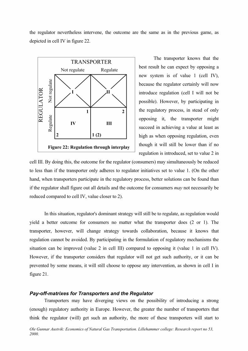
the regulator nevertheless intervene, the outcome are the same as in the previous game, as

depicted in cell IV in figure 22.

The transporter knows that the

best result he can expect by opposing a

new system is of value 1 (cell IV),

because the regulator certainly will now

introduce regulation (cell I will not be

possible). However, by participating in

the regulatory process, in stead of only

opposing it, the transporter might

succeed in achieving a value at least as

high as when opposing regulation, even

though it will still be lower than if no

regulation is introduced, set to value 2 in

cell III. By doing this, the outcome for the regulator (consumers) may simultaneously be reduced

to less than if the transporter only adheres to regulator initiatives set to value 1. (On the other

hand, when transporters participate in the regulatory process, better solutions can be found than

if the regulator shall figure out all details and the outcome for consumers may not necessarily be

reduced compared to cell IV, value closer to 2).

Figure 22: Regulation through interplay

TRANSPORTERNot regulate Regulate

Not

r eg u

late

Reg

ula t

e

REG

ULA

TOR

1

2

IV

2

1 (2)

III

II I

In this situation, regulator's dominant strategy will still be to regulate, as regulation would

yield a better outcome for consumers no matter what the transporter does (2 or 1). The

transporter, however, will change strategy towards collaboration, because it knows that

regulation cannot be avoided. By participating in the formulation of regulatory mechanisms the

situation can be improved (value 2 in cell III) compared to opposing it (value 1 in cell IV).

However, if the transporter considers that regulator will not get such authority, or it can be

prevented by some means, it will still choose to oppose any intervention, as shown in cell I in

figure 21.

Pay-off-matrixes for Transporters and the Regulator Transporters may have diverging views on the possibility of introducing a strong

(enough) regulatory authority in Europe. However, the greater the number of transporters that

think the regulator (will) get such an authority, the more of these transporters will start to


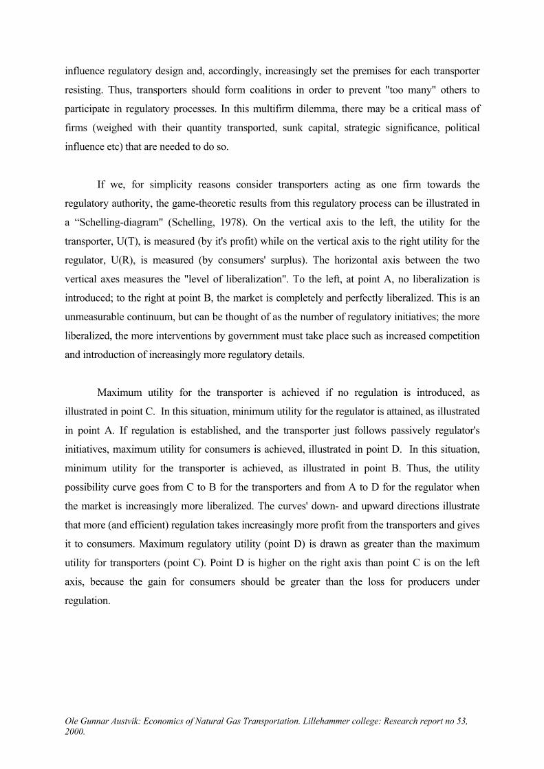
influence regulatory design and, accordingly, increasingly set the premises for each transporter

resisting. Thus, transporters should form coalitions in order to prevent "too many" others to

participate in regulatory processes. In this multifirm dilemma, there may be a critical mass of

firms (weighed with their quantity transported, sunk capital, strategic significance, political

influence etc) that are needed to do so.

If we, for simplicity reasons consider transporters acting as one firm towards the

regulatory authority, the game-theoretic results from this regulatory process can be illustrated in

a “Schelling-diagram" (Schelling, 1978). On the vertical axis to the left, the utility for the

transporter, U(T), is measured (by it's profit) while on the vertical axis to the right utility for the

regulator, U(R), is measured (by consumers' surplus). The horizontal axis between the two

vertical axes measures the "level of liberalization". To the left, at point A, no liberalization is

introduced; to the right at point B, the market is completely and perfectly liberalized. This is an

unmeasurable continuum, but can be thought of as the number of regulatory initiatives; the more

liberalized, the more interventions by government must take place such as increased competition

and introduction of increasingly more regulatory details.

Maximum utility for the transporter is achieved if no regulation is introduced, as

illustrated in point C. In this situation, minimum utility for the regulator is attained, as illustrated

in point A. If regulation is established, and the transporter just follows passively regulator's

initiatives, maximum utility for consumers is achieved, illustrated in point D. In this situation,

minimum utility for the transporter is achieved, as illustrated in point B. Thus, the utility

possibility curve goes from C to B for the transporters and from A to D for the regulator when

the market is increasingly more liberalized. The curves' down- and upward directions illustrate

that more (and efficient) regulation takes increasingly more profit from the transporters and gives

it to consumers. Maximum regulatory utility (point D) is drawn as greater than the maximum

utility for transporters (point C). Point D is higher on the right axis than point C is on the left

axis, because the gain for consumers should be greater than the loss for producers under

regulation.


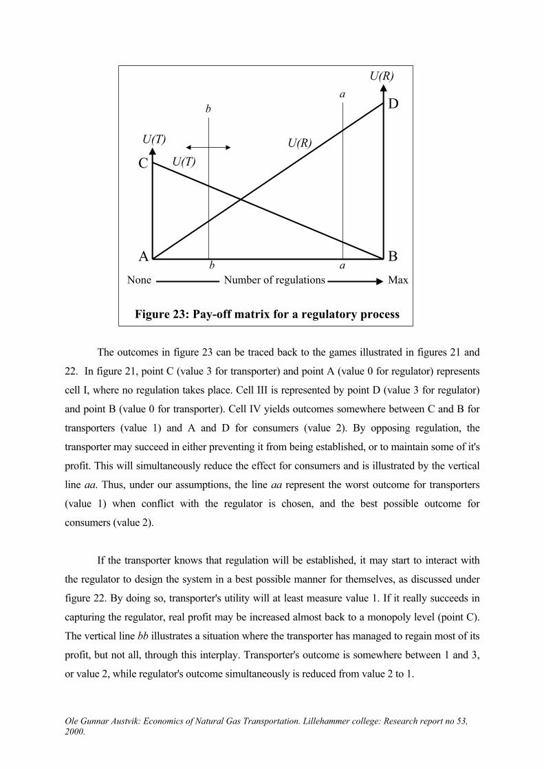
b

Figure 23: Pay-off matrix for a regulatory process

U(R)

U(R)U(T)

U(T)

a

b aA B

C

D

None Number of regulations Max

The outcomes in figure 23 can be traced back to the games illustrated in figures 21 and

22. In figure 21, point C (value 3 for transporter) and point A (value 0 for regulator) represents

cell I, where no regulation takes place. Cell III is represented by point D (value 3 for regulator)

and point B (value 0 for transporter). Cell IV yields outcomes somewhere between C and B for

transporters (value 1) and A and D for consumers (value 2). By opposing regulation, the

transporter may succeed in either preventing it from being established, or to maintain some of it's

profit. This will simultaneously reduce the effect for consumers and is illustrated by the vertical

line aa. Thus, under our assumptions, the line aa represent the worst outcome for transporters

(value 1) when conflict with the regulator is chosen, and the best possible outcome for

consumers (value 2).

If the transporter knows that regulation will be established, it may start to interact with

the regulator to design the system in a best possible manner for themselves, as discussed under

figure 22. By doing so, transporter's utility will at least measure value 1. If it really succeeds in

capturing the regulator, real profit may be increased almost back to a monopoly level (point C).

The vertical line bb illustrates a situation where the transporter has managed to regain most of its

profit, but not all, through this interplay. Transporter's outcome is somewhere between 1 and 3,

or value 2, while regulator's outcome simultaneously is reduced from value 2 to 1.


However, if the transporters could influence regulation in a way that improves efficiency

as compared to a situation with no interplay with the regulator, there may be Pareto

improvements in the process. This may happen because regulator's insight into the industry's

complexity may be limited and partly be depending on transporter's information. Such examples

can be found in the U.S. regulatory history, where regulator has made inadequate decisions for

the industry with huge losses in efficiency and resulting stop-and-go-policies. In this case, the

utility curve for the transporter will not be a straight line. In figure 24, U(T) is dropping when

some regulation is introduced. When the transporter starts to interact with the regulator in the

formulation of new governmental interventions, with a number of market interventions from the

regulator it manages to maintain its profit without reducing the benefit for the

regulator/consumers.

Figure 24: Pay-off matrix if the pipeline can improve regulatory efficiency

U(R)

U(R)U(T)

U(T)

c

cA B

None Number of regulations Max

C

D

E

This is due to the fact that it can suggest arrangements that are more efficient than the

regulator could do itself. Overall surplus in the market is increased compared to the more static

first strategy. At some level of liberalization, illustrated by the line cc, transporters may start to

suffer again, regulatory interventions are so comprehensive that transporter's utility curve drops

more steeply down to point B. The transporter would loose so much by passing cc, that it starts

to oppose regulation again. In this situation, it is possible that the best point for the regulator

could never be reached, because he lacks the ability to liberalize the market perfectly in an


efficient manner and, thus, needs the collaboration from the transporter. By trying to move the

transporter all the way to point B, the outcome for consumers may be worse than if stopped at cc.

Thus, utility for regulator may drop if more regulation is introduced.

The two ways the utility curves are drawn are just examples on their many possible natures. They may be bowed in various ways or even be discrete. The most important information we can get about transporter strategy from this analysis, independent of the shape of the curves, is that it depends heavily on whether a regulatory authority gets the power and have ability to liberalize the market or not. The transporters should adopt a dual strategy opposing any initiatives taken by authorities on market intervention and simultaneously prepare for interplay in designing optimal regulatory regimes, if or when they come. Transporters will be best served if they succeed in delaying or destroying political decisions giving such power to regulatory authorities, pointing out the complexity of regulations, security issues, risk or any other arguments that work. But when or if a decision about actual regulation is made, nevertheless, transporters should shift partly to a collaborative strategy. The regulator should try to penetrate a possible collaboration between transporters by starting to design regulatory regimes with only one or a few of them. If a critical mass of transporters interact, the rest must follow, as well.

In the dynamics of this decision making process, the strategies may shift from conflict to

elements of cooperation, and back. When and how the parties should or would collaborate and

when they confront each other, depends on the shape of the curves. The shape depends on

market complexity, competence among each party, ability to intervene etc. If one accepts that it

is difficult to reach a fully and perfectly liberalized market, one should rather discuss what would

be the optimal degree and form for regulation, not only in the sense of economic efficiency, but

also in terms of political feasibility (cc)

Of course, the highly stylized description of a completely liberalized market and possible

intermediates misses a lot of other information that may be important. Nevertheless, it is

interesting to identify segments where competition may be introduced and in which segments

regulation is necessary in order to assess liberalization. This also identifies why and where

economic rent is collected in today's gas market. This may be of interest for each party in the

market if liberalization actually should take place. Firms may have an interest in liberalization, if

they can be assured that it is confined to those areas that serve their interests. Ceteris paribus,

transporters may be interested in more competition among producers and customers, producers

may be interested in lower tariffs to transporters, LDCs may be interested in more competition

among producers and free access and low tariffs to transporters and so on.


5. Alternatives to Regulation

Public Ownership / Changing Property Rights An unregulated transmission company is behaving monopolistically because its owner

has an interest in maximizing profit. By changing it's property rights, the new owners may have

other goals. If the owner has, for example, overall efficiency in society, or maximum profit in the

distribution or production sector, as a goal, profit maximum in the pipeline may not be in the

owners' interest.

One way to change property rights is to socialize the firm by changing its ownership

from private to public. In Europe, this has, until recently, been a quite usual way of approaching

the problem for a wide range of branches, such as coal, electricity, railroads, post,

telecommunication, defense industries, steel, shipbuilding, buses, airports, water and gas. The

idea has been that the problems of monopoly power, externalities, inequality etc. can be dealt

with directly if they are run with social welfare as goal rather than private profit.

Nationalization has been argued for both on ideological grounds and because of the

market failures natural monopolies create. In Europe, labor parties have mostly favored

nationalization, advocating that ownership of means of production; distribution and exchange

should be common. The early advocates of nationalization in the 1930s and 1940s hoped that the

old class antagonism between workers and owners of businesses should be broken down.

Nationalization should be one means of rectifying the injustice in income distribution between

consumers and producers and across classes, when huge firms exploit their monopoly power.

However, there has been considerable debate through the twentieth century on how much of a

nation's industry should be under public ownership and how much should be managed trough

market mechanisms (as the “Austrian school”). As we have discussed, “untouched" natural

monopolies often do create inefficiencies in markets, restrain economic growth and lead to an

unfair distribution of rent, between producers and consumers and throughout the gas chain. The

question arises whether nationalization is superior to regulation or whether some other means

should be used to repair for the deficiencies.

One major argument for the privatization of publicly owned enterprises over the past 20

years, has been their relatively poor economic performance. Obviously, that these run a deficit,

and not a profit, is a non-valid argument. The nationalized industry should in many cases run a


loss if prices are set equal to marginal costs and average costs are falling, as discussed for

example in figure 8). Therefore, the assessment of nationalized industries should rather be done

on the basis of its costs and quality of service than on it's profit. Because such comparisons are

rather difficult17, especially for natural monopolies without competitors, it will not be possible to

observe such differences with certainty before they become rather significant.

Another argument in favor of privatization has been that private firms will be more

exposed to market forces than the publicly owned own one. Privatization should improve

efficiency, reduce costs, and improve quality and lead to greater responsiveness to the wishes of

the consumer. However, if a national firm is privatized in a non-competitive market or some

other regulatory mechanism are introduced, a private monopolist should not have much more

reason to behave more efficiently than the public one.18 Thus, in most such cases, privatization

must be followed by some sort of regulation should efficiency be improved. Ownership may be

only one determinant for the efficiency in an industry, while the degree of competition is another.

Also public enterprises can be more efficient if they face competition.

Whether publicly or privately owned and run, transporters in the (non-competitive)

European gas market must be followed closely by public authorities, which under whatever

approach will need independent competence and will to take a stand to the number of issues that

arises. The nationalized industry may lax efforts to improve if government always is ready to

increase subsidies when they run larger deficits. A private industry can do the same if regulations

are not followed in an optimal manner. Tough hands are often needed both on the amount and

the way subsidies are given and how regulations are enforced, including incentive-type

regulations. Thus, the government's attitude, competence and political standing may in many

situations be as important as the principles that it adheres to.

Market Forces versus Regulation Competitive markets should ensure entry of new firms on equal terms as the incumbent

firm. Firms should have costless exit; if a firm wants to leave business it could sell all it's capital

minus depreciation costs. The latter is rarely the case in the gas industry. For example, the ex

17 See for example Meyer(1975).

18 The main exception is perhaps that the private firm would not have to frequently adjust their targets for political reasons.


ante opportunity cost of an investment minus the investment's value ex post are considerable in

pipelines (the "sunk" costs). Usually the pipes laid cannot be sold for any other purposes than for

transportation of gas if a company should terminate operations.

With large sunk costs and economies of scale it is sometimes impossible to build another

pipeline. If, nevertheless, another company should make the required investments, i.e. in an

alternative pipeline, the outcome is uncertain. If demand is constant and the incumbent firm

operates as a strong natural monopoly (average cost are downward sloping over the entire range

of outputs) it would be no way a new firm could take a share of the market and produce at a

lower cost. However, if the incumbent firm operates as a weak natural monopoly (where

diseconomies has occurred at some range, but not sufficiently to make the industry a natural

duopoly), prices could be forced down, and the new-comer, possibly both, will loose money.

Thus, competition may be impossible or, if more pipelines enter the market, be destructive for

both the old line and the newcomer.

The idea of regulating transporters’ terms of operations is that if the market itself does not

produce optimal outcomes, then it can be mimicked to do so through regulatory and other public

instruments. However, no single theory of regulation and regulatory behavior seems fully to

explain the behavior of regulated firms or lead to first-best outcomes. For this, the issue is far

more complex than the partial and highly stylized models we have studied. The alternative

theories are not mutually exclusive and may be used in combination. Cost curves may change

over time as do demand. The regulatory instruments may include price regulation, profit

constraints and subsidies. As long as regulators shall 'repair' misallocation of resources with such

a wide range of instruments, the system may easily end up with outcomes that are either

overdetermined or have too many degrees of freedom to yield desired results. In a market for a

strategic and non-renewable commodity as natural gas is, regulatory authorities will easily

remain an arena of politically oriented interest groups in conjunction with market mechanisms

and firms operating more or less under competition, within and across borders. To avoid the

problems faced by the U.S. gas industry, which repeatedly has changed the way of intervening in

the market place(s) over the century, policy makers should by humble towards the task and take

an approach that accept some inefficiencies in the market in order to avoid the creation of new

(and perhaps more serious) ones.


From the outset, the non-competitive structure of the European gas industry indicates that

today some parties have more power than others do in contract negotiations. The investment

risks and economies of scope in vertical integration between many of these parties lead to an ex

post situation, which is relatively inflexible in face of altering market conditions. On the other

hand, the bundling of services, directly or through long-term contracts, provides assurances for

the companies involved to sunk investment in production, storage, pipelines and LDCs. If

unbundling should take place, the access to transportation under terms that is not incurring

losses, require a dynamic attitude from the regulator. The arrangements done should include a

variety that suites each actor and segment of the market. These arrangements should be permitted

to evolve gradually based upon market trends rather than radical change. In doing this, policy

makers must evaluate the development of market demand in each segment of the market,

horizontally and vertically, and how firms will respond to these changes.

Literature Andersen, Svein & Austvik, Ole Gunnar, 2000: Nasjonal handlefrihet - nye internasjonale rammebetingelser: Petroleum, makt og demokrati, Forprosjekt til Makt- og demokratiutredningen 1998-2003. Unipub forlag. August. Austvik, Ole Gunnar, 1984: "Tariffer for rørtransport av naturgass", Statistisk Sentralbyrå August 1984. 37 pages. ---, 1987: "Political Gas Pricing Premiums: The Development in West Germany 1977-1985", OPEC Review no. 2 June 1987. ISSN no. 0277-0180. --- , 1991: "Norwegian Energy Policy in an International Context; The U.S. Embargo of Soviet Gas in 1982" in O.G. Austvik: Norwegian Gas in the New Europe; How Politics Shape Markets. NUPI / Vett & Viten. ISBN 82-412-0064-1. ---, 1997: "Gas pricing in a Liberalized European market; Will the rent be taxed away?", EnergyPolicy vol 20/no.12 pp. 997-1012, London, Elsevier Science. ISSN 0301 4215. ---, 1999: ”Norges avhengighet av olje- og gassmarkedene”. Internasjonal Politikk nr. 3. . 0020-577X ---, 2000: "Norge som storeksportør av gass", forskningsrapport under "Norge i energiens geopolitikk". Europaprogrammet september 2000. ISSN 0804-3485. ca. 100 sider. Averch, H. & Johnson, L., 1962: "Behavior of the Firm Under Regulatory Constraint", American Economic Review, vol 52, No 3, page 1053-1069. Baumol, W., and Bradford, D., 1970: "Optimal Departures from Marginal Cost Pricing", American Economic Review, Vol. 60, No.3, page 265-283. Berg S.V. & Tschirhart J., 1989: Natural monopoly regulation. Principles and practice, Cambridge University Press, Cambridge


Binmore, Kent, 1992: Fun and Games. A Text on Game Theory, Heath & Company Broadman, Harry , 1986: "Elements of Market Power in the Natural Gas Industry", The Energy Journal, vol. 7, no. 1 --, 1987: "Deregulating entry and access to pipelines" page 125-150 in Kalt J.P. & Schuller F.C. (ed.), 1987:Drawing the Line on Natural Gas Regulation. The Harvard Study on the future of Natural Gas, Quorum Books, Energy and Environmental Policy Center, Kennedy School, Harvard University Coase, R., 1946: "The Marginal Cost Controversy", Economica, Vol.13, page 169-189. European Union (EU), 1988: The Internal Energy Market, "Commission Working Document", May. ---, 1998: The Single Market for Natural Gas, IGM Directive 98/30 (the ”Gas Directive"). Gerwig, Robert W., 1962: "Natural Gas Production: A Study on Costs of Regulation", Journal of Law and Economics, October, vol page 69-92 Hogan, W.W., 1987: "The Boundaries between competition and regulation" page xx-xx in Kalt J.P. & Schuller F.C. (ed.), 1987: Drawing the Line on Natural Gas Regulation. The Harvard Study on the future of Natural Gas, Quorum Books, Energy and Environmental Policy Center, Kennedy School, Harvard University. ---, February 1989: Firm Natural Gas Transportation: A Capacity Priority Allocation Model. Prepared for Pacific Gas & Electric Company. Putnam, Hayes & Bartlett, Inc. International Energy Agency, IEA, 1994: Natural Gas Transportation; Organisation and Regulation, IEA/OECD Paris. Kalt, J.,1988, The Redesign of Rate Structures and Capacity Auctioning in the Natural Gas Pipeline Industry, EEPC Discussion Paper, John F. Kennedy School of Government, Harvard University. Kalt J.P. & Schuller F.C. (ed.), 1987: Drawing the Line on Natural Gas Regulation. The Harvard Study on the future of Natural Gas, Quorum Books, Energy and Environmental Policy Center, Kennedy School, Harvard University Laffont J.J. & Tirole J., 1993: A Theory of Incentives in Procurement and Regulation, MIT Press, Cambridge Loeb, M., and Magat, W., 1979: "A Decentralized Method for Utility Regulation", Journal of Law and Economics, Vol. 22, page 399-404. Marbro, Robert & Wybrew Bond, Ian, 1999: Gas to Europe: The Strategies of Four Major Suppliers, Oxford Univresity Press. Meyer, R.A., 1975: Publicly Owned versus Privately Owned Utilities: A Policy Choice", Review of Economics and Statistics, Vol.57, page 391-399. Nese, Gjermund og Kåre P. Hagen, 1998: Pricing of Natural Gas Transportation, SNF-rapport no. 64/98, Stiftelsen for samfunns- og næringslivsforskning Ramsey, F., 1927: "A Contribution to the Theory of Taxation", Economic Journal, Vol.37, No.1, page 47-61. Riordan, M., 1984: "On Delegating Price Authority to a Regulated Firm", Rand Journal of Economics, Vol.15, No.1, page 108-115. Sappington, D. and Sibley, D., 1988: "Regulating without Cost Information: The Incremental Surplus Subsidy Scheme", International Economic Review, Vol 29, No.2, page 297-306. Schelling, Thomas, 1978: Micromotives and Macrobehavior. W.W. Norton. ---, 1984: Choice and Consequence, Harvard University Press



Sharkey, W.W., 1989: The Theory of Natural Monopoly, Cambridge University Press, Cambridge Stiegler, G. J., 1971: "The Theory of Economic Regulation", Bell Journal of Economics, vol 2, page 3-21 Teece, David J., 1990: "Structure and organization of the natural gas industry: Differences between the United States and the Federal Republic of Germany and implications for the carrier status of pipelines", The Energy Journal, vol 11. no.3. Tirole, J., 1992: The Theory of Industrial Organization, MIT Press, Cambridge Train, K., 1991: Optimal Regulation. The Economic Theory of Natural Monopoly, MIT Press, Cambridge Vogelsang, I., and Finsinger, J., 1979: "A Regulatory Adjustment Process for Optimal Pricing by Multiproduct Monopoly Firms", Bells Journal of Economics, Vol. 10, No.1, Page 157-171.

Ole Gunnar Austvik Economics of Natural Gas Transportation ...

Documents

Transcript of Ole Gunnar Austvik Economics of Natural Gas Transportation ...