LANDSLIDES OWN

Special Report 176

TRANSPORTATION RESEARCH BOARD NATIONAL ACADEMY OF SCIENCES

LAN-DSLIDES . Anadysis .and Control Special Report 176

Robert L. Schuster Raymond I. Krizek editors

Transportation Research Board

Commission on Sociotechnical Systems

National Research Council

NATIONAL ACADEMY OF SCIENCES Washington, D.C. 1978

Transportation Research Board Special Report 176 Edited for TRB by Mildred Clark Price: paper cover $12.00; hard cover $14.00

Additional copies of Figure 2.1 (in pocket in back of book) are available for $2.00 each. Please send payment with order.

modes 1 highway transportation 3 rail transportation

subject area 63 mechanics (earth mass)

Transportation Research Board publications are available by order-ing directly from the board. They may also be obtained on a regular basis through organizational or individual supporting membership in the board; members or library subscribers are eligible for substantial discounts. For further information, write to the Transportation Re-search Board, National Academy of Sciences, 2101 Constitution Avenue, N.W., Washington, D.C. 20418.

Notice The project that is the subject of this report was approved by the Governing Board of the National Research Council, whose members are drawn from the councils of the National Academy of Sciences, the National Academy of Engineering, and the Institute of Medicine. The members of the committee responsible for the report were cho-sen for their special competence and with regard for appropriate balance.

This report has been reviewed by a group other than the authors according to procedures approved by a Report Review Committee consisting of members of the National Academy of Sciences, the National Academy of Engineering, and the Institute of Medicine.

The views expressed in this report are those of the authors and do not necessarily reflect the view of the committee, the Transportation Research Board, the National Academy of Sciences, or the sponsors of the project.

Library of Congress Cataloging in Publication Data National Research Council. Transportation Research Board.

Landslides, analysis and control.

(Special report - Transportation Research Board, National Re-search Council; 176)

Includes bibliographies and index. 1. Slopes (Soil mechanics) 2. Landslides. I. Schuster, Robert

L. II. Krizek, Raymond J. III. Title. IV. Series: National Re-search Council. Transportation Research Board. Special report - Transportation Research Board, National Research Council; 176. TA71O.N32 1978 624'.151 78-27034 ISBN 0-309-02804-3

© 1978 by the National Academy of Sciences. All rights, including that of translation into other languages, are reserved. Photomechan-ical reproduction (photocopy, microcopy) of this book or parts thereof without special permission of the publisher is prohibited.

This work may be reproduced in whole or in part for official use of the U.S. government.

Sponsorship of the Papers in This Special Report

DIVISION A—REGULAR TECHNICAL ACTIVITIES Kurt W. Bauer, Southeastern Wisconsin Regional Planning Coin-

mission, chairman

GROUP 2—DESIGN AND CONSTRUCTION OF TRANSPORTA-TION FACILITIES Eldon J. Yoder, Purdue University, chairman

Task Force on Review of Special Report 29—Landslides Robert L. Schuster, U.S. Geological Survey, Denver, chairman David S. Gedney, Federal Highway Administration Raymond J. Krizek, Northwestern University David L. Royster, Tennessee Department of Transportation Dwight A. San.grey, Cornell University William G. Weber, Jr., Washington Department of Transportation,

Yakima Tien H. Wu, Ohio State University

John W. Guinnee, Transportation Research Board staff

Contents

Chapter]: Robert L. Schuster INTRODUCTION

Scope of This Volume, 1 Definitions and Restrictions, 2 Economics of Slope Movements, 2 Legal Aspects of Slope Movements, 6

Landslides and Transportation Routes, 6 Landslides and Property Development, 8

Acknowledgments, 9 References, 9

Chapter 2: David J. Varnes SLOPE MOVEMENT TYPES AND PROCESSES

Terms Relating to Movement, 12 Kinds of Movement, 12 Sequence or Repetition of Movement, 23 Rate of Movement, 24

Terms Relating to Material, 24 Principal Divisions, 24 Water Content, 24 Texture, Structure, and Special Properties, 24

Terms Relating to Size or Geometry, 25 Terms Relating to Geologic, Geomorphic, Geographic,

or Climatic Setting, 25 Terms Relating to Age or State of Activity, 26 Forming Names, 26 Causes of Sliding Slope Movements, 26

Factors That Contribute to Increased Shear Stress, 26 Factors That Contribute to Low or Reduced Shear

Strength; 27 References, 28 Bibliographies, 33

Chapter 3: Harold T. Rib and Ta Liang RECOGNITION AND IDENTIFICATION

Terrain Evaluation for Landslide Investigations, 34 Basic Factors, 34

Regional Approach to Landslide Investigations, 36 Landforms Susceptible to Landslides, 36 Vulnerable Locations, 37 Procedure for Preliminary Investigations of

Landslides, 41 Map Techniques for Landslide Detection, 43

Topographic Maps, 43 Geologic Maps and Reports, 44 Agricultural Soil Survey Reports, 47 Special Maps and Reports, 47

Remote-Sensing Techniques for Landslide Detection, 48 Use of Aerial Photography, 48 Use of Other Remote-Sensing Systems, 66

Field Reconnaissance Techniques, 69 Field Evidence of Movement, 71 Field Identification of Slope-Movement Types, 72

Conclusions, 78 References, 79

Chapter 4: George F. Sowers and David L. Royster FIELD INVESTIGATION

Scope of Field Investigations, 81 Topography, 82 Geology, 82 Water, 83 Physical Properties, 83 Ecological Factors, 83

Planning Investigations, 84 Area of Investigation, 84 Time Span, 84 Stages of Investigation, 84

Site Topography, 85 Aerial Survey, 85 Ground Surveys, 86 Representation of Topographic Data, 89 Profiles, 90 Displacement Vectors and Trajectories, 90

Iff

Subsurface Exploration, 91 Geologic Reconnaissance, 91 Boring, Sampling, and Logging, 94 Test Pits and Trenches, 95 Geophysical Studies, 95 Correlation Representation, 98

Surface Water and Groundwater, 99 Importance of Water, 99 Surface Water, 100 Groundwater, 100 Groundwater Observations, 101 Permeability, 102 Springs and Seeps, 102 Correlation, 102

Environmental Factors, 103 Weather, 103 Human Changes Before Construction, 103 Changes Brought by Construction, 104 Effect of Ecosystem on Sliding, 104 Effect of Sliding on Ecosystem, 104

Field Testing, 105 Borehole Tests, 105 Large-Scale Pit Tests, 108 Borehole Dynamics, 109 Geophysical Tests, 109

Correlation of Data, 110 Areal Variations, 1.10 Cross Sections, 110 Time-Based Observations and Correlations, 110

Conclusions, 110 References, 111

Chapter 5: Stanley D. Wilson and P. Erik Mikkelsen FIELD INSTRUMENTATION

Instrumentation Planning, 112 Types of Measurements Required, 113 Selection of Instrument Types, 113

Surface Surveying, 113 Conventional Surveying, 113 Other Types of Surface Surveying, 117 Crack Gauges, 118 Tiltmeters, 118

Inclinometers, 118 Inclinometer Sensors, 121 Casing Installation, 122 In-Place Inclinometers, 124

Extensometers and Strain Meters, 124 Pore-Pressure and Groundwater Measurements, 125

Observation Well, 125 Piezometers, 125 Piezometer Sealing, 127 •.

Systems for Monitoring Rock Noise, 128 Sensors, 128 Sign al-Con ditioning Equipment, 128 Recording and Data-Acquisition Equipment, 129

Automatic Warning and Alarm Systems, 129 Data Acquisition and Evaluation, 129

Data-Acquisition Methods, 129 Inclinometer Observations, 130 Inclinometer Data Reduction, 131 Evaluation and Interpretation, 132

Examples, 133.

Minneapolis Freeway, 133 Potrero Tunnel Movements, 134 Seattle Freeway, 134 Fort Benton Slide, 135

References, 137

Chapter 6: Tien H. Wu and Dwight A. Sangrey STRENGTH PROPERTIES AND THEIR MEASUREMENT

General Principles, 139 Mohr-Coulomb Failure Criterion, 139 Effective Stress Versus Total Stress Analysis, 139 Common States of Stress and Stress Change, 140 Stress-Strain Characteristics, 140 Effect of Rate of Loading, 140

Laboratory Measurement of Shear Strength, 141 Simple Tests, 141 Triaxial Test, 141 Plane-Strain Test, 143 Direct Shear' Test, 143 Simple Shear Test, 143

Shear Strength Properties of Some Common Soils, 144 Cohesionless Soils, 144

- Soft Saturated Clays and Clayey Silts, 144 Heavily Overconsolidated Clays, 145 Sensitive Soils, 148 'Partially Saturated Soils, 149 Residual Soil and Colluvium, 149 Rocks, 150

Soil Behavior Under Repeated Loads, 151 Repeated Load Tests, 151 Stress-Strain Characteristics, 15 1 Failure Under Repeated Loading, 152

References, 152

Chapter 7: N. R. Morgenstern and Dwight A. 'Sangrey METHODS OF STABILITY ANALYSIS

Roles of Limit Equilibrium and Deformation Analyses, 155

Limit Equilibrium Analysis;i 56 Total and Effective Stress Analyses, 157 Total Stress Analysis of Soil Slopes (0 = 0), 157 Effective Stress Analysis of Soil Slopes, 160 Pore-Pressure Distribution, 165 Analysis of Rock Slopes, 165

Deformation Analysis, 168 References, 169

Chapter 8: David S. .Gedney and William G. Weber, Jr. DESIGN AND CONSTRUCTION OF SOIL SLOPES

Philosophy of Design, 172 Safety Factor, 172 Design Procedures, 173

Avoid Problem, 173 Reduce Driving Forces, 175 Increase Resisting Forces, 183

Toe Erosion, 190 References, 190

iv

Chapter 9: Douglas R. Piteau and F. Lionel Peckover Determination of Structural Domains and Design ENGINEERING OF ROCK SLOPES Sectors, 198

Significant Factors in Design of Rock Slopes, 193 Development of a Rock Mass Model Depicting Structural Discontinuities, 193 Geologic Structure, 198 Groundwater, 194 Determination of Kinematically Possible Failure Lithology, Weathering, and Alteration, 194 Modes and Performance of Slope-Stability Climatic Conditions, 195 Analysis, 199 Slope Geometry in Plan and Section, 196 Slope Design and Remedial Measures, 201 Time Factor and Progressive Failure, 196 Planning and RelatedProcedures, 201 Residual and Induced Stress, 196 Methods of Stabilization, 205 Existing Natural and Excavated Slopes, 197 Methods of Protection, 218

Dynamic Forces, 197 Methods of Warning, 223 Fundamental Procedures in Analysis of Rock Slopes, 197 References, 225

Determination of Structural and Other Relevant Geologic Characteristics, 197 INDEX, 229

v

The'Ed.itors. and Authors

David S. Gedney. Acting director, Northeast Corridor Project, Federal Railroad Administration. Formerly chief, Construction and Maintenance Division, Federal Highway Administration; regional engineer, Region 15, Federal Highway Administration; and chief, Soil and Rock Me-chanics Branch, Construction and Maintenance Division, Federal Highway Administration. His field of specializa-tion is geotechnical engineering as applied to transporta-tion problems.

Raymond J. Krizek. Professor of civil engineering, North-western University, Evanston, Illinois. Formerly faculty member at the University of Maryland and lecturer at the Catholic University of America. He is a specialist in soil mechanics and foundation engineering and has a variety of teaching, research, and professional engineering experience.

Ta Liang. Professor of civil and environmental engineering and director, Remote Sensing Program, Cornell University, Ithaca, New York. He has long been engaged in teaching and research in the fields of aerial photograph interpreta-tion, remote sensing, and geotechnical and geological en-gineering and has been a consultant to industrial, national, and international organizations on engineering and economic development projects in many parts of the world.

P. Erik Mikkelsen. Senior associate engineer, Shannon and Wilson, Inc., Seattle. During his 15 years of geotechnical engineering experience, he has become an expert in instru-mentation used in landslides, embankments, deep excava-tions, and deep foundations.

N. R. Morgenstem. Professor of civil engineering, University of Alberta, Edmonton. He has been a consultant in geo-technical engineering and applied earth sciences since 1961 His area of professional specialization is geotechnical engi-neering; he has made noteworthy contributions on the sub-

jects of landslides, rock mechanics, soil-structure interac-tion, and soil engineering problems in cold regions.

F. Lionel Peckover. Geotechnical consultant, Vaudreuil, Quebec.. Formerly in charge of geotechnical engineering work with Canadian National Railways (1959-1976), Cana-than St. Lawrence Seaway Authority (1953.1959), and Di-vision of Building. Research, National Research Council of Canada (1947-1953). His field of specialization is geotech-nical engineering with emphasis on railway application, particularly the treatment of unstable rock slopes.

Douglas R. Piteau. President, Piteau and Associates, Van-couver, British Columbia.. He has extensive experience in engineering geology and rock mechanics related to railways and highways, mine development and operations, and site evaluation ofdams and tunnels.

Harold T. Rib. Chief, Aerial Surveys Branch, Federal High-way Administration. Formerly chief, Exploratory Tech-niques Group, and highway research engineer, Federal Highway Administration. His field of specialization is ap-plication of remote-sensing techniques to transportation. engineering and terrain analysis.

David L. Royster. Chief, Soils and Geological Engineering Division, Tennessee Department of Transportation, Nash-ville. He has held various positions with Tennessee Depart-ment of Transportation since 1958. His field of specializa-tion is engineering geology as applied to highway design and construction.

Dwight A. Sangrey. Professor of civil and environmental engineering, Cornell University, Ithaca, New York. In ad-dition to teaching and research at Cornell, he has been ac-tive in practice and as a consultant on projects involving instability of slopes. Major areas of professional activity

vi

involve dynamic loading of soils, soil sensitivity, and marine geotechnical engineering.

Robert L. Schuster. Chief, Engineering Geology Branch, U.S. Geological Survey, Denver. Formerly professor and chairman, Department of Civil Engineering, University of Idaho, and associate professor and professor, Department of Civil Engineering, University of Colorado. Major areas of professional specialization are engineering geology and geotechnical engineering.

George F. Sowers. Senior geotechnical consultant and senior vice president, Law Engineering Testing Company, Marietta, Georgia, and regents professor of civil engineer-ing, Georgia Institute of Technology, Atlanta. He is a geo-technical engineer specializing in the interrelation of geol-ogy, engineering design, and construction and has been a worldwide consultant on earthfill dams, foundations, and earth and rock construction.

David J. Varnes. Geologist, Engineering Geology Branch, U.S. Geological Survey, Denver. He has had 37 years of experience as an engineering geologist with USGS, includ-ing being chief of the Engineering Geology Branch. Fields of specialization are slope stability in rock and soil and en-gineering geologic mapping.

William G. Weber, Jr. Washington Department of Trans-portation, Yakima. Formerly research engineer, Bureau of Materials, Pennsylvania Department of Transportation, and senior materials and research engineer, Materials and Research Department, California Division of Highways. He has expertise in geotechnical design of structures involving soft soils, groundwater flow, and stability of slopes.

Stanley D. Wilson. Consulting engineer. Seattle. Formerly executive vice president of Shannon and Wilson, Inc. His significant contributions in the development of field opera-tional equipment, his advocacy of its use in dams and other civil engineering projects, and his analyses of the results have led to better understanding of the mechanisms of land-slides and of the performance of embankments and dams.

Tien H. Wu. Professor of civil engineering, Ohio State Uni-versity, Columbus. Formerly professor, Department of Civil Engineering, Michigan State University, and visiting professor, Norwegian Geotechnical Institute and National University of Mexico. He has specialized in the relation of the engineering properties of soils to their mechanical behav-ior and has been a consultant on a variety of problems in soil mechanics and geotechnical engineering.

vi'

Chapter 1

Introdu, ction Robert L. Schuster

This book is a successor to Highway Research Board Special Report 29, Landslides and EngineeringPractice (1.8). Spe-cial Report 29, which was written by the Highway Research Board Committee on Landslide Investigations and published in 1958, achieved an excellent reputation, both in North America and abroad, as a text on landslides. Because of its popularity, the original printing was sold out within a few years after publication. Since then, there has been a con-tinuing interest in reissuing the original text or publishing a worthwhile successor.

In 1972 the Highway Research Board organized the Task Force for Review of Special Report 29—Landslides. The membership of this task force was selected from several committees within the HRB Soils and Geology Group: its charge was

To review the out-of-print Special Report 29—Landslides—and to recommend what action should be taken in response to the high interest in revising this publication.

This task force was further instructed to act as the coordi-nating unit to implement its recommendations.

After considerable study of the original report, the task force concluded that, because of the large amount of new technical information that had become available since 1958 on landslides and related engineering, the best course of ac-tion would be to completely rewrite the book rather than to reprint it or to revise it in part. The task force decided that the general format of the original volume would be re-tained but that the contents would be expanded to include concepts and methods not available in 1958. To achieve that objective, the task force secured the aid of authors who have broad geotechnical expertise. They were drawn from the fields of civil engineering and geology and have specializations in soil mechanics, engineering geology, and interpretation of aerial photographs.

SCOPE OF THIS VOLUME

The scope of this volume is the same as that for Special Report 29: to bring together in coherent form and from a wide range of experience such information as may be useful to those who must recognize, avoid, control, design for, or correct landslide movement.

This new version, however, introduces geologic concepts and engineering principles and techniques that have been developed since publication of Special Report 29 so that both the analysis and the control of soil and rock slopes are addressed. For example, included are new methods of stability analysis and the use of computer techniques in im-plementing these methods. In addition, rock-slope engineer-ing and the selection of shear-strength parameters for slope-stability analyses are two topics that were poorly under-stood in 1958 and therefore were given scant attention in Special Report 29. Since that time,these two subjects have received a significant amount of study and have become fairly well understood;thus, they are presented as separate chapters in the present volume.

The book is divided into two general parts. The first part deals principally with the definition and assessment of the landslide problem. It includes chapters on slope-movement types and processes, recognition and identification of land-slides, field investigations, instrumentation, and evaluation of strength properties. The second part of the book deals with solutions to the landslide problem. Chapters are in-cluded on methods of slope-stability analysis, design tech-niques, and remedial measures that can be applied to both soil and rock-slope problems.

Although considerable effort has been made to eliminate presentation of the same material in different chapters, some repetition has been necessary to provide continuity of thought and to allow adequate explanation of specific topics. We consider this repetition to be more acceptable than constant referral in the text to other chapters.

DEFINITIONS AND RESTRICTIONS

In Special Report 29 the term landslide is defined as the downward and outward movement of slope-forming ma-terials—natural rock, soils, artificial fills, or combinations of these materials. Today the term deserves further refine-ment because, as shown in Chapter 2, slope movements can now be divided into five groups: falls, topples, slides, spreads, and flows. As used in this text, a landslide con-stitutes the group of slope movements wherein shear fail-ure occurs along a specific surface or combination of sur-faces.

Although this volume deals primarily with slope failures belonging to the group designated as slides, some attention is given to the other four types of slope movements. The use of the term landslide in the title is somewhat inaccurate in that theoretically it does not cover the five basic failure modes described above; however, the decision was made to use this term because it is popular and easily recognized and because the book is mainly devoted to landslides.

In keeping with the practice followed in Special Report 29, surficial creep was excluded from consideration: how-ever, creep of a more deep-seated nature is considered in discussions dealing with slope movements. Also excluded are subsidence not occurring on slopes and most types of movement primarily due to freezing and thawing of water. In addition, snow and ice avalanches and mass wasting due to slope-failure phenomena in tropic and arctic climates are not considered. Although a few examples are drawn from other parts of the world, most of the descriptions of slope movements and engineering techniques involve slopes in North America.

Of the five groups of potential slope movements con-sidered, only slides are currently susceptible to quantitative stability analysis by use of the conventional sliding-wedge or circular-arc techniques. These methods of slope-stability analysis are not applicable to falls, topples, spreads, or flows. However, enough is now known about the kinematics and nature of development of such failures that qualitative or statistical approaches or both can be used to make rea-sonable assessments in problem areas or potential prob-1cm areas. Research dealing with such problems is cur-rently being undertaken to enable at least crude quantita-tive stability analyses to be performed on slopes subject to spreads and flows and possibly even to falls and top-ples.

Although slope-stability problems related to transpor-tation facilities are stressed, most of the examples apply equally well to all cases of slope failure, such as those re-lating to coastlines, mining, housing developments, and farmlands. As noted by Eckel in the Introduction in Spe-cial Report 29(1.7, p. 2):

The factors of geology, topography, and climate that inter-act to cause landslides are the same regardless of the use to which man puts a given piece of land. The methods for ex-amination of landslides are equally applicable to problems in all kinds of natural or human environ,nent. And the known methods for prevention or correction of land-slides are, within economic limits, independent of the use to which the land is put. It is hoped, therefore, that de-spite the narrow range of much of its exemplary material,

this volume will be found useful to any engineer whose practice leads him to deal with landslides.

ECONOMICS OF SLOPE MOVEMENTS

Although individual slope failures generally are not so spectacular or so costly as certain other natural catas-trophes such as earthquakes, major floods, and tornadoes, they are more widespread and the total financial loss due to slope failures probably is greater than that for any other

Figure 1.1. Damage to embankment on 1-75 in Campbell County, Tennessee, from a landslide that occurred April 1972.

Figure 1.2. Homes and Street damaged in October 1978 Laguna Beach, California, landslide.

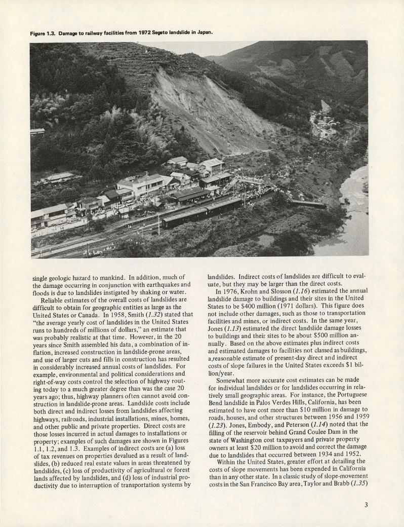
Figure 1.3. Damage to railway facilities from 1972 Segeto landslide in Japan.

single geologic hazard to mankind. In addition, much of the damage occurring in conjunction with earthquakes and floods is due to landslides instigated by shaking or water.

Reliable estimates of the overall costs of landslides are difficult to obtain for geographic entities as large as the United States or Canada. In 1958, Smith (1.32) stated that "the average yearly cost of landslides in the United States runs to hundreds of millions of dollars," an estimate that was probably realistic at that time. However, in the 20 years since Smith assembled his data, a combination of in-flation, increased construction in landslide-prone areas, and use of larger cuts and fills in construction has resulted in considerably increased annual costs of landslides. For example, environmental and political considerations and right-of-way costs control the selection of highway rout-ing today to a much greater degree than was the case 20 years ago; thus, highway planners often cannot avoid con-struction in landslide-prone areas. Landslide costs include both direct and indirect losses from landslides affecting highways, railroads, industrial installations, mines, homes, and other public and private properties. Direct costs are those losses incurred in actual damages to installations or property: examples of such damages are shown in Figures 1.1, 1 .2, and 1 3. Examples of indirect costs are (a) loss of tax revenues on properties devalued as a result of land-slides, (b) reduced real estate values in areas threatened by landslides, (c) loss of productivity of agricultural or forest lands affected by landslides, and (d) loss of industrial pro-ductivity due to interruption of transportation systems by

landslides. Indirect costs of landslides are difficult to eval-uate, but they may be larger than the direct costs.

In 1976, Krohn and Slosson (1.16) estimated the annual landslide damage to buildings and their sites in the United States to be S400 million (1971 dollars). This figure does not include other damages, such as those to transportation facilities and mines, or indirect costs. In the same year, Jones (1.13) estimated the direct landslide damage losses to buildings and their sites to be about S500 million an-nually. Based on the above estimates plus indirect costs and estimated damages to facilities not classed as buildings, a.reasonable estimate of present-day direct and indirect costs of slope failures in the United States exceeds $1 bil-lion/year.

Somewhat more accurate cost estimates can be made for individual landslides or for landslides occurring in rela-tively small geographic areas. For instance, the Portuguese Bend landslide in Palos Verdes Hills, California, has been estimated to have cost more than $10 million in damage to roads, houses, and other structures between 1956 and 1959 (1.23). Jones, Embody, and Peterson (1.14) noted that the filling of the reservoir behind Grand Coulee Dam in the state of Washington cost taxpayers and private property owners at least $20 million to avoid and correct the damage due to landslides that occurred between 1934 and 1952.

Within the United States, greater effort at detailing the costs of slope movements has been expended in California than in any other state. In a classic study of slope-movement costs in the San Francisco Bay area,Taylor and Brabb (1.35)

documented information on these costs for nine Bay-area counties during the winter of 1968-1969. The data were derived largely from interviews with planners and assessors in the county government and engineers and geologists in city, county, and state governments. Costs of slope move-ments totaled at least $25 million, of which about $9 mil-lion was direct loss or damage to private property (due mainly to drop in market value); $10 million was direct loss or damage to public property (chiefly for repair or re-location of roads and utilities); and about $6 million con-sisted of miscellaneous costs that could not be easily clas-sified in either the public or the private sector. This is a tremendous expense for the relatively small area involved. In addition, Taylor and Brabb noted that their data are in-complete in that they were not able to obtain costs on many of the slope movements. They felt, therefore, that the total cost of the 1968-1969 slope movements for the San Francisco Bay area may possibly have been several times greater than the estimated $25 million.

A survey conducted by the Federal Highway Administra-tion indicates that approximately $50 million is spent annually to repair major landslides on the federally financed portion of the national highway system (1.3, 1.4). This system in-cludes federal and state highways but does not include most county and city roads or streets, private roads and streets, or roads built by other governmental agencies such as the U.S. Forest Service. Distribution of the direct costs of major landslides for 1973 by Federal Highway Adthinistration re-gions within the United States is shown in Figure 1.4 (1.3). The cost for an individual region is based on both the land-slide risk and the amount of highway construction in the area. In addition, the given costs represent a single year; the average annual cost for a particular region could vary significantly from the given cost.

Total annual costs of landslides to highways in the United States are difficult to determine precisely because of the difficulty in defining the following factors: (a) costs of smaller slides that are routinely handled by main-tenance forces; (b) costs of slides on non-federal-aid routes; and (c) indirect costs that are related to landslide damage, such as traffic disruption and delays, inconve-nience to motorists, engineering costs for investigation, and analysis and design of mitigation measures. If these factors are included, Chassie and Goughnour (1.3) of the

Federal Highway Administration believe that $100 mil-lion is a conservative estimate of the total annual cost of landslide damage to highways and roads in the United States.

For planning purposes, other studies have attempted to project costs of slope movements. In a study predict-ing the cost of geologic hazards in California from 1970 to 2000, the California Division of Mines and Geology (1.1) estimated that the costs of slope movements throughout the state during that period would be nearly $10 billion, or an average of more than $300 million a year. This estimate is based on the assumption that loss-reduction practices in use in California in 1970 for slope failures will remain unchanged. Figure 1.5 (1.1) shows a comparison of the estimated losses due to slope move-ments and losses due to other geologic hazards and ur-banization. Of the so-called "catastrophic" geologic hazards included in the study, losses due to slope move-ments exceed those due to floods and, in turn, are ex-ceeded by those due to earthquakes. California, how-ever, is particularly prone to earthquake activity, and in most other parts of the United States and Canada losses due to slope movements probably would be greater than those due to earthquakes.

Various studies have shown that most damaging land-slides are human related; thus, the degree of hazard can be reduced beforehand by introduction of measures such as improved grading ordinances, land-use controls, and drainage or runoff controls (1.37). For example, Nilsen and Turner (1.25) showed that in Contra Costa County, California, approximately 80 percent of the landslides have been caused by human activity. Briggs, Pomeroy, and Davies (1.2) noted that more than 90 percent of the landslides in Allegheny County, Pennsylvania, have been related to human activities. The study by the California Division of Mines and Geology (1.1) indicated that the $9.9 billion es-timated losses due to slope movements can be reduced 90 percent or more by a combination of measures involving adequate geologic investigations, good engineering practice, and effective enforcement of legal restraints on land use and disturbance.

Chassie and Goughnour (1.4) further substantiated the concept that improved geologic and geotechnical studies can significantly reduce the landslide hazard. They noted that

Figure 1.4. Costs of landslide repairs to federal-aid highways in United States for 1973 (1.3).

REGION 10 $7 MILLION

REGION 9

REGION 8 $6 MILLION

' r- ILL 10 I

) '-%REGION REGION 7 REGION 5 I $1 MILLION ( $4 MILLION / $6

'\ J' MILLION

$3.5 MILLION

REGION 6 / REGION 4

$7 MILLION j' $12 MILLION

4

Figure 1.5. Predicted economic losses from geologic hazards and urbanization in California from 1970 to 2000(1.1).

LOSS OF MINERAL RESOURCES

DUE TO URBANIZATION

$17 BILLION

SLOPE MOVEMENTS

$9.9 BILLION

EARTHQUAKE SHAKING

$21 BILLION

FLOODING

$6.5 BILLION

EROSION $600 MILLION EXPANSIVE SOIL $150 MILLION

FAULT DISPLACEMENT $76 MILLION VOLCANIC ERUPTION $49 MILLION

TSUNAMI $41 MILLION SUBSIDENCE $26 MILLION

improved geotechnical techniques in New York State re-duced landslide repair costs by as much as 90 percent in the 7 years prior to 1976. Slosson (1.31) showed. that landslide losses sustained by the city of Los Angeles as a result of the 1968-1969 winter storm were 97 percent lower for those sites developed under modern grading codes by using mod-ern geotechnical methods than for sites developed before 1952, when no grading codes existed and engineering geol-ogy and geotechnical engineering studies were not required. For the state of California, Leighton (1.19) estimated that reductions of 95 to 99 percent in landslide losses can be obtained by means of preventive measures that incorporate thorough preconstruction investigation, analysis, and de-sign and that are followed by careful construction proce-dures.

In addition to the economic losses due to slope move-ments, a significant loss of human life is directly attribut-able to landslides and other types of slope failures. Fa-talities due to catastrophic slope failures have been re-corded since people began to congregate in areas subject to such failures. One such catastrophe (probably a debris flow) was noted by Spanish conquistadors in Bolivia in the.sixteenth century (1.30). According to the priest Padre Calancha,who observed the event from a distance,Hanco-Hanco, a community of about 2000 inhabitants, disap-peared "in a few minutes and was swallowed by the earth without more evidence of its former existence than a cloud of dust which arose where the village had been situated."

In the twentieth century many individual slope failures have resulted in large numbers of fatalities. Probably the best known of these catastrophic failures are the debris avalanches of 1962 and 1970 on the slopes of Mt. Huas-caran in the Andes Mountains of Peru. In January 1962,

a debris avalanche, which started as an ice avalanche from a glacier high on the north peak of Mt. Huascaran but soon became a mixture of ice, water, rock, and soil, roared through valley villages, killing some 4000 to 5000 people (1.5, 1.22). An even greater number of people were killed in a repeat of this tragedy 8 years later,when an earthquake of magnitude 7.75 occurred off the coast of Peru and triggered another disastrous debris avalanche on the slopes of Huascarân (1.5, 1.28). This debris avalanche descended at average speeds of roughly 320 km/h (200 mph) into the same valley but over a much larger area and killed more than 18 000 people. The village of Ranrahirca, which had been rebuilt after being destroyed by the 1962 debris avalanche in which 2700 of its people were killed, was par-tially destroyed by the 1970 avalanche. The 1962 avalanche was prevented from flowing into the town of Yungay by a protective ridge, but the 1970 avalanche overtopped this ridge and buried the town along with an estimated 15 000 of its 17 000 inhabitants. Only the tops of a few palm trees in the central plaza and parts of the walls of the main cathedral were left protruding above the mud to mark the site of this formerly prosperous and picturesque city (1.28).

In 1974, another massive landslide in the Andes Moun. tains of Peru killed approximately 450 people (1.18). This landslide, which occurred in the valley of the Mantaro River, had a volume of 1.6 Gm3 (2.1 billion yd3), making it one of the largest in recorded history. It temporarily damrñed the Mantaro River, forming a lake with a depth of about 170 m (560 ft) and a length of about 31 km (19 niiles). In overtopping this landslide dam, the river caused extensive damage downstream, destroying approximately 20 km (12 miles) of road, three bridges, and many farms.

On October 9, 1963, the most disastrous landslide in European history—the Vaiont Reservoir slide—occurred in northeastern Italy. A mass of rock and soil having a volume of about 250 Mm3 (330 mfflion yd3) slid into the reservoir, sending a wave 260 m (850 ft) up the opposite slope and at least 100 m (330 ft) over the crest of the dam into the valley below, where it destroyed five villages and took 2000 to 3000 lives (1.15, 1.17).

Japan has also suffered continuing large loss of life and property from landslides and other slope movements. Al-though some slope failures in Japan have been triggered by earthquakes, most are a direct result of heavy rains during the typhoon season. Data from a Japan Ministry of Construction publication (1.12) and a written commu-nication in 1974 are given in Table 1.1 and show the num-ber of deaths and damaged houses caused by slope failures in Japan for the 4-year period from 1969 through 1972.

Table 1.1. Deaths and damage due to recent slope-failure disasters in Japan.

Deaths

Year Houses Damaged Number Percenta

1969 521 82 50 1970 38 27 26 1971 5205 171 54 1972 1564 239 44

a0f deaths due to slope failure in relation to deaths due to all other natural disasters.

Of particular interest is the high ratio of deaths due to slope failures to deaths from all other natural disasters, including earthquakes.

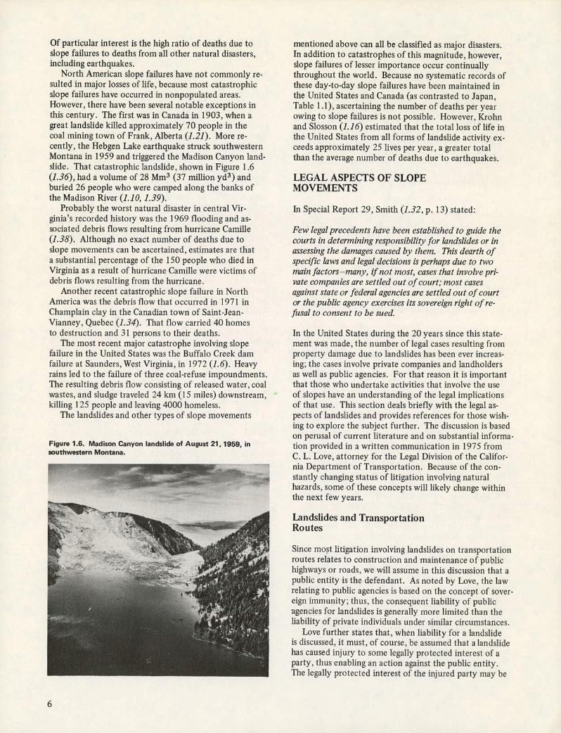
North American slope failures have not commonly re-suited in major losses of life, because most catastrophic slope failures have occurred in nonpopulated areas. However, there have been several notable exceptions in this century. The first was in Canada in 1903, when a great landslide killed approximately 70 people in the coal mining town of Frank, Alberta (1.21). More re-cently, the Hebgen Lake earthquake struck southwestern Montana in 1959 and triggered the Madison Canyon land-slide. That catastrophic landslide, shown in Figure 1.6 (1.36), had a volume of 28 Mm3 (37 million yd3) and buried 26 people who were camped along the banks of the Madison River (1.10, 1.39).

Probably the worst natural disaster in central Vir-ginia's recorded history was the 1969 flooding and as-sociated debris flows resulting from hurricane Camille (1.38). Although no exact number of deaths due to slope movements can be ascertained, estimates are that a substantial percentage of the 150 people who died in Virginia as a result of hurricane Camille were victims of debris flows resulting from the hurricane.

Another recent catastrophic slope failure in North America was the debris flow that occurred in 1971 in Champlain clay in the Canadian town of Saint-Jean-Vianney, Quebec (1.34). That flow carried 40 homes to destruction and 31 persons to their deaths.

The most recent major catastrophe involving slope failure in the United States was the Buffalo Creek dam failure at Saunders, West Virginia, in 1972 (1.6). Heavy rains led to the failure of three coal-refuse impoundments, The resulting debris flow consisting of released water, coal wastes, and sludge traveled 24 km (15 miles) downstream, killing 125 people and leaving 4000 homeless.

The landslides and other types of slope movements

Figure 1.6. Madison Canyon landslide of August 21, 1959, in southwestern Montana.

mentioned above can all be classified as major disasters. In addition to catastrophes of this magnitude, however, slope failures of lesser importance occur continually throughout the world. Because no systematic records of these day-to-day slope failures have been maintained in the United States and Canada (as contrasted to Japan, Table 1.1), ascertaining the number of deaths per year owing to slope failures is not possible. However, Krohn and Slosson (1.16) estimated that the total loss of life in the United States from all forms of landslide activity ex-ceeds approximately 25 lives per year, a greater total than the average number of deaths due to earthquakes.

LEGAL ASPECTS OF SLOPE MOVEMENTS

In Special Report 29, Smith (1.32, p. 13) stated:

Few legal precedents have been established to guide the courts in determining responsibility for landslides or in assessing the damages caused by them. This dearth of specific laws and legal decisions is perhaps due to two main factors—many, if not most, cases that involve pri-vate companies are settled out of court; most cases against state or federal agencies are settled out of court or the public agency exercises its sovereign right of re-fusal to consent to be sued.

In the United States during the 20 years since this state-ment was made, the number of legal cases resulting from property damage due to landslides has been ever increas-ing; the cases involve private companies and landholders as well as public agencies. For that reason it is important that those who undertake activities that involve the use of slopes have an understanding of the legal implications of that use. This section deals briefly with the legal as-pects of landslides and provides references for those wish-ing to explore the subject further. The discussion is based on perusal of current literature and on substantial informa-tion provided in a written communication in 1975 from C. L. Love, attorney for the Legal Division of the Califor-nia Department of Transportation. Because of the con-stantly changing status of litigation involving natural hazards, some of these concepts will likely change within the next few years.

Landslides and Transportation Routes

Since most litigation involving landslides on transportation routes relates to construction and maintenance of public highways or roads, we will assume in this discussion that a public entity is the defendant. As noted by Love, the law relating to public agencies is based on the concept of sover-eign immunity; thus, the consequent liability of public agencies for landslides is generally more limited than the liability of private individuals under similar circumstances.

Love further states that, when liability for a landslide is discussed, it must, of course, be assumed that a landslide has caused injury to some legally protected interest of a party, thus enabling an action against the public entity. The legally protected interest of the injured party may be

his or her personal property, real estate, or physical well-being. It also must be assumed that the public entity is in some way responsible for the landslide. Such respon-sibility, or liability, can be based on construction or main-tenance operations that createor activate a landslide on public property or on mere public ownership of property that either contains or is in the immediate vicinity of an active or potentially active landslide.

Love notes that there have been numerous cases in which private property has been damaged or personal in-jury has resulted from landslides or rock falls or both on public highways in the United States. Ih these instances the liability of the public entity having jurisdiction over the highway has varied from stateto state. Some states, for all intents and purposes, bar suits against public en-tities because of sovereign immunity; however, many states have established statutory provisions under which recovery can be realized. Such statutes generally delin-eate specific duties and responsibilities of public agen-cies, specific circumstances of the slope failure, proce-dural requirements for bringing action against the public entity, and specific defenses available to the public en-tity.

Although the protection of sovereign immunity com-monly has been invoked successfully in cases in which a reasonable degree of prudence has been exercised by those who have designed and constructed the works, Professor G. F. Sowers of the Department of Civil En-gineering, Georgia Institute of Technology, stated in a written communication in 1976:

While it is presently true that states and the federal gov-ernment as owners invoke the protection of "sovereign immunity," there are many indications that this sheltered position will not always be the case. Public sympathy has generated pressure on state legislatures that has caused them to admit liability. In cases where the doctrine of sovereign immunity has held, the injured party and, too often, some overly zealous members of the legal profes-sion have sought other sources of relief. These involve the designers of the works, the builders, and even private maintenance forces. While presently employees of the gov-ernmental bodies appear to be held harmless from legal ac-tion, there are indications that it is possible to bring per-sonal suits for negligence against such employees. While such lawsuits may eventually be lost, there are enough lawyers who will take the statistical chance that some cases will not be thrown out of court that we should ex-pect to see personal suits against political administrators, public employees, and everyone who has anything to do with construction, whether they are responsible or not.

Lewis and others (1.20) divided the legal rights of pri-vate citizens against public agencies with regard to land-slides into two categories:

A property owner's rights in response to invasion of the property by sliding material or interference with the lateral support of the property by construction or maintenance of a public way and

A highway traveler's rights in tort against a public entity for injuries sustained from a landslide that resulted

in part from the negligent construction or maintenance of a public way.

The extent of such rights varies among states, but a general discussion is given below.

Liability in Invasion of Property or Loss of Support

When a landslide results in damage to property, either by invasion of the property or loss of its lateral support, the liability of a public entity is not necessarily based on stat-utes. Under the fifth amendment to the U.S. Constitution, just compensation must be paid when public works or other governmental activities result in the taking of private property; that concept can be extended to the damaging of property as a result of an action of a public agency. The owner of the property brings an action known as an inverse condemnation suit to recover damages. According to Love, many state constitutions contain provisions similar to those of the fifth amendment, but, even in the absence of such a limitation in a state constitution, the courts have held that a state cannot take (or damage) private property for public use without just compensation.

The case of Albers v. County of Los Angeles [62 Cal. 2d 250, 42 Cal. Rptr. 89 (1965)], which established, or broadened, the concept of inverse condemnation in Califor-nia, provides an outstanding example of the manner in which the state courts have interpreted constitutional provisions for the payment of just compensation in the event that private property is either taken or damaged. In that litigation, which was concerned with the Portuguese Bend landslide on the Palos Verdes Peninsula in southern California, the plaintiffs alleged that the county of Los Angeles had constructed Cren-thaw Boulevard through an ancient landslide area and that in the course of carrying out the construction program had placed some 134 000 m3 (175 000 yd3) of earth at a critical spot in the landslide area, causing reactivation of movement and consequent damage to the plaintiffs' properties (1.26, 1.29). The constitution of the state of California guarantees that property of a private property owner will not be dam-aged or taken for public use unless just compensation for it is given to the property owner. This constitutional protec-tion is the basis on which the property owners recovered $5 360 000 from the county of Los Angeles (1.24).

It can be concluded-that, if public-works activities result in the creation of a new landslide or the reactivation of an old landslide that causes damage to private property, the public entity is liable, to the full extent of such damage if the particular state has such a constitutional provision. According to Love, even in jurisdictions that do not have a provision relating directly to damage of private property, the courts have tended to find that the damage that re-sulted to the private property constitutes a taking for which just compensation must be paid.

Liability for Injuries Sustained From a Landslide

Love states that, although the courts have made it clear that a public entity is not an insurer of the safety of persons using its highways, in certain circumstances travelers are

protected by law from landslides. In general, the public entity will not be held liable for injuries if it can be shown that the acts or omissions that created the dangerous con-dition were reasonable or that the action taken to protect against such injuries or the failure to take such action was reasonable. The reasonableness of action or inaction is de-termined by considering the time and opportunity that the public employees had to take action and by weighing the probability and gravity of potential injury to persons fore-seeably exposed to the risk of injury against the practical-ity and cost of protecting against such injury.

In California, most actions involving personal injury to highway travelers as a result of landslides are based on a stat-ute that imposes liability for the dangerous condition of public property. The injured person must prove that the public property was in dangerous condition at the time of the injury, that the injury resulted from that dangerous con-dition, and that the dangerous condition created a foresee-able risk of the kind of injury incurred. Love points out that, in addition, the dangerous condition must be the result of negligence, a wrongful act, or failure of an employee of the public entity to act within the scope of his or her em-ployment, and the public entity must have had notice of the dangerous condition in sufficient time prior to the in-jury to have taken measures to protect against it. Thus, liability depends on whether circumstances and conditions were such that the danger was reasonably foreseeable in the exercise of ordinary care and, if so, on whether reasonable measures were taken by the public entity to prevent injury (39 Am. Jur. 2dHighways § 532, p. 939).

A public entity, since it is not an insurer of the safety of travelers on its highways, need only maintain highways in reasonably safe condition for ordinary travel under ordinary conditions or under such conditions as should reasonably be expected (1.20). In the case of Boskovich v. King County [188 Wash. 63,61 P. 2d 1299 (1936)] ,the court held that a motorist was not entitled to recover from the highway de-partment for injuries sustained when a landslide broke loose from a steep hillside bordering a highway and struck his auto-mobile because there was no proof that negligence in con-struction or maintenance of the highway was the cause of the landslide.

Landslides and Property Development

This section discusses liability related to damages from landslides caused by the development of private property. Detailed information on litigation related to landslides in property developments is given by Sutter and Hecht (1.33).

The current trend in public policy is toward protection of the consumer, a reversal of the days when caveat emptor (let the buyer beware) reflected public policy (1.27). This trend has extended to home purchasers since they are pro-tected by law against losses due to improper workmanship or poor planning, including certain losses due to landslides.

The trend toward increased protection for the home-owner has resulted in a drastic increase in the number of legal cases involving landslides on private property. After consulting with an attorney, the owner of a home that has suffered damage from a landslide typically files legal action against the developer, the civil engineer who laid out the development, the geotechnical engineer, the

geologist, the grading contractor, the city, the builder, the lending agency, the insurance company that insured the home, the former owner, and the real estate agent handling the sale if the property was, not purchased di-rectly from the developer (1.11). A typical complaint may seek recovery on theories of strict liability (i.e., liability without fault), negligence, breach of warranty, negligent misrepresentation, fraud, and, if a public en-tity is involved, inverse condemnation (1.27). In most cases, the developer is the prime target because he is sub-ject to strict liability for "defects" in the construction of the house or grading of the lot; to establish strict liability against any of the other parties such as the soils engineer or the geologist is much more difficult.

Liability of Engineers and Geologists for Landslide Damages

There has been a certain amount of variability in legal inter-pretations of liability of geotechnical engineers and geolo-gists in regard to landslide losses; such liability is discussed below, but the conclusions reached are general in nature and not necessarily valid in any specific court.

Liability of geotechnical engineers and engineering geologists for landslide damages to home sites is based most often on the theory of negligence and occasionally on negligent misrepresentation. Although allegations seeking to recover damages from geotechnical engineers and geologists on the basis of strict liability, breach of war-ranty, or intentional misrepresentation are often included in a complaint, they are not usually applicable under nor-mal circumstances. Patton (1.27) discussed each of these theories of liability as it applies to engineering geologists as follows, and it is felt that Patton's line of reasoning can be extended to include geotechnical engineers involved in development of private property.

1. Negligence

The most common theory of liability alleged against engi-neering geologists is negligence. Negligence is the omission to do something which an ordinarily prudent person would have done under similar circumstances or the doing of some-thing which an ordinarily prudent person would not have done under those circumstances. An engineering geologist is required to exercise that degree of care and skill ordi-narily exercised in like cases by reputable members of his profession practicing in the same or similar locality at the same time under similar conditions. He has the duty to exercise ordinary care in the course of performing his duties for the protection of any person who foreseeably and with reasonable certainty may be injured by his fail-ure to do so.

Although failing to comply with a state statute or with county or municipal ordinances normally is considered to be negligence per se, the mere compliance with the letter of the law in such cases does not necessarily relieve one of liability since it generally is recognized that statutes and ordinances set forth only minimum requirements and cir-cumstances may require more than the minimum. An en-gineering geologist cannot rely upon the approval of a project by an inspector for a governmental agency to re-lieve him of liability.

8

Negligent misrepresentation

Negligent misrepresentation is a species of fraud along with intentional misrepresentation and concealment. Negligent misrepresentation is simply the assertion, as a fact, of that which is not true by one who has no reasonable ground for believing it to be true. Although misrepresentations of opinions generally are not actionable, they become ac-tionable where the person making the alleged misrepresen-tation holds himself to be specially qualified to render the opinion. A statement of opinion by an engineering geol-ogist that no unsupported bedding occurs in a particular slope, could be actionable as negligent misrepresentation if he has no basis for that opinion.

Intentional misrepresentation and concealment

Intentional misrepresentation (the assertion, as a fact, of that which is not true by one who does not believe it to be true) and concealment (the suppression of a fact or condi-tion by one who is bound to disclose it) are species of fraud which are seldom if ever applicable to engineering geologists. Such conduct on the part of an engineering geologist is not only legally actionable but raises serious doubts about the professional integrity of the geologist involved.

Breach of warranty

Breach of warranty is generally not available as a viable theory

of recovery against an engineering geologist.

Strict liability

Although the theory of strict liability is still developing and its limits are not as yet clearly defined, it would appear now that an engineering geologist would not be liable on the theory of strict liability lacking some participation as the developer of mass produced property. Other cases indi-cate that the theory is available only against the developers of mass-produced property and would not be available against the developer of a single lot or building site. There is no clear indication as to at what point between develop-ment of a single lot and development of a tract the theory becomes applicable. It does seem clear at this time that if an engineering geologist offers only professional services in connection with the development of even a large tract he will not subject himself to strict liability.

In regard to negligence, Sowers noted:

Unfortunately, the legal profession has been expanding the definition of negligence to any act committed by the public official, engineer or contractor. Some courts have applied the most extravagant standards of professional knowledge to average run-of-the-mill design and construction. In other words, some courts would presume that every engineer must possess the wisdom and expertise of a Terzaghi.

In voicing an opinion somewhat different from Patton's in regard to strict liability, Fife, another California attorney active in litigation involving geologists and geotechnical en-

gineers, stated in 1973 that professional liability of the technical professional was approaching a major crossroad in its development (1.9). Fife felt that the scope of pro-fessional liability in the technical disciplines was at the point where it would proceed either toward strict liability under pressure from skilled plaintiffs counsel or toward a "reasonableness standard" by which adherence to the aver-age standards of the profession involved would constitute a complete defense. However, unless professional groups become more actively involved in the process of shaping the future scope of their professional liability, eventual application of strict liability to technical professionals seems inevitable.

In their book, Landslide and Subsidence Liability (1.33), Sutter and Hecht present considerable information on strict liability in California. Since November 1913,the cutoff date for the cases included in this reference, certain California court decisions have changed the liability of geol-ogists and geotechnical engineers from strict liability to lia-bility for negligence only. The publisher, California Con-tunuing Education at the Bar, plans periodic supplements to cover changes that have occurred since Sutter and Hecht's book was published.

ACKNOWLEDGMENTS

Sincere appreciation is expressed to all those who contrib-uted information, both published and unpublished, with-out which this volume could not have been written. To list all contributors would be impossible; to list the most important would be unfair to the others. Thus, the most reasonable and equitable approach is simply to acknowledge the help and cooperation of all who contributed informa-tion in the form of data, photographs, ideas, and advice.

Appreciation is also due the entire staff of the Transpor-tation Research Board. Our special thanks go to John W. Guinnee, engineer of soils, geology, and foundations, for his constant encouragement and advice, and to Mildred Clark, senior editor, who aided immensely in the technical aspects of the editoral process.

REFERENCES

1.1 Alfors, J. T., Burnett, J. L., and Gay, T. E., Jr. Urban Geology: Master Plan for California. California Division of Mines and Geology, Bulletin 198, 1973, 112 pp.

1.2 Briggs, R. P., Pomeroy, J. S., and Davies, W. E. Landslid- ing in Allegheny County, Pennsylvania. U.S. Geological Survey, Circular 728, 1975, 18 pp.

1.3 Chassie, R. G., and Goughnour, R. D. National Highway Landslide Experience. Highway Focus, Vol. 8, No. 1, Jan. 1976, pp. 1-9.

1.4 Chassie, R. G., and Goughnour, R. D. States Intensifying Efforts to Reduce Highway Landslides. Civil Engineer-ing, Vol.46, No. 4, April 1976, pp. 65-66.

1.5 duff, L. S. Peru Earthquake of May 31, 1970: Engineer- ing Geology Observations. Seismological Society of Amer-ica Bulletin, Vol. 61, No. 3, June 1971, pp. 511-521.

1.6 Davies, W. E. Buffalo Creek Dam Disaster: Why it Hap- pened. Civil Engineering, Vol.43, No. 7, July 1973, pp. 69-72.

1.7 Eckel, E. B. Introduction. In Landslides and Engineer- ing Practice, Highway Research Board, Special Rept. 29, 1958, pp. 1-5.

1.8 Eckel, E. B., ed. Landslides and Engineering Practice. Highway Research Board, Special Rept. 29, 1958, 232 pp.

1.9 Fife, P. K. Professional Liability and the Public Inter- 1.26 Nordin, J. G. The Portuguese Bend Landslide, Palos est. In Geology, Seismicity, and Environmental Impact, Verdes Hills, Los Angeles County, California.. In Land- Association of Engineering Geologists, Special PubI., slides and Subsidence, Resources Agency of California, 1973, pp. 9-14. 1965, pp. 56-62.

1.10 Hadley, J. B: Landslides and Related Phenomena Ac- 1.27 Patton, J. H., Jr. The Engineering Geologist and Pro- companying the Hebgen Lake Earthquake of August 17, fessional Liability. In Geology, Seismicity, and En- 1959. U.S. Geological Survey, Professional Paper 435, vironmental Impact, Association of Engineering Geol- 1964, pp. 107-138. ogists, 1973, pp. 5-8.

1.11 Hays, W. V. Panel discussion. Proc., Workshop on 1.28 Plafker, G., Ericksen, G E., and Fernandez Concha, J. Physical Hazards and Land Use: A Search for Reason. Geological Aspects of the May 31, 1970, Peru Earth- Department of Geology, San Jose State Univ., Calif or- quake. Seismological Society of America Bulletin, Vol. nia, 1974, pp. 8-14. 61, No. , June 1971, pp. 543-578.

1.12 Japan Ministry of Construction. Dangerous Slope Fail- 1.29 Pollock, J. P. Discussion. In Landslides and Subsi- ure. Division of Erosion Control, Department of River dence, Resources Agency of California, 1965, pp. Works, 1972, 14 pp. 74-77.

1.13 Jones, D. E. Handout for Roundtable Discussions. 1.30 Sanjines, A. G. Sintesis Historica de la Vida de Ia National Workshop on Natural Hazards, June 30-July Ciudad, 1548-1948. Primer Premio de Ia Alcaldia, 2, 1976, Univ. of Colorado, Boulder, Institute of Be- La Paz, Bolivia, 1948, 86 pp. havioral Science, 1976. 1.31 Slosson, J. E. The Role of Engineering Geology in

1.14 Jones, F. 0., Embody, D. R., and Peterson, W. L. Land- Urban Planning. In The Governors' Conference on slides Along the Columbia River Valley, Northeastern Environmental Geology, Colorado Geological Survey, Washington. U.S. Geological Survey, Professional Paper Special Publ. 1,1969, pp. 8-15. 367,1961,98 pp. 1.32 Smith, R. Economic and Legal Aspects. In Land-

1.15 Kiersch, G. A. Vaiont Reservoir Disaster. Civil Engineer- slides and Engineering Practice, Highway Research ing, Vol. 34, No. 3, 1964, pp. 32-39. Board, Special Rept. 29, 1958, pp. 6-19.

1.16 Krohn, J. P., and Slosson, J. E. Landslide Potential in 1.33 Sutter, J. H., and Hecht, M. L. Landslide and Subsi- the United States. California Geology, Vol. 29, No. 10, dence Liability. California Continuing Education at Oct. 1976, pp. 224-231. the Bar, Berkeley, California Practice Book 65, 1974,

1.17 Lane, K. S. Stability of Reservoir Slopes. In Failure 240 pp. and Breakage of Rock (Fairhurst, C., ed.), Proc., 8th 1.34. Tavenas, F., Chagnon, J. Y., and La Rochelle, P. The Symposium on Rock Mechanics, Univ. of Minnesota, Saint-Jean-Vianney Landslide: Observations and Eye- 1966, American Institute of Mining, Metallurgical and witnesses Accounts. Canadian Geotechnical Journal, Petroleum Engineers, New York, 1967, pp. 321-336. - Vol. 8, No. 3,1971, pp. 463-478.

1.18 Lee, K. L., and Duncan, J. M. Landslide of April 25, 1.35 Taylor, F. A., and Brabb, E. E. Distribution and Cost 1974, on the Mantaro River, Peru. National Academy by Counties of Structurally Damaging Landslides in of Sciences, Washington, D.C., 1975, 72 pp. the San Francisco Bay Region, California, Winter of

1.19 Leighton, F. B. Urban Landslides: Targets for Land-Use 1968-69. U.S. Geological Survey, Miscellaneous Field Planning in California. In Urban Geomorphology, Geo- Studies Map MF-327, 1972. logical Society of America, Special Paper 174, 1976, 1.36 U.S. Geological Survey. The Hebgen Lake, Montana, pp. 37-60. Earthquake of August 17, 1959. U.S. Geological Sur-

1.20 Lewis, H., McDaniel, A. H., Peters, R. B., and Jacobs, vey, Professional Paper 435, 1964, 242 pp. D. M. Damages Due to Drainage, Runoff, Blasting, and 1.37 Wiggins, J. H., Slosson, J. E., and Krohn, J. P. Natural Slides. National Cooperative.Highway Research Pro- Hazards: An Expected Building Loss Assessment. J. H. gram, Rept. 134, 1972, 23 pp. Wiggins Co., Redondo Beach, California, Draft rept. to

1.21 MCConnell, R. G., and Brock, R. W. The Great Land- National Science Foundation, 1977, 134 pp. slide at Frank, Alberta. In Annual Report of the Canada 1.38 Williams, G. P., and Guy, H. P. Erosional and Deposi- Department of the Interior for the Year 1902-03, Ses- tional Aspects of Hurricane Camille in Virginia, 1969. sional Paper 25, 1904, pp. 1-17. U.S. Geological Survey, Professional Paper 804, 1973,

1.22 McDowell, B. Avalanche! In Great Adventures With 80 pp. National Geographic, National Geographic Society, 1.39 Witkind, I. J. Events on the Night of August 17, 1959: Washington, D.C., 1963, pp. 263-269. The Human Story. U.S. Geological Survey, Professional

1.23 Merriam, R. Portuguese Bend Landslide, Palos Verdes Paper 435, 1964, pp. 1-4. Hills, California. Journal of Geology, Vol. 68, No. 2, March 1960, pp. 140-153.

1.24 Morton, D. M., and Streitz, R. Landslides: Part Two. California Division of Mines and Geology, Mineral In- PHOTOGRAPH CREDITS formation Service, Vol. 20, No. 11, 1967, pp. 135-140.

1.25 Nilsen, T. H., and Turner, B. L. Influence of Rainfall and Ancient Landslide Deposits on Recent Landslides Figure 1.1 Courtesy of Tennessee Department of Transportation (1950-71) in Urban Areas of Contra Costa County, Figure 1.2 Courtesy of The Register, Santa Ana, California California. U.S. Geological Survey, Bulletin 1388, Figure 1.3 Courtesy of Japan Society of Landslide 19759 18 pp. Figure 1.6 J. R. Stacy, U.S. Geological Survey

10

Chapter 2

Slope Movement Types and Processes DavidJ. Varnes

This chapter reviews a fairly complete range of slope-movement processes and identifies and classifies them ac-cording to features that are also to some degree relevant to their recognition, avoidance, control, or correction. Al-though the classification of landslides presented in Special Report 29 (2.182) has been well received by the profession, some deficiencies have become apparent since that report was published in 1958; in particular, more than two dozen partial or complete classifications have appeared in various languages, and many new data on slope processes have been published.

One obvious change is the use of the term slope move-ments, rather than landslides, in the title of this chapter and in the classification chart. The term landslide is widely used and, no doubt, will continue to be used as an all-inclusive term for almost all varieties of slope movements, including some that involve little o-r no true sliding. Never-theless, improvements in technical communication require a deliberate and sustained effort to increase the precision associated with the meaning of words, and therefore the term slide will not be used to refer to movements that do not include sliding. However, there seems to be no single simple term that embraces the range of processes discussed here. Geomorphologists will see that this discussion com-prises what they refer to as mass wasting or mass move-ments, except for subsidence or other forms of ground sinking.

The classification described in Special Report 29 is here extended to include extremely slow distributed movements of both rock and soil; those movements are designated in many classifications as creep. The classification also in-cludes the increasingly recognized overturning or toppling failures and spreading movements. More attention is paid to features associated with movements due to freezing and thawing, although avalanches composed mostly of snow and ice are, as before, excluded.

Slope movements may be classified in many ways, each

having some usefulness in emphasizing features pertinent to recognition,avoidance, control, correction,or other pur-pose for the classification. Among the attributes that have been used as criteria for identification and classification are type of movement, kind of material, rate of movement, geometry of the area of failure and the resulting deposit, age, causes, degree of disruption of the displaced mass, re-lation or lack of relation of slide geometry to geologic structure, degree of development, geographic location of type examples, and state of activity.

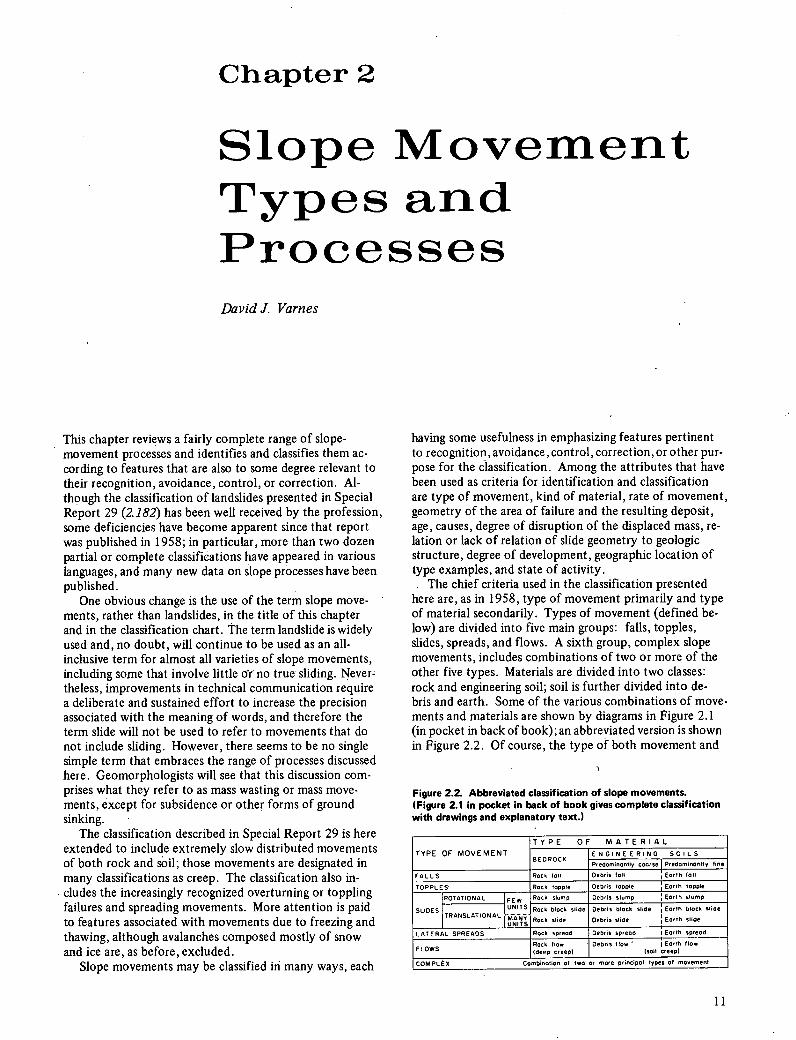
The chief criteria used in the classification presented here are, as in 1958, type of movement primarily and type of material secondarily. Types of movement (defined be-low) are divided into five main groups: falls, topples, slides, spreads, and flows. A sixth group, complex slope movements, includes combinations of two or more of the other five types. Materials are divided into two classes: rock and engineering soil; soil is further divided into de-bris and earth. Some of the various combinations of move-ments and materials are shown by diagrams in Figure 2.1 (in pocket in back of book); an abbreyiated version is shown in Figure 2.2. Of course, the type of both movement and

Figure 2.2. Abbreviated classification of slope movements. (Figure 2.1 in pocket in back of book gives complete classification with drawings and explanatory text.)

TYPE OF MOVEMENT

T Y P E OF M A T E R I A L

BEDROCK ENGINEERING SOILS

Predominontly coOrse Predominontly fine

FALLS Rock lou Debris toll Earth toll

TOPPLES Rock topple Debris topple Earth topple

SLIDES

ROTATIONAL FEW UNITS

Rock Slump Debris slump Earth Slump

TRANSLATIONAL Rock block slide

Rock slide

Debris block slide I Earth block Slide

Debris slide Earth slide

LATERAL SPREADS Rock Spread Debris np,eod I Earth spread

F OWS L Rock flow Ideep creepl

Debris flow I Earth flow

iscreepl

COM Combination of two or more principal types of movement PLEX

11

materials may vary from place to place or from time to time, and nearly continuous gradation may exist in both; therefore, a rigid classification is neither practical nor de-sirable. Our debts to the earlier work of Sharpe (2.146) remain and are augmented by borrowings from many other sources, including, particularly, Skempton and Hutchinson (2,154), Nemok, Paiek, and Rybâi (2.116), de Freitas and Watters (2.37), Záruba and Mend (2.193), and Zischinsky (2.194). Discussions with D. H. Radbruch-Hall of the U.S. Geological Survey have led to significant beneficial changes in both content and format of the presentation.

The classification presented here is concerned less with affixing short one- or two-word names to somewhat com-plicated slope processes and their deposits than with de-veloping and attempting to make more precise a useful vocabulary of terms by which these processes and deposits may be described. For example, the word creep is partic-ularly troublesome because it has been used long and widely, but with differing meanings, in both the material sciences, such as metallurgy, and in the earth sciences, such as geomorphology. As the terminology of physics and materials science becomes more and more applied to the behavior of soil and rock, it becomes necessary to en-sure that the word creep conveys in each instance the con-cept intended by the author. Similarly, the word flow has been used in somewhat different senses by various authors to describe the behavior of earth materials. To clarify the meaning of the terms used here, verbal definitions and dis-cussions are employed in conjunction with illustrations of both idealized and actual examples to build up descriptors of movement, material, morphology, and other attributes that may be required to characterize types of slope move-ments satisfactorily.

TERMS RELATING TO MOVEMENT

Kinds of Movement

Since all movement between bodies is only relative, a de-scription of slope movements must necessarily give some attention to identifying the. bodies that are in relative mo-tion. For example, the word slide specifies relative motion between stable ground and moving ground in which the vectors of relative motion are parallel to the surface of separation or rupture; furthermore, the bodies remain in contact. The word flow, however, refers not to the mo-tions of the moving mass relative to stable ground, but rather to the distribution and continuity of relative move-ments of particles within the moving mass itself.

Falls

In falls, a mass of any size is detached from a steep slope or cliff, along a surface on which little or no shear displacement takes place, and descends mostly through the air by free fall, leaping, bounding, or rolling. Movements are very rapid to extremely rapid (see rate of movement scale, Figure 2.1u) and may or may not be preceded by minor movements leading to progressive separation of the mass from its source.

Rock fall is a fall of newly detached mass from an area of bedrock. An example is shown in Figure 2.3. Debris

fall is a fall of debris, which is composed of de'trital frag-ments prior to failure. Rapp (2.131, p. 104) suggested that falls of newly detached material be called primary and those involving earlier transported loose debris, such as that from shelves, be called secondary. Among those termed debris falls here, Rapp (2.131, p.97) also distinguished pebble falls (size less than 20 mm), cobble falls (more than 20 mm, but less than 200 mm), and boulder falls (more than 200 mm). Included within falls would be the raveling of a thin collu-vial layer, as illustrated by Deere and Patton (2.36), and of fractured, steeply dipping weathered rock, as illustrated by Sowers (2.162).

The falls of less along bluffs of the lower Mississippi River valley, described in a section on debris falls by Sharpe (2.146, p. 75), would be called earth falls (or less falls) in the present classification.

Topples

Topples have been recognized relatively recently as a dis-tinct type of movement. This kind of movement consists of the forward rotation of a unit or units about some pivot point, below or low in the unit, under the action of gravity and forces exerted by adjacent units or by fluids in cracks. It is tilting without collapse. The most detailed descrip-tions have been given by de Freitas and Watters (2.37), and some of their drawings are reproduced in Figure 2.ldl and d2. From their studies in the British Isles, they concluded that toppling failures are not unusual, can develop in a va-riety of rock types,and can range in volume from 100 m3 to more than 1 Gm3 (130 to 1.3 billion yd3). Toppling may or may-not culminate in either falling or sliding, de-pending on the geometry of the failing mass and the orien-tation and extent of the discontinuities. Toppling failure has been pictured by Hoek (2.61), Aisenstein (2.1, p. 375), and Bukovansky, RodrIquez, and Cedri:in (2.16) and studied in detail in laboratory experiments with blocks by Hofmann (2.63). Forward rotation was noted in the Kimbley copper pit by Hamel (2.56), analyzed in a high rock cut by Piteau and others (2.125), and described among the prefailure movements at Vaiont by Hofmann (2.62).

Slides

In true slides, the movement consists of shear strain and displacement along one or several surfaces that are visible or may reasonably be inferred, or within a relatively nar-row zone. The movement may be progressive; that is, shear failure may not initially occur simultaneously over what eventually becomes a defined surface, of rupture, but rather it may propagate from an area of local failure. The displaced mass may slide beyond the original surface of rupture onto what had been the original ground surface, which then becomes a surface of separation.

Slides were subdivided in the classification published in 1958 (2.182) into (a) those in which the material in motion is not greatly deformed and consists of one or a few units and (b) those in which the material is greatly deformed or consists ofmany semi-independent units. These subtypes were further classed into rotational slides and planar slides. In the present classification, emphasis is put on the distinc-tion between rotational and translational slides, for that

12

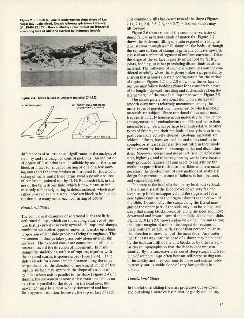
Figure 2.3. Rock fall due to undercutting along shore of Las Vegas Bay, Lake Mead, Nevada (photograph taken February

24, 1949) (2.182). Rock is Muddy Creek formation (Pliocene)

consisting here of siltstone overlain by indurated breccia.

Figure 2.4. Slope failure in uniform material (2.182).

1.1 DflOPd WAPFfl bI ROTATIONAL SHEAR ON CYLINDRICAL SURFACE

THRUSTING AT THE TOE

difference is of at least equal significance in the analysis of stability and the design of control methods. An indication of degree of disruption is still available by use of the terms block or intact for slides consisting of one or a few mov-ing units and the terms broken or disrupted for those con-sisting of many units; these terms avoid a possible source of confusion, pointed out by D. H. Radbruch-Hall, in the use of the term debris slide, which is now meant to indi-cate only a slide originating in debris material, which may either proceed as a relatively unbroken block or lead to dis-ruption into many units, each consisting of debris.

Rotational Slides

The commonest examples of rotational slides are little-deformed slumps, which are slides along a surface of rup-ture that is curved concavely upward. Slumps, and slumps combined with other types of movement, make up a high proportion of landslide problems facing the engineer. The movement in slumps takes place only along internal slip surfaces. The exposed cracks are concentric in plan and concave toward the direction of movement. In many slumps the underlying surface of rupture, together with the exposed scarps, is spoon-shaped (Figure 2.4). If the slide extends for a considerable distance along the slope perpendicular to the direction of movement, much of the rupture surface may approach the shape of a sector of a cylinder whose axis is parallel to the slope (Figure 2.4). In slumps, the movement is more or less rotational about an axis that is parallel to the slope. In the head area, the movement may be almost wholly downward and have little apparent rotation; however, the top surface of each

unit commonly tilts backward toward the slope (Figures 2.lg, 2.1i, 2.4, 2.5, 2.6, and 2.7), but some blocks may tilt forward.

Figure 2.6 shows some of the commoner varieties of slump failure in various kinds of materials. Figure 2.7 shows the backward tilting of strata exposed in a longitu-dinal section through a small slump in lake beds. Although the rupture surface of slumps is generally concave upward, it is seldom a spherical segment of uniform curvature. Often the shape of the surface is greatly influenced by faults, joints, bedding, or other preexisting discontinuities of the material. The influence of such discontinuities must be con-sidered carefully when the engineer makes a slope-stability analysis that assumes a certain configuration for the surface of rupture. Figures 2.7 and 2.8 show how the surface of rupture may follow bedding planes for a considerable part of its length. Upward thrusting and slickensides along the lateral margin of the toe of a slump are shown in Figure 2.9.

The classic purely rotational slump on a surface of smooth curvature is relatively uncommon among the many types of gravitational movement to which geologic materials are subject. Since rotational slides occur most frequently in fairly homogeneous materials, their incidence among constructed embankments and fills, and hence their interest to engineers, has perhaps been high relative to other types of failure, and their methods of analysis have in the past been more actively studied. Geologic materials are seldom uniform, however, and natural slides tend to be complex or at least significantly controlled in their mode of movement by internal inhomogeneities and discontinu-ities. Moreover, deeper and deeper artificial cuts for dam-sites, highways, and other engineering works have increas-ingly produced failures not amenable to analysis by the methods appropriate to circular arc slides and have made necessary the development of new methods of analytical design for prevention or cure of failures in both bedrock and engineering soils.

The scarp at the head of a slump may be almost vertical. If the main mass of the slide moves down very far, the steep scarp is left unsupported and the stage is set for a new failure (similar to the original slump) at the crown of the slide. Occasionally, the scarps along the lateral mar-gins of the upper part of the slide may also be so high and steep that slump blocks break off along the sides and move downward and inward toward the middle of the main slide. Figure 2.10 (2.183) shows a plan view of slump units along the upper margins of a slide; the longest dimensions of these units are parallel with, rather than perpendicular to, the direction of movement of the main slide. Any water that finds its way into the head of a slump may be ponded by the backward tilt of the unit blocks or by other irregu-larities in topography so that the slide is kept wet con-stantly. By the successive creation of steep scarps and trap-ping of water, slumps often become self-perpetuating areas of instability and may continue to move and enlarge inter-inittently until a stable slope of very low gradient is at-tained.

Translational Slides

In translational sliding the mass progresses out or down and out along a more or less planar or gently undulatory

13

surface and has little of the rotary movement or backward tilting characteristic of slump. The moving mass com-monly slides out on the original ground surface. The dis-tinction between rotational and translational slides is use-ful in planning control measures. The rotary movement of a slump, if the surface of rupture dips into the hill at the foot of the slide, tends to restore equilibrium in the un-stable mass; the driving moment during movement de-creases and the slide may stop moving. A translational slide, however, may progress indefinitely if the surface on which it rests is sufficiently inclined and as long as the shear resistance along this surface remains lower than the more or less constant driving force. A translational slide in which the moving mass consists of a single unit that is not greatly deformed or a few closely related units may be called a block slide. If the moving mass consists of many semi-independent units, it is termed a broken or disrupted. slide.

The movement of translational slides is commonly con-trolled structurally by surfaces of weakness, such as faults, j9ints, bedding planes, and variations in shear strength be-

tween layers of bedded deposits, or by the contact between firm bedrock and overlying detritus (Figure 2.11). Several examples of block slides are shown in Figures 2.lj2, 2.11, 2.12, 2.13 (2.136), 2.14 (2.107), and 2.15. In many trans-lational slides, the slide mass is greatly deformed or breaks up into many more or less independent units. As deforma-tion and disintegration continue, and especially as water content or velocity or both increase, the broken or dis-rupted slide mass may change into 'a flow; however, all gradations exist. Broken translational slides of rock are shown in Figure 2.lj3 and of debris in Figures 2.1k and 2.16 (2.83).

Lateral Spreads

In spreads, the dominant mode of movement is lateral ex-tension accommodated by shear or tensile fractures. Two types may be distinguished.

1. Distributed movements result in overall extension

Figure 2.5. Varieties of slump (2.182). 1 (a) SLOPE FAILURE IN HOMOGENEOUS MATERIAL.

CIRCULAR ARC. (1) SLIDE WHOLLY ON SLOPE AND (2) SURFACE OF RUPTURE INTERSECTS TOE OF SLOPE.

r2 I'

lId BASE FAILURE IN HOMOGENEOUS CLAY. SLIP CIRCLE TANGENT TO FIRM BASE, CENTER ON VERTICAL BISECTOR OF SLOPE.

lo

Soil (a) SLIDE BENEATH SIDEHILI.

Sand-stone

Fill

Coal

Clay

Shole

(g) FAILURE OF EMBANKMENT. GRAVEL COUNTER. WEIGHT ON LEFT SIDE PREVENTS SLIDE.

Zunterw:ht r Fill

)b) SLOPE FAILURE IN NONHOMOGENEOUS MATERIAL. SURFACE OF RUPTURE FOLLOWS DIPPING WEAK BED.

off clay

Firm

(d) BASE FAILURE IN NONHOMOGENEOUS MATERIAL. SURFACE OF RUPTURE FOLLOWS BED OF VERY SOFT CLAY.

-- -- Groben

erycloy/////////////

(f) FAILURE WITHIN A SIDEHILL FILL.

CU '\ Original ground line

Fill

(h) SLIDE IN FILL INVOLVING UNDERTHRUSTING OF FIRM SURFACE MATERIAL DOWN SLOPE.

Fill

Fill

Soft zone

Stable \

Firm...

14

Figure 2.6. Slump of fill, controlled in this instance by failure i in underlying soil 7' (2.182).

'.5

Figure 2.7. Slump in thinly bedded lake deposits of silt and clay in Columbia River valley (note backward tilting of beds above surface of rupture) (2.182).

.•._ -..•. -

. -..•* -4. 5—.' . .' ;•. ., .. . •e-- .".......'.- 4.'

Figure 2.8. Slump in bedded deposits similar to those shown in Figure 2.7 (note that surface of rupture follows horizontal bedding plane for part of its length) (2.182).

but without a recognized or well-defined controlling basal shear surface or zone of plastic flow. These appear to occur predominantly in bedrock, especially on the crests of ridges (Figure 2.1m1). The mechanics of movement are not well known.

2. Movements may involve fracturing and extension of coherent material, either bedrock or soil, owing to liquefac-tion or plastic flow of subjacent material. The coherent upper units may subside, translate, rotate, or disintegrate, or they may liquefy and flow. The mechanism of failure can involve elements not only of rotation and translation but also of flow; hence, lateral spreading failures of this type may be properly regarded as complex. They form, however, such a distinctive and dominant species in certain geologic situations that specific recognition seems worth-while.

Examples of the second type of spread in bedrock are shown in Figure 2.1m2 and 2.1m3. In both examples, taken from actual landslides in the USSR and Libya respec-tively, a thick layer of coherent rock overlies soft shale and

Figure 2.10. Ames slide near Telluride, Colorado (2.182, 2.183). This slump-earth flow landslide occurred in glacial till overlying Mancos shale. Repeated slumping took place along upper margins after main body of material had moved down. Long axes of slump

blocks B and B'are parallel with rather than perpendicular to direction of movement of main part of slide. Blocks B and B'

moved toward left, rather than toward observer.

WA

i- .4. .'

-.4- -.

lt&

ZONE A Movement chiefly by large-scal, slumping along slip surf ecu

A. A' A" Principal slump units

8,81 Narrow slump unit with axes perpendicular to axes of main slump units and parallel with length of main slide B Island remaining after

downward movement of unit D from area B.

Figure 2.9. Slickensides in foot area of shallow slide in Pennington shale residuum (highly weathered clay shale) along 1-40 in Roane County. Tennessee.

ZONE B Zone of earth flow; movement chiefly by flowage.

ZONE c Toe of slide area; original form altered by railroad reconstruction work.

I - •'- - -,

100 m

328 ft

15

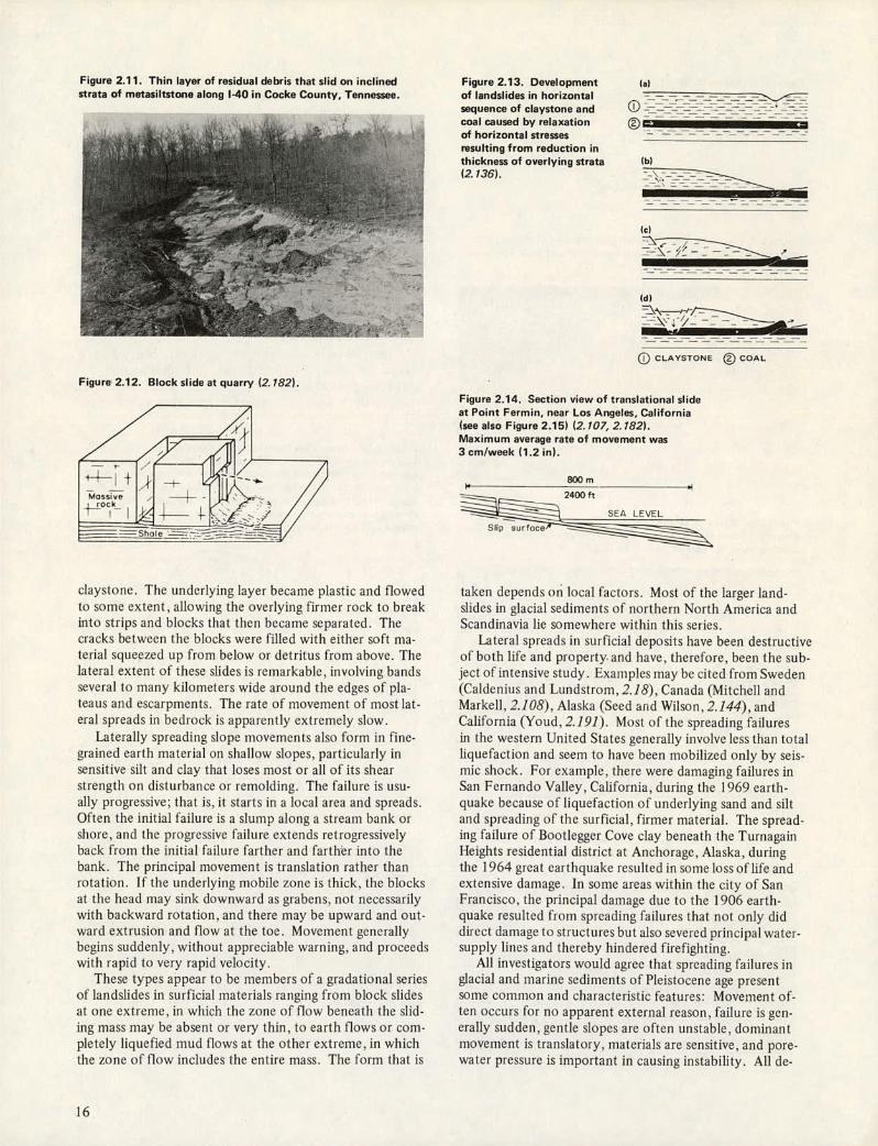
Figure 2.11. Thin layer of residual debris that slid on inclined strata of metasiltstone along 1-40 in Cocke County, Tennessee.

Figure 2.12. Block slide at quarry (2.182).

Figure 2.13. Development

of landslides in horizontal sequence of claystone and (D -- - coal caused by relaxation ® - of horizontal stresses - - - - resulting from reduction in thickness of overlying strata

(2.136).

Ic)

(d)

CLAYSTONE Q COAL

Figure 2.14. Section view of translational slide at Point Fermin, near Los Angeles, California (see also Figure 2.15) (2107, 2.182). Maximum average rate of movement was 3cm/week (1.2 in).

800 m .1

2400 ft

S 1!Rr ure

claystone. The underlying layer became plastic and flowed to some extent, allowing the overlying firmer rock to break into strips and blocks that then became separated. The cracks between the blocks were filled with either soft ma-terial squeezed UI) from below or detritus from above. The lateral extent of these slides is remarkable, involving hands several to many kilometers wide around the edges of pla-teaus and escarpments. The rate of movement of most lat-eral spreads in bedrock is apparently extremely slow.

Laterally spreading slope movements also form in fine-grained earth material on shallow slopes, particularly in sensitive silt and clay that loses most or all of its shear strength on disturbance or remolding. The failure is tisti-ally progressive; that is, it starts in a local area and spreads. Often the initial failure is a slump along a stream bank or shore, and the progressive failure extends retrogressively back from the initial failure farther and farther into the bank. The principal movement is translation rather than rotation. If the underlying mobile zone is thick, the blocks at the head may sink downward as grabens, not necessarily with backward rotation, and there may be upward and out-ward extrusion and now at the toe. Movement generally begins suddenly, without appreciable warning, and proceeds with rapid to very rapid velocity.

These types appear to be members of a gradational series of landslides in surficial materials ranging from block slides at one extreme, in which the zone of how beneath the slid-ing mass may be absent or very thin, to earth flows or com-pletely liquefied mud (lows at the other extreme, in which the zone of flow includes the entire mass. The form that is

taken depends on local factors. Most of the larger land-slides in glacial sediments of' northern North America and Scandinavia lie somewhere within this series.

Lateral spreads in surficial deposits have been destructive of both life and property and have, therefore, been the sub-ject olintensive study. Examples may be cited from Sweden (Caldenius and Lundstrom, 2.18), Canada (Mitchell and Markell, 2.108), Alaska (Seed and Wilson, 2J44), and California (Youd, 2.191). Most of the spreading failures in the western United States generally involve less than total liquefact ion and seem to have been mobilized only by seis-mic shock. For example, there were damaging failures in San Fernando Valley. California, during the 1969 earth-quake because of liquefaction of underlying sand and silt and spreading of the surficial, firmer material. The spread-ing failure of Bootlegger Cove clay beneath the Turnagain Heights residential district at Anchorage, Alaska, during the 1964 great earthquake resulted in some loss of life and extensive damage. In some areas within the city of San Francisco, the principal damage due to the 1906 earth-quake resulted from spreading failures that not only did direct damage to structures but also severed principal water-supply lines and thereby hindered firefighting.

All investigators would agree that spreading failures in glacial and marine sediments of Pleistocene age present some common and characteristic feat tires: Movement of-ten occurs for no apparent external reason, failure is gen-erally sudden, gentle slopes are often unstable, dominant movement is translatory, materials are sensitive, and pore-water pressure is important in causing instability. All de-

16

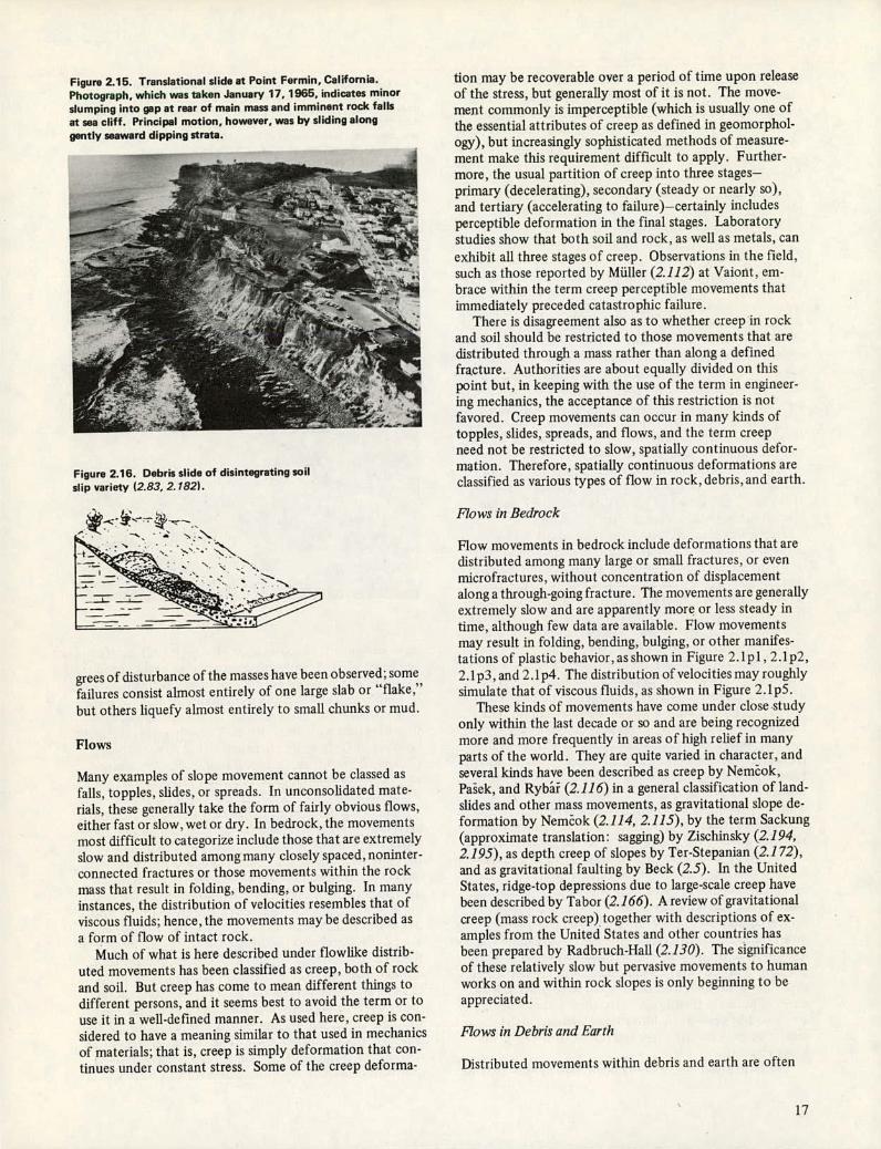
Figure 2.15. Translational slide at Point Fermin, California. Photograph, which was taken January 17, 1965, indicates minor slumping into gap at rear of main mass and imminent rock falls at sea cliff. Principal motion, however, was by sliding along gently seaward dipping strata.

Figure 2.16. Debris slide of disintegrating soil slip variety (2.83, 2.182).

grees of disturbance of the masses have been observed; some failures consist almost entirely of one large slab or "flake," but others liquefy almost entirely to small chunks or mud.

Flows

Many examples of slope movement cannot be classed as falls, topples, slides, or spreads. In unconsolidated mate-rials, these generally take the form of fairly obvious flows, either fast or slow, wet or dry. In bedrock, the movements most difficult to categorize include those that are extremely slow and distributed among many closely spaced, noninter-connected fractures or those movements within the rock mass that result in folding, bending, or bulging. In many instances, the distribution of velocities resembles that of viscous fluids; hence, the movements may be described as a form of flow of intact rock.

Much of what is here described under flowlike distrib-uted movements has been classified as creep, both of rock and soil. But creep has come to mean different things to different persons, and it seems best to avoid the term or to use it in a well-defined manner. As used here, creep is con-sidered to have a meaning similar to that used in mechanics of materials; that is, creep is simply deformation that con-tinues under constant stress. Some of the creep deforma-

tion may be recoverable over a period of time upon release of the stress, but generally most of it is not. The move-ment commonly is imperceptible (which is usually one of the essential attributes of creep as defined in geomorphol-ogy), but increasingly sophisticated methods of measure-ment make this requirement difficult to apply. Further-more, the usual partition of creep into three stages—primary (decelerating), secondary (steady or nearly so), and tertiary (accelerating to failure)—certainly includes perceptible deformation in the final stages. Laboratory studies show that both soil and rock, as well as metals, can exhibit all three stages of creep. Observations in the field, such as those reported by Muller (2.112) at Vaiont, em-brace within the term creep perceptible movements that immediately preceded catastrophic failure.

There is disagreement also as to whether creep in rock and soil should be restricted to those movements that are distributed through a mass rather than along a defined fracture. Authorities are about equally divided on this point but, in keeping with the use of the term in engineer-ing mechanics, the acceptance of this restriction is not favored. Creep movements can occur in many kinds of topples, slides, spreads, and flows, and the term creep need not be restricted to slow, spatially continuous defor-mation. Therefore, spatially continuous deformations are classified as various types of flow in rock, debris, and earth.

Flows in Bedrock

Flow movements in bedrock include deformations that are distributed among many large or small fractures, or even microfractures, without concentration of displacement along a through-going fracture. The movements are generally extremely slow and are apparently more or less steady in time, although few data are available. Flow movements may result in folding, bending, bulging, or other manifes-tations of plastic behavior, as shown in Figure 2.1pi, 2.1p2, 2.1 p3,and 2.1 p4. The distribution of velocities may roughly simulate that of viscous fluids, as shown in Figure 12.1p5.

These kinds of movements have come under close study only within the last decade or so and are being recognized more and more frequently in areas of high relief in many parts of the world. They are quite varied in character, and several kinds have been described as creep by Nemèok, Paek, and Rybâi (2.116) in a general classification of land-slides and other mass movements, as gravitational slope de-formation by Neinok (2.114, 2.115), by the term Sackung (approximate translation: sagging) by Zischinsky (2.194, 2.195), as depth creep of slopes by Ter-Stepanian (2.172), and as gravitational faulting by Beck (2.5). In the United States, ridge-top depressions due to large-scale creep have been described by Tabor (2.166). A review of gravitational creep (mass rock creep) together with descriptions of ex-amples from the United States and other countries has been prepared by Radbruch-HaIl (2.130). The significance of these relatively slow but pervasive movements to human works on and within rock slopes is only beginning to be appreciated.

Flows in Debris and Earth

Distributed movements within debris and earth are often

17

more accurately recognized as flows than those in rocks be-cause the relative displacements within the mass are com-monly larger and more closely distributed and the general appearance is more obviously that of a body that has be-haved like a fluid. Moreover, the fluidizing effect of water itself is, as a rule, a part of the process. Slip surfaces within the moving mass are usually not visible or are short lived, and the boundary between moving mass and material in place may be a sharp surface of differential movement or a zone of distributed shear.

There is complete gradation from debris slides to debris flows, depending on water content, mobility, and character of the movement, and from debris slide to debris avalanche as movement becomes much more rapid because of lower cohesion or higher water content and generally steeper slopes. Debris slides and, less commonly, debris avalanches may have slump blocks at their heads. In debris slides, the moving mass breaks up into smaller and smaller parts as it advances toward the foot, and the movement is usually slow. In debris avalanches, progressive failure is more rapid, and the whole mass, either because it is quite wet or because it is on a steep slope, liquefies, at least in part, flows, and tumbles downward, commonly along a stream channel, and may advance well beyond the foot of the slope. Debris avalanches are generally long and narrow and often leave a serrate or V-shaped scar tapering uphill at the head, as shown in Figures 2.1q3 and 2.17, in con-trast to the horseshoe.shaped scarp of a slump.

Debris flows, called mud flows in some other classifi. cations, are here distinguished from the latter on the basis of particle size. That is, the term debris denotes material that contains a relatively high percentage of coarse frag- ments, whereas the term mud flow is reserved for an earth flow consisting of material that is wet enough to flow rap. idly and that contains at least 50 percent sand-, silt-, and clay-sized particles. Debris flows commonly result from unusually heavy precipitation or from thaw of snow or frozen soil. The kind of flow shown in Figure 2.1ql often occurs during torrential runoff following cloudbursts. It is favored by the presence of soil on steep mountain slopes from which the vegetative cover has been removed by fire or other means, but the absence of vegetation is not a pre-requisite. Once in motion, a small stream of water heavily laden with soil has transporting power that is dispropor-tionate to its size, and, as more material is added to the stream by caving of its banks, its size and power increase. These flows commonly follow preexisting drainageways, and they are often of high density, perhaps 60 to 70 per. cent solids by weight, so that boulders as big as automo-biles may be rolled along. If such a flow starts on an un-broken hillside it will quickly cut a V-shaped channel. Some of the coarser material will be heaped at the site to form a natural levee, while the more fluid part moves down the channel (Figure 2.17). Flows may extend many kilometers, until they drop their loads in a valley of lower gradient or at the base of a mountain front. Some debris flows and mud flows have been reported to proceed by a series of pulses in their lower parts; these pulses presumably are caused by periodic mobilization of material in the source area or by periodic damming and release of debris in the lower channel.

The term avalanche, if unmodified, should refer only to

Figure 2.17. Debris avalanche or very rapid debris flow at Franconia Notch, New Hampshire, June 24, 1948, after several days of heavy rainfall (2.182). Only soil mantle 2 to 5 m (7 to 6 ft) thick, which lay over bedrock on a slope of about 1:1, was involved. Scar is about 450 m (1500 ft) long; natural levees can be seen along sides of flow. US-3 is in foreground.

slope movements of snow or ice. Rapp (2.132) and Temple and Rapp (2.169), with considerable logic, recommend that, because the term debris avalanche is poorly defined, it should be abandoned, and that the term avalanche should be used only in connection with mass movements of snow, either pure or mixed with other debris. The term debris avalanche, however, is fairly well entrenched and in common usage (Knapp, 2.86); hence, its appearance in the classification as a variety of very rapid to extremely rapid debris flow seems justified.

Recent studies have contributed much to a better un-derstanding of the rates and duration of rainfall that lead to the triggering of debris flows, the physical properties of the material in place, the effect of slope angle, the effect of pore-water pressure, the mobilization of material and mechanism of movement, and the properties of the result-ing deposit. The reader is referred especially to the works of Campbell (2.20), Daido (2.34), Fisher (2.46), Hutchin-son (2.70), Hutchinson and Bhandari (2.72), Johnson and Rahn (2. 76), Jones (2.78), Prior, Stephens, and Douglas (2.129), Rapp (2.131), K. M. Scott (2.141), R. C. Scott (2.142), and Williams and Guy (2.188). Flowing move-ments of surficial debris, including creep of the mantle of weathered rock and soil, are shown in Figure 2.1q2, 2.1q4, and 2.1q5. Soil flow, or sohifluction, which in areas of pe-rennially or permanently frozen ground is better termed gelifluction, takes many forms and involves a variety of

18

mechanisms that can be treated adequately only in works devoted to this special field, which is of great significance to engineering works at high latitudes and altitudes. The reader is referred to summaries by Dylik (2.40), Washburn (2.187), and Corte (2.27); the proceedings of the Interria-tional Conference on Permafrost (2.111); and recent work by McRoberts and Morgenstern (2.104, 2.105) and Emble-ton and King (2.42).

Subaerial flows in fine-grained materials such as sand, silt, or clay are classified here as earth flows. They take a variety of forms and range in water content from above saturation to essentially dry and in velocity from extremely rapid to extremely slow. Some examples are shown in Fig-ure 2.1rl through 2.1r5. At the wet end of the scale are mud flows, which are soupy end members of the family of predominantly fine-grained earth flows, and subaqueous flows or flows originating in saturated sand or silt along shores.

In a recent paper reviewing Soviet work on mud flows, Kurdin (2.91) recommended a classification of mud flows based on (a) the nature of the water and solid-material supply; (b) the structural-rheological model, that is, whether the transporting medium is largely water in the free state or is a single viscoplastic mass of water and fine particles; (c) the composition of the mud flow mass, that is, whether it consists of mud made up of water and particles less than 1 mm (0.04 in) in size or of mud plus gravel, rubble, boulders, and rock fragments; and (d) the force of the mud flow as defined by volume, rate of discharge, and observed erosive and destructive power. In the Soviet literature mud flows include not only what are here classified as debris flows but also heavily laden flows of water-transported sediment.

According to Andresen and Bjerrum (2.3), subaqueous flows are generally of two types: (a) retrogressive flow slide or (b) spontaneous liquefaction, as shown in Figure 2.18. The retrogressive flows, as shown in Figure 2.1r1, occur mostly along banks of noncohesive clean sand or silt. They are especially common along tidal estuaries in the coastal provinces of Holland, where banks of sand are subject to scour and to repeated fluctuations in pore-water pressure because of the rise and fall of the tide (Koppejan,

Figure 2.18. Retrogressive flow slide and spontaneous liquefaction (2.3).

(a) RETROGRESSIVE FLOW SLIDE (Mechanism after Koppejan. Van Wamelon, and Weinberg. 2.891

rAFTERFLOWSLIDE WATERLEVEL BEFORE FLOW SLIDE

—SCOURED OUT BY TIDAL CURRENT

LARGE STRAIN VELOCITIES 0.05 10 SE VERAL k,elh

IbI SPONTANEOUS LIQUEFACTION

- SECONDARY SLIDE SECO5DARY SLIDE

AFTER

LSTART EARTHQUAKEIPILE DRIVING

SMALL STRAIN VELOCITIES 10,0 100 Kmjh

Nole: 1 km(h 0.6 rnpl,.

Figure 2.19. Earth flow near Greensboro, Florida (2.80, 2.182). Material is flat-lying, partly indurated clayey sand of the Hawthorn formation (Miocene). Length of slide is 275 m (900 ft) from scarp to edge of trees in foreground. Vertical distance is about 15 m (45 ft) from top to base of scarp and about 20 m (60 ft) from top of scarp to toe. Slide occurred in April 1948 after year of unusually heavy rainfall, including 40cm (16 in) during 30 d preceding sl ide.

;sf: .-

_____

441.

Van Wamelon, and Weinberg, 2.89). When the structure of the loose sand breaks down along a section of the bank, the sand flows rapidly along the bottom, and, by repeated small failures, the slide eats into the bank and enlarges the cavity. Sometimes the scarp produced is an arc, concave toward the water, and sometimes it enlarges greatly, retain-ing a narrow neck or nozzle through which the sand flows. An extensive discussion and classification of subaqueous mass-transport processes and the resulting deposits have been presented by Carter (2.21).

Rapid earth flows also occur in fine-grained silt, clay, and clayey sand, as shown in Figures 2.1 r2 and 2.19 (2.80). These flows form a complete gradation with slides involving failure by lateral spreading, but they involve not only lique-faction of the subjacent material but also retrogressive fail-ure and liquefaction of the entire slide mass. They usually take place in sensitive materials, that is, in those materials whose shear strength on remolding at constant water con-tent is decreased to a small fraction of its original value. Rapid earth flows have caused loss of life and immense destruction of property in Scandinavia, the St. Lawrence River valley in Canada, and Alaska during the 1964 earth-quake. The properties of the material involved, which is usually a marine or estuarine clay of late Pleistocene age, have been thoroughly studied by many investigators during the last 15 years. Summary papers have been written by Bjerrum and others (2.12) on flows in Norway and by Mitchell and Markell (2.108),and Eden and Mitchell (2.41) on flows in Canada. Shoreline flows produced by the Alas-k.an earthquake at Valdez and Seward have been described by Coulter and Migliaccio (2.28) and Lenike (2.98). The large failure on the Reed Terrace near Kettle Falls, Wash-ington, shown in Figures 2.20 and 2.21 (2.79), resembles in some respects the earth flow at Riviere Blanche, Quebec, shown in Figure 2.1r2 (2.146).

The somewhat drier and slower earth flows in plastic earth are common in many parts of the world wherever there is a combination of clay or weathered clay-bearing

19

:cQ

7T' b!::I

rocks, moderate slopes, and adequate moisture; Figure 2.22 shows a typical example. A common elongation of the flow, channelization in depression in the slope, and spreading of the toe are illustrated in Figure 2.43 and also shown in an actual debris flow in Figure 2.23.

The word flow naturally brings water to mind, and some content of water is necessary for most types of flow move-ment. But small dry flows of granular material are common, and a surprising number of large and catastrophic flow movements have occurred in quite dry materials. There-fore, the classification of flows indicates the complete range of water content—from liquid at the top to dry at the bottom. Tongues of rocky debris on steep slopes moving extremely slowly and often fed by talus cones at the head are called block streams (Figure 2.lq5). Because of rain-wash, a higher proportion of coarse rocks may be in the sur-face layers than in the interior. Dry flows of sand are com-mon along shores or embankments underlain by dry gran-ular material. In form, they may be cliannelized, as shown in Figures 2.1r4 and 2.24, or sheetlike, as shown in Figure 2.25 (2.79). Small flows of dry silt, powered by impact

Figure 2.20. Reed Terrace area, right bank of Lake Roosevelt reservoir on Columbia River. near Kettle Falls, Washington, May 15, 1951 (2.182). Landslide of April 10. 1952, involving about 11 Mm3 (15 million yd3) took place by progressive slumping, liquefaction, and flowing out of glaciofluvial sediments through narrow orifice into bottom of reservoir.

Figure 2.21. Reed Terrace area, Lake Roosevelt, Washington, August 1, 1952, after landslide of April 10, 1952(2.79, 2.182).

on falling from a cliff, have been recognized, but so far as is known none has been studied in detail (Figure 2.26).

Flows of bess mobilized by earthquake shock have been more destructive of life than any other type of slope failure. Those that followed the 1920 earthquake in Kansu Province, China (Close and McCormick,2.23), shown in Figure 2.1r5, took about 100 000 lives. Apparently the normal, fairly coherent internal structure of the porous silt was destroyed by earthquake shock, so that, for all practical purposes, the bess became a fluid suspension of silt in air and flowed down into the valleys, filling them and overwhelming vil-lages. The flows were essentially dry, according to the re-port. Extensive flows of bess accompanied the Chait earth-quake of July 10, 1949, in Tadzhikistan, south-central Asia, and buried or destroyed 33 villages as the flows covered the bottoms of valleys to depths of several tens of meters for many kilometers (Gubin, 2.54).

Complex

More often than not, slope movements involve a combina-

Figure 2.22. Earth flow developing from slump near Berkeley. California (2.182).

- - F--. / .. L'- ...............•.

A. ......... ..-...-.:..........................-... - - Figure 2.23. Old debris flow in altered volcanic rocks west of Pahsimeroi River in south central Idaho.

20

Figure 2.24. Dry sand flow in Columbia River valley (2i82). Material is sand over lake-bed si It; dry sand from upper terrace flowed like liquid through notch in more compact sand and silt below.

1' 4t - •:i

¼

. .- -s..

x_ -.-'.-- .---.- . . - - -

Figure 2.25. Shallow, dry, sand flow along shore of Lake Roosevelt. Washington (2.79). Wave erosion or saturation of sediment by lake water caused thin skin of material to lose Jpport and ravel off terrace scarp.

- ..-

A"c.

Figure 2.26. Dry flow of silt (2.182). Material is lake-bed silt of Pleistocene age from high bluff on right bank of Columbia River, 4 km (2.5 miles) downstream from Belvedere, Washington. Flow was not observed while in motion, but is believed to result from blocks of silt falling down slope, disintegrating, forming a single high-density solid-in-air suspension, and flowing out from base of cliff.

- - - - •-- 5-....;. ... - - .- . '.-i __,%- - - - - -.- "— --• P - .-

tion of one or more of the principal typesof movement de-scribed above, either within various parts of the moving mass or at different stages in development of the movements. These are termed complex slope movements, and a few cx-ainpies of the many possible types are illustrated in Figure 2Js1 through 2Js5.

Of particular interest regarding hazards of landslides to life and property are large, extremely rapid rock fall-debris flows, referred to as rock-fragment now (variety rock-fall avalanche) in the 1958 classification (2.182). Rock slide-and rock fall-debris flows are most common in rugged mountainous regions. The disaster at Elm. Switzerland (Heim, 2.58, pp. 84, 109-1 12), which took 115 lives, startetl with small rock slides at each side of a quarry on the mountainside. A few minutes later the entire mass of rock above the quarry crashed down and shot across the valley. The movement of the rock fragments, which had to that moment been that of a rock slide and rock fall, ap-pears to have taken on the character of a flow. The mass rushed up the other side of the small valley, turned and streamed into the main valley, and flowed for nearly I 5 km (1 mile) at high velocity before stopping (Figure 2.lsl). About 10 Mm3 (13 million yd3) of rock descended an aver-age of 470 m (1540 ft) vertically in a total elapsed time of about 55 s. The kinetic energy involved was enormous. A similar and even larger rock-fall avalanche occurred at Frank, Alberta, in 1903 and also caused great loss of life and property (McConnell and Brock, 2103; Cruden and Krahn. 2.33).

These rock fall-debris flows are minor, however, com-pared with the cataclysmic flow that occurred at the time of the May 31, 1970, earthquake in Peru, which buried the city of Yungay and part of Ranrahirca, causing a loss of more than 18 000 lives. According to Plafker, Ericksen, and Fernandez Concha (2J26), the movement started high on Huascaran Mountain at an altitude of 5500 to 6400 ni and involved 50 Mni3 to 100 Mm3 (65 million to 130 million yd 3) of rock, ice, snow, and soil that traveled 14.5 km (9 miles) from the source to Yungay at a velocity between 280 and 335 km/h (175 to 210 mph). They reported strong evidence that the extremely high velocity and low friction of the flow were due, at least in part, to lubrication by a cushion of air entrapped beneath the debris. Pautre, Sabarly. and Schneider (2.122) suggested that the mass may have ridden on a cushion of steam. A sketch of the area affected is shown in Figure 2.27, taken from a paper by duff (224) on engineering geology observations. Crandell and Fahnestock (229) cited evidence for an air cushion beneath one or more rock fall-debris flows that occurred in December 1963 at Little Tahoma Peak and Emmons Glacier on the east flank of Mt. Rainier volcano, Washington.

Such flows probably cannot be produced by a few thou-sand or a few hundred thousand cubic meters of material. Many millions of megagrams are required: and, when that much material is set in motion, perhaps even slowly, pre-dictions of behavior based on past experience with small failures become questionable. The mechanics of large,ex-tremely rapid debris flows, many of which appear to have been nearly dry when formed, have conic under much re-cent study. The large prehistoric Blackhawk landslide (Figure 2.28) shows so little gross rearrangement 'within the

21

sheet of debris of which it is composed that Shreve (2.148) believed the broken material was not fluidized but slid on an ephemeral layer of compressed air. He reported, simi-larly, that the large landslide that was triggered by the Alaska earthquake of 1964 and fell onto the Sherman Glacier showed little large-scale mixing and did not flow like a viscous fluid but instead slid like a flexible sheet (Shreve, 2.149). On the other. hand, Johnson and Ragle (2.77) re-ported,

Many rock-snow slides that followed from the Alaska earth-quake of March 27, 1964, illustrated a variety of flow me-chanics. The form of some slides suggests a complete turbu-lence during flow, while the form of others gives evidence for steady-state flow or for controlled shearing.

From a detailed analysis of the kinematics of natural rock fall-debris flows and from model studies, Hsü (2.66) disputed Shreve's hypothesis that some slid as relatively undeformed sheets on compressed air and concluded, rather, that they flowed.

Obviously, there is much yet to be learned about these processes, particularly as similar features indicating mass movements of huge size have been recognized in Mariner 9 photographs of the surface of Mars (Sharp, 2.145), where it is yet uncertain that significant amounts of either liquid

or gas were available for fluidization. Getting back to Earth, we note self-explanatory examples

of complex movements in Figure 2-1: slump-topple in Fig-ure 2.1s2, rock slide-rock fall in Figure 2.1s3, and the com-mon combination of a slump that breaks down into an earth flow in its lower part in Figure 2.1s5.

The illustration of cambering and valley bulging in Figure 2.1s4 is adapted from the classical paper by Hollingworth and Taylor (2.65) on the Northampton Sand Ironstone in England, their earlier paper on the Kettering district (2.64), and a sketch supplied by J. N. Hutchinson. The complex movements were described by Hutchinson (2.68) as follows:

Cambering and Valley Bulging. These related features were first clearly recognized in 1944 by Hollingworth, Taylor, and Kellaway (see reference in Terzaghi, 1950) in the North-ampton Ironstone field of central England, where they are believed to have a Late Pleistocene origin. The ironstone oc-curs in the near-horizontal and relatively thin Northampton Sands, which are the uppermost solid rocks in the neighbor-hood. These are underlain, conformably, by a great thick-ness of the Lias, into which shallow valleys, typically 1200 to 1500 meters wide and 45 meters deep, have been eroded. Excavations for dam trenches in the valley bottoms have shown the Lias there to be thrust strongly upward and con-torted, while open cast workings in the Northampton Sands

Figure 2.27. Area affected by May 31, 1970, Huascarn debris avalanche, which originated at point A (2.24). Vungay was protected from January 10, 1962, debris avalanche by 180 to 240-rn (600 to 800-ft) high ridge (point B), but a portion of May 31, 1970, debris avalanche diverted from south side of canyon wall, topped "protective" ridge, and descended on Vungay below. Only safe place in Yungay was Cemetery Hill (point C), where some 93 people managed to run to before debris avalanche devastated surrounding area. Moving at average speed of 320 km (200 mph), debris arrived at point D, 14.5 km (9 miles) distant and 3660 m (12 000 ft) lower, within 3 to 4 min after starting from north peak of Huascarn. Debris flowed upstream along course of Rio Santa (point E) approximately 2.5 km 0.5 miles). Debris continued to follow course of Rio Santa downstream to Pacific Ocean. approximately 160 km (100 miles), devastating villages and crops occupying floodplain.

NEVADO HUANDOY NEVADO HUASCARAN NORTH PEAK SOUTH PEAK

_6663m 6767m

Area apparently overridden by avalanche debris but left undisturbed, suggesting air-cushioning effect

Note: 1 m = 3.3 ft.

22

occupying the inter/luves reveal a general valleyward in-crease of dip of "camber" of this stratum, often passing into dip and fault structure, suggesting corresponding downward movements along the valley margins. In adjust-ing to these movements, the rigid cap-rock has been dislo-cated by successive, regularly spaced fissures which paral-lel the valley and are known as "gulls." Similar features have been recognized in other parts of England and in Bo-hemia. The mechanisms by which cambering and valley bulging have been formed remain to be established.

Hutchinson (2. 70) also pointed out that Sharpe's defi-nition of flow (2i46), which requires zero relative dis-placement at the boundary of the flow (flow adheres to the stable material), does not fit the observed distribution of velocities at Beltinge, where a mud flow developed in a temperate climate on a 30-m-high (98-ft) coastal cliff of stiff, fissured London clay subject to moderate marine ero-sion. 1-lere the mud flow was bounded both oil the sides and on the bottom by discrete surfaces along which shear displacements occurred. For these kinds of movements Hutchinson and Bhandari (2. 72) proposed the term mtid-slides. These can be regarded as complex movements in which the internal distribution of velocities within the moving mass may or may not resemble that of viscous fluids, but the movement relative to stable ground is finite discontinuous shear. It would seem that the material of the sliding earth flow is behaving as a plastic body in plug flow, as suggested by Hutchinson (2.69, pp. 23 1-232) and as ana-lyzed in detail by Johnson (2. 75).

Sequence or Repetition of Movement

The term retrogressive has been used almost consistently for slides or flow failures that begin at a local area, usually along a slope, and enlarge or retreat opposite to the direction of movement of the material by spreading of the failure sur-face, successive rotational slumps, falls, or liquefaction of the material. Kojan, Foggin, and Rice (2.87, pp. 127-128) used the term for failure spreading downslope.

On the other hand, the term progressive has been used to indicate extension of the failure (a) downslope (Blong, 2.13; Kjellman,2.84: Ter-Stepanian .2.1 70, 2.1 71: Thomson and l-layley,2.177),(b) upslope (but not specifically up-slope only) (Seed, 2.143; Tavenas, Chagnon, and La Rochelle, 2.168), and (c) either upsiope or downslope, or unspecified (Terzaghi and Peck, 2.176: Bishop, 2.7; Roniani, Lovell, and Harr, 2.135; Lo, 2.100; Frölich, 2.51; Ter-Stepanian and Goldstein. 2.173, and many others).

I suggest that the term progressive be used for failure that is either advancing or retreating or both simultaneously, that the term retrogressive be used only for retreating fail-ures, and that failures that enlarge in the direction of move-ment be referred to simply as advancing failures.

The terms complex, composite, compound, multiple, and successive have been used in different ways by various authors. I suggest the following definitions.

1. Complex refers to slope movements that exhibit more than one of the major modes of movement. This is the sense of the meaning suggested by Blong (2.14). The term is syn-onymous with composite, as used by Prior, Stephens, and

Figure 2.28. Blackhawk landslide (2.147). Upslope view, southward over lobe of dark marble breccia spread beyond mouth of Blackhawk Canyon on north flank of San Bernardino Mountains in southern California. Maximum width of lobe is 3.2 km 12 miles); height of scarp at near edge is about 15 m 150 ft).

. '-.•

' - I'

••Ip. &'

Ccl SUCCESSIVE

Archer (2.128) to describe sliding mud flows. Compound refers to movements in which "the failure

surface is formed of a combination of curved and planar ele-ments and the slide movements have a part-rotational, part-translational character" (Skempton and Hutchinson, 2.154).

Multiple refers to manifold development of the same mode of movement. As applied to retrogressive rotational sliding, the term refers to the production of "two or more slipped blocks, each with a curved slip surface tangential to a common, generally deep-seated slip sole [Figure 2.291 Clearly, as the number of units increases, the overall char-acter of the slip becomes more translational, though in fail-ing, each block itself rotates backwards" (Hutchinson. 2.68). Leighton (2.97) distinguished two types of multiple slide blocks: superposed, in which each slide block rides out on the one below, and juxtaposed, in which adjacent

Figure 2.29. Main types of rotational slide (2.68).

(S) SINGLE - - - -.

a— Slope failure Cloy

Bose failure Cloy

Ibi MULTIPLE Cap rock --------------

Clay

Hard substratum

23

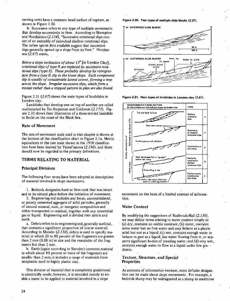
moving units have a common basal surface of rupture, as shown in Figure 2.30.

4. Successive refers to any type of multiple movements that develop successively in time. According to Skempton and Hutchinson (2.154), "Successive rotational slips con-sist of an assembly of individual shallow rotational slips. The rather sparse data available suggest that successive slips generally spread up a slope from its foot." Hutchin-son (2.67) states,

Below a slope inclination of about 130 [m London Clay], rotational slips of type R are replaced by successive rota-tional slips (typeS). These probably develop by retrogres-sion from a type R slip in the lower slope. Each component slip is usually of considerable lateral extent, forming a step across the slope. Irregular successive slips, which form a mosaic rather than a stepped pattern in plan are also found.

Figure 2.31 (2.67) shows the main types of landslides in London clay.

Landslides that develop one on top of another are called multistoried by Ter-Stepanian and Goldstein (2.173). Fig-ure 2.32 shows their illustration of a three-storied landslide in Sochi on the coast of the Black Sea.

Rate of Movement

The rate-of-movement scale used in this chapter is shown at the bottom of the classification chart in Figure 2.1u. Metric equivalents to the rate scale shown in the 1958 classifica-tion have been derived by Yemel'ianova (2.190), and these should now be regarded as the primary definitions.

TERMS RELATING TO MATERIAL

Principal Divisions

The following four terms have been adopted as descriptions of material involved in slope movements.

Bedrock designates hard or firm rock that was intact and in its natural place before the initiation of movement.

Engineering soil includes any loose, unconsolidated, or poorly cemented aggregate of solid particles, generally of natural mineral, rock, or inorganic composition and either transported or residual, together with any interstitial gas or liquid. Engineering soil is divided into debris and earth.

Debris refers to an engineering soil, generally surficial, that contains a significant proportion of coarse material. According to Shroder (2.150), debris is used to specify ma-terial in which 20 to 80 percent of the fragments are greater than 2 mm (0.08 in) in size and the remainder of the frag-ments less than 2 mm.

Earth (again according to Shroder) connotes material in which about 80 percent or more of the fragments are smaller than 2 mm; it includes a range of materials from nonplastic sand to highly plastic clay.

This division of material that is completely gradational is admittedly crude; however, it is intended mainly to en-able a name to be applied to material involved in a slope

Figure 2.30. Two types of multiple slide blocks (2.97).

(a) SUPERPOSED SLIDE BLOCKS

- - ------ 50 m

— IOLC.

)b) JUXTAPOSED SLIDE BLOCKS Shear ke5 Odd lot prof to Fill blanket

I Origifloltroand J ,•,_.- surface

Battresses

- --- - - - -

Figure 2.31. Main types of,landslides in London clay (2.67).

DIAGRAMMATIC CROSS SECTION All slip eurfaces are inferred and shown by broken line TYPE -

Ion and bank failures

rShallow otational

slips

I

...i............... ar:,_,

rotational slips

and nknoken .o...._. _aco9roY

Undulations or

Is rotational slips

Overr id i.n:g at toe

movement on the basis of a limited amount of informa-tioii.

Water Content

By modifying the suggestions of Radbruch-Hall (2.130), we may define terms relating to water content simply as (a) dry, contains no visible moisture; (b) moist, contains some water but no free water and may behave as a plastic solid but not as a liquid; (c) wet, contains enough water to behave in part as a liquid, has water flowing from it, or sup-ports significant bodies of standing water; and (d) very wet, contains enough water to flow as a liquid under low gra-clients,

Texture, Structure, and Special Properties

As amounts of information increase, more definite designa-tion can be made about slope movements. For example, a bedrock slump may be redesignated as a slump in sandstone

24

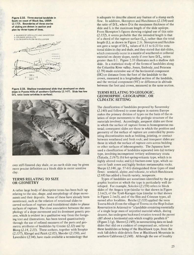
Figure 2.32. Three-storied landslide in Sochi on coast of Black Sea, USSR

(2.173). Boundaries of three Stories of sliding are shown in section and plan by three types of lines.

4 ELOCKS OF ARGILLITE AND SANDSTONE 5 CRUSHED AIDjILLITE 6 SLOW EARTH FLOW IN COLLUVIUM

32811

Figure 2.33. Shallow translational slide that developed on shaly slope in Puente Hills of southern California (2.147). Slide has low D/L ratio (note wrinkles in surface).

over stiff-fissured clay shale, or an earth slide may be given more precise definition as a block slide in moist sensitive clay.

TERMS RELATING TO SIZE OR GEOMETRY

A rather large body of descriptive terms has been built up relating to the size, shape, and morphology of slope move-nients and their deposits. Some of these have already been mentioned, such as the relation of rotational slides to curved surfaces of rupture and translational slides to planar surfaces of rupture. The close association between the mor-phology of a slope movement and its dominant genetic pro-cess, which is evident in a qualitative way from the forego-ing text and illustrations, has been tested quantitatively through the use of refined measures of the parts and geo-metric attributes of landslides by Crozier (232) and by Blong (2.14, 2.15). These authors, together with Snopko (2.157). Klengel and Paek (2,85), Shroder (2.150), and Laverdière (294), have made available a terminology that

is adequate to describe almost any feature of a slump earth now. In addition. Skempton and Hutchinson (2J54) used the ratio of D/L, where D is the maximum thickness of the slide and L is the maxiniurn length of the slide upslope. From Skempton's figures showing original use of this ratio (2.152), it seetns probable that the intended length is that of a chord of the rupture surface (La ), rather than the total length (L), as shown in Figure 2.1 t. Skempton and Hutchin-son gave a range of D/LC values of 0.15 to 0.33 for rota-tional slides in clay and shale, and they stated that slab slides, which commonly occur in a mantle of weathered or colluvial material on clayey slopes, rarely if ever have D/L, ratios greater than 0.1 - Figure 2.33 illustrates such a shallow slab slide. In a statistical study of the forms of landslides along the Columbia River valley, Jones, Embody, and Peterson (2. 79) made extensive use of the horizontal component (I-IC) or distance from the foot Of the landslide to the crown, measured in a longitudinal section of the landslide, and the vertical component (VC) or difference in altitude between the foot and crown, measured in the same section.

TERMS RELATING TO GEOLOGIC, GEOMORPHIC. GEOGRAPHIC, OR CLIMATIC SETTING

The classification of landslides proposed by Savarensky (2.140) and followed to some degree in eastern Europe makes the primary division of types on the basis of the re-lation of slope movements to the geologic structure of the materials iiivolved. Accordingly, asequent slides are those in which the surface of rupture forms in homogeneous ma-terial: consequent slides are those in which the position and geometry of the surface of rupture are controlled by preex-isting cliscontinuities such as bedding, jointing, or contact between weathered and fresh rock: and insequent slides are those in which the surface of rupture cuts across bedding or other surfaces of inhomogeneity. The Japanese have used a classification of landslides separated into (a) tertiary type, involving incompetent tertiary sedimentary strata (Takada, 2.167); (b) hot-spring-volcanic type, which is in highly altered rocks: and (c) fracture-zone type, which oc-curs in fault zones and highly broken metamorphic rocks. Sharpe (2i46. pp. 57-61) distinguished three types of mud flows: semiarid, alpine, and volcanic, to which 1-lutchinson (2.68) has added a fourth variety, temperate.

Types of landslides are sometimes identified by the geo-graphic location at which the type is particularly well de-veloped. For exaniple. Sokolov (2.159) refers to block slides of the Angara type (similar to that shown in Figure 2.1 m2), of the Tyub-Karagan type (similar to that shown in Figure 2.1 iii3), and of the Ilini and Crimean types, all named after localities. Reiche (2.133) applied the term Torcva-block (from the village of Toreva on the 1-lopi Indian Reservation in Arizona) to "a landslide consisting essentially of a single large mass of unjostled material which, during descent, has undergone backward rotation toward the parent cliff about a horizontal axis which roughly parallels it" (Figure 2.1 g). Shreve (2.149), in summarizing data on land-slides that slid on a cushion of compressed air, referred to these landslides as being of the Blackhawk type, from the rock fall-debris slide-debris flow at Blackhawk Mountain in southern California (2.148). Although the use of locality

25

terms may occasionally be a convenience, it is not recom-mended as a general practice, for the terms themselves are not informative to a reader who lacks knowledge of the locality.

TERMS RELATING TO AGE OR STATE OF ACTIVITY

Active slopes are those that are either currently moving or that are suspended, the latter term implying that they are not moving at the present time but have moved within the last cycle of seasons. Active slides are commonly fresh; that is, their morphological features, such as scarps and ridges, are easily recognizable as being due to gravitational movement, and they have not been significantly modified by surficial processes of weathering and erosion. However, in and regions, slides may retain a fresh appearance for many years.

Inactive slopes are those for which there is no evidence that movement has taken place within the last cycle of sea-sons. They may be dormant, in which the causes of failure remain and movement may be renewed, or they may be sta bilized, in which factors essential to movement have been removed naturally or by human activity. Slopes that have long-inactive movement are generally modified by erosion and weathering or may be covered with vegetation so that the evidence of the last movement is obscure. They are of-ten referred to as fossil (Záruba and Mend, 2.193; Klengel and Paek, 2.85; Nossin, 2.118) or ancient (Popov, 2.127) landslides in that they commonly have developed under dif ferent geomorphological and climatic conditions thousands or more years ago and cannot repeat themselves at present.

FORMING NAMES

The names applied to slope movements can be made pro-gressively more informative, as more data are obtained,by building up a designation from several descriptor words, each of which has a defined meaning. For example,a slow, moist, translational debris slab slide means material moving along a planar surface of a little-disturbed mass of frag-mented material having a D/LC ratio of 0.1 or less, contain-ing some water but none free, and moving at a rate between 1.5 rn/month and 1.5 rn/year (5 ft/month or year). Once all these particulars are established in the description, the movement could be referred to thereafter simply as a de-bris slide.

CAUSES OF SLIDING SLOPE MOVEMENTS

The processes involved in slides, as well as in other slope movements, comprise a continuous series of events from cause to effect. An engineer faced with a landslide is pri-marily interested in preventing the harmful effects of the slide. In many instances the principal cause of the slide cannot be removed, so it may be more economical to alle-viate the effects continually or intermittently without at-tempting to remove the cause. Some slides occur in a unique environment and may last only a few seconds. The damage can be repaired, and the cause may be of only academic in-terest unless legal actions are to be taken. More often, how-

ever, landslides take place under the influence of geologic, topographic, or climatic factors that are common to large areas. The causes must then be understood if other similar slides are to be avoided or controlled.

Seldom, if ever, can a landslide be.attributed to a single definite cause. As clearly shown by Zolotarev (2.196), the process leading to the development of the slide has its be-ginning with the formation of the rock itself, when its basic physical properties are determined, and includes all the sub-sequent events of crustal movements, erosion, and weather-ing. Finally, some action, perhaps trivial, sets a mass of material in motion downhill. The last action cannot be re-garded as the only cause, even though it was necessary in the chain of events. As Sowers and Sowers(2.161, p.506) point out,

In most cases a number of causes exist simultaneously and so attempting to decide which one finally produced failure is not only difficult but also incorrect. Often the final fac-tor is nothing more than a trigger that set in motion an earth mass that was already on the verge of failure. Calling the final factor the cause is like calling the match that lit the fuse that detonated the dynamite that destroyed the building the cause of the disaster.

In this connection, however, the determination of all the geologic causes of a landslide should not be confused with determination of legal responsibility. The interrelations of landslide causes are lucidly and graphically presented by Terzaghi (2.175). His work, that of Sharpe (2i46), Ladd (2.92), and Bendel (2.6), and that of more recent researchers, such as Ziruba and Mend (2.193), Skempton and Hutchin-son (2.154), Krinitzsky and Kolb (2.90), Rapp (2.131),and Legget (2.96) were used in the preparation of this section.

All slides involve the failure of earth materials under shear stress. The initiation of the process can therefore be reviewed according to (a) the factors that contribute to in-creased shear stress and (h) the factors that contribute to low or reduced shear strength. Although a single action, such as addition of water to a slope, may contribute to both an increase in stress and a decrease in strength, it is helpful to separate the various physical results of such an action. The principal factors contributing to the sliding of slope-forming materials are outlined in the following discussion. The operation of many factors is self-evident and needs no lengthy description; some factors are only discussed briefly, or reference is made to literature that gives examples or treats the subject in detail.

Factors That Contribute to Increased Shear Stress

Removal of Lateral Support

The removal of lateral support is the commonest of all fac-tors leading to instability, and it includes the following ac-tions:

1. Erosion by (a) streams and rivers, which produce most natural slopes that are subject to sliding (Hutchinson, 2.67; Jones, Embody, and Peterson, 2.79; Eyles, 2.43; Fleming, Spencer, and Banks, 2.48; California Division of

26

Highways, 2.19), (b) glaciers, which have deeply cut and oversteepened many valleys in mountainous regions that have been the sites of large slides and debris flows (Plafker, Ericksen, and Fernandez Concha, 2.126), (c) waves and longshore or tidal currents (Wood ,2.189; Ward, 2.186; Hutchinson, 2.71; Koppejan, Van Wamelon, and Weinberg, 2.89), and (d) subaerial weathering, wetting and drying, and frost action;

Previous rock fall, slide (Kenney and Drury, 2.81), subsidence, or large-scale faulting that create new slopes; and

Work of human agencies in which (a) cuts, quarries, pits, and canals (Van Rensburg, 2.181; Piteau, 2.124; Patton, 2J21; Cording, 2.26) are established, (b) retaining walls and sheet piling are removed, and (c) lakes and reser-voirs are created and their levels altered (Muller, 2.112; Jones, Embody, and Peterson, 2.79; Lane, 2.93; Dupree and Taucher, 2.39).

Surcharge

Surcharge also results from both natural and human agen-cies. The surcharge from natural agencies may be

Weight of rain, hail, snow, and water from springs; Accumulation of talus overriding landslide materials; Collapse of accumulated volcanic material, producing

avalanches and debris flows (Francis and others, 2.50); Vegetation (Gray, 2.53; Pain, 2.120); and Seepage pressures of percolating water.

The surcharge from human agencies may be

Construction of fill; Stockpiles of ore or rock; Waste piles (Bishop, 2.8; Davies, 2.35; Smalley, 2.156); Weight of buildings and other structures and trains;

and Weight of water from leaking pipelines, sewers,

canals, and reservoirs.

Transitory Earth Stresses

Earthquakes have triggered a great many landslides, both small and extremely large and disastrous. Their action is complex, involving both an increase in shear stress (hori-zontal accelerations may greatly modify the state of stress within slope-forming materials) and, in some instances, a decrease in shear strength (Seed, 2.143; Morton, 2.110; Solonenko, 2.160; Lawson, 2.95; Hansen, 2.57; Newmark, 2.117; Simonett, 2.151; Hadley, 2.55; Gubin, 2.54). Vi-brations from blasting, machinery, traffic, thunder, and ad-jacent slope failures also produce transitory earth stresses.

Regional Tilting

A progressive increase in the slope angle through regional tilting is suspected as contributing to some landslides (Terzaghi,2.175). The slope must obviously be on the point of failure for such a small and slow-acting change to be effective.

Removal of Underlying Support

Examples of removal of underlying support include

- Undercutting of banks by rivers (California Division of Highways, 2.19) and by waves;

Subaerial weathering, wetting and drying, and frost action;

Subterranean erosion in which soluble material, such as carbonates, salt, or gypsum is removed and granular ma-terial beneath firmer material is worked out (Ward, 2.186; Terzaghi, 2.1 74);

Mining and similar actions by human agencies; Loss of strength or failure in underlying material; and Squ.eezing out of underlying plastic material (Záruba

and Mend, 2.193, pp. 68-78).

Lateral Pressure

Lateral pressure may be caused by

Water in cracks and caverns, Freezing of water in cracks, Swelling as a result of hydration of clay or anhydrite,

and Mobilization of residual stress (Bjerrum, 2.9; Krinitzsky

and Kolb, 2.90).

Volcanic Processes

Stress patterns in volcanic edifices.and crater walls are mod-ified by general dilation due to inflation or deflation of magma chambers, fluctuation in lava-lake levels, and in-crease in harmonic tremors (Tilling, Koyanagi, and Holcomb, 2.178; Moore and Krivoy, 2.109; Fiske and Jackson, 2.47).

Factors That Contribute to Low or Reduced Shear Strength

The factors that contribute to low or reduced shear strength of rock or soil may be divided into two groups. The first group includes factors stemming from the initial state or in-herent characteristics of the material. They are part of the geologic setting that may be favorable to landslides, exhibit little or no change during the useful life of a structure, and may exist for a long period of time without failure. The second group includes the changing or variable factors that tend to lower the shear strength of the material.

Initial State

Factors in the initial state of the material that cause low shear strength are composition, texture, and gross structure and slope geometry.

Composition

Materials are inherently weak or may become weak upon change in water content or other changes. 'Included espe-cially are organic materials, sedimentary clays and shales, decomposed rocks, rocks of volcanic tuff that may weather to clayey material, and materials composed dominantly of soft platy minerals, such as mica, schist, talc, or serpentine.

Texture

The texture is a loose structure of individual particles in sensitive materials, such as clays, marl, bess, sands of low density, and porous organic matter (Aitchison, 2.2; Bjerrum and Kenney, 2.11 ; Cabrera and Smalley, 2.17). Roundness of grain influences strength as compressibility and internal friction increase with angularity.

Gross Structure and Slope Geometry

Included in gross structure and slope geometry are

Discontinuities, such as faults, bedding planes, folia-tion in schist, cleavage, joints, slickensides, and brecciated zones (Skempton and Petley, 2.155; Fookes and Wilson, 2.49; Komarnitskii, 2.88; St. John, Sowers, and Weaver, 2.138; Van Rensburg, 2.181; Jennings and Robertson, 2.74; Bjerrum and J$rstad, 2.10);

Massive beds over weak or plastic materials (Zãruba and Mend, 2.193; Nemok, 2.113);

Strata inclined toward free face; Alternation of permeable beds, such as sand or sand-

stone, and weak impermeable beds, such as clay or shale (Henkel, 2.59); and

Slope orientation (Rice, Corbett, and Bailey, 2.134; Shroder, 2.150).

Changes Due to Weathering and Other Physicochemical Reactions

The following changes can occur because of weathering and other physicochemical reactions:

Softening of fissured clays (Skempton,2.153; Sangrey and Paul, 2.139; Eden and Mitchell, 2.41);

Physical disintegration of granular rocks, such as granite or sandstone, under action of frost or by thermal expansion (Rapp, 2.131);

Hydration of clay minerals in which (a) water is ab. sorbed by clay minerals and high water contents decrease cohesion of all clayey soils, (b) montmorillonitic clays swell and lose cohesion, and (c) bess markedly consolidates upon saturation because of destruction of the clay bond between silt particles;

Base exchange in clays, i.e., influence of exchangeable ions on physical properties of clays (Sangrey and Paul, 2.139; Liebling and Kerr, 2.99; Torrance, 2.179);

Migration of water to weathering front under elec-trical potential (Veder, 2.184);

Drying of clays that results in cracks and loss of co-hesion and allows water to seep in;

Drying of shales that creates cracks on bedding and shear planes and reduces shale to chips, granules, or smaller particles; and

Removal of cement by solution.

Changes in Intergranular Forces Due to Water Content and Pressure in Pores and Fractures

Buoyancy in saturated state decreases effective intergranular

pressure and friction. Intergranular pressure due to capillary tension in moist soil is destroyed upon saturation. Simple softening due to water and suffusion and slaking are dis-cussed by Mamulea (2.101).

Changes can occur because of natural actions, such as rainfall and snowmelt, and because of a host of human ac-tivities, such as diversion of streams, blockage of drainage, irrigation and ponding, and clearing of vegetation and de- forestation. -

Crozier (2.30, 2.31), Shroder (2.150), and Spurek (2.163) discuss the general effect of climate; Temple and Rapp (2.169) Williams and Guy (2.188), Jones (2.78), and So (2.158), catastrophic rainfall; Conway (2.25), Denness (2.38), and Piteau (2.124), effect of groundwater; Gray (2.53), Bailey (2.4), Cleveland (2.22), Rice, Corbett, and Bailey (2.134), and Swanston (2.165), deforestation; Peck (2.123) and Hirao and Okubo (2.60), correlation of rainfall and movement;and Shreve (2.148), Voight (2.185), Kent (2.82), and Goguel and Pachoud (2.52), gaseous entrain-ment or cushion.

Changes in Structure

Changes in structure may be caused by fissuring of shales and preconsolidated clays and fracturing and loosening of rock slopes due to release of vertical or lateral restraints in valley walls or cuts (Bjerrum, 2.9; Aisenstein, 2.1; Ferguson, 2.45; Matheson and Thomson, 2.102; Mend, 2.106). Dis-turbance or remolding can affect the shear strength of ma-terials composed of fine particles, such as bess, dry or sat-urated loose sand, and sensitive clays (Gubin, 2.54; Youd, 2.191; Smalley, 2.156; Mitchell and Markell, 2.108).

Miscellaneous Causes

Other causes of low shear strength are (a) weakening due to progressive creep (Suklje, 2.164; Ter-Stepanian, 2.172; Trollope,2.180; Piteau,2.124) and actions of tree roots (Feld, 2.44) and burrowing animals.

REFERENCES

2.1 Aisenstcin, B. Some Additional Information About De- consolidation Fissures of Rock on Steep Slopes. Proc., 2nd Congress, International Society of Rock Mechanics, Belgrade, Vol. 3, 1970, pp. 37 1-376.

2.2 Aitchison, G. D. General Report on Structurally Un- stable Soils. Proc., 8th International Conference on Soil Mechanics and Foundation Engineering, Moscow, Vol. 3, 1973, pp. 161-1 90.

2.3 Andresen, A., and Bjerrum, L. Slides in Subaqueous Slopes in Loose Sand and Silt. In Marine Geotechnique (Richards, A. F., ed.), Univ. of Illinois Press, Urbana, 1967, pp. 221-239.

2.4 Bailey, R. G. Landslide Hazards Related to Land Use Planning in Teton National Forest, Northwest Wyoming. Intermountain Region, U.S. Forest Service, 1971, 131 pp.

2.5 Beck, A. C. Gravity Faulting as a Mechanism of Topo- graphic Adjustment. New Zealand Journal of Geology and Geophysics, Vol. 11, No. 1, 1967, pp. 191-1 99.

2.6 Bendel, L. lngenieurgeologie: Ein Handbuch fuer Studium und Praxis. Springer-Verlag, Vienna, Vol. 2, 1948, 832 pp.

2.7 Bishop, A. W. Progressive Failure, With Special Refer- ence to the Mechanism Causing It. Proc., Geotechnical Conference on Shear Strength Properties of Natural

28

Soils and Rocks, Norwegian Geotechnical Institute, Oslo, Vol. 2, 1967, pp. 142-150.

2.8 Bishop, A. W. The Stability of Tips and Spoil Heaps. Quarterly Journal of Engineering Geology, Vol. 6, No. 4, 1973, pp. 335-376.

2.9 Bjerrum, L. Progressive Failure in Slopes of Over- Consolidated Plastic Clay and Clay Shales. Journal of Soil Mechanics and Foundations Division, American Society of Civil Engineers, Vol. 93, No. SM5, 1967, pp. 3-49.

2.10 Bjerrum, L., and Jjrstad, F. A. Stability of Rock Slopes in Norway. Norwegian Geotechnical Institute, PubI. 79, 1968, pp. 1-11.

2.11 Bjerrum, L., and Kenney, T. C. Effect of Structure on the Shear Behavior of Normally Consolidated Quick Clays. Proc., Geotechnical Conference on Shear Strength Proper-ties of Natural Soils and Rocks, Oslo, Norwegian Geotech-nical Institute, Vol. 2, 1967, pp. 19-27.

2.12 Bjerrum, L., Lken, T., Heiberg, S., and Foster, R. A Field Study of Factors Responsible for Quick Clay Slides. Norwegian Geotechnical Institute, PubI. 85, 1971, pp. 17-26.

2.13 Blong, R. J. The Underthrust Slide: An Unusual Type of Mass Movement. Geografiska Annaler, Vol. 53A, No. 1, 1971, pp. 52-58.

2.14 Blong, R. J. A Numerical Classification of Selected Land- slides of the Debris Slide-Avalanche-Flow Type. Engineer-ing Geology, Vol. 7, No. 2, 1973, pp. 99-114.

2.15 Blong, R. J. Relationships Between Morphometric Attri- butes of Landslides. Zeitschrift fuer Geomorphologie, Supp. Band 18, 1973, pp. 66-77.

2.16 Bukovansky, M., RodrIquez, M. A., and Cedrôn, G. Three Rock Slides in Stratified and Jointed Rocks. Proc., 3rd Congress, International Society of Rock Mechanics, Denver, Vol. 2, Part B, 1974, pp. 854-85 8.

2.17 Cabrera, J. G., and Smalley, I. J. Quickclays as Products of Glacial Action: A New Approach to Their Nature, Geology, Distribution, and Geotechnical Properties. Engineering Geology, Vol. 7, No. 2, 1973, pp. 115-133.

2.18 Caldenius, C., and Lundstrom, R. The Landslide at Surte on the River Gta ilv. Sweden Geologiska undersdkningen, Series Ca, No. 27, 1955, 64 pp.

2.19 California Division of Highways. Bank and Shore Protec- tion in California Highway Practice. California Division of Highways, Sacramento, 1960, 423 pp.

2.20 Campbell, R. H. Soil Slips, Debris Flows, and Rainstorms in the Santa Monica Mountains and Vicinity, Southern California. U.S. Geological Survey, Professional Paper 851,1975,51 pp.

2.21 Carter, R. M. A Discussion and Classification of Sub- aqueous Mass-Transport With Particular Application to Grain-Flow, Slurry-Flow, and Fluxoturbidites. Earth-Science Reviews, Vol. 11,No. 2, 1975, pp. 145-177.

2.22 Cleveland, G. B. Fire + Rain = Mudflows: Big Sur 1972. California Geology, Vol. 26, No. 6, 1973, pp. 127-135.

2.23 Close, U., and McCormick, E. Where the Mountains Walked. National Geographic Magazine, Vol. 41, 1922, pp. 445-464.

2.24 Cluff, L. S. Peru Earthquake of May 31, 1970: Engi- neering Geology Observations. Seismological Society of America Bulletin, Vol. 61, No. 3,1971, pp. 511-521.

2.25 Conway, B. W. The Black Ven Landslip, Charmouth, Dorset. Institute of Geological Sciences, United King-dom, Rept. 74/3, 1974,4 pp.

2.26 Cording, E. J., ed. Stability of Rock Slopes. Proc., 13th Symposium on Rock Mechanics, Univ. of Illinois at Urbana-Champaign, American Society of Civil Engineers, New York, 1972, 912 pp.

2.27 Corte, A. E. Geocryology and Engineering. In Reviews in Engineering Geology (Varnes, D. J. and Kiersch, G. A., eds.), Geological Society of America, Vol. 2, 1969, pp. 119-185.

2.28 Coulter, H. W., and Migliaccio, R. R. Effects of the Earthquake of March 27, 1964, at Valdez, Alaska. U.S. Geological Survey, Professional Paper 542-C, 1966, 36 pp.

2.29 Crandell, D. R., and Fahnestock, R. K. Rockfalls and Avalanches From Little Tahoma Peak on Mount Rainier Volcano, Washington. U.S. Geological Survey, Bulletin 1221-A, 1965,30 pp.

2.30 Crozier, M. J. Earthfiow Occurrence During High Inten- sity Rainfall in Eastern Otago (New Zealand). Engineer- ing Geology, Vol. 3, No. 4, 1969, pp. 325-334.

2.31 Crozier, M. J. Some Problems in the Correlation of Landslide Movement and Climate. In International Geography, Proc., 22nd International Geographical Congress, Montreal, Univ. of Toronto Press, Ontario, Vol. 1, 1972, pp. 90-93.

2.32 Crozier, M. J. Techniques for the Morphometric Analy- sis of Landslips. Zeitschrift fuer Geomorphologie, Vol. 17, No. 1,1973, pp. 78-101.

2.33 Cruden, D. M., and Krahn, J. A Reexamination of the Geology of the Frank Slide. Canadian Geotechnical Journal, Vol. 10, No. 4, 1973, pp. 581-591.

2.34 Daido, A. On the Occurrence of Mud-Debris Flow. Bulletin of the Disaster Prevention Research Institute, Kyoto Univ., Japan, Vol. 21,Part 2, No. 187, 1971, pp. 109-1 35.

2.35 Davies, W. E. Coal Waste Bank Stability. Mining Con- gress Journal, Vol. 54, No. 7, 1968, pp. 19-24.

2.36 Deere, D. U., and Patton, F. D. Slope Stability in Resid- ual Soils. Proc., 4th Pan-American Conference on Soil Mechanics and Foundation Engineering, San Juan, American Society of Civil Engineers, New York, Vol. 1, 1971, pp. 87-170.

2.37 de Freitas, M. H., and Watters, R. J. Some Field Ex- amples of Toppling Failure. Geotechnique, Vol. 23, No. 4, 1973, pp. 495-514.

2.38 Denness, B. The Reservoir Principle of Mass Movement. Institute of Geological Sciences, United Kingdom, Rept. 72/7, 1972, 13 pp.

2.39 Dupree, H. K., and Taucher, G. J. Bighorn Reservoir Landslides, South-Central Montana. In Rock Mechanics, The American Northwest (Voight, B., ed.), Expedition Guide for 3rd Congress, International Society of Rock Mechanics, Denver, Pennsylvania State Univ., 1974, pp. 59-63.

2.40 Dylik, J. Solifluxion, Congelifluxion, and Related Slope Processes. Geografiska Annaler, Vol. 49A, No. 24, 1967, pp. 167-177.

2.41 Eden, W. J., and Mitchell, R. J. The Mechanics of Land- slides in Leda Clay. Canadian Geotechnical Journal, Vol. 7, No. 3, 1970, pp. 285-296.

2.42 Embleton, C., and King, C. A. M. Periglacial Geomor- phology. Wiley, New York, 1975, 203 pp.

2.43 Eyles, R. J. Mass Movement in Tangoio Conservation Reserve, Northern Hawke's Bay. Earth Science Journal, Vol.5, No. 2, 1971, pp. 79-91.

2.44 Feld, J. Discussion of Slope Stability in Residual Soils (Session 2). Proc., 4th Pan-American Conference on Soil Mechanics and Foundation Engineering, San Juan, American Society of Civil Engineers, New York, 1971, Vol. 3,p. 125.

2.45 Ferguson, H. F. Valley Stress Release in the Allegheny Plateau. Bulletin, Association of Engineering Geologists, Vol. 4, No. 1,1967, pp. 63-71.

2.46 Fisher, R. V. Features of Coarse-Grained, High- Concentration Fluids and Their Deposits. Journal of Sedimentary Petrology, Vol.41, No. 4, 1971, pp. 916-927.

2.47 Fiske, R. S., and Jackson, E. D. Orientation and Growth of Hawaiian Volcanic Rifts: The Effect of Regional Structure and Gravitational Stresses. Proc., Royal Society of London, Series A, Vol. 329, 1972, pp. 299-326.

2.48 Fleming, R. W., Spencer, G. S., and Banks, D. C. Empir- ical Study of Behavior of Clay Shale Slopes. U.S. Army Engineer Nuclear Cratering Group, Technical Rept. 15, Vols. 1 and 2, 1970, 397 pp.

2.49 Fookes, P. G., and Wilson, D. D. The Geometry of Dis- continuities and Slope Failures in Siwalik Clay. Geotech-nique, Vol. 16, No.4, 1966, pp. 305-320.

29

2.50 Francis, P. W., Roobol, M. J., Walker, G. P. L., Cobbold, Vol. 20, No. 4, 1970, pp.412-438. P. R., and Coward, M. The San Pedro and San Pablo Volca- 2.71 Hutchinson, J. N. The Response of London Clay Cliffs noes of Northern Chile and Their Hot Avalanche Deposits. to Differing Rates of Toe Erosion. Geologia Applicata Geologische Rundschau, Vol.63, No. 1,1974, pp.357-388. e ldrogeologia, Vol. 8, Part 1, 1973, pp. 221-239.

2.51 Frühlich, 0. K. General Theory of Stability of Slopes. 2.72 Hutchinson, J. N., and Bhandari, R. K. Undrained Load- Geotechnique, Vol. 5, No. 1, 1955, pp. 37-47. ing: A Fundamental Mechanism of Mudflows and Other

2.52 Goguel, J., and Pachoud, A. Gêologie et Dynamique de Mass Movements. Geotechnique, Vol. 21, No.4, 1971, l'écroulement du Mont Granier, dans le Massif de pp. 353-358. Chartreuse, en Novembre 1248. France Bureau de 2.73 Jahn, A. Slopes Morphological Features Resulting Recherches Géologiques et Minieres Bulletin, Section From Gravitation. Zeitschrift fuer Geomorphologie, 3—Hydrog6ologie-C6ologie de l'lngenieur, No. 1, 1972, Supp. Band 5, 1964, pp. 59-72. pp. 29-38. 2.74 Jennings, J. E., and Robertson, A. M. The Stability of

2.53 Gray, D. H. Effects of Forest Clear-Cutting on the Sta- Slopes Cut Into Natural Rock. Proc., 7th International bility of Natural Slopes. Bulletin, Association of Engi- Conference on Soil Mechanics and Foundations Engi- neering Geologists, Vol. 7, No. 1-2, 1970, pp. 45-66. neering, Mexico City, Vol. 2, 1969, pp. 585-590.

2.54 Gubin, I. Y. Regularity of Seismic Manifestations of 2.75 Johnson, A. M. Physical Processes in Geology. Freeman, the Tadzhikistana Territory. USSR Academy of Sciences, Cooper, and Co., San Francisco, 1970, 577 pp. Moscow, 1960, 463 pp. (in Russian). 2.76 Johnson, A. M., and Rahn, P. H. Mobilization of Debris

2.55 Hadley, J. B. Landslides and Related Phenomena Accom- Flows. Zeitschrift fuer Geomorphologie, Supp. Band 9, panying the Hebgen Lake Earthquake of August 17, 1959. 1970, pp. 168-186. U.S. Geological Survey, Professional Paper 435, 1964, pp. 2.77 Johnson, N. M., and Ragel, R. H. Analysis of Flow Char- 107-138. acteristics of Allen II Slide From Aerial Photographs. In

2.56 Hamel, J. V. Kimbley Pit Slope Failure. Proc., 4th Pan- The Great Alaska Earthquake of 1964: Hydrology, Na- American Conference on Soil Mechanics and Foundation tional Academy of Sciences, Washington, D.C., 1968, pp. Engineering, San Juan, American Society of Civil Engi- 369-373. neers, New York, Vol. 2, 1971, pp. 117-1 27. 2.78 Jones, F. 0. Landslides of Rio de Janeiro and the Serra

2.57 Hansen, W. R. Effects of the Earthquake of March 27, das Araras Escarpment, Brazil. U.S. Geological Survey, 1964, at Anchorage, Alaska. U.S. Geological Survey, Professional Paper 697, 1973,42 pp. Professional Paper 542-A, 1965,68 pp. 2.79 Jones, F. 0., Embody, D. R., and Peterson, W. L. Land-

2.58 Heim, A. Bergsturz und Menschenleben. Fretz and slides Along the Columbia River Valley, Northeastern Wasmuth Verlag, Zurich, 1932, 218 pp. Washington. U.S. Geological Survey, Professional Paper

2.59 Henkel, D. J. Local Geology and the Stability of Natu- 367, 1961,98 pp. ral Slopes. Journal of Soil Mechanics and Foundations 2.80 Jordan, R. H. A Florida Landslide. Journal of Geology, Division, American Society of Civil Engineers, Vol. 93, Vol. 57, No. 4, 1949, pp. 418419. No. SM4, 1967, pp. 437446. 2.81 Kenney, T. C., and Drury, P. Case Record of the Slope

2.60 Hirao, K., and Okubo, S. Studies on the Occurrence and Failure That Initiated the Retrogressive Quick-Clay Land- Expansion of Landslides Caused by Ebino-Yoshimatsu slide at Ullensaker, Norway. Geotechnique, Vol. 23, No. Earthquake. Report of Cooperative Research for Disas- 1, 1973, pp. 3347. ter Prevention, Japan Science and Technology Agency, 2.82 Kent, P. E. The Transport Mechanism in Catastrophic No. 26, 1971, pp. 157-189 (in Japanese with Engiish Rock Falls. Journal of Geology, Vol. 74, No. 1, 1966, summary). pp. 79-83.

2.61 Hoek, E. Recent Rock Slope Stability Research of the 2.83 Kesseli, J. E. Disintegrating Soil Slips of the Coast Ranges Royal School of Mines, London. Proc., 2nd Interna- of Central California. Journal of Geology, Vol. 51, No. 5, tional Conference on Stability in Open Pit Mining, Van- 1943, pp. 342-352. couver, 1971, Society of Mining Engineers, American 2.84 Kjellman, W. Mechanics of Large Swedish Landslips. Geo- Institute of Mining, Metallurgical and Petroleum Engi- technique, Vol. 5, No. 1, 1955, pp. 74.78. neers, New York, 1972, pp. 23-46. 2.85 Klengel, K. J., and Paek, J. Zur Terminologie von

2.62 Hofmann, H. The Deformation Process of a Regularly Hangbewegungen. Zeitschrift fuer Angewandte Geologie, Jointed Discontinuum During Excavation of a Cut. Vol. 20, No. 3,1974, pp. 128.132. Proc., 2nd Congress, International Society of Rock 2.86 Knapp, G. L., ed. Avalanches, Including Debris Avalanches: Mechanics, Belgrade, Vol. 3, 1970, pp. 267-273 (in A Bibliography. Water Resources Scientific Information German). Center, U.S. Department of the Interior, WRSIC 72-216,

2.63 Hofmann, H. Modellversuche zur Hangtektonik. 1972, 87 pp. Geologische Rundschau, Vol. 62, No. 1, 1973, pp. 16-29. 2.87 Kojan, E., Foggin, G. T.,III, and Rice, R. M. Prediction

2.64 Hollingworth, S. E., and Taylor, J. H. An Outline of the and Analysis of Debris Slide Incidence by Photogram- Geology of the Kettering District. Proc., Geologists' As- metry: Santa-Ynez-San Rafael Mountains, California. sociation, Vol. 57, 1946, pp. 204-233. Proc., 24th International Geological Congress, Montreal,

2.65 Hollingworth, S. E., and Taylor, J. H. The Northampton Section 13—Engineering Geology, 1972, pp. 124-131. Sand Ironstone: Stratigraphy, Structure, and Reserves. 2.88 Komarnitskli, N. I. Zones and Planes of Weakness in U.K. Geological Survey, Memoirs, 1951, 211 pp. Rocks and Slope Stability. Consultants Bureau, New

2.66 Hsu, K. J. Catastrophic Debris Streams (Sturzstroms) York, 1968, 108 pp. (translated from Russian). Generated by Rockfalls. Geological Society of America 2.89 Koppejan, A. W., Van Wamelon, B. M., and Weinberg, Bulletin, Vol. 86, No. 1, 1975, pp. 129-140. L. J. H. Coastal Flow Slides in the Dutch Province of

2.67 Hutchinson, J. N. The Free Degradation of London Zeeland. Proc., 2nd International Conference on Soil Clay Cliffs. Proc., Geotechnical Conference on Shear Mechanics and Foundations Engineering, Rotterdam, Strength Properties of Natural Soilsand Rocks, Nor- Vol. 5, 1948, pp. 89-96. wegian Geotechnical Institute, Olso, Vol. 1, 1967, pp. 2.90 Krinitzsky, E. L., and Kolb,C. R. Geological Influences 113-118. on the Stability of Clay Shale Slopes. Proc., 7th Sympo-

2.68 Hutchinson, J. N. Mass Movement. In The Encyclo- sium on Engineering Geology and Soils Engineering, pedia of Geomorphology (Fairbridge, R. W., ed.), Moscow, Idaho, Idaho Department of Highways, Univ. Reinhold Book Corp., New York, 1968, pp. 688-696. of Idaho, and Idaho State Univ., 1969, pp. 160-175.

2.69 Hutchinson, J. N. Field Meeting on the Coastal Land- 2.91 Kurdin, R. D. Classification of Mudflows: Soviet Hy- slides of Kent, 1-3 July, 1966. Proc., Geologists' Asso- drology, Vol. 12, No. 4, 1973, pp. 310-316. ciation, Vol. 79, Part 2, 1968, pp. 227-237. 2.92 Ladd, G. E. Landslides, Subsidences, and Rockfalls.

2.70 Hutchinson, J. N. A Coastal Mudflow on the London Proc., American Railway Engineering Association, Vol. Clay Cliffs at Beltinge, North Kent. Geotechnique, 36, 1935, pp. 1091-1162.

30

2,93 Lane, K. S. Stability of Reservoir Slopes. In Failure and Breakage of Rock (Fairhurst, C., ed.), Proc., 8th Symposium on Rock Mechanics, American Institute of Mining, Metallurgy and Petroleum Engineers, New York, 1967, pp. 321-336.

2.94 Laverdiêre, C. Quick Clay Flow-Slides in Southern Quebec. Revue de Geographie de Montreal, Vol. 26, No. 2, 1972, pp. 193-198 (French-English vocabulary).

2.95 Lawson, A. C. The California Earthquake of April 18, 1906: Landslides. Carnegie Institute of Washington, Washington, D.C., Vol. 1, Part 1, 1908, reprinted 1969, pp. 384-401.

2.96 Legget, R. F. Geology and Engineering. McGraw-Hill, New York, 2nd Ed., 1962, 884 pp.

2.97 Leighton, F. B. Landslides and Hillside Development. In Engineering Geology in Southern California, Association of Engineering Geologists, Special PubI., 1966, pp. 149-207.

2.98 Lemke, R. W. Effects of the Earthquake of March 27, 1964, at Seward, Alaska. U.S. Geological Survey, Pro-fessional Paper 542-E, 1966,43 pp.

2.99 Liebling, R. S., and Kerr, P. F. Observations on Quick Clay. Geological Society of America Bulletin, Vol. 76, No. 8, 1965, pp. 853-878.

2.100 La, K. Y. An Approach to the Problem of Progressive Failure. Canadian Geotechnical Journal, Vol. 9, No. 4, 1972, pp. 407-429.

2.101 Maniulea, M. A. Suffusion and Slaking: Physical Pro- cesses Prompting the Mass Movements. Bulletin, Inter-national Association of Engineering Geologists, No. 9, 1974, pp. 63-68 (in French with English summary).

2.102 Matheson, D. S., and Thomson, S. Geological Implica- tions of Valley Rebound. Canadian Journal of Earth Sciences, Vol. 10, No. 6, 1973, pp. 961-978.

2.103 McConnell, R. G., and Brock, R. W. The Great Land- slide at Frank, Alberta. In Annual Report of the Canada Department of the Interior for the year 1902-03, Sessional Paper 25, 1904, pp. 1-17.

2.104 McRoberts, E. C., and Morgenstern, N. R. Stability of Thawing Slopes. Canadian Geotechnical Journal, Vol. 11, No.4, 1974, pp.447-469.

2.105 McRoberts, E. C., and Morgenstern, N. R. The Stability of Slopes in Frozen Soil: Mackenzie Valley, N.W.T. Canadian Geotechnical Journal, Vol. 11, No.4, 1974, pp. 554-573.

2.106 Mend, V. EngineeringGeological Importance and Pos- sible Origin of the Stress Relief of the Rocks of the Cordillera Blanca, Peru. Bulletin, International Associa-tion of Engineering Geologists, No. 9, 1974, pp. 69-74.

2.107 Miller, W. J. The Landslide at Point Fermin, California. Scientific Monthly, Vol. 32, No. 5, 1931, pp. 464-469.

2.108 Mitchell, R. J., and Markell, A. R. Flowsliding in Sensi- tive Soils. Canadian Geotechnical Journal, Vol. 11, No. 1, 1974, pp. 11-31.

2.109 Moore, J. G., and Krivoy, H. L. The 1962 Flank Erup- tion of Kilauea Volcano and Structure of the East Rift Zone. Journal of Geophysical Research, Vol. 69, No. 10, 1964, pp. 2033-2045.

2.110 Morton, D. M. Seismically Triggered Landslides in the Area Above the San Fernando Valley. In The San Fer-nando, California, Earthquake of February 9, 1971, U.S. Geological Survey, Professional Paper 733, 1971, pp. 99-104.

2.111 National Research Council, Canada, and National Re- search Council, U.S. North American Contribution to 2nd International Conference on Permafrost, Yakutsk, USSR, July 1973. National Academy of Sciences, Wash-ington, D.C. 1973, 783 pp.

2.112 Muller, L. New Considerations on the Vaiont Slide. Felsmechanik und Ingenieur Geologie, Vol. 6, No. 1-2, 1968, pp. 1-91.

2.113 Nemöok, A. The Development of Landslides on the Boundaries of Geological Formations. Sbornik Geologick'ch véd, Rada HIG, No. 5, 1966, pp. 87-105 (in Slovak with English summary).

2.114 Nemêok, A. Gravitational Slope Deformation' in 'High

Mountains. Proc., 24th International Geological Con-gress, Montreal, Section 13-Engineering Geology, 1972, pp. 132-141.

2.115 Nemok, A. Gravitational Slope Deformations in the High Mountains of the Slovak Carpathians. Sbornik Geologickch véd, Rada HIG, No. 10, 1972, pp. 31-37.

2.116 Nemëok, A., Pasek, J., and Rybâ, J. Classification of Landslides and Other Mass Movements. Rock Mechanics, Vol.4, No. 2, 1972, pp. 71-78.

2.117 Newmark, N. M. Effects of Earthquakes on Dams and Embankments. Geotechnique, Vol. 15, No. 2, 1965, pp. 139-159.

2.118 Nossin, J. J. Landsliding in the Crati Basin, Calabria, Italy, Geologie en Mijnbouw, Vol.51, No. 6, 1972, pp. 591-607.

2.119 Ostaficzuk, S. Large-Scale Landslides in Northwestern Libya. Acta Geologica Polonica, Vol. 23, No. 2, 1973, pp. 231-244.

2.120 Pain, C. F. Characteristics and Geomorphic Effects of Earthquake-Initiated Landslides in the Adelbert Range, Papua New Guinea. Engineering Geology, Vol. 6, No. 4,1972, pp. 261-274.

2.121 Patton, F. D. Significant Geologic Factors in Rock Slope Stability. In Planning Open Pit Mines (Van Rensburg, P. W. J., ed.), Proc., Open Pit Mining Symposium, Johan-nesburg, South African Institute of Mining and Metallurgy, 1970, pp. 143-151.

2.122 Pautre, A., Sabarly, F., and Schneider, B. L'effet d'echelle dans les 6croulements de falaise. Proc., 3rd Congress, International Society of Rock Mechanics, Denver, Vol. 2, Part B, 1974, pp. 859-864.

2.123 Peck, R. B. Stability of Natural Slopes. Journal of Soil Mechanics and Foundations Division, American Society of Civil Engineers, New York, Vol. 93, SM4, 1967, pp. 403-417.

2.124 Piteau, D R. Geological Factors Significant to the Sta- bility of Slopes Cut in Rock. In Planning Open Pit Mines (Van Rensburg, P. W. J., ed.), Proc., Open Pit Mining Symposium, Johannesburg, South African Insti-tute of Mining and Metallurgy, 1970, pp. 33-5 3.

2.125 Piteau, D. R., Parkes, D. R., McLeod, B. C., and Lou, J. K. Overturning Rock Slope Failure at Hell's Gate, British Columbia. In Geology and Mechanics of Rock-slides and Avalanches (Voight, B., ed.), Elsevier, New York (in press).

2.126 Plafker, G., Ericksen, G. E., and Fernandez Concha, J. Geological Aspects of the May 31, 1970, Peru Earth-quake. Seismological Society of America Bulletin, Vol.. 61, No. 3, 1971, pp. 543-578.

2.127 Popov, I. V. A Scheme for the Natural Classification of Landslides. Doklady of the USSR Academy of Sciences, Vol. 54, No. 2, 1946, pp. 157-159.

2.128 Prior, D. B., Stephens, N., and Archer, D. R. Composite Mudflows on the Antrim Coast of Northeast Ireland. Geografiska Annaler, Vol. 50A, No. 2, 1968, pp. 65-78.

2.129 Prior, D. B., Stephens, N., and Douglas, G. R. Some Examples of Modern Debris Flows in Northeast Ireland. Zeitschrift fuer Geomorphologie, Vol. 14, No. 3, 1970, pp. 276-288.

2.130 Radbruch-Hall, D. H. Large-Scale Gravitational Creep of Rock Masses on Slopes. In Geology and Mechanics of Rockslides and Avalanches (Voight, B., ed.), Elsevier, New York (in press).

2.131 Rapp, A. Recent Development of Mountain Slopes in Kärkevagge and Surroundings, Northern Scandinavia. Geografiska Annaler, Vol. 42, No. 2-3, 1960, pp. 71-199.

2.132 Rapp, A. The Debris Slides at Ulvda1, Western Norway: An Example of Catastrophic Slope Processes in Scandi-navia. Nachrichten der Akademie der Wissenschaften Gottingen, Mathematisch-Physikalische Klasse, Vol. 13, 1963, pp. 195-210.

2.133 Reiche, P. The Toreva-Block: A Distinctive Landslide Type. Journal of Geology, Vol. 45, No. 5, 1937, pp. 538-548.

31

2.134 Rice, R. M., Corbett, E. S., and Bailey, R. G. Soil Slips Soils and Rocks, Norwegian Geotechnical Institute, Oslo, Related to Vegetation, Topography, and Soil in Southern Vol. 2, 1967, pp. 2946. California. Water Resources Research, Vol. 5, No. 3, 2.156 Smalley, I. J. Boundary Conditions for Flowslides in Fine- 1969, pp. 647-659. Particle Mine Waste Tips. Trans., Institution of Mining

2.135 Romani, F., Lovell, C. W., Jr., and Hair, M. E. Influence and Metallurgy, London, Vol. 81, Sec. A, 1972, pp. A31- of Progressive Failure on Slope Stability. Journal of Soil A37. Mechanics and Foundations Division, American Society 2.157 Snopko, L. Study of Deformation Elements Developed of Civil Engineers, New York, Vol. 98, No. SM1 1, 1972, in the Handlova Landslide. Geologickê Pracê, Vol. 28, pp. 1209-1223. No. 28, 1963, pp. 169-183.

2.136 Rybâ, J. Slope Deformations in Brown Coal Basins Un- 2.158 So, C. L. Mass Movements Associated With the Rain- der the Influence of Tectonics. Rock Mechanics, Vol. 3, storm of June 1966 in Hong Kong. Trans., Institute of No. 3, 1971, pp. 139-158 (in German with English sum- British Geographers, No. 53, 1971, pp. 55-65. mary). 2.159 Sokolov, N. I. Types of Displacement in Hard Frac-

2.137 Rybái, J., and Dobr, J. Fold Deformations in the North- tured Rocks on Slopes. In The Stability of Slopes Bohemian Coal Basins. Sbornik geologickch véd, Rada (Popov, I. V., and Kotlov, F. V., eds.), Trans., F. P. HIG, No. 5, 1966, pp. 133-140. Savarenskii Hydrogeology Laboratory, Vol. 35, 1963,

2.138 St. John, B. J., Sowers, G. F., and Weaver, C. E. Slicken- pp. 69-83; Consultants Bureau, New York (translated sides in Residual Soils and Their Engineering Significance. from Russian). Proc., 7th International Conference on Soil Mechanics 2.160 Solonenko, V. P. Seismogenic Destruction of Mountain and Foundation Engineering, Mexico City, Vol. 2, 1969, Slopes. Proc., 24th International Geological Congress, pp.591-597. Montreal, Section 13-Engineering Geology, 1972, pp.

2.139 Sangrey, D. A., and Paul, M. J. A Regional Study of Land- 284-290. sliding Near Ottawa. Canadian Geotechnical Journal, Vol. 2.161 Sowers, G. B., and Sowers, G. F. Introductory Soil 8, No. 2, 1971, pp. 315-335. Mechanics and Foundations. Macmillan, New York,

2.140 Savarensky, F. P. Experimental Construction of a Land- 3rd Ed., 1970,556 pp. slide Classification. Geologo-Razvedochnyi Institut 2.162 Sowers, G. F. Landslides in Weathered Volcanics in (TSNIGRI), 1935, pp. 29-37 (in Russian). Puerto Rico. Proc., 4th Pan-American Conference on

2.141 Scott, K. M. Origin and Sedimentology of 1969 Debris Soil Mechanics and Foundation Engineering, San Juan, Flows Near Glendora, California. U.S. Geological Sur- American Society of Civil Engineers, New York, 1971, vey, Professional Paper 750-C, 1971, pp. C242-C247. pp. 105-115.

2.142 Scott, R. C., Jr. The Geomorphic Significance of De- 2.163 Spirek, M. Retrospective Analysis of the Climatic Slid- bris Avalanching in the Appalachian Blue Ridge Moun- ing Agent. Sbornik Geologickch véd, Rada HIG, No. tains. Univ. of Georgia, PhD dissertation, 1972; Uni- 7, 1970, pp. 61-79 (in Czech with English summary). versity Microfilms, Ann Arbor, Mich. 2.164 Sukljc, L. A Landslide Due to Long-Term Creep. Proc.,

2.143 Seed, H. B. Landslides During Earthquakes Due to Soil 5th International Conference on Soil Mechanics and Liquefaction. Journal of Soil Mechanics and Founda- Foundation Engineering, Paris, Vol. 2, 1961, pp. 727- tions Division, American Society of Civil Engineers, New 735. York, Vol. 94, No. SMS, 1968, pp. 1053-1122. 2.165 Swanston, D. N. Slope Stability Problems Associated

2.144 Seed, H. B., and Wilson, S. D. The Turnagain Heights With Timber Harvesting in Mountainous Regions of the Landslide, Anchorage, Alaska. Journal of Soil Mechan- Western United States. U.S. Forest Service, General ics and Foundations Division, American Society of Civil Technical Rept. PNW-21, 1974, 14 pp. Engineers, Vol. 93, No. SM4, 1967, pp. 325-353. 2.166 Tabor, R. W. Origin of Ridge-Top Depressions by Large-

2.145 Sharp, R. P. Mass Movements on Mars. In Geology, Scale Creep in the Olympic Mountains, Washington. Seismicity, and Environmental Impact, Association of Geological Society of America Bulletin, Vol. 82, 1971, Engineering Geologists, Special PubI., 1973, pp. 115- pp. 1811-1822. 122. 2.167 Takada, Y. On the Landslide Mechanism of the Ter-

2.146 Sharpe, C. F. S. Landslides and Related Phenomena: tiary Type Landslide in the Thaw Time. Bulletin of the A Study of Mass Movements of Soil and Rock. Colum- Disaster Prevention Research Institute, Kyoto Univ., bia Univ. Press, New York, 1938, 137 pp. Japan, Vol. 14, Part 1, 1964, pp. 11-21.

2.147 Shelton, J. S. Geology Illustrated. W. H. Freeman and 2.168 Tavenas, F., Chagnon, J. Y., and La Rochelle, P. The Co., San Francisco, 1966, 434 pp. Saint-Jean-Vianney Landslide: Observations and Eye-

2.148 Shreve, R. L. The Blackhawk Landslide. Geological witnesses Accounts. Canadian Geotechnical Journal, Society of America, Memoir 108, 1968,47 pp. Vol. 8, No. 3, 1971, pp. 463478.

2.149 Shreve, R. L. Sherman Landslide. In The Great Alaska 2.169 Temple, P. H., and Rapp, A. Landslides in the Mgeta Earthquake of 1964: Hydrology. National Academy of Area, Western Uluguru Mountains, Tanzania. Geografiska Sciences, 1968, pp. 395-401. Annaler, Vol. 54A, No. 34, 1972, pp. 157-193.

2.150 Shroder, J. F. Landslides of Utah. Utah Geological and 2.170 Ter-Stepanian, G. On the Long-Term Stability of Slopes. Mineralogical Survey Bulletin, No. 90, 1971,51 pp. Norwegian Geotechnical Institute, PubI. 52, 1963, 14 pp.

2.151 Simonett, D. S. Landslide Distribution and Earthquakes 2.171 Ter-Stepanian, G. The Use of Observations of Slope in the Bewani and Toricelli Mountains, New Guinea: Sta- Deformation for Analysis of Mechanism of Landslides: tistical Analysis. In Landform Studies From Australia Problems of Geomechanics. Trans., Department of and New Guinea (Jennings, J. N., and Mabbutt, J. A., eds.), Geomechanics, Armenian SSR Academy of Sciences, Cambridge Univ. Press, 1967, pp. 64-84. No. 1, 1967, pp. 32-51.

2.152 Skempton, A. W. Soil Mechanics in Relation to Geology. 2.172 Ter-Stepanian, G. Depth Creep of Slopes. Bulletin, Proc., Yorkshire Geological Society, Vol. 29, Part 1,1953, International Society of Engineering Geologists, No. pp. 33-62. 9, 1974, pp. 97-102.

2.153 Skempton, A. W. Long-Term Stability of Clay Slopes. 2.173 Ter-Stcpanian,G.,and Goldstein, M. N. Multi-Storied Geotechnique, Vol. 14, No. 2, 1964, pp. 77-101. Landslides and Strength of Soft Clays. Proc., 7th In-

2.154 Skempton, A. W., and Hutchinson,J. N. Stability of Nat- ternational Conference on Soil Mechanics and Founda- ural Slopes and Embankment Foundations. Proc., 7th In- tion Engineering, Mexico City, Vol. 2, 1969, pp. 693- ternational Conference on Soil Mechanics and Founda- 700. don Engineering, Mexico City, State-of-the Art Vol., 2.174 Terzaghi, K. Earth Slips and Subsidences From Under- 1969, pp. 291-340. ground Erosion. Engineering News-Record, Vol. 107,

2.155 Skempton, A. W., and Petley, D. J. The Strength Along July 16, 1931, pp. 90-92. Structural Discontinuities in Stiff Clays. Proc., Geotech- 2.175 Terzaghi, K. Mechanism of Landslides. In Application nical Conference on Shear Strength Properties of Natural of Geology to Engineering Practice (Paige, S., ed.),

32

Geological Society of America, Berkey Vol., 1950, pp. 83-1 23.

2.176 Terzaghi, K., andpeck, R. B. Soil Mechanics in Engi- neering Practice. Wiley, New York, 2nd Ed., 1967, 729 pp.

2.177 Thomson, S., and Hayley, D. W. The Little Smoky Landslide. Canadian Geotechnical Journal, Vol. 12, No. 3, 1975, pp. 379-392.

2.178 Tilling, R. I., Koyanagi, R. Y., and Holcomb, R. T. Rockfall-Seismicity: Correlation With Field Observa-tions, Makaopuhi Crater, Kilauea Volcano, Hawaii. U.S. Geological Survey, Journal of Research, Vol. 3, No. 3, 1975, pp. 345-361.

2.179 Torrance, J. K. On the Role of Chemistry in the De- velopment and Behavior of the Sensitive Marine Clays of Canada and Scandinavia. Canadian Geotechnical Journal, Vol. 12, No. 3,1975, pp. 326-335.

2.180 Trollope, D. H. Sequential Failure in Strain-Softening Soils. Proc., 8th International Conference on Soil Me-chanics and Foundation Engineering, Moscow, Vol. 2, Part 2, 1973, pp. 227-232.

2.181 Van Rensburg, P. W. J., ed. Planning Open Pit Mines. Proc., Open Pit Mining Symposium, Johannesburg, South African Institute of Mining and Metallurgy, 1971, 388 pp.

2.182 Varnes, D. J. Landslide Types and Processes. In Land- slides and Engineering Practice (Eckel, E. B., ed.), HRB, Special Rept. 29, 1958, pp. 20-47.

2.183 Varnes, H. D. Landslide Problems of Southwestern Colorado. U.S. Geological Survey, Circular 31, 1949, 13 pp.

2.184 Veder, C. Phenomena of the Contact of Soil Mechan- ics. International Symposium on Landslide Control, Kyoto and Tokyo, Japan Society of Landslide, 1972, pp. 143-1 62 (in English and Japanese).

2.185 Voight, B. Architecture and Mechanics of the Heart Mountain and South Fork Rockslides. In Rock Mechan-ics, The American Northwest (Voight, B., ed.), Expedi-tion Guide, 3rd Congress of the International Society of Rock Mechanics, Pennsylvania State Univ., 1974, pp. 26-36.

2.186 Ward, W. H. The Stability of Natural Slopes. Geograph- ical Journal, Vol. 105, No. 5-6, 1945, pp. 170-1 91.

2.187 Washburn, A. L. Periglacial Processes and Environments. St. Martin's Press, New York, 1973, 320 pp.

2.188 Williams, G. P. and Guy, H. P. Erosional and Deposi- tional Aspects of Hurricane Camille in Virginia, 1969. U.S. Geological Survey, Professional Paper 804, 1973,

80 pp.

2.189 Wood, A. M. Engineering Aspects of Coastal Landslides. Proc., Institution of Civil Engineers, London, Vol. 50, 1971, pp. 257-276.

2.190 Yemel'ianova, Ye. P. Fundamental Regularities of Land- slide Processes. Nedra, Moscow, 1972, 308 pp. (excerpts translated by D. B. Vitaliano for U.S. Geological Survey).

2.191 Youd, T. L. Liquefaction, Flow, and Associated Ground Failure. U.S. Geological Survey, Circular 688, 1973, 12 pp.

2.192 Zâruba, Q. Periglacial Phenomena in the Turnov Region. Sbornik UstednIho Ustavu Geologického, Vol. 19, 1952, pp. 157-168 (in Czech with English and Russian sum-maries).

2.193 Zâruba, Q., and Mend, V. Landslides and Their Control. Elsevier, New York, and Academia, Prague, 1969, 205 pp.

2.194 Zischinsky, U. On the Deformation of High Slopes. Proc., 1st Congress, International Society of Rock Me-chanics, Lisbon, Vol. 2, 1966, pp. 179-1 85.

2.195 Zischinsky, U. Uber Bergzerreissung und Talzuschub. Geologische Rundschau, Vol. 58, No. 3, 1969, pp. 974-983

2.196 Zolotarev, G. S. Geological Regularities of the Develop-

ment of Landslides and Rockfalls as the Basis for the Theory of Their Study and Prognosis. Géologie de l'Ingénieur, Societe Géologique de Beligique, Liege, 1974, pp. 211-235.

BIBLIOGRAPHIES

2.1 Collins, T. Bibliography of Recent Publications on Slope Stability. Landslide, The Slope Stability Review, Vol. 1, No. 1, 1973, pp. 28-37.

2.2 Fisher, C. P., Leith, C. J., and Deal, C. S. An Annotated Bibliography on Slope Stability and Related Phenomena. North Carolina State Highway Commission and U.S. Bureau of Public Roads, 1965, 89 pp; NTIS, Springfield, Va., PB 173 029.

2.3 Hoek, E. Bibliography on Slope Stability. In Planning Open Pit Mines (Van Rensburg, P. W. J., ed.), Proc., Open Pit Mining Symposium, Johannesburg, South African In-stitute of Mining and Metallurgy, 1971, pp. 365-388.

2.4 Holtz, W. G. Bibliography on Landslides and Mudslides. Building Research Advisory Board, National Academy of Sciences, Washington, D.C., 1973.

2.5 Knapp, G. L., ed. Avalanches, Including Debris Ava- lanches: A Bibliography. Water Resources Scientific In-formation Center, U.S. Department of the Interior, WRSIC 72-216, 1972, 87 pp.

2.6 Larew, H. G., and others. Bibliography on Earth Move- ment. Research Laboratory for Engineering Science, Univ. of Virginia, Charlottesville, 1964, 239 pp.; NTIS, Springfield, Va., AD 641 716.

2.7 Spurek, M. Historical Catalogue of Slide Phenomena. Institute of Geography, Czechoslovak Academy of Sciences, Brno, StudiaGeographica 19, 1972, 178 pp.

2.8 Tompkin, J. M., and Britt, S. H. Landslides: A Selected Annotated Bibliography. HRB, Bibliography 10, 1951, 47 pp.

2.9 Záruba, Q., and Mend, V. Landslides and Their Control: Bibliography. Elsevicr, New York, and Academia, Prague, 1969, pp. 194-202.

PHOTOGRAPH AND DRAWING CREDITS

Figure 2.3 Courtesy of U.S. Bureau of Reclamation Figure 2.7 F. 0. Jones, U.S. Geological Survey Figure 2.8 F. 0. Jones, U.S. Geological Survey Figure 2.9 Courtesy of Tennessee Department of Transportation Figure 2.11 Courtesy of Tennessee Department of Transportation Figure 2.15 John S. Shelton Figure 2.17 Courtesy of New Hampshire Department of Public

Works and Highways Figure 2.19 Courtesy of Journal of Geology Figure 2.20 F. 0. Jones, U.S. Geological Survey Figure 2.21 0. Jones, U.S. Geological Survey Figure 2.22 K. Gilbert, U.S. Geological Survey Figure 2.23 John S. Shelton Figure 2.24 F. 0. Jones, U.S. Geological Survey Figure 2.25 F. 0. Jones, U.S. Geological Survey Figure 2.26 F. 0. Jones, U.S. Geological Survey Figure 2.28 From Geology Illustrated by John S. Shelton (2.147),

W. H. Freeman and Company, copyright 1966 Figure 2.29 From the Encyclopedia of Geomorphology, edited by

R. W. Fairbridge, copyright 1968 by Litton Educa- tional Publishing, Inc., reprinted by permission of Van Nostrand Reinhold Company

Figure 2.33 From Geology Illustrated by John S. Shelton (2.147), W. H. Freeman and Company, copyright 1966

33

Chapter 3

Recognition and Identif ication Harold T. Rib and Ta Liang

The adage that half the solution to a problem is the recogni-tion that a problem exists is especially appropriate to land-slides. The recognition of the presence or the potential de-velopment of slope movement and the identification of the type and causes of the movement are important in the de-velopment of procedures for-the prevention or correction of a slide.

Several basic guidelines developed through years of ex-perience in investigating landslides form the basis for the present-day approach to landslide investigations.

Most landslides or potential failures can be predicted if proper investigations are performed in time.

The cost of preventing landslides is less than the cost of correcting them except for small slides that can be handled by normal maintenance procedures.

Massive slides that may cost many times the cost of the original facility should be avoided in the first place.

The occurrence of the initial slope movement can lead to additional unstable conditions and movements.

This chapter discusses techniques for recognizing the presence or potential development of landslides and the ob-servable features that aid in identifying the types of slope movements and their probable causes. The techniques dis-cussed include (a) a review of topographic maps and geo-logic, pedologic, and engineering reports and maps; (b) the analysis of aerial photography and other forms of aerial images; and (c) preliminary field reconnaissance surveys. These three techniques complement one another and to-getherforni the, basis of the preliminary analysis in a land-slide investigation. The follow-up detailed field investiga-tions required to accurately delineate the landslides or landslide-prone areas, to identify the causative factors, and to determine the physical and chemical properties required for the design of corrective measures are discussed in sub-sequent chapters.

The use of aerial techniques for evaluating landslides is emphasized in this chapter because of their proven value and the unique advantages they offer. No other technique can provide a three-dimensional overview of the terrain from which the interrelations existing among slope, drain-age, surface cover, rock type and sequence, and human ac-tivities on the landscape can be viewed and evaluated. In addition, the availability of new types of aerial imagery, including satellite, infrared, radar, and microwave radiom-etry, extend the advantages of this technique. (In this chapter, the term imagery is used to describe .those data collected from sensor systems other than cameras.)

TERRAIN EVALUATION FOR LANDSLIDE INVESTIGATIONS

Basic Factors

Recognition and identification of landslides are as complex as are materials and processes that cause them. The basic causes of sliding movements are given in Chapter 2. Be-cause, as Chapter 2 states,a landslide can seldom be attrib-uted to a single definite cause, the overall terrain must be analyzed and the individual factors and the interrelations among those factors distinguished before a potential slope movement can be recognized and identified. For this pur-pose, the factors contributing to slides are more conveniently grouped into categories relating to features that can be de-lineated on maps and photographsor that can be measured and quantified, rather than into the mechanisms of failure listed in Chapter 2. The basic factors considered in evaluat-ing the terrain and the major elements included within each are given in Table 1 and discussed below.

Geologic Factors

The present-day landscape—including its topography, geo-

34

logic structure, and composition—is the result of millions of years of development and modification. The topographic features exposed on the surface are relatively young in age, but the geologic structures and composition from which the features were carved can be quite old. For example, the structural features that characterize the Rocky Moun-tains culminated at the close of the Cretaceous period (ap-proximately 60 million to 70 million years ago), but little of the topography in that area dates beyond the Pliocene (several million years), and the present canyons and details of relief are of Pleistocene or Recent age (less than 1 mil-lion years old) (137). Thus, to properly evaluate the present-day landscape requires an appreciation of the geo-logic and climatic changes that occurred during recent geo-logic periods (a determinant of topography) as well as an understanding of the development of the geologic structure and composition. The science that deals with landscape de-velopment is geomorphology.

The basic unit of the landscape distinguished in geomor-phology is the landform. The distinctive development of landforms depends on three factors: (a) initial composition and structure; (b) processes that act to modify the initial composition and structure; and (c) stage of development. A change in any one of these factors will produce a uniquely different landform.

To evaluate landforms, one must understand their geo-logic composition and structure including mineralogy and lithology; physical hardness of the constituent materials and their susceptibility to weathering; mode of deposition and subsequent stress history; structural attitude and pres-ence of structural discontinuities and weaknesses such as joints, bedding planes, faults, and folds; and permeability of constituent materials or layers.

The many physical and chemical ways by which the orig-inal composition and structure are modified are called geo-morphic processes. The most important of these processes are associated with changes due to (a) actions of water, wind, or ice; (b) weathering, mass wasting, and erosion; and (c) diastrophism and vulcanism.

The modification and eventual destruction of the land-forms are considered to occur in stages that geomorpholo-gists generally designate as youth, maturity, and old age. Qualifying adjectives such as early and late are often used to designate substages. Chronological age is not inferred, but rather a relative stage of development.

The concept of classifying distinct landforms is of prime importance in recognizing and identifying landslides. Ex-perience has demonstrated that certain landforms are more

susceptible to slope movement because of the nature of their development and the stage of their evolution.

Environmental Factors

The development of landforms and the occurrence of slope movements are greatly affected by environmental factors. Significantly different landscapes develop from the same geologic materials in different climatic zones. For example, a limestone bedrock will usually be found as a cliff or ridge in an and area, but will commonly form a low undulating plain in a humid area. The former situation would be much more susceptible to landslides than the latter. Similarly, landslides occurring in arid regions are usually distinct and easily recognized because of lack of cover, while those oc-curing in wet tropical climates are weathered, more subdued, covered by vegetation, and difficult to discern.

Variations in microclimate, such as differences in altitude, exposure to moisture-bearing winds, and exposure to sun-light, can cause significant differences in the geomorphic processes. Various observers have reported that some south-facing slopes of east-west valleys in the northern hemisphere are less steep than adjacent north-facing slopes. North-facing slopes have snow cover longer, experience fewer days of freeze and thaw, retain their soil moisture longer, and probably have a better vegetative cover, all of which result in less active erosion and steeper slopes (3.37).

Numerous investigators have demonstrated that there is a relation between slope movement and precipitation. Záruba and Mend (3.40) evaluated rainfall records for sev-eral different sites in Czechoslovakia covering periods of 50 to more than 75 years. They were able to correlate the years of heaviest precipitation with the most active periods of slope movements.

Sudden changes in the landscape, often represented by slope movement, have resulted from catastrophic occur-rences, such as earthquakes, hurricanes, and floods. Figure 3.1 shows numerous slides that occurred in western Virginia along the path of hurricane Camille in 1969. These slides were rapidly documented from the analysis of aerial photo-graphs taken after the storm (3.39). Other case histories documenting the effect of catastrophic occurrences are referenced in Chapters 1 and 2. Undercutting by stream and wave action and the erosion and mass movement of slopes by seepage, wetting and drying, and frost action are also well-known environmental phenomena resulting in slope movement.

Table 3.1. Basic factors considered in evaluating terrain.

Factor Element Examples

Geologic Landform Geomorphic history; stage of development

Composition Lithology; stratigraphy; weathering products

Structure Spacing and attitude of faults, ioints, foliation, and bedding surfaces

Environmental Climate and hydrology Rainfall; stream, current, and wave actions; groundwater flow; slope exposure; wetting and

drying; frost action

Catastrophes Earthquakes; volcanic eruptions; hurricanes, typhoons, and tsunamis; flooding; subsidence

Human Human activity Construction; quarrying and mining; stripping of surface cover; over loading, vibrations

Tempora a

aCommon to all categories and factors

35

Human Factors

Human activities, such as construction, quarrying, and min-ing, have caused drastic landscape changes. Much has been said about the aesthetic damage (wastelands and scarred landscapes resulting from strip mining and open-pit quarry-ing) that human activities have caused, but far more damag-ingto life and property have been the instabilities occasioned by those activities. Oversteepening of slopes, removal of support, removal of protective cover, overloading, blockage of drainage, increasing moisture levels in the ground, and vibrations are some of the human activities that have caused slope movements.

Temporal Factor

Time is common to all other factors. It is a basic condition of nature to wear away the high areas by weathering, ero-sion, and mass wasting and to fill in the low areas in a pro-cess of leveling. Even the occurrence of landslides by cata-strophic events normally can be related to conditions that have been building during a period of time. The time pe-riod of importance is the stage of development rather than an absolute time period. For example, for a given geologic material, evolution from youth to old age proceeds more rapidly under tropical wet conditions than under arid con-ditions. Thus, in the same elapsed time, the landform unit in a tropical wet area will be much further advanced than a similar unit in an and area.

The stage of development achieved in a given area is ex-pressed by its topographic characteristics. Thornbury (3.37) lists typical landscape characteristics for each stage of development for various idealized geomorphic cycles. The following major topographic features are typical of the respective stages of development in the common fluvial geomorphic cycle.

I. In youth, topography is relatively undissected, and only a few streams exist. Interstream tracts are extensive and poorly drained. Valleys have V-shaped cross sections, and their depths depend on the altitude of the region. Waterfalls or rapids exist where streams cross resistant rock,

In maturity, a well-integrated drainage system de-velops. Topography consists mostly of hillsides and valley-sides. Drainage divides are sharp, and the maximum possi-ble relief exists. Vertical cutting ceases, and lateral destruc-tion becomes important.

In old age, valleys are extremely broad and gently sloping both laterally and longitudinally. Development of floodplains is considerable, and stream meandering prevails. Interstream areas have been reduced in height, and stream divides are not so sharp as in maturity.

According to Sharpe (3.29) and others, landslides are most prevalent during youth and the transition into maturity when valley walls are steepest and down-cutting the most active.

Regional Approach to Landslide Investigations

Analyzing the regional geology and terrain is the appropriate

way to initiate preliminary landslide investigations. Geo-morphologists have divided various regional areas into phys-iographic regions, that is, regional areas within which the method of deposition of earth materials and soils is approx-imately the same, the landforms are similar, and the climate is approximately identical.

Early efforts to rate the landslide severity of the various physiographic regions of the United States were reported by Baker and Chieruzzi (3.3). Their ratings of landslide se-verity were based on information gathered for the various physiographic regions with regard to frequency of occurrence, size of moving mass, and dollars expended per year. This information was obtained from responses to a questionnaire by state highway organizations and from various case his-tories and published records. Baker and Chieruzzi further noted in their development of the correlation of landslide severity to physiographic regions that specific geologic for-mations were usually associated with the landslides in par-ticular regions. A listing of some of the more common landslide -susceptible formations is included in their report.

A map by Radbruch-Hall and others (3.24) is a recent effort at rating the severity of landslides in the United States. This map, a portion of which is illustrated in Figure 3.2, shows areas of relative incidence of landslides and areas sus-ceptible to landslides. The accompanying text discusses the slope stability characteristics of the physiographic re-gions of the United States and the geologic formations and geologic conditions that favor landsliding in the various provinces.

Figure 3.2, together with the information provided by Radbruch-Hall and others and by Baker and Chieruzzi, are offered only as a guide for use in preliminary evaluation of landslide potential from a regional concept. They are not intended to depict precise boundaries and conditions. The delineation of areas of low incidence means not that exten-sive landslides do not occur in those areas but that they are negligible in comparison with occurrences and magnitudes of those in the other areas. It should also be recognized that, even though as noted in these reports certain geologic formations are normally associated with landslides, no for-mation has developed slides throughout the entire extent of its outcrop area. A more detailed investigation is re-quired to pinpoint the actual slides or vulnerable locations.

Landforms Susceptible to Landslides

The designation of a specific landform connotes both a ge-netic classification and a type of landscape. For example, a sand dune landform denotes deposits formed by wind movement and sorting, which form unconsolidated, smooth, flowing hills and ridges. An appreciation of the genetic as-pects of landforms enables one to estimate their potential susceptibility for movement. The type of landscape of each landform provides a basis for separating the various land-forms and thus recognizing those most prone to sliding. Describing the genetic characteristics of landforms is be-yond the scope of this presentation; however, excellent de-scriptions can be found in textbooks on geomorphology (3.14, 3.37). In this chapter, landscape characteristics of landforms are used as the basis for recognizing landslides and landslide-prone areas.

I1

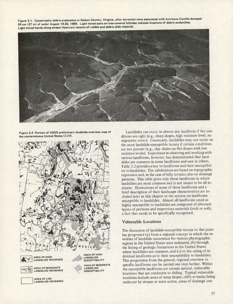
Figure 3.1. Catastrophic debris avalanches in Nelson County. Virginia, after torrential rains associated with hurricane Camille dumped 69cm (27 in) of water August 19-20, 1969. Light-toned scars on tree-covered hillsides indicate locations of debris avalanches.

Light-toned bands along stream floors are veneers of rubble and debris slide material.

Figure 3.2 Portion of USGS preliminary landslide overview map of

the conterminous United States (3.24).

AREA OF HIGH AREA OF HIGH LANDSLIDE 4Z LANDSLIDE INCIDENCE SUSCEPTIBILITY

AREA OF MODERATE AREA OF MODERATE LANDSLIDE

I tj LANDSLIDE INCIDENCE SUSCEPTIBILITY

[ IAREA OFLOW

_] LANDSLIDE INCIDENCE

Landslides can occur in almost any land iorm If the con-ditions are right (e.g., steep slopes, high moisture level, no vegetative cover). Conversely, landslides may not occur On the most landslide-susceptible terrain if certain conditions are not present (e.g., clay shales on flat slopes with low moisture levels). Experience in observing and working with various landforms, however, has demonstrated that land-slides are common in some landforms and rare in others. Table 3.2 provides a key to landforms and their susceptibil-ity to landslides. The subdivisions are based on topographic expression and, in the case of hilly terrains, also on drainage patterns. This table gives only those landforms in which landslides are most common and is not meant to be all in-clusive. Illustrations of some of these landforms and a brief description of their landscape characteristics are in-chided later in this chapter in the section on landforms susceptible to landslides. Almost all landforms rated as highly susceptible to landslides are composed of alternate layers of pervious and impervious materials (rock or soil), a fact that needs to be specifically recognized.

Vulnerable Locations

The discussion of landslide-susceptible terrain to this point has progressed (a) from a regional concept in which the Se-verities of landslide occurrence for various physiographic regions in the United States were indicated, (b) through the listing of geologic formations in the United States where landslides are common, and (c) to the rating of in-dividual landforms as to their susceptibility to landslides. This progression from the general, regional overview to specific landforms can be carried one step further. Within the susceptible landforms are certain natural, vulnerable locations that are conducive to sliding. Typical vulnerable locations include areas of steep slopes, cliffs or banks being undercut by stream or wave action, areas of drainage con-

37

centration and seepage zones, areas of hummocky ground, and areas of fracture and fault concentrations. Special at-tention should be directed to those locations when maps or aerial photographs are examined and field studies are per-formed. In addition, areas that have recently slid require immediate and close scrutiny because additional movement may occur.

Steep Slopes

If slopes are steep enough,movement can occur on any land-form. However, on landforms highly susceptible to land-slides, other factors being equal, the steepest slopes are the most vulnerable locations. Only slopes of similar materials should be compared. For example, a slope cut in earth or talus should not be compared with a rock cliff in an adja-cent landform, and slopes in bedrock generally are more stable, even though steeper, than slopes in adjacent soil areas.

The most common cause of the large number of slides that occur on steep slopes is residual or colluvial soils slid-ing on a bedrock surface. The loose, unconsolidated soils cannot maintainas steep a slope as the underlying rock sur-face and are, consequently, in a delicate balance. Any of

several factors, such as a sudden heavy rainfall (Figure 3.1) or an excavation at the toe of the slope (Figure 3.3) may result in sliding of the overlying soil mass. A study of cut-slope failures in North Carolina (3.12) reported that about two-thirds of the slides occurred in weathered soil mate-rials and one-third occurred in rock slopes.

Cliffs and Banks Undercut by Streams or Waves

Landslides are common in cliffs or banks that are subject to attack by streams or waves. If the banks are made up of soil or other unconsolidated materials, the weakest (and hence the most favorable) slide position is often located at the point of maximum curvature of the stream. At this point, the bank receives the greatest impact from the water. In areas of rock outcrops, on the other hand, the exposure at and near the point of maximum curvature is often hard rock, and the weak spots are to be found upstream and downstream of this point. These conditions are shown in Plate 3.1 and Figure 3.23.

Many landslides occur along the edges of oceans and lakes because of undercutting by waves. Locating the point of maximum water impact is more complex and difficult

Table 3.2. Key to landforms and their susceptibility to landslides.

Landform or Geologic Landslide Topography Materials Potentiala

Level terrain A. Not elevated Floodplain 3 B. Elevated

1. Uniform tones Terrace, lake bed 2 2. Surface irregularities, sharp cliff Basaltic plateau 1 3. Interbedded—porous over impervious layers Lake bed, coastal plain, sedi- 1

mentary plateau II. Hilly terrain

A. Surface drainage not well integrated 1. Disconnected drainage Limestone 3 2. Deranged drainage, overlapping hills, associated with lakes and swamps

(glaciated areas only) Moraine 2 B. Surface drainage well integrated

1. Parallel ridges -

a. Parallel drainage,dark tones Basaltic hills 1 b. Trellis drainage, ridge.and-valley topography, banded hills Tilted sedimentary rocks 1 c. Pinnate drainage, vertical-sided gullies Loess 2

2. Branching ridges, hilltops at common elevation a. Pinnate drainage, vertical-sided gullies Loess 2 b. Dendritic drainage

(1) Banding on slope Flat-lying sedimentary rocks 2 (2) No banding on slope

Moderately to highly disseáted ridges, uniform slopes Clay shale 1 Low ridges, associated with coastal features Dissected coastal plain 1 Winding ridges connecting conical hills, sparse vegetation Serpentjnite 1

3. Random ridges or hills a. Dendritic drainage

(1) Low, rounded hills, meandering streams Clay shale 1 (2) Winding ridges connecting conical hills, sparse vegetation Serpentinite 1 (3) Massive, uniform, rounded to A-shaped hills Granite 2 (4) Bumpy topography (glaciated areas only) Moraine 2

Ill. Level to hilly, transitional terrain Steep slopes Talus, colluvium 1 Moderate to flat slopes Fan, delta 3

C. Hummocky slopes with scarp at head Old slide 1

Note: This table updates Table 2 in the book on landslides published in 1958 by the Highway Research Board (3.10, p.91).

a1 = susceptible to landslides; 2 = susceptible to landslides under certain conditions; and 3 = not susceptible to landslides except in vulnerable locations.

38

Figure 3.3. Slides (1) caused by undercutting of slopes by coal stripping operations in Washington County. Ohio (3.22).

- ;.c

,— ., 1,;'

.-_.I ' - 11•i '-

along lake and ocean shores than along stream banks. Fac-tors to be considered include shape and slope of the shore-line, direction of wave action, and frequency and magni-tude of storms producing large waves. Data obtained at different periods of time are often of value in the analysis of these factors.

Areas of Drainage Concentration and Seepage

A survey conducted by the Federal Highway Administration of major landslides on the federal-aid highway system in the United States revealed that "water is the controlling or a major contributing factor in about 95 percent of all land-slides" (3.5). Thus, careful study of the drainage network and areas of concentration or outfall of water is extremely important. Close scrutiny of existing slide scars often indi-cates that a line connecting the scars points to drainage channels on higher ground. Such drainage may appear as seepage water, which is responsible for the damage. An ex-ample of this condition is shown in Figure 3.4

Seepage with subsequent sliding is likely to occur in areas below ponded depressions, reservoirs, irrigation canals, and diverted surface channels (Figure 3.4). Such circum-stances are sometimes overlooked on the ground because the water sources may be far above the landslide itself,but they become obvious in aerial photographs. The importance of recognizing the potential danger in areas below diverted surface drainage, especially in fractured and porous rocks, needs particular emphasis. Extensive field experience has proved repeatedly that within an unstable area one of the most dangerous sections is the lower part of an interstream divide through which surface water seeps from the higher to the lower stream bed. The recognition of seepage is

sometimes aided by the identification of near-surface chan-nels, wet areas, tall vegetation on the slope, and displaced or broken roads adjacent to the slope. Delineating the drain-age network, especially the presence of seeps or springs, is extremely important for planning new construction. Many

Figure 3.4. Oblique aerial view of extensive seepage zones (1) on

scarp face of massive landslide in Kittitas County, Washington. Seepage was major cause of slide in these unconsolidated sediments. Remnant of dry sand flow (2) is seen above scarp face and is re-sult of seepage at higher level. Landslide disrupted highway at base

of slope and water canal carried through slope.

39

dNL

Figure 3.5. Landslide in highway fill section of Ohio-22 in Jefferson County. Fill slid en masse as block slide with fill above block slumping into resultant hole as

aben. Ohio Department of Transportation staff report attributed failure to saturation

of colluvial materials on side slopes beneath fill by springs outcropping on hillsides. Few small drainageways commencing part way down slope (1) and small slide (2) on natural hillside indicate presence of seepage zones and instability of natural slopes.

highway fills have failed because the natural drainage was blocked by the fill and allowance Was not made for drain-age. Figure 3.5 shows such a situation.

Areas of Hummocky Ground

The presence of huminocky ground whose characteristics are inconsistent with those of the general regional slopes and the presence of a scan) surface (sometimes not very dis-tinct) at a higher elevation are often indications of an exist-ing landslide. The older the landslide is, the more estab-lished the drainage and vegetation become on the slide mass. The drainage and vegetation thus help in determining the relative age and stability of the slide.

Once an old landslide is found, it serves as a warning that the general area has been unstable in the past and that new disturbances may start new slides. However, such a warn-

ing should not discourage construction unconditionally, be-cause the unstable condition of the past may not necessarily exist today. In some parts of the western United States, for example, railroads built in extensive old landslide areas have been stable for a long time. Nevertheless, special care should be taken in construction on old slides. Figure 3.6 shows aerial photographs of the construction of a road on an existing slide and the consequences.

Areas of Concentration of Fractures and Bedding Planes

Movements of slopes may be structurally controlled by sur-faces or planes of weaknesses, such as faults, joints, bedding planes, and foliation. These structural features can divide a rock mass into a number of individual units, which may act independently of one another. The result can be an incor-

40

Figure 3.6. Before (top) and '

after (bottom) construction - of Ohio78 in Monroe County on unstable ground

(3.22). Before construction,

presence of hummocky

unstable a terrain q&t.'

R&ocation of side road to - meet new grade of highway

placed side road on slide r

prone slope which resulted // \ -' 4 in small slide of embankment

(2) Crack crossing road diagonally, seen as faint dark

line (3) is site of possible "\4i.v* future movement

. V

I AN

Vk

,. -.'. -' . q• ,

it

4-4

.--2

— ?' --• T /1

\ '

(

rect slope design because the designer considered the rock to be one continuous mass rather than a series of individual blocks. These planes of weakness also provide egress for water and vegetation, which further weaken the individual units by wedging action, frost heave, and reduction of slid-ing friction. A careful search should be made to locate areas with close spacing of faults and joints, especially where they cross and divide the rock mass into smaller blocks.

Recent Landslides

The occurrence of a landslide does not mean that final ad-justments to the unstable conditions have occurred and no further movement will occur. In many cases, especially in unconsolidated deposits, the materials present in the scarp face remain in an unstable condition because they are on a

very steep slope. The scarp face rapidly ret rogrades uphill by continued slumping until a more stable condition occurs. Thus, a new landslide should be investigated as soon as pos-sible not only to determine corrective measures but also to look for evidence of possible continued movement. The most significant sign of possible further instability is the presence of cracks on the crown of the slide. Figure 3.7 (top) shows some telltale signs at a recent slide. Figure 3.7 (bottom) shows the slide area 5 months later. Additional movement occurred in the area where the telltale signs were evident in the earlier photograph.

Procedure for Preliminary Investigations of Landslides

Not only must the presence or potential development of landslides be recognized, but the types and causes of

41

Figure 3.7. Sequential photography for use in I

evaluation of recent slide development along US-95 in Idaho County, Idaho, and 4

IF investigation of possible further movements. Aerial photography(top) taken in February 1974 . thortly after occurrence of - slide (1) shows features present - at crown of slide that forewarn of further movement fissures above scarp face (2), loose 4 colluvial materials on steep -. slopes at crown (3), and - 4 _________ evidence of water feeding into - \ ' -' these loose materials (4). . •. -, ,,

Photography obtained 5 months lat:r in July 1974 (bottom)

shows that additional slide

in photograph above

40

lie

-.. p

I,

' IF

.:.4

movement must be identified so that preventive or correc- A typical procedure, which has been developed over the tive action can be taken. Chapter 2, and specifically Figure years, for performing terrain investigations is used for a va- 2.1 ,gives the classification of the various types of landslides riety of programs, such as engineering soil surveys, location based on the dominant types of movement and the types of of construction materials, and landslide investigations. The materials involved. In this chapter, the emphasis is on how following steps are generally performed. Some excellent those various types of slides appear on the various data case studies demonstrating the application of this step-by- sources used in terrain investigations, step procedure are reported by Mintzer and Struble (3.20).

42

Obtain aerial photography and other special coverage. Small-scale photography for regional overview and large-scale coverage for detailed study are obtained from available sources. If landslides are already present, photographs taken both before and after the occurrence should be obtained to aid in locating causative factors that may have been obliter-ated by the slide. Special types of photography should be acquired as needed (the section on use of aerial photog-raphy gives details on types and scales of photography needed).

Review literature and maps. A review is made of ex-isting topographic maps, geologic maps and reports, water well logs, agricultural soil survey reports, and other litera-ture to develop an area] concept of the area under investiga-tion.

Analyze the photography and other special coverage. The patterns on the photographs are analyzed, and land-forms are identified and related to the areal concept de-veloped from the literature review. A careful examination is made of all vulnerable locations. Existing and potential landslide sites are delineated, and a three-dimensional con-cept of the terrain is developed. In this step, a mosaic is usually prepared and landform and drainage maps are de-veloped. Sites that offer the best opportunities for confirm-ing or extending the information developed are selected for field verification.

Perform field reconnaissance. A field reconnaissance of the area is performed to verify the three-dimensional con-cept developed in the earlier steps, to fill in information in questionable areas, and to observe the surface features and details that could not be determined from other data sources. The type of landslide movement is classified from the available data and from a study of the surface features and crack patterns observed in the field.

Conduct final analysis and plan field investigations. A final analysis of the photography is performed based on the results obtained from the field reconnaissance. A deter-mination is made as to what additional information is needed to fully define the three-dimensional model of the site and what samples and test data are required to design the corrective procedures. Based on those needs, the field investigation program is planned (this process is described fully in Chapter 4).

MAP TECHNIQUES FOR LANDSLIDE DETECTION

The acquisition and the analysis of various types of maps constitute one of the first steps in landslide investigations. Maps depicting topography, geology, agricultural soils, and other special terrain and cultural features are available for many areas of the world. The maps represent, in a two-dimensional format, the authors' interpretations of terrain and cultural features determined from field investigations, a study of available literature and photography, and map-making procedures. The nature and quality of the informa-tion relating to the presence of landslides or potential for landslides that can be derived from existing maps depend on the purpose, type, scale, and detail used in preparing the map. From most maps, only a general indication of land-slide susceptibility can be derived. In recent large-scale maps, more detail on locating existing landslides and rating

the terrain as to landslide susceptibility is included. Maps have certain inherent advantages for landslide

studies. They are prepared at a uniform scale and, there-fore, are subject to direct quantitative measurements. Fur-thermore, planimetric information is often included, thereby minimizing uncertainties in superimposing other informa-tion. Their disadvantage is that they are outdated as soon as they are published. Unless the maps are updated period-ically or no changes occur, the maps will not show the most recent terrain and cultural features.

The various maps discussed in this section are published mainly by governmental and public agencies and may be ob-tained free or at nominal costs. The published maps can also be viewed at many governmental and university li-braries and in some large public libraries. Included in the following discussions of the various types of maps is infor-mation on map sources.

Topographic Maps

Topographic maps show the size, shape, and distribution of features of the surface of the earth. These maps depict the features of relief, drainage, vegetation, and culture, usually in a color format. Some of the more recent topographic maps prepared in the United States use orthophotographs as the base for depicting drainage and culture as they actu-ally appear and superimpose contours on the orthophoto-graphs to depict the relief; these are published as ortho-photomaps.

Major landslide areas that are clearly evident are some-times labeled on topographic maps. On some maps, the boundaries of the slide and arrows pointing toward the di-rection of movement are also shown. Small slides, the types more commonly encountered in highway and other engi-neering works, are not usually labeled on such maps. Iden-tification of these smaller slides or unlabeled larger slides can be accomplished by noting the following features on topographic maps (Figure 3.8):

Topographic expression observable, for example, steep slope (closely spaced contours) at scarp head of slide, hummocky topography in slide mass (irregular nonsymmet-rical contour patterns with shallow depressions), and pres-ence of detached mass and flow characteristics at the lower end;

Wavy contour lines, uneven or broken local roads, and other artificial lineaments such as transmission lines; and

Minor movements or irregularities at "vulnerable lo-cations," as discussed in the section in this chapter on vul-nerable locations.

The potential for identifying landslides on topographic maps is essentially limited by the scale and contour interval of the maps. On small-scale maps, even moderate-sized landslides significant to engineering works may be such microfeatures that they are not identifiable. The U.S. Geo-logical Survey (USGS) publishes topographic maps at various scales from 1:20 000 to 1:1 000 000. Indexes to the status of topographic mapping for the United States are available free from USGS. Information on status of mapping in other countries can be obtained from similar mapping or-ganizationsin the respective countries.

43

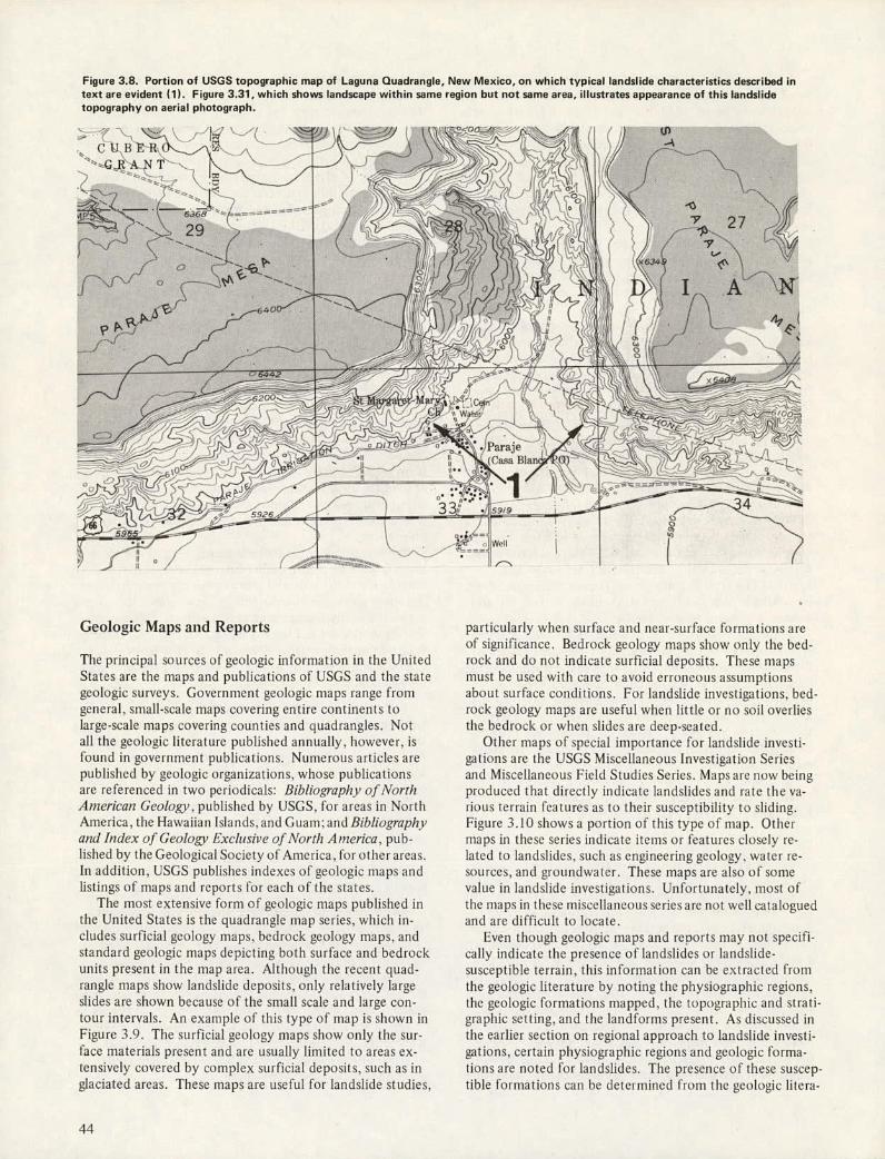
C U BE R.ô—GJANT.

Figure 3.8. Portion of USGS topographic map of Laguna Quadrangle, New Mexico, on which typical landslide characteristics described in text are evident (1). Figure 3.31, which shows landscape within same region but not same area, illustrates appearance of this landslide topography on aerial photograph.

Geologic Maps and Reports

The principal sources of geologic information in the United States are the maps and publications of USGS and the state geologic surveys. Government geologic maps range from general, small-scale maps covering en tire continents to large-scale maps covering counties and quadrangles. Not all the geologic literature published annually. however, is found in government publications. Numerous articles are published by geologic organizations. whose publications are referenced in two periodicals: Bibliography ojNorth American Geology, published by USGS, for areas in North America, the 1-lawa iia n I sian (Is. and Guam: and Bibliography and Index of Geology Exclusive of Non/i A inerica, pub-lished by the Geological Society of America. for other areas. In addition, USGS publishes iiidexcs of- ologic maps and listings of maps and reports for each of the states.

The most extensive fo mi of geologic maps published in the United States is the quadrangle map series, which in-cludes surficial geology maps, bedrock geology maps, and standard geologic maps depicting both surface and bedrock units present in the map area. Although the recent quad-rangle maps show landslide deposits, only relatively large slides are shown because of the small scale and large con-tour intervals. An example of this type of map is shown in Figure 3.9. The surficial geology maps show only the sur-face materials present and are usually limited to areas ex-tensively covered by complex surficial deposits, such as in glaciated areas. These maps are useful for landslide st udies.

particularly when surface and near-surface fo rnial ions are of significance. Bedrock geology maps show only the bed-rock and do not indicate surficial deposits. These maps must be used with care to avoid erroneous assumptions about surface conditions. For landslide investigations, bed-rock geology maps are useful when lit tie or no soil overlics the bedrock or when slides are deep-seated.

Other maps of special importance for landslide investi-gations are the USGS Miscellaneous Investigation Series and Miscellaneous Field Studies Series. Maps are now being produced that directly indicate landslides and rate the va-riotis terrain features as to their susceptibility to sliding. Figure 3.10 shows a portion of this type of map. Other maps in these series indicate items or features closely re-lated to landslides, such as engineering geology, \vater re-sources, and groundwater. These maps are also of some value in landslide investigations. Unfortunately, most of the maps in these miscellaneous series are not well catalogued and are difficult to locate.

Even though geologic maps and reports may not specifi-cally indicate the presence of landslides or landslide-susceptible terrain, this informal ion can be extracted from the geologic literature by noting the physiographic regions, the geologic format ions mapped, the topogra hic a it d strati-graphic setting, and the landforms present. As discussed in the earlier section on regional approach to landslide invest i-gations. certain physiographic regions and geologic forma-tions are noted for landslides. The presence of these suscep-tible format ions can be determined from the geologic lite ra-

44

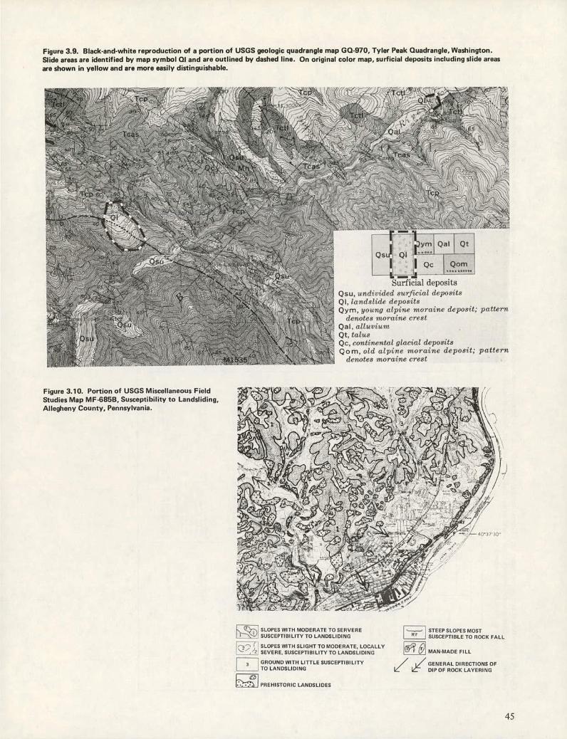
Figure 3.9. Black-andwhite repoduction of a portion of USGS geologic quadrangle map GQ-970, Tyler Peak Quadrangle, Washington. Slide areas are identified by map symbol 01 and are outlined by dashed line. On original color map, surficial deposits including slide areas are shown in yellow and are more easily distinguishable.

- I-

Qsu Ql 1 Q.lf1 L QOrn

Surficial deposits Qsu, undil'ided .uo:ficial deposits QI, landslde deposits Qym, young alpine moraine deposit; pattern

denotes morai-ne crest Qal, alluvium Qt. talus Qc, continental glacial deposits Qom, old alpine moraine deposit; pattern

deiwtes moraine crest

\ •;:\

Figure 3.10. Portion of USGS Miscellaneous Field Studies Map MF-68513, Susceptibility to Landsliding, Allegheny County, Pennsylvania.

7_F -- -4D'3? 30

SLOPES WITH MODERATE TOSERVERE I SUSCEPTIBILITY TO LANDSLIDING

SLOPES WITH SLIGHT TO MODERATE, LOCALLY SEVERE, SUSCEPTIBILITY TO LANDSLIDING

GROUND WITH LITTLE SUSCEPTIBILITY DTO LANDSLIDING

C ______ PREHISTORIC LANDSLIDES

STEEP SLOPES MOST SUSCEPTIBLE TO ROCK FALL

MAN-MADE FILL

GENERAL DIRECTIONS OF I DIP OF ROCK LAYERING

45

Figure 3.11. Portion of soil survey report for Chilton County, Alabama (3.18). Information on susceptibility to sliding in situ is indicated in column, Soil Features Affecting Highway Location. Presence of possible seepage zonesis also designated in this column. Some indication of slide susceptibility of soils placed in fill or embankment section is indicated in columns, Road Fill Material or Farm Ponds, Embankments.

8uitabtbty no o oouree of— Soil f tisree nllnrtint_ -

8oU .rrles and mop nymbolo r... Topsosl d and and gravel Rood fill muteal n o'a Htghy locut,00

ponds - _____________________________ Agricultural Irrigation Terrore. and Waterways

I(r'ervoir sr005 suduee layer) drainage

Embankment,

diversion,

tars-roe: LoB, L.W. InC. LoC2. Fair togood -------- -Poor: no nastier Fai.t,, Ito,.,: high Sosreptibletoolittlng; Moderate to sIns' ! low to moderate No drainage needed.. Slopes 01210 11 percent; High erodibility. LcD?. L.O. l'n02. L.F. gravel available. clay content; vert' lair tettTic-.ti.ln.rltng ovepage. these strength; oso,lerato' inlokr; Fr Ll..,.,v.'ll tart of LwC2, plootie. copocitv; .Iot0s.' poor stability. nedisan available

Lw02, and LwP, refer to bowel outer capacity.

High erodibilils...

series. -

2fcLau,jn: McB, McC. M.D -------- -Fair --------------- -Fair In pane: sand No lin,ilntions except Itapid veepage, - - ' Moderate shear No drainage needed.. Ste1,e of 2 to tS .eeevot; Slight credibility, Moderate ceodt- ot a depth .tf 50 elopen. . strength; fair r:,1,i,l a tab,-: no' 1st bility. orb.-.; fattr' Ito gravel available.

Good---------------

. otalolily. o',linr,,, :ss'ailat,l, seater capacity.

Mdioon: MdB2. MdC2. MdD2 ..... Fair to good -------- - P,n,r: n. sand a- Fair to good -------- - ll,-deoek at a tl,-1sth of 20 lno' to toodrrtte Mod-rate shear No deaionpr needed, SIo,l,'rot,'ietab-e; .504. . StaIn-, of Sto H. 111gb crodihility. geavel available, to 50 isis-bc,. ala-pope. uo.enth; fair ,'rti' in'roo':ilsiiit; .s'rs'.'t,t;n,oder. I .

- oi:slstlity. t',liao,as'silalste ntv to high Water rapacity. eroslilality.

Masada: MnA --------------------- Good to lair -------- Poor: no sand or Fair to good------- - elan ,reiage.......' Fair stability------- - No dr:iinage needed; Sloi.,'s 010102 pert-en?; No terraces or No wn(erw&y*. gravel availobk-.

• l,edroek at a o,o,l.'r;tle intake; depth I diversions oeodsd,

of 30 In 50 eeadrratc asnilable inches. water capacity.

seeded,

- -

Pane: no sand Sr Fair: high water .'lOO'St'5lt5ge - - - - Fair to good 111gb n'atvr tattle; : Sit.15,'. of 0 to 2 percent; No ierraeeo ne No o'aterwayn For Bibb part s.f MyA, refer to gravel available, tattle; th,oding. viability. . e,otivrate to toad. : locate to elan' diversions seeded. Blbbneeies. ' I i croivlyoioo' .ske; tone soil for needed.

Myatt: Ml. MpA------------------ Foir----------------

prr.neabrlrty; crops. outlets difficult to eatablish.

Ora: OeA.OrB. 0e62. 0cC. OrC2... Good ---- --------- - Poor: no sand oe Good- ------------- - Seepngn in eats aloof Moderate seepage.) Fair nhearseresgth; No drainage nrcdcd.. Slopes of 010 10 inches; Moderate erodi. Modrato erodi. gravel available. the lrogspan layer. fate stability. . ssodvraieintcke; bility. bitity; fe*glpso.

Oecnsii,sal flooding--------

t,.enteotsilty; medium os'ailablo water capacity.

Rock land: Ru. No Interpretations; properties too

senolable.

nflo,ton. R.A. RoB. RaC. RsC2. Good .............. Poor: no sand or Good -------------

high seater t5lsle----------

No limitation, except Moderate In rapid : Moderate shear No drainage needed,,' Slops's of 010 IS inches; Moderate erodi- Moderate erodt. R,D2, RuE. RIP, gravel available, elopes. seepage. , strength; pone to ,,ndeeatn to ropid bility. bility. For Bhubuta nnd Troop parts of . lose stability, irtalse; i,,cdiam RIE and RIP, refe, to

Shabuta :

-

available a'oter and Troop melee, rapacity. -

Baffell: SuB. SaC. S.D ............. . Fair to poor: Fair to poor: us-

.

Good .............. . No listilations except .Rapid seepage. .. Poor to fair otability. No drainage needed,,' Slopes of 210 IS inehes; Moderate eeodt. Gravelly; lIttle grave ly. dcrinto b- sand . elopes. notlrrate to ropid i bility. motstare. and gravel at a depth of 4 toO

I , lislatin; medium to

feet; grovel gand I ' lose available .tcr

for road eon. I capacity, -.

otroctina tnatcriol.

8hubuIn: ShD2 .................... . Fair to good......... Poor: no sand or . Fair: high clay Sosceptible to sliding; Slow seepage.-..... Lose shear strength; No drainage aeedrd. Slopes of 2 to 15 inches' I High crodibility.. Highcoodiblltty. gravel available---- contest; very seepage in cttts; . lair to poor - moderate to slow plastic, moderate sheiol.. , ntohility. 'itstake; medium

well poteotiat. ' available macor - capacity,

ture. In addition, as noted in the sections oil landforms sus-ceptible to landslides and on vulnerable locations, certain landlorms and topographic settings are especially suscep-tible to landslides. For example, one of the most favorable settings for landslides is the presence of permeable or solu-ble beds overlying or interbedded with relatively impervious beds in an elevated topographic setting. The beds could be either rock or soil. Conditions such as this can be deter-mined from the geologic literat ure.

Agricultural Soil Survey Reports

The Soil Conservation Service (SCS). U.S. Department of Agriculture, in cooperation with state agricultural experi-ment stations and other federal and state agencies, has per-formed and published soil surveys since 1899. The agricul-tural areas in the United States are, therefore, covered by fairly detailed soil surveys, and much of the remaining area is mapped in less detail. Similarly, agricultural areas in other countries are covered by soil surveys with varying degrees of detail and are available in published form.

Although SCS soil survey reports are compiled primar-ily for agricultural purposes, those published since 1957 are of special value for landslide investigations. Most of these soil surveys contain information on the engineering uses of the soils. In addition, most of the soil maps published in these reports are printed on a photomosaic base at a scale of I : 15 840 or 1:20 000, and the soil information is super-imposed on the mosaic. This provides for easier identifica-tion of natural and cultural features.

Soil surveys provide a three-dimensional concept of the land and contain information about the areal extent and vertical profile for each soil unit. The insight given of each soil unit and its relation to adjacent soil units enables one to estimate the environmental setting and potential stabil-ity.

The engineering sections included in the recent reports contain engineering test data for the major soils mapped in the counties: a table of estimated engineering properties of the soils, including depth to water, depth to bedrock, typi-cal profile, and grain-size distribution: a table of engineer-ing interpretation of the soils; and accompanying text dis-cussing the special engineering features of the soils. Es-tinlates of susceptibility to landslides for the Various soils mapped can be made from the data furnished. In some cases, these estimates are indicated in the table on engineer-ing interpretations. Figure 3.11 shows a portion of such a table from the Chil ton Cowi ty, Alabama. soil survey re-port (3.18). 1-laying identified from this table the soils sus-ceptible to sliding, one can then locate those soil units on the photomosaic and thus delineate the most susceptible areas.

Other county soil surveys and generalized reconnaissance surveys can also provide useful information for landslide in-vestigations, even though engineering sections are not in-cluded. Those surveys provide information on parent ma-terials and their geologic origin, climate, physiographic set-ting, and soil profiles.

The status of availability of agricultural soil survey re-ports in the United States is published annually by SCS in List of Published Soil Surveys. In addition, those state soil conservation services that publish their own soil surveys

provide lists for the respective states. For copies of the pub-lished reports, the unpublished field sheets, and the most up-to-date information about surveys in progress, one should check with the local soil conservat ion service office in the county of interest. The Canada Department of Agriculture provides lists of Canadian soil survey maps and reports. Sources of information on soil surveys in foreign countries include World Soil Map Office, SCS: libraries in major ag-ricultural colleges and universities: and departments of agri-culture in other countries.

Special Maps and Reports

The susceptibility of the terrain to landslides is also dis-cussed in special maps and reports prepared by various or-ganizations. Included in this group are engineering soil maps, engineering soil surveys, geologic reconnaissance surveys, and engineering guides to agricultural soil series.

Engineering soil maps depict the relation of the landforni and engineering soils. The lanclform - which const it utes the foundation of this mapping, is subdivided on the basis of its engineering characteristics, such as soil textuic, drainage conditions, and slope category. Although these reports gen-erally do not iidicate landslide conditions, estimates of landslide susceptibility can be determined by evaluating the landfornl types, soil characteristics, and slope conditions. In the United States, engineering soil mapping is performed at a variety of regional levels. For example, New Jersey and Rhode Island are completely covered: Indiana and Tennessee are preparing maps on a county basis: and Kansas, Louisiana. and New Mexico prepare maps on a project-by-project basis.

For most engineering projects, preliminary engineering soil surveys and geologic reconnaissance surveys are per-formed. In many of these surveys, landslides or landslide-susceptible areas are depicted prior to construction. Figure 3.12 shows -,in example of' such an investigation performed for a route location in Kansas. The results of the survey influenced the final location of the highway (3.31).

Since large parts of the United States are covered by ag-ricultural soil surveys and extensive data are available for the basic soil units mapped (the soil series), several state highway organizations have (lCvCIoped information on t he

Figure 3.12. Delineation of landslide terrain during preliminary route location in Lincoln and Ellsworth counties, Kansas, aided in minimizing damage due to landslides (3.31).

. 'N ,—i'? J''"-.'

4L/L TM c

47

engineering characteristics of the soil series mapped in their states. The information generally provided for each soil series includes origin,topographic setting, soil profile, drain-age characteristics, and engineering significance for items such as location, slope stability, foundation and pavement support, and source of construction materials. Several states, such as Indiana, Michigan, New York, and Ohio, have summarized this information in report form. In many areas, and particularly in densely developed areas, existing reports for geologic and engineering investigations may be available and should be acquired for reference. Detailed boring logs, well logs, and similar valuable soil and geologic information can be obtained at little cost.

REMOTE-SENSING TECHNIQUES FOR LANDSLIDE DETECTION

Remote sensing is the collecting of information about an object or phenomenon by the use of sensing devices not in physical or intimate contact with the subject under investi-gation. The distance of separation might be as close as a few millimeters, as in the case of nuclear moisture-density devices, or as far as 800 km (500 miles) or more, as in the case of satellites. The devices range from cameras to vari-ous scanners and radiometers.

Most remote-sensing devices collect information from the electromagnetic spectrum (Figure 3.13), which extends through many decades of wavelength from very long radio waves to extremely short gamma and cosmic radiation waves. As shown in Figure 3.13, various types of sensors are avail-able for obtaining information in the different regions of the spectrum. The Manual of Remote Sensing (3.25) gives greater detail on the electromagnetic spectrum and sensor systems.

The attractiveness of these systems to various investiga-tors is that they greatly expand the scope of possibilities for uniquely and more accurately identifying subjects of in-terest. In addition to the sensors that provide information on the spectral reflectance phenomena of objects are those that provide information on the thermal-emission proper-ties of objects in the infrared region, the backscatter of radar energy in the microwave region, and the reflectance and fluorescence phenomena in the ultraviolet region. Ana-lyzmg spectral regions individually provides special data about the properties of objects in that region (e.g., thermal characteristics or reflectance properties).

Collecting data simultaneously in several spectral regions and comparing the various responses in those regions, how-ever, provide more data than can be obtained in each region individually and increase the accuracy of interpretation. This approach is referred to as multisensor analysis and is based on the following principle: Although two or more objects may have similar responses in one region, they will not respond similarly in all regions. Thus, evaluating the response of various objects in different regions of the spectrum increases the ability to uniquely identify each of the objects.

In almost all engineering evaluations of various sensor systems, the conclusion has been that photography is the best sensor system and provides the most information. Al-though other sensor systems provide some useful data that cannot be obtained from photography alone, except for

special applications, the additional data are not cost-effective. That being the case, the ensuing discussion on the use of remote-sensing techniques to recognize and iden-tify landslides deals mostly with the use of aerial photog-raphy. The special applications in which other forms of remote-sensing data are useful are also discussed. Some comments are included on systems that have potential value but have yet to be demonstrated for this application.

Use of Aerial Photography

The material in this section expands and updates Chapter 5 in the book on landslides published by the Highway Re-search Board in 1958 (3.10).

The interpretation of aerial photography has proved to be an effective technique for recognizing and delineating landslides. No other technique can provide a three-dimensional overview of the terrain from which the inter-relations of topography, drainage, surface cover, geologic materials, and human activities on the landscape can be viewed and evaluated. Aerial photographs at suitable scales are available for almost all of the United States and a large part of the world. New photography of various types and scales can readily be obtained. In addition, new techniques in production and interpretation processes have continued to extend the advantages of aerial photography.

The value of aerial photography in landslide investigations has been reported by many investigators (3.13, 3.16, 3.19, 3.28, 3.31). The effectiveness of this technique was well demonstrated by Maruyasu and others (3.16) in analyzing a mountainous region where landslides were common in Japan. Using photo-interpretation techniques, they iden-tified 365 landslides. After the region was field checked, an additional 68 landslides were identified, resulting in an 84 percent accuracy in overall identification. An accuracy of 96 percent was reported in identification of landslides in areas such as paddy fields not covered by trees and shrubs.

The major advantages of using aerial photography in landslide investigations include the following:

Photographs present an overall perspective of a large area (when examined with a pocket or mirror stereoscope, overlapping aerial photographs provide a three-dimensional view);

Boundaries of existing slides can readily be delin-eated on aerial photographs;

Surface and near-surface drainage channels can be traced;

Important relations in drainage, topography, and other natural and man-made elements that seldom are cor-related properly on the ground become obvious on the photographs;

A moderate vegetative cover seldom blankets de-tails to the photo interpreter as it does to the ground ob-server;

Soil and rock formations can be. seen and evaluated in their undisturbed state;

Continuity or repetition of features is emphasized; Routes for field investigations and programs for sur-

face and subsurface exploration can be effectively planned; Recent photographs can be compared with old

ones to examine the progressive development of slides;

48

Figure 3.13. Electromagnetic Frequency in cycles /second

spectrum and types of remote-sensing systems used for 020 iO° 06 io0 02 to'° 0 8 02

collecting data in each major I I I I I

I I

spectral region. I I INFRARED I I

RAYS X RAYS I -j

MICROWAVE UV I I I I

MEDIUM ond FAR I

VHF I IF

I I Z

E S SEE E P P 0

8

Wovelenglh - o I

2 2 0 - I

00—

I I I I I en

I I

I

'N

Scintillation IScanners with Film in cameras Cameras with Solid-state Radar: rI ) Electromagnetic

counters: y rays filtered photo- i infrared i

detectors receivers in sum

spectrometers multipliers: I in scanners and scanners and i sensitive film: so l id- radiometers

radiometers

techniques

image orfhicons and cameras state detectors

I with filtered I I

in scanners and I

I infrared film I I radiometers I I

Aerial photographs can be studied at any time, in any place, and by any person; and

Through the use of aerial photographs, information about slides can be transmitted to others with a minimum of ambiguous description.

Factors Influencing Aerial-Photograph Interpretation

Success in the application of aerial-photograph interpreta-tion techniques for landslide investigations depends on four major items: (a) qualifications of the interpreter; (b) photo-graphic parameters; (c) natural factors; and (d) equipment and analysis techniques used. Analysis by competent inter- - preters with suitable equipment will certainly be an impor-tant factor in the successful application of this technique. However, a proper understanding of the photographic param-eters and natural factors that can influence the data is im-portant to the proper use of aerial photography; these two items are discussed below.

Photographic Parameters

Photographic parameters include types of photography, for-mat, scale, coverage, quality, and availability.. General infor-mation concerning these parameters is given in many stan-dard references, such as those published by the American Society of Photogrammetry (3.7, 3.25, 3.30).The following discussion covers-only those items pertinent to landslide in-vestigations.

Aerial photographs typically used for landslide studies include panch.romatic and infrared black-and-white films and natural color and color infrared films. Panchromatic black-and-white film is the most common type used because it is low cost, convenient to handle, and readily available, but natural color and color infrared fihns are now being more extensively used. Color photography is especially valuable for outlining differences in moisture, drainage, vegetation conditions, and soil and rock contacts. Plates 3.1 through 3.6 show the uses and advantages of colorfilms. The strati-fication in exposed soils and rocks is most easily recognized on natural color film. Color infrared films are most helpful

for delineating the presence of water on the surface and for giving clues to subsurface water conditions by showing the vigor of the surface vegetative cover. This has made color infrared film especially valuable for locating the presence of seepage zones at or near the surface.

The format commonly used for landslide investigations is 23 x 23-cm (9 x 9-in) vertical photographs taken with an aerial mapping camera. Consecutive photographs having an average overlap of 60 percent are obtained to provide stereoscopic coverage. In addition to their use for interpre-tation purposes, these photographs can be used for prepar-ing maps of the slide areas by photogrammetric methods. Details on flight planning and mapping are given in the Manual of Photogrammetry (3.35). Oblique photographs, such as those shown in Figures 3.1 and 3.4, are also ob-tained for landslide investigations. The view they provide of the unstable slopes and valley walls is more unobstructed than that provided in vertical photographs. In recent years, oblique views of landslide areas are being obtained with small format, nonmapping cameras in low-flying planes and helicopters; 35 and 70-mm cameras are commonly used.

Scale of photography can be critical to the interpreter's ability to identify landslides in that it influences his or her ability to denote topographic features indicative of land-slides. In some cases, the landslides are so massive [some-times involving more than 4km3 (1 mile3)] of material that they are virtually impossible to detect on the ground or on large-scale photographs (3.9). Small-scale photographs (1:48 000 or smaller) are required in order to view stereo-scopically the full extent of massive slides. However, most landslides encountered in engineering construction are small. Cleaves (3.6) stated: "Within the scope of the author's ex-perience, more than 90 percent of all landslides requiring, control or correction have been small, averaging less than 500-feet in width from flank to flank, and 100 to 200 feet in length from crown to toe." Hence, many small landslides would not be readily discernible on normal-scale photography (1:15 000 to 1:30 000) and would require large-scale photog-raphy (1:4800 or larger) for identification. At these large scales, however, the area covered in each photograph is limited, and the overall perspective is more difficult to grasp. Whenever practicable, it is desirable to examine both small-

49

Plate 3.1. Slides in Douglas County, Oregon, caused by undercutting of slopes by stream. Slides largely composed of weathered colluvial materials are evident at almost every bend of stream where it undercuts naturally steep slopes (1). Advantages provided by use of color film include distinction of potentially more unstable colluv jal material from more stable bedrock surfaces; ease of distinguishing seepage areas; and indication of vegetation under stress due to insufficient moisture, which could occur because of slope movement.

:1 ...

Plate 3.2. Color infrared photography of landslide terrain in Skamania County, Washington, best shows subtle features indicative of slide or slide-prone areas: presence of seepage areas as indicated by dark-toned streaks or "tails" (1) or by concentration of lush vegetation (2); vegetation under stress due to moisture deficiency as indicated by lighter reddish tones and by sparser leaf coverage (3); and presence of leaning and fallen trees (4).

Plate 3.3. Oblique view of area shown in Plate 3.2 allows some of subtle features to be more easily identified.

50

Plate 3.4. Black-and-white

photographs taken October 25, fr -• -i . .. : 41

1954, of delta deposits overlying , , .•

lake bed in Tompkins County, - - ,,• -

New York. Many landslides in '-' .' • . - glaciated areas occur in lake bed r .. -' materialsoverlain by granular '. . . '.,, ,.- r.. deposits. Slides occur on both

• . . I -. -- - .17

sides of creek. Benching and - . ." . • other slope-stabilizing practices

were incorporated to stop . ... -. - —•- ., .- .. ' .:

sliding. Large landslide is easily .•. \. ..C4 t' t' -

identified (1), but evidence of •v. / - seepage and boundary between

delta and lake-bed deposits is

isinguishsubtle anddcuto ,. - • - -

on this film type. .•i._.' .'i, - '- 'I ._t.:

; s4

'A

Plate 3.5. Natural color photographs taken April 9. 1976, of area shown in Plate 3.4. Presence of seepage at contact between delta and lake-bed deposits (2) and change in color tones of soils of these two materials make it easier to distinguish between these two deposits: Darker brown tones are seepage zones; bluish gray tones are lake bed; and lighter tan tones are delta deposits.

Plate 3.6. Color infrared photographs taken April 9, 1976, of area shown in Plate 34. Seepage zones and wet areas (2) are best seen on this film type. Dark tones are clearly distinct. It is too early for presence of luxurious vegetation, which could aid in delineating seepage areas. Boundary between two deposits is more distinct on this film than on black-and-white film, but contrast is not so sharp as on natural color film.

:

7-

51

and large-scale photographs: the smaller scale (1:20 000 or smaller) to provide the regional setting and landform boun-daries and the larger scale (1:8000 or larger) to provide the details.

Sufficient coverage is required in order to determine the full extent of the slide, the potential areas affected, and the changes occurring with time, In some instances the active slide is present only at the lower or toe end of a slope while unnoticed far up the mountainside are tension cracks that indicate the instability of the entire slope. With time, the slides may retrogress up the slope until the whole mountain-side is affected. Clearly, the plans for stabilization will dif-fer depending on whether one is dealing with a small con-fined slide area or with a whole mountainside. A situation of this type can be dealt with satisfactorily if two scales of photography are obtained, as previously recommended. Coverage at the larger scale should include the full height and depth (mountain top to valley bottom) of the area under investigation and at least three to five times the width of the present unstable area.

Many areas, particularly in the United States, have been photographed at various times since the 1930s, and this se-quential photography is valuable for noting the changes in terrain conditions, such as drainage, slope stability, land use, and vegetation, that have occurred during a period of time. These changes provide a clue to the origin and irate of move-ment of a slide. Besides denoting changes, such photographs were probably taken at different seasons, times of day,,and moisture conditions and will often show detailed features that might otherwise have been obscured. These older photo-graphs can also be of value in planning new coverages.

The quality of the photography obtained has a direct, in-fluence on the amount of detail that an interpreter can de-rive from the photographs. The quality depends on the products used and the various processes the images pass through. Proper selection and control of the film-filter combinations require close cooperation between a knowl-edgeable interpreter who can specify the requirements of the end product needed and an experienced contractor who knows the capabilities and limitations of the various systems and can aid in selecting the optimum combination for the specific job.

Availability and access to existing photography are ex-cellent in the United States and Canada and in much of the rest of the world. In the United States, most aerial photog-raphy has been taken for federal and state agencies. Many areas in the United States have been covered several times byone or more agencies. The National Cartographic Infor-mation Center (NCIC) of USGS publishes a catalog, Aerial Photography Summary Record System Catalog, of existing, in-progress, and planned aerial photography of the conter-minous United States held by several federal agencies. The catalog includes a series of outline map indexes, indicating coverage within a 75 x 7.5 -min geographic cell, and acorn-puter listing on microfiche film that shows amount of cloud cover, camera used, specific scale, date of coverage, film type and format, and agency holding the photography. The NCIC address and other U.S. and Canadian agencies that have large holdings of aerial photography are given below. Several of the government agencies whose holdings are listed in the NCIC catalog also publish status maps of aerial photography held by their organizations. For example, the

Agricultural Stabilization and Conservation Service (ASCS), U.S. Department of Agriculture, periodically publishes the ASCS Aerial Photography Status Maps and the Comprehen-sive Listing of Aerial Photography, which indicate the cov-erage available from ASCS for each county in each of the 50 states. The National Archives in Washington, D.C., is the depository of all nitrate-base photography collected during the years 1936 to 1941. The EROS Data Center has USGS and National Aeronautics and Space Administra-tion photography.

National Cartographic Information Center U.S. Geological Survey 507 National Center Reston, Virginia 22092

Aerial Photography Field Office Agricultural Stabilization and Conservation Service U.S. Department of Agriculture 2222 West, 2300 South Post Office Box 30010 Salt Lake City, Utah 84125

Forest Service U.S. Department of Agriculture Washington, D.C. 20250

Headquarters, Defense Mapping Agency U.S. Naval Observatory Building 56 Washington, D.C. 20305

Coastal Mapping Division, C-34 15 National Ocean Survey National Oceanic and Atmospheric Administration 6001 Executive Boulevard Rockville, Maryland 20852

EROS Data Center U.S. Geological Survey Sioux Falls, South Dakota 57198

Audiovisual Department National Archives and Records Service Eighth Street and Pennsylvania Avenue, NW Washington, D.C. 20408

Maps and Surveys Branch Tennessee Valley Authority 210 Haney Building Chattanooga, Tennessee 37401

National Airphoto Library Canada Department of Energy, Mines and Resources 601 Booth Street Ottawa, Canada K1AOE8

Several state highway and transportation departments similarly have available for public review index maps that in-dicate the type and extent of coverage held by state organi-zations. Some state agencies publish lists of all the aerial coverage available for their states from all sources (3.2).

Using existing photography in a landslide investigation is of course less expensive than acquiring new coverage. Existing photographs, however, may be several years old, may not show the present terrain conditions, or may be at a scale too small for performing detailed analyses, and new

52

coverage may thus be necessary. The existing photography can then be useful in the initial analysis and planning for the new coverage.

When the organization performing the investigation does not have the facilities for obtaining new photographic cov-erage, the best approach is to engage a reputable firm with a base of operation close to the study site. In some cases, a small plane can be hired locally, and a hand-held camera can be used to make oblique photographs that are economical and suitable for preliminary analysis and planning.

Natural Factors

Consideration of natural factors is important in planning aerial photography for landslide studies. Flight planning is certainly controlled by meteorological conditions, but con-sideration must also be given to time of year and time of day in which the photography is obtained.

Meteorological conditions include cloud cover, haze, tur- bulence, and solar angle, all of which affect the quality of definition of images on the film. Suitable conditions for color photography are when the sun angle exceeds 300 from the horizontal, cloud cover is less than 10 percent, visibility at aircraft altitude when one looks toward the sun exceeds 24km (15 miles), and the atmosphere is free of turbulence (3.30, p. 43).

Time of year is also critical to the quality of aerial photog- raphy. Although no clear-cut recommendations can be made to fit all situations or localities, some of the desirable con-ditions are discussed below.

1. Optimum soil-moisture contrasts. The optimum con- trast of soil moisture occurs under two different conditons: (a) when the soils are wet but not totally saturated or (b) when the moisture levels are low. The former occurs in the spring or early summer because of high water conditions. Wet areas and seepage zones present in unstable or poten- tially unstable areas are directly visible outcropping on hill-sides or are evident by the presence of luxuriant vegetative growth over those wet areas. The latter occurs during dry periods in late summer or fall or over disrupted areas. Dur- ing dry periods, vegetation in wet areas or seepage zones has more growth and color than that in areas that have nor-mal moisture levels. Areas disrupted by cracks and fissures are better drained and thus drier, and vegetation located over those areas shows evidence of stress earlier. Contrast- ing vegetation and moisture conditions are best noted on color infrared photography, as illustrated in Plates 3.2 and 3.3.

Optimum ground cover. A minimal cover of snow and tree foliage is desirable. In humid, temperate climates, this usually occurs in early spring after the snow melts and before the deciduous trees leaf or in late fall after the leaves fall and before snow falls.

Optimum shadow conditions. Photographs taken when the sun angle is high and shadows on the hillsides and slopes are minimal are the best for interpretation. However, in some special cases, such as in areas of low topography, small slope failures are enhanced by the presence of long shadows produced when the photography is taken with a low sun angle (either early in the morning or late in the afternoon).

These optimum conditions are not always present at one time, and a compromise may be required to obtain as many of the ideal conditions as possible. Some detailed investiga-tions may require photographs to be taken several times during the year.

Principles of Aerial-Photograph Interpretation

The interpretation of aerial photographs involves three major steps:

Examine the photographs to get a three-dimensional perception,

Identify ground conditions by observing certain ele-ments appearing in the photographs, and

Using photo-interpretation techniques, analyze spe-cific problems by the association of ground conditions with one's background experiences.

The quality and the reliability of any interpretation are, of course, enhanced in direct ratio to the interpreter's knowl-edge of the soils and geology of the area under study. The acquirement of such knowledge, either by field examination or by study of available maps and reports, should, therefore, be considered an essential part of any photo-interpretation job.

The technique used in interpreting aerial photographs is referred to as pattern analysis. This approach is based on the premise that the landforms, the basic units of the land-scape, have distinct patterns in aerial photographs. Those landforms developed by the same geologic processes and in the same environmental setting will have similar patterns, while those developed by different processes will have dif-ferent patterns. These patterns are composed of several major elements that are evaluated in the process of interpre-tation: topographic expression,drainage, erosion, soil tones, vegetation, and culture. These elements are discussed briefly in the following paragraphs; more thorough treatments are given by Lueder (3.15), Way (3.38), and Colwell (3.7).

Topographic Expression

The features of importance in describing topographic expres-sion include topography, shape, and relative relief. Topog-raphy represents the three-dimensional aspect of the land, scape, such as hill, basin, ridge, or mountain. Shape refers to a unique character of the landscape, such as conical hill, sinuous ridge, or A-shaped mountain, that aids in describing or separating different forms of topography. Relative relief refers to the comparative position of the landform in rela-tion to other landforms in the vicinity, for example, the po-sition (or relative relief) of the sloping fan-shaped plain lying at the foot of A-shaped hills and sloping downward to a level basin area. In this example, three different landforms are in-dicated based on their relative relief: the mountainous area, the sloping plain area, and the basin area. Topographic ex-pression of landforms is easily determined by a stereoscopic examination of the photographs. In such an examination, various landforms can be separated and clues obtained as to the nature and stability of the materials constituting the landform.

53

Drainage and Erosion

The density and pattern of drainage channels in a given area directly reflect the nature of the underlying soil and rock. The drainage pattern is obvious in some cases, but more of-ten the channels must be traced on a transparent overlay to allow the pattern to be successfully studied. Under other-wise comparable conditions, a closely spaced drainage sys-tem denotes relatively impervious underlying materials; widely spaced drainage, on the other hand, indicates that the underlying materials are pervious. In general, a treelike drainage pattern develops in flat-lying beds and relatively uniform material; a parallel stream pattern indicates the pres-ence of a regional slope; rectangular and vinelike patterns composed of many angular drainageways are evidence of con-trol by underlying bedrock; and a disordered pattern, inter-rupted by haphazard deposits, is characteristic of most gla-ciated areas. Other patterns have develope4 in response to special circumstances. A radial pattern, for instance, is found in areas where there is a domal structure, and a featherlike pattern is common in areas where there is severe erosion in rather uniform silty material, such as bess.

The shapes of, gullies appearing in aerial photographs pro-vide valuable information regarding the characteristics of surface and near-surface materials. Typically, long, smoothly rounded gullies indicate clays; U-shaped gullies, silts; and short, V-shaped gullies, sands and gravels.

Soil Tones

Soil tones are recognizable in photographs unless there is a heavy vegetative cover. On black-and-white photographs, the tones are merely shades of gray, ranging from black to white. Because gray tones are highly respondent to soil-moisture conditions on the ground, they are an important aerial-photographic element in landslide investigations.

A soil normally registers a dark tone if it has a high mois-ture content and a light tone if it has a low moisture con-tent. The moisture condition is the result of the physical properties of the soil, its topographic position, and the po-sition of the groundwater table. The degree of sharpness of the tonal boundary between dark and light soils aids in the determination of soil properties. Well-drained, coarse-textured soils show distinct tonal boundaries whereas poorly drained, fine-textured soils show irregular, fuzzy tonal boundaries.

Color photography greatly increases the number of tones that can be distinguished by the interpreter and improves the amount of detail and accuracy of the information de-rived. In addition, the use of special visual, photographic, or electronic enhancement techniques increases the effective-ness of analysis of the tonal pattern element.

Vegetation

Vegetative patterns reflect both regional and local climatic conditions. The patterns in different temperature and rain-fall regions can be recognized in aerial photographs. Locally, a small difference in soil moisture condition is often detected by a corresponding change of vegetation. A detailed study of such local changes is helpful in landslide investigations. For instance, areas of wet vegetation, represented on the

photographs by dark spots or "tails," are a clue to seepage on slopes. Cultivated fields, as well as natural growths, are good indicators of local soil conditions. Thus, an orchard is often found on well-drained soils; black ash, tamarack, and white elm are normally found on wet, fine-grained soils; and vegetation is sparse in nonproductive serpentine soils, where landslides are common.

The use of color photography, especially color infrared, greatly facilitates vegetation analysis and thus the overall in-terpretation. The vigor of vegetative growth and the pres-ence of vegetation stress due to detrimental soil and mois-ture conditions are best noted on color infrared photography. Point 2 in Plates 3.2 and 3.3 shows areas of seepage, as in-dicated by lush vegetation, and point 3 indicates vegetation under stress on the unstable slide debris.

Culture

Cultural patterns reflect how humans adjust to the natural terrain on which they live and work. An understanding of these patterns and the reasons for their presence can be valu-able indicators of soil, moisture, and other terrain conditions. For example, drainage ditches and tile fields indicate the presence of a high water table; steep, vertical cuts along highways denote the presence of bedrock; sloping cuts usu-ally typify unconsolidated soils; and contour farming or an irregular wavy plowing pattern characterizes sloping terrain or erodible soils.

Interpretation of Landslides on Aerial Photographs

As previously described in the section of this chapter on landforms susceptible to landslides and the section on vul-nerable locations, landslides are more prevalent in certain landforms and occur most frequently at certain vulnerable locations. The interpretation of aerial photographs by the pattern-analysis technique is a valuable tool for delineating landslide-susceptible landforms and pinpointing the vulner-able locations. The identifying pattern elements on the photographs and significant features about these landforms are summarized in the following discussion and illustrated in the accompanying figures.

Diagnostic Patterns of Landslides on Aerial Photographs

An investigator already familiar with the appearance of land-slides on the ground should become oriented to the aerial view of landslides by an examination of photographs of some known examples. The difference between an aerial view and a ground view results chiefly from the fact that the former gives a three-dimensional perspective of the entire slide area, but at a rather small scale. Ground photographs, on the other hand, show only two dimensions, but on a larger scale.

The following features discernible on aerial photography are typical of landslides or landslide-susceptible terrain, but not all features are evident for each landslide. Most of these features are shown in Figure 3.14; those features not evident are shown in other figures in this chapter. The numbers in Figure 3.14 correspond to those in the list below.

54

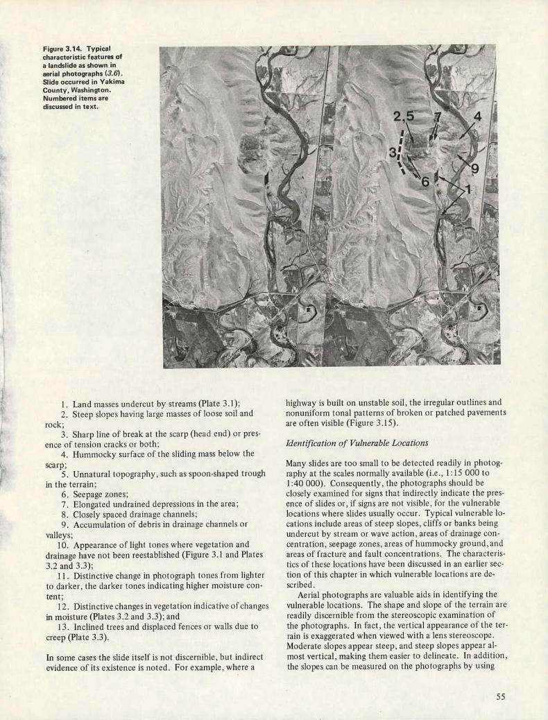
- 5'

-

It ••- .

:Y

Figure 3.14. Typical characteristic features of a landslide as shown in aerial photographs (3.6). Slide occurred in Yakima County, Washington. Numbered items are

discussed in text.

Land masses undercut by streams (Plate 3.1): Steep slopes having large masses of loose soil and

rock: Sharp line of break at the scarp (head end) or pres-

ence of tension cracks or both; Hummocky surface of the sliding mass below the

scarp; Unnatural topography, such as spoon-shaped trough

in the terrain: Seepage zones; Elongated undrained depressions in the area; Closely spaced drainage channels; Accumulation of debris in drainage channels or

valleys; Appearance of light tones where vegetation and

drainage have not been reestablished (Figure 3.1 and Plates 3.2 and 3.3);

II . Distinctive change in photograph tones from lighter to darker, the darker tones indicating higher moisture con-tent;

Distinctive changes in vegetation indicative of changes in moisture (Plates 3.2 and 3.3); and

Inclined trees and displaced fences or walls due to creep (Plate 3.3).

In sonic cases the slide itself is not discernible, but indirect evidence of its existence is noted. For example, where a

highway is built on unstable soil, the irregular outlines and nonuniform tonal patterns of broken or patched pavements are often visible (Figure 3.15).

Identification of Vulnerable Locations

Many slides are too small to be detected readily in photog-raphy at the scales normally available (i.e., I : 15 000 to 1:40 000). Consequently, the photographs should be closely examined for signs that indirectly indicate the pres-ence of slides or, if signs are not visible, for the vulnerable locations where slides usually occur. Typical vulnerable lo-cations include areas of steep slopes, cliffs or banks being undercut by stream or wave action, areas of drainage con-centration, seepage zones, areas of hummocky ground, and areas of fracture and fault concentrations. The characteris-tics of these locations have been discussed in an earlier see-tion of this chapter in which vulnerable locations are de-scribed.

Aerial photographs are valuable aids in identifying the vulnerable locations. The shape and slope of the terrain are readily discernible from the stereoscopic examination of the photographs. In fact, the vertical appearance of the ter-rain is exaggerated when viewed with a lens stereoscope. Moderate slopes appear steep, and steep slopes appear al-most vertical, making them easier to delineate. In addition, the slopes can be measured on the photographs by using

55

Figure 3.15. Presence of limited sections of patched pavement (1) in generally unpatched roadway can be indicative of possible slope movement in area. Presence of fissures on hillside above this patched section (2) in Washington County, Ohio, confirms instability of slope.

V-4 "' r : ;.

simple measuring devices, such as an engineer's scale or a parallax bar, and by applying photogrammetric principles. Details of this technique are described by Ray (3.23).

The presence of drainageways, seepage zones, fractures, and fault zones is also readily evident on aerial photographs. By means of stereoscopic examination, the complete drain-age network can be mapped, including the intermittent streams and small gullies. The presence of wet zones or seepage areas is evidenced by darker tones caused by the higher moisture content in the soils or by a more luxuriant vegetative growth over the wet areas. Areas of drainage or water concentration above a slope should be closely ex-amined because they are vulnerable locations. Subsurface seepage from these areas can lead to slope failures: Figure 3.4 shows such a case. Fracture and fault zones are indi-cated on the photographs by dark linear or curvilinear lines. The darker tones are usually due to the better growl h of vegetation along the fracture zones where it is easier for the roots of plants to grow and where moisture levels are usually higher. In delineating fracture zones, care must be taken not to interpret man-made features, such as fence lines or field boundaries, as fracture zones. Generally, fea-tures having straight lines, right-angle intersections, and standard geometric patterns are man-made. Several of the above features are illustraled in succeeding figures that show landslides in various landforms.

L.andforms/Geologic Materials Susceptible to Landslides

Landslides are rare in some landforms and common in others

Most of the forms susceptible to landslides are readily recog-nizable on aerial photographs. The identifying elements on black-and-white photography and significant facts about the landforms are summarized and illustrated in the following sections. Table 3.2 gives the landslide potential of various landforms/geologic materials grouped on the basis of their topographic form. The order of presentation in this section follows a sequence based on origin and character of the ma-terials.

Sedimentary Rocks and Their Residual Soils

The discussion of rocks and their residual soils is combined in this and the following two sections because the recogni-tion of types of residual soils depends primarily on the rec-ognition of the landform developed on the parent rocks. The determination of depth of residual soil requires consid-erable judgment - However, investigators working constantly in their own regions should have no difficulty in estimating the depth once they are familiar with local conditions.. In general, rounded topography, intricate, smoothly curving drainage channels, and heavy vegetation are indicators of probable deep soils: in contrast, sharp, steep, resistant ridges and rock -cont rolled angular channels are commonly found in areas of shallow soils. The local climatic and erosion pat-terns should be considered in the interpretation.

Many landslides occur in residual soils and weathered rocks; they are usually in the form of slides or flows. For example, in a study in North Carolina (3i2), two-thirds of the slides involved in cut-slope failures occurred in the

56

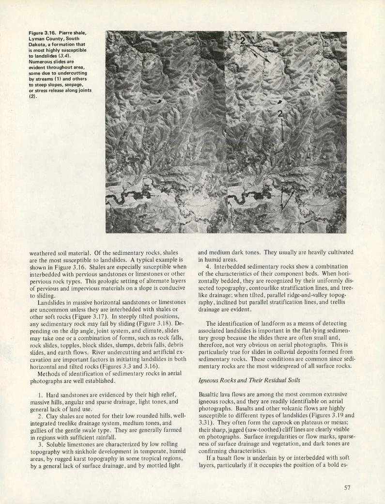
Figure 3.16. Pierre shale, Lyman County, South Dakota, a formation that is most highly susceptible to landslides (3.4). Numerous slides are evident throughout area, some due to undercutting by streams (1) and others to steep slopes, seepage, or stress release along joints

(2).

weathered soil material. Of the sedimentary rocks, shales are the most susceptible to landslides. A typical example is shown in Figure 3.16, Shales are especially susceptible when interbedded with pervious sandstones or limestones or other pervious rock types. This geologic setting of alternate layers of pervious and impervious materials on a slope is conducive to sliding.

Landslides in massive horizontal sandstones or limestones are uncommon unless they are interbedded with shales or other soft rocks (Figure 3.17). In steeply tilted positions, any sedimentary rock may fail by sliding (Figure 3.18). De-pending on the (lip angle, joint syste iii, and climate, slides may take one or a combination of forms, such as rock falls, rock slides, topples, block slides, slumps. debris falls, debris slides, and earth flows. River undercutting and artificial ex-cavation are important factors in initiating landslides in both horizontal and tilted rocks (Figures 3.3 and 3.16).

Methods of identification of sedimentary rocks in aerial photographs are well established.

I . I-lard sandstones are evidenced by their high relief, massive hills, angular and sparse drainage, light tones, and general lack of land use.

Clay shales are noted for their low rounded hills, well-integrated treelike drainage system, medium tones, and gullies of the gentle swale type. They are generally farmed in regiuns with sufficient rainfall.

Soluble limestones are characteriied by low rolling topography with sinkhole development in temperate, humid areas, by rugged karst topography in some tropical regions, by a general lack of surface drainage, and by mottled light

and medium dark tones. They usually are heavily cultivated in humid areas.

Interbedded sedimentary rocks show a combination of the characteristics of their component beds. When hori-zontally bedded, they are recognized by their uniformly dis-sected topography, contourlike stratification lines, and tree-like drainage: when tilted, parallel ridge-and-valley topog-raphy, inclined but parallel stratification lines, and trellis drainage are evident.

The identification of land form as a means of detect ing associated landslides is important in the flat-lying sedimen-tary group because the slides there are often small and, therefore, not very obvious on aerial photographs. This is particularly true for slides in colluvial deposits formed from sedimentary rocks. These conditions are common since sedi-mentary rocks are the most widespread of all surface rocks.

Igneous Rocks and Their Residual Soils

Basaltic lava flows are among the most common extrusive igneous rocks, and they are readily identifiable on aerial photographs. Basalts and other volcanic flows are highly susceptible to different types of landslides (Figures 3.19 and 3.31). They often form the caprock on plateaus or mesas: their sharp,jagged (saw-toothed) cliff lines are clearly visible on photographs. Surface irregularities or flow marks, sparse-ness of surface drainage and vegetation, and (lark tones are con firming characteristics.

If it basalt flow is underlain by or interbedded with soft layers, particularly if it occupies the position of a bold es-

57

carpment, a favorable condition for large slumps is present The joints and cracks in basalt give rise to springs and seep age zones and greatly facilitate movement. Rock falls and rock slides along rim rock are usually favored by vertical jointing of basalt and by undercutting of basaltic cliffs. Talus accumulations of various magnitudes are found at

the foot of cliffs. Disturbance of talus slopes during road construction has caused some large slides of talus materials. Old slides and fissures indicating incipient slides often can be seen on photographs. In areas of relatively deep weather-big, the landscape is somewhat modified. A more rounded topography and heavier vegetation develop, although dark

Figure 3.17. Interbedded . ' . '' •.• •4.,.,•.- j? er sedimentary rocks W 4 (3.22). Hummocky -. -. . . .'•• ... topography, heavy ,• -. .... . . •.•. . . :• ..•• . ;. . . . .. erosion, and extensive . .. . . . . . . . . . . .. drainage characterize •.• . ....

E . 1

slialematerial '.•J, .. -. .'

underlying sandstone

cap rock in Morgan ), County, Ohio Almost all hillsidt.s show evidence of instability (1). Evidence of slides . .• . . ..

in capping sandstone .. . . ' s .•.

due to undermining .. . . '.: . . .. by sliding out of the

k . ... ... ...., ... . .•4&., .... -. / ••.i .,

shas is also apparent 2

- 41

.

. :''••. ...S.....

,.i

S. k... ." . . . '. • .. ... . . .• :.) . . .;... ....

dr0ck prodes 5te0 ply

dipping slopes ide ii for i

slides (3.8). No large

slide masses are . . . .. •

apparent in this Le Fiore County, Oklahoma, area, but

wasting is indicated by oversteepened slopes

I

I

having light tones (1); . __. .. . bulging of lower slopes 3 (2); and accumulation of loose scree materials r• \ '. '

. •. . at base of slopes (3)

- 3

58

tones still predominate. Slumps of both large and small size are common in basaltic soils.

Granite and related rocks constitute the most widely oc-curring intrusive igneous rock types. The landslide poten-tial of granitic rocks varies widely, depending on the com-position of the rock and its fracture pattern, the topography, and the moisture conditions. In granites that are highly re-sistant to weathering or are of low relief, there is generally no slide problem. In hilly country where the granite is deeply weathered, slumps in cut slopes, as well as in natural steep slopes, are common. Fractures in the rock and high moisture conditions undoubtedly are favorable factors in producing landslides. Figure 3.20 shows an example of an extensive slide in granitic materials. Granitic masses are identified on aerial photographs by the rounded (old) to A-shaped (young), massive hills and by the integrated tree-like drainage pattern with characteristic curved branches. The presence of criss-cross fracture patterns and light tones and the absence of stratification and foliation aid in confirm-ing the material.

Metamorphic Rocks and Their Residual Soils

As reported by Leith and others (112) and other investiga-tors, the frequency of landslides per unit area is greater in metamorphic rocks than in most other rock types. The pres-ence and attitude of the foliation and joints in these rock types greatly influence the stability of the slopes.. Although the characteristics of the major types of metamorphic rocks gneiss, schist, slate, and serpentinite—have been identified on aerial photographs for specific areas, they are not sufficiently consistent to develop typical pattern elements. Neverthe-less, the presence and attitude of the foliation and joints

Figure 3.19. Basalt cap rock overlying impermeable shale deposits has resulted in massive landslides in Mesa County, Colorado. Large blocks of material have toppled and stumped off scarp face (1). Presence of incipient slide is indicated by ciacks on crown of slide (2).

can be distinguished on aerial photography by an indication of banding or lineation of the topography and drainage net-work, and landslides, when present, are clearly evident. Fig-ure 3.21 shows an example of landslides in metamorphic terrain (mica schists). The attitude of the foliation seen at point 3 indicates that the dip of these layers may have been a significant factor in the presence of numerous slides (point I) found just across the river where the layers are steeply dipping toward the river.

Within the metamorphic group, many slides are associated with serpentinite areas, which are identified on aerial photo-graphs by sinuous ridges, smoothly rounded surfaces, short steep gullies, poor vegetative cover, and dull gray tones. Within a general area, local conditions, such as vegetation, moisture, and slope, may create special, favorable circum-stances for landslides. In genera!, low relief and low rain-fall are among the factors responsible for the stability of some of the serpentinite slopes.

Glacial Deposits

Landslides are common in some glacial and glaciofluvial de-posits. Although most of the distinct glacial forms are easily identified on aerial photographs, there are complex areas that require a high degree of skill for their identifica-tion. Moraines are found in nearly all glaciated areas. They are identified on aerial photographs by jumbled, strongly rolling to hilly terrain. Moraines, particularly in semiarid areas, contain a large proportion of untilled ]and. Deranged drainage patterns, irregular fields, and winding roads are con-firming clues. Minor slumps, debris slides, and earth flows are common in cut slopes iii moraines as a result of un-drained depressions and seepage zones in the mass. Because morainic hills are usually small, these slides are not exten-

_ .,v ft..,. .'.. .

.et!

59

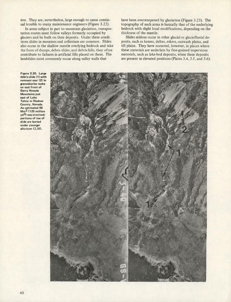
sive. They are, nevertheless, large enough to cause contin-ual trouble to many maintenance engineers (Figure 3.22).

In areas subject in part to mountain glaciation, transpor-tation routes must follow valleys formerly occupied by glaciers and be built on their deposits. Under these condi-tions slides in moraines and colluvium are common. Slides also occur in the shallow mantle overlying bedrock and take the form of slumps, debris slides, and debris falls: they often contribute to failures in artificial fills placed on them. The landslides most commonly occur along valley walls that

have been oversteepened by glaciation (Figure 3.23). The topography of such areas is basically that of the underlying bedrock with slight local modifications, depending on the thickness of the mantle.

Slides seldom occur in other glacial or glaciofluvial de-posits, such as kames, deltas, eskers, outwash plains, and till plains. They have occurred, however, in places where these materials are underlain by fine-grained impervious materials, such as lake-bed deposits, when these deposits are present in elevated positions (Plates 3.4, 3.5, and 3.6).

Figure 3.20. Large debris slide (1) with remnant scar (2) in

'anodiorite rocks on east front of Sierra Nevada Mountains just east of Lake Tahoe in Washoe County, Nevada. An estimated 95 Mm3 (125 million yd3) was involved; portions of toe of slide are buried under younger alluvium (3.36).

Ta

1 t! "--,! • Sj

7 P, )J

- '-1

VEJ

I .

1'

rjf '

I ,_j.. ',;.••• •iv.fl••• • ' '

- r-

'.'.' NI...

-

pk ,.-- -

41

,..-.-

Water-Laid Deposits

Water-deposited landforms most susceptible to landslides include coastal plain deposits, river terraces, and lake beds.

Coastal plain deposits can be subdivided into three dis-tinct subforms for analysis by aerial photographic methods: the dissected or upper coastal plain, the undissected or lower coastal plain, and the beach zone. Landslides are un-common in the beach zone. The lower coastal plain is iden-tified by its low, flat topography; its association with tidal

flats, marshes, and swamps; and the presence of broad, shal. low, tidal stream channels. The upper coastal plain is iden-tified by its rolling to rugged topography: an integrated drainage system with wide, vegetation-filled main drainage-ways: and irregular land-use patterns. It is also associated with coastal features and appears on aerial photographs to be somewhat similar to areas underlain by consolidated sedi-mentary rocks. In the lower coastal plains, landslides offer a problem only in the construction of canals or similar struc-tures that require deep excavation in flat lands. In the upper

Figure 3.21. Typical landslide topography in weathered mica schists evident on valley walls on both sides of Little Salmon River in Idaho County, Idaho. Old slide scars with hummocky terrain below can be seen (1). Slide debris has covered road many times (2) necessitating high maintenance costs and final relocation. Presence and attitude of foliation are also apparent (3).

04,

I

Figure 3.22. Moraine and lake bed, Tompkins County, New York (3. 10). New slumps and debris slides, as well as old slide scars, are common occurrences in this glaciated valley where postglacial erosion has dissected moraines and overlying lake deposits. Morainal deposits (1) are recognized by their irregular, jumbled topography. Overlying lake deposits have smoothed topographic appearance; their silty clay composition is characterized by smooth slopes, high degree of dissection, and gradual change of gray tones (2). Prominent old slump is visible (3). Almost all highway excavations experience slumps and debris slides (4). Although deep-seated and large-scale slides are not common in such an area, continual maintenance work in clearing sliding material and in protecting slopes from erosion has been necessary.

61

0 ..

2/-:. ' 0

: .

I . - t- ...

62

coastal plains, however, slumps in natural hill slopes, as well as in road cuts, are common (Figure 3.24). The stratified and unconsolidated nature of the sands, silts, and clays that characterize most coastal plains provides a favorable situa-tion for landslides.

Terraces are easily recognized on aerial photographs as elevated flat land along major or minor valleys. Terraces of gravel and sand are usually stable, maintaining clean slopes on their faces. However, where terraces are composed of fine sands or interbedded silts and clays or where the natu-

ral equilibrium is disturbed by artificial installations, slides will occur. Slides in terraces naturally start on unsupported slopes facing the low land (Figure 3.25).

Lake-bed deposits generally display flat topography un-less they are dissected. Although generally composed of clays, lake beds have little chance to slide except when ex-posed in valley walls or cuts (Figure 3.26). Slides of con-siderable magnitude have occurred in lake clays under each of the following circumstances: (a) where lake clays are in-terbedded with or, especially, are overlain by granular de-

Figure 3.23. Thin till deposit overlying bedrock in glaciated valley in Broome County, New York. Highway cuts in hillsides oversteepened by glaciation create slides (A and B). Slides generally extend to full depth of soil material until competent rock bed (in this case sandstone) is encountered. Between A and B, section of highway entirely in rock has not experienced any slides. In this respect, landslides serve as indicators of depth of soil to rock. On other side of river, site of future slide is indicated at C. an area of Concentration of drainage, loose

fill, and lack of bedrock control.

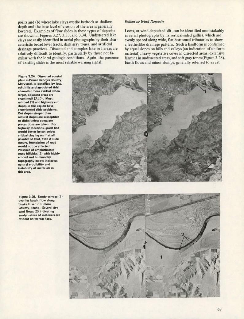
posits and (b) where lake clays overlie bedrock at shallow depth and the base level of erosion of the area is generally lowered. Examples of flow slides in these types of deposits are shown in Figures 3.27, 3.33, and 3.34. Undissected lake clays are easily identified in aerial photographs by their char-acteristic broad level tracts, dark gray tones, and artificial drainage practices. Dissected and complex lake-bed areas are relatively difficult to identify, particularly by those not fa-miliar with the local geologic conditions. Again, the presence of existing slides is the most reliable warning signal.

Eolian or Wind Deposits

Loess, or wind-deposited silt, can be identified unmistakably in aerial photographs by its vertical-sided gullies, which are evenly spaced along wide, flat-bottomed tributaries to show a featherlike drainage pattern. Such a landform is confirmed by equal slopes on hills and valleys (an indication of uniform material), heavy vegetative cover in dissected areas, extensive farming in undissected areas, and soft gray tones (Figure 3.28). Earth flows and minor slumps, generally referred to as cat

Figure 3.24. Dissected coastal plain in Prince Georges County, Maryland, is identified by low, soft hills and associated tidal channels (more evident when larger, adjacent areas are examined) (3.10). Most railroad (1) and highway cut slopes in this region have experienced slide problems. Cut slopes steeper than natural slopes are susceptible to slides unless adequate precautions are taken. For highway locations, grade line would better be set below critical clay layers if at all possible so that, even if slide occurs, foundation of road would not be affected. Presence of amphitheater scarp hillsides (2) with highly eroded and hummocky topography below indicates natural erodibility and instability of materials in this area.

;: .•t.%."• 4i; t

1•

Figure 3.25. Sandy terrace (1) overlios basalt flow along -

..._,.,...-r Lb......

Snake River in Elmore '.. County. Idaho. Several dry ' sand flows (2) indicating * • ,

: 1

1 •t

) ci "' ?• (

I -

t 1• J t

63

' \t

I

r -•

steps, are commonly found in bess. The cat steps appear as fine, roughly parallel, light tone contours on the aerial photographs. Because of their small size, they are not al-ways evident. The individual steps of these small slumps are commonly about a meter wide and several centimeters to a meter high. These subtle features are shown in Figure 3.29.

Gravity Deposits

Loose, unconsolidated talus and colluvial materials formed by weathering of parent soil and rock materials and moved downslope by gravity are found on steep slopes. These de-posits are easily identified on aerial photographs as bare slopes in mountainous areas, but they are not so obvious on

Figure 3.26. Sewage lagoons (1) at Harwood Rest Area along 1-29, Cass County, North Dakota, may be endangered by slides occurring along stream bank just below (2). Lake-bed deposits in this area are highly susceptible to slides as shown by presence of other slides along stream bank (3).

Figure 3.27. Example of earth flow in sensitive clays along Ottawa River east of Ottawa. Canada (3.17).

64

- :::

-[;; j:" •' - - - I

y '1% -

Figure 3.28. Highly dissected nature of the bess terrain in Lincoln County, Nebraska, illustrates great erodibility of these materials (3.10). Presence of earth flows (1) is indicated by broad amphitheater scarp faces at crown, steep side slopes of gullies, and light-toned deposits in gulley bottoms. Numerous little erosional scars and slumps can be seen on hillsides (2). Section (3) is shown enlarged in Figure 3.29.

Figure 3.29. Cat steps can be seen on this enlarged section of area shown in Figure 3.28. Because of their small size, they appear as thin, wavy contours on hillside.

t -

kn~ Ilk

& q . ... '

'it I I9.

4 t. got OXN

5: L;

Ov '1

- '

41 -"-

-, <

AO

AN .14

iji

65

vegetated lower slopes. Excavation into these materials usu-ally creates stability problems. Old landslide deposits are themselves part of this group (Figure 3.30).

Complex Forms

Most of the landforms previously described can be called simple forms because they consist predominantly of one type of material in each unit. In nature, however, complex or superimposed forms are numerous and of common oc-currence, especially in glaciated areas, as mentioned pre-viously. They are further emphasized here because of their significance in landslide studies. A change of material ver-tically or horizontally in complex areas often affects the in-ternal drainage characteristics and creates slope stability problems. The common situation most favorable to slides is one in which pervious formations are underlain by rela-tively impervious beds.

Procedure for Landslide Investigation Using Aerial Photographs

The following procedure is recommended for photographic studies of landslides.

Lay out sites of planned facility on photographs. Delineate areas that show consistent characteristics

of topography, drainage, and other natural elements and classify into landform types. Large and obvious slides are identified at this stage.

Evaluate the general landslide potential of the land-form types. Use Table 3.2 and the section on landforms susceptible to landslides as a guide.

Make a detailed study of cliffs or banks adjacent to river bends and all steep slopes. Compare slopes within the same landform type: For instance, slopes in bedrock land-forms are more stable, even though steeper, than slopes in adjacent soil areas. Because slides are usually small in size on photographs, look carefully and inspect slopes in minute detail. Give particular attention to the following features:

Slide Feature

Existing Hillside scarps and hummocky topography Parallel spoon-shaped dark patches on hillsides Irregular outlines of highways and random cracks or

patches on existing pavements. Potential Ponded depressions and diverted drainageways

Seepage areas suggested by faint dark lines, which may mean near-surface channels, and fan-shaped dark patches, probably reflecting wet vegetation

Relatively new slides appear in light tones because vegeta-tion and drainage are not well established. The parallel spoon-shaped dark patches on hillsides are likely to reflect vegetation in minor depressions. Lines drawn through the axes of the scarps in the slides often point to drainageways on higher ground that contribute to landslide movement.

Ground check all suspected slides.

Use of Other Remote-Sensing Systems

Multisensor investigations for terrain analysis and landslide

investigations have been performed by several investigators, including Alfäldi (3.1), Gagnon (3.11), Rib (3.26), Stallard and Myers (3.32), and Tanguay and Chagnon (3.33). The general consensus of those studies is that large-scale aerial photography (most preferred color) provides the most in-formation on terrain conditions, specifically for landslide detection. Several of the reports did indicate, however, that satellite and infrared imagery offered some unique in-formation that would prove useful for landslide investiga-tions.

Satellite Imagery

Since July 1972, multispectral satellite coverage has been obtained for the United States, most of Canada, and many other areas of the world. Data are collected in four bands onan 18-d cycle:

Band Color Wavelength (nm)

Green 0.5 to 0.6 Red 0.6 to 0.7 Near infrared 0.7 to 0.8 Near infrared 0.8 to 1.1

A second satellite launched in 1975, as well as others sched-uled for launching, provides data on a shorter time cycle. Each satellite scene covers an area of approximately 33 000

2 (10 000 miles2) and has a resolution of about 80 m (250 ft). The satellite scene can be provided as a 70-mm film at a scale of 1:3 369 000; as a 185 x 185-mm (7.3 x 7.3-in) black-and-white print of each band; as a color com-posite at a scale of I : 1 000 000; and on computer-compatible tapes for computer processing. The scenes can also be pro-vided on 35-mm slides.

In addition to the LANDSAT images provided by these two satellites, the National Aeronautics and Space Admin-istration (NASA) has obtained photographic and image coy-erages of considerable areas of the United States and scattered areas of many foreign countries during the manned satellite SKYLAB missions (May 1973 through February 1974). SKYLAB data of special interest to landslide inves- tigators are those collected by (a) the multispectral camera (S-190A) at a scale of 1:2 850 000 with 30 to 79-m (100 to 260-ft) resolution and (b) the earth terrain camera (S-190B) at a scale of 1:950 000 with 17 to 30-m (55 to 100-ft) reso-lution. Black and white, black-and-white infrared, color, and color infrared products are included. Detailed informa-tion about film types, spectral characteristics, and areal coy- erages has been published by NASA (3.21). Compared with LANDSAT products, SKYLAB products provide better reso-lution but lack universal coverage and repeated sequence.

At the small scale of satellite imagery, only extremely large landslides can be identified directly. Figure 3.31 shows a typical stereographic aerial photograph coverage of a large landslide zone. Figure 3.32 shows the satellite scene covering this landslide zone. The scalloped edges of the scarp slopes and the hummocky topography of this large slide are evident on the satellite scene.

Since most landslides are much smaller than the land- slide shown in Figure 3.31,they are not directly identifiable on satellite imagery. However, the value of satellite imagery, as noted by Alföldi (3.1) and Gagnon (3.11), is that the

66

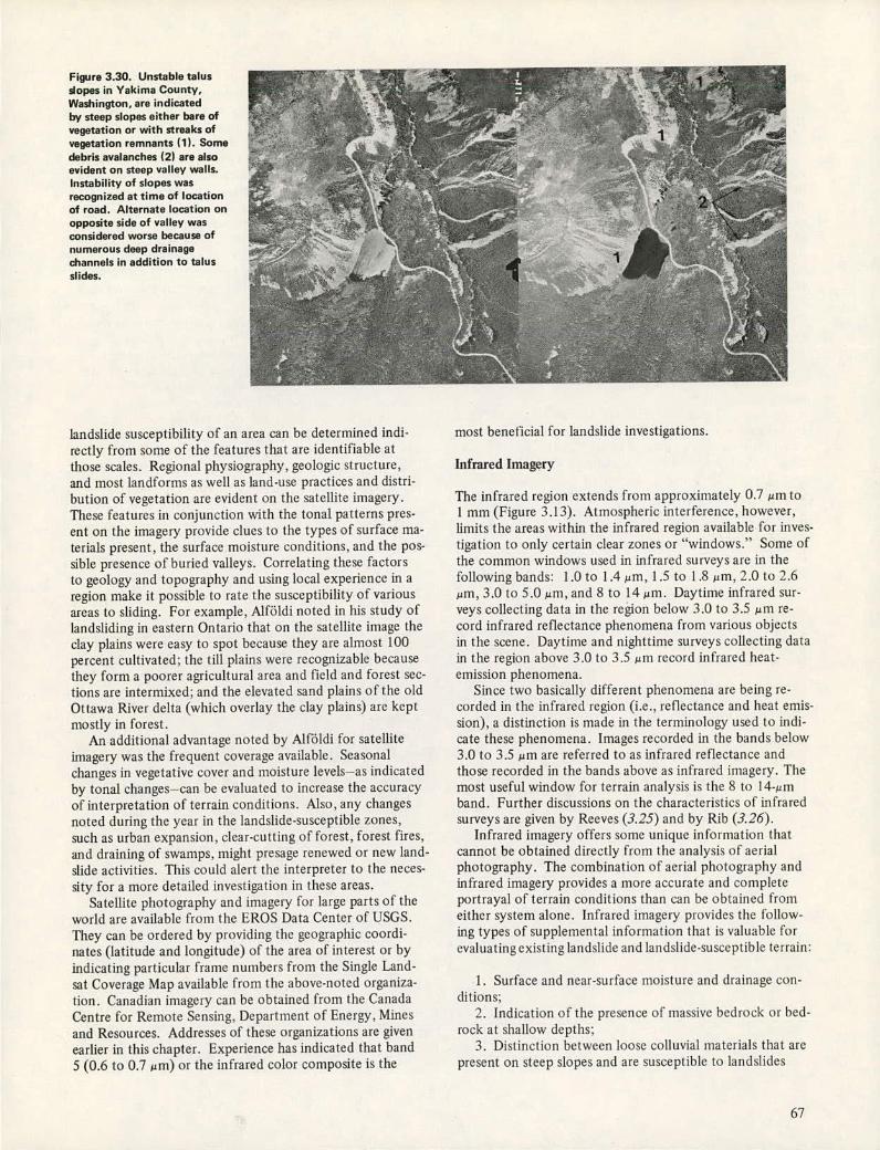
Figure 3.30. Unstable talus slopes in Yakima County, Washington, are indicated by steep slopes either bare of vegetation or with streaks of vegetation remnants (1). Some debris avalanches (2) are also evident on steep valley walls. Instability of slopes was

recognized at time of location

of road. Alternate location on

opposite side of valley was considered worse because of numerous deep drainage channels in addition to talus

slides.

landslide susceptibility of an area can be determined indi-rectly from some of the features that are identifiable at those scales. Regional physiography, geologic structure, and most landfornis as well as land-use practices and distri-bution of vegetation are evident on the satellite imagery. These features in conjunction with the tonal patterns pres-ent on the imagery provide clues to the types of surface ma-terials present, the surface moisture conditions, and the pos-sible presence of buried valleys. Correlating these factors to geology and topography and using local experience in a region make it possible to rate the susceptibility of various areas to sliding. For example, Alföldi noted in his study of landsliding in eastern Ontario that on the satellite image the clay plains were easy to spot because they are almost 100 percent cultivated; the till plains were recognizable because they form a poorer agricultural area and field and forest sec-tions are intermixed; and the elevated sand plains of the old Ottawa River delta (which overlay the clay plains) are kept mostly in forest.

An additional advantage noted by Alföldi for satellite imagery was the frequent coverage available. Seasonal changes in vegetative cover and moisture levels—as indicated by tonal changes—can be evaluated to increase the accuracy of interpretation of terrain conditions. Also, any changes noted during the year in the landslide-susceptible zones, such as urban expansion, clear-cutting of forest, forest fires, and draining of swamps, might presage renewed or new land-slide activities. This could alert the interpreter to the neces-sity for a more detailed investigation in these areas.

Satellite photography and imagery for large parts of the world are available from the EROS Data Center of USGS. They can be ordered by providing the geographic coordi-nates (latitude and longitude) of the area of interest or by indicating particular frame numbers from the Single Land-sat Coverage Map available from the above-noted organiza-tion. Canadian imagery can be obtained from the Canada Centre for Remote Sensing, Department of Energy, Mines and Resources. Addresses of these organizations are given earlier in this chapter. Experience has indicated that band 5 (0.6 to 0.7 pm) or the infrared color composite is the

most beneficial for landslide investigations.

Infrared Imagery

The infrared region extends from approximately 0.7 pm to I mm (Figure 3.13). Atmospheric interference, however, limits the areas within the infrared region available for inves-tigation to only certain clear zones or "windows." Some of the common windows used in infrared surveys are in the following bands: 1.0 to 1.4 pm, 1.5 to 1.8 pm, 2.0 to 2.6 pm, 3.0 to 5.0 pm, and 8 to 14 pm. Daytime infrared sur-veys collecting data in the region below 3.0 to 3.5 pm re-cord infrared reflectance phenomena from various objects in the scene. Daytime and nighttime surveys collecting data in the region above 3.0 to 3.5 pm record infrared heat-emission phenomena.

Since two basically different phenomena are being re-corded in the infrared region (i.e., reflectance and heat emis-sion), a distinction is made in the terminology used to indi-cate these phenomena. Images recorded in the bands below 3.0 to 3.5 pm are referred to as infrared reflectance and those recorded in the bands above as infrared imagery. The most useful window for terrain analysis is the 8 to 14-pm band. Further discussions on the characteristics of infrared surveys are given by Reeves (3.25) and by Rib (3.26).

Infrared imagery offers some unique information that cannot be obtained directly from the analysis of aerial photography. The combination of aerial photography and infrared imagery provides a more accurate and complete portrayal of terrain conditions than can be obtained from either system alone. Infrared imagery provides the follow-ing types of supplemental information that is valuable for evaluatingexisting landslide and landslide-susceptible terrain:

Surface and near-surface moisture and drainage con-ditions;

Indication of the presence of massive bedrock or bed-rock at shallow depths;

Distinction between loose colluvial materials that are present on steep slopes and are susceptible to landslides

67

and the massive bedrock that is more stable on steep slopes; and

4. Diurnal temperature changes that occur in soil masses (these provide clues to the soil-water mass conditions).

Tanguay and Chagnon (3.33) demonstrated the value of infrared imagery and aerial photography for evaluating the moisture and drainage regime associated with a landslide. A flow slide had occurred within the crater of a former slide in clay lake beds in the vicinity of Saint-Jean-Vianney, Quebec. To plan a drilling program to evaluate the poten-tial of further movements required that the areas of seepage, water runoff, and wet soils be identified. By means of photography alone, these features could not be uniquely separated from areas of standing water, topographic shad-ows, and dense vegetation (brush and forested zones) be-cause they all produced similar dark tonal patterns. 1-low-ever, the combination of photography and daytime and nighttime imagery made it possible to separate these va-rious features and identify the critical items for planning the drilling program.

Figures 3.33 and 334 show some of the results reported by Tanguay and Chagnon. Figure 3.33 shows daytime ther-mal infrared imagery obtained in the 8 to 14-jim band and black-and-white infrared photographs of a portion of the area shown in the imagery. Several of the seepage areas (points a and b) interpreted from this figure were drilled and indicated very deep and soft clay starting from the sur-face. The c points indicate both seepage and runoff in a farm field: the d points show standing water coming from snowmelt and surface drainage: and the e points depict the boundary of the recent slide. Point f indicates the upper-most boundary of an older slide surface. In this figure,

seepage areas, runoff, and standing water are dark on both images. On the predawn infrared imagery in Figure 3.34, standing water (points a and f) is warmer and has light tones while seepage zones and runoff (points c and d) are cooler and have darker tones. On the photography, all of these areas have dark tones. Vegetated areas occurring be-tween the areas of standing water in this figure have a me-dium tone on the imagery and appear as white specks on a dark background on the photography.

Figure 3.35 shows a nighttime (predawn) infrared image of an area along a railroad line being investigated for locat-ing potential areas for landslides. The railroad had been plagued for years with landslide problems. The circled darker areas were interpreted as zones of seepage and high moisture levels -potential for landslides. Based on this anal-ysis, the circled areas were drained, and no further slides have occurred in those areas.

Another example of the value of infrared imagery is shown in Figure 3.36, which illustrates nighttime infrared imagery of an area of tilted sedimentary rocks. The mas-sive bedrock areas (point 2) are indicated by light tones. The fractured rock zones and colluvial slopes, which are more susceptible to landslides, are indicated by medium dark tones (point 3). These types of data would be useful in conjunction with aerial photography for rating the land-slide susceptibility of the terrain.

Other remote-sensing techniques, such as multispectral imagery and microwave radiometry, offer potential for in-dicating the presence of landslides. Multispectral systems obtain simultaneous coverage of data in several spectral re-gions- usually a portion of the ultraviolet, the visible, and both infrared reflectance and infrared emission regions. The data are collected on magnetic tape, which makes them

Figure 3.31. Old, massive landslide terrain in Rio Arriba County, New Mexico. Landslides (1) are of such magnitude that they are easily identifiable on common 1:20 000 aerial photographs as well as on smaller scaled photo-index sheets or even 1:1 000 000 satellite imagery (Figure 3.32). Most slides encountered in engineering projects are of smaller magnitude and difficult to identify at scales of 1:20 000.

6

amenable to the use of computer analysis techniques. Micro-wave radiometers collect radiomet nc (temperature varying) data in the microwave or radar regions. The particular ad-vantage of this system is that at the longer wavelengths in-formation from subsurface layers is included in the data. Rib and others (3.27) have demonstrated that, under cer-tain condit ions, informal ion on subsurface moist tire condi-tions (i.e., presence of zones of high moisture level) can be determined by comparative evaluation of photography, nighttime infrared imagery, and microwave radiometry. These techniques are not described in detail because at this

time either further development is needed or the systems are too costly in comparison to the level of information furnished. However, they do offer some future potential for landslide investigations.

FIELD RECONNAISSANCE TECHNIQUES

The discussion in this section is based to a large extent on informal ion in Chapter 4 in the book on landslides published by the Highway Research Board in 1958 (3.10).

Figure 3.32. LANDSAT-1 satellite scene 1657-17031, band 5, May 11, 1974, north central New Mexico. Arrow pointsto edge of small

basalt remnant shown in Figure 3.31. Massive landslides are evident on satellite scene by irregular, scalloped edges. Hummocky

appearance of slide material can be discerned by close examination of scarp edges.

- 'r

- • . .

-- .

'•.i

69

IA'

C

C,,

b-

Figure 3.33. Daytime thermal infrared imagery in 8 to 14-11m band (above) and mosaic prepared from black-and-white infrared photography (below) taken in Ontario, Canada (3.33). Lines AB and AB' represent equivalent coverages on the two image formats. Lettered areas are discussed in text.

B,

Figure 3.34. Predawn infrared imagery in 410 5-,m band (above) and mosiic prepared from black•and•white infrared photography (below) taken in Ontario, Canada (3.33). Line c-c represents common line on both Images. Lettered areas are discussed in text.

:

dbb Ak Al-

P. 1kIJ e

70

Figure 3.35. Nighttime infrared imagery. 0645 h, station 560 to 580, Muskingum Mine Railroad in Ohio. Dark-toned regions within circled areas are interpreted as zones of seepage and high moisture levels and have been associated with slides along railroad right-of-way. Light-toned areas (1) represent standing water on surface.

Figure 3.36. Nighttime infrared imagery of tilted sedimentary rocks in Schuylkill County, Pennsylvania. Lightest tones (1) are water or roads; next lightest (2) are shallow soils over continuous bedrock; medium gray tones (3) in bedrock area generally indicate more fractured rock and colluvial slopes.

An important phase in the preliminary investigation is field reconnaissance to verify the three-dimensional concept of the terrain developed from the literature review and the analysis of remote-sensing data. Many of the fine details and more subtle evidences of slope movement cannot be identi-fied at the scales of photographs and maps analyzed and can be detected only in a field survey. Until that survey is made, part, or even most, of the concepts developed remains con-jecture. Performing a field survey at the time corrective measures are being planned is especially important. Many landslides are complex and as time passes frequently change their physical characteristics and marks of identification. For instance, a landslide examined a year after its occurrence may have changed remarkably from the conditions immedi-ately following the original movement. If a landslide de-veloped as a slump slide and eventually turned into a flow, the orinal report on the slide would be invalid as a basis for planning a correction of the slide. The identification of type should be made at the same time the slide is to be cor-re c ted.

Field Evidence of Movement

The term landslide, by definition, implies that movement has taken place: hence, an analysis of the kind and amount of movement becomes a key to the nature of an active slide. It is imperative to learn to recognize the features that first indicate the onset of ground movement and to learn to rec-ognize the kind of slide that already exists. Quite com-monly the first visible sign of ground movement is recorded by settlement of the roadway or, depending on the location of the roadway within the moving mass, a bulge of the pave-

mnent. Evidence may also be found of landslide movement that has not yet affected the highway but that may do SO in time: Minor failure in an embankment, material that falls on the roadway from an upper slope, or even the progres-sive failure of the region below a fill may presage a larger landslide that will endanger the road itself. Other evidences of movement are to be found in broken pipe or power lines, spalling or other signs of distress in concrete structures, closure of expansion joints in bridge plates or rigid pave-merits (Figures 3.37 and 3.38), or loss of alignment of build-ing foundations. In many eases, arcuate cracks and minor scarps in the soil give advance notice of serious failure.

Table 3.3 gives the chief evidence of movement in the va-rious parts of each type of landslide. The following discus-sion elaborates on the significance of cracks in recognizing and classifying slides and on features that aid in identifying the various types of landslides.

The ability to recognize small cracks and displacements in the surface soils and to understand their meaning de-serves cultivation because it can produce accurate knowl-edge of the cause and character of movement that is pre-requisite to correction. Surface cracks are not necessarily normal to the direction of ground movement, as is com-nionly assumed by some. For example, cracks near the head of a slump are indeed normal to the direction of hori-zontal movement, but the cracks along its flank are nearly parallel to it.

Small en echelon cracks commonly develop in the stir-face soil before other signs of rupture take place: thus, they are particularly important in the recognition of potential or incipient slides. They result from a force couple in which the angle between the direction of motion and that of the

71

Field Iden tifica tb ml of Slope-Movement Types

Once it has been established that slope movement has taken

Figure 3.39. Tension cracks that typically

develop in slump slide in cohesive materials Q. 10, - - 3.34). /

DEPRESSION

/ EN ECHELON / CRACES

ZONE OF UPLIFT

-

FOOT

'\

ME

cracks is a function of the location within the landslide area Thus, in many cases a map of the en echelon cracks will de-lineate the slide accurately, even though no other visible movement has taken place (Figure 3.39).

In addition to indicating incipient or actual movement, cracks in surface soils are locally useful in helping to deter-mine the type of slide with which one is dealing. For cx-

Figure 3.37. Early signs of impending debris slide along Clear Creek, Colorado (3. 10). Displacement of fence, bulging of pavement, and distress in bridge abutment (Figure 3.38) all give early indications of movement at toe of incipient slide. In several places, now covered by patching, centerline stripe was offset along cracks.

t;- q.k

ft' ..iI.. ; ,.

.;

Figure 3.38. Right wing wall shown in lower center of Figure 3.37 (3. 10). Distress in bridge abutment indicates incipient slide. In addition to offset of wing wall shown here, rockers beneath bridge girders were tipped.

ample, in a slump the walls of cracks are slightly curved in the vertical plane and concave toward the direction of move-ment; if the rotating slump block has an appreciable vertical offset, the curved cracks wedge shut at depth. In block slides, on the other hand, the cracks are nearly equal in width from top to bottom and do not wedge out at depth because failure in a block slide begins with tension at the base of the block and progresses upward toward the surface. The presence of a few major breaks in the upper parts of a block slide (Figure 3.40) distinguish it from lateral spreading, which is characterized by a maze of intersecting cracks. The inclination of cracks is commonly almost vertical in block slides in cohesive soils, regardless of the dip of the slip plane, but depends on the joint systems in the rock in block slides of rock.

Distinguishing between incipient block slides and slumps is one of the most helpful applications of a study of cracks. If the outline of the crack pattern is horseshoe-shaped in plan, with or without concentric cracks within it, a slump is almost certainly indicated. If, on the other hand, most of the surface cracks are essentially parallel to the slope or cliff face, a block slide is probably in the making. In either case, additional cracks may develop as major movement gets under way, but these will generally conform to the earlier crack pattern (Figures 2.14 and 2.15).

Evidence of soil creep and of "stretching" of the ground surface should also be sought. Stretching indicates compar-atively deep-seated movement whereas soil creep is of sur-ticial origin. The phenomenon of stretching is most corn-nionly observed in noncohesive materials that do not form or retain minor cracks readily. The best evidence of stretch-ing consists of small cracks that surround or touch some rigid body, such as a root or boulder, in otherwise homno-gencous materials: these cracks form because the tension forces tend to concentrate at or near the rigid bodies.

72

place or is in progress, the next essential step is to identify the type of movement. Table 3.3 gives the surface features that aid in the field identification of slope movements. This table gives only the most common types and not all of the types shown in Figure 2.1 . Further generalizations are given in the following paragraphs.

Falls and Topples

Although the initial mecha ii isms of falls and topples are dif-ferent (Chapter 2), their final appearances after movement are similar. Falls and topples are best recognized by the ac-cumulation of material that is not derived trorn the under-lying slope and that is foreign to normal processes of erosion. In most cases, this material consists of blocks of rock, de-bris. or earth scattered over the surface or forming a talus slope. If undercutting by lake or stream waters has caused the fall, the rate of failure is proportional to the ability of the water to remove the fallen material. A fast-moving stream may remove material almost as fast as it falls, thus removing the evidence but encouraging continuing falls. On the other hand, a lake or some parts of an ocean shore must depend only on wave action to disintegrate and re-move the fallen material: hence, the evidence tends to re-main in sight but continued falls tend to be inhibited. Most of the material yielded by rock topples and rock falls is necessarily close to the steep slopes from which it came, but some may bound down the slope and come to rest far from its present source.

In active or very recent slides, the parent cliff is com-mon!)' marked by a fresh irregular scar that lacks the cres-cent shape that is characteristic of slumps. Instead, the ir-regularity of its surface is controlled by the joints and bed-ding planes of the parent material (Figures 2.3 and 3.41).

Some idea of the intensity and state of activity of a rock fall or rock topple can be inferred from the presence or ab-sence of vegetation on the scarp and by the damage done to trees by the falling rocks. In active areas, the trees are scarred and debarked or show evidence of healed wounds. If the rock fall or rock topple is severe or of long duration - conifers and other long-lived trees are absent: their places may or may not be taken by aspen or other fast-growing species. Many rock falls follow chutes or dry canyons that can usually be differentiated from normal watercourses or paths cut by snow avalanches (Figure 3.42).

Some debris and earth falls and topples exhibit most of the characteristics of rock falls and rock topples. Others proceed by mere spallirig of the surface, but even this activ-ity, it' long continued, can lead to removal of considerable quantities of material. Any fall or topple may • of course. presage major landslide movement in the near future.

Slides

Slides, as distinct from falls, topples, lateral spreads, and flows, are characterized by a host of features that are obser-vable at the surface. These features are related to the kind of material in which the slide occurs and to the amount and direction of motion. Rotational slides are character-ized by rotation of the block or blocks of which they are composed whereas translational slides are marked by lateral separation with little vertical displacement and by vertical,

rather than concave, cracks. Lateral spreading with few, if any, cracks, on the other hand, is characteristic of earth flows.

Translational rock slides are generally easy to recognize because they are composed wholly of rock, boulders, or rock fragments. Individual fragments may be very large and may move great distances from their source. Rock slides

Figure 3.40. Block slide in cohesive materials, near Portage.

Montana (3. 10). The slide, in alluvium, colluvium, and some wind-deposited silt, is moving out over surface of alluvium-filled stream channel with little or no rotation of block and without developing zone of uplift at foot. Parallel step scarps along main scarp and drag effects along flanks are both characteristic of block slides. Arrows indicate overbreak cracks that develop after main scarp is formed; possibly because of abrupt break in slope, these are more sharply curved than are those above most slump slides.

: ' ' .--- - -

Figure 3.41. Rock slide and rock fall along Penn-105 (3. 10). Beds are nearly flat; slide is controlled by joints dipping at steep angle toward road.

73

Table 3.3. Features that aid in recognition of common types of slope movements.

Parts Surrounding Slide

Kind of Type of Motion Material Crown Main Scarp Flanks

Falls, topples Rock Consists of loose rock; probably Is usually almost vertical, irregu- Are mostly bare edges of rock - has cracks behind scarp; has ir- lar, bare, and fresh; usually con-

regular shape controlled by local sists of joint or fault surfaces joint system

Soil Has cracks behind scarp Is nearly vertical, fresh, active, Are often nearly vertical and spalling on surface

Slides Rotational Slump Soil Has numerous cracks that are Is steep, bare, concave toward Have striae with strong vertical

mostly curved concave toward slide, and commonly high; may component near head and slide show striae and furrows on sur- strong horizontal component

face running from crown to near foot; have scarp height head; may be vertical in upper that decreases toward foot; part may be higher than original

ground surface between foot and toe; have en echelon cracks that outline slide in early stages

Rock Has cracks that tend to follow Is steep, bare, concave toward Have striae with strong vertical fracture pattern in original rock slide, and commonly high; may component near head and

show striae and furrows on sur- strong horizontal component face running from crown to near foot; have scarp height head; may be vertical in upper that decreases toward foot; part may be higher than original

ground surface between foot • and toe; have en echelon

cracks that outline slide in early stages

Translational Block Rock Has cracks most of which are Is nearly vertical in upper part Have low scarps with vertical

or nearly vertical and tend to fol- and nearly plane and gently to cracks that usually diverge Soil low contour of slope steeply inclined in lower part downhill

Rock Rock Contains ioose rock; has cracks Is usually stepped according to Are irregular between blocks spacing of joints or bedding

planes; has irregular surface in upper part and is gently to steeply inclined in lower part; may be nearly planar.or com- posed of rock chutes

Flows Dry Rock Consists of loose rock: probably Is usually almost vertical, irregu- Are mostly bare edges of rock

has cracks behind scarp; has ir- lar, bare, and fresh: usually con- regular shape controlled by local sists of joint or fault surfaces joint system

Soil Has no cracks Is funnel shaped at angle of repose Have Continuous curve into main

Wet scarp

Debrisavalanche Soil Has few cracks Typically has serrated or V-shaped Are §1eep and irregular in upper Debris flow upper part: is long and narrow, part; may have Ieveesbuilt up

bare, and commonly striated in lower parts

Earth flow Soil May have a few cracks Is concave toward slide; in some Are curved; have steep sides types is nearly circular and slide issues through narrow orifice

Sand flow • Soil Has few cracks Is steep and concave toward slide; Commonly diverge in direction Silt flow may have variety of shapes in of movement

outline: nearly straight, gentle arc, circular, or bottle shaped

Note: This table updates Table 1 in book on landslides published in 1958 by Highway Research Board (3.10, chap. 4 by A. M. Ritchie, pp. 56.57)

74

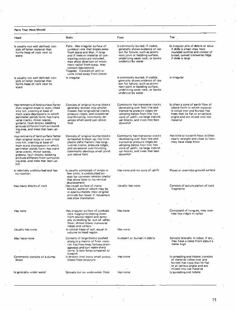
Parts That Have Moved

Head Body Foot Toe

Is usually not well defined; con-sists of fallen material that forms heap of rock next to scarp

Is usually not well defined; con sists of fallen material that forms heap of rock next to scarp

Falls:. Has irregular surface of jumbled rock that slopes away from scarp and that, if large and if trees or material of Con-trasting colors are included, may show direction of move-ment radial from scarp; may contain depressions

Topples: Consists of unit or units tilted away from crown

Is irregular

Is commonly buried; if visible, generally shows evidence of rea-son for failure, such as promi-nent joint or bedding surface, underlying weak rock, or banks undercut by water

Is commonly buried; if visible, generally shows evidence of rea-son for failure, such as promi-nent joint or bedding surface, underlying weak rock, or banks undercut by water

Is irregular pile of debris or talus if slide is small; may have rounded outline and Consist of broad, curved transverse ridge if slide is large

Is irregular

Has remnants of land surface flatter than original slope or even tilted into hill, creating at base of main scarp depressions in which perimeter ponds form; has trans-verse cracks, minor scarps, grabens, fault blocks, bedding attitude different from surround-ing area, and trees that lean up-hill

Has remnants of land surface flatter than original slope or even tilted into hill, creating at base of main scarp depressions in which perimeter ponds form; has trans-verse cracks, minor scarps, grabens, fault blocks, bedding attitude different from surround-ing area, and trees that lean up-hill

Is relatively undisturbed and has no rotation

Has many blocks of rock

Has none

Usually has none

May have none

Commonly Consists of a slump block

Is generally under water

Consists of original slump blocks generally broken into smaller masses; has longitudinal cracks, pressure ridges, and occasional overthrusting; commonly de-velops small pond just above foot

Consists of original slump blocks somewhat broken up; has little plastic deformation: has longi-tudinal cracks, pressure ridges, and occasional overthrusting: commonly develops small pond just above foot

Is usually composed of single or few units; is undisturbed ex-cept for common tension cracks that show little or no vertical displacement

Has rough surface of many blocks, some of which may be in approximately their original attitude but lower if movement was slow translation

Has irregular surface of jumbled rock fragments sloping down from source region and gener-ally extending far out on valley floor: shows lobate transverse ridges and valleys

Is conical heap of soil, equal in volume to head region

Consists of large blocks pushed along in a matrix of finer mate-rial: has flow lines: follows drain-ageways and can make sharp turns; is very long compared to breadth

Is broken into many small pieces: shows flow structure

Spreads out on underwater floor

Commonly has transverse cracks developing over foot line and transverse pressure ridges de-veloping below foot line; has zone of uplift, no large individ-ual blocks, and trees that lean downhill

Commonly has transverse cracks developing over foot line and transverse pressure ridges de-veloping below foot line: has zone of uplift, no large individ-ual blocks, and trees that lean downhill

Has none and no zone of uplift

lisually has none

Has none

Has none

Is absent or buried in debris

Has none

Has none

Is often a zone of earth flow of lobate form in which material is rolled over and buried: has trees that lie flat or at various angles and are mixed into toe material

Has little or no earth flow; is often nearly straight and close to foot: may have steep front

Plows or overrides ground surface

Consists of accumulation of rock fragments

Composed of tongues; may over-ride low ridges in valley

Spreads laterally in lobes; if dry, may have a steep front about a meter high

Is spreading and lobate; consists of material rolled over and buried; has trees that lie flat or at various angles and are mixed into toe material

lsspreading and lobate

75

commonly occur only on steep slopes. The numerous small block units with random rotation are mixed in a matrix of finer grained material; the large rock fragments tend to float on or in the matrix. Rock slides have translational failure surfaces rather than the concave surfaces of slumps, and they do not move as unrotated multiple units, like block slides. Most rock slides are controlled by the spacing of joints and bedding planes in the original rock. There is par-ticular danger of forming a rock slide of serious proportions if construction is undertaken in an area marked by a system of strongly developed joints or bedding planes that dip steeply outward toward the natural slope. This is especially true if the natural slope angle is steeper than the angle of re-pose of the broken rock. Water is not so important a factor in causing rock slides as in causing slides in soil. In sonic in-stances, however, water helps to weaken bedding or joint planes that otherwise would offer high frictional resistance. Any seepage that is apparent after a rock slide has taken place is most likely to be visible in the scarp region or, per-haps, in the slide material itself.

Many rock slides are thinner than either slumps or block slides because they commonly are restricted to the weathered zone in bedrock or to surficial talus. The shape of the shear zone, therefore, conforms to the unweathered bedrock sur-face and is not controlled to any large extent by joints or bedding planes in the bedrock. Many talus slopes produce rock slides by failure within the body of talus.

Rotational slumps rarely form from solid. hard rocks, although special combinations of factors have been known to produce them. Slumps are widespread, however, in sands, silts, and clays and in the weaker bedded rocks. There they can be identified readily from surface indica-tions, though only after considerable movement has taken place. The head region of a slump is characterized by steep escarpments and by visible offsets between separate blocks of material (Figure 3.19). The highest escarpment is com-monly just below the crown: because the crests of the flanks are lower than the crown, they can be recognized as flanks, even if the escarpment on one of them happens to be larger than the one below the crown. If the landslide is active or has been active recently, the scarp is bare of vegetation and may be marked by striations or grooves that indicate the di-rection of movement that has taken place. Striations at the head tend to reflect downward movement whereas striations along the flanks may be nearly horizontal. If the slump is compound, its several crescent-shaped scarps will appear as a scalloped edge in plain view (Figure 2.21).

Undrained depressions and perimeter lakes, bounded on the uphill side by the main scarp, characterize the head re gions of many slumps: even if internal drainage prevents such ponds from holding water for long periods, their de-pressions may be evident. In humid regions, the head area may remain greener than surrounding areas because of the swampy conditions. In the San Juan region of south-western Colorado. for instance, groves of aspen trees are commonly good indications of wet ground conditions and hence of slides and unstable ground. In northern West Vir-ginia, the swampy areas in the head remain green during the winter whereas the well-drained low areas are brown.

The tension cracks near the head of a slump are generally concentric and parallel to the main scarp. Many such cracks are obscured by rubble or other noncohesive materials, but

Figure 3.42. Rock fall and rock slide near Skihist, British Columbia, on Canadian National Railroad (3.10). Note bare active slopes, closely spaced jointing of rocks, rock chutes, and absence of water. Wooden and concrete sheds bypass debris falling over tracks from above.

even so they may be indicated by evidence of surface stretch-ing, by lines of rock fragments that have been displaced, or even by blades of grass that have been pulled down into the cracks by sand or other loose surface material as it sifted into them. The head region of a slump or an earth block slide with surficial slump characteristics may also be recog-nized by the presence of slump grabens that have experi-enced some rotation (Figures 3.19 and 3.43). These are de-pressed fault blocks of soil or rock, caused in part by de-crease in curvature of the shear plane. This produces ten-sion and ultimate failure in the main slump block because of lack of support on its uphill side.

The amount and direction of rotation that any slump block has undergone can usually be ascertained by deter-mining the slope of its surface as compared with that of the original slope. Comparison of the (lip and strike of bedded material within the slump block with the original attitude of the unslumped material is an even more exact and fool-proof method of determining the amount of rotation, be-cause erosional alternation of the surfaces may give an er-roneous impression. In a general way, the amount of ro-tation is a measure of the amount of displacement.

The part just above the foot of a slump is a zone of com-pression. The slumped material is con fined by the foot and by the flanks of the main scarp SO that it is compressed by the load above into the bot torn part of the howl-shaped sur-face of rupture. In this region, therefore, there are no open cracks. The foot region is marked by a zone of tension and uplifl because the slumped material is required to stretch over the foot before it passes farther downhill. This stretch-ing destroys any remaining slump blocks because of the change in direction of the forces. The small blocks and frag-ments that result tend to weather to rounded forms, produc-ing hummocky ground. Pavement uplifts and cracks, so disconcerting to the motorist and highway engineer. are also most likely to take place in the foot zone. Seeps, springs, and marshy conditions commonly mark the foot and toe of a slump. Moreover, trees tend to be tilted down.

76

Figure 3.43. Graben on slump slide (3. 10). Rotation of slump block is uphill, resulting in flattening of original ground surface, but graben block, which breaks off from slump block, rotates downhill. Grabens do not form if slump block has sheared on surface that approaches arc of circle; instead, they form on slump blocks that slide over principal surface of rupture having marked decrease in its curvature, causing greater horizontal movement for each unit of vertical offset in center portion of slide than in head region.

HEAVY LINE INOICATES

GRV8EN / ORIGINAL SURFACE

MPMP J//

Figure 3.44. General orientation of trees on slump landslide (3. 10). As a result of rotation, trees on blocks are bowed uphill because tree tops tend to grow vertically while stump portion changes with rotating land surface. Contrast head and toe regions and compare with Plates 3.2 and 3.3.

hill rather than uphill as they near the head (Figure 3.44 and Plate 3.3).

The approximate age of some slumps can be inferred by study of the bent trees. If older trees are bent but younger ones are straight, for instance, the slide probably has not moved during the life of the younger trees. On the other hand, the sizes of the tree trunks at the points where the bends occur give a running history of the rotation.

Just below the foot of a slump the ground is commonly marked by long transverse ridges that are separated from one another by open tension cracks. These cracks seldom remain open for long periods of time, and they do not form scarps or other evidence of displacement because the mate-rial is no longer confined but spreads out laterally and de-velops radial cracks at the toe.

Lateral Spreads and Flows

In lateral spreads, a coherent upper block is broken into strips or blocks and extended or stretched by plastic flow or liquefaction of the lower layer. The mechanism of fail-ure can involve not only rotation and translation, but also flow, and thus surface characteristics will contain elements of both slides and flows. One form of lateral spread, in which a plastic layer is squeezed out by the weight of an overlying rigid layer, is here termed a piston slide. In this type, a part of the upper layer may drop vertically,

without rotation, into the space left by removal of the plastic layer.

Dry flows are not difficult to recognize after they have occurred, but it is virtually impossible to predict them in ad-vance. They are commonly very rapid and short-lived. Dry flows are rarely composed of rock fragments; they usually consist of uniformly sized silt or sand. They exhibit no cracks above the main scarp and have poorly developed or nonexistent flow lines. Except for sand runs, they have no well-defined foot. Dry bess may become fluid and flow down a slope because of an earthquake or other external vibrations. Sand runs also behave somewhat as fluids, but in the latter part of their course the sand particles are more likely to slide than to flow.

Wet flows occur when fine-grained soils, with or without coarser debris, become mobilized by an excess amount of water. Most of them behave like wet concrete in a chute (differences are due to water content), but the flow of some wet silts and fine sands is triggered by shocks. "Quick" or sensitive clays may be liquefied by the leaching of salts or by other causes that are not completely understood.

Wet flows are generally characterized by their great lengths, generally even gradients and surfaces, absence of tension cracks, and lack of blocky units and minor scarps. If tension cracks are present, they are bowed in the direc-tion of movement (Figure 3.45), showing the effects of movement of wetter materials at depth beneath the drier crust. An older flow that has had time to dry may show large shrinkage cracks or flow lines. In many cases, the main scarp area is emptied by the removal of all flow ma-terial and resembles a glacial cirque. In other cases, the gra-dation may be imperceptible downward from soil creep to mud flow.

The rate of flow is dependent on the total amount of material that feeds the slide; the accumulated debris im-poses a load on the entire mass below it and tends to main-tain a constant rate of movement. The flow is under pres-sure everywhere from the material above it; consequently, the mass shows few, if any, cracks over the foot. Flows can and do make sharp turns and move around firmly fixed ob-stacles that appear in their paths. A very wet flow moving at high velocity may leave debris marks high on trees or other objects and ridges of debris called torrent levees along its sides.

Hidden Landslides

Among the most difficult kinds of slides to recognize and guard against are old landslides that have been covered by glacial till or other more recent sediments. To predict, in detail, the existence of old buried slides or the effect that they may have on new construction work that exposes them is probably impossible. One who knows the recent geologic history of the region intimately, however, may be able to make some educated guesses as to the probable ex-istence of such slides and even as to where they are most likely to be found. One example is shown in Figure 3.46; the indicated unstable body of soft shale and chalk is clearly related to a fault in the bedrock, but it also has the characteristics of a surface landslide. Since this slide took place, the area was covered by two or more layers of bess, which completely obscured the landslide until the rising

VIA

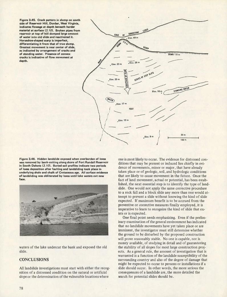
Figure 3.45. Crack pattern in slump on south side of Reservoir Hill, Dunbar, West Virginia, indicates flowage at depth beneath harder

material at surface (3. 10). Broken pipes from reservoir at top of hill dumped large amount of water into old slide and reactivated it. Horseshoe-shaped scarp is imperfect, differentiating it from that of true slump. Greatest movement is near center of slide, as indicated by arrangement of cracks and of standing water. Presence of convex cracks is indicative of flow movement at depth.

EDGE OF

Elm 49m

Elev. 23 m Etev. 28 m

Elev, 23 m

EI~lm

,Etev. 17 m

oo

EIev. 12 m

, EIev. 9 m / 30 m

bOlt

/

Figure 3.46. Hidden landslide exposed when overburden of bess was removed by bank-cutting along shore of Fort Randall Reservoir in South Dakota (3. 10). Buried soil profiles indicate two periods of bess deposition after faulting and landsliding took place in underlying shale and chalk of Cretaceous age. All surface evidence of landsliding was obliterated by bess until lake waters cut new face.

- - --- -

*---

waters of the lake undercut the bank and exposed the old slide.

CONCLUSIONS

All landslide investigations must start with either the recog-nition of a distressed condition on the natural or artificial slope or the determination of the vulnerable locations where

one is most likely to occur. The evidence for distressed con-ditions that may be present or induced lies chiefly in evi-dence of movements, minor or major, that have already taken place or of geologic, soil, and hydrologic conditions that are likely to cause movement in the future. Once the fact of land movement, actual or potential, has been estab-lished, the next essential step is to identify the type of land-slide. One would not apply the same corrective procedure to a rock fall and a block slide any more than one would at-tempt to prevent a slide without knowing the kind of slide expected. If maximum benefit is to be accrued from the preventive or corrective measures finally employed, it is imperative to learn to recognize the kind of slide that ex-ists or is expected.

One final point needs emphasizing. Even if the prelim-inary examination of the general environment has indicated that no landslide movements have yet taken place or are imminent, the investigator must still determine whether the ground to be disturbed by the proposed construction will prove reasonably stable. No one is capable, nor is money available, of studying in detail and of guaranteeing the stability of all slopes for most large construction proj-ects. As a general rule, the amount of investigation that is warranted is a function of the landslide susceptibility of the surrounding country and also of the degree of damage that might be expected to occur to persons or installations if a slide should occur. In other words, the more serious the consequences of a landslide are, the more detailed the search for potential slides should be.

78

REFERENCES

3.1 Alföldi, T. T. Regional Study of Landsliding in Eastern Ontario by Remote Sensing. Department of Civil Engi-neering, Univ. of Toronto, MS thesis, 1974,79 pp.

3.2 Anderson, R. R., Hoyer, B. E., and Taranik, J. V. Guide to Aerial Imagery of Iowa. Iowa Geological Survey, Public Information Circular 8, Sept. 1974, 142 pp.

3.3 Baker, R. F., and Chieruzzi, R. Regional Concept of Landslide Occurrence. Highway Research Board, Bulletin 216, 1959, pp. 1-16.

3.4 Bruce, R. L., and Scully, J. Manual of Landslide Recog- nition in Pierre Shale, South Dakota. South Dakota De-partment of Highways, Pierre, Final Rept. of Research Project 615(64), Dec. 1966, 70 pp.

3.5 Chassie, R. G., and Goughnour, R. D. National Highway Landslide Experience. Highway Focus, Vol. 8, No. 1, Jan. 1976, pp. 1-9.

3.6 Cleaves, A. B. Landslide Investigations: A Field Hand- book for Use in Highway Locations and Design. U.S. Bureau of Public Roads, 1961,67 pp.

3.7 Colwell, R. N., ed. Manual of Photographic Interpreta- tion. American Society of Photogrammetry, Falls Church, Va., 1960, 868 pp.

3.8 Denny, C. S., Warren, C. R., Dow, D. H., and Dale, W. J. A Descriptive Catalog of Selected Aerial Photographs of Geologic Features in the United States. U.S. Geological Survey, Professional Paper 590, 1968, 79 pp.

3.9 Dishaw, H. E. Massive Landslides. Photogrammetric En- gineering, Vol. 32, No. 6, June 1967, pp. 603-609.

3.10 Eckel, E. B., ed. Landslides and Engineering Practice. Highway Research Board, Special Rept. 29, 1958, 232 pp.

3.11 Gagnon, H. Remote Sensing of Landslide Hazards on Quick Clays of Eastern Canada. Proc., 10th International Symposium of Remote Sensing of Environment, Environ-mental Research Institute of Michigan, Ann Arbor, 1975, pp. 803-810.

3.12 Leith, C. J., Fisher, C. P., Deal, C. S., Gupton, C. P., and Yorke, C. A. An Investigation of the Stability of High-way Cut Slopes in North Carolina. North Carolina State Univ., Raleigh, Project ERO-110-U, June 1964, 129 pp.

3.13 Liang, T. Landslides: An Aerial Photographic Study. Cornell Univ., Ithaca, N.Y., PhD thesis, 1952, 274 pp.

3.14 Lobeck, A. K. Geomorphology. McGraw-Hill, New York, 1939, 731 pp.

3.15 Lueder, D. R. Aerial Photographic Interpretation: Prin- ciples and Applications. McGraw-Hill, New York, 1959, 462 pp.

3.16 Maruyasu, T., Nakano, T., Nishio, M., Takeda, Y., Kawasaki, T., Kimata, K., Ozarki, Y., and Fuchimoto, M. Statistical Analysis of Landslides and Related Phenomena on Aerial Photographs. Journal of Japan Society of Photogrammetry, Special Vol. 1, June 1964, pp. 93-100.

3.17 Mathur, B. S., and Gartner, J. F. Principles of Photo In- terpretation in Highway Engineering Practice. Materials and Testing Division, Ontario Department of Highways, 1968, 236 pp.

3.18 McNutt, R. B., and others. Soil Survey of Chilton County, Alabama. U.S. Soil Conservation Service, U.S. Forest Ser-vice, Alabama Agricultural Experiment Station, and Ala-bama Department of Agriculture and Industries, Oct. 1972.

3.19 Mintzer, 0. W. Application of Photo Interpretation to Highway Engineering Design. Engineering Experiment Station, Ohio State Univ., Columbus, Final Rept. EES 196, Oct. 1966, 213 pp.

3.20 Mintzer, 0. W., and Struble, R. A. Manual of Terrain In- vestigation Techniques for Highway Engineers. Engineer-ing Experiment Station, Ohio State Univ., Columbus, Rept. 196-2 and Appendix I, Oct. 1965, 384 pp.

3.21 National Aeronautics and Space Administration. Skylab Earth Resources Data Catalog. National Aeronautics and Space Administration, Houston, 1974, 359 pp.

3.22 Norell, W. F. Air Photo Patterns of Landslides in South-

eastern Ohio. Ohio Department of Highways, Columbus, Vols. 1 and 2, 1965.

3.23 Ray, R. G. Aerial Photographs in Geologic Interpretation and Mapping. U.S. Geological Survey, Professional Paper 373, 1960, 230 pp.

3.24 Radbruch-Hall, D. H., Colton, R. B., Davies, W. E., Skipp, B. A., Lucchitta, I., and Vanes, D. J. Preliminary Land-slide Overview Map of the Conterminous United States. U.S. Geological Survey, Miscellaneous Field Studies Map MF-771, 1976.

3.25 Reeves, R. G., ed. Manual of Remote Sensing. American Society of Photogrammetry, Falls Church, Va., Vols. 1 and 2, 1975, 2144 pp.

3.26 Rib, H. T. An Optimum Multisensor Approach for De- tailed Engineering Soils Mapping. Purdue Univ., Lafayette, Ind., Joint Highway Research Project 22, Vols. 1 and 2, 1966, 406 pp.

3.27 Rib, H. T., Spencer, J. M., Jr., Falls, C. P., and Koca, J. F. Evaluation of Aerial Remote Sensing Systems for Detect-ing Subsurface Cavities in Kansas. Federal Highway Ad-ministration, Rept. FHWA RD-75-119, 1977.

3.28 Scully, J. Landslides in Pierre Shale in Central South Dakota. South Dakota Department of Transportation, Pierre, Final Rept. of Project 635(67), Dec. 1973, 707 pp.; Federal Highway Administration.

3.29 Sharpe, C. F. S. Landslides and Related Phenomena: A Study of Mass Movements of Soil and Rock. Columbia Univ. Press, New York, 1938, 137 pp.

3.30 Smith, J. T., Jr., ed. Manual of Color Aerial Photography. American Society of Photogrammetry, Falls Church, Va., 1968, 550 pp.

3.31 Stallard, A. H., and Anschutz, G. Use of the Kelsh Plotter in Geoengineering and Allied Investigations in Kansas. Highway Research Board, Highway Research Record 19, 1963, pp. 53-107.

3.32 Stallard, A. H., and Myers, L. D. Soil Identification by Remote Sensing Techniques in Kansas: Part I. State Highway Commission of Kansas, Topeka, 1972, 107 pp.; Federal Highway Administration.

3.33 Tanguay, M. G., and Chagnon, J. Y. Thermal Infrared Imagery at the St. Jean-Vianney Landslide. Proc., 1st Canadian Symposium on Remote Sensing, Canada Center for Remote Sensing and Canadian Institute of Surveying, Ottawa, 1972, pp. 387-402.

3.34 Terzaghi, K., and Peck, R. B. Soil Mechanics in Engineer- ing Practice. Wiley, New York, 1948, 566 pp.

3.35 Thomas, M. M., ed. Manual of Photogrammetry. Ameri- can Society of Photogrammetry, Falls Church, Va., Vols. 1 and 2,3rd Ed., 1966, 1199 pp.

3.36 Thompson, G. A., and White, D. E. Regional Geology of the Steamboat Springs Area, Washoe, Nevada. U.S. Geological Survey, Professional Paper 458 A, 1964.

3.37 Thornbury, W. D. Principles of Geomorphology. Wiley, New York, 1954, 618 pp.

3.38 Way, D. S. Terrain Analysis: A Guide to Site Selection Using Aerial Photographic Interpretation. Dowden, Hutchinson and Ross, Stroudsburg, Penn., 1973, 329 pp.

3.39 Williams, G. P., and Guy, H. P. Erosional and Depositional Aspects of Hurricane Camile in Virginia, 1969. U.S. Geo-logical Survey, Professional Paper 804, 1973, 80 pp.

3.40 Zâruba, Q., and Mend, V. Landslides and Their Control. Elsevier, New York, and Academia, Prague, 1969, 205 pp.

PHOTOGRAPH CREDITS

Plate 3.1 Courtesy of Region 10, Federal Highway Administra- tion

Plate 3.2 Courtesy of Washington State Highway Commission Plate 3.3 Courtesy of Washington State Highway Commission Plate 3.4 Courtesy of U.S. Department of Agriculture Plate 3.5 Courtesy of National Aeronautics and Space Adminis-

tration Plate 3.6 Courtesy of National Aeronautics and Space Adminis-

tration Figure 3.1 Courtesy of Virginia Division of Mineral Resources

79

Figure 3.3 Courtesy of Ohio Department of Transportation Figure 3.4 Courtesy of Washington State Highway Commission Figure 3.5 Courtesy of Ohio Department of Transportation Figure 3.6 Courtesy of Ohio Department of Transportation Figure 3.7 Courtesy of Idaho Transportation Department Figure 3.12 Courtesy of Kansas Department of Transportation Figure 3.14 Courtesy of U.S. Department of Agriculture Figure 3.15 Courtesy of Ohio Department of Transportation Figure 3.16 Courtesy of South Dakota Department of Transporta-

tion Figure 3.17 Courtesy of Ohio Department of Transportation Figure 3.18 Courtesy of U.S. Geological Survey Figure 3.19 Courtesy of U.S. Department of Agriculture Figure 3.20 Courtesy of U.S. Geological Survey Figure 3.21 Courtesy of U.S. Department of Agriculture Figure 3.22 Courtesy of U.S. Department of Agriculture Figure 3.23 Courtesy of U.S. Department of Agriculture Figure 3.24 Courtesy of U.S. Department of Agriculture Figure 3.25 Courtesy of U.S. Department of Agriculture Figure 3.26 Courtesy of North Dakota State Highway Department

Figure 3.27 Courtesy of Ontario Ministry of Transportation and Communications

Figure 3.28 Courtesy of U.S. Department of Agriculture Figure 3.30 Courtesy of U.S. Department of Agriculture Figure 3.31 Courtesy of U.S. Geological Survey Figure 3.32 Courtesy of National Aeronautics and Space Adminis-

tration Figure3.33 Courtesy of M. G. Tanguay Figure 3.34 Courtesy of M. G. Tanguay Figure 3.35 Courtesy of D. Rubin, American Power Service Corpo-

ration, and F. J. Buckmeier, Texas Instruments, Inc. Figure 3.36 Courtesy of Federal Highway Administration Figure 3.37 D. J. Varnes, U.S. Geological Survey Figure 3.38 D. J. Varnes, U.S. Geological Survey Figure 3.40 E.K. Maughan, U.S. Geological Survey Figure 3.41 Courtesy of Pennsylvania Department of Transporta-

tion Figure 3.42 F. 0. Jones, U.S. Geological Survey Figure 3.45 Robert C. Lafferty, consulting geologist Figure 3.46 C. F. Erskine, U.S. Geological Survey

Me

Chapter 4

Field, Investigation George F. Sowers and David L. Royster

The field investigation is the central and decisive part of a study of landslides and landslide-prone areas (4.9). The in-vestigation serves two essential purposes: (a) to identify areas subject to sliding when future construction is being planned and (b) to define features of and environmental factors involved in an existing slide. Unstable areas prone to sliding usually exhibit symptoms of past movement and incipient failure; most of these can be identified in a de-tailed field investigation before design. Such investigations can show how to prevent or at least minimize future move-ments, and they can suggest alternate routes that are less likely to slide. Once a landslide has developed (either be-fore the construction of a facility or after work is under way), the investigation is made to diagnose the factors re-sponsible for the movement and to determine what correc-tive measures are appropriate to prevent or minimize con-tinuing movements.

Because landslides are continually changing phenomena, the field investigation cannot be considered an isolated or easily defined activity; instead, it is iterative. New data gen erate new questions that require more data for answers. Al. though the investigation must continue for a period of time consistent with the shifting topography and changing en-vironment, it is constrained by the timely needs for preven-tive or corrective design. Thus, field investigations should commence long before construction is anticipated and sometimes continue long after the area has been changed by the anticipated construction.

SCOPE OF FIELD INVESTIGATIONS

A number of features require study in a field investigation; these are enumerated below as a checklist for planning a study.

I. Topography A. Contour map

Land form Anomalous patterns (jumbled, scarps, bulges)

B. Surface drainage Continuous Intermittent

C. Profiles of-slope Correlate with geology (II) Correlate with contour map (IA)

D. Topographic changes 1. Rate of change by. time 2. Correlate with groundwater (III), weather (IV),

and vibration (V) II. Geology

A. Formations at site 1. Sequence of formations 2. Colluvium

Bedrock contact Residual soil

3. Formations with bad experience 4. Rock minerals susceptible to alteration

B. Structure: three-dimensional geometry I. Stratification 2. Folding 3. Strike and dip of bedding or foliation

Changes in strike and dip Relation to slope and slide

4. Strike and dip of joints with relation to slope 5. Faults, breccia, and shear zones with relation

to slope and slide C. Weathering

Character (chemical, mechanical, and solution) Depth (uniform or variable)

III. Groundwater A. Piezometric levels within slope

I. Normal 2. Perched levels, relation to formations and struc-

ture

3. Artesian pressures, relation to formations and structure

B. Variations in piezometric levels-correlate with weather (IV), vibration (V), and history of slope changes (VI)

Response to rainfall Seasonal fluctuations Year-to-year changes Effect of snowmelt

C. Ground surface indications of subsurface water Springs Seeps and damp areas Vegetation differences

D. Effect of human activity on groundwater Groundwater utilization Groundwater flow restriction Impoundment and additions to groundwater Changes in ground cover and infiltration oppor-tunity Surface water changes

E. Groundwater chemistry Dissolved salts and gases Changes in radioactive gases

IV. Weather A. Precipitation

Form (rain or snow) Hourly rates Daily rates Monthly rates Annual rates

B. Temperature Hourly and daily means Hourly and daily extremes Cumulative degree-day deficit (freezing index) Sudden thaws

C. Barometric changes V Vibration

A. Seismicity Seismic events Microseismic intensity Microseismic changes

B. Human induced Transport Blasting Heavy machinery

History of slope changes A. Natural process

Long-term geologic changes Erosion Evidence of past movement Submergence and emergence

B. Human activity Cutting Filling Changes in surface water Changes in groundwater Changes in vegetation cover, clearing, excava-tion, cultivation, and paving Flooding and sudden drawdown of reservoirs

C. R.ate of movement 1. Visual accounts 2. Evidence in vegetation

3. Evidence in topography 4. Photographs (see Chapter 3)

Oblique Aerial Stereoptical data (photographic) Spectral changes

5. Instrumental data (see Chapter 5) Vertical changes, time history Horizontal changes, time history Internal strains and tilt, including time his-tory

D. Correlations of movements Groundwater-correlate with groundwater (III) Weather-correlate with weather (IV) Vibration-correlate with vibration (V) Human activity-correlate with human-induced vibration (VB)

The techniques for obtaining the data will be discussed at greater length later in this chapter. The extent to which any one feature requires evaluation is difficult to determine in advance. Whether any more data are needed will depend on the amount of information already available. However, the process is seldom completed; instead, the work stops when time, money, and patience commensurate with risks and potential costs have been exhausted.

Topography

The topography or geometry of the ground surface is an overt clue to past landslide activity and potential instability. More detail than that shown on existing topographic or project design maps is usually required for landslide studies. Moreover, interpretations made by topographerswho.are not specifically looking for landslide features can obscure the special geometric or topographic forms that are diag-nostic of landslides. Therefore, special mapping is usually necessary. Because the topography of a landslide is con-tinually changing, the area must be mapped at several dif-ferent times: (a) several years before construction (if data are available), (b) at the time a specific landslide investiga-tion is initiated, (c) at appropriate intervals during the prog-ress of the investigation, and (d) after remedial measures are undertaken. Ultimately, the effectiveness of corrective measures is expressed by whether the topography changes.

Because of the long time span involved, the location of the area should be referenced with some standard location system. Latitude and longitude may be sufficient for studies in remote areas or studies encompassing large sites. State survey coordinate systems and road stationing out-side the area of study can provide an effective frame for lo-cation. In addition, nearby prominent topographic fea-tures should be referenced because man-made features often change and those who must use the data referenced to them may not be aware of those changes.

Geology

The geometry of the subsurface is the most important sin-gle factor in the analysis of a landslide. First, the various soil and rock units must be identified. Although it is de-sirable to associate the geologic units with the named geo-

82

logic formations that have been defined or previously studied in the area, this activity frequently dissipates more time and effort than are relevant to the evaluation of the landslide. Because the name of a formation seldom re-flects its engineering behavior, determining the structural, lithologic, and engineering properties of the formation is far more important than determining its exact age and identification. However, names do have value in compar-ing landslide activity in one area with that in another that includes the same formations, and relative age can help in describing structural features.

Geologic structure is frequently a major factor in land-slides. Although this includes the major large-scale struc-tural features such as folds and faults to which most impor-tance is attached in regional geologic studies, the minor structural details, including joints, small faults, and local shear zones, may be even more important. Changes in the geologic conditions with location give important clues to areas of distress and to potential landslide activity. Off-sets in strata, changes in joint orientation, and abrupt changes in dips and strikes are indicators of nonuniform geologic conditions. These must be identified both within the area of potential or observed movement and far enough beyond that area to predict the effect of any planned con-struction surrounding the landslide zone.

Water

Water is a major factor in most landslides. Concentrations of surface water from rainfall runoff, seeps, and springs are overt indications of topographic changes in landslide-prone areas. For example, unusually deep erosion gullies some-times suggest that soils and rocks have been weakened by landslide activity. Moreover, surface water entering cracks and fissures caused by earth movement aggravates instability.

Seeps and springs that serve as groundwater exits are another dimension of the water problem. Sometimes, how-ever, too much attention is paid to the exit and not enough to the source. If there is a groundwater exit, there also must be a path of seepage leading to it; thus, the exit of groundwater is a clue to internal water pressures elsewhere. Unfortunately, the layperson sometimes considers seeps and springs to be the- causeof earth movements. Seeps up-hill from the slide serve as a source of surface water that can infiltrate back into the soil within the slide, thus con-tributing to instability. However, within the slide zone and downhill from it, the opposite is usually true. Less pressure builds up when water is seeping out of the ground than when the exits for groundwater are blocked. For example, in one major slide area, landslide activity was always pre-ceded by a stoppage of spring discharge near the slide toe; the cessation of movement was marked by an increase in spring discharge.

The various joints, fissures, and more pervious strata that conduct water underground must be identified. These features constitute a part of the subsurface geometry that is not always reflected by the strike and dip of the forma-tions. Even the most insignificant water-bearing stratum can sometimes be the source of trouble and is too often overlooked in favor of the more obvious, but perhaps less dangerous, aquifers. Within each water-bearing formation or fissure is a definite (but changing) groundwater pressure

or piezometric level. The groundwater is sometimes perched, leaving the overlying and underlying strata only partially saturated. The formation or fissure can be carrying water under sufficient confined pressure to cause significant re-duction in effective stresses within the soil or rock between blocks of impervious materials separated by fissures. To the geologist interested in rock formations and to the geo-technical engineer interested in soil samples, groundwater aquifer identification and piezometric pressure studies are often considered to be of secondary interest, but, in many cases, they constitute the most valuable data gained in the investigation.

Physical Properties

Evaluating the stability of a zone of questionable move-ment or determining the effectiveness of various corrective measures requires a knowledge of the physical properties of the soil and rock strata. The required data include the properties of both the intact formation and the formation after it has been subject to water pressure changes and to large strains.

The physical properties can be determined in three ways. The conventional approach, which is to test undisturbed samples in the laboratory, has the advantage that stresses and water pressures can be controlled to simulate future environmental changes produced by the anticipated con-struction and climate variations. However, the process of sampling, transportation to the laboratory, and preparation for testing causes definite changes in the character of the soil and rock before their laboratory testing. A second ap-proach, which is to test the soil and rock in place in the ground, minimizes the disturbing effects of sampling. How-ever, the range in environmental changes that can be induced in the field is severely limited. A third approach is to use indirect tests that measure some physical property related to the engineering parameters involved in the landslide. For example, the compression-wave velocity in a formation, as determined by a seismic refraction geophysical investiga-tion, is related to the joint spacing, density, and rigidity of the soils and rocks through which the wave passes. A for-mation exhibiting a low compression-wave velocity is gen-erally weaker and less rigid than one exhibiting a high ve-locity. Unfortunately, the indirect tests require subjective interpretation; therefore, their use in measuring the physi-cal properties of the materials involved is limited by the experience and imagination of the interpreter.

Ecological Factors

A landslide, even one that occurred in the geologic past, has a distinct influence on life systems in the surrounding area. For example, a landslide in a steep, fractured rock mass can produce a loose, jumbled mass of colluvium that is more easily saturated by rain and therefore supports a more luxuriant growth of vegetation than does the undis-turbed slope. Thus, the ecosystem of an area can provide a subtle hint of landslide activity. Conversely, the ecosys-tem effects changes in landslides. For example, deep masses of roots can provide sufficient reinforcement to distort the geometry of the failing soil mass; trees with deep tap roots may even curtail severe movement. A thick

83

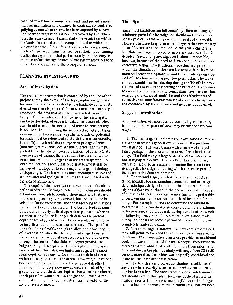
cover of vegetation minimizes rainwash and provides more uniform infiltration of moisture. In contrast, concentrated gullying occurs when an area has been exposed by excava-tion or when vegetation has been destroyed by fire. There. fore, the ecosystem, and particularly the vegetation within the landslide area, should be compared to that within the surrounding area. Since life systems are changing, a single study at a particular time may not be sufficient; continuing studies during an extended period usually are necessary in order to define the significance of the interrelation between the earth movements and the ecology of an area.

PLANNING INVESTIGATIONS

Area of Investigation

The area of an investigation is controlled by the size of the project and by the extent of the topographic and geologic features that are to be involved in the landslide activity. At sites where there is potential for movement that has not yet developed, the area that must be investigated cannot be easily defined in advance. The extent of the investigation can be better defined once a landslide has occurred. How-ever, in either case, the area studied must be considerably larger than that comprising the suspected activity or known movement for two reasons: (a) The landslide or potential landslide must be referenced to the stable area surrounding it, and (b) most landslides enlarge with passage of time (moreover, many landslides are much larger than first sus-pected from the obvious overt indications of activity). As a crude rule of thumb, the area studied should be two to three times wider and longer than the area suspected. In some mountainous areas, it is necessary to investigate to the top of the slope or to some major change in lithology or slope angle. The lateral area must encompass sources of groundwater and geologic structures that are aligned with the area of instability.

The depth of the investigation is even more difficult to define in advance. Borings or other direct techniques should extend deep enough to identify those materials that have not been subject to past movement, but that could be in-volved in future movement, and the underlying formations that are likely to remain stable. The boring depth is some-times revised hourly as field operations proceed. When in. strumentation of a landslide yields data on the present depth of activity, planned depths are sometimes found to be insufficient and increases are necessary. The specifica-tions should be flexible enough to allow additional depth of investigation when the data obtained suggest deeper movements. Longitudinal cross sections should be drawn through the center of the slide and depict possible toe bulges and uphill scarps; circular or elliptical failure sur-faces sketched through these limits can suggest the maxi-mum depth of movement. Continuous thick hard strata within the slope can limit the depth. However, at least one boring should extend far below the suspected depth of shear; sometimes deep slow movements are masked by the greater activity at shallower depths. For a second estimate, the depth of movement below the ground surface at the center of the slide is seldom greater than the width of the zone of surface motion.

Time Span

Since most landslides are influenced by climatic changes, a minimum period for investigation should include one sea-sonal cycle of weather—i year in most parts of the world. However, because long-term climatic cycles that occur every ii or 22 years are superimposed on the yearly changes, a landslide investigation could be necessary for more than 2 decades. Such a long investigation is almost impossible, however, because of the need to draw conclusions and take corrective action. Investigations made during a period in which the climatic conditions are less severe than the maxi-mum will prove too optimistic, and those made during a pe-riod of bad climate may appear too pessimistic. The worst climatic conditions that develop during the life of the proj-ect control the risk to engineering construction. Experience has indicated that many false conclusions have been reached regarding the causes of landslides and the effectiveness of corrective measures because worsened climatic changes were not considered by the engineers and geologists concerned.

Stages of Investigation

An investigation of landslides is a continuing process but, from the practical point of view, may be divided into four stages.

The first stage is a preliminary investigation or recon-naissance in which a general overall view of the problem area is gained. The work begins with a review of the pub-lished geology in the area and accounts of past land insta-bility. The field study is largely visual and the interpreta-tion is highly subjective. The results of this preliminary evaluation are used as a guide in planning the more inten-sive, specific investigation during which the major part of the quantitative data are obtained.

The second stage, which is more intensive and de-tailed, includes boring, sampling, trenching, and other spe-cific techniques designed to obtain the data needed to sat-isfy the objectives outlined in the above checklist. Because of climatic changes, the intensive investigation is preferably undertaken during the season that is least favorable for sta-bility. For example, borings to determine the minimum soil strength or groundwater studies to determine maximum water pressures should be made during periods of snowmelt or following heavy rainfall. A similar investigation made during the driest and hottest period of the year could give completely misleading data.

The third stage is iterative. As new data are obtained, they will point to the need for additional data from specific locations. The investigative plan must provide for additional work that was not a part of the initial scope. Experience in-dicates that the additional work stemming from information obtained during the planned study will range from 30 to 50 percent more than that which was originally considered ade-quate for the intensive investigation.

The fourth stage involves continuing surveillance of any area where activity is suspected or where corrective ac-tion has been taken. The surveillance period is indeterminate but should extend through at least one cycle of annual cli-matic change and, to be most meaningful, should be longer term to include the worst climatic conditions. For example,

84

corrective work may be done during a number of consecu-tively dry years, and the area may not be subjected to its worst climatic test until 4 or 5 years later (assuming an 11-year cycle of climatic change). If the climatic changes oc-cur in a 22-year cycle, the period of observation required could be correspondingly much longer. Rarely do those who finance such long-term surveillance have the wisdom and foresight to continue the data gathering, because the period required extends beyond the tenure of most public officials or private managers. However, public and profes-sional interests are best served if surveillance is maintained long enough for the occurrence of the full range of environ-mental conditions that can reasonably be expected; other-wise, the extent of continuing risk may never be adequately defined.

SITE TOPOGRAPHY

As previously stated, the site topography (surface geometry) is the first clue to potential instability and the degree to which an area has undergone landslide activity. The topog-raphy is first determined by aerial surveys (photogrammetry), which provide an overall view of the site conditions. How-ever, because of the detail required and the masking of the vegetation and the landslide itself, detailed ground surveys must be included as a major tool in landslide investigation.

Aerial Survey

Existing Sources of Photography

All of the United States and most of the remainder of the world have been covered by some form of aerial photog-raphy or remote sensing, including LANDSAT; the principal sources are given in Chapter 3. Generally, these existing photographs have been made at moderately high altitudes (typically at a scale of 1:10000 to 1:40000). Probably the most widely used scales of photography by these agencies are 1:20000(1 cm = 200 m; 1 in = 1667 ft) or 1: 24000 (1 cm = 240 in; 1 in = 2000 ft). At this scale, most land-slides appear as minor topographic anomalies and their de-tailed features, such as scarps, toe bulges, and seeps, can seldom be identified, even from enlargements. However, these photographs are useful in identifying areas that may be prone to landsliding because they may show the typical undulating disturbed topography or arcuate scarps that are associated with past landslides. Such existing photography is frequently a good starting place for evaluating the surface geometry of the site, but it is seldom of sufficient accuracy to provide useful data for detailed landslide studies.

Smaller scale photography can be obtained by the more sophisticated remote-sensing systems of high-altitude photography (1:60 000 and 1:120000) provided by the National Aeronautics and Space Administration. Although the imagery obtained from LANDSAT with a resolution of 56 x 79 m (185 x 260 ft) is not sufficient to identify the topography of most landslides, it does provide clues to the major geologic structures that sometimes influence land-slide activity. However, such high-altitude, small-scale data should be considered as supplementary information that provides clues of regional significance rather than as the primary source of topographic data on landslide-prone

areas. One distinct advantage of existing photographic and remote-sensing imagery is that it provides information on ground surface conditions before the particular site be-comes of interest for construction. Some aerial photo-graphs of the U.S. Department of Agriculture date from the late 1930s, and imagery of LANDSAT and the Earth Resources Technology satellite dates from the early 1970s.

Color and Color Infrared Photography

For mapping purposes, black-and-white panchromatic photography generally provides the best detail at the lowest cost. However, in the study of landslides, certain features become more obvious in color (4.15). Color photography emphasizes differences in vegetation and wet areas through changes in soil color and vegetation vigor. Stratification in exposed soil and rock is often more easily recognized and mapped in color. Color infrared photography is particularly helpful because of two properties. First, most water ap-pears blue in such photography; seeps issuing from bare ground frequently will have a blueish tinge that is far more obvious in the color infrared photography than in either black-and-white or color photography. Second, color in-frared photography is useful in mapping hidden cracks and fissures through their influence on growth of vegetation. Fissures above the water table act as drains; the color or image depicts dull red colors of inhibited growth, and springs and sheared zones that hold water sometimes fea-ture more vigorous growth by brilliant reds. However, such inferences should be verified on the ground before they are included on maps.

Thermal Sensing

Thermal sensing involves scanning the ground with a detec-tor that is sensitive to selected portions of infrared radiation. The image produced by the shorter wave (2 to 5 urn) is com-parable to the image produced by black-and-white or color infrared photography. In the second range (approximately 8 to 14 um), the radiation is comparable to the heat radi-ated from the ground. Thus, for any given texture of ground surface, the level of radiation measured is proportional to• the ground temperature. This range of thermal sensing is highly sensitive to small differences in ground temperature. For example, if the imagery is obtained during winter, seeps and springs issuing from the warmer, deep ground will be depicted as warm points contrasting with the cold ground; similar imagery obtained during summer nights will show the seeps and springs as colder than the surround-ing ground surface. To be most effective, this sensing must be done during the night or early dawn when there is insig-nificant infrared reflectance from the sun.

Because of changing angles associated with aircraft move-ment, the thermal infrared image is seldom a scale represen-tation of the ground feature. Instead, it must be used in conjunction with aerial photographs or accurate maps so that the distorted geometry of the infrared image can be related to the actual geometry of the ground surface and the points depicted on the imagery can be located exactly. The resolution of the imagery is not great because the sens-ing generally encompasses 0.002 to 0.005 rad (0.115° to 0.286°) of angle from the aircraft or 2 to 5-rn (7 to 16-ft)

85

Figure 4.1. Bench marks and triangulation leveling network.

IIPcInPF

enhanced movement. Thermal imagery is useful after pe-riods of unusually dry or wet weather. However, the vari-ous forms of thermal imagery are most revealing when the ground surface can be observed (that is, when deciduous vegetation is free from leaves). Aerial photographs taken at intervals for several years after corrective measures are taken provide an excellent tool for assessing the overall benefits achieved by the measures and for obtaining a pre-liminary view of the effect of the landslide and associated corrective measures on the ecosystem of the area. Since satisfying all those needs is not always possible, it may not be feasible to bring all of the tools of aerial photography and remote sensing into play in any single investigation.

Ground Surveys

On-the-ground surveys are necessary to (a) establish the ground control for photogrammetric mapping and instru-mentation, (b) obtain topographic details where the ground surface is obscured by vegetation (this is particularly impor-tant because of the accuracy required in mapping landslides), and (c) establish a frame of reference against which move-ments of the ground surface can be compared.

resolution for 1000-rn (3300-ft) height. At high altitude, the heat radiation from significant areas is averaged and small features cannot be detected. Therefore, for locating seeps, springs, small water courses, and other features of particular significance in landslide investigation, the thermal infrared imagery must be flown at low levels, generally 300 to 1000 m (980 to 3300 ft) above the ground surface. In hilly country, this presents problems for aircraft navigation.

In planning for thermal infrared imagery, one must be sure that the exact needs or objectives of the work are trans-mitted to those who obtain the imagery so'that the proper altitudes and sensing range can be selected. Thermal infra-red imagery detects temperature differences as small as 1°C (1.8°F), and those differences, in turn, reflect variations in soil moisture and ground heat storage.

Use of Aerial Survey Data

Aerial survey data are used in two ways. First, and most im-portant, when used in coordination with ground surveys (in-cluding reference points established on the ground surface), they provide detailed topographic maps of the area through photogrammetric processes. This is the procedure with which organizations obtaining aerial survey data are most familiar and that requires the least guidance. A second use of aerial photography and remote-sensing data is in interpreta-tion or terrain evaluation (described in Chapter 3). Because the technical quality of photographs and imagery for accu-rate mapping is more demanding, the specifications for photography should be directed by topographic require-ments. However, the special needs for interpretation should also be considered so that one photographic mission can serve both purposes.

Terrestrial Photogrammetry

Photogrammetric measurements of ground geometry can be made from oblique photographs obtained at the ground sur-face. For example, two or more permanent photographic sites that overlook a slide area can be used to monitor slide movement by successive sets of simultaneous photographs. Such observations have been used to measure changing dam deflections. Although the data reduction is more complex than that for photogrammetric mapping, the technique is useful for determining movement of any selected points, provided they can be seen in the photograph.

Specifying Scale and Coverage Quality Ground Control for Instrumentation

The scale of photography and thermal imagery must be de-termined on the basis of the size of the features to be iden-tified. In the mapping of springs, seeps, and fissures, a reso-lution circle 0.5 to 1 m (1.5 to 3 ft) in diameter is desirable. A suitable scale for the aerial photography for landslide studies is of the same order that is required for final high-way alignment studies (from 1:3000 to 1:6000 on contact prints). Maps are drawn to a scale of 1: 1000 (1 cm = 10 m; lin83 ft) tol:5000(lcm50m;lin=4l7 ft) and with contour intervals of 0.5 m (1 to 2 ft) for most slides. Good quality aerial photographs for mapping and interpre-tation are necessary tools at the beginning of an investiga-tion, but additional coverage is desirable after episodes of

The first requirement is a system of local bench marks that will remain stable during the course of the investigation and as far into the future as movements will be observed. These must be located far enough outside the suspected zone of sliding that they will not be affected by any movements. Ultimately, the bench marks should be referenced to control monuments of federal and state survey systems. However, for convenience, a subsystem of local bench marks should be established close enough to the zone of movement that they can be used as ready references for continuing surveys. At least two monuments of position and elevation should be established on each side of the zone of sliding or sus-

DOWNSLOPE

SSI BLY SHEAR DISPLACEMENT DOWNHILL

TENSION CR ACK ON TOE BU LGE

SPRINGS. SEEPS

CRACKS -

/

1' - ZONE OF BULGING

TOE

MUD WAVE OR TOE RIPPLE

87

Figure 4.2. Cracks, bulges, scarps, and springs.

DIAC TEN5 CRAI EN ECHELON I

MAIN SCARP

NOR SCARP

ZONE OF DEPRESSION OR SUBSIDENCE

\ \

U PS L OP E

,1 /

ONAL / ION-SHEAR /

I,

pected movement; as indicated in Figure 4.1, these should be as close as possible to the movement zone, but not influ-enced by future enlargement of the slide. Experience sug-gests that the distance from a bench mark to the closest point of known movement should be at least 25 percent of the width of the slide zone. In areas of previous landslides, the minimum distance may be greater. In mountainous areas, adequate outcrops of bedrock can sometimes be found uphill or downhill from the landslide; in areas of thick soil, deep-seated bench marks may be necessary.

Control Network

The bench marks should be tied together by triangulation and precise leveling loops. If there are enough bench marks, the movement of any one can be detected by changes in the control network. Intermediate or temporary bench marks are sometimes established closer to the zone of movement for use in the more frequent surveys of the landslide area. However, these should be checked against the permanent monument grid each time they are used.

Topography

As previously stated, topography obtained from aerial

photography may not be sufficiently, accurate or detailed for landslide studies because vegetation obscures the ground 'surface. Therefore, detailed on-site mapping is necessary. Major features, such as scarps, bulges, and areas of jumbled topography, should be defined (Figure 4.2). Because of the changing nature of landslides, the surface surveys should be conducted at the same time the photography is taken; otherwise, the movements of the landslide will confuse the topographic map. Even then, it may not be possible to ob-tain a precise correlation between the surface topography determined on the ground over a period of days or weeks and that obtained at a single instant from aerial surveys. Differences should be expected, and these should be noted on the topographic maps that are produced.

Cracks, Seeps, and Bulges

Although many cracks, seeps, and bulges, as well as other minor topographic details, can be identified in aerial photog-raphy, their full extent can seldom be determined unless the photographs are taken with an unusually high degree of res-olution in vegetation-free areas. Therefore, independent crack and bulge surveys should be made by surface methods. Developing cracks are often obscured by grass, leaves, and root mats, particularly at their ends; these cracks should be

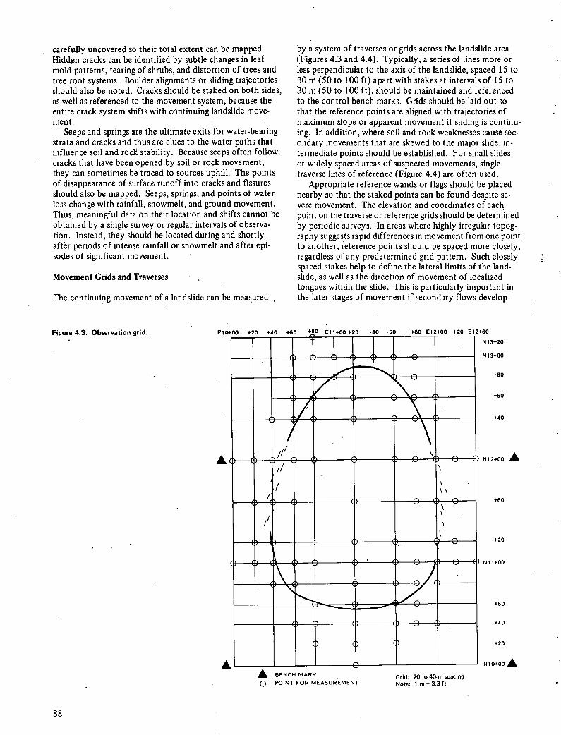
carefully uncovered so their total extent can be mapped. Hidden cracks can be identified by subtle changes in leaf mold patterns, tearing of shrubs, and distortion of trees and tree root systems. Boulder alignments or sliding trajectories should also be noted. Cracks should be staked on both sides, as well as referenced to the movement system, because the entire crack system shifts with continuing landslide move-ment.

Seeps and springs are the ultimate exits for water-bearing strata and cracks and thus are clues to the water paths that influence soil and rock stability. Because seeps often follow cracks that have been opened by soil or rock movement, they can sometimes be traced to sources uphill. The points of disappearance of surface runoff into cracks and fissures should also be mapped. Seeps, springs, and points of water loss change with rainfall, snowmelt, and ground movement. Thus, meaningful data on their location and shifts cannot be obtained by a single survey or regular intervals of observa-tion. Instead, they should be located during and shortly after periods of intense rainfall or snowmelt and after epi-sodes of significant movement.

Movement Grids and Traverses

The continuing movement of a landslide can be measured

by a system of traverses or grids across the landslide area (Figures 4.3 and 4.4). Typically, a series of lines more or less perpendicular to the axis of the landslide, spaced 15 to 30 in (50 to 100 ft) apart with stakes at intervals of 15 to 30 m (50 to 100 ft), should be maintained and referenced to the control bench marks. Grids should be laid out so that the reference points are aligned with trajectories of maximum slope or apparent movement if sliding is continu-ing. In addition, where soil and rock weaknesses cause sec-ondary movements that are skewed to the major slide, in-termediate points should be established. For small slides or widely spaced areas of suspected movements, single traverse lines of reference (Figure 4.4) are often used.

Appropriate reference wands or flags should be placed nearby so that the staked points can be found despite se-vere movement. The elevation and coordinates of each point on the traverse or reference grids should be determined by periodic surveys. In areas where highly irregular topog-raphy suggests rapid differences in movement from one point to another, reference points should be spaced more closely, regardless of any predetermined grid pattern. Such closely spaced stakes help to define the lateral limits of the land-slide, as well as the direction of movement of localized tongues within the slide. This is particularly important in the later stages of movement if secondary flows develop

Figure 4.3. Observation grid. ElO.

A

r

00 +20 +40 +60 El1+00+20 +40 +60 +80 E12+00 +20 E12

A BENCH MARK Grid: 20 to 40-rn spacing 0 POINT FOR MEASUREMENT Note: 1 m = 3.3 ft.

60

N 13+20

N 13+00

+80

+60

+40

N12+00 A

+60

+20

NI 1+00

+60

+40

+20

N 10+00 A

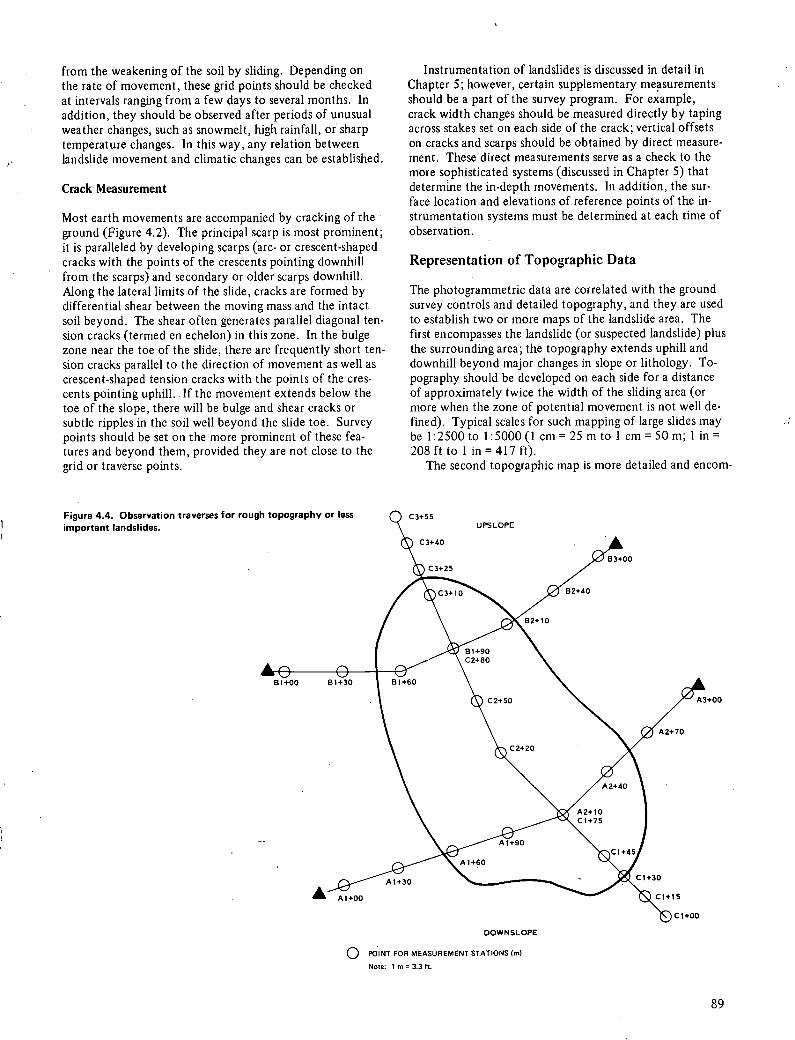
from the weakening of the soil by sliding. Depending on the rate of movement, these grid points should be checked at intervals ranging from a few days to several months. In addition, they should be observed after periods of unusual weather changes, such as snowmelt, high rainfall, or sharp temperature changes. In this way, any relation between landslide movement and climatic changes can be established.

Crack Measurement

Most earth movements are accompanied by cracking of the ground (Figure 4.2). The principal scarp is most prominent; it is paralleled by developing scarps (arc- or crescent-shaped cracks with the points of the crescents pointing downhill from the scarps) and secondary or older scarps downhill. Along the lateral limits of the slide, cracks are formed by differential shear between the moving mass and the intact soil beyond. The shear often generates parallel diagonal ten-sion cracks (termed en echelon) in this zone. In the bulge zone near the toe of the slide, there are frequently short ten-sion cracks parallel to the direction of movement as well as crescent-shaped tension cracks with the points of the cres-cents pointing uphill. If the movement extends below the toe of the slope, there will be bulge and shear cracks or subtle ripples in the soil well beyond the slide toe. Survey points should be set on the more prominent of these fea-tures and beyond them, provided they are not close to the grid or traverse points.

Instrumentation of landslides is discussed in detail in Chapter 5; however, certain supplementary measurements should be a part of the survey program. For example, crack width changes should be measured directly by taping across stakes set on each side of the crack; vertical offsets on cracks and scarps should be obtained by direct measure-ment. These direct measurements serve as a check to the more sophisticated systems (discussed in Chapter 5) that determine the in-depth movements. In addition, the sur-face location and elevations of reference points of the in-strumentation systems must be determined at each time of observation.

Representation of Topographic Data

The photogrammetric data are correlated with the ground survey controls and detailed topography, and they are used to establish two or more maps of the landslide area. The first encompasses the landslide (or suspected landslide) plus the surrounding area; the topography extends uphill and downhill beyond major changes in slope or lithology. To-pography should be developed on each side for a distance of approximately twice the width of the sliding area (or more when the zone of potential movement is not well de-fined). Typical scales for such mapping of large slides may be 1:2500 to 1:5000 (1 cm = 25 m to 1 cm = 50 m; I in = 208 ft to 1 in = 417 ft).

The second topographic map is more detailed and encom-

Figure 4.4. Observation traverses for rougi important landslides.

1+00

DOWN SLOPE

POINT FOR MEASUREMENT STATIONS (ml

Note: I m = 3.3 ft.

go

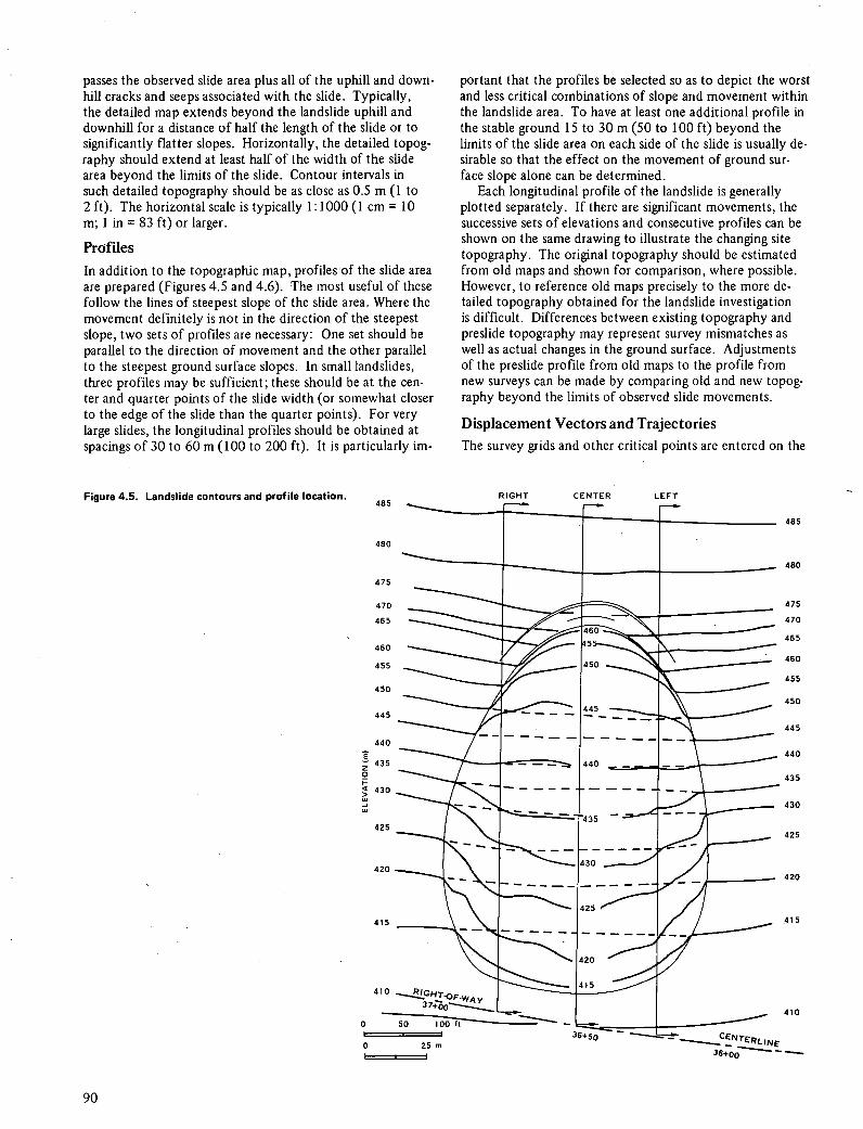
485

480

475

470

465

460

455

450

445

440

C 435

0 I-

430

425

420

415

410

0

o 25m

410

- 'LINE

+0Q 36 -

Figure 4.5. Landslide contours and profile location.

485

480

475

470

465

460

455

450

445

440

435

430

425

420

415

RIGHT CENTER LEFT

passes the observed slide area plus all of the uphill and down-hill cracks and seeps associated with the slide. Typically, the detailed map extends beyond the landslide uphill and downhill for a distance of half the length of the slide or to significantly flatter slopes. Horizontally, the detailed topog-raphy should extend at least half of the width of the slide area beyond the limits of the slide. Contour intervals in such detailed topography should be as close as 0.5 m (1 to 2 ft). The horizontal scale is typically 1:1000(1 cm = 10 m; I in = 83 ft) or larger.

Profiles

In addition to the topographic map, profiles- of the slide area are prepared (Figures 4.5 and 4.6). The most useful of these follow the lines of steepest slope of the slide area. Where the movement definitely is not in the direction of the steepest slope, two sets of profiles are necessary: One set should be parallel to the direction of movement and the other parallel to the steepest ground surface slopes. In small landslides, three profiles may be sufficient; these should be at the cen-ter and quarter points of the slide width (or somewhat closer to the edge of the slide than the quarter points). For very large slides, the longitudinal profiles should be obtained at spacings of 30 to 60 m (100 to 200 ft). It is particularly im-

portant that the profiles be selected so as to depict the worst and less critical combinations of slope and movement within the landslide area. To have at least one additional profile in the stable ground 15 to 30 m (50 to 100 ft) beyond the limits of the slide area on each side of the slide is usually de-sirable so that the effect on the movement of ground sur-face slope alone can be determined.

Each longitudinal profile of the landslide is generally plotted separately. If there are significant movements, the successive sets of elevations and consecutive profiles can be shown on the same drawing to illustrate the changing site topography. The original topography should be estimated from old maps and shown for comparison, where possible. However, to reference old maps precisely to the more de-tailed topography obtained for the landslide investigation is difficult. Differences between existing topography and preslide topography may represent survey mismatches as well as actual changes in the ground surface. Adjustments of the preslide profile from old maps to the profile from new surveys can be made by comparing old and new topog-raphy beyond the limits of observed slide movements.

Displacement Vectors and Trajectories The survey grids and other critical points are entered on the

all

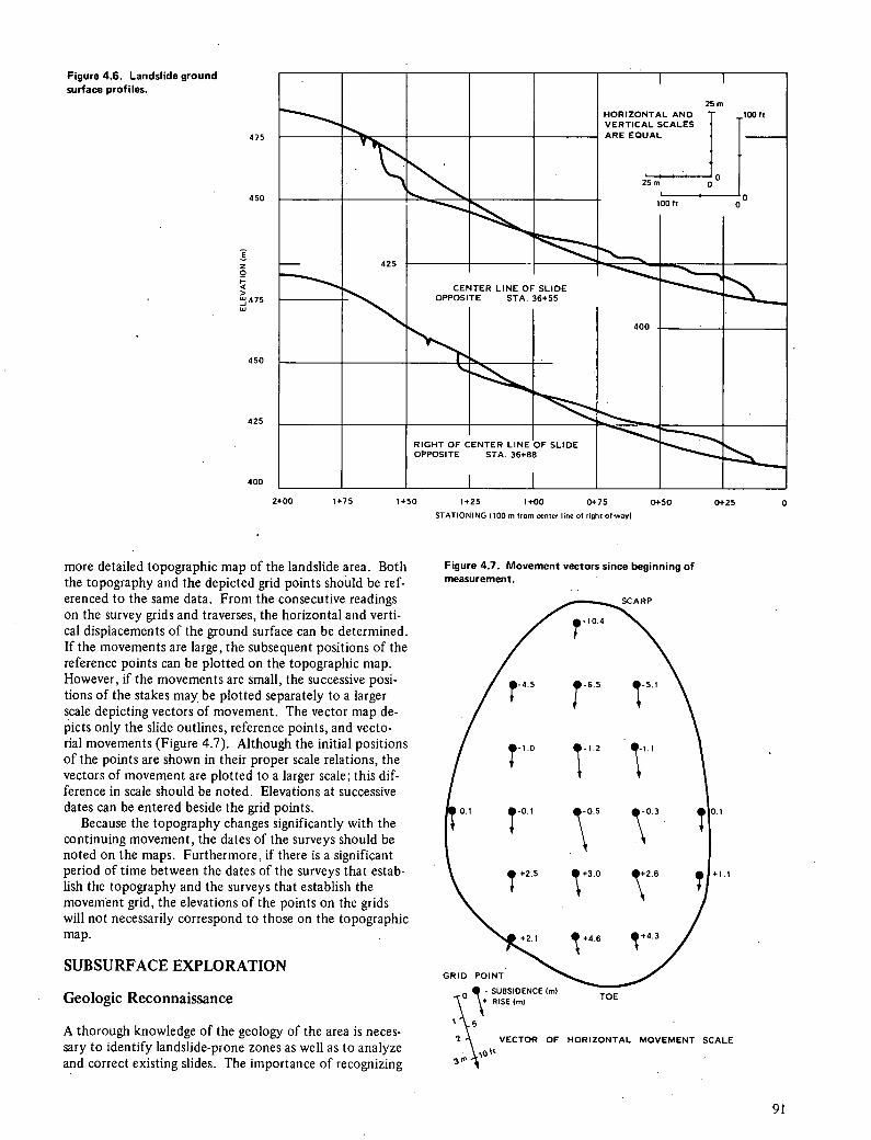
I I

25 m HORIZONTAL AND r 100 ft VERTICAL SCALES I T ARE EQUAL

25m' cfo I

100 It 0

- 425

OPPOSITE CENTER LINE OF

STA. SLIDE

36+55

400

......

RIGHT OF CENTER LINE OF SLIDE OPPOSITE STA. 36+88

I I

Figure 4.6. Landslide ground surface profiles.

475

450

E

475

450

425

400

2+00 1+75 1+50 1+25 1+00 0+75 0+50 0+25

0 STATIONING 1100 m from center line of right-of-wayl

more detailed topographic map of the landslide area. Both the topography and the depicted grid points should be ref-erenced to the same data. From the consecutive readings on the survey grids and traverses, the horizontal and verti-cal displacements of the ground surface can be determined. If the movements are large, the subsequent positions of the reference points can be plotted on the topographic map. However, if the movements are small, the successive posi-tions of the stakes may be plotted separately to a larger scale depicting vectors of movement. The vector map de-picts only the slide outlines, reference points, and vecto-rial movements (Figure 4.7). Although the initial positions of the points are shown in their proper scale relations, the vectors of movement are plotted to a larger scale; this dif-ference in scale should be noted. Elevations at successive dates can be entered beside the grid points.

Because the topography changes significantly with the continuing movement, the dates of the surveys should be noted on the maps. Furthermore, if there is a significant period of time between the dates of the surveys that estab-lish the topography and the surveys that establish the movement grid, the elevations of the points on the grids will not necessarily correspond to those on the topographic map.

SUBSURFACE EXPLORATION

Geologic Reconnaissance

A thorough knowledge of the geology of the area is neces-sary to identify landslide-prone zones as well as to analyze and correct existing slides. The importance of recognizing

Figure 4.7. Movement vectors since beginning of measurement.

SCARP

7 - 6.5

T 5.1

1.1

0.1 -0.1 • 0.5 • 0.3 0.1

+2.5 +3.0 •\+2.8 +1.1

+2.1 +4.6 4.3

GRID POINT

o SUBSIDENCE (ml TOE RISE (ml

VECTOR OF HORIZONTAL MOVEMENT SCALE \

01

structure, groundwater, and weathering in the prevention and evaluation of sliding has been emphasized by Philbrick and Cleaves (4.9), Zâruba and Mend (4.18), and Deere and Patton (4.4). Although data have been published on the major geologic formations and structural features of most of the world, they are seldom in sufficient detail for land-slide studies. As long as their extent is comparable to that of the failure zone, small changes in bedding and geologi-cally minor fractures or irregularities in structure, which are seldom shown in published maps and reports, influence failure as significantly as regional features. The local geol-ogy is determined by surface observation (geologic recon-naissance) and by interpretation of the subsurface explora-tion data. The reconnaissance generates an estimate of the local geology and aids in selecting locations and techniques for subsequent exploration and in interpreting the results of the overall investigation.

Outcrops

The principal means for estimating the geology of an area is the outcrop, which is defined as "that part of a geologic for-mation or structure that appears at the surface of the earth" (4.1). Some geologic formations can be identified indirectly by characteristic landforms and others can be deduced from soils that are derived from the weathering of the formation; however, the primary element used in identification is the outcrop itself (rock, residual soil, or even old landslide de-bris). Outcrops can be examined on steep slopes, in river channels, in highway and railroad cuts, and in quarries and borrow pits. The relation between geologic formations is determined by correlating structure, lithology, and unit thicknesses with site topography. This is a major technique for geologic mapping and is described in texts on field geol-ogy (4.3, 4.7). However, outcrops can be misleading. The

formations may have been displaced or distorted by an-cient landslides or by rapid weathering of less-resistant strata. Some formations harden on exposure, especially in regions of highly seasonal rainfall, and give a false impression of the strength or stability of the formation. The outcrop data should be correlated with deep samples before final conclu-sions are reached.

Faults and Joints

Many geologic discontinuities, such as unconformities, cavi-ties, formation contacts, and facies changes, can affect slope stability. Two of the most prominent, and perhaps most readily identified, are faults and joints. A fault is defined as a surface or zone of rock fracture along which there has been displacement parallel to the surface of the fracture. Joints are rock cracks or partings without displacement parallel to the surface. The recognition of faults and joints is particularly important to predesign and site or route se-lection. The potential for instability is greater in areas with extensive faulting or close jointing than in areas without discontinuities. Revisions in route or locations of engineer-ing structures may be imperative if the potential is serious; alternatively, the design can be altered to fit the situation.

The strike of the fault, angle of dip of the fault plane, type and competency of the associated rock, extent of the fault (especially the thickness of the sheared or gouge zone), and condition of the rocks and materials on either side of the zone should be determined for both site selection and evaluation of an existing slide. If available, geologic maps may show the location of major faults. If detailed maps are not available, an experienced interpreter can often iden-tify questionable areas from their topographic reflections on maps, aerial photographs, and LANDSAT imagery. These areas are then located in the field to determine their

Figure 4.8. Slide in sands-tone overlying shale in Tennessee.

.T

/

-'1.'.:-:;. • ._'/;.-•

ff .

92

,-,-

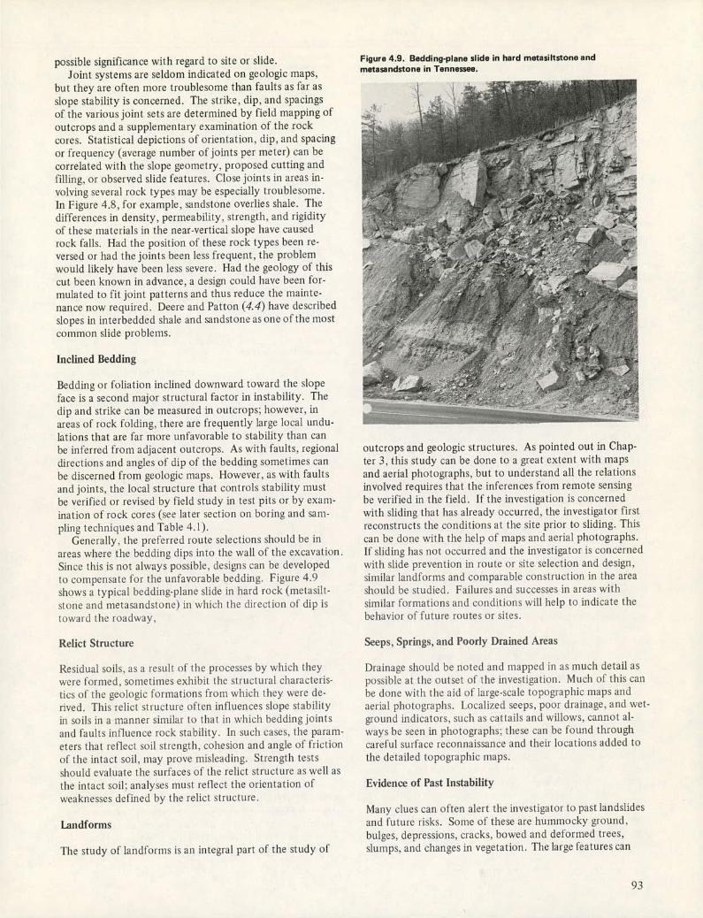
x.

-

possible significance with regard to site or slide. Joint systems are seldom indicated on geologic maps,

but they are often more troublesome than faults as far as slope stability is concerned. The strike, dip, and spacings of the various joint sets are determined by field mapping of outcrops and a supplementary examination of the rock cores. Statistical depictions of orientation, dip, and spacing or frequency (average number of joints per meter) can be correlated with the slope geometry, proposed cutting and filling, or observed slide features. Close joints in areas iii-volving several rock types may be especially troublesome. In Figure 4.8, for example, sandstone overlies shale. The differences in density, permeability, strength. and rigidity of these materials in the near-vertical slope have caused rock falls. I-lad the position of these rock types been re-versed or had the joints been less frequent, the problem would likely have been less severe. Had the geology of this cut been known in advance, a design could have been for-mulated to fit joint patterns and thus reduce the mainte-,iance now required. Deere and Patton (4.4) have described slopes in interbedded shale and sandstone as one of the most common slide problems.

Inclined Bedding

Bedding or foliation inclined downward toward the slope face is a second major structural factor in instability. The (lip and strike can be measured in outcrops: however, in areas of rock folding, there are frequently large local undu-lations that are far more unfavorable to stability than can be inferred from adjacent outcrops. As with faults, regional directions and angles of dip of the bedding sometimes can be discerned from geologic maps. l-lowever. as with faults and joints, the local structure that controls stability must be verified or revised by field study in test pits or by exam-ination of rock cores (see later sect ion on boring and sam-pling techniques and Table 4.1).

Generally, the preferred route selections should be in areas where the bedding dips into the wall of the excavation Since this is not always possible. designs can be developed to compensate for the unfavorable bedding. Figure 4.9 shows a typical bedding-plane slide in hard rock (metasilt-stone and metasandstone) in which the direction of dip is toward the roadway.

Relict Structure

Residual soils, as a result of the processes by which they were formed, sometimes exhibit the structural characteris-tics of the geologic formations from which they were (IC-

rived. This relict structure often influences slope stability in soils in a manner similar to that in which bedding joints and faults influence rock stability, in such cases, the param-eters that reflect soil strength, cohesion and angle of friction of t he intact soil, may prove misleading. Strengt It tests should evaluate the surfaces of the relict structure as well as the intact soil: analyses must reflect the orientation of weaknesses defined by the relict structure.

Landforms

The study of landt'ornts is an integral part of the study of

Figure 4.9. Bedding-plane slide in hard metasiltstone and

metasandstone in Tennessee.

outcrops and geologic structures. As pointed out in Chap-ter 3, this study can be done to a great extent with maps and aerial photographs. but to understand all the relations involved requires that the inferences from remote sensing be verified in the field. If the investigation is concerned with sliding that has already occurred, the investigator first reconstructs the conditions at the site prior to sliding. This can be done with the help of maps and aerial photographs. If sliding has not occurred and the investigator is concerned with slide prevention in route or site selection and design. similar Iandforms and comparable construction in the area should be studied. Failures and successes in areas with similar formations and conditions will help to indicate the behavior of future routes or sites.

Seeps, Springs, and Poorly Drained Areas

Drainage should be noted and mapped in as much detail as possible at the outset of the investigation. Much of this can be done with the aid of' large-scale topographic maps and aerial photographs. Localized seeps, poor drainage, and wet-ground indicators, such as cat tails and willows, cannot al-ways be seeii in photographs: these can be found through careful surface reconnaissance and their locations added to the detailed topographic maps.

Evidence of Past Instability

Many clues can often alert the investigator to past landslides and future risks. Some of these are hummocky ground, bulges. depressions, cracks, bowed and deformed trees, slumps, and changes in vegetation. The large features can

93

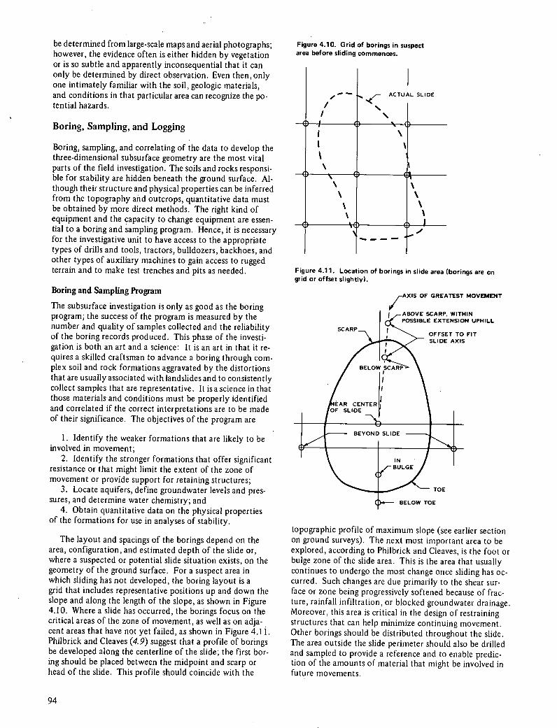
be determined from large-scale maps and aerial photographs; however, the evidence often is either hidden by vegetation or is so subtle and apparently inconsequential that it can only be determined by direct observation. Even then, only one intimately familiar with the soil, geologic materials, and conditions in that particular area can recognize the po-tential hazards.

Boring, Sampling, and Logging

Boring, sampling, and correlating of the data to develop the three-dimensional subsurface geometry are the most vital parts of the field investigation. The soils and rocks responsi-ble for stability are hidden beneath the ground surface. Al-though their structure and physical properties can be inferred from the topography and outcrops, quantitative data must be obtained by more direct methods. The right kind of equipment and the capacity to change equipment are essen-tial to a boring and sampling program. Hence, it is necessary for the investigative unit to have access to the appropriate types of drills and tools, tractors, bulldozers, backhoes, and other types of auxiliary machines to gain access to rugged terrain and to make test trenches and pits as needed.

Boring and Sampling Program

The subsurface investigation is only as good as the boring program; the success of the program is measured by the number and quality of samples collected and the reliability of the boring records produced. This phase of the investi-gation is both an art and a science: It is an art in that it re-quires a skilled craftsman to advance a boring through com-plex soil and rock formations aggravated by the distortions that are usually associated with landslides and to consistently collect samples that are representative. It isa science in that those materials and conditions must be properly identified and correlated if the correct interpretations are to be made of their significance. The objectives of the program are

Identify the weaker formations that are likely to be involved in movement;

Identify the stronger formations that offer significant resistance or that might limit the extent of the zone of movement or provide support for retaining structures;

Locate aquifers, define groundwater levels and pres-sures, and determine water chemistry; and

Obtain quantitative data on the physical properties of the formations for use in analyses of stability.

The layout and spacings of the borings depend on the area, configuration, and estimated depth of the slide or, where a suspected or potential slide situation exists, on the geometry of the ground surface. For a suspect area in which sliding has not developed, the boring layout is a grid that includes representative positions up and down the slope and along the length of the slope, as shown in Figure 4.10. Where a slide has occurred, the borings focus on the critical areas of the zone of movement, as well as on adja-cent areas that have not yet failed, as shown in Figure 4.11 Philbrick and Cleaves (4.9) suggest that a profile of borings be developed along the centerline of the slide; the first bor-ing should be placed between the midpoint and scarp or head of the slide. This profile should coincide with the

Figure 4.10. Grid of borings in suspect

area before sliding commences.

Figure 4.11. Location of borings in slide area (borings are on grid or offset slightly).

TAXIS OF GREATEST MOVEMENT

ABOVE SCARP, WITHIN POSSIBLE EXTENSION UPHILL

SCARP OFFSET TO FIT SLIDE AXIS

BELOW SCARP

EAR CENTER OF SLIDE

­1~ -

BEYOND SLIDE

BULGE

TOE

- BELOW TOE

topographic profile of maximum slope (see earlier section on ground surveys). The next most important area to be explored, according to Philbrick and Cleaves, is the foot or bulge zone of the slide area. This is the area that usually continues to undergo the most change once sliding has oc-curred. Such changes are due primarily to the shear sur-face or zone being progressively softened because of frac-ture, rainfall infiltration, or blocked groundwater drainage. Moreover, this area is critical in the design of restraining structures that can help minimize continuing movement. Other borings should be distributed throughout the slide. The area outside the slide perimeter should also be drilled and sampled to provide a reference and to enable predic-tion of the amounts of material that might be involved in future movements.

94

Boring and Sampling Techniques

The boring and sampling techniques that can be employed are innumerable, and selection depends on the information required, the nature of the soil and rock, the topography and ground trafficability, and the amount of money avail-able. ASTM standards, standards of other associations, books on drilling and sampling, and textbooks on geotech-nical engineering (for example, 4.14, 4.16) describe methods of boring and sampling and their applications and should be consulted for details. Those techniques particularly adapted to landslide studies are summarized in Table 4.1.

The type of sample obtained depends on the information needed. Oriented cores are required to determine the strike of inclined bedding or fractures. Samples from test borings are adequate for identification of formations, but samples from thin-wall tubes or rotary coring are required for good shear and consolidation tests. Accurate and detailed records of the conditions encountered are essential. If samples are lost, a description of the drilling peculiarities may imply the soil and rock condition. When samples are obtained, their value must be assessed from a detailed examination by a geologist or geotechnical engineer, guided by the driller's records. Because the act of sampling changes soils and rocks, the factors involved in those changes must be known to estimate the extent of alteration. Finally, the samples must be carefully preserved, packed, and handled so they will not be unduly changed by exposure and shipping.

Drilling Equipment

One of the problems common to most landslide investiga-tions is accessibility. The same instability that generates movement makes accessibility difficult. For this reason, the investigative unit should be equipped with some type of all-terrain vehicle. Too often, materials and conditions within a particular slide may be underestimated or over-looked simply because of inadequate borings at critical, but inconvenient, inaccessible points. The drilling industry, in collaboration with manufacturers of specialized vehicles, has been able to develop subsurface exploration equipment that is highly versatile and mobile for work in rugged, steep terrain.

Borehole Logging

Because of the extreme variations in the character of the soil and rock and perhaps because of inadequacies on the part of those who perform the boring and sampling and test pit work, there may be gaps in the underground pro-files established from any of the borings or geophysical studies. In some instances, the techniques of borehole log-ging borrowed from the petroleum exploration industry are fruitful. All are based on lowering a sensing device into an open borehole and measuring the soil and rock character-istics at closely spaced intervals of depth. A number of dif-ferent qualities can be observed, including self.potential of the ground, electrical resistivity within a relatively short ver-tical distance,nuclear radiation,sound wave or impulse re-sponse, density based on nuclear absorption, and water con-tent based on hydrogen ion reaction.

The product of this logging is a graph of each property

plotted as a function of depth. The results may have signifi-cance in identifying the ion concentration and density of the strata. These aid in identifying soils and rock directly from the boring data. They are particularly useful where there are gaps in the data, such as core loss in broken rock. An even more valuable use of this information lies in estab-lishing the correlation of strata between one boring and an-other. For example, it is difficult to compare samples ob-tained from two different holes to determine whether soils or rocks that have similar classification characteristics rep-resent the same stratum. However, by comparing the con-tinuous borehole logs, one can match the patterns of the different properties; similar patterns suggest similar stratifi-cation. Thus, while borehole logging may have limited en-gineering significance by itself in one hole, it is a significant tool for boring interpretation and correlation when used in adjacent holes.

Test Pits and Trenches

One of the best ways to sample and determine the structure and other physical properties of soils and weathered or weak rock foundations is by excavating pits or trenches. Shallow test pits can be excavated with hand tools. Mechanical equipment, such as backhoes, clamshells, draglines, or trac-tors equipped with front-end loaders, are required for deep pits or long trenches. The sides of the excavation should be sampled, logged, and photographed in detail to provide a three-dimensional picture of the materials and structure. Pits and trenches also provide excellent sites for in situ test-ing. When the observations and tests are complete, the ex-cavation should be filled or, in some cases, incorporated in the remedial design by serving as a drainage outlet.

Geophysical Studies

Geophysical exploration uses the changes in certain force sys-tems in the earth to define possible boundaries between dif-ferent materials as well as to estimate some of the engineer-ing properties. The forces include elastic shock waves, gravity, and electric current, none of which is directly con-cerned in landslide behavior. Thus, the methods are some-times termed indirect exploration; the data of interest are inferred from the properties measured. Geophysical methods do not replace borings and sampling or test pits and trenches. Rather, they supplement these procedures and greatly re-duce the time and cost and the environmental problems that often result from large-scale drilling operations.

Resistivity

Resistivity measurements are made by passing electric cur-rent through the ground and measuring the resistance of the various formations to current flow. The current flow is largely electrolytic in that it is dependent on moisture and dissolved salts within the soils and rocks. The Wenner method, which is the simplest and most commonly used, uses four electrodes, spaced equally in a straight line at the ground surface. Current is passed into the ground through the outer two electrodes, and the difference in potential generated by the resistance to current flow is measured be-tween the inner two electrodes. The greater the spacings

95

Soil cylinder 28.5 to 53.2 In soils and soft rocks that Sample smaller; equipment mm wide and 600 to 1500 swell or disintegrate more complex mm long encased in plastic rapidly in air (protected tube by plastic tube)

Rock cylinder 22 to 100 mm wide and as long as 6 m depending on rock soundness

To obtain continuous core in sound rock (percentage of core recovered for dis-tance drilled depends on fractures, rock variability, equipment, and skill of driller)

Core lost in fracture or vari-able rock; blockage prevents drilling in badly fractured rock; dip of bedding and joints evident but not strike

To determine strike of joints Method may not be effective and bedding in fractured rock

To recover core better in frac- Same as ASTM D 2113 but tured rock, which has less

to lesser degree

tendency for caving during core removl; to obtain much faster cycle of core recovery and resumption of drilling in deep holes:

Rock cylinder, typically 54 mm wide and 1.5 m long with compass orien-tation

Rock cylinder 36.5 to 85 mm wide and 1.5 to 4.6 m long

Table 4.1. Boring, core drilling, sampling, and other exploratory techniques (4.2, 4.8, 4.11, 4.14).

Method and Reference Procedure Type of Sample Applications Limitations

Auger boring, Dry hole drilled with hand Augercuttings; disturbed, In soil and soft rock; to Soil and rock stratification ASTM D 1452 or power auger; samples ground up, partially dried identify geologic units destroyed; sample mixed

preferably recovered from from drill heat in hard ma- and water content with water below water auger flutes terials above water table table

Test boring, Hole drilled with auger or Intact but partially disturbed To identify soil or soft rock; Gaps between samples, 30 to ASTM D 1586 rotary drill; at intervals (number of hammer blows to determine water content; 120cm; sample too distorted (Figure 4.15) samples taken 36-mm ID for second plus third incre- in classification tests and for accurate shear and con-

and 50-mm OD driven ment of driving is standard crude shear test of sample solidation tests; sample lim- 0.45 m in three 150-mm in- penetration resistance or (N-value a crude index to ited by gravel; N-value sub- crements by 64-kg hammer N) density of cohesionless ject to variations depending falling 0.76 m; hydrostatic soil and undrained shear on free fall of hammer balance of fluid maintained strength of cohesive soil) below water level

Test boring of 50 to 75-mm ID and 63 to Intact but partially disturbed In gravelly soils Sample limited by larger large samples 89-mm OD samplers (number of hammer blows gravel

driven by hammers up for second plus third incre- to 160 kg ment of driving is penetra-

tion resistance)

Test boring Hole advanced by hollow- Intact but partially disturbed In gravelly soils (not well Sample limited by larger through stem auger; soil sampled (number of hammer blows adapted to harder soils or gravel; maintaining hydro- hollow-stem below auger as in test for second plus third incre- soft rock) static balance in hole below auger boring above ment of driving is standard water table more difficult

penetration resistance or N); N-value may be dis- torted by auger and should be compared with ASTM D 1586

Rotary coring Outer tube with teeth ro- of soil or tated; soil protected and soft rock held by stationary inner

tube; cuttings flushed up-ward by drill fluid (Deni-son—fixed cutter on Outer tube; Pitcher—spring-loaded on outer tube; Acker air-mud core bar-rel—larger clearances for viscous driling fluid)

Rotary coring Similar to rotary coring of of swelling rock; swelling core re- clay or soft tamed by third inner plas- rock tic liner

Rotary coring Outer tube with diamond of rock, bit on lower end rotated to ASTM D 2113 cut annular hole in rock;

core protected by station- ary inner tube; cuttings flushed upward by drill fluid

Rotary coring Similar to rotary coring of of rock, rock above; continuous oriented core grooves scribed on rock core

with compass direction

Rotary coring Outer tube with diamond of rock, bit on lower end rotated wire line to cut annular hole in rock;

core protected by stationary inner tube; cuttings flushed upward by drill fluid; core and stationary inner tube retrieved from outer core barrel by lifting device or "overshot" suspended on thin cable (wire line) through special large diam-eter drill rods and outer core barrel

Relatively undisturbed sam- In firm to stiff cohesive soils Sample may twist in soft pIe, 50 to 200-mm wide and soft but coherent rock clays; sampling loose sand and 0.3 to 1.5 m long in below water table difficult; liner tube success in gravel seldom oc-

curs

92

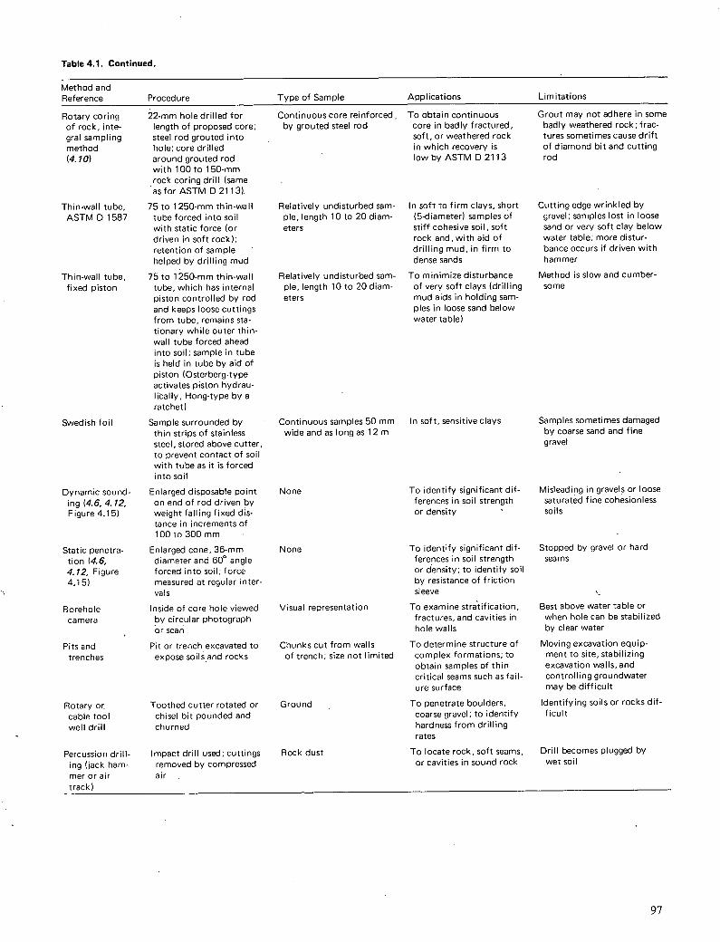
Table 4.1. Continued.

Method and Reference Procedure Type of Sample Applications Limitations

Continuous core reinforced. To obtain continuous Grout may not adhere in some

by grouted steel rod core in badly fractured, badly weathered rock;frac- soft, or weathered rock tures sometimes cause drift in which recovery is of diamond bit and cutting low by ASTM 02113 rod

Relatively undisturbed sam pIe, length 10 to 20 diam-eters

Relatively undisturbed sam-ple, length 10 to 20 diam-eters

Rotary coring of rock, inte-gral sampling method (4.10)

Thin-wall tube, ASTM 01587

Thin-wall tube fixed piston

Swedish foil

Dynamic sound-

ing (4.6, 4. 12, Figure 4.15)

Static penetra-tiOn (4.6, 4.12, Figure

4.15)

Borehole camera

Pits and trenches

Rotary or. cable tool well drill

Percussion drill-ing (jack ham-mer or air

track)

22-mm hole drilled for length of proposed core; steel rod grouted into hole; core drilled around grouted rod with 100 to 150-mm rock coring drill (same asforASTM 02113).

75to 1250-mm thin-wall tube forced into soil with static force (or driven in soft rock); retention of sample helped by drilling mud

75 to 1250-mm thin-wall tube, which has internal piston controlled by rod and keeps loose cuttings from tube, remains sta-tionary while outer thin-wall tube forced ahead into soil; sample in tube is held in tube by aid of piston (osterberg-type activates piston hydrau-lically; Hong-type by a ratchet)

Sample surrounded by thin strips of stainless steel, stored above cutter, to prevent contact of soil with tube as it is forced into soil

Enlarged disposable point

None on end of rod driven by weight falling fixed dis-tance in increments of 100 to 300 mm

Enlarged cone, 36-mm

N one

diameter and 60° angle forced into soil; force measured at regular inter-vals

Inside of core hole viewed by circular photograph or scan

Pit or trench excavated to expose soils and rocks

Toothed cutter rotated or

Ground

chisel bit pounded and churned

Impact drill used; cuttings

Rock dust

removed by compressed air

In soft to firm clays, short (5-diameterl samples of stiff cohesive soil, soft rock and, with aid of drilling mud, in firm to dense sands

To minimize disturbance of very soft clays (drilling mud aids in holding sam-ples in loose sand below

water table)

To identify significant dif ferences in soil strength or density

To identify significant dif-ferences in soil strength or density; to identify soil by resistance of friction sleeve

To examine stra'tification, fractures, and cavities in hole walls

To determine structure of complex formations; to obtain samples of thin critical seams such as fail-ure surface

To penetrate boulders, coarse gravel; to identify hardness from drilling rates

To locate rock, soft seams, or cavities in sound rock

Cutting edge wrinkled by gravel; samples lost in loose sand or very soft clay below water table; more distur-bance occurs if driven with hammer

Method is slow and cumber-some

Samples sometimes damaged by coarse sand and fine gravel

Misleading in gravels or loose saturated fine cohesionless soils

Stopped by gravel or hard seams

Best above water table or when hole can be stabilized by clear water

Moving excavation equip-ment to site, stabilizing excavation walls, and controlling groundwater may be difficult

Identifying soils or rocks dif-ficult

Drill becomes plugged by wet soil

Visual representation

Chunks cut from walls of trench; size not limited

Continuous samples 50 mm In soft, sensitive clays

wide and as long as 12 m

97

are between the electrodes, the greater the depth of influ-ence measured relative to the center of the electrode line or spread will be. Dense rock with few voids and little moisture, such as most granites, will have high resistance, but saturated clay will have low resistance. Sometimes the failure surface of a landslide can be detected as a zone of low resistance due to the concentration of moisture. The major advantages of resistivity lie in the portability of the instrument and the fact that large areas can be covered at a relatively small cost. The major disadvantage is that data interpretation is difficult and largely conjectural where strata are not horizontal or uniform in thickness and where contrasts in the resistivities of the materials are not sharp.

Seismic Refraction

The seismic refraction method is based on the measurement of the time required for a shock compression wave to pass from one point to another thiough the earth. The shock waves are generated by hammer impact or by detonating an explosive at or just below the ground surface. Some of the waves are deflected or refracted by the more rigid, deeper formations and return to the surface where their times of arrival are recorded. In most seismic work involv-ing landslides, a multichannel seismograph system is used. It includes a number of detectors or geophones that are placed at the surface at varying distances from the shock source, amplifiers that enhance the signals, and a recording oscillograph that produces a time-based record of the sig-nals received from all the detectors simultaneously.

When the shock wave from the explosion reaches each geophone,it appears on the recording as a pronounced change in the trace and is termed the first arrival. The time of first arrival at each geophone is used to compute the depth to successively more rigid strata. Seismic measure-ments are like resistivity measurements in that the environ-ment is not disturbed, the equipment is portable, and rather large areas can be covered at relatively small cost. But, inter-pretation of seismic measurements, also like that of resis-tivity measurements, is conjectural where the geology is complex and where velocities of the various materials are not in sharp contrast. The technique is limited to strata that are successively more rigid with depth; it cannot dif-ferentiate softer strata below rigid ones.

Gravity

Precise measurements of the earth's gravity field can detect areas of low density. Colluvium or old landslide debris is usually less dense than the virgin materials. Large bodies of loosened rock can be identified where the density con-trast is great; boundaries cannot be defined except by bore-hole logging.

Correlation Representation

The most complete survey or study of an actual or poten-tial landslide is of little value unless it can be depicted in forms that will aid in analyzing and correcting the condi-tions. These include maps, profiles, cross sections, and three-dimensional representations. Each of these is dis-cussed below.

Geologic Maps

As indicated in the earlier section on geologic reconnaissance, geologic maps provide information on physical features, lithology, and geologic structure. However, existing maps seldom have sufficient detail for the evaluation of an actual or anticipated problem. A geologic map has as its base a topographic map and depicts formations that immediately underlie the ground surface. The projection of each forma-tion to the ground surface is developed from the outcrop mapping and boring data. In problem areas, detailed engi-neering geologic maps should be prepared on a large scale—the same as that for topographic maps, such as 1:1000 to 1:6000(1cm = 10 in to 1cm = 60 in; I in=83ftto 1 in 500 ft). The engineering geology map should also depict features such as rock outcrops, depths to bedrock, strike and dip of beds, faults, and joints, and locations of seeps and springs. The area covered in the detailed geologic map will depend on terrain and topography, alignment and grade of roadway, anticipated soil and geologic conditions, and extent of the slide, if one has already occurred.

Profiles

Centerline profiles of roadway location (made for design) often include data on soil and rock formations as inter-preted from geologic maps and borings at representative cross sections. In landslide-prone areas, the number of these routine borings and map interpretations should be increased. The spacings along the centerlines of routine surveys are usually 15 to 150 m (50 to 500 ft). In landslide-prone areas, spacings should be on the order of 8 to 30 in (25 to 100 ft). The profile should show each of the materials en-countered in each boring and appropriate additional infor-mation, such as moisture content, penetration resistance, strength, and rock core recovery.

Cross Sections

Cross sections, such as the one shown in Figure 4.12, are beneficial in depicting detailed subsurface conditions for landslide studies. These should show soil and rock in and below the slide, dip of the strata, groundwater, moisture contents, and sliding surface or zone of rupture. In all cases, the sections should extend from well into the stable ground above the scarp or crown of the slide to some dis-tance beyond the toe. Geologic cross sections should be plotted by using an undistorted scale (horizontal scale equal to vertical scale); this is essential for a quantitative evaluation of the subsurface geometry that influences the slide.

Three-Dimensional Diagrams and Models

Since landslides are three-dimensional phenomena, the ma-terials and conditions should be viewed in this perspective. To do so, diagrams of the slide from various viewpoints can be prepared in which all available surface information as well as the logs from at least three borings not in a straight line are used. Because of the problem of irregular boundaries and variations in material thicknesses, developing an accu-rate diagram is difficult. One form of three-dimensional

Wt

Figure 4.12. Cross section through center of slide.

PIEZOMETER

V PIEZOMETRIC LEVEL IN SILTY FINE SAND

1_X

. SILTY FINE SAND .

GRAVELLY. VERY

ELI SOFT SILTY CLAY ..... SILTY FINE SAND

LOOSE. VERY SILTY SOFT CLAY l- l FINE SAND

Figure 4.13. Three-dimensional

B-i representation of stratification extrapolated from boring.

-3

B-i

A AND B HORIZONS

SAP RO U TE : M ICA, SANDY SI LT

Note: 1 m = 33 ft • GRANITE GNEISS

8-4

)Ot<'

approach in developing a model involves the use of peg-board and string. The board represents some elevation well below the sliding surface. Holes are drilled in the board to plan scale. Pegs are inserted that represent the borings; the top of the peg is at ground level. The pegs are colored to depict the changes in materials and structure in the boring. The scale in all cases should be the same in all three direc-tions. Strings with different colors or thin plastic sheets can then be laced between the pegs to depict the different boundaries, strata, ground surface, and shear surfaces. Such models can be especially beneficial in the analysis of com-plex slides or in exhibits for litigation. A fence diagram is a second form of three-dimensional representation (Figure 4.13). The borings are displayed as vertical lines on an iso-metric plot of location. An exaggerated vertical scale can be helpful in visualizing three-dimensional relations, but it distorts the perspective of the slopes.

Slide Enlargement

Landslides usually continue to increase in size after the mi-

tial failure, and the amount of increase can be depicted by using a series of transparent overlays on the original base map or by simply color coding successive new scarps and fractures on the original map. Often there is a considerable time lapse (months to years) between the failure and the correction. In the meantime, the slide sometimes increases in size so that the proposed corrective measures are no longer valid. Thus, it is imperative that the slide continue to be monitored and the displays revised until repair is com-plete. Some observations should be continued after repairs are made so that the effectiveness of the measures selected can be evaluated and the risk of future movement detected.

SURFACE WATER AND GROUNDWATER

Importance of Water

Next to gravity, water is the most important factor in slope instability. Therefore, identification of the source, move-ment, amount of water, and water pressure is as important

99

as identification of the soil and rock strata. Yet, those who conduct the field investigations often pay insufficient atten-tion to water for two reasons. First, the investigative tech-niques, particularly wet drilling, often obscure groundwater. Second, water conditions change, depending on the weather at the time of investigation and on the cumulative effects of rainfall, snowmelt, surface runoff, infiltration, evapora-tion, and transpiration throughout the year and during long-term climatic cycles.

Surface Water

In many landslides and potential landslides, the surface run-off is a major factor contributing to groundwater and the soil and rock pore-water pressures that lead to reduced soil strength and movement. Moreover, the diversion or block-ing of intermittent and continuous surface streams by the landslide movement can add surface water (which originally flowed elsewhere) to the groundwater in the slide area. The permanent surface-water streams can be identified from aerial photography, particularly with the aid of color infrared photography (Chapter 3). Intermittent streams can be identified as significant water sources only during runoff periods in wet weather. However, the suspicion of intermittent surface water for streams can be raised by topo-graphic details, such as gullying and surface washes.

In some arid regions where the surface-water channels are above the general groundwater table, infiltration from stream beds directly into the ground may be considerable and be aggravated when the stream bed has been loosened, fractured, distorted, or dammed by landslide activity. When water courses appear uphill or adjacent to a landslide, the establishment of flow gauges both upstream and downstream from suspected zones of surface-water loss into the ground is usually prudent. If a stream is very small, a sheet metal V-notch weir and a stilling basin upstream (to establish the appropriate approach velocity) are sufficient. The head is measured by a ruler, staff gauge, or continuous recorder. In larger streams, water-measuring flumes or large weirs may have to be established.

In addition, visual observations of surface water, includ-ing sheet runoff, during periods of high rainfall are desirable. An engineer or geologist who can adequately describe and record the flow should make the observations, even though the task is seldom convenient or pleasant. Evidence of sheet runoff sometimes can be found by mud lines and de-bris that become lodged in tall grass and shrubs. Experience shows that the contributions of sheet runoff and intermittent streams to groundwater and pore pressures influencing land-slides are often overlooked in investigations. Securing evi-dence of surface water and groundwater is a major objective of reconnaissance.

Hints of excessive soil moisture frequently can be found in the character of the vegetation or wildlife in the vicinity of the suspect or sliding area. For example, cattails do not ordinarily grow in low dry areas, and bullfrogs require water for their reproduction and life cycle. The locations of permanent and intermittent surface flows are recorded on topographic maps of the slide or incorporated on map overlays. Attention should be paid to the relation of the changes in these water courses to the continuing changes in the slide and slide area topography.

Groundwater

Groundwater can be defined broadly as all water below the ground surface. Generally, however, the term is restricted to the water that is not restrained in the soil by capillary tension, partially immobilized in the stress field surrounding clay minerals, or linked to the soil or rock minerals. Al-though soil capillary moisture, absorbed water, and water of hydration may not be considered true groundwater, they are a part of the total ground moisture system. During wet weather, infiltration reduces capillary tension, allowing the groundwater to rise and encompass part of the capillary zone; during dry weather, transpiration depletes capillary moisture, increases capillary tension, and decreases the level of free groundwater. Capillary tension increases the effec-tive stresses among soil particles and temporarily increases soil strength. Loss of capillary tension either by saturation or by drying causes loss of soil strength. An increase in ab-sorbed moisture is a major factor in the decrease in strength of cohesive soils and some weakly cemented rocks. An in-crease in the water of hydration of minerals such as anhy-drite is accompanied by expansion, which can destroy the bonding between soil or rock particles and decrease their strengths. Thus, in most cases, an increase in soil or rock moisture is accompanied by a decrease in strength.

A sudden moisture increase in a dry soil can produce a pore-pressure increase in trapped pore air accompanied by local soil expansion and strength decrease. The slaking or sudden disintegration of hard dry clay or clay-bonded rock is caused both by an increase in absorbed water and by pore air pressure.

Groundwater has been more narrowly defined as that part of the soil-rock-water system that is free to move from point to point under the influence of gravity. The surface of that body of free water, which is at atmospheric pres-sure, is the groundwater table. In simple terms, the ground-water table is the elevation of zero (atmospheric) water pressure; water is in tension above the water table in the zone of capillary saturation and in the unsaturated capillary fringe, and is under pressure below that table. At any level, the water pressure is equal to the unit mass of water multi-plied by the distance (z) below the water table. Above the water table, z is negative and the computed pressure is nega-tive.

Aquifers

In engineering usage, an aquifer is a soil or rock stratum that is significantly more pervious than the adjoining strata. An aquifer can also be an opening in the soil or rock forma-tion, such as an animal burrow, a shrinkage crack, voids left by rotting of vegetation, joints, fracture zones, and other discontinuities that provide localized ability to trans-mit water. As the term implies, an aquifer contains water, the source of which may be infiltration from precipitation, infiltration from streams, leaking water pipes, or even the upward discharge from a deeper artesian aquifer. Potential aquifers can be identified from detailed records of the soil and rock boring that should describe all of the more per-vious strata or fracture systems that are capable of trans-mitting water. The absolute permeability of the stratum does not determine whether it is an aquifer. Instead, its

110

jelative permeability compared to the strata above and particularly the strata below is more significant. For ex-ample, a stratum of silty fine sand could be an aquifer if it were confined between clay strata, but would be an aqui-clude compared to a stratum of coarse clean sand. The iden-tification of some discontinuities, such as vertical cracks and joints that are potential aquifers, is more difficult be-cause borings have little chance statistically of encounter-ing them uniess the borings are inclined. Test pits and test trenches described in the earlier section on subsurface ex-ploration are far more useful in determining the presence and spacing of such localized discontinuities. A thorough understanding of the geology of the individual formation also provides clues to potential discontinuities that might act as aquifers.

An aquiclude is a stratum or discontinuity that is suffi-ciently less pervious than the adjoining strata that it is a barrier to groundwater. For example, silt washing into a crack in the ground can produce a clastic dike or aquiclude that will block the flow in a sandy seam. The very move-ment of a landslide can shift pervious strata to align with impervious strata, generating localized aquicludes. These aquicludes change with the continuing movement of the landslide.

Once potential aquifers have been identified, one must determine whether they transmit water or are subject to water pressure. Long-term observations, particularly dur-ing periods of wet weather and high general groundwater levels, are necessary. Moreover, because of changing topog-raphy and changing interrelations of the strata with the movement of a landslide, an aquifer today can be dry to-morrow. Therefore, potential aquifers are evaluated by the variations in water pressure as measured by piezometers.

Piezometric Level

The piezometric level at a point is the elevation to which water eventually will rise in a small tube sealed into the ap-propriate aquifer. The water pressure (u) at a point is equal to the piezometric level (hpiez) minus the elevation of the point (h 01 ) multiplied by the unit weight of water:

u = 'y (hpiez h 01) [4.1]

The water pressure within a soil or rock stratum or crack, as reflected by the piezometric level, is a major factor in shear strength and the most significant single factor in land-slide activity. A number of piezometric levels can be de-lined at any location. Although the two types of water tables (normal and perched) are well recognized by geol-ogists and geotechnical engineers, the multiplicity of pi-ezornetric levels present in hillside areas, particularly in areas prone to landsliding, may surprise even experienced groundwater hydrologists.

A normal water table is the level to which the surface water infiltrates in the ground or the level at which the water pressure is atniospheric. Below this level, the groundwater is more or less continuous and pressure in-creases hydrostatically. A perched water table is one that is sustained above an underlying independent body of groundwater table by an aquiclude. Normal aquifers are sometimes converted to perched aquifers by the rotational

movement associated with landslides. The water table changes with rainfall, groundwater flow from outside the area, and movement of the landslide. Thus, the changing nature of a perched water table is one of its most impor-tant characteristics.

An artesian aquifer is one in which the level of atmo-spheric water pressure is higher than the upper surface of the aquifer, but the water is confined by an overlying aqui-clude. If the water pressure level in a confined aquifer coin-cides with that of the aquifer above, a normal water table is present at that instant. However, drainage of the overlying aquifer may not necessarily affect an underlying confined aquifer; thus, a confined aquifer could be normal on one day and artesian on the next, without a change in pressure. Moreover, it might even become perched with more drastic changes in water distribution below the aquifer.

Groundwater Observations

Piezometers

Essentially, a piezometer is a small-diameter well in which the water level or water pressure in an aquifer can be ob-served. Piezometers have many forms. Simple borings with slotted or perforated casings become observation wells that reflect normal or perched water levels. Wells penetrating into a confined aquifer can measure artesian pressure if the casing is sealed into the aquicludes above. The design and the installation of an adequate system of piezometers re-quire a thorough understanding of the location and perme-ability of the aquifer and of the surrounding aquicludes. If the volume of water within a piezometer tube or well is large with respect to the flow through an aquifer, the pi-ezometer will be slow to respond to pressure changes. Thus, in aquifers of low permeability or flow, piezometers that re-quire small water volume changes in order to respond to pressure changes are essential. In pervious aquifers, simple holes supported with perforated, screened plastic pipe sur-rounded by a filter of sand are adequate. Details of typical piezometers and an electric water-level detector are shown in Figure 4.14.

Monitoring Changes

The changing nature of groundwater is well recognized by geologists and geotechnical engineers. Changes in rainfall infiltration and changes produced by groundwater usage are common. However, the changes produced by a landslide are less well recognized. For example, the cracks associated with the landslide may create a more pervious zone of soil or rock that drains well-established aquifers. The opposite may also be true: Aquifers may be blocked by the land-slide movements, and thus a normal water table becomes artesian. Groundwater levels must be observed throughout the period of slide investigation. During periods of dry weather, in which there is little movement of the landslide, observations at intervals of a week or two may be adequate. When the slide is moving rapidly, and particularly during and following periods of snowmelt and rainfall, daily, hourly, or continuous readings by a recorder may be de-sirable to correlate episodes of ground movement with groundwater changes.

101

Permeability

A knowledge of the ability of a formation to transmit water (permeability) is essential in the planning of drain-age systems to correct landslide activity. However, the ef-fects of minor variations in soil texture and particularly the effects of cracks and fissures cannot be easily determined. The permeability of the soil probably varies more from point to point than does any other soil property. Further-more, the order of magnitude of the variation of permeabil-ity in common soils, ranging from gravels to clays, is greater than the variation of the other properties relevant to land-slide analyses.

The simplest form of in-place permeability tests is a bor-ing that is cased through the various soil strata down into the aquiclude above the aquifer whose permeability is to be measured. The hole is then drilled into the aquifer. The soil permeability is measured by adding water to the hole to a predetermined level and noting the rate at which the water level drops (4.17). The test should be repeated sev-eral times if it is suspected that the aquifer is not saturated; otherwise, the inflow during the first few trials may merely represent the filling of empty soil voids. Numerous modifi-cations of this simple approach have been proposed to take into account the penetration of the hole into the aquifer, the hole diameter, and other geometric characteristics. However, experience shows that highly refined analyses of such a simple test are seldom justified.

A better field permeability test involves pumping water into the hole and measuring the rate of flow once equilib-rium has been established. The-water pressure is measured at several different locations and distances within the same aquifer at points surrounding the hole. Typical distances from the inflow hole are 5 and 15 m (15 and 50 ft); the pi-ezometric holes are aligned in at least four directions. A more thorough investigation involves three sets of piezom-eters at distances such as 5, 10, and 20 in (15, 33, and 65 ft) and at least four different directions from the inflow hole (4.14). If the piezometric level in the aquifer is suffi-ciently high, a pump-out test can be used instead of a pump-in test. The arrangement of observation wells or piezom-eters is similar. The test hole must be sufficiently large so that the pump can be placed inside it; otherwise, the water can be lifted only about 8 m (25 ft). Pump-out tests are sometimes more reliable than pump-in tests because any soil fines that accumulate in the well are flushed out by the flowing water. In pump-in tests, those fines can ac-cumulate in the soil or rock pores and give a false indica-tion of low permeability. In pump-in tests, care must be taken not to contaminate an aquifer that is used for drink-ing water. For example, river water for pump-in tests should be chlorinated.

If the groundwater is definitely discharged through seeps and springs whose flow can be collected and measured, the permeability of an aquifer from those discharges and the gradient found within the aquifer may possibly be estimated by a grid of piezometers. Typically, the flow is downhill through an aquifer toward the toe of the slope. The pi-ezometers, therefore, should be in lines parallel to the di-rection of maximum slope in order to measure the hydraulic gradient. Of course, a single piezometer might be intro-duced into the aquifer on the assumption that the water

pressure at the point of exit is approximately atmospheric. However, the actual water pressure just within the aquifer at the point of exit is usually greater than atmospheric, and such estimates are likely to be high. When several such determinations are made, they can yield the order of mag-nitude of the permeability of the stratum under its natural conditions of flow.

Springs and Seeps

The intersection of an aquifer with the ground surface pro-duces either a concentrated flow in the form of a spring or a diffused flow in the form of a seep. Both of these repre-sent the exit or discharge of the aquifer and may be re-garded as safety valves for the release of groundwater pres-sure. So long as springs or seeps flow freely, an unusual buildup of groundwater pressure in the aquifer that sup-ports the spring or seep will not be likely. If the rate of discharge of the spring or seep is known and if the perme-ability of the formation can be estimated, an estimate is even possible of the pore-water pressure within the aquifer at varying distances within the hillside. Unfortunately, en-gineers and geologists who evaluate landslides often regard a spring or seep as a causative factor (it can be, if the efflu-ent of a spring above a slide infiltrates downhill into the slide zone), but generally the total effect is more beneficial than detrimental. For example, a sudden stoppage of a spring or seep may be the precursor of landslide activity. Increased flow in a seep or spring frequently indicates that an aquifer is draining, the piezometric pressures are reduc-ing, and the stability is increasing. Springs and seeps sug-gest which potential aquifers contain water and could be involved in the buildup of pore-water pressure. Thus, a spring or seep once located should be identified with the particular soil stratum or rock formation that produces the flow.

A significant discharge of a spring or seep should be col-lected and the quantity monitored by a V-notch weir or similar device. The discharge from small springs can be col-lected by use of 5 to 10-cm (2 to 4-in) plastic pipes em-bedded in gravel-filled collecting wells. The flow can be piped to a buried oil drum, which serves as a catch basin for silt; the edge of the oil drum can be cut to form a V-notch weir, which serves as a measuring device. It is sometimes helpful to install a continuous water-level recorder to indi-cate rapid changes in the spring or seep discharge. As pre-viously pointed out, infrared photography, as well as ther-mal sensing, can show where springs and seeps are located, even though they may be partially obscured by vegetation or colluvium cover.

Correlation

The location of aquifers and springs or seeps should be shown on both the topographic maps of the landslide area and the various landslide cross sections that are plotted from topographic data. Since water comingither from runoff or from infiltration or groundwater originating elsewhere is a major factor in most landslides, the evaluation of the groundwater aquifers and the changes in the piezometric level are a vital part of the investigation. Unfortunately, experience shows that these groundwater changes seldom

102

Figure 4.14. Groundwater observation devices.

(a) SIMPLE OBSERVATION WELL (b) SIMPLE SEALED PIEZOMETER WITH PLASTIC CASING

GAUGE VENT HOLE VALVE r

CEMENT MORTAR

.. . . .. . ... . 77777..

. .. . . . .

=(2) . . . . .

0A MORTAR SAND •. .: : A. 1. : .:. :.

RAM1ED E IMPERVIOUS CLAY ' STRATUM SEAL u

..... ..:..• 0 .: .- .. ....... 0..:. .........:...... . 0

II

777777

SLOTTED SAND PLASTIC PIPE

. SLOTTED :

.. . .: ... AQUIFER

PLASTIC PIPE

Note: 1 mm = 0.04 in.

Cc) ELECTRIC WATER LEVEL PROBE

= / MILLIAMMETER

INSULATED WIRE + - MARKED IN LENGTH

UNITS

COPPAJ j

100mm

PLASTIC WITH h) iA•

LEAD SHOT •1 Iul r. A. . A

BARE WIRE

10mm

are evaluated in sufficient detail to obtain a complete pic-ture of the factors leading to landslide activity.

ENVIRONMENTAL FACTORS

Both natural and human changes in the environment have a profound effect on landslides. The history of the area, both during human occupation and during recent geologic times, determines the conditions leading to land movement; moreover, as mentioned previously, the historical behavior provides clues to potential instability. Therefore, the total environment must be investigated to provide both the his-torical background and a key to future changes.

Weather

The climate of the area, as expressed in the various compo-nents of weather, is the ultimate dynamic factor influencing most landslides. The data ordinarily available for landslide investigations from weather stations within 100 to 200 km (60 to 120miles) include rainfall (15 mm, hourly, and daily), temperature (daily maximum and minimum and daily and monthly mean), evaporation (daily and monthly), wind (maximum, hourly, daily, and monthly), snowfall (daily and monthly), relative humidity (daily and monthly), and barometric pressure (maximum and minimum daily). Unfortunately, the weather station may be too distant for the data to be fully representative of the site. The effects of these factors can seldom be evaluated analytically be-cause the relations are too complex. Empirical correla-tions of one or more of the weather factors (particularly rainfall, snow, and melting temperatures) with episodes of movement or movement rates can point out those environ-mental influences that must be controlled to minimize movements.

Human Changes Before Construction

Many areas of the world have been altered by human activ-ities, such as terracing for agriculture, diversion of streams, mining, leveling for housing and industrial construction, and cuts and fills for highways, airfields, and railroads. An-other human activity is alteration of the groundwater table. The piezometric level is lowered significantly by wells. In areas adjacent to large cities that depend on groundwater or in areas in which wells are used for irriga-tion, the level has been depressed more than 100 m (300 ft); the affected area may extend for many kilometers. This lowering of the piezometric level within the soil and rock imposes an increased effective stress, which in some instances contributes to the stability of the slope. Para-doxically, lowering the groundwater table can also trigger sliding because of the difference in the total and buoyed weight of the soil. Draining land for agriculture may lower the water table, but this is seldom of significance in land-slides because such drainage is generally in bottomlands, which are not subject to sliding.

A rise in the water table can ultimately have an adverse effect on slope stability. Such a rise may occur around small towns that begin to use surface water instead of groundwater to meet increased water demands. Irrigation in and regions has significantly elevated the groundwater table and thereby significantly decreased the strength of soils that are cemented by water-soluble agents such as calcium carbonate or dry clay. For example, in certain areas of India, hilly land, which for years had been stable, suddenly became landslide-prone after irrigation began. In one area of the Himalayas, a mountain road was destroyed each year by landslides for a distance of about 10km (6 miles) be-cause of irrigation of the terraced mountainsides above. The irrigation water penetrated through the closely jointed

103

rock and produced flow slides. Similarly, water impound-ments can raise the water table and change the stability of nearby hillsides. For example, a highway fill across a reser-voir suddenly experienced sliding when the soil was satu-rated at high water levels, and then stress and localized pore-water pressure increased when the reservoir was rapidly drawn down.

Changes in slope by excavation and filling in the vicinity of the study area may give clues as to the long-term effects of excavation and filling. For example, some rocks, such as shale, are hard and strong when first excavated. How-ever, exposure to air and changing weather causes the shale to break down, soften, and slide. Such failures have been experienced in the Appalachian Mountains, on the eastern flanks of the Rocky Mountains, and along the Pacific Coast. Although older cuts and fills may not be so deep as those currently contemplated, they sometimes exhibit symptoms of long-term deterioration. Their overall per-formance, particularly local sliding, constitutes full-scale, in-place tests of the physical properties of the soil and rock. Such tests are more reliable indicators of future sta-bility than the short-term laboratory tests that are custom-arily made to evaluate potential sliding.

A reconnaissance of older cuts and fills is recommended to evaluate the stability of human changes in topography. Calculations based on information regarding unstable areas will provide valuable data on the ultimate strength of the materials and on the degree and rate of change that can oc-cur because of weathering. This reconnaissance of existing cuts and fills has been sorely neglected in most landslide studies, yet the data obtained are probably the most reli-able of all in evaluating the strength of the materials. To make a valid correlation between the performances of old cuts or fills and those proposed requires that the geologic similarity of the two areas be established. Moreover, the climate at the area of old construction must be correlated with that at the new area if the older area is not in the im-mediate vicinity of the site under construction.

Changes Brought by Construction

New construction in areas in which landslide activity is sus-pected or has commenced should be monitored to deter-mine whether changes predicted by studies made before construction actually occur, to evaluate the methods used in such studies, and to predict future landslide activity in an area where movement is just commencing. The major purpose of monitoring, however, is to determine what changes the construction actually produces. Because changes in the design of slope and drainage features are often made in the field, the completed project is usually different from that shown in the plans and specifications. Moreover, fills may not be compacted as specified or in-tact materials in virgin cuts may be loosened by uncon-trolled blasting. Sometimes, the person responsible for changes in the plans and specifications will take no notice of them because of ignorance of their importance or will hide them because of\fear of criticism or recrimination. Thus, the investigato/ has difficulty in finding out exactly what changes might have been made to the provisions of the plans and specifications and is often placed in the po-sition of a detective ferreting out information.

A detailed study of the daily logs of inspectors, daily reports of project superintendents, records of blast-hole advance and explosives used, andjournals of the contractor will provide clues to the actual construction conditions. Sometimes these records contain references to springs that have been covered by embankments, references to unsuit-able materials that have been inadvertently placed in fills, and evidence of overblasting or movements that have been forgotten in the scramble to complete construction on time. The written records supplemented by personal inter-views often provide the best clues to the factors that trig-gered landslide activity.

Effect of Ecosystem on Sliding

The biological environment of the site plays a part (although usually minor) in the behavior of a landslide. For example, a good vegetation cover promotes infiltration of rainfall and minimizes surface runoff and local gullying. The effect of the increase in the local groundwater by infiltration may be less serious than that of the concentrations of stress by local gullyiñg. A thick mat of vegetation will also reduce the amount of water that becomes groundwater by enhanc-ing water loss due to transpiration. Of course, during cold periods and periods of snowmelt, the water loss by trans-piration is negligible.

The reinforcing effect of a strong root mat is significant in the scarp area of landslides. In some marginally stable slopes, the root mat can be the difference between sliding and creep. Moreover, a well-developed root system signifi-cantly reduces retrogression of the scarp up the hill. In highway excavation, the root mat may be affected by fac-tors other than the slope. For example, the intercepting ditch, which is sometimes excavated above a deep highway cut on a hillside, may cut through the root mat and be-come the focal point for future sliding. Haul roads above cuts similarly damage the roots and promote local sliding, which leads to retrogression.

Animal burrows may also play some part in small slides. For example, the interlacing burrows of rodents can weaken the soil and provide channels for concentration of surface water and its infiltration into the ground. However, there is little documented evidence of such effects.

Overgrazing of hillsides reduces the vegetation cover and frequently promotes more rapid infiltration and localized sliding, which then triggers more profound movements, particularly in semiarid regions where vegetation does not recover rapidly from the overgrazing and where the rainfall may be extremely intense during short periods.

Effect of Sliding on Ecosystem

Landslides may also change the ecosystem of an area. Groundwater flows are altered by landslide movement; lo-cations of springs and seeps change, and these changes are reflected in differences in vegetation. For example, wet-area vegetation, such as cattails, often develops within a few months in the depressed areas commonly associated with landslides. Similarly, the cracks and the scarp areas above a landslide provide local drainage of the topsoil and an associated loss in the ability of this material to sustain growth of vegetation during periods of dry weather. Thus,

104

scarps that are hidden by vegetation are revealed by a reduc-tion in the vigor of that vegetation. This can be sensed by color infrared photography during dry weather. On the other hand, in areas of bare rock, open joints in which moisture is trapped and roots penetrate provide the only zones that can sustain life. In one particular major rock slide in a steep mountainous area, the joints were clearly delineated by lines of small shrubs, but the remaining rocks were bare. Those joints became the scarps of multiple rock slides. The continuing enlargement of uphill joints above the rock slide could be seen in the gaps between the root mats and the walls of the cracks. Thus, a study of the vegetation of an area may provide supplementary clues to the rate of earth movement and its focal points, such as seeps, springs, cracks, and fissures in the ground.

FIELD TESTING

To evaluate the potential stability of a slope that has not failed or to assess the effectiveness of corrective measures for a slope that has failed requires that the physical proper-ties of the materials involved be measured. Of course, mea-surements are most conveniently done in laboratory tests of undisturbed samples secured from the site, but obtaining representative samples is difficult for a number of reasons.

Discontinuous samples with relatively small diameters can miss thin critical strata (such as the slickensided surface of movement of an ancient slide) that control sliding.

The laboratory tests can integrate neither the effects of the discontinuities, such as cracks, within the soil nor the effects of localized hard spots, such as gravel, in a clay matrix.

Distortion, disturbance, and moisture and stress changes are always associated with taking a sample out of the ground, handling it, transporting it, and preparing it for laboratory testing.

To eliminate these difficulties, various in-place tests have been devised. An important difference between lab-oratory and in-place tests is their relation to the initial in situ state of stress. A laboratory test must often reproduce this state of stress whereas a field test inevitably begins at this state of stress. In either case, the in situ state of stress must be evaluated, which is often difficult and expensive. For some soil deposits, such as a deep, normally consoli-dated clay with a horizontal surface, the horizontal stress will be a fraction of the vertical stress, depending on the coefficient of earth pressure at rest. Unfortunately, such a simple situation is seldom valid for landslide studies be-cause the ground surface is not level and other significant stresses may be imposed by desiccation, artesian water pressures, tectonic forces, residual forces from strains pro-duced by past earth movements, and changes produced in any of the above by erosion or construction.

The fact that any in-place test must be conducted with reference to the existing in situ state of stress is an impor-tant limitation in itself. Although the stress field is altered somewhat by boring or introducing some testing device into the soil, the existing stress field cannot be changed signifi-cañtly. Thus, in-place testing usually cannot simulate the large changes in stress that accompany environmental

changes, cutting, filling, and landslides. Although labora-tory tests can simulate an almost unlimited range of stress changes, the sample tested has already been subjected to a significant stress cycle (unloading during sampling and re-loading during testing) that is not necessarily similar to the stress changes involved in a landslide. These inherent stress limitations of both in-place and laboratory tests must be understood by those who use soil or rock test data in eval-uating slides.

Borehole Tests

Certain tests have been devised to be performed in the same bore holes that are drilled for identifying the soil strata and for securing the small-diameter samples. Although bore-hole tests suffer from the limited volume of material tested, they do allow the soil to be tested without.the disturbance produced by removing the sample from the ground, taking it to the laboratory, and preparing it for testing. However, some disturbance and sloughing are caused by stress relief in the bore-hole walls.

Dynamic Penetration Test

Driving a device into the ground by impact measures the resistance of the soil to rapid or dynamic displacement. Thus, it indirectly measures shear strength under the same form of impact loading produced in the test. If the dy-namic and static shear strengths are similar, the test can be an indicator of the static shear strength, which may also be empirically related to other soil properties, such as the relative density of sands or the compression index of clays. Typical correlations are summarized by Sowers and Sowers (4.14).

The standard penetration test (ASTM D 1586) is an ad-junct to split-tube sampling. A split-tube sampler 37 mm (1.4 in) ID, 50mm (2 in) OD, and 660mm (26.0 in) long (Figure 4.15) is driven 450mm (18 in) in three 150-mm (6-in) increments into undisturbed soil at the bottom of a borehole by blows of a 63.5-kg (140-1b) hammer falling 760 mm (30 in). The sum of the blows for the second and third increments is the standard penetration resistance (N); it is expressed in blows per 300 mm (blows per 1 ft). Be-fore the test, the sampler is seated 20 to 40 mm (8 to 16 in) in the hole bottom. Because of cuttings or other weakened material in the bottom of a bore hole, the first 100 to 150mm (40 to 60 in) may not be meaningful. Therefore, the standard penetration test includes gaps in the penetration resistance record. The N-value encompasses both hard and soft seams in the 300-mm distance. Al-though some investigators have attempted to drive such sampling tubes as far as 1.8 m (5 ft), counting blows for each 150-mm increment, the accumulating skin friction and the buildup of soil resistance within the samples usu-ally produce resistances that increase with each successive increment until the sample is withdrawn and the bore-hole cleaned out.

A more sensitive dynamic test involves driving a cone point that is 25 to 100 mm (2 to 4 in) in diameter and has a point angle of 60° into the soil by means of a weight [typically 50 to 100 kg (110 to 220 ib) falling 0.5 to 1 m (1.5 to 3 ft)] ; the drive rod is 25 to 30mm (1 to 1.2 in) in

105

Figure 4.15. Penetrometers. (a) SPLITTUBE SAMPLER FOR STANDARD PENETRATION TEST WATER DRILL SHOE SPLIT TUBE PORT ROD

50

(bI DRIVE CONE ON 25-,rnn DRILL ROD

25..

DISPOSABLE CONE POINT

6O

36 mm

cl DUTCH CONE WITH FRICTION SLEEVE FOR STATIC TEST

CONE ROD

SLEEVE TUBE

FRICTION SLEEVE

100 mm

i

Nole: 1 mm = 0.04 in. 36 mm

diameter. By such a procedure, the penetration resistance for each 100 to 300mm (4 to 12 in) can be measured with-out the accumulation of soil friction along the drive rod. In many soils, a 50-mm (2-in) point driven with the 63.5-kg (140-1b) hammer falling 760 mm (30 in) gives penetra-tion resistances for 0.3 m (1 ft) of driving that are equiva-lent to N. The drive cone on a 25-mm rod is also shown in Figure 4.15.

Dynamic penetration resistance is generally correlated empirically with soil properties measured by either labora-tory tests or field tests of the same material. In this way, large numbers of low-cost penetration tests supplement the more limited information obtained by more expensive lab-oratory tests. Although many relations between resistance and soil properties such as angle of internal friction in sands and undrained shear strength (cohesion) of saturated clays have been published (4.14, 4.16), these should not be used indiscriminately. Instead, a new correlation should be es-tablished from the data obtained on the site in question, or the data should be used to verify the accuracy of the published relations (4.5, 4.13).

Static Penetration Test

Static penetrometers measure the resistance of the soil to displacement of a point by a static or slowly increasing load. Most tips are in the form of cones having point angles

ranging from 30° to 90° and diameters from 36 to 50 mm (1.4 to 2 in), as shown by Hvorslev (4.6). One form of cone widely used in the Netherlands and generally termed the Dutch cone employs a cylindrical sleeve that is 100 mm (4 in) long and 36 mm (1.4 in) in diameter and is above a 60°, 36-mm (1.4-in) conical point, as shown in Figure 4.15. The cone is forced ahead slowly by a steady pressure that is measured. Simultaneously or successively, depending on the design, the frictional resistance of the sleeve against the soil is measured. The cone directly pro-vides information on the point bearing capacity of the soil. It can be interpreted in terms of the point bearing of piles. Although at one time the cone resistance of soil was believed to be identical to that of a pile, experience has shown that cone resistance may be double that of piles. The cone does provide detailed information on the relative strength of the soil at small intervals. For example, some cones have an electronic readout that generates a continuous graph or electromagnetic tape showing both cone resistance and sleeve resistance as a function of depth. The record is well suited to identifying weak zones, such as the shear surface of the slide, which may be less than a few centimeters thick. By way of contrast, conventional sampling might not find such a thin zone of weakness. The ratio of cone resistance to sleeve resistance is an indicator of the type of soil (4.12). The cone penetrometer is an ex-tremely valuable supplement to the more direct boring and

106

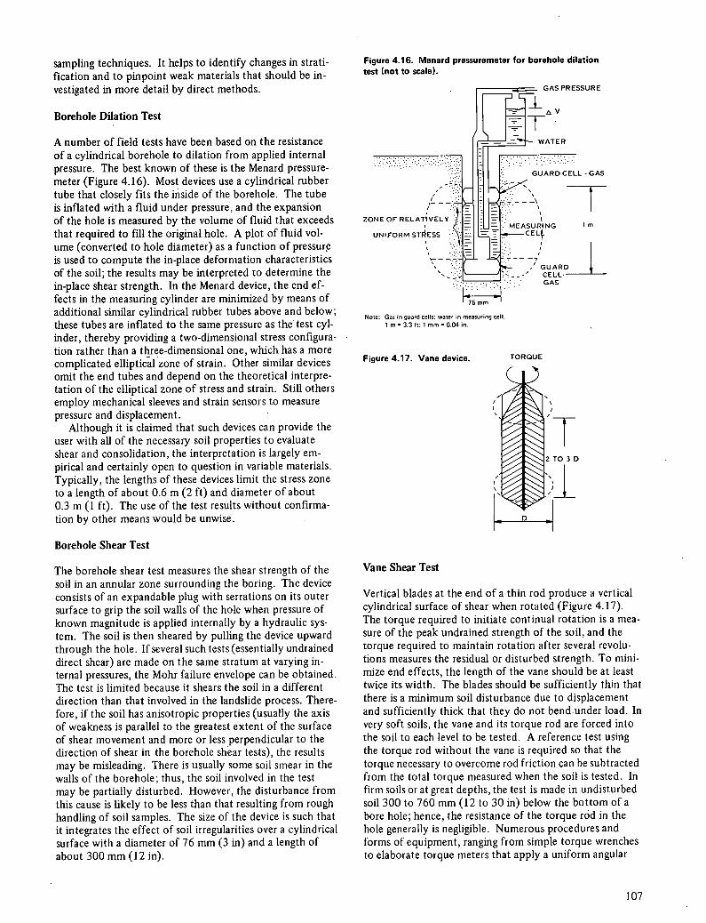
sampling techniques. It helps to identify changes in strati fication and to pinpoint weak materials that should be in-vestigated in more detail by direct methods.

Borehole Dilation Test

A number of field tests have been based on the resistance of a cylindrical borehole to dilation from applied internal pressure. The best known of these is the Menard pressure-meter (Figure 4.16). Most devices use a cylindrical rubber tube that closely fits the inside of the borehole. The tube is inflated with a fluid under pressure, and the expansion of the hole is measured by the volume of fluid that exceeds that required to fill the original hole. A plot of fluid vol-ume (converted to hole diameter) as a function of pressure is used to compute the in-place deformation characteristics of the soil; the results may be interpreted to determine the in-place shear strength. In the Menard device, the end ef-fects in the measuring cylinder are minimized by means of additional similar cylindrical rubber tubes above and below; these tubes are inflated to the same pressure as the test cyl-inder, thereby providing a two-dimensional stress configura-tion rather than a three-dimensional one, which has a more complicated elliptical zone of strain. Other similar devices omit the end tubes and depend on the theoretical interpre-tation of the elliptical zone of stress and strain. Still others employ mechanical sleeves and strain sensors to measure pressure and displacement.

Although it is claimed that such devices can provide the user with all of the necessary soil properties to evaluate shear and consolidation, the interpretation is largely em-pirical and certainly open to question in variable materials. Typically, the lengths of these devices limit the stress zone to a length of about 0.6 m (2 ft) and diameter of about 0.3 m (1 ft). The use of the test results without confirma-tion by other means would be unwise.

Borehole Shear Test

The borehole shear test measures the shear strength of the soil in an annular zone surrounding the boring. The device consists of an expandable plug with serrations on its outer surface to grip the soil walls of the hole when pressure of known magnitude is applied internally by a hydraulic sys-tem. The soil is then sheared by pulling the device upward through the hole. If several such tests (essentially undrained direct shear) are made on the same stratum at varying in-ternal pressures, the Mohi failure envelope can be obtained. The test is limited because it shears the soil in a different direction than that involved in the landslide process. There-fore, if the soil has anisotropic properties (usually the axis of weakness is parallel to the greatest extent of the surface of shear movement and more or less perpendicular to the direction of shear in the borehole shear tests), the results may be misleading. There is usually some soil smear in the walls of the borehole; thus, the soil involved in the test may be partially disturbed. However, the disturbance from this cause is likely to be less than that resulting from rough handling of soil samples. The size of the device is such that it integrates the effect of soil irregularities over a cylindrical surface with a diameter of 76 mm (3 in) and a length of about 300 mm (12 in).

Figure 4.16. Menard pressuremeter for borehole dilation test (not to scale).

GAS PRESSURE

WATER

ZONEOFRELATELY '\

CELL GAS

75 mm

Note: Gas in guard cells: water in measuring cell. 1 m = 3.3 It: 1 mm = 0.04 in.

Figure 4.17. Vane device. TORQUE

Vane Shear Test

Vertical blades at the end of a thin rod produce a vertical cylindrical surface of shear when rotated (Figure 4.17). The torque required to initiate continual rotation is a mea-sure of the peak undrained strength of the soil, and the torque required to maintain rotation after several revolu-tions measures the residual or disturbed strength. To mini-mize end effects, the length of the vane should be at least twice its width. The blades should be sufficiently thin that there is a minimum soil disturbance due to displacement and sufficiently thick that they do not bendunder load. In very soft soils, the vane and its torque rod are forced into the soil to each level to be tested. A reference test using the torque rod without the vane is required so that the torque necessary to overcome rod friction can be subtracted from the total torque measured when the soil is tested. In firm soils or at great depths, the test is made in undisturbed soil 300 to 760 mm (12 to 30 in) below the bottom of a bore hole; hence, the resistance of the torque rod in the hole generally is negligible. Numerous procedures and forms of equipment, ranging from simple torque wrenches to elaborate torque meters that apply a uniform angular

107

strain rate, have been utilized (4.6). Our opinion is that the increased accuracy of the results does not justify the use of elaborate procedures and complex equipment. Cau-tion should be exercised when one interprets the peak strength; in some cases, the strength measured in a vane test has been found to be as much as 30 percent greater than that measured by other methods. Moreover, safety factors computed from such strengths have been found to be unrealistically high. Vane data should be correlated with other shear data for use in analysis and design.

large-Scale Pit Tests

As previously stated, one of the major limitations of lab-oratory tests is their inability to integrate the variations in the soil, particularly in zones with weak or hard spots. This can be overcome by large-scale, in-place tests per-formed in pits or trenches excavated to the questionable strata or zones of slickensiding. Although the range of stresses and particularly the range of groundwater pres-sures that can be evaluated by such tests are limited, the tests permit large volumes of soil to be evaluated under the conditions present within the total mass without the problems of sample disturbance and exposure inherent in small-scale sampling and laboratory testing.

Load Test

The oldest form of in-place test is the plate load test (4.14). A pit is excavated to the surface of the stratum in question, and a rigid square or circular plate is placed on the ground. Its width should be as great as possible, but no wider than about two-thirds the thickness of the stratum whose strength is to be evaluated. The plate is loaded incrementally so that at least 10 successively greater loads are applied before the plate shears the soil beneath it. The results of such a test can be interpreted in terms of soil bearing capacity to give the shear strength of the soil along a curvilinear surface (which may crudely approximate the failure surface of a landslide). However, there are many different interpreta-tions of such tests, all yielding different values for the shear strength parameters. Therefore, the test has limited value in determining the strength of the soil involved in the in-stability of large earth masses.

Large-Scale Direct Shear Test

A large-scale direct shear test can be performed in a pit at the level of the suspected weak stratum; in the case of an existing landslide, the test may be performed on the actual failure surface of the soil. The pit is excavated to the level of the stratum or shear surface to be evaluated and should be large enough to allow engineers and technicians to work around the sides without disturbing the soil to be tested in the center. All the soil within the pit is excavated, except that to be tested, which is left in the form of a block or crude stump above the bottom of the pit. The size of the block is dictated by the engineer's or geologist's evaluation of the variations of soil strength. It should be large enough to be representative of the stratum as a whole and not just its weaker or stronger segments. A double box is placed around the block in question. If there is a definite plane

of weakness, the sides of the box should be perpendicular to that plane, and the plane should lie between the top and bottom halves of the box. Such a test setup is shown in Figure 4.18. Good contact is secured between the soil and the box either by careful trimming of the soil or by pour-ing plaster to fill the space between the box and the soil. Because of the difficulties in trimming gravelly soils or soft rock, the plaster filling is recommended.

A normal load is placed on the block to be tested by means of a plate, the dimensions of which are slightly smaller than that of the box, fitting just inside the upper half of the box. The load is applied by jacking against a piece of heavy machinery above the pit or against a heavy steel beam anchored to the ground by earth anchors. The anchors must be sufficiently far from the test zone so that the stresses around them do not influence the test. The bottom half of the box is anchored securely in place by packed soil, concrete, or plaster in the bottom of the test pit. The top half is then jacked sideways by a calibrated system so that the amount of lateral movement and the load causing the movement can be measured. The direc-tion of jacking should be parallel to that which is suspected in a potential landslide zone or parallel to the movement that has occurred in an actual landslide (as indicated by slickensides on the shear surface). The same surface can be tested at several different normal loads if the test for each vertical load increment is stopped soon after peak strength or significant movement develops. At this point, a larger normal load is applied and the test is resumed. Such a direct shear test determines the average shear stress required to produce failure on a predetermined failure plane. If the peak strength of the soil must be determined, separate tests should be performed on fresh sample blocks for each normal load applied. This will require a large test trench or more than one test pit.

The results of a large-scale shear test simulate the shear strength of the soil along an actual failure surface. The re-sults integrate the effects of both hard and soft zones if the test sample is sufficiently large. Unfortunately, it is diffi-cult to include the effects of changing water pressure. However, our experience shows that meaningful shear test data have been obtained from such tests, particularly if done during the wet season. Correlating the results of an in-place test with those of smaller laboratory tests on sim-ilar soils makes it possible to extend the data obtained from the in-place tests to include the effects of changing water pressure introduced under controlled laboratory conditions. Thus, a more reliable combination of data for evaluating the strength of the soil mass involved in the landslide is provided by a combination of judiciously se-lected large-scale field tests and laboratory tests than by laboratory tests alone.

Standard equipment for making such tests is ordinarily not available. Instead, the equipment is fabricated to fit the size of the sample needed for the particular situation, the space available within the test pits or trenches, and the geometry of the shear surface. It can be improvised out of steel angles, channels, and plates at a reasonable cost. The loading is provided by calibrated hydraulic jacks or jacks with load cells; and the movements are measured by mi-crometer dial gauges. Although such measurements may be characterized as crude, their lack of precision is more

W.

Figure 4.18. Direct shear test of strength along failure surface. a) PLAN VIEW TRACTOR

E SHEAR~BOX TR E NC H

I.

I I L-------

(b) CROSS SECTION

TRACTOR

CONCRETE - - THRUST

BLOCK

CALIBRATED

HYDRAULIC JACK .-- BALL JOINT

NORMAL LOAD PLATE

UPPER SHEAR BOX SHEAR BOX

- .---

- SHEAR

Note: Trench shored for safety and support of tractor. STRUT GRILLAGE SURFACE

than compensated for in their realistic representation of field conditions.

Borehole Dynamics

The effect of a landslide on a borehole, particularly in squeezing or shearing, can be a valuable indicator of rates of movement and locations of shear surfaces. Although equipment for measuring such changes is available, much meaningful information also can be obtained from drillers' observations in those borings that are not instru-mented. Among the factors to be observed are loss of drilling fluid, gain of water or fluid, gas, squeezing of hole, damage to drilling tools, loss of samples, blocking of cores, drill rod drop, broken core, slickensided samples, and un-usually weak zones.

Geophysical Tests

The geophysical studies previously described can be used not only as a means to define the stratification but also as a direct measure of certain physical properties of the soils. Although these properties may not necessarily be those needed to evaluate stability, an empirical correlation among the properties of interest can sometimes be estab-lished in the stability analysis of the landslide.

The seismic refraction technique yields the compression wave velocity of the soil or rock. If the density is known, the dynamic modulus of elasticity in compression can be

calculated. Since the density of various soils and rocks does not vary greatly from point to point, calculations based on estimates may be sufficiently reliable for esti-mates of the rigidity of the mass. The seismic compres-sion wave velocity is particularly valuable as an indication of discontinuities in rock, because it is reduced by cracks or microfissures.

The refraction technique does not allow identification of a weak fractured zone beneath a sounder, higher velocity stratum. However, this identification can be done by cross-hole seismic measurements, utilizing borings from 3 to 12 in (10 to 40 ft) apart. The seismic impulse is generated at the depth of the stratum measured by an explosion, and the time required for the shock wave to travel through the material is measured in the second hole by a geophone sus-pended at the level of the stratum in question. Although engineering properties relevant to landslide evaluation, such as shear strength, cannot be determined directly by such techniques, the suspect stratum can be identified and a crude empirical correlation can be developed between seismic velocity and engineering properties. Below the water table the compression wave velocity in materials of low rigidity is obscured by the compression wave velocity in water.

The apparent resistivity of a soil can be related empiri-cally to soil type and soil moisture. An aquifer with highly ionized water exhibits a far lower apparent resistivity than a dry stratum in which the minerals do not ionize readily. For example, the shear surface within a landslide frequently

ME

Figure 4.19. Correlation of slide movement with precipitation.

210

180

150

0 120

C 0,

90 0,

60

30

0 - 6 F-

E

200 z 0

150 F- 0.

100 0

0 50

N D J F 11 A M J J A S 0 N D J F M A M J J MONTHS

exhibits a marked lower electrical resistance than the sur-rounding intact soils, probably because of the disturbance of the minerals and the accumulation of water along the shear surface.

At best, however, geophysical tests are only indirect supplements to the more direct means of evaluating the qualities of the soil and rock in place. The tests are simple, can be performed in a short period of time, and are rela-tively inexpensive. However, interpretation of the results must be done with extreme caution; too often interpreters jump to conclusions and obtain misleading results.

CORRELATION OF DATA

During an investigation, considerable data will be accumu-lated. The variations of these data, which may occur ran-domly or in some definitepattern, should be studied in three dimensions because the mass of soil or rock involved in a landslide is three dimensional. Some of the ways in which this can be accomplished are discussed briefly below

Areal Variations

Some of the data obtained will vary with geographic posi-tion. These data can be depicted best in the form of maps. If the variations in the data are systematic, they can be de-picted as contours, such as lines of equal strength or lines of equal groundwater pressure. These variations are fre-quently plotted on overlays to the topographic map of the site; several overlays may be desirable.

Cross Sections

Depicting the data in the form of cross sections is particu-larly useful because the stability of the mass is usually eval-uated by use of cross sections (Figure 4.12). Cross sections parallel to the direction of the maximum slope, to the

maximum water pressure gradient, or to the observed tra-jectories of movement are the beginning point for a stability analysis of an earth mass. The various strata encountered and the groundwater levels or pressures are depicted on these cross sections. In addition, overlays should show the engineering properties relevant to the stability analyses. The surfaces of failure, as deduced from ground surface ob-servations, sophisticated instrumentation, borings, test trenches, and pits, define a body of soil on which various force systems act. The external forces depicted on an over-lay to the cross sections provide the beginnings of the anal-yses described in Chapter 7.

Time-Based Observations and Correlations

The significance of the different factors involved in a land-slide can frequently be found from empirical correlations between movement and observed forces or environmental factors. For example, a time-based graph of both landslide displacement and rainfall or accumulated rainfall and snow-melt may show a visual relation (Figure 4.19). Similar time-based relations can be observed between construction operations and movement. In some cases, plots of the ob-served phenomena as functions of the logarithm of time are instructive. For example, stochastic processes, such as the readjustment of coarse particles through creep and secondary soil compression, often can be approximated by a straight line on a plot of movement as a function of the logarithm of time. Thus, the time graph or the logarithm of the time graph becomes a diagnostic tool in analyzing the causes of movement.

CONCLUSIONS

The field investigation identifies potential problem areas and defines the features involved in an existing landslide.

110

More intensive investigation uncovers the soil and environ-mental factors that produced the movement. The mathe-matical analysis of a landslide is based on the field investi-gation and obviously can be no more accurate than the data obtained from the field work; likewise, the corrective measures based on the analyses can be no more effective than the quality of the data used in the analyses. Unfor-tunately, our experience has been that field investigations are often inadequate and that geologists and engineers sometime jump to conclusionsbefore the data have been obtained and evaluated; thus, they merely perpetuate their past mistakes. A technically sound solution can be derived only from technically sound data.

REFERENCES

4.1 American Geological Institute. Glossary of Geology. AGI, Washington, D.C., 1972, 805 pp.

4.2 American Society for Testing and Materials. Annual Book of ASTM Standards: Part 19—Soil and Rock; Building Stones; Peats. ASTM, Philadelphia, 1977, 494 pp.

4.3 Compton, R. R. Manual of Field Geology. Wiley, New York, 1962, 378 pp.

4.4 Deere, D. U., and Patton, F. D. Slope Stability in Resid- ual Soils. Proc., 4th Pan-American Conference on Soil Mechanics and Foundation Engineering, San Juan, American Society of Civil Engineers, New York, Vol. 1, 1971, pp. 87-170.

4.5 Fletcher, G. F. A. Standard Penetration Test: Its Uses and Abuses. Proc., Journal of Soil Mechanics and Foun-dations Division, American Society of Civil Engineers, New York, Vol. 91, No. SM4, 1965, pp. 67-75.

4.6 Hvorslev, M. J. Subsurface Exploration and Sampling of Soils for Civil Engineering Purposes. U.S. Army Engineer Waterways Experiment Station, Vicksburg, Miss., 1949, 521 pp.

4.7 Lahee, F. H. Field Geology. McGraw-Hill, New York, 6th Ed., 1961, 926 pp.

4.8 Lambe, T. W. Soil Testing for Engineers. Wiley, New York, 1951, 165 pp.

4.9 Philbrick, S. S., and Cleaves, A. B. Field and Laboratory Investigations. In Landslides and Engineering Practice (Eckel, E. B., ed.), Highway Research Board, Special Rept. 29, 1958, pp. 93-111.

4.10 Rocha, M. A Method of Integral Sampling of Rock Masses. Rock Mechanics, Vol. 3, No. 1, 1971, pp. 1-12.

4.11 Sangierat, G. The Penetrometer and Soil Exploration. Elsevier, New York, 1972, 464 pp.

4.12 Schmertmann, J. H. Static Cone Penetrometers for Soil Exploration. Civil Engineering, Vol. 37, No. 6, 1967, pp. 71-73.

4.13 Schultze, E., and Melzer, K. J. The Determination of the Density and the Modulus of Compressibility of Non-Cohesive Soils by Soundings. Proc., 6th International Conference on Soil Mechanics and Foundation Engineer-ing, Montreal, Vol. 1, 1965, pp. 354-358.

4.14 Sowers, G. B., and Sowers, G. F. Introductory Soil Mechanics and Foundations. Macmillan, New York, 3rd Ed., 1970, 556 pp.

4.15 Sowers, G. F. Remote Sensing: A New Tool in Site In- vestigation. Law Engineering Testing Co., Marietta, Ga., Bulletin G-5, 1973.

4.16 Terzaghi, K., and Peck, R. B. Soil Mechanics in Engineer- ing Practice. Wiley, New York, 2nd Ed., 1967, 729 pp.

4.17 U.S. Bureau of Reclamation. Design of Small Dams. U.S. Bureau of Reclamation, Denver, 1973, 816 pp.

4.18 Zâruba, Q., and Mend, V. Landslides and Their Con- trol. Elsevier, New York, and Academia, Prague, 1969, 205 pp.

PHOTOGRAPH CREDITS

Figure 4:8 Courtesy of Tennessee Department of Transportation Figure 4.9 Courtesy of Tennessee Department of Transportation

Chapter 5

Field Instrumentation Stanley D. Wilson and P. Erik Mikkelsen

The development of field instrumentation has had a signifi-cant impact on geotechnical engineering in the past 15 years. Of particular importance is the notable contribution of instrumentation to landslide-oriented problems (5.50). The usefulness of field instrumentation for the identifica-tion of landslide movements, for the monitoring of slides that have been remedially treated, and for other geotech-nically oriented measurements has been described in the literature (5.1, 5.8, 5.18, 5.36, 5.45, 5.48, 5.50, 5.56). Al-though the earlier Highway Research Board Special Report on landslides (5.20) mentioned the use of simple instru-mentation (which is by no means obsolete and is described in this chapter), its publication generally preceded the in-troduction of modern instruments. The economic impact of slope failures created a demand for better instrumenta-tion and led to its general acceptance and use. This chap-ter describes the types of instrumentation currently avail-able, their limitations, and their specific applications to slope instability problems. In addition, traditional ap-proaches to the determination of slide movements and groundwater levels are reviewed.

The need to gather certain quantitative data to analyze slope-stability problems and to design remedial measures is discussed in other chapters. Topographic mapping, geo-logic mapping, subsurface soil and groundwater investiga-tions, and laboratory strength testing are normally per-formed to aid in determining the cause of the slide, the mode of failure, and the physical and engineering character. istics of the soil and rock involved. Such investigations are necessarily performed on already developed landslides, the characteristics of which may be observed and noted. How-ever, small movements of a soil mass prior to or even at in-cipient failure are usually not visually evident; so the value of information that can be obtained at the ground surface is limited. However, instrumentation can provide valuable information on incipient, as well as fully developed, land-slides. In this respect, instrumentation is not intended to

replace field observations (5.38) and investigative procedures discussed in other chapters. Instead, it augments other data by providing supplementary information and by warn-ing of impending major movements. Typical situations for which various instruments have been used are

To determine the depth and shape of the sliding sur-face in a developed slide so that calculations can be made to determine the available soil strength parameters at fail-ure and so that remedial treatments can be designed;

To determine absolute lateral and vertical move-ments within a sliding mass;

To determine the rate of sliding (accelerating or de-celerating movements) and thus warn of impending dangers;

To monitor the activity of marginally stable natural slopes or cut slopes and the effects of construction activity or precipitation on them;

To monitor groundwater levels or pore pressures nor-mally associated with landslide activity to enable effective stress analyses to be performed;

To provide remote digital readout or a remote alarm system that would warn of possible dangers; and

To monitor and evaluate the effectiveness of various control measures.

In the last situation, savings are often realized in remedial treatment by a planned and monitored sequence of con-struction. For example, drainage might be initially installed and its effect monitored to determine whether a planned buttress is actually necessary.

INSTRUMENTATION PLANNING

Adequate planning is required before a specific landslide is instrumented. The steps are (a) determine what types of measurements are required, (b) select the specific types of instruments best suited to make the required measurements,

112

(c) plan the location, number, and depth of instrumentation, and (d) develop the recording techniques.

Initially the planning process requires the development of ideas on the causes of the landslide and the probable limits of the depth and outer boundaries of the movements. Of course, to have the answers before the system is planned would be helpful. Reconnaissance of the area, study of the geology, review of rainfall records, and observation of topographic features, especially recent topographic changes, will often provide clues. Unfortunately, no two slides are alike in all details, and experience alone without the appli-cation of judgment may lead to erroneous concepts.

An instrumentation system in which the instruments do not extend below the zone of movement, were installed at the wrong locations, or are unsuitable is a waste of time and money. Loss of time may mean that corrective treat-ment is started too late to save the project.

Types of Measurements Required

Landslides, by definition, involve movement, and the mag-nitude, rate, and distribution of this movement are gener-ally the most important measurements required. Equally important in many slide problems, however, are measure-ments of pore-water pressures within the slide area, partic-ularly in layered systems in which excess hydrostatic pressures may exist between layers.

If the depth of sliding is readily apparent from visual observations, surface measurements may be sufficient for obtaining the rate of movement. The surface measure-ments should extend beyond the uppermost limit of visual movement so that possible extension in advance of crack-ing can be monitored. Vertical and horizontal measure-ments of movement of the ground surface at various loca-tions within the slide area should be obtained. Vertical offsets, widening of cracks, and toe heave should be mon-itored. The direction of movement can often be inferred from the pattern of cracking, particularly by the matching of the irregular edges of the cracks. If the depth and thick-ness of the zone of movement are not apparent, inclinom-eters or similar devices that can detect the movement with depth must be used. Pore pressures at or near the sliding surface must be measured to enable an effective stress anal-ysis to be performed and to assess the adequacy of drain-age measures. Rapid-response piezometers are advantageous, particularly in impervious soils.

Selection of Instrument Types

Many types and models of instruments are available for measuring the changing conditions in a landslide; they vary in degree of sophistication, particularly in regard to read-out capabilities. Instruments have been developed to mea-sure vertical and horizontal earth movements, pore-water pressures, in situ stresses and strains, dynamic responses, and many other parameters. However, in most landslide problems, the measurement of horizontal movement of the foundation soil or rock and the measurement of pore-water pressures are of primary concern. Instruments com-monly used for these purposes are described in this chapter

If the movement is known to be along a well-defined shear plane, such as a bedding plane or fracture, simple

probe pipes will suffice to determine the depth. If the movements are large and rapid, accuracy is not an essential requirement and even relatively crude inclinometers may suffice. When the rate of movement is small and the depth and distribution are not known, more precise instrumenta-tion is required. Carefully installed precision inclinometers are best in such instances, although there may be cases in which extensometers or strain meters can be used to advan-tage.

The Casagrande type of piezometer is the most useful general purpose pore-pressure measuring device, but may give too slow an initial response in fine-grained soils; there-fore, pneumatic or electric types may be preferable. High-air-entry, low-flow piezometers should be used in clays or clay-shales in which permeabilities are low or suctions may be present because of unloading (5.53).

The types of instruments, layout, and monitoring schedules are usually determined by the specific needs of a project. Several basics, however, should be thoroughly evaluated for any system. Instruments should be reliable, rugged, and capable of functioning for long periods of time without repair or replacement. They must also be capable of responding rapidly and precisely to changes so that a true picture of events can be maintained at all times. High sensitivity is usually a prerequisite when performance is monitored during construction, since it is often the rate of change rather than the absolute value that provides the key to proper interpretation. The location of instruments re-quires a thorough understanding of the geologic and sub-surface conditions if meaningful data are to be obtained. This is particularly true of pore-pressure recording devices that are intended to measure pressures in specific zones of weakness or potential instability. Since most measure-ments are relative, a stable base or datum must be provided so that absolute movements can be determined.

In this chapter, the primary emphasis is on measurement techniques and instruments for landslides; less emphasis is placed on conventional surface surveying techniques. Con-ventional surveying methods are fundamental to displace-ment measurements at the surface (5.23); this has been dis-cussed more fully in Chapter 4. Modern deformation in-struments for landslides have augmented the methods of surface measurements, but more important they have ex-panded capabilities in terms of accuracy, simplicity, and ease or convenience of operation. In addition, an ever-expanding range of instruments makes possible the mea-surements of subsurface deformations (5.13, 5.17, 5.21, 5.25, 5.44). Table 5.1 gives summaries of various survey methods, instruments for measuring subsurface deforma-tions, and piezometers.

SURFACE SURVEYINQ

Conventional Surveying

In an active slide area, surface movements are normally monitored to determine the extent of slide activity and the rate of movement (5.21, 5.32). Optical instrument surveys and tape measurements are used to determine lateral and vertical movements. Bench marks and transit stations, lo-cated on stable ground, provide the basis for which subse-quent movements of hubs can be determined optically and

113

Table 5.1. Surveying methods, horizontal movement devices, extensometers, and piezometers (5.13)

Method or Measurement Instrument Type Range Accuracy Advantages

Limitations and Precautions

Reli-ability

Method Chaining Variable ±1/5000 to Is simple and inexpensive; Requires clear, relatively Excellent Ordinary, 1/10 000 of has direct observation flat surface between

third order distance points and stable refer- Precise. ± 1/20 000 to ence monuments first order 1/200 000 of Corrections for tempera-

distance ture and slope should be applied and a standard chain tension used

Electronic dis- 20 to 3000m ± 1/50 000 to Is precise, long range, fast, Accuracy is infl'jenced by Good tance mea- 1/300 000 of usable over rough terrain atmospheric conditons; surement distance accuracy at short ranges (EDM) (<30 to 90 m) is lim-

ited for most instruments Optical leveling ±3 to 6 mm Is simple, fast, particularly Has limited precision; re- Excellent

Ordinary, with self-leveling instru- quires good bench mark second and ments nearby third order

Precise, first ±0.6 to 1.2 mm Is more precise Requires good bench Excellent order (paral- mark and reference lel plate points and careful ad- micrometer . herence to standard attachment, procedures special rod)

Off sets from a baseline

Theodolite 0 to 1.5 m ±0.6 to 1.5 mm Is simple; has direct observa- Requires baseline unaf- Excellent and scale tion fected by movements

and good monuments; accuracy can be im- proved by using a tar- get with a vernier and by repeating the sight from the opposite end of the baseline

Laser and 0 to 1.5 m ±1.5 mm Is faster than transit Is seriously affected by Good photocell atmospheric conditions detector

Triangulation ±0.6 to 12 mm Is usable when direct mea- Requires precise measure- Good surements are not possible; ment of base distance is good for tying into points and angles; requires outside of construction good reference monu- area ments

Photogram- ± 1/5000 to Can record hundreds of po- Weather conditions can Good metric 1/50 000 of tential movements at one limit use

distance time for determination of overall displacement pat- tern

Horizontal Long base 150mm 0.3mm Is precise; can be used to Has risk of electrical Good movement strain meter check horizontal move- failure; has limited ap- instrument with electrical ment at top of other de- plication for tunnels

readout vices, such as inclinom- eters

Fixed multi- ±20 arc 5a Is available in portable Is complex; does not point bore- version and double pivot measure continuous hole deflec- version to measure move- prof ile tometers ment along two axes

Fixed multi- ±0.03 mm in 3 m Is precise; can be removed Is complex; does not point bore- for repairs or reuse; uses measure continuous hole inch- standard inclinometer , profile nometers casing Accuracy is lost when

removed and replaced Portable bore-

hole inch- nometers

Wheatstone ±12° , op- ±20mm in 30 m Has long experience record; Requires lengthy calcula- Very bridge tional to is not sensitive to tempera- tions; reads one axis at good pendulum ±25° ture a time; has no provi-

- sions for automatic readout

114

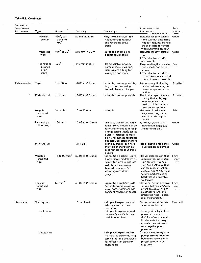
Table 5.1. Continued.

Method or Measurement Limitations and Reli- Instrument Type Range Accuracy Advantages Precautions ability

Acceler- ±300 op- ±5 mm in 30 m ometer tional to

±900

Vibrating ±15° or 20° ±10mm in 30 m wire

Bondedre- ±20° ±10mmin30m sistance St rain gauge

Extensometer Tape ito 30 m ±0.03 to 0.3mm

Portable rod i to 8 m

±0.03 to 0.3 mm

Weight- Variable

±5 to 20 mm tensioned wire

University of

150mm ±0.03to0.13mm Illinois rod

Interfels rod

Variable

Variable-

15 to 90 mmb ±0.05 to 0.13mm tensioned wire

Constant- 50 mmb

±0.05 to 013 mm tensioned wire

Piezometer Open system

±3mm head

Well point

Casagrande

Reads two axes at a time; Requires lengthy calcula- Good has automatic readout tions without automatic and recording provi- readout; requires manual sions check of data for errors

with automatic readout Is available in single or Requires lengthy calcula- Good double axis models tions

Errors due to zero drift are possible

Has adjustable range on Requires lengthy calcula- Fair some models; uses ordi- tions; reads one axis at nary square tubing for a time casing on one model Errors due to zero drift,

temperature, or electrical connections are possible

Is simple, precise, portable; Has accuracy limited by Excellent is good for measuring tension adjustment; re- tunnel diameter changes quires temperature cor-

rection Is simple, precise, portable Has limited span; has ac- Excellent

curacy limited by sag; invar tubes can be used to minimize tem- perature corrections

Is simple Has creep in wire that Fair leads to errors; is vul- nerable to damage in tunnel

Is simple, precise, and large Is not adaptable to re- Good range (some models can be mote reading; has two reset and extended through anchor units only linings placed later); can be quickly installed; is more blast and damage resistant; has easily adjusted anchors

Is simple, precise; can have Has projecting head that Good multiple anchors; can ac- is vulnerable to damage cept remote readout trans- ducers

Has multiple anchors, up to - Has variable tension that Fair; 6 or 8 (some models are de- requires varying calibra- short signed for remote readings tion factors, wire fric- term with transducers using tion and hysteresis that bonded resistance or can seriously affect ac- vibrating-wire strain curacy, risk of electrical

gauges) failure, and projecting head that is vulnerable to damage

Has multiple anchors; is de- Has wire friction and hys- Fair; signed for remote reading teresis that can seriously short using potentiometers; has affect accuracy, risk of term constant calibration factor electrical failure, and

projecting head; is com- plex mechanically

Is simple, inexpensive, and Central observation sys- Excellent adequate for most earth tem cannot be used problems

Is simple, inexpensive, and Has large time lag in low universally available; can porosity materials be driven in place (k < 1 .zm/s) and metal-

lic elements that may corrode; cannot mea- sure negative pore pressures

Is simple, inexpensive; has Cannot measure negative no metallic elements, long pore pressures; requires

service life, and provisions borehole and carefully for offset riser pipe and placed bentonite or

flushing tip grout seal

115

Table 5.1. Continued.

Method or Measurement Limitations and Reli-

Instrument Type Range Accuracy Advantages Precautions ability

Cannot measure negative pore pressures

Geonor

Cambridge

Closed sys- -c tem

USB R

Bishop

Diaphragm ±1% of full scalec

Pneumatic

Hydraulic

Electrical re- ±1% of ranged resistance strain gauge

Vibrating-wire strain gauge

Can be pushed or driven into soft ground; can be placed in borehole with filter zone to re-duce time lag

Has simple drivable pi-ezometer with inexpen-sive tip and shield to pro-tect tip during driving

Allows central observation system to be used; can measure negative pore pressures; is usable in low permeability soils

Is simple, inexpensive, and readily available; has long experience record

Is simple, and designed for less frequent deairing than USBR type; can be pushed into soil from bottom of borehole

Has small time lag; is usable in low permeability situa-tions; allows central obser-vation system to be used; can measure negative pore pressures

Is not subject to freezing; uses smaller, less expen-sive tubing

Is simple and easy to seal against leakage

Can often be locally fabri-cated from commercially available parts; is adaptable to automatic data record-ing; can measure negative pore pressures

Is more reliable than resis-tance strain gauge type; is adaptable to automatic data recording

Cannot measure negative pore pressures; has me-tallic elements that may corrode

Is more difficult to install Excellent than open system pi- ezometers; requires fre- quent and careful deair- ing

Is costly and difficult to Good to install and operate fair

Cannot measure negative pore pressures; has leak-age and moisture in lines

Cannot measure negative pore pressures; requires constant volume pumps or flow control valves

Has often limited service life; is susceptible to wiring damage

Note: 1 m = 3.3ft; 1 mm = 0.39 in.

a Total displacement accuracy depends on pivot spacing. c Depends on pressure gauge used.

bCan be reset. dDepends on transducer.

by tape measurement. As shown in Figure 5,1,transit lines can be established so that the vertical and horizontal dis-placements at the center and toe of the slide can be observed. Lateral motions can be detected by transit and tape mea-surements from each hub. When a tension crack has opened above the top of a slide

'simple daily measurements across

the crack can be made between two hubs driven into the ground. In many cases, the outer limit of the ground move-ments is not known, and establishing instrument setups on stable ground may be a problem.

Various techniques and accuracy achieved in optical leveling, offset measurements from transit lines, chaining distances, and triangulation have been discussed extensively in the literature (5,8, 5.23), particularly for dams, embank-ments, and buildings. Although conventional surveys, par-

ticularly higher order surveys, can define the area of move-ment, more accurate measurements may be required in many cases. Terzaghi (5.47) stated that "if a landslide comes as a surprise to the eyewitness, it would be more ac-curate to say that the observers failed to detect the phenom-ena which preceded the slide," The implication is that the smallest movements possible should be measured at the earliest possible time. Terzaghi (5.47) also describes the movements that precede a landslide.

The detection of small surface movements when crack-ing is not apparent requires a trained observer. If the ground surface is covered with rocks, or if there is a rock embank-ment, horizontal stretching will result in local instability of individual rocks such that walking over the slope gives one a sense of insecurity. Overturned rocks can be detected by

a change in coloring or surface weathering. Trees inclined at the base but changing to vertical trunks a meter or so above the ground may indicate old slide movements. In-clined but straight trunks indicate recent movements. Cracks covered over with leaves or surface duff can be de-tected by walking over the area and noting the firmness of support. Frequently animals will avoid grazing in a po-tential landslide area because of uncertain support or hid-den fissures. Small openings on the downhill side of struc-tures, or next to tree trunks, may indicate creep. Overtaut or excessively sagging utility lines or misalignment of fence posts or utility poles are excellent indicators of ground movements. Such movements, when accurately monitored, serve as an important tool in assessing the potential hazard to structures, nearby residents, and the public.

Other Types of Surface Surveying

There are three rapidly developing surveying techniques today, and these will undoubtedly find increasing use in field measurements. Some are already in extensive use (e.g., electronic distance measurement and lasers); others are in limited use or are in the experimental stage (e.g., terrestrial photogrammetry). Electronic distance measure-ment (EDM) has changed surveying practices more than anything else in the last 100 years (5.15). EDM devices have proved particularly suited for use over rugged terrain; they perform more accurately and much faster than ordi-nary surveying techniques and require fewer personnel. Lightweight EDM instruments can be used efficiently under ideal conditions for distances as short as 20 m (66 ft) and as long as 3 km (2 miles); errors are as small as ±0.0032 m (± 0.010 ft) (5.28, 5.43). Larger instruments using light waves or microwaves can be used at much longer distances. The accuracy of EDM is influenced by weather and atmospheric conditions; comparative read-ings with three different instruments are described by Pen-man and Charles (5.40).

EDM can be used to monitor large slides with large move-ments and provide a rapid way to survey many points on the mass from a single, readily accessible location. An ex-ample of such an installation involves an ancient landslide in Washington along the Columbia River, where the boun-daries of the active slide are more than 0.6 km (1 mile) in width and 4.8 km (3 miles) in length. Yearly movements vary from only 1 m to 6 to 9 m (0.3 ft to 20 to 30 ft) and depend on the time of year and the rainfall. A permanent station, readily accessible all year, has been set up on the opposite side of the river, and monthly distance readings are taken to 14 points on the slide area and to 2 points lo-cated outside the slide zone. The distances involved vary from about 1500 to 6000 m (5000 to 20000 ft). Figure 5.2a shows the movements (changes in distance) recorded by the EDM (electrotape) during a 1-year period for 2 selected 'points at the Columbia River slide, based on monthly readings. At the end of the year, the points were resurveyed by triangulation. The discrepancy is about 10 cm (4 in), which, although larger than anticipated, is quite satisfactory considering the total movements. Figure 5.2b shows recorded changes for 2 points believed to be on stable ground. The variation of monthly readings is seen to be ± 0.06 m (± 0.2 ft); variation is no greater for a 4765-m (15 630-ft) length than for a 1844-rn (6050-ft) length.

Laser instruments are already widely used for setting alignments, and they are well suited for setting a reference line for offset measurements to surface monuments. Laser beams are also used with some EDM instruments. It should be possible to measure offsets with an error no greater than 0.003 to 0.006 m (0.01 to 0.02 ft) (5.23).

Terrestrial photogrammetry has been used in some cases on dam projects (5.35) and in mines, but no landslide mea-surements using this method have been found in the litera-ture. Phototheodolites are used to take successive stereo-photographs from a fixed station along a fixed camera axis; movements are identified in a stereocomparator, and accuracies of 0.006 to 0.009 m (0.02 to 0.03 ft) have been

Figure 5.1. Movement measurements in a typical slide area.

- -- - BARKER eo*io clAck •ONITORING POINTS

A163

BEIIC i7? ' - FESET 0 (0

/ -

117

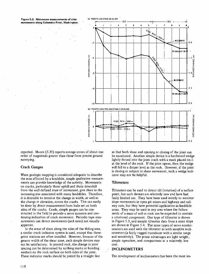
Figure 5.2. Microwave measurements of slide (a) POINTS LOCATED ON SLIDE

movements along Columbia River, Washington. I (912

N J ( A

1913 -I N A N

MICROWAVE

RIANCU AT ION

— —

--------

-MICROWAVE

TRIANGULATION

IbI POINTS LOCATED ON STABLE GROUND

-0.6

2.4

-3.0

(CAT PA Hr 4760m

B

C, z I 0

0 2

C-CO a

iw

reported. Moore (5.35) reports average errors of about one order of magnitude greater than those from precise ground surveying.

Crack Gauges

When geologic mapping is considered adequate to describe the area affected by a landslide, simple qualitative measure-ments can provide knowledge of the activity. Movements on cracks, particularly those uphill and those downhill from the well-defined zone of movement, give clues to the increasing size associated with many landslides. Therefore, it is desirable to monitor the change in width, as well as the change in elevation, across the cracks. This can easily be done by direct measurement from hubs set on both sides of the cracks. Crude, simple gauges can be con-structed in the field to provide a more accurate and con-tinuing indication of crack movement. Periodic tape mea-surements can detect movements (and rates) not visually apparent.

In the areas of shear along the sides of the sliding area, a similar crack indicator system is used, except that three-point stations are often installed. However, because of the greater width of the shear zone, such simple devices may not be satisfactory. In jointed rock, the change in joint spacing can be determined by scribing marks or bonding washers on the rock surface on both sides of the joint. These indicator marks should be joined by a straight line

so that both shear and opening or closing of the joint can be monitored. Another simple device is a hardwood wedge lightly forced into the joint crack with a mark placed on it at the level of the rock. If the joint opens, then the wedge will fall to a deeper level in the rock. However, if the joint is closing or subject to shear movement, such a wedge indi-cator may not be helpful.

Tiltmeters

Tiltmeters can be used to detect tilt (rotation) of a surface point, but such devices are relatively new and have had fairly limited use. They have been used mostly to monitor slope movements in open pit mines and highway and rail-way cuts, but they have potential application in landslide areas. They may be used in any area where the failure mode of a mass of soil or rock can be expected to contain a rotational component. One type of tiltmeter is shown in Figure 5.3, and sample tiltmeter data from a mine slope are shown in Figure 5.4. The same types of servo acceler-ometers are used with the tiltmeter as with sensitive mdi-

nometers (a fairly rugged transducer with a similar range and sensitivity). The prime advantages are light weight, simple operation, and compactness at a relatively low cost.

INCLINOMETERS

The development of inclinometers has been the most im-

'U

LONGITUDINAl AXIS

I TAN AXIS

AS VEX S 0

NoreI in - 3.3 It. I rrnr, 0.04 n.

—Inc —50 0 ..-50 -'-100 I50 *200 ,250

FACE ADVANCE Irvil - NO-

+2.0

+1.5

0'

I-

z D + 0.5 0 x 0

-0.5

'- 30

-200

portant contribution to the analysis and detection of land-slide movements in the past 2 decades. Although it has been used most extensively to monitor landslides, the in-clinometer has gained widespread use as a monitoring in-strument for dams, bulkheads, and other earth-retaining structures and in various areas of research (5.1, 5.13, 5.17, 5.34, 5.44, 5.55, 5.59). Since the introduction in the early 1950s of the pendulum-actuated inclinometer operating in grooved plastic casing (5.45, 5.50), the same basic concepts have been applied to instruments manufactured by at least 12 U.S. and foreign firms. Although the principle of opera-tion has remained unchanged (Figure 5.5), inclinometers have been improved in accuracy and ease of operation and have undergone numerous modifications to adapt them to individual projects.

The inclinometer measures the change in inclination (or tilt) of a casing in a borehole (Figure 5.5) and thus allows the distribution of lateral movements to be determined as

a function of depth below the ground surface and as a func-tion of time (Figure 5.6). The application of the inclinom-eter to landslides is readily apparent, namely, to define the slip surface or zones of movement relative to the stable zones. Inclinometers have undergone rapid development to improve reliability, provide accuracy, reduce weight and bulk of instruments, lessen data acquisition and reduction time, and improve versatility of operations under adverse conditions. Automatic data-recording devices, power cable reels, and other features are now available.

An inclinometer system has four main components.

A guide casing is permanently installed in a near ver-tical borehole in the ground. The casing may be made of

plastic, steel, or aluminum. Circular sections generally have longitudinal slots or grooves for orientation of the sensor unit, but square sections are used with some types.

A portable sensor unit is commonly mounted in a

Figure 5.3. Portable tiltmeter. Figure 5.4. Tilt at ground surface due to advance of longwall mining face.

Figure 5.5. Principle of inclinometer

operation.

Total displaceoerit

i SinSf)

0isfancebeleen puccesove readings

1016

Guide :heeis

Probe

True Yell cal of initial

profile

119

Figure 5.6. Measurement of slide movements with inclinometer.

IaI PROFILE THROUGH SLIDE IA) CROSS SECTION THROUGH SLIDE

SLIDE - SLIDE PLAST IC

SKEAR ZONE S

ON ABLE

BULCE — FROM INCLINOMETER> WELL WELL HIlTS

A B OF SLIDE

(c) OBSERVATIONAL DATA, WELL A dl COMPUTED MOVEMENTS, WELL A

CHANGE IN INCLINAIIONISiO4I MOVEMENT)cn,I

0.03 0.06 0.09 2.5 5 1.5

10

Note. 1m331t;lcn,-04r.

carriage designed for operation in the guide casing (often referred to as the probe or torpedo).

A control cable raises and lowers the sensor unit in the casing and transmits electrical signals to the surface. For accurate depth control of the sensor unit, the cable is usually graduated or lowered on a separate surveyor's steel tape.

A portable control and readout unit at tile surface supplies power, receives electric signals, and displays read. ings in dial or digital format.

Components other than these four are accessories. The need for accessories increases with the volume of output data (depth and number of inclinometers installed) and the need for rapid and efficient data retrieval, reduction, and presentation.

In landslide applications, inclinometer casings are nor-mally installed in exploration drill holes extending through soil and rock suspected of movement and preferably well into materials that, in the best judgment at the time, are assumed to be stable. Samples are generally taken from the borings and tested to confirm such assumptions. The annular Space between the drill hole and the outer wall of the casing is generally grouted or hackfilled with sand. The success of the casing installation depends on the ex-perience and the skill of the personnel: soil, rock, and groundwater conditions: depth of installation: and acces-sibility to the area.

The inclinometer instrument sensor unit (Figure 5.7) is lowered and raised on an accurately marked cable, its wheels or guides following the oriented, longitudinal slots of the casing. The response to slope changes in the casing are monitored and recorded at the surface. Readings are taken at fixed, usually equal, increments throughout the entire depth. Instruments differ primarily in the type of sensor used, in the accuracy with which the sensor detects the inclination - and in the method of alignment and depth control within the borehole.

Figure 5.7. Inclinometer.

Figure 5.8. Pendulum-activated Wheatstone bridge circuit for typical inclinometer.

BATTERY

PRECISION

GALVANOMETER

INDICATOR

L — T_' - - WATERTIGHT

- SLE

PENDULUM

10 SENSOR

PLATE GROL \PRECI WIRE WOUND

L RESISTANCE

Four basic categories of inehinometers are in use in the United States today, and within each category are instru-ments of several different manufacturers. These categories are distinguished by the type of sensor selected to measure the inclination of the probe relative to the direction of gravity.

- The pendulum-activated Wlieatstone bridge circuit consists of a free-swinging. magnetically damped pendulum moving across a resistance coil: measurement for each sen-sor is in one plane (5.24, 5.33, 5.54).

In the strain-gauge type, bonded or vibrating-wire strain gauges are mounted around a stiff pendulum: mea-surement for each sensor is in one plane (5.24).

The accelerometer type is a closed-loop, servo-accelerometer circuit: measurement for each sensor is in one plane, and the use of two sensors per unit (biaxial) is common (5.34).

120

4. The photographic type photographically records the projection of a pendulum with two degrees of freedom on a target oriented by a magnetic compass; no orientation is needed within the casing or borehole. This type is not often used because its accuracy is generally much lower than that of previous types and data reduction is much more time consuming. Measurements with this instrument are described by Hanna (5.25).

With the exception of the photographic type, most incli-nometers measure the inclination of the casing in two mu-tually perpendicular near-vertical planes. Thus, horizontal components of movement, both transverse and parallel to any assumed direction of sliding, can be computed from the inclinometer measurements. Deviations from this ideal occur because of limitations and compromises in manufac-turing and because of installation circumstances. Instru-ments of different manufacture cannot generally be used in-terchangeably. In the interest of accuracy, the interchange-able use of instruments (probes) of the same manufacture also should be avoided.

The function of the inclinometer is to detect the change in. inclination of the casing from its original near-vertical position. Readings taken at regular preestablished depths inside the casing allow the change in slope at various points to be determined; integration of the slope changes between any two points yields the relative deflection between those points. Repeating such measurements periodically provides data on the location, magnitude, direction, and rate of cas-ing movement. The integration is normally performed from the bottom of the boring, since the bottom is assumed to be fixed in position and inclination (Figure 5.5).

All too often, confusing or unexplainable results appear because of instrumentation problems. These problems are common to all inclinometers; therefore, they are discussed in some detail so that, even without a detailed understand-ing of the inner workings of the instruments, one will be able to recognize these anomalies, the limits of accuracy, and the meaning of the results. In simple terms, the person closest to the job should be able to answer the basic ques-tions: Is the slide active? How fast is it moving? How deep is it?

Inclinometer Sensors

Before a description is given of some of the sophisticated types of inclinometers, one device deserves mention. The borehole probe pipe, also called the slip indicator or poor boy, is one of the crudest of the subsurface measuring devices. It typically consists of a 25-mm (1-in) diameter semirigid plastic tube in a borehole. Metal rods of increas-ing length are lowered inside the tubing in turn, and the rod length that is just unable to pass a given depth gives a measure of the curvature of the tubing in the vicinity of that point. Tonis and Bartlett (5.49) describe the use of this technique for the location of slip surfaces in unstable slopes. This type of measurement can easily be performed in the riser pipe of an observation well or open piezometer. If there are several shear planes, or if the shear zone is thick, a section of rod hung on a thin wire initially can be left at the bottom of the pipe; subsequently, the rod is pulled up to detect the lower limit of movement.

As originally conceived, the first modern inclinometers used pendulum-activated resistors to convert inclinations into electrical measurements; instruments of this type have had long and successful experience records (5.45). A typical inclinometer of this type consists of a pendulum, the tip of which makes contact with a resistance coil, subdividing the coil into two resistances that form one-half of a Wheatstone bridge (Figure 5.8). The other half of the bridge, contained in the portable control box, includes a precision potenti-ometer. The potentiometer readings are proportional to the inclination of the torpedo. The system has a sensitivity of about 3 min of arc and generally demonstrates a preci-sion of±l3 to 25mm (±0.50 to 1.0 in) over a 33-rn (100-ft) casing (1: 1000). The instrument is adaptable to most measurement programs; however, the data acquisition time is at least twice that of the more recent accelerometer types. Cornforth (5.14) and Green (5.24) describe the per-formance of this type of inclinometer in more detail.

The most sensitive transducer commercially available is the servo accelerometer. A servo accelerometer is com-posed of a pendulous "proof mass," that is free to swing within a magnetic field (Figure 5.9). The proof mass is provided with a coil or "torquer," which allows a linear force to be applied to the proof mass in response to cur-rent passed through the coil. A special sensing unit, called a pick-off, detects movement of the proof mass from a ver-tical position. A signal is then generated and converted by a restorer circuit, or servo, into a current through the coil, which balances the proof mass in its original position. In this manner, the current developed by the servo becomes an exact measure of the inertial force and thus of the trans-ducer's inclination. The proof mass consists of either a pendulum with jewel-bearing support or a flexure unit that operates on the cantilever principle. Jewel-bearing acceler-ometers are fragile and subject to frictional interference at their bearings. Flexure accelerometers generally offer the same precision and have greater durability. Accelerometer systems have a sensitivity of approximately 18 s of arc in ranges from 30° to 90°, and they generally demonstrate a precision of ± 1.3 to 2.5 mm (± 0.05 to 0.10 in) over a 33-m (lOO-ft) casing (1:10 000). One excellent example of the precision of such measurements is shown in Figure 5.10. These data were taken with a servo-accelerometer sensor by the U.K. Transport and Road Research Labora-tory during the advancement of a tunnel (5.6).

Temperature has only a negligible effect on readings taken with pendulum or accelerometer transducers. How-ever, a marked variation of reading with temperature has been demonstrated for transducers using bonded resistance strain gauges (5.24), and errors resulting from temperature changes, as well as variations in zero drift, have been re-ported for inclinometers using vibrating-wire transducers (5.17). Even so, Burland and Moore (5.11) used a strain-gauge-based inclinometer to obtain some precise results for a diaphragm wall.

A recently developed inclinometer that is also used in a square casing (45-mm, 1.8-in, internal dimension) is de-scribed by Phillips and James (5.41). The unit has a canti-levered pendulum device with a four-arm resistance gauge bridge. Over a 5° range, the repeatability under ideal con-ditions is reported to be ± 5 s of arc. However, the rela-tively small range may render it impractical for use in a

121

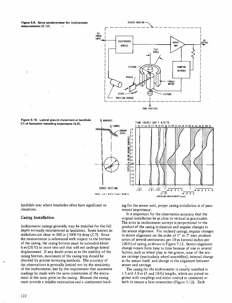
Figure 5.9. Servo accelerometer for inclinometer SEALED HOUSING measurements (5.13).

1 --------------------1

DC POWER

11: [ I F I CS] 1: R " P~0'~1'1

TILT ANGIE

FLEXURE

&LE

OAMPING

PAGO

TOR TORQUE

E

NETWORK

STO PS POSITION SENSOR

_______

-I - - - - - - - - - - — J

TRUE VERTICAL

Figure 5.10. Lateral ground movement at borehole

Cl of bentonite tunneling experiment (5.6). BOREHOLE

CROSS SECTION - PUP UI_jiL LIZ CL • U

Note: 1 m = 3.3 ft; 1 n,,o 0.04 in. -2 01 '4 2 0 2 GROUND MOVEMENT ImmI

landslide area where boreholes often have significant in-clinations.

Casing Installation

Inclinometer casings generally may be installed for the full depth normally encountered in landslides. Some known in-stallations are close to 300 m (1000 ft) deep (5.7). Since the measurement is referenced with respect to the bottom of the casing, the casing bottom must be extended about 6 m (20 ft) or more into soil that will not undergo lateral displacement. If any doubt arises as to the stability of the casing bottom, movement of the casing top should be checked by precise surveying methods. The accuracy of the observations is generally limited not by the sensitivity of the inclinometer, but by the requirement that successive readings be made with the same orientation of the instru-ment at the same point in the casing. Because the casing must provide a reliable orientation and a continuous track-

ing for the sensor unit, proper casing installation is of para-mount importance.

It is important for the observation accuracy that the original installation be as close to vertical as practicable. The error in inclinometer surveys is proportional to the product of the casing inclination and angular changes in the sensor alignment. For inclined casings, angular changes in sensor alignment on the order of 1° to 2° may produce errors of several centimeters per 10 m (several inches per 100 ft) of casing, as shown in Figure 5.11. Sensor-alignment change occurs from time to time because of one or several factors, such as wheel play in the groove, wear of the sen-sor carriage (particularly wheel assemblies), internal change in the sensor itself, and change in the alignment between sensor and carriage.

The casing for the inclinometer is usually installed in 1.5 and 3.0-m (5 and I 0-ft) lengths, which are joined to-gether with couplings and either riveted or cemented or both to ensure a firm connection (Figure 5.12). Each

122

TINE (DAYS) DAY I 4/2/13

3ROUNO 10 LEVEL r'

45 9-6

1-8

Ii

12

13

14

IS

-16

OUTSIDE OF COUPLING

ABS PLASTIC

- GROOVES TO ALIGN - INCLINOMETER SENSOR

coupling represents a possible source of leakage for grout or mud, which can seep into the casing and be deposited along the internal tracking system. For this reason, cou-plings should be sealed with tape or glue. The bottom sec-tion of the casing is closed with an aluminum, plastic, or wooden plug, which also should be sealed. If the drill hole is filled with water or drilling mud, the inclinometer casing must be filled with water to overcome buoyancy. Some-times, extra weight (sand bags, drill stem) may be needed.

The annular space between the boring wall and the in-clinometer casing may be backfilled with sand, pea gravel, or grout. The selection of backfill depends mostly on soil, rock, and groundwater conditions (i.e., whether the bore-hole is dry, wet, caving, stable without mud). The type of drilling technique (e.g., rotary, hollow-stem, cased holes) is also important. Poorly backfilled casings can introduce a scatter in initial measurements, and, if maximum precision is required, great care should be taken in the selection of the proper backfilling material. Grouting is generally pre-ferred, but may not always be possible, particularly in per-vious geologic materials, such as talus. Grouting may be facilitated by use of a 20 to 25-mm (3% to I-in) diameter plastic tube firmly attached to the casing bottom through which grout is pumped from the ground surface until the entire hole is filled. In a small clearance, drill-hole grout can be tremied through drill rods via, a one-way valve at the inside bottom of the casing.

The as-manufactured casing may have some spiral to the

grooves. During installation, the casing can become even more twisted or spiraled so that, at some depth, the casing grooves may not have the same orientation as at the ground surface. Spiraling as great as 18° in a 24-rn (80-ft) plastic casing has been reported (5.24); 1°/3-rn (10-ft) section is not uncommon. Because significant errors in the assumed direction of movement may result, deep inclinometer cas-ings should be checked after installation by using spiral in-dicators available from the inclinometer manufacturer. For a particular installation, groove spiraling is generally a sys-tematic error occurring for each section in the same amount and the same direction. In any event, spiraling, whether it is due to manufacture or to torque of the casing during in-stallation, can be measured and is thus not really an "error" in inclinometer measurement. Spiraling is important only when the true direction of the movement is determined and at that time can and should be measured and the results ad-justed accordingly.

Small irregularities in the tracking surface of the casing can lead to errors in observation, especially if careful repe-tition of the depth to each previous reading is not exer-cised. If plastic casing has been stored in the sun before installation, each section may be locally warped (opposite grooves not parallel) and large measurement errors can oc-cur with minor variations at the depths at which the read-ings are taken (5.23).

Aluminum casings should be used with some caution because severe corrosion may occur if the casing is exposed

Figure 5.11. Measurement error as a result of casing inclination and sensor rotation.

CASING DRIFT In,)

I 2 3

50 ISO I CASING DRIFT (in)

NOTE CASING DRIFT OVER ANY DEPTH INCREMENT IS MEASURED AS HORIZONTAL DEVIATION FROM TRUE VERTICAL AXIS IN TWO MUTUALLY PERPENDICULAR PLANES. DEFLECTION ERROR IN ONE PLANE IS RESULT OF DRIFT IN OTHER PERPENDICULAR PLANE.

Figure 5.12. Details of inclinometer casing.

152 rn,n (6 in)

ALUMINUM CASING ALUMINUM COUPLING

BUTT JOINT AT CASING END

305 ,nm (12 in) ALUMINUM COUPLING

POINT OF CONTACT FOR SETTLEMENT STANDARD PROBE WHEN CASING MAKING SETTLEMENT LENGTHS MEASUREMENTS 1.5 n, IS H)

or3rn(lOft)

ALUMINUM - BOTTOM PLUG

'O.P RIVETS AT END OF COUPLING

0.01

0.06

0.05

0

0.04

00.03 z

0.02

0.0)

11 Jo• 50

15

C AS IN

POP RIVETS AT END OF COUPLING

- ALUMINUM CASING

POP RIVETS AT Y. P0 IN TS

123

to alkaline soil, corrosive groundwater, or grout. Epoxy coatings help to minimize this problem. Burland and Moore (5.11) recommend cleaning the casing with a stiff brush be-fore taking readings. Frequent flushing with water is also helpful. The top of the casing is generally capped with a tight-fitting plug to prevent intrusion of debris. In addition, the inclinometer casing should be protected and padlocked at the ground surface. When selecting protective casing or monument covers for use around the top, one should keep in mind the casing-mounted pulley or similar device.

In-Place memo meters

An inclinometer that remains in place in the borehole to continually monitor displacements normal to the borehole axis at discrete points along the borehole is called an in-place inclinometer. The sensors are permanently posi-tioned at intervals along the borehole axis and may be more closely spaced (to increase resolution of the displace-ment profile) in zones of expected movement. Total movements are determined by summing the relative move-ments measured at each sensor along the borehole. Since fixed units consist of a number of sensors, they are more expensive and complex than portable inclinometers.

The major advantage of the fixed borehole inclinometer over the portable unit is the elimination of problems of tracking inaccuracies and repeatable positioning. If the fixed unit is removed for repairs, the overall accuracy will be reduced to that of a portable unit or less. Also,acceler-ometers may have long-term drift. With portable units, these and other effects are canceled by taking readings in oppo-site directions. Fixed units can be monitored remotely or connected to alarm systems, which are additional advan-tages. In some systems, a standard grooved inclinometer casing is used so that a portable inclinometer can be used to check readings of the fixed system.

Because of its accuracy, the fixed borehole inclinometer may be used to measure small movements in rock. Its adapt-ability to various remote-monitoring systems allows for a continuous record of displacement. As designed, most sys-tems are not intended to obtain a continuous profile of de-formation. Rather, they measure critical movements of a few sections within the borehole inclinometer. This instru-ment, therefore, is not necessarily a replacement for the portable units, but rather has its own purpose and is worthy of consideration for continuous monitoring of movements during critical construction stages.

A recently developed in-place inclinometer (Figure 5.13) employs a series of servo-accelerometer sensors; it is available with both one- and two-axis sensors (5.13). The sealed accelerometer packages are spaced along stan-dard grooved inclinometer casing by a series of rods. The rods and sensors are linked by universal joints so that they can deflect freely as the soil and the casing move. The sen-sors are aligned and secured in the casing by spring-loaded fins or wheels, which fit the casing grooves. Use of the grooved casing and guide wheels allows removal of the in-strument for maintenance, adjustments, and salvage. Since the casing is standard inclinometer casing, portable inch-nometers can be used in the casing when the fixed instru-ment is removed.

Readings are obtained by determining the change in tilt

Figure 5.13. Installation and detail of multiposition in-place inclinometer.

8.4mm (3.34 in) O.D. ABS PLASTIC INCLINOMETER CASING JUNCTION

Box

ij

00 FIXED SPRING WHEEL ''-/il- LOADED ,

WHEEL

TOP ANCHOR . S; (DUMMY HOUSING);,

WIRING TO ELECTRICAL—. J TRUE :. HARNESS

: ...,

SPRING .: SENSOR LOADED ; II HOUSING WHEEL

SENSOR -• .1

GAUGE . LENGTH 0 0 0 (ADJUSTABLE

I. UPON .- INSTALLATION) S..'

UNIVERSAL . .. JOINT

-- SENSOR

TUBE 4' ASSEMBLIE

MIN 115-mm (4.5-in) .. BORING

PORTLAND CEMENT / GROUT BACKFILL— ,.

GROOVED PLASTIC CASING ', ''I

6:11

CAST IN PLACE OR GROUTEDIN PLACE IN BOREHOLE.'.: t1' I

of the accelerometer and multiplying by the gauge length or spacing between sensors. This gives the relative displace-ment of each sensor, and these relative displacements can be summed to determine the total displacement at each sensor. Since the grooves in the casing may spiral, the spiral should be checked after the casing is installed so that the exact direction of displacement measurement is known. Any number of sensors at any spacing can be used in one borehole. Maximum deflection range is ±300, and sensitiv-ity is reported to be ± 0.01 mm in I m (± 0.001 in in 10 ft), but this is not usually attained because of long-term drift. Monitor and alarm consoles and telemetry systems are available.

EXTENSOMETERS AND STRAIN METERS

Extensometers and strain meters measure the increase or

124

decrease in the length of a wire or rod connecting two points that are anchored to the soil in the borehole and whose distance apart is approximately known. One com-mercially available device is shown in Figure 5.14. When gauge lengths are on the order of a rneteror less, these de-vices are often referred to as strain meters rather than as extensometers. When they are used as extensometers, the accuracy and repeatability depend on the type of sensing element and its range of travel and also on the type of con-necing wire or rod and the methods used to control the tension. Dead weights are best for maintaining constant tension in wires; if these cannot be used, constant tension springs are acceptable, although there may be some hyster-esis. Relatively inexpensive wire-wound or conducting plas-tic linear potentiometers are often used as sensors, and rel-atively simple, battery-operated Wheatstone bridge cir-cuits are used for manual readout. Sensitivity is on the order of 0.1 percent of the range of travel, but repeatabil-ity and accuracy may be no better than 0.5 mm (0.02 in), depending on the type of anchor and connecting member; this is usually sufficient, however.

When the devices are used as strain meters, the repeat-ability and accuracy are essentially the same as the sensi-tivity. Thus, for a grouted-in-place assembly 3 in (10 It) long with an invar rod and a range of 25 mm (1 in), unit strains as low as 0.000 01 may be detected with relatively inexpensive instrumentation. Horizontal stretching of em-bankments has been observed by installing anchors at vari-ous positions at a given elevation and attaching horizontal wires to dead weights on the downstream lace; this was done at Oroville Dam (5.55). Care is required to ensure that the wires (or rods) do not get pinched off if localized vertical shear movements occur. Other cases of application are'described by Dutro and Dickinson (5.19) and Heinz (5.26).

PORE-PRESSURE AND GROUNDWATER MEASUREMENTS

Observation Well

The most common water-level recording technique, despite more sophisticated methods, is the observation of the water level in an uncased borehole or observation well. A particu-lar disadvantage of this system is that a perched water table or artesian pressure can occur in specific strata that may

be interconnected by the borehole so that the recorded water level may be of little significance.

Piezometers

Pore pressures and groundwater levels in a slide area can be measured by a variety of commercially available piezom-eters (5.25). The selection of the best type for a particular installation involves several considerations.

Piezometers are usually installed in a difficult en-vironment and may become inoperative because of pinch-ing off of the tubes, blockage by air bubbles, electrical short circuits, and malfunctions of buried moving parts. Therefore, reliability and durability are often of greater importance than sensitivity and precision. For example, in some cases it does not matter that the actual head may be in error by 0.3 in (1 ft) or so as a result of time lag, provided the piezometer is functioning properly. If a mal-function occurs, the fact that the apparent head can be re-corded to a millimeter is of little importance.

The basic problem with a piezometer is that the en-ergy required to operate it prevents the instrument from recording a pore-pressure change immediately. For a given pressure change, this energy is proportional to the volume of pore water that must flow into the instrument. A pi-ezometer with an open standpipe, for example, requires a much greater volume of water than one with a stiff dia-phragm and therefore requires a correspondingly greater time to respond to a change of pore pressure. Hvorslev (5.27) discusses time-lag effects for open-standpipe piezom-eters; Brooker and Lindberg (5.10) evaluated these effects for closed types; and Penman (5.39) and Vaughan (5.52) studied the response times of various types of piezometers. In slides in which piezometers are placed in boreholes, it is usually possible to provide a large collecting volume of porous material (sand) around the tip and thus to reduce the time lag in open standpipes.

Partially saturated soils (fills, soils above the water table, and soils in which gas is generated from organic mat-ter) pose particular problems because the gas in the voids exists at'higherpressures than the water as a result of sur-face tension (capillarity). Thus, one must know whether the piezometer is reading the pore-air pressure or the pore-water pressure. To prevent the entry of air into the pi-ezometer tip and thus to ensure that pore-water pressure

Figure 5.14. Extensometer. ROTARY POTENTIOMETER CONNECTED TO PULLEY

\ - CONSTANT TENSION SPRING

FLANGED PIPE r

13.mm (0.5-in) GROUT TUBES7 2.5.mm (1-in) TUBING

PLASTIC PLUG 1_- ANCHOR ASSEMBLY

WIRES

EXTENSOMETER

TO REMOTE READOUT

125

is being measured, fine ceramic tips, with high air-entry values, can be used (5.2). Even with a high air-entry value filter, air will slowly enter the piezometer cavity by diffu-sion and, if reliable long-term readings are required, deair-ing facilities must be provided (5.52).

4. Additional problems resulting from diffusion of either air or water vapor through the walls of connecting tubing are described by Bishop, Kennard, and Penman (5.2). Furthermore, either settlement or horizontal movement may pinch off the connecting tubing or, in the case of open standpipes, may prevent the lowering of a probe to detect the water level.

Figure 5.15. Open-standpipe

piezometer.

SCREW CAP OR WOODEN PLUG

CEMENT/SAND OR BENTONITE BACKFILL

5cr,, DIAMETER STANDPIPE /

The features and uses of various types of piezometers are discussed below.

Open Standpipe

Open-standpipe piezometers vary mainly in diameter of standpipe and type and volume of collecting chamber. The simplest type (Figure 5.15) is merely a cased or open obser-vation well in which the elevation to which the water rises is measured directly by means of a small probe. In this case, the static head is the average head that exists over the depth of the inflow part of the well below the water table. This measured head may be higher or lower than the free water table and, in the case of moderately impervious soils, may be subject to a large time lag. Although the open standpipe is not satisfactory in impervious soils because of time lag or in partially saturated soils because the signifi-cance of the measured head may be difficult to evaluate, its simplicity, ruggedness, and overall reliability dictate its use in many installations.

Casagrande

The Casagrande type of piezometer (Figure 5.16) consists of a porous stone tip embedded in sand in a sealed-off por-tion of a boring and connected with a 1-cm (3/8 -in) diam-eter plastic riser tube (5.45). When properly installed, this type of piezometer has proved successful for many materials, particularly in the long term, for it is self-deairing and its nonmetallic construction is corrosion resistant. The reliability of unproven piezometers is usually evaluated on the basis of how well the results agree with those of adja-cent Casagrande piezometers.

Pneumatic

The pneumatic piezometer consists of a sealed tip contain-ing a pressure-sensitive valve. The valve opens or closes the connection between two tubes that lead to the surface, or the slope face, at any convenient location and elevation. In the piezometer shown in Figure 5.17, flow of air through the outlet tube is established as soon as the inlet-tube pres-sure equals the pore-water pressure. In the hydraulic pi-ezometer (Figure 5.18), hydraulic fluid is used instead of gas, but the basic principle remains the same. Pneumatic piezometers have the following advantages: (a) negligible time lag because of the small volume change required to operate the valve, (b) simplicity of operation, (c) capabil-ity of purging the lines, (d) minimum interference with

SAND OR SAND AND GRAVEL BACKFILL

PERFORATEd I. SECTION OF PIPE APPROX. ln,LONG

0.3. :..t Note: 1 n, = 3.31t; 1cm0.4in.

Figure 5.16. Casagrande

borehole piezometer.

10.,,,,,,

PLAST I

TUBING

I m BENTONITE SEAL

30 cm

30 Cm •. . POROUS TUBE 38-rn,,, O.D.

30 cm SAND FILTER

Note: it,, = 3.3 It; Icot = 0.4 in;

5 cm lnrmO.O4in.

construction, and (e) long-term stability. Their main dis-advantage is the absence of a deairing facility.

Electric

Electric piezometers have a diaphragm that is deflected by the pore pressure against one face. The deflection of the diaphragm is proportional to the pressure and is mea-sured by means of various electric transducers. A typical design is shown in Figure 5.19. Such devices have negligi-

BACKFILL

126

NYLON TUBING

E E

Note: 1 mm = 0.04 in.

Figure 5.17. Pneumatic piezometer. (a) PORTABLE PORE-PRESSURE INDICATOR

- CHECK VENT - SUPPLY PRESSURE SUPPLY PRESSURE FILTER VALVE VALVE COUPLING

p - TRANSDUCER INPUT

COUPLING

TRANSDUCER OUTPUT SUPPLY PRESSURE COUPLING -

OUTPUT PRESSURE GAUGE

GAUGE

- -

(b) PORE-PRESSURE TRANSDUCER

300mm(l2 in) -'

ELECTRICAL

RESIN

PVC SLEE;

INSULATIN 7 TSKET7 [TPTRAG. 1! 3.8mm 11.5 in)

Dia.

PVC JACKETJ 3mm (O.125in)/ BALL '—STAINLESS POLYI NYLON - TUBING CHECK STEEL PWG

VALVE BODY

Figure 5.18. Hydraulic piezometer. Figure 5.19. Electric piezometer.

ble time lag and are extremely sensitive. Piezometers of this type are described by Shannon, Wilson, and Meese (5.45), Cooling (5.12), Brooker and Lindberg (5.10), Pen-man (5.39), Bishop, Kennard, and Vaughan (5.3), and Hanna (5.25). Because they are affected by the environ-ment and have poor long-term stability, electric piezom-eters are not generally recommended for installations in which reliable readings are required during an extended peridd of time. Generally, they cannot be deaired nor can the sensitive electric transducers be recalibrated in situ, although there are exceptions (5.16). For short-term observations at installations in which transmission is over limited distances, standard resistance strain-gauge pressure transducers are suitable. A new type of electric piezom-eter, using a pressure-sensitive crystal, has been developed, but its long-term stability has not yet been verified.

Piezometer Sealing

Piezometers in landslides can be installed in boreholes ad-vanced into soil or rock. Based on the drill log of mate-rials encountered and the estimated position of the water table and of the sliding surface, the depth of each piezom-eter is selected. A simple open-standpipe piezometer de-

ECTR DNA ONE IS

(ORATING JIRE

ENSING TUBE

I APORAGN

OROUS STONE FILTER

TEEL CONICAL TIP

mm - 0.04 in.

127

vice consists of a tube placed in the drilled hole extending to the ground surface. The bottom of the tube should be slotted or made of a porous material or a sufficiently fine screen that it will restrict movement of soil into the piezom-eter but at the same time permit free access of water. Only that part of the tube that is actually within the stratum in question should be pervious. When the tube is centered in the drilled hole, a known volume of clean sand is placed around the piezometer; the purpose is to create a sand fil-ter between the soil and the piezometer tip.

Construction of an impervious barrier above the piezom-eter tip and sand pocket is essential. A well-established procedure is to drop balls of soft bentonite into the hole and then tamp those balls around the piezometer tubes by using an annular hammer. Prepared bentonite in ball or pellet form is now available commercially; it has a specific gravity that is sufficiently large to allow it to sink through the water in the piezometer hole so that a hammer is not necessary. Alternatively, a cement-bentonite grout can be tremied into the hole above the sand filter. Such a seal can be pumped through a 1.3 to 1.9-cm (½ to 3/4-in) diam-eter pipe adjacent to the piezometer tube. Installing only one, or at most two, piezometers in a borehole has gener-ally been found preferable because bentonite seals are sometimes difficult to construct and may leak slightly de-spite precautions. However, special-purpose, multiple-point piezometers (with four tips) have been used success-fully by Vaughan (5.51) and merit consideration.

Both pneumatic and electric piezometers can be sealed in a similar manner to an open-standpipe or a Casagrande piezometer in a borehole. Since the piezometer tip cannot be deaired after installation, it should be soaked in deaired water beforehand and kept in the water until it is lowered into the borehole. A low air-entry filter tip can be placed in a saturated sand pocket, but a high air-entry tip should be pushed into the soil beyond the base of the hole or sur-rounded by a porous grout, such as plaster of paris. This will ensure more rapid equalization, which may be of con-siderable value in obtaining reliable pore-pressure measure-ments soon after installation in low-permeability clay. Both electric and pneumatic piezometers should be checked for malfunction before and during installation, and particular care is needed in driving electric piezometers to prevent overpressure.

In soft and medium-stiff soils, it may be preferable to push the piezometer directly into the ground. Flush-coupled heavy steel water pipe will be required, and the piezometer tip must be robust enough to resist damage to the well point and should be designed to minimize distur-bance around the tip (5.34). It may be of the Casagrande, pneumatic, or, less commonly, electric type. This drive-in piezometer is self-sealing and rapidly installed and, if pneu-matic, has a rapid response. Recently, an improved method of sealing piezometers in boreholes was described by Vaughan (5.51). Instead of compacting bentonite balls just above the sand filter, the borehole is completely grouted with cement-bentonite grout. Even if the perme-ability of the grout is significantly higher than that of the surrounding soil, little error will result because of the rela-tively large grouted length. In many cases, a sand filter need not be included, and the piezometer tip can be grouted directly with little error.

SYSTEMS FOR MONITORING ROCK NOISE

Use of the rock-noise detection method for observing the stability of soil and rock materials is a relatively new con-cept, and most practical applications so far have been in mines (5.4, 5.5, 5.30, 5.60). More work has been done in basic research than in practical application of the technique, although sufficient laboratory and field tests have been per-formed to demonstrate the importance and usefulness of the method. The ability to detect the occurrence of dis-tress in a rock mass before the development of measurable movement is obviously a significant technological advance. Experimental work that has led to the development of techniques and instrumentation for measuring microacous-tic, microseismic, or subaudible rock noise has been car-ried on in the United States since the early 1940s (5.5). All of this work, regardless of terminology, has been re-lated to measuring transient noise disturbances in earth (soil and rock) materials for the purpose of establishing the relative stability and, in some instances, locating zones of weakness in earth materials (5.29, 5.31, 5.42, 5.60). In the mid-l960s, Goodman, Blake, and others (5.4, 5.22, 5.31)adapted the techniques developed by the U.S. Bureau of Mines to civil engineering applications and the study of soil and rock slides. Particular emphasis was placed on the determination of relative stability, location of failure planes, determination of the epicentral location of specific distur-bances, and improvement of field equipment. Rock-noise detection systems can be divided into three basic elements: sensors, signal-conditioning equipment, and recording and data-acquisition equipment.

Sensors

The frequency response of the sensors is a critical design parameter. Rock noise is reported to occur over a broad range of frequencies between about 50 and 10 000 Hz (5.4); however, disturbances at lower frequencies (20 to 40 Hz) have been observed at Downie slide, British Colum-bia, and are believed to be important. The occurrence of rock noise at frequencies above 10 kHz has been observed in the laboratory when rock specimens are placed under high compressive loads (5.30). Because the frequency range of noise phenomena at a particular site is unknown, the frequency response of the sensors must be sufficiently broad to ensure that the system will respond properly to any meaningful noises that occur. In addition, the sensors must be capable of (a) producing a high-level signal that is proportional to the amplitude and frequency of the excit-ing noise and is without spurious response and (b) transmit-ting the signal through long electric cables. For this rea-son, the output impedance of the sensor must be relatively low to prevent the cable from acting as an antenna that could pick up radio, television, and ignition interference.

Signal-Conditioning Equipment

Signal-conditioning equipment includes amplifiers and fil-ters for the enhancement of the rock-noise signals and re-jection of unwanted noise or interference. It also includes the alteration of the received signal to whatever form is re-

128

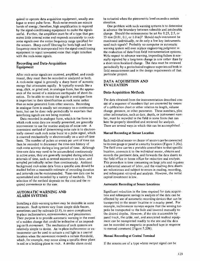
quired to operate data acquisition equipment, usually ana-logue or event pulse form. Rock-noise events are minute bursts of energy; therefore, high amplification is required by the signal-conditioning equipment to make the signals useful. Further, the amplifiers must be of a type that gen-erates little internal noise and responds accurately to rock-noise signals over the entire frequency range specified for the sensors. Sharp cutoff filtering for both high and low frequency must be incorporated into the signal-conditioning equipment to reject unwanted noise that might interfere with the rock-noise signals.

Recording and Data-Acquisition Equipment

After rock-noise signals are received, amplified, and condi-tioned, they must then be recorded or analyzed or both. A rock-noise signal is generally a sharp burst of acoustic energy that attenuates rapidly. It typically sounds like a snap, click, or grind and, in analogue form, has the appear-ance of the record of a miniature earthquake of short du-ration. To be able to record the signals in analogue form is important in their identification as rock noise rather than as noise generated from other sources. Recording in analogue form is usually not necessary on a continuous basis, but can be done only periodically to ascertain that interfering signals are not being received.

Data recorded in analogue form, which is the form in which rock noise data are usually presented, are generally inconvenient to use for routine analysis of noise rate. A convenient method of determining noise rate is to electron-ically convert each rock noise burst to a pulse signal, which is counted mechanically or electronically on a unit-of-time basis. The number of pulses or events per unit of time can then be recorded to document the time-rate history of rock-noise activity during a long period of time. Although time-rate data may need to be accumulated continuously in active areas, they are generally sampled during selected intervals of time, such as several minutes or an hour, and sampled periodically rather than continuously. Ambient background rock-noise data from a specific area should be studied before a reasonable estimate of recording duration and intervals can be recommended. Time-rate data can be accumulated and recorded by a variety of methods. The selection of the method depends on the cost and the re-quired convenience to the user.

AUTOMATIC WARNING AND ALARM SYSTEMS

Installing a slide-warning system may be desirable in some instances. Such systems vary from simple slide fences, sometimes used by railroads (5.9), to more complicated in-place inclinometers, extensometers, and piezometers. Their purpose is to provide automatic warning in the event of a sudden change that could be indicative of an impend-ing earth movement. The mechanics of such systems are relatively simple to devise. An in-place inclinometer or ex-tensometer can be used to actuate a red light in a central location when the movement exceeds a certain threshold, which, for example, may occur along a specific shear plane in soil or a bedding plane in rock. A similar alarm could

be actuated when the piezometric level exceeds a certain elevation.

One problem with such warning systems is to determine in advance the boundary between tolerable and intolerable change. Should the extensometer be set for 0.25, 2.5, or 25 mm (0.01,0.1, or 1.0 in)? Should each instrument be monitored individually, or do only a few key instruments need such signals? Probably no computer or automatic warning system will ever replace engineering judgment in the evaluation of data from field instrumentation systems. With respect to advance warning, impending failure is nor-mally signaled by a long-term change in rate rather than by a short-term localized change. The data must be reviewed periodically by a geotechnical engineer experienced both in field measurements and in the design requirements of that particular project.

DATA ACQUISITION AND EVALUATION

Data-Acquisition Methods

The data obtained from the instrumentation described con-sist of a sequence of numbers that are converted by means of a calibration chart or other relation to length, volume change, pressure, or other parameter. These numbers, plus other information, such as date, depth, or instrument num-ber, must be recorded in the field in some form that can later be properly identified and retrieved for analysis. There are several ways in which this can be accomplished.

Manual Recording at Sensor Location

Each individual sensor or cluster of sensors can be connected to its own gauge or panel at a nearby location (Figure 5.20a). The field crew carries a portable control bOx to that specific location, connects it to the individual sensor, obtains and records the pertinent data, and forwards the data sheets to the field office or home office for reduction and analysis. This procedure is time consuming on large jobs and requires a substantial amount of labor, and the resulting data sheets are voluminous and subject to errors in reading, recording, and subsequent retrieval and analysis. However, the initial capital investment is low.

Automatic Recording at Sensor Locations

Significant reduction in the time required for data acquisi-tion and subsequent savings in analysis of the data can be effected by use of automatic recording devices that can be transported to the sensor location or a nearby panel. For example, inclinometer surveys require that the sensing tor-pedo be transported to the hole and lowered manually to the desired depths. However, if the site is accessible by panel truck, the cable, reel, and associated readout equip-ment can be transported readily to the site and the data can be recorded on magnetic or punched tape in response to manual command (Figure 5.20b).

Manual Recording at Central Terminal

If the sensors are of a type whose output signal can be

129

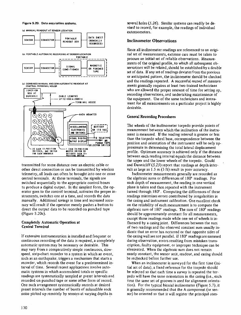
Figure 5.20. Data acquisition systems.

MANUAL READOUT AT SENSOR LOCATION

E~_ READOUT BOX (MANUALLY I

DATA SHEET I RECORDED)

PORTABLE AUTOMATIC RECORDING AT SENSOR LOCATION

PORTABLE

C OHN(CT OR FIA G E T

I C

Ic) COMBINED MANUAL AND SEMIAUTOMATIC READOUT AT CENTRAL TERMINAL HOUSE

I JUNCTION I oo AT

BOREH CABLE LENGTHS UPTO1000I30OOItI

.—TERMINAL HOUSE

RACK MOUNTED

LLAHEOU1Ir ELECTRONICS 110 VAC R SIITCHES -

SUAL OIGITALIt'TOTEL(TYP DISPLA.

PUNCM TAAR

P SELECTOR SIITC

20 EACH12-PQUITIOH '-----I EACH 24-POSITION SNITCIIES. DIE SNITCH BUYER IMITCI TH FOR EACH BOBUROL( ACTIVATE (ACM 2-

transmitted for some distance over an electric cable or other direct connection or can be transmitted by wireless telemetry, all leads can often be brought into one or more central terminals. At those terminals, the signals are switched sequentially to the appropriate control boxes to produce a digital output. In the simplest form, the op-erator goes to the control terminal, activates the proper in-struments, switches one at a time, and records the data manually. Additional savings in time and increased accu-racy will result if the operator merely pushes a button to direct the output data to be recorded on punched tape (Figure 5.20c).

Completely Automatic Operation at Central Terminal

If extensive instrumentation is installed and frequent or continuous recording of the data is required, a completely automatic system may be necessary or desirable. This may vary from a comparatively simple continuous, slow-speed, strip-chart recorder to a system in which an event, such as an earthquake, triggers a mechanism that starts a recorder, which records the event for a predetermined in-terval of time. Several recent applications involve auto-matic systems in which accumulated totals or specific readings are systematically sampled at preset intervals and recorded on punched tape or some other form of record. One such arrangement systematically records at desired preset intervals the number of bursts of subaudible rock noise picked up remotely by sensors at varying depths in

several holes (5.26). Similar systems can readily be de-vised to record, for example, the readings of individual extensometers.

Inclinometer Observations

Since all inclinometer readings are referenced to an origi-nal set of measurements, extreme care must be taken to procure an initial set of reliable observations. Measure-ments of the original profile, to which all subsequent ob-servations will be related, should be established by a double set of data. If any set of readings deviates from the previous or anticipated pattern, the inclinometer should be checked and the readings repeated. A successful record of measure-ments generally requires at least two trained technicians who are allowed the proper amount of time for setting up, recording observations, and undertaking maintenance of the equipment. Use of the same technicians and instru-ment for all measurements on a particular project is highly desirable.

General Recording Procedures

The wheels of the inclinometer torpedo provide points of measurement between which the inclination of the instru-ment is measured. If the reading interval is greater or less than the torpedo wheel base, correspondence between the position and orientation of the instrument will be only ap-proximate in determining the total lateral displacement profile. Optimum accuracy is achieved only if the distance between each reading interval equals the distance between the upper and the lower wheels of the torpedo. Gould and Dunnicliff (5.23) report that readings at depth inter-vals as large as 1.5 m (5 ft) result in poor accuracy.

Inclinometer measurements generally are recorded as the algebraic sums or differences of 180° readings. For each depth of measurement, the reading in one vertical plane is taken and then repeated with the instrument turned through 180°. Computing the differences of these readings minimizes errors contributed by irregularities in the casing and instrument calibration. One excellent check on the reliability of each measurement is to compute the algebraic sum of 180° readings. The sum of 180° readings should be approximately constant for all measurements, except those readings made while one set of wheels is in-fluenced by a casing joint. Differences between the sum of two readings and the observed constant sum usually in-dicate that an error has occurred or that opposite sides of the casing wall are not parallel. If 180° readings are summed during observation, errors resulting from mistaken trans-cription, faulty equipment, or improper technique can be eliminated. When the algebraic sum does not remain nearly constant, the sensor unit, readout, and casing should be rechecked before further use.

When an inclinometer is surveyed for the first time (ini-tial set of data), a fixed reference for the torpedo should be selected so that each time a survey is repeated the tor-pedo will have the same orientation in the casing (i.e., each time the same set of grooves is used for alignment orienta-tion). For the typical biaxial inclinometer (Figure 5.7), it is generally recommended that the A-component (or sen-sor) be oriented so that it will register the principal com-

130

ponent of the anticipated deformation as a positive change For example, in an area suspected of landslide activity, the first set of readings is taken by orienting the fixed wheels of the torpedo in the casing groove closest to the downhill position. For a complete survey, the torpedo is reversed 1800 after the first set and the readings are repeated. The algebraic difference of the two sets of readings is used to compute the profile of the casing or, more important, to determine any change compared to other surveys; using the algebraic difference is, in effect, the same as using the average of the two sets of readings.

Maintenance

Inclinometers are specialty items; consequently, the num-ber of suppliers is limited. Repair or replacement of an in-clinometer can be expensive and time-consuming and re-sult in loss of important data. The best insurance against damage is careful use and systematic maintenance. The sensor unit should be checked frequently during operation and its wheel fixtures and bearings tightened and replaced as necessary. After each casing has been read, the guide wheels should be cleaned and oiled. Most important, the electric readout should be protected against water at all times. The introduction of a few drops of water into the readout circuitry can cause the galvanometer to drift in a pendulum inclinometer or can induce a drift of numbers on the digital voltage display in an accelerometer instru-ment. If readings are made too rapidly or if an automatic recorder is used, this drift may not be detected and errone ous measurements may result. When the data are analyzed at a later time, the unexpected results cannot be related to the cause.

Inclinometer Data Reduction

Hand reduction of inclinometer data is a tedious and time-consuming operation. A single movement profile for a 33-m (100-ft) casing can involve more than 200 separate com-putations. Because of the amount of effort involved in taking readings and, subsequently, in computing displace-ments, a successful measurement program depends primar-ily on organization and discipline. Field readings must be transposed to discernible measurement, preferably in the form of summary plots indicating successive movement pro-files, as soon as possible after the field observation. This also provides perhaps the best check of instrument reliabil-ity. If a record of successive movement profiles is estab-lished, the consistency of new measurements can be refer-enced to previous readings and judged in light of anticipated soil behavior. Because of occasional error in the accumula-tion of field readings, the data reduction for a particular casing must be performed with a knowledge of both former movement and expected soil behavior. Excessively large 180° sums, which occur without precedence and are not explainable, should be discarded or the readings should be repeated.

Recording the data manually is adequate for many proj-ects of small and intermediate size. A special form of data sheet is used and is turned over to operators who transcribe the data into computer language. Once this is done, the punched cards or tape can be handled by the computer

Figure 5.21. Sample field data sheet for transcribing inclinometer data to punched cards.

INCLINOMETER FIELD DATA

I 2 3 4 5 6 1 8 9 IC 1112 13 II 151611 1619 2021 22 2324252621782030

I i Ri i 1E ii1•i 1' ,A1v1,i 1C11•1 1. JOB TITLE

i ,s-'ti i

2.108 NUMBER 3. HOLE NO. 4.SET NO. 5. DATE 6.1 I ME

I0II9IIIIqI1,4eIoI.IIII6I.!I III II

1. INS. 8.60. READ 9.REV. IA. 6—SCALE 11.0—SCALE 12. 0 03. Be

120,01 01 01. I i I - I 21 I 'ti 14.1 85. CONST . IS. 016. A. 16. DIR. A— II. DIR. 8, 16. DIR. 8—

. I

iuuiiuiniirrnii 0 nuIiii all rulllIIr1lilflI Illona

uuullluInIu•!ul•:n1uul•r

with any desired degree of sophistication. One must real-ize, however, that, in addition to the time delay (perhaps only a day or so), there are two potential sources of error: The first is in recording the data manually, and the second is in transcribing the data from digital form to punched card. Figure 5.21 shows a portion of a special field data sheet used for recording inclinometer data, which are to be subsequently transcribed onto punched cards.

Sources of error in recording and transcribing can be re-duced by automatic printout directly onto punched tape or magnetic tape. Provided the recordings are without ex-traneous data, these tapes can then be returned to the office and fed directly into the computer, which plots the move-ment. An example of this application is shown in Figure 5.22 for an inclinometer survey. The printed output from the computer is obtained within a few hours after the data are taken. In the case of a central terminal unit with auto-matic printout, the end result is the same; the only differ-ence is in the ease and speed of operation. The computer. programs vary from those that simply reduce data and pro-vide a digital printout of results to extremely sophisticated programs that reduce the data, compare the results with initial readings, plot the changes, and compare those changes with previous changes.

Many inclinometer systems, particularly servo-accelerometer types, can be adapted to automatic data re-cording for computerized data processing. Inclinometer manufacturers produce different systems that use punched paper tape, dual image tape, or magnetic tape for data re-cording. The inclinometer control boxes are modified to contain keys for recording the inclinometer well number and depth and an automatic switch to transfer the reading directly to the data tape. Automatic data recording and

131

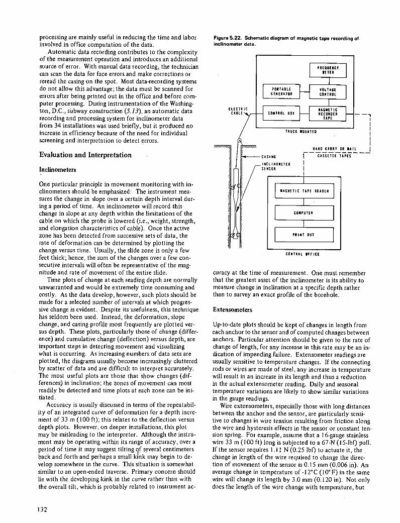
processing are mainly useful in reducing the time and labor involved in office computation of the data.

Automatic data recording contributes to the complexity of the measurement operation and introduces an additional source of error. With manual data recording, the technician can scan the data for face errors and make corrections or reread the.casing on the spot. Most data-recording systems do not allow this advantage; the data must be scanned for errors after being printed out in the office and before com-puter processing. During instrumentation of the Washing-ton, D.C., subway construction (5.13), an automatic data recording and processing system for inclinometer data from 34 installations was used briefly, but it produced no increase in efficiency because of the need for individual screening and interpretation to detect errors.

Evaluation and Interpretation

Indlinometers

One particular principle in movement monitoring with in-dinometers should be emphasized: The instrument mea-sures the change in slope over a certain depth interval dur-ing a period of time. An inclinometer will record this change in slope at any depth within the limitations of the cable on which the probe is lowered (i.e., weight, strength, and elongation characteristics of cable). Once the active zone has been detected from successive sets of data, the rate of deformation can be determined by plotting the change versus time. Usually, the slide zone is only a few feet thick; hence, the sum of the changes over a few con-secutive intervals will often be representative of the mag-nitude and rate of movement of the entire slide.

Time plots of change at each reading depth are normally unwarranted and would be extremely time consuming and costly. As the data develop, however, such plots should be made for a selected number of intervals at which progres-sive change is evident. Despite its usefulness, this technique has seldom been used. Instead, the deformation, slope change, and casing profile most frequently are plotted ver-sus depth. These plots, particularly those of change (differ. ence) and cumulative change (deflection) versus depth, are important steps in detecting movement and visualizing what is occurring. As increasing numbers of data sets are plotted, the diagrams usually become increasingly cluttered by scatter of data and are difficult to interpret accurately. The most useful plots are those that show changes (dif-ferences) in inclination; the zones of movement can most readily be detected and time plots at each zone can be ini-tiated.

Accuracy is usually discussed in terms of the repeatabil-ity of an integrated curve of deformation for a depth incre-ment of 33 m (100 ft); this relates to the deflection versus depth plots. However, on deeper installations, this plot may be misleading to the interpreter. Although the instru-ment may be operating within its range of accuracy, over a period of time it may suggest tilting of several centimeters back and forth and perhaps a small kink may begin to de-velop somewhere in the curve. This situation is somewhat similar to an open-ended traverse. Primary concern should he with the developing kink in the curve rather than with the overall tilt, which is probably related to instrument ac-

Figure 5.22. Schematic diagram of magnetic tape recording of inclinometer data.

FREIDUENCY II TEN

PORTABLE VOLTAGE GENERATOR H CONTROL

ELT CRECORDER CONTROL BOO

NAGNETIC _.,

TAPE

TRUCK bUNTED

/ ASING

NCLINOMETER

I

HAND CARRY OR NAIL

ENSOR

IAGNET IC TAPE READER

COMPUTER

PRINT OUT

CENTRAL OFFICE

curacy at the time of measurement. One must remember that the greatest asset of the inclinometer is its ability to measure change in inclination at a specific depth rather than to survey an exact.profile of the borehole.

Extensometers

Up-to-date plots should be kept of changes in length from each anchor to the sensor and of computed changes betweeii anchors. Particular attention should be given to the rate of change of length, for any increase in this rate may be an in-dication of impending failure. Extensometer readings are usually sensitive to temperature changes. If the connecting rods or wires are made of steel, any increase in temperature will result in an increase in its length and thus a reduction in the actual extensometer reading. Daily and seasonal temperature variations are likely to show similar variations in the gauge readings.

Wire extensometers, especially those with long distances between the anchor and the sensor, are particularly sensi-tive to changes in wire tension resulting from friction along the wire and hysteresis effects in the sensor or constant ten-sion spring. For example, assume that a 16-gauge stainless wire 33 in (100 ft) long is subjected to a 67-N (15-lbf) pull. If the sensor requires 1.11 N (0.25 lbf) to actuate it, the change in length of the wire required to change the direc-tion of movement of the sensor is 0.15 mm (0.006 in). An average change in temperature of -12°C (10° F) in the same wire will change its length by 3.0 mm (0.120 in). Not only does the length of the wire change with temperature, but

132

Figure 5.23. Geologic profile and inclinometer observations

at failure plane of landslide on 1-94, Minneapolis (5.57).

249

244-

iLINES70NE

0

243-Ls

__1

SEAN Ls NEASUREO

242_

POINTS

- ft

LINESTONE(Ls)

241 __' 8ENTONIT(

SEAl 0 10 20 3Q ' DEFLECTION torn)

Note: 1 to - 3.3 It; 1 tore = 0.04 in.

Figure 5.24. Section showing failure plane and movement distribution of landslide on 1-94 (5.57).

710] 212 0 212 E 2p—

_'_

$6 216

760 - NIILGA

GLACIAL DRIFT

() 250. 11101 SNALE 11111 LIut.1T

. ._._•_• _.

IN

STRING(R FAILURE SURFACE _._. _. _

JAR lION

18mm Note: 1 n, 3.31t; 1 roe,- 0.04 in

the ground itself will expand and contract as its temperature varies. At a hillside stability project in Montana, rock out-crops were found to expand and contract seasonally by as much as 1.5 mm (0.06 in). Electric lead wires also change their electric resistance with temperature and will cause erroneous readings unless such a change is properly taken into account.

Piezometers

Piezometric heads should be plotted on time graphs show-ing rainfall and other data that may influence the pore pres-sure. If drainage has been installed, the quantity of seepage should also be recorded and plotted. If possible, the re-sponse of each piezometer should be checked periodically to determine its recovery rate.

EXAMPLES

This section briefly describes several projects that were suc-cessfully instrumented to measure pore pressures and to detect the depth and rate of movement before corrective treatment was designed. The emphasis is on selection of instrumentation and analysis of data rather than on correc-tive treatment.

Minneapolis Freeway

In 1967, a landslide developed along a 335-rn (1 100-ft) sec-tion of 1-94 on the east side of Minneapolis (5.56, 5.57). The movements were evidenced by upheaval of the sub-grade and by cracking and slumping of the cut slope. Al-though the area had been investigated before construction, no instability problems had been anticipated. Therefore, determining the depth of movement was necessary before investigating the cause of the movements could begin. Fif-teen borings were drilled to serve the dual purpose of pro-viding subsurface soil information and holes for the instal-lation of field instrumentation. Two sections in the vicinity of the slide were instrumented rather extensively. To mea-sure the depth and rate of movement, 10 inclinometers were installed, and to evaluate groundwater conditions, 7 Casagrande piezometers were installed.

Several of the inclinometers detected movement within a few days, and within a month it was apparent that slope failure was occurring as a result of sliding along a near-horizontal plane approximately at elevation 243 m (798 ft). Figure 5.23 shows the geologic profile and the de-tailed movements recorded by one of the inclinometers, and Figure 5.24 shows the distribution of those movements along a cross section and the location of the failure plane. The piezometric data obtained during 2 months of observa-tion showed that there were several perched water tables, but none with high uplift pressures. Water levels also were observed in the 10 inclinometer casings: However, this is not always a reliable means of groundwater observation be-cause grout may tend to seal water either in or out of the aluminum well casing.

The data from the inclinometers demonstrated conclu-sively that slope failure was occurring along a near-horizontal plane only 3.3 to 4.5 m (10 to 15 ft) below the bottom of the subcut elevation, and, since the borings had failed to detect any unusual material at this depth, a decision was made to undertake a test-pit program to ob-serve the materials along the failure surface. Eight test pits were dug, varying in depth from 3.3 to 5.5 m (10 to 18 ft). During test-pit inspection, the soil within the fail-ure zone could be observed, sampled, and tested. The slide was found to be taking place on a thin seam of potassium bentonite, averaging less than 2.5 cm (1 in) in thickness; this material had been removed by the wash water during sampling and therefore had not been detected previously.

Stability computations were conducted on three repre-sentative cross sections where the limits of sliding were clearly defined by inclinometer data and by field observa-tion of the heaving and cracking. In addition, the geology was more completely mapped at those locations. Since the movement developed along a horizontal plane surface, a sliding wedge analysis was used. Hydrostatic pressures,

133

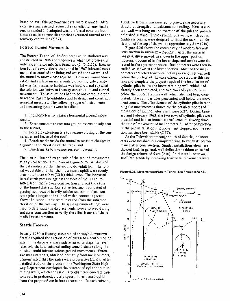
based on available piezometric data, were assumed. After extensive analysis and review, the remedial scheme finally recommended and adopted was reinforced concrete but-tresses cast in narrow slit trenches excavated normal to the roadway center line (5.57).

Potrero Tunnel Movements

The Potrero Tunnel of the Southern Pacific Railroad was constructed in 1906 and underlies a ridge that crosses the only rail entrance into San Francisco (5.46, 5.56). Excava-tion for a freeway above the tunnel in 1967 initiated move-ments that cracked the lining and caused the two walls of the tunnel to move closer together. However, visual obser-vation and surface measurements did not indicate clearly (a) whether a massive landslide was involved and (b) what the relation was between freeway construction and tunnel movements. Those questions had to be answered in order to resolve legal responsibilities and to design and construct remedial measures. The following types of instruments and measuring systems were installed:

Inclinometers to measure horizontal ground move-ments,

Extensometers to measure ground extension adjacent to the tunnel,

Portable extensometers to measure closing of the tun-nel sides and heave of the roof,

Bench marks inside the tunnel to measure changes in alignment and elevation of the track, and

Bench marks to measure surface movement.

The distribution and magnitude of the ground movements at a typical section are shown in Figure 5.25. Analysis of the data indicated that the ground downhill from the tun-nel was stable and that the movements uphill were evenly distributed over a 9-rn (30-ft) thick zone. The increased lateral earth pressure against the sides of the tunnel re-sulted from the freeway construction and was the cause of the tunnel distress. Corrective treatment consisted of placing two rows of heavily reinforced cast-in-place con-crete piles alongside the tunnel with a connecting strut above the tunnel; these were installed from the subgrade elevation of the freeway. The same instruments that were used to determine the displacements were also read during and after construction to verify the effectiveness of the re-medial measurements.

Seattle Freeway

In early 1960, a freeway constructed through downtown Seattle required the excavation of cuts into a gently sloping sidehill. A discovery was made at an early stage that even relatively shallow cuts, extending some distance along the hillside, could initiate serious ground movements. Exten-sive measurements, obtained primarily from inclinometers, demonstrated that the slides were progressive (5.56). After detailed study of the problem, the Washington State High-way Department developed the concept of cylinder-pile re-taining walls, which consist of large-diameter concrete cais-sons cast in prebored, closely spaced holes placed uphill from the proposed cut before excavation. In each caisson,

a massive H-beam was inserted to provide the necessary structural strength and resistance to bending. Next, a cur-tain wall was hung on the exterior of the piles to provide a finished surface. These cylinder pile walls, which act as cantilever beams, were designed to limit the maximum de-flection of the top of the wall to approximately 5 cm (2 in).

Figure 5.26 shows the complexity of modern freeway construction in urban development. After the material was partially removed, as shown in the upper portion, movement occurred in the lower slope and cracks were de-tected in the apartment house. Inclinometers were then in-stalled, as shown in the lower portion. Most of the inch-nometers detected horizontal offsets in various layers well below the bottom of the excavation. To stabilize this sec-tion and complete the project required the installation of cylinder piles below the lower retaining wall, which had already been completed, and two rows of cylinder piles below the upper retaining wall, which also had been com-pleted. The cylinder piles penetrated well below the move-ment zones. The effectiveness of the cylinder piles in stop-ping the movements is shown by the detailed records of movement of inclinometer 5 in Figure 5.27. During Janu-ary and February 1963, the two rows of cylinder piles were installed and had an immediate influence in slowing down the rate of movement of inclinometer 5. After completion of the pile installation, the movement stopped and the sec-tion has since been stable (5.37).

At the Tukwila interchange south of Seattle, inclinom-eters were installed in a completed wall to verify its perfor-mance after construction. Similar installations elsewhere showed that, in general, wall deflections seldom exceeded the design criteria of 5 cm (2 in). In this wall, however, small but gradually increasing horizontal movements were

Figure 5.25. Movements at Potrero Tunnel, San Francisco (5.56).

40 -

ORIGINAl GROUND ISrn,,,/n,o. I 15 r,,n,/n,o.I 35 -

RESULIANI NORENENI — TIED- ANON JO I — I

I REUININC STRUCTURE

\ ZONE)OF EXCAVATION 75 / / 7 WAIL/ANCOR (1961)

I \ / / \ /

/ / \

Si

SUNGRAGE- 10 / 1 >

I \ - I5/o.,' I ,/ \_- I I I / R I I

lA '

nt'I'M

/ TUNNEL 0 I FRANCISCAN /

(1906)

I FORMATION

-5 ISHALES, SAHOSTONU. SERPENTINE. RADII FRACTUREDI

-ID

NOTe: 1 re = 3.3 IT; I 100, = 0.04 in.

134

bRICK APT, I NOOSE

I _L -iRACK _) - - DEC. 62 -

CRACK DEC. 02

IbI COWLETED SECTION naimnsimm

60

5O

0I OACOF FILL

<I © MOVEMENT ZONE -

1 1TH I3O

Lj CYLINDER

1111 Li

CYLt.JI

D PILES NDEI

Notes: 1 m 3.3 It; f mm = 0.04 in. Circled numbers refer to inclinometer locations.

L -

33mm

MOVEMENT ZONES

Figure 5.26. Seattle freeway problem (5.56).

(a) CONSTRUCTION STAGES ORIGINAL GROUND SURFACE -.._

60

CCR AN.

Z 0

I 1 /

/ ,b oct.62

L50

/ DEC 62

I AN. MOVEMENT 63

Figure 5.27. Movement of inclinometer 5. Seattle freeway (5.56).

I DEPTH —15 to 16.5,n .0... •o• 30-I

I 00

I— I _______ : z I I INSTALLED I

IO qO

L20.1 y CYLINDER PILES' IS '

0

Ia

I Cr 50 25 0

I 1Q, MOVEMENT (mm)

I esP (12/15/62 - 3/19/63)

DEC. ' JAN. FEB. MAR. APR. • MA Note: 1 mn a 3.3 It; t nmm = 0.04 in.

detected in two zones well below the tip of the cylinder piles. Fortunately, the movements were detected at an early stage, thereby permitting the construction of a deeper wall before a failure condition developed. In this instance, there was no visual indication of a potential problem and surface alignment surveys would have been difficult be-cause the wall was on a long sweeping curve.

Fort Benton Slide

Along the Burlington Northern rail line from Great Falls to Havre in western Montana, the tracks are situated on a sideh.ill fillsome 12 to 15 m (40 to SOft) above the flood-plain of the Missouri River. During a period of many years, the fill has experienced vertical and horizontal movement. These continuing movements have necessitated almost con-tinuous maintenance, involving both realignment and res-

toration. In 1969, an investigation was undertaken to de-termine the probable cause of the continuing movements so that remedial treatment to improve stability could be initiated (5.58). To determine subsurface conditions be-neath the site, several test borings were made and inclinom-eters, designated S-4 and S-5,were installed at the crest and toe of the slope respectively to determine the slide plane or zone of movement (Figure 5.28). Later in this study, for reasons described subsequently, a second inclinometer (S-6) was installed at the toe of the slope.

The borings for inclinometers S-4 and S-S disclosed that the soils beneath the slope consisted of stiff to hard silts and clays of low to medium plasticity with intermittent zones or pockets of sand and gravel. These soils extended to a depth of about 16 m (5.2 ft) beneath the crest and 5 m (16 ft) beneath the toe. Below these depths, the soil encountered in both borings consisted of hard, mottled dark gray clay. It was first believed that the upper irregu-lar zone of clay, silt, and sand was ancient slide debris or soil that had sloughed from the bluffs above and that the underlying hard clay was "original" ground. However, sub-sequent data obtained from inclinometer S-6 proved this was not the case. It was later determined that slide debris beneath the toe extended to a depth of about 11 m (37 ft) and was underlain by hard clay-shale that extended beyond the 26-rn (85-ft) depth drilled. Although no additional drilling was accomplished at the top of the slope, move-ment recorded by inclinometer S-4 indicated that the sur-face of the hard clay-shale was probably at a depth of about 18 m (60 ft) beneath the tracks, about a meter below the bottom of the casing.

As stated earlier, movement of the sidehill fill had been occurring regularly for many years. Although no accurate

135

E

> 0

4.0 F- z 0 N

3.0 I 0 6 .5

2.0

1.0

ou

.1.8

5.2

U

I- z >

.0

10.2

Figure 5.28. Section through Fort Benton slide. Montana (5.58).

INCLINOMETER S—I SLOPE BEBRIS

20

APPRUX. 11111 OF OBSERVABLESURFACE

0

INCLINOMETER S—S INCLINOMETER S—U CRACBS BEHIND TRACUS

LIMIT OF HUIMOCRY TRACUS

AREA AT TOE OF SLOPE GROUNDWATER SURFACE

\ IGRABEN/ ," 00 COVIEMOED BUTTRESS

190 - - - - - - -

- HARD CLAY - SHALE KNOWN ZONE OF MOVEMENT

00 KNOWN ZONE OF MOVEMENT

DEPTH OF 26 ru 185 It)

2550

Figure 5.29. Movement of inclinometer S-5 at toe of slope, Fort Benton slide (5.58).

fr.LU II 1U

7777777

GROUND SURFACE

CL

C___

NORTH SOUTH

+20 0 —20 —40

LATERAL MOVEMENT )nrtt) V ii 25.4 31.

KR Dli NO SURFACE

SURFACE OF HARO CLAY SHALE

NORTH SOUTH

0 0.5 1.0 1.5

U 0 z .5 1.1

0 I I-

0

flUE

2650 2 0 I-. >

2600

CHANGE (INSTRUMENT DIAL UNITS) LATERAL MOVEMENT )i)

Figure 5.30. Movement of top of inclinometer S-4, Fort Benton slide (5.58).

1.0

6.0

I- 2 12 5.0

- ABSOLUTE VAL(S FTER 6/I /18 ABE WIHELIABLESIRCE HV(MEHTS CAASEB - LOOSENING OF UPPER SECTION OF p.1 • s CASING ,

I / AFTER 5,1 5/10 SLOPE INDICATOR INSRUMENT —j MOULD NUT PHSS BEND I .

I i — MO EMENT DETERNIHED FROM I TR NSIT SIGHT LINE

IF INSTALLED OR 5/15/1 - --- ---- - -,-- MOVEMENT DETERMINED - 14

FNOI SLOPE INOICATOR \ REHOINGS -.

-__ I ii I I 11I I II II II II fi II - DECEMBER JANUARY FEBRUARY NARCA APRIL NAY JUNE 1010 AUGUST SEPTEMBER

136

records of the magnitude and direction had been kept, the 5.7 British Columbia Hydro and Power Authority. Indlinom-

predominant track movement had been vertical and accu- eter Data, Downie Slide. British Columbia Hydro and

mulated settlement during the years amounted to nearly a 5.8 Power Authority, Vancouver, job file, 1976. British Geotechnical Society. Field Instrumentation in

meter. In addition, the movement rate varied seasonally, Geotechnical Engineering. Wiley, New York, 1974, being greatest in spring and summer and least during late 720

fall and winter. By mid-February 1970 (installation was 5.9 Broms, B. B. Landslides. In Foundation Engineering

in November 1969), the inclinometer at the crest of the Handbook (Winterkorn, H. F., and Fang, H. Y., eds.), Van Nostrand-Reinhold, New York, 1975, pp. 373401.

slope indicated about 1.5 cm (0.5 in) of lateral (southward) 5.10 Brooker, E. W., and Lindberg, D. A. Field Measurement movement; however, no change was recorded at the toe of of Pore Pressure in High Plasticity Soils. In Engineering

the slope during this 3-month period. Movement of md- Effects of Moisture Changes in Soils (Aitchison, G. D.,

nometer S-4 continued, accelerating somewhat in early May ed.), Proc., International Research and Engineering Con-

and decreasing in late July and August. Data from this ference on Expansive Clay Soils, Texas A&M Univ., College Station, 1965, pp. 57-68.

same installation showed that movement was occurring at 5.11 Burland, J. B., and Moore, J. F. A. The Measurement of a depth of 18 m (59 ft) and, because the bend in the casing Ground Displacement Around Deep Excavations. In

was relatively abrupt, was occurring within a relatively thin Field Instrumentation in Geotechnical Engineering

zone, probably only a few centimeters thick. Although re- (British Geotechnical Society), Wiley, New York, 1974,

liable data were being obtained from the installation at the 5.12 pp. 70-84. Cooling, L. F. Second Rankine Lecture: Field Measure-

top of the embankment, no changes were recorded at the ments in Soil Mechanics. Geotechnique, Vol. 12, No. 2,

toe of the slope, and it became apparent that the zone of 1962, pp. 75-104.

movement beneath the toe of the slope was passing below 5.13 Cording, E. J., Hendron, A. J., Jr., Hansmire, W. H.,

the 9-rn (30-ft) depth of the casing. Hence, a second, deeper Mahar, J. W., MacPherson, H. H., Jones, R. A., and O'Rourk, T. D. Methods for Geotechnical Observations

casing (S-6) was installed, and Instrumentation in Tunneling. Department of Civil Soon after the additional installation was made, the data Engineering, Univ. of illinois, Urbana-Champaign; Na-

showed definite displacement at the toe of the slope; move- tional Science Foundation, Vol. 2, 1975, pp. 293-566.

ment was occurring within a relatively narrow zone some 5.14 Cornforth, D. H. Performance Characteristics of the Slope

11 m (37 ft) below the ground surface. These data are Indicator Series 200-B Inclinometer. In Field Instrumen- tation in Geotechnical Engineering (British Geotechnical

shown in Figures 5.29 and 5.30. The zone of movement Society), Wiley, New York, 1974, pp. 126-1 35. correlated with the surface of the hard clay-shale layer that 5.15 Dallaire, E. E. Electronic Distance Measuring Revolution

was encountered at the same depth. Once the failure Well Under Way. Civil Engineering, Vol. 44, No. 10,

mechanism had been established from the instrumentation 5.16

1974, pp. 66-7 1. Dibiagio, E. Discussion: Session 2—Equipment. In

data, the design of corrective measures could be started. Field Instrumentation in Geotechnical Engineering Buttressing was selected as the most practicable means of (British Geotechnical Society), Wiley, New York, 1974, stabilizing the hillside. (Figure 5.28). Had the field data pp. 565-566.

revealed movement was occurring within a cohesive zone 5.17 Dunnidiff, C. J. Equipment for Field Deformation Mea-

(e.g., through a thin seam of bentonite clay), some other surements. Proc., 4th Pan-American Conference on Soil

approach to stabilization would have been necessary. Mechanics and Foundation Engineering, San Juan, Ameri-can Society of Civil Engineers, New York, Vol. 2, 1971, pp. 319-332.

REFERENCES 5.18 Durr, D. L. An Embankment Saved by Instrumentation. Transportation Research Board, Transportation Research

5.1 American Society of Civil Engineers. Proc., Specialty 5.19

Record 482, 1974, pp. 43-50. Dutro, H. B., and Dickinson, R. 0. Slope Instrumenta-

Conference on Performance of Earth and Earth- lion Using Multiple-Position Borehole Extensometers. Supported Structures, Purdue Univ., Lafayette, Ind., Transportation Research Board, Transportation Research American Society of Civil Engineers, New York, Vol. 1, Record 482, 1974, pp. 9-17. Part 1, 883 pp., Part 2, 1555 pp.; Vol. 2, 154 pp.; Vol. 3, 385 pp., 1972. 5.20 Eckel, E. B., ed. Landslides and Engineering Practice.

5.2 Bishop, A. W., Kennard, M. F., and Penman, A. D. M. 5.21

Highway Research Board, Special Rept. 29, 1958, 232 pp. Franklin, J. A., and Denton, P. E. The Monitoring of Pore-Pressure Observations at Selset Dam. In Pore Pres-

sure and Suction in Soils, Butterworths, London, 1961, Rock Slopes. Quarterly Journal of Engineering Geology,

pp. 91-1 02. Vol. 6, No. 3, 1973, pp. 259-286.

5.3 Bishop, A. W., Kennard, M. F., and Vaughan, P. R. De- 5.22 Goodman, R. E., and Blake, W. Rock Noise in Landslides

velopments in the Measurement and Interpretation of and Slope Failures. Highway Research Board, Highway

Pore Pressure in Earth Dams. Proc., 8th International Research Record 119, 1966, pp. 50-60.

Congress on Large Dams, Edinburgh, Vol. 2, 1964, pp. 5.23 Gould, J. P., and Dunnidiff, C. J. Accuracy of Field De-

47-7 2. formation Measurements. Proc., 4th Pan-American Con-

5.4 Blake, W., and Leighton, F. Recent Developments and ference on Soil Mechanics and Foundation Engineering,

Applications of the Microseismic Method in Deep Mines. San Juan, American Society of Civil Engineers, New

In Rock Mechanics: Theory and Practice, Proc., 11th Symposium on Rock Mechanics, American Institute of 5.24

York, Vol. 1, 1971, pp. 313-366. Green, G. E. Principles and Performance of Two Indi-

Mining, Metallurgy and Petroleum Engineers, New York, nometers for Measuring Horizontal Ground Movements.

1970, pp. 429-443. In Field Instrumentation in Geotechnical Engineering

5.5 Blake, W., Leighton, F., and Duvall, W. I. Techniques (British Geotechnical Society), Wiley, New York, 1974,

for Monitoring the Behavior of Rock Structures. U.S. Bureau of Mines, Bulletin 665, 1974, 65 pp. 5.25

pp. 166-179. Hanna, T. H. Foundation Instrumentation. Trans Tech

5.6 Boden, J. B., and McCauI, D. Measurements of Ground Publications, Clausthal, Germany, Series on Rock and Soil

Movements During a Bentonite Tunneling Experiment. Mechanics, Vol. 1, No. 3, 1973, 372 pp.

U.K. Transport and Road Research Laboratory, Crow- 5.26 Heinz, R. A. In Situ Soils Measuring Devices. Civil En-

thorne, Berkshire, England, Rept. 653, 1974, 8 pp. gineering, Vol. 45, No. 10, 1975, pp. 62-65.

137

5.27 Hvorslev, M. J. Time Lag and Soil Permeability in Groundwater Observations. U.S. Army Engineer Water-ways Experiment Station, Vicksburg, Miss., Bulletin 36, 1951,50 pp.

5.28 Kern and Company, Ltd. The Mekometer, Kern ME3000, 5.45 Electro-Optical Precision Distance Meter. Kern and Co., Ltd., Aarau, Switzerland, Technical Information 10, 1974,4 pp.

5.29 McCauley, M. L. Microsonic Detection of Landslides. Transportation Research Board, Transportation Research Record 581, 1976, pp. 25-30.

5.30 Malone, A. W. Elastic Wave Measurement in Rock Engi- neering. Imperial College, Univ. of London, PhD thesis, 1968, 299 pp.

5.31 Mearns, R., and Hoover, T. Subaudible Rock Noise (SARN) as a Measure of Slope Stability. Transportation Laboratory, California Department of Transportation, Sacramento, Final Rept. CA-DOT-TL-25 37-1-73-24, 1973, 16 pp.

5.32 Merriam, R. Portuguese Bend Landslide, Palos Verdes Hills, California. Journal of Geology, Vol. 68, No. 2, 1960, pp. 140-153.

5.33 Mexico Ministry of Public Works. Failures at the Tijuana- Ensenada Highway. Mexico Ministry of Public Works, Mexico City, 1975, 220 pp.

5.34 Mikkelsen, P. E., and Bestwick, L. K. Instrumentation and Performance: Urban Arterial Embankments on Soft Foundation Soil. Proc., 14th Symposium on Engineer-ing Geology and Soils Engineering, Boise, Idaho, Idaho Department of Highways, Univ. of Idaho, and Idaho State Univ., 1976, pp. 1-18.

5.35 Moore, J. F. A. The Photogrammetric Measurement of Constructional Displacements of a Rockfill Dam. Photogrammetric Record, Vol. 7, No. 42, 1973, pp. 6 28-64 8.

5.36 Mu?ioz, A., Jr., and Gano, D. The Role of Field Instru- mentation in Correction of the "Fountain Slide." Trans-portation Research Board, Transportation Research Rec-ord 482, 1974, pp. 1-8.

5.37 Palladino, D. J., and Peck, R. B. Slope Failures in an Overconsolidated Clay, Seattle, Washington. Geotech-nique, Vol. 22, No. 4, 1972, pp. 563-595.

5.38 Peck, R. B. Observation and Instrumentation: Some Elementary Considerations. Highway Focus, Vol. 4, No. 2, 1972, pp. 1-5.

5.39 Penman, A. D. M. A Study of the Response Time of Various Types of Piezometer. In Pore Pressure and Suc-tion in Soils, Butterworths, London, 1961, pp. 53-58.

5.40 Penman, A. D. M., and Charles, J. A. Measuring Move- ments of Embankment Dams. In Field Instrumentation in Geotechnical Engineering (British Geotechnical Society), Wiley, New York, 1974, pp. 341-358.

5.41 Phillips, S. H. E., and James, E. L. An Inclinometer for Measuring the Deformation of Buried Structures With Reference to Multitied Diaphragm Walls. In Field Instru-mentation in Geotechnical Engineering (British Geotech-nical Society), Wiley, New York, 1974, pp. 359-369.

5.42 Piteau, D. R., Mylrea, F. H., and Blown, J. G. The Downie Slide, Columbia River, British Columbia. In Natural Phenomena: Developments in Geotechnical Engineering—Rockslides and Avalanches (Voight, B., ed.), Elsevier, New York, Vol. 1, 1978.

5.43 St. John, C. M., and Thomas, T. L. The N.P.L. Mekometer and Its Application in Mine Surveying and Rock Mechan-ics. Trans., Institution of Mining and Metallurgy, London, Vol. 79, Sec. A, 1970, pp. A31-A36.

5.44 Schmidt, B., and Dunnicliff, J. C. Construction Monitor-

ing of Soft Ground Rapid Transit Tunnels. Urban Mass Transportation Administration, U.S. Department of Transportation, Vols. 1 and 2, 1974; NTIS, Springfield, Va., PB 241 536. Shannon, W. L., Wilson, S. D., and Meese, R. H. Field Problems: Field Measurements. In Foundation Engineer-ing (Leonards, G. A., ed.), McGraw-Hill, New York, 1962, pp. 1025-1080.

5.46

Smith, T. W., and Forsyth, R. A. Potrero Hill Slide and Correction. Journal of Soil Mechanics and Foundations Division, American Society of Civil Engineers, New York, Vol. 97, No. SM3, 1971, pp. 54 1-564.

5.47

Terzaghi, K. Mechanism of Landslides. In Application of Geology to Engineering Practice (Paige, S., ed.), Geological Society of America, Berkey Vol., 1950, pp. 83-1 23.

5.48

Tice, J. A., and Sams, C. E. Experiences With Landslide Instrumentation in the Southeast. Transportation Re-search Board, Transportation Research Record 482, 1974, pp. 18-29.

5.49

Toms, A. H., and Bartlett, D. L. Applications of Soil Mechanics in the Design of Stabilizing Works for Embank-ments, Cuttings and Track Formations. Proc., Institution of Civil Engineers, London, Vol. 21, 1962, pp. 705-711.

5.50

Transportation Research Board. Landslide Instrumenta- tion. TRB, Transportation Research Record 482, 1974, 51 pp.

5.51

Vaughan, P. R. A Note on Sealing Piezometers in Bore- holes. Geotechnique, Vol. 19, No. 3, 1969, pp. 405-413.

5.52

Vaughan, P. R. The Measurement of Pore Pressures With Piezometers. InField Instrumentation in Geotechnical Engineering (British Geotechnical Society), Wiley, New York, 1974, pp. 411-422.

5.53

Vaughan, P. R., and Walbancke, H. J. Pore Pressure Changes and the Delayed Failure of Cutting Slopes in Overconsolidated Clay. Geotechnique, Vol. 23, No. 4, 1973, pp. 531-539.

5.54

Wilson, S. D. The Use of Slope Measuring Devices to De- termine Movements in Earth Masses. In Field Testing of Soils, American Society for Testing and Materials, Phila-delphia, Special Technical PubI. 322, 1962, pp. 187-197.

5.55

Wilson, S. D. Investigation of Embankment Performance. Journal of Soil Mechanics and Foundations Division, American Society of Civil Engineers, New York, Vol. 93, No. SM4, 1967, pp. 135-156.

5.56

Wilson, S. D. Observational Data on Ground Movements Related to Slope Instability. Journal of Soil Mechanics and Foundations Division, American Society of Civil En-gineers, New York, Vol. 96, No. SMS, 1970, pp. 1521-1544.

5.57 Wilson, S. D. Landslide Instrumentation for the Minne- apolis Freeway. Transportation' Research Board, Trans- portation Research Record 482, 1974, pp. 30-42.

5.58 Wilson, S. D., and Hilts, D. E. Application of Instrumen- tation to Highway Stability Problems. Proc., Joint ASCE-ASME National Transportation Engineering Meet-ing, Seattle, American Society of Civil Engineers, New York, and American Society of Mechanical Engineers, New York, 1971.

5.59 Wilson, S. D., and Squier, R. Earth and Rockfill Dams. 7th International Conference on Soil Mechanics and Foundation Engineering, Mexico City, State-of-the-Art Vol., 1969, pp. 137-223.

5.60 Wisecarver, D. W., Merrill, R. H., and Stateham, R. M. The Microseismic Technique Applied to Slope Stability. Trans., Society of Mining Engineers, American Institute of Mining, Metallurgical and Petroleum Engineers, New York, Vol. 244, 1969, pp. 378-385.

138

Chapter 6

Strength Properties and Their measurement Tien H. Wu and Dwight A. Sangrey

The methods of limiting equilibrium are frequently used to analyze the stability of a soil or a rock mass (Chapter 7). In such analyses, the shear strength of the material is assumed to be fully developed along the slip surface at failure. This chapter outlines the basic principles that goyern the shear strength and the methods that may be used for its measure-men t.

GENERAL PRINCIPLES

Mohr-Coulomb Failure Criterion

The Mohr-Coulomb criterion is most widely used to define failure; it states that the shear strength (s) is

sc+atan4 [6.11

where

a = normal stress on slip surface, c = cohesion, and

= angle of internal friction.

In terms of principal stresses, the Mohr-Coulomb criterion becomes

01 =a3 tan2 [(/4)+(/2)]

+ 2c tan [(7r/4) + (/2)] [6.2]

where

a1 = major principal stress, and

03 = minor principal stress.

Other failure criteria, particularly the modified Tresca and Von Mises, are sometimes used for soils, but their applica-

tion to landslides has been limited (see later section on com-mon states of stress and stress change).

Effective Stress Versus Total Stress Analysis

Since the shear strength of soils and rocks is strongly influ-enced by the drainage conditions during loading, those con-ditions must be properly accounted for in the use of shear strength. A fundamental principle in soil engineering is the use of effective stress (a'), which is defined as

a'a - u [6.3]

where

a = total stress, and u = pore pressure.

The shear strength can be expressed consistently in terms of effective stress, or

sc'+a' tan'c'+(a-u)tan [6.4]

where c' and 0' are the strength parameters for effective stress. The use of the effective stress parameters requires that the pore pressure be known so that a' may be evaluated.

In general, pore pressure consists of the hydrostatic pore pressure related to groundwater level and the excess pore pressure due to applied loads. When soils are loaded under undrained or partially drained conditions, the tendency to change volume results in pore-pressure change. The excess pore pressure may be either positive or negative, depending on the type of soil and the stresses involved. Under the fully drained, long-term condition, the excess pore pressure is zero, and pore pressure due to groundwater flow can usu-ally be evaluated without serious difficulty. Hence, analysis

139

with the effective stress description of shear strength (Equa-tion 6.4) is most useful.

For partially drained and undrained conditions, the evalu-ation of excess pore pressure is often difficult. In some cases, a total stress description of shear strength may be used. One important case is the undrained loading of saturated soils. In this case, the undrained shear strength (sn) can be used, where s = s. This is the shear strength description in the common

= 0 method of analysis. The shear strength usually changes as drainage occurs. If the change results in a higher strength, the short-term, undrained stability is critical and the stability can be expected to improve with time. On the other hand, if drainage produces a decrease in strength, the, undrained shear strength can be used only for short-term or temporary situations.

Common States of Stress and Stress Change

The Mohr-Coulomb criterion does not indicate any effect of the intermediate principal stress (Uj) on the shear strength. In practical problems, or may range from aj to cr1 depending on the geometry of the problem. The direction of the major principal stress also changes during loading. Many stability problems can be approximated by the plane-strain condition in which a lies near the midpoint between uj and aj. Ex-perimental studies show that the relative value of a com-pared with a and a exerts some influence on the stress-strain characteristics and the shear strength.

Several common states of stress are shown in Figure 6.1. In the initial state, a is the effective overburden pressure,

= K) cri is the lateral pressure, and K0 is the coefficient of earth pressure at rest. In the stress state beneath the center of a circular loaded area, the vertical stress (a = a + a) is the major principal stress and the radial stress (cr3 is the minor principal stress. In the stress state below the center of a circular excavation, the vertical stress is the minor principal stress and the radial stress is the major principal stress. For the circular load, the intermediate principal stress (a) is equal to the minor principal stress (a); for the excavation, it is equal to the major principal stress (a). Slopes and re-taining structures can be approximated by the plane-strain condition in which the intermediate principal strain (€2) is zero. Then, the intermediate principal stress (cr) is Or; and, in Figure 6.1d, lies between a; and cr.

Another important feature in many stability problems is the rotation of the principal axes during loading or excava-tion. It has been reported that this reduces the shear strength of some soft clays (6.50). The rotation of principal axes is shown in Figure 6.2. Before the excavation of the cut, the state, of stress is represented by that shown in Figure 6.la. After excavation, the major principal stress is in the horizon-tal direction at the toe (point a). Thus, the principal axes are rotated through an angle of 90°; at point b, a rotation of approximately 450 occurs. At point c, the original principal stress directions remain the same although the values of the stresses change.

Stress-Strain Characteristics

Two stress-deformation curves are shown in Figure 6.3; stress-strain curves are of similar form. In common practice,

Figure 6.1. Common states of stress in soil.

(a) INITIAL ATREST STATE )b) BENEATH A LOADED AREA P

(c) BENEATH AN EXCAVATION Id) PLANESTRAIN CONDITION

o a

Figure 6.2. Rotation of principal stress axes in a slope.

the strength of the soil is defined as the peak strength (points a and b) measured in the test. When this is used in a stabil-ity analysis, the tacit assumption is that the peak strength is attained simultaneously along the entire slip surface.

Many soils demonstrate strain.softening behavior, as illu-strated by curve A. Any of several phenomena may explain the strength decrease, but it is important in design to account for this decrease. The lower limit to strength (point c) may be called the fully softened strength, remolded strength, or residual strength, depending on the type of soil involved (these terms are not synonymous). For such soils, it is un-reasonable to assume that all soil along a failure surface reaches its peak strength simultaneously. In fact, the soil at some points will suffer displacements greater than Aa before the soil at other points reaches this deformation. In the limit of a large deformation, all strength at all points will be reduced to the strain-softening limit (point c).

Effect of Rate of Loading

The difference between the rate of loading applied in a lab-oratory shear test and that experienced in the slope is usu-ally substantial. Most laboratory and in situ tests bring the soil to failure within several hours or at most a few days. For most real structures, the load remains permanently, al-though in some dynamic situations the peak load may be applied only for short durations. The effect of rate of load-ing on soil strength, excluding direct drainage effects, may be significant. In general, the undrained strength of soils

140

Figure 6.3. Typical stress-strain cUrves for soils.

0 fA

60

increases as the rate of loading increases; however, this ef-fect depends on the specific material and varies over a wide range (6.22, 6. 73).

LABORATORY MEASUREMENT OF SHEAR STRENGTH

A variety of methods is available for laboratory measure-ment of shear strength. The simple methods are designed to determine the shear strength of a sample in a particular con-dition, such as the water content or void ratio of the soil in situ. These methods are most often used to determine the undrained shear strength (se) of saturated cohesive soils. More elaborate laboratory tests are able to establish the shear strength relation defined by Equation 6.4. These methods allow combinations of normal and shear stresses to be em-ployed and pore pressures to be measured or controlled. The more elaborate tests allow more accurate simulation of the field stress or deformation conditions. For example, triaxial compression tests simulat Rankine's active state, and tri-axial extension simulates Rankine's passive state. The plane-strain and simple shear tests may be used to provide a better simulation of the actual deformation conditions in a slope.

Simple Tests

Three types of simple tests are discussed below.

The unconfined compression test is usually performed on a cylindrical sample with a diameter-to-length ratio of 1:2 or slightly more. The sample is compressed axially (Figure 6.4a) until failure occurs; the shear strength is taken as one-half the compressive strength.

In the cone test, a cone with an angle of U is forced into the soil (Figure 6.4b) under a force (Q), which may be its own weight. The shear strength is obtained from the re-lation

su = KQ/h2 [6.5]

where

h = penetration, and K = constant that depends on the angle 0 and the weight

Q.

Calibration curves for K have been published by Hansbo (6.34) and others.

In the vane test, a vane is pushed into the soil specimen, and a torque is applied to the stem to produce shear failure over a cylindrical surface (Figure 6.4c). The shear strength

Figure 6.4. Simple test methods for determining soil strength.

(a) UNCONFINED (b) CONE Ic) VANE SHEAR

COMPRESSION

plan profile

is obtained by equating the torque measured at failure to the moment produced by theshear stresses along the cylindrical surface. According to Cadling and Odenstad (6.21), the shear strength for vanes with a diameter-to-height ratio of 1:2 is

s = (6/7) (M/7rD3 ) [6.6]

where

M = torque, and D = diameter of the vane.

In the application of the results of these simple tests to the analysis of.slopes, consideration should be given to the type of soil and loading conditions in situ. The application of these test results is commonly limited to saturated co-hesive soils under undrained conditions. The results are all expressed in terms of total stress because pore pressures are not measured. When the soil is brought to failure rapidly under undrained conditions, the shear strength is defined by 5 = s. If the tests are run slowly or if the soil drains during shear, the results are generally not applicable.

It is usually assumed that the measured strength is equal to the in situ strength; however, a major uncertainty is the effect of sampling disturbance on strength. Several studies (6.15, 6.51) show that even "good" samples may suffer strength losses as great as 50 percent. The effect of sample disturbance is most severe in soft sensitive soils and appears to become more significant as depth of the sample increases. Other factors to be considered include the state of stress and deformation. The directions of the principal stresses and the orientations of failure surfaces in each of these tests are not the same. They may also be quite different from the direc-tions along the actual slip surface in a slope (6.50). Hence, caution should be exercised when the results of these simple strength tests are applied to slope stability problems (6.15).

Triaxial Test

The triaxial test is a highly versatile test, and a variety of stress and drainage conditions can be employed (6.10). The cylindrical soil specimen is enclosed within a thin rubber membrane and is placed inside a triaxial cell (Figure 6.5a). The cell is then filled with a fluid. As pressure is applied to the fluid in the cell, the specimen is subjected to a hydro-static compressive stress (a3). Drainage from the specimen is provided through the porous stone at the bottom, which is connected to a volume-change gauge. The volume-change gauge is often an enclosed burette so that back pressure can be applied. Volume compressibility can be determined by

141

Figure 6.5. Triaxial test.

(a) EQUIPMENT

Trio,i

VoI:n ff

CCII

Cap

Gouge

C

h..ge Porous slonQe

Pore pressure transducer

)b) STRESS (c( STRESS-STRAIN CURVES CONDITIONS

.300

2

:

00 LO3 'I00

the use of these measurements. Pore pressures in the sample are also measured by a device connected to the porous stone. Several devices may be used. Electric pressure transducers are becoming more common and are replacing the tradi. tional null indicator and hydraulic cylinder system.

The axial stress (a') may be increased by application of a load through the loading ram. From the known stresses at failure (cr = a and 03 = 02 = ar), Mohr circles or other stress plots can be constructed. Several triaxial tests, each using a different value of cell pressure (3), are usually per-formed on the same material for the definition of the failure envelope. The principal stresses at failure are then used to con-struct Mohr circles or other stress plots from which a failure envelope can be obtained. Typical plots of the principal stress difference versus axial strain are shown in Figure 6.5c. The stress-strain behavior is influenced by the confining pres-sure, the stress history, and other factors. Analytical repre-sentations of normalized stress-strain relations have been sug-gested for some soil types. The sample can also be loaded to failure in extension by increasing the radial stress while main-taining the axial stress constant; then, a, = 02 = °r and 03

= a. These two methods of loading simulate the stress states shown in Figures 6.1b and c respectively. -

The following tests are commonly performed with the triaxial apparatus.

I. In the consolidated-drained test (sometimes called a drained test or slow test), the soil is allowed to consolidate completely under an effective cell pressure (as) so that at the end of consolidation the excess pore pressure in the soil is zero. The water content of the specimen after consolida-tion is w. In the triaxial compression test, the axial stress is increased at a slow rate, and drainage is permitted. The rate should be slow enough so that water can drain through the soil, and no excess pore pressure should be allowed to build up. A drained test of soils of low permeability often requires several days.

The volume change during shear in a drained test can re-sult in either an increase or a decrease in the water content.

This will depend on the type of soil and the level of stress in-volved. The water content at failure (wf) will usually be dif-ferent from w.

Since the excess pore pressure is zero in the drained test, effective stresses are known throughout the test and partic-ularly at failure. In a compression test, the effective radial stress (as) is equal to the cell pressure, and the measured load on the ram can be used to evaluate the effective axial stress (Uj). The results of a series of drained tests can be used to evaluate the effective stress strength parameters in Equation 6.4.

In the consolidated-undrained test with pore pressure measurement (sometimes called consolidated-quick test), the drainage valves are closed after the initial consolidation of the sample to w. Stress changes are applied through the ram, and the excess pore pressure is measured. The pore pressure is subtracted from the total axial and radial stresses to give the effective stresses. The effective stresses at failure from a series of tests are used to define the failure criterion, as in the drained test. Since the test is run in the undrained condition after consolidation, the water content throughout the test and at failure is w,. Excess pore pressures developed during the test can be either positive or negative, depending on the type of soil and stress level.

Several equations have been proposed to describe the magnitude of the excess pore pressure developed as a result of stress changes in an undrained soil. For soils tested in the triaxial apparatus, or loaded so that Lar2 = L03 , Skempton (6.67) proposed that the excess pore pressure is given by

AuB[Aa3 +AA(a1 - (73)] [6.7]

where

B = empirical coefficient related to the soil's compressi-bility and degree of saturation, and

A = empirical coefficient related to the excess pore pres-sure developed because of shear of soil.

General relations between pore pressure and applied stresses have been suggested. For example, Henkel (6.37) proposed

Au = B(Aa + aA7-0 ) [6.81

where

a= empirical coefficient similar to A; TOCt = octahedral shear stress, equal to

i/(a 2)2 + ('92 - 0)2 + ((73- )2. and = octahedral normal stress, equal to (ai + a + (73)/3.

The consolidated-undrained test is sometimes performed without pore-pressure measurement. Obviously, effective stresses are not known during this test or at failure. The ap-plication of shear strength measured in this test to any field problem involves assumptions of excess pore pressure that are of questionable validity in most cases; thus, this test is not recommended. To relate strength parameters obtained from consolidated undrained tests without pore-pressure measurement to field conditions is difficult.

In the unconsolidated-undrained test (sometimes

142

called undrained test or quick test), no drainage is allowed during any part of the test. When the cell pressure is applied, a pore-water-pressure change (Aug ) occurs in the soil. When the axial stress is applied, additional pore-pressure changes (LUa) occur. These pore-pressure changes are not usually measured, so test results must be interpreted by the use of total stresses. At failure, the undrained shear strength (se) is taken to represent the strength at the in situ water content. The unconsolidated-undrained test is, therefore, similar to the simple tests defined in the earlier section on simple tests.

All of the tests described above are usually begun by in-creasing the cell pressure to the desired stress level. This ap-plies an isotropic or hydrostatic stress to the sample. This initial condition differs from the initial condition in situ (Figure 6.1a) if the vertical and horizontal principal stresses are different. In situ stresses can be simulated in a triaxial test by using an anisotropic stress state during consolidation. This can be accomplished by consolidating the specimen un-der a cell pressure and an axial load. Experimental results with a wide variety of soils show that effective stress strength parameters determined from isotropically or anisotropically consolidated tests are essentially the same. The stress-strain curves, however, are significantly different. If the stress-strain relation must be determined, anisotropic consolidation should be used.

Plane-Strain Test

The geometry of many geotechnical problems can be approx-imated by the condition of plane strain, in which the inter-mediate principal strain (€2) is zero. To simulate this condi-tion, plane-strain tests have been developed (6.30, 6.39). In plane-strain tests, the sample is consolidated anisotropically with zero lateral strain (ex = c,, = 0). After this, the sample is loaded to failure by increasing either a or a, and main-taining e,, = 0. The two methods of loading can be used to simulate the stress conditions at points c or a of Figure 6.2. Plane-strain tests can be conducted under undrained, consolidatedundrained, or drained conditions in manners similar to those described for triaxial tests.

Direct Shear Test

The direct shear test is shown in Figure 6.6. The soil speci-men is enclosed in a box consisting of upper and lower halves; porous stones on top and bottom permit drainage of water from the specimen. The potential plane of failure is a-a. A normal stress (ui) is applied on plane a-a through a loading head, and the shear stress is increased until the speci-men fails along plane a-a. A stress-deformation curve is ob-tained by plotting the shear stress versus the displacement. Because the thickness of shear zone a-a is not precisely known, the shear strain cannot be determined. The test gives the value of 7- 5 at failure. The vertical stress (a) and the shear stress (r5) at point b (Figure 6.6b) are known, but a, is not. The directions of the principal stresses are approx imately as shown in Figure 6.6c. Assuming that point a (Figure 6.6d) represents the conditions at failure, a Mohr circle can be constructed. The foregoing- represents the com-mon interpretation of the direct shear test. More elaborate analyses have been presented by Hill (6.41) and Morgenstern and Tchalenko (6.57).

Figure 6.6. Direct shear test.

(a) SHEAR BOX (b( STRESS STATE AT POINT b

Li

Ic) ORIENTATION OF (dl MOHR CIRCLE PRINCIPAL STRESSES

Figure 6.7. Simple shear test.

(a) INITIAL STATE )b) DEFORMATION OF STRESS CONSTRAINT

KD

The failure envelope isobtained from several tests, each using a different effective normal stress, performed on speci-mens of the same soil. The values of r, at failure are plotted against the values of or.. The loading is carried but slowly, so that no excess pore pressure develops; hence, the drained condition is obtained.

In saturated clays, the direct shear test can be performed at a rapid rate so that the time duration is too short for any appreciable amount of water to flow into or out of the sam-ple. This is an undrained condition, and excess pore pres-sures of unknown magnitude are usually developed in the soil. Consequently, this is essentially a simple test, and the shear stress at failure represents the undrained shear strength (Su).

Simple Shear Test

Several simple shear tests have been developed, but the one described by Bjerrum and Landva (6.17) is most commonly used for testing undisturbed samples. The cylindrical speci-men is enclosed in a rubber membrane reinforced by wire. This allows the shear deformation to be distributed fairly uniformly through the sample, as shown in Figure 6.7b. In the test, the sample is consolidated anisotropically under a vertical stress (Figure 6.7a) and sheared by application of stress r,. (Figure 6.7b). The simple shear test can be per-formed under undrained, consolidated-undrained, and drained conditions. Zero volume change during shear in an undrained test can be maintained by adjusting the ver-tical stress (at) continuously during the test. In the simple shear test, the principal axes are in the vertical and hori-zontal directions initially. At failure, the horizontal plane becomes the plane of maximum shear strain. This condi-tion approximates that at point b of Figure 6.2.

143

Effective normal stress

Figure 6.9. Strength behavior of soft saturated clay soils.

FAILURE ENVELOPE

SHEAR STRENGTH PROPERTIES OF SOME COMMON SOILS

Unlike steel or concrete, whose material properties are known or closely controlled, soil has material properties that are unique at every site. For that reason, the strength properties of the soil should be investigated at every site. Within broad groupings, however, the strength characteristics of many soils are similar. Appreciation of these characteristics can be help-ful in planning detailed investigations.

Cohesionless Soils

Granular soils, such as gravel, sand, and nonplastic silts, are called cohesionless soils. The effective stress failure enve-lope of a cohesionless soil is approximately a straight line passing through the origin. This means that, for those soils, c'= Oin Equation 6.4. The value of 0' rangesnormally from about 270 to 42° or more and depends on several factors. For a given soil, the value of 0' increases as relative density increases. If one considers several soils at the same relative density, the value of 0' is affected by particle-size distribu-tion and particle shape. The value of 0' for a well-graded soil may be several degrees greater than that for a uniform soil of the same average particle size. The same is true when a soil composed of angular grains is compared with one made up of rounded grains. The effect of moisture on ' is small and amounts to no more than 10 or 20 (6.42).

The failure envelope, which is a straight line at low pres-sures, cannot be extended to high confining pressures. Tests with effective normal stresses above 700 kPa (1460 lbf/in2) indicate that the failure envelope is curved, as shown in Figure 6.8 (6. 7, 6. 77). The high normal stresses apparently cause crushing of grain contacts and result in a lower friction angle. Another important factor is the difference in the val-ues of t ' as measured by different types of tests. The ' measured in triaxial tests, which permit change in the radial strain, is as much as 40 to 50 smaller than the ' measured in plane-strain tests (6.33). This difference has also been ob-served in field problems.

In ordinary construction situations, sandy and gravelly soils of high permeability can be considered to be loaded in the drained condition. Volume changes occur rapidly, and no excess pore pressures are sustained. Without excess pore pressures, effective stresses can be estimated from the ground-water levels. Stability analyses can be performed by using the effective stress strength parameters.

For silty soils, the permeability may be sufficiently low that excess pore pressures will develop during construction. When this is the case, the pore pressures must be measured or estimated if an effective stress analysis is to be performed.

The undrained response of sands and gravels is required for only a few situations. Saturated loose sand may fail so rapidly that excess pore pressures are sustained. Similarly, under rapid loading the undrained shear strength may be ap-plicable (see the later section on soil behavior under re-peated loads).

Soft Saturated Clays and Clayey Silts

Soils containing significant amounts of clay and silt are called cohesive soils. Because of the low permeability of

Figure 6.8. Typical failure envelope for cohesionless soils.

a +o

TYPICAL STRESS AND WATER CONTENT RELATION

Water content

fine-grained soils, undrained or partially drained situations are common. This is a most important difference between cohesionless soils and cohesive soils. Another important dis-tinction between normally consolidated or lightly overcon-solidated clays and heavily overconsolidated clays is based on the kind of excess pore pressures developed in these soils during shear. The general characteristics of normally con-solidated clays will be discussed first. Extremely sensitive normally consolidated clays are not discussed here but in the later section on sensitive soils.

A clay soil is considered to be normally consolidated if the consolidation pressures before shear are equal to or greater than the preconsolidation stress (p). When a series of drained triaxial tests is conducted on a normally consoli-dated soil, the failure envelope is a straight line that passes through the origin (Figure 6.9a); thus, c' = 0. A relation be-tween strength and water content is shown in Figure 6.9b. If consolidated-undrained tests are performed on a normally consolidated soil, positive excess pore pressures develop. The effective stresses at failure will define the same failure envelope in consolidated-undrained tests as in drained tests (c' = 0 and 0' = As a result of the positive excess pore pressures, however, the undrained strength (a1 - 03) will be less than the drained strength of a sample initi4lly consoli-dated under the same stresses. This characteristic can be ap-plied as a design principle.

If the load or stress change in the field induces positive

144

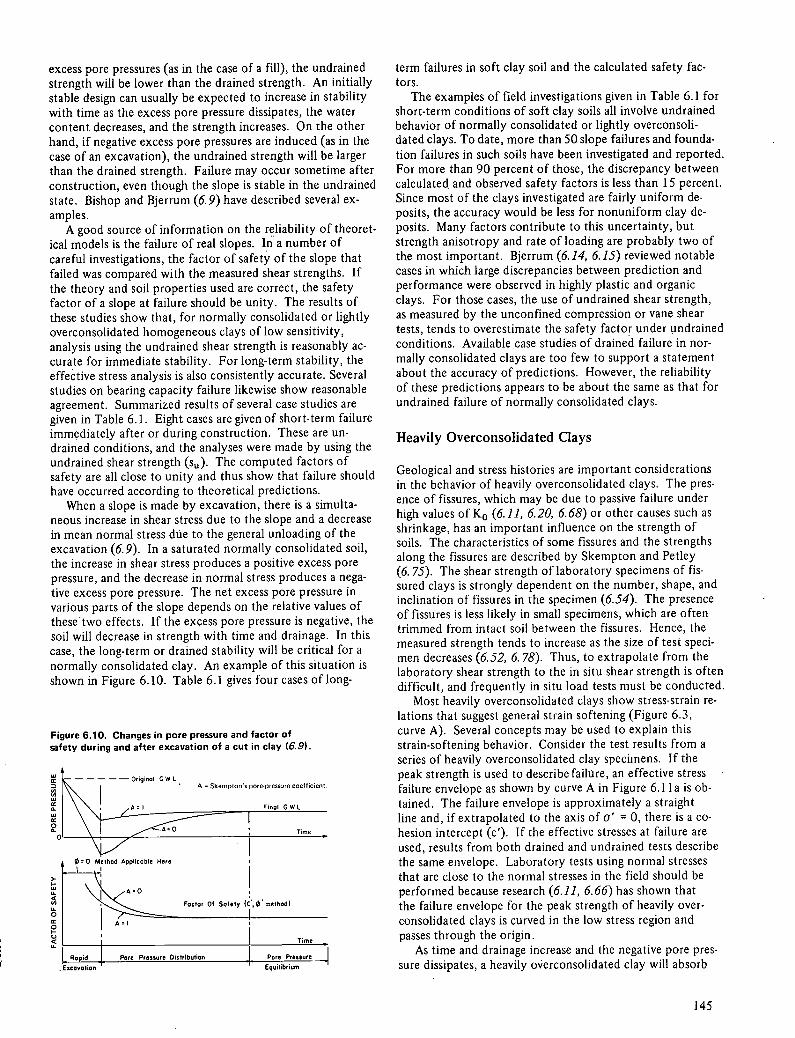
excess pore pressures (as in the case of a fill), the undrained strength will be lower than the drained strength. An initially stable design can usually be expected to increase in stability with time as the excess pore pressure dissipates, the water content decreases, and the strength increases. On the other hand, if negative excess pore pressures are induced (as in the case of an excavation), the undrained strength will be larger than the drained strength. Failure may occur sometime after construction, even though the slope is stable in the undrained state. Bishop and Bjerrum (6.9) have described several ex-amples.

A good source of information on the reliability of theoret-ical models is the failure of real slopes. In a number of careful investigations, the factor of safety of the slope that failed was compared with the measured shear strengths. If the theory and soil properties used are correct, the safety factor of a slope at failure should be unity. The results of these studies show that, for normally consolidated or lightly overconsolidated homogeneous clays of low sensitivity, analysis using the undrained shear strength is reasonably ac-curate for immediate stability. For long-term stability, the effective stress analysis is also consistently accurate. Several studies on bearing capacity failure likewise show reasonable agreement. Summarized results of several case studies are given in Table 6.1. Eight cases are given of short-term failure immediately after or during construction. These are un-drained conditions, and the analyses were made by using the undrained shear strength (se). The computed factors of safety are all close to unity and thus show that failure should have occurred according to theoretical predictions.

When a slope is made by excavation, there is a simulta-neous increase in shear stress due to the slope and a decrease in mean normal stress due to the general unloading of the excavation (6.9). In a saturated normally consolidated soil, the increase in shear stress produces a positive excess pore pressure, and the decrease in normal stress produces a nega-tive excess pore pressure. The net excess pore pressure in various parts of the slope depends on the relative values of thesetwo effects. If the excess pore pressure is negative, the soil will decrease in strength with time and drainage. In this case, the long-term or drained stability will be critical for a normally consolidated clay. An example of this situation is shown in Figure 6.10. Table 6.1 gives four cases of long-

Figure 6.10. Changes in pore pressure and factor of safety during and after excavation of a cut in clay (6.9).

t-------Oiginol GWI. 0 A Skemptons pore-pressure coefficient.

Al Final GWL

cc

Time

& 0 nO Method Applicoble Here

Factor Of Sotety (C,Ø',nethod)

Pee flu,e Equilibriwe

term failures in soft clay soil and the calculated safety fac-tors.

The examples of field investigations given in Table 6.1 for short-term conditions of soft clay soils all involve undrained behavior of normally consolidated or lightly overconsoli-dated clays. To date, more than 50 slope failures and founda-tion failures in such soils have been investigated and reported. For more than 90 percent of those, the discrepancy between calculated and observed safety factors is less than 15 percent. Since most of the clays investigated are fairly uniform de-posits, the accuracy would be less for nonuniform clay de-posits. Many factors contribute to this uncertainty, but strength anisotropy and rate of loading are probably two of the most important. Bjerrum (6.14, 6.15) reviewed notable cases in which large discrepancies between prediction and performance were observed in highly plastic and organic clays. For those cases, the use of undrained shear strength, as measured by the unconfined compression or vane shear tests, tends to overestimate the safety factor under undrained conditions. Available case studies of drained failure in nor-mally consolidated clays are too few to support a statement about the accuracy of predictions. However, the reliability of these predictions appears to be about the same as that for undrained failure of normally consolidated clays.

Heavily Overconsolidated Clays

Geological and stress histories are important considerations in the behavior of heavily overconsolidated clays. The pres-ence of fissures, which may be due to passive failure under high values of K0 (6.11, 6.20, 6.68) or other causes such as shrinkage, has an important influence on the strength of soils. The characteristics of some fissures and the strengths along the fissures are described by Skempton and Petley (6. 75). The shear strength of laboratory specimens of fis-sured clays is strongly dependent on the number, shape, and inclination of fissures in the specimen (6.54). The presence of fissures is less likely in small specimens, which are often trimmed from intact soil between the fissures. Hence, the measured strength tends to increase as the size of test speci-men decreases (6.52, 6. 78). Thus, to extrapolate from the laboratory shear strength to the in situ shear strength is often difficult, and frequently in situ load tests must be conducted.

Most heavily overconsolidated clays show stress-strain re-lations that suggest general strain softening (Figure 6.3, curve A). Several concepts may be used to explain this strain-softening behavior. Consider the test results from a series of heavily overconsolidated clay specimens. If the peak strength is used to describe failure, an effective stress failure envelope as shown by curve A in Figure 6.1la is ob-tained. The failure envelope is approximately a straight line and, if extrapolated to the axis of a' = 0, there is a co-hesion intercept (c'). If the effective stresses at failure are used, results from both drained and undrained tests describe the same envelope. Laboratory tests using normal stresses that are close to the normal stresses in the field should be performed because research (6.11, 6.66) has shown that the failure envelope for the peak strength of heavily over-consolidated clays is curved in the low stress region and passes through the origin.

As time and drainage increase and the negative pore pres-sure dissipates, a heavily overconsolidated clay will absorb

145

Channel 40 20 30 29to 43

Portsmouth, 38 22 50 10 to New 18 Hampshire, test fill

Rangsit, 77 37 65 20 to Thailand 30

England Chingford 145 36 90 14

Reservoir Newport 60 26 50 18

Huntspill 75 28 56 15

Long Norway term Drammen 35 18 35 - 11 32.5

Lodalen 36 18 31 40 to 10 27 60

Kimola, Finland

Upper 54 23 44 50 12 27.6 canal

Great slide 53 26 53 30 5 27.7

Overcon- Short England solidated term Selset 26 13 12 9 30

Bradwell 1 95 30 33 77

Table 6.1. Examples of stability prediction in soft and overconsolidated clays.

Shear Strength Parameters Factor

Condi- LL PL WC Su c' 0 Method of of Clay tion Site (%) (%) (%) (kPa) (kPa) (deg) (deg) Analysis Safety Remarks Reference

Soft Short Congress 32 18 25 40 to = 0 1.11 to Circular failure Ireland (6.43) term Street, 70 0.9

Chicago Wel land,

Ontario Test cut 53 27 35 60

Bradwell 2 95 30 33 72

Valdarno, 75 45 48 100 27 to Italy to 30

200

Long Caneleira, 45 30 - 30 40 term Brazil

England Brown

90a 30a - London clay (12 cases)

Lies clay 60a 28a - 0 23

(12 cases)

Sudbury 82 28 31 0 20 Hill

0 = 0 1.01 Analysis by Bjerrum (6.15) Kwan (6.48)

Janbu 0.69 to Analysis by Conlon, 0.94 Bjerrum Tanner, and

(6.15) Coldwell (6.26)

Simplified 0.86 to Test fill Ladd (6.49) Bishop 0.92

- 1.08 to Loading test Brand. 1.26 Muktabhant,

and Taecha- thumrnarak (6.19)

0 = 0 1.05 Fill Skempton and Golder (6.72)

0 = 0 1.08 Fill Skempton and Golder (6.72)

= 0 0.90 Cut slope Skempton and Golder (6.72)

Simplified 1.01 Kjaernsli and Bishop Simons (6.47)

Bishop 1.00 to Sevaldson 1.07 (6.64)

Simplified 1.16 Kankare (6.45) Bishop

Simplified 0.97 Kankare (6.45) Bishop

Bishop 1.05 Peak strength Skempton and Brown (6.71)

= 0 —1.0 Peak strength Skempton and corrected for LaRochelle fissures and (6.74) time to fail. ure

= 0 —1.0 Peak strength Skempton and corrected for LaRochelle fissures and (6.74) time to fail. ure

Block —1.0 Failure con- Esu (6.31) analysis trolled by

orientation of discon- tinuities

- 1.0 Peak strength Vargas and Pichler (6.76)

- 0.8 to Fully softened Skempton 1.0 (6.70)

Morgen- 0.75 to Fully softened Chandler stern and 1.0 (6.24) Price

Morgen- 1.05 Fully softened Skempton and stern and Hutchinson Price (6.73)

146

Table 6.1. Continued.

Condi- LL Clay tion Site 1%)

PL 1%)

Shear Strength Parameters

WC su c' 0' O'r Method of (%) (kPa) (kPa) (deg) (deg) Analysis

Factor of Safety Remarks Reference

Northolt 79 28 30 1 5b 20b Morgen- 1.0 R = 0.60 Skempton and OC 13C stern and Hutch inson

Price (6.73) Jackfield 44 22 21 0 <19 Morgen. 1.1 Residual Henkel and

stern and Skempton Price (6.38)

Sevenoaks 65 26 25 0 16 Fellenius 1.0 Residual Skempton and Petley (6.75)

River Beas 41 25 - 0 15 to Block 1.0 Residual Henkel and Valley, 20 analysis Yudhbir India (6.40)

Saskatchewan, 115 23 32 6 Block 0.9 Residual Bjerrum (6.12) Canada analysis

Balgheim, 61 25 37 17 Block 1.0 Residual Bjerrum (6.12) Germany analysis

Sadnes, 60 30 36 12 to - 1.0 Residual Bjerrum (6.12) Norway 18

Note: LL = liquid limit; PL = plastic limit; wc = water content; 5u = undrained shear strength; c' = cohesion intercept in terms of effective stress; 0' = angle of internal friction in terms of effective stress; Ø = residual angle of internal friction; R = residual factor = (peak strength - average strength at failure)/lpeak strength - residual strength); and 1 kPa = 0.145 lbf/in2.

aAverage bPeak. C Residual.

Figure 6.11. Shear strength levels developed by heavily overconsolidated clays.

(a) TYPICAL MOHR FAILURE ENVELOPES

)b) TYPICAL STRESS.STRAIN CURVE Peas strength

/ bi

k

,oftened strength

I

idaOI

C

water. In landslides, drainage is facilitated by opening of fissures after stress release; this leads to a softening of the clay (6.13). The water content, at least in the failure zone, will increase significantly as the strength is reduced to the fully softened strength (Figure 6.1 ib). For.example, several studies (e.g., 6.36, 6.75) included data on the differences be-tween soil properties along discontinuities and the same properties for the adjacent "intact" clay. In one case, the water content was 44 percent along the failure surface of London clay and 30 percent in the adjacent intact clay. The failure envelope of a fully softened strength can be defined

by curve B in Figure 6.1 Ia. This fully softened strength is typically the same as the strength of the same soil in the normally consolidated condition. The strain necessary to develop fully softened strength in a heavily overconsolidated clay varies from one soil to another, but is on the order of 10 to 100 percent. The significance of using the fully soft-ened strength in the long-term design of slopes has been dis-cussed by several authors (e.g., 6.24, 6. 70).

When much larger shear displacements take place within a narrow zone, the clay particles become oriented along the direction of shear, and a polished surface or slickenside is formed (6.46, 6.57). In natural slopes, slickensides may be developed along surfaces of old landslides, bedding planes, or zones of deformation caused by tectonic forces. Along these surfaces, the shear strength may approach the residual strength (6.69); this concept has been the subject of exten-sive study in the field and in the laboratory. The failure envelope, curve C in Figure 6.1 1a is typical for the residual strength. The straight line passing through the origin defines the residual angle of internal friction ('r). Kenney (6.46), as a result of an extensive series of laboratory direct shear tests, concluded that Or is dependent on soil mineralogy. As shown in Figure 6.12, massive minerals, like quartz, feldspar, and calcite, have high t values, which are littledifferent from the values of the peak strength parameter (0) for these soils. On the other hand, the various clay mineral groups all show significant differences between ' and i.. The largest difference was found in montmorillonitic clays, which have Or below 10°.

Both long-term and short-term stability must be consid-ered in the design of slopes in heavily overconsolidated clays. Because of the low permeability, the time required to de-velop the fully drained condition may be many years (6.12). For most slopes in heavily overconsolidated clays, the ex-cess pore pressures immediately after construction are nega-tive. Thus, the undrained strength will be greater than the drained strength. As time and drainage increase, the nega-tive pore pressures dissipate and water is drawn into the

147

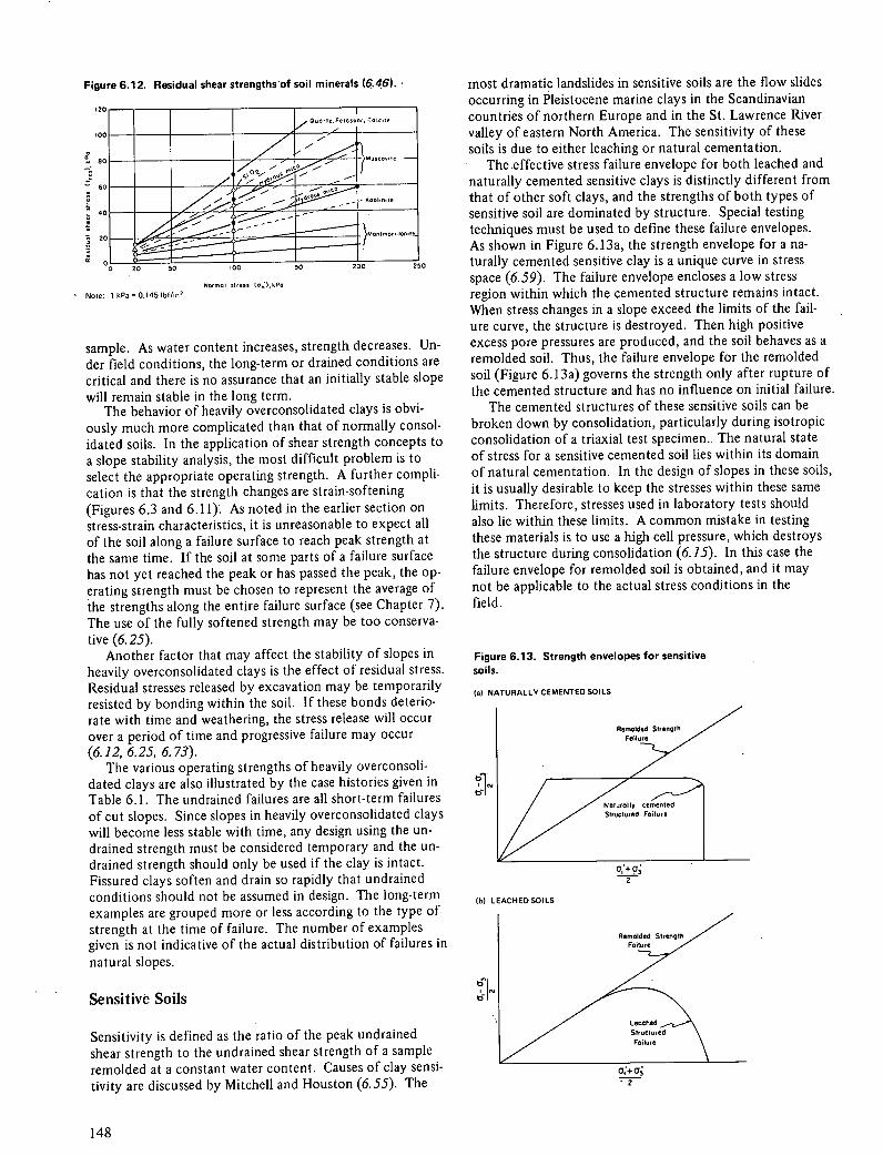
80

-. 60

40

20

0-- 0 20 50 00 150 200 250

00

20

U rr.

Figure 6.12. Residual shear strengths'of soil minerals (6.46).

Norma lot,,,, (Cr;). kPO

Note: 1 kPa = 0.145 IbI/:rr2

sample. As water content increases, strength decreases. Un-der field conditions, the long-term or drained conditions are critical and there is no assurance that an initially stable slope will remain stable in the long term.

The behavior of heavily overconsolidated clays is obvi-ously much more complicated than that of normally consol-idated soils. In the application of shear strength concepts to a slope stability analysis, the most difficult problem is to select the appropriate operating strength. A further compli-cation is that the strength changes are strain-softening (Figures 6.3 and 6.1 1). As noted in the earlier section on stress-strain characteristics, it is unreasonable to expect all of the soil along a failure surface to reach peak strength at the same time. If the soil at some parts of a failure surface has not yet reached the peak or has passed the peak, the op-erating strength must be chosen to represent the average of the strengths along the entire failure surface (see Chapter 7). The use of the fully softened strength may be too conserva-tive (6.25).

Another factor that may affect the stability of slopes in heavily overconsolidated clays is the effect of residual stress. Residual stresses released by excavation may be temporarily resisted by bonding within the soil. If these bonds deterio-rate with time and weathering, the stress release will occur over a period of time and progressive failure may occur (6.12, 6.25, 6.73).

The various operating strengths of heavily overconsoli-dated clays are also illustrated by the case histories given in Table 6.1. The undrained failures are all short-term failures of cut slopes. Since slopes in heavily overconsolidated clays will become less stable with time, any design using the un-drained strength must be considered temporary and the un-drained strength should only be used if the clay is intact. Fissured clays soften and drain so rapidly that undrained conditions should not be assumed in design. The long-term examples are grouped more or less according to the type of strength at the time of failure. The number of examples given is not indicative of the actual distribution of failures in natural slopes.

Sensitive Soils

Sensitivity is defined as the ratio of the peak undrained shear strength to the undrained shear strength of a sample remolded at a constant water content. Causes of clay sensi-tivity are discussed by Mitchell and Houston (6.55). The

most dramatic landslides in sensitive soils are the flow slides occurring in Pleistocene marine clays in the Scandinavian countries of northern Europe and in the St. Lawrence River valley of eastern North America. The sensitivity of these soils is due to either leaching or natural cementation.

The effective stress failure envelope for both leached and naturally cemented sensitive clays is distinctly different from that of other soft clays, and the strengths of both types of sensitive soil are dominated by structure. Special testing techniques must be used to define these failure envelopes. As shown in Figure 6.13a, the strength envelope for a na-turally cemented sensitive clay is a unique curve in stress space (6.59). The failure envelope encloses a low stress region within which the cemented structure remains intact. When stress changes in a slope exceed the limits of the fail-ure curve, the structure is destroyed. Then high positive excess pore pressures are produced, and the soil behaves as a remolded soil. Thus, the failure envelope for the remolded soil (Figure 6.13a) governs the strength only after rupture of the cemented structure and has no influence on initial failure.

The cemented structures of these sensitive soils can be broken down by consolidation, particularly during isotropic consolidation of a triaxial test specimen.. The natural state of stress for a sensitive cemented soil lies within its domain of natural cementation. In the design of slopes in these soils, it is usually desirable to keep the stresses within these same limits. Therefore, stresses used in laboratory tests should also lie within these limits. A common mistake in testing these materials is to use a high cell pressure, which destroys the structure during consolidation (6.15). In this case the failure envelope for remolded soil is obtained, and it may not be applicable to the actual stress conditions in the field.

Figure 6.13. Strength envelopes for sensitive

soils.

NATURALLY CEMENTED SOILS

Renoolded 5trençh FoIlo,e

NOIrOIIy cemented Stroclored Fo,Ire

LEACHED SOILS

148

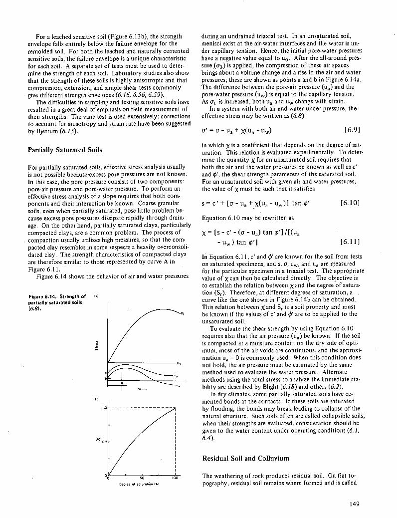
For a leached sensitive soil (Figure 6.13b), the strength envelope falls entirely below the failure envelope for the remolded soil. For both the leached and naturally cemented sensitive soils, the failure envelope is a unique characteristic for each soil. A separate set of tests must be used to deter-mine the strength of each soil. Laboratory studies also show that the strength of these soils is highly anisotropic and that compression, extension, and simple shear tests commonly give different strength envelopes (6.16, 6.56, 6.59).

The difficulties in sampling and testing sensitive soils have resulted in a great deal of emphasis on field measurement of their strengths. The vane test is used extensively; corrections to account for anisotropy and strain rate have been suggested by Bjerrum (6.15).

Partially Saturated Soils

For partially saturated soils, effective stress analysis usually is not possible because excess pore pressures are not known. In this case, the pore pressure consists of two components: pore-air pressure and pore-water pressure. To perform an effective stress analysis of a slope requires that both com-ponents and their interaction be known. Coarse granular soils, even when partially saturated, pose little problem be-cause excess pore pressures dissipate rapidly through drain-age. On the other hand, partially saturated clays, particularly compacted clays, are a common problem. The process of compaction usually utilizes high pressures, so that the com-pacted clay resembles in some respects a heavily overconsoli-dated clay. The strength characteristics of compacted clays are therefore similar to those represented by curve A in Figure 6.11.

Figure 6.14 shows the behavior of air and water pressures

Figure 6.14. Strength of (a)

partially saturated soils (6.8).

(b)

Degree of OOIa,OIiOn (5)

during an undrained triaxial test. In an unsaturated soil, menisci exist at the air-water interfaces and the water is un-der capillary tension. Hence, the initial pore-water pressures have a negative value equal to u0 . After the all-around pres-sure (cr3) is applied, the compression of these air spaces brings about a volume change and a rise in the air and water pressures; these are shown as points a and b in Figure 6.14a. The difference between the pore-air pressure (ua) and the pore-water pressure (u) is equal to the capillary tension. As a1 is increased, both ua and uw change with strain.

In a system with both air and water under pressure, the effective stress may be written as (6.8)

O'UUa +X(Ua _Uw) [6.9]

in which xis a coefficient that depends on the degree of sat-uration. This relation is evaluated experimentally. To deter-mine the quantity X for an unsaturated soil requires that both the air and the water pressures be known as well as c' and ', the shear strength parameters of the saturated soil. For an unsaturated soil with given air and water pressures, the value of x must be such that it satisfies

s=C'+[a_Ua+x(Ua-uw)] tan ct.' [6.10]

Equation 6.10 may be rewritten as

x=[s-c'-(a-ua) tan -u) tan '] [6.11]

In Equation 6.11, c' and Or are known for the soil from tests on saturated specimens, and s, a, u, and ua are measured for the particular specimen in a triaxial test. The appropriate value ofx can then be calculated directly. The objective is to establish the relation between X and the degree of satura-tion (Sr). Therefore, at different degrees of saturation, a curve like the one shown in Figure 6.14b can be obtained. This relation between X and Sr is a soil property and must be known if the values of c' and Or are to be applied to the unsaturated soil.

To evaluate the shear strength by using Equation 6.10 requires also that the air pressure (ua ) be known. If the soil is compacted at a moisture content on the dry side of opti-mum, most of the air voids are continuous, and the approxi-mation ua = 0 is commonly used. When this condition does not hold, the air pressure must be estimated by the same method used to evaluate the waterpressure. Alternate methods using the total stress to analyze the immediate sta-bility are described by Blight (6.18) and others (6.2).

In dry climates, some partially saturated soils have ce-mented bonds at the contacts. If these soils are saturated by flooding, the bonds may break leading to collapse of the natural structure. Such soils often are called collapsible soils; when their strengths are evaluated, consideration should be given to the water content under operating conditions (6.1, 6.4).

Residual Soil and Colluvium

The weathering of rock produces residual soil. On flat to-pography, residual soil remains where formed and is called

149

eluvium. It may develop to great depths, and natural or human-made slopes may be cut into the eluvium. Natural rock slopes also weather to produce residual soil, which will be acted on by forces of gravity. The soil and rock de-bris that moves down the face of a slope is called colluvium.

Residual soils have a wide range of properties, depending on the parent material and the degree of weathering (6.29, 6.53). In the initial stages of weathefing, coarse rock frag-ments are produced; the ultimate product of weathering is clay. Between these extremes is usually a mixture of grain sizes, and the behavior of residual soils is similar to that de-scribed in previous sections for the soils with similar particle size distributions. Some residual soils are also cemented. More detailed information about residual soils and their properties is given by Deere and Patton (6.29).

Colluvium presents some particular slope stability prob-lems (6.27, 6.53). The extremely heterogeneous nature of the material makes sampling and testing difficult. In some cases, loose structure and large grain size result in high values of permeability. This characteristic is often accentuated by the presence of less permeable layers immediately below the colluvium. Under this condition, infiltrating surface water flows through the colluvium, generally parallel to the slope, and the consequence is a decrease in stability. Where large landslides have occurred in the past, slickensides may be found along old slip surfaces. The shear strength along those surfaces may be close to the residual shear strength.

Rocks

The shear strength of rock masses is almost always deter-mined by the configuration of the joints and the nature of the joint surfaces (6.28), as explained in Chapter 9. Numer-ous theoretical and laboratory studies (6.5, 6.6, 6.32, 6.44) have been conducted to evaluate the apparent strength of rock masses with closed block joints (Figure 6.1 5a). These studies show that failure of jointed rock depends on several geometrical parameters, including orientation and spacing of joints, joint characteristics, and stress state, and on the strengths of the intact rock and the joint filling (see Chap-ter 9). In many field problems, the spacing of joints is small relative to the height of slope and the size of the fail-ure surface.

Under these conditions, failure of a jointed rock mass in-volves the interaction of sliding along the joints, dilatancy, separation and rotation of the blocks, and possible fracture of the intact rock. Most experimental studies indicate that for this type of failure the failure envelope for jointed rocks is nonlinear (Figure 6.15b). Each situation is unique, so such curves must be determined experimentally for the par-ticular situation. With certain joint orientations, failure will occur along a single joint or joint set. This commonly hap-pens in the field when the orientation of joints or other dis-continuities is close to that of the slope so that block or wedge sliding becomes possible. To analyze this condition requires that the strength of the rock along the joints be known.

The shear strength of a joint or other discontinuity de-pends on the characteristics of the joint. The strength of a freshly fractured joint surface will be different from that of a joint that is highly weathered and full of debris. Because fresh rock surfaces may weather rapidly, it is important to

recognize the potential for change in the strength of a joint or joint system during the lifetime of an engineering project. Experimental measurements of joint strengths can be made by the use of laboratory or field direct shear tests.

A stress-displacement curve of a rough joint is similar to curve A in Figure 6.3. The peak strength (point a) is ob-tained when the large projections along the joint are sheared off. Beyond this point, the strength decreases and ap-proaches the residual strength. The residual strength repre-sents the strength of the joint after the projections have been sheared off.

Typical results of drained tests in which effective stresses could be measured are given in Table 6.2. The strength is almost always frictional in character, even when large amounts of debris are present in the joint.

Figure 6.15. Strength of rock masses with closed block joints

(6.32).

(a) JOINTED ROCK MASS (b( FAILURE ENVELOPE

I I II I I peak strength criterion for joint

Table 6.2. Residual angle of friction obtained from sandblasted rough-sawed, and residual surfaces of various rocks (6.5).

Rock Moisture a (kPa) Or (deg)

Amphibolite Dry 98 to 4 100 32 Basalt Dry 98 to 8 300 35 to 38

Wet 98 to 7700 31 to36 Conglomerate Dry 294 to 3 300 35 Chalk Wet 0 to 390 30 Dolomite Dry 98 to 7 100 31 to 37

Wet 98to7 100 27to35 Gneiss (schistose) Dry 98 to 7 900 26 to 29

Wet 98 to 7 700 23 to 26 Granite

Fine grained Dry 98 to 7 400 31 to 35 Wet 98to7 300 29to31

Coarse grained Dry 98 to 7 200 31 to 35 Wet 98to7400 31 to 33

Limestone Dry 0 to 490 33 to 39 Wet 0 to 490 33 to 36 Dry 98to7 000 37to40 Wet 98 to 7 000 35 to 38 Dry 98to8 100 37 to 39 Wet 98to8100 35

Porphyry Dry Oto 980 31 Dry 4021 to 13000 31

Sandstone Dry 0 to 490 26 to 35 Wet 0 to 490 25 to 33 Wet 0 to 290 29 Dry 294 to 2 900 31 to 33 Dry 98to6900 32to34 Wet 98to7 200 31 to34

Shale Wet 0 to 290 27 Siltstone Wet 0 to 290 31

Dry 98to7400 31to33 Wet 98to7 100 27 to 31

Slate Dry Oto 1 100 25 to 30

Note: 1 kPa = 0.145 lbf/in2

150

SOIL BEHAVIOR UNDER REPEATED LOADS

Ground motion during earthquakes subjects slopes to re-peated loading. Consider again the slope shown in Figure 6.2. The stresses shown are those acting under static condi-tions. When subjected to earthquake motions, additional stresses of a cyclic nature are induced in the soil. The na-ture of the stresses at point b is shown in Figure 6.16. For simplicity, it is assumed here that the ground motion during an earthquake consists only of shear waves propagating ver-tically through the soil. The cyclic stress (Te) during an earthquake usually consists of a series of irregular pulses, as shown by the stress-time plot in Figure 6.16c.

Several methods can be used to calculate the response of a slope to repeated loading (see Chapter 7). Some require use of a constitutive relation for the soil, and others use the soil strength under dynamic loading. When most natural soils are subjected to earthquake or other types of repeated loading, the resulting fluctuations in stress produce irreversi-ble changes in pore pressures. These produce long-term and short-term changes in soil strength, and this must be recog-nized in the design of slopes to resist earthquakes and other kinds of dynamic loads. Strength changes in soils subjected

Figure 6.16. Stresses under dynamic loading.

al INITIAL STATE (bi EARTHQUAKE Ic) EARTHQUAKE STRESS OF STRESS STRESS VERSUS TIME

Time

Stress-Strain Characteristics

to repeated loading have been the subject of extensive re-search in recent years (6.3, 6.23, 6.58, 6.60, 6.62). In some of those studies, pore pressures and effective stresses were de-termined (6.23, 6.60, 6.65). In most cases, however, only total stress analysis was possible because rapid rates of load-ing did not permit the measurement of pore pressures. The present state of knowledge is based on contributions from both types of study.

Repeated Load Tests

Laboratory tests to measure soil strength under repeated loads can be made with the triaxial cell or the simple shear apparatus (6.63). Because of difficulties in interpretation and analysis of random loads, such as those shown in Figure 6.16c, current laboratory tests usually employ regular stress pulses. The shape of the stress pulse inay be square or tri-angular or sinusoidal. In the simple shear test, the stress con-ditions shown in Figure 6.16a and b can be simulated. The sample is consolidated under the static stresses (a and r), and the peak shear stress during an earthquake is T e Hence, the cyclic stress (Te - r) is applied (Figure 6.16b).

The triaxial test cannot simulate the rotation of principal axes under earthquake loading; therefore, this phenomenon must be ignored. The test procedures are similar to those for static tests discussed in the section on the triaxial test. The principal stresses under static loading are (71 and 03.

The sample is consolidated first under the static stresses (Figure 6.17a), after which the cyclic stresses (01 - 01 and

- 03 ) are applied (Figure 6.17b). Because of the relatively short duration of earthquakes, the cyclic stresses are usually applied in the undrained condition. If the soil is saturated, the effective stress does not change under an applied hydro-static stress. Thus, the loading can be simplified to fluctua-tion in axial stress only (Figure 6.17c).

Model tests of soil slopes and embankments loaded by means of a shaking table have also been used in design (6.3).

Figure 6.17. Dynamic triaxial test conditions.

(a) INITIAL STATE (b( CYCLIC OR (c) CYCLIC OR

OF STRESS EARTHQUAKE EARTHQUAKE STRESS STRESS

Figure 6.18. Stress-strain relation for cyclic loading.

Shear strain

Under repeated loading, the strain produced by a given peak stress is usually different from that produced by a static stress of the same magnitude. Strain continues to increase with successive cycles and depends on several factors, but particularly on the duration of the load, the magnitude of the stresses, and the number of load cycles. A typical stress-strain curve is shown in Figure 6.18. At small strain, the cyclic stress produces the hysteresis ioop ab. The shear modulus and damping are equal to the slope of ab and the area enclosed by the ioop respectively. At large Strains, the hysteresis ioop is cd. The shear modulus decreases with strain, and the damping increases with strain. Estimates of the shear modulus and damping factor can be made on the basis of available empirical data (6.35, 6.65). For dry soils and soils with low degrees of saturation, the modulus tends to increase with cycles of loading. Figure 6.19 compares soil behavior under repeated loading (curves B and C) with that under a monotonically increasing stress (curve A). The stress-strain relation and pore pressure under repeated load-ing depend on stress level, stress history, type of loading, number of stress cycles, and degree of saturation.

When a saturated soft clay or loose sand is subjected to a

151

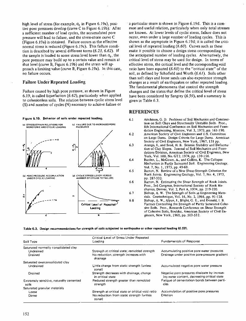
Critical Level of Loading

PORE PRESSURE ACCUMULATION UNDER CYCLIC LOADING

O'3

(di CYCLIC STRESS LEVER VERSUS NUMBER OF CYCLES TO FAILURE

high level of stress (for example, or, in Figure 6.19a), posi-tive pore pressures develop (curve C in Figure 6.19b); After a sufficient number of load cycles, the accumulated pore pressure will lead to failure, and the stress-strain curve C (Figure 6.19a) is obtained. Failure occurs as the effective normal stress is reduced (Figure 6.19c). This failure condi-tion is described by several different terms (6.23, 6.62). If the sample is loaded to some stress level lower than a, the pore pressure may build up to a certain value and remain at that level (curve B, Figure 6.19b) and the strain will ap-proach a limiting value (curve B, Figure 6.19a). In this case, no failure occurs.

Failure Under Repeated Loading

Failure caused by high pore pressure, as shown in Figure 6.19, is called liquefaction (6.62), particularly when applied to cohesionless soils. The relation between cyclic stress level (S) and number of cycles (N) necessary to achieve failure or

Figure 6.19. Behavior of soils under repeated loading.

STRESS-STRAIN RELATIONS FOR (c) FAILURE DUE TO INCREASED PORE MONOTONIC AND CYCLIC LOADING PRESSURES

a particular strain is shown in Figure 6.19d. This is a com-mon and useful relation, particularly when only total stresses are known. At lower levels of cyclic stress, failure does not occur, even under a large number of loading cycles. This is shown as the asymptote in Figure 6.19d; it is called the criti-cal level of repeated loading (6.60). Curves such as these make it possible to choose a design stress corresponding to the anticipated number of loading cycles. Alternatively, the critical level of stress may be used for design. In terms of effective stress, the critical level and the corresponding void ratio have been equated (6.60) to the "critical state" of the soil, as defined by Schofield and Wroth (6.61). Soils other than soft clays and loose sands can also experience strength changes as a result of earthquakes or other repeated loading. The fundamental phenomena that control the strength changes and the states that define the critical level of stress have been considered by Sangrey (6.59), and a summary is given in Table 6.3.

REFERENCES

6.1 Aitchison, G. D. Problems of Soil Mechanics and Construc- tion on Soft Clays and Structurally Unstable Soils. Proc., 8th International Conference on Soil Mechanics and Foun-dation Engineering, Moscow, Vol. 3, 1973, pp. 161-190.

6.2 American Society of Civil Engineers and U.S. Committee on Large Dams. Design Criteria for Large Dams. American Society of Civil Engineers, New York, 1967, 131 pp.

6.3 Arango, I., and Seed, H. B. Seismic Stability and Deforma- tion of Clay Slopes. Journal of Soil Mechanics and Foun-dations Division, American Society of Civil Engineers, New York, Vol. 100, No. GT2, 1974, pp. 139-156.

6.4 Barden, L., McGown, A., and Collins, K. The Collapse Mechanism in Partly Saturated Soil. Engineering Geology, Vol. 7, No. 1, 1973, pp. 49-60.

6.5 Barton, N. Review of a New Shear-Strength Criterion for Rock Joints. Engineering Geology, Vol. 7, No. 4, 1973, pp. 287-332.

6.6 Barton, N. Estimating the Shear Strength of Rock Joints. Proc., 3rd Congress, International Society of Rock Me-chanics, Denver, Vol. 2, Part A, 1974, pp. 2 19-220.

6.7 Bishop, A. W. The Strength of Soils as Engineering Mate- rials. Geotechnique, Vol. 16, No. 2, 1966, pp. 91-128.

6.8 Bishop, A. W., Alpan, I., Blight, G. E., and Donald, I. B. Factors Controlling the Strength of Partly Saturated Cohe-sive Soils. Proc., Research Conference on Shear Strength of. Cohesive Soils, Boulder, American Society of Civil En-gineers, New York, 1960, pp. 503-53 2.

Table 6.3. Design recommendations for strength of soils subjected to earthquake or other repeated loading (6.59).

Critical Level of Stress Under Repeated Soil Type Loading Fundamentals of Response

Strength at critical state; remolded strength Accumulating positive pore water pressures No reduction; strength increases with Drainage under positive pore-pressure gradient drainage

Little change from static strength (unless Accumulated negative pore water pressure zonal)

Strength decreases with drainage, change Negative pore pressures dissipate by increas- in critical state ing water content, decreasing critical state

Reduced strength greater than remolded Fatigue of cementation bonds between parti- strength des

Strength at critical state or critical void ratio Accumulation of positive pore pressures No reduction from static strength (unless Dilation zonal)

Saturated normally consolidated clay Undrained Drained

Saturated overconsolidated clay lJndrained

Drained

Extremely sensitive, naturally cemented soils

Saturated granular materials Loose Dense

152

6.9 Bishop, A. W., and Bjerrum, L. The Relevance of the Tri- axial Test to the Solution of Stability Problems. Proc., Re-search Conference on Shear Strength of Cohesive Soils, Boulder, American Society of Civil Engineers, New York, 1960, pp. 437-501.

6.10 Bishop, A. W., and Henkel, D. J. The Measurement of Soil Properties in the Triaxial Test. Edward Arnold Publishers, London, 1962, 227 pp.

6.11 Bishop, A. W., Webb, D. L., and Lewin, P. I. Undisturbed Samples of London Clay From the Ashford Common Shaft. Geotechnique, Vol. 15, No. 1, 1965, pp. 1-3 1.

6.12 Bjerrum, L. Progressive Failure in Slopes of Overconsoli- dated Plastic Clay and Clay Shales. Journal of Soil Me-chanics and Foundations Division, American Society of Civil Engineers, New York, Vol. 93, No. SM5, 1967, pp. 3-49.

6.13 Bjerrum, L. Closure to Main Session 5. Proc., 7th Interna- tional Conference on Soil Mechanics and Foundation En-gineering, Mexico City, Vol. 3, 1969, pp. 410-414.

6.14 Bjerrum, L. Embankments on Soft Ground. Proc., Spe- cialty Conference on Performance of Earth and Earth-Supported Structures, Purdue Univ., Lafayette, Ind., American Society of Civil Engineers, New York, Vol. 2, 1972, pp. 1-54.

6.15 Bjerrum, L. Problems of Soil Mechanics and Construction on Soft Clays and Structurally Unstable Soils. Proc., 8th International Conference on Soil Mechanics and Founda-tion Engineering, Moscow, Vol. 3, 1973, pp. 111-159.

6.16 Bjerrum, L., and Kenney, T. C. Effect of Structure on the Shear Behavior of Normally Consolidated Quick Clays. Proc., Geotechnical Conference on Shear Strength Proper-ties of Natural Soils and Rocks, Norwegian Geotechnical Institute, Oslo, 1967, Vol. 2, pp. 19-27.

6.17 Bjerrum, L., and Landva, A. Direct Simple-Shear Tests on a Norwegian Quick Clay. Geotechnique, Vol. 16, No. 1, 1966, pp. 1-20.

6.18 Blight, G. E. Effective Stress Evaluation for Unsaturated Soils. Journal of Soil Mechanics and Foundations Division, American Society of Civil Engineers, New York, Vol. 93, No. SM2, 1967, pp. 125-148.

6.19 Brand, E. W., Muktabhant, C., and Taechathummarak, A. Load Tests on Small Foundations in Soft Clay. Proc., Spe-cialty Conference on Performance of Earth and Earth-Supported Structures, Purdue Univ., Lafayette, Ind., American Society of Civil Engineers, New York, Vol. 1, Part 2, 1972, Pp. 903-928.

6.20 Brooker, E. W. and Ireland, H. 0. Earth Pressures at Rest Related to Stress History. Canadian Geotechnical Journal, Vol. 2, No. 1, 1965, pp. 1-15.

6.21 Cadling, L., and Odenstad, S. The Vane Borer: An Ap- paratus for Determining the Shear Strength of Clay Soils in the Ground. Proc., Royal Swedish Geotechnical Insti-tute, No. 2, 1950, 88 pp.

6.22 Casagrande, A., and Wilson, S. D. Effect of Rate of Load- ing on the Strength of Clays and Shales at Constant Water Content. Geotechnique, Vol. 2, No. 3, 1951, pp. 25 1-263.

6.23 Castro, G. Liquefaction and Cyclic Mobility of Saturated Sands. Journal of Geotechnical Engineering Division, American Society of Civil Engineers, New York, Vol. 101, No. GT6, 1975, pp. 55 1-569.

6.24 Chandler, R. J. Lias Clay: The Long-Term Stability of Cutting Slopes. Geotechnique, Vol. 24, No. 1, 1974, pp. 21-3 8.

6.25 Chandler, R. J., and Skempton, A. W. The Design of Permanent Cutting Slopes in Stiff Fissured Clays. Geotech-nique, Vol. 24, No. 4, 1974, pp. 457466.

6.26 Conlon, R. J., Tanner, R. G., and CoIdwell, K. L. The Geotechnical Design of the Townline Road-Rail Tunnel. Canadian Geotechnical Journal, Vol. 8, No. 2, 1971, pp. 299-3 14.

6.27 D'Appolonia, E., Alperstein, R., and D'Appolonia, D. J. Behavior of a Colluvial Slope. Journal of Soil Mechanics and Foundations Division, American Society of Civil Engi-neers, New York, Vol. 93, No. SM4, 1967, pp. 447-473.

6.28 Deere, D. U., Hendron, A. J., Jr., Patton, F. D., and Cording, E. J. Design of Surface and Near-Surface Con-

struction in Rock. In Failure and Breakage of Rock (Fairhurst, C., ed.), Proc., 8th Symposium on Rock Me-chanics, American Institute of Mining, Metallurgy and Petroleum Engineers, New York, 1967, pp. 237-302.

6.29 Deere, D. U., and Patton, F. D. Slope Stability in Residual Soils. Proc., 4th Pan-American Conference on Soil Me-chanics and Foundation Engineering, San Juan, American Society of Civil Engineers, New York, Vol. 1, 1971, pp. 87-170.

6.30 Duncan, J. M., and Seed, H. B. Strength Variation Along Failure Surfaces in Clay. Journal of Soil Mechanics and Foundations Division, American Society of Civil Engi-neers, New York, Vol. 92, No. SM6, 1966, pp. 81-104.

6.31 Esu, F. Short-Term Stability of Slopes in Unweathered Jointed Clays. Geotechnique, Vol. 16, No. 4, 1966, pp. 32 1-3 28.

6.32 Goodman, R. E. Methods of Geological Engineering in Dis- continuous Rocks. West Publishing, St. Paul, 1976,472 pp.

6.33 Green, G. E., and Bishop, A. W. A Note on the Drained Strength of Sand Under Generalized Strain Conditions. Geotechnique, Vol. 19, No. 1, 1969, pp. 144-149.

6.34 Hansbo, S. A New Approach to the Determination of the Shear Strength of Clay by the Fall-Cone Test. Proc., Royal Swedish Geotechnical Institute, No. 14, 1957, 47 pp.

6.35 Hardin, B. 0., and Drnevich, V. P. Shear Modulus and Damping in Soils: Measurement and Parameter Effects. Journal of Soil Mechanics and Foundations Division, American Society of Civil Engineers, New York, Vol. 98, No. SM6, 1972, pp. 603-624.

6.36 Henkel, D. J. Investigations of Two Long-Term Failures in London Clay Slopes at Wood Green and Northolt. Proc., 4th International Conference on Soil Mechanics and Foun-dation Engineering, London, Vol. 2, 1957, pp. 315-3 20.

6.37 Henkel, D. J. The Shear Strength of Saturated Remolded Clays. Proc., Research Conference on Shear Strength of Cohesive Soils, Boulder, American Society of Civil Engi-neers, New York, 1960, pp. 533-554.

6.38 Henkel, D. J., and Skempton, A. W. A Landslide at Jack- field, Shropshire, in a Heavily Overconsolidated Clay. Geotechnique, Vol. 5, No. 2, 1955, pp. 131-137.

6.39 Henkel, D. J., and Wade, N. H. Plane Strain Tests on a Saturated Remolded Clay. Journal of Soil Mechanics and Foundations Division, American Society of Civil Engineers, New York, Vol. 92, No. SM6, 1966, pp. 67-80.

6.40 Henkel, D. J., and Yudhbir. The Stability of Slopes in the Siwailk Rocks in India. Proc., 1st Congress, International Society of Rock Mechanics, Lisbon, Vol. 2, 1966, pp. 16 1-16 5.

6.41 Hill, R. The Mathematical Theory of Plasticity. Oxford Univ. Press, London, 1950, 355 pp.

6.42 Holtz, W. G., and Gibbs, H. J. Triaxial Shear Tests on Pervious Gravelly Soils. Journal of Soil Mechanics and Foundations Division, American Society of Civil Engi-neers, New York, Vol. 82, No. SM!, 1956, pp. 1-22.

6.43 Ireland, H. 0. Stability Analysis of the Congress Street Open Cut in Chicago. Geotechnique, Vol. 4, No. 4, 1954, pp. 163-168.

6.44 Jaeger, J. C. Friction of Rocks and Stability of Rock Slopes. Geotechnique, Vol. 21, No. 1, 1971, pp. 97-134.

6.45 Kankare, E. Failures at Kimola Floating Canal in Southern Finland. Proc., 7th International Conference on Soil Me-chanics and Foundation Engineering, Mexico City, Vol. 2, 1969, pp. 609-616.

6.46 Kenney, T. C. The Influence of Mineral Composition on the Residual Strength of Natural Soils. Proc., Geotechni-cal Conference on Shear Strength Properties of Natural Soils and Rocks, Norwegian Geotechnical Institute, Oslo, 1967, Vol. 1, pp. 123-129.

6.47 Kjaernsli, B., and Simons, N. Stability Investigations of the North Bank of Drammen River. Geotechnique, Vol. 12, No. 2, 1962, pp. 147-167.

6.48 Kwan, D. Observations of the Failure of a Vertical Cut in Clay at Welland, Ontario. Canadian Geotechnical Journal, Vol. 9, No. 3, 1971, pp. 283-298.

6.49 Ladd, C. C. Test Embankment on Sensitive Clay. Proc., Specialty Conference on Performance of Earth and Earth-

153

6.50

6.51

6.52

6.53

6.54

6.55

6.56

c ci

6.58

6.59

6.60

6.61

6.62

6.63

Supported Structures, Purdue Univ., Lafayette, md., 6.64 Sevaldson, R. A. The Slide in Lodalen, October 6, 1954. American Society of Civil Engineers, New York, Vol. 1, Geotechnique, Vol. 6, No.4, 1956, pp. 167-182. Part 1, 1972, pp. 101-128. 6.65 Silver, M. L., and Seed, H. B. Deformation Characteristics Ladd, C. C., and Foott, R. New Design Procedure for Sta- of Sands Under Cyclic Loading. Journal of Soil Mechanics bility of Soft Clays. Proc., Journal of Geotechnical Engi- and Foundations Division, American Society of Civil Engi- neering Division, American Society of Civil Engineers, New neers, New York, Vol. 97, No. SM8, 1971, pp. 1081-1098. York, Vol. 100, No. GT7, 1974, pp 763-786. 6.66 Singh, R., Henkel, D. J., and Sangrey, D. A. Shear and K0 Ladd, C. C., and Lambe, T.W. The Strength of "Undis- Swelling of Overconsolidated Clay. Proc., 9th International turbed" Clay Determined From Undrained Tests. Proc., Conference on Soil Mechanics and Foundation Engineering, Symposium on Laboratory Shear Testing of Soils, Ottawa, Moscow, Vol. 1, Part 2, 1973, pp. 367-376. American Society for Testing and Materials, Philadelphia, 6.67 Skempton, A. W. The Pore-Pressure Coefficients A and B. Special Technical PubI. 361, 1964, pp. 342-371. Geotechnique, Vol.4, No.4, 1954, pp. 143-147. Lo, K. Y. The Operational Strength of Fissured Clays. 6.68 Skempton, A. W. Horizontal Stresses in an Over- Geotechnique, Vol. 20, No. 1, 1970, pp. 57-74. Consolidated Eocene Clay. Proc., 5th International Con- Lumb, P. The Properties of Decomposed Granite. Geotech- ference on Soil Mechanics and Foundation Engineering, nique, Vol. 12, No. 3, 1962, pp. 226-243. Paris, Vol. 1, 1961, pp. 351-357. Marsland, A. The Shear Strength of Stiff Fissured Clays. 6.69 Skempton, A. W. Long-Term Stability of Clay Slopes. In Stress-Strain Behavior of Soils (Foulis, G. T., ed.), Geotechnique, Vol. 14, No. 2, 1964, pp. 77-101. Proc., Roscoe Memorial Symposium, Cambridge Univ. 6.70 Skempton, A. W. First-Time Slides in Over-Consolidated Press, 1971, pp. 59-78. Clays. Geotechnique, Vol. 20, No. 3, 1970, pp. 320-324. Mitchell, J. K., and Houston, W. N. Causes of Clay Sensi- 6.71 Skempton, A. W., and Brown, J. D. A Landslide in Boulder tivity. Journal of Soil Mechanics and Foundations Divi- Clay at Selset, Yorkshire. Geotechnique, Vol. 11, No.4, sion, American Society of Civil Engineers, New York, Vol. 1961, pp. 280-293. 95, No. SM3, 1969, pp. 845-871. 6.72 Skempton, A. W., and Golder, H. Q. Practical Examples of Mitchell, R. J., and Wong, K. K. The Generalized Failure the 0 = 0 Analysis of Stability of Clays. Proc., 2nd Inter- of an Ottawa Valley Champlain Sea Clay. Canadian Geo- national Conference on Soil Mechanics and Foundation En- technical Journal, Vol. 10, No. 4, 1973, pp. 607-616. gineering, Rotterdam, Vol. 2, 1948, pp. 63-70. iviorgenstern, N. R., and Tchalenko, J. S. Microscopic 6.73 Skempton, A. W., and Hutchinson, J. N. Stability of Nat- Structures in Kaolinite Subjected to Direct Shear. Geo- ural Slopes and Embankment Foundations. Proc., 7th technique, Vol. 17, No.4, 1967, pp. 309-328. International Conference on Soil Mechanics and Founda- Sangrey, D. A. Changes in Strength of Soils Under Earth- lion Engineering, Mexico City, State-of-the-Art Vol., quake and Other Repeated Loading. In Earthquake Engi- 1969, pp. 291-340. neering (Cherry, S., ed.), Proc., 1st Canadian Conference 6.74 Skempton, A. W., and La Rochelle, P. The Bradwell Slip: on Earthquake Engineering, Univ. of British Columbia, A Short-Term Failure in London Clay. Geotechnique, Vol. Vancouver, 1972, pp. 82-96. 15, No. 3, 1965, pp. 221-242.

Sangrey, D. A. Naturally Cemented Sensitive Soils. Geo- 6.75 Skempton, A. W., and Petley, D. J. The Strength Along

technique, Vol. 22, No. 1, 1972, pp. 139-152. Structural Discontinuities in Stiff Clays. Proc., Geotechni-

Sangrey, D. A., Henkel, D. J., and Esrig, M. I. The Effec- cal Conference on Shear Strength Properties of Natural

tive Stress Response of a Saturated Clay Soil to Repeated Soils and Rocks, Norwegian Geotechnical Institute, Oslo,

Loading. Canadian Geotechnical Journal, Vol. 6, No. 3 Vol. 2, 1967, pp. 29-46.

1969, pp. 241-252. 6.76 Vargas, M., and Pichler, E. Residual Soil and Rock Slides

Schofield, A., and Wroth, P. Critical State Soil Mechanics, in Santos (Brazil). Proc., 4th International Conference on

McGraw-Hill, New York, 1968, 310 pp. Soil Mechanics and Foundation Engineering, London, Vol.

Seed, H. B. Landslides During Earthquakes Due to Soil 2, 1957, pp. 394-398. Liquefaction. Journal of Soil Mechanics and Foundations 6.77 VesIc, A. S., and Clough, G. W. Behavior of Granular Ma-

Division, American Society of Civil Engineers, New York, terials Under High Stresses. Journal of Soil Mechanics and

Vol. 94, No. SM5, 1968, pp. 10554122. Foundations Division, American Society of Civil Engineers,

Seed, H. B., and Peacock, W. H. Test Procedures for Mea- New York, Vol. 94, No. SM3, 1968, pp. 661-668.

suring Soil Liquefaction Characteristics. Journal of Soil 6.78 Ward, W. H., Marsland, A., and Samuels, S. G. Properties

Mechanics and Foundations Division, American Society of the London Clay at the Ashford Common Shaft: In

of Civil Engineers, New York, Vol. 97, No. SM8, 1971, Situ and Undrained Strength Tests. Geotechnique, Vol.

pp. 1099-1119. 15, No.4, 1965, pp. 321-344.

154

Chapter 7

Methods of Stability Analysis N. R. Morgenstern and Dwight A. Sangrey

The functional design of a slope requires that the deforma-tions of the earth mass constituting the slope be limited to amounts governed by the use of the ground on or adjacent to the slope. If there is no particular development near the slope, the allowable deformations can be large, provided that the earth mass does not fail with resulting uncontrolled de-formations. On the other hand, if there are structures close to the slope or services buried within the soil beneath the slope, smaller deformations may result in unacceptable per-formance, and functional design would require that the aver-age stress level in the earth mass be lower in this case than in the case in which no development is near the slope.

Analysis is an important component of design, which also includes other equally important components, such as drain-age considerations and construction control. In analysis, the mechanical properties of the earth materials are evaluated quantitatively to arrive at a configuration consistent with the performance requirements of the slope. In this chapter, the relative roles of limit equilibrium and deformation anal-yses are discussed. The principles of limit equilibrium anal-ysis are outlined, and details of the techniques commonly used in practice are given with examples. Both soil and rock slopes are discussed. The chapter concludes with a brief dis-cussion of deformation analysis as it is currently used. Other aspects of design are discussed in Chapters 8 and 9.

ROLES OF LIMIT EQUILIBRIUM AND DEFORMATION ANALYSES

Although the performance of a slope often is dictated by allowable deformations, quantitative prediction of displace-ments of the slope is seldom undertaken routinely. Instead, analyses are made by the use of limit equilibrium methods, and the performance of a slope is evaluated in terms of its factor of safety (F). There are several reasons for this.

For realistic configurations commonly encountered in design, particularly in the design of cuts and natural slopes,

a method of analysis that predicts deformations to an ac-ceptable degree of accuracy would likely have to include

Representative stress-strain relations, including be-havior from peak to residual shear strengths;

Anisotropy; Variable pore pressure distributions; Nonhomogeneity arising from variation of material

properties with depth, layering, and discontinuities; Influence of initial stress; and Construction sequence.

Most of these factors have a major influence on the behavior of a slope; and, even if proven analytical techniques were readily available to predict deformations, the determination of all of these factors in a manner suitable for a deformation analysis would seldom be a practical undertaking. Appro-priate analytical techniques are not yet at hand, although im-pressive progress is being made by means of finite element methods.

The situation is not so pessimistic with regard to fills. Representative stress-strain relations within the working range can be specified with a greater degree of reliability for embankments than for cuts or natural slopes. Moreover, since the soil mass is a processed material, it is generally more uniform and homogeneous than naturally occurring deposits. Hence, deformation analysis has a role in the de-sign of embankment slopes, and that role will be reviewed in greater detail later in this chapter.

The stabilities of natural slopes, cut slopes, and fill slopes are commonly analyzed by limit equilibrium methods. These methods take into account all of the major factors that in-fluence the shearing resistance of a soil or rock mass; this is one of their significant advantages. In addition, they are simpler than deformation analyses. However, because the actual stress-strain relations are not used in the analysis, limit equilibrium methods do not result in calculation of ex-

155

pected deformations. Deformations are controlled by de-signing for an appropriate factor of safety. At least to this extent, the use of limit equilibrium methods of analysis is semiempirical. The factor of safety cannot be measured ex-cept when the slope is failing, in which case it is known to be unity. As noted previously, there are many instances in which the precise deformations in a slope are of little con-cern, provided the material stays in place. In such cases, it is entirely appropriate to undertake analyses with limit equilib-rium methods; however, regardless of the complexity of the method employed, the empirical nature of the design criteria should be borne in mind.

LIMIT EQUILIBRIUM ANALYSIS

Limit equilibrium methods for slope stability analysis have been used for several decades, and numerous techniques have been developed. Limit equilibrium analysis is used in design to determine the magnitude of the factor of safety. When a slope has failed, however, the factor of safety is unity, and the analysis can then be used to estimate the average shear-ing resistance along the failure surface or along part of the failure surface if the shearing resistance is assumed to be known along the remainder. Regardless of the specific pro-cedure for carrying out the computations, the following principles are common to all methods of limit equilibrium analysis.

A slip mechanism is postulated. This is done without any major kinematic restriction except that the mechanism be feasible and sensible. In the simpler configurations, the slopes are assumed to fail along planes or circular sliding sur-faces. When conditions are not uniform, more complex shapes are known to be appropriate, and analyses have been developed to handle surfaces of arbitrary shape.

The shearing resistance required to equilibrate the as-sumed slip mechanism is calculated by means of statics. The physical concepts used here are that the potential slip mass is in a state of limiting equilibrium and that the failure crite-rion of the soil or rock is satisfied everywhere along the pro-posed surfaces. Various methods differ in the degree to which the conditions for equilibrium are satisfied, and some common methods of analysis violate conditions of static equilibrium. This is an important factor in evaluating the rigor of any method.

The calculated shearing resistance required for equilib-rium is compared with the available shear strength. This comparison is made in terms of the factor of safety, which will be defined more precisely below.

The mechanism with the lowest factor of safety is found by iteration. For example, if it is assumed that the slip surface is circular, a search is made for the critical slip circle. When the position of the slip surface is dictated by a dominant weakness, such as sheared clay at residual strength, other trials are unnecessary.

The factor of safety should be defined as clearly as pos-sible and its role understood. The definition used here is as follows:

The factor of safety is that factor by which the shear strength parameters may be reduced in order to bring the slope into a state of limiting equilibrium along a given slip surface.

According to this definition, the factor of safety relates to the strength parameters and not to the strength itself, which in the case of an effective stress analysis depends on the ef-fective normal stress as well. Moreover, this definition im-plies that the factor of safety is uniform along the entire slip surface.

Other definitions of the factor of safety are also used in geotechnical engineering. For example, the factor of safety is commonly defined as the ratio of a disturbing moment to a restoring moment when the moment equilibrium about the center of rotation of a slip circle is under consideration. This definition is not convenient when slip surfaces are noncircu-lar and therefore is of limited applicability. It is equivalent to the definition given above in the case of a 0 = 0 analysis. When the bearing capacity of a foundation is calculated, the factor of safety is usually d'etermined as the ratio of the max-imum bearing capacity to the allowable bearing capacity. Used in this way, the factor of safety is a ratio of loads and differs from the factor of safety applied to strength param-eters. This is one reason why the magnitude of the factor of safety commonly adopted in design for bearing capacity dif-fers substantially from the values used in slope stability anal-yses. Occasionally, the factor of safety is also taken as the ratio of the calculated stress at a point to the allowable stress. This definition can only be applied when the stress distribu-tion in the slope is evaluated in detail, and it bears no simple relation to the definition adopted in limit equilibrium anal-ysis. As noted by Barron (7.2), even the definition given here is restrictive because it is based on an assumption for the likely stress path to failure. However, the implications of whether failure might occur under drained or undrained conditions and whether the soil may have a metastable struc-ture can be taken into account by adjusting the factor of safety accordingly.

Partial safety factors are sometimes used in stability anal-ysis. A simple case is the application of separate factors of safety to two strength parameters, for example, c'/F1 and tan '/F2 , where F1 and F2 have different values. Uncer-tainty about other terms in the stability equation might also be included by application of partial safety factors or coef-ficients to loads applied to the slope, water pressures, and other parameters. This practice has been common in some parts of Europe (7.29) and recently has been used in proba-bilistic methods of design.

An understanding of the role of the factor of safety is vital in the rational design of slopes. One well-recognized role is to account for uncertainty and to act as a factor of ignorance with regard to the reliability of the items that en-ter into analysis. These include strength parameters, pore-pressure distribution, and stratigraphy. In general, the lower the quality of the site investigation is, the higher the factor of safety should be, particularly if the designer has only li-mited experience with the materials in question. Another use of the factor of safety is to provide a measure of the average shear stress mobilized in the slope. This should not be confused with the actual stresses. A realistic stress distri-bution cannot, of course, be calculated from a limit equilib-rium analysis because stress-strain relations are not used in the analysis. As indicated earlier, a major role of the factor of safety is that it constitutes the empirical tool whereby de-formations are limited to tolerable amounts within economic restraints. In this way, the choice of the factor of safety is

156

greatly influenced by the accumulated experience with a par-ticular soil or rock mass. Since the degree of risk that can be taken is also much influenced by experience, the actual mag-nitude of the factor of safety used in design will vary with material type and performance requirements. These and re-lated topics influencing the design of stable slopes are dis-cussed in Chapter 8.

Total and Effective Stress Analyses

When a fully saturated soil is sheared to failure without per-mitting drainage, the soil behaves as though it is purely cohe-sive (i.e., 0 = 0 and s = s) and the results are interpreted in terms of total stresses. This behavior is more properly viewed as a response to the type of test and method of interpreta-tion than as a reflection of basic strength properties. Never-theless, simple, practical analyses result when 0 = 0 behavior is assumed, and, provided the available shearing resistance is selectedwith care, reasonable results can be obtained. Un-drained total stress analysis is limited to slopes where the pore pressures are governed by total stress changes and little time has elapsed so that no significant dissipation has oc-curred. This is the so-called end-of-construction class of problems. Even in the case of normally or lightly overcon-solidated soils, the factor of safety under undrained condi-tions may not be critical during the life of a slope, as Bishop and Bjerrum (7.4) point out. The case of the failure along the slope of the Kimola Canal in Finland is particularly in-structive in this regard (7.45, 7.48).

When pore pressures are governed by steady seepage con-figurations, stability analysis should be performed in terms of effective stresses. This is the usual condition for natural slopes in both soil and rock. Moreover, all permanent cuts or fills should be analyzed for long-term conditions to see whether these control the design. Some jointed and fissured clays respond to drainage along dominant discontinuities so quickly that it is doubtful that a 0 = 0 idealization is ever representative (7.24). These materials should be analyzed in terms of effective stresses regardless of the time of loading or unloading.

It is also possible to analyze slopes under undrained con-ditions in terms of effective stresses, but the pore pressures must be obtained either by prediction in terms of total stress changes and pore pressure parameters or from field observa-tions. Embankments on soft clay and silt foundations are commonly designed by the use of a 0 = 0 analysis and moni-tored during construction in terms of effective stress. If de-sign has been based on a factor of safety of 1.5 in terms of a total stress analysis, it does not follow that the factor of safety during construction should also be 1.5 in terms of an effective stress analysis. For a given problem the two coin-cide only at failure, in which case the factor of safety is unity.

A 0 = 0 analysis requires knowledge of only the undrained strength, while an effective stress analysis is based on c', 0', and the pore-pressure distribution. The selection of strength parameters is a key factor in analysis, and this is made diffi-cult by the fact that the relevant parameters are often aniso-tropic, depend on rate of test and size, and decay with time. Some of the problems associated with selecting appropriate parameters are discussed by Skempton and Hutchinson (7.66) and in Chapter 6. The analytical capabilities discussed

Figure 7.1. Geometry used in slip circle analysis

for 0 = 0 case.

in the following sections, particularly when facilitated by computer programs, invariably exceed our ability to identify the appropriate slip mechanism, determine representative shear strength parameters, and specify the correct water pres-sure distribution.

Total Stress Analysis of Soil Slopes (0=0)

Homogeneous Isotropic

Figure 7.1 shows a uniform isotropic purely cohesive slope. From considerations of moment equilibrium it can be shown that

F=Rfsds/Wx [7.1]

where

F = factor of safety, ds = increment of arc length, su = undrained shear strength,

and the other terms are specified in Figure 7.1. This problem is statically determinate, and it is possible to solve for the critical circle as a function of the slope angle and geometry (7.68). The solution takes the form

F = N(s/yH) [7.2]

where

= unit weight of the soil, H = height of the slope, and N = stability factor.

N is a function only of the slope angle (0) and the depth fac-tor (fld). Charts presenting the results of analytical studies are given by Taylor (7.68, 7.69) and Terzaghi and Peck (7.71).

Nonhomogeneous Isotropic

Normally consolidated clays characteristically exhibit a linear increase of strength with depth. This often is ex-

157

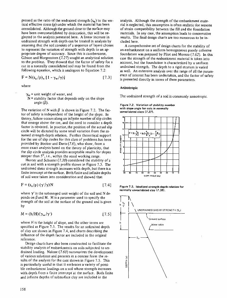
pressed as the ratio of the undrained strength (su) to the ver-tical effective stress (p) under which the material has been consolidated. Although the ground close to the surface may have been overconsolidated by desiccation, this will be ne-glected in the analysis presented here. A linear increase in undrained strength with depth can be treated in analysis by assuming that the soil consists of a sequence of layers chosen to represent the variation of strength with depth to an ap-propriate degree of accuracy. Since this is cumbersome, Gibson and Morgenstern (727) sought an analytical solution to the problem. They showed that the factor of safety for a cut in a normally consolidated soil may be found from the following equation, which is analogous to Equation 7.2:

F = N (s. /P)n [1 - Iy)] [7.31

where

= unit weight of water, and N = stability factor that depends only on the slope

angle (0).

The variation of N with 0 is shown in Figure 7.2. The fac-tor of safety is independent of the height of the slope. In theory, failure occurs along an infinite number of slip circles that emerge above the toe, and the need to consider a depth factor is obviated. In practice, the position of the actual slip circle will be dictated by some small variation from the as-sumed strength-depth relation. Further theoretical support for the use of slip circles for this class of problems has been provided by Booker and Davis (7.6), who show, from a more exact analysis based on the theory of plasticity, that the slip circle analysis provides acceptable results for slopes steeper than 50, i.e., within the usual working range.

Hunter and Schuster (7.38) considered the stability of a cut in soil with a strength profile shown in Figure 7.3. The undrained shear strength increases with depth, but there is a finite intercept at the surface. Both finite and infinite depths of soil were taken into consideration and showed that

F = (se /p) ('y'/y)N [7.4]

where y' is the submerged unit weight of the soil and N de-pends on 0 and M. M is a parameter used to specify the strength of the soil at the surface of the ground and is given by

M = (h/H)(y/'y') [7.5]

where H is the height of slope, and the other terms are specified in Figure 7.3. The results for an unlimited depth of clay are shown in Figure 7.4, and charts describing the influence of the depth factor are included in the original reference.

Design charts have also been constructed to facilitate the stability analysis of embankments on soils subjected to un-drained loading. Nakase (7.60) summarizes the development of various solutions and presents in a concise form the re-sults of the analysis for the case shown in Figure 7.5. This is particularly useful in that it em braces a variety of possi-ble embankment loadings on a soil whose strength increases with depth from a finite intercept at the surface. Both finite and infinite depths of subsurface clay are included in the

analysis. Although the strength of the embankment mate-rial is neglected, this assumption is often realistic for reasons of strain compatibility between the fill and the foundation materials. In any case, the assumption leads to conservative results. The final design charts are too numerous to be in-cluded here.

A comprehensive set of design charts for the stability of an embankment on a uniform homogeneous purely cohesive foundation was prepared by Pilot and Moreau (7.62). In this case the strength of the embankment material is taken into account, but the foundation is characterized by a uniform undrained strength. The depth to a rigid stratum is varied as well. An extensive analysis over the range of all the param-eters of interest has been undertaken, and the factor of safety is presented directly in terms of these parameters.

Anisotropic

The undrained strength of a soil is commonly anisotropic.

Figure 7.2. Variation of stability number with slope angle for cuts in normally consolidated clays (7.27).

L====iMWM .....u•. iiu••iu SLOPE ANGLE Idegl

Figure 7.3. Idealized strength-depth relation for normally consolidated clay (7.38).

\ UNDRAINED SHEAR STRENGTH (Si,)

158

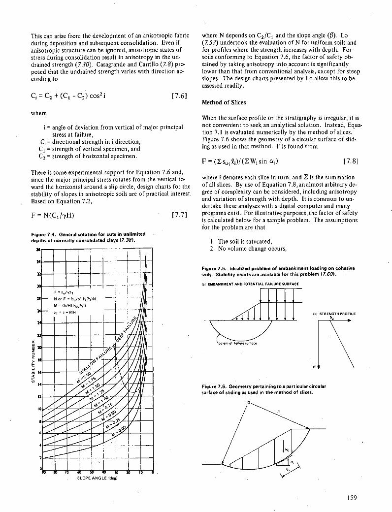
N or F (s/p)(-I-j)N -

= (h/HU/)

Figure 7.6. Geometry pertaining to a particular circular surface of sliding as used in the method of slices.

(b) STRENGTH PROFILE Su

iN

This can arise from the development of an anisotropic fabric during deposition and subsequent consolidation. Even if anisotropic structure can be ignored, anisotropic states of stress during consolidation result in anisotropy in the un-drained strength (7.30). Casagrande and Carrillo (7.8) pro-posed that the undrained strength varies with direction ac-cording to

where N depends on C2/Cl and the slope angle (0). Lo (Z53) undertook the evaluation of N for uniform soils and for profiles where the strength increases with depth. For soils conforming to Equation 7.6, the factor of safety ob-tained by taking anisotropy into account is significantly lower than that from conventional analysis, except for steep slopes. The design charts presented by Lo allow this to be assessed readily.

C, = C2 + (Cl - C2) cos2i [ 7.6] Method of Slices

where

= angle of deviation from vertical of major principal stress at failure,

C1 = directional strength in i direction, C1 = strength of vertical specimen, and C2 = strength of horizontal specimen.

There is some experimental support for Equation 7.6 and, since the major principal stress rotates from the vertical to-ward the horizontal around a slip circle, design charts for the stability of slopes in anisotropic soils are of practical interest Based on Equation 7.2,

F = N(C1/'yH)

[7.7]

Figure 7.4. General solution for cuts in unlimited depths of normally consolidated clays (7.38).

When the surface profile or the stratigraphy is irregular, it is not convenient to seek an analytical solution. Instead, Equa-tion 7.1 is evaluated numerically by the method of slices. Figure 7.6 shows the geometry of a circular surface of slid-ing as used in that method. F is found from

F = ( s 1Q)/(Wsin a) [7.8]

where i denotes each slice in turn, and Z is the summation of all slices. By use of Equation 7.8, an almost arbitrary de-gree of complexity can be considered, including anisotropy and variation of strength with depth. It is common to un-dertake these analyses with a digital computer and many programs exist. For illustrative purposes, the factor of safety is calculated below for a sample problem. The assumptions for the problem are that

The soil is saturated, No volume change occurs,

Figure 7.5. Idealized problem of embankment loading on cohesive soils. Stability charts are available for this problem (7.60).

(a) EMBANKMENT AND POTENTIAL FAILURE SURFACE

SLOPE ANGLE (deg)

159

(a) SCALED CROSS SECTION

/*

5 kPa 8.9 kN/m3

5 kPa;,' = 19.0 kNIm3

5 kPa 0.4 kN/m3

No dissipation of pore pressure occurs, The critical slip circle and the minimum F must be found by The mode of failure is slip circle, and

iteration. Convergence isfastest if 0 is moved horizontally.

The shear strength along the slip surface is the only factor contributing to resistance. Effective Stress Analysis of Soil Slopes

Figure 7.7 shows the cross section of the failure and the force diagram.

The factor of safety is determined by the use of Equa-tion 7.8; i.e., F is the resisting moment divided by the driv-ing moment. The resisting moment is the sum of the mo-bilized strength (sn) in each layer times the radius of the circle, and the driving moment is the sum of the weight of each slice times its moment arm from center of rotation. F can be defined this way only because all terms in the re-sisting moment have s.

The calculated dimensions of the slices shown in Figure 7.7 are given in Table 7.1. The remaining calculations are

Sum of the driving moments = 29 507 kN-m; Resisting moments = 24(25 x AB + 15 x BC + 35

xCD)=24(25 x7.5+ 15x4+35 x34)=34500kNm; and

For this example, F = 34 500/29 507 = 1.17.

Figure 7.7. Cross section and force diagram of example slip surface failure.

)h( FORCE DIAGRAM (typical slice of width b) Center of Rotation

0

1wn LR 0\ (b

[1 Slice

on failure surface Sc = nrobilized.strength

Note: 1kPa = 0.145 tbt/in2 nosses h r oughrwal fo

trCe

lkN-2.251bt;and po

1 m3 = 35.3 ft3

Table 7.1. Calculated dimensions of slices in example.

Slice Width (m)

Height (m)

Force (kN(

Lever Arm (m)

Driving Moment (kN-m)

1 3 3 170 20 3400 2 3 7.5 426 17.5 7455 3 3.5 10.5 703 14 9 842 4 6 12 1400 9 12600 5 6 10 1182 3 3546 6 6 7 844 -3 -2532 7 4 4 326 -8 -2608 8 6 1.5 183 -12 -2 196

Total 29 507

Note: 1 m = 3.3 ft; 1 kN = 2.25 lbf; and 1 kN-m = 0.74 lbf -ft.

Planar Slip Surface

When a soil mass moves predominantly in a translational manner, there is little internal distortion and an infinite slope analysis is often representative. In this analysis, the slip surface is assumed to be a plane parallel to the ground sur-face and the end effects can be neglected. When sliding takes place in the mantle of weathered material with small ratios of depth to length, this type of analysis is often appro-priate. The mechanics of sliding along a planar slip surface will be presented in detail, for they are instructive with re-gard to all effective stress analyses.

Consider the slope and slip surface shown in Figure 7.8. In an effective stress analysis the pore pressure distribution is assumed to be known, and in this case steady seepage is assumed to be parallel to the surface with the groundwater table as indicated. The forces acting on a slice of width b are shown. Since there is no internal distortion and end ef-fects are neglected,

dE=dX=0

The weight of a slice W is given by

W=7bd [7.10]

The total normal force (N) is related to the effective force (N') and pore pressure (u) by

N=N'+uQ [7.11]

and

uQ('yh)bseca [7.12]

where h is the piezometric head acting on the slip surface. The shear force acting along the base of the slice (S) is

S = [(c'b sec a)/F] + (N - uQ)(tan '/F) [7.13]

where

c' = cohesion intercept in terms of effective stress, and = angle of internal friction in terms of effective stress.

By resolving W into components parallel and perpendicular to the slope, we get

SWsina [7.14]

and

NW cos a [7.15]

The S and N forces can be eliminated by combining Equa-tions 7.13, 7.14, and 7.15, and an explicit relation for F can be found as

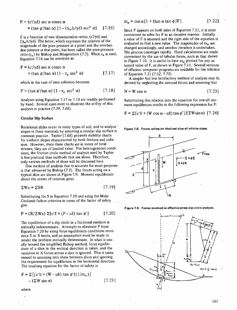
F = (c'/7d) sec a cosec a mcosa[1 + (tan atanØ'/F]. [7.22]

+ (tan '/tana) [1 -(yh/'yd)sec' a] [7.16]

F is a function of two dimensionless ratios, (c'/yd) and (yh/'yd). The latter, which expresses the relation of the magnitude of the pore pressure at a point and the overbur-den pressure at that point, has been called the pore-pressure ratio (rn) by Bishop and Morgenstern (7.5). When r is used, Equation 7.16 can be rewritten as

F = (c'/'yd) sec a cosec a

+ (tan '/tan a) (1 - ru sec2 a) [7.17]

which in the case of zero cohesion becomes

F= (tan '/tana)(1-r sec2 a) [7.18]

Analyses using Equation 7.17 or 7.18 are readily performed by hand. Several cases exist to illustrate the utility of this analysis in practice (7.39, 7.66).

Circular Slip Surface

Rotational slides occur in many types of soil, and to analyze slopes in these materials by assuming a circular slip surface is common practice. Taylor (7.68) presents stability charts for uniform slopes characterized by both friction and cohe-sion. However, since these charts are in terms of total stresses, they are of limited value. For heterogeneous condi-tions, the friction circle method of analysis used by Taylor is less practical than methods that use slices. Therefore, only various methods of slices will be discussed here.

One method of analysis that is accurate for most purposes is that advanced by Bishop (73). The forces acting on a typical slice are shown in Figure 7.9. Moment equilibrium about the center of rotation gives

Wx=SR [7.19]

Substituting for S in Equation 7.19 and using the Mohr-Coulomb failure criterion in terms of the factor of safety give

F = (R/Wx) 2jcl + (P - u) tan q'] [7.20]

The equilibrium of a slip circle in a frictional medium is statically indeterminate. Attempts to eliminate P from Equation 7.20 by using force equilibrium conditions intro-duce E or X terms, and an assumption must be made to render the problem statically determinate. In what is usu-ally termed the simplified Bishop method, force equilib-rium of a slice in the vertical direction is taken, and the variation in X forces across a slice is ignored. This is tanta-mount to assuming zero shear between slices and ignoring the requirement for equilibrium in the horizontal direction. The resulting equation for the factor of safety is

F = [[c'b + (W - ub) tan '] (1/ma ))

~(Wsina) [7.21]

where

Since F appears on both sides of Equation 7.21, it is most convenient to solve for F in an iterative manner. Initially a value of F is assumed and the right side of the equation is evaluated to find a new value. The magnitudes of in,,, are changed accordingly, and another iteration is undertaken. The process converges rapidly. Hand calculations are made convenient by the use of tabular forms, such as that shown in Figure 7.10. It is useful to have in,,, plotted for any as-sumed value of F, as shown in Figure 7.11. Several versions of efficient computer programs are available for the solution of Equation 7.21 (7.52, 7.73).

A simpler but less satisfactory method of analysis may be derived by neglecting the internal forces and assuming that

N=W cos a [7.23]

Substituting this relation into the equation for overall mo-ment equilibrium results in the following expression for F:

F=[c'+(W cos a-uQ) tan ']/(Wsina) [7.24]

Figure 7.8. Forces acting on idealized slice of infinite slope.

b

E+dE

T

x_--

f 1W

Flow

rx+dx

Figure 7.9. Forces involved in effective stress slip circle analysis.

-----. .lo

tan 0 •t,, 0

IN

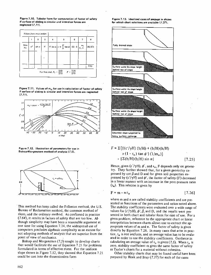
Figure 7.10. Tabular form for computation of factor of safety if surface of sliding is circular and interslice forces are neglected (7.71).

Values from cross section

I 2 3 4 5 6 7 8

a' sin a IV II sin a c + tan (5) 6 (6)1(7)

(s)

For first trial, F. = F = 2(4) ?(41

Figure 7.11. Values of m0 for use- in calculation of factor of safety if surface of sliding is circular and interslice forces are neglected (7.71).

/4

1.2

' /0

08

06

5,"sa tO,, ,,,0 'cosa * F

Figure 7.13. Idealized cases of seepage in slopes for which chart solutions are available (7.37).

Fully droined slope

Surface water 8n slope height

behind toe of slope

Surface water 4x slope height

behind toe of slope

Surface water 2s slope height

behind toe of slope

Q -30 -/'O -/0 0 /0 20 30 40 50 60 70

Saturated slope subjected to

a (deg)

Figure 7.12. Illustration of parameters for use in Bishop.Morgenstern method of analysis (7.5).

This method has been called the Fellenius method, the U.S. Bureau of Reclamation method, the common method of slices, and the ordinary method. As confirmed in practice (7.64), it results in factors of safety that are too low. Al-though simplicity may have been a reasonable argument at one time for using Equation 7.24, the widespread use of computers precludes algebraic complexity as an excuse for not adopting methods of analysis that are superior from the point of view of mechanics.

Bishop and Morgenstern (7.5) sought to develop charts that would facilitate the use of Equation 7.21 for problems formulated in terms of effective stress. For the uniform slope shown in Figure 7.12, they showed that Equation 7.21 could be cast into the dimensionless form

F = [[(c'/7H) (b/H) + (b/H)(h/H)

x (1 - r) tan qY] (l/m)J [(b/H)(h/H) sin a] [7.25]

Hence, given (c'/'yH), qY, and r, F depends only on geome-try. They further showed that, for a given geometry ex-pressed by cot f3 and D and for given soil properties ex-pressed by (c'/yH) and tb', the factor of safety (F) decreased in a linear manner with an increase in the pore-pressure ratio (rn). This relation is given by

F=m- nr [7.26]

where m and n are called stability coefficients and are pre-sented as functions of the parameters and ratios noted above. The stability coefficients were evaluated over a wide range of values for (c'/'yH), ', , and D, and the results were pre-sented in both chart and tabular form for ease of use. For a given problem, reference to the appropriate chart or linear interpolation between charts allows one to extract the ap-propriate values of In and n. The factor of safety is given directly by Equation 7.26. In many cases that arise in prac-tice, ru is not uniform, and an average value has to be evalu-ated in order to use the stability coefficients. Guidance in calculating an average value of ru is given (7.5). When ru is zero, stability coefficient m gives the same factor of safety as Taylor's charts for a material without cohesion.

Other stability charts that may be found useful have been prepared by Hoek and Bray (7.37) for each of the cases

162

Figure 7.15. Examples of variation of Fm and Ff with 0 in Spencer's analysis (7.67).

(a) E c'yH0.02 (0

T

rO.5 Dotted line passes through

I -.. points of action of

4 4OO

interslice forces.

Cli

I Note: 1 m = 3.3 ft.

Figure 7.14. Slip surface dimensions and slice forces for use in Spencer's analysis (7.67).

b/2 b/?

F.I.070 - ---- -----

Fm

E,: 15

i 0 15 20 25

eo

0.9

shown in Figure 7.13. These cases represent failure along a circular slip surface in a soil mass subjected to steady seepage and containing a tension crack. The magnitudes of(c'/'yH),

', and 13 are needed to enter a particular chart representing one of the cases shown in Figure 7.13. The factor of safety is then readily found. The charts are based on a form of fric. tion circle analysis that tends to underestimate the factor of safety. Although they are convenient to use for preliminary design, final design should be checked with a more rigorous analysis.

As pointed out previously, the simplified Bishop method of analysis is adequate for circular slip surfaces, but it as-sumes that no shear is mobilized between slices and it does not satisfy the condition of force equilibrium in the horizon-tal direction. Why the method works can be demonstrated by reference to the method presented by Spencer (7.67). Spencer followed the usual procedures in the method of slices (Figure 7.14) and argued that the action of the internal forces acting on a slice can be replaced by their resultant (Q) inclined at 0 to the horizontal and passing through the mid-point of a thin slice in order to satisfy moment equilibrium. In general, both Q and 0 will vary from slice to slice, and from force equilibrium it can be shown that

Q = [(c'b sec a/F) + (tan Ø'/F)

x(W cos a-ub seca)-W sinai

I cos(a-0)[l+(tan'/F)tan(a-0)] [7.27]

For overall equilibrium, the sum of the horizontal compo-nents and the vertical components of the interslice forces must each be zero; that is,

[Qcos0] =0 [7.281

and

[Q sin 0] =0 [7.29]

Moreover, if the sum of the moments of the external forces about the center of rotation is zero,the sum of the moments of the interslice forces about the center of rotation is also zero. For a circular slip surface,

[Qcos(a-0)] = 0

[7.30]

If 0 is assumed constant in order to make the problem de-terminate, Equations 7.28 and 7.29 reduce to

YIQ = 0

[7.31]

In either Equation 7.30 or 7.31, the value of F will depend on the assumed constant value of 0. For all but one value of 0, the safety factor determined (Equation 7.31) by force equilibrium (Ff) will not equal the safety factor determined (Equation 7.30) by moment equilibrium (Fm). This is shown in Figure 7.15 by the intersection of curves of Ff and

163

Fm plotted against values of 0. This intersection gives the pair of values of 0 and F that satisfy both equations simul-taneously. If 0 is set equal to zero and substituted into Equation 7.30, the equation governing Bishop's simplified method (Equation 7.21) is recovered. Therefore, Bishop's simplified method represents the solution for Fm with 0 equal to zero. In general, the equation governing moment equilibrium is rather insensitive to variations in 0, and errors of only a few percent result. For the assumption that 0 equals zero used in the Bishop simplified method, these er-rors are not conservative with respect to actual values of 0 greater than zero.

Noncfrcular Slip Surface

When the distribution of shearing resistance within an earth mass becomes nonuniform, slip can occur along surfaces more complex than a circle. Since the shape of the failure surface will be controlled to a large degree by the departure from uniformity, one may wish to analyze the stability along surfaces of arbitrary shapes. Noncircular analysis has proved useful in a number of cases of actual slides (7.22, 7.40).

Morgenstern and Price (757) developed a method of anal-ysis that treats a slip surface of arbitrary shape and satisfies all equilibrium requirements. To make the analysis statically determinate, a relation between the internal forces is as-sumed of the form

X=Xf(x)E [7.32]

where

X = factor to be determined in the solution, and f(x) = arbitrary function concerning the distribution of

internal forces.

The choice of f(x) is limited by conditions of physical ad-missibility, which require that no tension be developed in the earth mass and that the failure criterion not be violated. Subject to these conditions, the factor of safety is rather in-sensitive to variations in f(x). A digital computer is needed to solve resulting Equations 7.30 and 7.31. The Spencer analysis of a slip circle discussed previously is equivalent to setting f(x) equal to unity.

Figure 7.16. Curves for use in Janbu's simplified analysis (7.42, 7.43).

d 2heeor surface

Ratio d/L—

A convenient approximate method of analysis suitable for hand calculations and sufficiently accurate for many practical purposes is described by Janbu, Bjerrum, and Kjaernsli (7.43) and Janbu (7.42). This method follows the method of slices and is based on a more elaborate pro-cedure described in detail in the latter reference. The factor of safety is given by

F = f0 Z [[c'b + (W - ub) tan çb']/cos a ma ]] (Wtana) [7.33]

where in,,, is defined in Equation 7.22 and used as shown in Figure 7.10. The term f0, which is a correction factor for the role of the internal forces, is a function of the curvature of the slip surface and the type of soil; recommended values for this factor are given in Figure 7.16.

Another approximation procedure for analyzing slip along a noncircular sliding.surface is the wedge analysis. In this method the potential sliding mass is separated into a series of wedges, and the equilibrium of each wedge is considered in turn. Only the conditions of horizontal and vertical equilib-rium are used in the analysis, which is often performed in a graphical manner. Moreover, an assumption must be made regarding the inclination of the force transmitted across the interface between any two wedges. The forces utilized in this method of analysis are shown in Figure 7.17 for a rock mass separated into two wedges; the notation is defined be-low.

W1 ,W2 = weight of wedge, U1 ,U2 = resultant water pressure acting on base of wedge, N1 ,N2 = effective force normal to base, T1 ,T2 = shear force acting along base of wedge, L1 ,L2 = length of base, a1 ,a2 = inclination of base to horizontal, Pw12 = resultant water pressure at interface,

P12 = effective force at interface, and 6 = inclination of P12 to horizontal.

Although the rock mass shown in Figure 7.17 is separated into two wedges, the analysis can be extended readily to any number of wedges. The factor of safety is varied so that the force polygons constructed for each of the wedges satisfy horizontal and vertical equilibrium. A value of 6 is

Figure 7.17. Forces used in typical wedge analysis.

a2-f 2LJ2

W2

WI

164

assumed, and an initial value of F is taken; this allows the force polygon for the first wedge to be constructed, as shown by the dashed line in Figure 7.17. With the value of P12 obtained in this manner, the force polygon for the sec-ond wedge is readily constructed. This will not close, in general, and the value of F must be varied until it does. The final solution also is given in Figure 7.17.

The factor of safety is sensitive to the assumed value of 6. Conservative values of the factor of safety may be found by setting 6 equal to zero. The maximum possible value of 6 is that value which is compatible with failure in the direc-tion of the interface, but this usually leads to an overesti-mate of the factor of safety. Experience indicates that put-ting 6 between 100 and 150 usually gives reasonable results.

Pore-Pressure Distribution

To perform a stability analysis in terms of effective stress re-quires that the pore pressures be specified. A distinction is made between problems of undrained and drained loading. In the first case, the magnitude of the pore pressure is influ-enced to a large degree by the changes in total stress to which the earth mass is subjected; in the second case, the pore-pressure distribution is controlled by steady seepage conditions. When an analysis of a soil loaded under un-drained conditions is made in terms of effective stress, the pore pressures must be either predicted or measured. The confidence level for predicting pore pressures in cuts is not high; however, it is somewhat better in the case of founda-tions beneath embankments because the total stress change is less influenced by the initial state of stress in the ground. For a clay soil, the initial stresses in the ground are not usu-ally known to a high degree of accuracy. In general, the pore pressure (u) that is used in a stability analysis is given by

[7.341

where

u0 = pore pressure before any stress change, and Au = change in pore pressure due to change in total

stress.

The change in pore pressure (Au) can be estimated approxi-mately if the pore-pressure coefficients and the changes in total stresses are known. In turn, the change in total stress at a point may be estimated from stress analyses. Linear elasticity is commonly assumed; therefore, the results are of limited applicability, particularly if the factor of safety ap-proaches unity and a substantial volume is permitted to yield. In the case of cuts, the total stresses decrease so that with time the pore pressures increase from their end-of-construction values, thereby resulting in reduction of the factor of safety.

Although it is not common to predict pore-pressure changes in slopes due to changes in total stress, it is common to measure them on major projects and to use the data di-rectly in stability analyses. Instrumentation for measuring pore pressures is discussed in ChapterS. In the case of em-bankments on soft impervious foundations, monitoring pore pressures is almost routine. However, this monitoring may not be adequate to avert a slip (7.1).

Steady seepage through a soil is governed by the Laplace equation, for which a variety of methods are available to find solutions subject to appropriate boundary conditions (7.9, 7.31). These techniques are equally useful in the de-sign of drainage measures if the influence of the design on the magnitude and distribution of the pore pressures must be ascertained. In some cases, analytical methods will have the capability to provide solutions in closed form, but more generally the problems that arise in practice are analyzed by constructing flow networks graphically by the use of elec-tric analogue techniques or numerically by means of the finite element method (7.33, 7.46, 7.70).

An understanding of hydrogeologic controls is important in the solution, either by analysis or by observation, of any steady seepage problem. In particular, it is essential to rec-ognize the control that regional groundwater systems have on the local pore-pressure distribution in a natural slope or excavation. The recognition of groundwater discharge areas and an identification of the recharge areas are a starting point for almost all seepage studies, either computational or observational. High pore pressures are often found in dis-charge areas associated with topographic lows, and they may have a controlling influence on the stability of slopes. Anal-yses of regional groundwater systems have been made by Toth (7:72) and Freeze and Witherspoon (7.25, 7.26), and their significance for slope stability problems is noted by Patton and Deere (7.61).

Heterogeneity of soil deposits has a marked influence on the pore-pressure distribution under steady seepage condi-tions. Kenney and Chan (7.47) describe a detailed field study of the anisotropy of the permeability in a varved soil. The ratio of the permeability of flow parallel to the varves to that perpendicular to the varves was found to be less than five. Although this is less than might be expected, it still exerts a significant influence on the pressure distribution that develops during steady seepage conditions. Eigenbrod and Morgenstern (7.22) report a striking example of the influence of geologic detail on the pore-pressure distribu-tion within a slope about 20 in (70 ft) high in Cretaceous bedrock overlain by till. This slope was shown to possess at least three water tables, the upper two of which were perched on bentonitic layers. Moreover, no pore pressures acted along much of the failure surface, since it lay on a fractured free-draining coal layer. Careful field observations guided by an appreciation for the role of geologic details are needed in cases like this if misleading results are to be avoided.

Analysis of Rock Slopes

The analysis of the stability of a rock slope is normally un-dertaken in terms of effective stress because the permeability of rock masses is usually so high that undrained loading does not arise. To perform an analysis requires that the shear strength parameters, the pore-water pressures, and the slid-ing mechanism be specified. In hard rocks, the sliding mech-anism is controlled by structural features, and a detailed study of those features is a prerequisite for rational design of a rock slope. Further guidance on the evaluation of rock structure characteristics is given in Chapter 9.

The analysis of a rock slope in terms of a factor of safety is a subordinate activity to achieving a clear understanding

of the controlling geology and water-pressure configuration. In the case of slopes in soil, the confidence limits attached to the application of the total process of investigation, test-ing, and analysis are determined by the successful explana-tion of well-documented case histories (7.66). However, in the case of rock slides, few such case histories report com-pletely the geologic configuration, give good quality test data, and have been subjected to an acceptable analysis. Moreover, the shearing resistance in rocks is often sensitive to movements. Small movements can result in substantial decreases in available shearing resistance and hence in the factor of safety. Therefore, the confidence limits of design for a given factor of safety are generally lower for rock slopes than for soil slopes. In other words, rock slopes de-signed for a given factor of safety have a higher degree of risk associated with them than most soil slopes designed for the same factor of safety. If the degree of risk is to be the same, it is prudent to design rock slopes for higher factors of safety, unless only the residual shearing resistance is being mobilized. However, design for a higher factor of safety is not always economically feasible.

The shearing resistance of rock is more variable than that of soil, and the same is true of the water-pressure distribu-tion. Both the strength and the water-pressure distribution are dominated to a large degree by the pattern of discontin-uities in the rock mass. In the case of strength, the usual procedures for investigation involve in situ testing or sam-pling and testing, as discussed in Chapter 4. The water-pressure distribution can only be evaluated by field investi-gations coupled with an appreciation of the hydrogeologic constraints.

Morgenstern (7.55) reviews the influence of ground-water on the stability of rock slopes and shows how flow through a discrete network of discontinuities can be re-placed by flow through an imaginary medium of equivalent permeability. If the crack spacing is small compared to the size of the discontinuity, conventional procedures for solving problems of flow through porous media are applicable. If this is not the case, the attitudes and hydraulic conductivi-ties of the actual discontinuities should be considered (Z54, 7. 74). This is difficult to do, and considerable judgment is required to properly evaluate the water pressure distribution. Patton and Deere (7.61) stress the large local differences in water pressures that can arise in a jointed rock mass and the large fluctuations that can develop as a consequence of rain-fall. They also note the significant effects that faults can have on groundwater conditions. Those effects can be either beneficial or deleterious, depending on the attitude and char-acteristics of the fault gouge. Groundwater flow around faults and other similar features requires special study in slope-stability analyses. The evaluation of water pressures in a rock mass is made more difficult by the sensitivity of the hydraulic conductivity to small deformations. A small amount of slip along a discontinuity can result in a dispro-portionate change in hydraulic conductivity (7.65). Although methods of analysis can be developed to take these effects into consideration (7.7, 7.56), the information needed to conduct these analyses is only rarely available.

Stability analyses are usually concerned with sliding. However, discrete blocks of rock can also rotate outward or topple. A tendency to topple depends on the shape of the block and is usually readily discernible in the field. The

condition for toppling is dictated by the position of the weight vector of the block relative to the base of the block. If the weight vector passing through the center of gravity of the block falls outside the base of the block, toppling will occur; this is shown in Figure 7.18 (7.37).

A common case of instability in rock slopes is sliding along a planar surface. The analysis of this case is a simple extension of the stability of a rough rigid block on an in-clined plane, and, for the case shown in Figure 7.19a, we have

F=(2c/yH)P+[Q cot i-.R(P+S)]tanØ

- (Q+RS cot [7.35]

where

P = [1 -(Z/H)] cosec Op [7.36]

[7.37]

R (yw/'y) (Z/Z) (Z/H),and [7.38]

S = (Z/Z) (Z/H) sin [7.39]

But if the tension crack is in the surface above the slope (Figure 7.19h),

Q=[[1 - (Z/H)]2 cos Op

(cot O p tan of - 1)) [7.40]

should be used. All other terms are as shown in the figure. Hock and Bray (7.37) undertook a systematic study of the influence of the various parameters that enter into Equation 7.35 and prepared design charts to facilitate its use. If a planar mechanism is appropriate, it is also possible to assess the influence of drainage and other stabilizing measures, such as berms or cables, by using simple extensions of Equa-tion 7.35.

Often two or three sets of discontinuities intersect, and sliding of a wedge of rock becomes possible. In general, dif-fering amounts of friction and cohesion can act on the planes, and the water pressure acting normal to the surfaces bounded by the planes should be taken into consideration. A comprehensive analysis of the mechanics of wedge failure is given by Hendron, Cording, and Aiyer (7.32). Figure 7.20 shows a tetrahedron bounded by two base planes, which may be intersecting joint sets. Failure may occur by sliding along the line of intersection of the two planes or by sliding on either one of the two planes. General procedures have been developed for determining the factor of safety graph-ically by vector analysis by the use of stereo networks and numerically by hand or by computer (7.32, 7.37). The following steps are included in the analysis.

The intersections of the various joint sets with one an-other and with the slope face are inspected to determine the tetrahedra that may be potential failure wedges; these are then analyzed in detail.

The forces tending to disturb the equilibrium of the wedge are added vectorially to give the resultant driving force. These disturbing forces arise from the weight of the

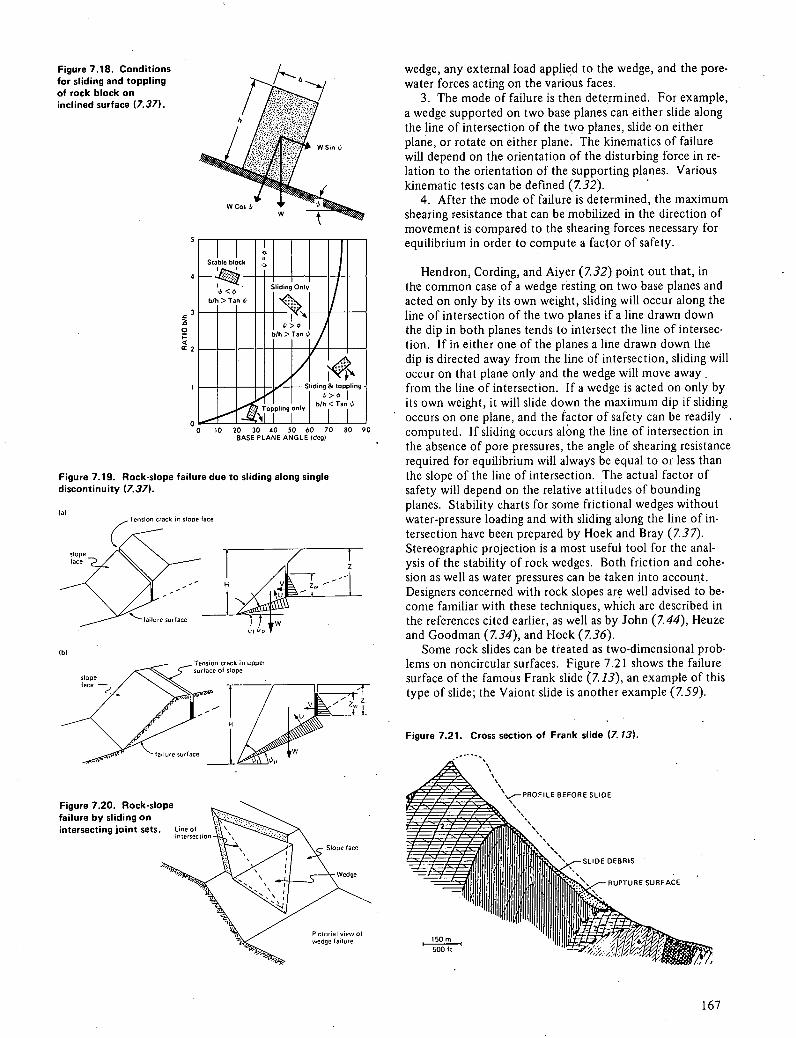
0 -I---- -

Stable blocb

—:— - SlngOMy

Th b>Tand

-}-- - - b/h > Tan ,

4 _ ding & toppling

Topplrng only b/h<Tan

___

Slope lace

Pictorial view of wedge failure

Figure 7.18. Conditions for sliding and toppling of rock block on inclined surface (7.37).

0 0 0 20 30 40 50 60 70 80 90

BASE PLANE ANGLE (deg)

Figure 7.19. Rock-slope failure due to sliding along single discontinuity (7.37).

Tension crack in slul,e face

cx~~

(b)

57— surface of slope slope face

failure surface W

Figure 7.20. Rock-slope failure by sliding on intersecting joint sets. Line 01

Interseclron

wedge, any external load applied to the wedge, and the pore-water forces acting on the various faces.

The mode of failure is then determined. For example, a wedge supported on two base planes can either slide along the line of intersection of the two planes, slide on either plane, or rotate on either plane. The kinematics of failure will depend on the orientation of the disturbing force in re-lation to the orientation of the supporting planes. Various kinematic tests can be defined (7.32).

After the mode of failure is determined, the maximum shearing resistance that can be mobilized in the direction of movement is compared to the shearing forces necessary for equilibrium in order to compute a factor of safety.

Hendron, Cording, and Aiyer (7.32) point out that, in the common case of a wedge resting on two base planes and acted on only by its own weight, sliding will occur along the line of intersection of the two planes if a line drawn down the dip in both planes tends to intersect the line of intersec-tion. If in either one of the planes a line drawn down the dip is directed away from the line of intersection, sliding will occur on that plane only and the wedge will move away. from the line of intersection. If a wedge is acted on only by its own weight, it will slide down the maximum dip if sliding occurs on one plane, and the factor of safety can be readily computed. If sliding occurs along the line of intersection in the absence of pore pressures, the angle of shearing resistance required for equilibrium will always be equal to or less than the slope of the line of intersection. The actual factor of safety will depend on the relative attitudes of bounding planes. Stability charts for some frictional wedges without water-pressure loading and with sliding along the line of in-tersection have been prepared by Hoek and Bray (737). Stereographic projection is a most useful tool for the anal-ysis of the stability of rock wedges. Both friction and cohe-sion as well as water pressures can be taken into account. Designers concerned with rock slopes are well advised to be-come familiar with these techniques, which are described in the references cited earlier, as well as by John (7.44), Heuze and Goodman (734), and 1-loek (7.36).

Some rock slides can be treated as two-dimensional prob-lems on noncircular surfaces. Figure 7.21 shows the failure surface of the famous Frank slide (7.13), an example of this type of slide; the Vaiont slide is another example (759).

Figure 7.21. Cross section of Frank slide (7.13).

167

These cases are amenable to analysis by the use of the same methods adopted for noncircular slides in soil.

DEFORMATION ANALYSIS

The use of deformation analysis in the design of slopes is an attractive concept; however, practical applications of defor-mation analysis are limited at present. Until the last decade, this limitation was imposed by the absence of suitable analyt-ical methods to perform deformation analysis. Few elastic solutions were available for boundary value problems simi-lar to slopes, and the solutions available were not well suited to practical design. The development of the finite element method has largely eliminated this impediment. As engineers have taken advantage of this analytical tool, however, other equally vexing problems have been recognized, and these still severely limit the practical application of the finite ele-ment method in most slope design problems.

In principle, a deformation analysis, particularly an anal-ysis utilizing the finite element method, must include the fol-lowing characteristics.

The stress field must satisfy equilibrium at every point. The prediction of this equilibrium stress field is usually done by use of elastic theory to describe the stresses and deforma-tions, but plasticity or other material models might also be used. To predict a stress field requires that the stress-strain relation for the soil be known.

Boundary conditions of stress and deformation must be satisfied. These characteristics can be contrasted to the principles of limit equilibrium noted in the earlier section on principles of limit equilibrium analysis.

The lack of success in applying deformation analysis in the design of slopes can be attributed directly to the difficul-ties associated with the stress-strain relation noted above. Soil is generally nonlinear, nonuniform, inelastic, and aniso-tropic. Each of these characteristics must be idealized and used in a deformation analysis, and the difficulty in describ-ing natural soil deposits in these terms is the major factor that limits application of the finite element method in the analysis of slopes. The problem is aggravated by our lim-

ited knowledge of the in situ stresses before excavation. Under special conditions, particularly in analysis of dams and embankments of compacted earth fill, the method is being used successfully (7.51); but the deformation analysis of nat-ural soils is primarily a research activity at present and has little practical application. A review of the principles of the finite element method is nevertheless appropriate because some practical applications are being made at present and progress in developing practical applications in the future is anticipated.

The finite element method has been applied to geotech-nical engineering problems since the late 1960s, having been developed a decade earlier for applications in structural en-gineering and continuum mechanics. Since that time, ex-tensive literature has developed, including several texts. An important and useful reference and summary of this work was compiled by Desai (7.16); this volume is recommended as a starting point for those interested in the method.

The underlying principle of the finite element method is that the behavior of a complex continuum can be approxi-mated by the collective behavior of parts representing the continuum. The parts are selected so that their individual behaviors can be described simply. By requiring adjacent elements to behave similarly at selected points of contact or nodes, the overall continuum is modeled.

In a typical application (Figure 7.22a), an embankment deformation analysis begins by using a group of simple ele-ments to approximate the fill. In a two-dimensional anal-ysis, either triangular or quadrilateral elements are commonly used. For a two-dimensional analysis, equations describing the behavior of these elements in plane strain are used in con-trast to the plane stress formulation often used for problems in structural engineering (7J8). A three-dimensional prob-lem can be modeled by using solid elements. For each ele-ment in the model, a series of equations and an appropriate stress-strain relation, such as elasticity, are used to relate the application of loads to deformation at the nodes. In the di-rect method of element formulation (Figure 7.22b), a tri-angular element with nodes only at the corners can be used. Other elements in the problem are formulated in a similar fashion. The deformation of adjacent elements is then constrained to be identical at the nodal points. There

Figure 7.22. Finite element idealization of (a) FINITE ELEMENT REPRESENTATION OF EMBANKMENT CROSS SECTION

embankment.

(b) TRIANGULAR ELEMENT OF NETWORK ABOVE SHOWING FORCES AT NODAL POINTS

II > FZ2

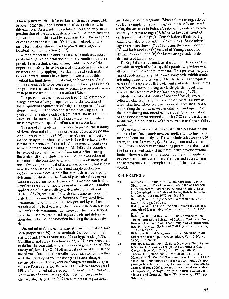
is no requirement that deformations or stress be compatible between other than nodal points on adjacent elements in this example. As a result, this solution would be only an ap-proximation of the actual system behavior. A more accurate approximation might result by adding nodes at the midpoint of each side of the element. Variational methods of ele-ment formulation also add to the power, accuracy, and flexibility of the procedure (7.1 7).

After a model of the embankment is formulated, appro-priate loading and deformation boundary conditions are im posed. In geotechnical engineering problems, one of the important loads is the self-weight of the material, which can be represented by applying a vertical force at each node (7.21). Several studies have shown, however, that this method has limitations in predicting deformations. An al-ternate approach is to perform a sequential analysis in which the problem is solved in successive stages to represent a series of steps in construction or excavation (7.20).

The procedures described above lead to the assembly of a large number of simple equations, and the solution of these equations requires use of a digital computer. Finite element programs applicable to geotechnical engineering problems are readily available from several sources and the literature. Because continuing improvements are made in these programs, no specific references are given here.

The use of finite element methods to predict the stability of slopes does not offer any improvement over accurate lim-it equilibrium methods (7.19). Its usefulness lies in defor-mation analysis, in which accuracy is directly related to the stress-strain behavior of the soil. Active research continues to be directed toward this subject. Modeling the complex behavior of soil has progressed from initial efforts using linear elasticity to include many of the more complicated elements of the constitutive relation. Linear elasticity is al-most always a poor model of actual soil behavior, but it does have the advantages of low cost and simple application (7.19). In some cases, simple linear models can be used to determine qualitatively the form of particular slope or em-bankment deformations. However, this method can lead to significant errors and should be used with caution. Another application of linear elasticity is described by Cole and Burland (7.12), who used finite element analysis to extrap-olate from measured field performance. They used field measurements to calibrate their analysis and by trial and er-ror selected the best values of the linear stress-strain relation to match their measurements. These constitutive relations were then used to predict subsequent loads and deforma-tions during further construction involving the same mate-rial.

Several other forms of the basic stress-strain relation have been proposed (7.19). Most methods deal with nonlinear elastic forms, such as bilinear (7.20) or hyperbolic (7.49). Multilinear and spline functions (7.15, 7.23) have been used to define the constitutive relation in even greater detail. The theory of plasticity (7.63) offers great potential through the use of yield functions to describe nonlinear effects, together with the coupling of volume changes to stress changes. In the use of elastic theory, volume changes are modeled by a variable Poisson's ratio. Because of the relative incompressi-bility of undrained saturated soils, Poisson's ratio has a con-stant value of approximately 0.5. This number may be changed slightly (e.g., to 0.49) to eliminate computational

instability in some programs. When volume changes do oc-cur (for example, during drainage or in partially saturated soils), the variation in Poisson's ratio can be related experi-mentally to stress changes (7.50) or to the coefficient of earth pressure at rest (K0). Consolidation effects during loading can also be considered (7.10, 7.41). Some advan-tages have been shown (7.11) for using the shear modulus (G) and bulk modulus (K) instead of Young's modulus (E) and Poisson's ratio (v) for formulating elastic finite element problems in soil.

During deformation analysis, it is common to exceed the available strength of soil at specific points long before over-all collapse of the slope is imminent. This presents the prob-lem of modeling local yield. Since many soils exhibit strain-softening behavior after yield (Chapter 6), it is appropriate to model this by use of finite element methods. Höeg (7.35) describes one method using an elastic-plastic model, and several other techniques have been proposed (Z17).

Modeling natural deposits of rock and heavily overcon-solidated clay requires consideration of joints and similar discontinuities. These features can experience shear trans-lation along the joints, as well as dilatancy and opening of the joints during movement of the slope. The application of the finite element method to rock (7. 75) and particularly to dilating jointed rock (7.28) has relevance to slope-stability problems.

Other characteristics of the constitutive behavior of soil and rock have been considered for application to finite ele-ment deformation analysis. These include anisotropy (7.14), creep, and tensile cracking (7.23). As greater and greater complexity is added to the modeling parameters, the cost of the finite element analysis increases, often beyond practical limits. However, the major problem limiting the application of deformation analysis to natural slopes and cuts remains the heterogeneous and complex nature of the materials in-volved.

REFERENCES

7.1 Al-dhahir, Z., Kennard, M. F., and Morgenstern, N. R. Observations on Pore Pressures Beneath the Ask Lagoon Embankments at Fiddler's Ferry Power Station. In In Situ Investigations in Soils and Rocks, British Geotechni-cal Society, London, 1970, pp. 26 5-276.

7.2 Barron, R. A. Correspondence. Geotechnique, Vol. 14, No.4, 1964, pp. 360-361.

7.3 Bishop, A. W. The Use of the Slip Circle in the Stability Analysis of Slopes. Geotechnique, Vol. 5, No. 1, 1955, pp. 7-17.

7.4 Bishop, A. W., and Bjerrurn, L. The Relevance of the Triaxial Test to the Solution of Stability Problems. Proc., Research Conference on Shear Strength of Cohesive Soils, Boulder, American Society of Civil Engineers, New York, 1960, pp. 437-501.

7.5 Bishop, A. W., and Morgenstern, N. R. Stability Coeffi- cients for Earth Slopes. Geotechnique, Vol. 10, No. 4, 1960, pp. 129-150.

.7.6 Booker, J. R., and Davis, E. H. A Note on a Plasticity So- lution to the Stability of Slopes in Horn ogenous Clays. Geotechnique, Vol. 22, No.4, 1972, pp. 509-513.

7.7 Brekke, T. L., Noorishad, J., Witherspoon, P. A., and Maini, Y. N. T. Coupled Stress and Flow Analysis of Frac-tured Dam Foundations and Rock Slopes. Proc., Sympo-sium on Percolation Through Fissured Rock, International Society of Rock Mechanics and International Association of Engineering Geology, Stuttgart, Deutsche Gesellschaft für Erd- und Grundbau, Essen, West Germany, 1972, pp. T4-J, 1-8.

169

7.8 Casagrande, A., and Carrfflo, N. Shear Failure of Aniso- tropic Materials. In Contributions to Soil Mechanics: 1941-1953, Boston Society of Civil Engineers, 1944, pp. 122-135.

7.9 Cedergren, H. R. Seepage, Drainage, and Flow Nets. Wiley, New York, 1967, 489 pp.

7.10 Christian, J., and Boehmer, J. W. Plane Strain Consolida- tion by Finite Elements. Journal of Soil Mechanics and Foundations Division, American Society of Civil Engineers, New York, Vol. 96, No. SM4, 1970, pp. 143 5-1457.

7.11 Clough, R. W., and Woodward, R. J. Analysis of Embank- ment Stresses and Deformations. Journal of Soil Mechanics and Foundations Division, American Society of Civil Engi-neers, New York, Vol. 93, No. SM4, 1967, pp. 529-549.

7.12 Cole, K. W., and Burland, J. B. Observations of Retaining Wall Movements Associated With A Large Excavation. Proc., 5th European Conference on Soil Mechanics and Foundation Engineering, Spanish Society for Soil Me-chanics and Foundations, Madrid, 1972, pp. 327-342.

7.13 Cruden, D. M., and Krahn, J. A Reexamination of the Geology of the Frank Slide. Canadian Geotechnical Jour-nal, Vol. 10, No. 4, 1973, pp. 581-591.

7.14 D'Appolonia, D. J., and Lambe, T. W. Method for Predict- ing Initial Settlement. Journal of Soil Mechanics and Foundations Division, American Society of Civil Engineers, New York, Vol. 96, No. SM2, 1970, pp. 523-544.

7.15 Desai, C. S. Nonlinear Analyses Using Splice Functions. Journal of Soil Mechanics and Foundations Division, Amer-can Society of Civil Engineers, New York, Vol. 97, No. 5M1, 1971, pp. 1461-1480.

7.16 Desai, C. S., ed. Applications of the Finite Element Method in Geotechnical Engineering: A Symposium. U.S. Army Engineer Waterways Experiment Station, Vicksburg, Miss., 1972, 1227 pp.

7.17 Desai, C. S. Theory and Applications of the Finite Ele- ment Method in Geotechnical Engineering. In Application of the Finite Element Method in Geotechnical Engineering: A Symposium (Desai, C. S., ed.), U.S. Army Engineer Waterways Experiment Station, Vicksburg, Miss., 1972, pp. 3-90.

7.18 Desai, C. S., and Abel, J. F. Introduction to the Finite Element Method: A Numerical Method for Engineering Analysis. Van Nostrand-Reinhold, New York, 1972, 477 pp.

7.19 Duncan, J. M. Finite Element Analysis of Stresses and Movements in Dams, Excavations, and Slopes. In Appli-cation of the Finite Element Method in Geotechnical En-gineering: A Symposium (Desai, C. S., ed.), U.S. Army Engineer Waterways Experiment Station, Vicksburg, Miss., 1972, pp. 267-326.

7.20 Dunlop, P., and Duncan, J. M. Development of Failure Around Excavated Slopes. Journal of Soil Mechanics and Foundations Division, American Society of Civil Engineers, New York, Vol. 96, No. SM2, 1970, pp. 47 1-493.

7.21 Dunlop, P., Duncan, J. M., and Seed, H. B. Finite Element Analyses of Slopes in Soil. Department of Civil Engineer-ing, Univ. of California, Berkeley, Rept. TE-68-3, 1968.

7.22 Eigenbrod, K. D., and Morgenstern, N. R. A Slide in Cretaceous Bedrock at Devon, Alberta. In Geotechnical Practice for Stability in Open Pit Mining (Brawner, C. 0., and Milligan, V., eds.), Society of Mining Engineers, Amer-ican Institute of Mining, Metallurgical and Petroleum En-gineers, New York, 1972, pp. 223-23 8.

7.23 Eisenstein, Z., Krishnayya, A. V., and Morgenstern, N. R. An Analysis of the Cracking at Duncan Dam. Proc., Spe-cialty Conference on Performance of Earth and Earth-Supported Structures, Purdue Univ., Lafayette, md., American Society of Civil Engineers, New York, Vol. 1, Part 1, 1972, pp. 765-778.

7.24 Esu, F. Short-Term Stability of Slopes in Unweathered Jointed Clays. Geotechnique, Vol. 16, No. 4, 1966, pp. 321-328.

7.25 Freeze, R. A., and Witherspoon, P. A. Theoretical Anal- ysis of Regional Groundwater Flow: 1—Analytical and Numerical Solutions to the Mathematical Model. Water Resources Research, Vol. 2, No. 4, 1966, pp. 641-656.

7.26 Freeze, R. A., and Witherspoon, P. A. Theoretical Anal- ysis of Regional Groundwater Flow: 3—Quantitative In-terpretations. Water Resources Research, Vol. 4, No. 3, 1968, pp. 581-590.

7.27 Gibson, R. E., and Morgenstern, N. R. A Note on the Stability of Cuttings in Normally Consolidated Clays. Geotechnique, Vol. 12, No. 3, 1962, pp. 212-216.

7.28 Goodman, R. E., and Dubois, J. Duplication of Dilatancy in Analysis of Jointed Rocks. Journal of Soil Mechanics and Foundations Division, American Society of Civil En-gineers, New York, Vol. 98, No. SM4, 1972, pp. 399-422.

7.29 Hansen, J. B. The Philosophy of Foundation Design: De- sign Criteria, Safety Factors, and Settlement Limits. In Proc. (Vesic, A. S., ed.), Symposium on Bearing Capacity and Settlement of Foundations, Duke Univ., Durham, N.C., 1965, 1967, pp. 9-14.

7.30 Hansen, J. B., and Gibson, R. E. Undrained Shear Strengths of Aniso tropically Consolidated Clays. Geotechnique, Vol. 1, No. 3, 1949, pp. 189-204.

7.31 Harr, M. E. Groundwater and Seepage. McGraw-Hill, New York, 1962, 315 pp.

7.32 Hendron, A. J., Jr., Cording, E. J., and Aiyer, A. K. Ana- lytical and Graphical Methods for the Analysis of Slopes in Rock Masses. U.S. Army Engineer Nuclear Cratering Group, Livermore, Calif., Technical Rept. 36, 1971.

7.33 Herbert, R., and Rushton, K. R. Ground-Water Flow Studies by Resistance Networks. Geotechnique, Vol. 16, No. 1, 1966, pp. 53-75.

7.34 Heuze, F. E., and Goodman, R. E. Three-Dimensional Approach for Design of Cuts in Jointed Rock. In Stability of Rock Slopes (Cording, E. J., ed.), Proc., 13th Sympo-sium on Rock Mechanics, Univ. of Illinois at Urbana-Champaign, American Society of Civil Engineers, New York, 1972, pp. 397-404.

7.35 Hdeg, K. Finite Element Analysis of Strain-Softening Clay. Journal of Soil Mechanics and Foundations Division, Amer-ican Society of Civil Engineers, New York, Vol. 98, No. SM1, 1972, pp. 43-58.

7.36 Hoek, E. Methods for the Rapid Assessment of the Stabil- ity of Three-Dimensional Rock Slopes. Quarterly Journal of Engineering Geology, Vol. 6, No. 3, 1973, pp. 243-255.

7.37 Hoek, E., and Bray, J. W. Rock Slope Engineering. Insti- tution of Mining and Metallurgy, London, 1974, 309 pp.

7.38 Hunter, J. H., and Schuster, R. L. Stability of Simple Cut- tings in Normally Consolidated Clays. Geotechnique, Vol. 18, No. 3, 1968, pp. 372-378.

7.39 Hutchinson, J. N. A Landslide on a Thin Layer of Quick Clay at Furre, Central Norway. Geotechnique, Vol. 11, No. 2, 1961, pp. 69-94.

7.40 Hutchinson, J. N. A Reconsideration of the Coastal Land- slides at Folkestone Warren, Kent. Geotechnique, Vol. 9, No. 1, 1969, pp. 6-38.

7.41 Hwang, C. T., Morgenstern, N. R., and Murray, D. W. Ap- plication of the Finite Element Method to Consolidation Problems. In Application of the Finite Element Method in Geotechnical Engineering: A Symposium (Desai, C. S., ed.), U.S. Army Engineer Waterways Experiment Station, Vicksburg, Miss., 1972, pp. 739-765.

7.42 Janbu, N. Slope Stability Computations. In Embankment- Dam Engineering (Hirschfeld, R. C., and Poulos, S. J.,eds.), Wiley, New York, 1973, pp. 47-86.

7.43 Janbu, N., Bjerrum, L., and Kjaernsli, B. Soil Mechanics Applied to Some Engineering Problems. Norwegian Geo- technical Institute, Oslo, PubI. 16, 1956, pp. 5-26.

7.44 John, K. W. Engineering Analysis of Three-Dimensional Stability Problems Utilizing the Reference Hemisphere. Proc., 2nd Congress, International Society of Rock Me-chanics, Belgrade, Vol. 3, 1970, pp. 385-391.

7.45 Kankare, E. Failures at Kimola Floating Canal in Southern Finland. Proc., 7th International Conference on Soil Me-chanics and Foundation Engineering, Mexico City, Vol. 2, 1969, pp. 609-6 16.

7.46 Kealy, C. D., and Busch, R. A. Determining Seepage Char- acteristics of Mill-Tailings Dams by the Finite Element Method. U.S. Bureau of Mines, Rept. RI 7477, 1971, 113 pp.

170

7.47 Kenney, T. C., and Chan, H. T. Field Investigation of Per- meabifity Ratio of New Liskeard Varved Soil. Canadian Geotechnical Journal, Vol. 10, No. 3, 1973, pp. 473488.

7.48 Kenney, T. C., and Uddin, S. Critical Period for Stability of an Excavated Slope in Clay Soil. Canadian Geotechni-cal Journal, Vol. 11, No. 4, 1974, pp. 620.623.

7.49 Kondner, R. L., and Zelasko, J. S. A Hyperbolic Stress- Strain Formulation for Sands. Proc., 2nd Pan-American Conference on Soil Mechanics and Foundations Engineer-ing, Brazil, American Society of Civil Engineers, New York, Vol. 1, 1963, pp. 289-324.

7.50 Kulhawy, F. H., and Duncan, J. M. Stresses and Movements in Oroville Dam. Journal of Soil Mechanics and Founda-tions Division, American Society of Civil Engineers, New York, Vol. 98, No. SM7, 1972, pp. 653-655.

7.51 Lefebvre, G., Duncan, J. M., and Wilson, E. L. Three- Dimensional Finite Element Analysis of Dams. Journal of Soil Mechanics and Foundations Division, American Society of Civil Engineers, New York, Vol. 99, No. 5M7, 1973, pp. 495-507.

7.52 Little, A. L., and Price, V. E. The Use of an Electronic Computer for Slope Stability Analysis. Geotechnique, Vol. 8, No. 3, 1958, pp. 113-1 20.

7.53 Lo, K. Y. Stability of Slopes in Anisotropic Soils. Journal of Soil Mechanics and Foundations Division, American Society of Civil Engineers, New York, Vol. 91, No. SM4, 1965, pp. 85-106.

7.54 Louis, C. Stiomungsvorgànge in klüftigen Medien und ihre Wirkung auf die Standsicherheit von Bauwerken und Boschungen im Fels. Institut Bodenmechanik und Felsmechanik, Universitat Fridericiana Karlsruhe, Vol. 30, 1967, 121 pp.

7.55 Morgenstern, N. R. The Influence of Groundwater on Stability. In Stability in Open Pit Mining (Brawner, C. 0., and Milligan, V., eds.), Society of Mining Engineers, Amer-ican Institute of Mining, Metallurgical and Petroleum En-gineers, New York, 1971, pp. 65-81.

7.56 Morgenstern, N. R., and Guther, H. Seepage Into an Ex- cavation in a Medium Possessing Stress-Dependent Permea-bility. Proc., Symposium on Percolation Through Fissured Rock, International Society of Rock Mechanics and Inter-national Association of Engineering Geology, Stuttgart, Deutsche Gesellschaft für Erd- und Grundbau, Essen, West Germany, 1972, pp. T2-C, 1-15.

7.57 Morgenstern, N. R., and Price, V. E. The Analysis of the Stability of General Slip Surfaces. Geotechnique, Vol. 15, No. 1, 1965, pp. 79-93.

7.58 Morgenstern, N. R., and Price, V. E. A Numerical Method for Solving the Equations of Stability of General Slip Sur-faces. Computer Journal, Vol. 9, No. 4, 1967, pp. 388-393.

7.59 Muller, L. The Rock Slide in the Vaiont Vailey. Felsme- chanik und Ingenieur Geologie, Vol. 2, No. 3-4, 1964, pp. 148-212.

7.60 Nakase, A. Stability of Low Embankment on Cohesive Soil Stratum. Soils and Foundations, Vol. 10, No. 4, 1970, pp. 39-64.

7.61 Patton, F. D., and Deere, D. U. Geologic Factors Con- trolling Slope Stability in Open Pit Mines. In Stability in

Open Pit Mining (Brawner, C. 0., and Milligan, V., eds.), Society of Mining Engineers, American Institute of Min-ing, Metallurgical and Petroleum Engineers, New York, 1971, pp. 23-48.

7.62 Pilot, G., and Moreau, M. La Stabllité des Remblais Sur Sols Mous. Eyrolles, Paris, 1973.

7.63 Prevost, J-H., and Hdeg, K. Effective Stress-Strain-Strength Model for Soils. Journal of Geo technical Engineering Di-vision, American Society of Civil Engineers, New York, Vol. 101, No. GT3, 1975, pp. 259-278.

7.64 Sevaldson, R. A. The Slide in Lodalen, October 6, 1954. Geotechnique, Vol. 6, No. 4, 1956, pp. 167-1 82.

7.65 Sharp, J. C., and Malni, Y. N. T. Fundamental Considera- tions on the Hydraulic Characteristics of Joints in Rock. Proc., Symposium on Percolation Through Fissured Rock, Stuttgart, International Society of Rock Mechanics and International Association of Engineering Geology, Deutsche Geseilschaft für Erd- und Grundbau, Essen, West Germany, 1972, pp. Ti-F, 1-15.

7.66 Skempton, A. W., and Hutchinson, J. N. Stability of Nat- ural Slopes and Embankment Foundations. Proc., 7th International Conference on Soil Mechanics and Founda-tion Engineering, Mexico, State-of-the-Art Volume, 1969, pp. 291-340.

7.67 Spencer, E. A Method of Analysis of the Stability of Em- bankments Assuming Parallel Inter-Slice Forces. Geotech-nique, Vol. 17, No. 1, 1967, pp 11-26.

7.68 Taylor, D. W., Stability of Earth Slopes. Journal of Boston Society of Civil Engineers, Vol. 24, No. 3, 1937, pp. 197-246.

7.69 Taylor, D. W. Fundamentals of Soil Mechanics. Wiley, New York, 1948, 700 pp.

7.70 Taylor, R. L., and Brown, C. B. Darcy Flow Solutions With a Free Surface. Journal of Hydraulics Division, American Society of Civil Engineers, New York, Vol. 93, No. HY2, 1967, pp. 25-33.

7.71 Terzaghi, K., and Peck, R. B. Soil Mechanics in Engineer- ing Practice. Wiley, New York, 1967, 729 pp.

7.72 16th, J. A Theoretical Analysis of Groundwater Flow in Small Drainage Basins. Proc., 3rd Hydrology Symposium, National Research Council of Canada, Ottawa, 1962, pp. 75-96.

7.73 Whitman, R. V., and Bailey, W. A. Use of Computers for Slope Stability Analysis. Journal of Soil Mechanics and Foundations Division, American Society of Civil Engineers, New York, Vol. 93, No. SM4, 1967, pp. 475-498.

7.74 Wittke, W., Rissler, P., and Semprich, S. Three-Dimensional Laminar and Turbulent Flow Through Fissured Rock Ac-cording to Discontinuous and Continuous Models. Proc., Symposium on Percolation Through Fissured Rock, Inter-national Society of Rock Mechanics and International As-sociation of Engineering Geology, Stuttgart, Duetsche Gesellschaft für Erd- und Grundbau, Essen, West Germany, 1972, pp. Ti-H, 1-18 (in German).

7.75 Zienkiewicz, 0. C., Best, B., Dullage, C., and Stagg, K. G. Analysis of Nonlinear Problems in Rock Mechanics With Particular Reference to Jointed Rock Systems. Proc., 2nd Congress, International Society of Rock Mechanics, Bel-grade, Vol. 3, 1970, pp. 501-509.

171

Chapter 8

Design and Construction of Soil Slopes David S. Gedney and William G. Weber, Jr.

The design of stable slopes in soil has been extensively studied by engineers and geologists . In recent years , sub­stantial advancements have been made in understanding the engineering characteristics of soils as they relate to stability. Chapters 6 and 7 describe the state of the art re­garding the determination of pertinent soil parameters and the recommended approaches to engineering analysis. These techniques allow the design and construction of safe and economic slopes under varying conditions. This chapter applies the basic principles established in Chapters 6 and 7 to procedures for the design of stable slopes. The proce­dures can also be applied to preconstructed slopes and to correction of existing landslides.

PHILOSOPHY OF DESIGN

There are several basic considerations in the design of stable slopes. First, because of the nature of soils and the geologic environment in which they are found, each slope design is different. Second, the basic mechanics applied to estimate the stability of a cut slope in soil are the same as those used to estimate the stability ofa fill slope. Third, finding th e correct method of stability analysis solves only part of the design problem. Designing a stable slope includes field in­vestigation, laboratory investigation, and construction con­trol. The details involved in this work cannot be standard­ized because maximum flexibility is needed as each problem is assessed. Judgment , experience, and intuition, coupled with the best data-gathering and analytical techniques, all contribute to the solution .

SAFETY FACTOR

The specific analytical techniques used to predict the sta­bility of slopes are explained in Chapter 7. In all cases , the geotechnical engineer determines the safety factor, which is defined several ways but most commonly as

172

I. The ratio of resisting forces to driving forces along a potential failure surface;

2. The ratio of resisting moments to driving moments about a point;

3. The ratio of available shear strength to the average shear stress in the soil along a potential failure surface ; and

4. The factor by which the shear strength parameters may be reduced in order to bring the slope into a state of limiting equilibrium along a given slip surface.

The last definition is used in Chapter 7, and, unless other­wise noted, effective stress parameters are implicit.

Ideally, failure is represented by factor of safety values less than one, and stability is represented by values greater than one. The geotechnical engineer must be aware that the safety factor for a given slope depends heavily on the quality of the data used in the analysis . In addition, the various methods used to compute safety factors give wide ranges of values, except when the ratio equals unity .

The problem of determining a meaningful safety factor is complicated by factors such as interpretation of field and laboratory data, uncertainty of construction control, and the designer's incomplete information about the de­sign problem. In any case , using the best information at­tainable and the procedures outlined in Chapters 6 and 7 allows the engineer to compute a minimum factor of safety against failure as a basis for comparing design alternatives.

After consideration of the factors that influence design and the consequences of failure, the reasonableness of re­ducing the safety factor can be established. In highway en­gineering, slope designs generally require safety factors in the range of 1.25 to 1.50. Higher factors are required if there is a high risk for loss of human life or uncertainty re­garding the pertinent design parameters. Likewise, lower safety factors can be used if the engineer is fairly confident of the accuracy of input data and if good construction con­trol can be executed.

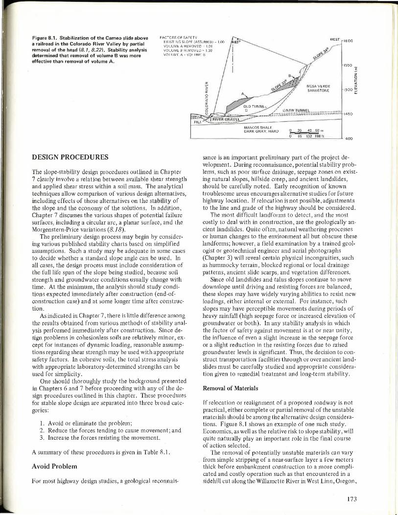
FACTORS OF SA FETY Figure 8.1. Stabilization of the Cameo slide above a railroad in the Colorado River Valley by partial removal of the head (8.1, 8.22). Stability analysis determined that removal of volume B was more effective than removal of volume A.

EX ISTING SLOPE IASSUMEDI O 1.00 VOLUM E A REMOVED O 1 0 1 VO LUME B REMOV ED • 1,30 VOLUM E A • VOLUME B

DESIGN PROCEDURES

The slope-stability design procedures outlined in Chapter 7 clearly involve a relation between available shear strength and applied shear stress within a soil mass. The analytical techniques allow comparison of various design alternatives, including effects of those alternatives on the stability of the slope and the economy of the solutions. In addition, Chapter 7 discusses the various shapes of potential failure surfaces, including a circular arc, a planar surface, and the Morgenstern-Price variations ( 8.18).

The preliminary design process may begin by consider­ing various published stability charts based on simplified assumptions. Such a study may be adequate in some cases to decide whether a standard slope angle can be used. In all cases, the design process must include consideration of the full life span of the slope being studied, because soil strength and groundwater conditions usually change with time . At the minimum, the analysis should study condi­tions expected immediately after construction ( end-of­construction case) and at some longer time after construc­tion.

As indicated in Chapter 7, there is little difference among the results obtained from various methods of stability anal­ysis performed immediately after construction. Since de­sign problems in cohesionless soils are relatively minor, ex­cept for instances of dynamic loading, reasonable assump­tions regarding shear strength may be used with appropriate safety factors. In cohesive soils, the total stress analysis with appropriate laboratory-determined strengths can be used for simplicity.

One should thoroughly study the background presented in Chapters 6 and 7 before proceeding with any of the de­sign procedures outlined in this chapter. These procedures for stable slope design are separated into three broad cate­gories :

1. Avoid or eliminate the problem ; 2. Reduce the forces tending to cause movement ; and 3. Increase the forces resisting the movement.

A summary of these procedures is given in Table 8 .1.

Avoid Problem

For most highway design studies, a geological reconnais-

1550

0:

] z 0 .: <i > UJ

> a: 0 0 <i 0:

MESA VERDE SANDSTONE 1500 ~

MANCOS SHALE DARK GRAY, HARD 0 20 4060m

1450

._ ____ __________ o'---'-66'--'=32"--"18 .. 8"""1& __ _,_1400

sance is an important preliminary part of the project de­velopment. During reconnaissance, potential stability prob­lems, such as poor surface drainage, seepage zones on exist­ing natural slopes, hillside creep, and ancient landslides, should be carefully noted. Early recognition of known troublesome areas encourages alternative studies for future highway location. If relocation is not possible, adjustments to the line and grade of the highway should be considered.

The most difficult landforms to detect, and the most costly to deal with in construction , are the geologically an­cient landslides . Quite often, natural weathering processes or human changes to the environment all but obscure these landforms; however , a field examination by a trained geol­ogist or geotechnical engineer and aerial photographs (Chapter 3) will reveal certain physical incongruities, such as hummocky terrain, blocked regional or local drainage patterns , ancient slide scarps, and vegetation differences.

Since old landslides and talus slopes continue to move downslope until driving and resisting fo rces are balanced, these slopes may have widely varying abilities to resist new loadings, either internal or external. For instance, such slopes may have perceptible movements during periods of heavy rainfall (high seepage force or increased elevation of groundwater or both). In any stability analysis in which the factor of safety against movement is at or near unity, the influence of even a slight increase in the seepage force or a slight reduction in the resisting forces due to raised groundwater levels is significant. Thus, the decision to con­struct transportation facilities through or over ancient land­slides must be carefully studied and appropriate considera­tion given to remedial treatment and long-term stability.

Removal of Materials

If relocation or realignment of a proposed roadway is not practical , either complete or partial removal of the unstable materials should be among the alternative design considera­tions. Figure 8.1 shows an example of one such study. Economics, as well as the relative risk to slope stability, will quite naturally play an important role in the final course of action selected.

The removal of potentially unstable materials can vary from simple stripping of a near-surface layer a few meters thick before embankment construction to a more compli­cated and costly operation such as that encountered in a side hill cut along the Willamette River in West Linn, Oregon,

173

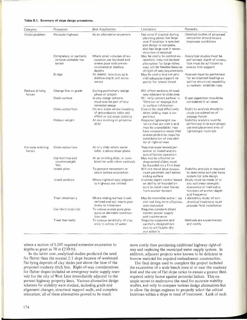
r Table 8.1. Summary of slope design procedures.

Category

Avoid problem

Reduce driving forces

Procedure

Relocate highway

Completely or partially remove unstable ma­teria Is

Bridge

Change I ine or grade

Ora in surface

Drain subsurface

Reduce weight

Increase resisting Drain subsurface forces

Use buttress and counterweight fi I ls

Install piles

I nsta 11 anchors

Treat chemically

Use electroosmosis

Treat thermally

Best Application

As an alternative anywhere

Where small volumes of ex­cavation are involved and where poor soils are en­countered at shallow depths

At sidehill locations with shallow-depth soil move­ments

During preliminary design phase of project

In any design scheme; must also be part of any remedial design

On any slope where lowering of groundwater table will effect or aid slope stability

At any existing or potential slide

At any slide where water table is above shear plane

At an existing slide, in com­bination with other methods

To prevent movement or strain before excavation

Where rights-of-way adjacent to highway are limited

Where sliding surface is well defined and soi I reacts posi· tively to treatment

To relieve excess pore pres­sures at desirable construc­tion rate

To reduce sensitivity of clay soils to action of water

Limitation

Has none if studied during planning phase; has large cost if location is selected and design is complete; also has large cost if recon­struction is required

May be costly to control ex­cavation; may not be best alternative for large slides; may not be feasible because of right-of-way requirements

May be costly and not pro­vide adequate support ca­pacity for lateral thrust

Wi 11 affect sections of road­way adjacent to slide area

Will only correct surface in­filtration or seepage due to surface infiltration

Cannot be used effectively when sliding mass is im­pervious

Requires lightweight ma­terials that are costly and may be unavailable; may have excavation waste that creates problems; requires consideration of availabil­ity of right-of-way

Requires experienced per­sonnel to install arid en­sure effective operation

May not be effective on deep-seated slides; must be founded on a firm base

Will not stand large strains; must penetrate well below sliding surface

Involves depth control based on ability of foundation soils to resist shear forces from anchor tension

May be reversible action; has not had long-term effective­ness evaluated

Requires constant direct current power supply and maintenance

Requires expensive and carefully designed sys­tem to artificially dry out subsoils

Remarks

Detailed studies of proposed relocation shou Id ensure improved conditions

Analytical studies must be performed; depth of excava­tion must be sufficient to ensure firm support

Analysis must be performed for anticipated loadings as well as structural capability to restrain landslide mass

Slope vegetation should be considered in all cases

Stability analysis should in­clude consideration of seepage forces

Stability analysis must be performed to ensure proper use and placement area of lightweight materials

Stability analysis is required to determine soil-pile force system for safe design

Study must be made of in situ soil shear strength; economics of method is function of anchor depth and frequency

Laboratory study of soi 1-chemica I treatment must precede field installation

Methods are experimental and costly

where a section of 1-205 required extensive excavation to depths as great as 70 m (230 ft).

In the latter case, analytical studies predicted the need for flatter than the normal 2: 1 slope because of weakened flat-lying deposits of clay shales just above the base of the proposed roadway ditch line. Right-of-way considerations for flatter slopes included an emergency water supply reser­voir for the city of West Linn immediately adjacent to the present highway property lines. Various alternative design schemes for stability were studied, including grade and alignment changes, structural support walls, and complete relocation; all of these alternatives proved to be much

more costly than purchasing additional highway right-of­way and replacing the municipal water supply system. In addition, adjacent projects were known to be deficient in borrow material for required embankment construction.

174

The final design used to complete the project included the excavation of a wide bench zone at or near the roadway level and the use of flat slope ratios to ensure a greater than required safety factor against potential failure. This ex­ample serves to underscore the need for accurate stability studies, not only to compare various design alternatives but to allow the design engineer to properly select the critical locations within a slope in need of treatment. Lack of such

analysis could have substantially increased construction costs on the West Linn project.

Bridging

In some instances, removal of especially steep and long nar­row unstable slopes is too costly. One alternative design is to span the unstable area with a land bridge or a structure whose support is founded on piles placed well below the un­stable foundation materials (8.1). Stability studies must as­certain that the bridge is indeed founded at sufficient depth below the unstable materials and not just penetrating into a more stable stratum. If supports must penetrate through the moving soil, as shown in Figure 8.2, the foundation piling must be designed to withstand the predicted lateral forces. Bridging may also include limited excavation and the use of surface and subsurface drainage.

Reduce Driving Forces

Since the stability of soil slopes is a limiting equilibrium problem in which the external forces acting on a soil mass are at least balanced, the design of stable slopes must ad­dress ways to ensure proper safety from the forces tending to cause movements. Since the driving forces are essentially gravitational because of the weight of the soil and water, the simplest approach to reducing such forces is to reduce the mass that is involved. Flattened slopes, benched slopes, reduced cut depths, internal soil drainage, and lightweight

Figure 8.2. Landslide avoidance by bridging near Santa Cruz, California (8.24).

fill all represent feasible treatments. The reduction of driv­ing forces can be divided into three main categories:

1. Change of line or grade or both, 2. Drainage, and 3. Reduction of weight.

The stability of embankment slopes and natural slopes can­not necessarily be approached in the same way. Except in certain unique instances, the stability of embankment slopes increases with time because of consolidation and strength increases in the slope-forming materials. One no­ticeable exception could be embankments composed of degradable compacted shale, which will deteriorate with time and result in subsequent settlement and distortion or failure of the fills. In cut slopes, the long-term stability may be far less than that available at the time of construc­tion. The ability of a cut slope to withstand the effects of time and stress change is discussed in Chapter 6.

Talus slopes often have marginal stability and deserve particular attention. Talus can be defined as rock fragments that have any size or shape and have been heterogeneously deposited by nature at the base of steep slopes. Runoff from normal rainfall may cause a sufficient increase in seepage forces to initiate movement within talus slopes. Recogni­tion of talus slope forms is important in the predesign pro­cess; such slopes should be avoided during construction un­less other alternatives are not available. If talus slopes must be disturbed by construction activity, careful analysis should consider the benefits of internal drainage to control potential slope movements that may be triggered by the buildup of large internal water pressures.

Change of Line or Grade

Early in the design stage, cut and fill slopes should be eval­uated for potential stability. If conditions warrant, adjust­ments to the line and grade can be effected to minimize or completely eliminate the stability problem. This approach can also be applied to landslides during and after construc­tion. The economics of various alternative solutions should ensure the feasibility of this approach. An example of a grade revision to prevent a cut slope movement is shown in Figure 8.3.

Line or grade changes are usually associated with a reduc­tion of driving forces . Movement of the roadway alignment

Figure 8.3. Grade change effected during construction to preclude failure at cut slope.

"'"'° i FINAL

PROPOSED GR/\OEl ••

/ •• ..----;~~I\NKMENT FILL

r""'""' • GROUND SURFACE

COLLU V IUM AND DI SPLACED SAPAOLITE

,,, .,,. ,.. ..... ~ /

,,,,_,,:,. /

r•'~ ':;.'/ ,.-,,, ... ---=~-----:::.,7' -;.-- ,,. / ,..

·· - •• • / . / PRED ICTED FAILURE ZONE

AFTE R FAILURE

.-, - .-:- ~ -1' .. --('0RIGINAL PROPOSED GRADE

,_., .- l=-;11--~ HIGHEST WATER LEVEL L sPRING

(PRECON ST RUCTI ON)

175

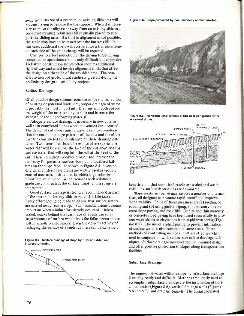
away from the toe of a potential or existing slide area will prevent having to remove the toe support. When it is neces­sary to move the alignment away from an existing slide as a corrective measure, a buttress fill is u ually placed to sup­port the sliding mass. If a shift in alignment is not possible, the grade may have to be raised over the buttress fill. In this case, additional costs will accrue, since a transition zone on each side of the grade change wHI be required .

Changes lo effecl reduction in the driving forces during construction operations are nol only difficult but expensive. To flatten construction slopes often requires additional rigl1t-of-way and could involve aJignment shifts that affect the design on either side of the troubled area. The co t­effectiveness of geotechnical studies is greatest during the preliminary design stages of any project.

Surface Drainage

Of all possible design schemes considered for the correction of existing or potential landslides, proper drainage of water is probably the most important. Drainage will both reduce the weight of the mass tending to slide and increase the strength of the slope-forming material.

Adequate surface drainage is necessary in new cuts, as well as in completed slopes where movement has occurred. The design of cut slopes must always take into considera­tion the natural drainage patterns of the area and the effect that the constructed slope will have on these drainage pat­terns. Two items that should be evaluated are (a) surface water that will flow across the face of the cut slope and (b) surface water that will seep into the soil at the head of the cut. These conditions produce erosion and increase the tendency for potential surface slumps and localized fail­ures on the slope face. As shown in Figure 8.4, diversion ditches and interceptor drains are widely used as erosion control measures in situations in which large volumes of runoff are anticipated. When trenches with a definite grade are constructed, the surface runoff and seepage are intercepted.

Good surface drainage is strongly recommended as part of the treatment for any slide or potential slide (8.8). Every effort should be made to ensure that surface waters are carried away from a slope. Such considerations become important when a failure has already occurred. Unless sealed, cracks behind the scarp face of a slide can carry large volumes of surface waters into the failure zone and re­sult in serious consequences. Even the obvious activity of reshaping the surface of a landslide mass can be extremely

Figure 8.4. Surface drainage of slope by diversion ditch and interceptor drain.

176

Figure 8.5. Slope protected by pneumatically applied mortar.

Figure 8.6. Horizontal and vertical drains to lower groundwater in natural slopes.

beneficial, in that unnoticed cracks are sealed and water­collecting surface depressions are eliminated.

Slope treatment per se may involve a number of alterna­tives all designed to promote rapid runoff and improve slope stability. Some of these measures are (a) seeding or sodding and (b) using gunite, riprap, thin masonry or con­crete slope paving and rock fills. Gunlte and thin masonry or concrete slope paving Jiave been used successfully to pro­tect weak shales or claystones from rapid weathering (Fig­ure 8.5). The use of asphalt paving to prevent infillration of surface water i also common in some areas. These methods of controlling surface runoff are effective when used in conjunction with various subsurface drainage tech· niques. Surface drainage measures require minimal design and offer positive protection to slopes along transportation facilities.

Subsurface Drainage

The removal of water within a slope by subsurface drainage is usually costly and difficult. Methods frequently used to accomplish subsurface drainage are the installation of hori­zontal drains (Figure 8.6), vertical drainage wells (Figures 8.6 and 8.7), and drainage tunnels. The drainage-related

Figure 8.7. Vertical wells to lower groundwater in roadway slope.

Figure 8.8. Corrective measures for Castaic-Alamos Creek slides, California (8.10).

SATURATED PLASTIC TOPSOIL

G) Strip slide material.

@ Place perforated pipe in

horizontal boring.

@ Construct intercepting trench.

© Construct gravel subdrain_

@ Rebuild fill.

expense is generally less when these measures are incorpo­rated into the preliminary design process than when they are included as remedial measures during or following con­struction. Occasionally, attempts are made to intercept subsurface flows above the sliding mass; however, the ex­pense usually precludes treatment by this procedure for all but special cases. Since seepage forces act to increase the driving force on a landslide, the control of subsurface water is of major importance to the geotechnical engineer. If the preliminary investigation reveals the presence of ground­water, if design studies predict slide movement, and if posi­tive subsurface drainage can preclude failure, a suitable de­sign should be prepared for cost comparison with other al­ternatives.

Subsurface drainage is equally important in cut areas and under proposed embankments. The effectiveness and frequency of use of the various types of drainage treatment vary according to the geology and the climatic conditions. It is generally agreed, however, that groundwater constitutes the most important single contributory cause for the major­ity of landslides; thus, in many areas of the country the most generally used successful methods for both preven­tion and correction of landslides consist entirely or par­tially of groundwater control (8.8, 8.29). Figure 8 .8 hows the use of both surface and subsurface drainage to satisfy

stablJity requirements for finished slopes on a highway proj­ect. Although most types of subsurface-drainage treatment are applicable to the prevention and correction oflandslides in both embankment and excavation areas, the differences in methods are considered of sufficient importance to jus­tify separate discussion of the subsurface-drainage treat­ments applied to these two general types of landslides.

Embankment Areas

Landslides may occur when the imposed embankment load results in shear stresses that exceed the shear strength of the foundation soil or when the construction of the embank­ment interferes with the natural movement of groundwater. Therefore, two factors must be considered in the investiga­tion of possible landslides: (a) weak zones in the founda­tion soil that may be overstressed by the proposed embank­ment load and (b) subsurface water that may result in the de­velopment of hydrostatic pressures so as to induce slide movement by a significant reduction in the shear strength of the soil. Because there often is no apparent surface in­dication of unstable slope conditions, a careful exploration must be made if these conditions are to be predicted before construction. Some of the methods of preventing landslides related to drainage are discussed below (8.4).

If a surface layer of weak soil is relatively shallow and underlain by stable rock or soil, the most economical treat­ment is usually to strip the unsuitable material, as shown in Figure 8.9. If seepage is evident after stripping or if there is a possibility that it may develop during wet cycles, a layer of pervious material should be placed before the embank­ment is constructed. This layer may consist of clean pit-run gravel, free-draining sand, or other suitable local materials. If springs or concentrated flows are encountered, drain pipes may also be required.

Where subsurface water or soil of questionable strength is found at such great depths that stripping is uneconomi­cal, stabilization trenches have been used successfully to prevent landslides. Stabilization trenches (Figure 8.10) are usually excavated with the steepest side slopes that will be stable for the construction period.

The trench should extend below any water-bearing layers and into firm material. A layer of pervious material is used as a lining within the excavation, and an underdrain pipe is used as a collector. The trench is backfilled, and the embankment is constructed. If the unstable area is in a natural depression of limited areal extent, one trench normal to the centerline of the road may be sufficient. In

Figure 8.9. Stripping of unstable surface material as a slide-prevention measure on Redwood Highway, Humboldt County, California (8.24). Filter material ensures drainage at base of new embankment fill.

PROPOSED ROADWAY EMBANKMENT

-.,,,....,. ..... _.10m 16,5 33 ft

177

r

Figure 8.10. Stabilization trench with pervious material 'and perforated pipe for subsurface drainage (8.24).

PERFORATED METAL PIPE

Figure 8.11. Drainage tunnels to prevent lands! ides near Crockett, California (8.24).

the case of large areas, an extensive system of stabilization trenches may be necessary, frequently arranged in a herring­bone pattern. In addition to providing subdrainage, the trenches add considerable structural strength to the foun­dation.

Stabilization trenches facilitate drainage and provide in­creased resistance to possible sliding due to the effect of "keying" the compacted backfill of the trench section into the firm material beneath the trench. This procedure has generally been effective in preventing embankment landslides, but a few failures have occurred because the trenches were not carried down to firm material or they were too widely spaced.

Stabilization trench design requires a thorough subsur­face investigation program, which must adequately define the subsurface soil layers and locate all water levels in the zone affected by the proposed embankment. One method of designing stabilization trenches is as follows: A line on a 1: 1 slope is projected from the outside edge of the top of

178

the embankment to a point of intersection with the surface of competent material; this point locates the outside toe of the trench. Some deviation from the above concept is tolerable, and may even be required, to provide a fairly uni­form trench alignment and grade.

Where the depth to subsurface water is so great that the cost of stripping or placing drainage trenches is prohibitive, drainage tunnels are sometimes used (8.23). Although orig­inally and more commonly used as a correctional treatment, drainage tunnels are sometimes constructed as a preventive measure. The use of drainage tunnels was fairly common at one time by both railroad companies and some highway departments, but at present this method is used rather in­frequently largely because of the high construction cost.

An elaborate installation of drainage tunnels, together with an ingenious hot-air furnace for drying the soil, was used to control a large slide near Santa Monica, California (8.15). The use of drainage tunnels in Oregon has also been reported (8.23). These tunnels, usually about 1 m (3 ft)

wide by 2 m ( 6 ft) high (in cross section), must be excavated manually; since skilled tunnel workers are not normally em­ployed on such construction projects, other methods of treatment that permit the use of construction equipment are likely to cost less than the tunnels. Figure 8 .11 shows an installation of drainage tunnels on a highway project.

Horizontal drains have supplanted drainage tunnels in most cases. Like drainage tunnels, they were first installed as corrective treatment. Although they are still used for this purpose, horizontal drain installations are now com­monly used as a preventive measure for slope instability. A horizontal drain is a small-diameter well drilled into a slope on approximately a 5 to 10 percent grade and fitted with a perforated pipe. Pipes should be provided to carry the collected water to a safe point of disposal to prevent surface erosion.

Both vertical and horizontal drains were used in a slide that occurred in 1968 during construction on I-580 at Alta­mont Pass in California. Figure 8.12 shows such an instal­lation. The slide extended along 310 m ( 1015 ft) of road­way with about 30 m (I 00 ft) of embankment. Remedial measures were (a) installation of a line of vertical drainage wells along the edge of the eastbound lanes; (b) construc­tion of a berm between the eastbound and westbound lanes and a berm adjacent to the eastbound lanes; (c) in­stallation of horizontal drains in five general areas to con­trol groundwater, relieve excess hydrostatic pressure, and intercept and drain the vertical wells; and ( d) completion of the construction of the embankment at a controlled rate of loading. The vertical wells were about 1 m (3 ft) in diameter, 12 m (40 ft) deep, and belled at the bottom so that they interconnected to form a somewhat con­tinuous curtain. The drain had a 20-cm (8-in) perfo­rated pipe in the center for the full depth of the vertical drain and was backfilled with pervious material. The hori­zontal drains were then drilled to intersect and drain the belled portion of the vertical well. The 20-cm perforated pipe was used to observe the water tables and to monitor

Figure 8.12. Horizontal and vertical drains to prevent slides (8.24).

---- - - .---- .--,-- ---SLIP PLANE

the success of the system. Inspection of the system during September 1973 indicated that all water tables were suc­cessfully maintained at levels near the bottoms of the ver­tical drains.

A similar combination drainage system was used on a landslide on I-80 near Pinole, California. This roadway had been open to traffic for several years when a 23-m (75-ft) embankment failed abruptly and closed the freeway in both directions. A drainage gallery formed by a line of vertical wells with overlapping belled bases was placed on each side of the embankment, as shown in Figure 8 .13. The lower line of vertical wells was drained with a 30-cm ( 12-in) pipe , and the uphill line of vertical wells was drained by means of horizontal drains. Berms were used to support the ma­terial placed in the failed area. A field and laboratory inves­tigation of the Pinole slide included borings, installation of inclinometers, casings, and laboratory triaxial tests. The ex­istence of water pressure in the layered subsoils was evi­denced by a rise of water in the borings of 3 to 4.5 m (I 0 to 15 ft) when pervious strata were encountered.

Based on the observed excessive seepage at the upstream toe of the fill and the water level data, engineers from the California Division of Highways concluded that hydrostatic pressures had indeed triggered this failure . Two vertical wells were immediately installed upstream of the failed em­bankment and pumped to a depth of 10 m (33 ft); they pro­duced water at the rate of 5400 L/d (1425 gal/d). Twelve horizontal drains were then installed, varying from 170 to 250 m (560 to 820 ft) in length, and these produced a total flow of 38 000 to 46 000 L/d ( 10 000 to 12 000 gal/d). In a 6-week period this subdrainage system lowered the groundwater 2 m (6.5 ft) at the upstream toe, 0.7 m (2.3 ft) beneath the sliding mass, and 0.3 m (1 ft) at the downstream toe. The triaxial tests indicated that the im­pervious soils forming the mass of the foundation material had cohesion values ranging from 25 to 145 kPa (3.5 to _Q lbf/in 2) with a negligible friction angle. The minimum fac­tor of safety was calculated to be 1.01 when the failure oc-

, ~~:l~~NT~l~~~:li~~ici~ s / / OF HORIZONTAL DRAINS

'EXPLORATORY BORINGS

' VERTICAL DRAINS

10 20 m

33 66 ft

Figure 8.13. Cross section along axis of movement of landslide on 1-80 near Pinole, California.

80

70

ORI GIN A L CO NST RU CTED SECTION~ APP ROX IMATE LIMI TS OF EXCAVATED MATERI AL • PR IOR TO RECO NSTRUCTION

RECONSTRUCTED SECTION _ _

60

50

40

30

120 100 80

FA I LED SECTI ON -

WATER LE V EL AS DETER MINE D FROM / BO RE HO LES

- - - -....:;_CRITICA L CIRCLE FROM

COMPUTER ANA LYSIS

0 10 20 30 m UPPER DRAINAGE GALLERY

0 33 66 99 It

60 40 20 20 40 60 80

SECTI ON ALONG AXIS OF MOVEM ENT

179

I!"'-- -

curred. The location of the critical circle was confirmed by movements observed from slope indicator readings. A fac­tor of safety of 1.4 was obtained for the conditions after treatment and reconstruction ( 8. 3 J).

· Figure 8.14 shows a system of horizontal drains that was installed as a slide-correction me~sure; similar installa­tions are frequently used as corrective treatments at other locations.

Vertical drain wells have also been installed under em­bankments to accelerate the consolidation of weak com­pressible foundation soils. Discussion of the various uses of vertical drains for this purpose is beyond the scope of th.is chapter, but many excellent references to vertical sand drain design and construction practices are available in the soil mechanics literature (e.g., 8. 7, 8.16).

The continuous siphon is an excellent method devised by the Washington State Highway Commission for pro­viding a drainage outlet for drainage wells or sumps (Figure 8.15). This siphon arrangement can be used to drain trenches, wells, or sumps and is less costly than tunnels, drilled-in pipes, or similar conventional outlet systems. In addition, it permits the installation of subdrainage systems

Figure 8.14. l-lorizontal drains used to control large land movements (8. 1, 8.14).

Note: 1 m = 3 3 ft

in areas that do not have readily accessible outlets. A con­tinuous siphon method has the usual limitation of depth, but is useful where applicable.

Excavation Areas

All of the subsurface drainage methods discussed in connec­tion with prevention of landslides in embankments can also be applied to prevention of landslides in excavation areas . Drainage is sometimes installed to intercept subsurface water above the limits of the excavation, but there is seldom any assurance that such interceptor trenches will effectively cut off all groundwater that might contribute to slope failure . If deep trenches are required, the cost is frequently prohibi­tive, considering the probable effectiveness of the drainage trenches.

Deep trench drains (which, when finally extended deep enough, did work effectively to halt a large slope move­ment) were used during the construction of a portion of 1-81 near Hollins, Virginia (Figure 8.16); this section of highway required a small cut about 10 m (33 ft) deep with 2: 1 slopes. The removed material consisted primarily of

Figure 8.15. Washington siphon used by Washington Department of Transportation to lower water level and stabilize landslides (8.24).

DEAIRING DEVICE DETAIL OF CUP PIPE

SECTION OF

•' .

Note: 1 cm = 0,4 in

180

20 cm PIPE

20cm UNPERFORATED

colluvium and residual soil weathered from a deeper shale bedrock. During construction a small landslide occurred, and the first attempts toward stabilization called for reduc­ing the driving forces by flattening the slope to 3: 1. Al­though stability analyses based on the assumption that the water table was at the ground surface predicted a safe con­dition, the regraded slope remained stable only until the following spring, when a second much larger slide occurred. It was obvious that a close relation existed between rainfall intensity and slope movement. Also, calculations in stabil­ity studies indicated that the average soil shear strength was much lower than originally assumed.

After consideration of many alternatives, including com­plete relocation of the roadway, construction of a drilled­pile restraint structure, and complete removal of the sliding mass, a remedial scheme was designed to further unload the slope and to ensure interception of subsurface waters. The design included (a) installing a trench drain around the slide scarp and up the face of the slide more or less at right angles to the roadway; (b) flattening the slope to 4: 1; and ( c) cut­ting an intermediate bench at approximately the midheight of the slope. Unfortunately, the trench around the scarp area did not totally halt the heavy subsurface water flow, and the movement continued during periods of heavy rain­fall. Some 9 years of costly maintenance followed until the headward progression of the slide necessitated large in­creases in rights-of-way. The final remedial scheme con­sisted of (a) using a large rock buttress to restrain the slope above the existing scarp face and to effect deeper drainage interception; (b) placing large granular drainage trenches in two channels down the slope within the flow debris; and (c) regrading the final slope to attain full surface drainage and allow grass establishment. The final slope has remained stable for the past 3 years. The total cost for remedial con­struction was more than $1 million. However, this proved to be at least $1 million less than the closest alternative, which was to completely relocate the highway away from the slide area ( 8.13).

The most widely used method of subsurface drainage for cut slopes is probably the use of horizontal drains, which are described in the previous section. In excavation areas the drains are installed as the cut is excavated (Figure 8.17), often from one or more benches in the cut slope. Numer­ous cut slopes drained by this method have remained stable in spite of unfavorable soil formations and the pres­ence of large amounts of subsurface water. If the treat­ment is delayed until after a landslide has developed, the cost of correcting the slide by subsurface drainage will be much greater and have much less chance of success.

Reduction of Weight

Another technique for reducing the driving forces is referred to as selective "unloading" of a slide. Unloading refers to removal or excavation of a sufficient quantity of slope­forming material at the head of the slide to ensure stability of the mass. This approach is ineffective for infinite slopes or for flow types of earth movement, as discussed in Chap­ter 6. The required quantity of material to be removed must be carefully predicted by stability analyses using high­quality laboratory and field data. In addition, economics and material usage may dictate whether unloading proce-

Figure 8 .16. Aerial view of Hollins slide on 1-81 near Roanoke, Virginia.

dures are reasonable on any project. The design of removal procedures must always consider the stability of the slope behind the area to be removed. In some instances, either through project needs for borrow materials or through con­sideration of the size of total volumes of slide materials, simply to remove the total slide mass is feasible. This pro­cedure is usually limited to slides in which material vol­umes are relatively small, and it is an effective means of reducing problems when used during the design stage. In addition, the use of variable or flattened slopes at the top of a cut will often aid in unloading a potential slide area.

Slope flattening was used effectively on a 98-m (320-ft) cut for a southern California freeway (Figure 8.18). A fail­ure took place during construction on a 1: 1 benched cut slope composed predominantly of sandstone and interbed­ded shales. After considerable study and analysis, the slope was modified to 3: 1, and the final roadway grade was raised some 18 m (60 ft) above the original design elevation. Moreover, to provide additional stability, earth buttresses were placed from roadway levels to a height of 21 m (69 ft) along the final slopes.

In the past, benching has been used by some engineers to reduce the driving force on a potential or existing slide . However, both field experience and stability analyses indi­cate that this objective is not always achieved (8.25). Hence, a careful study and review of alternatives is recommended when benching is proposed. The use of benching to reduce the driving forces is not generally recommended, but

18 1

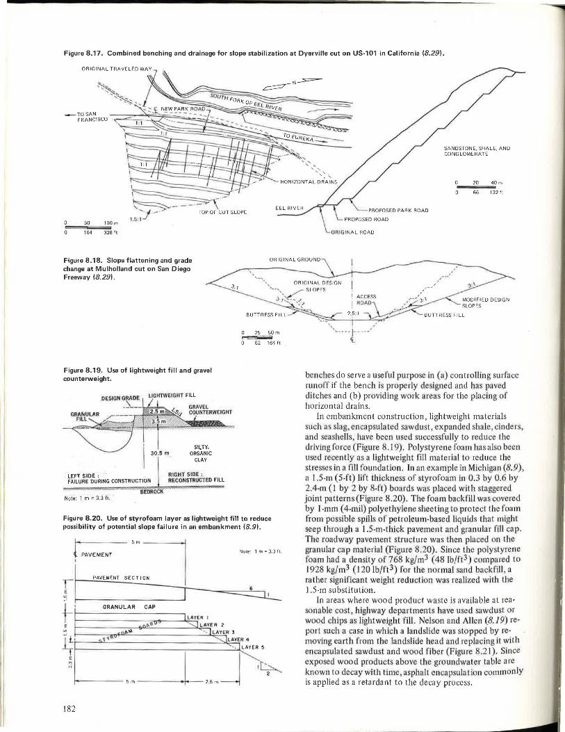
Figure 8.17. Combined benching and drainage for slope stabilization at Dyerville cut on US-101 in California (8.29).

0

0

50 100 rn

164 328 ft

PROPOSED PARK ROAD

SANDSTONE, SHALE, ANO CONGLOMERATE

0

0

20 40 rn

66 132 ft

Figure 8 .18. Slope flattening and grade change at Mulholland cut on San Diego Freeway (8.29).

'" · " .,, ORIGINAL DESIGN ,, .....

/

'-· •,,, /" SLOPES

3: I <f': ... " ·

Figure 8.19. Use of lightweight fill and gravel counterweight.

Sl~TY, ORGANIC

CLAY

0 25 50 rn

0 82 164ft

LEFT SIDE : RIGHT SIDE : FAILURE DURING CONSTRUCTION RECONSTRUCTED FILL

,,,, • . ,,,. ,,,_:omrn , .•. ''if€D 0 0CK 0. ' • · ¥

Note: 1 m ~ 3,3 ft .

Figure 8.20. Use of Styrofoam layer as lightweight fill to reduce possibility of potential slope failure in an embankment (8.9).

PAVEMENT 5m l

Note: 1 m = 3.3 f t,

t---'PC..:A:.:.;VE:.::M:.:.EN::.:T....::..S:.:EC:.:T..:.:I ~ I --,---~- - .J6!..........., e

~

E "'

E M 0

182

--==--===--u._ GRANULAR CAP

I~ 2

",·:

benches do serve a useful purpo e in (a controlling surface runoff if the bench is properly de igned and has paved ditches and (b) providing work areas for the placing or horizontal drains.

In embankment construction, lightweight materials such as sli1g, encapsu lated sawdust eX-panded sha le, cinders, and seashell , have been used successfully to reduce the driving force (Figure 8.19). Polystyrene foam has also been used recently as a lightweight fill mate.rial to .reduce the sLres es in a fill foundation. ln an example in Micltigan (8.9), a 1.5-m (5-ft) Hft thickness of Styrofoam in 0. by 0.6 by 2.4-m ( I by 2 by 8-ft) boards wa · placed with staggered joinl patterns(Fjgure 8.20). The foam backfiJJ was covered by 1-mm ( 4-mil) polyethylene sheeting to protect the foam from possible spills of petroleum-based liquids that might seep thrnugh a I .5-m-thick pavement and granular till cap. The roadway pavement structure was then placed on the granular cap material (Figu1e 8.20 . Since lhe polystyrene foam had a density of 768 kg/m3 (48 lb/ft3) compared to 1928 kg/1113 ( 120 lb/ft3) for the normal sand backfill, a rather significan t weight reduction was realized with the 1.5-m substitution.

In areas where wood product waste is available at rea­sonable cost highway departments have used sawdust or wood chips as lightweight fill . Ne.Ison and Allen (8. 19) re­port such a case in which a landslide was stopped by re­moving earth from the landslide head and replacing it with encapsulated sawdust and wood fiber (Figure 8.2 1 ). Si11ce exposed wood products above the groundwater table are known to decay with time , asphalt encapsulation commonJy is applied as a retardant to the decay process.

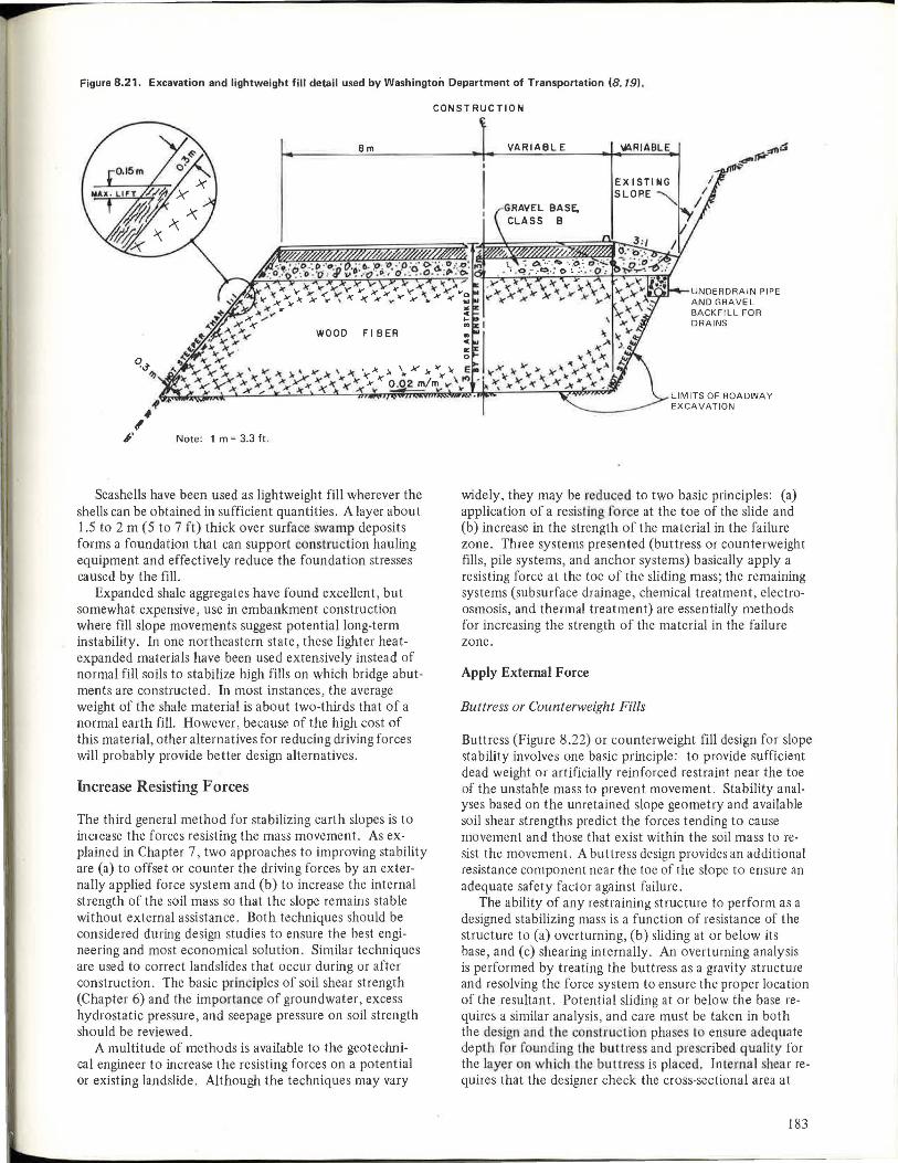
Figure 8.21. Excavation and lightweight fill detail used by Washington Department of Transportation (8.19).

em

WOOD Fl BER

Note: 1 m = 3.3 ft .

Seashells have been used as lightweight fill wherever the shells can be obtained in sufficient quantities. A layer about 1.5 to 2 m (5 to 7 ft) thick over surface swamp deposits forms a foundation that can support construction hauling equipment and effectively reduce the foundation stresses caused by the fill.

Expanded shale aggregates have found excellent, but somewhat expensive, use in embankment construction where fill slope movements suggest potential long-term instability. In one northeastern state, these lighter heat­expanded materials have been used extensively instead of normal fill soils to stabilize high fills on which bridge abut­ments are constructed. In most instances, the average weight of the shale material is about two-thirds that of a normal earth fill. However, because of the high cost of this material, other alternatives for reducing driving forces will probably provide better design alternatives.

Increase Resisting Forces

The third general method for stabilizing earth slopes is to increase the forces resisting the mass movement. As ex· plained in Chapter 7, two approaches to improving stability are (a) to offset or counter the driving forces by an exter­nally applied force system and (b) to increase the internal strength of the soil mass so that the slope remains stable without external assistance. Both techniques should be considered during design studies to ensure the best engi­neering and most economical solution. Similar techniques are used to correct landslides that occur during or after construction. The basic principles of soil shear strength (Chapter 6) and the impor tance of groundwater, excess hydrostatic pressure, and seepage pressure on soil strength should be reviewed.

A multitude of methods is available to the geotechni­cal engineer to increase the resisting forces on a potential or existing landslide. Although the techniques may vary

CONSTRUCTION

VARIABLE ~RIABLE

EXISTING SLOP.E"

DRAINS

widely, they may be reduced to two basic principles: (a) application of a resisting r· rce at the toe of the slide and (b) increase in the strength of the material in the failure zone. Three systems presented (buttress or counterweight fills, pile systems, and anchor systems) basically apply a resisting force at the toe of the sliding mass; the remaining systems (subsurface drainage, chemical treatment, electro­osmosis, and thermal treatment) are essentially methods for increasing the strength of the material in the failure zone.

Apply External Force

Buttress or Counterweight Fills

Buttress (Figure 8.22) or counterweight fill design for slope stability involves one basic principle: to provide sufficient dead weight or artificially reinforced restraint near the toe of the unstable mass to prevent movement. Stability anal­yses based on the unretained slope geometry and available soil shear strengths predict the forces tending to cause movement and those that exist within the soil mass to re­sist the movement. A buttress design provides an additional resistance component near the toe of the slope to ensure an adequate safety factor against failure.

The ability of any restraining structure to perform as a designed stabilizing mass is a function of resistance of the structure to (a) overturning, (b) sliding at or below its base, and (c) shearing internally. An overturning analysis is performed by treating the buttress as a gravity structure and resolving the force system to ensure the proper location of the resultant. Potential sliding at or below the base re­quires a similar analysis, and care must be taken in both the design and the construction pha es to ensure adequate depth for founding the buttress and prescribed quality for the layer on which the buttress is placed . Internal shear re­quires that the designer check the cross-sectional area at

183

Figure 8.22. Rock buttress used to control unstable slope.

Figure 8.23. Stabilization berm used to correct landslide in shale on 1-74 in Indiana.

230

22.5 m

~1 . ~ A ... o·,\ 'B

200 STABILIZING BERM

170

APPROX, ) SHALE LINE

HORIZONTAL SCALE O 10 20 m

STABILIZING KEYWAY 0 33 66ft

various elevations within the buttress or counterweight fill to ensure that the resisting structure does not fail by shear within itself.

Several important highway sections have been con­structed with or treated remedially by a buttress type of restraining structure. The construction of 1-74 in south­eastern Indiana in the 1960s included the placement of many kilometers of embankment. The borrow material used in the embankments was predominantly local shale materials that were inter bedded with limestone and sand­stone. Unfortunately, shales deteriorate with time when exposed to the environment, and cut slopes in fresh shale steeper than 1: 1 will deteriorate and slough on the surface until a final stable slope of about 2: 1 is attained. These same shale materials , when placed and manipulated into an embankment by the use of accepted construction tech­niques, will similarly degrade with time. Ultimately, the embankment slopes may slough and eventually fail. The first indications of the degradation process are localized

184

depressions of the roadway; these gradually spread laterally to include large areas of the pavement surface. These de­pressions occur as the embankment volume decreases be­cause voids occur between rock blocks and become filled with soil and degraded rock fragments.

Several fill slopes that did shear along 1-74 have been thoroughly investigated and analyzed, and alternative re­medial treatments have been evaluated. On one slide, known locally as the Chicken slide, careful studies of the in situ shear strength of the shales ( ¢ = 14° to l 6°) versus the original strengths used in the preconstruction studies showed an approximate reduction of one-half from the as­built condition (8.12) . The alternatives considered by the Indiana State Highway Commission were (a) relocate , (b) remove and replace, (c) buttress with earth and rock coun­terweight, and (d) buttress with reinforced earth wall.

Each alternative was thoroughly studied, and appropri­ate cost figures were determined. By far the least expen­sive and least disruptive to traffic were the two buttress

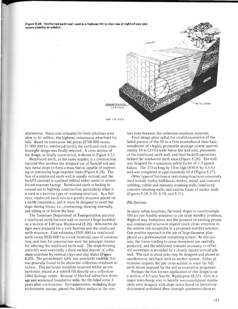
Figure 8.24. Reinforced earth wall used as a highway fill to limit use of right-of-way and ensure stability to sidehill.

1.5mx 1.5m

Note : 1 m = 3.3 ft.

alternatives. Since cost estimates for both solutions were close to $1 million, the highway commission advertised for bids. Based on contractor bid prices ($700 000 versus $1 000 000 for reinforced earth), the earth and rock coun­terweight design was finally selected. A cross section of the design, as finally constructed, is shown in Figure 8.23.

Reinforced earth, as the name implies, is a construction material that involves the designed use of backfill soil and thin metal strips to form a mass that is capable of support­ing or restraining large imposed loads (Figure 8.24) . The face of a reinforced earth wall is usually vertical , and the backfill material is confined behind either metal or unrein­forced concrete facings. Reinforced earth is finding in­creased use in highway construction, particularly when it is used as a buttress type of retaining structure. As a but­tress, reinforced earth acts as a gravity structure placed on a stable foundation, and it must be designed to resist the slope driving forces, i.e., overturning, shearing internally, and sliding at or below the base.

The Tennessee Department of Transportation selected a reinforced earth buttress wall to correct a large landslide on a section of I-40 near Rockwood (8.26). Alternative de­signs were prepared for a rock buttress and the reinforced earth structure. Cost estimates ($505 000 for reinforced earth versus $930 000 for a rock buttress), ease of construc­tion, and time for construction were the principal reasons for selecting the reinforced earth wall. The slope-forming materials were essentially a thick surface deposit of collu­vium underlain by residual clays and clay shales (Figure 8.25). The groundwater table was seasonally variable , but was generally found to be above the col!uvium-residuum in­terface. This particular landslide occurred within an em­bankment placed as a sidehill fill directly on a colluvium­filled drainage ravine. Because of blocked subsurface drain­age and weakened foundation soils, the fill failed some 4 years after construction. Instrumentation, including slope inclinometer casings, placed the failure surface at the con-

tact zone between the colluvium-residuum materials. Final design plans called for careful excavation of the

failed portion of the fill to a firm unweathered shale base, installation of a highly permeable drainage course approxi­mately IO m (33 ft) wide below the wall area , placement of the reinforced earth wall, and final backfill operations behind the reinforced earth mass (Figure 8.26). The wall was designed for a minimum safety factor of 1 .5 against failure. The 253-m long by 10-m high (830-ft by 3.3-ft) wall was completed in approximately 60 d (Figure 8.27).

Other types of buttress or restraining structures commonly used include timber bulkheads; timber, metal, and concrete cribbing; rubble and masonry retaining walls; reinforced concrete retaining walls; and various forms of anchor walls (Figures 8.28 , 8.29, 8.30, and 8.31).

Pile Systems

In many urban locations, flattened slopes or counterweight fills are not feasible solutions to cut slope stability problems. Right-of-way limitations and the presence of existing private and commercial structures require much closer attention to the relative risk-acceptable in a proposed stability solution. One positive approach is the use of large-diameter piles placed as a preexcavation restraining system. In this sys­tem, the forces tending to cause movement are carefully predicted, and the additional restraint necessary to offset soil movement is provided by a closely spaced vertical pile wall. °The cast-in-place piles may be designed and placed as cantilevers or tied back with an anchor system. Either al­ternative requires the pile cross section to resist the full earth thrust imposed by the soil as excavation progresses.

Perhaps the best known application of this design is on a section of 1-5 near Seattle , Washington (8.21). Cuts in a major interchange area in heavily overconsolidated marine clays were de signed with slope ratios based on laboratory­determined undrained shear strength parameters from re-

185

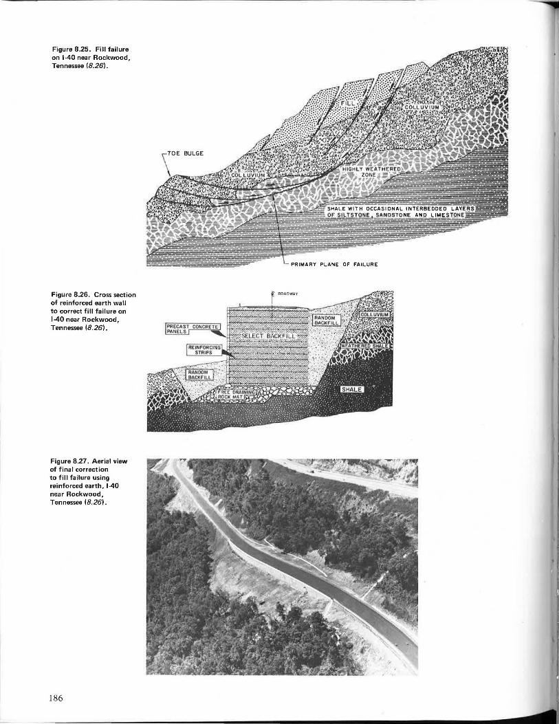
Figure 8.25 . on 1-40 n · Fill failure T ear Rock

ennessee (8.26). wood,

Figure 8.26 of reinforced Cross section to correct fill :a~th wall 1-40 near R a1lure on T ockwood

ennessee (8.26). '

Figure 8.27 A . of final c . enal view to fill ta ·rorrection

. • ure usin reinforced g near Rock earth, 1-40 T wood

ennessee (8. 26\.

186

- PRIMARY PLANE OF FAILURE

Figure 8.28. Concrete crib wall and gravel backfill installed to prevent movement in Arcata, California (8.24) .

Figure 8.29. Uses of retaining walls for slope stabilization (8.27) .

{a) CONCRETE GRAVITY RETAINING WALLS: APPLICABLE TO BOTH CUT ANO FILL SECTIONS

Figure 8.30. Gabion·wall retaining structure .

Enlargement of portion of single gabion showing relative size of stone and

(Cut, Fill or

Natural)

lb) CANTILEVER RETAINING WALLS: COMMONLY USED TO CONTROL MOVEMENTS OF SMALL SOIL MASSES OR SIOEHILL FILL SECTIONS

Cantilever Retaining Wall

---\ ,/ ----/" Weep holes

/ Highway

Figure 8.31 . Design of strut to correct cut slope failure on 1-94 in Minneapolis-St. Paul (8.28).

/FAILURE SURFACE

PORTLAND CEM ENT CONCRETE BUTTRESS

187

Figure 8.32. Cylinder pile wall system proposed to stabilize deep-seated slope failure on 1-94 in Minneapolis-St. Paul (8.28).

Cut Slope

Cantilever Wall (To prevent local sloughing)

ft. Highway

I

---+-t ~ Cylinder Piles

--covered soil samples. Some weeks after the cuts had been opened, movements in the form of bulges and sloughing began on several slope faces. Detailed analysis by geotech­nical engineers laid the cause for these movements to the release of large "locked-in" soil stresses. The stresses were caused geologically by massive overburden pressures pre­viously applied to the clays. The subsequent removal of these loads was not accompanied by equally large elastic rebounds by the soil; thus, the soil retained a large pre­stress history. During roadway excavations, substantial cuts were made through these prestressed soils, and the re­moval of the lateral support, together with the increased moisture content , permitted expansion and subsequent loss of soil strength.

Further slope flattening was not feasible on this project , and large-diameter (I to 4 m, 3 to 13 ft) drilled, cast-in­place concrete shafts were spaced to form an almost con­tinuous wall to minimize the potential for large soil strains as the excavations were made. Since the anticipated lateral soil forces were large, heavy steel H-pile sections formed the cores of the shafts, and high-strength concrete was placed around those sections. Only minor lateral expan­sion occurred during the excavation process, and the shafts were designed by using the fully mobilized shear strength of the clay. Drilled shafts were also used in remedial work for the slope of the Potrero Hill cut in San Francisco (8.30)

Figure 8.33. Section of tied-back wall to correct slide condition on New York Avenue in Washington, D.C. (8.20).

188

HIGHWAY RIGHT OF WAY

12m •

Note: 1 m = 3.3 ft ,

and in the 1-94 cuts (Figure 8.32) in and around Minneapolis­St. Paul (8.33).

Recorded attempts to use driven steel piles or wood piles of nominal diameter to retard or prevent landslides have sel­dom been successful. For most earth or rock movements, such piles are incapable of providing adequate shearing re­sistance. In addition, when they are used in even small earth slides, movement of soil between and around the piles must be considered . Quite often, a major earth move­ment develops a rupture surface in the soil below the pile tips. All such pile schemes should be carefully designed by using realistic soil parameters (8.2). The forces involved in even the smallest landslide are large, and for the piles to be effective they must have sufficient cross section and depth to prevent movement.

Anchor Systems

One type of anchor system is tied-back walls, many varia­tions of which are available to the design engineer. Most such wall designs use the basic principle of carrying the backfill forces on the wall by a "tie" system to transfer the imposed load to an area behind the slide mass where satisfactory resistance can be established. The ties may consist of pre- or post-tensioned cables, rods, or wires and some form of deadmen or other method to develop ade­quate passive earth pressure.

A good example of such a design was used to retain a large movement in Washington, D.C. (8.20). A section of New York Avenue , a major street in the District of Colum­bia, was to be widened sufficiently to provide an additional two lanes of roadway. The original street was built in a sidehill cut; the shoulder area was founded on an uncom­pacted fill of clay, rubble, and cinders. The natural soil be­low the miscellaneous fill was an overconsolidated clay with a residual shear strength of 31.6 kPa ( 660 !bf /ft2) ( 60 percent of laboratory-measured peak value) and a sensitiv­ity of about 4. Since the new construction required an ad­ditional width for the roadway fill , the final design called for removal and replacement of the miscellaneous existing embankment as a first order of work. Right-of-way con­siderations did not permit the 4: 1 slopes dictated by the

rfJADWAY

4m IOm

CURB

CONCRETE CAP

stability studies of the widened embankment section. A comparison of the various design alterna'lives indicated

the economic use of a tied-back sheet pile wall (Figure 8.33). The depth of embedment for the tie-back system varied from 12 to 21 m (40 to 69 ft) to ensure adequate anchor­age in the stiff clays. A system of belled concrete anchors into which 3.2-cm (1.25-in) diameter high-strength steel rods were cast acted as the principal support against pull­out. The rods were pretensioned against the sheet-pile wall system to the full design loads following installation. A maximum allowable long-term shear stress of 23.9 kPa (500 lbf/fl2) for the clay was used in analysis; this stress pro­vided a safety factor of about 2. lnstruments .left in place to facilitate the Jong-term recording o actual stress levels indicate that the tensile stresses in the steel were well within predicted values.

Increase Internal Strength

Subsurface Drainage

One of the most effective treatments of landslides is to in­crease the forces available to resist motion by increasing the shear strength of the soil through subsurface drainage (increase in the effective normal stress on the failure sur­face). Thjs treatment is discussed earlier in this chapter .

Chemical Treatment

Various schemes have been tried by researchers and prac­titioners to treat unstable soil slopes with injected chemi­cals. One interesting application under research in Califor­nia is a patented ion-exchange tecltnique described by Smith and Forsyth (8.30). The ion-exchange technique consists of treating the clay minerals along the plane of po­tential movement with a concentrated chemical solution. The actual chemicals used in the ion exchange are deter­mined by the clay mineralogy of the soil to be treated and by the prevailing groundwater conditions in the slide mass.

To chemically change a clay soil by ion exchange, some cations in the clay minerals are replaced with different cat­ions that are introduced by chemical solution. In a satu­rated clay, the rate of migration through the soil structure appears to be much greater for cations than for water. Catio11 replacement can result in as much as a 200 to 300 percent increase in soil hear trength. SiJ1ce the initial strength in the shear zone is low for most clays in which this method can be used this relatively minor increase in strength may be sufficient to stabilize a landslide. Although the ion-exchange technique was uccessfully used in northern California to stabilize a slide (8.17), it may have lilt le chance for success on other landslides.

Other chemical treatments used with varying degrees of success are lime or lime-soil mixtures, cement grout, and potassium injections. Perhaps the chemical treatment most used in attempts to increase soil shear strength is Hme. High-pressure injections of lime slurry have been used in several stales with limited success. One successful Lreat­ment was reported by Handy and WiUfams (8.11); approxi­mately 45 000 kg ( I 00 00.0 lb) of quickUme were placed in predrilled 0.2-rn (0.5-ft) diameter holes on 1.5-m (5-ft) centers throughout an extensive slide area. The 1Jme mi·

grated a distance of 0.3 m (1 ft) from the drilled holes in I year. Slide movements subsequently ceased, and the area has remained stable to date.

An interesting application of cement grout occurred on a section of 1-40 along the Pigeon River in North Carolina. A 90-m (300-ft) benched cut slope for the roadway began moving forward , threatening the road and a large water sup­ply reservo.ir on the downbill side of the roadway. Subse­quent investigations and analyses showed the roadway foundation area to consist or broken rubble and talus de­bris Lo great depths. Instruments placed movement along a definite plane where rock voids were large. Large vol­umes of cement grout were injected into the voids of this layer and surrounding areas in an attempt to increa e the shearing resistance of the slope foundation. Although great volumes of grout were required at considerable ex­pense the slope did become stable, and the water supply for a major city was not lost.

Electroosmosis

One method that effectively increases soil shear strength in situ is electroosmosis (8.5, 8.6). This technique, al­though extremely expensive , causes migration of pore water between previously placed electrodes; the lo s of poJe water , in turn, causes c n olidation of the soil and a S\lbsequent increase in shear strength. Casagrande Loughney and Matich (8.6) describe a highway project that required an excavation approximately 4.5 m (15 ft) in depth and some 24 by 12 m (80 by 40 ft) in area to install a bridge foundation support system. The side slopes were predom­inantly a saturated somewhat uniform ilt material placed on a 2.5:J slope. Dudng excavation a slide ccurred. After consideration of alternatives such as freezing, chemical in ­jection, slope flattening, and restraining waUs, the designers selected electroosmosis as the most economical solution. Some 3 months were required to lower the groundwater sufficiently to proceed with construction; however, the final slope excavation was steepened to I: I and the project was successfully completed. Long-term solutions using electroosmosis must give full consideration to the need for a constant supply of direct current and the need for main­tenance personnel to periodically check the system for re­placement of field-installed electrodes.

One interesting variation of the electroosmotic effect is that suggested by Veder (8.32). Where landslides occur at the contact zone between soil layers, Veder reports that differences in water content between the layers means a difference in electropotential. This difference in potential creates a gradient that forces water to move through the soil toward the region of lower potential. Veder suggests that the insertion of metallic conductors into the soil to create short-circuit electrodes will halt soil-water move­ment. Thus, the imposed short-circuit effectively acts in the reverse of electroosmosis where an external source of direct current is used to cause soil water migration. Veder reports several cases.in which this procedure has success­fully stabilized landslides.

Thermal Treatment

For several years the Russians have experimented and re-

189

ported on the success of thermal treatment of plastic and loessial soils. The high lemperatu.re treatments cause a per­manent drying of the embankment r cut slope. Hill (8.15) discusses the use of thermal treatmenl in the Unit · d States. Beles and Stanculescu (8.3) describe an interesting use of thermal methods to reduce the in situ water contents of heavy clay soi l in Romania. Applications to highway land­slides and to unstable railroad upport fills are cited.

Combination of Treatments

In most applications, a combination of the various methods outlined above is used. A buttress fill may be combined with a subdrnlnage system to provide a resisting force that allows the drainage system to become effective, thus tend­ing to increase the stability of the slope with time. Verti­cal well may be pumped Lo stabilize a cut during construc­tion· however horizontal drain usually are in tailed as a long-term solution and pumping the vertical wells is then discontinued. This procedure was used in California to sta­bilize the Pinole slide (Figure 8.13); two vertical wells were pumped immediately to relieve the water pre sure whHe the horizontal drain were in tailed. Then, berms were placed as the embankment was reconstructed to ensure lhe integrity

f (he recon !ruction while lhe horizontal drains continued to reduce the water pressure. The 1 ng-term stability of this treatment requires that the horizontal drains function properly for the life of the structure. On another project in California, several different approaches were also used to stabilize a slow moving landslide by che111ical injection to effect a strength increase within the predetermined slide zone. Then , horiz ntal dra in were iJ1Stalled a year la1er to effect positive drainage by gravity now deep withjn the slide and thereby ensure long-term tabi!Hy to Lhe area.

Each case in wh.ich combination of variou methods have been used bo lit in design and conslruclion re pre ents a tudy of carerully considered and applied engineering principles to reneh a reasonably economic olution. Per­haps the relation between design and actual construction is somewhat unique in geotechnical engineering because a failure of the slope may resuit if various combinations of soil strength, groundwater levels, and slope geometrics that occur during construction arc not fully considered in design.

TOE EROSION

Toe erosion, as used in this chapter, is the removal of ma­terial from the base or toe o a slide or natural slope by natural forces. Although wind erosi 11 can be appreciable, the mo t c mm n type of toe ero ion enc unlered by a g-cotechnical enginee r i that cau ed by moving water in rivers streams. or oceans erod in g slope-rorming materials. The general so.lution for this type or problem i LO protect the toe of a lope by either a riprap surface layer or a free­draining durable rock layer placed al the base of the slope to an elevation or about I 111 (3. rt) above the expected mean high water level.

The erosion of natural or human-made slopes by rivers or streams is a major cause of land instability. Geologic studies refer to the erosion of stream valleys cliff fonrn1-tions on oceanfronts, and loss of land due to 111 vlng waters. Engineers are faced with these problems in design and con-

190

struction of transportation facilities. Careful attention must be given to the protection of earth slopes in any channel design. Protection may be in the f rm or (a) rip­rap or other suitable material or (b) 11 lining of rein forced concrete with designed hydsaulic features to ensure clissipa­ti n of lh,e de tructive fo1·ces of the ant icipated flow. One hould never assume that a slope adjacent to natural water­

courses is adequate until thorough hydraulic studies are made and corresponding protection of the slope provided for the anticipated long-term effects of the water.

Various buttress systems have been used successfu lly in situati ns in which the general lack of space precludes ther treatments, particularly where a facility follows a river or ocean face. Pile systems have had little success where the ocean is.eroding away the toe of a cliff. Various surface and subsurface drainage systems have been used in combi­nation with buttress systems, and, if properly designed and constructed, these will be succe ful. In general, the so lu­tion to the toe erosion problem i to instaU a sy ten, that prevents further loss of support 1or the lope and lo u e oth r means for increa ing lhe resisting rorces. Thus, a combination of several metho ls will generally be requ ired.

REFERENCES

8.1 Baker, R. F., and Marshall, H. C. Control and Correction. In Landsl ides and Engineering Practice (Eckel, E. B., ed.), Highway Research Board, Special Rcpt. 29, 1958, pp. 150-188.

8.2 Baker, R. F., and Yoder, E. J. Stability Analyses and De­sign of Control Methods. In L:indslidc and Engineering Prnctico (Eckel, E. B. ccl.)~Highway Research Board, SpcciaJ Rept. 29, L9S8, pp. 189-216.

8.3 Beles, A. A., and Stanculescu, I. I. Thermal Treatment as a Means of Im proving the Stnbilily of Earth Masses. Gcotcchniquc, Vol. 8, No. 4, 1.958, pp. 158-165.

8.4 alifomia Dcpartmcnl of Tra11Sportation. Foundation Exploralion. Testing, and Analy i Procedures. ln Mo­tcrials Manual, California Department of Transportation, n.crnmcnto, Vol. 6, 1973.

8.5 Casanrundc, L. Electro-Osmosis. Proc., 2nd lnte.rnationnl Conference on Soil Mechanics :md roundat.ion Engineer­ing Rotterdam Vol. l 1948, pp. 218-223.

8.6 Casagrande, L., Loughney, R. W., and Malich, M. A. J. Elec1ro-Osm0Li.c Stnbi!ization of a lligh Slope in o·e Saturated Silt. Proc., 5th International onfcrence on Soil Mechanics and Foundation Engineering, Paris , Vol. 2, 1961, pp. 555-561.

8. 7 Casagrande, L., and Poulos, S. On the Effectiveness of Sand Drains. Canadian Geotechnical Journal, Vol. 6, No. 3, 1969, pp. 287-326.

8.8 Cedergr n, H. R. Seepage, Drainage, and Flow Nets. Wiley, New York, 1967, 489 pp.

8.9 Coleman, T. A. Polystyrene Foam Is Competitive, Light­weight Fill. Civil Gngincering, Vol. 44, No. 2, 1974, pp. 68-69.

8.10 Dennis, T. H., and Allan, R. J. Slide Problem: Storms D Costly Damage on State Highways Yearly. California llighways and Public W rks, Vol. 20, July 1941, pp. 1-3 , 10, 23.

8.11 Handy , R. L., and Williams, W.W. Chemical Stabilization of an Active Landslide. Civil Engineering, Vol. 37, No. 8, 1967, pp. 62-65.

8.12 Haugen, J. J. and DiMillio, A. F. A History of Recent Shale Problems in Indiana. Highway Focus, Vol. 6, No. 3,July 1974, pp.15-21.

8.13 Herbold, K. D. Cut Slope railurc in Residual Soil. Proc., 23rd Hi •hway Geology Symposium, 1972, pp. 33-49.

8.14 [I rlinger , rs. W., and Stafford, G. Orinda Slide. Califor­nia Highways and Public Works, Vol. 31, Jan.-Feb. 1952,

8.15

8.16

8.17

8.18

8.19

8.20

8.21

8.22

8.23

8.24

8.25

8.26

8.27

8.28

pp. 45 , 50-52 59-60. Hill , R. A. Clay Stratum Dried Out to Preven t Land lips.

ivil Engineering, Vol. 4 , No . 8 , 1934, pp. 403-407. Johnson, S. J. ·oundation Prceompression With Vertica l Sand Dra in . Journal of Soil Mechanics a nd Foundations Division , American S ciety of Civil Engineers, New York, Vo l. 96 , No. SMl 1970, pp . 145-175. Menrns R., Carney R. and Forsyth, R. A. · valuation of the Ion Exchange Landstidc Correction Technique. Ma­terials and Resea rch De partment, California Division of Highways, Ropt. A-HY-MR-211.6-1-72-39, 1973 26 pp. Morgenstern , N. R., a nd Price, V. •. l11c Analysis of the Sta bility of General Slip Surface . Ccotechnlquc, Vol. 15, No. l , 1965, pp. 79-93. Nelson, D.S. , and Allen, W. L., Jr. Sawdust as Light­weight Fill Material. Highway Focus, Vol. 6, No. 3, July 1974 , pp. 53-66. O'Colman, E., and Trigo Ramirez, J . Design and Construc­tion of Tied-.Back Sheet Pile Wall. Highway Focus, Vol. 2, No. 5, Dec. J 970, pp. 63-7 1 . Pa llad ino, O. J ., and Peck , R. 13. Slope f'/a ilure · in nn Overconsolida ted Ony SC,ltt lc, Washington. Goolech· niquc, Vol. 22, No. 4 , 1972 pp. 563-595. Peck, R. 13., and lrclnnd , Ii . 0. l11vc tigation or Stability Proble ms. American Ra ilway Engineer ing Association, Chicago, Bulletin 507, 1953, pp. l 116-1128. Roads and Str ets. uring Slides With Drainage Tunnels. Roods a nd Streets, Vo l. 90, No. 4, 1947, pp. 72, 74, 76. Root, A. W. Prevent ion of Lnnd lidc . In L'lndslidcs and ·nginceri ng Ptactice (f.ckcl, £ . .B. , ed.), Highway Re­search Board , Speciul Rcpt. 29, 1958, pp. 113-1.49. Royster, D. L. To Bench , or Not to Bench. Proc., 48·th Tennessee Hig hway Conference, Univ. or Tennessee, Knoxville , Tennessee Department of llighways, Naslwille , 1966, pp. 52-73. Royster, D. L. Const ructio n of a Reinforced Earth f,' ill Al ng 1-40 in Ten nessee. Proc ., 25th Highway Geology Symposium J 974, pp. 76-93. Schweizer, R. J ., ;1nd Wright , S. C. A Survey and Eva lua­tion of Re medial Measures for cmth Slo pe Stabilizat ion.

enter for Highway Rescurch, Univ. of Texas u~ Au tin , Research Rcpt. J61-2f', 1974, 123 pp. Sha m1on and Wilson, Inc. Slo pe Stability lnvcs tigu lion,

Vicinity of Prospect Park, Minneapolis-St. Paul. Shannon and Wilson, Seattle, 196 8.

8.29 Smith, T. W., and Cedergren, H. R. Cut Slope Design in f'i cld Testing of Soils and Landslides. American Society for Testing a nd Materials, Philadelphia , Special Technical Pub!. 322, J 962, pp. 135-158"

8.30 Smith, T. W., and Forsyth, R. A. Potrero Hill Slide and Correction. Journal of Soil Mechanics and Foundations Division, American Socie ty of Civil Engineers, New York, Vol. 97, No. SM3, 1971, pp. 541-564.

8.31 Smith, T. W., Prysock, R.H., and Campbell, J. Pinole Slide, 1-80, California. Highway Focus, Vol. 2, No. 5, Dec. 1970, pp . 51-61.

8.32 Veder, C. Phenomena of the Contact of Soil Mechanics. Proc., 1st International Symposium on Landslide Con­trol, Kyoto and Tokyo, Japan Society of Landslide , 1972, pp. 143-162 (in English a nd Japanese).

8.33 Wilson, S. D. Landslide lnsLrumentation for the Minne­apolis Freeway. Transportation Research Board, Trans­portation Research Record 482, 1974, pp. 30-42.

PHOTOGRAPH AND DRAWING CREDITS

Figure 8.2 Figure 8.3

Figure 8.5 figure 8. 7 Figure 8.9 Figure 8.11 figure 8.12 Figure 8.13 f'igure 8.16 Figure 8.20

Figure 8.22 Figure 8.23 Figure 8.24 Figure 8.28 Figure 8.30

Courtesy of California Department of Transportation Courtesy of North Carolina Department of Transpor­tation Courtesy of Alabama Highway Department Courtesy of Tennessee Department of Transportatio n Courtesy of California Department of Transporta tion Courtesy of California Department of Transportation Courtesy of California Department of Transportation Courtesy of California Department of Transportation Courtesy of Federal Highway Admini stration Courtesy of Michigan Department of State Highways and Transportation Courtesy of Tennessee Department of Transportatio n Courtesy of Indiana Department of Transportation Courtesy of Tennessee Department of Transporta tion Courtesy of California Department of Transportation Courtesy of Tennessee Department of Transportatio n

191

Chapter 9

Engineering of Rock Slopes Douglas R. Fiteau and F. Lionel Peckover

In transportation corridors, the objective of rock-slope engi-neering is to maintain slopes for maximum safety and effi-ciency. Minimizing rock excavation and predicting the safety and ultimate behavior of rock slopes, whether for highway, railway, spiliway, quarry, dam site, or opencut mine, are com-mon objectives of civil, geology, and mining engineers. The rational design of rock slopes is particularly important if slopes are steep, if safety is important, and if slope design significantly affects project costs.

The present empirically based, cut-and-try methods and techniques used to design rock slopes are inadequate. New principles and improved technological capability are needed, particularly in mining operations, in which the trend is to-ward open-pit mines, and in transportation facility construc-tion, which may be increasingly required in steep terrain.

That rock slopes must be treated differently from soil slopes cannot be emphasized enough. In the analysis of rock slopes, one must recognize the differences in the basic char-acteristics and behavior of soil and rock. Unlike a soil mass, which is a relatively homogeneous and continuous medium composed of uncemented particles, arock mass is a hetero-geneous and discontinuous medium composed essentially of partitioned solid blocks that are separated by discontinuities. The geometry of the spaces between the solid materials and the interlocking properties of the components of soil and rock are totally different. Failure in soil tends to occur within the soil mass, and the direction of the surface of fail-ure tends not to depend on variations of soil properties. The surface of failure in hard rock masses, however, tends to fol-low the preexisting discontinuities and not to occur through the intact rock to any great extent unless the rock is quite soft. The shear strength of a rock mass is determined largely by the presence of the discontinuities, and the result is that the rock mass is anisotropic in its strength and deformational properties..

The design of rock slopes involves both engineering and geology and, in addition, a combination of the knowledge of

precedent with the art of estimation and judgment. The engineer-geologist must obtain quantitative information on those factors that are necessary for making calculations of the probable stability of the slope. Those factors include structural geology, local topography, drainage, hydrogeology, tectonic history, and other environmental features that may add to or detract from the stability of the slope.

Whether a slope will be stable or unstable will depend on how the forces that tend to resist failure compare with those that tend to cause failure. This concept defines the factor of safety for the slope as the ratio of the sum of the resisting forces that act to prevent failure to the sum of the driving forces that tend to cause failure. To a considerable extent, the problem of rock-slope design and related aspects is one of applied mechanics, and the necessary margin of safety to be provided in any particular case is a question of judgment.

The terms of reference and related slope-design problems of an open-pit excavation, for example, may be entirely dif-ferent from those of highway and railway cuts. For that matter, slope-design problems and requirements for highways and for railways can also differ markedly. Highways can usu-ally have a greater degree of slope instability on their rights-of-way than railways. Unlike automobiles, trains cannot steer or brake readily and can be derailed by rocks no larger than 30 cm (1 ft). Therefore, a remedial measure that may be used on a highway slope may be entirely unacceptable on a railway slope. No particular attempt has been made here, however, to separate railway and highway rock-slope engi-neering techniques.

Rock-slope engineering is concerned not with large land-slides but with rock falls of individual blocks, translation of small rock masses, and occasional slides of accumulated de-bris from gullies, talus slopes, and postglacial slide areas. This chapter discusses the aspects of rock-slope engineering relevant to designing cut slopes and maintaining the long-term efficiency and safety of existing slopes. Discussed are the significant factors in rock-slope design, the procedures

192

and mechanical properties of the rock mass are a function of the attitude, geometry, and spatial distribution of these defective surfaces. The basic principles of rock-slope design are based on

Figure 9.1. Well-developed, steeply dipping set of joints along highway at Slocan Lake, British Columbia. Joints control slope stability almost entirely.

The systems of joints and other discontinuities: The relation of these systems to possible failure sur-

faces: The strength parameters of the joints, which include

the properties of both the joint surfaces and any joint infill-ing materials: and

The water pressure in the joints.

U •'-'• F

-- . .- - -'- -

f - ":---'• -

r.- I ,.

Figure 9.2. Well-developed discontinuities dipping toward highway at Porteau Bluffs, British Columbia. Two significant slides have occurred in this area.

t, ...

.j. . ., . ..

- ,.f ,......... . .

.. - 1/. •:

-',.--.

for the analysis of rock-slope stability, the general planning involved in extensive rock-slope engineering along transpor-tation corridors, and the stabilization, protection, anci warn-ing measures that can be used to remedy rock-slope prob-lems.

SIGNIFICANT FACTORS IN DESIGN OF ROCK SLOPES

This section describes the basic factors that are significant to the stability of rock slopes. Additional information is given by Stacey (9.105). Piteau (9.87). Hock and Bray (9.42). Duncan (9.23), Deere and others (9.21). Terzaghi (9.108). Jennings (9.47), Goodman (9.29). Coates (9.16), and the Canada Department of Energy, Mines and Resources (9.94).

Structural Discontinuities

The stability of rock slopes depends largely on the presence and nat ure of defective planes or discontinuities within the rock mass. For the greatest part, the significant physical

Examples of the significance of structural discontinuities in slope design are shown in Figures 9.1 and 9.2.

The stability of rock slopes, therefore, is assessed princi-pally by analyzing structural discontinuities in the rock mass and not by assessing the strength of the intact rock itself. Observations relating to shear failure along discontinuities should be made insofar as the discontinuities affect the co-hesion and friction developed with respect to shear along these features. The relations of discontinuities to the direc-tion and inclination of the rock slope and to any factors that might influence any potential surface failure must re-ceive special attention. These statements apply even more-so to faults, regardless of how great or small displacements have been.

Field studies show that rocks are usually jointed in l)ref-erential direct ions. Depending on their modes of origin, however, rocks have joint sets whose characteristics can vary greatly. Wide variations can occur in the average spacing be-tween joints, the nature and degree of joint mulling materials. the physical characteristics of their surfaces, and the degree of their development. One joint set can, therefore, have ef-fects on shear characteristics quite different from those of another set, and the various properties of each of the joint sets must be considered individually in rock-slope design. (Strength evaluations are explained in Chapter 6). The main properties that are associated with structural discontinuities and that require quantitative and qualitative evaluation fol- lOW.

Orientation or Position in Space

Orientation or position in space is the most important prop-erty. If the orientation of joints favors potential slope fail-ure, the effects of other properties are generally unimportant. Discontinuities dipping out of the slope must be carefully considered. Their potential instability increases proportion-ally as the strike of the discontinuities approaches that of the slope.

Continuity or Size

Continuity or size is the most difficult property to assess. The strength reduction on a failure surface that contains one or more discontinuities is a function of their size. The aver-age continuity of a particular joint set partly indicates the ex-tent to which the rock material and the discontinuities will separately affect the mechanical properties of the mass (9.23, 9.4 7): in addition, the average continuity affects the magni-tude of possible failu res involving these features.

193

Infiuing Materials and Openness

Infilling materials are those materials that occur between the walls of the discontinuities in the mass. The three most im-portant characteristics of infilling materials are thickness, type, and hardness. Jaeger (9.45) notes that, if infilling is sufficiently thick, the walls of the discontinuity will not touch and the strength properties will be those of the infill-ing material.

Spacing

The spacing of discontinuities partly indicates the extent to which the intact rock and the discontinuities will separately affect the mechanical properties of the rock mass. A rock mass is inherently weaker if spacing is close. Also, greater joint frequency increases the potential for dilatancy.

Asperities

Two orders of asperities are recognized. First-order asperi-ties (waviness) are unlikely to shear off; they affect the shear-movement characteristics along the discontinuity and effectively modify the direction of movement during slope failure (9.21). Undulations or waves on the discontinuity reduce the effective apparent dip of the plane, and this dip angle and not the mean dip angle should be used for calculat-ing the disturbing forces on a potential failure plane (9.68). Second-order asperities (roughness) are much smaller and are likely to shear off during movement; these produce an apparent increase in frictional strength along the discontin-uity (9.99).

Previous Shear Movement

Shear displacement on a discontinuity results in breaking through asperities and thus reducing the shear strength from initial peak values to values that approach residual shear strength (9.54).

Rock Type

When a slope consists of several rock types, their combined mechanical behavior may differ considerably from that of the constituent units themselves. Hence, each particular rock type may require individual assessment for its behavior in the slope. Different rock types and the products that re-sult from their alteration have inherently different weaknesses and strengths as a result of their origins and compositions. Hence, the properties of different rock and infilling materials can vary within wide limits (9.107). The characteristics of each rock type significantly influence the friction angle, na-ture of asperities, and hardness of the walls of the discontin-uities.

Rock Hardness

There is a relation between rock hardness and unconfined compressive strength. According to Jennings (9.46), an in-crease in hardness has a corresponding increase in the shear strength. Infilling material and second-order asperities are sheared through during shear failure along a discontinuity;

the shear strength of the discontinuity is a function of the shear strength of the infilling materials and the rock mate-rials that form the asperities.

Origins

The origins of discontinuities will affect their engineering significance in the slope. Faults, as compared to joints, for example, have different origins and accordingly different geometry, spatial distribution, weathering and infilling char-acteristics, and seepage characteristics.

Groundwater

The presence of water in joints has probably been respon-sible for more rock slides than all other causes combined. Hence, a thorough knowledge of the character and influence of the hydrogeologic regime is necessary, and a knowledge of the water pressure distribution and the factors that influence it is the most essential. One must consider the controlling influences of texture, stratigraphy, and structure on factors such as flow, permeability, recharge, and storage capacity. Consideration should also be given to environmental factors, such as variations in climatic conditions, that result in periods of either high or low recharge and other variations in ground-water conditions. Further discussions concerning climatic in-fluences are given later.

According to Terzaghi (9.108), Serafim (9.103), and Muller (9.77), water in the slope can affect stability by

I. Physically and chemically affecting the pore water and its pressure in joint infilling materials, thus altering the strength parameters of the materials;

Exerting hydrostatic pressure on joint surfaces, thus reducing the shearing resistance along potential failure sur-faces by reducing the effective normal stresses acting on them; and

Affecting intergranular shearing resistance, thus-causing a decrease in compressive strength.

Lithology, Weathering, and Alteration

Before one can completely comprehend the particular prob-lenis of stability, one must understand the lithology of the physical properties. not only of the rock mass itself but of all the materials in the mass. Usually a slope is made up of a complex of rocks of diverse geologic origins. It may have markedly different sequences of sediments, may be intruded by bodies of igneous rocks,or may be partly metamorphosed. The mass represents an association of several lithologic units whose mechanical behavior is that of an integral whole,which may differ considerably from the individual lithologic units themselves.

A sedimentary rock sequence, for example, is markedly different from an igneous series or a metamorphic complex. Each particular type is characterized by a certain texture, fabric, bonding strength, and macro and micro structures. The most important rock properties are the nature of the mineral assemblage and the strength of the constituent min-erals; a rock material cannot be strong if its mineral constit-uents are weak or if the strength of the bonds between the minerals is weak.

194

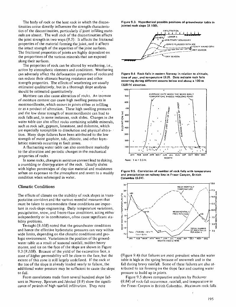
The body of rock or the host rock in which the discon-tinuities occur directly influences the strength characteris-tics of the discontinuities, particularly if joint infilling mate-nals are absent. The wall rock of the discontinuities affects the joint strength in two ways (9.5): It affects the frictional properties of the material forming the joint, and it affects the intact strength of the asperities of the joint surfaces. The frictional properties of joints are highly dependent on the proportions of the various minerals that are exposed along their surfaces.

The properties of rock can be altered by weathering, i.e., action by atmospheric elements and conditions. Weathering can adversely affect the deformation properties of rocks and can reduce their ultimate bearing resistance and other strength properties. The effects of weathering are usually estimated qualitatively, but in a thorough slope analysis should be estimated quantitatively.

Moisture can also cause alteration of rocks. An increase of moisture content can cause high swelling pressures in montmorillonite, which occurs in joints either as infilling or as a product of alteration. These high swelling pressures and the low shear strength of montmorillonite can lead to rock falls and, in some instances, rock slides. Changes in Lhe water table can also affect rocks containing soluble minerals, such as rock salt, gypsum, limestone, and dolomite, which are especially susceptible to dissolution and physical altera-tion. Many slope failures have been attributed to the low strength of moist graphite, talc, chlorite, and other layer-lattice minerals occurring in fault zones.

A fluctuating water table can also contribute markedly to the alteration and periodic changes in the mechanical properties of rocks.

In some rocks, changes in moisture content lead to slaking, a crumbling or disintegration of the rock. Usually shales with higher percentages of clay-size material and mudstones soften on exposure to the atmosphere and revert to a muddy condition when submerged in water.

Climatic Conditions

The effects of climate on the stability of rock slopes in trans-portation corridors and the various remedial measures that must be taken to accommodate these conditions are impor-tant in rock-slope engineering. Daily temperature variations, precipitation, snow, and freeze-thaw conditions, acting either independently or in combination, often cause significant sta-bility problems.

Terzaghi (9.108) noted that the groundwater conditions and hence the effective hydrostatic pressures can vary within wide limits, depending on the climatic conditions and geo-logic environment. Variations in the position of the ground-water table as a result of seasonal rainfall, sudden heavy storms, and ice on the face of the slope are shown in Figure 9.3 (9.108). Because of the yield of the excavation face, a zone of higher permeability will be close to the face, but the extent of this zone is still largely undefined. If the rock at the toe of the slope is already loaded nearly to failure, the additional water pressure may be sufficient to cause the slope to fail.

From correlations made from several hundred slope fail-ures in Norway, Bjerrum and Jçrstad (9.9) show the signifi-cance of periods of high rainfall infiltration. They note

Figure 93. Hypothetical possible positions of groundwater table in jointed rock slope (9.108).

INFILTRATION 4 4 4 1

IHIGHER/ LOWER S - S 4,ARBITRARY BOUNDARY

/ JOINTS PLUOGED WITH ICE ------HEAVY RAINSTORM .. SEASON --................

DRY SEASON

Figure 9.4 Rock falls in eastern Norway in relation to altitude, time of year, and temperature (9.9). Dots indicate rock falls occurring during different seasons below and above a 100-rn

(328-f t) elevation.

100 AVERAGE DATE WHEN THE MEAN DAILY TEMPERATURE PASSES FREEZING POINT 100 700 Soo

500

00

100

100

JAN t0 MAN MVN MAY JUN JUL AUL, btV ULI N(JV UtL. MONTH Note: 1 m = 3.3 ft.

Figure 9.5. Correlation of number of rock falls with temperature and precipitation on railway line in Fraser Canyon, British Columbia (9.84).

- TEMPERATURE --60

10.0 7.5

BER LLS

MONTH 11933,019701

(Figure 9.4) that failures are most prevalent when the water table is high in the spring because of snowmelt and in the fall during heavy rainfall. Some of these failures are also at-tributed to ice forming on the slope face and causing water pressure to build up in joints.

Figure 9.5 shows comparative analyses by Peckover (984) of rock-fall occurrence, rainfall, and temperature in the Fraser Canyon in British Columbia. Maximum rock falls

195

occur in the spring and fall when the mean temperature is about 0°C (32°F) and frequent freeze-thaw cycles are occur-ring. When temperatures are above freezing, the frequency of rock falls is a function of degree of rainfall. The number of rock falls originating on the steep rock faces in the Fraser Canyon is probably high because of the absence of snow, vegetation, and soil, the presence of which would insulate the rock from unusually low temperatures and from changes in temperature.

Frost action probably directly or indirectly accounts for more rock falls than all other factors combined. Water un-dergoes about a 9 percent volume increase when it freezes and exerts tremendous pressure when it freezes in a confined space. According to Reiche (9.97), "Water-filled cracks or joints which terminate downward and which are narrow and perhaps irregular may be converted into essentially closed systems by preliminary freezing of the water in the superfi-cial parts. In such cases the combination of expansion and low compressibility may exert a disruptive force which, if the temperature continued to fall and rock pressure per-mitted, would approach 30,000 pounds to the square inch at -22°C (i.e., -7.6°F)." Freezing temperatures of this order are not uncommon in temperate zones.

Piteau and others (9.93) correlated mean annual move-ments of an overturning failure with average monthly rain-fall, snowfall, and temperature. Although they found that a direct relation existed between movement and rainfall (i.e., groundwater pressure buildup), they found that snow-fall and freezing retarded movement. The average monthly rainfall peaked in January, but movement decreased in De-cember, when freezing and snowfall conditions started. The snow blanket prevented rainfall from infiltrating into the slope, and freezing temperatures reduced the availability of free water on the slope.

Slope Geometry in Plan and Section

Most current theories of slope stability consider the slope to be two dimensional (i.e., a unit length of an infinitely long slope is considered to be in plane strain) and the plan radii of the crest and toe of the slope to be infinite. However, this latter condition is not normally encountered in practice; slopes that are concave in plan tend to be more stable than those that are convex.

Highway or railway cut slopes in mountainous terrain are often convex and therefore have a greater tendency toward instability. In open-pit mines, on the other hand, slopes are usually concave and therefore more stable. In a study of slopes of diamond pipes in South Africa, Piteau and Jennings (9.92) and Piteau (9.89) found that the plan radius of curva-ture of the slopes has a marked effect on slope stability. They applied this finding to the DeBeers Mine to predict the final breakback position, subject to its slope geometry. Lorente de No (9.65) and Förster (9.27) made similar findings.

Horizontal tangential stress concentrations in such a slope can be either compressive or tensile, depending on the slope geometry (9.64). Horizontal stresses tangent to the slope are beneficial in a concave slope, for they create an archlike ef-fect whereby the blocks forming the partitioned rock mass tend to be squeezed together. Compressive stresses substan-tially improve the shearing strength. All three principal stresses are compressive, and the maximum and minimum

principal stresses act in the vertical and radial directions re-spectively. For the convex slope, the converse is the case, and horizontal tangential stresses are tensile. The maximum principal stress is still vertical, but the minimum principal stress acts in a horizontal direction tangent to the slope, and the slope material is in tension. Cohesion that would nor-mally have occurred is reduced. Since a rock mass is relatively weak in tension, tensile stress concentrations in the slope in-duce instability, causing unrestrained blocks to slide out.

For an infinite slope in rock (normally specified in rock mechanics when rock strength includes cohesion), a slope can be steeper than that indicated by the angle of friction. Normal stress increases downslope, and the effect of cohe-sion relative to that of friction decreases. The slope thus flattens to the angle of internal friction. The profile of such a slope, therefore, is theoretically concave from top to bot-tom. The variation of slope angle with slope height has a small but significant influence on the stress distribution in the slope according to Yu and Coates (9.111) and, therefore, can be expected to have some influence on the stability.

Time Factor and Progressive Failure

Natural rock slopes undergo progressive failure in time by the processes of creep and flow. Hence, it is of considerable importance that one recognize whether the analysis and ulti-mate design of the slope meet the requirements of short-term or long-term stability. Also, because of progressive failure, one must consider potential maintenance problems and design accordingly. For practical purposes, allowances must be made for some reduction in the strength properties of the rock mass with time (9.76).

Murrell and Misra (978) note that time-dependent strains occur when rock material is subjected to relatively high stresses for long periods. Most of the forces involved in such deformations are indeterminate functions of time, being de-pendent on the effects of the excavation, regional stresses, alteration processes in the mass, physical and cheinical action of groundwater, and seasonal variations of temperature and rainfall. These lead to fatigue and opening of cracks with ir-reversible deformations and progressive weakening of the mass. Therefore, continued movement of a rock slope is cause for concern. Movements are important, for relative displacements along defects in the rock mass tend to reduce the resistance along these defects and may bring about failure.

A slope maybe stable when first excavated but, because of gradual deterioration and adjustments toward equilibrium, may become unstable with the passage of time. The time re-quired for deep-seated failure in hard rocks is almost impos-sible to evaluate. Near-surface failure, such as raveling or de-taching of rock segments, however, may develop only a few years after the excavation has been completed. This kind of failure should be considered in the slope design and remedial measures proposed. Soft rocks, such as shale, mudstone, and other types of argillaceous materials, can undergo niag-nitudes of deformation that may lead to failure within sig-nificantly shorter periods, sometimes within several days.

Residual and Induced Stress

The cut slope created by an excavation affects the stresses in a rock mass at the boundary of the excavation. However,

IM

predictions of the magnitude of these stress concentrations and their effects on the stability of the slope are complex. To date, results of studies of stress distribution in slopes and the manner in which stresses affect the stability are largely hypothetical. No mathematical or physical models are avail-able to predict the effects of varying the slope excavation geometry and the ultimate variation in stress concentration (9.73). In this regard, probably the most significant advances have been made in using finite element procedures to consider the stress-strain compatibility of the slope.

Contrary to earlier views, bedrock is not a predictable platform in which the only acting forces are vertical due to the weight of the rock. Rocks may also be subject to signifi-cant horizontal residual stresses that under certain circum-stances could have important influences on the behavior of rocks at excavations. Hast (9.32) notes that this influence has been proved to be quite substantial in deep excavations. Regional stresses, denudation, tectonic uplift, glacioisostatic rebound, and other conditions might also affect the stability of surface excavations in rock, even though less dramatically

Existing Natural and Excavated Slopes

Slope design should take into account past experience with both stable and unstable slopes. KIey and Lutton (9.51), Lutton (9.66), and Shuk (9.104) show that analyses of both natural and excavated slopes will provide valuable background information for proposed excavation design, particularly those for mountainous terrain.

Usually the angles of both natural and excavated slopes provide conservative estimates of slope angles that can be achieved in slope design. Humans can invariably improve on the slope angles provided in nature by giving careful atten-tion to drainage, artificial stabilization methods, and control of natural slope-forming processes. Whether one is evaluating profiles from surface excavations or natural slopes, the prob-lem is in estimating the degree of the conservatism inherent in the population of slope profiles being considered. This problem is properly resolved by the engineer and the geolo-gist (primarily geomorphologist) complementing each other.

The safety factor of natural slopes is commonly not much greater than unity (9.76). The value of unity, however, ap-plies specifically to that situation in which the most adverse groundwater conditions develop naturally. A hillside will normally have a safety factor greater than one most of the time, but it may become one when the water conditions or the natural disturbing forces, such as recurring earthquakes, are as severe as are likely to occur.

Slopes should not be compared if the general modes of their formation (i.e., types of excavation and slope-forming processes) differ. When slope processes are similar, stable slope case histories can be relied on to predict a lower bound to the design slope angle. The use of slope case histories requires that factors such as slope and failure geometry, geology, and material properties be obtained. Slope monitoring can also be helpful when case histories are used in slope design.

In highway and railway slope problems, the most impor-tant factor relating to case history analyses is probably the in-cidence of failure. This is shown by Piteau (9.90) in a regional slope stability study of the Fraser Canyon. Comparative anal-yses of incidence of slope failures (rock falls, landslides, de-bris slides) and of geological factors (geomorphology, struc-

ture, lithology, groundwater, river hydraulics) were made to assess those factors controlling slope stability. More than two-thirds of all incidents occurred where the river had been de-flected into the bank and had undermined the slope. Severe lateral erosion by the river was the result of either general di-rectional changes in the river or the development of alluvial fans that forced the river into the opposite bank.

Until failure mechanisms of rock slopes are better under-stood,consistently reliable predictions of rock-slope behavior are not possible. Because natural slopes may provide some clues, as much attention as possible should be given to ex-amining the way in which local slides and deformations de-velop. Analysis of rock slides in an area can provide excel-lent information on the mechanics and patterns of their for-mation.

Coates and Gyenge (9.17) make use of information from the performance and characteristics of existing or previously existing slopes and have developed the principle of incre-mental design for slopes. This is the "process of extrapolat-ing from the known to the new, or predicting the conditions that result from a change in the present operations." Al-though this work is basically applied to open pits and the in-cremental predictions may not be of high accuracy, some of the basic concepts developed can be applied to rock-slope de-sign for transportation routes.

Dynamic Forces

The significance of earthquake vibrations is well documented elsewhere; effects of blasting are considered later in this chap-ter. The brief discussion here is of the effects of vibrations along transportation corridors due to vehicles.

There is some belief that traffic vibrations, particularly from trains, may be a significant factor with respect to slope stability. However, a comparison of relative masses shows that traffic-induced vibrations are extremely small, even for slopes close to the right-of-way. Therefore, such vibrations can be considered insignificant. According to Peckover (9.84), the incidence of slope failures along railways when the train is passing, for example, is no greater than would be expected from the proportion of total time that the railway is occupied.

FUNDAMENTAL PROCEDURES IN ANALYSIS OF ROCK SLOPES

This section describes the basic approach to analysis of rock slopes as well as the theoretical and analytical process. The process can be summarized as follows: Discontinuities in the rock mass are systematically measured and statistically ana-lyzed to determine their nature and distribution. Estimates are made of the strength properties of the discontinuities. These factors are quantitatively described and theoretically applied to determine the strength along any potential failure plane. Shear strength parameters are assessed, thus allowing. the factor of safety of the slope to be calculated and slope design to be considered.

Determination of Structural and Other Relevant Geologic Characteristics

In the analysis of a high rock slope, structural discontinuities

197

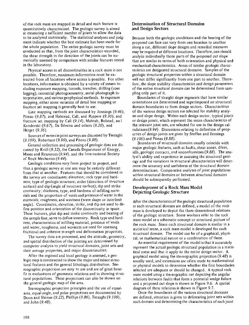
of the rock mass are mapped in detail and each feature is quantitatively characterized. The geologic survey is aimed at measuring a sufficient number of joints to allow the data to be analyzed statistically. The statistical analyses and judg-ment indicate whether the best estimate has been made for the whole population. The entire geologic survey must be conducted so that, from the joint characteristics recorded, the shear strength in the direction of the joints can be nu-merically assessed by comparison with similar features tested in the laboratory.

Physical access to all discontinuities in a rock mass is not possible. Therefore, maximum information must be ex-tracted from all locations where access is possible. For other locations, information is obtained by a variety of means in-cluding exposure mapping, tunnels, trenches, drilling (core logging), terrestrial photogrammetry, aerial photograph in-terpretation, and various geophysical methods. In exposure mapping, either some variation of detail line mapping or fracture set mapping is generally best to use.

Line mapping methods are discussed by Jennings (9.46), Piteau (9.87), and Haistead, Call, and Rippere (9.30), and fracture set mapping by Call (9.14), Mahtab, Bolstad, an I Kendorski (9.67), Da Silveira and others (9.20), and Herget (9.36).

Sources of errors in joint surveys are discussed by Terzaghi (9.109), Robertson (9.99), and Piteau (9.88).

General collection and processing of geologic data are dis-cussed by Knill (9.52), the Canada Department of Energy, Mines and Resources (9.94), and the International Society of Rock Mechanics (9.44).

Geologic conditions vary from project to project, and thus a geologic survey at one site may be entirely different from that at another. Features that should be considered in the survey are coordinates; elevation; rock type and hard-ness; type of geologic structure; strike (direction of structure surface) and dip (angle of structure surface); dip and strike continuity; thickness, type, and hardness of infilling mate-rials and the proportion of voids and presence of water in the materials; roughness; and waviness (wave shape or interlimb angle). Coordinates, elevation, strike, and dip are used to de-line position and orientation of the discontinuity in space. These features, plus dip and strike continuity and bearing of the sample line, serve to define intensity. Rock type and hard-ness, characteristics of in filling material, presence of voids and water, roughness, and waviness are used for assessing frictional and cohesive strength and deformation properties.

The survey data are processed, and the attitude, geometry, and spatial distribution of the jointing are determined by computer analysis to yield structural domains, joint sets and their average properties, and major discontinuities.

After the regional and local geology is assessed, a geo-logic iiap is constructed to show the major and minor struc-tural features and the general lithologic distribution. Ste-reographic projections are easy to use and are of great bene-fit in evaluations of geometric relations and in showing struc-tural populations. These projections can also be shown on the general geologic map of the area.

Stereographic projection principles and the use of equal-area, equal-angle, and polar projections are documented by Donn and Shimer (9.22), Phillips (9.86), Terzaghi (9.109), and John (9.48).

Determination of Structural Domains and Design Sectors

Because both the geologic conditions and the bearing of the proposed cut face can vary from one location to another along a cut, different slope designs and remedial measures may be required at different locations. Therefore ,one should analye individually those parts of the proposed cut slope that are similar in terms of both orientation and physical and mechanical characteristics. Areas of similar geologic charac-teristics are designated structural domains. Samples of the geologic structural properties within a structural domain will not differ significantly from one part to another. There-fore, the slope stability characteristics and design parameters of the entire structural domain can be determined from sam-pling only part of it.

Boundaries of straight slope segments that have similar orientations are determined and superimposed on structural domain boundaries to form design sectors. Characteristics of the various design sectors are selected for stability analy-sis and slope design. Within each design sector, typical joints or design joints, which represent the mean characteristics of the relevant joint sets, are selected for use in the design cal-culations(9.94). Discussions relating to definition of prop-erties of design joints are given by Steffen and Jennings (9.106) and Piteau (9.88).

Boundaries of structural domains usually coincide with major geologic features, such as faults, shear zones, dikes, sills, geologic contacts, and unconformities (9.88). The ana-lyst's ability and experience in assessing the structural geol-ogy and the variations in structural characteristics will deter-mine the accuracy and usefulness of the structural domain determinations. Comparative analyses of joint populations within structural domains or between structural domains should be subsequently performed.

Development of a Rock Mass Model Depicting Geologic Structure

After the characteristics of the geologic structural population in each structural domain are defined, a model of the rock mass is developed to depict the three-dimensional relations of the geologic structure. Some workers refer to the rock mass model as a schematic concept or structural picture of the rock mass. Since each structural domain is similar in a statistical sense, a rock mass model is developed for each structural domain. The model can be of a graphical, physi-cal, or mathematical nature or a combination of these.

An essential requirement of the model is that it accurately represent the actual geologic structural population in a statis-tical sense and that it apply to the entire design sector. A graphical model using the stereographic projection (9.48) is usually used, and extensions are often made to mathematical or physical models to determine whether the first boundaries selected are adequate or should be changed. A typical rock mass model using a stereographic net depicting the angular relations between faults that form a potential wedge failure and a proposed cut slope is shown in Figure 9.6. A spatial diagram of these relations is shown in Figure 9.7.

Once the boundaries of the various structural domains are defined, attention is given to delineating joint sets within each domain and determining the characteristics of each joint

198

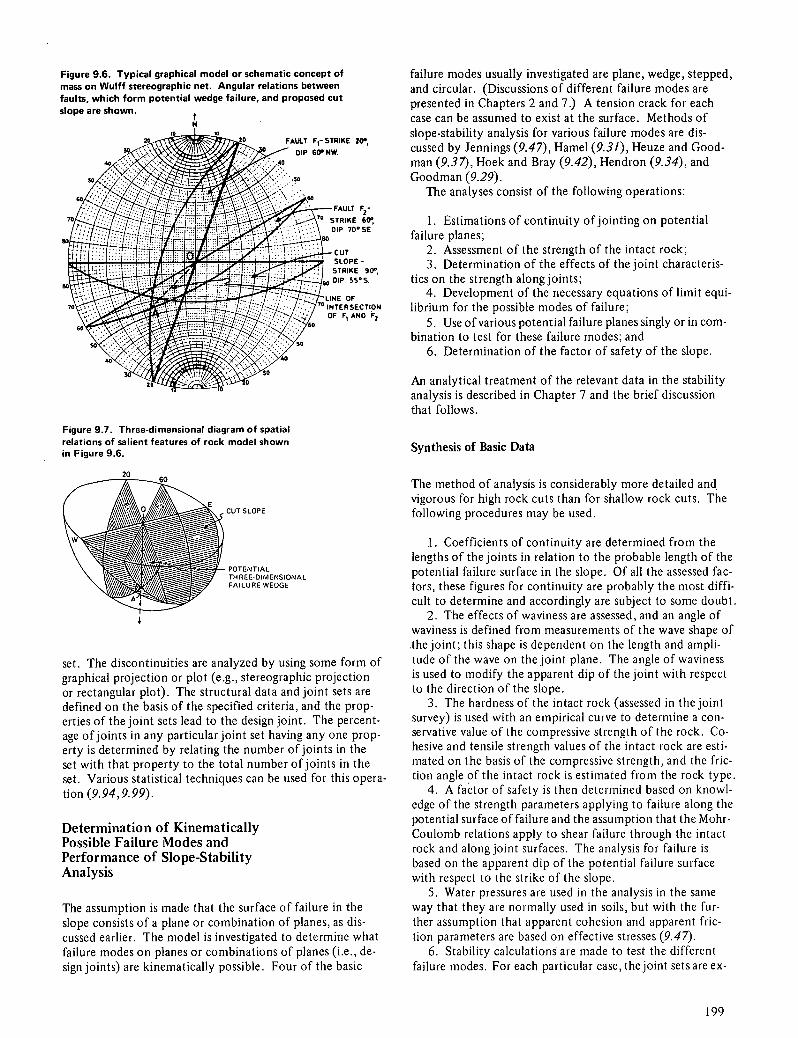
Figure 9.6. Typical graphical model or schematic concept of mass on Wuiff stereographic net. Angular relations between faults, which form potential wedge failure, and proposed cut slope are shown. *

Figure 9.7. Three-dimensional diagram of spatial relations of salient features of rock model shown in Figure 9.6.

'U

CUT SLOPE

POTENTIAL THREEDIMENSIONAL FAILURE WEDGE

set. The discontinuities are analyzed by using some form of graphical projection or plot (e.g., stereographic projection or rectangular plot). The structural data and joint sets are defined on the basis of the specified criteria, and the prop-erties of the joint sets lead to the design joint. The percent-age of joints in any particular joint set having any one prop-erty is determined by relating the number of joints in the set with that property to the total number of joints in the set. Various statistical techniques can be used for this opera-tion (9.94,9.99).

Determination of Kinematically Possible Failure Modes and Performance of Slope-Stability Analysis

The assumption is made that the surface of failure in the slope consists of a plane or combination of planes, as dis-cussed earlier. The model is investigated to determine what failure modes on planes or combinations of planes (i.e., de-sign joints) are kinematically possible. Four of the basic

failure modes usually investigated are plane, wedge, stepped, and circular. (Discussions of different failure modes are presented in Chapters 2 and 7.) A tension crack for each case can be assumed to exist at the surface. Methods of slope-stability analysis for various failure modes are dis-cussed by Jennings (9.47), Hamel (9.31), Heuze and Good-man (9.37), Hoek and Bray (9.42), Hendron (934), and Goodman (9.29).

The analyses consist of the following operations:

Estimations of continuity ofjointing on potential failure planes;

Assessment of the strength of the intact rock; Determination of the effects of the joint characteris-

tics on the strength along joints; Development of the necessary equations of limit equi-

librium for the possible modes of failure; Use of various potential failure planes singly or in com-

bination to test for these failure modes; and Determination of the factor of safety of the slope.

An analytical treatment of the relevant data in the stability analysis is described in Chapter 7 and the brief discussion that follows.

Synthesis of Basic Data

The method of analysis is considerably more detailed and vigorous for high rock cuts than for shallow rock cuts. The following procedures may be used.

Coefficients of continuity are determined from the lengths of the joints in relation to the probable length of the potential failure surface in the slope. Of all the assessed fac-tors, these figures for continuity are probably the most diffi-cult to determine and accordingly are subject to some doubt.

The effects of waviness are assessed, and an angle of waviness is defined from measurements of the wave shape of the joint; this shape is dependent on the length and ampli-tude of the wave on the joint plane. The angle of waviness is used to modify the apparent dip of the joint with respect to the direction of the slope.

The hardness of the intact rock (assessed in the joint survey) is used with an empirical curve to determine a con-servative value of the compressive strength of the rock. Co-hesive and tensile strength values of the intact rock are esti-mated on the basis of the compressive strength, and the fric-tion angle of the intact rock is estimated from the rock type.

A factor of safety is then determined based on knowl-edge of the strength parameters applying to failure along the potential surface of failure and the assumption that the Mohr-Coulomb relations apply to shear failure through the intact rock and along joint surfaces. The analysis for failure is based on the apparent dip of the potential failure surface with respect to the strike of the slope.

Water pressures are used in the analysis in the same way that they are normally used in soils, but with the fur-ther assumption that apparent cohesion and apparent fric-tion parameters are based on effective stresses (9.47).

Stability calculations are made to test the different failure modes. For each particular case, the joint sets are ex-

RUlE 20,

P.

FAULT F2-

TRIKE 60° )IP 70° SE

CUT SLOPE - STRIKE 90°, DIP 55°S.

E OF 'TSR SECTION F F AND F2

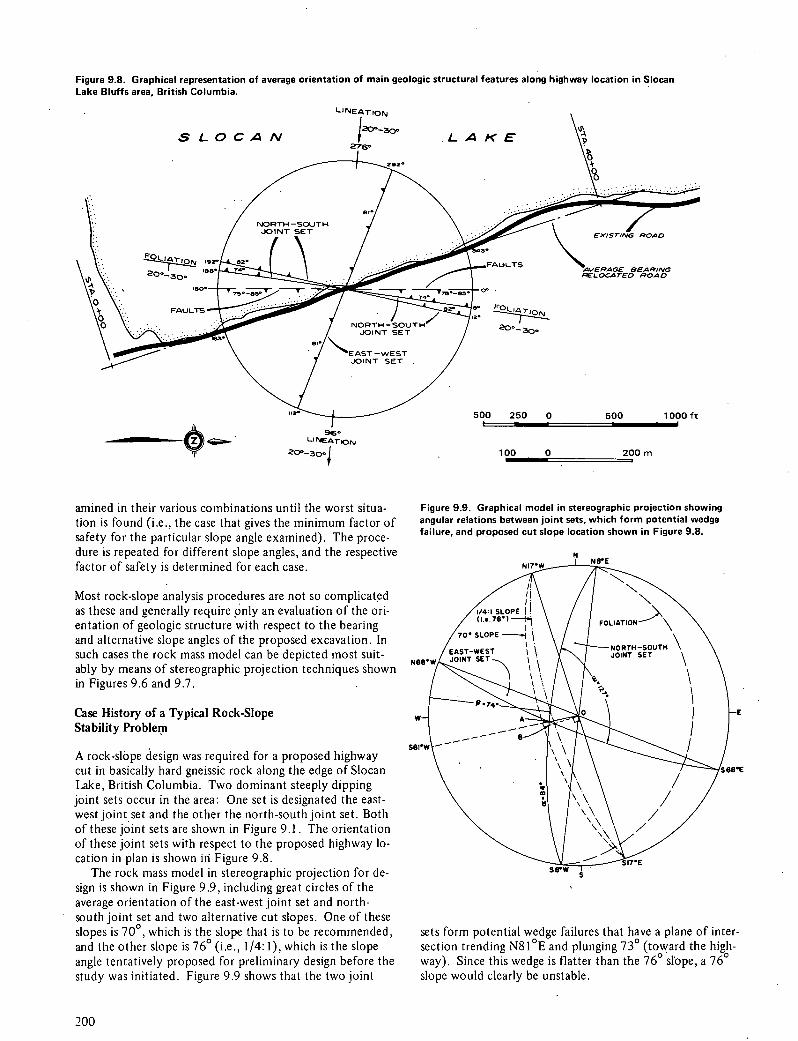
Figure 9.8. Graphical representation of average orientation of main geologic structural features along highway location in Slocan Lake Bluffs area, British Columbia.

SLOGAN

LI NEAT ION

i2cr--.O. . L A K E

276°

NORTI-4 —SOUT JOINT SET

\\•. \., \...

B0

FAULTS

96. LI NEAT ON

-

ROAD

T$

0.

'OLIAT

2O°

500 250 0 500 1000 ft

100 0 20Dm

amined in their various combinations until the worst situa-tion is found (i.e., the case that gives the minimum factor of safety for the particular slope angle examined). The proce-dure is repeated for different slope angles, and the respective factor of safety is determined for each case.

Most rock-slope analysis procedures are not so complicated as these and generally require only an evaluation of the ori-entation of geologic structure with respect to the bearing and alternative slope angles of the proposed excavation. In such cases the rock mass model can be depicted most suit-ably by means of stereographic projection techniques shown in Figures 9.6 and 9.7.

Case History of a Typical Rock-Slope Stability Problem

A rock-slope design was required for a proposed highway cut in basically hard gneissic rock along the edge of Slocan Lake, British Columbia. Two dominant steeply dipping joint sets occur in the area: One set is designated the east-west joint set and the other the north-south joint set. Both of these joint sets are shown in Figure 9.1. The orientation of these joint sets with respect to the proposed highway lo-cation in plan is shown in Figure 9.8.

The rock mass model in stereographic projection for de-sign is shown in Figure 9.9, including great circles of the average orientation of the east-west joint set and north-south joint set and two alternative cut slopes. One of these slopes is 700, which is the slope that is to be recommended, and the other slope is 760 (i.e., 1/4:1), which is the slope angle tentatively proposed for preliminary design before the study was initiated. Figure 9.9 shows that the two joint

Figure 9.9. Graphical model in stereographic projection showing angular relations between joint sets, which form potential wedge failure, and proposed cut slope location shown in Figure 9.8.

sets form potential wedge failures that have a plane of inter-section trending N810E and plunging 730 (toward the high-way). Since this wedge is flatter than the 760 slope, a 760 slope would clearly be unstable.

200

A mechanical stability analysis in this case is somewhat redundant because of the steepness of the potential wedges. For illustrative purposes, however, a simple three-dimensional analysis (9.13) can be carried out to show the minimum angle of residual joint friction (r), which would be required to hold up such a wedge if undercut. Consider the following values determined from the rock mass model shown in Fig-ure 9.9:

3= 740, average dip of the north-south joint set, a= 840, angle measured in the plane of the north-south

joint set between the strike of this plane and the line of intersection, and

w= 1270 ,angle measured in a plane perpendicular to the line of intersection of the two joint sets.

r would have to be a minimum of 57.20 in order to achieve a factor of safety of unity. Since the value of 0, was estimated to be on the order of 350 , a 760 slope would obviously lead to serious wedge failures. Cable anchors, bolts, or other artificial reinforcement, which would be re-quired in order to prevent failure of a 760 slope, would also be uneconomical. Hence, it was recommended that the slopes be cut at an angle of 700, which is 30 flatter than the line of intersection OA (Figure 9.9) of the potential wedge failures. -

SLOPE DESIGN AND REMEDIAL MEASURES

Remedial measures for rock slopes can consist of stabiliza-tion, protection, or warning methods or a combination of these basic methods. These remedial measures and the sug-gested order in which they should be considered are shown in Figure 9.10 and discussed below.

Stabilization methods give a positive solution to the problem in that either the driving forces are reduced or the resisting forces are increased. Because of the complex na-ture of the rock mass, the effectiveness of these methods is often difficult to assess quantitatively. Stabilization mea-sures reduce the likelihood of rocks moving out of place and generally should be considered first in the remedial treatment of rock slopes. Stabilization also reduceg the rate of deterio ration, a process that leads ultimately to failure.

Protection methods prevent rock materials that have moved out of place on the slope from reaching the roadway and thus offer an additional positive solution to slope-stability problems. The initial cost is usually considerably less than that of the stabilization measures, but the slopes usually require considerably more maintenance (in some cases almost continual maintenance). Protection measures can sometimes be combined effectively with warning mea-sures.

Warning methods warn that movements have taken place or that failure has occurred and that a hazard may be imminent in the vicinity of the roadway. These methods have no effect on the source of the hazard and may lead to mcreased maintenance costs and unnecessary delays when insignificant events accidentally trigger the warning system. Warning methods also tend to provide undue confidence, and sometimes result in relaxation of advisable precautions. Although they may seem economical in some instances, warn-

Figure 9.10. Order in which slope treatment methods should be

considered for selection.

SITE CONDITOINS ENGINEERING

ANGLE, HEIGHT, AND CONDITION OF SLOPE JUDGMENT

SIZE AND CONDITION OF ROCKS PATH OF ROCK FALL TO RIGHTOFWAY

MAINTENANCE REQUIRED

STABILIZATION PROTECTION __ WARNING

METHODS METHODS METHODS

EXCAVATION RELOCATION ELECTRIC WIRE

SCALING AND TRIMMING INTERCEPTING SLOPE, ELECTRIC FENCE

DRAINAGE DITCHES, AND BERMS COMBINATION WITH

SHOTCRETE DITCH SHAPING PROTECTION

BUTTRESSES OR BULKHEADS WIRE MESH COVERS

ROCKS BOLTS. DOWELS, AND CATCH NETS

ANCHORS CATCH FENCES

ANCHORED BEAMS AND WALLS CATCH WALLS CABLE WALLS AND LASHING ROCK SHEDS AND TUNNELS

ing measures are not an effective way to remedy rock-slope problems and generally should be considered only as a last resort. Except for railways in North America, warning methods are seldom used extensively on a permanent, long-term basis by those experienced in rock-slope engineering.

During the planning and construction phases of a project, the considerable advantages in recognizing rock-slope prob-lems that exist or that may develop and in applying the ap-propriate rock-slope remedial measures at the time cannot be overemphasized. Sound rock-slope engineering at the out-set of the project and during the excavation phase will obvi-ate both hazards and much more costly work at a later date. The cost of stabilization and protection measures applied during the excavation phase also can be largely absorbed in the initial construction cost; this is especially true if a con-tingency item is included in the contract budget.

The following discussions do not include costs of reme-dial measures, other than in a general way, because costs in one environment or location may be entirely different from those in another. Time, access, and space available for remedial work on highway rock slopes, for example, are often much greater than for similar work on narrow, busy railway lines in mountainous terrain. For this reason, both methods and costs of highway rock-slope engineering work are not always applicable to similar railway problems. Unit costs and other items can also vary widely, depending on local requirements and the skill of the planner.

Remedial measures for rock slopes are discussed by Zâruba and Mend (9.112), Baker and Marshall (9.3), Fookes and Sweeney (9.26), Root (9.100), Mehra and Natarajan (9.72), and Behr and Klengel (9.7). Landslide measures in urban developments are discussed by Legget (9.61) and Leighton (9.62). Crimmins, Samuels, and Monahan (9.19) provide practical information with regard to construction in rock although the reference is mainly to foundations.

Planning and Related Procedures

The stability of a rock slope will change significantly with

201

time because of strength changes, rock deterioration, fluc-tuating groundwater, and other environmental factors, which generally produce less stable slopes. The most eco-nomical overall design, therefore, accounts for this decrease in stability with time and includes consideration of a main-tenance and remedial program. Remedial measures for rock slopes along transportation corridors in steep terrain must be integrated with other maintenance tasks. If the route runs for some distance through mountainous terrain, work will probably be sufficient to keep personnel on rock-slope main-tenance work full time. Unlike most soil slopes, on which weathering is not an important factor, rock slopes require continual attention if serious problems are to be avoided. A consistent long-term remedial program is required that contains carefully selected priorities. Experienced people are needed for both engineering and construction. Judgment must be based on a detailed knowledge of occurrences at each dangerous location.

Personnel

In setting up a rock-slope remedial and maintenance program for a major transportation route, a project engineer should be assigned full time to the work. The project engineer should have available an experienced engineering geologist and geotechnical engineer and the capability to supervise contract work. If necessary, consultants should be used for highly specialized parts of the work and to provide some personnel on a temporary basis, depending on the magnitude and frequency of the problems. Continuity of personnel should be encouraged, for experience in rock-slope engineer-ing is a most important attribute. An engineering geologist on the team should be able to translate information clearly into engineering terms and integrate information with engi-neering requirements.

The project engineer must keep in touch with all develop-ments relating to the overall project. The geotechnical engi-neer and engineering geologist should make detailed inspec-tions, perform slope-stability analysis and design, exercise judgment on specific rock conditions, and help in planning and supervising remedial work. It is particularly important that the staff of the highway, railway, or other transporta-tion agency concerned with rock-slope problems develop sufficient expertise within the organization to critically eval-uate work performed by private companies or other agencies. Some of the principal functions of the project engineer and engineering geologist in planning, design, and maintenance are described by McCauley (9.70).

Work Arrangements

To estimate the cost of remedial measures in advance is dif-ficult, for unforeseen conditions are often revealed as the work proceeds. For this reason, decisions on an overall bud-get required for the improvement of rock-fall hazards are often based on judgment as well as analysis. All concerned should understand that some flexibility is needed in the total budget approved for an annual program so that adjust-ments can be made in expenditures required at different lo-cations as well as in contract provisions to deal with changed conditions during the work. Because major revisions often are required during the work, rock work should be done on

the basis of proposals or bids invited from contractors known to have up-to-date knowledge of the equipment and tech-niques required. The proposal or bid should be for a unit price or cost-plus-fixed-fee contract and not for a lump sum. The U.S. National Committee on Tunneling Technology (9. 79), although addressing mainly underground work, is a good source of information on sound contracting practices in construction engineering and contract law for rock con-struction work.

Selection of Priorities

The condition of all rock slopes along transportation routes in steep terrain should be thoroughly inspected once a year or more frequently depending on the severity and implica-tions involved. Inspection can be done by (a).a helicopter survey of inaccessible locations and of the overall conditions of the slopes and (b) a ground survey of hazards at specific locations to determine the need for detailed studies. Based on annual surveys and case histories of the slopes, detailed studies and alternative treatments are planned. Factors to be considered in deciding on locations for remedial work are

Maintenance costs, including patrols required; Costs of remedial measures and expected benefits to

be gained; Degree of risk to route, determined by considering the

amount of traffic, records of past events, measured rock movements, and frequency of clearing rocks from the vicin-ity;

Occurrence of accidents, rock falls, washouts, land-slides, and the like;

Conditions downhill from the right-of-way, which would indicate how serious an accident or derailment might be; and

Views of maintenance and patrol personnel.

The annual program should emphasize stabilizing or pro-tecting the greatest number of locations where rock-fall hazards exist in order to obtain the maximum economical improvement in safety. Large problem areas can often be divided into smaller areas for treatment. The tendency to overprotect the route at locations of recent accidents should be resisted in the interest of obtaining a balanced overall program. Conditions at each particular location may vary significantly, and the application of different remedial mea-sures should be considered accordingly. Details of remedial work must be developed section by section along the route and be based on detailed inspections, existing records, expe-rience, and sound judgment. However, the most careful choosing of hazardous locations and the most thorough anal-ysis in selecting remedial measures will never entirely prevent unexpected rock falls from occurring.

Records

For the efficient planning of rock-slope engineering work, a data storage and retrieval system should be organized and maintained for permanent reference. The following types of records should be maintained:

202

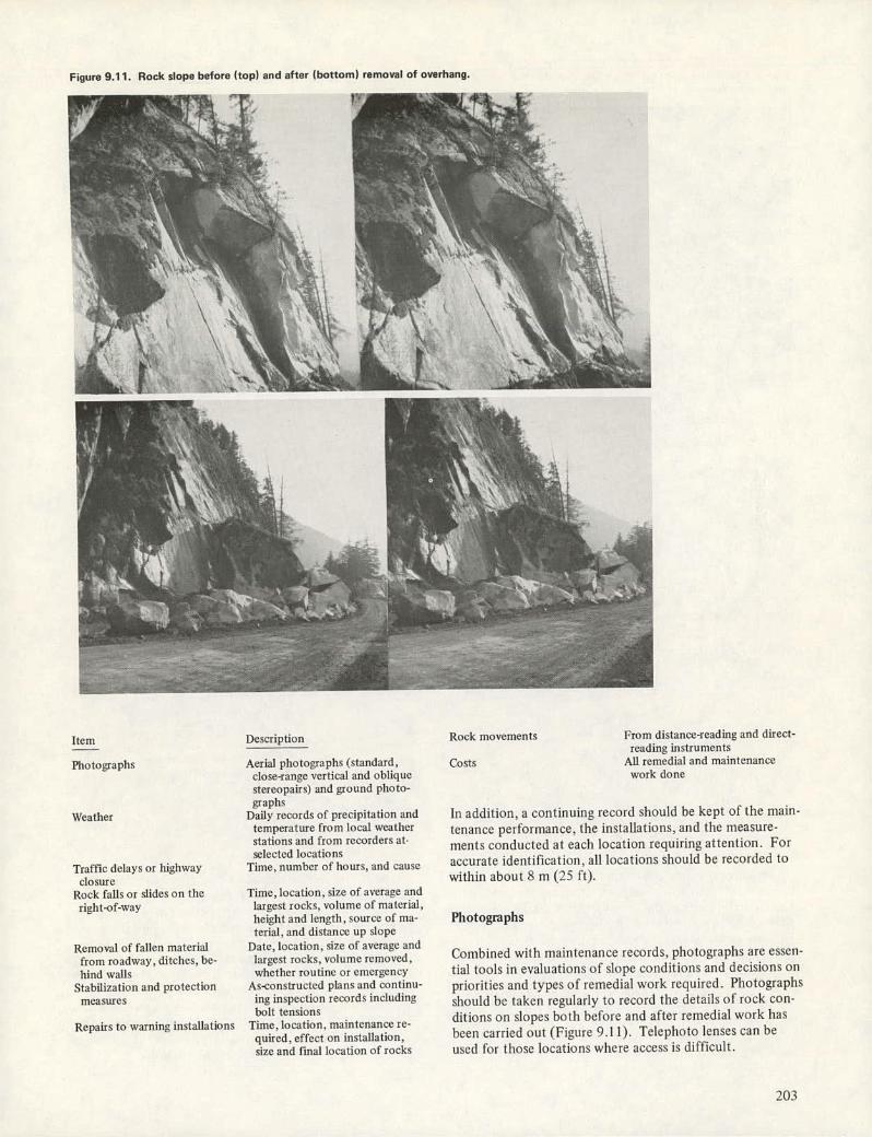
Figure 9.11. Rock slope before (top) and after (bottom) removal of overhang.

zro

Item Description Rock movements From distance-reading and direct- reading instruments

Photographs Aerial photographs (standard, Costs All remedial and maintenance close-range vertical and oblique work done stereopairs) and ground photo-

Weather graphs

Daily records of precipitation and In addition, a continuing record should be kept of the main- temperature from local weather tenance performance, the installations, and the measure- stations and from recorders at ments conducted at each location requiring attention. For

Traffic delays or highway selected locations

Time, number of hours, and cause -

accurate identification, all locations should be recorded to

closure within about 8 m (25 ft).

Rock falls or slides on the Time, location, size of average and right-of-way largest rocks, volume of material,

height and length, source of ma- Photographs terial, and distance up slope

Removal of fallen material Date, location, size of average and Combined with maintenance records, photographs are essen-

from roadway, ditches, be- hind walls

largest rocks, volume removed, whether routine or emergency tial tools in evaluations of slope conditions and decisions on

Stabilization and protection As-constructed plans and continu- priorities and types of remedial work required. Photographs measures ing inspection records including should be taken regularly to record the details of rock con-

ditions on slopes both before and after remedial work has Repairs to warnino installations Tirne,location. maintenance re-

quircd, effect on installation, been carried out (Figure 9.11). Telephoto lenses can be

size and final location of rocks used for those locations where access is difficult.

203

Figure 9.12. Oblique photographs of cut bench at Hell's Gate Bluffs, British Columbia, above which excavation was proposed to remedy overturning failure.

-:, i:.; "• . 'I -.

............- -. . . - . . .-. •

# A)' . . - -. .. . ,, '..•...'• •--

Aerial photographs can be useful for studying the condi-tion and con figuration of slopes in steep terrain and for giv-ing important cities to the causes and potential sources of' slope instability. High-level photographs are generally of minimal use for local slope-desiii purposes. If possible, low-level photographs at a scale of I cm equals 50 to 120 in (1 in equals 400 to 1000 it) should be obtained. Uses of aerial photographs for engineering purposes are described in Chapter 3 and by Norman (9.81) and Mollard (9.74).

Aerial oblique or terrestrial oblique single photographs or stereoscopic photographs are frequently used for rock-slope engineering work (Figure 911). Stereoscopic photo-

graphs can be used to examine slopes three-dimensionally for purposes of tentative slope-excavation design. Aerial oblique photographs can be taken with cameras mounted on the ends of a 5-ni (15-it) boom carried by a helicopter. Photographs can be taken at any angle from vertical to hori-zontal and contours can be plotted to a fixed datum. Cracks and features on the order of 5 to 8 cm (2 to 3 in) wide can be detected in this way. Photographs are particularly useful in evaluations of rock slopes that are in steep terrain and not easily accessible from the ground (Figure 9J2). Use of ter-restrial photogramniet ry in rock-slope engineering is dis-cussed by Ross-Brown and Atkinson (9J01).

204

j - '

Monitoring and Inspection

Planning for rock-slope engineering work should include a program of monitoring slope movements and identifying characteristics that indicate changing stability. Detection of general creep or slow translation of highly fractured or

ft slope-forming material is important in decisions regard-ing remedial work. Horizontal and vertical movements of points plotted against time or depth or both provide impor-tant information concerning the behavior of a rock slope. Graphs provide it clear indication of the onset of slope fail-tire when plots representing the change in position do not remain linear. When such accelerated movements are evident, the slope must be approaching failure, and measures should be taken to analyze and remedy the situation.

For studies of complex stability problems, the advice of a specialist is needed to determine the most suitable slope-monitoring program. A wide variety of commercial instru-ments is available for measuring both surface and subsur-face movements and for recognizing the characteristics in-dicative of potential instability. However, the simplest methods and mechanical equipment are not only the most practical but also invariably the most reliable. The various methods of instrumentation are discussed in Chapter 5, in the June 1972 issue of Highway Focus (9.39), and by Frank-liii and Denton (9.28). Benson (9.8), and Medley (9.33).

The simplest and generally most efficient method of mon-itoring recently excavated slopes is to measure both horizon-tal and vertical displacements of protected metal survey pins or hubs set in concrete or grout along a straight line at the crest and toe of the slope. Main control reference points should be located outside the area where movement may oc-cur. If. in the first year. movements appear negligible (other than what might be expected from normal elastic rebound due to unloading), the number of surveys in succeeding years may be decreased until the slope becomes stable. In this work, high precision is essential so that the onset of nonlin-ear movement can be determined as early as possible and re-medial work can be planned accordingly.

Individual cracks, which may be indicative of ceneral in-stability in an area, can be monitored simply by bridging the crack with a wad ofgrout or shotcrete or by inserting a wedge in the crack. A regular part of the work program for evaluat-ing and monito ring should involve inspect ion and niainte-nance of remedial installations, such as rock bolts, walls, nets, and drains, already in place. Regular inspection is an essential precaution in protecting a substantial capital invest-ment.

Methods of Stabilization

Excavation and Related Design Aspects

For purposes of improving the stability of rock slopes, exca-vation is used either to reduce the driving forces contributing to failure or to remove unstable or potentially unstable sec-tions of the slope that may lead to failure (i.e.. rock falls and slides). Stability, therefore, can be achieved by

- Removing unstable or potentially unstable material. Flattening the slope. Removing weight from the upper part of the slope.

Figure 9.13. Forty-three-meter (140-ft) presheared through cut

involving 130 000 m3 (170 000 yd3 ) near Britannia, British Columbia, and including cut bench to protect highway from rock falls. Photo is toward south, but sketch is toward north.

Incorporating benches in the slope, and Excavating in a manner that minimizes damage to the

rock mass.

Excavations made for remedial purposes should provide a per. nianent solution to the slope-stability problem so that addi-tional excavation work in the future need not be necessary. The principal problems and disadvantages associa ted with excavation methods lie in their cost. Accessibility after con-struction may be difficult and, since the slope usually must be excavated from the top downward, mobilization and setup costs can be prohibitive. Also, disposal sites often are limited with the result that waste rock may have to be transported for some distance, unless it can be used for local construction.

Benches

The overall slope angle and different slope angles that may be designed for different parts of the slope are determined by slope-stability analysis methods (Chapter 7). Each cut should be designed to suit the prevailing rock conditions. Slopes containing materials with strength properties that vary significantly in section may require that some parts be flatter than other parts if rock falls and maintenance costs are to be minimized. The use of' variable slopes, benches be-low layers of rapidly weathering rock, and St rue t oral support and correct blasting techniques can practically eliminate rock falls in new cuts.

Benches are used in slopes to minimize rock falls onto the roadway (Figures 9.13 and 9.14). For soft rocks (Figure 9.14), such as shale, mudstone. and other argillaceous rocks. benches tend to reduce excessive weathering and erosion and provide rock-fall catehments. Erosion due to groundwater runoff is also controlled since the energy of surface flows is

205

Figure 9.14. Benches that follow stratigraphy in Niagara Escarpment sedimentary rocks on Highway 403 near Hamilton, Ontario. Design also includes overburden being stripped back 3 m (10 ft) from top of rock and light fence barrier on edge of highway.

- :.

, -

\ -

.. :-.- - ......•

Figure 9.16. Use of multiple benches and controlled blasting techniques at Mica Dam, British Columbia, to maintain rock slope in soundest possible condition and to prevent rock falls.

:'- ____ - çs..'-.•

'.. . ' 4: '.

141 : -. •... ..

'4

Figure 9.15. Slope design parameters that are used when benches are incorporated in slopes.

LL SLOPE NGLE

dissipated. Construction safety on benched slopes is usually increased since the hazard of rock falls above workers is re-duced. In general, the faces of benches can be considerably steeper than the overall slope angle: hence, any rocks that do fall remain on the benches.

Benches appear to have no effect on the slope with re-spect to deep-seated failure. Although shear stresses in-crease with slope height. the direct ion ofthe inaxin urn shear stress is supposedly independent of slope height and bench geometry. Benches may require the top of the slope to be moved back and, therefore, considerable additional excava-tion . However, although they may add to the initial cost of construction, benches may significantly reduce subsequent maintenance costs and tItus sometimes more than offset the increased cost of construction. The Colorado Department of Highways, for example, found that the unit cost of cleanup and maintenance work after rock falls is about ten times the unit cost of the original excavation.

Figure 9.15 shows the parameters of a slope incorporat-ing benches, including bench height, berm width, and bench-face angle. These parameters are governed by the physical and mechanical characteristics of the rock mass. Bench height should provide a safe and efficient slope and all Optimtlnl overall slope angle. Bench height can be greater

in stronger rock, and the bench face can be terminated at the base of weaker horizons and water-bearing zones. Without affecting the overall slope angle, higher benches generally will allow for wider berrns,giving better protectioll and more reliable and easier access for the regular cleaning of debris. The width of herms should be governed by the size of the equipment working on the bench and by the nature of the slope-forming material, but should generally be no less than 7 in (20 ft).

If the bench faces are inclined, high tensile stresses are less likely to develop near bench crests and thLls tension cracks and overhangs are minimized. Avoiding these prob-lewis reduces the amount of rock-fall material and increases the safety of the slope. Tension zones in slopes involving benches are discussed by Bukovansky and Piercy (9.11). Design of the bench-face angle should be governed to -a large extent by the attitude of unfavorable structures in the slope to prevent excessive rock falls onto the berms. Figure 9.16 shows a high rock cut at Mica Darn in British Columbia, where all three bench design parameters change in different parts of the slope.

If benches are included in the slope design, berms should be equipped with drainage ditches to intercept surface run-off and water from drain holes and other drainage facilities and divert it off the slope and away from problem areas. These ditches should be kept opeit and free of all debris and ice to ensure adequate performance. Ditch lining (e.g., clay, slush grout - asphalt, polyethylene sheeting) may be required if ditch leakages are anticipated or develop afterward. Berm surfaces should be graded to assist the collection of water in ditches and also to facilitate general drainage in a direction away from potential areas of instability. Care must be taken so that ditches do not create problems by channeling water fro in one a rca to a not her -

Stepped benches may be used on slopes cut in highly weathered rock material to control erosioiì and to establish vegetation. Figure 9.17 (9.38) shows stepped cut slopes that consist of 0.6 to I .2-in (2 to 4-ft) high benches with approxi-niately similar berm width and an overall slope angle based on stability analysis. The design objective is that the mate-rial weathering front each rise will fill up the step of the bench and finally create a practically uniform overall slope. The steps are constructed horizon tally to avoid the bongit u-dinal movement of water, which could cause considerable

206

Figure 9.17. Idealized cross section showing stepped slope design in soft rock based on SLOPE ROUNDING

recommendations in several research papers (9.38). - OVERBURDEN AF)EA/ VARIABLE SLOPE RATiO'

- FT ROCK LINE - STEP TERMINI IWIDT14 - STEP.TREAO WIDTH) ORIGINAL GROUND SURFACE...3 ,.

CENTERLINE

/TERMINJ

STEP RISE HEIGHT VARIABLE I TO 2 (

EAD WIDTH STAKED SLOPE RATIO STEP RISEI

E LINE FOR SOFT ROCK PROFILE

DTH - 7. STEPIREAD WIDTH)

SLOPE HIGH POINT —1 Not, I to - 3,3 (1.

/

erosion. Seeding and mulching or other suitable methods of slope stabilization can be readily applied; however, for rapidly raveling slopes, about half of the bench or step width should be filled before seeding is done to prevent smothering of the seed.

Scaling and Trimming

Scaling of loose, overhanging, or protruding blocks is a basic maintenance operation on rock slopes of all sizes along trans-portation routes in steep terrain. Scaling on the upper reaches of high faces is usually carried out by workers on ropes with hand pry bars, hydraulic splitters or jacks, and explosives(Figure 9.18). Of necessity. I his work is slow and intermittent. Mechanical scaling equipment is more efficient and safer, but may have limitations because of severe access problems. Trimming involves drilling, blasting, and scaling to remove small ragged or protruding rock in overhang areas where repetitive scaling would otherwise be required.

Postconstruction scaling and trimming should be carried out on a regular basis. In temperate regions. this is usually started in the spring after the frost leaves the rock. If thorough scaling is performed during excavation, subsequent maintenance and remedial work can be greatly reduced. Be-fore work begins, an engineering geologist and rock foreman should thoroughly inspect each location and make decisions

Figure 9.18. Typical rock-scaling operation high above highway

on the rocks to be removed. Scaling and trimming work re-dluires specialized experience, and the performances of differ. ent contractors should be compared when additional work is considered. Depending on site conditions, potentially use-ful tools are bencher drills, gas jackhammers, air-operated scaling tools, suspended powered platforms (spiders), and hydraulic boom cranes (giraffes) for access to low and inter-mediate slopes. Fquipment for scaling and other related ac-tivities in lower and higher reaches of slopes is shown in Fig-tires 9.19 and 9.23 respectively.

Blasting Procedures

Rock should be preserved beyond excavation lines and grades in the soundest possible condition. The effects of tension, compression, and shear stresses developed in a rock mass as a result of blasting damage are documented by Bauer (9.6), Lang and Favreau (9.57), Langefors and Kihlstrom (9.59), the U.S. Bureau of Public Roads (9.12), Larocque (9.60), and Lamhooy and Espley.J ones (9.55). Uncontrolled blasting results in rough uneven contours, overhreak, over-hangs, excessive shattering, and extensive tension cracks in the crest of the slope. BlasI ing damage, therefore, can lead to significantly higher scaling, excavation, re-medial treatment, and maintenance costs. The results of blast shock waves and gases along faults, joints, bed-

Figure 9.19. Typical hydraulic crane (giraffe) and b.icket used for scaling lower reaches of slopes. ,. J.. lei Wf

0. / 4 • I •

— :

207

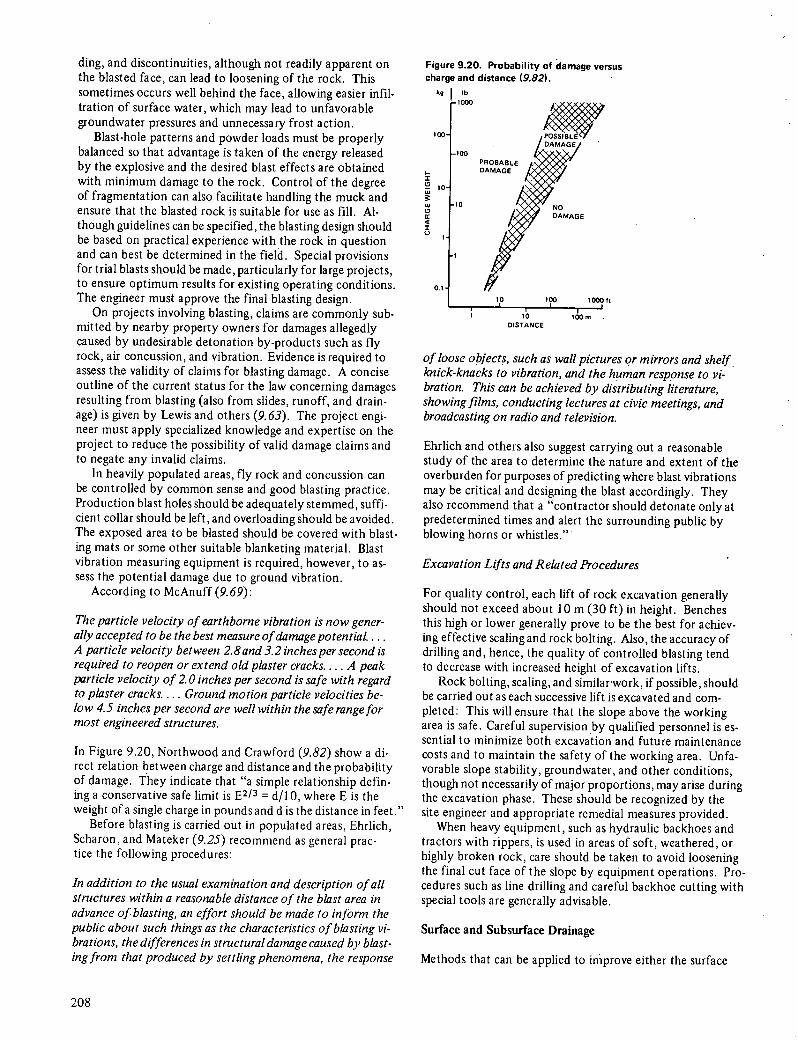
ding, and discontinuities, althougj1 not readily apparent on the blasted face, can lead to loosening of the rock. This sometimes occurs well behind the face, allowing easier infil-tration of surface water, which may lead to unfavorable groundwater pressures and unnecessary frost action.

Blast-hole patterns and powder loads must be properly balanced so that advantage is taken of the energy released by the explosive and the desired blast effects are obtained with minimum damage to the rock. Control of the degree of fragmentation can also facilitate handling the muck and ensure that the blasted rock is suitable for use as fill. Al-though guidelines can be specified, the blasting design should be based on practical experience with the rock in question and can best be determined in the field. Special provisions for trial blasts should be made, particularly for large projects, to ensure optimum results for existing operating conditions. The engineer must approve the final blasting design.

On projects involving blasting, claims are commonly sub-mitted by nearby property owners for damages allegedly caused by undesirable detonation by-products such as fly rock, air concussion, and vibration. Evidence is required to assess the validity of claims for blasting damage. A concise outline of the current status for the law concerning damages resulting from blasting (also from slides, runoff, and drain-age) is given by Lewis and others (9.63). The project engi-neer must apply specialized knowledge and expertise on the project to reduce the possibility of valid damage claims and to negate any invalid claims.

In heavily populated areas, fly rock and concussion can be controlled by common sense and good blasting practice. Production blast holes should be adequately stemmed, suffi-cient collar should be left, and overloading should be avoided. The exposed area to be blasted should be covered with blast-ing mats or some other suitable blanketing material. Blast vibration measuring equipment is required, however, to as-sess the potential damage due to ground vibration.

According to McAnuff (9.69):

The particle velocity of earthborne vibration is now gener-ally accepted to be the best measure of damage potential.... A particle velocity between 2.8 and 3.2 inches per second is required to reopen or extend old plaster cracks... . A peak particle velocity of 2.0 inches per second is safe with regard to plaster cracks.... Ground motion particle velocities be-low 4.5 inches per second are well within the safe range for most engineered structures.

In Figure 9.20, Northwood and Crawford (9.82) show a di-rect relation between charge and distance and the probability of damage. They indicate that "a simple relationship defin-ing a conservative safe limit is E2 /3 = d/l 0, where E is the weight of a single charge in pounds and d is the distance in feet."

Before blasting is carried out in populated areas, Ehrlich, Scharon, and Mateker (9.25) recomniend as general prac-tice the following procedures:

In addition to the usual examination and description of all structures within a reasonable distance of the blast area in advance of blasting, an effort should be made to inform the public about such things as the characteristics of blasting vi-brations, the differences in structural damage caused by blast-ing from that produced by settling phenomena, the response

Figure 9.20. Probability of damage versus charge and distance (9.82).

kg I b

1

000

POSSIBLE

PROBABLE DAMAGE

I

INO

0.1

10 DISTANCE

of loose objects'

such as wall pictures or mirrors and shelf knick-knacks to vibration, and the human response to vi-bration. This can be achieved by distributing literature, sho wing films, conducting lectures at civic meetings, and broadcasting on radio and television.

Ehrlich and others also suggest carrying out a reasonable study of the area to determine the nature and extent of the overburden for purposes of predicting where blast vibrations may be critical and designing the blast accordingly. They also recommend that a "contractor should detonate only at predetermined times and alert the surrounding public by blowing horns or whistles."

Excavation Lifts and Related Procedures

For quality control, each lift of rock excavation generally should not exceed about 10 in (30 ft) in height. Benches this high or lower generally prove to be the best for achiev-ing effective scaling and rock bolting. Also, the accuracy of drilling and, hence, the quality of controlled blasting tend to decrease with increased height of excavation lifts.

Rock bolting, scaling, and similarwork, if possible, should be carried out as each successive lift is excavated and com-pleted: This will ensure that the slope above the working area is safe. Careful supervision by qualified personnel is es-sential to minimize both excavation and future maintenance costs and to maintain the safety of the working area. Unfa-vorable slope stability, groundwater, and other conditions, though not necessarily of major proportions, may arise during the excavation phase. These should be recognized by the site engineer and appropriate remedial measures provided.

When heavy equipment, such as hydraulic backhoes and tractors with rippers, is used in areas of soft, weathered, or highly broken rock, care should be taken to avoid loosening the final cut face of the slope by equipment operations. Pro-cedures such as line drilling and careful backhoe cutting with special tools are generally advisable.

Surface and Subsurface Drainage

Methods that can be applied to improve either the surface

208

'f Sc-.--

or subsurface drainage conditions and, hence, increase the stability of the slope should be given high priority in the pro-posed work. Drainage measures, as compared with other pos-sible measures, frequently result in substantial benefits at significantly lower cost. Often large failures, involving sev-eral thousand cubic meters of material, cannot be controlled within practical limits by any means other than some form of drainage. The application of surface and subsurface drain-age as part of the general slope design or for stabilization pur-poses should be considered at the outset of the project be-cause substantial benefits may result at relatively low costs.

Surface Drainage Control

Adequate surface drainage facilities, particularly if the rocks are relatively soft or susceptible to erosion, can substantially improve the stability of a slope where unfavorable ground-water conditions exist. Areas behind the upper portions of unstable slopes should be thoroughly inspected to determine whether surface water is flowing toward unstable areas or into the ground or both. The following methods have been used successfully to control surface drainage (9.40,9.41):

Drain sag ponds, water-filled depressions, and kettles that occur above the working area from which water could seep into unstable zones;

Reshape the surface of the area to provide controlled flow and surface runoff;

Above the crest of the slope, use concrete, slush grout, asphalt, or polyethylene (Figure 9.21) to temporarily or per-manently seal or plug tension cracks and other obviously highly permeable areas that appear to provide avenues for excessive water infiltration (sealing cracks will also prevent frost action in the cracks):

Provide lined (e.g., paved, slush-grouted) or unlined surface ditches, culverts, surface drains, flumes, or conduits to divert undesirable surface flows into nonproblern areas; and

Minimize removal of vegetative cover and establish vegetative growth.

Drain Holes

Methods for subsurface drainage of slopes include drain holes, pumped wells, drainage galleries, shafts, and trenches. Note-worthy discussions concerning this subject have been pre-sented by Zâruba and Mend (9.112). Baker and Marshall (9.3). 1-lock and Bray (9.42). and Cedergren (9.15). Only under special circumstances are subsurface drainage methods other than subhorizontal drain holes used for highway and railway cut slopes; therefore, only a discussion of drain holes is given here.

The purpose of subsurface drainage facilities is to lower the water table and, hence, the water pressure to a level be-low that of potential failure surfaces. A practical approach that appears to be best suited for most rock-slope problems encountered in highway and railway cuts is to incorporate a system of drain holes to depress the water level below the zones in which failure would theoretically take place in the slope. The drain holes should be designed to extend behind the critical failure zone. Determining the drain-hole design with respect to the geometry of the potential failure mode

Figure 9.21. Temporary cover of polyethylene sandwiched between two layers of mesh to prevent precipitation infiltration into slope at Hell's Gate Bluffs, British Columbia.

provides a reasonable guideline for the preliminary design of the drain-hole system. If for design purposes one assumes a circular failure mode, for example, a reasonably conserva-tive drain-hole design results. In this case, the length of the drain holes is about half the height of the immediate slope needing removal of water. The direction of the drain holes may depend to a large degree on the orientation of the sig-nificant discontinuities. The optimum drain-hole design is to intersect the maximum number of significant discontin-uities for each meter of hole drilled.

The effectiveness of drains depends on the size, perme-ability, transmissibility, and orientation of the discontinu-ities. A drain does not have to produce any noticeable flow of water to be effective: it may have flow only under ex-treme conditions. Furthermore, the absence of damp spots on the rock face does not necessarily mean that unfavorable groundwater conditions do not exist. Groundwater may evaporate before it becomes readily apparent on the face, particularly in dry climates.

Drain holes usually are inclined upward from the hori-zontal about

50• In ero(lible materials, however, the holes may have to be inclined slightly downward to prevent ero-sion at the drain-hole outlet due to water flowing out of the drain hole. In this case, a small pipe can be left in the mouth of the drain hole to retard erosion. Spacing of drain holes can range from 7 to 30 iii (20 to 100 ft), but 10 to 15-rn (30 to 50-ft) spacing generally is used. For high rock cuts, installing drain holes at different levels on the slope may be advantageous to increase the effectiveness of the overall drainage system. For certain conditions on a slope, a series of drain holes may best be installed in a fan pattern so that drill machine setup and moving time is minimized.

Drain holes should be thoroughly cleaned of drill cut-tings, mud, clay, and other materials; drain holes not properly cleane(l may have their effectiveness reduced by 75 percent. High-pressure air, water, and in some instances a detergent should be used to clean drain holes. In highly fractured ground, care should be taken to ensure that caving does not block drain holes. If caving is significant, perforated linings should be installed so that drain holes remain open. If freez-ing conditions exist, drain-hole outlets should be protected from ice buildup that could cause blockage. Insulating ma-

209

Figure 9.22. Shotcrete applied to steep high slope that is prone to

Figure 9.24. Example of drainage behind shotcrete (9.1). minor slides and rock falls.

PERFORATED POLETHYLENE TullE

POLYURETHANE. CLOSED CELL FOAM

WA I F H lEAR ING DISCONTINUITY

FINE

REINFORCEMENT

Figure 9.23. Shotcreting dangerous overhang in extremely steep terrain along tracks of Canadian National Railways in Fraser Canyon, British Columbia: (a) steep highly fractured rock face with serious overhang; (b) shotcrete equipment and buildup of shotcrete at top of picture and under overhang; (c) start of shotcreting operation at tunnel portal: and (d) close-up of shotcrete buildup in overhang shown above.

(a) (b)

tcrials, such as straw, sawdust, gravel, or crushed rock, have been used for this purpose. Electric current has also been used to keep the drain-hole pipe warm enough to prevent ice buildup.

Shoterete

Shotcrete is a concrete that consists of Inortar with aggre-gate as large as 2 cm ( in) in size and that is projected by air jet directly onto the surface to be treated. It is one of the basic methods for treating unstable sections of rock slopes. It is used to prevent weathering and spalling of rock sur-faces and to provide surface reinforcement between blocks. The force of the jet compacts the mortar in place. Shot-crete is usually applied in 8 to 10-cm (3 to 4-in) layers, and each layer is allowed to set before successive layers are ap-plied. Shotcrete on rock slopes generally appears to have

replaced gunite, a similar material that contains smaller aggregate. Rock slopes should be thoroughly scaled to provide the soundest rock condition before shotcrete is applied. An extensive shotcrete application in an area prone to slides and rockfalls is shown in Figure 9.22. Figure 9.23 shows the use of shotcrete for an overhang in extremely steep terrain.

Specifications and discussions of the application of shot-crete arc given by the American Concrete Institute (9.2). When shotcrete is applied to an irregular rock surface, the resulting surface colt iiguratio ii is smoother. The shotcrete helps to maintain the adjacent rock blocks in place by means of its bond to the rock and its initial shear and ten-sile strength acting as a membrane. The result is that a composite rock-shotcrete structure is developed on the sur-face of the rock. There is no transfer of load from the rock mass to the shotcrete. In that the interlocking quality of the surface blocks is improved (9.10), shotcrete acts as re-inforcement and not as support. The more quickly the shot-crete is applied after excavation, the more effective the re-suits are.

Deterioration of shotcrete can result from frost action, -oundwater seepage, or rock spalling due to lack of shot-

crete bond. Theretrc, unfavorable groundwater flows should be drained for long-term stability of the shotcrete cover. Weep holes should be drilled or installed through the hardened shotcrete and into the rock to prevent building of water pressure behind the shotcrete. In Norway and Sweden, semirounded plastic pipes are glued to the rock surface to form surface drainage channels. Small volumes of water are protected against freezing by rock wool, plastic foil, or even heating cables. More universally used are short flexible plas-tic pipes, which are placed in cracks or holes drilled into water-bearing broken rock: an example of this technique, as described by Aiherts (9.1), is shown in Figure 9.24.

Initially dry rock surfaces are preferred in the shotcrete process. although careful control of setting admixtures and nozzle water can give successful applications on wet sur-laccs. Where alteration products, such as clay or mud, ex-ist on joint or fault planes, care should be taken to clean such surfices by air or water jet to ensure a good bond be-tween shotcrete and rock. As a rule of thumb, weak mate-rial should be removed to a depth at least equal to the width of the weak zone before shotcrete is applied. These areas are where the shotcrete will do the most good and where extra attention will be required in its application.

Shotcrete can be used in combination with steel wire mesh and rock bolts to give structural support and also to

210

form buttresses for small loads. Where shotcrete is applied to mesh, all loose material should be removed from the rock surface and the mesh fabric tightened. Shotcrete can also he used behind anchor beams to provide a uniform contact with the rough or uneven rock surface and,if applied across cracks, may provide a simple means of indicating where movement is occurring. An extensive application of steel fibrous shot-crete to stabilize potential rock falls in basaltic rocks along a railway is described by Kaden (9.49).

The most important advantage of shotcrete in treating rock slopes is that it offers a rapid, mechanized, and often uncomplicated solution to rock-fall problems. Various oilier

materials, such as polymers, fiber glass, epoxies, plastic, and rubberized and asphalt compounds, have been either tried or considered to protect rock slopes from the effects of cli-mate and infiltration of groundwater. However, none of these has yet proved entirely successful on a general basis. Polyvinyl chloride, butyl, and neoprene sheeting have been used with limited success in isolated cases, and spray-applied rubberized bitumen coatings have been used with success in retarding slaking of shales (9.50).

Support and Reinforcement Systems

Buttresses, bulkheads, and retaining walls are classified as external support systems in that they offer passive resistance to loads imposed by the slope-forming materials that undergo deformation in stages of slope failure and general elastic re-bound. Rock bolts, rock anchors, anchored beams, anchored cable nets, and cable lashing are classified as reinforcement systems because they add strength to the rock mass by in-creasing the general tensile strength and by improving its resistance to shear along discontinuities.

Buttresses and Bulkheads

Buttresses, bulkheads, and other support structures are used for stabilization where failure of overhangs appears to be im-minent or where slight cracking or vertical displacement ap--pears to be occurring. Buttresses are designed to take part of the weight of the slope, thus inducing stable conditions and preventing rock falls.

Buttresses, although often costly, are simple, effective, and permanent. They are most effective where overhangs have developed and where excavation to remove the over-hangs would be costly because of quantities involved or problems of accessibility. Buttresses are usually constructed at highway or railway level, but they can be just as effective in the upper reaches of the slope. In steep terrain, especially where considerable lateral river erosion has taken place, but-tresses or bulkheads are particularly useful. Typical rock buttresses that have been used in such areas are shown in Figures 9.25 and 9.26. Buttresses combined with rock an-chors are shown in Figure 9.27.

Retaining Walls

For purposes of rock-slope engineering, retaining walls are used to prevent large blocks in the slope from failing and to control or correct failures by increasing the resistance to slope movement. Retaining walls have the advantage of less-ening weathering of the rock slope and of, thus, offering per-

Figure 9.25. Cast-in-place reinforced concrete buttress approximately 15 m (50 ft) high providing stabilization protection of large overhanging slope.

Figure 9.26. Cast-in-place reinforced concrete buttress approximately 15 m (50 ft) high providing stabilization support against possible movement of large block above overhang (note unfavorable discontinuities in the slope).

manent protection. Basic design and use of retaining walls are documented by Peck, Hanson, and Thornburn (9.83).

The space along railways and highways is often too nar-row for normal gravity or cantilever types of walls, but an-chors or rock-bolt tiebacks may be used to overcome this problem. Tied-back walls need only have the strength required for bending and shear resistance between rock bolts. The use

211

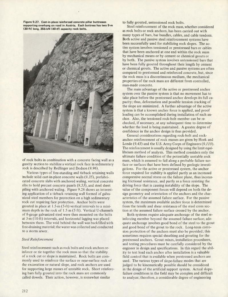
Figure 9.27. Cast-in-place reinforced concrete pillar buttresses supporting overhang on road in Austria. Each buttress has two 9-rn (30-ft) long. 356-kN (40-tf) capacity rock bolts.

-..--P.- 0

- OIL .I, - ..

•

-

#-,t-.;;.1 .._?

-. '.•i 1. - - :'

IN

'

: •" - .. IIlI,vll :_ .ffr

- . . .

. -. -.

JW

of rock bolts in combination with a concrete facing wall as a gravity section to stabilize a vertical rock face in sedimentary rock is described by Redlinger and Dodson (9.96).

Various types of free-standing and tieback retaining walls include solid cast-in-place concrete walls (9.35), prefabri-cated concrete slabs with anchored waling, vertical concrete ribs to hold precast concrete panels (9.53), and steel sheet piling with anchored waling. Figure 9.28 shows an interest-ing application of a tieback retaining wall formed of galva-nized steel members for protection on it high sedimentary rock cut requiring face protection. Anchor bolts were grouted in place at I 5-ni (5-fl) verticalintervals to a mini-mum depth in the rock of 1.5 m (5 fi) - Vertical U-channels of 8-gauge galvanized steel were then mounted on the bolts at 3-in (10-ft ) intervals, and horizontal lagging was placed between them. The void behind the wall was backfilled with free-draining material; the water was collected and conducted to a storm sewer.

Steel Reinforcenent

Steel reinforcement such as rock bolts and rock anchors re-inforce or tie together the rock massso that the stability of a rock cut or slope is maintained - Rock bolts are corn-nionly used to reinforce the surface or near-surface rock of the excavation or natural slope, and rock anchors are used for supporting large masses of unstable rock. Short reinforc-ing bars fully grouted into the rock mass are commonly called dowels. Their act ion - however, is somewhat similar

to fully grouted, untensioned rock bolts. Steel reinforcement of the rock mass, whether considered

as rock bolts or rock anchors, has been carried out with many types of bars, bar bundles, cables, and cable tendons. Both active and passive steel reinforcement systems have been successfully used for stabilizing rock slopes. The ac-tive system involves tensioned or prestressed bars or cables that have been anchored at one end within the rock mass by mechanical means or by cement or chemical grouts or by both. The passive system involves untensioned bars that have been fully grouted throughout their length by cement or chemical grouts. The active and passive systems are often compared to prestressed and reinforced concrete, but, since the rock mass is a discontinuous medium, the mechanical properties of the rock mass are different from controlled, man-made concrete.

The main advantage of the active or prestressed anchor system over the passive system is that no movement has to take place before the prestressed anchor develops its full ca-pacity; thus, deformation and possible tension cracking of the slope are minimized. A further advantage of the active system is that a known anchor force is applied, and proof loading can be accomplished during installation of each an-chor. Also, the tensioned rock-bolt member can be re-checked, if necessary. at any subsequent time to determine whether the load is being maintained. A greater degree of confidence in the anchor design is thus provided.

General considerations regarding rock-bolt and rock-anchor reinforcement of rock masses are given by Hock and Londe (9.43) and the U.S. Army Corps of Engineers (9.110). The reinforcement is usually designed by using the limit equi-librium met hod of analysis. This method co nsiders only the ultimate failure condition of the potentially unstable rock mass, which is assumed to fail along a probable failure sur-face or surfaces that have been defined by geologic investi-gations. For the active or prestressed system, the anchor force required for stability is applied partly as an increased compressive normal stress on the failure plane. thus increas-big frictional resistajice, and partly as a force resisting the driving force that is causing inst ability of the slope. The value of the component forces will depend on both the de-sign geometry and orientation of the anchors and the char-acterist ics of the assumed failure surface - For the passive system, the maxirnuni available anchor force is determined from the tensile and shear resistance of the steel cross sec-tion at the assumed failure surface crossed by the anchor.

Both systems require adequate anchorage of the steel re-inforcing member beyond the assumed failure surface; ade-quate anchorage involves good bond of the steel to the grout and good bond of the grout to the rock. Long-term corro-sioii protection of' the anchors must also be provided; this sometimes requires special sheathing and grouting for the prestressed anchors. Grout mixes, installation procedures, and testing procedures must be carefully considered by the engineer in design and specifications. In this regard the abil-ity to test load each anchor after installation is a valuable field control that is available when prestressed anchors are used. The various types of slope-failure modes that are judged to be kinematically possible should be considered in the design of the artificial support system. Actual slope-failure conditions in the field may be complex and diflicult to analyze; therefore, it considerable degree of engineering

212

DA - ••'S

- -

- r I

e : L

-.:'- ,L-..X--- - :'

Figure 9.28. Galvanized sheet steel retaining wall that is anchored by shallow rock bolts to prevent failures of high cut slope in sedimentary

rock above highway in Hamilton, Ontario.

judgment and experience will continue to be necessary for anchor design.

Analysis of rock-slope deformation is not generally re-quired for transportation routes, except for those involving support of adjacent structures. Theoretical procedures using the finite element met hod are dependent on the assumed boundary conditions and properties ofthe rock mass. At the present time, only cases involving small deformations can be analyzed wit Ii any reliability. Otherwise, the only proce-(lure is to use as high a factor of safety as possible against ultimate shear failure to minimize undesirable deformation. This problem is discussed by Morgenstern and Fisenstein (9.75).

Rock Bolts

The use of rock bolts is discussed by Lang (9.58) and Lancaster-Jones (9.56). Rock bolts are basically used to reinforce the surface and near-surface rock of the excavated or nat ural slope. In that it is essentially a tension member, the rock bolt exerts a compressive force, which tends to pre-vent elastic rebound, frost action phenomena, and general

relaxation or exfoliation by keeping the rock in its original position. The rock-bolt system should be designed in such a manner that shear resistance along discontinuities is itii-proved: the rock mass will then acquire significant tensile strength as a result of the operation.

To minimize the decompression or loosening effects as-sociated with recently excavated rock slopes, rock bolts should be installed and tensioned as soon as possible after each lift of an excavation and preferably before the next lift is blasted to inhibit dilation effects of the near-surface section of the excavation. The sooner the rock bolts are in-stalled, the less the subsequent postexcavation movements of the rock mass will be. Figure 9.29 shows a group of large-diameter rock bolts (980) concentrated in one area at the base of a slope to maintain the integrity of large fault blocks. Figure 930 shows numerous small-diameter rock bolts that have been applied over the entire slope in an attempt to se-cure smaller individual blocks in the slope.

The method used for transferring load t'rom the head of the rock bolt to the rock depends largely on the condition of the rock. Broken rock may weather away from the bolt head and cause the bolt to lose tension. A choice must be

213

Figure 9.29 Concentration on bank of 3.5-cm (1 3/8 -in) diameter 14-rn (45-it) long rock bolts at base of section at Hell's Gate Bluffs, British Columbia. Each rod was cold stretched and stress relieved to provide minimum ultimate strength of 1.1 MPa (160 000 lbf/in2). They were tensioned to 712 kN (80 tf) and dropped to 623 kN (70 tf) and then grouted.

v . "e• •' ' ...... .. -

'

\Th 4 I

S- . • .. '. 3 ' ,. - -. -, '..• c. - .. k ...

.. .

k 4 .g. ••\)

Ia •

Figure 9.30. Broadly distributed 1.6-cm (/-in) diameter by 1.2 to 3-rn (4 to 10-ft) long rock bolts at Hell's Gate Bluffs, British Columbia. These rock bolts were posttensioned to about 53.4 kN (6 tf) to maintain integrity of small individual blocks in slope.

madc between protecting the rock face around the head with wire mesh and shotcrete, retaining the rock in place by steel strapping, or distributing the point load by use of concrete pads. Usually the tentative design load does not exceed ap-proximately 60 percent of the ultimate strength of the bolt.

If grouted bolts are used, extreme care should be taken to ensure that the grout does not spread. Excessive grout spread will reduce the permeability of the rock mass and re-tard drainage by plugging joints through which groundwater would normally have free access. The grout must be pumped into the borehole under low pressure, possibly not exceeding 103 kPa (15 lbff in 2), and other measures must be taken to retard grout spread. If grouted bolts are used in the lower reaches of the slope, free drainage must be maintained.

Rock bolts should be installed by a carefully controlled procedure. The design of the rock-bolt system should be checked and tested during installation for bolt tension and adequate anchorage to ensure reliability and performance of the rock bolts. However, the most important responsibility of the site engineer is to regularly inspect the slope after the rock-bolt installation to guarantee that areas that may be-come unstable in the future have been suffIciently supported.

Dowels and Perjb bolts

Dowels consist essentially of steel reinforcing bars that are cemented into boreholes; they are not subjected to any posttensioning. Unlike rock bolts that provide a form of reinforcement, dowels are in the strict sense a form of rock-slope support. Whereas rock bolts increase both shearing re-sistance and normal stress, dowels basically increase the shearing resistance across potential failure surfaces. A typ-ical use of dowels for rock slope stabilization is shown in Figure 9.31. Dowels are also used to provide anchor keys and tiebacks for shearing resistance at the toe and flanks of retaining walls, as shown in Figure 9.32. Dowels, together with rock bolts, can fasten small blocky rocks when applied with strapping or bearing pads, stabilize broken rock zones when applied with wire mesh and shotcrete, and anchor but-tresses or beams placed below sloping blocks of rock. They can also anchor restraining nets and cables, catch nets, catch fences, cable catch walls, and cantilever rock sheds.

The perfoholt is a form of steel dowel encased within a thin sheet -metal liner filled with low-slump slush grout and perforated. The liner is inserted into a drilled hole in the rock, and a steel reinforcement bar is then inserted into the liner, displacing the grout and forcing it through the perfora-tions. A bond is thus effected with the rock. Perfoholts are particularly applicable in sections of the rock mass in which grouting of standard rock bolts would prove difficult be-cause of open cracks and in which fully grouted artificial support is required. Perfobolts as long as 6 in(20 ft) have been installed: for greater lengths. inserting the reinforcing bar in the liner by hand is difficult.

Tendon and Cable Anchors

Tendon and cable anchors are used to control large failure blocks and are accordingly longer than rock bolts. Anchors usually affect a much larger volume of rock than rock bolts. Although the basic principles that apply to rock bolts are

214

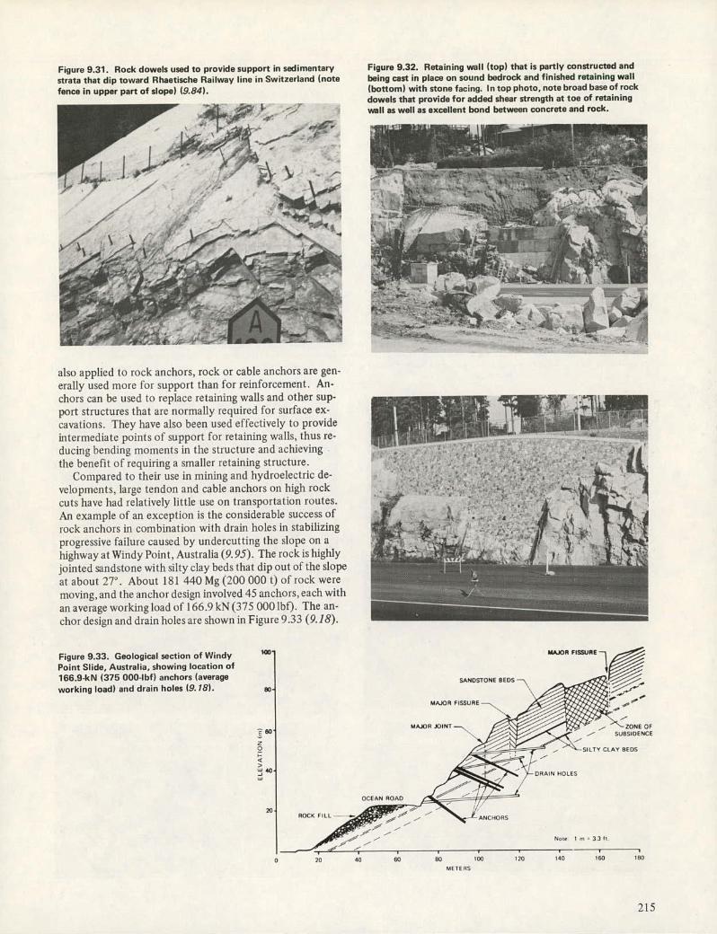
3

Figure 9.31. Rock dowels used to provide support in sedimentary strata that dip toward Rhaetische Railway line in Switzerland (note fence in upper part of slope) (9.84).

also applied to rock anchors, rock or cable anchors are gen-erally used more for support than for reinforcement. An-chors can be used to replace retaining walls and other sup-port structures that are normally required for surface ex-cavations. They have also been used effectively to provide intermediate points of support for retaining walls, thus re-ducing bending moments in the structure and achieving the benefit of requiring a smaller retaining structure.

Compared to their use in mining and hydroelectric de-velopments, large tendon and cable anchors on high rock cuts have had relatively little use on transportation routes. An example of an exception is the considerable success of rock anchors in combination with drain holes in stabilizing progressive failure caused by undercutting the slope on a highway at Windy Point, Australia (9.95). The rock is highly jointed sandstone with silty clay beds that dip out of the slope at about 27°. About 181 440 Mg (200 000 t) of rock were moving, and the anchor design involved 45 anchors, each with an average working load of 166.9 kN (375 000 IbO. The an-chor design and drain holes are shown in Figure 9.33 (9.18).

Figure 9.33. Geological section of Windy Point Slide, Australia, showing location of 166.9-kN (375 000-lbf) anchors (average working load) and drain holes (9.18).

Figure 9.32. Retaining wall (top) that is partly constructed and being cast in place on sound bedrock and finished retaining wall (bottom) with stone facing. In top photo, note broad base of rock dowels that provide for added shear strength at toe of retaining wall as well as excellent bond between concrete and rock.

..;.. ..., 'E% . . .... : ''•' -'.

. •,, . 'v

of

.-,. '1T--

MAJOR FISSURE

MAJOR FISSURE

MAJOR JOINT —., ..- —ZONE OF .— SUBSIDENCE

OCEAN ROAD

20 ANCHORS

- "—SILTY CLAY BEDS

.Al. HOLES

/

No, I ,n 331

20 40 60 80 IOU 120 140 lEO 180

METERS

215

S

/

An interesting anchorage system, shown in Figures 9.34 and 9.35, was carried out by Barron, Coates, and Gyenge

7 (9.4) at a Canadian mine. The system consisted of deep preloaded cable anchors to support the tentatively unstable ground between the slope face at angle a and some prede-termined potential failure plane at angle i. Welded wire mesh was placed over the surface, and horizontal stringers were installed between the cable terminations to prevent local rock falls and to provide bench support.

A practical guide for the use and installation of anchors is given by Coates and Sage (9.18), and other useful aspects relating to design and quality control of rock anchors are de-scribed by Seegmiller (9.102).

Anchored Beams

Anchored beams can be used to distribute the support of rock bolts over a wide area of the slope and, hence, mini-mize the number of bolts required. The beams can be made of concrete or steel and applied in any direction across a rock face. Anchored beams are particularly useful where

Figure 9.34. Schematic drawing of trial anchor / support system including cable anchors, horizontal stringers, and welded mesh between / anchor heads (9.4).

ANCHOR LOADING1 2 HORIZONTAL

STRINGERS

COVERING SURFACE

\%

Cr BOLTS On CABLES

Figure 9.35. Installation of system shown in Figure 9.34: (a) location of two benches where the trial anchor installation is conducted, (b) inserting the cable in the borehole, (c) formwork for horizontal concrete stringer on lower bench and 66.44 welded wire mesh, (d) formwork for anchor pads on top bench and steel bar horizontal stringer, (f) cable anchor tensioned and locked, and (f) completed trial anchor installation on lower bench (9.4).

':.

(c)

or

'-, •;. .4., ., r' .... p - . •;- s - #"T .% '

:':' '.'•'Z-.-'•' ' - f. . -,

- ...• . -_ - 2

(e)

216

Figure 9.37. Application of anchored cables and cable nets.

Figure 9.38. Cable lashing of a large, potentially hazardous. 2-rn (6-ft) diameter block about 90 m (300 ft) above highway in Fraser Canyon, British Columbia.

*

Figure 9.36. Cast-in-place reinforced concrete beams used to distribute point loads from rock bolts seated in the beams (9.84). Location is above main line of Austrian Federal Railways.

heavy slabs of rock are unstable and where a relatively uni-form distribution of point load forces of the anchors or bolts is required. Typical anchored beams installed in Austria are shown in Figure 9.36. Several variations of anchored beams have been used: In Czechoslovakia, for example, anchored concrete frames are used rather than beams. Anchored concrete aprons have been used on heavily jointed rock around bridge piers in Washington State.

Anchored Cable Nets

Anchored cable nets can be used to restrain masses of small loose rocks or individual loose blocks as large as 1.5 to 2.5 m (5 to 8 ft) in diameter that protrude from a rock face. In principle, an anchored cable net performs like a sling or re-inforcement net, which extends around the surface of the unstable broken rock to be supported. The cable net strands are gathered on each side by main cables leading to rock an-chors, as shown in Figure 9.37.

Beam and Cable Walls

Beam and cable walls can also be used to prevent smaller

Figure 9.39. Large, potentially hazardous rock block supporting considerable volume of smaller material secured by two cable strands that were inserted in boreholes through the block and anchored on

other side.

blocks of rock from falling out of the slope and may be used on slopes as high as 20 m (60 ft). Beam and cable walls con-sist of cable nets fastened to vertical ribs formed of steel beams laid against the slope at 3 to 6-rn (10 to 20-ft) inter-vals. The beams are held by anchored cables at the top of the slope and by concrete footings at ditch level.

Cable Lashing

Cable lashing is a simple, economical type of installation for restraining large rocks. As shown in Figure 9.37, this method merely involves tying or wrapping unstable blocks with indi-vidual cable strands anchored to the slope. Eckert (9.24) de-scribes a case in France in which cables with a capacity of 227 Mg (250 t) and a length of more than 90 in (300 ft) were extended around a mass of broken rock and anchored into sound rock at each side. Lashing using both cables and chains is described by Bjerruni and Jrstad (9.9). If rock is too broken to be restrained by individual cables, vertical concrete or steel ribs can be used to spread the points of contact of the cables with the rock. Typical cable lashing of a large block is shown in Figure 9.38. Figure 9.39 shows a unique application of cables in that two cables pass en-tirely through the block.

217

ASSUMED STARTING VELOCITY

Methods of Protection

Rock-Fall Characteristics Affecting the Design of Protection Measures

Loose rocks can be kept from reaching the transportation route right-of-way by retaining the rocks on the slope, in-tercepting falling rocks above the roadway, or directing fall-ing rocks to pass over or under the transportation route without causing harm. Before the best methods can be chosen for a particular location, the characteristics of the rock falls and the general geometry of the slope should be evaluated. The rate at which fallen rock accumulates is also an important factor. Without encroaching on the right-of-way, storage must be provided for rock falls that are likely to arrive during a reasonable maintenance interval. Protec-tion measures must be designed to protect against the vari-ous ways in which rock falls reach the right-of-way (9.85).

A rock can arrive at the base of a slope by free falling, bouncing, rolling, or sliding down the slope. For free-falling rocks, the only means of protection are to move the roadway away from the slope and prevent the rocks from bouncing and rolling after landing or to protect the roadway with a rock shed or tunnel. The paths of bouncing rocks are diffi-cult to predict, and interception measures above the right-of-way require high structures, such as a wall or net. Roll-

Figure 9.40. Rock-fall paths traced by calcomp plotter based on computer model for typical rock falls at Porteau Bluffs,

British Columbia (9.91).

ing or sliding rocks are easier to intercept since they are in constant contact with the slope; in gullies, their paths are even more predictable.

A rock-fall model developed by Piteau and Clayton (9.91) for a computer program can simulate several hundred rock falls for a slope of specified geometry in a matter of seconds. A coefficient of restitution is used for, the rock fall in the bouncing mode, and increased friction is used for the rolling mode to determine the paths of the rock falls for different input velocities and heights. The slope profile is divided into straight segments or slope cells (Figure 9.40), which are num-bered consecutively from the top to the bottom of the slope. Rock falls are introduced at different locations above the slope as desired. Probability factors can be assigned to these locations to recognize areas that are either more likely or less likely to be the source of the rock fall. Catch walls at various positions and heights can be assumed in the model to evaluate their effectiveness. In the same manner, the ef-fect of varying the slope geometry by including ditches, benches, and berms can be evaluated.

This rock-fall model was used to relocate a concrete catch wall at the base of an active rock-fall area (Figure 9.51). It was also used to determine whether large blocks located at the crest of a major slide area would reach facilities at the base of the mountainside located some 1500 to 1800 m (5000 to 6000 ft) away from the crest of the slide.

218

Figure 9.42. Shaped berm that is at toe of high rock face and cut in top of high talus slope above Hope.Agassiz highway in British

Columbia.

Figure 9.41. Intercepting slope ditch or cross ditch, north of Hope in Fraser Canyon, British Columbia, to catch rolling rocks originating up slope on steep rock faces (note that ditch is shaped partly in talus and makes use of blocks of rock).

Relocation

Relocation is most effective where rocks are free falling from steep rock faces in proximity to the roadway or where stabilization or some other protection measure is not feasi-ble. Relocation is feasible when space is available and the design criteria are not affected. When combined with proper ditch shaping and possibly with other ditch-level protection, relocation can be the most economical solution and, in some cases, one of the few solutions to the problem. Unless relo-cation practically eliminates the possibility of accidents, other measures also should be included along with relocation.

Intercepting Slope Ditches and Shaped Berms

Slope ditches are used to intercept rock falls partway up the slope, and shaped berms are used at the top of the slope. These methods ensure that rock falls get caught either be-fore they start to roll or while they are on their way down the slope. In some locations, ditches can be made to inter-cept rocks and guide them laterally into disposal areas. A typical intercepting slope ditch is shown in Figure 9.41 , and a shaped berm at the base of a steep slope is shown in Figure 9.42.

Depending on the nature of the terrain, these methods are generally inexpensive, simple to construct, and easy to main-tain. An intercepting slope ditch should only be installed on a slope that can accept the introduction of a ditch without the stability of the entire slope being impaired. The ditch must be designed and built carefully so that the upper slope is not at any time steeper than planned. The ditch should be suitably located to facilitate periodic cleaning by mechan-ical equipment.

Anchored Wire Mesh

Wire mesh is a versatile and economical material for use in protecting the right-of-way from small rocks. Layers of mesh are often pinned onto the rock surface to prevent small loose rocks from becoming dislodged (Figure 9.43). Figure 9.44 shows that mesh can also be used essentially as

a blanket draped over the rock surface to guide falling rock into the ditch at the base of the slope. The same arrange-ment can be used on stony overburden slopes to prevent dis-lodged stones from rolling down the slope. This practice is commonly used on talus slopes in steep mountainous terrain. Mesh can be combined with long rock bolts to provide a gen-erally deeper reinforcement. Mesh in combination with both shotcrete and rock bolts provides general reinforcement and surficial support and retards the deleterious effects of weathering.

Conditions for the use of mesh are particularly suitable if no individual rocks are larger than 0.6 to 1 in (2 to 3 ft) and if the slope is uniform enough for the mesh to be in al-most continuous contact with the slope. If large falling blocks in certain areas are likely to dislodge or tear the mesh and present a hazard, rock bolts should be used to reinforce these particular areas. For anchoring mesh at the top of overburden slopes, posts are cast in concrete blocks in hand-dug holes. For bedrock slopes,grouted rock bolts or dowels are used. A cable is slung between the anchorages: the mesh is then fastened to the cable and rolled down the slope, and the vertical seams of the mesh are wired together. For wire mesh blankets, the bottom end of the mesh is usually left a meter or so above ditch level (Figure 9.44) and only a nar-row ditch is required. The mesh normally used is 9 or II - gauge galvanized, standard chain-link or gabion wire mesh. Gabion mesh appears to have an advantage over the standard chain-link materials in that the gabion mesh has a double-twist hexagonal weave that does not unravel when broken.

Protection Methods at Ditch Level

Shaped Ditches

Depth, width, and steepness of the inside slope and storage volume of the ditch are important factors in the design of ditches to contain rock falls. The choice of ditch geometry should take into consideration the angle of the slope that in-fluences the behavior of falling rocks. Ritchie (9.98) evalu-ated the mechanicsof rock falls from cliffs and talus slopes and developed design criteria for ditches. The criteria, which

219

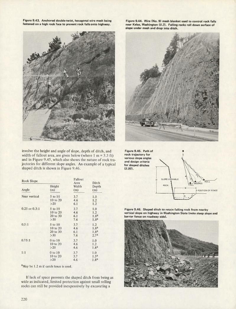
.:t-

Figure 9.43. Anchored double-twist, hexagonal wire mesh being Fastened on a high rock face to prevent rock falisonto highway.

Figure 9.44. Wire (No. 9) mesh blanket used to control rock falls near Kelso, Washington (9.3). Falling rocks roll down surface of slope under mesh and drop into ditch.

involve the height and angle of slope, depth of ditch, and Figure 9.45. Path of

width of fallout area, are given below (where I In = 33 It) rock trajectory for

and in Figu various slope angles

re 9.45. which also shows the nature of rock tra- and design criteria jectories for different slope angles. An example of a typical for shaped ditches shaped ditch is shown in Figure 9.46. (9.98).

Rock Slope Fallout Area Ditch

Height Width Depth Angle (m) (m) (in)

Near vertical 5 to tO 3.7 1.0 10to20 4.6 1.2 >20 6.1 1.2

0.25 or 0.3:1 5 to 10 3.7 1.0 10to20 4.6 1.2 2010 30 6.1 >30 7.6 183

0.5:1 5 to 10 3.7 1.2 10 to 20 4.6 18a

20 to 30 6.1 1 8a

>30 7.6

0.75:1 0 to 10 3.7 1.0 10to20 4.6 1.2 >20 4.6 18a

1:1 OtolO 3.7 1.0 lOto2O 3,7 >20 4.6

.----- aMay be 1.2 m if catch fence is used. - nk .. --

If lack of space prevents the shaped ditch from being as

wide as indicated, limited protection against small rolling

rocks can still be provided inexpensively by excavating a

Figure 9.46. Shaped ditch to retain falling rock from nearby vertical slope on highway in Washington State (note steep slope and barrier fence on roadway side).

220

T.

-

-•--.

l-

•-

(-1-

Figure 9.47. Shaped ditches, wire mesh catch fences, and wire

mesh catch nets (9.84).

SHAPED DITCHES WITHOUT CATCH FENCE

(a) (b)

ORIGINAL 01TC

GABION LEXCAVATED

SHAPED DITCHES WITH CATCH FENCE CATCHMENT AREA

(c) (dl PENCE OR

ORIGINAL jNCEVESH

(I --CABLE TIE8ACI(

CABLE CK FENCEMH

E E :i:..:

CATCH FENCES

tg) (h) .RE MESH ANCHORED

- WIRE .11511 - NE CABLE

CABLE ANCHORED

E LI VAT ON

CATCH FENCES CATCH NET ACROSS SLOPE OVER GULLY

catchment area, as shown in Figure 9.47b (9.84). by form-ing a windrow of material or by installing a low barrier formed of standard highway guardrail, precast concrete ele-ments, or gabions at the shoulder of the roadway. as shown

in Figure 9.47a (9.84). Bedrock should not remain exposed in the bottom of ditches. but should be covered with small broken rock or loose earth to keep falling rocks from bounc ing or shattering. Mearns (9.71) describes how a ditch at grade was filled with a 0.3-in (I -ft) layer of sand, which acted as an energy absorber to prevent lolling rock falls from reaching the road. Several workers have used a simi-lar technique to successfully dissipate energy of rock falls.

Wire-Mesh catch iVets and Fences

Wire mesh can be effective in intercepting or effectively slowing bouncing rocks as large as 0.6 to I in (2 to 3 ft) when the mesh is mounted as a flexible catch net rather than as I standard, fixed wire fence. If suspended oil a ca-ble. the mesh will absorb the energy of flying rocks with a minimum of damage to the wire catch net. Catch nets can consist of standard chain-link wire mesh or gabion mesh. This type of barrier has economic potential in some trouble-sonic locations, as shown in Figure 9.47li (9.84). It is best to locate catch nets al the lower end of steep gullies where rocks tend to bounce down to the right-of-way. The cable supporting the catch net is anchored to sound rock OII either side of the gully with the result that rocks hit the catch net and fall harmlessly at the base of the structure. If there is a steady accumulation of rock, a catch wall on the shoulder of the roadway also may be required.

The principle ofthe catch fence is similar to that of a catch net. Its purpose is to form a flexible barrier to dissi-pate the energy of rapidly moving rocks. Various arrange-ments are shown in Figure 9.47 (9.84) for catch fences to-

Figure 9.48. Special mobile catch fence mounted on flat deck to protect motorists from rock falls during excavation work and

scaling in extremely steep terrain.

cated at or near ditch level. The wire mesh (chain-link or gabion) forming the catch fences is hung on cables supported on posts or strung between posts or trees. Wire-mesh catch fences are usually located on the roadway side of the ditch or at the base of the slope and can be used with or without a shaped ditch. The fence should be suitably situated so that accumulated rocks can be removed easily. Figure 9.31 shows a catch fence, and Figure 9.48 shows a special appli-cation of a mobile catch fence for use in scaling operations.

Catch Walls

Catch walls can be used to form a rigid barrier to stop roll-ing or bouncing rocks as large as 1 .5 to 2 ni (S to 6 ft) from reaching the right-of-way. If effective, they usually increase the storage capacity of (lie ditch so that maintenance inter-vals can be extended. In many locations, large ditches them-selves are not effective for intercepting large rolling rocks and the use of catch walls is advised.

To achieve maximum protection and storage capacity, the catch walls should be located oil the side of the ditch closest to the road. In steep terrain, catch walls are commonly used where the right-of-way cuts across postglacial slide areas. Many postglacial slide areas that have been disturbed by ex-cavation are in a constant state of sloughing and readjust-ment. If broad areas require wall protection, gaps should be left in the catch wall to allow access of maintenance equip-ment required to remove rock.fall debris.

Concrete ('arc/i Walls

Concrete catch walls are the most widely used type of catch wall in steep mountainous terrain. Concrete walls may be cast in place or precast in short sectioisand assembled on the site. An efficient precast concrete wall installation is shown in Figure 9.49 (9.84). Figures 9.50 and 9.51 show

Figure 9.49. PrecaSt TIES AT 40.6cm c-to c. TO REDUCE IMPACT AND INCREASE HEIGHT OF

concrete wall that WALL FOR GREATER PROTECTION ELECTRIC WARNING

could be used for \. fwIRE IOPTIONALI

LI track protection

- 09m -I- - DITCH

(9.84).

EXCAVATED

ORIGINAL

CABLE - STRAPPING-. I.

~~-

09m

CATCH ELL COMPMENT

ACTED PRECAST AREA BACKFILL ----i 0.9-M-1 cONCRETE

NOte. 1 r,, 3.3 It; 1 ccc -0.4 ,n. \_ CATCH WALL

221

Figure 9.50. Reinforced cast-in-place concrete wall approximately 2 m (7 ft) high and 1 m (3 ft) wide across a major postglacial slide area along edge of Trans-Canada Highway in Fraser Canyon, British Columbia (note break in retaining wall where large blocks have hit wall).

fY if

1: E•,

,•

- .. ,•F t'1.'!J

-

Figure 9.51. Close-up of concrete catch wall shown in Figure 9.50 (note breaks in wall due to large blocks from postglacial slide debris rolling down slope).

- - -

•

..'y

:i .-

-

TTI -,. --

the use of a cast-in-place concrete catch wall in a postglacial slide area, where large rock falls resulted in breaking the wall.

Box Gab/on Catch Wa/I

The box gabion catch wall is a rectangular basket divided by diaphragms into smaller rectangles that are filled with slones. The basket is formed of woven hexagonal steel gal-vanized wire mesh. Baskets can be placed to be filled indi-vidually or wired logether in groups and filled accordingly. The wire mesh tends to reinforce the stone in tension. The gabion is a flexible structure that, upon settling or being hit by impact. tends to deflect and deform instead of break. Because gabion walls are highly deformable, differential settlement is not important. Like the gabion mesh, the ga-bion does not unravel if broken. Gabions make good catch-

wall structures, but only recently have they been recognized in North America as a feasible alternative to more rigid con-crete walls for protecting the right -of-way from rolling rocks. They prove particularly useful where the right-of-way crosses

postglacial slide areas. They can be used efficiently to stop rolling stones as large as 0.6 to I iii (2 to 3 ft). When ade-

qua te filter materials are used as backfill, they provide long-term, free-draining walls. A gabion catch wall is shown in Figure 9.52.

Rail Walls

Rail walls or rail-and-tie walls consist of vertical posts and

horizontal members that are extended between the vertical posts. The vertical posts are usually scrap steel rails set in holes, which are hand dug or blasted and backfilled with

concrete. The horizontal members are either ties, as shown

in Figure Figure 9.53. or scrap rails cut into 3 to 4-ni (10 to I 3-ft) lengths, as shown in Figure 9.54. If feasible, cables can be

anchored back from the top of the wall to provide resistance to overturning.

Cable Wa/Is

Cable walls consist of steel posts set in concrete, cables strung horizontally between, and a smaller cable or coarse wire woven between the cables to form a crude net or niesh. This type of installation is sometimes used in Europe.

Rock Sheds and Tunnels

Rock sheds and tunnels can be used for protection against rock falls and slides when warranted and when other forms of stabilization and protection are not effective. Although

expensive, they can give complete protection and should be considered in areas with serious problems. Maintenance costs are normally negligible. The methods of design and

construct ion of tunnels are dealt with thoroughly in the

literat tire. but the design of rock sheds is not so adequately covemed, and experience is required to decide on the most suitable type of structure and the loads to be carried. A rock shed should be able to resist the energy transmitted by the largest rock mass likely to pass over it during its life; therefore, probability analysis should be involved. The en-

ergy transmitted will depend on whether rocks are falling hee, bouncing, or rolling. High stress concentrations iii the

structure can be reduced by the provision of a thick cover of loose sand.

If foundation conditions on the outer side of the road-bed are not suitable for footings, heavy rock anchors cx-

/

:

tending into the upper slope may be used to support a cantilevered shed of the type shown in Figure 9.55. Tun-nel portals can also act as sheds to protect the roadway or track, as shown in Figure 9.56. When a rock shed is to be located at the lower end of a gully, wing walls are usually used above the structure to channel material onto it (Fig-ure 9.57). Wing walls should be sufficiently high because the debris will tend to clog and build up when its path is restricted by the structure. For this reason, the slope angle of the roof of the shed should be steeper than the angle of repose of the material to be conveyed over the roadway.

Methods of Wanfing

Although warning systems do not prevent rock falls, they are necessary on transportation routes where other measures are too expensive or impractical or where a new hazard has developed. In North America, warning methods have been used on railways in mountains to detect rock falls on tracks SO that trains can stop before hitting the material.

Patrols The simplest type of warning method is provided by human

Figure 9.52. Gabion catch wall along edge of high slope in unconsolidated material on main highway.

patrol. Patrols have the advantages of being reliable and flex-ible, and their frequency can be adjusted to the demands of traffic and weather conditions. The disadvantages are that they incur continuing costs and require personnel who are willing to work in uncomfortable and often hazardous con-ditions.

Electric Fences and Wires

There are several variations of electric warning methods. Electric fences are based on the principle that a falling rock large enough to endanger traffic will break or pull out one of the wires and thus actuate a signal to warn approaching traffic. This principle is particularly adaptable to railways on which a signal system to control traffic is already in use. The standard electric warning fence used on railways con-sists of a row of poles spaced along the uphill ditch line and wires strung between them at a vertical spacing of 25 cm (10 in). Overhead wires, which are supported on members cantilevered out from the top of the poles, as shown in the installation in Figure 9.58, are often required where rock faces are steep and close to the right-of-way.

Figure 9.54. Rail wall with vertical posts seated in cast-in-place footings (note top of wall anchored by cables to bedrock for support) -

Figure 9.53. Rail and tie wall founded on masonry wall to prevent rolling rock from reaching track of Austrian Railway.

• t '., .•4 J

0

Figure 9.55. Cantilevered rock shed supported by deep anchors inserted in upper slope protecting rail line in Switzerland (9.84).

)':ic-•- ,.'______.

223

I 4. .

14 L'• :-

-i A. :

p.,

Figure 9.56. Tunnel in steep terrain with extended portal shedlike structure to protect Canadian National Railway line from rock falls generated in a slide area (note use of retaining walls of rock blocks below track).

Figure 9.57. Rock sheds to carry rock debris originating in deep gullies over main line of Canadian National Railway in White Canyon in Thompson River Valley, British Columbia.

Electric warning fences have some advantages, and the design of each facility can be made to suit the individual sites. One disadvantage is low efficiency: in some instances 80 percent of the alarms have been found to be false. An-other disadvantage is that snow-clearing operations. if re-quired. are often impeded and maintenance of the fences proVeS difficult. These difficulties may be reduced or elim-inated by

I. Choosing the spacing of wires according to previous experience at a site.

Providing a catchmcnt ditch behind the warning fence. Eliminating the lower wires where the lower slope can

be scaled and stabilized, and

Figure 9.58. Standard type of railway electric warning fence with wires strung between upright poles and horizontal members that are cantilevered out from top of poles along Canadian National Railway line in Fraser Canyon, British Columbia.

Supporting overhead wires on a canopy type of frame bolted to the rock face on the uphill side and supported on poles on the downhill side.

A particularly effective type of electric warning system consists of a single wire, anchored at both ends and linked to a warning signal (9.85). Such a wire may be fastened around a large unstable rock or across a rock slope above the right-of-way, across a gully where large rocks roll down, or on top of a protective catch wall.as shown in Figure 9.49. The installation is simple, economical, and efficient.

Other Methods

Warning methods that are dependable under all conditions

224

are undergoing continued study. At this writing, the follow- Guide for Their Utilization and Installation. Mines Branch,

ing are being tried: (a) geophones or vibration meters buried Canada Department of Energy, Mines and Resources, Ot-

at intervals along the roadway shoulder to pick up vibrations tawa, Research Rept. R224, 1973. 9.19 Crimmins, R. S., Samuels, R., and Monahan, B. P. Con-

from falling rocks by the Canadian National Railways and struction Rock Work Guide. Wiley, New York, 1972, Swedish State Railways; (b) television monitoring by the 235 pp. Federal Highway Administration; (c) guided radar by the 9.20 Da Silveira, A. F., Rodrigues, F. P., Crossman, N. F., and

Canadian Institute of Guided Ground Transport and the Mendes, F. Quantitative Characterization of the Geomet-

Japanese National Railways and (d) laser beams by the nc Parameters of Jointing in Rock Masses. Proc., 1st Con- gress, International Society of Rock Mechanics, Lisbon,

Radio Corporation of America. However, none is known Vol. 1, 1966, pp. 225-233. to have been sufficiently developed to be recommended 9.21 Deere, D. U., Hendron, A. J., Patton, F. D., Jr., and for general use. Cording, E. J. Design of Surface and Near-Surface Con-

struction in Rock. In Failure and Breakage of Rock

REFERE,ES (Fairhurst, C., ed.), Proc., 8th Symposium on Rock Me- chanics, American Institute of Mining, Metallurgical and Petroleum Engineers, New York, 1967, pp. 237-302.

9.1 Alberts, C. Bergförstrkning genom betonsprutning och 9.22 Donn, W. L., and Shinier, J. A. Graphic Methods in Struc- injektering. Swedish Academy of Engineering Sciences, tural Geology. Appleton-Century-Crofts, Englewood Cliffs, Stockholm, IVA Pub!. 142, 1970, pp. 231-240. N.J., 1958, 180 pp.

9.2 American Concrete Institute. Use of Shotcrete for Under- 9.23 Duncan, N. Geology and Rock Mechanics in Civil Engi- ground Structural Support. ACI, Detroit, Pub!. SP-45, neering Practice. Water Power, Jan. 1965, pp. 25-32. 1974, 467 pp. 9.24 Eckert, 0. Consolidation de massifs rocheaux par ancrage

9.3 Baker, R. F., and Marshall, H. C. Control and Correction. de cables/Consolidation of Rock Masses by Cable Anchors. In Landslides and Engineering Practice (Eckel, E. B., ed.), Sols-Soils (Paris), Vol. 5, No. 18, 1966, pp. 33-40 (in Highway Research Board, Special Rept. 29, 1958, pp. English). 150-187. 9.25 Ehrlich, M. E., Scharon, H. L., and Mateker, E. J., Jr. Vi-

9.4 Barron, K., Coates, D. F., and Gyenge, M. Artificial Sup- bration Analysis and Construction Blasting. In Legal As- port of Rock Slopes. Mines Branch, Canada Department pects of Geology in Engineering Practice, Geological of Energy, Mines and Resources, Ottawa, Research Rept. Society of America, Engineering Geology Case Histories, R228, 1971, 145 pp. No. 7, 1969, pp. 13-20.

9.5 Barton, N. Review of a New Shear-Strength Criterion for 9.26 Fookes, P. G., and Sweeney, M. Stabilization and Con- Rock Joints. Engineering Geology, Vol. 7, No. 4, 1973, trol of Local Rock Falls and Degrading Rock Slopes. pp. 287-33 2. Quarterly Journal of Engineering Geology, Vol. 9, No.

9.6 Bauer, A. The Status of Rock Mechanics in Blasting. In 1, 1976, pp. 37-55. Status of Practical Rock Mechanics (Grosvenor, N. E., and 9.27 Frster, W. The Influence of the Curvature of Open Cuts Paulding, B. W., Jr., eds.), Proc., 9th Symposium on Rock on the Stability of Slopes in Open Work Mining. Proc., 1st Mechanics, American Institute of Mining, Metallurgical Congress, International Society of Rock Mechanics, Lisbon, and Petroleum Engineers, New York, 1967, pp. 249-262. Vol. 1, 1966, pp. 193-200.

9.7 Behr, H., and Klengel, K. J. Stability of Rock Slopes on 9.28 Franklin, J. A., and Denton, P. E. Monitoring for Rock the German State Railway. Deutsche Eisenbahntechnik, Slopes. Quarterly Journal of Engineering Geology, Vol.6, Germany, 1966, pp. 324-328. No. 3, 1973, pp. 259-286.

9.8 Benson, R. P. Experience With Instrumentation in Rock 9.29 Goodman, R. E. Methods of Geological Engineering in Slopes. Acres Consulting Engineers, Niagara Falls, N.Y., Discontinuous Rocks. West Publishing, St. Paul, 1976, 1971,49pp. 472pp.

9.9 Bjerrum, L., and J$rstad, F. A. Stability of Rock Slopes 9.30 Halstead, P. N., Call, R. D., and Rippere, K. H. Geologic in Norway. Norwegian Geotechnical Institute, Oslo, Publ. Structural Analysis for Open Pit Slope Design, Kimberley 79, 1968, 11 pp. Pit, Ely, Nevada. Paper presented at 97th Annual Meet-

9.10 Brekke, T. L. Shotcrete in Hard Rock Tunneling. Bulletin, ing, American Institute of Mining, Metallurgical and Pc- Association of Engineering Geologists, Vol. 9, No. 3, 1972, troleurn Engineers, New York, 1968, 25 pp. pp. 241-264. 9.31 Hamel, J. V. Stability of Slopes in Soft, Altered Rocks.

9.11 Bukovansky, M., and Piercy, N. H. High Road Cuts in a Univ. of Pittsburgh, PhD thesis, 1969. Rock Mass With Horizontal Bedding. In Design Methods 9.32 Hast, N. The State of Stress in the Upper Part of the in Rock Mechanics (Fairhurst, C., and Crouch, S. L., eds.), Earth's Crust. Engineering Geology, Vol. 11, No. 1, 1967, Proc., 16th Symposium on Rock Mechanics, Univ. of pp. 5-17. Minnesota, Minneapolis, American Society of Civil Engi- 9.33 Hedley, D. G. F. Design Parameters for Borehole Exten- neers, New York, 1977, pp. 47-52. someter Measuring Systems. Mines Branch, Canada De-

9.12 Bureau of Public Roads. Presplitting: A Controlled Blast- partrnent of Energy, Mines and Resources, Ottawa, Inter- ing Technique for Rock Cuts. U.S. Department of Corn- nat Rept. MR67/59-LD, 1967. merce, 1966, 36 pp. 9.34 Hendron, A. J. Analytical and Graphical Methods for the

9.13 Calder, P. N. Slope Stability in Jointed Rock. Bulletin, Analysis of Slopes in Rock Masses. Department of Civil Canadian Institute of Mining, May 1970. Engineering, Univ. of Illinois at Urbana-Champaign, July

9.14 Call, R. D. Analysis of Geologic Structure for Open Pit 1971, 178 pp. Slope Design. Univ. of Arizona, Tucson, PhD thesis, 9.35 Hcnnequin, M., and Cambefort, H. Consolidation du 1972, 201 pp. remblai de Malherbe/Stabilization of Fill at Malherbe.

9.15 Cedergren, H. R. Seepage, Drainage and Flow Nets. Revue General des Chernins de Fer (Pails), Vol. 85, Jan. Wiley, New York, 1967, 490 pp. 1966, pp. 78-86.

9.16 Coates, D. F. The Stability of Slopes in Open Pits. Proc., 9.36 Herget, G. Surveys of Geological Discontinuities in Con- 8th Commonwealth Mining and Metallurgical Congress, nection With the Mechanical Behavior of Rock Masses. Australian Institute of Mining and Metallurgy, Melbourne, Mines Branch, Canada Department of Energy, Mines and Vol. 6, 1967, pp. 543-550. Resources, Ottawa, Internal Rept. MR70/38, 1970, 28 pp.

9.17 Coates, D. F., and Gycnge, M. Incremental Design in Rock 9.37 Heuze, F. E., and Goodman, R. E. Three-Dimensional Ap- Mechanics. Mines Branch, Canada Department of Energy, proach for Design of Cuts in Jointed Rock. In Stability of Mines and Resources, Ottawa, Monograph 880, 1973. Rock Slopes (Cording, E. J., ed.), Proc., 13th Symposium

9.18 Coates, D. F., and Sage, R. Rock Anchors in Mining: A on Rock Mechanics, Univ. of Illinois at Urbana-Champaign,

/1 225

American Society of Civil Engineers, New York, 1971, pp. 397-441.

9.38 Highway Focus. Vol. 1, No. 3, Aug. 1969.

9.39 Highway Focus. Vol. 4, No. 2, June 1972.

9.40 Highway Research Board. Erosion Control on Highway Construction. HRB, Synthesis of Highway Practice 18, 1973, 52 pp.

9.41 Highway Research Board. Soil Erosion: Causes and Mech- anisms, Prevention and Control. HRB, Special Rept. 135, 1973, 141 pp.

9.42 Hoek, E., and Bray, J. W. Rock Slope Engineering. Insti- tution of Mining and Metallurgy, London, 1974, 309 pp.

9.43 Hock, E., and Londe, P. Surface Workings in Rock. Proc., 3rd Congress, Denver, International Society of Rock Me-chanics, Vol. 1, Pt. A, 1974, pp. 613-654.

9.44 International Society of Rock Mechanics. Suggested Methods for the Description of Rock Masses, Joints and Discontinuities. ISRM, 1976.

9.45 Jaeger, J. C. Brittle Fracture of Rocks. In Failure and Breakage in Rock (Fairhurst, C., ed.), Proc., 8th Sympo-sium on Rock Mechanics, American Institute of Mining, Metallurgical and Petroleum Enginners, New York, 1967, pp. 3-57.

9.46 Jennings, J. E. A Preliminary Theory for the Stability of Rock Slopes Based on Wedge Theory and Using Results of Joint Surveys. Univ. of Witwatersrand, South Africa, 1968.

9.47 Jennings, J. E. A Mathematical Theory for the Calcula- tion of the Stability of Slopes in Open Cast Mines. In Planning Open Pit Mines, Johannesburg (van Rensburg, P. W. J., ed.), Proc., Open Pit Mining Symposium, Johan-nesburg, South African Institute of Mining and Metallurgy, Balkema, Amsterdam, 1971, pp. 87-1 02.

9.48 John, K. W. Graphical Stability Analysis of Slopes in Jointed Rock. Journal of Soil Mechanics and Foundations Division, American Society of Civil Engineers, New York, Vol. 94, No. SM2, 1968, pp. 497-526.

9.49 Kaden, R. A. Steel Fibrous Shotcrete. Western Construc- tion, Vol. 49, No. 4, April 1974.

9.50 Kilburn, J. Discussion of Papers. In Planning Open Pit Mines (van Rensburg, P. W. J., ed), Proc., Open Pit Mining Symposium, Johannesburg, South African Institute of Mining and Metallurgy, Balkema, Amsterdam, 1971, pp. 270-271.

9.51 Kley, R. J., and Lutton, R. J. A Study of Selected Rock Excavations as Related to Large Nuclear Craters. U.S. Army Corps of Engineers, Plowshare, PNE-5010, 1967, 157 pp.

9.52 Knill, J. L. Collecting and Processing of Geological Data for Purposes of Rock Engineering. Univ. of Alberta, Ed-monton, 1971, 35 pp.

9.53 Kraus, J., and Tyc, P. Sanace Svahu Zeleznicnich Nasypu a Zarezu/Stabilization of Railway Fills and Cuts. Nakladatelstvi Dopravi a spoiu, Prague, 1965, 367 pp.

9.54 Krsmanovic, D. Initial and Residual Shear Strength in Hard Rocks. Geotechnique, Vol. 17, No. 2, 1967, pp. 145-16 0.

9.55 Lambooy, P., and Espley-Jones, R. C. Practical Considera- tions of Blasting in Open Pit Cast Mines. In Planning Open Pit Mines (van Rensburg, P. W. J., ed.), Proc., Open Pit Mining Symposium, Johannesburg, South African Institute of Mining and Metallurgy, Balkema, Amsterdam, 1971, pp. 22 7-234.

9.56 Lancaster-Jones, P. F. F. Methods of Improving the Prop- erties of Rock Masses. In Rock Mechanics in Engineering Practice (Zienkiewicz, (5. C., and Stagg, D., eds.), Wiley, New York, 1968, pp. 385-429.

9.57 Lang, L. C., and Favreau, R. F. A Modern Approach to Open-Pit Blast Design and Analysis. Bulletin, Canadian Institute-of Mining, June 1972, pp. 3745.

9.58 Lang, T. A. Rock Reinforcement. Bulletin, Association of Engineering Geologists, Vol. 9, No. 3, 1972, pp. 215-239.

9.59 Langefors, U., and Kihlstrom, B. The Modern Technique of Rock Blasting. Wiley, New York, 1963.

9.60 Larocque, G. A Proposed Method of Establishing Bench Blast Patterns. Mines Branch, Canada Department of En-ergy, Mines and Resources, Ottawa, Internal Rept. MR71/ 93-I1), 1971.

9.61 Legget, R. F. Cities and Geology. McGraw-Hill, New York, 1973, 624 pp.

9.62 Leighton, F. B. Landslides and Hillside Development. In Engineering Geology in Southern California, Association of Engineering Geologists, Special Publ., 1966, pp. 149-207.

9.63 Lewis, H., McDaniel, A. H., Peters, R. B., and Jacobs, D. M. Damages Due to Drainage Runoff, Blasting and Slides. National Cooperative Highway Research Program, Rept. 134, 1972, 23 pp.

9.64 Long, A. E., Merrill, R. H., and Wisecarver, D. W. Stability of High Road Bank Slopes in Rock: Some Design Con-cepts and Tools. Highway Research Board, Highway Re-search Record 135, pp. 10-26.

9.65 Lorente de No, C. Stability With Curvature in Plane View. Proc., 7th International Conference on Soil Mechanics and Foundation Engineering, Mexico City, Vol. 2, 1969, pp. 63 5-6 3 8.

9.66 Lutton, R. J. Rock Slope Chart From Empirical Slope Data. Trans., Society of Mining Engineers, American In-stitute of Mining, Metallurgical and Petroleum Engineers, Vol. 247, June 1970, pp. 160-162.

9.67 Mahtab, M. A., Bolstad, D. D., and Kendorski, F. S. Anal- ysis of the Geometry of Fractures in San Manuel Copper Mine, Arizona. Bureau of Mines, U.S. Department of the Interior, Rept. RI 7715, 1973, 24 pp.

9.68 Martin, D. C., and Piteau, D. R. Application of Waviness of Structural Discontinuities to Rock Slope Design. Proc., 29th Canadian Geotechnical Conference on Slope Design, Vancouver, B.C., Canadian Geotechnical Society, Montreal, 1976, pp. VIIl.1-VIII.17.

9.69 McAnuff, A. L. Blasting Is an Art as Well as a Science. Canadian Consulting Engineer, Vol. 15, No. 6, 1973, pp. 24-26.

9.70 McCauley, M. L. Engineering Geology Related to High- ways and Freeways. In Engineering Geology in Southern California, Association of Engineering Geologists, Special Publ., 1966, pp. 117-121.

9.71 Mearns, R. Solving a Rockfall Problem in Nevada County, California. Highway Research News, No. 49, Autumn 1972, pp. 14-17.

9.72 Mehra, S. R., and Natarajan, T. K. Landslide Analysis and Correction. Central Road Research Institute, New Delhi, India, 1966.

9.73 Merrill, R. H., and Wisecarver, D. W. The Stress in Rock Around Surface Openings. In Failure and Breakage in Rock (Fairhurst, C., ed.), Proc., 8th Symposium on Rock Mechanics, American Institute of Mining, Metallurgical and Petroleum Engineers, New York, 1967, pp. 337-350.

9.74 Mollard, J. D. Photo Analysis in Interpretation in Engi- neering Geology Investigations: A Review. In Reviews in Engineering Geology, Geological Society of America, Vol. 1, 1962.

9.75 Morgenstern, N. R., and Eisenstein, Z. Methods of Esti- mating Lateral Loads and Deformations. Proc., Specialty Conference, Cornell Univ., Ithaca, N.Y., Soil Mechanics and Foundations Division, American Society of Civil En-gineers, New York, 1970, pp. 5 1-102.

9.76 MUller, L. Application of Rock Mechanics in the Design of Rock Slopes. In State of Stress in the Earth's Crust (Judd, W., ed.), Elsevier, New York, 1964, pp. 575-598.

9.77 MUller, L. The Stability of Rock Bank Slopes and the Ef- fect of Rock Water on Same. International Journal of Rock Mechanics and Mining Sciences, Vol. 1, No. 4, 1964, pp. 475-504

9.78 Murrell, S. A, and Misra, A. K. Time-Dependent Strain on Creep in Rocks and Similar Non-Metallic Materials. Trans., Institution of Mining and Metallurgy, London, Vol. 71, 1962, pp. 353-378.

9.79 National Academy of Sciences. Better Contracting for Underground Construction. U.S. National Committee on

226

Tunneling Technology, National Academy of Sciences, Washington, D.C.,.1974, 143 pp.

9.80 Nesbitt, M. D. The Stabilization of Rock Slopes at Hell's Gate, British Columbia. Proc., Canadian Good Roads As-sociation, Sept. 1967, pp. 295-309.

9.81 Norman, J. W. The Photogeological Detection of Unstable Ground. Journal of Institution of Highway Engineers (London), Vol. 18, No. 2, 1970, pp. 19-22.

9.82 Northwood, T. D., and Crawford, R. Blasting and Build- ing Damage. Canada National Research Council, Ottawa, CBD 63, 1965,4 pp.

9.83 Peck, R. B., Hanson, W. E., and Thornburn, T. H. Founda- tion Engineering. Wiley, New York, 2nd Ed., 1973, 514

pp.

9.84 Peckover, F. L. Treatment of Rock Falls on Railway Lines. American Railway Engineering Association, Bulletin 653, Chicago, 1975, pp. 471-503..

9.85 Peckover, F. L., and Kerr, J. W. G. Treatment and Main- tenance of Rock Falls on Transportation Routes. Cana-dian Geotechnical Journal, Vol. 14, No. 4, 1977, pp. 487-50 7.

9.86 Phillips, F. C. The Use of Stereographic Projection in Structural Geology. Arnold, London, 1971.

9.87 Piteau, D. R. Geological Factors Significant to the Stabil- ity of Slopes Cut in Rock. In Planning Open Pit Mines (van Rensburg, P. W. J., ed.), Proc., Open Pit Mining Sym-posium, Johannesburg, South African Institute of Mining and Metallurgy, Balkema, Amsterdam, 1971, pp. 33-53.

9.88 Piteau, D. R. Characterizing and Extrapolating Rock Joint Properties in Engineering Practice. Rock Mechanics, Supp. 2, Springer-Verlag, Vienna, 1973,31 pp.

9.89 Piteau, D. R. Plan Geometry and Other Factors Relating to Natural Rock Slope Stability Applied to Design of DeBeers Mine. Mines Branch, Canada Department of En-ergy, Mines and Resources, Rept. TB 190, 1974, 120 pp.

9.90 Piteau, D. R. Regional Slope Stability Controls and Re- lated Engineering Geology of the Fraser Canyon, British Columbia. In Landslides (Coates, D. R., ed.), Geological Society of America, 1977.

9.91 Piteau, D. R., and Clayton, R. Discussion of paper, Com- puterized Design of Rock Slopes Using Interactive Graphics for the Input and Output of Geometrical Data, by P. A. Cundall, M. D. Voegele, and C. Fairhurst. In Design Methods in Rock Mechanics (Fairhurst, C., and Crouch, S. L., eds.), Proc., 16th Symposium on Rock Mechanics, Univ. of Minnesota, Minneapolis, American Society of Civil Engineers, New York, 1977, pp. 62-63.

9.92 Piteau, D. R., and Jennings, J. E. The Effects of Plan Geometry on the Stability of Natural Slopes in Rock in the Kimberley Area. Proc., 2nd Congress, International Society of Rock Mechanics, Belgrade, Vol. 3, 1970, pp. 289-295.

9.93 Piteau, D. R., McLeod, B. C., Parkes, D. R., and Lou, J. K. Overturning Rock Slope Failure at Hell's Gate, British Columbia. In Geology and Mechanics of Landslides and Avalanches (Voight, B., ed.), Elsevier, New York, 1977.

9.94 Pit Slope Manual. Canada Department of Energy, Mines and Resources, Ottawa, 1977.

9.95 Rawlings, G. E. Stabilization of Potential Rock Slides in Folded Quartzite in Northwestern Tasmania. Engineering Geology, Vol. 12, No. 5, 1968, pp. 283-292.

9.96 Redlinger, J. F., and Dodson, E. L. Rock Anchor Design. Proc., 1st Congress, International Society of Rock Me-chanics, Lisbon, Vol. 3, 1966, pp. 173-1 75.

9.97 Reiche, P. A Survey of Weathering Processes and Products. Univ. of New Mexico, Albuquerque, Geology PubI. 3, 1950,95 pp.

9.98 Ritchie, A. M. Evaluation of Rockfall and Its Control. Highway Research Board, Highway Research Record 17, 1963, pp. 13-28.

9.99 Robertson, A. M. The Interpretation of Geological Fac- tors for Use in Slope Theory. In Planning Open Pit Mines (van Rensburg, P. W. J., ed.), Proc., Open Pit Mining Sym-posium, Johannesburg, South African Institute of Mining and Metallurgy, Balkema, Amsterdam, 1971, pp. 55-71.

9.100 Root, A. W. Prevention of Landslides. In Landslides and Engineering Practice (Eckel, E. B., ed.), Highway Research Board, Special Rept. 29, 1958, pp. 113-149.

9.101 Ross-Brown, D. M., and Atkinson, K. B. Terrestrial Photo- grammetry in Open Pits: Description and Use of the Phototheodolite in Mine Surveying. Trans., Institution of Mining and Metallurgy, London, Vol. 81, pp. 205-213.

9.102 Seegmiller, B. L. Artificial Stabilization in Open Pit Mines: A New Concept to Achieve Slope Stability. Paper pre-sented at Intermountain Minerals Conference, Vail, Cob., American Institute of Mining, Metallurgical and Petrol-eum Engineers, New York, 1974.

9.103 Serafim, J. L. Influence of Interstitial Water on the Behav- ior of Rock Masses. In Rock Mechanics in Engineering Practice (Zienkiewicz, 0. C., and Stagg, D., eds.), Wiley, New York, 1968, pp. 55-97.

9.104 Shuk, T. E. A Simple Method to Minimize Cost of Rock Slopes. In Estimation of Upper Bounds to Rock Slopes by Analysis of Existing Slope Data, Mines Branch, Canada Department of Energy, Mines and Resources, Ottawa, Rept. 76-14, 1976, pp. 18-34.

9.105 Stacey, T. R. Stability of Rock Slopes in Mining and Civil Engineering Situations. National Mechanical Engineering Research Institute, Council for Scientific and Industrial Research, Pretoria, MEG/4415, 1973, 193 pp.

9.106 Steffen, 0. K. H., and Jennings, J. E. Definition of Design Joints for Two-Dimensional Rock Slope Analyses. Proc., 3rd Congress, International Society of Rock Mechanics, Denver, Vol. 2, Part 13, 1974, pp. 827-832.

9.107 Stimpson, B. S. Physical Properties of Rock. Univ. of California, Berkeley, March 1976, 70 pp.

9.108 Terzaghi, K. Stability of Steep Slopes in Hard Unweathered Rock. Geotechnique, Vol. 12, No. 4, 1962, pp. 25 1-270.

9.109 Terzaghi, R. Sources of Error in Joint Surveys. Geotech- nique, Vol. 15, No. 3, 1965, pp. 287-304.

9.110 U.S. Army Corps of Engineers. Rock Reinforcement in Civil Engineering Works. U.S. Department of the Army, EM 1110-1-2907, Feb. 1975.

9.111 Yu, Y., and Coates, D. F. Analysis of Rock Slopes Using the Finite Element Method. Mines Branch, Canada De-partment of Energy, Mines and Resources, Ottawa, Re-search Rept. R229, 1970.

9.112 Záruba, Q., and Mend, V. Landslides and Their Control. Elsevier, New York, and Academia, Prague, 1969, 205 pp.

PHOTOGRAPH CREDITS

Figure 9.1 D. R. Piteau, Piteau and Associates Figure 9.2 D. R. Piteau, Piteau and Associates Figure 9.11 D. Johnson; courtesy of British Columbia Department

of Highways Figure 9.12 G. Miller, Miller Engineering Surveys, Ltd. Figure 9.13 D. R. Piteau, Piteau and Associates (photograph);

British Columbia Department of Highways (sketch) Figure 9.14 Courtesy of A. Rutka, Ontario Ministry of Transporta-

tionand Communications Figure 9.16 Courtesy of G. E. Crippen and Associates, Ltd. Figure 9.18 J. Rupert, British Columbia Department of Highways Figure 9.19 D. Johnson, courtesy of British Columbia Department

of Highways Figure 9.21 D. R. Piteau, Piteau and Associates Figure 9.22 D. R. Piteau, Piteau and Associates Figure 9.23 J. W. Stewart; courtesy of Dolmage, Mason and Stewart,

Ltd. Figure 9.25 D. R. Piteau, Piteau and Associates Figure 9.26 D. R. Piteau, Piteau and Associates Figure 9.27 F. L. Peckover Figure 9.28 Courtesy of Dofasco Figure 9.29 D. R. Piteau, Piteau and Associates Figure 9.30 B. McLeod; courtesy of British Columbia Department

of Highways Figure 9.31 F. L. Peckover

227

Figure 9.32 D. Johnson; courtesy of British Columbia Department of Highways (top); D. R. Piteau, Piteau and Associates (bottom)

Figure 9.35 K. Barron and others Figure 9.36 F. L. Peckover Figure 9.38 D. R. Piteau, Piteau and Associates Figure 9.39 F. L. Peckover Figure 9.41 D. R. Piteau, Piteau and Associates Figure 9.42 D. R. Piteau, Piteau and Associates Figure 9.43 Courtesy of B. Peirone, Maccaferri Gabions of Canada,

Ltd. Figure 9.44 Courtesy of American Hoist and Derrick Company Figure 9.46 F. L. Peckover

Figure 9.48 D. R. Piteau, Piteau and Associates Figure 9.50 T. Kirkbride; courtesy of British Columbia Department

of Highways Figure 9.51 D. R. Piteau, Piteau and Associates Figure 9.52 B. Peirone; courtesy of Maccaferri Gabions of Canada,

Ltd. Figure 9.53 F. L. Peckover Figure 9.54 F. L. Peckover Figure 9.55 F. L. Peckover Figure 9.56 George Allen Aerial Photos, Ltd.; courtesy of Canadian

National Railway Figure 9.57 D. C. Martin, Piteau and Associates Figure 9.58 D. R. Piteau, Piteau and Associates

228

Index

Abel, J. F. 168 accumulation zone of slide

Fig. 2.lt active slope 26 advancing failure 23 aerial photography 48-66, 68,

85, 86, 204 interpretation 49-56 sources 52

Aisenstein, B. 12, 28 Aitchison, G. D. 28, 149 Aiyer, A. K. 166, 167 Alberts, C. 210 Al-dhahir, Z. 165 Alföldi, T. T. 66, 67 Alfors,J.T. 4 alteration of rock 195 Allan, R. J. 177 Allen, W. L., Jr. 182, 183 Alpan, 1. 149 Alperstcin, R. 150 American Concrete

Institute 210 American Geological

Institute 92 American Society for Testing

and Materials 96, 97 American Society of Civil

Engineers 112, 119, 149 ..

Ames (Colorado) slide 15 analysis method

common slices 162 Fellenius 162 finite element 168, 169,

197 infinite slope 160-16 1 multisensor 48 limit equilibrium 155-167,

212 ordinary 162 simplified Bishop 161,

163, 164 slices 159, 160 U.S. Bureau of

Reclamation 162 anchor 188, 189, 214-216

cable 215, 216 tendon 215

anchored beam 216, 217 Anderson, R. R. 52 Andresen, A. 19 Anschutz, G. 47,48 aquifer 100, 101 Arango, 1. 151 Archer, D. R. 23 artesian aquifer 101 asequent slide 25 Atkinson, K. B. 204 avalanche 18

debris 18, 22, 37, 67, Fig. 2.1q3

rock fall 21

Bailey, R. G. 28 Bailey,W.A. 161 Baker, R. F. 36, 175, 188,

201, 209 Banks, D. C. 26 Barden, L. 149 Barron, K. 216 Barron, R. A. 156 Bartlett, D. L. 121 Barton, N. 150, 195 basalt 57 baseline offset survey

method 114 Bauer, A. 207 Beck, A. C. 17, Fig. 2.1 bedding plane 40, 93 bedrock 24 Behr, H. 201 Beles, A. A. 190 bench 181, 182, 205-207 bench mark 86-88, 113, 117 Bendel, L. 26 Benson, R. P. 205 berm 219 Best, B. 169 Bestwick, L. K. 119, 120,128

Bhandari, R. K. 18,23 Bishop, A. W. 23, 27, 126,

127, 141, 144, 145, 149, 157, 161, 162

Bjerrum, L. 19, 27, 28, 141, 143, 145, 147, 148, 149, 157, 164, 195, 217

Blackhawk (California) slide 23

Blake, W. 128 blasting 207, 208 Blight, G. E. 149 block slide 14, 16, 23, 24,

40, 73, 74, Fig. 2.1j2, Fig. 2.11

earth Fig. 2.11 juxtaposed 23, 24 superposed 23, 24

block stream 5, 20, Fig. 2.1q Blong, R. J. 23, 25 Blown,J.G. 128 Boden,J.B. 121 Boehmer,J.W. 169 Bolstad, D. D. 198 Booker,J.R. 158 borehole logging 95 borehole tests 105-108

dilation 107 shear 107

Brabb, E. E. 3 Brand, E. W. 146 Bray, J. W. 162,166, 167,

193, 199, 209 Brekke, T. L. 166, 210 bridging unstable material

175 Briggs, R. P. 4 British Columbia Hydro and

Power Authority 122 British Geotechnical Society

112,113 Brock, R. W. 6, 21 broken slide 14 Broms, B. B. 129

Brooker, E. W. 125, 127, 145

Brown,C.B. 165 Brown, J. D. 146 Bruce, R. L. 57 Buffalo Creek (West Virginia)

dam failure 6 Bukovansky, M. 12, 206 bulkhead 211 Burland, J. B. 121, 124, 169 Burnett, J. L. 4 Busch, R. A. 165

cable anchor 215, 216 lashing 217 net 217 waIl 217

Cabrera, J. G. 28 Cadling, L. 141 Caldenius, C. 16 Calder, P. N. 201 California Department of

Transportation 177 California Division of

Highways 27 Call, R. D. 198 cambering 22, 23, Fig. 2.1 Campbell,J. 180 Campbell, R. H. 18 Cambefort, H. 212 Canada Department of Energy,

Mines and Resources 193, 198, 199

capillary tension 100 Carney, R. 189 Carrillo, N. 159 Carter, R. M. 19 Casagrande, A. 141, 159 Casagrande, L. 180, 189 Castro,G. 151, 152 cat step 64, 65 catastrophe 35 catch

fence 221

229

net 221 waIl 221-223

cause of slope movement 4, 26-28, 38, 39, 177, 196

Cedergren, H. R. 165, 176, 177, 182, 209

CedrCin,G. 12 Chagnon, J. Y. 6, 23,66,68,70 chaining survey method 114 Chan, H. T. 165 Chandler, R. J. 146, 147, 148 Charles,J. A. 117 Chassie, R. G. 4, 39 chemical injection 189 Chieruzzi, R. 36 Christian, J. 169 circular slip surface 16 1-164 clay soil 144-148 Clayton, R. 218 Cleaves, A. B. 49, 55, 81,

92,94 Cleveland, G. B. 28 climate 35, 195, 196 Close, U. 20 Clough,G.W. 144 Clough,R.W. 169 Cluff, L. S. 5,21,22 coastal plain 6 1-63 Coates, D. F. 193, 196, 197,

215, 216 Cobbold, P. R. 27 cohesionless soil 144 cohesive soil 144-148 Coldwell, K. L. 146 Cole,K.W. 169 Coleman, T. A. 182 collapsible soil 149 Collins, K. 149 colluvium 149, 150 Colton, R. B. 36, 37 common slices method of

analysis 162 complex slope movement

21, 23, Fig. 2.1 composite slope movement

23 Compton, R. R. 92 concave slope 196 conc test 141 Conlon,R.J. 146 consolidated-drained test

142 con solida ted-u n drained test

142, 143 construction 104 contour of slide 90, 91 convex slope 196 Conway, B. W. 28 Cooling, L. F. 127 Corbett, E. S. 28 Cording, E. J. 113-116, 119,

124, 132, 150, 166, 167, 193, 194

coring 96, 97 Cornforth, D. H. 121 Corte, A. E. 19 cost of slope movement 3,4 Coulter, H. W. 19 counterweight fill 183-185 Coward, M. 27 cracks 7 1-73, 78, 87-89, 118 Crandell, D. R. 21 Crawford, R. 208 creep in soil Fig. 2.1q4 crib wall 187

Crimmins, R. S. 201 cross section of slide 98, 99,

110 Crossman, N. F. 198 crown of slide Fig. 2.1t Crozier, M. J. 25,28 Cruden, D. M. 21, 167

Da Silveira, A. F. 198 Daido,A. 18 Dale,W.J. 58 Dallaire, E. E. 117 D'Appolonia, D. J. 150, 169 D'Appolonia, E. 150 data acquisition 129-132 data correlation 110 Davies, W. E. 4, 6, 27, 36, 37 Davis, E. H. 158 de Freitas, M. H. 12, Fig. 2.1 Deal, C. S. 38, 56, 59 debris 24

avalanche 18, 22, 37, 67 Fig. 2.1q3

fall 12, Fig. 2.1b flow 18, 20, 74, Fig. 2.lql flow and rock fall 21, 22

Fig. 2.lsl slide 17, 18,60,61,72

Fig. 2.1k slump Fig. 2.1h topple Fig. 2.le

Deere, D. U. 12, 92, 93, 150, 165, 166, 193, 194

deflectometer 114 deformation analysis 168, 169 Denness, B. 28 Dennis, T. H. 177 Denny, C. S. 58 Denton, P. E. 113, 205 depletion zone of slide

Fig. 2.lt Desai, C. S. 168, 169 design rock joint 198 Dibiagio, E. 127 Dickinson, R. 0. 125 DiMillio, A. F. 184 direct shear test 108, 143 discontinuity in rock mass

193,194 Dishaw, H. E. 49 disrupted slide 14 ditch

diversion 176 for falling rock 2 19-221

D/L ratio 25 Dobr,J. Fig. 2.1 Dodson, E. L. 212 Donald, I. B. 149 Donn,W.L. 198 Douglas, G. R. 18 Dow, D. H. 58 dowel 214 drain 176-181

horizontal 176, 179-181 interceptor 176 siphon 180 trench 177, 178, 180 vertical 176, 177, 179,

180 drain hole 209,210 drainage 54, 93, 102, 176-182,

189, 209, 210 embankment area 177-180 excavation area 180-181 subsurface 176-18 1, 189,

209,210

surface 176, 209 drainage tunnel 178 drained test 142 driving-force reduction

17 5-182 Drnevich, V. P. 151 Drury, P. 27 Dubois, J. 159, 169 Dullage, C. 169 Duncan, J. M. 5, 143, 168,

169 Duncan, N. 193 Dunlop, P. 169 Dunnicliff, C. J. 113, 116,

117, 119, 121, 123, 130

Dupree, H. K. 27 Durr,D.L. 112 Dutch cone 106 Dutro, H. B. 125 Duvall, W. 1. 128 Dylik,J. 19

earth 24 block slide Fig. 2.11 fall 12, Fig. 2.1c now 19, 20, 64, 65, 74,

Fig. 2.1r2 lateral spread Fig. 2.10 slump Fig. 2.1i topple Fig. 2.1f

earthquake 27, 151, 152 Eckel, E. B. 2 Eckert,O. 217 Eden,W.J. 19,28 effective Stress 139, 149

analysis 157, 160-165 Ehrlich, M. E. 208 Eigenbrod, K. D. 164, 165 Eisenstein, Z. 169, 213 electronic distance

measurement 114, 117 electromagnetic spectrum

48,49 electroosmosis 189 Elm (Switzerland) slide 21,

Fig. 2.lel eluvium 150 embankment-area drainage

177-180 Embleton, C. 19 Embody, D. R. 3, 19, 20, 21,

25, 26, 27 engineering soil 24 Ericksen,G. E. 5,21,27 erosion 54 Espley-Jones, R. C. 207 Esrig, M. 1. 151, 152 Esu, F. 146, 157 excavation 205-208 excavation-area drainage

180-181 extensometer 115, 117, 124,

125, 132, 133 Eyles, R. J. 26

Fahnestock, R. K. 21 fall 12, 73, 74, Fig. 2.1

debris 12, Fig. 2.1b earth 12, Fig. Z.lc bess 12, Fig. 2.1c rock 12,13, 73, 76, 218

Falls, C. P. 69 fatalities 5, 6, 20, 21 fault 92, 93 Favreau, R. F. 207

Feld,J. 28 Fellenius method of analysis

162 Ferguson, H. F. 28 Fernandez Concha, J. 5, 21,

27 field investigation 81-110

area 84 period 84 scope 81-85 stages 84, 85

field test 105-110 life, P. K. 9 fill

counterweight 183-185 lightweight 182, 183

finite element method of analysis 168, 169., 197

lisher, C. P. 38,56,59 Fisher, R. V. 18 Fiske, R. S. 27 flank of slide Fig. 2.lt Fleming, R. W. 26 Fletcher, G. F. A 106 flow 17, 23, 74, 77, Fig. 2.1

debris 18, 20, 74, Fig. 2.lql

debris and rock fall 21, 22, Fig. 2.lsl

earth 19, 20, 64, 65, 74, Fig. 2.1r2

earth and slump 15, Fig. 2.ls5

bess 20, Fig. 2.1r5 mud 18, 19, 23, 25 retrogressive 19 rock fragment 21 sand 21, 63, 74, Fig. 2.lrl,

Fig. 2.1r4 silt 21, 74, Fig. 2.1rl soil 18 spontaneous liquefaction

19 subaerial 19 subaqueous 19

Foggin, G. T., 111 23 foliation 93 Fookcs, P. G. 28, 201 foot of slide Fig. 2.1 Foott, R. 140, 141 Förstcr, W. 196 Forsyth, R. A. 134, 188, 189 Fort Benton (Montana) slide

135,136 Foster, R. A. 19 fracture 40 fracture-zone slide 25 Francis, P. W. 27 Frank (Alberta, Canada) slide

6,21, 167 Franklin, J. A. 113, 205 lreeze, R. A. 165 Fröhlich, 0. K. 23 frost action 35, 196 Fuchirnoto, M. 48

Gagnon, H. 66 Gano,D. 112 Gartner, J. F. 64 Gay, T. E., Jr., 4 gelifluction 18 geologic map 44, 98, 198 geologic survey 91-94, 198 geology 82, 83 geomorphic process 35 geomorphic stages 36

230

geomorphology 35 geophysical study 95, 98, 109,

110 Gibbs,H.J. 144 Gibson, R. E. 158, 159 glacial deposit 59, 62 Goguel,J. 28 Golder, H. Q. 146 Goldstein, M. N. 23, 24, 25 Goodman, R. E. 128, 150,

167, 169, 193, 199 Goughnour, R. D. 4, 39 Gould,J.P. 113, 116, 117,

123,130 graben 77 granite 59, 60 granular soil 144 gravity 98 Gray, D. H. 27, 28 Green, G. E. 120, 121, 123,

144 grid for slope-movement

measurement 88, 89, 91 ground survey 86-89 groundwater 83, 100, 101,

103, 125-128, 194 measurement 103, 125-128 observation well 103, 125 table 100, 103

Gubin, I. Y. 20, 27, 28 gunite 210 Gupton, C. P. 38,56,59 Guther, H. 166 Guy, H. P. 6,18,28,35 Gyenge,M. 197,216

Hadley, J. B. 6, 27 Halstead, P. N. 198 Hamel, J. V. 12, 199 Handy, R. L. 189 Hanna,T. H. 113, 121, 125,

127 Hansbo,S. 141 Hajisen, J. B. 156, 159 Hansen, W. R. 27, Fig. 1.2 Hansmire, W. H. 113-116, 119,

124, 132 Hanson,W.E. 211 Hardin, B. 0. 151 Harr, M. E. 23, 165 Hast,N. 197 Haugen,J.J. 184 Hauscarán Mountain (Peru)

slide 5, 21 Hayley,D.W. 23 Hays, W. V. 8 Hecht, M. L. 8, 9 Hedley, D. G. F. 205 Heiberg, S. 19 Heim, A. 21, Fig. 2.1 Heinz, R. A. 125, 130 Hendron, A. J., Jr. 113-116,

119, 124, 132, 150, 166, 167, 193, 194, 199

Henkel, D. J. 28, 141, 142, 143, 145, 147, 152

Hennequin, M. 212 Herbert, R. 165 Herbold, K. D. 181 Herget,G. 198 Herlinger, E. W. 180 Heuze, F. E. 167, 199 highway damage 5 Highway Focus 205, 206, 207 Highway Research Board 209

Hill, R. 143 Hill, R. A. 178, 190 Hilts, D. E. 135, 136 Hirao,K. 28 Höeg,K. 169 Hoek, E. 12, 162, 166, 167,

199, 209, 212 Hofmann,H. 12 Holcomb, R. T. 27 Hollingworth, S. E. 22 Holtz, W. G. 144 Hoover, T. 128 horizontal component of

slide 25 horizontal drain 176, 179-181 horizontal-movement

measurement instrument 114,115

hot spring-volcanic slide 25 Houston, W. N. 148 Hoyer, B. E. 52 Hsu,K.J. 22 human activity 4, 27, 28, 54,

103, 104 hummocky ground 40 Hunter, J. H. 158, 159 Hutchinson, J. N. 12, 18, 22,

23, 24, 25, 26, 27, 141, 146, 147, 148, 157, 161, 164, 166

Hvorslev, M. J. 97, 106, 108, 125

Hwang, C. T. 169

igneous rock 57 inactive slope 26 infinite slope method of

analysis 160-161 infrared reflectance 67 infrared imagery 67-71, 85, 86 inclinometer 114, 118-125,

132 casing 120, 122-124 data evaluation 132 data reduction 131 maintenance 131 readings 130 sensor 120-122

insequent slide 25 instrumentation 112-137 instrumented slide areas

133-13 7 interceptor drain 176 International Society of Rock

Mechanics 198 Ireland, H. 0. 145, 146, 173

Jackson, E. D. 27 Jacobs, D. M. 7, 208 Jaeger, J. C. 150, 194 Jahn, A. Fig. 2.1 James, E. L. 121 Janbu,N. 164 Japan Ministry of Construction

5 Jennings, J. E. 28, 193, 194,

196, 198, 199 John, K. W. 167, 198 Johnson, A. M. 18,23 Johnson, N. M. 22 Johnson, S. J. 180 joint of rock 92, 93, 150, 193,

198 Jones, D. E. 3 Jones, F. 0. 3, 18, 19, 20, 21,

25, 26, 27, 28

Jones, R. A. 113-116, 119, 124, 132

Jordan, R. H. 19 Jrstad, F. A. 28, 195, 217 juxtaposed block slide 23, 24

Kaden,R.A. 211 Kankare, E. 146, 157 Kawasaki, T. 48 Kealy,C.D. 165 Kendorski, F. S. 198 Kennard, M. F. 126, 127, 165 Kenney, T. C. 27, 28, 147,

148, 149, 157, 165 Kent, P. E. 28 Kern and Company, Ltd. 117 Kerr,J.W.G. 218,224 Kerr, P. F. 28 Kesseli, J. E. 13, 17 Kiersch, G. A. 5 Kihlstrom, .B. 207 Kilburn,J. 211 Kimata, K. 48 King,C.A.M. 19 Kittitas County (Washington)

slide 39 Kjaernsli, B. 146, 164 Kjellman, W. 23 Klengel, K. J. 25, 26, 201 Kley, R. J. 197 Knill, J. L. 198 Koca,J.F. 69 Kojan,E. 23 Kolb,C.R. 26,27 Komarnitskii, N. I. 28 Kondner, R. L. 169 Koppejan, A. W. 27 Koyanagi, R. Y. 27 Krahn,J. 21, 167 Kraus, J. 212 Krishnayya, A. V. 169 Krohn,J.P. 3,4,6 Krinitsky, E. L. 26, 27 Krivoy, H. L. 27 Krsmanovic, D. 194 Kulhawy, F. H. 169 Kurdin,R.D. 19 Kwann,D. 146

La Rochelle, P. 6, 23, 146 laboratory test 141-143 L.add,C.C. 140, 141, 146 Ladd, G. E. 26 Lahee, F. H. 92 lake bed 51,61-63 Lake Roosevelt (Washington)

slide 20, 21 Lambe, T. W. 96, 97,141, 169 Lambooy, P. 207 Lancaster-Jones, P. F. F. 213 landform 35, 53, 93 landslide definition 1 Landva, A. 143 Lane, K. S. 5, 27 Lang, L. C. 207 Lang,T.A. 213 Langefors, U. 207 Larocque, G. 207 laser instruments 117 lateral spread 14-16, 77,

Fig. 2.1 Laverdière, C. 25 Lawson, A. C. 27 LeeK. L. 5 Lcfebvre, G. 168 legal aspects of landslides 69

Legget, R. F. 26, 201 Leighton, F. 128 Leighton, F. B. 5, 23, 24, 201 Lemke, R. W. 19 Lewin,P.I. 145 Lewis, H. 7, 208 Liebling, R. S. 28 Leith, C. J. 381 56,59 liability 6-9

engineers and geologists 8,9

private agencies 8 public agencies 6-8

Liang, T. 48 lightweight fill 182, 183 limestone 57 limit equilibrium method of

analysis 155-167, 212 Lindberg, D. A. 125, 127 liquefaction 15, 152 Little, A. L. 161 Lo, K. Y. 23, 145, 159 load test 108, 151 loading of soil 151, 152 Lobeck, A. K. 36 bess 12, 20, 63, 65, Fig. 2.1

fall 12, Fig. 2.1c flow 20, Fig. 2.lr5

I4ken,T. 19 Londe,P. 212 Long, A. E. 196 Lorente de No, C. 196 Lou,J.K. 12,196 Loughney, R. W. 189 Louis, C. 166 Love, C. L. 6, 7, 8 Lovell, C. W., Jr. 23 Lucchita, 1. 36, 37 Lueder, D. R. 53 Lunib, P. 150 Lundstrom, R. 16 Lutton, R. J. 197

Madison Canyon (Montana) slide 5

Mamulca, M. A. 28 MacPhcrson, H. H. 113-116,

119, 124, 132 Mahar,J.W. 113-116,119,

124, 132 Mahtab, M. A. 198 Maini, Y. N. T. 166 Malone, A. W. 128 map

geologic 44, 98, 198 quadrangle 44, 45 soil 47 topographic 43, 44, 87, 89,

91 Markell, A. R. 16, 19, 28 Marshall, H. C. 175, 180,

201, 209, 220 Marsland, A. 145 Martin,D.C. 194 Maruyasu, T. 48 Matcker, 13. J., Jr. 208 Matheson, D. S. 28 Mathur, B. S. 64 Matich, M. A. J. 189 maturity (landform) 36 McAnuff, A. L. 208 McCaul, D. 121 McCauley, M. L. 128, 202 McConnell, R. G. 6,21 McCormick, E. 20 McDaniel, A. H. 7, 208

231

McDowell, B. 5 McGown, A. 149 McLeod, B. C. 12, 196 McNutt, R. B. 46,47 McRoberts, E. C. 19 Mearns, R. 128, 189, 221 Meese, R. H. 112, 119, 121,

126, 127 Mehra,S.R. 201 Melzer, K. J. 106 Mend, V. 12, 26, 27, 28,

35, 92, 201, 209, Fig. 2.1

Mendes, F. 198 Merriam, R. 3, 113 Merrill,R. H. 128, 196, 197 metamorphic rock 59,61 Mexico Ministry of Public

Works 120 microwave radiometry 68 Migliaccio, R. R. 19 Mikkelsen, P. E. 119, 120, 128 Miller, W. J. 13, 16 Minneapolis-St. Paul (Minnesota)

slide 133, 134, 187 Mintzer, 0. W. 42,48 Misra,A.K. 196 Mitchell, J. K. 148 Mitchell, R. J. 16, 19, 28, 149 model of slide 98, 99 Mohr-Coulomb criterion 139 Mollard,J. D. 204 Monahan, B. P. 201 Montaro Valley (Peru) slide 5 moraine 59,61 Moreau,M. 158 Morgenstern, N. R. 19,143,

147, 158, 161, 162, 164, 165, 166, 169, 173,213

Moore,J. F. A. 117, 118,121, 124

Moore,J.G. 27 Morton, D. M. 7, 27 mud

flow 18, 19, 23, 25 slide 23

Muktabhant, C. 146 Muller, L 17, 27, 167, 194,

196,197 multiple slope movement 23 multisensor method of analysis

48 multispectral imagery 68 multistoried slide 24, 25 MuToz,A.,Jr. 112 Murray, D. W. 169 Murrell, S. A. 196 Myers, L. D. 66 Mylrea, F. H. 128

Nakano,T. 48 Nakase, A. 158, 159 Natarajan, T. K. 201 National Academy of Sciences

202 National Aeronautics and

Space Administration 66

National Research Council, Canada and United States 19

Nesbitt, M. D. 213 Nelson County (Virginia) slide

37 Nelson, D. S. 182, 183

Nemöok, A. 12, 17, 28, Fig. 2.1

New York Avenue (District of Columbia) slide 188

Newmark,N.M. 27 Nilsen, T. H. 4 Nishio, M. 48 noncircular slip surface 164,

165, 167, 168 Noorishad,J. 166 Nordin,J.G. 7 Norell, W. F. 39, 58 normal water table 101 normally consolidated clay soil

144, 145 Norman, J. W. 204 Nossin, J. J. 26 Northwood, T. D. 208

O'Colman, E. 188 Odenstad, S. 141 Okubo, S. 28 old age (land form) 36 optical leveling survey method

114 ordinary method of analysis

162 O'Rourk, T. D. 113-116, 119,

124, 132 orthophotomap 43 Ostaficzuk, S. Fig. 2.1 outcrop 92 overconsolidated clay soil

145-147 Ozarki, Y. 48

Pachoud, A: 28 Pain, C. F. 27 Palladino, D. J. 134, 185 Parkes, D. R. 12, 196 partially saturated soil 149 Paiek,J. 12, 17, 25, 26,

Fig. 2.1 Patton, F. D. 12, 27, 92, 93,

150, 165, 166, 193, 194 Patton, J. H., Jr. 8 Paul,M.J. 28 Pautre, A. 21 Peacock, W. H. 151 Peck, R. B. 23, 28, 72, 95, 106,

112, 134, 157, 162, 173, 185,211

Peckover, F. L. 195, 197, 215, 217, 218, 221, 223, 224

penetration test 102 Penman, A. D. M. 117, 125,

126,127 perched water table 101 perfobolt 214 permeability 102 Peters, R. B. 7, 208 Peterson, W. L. 3, 19, 20, 21,

25, 26, 27 Petley, D. J. 28, 145, 147 Pflafker, G. 5, 21, 27 Philbrick, S. S. 81, 92, 94 Phillips, F. C. 198 Phillips, S. H. E. 121 photogrammetry 49, 85, 86,

114,117 physical properties of soil and

rock 83 physiographic regions 36 Piercy, N. H. 206 piezometer 101-103, 115,

125-128, 133

piezometrie level 101 Pichler, E. 146 piles 185, 188 Pilot,G. 158 Pinole (California) slide 179 pit test 95, 97, 108, 109 Piteau, D. R. 12, 27, 28, 128,

193, 194, 196, 197, 198, 218

planar slip surface 160, 161, 166, 167

plane-strain 140, 143 condition 143 test 143

Pollock,J.P. 7 Pomeroy,J.S. 4 Popov, I. V. 26 pore pressure 125-128, 139,

161, 165 distribution 165 measurement 125-128 ratio 161

Portuguese Bend (California) slide 7

Poulos, S. 180 precipitation 35, 195 pressuremeter 107 Prevost,J-H. 169 Price, V. E. 161, 164, 173 Prior, D. B. 18, 23 profile of slide 90,91,98 progressive failure 23, 196 property damage 5, 20, 21 Prysock, R. H. 180

quadrangle map 44, 45 quick test 143

Radbruch-Hall, D. H. 12, 13, 17, 24, 36, 37

Ragel, R. H. 22 Rahan,P.H. 18 Rapp, A. 12, 18,26,28 Ray, R. C. 56 Rawlings, G. E. 215 Redlinger, J. F. 212 Reiche, P. 25, 196 reinforced earth wall 185, 186 reinforcement systems 212-216 relict structure 93 remote sensing 48-69, 85, 86 removal of unstable material

173, 174 residual angle of friction 147 residual soil 56-59, 93, 149,

150 resisting-force increase 183-190 resistivity 95, 98, 109 retaining wall 187, 21 1-213,

215 retrogressive failure 23 retrogressive flow 19 Rib, H. T. 66, 67,69 Rice, R. M. 23, 28 Richmond, C. M. Fig. 1.2 Rippere, K. H. 198 Rissler, P. 166 Ritchie, A. M. 219, 220 Roads and Streets 178 Robertson, A. M. 28, 198,

199 Rocha, M. 97 rock

alteration 195 bolt 213, 214, 217-223 igneous 57

mass 150 metamorphic 59, 61 physiealproperties 83 scaling 207 sedimentary 56, 57 shed 222-224 slump Fig. 2.lg stress-strain 197 topple 166, 167, Fig. 2.1d trimming 207

rock fall 12, 13, 73, 76, 218 and debris flow 21, 22,

Fig. 2.lsl and rock slide Fig. 2.1s3 avalanche 21 characteristics 218 model 218

rock fragment flow 21 rock joint 92, 93, 150, 193,

194, 198 rock-mass model 198-200 rock-noise detection equipment

128, 129 rock slide 73, 74, 76, 166,

167, Fig. 2.1j3 and debris flow 21 and rock fall Fig. 2.1s3

rock slope analysis 197-201 design factors 193-197 engineering 192-225 failure mode 199-201 geometry 196 monitoring 205 protection methods 201,

218-222 remedial measures 201-225 stabilization methods 201,

205-2 17 Rockwood (Tennessee) slide

185, 186 Rodrigues, A. F. 198 RodrIquez, M. A. 12 Romani, F. 23 Roobol, M. J. 27 Root, A. W. 175, 177-1 80,

187, 201 Ross-Brown, D. M. 204 rotational slide 13, 73, 74,

Fig. 2.1 Royster, D. L. 181, 185, 186 Rushton, K. R. 165 Rybâ, J. 12, 14, 16, 17,

Fig. 2.1

Sabarly, F. 21 safety factor 156, 172, 192 Sage, R. 215, 216 Saint-Jean-Vianney (Quebec,

Canada) slide 6,68 St.John,C.M. 117 St.John,B.J. 28 sampling 94-97, 105 Sams, C. E. 112 Samuels, R. 201 Samuels, S. G. 145 sand flow 21, 63, 74, Fig. 2.lrl,

Fig. 2.1r4 sandstone 57, 58 Sanglerat, G. 96, 97 Sangrey, D. A. 28, 145, 148,

149, 151, 152 Sanjines, A. G. 5 satellite imagery 66, 67, 69 Savarensky, F. P. 25 scaling rock 207

232

scarp Fig. 2.lt Scharon, H. L. 208 Schmertmann, J. H. 97, 106 Schmidt, B. 113, 119 Schneider, B. 21 Schofield, A. 152 Schuster, R. L. 158, 159 Schultze, E. 106 Schweizer, R. J. 187 Scott, K. M. 18 Scott, R. C., Jr. 18 Scully,J. 48,57 Seattle (Washington) slide

134, 135, 185, 188 sedimentary rock 56, 57 Seed, H. B. 16, 23, 27, 143,

151, 152, 169 Seegmiller, B. L. 216 seeps 39, 83, 88, 102, 165 seismic measurement 98, 109 Semprich, S. 166 sensitive soil 19, 148, 149 Serafim,J. L. 194 serpentinite areas 59 Sevaldson, R. A. 146, 162 shale 57,58 Shannon and Wilson, Inc. 187,

188 Shannon,W. L. 112, 119, 121,

126, 127 Sharp,J.C. 166 Sharp, R. P. 22 Sharpe, C. F. S. 12, 19, 23, 25,

26, Fig. 2.1,37 shear strength 26, 27, 139-143,

150 measurement 141-143 of rock joint 150 reduction 26, 27 undrained 140

shear stress increase 26, 27 shearing resistance 156, 166 Shelton, J. S. 23, 25 Shimer,J.A. 198 shoterete 210, 211 Shreve, R. L. 22, 25, 28 Shroder, J. F. 24, 25, 28 Shuk,T. E. 197 silt flow 21, 74, Fig. 2.lrl Silver, M. L. 151 Simonett, D. S. 27 Simons, N. 146 simple shear test 143 simplified Bishop method of

analysis 161, 163, 164 Singh, R. 145 siphon drain 180 Skempton, A. W. 12, 23, 24,.

25, 26, 28, 141, 142, 145, 146, 147, 148, 157, 161, 166

Skipp, B. A. 36,37 slab slide 25 slices method of analysis

159, 160 slickenside 15, 147 slide 12, 73, 74, Fig. 2.1

accumulation Fig. 2.1t asequent 25 avoidance 173-175 block 14, 16, 23, 24, 40,

73, 74, Fig. 2.1j2, Fig. 2.11

contour 90, 91 cross section 98, 99, 110 crown Fig. 2.1t

debris 17, 18, 60, 61, 72, Fig. 2.1k

depletion zone Fig. 2.lt disrupted 14 flank Fig. 2.lt foot Fig. 2.1t fracture-zone 25 horizontal component 25 hot spring-volcanic 25 insequent 25 investigation by aerial

photographs 66 model 98, 99 mud 23 multistoried 24, 25 profile 90, 91, 98 rock 73, 74, 76, 166, 167

Fig. 2.1j3 rotational 13, 73, 74,

Fig. 2.1 slab 25 subsidence zone 87 tertiary 25 toe Fig. 2.lt translational 13, 16, 17,

73, 74, Fig. 2.1 vertical component 25 warning system 129, 201,

223-225 slide-susceptible landforms

36-3 8, 54-56 slide-vulnerable locations

37, 55, 56 slip mechanism 156 slip surface

circular 161-164 noncircular 164, 165, 167,

168 planar 160, 161, 166, 167

slope active 26 inactive 26 concave 196 convex 196 flattening 181 stability analysis 155-169 weight reduction 181-183

slope movement complex 21, 23, Fig. 2.1 composite 23 cost 3,4 cause 4, 26-28, 38, 39,

177,196 evidence 71, 72, 74, 75 identification 72-78 material 24 multiple 23 process 11-28 rate 24, Fig. 2.lu recognition 34-78 successive 24 type 12-24, 72-76, Fig. 2.1

Slosson, J. E. 3,4,5,6 slow test 142 slump 14, 15, 61, 74, 76-78

and earth flow 15, Fig. 2.1s5

and topple Fig. 2.1s2 debris Fig. 2.1 h earth Fig. 2.1i rock Fig. 2.1g

Smalley, 1. J. 27, 28 Smith, R. 3,6 Smith, T. W. 134, 177, 180,

182, 188, 189 Snopko, L. 25

So, C. L. 28 soil

clay 144-148 cohesioriless 144 cohesive 144-148 collapsible 149 creep Fig. 2.1q4 engineering 24 flow 18 granular 144 loading 151, 152 map 47 normally consolidated

clay 144, 145 overconsolidated clay

145-147 partially saturated 149 physical properties 83 residual 56-59, 93, 149,

150 sensitive 19, 148, 149 strength properties

144-150 stress state 140 stress-strain 140, 151, 152 survey 46, 47 tone 54

soil-slope design 172-190 stability analysis 157-165 stress analysis 157-165

Sokolov, N. 1. 25 solifluction 18, Fig. 2.1q2 Solonenko, V. P. 27 Sowers, G. B. 26, 95, 102,

105, 106, 108 Sowers, G. F. 7, 12, 26, 28,

85, 95, 102, 105, 106, 108

Spencer, E. 163 Spencer, G. S. 26 Spencer, J. M., Jr. 69 split-tube sampler 105, 106 spontaneous liquefaction now

19 Springs 83, 88, 102 Spirek, M. 28 Squier, R. 119 Stacey, T. R. 193 Stafford, G. 180 Stanculescu, 1. 1. 190 Stagg, K. G. 169 Stallard, A. H. 47, 48, 66 Stateham, R. M. 128 Steffen, 0. K. H. 198 Stephens, N. 18, 23 Stimpson, B. S. 194 Strain meter 114, 124, 125 Streitz, R. 7 strength

measurement 139-152 properties 139-152

stress effective 139, 149, 157,

160-165 total 139, 140, 157-160

stress-strain in rock 197 in soil 140, 151, 152

Struble, R. A. 42 structural domain 198 subaqueous flow 19 subaerial flow 19 subsurface drainage 176-181,

189, 209, 210 subsurface exploration 91-99

successive slope movement 24 Suklje, L. 28 superposed block slide 23, 24 surface drainage 176, 209 surface survey 113-125 surface water 100 survey

geologic 91-94, 198 ground 86-89 soil 46,47 surface 113-125 topography 85-9 1

survey method baseline offset 114 chaining 114 optical leveling 114

Sutter, J. H. 8,9 Swanston, D. N. 28 Sweeney, M. 201

Tabor, R. W. 17 Taechathummarak, A. 146 Takada, Y. 25 Takeda, Y. 48 talus 58, 175 Tanguay, M. G. 66, 68, 70 Tanner, R. G. 146 Taranik, J. V. 52 Taueher,G.J. 27 Tavenas, F. 6, 23 Taylor, D. W. 157, 161 Taylor, F. A. 3 Taylor, J. H. 22 Taylor, R. L. 165 Tchalenko, J. S. 143, 147 Temple, P. H. 18, 28 tendon anchor 215 terrace 62 terrain

evaluation 34, 35 investigation 42,43

Ter-Stepanian, G. 17, 23, 24, 25, 28

tertiary slide 25 Terzaghi, K. 23, 26, 27, 72,

95, 103, 106, 116, 157, 162, 194, 195

Terzaghi, R. 198 test

cone 141 consolidated-drain 142 consolidated-undrained

142,143 direct shear 108, 143 drained 142 field 105-110 laboratory 141-143 load 108,151 penetration 102 pit 95, 97, 108, 109 plane strain 143 quick 143 simple shear 143 slow 142 triaxial 141, 142 uneonfined compression

141 undrained 143 vane shear 107, 141

thermal infrared imagery 68, 70, 71, 85, 86

thermal treatment 189, 190 Thomas,T. L. 117 Thompson, G. A. 60 Thomson, S. 23, 28 .Thornburn,T. H. 211

233

Thornbury, W. D. 35, 36 Tice, J. A. 112 tied-back wall 188-189, 211,

212 Tilling, R. 1. 27 tiltmeter 118, 119 toe of slide Fig. 2.1t Toms,A.H. 121 topographic map 43, 44, 87,

89, 91 topography 53, 82

survey 85-91 topple 12, 73, 74, 166, 167,

Fig. 2.1 and slump Fig. 2.1s2 debris Fig. 2.1e earth Fig. 2.1f rock 166, 167, Fig. 2.1d

Torrance, J. K. 28 total stress 139, 140

analysis 157-160 Toth,J. 165 traffic-induced vibration 197 translational slide 13, 16, 17,

73, 74, Fig. 2.1 Transportation Research

Board 112,119 traverse line 88, 89, 91 trench drain 177, 178, 180 triangulation 86, 87, 114 triaxial test 141, 142 Trigo Ramirez, J. 188 trimming rock 207 Trollope, D. H. 28 tunnel 222-224 Turner, B. L. 4 Tyc,P. 212

Uddin, S. 157 unconfined compression test

141 undrained test 143 undrained shear strength 140 U.S. Army Corps of Engineers

212 U.S. Bureau of Public Roads

207 U.S. Bureau of Reclamation

102 method of analysis 162

U.S. Committee on Large Dams 149

U.S. Geological Survey 6 "unloading" slide 181

Vaiont reservoir (Italy) slide 5,167

valley bulging 22, 23, Fig. 2.1s4

Van Wamelon, B. M. 19, 27 vane shear test 107, 141 Vargas, M. 146 Varnes,D.J. 11,12,21,36,

37 Varnes, H. D. 13, 15 Vaughan, P. R. 113, 125, 126,

127, 128 vector of slide movement 91 Veder, C. 28, 189 vegetation 54, 83, 84, 104,

105 vertical component of slide

25 vertical drain 176, 177, 179,

180

Vésic, A. S. 144 Voight,B. 28 volcanic flow 57

Wade, N. H. 143 Walbancke, H. J. 113 Walker, G. P. L. 27 wall

cable 217 catch 221-223 crib 187 reinforced earth 185, 186 retaining 187 tied-back 188-189, 211,

212 Ward, W. H. 27, 145 Warren, C. R. 58 Washburn, A. L. 19 water 83, 99-103 water content of slope

movement 24 water-laid deposits 61 water-level probe 103 water pressure 100, 101, 166,

199 water table

normal 101 perched 101

Watters, R. J. 12, Fig. 2.1 wave velocity 109 Way, D. S. 53 weather 103, 199 weathering 28, 195 Weaver, C. E. 28 Webb, D. L. 145 Weinberg,L. J. H. 19, 27 White, D. E. 60

Whitman, R. V. 161 Wiggins, J. H. 4 Williams, G. P. 6, 18, 28, 35 Williams, W. W. 189 Wilson, D. D. 28 Wilson, E. L. 168 Wilson, S.D. 16, 112, 119,

120, 121, 125, 126, 127, 133, 134, 135, 141,188

wind deposits 63, 64 wire mesh 219-221 Wisecarver, D. W. 128, 196,

197 Witherspoon, P. A. 165, 166 Witkin, I. J. 6 Wittke,W. 166 Wong, K. K. 149 Wood, A. M. 27 Woodward, R. J. 169 Wroth, P. 152 Wright, S.G. 187

Yemel'ianova, Ye. P. 24 Yoder,E.J. 188 Yorke, C. A. 38, 56, 59 Youd,T.L. 16,28 youth (landforni) 36 Yu,Y. 196 Yudhbir 147

Zruba, Q. 12, 26, 27, 28, 35, 92, 201, 209, Fig. 2.1

Zelasko,J.S. 169 Zienkiewicz, 0. C. 169 Zischinsky, U. 12, 17, Fig. 2.1 Zolotarev, G. S. 26

234

TRANSPORTATION RESEARCH BOARD 1978

Officers

SCHEFFER LANG, Chairman PETER G. KOLTNOW, Vice Chairman W. N. CAREY, JR., Executive Director

Executive Corn mittee

KARL S. BOWERS, Federal Highway Administrator, U.S. Department of Transportation (ex officio) HARVEY BROOKS, Chairman, Commission on Sociotechnical Systems, National Research Council (ex officio) HOWARD L. GAUTHIER, Department of Geography, Ohio State University (ex officio, MTRB) ROBERT N. HUNTER, Chief Engineer, Missouri State Highway Department (ex officio, Past Chairman, 1977) HAROLD L. MICHAEL, Head, Civil Engineering Department, School of Civil Engineering, Purdue University (ex officio, Past Chairman, 1976) RICHARD S. PAGE, Urban Mass Transportation Administrator, U.S. Department of Transportation (ex officio) HENRIK E. STAFSETH, Executive Director, American Association of State Highway and Transportation Officials (ex officio) JOHN McGRATH SULLIVAN, Federal Railroad Administrator, U.S. Department of Transportation (ex officio)

KURT W. BAUER, Executive Director, Southeastern Wisconsin Regional Planning Commission LAWRENCE D. DAHMS, Executive Director, Metropolitan Transportation Commission for the San Francisco Bay Area

L. DeBERRY, Engineer-Director, Texas State Department of Highways and Public Transportation ARTHUR C. FORD, Assistant Vice President—Long Range Planning, Delta Air Lines, Inc. FRANK C. HERRINGER, General Manager, San Francisco Bay Area Rapid Transit District ARTHUR J. HOLLAND, Mayor, city of Trenton, New Jersey ANN R. HULL, Speaker Pro Tern, Maryland House of Delegates ROBERT R. KILEY, Chairman, Massachusetts Bay Transportation Authority PETER G. KOLTNOW, President, Highway Users Federation for Safety and Mobility THOMAS J. LAMPHIER, President—Transportation Division, Burlington Northern, Inc. A. SCHEFFER LANG, Assistant to the President —Staff Studies Group, Association of A merican Railroads ROGER L. MALLAR, Commissioner, Maine Department of Transportation MARVIN L. MANHEIM, Professor, Department of Civil Engineering, Massachusetts Institute of Technology DARRELL V MANNING, Director, Idaho Transportation Department ROBERTS. MICHAEL, Director of A viation, city and county of Denver THOMAS D. MORELAND, Commissioner and State Highway Engineer, Georgia Department of Transportation GEORGE E. PAKE, Vice President, Xerox Corporation, and Manager, Palo Alto Research Center DOUGLAS N. SCHNEIDER, JR., Director, District of Columbia Department of Transportation WILLIAM K. SMITH, Vice President— Transportation, General Mills, Inc. JOHN R. TABB, Director, Mississippi State Highway Department JOHN P. WOODFORD, Director, Michigan Department of State Highways and Transportation

The Transportation Research Board is an agency of the National Re-search Council, which serves the National Academy of Sciences and the National Academy of Engineering. The Board's purpose is to stimulate research concerning the nature and performance of trans-portation systems, to disseminate information that the research pro-duces, and to encourage the application of appropriate research find-ings. The Board's program is carried out by more than 260 commit-tees and task forces composed of more than 3100 administrators, engineers, social scientists, and educators who serve without compen-sation. The program is supported by state transportation and high-way departments, the major administrations of the U.S. Department of Transportation, the Association of American Railroads, and other organizations interested in the development of transportation.

The Transportation Research Board operates within the Commis-sion on Sociotechnical Systems of the National Research Council. The Council was organized in 1916 at the request of President Wood-row Wilson as an agency of the National Academy of Sciences to en-able the broad community of scientists and engineers to associate their efforts with those of the Academy membership. Members of the Council are appointed by the president of the Academy and are drawn from academic, industrial, and governmental organizations throughout the United States.

The National Academy of Sciences was established by a congres-sional act of incorporation signed by President Abraham Lincoln on March 3, 1863, to further science and its use for the general welfare by bringing together the most qualified individuals to deal with sci-entific and technological problems of broad significance. It is a pri-vate, honarary organization of more than 1000 scientists elected on the basis of outstanding contributions to knowledge and is supported by private and public funds. Under the terms of its congressional charter, the Academy is called upon to act as an official—yet inde-pendent—advisor to the federal government in any matter of science and technology, although it is not a government agency and its activ-ities are not limited to those on behalf of the government.

To share in the task of furthering science and engineering and of advising the federal government, the National Academy of Engineer-ing was established on December 5, 1964, under the authority of the act of incorporation of the National Academy of Sciences. Its ad-visory activities are closely coordinated with those of the National Academy of Sciences, but it is independent and autonomous in its organization and election of members.

I. FALLS

(DOMINANT)

TYPE OF MOVEMENT

Mass in motion travels most of the distance through the air. Includes free fall, movement by leaps and bounds, and rolling of fragments of bedrock or soil.

II . TOPPLES Movement due to forc es that cause an overturning moment abou t a pivot point

below the center of gravity of the unit. If unchecked, will result in a fall or slide.

I. SLIDES Movement invo lves

shear'displace­ment along one or several sur· faces, or within a relatively nar­row zone, which are visible or reasonably be inferred.

A. ROTATIONAL Movement due to fo rces that cause a turning moment

about a point above the center of gravity of the unit. Surface of rupture concaves upward.

B. TRANSLATIONAL Movement predominantly along more or less planar or

gently undulatory surfaces. Movement frequently is structurall y controlled by surfaces

of W'eakness, such as faults, joints, bedding planes, and ~~,.-i~HiQn~ Jn ~J'l~~r ~!n~ng!h b11t:m~n l~y~r~ 9f !;;ledded deposi ts, or by the contact between firm bedrock and overlying detritus.

IV. LATERAL SPREADS Distributed lateral extension movements in a fractured mass.

A. Without a well--defined controlling basal shear surface or zone of plastic flow (predominantly in bedrock).

B. In which extension of rock or soil results from liquefaction or plastic flow o r subjacent material.

V. FLOWS A. IN BEDROCK

Includes spatially continuous deformation and surficial as well as deep creep. Involves extremely slow and generally nonaccelerating dif­ferential movements among relat ive ly in tac t units. Movements may

1. Be along many shear surfaces that are apparently not connected; 2 . Result in folding, bending, or bulging; or 3. Roughly simulate those of viscous fluids in distribution of

velocities.

B. IN SOIL Movement within displaced mass such that the form taken by moving

material or the apparent distribution o f velocities and displacements resemble those of viscous fluids. Slip surfaces within moving material are usually not visible or are short-lived. Boundary between moving mass and material in place may be a sharp surface of differential move­ment or a zone of distributed shear. Movement ranges from extremely rapid to extremely slow.

VI. COMPLEX Movement is by a combination of one or more of the five principal types of

movement described above. Many landslides are complex, although one type of movement generally dominates over the others at certain areas within a slide or at a particular time.

(2.11) SLUMP·EARTH FLOW

(2.1a)

\ I

I I

BEDROCK

TYPE OF MATERIAL (BEFORE MOVEMENT)'

a

DEBRIS FALL

t2.1d1) ROCK TOPPLE (de Freitas and Watters, 2.371. d (2.1o) DEBRIS TOPPLE

(2.1g} ROCK SLUMP. extremely slow to moderate

(2.1j1) (Nomeok. 2115. af1or Bock. 251

A'2.1p1)

EXAMPLES

500 m 11640 tt1

IZ.lruba and Mencl, 2.1931

(2.1j2) ROCK BLOCK SLIDE

500m 1640 ft

(2.1p3) (Zil<hinsky, 2.194)

(2.1j3) ROCK SLIDE

100m

328ft

(2.1p4) {Rybai and Dobr, 2.1371

~~~~~~~{~:

--.. ' ~

'-~

~ Gravity downslope movement of

clayey rocks and coal on the margin of a sedimentary basin

Note: Sackung or

gravitational sagging is illustrated by p1, p2, and p3.

g

J

m

p B

{2.1q3) DEBRIS AVALANCHE, very rapid to extremely rapid

w~thered bedroc ... . t ... · · ·~'"' · f .

.. ,,.,. T

(2.1q51 BLOCK STREAM

DEB RIS SLUMP

l2.1k) DEBRIS SLIDE . very slow to rapid

t -1 2.1q4) SOIL CREEP, extremely slow

Note: Drawings in q2. q4. and q5 courtesy of G. M. Richmond, from Colluvium. an

unpublished chart.

(2.1s1) ROCK FALL-DEBRIS FLOW IROCK·FALL AVALANCHE), Extremely rapid (After Heim, 2.58, Elm, Switzerland, 1881}

(2.1s41 CAMBERING AND VALLEY BULGING 12.1s5) SLUMP-EARTH FLOW Normal ~ub-horll'Ot1tll

(2.1s3) ROCK SLIDE-ROCK FALL (NemCok, PaSek, Aybar. 2. 116}

500 m , __ , 1640 ft

NOMENCLATURE

/f>:-.".,._, / "

""'' ·'-x / J/~ "..'

~~-~~~ ..... ~- >- ;~y .. / , "" / \ ~ ~ / / \

MAIN SCARP-A steep surface on the undisturbed ground around the periphery of the slide, caused by the movement of slide material away from undisturbed ground. The projection ofthe scarp surface under the displaced· material becomes the surface of rupture.

MINOR SCARP-A steep surface on the displaced material produced by differential movements within the sliding mass.

HEAD--The upper parts of the slide material along the contact between the displaced material and the main scarp.

TOP-The highest point of contact between the displaced material and the main scarp.

TOE OF SURFACE OF RUPTURE-The intersection (sometimes buried} between the lower part of the surface of rupture and the oriQinal ground surface.

TOE-The margm of displaced material most distant from the main scarp.

TIP-The point on the toe most distant from the top of the slide. FOOT-That portion oft he displaced material that lies downslope from the toe

of the surface of rupture. MAIN BODY-That part of the displaced m.aterial that overlies the surface of

rupture between the main scarp and toe of the surface of rupture.

FLANK-The side of the landslide. CROWN-The material that is still in place, practically undisplace"d and

adjacent to the highest parts of the main scarp. ORIGINAL GROUND SURFACE-The slope that existed before the movement

which is being considered took place. If this is the surface of an older landslide , that fact should be stated.

LEFT AND RIGHT-Compass directions are preferable in describing a slide, but if riijht and left are used they refe"rto the slide as viewed from the crown.

SURFACE OF SEPARATION-The surface separating displaced ma1erial from stable material but not known to have been a surface on which failure Occurred.

DISPLACED MATERIAL-The material that has moved away from its original position on the slope. It may be in a deformed or undeformed state.

ZONE OF DEPLETION-The area within which the displaced material lies below the original ground surface.

ZONE OF ACCUMULATION-The area within which the displaced material lies above the original ground surface.

(2.1u) RATE OF MOVEMENT SCALE

Approximate ranges of rates of movement are according to the scale below

It/ sec

10 ' extremely rapid

extremelv slow

*The type of material involved is classified according to its state prior to initial movement or, if the type of movement changes, according to its state at the

time of the change in movement. Thus, the Elm slide began as a rock slide and rock fall in bedrock. but at the time a flowing type of movement started the

material was an unconsolidated mass of extremely rapidly moving rock fragments.

b

e

h

k

n

DRY

EARTH FALL

EARTH TOPPLE

(2.1;) EARTH SLUMP

(2.1o) EARTH LATERAL SPREAD, very rapid

Soft clavwilh ~~::;:::·::.~~~~~~~~~~~~~~~ silt <11nd and liih'8fS

Firm clayey

(2.1r11 WETSANDORSILTFLOW, rapid to very rapid

{2.1r4) DRY SAND FLOW, rapid to very rapid

(2.1r5) LOESS FLOW (dry, caused by earthquakes), extremely rapid

Also moist or wet

Riviere Blanche, Quebec

MUD FLOW

l2.1r31 EARTH FLOW, "ery slow to rapid (Z8ruba and Mencl , 2.1931

c

f

0

r

s

Note: Most. if not all slow earth flows in cohesive materials are complex in that finite shear

occurs along the flanks and basal surface. although the distribution of velocities within the displaced material may indicate plastic flow.

Figure 2.1. Types of slope movement.

David J. Varnes. Slope Movement and Types and Processes. J.n. Landslides: Analysis and Control. Transporta· tion Research Board, National Academy of Sciences, Washington, D .C .• Special Report 176, Chapter 2, 1978.

Additional copies of this figure may be ordered from the Transportation Research Board, 2101 Constitution Avenue, N.W., Washington, D.C. 20418. The price per copy is $2.00, and payment should be enclosed with the order.