The relaxation of two-well energies with possibly unequal moduli
71
Digital Object Identifier (DOI) 10.1007/s00205-007-0075-3 Arch. Rational Mech. Anal. 187 (2008) 409–479 The Relaxation of Two-well Energies with Possibly Unequal Moduli Isaac V. Chenchiah & Kaushik Bhattacharya Communicated by R. D. James Abstract The elastic energy of a multiphase solid is a function of its microstructure. Determining the infimum of the energy of such a solid and characterizing the asso- ciated optimal microstructures is an important problem that arises in the modeling of the shape memory effect, microstructure evolution, and optimal design. Mathe- matically, the problem is to determine the relaxation under fixed phase fraction of a multiwell energy. This paper addresses two such problems in the geometrically linear setting. First, in two dimensions, we compute the relaxation under fixed phase fraction for a two-well elastic energy with arbitrary elastic moduli and trans- formation strains, and provide a characterization of the optimal microstructures and the associated strain. Second, in three dimensions, we compute the relaxation under fixed phase fraction for a two-well elastic energy when either (1) both elastic moduli are isotropic, or (2) the elastic moduli are well ordered and the smaller elastic modulus is isotropic. In both cases we impose no restrictions on the trans- formation strains. We provide a characterization of the optimal microstructures and the associated strain. We also compute a lower bound that is optimal except possibly in one regime when either (1) both elastic moduli are cubic, or (2) the elastic moduli are well ordered and the smaller elastic modulus is cubic; for moduli with arbitrary symmetry we obtain a lower bound that is sometimes optimal. In all these cases we impose no restrictions on the transformation strains and whenever the bound is optimal we provide a characterization of the optimal microstructures and the associated strain. In both two and three dimensions the quasiconvex envelope of the energy can be obtained by minimizing over the phase fraction. We also charac- terize optimal microstructures under applied stress. Contents 1. Introduction ..................................... 410 2. Overview ....................................... 414
Transcript of The relaxation of two-well energies with possibly unequal moduli

Digital Object Identifier (DOI) 10.1007/s00205-007-0075-3Arch. Rational Mech. Anal. 187 (2008) 409–479
The Relaxation of Two-well Energieswith Possibly Unequal Moduli
Isaac V. Chenchiah & Kaushik Bhattacharya
Communicated by R. D. James
Abstract
The elastic energy of a multiphase solid is a function of its microstructure.Determining the infimum of the energy of such a solid and characterizing the asso-ciated optimal microstructures is an important problem that arises in the modelingof the shape memory effect, microstructure evolution, and optimal design. Mathe-matically, the problem is to determine the relaxation under fixed phase fraction ofa multiwell energy. This paper addresses two such problems in the geometricallylinear setting. First, in two dimensions, we compute the relaxation under fixedphase fraction for a two-well elastic energy with arbitrary elastic moduli and trans-formation strains, and provide a characterization of the optimal microstructuresand the associated strain. Second, in three dimensions, we compute the relaxationunder fixed phase fraction for a two-well elastic energy when either (1) both elasticmoduli are isotropic, or (2) the elastic moduli are well ordered and the smallerelastic modulus is isotropic. In both cases we impose no restrictions on the trans-formation strains. We provide a characterization of the optimal microstructures andthe associated strain. We also compute a lower bound that is optimal except possiblyin one regime when either (1) both elastic moduli are cubic, or (2) the elastic moduliare well ordered and the smaller elastic modulus is cubic; for moduli with arbitrarysymmetry we obtain a lower bound that is sometimes optimal. In all these caseswe impose no restrictions on the transformation strains and whenever the boundis optimal we provide a characterization of the optimal microstructures and theassociated strain. In both two and three dimensions the quasiconvex envelope ofthe energy can be obtained by minimizing over the phase fraction. We also charac-terize optimal microstructures under applied stress.
Contents
1. Introduction . . . . . . . . . . . . . . . . . . . . . . . . . . . . . . . . . . . . . 4102. Overview . . . . . . . . . . . . . . . . . . . . . . . . . . . . . . . . . . . . . . . 414

410 Isaac V. Chenchiah & Kaushik Bhattacharya
3. Two-phase solids in two dimensions . . . . . . . . . . . . . . . . . . . . . . . . . 4194. Two-phase cubic solids in three dimensions . . . . . . . . . . . . . . . . . . . . . 4335. Ancillary results . . . . . . . . . . . . . . . . . . . . . . . . . . . . . . . . . . . 474References . . . . . . . . . . . . . . . . . . . . . . . . . . . . . . . . . . . . . . . . 476
1. Introduction
1.1. Relaxation
The elastic energy of a multiphase solid is a function of its microstructure.Determining the infimum of the energy of such a solid and characterizing the asso-ciated optimal microstructures is an important problem that arises in the modelingof the shape memory effect, microstructure evolution, and optimal design. Mathe-matically, the problem is to determine the relaxation under fixed phase fraction ofa multiwell energy.
We work in the framework of geometrically linear (infinitesimal) kinematics.Let εT
i ∈ Rn×nsym be the stress-free (transformation) stain of the i th phase relative to
a reference configuration, αi ∈ L∗>(R
n×nsym
)be its elastic modulus, and wi ∈ R be
its chemical energy. (We use L∗ (·) to denote self-adjoint linear operators, L∗ (·)to denote positive-semidefinite self-adjoint linear operators and L∗> (·) to denotepositive-definite self-adjoint linear operators on ·, respectively.) Then the energydensity Wi : Rn×n
sym → R of this phase subject to a linearized strain ε ∈ Rn×nsym is
given by
Wi (ε) = 1
2
⟨αi (ε − εT
i ), (ε − εTi )⟩+ wi . (1.1)
Here, the inner product 〈·, ·〉 is defined as usual by ∀ε1, ε2 ∈ Rn×nsym , 〈ε1, ε2〉 :=
Tr(ε1ε2). We write the energy density W : Rn×nsym → R of the material with N phases
as the minimum over N quadratic energy wells,
W (ε) := mini=1,...,N
Wi (ε). (1.2)
Classically one postulates that the state of the solid occupying a region Ω ⊂ Rn
is described by displacement fields u : Ω → Rn that minimize the potential energy,
∫
Ω
W (ε(u)) dx . (1.3)
Here ε(u) = 12 (∇u + (∇u)T ). (Henceforth we shall not write the dependence of
ε on u—and on x ∈ Ω through u—explicitly.) Since W has a multiwell structure,the problem of minimizing the total energy might not have any solution; insteadminimizing sequences develop oscillations and do not converge in any classicalsense [17]. In other words, we find ourselves in a situation where we can reduce theenergy with strain fields that have finer and finer oscillations but can never attainthe minimum. We interpret this as the emergence of microstructure [9, 14]. Werefer the reader to [7] for a detailed introduction.

The Relaxation of Two-well Energies with Possibly Unequal Moduli 411
Relaxation (with affine boundary conditions). Once a material forms microstruc-ture, its effective behavior is not described by W but by a relaxed energy densityW : Rn×n
sym → R that describes its overall effective energy after the formation ofmicrostructure. The theory of relaxation [2, 16–18, 32] provides a characterizationof such an energy:
W (ε) := infu|∂Ω=ε·x −
∫
Ω
W (ε) dx . (1.4)
(We use −∫Ω· dx and 〈·〉 to denote 1
volume(Ω)
∫Ω· dx .) This definition is independent
of the choice of domain, Ω (cf., for example, [17, Section 4.1.1.1, p. 101] or [47,Section 31.2, p. 674]).
The relaxed energy density can be thought of as the average energy density ofthe solid accounting for microstructure and describes the behavior of the solid onmacroscopic length scales. The theory justifies this since minimizing −
∫Ω
W (·) dxwith specified boundary conditions is equivalent to minimizing the relaxed problem−∫Ω
W (·) dx with the same boundary conditions:
infε∈E−∫
Ω
W (ε) dx = minε∈E−∫
Ω
W (ε) dx,
where E is the set of all strain fields that satisfy the specified boundary conditions.
Relaxation (with affine boundary conditions) with fixed phase fractions. Now consi-der the problem of finding the optimal microstructure (arrangement of phases) andthe optimal strain field when the phase fractions of the phases and overall strain aregiven.
A microstructure of N phases can be described by a characteristic functionχ : Ω → 0, 1N chosen such that for i = 1, . . . , N ,
χi (x) =
1 if the point x ∈ Ω is occupied by the i th phase,
0 otherwise.
(Consequently∑N
i=1 χi = 1.) The phase fractions λ = (λ1, . . . , λN ) ∈ [0, 1]N(satisfying
∑Ni=1 λi = 1) are given by λ = 〈χ〉.
Given some microstructure χ and a displacement field u, the potential energyof the crystal is
∫
Ω
N∑i=1
χi (x)Wi (ε) dx . (1.5)
We define the relaxed energy density under fixed phase fraction, W λ : Rn×nsym → R,
through the variational problem
W λ(ε) := inf〈χ〉=λinf
u|∂Ω=ε·x −∫
Ω
N∑i=1
χi (x)Wi (ε) dx . (1.6)

412 Isaac V. Chenchiah & Kaushik Bhattacharya
Relationship between W λ and W . From (1.2) and (1.4),
W (ε) = infu|∂Ω=ε·x
∫
Ω
mini=1,...,N
Wi (ε) dx .
Note that the minimization over i is to be carried out pointwise. Using the charac-teristic function χ introduced earlier,
W (ε) = infu|∂Ω=ε·x
∫
Ω
minχ
N∑i=1
χi (x)Wi (ε) dx
= infu|∂Ω=ε·x min
χ
∫
Ω
N∑i=1
χi (x)Wi (ε) dx
= infχ
infu|∂Ω=ε·x
∫
Ω
N∑i=1
χi (x)Wi (ε) dx
= minλ
inf〈χ〉=λinf
u|∂Ω=ε·x
∫
Ω
N∑i=1
χi (x)Wi (ε) dx
= minλ
W λ(ε). (1.7)
Note that the evaluation of W from W λ is a simple finite-dimensional minimizationproblem. Therefore, for the energy density (1.2), the problem of computing W isessentially that of computing W λ. Thus the problem we study is the characterizationof W λ and the optimal microstructures.
Relaxation with traction boundary conditions. When the specimen is subjected totractions at the boundary the relevant potential energy is not (1.3) but
∫
Ω
W (ε) dx −∫
∂Ω
t (x) · u(x) dS.
If it is further supposed that the applied traction corresponds to a uniform stress,that is, ∃σ ∈ R
n×nsym , ∀x ∈ ∂Ω, t (x) = σ · n(x), where n is the unit outward normal
to ∂Ω , this reduces to ∫
Ω
W (ε)− 〈σ , ε〉 dx .
Analogous to (1.4) we define the relaxed conjugate energy density, Wσ : Rn×n
sym →R, through the variational problem
Wσ(σ ) := inf
εu|∂Ω=ε·x
−∫
Ω
W (ε)− 〈σ , ε〉 dx; (1.8)
and analogous to (1.6) (cf., (1.5)) we define the relaxed conjugate energy densityunder fixed phase fraction, W
σ
λ : Rn×nsym → R, through the variational problem
Wσ
λ (σ ) := inf〈χ〉=λinfε
u|∂Ω=ε·x−∫
Ω
N∑i=1
χi (x)Wi (ε)− 〈σ , ε〉 dx . (1.9)

The Relaxation of Two-well Energies with Possibly Unequal Moduli 413
As beforeW
σ(σ ) = min
λW
σ
λ (σ ).
Relationship between relaxation with affine boundary conditions and relaxationwith traction boundary conditions. W
σ
λ is the negative of the Legendre–Fencheltransform of W λ:
Wσ
λ (σ ) = inf〈χ〉=λinfε
u|∂Ω=ε·x−∫
Ω
N∑i=1
χi (x)Wi (ε)− 〈σ , ε〉 dx
= minε
(inf〈χ〉=λ
infu|∂Ω=ε·x −
∫
Ω
N∑i=1
χi (x)Wi (ε) dx − 〈σ , ε〉)
= minε
(W λ(ε)− 〈σ , ε〉)
= −maxε
(〈σ , ε〉 −W λ(ε)).
Wσ
is similarly related to W .
1.2. Previous results
Two phases in two dimensions. Lurie & Cherkaev [42] used the translationmethod to find the relaxation of a two-phase material with equal isotropic elas-tic moduli (cf. also [52]). Allaire & Kohn [3] extended this to two arbitraryisotropic phases (cf. also [53]) and Grabovsky [30] to two arbitrary elastic elasticphases. Both assume that the transformation strains are equal. However, there is noloss of generality due to this assumption if the difference between the elastic moduliis invertible [27]. Lu [43] found the relaxation for two arbitrary isotropic phases,again assuming the invertibility of the difference between the elastic moduli. Ourwork completes this by studying a general two-phase material with no restrictionson the elastic moduli or transformation strains. We use the same general approachas Lu [43] and Grabovsky [30].
Two phases in arbitrary dimension. Pipkin [50] and Kohn [31] considered therelaxation of a two-phase material with equal elastic moduli (α1 = α2). Pipkin’sapproach was to determine the rank-one lamination envelope of the energy andthen show that it coincided with the quasiconvex hull. This approach fails when theelastic moduli are unequal since then rank-one laminates are no longer necessarilyoptimal (cf., in two dimensions, [30, 43] and Section 3; and, in three dimensions,Section 4).
Kohn’s approach was to compute a lower bound using Fourier analysis andthen show its optimality by constructing microstructures whose energies attain thisbound. Fourier analysis is not an useful approach when the elastic moduli of the twophases are unequal. Kohn also used the translation method, and it remains viableeven for unequal elastic moduli. Our work here too uses the translation method,though the translation we use is different from that used by Kohn.
414 Isaac V. Chenchiah & Kaushik Bhattacharya
Allaire & Lods [6] considered this and related problems for the case of well-ordered1 isotropic materials; Allaire and Kohn considered well-ordered materials[4] and non-well-ordered isotropic materials [5]. In these papers the transformationstrain of both phases was taken to be equal, though this restriction can be removedif the difference in moduli is invertible.
More than two phases. Very little is known when one has more than two phases. Inthe simple situation where the elastic moduli are equal and the transformation strainsare pairwise strain compatible, W is the convexification of the W [7, Result 12.1,p. 215]. The problem remains open, even for equal moduli, when the transformationstrains are not strain compatible. For a discussion of difficulties see [31]; for recentprogress see [15, 21, 23, 29, 55].
2. Overview
Two dimensions. In Section 3 we compute the relaxation under fixed phase frac-tion for a two-well elastic energy in two dimensions for arbitrary elastic moduliand arbitrary transformation strains, and provide a characterization of the optimalmicrostructures and the associated strain (Theorem 2.1).
Three dimensions. In Section 4 we attempt to compute the relaxation under fixedphase fraction for a two-well elastic energy in three dimensions when either (1)both elastic moduli are cubic,2 or (2) the elastic moduli are well ordered and thesmaller elastic modulus is cubic. In both cases we impose no restrictions on thetransformation strains.
We succeed in doing so if either (1) both elastic moduli are isotropic, or (2) theelastic moduli are well ordered and the smaller elastic modulus is isotropic; other-wise we are partially successful: we obtain a lower bound that is optimal exceptpossibly in one regime. When the lower bound is optimal we provide a characteri-zation of the optimal microstructures and the associated strain (Theorem 2.2).
For moduli with arbitrary symmetry (still with no restrictions on the transforma-tion strains) we obtain a lower bound for the relaxation under fixed phase fraction.This lower bound is sometimes optimal. For the regimes where the lower bound isknown to be optimal we provide a characterization of the optimal microstructuresand the associated strain (Theorem 2.3).
Ancillary results. In both two and three dimensions we can obtain the quasicon-vex envelope by minimizing over the phase fraction. We discuss the problem ofrelaxation under applied stress in Section 5.1. In [10] we relate these results to expe-rimental observations on the equilibrium morphology and behavior under externalloads of precipitates in nickel superalloys.
1Two materials are well-ordered if their elastic moduli satisfy either α1 α2 or α2 α1.2cf. Definition 4 in Section 4 for the definition of “cubic moduli”. We use the term “cubic”
to include isotropy as a special case.
The Relaxation of Two-well Energies with Possibly Unequal Moduli 415
Theorem 2.1. (Two dimensions) Let W : R2×2sym → R be given by (1.1) and (1.2)
for N = 2. Then, W λ : R2×2sym → R, defined in (1.6), is given by
W λ(ε) = maxβ∈[0,γ(α1,α2)]
minε1,ε2∈R2×2
symλ1ε1+λ2ε2=ε
2∑i=1
λi Wi (εi )+ βλ1λ2 det(ε2 − ε1).
The interval [0, γ(α1,α2)] over which β ranges is defined as follows: let
T ∈ L∗(R
2×2sym
)be defined by,
T ε := ε − Tr(ε)I,
I :=(
1 00 1
);
and let
γα :=(
max‖ε‖=1
⟨(α−
12 T α−
12
)ε, ε
⟩)−1
, (2.1a)
γ(α1,α2) := min(γα1, γα2). (2.1b)
Explicitly,
W λ(ε) =2∑
i=1
λi Wi (εi (β(ε), ε))+ β(ε)λ1λ2 det(ε
2(β(ε), ε)− ε
1(β(ε), ε)),
where,
ε1(β
(ε), ε) := (λ2α1 + λ1α2 − β(ε)T )−1
× ((α2 − β(ε)T )ε − λ2(α2ε
T2 − α1ε
T1)),
ε2(β
(ε), ε) := (λ2α1 + λ1α2 − β(ε)T )−1
((α1 − β(ε)T )ε + λ1(α2ε
T2 − α1ε
T1));
β(ε) :=
⎧⎪⎪⎪⎨⎪⎪⎪⎩
0 if φ(·, ε) ≡ 0 (Regime 0),
0 if φ(0, ε) > 0 (Regime I),
βII if φ(0, ε) 0 and φ(γ(α1,α2), ε) 0 (Regime II),
γ(α1,α2) if φ(γ(α1,α2), ε) < 0. (Regime III);φ(·, ε) is the mapping
[0, γ(α1,α2)] β → − det((λ2α1 + λ1α2 − βT )−1 (α2(ε
T2 − ε)− α1(ε
T1 − ε)
))
and, in Regime II, βII ∈ [0, γ(α1,α2)] is the unique root of φ(·, ε) when φ(0, ε) 0and φ(γ(α1,α2), ε) 0.
Further,
1. In Regime 0 every microstructure is optimal. The optimal strain and stress areconstant.
416 Isaac V. Chenchiah & Kaushik Bhattacharya
2. In Regime I the optimal microstructure is either a rank-one laminate, witheither of two possible layering directions, or a microstructure made of theselaminates. The optimal strain takes the value ε
1 in phase 1 and ε2 in phase 2
while the optimal stress is constant.3. In Regime II the optimal microstructure is unique and is a rank-one laminate.
The optimal strain takes the value ε1 in phase 1 and ε
2 in phase 2.4. In Regime III, no rank-one laminate is optimal. The class of optimal micro-
structures is possibly large3 and includes at least two rank-two laminates.In any optimal microstructure, in phase i , i = 1, 2, the strain is confined toan affine subspace of dimension dim ker(αi − γ(α1,α2)T ) 2; the sum of thedimension of the two affine subspaces is also at most 2. In particular, if phasei is harder than the other phase (that is, if γαi > γ(α1,α2)) then the strain is ε
iin that phase.
Theorem 2.2. (Cubic moduli in three dimensions) Let W : R3×3sym → R be given
by (1.1) and (1.2) for N = 2. Moreover, let one of the following conditions hold:
1. Both elastic moduli are cubic (cf. Definition 4 in Section 4).2. The elastic moduli are well ordered4 and the smaller elastic modulus is cubic.
Then a lower bound for W λ : R3×3sym → R, defined in (1.6), is given by
W λ(ε) maxβ∈S(α1,α2)
maxR∈SO(3)
minε1,ε2∈R3×3
symλ1ε1+λ2ε2=ε
2∑i=1
λi Wi (εi )− λ1λ2β · φR(ε2 − ε1).
Here,
S(α1,α2) :=
⎧⎪⎨⎪⎩
Sα1 ∩ Sα2 if α1 and α2 are cubic,
Sα1 if α1 α2,
Sα2 if α2 α1;for a cubic elastic modulus α with Lamé modulus , diagonal shear modulus µ andoff-diagonal shear modulus η,
Sα =
⎧⎪⎪⎪⎪⎨⎪⎪⎪⎪⎩
β ∈ R3+
∣∣∣∣∣∣∣∣∣∣
2β1β2β3 − (+ 2 min(µ, η))(β21 + β2
2 + β23 )
+ 2(β1β2 + β2β3 + β3β1)
− 4 min(µ, η)(β1 + β2 + β3)
+ 12(min(µ, η))2 + 8(min(µ, η))3 0
⎫⎪⎪⎪⎪⎬⎪⎪⎪⎪⎭;
and φR : R3×3sym → R
3 is defined by
φR(ε) := φ(RT εR), R ∈ SO(3), (2.2a)
φ(ε) :=
⎛⎜⎜⎝
ε223 − ε22ε33
ε231 − ε33ε11
ε212 − ε11ε22
⎞⎟⎟⎠ . (2.2b)
3In a sense explained in the proof of Theorem 3.16.4That is, α1 α2 or α2 α1.

The Relaxation of Two-well Energies with Possibly Unequal Moduli 417
To present a more-explicit expression let T ∈ L∗(R
3×3sym
)be defined by,
T ε := ε − Tr(ε)I,
I :=⎛⎝
1 0 00 1 00 0 1
⎞⎠ ;
let γα1 , γα2 , γ(α1,α2) be as in (2.1); let Wλ(β, ε) : R3+ × R3×3sym → R be defined by
Wλ(β, ε) := maxR∈SO(3)
minε1,ε2∈R3×3
symλ1ε1+λ2ε2=ε
λ1W1(ε1)+ λ2W2(ε2)
− λ1λ2β · φR(ε2 − ε1);let R(β, ε), ε
1(R(β, ε), β, ε), ε2(R(β, ε), β, ε) attain the extreme above and
let ∆ε(R, β, ε) := ε2(R, β, ε)− ε
1(R, β, ε). We use to mean parallel and notanti-parallel. For x ∈ R
n and S ⊂ Rn we say x S if ∃y ∈ S, x y. Then,
W λ(ε) ⎧⎪⎪⎪⎪⎪⎪⎪⎪⎪⎪⎪⎪⎪⎪⎪⎪⎪⎪⎪⎪⎪⎪⎪⎪⎪⎪⎪⎪⎪⎪⎨⎪⎪⎪⎪⎪⎪⎪⎪⎪⎪⎪⎪⎪⎪⎪⎪⎪⎪⎪⎪⎪⎪⎪⎪⎪⎪⎪⎪⎪⎪⎩
Wλ(0, ε) if ∆ε(·, ·, ε) ≡ 0 (Regime 0),
Wλ(βI, ε) if ∃βI ∈ S(α1,α2) ∩(0 × R
2 ∪ R× 0 × R ∪ R2 × 0),
0 = −φR(βI,ε)(∆ε(R(βI, ε), βI, ε)) −e1,−e2,−e3(Regime I),
Wλ(βII, ε) otherwise. Here βII is the unique solution in S(α1,α2) of
φR(·,ε)(∆ε(R(·, ε), ·, ε)) = 0 (Regime II),
Wλ(βIII, ε) if ∃βIII ∈β ∈ R
3+ | β1 = γ(α1,α2), β2 = β3 ∈ [0, γ(α1,α2)]
∪ β ∈ R
3+ | β2 = γ(α1,α2), β3 = β1 ∈ [0, γ(α1,α2)]
∪ β ∈ R
3+ | β3 = γ(α1,α2), β1 = β2 ∈ [0, γ(α1,α2)],
0 = −φR(βIII,ε)(∆ε(R(βIII, ε), βIII, ε)) e1, e2, e3(Regime III),
Wλ(βIV, ε) if 0 = −φR(βIV,ε)(∆ε(R(βIV, ε), βIV, ε)) Int(R3+)
where βIV = γ(α1,α2)(1, 1, 1)T (Regime IV).
In Regime II,βII is the unique solution ofφR(·,ε)(∆ε(R(·, ε), ·, ε)) = 0 in S(α1,α2).Assume, renumbering if necessary, that γα1 γα2 . Also let
DIV :=
⎧⎪⎨⎪⎩
2 if µ1 < η1,
5 if µ1 = η1,
3 if µ1 > η1.
The lower bound is sharp except possibly in Regime IV when µ1 = η1. Further,
1. In Regime 0 every microstructure is optimal. The optimal strain and stress areconstant.

418 Isaac V. Chenchiah & Kaushik Bhattacharya
2. In Regime I the optimal microstructure is either a rank-one laminate, witheither of two possible layering directions, or a microstructure made of theselaminates. The optimal strain is constant in each phase while the optimal stressis (globally) constant.
3. In Regime II the optimal microstructure is unique and is a rank-one laminate.The optimal strain is constant in each phase.
4. In Regime III, no rank-one laminate is optimal. The class of optimal micro-structures is possibly large3 and includes at least two rank-two laminates.In any optimal microstructure the strain in each phase is confined to an affinesubspace of dimension at most DIV; the sum of the dimension of the two affinesubspaces is also at most DIV.5 Moreover, if one phase is harder than the other(that is, if γα2 > γα1 ) then the strain in the harder phase is constant.
5. In Regime IV the lower bound is possibly non-optimal when µ1 = η1. If thebound is optimal then:(a) No rank-one laminate is optimal.(b) If one phase is harder than the other then no rank-two laminate is optimal.(c) If µ1 = η1 then there exists an optimal rank-three laminate.(d) In any optimal microstructure the strain in each phase is confined to an
affine subspace of dimension at most DIV; the sum of the dimension of thetwo affine subspaces is also at most DIV. Moreover, if one phase is harderthan the other then the strain in the harder phase is constant.
Theorem 2.3. (Arbitrary moduli in three dimensions) Let W : R3×3sym → R be given
by (1.1) and (1.2) for N = 2. Then a lower bound for W λ : R3×3sym → R, defined
in (1.6), is given by
W λ(ε) maxβ∈∩R∈SO(3) B(α1,α2)(R)
maxR∈SO(3)
minε1,ε2∈R3×3
symλ1ε1+λ2ε2=ε
×2∑
i=1
λi Wi (εi )− λ1λ2β · φR(ε2 − ε1).
Here, for R ∈ SO(3)
B(α1,α2)(R) := Bα1(R) ∩ Bα2(R),
Bα(R) :=β ∈ R
3+ | ∀ε ∈ R3×3sym ,
1
2〈αε, ε〉 − β · φR(ε) 0
;
and φR : R3×3sym → R
3 is defined in (2.2).Let β, R attain the maximum above. This lower bound is sharp when
1. (Regime 0) α2εT2 − α1ε
T1 = (α2 − α1)ε.
2. (Regime I) β ∈ (0 × R2 ∪ R× 0 × R ∪ R
2 × 0) and
0 = −φR(β,ε)(∆ε(R(β
, ε), β, ε)) −e1,−e2,−e3.
5Sharper results are presented in Theorem 4.37.

The Relaxation of Two-well Energies with Possibly Unequal Moduli 419
3. (Regime II) β solves φR(·,ε)(∆ε(R(·, ε), ·, ε)) = 0.
(The notation is explained in Theorem 2.2.) Further the statements (1), (2),and (3) in Theorem 2.2 hold.
Strategy. We prove Theorems 2.1, 2.2 and 2.3 by first using the translation methodto obtain a lower bound for W λ in Sections 3.2.1 and 4.10, and then constructingmicrostructures whose effective energy equals this bound in Sections 3.2.1 and4.10.
(Note that the construction of a microstructure immediately leads to an upperbound for W λ. Various such microstructures, and thus upper bounds—includingsome bounds now known to be optimal—are explicit or implicit in the metallurgyliterature. Roytburd [51] surveys work in this direction. The challenge is to provea matching lower bound for W λ.)
Good introductions and overviews of the translation method can be found in [12,Chaps. 8, 15, 16] and [47, Chaps. 4, 24, 25]. For development of the method andapplications to a wide range of problems cf., for example, Tartar [56–58]; Lurie &Cherkaev [38–41]; Kohn & Strang [33–37, 54]; Cherkaev & Gibiansky [11,24, 25]; Murat & Tartar [48]; Murat [49]; Avellaneda et al. [1]; Milton[45, 46]; and Firoozye [20].
Laminates. The microstructures we construct are laminates; these have been used ina variety of problems; cf., for example, [22, 57–59], [12, Chap. 7], [47, Chap. 9], andreferences therein. Good introductions and overviews can be found in [12, Chap. 7]and [47, Chap. 9]. Rank-one laminates are alternating layers of two phases at fixedphase fraction; rank-two laminates are rank-one laminates where at least one of thelayers is itself a rank-one laminate at a smaller scale; and so on. In order to uselaminates in our context, one has to think of them as a sequence of microstructureswith fixed geometry but smaller and smaller scales.
3. Two-phase solids in two dimensions
In this section, we consider the two-well problem in two dimensions.
3.1. A lower bound on the relaxed energy
3.1.1. A lower bound using the translation method. We use the translationmethod to derive a lower bound. We state the basic principle in R
n since we use itfor both two and three dimensions. Recall that f : Rn×n
sym → R is quasiconvex if
f (ε) infu|∂Ω=ε·x −
∫
Ω
f (ε) dx . (3.1)
for each ε ∈ Rn×nsym . Any quasiconvex function can be used to derive a lower bound
on the relaxed energy at fixed phase fraction using the translation method:

420 Isaac V. Chenchiah & Kaushik Bhattacharya
Proposition 3.1. (Translation lower bound) Let W : Rn×nsym → R be as in (1.1)
and (1.2) for N = 1, 2. Let f : Rn×nsym → R be quasiconvex and β ∈ R+. Then
W λ : Rn×nsym → R defined in (1.6) satisfies the lower bound
W λ(ε) maxβ0
Wi−β f : convex
minε1,ε2∈Rn×n
symλ1ε1+λ2ε2=ε
2∑i=1
λi (Wi − β f )(εi )+ β f (ε). (3.2)
Proof. From (1.6),
W λ(ε) := inf<χi >=λi
infu|∂Ω=ε·x −
∫
Ω
2∑i=1
χi Wi (ε) dx .
Since f is quasiconvex we have the lower bound,
W λ(ε) inf<χi >=λi
infu|∂Ω=ε·x −
∫
Ω
2∑i=1
χi (Wi (ε)− β f (ε)) dx + β f (ε)
for each β 0. Choosing β optimally subject to the restriction that the functionsWi − β f are convex (the reason for this will become clear in the next step), wehave
W λ(ε) maxβ0
Wi−β f : convex
min<χi >=λi
infu|∂Ω=ε·x −
∫
Ω
2∑i=1
χi (Wi (ε)− β f (ε)) dx + β f (ε).
Since Wi − β f is convex, using Jensen’s inequality,
W λ(ε) maxβ0
Wi−β f : convex
min<χi >=λi
infu|∂Ω=ε·x
2∑i=1
λi (Wi−β f )
(−∫Ω
χiε dx
−∫Ω
χi dx
)+β f (ε).
Setting εi = 〈χi ε〉〈χi 〉 and noting that λ1ε1 + λ2ε2 = ε, we obtain the desired result.
3.1.2. The determinant as translation. The lower bound presented inProposition 3.1 is valid for any translation f : Rn×n
sym → R that is quasiconvex. Theart of the translation method lies in choosing the right translation. In two dimen-sions, we pick the translation to be the negative of the determinant: f ≡ φ := −det,that is,
φ(ε) = ε212 − ε11ε22.
This choice of translation might appear to be arbitrary, but in fact is a posteriorinatural.
The Relaxation of Two-well Energies with Possibly Unequal Moduli 421
Quadraticity of φ. It is easy to verify that
φ(ε) = 1
2〈T ε, ε〉
where T ∈ L∗(R
2×2sym
)is defined by
T ε := ε − Tr(ε)I,
I :=(
1 00 1
)
(that is, −T ε is the adjoint of ε). Alternatively,
T ≡ −Λh +Λd +Λo, (3.3)
where Λh,Λd,Λo ∈ L∗(R
2×2sym
)are orthogonal projection operators defined by
Range(Λh) = Span I , (3.4a)
Range(Λd) = Span(
1 00 −1
), (3.4b)
Range(Λo) = Span(
0 11 0
). (3.4c)
In particular T has eigenvalues−1 and 1, repeated once and twice, respectively. Itfollows that T is invertible and is neither positive nor negative definite. Note alsothat T 2 = I .Quasiconvexity of φ. φ is quasiconvex since it is quadratic and rank-one convex [17,p. 126]: ∀m, n ∈ R
2, φ(m ⊗s n) 0. Here m ⊗s n := 12 (n⊗ m + m ⊗ n); m ⊗ n
is defined by (m ⊗ n)i j = mi n j , i, j = 1, 2.A lower bound on the relaxed energy. With this choice for the translation, andexploiting the fact that Wi and φ are quadratic, we may rewrite (3.2) as
W λ(ε) maxβ0
Wi−βφ : convex
Wλ(β, ε), (3.5a)
where Wλ : R× R2×2sym → R is defined by
Wλ(β, ε) := minε1,ε2∈R2×2
symλ1ε1+λ2ε2=ε
λ1W1(ε1)+ λ2W2(ε2)− βλ1λ2φ(ε2 − ε1). (3.5b)
3.1.3. Determining the amount of permissible translation. Our next step is tocharacterize the set β 0 | Wi − βφ : convex, i = 1, 2.Lemma 3.2. (Convexity of translated energies) Let α, α1, α2 ∈ L∗>
(R
2×2sym
). Let
γα, γ(α1,α2) > 0 be defined by
γα :=(
max‖ε‖=1
⟨(α−
12 T α−
12
)ε, ε
⟩)−1
,
γ(α1,α2) := min(γα1, γα2).

422 Isaac V. Chenchiah & Kaushik Bhattacharya
Then,
[0, γ(α1,α2)] = β 0 | Wi − βφ : convex, i = 1, 2,[0, γ(α1,α2)) = β 0 | Wi − βφ : strictly convex, i = 1, 2.
Proof. Let i = 1, 2. The convexity of Wi − βφ is equivalent to the positive-semidefiniteness of αi − βT , that is, to the nonnegativity of ε → 〈(αi − βT )ε, ε〉.Now,
〈(αi − βT )ε, ε〉 =⟨α
12i
(I − βα
− 12
i T α− 1
2i
)α
12i ε, ε
⟩
= ‖ε‖2 − β
⟨α− 1
2i T α
− 12
i ε, ε
⟩,
where ε = α12i ε and α
12i is the unique positive-definite self-adjoint square root of
αi . Thus
∀ε, 〈(αi − βT )ε, ε〉 0 ⇐⇒ ∀ε, ‖ε‖2 − β
⟨(α− 1
2i T α
− 12
i
)ε, ε
⟩ 0
⇐⇒ ∀ε = 0,1
β
⟨(α− 1
2i T α
− 12
i
)ε, ε
⟩
‖ε‖2 ,
where we have used the invertibility of α12i . (γαi is non-negative since T has a
positive eigenvalue and all eigenvalues of αi are positive.) The result follows. Note 3.3. From (3.3),
〈(α − γαT )I, I 〉 = 〈α I, I 〉 + γα‖I‖2 > 0.
This, with Lemma 3.2 gives,
1 dim ker(α − γαT ) dim R2×2sym − 1 = 2. (3.6)
Note 3.4. For cubic α, aligning our axis with the principal axis of α, we have,
α = 2κΛh + 2µΛd + 2ηΛo,
where κ(α), µ(α), η(α) > 0 are, respectively, the bulk, diagonal shear, and off-diagonal shear moduli. (Henceforth we shall leave the dependence on α implicit.)Since T ≡ −Λh +Λd +Λo,
α−12 T α−
12 = −1
2κΛh + 1
2µΛd + 1
2ηΛo.
Thus
γα =
2 min(µ, η) when α is cubic,
2µ when α is isotropic.

The Relaxation of Two-well Energies with Possibly Unequal Moduli 423
(An isotropic modulus is a cubic modulus for which µ = η.) Moreover, as is easyto verify,
ker(α − γαT ) =
⎧⎪⎨⎪⎩
Span(
1 00 −1
)if α is cubic with µ < η,
Span(
0 11 0
)if α is cubic with η < µ,
Span(
1 00 −1
),(
0 11 0
)if α is isotropic.
3.1.4. Explicit expressions for the optimal strains and stresses. Let us returnto the minimization problem (3.5b) and find the minimizers ε
1(β, ε) and ε2(β, ε).
By differentiating the argument on the right-hand side of (3.5b),
α1(ε1 − εT
1)− α2(ε2 − εT
2)+ βT (ε2 − ε
1) = 0. (3.7)
In other words,∆σ = βT ∆ε, (3.8)
where
∆ε := ε2 − ε
1,
∆σ := σ2 − σ
1 ,
σ i := αi (ε
i − εT
i ), i = 1, 2.
Since λ1ε1 + λ2ε2 = ε, (3.7) gives
(λ2α1 + λ1α2 − βT )ε1 = (α2 − βT )ε − λ2∆(αεT)
(λ2α1 + λ1α2 − βT )ε2 = (α1 − βT )ε + λ1∆(αεT)
(λ2α1 + λ1α2 − βT )∆ε = ∆(αεT)− (∆α)ε,
where
∆(αεT) := α2εT2 − α1ε
T1,
∆α := α2 − α1.
If β ∈ [0, γ(α1,α2)), then from Lemma 3.2 it follows that λ2α1 + λ1α2 − βT ispositive-definite since it is the sum of the two positive-definite linear operatorsλ2(α1 − βT ) and λ1(α2 − βT ). Consequently, we may invert the relations aboveto conclude that
ε1(β, ε) = (λ2α1 + λ1α2 − βT )−1 ((α2 − βT )ε − λ2∆(αεT)
), (3.9a)
ε2(β, ε) = (λ2α1 + λ1α2 − βT )−1 ((α1 − βT )ε + λ1∆(αεT)
), (3.9b)
∆ε(β, ε) = (λ2α1 + λ1α2 − βT )−1 (∆(αεT)− (∆α)ε). (3.9c)
If β = γ(α1,α2), then λ2α1 + λ1α2 − βT might only be positive semidefinite.However, the minimization problem (3.5b) is quadratic. So we can have one of twosituations: either (1) the minimum is finite and the solutions in (3.9) are defined upto a constant in ker(λ2α1 + λ1α2 − βT ), or (2) Wλ(γ(α1,α2), ε) = −∞, in whichcase,
limβ→γ(α1,α2)
φ(∆ε) = ∞. (3.10)
424 Isaac V. Chenchiah & Kaushik Bhattacharya
For future use we observe that for β ∈ [0, γ(α1,α2)),
∂∆ε
∂β= (λ2α1 + λ1α2 − βT )−1T ∆ε. (3.11)
From (3.9) we also calculate, for β ∈ [0, γ(α1,α2)),
σ1 =
(α−1 − βα−1
2 T α−11
)−1α−1
2
((α2 − βT )ε − λ2∆(αεT)
)− α1εT1
σ2 =
(α−1 − βα−1
1 T α−12
)−1α−1
1
((α1 − βT )ε + λ1∆(αεT)
)− α2εT2,
where α−1 := λ1α−11 + λ2α
−12 .
3.1.5. A lower bound on the relaxed energy. We are now in a position to derivean explicit lower bound. Applying Lemma 3.2 to the lower bound (3.5a), we have
W λ(ε) maxβ∈[0,γ(α1,α2)]
Wλ(β, ε). (3.12)
Determining this maximum is easy since we have the following lemma:
Lemma 3.5. (0, γ(α1,α2)) β → Wλ(β, ε) is either constant or strictly concave.
Proof. From (3.5b) and (3.11),
∂
∂βWλ(β, ε) = −λ1λ2φ(∆ε(β, ε)). (3.13)
∂2
∂β2 Wλ(β, ε) = −λ1λ2
⟨T ∆ε(β, ε),
∂
∂β∆ε(β, ε)
⟩
= −λ1λ2
⟨T ∆ε(β, ε), (λ2α1 + λ1α2 − βT )−1T ∆ε(β, ε)
⟩
< 0
except when ∆ε(β, ε) = 0. Note, from (3.9), that ∆ε(β, ε) = 0 for some β ∈(0, γ(α1,α2)) implies that ∆ε(β, ε) = 0 for all β ∈ (0, γ(α1,α2)). However when∆ε(β, ε) ≡ 0, from (3.13), Wλ(β, ε) is independent of β.
Incidentally, we also observe that:
Lemma 3.6. ε → Wλ(β, ε) is strictly convex.
Proof. From (3.5b),
∂2
∂ε2 Wλ(β, ε)
= λ1∂2
∂ε2 (W1 − βφ)(ε1(β, ε))+ λ2
∂2
∂ε2 (W2 − βφ)(ε2(β, ε))+ β
∂2
∂ε2 φ(ε)
= λ1(α1 − βT )+ λ2(α2 − βT )+ βT
= λ1α1 + λ2α2
> 0
The Relaxation of Two-well Energies with Possibly Unequal Moduli 425
We now obtain the desired lower bound.
Theorem 3.7. (Lower bound) W λ Wlλ, where W
lλ : R2×2
sym → R is defined by
Wlλ(ε) :=
⎧⎪⎪⎪⎨⎪⎪⎪⎩
Wλ(0, ε) if ∆ε(·, ε) ≡ 0 (Regime 0),
Wλ(0, ε) if φ(∆ε(0, ε)) > 0 (Regime I),
Wλ(βII, ε) otherwise (Regime II),
Wλ(γ(α1,α2), ε) if φ(∆ε(γ(α1,α2), ε)) < 0. (Regime III);(3.14)
and, in Regime II, βII ∈ [0, γ(α1,α2)] is the unique solution of φ(∆ε(β, ε)) = 0.
Proof. When ∆ε(β, ε) ≡ 0, from Lemma 3.5, β → Wλ(β, ε) is constant and wemay set β = 0 in (3.12).
Otherwise, from Lemma 3.5, β → Wλ(β, ε) is strictly concave. Using (3.13),the maximum occurs at
β =
0 when φ(∆ε(0, ε)) 0,
β = γ(α1,α2) when φ(∆ε(γ(α1,α2), ε)) 0.
Since β → Wλ(β, ε) is strictly concave, from (3.13) that β → φ(∆ε(β, ε)) isstrictly increasing. Thus when φ(∆ε(0, ε)) 0 and (if necessary, interpreting asa limit) φ(∆ε(γ(α1,α2), ε)) 0 there exists a unique root βII ∈ [0, γ(α1,α2)] suchthat φ(∆ε(βII, ε)) = 0 and the maximum of Wλ occurs at β = βII. Note 3.8. From (3.10), Regime III does not occur whenever φ(∆ε(γ(α1,α2), ε))
does not exist. From Section 3.1.4 this happens when ker(α1 − γ(α1,α2)T ) ∩ker(α2 − γ(α1,α2)T ) = 0. This includes, in particular, the cases (i) α1 = α2(cf. Note 3.9 below) and (ii) both phases being isotopic with equal shear moduli.
Note 3.9. (Equal moduli) We remark on the special case α1 = α2 =: α studiedby Pipkin [50] and Kohn [31]. In this case, γα1 = γα2 = γ(α1,α2) so that λ2α1 +λ1α2− γ(α1,α2)T = α− γ(α1,α2)T is not invertible. Thus, as mentioned in Note 3.8above, Regime III does not occur.
From (3.9), ∆ε(·, ·, ε) ≡ 0 implies that εT1 = εT
2. Thus Regime 0 does notoccur for distinct materials.6
Let ∆εT := εT2 − εT
1. From (3.5b) and (3.14) we obtain
Wlλ(ε) =
λ1W1(ε
1(0, ε))+ λ2W2(ε
2(0, ε)) if φ(∆εT) > 0 (Regime I),
λ1W1(ε1(βII, ε))+ λ2W2(ε
2(βII, ε)) if φ(∆εT) 0 (Regime II).
(3.15)
Here, from (3.9),
ε1(β, ε) = ε − λ2(α − βT )−1α ∆εT, (3.16a)
ε2(β, ε) = ε + λ1(α − βT )−1α ∆εT; (3.16b)
6That is, when either α1 = α2 or εT1 = εT
2.

426 Isaac V. Chenchiah & Kaushik Bhattacharya
and, in Regime II, βII is the unique solution in [0, γ(α1,α2)) of
φ((α − βT )−1α ∆εT
)= 0. (3.17)
Note that βII is independent of ε.From (3.16)
ε1(β, ε)− εT
1 = (ε − εT)− λ2β(α − βT )−1T ∆εT,
ε2(β, ε)− εT
2 = (ε − εT)+ λ1β(α − βT )−1T ∆εT,
where εT := λ1εT1 + λ2ε
T2. Substituting this in (3.15) gives
Wlλ(ε) =
1
2
⟨α(ε − εT), (ε − εT)
⟩+ (λ1w1 + λ2w2)
+
0if φ(∆εT) > 0 (Regime I),12λ1λ2β
2II ‖α
12 (α − βIIT )−1T ∆εT‖2 if φ(∆εT) 0 (Regime II);
where βII is the unique solution in [0, γ(α1,α2)) of (3.17).
3.2. Optimality of the lower bound and optimal microstructures
In this section we prove that the lower bound presented in Theorem 3.7 isoptimal, and characterize the optimal microstructures. This will complete the proofof Theorem 2.1. Our strategy is to construct upper bounds on the relaxed energyW λ by constructing microstructures and using test strain fields whose energy is
exactly equal to the lower bound Wlλ. In the process we will also build insight that
will allow us to identify properties of optimal microstructures that attain the relaxedenergy.
3.2.1. Optimality of the lower bound.
Theorem 3.10. (Optimality of the lower bound) W λ = Wlλ.
Before we present the proof of Theorem 3.10, we present the (geometric) picturethat underlies it. In the three-dimensional linear space of two-dimensional strains,the set of ε : φ(ε − ε
2) = 0 is the surface of the large dark cone shown inthe Fig. 1a; the set ε : φ(ε − ε
2) < 0 is inside the large dark cone and the setε : φ(ε − ε
2) > 0 is outside the large dark cone. From Lemma 3.11 it followsthat one can form rank-one laminates between ε
2 and any point that does not lieinside the large dark cone. In Regimes I and II ε
1 does not lie inside the large darkcone, and we may form optimal rank-one laminates between them. In Regime III,ε
1 lies inside the large dark cone and we cannot form a rank-one laminate. So weproceed from ε
1 along the degenerate direction (which, from Section 3.1.2, is nothydrostatic, that is, vertical) until we hit the large dark cone at ε I. Pick ε II alongthis line so that ε
1 is the average of ε I and ε II. Now construct a cone centered atε II, the small grey cone in the figure. ε III is the intersection between the line joiningε I and ε
2 and the ellipse defined by the intersection of the two cones. All relationsin (3.20) follow.

The Relaxation of Two-well Energies with Possibly Unequal Moduli 427
Fig. 1. An optimal rank-two laminate in Regime II. In the two-dimensional diagram solidlines represent strain-compatible directions; dashed lines represent directions that need notbe strain compatible
Proof. From (1.6) we readily obtain the following upper bound on W λ: for anymicrostructure χ and displacement field u : Ω → R
n such that u|∂Ω = ε · x ,
W 〈χ〉(ε) Wχ (u) := −∫
Ω
(χ1W1(ε)+ χ2W2(ε)) dx . (3.18)
In view of the lower bound in Theorem 3.7 and the upper bound in (3.18), it sufficesto construct (a sequence of) microstructures χ and displacement fields u (satisfying
u|∂Ω = ε · x) such that Wχ (u) = Wl〈χ〉(ε). In order to do so, we seek to construct
microstructures which use as closely as possible the optimal strains we computedin Section 3.1.4. We are able to do so directly in Regimes 0, I and II, and need amore elaborate construction in Regime III.
Regime 0: When ∆ε ≡ 0, from (3.9), ε1 ≡ ε
2 ≡ ε. Thus for any microstructure
χ and any displacement field u (satisfying u|∂Ω = ε · x), Wχ (u) = Wl〈χ〉(ε). The
result follows by combining this with Theorem 3.7 and (3.18).Regimes I and II: Recall from (3.14) that φ(∆ε(β, ε)) 0, where β = 0 in
Regime I and β = βII in Regime II. Therefore, from Lemma 3.11 below we canfind m, n ∈ R
2 such that
ε2 − ε
1 = ∆ε ‖ m ⊗s n (3.19)
where ε1 and ε
2 are given by (3.9) for β = β. Now construct a rank-one laminateχ in which phases 1 and 2 have phase fractions λ1 and λ2, respectively, and thelayers have normal n or m. The condition (3.19) assures us that we can construct acontinuous displacement field u (satisfying u|∂Ω = ε · x) with strain ε
1 in phase 1and ε
2 in phase 2. For this microstructure and displacement field,
Wχ (u) = λ1W1(ε1)+ λ2W1(ε
2)
= λ1W1(ε1)+ λ2W1(ε
2)− βλ1λ2φ(ε
2 − ε1)
= Wlλ(ε).

428 Isaac V. Chenchiah & Kaushik Bhattacharya
The second equality holds above because β = 0 in Regime 1 and φ = 0 inRegime II. The result follows by combining this with Theorem 3.7 and (3.18).
Regime III: φ(∆ε(γ(α1,α2), ε)) < 0, and so, from Lemma 3.11, we cannotconstruct a continuous displacement field directly with the optimal strains. Howe-ver, one of the translated energies loses strict convexity at β = γ(α1,α2) (Lemma 3.2);we can use this to construct optimal rank-two laminates:
Assume, renumbering if necessary, that γ(α1,α2) = γα1 . It follows that thereexists 0 = εn ∈ ker(α1 − γ(α1,α2)T ) and that
R z → (W1 − γ(α1,α2)φ)(ε1 + zεn)
is affine. In Lemma 3.12 below, we show that there exist ε I, ε II, εA ∈ R2×2sym ,
ρ ∈ (0, λ1), m ∦ n ∈ R2 such that
(ε II − ε I) ‖ εn, (3.20a)
λ1 − ρ
λ1(1− ρ)ε II + ρλ2
λ1(1− ρ)ε I = ε
1, (3.20b)
φ(ε2 − ε I) = 0 (3.20c)
(or equivalently, from Lemma 3.11, ∃n ∈ R2, ε
2 − ε I ‖ n ⊗ n),
ρε I + (1− ρ)ε2 = εA, (3.20d)
φ(εA − ε II) = 0 (3.20e)
(or equivalently, from Lemma 3.11, ∃m ∈ R2, εA − ε II ‖ m ⊗ m),
λ1 − ρ
1− ρε II + λ2
1− ρεA = ε. (3.20f)
Note that ρ ∈ (0, λ1) implies that (λ1−ρ)/(1−ρ) ∈ (0, λ1) so that the left-hand-sides of (3.20b), (3.20d) and (3.20f) are convex combinations. These equations areschematically represented in Fig. 1b.
We can now construct our rank-two laminate as follows. First construct a rank-one laminate in which phases 1 and 2 have phase fractions ρ and 1−ρ, respectively,and the layers have normal n. Next construct a rank-two laminate in which this rank-one laminate and phase1 have phase fractions (λ2)(1 − ρ) and (λ1 − ρ)(1 − ρ),respectively, and the layers have normal m. The compatibility equations (3.20c)and (3.20e) allows the construction of a continuous displacement field u (up toboundary layers) such that the strains take the value ε I in the interior phase 1,ε
2 in the interior phase 2 and ε II in the exterior phase 1. Moreover from (3.20b)and (3.20f) u can be chosen to satisfy u|∂Ω = ε · x . For this microstructure and

The Relaxation of Two-well Energies with Possibly Unequal Moduli 429
displacement field,
Wχ (u)
= λ1 − ρ
1− ρW1(ε
II)+ λ2
1− ρ
(ρW1(ε
I)+ (1− ρ)W2(ε2))
= λ2W2(ε2)+
λ1 − ρ
1− ρW1(ε
II)+ ρλ2
1− ρW1(ε
I)
= λ2W2(ε2)+
λ1 − ρ
1− ρ(W1 − γ(α1,α2)φ)(ε II)+ ρλ2
1− ρ(W1 − γ(α1,α2)φ)(ε I)
+ λ1 − ρ
1− ργ(α1,α2)φ(ε II)+ ρ(1− λ1)
1− ργ(α1,α2)φ(ε I).
Since W1 − γ(α1,α2)φ is affine in the direction εn , from it follows that
λ1 − ρ
1− ρ(W1 − γ(α1,α2)φ)(ε II)+ ρλ2
1− ρ(W1 − γ(α1,α2)φ)(ε I)
= λ1(W1 − γ(α1,α2)φ)
(λ1 − ρ
λ1(1− ρ)ε II + ρλ2
λ1(1− ρ)ε I
)
= λ1(W1 − γ(α1,α2)φ)(ε1),
where the second equality uses (3.20b). So,
Wχ (u) = λ1(W1 − γ(α1,α2)φ)(ε1)+ λ2W2(ε
2)
+γ(α1,α2)
(λ1 − ρ
1− ρφ(ε II)+ ρλ2
1− ρφ(ε I)
).
Since φ is quadratic, it follows from (3.20) that
λ1 − ρ
1− ρφ(ε II)+ λ2
1− ρφ(εA) = φ(ε),
ρφ(ε I)+ (1− ρ)φ(ε2) = φ(εA).
Putting these together, and once again using the quadraticity of φ,
Wχ (u) = λ1(W1 − γ(α1,α2)φ)(ε1)+ λ2(W2 − γ(α1,α2)φ)(ε
2)+ γ(α1,α2)φ(ε)
= λ1W1(ε1)+ λ2W2(ε
2)− γ(α1,α2)λ1λ2φ(ε
2 − ε1)
= Wlλ(ε).
The result follows by combining this with Theorem 3.7 and (3.18). The proof above used the following Lemmas. The first is well known (see, for
example, [31]) and the proof is omitted.
Lemma 3.11. (Strain and rank-one compatibility) Let ε ∈ Rn×nsym with eigenvalues
λ1 λ2 · · · λn. Then, there exist m ∦ n ∈ Rn such that
ε ‖ m ⊗s n ⇐⇒ λ1 < 0 < λ2 ⇐⇒ φ(ε) > 0,
ε ‖ n ⊗ n ⇐⇒ λ1λ2 = 0 ⇐⇒ φ(ε) = 0

430 Isaac V. Chenchiah & Kaushik Bhattacharya
when n = 2; and when n > 2,
ε ‖ m ⊗s n ⇐⇒ λ1 < 0 = λ2, . . . , λn−1 = 0 < λn
ε ‖ n ⊗ n ⇐⇒ λ2 = λ3 = · · · = λn−1 = 0 and λ1λn = 0.
Lemma 3.12. Let α ∈ L∗>(R
3×3sym
)and 0 = εn ∈ ker(α − γαT ). Let φ(∆ε) < 0.
Then there exist ε I, ε II, εA ∈ R2×2sym , ρ ∈ (0, λ1), m ∦ n ∈ R
2 such that (3.20) holds.
Proof. Since εn ∈ ker(α − γαT ) and α is positive-definite, it follows that
φ(εn) = 1
2〈T εn, εn〉 = 1
2γα
〈αεn, εn〉 > 0. (3.21)
Combining this with the fact that φ(∆ε) < 0 we conclude that the quadraticpolynomial R z → φ(∆ε + zεn) has two real roots z1 < 0 < z2 since
φ(∆ε + zεn) = 0 ⇐⇒ φ(∆ε)+ z⟨T ∆ε, εn
⟩+ z2φ(εn) = 0. (3.22)
Set
ρ := −z1z2
z2 − z1λ1,
ε I := ε1 − z2εn, (3.23a)
ε II := ε1 − (ρz2 + (1− ρ)z1)εn, (3.23b)
εA := ρε I + (1− ρ)ε2 . (3.23c)
With these definitions, ρ ∈ (0, λ1) as required, and (3.20a), (3.20b), (3.20d), and(3.20f) are obvious. Now observe that
ε2 − ε I = ε
2 − ε1 + z2εn
= ∆ε + z2εn . (3.24a)
εA − ε II = ρε I + (1− ρ)ε2 − ε
1 + (ρz2 + (1− ρ)z1)εn
= ρ(ε1 − z2εn)+ (1− ρ)ε
2 − ε1 + (ρz2 + (1− ρ)z1)εn
= (1− ρ)(∆ε + z1εn). (3.24b)
Since z1 and z2 are roots of φ(∆ε + zεn) = 0, (3.20c) and (3.20e) follow. Itremains to show that m ∦ n. If the contrary were true, then,
(εA − ε II) ‖ (ε2 − ε I),
and thus, from (3.24),
(∆ε + z2εn) ‖ (∆ε + z1εn),
that is, since z1 = z2, either ∆ε ‖ εn or ∆ε = 0 . It follows from (3.21) thatφ(∆ε) 0, which, however, contradicts the assumption that φ(∆ε) < 0.

The Relaxation of Two-well Energies with Possibly Unequal Moduli 431
Note 3.13. The construction of the rank-two laminate in the proof of Theorem 3.10uses only rank-one connections, as opposed to symmetrized rank-one connections[that is, (3.20c) and (3.20e) enforce equalities instead of the inequality permittedby Lemma 3.11]. This note explains why.
Optimal microstructures satisfy the the Euler–Lagrange equation associatedwith the variational principle, that is, the equilibrium equation. In particular, at aninterface with normal n ∈ R
2 the stress difference σ is required to satisfy therelation
σ n = 0. (3.25a)
From (3.8) and (3.24), using α1εn = γα1 T εn , in Regime III, at any interface thestress difference is related to the strain difference through
σ ‖ T ε (3.25b)
and the constant of proportionality is nonzero. The strain compatibility conditionis
ε ‖ m ⊗s n (3.25c)
for some m ∈ R2. Lemma 3.14 below shows that (3.25) is equivalent to requiring
ε ‖ n ⊗ n, which in turn necessitates φ(ε) = 0.
Lemma 3.14. Let m, n ∈ R2. Then the following are equivalent.
1.(T (m ⊗s n)
)m = 0.
2.(T (m ⊗s n)
)n = 0.
3. m ‖ n.
Proof. The equivalence of the first two statements is trivial. The rest of the lemmafollows from the observation that
T (m ⊗s n) = m⊥ ⊗s n⊥,
where, for every v ∈ R2, v⊥ := (
0 1−1 0
)v.
3.2.2. Optimal microstructures. A microstructure χ for which the energy isoptimal, that is, for which
W 〈χ〉(ε) = infu|∂Ω=ε·x Wχ (u)
is an optimal microstructure. Given a microstructure, any displacement fieldu : Ω → R
n (with u|∂Ω = ε · x) whose energy is optimal, that is, for which
Wχ (u) = infu|∂Ω=ε·x Wχ (u)
is an optimal displacement field for that microstructure; the associated strain fieldis an optimal strain field.
We have proved (cf. Theorems 3.7 and 3.10) the translated variational principle
W λ(ε) = infχ,u−∫
Ω
2∑i=1
χi (Wi − βφ)(ε) dx + βφ(ε), (3.26a)
432 Isaac V. Chenchiah & Kaushik Bhattacharya
where 〈χ〉 = λ, u|∂Ω = ε · x and
β :=
⎧⎪⎨⎪⎩
0 in Regimes 0 and I,
βII in Regime II,
γ(α1,α2) in Regime III.
(3.26b)
Theorem 3.15. (Equivalence of optimal microstructures for original and translatedvariational principles) A microstructure and strain field is optimal for the originalvariational principle (1.6) if and only if it is optimal for the translated variationalprinciple (3.26).
Proof. The variational principles are identical when β = 0, which occurs inRegimes 0 and I, and possibly in Regime II. We consider the case when β = 0.
Consider a minimizing sequence (χη, uη) for the original variational statementof W λ(ε) in (1.6). We have
W λ(ε) = limη→0−∫
Ω
2∑i=1
χηi (Wi − βφ)(εη) dx + βφ(ε)
= W λ(ε) − β
(limη→0−∫
Ω
φ(εη) dx − φ(ε)
).
Thus
φ(ε) = limη→0−∫
Ω
φ(εη) dx,
from which the result follows.
Theorem 3.16. (Optimal microstructures)
1. In Regime 0 any microstructure is optimal. The optimal strain and stress areconstant.
2. In Regime I the optimal microstructure is either a rank-one laminate, witheither of two possible layering directions, or a microstructure made up of theselaminates. The optimal strain takes the value ε
1 in phase 1 and ε2 in phase 2
while the optimal stress is constant.3. In Regime II the optimal microstructure is unique and is a rank-one laminate.
The optimal strain takes the value ε1 in phase 1 and ε
2 in phase 2.4. In Regime III, no rank-one laminate is optimal. The class of optimal micro-
structures is possibly large (in a sense explained in the proof) and includes atleast two rank-two laminates.In any optimal microstructure, in phase i , i = 1, 2, the strain is confined toan affine subspace of dimension dim ker(αi − γ(α1,α2)T ) 2; the sum of thedimensions of the affine subspaces is also at most 2. In particular, if phase i isharder than the other phase [that is, if γαi > γ(α1,α2)] then the strain is ε
i inthat phase.

The Relaxation of Two-well Energies with Possibly Unequal Moduli 433
Proof. In the proof of Theorem 3.10, we showed that in Regimes 0, I and II,
W λ(ε) = λW1(ε1)+ (1− λ)W2(ε
2).
Further, recall that α1 and α2 are positive-definite by assumption, so that W1 andW2 are strictly convex. It follows that in any optimal microstructure the optimalstrain field is as in the statement of the theorem.
The other statements pertaining to Regime 0 follow immediately from the proofof Theorem 3.10 and (3.8).
In Regime I, φ(∆ε) < 0 so that from Lemma 3.11, we find m ∦ n ∈ R2 such
that ∆ε ‖ m ⊗s n. It follows that the strain and thus the microstructure is eithera rank-one laminates (with layering direction either m or n) or a microstructureof these laminates. Finally since β = 0 in this regime, it follows from (3.8) that∆σ = 0; thus the stress is constant.
In Regime II, φ(∆ε) = 0 so that from Lemma 3.11, we find unique (up toscaling) n ∈ R
2 such that ∆ε ‖ n ⊗ n. It follows that the strain and thus themicrostructure is a unique rank-one laminate with layering direction n.
We now turn to Regime III. The non-existence of optimal rank-one laminatesand the existence of an optimal rank-two laminate follows from Theorem 3.10 (andLemma 3.12). There exists at least one other optimal rank-two laminate whichcan be obtained by interchanging the roles of z1 and z2 in (3.23) (and (3.24)). Ifdim(ker(αi−γ(α1,α2)T )) > 1 (which is the case, for example, when αi is isotropic),i = 1, 2, then one can find an uncountably infinite number of directions εn whichone can use in the proof of Theorem 3.10 (and Lemma 3.12) to construct the rank-two laminates; moreover, one can also construct optimal microstructures that are notlaminates but Hashin–Strikhman confocal ellipses or Vigdergauz microstructures.The reader is referred to [26–28, 30, 43, 60] for a discussion of these microstructures.
That dim ker(αi −γ(α1,α2)T ) 2 restates (3.6) and∑2
i=1 dim ker(αi −γ(α1,α2)
T ) 2 follows from Notes 3.3 and 3.8. Finally, we turn to characterizing theoptimal strains. Since
infχ,u−∫
Ω
2∑i=1
χi (Wi − γ(α1,α2)φ)(ε) dx + γ(α1,α2)φ(ε)
=2∑
i=1
λi (Wi − γ(α1,α2)φ)(εi ) + γ(α1,α2)φ(ε),
the result about the optimal strains follows from the strict convexity ofW2 − γ(α1,α2)φ and the non-strict convexity of W1 − γ(α1,α2)φ.
4. Two-phase cubic solids in three dimensions
We generalize the preceding approach to the problem in three dimensions whenthe elastic moduli α1 and α2 are either (1) both cubic (cf., Definition 4), or (2) wellordered (that is, either α1 α2 or α2 α1) and the smaller elastic modulus iscubic.
434 Isaac V. Chenchiah & Kaushik Bhattacharya
Our approach succeeds when the elastic moduli are (1) both isotropic, or (2)well ordered and the smaller elastic modulus is isotropic. Otherwise we obtain alower bound which is optimal except possibly in one regime.
For ease of exposition we will only present results for the case of both elasticmoduli being either isotropic or cubic. The extension of the results to the other caseis immediate (cf. (4.11) below) and is thus left as an exercise to the reader.
Overview of Section 4. After introducing some preliminary definitions in Sec-tion 4.1, we introduce the translation that we shall be using in Section 4.2 and useit to obtain a (non-explicit) lower bound on the relaxed energy in Section 4.3. Sec-tions 4.4, 4.5 and 4.6 are concerned with determining the amount of permissibletranslation. An important intermediate result is presented in Section 4.7 and explicitexpressions for the optimal strains in Section 4.8. In Section 4.9 we are finally readyto explicitly compute the lower bound presented in Section 4.3. In Section 4.10 wecomment on optimality and the optimal microstructures.
4.1. Preliminary definitions
Definition 1. Let R ∈ SO(3). The linear operator L∗(R
3×3sym
) L
·R → L R ∈L∗
(R
3×3sym
)is defined by
L Rε := R(L(RT εR))RT , ∀ε ∈ R3×3sym .
It is easy to check that ·R preserves the algebraic structure of L∗(R
3×3sym
):
∀L1, L2 ∈ L∗(R
3×3sym
),
(L1L2)R = L R
1 L R2 .
In particular, when L ∈ L∗(R
3×3sym
)is invertible,
(L−1)R = (L R)−1.
Clearly,ker(L R) = R ker(L)RT . (4.1)
Finally, we note that ∀R1, R2 ∈ SO(3),
·(R1 R2) =(·R1
)R2.
Definition 2. (Orthogonal subspaces of R3×3sym ) Let
H := Span I ,I :=
(1 0 00 1 00 0 1
),
D := Span( 1 0 0
0 −1 00 0 0
),( 0 0 0
0 1 00 0 −1
),
O := Span(
0 1 01 0 00 0 0
),(
0 0 10 0 01 0 0
),(
0 0 00 0 10 1 0
).

The Relaxation of Two-well Energies with Possibly Unequal Moduli 435
(These symbols stand for hydrostatic, diagonal, and off-diagonal, respectively.)Note that R
3×3sym = H⊕D ⊕O.
We write Diag( x1
x2x3
)to mean
(x1 0 00 x2 00 0 x3
).
Definition 3. (Orthogonal projection operators) Analogous to (3.4), the orthogo-
nal projection operators Λh,Λs,Λd ,Λo ∈ L∗(R
3×3sym
)are defined by
Range(Λh) = H,
Λs := Λd +Λo,
Range(Λd) = D,
Range(Λo) = O.
Note that
Λhε = 1
3Tr(ε)I,
andΛh +Λs = I ∈ L∗>
(R
3×3sym
),
the identity operator. Moreover, ∀R ∈ SO(3), ΛhR = Λh and Λs
R = Λs.
Definition 4. (Cubic elastic moduli) α ∈ L∗>(R
3×3sym
)is cubic if∃Rα(α) ∈ SO(3)
and κ(α), µ(α), η(α) > 0 such that
αRα = 3κΛh + 2µΛd + 2ηΛo. (4.2)
(Henceforth we shall leave the dependence on α implicit.) Here κ is the bulkmodulus, µ the diagonal shear modulus, and η the off-diagonal shear modulus.
Definition 5. (Isotropic elastic moduli) α ∈ L∗>(R
3×3sym
)is isotropic if
∀R ∈ SO(3), αR = α. (4.3a)
Such an elastic modulus is of the form
α = 3κΛh + 2µΛs, (4.3b)
where κ(α) > 0 is the bulk modulus and µ(α) > 0 the shear modulus. (Henceforthwe shall leave the dependence on α implicit.) Note that isotropic moduli are cubicmoduli for which µ = η. Note also that
α = Tr(·)I + 2µI, (4.3c)
where = κ − 23µ > 0 is the Lamé modulus.
436 Isaac V. Chenchiah & Kaushik Bhattacharya
Definition 6. For ε ∈ R3×3sym we define υ1(ε) υ2(ε) υ3(ε) to be the eigenvalues
of ε. Moreover for a permutation σ on 1, 2, 3 let,
diagσ (ε) :=(
υσ(1)(ε) 0 00 υσ(2)(ε) 00 0 υσ(3)(ε)
),
Υσ (ε) :=(
υσ(2)(ε) υσ(3)(ε)
υσ(3)(ε) υσ(1)(ε)
υσ(1)(ε) υσ(2)(ε)
)(4.4)
and Rσ (ε) ∈ SO(3) to be a rotation that σ -diagonalizes ε, that is,
ε = RTσ (ε)diagσ (ε)Rσ (ε).
The subscript σ is dropped when σ is the identity map.
4.2. Rotated diagonal subdeterminants as translations
The determinant is a useful translation in two dimensions because it capturesinformation on strain compatibility: ε1, ε2 ∈ R
2×2sym are strain compatible (that is,
∃m, n ∈ R2, ε2 − ε1 ‖ m ⊗s n) if and only if det(ε2 − ε1) 0; the three-
dimensional analogue is that ε1, ε2 ∈ R3×3sym are strain compatible if and only if of
the three eigenvalues of ε2 − ε1, one is non-negative, another is zero and the thirdis non-positive (cf. Lemma 3.11).
Motivated by this we choose a translation of the form β · φR , where β ∈ R3+,
R ∈ SO(3) and φR : R3×3sym → R
3 is given by
φR(ε) := φ(RT εR), (4.5a)
φ(ε) :=⎛⎝
ε223 − ε22ε33
ε231 − ε33ε11
ε212 − ε11ε22
⎞⎠ . (4.5b)
For convenience we also define φ j : R3×3sym → R, j = 1, 2, 3 by
φ j (ε) := (φ(ε)) j ; (4.5c)
note that these are the diagonal subdeterminants.
Quadraticity of β · φR. It is easy to verify that
φ j (ε) = 1
2〈Tjε, ε〉, j = 1, 2, 3, (4.6a)
The Relaxation of Two-well Energies with Possibly Unequal Moduli 437
where Tj ∈ L∗(R
3×3sym
), j = 1, 2, 3 are defined by
T1ε :=(
0 0 00 −ε33 ε230 ε23 −ε22
), (4.6b)
T2ε :=(−ε33 0 ε31
0 0 0ε31 0 −ε11
), (4.6c)
T3ε :=(−ε22 ε12 0
ε12 −ε11 00 0 0
). (4.6d)
It is clear that Tj , j = 1, 2, 3, has eigenvalues −1, 0, and 1 repeated once, thrice,and twice, respectively. It is easy to verify that
ker(Λs − T1) = Span
I,( 0 0 0
0 1 00 0 −1
),(
0 0 00 0 10 1 0
), (4.7a)
ker(Λs − T2) = Span
I,(−1 0 0
0 0 00 0 1
),(
0 0 10 0 01 0 0
), (4.7b)
ker(Λs − T3) = Span
I,( 1 0 0
0 −1 00 0 0
),(
0 1 01 0 00 0 0
). (4.7c)
For β ∈ R3+ and R ∈ SO(3), let β · T R ∈ L∗
(R
3×3sym
)be defined by
β · T Rε :=3∑
j=1
β j TRj ε. (4.8a)
Then, as is easy to verify,
β · φR(ε) := 1
2〈(β · T R)ε, ε〉. (4.8b)
Let e := (1, 1, 1)T . We digress for a useful remark on e · T R and e · φR whichcan be easily verified from (4.6).
Note 4.1. e · T R and e · φR are independent of R. In particular,
e · T = I − Tr(·)I
= −2Λh +Λs, (4.9a)
e · φ(ε) =(ε2
12 + ε223 + ε2
31
)− (ε11ε22 + ε22ε33 + ε33ε11)
= 1
2
(Tr(ε2)− (Tr(ε))2
)
= − (ν1(ε)ν2(ε)+ ν2(ε)ν3(ε)+ ν3(ε)ν1(ε)). (4.9b)
Here υ1(ε) υ2(ε) υ3(ε) are the eigenvalues of ε.

438 Isaac V. Chenchiah & Kaushik Bhattacharya
Quasiconvexity of β · φR. φRj , j = 1, 2, 3, is quasiconvex since it is quadratic and
rank-one convex: ∀m′, n′ ∈ R3,
φRj (m′ ⊗s n′) = φ j (RT (m′ ⊗s n′)R)
= φ j ((RT m′)⊗s (RT n′))= φ j (m ⊗s n),
where m = RT m′, n = RT n′, and, for example,
φ1(m ⊗s n) = 1
4(m2n3 + m3n2)
2 − m2n2m3n3
= 1
4(m2n3 − m3n2)
2
0.
It follows that ∀β ∈ R3+, β · φR is quasiconvex. From [61, Theorem 1.2] it follows
that ∀β ∈ R3+, ∀R ∈ SO(3), β · T R has at least two positive eigenvalues.
β · φR is not quasiconvex when β ∈ R3\R3+ since, for i = j = 1, 2, 3,
β · T ei ⊗s e j = β1,2,3\i, jei ⊗s e j ,
where e1, e2, e3 is the standard basis for R3.
4.3. A lower bound on the relaxed energy. I
For α ∈ L∗>(R
3×3sym
)let
Bα(R) :=β ∈ R
3+ | α − β · T R 0
(4.10a)
=β ∈ R
3+ | ∀ε ∈ R3×3sym ,
1
2〈αε, ε〉 − β · φ(RT εR) 0
=β ∈ R
3+ | ∀ε ∈ R3×3sym ,
1
2〈αRεRT , RεRT 〉 − β · φ(ε) 0
(4.10b)
=β ∈ R
3+ | αRT − β · T 0
.
Note thatBαi (R) = β ∈ R
3+ | Wi − β · φR : convex. (4.10c)
It is easy to show, for example, using (4.10), that Bα(R) is compact and convex.Since ∀β ∈ R
3+, ∀R ∈ SO(3), β · T R has at least one (in fact, at least two)positive eigenvalues,
α1 α2 =⇒ ∀R ∈ SO(3), Bα1(R) ⊆ Bα2(R). (4.11)
For α1, α2 ∈ L∗>(R
3×3sym
)let
B(α1,α2)(R) :=2⋂
i=1
Bαi (R).

The Relaxation of Two-well Energies with Possibly Unequal Moduli 439
Since β ·φR is quadratic and quasiconvex we immediately obtain the followinganalogue of (3.5) (cf., Proposition 3.1 and Section 3.1.2):
W λ(ε) maxR∈SO(3)
maxβ∈B(α1,α2)(R)
Wλ(R, β, ε), (4.12a)
whereWλ(R, β, ε) := min
ε1,ε2∈R3×3sym
λ1ε1+λ2ε2=ε
λ1W1(ε1)+ λ2W2(ε2)
− λ1λ2 β · φR(ε2 − ε1).
(4.12b)
This immediately implies that
W λ(ε) maxβ∈∩R∈SO(3) B(α1,α2)(R)
Wλ(β, ε), (4.13a)
where
Wλ(β, ε) := maxR∈SO(3)
minε1,ε2∈R3×3
symλ1ε1+λ2ε2=ε
λ1W1(ε1)+ λ2W2(ε2)
− λ1λ2β · φR(ε2 − ε1).
(4.13b)
We have potentially lost some information in going from (4.12) to (4.13). Weshow in Corollary 4.9 that this is not the case when the elastic moduli are isotropic,and in Theorem 4.32 that this is sometimes not the case when the elastic moduliare cubic. We do not know whether this is true in general.
To evaluate the lower bound (4.13) we need more information about the set∩R∈SO(3) B(α1,α2)(R). Thus in the next three sections we investigate first the setBα(R) and then the set ∩R∈SO(3) B(α1,α2)(R) when elastic moduli are isotropic(Section 4.5) and cubic (Section 4.6).
4.4. Characterizing the set of allowable translations. I. Preliminaries
For α ∈ L∗>(R
3×3sym
)let
Bα,I(R) := ∂ Bα(R) ∩ ∂R3+,
Bα,II+(R) := ∂ Bα(R) ∩ Int(R3+).
In other words Bα,I(R) is that part of the boundary of Bα(R) that intersects thecoordinate planes and Bα,II+(R) is that part of the boundary of Bα(R) that doesnot intersect the coordinate planes; ∂ Bα(R) is the disjoint union of Bα,I(R) andBα,II+(R).
From (4.10a) and (4.10c) it is easy to see that
Bαi ,II+(R) =β ∈ R
3+ | Wi − β · φR : convex but not strictly convex
=β ∈ R
3+ | αi − β · T R 0, αi − β · T R≯ 0
,
Bαi (R)\Bαi ,II+(R) =β ∈ R
3+ | Wi − β · φR : strictly convex
=β ∈ R
3+ | αi − β · T R > 0,

440 Isaac V. Chenchiah & Kaushik Bhattacharya
Thus αi − β · T R is invertible on Bαi (R)\Bαi ,II+(R) but not on Bαi ,II+(R).
For α1, α2 ∈ L∗>(R
3×3sym
)let
B(α1,α2),II+(R) := ∂ B(α1,α2)(R) ∩ Int(R3+).
From (4.10a) and (4.10c) it is easy to see that
B(α1,α2),II+(R) =2⋂
i=1
Bαi ,II+(R),
B(α1,α2)(R)\B(α1,α2),II+(R) =2⋂
i=1
(Bαi (R)\Bαi ,II+(R)
).
Thus, both α1−β ·T R and α2−β ·T R are invertible on B(α1,α2)(R)\B(α1,α2),II+(R)
and at least one of them is not invertible on B(α1,α2),II+(R).
Lemma 4.2. For α, α1, α2 ∈ L∗>(R
3×3sym
)let γα, γ(α1,α2) > 0 be defined by
γα :=(
max‖ε‖=1
⟨(α−
12 (e · T )α−
12
)ε, ε
⟩)−1
, (4.14a)
γ(α1,α2) := min(γα1 , γα2). (4.14b)
Then,
γαe ∈ ∂(∩R∈SO(3) Bα(R)
), ∂
(∩R∈SO(3) Bα,II+(R)),
γ(α1,α2)e ∈ ∂(∩R∈SO(3) B(α1,α2)(R)
), ∂
(∩R∈SO(3) B,II+(R)).
In particular, ∀R ∈ SO(3),
γαe ∈ Bα(R), Bα,II+(R),
γ(α1,α2)e ∈ B(α1,α2)(R), B,II+(R).
Proof. Since, from Note 4.1, e · T R is independent of R, it follows that, for suffi-ciently small γ ′ > 0,
∀R ∈ SO(3), γ ′e · T ∈ Bα(R).
Since ∀R ∈ SO(3), Bα(R) is closed it follows that ∃γα > 0 such that
∀R ∈ SO(3), γαe · T ∈ Bα,II+(R).
That γα and γ(α1,α2) are given by (4.14) follows from a proof similar to the proofof Lemma 3.2. The results follow. Note 4.3. From (4.9a),
〈(α − γα(e · T ))I, I 〉 = 〈α I, I 〉 + 2γα‖I‖2 > 0.
This, with Lemma 4.2 gives,
1 dim ker(α − γαT ) dim R3×3sym − 1 = 5. (4.15)
We end this section by observing that as a consequence of (4.1),
ker(α − β · T R) = R ker(αRT − β · T )RT . (4.16)

The Relaxation of Two-well Energies with Possibly Unequal Moduli 441
4.5. Characterizing the set of allowable translations. II. Isotropic elastic moduli
4.5.1. The set Bα(R). In this section we first show that, for an isotropic elasticmodulus α, Bα(R) is independent of R (Lemma 4.4). Then we explicitly characte-rize Bα (Lemma 4.5), the normal cone to Bα,II+ (Lemma 4.7), and ker(α − β · T R)
on a subset of Bα,II+ (Lemma 4.8).
Lemma 4.4. When α is isotropic, Bα(R) is independent of R.
Proof. By the definition of isotropy,
∀R ∈ SO(3), 〈αRεRT, RεRT 〉 = 〈αε, ε〉.This, with (4.10b), immediately implies that, for isotropic α, Bα(R) is independentof R and has the characterization
Bα =β ∈ R
3+ | α − β · T 0
=β ∈ R
3+ | ∀ε ∈ R3×3sym ,
1
2〈αε, ε〉 − β · φ(ε) 0
.
(4.17)
Lemma 4.5. (Characterization of the set of allowable translations. I) Let α beisotropic. Then,
Bα = S(κ, µ)
:=β ∈ [0, 2µ]3 | 2β ′1β ′2β ′3 −
((β ′1)2 + (β ′2)2 + (β ′3)2
)+ 1 0
,
(4.18a)
Bα,I = SI+(κ, µ)
:=β ∈ [0, 2µ]3 ∩ ∂R
3+ | 2β ′1β ′2β ′3 −((β ′1)2 + (β ′2)2 + (β ′3)2
)+ 1 0
,
Bα,II+ = SII+(κ, µ)
:=β ∈ (0, 2µ]3 | 2β ′1β ′2β ′3 −
((β ′1)2 + (β ′2)2 + (β ′3)2
)+ 1 = 0
.
(4.18b)
Here, for i = 1, 2, 3,
β ′i :=+ βi
+ 2µ. (4.19)
Proof. From (4.17),
Bα =β ∈ R
3+ | ∀ε ∈ R3×3sym , 〈αε, ε〉 − 2β · φ(ε) 0
.
A calculation reveals that
〈αε, ε〉 − 2β · φ(ε) = (+ 2µ)(ε211 + ε2
22 + ε233)
+2(+ β3)ε11ε22 + 2(+ β1)ε22ε33 + 2(+ β2)ε33ε11
+2(2µ− β3)ε212 + 2(2µ− β1)ε
223 + 2(2µ− β2)ε
231.

442 Isaac V. Chenchiah & Kaushik Bhattacharya
This function is non-negative precisely when β1, β2, β3 2µ (that is, β ′ ∈[ +2µ
, 1]3) and the Hessian
H := 2
(+2µ +β3 +β2
+β3 +2µ +β1
+β2 +β1 +2µ
)
of (+2µ)(ε211+ε2
22+ε233)+2(+β3)ε11ε22+2(+β1)ε22ε33+2(+β2)ε33ε11
is positive-semidefinite. Set
H ′ := 1
2(+ 2µ)H =
(1 β ′3 β ′2β ′3 1 β ′1β ′2 β ′1 1
),
and verify through calculations that its invariants are
Tr H ′ = 3,
1
2
((Tr(H ′))2 − Tr((H ′)2)
)= 3−
((β ′1)2 + (β ′2)2 + (β ′3)2
),
det H ′ = 2β ′1β ′2β ′3 −((β ′1)2 + (β ′2)2 + (β ′3)2
)+ 1.
The result follows.
Note 4.6. The surface SII+
( 43 , 1
2
)is illustrated in Fig. 2. We highlight certain features
of S so that its geometry could be better understood.
Fig. 2. The set SII+
( 43 , 1
2
)

The Relaxation of Two-well Energies with Possibly Unequal Moduli 443
1. S(κ, µ), SI+(κ, µ), and SII+(κ, µ) intersect the coordinate axes at 2µ.2. SI+(κ, µ) consists of three segments of ellipses: When β3 = 0, (4.18b) reduces
to −( + 2µ)(β21 + β2
2 ) + 2β1β2 − 4µ(β1 + β2) + 12µ2 + 8µ3 = 0,which is the equation of an ellipse. The same is true when β3 = β1 = 0 andβ1 = β2 = 0.
3. The intersection of S(κ, µ) and SII+(κ, µ) with the plane β3 = 2µ is the straightline segment β1 = β2 ∈ [0, 2µ]; similar statements are true when β2 = 2µ
and β3 = 2µ. Thus the intersection of S(κ, µ) with Span e is 2µe. Thus,when α is isotropic (cf. (4.14)),
γα = 2µ.
Subregions of SI+ and SII+. It is useful to divide SI and SII+(κ, µ) into subregions.The definitions below are motivated partially by Note 4.6 and partially by resultsto follow. Note that some of these subregions are independent of κ .
SI(κ, µ) := SI+(κ, µ)\SI&III(µ),
SI&III(µ) :=3⋃
i=1
S(i)I&III(µ); (4.20a)
S(1)I&III(µ) := (2µ, 0, 0)T , (4.20b)
S(2)I&III(µ) := (0, 2µ, 0)T , (4.20c)
S(3)I&III(µ) := (0, 0, 2µ)T ; (4.20d)
S(1)II+ (κ, µ) := SII+(κ, µ) ∩
β ∈ R
3+ | β2, β3 > β1
, (4.21a)
S(2)II+ (κ, µ) := SII+(κ, µ) ∩
β ∈ R
3+ | β3, β1 > β2
, (4.21b)
S(3)II+ (κ, µ) := SII+(κ, µ) ∩
β ∈ R
3+ | β1, β2 > β3
; (4.21c)
SIII(µ) := ∪3i=1S(i)
III (µ); (4.22a)
S(1)III (µ) :=
β ∈ R
3+ | β2 = β3 ∈ (0, 2µ), β1 = 2µ, (4.22b)
S(2)III (µ) :=
β ∈ R
3+ | β3 = β1 ∈ (0, 2µ), β2 = 2µ, (4.22c)
S(3)III (µ) :=
β ∈ R
3+ | β1 = β2 ∈ (0, 2µ), β3 = 2µ; (4.22d)
SIII&IV(µ) := 2µe. (4.23)

444 Isaac V. Chenchiah & Kaushik Bhattacharya
Note that SII+(κ, µ) is the union of the disjoint sets S(1)II+ (κ, µ), S(2)
II+ (κ, µ), S(3)II+ (κ, µ),
SIII(µ), and SIII&IV(µ). For conciseness we shall write, for example, (S(1)I&III ∪ S(1)
III )(µ)
to mean S(1)I&III(µ) ∪ S(1)
III (µ).The surface SII+(κ, µ)\SIII&IV(µ) is smooth. From (4.18b), N (β), the outward
normal to S(κ, µ) at β ∈ SII+(κ, µ)\SIII&IV(µ) is given by
N (β) − ∂
∂β
(2β ′1β ′2β ′3 −
((β ′1)2 + (β ′2)2 + (β ′3)2
)+ 1
)
∂
∂β ′(
2β ′1β ′2β ′3 −((β ′1)2 + (β ′2)2 + (β ′3)2
)+ 1
)
⎛⎝
β ′1−β ′2β ′3β ′2−β ′3β ′1β ′3−β ′1β ′2
⎞⎠ . (4.24)
(We use “” to mean parallel and not anti-parallel.) The next Lemma fills in someimportant details.
Lemma 4.7. (Outward normal cone to SII+) Let α be isotropic. Let N (β) belongto the outward normal cone to S(κ, µ) at β ∈ SII+(κ, µ). Then
sign(N ) ∈
⎧⎪⎪⎪⎪⎪⎪⎪⎨⎪⎪⎪⎪⎪⎪⎪⎩
R3+ on SIII&IV(µ),
(+00
),(
0+0
),(
00+)
on SIII(µ),
(−++),(+−+
),(++−
)elsewhere on SII+(κ, µ).
More precisely (4.25) and (4.26) below hold.
Proof. We prove the last case by showing that,
sign(N ) =
⎧⎪⎪⎪⎨⎪⎪⎪⎩
(−,+,+)T on S(1)II+ (κ, µ),
(+,−,+)T on S(2)II+ (κ, µ),
(+,+,−)T on S(3)II+ (κ, µ).
(4.25)
Let β ∈ S(1)II+ (κ, µ). From (4.19),
β2, β3 > β1 ⇐⇒ β ′2, β ′3 > β ′1.
Clearly,
β ′2 − β ′3β ′1 β ′2 − β ′1 > 0,
β ′3 − β ′1β ′2 β ′3 − β ′1 > 0;

The Relaxation of Two-well Energies with Possibly Unequal Moduli 445
Fig. 3. A section of the set Bi,II+ through the plane β ′1 = constant
so, from (4.24), it remains to show that β ′1 − β ′2β ′3 < 0. It is a calculation to verifythat (4.18b), which defines SII+(κ, µ), may be rewritten as
(β ′2 + β ′3)2
2(1+ β ′1)+ (β ′2 − β ′3)2
2(1− β ′1)= 1.
Thus, the intersection of SII+(κ, µ) with a plane of constant β ′1 is an ellipse with
minor and major axes equal to√
2(1+ β ′1) and√
2(1− β ′1) and oriented in the
(1, 1) and (1,−1) directions respectively. This is shown in Fig. 3. This ellipseintersects the hyperbola β ′2β ′3 = β ′1 at (β ′2, β ′3) = (1, β ′1) and (β ′2, β ′3) = (β ′1, 1),and the portion of the ellipse consistent with our assumption β ′1 β ′2, β ′3 satisfies
β ′1 − β ′2β ′3 < 0. The cases β ∈ S(2)II+ (κ, µ) and β ∈ S(3)
II+ (κ, µ) are analogous.The second case follows immediately from (4.19), (4.22) and (4.24). Indeed,
sign(N ) =
⎧⎪⎨⎪⎩
(+, 0, 0)T on S(1)III (µ),
(0,+, 0)T on S(2)III (µ),
(0, 0,+)T on S(3)III (µ).
(4.26)
Thus,
limS(i)
III (µ)β ′→eN (β) = ei , i = 1, 2, 3.
The first case follows from this and the fact that the normal cone to any surface isconvex.
We end this section by characterizing ker(α − β · T R).

446 Isaac V. Chenchiah & Kaushik Bhattacharya
Lemma 4.8. (Kernel of the translated elastic modulus) Let α be isotropic. Then,
ker(α − β · T R) = R ker(α − β · T )RT ,
ker(α − β · T ) =
⎧⎪⎪⎪⎪⎪⎪⎪⎪⎪⎪⎪⎪⎪⎨⎪⎪⎪⎪⎪⎪⎪⎪⎪⎪⎪⎪⎪⎩
Span( 0 0 0
0 1 00 0 −1
),(
0 0 00 0 10 1 0
)on (S(1)
I&III ∪ S(1)III )(µ),
Span( 1 0 0
0 0 00 0 −1
),(
0 0 10 0 01 0 0
)on (S(2)
I&III ∪ S(2)III )(µ),
Span( 1 0 0
0 −1 00 0 0
),(
0 1 01 0 00 0 0
)on (S(3)
I&III ∪ S(3)III )(µ),
D ⊕O on SIII&IV(µ).
Proof. The first statement follows from (4.16) and the isotropy of α.When β ∈ (S(1)
I&III ∪ S(1)III )(µ), from (4.22) and (4.20), β1 = 2µ and β2 = β3 ∈
[0, 2µ). Thus from (4.3) and (4.6),
(α − β · T )ε
= αε − (2µT1 + β2T2 + β2T3)ε
= κ(ε11 + ε22 + ε33)
+ 2µ
⎛⎝
ε11− ε11+ε22+ε333
ε12 ε31
ε12 ε22− ε11+ε22+ε333
ε23
ε31 ε23 ε33− ε11+ε22+ε333
⎞⎠
− 2µ
(0 0 00 −ε33 ε230 ε23 −ε22
)− β2
(−ε33 0 ε310 0 0
ε31 0 −ε11
)− β2
(−ε22 ε12 0ε12 −ε11 00 0 0
)
=
⎛⎜⎜⎜⎝
(κ− 23 µ)(ε11+ε22+ε33)
+2µε11+β2ε22+β2ε33(2µ−β2)ε12 (2µ−β2)ε31
(2µ−β2)ε12(κ− 2
3 µ)(ε11+ε22+ε33)
+β2ε11+2µε22+2µε330
(2µ−β2)ε31 0 (κ− 23 µ)(ε11+ε22+ε33)
+β2ε11+2µε22+2µε33
⎞⎟⎟⎟⎠ . (4.27)
Thus (α − β · T )ε = 0 if and only if ε31 = ε12 = 0 and
(κ − 2
3µ
)(ε11 + ε22 + ε33)+ 2µε11 + β2ε22 + β2ε33 = 0,
(κ − 2
3µ
)(ε11 + ε22 + ε33)+ β2ε11 + 2µε22 + 2µε33 = 0.
When β2 = 2µ these four equations are independent: dim(ker(α − β · T )) = 2.It is easy to verify that
( 0 0 00 1 00 0 −1
),(
0 0 00 0 10 1 0
)∈ ker(α − β · T ).

The Relaxation of Two-well Energies with Possibly Unequal Moduli 447
This proves the first statement; the proofs of the second and third statements arealmost identical.
The fourth statement immediately follows by setting β2 = β3 = 2µ in (4.27).Alternatively, from (4.3) and Note 4.1,
(α − 2µe · T ) ε = ( Tr(ε)I + 2µε)− 2µ(ε − Tr(ε)I )
= (+ 2µ) Tr(ε)I.
It follows that,ε ∈ ker(α − 2µe · T ) ⇐⇒ Tr(ε) = 0.
This completes the proof. 4.5.2. The set B(α1,α2)(R). Finally, we explicitly characterize B(α1,α2)(R) (Corol-lary 4.9) and the normal cone to B(α1,α2),II+ (Corollary 4.10).
Using (4.11) if necessary, we immediately have the following corollary to Lem-mas 4.4 and 4.5:
Corollary 4.9. (Characterization of the set of allowable translations. II) Let α1and α2 be isotropic. Then B(α1,α2)(R) is independent of R. Moreover
B(α1,α2) = S(κ1, µ1) ∩ S(κ2, µ2)
and (cf., (4.14)),γ(α1,α2) = 2 min(µ1, µ2).
Lemma 4.7 can also be extended:
Corollary 4.10. Let α1 and α2 be isotropic. Let N ∈ R3+ belong to the outward
normal cone to B(α1,α2),II+. Then
sign(N ) ∈
⎧⎪⎪⎪⎪⎪⎪⎪⎨⎪⎪⎪⎪⎪⎪⎪⎩
R3+ on SIII&IV(min(µ1, µ2)),
(+00
),(
0+0
),(
00+)
on (SI&III ∪ SIII)(min(µ1, µ2)),
(−++),(+−+
),(++−
)elsewhere.
Proof. The first two cases are easy, once it is observed that, from the geometry ofS(κ, µ),
(SIII ∪ SIII&IV)(min(µ1, µ2)) SII+(κ1, µ1) ∩ SII+(κ2, µ2).
We turn to the third case. In addition to the corners of SII+(κ1, µ1) and SII+(κ2, µ2),SII+(κ1, µ1) ∩ SII+(κ2, µ2) can have corners where SII+(κ1, µ1) and SII+(κ2, µ2)
intersect.Consider the case β ∈ S(1)
II+ (κ1, µ1) ∩ S(1)II+ (κ2, µ2). From (4.25) the sign of
the normals at β to both S(1)II+ (κ1, µ1) and S(1)
II+ (κ2, µ2) is (−,+,+)T . It followsthat sign(N ) = (−,+,+)T . The cases β ∈ S(2)
II+ (κ1, µ1) ∩ S(2)II+ (κ2, µ2) and β ∈
S(3)II+ (κ1, µ1)∩ S(3)
II+ (κ2, µ2) are analogous. [From (4.21) it is clear that there are noother cases.]

448 Isaac V. Chenchiah & Kaushik Bhattacharya
4.6. Characterizing the set of allowable translations. III. Cubic elastic moduli
In this section we extend the results of the previous section (Section 4.5) tocubic moduli. Since the case µ = η has already been considered there we shallprove the results in this section only for µ = η.
4.6.1. The set ∩R∈SO(3)Bα(R). After some preliminary results, in Lemma 4.13we at least partially characterize∩R∈SO(3) Bα(R). This result derives its importancefrom Lemma 4.14, which shows that ∀R ∈ SO(3), αR − β · T is not invertible ona certain subset of ∩R∈SO(3) Bα(R). We end by characterizing ker(αRα − β · T ) onthis subset (Lemma 4.16) and characterizing ker(α − γαe · T ) (Lemma 4.17).
Lemma 4.11. Let α be cubic. Then
S(κ, min(µ, η)) ⊆ ∩R∈SO(3) Bα(R) ⊆ S(κ, max(µ, η)).
Proof. From (4.2),
3κΛh + 2 min(µ, η)Λs αRα 3κΛh + 2 max(µ, η)Λs
and thus, by using (4.3), ∀R ∈ SO(3),
3κΛh + 2 min(µ, η)Λs αR 3κΛh + 2 max(µ, η)Λs.
From (4.11) and Lemmas 4.4 and 4.5,
S(κ, min(µ, η)) ⊆ Bα(R) ⊆ S(κ, max(µ, η)),
from which the result follows. When α is cubic, BαRα and BαRα ,II+ have simple explicit characterizations:
Lemma 4.12. When α is cubic,
BαRα =
S(κ, µ) if η µ,
S(κ, µ) ∩ [0, 2η]3 if µ η;
BαRα ,II+ =
SII+(κ, µ) if η µ,
SII+(κ, µ) ∩ (0, 2η]3 if µ η.
The proof of Lemma 4.12 is almost identical to that of Lemma 4.5. Lem-mas 4.11 and 4.12 immediately lead to the following at least partial characterizationof ∩R∈SO(3) Bα(R) when α is cubic:
Lemma 4.13. Let α be cubic. Then, when η µ,
∩R∈SO(3) Bα(R) = S(κ, µ); (4.28a)
and, when µ η,
S(κ, η) ⊆ ∩R∈SO(3) Bα(R) ⊆ S(κ, µ) ∩ [0, 2η]3. (4.28b)
In particular,
S(κ, min(µ, η)) ⊆ ∩R∈SO(3) Bα(R), (4.28c)
(SI&III ∪ SIII ∪ SIII&IV)(min(µ, η)) ∂(∩R∈SO(3) Bα(R)
). (4.28d)

The Relaxation of Two-well Energies with Possibly Unequal Moduli 449
Proof. When η > µ, (4.28a) follows immediately from the observation that
S(κ, µ) ⊆ ∩R∈SO(3) Bα(R) ⊆ Bα(RTα ) = S(κ, µ).
(The first inclusion follows from Lemma 4.11 and the last equality fromLemma 4.12.) When µ > η, again from Lemmas 4.11 and 4.12,
S(κ, η) ⊆ ∩R∈SO(3) Bα(R) ⊆ Bα(RTα ) = S(κ, µ) ∩ [0, 2η]3.
In both cases (4.28c) and (4.28d) follow immediately from (4.28a) and (4.28b). Thus, for cubic α, (cf. (4.14)),
γα = 2 min(µ, η). (4.29)
Lemma 4.14. Let α be cubic. For any R ∈ SO(3), α − β · T R is not invertiblewhen β ∈ (SI&III ∪ SIII)(min(µ, η)).
Lemma 4.17 shows that the result is true also for β ∈ SIII&IV(min(µ, η)).
Proof. We begin by observing that αRα can be written as the sum of non-negativeoperators as
αRα =
3κΛh + 2µΛs + 2(η − µ)Λo if η > µ,
3κΛh + 2ηΛs + 2(µ− η)Λd if µ > η.
Let R′ ∈ SO(3) and R := R−1α R′. Then
αR′ = αRα R
=
3κΛh + 2µΛs + 2(η − µ)ΛoR if η > µ,
3κΛh + 2ηΛs + 2(µ− η)ΛdR if µ > η.
From (4.1) it suffices to show that ∀R′ ∈ SO(3), αR′ −β · T is not invertible whenβ ∈ (SI&III ∪ SIII)(min(µ, η)). Consider first the case
β ∈ (S(1)I&III ∪ S(1)
III ∪ SIII&IV)(min(µ, η)).
Then from (4.22), (4.23), and (4.20), β = (2 min(µ, η), β2, β2)T and β2 ∈ [0,
2 min(µ, η)). We consider the cases µ > η and η > µ separately.µ > η: Using Note 4.1,
αR′ − β · T = αR′ − β2e · T − (2η − β2)T1
= (3κ + 2β2)Λh + (2η − β2)(Λs − T1)+ 2(µ− η)ΛdR . (4.30)
Since, from (4.7),
ker ((3κ + 2β2)Λh + (2η − β2)(Λs − T1)) = Span( 0 0 0
0 1 00 0 −1
),(
0 0 00 0 10 1 0
),
(4.31)

450 Isaac V. Chenchiah & Kaushik Bhattacharya
αR′ − β · T is invertible only if
ker(ΛdR) ⊆
(Span
( 0 0 00 1 00 0 −1
),(
0 0 00 0 10 1 0
))⊥
= Span
I,( 2 0 0
0 −1 00 0 −1
),(
0 1 01 0 00 0 0
),(
0 0 10 0 01 0 0
).
Since dim ker(Λd
R) = dim ker(Λd) = 4 the inclusion above is in fact an equality.
That is, αR′ − β · T is invertible only if ∀x ∈ R3,
Λd
(RT
(2x1 x2 x3x2 −x1 0x3 0 −x1
)R
)= 0.
That is, ∀x ∈ R3,
(3R211 − 1)x1 + 2R11 R21x2 + 2R11 R31x3 = 0,
(3R212 − 1)x1 + 2R12 R32x2 + 2R12 R32x3 = 0,
(3R213 − 1)x1 + 2R13 R23x2 + 2R13 R33x3 = 0.
This implies that R = 0 (for example, pick x = e1, e2, e3), which is a contradiction.η > µ: Similar to the case µ > η,
αR′ − β · T = (3κ + 2β2)Λh + (2µ− β2)(Λs − T1)+ 2(η − µ)ΛoR (4.32)
and αR′ − β · T is invertible only if
ker(Λo
R)⊆
(Span
( 0 0 00 1 00 0 −1
),(
0 0 00 0 10 1 0
))⊥.
Now,
ker(Λo
R)= R ker(Λo)RT =
R
(x1 0 00 x2 00 0 x3
)RT | x ∈ R
3
.
Thus αR′ − β · T is invertible only if ∀x ∈ R3,
⟨R
(x1 0 00 x2 00 0 x3
)RT ,
( 0 0 00 1 00 0 −1
)⟩= 0,
⟨R
(x1 0 00 x2 00 0 x3
)RT ,
(0 0 00 0 10 1 0
)⟩= 0.
That is, ∀x ∈ R3,
R21 R31x1 + R22 R32x2 + R23 R33x3 = 0,
(R221 − R2
31)x1 + (R222 − R2
32)x2 + (R223 − R2
33)x3 = 0.
This implies that R = 0 (for example, pick x = e1, e2, e3), which is a contradiction.Similar results hold for β ∈ (S(2)
I&III ∪ S(2)III )(min(µ, η)) and β ∈ (S(3)
I&III ∪ S(3)III )
(min(µ, η)).

The Relaxation of Two-well Energies with Possibly Unequal Moduli 451
Corollary 4.15. Let α be cubic and β ∈ (SI&III ∪ SIII)(min(µ, η)). Then, for anyR ∈ SO(3),
dim ker(α − β · T R) =
2 if α is isotropic,
1 otherwise.
Proof. When α is isotropic the result is immediate from Lemma 4.8; we turn tothe case when α is not isotropic.
From the proof of Lemma 4.14 [cf. (4.30), (4.31), and (4.32)],
1 dim ker(α − β · T R) 2. (4.33)
Let β ∈ (S(1)I&III∪S(1)
III )(min(µ, η)). We consider the cases µ > η and η>µ separately.µ > η: From the proof of Lemma 4.14 (cf., (4.30) and (4.31)),
dim ker(α − β · T R) = 2
⇐⇒ ker(ΛdR) = Span
( 0 0 00 1 00 0 −1
),(
0 0 00 0 10 1 0
)
=⇒ ∀x, y ∈ R, Λd
(RT
(0 0 00 x y0 y −x
)R
)= 0
⇐⇒ ∀x, y ∈ R,
⎧⎪⎨⎪⎩
(R221 − R2
31)x + 2R21 R31 y
=(R222 − R2
32)x + 2R22 R32 y
=(R223 − R2
33)x + 2R23 R33 y.
This implies
R221 − R2
31 = R222 − R2
32 = R223 − R2
33 =: k1 (say), (4.34a)
R21 R31 = R22 R32 = R23 R33. (4.34b)
(4.34a) implies
1 = R221 + R2
22 + R223 = R2
31 + R232 + R2
33 + 3k1 = 1+ 3k1,
and thus k1 = 0, giving, R221 = R2
31, R222 = R2
32 and R223 = R2
33. This, with (4.34b),implies
R221 = R2
31 = R222 = R2
32 = R223 = R2
33 = k22 (say).
Thus R ∈ SO(3) is of the form
( · · ·±k2 ±k2 ±k2±k2 ±k2 ±k2
),
which is a contradiction since the second row of the matrix above cannot be ortho-gonal to the third row (for any choice of signs). Thus dim ker(α − β · T R) = 2.The result follows from (4.33).

452 Isaac V. Chenchiah & Kaushik Bhattacharya
η > µ: From the proof of Lemma 4.14 (cf., (4.31) and (4.32)),
dim ker(α − β · T R) = 2
⇐⇒ ker(ΛoR) = Span
( 0 0 00 1 00 0 −1
),(
0 0 00 0 10 1 0
)
=⇒ ∀x, y ∈ R, Λo
(RT
(0 0 00 x y0 y −x
)R
)= 0
⇐⇒ ∀x, y ∈ R,
⎧⎪⎨⎪⎩
(R21 R22 − R31 R32)x + (R22 R31 + R21 R32)y = 0,
(R21 R23 − R31 R33)x + (R23 R31 + R21 R33)y = 0,
(R22 R23 − R32 R33)x + (R23 R32 + R22 R33)y = 0.
=⇒
⎧⎪⎨⎪⎩
R21 R22 − R31 R32 = 0, R22 R31 + R21 R32 = 0,
R21 R23 − R31 R33 = 0, R23 R31 + R21 R33 = 0,
R22 R23 − R32 R33 = 0, R23 R32 + R22 R33 = 0.
Squaring and adding these three pairs of equations gives,
(R221 + R2
31)(R222 + R2
32) = 0,
(R221 + R2
31)(R223 + R2
33) = 0,
(R222 + R2
32)(R223 + R2
33) = 0.
That is, at least two of R221+ R2
31, R222+ R2
32 and R223+ R2
33 must vanish. It is easyto see that no such R ∈ SO(3) exists. Thus dim ker(α − β · T R) = 2. The resultfollows from (4.33).
Similar results hold for β ∈ (S(2)I&III ∪ S(2)
III )(min(µ, η)) and β ∈ (S(3)I&III ∪ S(3)
III )
(min(µ, η)).
We end this section by characterizing, in Lemma 4.16, ker(αRα − β · T ) forβ ∈ (SI&III ∪ SIII)(min(µ, η)) and characterizing, in Lemma 4.17, ker(α − β · T R)
for β ∈ SIII&IV(min(µ, η)):
Lemma 4.16. Let α be cubic. When η > µ,
ker(αRα − β · T ) =
⎧⎪⎪⎪⎪⎪⎪⎪⎪⎪⎪⎪⎪⎪⎨⎪⎪⎪⎪⎪⎪⎪⎪⎪⎪⎪⎪⎪⎩
Span( 0 0 0
0 1 00 0 −1
)on (S(1)
I&III ∪ S(1)III )(µ),
Span( 1 0 0
0 0 00 0 −1
)on (S(2)
I&III ∪ S(2)III )(µ),
Span( 1 0 0
0 −1 00 0 0
)on (S(3)
I&III ∪ S(3)III )(µ),
D on SIII&IV(µ);

The Relaxation of Two-well Energies with Possibly Unequal Moduli 453
and when µ > η,
ker(αRα − β · T ) =
⎧⎪⎪⎪⎪⎪⎪⎪⎪⎪⎪⎪⎪⎨⎪⎪⎪⎪⎪⎪⎪⎪⎪⎪⎪⎪⎩
Span(
0 0 00 0 10 1 0
)on (S(1)
I&III ∪ S(1)III )(η),
Span(
0 0 10 0 01 0 0
)on (S(2)
I&III ∪ S(2)III )(η),
Span(
0 1 01 0 00 0 0
)on (S(3)
I&III ∪ S(3)III )(η),
O on SIII&IV(η).
The case µ = η was considered in Lemma 4.8.
Proof. We consider the cases η > µ and µ > η separately.
η > µ: When β ∈ (S(1)I&III ∪ S(1)
III )(µ), from (4.22) and (4.20), β1 = 2µ andβ2 = β3 ∈ [0, 2µ). From (4.2) and (4.6),
(αRα − β · T )ε
= αRα ε − (2µT1 + β2T2 + β2T3)ε
= κ(ε11 + ε22 + ε33)I
+ 2µ
⎛⎝
ε11− ε11+ε22+ε333
0 0
0 ε22− ε11+ε22+ε333
0
0 0 ε33− ε11+ε22+ε333
⎞⎠+ 2η
(0 ε12 ε31
ε12 0 ε23ε31 ε23 0
)
− 2µ
(0 0 00 −ε33 ε230 ε23 −ε22
)− β2
(−ε33 0 ε310 0 0
ε31 0 −ε11
)− β2
(−ε22 ε12 0ε12 −ε11 00 0 0
)
=
⎛⎜⎜⎜⎝
(κ− 23 µ)(ε11+ε22+ε33)
+2µε11+β2ε22+β2ε33(2η−β2)ε12 (2η−β2)ε31
(2η−β2)ε12(κ− 2
3 µ)(ε11+ε22+ε33)
+β2ε11+2µε22+2µε332(η−µ)ε23
(2η−β2)ε31 2(η−µ)ε23(κ− 2
3 µ)(ε11+ε22+ε33)
+β2ε11+2µε22+2µε33
⎞⎟⎟⎟⎠ . (4.35)
Thus (α − β · T )ε = 0 if and only if ε23 = ε31 = ε12 = 0 and
(κ − 2
3µ
)(ε11 + ε22 + ε33)+ 2µε11 + β2ε22 + β2ε33 = 0,
(κ − 2
3µ
)(ε11 + ε22 + ε33)+ β2ε11 + 2µε22 + 2µε33 = 0.
When β2 = 2µ the last two equations are independent: dim(ker(α − β · T )) = 1.It is easy to verify that ( 0 0 0
0 1 00 0 −1
)∈ ker(α − β · T ).

454 Isaac V. Chenchiah & Kaushik Bhattacharya
This proves the first case; the proofs of the second and third cases are almostidentical.
The fourth case immediately follows by setting β2 = β3 = 2µ in (4.35).Alternatively, from (4.2) and Note 4.1,
αRα − 2µe · T = (3κ + 4µ)Λh + 2(η − µ)Λo.
It follows that,
ε ∈ ker(αRα − 2µe · T ) ⇐⇒ Λhε = Λoε = 0.
µ > η: When β ∈ (S(1)I&III ∪ S(1)
III )(η), from (4.22) and (4.20), β1 = 2η andβ2 = β3 ∈ [0, 2η). From (4.2) and (4.6),
(αRα − β · T )ε
= αRα ε − (2ηT1 + β2T2 + β2T3)ε
= κ(ε11 + ε22 + ε33)I
+ 2µ
⎛⎝
ε11− ε11+ε22+ε333
0 0
0 ε22− ε11+ε22+ε333
0
0 0 ε33− ε11+ε22+ε333
⎞⎠+ 2η
(0 ε12 ε31
ε12 0 ε23ε31 ε23 0
)
− 2η
(0 0 00 −ε33 ε230 ε23 −ε22
)− β2
(−ε33 0 ε310 0 0
ε31 0 −ε11
)− β2
(−ε22 ε12 0ε12 −ε11 00 0 0
)
=
⎛⎜⎜⎜⎝
(κ− 23 µ)(ε11+ε22+ε33)
+2µε11+β2ε22+β2ε33(2η−β2)ε12 (2η−β2)ε31
(2η−β2)ε12(κ− 2
3 µ)(ε11+ε22+ε33)
+β2ε11+2µε22+2ηε330
(2η−β2)ε31 0 (κ− 23 µ)(ε11+ε22+ε33)
+β2ε11+2ηε22+2µε33
⎞⎟⎟⎟⎠ (4.36)
Thus (α − β · T )ε = 0 if and only if ε31 = ε12 = 0 and
(κ − 2
3µ
)(ε11 + ε22 + ε33)+ 2µε11 + β2ε22 + β2ε33 = 0,
(κ − 2
3µ
)(ε11 + ε22 + ε33)+ β2ε11 + 2µε22 + 2ηε33 = 0,
(κ − 2
3µ
)(ε11 + ε22 + ε33)+ β2ε11 + 2ηε22 + 2µε33 = 0.
When β2, µ and η are distinct, the last three equations are independent: dim(ker(α−β · T )) = 1. From (4.36) it is clear that
(0 0 00 0 10 1 0
)∈ ker(α − β · T ).
This proves the first case; the proofs of the second and third cases are almostidentical.

The Relaxation of Two-well Energies with Possibly Unequal Moduli 455
The fourth case immediately follows by setting β2 = β3 = 2η in (4.35).Alternatively, from (4.2) and Note 4.1,
αRα − 2ηe · T = (3κ + 4µ)Λh + 2(µ− η)Λo.
It follows that,
ε ∈ ker(αRα − 2µe · T ) ⇐⇒ Λhε = Λdε = 0.
Lemma 4.17. Let α be cubic. For any R ∈ SO(3), α − β · T R is not invertiblewhen β ∈ SIII&IV(min(µ, η)), that is, when β = 2 min(µ, η)e. Moreover,
ker(α − 2 min(µ, η)e · T ) =
⎧⎪⎨⎪⎩
RTα DRα if η > µ,
D ⊕O if µ = η,
RTα ORα if µ > η.
Proof. We observe first that
ker(α − β · T R) = ker(αRα RT
α − β · T R Rα RTα
)
= RTα ker
(αRα − β · T R Rα
)Rα
where we have used (4.1). In particular, when β = 2 min(µ, η)e, from Note 4.1,
ker(α − 2 min(µ, η)e · T R) = RTα ker(αRα − 2 min(µ, η)e · T )Rα.
The result follows by combining this with Lemmas 4.8 and 4.16. 4.6.2. The set ∩R∈SO(3)B(α1,α2)(R). Finally, in Corollary 4.18, we partially cha-racterize ∩R∈SO(3) B(α1,α2)(R) and, in Corollary 4.19, the normal cone to∩R∈SO(3) B(α1,α2),II+.
Using (4.11) if necessary, we immediately have the following corollary toLemma 4.13:
Corollary 4.18. Let α1 and α2 be cubic. Then
∩R∈SO(3) B(α1,α2)(R) ⊇ S(κ1, min(µ1, η1)) ∩ S(κ2, min(µ2, η2)), (4.37)
∂(∩R∈SO(3) B(α1,α2)(R)
) (SI&III ∪ SIII ∪ SIII&IV)(min(µ1, η1, µ2, η2))
andγ(α1,α2) = 2 min(µ1, η1, µ2, η2).
Lemma 4.7 can also be extended:
Corollary 4.19. Let α1 and α2 be cubic. Let N ∈ R3+ belong to the outward normal
cone to B(α1,α2),II+. Then
sign(N ) ∈
⎧⎪⎪⎪⎪⎪⎪⎪⎨⎪⎪⎪⎪⎪⎪⎪⎩
R3+ on SIII&IV(min(µ1, η1, µ2, η2)),
(+00
),(
0+0
),(
00+)
on (SI&III ∪ SIII)(min(µ1, η1, µ2, η2)),
(−++),(+−+
),(++−
)elsewhere.
456 Isaac V. Chenchiah & Kaushik Bhattacharya
4.7. An optimal rotation diagonalizes the optimal strain jump
Now that we have attained our goal of characterizing—to a degree sufficientfor our purposes—the set ∩R∈SO(3) B(α1,α2)(R) [cf. (4.13a)] we turn to the maxi-mization over SO(3) in (4.13b). The main result of this section is:
Theorem 4.20. (An optimal rotation diagonalizes the optimal strain jump) Thereexist R(β, ε) ∈ SO(3) and ε
1(R, β, ε), ε2(R, β, ε) ∈ R
3×3sym that extremize
(4.13b) such that RT ∆ε R is diagonal.
(From Note 4.1 this is trivially true when β ‖ e.) Our proof of Theorem 4.20uses doubly stochastic matrices and is presented at the end of this section.
Doubly stochastic matrices. Doubly stochastic matrices are square matrices, all ofwhose entries are non-negative and each of whose rows and columns add up to one.Ωn , the set of all doubly stochastic matrices in R
n×n , is a (n − 1)2-dimensionalconvex set. The set of extreme points of Ωn is Pn , the set of permutation matrices inR
n×n ([8] or, for example, [44, p. 19, 34]). In particular, the set of extreme pointsof Ω3 is
P3 :=(
1 0 00 1 00 0 1
),(
0 1 00 0 11 0 0
),(
0 0 11 0 00 1 0
),(
1 0 00 0 10 1 0
),(
0 1 01 0 00 0 1
),(
0 0 10 1 01 0 0
).
Note that the first three of these belong to SO(3) and the next three to O(3)\SO(3).The following lemma is elementary:
Lemma 4.21. Let v,w ∈ Rn. Then
1. ∃D ∈ Pn that maximizes Ωn D → Dv · w ∈ R.2. The ordering of the components of Dv is the same as the ordering of the
components of w. That is, if σ is a permutation of 1, 2, . . . , n such thatwσ(i) wσ(i+1), i = 1, 2, . . . , n − 1, then (Dv)σ(i) (Dv)σ(i+1), i =1, 2, . . . , n − 1.
3. The maximizer is unique precisely when all the components of v are distinctand all the components of w are distinct.
We define S : SO(3)→ Ω3 by
SO(3) ⎛⎝
R11 R12 R13R21 R22 R23R31 R32 R33
⎞⎠ S →
⎛⎜⎝
R211 R2
12 R213
R221 R2
22 R223
R231 R2
32 R233
⎞⎟⎠ ∈ Ω3. (4.38)
Some of the following properties of S will be used in the sequel.
Lemma 4.22.
1. ∀P ∈ P3, φ(PT εP) = PT φ(ε).2. ∀P ∈ P3\SO(3) there exists R(P) ∈ SO(3) such that
φ(PT εP) = φ(R(P)T εR(P).

The Relaxation of Two-well Energies with Possibly Unequal Moduli 457
3. For R(P) defined as in (2), S(R(P)) = P. Thus P3 ⊂ Range(S).4. The fixed points of S are precisely P3 ∩ SO(3) [and thus P3 ∩ SO(3) ⊂
Range(S)]; S can be extended to a map from O(3) to Ω3, in which case itsfixed points are precisely P3.
5. S is not onto.
Proof. The first statement is easily verified.(2): Each P ∈ P3 is a matrix precisely three of whose components is 1. For
each P ∈ P\SO(3) replacing one or three 1s by −1 generates a matrix R(P) ∈SO(3). It is easily verified that for every such choice of R(P), Φ(PT εP) =Φ(R(P)T εR(P)).
(4): This follows from the fact that the only fixed points of R x → x2 ∈ R
are 0 and 1.(5): Assume on the contrary that ∃R ∈ SO(3) such that
S(R) = 1
3
(1 1 11 1 11 1 1
)∈ Ω3.
Then, from (4.38), for some choice of signs
R = 1√3
(±1 ±1 ±1±1 ±1 ±1±1 ±1 ±1
).
However the rows and columns of this R cannot be orthogonal: R /∈ SO(3), whichis a contradiction. Lemma 4.23. Let ε ∈ R
3×3sym and R ∈ SO(3). There exists D ∈ Ω3 such that
β · φR(ε) = −Dβ · Υ (ε).
Proof. Let R′ := R(ε)R. Then
RT εR = (R(ε)R)T diag(ε) R(ε)R = (R′)T diag(ε) R′.An easy exercise reveals that
φR(ε)
= −⎛⎜⎝
(R′22 R′33 − R′32 R′23)2 (R′23 R′31 − R′33 R′21)
2 (R′21 R′32 − R′31 R′22)2
(R′32 R′13 − R′12 R′33)2 (R′33 R′11 − R′13 R′31)
2 (R′31 R′12 − R′11 R′32)2
(R′12 R′23 − R′22 R′13)2 (R′13 R′21 − R′23 R′11)
2 (R′11 R′22 − R′21 R′12)2
⎞⎟⎠Υ (ε).
(4.39)
Using the fact that the rows and columns of R′ are orthonormal,
β · φR(ε) = −β ·⎛⎜⎝
(R′11)2 (R′12)
2 (R′13)2
(R′21)2 (R′22)
2 (R′23)2
(R′31)2 (R′13)
2 (R′11)2
⎞⎟⎠Υ (ε)
= −β · S(R′)Υ (ε)
= −S(R′)T β · Υ (ε) (4.40)
= −Dβ · Υ (ε),
where D := (S(R(ε)R))T .

458 Isaac V. Chenchiah & Kaushik Bhattacharya
We are now ready to prove Theorem 4.20:
Proof of Theorem 4.20. The existence of R(β, ε) ∈ SO(3) and ε1(R, β, ε),
ε2(R, β, ε) ∈ R
3×3sym that extremize (4.13b) follows from the continuity of SO(3)×
R3×3sym (R, ε) → Wλ(R, β, ε), the convexity for each R ∈ SO(3) of Wi −β ·φR ,
and the compactness of SO(3). It remains to show that RT ∆ε R is diagonal.
From (4.13b) and (4.40),
Wλ(β, ε) = maxR∈SO(3)
minε1,ε2∈R3×3
symλ1ε1+λ2ε2=ε
λ1W1(ε1)+ λ2W2(ε2)
+ λ1λ2ST (R(ε2 − ε1)R)β · Υ (ε2 − ε1).
Thus
Wλ(β, ε) maxD∈Range(S)
minε1,ε2∈R3×3
symλ1ε1+λ2ε2=ε
λ1W1(ε1)+ λ2W2(ε2)
+ λ1λ2 Dβ · Υ (ε2 − ε1),
(4.41)
where the inequality arises since we are replacing ST (R(ε2−ε1)R) with an arbitraryD ∈ Ω3. From Lemma 4.21(1), there exists D ∈ P3 that maximizes the function
Ω3 D → minε1,ε2∈R3×3
symλ1ε1+λ2ε2=ε
λ1W1(ε1)+ λ2W2(ε2)+ λ1λ2 Dβ · Υ (ε2 − ε1).
Since, from Lemma 4.22(4), P3 ⊂ Range(S), this implies the existence of R ∈SO(3) such that S(R(∆ε)R) = D. Thus the inequality in (4.41) is actually anequality. Further
S(R(∆ε)R) ∈ P3 =⇒ R(∆ε)R is a signed permutation matrix
=⇒ (R(∆ε)R)T diag(∆ε)(R(∆ε)R) is diagonal
=⇒ RT ∆ε R is diagonal,
which completes the proof. Note that, since RT
∆ε R is diagonal, for some permutation σ [cf. (4.5)and (4.4)],
φR (∆ε) = φ(RT ∆ε R) = −Υσ (∆ε). (4.42)
4.8. Explicit expressions for the optimal strains and stresses
We return to the minimization problem (4.12b) and find the minimizersε
1(R, β, ε) and ε2(R, β, ε).
The expressions in this section can be obtained from those in Section 3.1.4by the formal substitution of β · T R for βT , β ∈ B(α1,α2)(R)\B(α1,α2),II+(R) forβ ∈ [0, γ(α1,α2)) and β ∈ B(α1,α2),II+(R) for β = γ(α1,α2).
By differentiating the argument on the right-hand side of (4.12b),
α1(ε1 − εT
1)− α2(ε2 − εT
2)+ (β · T R)(ε2 − ε
1) = 0. (4.43)

The Relaxation of Two-well Energies with Possibly Unequal Moduli 459
In other words,
∆σ = (β · T R)∆ε, (4.44)
where
∆ε := ε2 − ε
1,
∆σ := σ2 − σ
1 ,
σ i := αi (ε
i − εT
i ), i = 1, 2.
Since λ1ε1 + λ2ε
2 = ε, (4.43) gives
(λ2α1 + λ1α2 − β · T R)ε1 = (α2 − β · T R)ε − λ2∆(αεT),
(λ2α1 + λ1α2 − β · T R)ε2 = (α1 − β · T R)ε + λ1∆(αεT),
(λ2α1 + λ1α2 − β · T R)∆ε = ∆(αεT)− (∆α)ε.
where
∆(αεT) := α2εT2 − α1ε
T1,
∆α := α2 − α1.
If β ∈ B(α1,α2)(R)\B(α1,α2),II+(R), then from Section 4.4 it follows that λ2α1 +λ1α2− β · T R = λ2(α1− β · T R)+ λ1(α2− β · T R) is positive-definite since it isthe sum of two positive-definite linear operators. Consequently, we may invert therelations above to conclude that
ε1(R, β, ε) =
(λ2α1 + λ1α2 − β · T R
)−1 ((α2 − β · T R)ε − λ2∆(αεT)
),
(4.45a)
ε2(R, β, ε) =
(λ2α1 + λ1α2 − β · T R
)−1 ((α1 − β · T R)ε + λ1∆(αεT)
),
(4.45b)
∆ε(R, β, ε) =(λ2α1 + λ1α2 − β · T R
)−1 (∆(αεT)− (∆α)ε
). (4.45c)
If β ∈ B(α1,α2),II+(R), then λ2α1+λ1α2−β ·T R might only be positive semide-finite. However, the minimization problem (4.12b) is quadratic. So we can have oneof two situations: either (1) the minimum is finite and the solutions in (4.45) makesense up to a constant in ker(λ2α1 + λ1α2 − β · T R), or (2) Wλ(R, β, ε) = −∞,in which case,
limβ ′→β
β ′ · φR(∆ε) = ∞. (4.46)
For future use we observe that for β ∈ B(α1,α2)(R)\B(α1,α2),II+(R),
∂∆ε
∂βi= (λ2α1 + λ1α2 − β · T R)−1T R
i ∆ε. (4.47)

460 Isaac V. Chenchiah & Kaushik Bhattacharya
From (4.45) we also calculate, for β ∈ B(α1,α2)(R)\B(α1,α2),II+(R),
σ1 =
(α−1 − α−1
2 β · T Rα−11
)−1α−1
2 ((α2 − β · T R)ε − λ2∆(αεT))− α1εT1
σ2 =
(α−1 − α−1
1 β · T Rα−12
)−1α−1
1
((α1 − β · T R
)ε + λ1∆(αεT)
)− α2ε
T2
where α−1 := λ1α−11 + λ2α
−12 .
4.9. A lower bound on the relaxed energy. II
We are now in a position to derive an explicit lower bound. Recall (4.13a):
W λ(ε) maxβ∈∩R∈SO(3) B(α1,α2)(R)
Wλ(β, ε),
where Wλ(β, ε) is given by (4.13b). Determining maxβ∈∩R∈SO(3) B(α1,α2)(R) Wλ(β, ε)
is easy since we have the following lemma.
Lemma 4.24. Forβ ∈ Int(∩R∈SO(3) B(α1,α2)(R)
),β → Wλ(β, ε) is either constant
or strictly concave.
Proof. From (4.13b),
∇β Wλ(β, ε)
= −λ1λ2φR (∆ε(R, β, ε)). (4.48)
∂2
∂β j∂βkWλ(β, ε)
= −λ1λ2
⟨T R
j ∆ε(R, β, ε),∂
∂βk∆ε(R, β, ε)
⟩
= −λ1λ2
⟨T R
j ∆ε(R, β, ε), (λ2α1 + λ1α2 − β · T R )−1T R
k ∆ε(R, β, ε)⟩
< 0
except when ∆ε(R, β, ε) = 0. Note, from (4.45), that ∆ε(R, β, ε) = 0 for some(R, β) ∈ SO(3)× B implies that ∆ε(R, β, ε) = 0 for all (R, β) ∈ SO(3)× B.However when ∆ε(·, ·, ε) ≡ 0, from (4.48), Wλ(β, ε) is independent of β.
Incidentally, we also observe that:
Lemma 4.25. ε → Wλ(β, ε) is strictly convex.

The Relaxation of Two-well Energies with Possibly Unequal Moduli 461
Proof. From (4.13b),
∂2
∂ε2 Wλ(β, ε)
= λ1∂2
∂ε2 (W1 − β · φR(β,ε))(ε1(R, β, ε))
+ λ2∂2
∂ε2 (W2 − β · φR(β,ε))(ε2(R, β, ε))+ ∂2
∂ε2 β · φR(β,ε)(ε)
= λ1(α1 − β · T R(β,ε))+ λ2(α2 − β · T R(β,ε))+ β · T R(β,ε)
= λ1α1 + λ2α2
> 0
We now obtain the desired lower bound when the elastic moduli are cubic.
Recall that we use “” to mean “parallel” and not anti-parallel. For x ∈ Rn and
S ⊂ Rn we say x S if ∃y ∈ S, x y.
Theorem 4.26. (Lower bound) Let α1 and α2 be cubic. Then
W λ(ε) Wlλ(ε),
where
Wlλ(ε) =⎧⎪⎪⎪⎪⎪⎪⎪⎪⎪⎪⎪⎪⎪⎪⎪⎪⎪⎪⎪⎪⎪⎪⎪⎪⎪⎪⎪⎨
⎪⎪⎪⎪⎪⎪⎪⎪⎪⎪⎪⎪⎪⎪⎪⎪⎪⎪⎪⎪⎪⎪⎪⎪⎪⎪⎪⎩
Wλ(0, ε) if ∆ε(·, ·, ε) ≡ 0 (Regime 0),
Wλ(βI, ε) if ∃βI ∈ (SI ∪ SI&III)(κ1, min(µ1, η1))
∩(SI ∪ SI&III)(κ2, min(µ2, η2)),
0 = −φR(βI,ε)(∆ε(R(βI, ε), βI, ε)) −e1,−e2,−e3(Regime I),
Wλ(βII, ε) otherwise (Regime II),
Wλ(βIII, ε) if ∃βIII ∈ (SI&III ∪ SIII ∪ SIII&IV)(min(µ1, η1, µ2, η2)),
0 = −φR(βIII,ε)(∆ε(R(βIII, ε), βIII, ε)) e1, e2, e3(Regime III),
Wλ(βIV, ε) if ∃βIV ∈ SIII&IV(min(µ1, η1, µ2, η2)),
0 = −φR(βIV,ε)(∆ε(R(βIV, ε), βIV, ε)) Int(R3+)
(Regime IV).
(4.49)
Here, in Regime II, βII is the unique solution of φR(·,ε)(∆ε(R(·, ε), ·, ε)) = 0 inS(κ1, min(µ1, η1))∩ S(κ2, min(µ2, η2)). Note that it is possible that βII ∈ (SI&III ∪SIII ∪ SIII&IV)(min(µ1, η1, µ2, η2)).

462 Isaac V. Chenchiah & Kaushik Bhattacharya
Proof. Sinceα1 andα2 are cubic, from (4.37) we obtain a lower bound for W λ(ε)byreplacing ∩R∈SO(3) B(α1,α2)(R) by S(κ1, min(µ1, η1)) ∩ S(κ2, min(µ2, η2))
in (4.13a).When ∆ε(β, ε) ≡ 0, from Lemma 4.24, β → Wλ(β, ε) is constant and
we may set β = 0 in (4.13a); this is Regime 0. Otherwise, from Lemma 4.24,β → Wλ(β, ε) is strictly concave.
Suppose there exists βII ∈ S(κ1, min(µ1, η1)) ∩ S(κ2, min(µ2, η2)) such that∇β Wλ(β, ε)|β=βII = 0. Then, by the strict concavity of β → Wλ(β, ε), βII maxi-mizes Wλ(β, ε) in S(κ1, min(µ1, η1)) ∩ S(κ2, min(µ2, η2)) and is the uniquesolution of φR(·,ε)(∆ε(R(·, ε), ·, ε)) = 0. This is Regime II.
Otherwise the maximum is attained on ∂(S(κ1, min(µ1, η1)) ∩ S(κ2, min(µ2,
η2))) at β (say). Using (4.48), (4.42), and (4.4), we have
N (β) = ∇β Wλ(β, ε)|β=β
= −λ1λ2φR (∆ε(R, β
, ε))
= λ1λ2Υσ (∆ε(R, β, ε))
= λ1λ2
(υσ(2)(∆ε) υσ(3)(∆ε)
υσ(3)(∆ε) υσ(1)(∆ε)
υσ(1)(∆ε) υσ(2)(∆ε)
). (4.50)
In particular we observe that the components of N are the pairwise product of threenumbers. Three cases arise:
1. β ∈ SI(κ1, min(µ1, η1)) ∩ SI(κ2, min(µ2, η2)). In this case it is immediatethat
N (β) −e1,−e2,−e3.Note that this is true even at the edges and the corner of ∂R
3+ since if onecomponent of N is zero then two components on N must be zero. This isRegime I.
2. β ∈ SI&III(min(µ1, η1)) ∪ SI&III(min(µ2, η2)). Since the components of N arepairwise product of three numbers, it not possible that precisely one be (strictly)negative and precisely two be (strictly) positive. Thus, from Corollary 4.19,we conclude that either
N (β) −e1,−e2,−e3,which is Regime I; or, in fact β ∈ SI&III(min(µ1, η1, µ2, η2)) and
N (β) e1, e2, e3,which is Regime III.
3. β /∈ (SI∪ SI&III)(κ1, min(µ1, η1))∩ (SI∪ SI&III)(κ2, min(µ2, η2)). Again, sincethe components of N are pairwise product of three numbers, it not pos-sible that precisely one be (strictly) negative and precisely two be (strictly)positive. Thus, from Corollary 4.19, we conclude that in fact β ∈ (SIII ∪SIII&IV)(min(µ1, η1, µ2, η2)) and
N (β)
e1, e2, e3 if β ∈ SIII(min(µ1, η1, µ2, η2))
R3+ if β ∈ SIII&IV(min(µ1, η1, µ2, η2)).
Two subcases arise:

The Relaxation of Two-well Energies with Possibly Unequal Moduli 463
(a) β ∈ (SIII ∪ SIII&IV)(min(µ1, η1, µ2, η2)) and N (β) e1, e2, e3. Thisis Regime III.
(b) β ∈ SIII&IV(min(µ1, η1, µ2, η2)) and N (β) Int(R3+). This is RegimeIV.
Note 4.27. In particular the proof above shows that,
(υσ(2)(∆ε) υσ(3)(∆ε)
υσ(3)(∆ε) υσ(1)(∆ε)
υσ(1)(∆ε) υσ(2)(∆ε)
)
⎧⎪⎪⎪⎪⎪⎪⎪⎪⎪⎪⎪⎪⎪⎪⎪⎨⎪⎪⎪⎪⎪⎪⎪⎪⎪⎪⎪⎪⎪⎪⎪⎩
−e1,−e2,−e3 in Regime I
(β ∈ (SI ∪ SI&III)(κ1, min(µ1, η1))
∩(SI ∪ SI&III)(κ2, min(µ2, η2))),
0 in Regime II
(β ∈ S(κ1, min(µ1, η1)) ∩ S(κ2, min(µ2, η2))),
e1, e2, e3 in Regime III
(β ∈ (SI&III ∪ SIII ∪ SIII&IV)(min(µ1, η1, µ2, η2))),
Int(R3+) in Regime IV
(β ∈ SIII&IV(min(µ1, η1, µ2, η2))).
(4.51)
The following corollary follows immediately from (4.51).
Corollary 4.28. (Eigenvalues of the optimal strain jump)
1. In Regime I: υ2(∆ε) = 0, υ1(∆ε)υ3(∆ε) < 0.2. In Regime II: υ2(∆ε) = 0, υ1(∆ε)υ3(∆ε) = 0.3. In Regime III: υ2(∆ε) = 0, υ1(∆ε)υ3(∆ε) > 0.4. In Regime IV: υ1(∆ε)υ3(∆ε) > 0. Thus all eigenvalues of ∆ε have the
same sign, that is, ∆ε is either negative- or positive-definite.
The following corollary also follows from the proof of Theorem 4.26.
Corollary 4.29.
1. In Regime 0,
Wlλ(ε) = min
ε1,ε2∈R3×3sym
λ1ε1+λ2ε2=ε
λ1W1(ε1)+ λ2W2(ε2).
2. In Regime I,
βI · φR (∆ε) = 0. (4.52)
3. In Regime II,
φR (∆ε) = 0.
464 Isaac V. Chenchiah & Kaushik Bhattacharya
4. In Regime III,
RT ∆ε R
=
⎧⎪⎪⎪⎪⎪⎪⎪⎪⎪⎪⎪⎪⎪⎪⎪⎪⎪⎪⎨⎪⎪⎪⎪⎪⎪⎪⎪⎪⎪⎪⎪⎪⎪⎪⎪⎪⎪⎩
(0 0 00 υσ(2)(∆ε) 00 0 υσ(3)(∆ε)
)
when βIII ∈ (S(1)I&III ∪ S(1)
III ∪ SIII&IV)(min(µ1, η1, µ2, η2)),
(υσ(1)(∆ε) 0 0
0 0 00 0 υσ(3)(∆ε)
)
when βIII ∈ (S(2)I&III ∪ S(2)
III ∪ SIII&IV)(min(µ1, η1, µ2, η2)),
(υσ(1)(∆ε) 0 0
0 υσ(2)(∆ε) 00 0 0
)
when βIII ∈ (S(3)I&III ∪ S(3)
III ∪ SIII&IV)(min(µ1, η1, µ2, η2)).
(4.53)
5. In Regime III when βIII ∈ SIII&IV and in Regime IV, from Note 4.1,
Wlλ(ε) =
minε1,ε2∈R3×3
symλ1ε1+λ2ε2=ε
λ1W1(ε1)+λ2W2(ε2)−2λ1λ2 min(µ1, η1, µ2, η2)e·φ(ε2−ε1).
Note 4.30. From (4.46), Regimes III and IV do not occur whenever
φR(βII+,ε)j (∆ε(R(βII+, ε), βII+, ε))
does not exist. From Section 4.8 this happens when
ker(α1 − βII+ · T R(βII+,ε)) ∩ ker(α2 − βII+ · T R(βII+,ε)) = 0.This includes, in particular, the cases (i) α1 = α2 (cf. Note 4.31 below) and (ii)both phases being cubic with the smaller shear moduli being equal.
Note 4.31. (Equal moduli) We remark on the special case α1 = α2 ≡ α studied byPipkin [50] and Kohn [31]. In this case, λ2α1 + λ1α2 − β · T R = α − β · T R isnot invertible when β ∈ SII+(κ, µ). Thus, as mentioned in Note 4.30 above, RegimeIII does not occur.
From (4.45), ∆ε(·, ·, ε) ≡ 0 implies that εT1 = εT
2. Thus Regime 0 does notoccur for distinct materials.6
From (4.13b), (4.49) and (4.52) we obtain
W λ(ε)=
⎧⎪⎪⎪⎨⎪⎪⎪⎩
λ1W1(ε1(R(βI, ε), βI, ε))+ λ2W2(ε
2(R(βI, ε), βI, ε))
in Regime I,
λ1W1(ε1(R(βII, ε), βII, ε))+ λ2W2(ε
2(R(βII, ε), βII, ε))
in Regime II.
6That is, when either α1 = α2 or εT1 = εT
2.
The Relaxation of Two-well Energies with Possibly Unequal Moduli 465
Here, from (4.45),
ε1(R, β, ε) = ε − λ2(α − β · T R)−1α ∆εT, (4.54a)
ε2(R, β, ε) = ε + λ1(α − β · T R)−1α ∆εT, (4.54b)
∆ε(R, β, ε) = (α − β · T R)−1α ∆εT. (4.54c)
From (4.54c) ∆ε is independent of ε. From the proof of Theorem 4.20 it followsthat R is also independent of ε.
From (4.49) and (4.54) Regime I occurs when
∃βI ∈ S(κ1, min(µ1, η1)) ∩ S(κ2, min(µ2, η2)) ∩ ∂R3+,
0 = φR(βI)((α − βI · T R(βI))−1α ∆εT
) e1, e2, e3; (4.55)
and Regime II when
∃! βII ∈ S(κ, min(µ, η)), φ((α − β · T R(βII))−1α(∆εT)
)= 0 (4.56)
(κ := κ1 = κ2, µ := µ1 = µ2 and η := η1 = η2). Note that βII is independent ofε.
From (4.54),
ε1(R, β, ε)− εT
1 = (ε − εT)− λ2(α − β · T R)−1β · T R∆εT,
ε2(R, β, ε)− εT
2 = (ε − εT)+ λ1(α − β · T R)−1β · T R∆εT,
where εT := λ1εT1 + λ2ε
T2. Thus
Wlλ(ε) =
1
2
⟨α(ε − εT), (ε − εT)
⟩+ (λ1w1 + λ2w2)
+
⎧⎪⎪⎪⎪⎨⎪⎪⎪⎪⎩
12λ1λ2‖α 1
2 (α − βI · T R(βI))−1βI · T ∆εT‖2 if (4.55) holds
(Regime I),12λ1λ2‖α 1
2 (α − βII · T R(βII))−1βII · T ∆εT‖2 otherwise, that is, if (4.56)
holds (Regime II).
4.10. Optimality of the lower bound and optimal microstructures
In this section we prove that the lower bound presented in Theorem 4.26 isoptimal in Regimes 0–III when the elastic moduli are cubic, and in Regime IVwhen the elastic moduli are isotropic. Further we characterize the optimal micro-structures. This will complete the proof of Theorem 2.2. Our strategy is the sameas in Section 3.2.
The Proof of Theorem 2.3 is almost identical to that of Theorem 2.2 and is thusomitted.
466 Isaac V. Chenchiah & Kaushik Bhattacharya
4.10.1. Optimality of the lower bound. We have the following results:
Theorem 4.32. (Optimality of the lower bound) Let α1 and α2 be cubic. Assume,
renumbering if necessary, that γα1 γα2 . Then W λ(ε) = Wlλ(ε) in Regimes 0–III,
and in Regime IV when µ1 = η1.
Proof. For Regimes 0–II, the proof is almost identical to the proof ofTheorem 3.10 with the following changes: In Regime 0 we use (4.45) insteadof (3.9); in Regimes I and II we use Corollary 4.28 in addition to Lemma 3.11.
In Regimes III and IV, from Corollary 4.28 and Lemma 3.11 we cannot constructa continuous displacement field with the optimal strains. However one of thetranslated energies loses strict convexity in these Regimes (cf. Section 4.4 andLemma 4.14); we can use this to construct optimal rank-two and rank-three lami-nates. Assume, renumbering if necessary, that γα1 γα2 . Then α1 − β · T R isdegenerate in Regimes III and IV.
Regime III: Let P j : R3×3sym → R
2×2sym , j = 1, 2, 3, be the projections and
I j : R2×2sym → R
3×3sym , j = 1, 2, 3, be the embeddings defined by
(ε11 ε12 ε13ε12 ε22 ε23ε13 ε23 ε33
)P1 → (
ε22 ε23ε23 ε33
) I1 →(
0 0 00 ε22 ε230 ε23 ε33
), (4.57a)
(ε11 ε12 ε13ε12 ε22 ε23ε13 ε23 ε33
)P2 → (
ε11 ε13ε13 ε33
) I2 →(
ε11 0 ε130 0 0
ε13 0 ε33
), (4.57b)
(ε11 ε12 ε13ε12 ε22 ε23ε13 ε23 ε33
)P3 → (
ε11 ε12ε12 ε22
) I3 →(
ε11 ε12 0ε12 ε22 00 0 0
). (4.57c)
Note that these mappings preserve rank-one-ness and symmetrized rank-one-ness.Let J ∈ 1, 2, 3 such that βIII ∈ (S(J )
I&III ∪ S(J )III ∪ SIII&IV)(min(µ1, η1)). From (4.53),
P J
(RT
∆ε R
)=
⎧⎪⎪⎪⎪⎪⎪⎪⎨⎪⎪⎪⎪⎪⎪⎪⎩
(υσ(2)(∆ε) 0
0 υσ(3)(∆ε)
)if J = 1,
(υσ(1)(∆ε) 0
0 υσ(3)(∆ε)
)if J = 2,
(υσ(1)(∆ε) 0
0 υσ(2)(∆ε)
)if J = 3;
(4.58)
and from Corollary 4.28(3),
det(
P J
(RT
∆ε R
))> 0. (4.59)
From (4.58), (4.59), and the proof of Theorem 3.10, for every choice
εn ∈ P J
(RT
ker(α1 − βIII · T R )R
),

The Relaxation of Two-well Energies with Possibly Unequal Moduli 467
there exist two rank-two laminates (χ1, χ2) in R2 of the form described in the
proof of Theorem 3.10. Likewise there exists two displacement fields u in R2 with
corresponding strains in R2×2sym [schematically represented in Fig. 1b with ε
1 and
ε2 replaced by P J
(RT
ε1 R
)and P J
(RT
ε2 R
), respectively]. These rank-two
laminates, the displacement fields and the corresponding strain fields can each beimbedded in R
3, R3 and R
3×3sym , respectively, using the imbeddings
(χ1, χ2)(x1, x2, x3)←
⎧⎪⎨⎪⎩
(χ1, χ2)(x2, x3) if J = 1,
(χ1, χ2)(x1, x3) if J = 2,
(χ1, χ2)(x1, x2) if J = 3;
u(x1, x2, x3)←
⎧⎪⎨⎪⎩
((ε1)11, (ε
1)12, (ε
1)13)
T · x + u(x2, x3) if J = 1,
((ε1)21, (ε
1)22, (ε
1)23)
T · x + u(x1, x2) if J = 2,
((ε1)31, (ε
1)32, (ε
1)33)
T · x + u(x1, x2) if J = 3;ε → RT
ε1 R − I J P J
(RT
ε1 R
)+ I J ε,
respectively. The resulting microstructure and displacement field shows that thelower bound (4.49) is optimal in Regime III. Examples 4.33 and 4.34 below illustratethis construction.
Regime IV when µ1 = η1: Since µ1 = η1, α1 is isotropic. Recall that
∆ε = R(∆ε)Diag
(υσ(1)(∆ε)
υσ(2)(∆ε)
υσ(3)(∆ε)
)RT (∆ε).
Let
ε I := Diag
(υσ(1)(∆ε)+υσ(2)(∆ε)+υσ(3)(∆ε)
00
),
ε II := Diag
(λ1υσ(1)(∆ε)
λ2υσ(1)(∆ε)+υσ(2)(∆ε)+υσ(3)(∆ε)
0
),
ε III := Diag
(λ1υσ(1)(∆ε)
λ1υσ(2)(∆ε)
λ2υσ(1)(∆ε)+λ2υσ(2)(∆ε)+υσ(3)(∆ε)
).
Note that
ε I, ε II, ε III ∈ Diag
(υσ(1)(∆ε)
υσ(2)(∆ε)
υσ(3)(∆ε)
)+ Span
( 1 0 00 −1 00 0 0
),( 0 0 0
0 1 00 0 −1
),(−1 0 0
0 0 00 0 1
), (4.60)
and, from Lemma 4.8,
R(∆ε)( 1 0 0
0 −1 00 0 0
),( 0 0 0
0 1 00 0 −1
),(−1 0 0
0 0 00 0 1
)RT (∆ε) ker(α1 − 2µ1 · T R ).

468 Isaac V. Chenchiah & Kaushik Bhattacharya
Let
ρ I := λ1υσ(1)(∆ε)
υσ(1)(∆ε)+ υσ(2)(∆ε)+ υσ(3)(∆ε),
ρ II := λ1υσ(2)(∆ε)
λ2υσ(1)(∆ε)+ υσ(2)(∆ε)+ υσ(3)(∆ε),
ρ III := λ1υσ(3)(∆ε)
λ2υσ(1)(∆ε)+ λ2υσ(2)(∆ε)+ υσ(3)(∆ε).
Clearly ρ I, ρ II, ρ III ∈ (0, 1). It is easy to verify that
ε I ‖ e1 ⊗ e1, (4.61a)
ε II − ρ Iε I ‖ e2 ⊗ e2, (4.61b)
ε III − ((1− ρ II)ρ Iε I + ρ IIε II
) ‖ e3 ⊗ e3. (4.61c)
Further,
(1− ρ III)((1− ρ II)ρ Iε I + ρ IIε II
)+ ρ IIIε III = λ1Diag
(υσ(1)(∆ε)
υσ(2)(∆ε)
υσ(3)(∆ε)
). (4.62)
We can now construct our rank-three laminate as follows. First construct a rank-onelaminate in which phases 2 and 1 have phase fractions 1− ρ I and ρ I, respectively,and the layers have normal R(∆ε)e1. Next construct a rank-two laminate in whichthis rank-one laminate and phase 1 have phase fractions 1−ρ II and ρ II, respectively,and the layers have normal R(∆ε)e2. Finally construct a rank-three laminate inwhich this rank-two laminate and phase 1 have phase fractions 1 − ρ III and ρ III
respectively and the layers have normal R(∆ε)e3.The compatibility equations (4.61) allow the construction of a continuous
displacement field u (up to boundary layers) such that the strains take the va-lue ε
1 − R(∆ε)ε I RT (∆ε) in the interior phase 1, ε1 − R(∆ε)ε II RT (∆ε) in
the middle phase 1, ε1 − R(∆ε)ε III RT (∆ε) in the exterior phase 1, and ε
2 inphase 2. For this microstructure and displacement field, the average strain is ε (cf.,
(4.62)) and Wχ (u) = Wlλ(ε) (as the reader can verify). This shows that the lower
bound (4.49) is optimal in Regime IV for isotropic α1.[It is easy to see that similar rank-three laminates exist for five other choices of
ε I, ε II and ε III in (4.60).] When α1 is isotropic, the next two examples illustrate the construction of rank-
two laminates described in the proof of Theorem 4.32 (Regime III). For simplicitythe figures are drawn for a specific choice of σ .
Example 4.33. When α1 is isotropic, from Lemma 4.8 we can pick εn =(
1 00 −1
).
The analogues of Fig. 1b are shown in Fig. 4 for this choice of εn . The rank-onecone at the origin (in the space of diagonal 2 × 2 matrices) is the union of theaxes (that is, Span
Diag
(10
)∪SpanDiag
(01
)). The shaded quadrants form the
symmetrized-rank-one cone at the origin (in the space of diagonal 2× 2 matrices).

The Relaxation of Two-well Energies with Possibly Unequal Moduli 469
Fig. 4. Two optimal rank-two laminates in Regime III (cf. Proof of Theorem 4.32 andExample 4.33)
It is easy to verify that (3.20) is satisfied. In particular for the rank-two laminateshown in Fig. 4a, (3.20b) is
λ1 − ρ
λ1(1− ρ)Diag
(ρ(υ1+υ2)
(1−ρ)(υ1+υ2)
)+ ρλ2
λ1(1− ρ)Diag
(υ1+υ2
0
) = Diag(
υ1υ2
),
which implies that ρ = λ1υ1
υ1+υ2; for the rank-two laminate shown in Fig. 4b,
(3.20b) is
λ1 − ρ
λ1(1− ρ)Diag
((1−ρ)(υ1+υ2)
ρ(υ1+υ2)
)+ ρλ2
λ1(1− ρ)Diag
(0
υ1+υ2
) = Diag(
υ1υ2
),
which implies that ρ = λ1υ2
υ1+υ2.
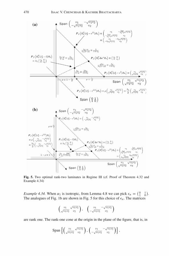
470 Isaac V. Chenchiah & Kaushik Bhattacharya
Fig. 5. Two optimal rank-two laminates in Regime III (cf. Proof of Theorem 4.32 andExample 4.34)
Example 4.34. When α1 is isotropic, from Lemma 4.8 we can pick εn =(
0 11 0
).
The analogues of Fig. 1b are shown in Fig. 5 for this choice of εn . The matrices
(υ1
√υ1υ2√
υ1υ2 υ2
),
(υ1 −√υ1υ2
−√υ1υ2 υ2
)
are rank one. The rank-one cone at the origin in the plane of the figure, that is, in
Span(
υ1√
υ1υ2√υ1υ2 υ2
),(
υ1 −√υ1υ2−√υ1υ2 υ2
),
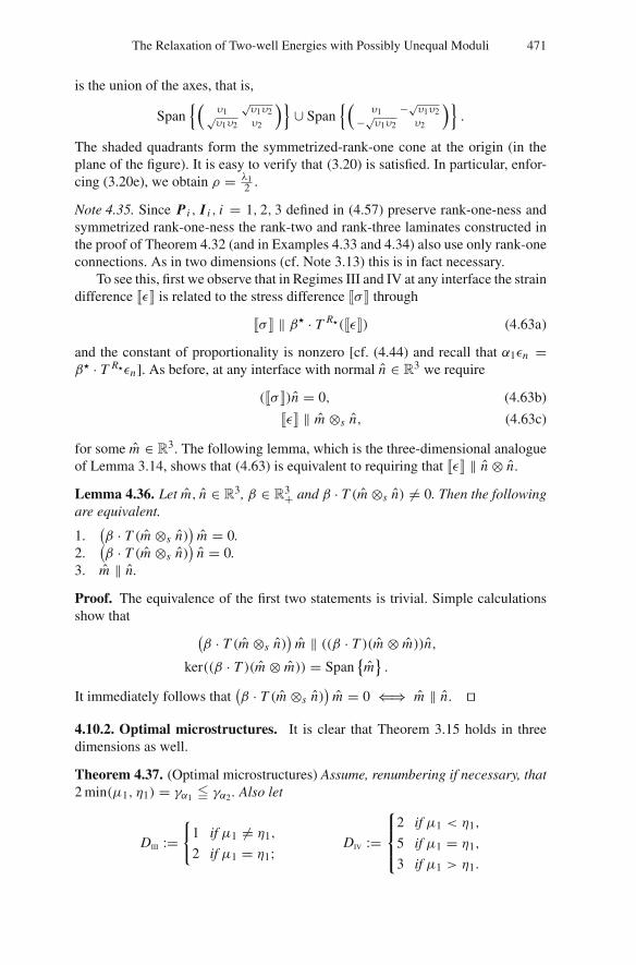
The Relaxation of Two-well Energies with Possibly Unequal Moduli 471
is the union of the axes, that is,
Span(
υ1√
υ1υ2√υ1υ2 υ2
)∪ Span
(υ1 −√υ1υ2
−√υ1υ2 υ2
).
The shaded quadrants form the symmetrized-rank-one cone at the origin (in theplane of the figure). It is easy to verify that (3.20) is satisfied. In particular, enfor-cing (3.20e), we obtain ρ = λ1
2 .
Note 4.35. Since P i , I i , i = 1, 2, 3 defined in (4.57) preserve rank-one-ness andsymmetrized rank-one-ness the rank-two and rank-three laminates constructed inthe proof of Theorem 4.32 (and in Examples 4.33 and 4.34) also use only rank-oneconnections. As in two dimensions (cf. Note 3.13) this is in fact necessary.
To see this, first we observe that in Regimes III and IV at any interface the straindifference ε is related to the stress difference σ through
σ ‖ β · T R (ε) (4.63a)
and the constant of proportionality is nonzero [cf. (4.44) and recall that α1εn =β · T Rεn]. As before, at any interface with normal n ∈ R
3 we require
(σ )n = 0, (4.63b)
ε ‖ m ⊗s n, (4.63c)
for some m ∈ R3. The following lemma, which is the three-dimensional analogue
of Lemma 3.14, shows that (4.63) is equivalent to requiring that ε ‖ n ⊗ n.
Lemma 4.36. Let m, n ∈ R3, β ∈ R
3+ and β · T (m ⊗s n) = 0. Then the followingare equivalent.
1.(β · T (m ⊗s n)
)m = 0.
2.(β · T (m ⊗s n)
)n = 0.
3. m ‖ n.
Proof. The equivalence of the first two statements is trivial. Simple calculationsshow that
(β · T (m ⊗s n)
)m ‖ ((β · T )(m ⊗ m))n,
ker((β · T )(m ⊗ m)) = Spanm.
It immediately follows that(β · T (m ⊗s n)
)m = 0 ⇐⇒ m ‖ n.
4.10.2. Optimal microstructures. It is clear that Theorem 3.15 holds in threedimensions as well.
Theorem 4.37. (Optimal microstructures) Assume, renumbering if necessary, that2 min(µ1, η1) = γα1 γα2 . Also let
DIII :=
1 if µ1 = η1,
2 if µ1 = η1; DIV :=
⎧⎪⎨⎪⎩
2 if µ1 < η1,
5 if µ1 = η1,
3 if µ1 > η1.

472 Isaac V. Chenchiah & Kaushik Bhattacharya
1. In Regime 0 any microstructure is optimal. The optimal strain and stress areconstant.
2. In Regime I the optimal microstructure is either a rank-one laminate, witheither of two possible layering directions, or a microstructure made up of theselaminates. The optimal strain takes the value ε
1 in phase 1 and ε2 in phase 2
while the optimal stress is constant.3. In Regime II the optimal microstructure is unique and is a rank-one laminate.
The optimal strain takes the value ε1 in phase 1 and ε
2 in phase 2.4. In Regime III, no rank-one laminate is optimal. The class of optimal micro-
structures is possibly large (in a sense explained in the proof) and includes atleast two rank-two laminates.In any optimal microstructure, in phase i , i = 1, 2, the strain is confined to anaffine subspace of dimension
dim ker(αi − βIII · T R )
DIII if β < 2 min(µ1, η1),
DIV if β = 2 min(µ1, η1);the sum of the dimensions of the affine subspaces is at most
2 if β < 2 min(µ1, η1),
5 if β < 2 min(µ1, η1).
In particular, if phase i is harder than the other phase (that is, if γαi > γ(α1,α2))
then the strain is εi in that phase.
5. In Regime IV: If µ1 = η1 then there exists an optimal rank-three laminate;otherwise the lower bound is possibly non-optimal. Whenever the bound isoptimal:
(a) No rank-one laminate is optimal.(b) If one phase is harder than the other (that is, if γα2 > γα1) then no
rank-two laminate is optimal.(c) In any optimal microstructure the strain in each phase is confined to an
affine subspace of dimension at most dim ker(αi − γ(α1,α2)T ) DIV; thesum of the dimension of the two affine subspaces is at most 5. Moreover,if one phase is harder than the other then the strain in the harder phaseis constant.
Proof. The proof for the statement pertaining to Regime 0 remains unchangedexcept that (4.44) is used instead of (3.8).
In Regime I, from Corollary 4.28, υ2(∆ε) = 0 and υ1(∆ε)υ3(∆ε) < 0.Thus from Lemma 3.11, we find m ∦ n ∈ R
3 such that ∆ε ‖ m ⊗s n. It followsthat the strain and thus the microstructure is either of two rank-one laminates (withlayering direction m or n) or a microstructure of these laminates. Finally from (4.52)and (4.44), ∆σ = 0: the stress is constant.
In Regime II, from Corollary 4.28, υ2(∆ε) = 0 and υ1(∆ε)υ3(∆ε) = 0 sothat from Lemma 3.11, we find unique (upto scaling) n ∈ R
3 such that ∆ε ‖ n⊗ n.It follows that the strain and thus the microstructure is a unique rank-one laminatewith layering direction n.

The Relaxation of Two-well Energies with Possibly Unequal Moduli 473
Fig. 6. Geometric and schematic diagrams of two rank-two laminates. In the geometric dia-gram solid lines represent strain compatible directions; dotted lines represent strain incom-patible directions; and dashed lines represent directions that need not be strain incompatible
The proof for the statement pertaining to Regime III remains unchanged exceptthat ker(αi−γ(α1,α2)T ) must be replaced as indicated. The inequalities follow fromCorollary 4.15, Lemma 4.17, and Notes 4.3 and 4.30.
We turn to Regime IV. If, when one phase is harder than another, in any opti-mal microstructure the strain is constant in the harder phase, then the non-existenceof optimal rank-two laminates follows from Lemma 4.38 below. The rest of thestatement follows by a reasoning almost identical to that for Regime III; that∑2
i=1 dim ker(αi − γ(α1,α2)T ) 5 follows from Notes 4.3 and 4.30.
Lemma 4.38. Let n 3. Let ε (viewed as a linear operator on Rn) be either
negative- or positive-definite. Then ε and 0 cannot form the two rank-two laminatesschematically shown in Fig. 6. That is, neither the following
∃µ ∈ (0, 1), ∃ε I, ε II ∈ Rn×nsym , µε I + (1− µ)ε II = ε, (4.64a)
∃m I, nI ∈ Rn, ε I = m I ⊗s nI, (4.64b)
∃ρ ∈ (0, 1), ∃m, n ∈ Rn, ρε I − ε II = m ⊗s n (4.64c)

474 Isaac V. Chenchiah & Kaushik Bhattacharya
nor the following
∃µ ∈ (0, 1), ∃ε I, ε II ∈ Rn×nsym , µε I + (1− µ)ε II = ε, (4.65a)
∃m I, nI ∈ Rn, ε I = m I ⊗s nI, (4.65b)
∃m II, nII ∈ Rn, ε II = m II ⊗s nII (4.65c)
can hold.
Proof. Assume on the contrary that either (4.64) or (4.65) holds. Either of these,along with Lemma 3.11 implies: ∃ρ−, ρ+, ρ′−, ρ′+ 0, v−, v+, v′−, v′+ ∈ R
n suchthat
ε = −ρ−v− ⊗ v− + ρ+v+ ⊗ v+ − ρ′−v′− ⊗ v′− + ρ′+v′+ ⊗ v′+Let w+ ∈ Span
v−, v′−
⊥ and w− ∈ Spanv+, v′+
⊥. Then
(εw−) · w− = −ρ−(v+ · w−)2 − ρ′−(v′+ · w−)2 0,
(εw+) · w+ = ρ+(v+ · w+)2 + ρ′+(v′+ · w+)2 0.
This contradicts ε being either negative- or positive-definite.
5. Ancillary results
5.1. The uniform traction problem
We now turn to the uniform traction problem (1.9) for W given by (1.2).From (1.9), in two dimensions,
Wσ
λ (σ ) = inf<χi >=λi
infε∈R2×2
sym
infu|∂Ω=ε·x −
∫
Ω
2∑i=1
χi (x)Wi (ε(x))− 〈σ , ε〉 dx
= infε∈R2×2
sym
inf<χi >=λi
infu|∂Ω=ε·x −
∫
Ω
2∑i=1
χi (x)Wi (ε(x)) dx − 〈σ , ε〉
= infε∈R2×2
sym
maxβ∈[0,γ(α1,α2)]
(Wλ(β, ε)− 〈σ , ε〉)
maxβ∈[0,γ(α1,α2)]
minε∈R2×2
sym
(Wλ(β, ε)− 〈σ , ε〉) . (5.1)
From Lemmas 3.5 and 3.6 and a saddle point theorem [19, Proposition II.2.4,p. 176], (5.1) is in fact an equality. The analogous expression in three dimensions isobtained by replacing [0, γ(α1,α2)] with ∩R∈S0(3) B(α1,α2)(R) and R
2×2sym with R
3×3sym ;
and using Lemmas 4.24 and 4.25 instead of Lemmas 3.5 and 3.6. Note that
Wi (ε)− 〈σ , ε〉 = 1
2〈αi (ε − εT
i ), (ε − εTi )〉 + wi − 〈σ , ε〉
= 1
2〈αiε, ε〉 −
⟨αi (ε
Ti + α−1
i σ ), ε⟩
+ 1
2
⟨αi (ε
Ti + α−1
i σ ), (εTi + α−1
i σ )⟩
+ wi − 〈αiεTi , σ 〉 −
1
2〈α−1
i σ , σ 〉.

The Relaxation of Two-well Energies with Possibly Unequal Moduli 475
Thus with the substitutions
εTi → εT
i + α−1i σ (5.2a)
wi → wi − 〈αiεTi , σ 〉 − 1
2 〈α−1i σ , σ 〉 (5.2b)
W λ(β, ε)− 〈σ , ε〉 can be put in the same form as W λ(β, ε). The lower bounds inSections 3.1.5 and 4.9, the proofs of optimality of the lower bound in Sections 3.2.1and 4.10.1, and remarks on the optimal microstructures in Sections 3.2.2 and 4.10.2remain valid with the appropriate substitutions from (5.2). In particular, this inde-pendently shows that (5.1) is in fact an equality.
Performing the minimization in (3.5b) without the constraint λ1ε1+ λ2ε2 = ε,we obtain, in two dimensions,
α1(ε1 − εT
1)+ βλ2T (ε2 − ε
1) = σ , (5.3a)
α2(ε2 − εT
2)− βλ1T (ε2 − ε
1) = σ . (5.3b)
Similarly, in three dimensions, beginning with (4.12b), we obtain,
α1(ε1 − εT
1)+ λ2β · T R (ε2 − ε
1) = σ , (5.4a)
α2(ε2 − εT
2)− λ1β · T R (ε2 − ε
1) = σ . (5.4b)
Thus, as in (3.8) and (4.44),
∆σ =
βT ∆ε in two dimensions,
β · T R∆ε in three dimensions.
Explicit expressions for the optimal strains and stresses in three dimensions can beobtained by solving (5.4):
ε1 = α−1
1
(I − β · T R
(λ1α−12 + λ2α
−11
))−1
×((
I − β · T Rα−12
)σ − λ2β · T R (∆εT)
)+ εT
1, (5.5a)
ε2 = α−1
2
(I − β · T R
(λ1α−12 + λ2α
−11
))−1
×((
I − β · T Rα−11
)σ + λ1β · T R (∆εT)
)+ εT
2; (5.5b)
and
σ1 =
(I − β · T R
(λ1α−12 + λ2α
−11
))−1
×((
I − β · T Rα−12
)σ − λ2β · T R (∆εT)
), (5.6a)
σ2 =
(I − β · T R
(λ1α−12 + λ2α
−11
))−1
×((
I − β · T Rα−11
)σ + λ1β · T R (∆εT)
), (5.6b)
∆σ =(
I − β · T R
(λ1α−12 + λ2α
−11
))−1β · T R
(∆(α−1)σ +∆εT
).
(5.6c)

476 Isaac V. Chenchiah & Kaushik Bhattacharya
Likewise explicit expressions for the optimal strains and stresses in two dimen-sions can be obtained by solving (5.3). These can also be obtained by formallysubstituting βT for β · T R in (5.5) and (5.6).
5.2. Applications
We discuss the applications of these results to the study of nickel superalloysused in turbine blades and other high-temperature applications in [10]. These mate-rials are made by quenching an off-stoichiometric alloy and spinodal decompositionresults in a two-phase solids (for example, NiAl and Ni3Al, which are both cubicwith different elastic moduli and whose stress-free strains differ by a dilatation)with fixed phase fractions. The microstructure subsequently evolves (by diffusio-nal mass transport) to minimize a combination of interfacial and elastic energies.The late stages of this process are controlled by elastic energy. The microstructurecan further evolve during applications due to the presence of stress. There has beenconsiderable numerical and experimental effort to study this problem. Unfortuna-tely the experiments are difficult and the computations expensive. In particular,the computational expense limits the number of particles, leading to uncertainty asto whether the system is in a metastable state. The results we prove here and theconsequent insights into optimal elastic microstructures provide a benchmark toevaluate the computations. Our results on applied stress also provide insight intothe possible change of microstructure with stress.
Conclusion
In this paper we have studied the relaxation of a two-well energy under fixedphase fractions. From a mathematical standpoint, the methods we use follow clo-sely those that have been used before. However, we find a surprising extensionto three dimensions. The method also provides a lower bound when the moduliare anisotropic; however it is not clear at this point whether this bound is optimal.Similarly, the extension of such methods to more than two wells remains open.
Acknowledgments. This work draws on IVC’s doctoral thesis at the California Institute ofTechnology [13] and was completed and written up during his stay at the Max Planck Institutefor Mathematics in the Sciences, Leipzig. We gratefully acknowledge the partial financialsupport of the the US Army Research Office (MURI grant DAAD19-01-1-0517) and theUS Office of Naval Research (N00014-01-1-0937). We thank Robert Kohn for variousdiscussions and suggestions.
References
1. Avellaneda, M., Cherkaev, A.V., Lurie, K.A., Milton, G.W.: On the effectiveconductivity of polycrystals and a three-dimensional phase interchange inequality.J. Appl. Phys. 63, 4989–5003 (1988)
2. Acerbi, E., Fusco, N.: Semicontinuity problems in the calculus of variations. Arch.Ration. Mech. Anal. 86, 125–145 (1984)
3. Allaire, G., Kohn, R.V.: Explicit optimal bounds on the elastic energy of a two-phasecomposite in two space dimensions. Q. Appl. Math. 12(4), 643–674 (1993)

The Relaxation of Two-well Energies with Possibly Unequal Moduli 477
4. Allaire, G., Kohn, R.V.: Optimal bounds on the effective behavior of a mixture oftwo well-ordered elastic materials. Q. Appl. Math. 12(4), 643–674 (1993)
5. Allaire, G., Kohn, R.V.: Optimal lower bounds on the elastic energy of a compositemade from two non-well-ordered isotropic materials. Q. Appl. Math. 52(2), 311–333(1994)
6. Allaire, G., Lods, V.: Minimizers for a double-well problem with affine boundaryconditions. Proc. R. Soc. Edinb. Sect. A 129, 439–466 (1999)
7. Bhattacharya, K.: Microstructure of martensite: Why it forms and how it gives riseto the shape-memory effect. Oxford Series on Materials Modelling 2. Oxford UniversityPress, Oxford, 2003
8. Birkhoff, G.: Tres observaciones sobre el algebra lineal. Univ. Nac. Tucumán Rev. Ser.A 5, 147–151 (1946)
9. Ball, J.M., James, R.D.: Fine phase mixtures as minimizers of energy. Arch. Ration.Mech. Anal. 100(1), 13–52 (1987)
10. Chenchiah, I.V., Bhattacharya, K.: Equilibrium microstructures in elastic solids(in preparation)
11. Cherkaev, A.V., Gibiansky, L.V.: The exact coupled bounds for effective tensorsof electrical and magnetic properties of two-component two-dimensional composites.Proc. R. Soc. Edinb. Sect. A 122(1–2), 93–125 (1992)
12. Cherkaev, A.V.: Variational methods for structural optimization. Appl. Math. Sci.,vol. 140. Springer, Heidelberg, 2000
13. Chenchiah, I.V.: Energy-minimizing microstructures in multiphase elastic solids,Ph.D. Thesis, California Institute of Technology, January 2004
14. Chipot, M., Kinderlehrer, D.: Equilibrium configurations of crystals. Arch. Ration.Mech. Anal. 103, 237–277 (1988)
15. Chenchiah, I.V., Schlömerkemper, A.: The symmetrized rank-one convex hull ofmonoclinic-I martensite (in preparation)
16. Dacorogna, B.: Quasiconvexity and relaxation of nonconvex problems in the calculusof variations. J. Funct. Anal. 31, 102–118 (1982)
17. Dacorogna, B.: Direct methods in the calculus of variations. Appl. Math. Sci., vol.78. Springer, Heidelberg, 1989
18. Dal Maso, G.: An introduction to Γ -convergence. Birkhäuser, 199319. Ekeland, I., Temam, R.: Convex analysis and variational problems. North-Holland,
Amsterdam, 197620. Firoozye, N.B.: Optimal use of the translation method and relaxations of variational
problems. Commun. Pure Appl. Math. 44, 643–678 (1991)21. Firoozye, N.B., Kohn, R.V.: Geometric parameters and the relaxation of multiwell
energies. In: Microstructure and phase transition (Eds. D. Kinderlehrer, R. James,M. Luskin, and J.L. Ericksen) The IMA Volumes in Mathematics and its Applications54, 85–109. Springer, Heidelberg, 1993
22. Francfort, G.A., Müller, S.: Homogenization and optimal bounds in linear elasticity.Arch. Ration. Mech. Anal. 94(4), 307–334 (1986)
23. Fuchs, M., Seregin, G.A.: A two-dimensional variational model for the equilibriumconfiguration of an incompressible elastic body with a three-well elastic potential.J. Convex Anal. 7, 209–241 (2000)
24. Gibiansky, L.V., Cherkaev, A.V.: Design of composite plates of extremal rigidity.Technical Report 914, Ioffe Physico-technical Institute, Academy of Sciences, USSR,Leningrad, USSR, 1984
25. Gibiansky, L.V., Cherkaev, A.V.: Microstructures of composites of extremal rigidityand exact bounds on the associated energy density. Technical Report 1115, Ioffe Physico-technical Institute, Academy of Sciences, USSR, Leningrad, USSR, 1987
26. Grabovsky, Y., Kohn, R.V.: Anisotrophy of the Vigdergauz microstructure. Trans.ASME J. Appl. Mech. 62(4), 1063–1065 (1995)
27. Grabovsky, Y., Kohn, R.V.: Microstructures minimizing the energy of a two-phaseelastic composite in two space dimensions. I. The confocal ellipse construction. J. Mech.Phys. Solids 43(6), 933–947 (1995)

478 Isaac V. Chenchiah & Kaushik Bhattacharya
28. Grabovsky, Y., Kohn, R.V.: Microstructures minimizing the energy of a two-phaseelastic composite in two space dimensions. II. The Vigdergauz microstructure. J. Mech.Phys. Solids 43(6), 949–972 (1995)
29. Govindjee, S., Mielke, A., Hall, G.J.: The free energy of mixing for n-variant mar-tensitic phase transformations using quasi-convex analysis. J. Mech. Phys. Solids 50(9),1897–1922 (2002)
30. Grabovsky, Y.: Bounds and extremal microstructures for two-component composites:a unified treatment based on the translation method. Proc. R. Soc. Lond. A 452, 919–944(1996)
31. Kohn, R.V.: The relaxation of a double-well energy. Contin. Mech. Thermodyn. 3,193–236 (1991)
32. Kinderlehrer, D., Pedregal, P.: Characterizations of gradient young measures. Arch.Ration. Mech. Anal. 115, 329–365 (1991)
33. Kohn, R.V., Strang, G.: Structural design, optimization, homogenization andrelaxation of variational problems. Macroscopic Properties of Disordered Media (Eds.G. Papanicolaou, R. Burridge, and S. Childress) Lecture Notes in Physics, Vol.154. Springer, Heidelberg, 1982
34. Kohn, R.V., Strang, G.: Explicit relaxation of a variational problem in optimal design.Bull. Am. Math. Soc. 9, 211–214 (1983)
35. Kohn, R.V., Strang, G.: Optimal design and relaxation of variational problems I.Commun. Pure Appl. Math. 39, 1–25 (1986)
36. Kohn, R.V., Strang, G.: Optimal design and relaxation of variational problems II.Commun. Pure Appl. Math. 39, 139–182 (1986)
37. Kohn, R.V., Strang, G.: Optimal design and relaxation of variational problems III.Commun. Pure Appl. Math. 39, 353–357 (1986)
38. Lurie, K.A., Cherkaev, A.V.: G-closure of some particular sets of admissible materialcharacteristics for the problem of bending of thin elastic plates. Technical Report 214,DCAMM, Technical University of Denmark, 1981
39. Lurie, K.A., Cherkaev, A.V.: Exact estimates of conductivity of composites formedby two isotropically conducting media taken in prescribed proportion. Technical Report783, Ioffe Physico-technical Institute, Academy of Sciences, USSR, Leningrad, USSR,1982
40. Lurie, K.A., Cherkaev, A.V.: Exact estimates of the conductivity of a binary mixtureof isotropic materials. Technical Report 894, Ioffe Physico-technical Institute, Academyof Sciences, USSR, Leningrad, USSR, 1982
41. Lurie, K.A., Cherkaev, A.V.: Effective characteristics of composite materials and theoptimal design of structural elements. Uspekhi Mekhaniki [Advances in Mechanics] 9,3–81 (1986)
42. Lurie, K.A., Cherkaev, A.V.: On a certain variational problem of phase equilibrium. In:Material instabilities in continuum mechanics (Proceedings of the Symposium Year heldat Heriot-Watt University, Edinburgh, 1985–1986) (Ed. J.M. Ball) Oxford UniversityPress, Oxford, pp. 257–268, 1988
43. Lu, J.: Extremal microstructures for two isotropic phases with distinct stress-free strainsin two space dimensions. Ph.D. Thesis, New York University, July 1993
44. Marshall, A.W., Ingram, O.: Inequalities: Theory of majorization and its applica-tions. Math. Sci. Eng., Vol. 143, Academic, New York, 1979
45. Milton, G.W.: A brief review of the translation method for bounding effective elastictensors of composites. In: Continuum Models and Discrete Systems (Ed. G.A. Maugin)Longman Scientific and Technical, pp. 60–74, 1990
46. Milton, G.W.: On characterizing the set of possible effective tensors of composites:the variational method and the translation method. Commun. Pure Appl. Math. 43(1),63–125 (1990)
47. Milton, G.W.: The theory of composites. Cambridge Monogr. Appl. Comput. Math.,Vol. 6. Cambridge University Press, Cambridge, 2001

The Relaxation of Two-well Energies with Possibly Unequal Moduli 479
48. Murat, F., Tartar, L.: Calcul des variations et homogénéisation [Calculus of variationsand homogenization]. Collection de la Direction des Études et Recherches d’Électricitéde France 57 (1985), 319–369, Homogenization methods: theory and applications inphysics (Bréau-sans-Nappe, 1983)
49. Murat, F.: A survey on compensated compactness. In: Contributions to Modern Cal-culus of Variations (Ed. L. Cesari) Longman Scientific and Technical, pp. 145–183,1987
50. Pipkin, A.C.: Elastic materials with two preferred states. Q. J. Mech. Appl. Math. 44(1),1–15 (1991)
51. Roytburd, A.L.: Elastic domains and polydomain phases in solids. Phase Transit. 45,1–33 (1993)
52. Seregin, G.A.: The uniqueness of solutions of some variational problems of the theoryof phase equilibrium in solid bodies. J. Math. Sci. 80(6), 2333–2348 (1996)
53. Seregin, G.A.: J 1p-quasiconvexity and variational problems on sets of solenoidal vector
fields. St. Petersburg Math. J. 11(2), 337–373 (2000)54. Strang, G., Kohn, R.V.: Optimal design of a two-way conductor. In: Topics in
Nonsmooth Mechanics (Eds. J.J. Moreau, P.D. Panagiotopoulos, and G. Strang)Birkhäuser, pp. 143–155, 1988
55. Smyshlyaev, V.P., Willis, J.R.: On the relaxation of a three-well energy. Proc. R. Soc.Lond. A 455(1983), 779–814 (1999)
56. Tartar, L.: Compensated compactness and applications to partial differential equations.In: Nonlinear Analysis and Mechanics (Ed. R.J. Knops) Heriot-Watt Symposium, IV,Pitman Publishing, London, pp. 136–212, 1979
57. Tartar, L.: Estimation de coefficients homogénéisés [Estimation of homogenizedcoefficients]. In: Computing methods in applied sciences and engineering: third in-ternational symposium, Versilles, France, December 5–7, 1977 (Eds. R. Glowinski,and J.L. Lions) Springer, Heidelberg, 1979
58. Tartar, L.: Estimation fines des coeffcients homogénéisés [Fine estimations of ho-mogenized coefficients]. In: Ennio de Giorgi Colloquium: Papers Presented at a Col-loquium Held at the H. Poincaré Institute in November 1983 (Ed. P. Kree) PitmanPublishing, London, pp. 168–187, 1985
59. Tartar, L.: An introduction to the homogenization method in optimal design. Optimalshape design. Lectures given at the joint C.I.M./C.I.M.E. Summmer school held atTróia, June 1–6, 1998 (Eds. A. Cellina, and A.A. Ornelas) Springer, Heidelberg, pp.47–156, 2000
60. Vigdergauz, S.B.: Two-dimensional grained composites of extreme rigidity. Trans.ASME J. Appl. Mech. 61(2), 390–394 (1994)
61. Zhang, K.: The structure of rank-one convex quadratic forms on linear elastic strains.Proc. R. Soc. Edinb. Sect. A 133, 213–224 (2003)
Department of Mathematics,University of Bristol,
University Walk,Bristol BS8 1TW, UK.
e-mail: [email protected]
and
Division of Engineering and Applied Science,California Institute of Technology,
Pasadena, CA 91125, USA.e-mail: [email protected]
(Received July 2, 2007 / Accepted July 17, 2007)Published online October 5, 2007 – © Springer-Verlag (2007)