Resonant ultrasound spectroscopic techniques for measurement of the elastic moduli of solids
Upload
khangminh22Category
view
3download
0
mspGeometry & Topology 16 (2012) 2097–2134
MPS degeneration formula for quiver moduliand refined GW/Kronecker correspondence
MARKUS REINEKE
JACOPO STOPPA
THORSTEN WEIST
Motivated by string-theoretic arguments Manschot, Pioline and Sen discovered a newremarkable formula for the Poincaré polynomial of a smooth compact moduli spaceof stable quiver representations which effectively reduces to the abelian case (ie thindimension vectors). We first prove a motivic generalization of this formula, valid forarbitrary quivers, dimension vectors and stabilities. In the case of complete bipartitequivers we use the refined GW/Kronecker correspondence between Euler characteris-tics of quiver moduli and Gromov–Witten invariants to identify the MPS formula forEuler characteristics with a standard degeneration formula in Gromov–Witten theory.Finally we combine the MPS formula with localization techniques, obtaining a newformula for quiver Euler characteristics as a sum over trees, and constructing manyexamples of explicit correspondences between quiver representations and tropicalcurves.
16G20, 14N35, 14T05
1 Introduction
In [13], Manschot, Pioline and Sen derive a remarkable formula for the Poincarépolynomial of a smooth compact moduli space of stable quiver representations (calledMPS degeneration formula in the following), motivated by string-theoretic techniques(more precisely an interpretation relating quiver moduli to multicentered black holesolutions to N D 2 supergravity); see also Manschot [12]. In contrast to the previouslyavailable formulae (see the first author [15]) expressing the Poincaré polynomial explic-itly using (a resolution of) a Harder–Narasimhan type recursion, the MPS degenerationformula expresses it as a summation over Poincaré polynomials of moduli spaces ofseveral other quivers, but only involving very special (thin, ie type one) dimensionvectors (in the language of [13] the index of certain nonabelian quivers without orientedloops can be reduced to the abelian case, by a physical argument which allows tradingBose–Fermi statistics with its classical limit, Maxwell–Boltzmann statistics). One
Published: 8 November 2012 DOI: 10.2140/gt.2012.16.2097

2098 M Reineke, J Stoppa and T Weist
immediate advantage is that the MPS formula specializes to a similar formula for theEuler characteristics, a specialization which is not possible for the Harder–Narasimhanrecursion. Surprisingly, the derivation of the MPS formula in [13, Appendix D] reliescompletely on the resolved Harder–Narasimhan recursion of [15]. One should notehowever that even in the very special cases when Euler characteristics of quiver moduliwere already known, the MPS degeneration formula derives these numbers in a highlynontrivial way.
As a first result of the present work we prove a motivic generalization of the MPSdegeneration formula (Theorem 3.5) which is meaningful for arbitrary quivers, dimen-sion vectors and stabilities. Essentially, the motivic MPS formula expresses the motiveof the quotient stack of the locus of semistable representations by the base changegroup in terms of similar motives for thin dimension vectors of a covering quiver, asan identity in a suitably localized Grothendieck ring of varieties. The proof essentiallyproceeds along the lines of [13, Appendix D], but avoids the resolution formula for theHarder–Narasimhan recursion, and clarifies the role of symmetric function identitiesimplicit in [13]. Specialization of the motivic identity to Poincaré polynomials recoversa generalization of the formula of [13], which is now shown to hold for arbitraryquivers, arbitrary stabilities and coprime dimension vectors. We also derive a dual MPSdegeneration formula (Corollary 3.9), which has the advantage of reducing to a smallercovering quiver, at the expense of having more general dimension vectors.
In Section 4 we take up a second line of investigation, connected with the so-calledGW/Kronecker correspondence based on Gross and Pandharipande [4], Gross, Pand-haripande and Siebert [5] or more precisely its refinement described by the first andthird authors in [17]. A typical result of this type states that the Euler characteristic ofcertain moduli spaces of representations for suitable quivers (eg generalized Kroneckerquivers) can be computed alternatively as a Gromov–Witten invariant (on a weightedprojective plane). In particular this is the case for coprime dimension vectors ofcomplete bipartite quivers, to which we restrict throughout Section 4. Writing downthe MPS degeneration formula for quiver Euler characteristics in this context onenotices a striking similarity with the degeneration formulae which are commonly usedin Gromov–Witten theory, expressing a given Gromov–Witten invariant in terms ofrelative invariants, with tangency conditions along divisors. Theorem 4.1 puts thisintuition on firm ground: at least for coprime dimension vectors of bipartite quivers, theMPS formula is indeed completely equivalent to a much more standard degenerationformula in Gromov–Witten theory. The proof hinges on the equality of certain Eulercharacteristics with tropical counts (Proposition 4.3).
Combining localization techniques with the MPS formula leads to the remarkableconclusion that the Euler characteristic of moduli spaces of stable representations is
Geometry & Topology, Volume 16 (2012)

MPS degeneration formula for quiver moduli 2099
obtained in a purely combinatorial way. Indeed, since the dimension vectors consideredafter applying the MPS formula are of type one, the moduli spaces corresponding totorus fixed representations are just isolated points, so that every such moduli spacecorresponds to a tree with a fixed number of (weighted) vertices. We describe thismethod for bipartite quivers in Section 5 (see especially Corollary 5.3), but it couldeasily be transferred to general quivers without oriented cycles.
In Section 6 we analyse the identity of Euler characteristics with tropical counts foundin Proposition 4.3 from this point of view. On the one hand with a pair of weightvectors .w.k1/;w.k2// we can associate a tropical curve count N tropŒ.w.k1/;w.k2//�,which effectively counts suitable trees. On the other hand with the same weight vectorwe can associate a quiver Euler characteristic �
�M‚l�std.k1;k2/
.N /�, which by the above
argument (MPS plus localization) is also enumerating certain trees.
Thus one would expect to be able to find an explicit way of assigning a quiver lo-calization data to one of our tropical curves, and vice versa. The analogy betweenquiver localization data and tropical curves was already pointed out by the secondauthor in [18], but the MPS formula makes it even stronger. Notice that both tropicalcurves and localization data naturally carry multiplicities: for curves this is the standardtropical multiplicity (recalled in Section 4), while in the case of quiver moduli spaces,a fixed tree can be coloured in different ways to obtain a number of torus fixed points.The first natural guess is that the number of colourings and the multiplicity of somecorresponding tropical curve coincide. Unfortunately this does not work, simply becausein general the numbers of underlying curves and trees (forgetting the multiplicity) aredifferent.
The next more promising attempt is described in Section 6. On both sides there isa way to construct new combinatorial data recursively. On the one hand we showthat our tropical curves of prescribed slope can be obtained by gluing smaller onesin a unique way (at least when the set of prescribed, unbounded incoming edges ischosen generically). This construction also gives a recursive formula for the tropicalcounts; see Theorem 6.4. On the other hand we have a similar construction for quiverlocalization data. Starting with a number of semistable tuples, ie tuples consisting of atree and a dimension vector such that the corresponding moduli space of semistables isnot empty, we can glue them in a similar way to obtain a localization data with greaterdimension vector; see Theorem 6.6.
In many cases these recursive constructions lead to a direct correspondence betweentropical curves and quiver localization data. In Section 6.3 we describe two suchfamilies of examples in detail. We do not know at the moment a method which gives aconcrete geometric correspondence in full generality.
Geometry & Topology, Volume 16 (2012)

2100 M Reineke, J Stoppa and T Weist
Acknowledgements We are grateful to So Okada for drawing our attention to the for-mula of Manschot, Pioline and Sen, and to an anonymous referee for many correctionsand suggestions. This research was partially supported by Trinity College, Cambridge.Part of this work was carried out at the Isaac Newton Institute for Mathematical Sciences,Cambridge and at the Hausdorff Center for Mathematics, Bonn.
2 Recollections and notation
2.1 Quivers
Let Q be a quiver with vertices Q0 and arrows Q1 denoted by ˛W i ! j . We denoteby ƒDZQ0 the free abelian group over Q0 and by ƒCDNQ0 the set of dimensionvectors written as d D
Pi2Q0
dii . Define 0ƒC WD ƒCnf0g. The Euler form is thebilinear form on ƒ given by
hd; ei DX
i2Q0
diei �
X˛W i!j
diej :
We denote its antisymmetrization by fd; eg D hd; ei � he; di. A representation X
of Q of dimension d 2ƒC is given by complex vector spaces Xi of dimension di forevery i 2Q0 and by linear maps X˛W Xi ! Xj for every arrow ˛W i ! j 2Q1 . Avertex q is called a sink (resp. source) if there does not exists an arrow starting at (resp.terminating at) q . A quiver is bipartite if Q0 D I [J with sources I and sinks J . Inthe following, we denote by Q.I/[Q.J / the decomposition into sources and sinks.
For a fixed vertex q 2Q0 we denote by Nq the set of neighbours of q and for V �Q0
define NV WDS
q2V Nq .
For a representation X of the quiver Q we denote by dimX 2ƒC its dimension vector.Moreover we choose a level l W Q0!NC on the set of vertices. Let .‚q/q2Q0
2N jQ0j .Define two linear forms ‚ and � in Hom.ZQ0;Z/ by ‚.d/ D
Pq2Q0
‚qdq and�.d/D
Pq2Q0
l.q/dq , and a slope function �W 0ƒC!Q by
�.d/D‚.d/
�.d/:
For � 2Q we denote by 0ƒC� �0ƒC be the set of dimension vectors of slope � and
define ƒC� D0ƒC� [f0g. This is a subsemigroup of ƒC .
For a representation X of the quiver Q we define �.X / WD �.dimX /. The repre-sentation X is called (semi)stable if the slope (weakly) decreases on proper nonzerosubrepresentations. Fixing a slope function as above, we denote by R‚�sst
d.Q/ the
Geometry & Topology, Volume 16 (2012)

MPS degeneration formula for quiver moduli 2101
set of semistable points and the set of stable points by R‚�std
.Q/ in the affine varietyRd .Q/ WD
L˛Wi!j Hom.Cdi ;Cdj / of representations of dimension d 2NQ0 . On
these varieties, the group Gd DQ
q2Q0GL.Cdq / acts via base change .gq/q.X˛/˛ D
.gj X˛g�1i /˛W i!j , so that the Gd –orbits correspond bijectively to the isomorphism
classes of representations of dimension vector d . There exist moduli spaces M‚�std
.Q/
(resp. M‚�sstd
.Q/) of stable (resp. semistable) representations parameterizing isomor-phism classes of stable (resp. polystable) representations, obtained as suitable GITquotients by Gd ; see [7]. If Q is acyclic and M‚�st
d.Q/ is nonempty, it is a smooth
irreducible variety of dimension 1� hd; di. Moreover it is projective if semistabilityand stability coincide.
Fixing a quiver Q and a dimension vector d 2NQ0 such that there exists a (semi)stablerepresentation for this tuple we call this tuple (semi)stable.
2.2 The tropical vertex
We briefly review the definition of one of the tools we shall use, the tropical vertexgroup, following that in [5, Section 0].
We fix nonnegative integers l1; l2 � 1 and define R as the formal power series ringRDQŒŒs1; : : : ; sl1
; t1; : : : ; tl2��, with maximal ideal m. Let B be the R–algebra
B DQŒx˙1;y˙1�ŒŒs1; : : : ; sl1; t1; : : : ; tl2
��DQŒx˙1;y˙1� bR
(a suitable completion of the tensor product). For .a; b/ 2 Z2 and a series
f 2 1CxaybQŒxayb � bm
we consider the R–linear automorphism of B defined by
�.a;b/;f W
(x 7! xf �b;
y 7! yf a:
Notice that these automorphisms preserve the symplectic form dx=x ^ dy=y .
Definition 2.1 The tropical vertex group VR � AutR.B/ is the completion withrespect to m of the subgroup of AutR.B/ generated by all elements �.a;b/;f as above.
We recall that by a result of Kontsevich and Soibelman [8] (see also [5, Theorem 1.3])there exists a unique infinite ordered product factorization in VR of the form
�.1;0/;Q
k.1Cskx/�.0;1/;Q
l .1Ctl y/ D
Yb=a decreasing
�.a;b/;f.a;b/ ;
the product ranging over all coprime pairs .a; b/ 2N2 .
Geometry & Topology, Volume 16 (2012)

2102 M Reineke, J Stoppa and T Weist
3 Motivic MPS formula
3.1 Some symmetric function identities
We start with some preliminaries on symmetric functions following that in Macdon-ald [11]. Partitions � of n are written �` n. With a partition �` n we associate a mul-tiplicity vector m�.�/, where mi.�/ is the multiplicity of the part i in �. Converselywith a vector m� D .ml 2 N/l�1 we associate the partition �.m�/D .1m12m2 � � � /.This induces a bijection between partitions of n and the set of multiplicity vectors m�such that
Pl lml D n. In this case, we also write m� ` n.
Denote by PQ the ring of symmetric functions with rational coefficients in variables xi
for i � 1. We consider the so-called principal specialization map p W PQ ! Q.q/given by xi 7! qi�1 for all i � 1.
Denote by en DP
i1<���<inxi1� � �xin
the n–th elementary symmetric function andby pn D
Pi xn
i the n–th power sum function. We consider the following generatingfunctions in PQŒŒt ��:
E.t/DXn�0
entn; P .t/DXn�1
pntn�1:
Then P .�t/D .d=dtE.t//=E.t/ [11, I,(2.10 0 )]. Defining e� D e�1e�2� � � , and p�
similarly, for an arbitrary partition �, both sets .e�/� , respectively .p�/� , are basesof PQ [11, I, (2.4), (2.12)]. We consider the base change between these bases.
We have
en D
X�`n
"�z�1� p�;
where "� D .�1/j�j�l.�/ and z� DQ
l ml.�/!lml .�/ [11, I,(2.14 0 )].
Lemma 3.1 (1) The previous identity can be rewritten as
en D
Xm�`n
Yl
1
ml !
.�1/l�1
l
!ml
p�.m�/:
(2) Conversely, we have
pn D .�1/n�1nX�`n
.�1/l.�/�1
l.�/
l.�/!Qlml.�/!
e�:
Geometry & Topology, Volume 16 (2012)

MPS degeneration formula for quiver moduli 2103
Proof The first identity follows from the definitions. For the second identity we uselog.1Cx/D
Pk�1..�1/k�1=k/xk to calculate
log E.t/D log.1CXn�1
entn/
D
Xk�1
.�1/k�1
k
�Xn�1
entn�k
D
Xk�1
.�1/k�1
k
Xn1;:::;nk�1
en1: : : enk
tn1C���Cnk
D
Xk�1
.�1/k�1
k
X�Wl.�/Dk
k!Ql ml.�/!
e�t j�j
D
Xn�1
X�`n
.�1/l.�/�1
l.�/
l.�/!Ql ml.�/!
e�tn;
where we have used the fact that the number of rearrangements of a partition � isl.�/!=
Ql ml.�/!. Differentiating and using P .�t/ D d=dt.log E.t//, the lemma
follows.
For partitions �, � of n, denote by L�� the number of functions f from f1; : : : ; l.�/gto N such that �i D
Pj Wf .j/Di �j . Then e� D
P� "�z�1
� L��p� [11, I, (6.11)].
Lemma 3.2 We have
e� DX
m�`n
�Xm��
Yl�1
ml !Qj m
j
l!
�Yl�1
1
ml !
�.�1/l�1
l
�ml
p�.m�/;
where the inner sum ranges over all tuples .mj
l/j ;l�1 such that
Pj m
j
lDml for all
l � 1 andP
l lmj
lD �j for all j � 1.
Proof Assume �D .1m12m2 � � � /. To a function f as above, we associate the sets
Ij
lD fi 2 f1; : : : ;mlg j f .m1C � � �Cml�1C i/D j g
for j ; l � 1. Then, for all l � 1, the set f1; : : : ;mlg is the disjoint union of the Ij
l.
Defining mj
las the cardinality of I
j
l, we thus have
Pj m
j
lDml for all l � 1, andP
l lmj
lD �j by definition of f . This establishes a bijection between the set of
functions f which is counted by L�� and the set of pairs .m��; I�� / which is counted
by the inner sum.
Geometry & Topology, Volume 16 (2012)

2104 M Reineke, J Stoppa and T Weist
Under the principal specialization map, en maps to q.n2/=..1�q/.1�q2/ � � � .1�qn//,
and pn maps to 1=.1� qn/ [11, I, 2 Example 4]. Using the first identity of Lemma 3.1,this yields the identity
q.n2/
.1� q/ � � � .1� qn/D
Xm�`n
Yl�1
1
ml !
�.�1/l�1
l.1� ql/
�ml
:
Replacing q by q�1 and multiplying by an appropriate power of q , this is equivalentto the following.
Lemma 3.3 We have
q.n2/
.qn� 1/ � � � .qn� qn�1/D
Xm�`n
Yl�1
1
ml !
�.�1/l�1
l Œl �q
�ml 1
.q� 1/P
l ml;
where Œl �q D .ql � 1/=.q� 1/.
3.2 The motivic MPS formula
We assume throughout that an arbitrary finite quiver Q with level function l W Q0!NC
and a stability ‚ for Q are given and we fix a vertex i 2Q0 .
We introduce a new (levelled) quiver yQ by replacing the vertex i by vertices ik;l fork; l � 1, thus yQ0 DQ0 n fig[ fik;l j k; l � 1g, with vertex ik;l being of level l � l.i/
(the level is unchanged on all vertices j 6D i ). The arrows in yQ are given by thefollowing rules:
� all arrows ˛W j ! k in Q which are not incident with i induce an arrow˛W j ! k in yQ;
� all arrows ˛W i! j (resp. ˛W j! i ) in Q for j 6D i induce arrows pW ik;l! j
(resp. pW j ! ik;l ) for k; l � 1 and p D 1; : : : ; l in yQ;
� all loops ˛W i! i in Q induce arrows p;qW ik;l ! ik0;l 0 for k; l; k 0; l 0 � 1 andp D 1; : : : ; l , q D 1; : : : ; l 0 in yQ.
Given a dimension vector d for Q and a multiplicity vector m� ` di (ie,P
l lml D di )as above, we define a dimension vector yd.m�/ for yQ by yd.m�/j D dj for j 6D i
in Q0 and
yd.m�/ik;lD
(1 k �ml ;
0 k >ml :
Geometry & Topology, Volume 16 (2012)

MPS degeneration formula for quiver moduli 2105
We haveG yd.m�/ '
Yj 6Di
GLdj .C/�GP
l mlm ;
where GmDC� denotes the multiplicative group of the field C . We choose an arbitrarybasis of Cdi indexed by vectors vk;l;p for l � 1, 1� k �ml and 1� p � l (this ispossible since
Pl lml D di ). Then the group G yd.m�/
embeds into Gd by letting thei.k;l/–component of G yd.m�/
, which is isomorphic to Gm , scale the vectors vk;l;p forp D 1; : : : ; l simultaneously, for all l � 1, 1� k �ml .
We define a stability y‚ for yQ by y‚j D‚j for all j 6D i in Q0 and y‚ik;lD l �‚i for
all k; l � 1. The associated slope function is denoted by y�. The following lemma iseasily verified by working through the definitions of yQ, yd and y�.
Lemma 3.4 Via the above embedding, we have a G yd.m�/–equivariant isomorphismbetween Rd .Q/ and R yd.m�/.
yQ/. Furthermore, we have y�. yd.m�//D �.d/.
Our motivic version of the MPS formula is an identity in a suitably localized Grothen-dieck ring of varieties; we refer to Bridgeland [1] for an introduction to this topicsuitable for our purposes. Let K0.Var =C/ be the free abelian group generated byrepresentatives ŒX � of all isomorphism classes of complex varieties X , modulo therelation ŒX �D ŒA�C ŒU � if A is isomorphic to a closed subvariety of X , with comple-ment isomorphic to U . Multiplication is given by ŒX � � ŒY �D ŒX �Y �. Denote by Lthe class of the affine line. We work in the localization
KD .K0.Var =C/˝Q/ŒL�1; .Ln� 1/�1
j n� 1�:
Theorem 3.5 For arbitrary Q, d , ‚ and i as above, the following identity holdsin K :
L.di2/
hR
sst.Q/d
iŒGd �
D
Xm�`di
Yl�1
1
ml !
�.�1/l�1
l ŒP l�1�
�ml
hRsstyd.m�/
. yQ/i
ŒG yd.m�/�:
Proof We start the proof by translating the identity of Lemma 3.3 into the ring K .We note the following identities:
ŒGLn.C/�Dn�1YiD0
.Ln�Li/; ŒGm�D L� 1; ŒPn�1�D .Ln
� 1/=.L� 1/D Œn�L:
Then the identity of Lemma 3.3 translates into
L.n2/
ŒGLn.C/�D
Xm�`n
Yl�1
1
ml !
�.�1/l�1
l ŒP l�1�
�ml 1hGP
l mlm
i :Geometry & Topology, Volume 16 (2012)

2106 M Reineke, J Stoppa and T Weist
Replacing n by di , multiplying by ŒRd .Q/�=Q
j 6Di ŒGLdj .C/� and using the aboveidentifications and Lemma 3.4, this yields the MPS formula for trivial stability ‚D 0,
L.di2/ ŒRd .Q/�
ŒGd �D
Xm�`di
Yl�1
1
ml !
�.�1/l�1
l ŒP l�1�
�ml
hR yd.m�/
. yQ/i
�G yd.m�/
� :
Now we make use of the Harder–Narasimhan stratification of Rd .Q/ constructedin [15]: We fix a decomposition d D d1C� � �Cd s into nonzero dimension vectors with�.d1/>� � �>�.d s/, which we call a HN type for d , denoted by d�D .d1; : : : ; d s/ˆd .Denote by Rd�
d.Q/ the set of all representations M 2Rd .Q/ such that in the Harder–
Narasimhan filtration 0DM 0 �M 1 � � � � �M s DM of M , the dimension vectorof M i=M i�1 equals d i for all i D 1; : : : ; s . By [15], we have
Rd�
d .Q/'Gd �Pd� Vd� ;
where Pd� is a parabolic subgroup of Gd with Levi isomorphic toQs
kD1 Gdk , and Vd�
is a vector bundle overQs
kD1Rsstdk .Q/ of rank rd�D
Pk<l
Pp!q d l
pdkq . This implies
the following identity in K :
ŒRd .Q/�DX
d�ˆd
ŒGd �Pd� Vd� �D
Xd�ˆd
ŒGd �
ŒPd� �Lrd�
hYk
Rsstdk .Q/
i:
Using ŒPd� �D LP
k<l
Pi d l
idk
i
Qk ŒGdk � and dividing by ŒGd � yields a motivic version
of the Harder–Narasimhan recursion [15] determining ŒRsstd.Q/�=ŒGd � recursively:
ŒRd .Q/�
ŒGd �D
Xd�ˆd
L�P
k<l hdl ;dki
sYkD1
hRsst
dk .Q/i
�Gdk
� :
We now derive the MPS formula by induction over the dimension vector d . Theinduction starts with d of total dimension one. In this case, all points are semistable,and the formula is already proved. In the general case, we compute L.
di2/ŒRd .Q/�=ŒGd �
in two ways. By applying first the MPS formula for trivial stability, then the HNrecursion, we get
L.di2/ ŒRd .Q/�
ŒGd�D
Xm�`di
Yl�1
1
ml !
�.�1/l�1
l ŒP l�1�
�ml Xyd�ˆyd.m�/
L�P
k<l hyd l ; ydki
sYkD1
�Rsstydk. yQ/
�ŒG ydk �
:
In choosing a HN type yd� ˆ yd.m�/, we choose a HN type d� ˆ d , together withset partitions f1; : : : ;mlg D
Sk Ik
lfor all l � 1 such that for mk
lD jIk
lj, we haveP
l lmklD dk
i for all k D 1; : : : ; s ; Lemma 3.4 ensures that the respective slopeconditions are compatible. Note that Rsst
ydk. yQ/ and G ydk only depend on d� and on
Geometry & Topology, Volume 16 (2012)

MPS degeneration formula for quiver moduli 2107
the mkl
, but not on the actual parts Ikl
; in fact, ydk Dcdk.mk
�/. A short calculationusing the definition of yQ shows that
hd l ; dki � h yd l ; ydk
i D d li dk
i :
Thus the above sum can be rewritten as
Xd�ˆd
X.mk�`dk
i/k
Yl�1
�Pk mk
l
�!Q
k mkl!
Yl�1
1Pk mk
l/!
�.�1/l�1
l ŒP l�1�
�Pk mk
l
�L�P
k<l hdl ;dkiC
Pk<l d l
idk
i
sYkD1
hRsstcdk .mk
�/
. yQ/i
hGcdk .mk
�/
i
DL.di2/X
d�ˆd
L�P
k<l hdl ;dki
sYkD1
L�.dk
i2/X
m�`dki
Yl�1
1
ml !
�.�1/l�1
l ŒP l�1�
�ml
hRsstcdk .mk
�/
. yQ/i
hGcdk .mk
�/
i :
On the other hand, L.di2/ŒRd .Q/�=ŒGd � evaluates to
L.di2/ ŒRd .Q/�
ŒGd �D L.
di2/X
d�ˆd
L�P
k<l hdl ;dki
sYkD1
�Rsst
dk .Q/�
ŒGdk �
by the HN recursion. Using the inductive hypothesis, all summands of the last twosums corresponding to HN types of length at least two coincide, thus the summandscorresponding to the trivial HN type d coincide; this yields the MPS formula for d .
Sometimes it might be convenient to rewrite the MPS formula in terms of partitionsinstead of multiplicity vectors.
Corollary 3.6 We have
L.di2/
�Rsst
d.Q/
�ŒGd �
D
X�`di
"�z�1�
1Qj ŒP
�j�1�
�Rsstyd.m�.�//
. yQ/�
�G yd.m�.�//
� :
There is a well-defined ring homomorphism � W K ! Q.t/ mapping the class ofa smooth projective variety X to its Poincaré polynomial in singular cohomologyP .X; t/ D
Pi dim H i.X;Q/t i . In the case where the dimension vector d is ‚–
coprime, that is, �.e/ 6D �.d/ for all nonzero dimension vectors e < d , the moduli
Geometry & Topology, Volume 16 (2012)

2108 M Reineke, J Stoppa and T Weist
space M sstd.Q/DRsst
d.Q/=Gd .C/ is a smooth variety, and we have
P .M sstd .Q/; t/D .t2
� 1/ ��.ŒRsstd .Q/�=ŒGd �/I
see Engel and the first author [2, Theorem 2.5]. Specialization of the motivic MPSformula to this case yields a formula for its Poincaré polynomial, and in particular forits Euler characteristic.
Corollary 3.7 If d is ‚–coprime, we have
tdi .di�1/P .M sstd .Q/; t/D
Xm�`di
Yl�1
1
ml !
.�1/l�1
l Œl �t2
!ml
P .M sstyd.m�/
. yQ/; t/;
�.M sstd .Q//D
Xm�`di
Yl�1
1
ml !
.�1/l�1
l2
!ml
�.M sstyd.m�/
. yQ//:
3.3 Dual MPS formula
We define a quiver LQ as the “relative level one part” of yQ, and therefore we haveLQ0 DQ0 n fig[ fik j k � 1g, and the arrows in LQ are given by the following rules:
� all arrows ˛W j ! k in Q which are not incident with i induce an arrow˛W j ! k in LQ;
� all arrows ˛W i ! j (resp. ˛W j ! i ) in Q for j 6D i induce arrows ˛W ik ! j
(resp. ˛W j ! ik ) for k � 1 in LQ;
� all loops ˛W i ! i in Q induce arrows ˛W ik ! ik0 for k; k 0 � 1 in LQ.
Given a dimension vector d for Q and a partition � ` di , we define a dimensionvector Ld.�/ for LQ by Ld.�/j D dj for j 6D i in Q0 and Ld.�/ik
D �k for k � 1.
Application of the MPS formula to all vertices ik for k � 1 of LQ yields
LPj .�j2/
hRsstLd.�/. LQ/
i�G Ld.�/
� D X.mj�`�j /j
Yj�1
Yl�1
1
mj
l!
�.�1/l�1
l ŒP l�1�
�mj
l
hRsstyd.Pj m
j�/. yQ/
i�G yd.
Pj m
j�/
�D
Xm�`di
�Xm��
Yl�1
ml !Qj m
j
l!
�Yl�1
1
ml !
�.�1/l�1
l ŒP l�1�
�ml
hRsstyd.m�/
. yQ/i
�G yd.m�/
� ;
where the inner sum runs over all tuples .mj
l/j ;l�1 such that ml D
Pj m
j
lfor all l
and �j DP
l lmj
lfor all j . Comparison with Lemma 3.2 yields the following.
Geometry & Topology, Volume 16 (2012)

MPS degeneration formula for quiver moduli 2109
Proposition 3.8 There is a well-defined map PQ!K of Q–vector spaces such that
e� 7! LPj .�j2/
hRsstLd.�/
. LQ/i
�G Ld.�/
� ; p� 7!Yj
1
ŒP�j�1��
hRsstyd.m�.�//
. yQ/i
�G yd.m�.�//
� :
It might be interesting to ask whether the images of other bases of the ring of symmet-ric functions (monomial symmetric functions, complete symmetric functions, Schurfunctions,: : :) have a natural interpretation in terms of motives of quiver moduli.
We can now map the second identity of Lemma 3.1 to K to get the following dualversion of the MPS formula.
Corollary 3.9 For given d , denote by yd0 the dimension vector for yQ with a singleentry 1 at vertex i1;di
. Then
1
ŒPdi�1��
hRsstyd0. yQ/
i�G yd0. yQ/
� D .�1/di�1di
X�`di
.�1/l.�/�1 .l.�/� 1/!Ql ml.�/!
LPj .�j2/
hRsstLd.�/
. LQ/i
�G Ld.�/
� :
4 The MPS formula as a degeneration formula in Gromov–Witten theory
In the rest of the paper for every bipartite quiver Q we consider the linear form ‚2NQ0
defined by ‚i D 1 for every i 2Q.I/ and ‚j D 0 for every j 2Q.J /. Additionallyfixing a level l W Q! NC , we define the linear form ‚l by .‚l/q D l.q/‚q andconsider the slope � D ‚l=� where � is defined as in Section 2. Note that for thetrivial level structure, ie l.q/D 1 for every q 2Q0 , we have ‚l D‚ and � D dim.
In this section we specialize the MPS formula to Euler characteristics, and at the sametime we restrict to a special class of quivers. These are the complete bipartite quiversK.l1; l2/ of [17, Section 5], defined by the vertices
K.l1; l2/0 D fi1; : : : ; il1g[ fj1; : : : ; jl2
g
and the arrows
K.l1; l2/1 D f˛k;l W ik ! jl j k 2 f1; : : : l1g; l 2 f1; : : : l2gg:
A dimension vector for K.l1; l2/ is uniquely determined by a pair of ordered partitions
.P1;P2/D
� l1XiD1
p1i ;
l2XjD1
p2j
�:
Geometry & Topology, Volume 16 (2012)

2110 M Reineke, J Stoppa and T Weist
We assume throughout this section that the sizes jP1j, jP2j are coprime. In particular‚–stability and ‚–semistability are equivalent for the dimensions vector we consider.We fix the trivial level structure given by l.q/D 1 for all q 2K.l1; l2/0 . We denote by
M‚�st.P1;P2/DM‚�st.P1;P2/
.K.l1; l2//
the moduli space of stable representations with respect to this choice.
The MPS formula in this context can be expressed uniformly for all l1; l2 and alldimension vectors by introducing an infinite quiver N with a suitable level structure.We define its vertices by
N0 D fi.w;m/ j .w;m/ 2N2g[ fj.w;m/ j .w;m/ 2N2
g;
and the arrows by
N1 D f˛1; : : : ; ˛w�w0 W i.w;m/! j.w0;m0/; 8w;w0;m;m0 2Ng:
The level function is given by
l.q.w;m//D w; 8q 2 fi; j g;m 2N
and we fix the linear form ‚l . A refinement of .P1;P2/ is a pair of sets of integers
.k1; k2/D .fk1wig; fk
2wj g/
such that for i D 1; : : : ; l1 and j D 1; : : : ; l2 we have
p1i D
Xw
wk1wi ; p2j D
Xw
wk2wj :
We will denote refinements by .k1; k2/` .P1;P2/. The number of entries of weight win ki is defined by
mw.ki/D
liXjD1
kiwj :
A fixed refinement .k1; k2/ induces a dimension vector d.k1; k2/ for N by setting
d.k1; k2/q.w;m/ D
(1 for mD 1; : : : ;mw.k
p/;
0 for m>mw.kp/;
Geometry & Topology, Volume 16 (2012)

MPS degeneration formula for quiver moduli 2111
for q 2 fi; j g, and pD 1; 2 for q D i; j . With this notation in place, the MPS formulaat the level of Euler characteristics can be expressed by
(1)
�.M‚�st.P1;P2//
D
X.k1;k2/`.P1;P2/
��M‚l�std.k1;k2/
.N /� 2Y
iD1
liYjD1
Yw
.�1/kiw;j
.w�1/
kiw;j !w2ki
w;j
:
This follows from applying Corollary 3.7 repeatedly to all the vertices of K.l1; l2/.Note in particular M
‚l�std.k1;k2/
.N / DM‚l�sstd.k1;k2/
.N / (since stability and semistabilitycoincide for our choice of dimension vectors on K.l1; l2/, and each application ofCorollary 3.7 preserves this property).
The ordered partition .P1;P2/ also encodes an a priori very different kind of data,namely the Gromov–Witten invariant N Œ.P1;P2/� [5, Section 0.4]. Roughly speakingthis is a virtual count of rational curves in the weighted projective plane P .jP1j; jP2j; 1/
which pass through lj specified distinct points lying on the distinguished toric divi-sor Dj for j D 1; 2. We require that these points are not fixed by the torus action,that the multiplicities at the points are specified by Pj , and that the curve touchesthe remaining toric divisor Dout at some point which is also not fixed by the torus.The refined GW/Kronecker correspondence of [17] (based on [5; 4]) leads to a ratherstriking consequence [17, Corollary 9.1]:
N Œ.P1;P2/�D �.M‚�st.P1;P2//:
The powerful degeneration formula of Gromov–Witten theory in Ionel and Parker [6],Li [10] and Li and Ruan [9] allows one to express N Œ.P1;P2/� in terms of certain relativeGromov–Witten invariants, enumerating rational curves with tangency conditions, aswe now briefly discuss. Following [5, Section 2.3] we define a weight vector wi as asequence of integers .wi1; : : : ; witi
/ with
0<wi1 � wi2 � � � � � witi:
The automorphism group Aut.wi/ of a weight vector wi is the subset of the symmetricgroup on ti letters which stabilizes wi . A pair of weight vectors .w1;w2/ encodes arelative Gromov–Witten invariant N relŒ.w1;w2/�, virtually enumerating rational curvesin P .jw1j; jw2j; 1/ which are tangent to Di at specified points (not fixed by the torus),with order of tangency specified by wi . The rigorous construction of these invariantsis carried out in [5, Section 4.4]. Let us now fix weight vectors wi with jwi j D jPi j
for i D 1; 2. A set partition I� of wi is a decomposition of the index set
I1[ � � � [ IliD f1; : : : ; tig
Geometry & Topology, Volume 16 (2012)

2112 M Reineke, J Stoppa and T Weist
into li disjoint, possibly empty parts. We say that the set partition I� is compatiblewith Pi (or simply compatible) if for all j we have
pij D
Xr2Ij
wir :
The relevant degeneration formula involves the ramification factors
RPi jwiD
XI�
tiYjD1
.�1/wij�1
w2ij
;
where we are summing over all compatible set partitions I� . Notice that in fact thesummands are independent of I� , so this equals
Qti
jD1..�1/wij�1=w2
ij / times thenumber of set partitions. Then [5, Proposition 5.3] yields the equality
(2) N Œ.P1;P2/�DX
.w1;w2/
N relŒ.w1;w2/�
2YiD1
Qti
jD1wij
jAut.wi/jRPi jwi
:
We come to the central claim of this section.
Theorem 4.1 Let P1;P2 be coprime. Then N Œ.P1;P2/�D �.M‚�st.P1;P2//, and
the MPS formula (1) for the Euler characteristics of quiver representations is equivalentto the Gromov–Witten degeneration formula (2).
The equality N Œ.P1;P2/� D �.M‚�st.P1;P2// is the coprime case of the refinedGW/Kronecker correspondence. The rest of this section is devoted to a proof of thestatement about the MPS formula. As a first step, to simplify the comparison, we willrewrite the degeneration formula (2) as a sum over pairs of refinements .k1; k2/ ratherthan pairs of weight vectors .w1;w2/. Notice that a fixed refinement ki induces aweight vector w.ki/D .wi1; : : : ; witi
/ of length ti DPw mw.k
i/, by
wij D w for all j D
w�1XrD1
mr .ki/C 1; : : : ;
wXrD1
mr .ki/:
Of course the weight vector w.ki/ only depends on ki through fmw.ki/gw . However
we wish to think of w.ki/ as coming with a distinguished set partition I�.ki/: the
segment of weight w entries in w.ki/ is partitioned into li consecutive chunks of sizek1w1; � � � ; k1
wli, and we declare the indices for the j –th chunk to lie in Ij .k
i/.
Geometry & Topology, Volume 16 (2012)
MPS degeneration formula for quiver moduli 2113
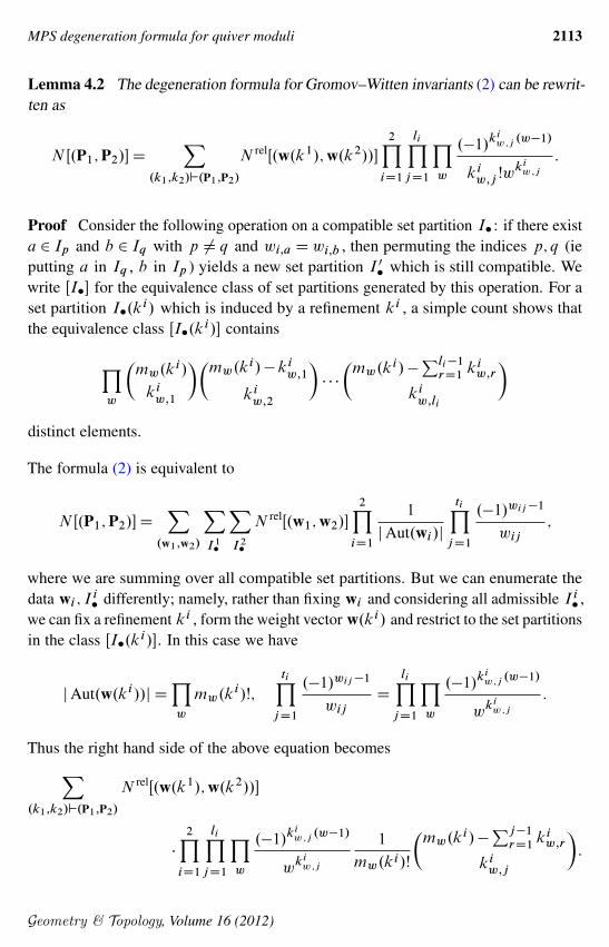
Lemma 4.2 The degeneration formula for Gromov–Witten invariants (2) can be rewrit-ten as
N Œ.P1;P2/�DX
.k1;k2/`.P1;P2/
N relŒ.w.k1/;w.k2//�
2YiD1
liYjD1
Yw
.�1/kiw;j
.w�1/
kiw;j !wki
w;j
:
Proof Consider the following operation on a compatible set partition I� : if there exista 2 Ip and b 2 Iq with p ¤ q and wi;a D wi;b , then permuting the indices p; q (ieputting a in Iq , b in Ip ) yields a new set partition I 0� which is still compatible. Wewrite ŒI�� for the equivalence class of set partitions generated by this operation. For aset partition I�.k
i/ which is induced by a refinement ki , a simple count shows thatthe equivalence class ŒI�.ki/� contains
Yw
�mw.k
i/
kiw;1
��mw.k
i/� kiw;1
kiw;2
�� � �
�mw.k
i/�Pli�1
rD1kiw;r
kiw;li
�distinct elements.
The formula (2) is equivalent to
N Œ.P1;P2/�DX
.w1;w2/
XI 1�
XI 2�
N relŒ.w1;w2/�
2YiD1
1
jAut.wi/j
tiYjD1
.�1/wij�1
wij;
where we are summing over all compatible set partitions. But we can enumerate thedata wi ; I
i� differently; namely, rather than fixing wi and considering all admissible I i
� ,we can fix a refinement ki , form the weight vector w.ki/ and restrict to the set partitionsin the class ŒI�.ki/�. In this case we have
jAut.w.ki//j DYw
mw.ki/!;
tiYjD1
.�1/wij�1
wijD
liYjD1
Yw
.�1/kiw;j
.w�1/
wkiw;j
:
Thus the right hand side of the above equation becomesX.k1;k2/`.P1;P2/
N relŒ.w.k1/;w.k2//�
�
2YiD1
liYjD1
Yw
.�1/kiw;j
.w�1/
wkiw;j
1
mw.ki/!
�mw.k
i/�Pj�1
rD1kiw;r
kiw;j
�:
Geometry & Topology, Volume 16 (2012)

2114 M Reineke, J Stoppa and T Weist
The result follows from the simple calculation
1
mw.ki/!
�mw.k
i/
kiw;1
��mw.k
i/� kiw;1
kiw;2
�� � �
�mw.k
i/�Pli�1
rD1kiw;r
kiw;li
�D
liYjD1
1
kiw;j !
:
Comparing the degeneration formula as rewritten in Lemma 4.2 with the MPS for-mula (1), we see that proving Theorem 4.1 is equivalent to establishing the identity
(3) ��M‚l�std.k1;k2/
.N /�DN relŒ.w.k1/;w.k2//�
2YiD1
liYjD1
Yw
wkiw;j :
In fact the right hand side of (3) has a geometric interpretation as a suitable tropicalcount. Here we will confine ourselves to the basic notions we need to state thisequivalence, following those in [5, Section 2.1].
Let x� be a weighted, connected tree with only 1–valent and 3–valent vertices, thoughtof as a compact topological space in the canonical way. We remove the 1–valentvertices to form the graph � . The noncompact edges are called unbounded edges.We denote the induced weight function on the edges of � by w� . A parameterizedrational tropical curve in R2 is a proper map hW �!R2 such that the following hold:
� the restriction of h to an edge is an embedding whose image is contained in anaffine line of rational slope;
� a balancing condition holds at the vertices. Namely, denoting by mi the primitiveintegral vector emanating from the image of a vertex h.V / in the direction ofan edge h.Ei/, we require
3XiD1
w�.Ei/mi D 0;
where we are summing over all the edges which are adjacent to V .
A rational tropical curve is the equivalence class of a rational parameterized tropicalcurve under parameterizations which respect w� . The multiplicity at a vertex V isdefined as
MultV .h/D w�.E1/w�.E2/jm1 ^m2j;
where by the balancing condition we can choose E1;E2 to be any two edges adjacentto V . The total multiplicity of h is then defined as
Mult.h/DYV
MultV .h/:
Geometry & Topology, Volume 16 (2012)

MPS degeneration formula for quiver moduli 2115
Let us write e1; e2 for the standard unit vectors of R2 . A pair of weight vectors.w1;w2/ encodes a tropical invariant, counting rational tropical curves h which satisfythe following conditions:
� the unbounded edges of � are Eij for 1 � i � 2; 1 � j � ti , plus a single“outgoing” edge Eout . We require that h.Eij / is contained in a line eij CRei
for some prescribed vectors eij , and its unbounded direction is �ei ;� w�.Eij /D wij .
Notice that the balancing condition implies that h.Eout/ lies on an affine line withdirection .jw1j; jw2j/. The set of such tropical curves h is finite (at least for a genericchoice of eij ), and it follows from the general theory (see eg Gathmann and Markwig [3],Mikhalkin [14]) that when we count curves h taking into account the multiplicityMult.h/ we get an integer N tropŒ.w1;w2/� which is independent on the (generic)choice of displacements eij . The comparison result that we need, relating the Gromov–Witten invariants which appear in the degeneration formula to tropical counts, is thenobtained (see [5, Theorems 3.4 and 4.4]):
(4) N tropŒ.w1;w2/�DN relŒ.w1;w2/�
2YiD1
tiYjD1
wij :
Thanks to the equivalence (4), Theorem 4.1 follows from the following result.
Proposition 4.3 We have equality of Euler characteristics and tropical counts, ie
(5) N tropŒ.w.k1/;w.k2//�D ��M‚l�std.k1;k2/
.N /�:
We will now give a proof of this equality, using the scattering diagrams of [5] and thefirst author [16, Theorem 2.1]. Notice however that in the special case when all the partsof the refinement .k1; k2/ equal 1 the corresponding subquiver of N is isomorphicto K.l1; l2/, and (5) is an immediate consequence of the refined GW/Kroneckercorrespondence.
Let us denote by Q � N the subquiver spanned by the support of the dimensionvector d.k1; k2/. This is a complete bipartite quiver with t1 sources and t2 sinks. Foreach w , Q contains mw.k
1/ sources (respectively mw.k2/ sinks) with level w . We
introduce the ring
(6) RDCŒŒxj.w0;m0/ ;yi.w;m/ j w;w0;m;m0 2N��
with a Poisson bracket defined by
fxj.w0;m0/ ;yi.w;m/g D fj.w0;m0/; i.w;m/gxj.w0;m0/ �yi.w;m/ D ww0xj.w0;m0/ �yi.w;m/ :
Geometry & Topology, Volume 16 (2012)

2116 M Reineke, J Stoppa and T Weist
We define Poisson automorphisms of R by
Tj.w;m/.xj.w0;m0//D xj.w0;m0/ ;
Tj.w;m/.yi.w0;m0//D yi.w0;m0/
�1Cxj.w;m/
�ww0;
and similarly
Ti.w;m/.xj.w0;m0//D xj.w0;m0/
�1Cyi.w;m/
��ww0;
Ti.w;m/.yi.w0;m0//D yi.w0;m0/ :
These are a version of the Poisson automorphisms introduced by Kontsevich andSoibelman (see eg [8, Section 10]). According to [16, Theorem 2.1], the product ofoperators Y
j.w;m/2Q0
Tj.w;m/ �
Yi.w0;m0/2Q0
Ti.w0;m0/
can be expressed alternatively as a slope-ordered productQ �2QT� , acting eg on the y
variables asT�.yi.w;m//D yi.w;m/
Yj.w0;m0/2Q0
.Q�;j.w0;m0//ww0 ;
where we have denoted by Q�;j.w0;m0/ the generating series of Euler characteristicsfor moduli spaces of semistable framed representations of Q with slope � and a1–dimensional framing at j.w0;m0/ . Recall however we are only interested in theEuler characteristic �
�M‚l�std.k1;k2/
.N /�, ie for representations with dimension 1 at
each vertex. In this case semistable framed representations coincide with ordinarysemistable representations, and so with ordinary stable representations. Moreover thefirst nontrivial monomial (after 1) appearing in each series Q�.d.k1;k2//;j.w0;m0/
is
(7)Y
j.w0;m0/2Q0
xj.w0;m0/ �
Yi.w;m/2Q0
yi.w;m/ ;
since the presence of a lower order term would imply the existence of a subrepresentationof a representation of dimension vector d.k1; k2/ with equal slope. So we find thatthe monomial (7) appears in the series y�1
i.w;m/T�.d.k1;k2//.yi.w;m// with coefficient
given by
(8) wXw0
w0mw0.k2/�
�M‚l�std.k1;k2/
.N /�:
On the other hand we can compute the coefficient of (7) in a different way, by settingup an appropriate scattering diagram in the sense of [5, Definition 1.2]. To this end we
Geometry & Topology, Volume 16 (2012)

MPS degeneration formula for quiver moduli 2117
need to identify Ti.w;m/ ;Tj.w0;m0/ with operators acting on the subalgebra
R0 �CŒx˙1;y˙1�ŒŒ�j.w;m/ ; �i.w0;m0/ j w;w0;m;m0 2N��
generated by �j.w0;m0/x˙1; �i.w0;m0/y
˙1 . We embed R�R0 by
xj.w;m/ 7!��j.w;m/x
�w;
yi.w0;m0/ 7!��i.w0;m0/y
�w0;(9)
and define operators on R0 by
Tj.w;m/.�j.w0;m0/x/D �j.w0;m0/x;
Tj.w;m/.�i.w0;m0/y/D �i.w0;m0/y�1C
��j.w;m/x
�w�w;
and respectively
Ti.w;m/.�j.w0;m0/x/D �j.w0;m0/x�1C
��i.w;m/y
�w��w;
Ti.w;m/.�i.w0;m0/y/D �i.w0;m0/y:
Then clearly these new Ti.w;m/ ;Tj.w0;m0/ restrict to the old ones on R � R0 , andfollowing the notation of [5, Section 0.1], we can make the identification
Tj.w;m/ D �.1;0/;.1C.�j.w;m/x/w/w
with a standard element of the tropical vertex group VR0 , and similarly
Ti.w;m/ D �.0;1/;.1C.�i.w;m/y/w/w :
We are led to consider the saturated scattering diagram S (in the sense of [5, Section 1])for the product
(10)Y
j.w;m/2Q0
�.1;0/;.1C.�j.w;m/x/w/w �
Yi.w0;m0/2Q0
�.0;1/;.1C.�i.w0;m0/y/w0/w0 :
We only recall briefly that according to the general theory one starts with a genericconfiguration of horizontal lines dj.w;m/ in R2 (respectively vertical lines di.w0;m0/ ),with attached weight functions .1C .�j.w;m/x/
w/w (and .1C .�i.w0;m0/y/w0/w
0
respec-tively). With a generic path W Œ0; 1�!R2 one can associate an element � 2 VR0 [5,Section 1.2]. The (essentially unique) saturated scattering diagram S is obtained byadding rays (with attached certain elements of R0 , which we will call weight functions)to the original configuration of lines so that for each closed loop the group element � becomes trivial (if at all defined); see [5, Theorem 1.4]. The crucial point for us is that,
Geometry & Topology, Volume 16 (2012)
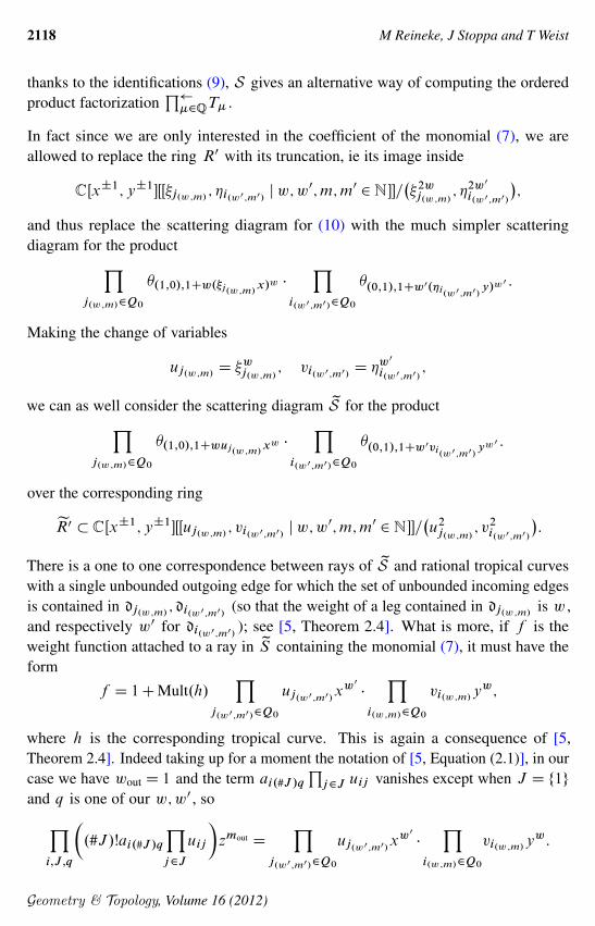
2118 M Reineke, J Stoppa and T Weist
thanks to the identifications (9), S gives an alternative way of computing the orderedproduct factorization
Q �2QT� .
In fact since we are only interested in the coefficient of the monomial (7), we areallowed to replace the ring R0 with its truncation, ie its image inside
CŒx˙1;y˙1�ŒŒ�j.w;m/ ; �i.w0;m0/ j w;w0;m;m0 2N��=
��2wj.w;m/
; �2w0
i.w0;m0/
�;
and thus replace the scattering diagram for (10) with the much simpler scatteringdiagram for the productY
j.w;m/2Q0
�.1;0/;1Cw.�j.w;m/x/w �
Yi.w0;m0/2Q0
�.0;1/;1Cw0.�i.w0;m0/y/w0 :
Making the change of variables
uj.w;m/ D �wj.w;m/
; vi.w0;m0/ D �w0
i.w0;m0/;
we can as well consider the scattering diagram zS for the productYj.w;m/2Q0
�.1;0/;1Cwuj.w;m/xw �
Yi.w0;m0/2Q0
�.0;1/;1Cw0vi.w0;m0/yw0 :
over the corresponding ring
eR0 �CŒx˙1;y˙1�ŒŒuj.w;m/ ; vi.w0;m0/ j w;w0;m;m0 2N��=
�u2
j.w;m/; v2
i.w0;m0/
�:
There is a one to one correspondence between rays of zS and rational tropical curveswith a single unbounded outgoing edge for which the set of unbounded incoming edgesis contained in dj.w;m/ ; di.w0;m0/ (so that the weight of a leg contained in dj.w;m/ is w ,and respectively w0 for di.w0;m0/ ); see [5, Theorem 2.4]. What is more, if f is theweight function attached to a ray in zS containing the monomial (7), it must have theform
f D 1CMult.h/Y
j.w0;m0/2Q0
uj.w0;m0/xw0�
Yi.w;m/2Q0
vi.w;m/yw;
where h is the corresponding tropical curve. This is again a consequence of [5,Theorem 2.4]. Indeed taking up for a moment the notation of [5, Equation (2.1)], in ourcase we have wout D 1 and the term ai.#J /q
Qj2J uij vanishes except when J D f1g
and q is one of our w;w0 , soYi;J ;q
�.#J /!ai.#J /q
Yj2J
uij
�zmout D
Yj.w0;m0/2Q0
uj.w0;m0/xw0�
Yi.w;m/2Q0
vi.w;m/yw:
Geometry & Topology, Volume 16 (2012)

MPS degeneration formula for quiver moduli 2119
Notice that h is one of the set of tropical curves which correspond to the pair of weightvectors .w.k1/;w.k2//. Therefore the product of all weight functions f attached torays of zS containing the monomial (7) equals
ˆD 1CN tropŒ.w.k1/;w.k2//�Y
j.w0;m0/2Q0
uj.w0;m0/xw0�
Yi.w;m/2Q0
vi.w;m/yw :
Thanks to the choice of level structure on N (ie l.i.w;m//D w; l.j.w0;m0//D w0 ), the
slope �.d.k1; k2// equals the slope in R2 of each ray underlying one of the weightfunctions f . By the uniqueness of ordered product factorizations in V zR0 , we havethat the coefficient of the monomial (7) in the series y�1
i.w;m/T�.yi.w;m// is equal to the
nontrivial coefficient of the action of �.P2;P1/;ˆ on vi.w;m/yw . Namely we have
�.P2;P1/;ˆ.vi.w;m/yw/D �.P2;P1/;ˆ.�
wi.w;m/
yw/D �wi.w;m/yw�ˆw
Pw0 w
0mw0 .k2/;
which when expanded contains as the only nontrivial coefficient
(11) wXw0
w0mw0.k2/N tropŒ.w.k1/;w.k2//�:
Our claim (5) follows by comparing (8), (11).
Remark 4.4 One can show (arguing by induction on jpij j) that the MPS formula andthe coprime case of the refined GW/Kronecker correspondence imply the equality (5).
5 Euler characteristic via counting trees
In this section we continue the investigation of the MPS formula 4. Combined withlocalization techniques it implies that to calculate the Euler characteristic of modulispaces it suffices to count trees. For a quiver Q we denote by zQ its universal covergiven by the vertex set
zQ0 D f.q; w/ j q 2Q0; w 2W .Q/g
and the arrow set
zQ1 D f˛.q;w/W .q; w/! .q0; w˛/ j ˛W q! q0 2Q1g:
Here W .Q/ denotes the set of words of Q, ie the set generated by the arrows and theirformal inverses; see the third author [19, Section 3.4] for a precise definition. Everyw0 2W .Q/ defines a bijection w0W zQ0!
zQ0 , .q; w/ 7! .q; ww0/. This induces anequivalence on the set of dimension vectors N zQ0 .
Geometry & Topology, Volume 16 (2012)

2120 M Reineke, J Stoppa and T Weist
Let T WD .C�/jQ1j be the jQ1j–dimensional torus. It acts on Rd .Q/ via
t � .X˛/˛2Q1WD .t˛ �X˛/˛2Q1
;
which induces a torus action on M‚�std
.Q/ because it commutes with the action ofGd D
Qi2Q0
Gldi.C/ via base change. Denote by M‚�st
d.Q/T the torus fixed points.
Recall the localization theorem [19, Corollary 3.14].
Theorem 5.1 We have
��M‚�st
d .Q/�D �.M‚�st
d .Q/T /DXzd
��Mz‚�stzd
. zQ/�;
where zd ranges over all equivalence classes being compatible with d , and the slopefunction considered on zQ is the one induced by the slope function fixed on Q, ie wedefine the corresponding linear form z‚ by z‚.q;w/D‚q for all q 2Q0 and w 2W .Q/.
We call a tuple .Q; zd/ consisting of a finite subquiver Q of zQ and a dimension vectorzd 2 NQ0 with zdq ¤ 0 for every q 2 NQ0 localization data if M
z‚�stzd
.Q/ ¤ ∅.Then every stable representation of Q of dimension zd defines a torus fixed point ofM‚�st
d.Q/ where zd is compatible with d . If we do not want to specify the dimension
vector of a torus fixed point of a moduli space M‚�std
.Q/, we sometimes speak abouttorus fixed points of the quiver Q.
Even if the following machinery applies in a more general setting, we concentrate onthe quivers K.l1; l2/ and N and the linear forms ‚ and ‚l as introduced in Section 4.Recall that the moduli spaces derived from N and K.l1; l2/ are connected by theMPS-formula. Fixing a dimension vector of K.l1; l2/, the corresponding dimensionvectors of N have only entries consisting of zeroes and ones.
We fix a partition .P1;P2/ and a refinement .k1; k2/ which as in Section 4 in-duces a dimension vector of N denoted by d.k1; k2/. We consider the quiverN .k1; k2/ WD supp.d.k1; k2// consisting of the full subquiver of N with verticessupp.d.k1; k2//0Dfq 2N0 j d.k
1; k2/q ¤ 0g. Every localization data .T; d/ definesa subtree T of zN , ie a subquiver without cycles with at most one arrow between eachtwo vertices. Since we have d.k1; k2/q D 1 for all q 2N .k1; k2/0 , the vertices of T
are in one-to-one correspondence to the vertices of N .k1; k2/. Indeed, in generalevery vertex of the quiver of a localization data corresponds to a vertex of the originalquiver. But since d.k1; k2/q D 1 this correspondence is one-to-one. Thus T alreadydefines a subtree of N .
Geometry & Topology, Volume 16 (2012)

MPS degeneration formula for quiver moduli 2121
Fixing a subtree T of N and a dimension vector ˇ 2NT0 , we call the tuple .d; e/defined by
d WDX
i2T .I /
ˇil.i/; e WDX
j2T .J /
j l.j /;
the dimension type of ˇ .
Remark 5.2 Let T be a subtree of N and ˇ 2 NT0 . If we have ˇq D 1 forall q 2 T0 , since T is a tree, there exists only one stable representation X up toisomorphism. In particular, we can assume that X˛ D 1 for all ˛ 2 T1 . Moreover, wehave M
z‚l�stˇ
.T /D fptg.
Since, in general, every connected tree with n vertices has n� 1 edges, then we havethat every connected subtree of N .k1; k2/, having the same vertices as N .k1; k2/,has
P2iD1
Pw
Pli
jD1kiw;j � 1 arrows. Let T .k1; k2/ be the set of connected subtrees
of N .k1; k2/. Then for a tree T 2 T .k1; k2/ and a subset I 0 ¨ T .I/ we define�I 0.T /D
Pj2NI0
l.j /. Recall that NI 0 WDS
q2I 0 Nq and that Nq was defined as theset of neighbours of q . Then .T; ˇ/ with ˇq D 1 for all q 2 T0 is a localization dataif and only if �I 0.T / > .e=d/jI
0j for all ∅ ¤ I 0 ¨ T .I/, where jI 0j WDP
i2I 0 l.i/.Moreover since we have that �
�Mz‚l�stˇ
.T /�D 1 it suffices to count such subtrees in
order to calculate the Euler characteristic. More precisely defining
w.T /D
(1 if �I 0.T / >
edjI 0j for all ∅¤ I 0 ¨ T .I/;
0 otherwise;
we obtain the following.
Corollary 5.3 We have ��M‚l�std.k1;k2/
.N /�DP
T2T .k1;k2/w.T /.
Every localization .T; ˇ/ data defines a colouring cW T1!N1 of the arrows of T1 .Notice that fixing a tree T 2 T .k1; k2/ with w.T / D 1 we can also forget aboutthe colouring (but fix the level structure), and ask for the number of different embed-dings of T into N .k1; k2/ in order to determine the Euler characteristic. Each suchembedding again induces a colouring of the arrows.
6 A connection between localization data and tropical curves
In this section we connect a recursive construction of tropical curves to a similarconstruction of localization data. This gives a possible recipe to obtain a direct corre-spondence between rational tropical curves and quiver localization data, as suggested
Geometry & Topology, Volume 16 (2012)

2122 M Reineke, J Stoppa and T Weist
by the equality of the respective counts found in Proposition 4.3. We work out thiscorrespondence in some examples in the following sections. In every case this construc-tion can be used to compute the number of tropical curves and, therefore, the Eulercharacteristic of the corresponding moduli spaces recursively.
6.1 Recursive construction of curves
The aim of this section is to construct tropical curves recursively. Therefore we firstshow that by choosing the lines h.Eij / in a suitable (but generic) way we can removethe last edge E2;t2
, effectively decomposing one of our tropical curves into smallerones. Moreover this construction works in the other direction as well. In particular weshow that every tropical curve is obtained by gluing smaller ones.
In the following we denote the coordinates of a vector x 2 R2 by .x1;x2/. LethW � ! R2 be a connected parameterized rational tropical curve with unboundededges Eij of weights wij and Eout for 1 � i � 2 and 1 � j � ti . Let h.Eij / becontained in the line eij CRei . For every unbounded edge E there exists a uniquevertex V such that E is adjacent to V . We denote this vertex by V .E/. For everycompact edge E there exist two vertices V1.E/ and V2.E/ which are adjacent to E .For a fixed tropical curve hW �!R2 we have h.V1.E//D h.V2.E//C�w�.E/m forsome � 2R where m denotes the primitive vector emanating from h.V1.E// in thedirection of h.V2.E//. Let E ¤Eij for 1� i � 2 and 1� j � ti . Since the weightsare chosen to be positive natural numbers, the balancing condition inductively impliesthat m1;m2 > 0. In particular, we can assume h.V2.E//
1 > h.V1.E//1 . Moreover,
for the slope w�.E/m2=w�.E/m1 of h.E/, which is abbreviated to �.E/ in the
following, we have �.E/ > 0. Note that, for the following calculations it is importantthat the weight of E is taken into account.
By the methods of [3; 5, Proposition 2.7], we have N tropŒ.w1;w2/� does not dependon the (general) choice of the vectors eij . So we always assume e1
2;j> e1
2;j�1and
e21;j> e2
1;j�1.
Let F1; : : : ;Fn be a complete list of compact edges such that there exists a point.x1
i ;x2i / 2 h.Fi/ satisfying e1
2;t2�1< x1
i < e12;t2
and, moreover, h.V2.Fi//1 � e1
2;t2.
Moreover, let h.Fi/ � Rf1;i C f2;i DW fi and denote by si;j 2 R2 , 1 � i < j � n,the intersection point of fi and fj if there exists one. Again, by the methods of [3]we may assume that s1
i;j < e12;t2
(by moving e2;t2). This means that all intersection
points of any two affine lines fi and fj lie on the left hand side of the line e2;t2CRe2 .
Clearly we can order the edges Fi by slope, ie �.Fi/� �.Fj / for i < j . Moreover,we can assume that h.V2.Fi//
2 < h.V2.Fj //2 if i < j and �.Fi/D�.Fj /. Note that
this already implies that h.V2.Fi//k < h.V2.Fj //
k if i < j where k D 1; 2.
Geometry & Topology, Volume 16 (2012)

MPS degeneration formula for quiver moduli 2123
In the following, we say that a tropical curve satisfying these conditions is slope ordered.Then we have the following lemma.
Lemma 6.1 We can choose the lines h.Eij / in such a way that every tropical curve isslope ordered.
In the following we assume we have chosen the lines in this way and we also call suchan arrangement of lines slope ordered. Let �.Fi/D ei=di with ei ; di 2N and di > 0.Clearly the vertex V1 WDV .E2;t2
/ must be adjacent to F1 and G0 WDE2;t2. Thus there
exists a third edge G1 , which is also adjacent to V1 with �.G1/D .e1Cw2;t2/=d1
such that .e1 Cw2;t2/=d1 > e2=d2 D �.F2/. Note that the last inequality follows
because hW �!R2 was assumed to be connected and slope ordered: there has to existan edge Fk which is adjacent to V2.G1/ and since h is slope ordered, it follows thatk D 2 and �.G1/� �.F2/.
With this notation in place, by applying the same argument repeatedly, we inductivelyget that there exists a vertex Vk which is adjacent to Gk�1 , Fk and Gk . We alsoget that F1; : : : ;Fn;G1; : : : ;Gn is a complete list of edges E such that there exists apoint .x1;x2/2 h.E/ with x1� e1
2;t2. Since the edges F1; : : : ;Fn;G1; : : : ;Gn�1 are
compact, we obtain Gn DEout . Thus the corresponding graph looks like the following(where we have to think of the right hand side being above the left hand side):
����
F1
E2;t2
������
��
��
���
F2
����7
��
���
��
G1
G2
. . . . . .Fn
Gn�1
Gn DEout
In summary, we obtain the following lemma.
Lemma 6.2 Let hW �!R2 be a slope ordered tropical curve. Then there exist edgesG1; : : : ;Gn and vertices V1; : : : ;Vn such that Vk is adjacent to Fk , Gk�1 and Gk
Geometry & Topology, Volume 16 (2012)

2124 M Reineke, J Stoppa and T Weist
and such that
�.Gk/Dw2;t2
CPk
iD1 eiPkiD1 di
>ekC1
dkC1
for k D 1; : : : ; n� 1. Moreover we have Gn DEout .
Remark 6.3 Note that for w2;t2D 1 these conditions are part of the gluing conditions
of [19, Section 4.3]. The only missing property is the fourth one.
Fixing .d; e/ 2 N2 and w 2 N we call a tuple .di ; ei/iD1;:::;n of pairs of naturalnumbers satisfying
(12) wC
nXiD1
ei D e;
nXiD1
di D d;ei
di�
eiC1
diC1
;wC
PkiD1 eiPk
iD1 di
>ekC1
dkC1
;
a w–admissible decomposition of .d; e/. Obviously every slope ordered tropical curvedefines a wt2
–admissible decomposition of .d; e/.
We call a set partition I� as introduced in Section 4 proper if all parts are not empty.Fix a weight vector .w1;w2/ with d D
Pt1
jD1w1j and e D
Pt2
jD1w2j satisfying
wij � wi.jC1/ . Every w2;t2–admissible decomposition of .d; e/ defines two ordered
partitions of d and e�w2;t2respectively. Recall the definition of compatibility intro-
duced in Section 4. Then every tuple of set partitions of f1; : : : ; t1g and f1; : : : ; t2�1g
respectively which is compatible with .di ; ei/iD1;:::;n , defines n tuples of weightvectors .w.i/1;w.i/2/ with di D
Pj w.i/1j and ei D
Pj w.i/2j .
Let � be the tropical curve which only consists of the unbound edge E2;t2and let
h0W �!R2 its embedding where we assume h0.E2;t2/� e2;t2
CRe2 . Moreover, lethi W �i!R2 , i D 1; : : : ; n, be tropical curves with unbounded edges corresponding tothe weights .w.i/1;w.i/2/ and with outgoing edges Ei;out . We may assume for allintersection points sij of the affine lines fi DRf1;i Cf2;i containing hi.Ei;out/ wehave s1
ij < e12;t2
. We may also assume f 11;i�0 and, moreover, �.Ei;out/��.EiC1;out/.
Therefore these curves recursively define a tropical curve hW �!R2 in the followingway: h1.E1;out/ and h0.E2;t2
/ have a unique intersection point s1 . Thus to � weadd a vertex V1 with h.V1/D s1 and an unbounded edge F1 with adjacent vertex V1
setting h.F1/D fh.V1/CR�0..d1; e1/C .0; w2;t2//g. Additionally we bind E1;out
by V1 and so we modify its image in an appropriate way. In general, since .di ; ei/iis a wt2
–admissible decomposition, there exists an intersection point sjC1 of h.Fj /
and hjC1.EjC1;out/. Thus we add a vertex VjC1 with h.VjC1/ D sjC1 and anunbounded edge FjC1 with adjacent vertex VjC1 setting h.FjC1/ D
˚h.VjC1/C
Geometry & Topology, Volume 16 (2012)

MPS degeneration formula for quiver moduli 2125
R�0�PjC1
iD1.di ; ei/C .0; w2;t2
/�
. As above we bind EjC1;out and Fj by VjC1 andwe again modify their images appropriately.
Considering all the wt2–admissible decompositions and all the sets of tropical curves
(embedded in the chosen line arrangement) as above at once we can assume thats1ij < e1
2;t2for all possible intersection points. So we have the following theorem.
Theorem 6.4
N trop.w1;w2/
D
X.di ;ei /i
XI�
nYiD1
N tropŒw.i/1;w.i/2�ˇ nYkD1
�ek
k�1XiD1
di � dk
� k�1XiD1
ei Cw2;t2
��ˇ;
where we first sum over all wt2–admissible decompositions of .d; e/ and then over
all proper set partitions I� which are compatible with the partitions .d; e�w2;t2/D�Pn
iD1 di ;Pn
iD1 ei
�.
Proof We just need to determine the multiplicities of the vertices where the originalcurves are glued. For their multiplicities we get
MultVk.h/D
ˇˇ Pk�1
iD1 di dkPk�1iD1 ei Cw2;t2
ek
!ˇˇ
for k D 1; : : : ; n.
6.2 Recursive construction of localization data
On the quiver side we have a similar construction: Recall the definition of semistablepairs introduced in Section 2 and let .Q1; ˇ1/; : : : ; .Qn; ˇn/ be semistable consistingof disjoint subquivers of N and a dimension vector ˇi 2N.Qi/0 of type one (namely.ˇi/q D 1 for all q 2 .Qi/0 ), of dimension type .di ; ei/, ie we haveX
q2Qi .I /
l.q/D di ;X
q2Qi .J /
l.q/D ei ;
and M‚l�sstˇi
.Qi/ ¤ ∅. Moreover let the tuple .di ; ei/iD1;:::;n be a w–admissibledecomposition of .d; e/ where e WD wC
PniD1ei and d WD
PniD1di . Consider the
tuple .Q; ˇ/ consisting of the quiver Q defined by the vertices Q0DSn
jD1.Qj /0[fqg
with l.q/Dw and the arrows Q1DSn
jD1.Qj /1[f˛W i! q j i 2Qj .I/; j D 1; : : : ; ng
and the dimension vector ˇ obtained by setting ˇq D 1. Clearly we can understand Qas a subquiver of N . On Q we consider the stability induced by the one on N .
Geometry & Topology, Volume 16 (2012)

2126 M Reineke, J Stoppa and T Weist
Lemma 6.5 Let .di;ei/i be a w–admissible decomposition of .d;e/ and I ¨f1; : : : ;ng.Then we have
(1)P
i2I ei=P
i2I di � en=dn ;
(2) .wCP
i2I ei/=P
i2I di > .wCPn
iD1 ei/=Pn
iD1 di .
Proof Let Imax 2 I the largest number in I . We proceed by induction on n. If n 2 I ,the first inequality is equivalent toP
i2Infng eiPi2Infng di
�en
dn:
By induction hypothesis we havePi2Infng eiPi2Infng di
�e.Infng/max
d.Infng/max
�en�1
dn�1
�en
dn:
If n 62 I , we can apply the induction hypothesis.
In order to prove the second inequality, we first assume that n 62 I . Then we proceedby induction on n. It is easy to check that
wCPn�1
iD1 eiPn�1iD1 di
>wC
PniD1 eiPn
iD1 di
,wC
Pn�1iD1 eiPn�1
iD1 di
>en
dn:
Moreover by the induction hypothesis we have
wCP
i2I eiPi2I di
>wC
Pn�1iD1 eiPn�1
iD1 di
:
If n 2 I , then by the first statement we have that .P
i2I 0 ei/=.P
i2I 0 di/ � en=dn ,where I 0 WD f1; : : : ; ngnI . Since the second inequality of the statement is equivalent to
wCP
i2I eiPi2I di
>
Pi2I 0 eiPi2I 0 di
;
it suffices to show thatwC
Pi2I eiP
i2I di>
en
dn:
Since this is equivalent to
wCP
i2Infng eiPi2Infng di
>en
dn;
we can apply the induction hypothesis using .wCPn�1
iD1 ei/=Pn�1
iD1 di > en=dn .
Geometry & Topology, Volume 16 (2012)

MPS degeneration formula for quiver moduli 2127
Theorem 6.6 The tuple .Q; ˇ/ is stable. In particular, every torus fixed point ofMz‚l�stˇ
.Q/ defines a torus fixed point of M‚l�stˇ
.N / of dimension type .d; e/.
Proof Since we have ˇqD 1 for all q 2Q0 , we consider the representation X definedby X˛ D 1 for all ˛ 2Q1 . Let Ik �Qk.I/ be arbitrary subsets with tk WD
Pi2Ik
l.i/
and let sk WDP
j2NIkl.j / such that Ik ¤Qk.I/ for at least one k and Ik ¤∅ for
at least one k . We have to show
wC
nXiD1
si >wC
PniD1 eiPn
iD1 di
� nXiD1
ti
�:
Since the tuples we started with are semistable, we have
wC
nXiD1
si � wC
nXiD1
ei
diti :
Thus it suffices to show
w >
nXjD1
tjdj .wC
PniD1 ei/� ej
�PniD1 di
�dj
�PniD1 di
� :
But, since
kj WDdj
�wC
PniD1 ei
�� ej
�PniD1 di
�dj
�PniD1 di
� > 0,wC
Pi2Inj eiP
i2Inj di>
ej
dj;
by the w–admissibility of the decomposition and the second inequality of the precedinglemma, it follows that kj > 0 for all 1� j � n. In particular, from wD
PnjD1dj kj it
follows that w >Pn
jD1tj kj if tj < dj for at least one j .
Remark 6.7
� It would be interesting to know if every localization data can be obtained by thisconstruction. We conjecture that this is true, but it seems more difficult to provethis than the tropical analogue.
� The main goal we have in mind is to construct a direct correspondence betweentropical curves and localization data. Given a tropical curve of slope .d; e/, saywith multiplicity m, there should be m localization data of dimension type .d; e/corresponding to this tropical curve. We see the two recursive constructionswhich we have described as a step in this direction: they give us a way to gluesmaller objects in order to build more complicated ones. Moreover on both sideswe have the same numerical conditions. So starting with smaller objects for
Geometry & Topology, Volume 16 (2012)

2128 M Reineke, J Stoppa and T Weist
which a correspondence is known this should give a correspondence betweenthe glued objects.
� In some cases such a correspondence is obtained immediately: assume that wehave decomposed .d; e/D .ds; es/C .d
0; e0/ as in [19, Section 4.3]. Then wehave jdse � desj D 1. In particular, the preceding methods give a one-to-onecorrespondence in this case. Indeed, we can understand the vertex correspondingto the last leg as the gluing vertex.
� Unfortunately, the construction does not always give a canonical correspondence.Consider the data
1
1
@@
��1 1oo // 1
1
@@
��1
with a fixed colouring. Gluing an additional sink, we get the data
1
1
1
HH
@@
��1 1
TT
oo // 1
1
>>
@@
��1
which has six subdata defining localization data, obtained by deleting two arrowsin an appropriate way.But on the tropical curve side we only get three new curves in this way becausewe glue a curve of slope .3; 4/ and one of slope .0; 1/. This already givesthe impression that we should not consider all possible localization data of theconstructed stable tuples (with cycles as above).
Geometry & Topology, Volume 16 (2012)

MPS degeneration formula for quiver moduli 2129
� Notice that Theorem 6.4 also gives a recursive formula for the Euler characteristicof moduli spaces. Indeed, even for w–admissible decompositions of .d; e/involving nonprimitive vectors .di ; ei/ one ends up with primitive vectors afterfinitely many steps.
6.3 Examples and discussion
In this section we discuss two examples in which we obtain a direct correspondencebetween tropical curves and localization data by using the methods described above.
6.3.1 The case .2; 2nC1/ We consider the example of 2nC1 points in the projectiveplane, ie .P1;P2/D .2; 1
2nC1/. There exist two refined partitions: the partition itselfand .k1; k2/D .1C 1; 12nC1/. In the first case, the only tree to consider is
j
i1
77
: : : : : : : : : i2nC1
hh
with l.j /D 2 and l.ik/D 1. In the second case, the only tree to consider is
j1 j2
i1
??
: : : inC1
bb <<
: : : i2nC1
cc
Now it is easy to check that we have 22nC1 different embeddings (or colourings) inthe first case and �
2nC 1
n
��nC 1
n
�different embeddings in the second case. Thus by the MPS formula for the Eulercharacteristic we get
(13) ��M‚�st.2; 12nC1/
�D
1
2
�2nC 1
n
��nC 1
n
��
1
422nC1:
Following the construction of the last section, we have to decompose the vector.2; 2nC 1/ into a 1–admissible tuple .di ; ei/. The only two possibilities are
.d1; e1/D .d2; e2/D .1; n/; .d1; e1/D .2; 2n/;
and, moreover, the only 1–admissible decomposition of .2; 2n/ is .d1; e1/D .2; 2n�1/.In order to get a direct correspondence, we can proceed as follows: For the first 1–admissible decomposition, the construction is straightforward. We just pick the twocorresponding localization data of type .1; n/ and glue them in i2nC1 . In the second
Geometry & Topology, Volume 16 (2012)

2130 M Reineke, J Stoppa and T Weist
case assume that we have already constructed the curves corresponding to .2; 2n� 1/.The only way to obtain a curve corresponding to .2; 2nC 1/ from such a curve is toglue twice a curve of slope .0; 1/ to it. If m is the multiplicity of the tropical curve ofslope .2; 2n� 1/, the multiplicity of the resulting curve is 4m. On the quiver side thismeans that we have to construct four localization data of type .2; 2nC 1/ from everylocalization data of type .2; 2n� 1/. Consider the uncoloured localization data
j1 j2
i1
>>
: : : in
`` >>
: : : i2n�1
cc
Considering the construction of the last section we can construct a stable data of type.2; 2n/ starting with this one. This leads to two semistable tuples by deleting one ofthe two new arrows. In short, we just glue the vertex i2n to one of the sinks. By thelast section we now have to consider the following tuple
i2nC1
##{{j1 j2
i1
>>
: : : in
cc ;;
: : : i2n�1
cc
i2n
ii
But now it is easy to check that we have two possibilities to obtain a localization datafrom this. On the curve side we consider a line arrangement of the following shape,with 2nC 1 vertical legs:
. . . . . .
In order to determine the corresponding tropical curves, we first consider the tropicalcurve of weight one for the partition .1; 1n/ (here for nD 3), ie
����������
Geometry & Topology, Volume 16 (2012)

MPS degeneration formula for quiver moduli 2131
For general n we have�2nn
�possibilities to embed the curves corresponding to the
partition .1; 1n/ into the upper row of the line arrangement above and another curveof the same slope into the lower row. Then we can glue these two curves as de-scribed in the last section. For the other refined partition which is the partitionitself we obviously get one curve of weight 22nC1 . To summarize this, we get thatN trop.2; 12nC1/D 1
2
��2nn
�C 4
�n
n�1
��2n�1n�1
���
1422nC1 which is easily seen to be the
same as the expression (13). For nD 1 we get the following localization data and thefollowing curves of multiplicity four, one and one respectively:
i1
i2
j1 j2 j3
���
��
���
�
ik1��
����*
HHHHHHj
ik2��
����*
HHHHHHj
jl3
jl2
jl1
with l1; l2 2 f1; 2g and k1; k2 2 f1; 2g and l3D 3 which are four localization data. Forthe curves
i1
i2
j1 j2 j3
������
����
i1
i2
j1 j2 j3
��
�������
���������
we get the same quiver coloured by k1D 1, k2D 2, l1D 2, l2D 3, l3D 1 and k1D 1,k2 D 2, l1 D 1, l2 D 3, l3 D 2 respectively.
Geometry & Topology, Volume 16 (2012)
2132 M Reineke, J Stoppa and T Weist
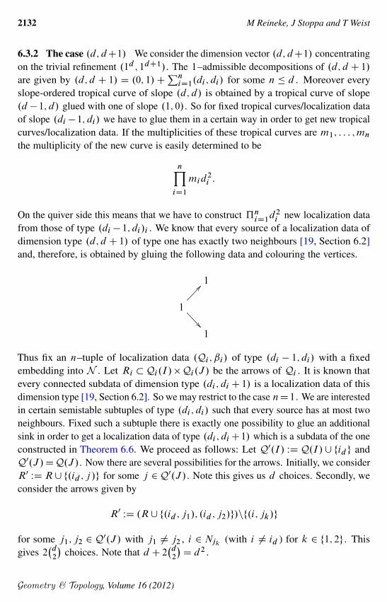
6.3.2 The case .d; dC1/ We consider the dimension vector .d; dC1/ concentratingon the trivial refinement .1d ; 1dC1/. The 1–admissible decompositions of .d; d C 1/
are given by .d; d C 1/ D .0; 1/CPn
iD1.di ; di/ for some n � d . Moreover everyslope-ordered tropical curve of slope .d; d/ is obtained by a tropical curve of slope.d � 1; d/ glued with one of slope .1; 0/. So for fixed tropical curves/localization dataof slope .di � 1; di/ we have to glue them in a certain way in order to get new tropicalcurves/localization data. If the multiplicities of these tropical curves are m1; : : : ;mn
the multiplicity of the new curve is easily determined to be
nYiD1
mid2i :
On the quiver side this means that we have to construct …niD1
d2i new localization data
from those of type .di � 1; di/i . We know that every source of a localization data ofdimension type .d; d C 1/ of type one has exactly two neighbours [19, Section 6.2]and, therefore, is obtained by gluing the following data and colouring the vertices.
1
1
@@
��1
Thus fix an n–tuple of localization data .Qi ; ˇi/ of type .di � 1; di/ with a fixedembedding into N . Let Ri �Qi.I/�Qi.J / be the arrows of Qi . It is known thatevery connected subdata of dimension type .di ; di C 1/ is a localization data of thisdimension type [19, Section 6.2]. So we may restrict to the case nD1. We are interestedin certain semistable subtuples of type .di ; di/ such that every source has at most twoneighbours. Fixed such a subtuple there is exactly one possibility to glue an additionalsink in order to get a localization data of type .di ; diC1/ which is a subdata of the oneconstructed in Theorem 6.6. We proceed as follows: Let Q0.I/ WDQ.I/[ fidg andQ0.J /DQ.J /. Now there are several possibilities for the arrows. Initially, we considerR0 WDR[f.id ; j /g for some j 2Q0.J /. Note this gives us d choices. Secondly, weconsider the arrows given by
R0 WD .R[f.id ; j1/; .id ; j2/g/nf.i; jk/g
for some j1; j2 2 Q0.J / with j1 ¤ j2 , i 2 Njk(with i ¤ id ) for k 2 f1; 2g. This
gives 2�d2
�choices. Note that d C 2
�d2
�D d2 .
Geometry & Topology, Volume 16 (2012)

MPS degeneration formula for quiver moduli 2133
Theorem 6.8 By this construction we getQn
iD1d2i localization data of type .di ; diC1/
starting with localization data of type .di � 1; di/ for i D 1; : : : ; n. Moreover everylocalization data is obtained in this way.
Proof Consider a localization data of type .d; d C 1/. By deleting the vertex jdC1
(including the corresponding arrows) we get n semistable subdata of type .di ; di/
for i D 1; : : : ; n. Let q.i/max 2 Qi.I/ be the source with the maximal index. IfjNq.i/max j D 1 we also delete this vertex and get a localization data of type .di �1; di/.If jNq.i/max j D 2 there exists exactly one source q.i/ 2Qi.I/ such that jNq.i/j D 1.After deleting q.i/max , there exists one possibility to obtain a localization data byadding an extra arrow .q.i/; j / where j 2 Nq.i/max . This already shows that everylocalization data of type .d; d C 1/ is obtained by this construction.
This is enough to describe the required correspondence between localization data andcurves in this case.
References[1] T Bridgeland, An introduction to motivic Hall algebras, Adv. Math. 229 (2012) 102–
138 MR2854172
[2] J Engel, M Reineke, Smooth models of quiver moduli, Math. Z. 262 (2009) 817–848MR2511752
[3] A Gathmann, H Markwig, The numbers of tropical plane curves through points ingeneral position, J. Reine Angew. Math. 602 (2007) 155–177 MR2300455
[4] M Gross, R Pandharipande, Quivers, curves, and the tropical vertex, Port. Math. 67(2010) 211–259 MR2662867
[5] M Gross, R Pandharipande, B Siebert, The tropical vertex, Duke Math. J. 153 (2010)297–362 MR2667135
[6] E-N Ionel, T H Parker, Relative Gromov–Witten invariants, Ann. of Math. 157 (2003)45–96 MR1954264
[7] A D King, Moduli of representations of finite-dimensional algebras, Quart. J. Math.Oxford Ser. 45 (1994) 515–530 MR1315461
[8] M Kontsevich, Y Soibelman, Affine structures and non-Archimedean analytic spaces,from: “The unity of mathematics”, (P Etingof, V Retakh, M Singer, I editors), Progr.Math. 244, Birkhäuser, Boston, MA (2006) 321–385 MR2181810
[9] A-M Li, Y Ruan, Symplectic surgery and Gromov–Witten invariants of Calabi–Yau3–folds, Invent. Math. 145 (2001) 151–218 MR1839289
Geometry & Topology, Volume 16 (2012)

2134 M Reineke, J Stoppa and T Weist
[10] J Li, A degeneration formula of GW-invariants, J. Differential Geom. 60 (2002) 199–293 MR1938113
[11] I G Macdonald, Symmetric functions and Hall polynomials, 2nd edition, Oxford Math-ematical Monographs, The Clarendon Press Oxford University Press, New York (1995)MR1354144 With contributions by A. Zelevinsky
[12] J Manschot, BPS invariants of semi-stable sheaves on rational surfaces arXiv:1109.4861
[13] J Manschot, B Pioline, A Sen, Wall crossing from Boltzmann black hole halos, J. HighEnergy Phys. (2011) 059, 73 MR2875965
[14] G Mikhalkin, Enumerative tropical algebraic geometry in R2 , J. Amer. Math. Soc. 18(2005) 313–377 MR2137980
[15] M Reineke, The Harder–Narasimhan system in quantum groups and cohomology ofquiver moduli, Invent. Math. 152 (2003) 349–368 MR1974891
[16] M Reineke, Poisson automorphisms and quiver moduli, J. Inst. Math. Jussieu 9 (2010)653–667 MR2650811
[17] M Reineke, T Weist, Refined GW/Kronecker correspondence arXiv:1103.5283
[18] J Stoppa, Universal covers and the GW/Kronecker correspondence, Commun. NumberTheory Phys. 5 (2011) 353–395 MR2851154
[19] T Weist, Localization in quiver moduli spaces arXiv:0903.5442v2
MR, TW: Fachbereich C - Mathematik, Bergische Universität WuppertalD 42097 Wuppertal, Germany
Dipartimento di Matematica “F. Casorati”, Università degli Studi di PaviaVia Ferrata 1, 27100 Pavia, Italy
[email protected], [email protected],[email protected]
Proposed: Richard Thomas Received: 28 November 2011Seconded: Jim Bryan, Yasha Eliashberg Revised: 13 July 2012
Geometry & Topology Publications, an imprint of mathematical sciences publishers msp
Copyright © 2022 FDOKUMEN